
Introduction to Corrosion Science
573
Introduction to Corrosion Science
-
Upload
khangminh22 -
Category
Documents
-
view
2 -
download
0
Transcript of Introduction to Corrosion Science

Introduction to Corrosion Science

E. McCafferty
Introduction to Corrosion Science
123

E. McCaffertyAlexandria VA 22309USA
ISBN 978-1-4419-0454-6 e-ISBN 978-1-4419-0455-3DOI 10.1007/978-1-4419-0455-3Springer New York Dordrecht Heidelberg London
Library of Congress Control Number: 2009940577
© Springer Science+Business Media, LLC 2010All rights reserved. This work may not be translated or copied in whole or in part without the written permission of thepublisher (Springer Science+Business Media, LLC, 233 Spring Street, New York, NY 10013, USA), except for brief excerptsin connection with reviews or scholarly analysis. Use in connection with any form of information storage and retrieval,electronic adaptation, computer software, or by similar or dissimilar methodology now known or hereafter developed isforbidden.The use in this publication of trade names, trademarks, service marks, and similar terms, even if they are not identified assuch, is not to be taken as an expression of opinion as to whether or not they are subject to proprietary rights.
Printed on acid-free paper
Springer is part of Springer Science+Business Media (www.springer.com)

Preface
This textbook is intended for a one-semester course in corrosion science at the graduate or advancedundergraduate level. The approach is that of a physical chemist or materials scientist, and the textis geared toward students of chemistry, materials science, and engineering. This textbook shouldalso be useful to practicing corrosion engineers or materials engineers who wish to enhance theirunderstanding of the fundamental principles of corrosion science.
It is assumed that the student or reader does not have a background in electrochemistry. However,the student or reader should have taken at least an undergraduate course in materials science orphysical chemistry. More material is presented in the textbook than can be covered in a one-semestercourse, so the book is intended for both the classroom and as a source book for further use.
This book grew out of classroom lectures which the author presented between 1982 and thepresent while a professorial lecturer at George Washington University, Washington, DC, where heorganized and taught a graduate course on “Environmental Effects on Materials.” Additional materialhas been provided by over 30 years of experience in corrosion research, largely at the Naval ResearchLaboratory, Washington, DC and also at the Bethlehem Steel Company, Bethlehem, PA and as aRobert A. Welch Postdoctoral Fellow at the University of Texas.
The text emphasizes basic principles of corrosion science which underpin extensions to practice.The emphasis here is on corrosion in aqueous environments, although a chapter on high-temperatureoxidation has also been included. The overall effort has been to provide a brief but rigorous intro-duction to corrosion science without getting mired in extensive individual case histories, specificengineering applications, or compilations of practical corrosion data. Some other possible topicsof interest in the field of corrosion science have not been included in accordance with the goal tokeep the material introductory in nature and to keep the size of the book manageable. In addition,references are meant to be illustrative rather than exhaustive.
Most chapters also contain a set of problems. Numerical answers to problems are found at theend of the book.
Finally, the author wishes to recognize the various mentors who have graciously shaped his pro-fessional life. These are: Dr. J. B. Horton and A. R. Borzillo of the Bethlehem Steel Corporation,who introduced the author to the field of corrosion; the late Prof. A. C. Zettlemoyer of LehighUniversity, who taught the author the beauty of surface chemistry while his Ph. D. advisor; the lateDr. Norman Hackerman, postdoctoral mentor at the University of Texas; the late Dr. B. F. Brownand M. H. Peterson of the Naval Research Laboratory; and Prof. James P. Wightman of the VirginiaPolytechnic Institute and State University, a “surface agent extra-ordinaire” with whom the authorhas spent an enjoyable and exciting sabbatical year.
The author is also grateful to Harry N. Jones, III, James R. Martin, Farrel J. Martin, Paul M.Natishan, Virginia DeGeorgi, Luke Davis, Robert A. Bayles, and Roy Rayne, all of the NavalResearch Laboratory, who helped in various ways. The author also appreciates the kind assistance of
v

vi Preface
A. Pourbaix of CEBELCOR (Centre Belge d’Etude de la Corrosion), C. Anderson Engh, Jr., M.D.of the Anderson Orthopaedic Clinic, Alexandria, VA; Phoebe Dent Weil, Northern Light Studio,Florence, MA; Erik Axdahl, and Harry’s U-Pull-It, West Hazleton, PA.
Finally, the author wishes to thank Dr. Kenneth Howell, Senior Chemistry Editor at Springer, forhis encouragement and support.
Washington, DC E. McCafferty2009

Contents
1 Societal Aspects of Corrosion . . . . . . . . . . . . . . . . . . . . . . . . . . . . . . . 1We Live in a Metals-Based Society . . . . . . . . . . . . . . . . . . . . . . . . . . . . . 1Why Study Corrosion? . . . . . . . . . . . . . . . . . . . . . . . . . . . . . . . . . . . 1Corrosion and Human Life and Safety . . . . . . . . . . . . . . . . . . . . . . . . . . . 1Economics of Corrosion . . . . . . . . . . . . . . . . . . . . . . . . . . . . . . . . . . 4Corrosion and the Conservation of Materials . . . . . . . . . . . . . . . . . . . . . . . . 5The Study of Corrosion . . . . . . . . . . . . . . . . . . . . . . . . . . . . . . . . . . . 6Corrosion Science vs. Corrosion Engineering . . . . . . . . . . . . . . . . . . . . . . . 8Challenges for Today’s Corrosion Scientist . . . . . . . . . . . . . . . . . . . . . . . . . 9Problems . . . . . . . . . . . . . . . . . . . . . . . . . . . . . . . . . . . . . . . . . . 10References . . . . . . . . . . . . . . . . . . . . . . . . . . . . . . . . . . . . . . . . . . 10
2 Getting Started on the Basics . . . . . . . . . . . . . . . . . . . . . . . . . . . . . . . 13Introduction . . . . . . . . . . . . . . . . . . . . . . . . . . . . . . . . . . . . . . . . . 13
What is Corrosion? . . . . . . . . . . . . . . . . . . . . . . . . . . . . . . . . . . . . 13Physical Processes of Degradation . . . . . . . . . . . . . . . . . . . . . . . . . . . . 13Environmentally Assisted Degradation Processes . . . . . . . . . . . . . . . . . . . . 14
Electrochemical Reactions . . . . . . . . . . . . . . . . . . . . . . . . . . . . . . . . . 15Half-Cell Reactions . . . . . . . . . . . . . . . . . . . . . . . . . . . . . . . . . . . . 15Anodic Reactions . . . . . . . . . . . . . . . . . . . . . . . . . . . . . . . . . . . . . 15Cathodic Reactions . . . . . . . . . . . . . . . . . . . . . . . . . . . . . . . . . . . . 16Coupled Electrochemical Reactions . . . . . . . . . . . . . . . . . . . . . . . . . . . 17A Note About Atmospheric Corrosion . . . . . . . . . . . . . . . . . . . . . . . . . . 18Secondary Effects of Cathodic Reactions . . . . . . . . . . . . . . . . . . . . . . . . 19
Three Simple Properties of Solutions . . . . . . . . . . . . . . . . . . . . . . . . . . . . 21The Faraday and Faraday’s Law . . . . . . . . . . . . . . . . . . . . . . . . . . . . . . 23Units for Corrosion Rates . . . . . . . . . . . . . . . . . . . . . . . . . . . . . . . . . . 24Uniform vs. Localized Corrosion . . . . . . . . . . . . . . . . . . . . . . . . . . . . . . 25
The Eight Forms of Corrosion . . . . . . . . . . . . . . . . . . . . . . . . . . . . . . 27Problems . . . . . . . . . . . . . . . . . . . . . . . . . . . . . . . . . . . . . . . . . . 28References . . . . . . . . . . . . . . . . . . . . . . . . . . . . . . . . . . . . . . . . . . 31
3 Charged Interfaces . . . . . . . . . . . . . . . . . . . . . . . . . . . . . . . . . . . . . 33Introduction . . . . . . . . . . . . . . . . . . . . . . . . . . . . . . . . . . . . . . . . . 33Electrolytes . . . . . . . . . . . . . . . . . . . . . . . . . . . . . . . . . . . . . . . . . 33
The Interior of an Electrolyte . . . . . . . . . . . . . . . . . . . . . . . . . . . . . . . 33Interfaces . . . . . . . . . . . . . . . . . . . . . . . . . . . . . . . . . . . . . . . . . . 35
vii

viii Contents
Encountering an Interface . . . . . . . . . . . . . . . . . . . . . . . . . . . . . . . . 35The Solution/Air Interface . . . . . . . . . . . . . . . . . . . . . . . . . . . . . . . . 36The Metal/Solution Interface . . . . . . . . . . . . . . . . . . . . . . . . . . . . . . . 37Metal Ions in Two Different Chemical Environments . . . . . . . . . . . . . . . . . . 38
The Electrical Double Layer . . . . . . . . . . . . . . . . . . . . . . . . . . . . . . . . 39The Gouy−Chapman Model of the Electrical Double Layer . . . . . . . . . . . . . . 40The Electrostatic Potential and Potential Difference . . . . . . . . . . . . . . . . . . . 40The Stern Model of the Electrical Double Layer . . . . . . . . . . . . . . . . . . . . . 41The Bockris−Devanathan−Müller Model of the Electrical Double Layer . . . . . . . 42Significance of the Electrical Double Layer to Corrosion . . . . . . . . . . . . . . . . 43
Electrode Potentials . . . . . . . . . . . . . . . . . . . . . . . . . . . . . . . . . . . . . 44The Potential Difference Across a Metal/Solution Interface . . . . . . . . . . . . . . . 44Relative Electrode Potentials . . . . . . . . . . . . . . . . . . . . . . . . . . . . . . . 45The Electromotive Force Series . . . . . . . . . . . . . . . . . . . . . . . . . . . . . 46
Reference Electrodes for the Laboratory and the Field . . . . . . . . . . . . . . . . . . . 48Measurement of Electrode Potentials . . . . . . . . . . . . . . . . . . . . . . . . . . . . 52Problems . . . . . . . . . . . . . . . . . . . . . . . . . . . . . . . . . . . . . . . . . . 53References . . . . . . . . . . . . . . . . . . . . . . . . . . . . . . . . . . . . . . . . . . 55
4 A Brief Review of Thermodynamics . . . . . . . . . . . . . . . . . . . . . . . . . . . 57Introduction . . . . . . . . . . . . . . . . . . . . . . . . . . . . . . . . . . . . . . . . . 57Thermodynamic State Functions . . . . . . . . . . . . . . . . . . . . . . . . . . . . . . 57
Internal Energy . . . . . . . . . . . . . . . . . . . . . . . . . . . . . . . . . . . . . . 57Entropy . . . . . . . . . . . . . . . . . . . . . . . . . . . . . . . . . . . . . . . . . . 58Enthalpy . . . . . . . . . . . . . . . . . . . . . . . . . . . . . . . . . . . . . . . . . 59Helmholtz and Gibbs Free Energies . . . . . . . . . . . . . . . . . . . . . . . . . . . 59Free Energy and Spontaneity . . . . . . . . . . . . . . . . . . . . . . . . . . . . . . . 60Relationships Between Thermodynamic Functions . . . . . . . . . . . . . . . . . . . 61
The Chemical Potential and Standard States . . . . . . . . . . . . . . . . . . . . . . . . 63More About the Chemical Potential . . . . . . . . . . . . . . . . . . . . . . . . . . . 63A Note About Units for �Go or �G . . . . . . . . . . . . . . . . . . . . . . . . . . . 64The Free Energy and Electrode Potentials . . . . . . . . . . . . . . . . . . . . . . . . 65
The Nernst Equation . . . . . . . . . . . . . . . . . . . . . . . . . . . . . . . . . . . . 66Standard Free Energy Change and the Equilibrium Constant . . . . . . . . . . . . . . 67
A Quandary – The Sign of Electrode Potentials . . . . . . . . . . . . . . . . . . . . . . 68Factors Affecting Electrode Potentials . . . . . . . . . . . . . . . . . . . . . . . . . . 69
Problems . . . . . . . . . . . . . . . . . . . . . . . . . . . . . . . . . . . . . . . . . . 70References . . . . . . . . . . . . . . . . . . . . . . . . . . . . . . . . . . . . . . . . . . 72
5 Thermodynamics of Corrosion: Electrochemical Cellsand Galvanic Corrosion . . . . . . . . . . . . . . . . . . . . . . . . . . . . . . . . . . 73Introduction . . . . . . . . . . . . . . . . . . . . . . . . . . . . . . . . . . . . . . . . . 73Electrochemical Cells . . . . . . . . . . . . . . . . . . . . . . . . . . . . . . . . . . . . 73
Electrochemical Cells on the Same Surface . . . . . . . . . . . . . . . . . . . . . . . 75Galvanic Corrosion . . . . . . . . . . . . . . . . . . . . . . . . . . . . . . . . . . . . . 76
Galvanic Series . . . . . . . . . . . . . . . . . . . . . . . . . . . . . . . . . . . . . . 76Cathodic Protection . . . . . . . . . . . . . . . . . . . . . . . . . . . . . . . . . . . . 79
Two Types of Metallic Coatings . . . . . . . . . . . . . . . . . . . . . . . . . . . . . . 80Titanium Coatings on Steel: A Research Study . . . . . . . . . . . . . . . . . . . . . 82

Contents ix
Protection Against Galvanic Corrosion . . . . . . . . . . . . . . . . . . . . . . . . . . . 83Differential Concentration Cells . . . . . . . . . . . . . . . . . . . . . . . . . . . . . . 84
Metal Ion Concentration Cells . . . . . . . . . . . . . . . . . . . . . . . . . . . . . . 84Oxygen Concentration Cells . . . . . . . . . . . . . . . . . . . . . . . . . . . . . . . 86The Evans Water Drop Experiment . . . . . . . . . . . . . . . . . . . . . . . . . . . 88Waterline Corrosion . . . . . . . . . . . . . . . . . . . . . . . . . . . . . . . . . . . 88Crevice Corrosion: A Preview . . . . . . . . . . . . . . . . . . . . . . . . . . . . . . 89
Problems . . . . . . . . . . . . . . . . . . . . . . . . . . . . . . . . . . . . . . . . . . 89References . . . . . . . . . . . . . . . . . . . . . . . . . . . . . . . . . . . . . . . . . . 93
6 Thermodynamics of Corrosion: Pourbaix Diagrams . . . . . . . . . . . . . . . . . . 95Introduction . . . . . . . . . . . . . . . . . . . . . . . . . . . . . . . . . . . . . . . . . 95Pourbaix Diagram for Aluminum . . . . . . . . . . . . . . . . . . . . . . . . . . . . . . 96
Construction of the Pourbaix Diagram for Aluminum . . . . . . . . . . . . . . . . . . 96Comparison of Thermodynamic and Kinetic Data for Aluminum . . . . . . . . . . . . 101
Pourbaix Diagram for Water . . . . . . . . . . . . . . . . . . . . . . . . . . . . . . . . 101Pourbaix Diagrams for Other Metals . . . . . . . . . . . . . . . . . . . . . . . . . . . . 103
Pourbaix Diagram for Zinc . . . . . . . . . . . . . . . . . . . . . . . . . . . . . . . . 103Pourbaix Diagram for Iron . . . . . . . . . . . . . . . . . . . . . . . . . . . . . . . . 103Pourbaix Diagrams for Additional Metals . . . . . . . . . . . . . . . . . . . . . . . . 106
Applications of Pourbaix Diagrams to Corrosion . . . . . . . . . . . . . . . . . . . . . . 108Limitations of Pourbaix Diagrams . . . . . . . . . . . . . . . . . . . . . . . . . . . . . 111
Pourbaix Diagrams for Alloys . . . . . . . . . . . . . . . . . . . . . . . . . . . . . . 111Pourbaix Diagrams at Elevated Temperatures . . . . . . . . . . . . . . . . . . . . . . . 112Problems . . . . . . . . . . . . . . . . . . . . . . . . . . . . . . . . . . . . . . . . . . 114References . . . . . . . . . . . . . . . . . . . . . . . . . . . . . . . . . . . . . . . . . . 116
7 Kinetics of Corrosion . . . . . . . . . . . . . . . . . . . . . . . . . . . . . . . . . . . 119Introduction . . . . . . . . . . . . . . . . . . . . . . . . . . . . . . . . . . . . . . . . . 119
Units for Corrosion Rates . . . . . . . . . . . . . . . . . . . . . . . . . . . . . . . . 119Methods of Determining Corrosion Rates . . . . . . . . . . . . . . . . . . . . . . . . . 119
Weight Loss Method . . . . . . . . . . . . . . . . . . . . . . . . . . . . . . . . . . . 120Weight Gain Method . . . . . . . . . . . . . . . . . . . . . . . . . . . . . . . . . . . 120Chemical Analysis of Solution . . . . . . . . . . . . . . . . . . . . . . . . . . . . . . 121Gasometric Techniques . . . . . . . . . . . . . . . . . . . . . . . . . . . . . . . . . . 122Thickness Measurements . . . . . . . . . . . . . . . . . . . . . . . . . . . . . . . . . 124Electrical Resistance Method . . . . . . . . . . . . . . . . . . . . . . . . . . . . . . . 124Inert Marker Method . . . . . . . . . . . . . . . . . . . . . . . . . . . . . . . . . . . 124Electrochemical Techniques . . . . . . . . . . . . . . . . . . . . . . . . . . . . . . . 126
Electrochemical Polarization . . . . . . . . . . . . . . . . . . . . . . . . . . . . . . . . 127Anodic and Cathodic Polarization . . . . . . . . . . . . . . . . . . . . . . . . . . . . 127Visualization of Cathodic Polarization . . . . . . . . . . . . . . . . . . . . . . . . . . 127Visualization of Anodic Polarization . . . . . . . . . . . . . . . . . . . . . . . . . . . 128Ohmic Polarization . . . . . . . . . . . . . . . . . . . . . . . . . . . . . . . . . . . . 130
Electrode Kinetics for Activation Polarization . . . . . . . . . . . . . . . . . . . . . . . 131Absolute Reaction Rate Theory . . . . . . . . . . . . . . . . . . . . . . . . . . . . . 131Electrode Kinetics for Non-Corroding Metals . . . . . . . . . . . . . . . . . . . . . . 132How to Plot Polarization Curves? . . . . . . . . . . . . . . . . . . . . . . . . . . . . 136The Tafel Equation . . . . . . . . . . . . . . . . . . . . . . . . . . . . . . . . . . . . 138

x Contents
Reversible and Irreversible Potentials . . . . . . . . . . . . . . . . . . . . . . . . . . 139Mixed Potential Theory (Wagner and Traud) . . . . . . . . . . . . . . . . . . . . . . 140Electrode Kinetic Parameters . . . . . . . . . . . . . . . . . . . . . . . . . . . . . . . 144
Applications of Mixed Potential Theory . . . . . . . . . . . . . . . . . . . . . . . . . . 146Metals in Acid Solutions . . . . . . . . . . . . . . . . . . . . . . . . . . . . . . . . . 146Tafel Extrapolation . . . . . . . . . . . . . . . . . . . . . . . . . . . . . . . . . . . . 148Verification of Corrosion Rates Obtained by Tafel Extrapolation . . . . . . . . . . . . 150Cathodic Protection of Iron in Acids . . . . . . . . . . . . . . . . . . . . . . . . . . . 150Effect of the Cathodic Reaction . . . . . . . . . . . . . . . . . . . . . . . . . . . . . 154Effect of Cathode Area on Galvanic Corrosion . . . . . . . . . . . . . . . . . . . . . 154Multiple Oxidation–Reduction Reactions . . . . . . . . . . . . . . . . . . . . . . . . 156Anodic or Cathodic Control . . . . . . . . . . . . . . . . . . . . . . . . . . . . . . . 158
The Linear Polarization Method (Stern and Geary) . . . . . . . . . . . . . . . . . . . . 159Advantages and Possible Errors for the Linear Polarization Technique . . . . . . . . . 162Applications of the Linear Polarization Technique . . . . . . . . . . . . . . . . . . . 163Small-Amplitude Cyclic Voltammetry . . . . . . . . . . . . . . . . . . . . . . . . . . 164
Experimental Techniques for Determination of Polarization Curves . . . . . . . . . . . . 165Electrode Samples . . . . . . . . . . . . . . . . . . . . . . . . . . . . . . . . . . . . 165Electrode Holders . . . . . . . . . . . . . . . . . . . . . . . . . . . . . . . . . . . . . 166Electrochemical Cells . . . . . . . . . . . . . . . . . . . . . . . . . . . . . . . . . . 167Instrumentation and Procedures . . . . . . . . . . . . . . . . . . . . . . . . . . . . . 168
Problems . . . . . . . . . . . . . . . . . . . . . . . . . . . . . . . . . . . . . . . . . . 169References . . . . . . . . . . . . . . . . . . . . . . . . . . . . . . . . . . . . . . . . . . 173
8 Concentration Polarization and Diffusion . . . . . . . . . . . . . . . . . . . . . . . . 177Introduction . . . . . . . . . . . . . . . . . . . . . . . . . . . . . . . . . . . . . . . . . 177
Where Oxygen Reduction Occurs . . . . . . . . . . . . . . . . . . . . . . . . . . . . 177Concentration Polarization in Current Density–Potential Plots . . . . . . . . . . . . . 178
Solubility and Diffusion . . . . . . . . . . . . . . . . . . . . . . . . . . . . . . . . . . . 179Solubility of Oxygen in Aqueous Solutions . . . . . . . . . . . . . . . . . . . . . . . 179Fick’s First Law of Diffusion . . . . . . . . . . . . . . . . . . . . . . . . . . . . . . . 181Diffusion and Random Walks . . . . . . . . . . . . . . . . . . . . . . . . . . . . . . 183
Electrode Kinetics for Concentration Polarization . . . . . . . . . . . . . . . . . . . . . 186Concentration Profile Near an Electrode Surface . . . . . . . . . . . . . . . . . . . . 186Limiting Diffusion Current Density . . . . . . . . . . . . . . . . . . . . . . . . . . . 187Diffusion Layer vs. The Diffuse Layer . . . . . . . . . . . . . . . . . . . . . . . . . . 189Current–Potential Relationship for Concentration Polarization . . . . . . . . . . . . . 189Wagner–Traud Theory for Concentration Polarization . . . . . . . . . . . . . . . . . . 191
Effect of Environmental Factors on Concentration Polarization and Corrosion . . . . . . 192Effect of Oxygen Concentration . . . . . . . . . . . . . . . . . . . . . . . . . . . . . 193Effect of Solution Velocity . . . . . . . . . . . . . . . . . . . . . . . . . . . . . . . . 194Effect of Temperature . . . . . . . . . . . . . . . . . . . . . . . . . . . . . . . . . . 196
Further Applications of Concentration Polarization Curves . . . . . . . . . . . . . . . . 197Cathodic Protection . . . . . . . . . . . . . . . . . . . . . . . . . . . . . . . . . . . . 197Area Effects in Galvanic Corrosion . . . . . . . . . . . . . . . . . . . . . . . . . . . 199Linear Polarization . . . . . . . . . . . . . . . . . . . . . . . . . . . . . . . . . . . . 199Concentration Polarization in Acid Solutions . . . . . . . . . . . . . . . . . . . . . . 200Combined Activation and Concentration Polarization . . . . . . . . . . . . . . . . . . 202

Contents xi
The Rotating Disc Electrode . . . . . . . . . . . . . . . . . . . . . . . . . . . . . . . 202Problems . . . . . . . . . . . . . . . . . . . . . . . . . . . . . . . . . . . . . . . . . . 205References . . . . . . . . . . . . . . . . . . . . . . . . . . . . . . . . . . . . . . . . . . 208
9 Passivity . . . . . . . . . . . . . . . . . . . . . . . . . . . . . . . . . . . . . . . . . . 209Introduction . . . . . . . . . . . . . . . . . . . . . . . . . . . . . . . . . . . . . . . . . 209
Aluminum: An Example . . . . . . . . . . . . . . . . . . . . . . . . . . . . . . . . . 209What is Passivity? . . . . . . . . . . . . . . . . . . . . . . . . . . . . . . . . . . . . 210Early History of Passivity . . . . . . . . . . . . . . . . . . . . . . . . . . . . . . . . 210Thickness of Passive Oxide Films . . . . . . . . . . . . . . . . . . . . . . . . . . . . 210Purpose of This Chapter . . . . . . . . . . . . . . . . . . . . . . . . . . . . . . . . . 211
Electrochemical Basis for Passivity . . . . . . . . . . . . . . . . . . . . . . . . . . . . . 211Theories of Passivity . . . . . . . . . . . . . . . . . . . . . . . . . . . . . . . . . . . . 215
Adsorption Theory . . . . . . . . . . . . . . . . . . . . . . . . . . . . . . . . . . . . 215Oxide Film Theory . . . . . . . . . . . . . . . . . . . . . . . . . . . . . . . . . . . . 216Film Sequence Theory . . . . . . . . . . . . . . . . . . . . . . . . . . . . . . . . . . 218
Surface Analysis Techniques for the Examination of Passive Films . . . . . . . . . . . . 218X-ray Photoelectron Spectroscopy (XPS) . . . . . . . . . . . . . . . . . . . . . . . . 220X-ray Absorption Spectroscopy . . . . . . . . . . . . . . . . . . . . . . . . . . . . . 222Scanning Tunneling Microscopy . . . . . . . . . . . . . . . . . . . . . . . . . . . . . 223
Models for the Passive Oxide Film on Iron . . . . . . . . . . . . . . . . . . . . . . . . . 224Bilayer Model . . . . . . . . . . . . . . . . . . . . . . . . . . . . . . . . . . . . . . 224Hydrous Oxide Model . . . . . . . . . . . . . . . . . . . . . . . . . . . . . . . . . . 227Bipolar-Fixed Charge Model . . . . . . . . . . . . . . . . . . . . . . . . . . . . . . . 228Spinel/Defect Model . . . . . . . . . . . . . . . . . . . . . . . . . . . . . . . . . . . 229What Do These Various Models Mean? . . . . . . . . . . . . . . . . . . . . . . . . . 230
Passive Oxide Films on Aluminum . . . . . . . . . . . . . . . . . . . . . . . . . . . . . 230Air-Formed Oxide Films . . . . . . . . . . . . . . . . . . . . . . . . . . . . . . . . . 231Films Formed in Aqueous Solutions . . . . . . . . . . . . . . . . . . . . . . . . . . . 231
Properties of Passive Oxide Films . . . . . . . . . . . . . . . . . . . . . . . . . . . . . 232Thickness . . . . . . . . . . . . . . . . . . . . . . . . . . . . . . . . . . . . . . . . . 233Electronic and Ionic Conductivity . . . . . . . . . . . . . . . . . . . . . . . . . . . . 233Chemical Stability . . . . . . . . . . . . . . . . . . . . . . . . . . . . . . . . . . . . 233Mechanical Properties . . . . . . . . . . . . . . . . . . . . . . . . . . . . . . . . . . 234Structure of Passive Films . . . . . . . . . . . . . . . . . . . . . . . . . . . . . . . . 235
Passivity in Binary Alloys . . . . . . . . . . . . . . . . . . . . . . . . . . . . . . . . . . 237Electron Configuration Theory . . . . . . . . . . . . . . . . . . . . . . . . . . . . . . 238Oxide Film Properties . . . . . . . . . . . . . . . . . . . . . . . . . . . . . . . . . . 241Percolation Theory . . . . . . . . . . . . . . . . . . . . . . . . . . . . . . . . . . . . 242Graph Theory Model . . . . . . . . . . . . . . . . . . . . . . . . . . . . . . . . . . . 243
Passivity in Stainless Steels . . . . . . . . . . . . . . . . . . . . . . . . . . . . . . . . . 249Electrochemical Aspects . . . . . . . . . . . . . . . . . . . . . . . . . . . . . . . . . 250Composition of Passive Films on Stainless Steels . . . . . . . . . . . . . . . . . . . . 252
Passivity by Alloying with Noble Metals . . . . . . . . . . . . . . . . . . . . . . . . . . 254Anodic Protection . . . . . . . . . . . . . . . . . . . . . . . . . . . . . . . . . . . . . . 255Problems . . . . . . . . . . . . . . . . . . . . . . . . . . . . . . . . . . . . . . . . . . 257References . . . . . . . . . . . . . . . . . . . . . . . . . . . . . . . . . . . . . . . . . . 260

xii Contents
10 Crevice Corrosion and Pitting . . . . . . . . . . . . . . . . . . . . . . . . . . . . . . 263Introduction . . . . . . . . . . . . . . . . . . . . . . . . . . . . . . . . . . . . . . . . . 263Crevice Corrosion . . . . . . . . . . . . . . . . . . . . . . . . . . . . . . . . . . . . . . 263
Initiation of Crevice Corrosion . . . . . . . . . . . . . . . . . . . . . . . . . . . . . . 264Propagation of Crevice Corrosion . . . . . . . . . . . . . . . . . . . . . . . . . . . . 269Crevice Corrosion Testing . . . . . . . . . . . . . . . . . . . . . . . . . . . . . . . . 272Area Effects in Crevice Corrosion . . . . . . . . . . . . . . . . . . . . . . . . . . . . 274Protection Against Crevice Corrosion . . . . . . . . . . . . . . . . . . . . . . . . . . 275
Pitting . . . . . . . . . . . . . . . . . . . . . . . . . . . . . . . . . . . . . . . . . . . . 277Critical Pitting Potential . . . . . . . . . . . . . . . . . . . . . . . . . . . . . . . . . 278Experimental Determination of Pitting Potentials . . . . . . . . . . . . . . . . . . . . 280Effect of Chloride Ions on the Pitting Potential . . . . . . . . . . . . . . . . . . . . . 282Effect of Inhibitors on the Pitting Potential . . . . . . . . . . . . . . . . . . . . . . . 283Mechanism of Pit Initiation . . . . . . . . . . . . . . . . . . . . . . . . . . . . . . . 283Mechanism of Pit Propagation . . . . . . . . . . . . . . . . . . . . . . . . . . . . . . 286Protection Potential . . . . . . . . . . . . . . . . . . . . . . . . . . . . . . . . . . . . 288Metastable Pits and Repassivation . . . . . . . . . . . . . . . . . . . . . . . . . . . . 290Experimental Pourbaix Diagrams for Pitting . . . . . . . . . . . . . . . . . . . . . . . 291Effect of Molybdenum on the Pitting of Stainless Steels . . . . . . . . . . . . . . . . 293Effect of Sulfide Inclusions on the Pitting of Stainless Steels . . . . . . . . . . . . . . 294Effect of Temperature . . . . . . . . . . . . . . . . . . . . . . . . . . . . . . . . . . 294Protection Against Pitting . . . . . . . . . . . . . . . . . . . . . . . . . . . . . . . . 296
Pitting of Aluminum . . . . . . . . . . . . . . . . . . . . . . . . . . . . . . . . . . . . 297Occluded Corrosion Cells . . . . . . . . . . . . . . . . . . . . . . . . . . . . . . . . . . 300
Occluded Corrosion Cell (OCC) on Iron . . . . . . . . . . . . . . . . . . . . . . . . . 301Occluded Corrosion Cells on Copper and Aluminum . . . . . . . . . . . . . . . . . . 303Differences Between Pitting and Crevice Corrosion . . . . . . . . . . . . . . . . . . . 306
Detection of Corrosion Pits . . . . . . . . . . . . . . . . . . . . . . . . . . . . . . . . . 306Problems . . . . . . . . . . . . . . . . . . . . . . . . . . . . . . . . . . . . . . . . . . 308References . . . . . . . . . . . . . . . . . . . . . . . . . . . . . . . . . . . . . . . . . . 311
11 Mechanically Assisted Corrosion . . . . . . . . . . . . . . . . . . . . . . . . . . . . . 315Introduction . . . . . . . . . . . . . . . . . . . . . . . . . . . . . . . . . . . . . . . . . 315Stress-Corrosion Cracking . . . . . . . . . . . . . . . . . . . . . . . . . . . . . . . . . 318
Mechanical Metallurgy . . . . . . . . . . . . . . . . . . . . . . . . . . . . . . . . . . 318Characteristics of Stress-Corrosion Cracking . . . . . . . . . . . . . . . . . . . . . . 319Stages of Stress-Corrosion Cracking . . . . . . . . . . . . . . . . . . . . . . . . . . . 320Fracture Mechanics and SCC . . . . . . . . . . . . . . . . . . . . . . . . . . . . . . . 323SCC Testing . . . . . . . . . . . . . . . . . . . . . . . . . . . . . . . . . . . . . . . 331Interpretation of SCC Test Data . . . . . . . . . . . . . . . . . . . . . . . . . . . . . 334Metallurgical Effects in SCC . . . . . . . . . . . . . . . . . . . . . . . . . . . . . . . 335Environmental Effects on SCC . . . . . . . . . . . . . . . . . . . . . . . . . . . . . . 336Mechanisms of SCC . . . . . . . . . . . . . . . . . . . . . . . . . . . . . . . . . . . 339Protection Against Stress-Corrosion Cracking . . . . . . . . . . . . . . . . . . . . . . 345
Corrosion Fatigue . . . . . . . . . . . . . . . . . . . . . . . . . . . . . . . . . . . . . . 346Corrosion Fatigue Data . . . . . . . . . . . . . . . . . . . . . . . . . . . . . . . . . . 347Protection Against Corrosion Fatigue . . . . . . . . . . . . . . . . . . . . . . . . . . 348
Cavitation Corrosion . . . . . . . . . . . . . . . . . . . . . . . . . . . . . . . . . . . . 349

Contents xiii
Erosion Corrosion and Fretting Corrosion . . . . . . . . . . . . . . . . . . . . . . . . . 352Problems . . . . . . . . . . . . . . . . . . . . . . . . . . . . . . . . . . . . . . . . . . 353References . . . . . . . . . . . . . . . . . . . . . . . . . . . . . . . . . . . . . . . . . . 354
12 Corrosion Inhibitors . . . . . . . . . . . . . . . . . . . . . . . . . . . . . . . . . . . . 357Introduction . . . . . . . . . . . . . . . . . . . . . . . . . . . . . . . . . . . . . . . . . 357Types of Inhibitors . . . . . . . . . . . . . . . . . . . . . . . . . . . . . . . . . . . . . 359Acidic Solutions . . . . . . . . . . . . . . . . . . . . . . . . . . . . . . . . . . . . . . . 360
Chemisorption of Inhibitors . . . . . . . . . . . . . . . . . . . . . . . . . . . . . . . 361Effect of Inhibitor Concentration . . . . . . . . . . . . . . . . . . . . . . . . . . . . . 362Chemical Factors in the Effectiveness of Chemisorbed Inhibitors . . . . . . . . . . . . 363Involvement of Water . . . . . . . . . . . . . . . . . . . . . . . . . . . . . . . . . . . 367Competitive vs. Co-operative Adsorption . . . . . . . . . . . . . . . . . . . . . . . . 369Effect of the Electrical Double Layer . . . . . . . . . . . . . . . . . . . . . . . . . . 370The Potential of Zero Charge . . . . . . . . . . . . . . . . . . . . . . . . . . . . . . . 372Effect of Molecular Structure . . . . . . . . . . . . . . . . . . . . . . . . . . . . . . 373Adsorption Isotherms . . . . . . . . . . . . . . . . . . . . . . . . . . . . . . . . . . . 376
Nearly Neutral Solutions . . . . . . . . . . . . . . . . . . . . . . . . . . . . . . . . . . 379Effect of Oxide Films . . . . . . . . . . . . . . . . . . . . . . . . . . . . . . . . . . . 379Chelating Compounds as Corrosion Inhibitors . . . . . . . . . . . . . . . . . . . . . . 380Chromates and Chromate Replacements . . . . . . . . . . . . . . . . . . . . . . . . . 381
Inhibition of Localized Corrosion . . . . . . . . . . . . . . . . . . . . . . . . . . . . . . 382Pitting Corrosion . . . . . . . . . . . . . . . . . . . . . . . . . . . . . . . . . . . . . 382Crevice Corrosion . . . . . . . . . . . . . . . . . . . . . . . . . . . . . . . . . . . . 386Stress-Corrosion Cracking and Corrosion Fatigue . . . . . . . . . . . . . . . . . . . . 387
New Approaches to Corrosion Inhibition . . . . . . . . . . . . . . . . . . . . . . . . . . 389Biological Molecules . . . . . . . . . . . . . . . . . . . . . . . . . . . . . . . . . . . 390Langmuir–Blodgett Films and Self-assembled Monolayers . . . . . . . . . . . . . . . 393
Vapor-Phase Inhibitors . . . . . . . . . . . . . . . . . . . . . . . . . . . . . . . . . . . 396Problems . . . . . . . . . . . . . . . . . . . . . . . . . . . . . . . . . . . . . . . . . . 398References . . . . . . . . . . . . . . . . . . . . . . . . . . . . . . . . . . . . . . . . . . 400
13 Corrosion Under Organic Coatings . . . . . . . . . . . . . . . . . . . . . . . . . . . 403Introduction . . . . . . . . . . . . . . . . . . . . . . . . . . . . . . . . . . . . . . . . . 403Paints and Organic Coatings . . . . . . . . . . . . . . . . . . . . . . . . . . . . . . . . 404Underfilm Corrosion . . . . . . . . . . . . . . . . . . . . . . . . . . . . . . . . . . . . 405
Water Permeation into an Organic Coating . . . . . . . . . . . . . . . . . . . . . . . 406Permeation of Oxygen and Ions into an Organic Coating . . . . . . . . . . . . . . . . 410Breakdown of an Organic Coating . . . . . . . . . . . . . . . . . . . . . . . . . . . . 411Adhesion of Organic Coatings . . . . . . . . . . . . . . . . . . . . . . . . . . . . . . 412Improved Corrosion Prevention by Coatings . . . . . . . . . . . . . . . . . . . . . . . 416
Filiform Corrosion . . . . . . . . . . . . . . . . . . . . . . . . . . . . . . . . . . . . . 417Corrosion Tests for Organic Coatings . . . . . . . . . . . . . . . . . . . . . . . . . . . . 419
Accelerated Tests . . . . . . . . . . . . . . . . . . . . . . . . . . . . . . . . . . . . . 419Cathodic Delamination . . . . . . . . . . . . . . . . . . . . . . . . . . . . . . . . . . 419AC Impedance Techniques – A Brief Comment . . . . . . . . . . . . . . . . . . . . . 422
Recent Directions and New Challenges . . . . . . . . . . . . . . . . . . . . . . . . . . . 422Problems . . . . . . . . . . . . . . . . . . . . . . . . . . . . . . . . . . . . . . . . . . 423References . . . . . . . . . . . . . . . . . . . . . . . . . . . . . . . . . . . . . . . . . . 425
xiv Contents
14 AC Impedance . . . . . . . . . . . . . . . . . . . . . . . . . . . . . . . . . . . . . . . 427Introduction . . . . . . . . . . . . . . . . . . . . . . . . . . . . . . . . . . . . . . . . . 427
Relaxation Processes . . . . . . . . . . . . . . . . . . . . . . . . . . . . . . . . . . . 427Experimental Setup . . . . . . . . . . . . . . . . . . . . . . . . . . . . . . . . . . . . 429Complex Numbers and AC Circuit Analysis . . . . . . . . . . . . . . . . . . . . . . . 430
The Metal/Solution Interface . . . . . . . . . . . . . . . . . . . . . . . . . . . . . . . . 431Impedance Analysis . . . . . . . . . . . . . . . . . . . . . . . . . . . . . . . . . . . 432Additional Methods of Plotting Impedance Data . . . . . . . . . . . . . . . . . . . . 434Multiple Time Constants and the Effect of Diffusion . . . . . . . . . . . . . . . . . . 436Kramers–Kronig Transforms . . . . . . . . . . . . . . . . . . . . . . . . . . . . . . . 437Application to Corrosion Inhibition . . . . . . . . . . . . . . . . . . . . . . . . . . . 438
Organic Coatings . . . . . . . . . . . . . . . . . . . . . . . . . . . . . . . . . . . . . . 441Oxide Films and Surface Treatments . . . . . . . . . . . . . . . . . . . . . . . . . . . . 446Concluding Remarks . . . . . . . . . . . . . . . . . . . . . . . . . . . . . . . . . . . . 449Problems . . . . . . . . . . . . . . . . . . . . . . . . . . . . . . . . . . . . . . . . . . 449References . . . . . . . . . . . . . . . . . . . . . . . . . . . . . . . . . . . . . . . . . . 451
15 High-Temperature Gaseous Oxidation . . . . . . . . . . . . . . . . . . . . . . . . . . 453Introduction . . . . . . . . . . . . . . . . . . . . . . . . . . . . . . . . . . . . . . . . . 453Thermodynamics of High-Temperature Oxidation . . . . . . . . . . . . . . . . . . . . . 453
Ellingham Diagrams . . . . . . . . . . . . . . . . . . . . . . . . . . . . . . . . . . . 454Equilibrium Pressure of Oxygen . . . . . . . . . . . . . . . . . . . . . . . . . . . . . 455
Theory of High-Temperature Oxidation . . . . . . . . . . . . . . . . . . . . . . . . . . 456Oxidation Rate Laws . . . . . . . . . . . . . . . . . . . . . . . . . . . . . . . . . . . . 457
Linear Rate Law . . . . . . . . . . . . . . . . . . . . . . . . . . . . . . . . . . . . . 458Parabolic Rate Law . . . . . . . . . . . . . . . . . . . . . . . . . . . . . . . . . . . . 459Logarithmic Rate Law . . . . . . . . . . . . . . . . . . . . . . . . . . . . . . . . . . 460Comparison of Rate Laws . . . . . . . . . . . . . . . . . . . . . . . . . . . . . . . . 460The Wagner Mechanism and the Parabolic Rate Law . . . . . . . . . . . . . . . . . . 460Effect of Temperature on the Oxidation Rate . . . . . . . . . . . . . . . . . . . . . . 463
Defect Nature of Oxides . . . . . . . . . . . . . . . . . . . . . . . . . . . . . . . . . . 463Semiconductor Nature of Oxides . . . . . . . . . . . . . . . . . . . . . . . . . . . . . 465Hauffe Rules for Oxidation . . . . . . . . . . . . . . . . . . . . . . . . . . . . . . . . 466Effect of Oxygen Pressure on Parabolic Rate Constants . . . . . . . . . . . . . . . . . 471
Non-uniformity of Oxide Films . . . . . . . . . . . . . . . . . . . . . . . . . . . . . . . 472Protective vs. Non-protective Oxides . . . . . . . . . . . . . . . . . . . . . . . . . . . . 473
Pilling–Bedworth Ratio . . . . . . . . . . . . . . . . . . . . . . . . . . . . . . . . . 473Properties of Protective High-Temperature Oxides . . . . . . . . . . . . . . . . . . . 473
Problems . . . . . . . . . . . . . . . . . . . . . . . . . . . . . . . . . . . . . . . . . . 474References . . . . . . . . . . . . . . . . . . . . . . . . . . . . . . . . . . . . . . . . . . 475
16 Selected Topics in Corrosion Science . . . . . . . . . . . . . . . . . . . . . . . . . . . 477Introduction . . . . . . . . . . . . . . . . . . . . . . . . . . . . . . . . . . . . . . . . . 477Electrode Kinetics of Iron Dissolution in Acids . . . . . . . . . . . . . . . . . . . . . . 477
Bockris–Kelly Mechanism . . . . . . . . . . . . . . . . . . . . . . . . . . . . . . . . 478Heusler Mechanism . . . . . . . . . . . . . . . . . . . . . . . . . . . . . . . . . . . 480Reconciliation of the Two Mechanisms . . . . . . . . . . . . . . . . . . . . . . . . . 481Additional Work on Electrode Kinetics . . . . . . . . . . . . . . . . . . . . . . . . . 482
Distribution of Current and Potential . . . . . . . . . . . . . . . . . . . . . . . . . . . . 483

Contents xv
Laplace’s Equation . . . . . . . . . . . . . . . . . . . . . . . . . . . . . . . . . . . . 483Circular Corrosion Cells . . . . . . . . . . . . . . . . . . . . . . . . . . . . . . . . . 483Parametric Study . . . . . . . . . . . . . . . . . . . . . . . . . . . . . . . . . . . . . 486Application to the Experiments of Rozenfeld and Pavlutskaya . . . . . . . . . . . . . 488
Large Structures and Scaling Rules . . . . . . . . . . . . . . . . . . . . . . . . . . . . . 489Modeling of the Cathodic Protection System of a Ship . . . . . . . . . . . . . . . . . 491Scaling Rules . . . . . . . . . . . . . . . . . . . . . . . . . . . . . . . . . . . . . . . 492
Acid–Base Properties of Oxide Films . . . . . . . . . . . . . . . . . . . . . . . . . . . . 494Surface Hydroxyl Groups . . . . . . . . . . . . . . . . . . . . . . . . . . . . . . . . 494Nature of Acidic and Basic Surface Sites . . . . . . . . . . . . . . . . . . . . . . . . 495Isoelectric Points of Oxides . . . . . . . . . . . . . . . . . . . . . . . . . . . . . . . 495Surface Charge and Pitting . . . . . . . . . . . . . . . . . . . . . . . . . . . . . . . . 497Pitting Potential of Aluminum as a Function of pH . . . . . . . . . . . . . . . . . . . 498
Surface Modification by Directed Energy Beams . . . . . . . . . . . . . . . . . . . . . . 499Ion Implantation and Related Processes . . . . . . . . . . . . . . . . . . . . . . . . . 499Applications of Ion Implantation . . . . . . . . . . . . . . . . . . . . . . . . . . . . . 501Laser-Surface Processing Techniques . . . . . . . . . . . . . . . . . . . . . . . . . . 505Applications of Laser-Surface Processing . . . . . . . . . . . . . . . . . . . . . . . . 507Comparison of Ion Implantation and Laser–Surface Processing . . . . . . . . . . . . . 509
Problems . . . . . . . . . . . . . . . . . . . . . . . . . . . . . . . . . . . . . . . . . . 510References . . . . . . . . . . . . . . . . . . . . . . . . . . . . . . . . . . . . . . . . . . 512
17 Beneficial Aspects of Corrosion . . . . . . . . . . . . . . . . . . . . . . . . . . . . . . 515Introduction . . . . . . . . . . . . . . . . . . . . . . . . . . . . . . . . . . . . . . . . . 515
Rust Is Beautiful . . . . . . . . . . . . . . . . . . . . . . . . . . . . . . . . . . . . . 515Copper Patinas Are Also Beautiful . . . . . . . . . . . . . . . . . . . . . . . . . . . . 515Cathodic Protection . . . . . . . . . . . . . . . . . . . . . . . . . . . . . . . . . . . . 517Electrochemical Machining . . . . . . . . . . . . . . . . . . . . . . . . . . . . . . . 517Metal Cleaning . . . . . . . . . . . . . . . . . . . . . . . . . . . . . . . . . . . . . . 517Etching . . . . . . . . . . . . . . . . . . . . . . . . . . . . . . . . . . . . . . . . . . 517Batteries . . . . . . . . . . . . . . . . . . . . . . . . . . . . . . . . . . . . . . . . . 517Passivity . . . . . . . . . . . . . . . . . . . . . . . . . . . . . . . . . . . . . . . . . 517Anodizing . . . . . . . . . . . . . . . . . . . . . . . . . . . . . . . . . . . . . . . . . 518Titanium Jewelry and Art . . . . . . . . . . . . . . . . . . . . . . . . . . . . . . . . . 518
Caution to Inexperienced Artisans: . . . . . . . . . . . . . . . . . . . . . . . . . . . . . 518References . . . . . . . . . . . . . . . . . . . . . . . . . . . . . . . . . . . . . . . . . . 518
Answers to Selected Problems . . . . . . . . . . . . . . . . . . . . . . . . . . . . . . . . 521Chapter 2 . . . . . . . . . . . . . . . . . . . . . . . . . . . . . . . . . . . . . . . . . . 521Chapter 3 . . . . . . . . . . . . . . . . . . . . . . . . . . . . . . . . . . . . . . . . . . 521Chapter 4 . . . . . . . . . . . . . . . . . . . . . . . . . . . . . . . . . . . . . . . . . . 522Chapter 5 . . . . . . . . . . . . . . . . . . . . . . . . . . . . . . . . . . . . . . . . . . 522Chapter 6 . . . . . . . . . . . . . . . . . . . . . . . . . . . . . . . . . . . . . . . . . . 523Chapter 7 . . . . . . . . . . . . . . . . . . . . . . . . . . . . . . . . . . . . . . . . . . 524Chapter 8 . . . . . . . . . . . . . . . . . . . . . . . . . . . . . . . . . . . . . . . . . . 524Chapter 9 . . . . . . . . . . . . . . . . . . . . . . . . . . . . . . . . . . . . . . . . . . 524Chapter 10 . . . . . . . . . . . . . . . . . . . . . . . . . . . . . . . . . . . . . . . . . . 525Chapter 11 . . . . . . . . . . . . . . . . . . . . . . . . . . . . . . . . . . . . . . . . . . 526Chapter 12 . . . . . . . . . . . . . . . . . . . . . . . . . . . . . . . . . . . . . . . . . . 526

xvi Contents
Chapter 13 . . . . . . . . . . . . . . . . . . . . . . . . . . . . . . . . . . . . . . . . . . 527Chapter 14 . . . . . . . . . . . . . . . . . . . . . . . . . . . . . . . . . . . . . . . . . . 528Chapter 15 . . . . . . . . . . . . . . . . . . . . . . . . . . . . . . . . . . . . . . . . . . 528Chapter 16 . . . . . . . . . . . . . . . . . . . . . . . . . . . . . . . . . . . . . . . . . . 528
Appendix A: Some Properties of Various Elemental Metals . . . . . . . . . . . . . . . . 531
Appendix B: Thermodynamic Relationships for Use in Constructing PourbaixDiagrams at High Temperatures . . . . . . . . . . . . . . . . . . . . . . . . . . . . . 533References . . . . . . . . . . . . . . . . . . . . . . . . . . . . . . . . . . . . . . . . . . 534
Appendix C: Relationship Between the Rate Constant and the ActivationEnergy for a Chemical Reaction . . . . . . . . . . . . . . . . . . . . . . . . . . . . . 535
Appendix D: Random Walks in Two Dimensions . . . . . . . . . . . . . . . . . . . . . . 537
Appendix E: Uhlig’s Explanation for the Flade Potential on Iron . . . . . . . . . . . . . 541
Appendix F: Calculation of the Randic Index X(G) for the Passive Filmon Fe–Cr Alloys . . . . . . . . . . . . . . . . . . . . . . . . . . . . . . . . . . . . . . 543References . . . . . . . . . . . . . . . . . . . . . . . . . . . . . . . . . . . . . . . . . . 545
Appendix G: Acid Dissociation Constants pKa of Bases and the Base Strength . . . . . 547
Appendix H: The Langmuir Adsorption Isotherm . . . . . . . . . . . . . . . . . . . . . 549
Appendix I: The Temkin Adsorption Isotherm . . . . . . . . . . . . . . . . . . . . . . . 551
Appendix J: The Temkin Adsorption Isotherm for a Charged Interface . . . . . . . . . 553
Appendix K: Effect of Coating Thickness on the Transmission Rateof a Molecule Permeating Through a Free-Standing Organic Coating . . . . . . . . 557
Appendix L: The Impedance for a Capacitor . . . . . . . . . . . . . . . . . . . . . . . . 559Reference . . . . . . . . . . . . . . . . . . . . . . . . . . . . . . . . . . . . . . . . . . 559
Appendix M: Use of L’Hospital’s Rule to Evaluate |Z| for the Metal/SolutionInterface for Large Values of Angular Frequency ω . . . . . . . . . . . . . . . . . . 561
Appendix N: Derivation of the Arc Chord Equation for Cole−Cole plots . . . . . . . . 563References . . . . . . . . . . . . . . . . . . . . . . . . . . . . . . . . . . . . . . . . . . 565
Appendix O: Laplace’s Equation . . . . . . . . . . . . . . . . . . . . . . . . . . . . . . 567Reference . . . . . . . . . . . . . . . . . . . . . . . . . . . . . . . . . . . . . . . . . . 569
Index . . . . . . . . . . . . . . . . . . . . . . . . . . . . . . . . . . . . . . . . . . . . . . 571

Chapter 1Societal Aspects of Corrosion
We Live in a Metals-Based Society
Residents of industrialized nations live in metal-based societies. Various types of steel are usedin residential and commercial structures, in bridges and trusses, in automobiles, passenger trains,railroad cars, ships, piers, docks, bulkheads, in pipelines and storage tanks, and in the constructionof motors. Aluminum alloys find a variety of uses ranging from aircraft frames to canned foodcontainers to electronic applications. Copper is used in water pipes, in electrical connectors, and indecorative roofs. Chromium and nickel, to name just two more metals, are used in the production ofstainless steels and other corrosion-resistant alloys.
In addition, metals are also used in various electronic applications, such as computer discs,printed circuits, connectors, and switches. Metals are even used in the human body as hip or kneereplacements, as arterial stents, and as surgical plates, screws, and wires. See Fig. 1.1.
Metals also find use as coins of daily commerce, in jewelry, in historical landmarks (such asstatues), and in objects of art.
There are 85 metals in the Periodic Table. Whatever be their end use, all common metals tend toreact with their environments to different extents and at different rates. Thus, corrosion is a naturalphenomenon and is the destructive attack of a metal by its environment so as to cause a deteriorationof the properties of the metal. Figure 1.2 shows an example of a harsh corrosive environment inwhich the deck of an aircraft carrier is splashed and sprayed by seawater so that both the structuralmetals and electronic components in the aircraft may suffer corrosion.
Why Study Corrosion?
There are four main reasons to study corrosion. Three of these reasons are based on societal issuesregarding (i) human life and safety, (ii) the cost of corrosion, and (iii) conservation of materials. Thefourth reason is that corrosion is inherently a difficult phenomenon to understand, and its study is initself a challenging and interesting pursuit.
These reasons are discussed in more detail below.
Corrosion and Human Life and Safety
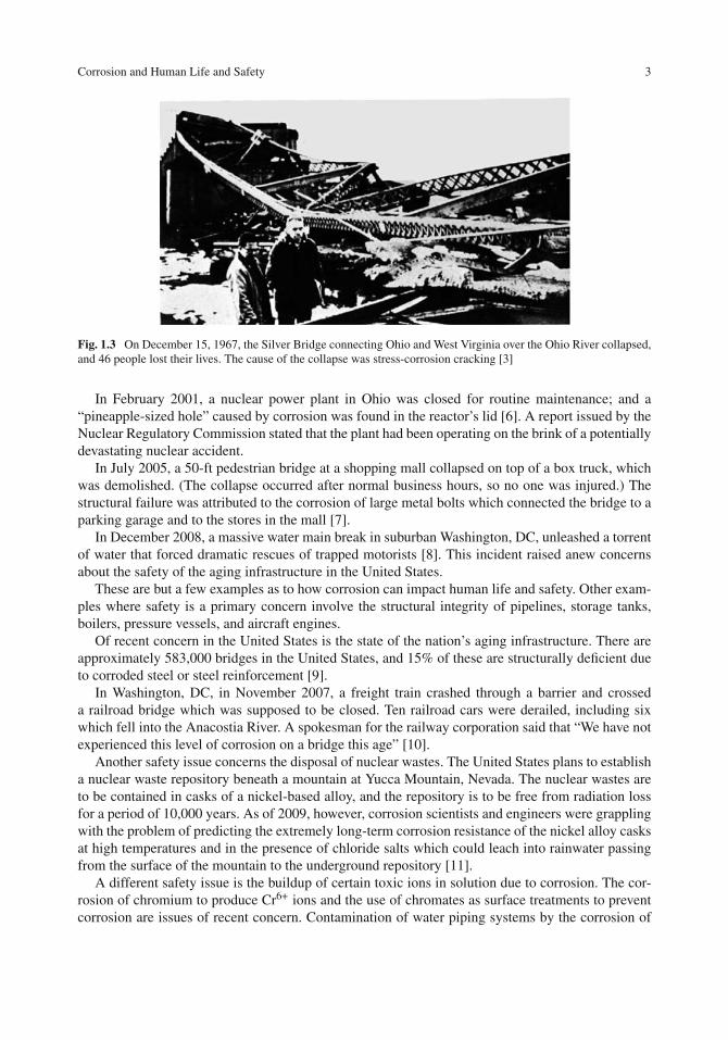
On December 15, 1967, the “Silver Bridge” over the Ohio River linking Point Pleasant, WestVirginia, and Kanauga, Ohio, collapsed carrying 46 people to their deaths [3]. See Fig. 1.3. Thecause of the failure was due to the combined effects of stress and corrosion.
1E. McCafferty, Introduction to Corrosion Science, DOI 10.1007/978-1-4419-0455-3_1,C© Springer Science+Business Media, LLC 2010

2 1 Societal Aspects of Corrosion
Porous-coatedfemoral component(stem)
Femoral head (ball)
Polyethylene liner
Porous-coatedacetabularcomponent(cup)
Fig. 1.1 An artificial hip used in hip-replacement surgery [1]. Titanium alloys or alloys of cobalt–chromium–molybdenum are currently used in artificial hips because these alloys resist corrosion in the human body. Figurecourtesy of Dr. C. Anderson Engh, Anderson Orthopedic Clinic, Alexandria, VA
Fig. 1.2 An example of a harsh corrosive environment [2], in which both the structural and electronic metals in theaircraft will be subject to corrosion
On June 28, 1983, a 100-ft long section of a bridge span on a major US Interstate highwaycollapsed [4]. Three people died and three more were seriously injured. The cause of the collapsewas due to the corrosion of a support pin.
On April 28, 1988, the cabin of a commercial airliner en route from Hilo to Honolulu, Hawaii,suddenly disintegrated, and a flight attendant was tragically lost and 65 passengers were injured [5].The cause of the problem was the combined effects of metal fatigue and corrosion.
Corrosion and Human Life and Safety 3
Fig. 1.3 On December 15, 1967, the Silver Bridge connecting Ohio and West Virginia over the Ohio River collapsed,and 46 people lost their lives. The cause of the collapse was stress-corrosion cracking [3]
In February 2001, a nuclear power plant in Ohio was closed for routine maintenance; and a“pineapple-sized hole” caused by corrosion was found in the reactor’s lid [6]. A report issued by theNuclear Regulatory Commission stated that the plant had been operating on the brink of a potentiallydevastating nuclear accident.
In July 2005, a 50-ft pedestrian bridge at a shopping mall collapsed on top of a box truck, whichwas demolished. (The collapse occurred after normal business hours, so no one was injured.) Thestructural failure was attributed to the corrosion of large metal bolts which connected the bridge to aparking garage and to the stores in the mall [7].
In December 2008, a massive water main break in suburban Washington, DC, unleashed a torrentof water that forced dramatic rescues of trapped motorists [8]. This incident raised anew concernsabout the safety of the aging infrastructure in the United States.
These are but a few examples as to how corrosion can impact human life and safety. Other exam-ples where safety is a primary concern involve the structural integrity of pipelines, storage tanks,boilers, pressure vessels, and aircraft engines.
Of recent concern in the United States is the state of the nation’s aging infrastructure. There areapproximately 583,000 bridges in the United States, and 15% of these are structurally deficient dueto corroded steel or steel reinforcement [9].
In Washington, DC, in November 2007, a freight train crashed through a barrier and crosseda railroad bridge which was supposed to be closed. Ten railroad cars were derailed, including sixwhich fell into the Anacostia River. A spokesman for the railway corporation said that “We have notexperienced this level of corrosion on a bridge this age” [10].
Another safety issue concerns the disposal of nuclear wastes. The United States plans to establisha nuclear waste repository beneath a mountain at Yucca Mountain, Nevada. The nuclear wastes areto be contained in casks of a nickel-based alloy, and the repository is to be free from radiation lossfor a period of 10,000 years. As of 2009, however, corrosion scientists and engineers were grapplingwith the problem of predicting the extremely long-term corrosion resistance of the nickel alloy casksat high temperatures and in the presence of chloride salts which could leach into rainwater passingfrom the surface of the mountain to the underground repository [11].
A different safety issue is the buildup of certain toxic ions in solution due to corrosion. The cor-rosion of chromium to produce Cr6+ ions and the use of chromates as surface treatments to preventcorrosion are issues of recent concern. Contamination of water piping systems by the corrosion of

4 1 Societal Aspects of Corrosion
cadmium components in the water delivery system has also been under scrutiny. Galvanized steelpipes (zinc coated) usually contain some cadmium as does the solder used to join them together[12]. The toxic effect of dissolved lead ions in water pipes constructed of lead metal has long beenrecognized and will be a potential problem as long as lead piping already in place continues in ser-vice. In the winter of 2004, toxic levels of dissolved lead ions were found in the drinking waterin Washington, DC, homes which were serviced by lead pipes [13]. The problem arose from achange in the water treatment procedure which inadvertently disturbed the protective oxide filmon lead, thus allowing the underlying metal to corrode and discharge lead ions into the drinkingwater. Orthophosphates are being added to the water supply in order to re-form the protective oxidefilm on the interior of the lead pipes.
Corrosion of water pipes constructed of copper can sometimes produce the phenomenon of dis-colored “blue water” due to dissolved Cu2+ ions [14, 15]. Concentrations of Cu2+ in excess of 2 mg/Lcan produce a bitter metallic taste.
Economics of Corrosion
In 1978 a comprehensive landmark study was carried out on the economic effects of metallic cor-rosion in the United States [16]. The results of this study were that the total cost of corrosion in theUnited States for the year 1975 was the staggering total of $70 billion or approximately 5% of theGross National Product for that year.
The figure of $70 billion now seems small compared to the results of a more recent study con-ducted between 1999 and 2001 [9], which places the annual direct cost of corrosion in the UnitedStates at $276 billion. This is approximately 3% of the Gross Domestic Product for the period ofstudy.
There have been various previous studies on the economic loss due to corrosion carried out at var-ious times in various industrialized nations [17]. The results have always been consistent. Corrosionconsumes 3–5% of the Gross National Product of that particular nation.
The 1978 report divided the $70 billion cost of corrosion into avoidable costs and unavoidablecosts. Avoidable costs are those which could have been reduced by the application of availablecorrosion control practices. Unavoidable costs are those which require advances in new materialsand in corrosion technology and control. The avoidable costs in the 1978 study were about 15% ofthe total cost of $70 billion.
In addition, in the 1978 study, corrosion costs could be divided into direct costs and indirect costs.The following are some examples of direct costs listed by Uhlig [18]:
1. Capital costs – cost of replacement parts, e.g., automobile mufflers, water lines, hot water heaters,sheet metal roofs.
2. Control costs – maintenance, repair, painting.3. Design costs – extra cost of using corrosion-resistant alloys, protective coatings, corrosion
inhibitors.
Examples of indirect losses are as follows [18]:
1. Shutdown – of power plants and manufacturing plants. (See the example of the nuclear powerplant mentioned earlier.)
A second example is provided by a widespread corrosion problem which occurred in August2006 and forced a shutdown of an oil pipeline in Alaska [19]. Sixteen miles of pipeline had to be

Corrosion and the Conservation of Materials 5
replaced. The oil leakage caused environmental damage and the pipeline closure sent the price ofoil higher.
2. Loss of product due to leakage – leakage of pipelines due to corrosion.3. Contamination of product – In 1991, 100,000 residents of Northern Virginia were surprised to find
that sediment and rust from a temporary pumping station caused discoloration of their drinkingwater [20]. Public officials claimed no health risks were involved, but the prospect of drinkingrusty water was unpleasant and disconcerting. Another example of contamination is provided byfood spoilage due to the corrosion of containers.
Corrosion and the Conservation of Materials
Corrosion destroys metals by converting them into oxides or other corrosion products. Thus, cor-rosion affects the global supply of metals by removing components or structures from service sothat their replacement consumes a portion of the total supply of the earth’s material resources.Environmentalists are interested in conserving our supply of metals not only to conserve minerals butalso to reduce the amount of solid materials at landfills or recycling centers. See Fig. 1.4. In addition,extension of the service life of a metal product or component forestalls additional manufacturing orprocessing, thus decreasing emissions of greenhouse gases.
Fig. 1.4 (Top) Corrosion of vintage US automobiles. (Bottom) A view on the storage, recycling, and reclamation ofused automobiles. Photographs courtesy of Harry’s U-Pull-It, West Hazleton, PA
There are two important issues concerning the world’s supply of metals. The first of these is thequestion as to what total supplies of various metals (or their ores) actually exist in nature. Over thepast 30 years, there have been various assessments as to the earth’s reserves of important metal ores.

6 1 Societal Aspects of Corrosion
Table 1.1 1975 and 1995 estimates of the global reserves of various metals
1975 Estimate of years of supply [19] 1995 Estimate of years of supply [20]
Aluminum 185 162Iron 110 77Nickel 100 43Molybdenum 90 –Chromium 64 –Copper 45 22Zinc 23 16
Selected results from two studies [21, 22] are given in Table 1.1, which shows that there is a finitelimited supply of the metals listed in the table.
Of course, these studies are estimates, and these estimates will change as new supplies of oresare located, as the demand for a given metal changes, and as recycling efforts intensify. In addition,prolonging the service lifetime through the development and use of more effective corrosion-resistantalloys or improved corrosion control measures will stretch the supply of the earth’s natural resources.
A second issue regarding the world’s supply of metals is the geographical location of certainores and minerals. Industrialized nations (primarily the United States, western Europe, and Japan)import 90–100% of their total requirements for chromium, cobalt, manganese, and platinum groupmetals from additional sources [23]. These metals have been referred to as “critical materials.” Thelargest use of chromium is in the manufacture of stainless steels; the largest use of cobalt is inhigh-temperature alloys.
In order to develop a national self-reliance in regard to these critical materials, there is a continu-ing interest in the development of new corrosion-resistant and oxidation-resistant alloys containingsubstitutes for chromium and cobalt. This goal is a formidable challenge for corrosion scientists andengineers, and research in this direction still continues.
In 2006, China announced that it plans to build strategic reserves of various minerals includinguranium, copper, aluminum, manganese, and others that the country urgently needs [24].
Finally, corrosion takes its toll on national landmarks, works of art, and historical artifacts[25–27]. See Fig. 1.5. Preservation and restoration of these objects are an important part of materialconservation. For example, the Statue of Liberty was found to have suffered extensive corrosion inthe iron structure, which supports its copper skin as well as perforation of copper in the torch area[27]. A massive restoration project was completed in 1986.
Despite all the problems with corrosion mentioned so far, corrosion is sometimes (but not usually)good. Rust possesses an attractive reddish brown hue so that protective layers of rust can be attractivein outdoor settings. Figure 1.6 is a photograph of an attractive rust-colored giant watering can, whichcan be found in a garden center south of Alexandria, VA. More about the unusual beneficial aspectsof corrosion is given in Chapter 17.
The Study of Corrosion
In addition to the importance of corrosion discussed above, the study of corrosion is in itself a chal-lenging and interesting pursuit. Corrosion science is an interdisciplinary area embracing chemistry,materials science, and mechanics, as shown in Fig. 1.7. The study of aqueous corrosion processes

The Study of Corrosion 7
Fig. 1.5 Details of the statue of Thomas Jefferson from the Washington Monument (1858), by Thomas Crawford andRandolph Rogers, Virginia State Capitol, Richmond, VA, showing corrosion damage caused by industrial pollution.Photograph courtesy of Phoebe Dent Weil, Northern Light Studio, Florence, MA
Fig. 1.6 Photograph of a rust-covered outdoor work of art near Alexandria, VA
involves the intersection of chemistry and materials science. But the science of mechanics must beadded to understand mechanically assisted corrosion processes, such as stress-corrosion crackingand corrosion fatigue.

8 1 Societal Aspects of Corrosion
Various environments{ } Various
metal systems}{ Specific conditions}{+ + =
Manydifferentcase studies{ }
Concentrations
Temperature
Fluid flow
Stress
Presence of O2Absence of O2Pressure
Organic inhibitors
Biofilms
.
.
.
Corrosion science Corrosion engineering
Basic scientific knowledgeCorrosion mechanisms
Accumulated scientific knowledgeCorrosion protection
SteelsStainless steelsAluminum alloysTitanium alloysCopper alloysNickel alloys
.
.
.Surface alloysMetallic coatingsOrganic coatings
.
.
.
The oceanThe atmosphere
industrial(SO2, H2O)
marine
(Cl –, H2O)
ruralindoor
(SO2, H2O, NH3, NO2)
SoilsChemicals
manufacturing plantsstorage tankstransport linesautomobile coolants
Geothermal brinesThe human body
Pigeon excrement
.
.
.
Fig. 1.7 Various disciplines involved in corrosion science
Other relationships exist between the various disciplines, as shown in Fig. 1.7. A blend of mechan-ics and materials science can address dry fracture processes, and mechanics and chemistry can studychemico-mechanical processes such as adhesion and wear, among others. But again, the science ofchemistry must be included to understand environmentally assisted fracture, i.e., stress-corrosioncracking and corrosion fatigue.
Corrosion Science vs. Corrosion Engineering
Corrosion science is directed toward gaining basic scientific knowledge so as to understand corrosionmechanisms. Corrosion engineering involves accumulated scientific knowledge and its application tocorrosion protection. Ideally, corrosion science and corrosion engineering complement and reinforceeach other, but it has been the author’s observation that most workers in the field of corrosion settleinto one camp or the other. The most effective corrosionists are those who understand both thescience and the engineering of corrosion.

Challenges for Today’s Corrosion Scientist 9
Chemistry
Materials Science Mechanics/Engineering
Aqueous corrosionHigh temperature oxidation
Stress-induced adsorptionSurface energy effectsAdhesionWearNanomechanics
FractureFatigue
Stress-corrosion crackingCorrosion fatigue
Fig. 1.8 Schematic relationship between corrosion science and corrosion engineering and the large number ofvariables which can be operative when corrosion occurs
Figure 1.8 shows schematically the relationship between corrosion science and engineering inaddition to pointing out the many various factors which can be present in any given situation. Thelarge number of possible various environments in which metals are used plus the large number ofpossible metals which can be used (with or without protective coatings) plus the large number of pos-sible specific conditions of use generate a very large number of individual case studies. Corrosionscience aids corrosion engineering by providing connections between various case studies. In addi-tion, the understanding of corrosion mechanisms can lead to possible new corrosion-resistant alloys,better surface treatments, and improved corrosion control measures.
This text emphasizes the corrosion science approach but will also include extensions to practice.
Challenges for Today’s Corrosion Scientist
Based partly on the introductory material in this chapter and partly on more detail to follow insubsequent chapters, several important timely challenges to the corrosion scientist can be listed.These are the following:
1. The development of protective surface treatments and corrosion inhibitors to replace inorganicchromates, which are environmentally objectionable.
2. An improved conservation of materials through the development of corrosion-resistant sur-face alloys which confine alloying elements to the surface rather than employing conventionalbulk alloying. (Initial research strides have been made in this direction, as will be seen inChapter 16).
3. The formulation of a new generation of stainless steels containing replacements for chromiumand other critical metals.
4. An improved understanding of passivity so as to use our fundamental knowledge to guide thedevelopment of alloys having improved corrosion resistance.
5. Understanding the mechanism of the breakdown of passive oxide films by chloride ions andsubsequent pitting of the underlying metal.

10 1 Societal Aspects of Corrosion
6. The development of “smart” organic coatings which can detect a break in the coating and auto-matically dispatch an organic molecule to the required site to both heal the coating and inhibitcorrosion.
7. The ability to predict the lifetime of metals and components from short-term experimentalcorrosion data.
It is suggested that the reader refer back to these challenges as he or she proceeds through thistext. Perhaps the reader can provide additions to this list.
Problems
1. Examples of corrosion can be found in everyday life. Describe one example which you have seen.Is this particular instance of corrosion primarily an example of wastage of materials, an economicloss, or a safety issue? Or is this example a combination of some of these factors? Note: manyphotographs of corrosion can be found on the Internet. If you are not familiar with an example ofcorrosion, select one photograph from the Internet and then complete this problem.
2. Based on your everyday experience, name one method of corrosion protection which you haveobserved in use.
3. Ordinary garbage cans are often constructed from galvanized steel (a coating of zinc on steel).What direct costs and indirect costs of corrosion are involved if you need to replace such a garbagecan with a similar one because your old one is no longer useable due to severe corrosion?
4. Various studies on the annual cost of corrosion always conclude that corrosion amounts to 3–5%of a nation’s Gross National Product, no matter in what year the study was undertaken. Does thismean that corrosion science and engineering are not making any headway?
Note: Before answering this problem, ask yourself the following additional questions: (a) Canyou think of any industries which would not exist without the development of corrosion-resistantalloys or corrosion control measures? (b) Are metals being required to perform in increasinglysevere environments? (Recall Fig. 1.2). (c) Would you like your automobile to have a longerlifetime before its paint system fails and is overtaken by rusting?
5. Refer to Fig. 1.8 which illustrates the interdisciplinary nature of corrosion. What additionalformal disciplines of study would be useful in expanding our knowledge of corrosion?
6. Increasing the corrosion resistance of a metal part or structure so as to make the metal piece lastlonger is one way to conserve the earth’s supply of metals. What other practices can be undertakento help stretch our natural supply of metals?
References
1. “Hip Replacement Patient Information Booklet”, Anderson Orthopedic Institute, Alexandria, VA, p. 1.2. Front cover of “AMPTIAC Quarterly”, (Advanced Materials and Process Technology Information Analysis
Center), AMPTIAC Quart., 7 (4), (2003).3. B. F. Brown, “Stress Corrosion Cracking Control Measures”, National Bureau of Standards Monograph 156,
Washington, DC (1977).4. “National Transportation Safety Board Report HAR-84/03”, June 28, 1983, Web site http://www.ntsb.gov, July
(2004).5. “Aging Airplanes”, S. Derra, R & D Magazine, p. 29, January (1970).6. “FirstEnergy Faced String of Difficulties”, Washington Post, p. E1, August 19 (2003).7. “Walkway Collapse Shuts Laurel Mall”, Washington Post, p. B4, July 2 (2005).

References 11
8. “Tense Rescues Follow Massive Water Main Break”, washingtonpost.com, December 23 (2008).9. G. H. Koch, M. P. H. Brongers, N. G. Thompson, Y. P. Virmani, and J. H. Payer, “Corrosion Costs and
Preventative Strategies in the United States”, Mater. Perform., 42 (Supplement), 3, July (2002).10. “At Accident Site, a Bridge Too Far Corroded”, Washington Post, p. B2, November 15 (2007).11. “DOE Defends ‘Hot’ Repository Design”, C & E News, p. 19, May 31 (2004).12. Excerpted from E. M. Haas, “Staying Healthy with Nutrition”, Web site http://www.healthy.net, July (2004).13. “Agencies Brushed Off Lead Warnings”, Washington Post, p. A1, February 29 (2004).14. Australian Water Association, “Fact Sheet: The problem of blue-water and copper pipes”, July (2004).15. D. J. Fitzgerald, Am. J. Clin. Nutr., 67 (5), 1098S, (Supplement S) (1998).16. L. H. Bennet, J. Kruger, R. I. Parker, E. Passiglia, C. Reimann, A. W. Ruff, H. Yakowitz, and E. B. Berman,
“Economic Effects of Metallic Corrosion in the United States”, National Bureau of Standards Special Publication511, Washington, DC (1978).
17. J. Kruger in “Uhlig’s Corrosion Handbook”, R. W. Revie, Ed., p. 3, John Wiley, New York (2000).18. H. H. Uhlig and W. R. Revie, “Corrosion and Corrosion Control”, Chapter 1, John Wiley, New York (1985).19. “Pipeline Closure Sends Oil Higher”, Washington Post, p. A1, August 8 (2006).20. “Rusty water rattles N. Va. residents”, Fairfax J., p. A5, April 29 (1991).21. J. J. Harwood, ASTM Stand. News, 3 (1), 12 (1975).22. T. E. Norgate and W. J. Rankin, “The role of metals in sustainable development”, in “Proceedings, Green
Processing 2002, International Conference on the Sustainable Processing of Minerals”, p. 49, Australian Instituteof Mining and Metallurgy, May (2002).
23. W. L. Swager in “Battelle Today” Vol. 18, p. 3, June (1980).24. “China to Build Up Mineral Reserves, Ministry Says”, Washington Post, p. D10, May 17 (2006).25. B. F. Brown et al., “Corrosion and Metal Artifacts”, National Bureau of Standards Special Publication 479,
Washington, DC (1977).26. R. Baboian, Mater. Perform., 33 (8), 12 (1994).27. N. Nielsen, Mater. Perform., 23 (4), 78 (1984).

Chapter 2Getting Started on the Basics
Introduction
What is Corrosion?
Corrosion is the destructive attack of a metal by its reaction with the environment. A more scientificdefinition of corrosion will be given later in this chapter, but the description just provided is a goodworking one. As seen in Chapter 1, there are very many different specific environments which arepossible, depending upon how the particular metal is used. The most general case is that in whichthe environment is a bulk aqueous solution. For atmospheric corrosion, the aqueous solution is acondensed thin-layer rather than a bulk solution, but the overall principles are, for the most part, thesame.
Note that the word “corrosion” refers to the degradation of a metal by its environment. Othermaterials such as plastics, concrete, wood, ceramics, and composite materials all undergo dete-rioration when placed in some environment; but this text will deal with only the corrosion ofmetals.
The word “rusting” applies to the corrosion of iron and plain carbon steel. Rust is a hydrated ferricoxide which appears in the familiar color of red or dark brown. See Fig. 2.1. Thus, steel rusts (andalso corrodes), but the non-ferrous metals such as aluminum, copper, and zinc corrode (but do notrust). The term “white rust” is often used to describe the powdery white corrosion product formed onzinc. The “white rusting” of sheets of galvanized steel (zinc-coated steel) is a frequent problem if thesheets are stacked and stored under conditions of high relative humidity. Condensation of moisturebetween stacked sheets will often lead to “white rusting”.
Physical Processes of Degradation
Metals may undergo degradation by physical processes which occur in the absence of a chemicalenvironment. Physical degradation processes include the following:
Fracture – failure of a metal under an applied stress.Fatigue – failure of a metal under an applied repeated cyclic stress.Wear – rubbing or sliding of materials on each other.Erosion or cavitation erosion – mechanical damage caused by the movement of a liquid or the
collapse of vapor bubbles against a metal surface.Radiation damage – interaction of elementary particles (e.g., neutrons or metal ions) with a
solid metal so as to distort the metal lattice.
13E. McCafferty, Introduction to Corrosion Science, DOI 10.1007/978-1-4419-0455-3_2,C© Springer Science+Business Media, LLC 2010

14 2 Getting Started on the Basics
Red rust
Waterline
Fig. 2.1 An example of red rust showing the corrosion of a ship near the waterline. Photograph courtesy of James R.Martin, Naval Research Laboratory, Washington, DC
Environmentally Assisted Degradation Processes
Each of the physical degradation processes above can be assisted or aggravated in the pres-ence of an aqueous environment. Thus, corresponding to each of the degradation processes listedimmediately above are environmentally assisted counterparts, as given in Table 2.1. In each case,metal degradation is intensified by the conjoint action of the physical process and the chemicalenvironment.
Examples of each of these environmentally assisted processes are also given in Table 2.1, andmore detail is provided in Chapter 11.
Table 2.1 Physical degradation processes and their environmentally assisted counterparts
Environmentally assistedprocess
Example of environmentally- assistedprocess
Fracture Stress-corrosion cracking Stress-corrosion cracking of bridgecables, of landing gear on aircraft
Fatigue Corrosion fatigue Vibrating structures, such as aircraftwings, bridges, offshore platforms
Wear Fretting corrosion Ball bearings in chloride-contaminated oilCavitation erosion Cavitation corrosion Ship propellers, pumps, turbine blades,
fast fluid flow in pipesRadiation damage Radiation corrosion Increased susceptibility of stainless steels
to dissolution or to stress-corrosioncracking [1, 2]

Electrochemical Reactions 15
Electrochemical Reactions
Corrosion is an electrochemical process. That is, corrosion usually occurs not by direct chemicalreaction of a metal with its environment but rather through the operation of coupled electrochemicalhalf-cell reactions.
Half-Cell Reactions
A half-cell reaction is one in which electrons appear on one side or another of the reaction as written.If electrons are products (right-hand side of the reaction), then the half-cell reaction is an
oxidation reaction.If electrons are reactants (left-hand side of the reaction), then the half-cell reaction is a reduction
reaction.
Anodic Reactions
The loss of metal occurs as an anodic reaction. Examples are
Fe(s)→ Fe2+(aq)+ 2e− (1)
Al(s)→ Al3+(aq)+ 3e− (2)
2Cu(s)+ H2O(1)→ Cu2O(s)+ 2H+(aq)+ 2e− (3)
where the notations (s), (aq), and (l) refer to the solid, aqueous, and liquid phases, respectively. Eachof the above reactions in Eqs. (1), (2), and (3) is an anodic reaction because of the following:
(1) A given species undergoes oxidation, i.e., there is an increase in its oxidation number.(2) There is a loss of electrons at the anodic site (electrons are produced by the reaction).
These ideas are illustrated schematically in Fig. 2.2.The following reaction is also an anodic reaction:
Fe(CN)4−6 (aq)→ Fe(CN)3−
6 (aq)+ e− (4)
Fe+2
Fe
Anodic reaction: Fe Fe+2 + 2e–
Solution
e–
e–
Fig. 2.2 Example of an anodic reaction – the dissolution of iron

16 2 Getting Started on the Basics
The oxidation number of the Fe species on the left, i.e., in the ferrocyanate ion, is +2, and theoxidation number of Fe in the ferricyanate ion on the right is +3. Thus, there is an increase inoxidation number. In addition, electrons are produced in the electrochemical half-cell reaction, soEq. (4) is an anodic reaction. By the same reasoning the following is also an anodic reaction:
Cr3+(aq)+ 4H2O→ CrO2−4 (aq)+ 8H+(aq)+ 3e− (5)
Although Eqs. (4) and (5) are anodic reactions, they are not corrosion reactions. There is a chargetransfer in each of the last two equations, but not a loss of metal. Thus, not all anodic reactions arecorrosion reactions. This observation allows the following scientific definition of corrosion:
Corrosion is the simultaneous transfer of mass and charge across a metal/solution interface.
Cathodic Reactions
In a cathodic reaction
(1) A given species undergoes reduction, i.e., there is a decrease in its oxidation number.(2) There is a gain of electrons at the cathodic site (electrons are consumed by the reaction).
An example of a cathodic reaction is the reduction of two hydrogen ions at a surface to form onemolecule of hydrogen gas:
2H+(aq)+ 2e− → H2(g) (6)
This is the predominant cathodic reaction in acidic solutions. See Fig. 2.3 for a schematicrepresentation of this reduction reaction.
Fe
Cathodic reaction: 2 H+ + 2e– H2
Solution
e–
e–
H+
H+ H2
Fig. 2.3 Example of a cathodic reaction – hydrogen evolution on iron immersed in an acid solution
Another common cathodic reaction is the reduction of dissolved oxygen to hydroxyl ions, areduction reaction which occurs in neutral or basic solutions.
O2(g)+ 2H2O+ 4e− → 4OH−(aq) (7)

Electrochemical Reactions 17
Coupled Electrochemical Reactions
On a corroding metal surface, anodic and cathodic reactions occur in a coupled manner at differentplaces on the metal surface. See Fig. 2.4, which illustrates this behavior for an iron surface immersedin an acidic aqueous environment. At certain sites on the iron surface, iron atoms pass into solutionas Fe2+ ions by Eq. (1). The two electrons produced by this anodic half-cell reaction are consumedelsewhere on the surface to reduce two hydrogen ions to one H2 molecule.
Fe+2
e–
e–
Fe
At anodic sites: Fe Fe+2 + 2e–
At cathodic sites: 2 H+ + 2e– H2
Overall reaction: Fe + 2 H+ Fe+2 + H2
Solution
H+H+ H2
Fig. 2.4 Coupled electrochemical reactions occurring at different sites on the same metal surface for iron in an acidsolution. The electrons lost by the oxidation of Fe atoms are consumed in the reduction of two H+ ions to formhydrogen gas (H2)
The reason that two different electrochemical half-cell reactions can occur on the same metalsurface lies in the heterogeneous nature of a metal surface. Polycrystalline metal surfaces contain anarray of site energies due to the existence of various crystal faces (i.e., grains) and grain boundaries.In addition, there can be other defects such as edges, steps, kink sites, screw dislocations, and pointdefects. Moreover, there can be surface contaminants due to the presence of impurity metal atomsor to the adsorption of ions from solution so as to change the surface energy of the underlying metalatoms around the adsorbate. Some of these effects are illustrated in Fig. 2.5.
Adsorbedion from solution
Impurity atom
Grain boundaries
Kink
Step
Missing atom(vacancy)
Screwdislocation
Fig. 2.5 The heterogeneous nature of a metal surface showing various types of imperfections
Metal atoms at the highest energy sites are most likely to pass into solution. These high-energysites include atoms located at the edges and corners of crystal planes, for example. Stressed surfacesalso contain atoms that are reactive because they have a less stable crystalline environment. When a
18 2 Getting Started on the Basics
metal is cold worked or shaped, the metal lattice becomes strained, and atoms located in the strainedregions tend to go into solution more readily than do atoms in unstrained regions. Once the process ofmetal dissolution process begins, a new energy distribution of sites is established. Then, the positionsof anodic and cathodic surface sites change randomly with time so that the overall effect is uniformcorrosion of the metal.
The overall chemical reaction is thus the sum of the two half-cell reactions. For the process shownin Fig. 2.4:
At the local anodes
Fe(s)→ Fe2+(aq)+ 2e− (1)
At the local cathodes
2H+(aq)+ 2e− → H2(g) (6)
The overall reaction is the sum of these two half-cell reactions:
Fe(s)+ 2H+(aq)→ Fe2+(aq)+ H2(g) (8)
Figure 2.4 illustrates the four conditions which are necessary for corrosion to occur. These are thefollowing:
(1) An anodic reaction(2) A cathodic reaction(3) A metallic path of contact between anodic and cathodic sites(4) The presence of an electrolyte
An electrolyte is a solution which contains dissolved ions capable of conducting a current. Themost common electrolyte is an aqueous solution, i.e., water containing dissolved ions; but otherliquids, such as liquid ammonia, can function as electrolytes.
Figure 2.6 illustrates the coupled electrochemical reactions for an iron surface immersed in a neu-tral or a basic aqueous solution. Figure 2.7 schematically shows the continuation of these reactionsen route to the formation of hydrated ferric oxide (rust).
A Note About Atmospheric Corrosion
The need for the presence of an electrolyte as a condition for corrosion to occur is illustratedby the phenomenon of atmospheric corrosion, i.e., the corrosion of metals in the natural outdooratmosphere. Vernon [3] observed that a critical relative humidity exists below which atmosphericcorrosion is negligible and above which corrosion occurs. Figure 2.8 shows Vernon’s results for ironexposed to water vapor containing 0.01% SO2 [3]. It can be seen that the corrosion of iron occursabove 60% relative humidity. (The critical relative humidity is typically 50–70% for most metals.)
The critical relative humidity is the condition where multimolecular layers of water vapor phys-ically adsorb from the atmosphere onto the oxide-covered metal surface. (Physical adsorptioninvolves the accumulation of a gas or a liquid on a solid surface due to the secondary short-rangeforces.) Oxide films on iron can contain various iron oxides, including Fe2O3. Figure 2.9 showsadsorption isotherms for water on α-Fe2O3 [4], in which it is seen that two or more layers of adsorbed

Electrochemical Reactions 19
Fe+2
e–
e–
Fe
At anodic sites: 2 [ Fe (s) Fe+2 (aq) + 2e–]
At cathodic sites: O2 (g) + 2 H2O (l) + 4e– 4 OH–
(aq)
Overall reaction: 2 Fe (s) + O2 (g) + 2 H2O (l) 2 Fe+2 (aq) + 4 OH–(aq)
Solution
Fe+2
O2 H2O
H2OOH– OH–
OH– OH–
e–
e–
Fig. 2.6 Coupled electrochemical reactions occurring at different sites on the same metal surface for iron in a neutralor a basic solution
(a)
2 Fe(OH)2(s) + (x–1) H2O (l) 2O3. x H2O (s) + 2 H+ (aq) + 2e–
Fe+2(aq) + 2 OH–(aq) Fe(OH)2 (s)
Fe
Fe+2OH–
Solution
Fe
Fe
SolutionSolution
Fe
Fe2O3. x H2O
(b)
Fe
Fig. 2.7 The continuation of reactions initiated in Fig. 2.6. (a) The precipitation of ferrous hydroxide on the ironsurface. (b) The conversion of ferrous hydroxide to a hydrated ferric oxide
water are formed at relative humidities greater than 60%. Thus, the thin layer of electrolyte requiredfor atmospheric corrosion to occur is provided at or above this critical relative humidity.
Secondary Effects of Cathodic Reactions
Cathodic reactions do not involve the loss of the metal substrate and thus are not per se corrosionreactions. However, cathodic reactions are very important for two reasons. First, as seen above, thecathodic reaction is coupled to the anodic reaction so that impeding the cathodic reaction will alsoimpede the anodic reaction. Similarly, accelerating the cathodic reaction will also accelerate theanodic reaction.

20 2 Getting Started on the Basics
0.0
0.2
0.4
0.6
0.8
1.0
1.2
0 20 40 60 80 100
Wei
ght G
ain
in m
g/cm
2
Relative Humidity in Percent
Fig. 2.8 Corrosion of iron in air containing 0.01% SO2 after 55 days of exposure showing the effect of a criticalrelative humidity (approximately 60%). Redrawn from Vernon [3] by permission of the Royal Society of Chemistry
0.0
1.0
2.0
3.0
4.0
5.0
0.0 0.2 0.4 0.6 0.8 1.0
35o C
25o C
15o C
5o C
Cov
erag
e in
Num
ber
of W
ater
laye
rs
Relative Pressure, P/Po (Relative Humidity)
Fig. 2.9 Adsorption isotherms for water vapor on α-Fe2O3 [4] showing that multimolecular layers of adsorbed waterare formed at a relative humidity of 60% and higher
In addition, cathodic reactions may induce corrosion through secondary effects caused by theproducts of the cathodic reaction. In stress-corrosion cracking (considered in Chapter 11), the nar-row confines of the stress-corrosion crack limit the exchange of dissolved metal ions with the bulkelectrolyte, as shown in Fig. 2.10. Thus, metal cations, in this case Fe2+ ions, accumulate within thestress-corrosion crack and are then hydrolyzed to form hydrogen ions:
Fe2+(aq)+ H2O(1)→ FeOH+(aq)+ H+(aq) (9)

Three Simple Properties of Solutions 21
Limited exchangeof bulk and local electrolytes
Bulksolution
Crackelectrolyte
Fe (s) Fe+2 (aq) + 2e–
Fe+2 (aq) + H2O (l) FeOH+ (aq) + H+ (aq)
H
H
Fe
Crack tip
Hadsorbed Habsorbed
H+ (aq) + e– Hadsorbed
Fig. 2.10 Crack tip reactions can produce hydrogen atoms available for migration into the metal at stressed regionsahead of the crack tip
The local environment within the crack tip becomes acidified due to the production of hydrogenions. As discussed earlier, in acidic solutions, the major cathodic reaction is the reduction of hydro-gen ions. Thus, hydrogen ions produced within the crack can be reduced to form hydrogen atomswhich adsorb on the metal surface:
H+(aq)+ e− → H(adsorbed) (10)
Some of these hydrogen atoms then migrate into the stressed region ahead of the crack tip (ratherthan combining to form hydrogen gas). The presence of hydrogen atoms in stressed areas promotesthe growth of the stress-corrosion crack by the process of hydrogen embrittlement, as discussed inChapter 11.
In neutral or basic solutions, the major cathodic reaction is the reduction of dissolved oxygen,as given by Eq. (7). Note that hydroxyl ions are produced by this cathodic reaction. In a thin-layerelectrolyte, such as that which exists in atmospheric corrosion, the continued production of OH– ionsand their accumulation will cause an increase in the pH of the thin layer of solution. (See Problem2.12 at the end of this chapter.) If the pH increases, i.e., the solution becomes more alkaline, thenthe corrosion behavior of the underlying substrate can be altered. Aluminum, for example, has a lowcorrosion rate at pH 7, but the corrosion rate increases dramatically with increasing pH, as shown inFig. 2.11 [5].
Three Simple Properties of Solutions
The pH is a measure of the acidity (or alkalinity) of a solution and is defined as
pH = −log[H+] = log1
[H+](11)
where [H+] is the concentration of hydrogen ions in solution. Neutral solutions have a pH valueof 7.0, while acid solutions have pH values less than 7.0 and alkaline (basic) solutions have pHvalues greater than 7.0. Most solutions have pH values between 0 and 14, but lower and highervalues are possible. (For example, the pH of 12 M HCl is –1.1.)

22 2 Getting Started on the Basics
0.001
0.01
0.1
1
10
100
1000
0 2 4 6 8 10 12 14
Cor
rosi
on R
ate
in m
g/cm
2 da
y
pH
Aluminum in solutions
saturated with air
Fig. 2.11 Aluminum has high corrosion rates for both acidic (low pH) and basic (high pH) solutions [5]. Reproducedby permission of ECS – The Electrochemical Society
The concentration of hydrogen ions and of hydroxyl ions (OH–) in aqueous solutions are relatedby the following equation:
Kw = [H+][OH−] = 1.0× 10⁻¹⁴ (12)
where Kw is called the ionization constant for water.When an ionic solid (acid, base, or salt) dissociates into ions in solution:
AxBy(s) � xAy+(aq)+ yBx−(aq) (13)
the solubility product Ksp is defined by
Ksp = [Ay+]× [Bx−]y (14)
where [Ay+] and [Bx–] are the concentrations of the dissolved ions. If the ion product [Ay+]x [Bx–]y
exceeds the tabulated value of Ksp, then precipitation of solid AxBy occurs. Otherwise, precipitationdoes not occur.
Example 2.1: The corrosion of aluminum produces Al3+ ions in solution. Write an expression forthe solubility product of aluminum hydroxide. If the concentration of Al3+ ions in solution is 1.0 ×10⁻⁶ M, will aluminum hydroxide precipitate at pH 9.0? The tabulated value for Ksp for aluminumhydroxide is 1.3 × 10⁻³³.
Solution: The equilibrium between Al(OH)3 and its ions is
Al(OH)3(s) � Al3+(aq)+ 3OH−(aq)
and Ksp is given by
Ksp = [Al3+][OH−]3

The Faraday and Faraday’s Law 23
where [Al3+] and [OH–] are the concentrations in moles per liter of Al3+ and OH–, respectively.At pH 9.0
9.0 = −log[H+]
or [H+] = 1.0 × 10⁻⁹ M. The concentration of OH– is then obtained from the following equation:
(1.0× 10⁻⁹)[OH−] = 1.0× 10⁻¹⁴
or [OH–] = 1.0 × 10⁻⁵. Then
[Al3+][OH−]3 = (1.0× 10⁻⁶)(1.0× 10⁻⁵)3 = 1.0× 10⁻²¹
This product is much greater than Ksp for aluminum hydroxide so that Al(OH)3 is precipitated underthe conditions given.
The Faraday and Faraday’s Law
As stated earlier, the process of corrosion involves simultaneous charge transfer and mass transferacross the metal/solution interface.
The unit of charge is the coulomb, which is the product of the current and its time of passage. Theunit of mass is, of course, the gram, which can be obtained from the number of equivalents of metallost and the equivalent weight of the metal.
The link between charge transfer and mass transfer is the Faraday (F):
F ≡ 96, 500 C
equivalent
Faraday’s law states that the mass (w) of metal corroded is given by
W = I t A
n F(15)
where I is the current in amperes, t is the time in seconds, A is the atomic weight of the metal,and n is the number of equivalents transferred per mole of metal. For example, n = 2 for the anodicreaction
Fe(s)→ Fe2+(aq)+ 2e−
whereas n = 3 for
Al(s)→ Al3+(aq)+ 3e−
The various simple concepts associated with Faraday’s law are assembled for convenience inTable 2.2. It should be noted that all Faraday’s law problems can be worked through by using simpleunits analysis.

24 2 Getting Started on the Basics
Table 2.2 Useful information regarding Faraday’s law
Current in amperes= charge in coulombs
time in seconds
There are96, 500 C
equivalent.
For the anodic half-cell rection M→ Mn+, there aren equivalents
mole M.
Example 2.2: Plain carbon steel immersed in seawater has a uniform corrosion rate expressed as apenetration rate of 5.0 mpy (mils per year, where 1 mil= 0.001 in.). The density of iron is 7.87 g/cm3.The atomic weight of Fe is 55.8 g/mol.
(a) Calculate the weight loss after 1 year.(b) Calculate the corresponding corrosion current density in microamperes per square centimeter
assuming that the corrosion current is given by
Fe −→ Fe2+ + 2e−
Solution: (a) The weight loss is given by
(5.0 mils
year
)(0.001 in
mil
)(2.54 cm
in.
)(7.87g
cm3
)= 0.10 g
cm2 year
(b) The corrosion current density is:
(0.10 g
cm2 year
)(1 year
356 days
)(1 day
24 h
)(1h
3600 s
)(1 mol
55.8 g
)(2 equiv
mol
)(96,500 C
equiv
)=(
1.10 × 10⁻⁵
s cm2
)
or
(1.10 × 10⁻⁵ A
cm2
)(1 × 10⁶μA
A
)= 11 μA
cm2
Units for Corrosion Rates
Common units for the corrosion current density include microamperes per square centimeter, mil-liamperes per square centimeter, and amperes per square meter. Various units have been used whenthe mass loss is the experimentally observed variable. These include grams per square centimeter perday and mdd (milligrams per square decimeter per day). Sometimes the corrosion rate is given as auniform penetration rate. Units include ipy (inches per year), inches per month, and mpy (mils peryear, where 1 mil = 0.001 in.). The units millimeters per year and micrometers per year have also

Uniform vs. Localized Corrosion 25
Table 2.3 Relative severity of corrosion rates
Corresponding corrosion current density fromFaraday’s law (in μA/cm2)Relative
corrosionresistance
Corrosionrate (mils peryear, mpy) Aluminuma Ironb Leadc
Outstanding < 1 2.3 2.2 0.85Excellent 1–5 2.3–12 2.2–11 0.8–4.3Good 5–20 12–47 11–43 4.2–17Fair 20–50 47–180 43–109 17–42Poor 50–200 180–470 109–430 42–170Unacceptable > 200 > 470 > 430 > 170
aAl→ Al3+ + 3e−bFe→ Fe2+ + 2e−cPb→ Pb2+ + 2e−
been used. Collections of corrosion rate data are available for various metals and alloys in differentenvironments [6–10].
A compilation of corrosion rate data by NACE International [6] provides a qualitative rankingof the severity of corrosion rates in terms of the units mils per year. See Table 2.3, which also listscorresponding electrochemical corrosion rates in microamperes per square centimeter calculatedfrom Faraday’s law for aluminum (a light metal), iron (a transition metal), and lead (a heavy metal).The electrochemical corrosion rate depends, of course, on the atomic weight of the metal and theoxidation state of the metal ion, but in general, corrosion rates greater than about 100 μA/cm2 areconsidered unacceptable.
Rigorous metric units, such as nanometers per second, have not held wide appeal to corrosionscientists or engineers.
Uniform vs. Localized Corrosion
There are two major types of corrosion: uniform corrosion and localized corrosion.Uniform corrosion and three forms of localized corrosion are illustrated schematically inFig. 2.12.
In uniform corrosion, the metal is attacked more or less evenly over its entire surface. No portionsof the metal surface are attacked more preferentially than others, and the metal piece is thinned awayby the process of corrosion until the piece eventually fails. Examples include the corrosion of zinc inhydrochloric acid and the atmospheric corrosion of iron or steel in aggressive outdoor environments.In these cases, localized anodes and cathodes exist and operate as discussed earlier. However, thepositions of these localized anodes and cathodes change with time and “dance” all over the metalsurface so that the overall effect is that the metal is attacked uniformly. Figure 2.13 shows an exampleof uniform corrosion.
In localized corrosion, local anodes and cathodes also exist, but their positions become fixedso that corrosion proceeds on established portions of the metal surface. An example of localizedcorrosion is seen in Fig. 2.14, which shows that corrosion is limited to certain fixed locations onthe metal surface. The three most prevalent forms of localized corrosion are (i) pitting, (ii) crevicecorrosion, and (iii) stress-corrosion cracking. In pitting, the metal is attacked at certain fixed siteson the metal surface where the otherwise protective oxide film breaks down locally, usually due

26 2 Getting Started on the Basics
uniform
corrosion
Oxide film
geometrical crevice
Oxide film
loss inmetal thickness}
crevicecorrosion
Fig. 2.12 Schematic representation of uniform corrosion (top) and three different forms of localized corrosion
Fig. 2.13 The uniform corrosion of zinc after immersion in hydrochloric acid
to the action of chloride ions. In crevice corrosion, the metal within narrow clearances undergoeslocalized attack. In stress-corrosion cracking, the combined action of an applied stress and a chemicalenvironment causes the initiation and propagation of cracks in the metal.

Uniform vs. Localized Corrosion 27
13 inches
Fig. 2.14 An example of localized corrosion, showing a hole in an automobile muffler caused by the combined actionof hot exhaust gases, condensed moisture, and road spray consisting of water and de-icing salts. For an example oflocalized corrosion on a much finer scale, see Fig. 10.43
Each of these three forms of localized corrosion shares the common feature that there is a geomet-rical constraint on the system. In the case of pitting corrosion, the geometrical constraint is the capof corrosion products above the propagating pit. For crevice corrosion and stress-corrosion crack-ing, the geometrical constraints are the narrow dimensions of the crevice or the crack itself. Morethorough discussions of these three types of localized corrosion are given in Chapters 10 and 11.
The Eight Forms of Corrosion
Fontana and Greene [11] have conveniently classified the various types of corrosion into eight forms.The eight forms of corrosion are as follows:
(1) Uniform attack (or general corrosion)(2) Crevice corrosion(3) Pitting(4) Stress-corrosion cracking(5) Galvanic corrosion (two metal corrosion)(6) Intergranular corrosion(7) Selective leaching (dealloying)(8) Erosion corrosion
We have already mentioned four of these forms in the previous section of this chapter. Moredetails on uniform corrosion are given in Chapters 6, 7, and 8, crevice corrosion and pitting arediscussed further in Chapter 10, and stress-corrosion cracking is considered in Chapter 11.
Galvanic corrosion occurs when two metals are in mechanical or electrical contact. In a corrosiveenvironment, one of the metals acts as an anode and undergoes corrosion, while the second metal actsas a cathode and remains unattacked. Galvanic corrosion is discussed in more detail in Chapter 5.
Intergranular corrosion is the pronounced localized attack that occurs in narrow regions at orimmediately adjacent to grain boundaries of an alloy. Type 304 stainless steel (which contains 18%Cr and 8% Ni as well as small amounts of carbon) is subject to intergranular corrosion if the stainlesssteel is heated to the temperature range of 425–790◦C (and then cooled). The stainless steel is saidto be sensitized and is susceptible to intergranular corrosion. During sensitization, carbon diffuses to

28 2 Getting Started on the Basics
Cr-depleted zone(< 12% Cr)(subject to attack)
Chromium carbide
Bulk grain(18% Cr)
Grain boundary
Fig. 2.15 Schematic representation of sensitized stainless steel. After Myers [12]. Chromium-depleted zones adjacentto grain boundaries are susceptible to intergranular corrosion
the grain boundaries where it combines with chromium to form chromium carbide precipitates (suchas Cr23C6). This process depletes chromium from the areas in and adjacent to the grain boundaries sothat these regions locally contain less than the 12% Cr required for a stainless steel. Thus, localizedcorrosion occurs in certain aqueous environments in the form of intergranular corrosion, as depictedin Fig. 2.15.
Selective leaching or dealloying is the preferential removal of one element from a solid alloy bycorrosion. Examples include the preferential removal of zinc from copper zinc alloys (dezincifica-tion) and the preferential removal of iron from gray cast iron (graphitic corrosion) [11]. (Gray castiron contains carbon in the form of graphite.)
Erosion–corrosion is caused by the mechanical action provided by the movement of a corrosiveliquid against the metal surface. This form of corrosion is discussed further in Chapter 11.
Problems
1. Are the following degradation processes strictly physical processes or do they also involve anenvironmentally assisted component?
(a) The cleaning of a metal piece by sandblasting.(b) Damage to the interior of a pipeline used to transport an abrasive slurry of coal.(c) The deterioration of steel reinforcing bars in concrete bridges.(d) The fracture of an artificial hip constructed of an alloy of cobalt and chromium when in
service in the human body.
2. When pure zinc undergoes corrosion in aerated hydrochloric acid, what is the anodic half-cellreaction? Which cathodic half-cell reactions are possible? What is the overall reaction in eachcase?
3. Type 430 stainless steel is an alloy of iron and chromium. Suppose that this alloy is used inflowing seawater (pH 8.0) which contains dissolved oxygen. Write the possible anodic half-cellreactions. What is the cathodic half-cell reaction?
4. The corrosion of copper in water occurs by the reaction
2Cu(s)+ O2(g)+ 2H2O(1)→ 2Cu2+(aq)+ 4OH−(aq)
(a) Separate this overall reaction into its two half-cell reactions.
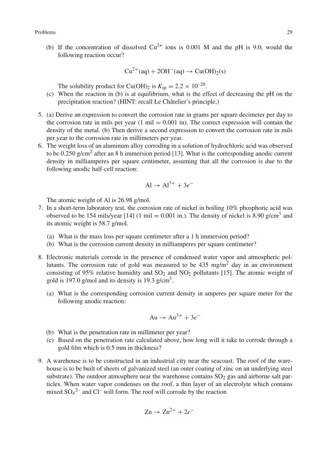
Problems 29
(b) If the concentration of dissolved Cu2+ ions is 0.001 M and the pH is 9.0, would thefollowing reaction occur?
Cu2+(aq)+ 2OH−(aq)→ Cu(OH)2(s)
The solubility product for Cu(OH)2 is Ksp = 2.2 × 10⁻²⁰.(c) When the reaction in (b) is at equilibrium, what is the effect of decreasing the pH on the
precipitation reaction? (HINT: recall Le Châtelier’s principle.)
5. (a) Derive an expression to convert the corrosion rate in grams per square decimeter per day tothe corrosion rate in mils per year (1 mil = 0.001 in). The correct expression will contain thedensity of the metal. (b) Then derive a second expression to convert the corrosion rate in milsper year to the corrosion rate in millimeters per year.
6. The weight loss of an aluminum alloy corroding in a solution of hydrochloric acid was observedto be 0.250 g/cm2 after an 8 h immersion period [13]. What is the corresponding anodic currentdensity in milliamperes per square centimeter, assuming that all the corrosion is due to thefollowing anodic half-cell reaction:
Al→ Al3+ + 3e−
The atomic weight of Al is 26.98 g/mol.7. In a short-term laboratory test, the corrosion rate of nickel in boiling 10% phosphoric acid was
observed to be 154 mils/year [14] (1 mil = 0.001 in.). The density of nickel is 8.90 g/cm3 andits atomic weight is 58.7 g/mol.
(a) What is the mass loss per square centimeter after a 1 h immersion period?(b) What is the corrosion current density in milliamperes per square centimeter?
8. Electronic materials corrode in the presence of condensed water vapor and atmospheric pol-lutants. The corrosion rate of gold was measured to be 435 mg/m2 day in an environmentconsisting of 95% relative humidity and SO2 and NO2 pollutants [15]. The atomic weight ofgold is 197.0 g/mol and its density is 19.3 g/cm3.
(a) What is the corresponding corrosion current density in amperes per square meter for thefollowing anodic reaction:
Au→ Au3+ + 3e−
(b) What is the penetration rate in millimeter per year?(c) Based on the penetration rate calculated above, how long will it take to corrode through a
gold film which is 0.5 mm in thickness?
9. A warehouse is to be constructed in an industrial city near the seacoast. The roof of the ware-house is to be built of sheets of galvanized steel (an outer coating of zinc on an underlying steelsubstrate). The outdoor atmosphere near the warehouse contains SO2 gas and airborne salt par-ticles. When water vapor condenses on the roof, a thin layer of an electrolyte which containsmixed SO4
2– and Cl– will form. The roof will corrode by the reaction
Zn→ Zn2+ + 2e−

30 2 Getting Started on the Basics
Suppose that you have made a chemical analysis of condensed electrolytes in this geograph-ical region and can simulate the condensate with a bulk electrolyte having the appropriateconcentrations of SO4
2– and Cl–. In your laboratory you measure the steady-state corrosionrate of Zn in this electrolyte to be 0.50 μA/cm2. Galvanized roofs are expected to last 20years before they are replaced. What is the minimum thickness in mils of zinc coating that isrequired for this roof to last 20 years? The atomic weight of Zn is 65.4 g/mol, and its density is7.14 g/cm3.
10. If metallic iron in an aqueous solution corrodes at the rate of one atomic layer persecond, what is the corrosion current density in milliamperes per square centimetercorresponding to:
Fe→ Fe2+ + 2e−
The radius of an iron atom is 0.124 nm.11. If zirconium and hafnium each separately have the same corrosion current density in a given
corrosive environment, which of the two metals will suffer the greater weight loss? Explain orshow why. Assume that
Zr→ Ze4+ + 4e−
Hf→ Hf4+ + 4e−
12. In the atmospheric corrosion of aluminum, suppose that the cathodic reduction of oxygen
O2 + 2H2O+ 4e− → 4OH−
occurs for a period of 48 h at a current density of 25 μA/cm2 in a thin electrolyte film which is165 μm in thickness [16]. What is the resulting pH in this thin layer of electrolyte if the totalelectrode area is 2.0 cm2? If the initial pH was 7.0, would you expect the final pH to cause achange in the corrosion rate? Answer this question by referring to Fig. 2.11.
13. Walk around your campus or drive around your town or locality and identify three instances ofcorrosion. Describe what you see. Is each individual instance an example of uniform corrosionor of localized corrosion?
14. The occurrence of anodic and cathodic sites on the same surface can be demonstrated by thefollowing experiment [17]. In a small petri dish containing a 3% NaCl solution, immerse a plainiron nail which has been thoroughly cleaned with abrasive paper just prior to its immersion.Add 5 ml of 5% potassium ferricyanide solution and 1 ml of a 1% phenolphthalein solutionin alcohol. When anodic areas develop on the nail, they will appear as a blue color. The bluecolor reveals the presence of ferrous ions. Cathodic areas which produce hydroxyl ions, as perEq. (7), will give a red color in the presence of the acid–base indicator phenolphthalein.
(a) On what part of the nail do the anodic areas appear? Explain why they appear at thatlocation.
(b) Suppose that the nail is bent in half before immersion. Would the bent part of the nailproduce anodic or cathodic regions? Explain your answer.
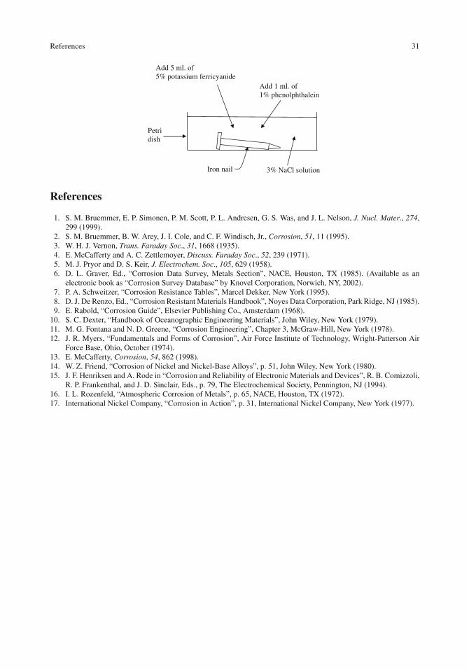
References 31
Add 1 ml. of 1% phenolphthalein
3% NaCl solution
Add 5 ml. of 5% potassium ferricyanide
Petri dish
Iron nail
References
1. S. M. Bruemmer, E. P. Simonen, P. M. Scott, P. L. Andresen, G. S. Was, and J. L. Nelson, J. Nucl. Mater., 274,299 (1999).
2. S. M. Bruemmer, B. W. Arey, J. I. Cole, and C. F. Windisch, Jr., Corrosion, 51, 11 (1995).3. W. H. J. Vernon, Trans. Faraday Soc., 31, 1668 (1935).4. E. McCafferty and A. C. Zettlemoyer, Discuss. Faraday Soc., 52, 239 (1971).5. M. J. Pryor and D. S. Keir, J. Electrochem. Soc., 105, 629 (1958).6. D. L. Graver, Ed., “Corrosion Data Survey, Metals Section”, NACE, Houston, TX (1985). (Available as an
electronic book as “Corrosion Survey Database” by Knovel Corporation, Norwich, NY, 2002).7. P. A. Schweitzer, “Corrosion Resistance Tables”, Marcel Dekker, New York (1995).8. D. J. De Renzo, Ed., “Corrosion Resistant Materials Handbook”, Noyes Data Corporation, Park Ridge, NJ (1985).9. E. Rabold, “Corrosion Guide”, Elsevier Publishing Co., Amsterdam (1968).
10. S. C. Dexter, “Handbook of Oceanographic Engineering Materials”, John Wiley, New York (1979).11. M. G. Fontana and N. D. Greene, “Corrosion Engineering”, Chapter 3, McGraw-Hill, New York (1978).12. J. R. Myers, “Fundamentals and Forms of Corrosion”, Air Force Institute of Technology, Wright-Patterson Air
Force Base, Ohio, October (1974).13. E. McCafferty, Corrosion, 54, 862 (1998).14. W. Z. Friend, “Corrosion of Nickel and Nickel-Base Alloys”, p. 51, John Wiley, New York (1980).15. J. F. Henriksen and A. Rode in “Corrosion and Reliability of Electronic Materials and Devices”, R. B. Comizzoli,
R. P. Frankenthal, and J. D. Sinclair, Eds., p. 79, The Electrochemical Society, Pennington, NJ (1994).16. I. L. Rozenfeld, “Atmospheric Corrosion of Metals”, p. 65, NACE, Houston, TX (1972).17. International Nickel Company, “Corrosion in Action”, p. 31, International Nickel Company, New York (1977).

Chapter 3Charged Interfaces
Introduction
Interfaces form at the physical boundary between two phases, such as between a solid and a liquid(S/L), a liquid and its vapor (L/V), or a solid and a vapor (S/V). There can also be interfaces betweentwo different solids (S1/S2) or between two immiscible liquids (L1/L2). This chapter will considertwo special interfaces, the solution/air interface and the metal/solution interface. A brief discus-sion of the solution/air interface is useful in pointing out some general properties of interfaces. Themetal/solution interface is, of course, of paramount interest to the study of corrosion.
This chapter shows how a potential difference originates across a metal/solution interface anddiscusses the concept of the electrode potential for use in subsequent chapters.
Electrolytes
The Interior of an Electrolyte
An electrolyte is a solution which contains dissolved ions capable of conducting a current. Theinterior of an electrolyte may consist of a variety of charged and uncharged species.
Consider an aqueous solution which contains the following species:
(1) H2O molecules(2) Na+ ions(3) Cl− ions(4) Organic molecules (which may be present as impurities, biological entities, or may be
intentionally added as a corrosion inhibitor).
In a single water molecule, the angle between the two O–H bonds is 105◦, and the oxygen atomis more electronegative than the hydrogen atom, so the oxygen end of the molecule contains a partialnegative charge. Thus, the water molecule is a dipole, as represented by the vector shown in Fig.3.1(a). In the interior of liquid water, water molecules are oriented randomly in all directions at anygiven time, as shown diagrammatically in Fig. 3.1(b). Thus, there is no net electrical field in theinterior of liquid water.
In a sodium chloride solution, the electrolyte contains an equal concentration of Na+ ions andCl− ions. In any volume element of solution, there is an equal number of positive and negative ions,and these ions are randomly distributed, as shown in Fig. 3.2. Moreover, these ions are in constantmotion migrating through the solution in a random walk. Thus, there is no net charge within anyvolume element of solution due to the existence of dissolved ions.
33E. McCafferty, Introduction to Corrosion Science, DOI 10.1007/978-1-4419-0455-3_3,C© Springer Science+Business Media, LLC 2010

34 3 Charged Interfaces
(b)
H
H
OOxygen
Hydrogen
Negativeend
Positive end
105 o
(a)
Fig. 3.1 (a) The water dipole. (b) In the bulk, liquid water consists of an array of randomly oriented dipoles, so thenet charge is zero
Spaces between ions are occupied by water molecules, but as shown previously, the net charge due to H2O dipoles is zero.
Na+
Cl–
Cl–
Cl–
Cl–
Na+Na+
Na+
etc.
etc.
Cl–
Na+
In any volume element, there is an equal numberof positive and negative charges, so that the net charge due to the presence of ions is zero.
Fig. 3.2 A volume element of sodium chloride solution showing the distribution of ions
This statement needs to be examined more carefully by considering the character of watermolecules in ionic solutions. Water molecules in the immediate vicinity of positive or negativeions are attracted toward the charge on the ion. The charge on the ion orients these nearest watermolecules with the appropriate end of the dipole pointing toward the ion, as shown in Fig. 3.3. Due

Interfaces 35
Cl–
(b)
Na+
(a)
Fig. 3.3 Primary waters of hydration for (a) Na+ ion, (b) Cl− anion. Primary hydration numbers are from Bockrisand Reddy [1]
to these ion−dipole forces, a certain number of water molecules become attracted to the centralion. Such water molecules are called primary waters of hydration, and their number usually variesfrom 1 to 5, depending on the specific ion. Located just outside the primary sheath of oriented watermolecules is a secondary region of partially ordered water molecules, called secondary waters ofhydration, which balance the localized oriented charge which has developed in the primary watersheath. Thus, the overall effect of ionic hydration is that there is no net charge due to ionic hydra-tion. It can easily be shown that the number of water molecules located in primary water sheaths isa very small percentage of the total number of water molecules in solution. See Problem 3.1 at theend of this chapter.
Outside the region of hydration, the “spaces” between dissolved ions are occupied by bulk watermolecules, but we have already established above that there is no net charge for a random distributionof water dipoles. The same situation exists in the bulk of an aqueous solution, so there is no net chargein the interior of an electrolyte due to the existence of water dipoles.
Organic molecules dissolved in solution usually contain functional groups, such as –COOH,which assist in their solubility. Proteins, for instance, contain both –COOH and –NH groups.Suppose that the molecule CH3(CH2)10COOH (dodecanoic acid) is contained in solution. Decanoicacid is a weak acid, so in aqueous solution, not all molecules completely ionize, but a certain fractionof the dissolved molecules dissociate into hexanoate ions and protons:
CH3 (CH2)10 COOH(aq) � CH3(CH2)10COO−(aq)+ H+
The ions produced by this dissociation are free to migrate throughout the solution, and they dis-tribute themselves in a random fashion so that the dissolved organic molecule does not impart anylocalized charge to the interior of the electrolyte.
Interfaces
Encountering an Interface
Eventually an aqueous solution must terminate in a boundary with another phase. This commonboundary is called an interface. In an aqueous solution contained in a laboratory beaker or a testcell, one interface is with the vapor phase above the solution, i.e., the solution/air interface. Even

36 3 Charged Interfaces
enormous volumes of solution terminate in interfaces. For example, the ocean, which is 35,840 ft(10,924 m) at its deepest level, forms an interface with air at its uppermost level.
The natural world is composed of a variety of interfaces. These include liquid/vapor, liquid/liquid,solid/liquid, solid/vapor, and solid/solid interfaces. The interface of major interest to us is themetal/solution interface. This interface will be treated in more detail after solution/air interfacesare first considered.
The Solution/Air Interface
The properties of a surface region are different than the properties of the bulk. In the bulk of asolution, each ion or molecule is surrounded in all directions by other ions or molecules so thattheir time-averaged arrangement is the same throughout the interior of the solution. At the surface,however, ions or molecules do not have neighbors distributed in all directions. Figure 3.4 illustratesthe situation for a water/air interface. Water molecules exist in the vapor part of the interface due tothe vapor pressure of liquid water, but the concentration of these gaseous water molecules is muchless than the concentration of water molecules in the liquid. Thus, there is an imbalance of forces formolecules located in the surface region. This unbalance results in a net force inward into the liquid,and this net inward force is the origin of the surface tension of the liquid.
H2O
H2O
H2OH2O H2O
H2O H2O H2O H2O H2OH2O
H2OH2O
H2O
H2O H2O H2O
Air
Water
Weak attractive forces
Net attractive forceinward
Fig. 3.4 Water molecules at the water/air interface and the origin of surface tension
A similar situation exists for aqueous solutions. With a sodium chloride solution, for example,there is a complete absence of Na+ or Cl−ions in the vapor-phase component of the interface. Thus,water molecules near the surface interact not only with interior water molecules in the bulk solutionbut also with interior Na+ and Cl− ions. The net result is that the surface tension of sodium chloridesolutions and other strong electrolytes increases slightly with the concentration of the dissolvedsalt [2].
Because surface ions and molecules experience different chemical neighborhoods than thoselocated in the bulk, there can be a tendency for certain species in solution to preferentially accu-mulate (i.e., adsorb) near the interface. Such “surface-active” species serve to reduce the surfacetension of the solution, as shown in Fig. 3.5. (For a liquid, the surface tension is identical to thesurface free energy. The concept of free energy is discussed further in Chapter 4.) There is no exper-imental evidence to suggest that either Na+ or Cl− ions are surface active. However, certain organicmolecules such as carboxylic acids, amines, and alcohols are indeed surface active.
Figure 3.6 illustrates the random orientation for CH3(CH2)10COOH molecules dissolved in thebulk of the solution. The zigzag portion of the molecules represents the non-polar hydrocarbon tail.

Interfaces 37
Concentration of organic molecule
Surfacetension of solution
Fig. 3.5 Reduction in the surface tension of a solution by a dissolved surface-active agent (schematic)
COO–
H+COO–
H+COO–
H+Solution
Air
COO–
H+COO–
H+
COO–
COO–
H+
COO–H+
H+
COO–
electricaldouble layer}
Hydrocarbontails
H+
Fig. 3.6 Orientation of CH3(CH2)10COOH molecules at the solution/air interface and the formation of an electricaldouble layer
At the surface, however, the −COO− polar head group is hydrophilic and is located in the aqueousside of the interface. The non-polar hydrocarbon tail extends outward into the gaseous phase. Thesesurface-active molecules form an oriented layer one molecule in thickness (a monolayer).
It can be seen that an oriented monolayer of a carboxylic acid at an interface, as shown schemati-cally in Fig. 3.6, produces an accumulation of negative charges at the aqueous side of the solution/airsurface. This array of negative charges is balanced in solution by nearby positive H+ counterions,and the effect is to establish an electrical double layer at the solution/air interface.
The Metal/Solution Interface
Immersion of a metal into a solution creates another type of interface, the metal/solution interface.This interface is much more complicated than the solution/air interface for several reasons.

38 3 Charged Interfaces
First, the metal is a conductor of electricity. By connecting external leads to the metal (withoutimmersing these leads into the aqueous solution) and then connecting the metal under study to anexternal device, we can supply electrons to the metal side of the metal/solution interface, or we canextract electrons from the metal side of the interface. Thus, the metal side of the interface can becharged negatively or positively, respectively.
Second, chloride ions (and other inorganic anions) which are not surface active at solution/airinterfaces are adsorbed at metal/solution interfaces.
Third, the water molecule itself is adsorbed at metal/solution interfaces. Moreover, the watermolecule being a dipole is oriented at the interface, as shown in Fig. 3.7.
+++
+
OH
H
Metal Solution
OH
H
–
–
––
Metal Solution
–
Fig. 3.7 The orientation of water molecules at a metal/solution interface. Top: the “flop-down” orientation of thewater dipole. Bottom: the “flip-up” orientation [3]
Fourth, the metal/solution interface is not always a stable one. If the metal corrodes, then theinterface is neither chemically nor geometrically stable. Under freely corroding conditions, the metalsurface supports both local anodic and local cathodic processes, as discussed in Chapter 2. Underthese conditions, the metal/solution interface is a hubbub of activity.
Metal Ions in Two Different Chemical Environments
Metals contain closely packed atoms which have strong overlap of electrons between one another. Asolid metal therefore does not possess individual well-defined electron energy levels as are found ina single atom of the same material. Instead a vast number of molecular orbitals exist which extendthroughout the entire metal, and there is a continuum of energy levels. The electrons can move freelywithin these molecular orbitals, and so each electron becomes delocalized from its parent atom. Thesituation is sometimes described as an array of positive ions in a Fermi sea of electrons, as depictedin Fig. 3.8.
The process of corrosion may be thought of as the transfer of a positive ion from the metal latticeinto solution. In the metal lattice, the positive ion is stabilized by the Fermi sea of electrons. Insolution, the positive ion is stabilized by its water of hydration. This idea is illustrated schematicallyin Fig. 3.9. To effect this transfer, however, the positive ion must pass outward through the electrical
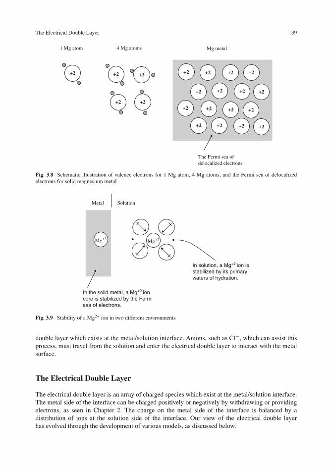
The Electrical Double Layer 39
+2 +2 +2
+2+2
1 Mg atom 4 Mg atoms Mg metal
+2 +2
+2+2
+2
+2
+2
+2
The Fermi sea ofdelocalized electrons
+2
+2
+2
+2+2+2 +2
+2
Fig. 3.8 Schematic illustration of valence electrons for 1 Mg atom, 4 Mg atoms, and the Fermi sea of delocalizedelectrons for solid magnesium metal
Metal Solution
Mg+2
In solution, a Mg+2 ion isstabilized by its primarywaters of hydration.
In the solid metal, a Mg+2 ioncore is stabilized by the Fermisea of electrons.
Mg+2
Fig. 3.9 Stability of a Mg2+ ion in two different environments
double layer which exists at the metal/solution interface. Anions, such as Cl−, which can assist thisprocess, must travel from the solution and enter the electrical double layer to interact with the metalsurface.
The Electrical Double Layer
The electrical double layer is an array of charged species which exist at the metal/solution interface.The metal side of the interface can be charged positively or negatively by withdrawing or providingelectrons, as seen in Chapter 2. The charge on the metal side of the interface is balanced by adistribution of ions at the solution side of the interface. Our view of the electrical double layerhas evolved through the development of various models, as discussed below.

40 3 Charged Interfaces
The Gouy−Chapman Model of the Electrical Double Layer
Figure 3.10 shows a metal having a positive charge, which is partially balanced in solution by adiffuse layer of negative ions. In this diffuse layer (called the diffuse part of the double layer), ionsare in thermal motion, but there is an overall increase in the concentration of negative ions withinthis layer so as to partly balance the positive charge on the metal side of the interface. This view ofthe electrical double layer is called the Gouy−Chapman model.
Metal Solution
–
–
–
–
++
++
++
++
+
+
+
+
+
–
–
Fig. 3.10 The Gouy−Chapman model of the electrical double layer at a metal/solution interface
The Electrostatic Potential and Potential Difference
As seen in Fig. 3.10, there is a net charge within the diffuse part of the electrical double layer.This is in marked contrast to the interior of the solution, which, as shown earlier, does not exhibit anet charge. This difference in local chemical environments leads to the concept of the electrostaticpotential.
The electrostatic potential (at some point) is the work required to move a small positive unitcharge from infinity to the point in question. This is a thought experiment for which
(1) the positive test charge is small enough not to perturb the existing electrical field;(2) the work involved is independent of the path taken.
The potential difference (between two points) is the work required to move a small unit positivecharge between the two points, as shown in Fig. 3.11. The potential difference, PD, between A andB is given by
PDBA = φB − φA (1)
where φB and φA are the electrostatic potentials at points B and A, respectively. The potentialdifference, PD, has the units of joules per coulomb, or volts.
In Fig. 3.10, suppose that a unit positive test charge travels from some point A in the interior ofthe electrolyte, which is neutral in charge, to some point B within the diffuse double layer, wherethere is a net charge. There is a potential difference between the two points, and it is the electricaldouble layer which gives rise to this potential difference.

The Electrical Double Layer 41
+
AB
Unit test charge(small enough not to perturbelectrical field)
PDBA = φB – φA = joules
coulombs = volts
Fig. 3.11 A positive unit test charge and the definition of a potential difference
The Stern Model of the Electrical Double Layer
The Stern model takes into account adsorption of anions or cations at the metal surface.Figure 3.12 shows the case for the adsorption of anions. The distance of closest approach of the ion isits radius, and the plane through the center of these adsorbed ions is called the Helmholtz plane. Theexcess charge at the metal surface is balanced in part by ions located in a Gouy−Chapman diffusedouble layer, which exists outside the Helmholtz plane.
A typical potential difference across the Helmholtz plane is of the order of 1 V. The thicknessof the Helmholtz layer is about 10 Å (1 Å = 10−8 cm). This amounts to a field strength of 1 ×10⁷ V/cm. This is a very high field strength and is, of course, the consequence of having a localizedcharge confined within the narrow region of the interface.
Metal Solution
–
–
–
++++++++
+
–
+
+
+
+
–
–
+
–
Gouy–Chapman layer
+
Inner Helmholtz plane
Fig. 3.12 The Stern model of the electrical double layer at a metal/solution interface

42 3 Charged Interfaces
The Bockris−Devanathan−Müller Model of the Electrical Double Layer
The Bockris−Devanathan−Müller model is the most recent and most rigorous model of the elec-trical double layer [4]. This model of the electrical double layer retains all the features of the Sternmodel and in addition embraces two important considerations.
First, this model takes into account the adsorption of water molecules at the metal/solution inter-face. For a positive charge on the metal side of the interface, water molecules are oriented with thenegative ends of their dipoles toward the metal surface, as shown in Fig. 3.13. This model recognizesthat water molecules and ions in solution compete for sites on the metal surface. The adsorption ofthe chloride ion, for example, may be considered a replacement reaction in which Cl− ions replacewater molecules adsorbed at the metal/solution interface. The plane through the center of theseadsorbed ions is called the inner Helmholtz plane in this model.
+
+
++
–
–+
+
++
+
Layer of oriented water
Hydrated cation
Inner Helmholtz plane
Outer Helmholtz plane
Distance from surface
φ
Adsorbed anion
Guoy–Chapmandiffuse layer
Metal
Fig. 3.13 The Bockris−Devanathan−Müller model of the electrical double layer at a metal/solution interface [4]
The second added feature of this model is that the charge introduced by the adsorption of anionsat the metal surface is balanced in part by counterions of the opposite charge. These counterions arenot adsorbed on the metal surface, but exist in solution, and have associated with them their watersof hydration. The plane through the center of these counter ions is called the outer Helmholtz plane.
According to the Bockris−Devanathan−Müller model, water molecules adsorbed at themetal/solution interface have a dielectric constant of 6, and water molecules in the outer Helmholtzplane have a dielectric constant of 30−40. The dielectric constant of water molecules outside thediffuse double layer and in the bulk is the usual value of 78.

The Electrical Double Layer 43
Significance of the Electrical Double Layer to Corrosion
The significance of the electrical double layer (edl) to corrosion is that the edl is the origin of thepotential difference across an interface and accordingly of the electrode potential (to be discussedin the next section). Changes in the electrode potential can produce changes in the rate of anodic(or cathodic) processes, as will be seen in Chapter 7. Emerging (corroding) metal cations must passacross the edl outward into solution, and solution species (e.g., anions) which participate in thecorrosion process must enter the edl from solution in order to attack the metal.
Thus, the properties of the edl control the corrosion process. The edl on a corroding metal can bemodeled by a capacitance in parallel with a resistance, as shown in Fig. 3.14. In the simple equivalentcircuit shown in Fig. 3.14, the double layer capacitance Cdl ensues because the edl at a metal surfaceis similar to a parallel plate capacitor. The Faradaic resistance RP in parallel with this capacitancerepresents the resistance to charge transfer across the edl. The quantity RP is inversely proportionalto the specific rate constant for the half-cell reaction. The term RS is the ohmic resistance of thesolution.
Cdl
RP
RS
Metal Solution
Fig. 3.14 Simple equivalent circuit model of the electrical double layer. Cdl is the double layer capacitance, RP is theresistance to charge transfer across the edl, and RS is the ohmic resistance of the solution
Example 3.1: The double layer capacitance of freely corroding iron in 6 M HCl has been measuredto be 34 μF/cm2 [5]. If the thickness of the entire double layer is 100 Å, what is the average valueof the dielectric constant within the electrical double layer?
Solution: The formula for the capacitance C of a parallel plate condenser is
C = εA
d
where ε is the dielectric constant, A is the area of the plates, and d is the distance between plates.Thus
Cdl= ε
d
where Cdl is the double layer capacitance per unit area. The farad is the SI (System Internationale)unit of capacitance, but in the cgs (centimeter−gram−second) system of units, the capacitance mustbe expressed in statfarads, there being 1.113 × 10⁻¹² F/statF. Thus

44 3 Charged Interfaces
(34× 10−6F
cm2
)(1 stat F
1.113 × 10⁻¹² farads
)= ε(
100Å) ( 1.00×10⁻⁸ cm
Å
)
The result is ε = 31. Note that this value for the dielectric constant lies between the value 6 fororiented water dipoles adsorbed on the metal surface and lying in the inner Helmholtz plane and thevalue of 78 for bulk water.
Electrode Potentials
The Potential Difference Across a Metal/Solution Interface
An earlier section discussed the concept of the electrostatic potential (at a fixed point) in terms ofa thought experiment. Recall that the electrostatic potential is the work required to move a smallpositive unit charge from infinity to the point in question. The potential difference (between twopoints) was also discussed. What happens if we attempt to measure the potential difference acrossa metal/solution interface in the laboratory? The idea of conceptually moving a test positive unitcharge across the metal/solution interface is not of much practical help to us in the laboratory.
We quickly realize that in order to measure the potential difference across the metal/solutioninterface of interest, we must create additional interfaces [3]. These new interfaces are necessary inorder to connect the metal/solution interface of interest to the potential-measuring device so as tocomplete the electrical circuit. See Fig. 3.15. The metal of interest is designated as M. A secondmetal which forms a second metal/solution interface is a reference metal, designated by “ref.” Therequired properties of this new interface will be given later. The metal M1 connects the metals M and“ref” to the potential-measuring device. S and S′ are two points in solution, just outside the electricaldouble layers on M and “ref”, respectively.
M ref
V
M1M1
solution
S S′
Fig. 3.15 In order to measure the potential difference across the metal/solution interface of interest (M/S), anadditional interface must be created using a reference metal “ref” [3]
Consider a point located in solution just outside the electrical double layer on the metal of interest(M). The electrostatic potential has some value φs. For a second point just inside the interior of themetal M, the electrostatic potential has a value φM. Accordingly, as one moves inward across theM/S interface, the electrostatic potential will change from value φs to φM. Let us continue in aclosed path across all interfaces writing the changes in electrostatic potential as we proceed. Thesum total of changes in electrostatic potential must be zero by Kirchhoff’s law. That is [3]
(φS − φM)+ (φM − φM1)+ V + (φM1 − φref)+(φref − φ′s
)+ (φ′s − φs) = 0 (2)
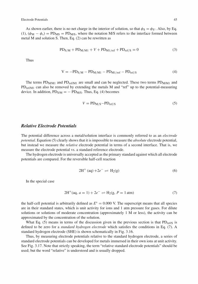
Electrode Potentials 45
As shown earlier, there is no net charge in the interior of solution, so that φS = φS ′ . Also, by Eq.(1), (φM − φs) = PDMS = PDM/S, where the notation M/S refers to the interface formed betweenmetal M and solution S. Then, Eq. (2) can be rewritten as
PDS/M + PDM/M1 + V + PDM1/ref + PDref/S = 0 (3)
Thus
V = −PDS/M − PDM/M1 − PDM1/ref − PDref/S (4)
The terms PDM/M1 and PDref/M1 are small and can be neglected. These two terms PDM/M1 andPDref/M1 can also be removed by extending the metals M and “ref” up to the potential-measuringdevice. In addition, PDS/M = − PDM/S. Thus, Eq. (4) becomes
V = PDM/S−PDref/S (5)
Relative Electrode Potentials
The potential difference across a metal/solution interface is commonly referred to as an electrodepotential. Equation (5) clearly shows that it is impossible to measure the absolute electrode potential,but instead we measure the relative electrode potential in terms of a second interface. That is, wemeasure the electrode potential vs. a standard reference electrode.
The hydrogen electrode is universally accepted as the primary standard against which all electrodepotentials are compared. For the reversible half-cell reaction
2H+ (aq)+2e− � H2(g) (6)
In the special case
2H+(aq, a = 1)+ 2e− � H2(g, P = 1 atm) (7)
the half-cell potential is arbitrarily defined as E◦ = 0.000 V. The superscript means that all speciesare in their standard states, which is unit activity for ions and 1 atm pressure for gases. For dilutesolutions or solutions of moderate concentration (approximately 1 M or less), the activity can beapproximated by the concentration of the solution.
What Eq. (5) means in terms of the discussion given in the previous section is that PDref/S isdefined to be zero for a standard hydrogen electrode which satisfies the conditions in Eq. (7). Astandard hydrogen electrode (SHE) is shown schematically in Fig. 3.16.
Thus, by measuring electrode potentials relative to the standard hydrogen electrode, a series ofstandard electrode potentials can be developed for metals immersed in their own ions at unit activity.See Fig. 3.17. Note that strictly speaking, the term “relative standard electrode potentials” should beused; but the word “relative” is understood and is usually dropped.

46 3 Charged Interfaces
H2 out
To cell
Stopcock or glass frit
Platinized Pt
Unit activity
H+
H2 in
Glass frit
Stopcock
Fig. 3.16 A standard hydrogen reference electrode (SHE)
Activity H+ = 1
E
Platinized Pt
H2 H2
Activity M+n = 1
Metal MGlassfrit
Fig. 3.17 Experimental determination of a standard electrode potential for some metal M using a standard hydrogenreference electrode
The Electromotive Force Series
An ordered listing of the standard half-cell potentials is called the electromotive force (emf) series.See Table 3.1 [6]. Note that all of the half-cell reactions are written from left to right as reductionreactions. This practice follows the Stockholm Convention of 1953 but is a source of some annoyanceto corrosion scientists, who are primarily interested in the reverse (i.e., oxidation) reaction. (Differentcompilations [7−9] of standard electrode potentials may list slightly different values for some half-cell reactions, but these variations are usually of the order of millivolts and should not be consideredto be significant.)
Notice that the sign of the standard electrode potential in Table 3.1 ranges from positive to neg-ative values, passing through the value 0.000 which is defined as such for the hydrogen reductionreaction. The most positive potential listed in Table 3.1 is for
Au3+ + 3e− � Au E◦ = +1.498 V
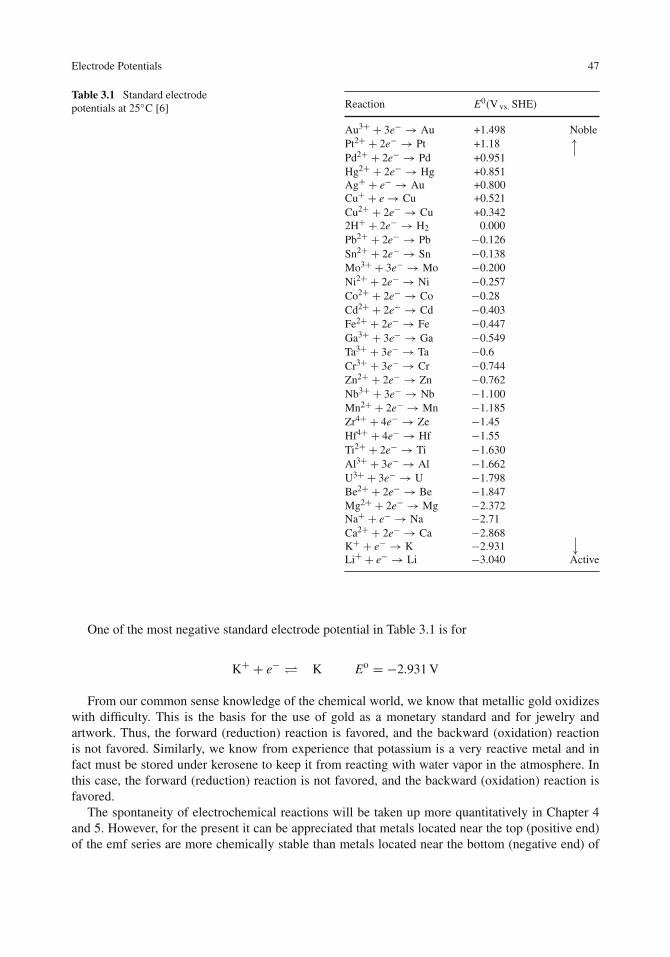
Electrode Potentials 47
Table 3.1 Standard electrodepotentials at 25◦C [6] Reaction E0(V vs. SHE)
Au3+ + 3e− → Au +1.498 NoblePt2+ + 2e− → Pt +1.18 −→Pd2+ + 2e− → Pd +0.951Hg2+ + 2e− → Hg +0.851Ag+ + e− → Au +0.800Cu+ + e→ Cu +0.521Cu2+ + 2e− → Cu +0.3422H+ + 2e− → H2 0.000Pb2+ + 2e− → Pb −0.126Sn2+ + 2e− → Sn −0.138Mo3+ + 3e− → Mo −0.200Ni2+ + 2e− → Ni −0.257Co2+ + 2e− → Co −0.28Cd2+ + 2e− → Cd −0.403Fe2+ + 2e− → Fe −0.447Ga3+ + 3e− → Ga −0.549Ta3+ + 3e− → Ta −0.6Cr3+ + 3e− → Cr −0.744Zn2+ + 2e− → Zn −0.762Nb3+ + 3e− → Nb −1.100Mn2+ + 2e− → Mn −1.185Zr4+ + 4e− → Ze −1.45Hf4+ + 4e− → Hf −1.55Ti2+ + 2e− → Ti −1.630Al3+ + 3e− → Al −1.662U3+ + 3e− → U −1.798Be2+ + 2e− → Be −1.847Mg2+ + 2e− → Mg −2.372Na+ + e− → Na −2.71Ca2+ + 2e− → Ca −2.868 −→
K+ + e− → K −2.931Li+ + e− → Li −3.040 Active
One of the most negative standard electrode potential in Table 3.1 is for
K+ + e− � K Eo = −2.931 V
From our common sense knowledge of the chemical world, we know that metallic gold oxidizeswith difficulty. This is the basis for the use of gold as a monetary standard and for jewelry andartwork. Thus, the forward (reduction) reaction is favored, and the backward (oxidation) reactionis not favored. Similarly, we know from experience that potassium is a very reactive metal and infact must be stored under kerosene to keep it from reacting with water vapor in the atmosphere. Inthis case, the forward (reduction) reaction is not favored, and the backward (oxidation) reaction isfavored.
The spontaneity of electrochemical reactions will be taken up more quantitatively in Chapter 4and 5. However, for the present it can be appreciated that metals located near the top (positive end)of the emf series are more chemically stable than metals located near the bottom (negative end) of

48 3 Charged Interfaces
the series. Said simply, metals near the top of the emf series are less prone to corrosion. But thefollowing limitations must be recognized:
(1) The emf series applies to pure metals in their own ions at unit activity.(2) The relative ranking of metals in the emf series is not necessarily the same (and is usually not
the same) in other media (such as seawater, groundwater, sulfuric acid, artificial perspiration).(3) The emf series applies to pure metals only and not to metallic alloys.(4) The relative ranking of metals in the emf series gives corrosion tendencies (subject to the
restrictions immediately above) but provides no information on corrosion rates.
Metals located near the positive end of the emf series are referred to as “noble” metals, whilemetals near the negative end of the emf scale are called “active” metals.
The electrode potential for a half-cell reaction for a metal immersed in a solution of its ionsat some concentration other than unit activity is related to its standard electrode potential (at unitactivity) by the Nernst equation. See Chapter 4.
It should be noted that in some older texts and data compilations, standard electrode potentialsare written for half-cell oxidation reactions, and the signs for E◦ listed in Table 3.1 are then reversed.
Reference Electrodes for the Laboratory and the Field
Although the standard hydrogen electrode (depicted in Fig. 3.16) is the reference electrode againstwhich electrode potentials are defined; this reference electrode is not commonly used in the labo-ratory. The hydrogen electrode is somewhat inconvenient to use as it requires a constant externalsource of hydrogen gas. (Hoare and Schuldiner [10] have developed a more compact hydrogen ref-erence electrode which employs hydrogen gas discharged in a palladium wire, but this referenceelectrode has not found much use in corrosion studies.)
Instead of using the standard hydrogen electrode, other reference electrodes are commonly usedin the laboratory. The saturated calomel electrode (SCE) has long been used, especially in chloride
Hg2Cl
2(calomel)
Saturated KCl
Porous
glass
KCl crystals
Hg
Fig. 3.18 A saturated calomel reference electrode

Reference Electrodes for the Laboratory and the Field 49
solutions. Its construction is shown in Fig. 3.18, and its half-cell reaction is
Hg2Cl2(s)+ 2e− � 2Hg(s)+ 2Cl−(aq, sat,d)
The electrode potential under these conditions at 25◦C is E = + 0.242 V.Another reference electrode in wide use in the laboratory (usually in chloride solutions) is the
silver−silver chloride reference electrode, and its half-cell reaction is
AgCl(s)+ e− � Ag(s)+ Cl−(aq)
In its most common form, the silver−silver chloride electrode consists of a solid AgCl coatingon a silver wire immersed in a solution of 4 M KCl plus saturated AgCl, as shown schematically inFig. 3.19. The electrode potential under these conditions at 25◦C is E = + 0.222 V.
Porousglass
Chloridized Ag(AgCl coating on Ag)
4 M KCl plussaturated AgCl
Fig. 3.19 A silver/silver chloride reference electrode
Peterson and Groover [11] have developed a silver−silver chloride reference electrode for usein natural seawater. The electrode consists of a solid mass of AgCl in contact with an Ag wire and
Outer spiral
retainer
of Ag gauze
Ag rod
Solid AgCl
(solidified from
molten AgCl)
~1 cm
Fig. 3.20 The Peterson−Groover silver/silver chloride reference electrode for use in natural seawater [11]

50 3 Charged Interfaces
held in place with an outer retainer of silver gauze. The electrode itself contains no aqueous fill-ing solution but is immersed directly into the ocean, which then provides the source of the Cl− ion(approximately 0.6 M Cl−). See Fig. 3.20. This electrode maintains a steady half-cell potential whichcan be then calibrated vs. the standard silver−silver chloride electrode. The Peterson−Groover ref-erence electrode has been used with much success in measuring the electrode potentials of testspecimens in seawater and in various marine applications, such as measuring the electrode poten-tials at various locations around the hull of a ship. In the latter application, the Peterson−Grooverreference electrode may be delivered to the desired location at the end of a fishing line.
There are various other reference electrodes which are used in various aqueous solutions. Forexample, the mercury−mercurous sulfate electrode is used in sulfate solutions to avoid contami-nation by Cl−, and the mercury−mercuric oxide electrode is used in alkaline solutions. For moredetails, specialized texts on experimental electrochemistry should be consulted [12]. Values for thehalf-cell potentials of several reference electrodes are given in Table 3.2 [13, 14].
Table 3.2 Electrode potentials of various reference electrodes [13, 14]
Reference electrode Potential (V vs. SHE) Conversion to SHE
Standard hydrogen electrode 0.000 −Saturated calomel + 0.242 E vs. SCE = E vs.
SHE − 0.242Silver/silver chloride(saturated)
+ 0.222 E vs. Ag/AgCl = Evs. SHE − 0.222
Peterson−Groover silver/silverchloride (in seawater)
+ 0.248 E vs. Ag/AgCl (inseawater) = E vs.SHE − 0.248
Copper/copper sulfate(saturated)
+ 0.316 E vs. Cu/CuSO4 =E vs. SHE − 0.316
Mercury/mercurous sulfate + 0.615 E vs. Hg/Hg2SO4 = E vs.SHE − 0.615
The copper−copper sulfate reference electrode is used commonly in the field to measure thepotential of buried structures such as pipelines or tanks. The construction of this reference electrodeis shown in Fig. 3.21. A porous wooden plug provides the electrolyte path between the reference
CuSO4.5 H2O
Saturated CuSO4
Copper
Porous wooden plugthreaded into place
Fig. 3.21 The copper/copper sulfate reference electrode for use in soils

Reference Electrodes for the Laboratory and the Field 51
E
High impedance electrometer
Cu/CuSO 4 referenceelectrode in moist earth
Insulated lead
Underground pipe
Fig. 3.22 Measurement of the electrode potential of a buried pipe using a copper/copper sulfate reference [15]
electrode and the moist soil. This reference electrode is used more for its rugged and simple naturethan for its high precision. Figure 3.22 gives a schematic diagram showing the measurement of thepotential of an underground pipe [15].
Example 3.2: An electrode potential was measured to be −0.500 V vs. Cu/CuSO4. What is thiselectrode potential on the SCE scale?
Solution: From Table 3.2
E vs. SCE = E vs. SHE− 0.242
Also
E vs. Cu/CuSO4 = E vs. SHE− 0.316
Subtracting the second of these equations from the first gives
(E vs. SCE)− (E vs. Cu/CuSO4) = −0.242+ 0.316 = +0.074
Thus
(E vs. SCE)− (−0.500) = 0.074
or
(E vs. SCE) = −0.426V

52 3 Charged Interfaces
S.H.E. S.C.E. Ag/AgCl Cu/CuSO4
+1.0
+0.5
0.0
–0.5
+0.5
–0.5
0.0
+0.5
–0.5
0.0
+0.5
–0.5
0.0E
Fig. 3.23 A graphical aid for conversion between reference electrode scales
Using the information in Table 3.2, graphs may be constructed for converting the elec-trode potential on one reference scale into an electrode potential on another scale, as inFig. 3.23.
All reference electrodes whether they are used in the laboratory or in the field have the samecommon features. These are the following: (i) the half-cell potential must be constant, (ii) the half-cell potential should not change with the passage of a small current through the reference electrode,and (iii) the half-cell potential must not drift with time. These three conditions are met if there is anexcess of both reactants and products in the half-cell reaction.
It should be noted that the use of any reference electrode introduces a liquid junction potential atthe liquid/liquid interface between the test solution and the filling solution of the reference electrode.Such liquid junction potentials are caused by differences in ion types or concentrations across a liq-uid/liquid interface. The liquid junction potential can be minimized by the proper choice of referenceelectrode, i.e., use of a saturated calomel electrode in chloride solutions. Liquid junction potentialsare usually small (of the order of 30 mV) [12] and are included in the measurement of electrodepotentials.
Measurement of Electrode Potentials
Electrode potentials are usually measured with an instrument called an electrometer, which has ahigh input impedance. The input impedance can be as high as 1014 � so that for a potential dropof 1 V across the electrical double layer, an extremely small current of 10−14 amp will flow in themeasuring circuit. This current is too small to interfere with the electrode reactions occurring at themetal/solution interface or to change the electrode potential of the reference electrode. Thus, theelectrode potential of the metal under study will not be altered during the measurement.
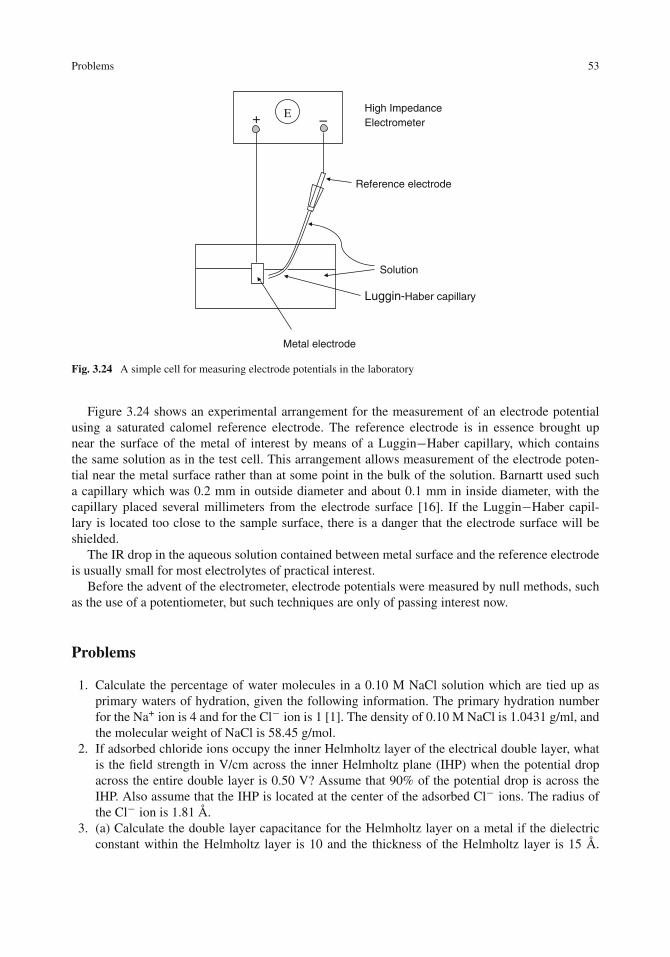
Problems 53
High ImpedanceElectrometer
Metal electrode
Solution
Reference electrode
E
Luggin-Haber capillary
+ –
Fig. 3.24 A simple cell for measuring electrode potentials in the laboratory
Figure 3.24 shows an experimental arrangement for the measurement of an electrode potentialusing a saturated calomel reference electrode. The reference electrode is in essence brought upnear the surface of the metal of interest by means of a Luggin−Haber capillary, which containsthe same solution as in the test cell. This arrangement allows measurement of the electrode poten-tial near the metal surface rather than at some point in the bulk of the solution. Barnartt used sucha capillary which was 0.2 mm in outside diameter and about 0.1 mm in inside diameter, with thecapillary placed several millimeters from the electrode surface [16]. If the Luggin−Haber capil-lary is located too close to the sample surface, there is a danger that the electrode surface will beshielded.
The IR drop in the aqueous solution contained between metal surface and the reference electrodeis usually small for most electrolytes of practical interest.
Before the advent of the electrometer, electrode potentials were measured by null methods, suchas the use of a potentiometer, but such techniques are only of passing interest now.
Problems
1. Calculate the percentage of water molecules in a 0.10 M NaCl solution which are tied up asprimary waters of hydration, given the following information. The primary hydration numberfor the Na+ ion is 4 and for the Cl− ion is 1 [1]. The density of 0.10 M NaCl is 1.0431 g/ml, andthe molecular weight of NaCl is 58.45 g/mol.
2. If adsorbed chloride ions occupy the inner Helmholtz layer of the electrical double layer, whatis the field strength in V/cm across the inner Helmholtz plane (IHP) when the potential dropacross the entire double layer is 0.50 V? Assume that 90% of the potential drop is across theIHP. Also assume that the IHP is located at the center of the adsorbed Cl− ions. The radius ofthe Cl− ion is 1.81 Å.
3. (a) Calculate the double layer capacitance for the Helmholtz layer on a metal if the dielectricconstant within the Helmholtz layer is 10 and the thickness of the Helmholtz layer is 15 Å.
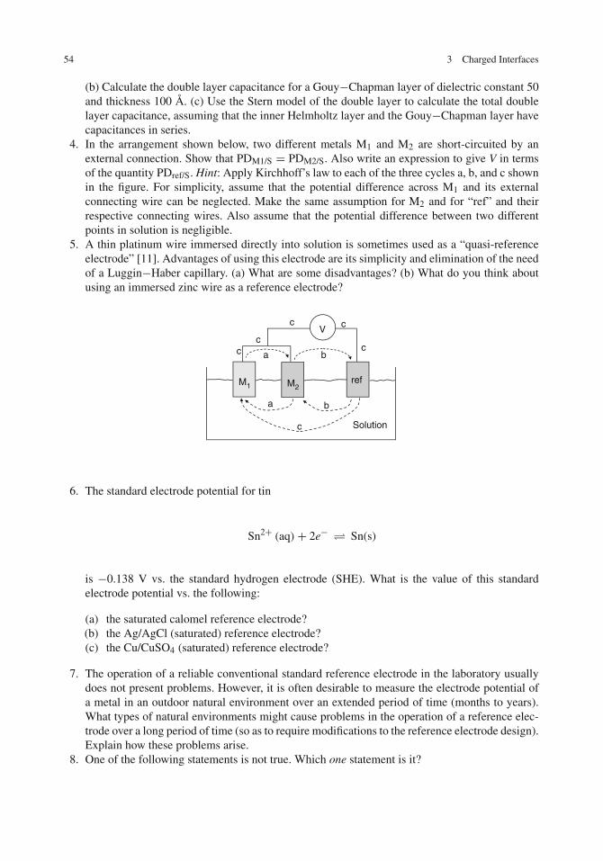
54 3 Charged Interfaces
(b) Calculate the double layer capacitance for a Gouy−Chapman layer of dielectric constant 50and thickness 100 Å. (c) Use the Stern model of the double layer to calculate the total doublelayer capacitance, assuming that the inner Helmholtz layer and the Gouy−Chapman layer havecapacitances in series.
4. In the arrangement shown below, two different metals M1 and M2 are short-circuited by anexternal connection. Show that PDM1/S = PDM2/S. Also write an expression to give V in termsof the quantity PDref/S. Hint: Apply Kirchhoff’s law to each of the three cycles a, b, and c shownin the figure. For simplicity, assume that the potential difference across M1 and its externalconnecting wire can be neglected. Make the same assumption for M2 and for “ref” and theirrespective connecting wires. Also assume that the potential difference between two differentpoints in solution is negligible.
5. A thin platinum wire immersed directly into solution is sometimes used as a “quasi-referenceelectrode” [11]. Advantages of using this electrode are its simplicity and elimination of the needof a Luggin−Haber capillary. (a) What are some disadvantages? (b) What do you think aboutusing an immersed zinc wire as a reference electrode?
M1 M2ref
V
a b
b
c
cc
c
c
Solution
a
c
6. The standard electrode potential for tin
Sn2+ (aq)+ 2e− � Sn(s)
is −0.138 V vs. the standard hydrogen electrode (SHE). What is the value of this standardelectrode potential vs. the following:
(a) the saturated calomel reference electrode?(b) the Ag/AgCl (saturated) reference electrode?(c) the Cu/CuSO4 (saturated) reference electrode?
7. The operation of a reliable conventional standard reference electrode in the laboratory usuallydoes not present problems. However, it is often desirable to measure the electrode potential ofa metal in an outdoor natural environment over an extended period of time (months to years).What types of natural environments might cause problems in the operation of a reference elec-trode over a long period of time (so as to require modifications to the reference electrode design).Explain how these problems arise.
8. One of the following statements is not true. Which one statement is it?

References 55
(a) Zinc and chromium have similar standard potentials in the emf series. Thus, these twometals are certain to have similar electrode potentials in seawater.
(b) Standard electrode potentials are reduction potentials.(c) The liquid junction potential for a solution of 0.1 M HCl separated by porous diaphragm
from a solution of 0.1 M NaCl is less than the liquid junction potential between 0.1 M HCland 0.1 M Na2SO4.
9. Only one of the following statements is true. Which one statement is it?
(a) The standard electrode potential for copper immersed in unit activity Ni2+ ions is the aver-age of the standard electrode potential for nickel immersed in unit activity Ni2+ and copperimmersed in unit activity Cu2+.
(b) Use of a Luggin−Haber capillary can reduce the IR drop between a metal electrode understudy and the reference electrode.
(c) Any two metals in the same Group (i.e., column) of the Period Table will have standardelectrode potentials having the same sign.
10. The following laboratory data were taken for iron in 6 M HCl with and without a straight-chainorganic amine added as a corrosion inhibitor:
Concentration ofinhibitor (M) Cdl (μF/cm2)
Corrosion rate(μA/cm2)
0 33 2,0008 × 10⁻⁴ 22 1,4002 × 10⁻³ 17 1,0002 × 10⁻² 8 200
Comment on the possibility of measuring the double layer capacitance of a test coupon as acorrosion rate monitor in a steel tank storing waste HCl with an added amount of the inhibitorto reduce corrosion of the storage tank walls.
11. Organic amines as in Problem 3.10 reduce the corrosion rate by adsorption at the metal/solutioninterface (as is discussed in Chapter 12). Why is there a corresponding decrease in the doublelayer capacitance? Hint: Consider the effect of the organic molecule on the dielectric constantwithin the edl and on the thickness of the edl.
12. Sketch a figure of the Bockris−Devanathan−Müller model of the edl when the charge on themetal side of the interface is negative instead of positive, as was the case in Fig. 3.13.
References
1. J. O’M. Bockris and A. K. N. Reddy, “Modern Electrochemistry”, Second Edition, Vol. 1, Chapter 2, PlenumPress, New York (1998). Also, First Edition, Vol. 1, Chapter 2 (1977).
2. A. W. Adamson, “Physical Chemistry of Surfaces”, p. 74, John Wiley, New York (1990).3. J. O’M. Bockris and A. K. N. Reddy, “Modern Electrochemistry”, Vol. 2, Chapter 7, Plenum Press, New York
(1977).4. J. O’M. Bockris, M. A. V. Devanathan, and K. Müller, Proc. R. Soc., 274, 55 (1963).5. E. McCafferty and N. Hackerman, J. Electrochem. Soc., 119, 146 (1972).6. P. Vanysek in “CRC Handbook of Chemistry and Physics”, D. R. Lide, Ed., pp. 8−21, CRC Press, Boca Raton,
FL (2001).

56 3 Charged Interfaces
7. W. M. Latimer, “The Oxidation States of the Elements and Their Properties in Aqueous Solutions”, Prentice-Hall,New York (1952).
8. M. Pourbaix, “Atlas of Electrochemical Equilibria in Aqueous Solutions”, National Association of CorrosionEngineers, Houston, TX (1974).
9. A. J. Bard, R. Parsons, and J. Jordan, Eds., “Standard Potentials in Aqueous Solutions”, Marcel Dekker, NewYork (1985).
10. J. P. Hoare and S. Schuldiner. J. Phys. Chem., 61, 399 (1957).11. M. H. Peterson and R. E. Groover, Mater. Prot. Perform., 11 (5), 19 (1972).12. D. T. Sawyer and J. L. Roberts, Jr., “Experimental Electrochemistry for Chemists”, Chapter 2, Wiley Interscience,
New York (1974).13. H. H. Uhlig and R. W. Revie, “Corrosion and Corrosion Control”, Chapter 3, John Wiley, New York (1985).14. D. G. Ives and G. J. Janz, Eds., “Reference Electrodes: Theory and Practice”, Chapters 2 and 3, Academic Press,
New York (1961).15. J. R. Myers, “Fundamentals and Forms of Corrosion”, Air Force Institute of Technology, Wright-Patterson Air
Force Base, Ohio, October (1974).16. S. Barnartt, J. Electrochem. Soc., 108, 102 (1961).

Chapter 4A Brief Review of Thermodynamics
Introduction
This chapter will review briefly the principles of thermodynamics needed to consider corrosion froma thermodynamic point of view. In particular we are working toward the treatment of galvanic corro-sion and the construction and analysis of Pourbaix diagrams. As will be seen in Chapter 6, Pourbaixdiagrams are useful diagrams to summarize concisely the corrosion behavior of a given metal.
Thermodynamic State Functions
A state function is one whose properties depend only on the present state of the system and noton the path taken to get there. (By the “state” in thermodynamics we mean having a certain setof descriptors, rather than the specific physical state of the system). There are five common statefunctions: (i) the internal energy E, (ii) the entropy S, (iii) the enthalpy H, (iv) the Helmholtz freeenergy A, and (v) the Gibbs free energy G.
Internal Energy
The internal energy E of a system is the total energy contained within the system. The internal energyincludes contributions from both kinetic energy and potential energy sources. These include trans-lational, rotational, and vibrational motion of atoms. Forces within an atom, such as the attractionof an electron to the positively charged nucleus, as well as intermolecular forces between molecules(such as van der Waals forces) are included. The internal energy also includes gravitational forces,magnetic forces, and electrical forces.
The fact that E is a state function means that when the system changes from some condition(condition 1) to another condition (condition 2), the change in internal energy is given by
�E = E2 − E1 (1)
Because both E2 and E1are state functions, their change (E2 – E1) does not depend on the pathtaken between 1 and 2. An analogy is provided in Fig. 4.1. The potential energy difference betweenthe elevation of the second floor of a building and the first floor of that building depends only on theheights of the two floors and not on whether a person climbed the stairs to the second floor from thefirst or rode the elevator.
57E. McCafferty, Introduction to Corrosion Science, DOI 10.1007/978-1-4419-0455-3_4,C© Springer Science+Business Media, LLC 2010
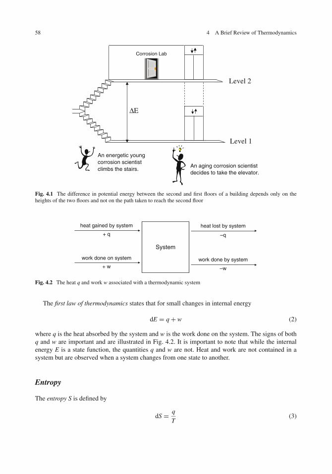
58 4 A Brief Review of Thermodynamics
An aging corrosion scientistdecides to take the elevator.
Level 1
An energetic youngcorrosion scientistclimbs the stairs.
Corrosion Lab
Level 2
ΔE
Fig. 4.1 The difference in potential energy between the second and first floors of a building depends only on theheights of the two floors and not on the path taken to reach the second floor
System
–w
–q
work done by system
heat lost by systemheat gained by system
work done on system
+ w
+ q
Fig. 4.2 The heat q and work w associated with a thermodynamic system
The first law of thermodynamics states that for small changes in internal energy
dE = q+ w (2)
where q is the heat absorbed by the system and w is the work done on the system. The signs of bothq and w are important and are illustrated in Fig. 4.2. It is important to note that while the internalenergy E is a state function, the quantities q and w are not. Heat and work are not contained in asystem but are observed when a system changes from one state to another.
Entropy
The entropy S is defined by
dS = q
T(3)

Thermodynamic State Functions 59
where T is the Kelvin temperature (degrees centigrade plus 273.1◦C). The entropy S is also a statefunction and has the properties that
(1) �S = S2 − S1(2) dS = 0 for a reversible system(3) dS > 0 for an irreversible system
The entropy is a measure of the disorder of a system, with the entropy increasing for an irre-versible system. This observation is the basis for the familiar statement that the entropy of theuniverse is increasing.
Enthalpy
The enthalpy H is defined by
H = E + PV (4)
where P and V are the pressure and the volume of gases involved. The change in enthalpy �Hbetween two states measures the heat of a reaction at constant pressure. That is, at constant pressure,the heat qp (the subscript indicates constant pressure) is given by
qp = �H (5)
Corrosion reactions usually occur under the conditions of a constant pressure (i.e., atmosphericpressure).
Helmholtz and Gibbs Free Energies
The Helmholtz free energy A is defined by
A = E − TS (6)
and the Gibbs free energy G by
G = H − TS (7)
Both A and G are state functions. Their significance is as follows:At constant temperature T and volume V, the system is at equilibrium when dA = 0.At constant temperature T and pressure P, the system is at equilibrium when dG = 0.Most corrosion reactions occur at constant temperature and pressure so that the Gibbs free energy
G is the appropriate measure of equilibrium for corrosion scientists and engineers. At constanttemperature and pressure, Eq. (7) gives
�G = �H − T�S (8)
where �G, �H, and �S are the changes in Gibbs free energy, enthalpy, and entropy, respectively,when the system undergoes a change from one state to another.
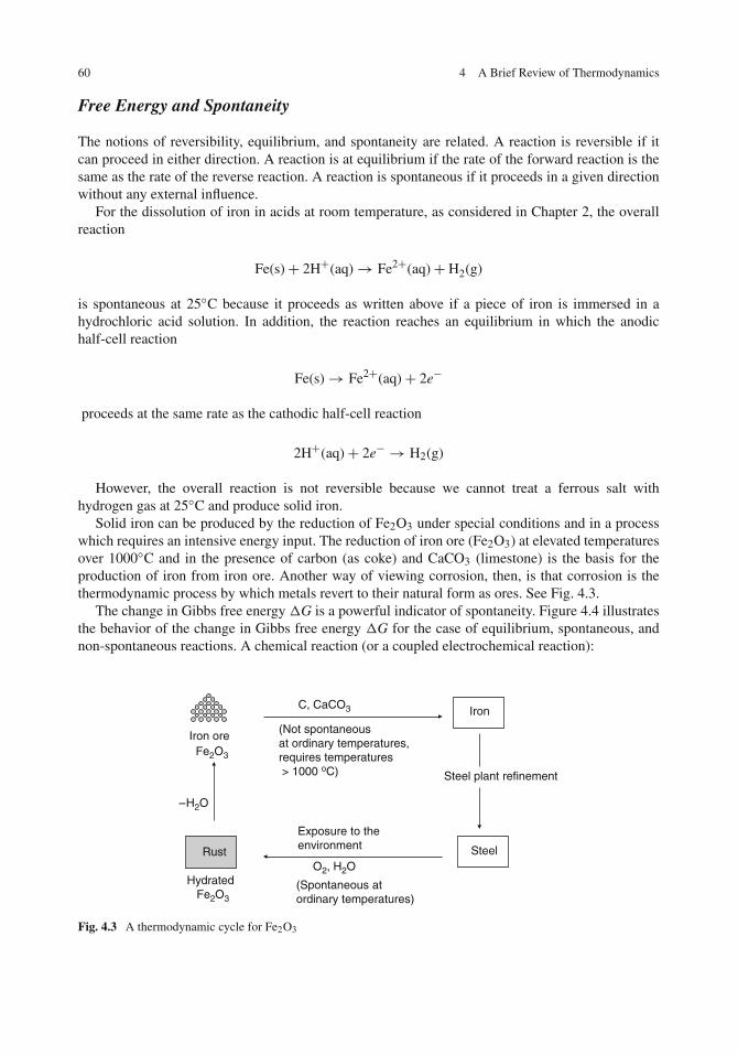
60 4 A Brief Review of Thermodynamics
Free Energy and Spontaneity
The notions of reversibility, equilibrium, and spontaneity are related. A reaction is reversible if itcan proceed in either direction. A reaction is at equilibrium if the rate of the forward reaction is thesame as the rate of the reverse reaction. A reaction is spontaneous if it proceeds in a given directionwithout any external influence.
For the dissolution of iron in acids at room temperature, as considered in Chapter 2, the overallreaction
Fe(s)+ 2H+(aq)→ Fe2+(aq)+ H2(g)
is spontaneous at 25◦C because it proceeds as written above if a piece of iron is immersed in ahydrochloric acid solution. In addition, the reaction reaches an equilibrium in which the anodichalf-cell reaction
Fe(s)→ Fe2+(aq)+ 2e−
proceeds at the same rate as the cathodic half-cell reaction
2H+(aq)+ 2e− → H2(g)
However, the overall reaction is not reversible because we cannot treat a ferrous salt withhydrogen gas at 25◦C and produce solid iron.
Solid iron can be produced by the reduction of Fe2O3 under special conditions and in a processwhich requires an intensive energy input. The reduction of iron ore (Fe2O3) at elevated temperaturesover 1000◦C and in the presence of carbon (as coke) and CaCO3 (limestone) is the basis for theproduction of iron from iron ore. Another way of viewing corrosion, then, is that corrosion is thethermodynamic process by which metals revert to their natural form as ores. See Fig. 4.3.
The change in Gibbs free energy �G is a powerful indicator of spontaneity. Figure 4.4 illustratesthe behavior of the change in Gibbs free energy �G for the case of equilibrium, spontaneous, andnon-spontaneous reactions. A chemical reaction (or a coupled electrochemical reaction):
(Spontaneous at ordinary temperatures)
C, CaCO3
(Not spontaneousat ordinary temperatures,requires temperatures> 1000 oC)
Iron oreFe2O3
Exposure to the environment
O2, H2ORust
HydratedFe2O3
–H2O
Iron
Steel
Steel plant refinement
Fig. 4.3 A thermodynamic cycle for Fe2O3

Thermodynamic State Functions 61
Equilibrium
ΔG = G(products) – G(reactants) = 0
Extent of reaction
Extent of reaction
G
Spontaneous reaction
ΔG < 0
Extent of reaction
G
Non–spontaneous reaction
ΔG > 0G
ΔG
ΔG
Fig. 4.4 The change in Gibbs free energy �G for the case of equilibrium, spontaneous, and non-spontaneous reactions
(1) is at equilibrium if the free energy change �G is zero,(2) proceeds spontaneously if �G is negative,(3) is not spontaneous if �G is positive.
Relationships Between Thermodynamic Functions
From Eqs. (4) and (7)
G = H − TS = (E + PV)− TS (9)
Taking differentials
dG = dE + P dV + V dP− T dS− S dT (10)

62 4 A Brief Review of Thermodynamics
Use of Eq. (2) gives
dG = q+ w+ P dV + V dP− T dS− S dT (11)
From Eq. (3), q = T dS, and also w = −P dV (the minus sign is needed for work done on thesystem). Then Eq. (11) becomes
dG = T dS− P dV + P dV + V dP− T dS− S dT (12)
or
dG = V dP− S dT (13)
Equation (13) applies to a closed system, i.e., one in which there is no mass transfer in or out ofthe system. Suppose that an ideal gas is present. Then PV = RT, where R is the ideal gas constant.(See Table 4.1.) Then, substitution for V = RT/P in Eq. (13) gives
dG = RT
PdP− SdT (14)
At constant temperature T
dG = RT
PdP (15)
The free energy change in going from a standard state (denoted by the superscript zero) to anynew state is given by
G∫Go
dG = RT
P∫Po
d lnP (16)
Integrating gives
G− Go = RT ln(PlPo) (17)
But the pressure in the standard state is 1 atm (see Chapter 3). Then Eq. (17) becomes
G = Go + RT ln P (18)
Table 4.1 Units for the ideal gas constant R and some additional conversion factors
R
0.082058 L atm mole-1K-1 P is in atm62.364 L torr mole-1K-1 P is in torr8.314 J mole-1K-1 P is in Pa, V is in m3
1.987 cal mole-1K-1 P is in Pa, V is in m3
1 cal = 4.184 joules (J).1 J = 1 V C = 1 N m.

The Chemical Potential and Standard States 63
The Chemical Potential and Standard States
The total energy of a system can be changed by
(1) thermal energy +q or −q(2) work +w or −w(3) by adding or subtracting various chemical substances to the system.
If the above third possibility occurs and the system contains ni moles of various species i, thenEq. (13) must be extended to
dG = VdP – SdT +�i
μidni (19)
where μi is the chemical potential of species i defined as
μi =(
∂G
∂ni
)T , P, nj
≡ Gi (20)
That is, the chemical potential is the change in Gibbs free energy with respect to a change in thechemical composition of a given chemical species, at constant temperature T, constant pressure P,and constant composition of the other chemical species which are present. The chemical potential isalso called the partial molar Gibbs free energy and is also given the symbol Gi.
More About the Chemical Potential
For a system containing i components, Eq. (18) becomes
μi = μoi + RT ln Pi (21)
For solids and liquids, Eq. (21) is written as
μi = μoi + RT ln ai (22)
where ai is the activity of the ith species and
(1) for solids, a = 1.(2) for liquid H2O, a = 1.(3) for other liquids and for ions, the activity a is usually replaced by concentration C. This is a
valid approximation for dilute solutions.(4) for gases, the activity a is replaced by pressure P.
Consider a chemical reaction
v1A1 + v2A2 + · · · .→ v1′B1 + v2
′B2 + · · · (23)
where ν1 refers to the number of moles of reactant A1, ν2 refers to the number of moles of reactantA2, etc., and the primes and B′s have similar meanings for the products. When all the reactants and
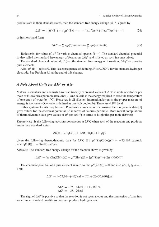
64 4 A Brief Review of Thermodynamics
products are in their standard states, then the standard free energy change �Go is given by
�Go = v ′1μo(B1)+ v ′2μo(B2)+ · · ·−[v1μo(A1)+ [v2μ
o(A2)+ · · · ] (24)
or in short-hand form
�Go = �i
viμoi (products)−�
iviμ
oi (rectants) (25)
Tables exist for values of μo for various chemical species [1−4]. The standard chemical potentialis also called the standard free energy of formation �Gf
o and is listed as such in some tables.The standard chemical potential μo (i.e., the standard free energy of formation, �Gf
o) is zero forpure elements.
Also, μo (H+ (aq))= 0. This is a consequence of defining Eo = 0.000 V for the standard hydrogenelectrode. See Problem 4.1 at the end of this chapter.
A Note About Units for �Go or �G
Materials scientists and chemists have traditionally expressed values of �Go in units of calories permole or kilocalories per mole (kcal/mol). (One calorie is the energy required to raise the temperatureof one gram of water by 1◦C). However, in SI (System Internationale) units, the proper measure ofenergy is the joule. (One joule is defined as one volt coulomb). There are 4.184 J/cal.
Either system of units may be used. Pourbaix’s classic atlas of corrosion thermodynamic data [1]gives values for the chemical potential μo in terms of calories per mole. More recent compilationsof thermodynamic data give values of μo (or �Gf
o) in terms of kilojoules per mole (kJ/mol).
Example 4.1: Is the following reaction spontaneous at 25◦C when each of the reactants and productsare in their standard states:
Zn(s)+ 2H2O(I)→ Zn(OH)2(s)+ H2(g)
given the following thermodynamic data for 25◦C [1]: μo(Zn(OH)2)(s)) = −75,164 cal/mol;μo(H2O (l)) = −56,690 cal/mol.
Solution: The standard free energy change for the reaction above is given by
�Go = [μo(Zn(OH)2(s)) + μo(H2(g))]− [μo(Zn(s))+ 2μo(H2O(l))]
The chemical potential of a pure element is zero so that μo(Zn (s)) = 0 and also μo(H2 (g)) = 0.Thus
�Go = [−75,164+ (0)]cal− [(0)+ 2(−56,690)]cal
�Go = −75,164 cal+ 113,380 cal�Go = +38,126 cal
The sign of �Go is positive so that the reaction is not spontaneous and the immersion of zinc intowater under standard conditions does not produce hydrogen gas.
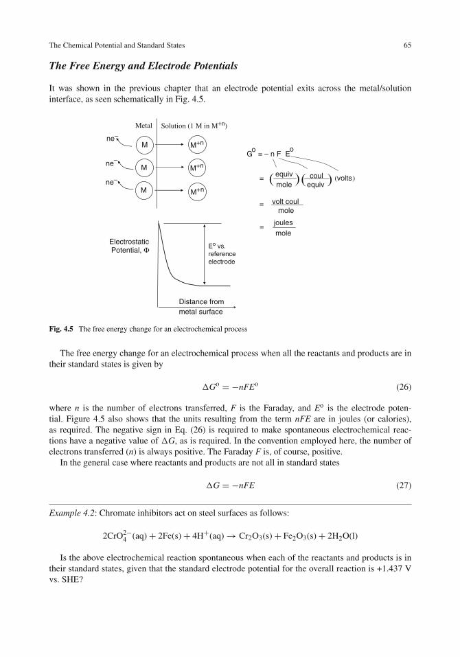
The Chemical Potential and Standard States 65
The Free Energy and Electrode Potentials
It was shown in the previous chapter that an electrode potential exits across the metal/solutioninterface, as seen schematically in Fig. 4.5.
= equiv mole
coul equiv
volts
Metal Solution (1 M in M+n)
ne–
ne–
ne–
M+n
M+n
M+n
M
M
M
ElectrostaticPotential, Φ
= volt coulmole
= joulesmole
Go
= – n F Eo
Distance frommetal surface
Eo vs.referenceelectrode
( ( () ) )
Fig. 4.5 The free energy change for an electrochemical process
The free energy change for an electrochemical process when all the reactants and products are intheir standard states is given by
�Go = −nFEo (26)
where n is the number of electrons transferred, F is the Faraday, and Eo is the electrode poten-tial. Figure 4.5 also shows that the units resulting from the term nFE are in joules (or calories),as required. The negative sign in Eq. (26) is required to make spontaneous electrochemical reac-tions have a negative value of �G, as is required. In the convention employed here, the number ofelectrons transferred (n) is always positive. The Faraday F is, of course, positive.
In the general case where reactants and products are not all in standard states
�G = −nFE (27)
Example 4.2: Chromate inhibitors act on steel surfaces as follows:
2CrO2−4 (aq)+ 2Fe(s)+ 4H+(aq)→ Cr2O3(s)+ Fe2O3(s)+ 2H2O(l)
Is the above electrochemical reaction spontaneous when each of the reactants and products is intheir standard states, given that the standard electrode potential for the overall reaction is +1.437 Vvs. SHE?

66 4 A Brief Review of Thermodynamics
Solution:
�Go = −nFEo
�Go = −(+n)(+F)(+1.437) < 0
Thus, the reaction is spontaneous as written. Note, for our purposes here, we do not need to knowthe value of n but only that it is positive. We can determine that n = 6 by separating the overallelectrochemical reaction into its two half-cell reactions:
2Fe(s)+ 3H2O(I)→ Fe2O3(s)+ 6H+ + 6e−
2CrO2−4 (aq)+ 10H+(aq)+ 6e− → Cr2O3(s)+ 5H2O(l)
The sum of these two half-cell reactions is the overall reaction given above. More detail onelectrochemical cells is given in Chapter 5.
The Nernst Equation
As noted in Chapter 3, standard electrode potentials Eo apply only to the situation where a metalis immersed in a solution of its own ions at unit activity. This condition is rarely encountered incorrosion reactions. The Nernst equation allows calculation of the half-cell potential for some otherconcentration in terms of the standard electrode potential. The derivation is given here.
Consider a general electrochemical reaction
aA+ bB+ ne � cC+ dD (28)
where a is the number of moles of reactant A, b is the number of moles of reactant B, etc. FromEq. (25)
�G =�i
viμi (products)−�i
viμi (rectants) (29)
or
�G = cμC + dμD − aμA − bμB (30)
But from Eq. (22)
μC = μoC + RT ln aC
μD = μoD + RT ln aD
μA = μoA + RT ln aA
μB = μoB + RT ln aB
(31)
Substitution of Eq. (31) in Eq. (30) gives
�G = c[μoC + RT ln aC]+ d[μo
D + RT ln aD]− a[μoA + RT ln aA]− b[μo
B + RT ln aB] (32)

The Nernst Equation 67
Grouping terms gives
�G = [cμoC + dμo
D − aμoA − bμo
B]+[
RT lnac
C adD
aaAab
B
](33)
But from Eq. (25)
�Go = cμoC + dμo
D − aμoA − bμo
B (34)
so that Eq. (33) becomes
�G = �G0 + RT lnac
c adD
aaA ab
B
(35)
With �G = − nFE and �Go = − nFEo, Eq. (35) becomes
E = Eo − 2.303RT
nFlog
acCad
D
aaAab
B
(36)
which is the Nernst equation. This equation is very useful in the analysis of electrochemical cellsand in the construction of Pourbaix diagrams. These subjects are treated in the next two chapters. At25◦C, Eq. (36) can be written as
E = Eo − 0.0591
nlog
acC ad
D
aaA ab
B
(37)
Standard Free Energy Change and the Equilibrium Constant
The equilibrium constant for Eq. (28) is
K = acC ad
D
aaA ab
B
(38)
so that Eq. (35) can be rewritten as
�G = �Go + RT ln K (39)
At equilibrium, �G = 0 so that Eq. (39) becomes
�Go = −RT ln K (40)
or
�Go = −2.303 RT log K (41)
This equation is useful because it is the link between the standard free energy change and theequilibrium constant for a reaction.

68 4 A Brief Review of Thermodynamics
Equilibrium constant K
Standard free energy
change, ΔG o
Standard electrode
potential, Eo
ΔGo = – RT ln K E = Eo– 2.303 RT
n F log K
ΔGo = – n F Eo
Fig. 4.6 Summary of relationships between the standard free energy change, the standard electrode potential, and theequilibrium constant for electrochemical reactions
Figure 4.6 summarizes relationships between the standard free energy change, the standardelectrode potential, and the equilibrium constant for electrochemical reactions.
A Quandary – The Sign of Electrode Potentials
Throughout this chapter we have been adhering to a system of thermodynamics commonly calledthe American sign convention [4, 5]. We write
Zn2+(a = 1)+ 2e− → Zn E = −0.762 V
but we write
Zn→ Zn2+(a = 1)+ 2e− E = +0.762 V
These are thermodynamic half-cell potentials, but what is the sign of the electrode potential forthe physical electrode of an actual sample of zinc metal immersed in an actual solution of unitactivity of Zn2+ ions?
At the physical electrode, there is an equilibrium between zinc metal and zinc ions so that zincions pass into solution at the same rate at which they are reduced back onto the metal surface, asdepicted in Fig. 4.7. So what is the electrode potential for the physical electrode? Is it the average of
Zn Zn+2
Metal Solution
(unit activity )
Fig. 4.7 The Zn/Zn2+ electrode at equilibrium. The rate at which Zn goes into solution is equal to the rate at whichZn2+ ions are reduced to solid Zn

A Quandary – The Sign of Electrode Potentials 69
the reduction and oxidation potentials? This cannot be, for the average potential would be 0.000 V,and this is the standard electrode potential for the reduction of hydrogen ions to hydrogen gas.Moreover, the physical electrode potentials for all metals listed in the emf series would also be0.000 V, so actual electrode potentials would be a meaningless concept.
Note that in Fig. 3.24, the metal electrode under study is connected to the positive terminal of theelectrometer and the reference electrode is connected to the negative terminal. This is a conventionadapted by the American Society of Testing and Materials [6], and this arrangement gives the propersign of the measured electrode potential. The proper sign for the actual physical electrode potentialof zinc in contact with a solution of unit activity Zn2+ ions is negative. (A simple test cell of zinc incontact with Zn2+ ions can be used to see if your test setup in the laboratory is correct in regard to thesigns of measured electrode potentials.) But suppose that the connections to the test and referenceelectrodes would be reversed. Then the sign of the measured physical electrode potential would alsobe reversed.
Thus, the sign of a physical electrode potential is a convention. This is in addition to the earlierconvention that the forward direction of a half-cell reaction is taken to be the direction in whichreduction occurs.
We want to relate a direction-sensitive quantity �G to a direction-insensitive observable E. This isthe origin of all confusion regarding electrode potentials. Enlightening comments about this situationhave been written by Anson [7] and deBethune [8].
Thus, in the American system of signs conventions, the sign of a thermodynamic half-cell reactionis sign bivariant (depending on whether the half-cell reaction is a reduction or an oxidation reaction),but the number of electrons transferred is always positive when using Eqs. (26), (27) or the Nernstequation, Eq. (36).
Mention should also be made of the European sign convention, used by Pourbaix [1]. Accordingto this system
Zn2+(a = 1)+ 2e− → Zn(s) E =− 0.762 V
and also
Zn(s)→ Zn2+(a = 1)+ 2e− E = −0.762 V
Thus, in the European system of signs conventions, the sign of a thermodynamic half-cell reac-tion is invariant (i.e., the same for a reduction or an oxidation reaction). However, the number ofelectrons transferred is sign bivariant (negative when the half-cell reaction is a reduction reactionand positive when the half-cell reaction is anoxidation reaction). In this system, �G = nFE andthe Nernst equation also has a slightly different form. See Table 4.2 for a comparison of these twoconventions.
Confusing? Sort of, but not if one follows a given convention consistently. Throughout this text,we will be adhering to the American sign convention.
Factors Affecting Electrode Potentials
Actual physical electrode potentials are affected by several variables including (i) the nature of themetal, (ii) the chemical nature of the aqueous solution, (iii) the presence of oxide films on the metalsurface, (iv) the presence of adsorbed gases on the metal surface, and (v) the presence of mechanicalstress on the metal [9]. See Table 4.3, which lists the magnitude of these effects.

70 4 A Brief Review of Thermodynamics
Table 4.2 A comparison of American and European sign conventions for thermodynamic systems
American convention European convention
Zn2+(a = 1)+ 2e− → Zn(s)Eo = −0.762 V
Zn2+(a = 1)+ 2e− → Zn(s)Eo = −0.762 V
Zn(s)→ Zn2+(a = 1)+ 2e−Eo = +0.762 V
Zn(s)→ Zn2+(a = 1)+ 2e−Eo = −0.762 V
Cu2+(a = 1)+ 2e− → Cu(s)Eo = +0.342 V
Cu2+(a = 1)+ 2e− → Cu(s)Eo = +0.342 V
Cu(s)→ Cu2+(a = 1)+ 2e−Eo = −0.342 V
Cu(s)→ Cu2+(a = 1)+ 2e−Eo = +0.342 V
�Go = −nFEo
Eo is sign bivariantn is sign invariant (always positive)
�Go = nFEo
Eo is sign invariantn is sign bivariant(negative for reduction, positive for
oxidation)
Nernst equation
E = Eo − 2.303RT
nFlog
acC ad
D
aaAab
BEo is sign bivariantn is sign invariant (always positive)
Nernst equation
E = Eo + 2.303RT
nFlog
acC ad
D
aaA ab
BEo is sign invariantn is sign bivariant(negative for reduction, positive for
oxidation
Table 4.3 Effect of various factors on the electrode potential [9]
EffectMagnitude of effect on electrodepotential
Nature of the metal Whole voltsChemical nature of the aqueous
solutionTenths to whole volts
Surface state (oxide films) Tenths of a voltAdsorbed gases Hundreds to tenths of voltsMechanical stress Thousandths to hundreds of volts
Problems
1. Show that μo(H+(aq)) = 0 is a consequence of defining Eo = 0.000 as the standard electrodepotential for reduction of the hydrogen ion:
2H+(aq) + 2e−→H2 (g)
2. (a) Calculate 2.303RT in joules per mole and calories per mole at 25◦C.(b) Show that 2.303RT/F is equal to 0.0591 V equiv/mol at 25◦C.
3. Calculate the electrode potential at 25◦C for the Peterson–Groover Ag/AgCl reference electrodewhen it is used in natural seawater, for which the Cl– concentration is 0.6 M. (b) How does thiselectrode potential compare with that for the saturated calomel electrode?

Problems 71
4. Dissolved lead can enter the public drinking supply through the use of lead piping systems andlead solder. The present standard for allowable dissolved Pb2+ ions is 15 μg/L. Calculate thereduction potential for lead metal in contact with this concentration of dissolved Pb2+ ions:
Pb2+(aq)+ 2e− → Pb(s)
5. For health reasons the concentration of dissolved copper ions in drinking water should be lessthan 2 mg/L of Cu2+[10]. Calculate the reduction potential of copper metal in contact with asolution containing 2 mg/L of dissolved Cu2+ at 25◦C.
6. Calculate whether copper will spontaneously corrode at 25◦C by the following half-cellreaction:
2Cu(s)+ H2O(l)+ O2(g)→ 2CuO(s)+ H+(aq)+ OH−(aq)
given the following standard chemical potentials μo (in cal/mol):
CuO (s) = –30,400; OH– (aq) = –37, 595; H2O (l) = –56,690.
7. Research has been conducted on molybdates as replacements for chromates in the surface treat-ment of various metals in order to reduce corrosion by the formation of a surface film of MoO2.The overall reaction with iron is
2Fe(s)+ 3MoO2−4 (aq)+ 6H+(aq)→ Fe2O3(s)+ 3MoO2(s)+ 3H2O(l)
(a) Given the following standard chemical potentials (μo) in calories per mole at 25◦C:Fe2O3 (s) = –177,100, MoO2 (s) = –120,000, H2O (l) = –56,690, MoO4
–2 (aq) =–205,420:
(a) Is the above overall reaction spontaneous under standard conditions?(b) Calculate the standard electrode potential for the above overall reaction.(c) Write an expression for the electrode potential as a function of molybdate ion
concentration and pH.(d) Is the overall reaction spontaneous for a molybdate ion concentration of 0.001 M at pH
7.0?(e) Based solely on thermodynamic considerations, what do the results in (a) and (d)
suggest about the possibility of molybdates as chromate replacements?
8. Calculate the standard chemical potential of Sn2+ ions, μo(Sn2+ (aq)), from the appropriatestandard electrode potential in Table 3.1.
9. Magnesium corrodes in an aqueous solution of pH 9.0 to produce precipitated Mg(OH)2. Whatis the reduction potential of magnesium in this solution at 25◦C for the reaction
Mg2+(aq)+ 2e− → Mg(s) Eo = −2.372 V
The solubility product of Mg(OH)2 is Ksp = 1.8 x 10−11.10. Waste acid of pH 3.0 is stored in a lead-lined vessel, as shown in the figure below. If the walls
of the container undergo corrosion by the following reaction:
Pb(s)+ 2H+(aq)→ Pb2+(aq)+ H2(g)
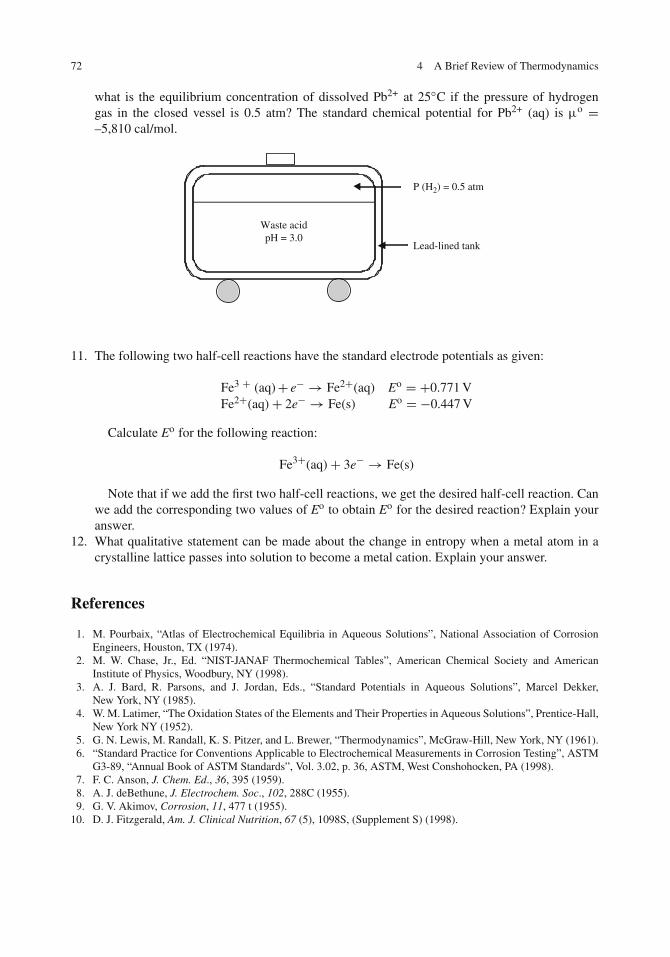
72 4 A Brief Review of Thermodynamics
what is the equilibrium concentration of dissolved Pb2+ at 25◦C if the pressure of hydrogengas in the closed vessel is 0.5 atm? The standard chemical potential for Pb2+ (aq) is μo =–5,810 cal/mol.
P (H2) = 0.5 atm
Waste acidpH = 3.0
Lead-lined tank
11. The following two half-cell reactions have the standard electrode potentials as given:
Fe3 + (aq)+ e− → Fe2+(aq) Eo = +0.771 VFe2+(aq)+ 2e− → Fe(s) Eo = −0.447 V
Calculate Eo for the following reaction:
Fe3+(aq)+ 3e− → Fe(s)
Note that if we add the first two half-cell reactions, we get the desired half-cell reaction. Canwe add the corresponding two values of Eo to obtain Eo for the desired reaction? Explain youranswer.
12. What qualitative statement can be made about the change in entropy when a metal atom in acrystalline lattice passes into solution to become a metal cation. Explain your answer.
References
1. M. Pourbaix, “Atlas of Electrochemical Equilibria in Aqueous Solutions”, National Association of CorrosionEngineers, Houston, TX (1974).
2. M. W. Chase, Jr., Ed. “NIST-JANAF Thermochemical Tables”, American Chemical Society and AmericanInstitute of Physics, Woodbury, NY (1998).
3. A. J. Bard, R. Parsons, and J. Jordan, Eds., “Standard Potentials in Aqueous Solutions”, Marcel Dekker,New York, NY (1985).
4. W. M. Latimer, “The Oxidation States of the Elements and Their Properties in Aqueous Solutions”, Prentice-Hall,New York NY (1952).
5. G. N. Lewis, M. Randall, K. S. Pitzer, and L. Brewer, “Thermodynamics”, McGraw-Hill, New York, NY (1961).6. “Standard Practice for Conventions Applicable to Electrochemical Measurements in Corrosion Testing”, ASTM
G3-89, “Annual Book of ASTM Standards”, Vol. 3.02, p. 36, ASTM, West Conshohocken, PA (1998).7. F. C. Anson, J. Chem. Ed., 36, 395 (1959).8. A. J. deBethune, J. Electrochem. Soc., 102, 288C (1955).9. G. V. Akimov, Corrosion, 11, 477 t (1955).
10. D. J. Fitzgerald, Am. J. Clinical Nutrition, 67 (5), 1098S, (Supplement S) (1998).

Chapter 5Thermodynamics of Corrosion: Electrochemical Cellsand Galvanic Corrosion
Introduction
The previous chapter has dealt largely with the corrosion thermodynamics of half-cell reactions forsingle metals. This chapter considers the effect of coupling two half-cells to form an electrochemicalcell. The galvanic corrosion of coupled dissimilar metals is also treated in this chapter.
Electrochemical Cells
Consider the two half-cells shown in Fig. 5.1(a). In the compartment on the left, zinc ions arein equilibrium with the solid zinc electrode. This means that the rate at which Zn2+ ions passinto solution is equal to the rate at which they are reduced to solid zinc. The standard reductionpotential is
Zn2+ (aq)+ 2e− → Zn(s) Eo = −0.762 V
In the compartment on the right, copper ions are in equilibrium with the solid copper electrode.Thus, the rate at which Cu2+ ions pass into solution is equal to the rate at which they are reduced tosolid copper. The standard reduction potential is
Cu2+(aq)+ 2e–→ Cu (s) Eo= +0.342 V
When the two unconnected half-cells are coupled by closing the switch in the external circuit, asin Fig. 5.1(b), an electrochemical cell is formed. One of the metals will be the anode and the otherwill be the cathode, although we cannot yet tell which is which. First suppose that the zinc electrodeis the anode. Then
At the cathode
Cu2+(aq)+ 2e− → Cu (s) Eo = +0.342 V
At the anode
Zn(s)→ Zn2+(aq)+ 2e− − Eo= −(− 0.762 V)
73E. McCafferty, Introduction to Corrosion Science, DOI 10.1007/978-1-4419-0455-3_5,C© Springer Science+Business Media, LLC 2010

74 5 Thermodynamics of Corrosion
Zn+2
Zn+2
Zn
porous glass frit
a (Zn+2) = 1
Cu+2
Cu+2
Cu
a (Cu+2) = 1
(a)
Zn+2Zn
porous glass frit
a (Zn+2) = 1
+ 1.104 V
e− e−
Cu+2Cu
a (Cu+2) = 1
(b)
Fig. 5.1 An electrochemical galvanic cell
Adding the two half-cell reactions gives the overall chemical reaction:
Cu2+(aq)+Zn(s) → Cu(s)+Zn2+(aq) (1)
and adding the half-cell potentials gives
Eocell = Eo
cathode − Eoanode (2)
or Eocell = + 0.342V− (− 0.762 V) = +1.104 V. From
�Gcell = −nFEcell (3)
the free energy change is negative because the cell potential is positive. Thus, the reaction proceedsspontaneously as written above in Eq. (1), and we have correctly identified the anode and the cathodein the coupled cell.
If we had assumed initially that the copper electrode was the anode and the zinc electrode thecathode, then the calculated cell potential would be E◦cell = –1.104 V. But then the calculated changein free energy would have been positive so that the assumed reaction would not be spontaneous.Thus, we would have reached the same conclusion as above.
The following general conclusions can be drawn:

Electrochemical Cells 75
(1) In an electrochemical cell, the metal with the lower electrode potential (more negative reductionpotential) in the emf series is the anode; the metal with the higher electrode potential (morepositive reduction potential) is the cathode.
(2) The cell potential (also called the cell voltage or cell emf) is given by
Ecell = Ecathode − Eanode (4)
where both Ecathode and Eanode are reduction potentials.If the concentration of dissolved ions is not unit activity, the half-cell potentials can be calculated
using the Nernst equation, and the procedure is then continued as described above.
Electrochemical Cells on the Same Surface
An electrochemical cell can also exist on different portions of the same metal surface, as shown inthe following example.
Example 5.1: Calculate whether copper can corrode at 25◦C in an acid solution of pH 2.0 to producea solution containing 0.10 M Cu2+ ions and 0.5 atm hydrogen gas.Solution: The overall chemical reaction is
Cu(s)+ 2H+(aq)→ Cu2+(aq) + H2 (g)
At the local cathodes
2H+ (aq)+ 2e− → H2(g) Ecathode
At the local anodes
Cu (s)→ Cu2+ (aq)+ 2e− Eanode
We calculate the electrode potentials for each half-cell reaction written as a reduction reaction.Using the Nernst equation
Ecathode=EoH+/H2
− 0.0591
2log
P(H2)
[H+]2
Ecathode = 0.000 − 0.0591
2log
0.5
[1.0x10⁻²]2
or
Ecathode = −0.109 V
Then
Eanode=EOCu+2/Cu
− 0.0591
2log
1
[Cu+2]

76 5 Thermodynamics of Corrosion
Eanode = + 0.342 − 0.0591
2log
1
0.10
or
Eanode = +0.312
Thus
Ecell = Ecathode − Eanode
Ecell = −0.109− (+ 0.312) = −0.421 V
Because the cell voltage is negative, �Gcell = – nFEcell is positive, and thus the reaction will notproceed spontaneously to produce the conditions which were described.
Galvanic Corrosion
Galvanic corrosion occurs when two dissimilar metals are in physical (and electrical) contact inan aqueous electrolyte, as shown in Fig. 5.2. Alternately (and less usual), the two metals may beconnected by an external metal path. Galvanic coupling of metals in equilibrium with their ownions rarely occurs, but instead each of the two individual metals is usually immersed in a commonelectrolyte. Some examples of galvanic corrosion include the following:
IronCopper
Electrolyte
Iron
Fig. 5.2 Two dissimilar metals in a galvanic couple
(1) Copper piping connected to steel tanks.(2) Boats having a nickel alloy hull and steel rivets.(3) Zinc-coated screws in a sheet of copper.(4) Tin-plated electrical connector pins mated with gold-plated sockets.(5) A stainless steel screw in contact with a cadmium-plated steel washer.
The galvanic series described below is very useful in indicating whether combined pairs ofcoupled metals will be prone to galvanic corrosion.
Galvanic Series
As noted in Chapter 3, the emf series has limited practical use. The standard electrode potentials arefor half-cell reactions for metals in solutions of their own ions at unit activity. This set of conditionsis important in the development of the concept of electrode potentials, but these conditions are quiterestrictive and are not those found in most corrosion applications. The concentration of dissolvedmetal ions in equilibrium with a given metal depends on the environment and on the details of thesystem, such as the corrosion rate, the degree of mass transfer, and the volume of the solution.

Galvanic Corrosion 77
The restriction of unit activity in the emf series can be removed by using the Nernst equation tocalculate the potential for a half-cell reaction at some concentration other than unit activity. However,there is still the restriction in the emf series that the solution contains cations of only the metal ofinterest. In addition, the emf series applies only to pure metals and not to alloys.
Any metal or alloy placed in a corrosive environment has its own electrode potential, called thecorrosion potential Ecorr. The galvanic series (in seawater) is an ordered listing of experimentallymeasured corrosion potentials in natural seawater for both pure metals and alloys. See Fig. 5.3[1].Metals and alloys with more positive potentials (like platinum) are called noble metals, and met-als with more negative potentials (like magnesium) are called active metals. Note that the electrodepotentials in the galvanic series in Fig. 5.3 are measured relative to a saturated calomel electrode(although any suitable reference electrode can be used), whereas standard half-cell electrode poten-tials are always referred to as the standard hydrogen electrode. Note also that all the alloys given inFig. 5.3 exhibit a range of electrode potentials.
–1.5–1.0–0.50.00.5
E in V vs. S.C.E.
ZincMagnesium
BeryliumAluminum alloys
CadmiumMild steel, cast iron
Low alloy steelAustenitic Ni cast iron
Aluminum bronzeNaval brass, yellow brass, red brass
TinCopper
GraphitePlatinum
Ni-Cr-Mo alloy CTitanium
Ni-Cr-Mo-Cu-Si alloy BNi-Fe-Cr alloy 825
Stainless steel- Type 316Alloy 20
Ni-Cu alloys 400, K-500 (Monel)Stainless steel- Type 304SilverNickelSilver braze alloysNi-Cr alloy 600Ni-Al bronze70-30 Cu-NiLeadStainless steel- Type 43080-20 Cu-Ni90-10 Cu-NiNickel silverStainless steel Types 410, 416Tin bronzesSilicon bronzeManganese bronzeAdmiralty brass, aluminum brass
Pd-Sn solder (50/50)
Fig. 5.3 The galvanic series in seawater. Redrawn from [1] by permission of John Wiley & Sons, Inc

78 5 Thermodynamics of Corrosion
The utility of the galvanic series is as follows:In a galvanic couple, the metal or the alloy with the more negative electrode potential is the
anode. The metal or the alloy with the more positive electrode potential is the cathode.This conclusion follows from the analysis of electrochemical cells using the emf series.
Example 5.2: Composite materials consisting of magnesium containing graphite-reinforcing fibershave been developed to increase the mechanical strength of the light metal magnesium. Will theintroduction of graphite into magnesium pose a problem if this composite material is used inseawater?
Solution: From Fig. 5.3, the electrode potential of graphite in seawater is approximately +0.25 Vvs. SCE. The electrode potential of magnesium is –1.6 V vs. SCE. Thus, in a magnesium–graphitecouple, magnesium will be the anode. Because of the large difference in the two electrode potentials,there will be a large galvanic effect between magnesium and graphite. This couple should not be usedin seawater unless the composite material is provided corrosion protection, such as a barrier of paintor some other organic coating.
The order of a series of metals in any galvanic series may not be the same as their order in the emfseries. Thus, the emf series cannot be used reliably to predict the corrosion tendencies of coupledmetals in other environments.
Similarly, the galvanic series for seawater should not be used to predict corrosion tendencies insolutions which are very much different than seawater. For example, the galvanic series in seawatermay be applied (with some caution) to the behavior of metals and alloys used for joint replacementsin the human body. This is because a simulated physiological fluid known as Ringer’s solution con-tains a mixture of dissolved NaCl, KCl, and CaCl2, which is 0.16 M in total chlorides. Thus, bodyfluids and Ringer’s solution can be considered to be dilute seawater so that the galvanic series forseawater can be used as a first approximation, although data in Ringer’s solution itself should beused when available.
While the use of the galvanic series in seawater is possible for similar aqueous solutions, itsextension to additional solutions, such as hydrochloric acid, for example, should be considered withmuch reservation.
Another limitation of any galvanic series is that the series gives no information about rates ofcorrosion, but only about corrosion tendencies. Actual corrosion rates must be determined in separateexperiments or tests, to be discussed in Chapter 7.
Although it is not possible to predict corrosion rates from the use of the galvanic series, theanodic metal will have a higher corrosion rate in the couple than in the freely corroding (uncou-pled) condition. LaQue [1] has tabulated seawater corrosion data for aluminum coupled to variousmetals located above it in the galvanic series in seawater. In each case, aluminum was the anodein the galvanic couple, and its corrosion rate when coupled was accelerated relative to its corro-sion rate in its freely corroding (uncoupled) condition. Figure 5.4 shows corrosion data in naturalseawater for aluminum coupled to various metals after 30 days of immersion in seawater flowing at7.8 ft/s. In each case, the electrode potential of uncoupled aluminum was more negative than the elec-trode potential of the uncoupled second metal, as may be seen by referring to the galvanic series inFig. 5.3. Thus, aluminum is the anode in each metal couple. As seen in Fig. 5.4, the corrosion rate inseawater in each galvanic couple was greater than the corrosion rate of freely corroding aluminum.The galvanic effect in each case is the difference in the corrosion rate of aluminum in each coupleand the corrosion rate of aluminum coupled to itself.
For each couple in Fig. 5.4, the anodic to cathodic area ratios were held constant. The effect ofthe ratio of anodic and cathodic areas on galvanic corrosion will be considered in Chapter 7.

Galvanic Corrosion 79
0
50
100
150
200
250
300
–0.90–0.30–0.15–0.10–0.100.0Sea
wat
er C
orro
sion
Rat
e of
Alu
min
um in
mg/
cm2
Electrode Potential in Seawater of Second Metal
Fre
ely
corr
odin
g (u
ncou
pled
) al
umin
um
Alu
min
um c
oupl
ed to
tita
nium
Alu
min
um c
oupl
ed to
Mon
el
Alu
min
um c
oupl
ed to
304
stai
nles
s st
eel
Alu
min
um c
oupl
ed to
nic
kel
Alu
min
um c
oupl
ed to
cop
per
Fig. 5.4 Galvanic corrosion data for various metals coupled to aluminum in seawater [1]
To date, the galvanic series in seawater is the most extensive set of corrosion potentials developedfor any corrosive environment. However, galvanic series exist for metals in flowing hot water [2], inphthalate buffers [3], in solutions of NaHCO3 or Cl–-containing NaHCO3 solutions [4].
Cathodic Protection
Galvanic corrosion is usually not a desired occurrence. However, by an appropriate selection of metalpairs, galvanic corrosion can be employed as a method of corrosion protection. Zinc metal platesfastened to the steel hulls of ships are used to protect the ship hulls by sacrificially corroding, ratherthan having the hull itself corrode. Such a practice is called cathodic protection, and its principle isillustrated in Fig. 5.5.
Zn Zn+2
2e–
–
Zn+2Zn
2e
O2 + 2 H 2O + 4e– 4 OH–
Fe Solution
Fig. 5.5 Schematic diagram of the cathodic protection of iron by zinc

80 5 Thermodynamics of Corrosion
As shown in Fig. 5.3, the electrode potential of low alloy steel in seawater is approximately–0.6 V vs. SCE. The electrode potential of zinc is –1.0 V. Thus, when zinc is coupled to steel, zincwill be the anode and steel will be the cathode, as illustrated in Fig. 5.5. Hence the term “cathodicprotection.”
In actual practice, the exterior hull of the ship will most likely be painted. But when the layer ofpaint protection breaks down locally (“holidays” in the paint film), then cathodic protection takesover. Cathodic protection by sacrificial zinc anodes is used to protect bare steel in interior holdingtanks of commercial and military vessels, in hot water heaters, water storage tanks, buried pipelines,and steel reinforcing bars in concrete structures located in marine environments, to name a fewexamples.
In addition to the use of sacrificial anodes, as described above, cathodic protection can also beprovided through the use of external impressed current systems. In this latter approach, a source ofdirect current is applied using a power supply and an external anode located some distance away buthaving an electrical connection to the protected structure. See Fig. 5.6. Various anodes have beenused, including high silicon cast iron, graphite, and platinum claddings.
PowerSupply
Anode
Structure to be protected(e.g., steel)
e
e
–
–
e–
e–
Electrolyte
O2 + 2 H2O + 4e–
4 OH–
Fig. 5.6 Schematic diagram of cathodic protection by an impressed current device
Two Types of Metallic Coatings
There are two types of metallic coatings used to protect underlying metal substrates. These are (i)sacrificial and (ii) noble metal coatings.
The first of these types, sacrificial coatings, functions by cathodic protection of the substrate.The most common example is the use of an outer layer of zinc on a steel substrate (“galvanized”steel). Zinc has a more negative electrode potential than does steel in most environments, so zinc isagain the anode when it is coupled to steel. When defects such as a pinhole or a crack develop inthe outermost zinc coating, the underlying steel is protected by the sacrificial corrosion of zinc, asshown schematically in Fig. 5.7.

Two Types of Metallic Coatings 81
Zinc
Steel
Seawater
(a)
Zinc
Steel
Seawater
(b)
Fig. 5.7 A sacrificial protective coating. When a break or an imperfection develops in the coating and extends downto the substrate, as shown in (a), the zinc coating will galvanically corrode to protect the underlying substrate, asshown in (b)
Fig. 5.8 The corrosion of a galvanized roof in the natural atmosphere. When the protective zinc coating is breached,the underlying steel eventually suffers corrosion
Galvanized steel sheet is a common roofing material for both industrial and agricultural buildings.The thickness of the zinc coating is usually of the order of 0.001 in. (0.025 mm) [5], and the lifetimeof galvanized roofs in outdoor atmospheric exposures is about 20 years or more, depending on theseverity of the corrosive environment [5, 6]. When the entire zinc coating has been consumed dueto corrosion, the effect of cathodic protection is lost, and the underlying steel substrate corrodes todisplay the familiar red color often seen in the roofs of deteriorating structures. See Fig. 5.8.
An alloy coating of zinc and aluminum has also been used in outdoor environments as a sacri-ficial coating. This zinc–aluminum coating provides cathodic protection while lasting longer thanconventional zinc galvanized coatings [6].
The second type of metallic coating, the noble metal coating, is illustrated by a coating of nickelon steel, as shown in Fig. 5.9. In most aqueous environments, the electrode potential of nickel ismore positive than the electrode potential of steel. Thus, steel is the anode when coupled to nickel.

82 5 Thermodynamics of Corrosion
Nickel
Stee l
Seawater
(a)
(b)
Nickel
Steel
Seawater
Fig. 5.9 A noble metal protective coating. When a break or an imperfection develops in the nickel coating and extendsdown to the substrate, as shown in (a), the underlying steel substrate will galvanically corrode, as shown in (b)
The protective effect of the nickel coating lies in its greater corrosion resistance in the corrosive envi-ronment. However, when defects arise in the noble metal coating, then the steel substrate undergoescorrosion, and the attack is concentrated in the steel substrate at the base of the defect. This is nota desired situation, as the attack can be deep and localized. This is in contrast to sacrificial coatingswhere the substrate is protected when a breach develops in the coating, and the attack is distributedto some extent along the coating.
In general, the situation involving a small anode area coupled to a large cathode area is unfavor-able, because corrosion will be concentrated at the anode and will usually lead to intense localizedattack.
Titanium Coatings on Steel: A Research Study
Plasma spraying is a useful technique for applying protective metal coatings to engineering alloys.However, plasma-sprayed coatings generally exhibit porosity because the molten droplets depositedby the plasma cool so rapidly that they cannot flow and completely wet the surface of the metalsubstrate. Thus small voids are trapped as the coating builds up droplet by droplet. As discussedabove, voids or defects in metallic coatings bring on the onset of electrochemical cells between thecoating and the substrate.
In order to improve the corrosion behavior of a porous titanium coating on steel (a noble metalcoating), Ayers and co-workers [7] have employed the use of a high-power laser to melt partiallythrough the porous plasma-sprayed titanium layer so as to consolidate the pores in the coating.(More about laser processing for improved corrosion resistance is given in Chapter 16).
Figure 5.10 shows electrode potentials measured in natural seawater for various samples. After15 days of immersion, the electrode potential of pure titanium was approximately –0.2 V vs. SCE,whereas the electrode potential of the mild steel substrate was approximately –0.7 V vs. SCE. Thus,the titanium coating is a noble coating, and if coupled to steel, the steel member of the couple wouldbe the anode.

Protection Against Galvanic Corrosion 83
Fig. 5.10 Electrode potentials of titanium, steel, and titanium coatings in seawater [7]. Reprinted with permission of© NACE International 1981
Figure 5.10 shows that the electrode potential of the laser-consolidated coating was similar tothat of pure titanium. During the immersion period this laser-processed coated sample remainedunattacked and had the same general appearance of pure titanium. In contrast, the plasma-sprayedtitanium coating had an electrode potential closer to that of steel rather than titanium. This sampleshowed visible rust staining during the test period.
Figure 5.11 shows cross sections through the two types of titanium coatings after the 15-dayimmersion period. As seen in the figure, corrosion pitting occurred at the steel substrate beneaththe porous coating, and the attack was localized as deep pits, as illustrated schematically inFig. 5.9 for a noble metal coating. Figure 5.11 also shows that laser remelt consolidation preventedthe occurrence of such pitting by successfully eliminating pores in the laser-melted region.
Protection Against Galvanic Corrosion
Practices for minimizing galvanic corrosion are as follows [8]:
(1) Select combinations of metals as near to each other as possible in the galvanic series.(2) Insulate the contact between dissimilar metals whenever possible.(3) Apply organic coatings, but coat both members of the couple or coat only the cathode. Do not
coat only the anode, because if a defect (holiday) develops in the organic coating, an acceleratedattack will occur because of the unfavorable effect of a small anode area and a large cathodearea, as shown in Fig. 5.9.
(4) Avoid the unfavorable area effect of having a small anode coupled to a large cathode.(5) Install a third metal which is anodic to both metals in the galvanic couple.
Several of the measures listed above are illustrated schematically in Fig. 5.12. Area effectsin galvanic corrosion will be revisited in Chapter 7 when the kinetic aspects of corrosion areconsidered.

84 5 Thermodynamics of Corrosion
Fig. 5.11 Cross-sectional views through the coated specimen after 15 days of immersion in flowing seawater. Top:The unconsolidated sample shows pitting attack of the steel at the coating/substrate interface. Bottom: The sample wasconsolidated by laser melting approximately one-third of the coating thickness and showed no evidence of corrosion[7]. Reprinted with permission of © NACE International 1981
Differential Concentration Cells
As seen above, a difference in electrode potentials will exist for two different metals located in thesame solution. A difference in electrode potentials will also exist for the same metal placed in twodifferent concentrations of the same solution. Such a cell consisting of two half-cells of the samemetal but with differing ionic or molecular concentrations is called a differential concentration cell.
There are two main types of differential concentration cells: (i) metal ion concentration cells and(ii) oxygen concentration cells. Either can cause corrosion to occur.
Metal Ion Concentration Cells
Consider two isolated (i.e., initially unconnected) copper electrodes in contact with differentconcentrations of dissolved cupric ions (Cu2+), as in Fig. 5.13.

Differential Concentration Cells 85
Zinc Copper
Zinc Copper
Zinc Copper
Zinc Copper
Coat only the cathode
Coat both the cathode and anode
Separate the two metals with anon-conducting insert
Zinc Magnesium
Use a third metal which is anodicto the other two
4 [Mg Mg+2 + 2 e–]2 [O2 + 2 H2 O + 4e– 4 OH – ]
4 e-
4 e-
Copper
Fig. 5.12 Protective measures against galvanic corrosion
For the half-cell reaction
Cu2+(aq)+ 2e− → Cu(s)
application of the Nernst equation at 25◦C gives
E=EO− 0.0591
2log
1
[Cu2+](5)
With E◦ = + 0.342 V vs. SHE, the electrode potential for the copper metal in contact with the0.01 M Cu2+ solution is calculated to be E= + 0.283. The electrode potential for the copper metal incontact with the 0.5 M Cu2+ solution is calculated to be E = + 0.333. Thus, the copper electrode incontact with the more dilute Cu2+ solution has more negative (i.e., less positive) electrode potentialwhen the two electrodes are coupled. The cell voltage is given in the usual manner as
Ecell = Ecathode − Eanode

86 5 Thermodynamics of Corrosion
Cu+2
Cu+2
Cu
porous glass frit
[Cu+2] = 0.01 M
Cu+2
Cu+2
Cu
[Cu+2] = 0.5 M
(a)
Cu+2Cu
porous glass frit
[Cu+2] = 0.01 M
e− e−
Cu+2Cu
[Cu+2] = 0.5 M
(b)
+ 0.050
Fig. 5.13 A copper ion concentration cell
Ecell = 0.333V − 0.283 = 0.050 V
Thus, there is a difference in electrode potential between the two half-cells, and a galvanic cellresults due to the differences in metal ion concentrations. The copper specimen in the more dilutesolution of Cu2+ will continue to corrode until the metal ion concentrations in the two half-cellsbecome equal.
In general, areas on a surface where the electrolyte contains a lower quantity of the metal’s ionswill be anodic compared to locations where the metal ion concentration is higher.
For example, a copper pipe in contact with copper ion solutions of different concentrations willcorrode at the part in contact with the more dilute solution of Cu2+. Differences in concentration canbe set up when the copper pipes carry moving water. The faster flowing portions of solutions willcontain less Cu2+ as the dissolved ion is swept away, while the more stagnant areas will accumulateCu2+. The result is that the parts of the copper surface in contact with the faster moving fluid willexperience corrosion due to the operation of a differential concentration cell.
Oxygen Concentration Cells
U. R. Evans has reported on a simple but elegant experiment performed to show the existence ofoxygen concentration cells (also called differential oxygen cells or differential aeration cells) [9]. Asshown in Fig. 5.14, two separate electrodes of the same metal were placed in a two-compartment

Differential Concentration Cells 87
IO2 N2 or H2 or Ar
Iron IronGlass frit
KCl solutionKCl solution
Fig. 5.14 An oxygen concentration cell [9]
cell, with each compartment containing the same solution but separated by a porous diaphragm.Oxygen (or air) was bubbled through one compartment, and when the two electrodes were coupled,a small current was observed to flow between them. It was established that the metal exposed to thelower concentration of oxygen was the anode. The direction of the cell current could be reversed bybubbling oxygen through the other compartment instead of the one originally used.
Modifications of this setup have also been used in which oxygen is bubbled through one com-partment of the cell, and the other compartment is deaerated with hydrogen or nitrogen. The effectis the same as above.
The Nernst equation can be used again to explain a difference in electrode potentials. Supposethat two portions of the same metal are immersed into solutions which are identical except thateach solution contains a different concentration of dissolved oxygen. The two solutions are again incontact through porous partition, as in Fig. 5.14. For the oxygen reduction reaction
O2+2H2O+ 4e− → 4OH−
the Nernst equation at 25◦C gives
E1 = Eo − 0.0591
4log
[OH−]4
P(O2)1(6)
and
E2 = Eo − 0.0591
4log
[OH−]4
P(O2)2(7)
where E1 and E2 are the half-cell potentials for electrodes 1 and 2 (chemically the same metal)having oxygen pressures P(O2)1 and P(O2)2, respectively. The pH is assumed to be the same forboth half-cells so that [OH–] is the same in both cases. Then Eqs. (6) and (7) combine to give

88 5 Thermodynamics of Corrosion
E1 − E2 = 0.0148 logP(O2)1
P(O2)2(8)
If P(O2)1 < P(O2)2, then it follows that E 1 < E 2. Or, the half-cell potential of specimen 1 is lessthan the half-cell potential of specimen 2. Thus, specimen 1 (in contact with the solution of loweroxygen content) is anodic (i.e. more negative) to specimen 2 (in contact with the solution of higheroxygen content).
In general, areas on a surface in contact with an electrolyte having a low oxygen concentrationwill be anodic relative to those areas where more oxygen is present.
The Evans Water Drop Experiment
U. R. Evans also conducted a well-known water drop experiment to illustrate the operation of anoxygen concentration cell [10]. Evans placed a drop of dilute NaCl on a horizontal steel surfaceand then followed the development of anodic and cathodic areas under the drop. Evans used smallamounts of phenolphthalein and ferricyanide indicators, as in Problem 2.14. Cathodic areas turnedred due to the formation of OH– ions, and anodic areas turned blue due to the formation of Fe2+ ions.
Areas near the periphery of the drop had ready access to oxygen from the air and functioned ascathodes. Areas under the center of the drop had less access to oxygen. This is because dissolvedoxygen needed to diffuse through the volume of the drop to replenish the oxygen initially consumedat the steel surface beneath the center of the drop. Thus, areas under the center of the drop becamelow in oxygen and functioned as anodes. These events are depicted schematically in Fig. 5.15. Withtime, the central anodic areas migrated outward to meet the cathodic areas, and rings of rust weredeposited at their juncture.
Good accessto oxygen
Poor accessto oxygen
Cathodic area
Good accessto oxygen
Cathodicarea
Anodic area Rust ring
Rust ring
Fig. 5.15 The Evans water drop experiment. Redrawn from [10] by permission of Edward Arnold (Publishers) Ltd
Waterline Corrosion
A related phenomenon is the corrosion of partially immersed metals at a location just below thewaterline, i.e., the level of submersion [10]. The electrode areas near the water surface again haveeasy access to oxygen, whereas electrode areas below the waterline have less access to oxygen, asshown in Fig. 5.16. Thus an oxygen concentration cell is established, with the upper part of the metalacting as a cathode and the nearby submerged areas acting as an anode.

Problems 89
Lower in O2 concentration(Anodic areas)
Metal Air
Electrolyte
Higher in O2 concentration(Cathodic areas)
Fig. 5.16 Schematic diagram of waterline corrosion [10]
Waterline corrosion can be a problem in partially filled tanks and in partially submergedstructures.
Crevice Corrosion: A Preview
The most common occurrence of differential oxygen cells in corrosion processes is in the phe-nomenon of crevice corrosion. A metal confined within a narrow clearance experiences a reducedconcentration of dissolved oxygen relative to the metal outside the crevice, which is exposed tobulk electrolyte. This differential oxygen cell makes the metal inside the crevice anodic to the metaloutside the crevice. The stage is thus set for more action. Crevice corrosion is treated further inChapter 10.
Problems
1. An electrochemical cell consists of copper immersed in a solution of 0.01 M Cu2+ ions andnickel immersed in a solution of 0.1 M Ni2+ ions at 25◦C. (a) Which electrode will corrodewhen the cell is short-circuited? (b) Calculate the cell emf. (c) Write the overall cell reaction.
2. An electrochemical cell consists of nickel immersed in a solution of 0.10 M Ni2+ ions andaluminum immersed in a solution of 0.15 M Al3+ ions at 25◦C. (a) Which electrode will corrodewhen the cell is short-circuited? (b) Calculate the cell emf. (c) Write the overall cell reaction.
3. An electrochemical cell consists of cadmium immersed in a solution of CdSO4 and ironimmersed in a solution of FeSO4. What concentration ratio [Cd2+]/[Fe2+] is required at 25◦C toprevent corrosion in the short-circuited cell?
4. Lead piping sometimes undergoes concentration cell corrosion. (a) Which electrode is the anodeat 25◦C in a concentration cell consisting of one lead electrode immersed in 0.01 M PbSO4 anda second lead electrode immersed in 0.5 M PbSO4. (b) Calculate the cell emf at 25◦C
5. Compare the relative location of the following pairs of metals in the emf series and in thegalvanic series for seawater.
(a) Zinc and copper(b) Copper and tin(c) Nickel and silver(d) Titanium and iron (use low alloy steel for iron in the galvanic series for seawater)

90 5 Thermodynamics of Corrosion
What does the relative position of these various pairs of metals tell you about the use of the emfseries to predict possible galvanic corrosion in seawater?
6. (a) Can magnesium be used instead of zinc to cathodically protect steel in seawater? (b) Canaluminum protect steel? (c) Refer to the galvanic series for seawater and select one additionalmetal or alloy which can be used to cathodically protect steel.
7. The electrode potential of tin in grapefruit juice is –0.740 V vs. a calomel electrode. The elec-trode potential of steel in grapefruit juice is –0.650 V vs. the same reference electrode [11]. If atin can (a coating of tin on steel) develop a break in the tin coating which extends down to thesteel substrate, which member of the iron/tin couple will galvanically corrode in the grapefruitjuice electrolyte?
8. Refer to the galvanic series for seawater and predict the possibility of a galvanic effect in thefollowing systems when they are used in seawater. If there is a galvanic effect, which metal inthe couple is attacked?
Aluminum alloy
Graphite fiber
(a) Aluminum/graphite composite
Aluminum alloy
Al2O3 particle
(b) Aluminum/alumina composite
weld(304 stainless steel)
base plate(Monel)
base plate(Monel)
(c)

Problems 91
(d)
Aluminum sheet
Brass screw(cross-section)
Drop of seawater
9. The commercial aluminum alloy 2024 contains approximately 4% copper, 1.5% magne-sium, and 0.5% each of manganese and iron. These alloying elements produce second-phaseintermetallic compounds in the aluminum matrix, as shown below.
Al matrix
Al2CuMgAl3Fe
Alloy surface
The following electrode potentials in a test solution of 53 g/l NaCl plus 3 g/l H2O2 werereported for bulk uncoupled samples of the aluminum matrix and for the second-phase particlesAl2CuMg and Al3Fe [12]:
Al matrix –0.81 V vs. SCEAl2CuMg –0.91 V vs. SCEAl3Fe –0.47 V vs. SCE
In the commercial 2024 alloy, what is the galvanic effect between the second-phase particlesof Al2CuMg and the aluminum matrix and between the second-phase particles of Al3Fe and thealuminum matrix? In each case, state whether the aluminum matrix or the second-phase particlepreferentially corrodes in the test solution.
10. Cadmium coatings are often used to protect steel substrates in marine environments. (a) Classifythis type of metallic coating. (b) Which metal will corrode if a break develops in the cadmiumcoating and extends down to the steel substrate? (For the electrode potential of steel, use theelectrode potential of low alloy steel in the galvanic series.)
11. (a) For a metallic coating of type 430 stainless steel on mild steel, what happens if animperfection or a break develops in the coating, as shown below?
Mild steel
Seawater
Type 430 stainless steel
12. (a) For the duplex coating shown below, what happens if an imperfection or a break developsin the outermost nickel coating and extends down to the chromium inner coating? (b) If the

92 5 Thermodynamics of Corrosion
imperfection continues down to the steel substrate, what will happen? The electrode potentialsin seawater are –0.20 V for nickel, –0.40 V for chromium, and –0.61 V for carbon steel, allmeasured vs. SCE [13, 14].
4Chromium
Seawater
Nickel
Carbon steel
13. In Case A below, two steel plates are joined with a Monel bolt. In Case B, the reverse is done.Both systems are to be immersed in seawater, for which
E (steel) = –0.61 VE (Monel) = –0.08 V.
Thus, there is a galvanic effect in which the steel member of the couple will be attacked. InCase A, the steel plates will be galvanically attacked. In Case B, the steel bolt which keeps themtogether will be galvanically attacked. One case is much worse than the other. Which case is it?Why?
Plate Plate
Bolt
Monel bolt & nut
SteelSteel
Steel bolt & nut
MonelMonel
Case A
(side view)
Case B
(side view)
Top
view
Note: Assume that all crevices are sealed so that crevice corrosion is not a problem.14. The electrode potential of aluminum in 0.1 M NaCl which has been de-aerated with argon
gas is –1.4 V vs. SCE. The electrode potential of aluminum in the same solution but with thesolution open to the air is –0.6 V vs. SCE. Would waterline corrosion of aluminum be expectedto be possible for aluminum samples partially immersed in a saltwater estuary? Explain youranswer.

References 93
References
1. F. L. LaQue, “Marine Corrosion”, Chapter 6, John Wiley, New York (1975).2. G. Butler and H. C. K. Ison, “Corrosion and Its Prevention in Waters”, p. 104, Leonard Hill, London (1966).3. H. Kaesche, “Metallic Corrosion”, p. 293, National Association of Corrosion Engineers, Houston, TX (1985).4. G. Butler, P. E. Francis, and A. S. McKie, Corros. Sci., 9, 715 (1969).5. H. E. Townsend, L. Allegra, R. J. Dutton, and S. A. Kriner, Mater. Perform., 25 (8), 36 (1986).6. H. E. Townsend and A. R. Borzillo, Mater. Perform., 35 (4), 30 (1996).7. J. D. Ayers, R. J. Schaeffer, F. D. Bogar, and E. McCafferty, Corrosion, 37, 55 (1981).8. M. G. Fontana and N. D. Greene, “Corrosion Engineering”, p. 37, McGraw-Hill, New York (1978).9. U. R. Evans, “The Corrosion and Oxidation of Metals”, p. 128, Edward Arnold, London (1971).
10. U. R. Evans, “An Introduction to Metallic Corrosion”, pp. 35–37, 197–199, Edward Arnold, London (1982).11. G. G. Kamm and A. R. Wiley, “First International Congress on Metallic Corrosion”, p. 493, Butterworths, London
(1962).12. R. G. Buchheit, J. Electrochem. Soc., 142, 3994 (1995).13. F. W. Fink and W. K. Boyd, “The Corrosion of Metals in Marine Environments”, p. 7, Defense Metals Information
Center, Columbus, OH (1970).14. V. L’Hostis, C. Dagbert, and D. Feron, Electrochim. Acta, 48, 1451 (2003).

Chapter 6Thermodynamics of Corrosion: Pourbaix Diagrams
Introduction
Marcel Pourbaix has developed a unique and concise method of summarizing the corrosion thermo-dynamic information for a given metal in a useful potential–pH diagram. These diagrams indicatecertain regions of potential and pH where the metal undergoes corrosion and other regions of poten-tial and pH where the metal is protected from corrosion. Such diagrams are usually called “Pourbaixdiagrams” but are sometimes called “equilibrium diagrams” because these diagrams apply to con-ditions where the metal is in equilibrium with its environment. Pourbaix diagrams are available forover 70 different metals [1].
An example of a Pourbaix diagram is given in Fig. 6.1, which shows the Pourbaix diagramfor aluminum. The abscissa in the diagram is the pH of the aqueous solution, which is a mea-sure of the chemical environment. The ordinate is the electrode potential E, which is a measure ofthe electrochemical environment. In a Pourbaix diagram, there are three possible types of straightlines:(1) Horizontal lines, which are for reactions involving only the electrode potential E (but not
the pH),(2) Vertical lines, which are for reactions involving only the pH (but not the electrode potential E),(3) Slanted lines, which pertain to reactions involving both the electrode potential E and the pH.
Pourbaix diagrams also contain regions or fields between the various lines where specific chem-ical compounds or species are thermodynamically stable. The Pourbaix diagram for aluminum inFig. 6.1 identifies the various regions where the species Al (solid), Al2O3 (solid ), Al3+ ions, andAlO2
– ions are each stable. When the stable species is a dissolved ion, the region on the Pourbaixdiagram is labeled as a region of “corrosion.” When the stable species is either a solid oxide or asolid hydroxide, the region on the Pourbaix diagram is labeled as a region of “passivity,” in whichthe metal is protected by a surface film of an oxide or a hydroxide. When the stable species is theunreacted metal species itself, the region is labeled as a region of “immunity”. Kruger has describedthe Pourbaix diagram as being a “map of the possible” [2].
Example 6.1: After immersion in natural seawater (pH 7.6) for 70 days, the electrode potential ofpure aluminum was observed to be –1.47 V vs. SCE [3]. What behavior is expected in terms ofcorrosion, passivity, or immunity?
Solution: First convert the electrode potential to the standard hydrogen scale. From Table 3.2
95E. McCafferty, Introduction to Corrosion Science, DOI 10.1007/978-1-4419-0455-3_6,C© Springer Science+Business Media, LLC 2010

96 6 Thermodynamics of Corrosion: Pourbaix Diagrams
–2.5
–2.0
–1.5
–1.0
–0.5
0.0
0.5
1.0
0 4 8 12 16
E in
V v
s. S
.H.E
.
pH
Al +3
(corrosion)
Al2O
3
(passivity) AlO2–
(corrosion)
Al(immunity)
a
b
Fig. 6.1 Pourbaix diagram for aluminum at 25◦C. Drawn from data in [1]
E vs. SCE = E vs . SHE− 0.242−1.47 V = E vs . SHE− 0.242 V
∴ E vs. SHE = −1.47 V+ 0.242 V = −1.23 V
By referring to the Pourbaix diagram for pure aluminum in Fig. 6.1, it is seen that this electrodepotential at a pH of 7.6 corresponds to a region of passivity.
Example 6.2: An Al–1% Mn alloy immersed in 0.1 M sodium citrate solution (pH 3.5) for 24 hdisplayed an electrode potential of – 1.25 V vs. SCE [4]. What behavior is expected in terms ofcorrosion, passivity, or immunity? What assumptions are you making in your analysis?
Solution: First convert the electrode potential to the standard hydrogen scale
E vs. SHE = −1.25 V+ 0.242 V = −1.01 V
From the Pourbaix diagram for pure aluminum in Fig. 6.1, it is seen that this electrode potentialat a pH of 3.5 corresponds to a region of corrosion. The assumptions made are that (1) the Pourbaixdiagram for pure aluminum also holds for the dilute Al alloy (1% Mn) and (2) the system is inequilibrium after the relatively short immersion period of 24 h.
Pourbaix Diagram for Aluminum
Construction of the Pourbaix Diagram for Aluminum
Pourbaix diagrams are constructed from the first principles of thermodynamics. The Pourbaix dia-gram for aluminum serves as a simple example as to how these diagrams are developed. It is firstnecessary to assemble the appropriate chemical information about the specific metal being con-sidered. Aluminum undergoes dissolution in acid solutions as Al3+ ions and in basic solutions as

Pourbaix Diagram for Aluminum 97
aluminate ions (AlO2–). In neutral or nearly neutral solutions, aluminum is covered with a protective
oxide film.Thus, in the case of the Al/H2O system, the various chemical entities and their chemical potentials
are as follows [1]:
Dissolved substances μo(cal/mol)Al3+ – 115,000AlO2
– – 200,710H+ 0Solid substancesAl 0Al2O3 – 384,530Liquid substancesH2O – 56,690The chemical reactions involving these species are [1]
Al −→ Al3+ + 3e− (1)
2Al3+ + 3H2O −→ Al2O3 + 6H+ (2)
2Al+ 3H2O −→ Al2O3 + 6H+ + 6e− (3)
Al2O3 + H2O −→ 2AlO−2 + 2H+ (4)
Al+ 2H2O −→ AlO−2 + 4H+ + 3e− (5)
The dissolution of aluminum as Al3+ions by Eq. (1) is a reaction involving only the electrodepotential E (but not the pH). We first rewrite Eq. (1) as a reduction reaction. Then, for
Al3+ + 3e− −→ Al (6)
the Nernst equation gives
E = E0− 2.303RT
nFlog
1
[Al3+](7)
From Table 6.1, Eo = −1.663 V vs. SHE, and with 2.303RT/F = 0.0591 V and n = 3, Eq. (7)becomes
E = −1.663+ 0.0197 log[Al3+] (8)
The numerical value of the electrode potential E for the dissolution of Al as Al3+ ions dependson the concentration of the dissolved ion. Figure 6.2 shows the plot of Eq. (8) for two differentvalues of [Al3+]. As seen in Fig. 6.2, the electrode potential for the Al/Al3+ reaction becomes morepositive with increasing [Al3+] concentration. Thus, for a given concentration of Al3+, say 10–6 M,the oxidized form (Al3+) is stable for potentials above the appropriate straight line at concentrationsequal to or greater than 10–6 M. Below the given straight line, the oxidized species does not exist at

98 6 Thermodynamics of Corrosion: Pourbaix Diagrams
Table 6.1 Standard (reduction) potentials for various electrochemical reactions involving aluminum and/orwater [1]
Equation number in text Reaction (oxidation) Eo (for reduction) (V vs. SHE)
(1) Al −→ Al3+ + 3e− −1.662(3) 2Al + 3H2O −→ Al2O3 + 6H+ + 6e− −1.550(5) Al + 2H2O −→ AlO2
− + 4H+ + 3e− −1.262(22) 2H2O + 2e− −→ H2 + 2OH− −0.828
–2.0
–1.9
–1.8
–1.7
–1.6
–1.5
0 4 8 12 16
E in
V v
s. S
.H.E
.
pH
Al+3 stable
[Al +3 ] = 10–1 M
Al stable [Al +3 ] = 10 –6 M
Al+3 stable
Al stable
Fig. 6.2 Partial Pourbaix diagram for aluminum at 25◦C
the concentration being considered. That is, below the straight line, the reduced species (Al atoms)are stable.
A clearer way to see this is to consider an electrode potential which is considerably below thestraight line for [Al3+] = 10–6 M, say E = –2.5 V vs. SHE. Substituting this value of E intoEq. (8) gives the concentration of [Al3+] to be 2.9 x 10–43 M. This is a negligibly small value,so the oxidized species (Al3+) is not stable, and thus the reduced species (solid Al) is stable. In gen-eral, for any electrochemical reaction represented on a Pourbaix diagram, the oxidized species ofthe couple is stable above the straight line of the Nernst equation for the reaction, and the reducedspecies is stable below the straight line.
By convention, Pourbaix diagrams are usually constructed under the condition that corrosion isconsidered to have occurred when the minimum concentration of the dissolved ion is 1.0 × 10⁻⁶ M.That convention is followed in this text.
Equation (2) is a chemical rather than an electrochemical reaction in that there is no electrontransfer involved. The reaction depends on the pH but not on the electrode potential. Thus, fromChapter 4
�Go=μo(Al2O3(s))+ 6μo(H+(aq))− [2μo(Al3(aq)+ 3μo(H2O(l))] (9)
Using the various values of μogiven earlier gives �Go = +15,540 cal/mol Al2O3 for Eq. (2).Also from Chapter 4

Pourbaix Diagram for Aluminum 99
�Go= −2.303RT log K (10)
where the equilibrium constant K for Eq. (2) is
K = [H+]6
[Al3+](11)
Equation (10) yields
+ 15,540cal
mol= − 2.303
(1.98
cal
mol. K
)(298 K) log K (12)
or
log K= −11.436 (13)
Combining Eqs. (11) and (13) gives
3 pH+ log [Al3+] = 5.718 (14)
When [Al3+] = 1.0 × 10⁻⁶ M, then Eq. (14) gives the result pH = 3.91. This is the pH whichresults when dissolved Al3+ ions of concentration 1.0 × 10⁻⁶ M react with water according to Eq.(2). See Fig. 6.3, which summarizes the thermodynamic results so far. It can be shown easily thatAl3+ ions are stable to the left of the line pH 3.91 and Al2O3(s) is stable to the right of this line. Forexample, when the pH is 7.0, the concentration of Al3+ calculated from Eq. (14) is [Al3+] = 5.2 ×10⁻¹⁶M. That is, dissolved Al3+ ions are not stable for pH values greater than 3.91, but instead solidAl2O3 is stable in that region.
Continuing with the construction of the Pourbaix diagram for aluminum, we next turn to Eq. (3),which is a reaction depending on both the electrode potential and the pH. After Eq. (3) is first recastas a reduction reaction, writing the corresponding Nernst equation gives
–2.5
–2.0
–1.5
–1.0
–0.5
0.0
0.5
1.0
0 4 8 12 16
E in
V v
s. S
.H.E
.
pH
Al+3
Al
Al2O
3
Fig. 6.3 Partial Pourbaix diagram for aluminum at 25◦C

100 6 Thermodynamics of Corrosion: Pourbaix Diagrams
E = E0− 2.303 RT
nFlog
1
[H+]6(15)
The value of Eo for Eq. (3) is Eo = −1.550 V vs. SHE [1]. See Table 6.1. Alternately, Eo can becalculated from the free energy change for Eq. (3) using the chemical potentials. This approach isleft as an exercise in Problem 6.6. With Eo = −1.550 V and n = 6, Eq. (15) gives
E = −1.550− 0.0591pH (16)
See Fig. 6.4, which adds this line to the thermodynamic data accumulated so far and alsosummarizes the regions of stability for the various species as has been computed so far.
–2.5
–2.0
–1.5
–1.0
–0.5
0.0
0.5
1.0
0 4 8 12 16
E in
V v
s. S
.H.E
.
pH
Al+3 Al2O
3
Al
Fig. 6.4 Partial Pourbaix diagram for aluminum at 25◦C
Equation (4) in the set of possible reactions for the Al/H2O system can be treated in the samefashion as Eq. (2) because both are chemical (i.e., non-electrochemical reactions). The result forEq. (4) is
−pH+ log [AlO2−]=−14.644 (17)
This result is left as an exercise in Problem 6.7. When the concentration of the dissolved ion, inthis case AlO2
–, is 1.0 × 10⁻⁶ M, Eq. (17) gives the result
pH = 8.64 (18)
The Nernst equation for the electrochemical reaction in Eq. (5) gives the following result
E= − 1.262+ 0.0197 log [AlO2−]− 0.0788 pH (19)
See Problem 6.8. When [AlO2–] = 1.0 × 10⁻⁶ M, Eq. (19) gives
E= −1.380− 0.0788pH (20)

Pourbaix Diagram for Water 101
Addition of the straight lines for Eqs. (18) and (20) to Fig. 6.4 gives the completed Pourbaixdiagram for aluminum shown in Fig. 6.1. The lines labeled “a” and “b” are discussed below.
When the diagram indentifies only the regions of corrosion, passivity, and immunity (rather thanciting the individual stable species), the diagram is said to be a “simplified Pourbaix diagram.”
Comparison of Thermodynamic and Kinetic Data for Aluminum
According to the Pourbaix diagram in Fig. 6.1, aluminum corrodes only at low pH and at high pHvalues and does not corrode at pH values between 3.9 and 8.6. This thermodynamic information is inexcellent agreement with corrosion rate data for aluminum given earlier in Fig. 2.11 [5]. By referringback to Fig. 2.11, it can be seen that aluminum in aerated 1 M NaCl adjusted to various pH valueshas its lowest corrosion rates between pH 4 and pH 8.
Figure 6.5 shows additional corrosion data for pure aluminum and an aluminum alloy in aqueoussolutions of various pH values [6]. Again, the lowest corrosion rates for aluminum and the aluminumalloy were at intermediate pH values. Thus, while Pourbaix diagrams do not provide actual corrosionrates, the thermodynamic trends given by the Pourbaix diagram are expected to be consistent withthe results determined separately for experimental corrosion rates.
0
2
4
6
8
10
12
14
16
0 2 4 6 8 10 12
Cor
rosi
on R
ate
in m
m/y
pH
Pure Al
Al alloy 2091
Fig. 6.5 Corrosion rates of pure aluminum and aluminum alloy 2091 (minor additions of Cu, Li, and Mg and others)in aqueous solutions of various pH values. Redrawn from [6] with the permission of Elsevier, Ltd
Pourbaix Diagram for Water
The line labeled “a” in Fig. 6.1 is for the cathodic evolution of hydrogen. In acid solutions, thecathodic reaction is
2H+ + 2e− −→ H2 (21)
and in basic solutions, the cathodic reaction is

102 6 Thermodynamics of Corrosion: Pourbaix Diagrams
2H2O + 2e− −→ H2 + 2OH− (22)
For both Eqs. (21) and (22), the Nernst expression at 25◦C is
E= 0.000− 0.0591pH (23)
which is plotted as the “a” line in Fig. 6.1. As shown in Fig. 6.6, the reduced species (H2) in Eqs.(21) or (22) is stable below the “a” line. Above the “a line,” the oxidized species H+ is stable in acidsolutions, and OH– is stable in basic solutions.
–1.5
–1.0
–0.5
0.0
0.5
1.0
1.5
2.0
0 4 8 12 16
E in
V v
s. S
.H.E
.
pH
O2 stable
H2 stable
Region of stability of H2O
a
b
H+ stable
OH– stable
Fig. 6.6 Pourbaix diagram for water at 25◦C [1]
That Eq. (23) also applies to the cathodic reaction in Eq. (22) is posed as Problem 6.9.The line labeled “b” in Fig. 6.1 is for the anodic evolution of oxygen. At sufficiently high electrode
potentials, water molecules dissociate to liberate oxygen by the following anodic reaction:
2H2O −→ O2+ 4H++ 4e− (24)
The Nernst expression for this reaction at 25◦C and 1 atm of O2 is
E = 1.228− 0.0591 pH (25)
Equation (25) is plotted as the “b” line in Figs. 6.1 and 6.6. Below the “b” line the reducedspecies (H2O) is stable, and above the “b” line the oxidized species (O2) is stable. Between the “a”and “b” lines, water is thermodynamically stable. As stated earlier, below the “a” line, H2 evolutionis possible; and above the “b” line, O2 evolution is possible.
Figure 6.6 is referred to as the Pourbaix diagram for water because this diagram shows region ofstability for H2O (l), H+(aq), OH–(aq), H2(g), and O2(g). The “a” and “b” lines are usually super-imposed on the Pourbaix diagrams for metals. The “a” line is of particular interest because it showsconditions where hydrogen evolution is possible. As discussed in Chapter 2, hydrogen atoms areformed by the reduction of H+ ions, with two hydrogen atoms combining to form one molecule of

Pourbaix Diagrams for Other Metals 103
H2 gas. If, however, some hydrogen atoms migrate into the interior of the metal rather than com-bining to form H2, then the presence of H atoms in stressed regions can promote stress-corrosioncracking by the process of hydrogen embrittlement. Hydrogen embrittlement is a serious form offailure in various metals and alloys, as will be discussed in Chapter 11.
Example 6.3: In experiments on the stress-corrosion cracking of 4340 steel (predominately ironwith minor amounts of Cr, Mn, and Ni), the local pH of the electrolyte contained within thestress-corrosion crack attained values of 3.0–4.0, even though the pH of the bulk solution wasapproximately 7. The local electrode potentials corresponding to the pH values of 3.0 and 4.0 were–0.52 V and –0.58 V vs. SCE, respectively [7]. Is hydrogen embrittlement a possible mechanism ofstress-corrosion cracking for this alloy?Solution: First convert the electrode potentials to the standard hydrogen scale. For pH 3.0
E vs. SCE=E vs. SHE− 0.242−0.52 V =E vs. SHE− 0.242 VE vs. SHE = −0.52 V+ 0.242 V = −0.28 V
Similarly, at pH 4.0, the electrode potential is
E vs. SHE = −0.58 V+ 0.242 V = −0.34 V
Each of the points (3.0, – 0.28) and (4.0, –0.34) when superimposed onto the Pourbaix diagramfor water (Fig. 6.6) or for iron (Fig. 6.8) lie below the “a” line for hydrogen evolution. Thus, hydro-gen evolution is thermodynamically possible. Accordingly, H atoms can be formed, and hydrogenembrittlement is a possible mechanism of stress-corrosion cracking for this alloy.
Pourbaix Diagrams for Other Metals
Pourbaix Diagram for Zinc
Figure 6.7 shows the Pourbaix diagram for zinc. (Throughout this chapter, Pourbaix diagrams arecalculated using thermodynamic data and electrode potentials given by Pourbaix [1].) The diagramfor zinc is similar to that for aluminum because zinc, like aluminum, undergoes dissolution in acidsolutions (as Zn2+ ions) and in basic solutions (as zincate ions, ZnO2
2–). This thermodynamic infor-mation is in agreement with kinetic data in which zinc has a high corrosion rate at both low and athigh pH values, and a lower corrosion rate at intermediate pH values [8].
Pourbaix Diagram for Iron
The Pourbaix diagram for iron is shown in Fig. 6.8. This diagram is of considerable interest becauseof the widespread use of iron and its alloys as structural materials. Iron can undergo corrosion inacid or neutral solutions in two different oxidation states, i.e., Fe2+ or Fe3+. Passivity is provided byoxide films of Fe3O4 or Fe2O3. Corrosion in alkaline solutions occurs as the complex anion HFeO2
–,which is analogous to the dissolved ions AlO2
– and ZnO22– for aluminum and zinc, respectively, in
alkaline solutions.The Pourbaix diagram for iron shown in Fig. 6.8 is constructed from the set of equilibrium reac-
tions and expressions given in Table 6.2. The simplified Pourbaix diagram for iron shown in Fig. 6.9
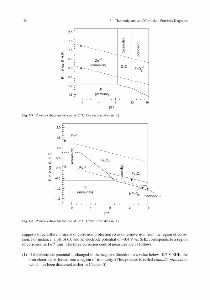
104 6 Thermodynamics of Corrosion: Pourbaix Diagrams
–1.5
–1.0
–0.5
0.0
0.5
1.0
1.5
2.0
0 4 8 12 16
E in
V v
s. S
.H.E
.
pH
Zn +2
(corrosion) ZnO
(pas
sivi
ty)
ZnO2
–2
(cor
rosi
on)
a
b
Zn(immunity)
Fig. 6.7 Pourbaix diagram for zinc at 25◦C. Drawn from data in [1]
–1.5
–1.0
–0.5
0.0
0.5
1.0
1.5
2.0
0 4 8 12 16
E in
V v
s. S
. H.E
.
pH
Fe+3
Fe+2
(cor
rosi
on)
Fe2O3
Fe3O4
(pas
sivi
ty)
Fe
(immunity) HFeO2– (corrosion)
b
a
Fig. 6.8 Pourbaix diagram for iron at 25◦C. Drawn from data in [1]
suggests three different means of corrosion protection so as to remove iron from the region of corro-sion. For instance, a pH of 6.0 and an electrode potential of –0.4 V vs. SHE corresponds to a regionof corrosion as Fe2+ ions. The three corrosion control measures are as follows:
(1) If the electrode potential is changed in the negative direction to a value below –0.7 V SHE, theiron electrode is forced into a region of immunity. (This process is called cathodic protection,which has been discussed earlier in Chapter 5).

Pourbaix Diagrams for Other Metals 105
Table 6.2 Equilibrium reactions and thermodynamic expressions for the Fe/H2O system [1]
Fe(s) −→ Fe2+(aq)+ 2e−E = −0.440− 0.0295 log [Fe2+]
3Fe(s)+ 4H2O(l) −→ Fe3O4(s)+ 8H+(aq)+ 8e−E = −0.085− 0.0591pH
3Fe2+(aq)+ 4H2O(l) −→ Fe3O4(s)+ 8H+(aq)+ 2e−E = 0.980− 0.2364pH − 0.0886log[Fe2+]
2Fe2+(aq)+ 3H2O(l) −→ Fe2O3(s)+ 6H+(aq)+ 2e−E = 0.728− 0.1773pH − 0.0591log[Fe2+]
2Fe3O4(s)+ 4H2O(l) −→ 2Fe2O3(s)+ 2H+(aq)+ 2e−E = 0.221− 0.0591pH
Fe(s)+ 2H2O(l) −→ HFeO−2 (aq)+ 3H+(aq)+ 2e−E = 0.493− 0.0886pH+ 0.0295 log [HFeO−2 ]
3HFeO−2 (aq)+ H+(aq) −→ Fe3O4(s)+ 2H2O(l)+ 2e−E = −1.819+ 0.0295pH− 0.0886 log [HFeO−2 ]
Fe2+(aq) −→ Fe3+ + (aq)+ e−E = 0.771+ 0.0591 log ([Fe3+]/[Fe2+])
2Fe3+(aq)+ 3H2O(l) −→ Fe2O3(s)+ 6H+log[Fe3+] = −0.72− 3pH
–1.5
–1.0
–0.5
0.0
0.5
1.0
1.5
2.0
0 4 8 12 16
E in
V v
s. S
.H.E
.
pH
Anodic protection
Cathodic protection
Increase the pH
(passivity)
(immunity)
(corrosion)
(corrosion)
Fig. 6.9 Simplified Pourbaix diagram for iron at 25◦C
(2) If instead, the electrode potential is changed in the positive direction to values above approx-imately 0.0 V vs. SHE, the iron electrode is forced into a region of passivity. This process iscalled anodic protection and will be taken up further in Chapter 9.
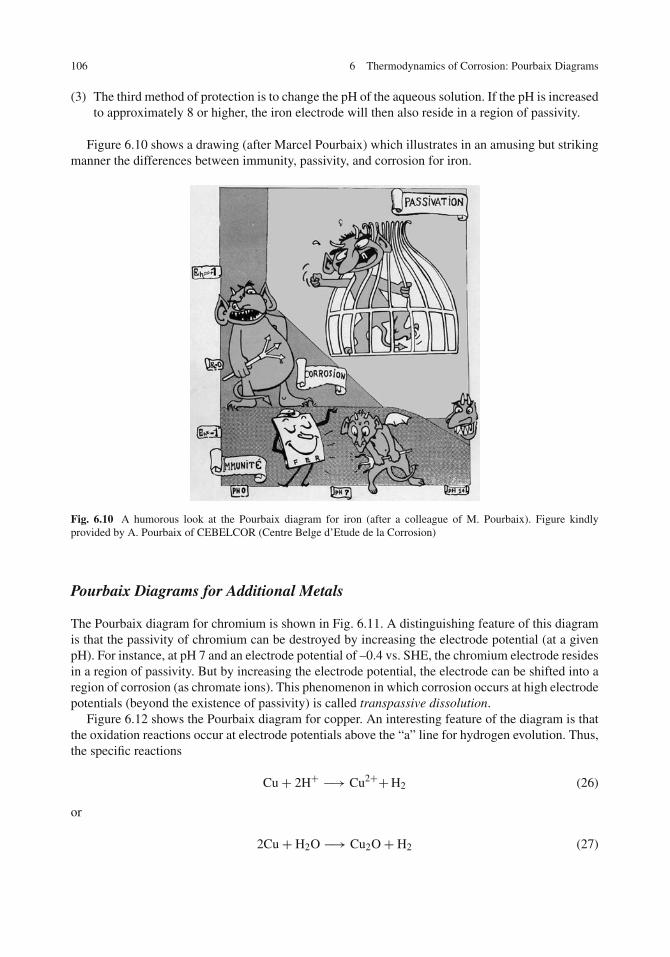
106 6 Thermodynamics of Corrosion: Pourbaix Diagrams
(3) The third method of protection is to change the pH of the aqueous solution. If the pH is increasedto approximately 8 or higher, the iron electrode will then also reside in a region of passivity.
Figure 6.10 shows a drawing (after Marcel Pourbaix) which illustrates in an amusing but strikingmanner the differences between immunity, passivity, and corrosion for iron.
Fig. 6.10 A humorous look at the Pourbaix diagram for iron (after a colleague of M. Pourbaix). Figure kindlyprovided by A. Pourbaix of CEBELCOR (Centre Belge d’Etude de la Corrosion)
Pourbaix Diagrams for Additional Metals
The Pourbaix diagram for chromium is shown in Fig. 6.11. A distinguishing feature of this diagramis that the passivity of chromium can be destroyed by increasing the electrode potential (at a givenpH). For instance, at pH 7 and an electrode potential of –0.4 vs. SHE, the chromium electrode residesin a region of passivity. But by increasing the electrode potential, the electrode can be shifted into aregion of corrosion (as chromate ions). This phenomenon in which corrosion occurs at high electrodepotentials (beyond the existence of passivity) is called transpassive dissolution.
Figure 6.12 shows the Pourbaix diagram for copper. An interesting feature of the diagram is thatthe oxidation reactions occur at electrode potentials above the “a” line for hydrogen evolution. Thus,the specific reactions
Cu+ 2H+ −→ Cu2++H2 (26)
or
2Cu+ H2O −→ Cu2O+ H2 (27)

Pourbaix Diagrams for Other Metals 107
–1.5
–1.0
–0.5
0.0
0.5
1.0
1.5
2.0
0 4 8 12 16
E in
V v
s. S
.H.E
.
pH
Cr2O
3
(passivity)
Cr(immunity)
Cr+3
Cr+2
Cr2O
7
–2
CrO4
–2
(corrosion)
b
a
CrO2–
CrO3
–3
Fig. 6.11 Pourbaix diagram for chromium at 25◦C. Drawn from data in [1]
are not thermodynamically favored. That is, copper cannot be oxidized by hydrogen ions or by watermolecules to produce H2 gas (because the product H2 is not stable in regions where Cu2+ or Cu2Oexists). Instead of Eq. (27), the following reaction is favored:
2Cu+ H2O −→ Cu2O+ 2H+ + 2e− (28)Compare this feature of the copper diagram with the Pourbaix diagrams for aluminum, zinc, and,
iron, for example.Figures 6.13 and 6.14 show Pourbaix diagrams for two noble metals silver and palladium,
respectively, each of which are used as electronic materials, as dental alloys, and in jewelry. In
–1.5
–1.0
–0.5
0.0
0.5
1.0
1.5
2.0
0 4 8 12 16
E in
V v
s. S
.H.E
.
pH
CuO
Cu2O
(passivity)
Cu+2
(corrosion)
Cu
b
a
CuO2
–2
(Cor
rosi
on)
(immunity)
Fig. 6.12 Pourbaix diagram for copper at 25◦C. Drawn from data in [1]

108 6 Thermodynamics of Corrosion: Pourbaix Diagrams
addition, palladium finds an important application in catalytic converters used to reduce emissionsof hydrocarbons from gasoline-powered vehicles.
–1.5
–1.0
–0.5
0.0
0.5
1.0
1.5
2.0
0 4 8 12 16
E in
V v
s. S
.H.E
.
pH
b
a
Ag +
Ag(immunity)
AgO(passivity)
AgO -(corrosion)
(corrosion)
Fig. 6.13 Pourbaix diagram for silver at 25◦C (assuming passivity is due to AgO). Drawn from data in [1]
Applications of Pourbaix Diagrams to Corrosion
Several applications of Pourbaix diagrams to corrosion have already been considered. Variousapplications can be catalogued as follows [1, 2]:
–1.5
–1.0
–0.5
0.0
0.5
1.0
1.5
2.0
0 4 8 12 16
E in
V v
s. S
.H.E
.
pH
Pd+2
(corrosion)
a Pd(immunity)
(pas
sivi
ty)
PdO
PdO2
b
Fig. 6.14 Pourbaix diagram for palladium at 25◦C. Drawn from data in [1]
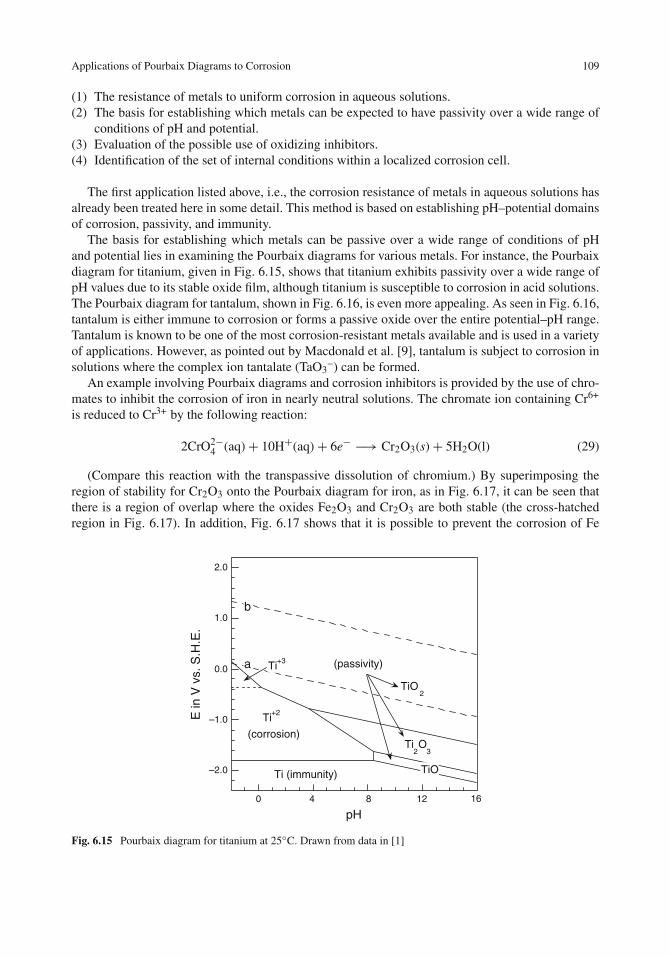
Applications of Pourbaix Diagrams to Corrosion 109
(1) The resistance of metals to uniform corrosion in aqueous solutions.(2) The basis for establishing which metals can be expected to have passivity over a wide range of
conditions of pH and potential.(3) Evaluation of the possible use of oxidizing inhibitors.(4) Identification of the set of internal conditions within a localized corrosion cell.
The first application listed above, i.e., the corrosion resistance of metals in aqueous solutions hasalready been treated here in some detail. This method is based on establishing pH–potential domainsof corrosion, passivity, and immunity.
The basis for establishing which metals can be passive over a wide range of conditions of pHand potential lies in examining the Pourbaix diagrams for various metals. For instance, the Pourbaixdiagram for titanium, given in Fig. 6.15, shows that titanium exhibits passivity over a wide range ofpH values due to its stable oxide film, although titanium is susceptible to corrosion in acid solutions.The Pourbaix diagram for tantalum, shown in Fig. 6.16, is even more appealing. As seen in Fig. 6.16,tantalum is either immune to corrosion or forms a passive oxide over the entire potential–pH range.Tantalum is known to be one of the most corrosion-resistant metals available and is used in a varietyof applications. However, as pointed out by Macdonald et al. [9], tantalum is subject to corrosion insolutions where the complex ion tantalate (TaO3
–) can be formed.An example involving Pourbaix diagrams and corrosion inhibitors is provided by the use of chro-
mates to inhibit the corrosion of iron in nearly neutral solutions. The chromate ion containing Cr6+
is reduced to Cr3+ by the following reaction:
2CrO2−4 (aq)+ 10H+(aq)+ 6e− −→ Cr2O3(s)+ 5H2O(l) (29)
(Compare this reaction with the transpassive dissolution of chromium.) By superimposing theregion of stability for Cr2O3 onto the Pourbaix diagram for iron, as in Fig. 6.17, it can be seen thatthere is a region of overlap where the oxides Fe2O3 and Cr2O3 are both stable (the cross-hatchedregion in Fig. 6.17). In addition, Fig. 6.17 shows that it is possible to prevent the corrosion of Fe
–2.0
–1.0
0.0
1.0
2.0
0 4 8 12 16
E in
V v
s. S
.H.E
.
pH
b
a
Ti+2
Ti+3
(corrosion)
TiO2
Ti2O
3
TiOTi (immunity)
(passivity)
Fig. 6.15 Pourbaix diagram for titanium at 25◦C. Drawn from data in [1]

110 6 Thermodynamics of Corrosion: Pourbaix Diagrams
–1.5
–1.0
–0.5
0.0
0.5
1.0
1.5
2.0
0 4 8 12 16
E in
V v
s. S
.H.E
.
pH
b
a Ta
2O
5
(passivity)
Ta(immunity)
Fig. 6.16 Pourbaix diagram for tantalum at 25◦C. Drawn from data in [1]
as Fe2+ at approximately neutral pH values through the formation of a Cr2O3 passive film. Thesurface analysis of oxide films formed on iron in chromate solutions has shown that the passive filmis a bilayer consisting of an outer layer of Cr2O3 and an inner layer of Fe2O3 [10]. Thus, films ofCr2O3 are responsible for corrosion inhibition by chromates, as predicted on the basis of corrosionthermodynamics.
–2.0
–1.5
–1.0
–0.5
0.0
0.5
1.0
1.5
2.0
0 4 8 12 16
E in
V v
s. S
.H.E
.
pH
Passivity for Fe
Passivity for Cr
Passivity forFe and Cr
Fig. 6.17 Superposition of the Pourbaix diagrams for iron (dotted lines) and chromium (solid lines) at 25◦C showingregions of passivity

Limitations of Pourbaix Diagrams 111
Pourbaix diagrams can also be applied to localized corrosion processes. Pourbaix diagrams areuseful in identifying potential–pH conditions which exist within a localized corrosion cell (crevice,corrosion pit, or stress-corrosion crack), provided that the values of E and pH pertain to the localelectrode potential and to the internal pH, as in Example 6.3. Further applications to localizedcorrosion are taken up in Chapter 10 and Chapter 11.
Limitations of Pourbaix Diagrams
Pourbaix diagrams provide a first guide as to the corrosion behavior of a given metal. Despite theirusefulness, as seen above, however, Pourbaix diagrams are subject to several important limitations.These limitations are as follows:
(1) Equilibrium is assumed. (But in practical cases, the actual conditions may be far fromequilibrium.)
(2) Pourbaix diagrams give no information on actual corrosion rates.(3) Pourbaix diagrams apply to single elemental metals only and not to alloys. (For a solid solution
binary alloy, the Pourbaix diagrams of the two constituents may be superimposed as a firstestimate, as will be shown later. For engineering alloys, experimental Pourbaix diagrams maybe developed, as will be seen in Chapter 10).
(4) Passivation is ascribed to all oxides or hydroxides, regardless of their actual protective prop-erties. (Corrosion may sometimes proceed by diffusion of ions through oxide films, a processwhich is ignored in the construction of the diagrams).
(5) Pourbaix diagrams do not consider localized corrosion by chloride ions. (Special experimentaldiagrams must be constructed, as will be seen in Chapter 10.)
(6) Conventional Pourbaix diagrams apply to a temperature of 25◦C. (Pourbaix diagrams exist forelevated temperatures, and examples are given later.)
Pourbaix Diagrams for Alloys
As mentioned above, one of the limitations of Pourbaix diagrams is that the diagrams can be cal-culated rigorously only for single elemental metals. However, Pourbaix diagrams can extended tometal alloys by three approaches:
(1) For binary solid solution alloys, the two individual Pourbaix diagrams may be superimposedonto each other.
(2) In the case of a mixed binary oxide, the corresponding Pourbaix diagram can be calculated if allappropriate thermodynamic data are available.
(3) For more complex alloys, including engineering alloys, experimental Pourbaix diagrams can bedetermined from electrochemical polarization measurements, as will be seen in Chapter 10.
Copper and nickel form solid solution alloys over their entire composition range; so as a firstguide as to corrosion trends for Cu-Ni alloys, the Pourbaix diagrams for copper and nickel canbe superimposed, as shown in Fig. 6.18. This superposition implies that each of the two metalsbehaves independently of the other. This assumption is reasonable for solid solution alloys but notfor heterogeneous alloys where galvanic effects may arise from the existence of second phases.Figure 6.18 shows that there are regions of potential vs. pH where the preferential dissolution ofcopper or nickel occurs, as well as regions where both metals undergo dissolution. Films of either

112 6 Thermodynamics of Corrosion: Pourbaix Diagrams
–1.5
–1.0
–0.5
0.0
0.5
1.0
1.5
2.0
0 4 8 12 16
E in
V v
s. S
.H.E
.
pH
Corrosion of Cu only
Corrosion of Ni only
Corrosion of Cu only
Corrosion of Cu and Ni
Corrosion ofCu and Ni
Corrosion of Ni only
Fig. 6.18 Superposition of the Pourbaix diagrams for copper (dotted lines) and nickel (solid lines) at 25◦C
Cu2O, CuO, or NiO provide passivity at neutral to mildly alkaline pHs. In practice, alloys of Cu–10%Ni and Cu–30% Ni find wide usage in various freshwater and seawater applications.
When thermodynamic information exists for mixed metal oxides, the Pourbaix diagrams can becalculated using such information. Examples include the Fe-Cu-H2O system for the mixed oxideFeCuO2 [11] and the Fe-Cr-H2O system for the mixed oxide FeCr2O4 [12]. Pourbaix diagrams havebeen computed also for other binary alloys [12] although these diagrams tend to be unduly complex,given their limitations.
Pourbaix Diagrams at Elevated Temperatures
The construction of Pourbaix diagrams at elevated temperatures is similar to their construction at25◦C, except that it is necessary to add a temperature correction for the free energy change of eachindividual reaction. The temperature affects:
(1) the electrode potential E of electrochemical reactions through the relationship �G = – nFE, inwhich the free energy change �G is a function of temperature,
(2) the Nernst equation, through the factor (2.303RT/F),(3) the equilibrium constant K in non-electrochemical reactions through the relationship
�G = – RT ln K, where �G and (of course) T are temperature dependent.
Consider the thermodynamic cycle shown in Fig. 6.19, which relates a chemical reaction at 25◦C(29)8 K) to the same reaction at an elevated temperature T. As shown in Appendix B, the standardfree energy change �Go
T at temperature T is related to the standard free energy change �Go298 at
25◦C by the following expression:

Pourbaix Diagrams at Elevated Temperatures 113
Reactants at 25 oC(298 oK)
Reactants at T oK
Products at 25 oC(298 oK)
Coolproducts
Products at T oK
Heatreactants
H298
HT
Fig. 6.19 Thermodynamic cycle for a chemical reaction at two different temperatures
�GoT = �G0
298 +∫ T
298
�CopdT − T
∫ T
298
�Copd ln T − (�T)�So
298(30)
where �Cpo is a difference in heat capacities given by �Cp
o = Cpo (products) – Cp
o (reactants),�T = T – 298, and �S298
o is the standard entropy change at 25◦C.The heat capacities required in Eq. (30) are either measured or estimated. Ionic entropies are
usually estimated by the empirical correlation method of Criss and Cobble [13, 14] which relatesentropies at elevated temperatures to entropies at 298 K.
One of the first Pourbaix diagrams for elevated temperatures was constructed by Townsend [15],who calculated the diagram for iron at temperatures up to 200◦C. The 25◦C and 200◦C diagramsare compared in Fig. 6.20. The two diagrams are similar, with the main difference being that theregime of stability for the complex ion HFeO2
– increases with increasing temperature. In addition,the reaction
2HFeO−2−→ Fe2O3 + H2O+ 2e− (39)
was considered to occur at high temperatures but not at 25◦C. In the Pourbaix diagram for ironat 200◦C, the regions between the complex ion HFeO2
– and the oxides Fe3O4 and Fe2O3 are
–1.5
–1.0
–0.5
0.0
0.5
1.0
1.5
E in
V v
s. S
. H.E
.
pH
Fe+3
Fe+2
Fe2O
3
Fe3O
4
Fe HFeO
2
–
b
a
–1.5
–1.0
–0.5
0.0
0.5
1.0
1.5
0 5 10 15 0 5 10 15
E in
V v
s. S
.H.E
.
pH
b
a Fe2O
3
Fe3O
4
Fe
Fe+2
Fe+3
HFeO2
–
Fig. 6.20 Pourbaix diagrams for Fe at 25◦C (top) and at 200◦C (bottom). The bottom figure is redrawn from [15]with the permission of Elsevier, Ltd

114 6 Thermodynamics of Corrosion: Pourbaix Diagrams
shown as bands rather than lines due to uncertainties in the calculation of �Go as a function oftemperature [15].
Pourbaix diagrams have been constructed by Cowan and Staehle [16] for the Ni-H2O systemin the temperature range of 25–200◦C. Analogous to the case for iron, the range of stability ofa complex ion HNiO2
– increases with increasing temperature, but for the most part, the Ni–H2Odiagram at elevated temperatures retains the same general features as the diagram at 25◦C.
Pourbaix diagrams at elevated temperatures are available for a variety of single metals and alloys[9, 15–19].
Problems
1. The following electrode potentials were observed after a 1-year immersion period in naturalseawater of pH 8.0 [20]:
Mild steel –0.65 V vs. SCEZinc –1.02 V vs. SCEMild steel/zinc couple – 0.95 V vs. SCE
(a) Refer to the appropriate Pourbaix diagrams and indicate what behavior is expected for eachof the two uncoupled electrodes. (b) Based on the Pourbaix diagrams, what behavior is expectedfor the mild steel and zinc components in the short-circuited couple? (c) Is the behavior in part(b) consistent with that predicted based on the galvanic couple approach in Chapter 5?
2. Suppose that an acid flux is inadvertently left on the surface of a silver contact and that in thepresence of a thin film of condensed moisture, the acid residue has a pH of 5.0. Under whatrange of electrode potentials could the corrosion of silver occur in the thin-film electrolyte?
3. Palladium (like gold and platinum) is a noble metal. However, the Pourbaix diagram for pal-ladium (Fig. 6.14) contains a region where palladium is subject to corrosion. Can palladiumcorrode by the following reaction:
Pd(s)+ 2H+(aq) −→ Pd2+(aq)+ H2(g)
Explain your answer.4. The electrode potential of titanium immersed in a sulfuric acid solution of pH approximately 1
was measured to be –0.70 V vs. SCE [21]. (a) Confirm that titanium undergoes active corrosionunder these conditions and (b) consult the Pourbaix diagram to suggest three different means toprovide corrosion protection.
5. In the interpretation of Pourbaix diagrams, corrosion is considered to occur when the concentra-tion of dissolved metal ions attains a minimum concentration of 1.0 × 10⁻⁶ M. Suppose that a0.50-cm2 sample of aluminum immersed in 1.0 L of an aqueous solution corrodes at a constantcurrent density of 100 μA/cm2. How long will it take to produce a concentration of 1.0 × 10⁻⁶
M Al3+?6. Calculate the standard reduction potential Eo for the reaction
Al2O3(s)+ 6H+(aq)+ 6e− −→ 2Al(s)+ 3H2O(l)
given the following chemical potentials (in calories per mole): μo(Al2O3(s)) = − 384,530,μo(H2O(l)) = – 56,690.

Problems 115
7. For the chemical reaction
Al2O3(s)+ H2O(l) −→ 2AlO−2 (aq)+ 2H+(aq)
show the result given in Eq. (17), i.e.,
−pH+ log[AlO−2 ] = −14.644
8. For the electrochemical reaction
Al(s)+ 2H2O(l) −→ AlO−2 (aq)+ 4H+(aq)+ 3e−
show the result given in Eq. (19), i.e.,
E = −1.262+ 0.0197 log [AlO−2 ]− 0.0788 pH
9. For the cathodic evolution of hydrogen from neutral or basic solutions
2H2O(l)+ 2e− −→ H2(g)+ 2OH−(aq)
for which the standard electrode potential is Eo = − 0.828 V vs. SHE, show that
E = 0.000− 0.0591pH
10. Refer to the Pourbaix diagram for chromium in Fig. 6.11. The equilibrium reaction for the lineseparating the regions of passivation by Cr2O3 and transpassive dissolution as chromate ions(CrO4
2–) corresponds to the reaction
2CrO2−4 (aq)+ 10H+(aq)+ 6e− −→ Cr2O3(s)+ 5H2O(l)
Show that the reduction potential for this half-cell reaction depends on both the pH and theconcentration of dissolved chromate ions. The standard electrode potential for the reductionreaction is Eo = 1.311 V vs. SHE.
11. Refer to Fig. 6.15, which is the Pourbaix diagram for titanium.
(a) Write the electrochemical half-cell reactions for the step-wise oxidation of titanium by thefollowing reactions
Ti (s) to TiO (s)TiO (s) to Ti2O3 (s)Ti2O3 (s) to TiO2 (s)
Note: H2O is a reactant in each of the above reactions.(b) What is the slope dE/dpH for each of these reactions?
12. The following thermodynamic data are for the Mg/H2O system [1].
Dissolved substances μo (cal/mol)Mg2+ − 108,990H+ 0
Solid substancesMg 0

116 6 Thermodynamics of Corrosion: Pourbaix Diagrams
Mg(OH)2 – 199,270
Liquid substancesH2O – 56,690The chemical reactions involving these species are
Mg −→ Mg2++2e− Eo (reduction) vs. SHE = −2.363VMg+ 2H2O −→ Mg(OH)2 + 2H+ + 2e− Eo (reduction) vs. SHE = −1.862VMg2+2H2O −→ Mg(OH)2 + 2H+
Calculate and construct the Pourbaix diagram for magnesium, assuming that the passivity ofmagnesium is provided by a layer of solid Mg(OH)2. Label all regions of corrosion, passivity,and immunity.
13. Construct the Pourbaix diagram for iron from the set of electrochemical and chemical equilibriagiven in Table 6.2. Label all regions of corrosion, passivity, and immunity.
14. If iron is immersed in a solution of pH 3.0, what electrode potential must be maintained toprevent the evolution of hydrogen gas?
15. In a study on the corrosion of iron in model crevices or pits, Pickering and Frankenthal [22]observed the egress of gas bubbles from the surface of iron contained in the model crevice.For a solution of 0.5 M sodium acetate/0.5 M acetic acid (pH 5.5) contained in the crevice,the electrode potential within the crevice was measured to be –0.5 V vs. SHE [23]. Based onthermodynamic considerations, what gas was evolved?
16. Consult the Pourbaix Atlas [1] or other suitable source for the Pourbaix diagram for niobium.How does this diagram compare with that for tantalum? Based on the location of niobium andtantalum in the periodic table of the elements, would you expect the two Pourbaix diagrams tobe similar?
References
1. M. Pourbaix, “Atlas of Electrochemical Equilibria in Aqueous Solutions”, National Association of CorrosionEngineers, Houston, TX (1974).
2. J. Kruger in “Equilibrium Diagrams: Localized Corrosion”, R. P. Frankenthal J. Kruger, Eds., p. 45, TheElectrochemical Society, Pennington, NJ (1984).
3. R. E. Groover, J. A. Smith, and T. J. Lennox, Jr., Corrosion, 28, 101 (1972).4. E. McCafferty, P. G. Moore, and G. T. Peace, J. Electrochem. Soc., 129, 9 (1982).5. M. J. Pyror and D. S. Keir, J. Electrochem. Soc., 105, 629 (1958).6. R. Ambat and E. S. Dwarakadasa, Corros. Sci., 33, 681 (1992).7. J. A. Smith, M. H. Peterson, and B. F. Brown, Corrosion, 26, 539 (1970).8. T. K. Christman, J. Payer, G. W. Kurr, J. B. Doe, D. S. Carr, and A. L. Ponikvar, “Zinc: Its Corrosion Resistance”,
pp. 4, 114, International Lead and Zinc Research Institute, New York, NY (1983).9. H. S. Betrabet, W. B. Johnson, D. D. Macdonald, and W. A. T. Clark in “Equilibrium Diagrams: Localized
Corrosion”, R. P. Frankenthal and J. Kruger, Eds., p. 83, The Electrochemical Society, Pennington, NJ (1984).10. E. McCafferty, M. K. Bernett, and J. S. Murday, Corros. Sci., 28, 559 (1988).11. D. Cubicciotti, Corrosion, 44, 875 (1988).12. D. Cubicciotti, J. Nucl. Mater., 201, 176 (1993).13. C. M. Criss and J. W. Cobble., J. Am. Chem. Soc., 86, 5385 (1964).14. J. W. Cobble, J. Am. Chem. Soc., 86, 5394 (1964).15. H. E. Townsend, Jr., Corros. Sci., 10, 343 (1970).16. R. L. Cowan and R. W. Staehle, J. Electrochem. Soc., 118, 557 (1971).17. J. B. Lee, Corrosion, 37, 467 (1981).18. B. Beverskog and I. Puigdomenech, J. Electrochem. Soc., 144, 3476 (1997).19. R. J. Lemire and G. A. McRae, J. Nuclear Mater., 294, 141 (2001).

References 117
20. M. H. Peterson and T. J. Lennox, Jr., Mater. Perform., 23 (3), 15 (1984).21. M. Stern and H. Wissenberg, J. Electrochem. Soc., 106, 755 (1959).22. H. W. Pickering and R. P. Frankenthal, J. Electrochem. Soc., 119, 1297 (1972).23. H. W. Pickering in “Equilibrium Diagrams: Localized Corrosion”, R. P. Frankenthal and J. Kruger, Eds., p. 535,
The Electrochemical Society, Pennington, NJ (1984).

Chapter 7Kinetics of Corrosion
Introduction
As seen in the previous chapter, potential–pH diagrams (Pourbaix diagrams) are a useful first guideas to the corrosion behavior of many different systems. However, Pourbaix diagrams do not giveany information as to corrosion rates. Although a given reaction may be spontaneous, it does notnecessarily proceed at a fast rate. The reaction may in fact proceed “slowly” rather than “quickly”,but we cannot determine this difference from thermodynamics alone.
This chapter deals with the rates of corrosion reactions. The corrosion rate of a given metal oralloy in its environment is a crucial factor in determining the lifetime of both structural and electronicmaterials.
Units for Corrosion Rates
Various units have been used to express corrosion rates. These include weight loss per unit area perunit time, penetration rates, and electrochemical rates. There is no standard unit to express corrosionrates, and many different units have been used, as given in Table 7.1.
Methods of Determining Corrosion Rates
Corrosion rates for metals undergoing uniform corrosion can be determined by any of the followingmethods:
(a) Weight loss(b) Weight gain(c) Chemical analysis of solution(d) Gasometric techniques (when one of the reaction products is a gas)(e) Thickness measurements(f) Electrical resistance probes(g) Inert marker method(h) Electrochemical techniques
Each of these methods is discussed briefly below. Most of this chapter, however, concerns themeasurement of corrosion rates by means of the electrochemical polarization method.
119E. McCafferty, Introduction to Corrosion Science, DOI 10.1007/978-1-4419-0455-3_7,C© Springer Science+Business Media, LLC 2010

120 7 Kinetics of Corrosion
Table 7.1 Some unitscommonly used to expresscorrosion rates
Weight lossg/cm2 hg/cm2 dayg/m2 hg/m2 daymg/m2 smdd (mg/dm2 day)
Penetrationipy (inches per year)mpy (mils per year)a
mm/yearμm/year
Corrosion current densityμA/cm2
mA/cm2
A/cm2
A/m2
a1 mil = 0.001 in.
Weight Loss Method
In this method, previously weighed metal samples are removed from the solution or the environmentat various timed intervals, and the loss in weight due to metallic corrosion is determined (per unitarea of the sample). For this method to be accurate, any solid corrosion products must be removedfrom the metal surface.
If the corrosion products are loose and non-adherent, they can be removed by mechanical means.Tight and adherent corrosion products can be removed by chemical or electrochemical methods,which are usually specific to the metal or the alloy being tested [1].
Figure 7.1 shows an example of weight loss data for the uniform corrosion of aluminum alloy7075 in 0.5 M hydrochloric acid [2]. After an initial incubation period of about 2 h., the rate ofweight loss becomes constant with time. The corrosion rate is simply the slope of the straight line,as shown in the figure.
Figure 7.2 shows weight loss data taken for a much longer period of time for the atmosphericcorrosion of various steels exposed in the natural atmosphere of Kearney, New Jersey [3, 4]. Notethat the time axis is in years of exposure and that the corrosion rate is not constant over the entireexposure period. The instantaneous corrosion rate at any given time is the slope of the tangent linedrawn at that given time. (The trends shown in Fig. 7.2 hold for up to 20 years [3, 4].)
Weight Gain Method
This method is generally not useful in aqueous corrosion studies but is more suited to dry oxidationwhere oxide films or products are more adherent than is in the case of aqueous corrosion. Laboratoryweight gain measurements in dry environments have the useful feature that the gain in weight canbe measured continuously and without removal of the specimen from the environment.

Methods of Determining Corrosion Rates 121
0.00
0.05
0.10
0.15
0.20
0 5 10 15 20
Wei
ght L
oss
in G
ram
s/cm
2
Immersion Time in Hours
Incubationperiod
Slope = 0.013 gm/cm2 hr
Fig. 7.1 Weight loss vs. time for Al alloy 7075 in 0.5 M HCl [2]. (Al alloy 7075 contains approximately 5% Zn, 1%Cu, and 2% Mg)
0
10
20
30
40
50
60
70
80
0 1 2 3 4
Wei
ght L
oss
in m
g/cm
2
Time in Years
Low alloy steel
Plain carbon steel
Copper steel
Fig. 7.2 Corrosion–time curves for the atmospheric corrosion of various steels exposed in the natural atmosphere ofKearney, New Jersey. Redrawn from [3] by permission of ECS – The Electrochemical Society
Chemical Analysis of Solution
When a metal undergoes corrosion in an electrolyte of a fixed volume, cations of the corrodingmetal will accumulate in the solution. Accordingly, the solution becomes more concentrated in thedissolved cation with the progression of time. Thus, chemical analysis of withdrawn aliquots of thesolution as a function of time allows determination of the corrosion rate.
Figure 7.3 shows chemical analysis data for the corrosion of aluminum alloy 7075 in 0.5 M HClcorresponding to the weight loss data in Fig. 7.1. From Fig. 7.3, the corrosion rate is 4.80× 10⁻³ mol

122 7 Kinetics of Corrosion
0
0.002
0.004
0.006
0.008
0 5 10 15 20
Mol
es A
l+3 D
isso
lved
/cm
2
Immersion Time in Hours
Incubationperiod Slope = 4.8 × 10⁻⁴ moles Al
+3/cm2 hr
Fig. 7.3 Amount of dissolved Al3+ in 0.5 M HCl as a function of time corresponding to the weight loss data inFig. 7.1. (The amount of dissolved Al3+ is calculated assuming that the anodic reaction is Al→ Al3+ + 3e–)
Al3+/cm2 day. This corrosion rate is converted to the rate in terms of weight loss by the followingsimple calculation:
(4.80 × 10⁻⁴molesAl+3
cm2hr
) (1 mole Al
1 mole Al+3
) (27.0 gm Al
1 mole Al
)= 0.0130 gm Al
cm2hr
The use of standard colorimetric techniques in the visible range is a common method for chemi-cal analysis of solutions. This method depends on the formation of a colored complex, the intensityof which is proportional to the concentration of the complex formed and correspondingly to theconcentration of the dissolved cation in solution. The intensity of the complex is determined by mea-suring the percent transmittance at a given wavelength of light and by comparison with a previouslyprepared standard plot.
The specific colorimetric technique to be used depends on the particular cation to be ana-lyzed, and standard reference texts should be consulted for more details [5]. The corrosion rateof iron, aluminum, or titanium in different environments has been determined using various specificcolorimetric procedures [6–10].
Another useful method for chemical analysis of solutions is atomic absorption spectrophotometry.The sample size required for this method is very small (typically about 10 mg). The sample isaccurately weighed and then sprayed into the flame of the instrument and atomized. Again, lightof a suitable wavelength for a particular element is directed through the flame, and some of thislight is absorbed by the atoms of the sample. The amount of light absorbed is proportional to theconcentration of the element in the solution. The method is sensitive to trace elements down to theparts per million level [11].
Gasometric Techniques
When aluminum (or a dilute alloy of aluminum) corrodes in acid solutions, the overall ionicreaction is

Methods of Determining Corrosion Rates 123
Al
Al (s) + 3 H + (aq) Al+3 (aq) + 32
H2 (g)
Measureweight loss
Measure concentration
of Al+3 Measure volumeof H2 evolved
Changes in pHare usually too small to be measuredquantitatively
or: Al (s) Al +3 (aq) + 3 e –
3 H+ (aq) + 3 e – 32 H2 (g)
Electrochemical measurements
Fig. 7.4 Various ways to determine the corrosion rate of an aluminum alloy immersed in an acid solution
Al(s)+ 3H+(aq)Al3+(aq)+ 3
2H2(g)
As depicted in Fig. 7.4, the corrosion rate may be determined by measuring the change in amountsof reactant Al or of products Al3+ or H2 as the reaction proceeds.
Figure 7.5 shows data for the volume of hydrogen gas evolved for corrosion of aluminum alloy7075 in 0.5 M HCl corresponding to the weight loss data in Fig. 7.1. From Fig. 7.5, the rate of hydro-gen evolution is 16.1 ml H2 (STP)/cm2 h, where STP refers to conditions of standard temperature(0◦C) and pressure (1 atm).
Example 7.1: Convert the rate of hydrogen evolution in Fig. 7.5 to the corresponding weight loss ofmetallic aluminum in terms of grams per square meter hour.Solution: We use the fact that under conditions of STP, 1 mol of a gas occupies 22.4 L. Thus
(16.1 mL H2(STP)
cm2h
) (1L
1000 mL
) (1 mol H2
22.4 L H2(STP)
)
×(
1 mol Al32 mol H2
)×(
27.0 g Al
1 mol Al
)= 0.0129 g Al
cm2h

124 7 Kinetics of Corrosion
0
50
100
150
200
250
0 5 10 15 20
Vol
ume
of H
2 E
volv
ed in
mL
(ST
P)
Immersion Time in Hours
Slope = 16.1 mL (STP)/cm2 hrIncubationperiod
Fig. 7.5 Volume of hydrogen gas evolved as a function of time when an aluminum alloy is immersed in0.5 M HCl. The amount of H2 gas evolved is calculated from the weight loss data in Fig. 7.1 and the reactionAl(s)+ 3H+ (aq)→ Al3+ (aq) + 3
2 H2 (g)
Thickness Measurements
Measurement of the thickness of a metal as a function of time is a method to monitor the corrosionbehavior of a system [12]. This method is used to survey the practical corrosion behavior of a systemin service, rather than as a laboratory technique, and has been used to track the progress of corro-sion in railroad hopper cars, storage tanks, and pipelines. Thickness measurements are based on theresponse of a specimen to an ultrasonic or a magnetic signal.
Electrical Resistance Method
Electrical resistance methods depend on an increase in the electrical resistance as a test metallic filmor wire is thinned due to corrosion [12, 13]. For example, the resistance of a metal wire of length land area A is given by R = ρl/A, where ρ is the resistivity. As the area A of the metal wire decreasesdue to corrosion, the resistance R increases. These types of instruments are commercially availableand are generally used to monitor the progression of corrosion rather than to determine the actualcorrosion rate. One drawback of this method is that conductive deposits on the sensor elements willdistort the resistance reading. However, this method is useful for solutions of low conductivity or fornon-aqueous solutions.
Inert Marker Method
This is a novel experimental method which is suited to the laboratory and requires a sophisticatedion implantation system. In this method, an inert marker, such as ion-implanted Xe (xenon), is usedin conjunction with the surface analysis technique of Rutherford backscattering (RBS). Ion implan-tation is a technique in which any ion can be placed in the near-surface region of any substrate(including metals), by allowing a high-energy beam of a selected ion to bombard the metal surface.

Methods of Determining Corrosion Rates 125
More information about ion implantation is given in Chapter 16. The RBS method is a surface anal-ysis method which uses He atoms (α particles) as collider particles to probe the composition of asurface. This method is described in detail elsewhere [14].
Figure 7.6 shows RBS data for the ion-implanted Xe in pure titanium before immersion intoboiling 1 M H2SO4 and for two different brief immersion times [10]. After immersion, the Xe signalis diminished as the titanium sample corrodes.
Corrosion rates were determined in the following manner. It is assumed that the shape of theXe profiles in Fig. 7.6 is changed only by the removal of Xe atoms from the surface as the surfacemoves inward. The shift in energy of the remaining Xe profile with respect to the initial profile(before corrosion) is converted into a thickness of material removed by means of a well-knownenergy loss rate d(Energy)/dx for He ions in titanium. For example, 2.5 MeV He ions incident on thesample that are scattered by a Xe atom and are subsequently detected have an effective d(Energy)/dx = 0.9 keV nm–1 (1 nm = 1.0 × 10⁻⁹ m). If an energy shift of 10 keV is measured in the Xeprofile, the thickness of the material removed t is 10 keV/0.9 keV nm–1 = 11.1 nm.
Fig. 7.6 Rutherford backscattering (RBS) profiles for Xe implanted into titanium before and after immersion inboiling 1 M H2SO4 [10]. Reproduced from [10] with the permission of Elsevier, Ltd

126 7 Kinetics of Corrosion
0
2
4
6
8
10
12
0 1 2 3 4 5 6 7 8
Ti D
isso
lved
in m
g/cm
2
Time in Hours
Slope = 2.0 mg/cm2 hr
-5
0
5
10
15
20
25
30
-10 0 10 20 30 40 50
Tita
nium
Rem
oved
in n
m
Time in Seconds
Slope = 2.2 nm/sec
= 3.6 mg/cm 2 hr
Fig. 7.7 Top: Titanium thickness removed as a function of immersion time in boiling 1 M H2SO4 as determined fromRBS profiles. Bottom: Colorimetric analysis of dissolved titanium in boiling 1 M H2SO4 assuming the anodic reactionis Ti→ Ti2+ + 2e–. Reproduced from [10] with the permission of Elsevier, Ltd
In this manner, Fig. 7.7(top), which is a plot of titanium thickness removed as a function of time,was determined. After an initial incubation time of approximately 15 s to remove the initial air-formed oxide film, the rate of titanium dissolution was constant. From Fig. 7.7(top), the corrosionrate is 2.2 nm/s. The use of the density of titanium (4.51 g/cm3) gives the corrosion rate to be3.6 mg/cm2 h, in approximate agreement with the rate of 2.2 mg/cm2 h determined by colorimetricanalysis of the solution for dissolved titanium. See Fig. 7.7 (bottom).
Electrochemical Techniques
Each of the methods described above has an application in either the laboratory or the field. Butnone of the methods above can provide insights into the underlying mechanism of corrosion.Electrochemical techniques have this capability and in addition offer the possibility of mitigating
Electrochemical Polarization 127
corrosion by controlling the electrode potential. There are various methods of determining the cor-rosion rate by electrochemical techniques, but this chapter will consider only the direct current (DC)polarization method and its offshoots. Alternating current (AC) techniques, which are very power-ful in determining corrosion rates and in monitoring the progress of corrosion, are treated later in aseparate chapter.
Electrochemical Polarization
Electrochemical polarization (usually referred to simply as “polarization”) is the change in electrodepotential due to the flow of a current. There are three types of polarization:
(1) Activation polarization is polarization caused by a slow electrode reaction.(2) Concentration polarization is polarization caused by concentration changes in reactants or
products near an electrode surface.(3) Ohmic polarization is polarization caused by IR drops in solution or across surface films, such
as oxides (or salts).
The degree of polarization is defined as the overvoltage (or overpotential) η given by the followingequation:
η = E − Eo (1)
where E is the electrode potential for some condition of current flow and Eo is the electrode potentialfor zero current flow (also called the open-circuit potential, corrosion potential, or rest potential).Note that the electrode potential of zero current flow Eo should not be confused with the standardelectrode potential Eo, which plays a prominent role in corrosion thermodynamics.
Anodic and Cathodic Polarization
Either an anode or a cathode can be polarized:
Anodic polarization is the displacement of the electrode potential in the positive direction sothat the electrode acts more anodic.
Cathodic polarization is the displacement of the electrode potential in the negative direction sothat the electrode acts more cathodic.
These processes are represented schematically in Fig. 7.8.
Visualization of Cathodic Polarization
Consider the hydrogen evolution reaction occurring at a metal surface. First, hydrogen atoms areproduced by the reduction reaction
2H+ + 2e− → 2Hads, (2)

128 7 Kinetics of Corrosion
Electrode potential, E
Cathodic polarization-displacement of the electrode potential in the negative direction. (The electrode acts more cathodic).
Both anodes and cathodes can be polarized.
Anodic polarization-displacement of the electrode potential in the positive direction. (The electrode acts more anodic).
E becomesmore (+)
Zn Zn +2
2 e–
E becomesmore (–)
e –
PtH+
anodic cathodic
more (+) more (–)
Fig. 7.8 Schematic representation of anodic and cathodic polarization
followed by their combination:
2Hads → H2 (3)
The process of activation polarization involves a slow step in the electrode reaction. Suppose thatelectrons are supplied to the metal electrode faster than they can react to form H atoms, as representedin Fig. 7.9. Then the concentration of electrons is increased at the metal side of the interface. Theresult is that the electrode potential E becomes more negative, due to activation polarization [15].
Suppose instead that there are concentration effects near the electrode surface for the hydrogenreduction reaction. If reactant hydrogen ions H+ are slow to diffuse to the electrode surface, as illus-trated in Fig. 7.10, then electrons again can accumulate at the metal side of the interface. The resultis that the electrode potential E again becomes more negative, but this time due to concentrationpolarization [15].
Visualization of Anodic Polarization
Consider the following anodic reaction:
Fe→ Fe2++2e− (4)
Suppose that the oxidation of Fe atoms to Fe2+ ions is slow. Then electrons exit the electrodefaster than Fe atoms leave the metal matrix, as illustrated in Fig. 7.11. This means that the electronconcentration is decreased at the metal side of the interface. The electrode potential E thus becomesmore positive due to activation polarization [15].
Suppose next that the products of the anodic reaction, i.e., Fe2+ ions, are slow to diffuse away fromthe metal surface, as represented in Fig. 7.12. Then the surface becomes more positively charged dueto the accumulation of Fe2+ ions. The electrode potential E again becomes more positive, but thistime due to concentration polarization [15].
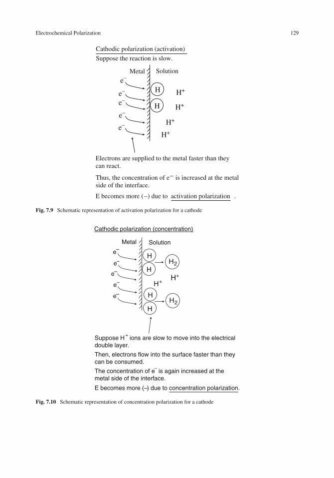
Electrochemical Polarization 129
Cathodic polarization (activation)
Suppose the reaction is slow.
Electrons are supplied to the metal faster than they can react.
Thus, the concentration of e– is increased at the metalside of the interface.
E becomes more (–) due to activation polarization .
e–
e–
e–
e–
e–
H
H H+
H+
H+
H+
Metal Solution
Fig. 7.9 Schematic representation of activation polarization for a cathode
Cathodic polarization (concentration)
Suppose H + ions are slow to move into the electrical double layer.
Then, electrons flow into the surface faster than they can be consumed.
The concentration of e– is again increased at the metal side of the interface.
E becomes more (–) due to concentration polarization.
H+ H+
e–
–
–
e
e–e
–e
H
HH2
H
HH2
Metal Solution
Fig. 7.10 Schematic representation of concentration polarization for a cathode

130 7 Kinetics of Corrosion
Suppose the reaction is slow.
Then, electrons exit from the surface faster than Fe atomsleave the matrix.
The concentration of e – is decreased at the metal side of the interface.
E becomes more (+) due to activation polarization .
Anodic polarization (activation)
2e–
Fe +2Fe
Metal Solution
Fig. 7.11 Schematic representation of activation polarization for an anode
Anodic polarization (concentration)
Suppose the products are slow to diffuse away from theinterface.
Again, the surface becomes more positively charged.
E becomes more (+) due to concentration polarization.
4e–
Fe
Metal Solution
Fe
Fe +2
Fe +2
Fig. 7.12 Schematic representation of concentration polarization for an anode
Ohmic Polarization
Ohmic polarization within a solution is due to the inability to place the reference electrode directlyat the metal surface under investigation, as illustrated in Fig. 7.13. As mentioned in Chapter 3,the use of a Luggin–Haber capillary minimizes the error due to IR drops [16–18]. Barnartt [16]found that the current distribution around an electrode surface is unaffected if the distance betweenthe electrode and the capillary is twice the capillary outer diameter. The term IRsolution is usually

Electrode Kinetics for Activation Polarization 131
Ohmic polarization
Metal
Reference electrode
Luggin-Habercapillary
IRsoln
Ohmic polarization is caused by the IR drop due tothe inability to place the reference electrode directlyat the metal surface under study
IRsoln is negligible for high conductivity solutions.
IRsoln is high for low conductivity solutions.(organic media, some solis)
Fig. 7.13 Schematic representation of ohmic polarization in an aqueous solution
negligible for high-conductivity solutions, such as most aqueous solutions, but can be a problem forlow-conductivity solutions, such as organic media, and for some soils.
If the IR drop is due to the existence of a surface film on a metal, such as an oxide, hydroxide,oxyhydroxide, or salt film, then such films are usually understood to be part of the system and theelectrode potential is considered to be that for the total system: metal/film/solution.
Electrode Kinetics for Activation Polarization
The remainder of this chapter deals with corrosion kinetics when both the anodic and the cathodicprocesses are under activation polarization. Situations in which concentration polarization occurs aretreated in Chapter 8.
Absolute Reaction Rate Theory
The electrode kinetics of activation polarization is treated using the absolute reaction rate theoryof Glasstone, Laidler, and Eyring [19]. According to the absolute reaction rate theory, a reactionproceeds along a reaction co-ordinate which measures the extent of the reaction. For reactants to beconverted into products, a transitory state is first reached, in which an “activated complex” is formed.Formation of such a complex requires overcoming a free energy barrier of height �G�=, as shown inFig. 7.14. For the general reaction
A+ B→ [AB]�= → products (5)
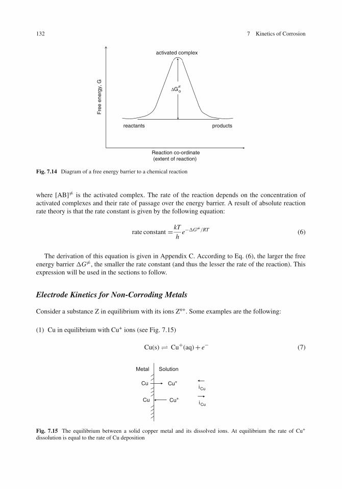
132 7 Kinetics of Corrosion
products
ΔGo≠
reactants
activated complex
Reaction co-ordinate(extent of reaction)
Fre
e en
ergy
, G
Fig. 7.14 Diagram of a free energy barrier to a chemical reaction
where [AB] �= is the activated complex. The rate of the reaction depends on the concentration ofactivated complexes and their rate of passage over the energy barrier. A result of absolute reactionrate theory is that the rate constant is given by the following equation:
rate constant =kT
he−�G�=/RT (6)
The derivation of this equation is given in Appendix C. According to Eq. (6), the larger the freeenergy barrier �G�=, the smaller the rate constant (and thus the lesser the rate of the reaction). Thisexpression will be used in the sections to follow.
Electrode Kinetics for Non-Corroding Metals
Consider a substance Z in equilibrium with its ions Zn+. Some examples are the following:
(1) Cu in equilibrium with Cu+ ions (see Fig. 7.15)
Cu(s) � Cu+(aq)+ e− (7)
Cu Cu+
Cu Cu+
iCu
iCu
Metal Solution
Fig. 7.15 The equilibrium between a solid copper metal and its dissolved ions. At equilibrium the rate of Cu+
dissolution is equal to the rate of Cu deposition
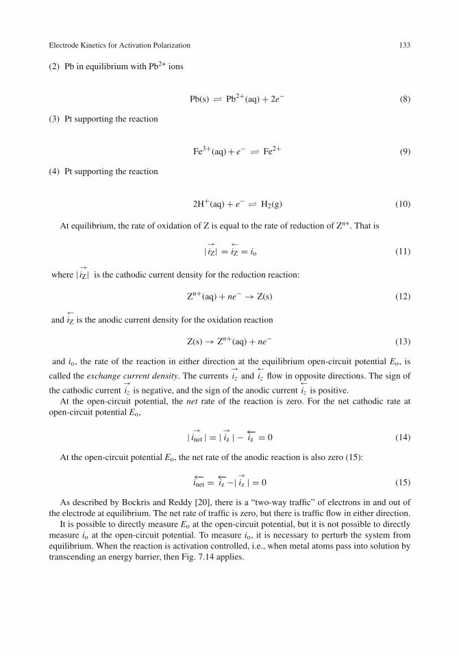
Electrode Kinetics for Activation Polarization 133
(2) Pb in equilibrium with Pb2+ ions
Pb(s) � Pb2+(aq)+ 2e− (8)
(3) Pt supporting the reaction
Fe3+(aq)+ e− � Fe2+ (9)
(4) Pt supporting the reaction
2H+(aq)+ e− � H2(g) (10)
At equilibrium, the rate of oxidation of Z is equal to the rate of reduction of Zn+. That is
→| iZ| =←iZ = io (11)
where→| iZ| is the cathodic current density for the reduction reaction:
Zn+(aq)+ ne− → Z(s) (12)
and←iZ is the anodic current density for the oxidation reaction
Z(s)→ Zn+(aq)+ ne− (13)
and io, the rate of the reaction in either direction at the equilibrium open-circuit potential Eo, is
called the exchange current density. The currents→iz and
←iz flow in opposite directions. The sign of
the cathodic current→iz is negative, and the sign of the anodic current
←iz is positive.
At the open-circuit potential, the net rate of the reaction is zero. For the net cathodic rate atopen-circuit potential Eo,
| →inet | = |→iz | −←−iz = 0 (14)
At the open-circuit potential Eo, the net rate of the anodic reaction is also zero (15):
←−inet =←−iz −|
→iz | = 0 (15)
As described by Bockris and Reddy [20], there is a “two-way traffic” of electrons in and out ofthe electrode at equilibrium. The net rate of traffic is zero, but there is traffic flow in either direction.
It is possible to directly measure Eo at the open-circuit potential, but it is not possible to directlymeasure io at the open-circuit potential. To measure io, it is necessary to perturb the system fromequilibrium. When the reaction is activation controlled, i.e., when metal atoms pass into solution bytranscending an energy barrier, then Fig. 7.14 applies.

134 7 Kinetics of Corrosion
products
(1–α ) n F (E – Eo)
α n F (E – Eo)
ΔGo≠
reactants
n F (E - Eo)
equivmole
coulequiv
volts = joulesmole
ΔG
Fig. 7.16 Effect of a change in electrode potential on the height of the free energy barrier. When the potential ischanged from Eo to some new electrode potential E, the shape of the free energy curve is changed from the solid lineto the dotted line
Consider the oxidation of Z(s) to Zn+ (aq). If the electrode potential is changed from Eo to someother value E, the rate of oxidation is either raised or lowered to some new value i depending onwhether the free energy barrier �G�= is raised or lowered. If the free energy barrier is lowered, as inFig. 7.16, then
�G�= = �G�=o − αnF(E − Eo) (16)
where �Go�= is the free energy barrier at Eo, and α is a dimensionless parameter (between 0 and 1,
but usually 0.5). The parameter α is a measure of the symmetry of the free energy barrier as modifiedby the new applied potential E. When α = 0.5, the degree of decrease in the free energy barrier inthe forward direction is the same as its degree of increase in the reverse direction.
Substitution of Eq. (16) in Eq. (6) gives
rate constant = kT
he− [�G�=o −αnF(E−Eo)]/RT (17)
or
rate constant = kT
he−�G�=o /RT eαnF (E−Eo)/RT (18)
From Fig. 7.17, the total current i across a surface of area A is
I = (rate constant)CsurfnFA (19)
where Csurf is the concentration of the surface reactant. (In this case the surface concentration of thespecies Z.). Substitution of Eq. (18) in Eq. (19) and setting I/A = i gives the anodic current densityto be

Electrode Kinetics for Activation Polarization 135
amperes sec –1 cm2coulequivmole
equiv
cm2
moles
I = (rate constant) Csurface
n F A
Z+n
iz
iz
Z
Area = A
Fig. 7.17 Current flow across the surface of an electrode
←iZ = I
A= kT
he−�G�=o /RT × eαnF(E−EO)/RT Csurf
Z nF (20)
When E = Eo,←iZ = io and Eq. (20) becomes
io = kT
he−[�G�=o /RT
CsurfZ nF (21)
Use of Eq. (21) in Eq. (20) gives
←iZ = io eαnF(E−Eo)/RT (22)
Similarly, the rate of the back reaction (reduction reaction) is
|→iZ | = io e−(l−α) n F (E−Eo)/RT (23)
The net anodic reaction is thus
←inet =
←iZ − |
→iZ | (24)
or
←inet = io
[eαnF(E−Eo)/RT − e−(1−α) nF (E−EO)/RT
](25)
Equation (25) is usually called the Butler–Volmer equation (19) (but is sometimes called theErdey–Gruz and Volmer equation) and is an important expression in electrode kinetics for bothcorroding and non-corroding metals. Equation (25) clearly shows that the rate of an electrochemicalreaction depends on the electrode potential E.
An expression similar to Eq. (25) holds for the net cathodic reaction. That is
| →inet| = io[e−(l−α) n F (E−Eo)/RT − eα n F (E−Eo)/RT
](26)
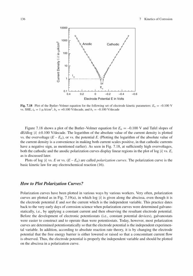
136 7 Kinetics of Corrosion
0.1
1
10
100
1000
10000
–0.6–0.4–0.200.20.4
Cur
rent
Den
sity
| i |
in μ
A/c
m2
Electrode Potential E in Volts
Anodic Cathodic
Eo
i o
Fig. 7.18 Plot of the Butler–Volmer equation for the following set of electrode kinetic parameters: Eo = –0.100 Vvs. SHE, io = 1 μA/cm2, ba = +0.100 V/decade, and bc = –0.100 V/decade
Figure 7.18 shows a plot of the Butler–Volmer equation for Eo = –0.100 V and Tafel slopes ofdE/dlog |i| ±0.100 V/decade. The logarithm of the absolute value of the current density is plottedvs. the overvoltage (E – Eo), or vs. the potential E. (Plotting the logarithm of the absolute value ofthe current density is a convenience in making both current scales positive, in that cathodic currentshave a negative sign, as mentioned earlier). As seen in Fig. 7.18, at sufficiently high overvoltages,both the cathodic and the anodic polarization curves display linear regions in the plot of log |i| vs. E,as is discussed later.
Plots of log |i| vs. E or vs. (E – Eo) are called polarization curves. The polarization curve is thebasic kinetic law for any electrochemical reaction (16).
How to Plot Polarization Curves?
Polarization curves have been plotted in various ways by various workers. Very often, polarizationcurves are plotted as in Fig. 7.19(a), in which log |i| is given along the abscissa, even though it isthe electrode potential E and not the current which is the independent variable. This practice datesback to the very early days of corrosion science when polarization curves were determined galvano-statically, i.e., by applying a constant current and then observing the resultant electrode potential.Before the development of electronic potentiostats (i.e., constant potential devices), galvanostatswere easier to construct and to operate than were potentiostats. Today, however, most polarizationcurves are determined potentiostatically so that the electrode potential is the independent experimen-tal variable. In addition, according to absolute reaction rate theory, it is by changing the electrodepotential that the free energy barrier is either lowered or raised so that a concomitant current flowis observed. Thus, the electrode potential is properly the independent variable and should be plottedon the abscissa in a polarization curve.

Electrode Kinetics for Activation Polarization 137
Rotated
90o
to left
Flipped
horizontally
(a)
(b)
(c)
0.1
1
10
100
1000
10000
–0.6–0.4–0.200.20.4
| i |
E
Anodic Cathodic
0.1
1
10
100
1000
10000
–0.6 –0.4 –0.2 0 0.2 0.4
| i |
E
AnodicCathodic
0.1 10 1000–0.6
–0.4
–0.2
0
0.2
0.4
| i |E
Anodic
Cathodic
Fig. 7.19 Various methods of presenting polarization curves
By rotating Fig. 7.19(a) 90◦ to the left, the independent variable E is placed along the abscissa,as shown in Fig. 7.19(b). The “disadvantage” of Fig. 7.19(b) is that electrode potentials increase inthe negative direction along the X-axis. However, this is a common convention in electroanalyticalchemistry [21].
Plots as in Fig. 7.19(b) are used in this text when both anodic and cathodic polarization curvesare shown. If only the anodic or the cathodic curve is given, then the curve is drawn from left to rightand the sense of the X-axis is clearly labeled.

138 7 Kinetics of Corrosion
Increasingly positive potentials can appear to the right along the X-axis if Fig. 7.19(b) is flippedhorizontally, as in Fig. 7.19(c). But such curves are then two operations removed from the familiarplots of Fig. 7.19(a).
The Tafel Equation
The semi-logarithmic plot in Fig. 7.18 is not linear near the open-circuit potential (i.e., near zeroovervoltage). This is because the other half-cell reaction is still appreciable and contributes to thetotal current. However, at sufficiently high overvoltages, the contribution of the reverse reactionbecomes negligible. In this linear “Tafel” region, the straight lines shown in Fig. 7.18 can be extrap-olated back to zero overvoltage (i.e., back to Eo) to give the open-circuit exchange current densityio, as shown below.
The well-known Tafel equation follows from the Butler–Volmer equation as follows. At suffi-ciently high overvoltages, the rate of the reverse reaction becomes negligible so that Eq. (25) can bewritten as
←inet = io eαnF(E−Eo)/RT (27)
or simply
i = io eαnF(E−Eo)/RT (28)
Taking logarithms in Eq. (28)
log i = log io + αnF
2.303 RT(E − Eo) (29)
Thus, a plot of log |i| vs. the overvoltage (E–Eo) (or of log |i| vs. the electrode potential E) givesa straight line, as shown in Fig. 7.18. From Eq. (29), when E= Eo, i= io. Thus, the Tafel region canbe extrapolated back to E = Eo to give the exchange current density io, as shown in Fig. 7.18.
Equation (29) can be rewritten as
ηa = ba logi
io(30)
which is one form of the Tafel equation, where ηa is the anodic overvoltage and ba is the anodicTafel slope given by
ba = d E
d log i= 2.303 RT
α n F(31)
Equation (30) can also be written as
ηa = a+ ba log i (32)
which is another form of the Tafel equation, where a is a constant given by
a = −2.303 RT
αnFlog io (33)
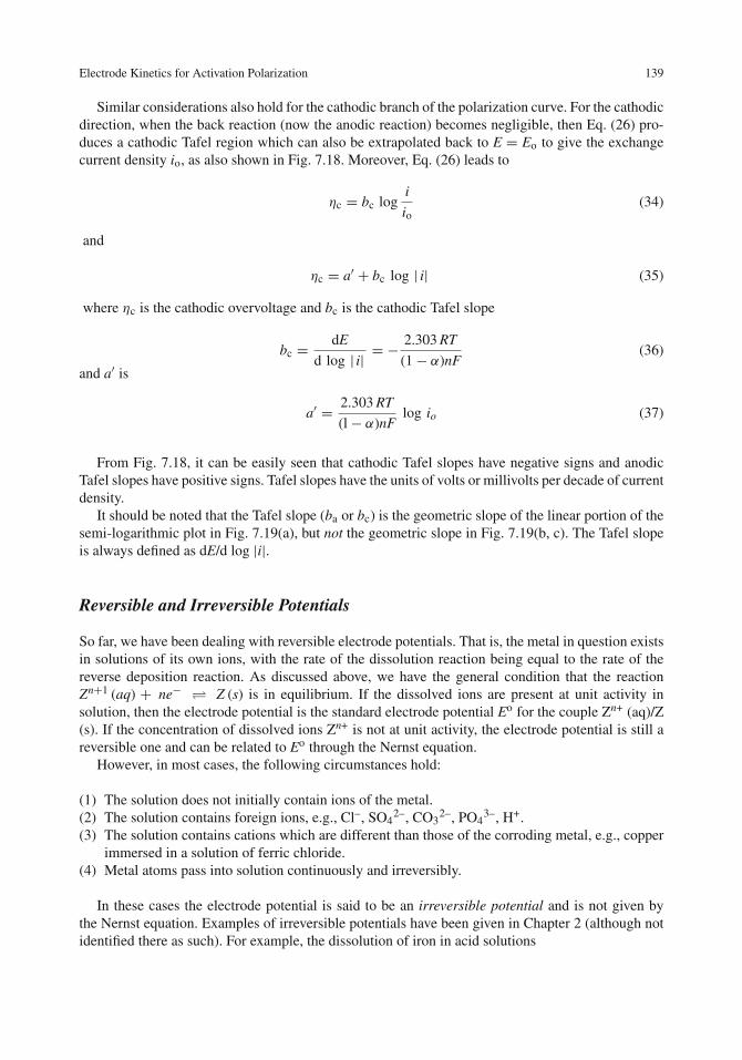
Electrode Kinetics for Activation Polarization 139
Similar considerations also hold for the cathodic branch of the polarization curve. For the cathodicdirection, when the back reaction (now the anodic reaction) becomes negligible, then Eq. (26) pro-duces a cathodic Tafel region which can also be extrapolated back to E = Eo to give the exchangecurrent density io, as also shown in Fig. 7.18. Moreover, Eq. (26) leads to
ηc = bc logi
io(34)
and
ηc = a′ + bc log | i| (35)
where ηc is the cathodic overvoltage and bc is the cathodic Tafel slope
bc = dE
d log | i| = −2.303 RT
(1− α)nF(36)
and a′ is
a′ = 2.303 RT
(l− α)nFlog io (37)
From Fig. 7.18, it can be easily seen that cathodic Tafel slopes have negative signs and anodicTafel slopes have positive signs. Tafel slopes have the units of volts or millivolts per decade of currentdensity.
It should be noted that the Tafel slope (ba or bc) is the geometric slope of the linear portion of thesemi-logarithmic plot in Fig. 7.19(a), but not the geometric slope in Fig. 7.19(b, c). The Tafel slopeis always defined as dE/d log |i|.
Reversible and Irreversible Potentials
So far, we have been dealing with reversible electrode potentials. That is, the metal in question existsin solutions of its own ions, with the rate of the dissolution reaction being equal to the rate of thereverse deposition reaction. As discussed above, we have the general condition that the reactionZn+1 (aq) + ne− � Z (s) is in equilibrium. If the dissolved ions are present at unit activity insolution, then the electrode potential is the standard electrode potential Eo for the couple Zn+ (aq)/Z(s). If the concentration of dissolved ions Zn+ is not at unit activity, the electrode potential is still areversible one and can be related to Eo through the Nernst equation.
However, in most cases, the following circumstances hold:
(1) The solution does not initially contain ions of the metal.(2) The solution contains foreign ions, e.g., Cl–, SO4
2–, CO32–, PO4
3–, H+.(3) The solution contains cations which are different than those of the corroding metal, e.g., copper
immersed in a solution of ferric chloride.(4) Metal atoms pass into solution continuously and irreversibly.
In these cases the electrode potential is said to be an irreversible potential and is not given bythe Nernst equation. Examples of irreversible potentials have been given in Chapter 2 (although notidentified there as such). For example, the dissolution of iron in acid solutions
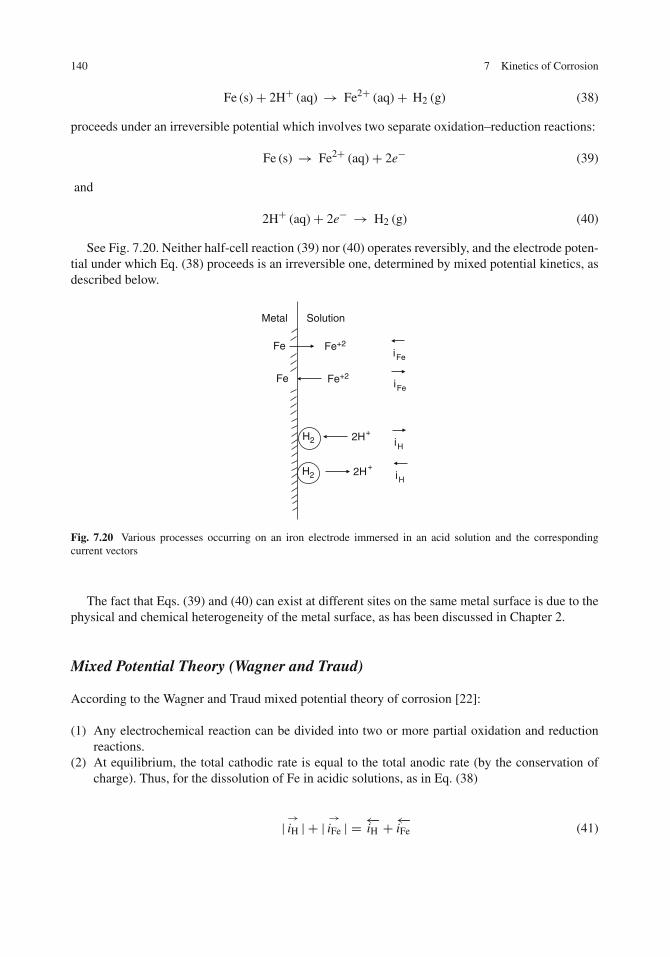
140 7 Kinetics of Corrosion
Fe (s)+ 2H+ (aq) → Fe2+ (aq)+ H2 (g) (38)
proceeds under an irreversible potential which involves two separate oxidation–reduction reactions:
Fe (s) → Fe2+ (aq)+ 2e− (39)
and
2H+ (aq)+ 2e− → H2 (g) (40)
See Fig. 7.20. Neither half-cell reaction (39) nor (40) operates reversibly, and the electrode poten-tial under which Eq. (38) proceeds is an irreversible one, determined by mixed potential kinetics, asdescribed below.
Fe Fe+2
Fe Fe+2
iFe
iFe
iHH2 2H+
H2 2H+iH
Metal Solution
Fig. 7.20 Various processes occurring on an iron electrode immersed in an acid solution and the correspondingcurrent vectors
The fact that Eqs. (39) and (40) can exist at different sites on the same metal surface is due to thephysical and chemical heterogeneity of the metal surface, as has been discussed in Chapter 2.
Mixed Potential Theory (Wagner and Traud)
According to the Wagner and Traud mixed potential theory of corrosion [22]:
(1) Any electrochemical reaction can be divided into two or more partial oxidation and reductionreactions.
(2) At equilibrium, the total cathodic rate is equal to the total anodic rate (by the conservation ofcharge). Thus, for the dissolution of Fe in acidic solutions, as in Eq. (38)
| →iH | + |→iFe | = ←−iH +←−iFe (41)

Electrode Kinetics for Activation Polarization 141
where | →iH | is the current density for the reduction reaction
2H+ (aq)+ 2e− → H2(g)
|→iFe| is the current density for the reduction reaction
Fe2+(aq)+ 2e− → Fe(s)
←iH is the current density for the oxidation reaction
H2(g)→ 2H+(aq)+ 2e−
and i←Fe is the current density for the oxidation reaction
Fe(s)→ Fe2+(aq)+ 2e−
(3) The electrode potential for the steady-state, freely corroding condition given by Eq. (41) is calledthe corrosion potential Ecorr.
(4) The corrosion potential is not related to the standard Eo values for either half-cell reaction bythe Nernst equation.
(5) The corrosion potential Ecorr lies between the electrode potentials for the two half-cell reactionsand is called a mixed potential.
From Eq. (41), at equilibrium
←iFe − |
→iFe|︸ ︷︷ ︸ = |
→iH| −
←iH︸ ︷︷ ︸ = icorr
/ \net rate of net rate ofiron dissolution hydrogen evolution
(42)
where icorr is the corrosion rate of the freely corroding metal. At equilibrium, there is no net currentflow, as per Eq. (41), but there is a loss of metal, i.e., corrosion, as per Eq. (42). The electrodepotential for the steady-state, freely corroding condition in Eq. (42) is called the corrosion potentialEcorr (also called the open-circuit potential or the rest potential).
We can directly measure the corrosion potential Ecorr, but we cannot measure icorr withoutpolarizing the electrode away from the corrosion potential. That is the individual oxidation rates(←−
iFe or←−iH)
or individual reduction rates (| →iFe | or | →iH |) cannot be measured.
Instead, it is necessary to make the entire corroding metal either the anode or the cathode in anelectrolytic cell and to deduce the steady-state condition in Eq. (42) from the polarized condition.For the anodic direction, the Tafel equation gives

142 7 Kinetics of Corrosion
ηa = ba log
←iH+
←iFe
icorr(43)
where
(←iH+
←iFe
)is the total anodic current density. At any potential, the net anodic current
density is
←inet =
(←iH+
←iFe
)−(| →iH | + |
→iFe |)
(44)
Substitution of Eq. (44) into Eq. (43) gives
ηa = ba log
←inet+(
→| iH| +→| iFe| )
icorr(45)
But the cathodic current densities | →iH | and | →iFe | are negligible at sufficiently high anodicovervoltages so that Eq. (45) reduces to
ηa = ba log
←inet
icorr(46)
or simply
ηa = ba logi
icorr(47)
An expression similar to Eq. (47) holds for the cathodic branch. That is
ηc= bc logi
icorr(48)
According to either Eq. (47) or Eq. (48), i = icorr when η = 0. Thus, anodic or cathodic Tafellines can be extrapolated back to the corrosion potential Ecorr to give the corrosion rate icorr.
Thus, the Wagner–Traud theory of mixed potentials places the electrochemistry of local actioncells on a firm theoretical basis (described qualitatively in Chapter 2). A consequence of the Wagner–Traud theory is that the Butler–Volmer equation can be written as follows for a corroding metal:
i←net = icorr
[eαnF(E−Ecorr)/RT − e−(1−α)nF(E−Ecorr)/RT
](49)
Comparison of Eqs. (49) and (25) for a single electrochemical reaction shows that for a corrodingmetal, icorr replaces io, and Ecorr replaces Ecorr. However, unlike Eo, the corrosion potential Ecorrdoes not have any thermodynamic significance attached to it and Ecorr is determined by the kineticsof the system.
Example 7.2: Suppose that a metal M has an oxidation–reduction exchange current density of0.1 μA/cm2 at its reversible potential of –0.160 V. The anodic Tafel slope is + 0.060 V and thecathodic Tafel slope is –0.060 V for the system M+ + e− → M. For hydrogen evolution on the

Electrode Kinetics for Activation Polarization 143
surface of M, the anodic and the cathodic Tafel slopes are + 0.100 and – 0.100 V, respectively. Theexchange current density for hydrogen evolution on the metal M is 1.0 μA/cm2 at the reversiblepotential of 0.00 V.
(a) Construct the individual polarization curves for the systems M+ + e− � M and 2H+ + 2e− �H2
(b) What is the corrosion potential?(c) What is the corrosion rate?(d) Plot the experimentally observed anodic and cathodic polarization curves.
Solution: The schematic polarization curves for the electrochemical reactions M+ + e− �M and 2H+ + 2e− � H2 are drawn graphically, as shown in Fig. 7.21. The corrosion poten-tial and the corrosion rate are indicated on the figure. The experimentally observed anodic andcathodic polarization curves are determined by first setting up Table 7.2, in which the net cathodicand anodic current densities are determined graphically from Fig. 7.21. The net current densitiesgiven in Table 7.2 are then plotted as open circles in Fig. 7.21 to give the experimental polarizationcurves.
Schematic polarization diagrams as in Fig. 7.21 are called Evans diagrams, after the notedcorrosion scientist U.R. Evans (1889–1980), who was instrumental in their development andinterpretation.
Fig. 7.21 Evans diagrams for the half cell reactions M+ + e− � M and 2H+ + 2e− � H2, as described by theelectrode kinetic parameters given in Example 7.2. Reproduced by permission of ECS – The Electrochemical Society

144 7 Kinetics of Corrosion
Table 7.2 Determination of the experimental polarization curve for Example 7.2
Cathodic:| →inet| = |→iH| + |
→iM| − (
←iH +
←iM)
|→iH| |→iM|←iH
←iM | →inet|
EH+reduction M deposition H2 oxidation M dissolution Cathodic
–0.070 5.0 – 0.2 3.0 1.8–0.080 6.2 – 0.16 2.1 3.9–0.090 8.0 – 0.13 1.4 6.5–0.100 10 – 0.10 1.0 8.9–0.110 12 – – 0.68 11.3–0.120 16 – – 0.45 15.5–0.140 25 – – 0.2 24.8–0.160 39 – – 0.1 38.9–0.180 64 – – – 64–0.200 100 – – – 100
Anodic:←inet =
←iH +
←iM −
(|→iH| + |
→iM|)
←iH
←iM |→iH| |→iM|
←inet
EH2 oxidation M dissolution H+ reduction M deposition Anodic
–0.060 0.26 4.4 4.2 – 0.46–0.050 0.32 6.4 3.2 – 3.5–0.040 0.4 9.2 2.5 – 7.1–0.030 0.5 14 2.0 – 12.5–0.020 0.7 20 1.6 – 19.1–0.010 0.8 28 1.3 – 27.50.000 1.0 41 1.0 – 41+0.010 1.3 60 0.8 – 61+0.020 1.6 88 0.6 – 89
Electrode Kinetic Parameters
Table 7.3 lists exchange current densities for the hydrogen evolution reaction on various metals ascompiled by Trasatti [23]. The value of the exchange current density for a given metal depends onvarious experimental factors, such as the particular electrolyte used, its concentration, the purityof the metal, its surface cleanliness, the time of immersion in solution, and whether equilibriumconditions had been attained.
The exchange current density for hydrogen evolution increases with the work function of themetal, as shown in Fig. 7.22. The work function is a measure of the ability of the metal to expel (i.e.,donate) electrons. Thus, the greater the electron-donating ability of the metal, the greater the rate ofthe electron-accepting reaction:
2 H+ + 2e− → H2
The relationships in Fig. 7.22 were first observed by Conway and Bockris [24].

Electrode Kinetics for Activation Polarization 145
Table 7.3 Exchange current densities io,H for the hydrogen evolution reaction [23]
Metal io,H (A/cm2) Metal io,H (A/cm2)
Ag 1.3 × 10⁻⁸ Ni 5.6 × 10⁻⁶
Al 1.0 × 10⁻⁸ Os 7.9 × 10⁻⁵
Au 3.2 × 10⁻⁷ Pb 4.0 × 10⁻¹²
Bi 1.6 × 10⁻⁸ Pd 7.9 × 10⁻⁴
Cd 2.5 × 10⁻¹² Pt 1.0 × 10⁻³
Co 5.0 × 10⁻⁶ Re 1.0 × 10⁻³
Cr 1.0 × 10⁻⁷ Rh 3.2 × 10⁻⁴
Cu 1.6 × 10⁻⁸ Ru 6.3 × 10⁻⁵
Fe 2.5 × 10⁻⁶ Sb 7.9 × 10⁻⁶
Ga 4.0 × 10⁻⁹ Sn 1.6 × 10⁻⁸
In 3.2 × 10⁻¹⁰ Ta 3.0 × 10⁻⁹
Ir 2.5 × 10⁻⁴ Ti 5.0 × 10⁻⁹
Mn 1.3 × 10⁻¹¹ Tl 2.5 × 10⁻¹⁰
Mo 5.0 × 10⁻⁸ W 4.0 × 10⁻⁷
Nb 4.0 × 10⁻⁹ Zn 3.2 × 10⁻¹¹
10–12
10–10
10–8
10–6
10–4
10–2
3.8 4.0 4.2 4.4 4.6 4.8 5.0 5.2
Exc
hang
e C
urre
nt D
ensi
ty in
A/c
m2
Work Function of Metal in eV
Au
Cu
Zn
PbCd
Ni
Mn
Ti
Al
Ta
Mo
CrFe
Pt
Fig. 7.22 The exchange current density for hydrogen evolution as a function of the work function of the metal. Mostmetals follow the trend shown in the upper set of data, but several metals follow the trend shown in the lower set ofdata. Plotted from data compiled by Trasatti [23]
Exchange current densities for the dissolution (or deposition) of several metals are listed inTable 7.4. In most cases, the numerical value of the exchange current density depends on the natureof the solution, the concentration of the dissolved cation, and the pH of the solution.
Cathodic Tafel slopes for the hydrogen evolution reaction have been usually observed to be nearthe theoretical value of –0.120 V/decade. This value is obtained from Eq. (36) with α = 0.5 andn = 1 assuming a single electron transfer step of H+ to Hads, followed by the combination of twoHads atoms to H2, or by the following reaction [25]:
Hads + H+ + e− → H2

146 7 Kinetics of Corrosion
Table 7.4 Exchange current densities io,M for metal dissolution/metal deposition half-cell reactions
Metal SolutionExchange current density(A/cm2) Source
Zn 1 M ZnSO4Zn(ClO4)0.057–0.46 M Zn2+, 3 M
ClO4–
2 × 10⁻⁵
3.5 × 10⁻⁴
Bockris [25]
Clark and Hampson [26]
Cu 1 M CuSO40.05–0.5 M CuSO4 + 0.5 M
H2SO4
2 × 10⁻⁵
7.0 × 10⁻³Bockris [25]Despic [27]
Fe 1 M FeSO4 10–8 Bockris [25]1 M HCl 4.0 × 10⁻⁸ to 1.0 × 10⁻⁷ Kaesche and
Hackerman [28]4% NaCl (pH 1.5) 4.1 × 10⁻⁸ Stern and Roth [29]4% NaCl (acidified) 1.0 × 10⁻⁷ Stern [30]0.1 M citric acid 9.3 × 10⁻⁸ Stern [30]0.1 malic acid 1.5 × 10⁻⁸ Stern [30]FeSO4 + Na2SO4 (pH = 3.1) 2.2 × 10⁻⁶ Bockris and Drazic [31]
Ni 1 M NiSO4 2.0 × 10⁻⁹ Bockris [25]Cd 0.049 M Cd2+
0.452 M Cd2+2.3 × 10⁻³
2.5 × 10⁻²Hampson et al. [32]
Pb 0.0027 M Pb2+
0.5 M Pb2+2.62 × 10⁻²
7.14 × 10⁻²Hampson and Larkin [33]
Ag 0.001 M Ag+
0.1 M Ag+0.154.5
Vetter [34]
Experimental anodic Tafel slopes for the dissolution of various metals usually range from 0.040to 0.080 V/decade. Chapter 16 deals with electrode kinetics and reaction mechanisms in more detail.See Problem 7.6 at the end of this chapter.
Applications of Mixed Potential Theory
Metals in Acid Solutions
One of the first applications of mixed potential theory was the dissolution of metals in acid solutions.Figure 7.23 considers the case of zinc immersed in hydrochloric acid. The overall chemical reaction
Zn+ 2H+ → Zn2+ + H2 (50)
can be separated into its two half-cell reactions:
Zn→ Zn2+ + 2e− (51)
and
2H+ + 2e− → H2 (52)

Applications of Mixed Potential Theory 147
100
10–2
10–4
10–6
10–8
10–10
10–12–1.20–0.80–0.400.000.40
| i | in
A/c
m2
E in V vs. S.H.E.
Reversereaction
Reversereaction
icorr
Ecorr
io,Zn
Eo,Zn
io,H
Eo,H
Fig. 7.23 Evans diagram for zinc in hydrochloric acid. The diagram is drawn using exchange current densities fromTables 7.3 and 7.4. Tafel slopes are taken to be± 100 mV/decade for H2 evolution and deposition and± 60 mV/decadefor zinc dissolution and deposition
Each half-cell reaction proceeds under its own set of polarization curves with its own individualopen-circuit potential Eo and its own exchange current density io. For the half-cell reaction in Eq.(52), io is io,H, as shown in Fig. 7.23, and is taken from Table 7.3 to be 3.2 × 10⁻¹¹ A/cm2 forhydrogen evolution on zinc [23]. The open-circuit equilibrium potential for Eq. (52) is exactly thestandard electrode potential Eo only if a(H+) = 1.0 and H2 gas is present at 1.0 atm pressure. Tafelslopes are taken to be ±100 mV/decade for H2 evolution and deposition.
Similarly, the half-cell reaction in Eq. (51) for zinc dissolution/deposition has its own exchangecurrent density io,Zn, taken in Fig. 7.23 to be 2.0× 10⁻⁵ A/cm2 (see Table 7.4). Again, the equilibriumopen-circuit potential Eo is exactly the standard electrode potential Eo for zinc if a(Zn2+)= 1.0. Tafelslopes are taken to be ±60 mV/decade for metal dissolution and deposition. As in Example 7.2, thepolarization curve for the total system is given by the superposition of the polarization curves for thetwo half-cell reactions.
From Fig. 7.23 it can be seen that the total cathodic current density at any electrode potential isessentially that due to the reaction
2H+ + 2e− → H2 (53)
(On a logarithmic scale, the contributions to the total cathodic density due to the reaction Zn2+ +2e− → Zn are negligible.) Similarly, from Fig. 7.23, the total anodic current density is essentiallythat due to the reaction
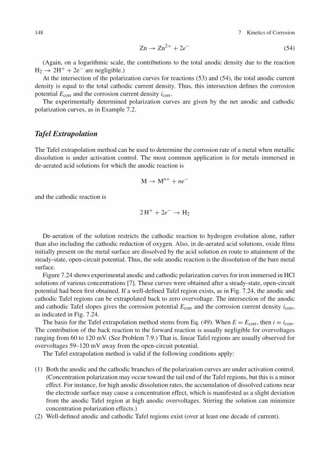
148 7 Kinetics of Corrosion
Zn→ Zn2+ + 2e− (54)
(Again, on a logarithmic scale, the contributions to the total anodic density due to the reactionH2 → 2H+ + 2e− are negligible.)
At the intersection of the polarization curves for reactions (53) and (54), the total anodic currentdensity is equal to the total cathodic current density. Thus, this intersection defines the corrosionpotential Ecorr and the corrosion current density icorr.
The experimentally determined polarization curves are given by the net anodic and cathodicpolarization curves, as in Example 7.2.
Tafel Extrapolation
The Tafel extrapolation method can be used to determine the corrosion rate of a metal when metallicdissolution is under activation control. The most common application is for metals immersed inde-aerated acid solutions for which the anodic reaction is
M→ Mn+ + ne−
and the cathodic reaction is
2 H+ + 2e− → H2
De-aeration of the solution restricts the cathodic reaction to hydrogen evolution alone, ratherthan also including the cathodic reduction of oxygen. Also, in de-aerated acid solutions, oxide filmsinitially present on the metal surface are dissolved by the acid solution en route to attainment of thesteady-state, open-circuit potential. Thus, the sole anodic reaction is the dissolution of the bare metalsurface.
Figure 7.24 shows experimental anodic and cathodic polarization curves for iron immersed in HClsolutions of various concentrations [7]. These curves were obtained after a steady-state, open-circuitpotential had been first obtained. If a well-defined Tafel region exists, as in Fig. 7.24, the anodic andcathodic Tafel regions can be extrapolated back to zero overvoltage. The intersection of the anodicand cathodic Tafel slopes gives the corrosion potential Ecorr and the corrosion current density icorr,as indicated in Fig. 7.24.
The basis for the Tafel extrapolation method stems from Eq. (49). When E = Ecorr, then i = icorr.The contribution of the back reaction to the forward reaction is usually negligible for overvoltagesranging from 60 to 120 mV. (See Problem 7.9.) That is, linear Tafel regions are usually observed forovervoltages 59–120 mV away from the open-circuit potential.
The Tafel extrapolation method is valid if the following conditions apply:
(1) Both the anodic and the cathodic branches of the polarization curves are under activation control.(Concentration polarization may occur toward the tail end of the Tafel regions, but this is a minoreffect. For instance, for high anodic dissolution rates, the accumulation of dissolved cations nearthe electrode surface may cause a concentration effect, which is manifested as a slight deviationfrom the anodic Tafel region at high anodic overvoltages. Stirring the solution can minimizeconcentration polarization effects.)
(2) Well-defined anodic and cathodic Tafel regions exist (over at least one decade of current).
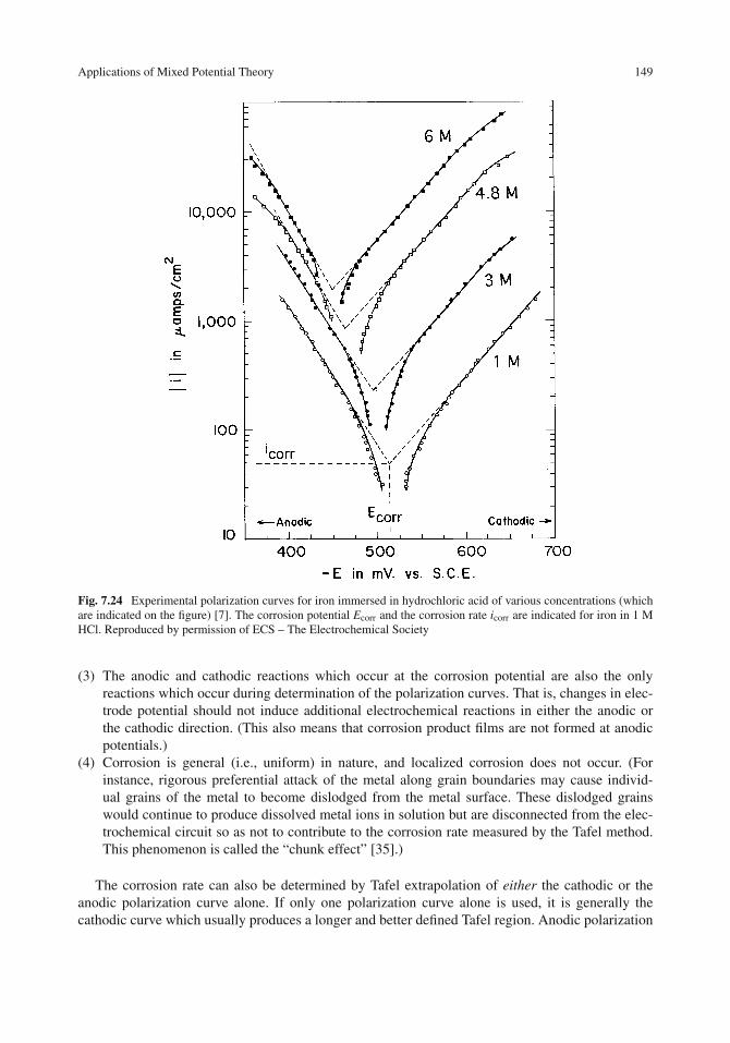
Applications of Mixed Potential Theory 149
Fig. 7.24 Experimental polarization curves for iron immersed in hydrochloric acid of various concentrations (whichare indicated on the figure) [7]. The corrosion potential Ecorr and the corrosion rate icorr are indicated for iron in 1 MHCl. Reproduced by permission of ECS – The Electrochemical Society
(3) The anodic and cathodic reactions which occur at the corrosion potential are also the onlyreactions which occur during determination of the polarization curves. That is, changes in elec-trode potential should not induce additional electrochemical reactions in either the anodic orthe cathodic direction. (This also means that corrosion product films are not formed at anodicpotentials.)
(4) Corrosion is general (i.e., uniform) in nature, and localized corrosion does not occur. (Forinstance, rigorous preferential attack of the metal along grain boundaries may cause individ-ual grains of the metal to become dislodged from the metal surface. These dislodged grainswould continue to produce dissolved metal ions in solution but are disconnected from the elec-trochemical circuit so as not to contribute to the corrosion rate measured by the Tafel method.This phenomenon is called the “chunk effect” [35].)
The corrosion rate can also be determined by Tafel extrapolation of either the cathodic or theanodic polarization curve alone. If only one polarization curve alone is used, it is generally thecathodic curve which usually produces a longer and better defined Tafel region. Anodic polarization

150 7 Kinetics of Corrosion
may sometimes produce concentration effects, as noted above, as well as roughening of the surfacewhich can lead to deviations from Tafel behavior. Thus, extrapolation of the cathodic Tafel regionback to zero overvoltage gives the net rate of the cathodic reaction at the corrosion potential; butfrom Eq. (42), this is also the net rate of the anodic reaction at the corrosion potential. Use of boththe anodic and the cathodic Tafel regions is preferred, of course, over the use of just one Tafel region.
Verification of Corrosion Rates Obtained by Tafel Extrapolation
It is now widely understood and accepted that the rate of general corrosion can be determined by theTafel extrapolation method (subject to the restrictions listed earlier). However, this acceptance wasnot forthcoming until the theory of polarization curves for corroding metals had been placed on afirm theoretical basis, as was done by the work of many individual investigators [15, 17, 22, 25, 28–30, 36–40]. Final acceptance of the polarization method was gained upon an experimental validationof the corrosion rates determined electrochemically. This validation was provided by comparison ofcorrosion rates determined from polarization curves with corrosion rates measured by an indepen-dent non-electrochemical method, such as weight loss measurements, colorimetric analysis of thesolution containing the dissolved metal, or determination of the amount of hydrogen gas evolved bythe corrosion reaction (for metals in acid solutions).
Table 7.5 compares corrosion rates determined electrochemically by the Tafel extrapolationmethod for iron in various solutions with corrosion rates determined separately by a second non-electrochemical method. Data are also given for the corrosion of other metals in various solutions.Weight loss measurements or solution analyses are converted into equivalent current densities usingFaraday’s law. For gas evolution measurements, the equivalent current density follows from themolar volume of a gas, 22,400 ml at standard temperature and pressure (0◦C and 760 Torr),and Faraday′s law. In each case in Table 7.5, there is a good agreement between the results forelectrochemical and non-electrochemical measurements.
Cathodic Protection of Iron in Acids
Chapter 5 considered the cathodic protection of iron by zinc from a thermodynamic point of view.In seawater, for example, the electrode potential of zinc is more negative than that of iron. Thus,when zinc and iron are coupled, zinc is the anodic member of the couple and the iron electrode inthe couple is cathodically protected.
This phenomenon of cathodic protection also applies in acid solutions and can be examined byconsidering the polarization curves for the zinc/acid and iron/acid systems. Figure 7.25 comparesschematic Evans diagrams for iron and zinc in hydrochloric acid. The Evans diagram for iron isconstructed using io,H = 2.5 × 10⁻⁶ A/cm2 (Table 7.3) and taking io,M to be 1.0 × 10⁻⁷ A/cm2
(Table 7.4).It can be seen that the corrosion rate of iron and of zinc is approximately the same, even though
the electrode potential of zinc is more active (i.e., more negative) than that of iron. The exchangecurrent density for hydrogen evolution on iron is higher than that on zinc. However, the exchangecurrent density for zinc dissolution io,Zn is higher than that for iron dissolution io,Fe (see Table 7.4).These differences combine to produce corrosion rates which are similar for iron and zinc in thisparticular acid solution. This observation illustrates the statement made in Chapter 5 that the emfseries or galvanic series cannot accurately predict the relative order of corrosion rates but can onlyidentify the anodic and cathodic members of a galvanic couple.

Applications of Mixed Potential Theory 151
Table 7.5 Comparison of corrosion rates determined by the Tafel extrapolation method with corrosion ratesdetermined by a second method [41]
icorr
EnvironmentImmersiontime Tafel method Second method
Type of secondmethod Reference
Iron 1 M HBr1 M HI
120 h110 h
23 μA/cm2
10 μA/cm216 μA/cm2
7 μA/cm2ColorimetricColorimetric
McCafferty [6]
Iron 1 M HCl 24 h 30 μA/cm2 36 μA/cm2 Colorimetric McCafferty [8]Iron 1 M HCl 8 h 50 μA/cm2 50 μA/cm2 Colorimetric Kaesche [28]Iron O2-free 4%
NaCl, pH 1100 h 10.5 μA/cm2 11.1 μA/cm2 Weight loss Stern [40]
Fe + 0.11%Cu
O2-free 4%NaCl, pH 1
100 h 154 μA/cm2 156 μA/cm2 weight loss Stern [40]
Fe + 0.08%Si
O2-free 4%NaCl, pH 1
100 h 270 μA/cm2 290 μA/cm2 Weight loss Stern [40]
Fe + 0.017%P
O2-free 4%NaCl, pH 1
100 h 390 μA/cm2 400 μA/cm2 Weight loss Stern [40]
Zinc 10% NH4Cl – 100 μA/cm2 100 μA/cm2 AAS ofsolutiona
Maja et al. [42]
Titanium Boiling1 M H2SO4
2.5 1.9 mA/cm2 2.2 mA/cm2
4.0 mA/cm2ColorimetricInert marker
McCafferty [41]
Al alloy 3003 Acetate buffer,pH 4.6
Citrate buffer,pH 2.5
Prune juice
1 week 8.2 μA/cm2
1.2 μA/cm2
1.4 μA/cm2
9.1 μA/cm2
1.3 μA/cm2
1.5 μA/cm2
H2 evolution
H2 evolution
H2 evolution
Evans and Koehler[43]
Al alloy 3003 0.1 M HCl1.0 M HCl
24 hrs.4 hrs.
31 μA/cm2
7.5 mA/cm231 μA/cm2
7.3 mA/cm2ColorimetricColorimetric
McCafferty,Moore, andPeace [9]
Copper 0.5 M H2SO425 ◦C55 ◦C
72 hrs72 hrs.
25.7 μA/cm2
54.6 μA/cm222.5 μA/cm2
39.3 mA/cm2Weight lossWeight loss
Quartarone [44]
Fe-14 Cr 1 N H2SO430 ◦C
20 min. 0.438 mA/cm2 0.479 mA/cm2 b Weight loss Yau and Streicher[45]
aAtomic absorption spectrophotometry.bAssumes divalent dissolution of each metal and stoichiometric dissolution of each component of the binary alloyon an atomic fraction basis.
When iron and zinc are coupled in hydrochloric acid, the situation is shown in Fig. 7.26. Thetotal cathodic current density for the Fe/Zn couple at any electrode potential is essentially that forhydrogen evolution on iron, because contributions from other reduction reactions are negligible ona logarithmic basis. Similarly, the total anodic current density for the Fe/Zn couple at any electrodepotential is essentially that for zinc dissolution, because contributions from other oxidation reactionsare negligible on a logarithmic scale. Thus, the corrosion potential for the Fe/Zn couple in acidsolutions and the corresponding corrosion current for zinc in the couple are given by the intersectionof the polarization curves for the reactions
2 H+ + 2e− → H2 (on iron)

152 7 Kinetics of Corrosion
Fig. 7.25 Comparison of Evans diagrams for zinc and iron in hydrochloric acid. The diagrams are drawn usingexchange current densities from Tables 7.3 and 7.4. Tafel slopes are taken to be ± 100 mV/decade for H2 evolutionand deposition and ± 60 mV/decade for metal dissolution and deposition
and
Zn→ Zn2+ + 2e−
The intersection point is indicated in Fig. 7.26.Figure 7.26 also shows the corrosion potential and the corrosion current density for iron alone
(uncoupled) and for zinc alone (uncoupled).Figure 7.26 shows the following:

Applications of Mixed Potential Theory 153
Fig. 7.26 Kinetic explanation of the cathodic protection of iron by zinc in an acid solution
(1) The corrosion potential for the Fe/Zn couple is intermediate between the corrosion potentialsfor each of the two uncoupled electrodes.
(2) The corrosion current density for zinc in the Fe/Zn couple is greater than the corrosion currentdensity of uncoupled zinc.
(3) The corrosion current density for iron in the Fe/Zn couple is less than the corrosion currentdensity of uncoupled iron.
Thus, mixed potential theory shows that the coupling of iron to zinc in acid solutions results inthe cathodic protection of iron by zinc. See Fig. 7.27 for a schematic representation and comparethis figure with Fig. 5.5.
Zn Zn+2
2e–
2 H+ + 2e– H2
Fe Acid Solution
Fig. 7.27 Schematic illustration of cathodic protection of iron by zinc in an acid solution showing the principalelectrode reactions

154 7 Kinetics of Corrosion
Effect of the Cathodic Reaction
The previous section has shown that the corrosion rate of zinc in the Zn/Fe couple is greater thanthat of uncoupled zinc because the exchange current density io,H for the cathodic reaction (hydrogenevolution) is greater on iron than on zinc. As seen in Table 7.3, the exchange current density forhydrogen evolution on Pt, Fe, and Zn follows the following order:
io,H(pt) > io,H(Fe) > io,H(Zn)
Accordingly, the Evans diagrams shown in Fig. 7.28 show that the corrosion rates follow thefollowing order:
10–12
10–10
10–8
10–6
10–4
10–2
100
102
104
–1–0.8–0.6–0.4–0.20
E in V vs. S.H.E.
Cur
rent
Den
sity
|i| i
n A
/cm
2
H 2 on Pt
H 2 on Fe
H 2 on ZnEo,H
Eo,Zn
Zn Zn+2
+ 2e–
icorr
(Pt/Zn)
icorr
(Fe/Zn)
i corr (Zn)
Fig. 7.28 Effect of the cathode metal on the corrosion rate of zinc in a galvanic couple in an acid solution. (Thecathodic Tafel slope is taken to be –100 mV/decade for H2 evolution and the anode slope is +60 mV/decade for zincdissolution)
icorr(Zn coupled to pt) > icorr(Zn coupled to Fe) > icorr(Zn alone)
Thus, the greater the rate of the hydrogen evolution reaction on the cathode, the greater thecorrosion rate.
Effect of Cathode Area on Galvanic Corrosion
The relative areas of cathode and anode are important in galvanic behavior. Figure 7.29 illustratesthis effect on a galvanic couple of iron and zinc. As noted previously, when iron and zinc are coupled,the iron member of the couple is the cathode and zinc is the anode.

Applications of Mixed Potential Theory 155
Fig. 7.29 Effect of the area ratios of cathode to anode on the corrosion rate of zinc in an iron/zinc couple in an acidsolution (The cathodic Tafel slope is again taken to be –100 mV/decade for H2 evolution and the anode slope is again+60 mV/decade for zinc dissolution)
The cathodic Tafel slope is again taken to be –100 mV/decade for H2 evolution on iron, and theanode slope for zinc dissolution is again +60 mV/decade. The exchange current density for hydrogenevolution on iron is 1.0 × 10⁻⁶ A/cm2 (see Table 7.3) but the exchange current density for hydrogenon zinc is only 3.2× 10⁻¹¹ A/cm2 (also Table 7.3). Thus, the total current due to hydrogen evolutionis due to that on the iron member (the cathode) of the couple. The exchange current density for zincdissolution/deposition is 2.0 × 10⁻⁵ A/cm2 (Table 7.4). Total current rather than current density isused in Fig. 7.29, but if 1.0 cm2 of zinc is considered, the total current and the current density forthe zinc member of the couple are numerically identical.
As seen in Fig. 7.29, when the cathode/anode area ratio is 1:1, the current density for the corrodingiron member is 4.0 × 10⁻² A/cm2. If the cathode/anode area ratio is increased to 10:1, the totalcurrent for the couple is also increased, and the current density on the corroding zinc member is 1.8× 10⁻¹ A/cm2. Figure 7.29 shows that the corrosion current density on the zinc continues to increasewith increasing area of the iron cathode in the couple.
Figure 7.30 shows that the logarithm of the corrosion current density increases linearly with thelogarithm of the area ratio of cathode to anode. Verification of this relationship is left as an exercisein Problem 7.10.
The situation involving a small anode and a large cathode is unfavorable in the case of a noblecoating on an active substrate, e.g., for a copper coating on steel, as shown in Fig. 7.31. When a breakor a pore develops in the noble metal coating, then a small anode (steel) is exposed to a larger areacathode (copper), and the anodic current density increases with the area of the cathode, as shownabove and mentioned previously in Chapter 5.

156 7 Kinetics of Corrosion
10-2
10-1
100
101
1.0 10 102 103
i corr
in A
/cm
2
Area Ratio of Fe to Zn
Fig. 7.30 The corrosion current density in an acid solution for 1 cm2 of zinc coupled to various surface areas of iron
Copper (cathodic)
Steel (anodic)
ElectrolyteCrack or defectin coating
Fig. 7.31 Schematic diagram of a crack or a defect in a noble metal coating showing accelerated attack at the anodicsubstrate
Multiple Oxidation–Reduction Reactions
Systems with more than two oxidation–reduction reactions can also be treated by the Wagner–Traud theory of mixed potentials. The example given in Fig. 7.32 is taken from Stern [39] for asystem of three oxidation–reduction reactions involving species H+/H2, M2+/M, and Y2+/Y. Theelectrode kinetic parameters describing this system of three oxidation–reduction reactions are givenin Table 7.6. It can be seen in Fig. 7.32 that the total anodic current density is essentially that due tothe reaction
M→ M2+ + 2e−
(because the contributions to the total current density from the other two anodic half-cell reactionsare negligible). The total cathodic current density indicated by the dotted line in Fig. 7.32 is the sumof the current densities due to the following two cathodic reactions:

Applications of Mixed Potential Theory 157
0.01
0.1
1
10
100
–0.3–0.2–0.10.00.10.20.3
| i |
in μ
A/c
m2
E in V vs. S.H.E.
Eo,Y E
o,M
Total cathodic
Ecorr
Total anodic
icorr
Eo,H
Fig. 7.32 Evans diagrams for a system of three oxidation–reduction reactions having the electrode kinetic parametersgiven in Table 7.6. The total anodic curve is essentially that for the reaction M→ M+2 + 2e–, but the total cathodiccurve (dotted line) is given by the sum of the curves for the two half-cell reactions Y2+ + 2e–→ Y and 2H+ + 2e–→H2. The intersection of the total anodic and total cathodic curves defines the corrosion potential Ecorr and the corrosionrate icorr, as shown. Redrawn from [39] by permission of ECS – The Electrochemical Society
Table 7.6 Electrode kinetic parameters for the three oxidation–reduction reactions considered in Fig. 7.32 [39]
System Eo V vs. SHE io (μA/cm2) ba (V/decade) bc (V/decade)
2H+ + 2e− � H2 0.000 1.0 +0.100 –0.100M2+ + 2e− � M –0.160 0.1 +0.060 –0.060Y2+ + 2e− � Y +0.200 0.1 +0.120 –0.120
2H+ + 2e− → H2
and
Y2+ + 2e− → Y
(The contribution to the total cathodic current density from the M2+/M system is negligible). Thecorrosion potential and the corrosion rate are then given by the intersection of the total anodic andthe total cathodic curves, as shown in Fig. 7.32.
Figure 7.33 shows the experimentally observed polarization curve corresponding to the Evansdiagrams in Fig. 7.32. The experimentally observed polarization curve is determined in the usualway. That is, the net anodic rate ia at any anodic overvoltage is again the sum of all the anodiccurrent densities minus all the cathodic current densities:
ia =←inet = (
←iH +
←iM +
←iY)− (
→| iH| +→| iM| +
→| iY| ) (55)

158 7 Kinetics of Corrosion
1
10
100
1000
10000
–0.40–0.30–0.20–0.100.00.100.20
Cur
rent
Den
sity
in m
A/c
m2
E in V vs. S.H.E.
Anodic Cathodic
bc = –0.110 V/decade
ba = 0.060 V/decade
Fig. 7.33 Experimental polarization curve corresponding to the Evans diagrams in Fig. 7.32. Note that theexperimental cathodic Tafel slope is intermediate between the values for bH and bY in the Evans diagrams
Similarly, the net cathodic rate ic at any cathodic overvoltage is the sum of all the cathodic currentdensities minus all the anodic current densities:
ic =→inet =
(| →iH | + |
→iM | + |
→iY |)−(←
iH+←iM+
←iY
)(56)
A Tafel region is observed for both anodic and cathodic plots, but a special feature of this case isthat the cathodic Tafel slope is intermediate between the values for bH and bY.
An example of a system with three simultaneous oxidation-reduction reactions is the cor-rosion of stainless steels in acid solutions containing Fe3+ ions [39], for which the additionaloxidation−reduction reaction is
Fe3+(aq)+ e− → Fe2+(aq)
Industrial acids may contain dissolved ions such as Fe3+ due to corrosion or contamination.
Anodic or Cathodic Control
Corrosion reactions can be classified as being under anodic, cathodic, or mixed control. When polar-ization occurs mostly at the local anodes, the corrosion reaction is said to be under anodic control.This situation is illustrated in Fig. 7.34(a), in which small changes in the current density result inlarger changes in the anode potential rather than in the cathode potential. An experimental exampleis passivation of various metals by chromate inhibitors.
When polarization occurs mostly at the local cathodes, as shown in Fig. 7.34(b), the corrosionreaction is under cathodic control. An example is the corrosion of iron in natural waters, where thecathodic reaction given by
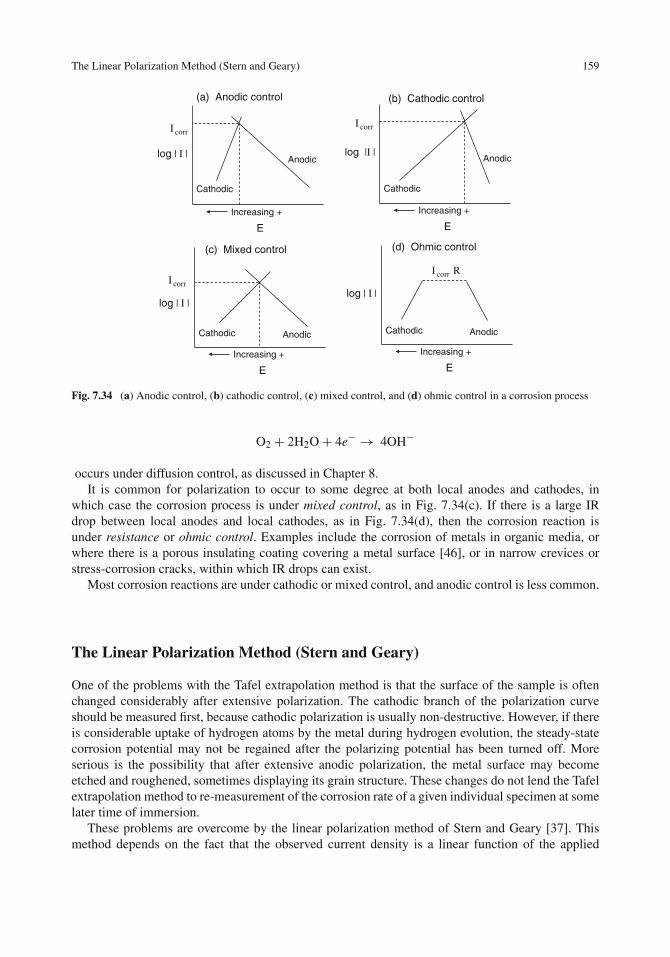
The Linear Polarization Method (Stern and Geary) 159
log | I |
Increasing +
E
AnodicCathodic
(d) Ohmic control
I corr R
(a) Anodic control
log | I |
Increasing +
E
Anodic
Cathodic
I corr
log |I |
Increasing +
E
Anodic
Cathodic
(b) Cathodic control
I corr
log | I |
Increasing +
E
AnodicCathodic
(c) Mixed control
I corr
Fig. 7.34 (a) Anodic control, (b) cathodic control, (c) mixed control, and (d) ohmic control in a corrosion process
O2 + 2H2O+ 4e− → 4OH−
occurs under diffusion control, as discussed in Chapter 8.It is common for polarization to occur to some degree at both local anodes and cathodes, in
which case the corrosion process is under mixed control, as in Fig. 7.34(c). If there is a large IRdrop between local anodes and local cathodes, as in Fig. 7.34(d), then the corrosion reaction isunder resistance or ohmic control. Examples include the corrosion of metals in organic media, orwhere there is a porous insulating coating covering a metal surface [46], or in narrow crevices orstress-corrosion cracks, within which IR drops can exist.
Most corrosion reactions are under cathodic or mixed control, and anodic control is less common.
The Linear Polarization Method (Stern and Geary)
One of the problems with the Tafel extrapolation method is that the surface of the sample is oftenchanged considerably after extensive polarization. The cathodic branch of the polarization curveshould be measured first, because cathodic polarization is usually non-destructive. However, if thereis considerable uptake of hydrogen atoms by the metal during hydrogen evolution, the steady-statecorrosion potential may not be regained after the polarizing potential has been turned off. Moreserious is the possibility that after extensive anodic polarization, the metal surface may becomeetched and roughened, sometimes displaying its grain structure. These changes do not lend the Tafelextrapolation method to re-measurement of the corrosion rate of a given individual specimen at somelater time of immersion.
These problems are overcome by the linear polarization method of Stern and Geary [37]. Thismethod depends on the fact that the observed current density is a linear function of the applied

160 7 Kinetics of Corrosion
0.1
1
10
100
1000
–0.40–0.200.000.20
| i |
in μ
A/c
m2
E in V vs. S.H.E.
ba = 0.060 V/decade
bc = –0.100 V/decade
Anodic Cathodic
–6.0
–4.0
–2.0
0.0
2.0
4.0
6.0
8.0
–0.18–0.14–0.10–0.06
Net
Cur
rent
Den
sity
in
μA/c
m2
E in V vs. S.H.E.
E corr
Anodic
Cathodic
Fig. 7.35 Top: An experimental polarization curve for which Ecorr = –0.100 V vs. SHE, icorr = 1 μA/cm2, ba =+0.060 V/decade, and bc = –0.100 V/decade. Bottom: Plot of the same polarization curve near the corrosion potential.Note the linear region near Ecorr
potential near the corrosion potential. Fig. 7.35 (top) shows the usual semi-logarithmic polariza-tion curves for a metal having the following parameters: Ecorr = –0.100 V, icorr = 1 μA/cm2,ba = 0.060 V/decade, and bc = –0.100 V/decade. Figure 7.35 (bottom) shows linear plots nearthe corrosion potential. It can be seen that there is a limited range over which the current density isa linear function of the electrode potential (50 mV in the cathodic direction and only 15 mV in theanodic direction for this example). The extent of the linear region depends on the values of ba andbc and is symmetric about Ecorr if the anodic and the cathodic Tafel slopes are numerically equal, asin Fig. 7.18.

The Linear Polarization Method (Stern and Geary) 161
Simmons [47] and Skold and Larson [48] were among the first to observe linear regions in apolarization curve near the corrosion potential. For a study of steel and cast iron in waters containingNaCl and NaHCO3, Skold and Larson [48] also showed empirically that the slope �E/�i of the lin-ear polarization region was correlated to the corrosion rate determined by weight loss measurements.The greater the parameter �E/�i, the less the corrosion rate.
A theoretical analysis has been provided by Stern and Geary [37], and the linear polarizationmethod is based on the following derivation. For small overvoltages, the exponential terms in theButler–Volmer equation for a corroding metal can be expanded using a MacLaurin series.
For any small variable x
ex = 1+ x+ x2
2! + . . .
e−x = 1− x+ x2
2! + . . .(57)
The use of Eq. (57) in Eq. (49) and dropping second-order terms gives
←inet = icorr
{1+ α n F
RTη −
[1− (l− α) n F
RTη
]}(58)
or
←inet = icorr
[α n F
RT+ (l− α) n F
RT
]η (59)
so that
←inet = 2.303 icorr
[1
ba+ 1
−bC
]η (60)
Solving for η and taking differentials gives
(d η
d←inet
)
η→0
= 1
2.303 icorr( 1ba+ 1| bc| )
(61)
(Recall that bc has a negative sign.) Solving for icorr gives
icorr = 1
2.303
(dη
d←inet
)η→0
( 1ba+ 1| bc| )
(62)
The differential in Eq. (61) is called the polarization resistance Rp, because it has the units ofresistance
(d η
d←inet
)
η→0
≡ Rp (63)
so that Eq. (62) can be written as
icorr = 1
2.303 Rp ( 1ba+ 1| bc| )
(64)

162 7 Kinetics of Corrosion
which is the Stern–Geary equation . An expression similar to Eq. (64) holds for linear polarizationin the cathodic direction except that the term dη/di (i.e., Rp) is evaluated for a net cathodic currentnear the corrosion potential.
Thus, the corrosion rate can be determined from Eq. (64) by polarization measurements closeto the corrosion potential. The required Tafel slopes are usually measured in separate experiments,although methods [49] have been developed to estimate ba and bc from polarization measurementsmade near the corrosion potential.
Example 7.3: Titanium alloys are finding recent use as dental implant materials. In a study [50]on the electrochemical behavior of a commercial titanium alloy, the polarization resistance Rp wasobserved to have the value 45,400 � cm2 in an electrolyte containing Cl– and HPO4
– ions (amongother constituents) intended to approximate the electrolyte found in the human mouth. What is thecorrosion rate of the titanium alloy in this electrolyte if the anodic and cathodic Tafel slopes are0.100 and –0.100 V, respectively?Solution: The experimental data can be entered directly into the Stern–Geary equation to give
icorr = 1
2.303 (45,400 � cm2) ( 10.100 V + 1
0.100 V )
The result is icorr = 0.48 μA/cm2. Thus, the commercial alloy has a low corrosion rate in theelectrolyte of interest.
The form of Eq. (64) is also useful in applications where the cathodic reaction is under diffusioncontrol. As will be seen in Chapter 8, the effective Tafel slope is infinity for a diffusion-controlledcathodic process which reaches a limiting current density. This value for bc can be convenientlyentered into Eq. (64) because 1/∞= 0.
Advantages and Possible Errors for the Linear Polarization Technique
An advantage of the linear polarization method is that the linearly polarized sample can be re-usedrepetitively to give corrosion rates as a function of immersion time. This is because the extent ofpolarization is at most about 50 mV removed from Ecorr, and any changes in the electrode surfacedue to polarization are minimal (if any). Thus, the linear polarization method can be used to monitorcontinuously the corrosion rate of test coupons as a function of time.
Possible errors in the linear polarization method include the following:
(1) Application of the Stern–Geary equation under conditions where the Butler–Volmer equa-tion does not apply (inclusion of the case when the cathodic reaction is under concentrationpolarization has been mentioned above).
(2) Application of the Stern–Geary equation under non-steady-state conditions.(3) Errors in achieving linearity near the corrosion potential.(4) Changes in Tafel slopes with time.(5) Errors because the equilibrium potentials of anodic or cathodic half-cell reactions are close to
the corrosion potential. This limitation has been treated in detail by various authors [51, 52].

The Linear Polarization Method (Stern and Geary) 163
In brief, when the corrosion potential Ecorr is close to the equilibrium potentials of either half-cell reaction, it cannot be assumed that the total anodic or cathodic current density in the mixedcouple is carried by a single half-cell reaction, as is assumed in the derivation of the Stern–Gearyequation. While important from a theoretical standpoint, this information is not always tractable,especially for complex systems.
Applications of the Linear Polarization Technique
This method has been used in a variety of applications [12]. Some examples include the evaluationof corrosion inhibitors [53, 54], the behavior of protective zinc coatings [55], atmospheric corrosionmonitors [56]), the oil industry [57, 58], pipelines [59, 60], chemical process industries [61], in pulpand paper plants [62], in water treatment applications [63], the corrosion of steel-reinforcing barsin chloride-contaminated concrete [64, 65], the corrosion behavior of biomedical implant alloys insimulated body fluids [50, 66], and the corrosion of aluminum alloys in beverages or liquid foods[43], or of aluminum alloys in crevices [67].
Two studies on reinforced steels in concrete systems serve to illustrate the utility of the linearpolarization method. For reinforcing steel in a saturated Ca(OH)2 solution, Andrate and Gonzalez[64] have observed an excellent correlation between weight losses calculated from the linear polar-ization method and weight losses determined from integration of current–time curves. For steelembedded in chloride-contaminated concrete, Lambert et al. [65] have observed an excellent agree-ment between weight losses calculated from the linear polarization method and actual gravimetricweight losses.
Figure 7.36 shows how the polarization resistance of an in-situ inaccessible sample can berelated to the instantaneous corrosion rate [67]. Plots such as in Fig. 7.36 can be used to monitorcontinuously the durability of corrosion test coupons.
0.01
0.1
1
10
103 104 105 106
Al alloy 5083
Al-10 Si
Al-7Si
Cor
rosi
on C
urre
nt D
ensi
ty in
μA
/cm
2
Polarization Resistance Rp in Ohm cm2
Fig. 7.36 Relationship between current density calculated from weight loss measurements and polarization resistanceof three different aluminum alloys in crevices in air-saturated 5% NaCl. Plotted from data in [67] by permission ofNACE International 1981

164 7 Kinetics of Corrosion
Table 7.7 Comparison of corrosion rates determined by the linear polarization technique with results obtained by asecond method
Metal Solution
Corrosion rate bylinearpolarization
Corrosion rate bya second method Second method Reference
Iron 1 M HCl 46 μA/cm2 42 μA/cm2 Tafel McCafferty [6]1 M HBr 21 μA/cm2 23 μA/cm2 Tafel
16 μA/cm2 Colorimetric1 M HI 10 μA/cm2 10 μA/cm2 Tafel
7 μA/cm2 ColorimetricPlain carbon
steel0.5 M H2SO4 157 μA/cm2 165 μA/cm2 Tafel Driver and
Meakins [54]0.5 M H2SO4
+ 10–4 Minhibitor
12 μA/cm2 14 μA/cm2 Tafel
Low alloysteel
Hydrocarbon/water mixture85◦C
0.11 mm/year 0.08 mm/year Weight loss Jasinski andEfird [58]
Fe–18Cr Molten carbonate 4.7 A/m2 5.6 A/m2 Tafel Zhu et al. [68]Al alloy 3003 Acetate buffer,
pH 4.68.1 μA/cm2 8.2 μA/cm2 Tafel Evans and
Koehler [43]9.1 μA/cm2 Hydrogen
evolutionAl brass 0.6 M NaCl
(flowing)0.068 mm/year 0.072 mm/year Weight loss Tamba [69]
Cu–Ni(90–10)
Seawater(flowing)
0.045 mg/dm3
O2
0.49 mg/day 0.42 mg/day Weight loss
Syrett andMacdonald[70]
26.3 mg/dm3 O2 0.35 mg/day 0.39 mg/day Weight loss
Various investigators have compared corrosion rates determined by the linear polarization methodwith the corrosion rate determined by an independent method. A partial list of examples for var-ious metals is given in Table 7.7. Additional examples have been compiled by Callow et al.(52). A sufficient number of suitable comparisons have been obtained over the years so thatthe linear polarization method has achieved widespread acceptance (subject, of course, to itslimitations).
The use of alternating current techniques to measure the polarization resistance Rp is discussedin Chapter 14.
Small-Amplitude Cyclic Voltammetry
As noted earlier, the linear polarization technique should be applied under steady-state conditions.That is, when the electrode potential is changed from Ecorr to some new value near Ecorr, sufficienttime must be allowed so that the resulting current reaches a steady-state value before the potentialis changed again. Very often, the potential is ramped with time so that the resulting current may bea function of the rate of potential sweep. Macdonald [71] has studied the response of copper–nickelalloys to a small-amplitude triangular potential excitation and has observed that there was significant

Experimental Techniques for Determination of Polarization Curves 165
0 10 20
Cur
rent
in μ
A
E in mV
20 mV/s
0.1 mV/s
0.2 mV/s
1 mV/s
2 mV/s
5 mV/s
10 mV/s
16.7 μA
Fig. 7.37 Small-amplitude cyclic voltammograms at 25oC for 90:10 Cu–Ni alloy in flowing seawater containingdissolved oxygen. Specimen area = 11.05 cm2, exposure time = 50 h. Redrawn from [71] by permission of ECS –The Electrochemical Society
hysteresis in the current–potential curves for high sweep rates. Small-amplitude cyclic voltammetry(SACV) plots are shown in Fig. 7.37 for 90:10 Cu–Ni alloys in flowing seawater. Macdonald con-cluded that the proper data to be used in the Stern–Geary equation were from SACV plots whichexhibited minimum hysteresis.
Experimental Techniques for Determination of Polarization Curves
This section is intended to present only a brief description of experimental techniques used todetermine polarization curves in the laboratory.
Electrode Samples
For polarization studies in the laboratory, several different types of metal electrodes can be used,including cylindrical rods, flat specimens, thin sheets of metal, or wires. The typical size of a spec-imen for laboratory studies is 1–10 cm2 in area. Sample preparation to clean the surface prior toimmersion of the electrode into the electrolyte may vary from mechanical polishing only to mechan-ical polishing followed by a chemical etch or electropolishing. The electrode surface is usually givena final cleaning in a mild solvent, such as methanol, and is then allowed to air-dry.

166 7 Kinetics of Corrosion
Electrode Holders
Specimen holders are needed to introduce the metal sample into solution in such a manner thatonly the metal surface of interest contacts the electrolyte. All extraneous metal surfaces (such asconnecting rods or wires) must be isolated from the electrolyte. For cylindrical metal specimensor sufficiently thick planar samples, a Stern–Makrides electrode holder is often used [72, 73]. SeeFig. 7.38. Electrical contact to the metal sample is made by means of a stainless steel threaded rod.This threaded rod is placed within a heavy-walled glass tube and the electrode sample is forcedfirmly against a compression Teflon R© piece by means of pressure hand applied to a knurled knoblocated at the top of the electrode holder. When the holder is properly constructed, the electrolytedoes not leak into the interior of the heavy-walled glass tube.
Heavy wallglass tubing
Metal rod(threaded as shown)
Teflon ringMetal washer
Retaining nutor knurled knob
Teflon
Electrode sample
Fig. 7.38 A Stern–Makrides compression-type electrode holder [72]
Electrical contact to flat samples can be made by a screw inserted into a hole drilled and tappedin the metal sample, as shown in Fig. 7.39. Extraneous surfaces including the edges of the samplecan be covered with an insulating varnish or lacquer which has sufficient adhesion so as to precludeundercutting of the varnish or the lacquer by the aqueous solution. Following Wilde et al. [74], theauthor has found a commercial alkyd resin to be effective. Flat samples can also be mounted in non-metallic materials, such as epoxy mounts. This arrangement makes handling of the sample easierfor polishing prior to immersion, but if localized corrosion inadvertently occurs in a crevice formedbetween the mount and the metal sample itself, then the experimental results are suspect.
Thin or brittle samples can also be used in epoxy mounts with an electrical contact provided tothe backside of the metal, as described by Jones [75].
Wire or thin rod metal specimens can be encased in heat-shrinkable Teflon R© or polymer tubingso as to expose only a certain fixed area of the sample to the solution.
Various types of samples and electrode holders are illustrated in Fig. 7.39.

Experimental Techniques for Determination of Polarization Curves 167
Metal sample(rodor wire)
Heat-shrinkablepolymer
Screw
Flat metal sample
Extraneous surfaces to be covered with mask-off lacquer
Connecting rod
Metal sample
Epoxy mount
Heat-shrinkablepolymer
(a) (b) (c)
Fig. 7.39 Various types of metal samples and electrode holders
Electrochemical Cells
Figure 7.40 shows the design of an electrochemical cell used for polarization measurements. Thecell has ports for the introduction of the working (test) electrode, an auxiliary electrode (usuallyplatinum) which is needed to complete the electrical circuit, and the reference electrode which ishoused in a Luggin–Haber capillary compartment. The cell also has gas inlets and outlets, whichcan be used to purge the electrolyte and the cell interior of oxygen by using an inert gas such asargon. The electrolyte can also be bubbled with oxygen if it is desired to conduct experiments inoxygen-saturated solutions. Bubbling with a gas also stirs the solution and minimizes concentrationpolarization effects. In addition, experiments can be conducted in quiescent solutions open to the airby simply keeping the gas ports open to the atmosphere.
In this type of cell, a split auxiliary electrode should be used, in which identical auxiliary elec-trodes are placed on each side of the working electrode. The two parts of the auxiliary electrode areconnected externally to the cell. The purpose of this arrangement is to minimize problems in currentdistribution which might otherwise exist between the working and the auxiliary electrodes. Cellssimilar to that in Fig. 7.40 have been described elsewhere [73, 75].
A two-compartment cell can also be used [6, 17] in which the working electrode and counterelectrode are contained in separate compartments joined by a porous glass frit. With this arrange-ment, any changes in electrolyte composition which may result from electrochemical reactions at thecounter electrode are not experienced by the solution in the compartment which houses the workingelectrode.
In either type of cell, graphite auxiliary electrodes can be used if platinum is not available.

168 7 Kinetics of Corrosion
Gas in
Stopcocks
Gas out
Test electrode
Auxiliary electrode (Pt)
Auxiliary electrode (Pt)
Gas bubbler
Reference electrode
Luggin-Habercapillary
Fig. 7.40 Schematic diagram of a glass cell commonly used for making polarization measurements
Instrumentation and Procedures
Modern potentiostats (constant potential devices) are commercially available having computer con-trol and a wide variety of software packages. Potentiostats are based on operational amplifiers, andother sources should be consulted as to their theory and design [76, 77]. These devices can be oper-ated either in the potentiostatic or the galvanostatic mode. In the potentiostatic mode, the electrodepotential is held constant and the resulting current is recorded. In the galvanostatic mode, the cur-rent is held constant and the resulting electrode potential is recorded. Either mode can be usedunless there is an active–passive transition, as shown schematically in Fig. 7.41. In such cases, thegalvanostatic mode, which determines E as a function of i, will not detect the “nose” in the anodicpolarization curve. (The subject of passivity is treated in Chapter 9.)
It should be noted that a simple and inexpensive galvanostat can be constructed using a 45 Vbattery in series with a bank of variable resistors and with the corrosion cell itself [7]. Because theelectrolytic resistance of the solution in the corrosion cell is much less than that of the variableresistors, a constant current is essentially defined by the setting of the variable resistors.
Polarization curves can be determined by the potential step or the potential sweep method. In thepotential step method, the electrode potential is changed abruptly from one discrete value to another,and the resulting current is then recorded as a function of time until the current reaches a steady-statevalue which either is invariant with time or changes only minimally with time. The process is thenrepeated, potential by potential, until the entire polarization curve is determined.
The time required to attain a steady-state current for a given potential depends on the nature ofthe system under investigation. For example, in a study on the corrosion of iron in 1 M HCl with andwithout organic inhibitors, potential steps of 10–15 mV were used, and the currents were observedto be constant after approximately 20 min [8]. The potential step method is sometimes tedious butensures that steady-state polarization curves are obtained.

Problems 169
Galvanostatic
Potentiostatic
Ecorr
i
EMore positive
Passive filmformation
Metaldissolution
O2 evolution
Active/passive transition
Fig. 7.41 An anodic polarization curve showing a transition from a region of active corrosion to a region of passivityand the response to this transition for galvanostatic vs. potentiostatic measurements
In the potential sweep method, the electrode potential is ramped continuously with time, and theresulting current is simultaneously recorded along with the applied potential. Care must be takenthat the sweep rate is sufficiently slow so that the steady state is approximated by the sweep. Sweeprates of 10–100 mV/min are commonly used.
Polarization curves should be determined only after the open-circuit electrode potential of the testmetal has attained a steady-state value. The length of time required to reach the steady state dependsmarkedly upon the nature of the system. For the well-defined set of laboratory conditions for iron inde-aerated 1 M HCl referred to above [8], only 24 h was required to reach a steady-state electrodepotential.
However, for the decidedly more complex environment of natural seawater open to the air, muchlonger times are required for immersed metals to reach stable open-circuit potentials. For example,the open-circuit electrode potential of zinc was stable after 75 days of immersion, whereas mildsteel required 250 days [78]. Electrode potentials of copper immersed in laboratory cells containingseawater or in a seawater flume were stable after 50 days of immersion, but similar copper specimensimmersed in seawater under a pier exhibited unstable potentials which were highly variable evenafter 1 year of immersion [78].
The next chapter will consider in detail the corrosion behavior of metals immersed in elec-trolytes open to the air where the principal cathodic reaction is the reduction of dissolvedoxygen.
Problems
1. The following weight loss data were observed for the corrosion of Al alloy 7075 in 1 MHCl [2]:

170 7 Kinetics of Corrosion
Time (h) Weight loss (g)
1.0 0.06282.0 0.39553.0 1.30974.0 1.87966.0 3.33727.6 3.8788
The sample size was 15.0 cm2 in each case.
(a) What is the corrosion rate in grams per square centimeter hour?(b) What is the equivalent current density in milliamperes per square centimeter assuming that
the anodic half-cell reaction is
Al→ Al3+ + 3e−
2. The following weight loss data were observed for the atmospheric corrosion of plain carbonsteel in an industrial atmosphere [79]:
Time (years) Weight loss (mg/cm2)
0.0 0.00.5 51.51.0 82.72.0 149.33.0 189.94.0 226.95.0 257.87.0 295.2
(a) What is the instantaneous corrosion rate in milligrams per square centimeter per year at 1year exposure?
(b) What is the trend in instantaneous corrosion rates with time?(c) What does the trend in (b) indicate about the protective nature of the rust layer formed on
the carbon steel in this particular environment?
3. Suppose that a 2.0 cm2 sample of iron is immersed in 500 ml of acid solution and thecorrosion rate is determined by Tafel extrapolation to be 10.0 mA/cm2. Assume that theiron corrodes to form Fe2+ ions with the evolution of hydrogen. After a 10 h immersionperiod:

Problems 171
(a) What is the total concentration of dissolved Fe2+ in solution?(b) What is the weight loss of the iron specimen per unit area of sample?(c) What volume of hydrogen gas in ml (STP) has been evolved per unit area of sample?
4. Convert the corrosion rate for titanium given in Fig. 7.7 in terms of nanometer per square cen-timeter per second to the equivalent weight loss of titanium metal in milligrams per squarecentimeter per hour. The density of titanium is 4.51 g/cm3.
5. Alloy C-276 is used in various applications where enhanced corrosion resistance is required.The alloy has the following composition by weight of the major components: 54.6% Ni, 16.2%Cr, 15.3% Mo, and 5.8% Fe. In a study [80] on the accelerated corrosion of alloy C-276, thealloy was anodically polarized in a small volume of electrolyte (300 μL) as shown in the figurebelow:
Electrolyte(300 μL) Alloy C-276
After anodic polarization, the ionic composition of the electrolyte was chemically analyzedusing atomic absorption spectrophotometry. The results of one trial were as follows:
Fe Cr Mo Ni
0.93 1.62 2.10 11.51
where the numbers refer to the total milligrams of each dissolved metal in the electrolytevolume. Under the conditions of this study, does the alloy corrode stoichiometrically in theelectrolyte? That is, does each alloying element in the alloy corrode in proportion to its amountin the bulk alloy? If not, which elements, if any, are preferentially corroded?
6. Calculate the theoretical Tafel slope for the anodic reaction
Fe(s)→ Fe2+(aq)+ 2e−
when the reaction is under activation control. Assume that the transfer coefficient α = 0.5 andthat the anodic reaction occurs in a single-step two-electron transfer.
7. Sketch the experimentally observed anodic and cathodic polarization curves for zinc whichresult from the Evans diagrams shown in Fig. 7.23.
8. The following data were taken for iron immersed in 1 M HCl [8]
(a) What is the corrosion potential?(b) What is the corrosion rate?

172 7 Kinetics of Corrosion
Cathodic polarization Anodic polarization
E vs. SCE i (μA/cm2) E vs. SCE i (μA/cm2)
–0.465 8.0 –0.443 5.7–0.475 19.6 –0.440 30.3–0.485 33.9 –0.435 71.4–0.495 51.8 –0.425 178–0.505 71.4 –0.415 339–0.515 94.6 –0.405 607–0.525 127 –0.395 1000–0.535 171 –0.385 1964–0.545 223–0.555 294–0.570 446–0.590 803–0.600 892–0.610 1363–0.620 1690
9. For a corrosion reaction under activation control,
(a) At what overvoltage does the rate of the reverse reaction become 10% of the rate of theforward reaction?
(b) At what overvoltage does the rate of the reverse reaction become 1% of the rate of theforward reaction?
10. Given the following Evans diagram, show that the logarithm of corrosion current density icorr ina galvanic cell is a linear function of the logarithm of the cathode to anode ratio (Ac/Ac). Thatis, show that icorr vs. Ac/Ac obeys a linear log–log relationship. Assume that ba = –bc = b.
E
log Ilog Io,c
log Io,a
Eo, a
log Icorr
EcorrEo, c

References 173
11. (a) Determine the corrosion rate of nickel in 1 M HCl graphically using the data in Tables 7.3,7.4, and 3.1. Assume that ba = 0.060 V and bc = –0.100 V. (b) What is the corrosion potential?
12. Evans and Koehler [43] determined the corrosion rate of Al alloy 3003 in apple juice by thelinear polarization method. If the measured polarization resistance is 0.0136 M� cm2, and theanodic and cathodic Tafel slopes are +0.100 and –0.100 V, respectively, what is the corrosionrate in microamperes per square centimeter of the aluminum alloy in apple juice?
13. The following data were obtained for the cathodic linear polarization of iron in 1 M HCl [6]:
Overvoltage η (V) Cathodic current density (μA/cm2)
–0.010 –25–0.020 –47–0.030 –69–0.040 –77
From the full cathodic polarization curve, the cathodic Tafel slope was determined to be–0.100 V, and the corrosion rate was 43.7 μA/cm2. What is the expected value of the anodicTafel slope?
14. By retaining quadratic terms in the MacLaurin expansion show that the Butler–Volmer equationfor a corrosion metal can be written as
←inet = 2.303 icorr
[(1
ba+ 1
|bc|)
η + 1.152
(1
b2a− 1
b2c
)η2]
(a) How could the corrosion rate be determined from this equation?(b) Does this approach offer any advantage over the linear polarization method?
15. Consider a set of tests (e.g., the addition of various corrosion inhibitors) in which the anodicand cathodic Tafel slopes do not vary from sample to sample. Show that under these conditions,a plot of log icorr vs. log Rp should have a slope of –1.
References
1. M. G. Fontana and N. D. Greene, “Corrosion Engineering”, p. 129, McGraw-Hill, New York, NY (1978).2. E. McCafferty, Corrosion, 54, 862 (1998).3. C. P. Larrabee, Trans. Electrochem. Soc., 85, 297 (1944).4. C. P. Larrabee and S. K. Coburn, “First International Congress on Metallic Corrosion”, p. 276, Butterworths,
London, (1962).5. E. B. Sandell, “Colorimetric Determination of Traces of Metals”, Interscience Publishers., New York (1959).6. E. McCafferty and A. C. Zettlemoyer, J. Phys. Chem., 71, 2444 (1967).7. E. McCafferty and N. Hackerman, J. Electrochem. Soc., 119, 999 (1972).8. E. McCafferty and J. V. McArdle, J. Electrochem. Soc., 142, 1447 (1995).9. E. McCafferty, P. G. Moore, and G. T. Peace, J. Electrochem. Soc., 129, 9 (1982).
10. G. K. Hubler and E. McCafferty, Corros. Sci., 20, 103 (1980).11. R. J. Williams and D. E. Bause in “A Guide to Materials Characterization and Chemical Analyses”, 2nd edition,
J. P. Sibilia, Ed., p. 115, VCH Publishers, New York, NY (1996).12. C. F. Jaske, J. A. Beavers, and N. G. Thompson, Corros. Prevention & Control, 49 (1), 3 (2002).

174 7 Kinetics of Corrosion
13. S. D. Cramer and B. S. Covino, Jr., Eds., “Corrosion, Fundamentals, Testing, and Protection”, ASM Handbook,Vol. 13A, pp. 82, 419, 514, 536, 544, 884, 889, ASM International, Materials Park, OH (2003).
14. L. C. Feldman in “Ion Spectroscopies for Surface Analysis”, A. W. Czanderna and D. M. Hercules, Eds., p. 311,Plenum Press, New York (1991).
15. G. V. Akimov, Corrosion, 11, 515t (1955).16. S. Barnartt, J. Electrochem. Soc., 99, 549 (1952).17. A. C. Makrides, Corrosion, 18, 338 (1962).18. D. T. Sawyer and J. L. Roberts, “Experimental Electrochemistry for Chemists”, p. 118, John Wiley, New York
(1974).19. H. Eyring, S. Glasstone, and K. J. Laidler, J. Chem. Phys., 7, 1053 (1939).20. J. O’M. Bockris and A. K. N. Reddy, “Modern Electrochemistry”, Vol. 2, Chapter 8, Plenum Press, New York
(1977).21. A. J. Bard and L. R. Faulkner, “Electrochemical Methods”, Wiley, New York (2001).22. C. Wagner and W. Traud, Z. Elektrochem., 44, 391 (1938).23. S. Trasatti, J. Electroanal. Chem., 39, 163 (1972).24. B. E. Conway and J. O’M. Bockris, J. Chem. Phys., 26, 532 (1957).25. J. O’M. Bockris in “Modern Aspects of Electrochemistry”, J. O′M. Bockris and B. E. Conway, Eds., Vol. 1, p.
180, Academic Press, New York (1954).26. J. T. Clark and N. A. Hampson, J. Electroanal. Chem., 26, 307 (1970).27. A. R. Despic in “Comprehensive Treatise of Electrochemistry”, Vol. 7, B. E. Conway, J. O′M. Bockris, E. Yeager,
S. U. Khan, and R. E. White, Eds., p. 451, Plenum Press, New York (1983).28. H. Kaesche and N. Hackerman, J. Electrochem. Soc., 105, 191 (1958).29. M. Stern and R. M. Roth, J. Electrochem. Soc., 104, 390 (1957).30. M. Stern, J. Electrochem. Soc., 102, 609 (1955).31. J. O’M. Bockris and D. Drazic, Electrochim. Acta, 7, 293 (1962).32. N. A. Hampson, R. J. Latham, and D. Larkin, J. Electroanal. Chem., 23, 211 (1969).33. N. A. Hampson and D. Larkin, Trans. Faraday Soc., 65, 1660 (1969)34. K. J. Vetter, “Electrochemical Kinetics”, p. 668, Academic Press, New York (1967).35. G. A. Marsh and E. Schaschl, J. Electrochem. Soc., 107, 960 (1960).36. H. H. Uhlig, Proc. New York Acad. Sci., 40, 276 (1954).37. M. Stern and A. L. Geary, J. Electrochem. Soc., 104, 56 (1957).38. M. Stern, J. Electrochem. Soc., 104, 559 (1957).39. M. Stern, J. Electrochem. Soc., 104, 645 (1957).40. M. Stern, J. Electrochem. Soc., 102, 663 (1955).41. E. McCafferty, Corros. Sci., 47, 3202 (2005).42. M. Maja, N. Penazzi, G. Farnia, and G. Sandona, Electrochim. Acta, 38, 1453 (1993).43. S. Evans and E. L. Koehler, J. Electrochem. Soc., 108, 509 (1961).44. G. Quartarone, T. Bellomi, and A. Zingales, Corros. Sci., 45, 715 (2003).45. Y.-H. Yau and M. A. Streicher, Corrosion, 47, 352 (1991).46. H. H. Uhlig and W. R. Revie, “Corrosion and Corrosion Control”, p. 51, John Wiley and Sons, New York
(1985).47. E. J. Simmons, Corrosion, 11, 255t (1955).48. R. V. Skold and T. E. Larson, Corrosion, 13, 139t (1957).49. F. Mansfeld, J. Electrochem. Soc., 120, 515 (1973).50. H.-H. Huang, Biomaterials, 24, 275 (2003).51. F. Mansfeld and K. B. Oldham, Corros. Sci., 11, 787 (1971).52. L. M. Callow, J. A. Richardson, and J. L. Dawson, Br. Corros. J., 11, 123, 132 (1976).53. T. J. Butler, R. M. Hudson, and C. J. Warning, Electrochem. Technol., 6, 227 (1968).54. R. Driver and R. J. Meakins, Br. Corros. J., 9, 227 (1974).55. G. W. Walter, Corros. Sci., 15, 47 (1975).56. F. Mansfeld, S. L. Jeanjaquet, M. W. Kendig, and D. K. Doe, Atmos. Environ., 20, 1179 (1986).57. C. F. Britton, Corros. Prevention & Control, 27 (2), 10 (1980).58. R. J. Jasinski and K. D. Efird, Corrosion, 41, 658 (1988).59. R. G. Asperger and P. G. Hewitt, Mater. Perform., 25 (8), 47 (1986).60. K. van Gelder, L. van Bodegom, and A. Vissar, Mater. Perform., 27 (4), 17 (1988).61. C. G. Arnold and D. R. Hixon, Mater. Perform., 21 (4), 25 (1982).62. D. C. Crowe and Y. A. Yeske, Mater. Perform., 25 (6), 18 (1986).

References 175
63. R. Rizzi, S. Bonato, and L. Forte, “Proc. 6th European Symposium on Corrosion Inhibitors”, p. 1145, Ferrara,Italy (1985).
64. C. Andrate and J. A. Gonzalez, Werkstoffe Korros., 29, 515 (1978).65. P. Lambert, C. L. Page, and P. R. W. Vassie, Mater. Struct., 24, 351 (1991).66. G. Lewis and K. Daigle, J. Appl. Biomater., 4, 47 (1993).67. M. Suzuki and Y. Sato, Corrosion, 37, 123 (1981).68. B. Zhu, G. Lindbergh, and D. Simonsson, Corros. Sci., 41, 1497 (1999).69. A. Tamba, Br. Corros. J., 17, 29 (1982).70. B. C. Syrett and D. D. Macdonald, Corrosion, 35, 505 (1979).71. D. D. Macdonald, J. Electrochem. Soc., 125, 1443 (1978).72. M. Stern and A. C. Makrides, J. Electrochem. Soc., 107, 782 (1960).73. “Standard Reference Test Method for Making Potentiostatic and Potentiodynamic Anodic Polarization measure-
ments”, ASTM Test Method G 5, “1998 Annual Book of ASTM Standards”, Section 3, p. 54, ASTM, WestConshohocken, PA (1998).
74. N. D. Greene, W. D. France, Jr., and B. E. Wilde, Corrosion, 21, 275 (1965).75. D. A. Jones, “Principles and Prevention of Corrosion”, pp. 104–105, Prentice Hall, Upper Saddle River, NJ
(1996).76. D. T. Sawyer and J. L. Roberts, “Experimental Electrochemistry for Chemists”, p. 236, John Wiley, New York
(1974).77. A. J. Bard and L. R. Faulkner, “Electrochemical Methods”, p. 632, John Wiley & Sons, New York, NY (2001).78. M. H. Peterson and T. J. Lennox, Jr., Mater. Perform., 23 (3), 15 (1984).79. R. Todoroki, S. Kado, and A. Teramae, “Proceedings of the Fifth International Congress on Metallic Corrosion”,
p. 764, National Association of Corrosion Engineers, Houston, TX (1974).80. M. A. Cavanaugh, J. A. Kargol, J. Nickerson, and N. F. Fiore, Corrosion, 39, 144 (1983).

Chapter 8Concentration Polarization and Diffusion
Introduction
The previous chapter has considered the electrode kinetics of corrosion processes under the controlof activation polarization. Most of the examples in Chapter 7 were for metals corroding in acid solu-tions, in which the cathodic reaction is the evolution of hydrogen, a reaction which usually proceedsunder activation control. As was also discussed in Chapter 7, a second major type of polarization pro-cess is concentration polarization, in which the electrode is polarized due to a concentration effectthat occurs at the electrode surface. For cathodic processes, the most important concentration effectis the diffusion of dissolved oxygen to the metal surface and the subsequent reduction of oxygen bythe half-cell reaction
O2(g)+ 2H2O(l)+ 4e− → 4OH−(aq) (1)
For anodic processes, concentration polarization occurs due to the slow diffusion away from themetal surface of the metal cations which are produced by anodic dissolution. For example, the anodicreaction
Fe(s)→ Fe2+(aq)+ 2e− (2)
will produce a concentration effect if Fe2+ ions are slow to diffuse away from the metal surface.Concentration polarization effects can also occur in the corrosion of metals in acid solutions (for
which the cathodic reaction is hydrogen evolution rather than oxygen reduction). But these instancesoccur far less frequently than does concentration polarization due to oxygen reduction. Discussionof concentration polarization for the case of hydrogen reduction will be given later in this chapter.
Where Oxygen Reduction Occurs
Oxygen reduction is the predominant cathodic reaction for any solution of neutral to alkaline pH andwhich is open to the atmosphere. This is because the electrolyte involved will contain a certain con-centration of dissolved O2 from the atmosphere. Thus, oxygen reduction occurs during the corrosionof metals in a wide variety of instances, including corrosion in
• natural waters, such as lakes, rivers, or streams• seawater and salt spray environments• structural metals in the natural outdoor atmosphere
177E. McCafferty, Introduction to Corrosion Science, DOI 10.1007/978-1-4419-0455-3_8,C© Springer Science+Business Media, LLC 2010

178 8 Concentration Polarization and Diffusion
• electronic components in indoor environments• piping systems which contain dissolved O2, such as copper pipes carrying drinking water• industrial cooling systems• waste water systems• hot water heaters and steam generators• moist soils• O2-containing body fluids near joints or in the oral cavity• systems with standing water, such as rain gutters, drains, and nozzles• oil-well and geothermal brines.
Oxygen reduction can also occur in acidic solutions open to the air, and some examples will beconsidered later in this chapter.
Concentration Polarization in Current Density–Potential Plots
Figure 8.1 shows schematically a typical current density–potential curve displaying activation polar-ization for both the anodic and the cathodic branches. This curve is typical of the corrosion of metalsin oxygen-free acid solutions and is the type of polarization curve considered in much detail in theprevious chapter.
E
Activationpolarization
Concentrationpolarization
Ecorr
icorr
Anodic Cathodic
log | i |
Fig. 8.1 Schematic diagram showing concentration polarization at the tail end of an activation polarization curve
Concentration polarization may also occur in such cases but usually as a secondary effect at thetail end of the Tafel regions, as shown in Fig. 8.1. On the anodic side of the curve, increased metaldissolution at large anodic overvoltages may lead to the accumulation of dissolved cations near theelectrode surface. If these accumulated dissolved cations diffuse away slowly, then concentrationpolarization will result. On the cathodic side of the curve, increased hydrogen evolution at largecathodic overvoltages may cause a depletion of reacting hydrogen ions near the electrode surface.In addition, the increased number of hydrogen gas molecules which are produced may be slow todiffuse away from the electrode surface. Either event will result in concentration polarization for thecathodic reaction. However, as seen in Fig. 8.1, such concentration polarization effects are minor

Solubility and Diffusion 179
compared to the effect of activation polarization, and the corrosion rate can be easily determined byTafel extrapolation.
Figure 8.2 shows an experimentally determined polarization curve for iron in 0.6 M NaCl solutionopen to the air [1]. The anodic curve is under activation control and is similar to the anodic polar-ization curve for iron in acid solutions shown in Fig. 7.24. However, the cathodic curve for oxygenreduction in Fig. 8.2 is quite different than the cathodic curves for hydrogen evolution in Fig. 7.24.The cathodic polarization curve in Fig. 8.2 “flattens out.” In the example shown, for electrode poten-tials more negative than –800 mV vs. Ag/AgCl, the current density essentially becomes independentof the electrode potential. This is a typical polarization curve under concentration control and is acharacteristic curve for the diffusion-limited reduction of oxygen.
1
10
100
1000
10000
-0.90-0.80-0.70-0.60
Cur
rent
Den
sity
in μ
A/c
m2
E in V vs. Ag/AgCl
Anodic Cathodic
Fig. 8.2 Experimental polarization curve for iron in 0.6 M NaCl open to the air [1]. Reproduced by permission ofECS – The Electrochemical Society
Solubility and Diffusion
Solubility of Oxygen in Aqueous Solutions
Any solution open to the air is in contact with oxygen molecules in the gaseous phase. Upon initialcontact of the solution with the air, there is a dynamic exchange between O2 molecules in the gasphase and O2 molecules which enter the liquid phase. Some of the dissolved O2 molecules in thenear-surface region escape back out into the gaseous phase, but other O2 molecules venture furtherinto the interior of the liquid phase by the process of diffusion. See Fig. 8.3. Diffusion is the randommovement of molecules (or ions) arising from the translation due to thermal energy. By the processof diffusion, the entire liquid phase eventually gets saturated in O2 and becomes uniform throughoutin its composition of dissolved O2.
Oxygen molecules can dissolve in water or in an aqueous solution due to intermolecular forceswhich exist between O2 and H2O molecules. The solubility of dissolved oxygen in an electrolyte

180 8 Concentration Polarization and Diffusion
O2
O2O2
O2 O2
O2O2O2
O2 O2
diffusiondiffusion
Air
Solution
Fig. 8.3 Schematic diagram showing the dynamic equilibrium between H2O molecules in the gas phase and the liquidsurface. Also represented is the process of diffusion by which H2O molecules enter the bulk of the liquid
depends on three factors: (i) the temperature of the solution, (ii) the pressure of the external gasphase, and (iii) the nature and concentration of the electrolyte.
0
5
10
15
20
0 10 20 30 40 50 60
Sol
ubili
ty o
f O
2 in
mg/
L
Temperature in oC
Fig. 8.4 Solubility of O2 in water as a function of temperature at 1 atm pressure [2]
The solubility of dissolved oxygen decreases with increasing temperature of the liquid, as shownin Fig. 8.4, which gives the solubility of dissolved O2 in water in equilibrium with 1 atm of air.With increasing temperature, the translational motion of molecules in the solution becomes morerapid so that dissolved O2 molecules are more likely to enter the interface and escape back into thegaseous phase. However, with increasing external partial pressure of oxygen, more O2 moleculesfrom the gas phase contact the surface of the liquid so that there is a greater likelihood that gaseousO2 molecules enter the liquid phase and are dissolved. If the atmosphere of air is replaced by one ofpure oxygen, the solubility of O2 in the liquid will increase according to Henry’s law
[O2] = KHPO2 (3)
where [O2] is the concentration of dissolved oxygen in the liquid, KH is the Henry’s law constant,and PO2 is the partial pressure of O2 in the gas. (The partial pressure of oxygen in air is PO2 =0.21 bar). More information on units of pressure is given in Table 8.1.

Solubility and Diffusion 181
Table 8.1 Units of pressure
1 Torr is the pressure produced by a column of mercury 1 mm high1 Pascal (Pa) equals a force of 1 Newton per square meter (N/m2) (a Newton is
the force required to give a mass of 1 kg an acceleration of 1 m/s)1 bar is equal to 100,000 Pa = 100 kPa
Units of atmospheric pressure:1 atmosphere (atm) = 760 mm Hg
= 760 Torr= 101,325 Pa= 1.01325 bar
0
5
10
15
0 10,000 20,000 30,000
Sol
ubili
ty o
f O
2 in
mg/
L
Chloride Concentration in mg/L
0 oC
15 oC
25 oC
50 oC
Fig. 8.5 Solubility of O2 in NaCl solutions as a function of temperature at 1 atm pressure [2]
Figure 8.5 shows the solubility of oxygen in NaCl solutions open to the air. It can be seenthat the concentration of dissolved O2 decreases with increasing salt concentration (for a giventemperature).
The solubility of O2 in an electrolyte also depends on the identity of the electrolyte. Figure 8.6shows solubility data for several different electrolytes [3].
Fick’s First Law of Diffusion
The flux J due to diffusion past a given plane is given by Fick’s first law:
J = −Dd C
dxmol
cm2 s
cm2
s
mol/cm3
cm
(4)
where the units are as indicated above. The proportionality constant D is called the diffusion coef-ficient and has the value of approximately 10–5 cm2/s for most ions and small molecules in water

182 8 Concentration Polarization and Diffusion
0.0
2.0
4.0
6.0
8.0
0 1 2 3 4 5 6
NaClKClMgCl2Na2SO4NaBr
Sol
ubili
ty o
f O2
in m
g/L
Concentration of Salt in M/L
NaCl
NaBr
KClNa2SO4
MgCl2
Fig. 8.6 Solubility of O2 in various salt solutions at 25◦C [3]
[4, 5]. The quantity dC/dx in Eq. (4) is the concentration gradient. The minus sign in Eq. (4) arisesbecause the diffusion flux J and the concentration gradient dC/dx act in opposite directions, as shownschematically in Fig. 8.7.
Diffusion flux
Concentration gradient
Distance from electrode surface
Con
cent
ratio
nE
lect
rode
Fig. 8.7 Diffusion of a molecule or an ion toward an electrode surface

Solubility and Diffusion 183
Diffusion and Random Walks
The driving force for the diffusion of a gas molecule (or an ion) in a solution is a difference inconcentrations of the molecule (or ion) in different regions of the solution. On a microscopic scale,diffusion can be considered to be a random walk of molecules or ions. For the diffusion of O2molecules in water, for example, an O2 molecule will travel only a short distance before it encountersa solvent H2O molecule. As a result, the O2 molecule wanders about to find a “space” betweenH2O molecules and in doing so executes a random walk. (The concept of spaces or holes betweenmolecules in the liquid phase arises from the theory of viscosity of liquids, in which liquid moleculesflow by movement into vacant sites in a liquid lattice-like structure [6].)
In the classic one-dimensional random walk, a diffusing molecule can take a random step fromthe origin either to the right or to the left along the X-axis (each step having equal probability). Thequestion is to determine how far the molecule can travel in some given time t. The distance traversedis referred to as a root mean square distance
√<d2>, because the actual net distance finally traveled
may have either a positive sign (to the right of the origin) or a negative sign (to the left of the origin).In the random walk, each diffusing molecule is assumed to move independently of all the others, andeach new step is independent of the previous step. For the diffusion of O2 in H2O, for example, theO2–H2O intermolecular forces which exist after a given step do not restrict the movement of the O2molecule in the next step.
The random motions of a diffusing molecule, such as O2, actually occur in three dimensions.Thus one-dimensional space is not realistic, but three-dimensional space is more difficult to visu-alize, so instead let us consider two-dimensional random walks. Let the diffusing molecule be ableto jump 1 distance unit in the directions N, NE, E, SE, S, SW, W, and NW, each occurring withequal probability 1/8. In this example, the jump distance is restricted to be 1 distance unit becauseit is unlikely that an O2 molecule in a liquid would take large jumps without encountering watermolecules.
Figure 8.8 shows several 20-step random walks which resulted from the use of a random numbergenerator, with the integers 1–8 being used to designate the directions N, NE, E, etc. In each case,the root mean square distance <d> is indicated in Fig. 8.8. The 20-step process shown in Fig. 8.8was carried out 300 times using a simple computer program which inputs a sequence of 20 random
–4
–2
0
2
4
–4 –2 0 2 4
Y
X
Start
Finish
d
–10
–8
–6
–4
–2
0
–4 –2 0 2 4
Y
X
Start
Finish
d
Fig. 8.8 Examples of a two-dimensional random walk showing the net distance (d) traveled in each case. Each randomwalk begins at the origin (0, 0)

184 8 Concentration Polarization and Diffusion
0
10
20
30
40
50
0.5 1.5 2.5 3.5 4.5 5.5 6.5 7.5 8.5 9.5 10.5 11.5
Num
ber
in In
terv
al
Endpoint of Interval
(N l 2)1/2 = 4.47
Results after 300
trials for root mean
square distance
Fig. 8.9 Histogram of the root mean square distance traveled for 300 two-dimensional random walks having 20 jumpseach of one distance unit
numbers varying from 1 to 8 and then tracks the successive change in co-ordinates as the particle inquestion is translated from the origin. The resulting net distance traveled d is obtained by calculatingthe distance between the origin and the final co-ordinates of the point. Figure 8.9 shows that after300 trials, the calculated values of <d> are distributed around a central range of 4.0–4.5 distanceunits.
For a random walk (in one, two, or three dimensions), the expected root mean square distance<d2> is given by [7]
<d2>= Nl2 (5)
where N is the number of jumps and l is the average distance of a single jump. This equation iswell known for a one-dimensional random walk [5–7]; the derivation of this equation for a two-dimensional walk is given in Appendix D. For the random walks constructed here, the expected rootmean square distance is <d> = (20 × 12)1/2 = 4.47 distance units. Thus, the observed histogram inFig. 8.9 shows a distribution around the expected value of <d>. The distribution is not symmetricalaround the mean expected value <d>. This is because distances less than <d> are constrained by thelower limit of zero, but large net distances traveled, e.g., <d>≈10 distance units, are possible, thoughinfrequent, as seen in the histogram. (It should be noted that the two-dimensional walk modeled hereis not entirely random in that movement has been restricted to certain discrete directions and thejump distance has been confined to a unit length.)
An important result from random walk theory is that the root mean square distance from therandom walk approach is related to the diffusion coefficient D. The relationship is [4, 5]
<d>= √ADt (6)
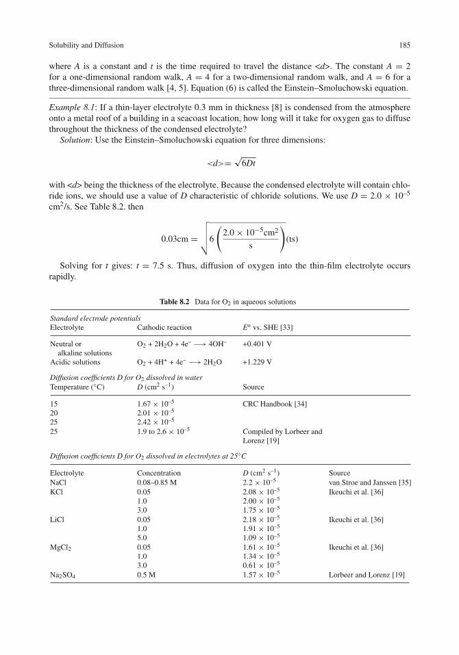
Solubility and Diffusion 185
where A is a constant and t is the time required to travel the distance <d>. The constant A = 2for a one-dimensional random walk, A = 4 for a two-dimensional random walk, and A = 6 for athree-dimensional random walk [4, 5]. Equation (6) is called the Einstein–Smoluchowski equation.
Example 8.1: If a thin-layer electrolyte 0.3 mm in thickness [8] is condensed from the atmosphereonto a metal roof of a building in a seacoast location, how long will it take for oxygen gas to diffusethroughout the thickness of the condensed electrolyte?
Solution: Use the Einstein–Smoluchowski equation for three dimensions:
<d>= √6Dt
with <d> being the thickness of the electrolyte. Because the condensed electrolyte will contain chlo-ride ions, we should use a value of D characteristic of chloride solutions. We use D = 2.0 × 10⁻⁵
cm2/s. See Table 8.2. then
0.03cm =√√√√6
(2.0× 10⁻⁵cm2
s
)(ts)
Solving for t gives: t = 7.5 s. Thus, diffusion of oxygen into the thin-film electrolyte occursrapidly.
Table 8.2 Data for O2 in aqueous solutions
Standard electrode potentialsElectrolyte Cathodic reaction Eo vs. SHE [33]
Neutral oralkaline solutions
O2 + 2H2O + 4e– −→ 4OH– +0.401 V
Acidic solutions O2 + 4H+ + 4e– −→ 2H2O +1.229 V
Diffusion coefficients D for O2 dissolved in waterTemperature (◦C) D (cm2 s–1) Source
152025
1.67 × 10⁻⁵
2.01 × 10⁻⁵
2.42 × 10⁻⁵
CRC Handbook [34]
25 1.9 to 2.6 × 10⁻⁵ Compiled by Lorbeer andLorenz [19]
Diffusion coefficients D for O2 dissolved in electrolytes at 25◦C
Electrolyte Concentration D (cm2 s–1) SourceNaCl 0.08–0.85 M 2.2 × 10⁻⁵ van Stroe and Janssen [35]KCl 0.05
1.03.0
2.08 × 10⁻⁵
2.00 × 10⁻⁵
1.75 × 10⁻⁵
Ikeuchi et al. [36]
LiCl 0.051.05.0
2.18 × 10⁻⁵
1.91 × 10⁻⁵
1.09 × 10⁻⁵
Ikeuchi et al. [36]
MgCl2 0.051.03.0
1.61 × 10⁻⁵
1.34 × 10⁻⁵
0.61 × 10⁻⁵
Ikeuchi et al. [36]
Na2SO4 0.5 M 1.57 × 10⁻⁵ Lorbeer and Lorenz [19]

186 8 Concentration Polarization and Diffusion
Electrode Kinetics for Concentration Polarization
Concentration Profile Near an Electrode Surface
When an electrolyte is open to the air, gaseous O2 molecules first dissolve in the electrolyte andthen diffuse throughout the liquid to become uniformly distributed therein, as described above. If ametal electrode is present in solution, then O2 molecules which diffuse to the electrode surface canundergo reduction by the half-cell reaction
O2 + 2H2O+ 4e− → 4OH− (1)
Thus, the concentration of dissolved O2 near the electrode surface will decrease as O2 moleculesare converted to OH– ions by the reaction above. The concentration profiles for dissolved O2molecules near the electrode surface are depicted schematically in Fig. 8.10. If all the dissolvedO2 near the metal surface are reduced to hydroxyl ions, the O2 concentration at the metal surfacewill go to zero.
The actual concentration profile near a metal surface for a diffusing species is given by [9]
C = Co − 1√D
[2√
t√π
e−x24Dt − x√
Derfc
(x2
4Dt
)1/2](7)
where C is the concentration of the diffusing species at a distance x from the electrode surface, Co isthe concentration in the bulk of the solution, D is the diffusion coefficient, and t is the elapsed time.The error function complement (erfc) has the form
O2 + 2 H2O + 4 e– 4 OH –
(a)
O2O2
O2O2
Metal Solution
OH–formed at surface
Con
cent
ratio
n
Distance from metal surface
to
t1
t2
t3
Concentration ofdissolved O2 inthe bulk of the solution
(b)
Fig. 8.10 (a) Oxygen depletion and OH– production near a metal surface due to the oxygen reduction reaction. (b)Schematic diagram of oxygen concentration profiles near a metal surface (to<t1<t2<t3)

Electrode Kinetics for Concentration Polarization 187
erfc(w) = 1− 2√π
w∫0
e−U2du (8)
As will be seen in the next section, rather than using the expression in Eq. (7), the expression forthe concentration profile near an electrode surface can be simplified considerably.
Limiting Diffusion Current Density
When a diffusing species participates in an electrochemical reaction, the flux (J) is related to thecurrent density (i) by
J=− |i|nF
(9)
where n is the number of electrons transferred and F is the Faraday. The minus sign results fromthe fact that the diffusion flux and the electron flux operate in opposite directions, as illustrated inFig. 8.11. Using Fick’s first law of diffusion, Eq. (4), in Eq. (9) and solving for the current densitygives
|i| = nFDdC
dx(10)
Overall reaction: 2 Fe + O2 + 2 H2O 2 Fe+2 + 4 OH–
At anodic sites: 2 [ Fe Fe+2 + 2e–]
At cathodic sites: O2+ 2 H2O + 4e – 4 OH–
Fe+2
Fe
Solution
Fe+2
O2
2 e–
O2
O2
2 e– 4 e– 4 e–
Fig. 8.11 Schematic diagram to show that the oxygen diffusion flux and the electron flux at a corroding metal havedifferent directions. (So too do the electron flux and the diffusion flux due to metal cations which are generated)
The concentration gradient dC/dx can be obtained from Eq. (7), but instead the concentrationprofile can be simplified by using a linear approximation near the metal surface, as shown inFig. 8.12. If we linearize the concentration gradient near the surface, then

188 8 Concentration Polarization and Diffusion
δ
C
C surf
Con
cent
ratio
n Actual concentration profile
Linear approximation
Distance from surface
Fig. 8.12 The linear approximation to an O2 concentration profile near a metal surface. The parameter δ is thethickness of the oxygen diffusion layer
|i| = nFDC − Csurf
δ(11)
The maximum current density is given by the condition that Csurf = 0. In the case of oxygenreduction, for example, this means that all oxygen molecules near the surface are reduced to OH–
ions, as per Eq. (1). Then Eq. (11) becomes
|iL| = nFDC
δ(12)
where iL is called the limiting diffusion current, C is the concentration of the diffusing species inthe bulk electrolyte (in moles per cubic centimeter), and δ is the thickness of the diffusion layer.
Example 8.2: Calculate the thickness of the oxygen diffusion layer on iron in 0.6 M NaCl using thedata in Fig. 8.2.
Solution: From Fig. 8.2, the limiting diffusion current density (i.e., the plateau value) for the cathodicreaction at 25◦C is 25 μA/cm2 = 2.5 × 10⁻⁵ A/cm2. From Table 8.2, we use 2.0 × 10⁻⁵ cm2/s forthe diffusion coefficient of O2 in NaCl. The concentration of Cl– ion in 0.6 M NaCl is given by
(0.6 mol Cl−
L
)(35.5 g Cl−
mol Cl−)(
1000 mg
g
)= 21300 mg Cl−
L
Then, from tabulated data [2] or from Fig. 8.5, the concentration of dissolved O2 is 6.7 mg/L.Then use
|iL| = nFDC
δ
2.5× 10⁻⁵ A
cm2=(
4 equivmol
) (96,500 coul
equiv
) (2.5×10⁻⁵ cm2
s
) (6.7×10⁻³ g O2
1000 cm3
) (1 mol
32 g O2
)δ
Solving for δ gives δ = 0.065 cm.

Electrode Kinetics for Concentration Polarization 189
Diffusion Layer vs. The Diffuse Layer
The diffusion layer is the thickness over which a concentration gradient exists for a diffusing elec-troactive species (such as oxygen). As seen in Example 8.2, the diffusion layer for the reduction ofoxygen on iron in 0.06 M NaCl has a thickness of 0.065 cm or 6.5 × 10⁶ Å.
Recall that the diffuse layer, i.e., the diffuse part of the electrical double layer (edl), is that outerportion of the edl which balances the charge on the inner part of the edl. As mentioned in Chapter 3,the thickness of the diffuse part of the edl is about 100 Å. Thus, the diffusion layer which arises fromconcentration gradients near an electrode surface is much greater in thickness than the diffuse partof the edl. In fact, for this example, the diffusion layer is about 65,000 times as thick as the diffuselayer. Thus, the entire edl including its diffuse (Gouy–Chapman) component fits easily inside theoxygen diffusion layer on iron in 0.06 M NaCl.
The water molecule can be used as a metric to size the thickness of the O2 diffusion layer. Fromthe density and the molecular weight of water, the diameter of a water molecule is easily calculatedto be 3.8 Å Thus, the O2 diffusion layer would embrace 1,600,000 water molecules laid end to end.In contrast, the diffuse part of the edl would contain 26 H2O molecules laid end to end.
Current–Potential Relationship for Concentration Polarization
The most important instance of concentration polarization in corrosion applications is the diffusion-limited reduction of oxygen:
O2 + 2H2O+ 4e− → 4OH− (1)
For this reaction to occur, O2 molecules first diffuse up to the electrode surface, are next reducedto OH– ions at cathodic sites on the metal surface, and finally the OH– ions which are formed diffuseaway from the electrode out toward the bulk of the solution. Because diffusion is a slow process,this sequence of events occurs under conditions of equilibrium or near-equilibrium. Thus, the Nernstequation can be used to describe the half-cell reaction. The Nernst equation for Eq. (1) is
E = Eo − 2.303 RT
4Flog
[OH−]4
[O2]surf(13)
where Eo is the standard electrode potential for Eq. (1), [OH–] is the concentration of the hydroxylions which are formed, and [O2]surf is the concentration of dissolved oxygen at the electrode surface.The quantity [O2]surf can be obtained by dividing Eq. (11) by Eq. (12) to give
|i||iL| = 1− [O2]surf
[O2](14)
where [O2] is the concentration of dissolved oxygen in the bulk of the electrolyte. Thus,
[O2]surf = [O2]
(1− |i||iL|
)(15)
Use of Eq. (15) in Eq. (13) gives

190 8 Concentration Polarization and Diffusion
E
log | i |
io
O2 + 2 H2O + 4 e– 4 OH –
Eo
inet = i – i = 0
CathodicAnodic
Fig. 8.13 Schematic Evans diagrams for O2 reduction and OH– oxidation
Eo = Eo − 2.303 RT
4Flog
[OH−]4
[O2]+ 2.303 RT
4Flog
(1− |i||iL|
)(16)
When there is no net current flow, i = 0 and E = Eo. See Fig. 8.13. Note the difference betweenEo (the potential corresponding to zero net current flow) and Eo (the standard electrode potential).Under the condition of zero net current, Eq. (16) becomes
Eo = Eo − 2.303 RT
4Flog
[OH−]4
[O2](17)
Equation (17) describes how the thermodynamic standard electrode potential Eo is modified bythe particular pH of the solution and the given concentration of dissolved O2 to yield the potentialEo of zero net current flow for the oxygen half-cell reaction. Use of Eq. (17) in Eq. (16) gives
E = Eo − 2.303 RT
4Flog
(1− |i||iL|
)(18)
With E – Eo = ηconc, the overvoltage due to concentration polarization, Eq. (18), becomes
ηconc = −2.303 RT
4Flog
(1− |i||iL|
)(19)
A plot of Eq. (19) is shown in Fig. 8.14. Figure 8.14 shows clearly that the cathodic current densitydue to concentration polarization reaches a limiting value and that the limiting value is reached inthis instance after a cathodic overvoltage of approximately –0.040 V. The plot in Fig. 8.14 is similarto the experimental cathodic curve in Fig. 8.2, where the limiting current is attained after a slightlylarger overvoltage (due to the existence of the back anodic reaction due to iron dissolution).
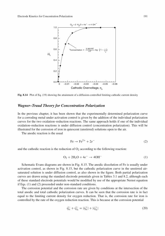
Electrode Kinetics for Concentration Polarization 191
0.0
0.2
0.4
0.6
0.8
1.0
–0.06–0.05–0.04–0.03–0.02–0.010
i/iL
Cathodic Overvoltage, ηc
O2 + 2 H2O + 4e– → 4 OH–
ηconcentration = 2.303 RT4 F
log (1 – iiL
)
Fig. 8.14 Plot of Eq. (19) showing the attainment of a diffusion-controlled limiting cathodic current density
Wagner–Traud Theory for Concentration Polarization
In the previous chapter, it has been shown that the experimentally determined polarization curvefor a corroding metal under activation control is given by the addition of the individual polarizationcurves for the two oxidation–reduction reactions. The same approach holds if one of the individualoxidation–reduction reactions is under diffusion control (concentration polarization). This will beillustrated for the corrosion of iron in quiescent (unstirred) solutions open to the air.
The anodic reaction is the usual
Fe→ Fe2+ + 2e− (2)
and the cathodic reaction is the reduction of O2 according to the following reaction:
O2 + 2H2O+ 4e− → 4OH− (1)
Schematic Evans diagrams are shown in Fig. 8.15. The anodic dissolution of Fe is usually underactivation control, as shown in Fig. 8.15, but the cathodic polarization curve in the unstirred air-saturated solution is under diffusion control, as also shown in the figure. Both partial polarizationcurves are drawn using the standard electrode potentials given in Tables 3.1 and 8.2, although eachof these standard electrode potentials would be modified by use of the appropriate Nernst equationif Eqs. (1) and (2) proceeded under non-standard conditions.
The corrosion potential and the corrosion rate are given by conditions at the intersection of thetotal anodic and total cathodic polarization curves. It can be seen that the corrosion rate is in factequal to the limiting current density for oxygen reduction. That is, the corrosion rate for iron iscontrolled by the rate of the oxygen reduction reaction. This is because at the corrosion potential
i←Fe + i←O2= |i→Fe | + |i→O2
| (20)

192 8 Concentration Polarization and Diffusion
log |i|
E More (–)More (+)
icorr
Ecorr
Experimental curves
Eo = +0.401
Fe Fe+2 + 2e–
Eo = –0.440
Cathodic
Fig. 8.15 Schematic Evans diagrams for the O2/OH– and Fe/Fe2+ oxidation–reduction couples and the resultingexperimental polarization curves
where the notation is the same as used in the previous chapter.Thus
i←Fe − |i→Fe | = |i→O2| − i←O2
(21)
That is, the net rate of iron corrosion is equal to the net rate of oxygen reduction.The experimental polarization curves as derived from the Evans diagrams are also shown
schematically in Fig. 8.15. As before, the net anodic current density at any potential is the totalanodic current density minus the total cathodic current density. An analogous expression holds forthe cathodic branch of the curve. The schematic experimental polarization curves are similar to theactual experimental curves observed in Fig. 8.2.
Thus, extrapolating the anodic Tafel slope for iron dissolution back to Ecorr gives the corrosionrate, which is the same as the limiting diffusion current density for oxygen reduction. This is a classiccase in which the corrosion reaction is under cathodic control.
Effect of Environmental Factors on Concentration Polarization and Corrosion
As was just shown, the corrosion rate of a metal is determined by the rate of oxygen reduction whenoxygen reduction is under diffusion control. Thus, environmental factors which affect the limitingdiffusion current for oxygen reduction will, in turn, affect the corrosion rate. The effect of severaldifferent environmental factors is considered below.

Effect of Environmental Factors on Concentration Polarization and Corrosion 193
Effect of Oxygen Concentration
Figure 8.16 shows schematically the effect of increasing the concentration of dissolved oxygenon the limiting current density for oxygen reduction. Increasing the concentration of dissolvedO2increases the limiting current density iL. This effect stems directly from Eq. (12), in which itis seen that iL is directly proportional to C, the concentration of dissolved O2.
log
| i |
E
Increasing O2concentration
Increasing solutionvelocity
More (–)
Fig. 8.16 Schematic diagram showing the effect of O2 concentration and solution velocity on the limiting diffusioncurrent for O2 reduction
Various experimental studies have shown that the corrosion rate increases with increasing O2content of the electrolyte [10, 11]. For example, Uhlig et al. [10, 11] have observed that for thecorrosion of mild steel in water containing small amounts of CaCl2, the corrosion rate increaseswith increasing O2 concentration, as shown in Fig. 8.17. This effect can be explained by the factthat the anodic polarization curve for iron dissolution intersects the cathodic polarization curve foroxygen reduction at increased values of iL, which result for increased O2 concentrations, as shownin Fig. 8.18.
However, Uhlig et al. [10, 11] also observed that additional increases in O2 concentration beyondthe range shown in Fig. 8.17 produced a decrease in the corrosion rate, as shown in Fig. 8.19. Thisdecrease is due to the onset of a new anodic reaction, i.e., the passivation of the iron surface as itreceived an additional supply of oxygen. This increased supply of O2 serves to form a protectiveoxide film on the surface, which acts to lower the corrosion rate. (More details on passivity are givenin Chapter 9).
In systems where the corrosion rate is under the control of the oxygen reduction reaction, theaddition of certain chemical compounds can reduce the corrosion rate by reducing the concentrationof dissolved O2. These chemicals are called “oxygen scavengers,” and two which are used frequentlyare sodium sulfite (Na2SO3) and hydrazine (N2H4). Sodium sulfite reacts with O2 as follows:
2Na2SO3 + O2 → 2Na2SO4
and thus serves to reduce the concentration of dissolved oxygen so as to lower the limiting diffusioncurrent density, as per Eq. (12). The corrosion rate is then lowered, as in Fig. 8.18.

194 8 Concentration Polarization and Diffusion
0
2
4
6
8
10
0 1 2 3 4 5 6
Cor
rosi
on R
ate
in g
/m2
day
Concentration of O2 in mL/L
Fig. 8.17 Effect of oxygen concentration on the corrosion of mild steel in water containing 165 ppm CaCl2. Redrawnfrom Uhlig and Revie [10] by permission of John Wiley & Sons, Inc
log
| i |
E
More (–)More (+)
IncreasingO2
Fig. 8.18 Schematic Evans diagrams for Fe in aqueous solutions where the oxygen reduction reaction is diffusioncontrolled. The intersection of the oxygen reduction and iron dissolution curves gives the corrosion potential and thecorrosion rate
Effect of Solution Velocity
Figure 8.16 also shows the effect of increasing velocity on the limiting diffusion current for oxygenreduction. Increasing the velocity of the solution brings reactants up to the electrode surface moreeasily, thus reducing δ, the thickness of the oxygen diffusion layer. As δ decreases, the value of thelimiting diffusion current iL will increase, as per Eq. (12).

Effect of Environmental Factors on Concentration Polarization and Corrosion 195
0
1
2
3
4
5
6
7
8
0 5 10 15 20 25 30
Cor
rosi
on R
ate
in g
/m2
day
O2 Concentration in mL/L
Air saturation
Formation of apassive oxide film
Fig. 8.19 Effect of oxygen concentration on the corrosion of mild steel in slowly moving distilled water. Redrawnfrom Uhlig and Revie [10] by permission of John Wiley & Sons, Inc
0.0
0.5
1.0
1.5
2.0
0 0.2 0.4 0.6 0.8 1 1.2
Cor
rosi
on R
ate
in m
m/y
ear
Flow Velocity in m/sec
100 ppm Cl –
50 ppm Cl –
0 ppm Cl –
10 ppm Cl –
A
B
C
D
Fig. 8.20 Effect of solution velocity on the corrosion of carbon steel in water containing various amounts of dissolvedCl–. Redrawn from Matsushima [12] by permission of John Wiley & Sons, Inc
Figure 8.20 shows the effect of solution velocity on the corrosion of a carbon steel in water con-taining various amounts of dissolved Cl– (12). For the highest concentration of Cl– (100 ppm), thecorrosion rate increases with increasing velocity, as described above. However, for a lower concen-tration of dissolved Cl– (e.g., 50 ppm), the corrosion rate first increases with increasing velocity upto point C in Fig. 8.20 and then decreases with increasing velocity (point D). This decrease is againdue to an increased supply of O2 and to the concomitant passivation of the metal surface, as shownschematically in Fig. 8.21.
In a more aggressive environment, such as natural seawater, where passivation does not occur, thecorrosion rate of steel increases with increasing velocity [13].
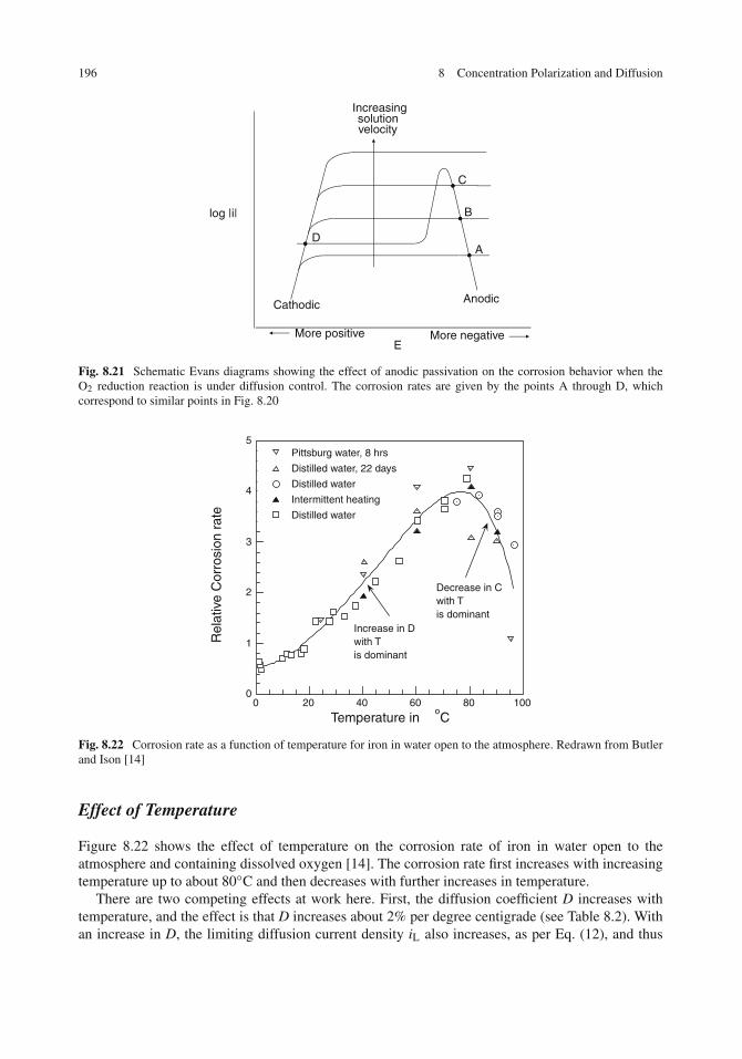
196 8 Concentration Polarization and Diffusion
E
log |i|
More positive More negative
AnodicCathodic
Increasingsolutionvelocity
A
B
C
D
Fig. 8.21 Schematic Evans diagrams showing the effect of anodic passivation on the corrosion behavior when theO2 reduction reaction is under diffusion control. The corrosion rates are given by the points A through D, whichcorrespond to similar points in Fig. 8.20
0
1
2
3
4
5
0 20 40 60 80 100
Pittsburg water, 8 hrs
Distilled water, 22 days
Distilled water
Intermittent heating
Distilled water
Rel
ativ
e C
orro
sion
rat
e
Temperature in oC
Increase in D with Tis dominant
Decrease in Cwith Tis dominant
Fig. 8.22 Corrosion rate as a function of temperature for iron in water open to the atmosphere. Redrawn from Butlerand Ison [14]
Effect of Temperature
Figure 8.22 shows the effect of temperature on the corrosion rate of iron in water open to theatmosphere and containing dissolved oxygen [14]. The corrosion rate first increases with increasingtemperature up to about 80◦C and then decreases with further increases in temperature.
There are two competing effects at work here. First, the diffusion coefficient D increases withtemperature, and the effect is that D increases about 2% per degree centigrade (see Table 8.2). Withan increase in D, the limiting diffusion current density iL also increases, as per Eq. (12), and thus

Further Applications of Concentration Polarization Curves 197
0
0.01
0.02
0.03
0 20 40 60 80 100 120 140 160
Cor
rosi
on R
ate
in in
ches
/yea
r
Temperature in °C
Closed system
Open system
Electrolyte
Electrolyte
Fig. 8.23 Schematic diagram showing the effect of temperature on the corrosion rate for a metal immersed in anaqueous solution in an open vs. a closed system. Redrawn from Uhlig and Revie [10] by permission of John Wiley &Sons, Inc
so will the corrosion rate. This effect is predominant for the portion of the curve in Fig. 8.22 overwhich the corrosion rate increases with temperature.
The second temperature effect is that the concentration of dissolved O2 decreases with increasingtemperature, as discussed earlier. Thus, as the O2 concentration decreases, so does iL, as per Eq.(12), and accordingly, so does the corrosion rate. This effect is predominant for the portion of thecurve in Fig. 8.22 over which the corrosion rate decreases with increasing temperature.
For a closed system, the effect of increasing temperature in an oxygen-containing electrolyte issomewhat different and is shown schematically in Fig. 8.23 [10]. In the closed system, dissolvedO2 molecules which enter the vapor phase cannot escape out into the open atmosphere, but insteadO2 molecules first accumulate in the vapor phase above the liquid. Then, the pressure of O2 abovethe liquid increases, which in turn produces an increase in the concentration of dissolved O2 in theelectrolyte by Henry’s law, Eq. (3). This effect predominates so that the corrosion rate increasesmonotonically with increasing temperature for a closed system.
Further Applications of Concentration Polarization Curves
Cathodic Protection
The corrosion rate of iron in seawater is 15 mpy (3.3 × 10⁻⁵ A/cm2), and the corrosion rate ofzinc in seawater is 2 mpy (3.4 × 10⁻⁶ A/cm2) [15]. For both metals in seawater, the corrosionrate is determined by the rate of oxygen reduction, which is under diffusion control. Thus, we canconstruct the Evans diagrams and the experimental polarization curves for both metals, as shown inFig. 8.24.
The open-circuit corrosion potential for uncoupled zinc is more negative than that for iron, sowhen the two metals are coupled, the zinc electrode is the anode of the pair. This is shown inFig. 8.25, which displays several important features:

198 8 Concentration Polarization and Diffusion
Ecorr (Fe)
icorr (Zn)
icorr (Fe) O2 on Fe
Eo (O2)
O2 on Zn
Fe
Ecorr (Zn)
Zn
log | i |
E More negativeMore positive
Fig. 8.24 Schematic Evans diagrams for iron and zinc immersed in an aqueous solution where the cathodic reactionis O2 reduction under diffusion control. The experimentally observed polarization curves are given for each metal bythe solid lines
E
log | i |
Ecorr (Fe)
icorr (Zn in couple)
O2 on Fe
Eo (O2)
O2 on Zn
Fe
Ecorr (Zn)
Zn
Ecorr(couple)
Total O2
icorr (Fe in couple)
Total anodic curve
More positive More negative
Fig. 8.25 Effect of galvanic coupling on the Fe/Zn system shown in Fig. 8.24
(1) The total cathodic curve for the Fe/Zn couple intersects the total anodic curve for the couple atan electrode potential which is slightly different than the corrosion potential of the uncoupledzinc. (This observation is often described as iron being polarized to the potential of zinc.)
(2) The corrosion rate of zinc in the Fe/Zn couple is higher than the corrosion rate of uncoupledzinc.
Further Applications of Concentration Polarization Curves 199
(3) The corrosion rate of iron in the Fe/Zn couple is much lower than the corrosion rate of uncouplediron.
Figure 8.25 forms the kinetic basis for cathodic protection in neutral electrolytes where the corro-sion rate of the individual metals is determined by the diffusion-limited oxygen reduction reaction.Compare Fig. 8.25 with Fig. 5.5, which presents a thermodynamic view of cathodic protection.
Area Effects in Galvanic Corrosion
When copper and iron are coupled in seawater, iron is the anode and copper is the cathode, asmay be seen by referring to the galvanic series in Fig. 5.3. The effect of increasing the area of thecopper cathode is shown schematically in Fig. 8.26 (a). Increasing the cathodic area results in anincrease in the value of the limiting diffusion current (i.e., the total current, not the current density).Thus the total cathodic curve intersects the total anodic curve (for a fixed area of the iron anode)at increasingly higher values. This intersection defines the corrosion rate so that the corrosion rateincreases with the area of the cathode.
Actual data are given in Fig. 8.26(b) for copper and iron coupled in seawater [16]. This effect issimilar to that seen in Chapter 7 for galvanic couples in acid solutions.
Linear Polarization
The linear polarization technique can also be used to determine the corrosion rate if the cathodicreaction is under concentration polarization. From Chapter 7, the Stern–Geary equation for linearpolarization near the corrosion potential is
icorr = 1
2.303(
dηdi
)η→0
(1ba+ 1|bc|) (22)
This equation follows from the Butler–Volmer equation and, strictly speaking, is applicable onlyfor the situation where both the anodic and cathodic polarization curves are under activation control.However, if the cathodic process is controlled by concentration polarization, the “effective” cathodicTafel slope bc = dE/d log |i| can be taken to be infinity for the region where a limiting diffusioncurrent density is observed. This can be seen by referring to Fig. 8.2. Thus, with |bc| = ∞, Eq. (22)reduces to
icorr = 1
2.303(
dηdi
)η→0
(1ba
) (23)
for a system in which the cathodic process is under diffusion control.
Example 8.3: In a study on the corrosion of mild steel in an alkaline lithium bromide solution [17],the cathodic process was observed to be under the control of diffusion-limited concentration polar-ization, and the anodic process was under activation control with an anodic Tafel slope of +0.062 V.Linear polarization measurements in the cathodic region near the corrosion potential gave a value ofdη/di = 0.089 V cm2/μa. What is the corrosion rate of mild steel in this solution?Solution: Use the Stern–Geary equation with |bc| = ∞.

200 8 Concentration Polarization and Diffusion
0
1000
2000
3000
4000
5000
6000
7000
0 5 10 15 20
Cor
rosi
on R
ate
of Ir
on in
mdd
Ratio of Area of Copper to Iron in Galvanic Couples
Area of iron anode = 4.7 cm2
(b)
(a)
log
|To
talC
urr
ent|
E
Increasing area of copper
More (–)
Fe Fe+2 + 2e –
O2 + 2H2O + 4e– 4OH –
(on copper)
Fig. 8.26 (a) Schematic Evans diagrams showing the effect of increasing cathode area on the corrosion rate of a cop-per/iron couple when the O2 reduction reaction is under diffusion control. The intersection of the anodic and cathodicpolarization curves defines the corrosion potential and the corrosion rate. (b) Effect of cathode area on the experi-mental corrosion rates for a copper/iron couple in seawater. Reproduced by permission of ECS – The ElectrochemicalSociety
icorr = 1
2.303(
0.089 V cm2
μA
) (1
0.062 V + 1∞)
Then, with 1/∞= 0, we can solve for icorr to get icorr = 0.30 μA/cm2.
Concentration Polarization in Acid Solutions
In the previous chapter, we considered that hydrogen reduction in acid solutions was under activationcontrol. That is, a cathodic Tafel region was observed experimentally. The half-cell reaction is theusual

Further Applications of Concentration Polarization Curves 201
0
0.1
1
10
100
1000
10000
–1.20–1.00–0.80–0.60–0.40–0.20
Cur
rent
Den
sity
in μ
A/c
m2
E in V vs. S.H.E.
pH 1.42
pH 2.19
pH 2.91
pH 3.69
pH 4.11
pH 5.26
Fig. 8.27 Experimental cathodic polarization curves for iron in unstirred, H2-saturated acid solutions [18].Reproduced by permission of ECS – The Electrochemical Society
2H+ + 2e− → H2
Stern [18] has shown that the hydrogen reduction reaction in unstirred air-free, H2-saturated solu-tions can undergo concentration polarization. Stern’s results are shown in Fig. 8.27, in which it isseen that the limiting diffusion current density for hydrogen reduction increases with decreasingpH (i.e., with increasing acidity). This result follows by writing Eq. (12) for the limiting diffusioncurrent density for hydrogen reduction:
iL = nFD (10−3) a(H+)
δ(24)
where a(H+) is the hydrogen ion activity in moles per liter. As a(H+) increases, (pH decreases), iLincreases, as per Eq. (24), as was observed by Stern. Stern took D, the diffusion coefficient for H+,as 7.39 × 10⁻⁵ cm2/s, δ = 0.05 cm, and n = 1 (see Chapter 7, which briefly discusses two differentmechanisms for the hydrogen evolution reaction shown above). The overall number of electronstransferred is two, but either reaction mechanism proceeds in two consecutive one-electron transfersteps. Use of the parameters listed above in Eq. (24) gives
log iL=− 0.845− pH (25)
Stern’s results for the limiting diffusion current density for hydrogen reduction as a function ofpH are given in Fig. 8.28. The observed experimental values for iL are in good agreement with valuescalculated using Eq. (25).

202 8 Concentration Polarization and Diffusion
0.1
1
10
100
1000
10000
1 2 3 4 5 6
i L in
μA
/cm
2
pH
Calculated
Experimental
Fig. 8.28 Comparison of experimental and calculated limiting diffusion current densities for hydrogen reduction oniron [18] in Fig. 8.27. Calculated values were obtained using Eq. (24). Reproduced by permission of ECS – TheElectrochemical Society
Combined Activation and Concentration Polarization
Activation polarization and concentration polarization can occur simultaneously for the samecathodic reaction. This situation is illustrated in Fig. 8.29, in which it is seen that the total cathodicpolarization curve is the sum of the two individual processes. These are the types of curves observedby Stern [18] in Fig. 8.27 for hydrogen reduction in unstirred acid solutions.
It is also possible for O2 reduction and H2 evolution to occur in the same solution. This may takeplace in acid solutions open to the air. In this case, the O2 reduction reaction can be under diffusioncontrol, and the H+ reduction reaction can be under activation control. Then, both a limiting diffusioncurrent density for O2 reduction (at lower cathodic overvoltages) and a Tafel region for H+ reduction(at higher cathodic overvoltages) are observed, as illustrated in Fig. 8.30. Such polarization curveshave been observed for iron [19, 20] and cadmium [21] in acidified solutions open to the air andcontaining dissolved oxygen.
The Rotating Disc Electrode
Throughout this chapter we have referred to solutions as being quiescent (unstirred) or stirred. Thus,flow conditions have not been stated rigorously, although it has been noted that the limiting diffusioncurrent density increases if the solution velocity increases. Reproducible control of flow conditionscan be achieved using a rotating disc electrode, as shown in Fig. 8.31.
If a planar disc rotates at a high speed in the liquid, the liquid layer close to the electrode movesunder centrifugal force toward the perimeter of the disc, as shown in Fig. 8.31 [22]. Liquid from thebulk of the electrolyte will flow toward the center of the disc.
Under these conditions, the limiting diffusion current density is given by the Levich equation[22, 23]:
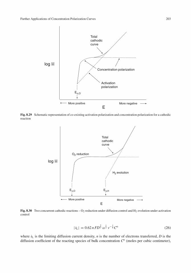
Further Applications of Concentration Polarization Curves 203
log |i|
EMore positive More negative
Activationpolarization
Total cathodiccurve
Eo,O
Concentration polarization
Fig. 8.29 Schematic representation of co-existing activation polarization and concentration polarization for a cathodicreaction
log |i|
EMore positive More negative
O2 reduction
H2 evolution
Total cathodiccurve
Eo,HEo,O
Fig. 8.30 Two concurrent cathodic reactions – O2 reduction under diffusion control and H2 evolution under activationcontrol
| iL| = 0.62 n FD23 ω
12 v−
16 Co (26)
where iL is the limiting diffusion current density, n is the number of electrons transferred, D is thediffusion coefficient of the reacting species of bulk concentration Co (moles per cubic centimeter),

204 8 Concentration Polarization and Diffusion
ElectrolyteMetaldisk
Rotation
Flow pattern
Fig. 8.31 Liquid flow patterns in the vicinity of a rapidly rotating disc electrode [22]
0
2
4
6
8
0 1 2 3 4 5
|i| x
104
in A
/cm
2
(Revolutions/sec)1/2 in sec–1/2
25 oC
50 oC
75 oC
Fig. 8.32 Effect of stirring on the corrosion rate of copper in 0.1 M H2SO4 solutions at various temperatures [24, 25].Reproduced by permission of Elsevier Ltd
ω is the angular frequency of rotation of the disc (2π times the rotation frequency), and ν is thekinematic viscosity (in square centimeter per second).
Rotating disc electrodes have found a large number of applications in mechanistic studies of cor-rosion processes (as well as in electrodeposition, electrocatalysis, and electrochemical machining).Only two examples will be given here.
A rotating disc electrode was used by Zembura [24, 25] to follow the corrosion of copper as thereaction changed from activation control to diffusion control with increasing temperature. Figure8.32 shows the corrosion current density of copper in air-saturated 0.1 M H2SO4 as a function of thesquare root of the rotation velocity [24, 25]. At 25◦C, the reaction is under activation control as thecorrosion current density is independent of rotation rate. At 75◦C, the corrosion current density obeysthe Levich equation, and the reaction is under diffusion control. At an intermediate temperature of50◦C, the reaction is transitioning from activation control to diffusion control.

Problems 205
0.0
1.0
2.0
3.0
4.0
5.0
6.0
7.0
8.0
0 5 10 15 20
|i L| in
mA
/cm
2
(ω)1/2
in sec –1/2
O2
saturated
Air saturated
Fig. 8.33 Levich plots for iron in 0.1 M NaCl solutions at pH 7 [26]. Reproduced by permission of Elsevier Ltd
In a study on the oxygen reduction reaction on rust-free iron surfaces in 0.1 M NaCl solutions,Miyata and Asakura [26] reported the Levich plots shown in Fig. 8.33. From the slope of the Levichplots and published values for the O2 concentration, diffusion coefficient, and kinematic viscosity ofthe solution, Miyata and Asakura calculated the number of electrons transferred to be n = 3.9 and3.8 for aerated and O2-saturated solutions, respectively. This result is consistent with the followingoverall reduction reaction which has been assumed throughout this chapter:
O2 + 2H2O+ 4e− → 4OH−
However, it is unlikely that all four electrons are transferred simultaneously in a single step.Various mechanisms have been proposed for the cathodic reduction of oxygen [27], but the exactmechanism is not known.
A variation of the rotating disc electrode is the rotating ring disc electrode (RRDE). In the RRDE,a rotating disc is surrounded by a concentric co-planar ring electrode, with the ring electrode beingelectrically isolated from the disc. The ring electrode does not disturb the flow pattern along thedisc so that cations produced by corrosion at the disc flow outward toward the ring. Moreover, thepotentials of the ring and the disc electrodes can be varied independently so that cations produced atthe disc can be reduced at the ring electrode and identified by their reduction potentials. Thus, thistechnique can be used to study the mechanism of corrosion of metal alloys [28].
Problems
1. Nitrate ions (NO3–) are often used to inhibit the corrosion of iron in aqueous solutions. Suppose
a nitrate ion takes 10,000 random three-dimensional jumps in water, with the distance of eachjump being the diameter of a NO3
– ion (3.0 Å).
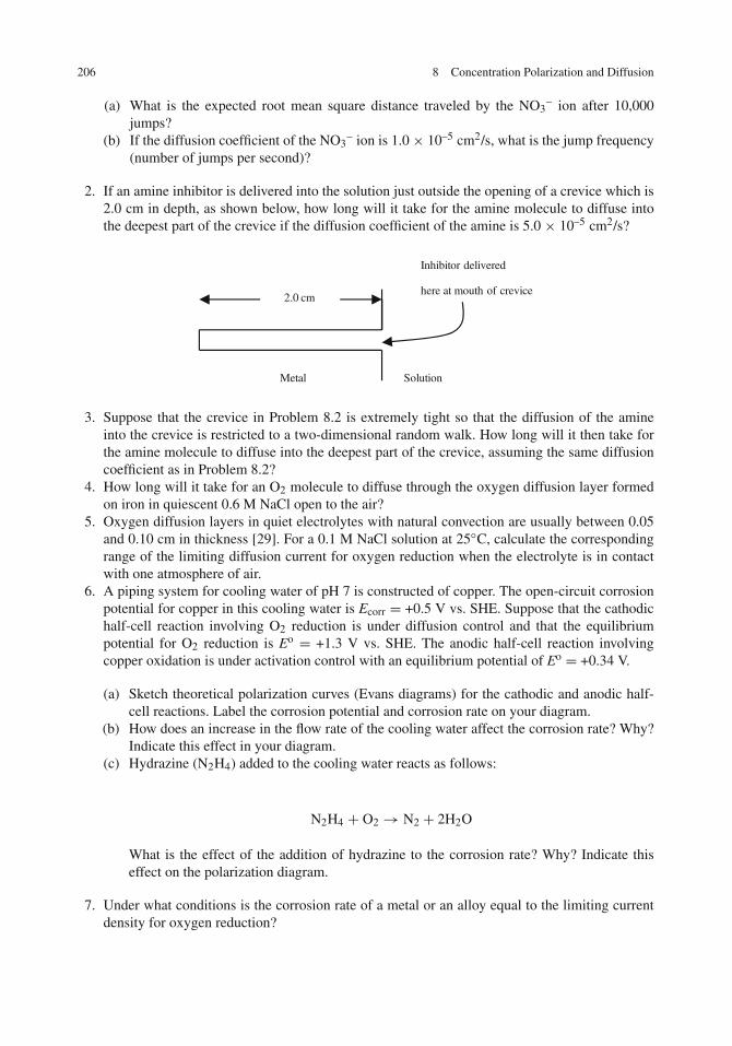
206 8 Concentration Polarization and Diffusion
(a) What is the expected root mean square distance traveled by the NO3– ion after 10,000
jumps?(b) If the diffusion coefficient of the NO3
– ion is 1.0× 10⁻⁵ cm2/s, what is the jump frequency(number of jumps per second)?
2. If an amine inhibitor is delivered into the solution just outside the opening of a crevice which is2.0 cm in depth, as shown below, how long will it take for the amine molecule to diffuse intothe deepest part of the crevice if the diffusion coefficient of the amine is 5.0 × 10⁻⁵ cm2/s?
Inhibitor delivered
here at mouth of crevice
Metal Solution
2.0 cm
3. Suppose that the crevice in Problem 8.2 is extremely tight so that the diffusion of the amineinto the crevice is restricted to a two-dimensional random walk. How long will it then take forthe amine molecule to diffuse into the deepest part of the crevice, assuming the same diffusioncoefficient as in Problem 8.2?
4. How long will it take for an O2 molecule to diffuse through the oxygen diffusion layer formedon iron in quiescent 0.6 M NaCl open to the air?
5. Oxygen diffusion layers in quiet electrolytes with natural convection are usually between 0.05and 0.10 cm in thickness [29]. For a 0.1 M NaCl solution at 25◦C, calculate the correspondingrange of the limiting diffusion current for oxygen reduction when the electrolyte is in contactwith one atmosphere of air.
6. A piping system for cooling water of pH 7 is constructed of copper. The open-circuit corrosionpotential for copper in this cooling water is Ecorr = +0.5 V vs. SHE. Suppose that the cathodichalf-cell reaction involving O2 reduction is under diffusion control and that the equilibriumpotential for O2 reduction is Eo = +1.3 V vs. SHE. The anodic half-cell reaction involvingcopper oxidation is under activation control with an equilibrium potential of Eo = +0.34 V.
(a) Sketch theoretical polarization curves (Evans diagrams) for the cathodic and anodic half-cell reactions. Label the corrosion potential and corrosion rate on your diagram.
(b) How does an increase in the flow rate of the cooling water affect the corrosion rate? Why?Indicate this effect in your diagram.
(c) Hydrazine (N2H4) added to the cooling water reacts as follows:
N2H4 + O2 → N2 + 2H2O
What is the effect of the addition of hydrazine to the corrosion rate? Why? Indicate thiseffect on the polarization diagram.
7. Under what conditions is the corrosion rate of a metal or an alloy equal to the limiting currentdensity for oxygen reduction?

Problems 207
8. The corrosion rate of 99.9% nickel in seawater after immersion in seawater near the PanamaCanal Zone for 16 years was observed to be 1.2 mpy (mils per year) [30]. (The correspondingcorrosion current density is 2.8 × 10⁻⁶ A/cm2.)
(a) Draw the hypothetical Evans diagram for this system when corrosion is under the controlof the diffusion-limited oxygen reduction reaction. Assume that Eo,O2 = +0.40 V vs. SHEand that io,O2 = 1.0 × 10⁻⁹ A/cm2. Assume that the anodic reaction for nickel dissolutionis under activation control with an anodic Tafel slope of +0.060 V. Use values for Eo,Ni andio,Ni from Tables 3.1 and 7.4, respectively.
(b) Based on the Evans diagram, what is the corrosion potential for nickel in seawater?(c) How does the corrosion potential from part (b) compare with the electrode potential for
nickel given in the galvanic series for seawater?(d) Sketch the anodic and cathodic experimental polarization curves which result from the
Evans diagram in part (a).
9. The polarization resistance of a 90Cu–10Ni alloy in flowing seawater containing 6.6 mg O2/Lwas observed to be RP = 2.7 k� after an immersion time of 40 h [31]. The sample area was11.05 cm2. The cathodic process was under O2 diffusion control, and the anodic process wasunder activation control with an anodic Tafel slope of + 0.070 V.
(a) What was the corrosion rate of the alloy in microamperes per square centimeter at 40 himmersion?
(b) What was the corresponding weight loss in grams per square meter day assuming thatcorrosion of the alloy occurs mainly as:
Cu→ Cu2+ + 2e−.
10. The following occurrence of corrosion as shown in the figure below can occur in heat exchangerswhere there are temperature differences along the metal [32]. Explain why corrosion occurspreferentially at the hot end of the metal.
Hot
Anode
Cathode
Cold
11. Suppose that the corrosion rate of a metal is 50.0 μA/cm2 when the metal is immersed in asolution open to the air and that the corrosion rate is under O2 diffusion control. What is thecorrosion rate when the air above the solution is replaced with pure O2 at 1 atm pressure?
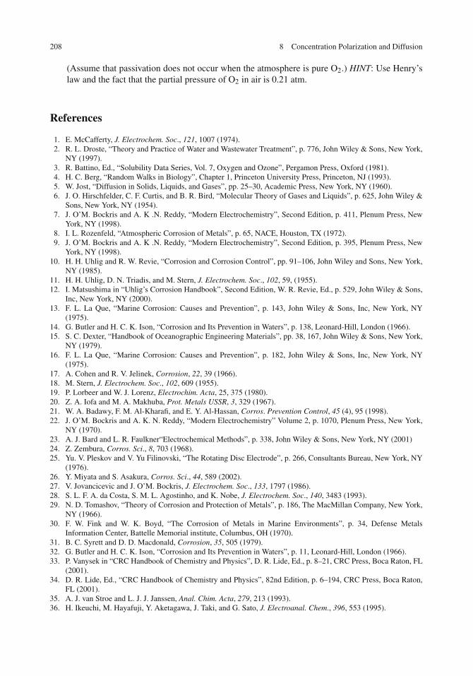
208 8 Concentration Polarization and Diffusion
(Assume that passivation does not occur when the atmosphere is pure O2.) HINT: Use Henry’slaw and the fact that the partial pressure of O2 in air is 0.21 atm.
References
1. E. McCafferty, J. Electrochem. Soc., 121, 1007 (1974).2. R. L. Droste, “Theory and Practice of Water and Wastewater Treatment”, p. 776, John Wiley & Sons, New York,
NY (1997).3. R. Battino, Ed., “Solubility Data Series, Vol. 7, Oxygen and Ozone”, Pergamon Press, Oxford (1981).4. H. C. Berg, “Random Walks in Biology”, Chapter 1, Princeton University Press, Princeton, NJ (1993).5. W. Jost, “Diffusion in Solids, Liquids, and Gases”, pp. 25–30, Academic Press, New York, NY (1960).6. J. O. Hirschfelder, C. F. Curtis, and B. R. Bird, “Molecular Theory of Gases and Liquids”, p. 625, John Wiley &
Sons, New York, NY (1954).7. J. O’M. Bockris and A. K .N. Reddy, “Modern Electrochemistry”, Second Edition, p. 411, Plenum Press, New
York, NY (1998).8. I. L. Rozenfeld, “Atmospheric Corrosion of Metals”, p. 65, NACE, Houston, TX (1972).9. J. O’M. Bockris and A. K .N. Reddy, “Modern Electrochemistry”, Second Edition, p. 395, Plenum Press, New
York, NY (1998).10. H. H. Uhlig and R. W. Revie, “Corrosion and Corrosion Control”, pp. 91–106, John Wiley and Sons, New York,
NY (1985).11. H. H. Uhlig, D. N. Triadis, and M. Stern, J. Electrochem. Soc., 102, 59, (1955).12. I. Matsushima in “Uhlig’s Corrosion Handbook”, Second Edition, W. R. Revie, Ed., p. 529, John Wiley & Sons,
Inc, New York, NY (2000).13. F. L. La Que, “Marine Corrosion: Causes and Prevention”, p. 143, John Wiley & Sons, Inc, New York, NY
(1975).14. G. Butler and H. C. K. Ison, “Corrosion and Its Prevention in Waters”, p. 138, Leonard-Hill, London (1966).15. S. C. Dexter, “Handbook of Oceanographic Engineering Materials”, pp. 38, 167, John Wiley & Sons, New York,
NY (1979).16. F. L. La Que, “Marine Corrosion: Causes and Prevention”, p. 182, John Wiley & Sons, Inc, New York, NY
(1975).17. A. Cohen and R. V. Jelinek, Corrosion, 22, 39 (1966).18. M. Stern, J. Electrochem. Soc., 102, 609 (1955).19. P. Lorbeer and W. J. Lorenz, Electrochim. Acta, 25, 375 (1980).20. Z. A. Iofa and M. A. Makhuba, Prot. Metals USSR, 3, 329 (1967).21. W. A. Badawy, F. M. Al-Kharafi, and E. Y. Al-Hassan, Corros. Prevention Control, 45 (4), 95 (1998).22. J. O’M. Bockris and A. K. N. Reddy, “Modern Electrochemistry” Volume 2, p. 1070, Plenum Press, New York,
NY (1970).23. A. J. Bard and L. R. Faulkner“Electrochemical Methods”, p. 338, John Wiley & Sons, New York, NY (2001)24. Z. Zembura, Corros. Sci., 8, 703 (1968).25. Yu. V. Pleskov and V. Yu Filinovski, “The Rotating Disc Electrode”, p. 266, Consultants Bureau, New York, NY
(1976).26. Y. Miyata and S. Asakura, Corros. Sci., 44, 589 (2002).27. V. Jovancicevic and J. O’M. Bockris, J. Electrochem. Soc., 133, 1797 (1986).28. S. L. F. A. da Costa, S. M. L. Agostinho, and K. Nobe, J. Electrochem. Soc., 140, 3483 (1993).29. N. D. Tomashov, “Theory of Corrosion and Protection of Metals”, p. 186, The MacMillan Company, New York,
NY (1966).30. F. W. Fink and W. K. Boyd, “The Corrosion of Metals in Marine Environments”, p. 34, Defense Metals
Information Center, Battelle Memorial institute, Columbus, OH (1970).31. B. C. Syrett and D. D. Macdonald, Corrosion, 35, 505 (1979).32. G. Butler and H. C. K. Ison, “Corrosion and Its Prevention in Waters”, p. 11, Leonard-Hill, London (1966).33. P. Vanysek in “CRC Handbook of Chemistry and Physics”, D. R. Lide, Ed., p. 8–21, CRC Press, Boca Raton, FL
(2001).34. D. R. Lide, Ed., “CRC Handbook of Chemistry and Physics”, 82nd Edition, p. 6–194, CRC Press, Boca Raton,
FL (2001).35. A. J. van Stroe and L. J. J. Janssen, Anal. Chim. Acta, 279, 213 (1993).36. H. Ikeuchi, M. Hayafuji, Y. Aketagawa, J. Taki, and G. Sato, J. Electroanal. Chem., 396, 553 (1995).

Chapter 9Passivity
Introduction
So far this text has considered (or has mentioned) several different methods of corrosion control.These methods have included cathodic protection, corrosion protection by organic coatings, the useof corrosion inhibitors, and the use of additives which can change the pH of the aqueous solution.One of the most effective means of corrosion protection is the use of metals or alloys which haveinherently low corrosion rates in a solution due to the existence of a passive oxide film.
As noted by Macdonald [1], metals such as iron, nickel, chromium, and aluminum are allinherently reactive, as evidenced by the fact that they occur in nature as their ores rather than inelemental form. Yet these metals are used in industry because they react with water and/or oxygento form stable passive oxide films. Macdonald states that “passivity is the key to our metals-basedcivilization.”
This chapter discusses the phenomenon of passivity and the nature of passive films.
Aluminum: An Example
Aluminum and its alloys are important structural metals because of their light weight, high strength(when alloyed), and excellent corrosion resistance. However, consider the reaction of aluminum withwater, as in conditions of immersion or exposure in the atmosphere:
4Al(s)+ 12H2O (l)+ 3O2(g)→ 2Al2O3(s)+ 12H+(aq)+ 12 OH− (aq) (1)
The free energy �Go of the reaction can be determined from the thermodynamic principlesconsidered in Chapters 4 and 6. Thus
�G◦ = 2μ◦(Al2O3(s))+ 12μo(OH−(aq))− 12μo(H2O(l)) (2)
where μo refers to the chemical potential. Using values tabulated by Pourbaix [2]:
�Go = 2(− 376,000 cal)+ 12(− 37,595 cal)− 12(− 56,690 cal) =− 522,860 cal
This large negative value of the free energy change for Eq. (1) indicates that the reaction ofaluminum with water is spontaneous. Thus, the surface of aluminum reacts with water to form anoxide film, as depicted in Fig. 9.1. However, the reaction essentially stops after the aluminum surfaceis covered with an oxide film, which may be only hundreds to thousands of angstroms in thickness.
209E. McCafferty, Introduction to Corrosion Science, DOI 10.1007/978-1-4419-0455-3_9,C© Springer Science+Business Media, LLC 2010

210 9 Passivity
Al
Al2O3 film
Al2O3 bulkX
H2O
H2O
Al
Fig. 9.1 Formation of a protective oxide film on aluminum (schematic)
In view of the spontaneous nature of Eq. (1), the question arises as to why the reaction doesnot continue until the entire thickness of the aluminum sample is converted to Al2O3. The answerto this question is that the reaction stops because the aluminum metal has formed a passive oxidefilm which protects the underlying metal from further attack. Thus, the passive oxide film on alu-minum and its alloys is what is responsible for the excellent corrosion resistance of aluminum inaqueous environments. In general, the phenomenon of passivity is the single most important factorwhich imparts chemical stability to a wide variety of metals and alloys for their use as structural orelectronic materials.
What is Passivity?
Passivity is defined as the reduction in chemical or electrochemical activity of a metal due to thereaction of the metal with its environment so as to form a protective film on the metal surface. Thisdefinition does not indicate what properties constitute a “protective” film nor does this definition tellus anything about the nature of the “film” itself. Today’s studies on passivity continue to be directedtoward gaining a better understanding of the chemical and physical properties of passive films.
Early History of Passivity
Observations on passivity date back to over 200 years. Uhlig [3] has traced the first use of the word“passivity” to C. Schonbein in 1836, although earlier observations on passivity had been made byM. Lomonosov in Russia in 1738, C. Wenzel in Germany in 1782, J. Keir in England in 1790,and subsequently by Schonbein and Michael Faraday. These early investigators established that thedissolution of iron in certain acid solutions ceased after first undergoing vigorous active dissolution.Early investigators also observed that the passive state could be destroyed by mechanical scratching,by the presence of chlorides, or by electrochemical reduction of the passive film.
Thickness of Passive Oxide Films
Oxide films on metals are often (but not always) very thin and are not visible to the eye. Thesefilms must be studied by special surface analytical techniques, which will be addressed later in thischapter. The transition metals (e.g., Fe, Cr, Co, Ni, Mo) and their alloys (e.g., the Fe−Cr stainless
Electrochemical Basis for Passivity 211
steels) tend to have thin passive films, which are tens to hundreds of angstroms (Å) in thickness. Theair-formed oxide film on titanium is 30–80 Å (3–8 nm) in thickness [4–6] and increases to 250 Å(25 nm) after 4 years of exposure to air [7].
The non-transition metals (e.g., Zn, Cd, Cu, Mg, Pb) tend to have much thicker passive films,which can be thousands to tens of thousands of angstroms in thickness. For instance, the passivefilm on copper piping in domestic water systems consists largely of Cu2O and is typically about5,000 Å (500 nm) in thickness [8]. In the open atmosphere, copper forms the familiar green patinathat is clearly visible on copper roofs, sheathing, and statues. In its most stable form, the patinaconsists of basic copper sulfate, CuSO4·3Cu(OH)2, although the patina may also contain chloridesif formed in marine atmospheres or carbonates if formed in industrial atmospheres [8]. The presenceof this patina protects the underlying copper from further atmospheric corrosion.
Aluminum can have either thin or thick passive films. The natural air-formed oxide film onaluminum which provides some measure of protection is only 30–40 Å thick (3–4 nm) [4, 5],whereas anodizing techniques can provide much thicker passive films. For example, anodizationof an aluminum alloy in phosphoric acid produced an oxide film approximately 4,000 Å (400 nm)in thickness [9].
Purpose of This Chapter
The passivity of metals and alloys is a subject of much current interest to corrosion scientistsand engineers. The first international symposium on passivity was convened in 1957, and suchmeetings continue to be hotbeds of ideas, presentations, and discussions. For example, the EighthInternational Symposium on Passivity of Metals and Semiconductors held in Jasper Park, Canada,in 1999 attracted over 100 participants and featured over 100 oral presentations or poster papers.The conference proceedings for this one symposium alone amount to over 900 pages. Thus, studieson the nature of passivity continue to be a topic of ongoing interest, so this brief chapter cannotsummarize adequately the latest research progress. Instead, an introduction to passivity is given andseveral current research ideas are presented, although no attempt at completeness is claimed.
The breakdown of passive films by the localized corrosion processes of pitting, crevice corrosion,and stress-corrosion cracking is treated in Chapters 10 and 11.
Electrochemical Basis for Passivity
The electrochemical basis for passivity is found in the anodic polarization curve illustrated inFig. 9.2. The shape of this curve is typical of various metals (e.g., iron) which undergo anactive–passive transition in acid solutions (such as sulfuric acid).
Beginning with the open-circuit corrosion potential and moving in the anodic direction, we firstpass through a region of active corrosion in which the open-circuit corrosion rate can be determinedas usual by the Tafel extrapolation method. But at a certain potential called the Flade potential,further increases in potential cause a decrease in the anodic current density. This is because a passivefilm is being formed on the metal surface, and the metal is said to be undergoing an active/passivetransition. The current is observed to drop precipitously as the passive oxide is formed and as themetal enters the passive region of the anodic polarization curve. The current density at the Fladepotential is called the critical current density for passivation, and the current density in the passiveregion is called the passive current density. With further increases in anodic potential, the current

212 9 Passivity
Criticalcurrentdensity
This increase is dueto O2 evolution:
Active/passivetransition
Activeregion
Passivecurrentdensity
FladepotentialEcorr
log |i|
E more +
Passive regionTranspassive
region
2 H2O O2 + 4H+ + 4e–
Fig. 9.2 Anodic polarization curve (schematic) showing the formation of a passive film after an active/passivetransition
again increases, but this increase is not due to metallic corrosion but rather is due to the evolution ofoxygen by the breakdown of water in the electrolyte:
2H2O(l)→ O2(g)+ 4H+(aq)+ 4e− (3)
The region beyond the passive region in which the current density again increases with increasingpotential is called the transpassive region.
Figure 9.3 shows the effect of pH on the anodic polarization curves for iron in phosphate solutions[10]. It can be seen that the Flade potential varies with pH, becoming more negative as the pHincreases. The variation in Flade potential with pH is shown in Fig. 9.4, which also contains datafor iron in additional aqueous solutions [11]. For these solutions, the Flade potential EF follows theempirical relationship:
EF = A− BpH (4)
where A and B are constants, which differ numerically for the two aqueous solutions.The critical current density for passivation also depends on the pH of the solution. As seen in
Fig. 9.3, the critical current density for passivation increases with increasing acidity (decreasingpH). Note that for the most alkaline phosphate solution (pH 11.50), iron achieves passivity withoutfirst undergoing extensive anodic dissolution.
In fact, it is not necessary for a metal to undergo an active/passive transition in order for it toenter the passive state. For example, oxidizing inhibitors such as chromate solutions (of neutral orbasic pH) can confer passivity without considerable anodic dissolution, as shown schematically in
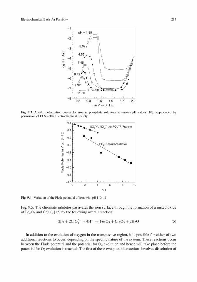
Electrochemical Basis for Passivity 213
–8
–7
–6
–5
–4
–3
–2
–1
–0.5 0.0 0.5 1.0 1.5 2.0
log
|i| in
A/c
m
E in V vs S.H.E.
pH = 1.85
3.02
11.50
9.37
8.42
4.55
7.45
Fig. 9.3 Anodic polarization curves for iron in phosphate solutions at various pH values [10]. Reproduced bypermission of ECS – The Electrochemical Society
–1.0
–0.8
–0.6
–0.4
–0.2
0.0
0.2
0.4
0.6
0 2 4 6 8 10
Fla
de P
oten
tial i
n V
vs.
S.H
.E.
pH
PO4–3 solutions (Sato)
SO4–2 , NO3
– , or PO4–3 (Franck)
Fig. 9.4 Variation of the Flade potential of iron with pH [10, 11]
Fig. 9.5. The chromate inhibitor passivates the iron surface through the formation of a mixed oxideof Fe2O3 and Cr2O3 [12] by the following overall reaction:
2Fe+ 2CrO2−4 + 4H+ → Fe2O3 + Cr2O3 + 2H2O (5)
In addition to the evolution of oxygen in the transpassive region, it is possible for either of twoadditional reactions to occur, depending on the specific nature of the system. These reactions occurbetween the Flade potential and the potential for O2 evolution and hence will take place before thepotential for O2 evolution is reached. The first of these two possible reactions involves dissolution of
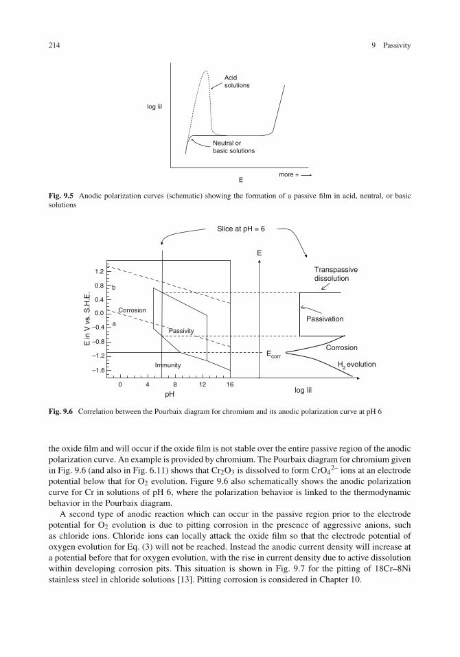
214 9 Passivity
log |i|
Emore +
Acidsolutions
Neutral orbasic solutions
Fig. 9.5 Anodic polarization curves (schematic) showing the formation of a passive film in acid, neutral, or basicsolutions
–1.6
–1.2
–0.8
–0.4
0.0
0.4
0.8
1.2
0 4 8 12 16
E in
V v
s. S
.H.E
.
pH
Passivity
Corrosion
b
a
Immunity
Corrosion
Passivation
Transpassivedissolution
E
log |i|
H2 evolution
Ecorr
Slice at pH = 6
Fig. 9.6 Correlation between the Pourbaix diagram for chromium and its anodic polarization curve at pH 6
the oxide film and will occur if the oxide film is not stable over the entire passive region of the anodicpolarization curve. An example is provided by chromium. The Pourbaix diagram for chromium givenin Fig. 9.6 (and also in Fig. 6.11) shows that Cr2O3 is dissolved to form CrO4
2– ions at an electrodepotential below that for O2 evolution. Figure 9.6 also schematically shows the anodic polarizationcurve for Cr in solutions of pH 6, where the polarization behavior is linked to the thermodynamicbehavior in the Pourbaix diagram.
A second type of anodic reaction which can occur in the passive region prior to the electrodepotential for O2 evolution is due to pitting corrosion in the presence of aggressive anions, suchas chloride ions. Chloride ions can locally attack the oxide film so that the electrode potential ofoxygen evolution for Eq. (3) will not be reached. Instead the anodic current density will increase ata potential before that for oxygen evolution, with the rise in current density due to active dissolutionwithin developing corrosion pits. This situation is shown in Fig. 9.7 for the pitting of 18Cr–8Nistainless steel in chloride solutions [13]. Pitting corrosion is considered in Chapter 10.

Theories of Passivity 215
10–4
10–3
10–2
10–1
100
–0.2 0 0.2 0.4 0.6 0.8 1 1.2 1.4
Cur
rent
Den
sity
in m
A/c
m2
E in V vs. S.H.E.
1 M H2SO4
0. 1 M NaCL
No pittingin 1 M H2SO4
Onset of pittingin 0.1 M NaCl
Fig. 9.7 Anodic polarization curves for 18Cr–8Ni stainless steel in 1 M H2SO4 or 0.1 M NaCl [13]. Reproduced bypermission of ECS – The Electrochemical Society
The above description of passivity is based on the kinetic point of view. We have already con-sidered passivity from a simple thermodynamic viewpoint in the treatment of Pourbaix diagrams.Recall that any oxide film that was formed was considered to be a passive film. This chapter willaddress in more detail the characteristics and properties of passive films.
Theories of Passivity
There are three main theories of passivity. These are (i) the adsorption theory [14–16], (ii) the oxidefilm theory [17], and (iii) the film sequence theory [18]. The film sequence theory actually combinesthe main ideas of the first two theories and attempts to bridge the differences in the first two pointsof view.
Adsorption Theory
According to this view of passivity, a chemically adsorbed (chemisorbed) monolayer of oxygen (i.e.,one molecular layer in thickness) reduces the reactivity of surface metal atoms and thus providesprotection against further attack. The adsorbed monomolecular film, of course, continues to grow inthickness; but proponents of this theory maintain that the initial act of chemisorption is the primarycause of passivity [14–16].
Support for the adsorption theory lies in the following observations:
(1) Electrochemical measurements yield the number of coulombs required to achieve passivity tocorrespond to one layer of oxygen.
(2) The transition metals (e.g., Fe, Cr, Ni) have high heats of adsorption of O2, corresponding tochemisorption or surface bond formation.

216 9 Passivity
(3) The observed Flade potential for iron is consistent with the formation of a chemisorbedmonolayer, as will be seen below.
(4) The critical alloy composition for the passivity of binary alloys can be explained by chemisorp-tion effects which respond to the electron configurations of the alloying metals. Passivity inbinary alloys is treated later in this chapter.
In regard to the first point listed above, coulometric measurements have determined that theamount of charge required to form a passive film on iron in NaOH solutions [19], 0.1 M Na2SO4[20], or in a borate buffer [21] corresponds to a monolayer of oxide. See Problem 9.1.
Uhlig [22] was able to explain the Flade potential of iron on the basis that a chemisorbed mono-layer is formed. The Flade potential for iron in sulfuric acid at pH 0 is +0.58 V vs. SHE, as observedby Franck [11] and given in Fig. 9.4. However, this value for the Flade potential cannot be explainedon the basis of a simple electrochemical reaction which occurs between iron and the solution toproduce a stoichiometric oxide. This can be seen from Table 9.1, in which none of the standard elec-trochemical reactions involving iron or its bulk oxides can be related to the observed Flade potentialfor iron at pH 0.
Table 9.1 Thermodynamic relationships for iron and its oxides in regard to the Flade potential EF
Reaction Nernst equation [2]E at pH 0(V vs. SHE)
Fe+ H2O � FeO+ 2H++2e− E = – 0.0417 – 0.0591 pH – 0.04173Fe+ 4H2O � Fe3O4+8H++8e− E = – 0.085 – 0.0591 pH – 0.0852Fe+ 3H2O � Fe2O3+6H++6e− E = – 0.051 – 0.0591 pH – 0.0512Fe3O4+H2O � 3Fe2O3+2H++2e− E = 0.221 – 0.0591 pH 0.221Fe in 1 M H2SO4 (experimental) – EF = + 0.58 V [22]
Uhlig assumed that the following surface reaction was responsible for passivation:
Fe(s)+ 3H2O(l)→ Fe(O2 · O)ads + 6H+(aq)+ 6e− (6)
where Fe(O2.O)ads refers to the chemisorbed monolayer with a second layer of adsorbed O2molecules. The approach was to calculate the standard free energy change �Go for Eq. (6) andthen to obtain Eo from �Go = – nFEo. Details of these calculations are given in Appendix E, but inbrief, Uhlig obtained �Go = 78,222 cal per mole of Fe(O2.O)ads for Eq. (6) and Eo = – 0.57 V vs.SHE. But this value of the electrode potential is for the oxidation reaction, and the standard electrodepotential is for the reduction reaction so that Eo = + 0.57 V vs. SHE. This value is in good agreementwith the Flade potential of + 0.58 V for Franck’s data for iron in sulfuric acid.
Oxide Film Theory
According to this theory, which is derived from the early work of U. R. Evans and co-workers, athin three-dimensional oxide film separates the metal from its environment. This oxide films acts asa barrier to the passage of the corrosive environment into the film and the passage of metal cationsfrom the substrate out through the film.
Support for the oxide film theory lies in the following observations:

Theories of Passivity 217
(1) Oxide films have been detached from the metal surface using chemicals such as alcoholicbromine, and the films have been analyzed by techniques such as electron microscopy andelectron diffraction [17, 23, 24].
(2) There have been numerous studies on the chemical composition of passive films using modernsurface analytical techniques, such as X-ray photoelectron spectroscopy (XPS).
(3) The presence of certain beneficial alloying elements (such as Cr, Ni, and Mo) in passive filmshas established that the chemical composition of a passive film on an alloy is an important factorin imparting passivity to the alloy.
Early evidence for three-dimensional oxide films was provided in the 1920s by U. R. Evans [17],who isolated the passive film on iron by stripping the film from the underlying metal by using asolution of bromine or iodine in methanol, as depicted in Fig. 9.8. Various workers have isolatedoxide films from iron, stainless steels, and aluminum and studied their properties by chemical anal-ysis, optical and electron microscopy, and electron diffraction [23–27]. For example, early studieson passive films isolated from stainless steels showed that the films were about 30 Å in thickness,were crystalline or semi-crystalline, and that both chromium and iron were present in the passivefilm [25].
Passive film
Base alloy
Scratch in metal surface
Alcoholic bromineor alcoholic iodine
Base alloy
Passive film
Fig. 9.8 Schematic diagram of the removal of a passive film by alcoholic bromine or alcoholic iodine. The bottomportion of the figure shows a cross section after a brief immersion in the solution
Proponents of the adsorption theory of passivity did not question the existence of such oxide filmsbut claimed that these films were not the primary cause of passivity but rather were its end result.
With the advent of modern surface analytical techniques, much information became availableabout the composition of passive films on a wide range of alloys. For instance, for a series of Fe−Cralloys passivated in sulfuric acid, X-ray photoelectron spectroscopy (XPS) was used to determine thechemical composition of oxide films as a function of the alloy composition [28]. Results are shownin Fig. 9.9, in which it is striking that the oxide film becomes enriched in Cr3+ at approximately 13 at.% Cr in the alloy, which is the critical alloy composition in Fe−Cr alloys for the onset of passivityby alloying.
More information about surface analysis techniques and the passivity of binary alloys is givenlater in this chapter.

218 9 Passivity
0.0
0.2
0.4
0.6
0.8
1.0
0.0 0.2 0.4 0.6 0.8 1.0
+100 mV
+500 mVC
atio
n F
ract
ion
Cr+
3 in O
xide
Atomic Fraction of Cr in alloy
Fig. 9.9 Chromium content in the passive film on Fe−Cr binary alloys as a function of the chromium content in thealloy after immersion in 1 M H2SO4 at two different electrode potentials [28]. Reproduced by permission of ElsevierLtd
Film Sequence Theory
The film sequence theory proposed by Hackerman [18] attempts to reconcile the differences betweenthe adsorption theory and the oxide film theory. Hackerman noted that an adsorbed film can causelarge potential changes associated with passivity, but that it is unlikely that an adsorbed monolayercould provide long-term protection against an aggressive environment. Thus, Hackerman proposedthe film sequence theory to take into account both adsorptive and oxide film characteristics ofpassivity.
According to the film sequence theory, a passive film is formed in a sequence of steps, whichinvolve: (i) chemisorption of O2, (ii) splitting of the adsorbed O2 molecule to form two adsorbedoxygen atoms Oads, (iii) formation of a charged surface species Oads
–, (iv) intrusion of metal ionsfrom the lattice into the adsorbed layer, and (v) growth of a three-dimensional oxide. In addition, thefilm must be able to regenerate itself when damaged so that steps (i) though (v) are repeated whenthe oxide film is breached. Thus, the film sequence theory draws on the properties of adsorbed filmsor three-dimensional oxides as needed.
A link between the adsorption theory and the oxide film theory of passivity is provided byFrankenthal’s study of the passive film on an Fe–24Cr alloy [29]. Coulometric measurements showedthat the primary film responsible for passivity was of the order of one monomolecular layer of oxideions, but that a secondary and more stable thicker film was formed at electrode potentials higher thanthe potential of primary passivation.
Surface Analysis Techniques for the Examination of Passive Films
Today it is generally accepted and understood that passivity is provided by a thin but three-dimensional oxide film. Prior to approximately 1970, passive films were examined mostly by

Surface Analysis Techniques for the Examination of Passive Films 219
electrochemical methods, with some use of electron diffraction techniques, either in the transmissionmode for films stripped from metal surfaces or in the reflection mode for films intact but removedfrom solution.
Starting in the 1970s and continuing today, there has been an explosion of new surface analyticaltechniques that have opened new approaches to corrosion science, especially in the area of passivity.These surface analytical techniques, which have been used to study the chemical composition orthe structure of passive films, include X-ray photoelectron spectroscopy (XPS), scattering ion massspectrometry (SIMS), Mössbauer spectroscopy, and X-ray absorption spectroscopy (XAS), whichincludes X-ray absorption near-edge spectroscopy (XANES) and extended X-ray absorption finestructure (EXAFS). These and other techniques which have been applied to the study of passivefilms are summarized in Table 9.2.
Table 9.2 Various surface analytical techniques which may be applied to the study of passive films [30–32]
TechniqueIncidentradiation
Detectedradiation Information obtained
Auger electron spectroscopy(AES)
Electrons Electrons Elemental analysisDepth profiles
X-ray photoelectron spectroscopy(AES)
X-rays(photons)
Electrons Elemental analysisOxidation statesDepth profiles
Secondary ion mass spectrometry(SIMS)
Ions Ions Elemental analysisDepth profiles
Reflection high-energy electrondiffraction (RHEED)
Electrons Electrons Surface structureCrystallinity
Transmission electron microscopy(TEM)
Electrons Electrons MorphologyMicrostructure
Scanning electron microscopy(SEM)
Electrons Electrons MorphologyMicrostructure
Energy dispersive analysis byX-rays (EDAX)
Electrons X-rays Chemical analysis
Mössbauer spectroscopy γ-rays Electrons Fe-containing phase identification(also Co- and Sn-)
Infrared spectroscopy Infrared radiation(photons)
Photons Functional groupsChemical structure
X-ray absorption near-edgespectroscopy (XANES)
X-rays(photons)
Photons Chemical composition
Extended X-ray absorption finestructure (EXAFS)
X-rays(photons)
Photons Bond distances
Scanning tunneling microscopy(STM)
Electrons Electrons Physical topographyAtomistic resolution
Rutherford backscattering (RBS) H+ ions(α-particles)
α-particles Chemical composition
Throughout this chapter, we will draw on the results of various surface analytical studies onpassivity, without going into details of the various techniques themselves. However, it is instructiveto first provide a brief description of three techniques which have been very useful in the study ofpassivity. These are X-ray photoelectron spectroscopy (XPS), X-ray absorption spectroscopy (XAS),and scanning tunneling microscopy (STM).

220 9 Passivity
X-ray Photoelectron Spectroscopy (XPS)
The “workhorse” of these surface techniques has proved to be X-ray photoelectron spectroscopy.In XPS, the surface to be analyzed is placed inside a vacuum system and then irradiated with abeam of X-rays of known energy. Transfer of the energy of the X-ray photons to atoms in the sur-face of the sample causes core electrons (photoelectrons) to be ejected, as shown schematicallyin Fig. 9.10. These photoelectrons are collected and analyzed by the XPS spectrometer, which mea-sures the kinetic energy of the photoelectrons EK. The kinetic energy of the photoelectrons, however,depends on the energy hν of the incident X-rays. The intrinsic material property is the binding energyof the electron EB given by
EB = hv− EK − φsp (7)
where φsp is the work function of the spectrometer, which can be measured. Thus, the binding energyEB can be readily determined from the three quantities on the right-hand side of Eq. (7). The bindingenergy is a characteristic quantity for the various elements and their different oxidation states, andextensive tables of binding energies have been compiled for identification of various peaks whichare obtained in an XPS spectrum.
An example of a typical XPS photopeak is given in Fig. 9.11, which shows the O 1s photo-peak for the air-formed oxide film on titanium [4, 5]. (XPS photopeaks are described in terms oftheir quantum numbers.) The O 1s peak in Fig. 9.11 has been resolved into three constituent sub-peaks, showing that there are three oxygen-containing species in the oxide film: O2– oxide ions,
X–ray(photons) Photoejected 1s electron
1s2s
2p
Fig. 9.10 Schematic diagram of the ejection of photoelectrons as used in X-ray photoelectron spectroscopy (XPS)
Fig. 9.11 The XPS O 1s photopeak for the air-formed oxide film on titanium [4, 5]. Reproduced by permission ofECS – The Electrochemical Society
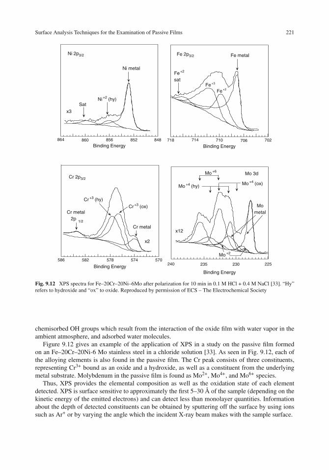
Surface Analysis Techniques for the Examination of Passive Films 221
848852856860864
Binding Energy
Ni 2p3/2 Fe 2p3/2
Cr 2p3/2
Ni metal
SatNi +2 (hy)
x3
570574578582586
Binding Energy
Cr +3 (ox)
Cr +3 (hy)
Cr metal 2p
1/2
Cr metal
x2
702706710714718
Binding Energy
Fe+2
satFe+3
Fe+2
Fe metal
225230235240
Binding Energy
Mo +2
Mometal
Mo +6
Mo +4 (ox)Mo +4 (hy)
x12
Mo 3d
Fig. 9.12 XPS spectra for Fe–20Cr–20Ni–6Mo after polarization for 10 min in 0.1 M HCl + 0.4 M NaCl [33]. “Hy”refers to hydroxide and “ox” to oxide. Reproduced by permission of ECS – The Electrochemical Society
chemisorbed OH groups which result from the interaction of the oxide film with water vapor in theambient atmosphere, and adsorbed water molecules.
Figure 9.12 gives an example of the application of XPS in a study on the passive film formedon an Fe–20Cr–20Ni-6 Mo stainless steel in a chloride solution [33]. As seen in Fig. 9.12, each ofthe alloying elements is also found in the passive film. The Cr peak consists of three constituents,representing Cr3+ bound as an oxide and a hydroxide, as well as a constituent from the underlyingmetal substrate. Molybdenum in the passive film is found as Mo2+, Mo4+, and Mo6+ species.
Thus, XPS provides the elemental composition as well as the oxidation state of each elementdetected. XPS is surface sensitive to approximately the first 5–30 Å of the sample (depending on thekinetic energy of the emitted electrons) and can detect less than monolayer quantities. Informationabout the depth of detected constituents can be obtained by sputtering off the surface by using ionssuch as Ar+ or by varying the angle which the incident X-ray beam makes with the sample surface.

222 9 Passivity
A disadvantage of XPS is that the sample must be removed from the aqueous electrolyte andplaced into a high-vacuum system for surface analysis, thus raising the question as to whether with-drawal from the electrolyte or exposure to a high vacuum alters the character of the passive film. Thisproblem can be minimized, however, through the use of special chambers which allow the sampleto be removed from the electrolyte with its liquid film intact and to be transferred under a blanketof inert gas into the spectrometer. However, the effect of exposure of the film to the vacuum stillremains open to question.
X-ray Absorption Spectroscopy
X-ray absorption spectra for various iron oxides and hydroxides have shown that the spectrum for thepassive film does not match that of any of the individual oxides or hydroxides [34, 35]. Figure 9.13shows XPS data for several oxides and for the passive film on iron grown in a borate buffer solution[35]. (Models for the passive film on iron are considered later in this chapter.)
–0.2
0.0
0.2
0.4
0.6
0.8
1.0
1.2
7110 7120 7130 7140 7150 7160
Inte
nsity
nor
m. (
a.u)
Energy (eV)
Fe2O3
Fe3O4
FeO
Passive Fe
Fig. 9.13 X-ray absorption spectra for several iron oxides and for the passive film on iron in a pH 8.4 buffer solution.Redrawn from Schmuki et al. [35] by permission of ECS – the electrochemical society
Each spectrum in Fig. 9.13 consists of two parts: an initial sharp increase in absorbance (anX-ray edge) and a region of oscillations following the edge. The observation and analysis of theedge portion of the spectrum is called X-ray absorption near-edge spectroscopy (XANES), whilethe information contained in the subsequent oscillation is termed X-ray absorption fine structure(EXAFS).
Absorption edges occur when the energy of the incident X-ray excites a core electron in thesample to an empty valence level or beyond. The positions (i.e., energies) of these edges are charac-teristic of the absorbing atom and are designated according to the core electron level which has beenexcited. Thus, a K edge arises from the 1s level and an L edge from a 2s or a 2p level.
The oscillations which arise in the EXAFS portion of the spectrum are due to interactions of thephotoelectron wave with its nearest neighbor atoms. Thus, this region contains information on atom–atom bond distances. For details, more advanced texts should be consulted [32, 36]. In addition, the

Surface Analysis Techniques for the Examination of Passive Films 223
pre-edge region can be expanded to yield more additional information as to similarities or differencesbetween various samples being investigated.
X-ray absorption spectroscopy requires a monochromatic high-intensity X-ray beam which canbe tuned through a wide range of energies. Such experiments are carried out using synchrotron X-raysources [36].
Scanning Tunneling Microscopy
The scanning tunneling microscope (STM) is capable of characterizing surface topography on anatomistic scale. In the STM, a voltage is applied between the surface to be imaged and a sharpprobe whose tip can be narrowed to a single atom. As the tip is moved to within a few atomicdiameters of the surface, a current flows between the sample and the probe. This is due to the overlapbetween the electronic wave functions of the atoms in the sample and the tip. The current falls offexponentially with the distance above the surface and is thus a measure of the height of the tipabove the surface. The tip can be scanned across the surface in the x- and y-directions, as shown inFig. 9.14.
ControlUnitVT
VZ
y piezo
z piezo
x piezo
Fig. 9.14 Schematic diagram of a scanning tunneling microscope (STM), as adapted from Vickerman [32]. VT is thesample bias voltage and VZ is the voltage applied to the z-piezo to maintain constant tunneling current. Reproducedby permission of John Wiley & Sons, Inc
The STM can operate in two modes: constant current or constant height. In the constant currentmode, the distance of the tip above the surface adjusts to maintain the constant current and thusresponds to the topography of the surface. In the constant height mode, the current output changesas the distance of the tip above the surface changes with respect to the atomic surface topography.
An example of the use of the STM in studies on passivity is given in Fig. 9.15, which showsan STM image of the passive film on an Fe–14 at.% Cr alloy [37]. The STM image shows that thepassive film is crystalline and has a slightly distorted close-packed hexagonal lattice.
A technique related to the STM is the atomic force microscope (AFM), which consists of acantilever beam having a sharp tip which can sense forces between the tip and the sample. As theinteraction force between the tip and the sample varies, deflections are produced in the cantilever,and these are used to construct a topographical map of the surface.

224 9 Passivity
Spacing of corrugations ~ 3.1 Å
Fig. 9.15 In situ STM image of the passive film on Fe–14Cr in 0.01 M H2SO4 at +0.400 V vs. SCE [37]. Reproducedby permission of ECS – The Electrochemical Society
Models for the Passive Oxide Film on Iron
The nature of the passive film on iron has been studied in great detail by many investigators who haveused a variety of techniques. However, even with this intense study and even with the remarkablecapabilities of modern surface analytical techniques, the exact nature of the passive film on elementaliron remains elusive. This is due in part to the fact that the passive film on iron is very thin (of theorder of 1.5–5.0 nm, i.e., 15–50 Å). In addition, the nature of the passive film may vary with thedetails of its formation and with the electrolyte in which the film exists.
Based on various experimental investigations, there are four principal models for the passive filmon iron. These are (i) the bilayer model, (ii) the hydrous oxide model, (iii) the bipolar-fixed chargemodel, and (iv) the spinel/defect model. Each of these models is discussed briefly below.
Bilayer Model
The bilayer model for the passive film on iron was developed by M. Cohen and co-workers atthe National Research Council of Canada [38–40]. According to this model, which is illustrated

Models for the Passive Oxide Film on Iron 225
γ -Fe2O3
Fe3O4
Fe
(a)
O
M
OH2
O
OHOH2
O
MOH2
OH2
OH2
OH2
(b)
HO
HO
M
OH2
O
OHOH2
O
MOH2
OH2
OH2
OH2
O–2
H+
Fe+2
Cl–
––
––
–Cationselective
Anionselective
(d)
–– –
+ O –2
H+
Fe+2
x
Cl -
x
––
Anionselective
Cationselective
(c)
++
++
++
++
+
O-2Fe+3
Fe
(e)
Fig. 9.16 Models for the passive film on iron: (a) the bilayer model [38–40], (b) the hydrous oxide model [48–53], (c)and (d) the bipolar model [10, 59], (e) the spinel/defect model [34, 61, 62]. Figure 9.16b reproduced with permissionfrom Elsevier Ltd. Figure 9.16c, d reproduced with the permission of ECS – The Electrochemical Society
schematically in Fig. 9.16(a), the passive film on iron consists of an inner layer of Fe3O4 adjacentto the metal and an outer layer of γ-Fe2O3. (In addition, there is an outermost thin layer of hydroxylgroups which exists on every oxide film and which usually consists of only one to several monolayers[4, 5, 41] and so is much thinner than the oxide film itself.)
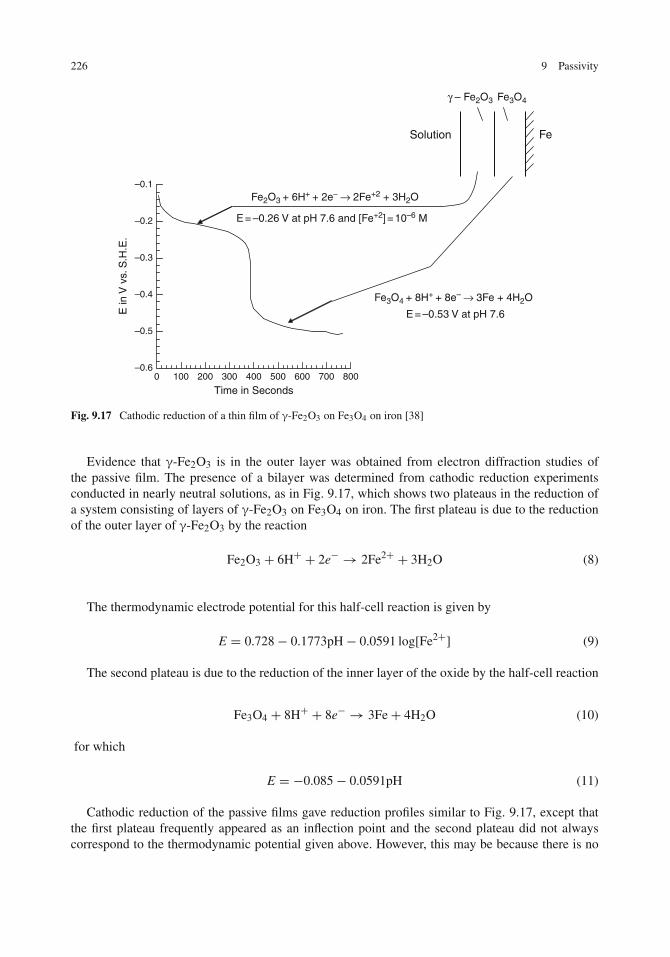
226 9 Passivity
–0.6
–0.5
–0.4
–0.3
–0.2
–0.1
0 100 200 300 400 500 600 700 800
E in
V v
s. S
.H.E
.
Time in Seconds
Fe2O3 + 6H+ + 2e– → 2Fe+2 + 3H2O
Fe3O4 + 8H+ + 8e– → 3Fe + 4H2O
E = –0.26 V at pH 7.6 and [Fe+2] = 10–6 M
E = –0.53 V at pH 7.6
γ – Fe2O3 Fe3O4
FeSolution
Fig. 9.17 Cathodic reduction of a thin film of γ-Fe2O3 on Fe3O4 on iron [38]
Evidence that γ-Fe2O3 is in the outer layer was obtained from electron diffraction studies ofthe passive film. The presence of a bilayer was determined from cathodic reduction experimentsconducted in nearly neutral solutions, as in Fig. 9.17, which shows two plateaus in the reduction ofa system consisting of layers of γ-Fe2O3 on Fe3O4 on iron. The first plateau is due to the reductionof the outer layer of γ-Fe2O3 by the reaction
Fe2O3 + 6H+ + 2e− → 2Fe2+ + 3H2O (8)
The thermodynamic electrode potential for this half-cell reaction is given by
E = 0.728− 0.1773pH− 0.0591 log[Fe2+] (9)
The second plateau is due to the reduction of the inner layer of the oxide by the half-cell reaction
Fe3O4 + 8H+ + 8e− → 3Fe+ 4H2O (10)
for which
E = −0.085− 0.0591pH (11)
Cathodic reduction of the passive films gave reduction profiles similar to Fig. 9.17, except thatthe first plateau frequently appeared as an inflection point and the second plateau did not alwayscorrespond to the thermodynamic potential given above. However, this may be because there is no

Models for the Passive Oxide Film on Iron 227
sharp phase boundary between the two thin bilayers but instead a varying concentration from themetal/oxide interface to the oxide/solution interface. See Problem 9.2 at the end of this chapter.
Support for this bilayer model has been provided from research involving surface analyticaltechniques, including AES, RHEED, and SIMS [30, 42, 43], which have been used to analyze thecomposition of the passive film. In particular, the results of SIMS data showed that the outer layerwas “dry” γ-Fe2O3 rather than “wet” γ-FeOOH. The yield of the FeO+ fragment for the passive filmwas higher than for the fragment FeOH+, in agreement with the results for an Fe2O3 standard butnot for FeOOH, as shown in Fig. 9.18.
2
3
4
5
6
FeO+
FeOH+
Passive Film on Fe
3
4
5
0 2 4 6 8 10
Sputter Time in Minutes
FeOH+
FeO+
FeOOH
Log
Cou
nts
in s
ec–
1
2
3
4
5
FeO+
FeOH+
Fe2O
3
Fig. 9.18 SIMS profiles for the passive film on iron, for Fe2O3, and for FeOOH [30]. Reproduced by permission ofElsevier Ltd
Modifications of the basic bilayer structure discussed above have also been proposed in whichthe outer of the two layers contains hydrogen atoms [44], is γ-FeOOH rather than γ-Fe2O3 [45, 46],or is a mixture of Fe3O4, γ-Fe2O3, and an unknown ferric oxide, hydroxide, or oxyhydroxide [47].
Hydrous Oxide Model
In contrast to the above model (of an anhydrous passive film), the main feature of the hydrous oxidemodel is that the passive film on the iron surface contains water, the exact form of which remainsunclear. Possibilities include molecular H2O, H atoms, and OH groups.

228 9 Passivity
There are considerable experimental indications that water (in some form) exists in passive oxidefilms. The earliest evidence is due to Rhodin [48], who found bound water in the passive film ofstainless steel by chemical analysis of the film stripped from the stainless steel surface.
Okamato and Shibata [49, 50] have used radiotracer techniques with stainless steel passivated in atritiated acid solution. The passivated surface was removed from the tritiated solution, washed thor-oughly with ordinary water, dried, and then immersed in a solution containing non-tritiated water.The desorption of bound tritiated water from the passive film was detected by an increase in thecounting rate upon immersion, as shown in Fig. 9.19. Similar experiments using radiotracer tech-niques have also been carried out on iron [51, 52] and have shown the existence of a hydrous speciesin the passive film on iron.
0
2
4
6
8
10
12
0.10 1.0 10 10 2 103
104C
ount
ing
Rat
e in
Cou
nts
Per
Min
x 1
00
Time in Minutes
Introduction oftritiated specimen
Fig. 9.19 Change in counting rate with time during the immersion into a scintillating solution for 304 stainless steelwhich had been previously passivated in a tritiated acid solution [49]. Reproduced by permission from MacmillanPublishers: Nature [49], copyright (1965)
Surface analytical measurements with SIMS [53] and Mössbauer spectroscopy [54–56] havealso suggested the presence of water in the passive film on iron. Using SIMS, Murphy et al. [53]observed a constant ratio of OH–/O– throughout the passive film formed on iron in a borate bufferand concluded that water is contained throughout the thickness of the passive film. (This conclusionis directly opposite to that reached by Mitchell and Graham [30] in their SIMS work.) The results ofMössbauer investigations have led to various interpretations, but all involve the presence of water inthe passive film. These interpretations are that the passive film contains a non-stoichiometric Fe3+
species [54], contains γ-FeOOH [55], is ferric hydroxide with excess water [56], and consists ofpolymeric chains of iron atoms bonded by dioxy and dihydroxy bridging bonds and linked togetherby water molecules [57].
The hydrous oxide model is represented schematically in Fig. 9.16(b) [58].
Bipolar-Fixed Charge Model
The bipolar-fixed charge model was proposed by Sakashita and Sato [10, 59] and is based on thetransport properties of hydrous oxide films in regard to anions or cations.

Models for the Passive Oxide Film on Iron 229
If the outer part of the passive oxide film is cation selective and the inner part of the film is anionselective, as in Fig. 9.16(c), then the inward passage of aggressive anions (such as Cl–) through thefilm is not favored. In addition, the outward passage of cations produced by metallic dissolution atthe iron/oxide interface is similarly not favored. The passive film also becomes dehydrated in thatH+ ions move outward through the cation-selective layer into solution, and OH– ions move inwardthrough the anion-selective layer to reinforce passivity at the metal/oxide interface. The joint actionof the selectivity properties of the film and dehydration of the film is proposed to produce a protectiveoxide film.
Reversal of the bipolarity of the film, as in Fig. 9.16(d), favors passage of aggressive anionsinto the film, passage of cations produced by corrosion out through the film, as well as continuedhydration of the film. Thus, this set of conditions produces a non-protective oxide film.
At present, it is not clear how the passive oxide film on an elemental metal (e.g., Fe) can producea bipolar ion-selective film. This model may be more better suited to the passivity of alloys wherethe oxide film may contain various ionic species. In fact, the bipolar model of passivity has beenextended by Clayton and Lu [60] to Fe−Cr−Ni−Mo stainless steels. A detailed surface analysis ofthe passive film formed anodically in 0.1 M HCl showed the presence of Mo (as MoO4
2–) in theouter part of the oxide film and of Cr3+ (as Cr(OH)3) in the inner regions of the passive film. Claytonand Lu have suggested that MoO4
2– is the basis for a cation-selective outer layer and Cr(OH)3 is thebasis for an anion-selective inner layer.
Spinel/Defect Model
Based on in situ X-ray studies of the passive film formed on iron in a buffer solution [34, 35, 61,62], a model of the passive film has been proposed which suggests that the film is a single-phasenanocrystalline spinel oxide which is related to but different than γ-Fe2O3 or Fe3O4.
The oxides Fe3O4 and γ-Fe2O3 are closely related, consisting of a unit cell of 32 cubic close-packed oxygen ions containing Fe cations as follows [63]:
Fe3O4: 8 Fe3+ in tetrahedral sites, 8 Fe2+ plus 8 Fe3+ in octahedral sites.γ-Fe2O3: 21 and 1/3 Fe3+ statistically scattered in the above 24 positions.
(See Fig. 9.20 for more about tetrahedral and octahedral sites.) The passive film on iron, however,was observed to have a distribution of Fe3+ or Fe2+ ions which does not follow either of the abovepatterns for Fe3O4 or γ-Fe2O3.
The groundwork for this model was laid by earlier work of Long et al. [64], who using surfaceEXAFS showed that passive films formed on iron in nitrate or chromate solutions had Fe−Fe bonddistances different from that of the known iron oxides or hydroxides.
In addition, the passive film was observed to contain point defects, such as vacancies and inter-stitials, and also extended defects, such as finite crystallite size and stacking faults. The crystallinenature of the passive film on iron was confirmed by scanning tunneling microscopy studies [65].
In addition, Schmuki et al. [35] showed that it is possible to have a two-stage reduction process(as observed by Cohen and co-workers) when there is only a single-phase Fe2O3 oxide film (so thatthe observation of a two-stage reduction does not necessarily imply a bilayer structure).
This model of the passive film is represented by Fig. 9.16(e).

230 9 Passivity
Tetrahedral site – above an O– 2in the bottom layer4 nearest neighbors(form a tetrahedron)
Octrahedral site – above a void in the bottom layer6 nearest neighbors(form an octahedron)
2nd layer O– 2ions
1st layer O– 2ions
Fig. 9.20 Octahedral and tetrahedral sites in iron oxides. The small gray circles refer to Fe3+ ions and the larger whitecircles refer to O2– ions
What Do These Various Models Mean?
Elucidation of the nature of the passive film on iron is primarily a matter of scientific concern.From the practical point of view, the corrosion engineer needs to know how to achieve passivitybut does not have to understand in detail its precise mechanism. However, there is much interest inunderstanding the nature of the passive film on iron because the results for iron provide a startingpoint for understanding passivity when alloying elements are added to iron (to produce stainlesssteels, for example). In addition, an improved understanding of mechanisms of passivity may leadto the design of new and improved corrosion-resistant bulk or surface alloys.
Passive Oxide Films on Aluminum
Aluminum reacts readily with water or aqueous solutions to form an oxide film, as shown in the“Introduction to this Chapter.” The composition, structure, and thickness of the oxide films varygreatly, depending upon details of their formation.
The aluminum–water system is much simpler than the iron–water system because the aluminumcation exists in only a single oxidation state (3+), unlike the case for iron. The possible reactionproducts are aluminum hydroxide, Al(OH)3, and aluminum oxide, Al2O3, although the latter mayexist in various degrees of hydration and in several different crystal structures [66]. See Table 9.3.The presence of water in oxide films on aluminum has been determined through the use of infraredspectroscopy and Rutherford back scattering spectrometry [66–68].

Passive Oxide Films on Aluminum 231
Table 9.3 Major reactionproducts formed betweenaluminum and water [66]
Al(OH)3γ-Al2O3γ-Al2O3·H2O (γ-AlOOH) (boehmite)β-Al2O3·3H2O (Bayerite)
Pseudoboehmite is a poorly crystalline modifica-tion of boehmite.
Air-Formed Oxide Films
The air-formed oxide film on aluminum is of the order of 30–40 Å in thickness and consists entirelyof Al2O3 [4, 5]. The outermost layer consists of surface hydroxyls which result from the interactionof the oxide film with water vapor in the atmosphere, but this hydroxylated region is only 8 Åin thickness and does not persist into the inner portion of the oxide film [4, 5]. Using a simpleweight gain technique, Godard [69] found that the oxide film thickness on pure aluminum wasapproximately 200 Å after 5 years of exposure to 52% relative humidity and 1,700 Å after 5 yearsof exposure to 100% relative humidity.
Films Formed in Aqueous Solutions
Aluminum reacts readily with water to form a hydrous oxide film. Growth of the film in water occursin two stages [70, 71]: a pseudoboehmite film is produced initially and is then covered by a layer ofbayerite crystals, as shown in Fig. 9.21. The thickness of the film in Fig. 9.21 was 2.8 μm (28,000 Å)after 4 days of immersion in distilled water at 40◦C [71]. Using weight gain measurements, Hart [70]observed that film growth was complete after about 12 days of immersion in water at 20◦C. Fromthe measured weight gain and the density of bayerite, the limiting film thickness is calculated to be50,000 Å.
Pseudoboehmite
Bayerite crystals
Al
(a) Top view of the oxide film on aluminum after 1 day at 40°C in distilled water.
(b) Cross section after longer immersion times.
Fig. 9.21 Idealized schematic representation of the growth of an oxide film on aluminum in water at 40◦C [70, 71]

232 9 Passivity
Oxide films on aluminum can be increased in thickness by the process of anodization, in whichoxide films are grown in aqueous solutions under conditions of controlled anodic potential. Twotypes of anodized films can be formed: barrier oxides and porous oxides. Ammonium tartrate, boricacid, and ammonium pentaborate are electrolytes commonly used to produce barrier-type oxides,which are compact films that can be varied in thickness between approximately 100 and 2,000 Å[72, 73].
The second type of anodic oxide film, the porous oxide film, typically has a total oxide thicknessof 3–35 μm (30,000–350,000 Å) [74]. This type of film is commonly formed by anodization insulfuric or phosphoric acids and consists of an inner compact layer and an outer porous layer. Theouter porous layer is characterized by a “scalloped” structure of hexagonal cells, each containinga central pore. See Fig. 9.22, which is a transmission electron micrograph of a cross section of aphosphoric acid anodized film [75]. A schematic representation of a phosphoric acid anodized filmis shown in Fig. 9.23. The fingers or protrusions of oxide shown in the figure are believed to improvethe adhesion of organic coatings or adhesives by interlocking with the organic overlayer [9, 76].
The open cells in the porous structure are usually sealed in boiling water to improve the corrosionresistance [77]. Organic dyes or pigments can be incorporated into the porous oxide to produce acolored anodic coating [78].
Properties of Passive Oxide Films
Passive oxide films have the following properties [79–81]:
Fig. 9.22 Transmission electron micrograph of the cross section of an anodized film formed on aluminum inphosphoric acid [75]. Reproduced by permission of Taylor and Francis Ltd and www.informaworld.com

Properties of Passive Oxide Films 233
4000 Å
100 Å
1000 Å
400 Å
Oxide
Al
Fig. 9.23 Schematic drawing of the oxide structure on an aluminum alloy after anodizing in phosphoric acid [9, 76].Reproduced by permission of Elsevier Ltd
Thickness
As discussed earlier, the thickness of passive films varies from tens to hundreds of thousands ofangstroms (essentially from nanometers to micrometers), depending on the metal, the electrolyte,and the conditions under which the film was formed.
Electronic and Ionic Conductivity
Passive layers on the transition metals (e.g., Fe, Cr, Ni) are generally thin (less than 100 Å, i.e.,10 nm) and possess good electronic conductivity. This is evidenced by the fact that passive filmson iron, for example, can support electron transfer reactions such as the Fe(CN)6
4–/ Fe(CN)63–
exchange [82]. There is considerable evidence, for example, that passive films on Fe, Ti, or Sn are n-type semiconductors, while the passive film on Cu or Ni is a p-type semiconductor [81]. In contrast,barrier passive films on metals like Al, Ta, and Pb are thicker and generally possess poor electronicconductivity.
The ionic conductivity of all passive films should be low to prevent the passage of aggressive ionssuch as chlorides inward though the film and the transfer of dissolved cations outward through thefilm.
Chemical Stability
The oxide film should have low chemical solubility and should be stable under a wide range ofelectrode potentials.
The range of stability for a given a passive film on a given metal is conveniently provided by thePourbaix diagram of the metal. For example, Fig. 9.24 compares Pourbaix diagrams for Al, Cr, and
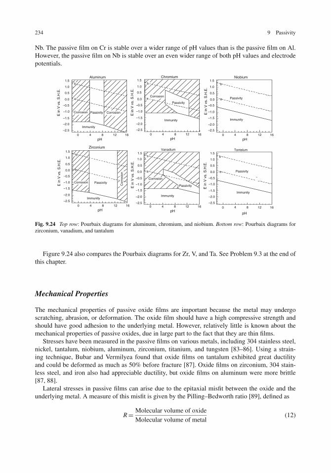
234 9 Passivity
Nb. The passive film on Cr is stable over a wider range of pH values than is the passive film on Al.However, the passive film on Nb is stable over an even wider range of both pH values and electrodepotentials.
–2.5
–2.0
–1.5
–1.0
–0.5
0.0
0.5
1.0
1.5
0 4 8 12 16
E in
V v
s. S
.H.E
.
pH
PassivityCorrosion
Cor
rosi
on
Zirconium
Immunity
b
a
–2.5
–2.0
–1.5
–1.0
–0.5
0.0
0.5
1.0
1.5
0 4 8 12 16
E in
V v
s. S
.H.E
.
pH
Corrosion Passivity Corrosion
Immunity
a
b
Aluminum
–2.5
–2.0
–1.5
–1.0
–0.5
0.0
0.5
1.0
1.5
0 4 8 12 16
E in
V v
s. S
.H.E
.
pH
Passivity
Immunity
b
a
Niobium
–2.5
–2.0
–1.5
–1.0
–0.5
0.0
0.5
1.0
1.5
0 4 8 12 16E
in V
vs.
S.H
.E.
pH
b
a Passivity
Immunity
Tantalum
–2.5
–2.0
–1.5
–1.0
–0.5
0.0
0.5
1.0
1.5
0 4 8 12 16
E in
V v
s. S
.H.E
.
pH
b
a
Immunity
Corrosion
Passivity
Vanadium
–2.5
–2.0
–1.5
–1.0
–0.5
0.0
0.5
1.0
1.5
0 4 8 12 16E
in V
vs.
S.H
.E.
pH
Passivity
Immunity
Corrosion
b
a
Chromium
Fig. 9.24 Top row: Pourbaix diagrams for aluminum, chromium, and niobium. Bottom row: Pourbaix diagrams forzirconium, vanadium, and tantalum
Figure 9.24 also compares the Pourbaix diagrams for Zr, V, and Ta. See Problem 9.3 at the end ofthis chapter.
Mechanical Properties
The mechanical properties of passive oxide films are important because the metal may undergoscratching, abrasion, or deformation. The oxide film should have a high compressive strength andshould have good adhesion to the underlying metal. However, relatively little is known about themechanical properties of passive oxides, due in large part to the fact that they are thin films.
Stresses have been measured in the passive films on various metals, including 304 stainless steel,nickel, tantalum, niobium, aluminum, zirconium, titanium, and tungsten [83–86]. Using a strain-ing technique, Bubar and Vermilyea found that oxide films on tantalum exhibited great ductilityand could be deformed as much as 50% before fracture [87]. Oxide films on zirconium, 304 stain-less steel, and iron also had appreciable ductility, but oxide films on aluminum were more brittle[87, 88].
Lateral stresses in passive films can arise due to the epitaxial misfit between the oxide and theunderlying metal. A measure of this misfit is given by the Pilling–Bedworth ratio [89], defined as
R= Molecular volume of oxide
Molecular volume of metal(12)
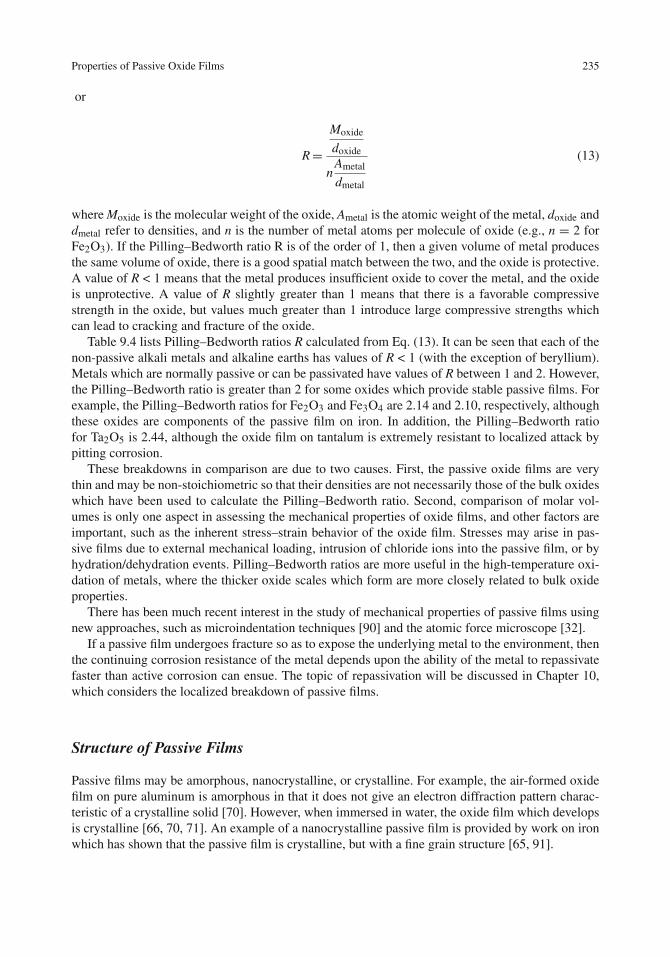
Properties of Passive Oxide Films 235
or
R=Moxide
doxide
nAmetal
dmetal
(13)
where Moxide is the molecular weight of the oxide, Ametal is the atomic weight of the metal, doxide anddmetal refer to densities, and n is the number of metal atoms per molecule of oxide (e.g., n = 2 forFe2O3). If the Pilling–Bedworth ratio R is of the order of 1, then a given volume of metal producesthe same volume of oxide, there is a good spatial match between the two, and the oxide is protective.A value of R < 1 means that the metal produces insufficient oxide to cover the metal, and the oxideis unprotective. A value of R slightly greater than 1 means that there is a favorable compressivestrength in the oxide, but values much greater than 1 introduce large compressive strengths whichcan lead to cracking and fracture of the oxide.
Table 9.4 lists Pilling–Bedworth ratios R calculated from Eq. (13). It can be seen that each of thenon-passive alkali metals and alkaline earths has values of R < 1 (with the exception of beryllium).Metals which are normally passive or can be passivated have values of R between 1 and 2. However,the Pilling–Bedworth ratio is greater than 2 for some oxides which provide stable passive films. Forexample, the Pilling–Bedworth ratios for Fe2O3 and Fe3O4 are 2.14 and 2.10, respectively, althoughthese oxides are components of the passive film on iron. In addition, the Pilling–Bedworth ratiofor Ta2O5 is 2.44, although the oxide film on tantalum is extremely resistant to localized attack bypitting corrosion.
These breakdowns in comparison are due to two causes. First, the passive oxide films are verythin and may be non-stoichiometric so that their densities are not necessarily those of the bulk oxideswhich have been used to calculate the Pilling–Bedworth ratio. Second, comparison of molar vol-umes is only one aspect in assessing the mechanical properties of oxide films, and other factors areimportant, such as the inherent stress–strain behavior of the oxide film. Stresses may arise in pas-sive films due to external mechanical loading, intrusion of chloride ions into the passive film, or byhydration/dehydration events. Pilling–Bedworth ratios are more useful in the high-temperature oxi-dation of metals, where the thicker oxide scales which form are more closely related to bulk oxideproperties.
There has been much recent interest in the study of mechanical properties of passive films usingnew approaches, such as microindentation techniques [90] and the atomic force microscope [32].
If a passive film undergoes fracture so as to expose the underlying metal to the environment, thenthe continuing corrosion resistance of the metal depends upon the ability of the metal to repassivatefaster than active corrosion can ensue. The topic of repassivation will be discussed in Chapter 10,which considers the localized breakdown of passive films.
Structure of Passive Films
Passive films may be amorphous, nanocrystalline, or crystalline. For example, the air-formed oxidefilm on pure aluminum is amorphous in that it does not give an electron diffraction pattern charac-teristic of a crystalline solid [70]. However, when immersed in water, the oxide film which developsis crystalline [66, 70, 71]. An example of a nanocrystalline passive film is provided by work on ironwhich has shown that the passive film is crystalline, but with a fine grain structure [65, 91].

236 9 Passivity
Table 9.4 Pilling–Bedworth ratios R for various metal/metal oxidesa
R < 1 1 < R < 2 R > 2
Li2O 0.57 Ag2O 1.57 Co2O3 2.41Na2O 0.58 AgO 1.61 Fe2O3 2.14K2O 0.46 Al2O3 1.29 Fe3O4 2.10Rb2O 0.42 BeO 1.67 MoO2 2.10MgO 0.81 CdO 1.22 MoO3 3.25CaO 0.65 Ce2O3 1.28 Mn2O3 2.10SrO 0.61 CeO2 1.09 MnO2 2.27BaO 0.71 CoO 1.75 Nb2O5 2.66
Co3O4 1.98 PtO2 2.11Cr2O3 2.00 SiO2 2.13Cu2O 1.68 Ta2O5 2.44CuO 1.78 Sb2O5 2.35FeO 1.69 U3O8 2.68MnO 1.75 UO3 3.14NbO 1.38 VO2 2.25NbO2 1.95 V2O5 3.20NiO 1.68 WO2 2.10PbO 1.30 WO3 3.38Pb2O3 1.25Pb3O4 1.40PtO 1.64Sb2O3 1.43SnO 1.28SnO2 1.35TaO2 1.93TiO 1.21Ti2O3 1.51TiO2 1.77UO2 1.98U4O9 1.96VO 1.37V2O3 1.81ZnO 1.58ZrO2 1.55
aMetal and oxide densities are from “Handbook of Chemistry andPhysics,” 82nd Ed. (2001–2002).
Amorphous metals generally have reduced corrosion rates compared to their crystalline coun-terparts. For example, Fig. 9.25 shows polarization curves for an 85Co–15Nb alloy in 0.5 M NaCl[92]. The crystalline alloy readily undergoes anodic dissolution at anodic potentials, but the amor-phous alloy exhibits an anodic current density which is several orders of magnitude lower over arange of approximately 1.0 V up to the localized breakdown of the passive film, which occurredabove +0.4 V.
In a study on the effect of progressive addition of Cr to iron, McBee and Kruger [93] showedby electron diffraction that the passive films go from polycrystalline to amorphous with the additionof increased amounts of Cr to the alloy. In view of observations like this and with the informationavailable on the improved corrosion behavior of amorphous metals [94], it has been proposed that animportant factor in the passivity of metals is the structure of the passive film [94, 95]. An amorphous
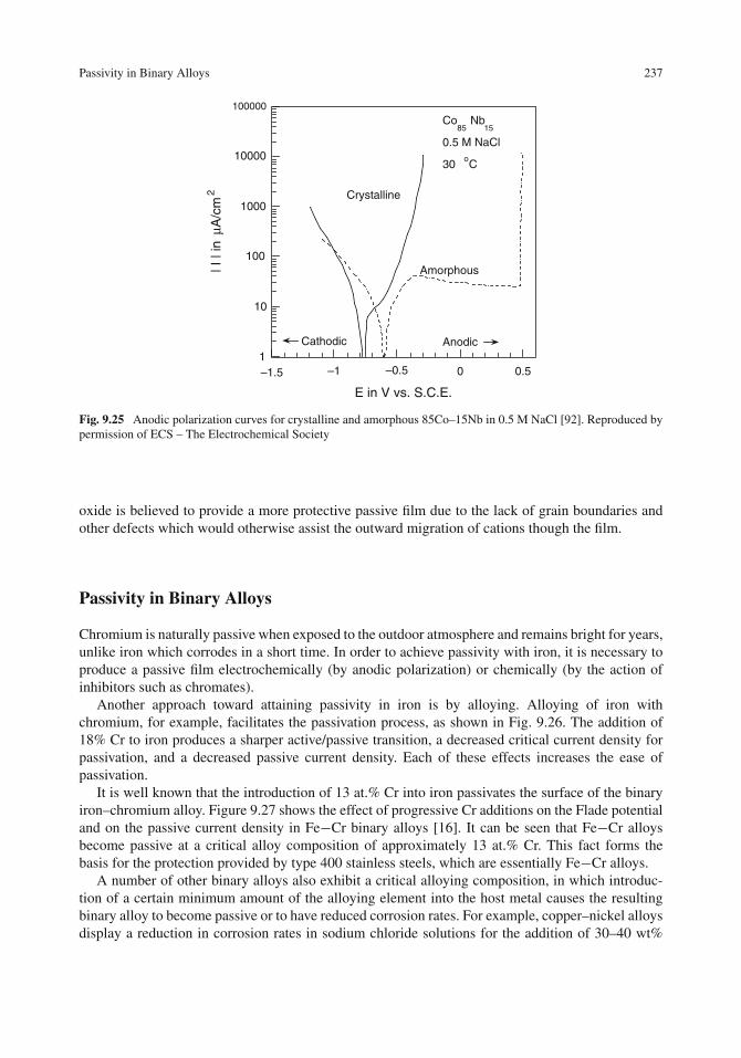
Passivity in Binary Alloys 237
1
10
100
1000
10000
100000
–1.5 –1 –0.5 0 0.5
| I |
in μ
A/c
m2
E in V vs. S.C.E.
Crystalline
Amorphous
Co85
Nb15
0.5 M NaCl
30 oC
AnodicCathodic
Fig. 9.25 Anodic polarization curves for crystalline and amorphous 85Co–15Nb in 0.5 M NaCl [92]. Reproduced bypermission of ECS – The Electrochemical Society
oxide is believed to provide a more protective passive film due to the lack of grain boundaries andother defects which would otherwise assist the outward migration of cations though the film.
Passivity in Binary Alloys
Chromium is naturally passive when exposed to the outdoor atmosphere and remains bright for years,unlike iron which corrodes in a short time. In order to achieve passivity with iron, it is necessary toproduce a passive film electrochemically (by anodic polarization) or chemically (by the action ofinhibitors such as chromates).
Another approach toward attaining passivity in iron is by alloying. Alloying of iron withchromium, for example, facilitates the passivation process, as shown in Fig. 9.26. The addition of18% Cr to iron produces a sharper active/passive transition, a decreased critical current density forpassivation, and a decreased passive current density. Each of these effects increases the ease ofpassivation.
It is well known that the introduction of 13 at.% Cr into iron passivates the surface of the binaryiron–chromium alloy. Figure 9.27 shows the effect of progressive Cr additions on the Flade potentialand on the passive current density in Fe−Cr binary alloys [16]. It can be seen that Fe−Cr alloysbecome passive at a critical alloy composition of approximately 13 at.% Cr. This fact forms thebasis for the protection provided by type 400 stainless steels, which are essentially Fe−Cr alloys.
A number of other binary alloys also exhibit a critical alloying composition, in which introduc-tion of a certain minimum amount of the alloying element into the host metal causes the resultingbinary alloy to become passive or to have reduced corrosion rates. For example, copper–nickel alloysdisplay a reduction in corrosion rates in sodium chloride solutions for the addition of 30–40 wt%

238 9 Passivity
0.1
1
10
100
1,000
10,000
100,000
1,000,000
–1 –0.5 0 0.5 1 1.5
Cur
rent
Den
sity
in
μA/c
m2
E in V vs. S.C.E.
430 stainless(Fe –18 Cr)
Fe
Cr
0.5 M H2SO4
Fig. 9.26 Anodic polarization curves for Fe, Cr, and Fe–18Cr (430 stainless steel) in 1 N H2SO4. Redrawn from [96]with permission of ECS – The Electrochemical Society and [97] with © NACE International (1962)
(32–43 at.%) nickel to copper [98], as shown in Fig. 9.28. In another example, the passive cur-rent densities for aluminum–zirconium alloys in 1 M HCl decrease dramatically for a critical alloycomposition of 24 at.% Zr [99], as shown in Fig. 9.29.
The Fe−Cr binary alloy system is the most important from an industrial point of view and has alsoattracted the most scientific interest. Several theories have been advanced to explain the occurrenceof a critical alloying composition in Fe−Cr binary alloys [93, 100–105], the most recent of which hasalso been extended to other binary alloys [104–109]. These theories are (i) the electron configurationtheory, (ii) oxide film effects, (iii) the percolation theory, and (iv) the graph theory model. The lastthree theories are not mutually exclusive, and in fact, the last two provide different explanations ofoxide film effects. Each of these theories is discussed briefly below.
Electron Configuration Theory
The electron configuration theory was proposed by Uhlig [100] and is an extension of the adsorptiontheory of passivity. Uhlig noted that a number of transition metals (which have unfilled d-shells)become passive at certain critical compositions when alloyed with a second metal. According to theelectron configuration theory, the passivity of a binary alloy depends on the tendency of unfilled d-bands of transition metals to become filled with electrons from alloying elements capable of donatingelectrons in such a way that chemisorption of oxygen is favored. For Fe−Cr alloys, the electronconfiguration of the two alloying elements are the following:
Fe [Ar] 3d6 4s2
Cr [Ar] 3d5 4s1
where [Ar] denotes that the inner shells of the atom have the same electron configuration as in theargon atom, and 3d6, for example, denotes that there are six electrons in the 3d level. Uhlig’s ideawas that a passive binary alloy would have an electron configuration as close as possible to that of

Passivity in Binary Alloys 239
–0.8
–0.6
–0.4
–0.2
0
0.2
0 5 10 15 20 25 30
King and Uhlig
Compiled from literaureCompiled from literatureF
lade
Pot
entia
l in
V v
s. S
.H.E
.
Percent Chromium
H2SO
4
pH 0
0.001
0.01
0.1
1
103
102
101
0 5 10 15 20
Crit
ical
Cur
rent
Den
sity
in m
A/c
m2
Percent Chromium
Deaerated 3% Na2SO
4
pH =7
Fig. 9.27 Top: the Flade potential of Fe–Cr alloys in H2SO4 (pH 0) as a function of the alloy composition. Bottom:The passive current density as a function of alloy composition [16]. Reproduced by permission of the AmericanChemical Society
an inert noble gas atom. In the Fe−Cr pair, Cr is the passive metal so that its d-bands become filledwith 4s electrons donated by Fe atoms. Electron configurations in a condensed (solid) metal aredifferent than in the isolated metal atom, as given in Table 9.5. The number of d-vacancies for themetal surface atom in Table 9.5 is the number of vacancies in the metal plus one due to the donationof one electron from each metal surface atom to a chemisorbed oxygen atom to form the O– surfacespecies, as shown in Fig. 9.30.
Thus, a Cr atom in the metal surface contains 4.0 d-electron vacancies. Iron atoms in the surfaceof the alloy can each donate (1.8–1.0) = 0.8 electrons to Cr. Thus, the number of Fe atoms required

240 9 Passivity
0.1
1.0
10.0
0 20 40 60 80 100
Cor
rosi
on R
ate
in g
md
Weight Percent Ni
30 wt. % Ni(32 at. % Ni)
Aerated 3% NaCl 80 oC
Uhlig and Revie
Fig. 9.28 Corrosion rates of copper–nickel binary alloys in 3% NaCl [98]. Reproduced by permission ofJohn Wiley & Sons, Inc
0.01
0.1
1
10
0 20 40 60 80 100
Pas
siva
tion
Cur
rent
Den
sity
in A
/m2
Atomic Percent Zr in Alloy
Al-Zr
1 M HCl
Fig. 9.29 Passive current densities for aluminum–zirconium binary alloys in 1 M HCl [99]
to donate electrons to fill the vacant d-bands of a surface Cr atom is 4.0/0.8 = 5.0 Fe atoms; theatomic percent of Cr is given by Cr/(Cr + Fe) = 1.0/(1.0 + 5.0) = 16.7 at.%, in nominal agreementwith the experimental value of 13 at.% where Fe−Cr alloys attain passivity.
This approach has also been used by Uhlig to explain critical alloy compositions in Cu–Ni, Fe–Ni, Fe–Co, Ni–Mo, Ni–Cr, and Co–Cr binary alloys, as shown in Table 9.6. In each case, there isa good agreement between predicted and observed critical alloy compositions. However, the usualcriticism of the electron configuration theory is that it fails to take into account the properties of theoxide film.

Passivity in Binary Alloys 241
Table 9.5 Electron configurations for various transition metals and for copper [100]
MetalAtomicconfiguration
d-Vacancies inatom
d-Vacancies inmetala
d-Vacancies inmetal surface
4s electronsdemoted tod-band
Cr [Ar] 3d5 4s 5 – 4.0b 2.0Fe [Ar] 3d6 4s2 4 2.2 3.2 1.8Co [Ar] 3d7 4s2 3 1.7 2.7 1.3Ni [Ar] 3d8 4s2 2 0.6 1.6 1.4Cu [Ar] 3d10 4s 0 0.0 0.0 0.0Mo [Kr] 4d6 5s 4 3.0 4.0 1.0
a From magnetic measurements.b Extrapolated value.
1e–O–
Cr
can accept4.0 e–
1e–
Cr
can accept4.0 e–
O–O–
1e–
Fe0.8 e–
Solution
Alloy surface
No. Fe atoms required = 4.00.8
= 5.0 Fe per Cr
At. % Cr = 1.0 Cr1.0 Cr + 5.0 Fe
= 16.7 at. %Cr
can donate
1.8 e–
Fig. 9.30 The electron configuration theory of passivity applied to Fe−Cr alloys [100]
Oxide Film Properties
There is considerable evidence that the properties of the oxide film are responsible for the onset ofpassivity in Fe-Cr binary alloys to occur at 13 at.% Cr. Various investigators have found that Cr isenriched in the passive film on Fe-Cr alloys [28, 101, 102]. The results of Asami et al. [28] have beengiven in Fig. 9.9, which shows that the cation fraction of Cr3+ in the oxide film increases dramaticallyat 10–13 at.% of Cr in the binary alloy. Recent in situ results of Oblonsky et al. [102] using XANESalso show an enrichment of Cr3+ in the passive films in a series of Fe−Cr alloys.
McBee and Kruger [93] showed the importance of the structure of the passive film on Fe−Cralloys in a study using electron diffraction. As Cr was added to Fe in a series of Fe−Cr alloys, thepassive films passed from crystalline to amorphous, as shown in Table 9.7. The authors attributedthe enhanced corrosion resistance of the higher content Cr alloys to the existence of an amorphousoxide film, with its concomitant improved properties, as discussed earlier.

242 9 Passivity
Table 9.6 Electron configurations and critical alloy compositions [100]
Predicted criticalcomposition
Binaryalloy
Acceptor ordonor?
d-Vacanciesin metalsurfacea
Number ofdonorelectrons At.% Wt%
Observedcriticalcomposition(wt%)b
NiCu
AD
1.61.0 38.5% Ni 36.6% Ni 30–40% Ni
CrFe
AD
4.00.8 16.7% Cr 15.7 % Cr 12% Cr
NiFe
AD
1.60.8 33.3% Ni 34% Ni 40% Ni
CoFe
AD
2.70.8 22.8% Co 23.8% Co 21–25% Co
MoNi
AD
4.00.4 9.1% Mo 14.7% Mo 10–15% Mo
CrNi
AD
4.00.4 9.1% Cr 8.2% Cr 7–9% Cr
CrCo
AD
4.00.3 7.0% Cr 6.2 % Cr 10% Cr
a After donation of one electron to O– surface species.b For specific aqueous environments, see [100].
Table 9.7 Structuralcharacteristics for the passiveoxide films on Fe−Cr binaryalloys [93]
Percentage Cr inalloy Structure of passive film
0 Well-oriented spinel5 Well-oriented spinel12 Poorly oriented spinel19 Mainly amorphous24 Completely amorphous
Percolation Theory
Sieradzki and Newman [103] applied percolation theory to explain the critical Cr composition forpassivity in Fe−Cr alloys. These authors considered that Cr atoms must come close enough to eachother so that adsorbed oxygen anions can bridge what is to become oxidized Cr. Based on atomicdistances and the concept of a cluster of Cr atoms in the body centered cubic lattice, percolationtheory was able to explain the threshold composition for passivity in Fe−Cr alloys.
As shown in Fig. 9.31, when an oxygen ion (O2–) bridges two Cr3+ ions, the maximum separationbetween the two Cr3+ ions is equal to twice the radius (0.69 Å) of the Cr3+ plus twice the radius(1.40 Å) of the O2– ion, or 4.18 Å. The distances between various nearest neighbors in the bccFe−Cr lattice having a lattice parameter a = 2.87 Å are given in Table 9.8.
Note that the distance of 4.18 Å required to bridge two Cr atoms is approximately the distancebetween third nearest neighbors in the bcc Fe−Cr lattice. Percolation processes show a sharp thresh-old pc, which represents the concentration of occupied sites at which a connected cluster suddenlyappears [110]. The pc for interactions up to third nearest neighbors is 10%. The pc for interactionsup to fourth nearest neighbors is 12%. These values correspond to Cr concentrations producing pas-sivity in Fe−Cr alloys. As the Cr atom concentration increases above pc, the infinite cluster growsrapidly absorbing smaller clusters [110].

Passivity in Binary Alloys 243
O– 2
Cr+3Cr+3
4.18 Å Max. separation between Cr+3 ions
Cr atoms must be close enough to be bridged by oxygen anions.
The distance 4.18 Å is approximately the distance between 3rd nearest neighbors in the bcc Fe–Crlattice. (See Table 9 – 8).
Percolation processes show a sharp threshold pc at which a connected cluster suddenly appears.
The pc for up to 3rd nearest neighbor is 10%.
The pc for up to 4th nearest neighbor is 12%.
As the Cr concentration increases above pc,
the cluster grows rapidly absorbing smaller clusters.
Fig. 9.31 Percolation theory and the passivity of Fe−Cr alloys [103]
Table 9.8 Distance between nearest neighbors in the Fe−Cr body centered cubic lattice [103]
Nearest neighbors
1st 2nd 3rd 4th
√3
2 a a√
2a√
3a2.49 Å 2.87 Å 4.06 Å 4.97 Å
a is the lattice parameter.
Graph Theory Model
Another approach [104–109] has recently been taken using graph theory and the concept of a con-nected network of −M−O−M− bridges in the passive oxide film, where M is the component of thebinary alloy giving rise to passivity. For Fe−Cr alloys, passivity is imparted by the addition of Cr toFe so that a connected network of −Cr−O−Cr− would lead to passivity.
A graph is a collection of points (vertices) connected by lines called edges. For example, Fig. 9.32is a graph of a floorplan in a residential home. The individual rooms are represented by points(vertices), and rooms which are physically connected in the house are connected on the graph byedges. Graphs have been used to represent and analyze various types of relationships in biology, thesocial sciences, and in systems research [111].
In regard to passivity, an oxide may be represented by a mathematical graph in which verticesand edges are used to designate atoms and their bonds. For Fe−Cr binary alloys, a network of unin-terrupted −Cr−O−Cr− bridges in the oxide film is first considered, and then random graph theoryis used to insert Fe3+ ions in a stochastic manner into the−Cr−O−Cr− network to form an oxide ofcomposition xFe2O3·(1–x)Cr2O3. The critical concentration of Fe3+ (and accordingly also of Cr3+)where the −Cr−O−Cr− network loses its connectivity is thus calculated. Or equivalently, the criti-cal concentration of Cr3+ in the oxide film (and also of Fe3+) is determined where the−Cr−O−Cr−

244 9 Passivity
bath
bath kitchendining roombedroom
bedroom bedroom
hallway living room
Fig. 9.32 The mathematical graph of the floorplan of a residence
network becomes connected. The composition of the oxide film is then related to the composition ofthe alloy substrate by means of empirical surface analysis information.
Based on the STM studies of Ryan et al. [65], as shown in Fig. 9.15, the structure of the passiveoxide film on an Fe–25 at.% Cr binary alloy can be represented by an array of irregular distortedhexagons. The corresponding mathematical graph is given in Fig. 9.33, where the vertices of thegraph represent Cr3+ ions and the edges represent O2– ions. If the total number of Cr3+ ions in thenetwork is given by N, then the total number of edges (O2– ions) is simply A(Go) = (3/2)N.
The−Cr−O−Cr− network, as represented by its graph Go, is characterized by two properties: itssize and configuration. The size of Go is given by the number of edges A(Go), and the configurationis given by a quantity called the Randic index X(Go) [112]:
Cr+3 ions are located at vertices
O– 2 ions are located at edges
Mathematical graph for Cr2O3
Fig. 9.33 The mathematical graph for Cr2O3 [104–106]. The vertices refer to Cr3+ ions and the edges connectingthem refer to O2– ions
X(Go) = �edges
(ij)−0.5 (14)
where i and j are the degrees of the vertices connecting the edge in question. (A vertex has a degree2, for example, if two edges meet at that vertex.) The Randic index has been used to characterize thedegree of branching of organic compounds, as shown in Fig. 9.34.

Passivity in Binary Alloys 245
7 carbons X(G) Randic
3.307
3.345
3.414
Fig. 9.34 Hydrocarbon isomers and the Randic index
Next, the composition of the oxide network is changed conceptually by insertion of Fe3+ ionsto produce a new graph G for the mixed oxide having new properties A(G) and X(G). The relativechange in the connectivity of the network is given by
δ = A(G)X(G)−A(Go)X(Go)
A(Go)X(Go)(15)
Large values of δ indicate that the connectivity of the new graph G (which contains the disruptingcation) is very much different than that for the original graph Go, whereas small values of δ meanthat the connectivity of the two graphs is similar. When the connectivities of the two graphs areidentical, then δ = 0, as can be seen by letting G = Go in Eq. (15).
The Randic index X(Go) for the −Cr−O−Cr− network is obtained as follows. Each vertex inFig. 9.33 has a degree 3 so that each edge contributes one-third to the Randic index:
(ij)−12 ≡
(1
3× 3
)12 = 1
3(16)
But there are (3/2)N total edges so that
X(Go) = 3
2N × 1
3= N
2(17)
See Table 9.9, which collects the various input quantities necessary to calculate theconnectivity δ.

246 9 Passivity
Table 9.9 Values of various quantities used in graph theory approach to passivity in Fe–Cr binary alloysa
Original graph Go for -Cr-O-Cr_
Number of edgesA(GO) = 3
2 N
Randic indexX(GO) = N
2
New graph G containing Fe3+
Number of edges
A(G)=N[
3−5x2(1−x)
]
X(G) =(
15
)5N
(1−x)5 (3− 5x){
24x4 + 24√
2x3(3− 5x)+ 4(√
3+ 3)x2(3− 5x)2 + 2√
6x(3− 5x)3 + 12 (3− 5x)4
}
Randic index
a N is the number of Cr3+ ions in the original graph Go for Cr2O3.x is the number of moles of Fe2O3 in the mixed oxide: xFe2O3·(1–x) Cr2O3.
Next, Fe3+ ions are introduced into the graph to produce the new graph G. See Fig. 9.35. Thecomposition of the oxide network after insertion of Fe3+ ions is xFe2O3·(1–x)Cr2O3. If D is thenumber of edges deleted in Go to form the new graph G and one Fe3+ is inserted per edge deletion(to preserve charge neutrality) then
Fe3+
Cr3+ =D
N=
x moles Fe2O3
(2 moles Fe3+mole Fe2O3
)
(1− x) moles Cr2O3
(2 moles Cr3+mole Cr2O3
) (18)
Then, A(G) = (3/2)N – D or
A(G) = N
[3− 5x
2(1− x)
](19)
x Fe 2 O3. (1 – x) Cr2 O3
Cr
Cr
Cr
Cr
CrCr
O
O
O
O
O
Cr
Cr
Cr Cr
CrCr
O
O
O
O
O
FeBreak an edge
and insert Fe+3
OO
Cr2 O3
Fig. 9.35 Insertion of Fe3+ ions into the graph for Cr2O3

Passivity in Binary Alloys 247
Unlike X(Go), the term X(G) cannot be calculated directly because it is not known which particu-lar edges have been deleted from Go to form G. A stochastic calculation is employed, the details ofwhich are given in Appendix F. The result is
X(G) =(
13
)5N
(1− x)5(3− 5x)
{24x4 + 24
√2x3(3− 5x)+ 4(
√3+ 3)x2(3− 5x)2
+ 2√
6x(3− 5x)3 + 1
2(3− 5x)4
} (20)
Insertion of expressions for A(G), X(G), A(Go), and X(Go) (as listed in Table 9.9) into Eq. (15)gives the following result:
δ =2(
13
)6(3− 5x)2
(1− x)6
{24x4 + 24
√2x3(3− 5x)+ 4(
√3+ 3)x2(3− 5x)2
+ 2√
6x(3− 5x)3 + 1
2(3− 5x)4
}− 1
(21)
Figure 9.36 shows the behavior of δ as a function of the composition of the oxide film. (δ ≈ 0when G ≈ Go.) It can be seen that an atomic fraction of Fe3+ in the oxide film of 0.70 suffices tobreak down the −Cr−O−Cr− network. That is, an atomic fraction of 0.30 of Cr3+ ions in the oxidefilm provides a continuous −Cr−O−Cr− network, for which δ ≈ 0. (The calculated results for δ
pass through 0 for (1–x) ≈ 0.30 but are plotted as absolute values in Fig. 9.36). Figure 9.36 clearlyshows that there is a critical concentration of Cr3+ ions in the oxide film which is needed to providea continuous network of −Cr−O−Cr− linkages in the oxide film.
–2
0
2
4
6
8
10
12
0.00 0.20 0.40 0.60
0.300.500.700.90
log
|δ|
x, mole fraction Fe2O3
(1–x), mole fraction Cr2O3
The mixed oxide network becomes like the –Cr–O–Cr–network at 0.30 mole fraction Cr2O3
(0.30 cation fraction Cr+3)
Fig. 9.36 The behavior of the connectivity function δ as a function of the oxide composition for Fe2O3–Cr2O3 mixedoxides [104–106]. Reproduced by permission of Elsevier Ltd

248 9 Passivity
0
20
40
60
80
100
8 10 12 14 16 18 20 22 24
Ato
mic
% o
f Cr+
3 in
Oxi
de
Atomic % of Cr 0 in Alloy
Oblonsky et al. (1998) Acetate buffer pH 4.5
Fig. 9.37 Chromium content in the passive film on Fe−Cr binary alloys as a function of the chromium contentin the alloy after immersion in an acetate buffer. Redrawn from [102]. Reproduced by permission of ECS – TheElectrochemical Society
From the XPS data of Asami et al. [28] for Fe−Cr alloys shown in Fig. 9.9, a cation fraction of0.30 Cr3+ in the oxide film corresponds to a metal alloy composition of approximately 13 at.% Cr.More recent in situ XANES data of Oblonsky et al. [102] show that an atomic fraction of 0.30 Cr3+
in the oxide film corresponds to an atomic fraction of 0.13 Cr in the Fe−Cr alloy. See Fig. 9.37. Thisresult is in excellent agreement with the well-known observation that 13 at.% chromium inducespassivity in Fe−Cr alloys.
The graph theory approach has successfully explained the occurrence of critical alloy composi-tions in 18 different binary alloys [104–109]. Some results are given in Table 9.10.
The exact mechanism of protection by a continuous network of the passivating oxide is not knownwith certainty. One possibility is that the network of −M−O−M− chains is more stable in theaqueous solution than is the second component of the oxide film. A second possibility (related to thefirst) is that the tangled network of −M−O−M− chains restricts the transport of ions and defectsthrough the passive oxide film.
Table 9.10 Results from application of graph theory to the passivity of various binary alloys [104–109]
Alloysystem
Critical molefraction of oxideobtained fromgraph theory δ
Calculated ionicmole fraction inoxide
Correspondingalloycompositionfrom surfaceanalysis data
Observed criticalalloycompositionfrom corrosiondata
Fe−Cr 0.31 Cr2O3 0.31 Cr3+ 13 at.% Cr 13 at.% CrNi−Cr 0.13 Cr2O3 0.23Cr3+ 7 at.% Cr 8–10 at.% CrCu−Ni 0.45 NiO 0.45 Ni2+ ∼30 at.% Ni 30–40 at.% NiFe−Si 0.36 SiO2 0.22 Si4+ 30 at.% Si 26–30 at.% SiCo−Cr 0.13 Cr2O3 0.23 Cr3+ 6 at.% Cr 9–11 at.% CrAl−Cr 0.31 Cr2O3 0.31 Cr3+ ∼50 at.% Cr 40–50 at.% CrCr−Mo 0.28 MoO2 0.16 Mo4+ 21 at.% Mo 20 at.% MoCr−Zr 0.28 ZrO2 0.16 Zr4+ 16 at.% Zr 10 at.% ZrMo−Ti 0.21 TiO2 0.21 Ti4+ 58 at.% Ti ˜60 at.% Ti

Passivity in Stainless Steels 249
Passivity in Stainless Steels
Stainless steels are commercial alloys containing a minimum of approximately 11 wt% chromium.This amount of chromium prevents the formation of rust in the natural atmosphere, and thisobservation is the origin of the term “stainless.” See Fig. 9.38. The stainless steel “family tree”is depicted in Fig. 9.39, and the compositions of several common stainless steels are given inTable 9.11. Type 304 stainless steel is commonly used for applications requiring good corrosionresistance and formability. However, this alloy is subject to pitting and crevice corrosion, and type316 is frequently used in its stead when localized corrosion poses a problem. Higher alloys, such as
Fig. 9.38 Not all steels are created equally. From the Washington Post, January 24, 2004 and by permission of DaveCoverly and Creators Syndicate, Inc

250 9 Passivity
Fe
Fe-Cr-Ni(e.g., Type 304)
Higher alloys(e.g., Alloy 625)
Fe-Cr-Ni-Mo(e.g., Type 316)
(e.g., Type 430)
Fig. 9.39 The stainless steel family tree
Table 9.11 Composition (by wt%) of selected stainless steels and higher alloys [135]
UNSa AISIb Cr Ni Mo Fe C Mn Other
S40300 403 11.5–13 Balance 0.15 1.0 Si 0.5S43000 430 16–18 Balance 0.12 1.0 Si 1.0S30400 304 18–20 8–10 Balance 0.08 2.0 Si 1.0S30403 304L 18–20 8–12 Balance 0.03 2.0 Si 1.0S31600 316 16–18 10–14 2–3 Balance 0.08 2.0 Si 1.0N06625 625 20–23 Balance
(∼ 60)8–10 5 0.1 0.5 Nb 4.15
N10276 C-276 14.5–16.5 Balance(∼55)
15–17 7 0.02 1.0 Co 2.5W 4.5
a Unified Numbering System.b American Iron and Steel Institute Designation.
alloy 625 and alloy C-276, which are Cr−Ni−Mo alloys (rather than steels), provide increased cor-rosion resistance in aggressive environments; but these two alloys can also suffer crevice corrosionin some instances.
The corrosion resistance of each of these alloys depends on the existence of a passive oxidefilm.
Electrochemical Aspects
Figure 9.40 compares anodic polarization curves in for pure iron, type 430 stainless steel, and type304 stainless steel in 0.5 M H2SO4 [113]. As seen in Table 9.11, type 430 stainless steel containschromium as an alloyed element, and type 304 contains both chromium and nickel. The criticalcurrent density for passivation follows the order: Fe > 430 stainless steel > 304 stainless steel. Thus,it is easier to passivate type 304 stainless steel than either type 430 stainless or pure iron. (The passivecurrent densities for type 430 stainless steel and type 304 are similar but are each considerably lowerthan that for iron).

Passivity in Stainless Steels 251
0.1
1
10
100
1,000
10,000
100,000
1,000,000
-0.50 0.0 0.50 1.0 1.5
Cur
rent
Den
sity
in
µA/c
m2
E in V vs. S.C.E.
Fe
430
304
0.5 M H 2SO4
H2-saturated
Fig. 9.40 Anodic polarization curves for iron, 430 stainless steel (Fe–18Cr), and 304 stainless steel (Fe–18Cr–8Ni)in 0.5 M H2SO4 [113]. Reproduced with permission from The McGraw-Hill Companies
The effect of various alloying elements on electrochemical passivation has been determined bystudies in which one element is systematically added to one or two others. For example, Fig. 9.41shows the effect of Mo additions on the anodic polarization curves of an Fe−Cr alloy in 0.5 MH2SO4 [114]. As seen in Fig. 9.41, progressive additions of Mo to the Fe−Cr alloy decrease thecritical current density for passivation icrit and also the passive current density ipass. By collectingobservations similar to this, a set of “rules” can be formulated as to whether a given alloying elementis beneficial to passivation. (An element will be considered to be beneficial if its addition reducesthe critical current density for passivation icrit and/or the passive current density ipass).
– 7
– 6
– 5
– 4
– 3
– 2
– 1
– 1000 – 500 0 500 1000 1500
log
|i| in
A/c
m2
E in mV vs. S.C.E.
Fe–18 Cr
Fe–18 Cr–2 Mo
Fe –18 Cr – 4.75 Mo
0. 5 M H2SO4
Fig. 9.41 Effect of Mo additions on the anodic behavior of Fe–18Cr alloys in 0.5 M H2SO4 [114]. Reproduced bypermission of ECS – The Electrochemical Society
252 9 Passivity
Thus, the following effects have been observed in passivation:
Cr is beneficial to Fe [15, 16, 115].Cr is beneficial to Ni [116].Cr is beneficial to Fe−Ni [117].Cr is beneficial to Fe−Ni−Mo [118].Cr is not beneficial to Mo [119, 120].
Mo is not beneficial to Fe [118, 121, 122].Mo is not beneficial to Ni [123].Mo is beneficial to Cr [119, 120].Mo is beneficial to Fe−Cr [114, 124].Mo is beneficial to Fe−Cr−Ni [118].
Hence, Mo is beneficial only when Cr is present.
Ni is beneficial to Fe [125].Ni is beneficial to Mo [123].Ni is not beneficial to Cr [116].
From these “rules”, the effect of Cr on the passivation of Fe, Ni, or Mo is illustrated in Fig. 9.42,where the arrow indicates the direction of beneficial alloying. The effect of alloying by the otherthree elements is also shown in Fig. 9.42. While the relationships in Fig. 9.42 hold for binary alloys,the trends may break down for ternary alloys.
Fe
Mo
Cr Ni
Trends for Binary Alloys
Fig. 9.42 The effect of various metallic elements on passivity in binary alloys. The arrow indicates that the effect isa beneficial one. For example, additions of Cr to Fe are beneficial, and additions of Mo to Fe are not beneficial
Polarization curves can provide interesting data on the effects of alloying on passivation butgive no information on the nature of the passive films which are formed on the alloy. Instead, itis necessary to employ surface analytical techniques to experimentally obtain the composition or thestructure of the passive films.
Composition of Passive Films on Stainless Steels
The nature of the passive film on stainless steels is complex but is a mixture of metal oxides andhydroxides or oxyhydroxides, with the films possibly containing bound water. The results of one ofthe earliest analyses of passive films using XPS are shown in Fig. 9.43 for type 304 stainless steel

Passivity in Stainless Steels 253
0
10
20
30
40
50
60
70
80
0.0 0.50 1.0 1.5 2.0 2.5 3.0
Ato
mic
Per
cent
Etch Depth in nm
Fe+3
O–2
Cr+3
Ni+2
Fig. 9.43 XPS sputter profiles of the passive film formed on type 304 stainless steel in flowing deoxygenated waterat 80◦C [126]. Reproduced by permission of Elsevier Ltd
[126]. It can be seen that the passive film contains oxides of both Cr and Ni, as well as of Fe. Theouter region of the film contains Cr3+, while the inner and outer regions contain both Cr3+ and Ni2+.
The results of a more recent XPS investigation on the passive film on a Mo-containing stainlesssteel were given earlier in Fig. 9.12. When the stainless steel contains molybdenum as an alloyingelement, Mo4+ is usually incorporated into the inner region of the passive film, whereas Mo6+ ispresent in the outer layer [60, 127]. It has been suggested that molybdate ions may act as cation-selective species in the outer layer producing a bipolar passive film, with the inner layer whichcontains Cr2O3 being anion selective, as discussed earlier. Thus, the inward passage of aggressiveanions (such as Cl–) through the film is not favored. In addition, the outward passage of cationsproduced by metallic dissolution at the metal/oxide interface is similarly not favored.
This model of the passive oxide film on Mo-containing stainless steels is given in Fig. 9.44[60, 127].
The surface analysis of passive films on stainless steels continues to be a subject of activeexperimental interest.
Cl–, OH–
x
–– –
––
Anionselectivelayer
Cationselectivelayer
x
Me+n
++
++
+
MeO4–n
Cr(O H)3
Cr Cr2O 3
OH– O–2 + H+
Inner oxidebarrierMetal
Fig. 9.44 The bipolar model of passivity applied to Mo-containing stainless steels [60, 127]. Reproduced bypermission of ECS – The Electrochemical Society

254 9 Passivity
Passivity by Alloying with Noble Metals
Metals which undergo an active/passive transition can be made passive by alloying with noble met-als such as palladium or platinum. This idea [128, 129] is illustrated in Fig. 9.45 for Ti-Pd alloys inhot acid solutions. Titanium can be passivated in boiling sulfuric acid solutions, but only after under-going an active/passive transition following extensive anodic dissolution. The cathodic polarizationcurve for titanium in Fig. 9.45 is drawn using the exchange current density for hydrogen evolution ontitanium given in Table 7.3 and with a cathodic Tafel slope of –0.100 V/decade. As seen in Fig. 9.45,the cathodic and anodic polarization curves for titanium intersect in the active region of the anodiccurve so that at open-circuit potential, titanium freely undergoes active dissolution.
log
|I| i
n A
/cm
2
Anodic (Ti)2
H++
2e–
H 2(o
n Pd
)H 2
(on
Ti)
more +E
Cathodic(Ti)
Eo,H
2 H
++
2e–
Icorr(Ti-Pd)
Io,H on Pd
Io,H on Ti
Ecorr (Ti-Pd)
Ecorr (Ti)
Icorr (Ti)
10–3
10–5
10–7
10–9
Fig. 9.45 Electrochemical basis for the passivation of titanium by alloying with palladium (drawn for a Ti–2% Pdalloy)
However, when titanium is alloyed with a noble metal, such as palladium, the hydrogen evo-lution reaction occurs both on Ti surface sites and on Pd surface sites, as depicted in Fig. 9.46.The exchange current density for hydrogen evolution on Pd is five orders of magnitude higher thanon Ti so that the total rate of hydrogen evolution at any electrode potential is dominated by thereaction on Pd sites, even for a dilute alloy, as shown in Fig. 9.45, which is constructed for a Ti–2 at.%
3 H+ + 3 e–→ 32
H2 (on Pd) 3 H+ + 3 e–→ 32
H2 (on Ti)
Pd
Ti+3 Ti+3
TiTi
3 e– 3 e–
Fig. 9.46 Types of surface sites on Ti-Pd alloys
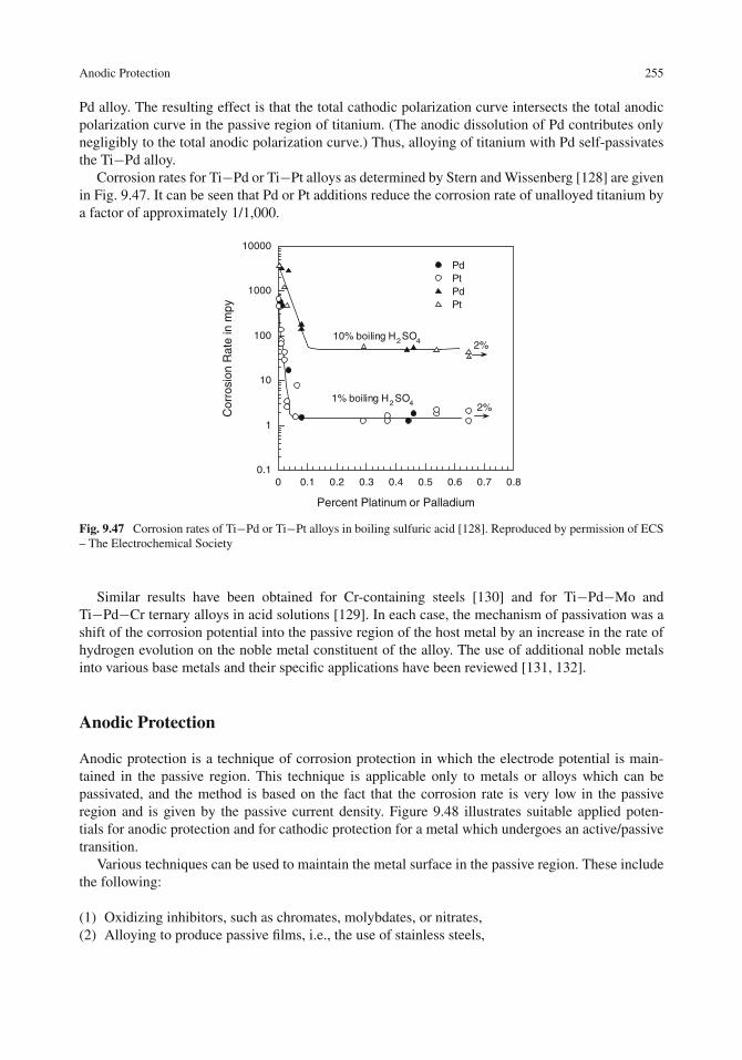
Anodic Protection 255
Pd alloy. The resulting effect is that the total cathodic polarization curve intersects the total anodicpolarization curve in the passive region of titanium. (The anodic dissolution of Pd contributes onlynegligibly to the total anodic polarization curve.) Thus, alloying of titanium with Pd self-passivatesthe Ti−Pd alloy.
Corrosion rates for Ti−Pd or Ti−Pt alloys as determined by Stern and Wissenberg [128] are givenin Fig. 9.47. It can be seen that Pd or Pt additions reduce the corrosion rate of unalloyed titanium bya factor of approximately 1/1,000.
0.1
1
10
100
1000
10000
0 0.1 0.2 0.3 0.4 0.5 0.6 0.7 0.8
PdPtPdPt
Cor
rosi
on R
ate
in m
py
Percent Platinum or Palladium
10% boiling H2SO4
1% boiling H2SO4
2%
2%
Fig. 9.47 Corrosion rates of Ti−Pd or Ti−Pt alloys in boiling sulfuric acid [128]. Reproduced by permission of ECS– The Electrochemical Society
Similar results have been obtained for Cr-containing steels [130] and for Ti−Pd−Mo andTi−Pd−Cr ternary alloys in acid solutions [129]. In each case, the mechanism of passivation was ashift of the corrosion potential into the passive region of the host metal by an increase in the rate ofhydrogen evolution on the noble metal constituent of the alloy. The use of additional noble metalsinto various base metals and their specific applications have been reviewed [131, 132].
Anodic Protection
Anodic protection is a technique of corrosion protection in which the electrode potential is main-tained in the passive region. This technique is applicable only to metals or alloys which can bepassivated, and the method is based on the fact that the corrosion rate is very low in the passiveregion and is given by the passive current density. Figure 9.48 illustrates suitable applied poten-tials for anodic protection and for cathodic protection for a metal which undergoes an active/passivetransition.
Various techniques can be used to maintain the metal surface in the passive region. These includethe following:
(1) Oxidizing inhibitors, such as chromates, molybdates, or nitrates,(2) Alloying to produce passive films, i.e., the use of stainless steels,
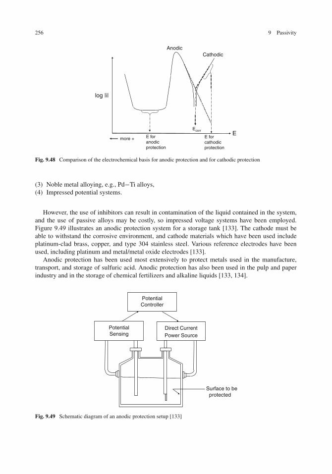
256 9 Passivity
log |i|
more + E forcathodicprotection
Ecorr
E foranodicprotection
E
AnodicCathodic
Fig. 9.48 Comparison of the electrochemical basis for anodic protection and for cathodic protection
(3) Noble metal alloying, e.g., Pd−Ti alloys,(4) Impressed potential systems.
However, the use of inhibitors can result in contamination of the liquid contained in the system,and the use of passive alloys may be costly, so impressed voltage systems have been employed.Figure 9.49 illustrates an anodic protection system for a storage tank [133]. The cathode must beable to withstand the corrosive environment, and cathode materials which have been used includeplatinum-clad brass, copper, and type 304 stainless steel. Various reference electrodes have beenused, including platinum and metal/metal oxide electrodes [133].
Anodic protection has been used most extensively to protect metals used in the manufacture,transport, and storage of sulfuric acid. Anodic protection has also been used in the pulp and paperindustry and in the storage of chemical fertilizers and alkaline liquids [133, 134].
PotentialSensing
Direct CurrentPower Source
PotentialController
Surface to beprotected
Fig. 9.49 Schematic diagram of an anodic protection setup [133]
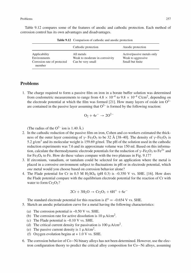
Problems 257
Table 9.12 compares some of the features of anodic and cathodic protection. Each method ofcorrosion control has its own advantages and disadvantages.
Table 9.12 Comparison of cathodic and anodic protection
Cathodic protection Anodic protection
Applicability All metals Active/passive metals onlyEnvironments Weak to moderate in corrosivity Weak to aggressiveCorrosion rate of protected
memberCan be very small Small but finite
Problems
1. The charge required to form a passive film on iron in a borate buffer solution was determinedfrom coulometric measurements to range from 4.8 × 10⁻⁴ to 9.8 × 10⁻⁴ C/cm2, depending onthe electrode potential at which the film was formed [21]. How many layers of oxide ion O2–
are contained in the passive layer assuming that O2– is formed by the following reaction:
O2 + 4e− → 2O2−
(The radius of the O2– ion is 1.40 Å.)2. In the cathodic reduction of the passive film on iron, Cohen and co-workers estimated the thick-
ness of the outer layer consisting of γ- Fe2O3 to be 32 Å [38–40]. The density of γ–Fe2O3 is5.2 g/cm3 and its molecular weight is 159.69 g/mol. The pH of the solution used in the cathodicreduction experiments was 7.6 and its approximate volume was 150 ml. Based on this informa-tion, calculate the thermodynamic electrode potentials for the reduction of γ–Fe2O3 to Fe2+ andfor Fe3O4 to Fe. How do these values compare with the two plateaus in Fig. 9.17?
3. If zirconium, vanadium, or tantalum could be selected for an application where the metal isplaced in a corrosive environment subject to fluctuations in pH or in electrode potential, whichone metal would you choose based on corrosion behavior alone?
4. The Flade potential for Cr in 0.5 M H2SO4 (pH 0.3) is –0.350 V vs. SHE. [16]. How doesthe Flade potential compare with the equilibrium electrode potential for the reaction of Cr withwater to form Cr2O3?
2Cr+ 3H2O→ Cr2O3 + 6H+ + 6e−
The standard electrode potential for this reaction is Eo = –0.654 V vs. SHE.5. Sketch an anodic polarization curve for a metal having the following characteristics:
(a) The corrosion potential is –0.50 V vs. SHE.(b) The corrosion rate for active dissolution is 10 μA/cm2.(c) The Flade potential is –0.10 V vs. SHE.(d) The critical current density for passivation is 100 μA/cm2.(e) The passive current density is 1 μA/cm2.(f) Oxygen evolution begins at + 1.0 V vs. SHE.
6. The corrosion behavior of Co−Ni binary alloys has not been determined. However, use the elec-tron configuration theory to predict the critical alloy composition for Co−Ni alloys, assuming

258 9 Passivity
that Ni is the acceptor in the alloy pair. What reservations do you have in using the electronconfiguration theory?
7. From film stripping studies have been conducted [23] on 304 stainless steel having the compo-sition by weight of 18% Cr, 8% Ni, and the balance Fe. The oxide film on this stainless steelwas found to contain 32 wt% Fe, 13.4 wt% Cr, and 9.4 wt% Ni (the balance is due to oxygeneither in the oxide or contained in bound water). The oxide film thickness was 30 Å, and thetypical weight gain due to oxide film formation was 2.0 μg/cm2. The density of 304 stainlesssteel is 7.0 g/cm3. Assume that the oxide film is a mixture of Fe2O3, Cr2O3, and NiO. Calculatethe Pilling–Bedworth ratio for this oxide and use this ratio to predict whether the oxide filmwould be protective. To calculate the Pilling–Bedworth ratio, it is first necessary to calculate theeffective molecular weight of the oxide, its effective value of n, and the effective atomic weightof the metal.
8. Use the alloying trends in Fig. 9.42 to predict the effect of Mo additions to Fe−Ni alloys on thepassivity in the resulting ternary alloy. Keep a constant nickel content in the ternary alloy.
9. A steel tank car is used to transport a fertilizer solution. This solution is corrosive to steel, soit is necessary to provide some form of protection to the internal surfaces of the tank car. Thetank car is equipped with a device which can control the electrode potential of the internal steelsurface when the tank car is filled. The polarization curve for steel in the fertilizer solution isshown below.
10
100
1000
10000
–1–0.8–0.6–0.4–0.200.20.40.6
Cur
rent
Den
sity
in μ
A/c
m2
E in V vs. S.C.E.
Anodic Cathodic
(a) What is the corrosion current density of the steel in the freely corroding condition?(b) What potential can be safely used in providing anodic protection?(c) What is the corrosion current density at this applied anodic potential?(d) Under the condition in Part (c), what is the loss of thickness of the tank car wall after a
10-day service period? Assume that the corrosion reaction is Fe→ Fe2++2e−. The atomicweight of Fe is 55.85 and its density is 7.87 g/cm3.
(e) What potential can be used if cathodic protection is applied to give the same corrosion rateas in Part (c)?
10. Sketch the experimentally observed anodic and cathodic polarization curves which result fromeach of the following sets of theoretical curves. Indicate the corrosion potential on each of theexperimental curves and indicate the anodic and cathodic portions of each experimental curve.What can you say about the stability of the system for curve (c) below?

Problems 259
log |i|
More +E
Anodic Cathodic(a)
log |i|
More +E
Anodic
Cathodic
(b)
log |i|
More +E
Anodic
Cathodic(c)

260 9 Passivity
References
1. D. D. Macdonald, Pure Appl. Chem., 71, 951 (1999).2. M. Pourbaix, “Atlas of Electrochemical Equilibria in Aqueous Solutions”, National Association of Corrosion
Engineers, Houston, TX (1974).3. H. H. Uhlig in “Passivity of Metals”, R. P. Frankenthal and J. Kruger, Eds., p. 1, The Electrochemical Society,
Princeton, NJ (1978).4. E. McCafferty and J, P. Wightman, Surf. Interface Anal., 26, 549 (1998).5. E. McCafferty, J. P. Wightman, and T. F. Cromer, J. Electrochem. Soc., 146, 2849 (1999).6. Z. Tun, J. J. Noël, and D. W. Shoesmith, J. Electrochem. Soc., 146, 988 (1999).7. V. V. Andreeva, Corrosion, 20, 35t (1964).8. C. A. Sequeira in “Uhlig’s Corrosion Handbook”, R. W. Revie, Ed., p. 729, John Wiley and Sons, New York
(2000).9. J. D. Venables, D. K. McNamara, J. M. Chen, T. S. Sun, and R. L. Hopping, Appl. Surf. Sci., 3, 88 (1979).
10. N. Sato in “Passivity of Metals”, R. P. Frankenthal and J. Kruger, Eds., p. 29, The Electrochemical Society,Princeton, NJ (1978).
11. U. F. Franck, Z. Naturforsch, 4a, 378 (1949).12. E. McCafferty, M. K. Bernett, and J. S. Murday, Corros. Sci, 28, 559 (1988).13. H. P. Leckie and H. H. Uhlig, J. Electrochem. Soc., 113, 1262 (1966).14. H. H. Uhlig, Official Digest, p. 650, October (1952).15. Y. M. Kolotrykin, “First International Congress on Metallic Corrosion”, p. 10, Butterworths, London (1962).16. P. F. King and H.H. Uhlig, J. Phys. Chem., 63, 2026 (1959).17. U. R. Evans, J. Chem. Soc. (London), 127, 1020 (1927).18. N. Hackerman, Z. Elektrochem., 62, 632 (1958).19. B. Kabanov, R. Burstein, and A. Frumkin, Discussions Faraday Soc., 1, 259 (1947)20. E. S. Snavely, Jr. and N. Hackerman, Can. J. Chem., 37, 268 (1959).21. R. P. Frankenthal, Electrochim. Acta, 16, 1845 (1971).22. H. H. Uhlig, Z. Elektrochem., 62, 626 (1958).23. N. A. Nielsen and T. N. Rhodin, Jr., Z. Elektrochem., 62, 707 (1958).24. T. N. Rhodin, Jr., Corrosion., 12, 123t (1956).25. E. M. Mahla and N. A. Nielsen, J. Electrochem. Soc., 93, 1 (1948).26. C. L. Foley, J. Kruger, and C. J. Bechtoldt, J. Electrochem. Soc., 114, 994 (1967).27. M. J. Pryor and D. S. Keir, J. Electrochem. Soc., 102, 370 (1955).28. K. Asami, K. Hashimoto, and S. Shimodaira, Corros. Sci., 18, 151 (1978).29. R. P. Frankenthal, J. Electrochem. Soc., 114, 542 (1967).30. M. J. Graham, Corros. Sci., 37, 1377 (1995).31. J. F. Watts, “An Introduction to Surface Analysis by Electron Spectroscopy”, p. 67, Oxford University Press,
Oxford, England (1990).32. J. C. Vickerman, Ed., “Surface Analysis- The Principal Techniques”, John Wiley & Sons, New York, NY (1997).33. F. Falkenberg and I. Olejford in “Passivity of Metals and Semiconductors”, M. B. Ives, J. L. Luo, and
J. R. Rodda, Eds., p. 570, The Electrochemical Society, Pennington, NJ (2001).34. A. J. Davenport and M. Sansome, J. Electrochem. Soc., 142, 725 (1995).35. P. Schmuki, S. Virtanen, A. J. Davenport, and C. M. Vitus, J. Electrochem. Soc., 143, 574 (1996).36. D. C. Koningsberger and R. Prins, Eds., “X-Ray Absorption”, John Wiley & Sons, New York, NY (1988).37. M. Ryan, R. C. Newman, and G. E. Thompson, J. Electrochem. Soc., 141, L164 (1994).38. C. D. Stockbridge, P. B. Sewell, and M. Cohen, J. Electrochem. Soc., 108, 928 (1961).39. P. B. Sewell, C. D. Stockbridge, and M. Cohen, J. Electrochem. Soc., 108, 933 (1961).40. M. Nagayama and M. Cohen, J. Electrochem. Soc., 109, 781 (1962).41. E. McCafferty and A. C. Zettlemoyer, Discuss. Faraday Soc., 52, 239 (1971).42. M. Seo, J. B. Lumsden, and R. W. Staehle, Surf. Sci., 42, 337 (1974).43. M. Cohen, D. F. Mitchell and K. Hashimoto, J. Electrochem. Soc., 126, 442 (1979).44. M. C. Bloom and L. Goldenberg, Corros. Sci., 5, 623 (1965).45. M. Cohen in “Passivity of Metals”, R. P. Frankenthal and J. Kruger, Eds., p. 521, The Electrochemical Society,
Princeton, NJ (1978).46. S. C. Tjong and E. Yeager, J. Electrochem. Soc., 128, 2251 (1981).47. V. Schroder and T. Devine, J. Electrochem. Soc., 146, 406 (1999).48. T. N. Rhodin, Jr., Annals N.Y. Acad. Sci., 58, 855 (1954).

References 261
49. G. Okamota and T. Shibata, Nature, 206, 1350 (1965).50. G. Okamota and T. Shibata, “Proc. 3rd International Congress on Metallic Corrosion”, Moscow (1966), Vol. 1,
p. 396 (1969).51. G. Okamota, and T. Shibata, Corros. Sci., 10, 371 (1970).52. H. T. Yolken, J. Kruger, and J. P. Calvert, Corros. Sci., 8, 103 (1968).53. O. J. Murphy, J. O’M. Bockris, T. E. Pou, D. L. Cocke, and G. Sparrow, J. Electrochem. Soc., 129, 2149 (1982).54. U. Stumm, W. Meisel, and P. Gütlich, Hyperfine Inter., 28, 923 (1986).55. C. Vertes, M. Lakatos-Varsanyi, A. Vertes, E. Kuzmann, W. Meisel, and P. Gütlich, Hyperfine Inter., 69, 731
(1991).56. J. Eldridge and R. W. Hoffman, J. Electrochem. Soc., 136, 955 (1989).57. W. E. O’Grady, J. Electrochem. Soc., 127, 555 (1980).58. G. Okamoto and T. Shibata, in Passivity of Metals”, R. P. Frankenthal and J. Kruger, Eds., p. 646, The
Electrochemical Society, Princeton, NJ (1978).59. M. Sakashita and N. Sato in Passivity of Metals”, R. P. Frankenthal and J. Kruger, Eds., p. 479, The
Electrochemical Society, Princeton, NJ (1978).60. C. R. Clayton and Y. C. Lu, J. Electrochem. Soc., 133, 2465 (1986).61. L. J. Oblonsky, A. J. Davenport, M. P. Ryan, H. S. Isaacs, and R. C. Newman, J. Electrochem. Soc., 144, 2388
(1997).62. L. J. Oblonsky, A. J. Davenport, M. P. Ryan, and M. F. Toney, in “Passivity of Metals and Semiconductors”,
M. B. Ives, J. L. Luo, and J. R. Rodda, Eds., p. 173, 962, The Electrochemical Society, Pennington, NJ (2001).63. A. F. Wells, “Structural Inorganic Chemistry”, p. 552, Clarendon Press, Oxford (1984).64. G. G. Long, J. Kruger, D. R. Black, and M. Kuriyama, J. Electroanal. Chem., 150, 603 (1983).65. M. P. Ryan, R. C. Newman, and G. E. Thompson, J. Electrochem. Soc., 142, L177 (1995).66. R. S. Alwitt in “Oxides and Oxide Films”, J. W. Diggle and A. K. Vijh, Eds., Vol. 4. p. 169, Marcel Dekker,
New York (1976).67. W. Vedder and D. A. Vermilyea, Trans Faraday Soc., 65, 561 (1969).68. T. Hurlen, A. T. Haug, and G. A. Salomonsen, Electrochim. Acta, 29, 1161 (1984).69. H. P. Godard, J. Electrochem. Soc., 114, 354 (1967).70. R. K. Hart, Trans. Faraday Soc., 52, 1020 (1957).71. R. S. Alwitt and L. C. Archibald, Corrosion Sci., 13, 687 (1973).72. S. Wernick, R. Pinner, and P. G. Sheasby, “The Surface Treatment and Finishing of Aluminum and its Alloys”,
Vol. 1, p. 471, ASM International, Metals Park, OH (1987).73. G. R. T. Scheuller, S. R. Taylor, and E. E. Hajcsar, J. Electrochem. Soc., 139, 2799 (1992).74. S. Wernick, R. Pinner, and P. G. Sheasby, “The Surface Treatment and Finishing of Aluminum and its Alloys”,
Vol. 1, p. 292, ASM International, Metals Park, OH (1987).75. G. E. Thompson, Y. Xu, P. Skeldon, K. Shimizu, S. H. Han, and G. C. Wood, Phil. Mag. B, 55, 651 (1987).76. S. Wernick, R. Pinner, and P. G. Sheasby, “The Surface Treatment and Finishing of Aluminum and its Alloys”,
Vol. 1, p. 453, ASM International, Metals Park, OH (1987).77. S. Wernick, R. Pinner, and P. G. Sheasby, “The Surface Treatment and Finishing of Aluminum and its Alloys”,
Vol. 2, p. 773, ASM International, Metals Park, OH (1987).78. S. Wernick, R. Pinner, and P. G. Sheasby, “The Surface Treatment and Finishing of Aluminum and its Alloys”,
Vol. 2, p. 729, ASM International, Metals Park, OH (1987).79. V. Brusic in “Oxides and Oxide Films”, Vol. 1, p. 1, J. W. Diggle, Ed., Marcel Dekker, New York (1972).80. J. Kruger, Inter. Mater. Revs., 33, 113 (1988).81. J. W. Schultze and M. M. Lohrengel, Electrochim. Acta., 45, 2499 (2000).82. F. M. Delnick and N. Hackerman in “Passivity of Metals”, R. P. Frankenthal and J. Kruger, Eds., p. 116, The
Electrochemical Society, Princeton, NJ (1978).83. D. Rodriguez-Marek, M. Pang, and D. F. Bahr, Met. Mater. Trans. A., 34, 1291 (2003).84. J.-D. Kim and M. Seo, J. Electrochem. Soc., 150, B193 (2003).85. L. C. Archibald and J. S. L. Leach, Electrochim. Acta, 22, 15 (1971).86. D. A. Vermilyea, J. Electrochem. Soc., 110, 345 (1963).87. S. F. Bubar and D. A. Vermilyea, J. Electrochem. Soc., 113, 892 (1966).88. S. F. Bubar and D. A. Vermilyea, J. Electrochem. Soc., 114, 882 (1967).89. A. S. Khanna, “Introduction to High Temperature Oxidation and Corrosion”, ASM International, Materials
Park, OH (2002).90. M. Seo, M. Chiba. and K. Suzuki, J. Electroanal. Chem., 473, 49 (1999)91. A. J. Davenport, L. J. Oblonsky, M. P. Ryan, and M. F. Toney, J. Electrochem. Soc., 147, 2162 (2000).

262 9 Passivity
92. H. Kobayashi, T. Yashiro, A. Kawashima, K. Asami, K. Hashimoto, and H. Fujimora in “Proceedings of theSymposium on Corrosion, Electrochemistry, and Catalysis of Metallic Glasses”, p. 254, R. B. Diegle andK. Hashimoto, Eds, The Electrochemical Society, Pennington, NJ (1988).
93. C. L. McBee and J. Kruger, Electrochim. Acta, 17, 1337 (1972).94. A. G. Revescz and J. Kruger in “Passivity of Metals”, R. P. Frankenthal and J. Kruger, Eds.,
p. 137, The Electrochemical Society, Princeton, NJ (1978).95. J. P. Fehlner in “Passivity of Metals”, R. P. Frankenthal and J. Kruger, Eds., p. 181, The Electrochemical Society,
Princeton, NJ (1978).96. R. F. Steigerwald and N. D. Greene, J. Electrochem. Soc., 109, 1026 (1962).97. N. D. Greene, Corrosion, 18, 136t (1962).98. H. H. Uhlig and R. W. Revie, “Corrosion and Corrosion Control”, p. 82, John Wiley and Sons, New York, NY
(1985).99. H. Yoshioka, H. Habazaki, A. Kawashima, K. Asami, and K. Hashimoto, Corros. Sci., 33, 425 (1992).
100. H. H. Uhlig, Z. Elektrochem., 62, 700 (1958).101. J. E. Holliday and R. P. Frankenthal, J. Electrochem. Soc., 119, 1190 (1972).102. L. J. Oblonsky, M. P. Ryan, and H. S. Isaacs, J. Electrochem. Soc., 145, 1922 (1998), and references therein.103. K. Sieradzki and R. C. Newman, J. Electrochem. Soc., 133, 1979 (1986).104. E. McCafferty, Electrochem. Solid State Lett., 3, 28 (2000).105. E. McCafferty, Corros. Sci., 42, 1993 (2000).106. E. McCafferty, Corros. Sci., 44, 1393 (2002).107. E. McCafferty, J. Electrochem. Soc., 149, B333 (2002).108. E. McCafferty, J. Electrochem. Soc., 150, B238 (2003).109. E. McCafferty, Corros. Sci. 47, 1765 (2005).110. D. Stauffer and A. Ahorony, “Introduction to Percolation Theory”, Taylor and Francis, Washington, DC (1992).111. R. J. Wilson and J. J. Watkins, “Graphs: An Introductory Approach”, John Wiley & Sons, New York, NY (1990).112. M. Randic, J. Am. Chem. Soc., 97, 6609 (1975).113. M. G. Fontana and N. D. Greene, “Corrosion Engineering”, p. 336, McGraw-Hill, New York, NY (1978).114. J. B. Lumsden in “Passivity of Metals”, R. P. Frankenthal and J. Kruger, Eds., p. 730, The Electrochemical
Society, Princeton, NJ (1978).115. H. H. Uhlig and G. E. Woodside, J. Phys. Chem., 57, 280 (1953).116. A. P. Bond and H. H. Uhlig, J. Electrochem. Soc., 107, 488 (1960).117. K. Osazawa and H.-J. Engell, Corros. Sci., 6, 389 (1966).118. K. Sugimoto and Y. Sawada, Corros. Sci., 17, 425 (1977).119. M. Klimmeck, Electrochim. Acta, 25, 1375 (1980).120. P. Y. Park, E. Akiyama, A. Kawashima, K. Asami, and K. Hashimoto, Corros. Sci, 37, 1843 (1995).121. D. A. Stout, J. B. Lumsden, and R. W. Staehle, Corrosion, 35, 141 (1979).122. V. V. Plaskeev and V. M. Knyazheva, Prot. Metals, 31, 35 (1995).123. M. B. Ives, V. Mitrovic-Scepanovic, and M. Moriyama in “Passivity of Metals and Semiconductors”,
M. Froment, Ed., p. 175, Elsevier, New York, NY (1983).124. M. B. Rockel, Corrosion, 29, 393 (1973).125. K. Shiobara, Y. Sawada, and S. Morioka, Trans. J. I. M., 6, 97 (1965).126. J. E. Castle and C. R. Clayton, Corros. Sci., 17, 7 (1977).127. C. R. Clayton and I. Olejford in “Corrosion Mechanisms in Theory and Practice”, P. Marcus and J. Oudar, Eds,
p. 175, Marcel Dekker, New York, NY (1995).128. M. Stern and H. Wissenberg, J. Electrochem. Soc., 106, 759 (1959).129. N. D. Tomashov, R. M. Altovsky, and G. P. Chernova, J. Electrochem. Soc., 108, 113 (1961).130. N. D. Tomashov, Corrosion, 14, 229t (1958).131. J. H. Potgieter, J. Appl. Electrochem., 21, 471 (1991).132. R. W. Schutz, Corrosion, 59, 1043 (2003).133. O. L. Riggs and C. E. Locke, “Anodic Protection”, Plenum Press, New York (1981).134. J. I. Munro and W. W. Shim, Mater. Perform., 40 (5), 22 (2001).135. A. J. Sedriks, “Corrosion of Stainless Steels”, Wiley-Interscience, New York, NY (1996).
Chapter 10Crevice Corrosion and Pitting
Introduction
Passive films, which were studied in the previous chapter, are remarkable in their ability to providecorrosion protection to a wide variety of metals and alloys. However, passive films are not perfectand often suffer localized breakdown at certain specific areas. Although the remainder of the passivefilm may remain intact and continue to offer protection against general corrosion, the occurrence oflocalized corrosion is dangerous because it is concentrated at a fixed area and can lead to catastrophicfailure of the metal piece. In addition, the presence of localized corrosion is usually more difficult todetect than general corrosion.
The most common forms of localized attack are crevice corrosion, pitting, and stress-corrosioncracking. The first two of these forms are considered in this chapter. Crevice corrosion is local-ized corrosion that occurs within narrow clearances or under shielded metal surfaces. Pitting is thelocalized breakdown of passive films, usually by chloride ions, and the subsequent attack of theunderlying metal at certain fixed specific sites. As will be seen, crevice corrosion and pitting differin their mechanisms of initiation, but the mechanism of propagation is similar for these two formsof localized corrosion.
The research literature on pitting corrosion alone (like that on passivity) is voluminous. Thischapter deals only with the most important aspects of pitting and does so in an introductory manner.No attempt has been made to present a comprehensive research review.
Crevice Corrosion
Crevice corrosion can occur in geometrical clearances, such as
• under gaskets or seals• under bolt heads• between overlapping metal sheets• within screw threads• within strands of wire rope
or crevice corrosion can occur under deposits, such as
• corrosion products• dust particles• barnacles (in seawater)
263E. McCafferty, Introduction to Corrosion Science, DOI 10.1007/978-1-4419-0455-3_10,C© Springer Science+Business Media, LLC 2010

264 10 Crevice Corrosion and Pitting
(a) (b)
Fig. 10.1 Alloy 625 after crevice corrosion testing at 65◦C in natural seawater [1]. (Left) +200 mV vs. Ag/AgClfor 24 h, (Right) +400 mV vs. Ag/AgCl for 24 h. The crevice (removed in the photographs) was provided witha compressed gasket. Reused with permission from F. J. Martin, K. E. Lucas, and E. A. Hogan, Copyright 2002,American Institute of Physics
At first glance it would appear that metals located within a crevice would be protected from theelectrolyte because the metal is sheltered from the bulk of the corrosive environment. But this isnot the case. For example, Fig. 10.1 shows crevice attack on an alloy 625 specimen after crevicecorrosion testing in natural seawater [1]. It can be seen that localized attack is quite severe beneaththe region where a crevice had been formed with a compressed gasket.
There are two distinct stages of crevice corrosion: (i) initiation and (ii) propagation [2].
Initiation of Crevice Corrosion
Crevice corrosion initiates due to the operation of a differential oxygen cell. Oxygen reduction occursboth on the metal surface which is exposed to the bulk electrolyte and also on the portion of the metalsurface which is contained within the crevice, as depicted in Fig. 10.2. The cathodic reaction is thesame on both internal and external metal surfaces:
O2 + 2H2O+ 4e− → 4OH− (1)
However, the metal exposed to the bulk electrolyte is in contact with an open supply of oxygenfrom the atmosphere, so as O2 is consumed near the external metal surface by Eq. (1), additionalO2 molecules diffuse to the metal surface and a steady-state concentration of O2 is maintained nearthe surface of the external metal. However, when O2 molecules are consumed within the narrowclearance of the crevice, they are not easily replaced due to the long narrow diffusion path formed bythe crevice. Thus, oxygen becomes depleted within the crevice, as shown in Fig. 10.3, which givesexperimental measurements for stainless steel within crevices in seawater [3].
Hence, an oxygen concentration cell is formed between the metal surface outside the crevice andthe metal surface within the crevice. This difference in O2 concentration between the bulk solutionand the sheltered crevice has two effects.
First, as was seen in Chapter 5, the metal exposed to the lower concentration of oxygen has amore negative potential (i.e., less positive) for oxygen reduction than does the metal exposed to ahigher concentration of oxygen.

Crevice Corrosion 265
O2 reduction alsooccurs within thecrevice
O2+ 2 H2O + 4 e- 4OH-
Crevice-former(Another metal piece
or a non-metallic)
O2 reduction occursfrom the bulk electrolyte
Bulk electrolyte
Metal surface
(a) O2reduction
Replenishment of O2
There is a hinderedsupply of O2to the crevice
Crevice-former(Another metal piece
or a non-metallic)
More O2 diffuses tothe open metal surface
Bulk electrolyte
Metal surface
O2O2O2
O2
O2
O2
Iron in the crevicebecomes anodicrelative to open ironoutside the crevice
O2
(b)
Initiation of crevice corrosion
Bulkelectrolyte
Metal surface
O2
Crevice-former(Another metal piece
or a non-metallic)
Fe Fe
Fe+24 OH-
2 e-2 e-
Fe+2
2 H2O
(c)
Fig. 10.2 Schematic illustration of the initiation stage of crevice corrosion: (c) is an expanded view of (a) and (b)
This can be seen easily by application of the Nernst equation to Eq. (1), for which E0 = 1.228 Vvs. SHE. At a pH of 7.0, when the concentration of dissolved O2 is 15 mg/L (often the case for bulksolutions), then E(O2) = 1.596 V vs. SHE. When the concentration of dissolved O2 within a creviceis 1 mg/L (see Fig. 10.3), then E(O2) = 1.579 V vs. SHE.

266 10 Crevice Corrosion and Pitting
0
2
4
6
8
10
0 10 20 30 40 50
O2
Con
cent
ratio
n in
mg/
L
Time in Hours
5 mm . crevice
2 mm . crevice
1 mm . crevice
Fig. 10.3 Variation of the oxygen concentration within crevices on a Cr-containing stainless steel. Redrawn from [3]
The second effect (which is more important) is that the limiting current density iL for O2 reductionwithin the crevice is decreased relative to that for the bulk solution. This is because the concentrationC of dissolved O2 decreases within the crevice, so that iL decreases according to
|iL| = nFDC
δ(2)
Figure 10.4 shows schematic Evans polarization curves which illustrate these effects. The corro-sion potential for creviced metal becomes more positive with time as oxygen is depleted within thecrevice. The differences in electrode potential between open and crevice metal may amount to onlytens of millivolts. Figure 10.5 shows that there is only a 25 mV difference in the electrode potentialbetween open iron and iron in crevices in 0.6 M NaCl [4]. But this difference is enough to initiatecorrosion within the crevice.
Figure 10.5 also shows that the electrode potential for metal within the crevice becomes morenegative with time before leveling off, as depicted in Fig. 10.4.
Figure 10.6 shows experimental cathodic polarization curves obtained in 0.06 M NaCl for iron increvices as well as for iron open to the bulk electrolyte [4]. The polarization curves for the iron increvices were obtained using the corrosion cell shown in Fig. 10.7 which featured a glass disc whichcould be adjusted to provide a desired crevice height. Figure 10.6 shows that the limiting cathodicdensity is less for the creviced iron than for open iron. In fact, the limiting cathodic rate is suppressedto a constant value for crevice heights between 0.13 and 0.50 mm. The crevice height of 0.50 mmis significant because it is approximately the thickness of the oxygen diffusion layer near the metalsurface. The thickness δ of the diffusion layer is given by Eq. (2) and was calculated in Chapter 8 tobe 0.65 mm for iron in NaCl solutions. Thus, when the crevice height is comparable to the thickness

Crevice Corrosion 267
O2 onopen iron O2 on
crevice iron
Fe Fe+2 + 2 e-
E in V
log |i|
More + More -
t∞
t1
t2
t3
Ecorr(crevice)
Ecorr(open)
1.596 1.579
Fig. 10.4 Evans diagrams for electrode reactions on an open or creviced metal (the X-axis is not to scale)
-700
-650
-600
-550
0 5 10 15 20 25
E in
mV
vs.
Ag/
AgC
l
Time in Hours
Open iron
0.50 mm crevice
0.25 mm crevice
0.6 M NaCl
Fig. 10.5 Establishment of steady-state potentials for open iron and iron within crevices in 0.6 M NaCl [4]. (Notethat the electrode potential for creviced iron is more negative than that for open iron.) Reproduced by permission ofECS – The Electrochemical Society

268 10 Crevice Corrosion and Pitting
10-6
10-5
10-4
10-3
-300-250-200-150-100-500
0.13 mm.
0.13 mm.
0.25 mm.
0.25 mm.
0.50 mm.
Cur
rent
in A
mpe
res
Overvoltage in mV
Open iron
Crevices
0.06 M NaCl
Fig. 10.6 Cathodic polarization curves for open iron and iron in crevices in 0.06 M NaCl [4]. (The numbers in thefigure refer to crevice heights.) Reproduced by permission of ECS – The Electrochemical Society
Fig. 10.7 A crevice corrosion electrochemical cell [4]. The micrometer assembly used to set the crevice height is notshown. Reproduced by permission of ECS – The Electrochemical Society
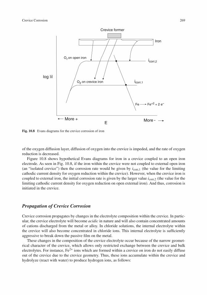
Crevice Corrosion 269
O2 on open iron
O2 on crevice iron
Fe Fe+2 + 2 e–
E
log |i|
icorr,2
icorr,1
More + More -
Crevice former
Iron
Fig. 10.8 Evans diagrams for the crevice corrosion of iron
of the oxygen diffusion layer, diffusion of oxygen into the crevice is impeded, and the rate of oxygenreduction is decreased.
Figure 10.8 shows hypothetical Evans diagrams for iron in a crevice coupled to an open ironelectrode. As seen in Fig. 10.8, if the iron within the crevice were not coupled to external open iron(an “isolated crevice”) then the corrosion rate would be given by icorr,1 (the value for the limitingcathodic current density for oxygen reduction within the crevice). However, when the crevice iron iscoupled to external iron, the initial corrosion rate is given by the larger value icorr,2 (the value for thelimiting cathodic current density for oxygen reduction on open external iron). And thus, corrosion isinitiated in the crevice.
Propagation of Crevice Corrosion
Crevice corrosion propagates by changes in the electrolyte composition within the crevice. In partic-ular, the crevice electrolyte will become acidic in nature and will also contain concentrated amountsof cations discharged from the metal or alloy. In chloride solutions, the internal electrolyte withinthe crevice will also become concentrated in chloride ions. This internal electrolyte is sufficientlyaggressive to break down the passive film on the metal.
These changes in the composition of the crevice electrolyte occur because of the narrow geomet-rical character of the crevice, which allows only restricted exchange between the crevice and bulkelectrolytes. For instance, Fe2+ ions which are formed within a crevice on iron do not easily diffuseout of the crevice due to the crevice geometry. Thus, these ions accumulate within the crevice andhydrolyze (react with water) to produce hydrogen ions, as follows:

270 10 Crevice Corrosion and Pitting
Fe→ Fe2+ + 2e− (3)
Fe2+ + H2O→ FeOH+ + H+ (4)
Fe2+ + 2H2O→ Fe(OH)2 + 2H+ (5)
The degree of acidity depends on the identity of the dissolved cation. For Eq. (4)
Kh = [H+]2
[Fe2+](6)
where Kh is the hydrolysis constant. From thermodynamic data compiled by Peterson [5], Eq. (6)can be written as follows:
pH = 4.75 − 1
2log [Fe2+] (7)
so if the concentration of dissolved Fe2+ ions within the crevice is 1 M, the internal crevice electrolyteis 4.75; see Table 10.1. Thus, a local internal pocket of acidity develops within the active crevice eventhough the external electrolyte has a neutral pH of 7.
Table 10.1 Expressions for the pH of various crevice hydrolysis reactions [5, 8]
Reaction Equilibrium pH pH of 1 M solution
Fe2+ + H2O→ FeOH+ + H+ pH = 4.75 − 0.500 log [Fe2+] 4.75Fe2+ + 2H2O→ Fe(OH)2 + 2H+ pH = 6.64 − 0.500 log [Fe2+] 6.64Fe3+ + 3H2O→ Fe(OH)3 + 3H+ pH = 1.61 − 0.333 log [Fe3+] 1.61Cr2+ + 2H2O→ Cr(OH)2 + 2H+ pH = 5.50 − 0.500 log [Cr2+] 5.50Cr3+ + 3H2O→ Cr(OH)3 + 3H+ pH = 1.60 − 0.333 log [Cr3+] 1.60Ni2+ + 2H2O→ Ni(OH)2 + 2H+ pH = 6.09 − 0.500 log [Ni2+] 6.09Al3+ + H2O→ Al(OH)2+ + H+ pH = 2.43 − 0.500 log [Al3+] 2.43
Experimentally measured values for the pH of crevice electrolytes on iron have ranged from3.1–4.7 to 5.5 [4, 6, 7], in nominal agreement with the value of 4.75 calculated from Eq. (7).
As shown in Table 10.1, an even lower pH is expected within a crevice on chromium. This hasbeen verified experimentally by the work of Bogar and Fujii [7], who showed that the pH withincrevices on Fe−Cr alloys decreased with increasing Cr content until a constant pH of approximately2.0 was attained, as shown in Fig. 10.9. Peterson et al. [5] measured the internal pH to be 1.2–2.0 onType 304 stainless steel in crevices.
Example 10.1: Chromium contained within a crevice of 0.5 cm2 area and 0.2 mm in height corrodesat the rate of 1 μA/cm2. What is the pH within the crevice after 10 days if Cr corrodes as Cr3+,and Cr3+ ions hydrolyze to form Cr(OH)3? Assume that all Cr3+ ions produced by crevice corrosionremain within the crevice.
Solution: The amount of Cr3+ ions produced is given by

Crevice Corrosion 271
0.0
1.0
2.0
3.0
4.0
5.0
0 20 40 60 80 100
Cre
vice
pH
Weight Percent Cr in Alloy
18 Ni
Fe-13 Cr-8 Ni
304 Stainless steel(Fe-18 Cr-8 Ni)
3.5% NaCl+0.300 v vs. S.C.E.5 hrs.
Fig. 10.9 Crevice pH of Fe−Cr binary alloys as a function of the chromium content of the alloy [7]. Data are alsoshown for two Fe−Cr−Ni alloys
(1.0× 10⁻⁶ A
cm2
)(0.5 cm2) (10 day)
(24h
day
)(3600 s
h
)=0.432 C
(0.432 C)
(1 equiv
96,500 C
)(1 mol Cr3+
3 equiv
)= 1.49× 10⁻⁶ mol Cr3+
The volume of the crevice is
(0.5 cm2)(2× 10⁻² cm) = 1.0× 10⁻²cm2
The concentration of Cr3+ within the crevice is
[Cr3+] =(
1.49× 10⁻⁶ mol
1.0× 10⁻² cm3
)(1000 cm3
L
)= 0.149 M
Then, from Table 10.1, the pH due to hydrolysis to Cr(OH)3 is
pH = 1.60− 0.333 log [Cl3+]
or
pH = 1.60− 0.333 log (0.149) = 1.9
With the accumulation of H+ ions and metallic cations within an active crevice, Cl− ions then migratefrom the bulk electrolyte to the crevice electrolyte in order to maintain charge neutrality within the

272 10 Crevice Corrosion and Pitting
Fe+2Fe+2 H+
Cl–
Cl–
Crevice former
Cl–
Iron
Fe+2+ 2 H2 O FeO H+ + H+
or, Fe+2+ 2 H2O Fe(O H)2+ 2 H+
H+
FeFe
Solution
Fig. 10.10 Schematic illustration of the propagation stage of crevice corrosion of iron
crevice solution. The presence of increased chloride levels (3–12 M) within corroding crevices hasbeen determined experimentally for artificial crevices on various stainless steel alloys [9, 10].
Thus, the propagation stage of crevice corrosion involves the formation of a highly corrosiveinternal electrolyte which is acidic and also concentrated in chloride ions and dissolved cations ofthe metal or alloy, as shown in Fig. 10.10 [11]. The initiation stage of crevice corrosion can bequite prolonged (months to years), but propagation may proceed rapidly due to the highly corrosivecrevice environment which is formed.
Crevice Corrosion Testing
Crevice corrosion can be studied using a variety of experimental test setups. To screen or test variousalloys for their susceptibility to crevice corrosion, metal samples can be situated beneath flat creviceformers made of plastic or fluorocarbon. The crevice can also be formed under a compressed rubbergasket. Metals in the form of pipes or tubing can be equipped with tight-fitting polymer sleeves toform a crevice. A crevice test assembly has been used in which a serrated fluorocarbon washer con-taining multiple grooves is compressed against a metal surface to provide multiple crevices on thesame metal specimen [12]. Martin and co-workers [1] have developed a crevice test assembly con-sisting of a VitonTM gasket and an acrylic test assembly which is capable of providing a reproduciblecrevice tightness by controlling the compression of the gasket against the metal surface.
In these types of testing, there is often a variability between replicate samples as to the occurrenceof crevice corrosion on a given alloy. In multiple crevice assemblies, for instance, not all crevicelocations may show crevice corrosion, but the number of sites showing attack in a given time is anindication of the susceptibility (or resistance) to initiation, and the depth of attack gives the rate ofpropagation.
The tests described above are useful for alloy testing and development, but provide no informationon the mechanism of crevice corrosion. In order to apply electrochemical techniques, a split electrodemust be used in which the metal in the crevice is physically separated (but electrically connected)to the open metal outside the crevice. A typical arrangement, sometimes called a “remote creviceassembly,” has been given in Fig. 10.7. By short circuiting the internal (crevice) electrode to the
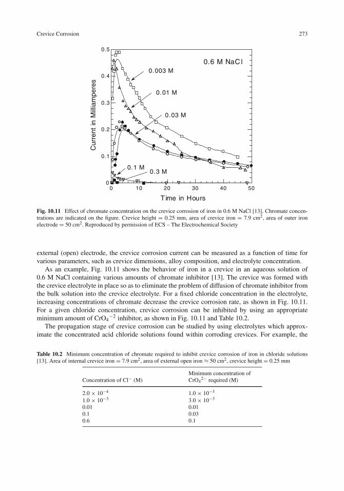
Crevice Corrosion 273
0
0.1
0.2
0.3
0.4
0.5
0 10 20 30 40 50
Cur
rent
in M
illia
mpe
res
T ime in Hours
0.003 M
0.01 M
0.03 M
0.1 M0.3 M
0.6 M NaC l
Fig. 10.11 Effect of chromate concentration on the crevice corrosion of iron in 0.6 M NaCl [13]. Chromate concen-trations are indicated on the figure. Crevice height = 0.25 mm, area of crevice iron = 7.9 cm2, area of outer ironelectrode = 50 cm2. Reproduced by permission of ECS – The Electrochemical Society
external (open) electrode, the crevice corrosion current can be measured as a function of time forvarious parameters, such as crevice dimensions, alloy composition, and electrolyte concentration.
As an example, Fig. 10.11 shows the behavior of iron in a crevice in an aqueous solution of0.6 M NaCl containing various amounts of chromate inhibitor [13]. The crevice was formed withthe crevice electrolyte in place so as to eliminate the problem of diffusion of chromate inhibitor fromthe bulk solution into the crevice electrolyte. For a fixed chloride concentration in the electrolyte,increasing concentrations of chromate decrease the crevice corrosion rate, as shown in Fig. 10.11.For a given chloride concentration, crevice corrosion can be inhibited by using an appropriateminimum amount of CrO4
−2 inhibitor, as shown in Fig. 10.11 and Table 10.2.The propagation stage of crevice corrosion can be studied by using electrolytes which approx-
imate the concentrated acid chloride solutions found within corroding crevices. For example, the
Table 10.2 Minimum concentration of chromate required to inhibit crevice corrosion of iron in chloride solutions[13]. Area of internal crevice iron = 7.9 cm2, area of external open iron ≈ 50 cm2, crevice height = 0.25 mm
Concentration of Cl− (M)Minimum concentration ofCrO4
2− required (M)
2.0 × 10⁻⁴ 1.0 × 10⁻³
1.0 × 10⁻³ 3.0 × 10⁻³
0.01 0.010.1 0.030.6 0.1
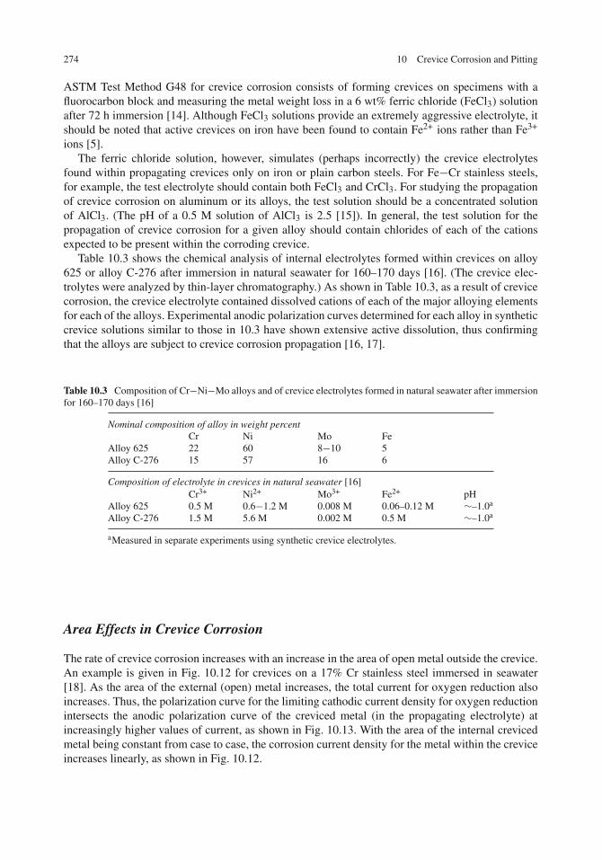
274 10 Crevice Corrosion and Pitting
ASTM Test Method G48 for crevice corrosion consists of forming crevices on specimens with afluorocarbon block and measuring the metal weight loss in a 6 wt% ferric chloride (FeCl3) solutionafter 72 h immersion [14]. Although FeCl3 solutions provide an extremely aggressive electrolyte, itshould be noted that active crevices on iron have been found to contain Fe2+ ions rather than Fe3+
ions [5].The ferric chloride solution, however, simulates (perhaps incorrectly) the crevice electrolytes
found within propagating crevices only on iron or plain carbon steels. For Fe−Cr stainless steels,for example, the test electrolyte should contain both FeCl3 and CrCl3. For studying the propagationof crevice corrosion on aluminum or its alloys, the test solution should be a concentrated solutionof AlCl3. (The pH of a 0.5 M solution of AlCl3 is 2.5 [15]). In general, the test solution for thepropagation of crevice corrosion for a given alloy should contain chlorides of each of the cationsexpected to be present within the corroding crevice.
Table 10.3 shows the chemical analysis of internal electrolytes formed within crevices on alloy625 or alloy C-276 after immersion in natural seawater for 160–170 days [16]. (The crevice elec-trolytes were analyzed by thin-layer chromatography.) As shown in Table 10.3, as a result of crevicecorrosion, the crevice electrolyte contained dissolved cations of each of the major alloying elementsfor each of the alloys. Experimental anodic polarization curves determined for each alloy in syntheticcrevice solutions similar to those in 10.3 have shown extensive active dissolution, thus confirmingthat the alloys are subject to crevice corrosion propagation [16, 17].
Table 10.3 Composition of Cr−Ni−Mo alloys and of crevice electrolytes formed in natural seawater after immersionfor 160–170 days [16]
Nominal composition of alloy in weight percentCr Ni Mo Fe
Alloy 625 22 60 8−10 5Alloy C-276 15 57 16 6
Composition of electrolyte in crevices in natural seawater [16]Cr3+ Ni2+ Mo3+ Fe2+ pH
Alloy 625 0.5 M 0.6−1.2 M 0.008 M 0.06–0.12 M ∼–1.0a
Alloy C-276 1.5 M 5.6 M 0.002 M 0.5 M ∼–1.0a
aMeasured in separate experiments using synthetic crevice electrolytes.
Area Effects in Crevice Corrosion
The rate of crevice corrosion increases with an increase in the area of open metal outside the crevice.An example is given in Fig. 10.12 for crevices on a 17% Cr stainless steel immersed in seawater[18]. As the area of the external (open) metal increases, the total current for oxygen reduction alsoincreases. Thus, the polarization curve for the limiting cathodic current density for oxygen reductionintersects the anodic polarization curve of the creviced metal (in the propagating electrolyte) atincreasingly higher values of current, as shown in Fig. 10.13. With the area of the internal crevicedmetal being constant from case to case, the corrosion current density for the metal within the creviceincreases linearly, as shown in Fig. 10.12.

Crevice Corrosion 275
0
2
4
6
8
10
12
0 20 40 60 80 100 120
Ave
rage
wei
ght L
oss
in g
ram
s
Area Outside Crevice in cm2
Fe –17% Cr steel87 days immersion in seawaterCrevice height = 0.02 mm.
Fig. 10.12 Effect of the area outside the crevice on the weight loss of an Fe-17% Cr steel inside a crevice in naturalseawater. Redrawn from [18] by permission of © NACE International (1951)
log |I|
O2 reductionoutside the crevice
M M+n + n e –
inside the crevice
EMore + More –
Increasingexternal area
Fig. 10.13 Schematic Evans diagrams showing the effect of external area on the rate of crevice corrosion
Protection Against Crevice Corrosion
Passive metals or alloys are particularly susceptible to crevice corrosion, because these metalsdepend on their passive oxide films for protection, but these passive films can be destroyed locallyby the acidic conditions which develop within propagating crevices.
Crevice corrosion can be prevented or minimized by several protective measures. These includethe following:

276 10 Crevice Corrosion and Pitting
–1200
–1000
– 800
– 600
– 400
–200
E in
mV
vs
. A
g/A
gCl
T ime in HoursNo C athodicPolarization
Time in HoursC athodic Polarization
by Zinc Anode
0 20 0 20 40 60
E xternal
89 cm.
13 cm.
89 cm.
E xternal
Fig. 10.14 Cathodic polarization of type 304 stainless steel in 0.05 mm crevices in 0.6 M NaCl [19]. The numbers inthe figure indicate the distance (in cm) from the crevice opening. Reproduced by permission of © NACE International(1974)
(1) Use of corrosion inhibitors, such as chromates, dichromates, nitrites, or phosphates.(2) Cathodic protection (using anodes located outside the crevice). Lennox and Peterson [19]
have shown that it is possible to cathodically protect deep crevices on stainless steel or cop-per. Figure 10.14 shows experimental data for stainless steel in 0.6 M NaCl. After 50–70 hof cathodic protection, the electrode potential and pH for stainless steel at a location 35 in.(13.8 cm) inside the crevice were –948 mV vs. SCE and 11.4, respectively, showing that deepcrevices can be protected. Similar results were obtained when the initial pH within the crevicewas 1.9, showing that cathodic protection is effective even after crevice corrosion has beeninitiated. Similar results were obtained for copper in crevices.
(3) Design considerations to minimize the existence of crevices. For example, Fig. 10.15 shows thatthe use of continuous welds is preferred over intermittent welds in order to prevent the occur-rence of multiple crevices [20]. Figure 10.16 shows that a discharge valve can be re-designed toprevent crevice corrosion under deposits [8].
(4) Materials selection: titanium and its alloys and Mo-containing alloys such as alloy 625 or alloyC-276 are more resistant to crevice corrosion (at ambient temperatures) than conventional stain-less steels. The presence of nitrogen is also beneficial to crevice corrosion resistance in alloyswhich contain molybdenum [21].
Example 10.2: Why does the internal pH within a crevice increase within a crevice when the creviceis being cathodically protected, as in the work of Lennox and Peterson [19]?
Solution: The principal reaction within the cathodically protected crevice is the reduction of oxygen:
O2 + 2 H2O+ 4e− → 4 OH−

Pitting 277
Intermittentwelds
Continuousweld
(b)(a)
Unsuitable Suitable
Fig. 10.15 Continuous welds in (b) are preferable to intermittent welds in (a) because intermittent welds introduceadditional crevices [20].
(a) (b)
Liquid Liquid
Deposits
Fig. 10.16 Discharge valves can be re-designed as in (b) to prevent crevice corrosion under deposits [8]. Reproducedby permission of © NACE International (1974)
The product of this reaction, hydroxyl ions (OH−), accumulates within the narrow confines of thecrevice, so that the crevice electrolyte becomes more alkaline. Thus, the pH increases.
Pitting
Pitting is a form of localized corrosion in which the attack is confined to a small fixed area of themetal surface. Pitting occurs due to localized breakdown of a passive film, usually by chloride ions.Figure 10.17 shows a cross section of a corrosion pit formed on Al alloy 6061 (Al-1% Mg) in 0.1 MNaCl by anodic polarization [22].
Pitting is a dangerous form of corrosion attack for several reasons. Pits can result in the perforationof a metal component while the rest of the metal piece remains unattacked. In the presence of anapplied stress, pits can serve as sites to initiate stress-corrosion cracking, another catastrophic form

278 10 Crevice Corrosion and Pitting
Fig. 10.17 Cross-sectional view of a corrosion pit on Al 6061 formed by anodic polarization in 0.1 M NaCl [22].Reproduced by permission of © NACE International (1990)
of corrosion attack. Finally, the presence of pits can be difficult to detect if they are covered withcorrosion products.
Pits can require a long time to appear in actual service (months to years), so that their absencein the short term is not a certainty that the metal or alloy is immune to pitting. All passive metalsare subject to pitting corrosion, although most experimental studies have involved stainless steels(and their alloying components), aluminum, and copper. Pitting is caused by the presence of an“aggressive” anion in the electrolyte, usually Cl− ions, but pitting of various metals or alloys hasalso occurred in the presence of other anions, including Br−, I−, SO4
2−, or NO3−. A more complete
list of ions which cause pitting attack has been given elsewhere [23].The chloride ion has a special importance in piitting corrosion for several reasons. First of all,
Cl− ions are ubiquitous, being constituents of seawater, brackish waters, de-icing salts, and airbornesalts. In addition, chlorides are found in the human body, so they can cause the pitting of biomedicalimplants. Chlorides are also common contaminants in various electronic systems due to handlingand processing. The chloride ion is a strong Lewis base (electron donor) and tends to interact withLewis acids (electron acceptors), such as metal cations. In addition, the chloride ion is a relativelysmall anion and has a high diffusivity.
Critical Pitting Potential
The tendency of a metal or alloy to undergo pitting is characterized by its critical pitting potential,as illustrated in Fig. 10.18. In the absence of chloride ions, the metal retains its passivity up tothe electrode potential of oxygen evolution. However, in the presence of chloride ions, the passivefilm suffers localized attack, and pitting initiates at a well-defined potential called the critical pittingpotential (or, usually just the pitting potential). (The critical pitting potential is also sometimes calledthe breakthrough potential, breakdown potential, or rupture potential). Once corrosion pits initiate,they usually propagate rapidly, as shown by the sharp rise in current density at electrode potentialsjust beyond the critical pitting potential.
An experimentally determined polarization curve for the pitting of type 304 stainless steel isshown in Fig. 10.19 [24]. In the absence of chlorides, the stainless steel remains passive up to the

Pitting 279
Pits initiate and grow
log |i|
EMore +
No pitting(O2 evolution)
Approximately1 V
Critical pittingpotential, Epit
Free from pitting(passive region)
Ecorr
ipassive
Pitting
Fig. 10.18 Schematic anodic polarization curve showing the critical pitting potential (for a passive metal)
0
0.001
0.01
0.1
1
10
100
0 0.2 0.4 0.6 0.8 1 1.2 1.4
Cur
rent
Den
sity
in m
A/c
m2
E in V vs. S.H.E.
0.1 M NaCl (pitting)
1 M Na2SO4
(no pitting)
Direction of polarization
Fig. 10.19 Experimental anodic polarization curves for type 304 stainless steel in 0.1 M NaCl or in 1 M Na2SO4.Redrawn from [24] by permission of ECS – The Electrochemical Society
potential of oxygen evolution (about +1.2 V vs. SHE.) but in the 0.1 M NaCl solution, pitting occursat +0.35 V vs. SHE (the pitting potential).
The critical pitting potential, Epit, is a characteristic property of a given metal or alloy, althoughthe value of Epit for a given metal depends on the chloride concentration. For a given chlorideconcentration, the more positive the critical pitting potential, the more resistant the metal or alloy to

280 10 Crevice Corrosion and Pitting
Table 10.4 Critical pitting potentials, Epit, in 0.1 M NaCl for various metals and alloys
Metal or alloya Epit in V vs. SCE Source
Zinc −1.02 Alvarez and Galvele [94]Aluminum −0.70 Natishan et al. [95]Al alloy 5656 (Al-5 Mg) −0.68 Trzaskoma et al. [96]Iron −0.41 Strehblow and Titze [97], Alvarez and Galvele [98]M-50 steel (Fe-4 Cr-5 Mo-1 V) −0.23 Wang et al. [99]Copper −0.04 Thomas and Tiller [100]Molybdenum +0.055 Wang et al. [99]Nickel +0.08 Strehblow and Titze [97]Chromium +0.125 Wang et al. [99]Zirconium +0.22 Cragnolino and Galvele [101]304 stainless steel +0.30 McCafferty and Moore [62]316 stainless steel +0.50 McCafferty and Moore [62]Titanium > +1.0b Dugdale and Cotton [102]
aThe resistance to pit initiation increases down this table.bThis value refers to dielectric breakdown of the oxide film rather than to pitting.
pit initiation. Table 10.4 lists critical pitting potentials for various metals and alloys in 0.1 M NaCl.In each case, the significance of the pitting potential is that
• below Epit, pitting does not occur,• above Epit, corrosion pits initiate and propagate.
The resistance to pit initiation decreases down Table 10.4. However, the characteristic pittingpotential is not the only parameter which should be used to assess the resistance to pitting attack.Other important parameters are the density of pits (number per unit area) and their propagation rate,which will determine the depths of pits and, accordingly, the lifetime of the structure.
Practical support for the existence of a critical pitting potential has been provided by long-termimmersion tests in natural seawater of a series of 19 different aluminum alloys (having various heattreatments as well) [25]. The electrode potential of each alloy was monitored over a 1-year immer-sion period, after which the alloys were removed from seawater, the corrosion products removed,and the depth of attack measured. As can be seen in Table 10.5, aluminum alloys which maintainedelectrode potentials below (more negative) than −0.89 V vs. Ag/AgCl displayed little or no pittingattack. Thus, the value of −0.89 V vs. Ag/AgCl can be taken to be the pitting potential of aluminumalloys in natural seawater.
Experimental Determination of Pitting Potentials
Critical pitting potentials are usually determined from steady-state anodic polarization curves. Themost reliable approach is to use a potentiostatic technique in which a constant potential is applied,and the current is recorded as a function of time, as shown schematically in Fig. 10.20. At elec-trode potentials below the pitting potential, the current decays to a constant value. But at the pittingpotential and above, the current increases with time as corrosion pits initiate and grow. At potentialssufficiently beyond the pitting potential, the anodic current sometimes increases to a limiting value.

Pitting 281
Table 10.5 Corrosion behavior of various aluminum alloys in seawater after 1-year immersion [25]
Alloy designationa E vs. Ag/AgCl Depth of attack in mils
Epit
Pitting
No pitting
5257-H25 −1.24 <15154-H38 −1.05 1−4X7005-T63Alc. X7002-T65052-H345052-H32
−1.01 to −1.02 <11−41−4<1
5456-H3215086-H325086-H34Alc. 7178-T6
−0.96 to −0.98 <1<1<11−4
7106-T636061-T6515086-H1125050-H341100-H145083-O
−0.92 to −0.94 <1<1<11−41−4<1
1100-F3000-H146061-T6
−0.88 to −0.89 5−1011−205−10
7178-T6X7002-T67075-T73517079-T62014-T6
−0.73 to −0.79 25−405−1011−2011−205−10
2024-T3512219-T87
−0.69 to −0.70 25−40
a Alloy 1100 is commercially pure aluminum. The other alloys have the following principal additions: 2000 series,Cu; 3000 series, Mn; 5000 series, Mg; 6000 series, Mg and Si; 7000 series, Zn. The amount of the alloy additionis generally 3–5 wt.%.
Time at Applied Potential
Current
E5
E4 =Epit
E2
E1
Increasinganodic
potentialE3
Fig. 10.20 Schematic illustration of experimental current–time curves obtained by the potential step method in themeasurement of the critical pitting potential. Below the pitting potential, the current decays with time in responseto a potential step. But at and above the pitting potential, when pits initiate and grow, the current increases withtime

282 10 Crevice Corrosion and Pitting
This is because the current within the propagating pit becomes diffusion-limited due to the formationof a concentrated solution within the pit, as is discussed later.
Pitting potentials have also been determined by anodic sweep (potentiodynamic) measurements,but the measured value for Epit usually depends on the sweep rate. This is caused by not allowingsufficient time at each electrode potential for pit initiation events to transpire.
In addition to the sweep rate, the critical pitting potential also depends on the surface finish of themetal. (Rough surfaces present more initiation sites and generally have lower values of Epit than forsmooth surfaces.) The pitting potential does not seem to depend on the oxide film thickness [26].
Effect of Chloride Ions on the Pitting Potential
Chloride ions (among others) cause pitting to occur. The critical pitting potential decreases (is lesspositive) as the chloride concentration increases. Said differently, for a dilute chloride solution, it isnecessary to drive the electrode potential farther in the positive direction to cause pitting to occur.Figure 10.21 shows the effect of chloride concentration on the pitting potential of type 304 stainlesssteel [24] and aluminum [27]. In each case, the critical pitting potential, Epit, is a linear function ofthe logarithm of the chloride ion concentration:
Epit = a+ b log [Cl−] (8)
where a and b are constants.
-0.6
-0.4
-0.2
0.0
0.2
0.4
0.01 0.1 1
Pitt
ing
Pot
entia
l in
V v
s. S
.H.E
.
Cl- Activity in M/L
Aluminum
304 Stainless Steel
Fig. 10.21 Effect of chloride concentration (activity) on the pitting potential of aluminum and type 304 stainless steel[24, 27]. Reproduced by permission of ECS – The Electrochemical Society

Pitting 283
Effect of Inhibitors on the Pitting Potential
The addition of a corrosion inhibitor to a solution increases the pitting potential. Figure 10.22 showsthat sulfate additions to a 0.1 M NaCl solution raise the pitting potential of type 304 stainless steel[24]. More about the action of corrosion inhibitors is given in Chapter 12.
0.001
0.01
0.1
1
10
100
0 0.2 0.4 0.6 0.8 1 1.2 1.4
0.1 M NaCl + x M Na2 SO4
x = 0
x = 0.05
x = 0.1
x = 0.0125
x = 0.15
Cur
rent
Den
sity
in m
A/c
m2
E in V vs. S.H.E.
Direction of polarization
Fig. 10.22 Effect of sulfate additions on the pitting potential of type 304 stainless steel in 0.1 M NaCl solutions.Redrawn from [24] by permission of ECS – The Electrochemical Society
Mechanism of Pit Initiation
Like crevice corrosion, pitting corrosion may be divided into initiation and propagation stages. Wewill consider the initiation stage to include both the breakdown of the passive film and the onsetof an anodic current at the metal surface. The exact mechanism of pit initiation is not known withgreat certainty, but it is generally understood [23, 28–30] that three main mechanisms are possible.These are (i) the penetration mechanism, (ii) the film thinning mechanism (also referred to as theadsorption mechanism), and (iii) the film rupture mechanism.
In the penetration mechanism, aggressive anions are transported through the oxide film to theunderlying metal surface where they participate in localized dissolution at the metal/oxide interface.This mechanism is depicted schematically in Fig. 10.23. There is recent evidence from X-ray pho-toelectron spectroscopy and X-ray absorption spectroscopy that Cl− ions penetrate passive films onboth stainless steel and aluminum [31, 32]. More details on chloride penetration are given in a latersection on the pitting of aluminum. The mechanism by which Cl− ions penetrate the oxide film isnot completely understood, but the radius of the Cl− ion is only slightly larger than that of an oxideion (1.81 vs. 1.40 Å, respectively), so that Cl− migration through oxygen vacancies is a possiblemechanism of chloride entry into the passive film [33].

284 10 Crevice Corrosion and Pitting
Adsorption of Cl- ions
Passive film M+n
ne-
O-2
Cl- M+n (aq)
Corrosion
Film formation
Penetration by Cl- ions
MetalM
OH-
O2 + H2O
Fig. 10.23 The penetration mechanism of pitting showing the competing processes of film rupture and film formation.Redrawn from [29]. Copyright Wiley VCH Verlag Gmbh & Co. Reproduced with permission
2 e-
Vacancycondensate
Fe(Oxide)
VFe"
Fe(Metal) + VFe"
Fe+2
Cl-
Metal Oxide Film Solution
Anionvacancy
Schottkypairformation
Adsorptionof Cl-
Fe+2 (aq)
Fig. 10.24 One mechanism leading to the breakdown of passive films [33]. Cation vacancies are transported inwardand chloride ions adsorb by occupying anion (oxygen ion) vacancies. VFe
′′ represents a cation vacancy of effec-tive charge –2, Fe(oxide) represents a metal cation in a cation site. Reproduced by permission of ECS – TheElectrochemical Society
Macdonald and co-workers [33] have developed a point defect model for the breakdown of pas-sivity involving the action of vacancies within the passive film. It is assumed that cation vacanciesmigrate from the oxide/electrolyte interface inward (as shown in Fig. 10.24), which is equivalentto the migration of cations outward from the metal to the solution. If the cation vacancies accumu-late at the metal/oxide interface, the resulting voids which form due to vacancy condensation leadto stresses within the passive film and to pit initiation. In addition, Cl− ions are carried inward bymigration through oxygen vacancies so as to assist in localized dissolution at the metal substrate.
An alternate mechanism of Cl− transport has been proposed by Bockris and co-workers [34, 35]who have suggested that chloride ions migrate through localized water channels in the hydrous oxidefilm.

Pitting 285
Metal
Film thinning and dissolution
Passive film
Metal
Adsorption of Cl- ions
Passive film
(a)
(b)
Continued film thinningand pitting
Passive film
Metal
(c)
Fig. 10.25 The film thinning mechanism of pitting in which chloride adsorption (a) initiates the process of filmthinning (b) leading to pitting (c) [29]. Copyright Wiley VCH Verlag Gmbh & Co. Reproduced with permission
Because pitting can also be caused by ions which are larger in size than the Cl− ion (e.g., Br−or I−), additional mechanisms of initiation must be considered which would apply not only to Cl−ions but also to other aggressive anions as well. In the film thinning mechanism, the aggressive ions(chloride or others) first adsorb on the oxide surface (perhaps in clusters) and then form surfacecomplexes with the oxide film which lead to local dissolution and thinning of the passive film,as shown schematically in Fig. 10.25. Nguyen and Foley [36] have shown that aluminum oxidedissolves to some extent in the presence of sodium chloride solutions. Yu et al. [37] using XPSrecently showed that the oxide film thickness on aluminum in 0.1 M NaCl remained essentiallyinvariant at electrode potentials leading up to the pitting potential, but then the passive film displayedthinning at−0.750 V (i.e., 0.050 V before the pitting potential). XPS measurements have shown thatF−, Cl−, Br−, and I−, ions all cause thinning of the passive film on iron [38].
In the film rupture mechanism (Fig. 10.26), chloride ions penetrate the oxide through cracks orflaws in the film. In addition to pre-existing defects in the oxide film, flaws may further developby hydration/dehydration events in the oxide film and by the intrusion of Cl− ions into the film.According to Sato [39], the presence of a high electric field in the oxide can lead to an electrome-chanical breakdown of the passive film. It should be noted that pre-existing flaws cannot extenddown to the underlying metal substrate because the metal would quickly react with water moleculesin the electrolyte and would re-oxidize. Then, chloride ions must penetrate the re-formed oxide filmby mechanisms discussed above.
Passive films can also be ruptured or disrupted due to metallurgical variables, such as grain bound-aries, impurity atoms, and inclusions. The role of sulfide inclusions in the pitting of stainless steelsis discussed later in this chapter.

286 10 Crevice Corrosion and Pitting
Electrolyte withaggressive ions
Pit growth
Competition betweenpassive film andchloride-enriched film
Passive film
Metal
Fig. 10.26 The film rupture mechanism of pitting [29]. Copyright Wiley VCH Verlag Gmbh & Co. Reproduced withpermission
These three mechanisms of pit initiation (chloride penetration, film thinning, and film rupture)are not necessarily mutually exclusive. For example, when Cl− ions are transported through oxygenvacancies, there may also be concomitant oxide film dissolution because atoms surrounding vacancydefects are expected to be less bonded to the bulk oxide [40]. Yu et al. [37] have shown evidence forboth chloride penetration and film thinning for the pitting of aluminum in chloride solutions. Moredetails on these three mechanisms of pit initiation are given elsewhere [29].
Mechanism of Pit Propagation
The mechanism of pit propagation is similar to that for the propagation of crevice corrosion, asillustrated in Fig. 10.27 [41]. When the corrosion pit has been initiated, the corresponding localcurrent density is very high because the current is confined to a small active geometrical area, with
Fe+2 + 2 H2O FeOH+ + H+
or, Fe+2 + 2 H2O Fe(OH)2 + 2 H+
Fe+2
Fe+2
Fe+2
H+
H+H+
Cl-
Cl-
Passive oxide film
Porous cap ofcorrosion products
Passive oxide film
IronIron
Tens to hundredsof microns
Fe
FeFe
Fig. 10.27 Schematic representation of the propagation stage of pitting. Note the similarity to Fig. 10.10

Pitting 287
the oxide film adjacent to the pit remaining passive and unattacked. As the pit grows, its volumeincreases, but dissolved metal cations are confined within the pit and do not diffuse out into the bulkelectrolyte due to the confinement of a restricted geometry or a cap of porous corrosion products,which exists in some cases. As a result, accumulated metal cations undergo hydrolysis, as in the caseof crevice corrosion, and a local acidity develops within the pit. Finally, the accumulation of H+ ionsand cations within an active pit, Cl− ions migrate from the bulk electrolyte to the crevice electrolytein order to maintain charge neutrality within the pit solution.
One of the earliest pieces of experimental evidence which showed that corrosion pits are acidifiedwas provided by Butler et al. [42], who scanned across a corrosion pit on iron using small diameter(5–25 μm) antimony/antimony oxide pH electrodes. Their results given in Fig. 10.28 show that theinterior of a corrosion pit is acidified and that the pH adjacent to the pit becomes alkaline because thecathodic reaction (reduction of O2 to OH−) occurs on the passive surface outside the pit. Butler et al.also measured electrode potentials across the same pit using a Ag/AgCl micro-electrode. Resultsgiven in Fig. 10.28 also show that the electrode potential above the pit is more active (more negative)than above the areas adjacent to the pit.
Thus, the propagation stage of pitting, like that of crevice corrosion, involves the formation ofa highly corrosive internal electrolyte which is acidic and concentrated in chloride ions and in dis-solved cations of the metal or alloy. When the corrosive pit electrolyte has been formed, pitting
2
3
4
5
6
7
8
9
-1.0 -0.5 0.0 0.5 1.0
pH
Distance from Center of Pit in mm
Solution pH
-0.50
-0.48
-0.46
-0.44
-0.42
-0.40
-0.38
-1.0 -0.5 0.0 0.5 1.0
E in
V v
s. S
. H. E
.
Distance from Center of Pit in mm
Fig. 10.28 Variations in pH (top) and electrode potential (bottom) across a growing pit on iron in a dilute chloridesolution. Redrawn from [42] by permission of Maney Publishing

288 10 Crevice Corrosion and Pitting
is considered to be autocatalytic in nature. That is, the local conditions which have developed arecapable of sustaining further pit growth.
Protection Potential
The concept of a protection potential against pitting arose from cyclic anodic polarization curves inwhich the scan direction was changed at anodic potentials beyond the pitting potential. As shownin Fig. 10.29, when the scan direction is changed, the current density decreases with decreasingelectrode potential until the reverse curve crosses the forward curve in the region of passivity.The electrode potential at this intersection is called the protection potential, Eprot. The significanceattached to the protection potential is that at this potential, the growth of active pits is diminished orpossibly stopped (because the passive current density has been regained).
E
log |i|
More +
Epit
Eprot
Hysteresisloop
Pitting will notinitiate or propagate
Pitting initiates and propagates
Pitting does not initiatebut propagates if initiatedat higher potentials
Fig. 10.29 Schematic illustration of the pitting potential Epit and the protection potential Eprot. The arrows show thedirection of polarization
Wilde and Williams [43] investigated this concept for various alloys which had been immersedunder crevices in natural seawater for 4.25 years. Cyclic anodic polarization curves were alsodetermined in 3.5% NaCl solutions for open samples cut from the same specimens previouslyimmersed in seawater for the 4.25 years of exposure period. Figure 10.30 lists the conditions used inmeasurement of the electrochemical polarization curves for the open samples. For each alloy, Wildeand Williams [43] determined the pitting potential, Epit, from the forward sweep of the anodic polar-ization curve and the protection potential, Eprot, from the reverse sweep of the anodic polarizationcurve.
As shown in Fig. 10.30, the amount of hysteresis for the open samples, as measured by thedifference (Epit – Eprot), correlates with the amount of crevice corrosion (the “first cousin” to pittingcorrosion). That is the less the hysteresis in the cyclic polarization curve, the less the amount of

Pitting 289
0
50
100
150
200
250
300
0 5 10 15 20 25 30
(Epi
t - E
prot
) in
mV
Weight Loss in mg/cm2
410
USS 100430
446304
316
Hastelloy C Aerated 3.5% NaCl
Fig. 10.30 The crevice weight loss of several stainless steels versus the difference between the pitting potential Epitand the protection potential Eprot for open samples [43]. The pitting potential was determined in aerated 3.5% NaClat 25◦C at a potential sweep rate of 10 mV/min, and the protection potential determined after reversing the sweep ata current density of 200 μA/cm2. The sample area was 1220 cm2 and the crevice area approximately 20 cm2. Alloytypes 4xx and USS 100 are Fe−Cr alloys, alloy types 3xx are Fe−Cr−Ni alloys, and Hastelloy C (alloy C-276) isprimarily a Ni−Cr−Mo alloy; see Table 9.11. Reproduced by permission of Elsevier Ltd
crevice corrosion observed in the actual seawater immersion test. At first glance, then, the use of theprotection potential is useful as an indicator of corrosion behavior.
However, Wilde and Williams [43] also established that the measured protection potentialdepends on the experimental conditions used in its determination. That is, once the electrode poten-tial has exceeded Epit, corrosion pits initiate and then propagate with concomitant acid hydrolysis,buildup of corrosion products, and increase in chloride ion concentration within the pit. When thesweep is reversed, the propagation processes which are potential dependent decrease until the rateof propagation becomes zero at the passive current density. Thus, the electrode potential for thisoccurrence, i.e., Eprot, should depend on the amount of propagation which has taken place within thepit. This was found to be the case for type 430 and 304 stainless steels, as shown in Fig. 10.31. Thus,the protection potential should not be regarded as a material property, although it can be used (withcaution) in ranking various alloys as to their pitting behavior.
Pessall and Liu [44] introduced a technique to measure pitting potentials by scribing through thepassive film and then observing its ability to re-form following mechanical rupture of the oxide film.The electrode potentials for the repair of oxide films on various Fe-Cr alloys, as determined by thisscratch test, were approximately 100 mV more negative than the critical pitting potential determinedby the conventional anodic polarization technique. These “scratch potentials” are now considered tobe associated with repassivation of the oxide film rather than with its initial chemical breakdown andare a measure of the protection potential.

290 10 Crevice Corrosion and Pitting
-0.60
-0.50
-0.40
-0.30
-0.20
-0.1010-2 10-2 100 101 102 103 104 105
Pro
tect
ion
Pot
entia
l, E
pro
t, in
V v
s. S
.C.E
.
Amount of Propagation in Coulombs
Type 430 stainless steel
Type 304 stainless steel
I M NaCl
25 °C Nitrogen-saturated
Initial sample area = 5 cm2
Fig. 10.31 Effect of extent of propagation on the value of the protection potential [43]. Reproduced by permission ofElsevier Ltd
Metastable Pits and Repassivation
The current–time traces shown schematically in Fig. 10.18 are idealized curves. At electrode poten-tials below the pitting potential, the current–time curves often contain transient excursions as shownin Fig. 10.32 [45]. These transients are due to metastable pits, i.e., pits that grow for a limited timebut are repassivated and stop growing. (The pitting potential marks the initiation of stable pits whichcan grow and propagate.) Metastable pits have a limited lifetime because the concentrated acidicchloride solution which promotes pit propagation has not yet developed within the metastable pit, sothat the metastable pit can be repassivated. Metastable pits are generally of micron size and have alifetime of the order of seconds or less [30].
The mechanism by which metastable pits repassivate is not known with certainty. It has beensuggested that salt films are formed at the base of metastable pits because the solubility product ofthe metal salt is easily exceeded, and that these salt films provide protection from further pit growthby limiting diffusion of dissolved cations out of the metastable pit [46]. The anodic behavior ofmetals in the presence of concentrated electrolytes, including salt films, depends on the chloride ionconcentration, pH, and electrode potential. Because of the small size of corrosion pits, repassivationprocesses have usually been studied using scaled-up artificial pits.
The importance of the internal pH has been shown by Jones and Wilde [47], who examined theanodic behavior of type 304 stainless steel in concentrated chloride solutions. In 1 N CrCl3, thestainless steel exhibited an “active/passive transition” similar to those discussed in Chapter 9, exceptthat the value of the current density at the nose of the anodic curve was of the order of 10 mA/cm2
and was much higher than values normally associated with passivity. In more concentrated CrCl3solutions (which also were more acidic), the “active/passive” transition was absent and only active
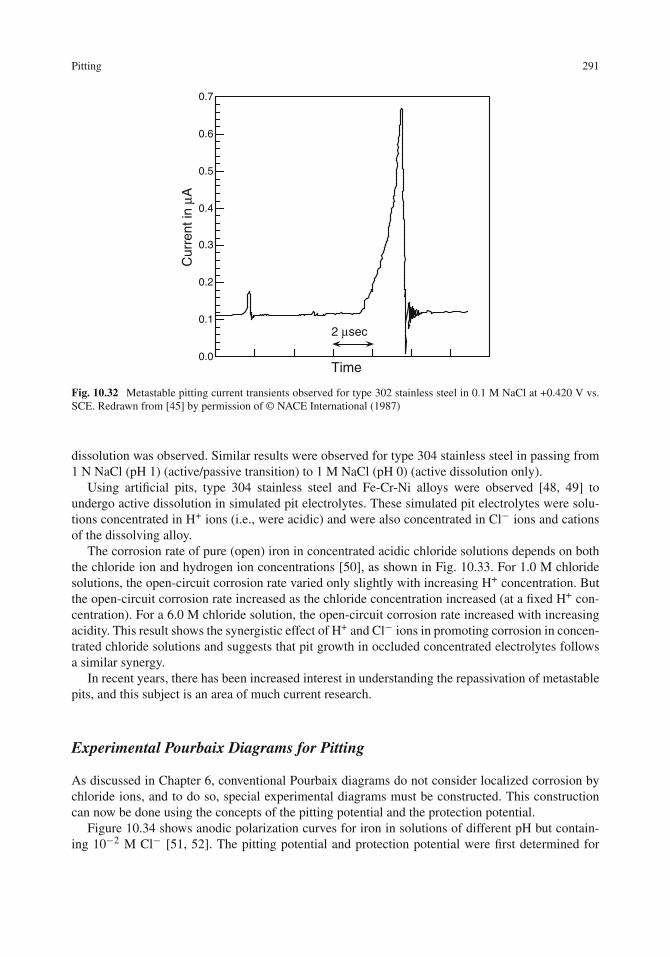
Pitting 291
0.0
0.1
0.2
0.3
0.4
0.5
0.6
0.7
Cur
rent
in μ
A
Time
2 μsec
Fig. 10.32 Metastable pitting current transients observed for type 302 stainless steel in 0.1 M NaCl at +0.420 V vs.SCE. Redrawn from [45] by permission of © NACE International (1987)
dissolution was observed. Similar results were observed for type 304 stainless steel in passing from1 N NaCl (pH 1) (active/passive transition) to 1 M NaCl (pH 0) (active dissolution only).
Using artificial pits, type 304 stainless steel and Fe-Cr-Ni alloys were observed [48, 49] toundergo active dissolution in simulated pit electrolytes. These simulated pit electrolytes were solu-tions concentrated in H+ ions (i.e., were acidic) and were also concentrated in Cl− ions and cationsof the dissolving alloy.
The corrosion rate of pure (open) iron in concentrated acidic chloride solutions depends on boththe chloride ion and hydrogen ion concentrations [50], as shown in Fig. 10.33. For 1.0 M chloridesolutions, the open-circuit corrosion rate varied only slightly with increasing H+ concentration. Butthe open-circuit corrosion rate increased as the chloride concentration increased (at a fixed H+ con-centration). For a 6.0 M chloride solution, the open-circuit corrosion rate increased with increasingacidity. This result shows the synergistic effect of H+ and Cl− ions in promoting corrosion in concen-trated chloride solutions and suggests that pit growth in occluded concentrated electrolytes followsa similar synergy.
In recent years, there has been increased interest in understanding the repassivation of metastablepits, and this subject is an area of much current research.
Experimental Pourbaix Diagrams for Pitting
As discussed in Chapter 6, conventional Pourbaix diagrams do not consider localized corrosion bychloride ions, and to do so, special experimental diagrams must be constructed. This constructioncan now be done using the concepts of the pitting potential and the protection potential.
Figure 10.34 shows anodic polarization curves for iron in solutions of different pH but contain-ing 10−2 M Cl− [51, 52]. The pitting potential and protection potential were first determined for

292 10 Crevice Corrosion and Pitting
0
500
1000
1500
2000
0 1 2 3 4 5 6 7
-420 to -498
-450 to -513
-470 to -545i c
orr in
mic
roam
ps/c
m2
[H+] in Moles/L
[Cl-] = 6 M
[Cl -] = 1 M
[H+] = [Cl-]
Ecorr in mV vs. S.C.E.
Fig. 10.33 Effect of the concentration of H+ and Cl– on the corrosion of open iron in concentrated solutions [50]
-1.0
0.0
1.0
0 2 4 6 8 10 12 14
E in
V v
s. S
.H.E
.
pH
Perfectpassivity
PittingGeneralcorrosion
Immunity
Imperfectpassivity
pH = 13
E
log i log i log i
pH = 9pH = 5
E E
Fig. 10.34 Experimental Pourbaix diagram for iron in 0.01 M Cl− (right) determined from experimental anodicpolarization curves, as on the left. Redrawn from [51, 52]. The arrows show the effect of a reverse potential sweep.The polarization curve furthest to the left shows general corrosion only; the polarization curve in the middle displaysa pitting potential and a protection potential; the polarization curve on the right shows general corrosion or passivity,but not pitting. Reproduced by permission of Elsevier Ltd
each solution in which pitting occurs, and then this information was transferred onto a potential–pHdiagram to establish various regions of corrosion behavior. These regions are regimes of immunity,general corrosion, perfect passivity, imperfect passivity, and pitting and are defined in Fig. 10.34.

Pitting 293
The condition of perfect passivity exists in the passive range below the protection potential wherepits do not nucleate or grow. The region of imperfect passivity lies between the protection potentialand the pitting potential and is a region where previously formed pits can grow before they arerepassivated at potentials at or below Eprot. The region of pitting exists above the pitting potential.
Thus, the experimental Pourbaix diagram for iron in Fig. 10.34 takes into account pitting cor-rosion with regions now defined for pit initiation, growth, or repassivation. Such a diagram ismore useful for engineering alloys rather than for pure metals because the general and localizedcorrosion behavior of complex alloys can be summarized in a convenient experimental Pourbaixdiagram (for a fixed concentration of chloride ions). Experimental Pourbaix diagrams taking intoaccount pitting corrosion have been determined for various alloys [53–56] and are similar toFig. 10.34.
Effect of Molybdenum on the Pitting of Stainless Steels
The addition of molybdenum to Fe-Cr alloys increases the pitting potential [57], as shown inFig. 10.35. The addition of Mo to alloys which contain Cr has already been noted to have a ben-eficial effect on passivity, as noted in Chapter 9. The mechanism by which Mo promotes resistanceto localized breakdown of the passive film has been studied by various authors, and several mech-anisms of increased resistance to pitting have been proposed [58]. These proposed mechanisms ofprotection include the following:
(1) Active sites are covered with molybdenum oxyhydroxide or molybdate salts, thereby inhibitinglocalized attack.
0.0
0.1
0.2
0.3
0.4
0.5
0.6
0 1 2 3 4 5 6
Pitt
ing
Pot
entia
l in
V v
s. S
.C.E
.
Weight Percent Molybdenum
18 % Cr
13 % Cr
1 M NaCl at 25oC
Fig. 10.35 Effect of molybdenum on pitting potentials of 13% Cr and 18% Cr stainless steels in 1 M NaCl at 25◦C[57]. Reproduced by permission of John Wiley & Sons, Inc

294 10 Crevice Corrosion and Pitting
(2) Dissolution of Mo in the alloy produces molybdate ions, which then act as a corrosion inhibitornear the metal surface.
(3) Mo6+ species in the passive film interact with cation vacancies of the opposite sign and reducethe flux of cation vacancies to the metal substrate (depicted in Fig. 10.24).
(4) Molybdate ions act as a cation-selective outer layer in the passive film, as shown schematicallyin Fig. 9.44, and thus hinder the transport of Cl− ions through the passive film.
(5) Mo interferes with the kinetics of active dissolution at the base of the developing pit.
The role of molybdenum on the improved pitting resistance of stainless steels is a topic ofcontinuing research.
Effect of Sulfide Inclusions on the Pitting of Stainless Steels
The integrity of the passive film on a metal or alloy can be affected by metallurgical variables in themetal. These include compositional heterogeneities at grain boundaries and disruption of the passivefilm by impurity atoms or inclusions. Sulfide inclusions, especially manganese sulfide (MnS), areknown to be pit initiation sites on stainless steels [59–61], although pitting also occurs on the metalmatrix itself and thus does not require the existence of sulfides.
Sulfur is present in stainless steels as an impurity (0.03% maximum) or as an intentional addi-tive (approximately 0.3%) to aid in the machining of the metal [61]. The most common sulfidewhich is formed in stainless steels is MnS, although other sulfide inclusions are also known toexist. Figure 10.36 shows a scanning electron micrograph of a typical sulfide inclusion on type 304stainless steel [62]. The approximate size of the inclusion is 10 μm in length.
It has long been postulated that such anodic dissolution of sulfide inclusions leads to an aggressiveelectrolyte composition near the inclusion, so as to disrupt the passive film. Recent studies using ascanning vibrating electrode (SVE) or nanometer-scale secondary ion mass spectrometry (SIMS)have verified that pits initiate at the edge of the sulfide inclusion and that anodic zones exist aroundthe inclusion [63, 64]. Ryan et al. attribute the anodic zones to be due to an area around the MnSparticle which is depleted in chromium, and thus susceptible to localized attack [64]; see Fig. 10.36.The MnS inclusion itself is unstable in the Cl−-rich acidic local environment which is established inthe propagating pit(s).
The pitting resistance of type 304 stainless steel can be improved by laser surface melting (seeChapter 16). The effect of treating the surface with a high-power laser is to remove large-scale sulfideinclusions during laser processing. The sulfides are melted and redistributed upon solidification intoa larger number of smaller particles [62] which are less disruptive to the passive film.
Effect of Temperature
The pitting potentials of type 304 and 316 stainless steels in an aqueous solution containing 200 mg/LCl− are given as a function of temperature in Fig. 10.37 [65]. It can be seen that at all temperatures,the pitting potential of the Mo-containing 316 stainless steels is higher than that of type 304 stainlesssteel. In addition, the pitting potential of each alloy decreases with increasing temperature.
Brigham [66] has developed the concept of a critical pitting temperature as a criterion to ratethe susceptibility of a series of alloys to pitting corrosion. A series of Mo-containing alloys wasimmersed in 10% FeCl3 solutions held at a constant temperature, and the alloys were examined

Pitting 295
MnS inclusion
Defective film
Cr-depletedzone(region of pitinitiation )
Passive filmCl-Cl-
(c)
0
20
40
60
80
0 2 4 6 8 10
Inte
nsity
in A
rbitr
ary
Uni
ts
Energy in keV
S
Cr
MnFe
Fe
NiCu
Zn
(b)
Fig. 10.36 (a) A top view scanning electron micrograph of a sulfide inclusion in type 304 stainless steel [62]. (b)EDAX (energy dispersive analysis by X-rays) showed that the sulfide inclusion contained Mn, Fe, Cr, and S. (c)Cross-sectional illustration of a MnS particle as a pit initiation site. Figure 10.36a–b adapted from [62] by permissionof ECS – The Electrochemical Society. Figure 10.36c reprinted with permission from Macmillan Publishers Ltd:Nature, copyright (2002) [64] (as shown)

296 10 Crevice Corrosion and Pitting
0.50
0.60
0.70
0.80
0.90
1.00
1.10
1.20
1.30
0 20 40 60 80 100
Pitt
ing
Pot
entia
l in
V v
s. S
.C.E
.
Temperature in oC
Type 304stainless steel
Type 316stainless steel
54 mg/L Cl-
Fig. 10.37 The effect of temperature on the pitting potential of type 304 and type 316 stainless steels in a dilutechloride solution. Redrawn from [65] by permission of © NACE International (1979)
for signs of pitting after a 24 h exposure period. If no pitting was observed, the temperature wasincreased, and this procedure was repeated until the first signs of pitting occurred at the “criticalpitting temperature” for that alloy. The higher the critical pitting temperature, the more resistant thealloy to pitting Fig. 10.38 shows that the pitting resistance increases with the Mo content of the alloyfor a series of alloys having the nominal base composition Fe-18 Cr-20 Ni.
A similar set of tests was conducted in 10% FeCl3 solutions for specimens having crevices, anda “critical crevice temperature” was determined, as also shown in Fig. 10.38. Again, increasingamounts of Mo were beneficial. Figure 10.38 also shows that the critical crevice temperature islower than the critical pitting temperature. This is because severe conditions already exist within theoccluded crevice in the FeCl3 solution, but must develop within a corrosion pit on an open surface.
Protection Against Pitting
Corrosion control measures to prevent or minimize pitting include the following:
(1) Maintain the electrode potential below (more negative, i.e., less positive than) the critical pittingpotential.
(2) Add inhibitors to raise the critical pitting potential.(3) Materials selection: metals and alloys which are resistant to crevice corrosion are also usually
resistant to pitting. The resistance to pitting corrosion increases in the order:
Fe-12% Cr < 304 stainless steel < 316 stainless steel < alloy C-276 < titanium.
The order of this series is due to progressive alloying changes, as shown in Fig. 10.39.

Pitting of Aluminum 297
2
3
4
5
6
7
8
9
-10 0 10 20 30 40 50 60 70
Wei
ght P
erce
nt M
o
Temperature inoC
Crevices
Pits
No crevice corrosion
Crevice corrosion
PittingNo pitting
Fig. 10.38 Critical pitting temperature and critical crevice temperature as a function of molybdenum content forseveral different stainless steels having the nominal composition Fe-18 Cr-20 Ni-x Mo. Plotted from data in [66] bypermission of © NACE International (1974)
Fe -13% Cr
304 stainless steel
316 stainless steel
Alloy C-276
Titanium
Increase Cr and add Ni
Add Mo
Increase Ni and Mo
Selection of a more stable passive film
Increased resistanceto pitting
Fig. 10.39 Effect of alloy selection on the pitting potential in solutions of fixed chloride concentration
Pitting of Aluminum
The purpose of this section is to give more details on the pitting corrosion of one particular metal.Aluminum is subject to general corrosion in acidic and alkaline environments but is passive in solu-tions of intermediate pH, as shown by the Pourbaix diagram in Fig. 6.1. However, in the presenceof chloride ions, the passive film on aluminum suffers localized breakdown, and pitting ensues. Inpractice, aluminum is usually alloyed with various elements to improve its mechanical strength, andthese alloying additions result in the formation of intermetallic second-phase particles which canalso disrupt the passive film on the alloy surface. However, the pitting corrosion of pure aluminum is

298 10 Crevice Corrosion and Pitting
(1) Surface charge
(2) Chloride adsorption
(3) Chloride penetration
(4) Localized reactions andblister formation
OHH+
OHH+
Cl-
OHH+
OHH+
Cl-Cl-
Cl-Cl-Oxide film
Aluminum
(5) Growth of blisterand blisterrupture
Corrosion pit
Aluminum
Oxide film
Fig. 10.40 Sequence of steps in the pitting of aluminum [67]
discussed here in order to illustrate the sequence of events that occurs from passive film breakdownthrough pit initiation to pit propagation.
The steps involved in the pit initiation process involve (i) adsorption of chloride ions at theoxide surface, (ii) penetration of the oxide film by chloride ions, and (iii) chloride-assisted disso-lution which occurs beneath the oxide film at the metal/oxide interface [67]; see Fig. 10.40. Thepropagation stage of pitting on aluminum produces blisters beneath the oxide film [68], due to con-tinuing localized reactions within the pit which lead to a localized acidic environment. The blisterssubsequently rupture due to the formation of hydrogen gas in the corrosion pit.
The first step in the pitting process is adsorption of chloride ions onto the oxide-covered surface.It is well known that the outermost surface of an oxide or an oxide film is covered with a layer ofhydroxyl groups, which results from the interaction of the outermost layer of the oxide film with theaqueous solution. In the case of aluminum oxide films in nearly neutral solutions, these hydroxylgroups interact with protons in solution to produce a positively charged surface, as is discussedfurther in Chapter 16:
− AlOHsurf + H+(aq) � AlOH+2 surf(9)
Thus, the adsorption of chloride anions on the oxide film occurs through the operation of attractivecoulombic forces between the positively charged oxide surface and the negatively charged Cl− ion.There is considerable evidence that Cl− ions adsorb on the oxide film on aluminum [31, 34, 35, 37,67], and additional work using a scanning chloride micro-electrode suggests that adsorption occursin clusters of Cl− ions on the oxide-covered 304 stainless steel surface [69].
Chloride ions next penetrate the oxide film, as has been shown by X-ray photoelectron spec-troscopy (XPS). Figure 10.41 shows an XPS Cl 2p spectrum for an aluminum surface held belowthe pitting potential [31]. Each Cl 2p spectrum is actually a doublet, and there are two distinct sets ofdoublets. The lower binding energy doublet was removed by sputtering, indicating that this doubletwas characteristic of surface chloride. The higher binding energy doublet persisted after sputtering,

Pitting of Aluminum 299
After sputter etching
Before sputter etching
1
3
2
4
3
4
After sputter etching
Before sputter etching
1
3
2
4
3
4
After sputter etching
Before sputter etching
1
3
2
4
3
4
After sputter etching
Before sputter etching
1
3
2
4
3
4
After sputter etching
Before sputter etching
1
3
2
4
3
4
After sputter etching
Before sputter etching
1
3
2
4
3
44
3
2
1
3
4
Bulk
202 200 198 196
Surface
Before sputtering
After sputtering
Binding Energy in eV
Fig. 10.41 XPS spectra of chloride on aluminum for a sample polarized at −0.750 V vs. SCE [31]. (Top) Beforesputtering. (Bottom) After sputtering. Peaks 1 and 2 are 2p3/2−2p1/2 doublets, as are peaks 3 and 4. The fact thatthe doublets 1 and 2 can be removed by sputtering shows that this doublet is due to surface chloride, while theremaining doublet 3 and 4 is due to chloride in the bulk of the oxide film. Reproduced by permission of ECS − TheElectrochemical Society
so that the higher energy species is related to chloride contained within the interior of the oxide film.Additional evidence for chloride entry into the oxide film on aluminum has been obtained usingX-ray absorption spectroscopy (XAS) [31, 37].
In addition, there is evidence from several studies using XPS or radiotracer techniques that thetotal amount of chloride (surface plus bulk) increases with increasing electrode potential en route tothe pitting potential [31, 37, 67, 70]. Figure 10.42 shows that the uptake of chloride ion by the passivefilm on aluminum increases up to the pitting potential [31]. At potentials above (more positive than)the pitting potential, the amount of Cl− in the passive film decreases as chloride ions are expelledfrom the ruptured pit [37, 70].
Thus, it is clear that chloride ions penetrate the oxide film on aluminum, although the exactmechanism by which this occurs is not known with certainty. The various possibilities, which havebeen mentioned earlier, include transport of chloride ions through the oxide film by way of oxygenvacancies, transport of chloride ions through water channels in the film, localized film dissolution orthinning, or penetration through cracks or flaws in the film.
The propagation of corrosion pits on aluminum occurs with the formation and rupture of blistersat the aluminum/oxide interface [68, 71–73]. Figure 10.43 shows such blisters in several stages ofdevelopment. Figure 10.43(a) shows a blister in an early stage formed beneath the oxide film due toelectrochemical reactions which are occurring at the oxide/metal interface. Figure 10.43(b) shows ablister with a surface crack. Figure 10.43(c) shows a blister in which corrosion has occurred alongits periphery due to changes in the local solution chemistry which occur due to acid hydrolysisreactions. This blister also contains surface cracks due to the mounting pressure of hydrogen withinits interior. As propagation proceeds, and when the hydrogen pressure within the blister becomessufficiently large, the blister ruptures as shown in Fig. 10.43(d); and the corrosion pit is opened tothe bulk electrolyte.

300 10 Crevice Corrosion and Pitting
-0.5
0.0
0.5
1.0
1.5
2.0
2.5
3.0
-1.10 -1.00 -0.90 -0.80 -0.70 -0.60
Cl- (o
xide
inte
rior)
/Cl - (o
xide
sur
face
)
E in V vs. S.C.E.
Epit
Ecorr
Fig. 10.42 XPS measurement of the uptake of Cl− by the passive film on aluminum as a function of electrodepotential [31]
Such blisters were first observed on aluminum by Bargeron and Givens [71, 72], who also foundthe presence of chloride ions within blisters. Similar blisters have also been found on pits formed onvarious aluminum alloys immersed in natural seawater [73].
A number of investigators have observed the evolution of gas from such localized corrosion cellson aluminum and have determined that hydrogen is the gas which is evolved [74, 75]. This is con-sistent with observations that the interior of corrosion pits on aluminum are locally acidic, as isdiscussed below.
Occluded Corrosion Cells
Active crevices, corrosion pits, and stress-corrosion cracks each develop local internal acidities evenwhen the bulk electrolyte is neutral or alkaline. For all three forms of localized corrosion, a spe-cial restrictive geometry “seals off” an active local corrosion cell by limiting the exchange of localand bulk electrolytes. In pitting corrosion, a cap of porous corrosion products acts as the barrier;within crevices and stress-corrosion cracks, the long narrow diffusion path limits the access to bulkelectrolyte; see Fig. 10.44.
Thus, the common features of restrictive geometry and local acidity have led to the point of viewthat all three forms of localized corrosion are different geometric manifestations of the same generalphenomenon of “occluded cell corrosion” [76]; that is, corrosion pits are “microcrevices” or crevicesare “macropits”. (It should be remembered, however, that the mechanisms of initiation are differentfor pitting and crevice corrosion.)
Brown [76] thus suggested that information gained in studying one form of localized corro-sion can be validly transferred to other forms of localized attack, and that in addition, scaled-up

Occluded Corrosion Cells 301
(a)
(b)
Fig. 10.43 Progressive growth of oxide blisters on aluminum surface alloys prepared by ion implantation [68] (seeChapter 16 for more on ion implantation). (a) Blister formation with no visible signs of cracks on the blister. (b)Cracks are visible on the blister. (c) The blister is cracked and crystallographic etching is observed under the blisteraround its periphery. (d) The blister is ruptured and is opened to the bulk electrolyte. Photographs courtesy of P. M.Natishan and reproduced by permission of ECS – The Electrochemical Society
experimental models may be used to study the general phenomenon of occluded cell corrosion.Figure 10.45 shows an example of an experimental device used to study occluded corrosioncell [77].
Occluded Corrosion Cell (OCC) on Iron
M. Pourbaix [51, 52] has suggested that when pitting, crevice corrosion, or stress-corrosion crackingoccurs on iron in chloride solutions, the solution within the active cavities becomes saturated withrespect to ferrous chloride (FeCl2) and also contains magnetite (Fe3O4). The aqueous solution wouldthen exist in the presence of three solid phases-: FeCl2·4H2O, Fe3O4, and Fe. Pourbaix’s sketch ofa corrosion pit or stress-corrosion crack on iron is shown in Fig. 10.46. Based on this model for theOCC on iron, the Pourbaix diagram for iron within an OCC is given in Fig. 10.47. The equilibriumE and pH within the OCC are given at the “triple point” where FeCl2.4H2O, Fe3O4, and Fe co-exist.The result is E = −0.368 V vs. SHE (−0.590 V vs. Ag/AgCl) and pH 4.8.

302 10 Crevice Corrosion and Pitting
(c)
(d)
Fig. 10.43 (continued)
Porous cap ofcorrosion products
on pitsLong narrow diffusion pathsin crevices orstress-corrosion cracks
Pits Crevices Stress-corrosioncracks
= ==?
=?
Fig. 10.44 Schematic illustration showing geometric similarities between pitting, crevice corrosion, and stress-corrosion cracking
These calculated results have been verified in various experimental studies, as shown inTable 10.6. For iron in crevices in various CrO4
2−/Cl− solutions, the internal electrode potentialwithin an active crevice was always slightly more negative than −0.600 V vs. Ag/AgCl. Wheneverthere was inhibition of crevice corrosion of iron, the crevice potential was always more positive than

Occluded Corrosion Cells 303
S.C.E.
Counterelectrode
Test electrode
Solution
Fig. 10.45 One type of experimental electrochemical cell used to study artificial pits. Redrawn from [77]. The sampleis a “lead-in-pencil” electrode prepared by mounting a 1 mm wire in a rod of epoxy to a depth of approximately 1 mm.Reproduced by permission of Elsevier Ltd
Fig. 10.46 Pourbaix’s sketch of a corrosion pit or stress-corrosion crack on iron. Redrawn from [51, 52] by permissionof © NACE International (1974)
−0.600 V vs. Ag/AgCl [13]. Thus, as seen in Table 10.6, experimentally measured electrode poten-tials within active crevices on iron agree with values calculated from thermodynamics or measuredin scaled-up-occluded corrosion cells.
Occluded Corrosion Cells on Copper and Aluminum
Figure 10.48 is a schematic drawing of a corrosion pit formed on copper in cold tap water [51, 52].This pit contains a layer of green malachite, CuCO3 · Cu(OH)2, white crystals of cuprous chloride(CuCl), and a loose deposit of red cuprous oxide, Cu2O. The solution at the bottom of the pit is incontact with Cu, Cu2O, and CuCl. Pourbaix has calculated the thermodynamic conditions to be E =+0.326 V vs. SHE and pH 2.45 [51, 52].
Using a scaled-up experimental OCC, the observed values for a pit interior were E = +0.265 Vvs. SHE and pH 3.5, in reasonable agreement with the thermodynamic model.
Descriptive models proposed for a corrosion pit on aluminum [51, 74, 78, 79] are similar to thosefor iron and copper in that the model consists of a porous cap of corrosion products over the pit

304 10 Crevice Corrosion and Pitting
-1.0
-0.5
0.0
0.5
0 1 2 3 4 5 6 7
E in
V v
s. S
.H.E
.
pH
Equilibrium E and pHwithin a pit, crevice, orstress-corrosion crackon iron
FeCl2 . 4 H2O
Fe2O3
Fe3O4
a
Fe
Fig. 10.47 The Pourbaix diagram for iron in a localized corrosion cell in a chloride solution [51, 52], as based on themodel for a pit or stress-corrosion crack shown in Fig. 10.46. Reproduced by permission of © NACE International(1974)
Table 10.6 Calculated and experimental conditions within an occluded corrosion cell on iron
Source E vs. Ag/AgCl pH
M. Pourbaix [51, 52, 78, 79]Thermodynamic calculationfor Fe/Fe3O4/FeCl2. 4H2O
−0.59 4.8
Fujii [103]Iron in scaled-up-occluded corrosion cell in a slurry ofFe3O4 and saturatedFeCl2. 4H2O
−0.55 to −0.57 2.9−3.8
A. Pourbaix [104]Iron in scaled-up artificial crevice or pit in various chloridesolutions
−0.57 to −0.60 3.1−4.3
Petersen et al. [105]Synthetic pit on steel in natural seawater
∼ −0.66 2.5−5.0
McCafferty [13]Real-sized crevices in various CrO4
2−/Cl− solutions−0.62 to −0.66 4.2−5.5
and an acidic chloride solution within. The local pH and electrode potential have been measured forcrevice corrosion [80, 81], stress-corrosion cracking [82, 83], and for a scaled-up model of occludedcorrosion cells [84] (i.e., an artificial pit).
Experimental values for the internal E and pH in each case are superimposed on the conven-tional Pourbaix diagram for aluminum in Fig. 10.49. Each of the data sets for the various localized

Occluded Corrosion Cells 305
CuCl (white)
loose Cu2O (red)
CuCO3 . Cu(OH)2 (green)
adherent Cu2O
Copper
Fig. 10.48 Sketch of a copper pit in cold tap water. Redrawn from [51, 52]. Reproduced by permission of ElsevierLtd
–2.5
–2.0
–1.5
–1.0
–0.5
0.0
0 1 2 3 4 5 6 7
E in
V v
s. S
.H.E
.
pH
Al+3
(corrosion)Al2O3
(passivity)
Al(immunity)
a
CC
CCSCC
SCC
H2Artificial
pit
2H+ + 2e–
Fig. 10.49 The electrode potential and pH within occluded cells on aluminum superimposed on a partial Pourbaixdiagram for aluminum. CC refers to crevice corrosion [80, 81] and SCC to stress-corrosion cracking [82, 83]. Theresults for an artificial pit on aluminum are due to Hagyard and Santhipillai [84]
corrosion cells either lie in the region of corrosion on the Pourbaix diagram for aluminum or else arevery close to this region.
The experimental pH values within the localized corrosion cells range from 2 to 4.5 and exper-imental points for each of the various forms of localized attack lie below the “a” line for hydrogenevolution, showing that hydrogen evolution is thermodynamically possible in each of these forms oflocalized corrosion. Hydrogen bubbles have in fact been observed for aluminum in active crevices[80].
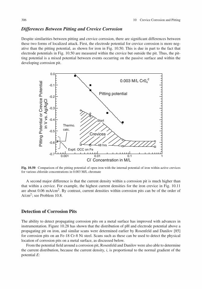
306 10 Crevice Corrosion and Pitting
Differences Between Pitting and Crevice Corrosion
Despite similarities between pitting and crevice corrosion, there are significant differences betweenthese two forms of localized attack. First, the electrode potential for crevice corrosion is more neg-ative than the pitting potential, as shown for iron in Fig. 10.50. This is due in part to the fact thatelectrode potentials in Fig. 10.50 are measured within the crevice but outside the pit. Thus, the pit-ting potential is a mixed potential between events occurring on the passive surface and within thedeveloping corrosion pit.
-0.7
-0.6
-0.5
-0.4
-0.3
-0.2
-0.1
0.0
0.001 0.01 0.1 1
Pitt
ing
Pot
entia
l or
Cre
vice
Pot
entia
lin
V v
s. A
g/A
gCl
Cl- Concentration in M/L
Thermo. calc.
Exptl. OCC on Fe
Pitting potential
Crevices
Start
48 hrs
0.003 M/L Cr04-2
Fig. 10.50 Comparison of the pitting potential of open iron with the internal potential of iron within active crevicesfor various chloride concentrations in 0.003 M/L chromate
A second major difference is that the current density within a corrosion pit is much higher thanthat within a crevice. For example, the highest current densities for the iron crevice in Fig. 10.11are about 0.06 mA/cm2. By contrast, current densities within corrosion pits can be of the order ofA/cm2; see Problem 10.8.
Detection of Corrosion Pits
The ability to detect propagating corrosion pits on a metal surface has improved with advances ininstrumentation. Figure 10.28 has shown that the distribution of pH and electrode potential above apropagating pit on iron, and similar scans were determined earlier by Rosenfeld and Danilov [85]for corrosion pits on an Fe-18 Cr-8 Ni steel. Scans such as these can be used to detect the physicallocation of corrosion pits on a metal surface, as discussed below.
From the potential field around a corrosion pit, Rosenfeld and Danilov were also able to determinethe current distribution, because the current density, i, is proportional to the normal gradient of thepotential E:

Detection of Corrosion Pits 307
i = −σ
(δE
δz
)(10)
where σ is the conductivity of the solution and z denotes the direction normal to the electrode surface;see Fig. 10.51. Isaacs [87] advanced the technique by scanning across a surface in the XY plane so asto produce traces of propagating pits. Later refinements [88] included a scanning vibrating electrode(SVE) which produces potential scans and also current scans by sampling the potential gradientnormal to the surface. For example, Fig. 10.52 shows the distribution of current density obtainedover active sites on an iron surface in a chloride solution [88].
0 5 10 15 200
2
4
6
8
10
12
Horizontal Distance in cm
Ver
tical
Dis
tanc
e in
cm
0.0 V
0.05 V
0.10 V0.15 V 0.20 V 0.25 V 0.30 V
0.35 V
0.40 V
0.45 V
Steel Nickel
Fig. 10.51 Distribution of potential (solid lines) and current density (dotted lines) for a steel/nickel co-planar couplein tap water. (The lines of constant current density are at right angles to the equipotential lines.) Redrawn from [86]by permission of ECS – The Electrochemical Society
With advances in scanning probe techniques, increased attention has turned to the more difficulttask of the detection of the initiation stage of pitting and of the imaging of sites which are pre cur-sors to pitting. In this regard, Smyrl and co-workers [89, 90] have successfully employed severalnew experimental scanning techniques. Smyrl et al. found that surface active sites corresponded tolocations of pit formation (although not all active sites led to pits). Inclusions, second-phase parti-cles, and other defects, such as grain boundaries, were among the sites of increased electrochemicalactivity.
Other advanced instrumental methods which have been used recently to study pit initiationinclude the use of the atomic force microscope (AFM) (discussed in Chapter 9) and the scanningKelvin probe (SKP) (which measures changes in work function) [91, 92].
At present these newer scanning techniques are useful in laboratory research studies, and wouldbe welcome inspection tools should they be transitioned into practice. At present there is a needfor reliable technique for the detection of pit initiation sites on metal structures or electroniccomponents.

308 10 Crevice Corrosion and Pitting
Fig. 10.52 The distribution of current density over an iron surface showing the location and progressive growth of apit in a solution of 1 mM NaCl plus 1 mM Na2SO4, as determined using a vibrating probe electrode [88]. Reproducedby permission of © NACE International (1990)
Problems
1. In what ways are crevice corrosion and pitting similar? In what ways are they different?2. (a) Name and discuss two different ways to test the resistance of an alloy to crevice corrosion.
(b) Name and discuss two different ways to test the resistance to pitting corrosion.3. (a) Sketch an Evans diagram showing the approximate shape of anodic and cathodic polarization
curves for a low alloy steel which undergoes general corrosion in seawater. Assume thatanodic dissolution is under activation control and that the cathodic half-cell reaction is con-trolled by oxygen diffusion.

Problems 309
(b) Show that the total weight loss for the low alloy steel in a crevice is the same for the followingtwo cases:
Crevice area External cathode area
1.0 cm2 10.0 cm2
2.0 cm2 10.0 cm2
(c) Which of the two cases above will have the greater weight loss per unit area?4. Sketch the approximate shapes of cyclic anodic polarization curves to explain the variation in the
protection potential, as shown in Fig. 10.31 for type 430 stainless steel. The corrosion potentialis −0.50 V vs. SCE and the pitting potential is −0.100 V vs. SCE.
5. Make a sketch analogous to Fig. 10.46 for a corrosion pit on aluminum in a chloride solution.6. The following laboratory data were taken for the anodic polarization of aluminum in 0.1 M
NaCl. The sample size is 8.0 cm2. Plot these data and determine the critical pitting potential.
E in V vs. SCE Current in μA
−1.30 0.40−1.20 0.58−1.10 0.68−1.00 0.70−0.900 0.78−0.800 0.71−0.775 0.75−0.750 0.76−0.725 0.79−0.700 1.20−0.685 4.00−0.670 104.−0.655 750.−0.640 2100.
7. What is the current density within a corrosion pit on aluminum if the pit size is given inFig. 10.43(d)? Assume that the pit is hemispherical in shape and that the total current withinthe corroding pit is given by the maximum current in the data set above.
8. (a) The following data are for the pitting of pure aluminum in chloride solutions for a short-termimmersion of 24 h [67]. What is the pitting potential for aluminum in 0.6 M NaCl (thechloride ion concentration in seawater)?
[Cl−] Pitting potential, Epit, vs. SCE
0.01 M −0.6200.1 M −0.6850.5 M −0.7300.5 M −0.7251.0 M −0.7601.0 M −0.745

310 10 Crevice Corrosion and Pitting
(b) How does the value for pure aluminum in the short-term immersion test compare with thepitting potential of aluminum alloys as determined from the long-term practical immersiontests in Table 10.5?
(c) If there is a difference between the two values, explain why.9. An Fe-12 Cr alloy was observed to have the following characteristic potentials in 0.1 M NaCl
[55].
pH Ecorr EFlade Epit Eprot
4.6 −0.580 −0.420 −0.040 −0.3505.4 −0.610 −0.470 0.0100 −0.2206.9 −0.700 −0.550 0.0100 −0.2208.9 −0.740 −0.600 0.175 −0.44010.7 −0.800 −0.445 0.210 −0.450
(a) Draw the corresponding experimental Pourbaix diagram and label regions of immunity,general corrosion, perfect passivity, imperfect passivity, and pitting. (b) Over what range ofelectrode potentials is it safe to use Fe-12 Cr in 0.1 M NaCl at pH 8?
10. Shown below are experimentally determined anodic polarization curves in 1 M H2SO4 and 1 MHCl for three alloys [93] (reproduced by permission of NACE International). These alloys arethe conventional 304 stainless steel and two possible replacements, alloy A and alloy B:
304: 18% Cr, 8% Ni, balance FeAlloy A: 12% Cr, balance FeAlloy B: 12% Cr, 10% Ni, 1.5 % Si, 2% Mo, balance Fe
Based on these polarization curves alone, which alloy or alloys can be used instead of 304stainless steel? Why?
1
10
100
1000
-400 0 400 800
Cur
rent
Den
sity
in μ
A/c
m2
E in mV vs. S.C.E.
304
A
B
1 M H2SO4

References 311
–100
0
100
200
300
400
500
600
–400 –300 –200 –100 0 100 200 300
Cur
rent
in μ
A
E in mV vs. S.C.E.
A B3041 M HCl
Reproduced by permission of © NACE International (1979).
11. Explain why the pitting potential decreases with increasing temperature.
References
1. F. J. Martin, K. E. Lucas, and E. A. Hogan, Rev. Sci. Instruments, 73, 1273 (2002).2. I. L. Rosenfeld and I. K. Marshakov, Corrosion, 20, 115t (1964).3. I. B. Ulanovski and Y. M. Korovin, J. Appl. Chem. USSR, 35, 1683 (1962).4. E. McCafferty, J. Electrochem. Soc., 121, 1007 (1974).5. M. H. Peterson, T. J. Lennox, Jr., and R. E. Groover, Mater. Protect. Perform., 9 (1), 23 (1970).6. A. Turnbull, Corros. Sci., 23, 833 (1983).7. F. D. Bogar and C. T. Fujii, “Solution Chemistry in Crevices on Fe-Cr Binary Alloys”, NRL Report 7690, Naval
Research Laboratory, Washington, DC, March 21, 19748. I. L. Rosenfeld in “Localized Corrosion”, R. W. Staehle, B. F. Brown, J. Kruger, and A. Agrawal, Eds., p. 373,
National Association of Corrosion Engineers, Houston, TX (1974).9. T. Suzuki, M. Yamabe, and Y. Kitamura, Corrosion, 29, 18 (1973).
10. J. Mankowski and Z. Szkarlarska-Smialowska, Corros. Sci., 15, 493 (1975).11. M. G. Fontana and N. D. Greene, “Corrosion Engineering”, p. 43, McGraw-Hill, New York (1978).12. R. M. Kain, J. Testing Evaluation, 18, 309 (1990).13. E. McCafferty, J. Electrochem. Soc., 126, 385 (1979).14. Standard Test Method G-48-97, “1998 Annual Book of ASTM Standards”, ASTM, West Conshohocken, PA
(1998).15. K. Sotoudeh, T. H. Nguyen, R. T. Foley, and B. F. Brown, Corrosion, 37, 358 (1981).16. E. McCafferty, F. D. Bogar, E. D. Thomas, C. A. Creegan, K. E. Lucas, and A. I. Kaznoff, Corrosion, 53, 755
(1997).17. R. S. Lillard, M. P. Jurinski, and J. R. Scully, Corrosion, 50, 251 (1994).18. O. B. Ellis and F. L. LaQue, Corrosion, 7, 362 (1951).19. T. J. Lennox, Jr. and M. H. Peterson in “Localized Corrosion”, R. W. Staehle et al., Eds., p. 173, National
Association of Corrosion Engineers, Houston, TX (1974).20. V. R. Pludek, “Design and Corrosion Control”, p. 173, John Wiley and Sons, New York, NY (1977).21. A. J. Sedriks, “Corrosion of Stainless Steels”, p. 201, Wiley-Interscience, New York (1996).22. E. McCafferty, P. P. Trazskoma, and P. M. Natishan in “Advances in Localized Corrosion”, H. S. Isaacs,
U. Bertocci, J. Kruger, and S. Smialowska, Eds., p. 181, National Association of Corrosion Engineers, Houston,TX (1990).

312 10 Crevice Corrosion and Pitting
23. J. R. Galvele in “Passivity of Metals”, R. P. Frankenthal and J. Kruger, Eds., p. 285, The ElectrochemicalSociety, Princeton, NJ (1978).
24. H. P. Leckie and H. H. Uhlig, J. Electrochem. Soc., 113, 1262 (1966).25. R. E. Groover, T. J. Lennox, Jr., and M. H. Peterson, Mater. Protect., 8 (11), 25 (1969).26. Z. A. Foroulis and M. J. Thubrikar, J. Electrochem. Soc., 122, 1296 (1975).27. H. Böhni and H. H. Uhlig, J. Electrochem. Soc., 116, 906 (1969).28. S. Szklarska-Smialowski in “Advances in Localized Corrosion”, H. S. Isaacs, U. Bertocci, J. Kruger, and
S. Smialowska, Eds., p. 41, National Association of Corrosion Engineers, Houston, TX (1990).29. H.-H. Strehblow, Werkstoffe u. Korros., 27, 792 (1976).30. G. S. Frankel, J. Electrochem. Soc., 145, 2186 (1998).31. P. M. Natishan, W. E. O′Grady, E. McCafferty, D. E. Ramaker, K. Pandya, and A. Russell, J. Electrochem. Soc.,
146, 1737 (1999).32. L. A. Krebs and J. Kruger in “Passivity of Metals and Semiconductors”, M. B. Ives, J. L. Luo, and J. R. Rodda,
Eds., p. 561, The Electrochemical Society, Pennington, NJ (2001).33. D. D. Macdonald, J. Electrochem. Soc., 139, 3434 (1992).34. J. O′M. Bockris and L. V. Minevski, J. Electroanal. Chem., 349, 375 (1993).35. J. O′M. Bockris and Y. K. Kang, J. Solid State Electrochem., 1, 17 (1997).36. T. H. Nguyen and R. T. Foley, J. Electrochem. Soc., 127, 2563 (1980).37. S. Yu, W. E. O′Grady, D. E. Ramaker, and P. M. Natishan, J. Electrochem. Soc., 147, 2952 (2000).38. W. Khalil, S. Haupt, and H.-H. Strehblow, Werkstoffe u. Korros., 36, 16 (1985)39. N. Sato, Electrochim. Acta, 16, 1683 (1971).40. W. A. Badawy, M. M. Ibrahim, M. M. Abou-Romia, and M. S. El-Bosiouny, Corrosion, 42, 324 (1986).41. I. L. Rosenfeld in “Proceedings of the Fifth International Congress on Metallic Corrosion”, p. 53, NACE,
Houston, TX (1974).42. G. Butler, P. Stretton, and J. G. Beynon, Br. Corros. J., 7, 168 (1972).43. B. E. Wilde and E. Williams, Electrochim. Acta., 16, 1971 (1971).44. N. Pessall and C. Liu, Electrochim. Acta, 16, 1987 (1971).45. G. S. Frankel, L. Stockert, F. Hunkeler, and H. Boehni, Corrosion, 43, 429 (1987).46. I. L. Rosenfeld, I. S. Danilov, and R. N. Oranskaya, J. Electrochem. Soc., 125, 1729 (1978).47. D. A. Jones and B. E. Wilde, Corros. Sci., 18, 631 (1978)48. T. Hakkarainen in “Proceedings of the Eighth International Congress on Metallic Corrosion”, Vol. 1, p. 157,
DECHEMA, Frankfurt am Main, (1981).49. R. C. Newman and H. S. Isaacs in “Passivity of Metals and Semiconductors”, M. Froment, Ed., p. 269,
Amsterdam (1983).50. E. McCafferty and N. Hackerman, J. Electrochem. Soc. 119, 999 (1972).51. M. Pourbaix, Corros. Sci., 12, 161 (1970).52. M. Pourbaix in “Localized Corrosion”, R. W. Staehle, B. F. Brown, J. Kruger, and A. Agrawal, Eds., p. 12,
National Association of Corrosion Engineers, Houston, TX (1974).53. R. A. Bonewitz and E. D. Verinck, Jr., Mater. Perform., 14 (8), 16 (1975).54. K. K. Starr, E. D. Verinck, Jr., and M. Pourbaix, Corrosion, 32, 47 (1976).55. E. D. Verinck, Jr., and M. Pourbaix, Corrosion, 27, 495 (1971).56. E. D. Verinck, Jr., K. K. Starr, and J. M. Bowers, Corrosion, 32, 60 (1976).57. A. J. Sedriks in “Corrosion of Stainless Steels”, p. 123, Wiley-Interscience, New York (1996).58. C. R. Clayton and I. Olejford in “Corrosion Mechanisms in Theory and Practice”, P. Marcus and J. Oudar, Eds,
p. 175, Marcel Dekker, New York, NY (1995).59. Z. Szklarska-Smialowska and E. Lunarska, Werkstoffe u. Korros., 32, 478 (1981).60. A. J. Sedriks, Intl. Met. Rev., 28, 295 (1983).61. A. J. Sedriks in A. J. Sedriks, “Corrosion of Stainless Steels”, p. 24, Wiley-Interscience, New York (1996).62. E. McCafferty and P. G. Moore, J. Electrochem. Soc., 133, 1090 (1986).63. B. Vuillemin, X. Phillipe, R. Oltra, V. Vignal, L. Coudreuse, L. C. Dufour, and E. Finot, Corros. Sci., 45, 1143
(2003).64. M. P. Ryan, D. E. Williams, R. J. Chater, B. M. Hutton, and D. S. McPhail, Nature, 415, 770 (2002).65. K. D. Efird and G. E. Moller, Mater. Perform., 18 (7), 34 (1979).66. R. J. Brigham, Corrosion, 30, 396 (1974).67. E. McCafferty, Corros. Sci., 45, 1421 (2003).68. P. M. Natishan and E. McCafferty, J. Electrochem. Soc., 136, 53 (1989).69. C. J. Lin, R. G. Du, and T. Nguyen, Corrosion, 56, 41 (2000).
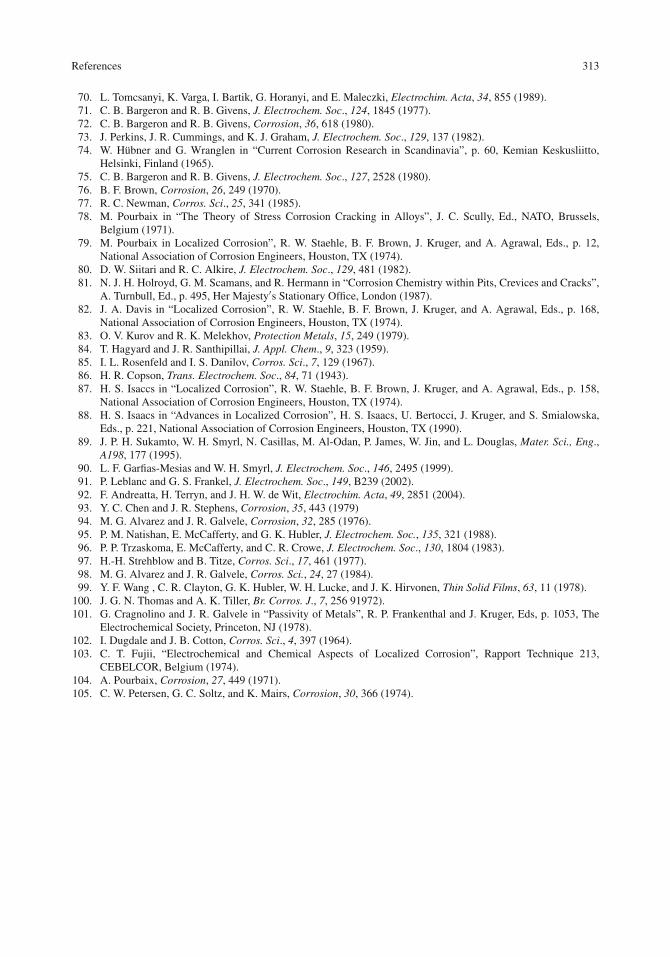
References 313
70. L. Tomcsanyi, K. Varga, I. Bartik, G. Horanyi, and E. Maleczki, Electrochim. Acta, 34, 855 (1989).71. C. B. Bargeron and R. B. Givens, J. Electrochem. Soc., 124, 1845 (1977).72. C. B. Bargeron and R. B. Givens, Corrosion, 36, 618 (1980).73. J. Perkins, J. R. Cummings, and K. J. Graham, J. Electrochem. Soc., 129, 137 (1982).74. W. Hübner and G. Wranglen in “Current Corrosion Research in Scandinavia”, p. 60, Kemian Keskusliitto,
Helsinki, Finland (1965).75. C. B. Bargeron and R. B. Givens, J. Electrochem. Soc., 127, 2528 (1980).76. B. F. Brown, Corrosion, 26, 249 (1970).77. R. C. Newman, Corros. Sci., 25, 341 (1985).78. M. Pourbaix in “The Theory of Stress Corrosion Cracking in Alloys”, J. C. Scully, Ed., NATO, Brussels,
Belgium (1971).79. M. Pourbaix in Localized Corrosion”, R. W. Staehle, B. F. Brown, J. Kruger, and A. Agrawal, Eds., p. 12,
National Association of Corrosion Engineers, Houston, TX (1974).80. D. W. Siitari and R. C. Alkire, J. Electrochem. Soc., 129, 481 (1982).81. N. J. H. Holroyd, G. M. Scamans, and R. Hermann in “Corrosion Chemistry within Pits, Crevices and Cracks”,
A. Turnbull, Ed., p. 495, Her Majesty′s Stationary Office, London (1987).82. J. A. Davis in “Localized Corrosion”, R. W. Staehle, B. F. Brown, J. Kruger, and A. Agrawal, Eds., p. 168,
National Association of Corrosion Engineers, Houston, TX (1974).83. O. V. Kurov and R. K. Melekhov, Protection Metals, 15, 249 (1979).84. T. Hagyard and J. R. Santhipillai, J. Appl. Chem., 9, 323 (1959).85. I. L. Rosenfeld and I. S. Danilov, Corros. Sci., 7, 129 (1967).86. H. R. Copson, Trans. Electrochem. Soc., 84, 71 (1943).87. H. S. Isaccs in “Localized Corrosion”, R. W. Staehle, B. F. Brown, J. Kruger, and A. Agrawal, Eds., p. 158,
National Association of Corrosion Engineers, Houston, TX (1974).88. H. S. Isaacs in “Advances in Localized Corrosion”, H. S. Isaacs, U. Bertocci, J. Kruger, and S. Smialowska,
Eds., p. 221, National Association of Corrosion Engineers, Houston, TX (1990).89. J. P. H. Sukamto, W. H. Smyrl, N. Casillas, M. Al-Odan, P. James, W. Jin, and L. Douglas, Mater. Sci., Eng.,
A198, 177 (1995).90. L. F. Garfias-Mesias and W. H. Smyrl, J. Electrochem. Soc., 146, 2495 (1999).91. P. Leblanc and G. S. Frankel, J. Electrochem. Soc., 149, B239 (2002).92. F. Andreatta, H. Terryn, and J. H. W. de Wit, Electrochim. Acta, 49, 2851 (2004).93. Y. C. Chen and J. R. Stephens, Corrosion, 35, 443 (1979)94. M. G. Alvarez and J. R. Galvele, Corrosion, 32, 285 (1976).95. P. M. Natishan, E. McCafferty, and G. K. Hubler, J. Electrochem. Soc., 135, 321 (1988).96. P. P. Trzaskoma, E. McCafferty, and C. R. Crowe, J. Electrochem. Soc., 130, 1804 (1983).97. H.-H. Strehblow and B. Titze, Corros. Sci., 17, 461 (1977).98. M. G. Alvarez and J. R. Galvele, Corros. Sci., 24, 27 (1984).99. Y. F. Wang , C. R. Clayton, G. K. Hubler, W. H. Lucke, and J. K. Hirvonen, Thin Solid Films, 63, 11 (1978).
100. J. G. N. Thomas and A. K. Tiller, Br. Corros. J., 7, 256 91972).101. G. Cragnolino and J. R. Galvele in “Passivity of Metals”, R. P. Frankenthal and J. Kruger, Eds, p. 1053, The
Electrochemical Society, Princeton, NJ (1978).102. I. Dugdale and J. B. Cotton, Corros. Sci., 4, 397 (1964).103. C. T. Fujii, “Electrochemical and Chemical Aspects of Localized Corrosion”, Rapport Technique 213,
CEBELCOR, Belgium (1974).104. A. Pourbaix, Corrosion, 27, 449 (1971).105. C. W. Petersen, G. C. Soltz, and K. Mairs, Corrosion, 30, 366 (1974).

Chapter 11Mechanically Assisted Corrosion
Introduction
In the previous chapter we discussed two forms of localized corrosion – crevice corrosion and pitting.This chapter considers five more forms of localized corrosion, and these have the added commonfeature that they are assisted by mechanical processes. These five forms of mechanically assistedlocalized corrosion are stress-corrosion cracking, corrosion fatigue, cavitation corrosion, erosioncorrosion, and fretting corrosion.
Stress-corrosion cracking is the cracking of a metal or alloy by the combined action of stress andthe environment. Stress-corrosion cracking (SCC) can occur in stressed structures such as bridgesand support cables, aircraft, pressure vessels, pipelines, and turbine blades, to name a few instances.Figure 11.1 shows the failure of a high strength rocket motor case due to stress-corrosion crackingin tap water [1].
During stress-corrosion cracking, most of the metal or alloy is virtually unattacked, as shownschematically in Fig.11.2 [2]. However, the presence of stress-corrosion cracks reduces the cross-section of the metal capable of carrying a load, as shown in Fig. 11.2. In the case of generalcorrosion, the same reduction in effective thickness due to the formation of rust layers may takeyears. Instances of stress-corrosion cracking are especially serious when they involve critical struc-tures such as bridges or aircraft as described in Chapter 1, because they involve the loss of life orpersonal injury.
The study of stress-corrosion cracking (SCC) requires an interdisciplinary approach involvingelectrochemistry, materials science, and mechanics, as suggested in Fig. 11.3. Some of the variableswhich affect SCC within each of these disciplines are also given in Fig. 11.3.
Corrosion fatigue is the cracking of a metal or alloy due to the combined action of a repeatedcyclic stress and a corrosive environment. Corrosion fatigue can occur in aircraft wings, in bridges,and in offshore platforms which are impacted by ocean waves, and in vibrating machinery. In addi-tion, stainless steel and titanium alloys used as orthopedic implants (for knee and hip replacements)can also undergo corrosion fatigue under cyclic stresses in the electrolyte found within the humanbody.
Cavitation corrosion is the combined mechanical and corrosion attack caused by the collapse andimpingement of vapor bubbles in a liquid near a metal surface. Cavitation corrosion can occur in shippropellers, within pumps, on turbine blades, on hydrofoils, and on other surfaces where there is ahigh-velocity fluid flow and where pressure changes are encountered. Figure 11.4 shows an exampleof cavitation corrosion.
Two additional forms of mechanically assisted corrosion are erosion corrosion and fretting cor-rosion. In erosion corrosion, the mechanical effect is provided by the movement of a corrosiveliquid against the metal surface (without the need for cavitating bubbles). In fretting corrosion, the
315E. McCafferty, Introduction to Corrosion Science, DOI 10.1007/978-1-4419-0455-3_11,C© Springer Science+Business Media, LLC 2010

316 11 Mechanically Assisted Corrosion
Fig. 11.1 Fracture of a high-strength steel rocket case due to stress-corrosion cracking [1]. The arrows indicate thelocation of the stress-corrosion crack
Sectiondimension
capableof carrying
load
σ
σ
σ
σ
Rust
Stresscorrosion
Sectiondimension
capableof carrying
load
σσ
σσ
σ
σ
σσ
σσ
Rust
Stresscorrosion
Fig. 11.2 Reduction in the effective cross section of a metal due to general corrosion or the presence of stress-corrosion cracks. The arrows show the direction of the applied stress, σ . Redrawn from Staehle [2] by permission of© NACE International 1969
mechanical effect is due to the abrasive wear of two metal surfaces sliding or vibrating past eachother. Erosion corrosion can occur in various types of equipment exposed to fast-moving liquids.These include piping systems, bends, elbows, valves, and pumps. Polymer, glass, and metal surfaceson moving aircraft can be damaged by rainwater erosion [3]. Solids suspended in a liquid can alsocause erosion corrosion, as in coal slurry pipelines. Fretting corrosion can occur in loaded interfaceswhich move past each other, such as in vibrating machinery, connecting rods, or springs. Fretting cor-rosion can also be a problem with orthopedic implants placed in the human body. Fretting corrosionis also called wear corrosion or tribocorrosion.

Introduction 317
ElectrochemistryElectrode potentialpHSolution speciesAdditivesTemperature
Materials scienceAlloy compositionMicrostructureGrain shape and sizeGrain boundary compositionStrength level
MechanicsApplied stressResidual stressSpecimen type
Metal Environment
Fig. 11.3 Disciplines used in studying stress-corrosion cracking and variables which affect SCC within eachdiscipline
Fig. 11.4 Cavitation damage on the outer edge of a propeller on a personal watercraft. Figure courtesy of Erik Axdahl,who took this photograph while he was an undergraduate research assistant at the University of Minnesota and who isnow a Graduate Research Assistant at the Georgia Institute of Technology
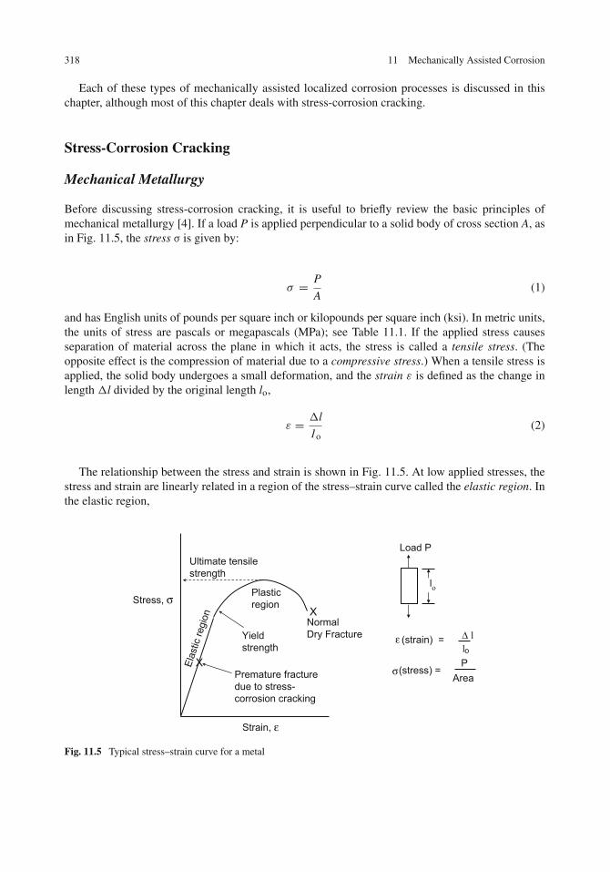
318 11 Mechanically Assisted Corrosion
Each of these types of mechanically assisted localized corrosion processes is discussed in thischapter, although most of this chapter deals with stress-corrosion cracking.
Stress-Corrosion Cracking
Mechanical Metallurgy
Before discussing stress-corrosion cracking, it is useful to briefly review the basic principles ofmechanical metallurgy [4]. If a load P is applied perpendicular to a solid body of cross section A, asin Fig. 11.5, the stress σ is given by:
σ = P
A(1)
and has English units of pounds per square inch or kilopounds per square inch (ksi). In metric units,the units of stress are pascals or megapascals (MPa); see Table 11.1. If the applied stress causesseparation of material across the plane in which it acts, the stress is called a tensile stress. (Theopposite effect is the compression of material due to a compressive stress.) When a tensile stress isapplied, the solid body undergoes a small deformation, and the strain ε is defined as the change inlength �l divided by the original length lo,
ε = �l
1o(2)
The relationship between the stress and strain is shown in Fig. 11.5. At low applied stresses, thestress and strain are linearly related in a region of the stress–strain curve called the elastic region. Inthe elastic region,
XNormalDry Fracture
Ultimate tensile strength
Yieldstrength
Elas
tic re
gion
Plasticregion
Strain, ε
Stress, σ
Premature fracturedue to stress-corrosion cracking
σ(stress) = P
Area
ε (strain) =loΔ l
Load P
ol
X
Fig. 11.5 Typical stress–strain curve for a metal

Stress-Corrosion Cracking 319
Table 11.1 Systems of units used in mechanics
Parameter English units Metric units
Force Poundsa or kilopoundskg m
sec2= netwtons (N)
Stress Pounds/in.2 (psi) or kilopounds/in.2 (ksi)N
m2= Pa
MN
m2= MPa
Stress intensity factor, KI ksi√in. MPa√m
aIn English units, a pound is the force which imparts to a given mass called a “slug” an acceleration of1 ft/s2.Useful conversion factors: 1 ksi = 6.89 MPa; 1 ksi√in. = 1.10 MPa√m.
σ = E ε (3)
where E is a proportionality constant called Young’s modulus and is a property of the solid material.Equation (3) is called Hooke’s law. In the elastic region the strains are reversible and if the load isremoved, the material returns to its original length.
However, if material is loaded to higher stresses, the deformation becomes permanent or plastic,and Hooke’s law no longer applies. The stress marking the beginning of plastic deformation is calledthe yield stress σY (also called the yield strength), and the point where the material can supportthe highest load is called the ultimate tensile stress (also called the ultimate tensile strength). InFig. 11.5, the material finally fractures at point X.
Characteristics of Stress-Corrosion Cracking
Figure 11.5 applies to the tensile testing of a solid metal in air or in the presence of an inert environ-ment. The effect of an electrolyte is to cause the metal to fail prematurely at lower stresses due tostress-corrosion cracking, as indicated in Fig. 11.5.
The following are the most important characteristics of SCC [5]:
(1) A tensile stress is required. The tensile stress may be external, as with an applied load, or thestress may be a residual stress due to metal-working processes, such as machining or welding.The stress may also be self-generated, as may be caused by the wedging action of solid corrosionproducts within an emerging crack.
(2) Metals or alloys which undergo SC usually have a good resistance to general corrosion. Forexample, stainless steels, aluminum alloys, and titanium all undergo SCC but are usually resis-tant to general corrosion (in neutral solutions). One exception is that high-strength low-alloysteels may undergo both general corrosion and SCC at the same time.
(3) Specific environments cause SCC in certain alloys. For example, Cl– solutions (but not NO3–
solutions) cause SCC of type 304 stainless steels. On the other hand NO3– solutions (but not
Cl–solutions) cause SCC of mild steel. In addition, ammonia or amines are specific reagents forthe SCC of brasses (Cu–Zn alloys). Some specific environments which cause SCC for variousmetals are listed in Table 11.2.

320 11 Mechanically Assisted Corrosion
Table 11.2 Some examples of stress-corrosion cracking
Types of alloys Environments
High-strength steels [33] Seawaterchloride solutionssolutions containing H2SNO3
– solutionsStainless steels [20] Cl–, Br–, F– solutions
hydroxide solutionspolythionic acids
(H2SxO6, x = 3, 4, 5)thiosulfate solutions
Aluminum alloys [24] Chloride solutionsmost aqueous solutionsorganic liquids
Titanium alloys [1, 66, 37, 34] SeawaterCl–, Br–, I– solutionscarbon tetrachloride and other organic solvents,
including alcoholsfuming nitric acid
Brass (Cu–Zn alloys) [41, 40] Ammonia solutionsaminescitrate solutionstartrate solutions
(4) The necessary corrodent species can be present in small concentrations. For example, a fewppm of Cl– in high-temperature water can cause SCC in certain stainless steels.
(5) A threshold stress or stress intensity must be exceeded for SCC to occur.(6) Stress-corrosion cracks are brittle in macroscopic appearance, i.e., have little evidence of plastic
deformation (but may show plastic flow on a smaller scale).
Stages of Stress-Corrosion Cracking
As with crevice corrosion and pitting, SCC also has two general stages – initiation and propagation.Measurement of the time to failure of a smooth specimen (without surface flaws) can be misleadingbecause such measurements do not differentiate between the initiation and propagation stages. Forinstance, titanium alloys in seawater do not readily pit (often a precursor to SCC) but these alloysundergo fast fracture once a crack is initiated. Thus, there is a long time to failure (consisting largelyof a long initiation time) which masks the susceptibility of titanium alloys to a much more rapidpropagation stage.
Initiation of SCC
The initiation stage of SCC involves a series of events which are depicted in Fig. 11.6 [6, 7]. Theseevents are as follows:
(1) localized breakdown of the passive oxide film due to mechanical damage or to chemical attackby aggressive ions, such as Cl–,
Stress-Corrosion Cracking 321
3. Initiationand growthof SCC
2. Corrosion pitformation
4. Terminalmechanicalrupture
σ1. Localized
breakdownof oxide film
Solution
Oxide
σ
Fig. 11.6 Stages in the initiation of stress-corrosion cracks. (The fourth stage of mechanical rupture deals with prop-agation.) The shaded arrows denote the direction of applied stress, σ . Some systems such as titanium do not easilypit, but a stress-corrosion crack can initiate from a fatigue crack. After Brown [1, 6, 7]
(2) formation of a corrosion pit after the oxide film has been broken, and(3) initiation and growth of a stress-corrosion crack.
The last event in Fig. 11.6 (mechanical rupture) deals with the propagation stage rather than withinitiation.
The corrosion pit can generate a stress corrosion crack in two ways. First, the corrosion pit servesas a stress intensifier, so that the local stress due to an external load is magnified locally near thecorrosion pit. (Stress intensity and the role of flaws in SCC are considered later in this chapter.)Second, the corrosion pit is a source of hydrogen ions, as discussed in Chapter 10. For instance, forstainless steels, the following reaction within the corrosion pit
Cr+3 + 3H2O→ Cr(OH)3 + 3 H+ (4)
generates H+ ions which can be reduced to hydrogen atoms at the tip of an emerging stress-corrosioncrack. This reaction can also occur within propagating stress-corrosion cracks, as depicted inFig. 11.7. This process of local acidification may lead to the phenomenon of hydrogen embrittlement,which assists crack growth, as discussed later in this chapter.
In some instances, stress-corrosion cracks may initiate without visible signs of pitting, as, forexample, in the SCC of titanium alloys in seawater. In addition, stress-corrosion cracks may alsoinitiate because of surface flaws, inherent microstructural defects (such as grain boundaries), or tomechanical damage (such as damage due to erosion).

322 11 Mechanically Assisted Corrosion
1. Dissolution of Cr at the crack tip
Cr H+Cr+3
2. Hydrolysis of Cr+3 to form H+ionsCr+3 + 3 H2O Cr(OH)3+ 3 H+
H++ e– Hads
H+
3. Reduction of H+ within the crack tip
3e–
(within the crack-tip electrolyte)
Metal
Electrolyte
Fig. 11.7 Schematic illustration showing a propagating stress-corrosion cracking in a Cr-containing alloy. This figureshows the production of H+ ions within a crack by the hydrolysis of dissolved Cr3+ ions and the reduction of H+ ionsnear the crack tip
Propagation of SCC
As with crevice corrosion and pitting, the local electrolyte within a stress-corrosion crack becomesacidic in nature due to the hydrolysis of dissolved hydrogen metal cations, as, e.g., in Eq. (4).Thus, the stress-corrosion cracks propagate and grow due to the combined effects of the appliedstress and the corrosive conditions within the crack arising from acidification of the crackelectrolyte.
The acidification of local electrolytes within crack tips was shown by Brown and co-workers[7–10] in a series of experiments in which a slot was cut into a metal, a wedge (of the same metal)was pressed into the slot to initiate a crack, and the sample was then placed into an electrolyte. Afterseveral hours of crack growth, the specimen was removed and placed into liquid nitrogen to freezethe corrodent within the crack. The specimen was broken open, and the pH of the electrolyte wasmeasured with pH indicators as the specimen warmed up and the crack electrolyte melted. ResultingpH values for stress-corrosion cracks within several metals are given in Table 11.3.
Peterson and co-workers [10] also measured the pH within a stress-corrosion crack using theexperimental arrangement shown in Fig. 11.8. By placing a pH electrode at the base of a crack, alens tissue was wet by solution which traveled down the length of the stress-corrosion crack. Someof Peterson’s results are also given in Table 11.3.
There are two modes by which stress-corrosion cracks can propagate within the metal. The crackpath may be intergranular, that is, cracks grow along grain boundaries, or cracks may be trans-granular, in which cracks travel across grain boundaries. Various alloys display various modes ofcrack growth and examples have been compiled by Scully [11]. Figure 11.9 shows an example ofintergranular and transgranular crack growth on the same alloy but in different concentrations of thesame electrolyte [12].

Stress-Corrosion Cracking 323
Table 11.3 pH within stress-corrosion cracks
AlloypH detected atcrack front Bulk solution Sources
7075 Al 3.5 3.5% NaCl Bown, Fujii, and Dahlberg [8]0.45% C steel 3.7 3.5% NaCl Sandoz, Fujii, and Brown [9]AISI type 4340 steel 3.7
3.5–3.93.5% NaCl3.5% NaCl (bulk pH
adjusted between2 and 10)
Sandoz, Fujii, and Brown [9]Smith, Peterson, and Brown [10]
17-4 PH steel(Fe-17 Cr-4 Niprecipitation-hardened)
3.7 3.5% NaCl Sandoz, Fujii, and Brown [9]
Ti-8 Al-1 Mo-1 V 1.7 3.5% NaCl Bown, Fujii, and Dahlberg [8]
Fig. 11.8 An experimental arrangement for determining the pH at a crack tip [7, 10]. Reproduced by permission of© NACE International 1970
Fracture Mechanics and SCC
An important advance in the study of SCC was the application of fracture mechanics to the problem.Fracture mechanics is a relatively new discipline based largely upon the work of G.R. Irwin [13] atthe Naval Research Laboratory in Washington, DC, and is used to treat fracture problems involvingcracks in a quantitative manner. The application of fracture mechanics to SCC is due in large partto the work of B.F. Brown, M.H. Peterson, C.D. Beachem, and their co-workers [14–16], also at theNaval Research Laboratory.
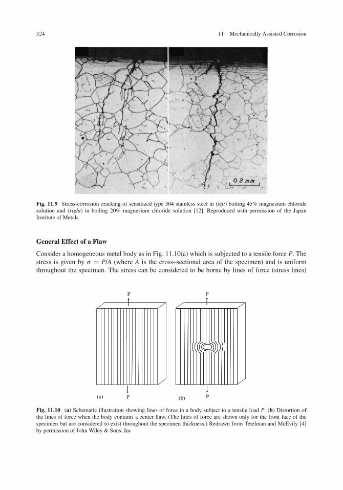
324 11 Mechanically Assisted Corrosion
Fig. 11.9 Stress-corrosion cracking of sensitized type 304 stainless steel in (left) boiling 45% magnesium chloridesolution and (right) in boiling 20% magnesium chloride solution [12]. Reproduced with permission of the JapanInstitute of Metals
General Effect of a Flaw
Consider a homogeneous metal body as in Fig. 11.10(a) which is subjected to a tensile force P. Thestress is given by σ = P/A (where A is the cross–sectional area of the specimen) and is uniformthroughout the specimen. The stress can be considered to be borne by lines of force (stress lines)
P P
P P
(a) (b)
Fig. 11.10 (a) Schematic illustration showing lines of force in a body subject to a tensile load P. (b) Distortion ofthe lines of force when the body contains a center flaw. (The lines of force are shown only for the front face of thespecimen but are considered to exist throughout the specimen thickness.) Redrawn from Tetelman and McEvily [4]by permission of John Wiley & Sons, Inc

Stress-Corrosion Cracking 325
which exist throughout the body, as shown in Fig. 11.10(a) [4]. These lines of force can be thoughtof as parallel columns of small area A′ (with A′ → 0) which support the external load P. Because thebody is uniform throughout, the lines of force exist with uniform spacing, as shown in Fig. 11.10(a).
But suppose there is a flaw in the structure, as shown in Fig. 11.10(b). Because there is no metalin the hole, the lines of force cannot continue through the hole, but must bend around the hole, asshown in Fig. 11.10(b). Thus, in the vicinity of the flaw (i.e., discontinuity), the lines of force (andthus the stresses) are highly concentrated. However, at distances removed from the discontinuity, thelines of force are more evenly spaced.
These considerations give rise to the concept of a stress intensity factor, K, which is defined asfollows:
K = σ (local)
σ (average)(5)
where σ (average) is the average stress in the bulk of the otherwise uniform body. Thus, the stressintensity factor K is a measure of how the stress is increased near a local discontinuity or flaw. Thepower of fracture mechanics is that stress-intensity factors have been derived for flaws of variousgeometries.
General Assumptions
The general assumptions which are made in the application of fracture mechanics to SCC are thefollowing:
(1) Flaws (i.e., cracks) are inherently present in structures.(2) These cracks exist in a linear elastic field (that is, the stress and strain are linearly related).(3) The stress ahead of a crack can be calculated from the stress intensity factor K.(4) The propagation of a crack leading to failure occurs above a critical stress intensity factor.
These ideas are discussed in more detail as we proceed into this chapter.
Fracture Mechanics and KI
There are three modes by which a metal may fracture, called mode I, mode II, and mode III andthese three modes are pictured in Fig. 11.11 [17]. The mode I fracture involves crack opening,mode II is edge sliding, and mode II is crack tearing, which has an additional sliding displacementsuperimposed on a mode I crack.
The mode I crack is the lowest energy mode and is the mode usually encountered in SCC. For aplane sharp defect as shown in Fig. 11.12, the stress components of the crack are given by [17]
σx = KI√2πr
cosθ
2
(1− θ
2sin
3θ
2
)(6)
σy = KI√2πr
cosθ
2
(1+ sin
θ
2sin
3θ
2
)(7)
where KI is the stress intensity factor for a mode I crack, r is the crack length measured from thecrack tip, and θ is measured relative to the crack direction.

326 11 Mechanically Assisted Corrosion
Mode
Mode
Mode Mode II(Edge sliding)
Mode III(Tearing)
Mode I(Opening)
Fig. 11.11 Three basic modes of crack displacements [17]. Reproduced by permission, from [17], copyright ASTMInternational, 100 Barr Harbor Drive, West Conshohocken, PA 19428
leading edge of crack
θX
Y
Z
leading edge of crack
r
θ
Fig. 11.12 Diagram of the leading edge of a mode I crack and the system of co-ordinates. The crack length isdesignated by r [17]. Reproduced by permission, from [17], copyright ASTM International, 100 Barr Harbor Drive,West Conshohocken, PA 19428
Stress Intensity Factors for Specific Types of Flaws
Expressions for the stress intensity factor KI which appears in Eqs. (6) and (7) have been derived forvarious types of specific flaws [17, 18]. For example, for a center crack in an infinite sheet, as shownin Fig. 11.13,
K1 = σ√
πa (8)
where a is half the crack length and σ is the average external stress. For a semi-infinite sheet ofwidth W (but infinite in length),
KI = σ√
πa
(W
πatan
πa
W
)1/2
(9)

Stress-Corrosion Cracking 327
σ
2a
σ
Fig. 11.13 A center crack in an infinite sheet
Two other configurations used in fracture mechanics are the single-edge notched specimen inFig. 11.14 and the thumbnail-shaped surface crack in Fig. 11.15. For the single-edge notchedspecimen:
σ
W
σ
a
Fig. 11.14 A single-edge notched specimen
KI = σ√
πa f (a/W) (10)
where a is the depth of the notch, W is the specimen thickness, and f(a/W) is a geometrical functiongiven by [6, 19]
f (a/W) = 1.12− 0.231a
W+ 10.56
( a
W
)2 − 21.72( a
W
)3 + 30.39( a
W
)4(11)
For the thumbnail-shaped surface crack:
K2I =
1.2πσ 2a
φ2 − 0.212(
σσy
)2(12)

328 11 Mechanically Assisted Corrosion
σ
2b a
σ
K2I =
1.2 π σ2 a
φ2 - 0.212 σσ
Y
2
σ
2b a
σ
K2I =
1.2 π σ2 a
φ2 - 0.212 σσ
Y
2
Fig. 11.15 Opened view of a tensile specimen with a thumbnail crack. The parameter φ is an integral func-tion of a/b. For an infinitely long crack, a/b ≈ 0 and φ2 = 1.00. For a typical thumbnail, a/b = 0.5 andφ2 = 1.46 [15]
where 2b is the crack length and a is now the crack depth, as shown in Fig. 11.15, and σY is theyield stress of the alloy. The parameter φ is an integral function given by φ2 = 1.00 for an infinitelylong surface crack (a/b = 0), and φ2 = 1.46 for a typical thumbnail crack (a/b= 0.5).
For each of these last two specimens, as well as for the center crack specimen, the stress intensityfactor has the form
KI = σ√
π a f (G) (13)
where f(G) is a factor specific to the particular geometry of the specimen and a is the criticaldimension of the crack. Note that KI increases with increasing crack length and with increasingstress σ .
Example 11.1: Calculate the stress intensity factor KI in both English and metric units for an infinitesheet having a center crack of length 0.01 in., a load of 10,000 pounds, and a cross-sectional area of0.50 in.2.Solution:
KI = σ√
π a
σ = 10,000 lbs
0.05 in.2= 20,000
lbs
in.2
a = 0.01 in.
2= 0.005 in.
KI = 20,000lbs
in.2√
π (0.005 in.)
KI = 2,500 psi√
in. = 2.50 ksi√
in.
σ =(10,000 lbs)
(454 g
Ib
) (1 kg
1,000 g
)
(0.50 in.2)(
2.54 cmin.
)2 (1 m
100 cm
)2= 1.41× 10⁷ kg
m2

Stress-Corrosion Cracking 329
In metric units it is necessary to convert the mass per unit area to the force per unit area by usingF = mg. Thus,
σ =(
1.41×10⁷ kg
m2
)(9.8066 m
s2
)
σ = 1.38×10⁸ kg m
m2 s2
σ = 1.38×10⁸ N
m2
σ = (1.38×10⁸ Pa)
(1MPa
1× 10⁶ Pa
)= 138 MPa
Then,
KI = 138 MPa
√π (0.005 in.)
(2.54 cm
in.
)(1 m
100 cm
)= 2.76 MPa
√m
The Cantilever Beam and KIscc
Stress-corrosion tests are often carried out in a pre-cracked cantilever beam experiment introducedby B. F. Brown and co-workers [14–16] at the Naval Research Laboratory (NRL). This test uses a barof square or rectangular cross section containing a notch and a small crack and having the geometryshown in Fig. 11.16. In a typical experiment by Brown and Beachem [15], the metal specimen sizewas 13 cm long, 1 cm thick, and 2.5 cm high. One end of the specimen was clamped in a standand the other end clamped to a loading arm, as shown in Fig. 11.16. The crack in the specimenwas surrounded by a plastic cell containing a reservoir of electrolyte (usually 3.5% NaCl or naturalseawater in the NRL experiments) and a load was applied at the end of a cantilever beam, as shownin Fig. 11.16.
The stress intensity factor for a given load P and crack length a (length of the notch plus thecrack length in the specimen) is calculated from the specimen dimensions, the crack length, and theload P:
KI =4.12 M
(1α3 − α3
)BD3/2
(14)
where α is given by
α = l− a
D(15)
where a is the crack length (notch plus fatigue pre-crack), B is the specimen width, and the otherdimensions are given in Fig. 11.16. The moment M is given by
M = P S (16)
where P is the applied load and S is the distance between the crack and the point of application ofthe load (see Fig. 11.16). The formula for KI for the cantilever beam specimen again has the same

330 11 Mechanically Assisted Corrosion
Dead weight P(or hydraulic load)
Corrosion cell
Specimen
S
Approx.100 cm.
Testframe
Notch
B
Da
Fatigue crack
KI =
4.12 M 1α3
– α31/2
BD3/2
where: α = 1 – aD
and M = P S
Fig. 11.16 (Top) Schematic diagram of a cantilever beam stress-corrosion test. (Center) Specimen details. (Bottom)Mathematical expression for the stress intensity factor KI [14–16, 65]
general form as in Eq. (13). see Problem 11.3. Thus, the units for KI are again ksi √in. in Englishunits or MPa√m in metric units. The depth of the crack increases during the SCC test, and thereforethe stress intensity factor also increases.
Figure 11.17 shows SCC cantilever beam data for AISI 4340 steel in 3.5% NaCl [15] in which KIis plotted vs. the logarithm of the time to failure. Large values of KI (large loads and/or large cracklengths) produce short times to failure, whereas smaller values of KI (small loads and/or small cracklengths) lead to longer times to failure. Note that SCC does not occur in these alloys in 3.5% NaClif KI has a value smaller than 15 ksi √in. Thus, this value of KI is called the critical stress intensityfactor for stress-corrosion cracking and is given the designation KIscc. The significance here is thatvalues of KI less than KIscc do not produce SCC, but values of greater than KIscc lead to SCC. Thevalue of KI which produces cracking in the dry specimen (in the absence of electrolyte) is called thefracture toughness and is given the symbol KIc. The value of KIc is also obtained or approached in thepresence of electrolytes when there is a large applied load, so that the sample suffers fast mechan-ical fracture and there is little or no effect of the electrolyte in the presence of the large appliedload.

Stress-Corrosion Cracking 331
0
10
20
30
40
50
60
70
80
10 100 1,000 10,000 100,000
Str
ess
Inte
nsi
ty F
acto
r K
I in
ksi
in1/
2
Time to Failure in Minutes
KIscc
Fig. 11.17 KIscc tests for type 4340 steel in 3.5% NaCl for cantilever beam specimens [15]. The arrows associatedwith data points indicate no fracture within the time given. Reproduced by permission of Elsevier Ltd
KIscc as a Characteristic Property
Brown [14] showed that the value of KIscc in Fig. 11.17 as measured by the cantilever beam methodwas in excellent agreement with values measured for center-cracked (Fig. 11.13) or surface-cracked(Fig. 11.15) specimens. This agreement shows that the value of KIscc for a given alloy and environ-ment is not a function of the test setup and KIscc is in fact considered to be a material property (forthe given environment).
The stress intensity factor KIscc is a function of the alloy type, alloy composition, strength levelof the alloy, and the nature of the electrolyte. Figure 11.18 shows that Mo additions increaseKIscc values for Fe–Cr–Ni alloys in aqueous 22% NaCl solutions at 105◦C [20]. (Recall fromChapters 9 and 10 that Mo also has a beneficial effect on the passivity and pitting resistance ofFe–Cr–Ni alloys.) Extensive tables of KIscc in 3.5% NaCl have been compiled for various titaniumalloys [21, 22] and for various precipitation-hardened stainless steels [20]. The effect of the strengthlevel of the alloy is considered in a later chapter.
For a given alloy KIscc is sometimes (but not always) lower for electrolytes than for non-electrolytes. Several examples are compiled in Table 11.4.
SCC Testing
There are two general approaches in conducting SCC tests. The first approach is to use pre-crackedspecimens, as discussed above, and the method involves determination of the threshold stress inten-sity factor for SCC, as shown in Fig. 11.19(a). The crack velocity can also be measured as a functionof the stress intensity factor, as shown in Fig. 11.19(b). (Sometimes the metal will fail before regionsII and III appear).

332 11 Mechanically Assisted Corrosion
0
10
20
30
40
50
60
0 1 2 3 4 5 6
KIs
cc in
MP
a m
-1/2
Weight Percent Molybdenum
904 L
317
316L
A286
X
Y
Fig. 11.18 Effect of molybdenum on the stress intensity factor of Fe–Cr–Ni–Mo alloys in 22% NaCl [20]. (The rangeof Cr is between 15 and 21%; the range of Ni is between 13 and 25%.) Reproduced by permission of John Wiley &Sons, Inc
Table 11.4 Comparison of KIscc for electrolyte solutions vs. non-electrolytes at approximately 25◦C
Alloy Electrolyte ksi√in. MPa√m Non-electrolyte ksi√in. MPa√m
AISI 4340 steel [33](220 ksi yieldstrength)
Seawater 10 11 Methanol 40 44
Uranium alloy [65] 3.5% NaCl 15 17 Water 21 23Ti-8 Al-1 Mo-1 V
[67, 68]3.5% NaCl 18–23 20–25 CCl4 18–23 20–25
0.6 M NaCl 20 22 Methanol 14 150.1 M LiCl 25 28 Glycerine 26 29
The second approach is to use smooth (but stressed) specimens which do not contain defects of aknown size or shape, such as a U-bend specimens, as shown in Fig. 11.20. For smooth specimens,the SCC data are presented as the time to failure as a function of applied stress (not stress intensity).Such curves define a threshold stress level, σ th, below which SCC does not occur, as shown inFig. 11.19(c).
Several different types of metal specimens used in smooth or pre-cracked tests are shown inFig. 11.20 [23]. More details on SCC test methods have been given by Sedriks [23]. The environ-ments used in SCC tests should duplicate or simulate the actual environment in which SCC occurred;and as shown in Table 11.2, the SCC environments are often specific to the type of alloy.

Stress-Corrosion Cracking 333
Time to Failure
Stre
ss In
tens
ity F
acto
r KI Notched and
precracked specimens
KIscc
(a)
Stress Intensity Factor KI
Log
Cra
ck V
eloc
ity
KIcKIscc
RegionI
Region II
RegionIII
Notched andprecrackedspecimens
(b)
Time to Failure
Stre
ss σ
σthreshold
Smooth specimens
(c)
Fig. 11.19 Three different ways to present stress-corrosion cracking data [1, 6, 14]. KIscc refers to the critical stressintensity factor for stress-corrosion cracking and KIc to the value for purely mechanical rupture
Bent beam
(a)(b)
(c) (d)
U – bend C – ring
Tensile
Fig. 11.20 Several different types of smooth specimens used in stress-corrosion cracking tests [1, 23]. None of thesespecimens contain pre-cracks. Reproduced by permission of NACE International

334 11 Mechanically Assisted Corrosion
Interpretation of SCC Test Data
The fracture mechanics approach assumes that there is a critical flaw size which leads to SCC and tofailure if the operating stress intensity factor exceeds a critical value, KIscc. In this approach, KIscc isused as a characteristic parameter of the metal/electrolyte system. But in smooth specimens whichdo not contain intentional flaws, a measure of the resistance to SCC is the threshold stress, σ th,below which SCC does not occur. This section describes how to combine the SCC data from smoothand pre-cracked specimens in order to provide a fracture-safe set of operating conditions [1, 24].
For Al alloy 7079 (Al-4 Zn-3 Mg-0.5 Cu), for a thumbnail-shaped crack the value of KIscc wasobserved to be 4 ksi √in. (4.4 MPa √m) [1]. The threshold stress was found to be σ th = 8 ksi(55 MPa) and the yield stress of the alloy was σ Y = 67 ksi (460 MPa) [1]. Inserting these values ofKIscc and σY into Eq. (12) and assuming a shallow surface crack (a/b ≈ 0, φ2 = 1.00) gives
σ =(
1.00
0.2356 a + 4.73 × 10⁻⁵
)1/2
(17)
where σ is in ksi and b is in inches. Thus, for a flaw depth, a, the critical allowable stress, σ , can becalculated from Eq. (17). Results are given by the slanted line in Fig. 11.21. Any combination of band σ which lies below this slanted line will produce a KI less than KIscc, so that SCC will not occur.But because the yield stress of the alloy should not be exceeded, a safe region for the pre-crackedspecimen is the region below the yield stress and the slanted line.
1
10
100
0.0010 0.010 0.10 1.0
0.010 0.10 1.0
10
100
Cro
ss S
ectio
n S
tres
s, σ
, in
ksi
Flaw Depth, a, in inches
σth
= 8 ksi
σY = 67 ksi
Stress Critical
Stress Intensity Critical
Flaw Depth, a, in cm
Cro
ss S
ectio
n S
tres
s, σ
, in
Mpa
PRE-CRACKED
SMOOTH
Fig. 11.21 A plot of flaw depth vs. stress σ for aluminum alloy 7079-T651 containing a thumbnail-shaped crack [1].The parameter a refers to the depth of the crack, σY is the yield stress of the alloy, and σ th is the threshold stress forsmooth specimens. This “safe-zone plot” shows where the alloy can be used safely for both smooth and pre-crackedspecimens

Stress-Corrosion Cracking 335
However, for smooth specimens, the threshold strength σ th should not be exceeded. Thus, a con-servative estimate of the fracture-safe region is below the hatched line in Fig. 11.21. That is, weshould take into account data for both the smooth and pre-cracked specimens. The intersection ofthe straight line for the threshold stress with the sloping line from fracture mechanics has sometimesbeen interpreted to give the inherent flaw size of a smooth specimen. Plots as in Fig. 11.21 are calledsafe-zone plots.
Note that the “stress critical” and “stress intensity critical” lines in Fig. 11.21 intersect at a flawsize of 0.06 in. (1.5 mm). Two interpretations regarding this flaw size are possible. First, this flawsize is the inherent flaw size resident in a “smooth sample.” Second, other forms of corrosion suchas pitting or intergranular corrosion first occur so as to produce a defect of this size, which in turnleads to stress-corrosion cracking.
Metallurgical Effects in SCC
For high-strength steels, KIscc depends on the strength level of the steel. Figure 11.22 shows that thevalue of KIscc for AISI 4340 steel in seawater decreases with increasing yield strength of the alloy.This means that any advantage in using a higher strength steel is negated in the presence of seawater,which increases the susceptibility to SCC [7, 16].
0
20
40
60
80
100
120 140 160 180 200 220 240
Str
ess
Inte
nsi
ty F
acto
r K
I in
ksi
in1/
2
Yield Strength in ksi
KIc (Dry fracture)
KIscc (Stress-corrosion)
Fig. 11.22 Effect of the yield strength (yield stress) of type 4340 steel on the stress intensity factor for dry fracture KIcor for stress-corrosion cracking KIscc in flowing seawater [7, 16]. Reproduced by permission of © NACE International1990
The resistance to SCC also depends on the shape of the metal grains and on the stressing direction.This is illustrated in Fig. 11.23, which shows the resistance to stress corrosion for Al alloy 7075 (Al-5.5 Zn-2.5 Mg-1.5 Cu) having three different grain shapes [24, 25]. For each case the specimenswere stressed in directions parallel to (A) or perpendicular to (B), the principal grain axis. Thestress-corrosion resistance was defined as the highest initial applied stress that did not cause SCC in84 days exposure to 3.5% NaCl in an alternate immersion test. Figure 11.23 shows that the resistanceto SCC was the highest where the most highly oriented grain was stressed parallel to the principalgrain axis.

336 11 Mechanically Assisted Corrosion
0
10
20
30
40
50
60
70
80 B B
A
A
StressingDirection
A B A B A B
Str
ess
at F
ailu
re (
ksi)
Fig. 11.23 Effect of grain shape and stress direction on the stress-corrosion cracking of Al alloy 7075 in a 3.5% NaClalternate immersion test [25]. Reproduced by permission of NACE International
In addition to the grain shape, the grain size is also a factor in determining the resistance to SCC.A fine grain size has been shown to increase the resistance to SCC of carbon steels in solutions con-taining H2S or nitrates [26], of brass in ammonia [27], and of stainless steels in boiling magnesiumchloride [28]. The effect of a coarse grain size on increased susceptibility to SCC has been attributedto changes in the grain boundary composition and microstructure. That is, the total quantity of aprecipitated phase that is responsible for SCC will become more enriched in the grain boundary asthe grain becomes larger. (Mechanisms of SCC are discussed in a later section.) However, Parkins[29] suggested that the effect of grain size is explained by the well-known experimental observationthat the yield strength of the alloy decreases with increasing grain size. (This is called the Hall andPetch effect [30], in which the barrier to slip across a grain increases with increasing grain size.)
Environmental Effects on SCC
So far we have considered stress-corrosion cracking largely from a mechanics point of view. The roleof the electrolyte has been to lower the critical value of the stress intensity factor for SCC (KIscc)relative to the critical value in the absence of the electrolyte (KIc).
In general, environmental factors which influence SCC include the nature of the electrolyte, theelectrode potential, the concentration of corrodent species, and the temperature.
Effect of Electrode Potential
The electrode potential is one of the major controlling parameters in SCC. Evidence is anecdotal innature, having been accumulated though various case histories of SCC. For smooth specimens the

Stress-Corrosion Cracking 337
electrode potential can affect the threshold stress or the time to failure (or equivalently, the crackingrate). For pre-cracked specimens the electrode potential can affect the value of KIscc.
Uhlig and Cook [31] conducted experiments on the effect of the electrode potential on the SCCof type 304 stainless steel in boiling magnesium chloride solutions. The time to failure of U-bendspecimens was decreased by polarization in the anodic direction but the time to failure was increaseddramatically by cathodic polarization. As shown in Fig. 11.24, there is a critical electrode potentialbelow which (more negative than) SCC does not occur. Uhlig and Cook explained this behavioron the basis that the damaging Cl– ion adsorbs on the plastically deformed metal surface abovethe critical potential, but desorbs below this potential. This effect is considered again later whenmechanisms of SCC are discussed.
–0.20
–0.15
–0.10
–0.05
0.1 1 10 100
Time to Failure in Hours
Pot
ent
ial i
n V
vs.
S.H
.E.
Cl– adsorbs
Cl– desorbs
Corrosion potential
Fig. 11.24 Effect of electrode potential on the stress-corrosion cracking of type 304 stainless steel C-ring specimensin boiling magnesium chloride solutions [31]. Reproduced by permission of ECS – The Electrochemical Society
Other examples where the electrode potential affects the susceptibility to SCC or the cracking rateinclude the SCC of alloy 825 (a Ni–Cr–Fe–Mo alloy) in acidified solutions containing Cl– ions andH2S [32], the SCC of Fe-18 Cr-9 Ni stainless steel in boiling magnesium chloride solutions [20], andthe SCC of various steels in chloride solutions [33, 20]. Beck [34] has shown that the crack growthrate of Ti-8Al-1Mo-1 V in 0.6 M halide solutions is a linear function of the electrode potential andthat the effect is similar for Cl–, Br–, or I– solutions.
The electrode potential also affects KIscc values. Fujii and Metzbower [35] found that the val-ues for the high-strength steel HY 130 decreases with increasing negative potential, as shown inTable 11.5. Data compiled for various steels [6, 33] also indicate that cathodic protection decreases
Table 11.5 Effect of potential on KIscc values for HY-130 steel in 3.5% NaCl solutions [35]
Condition E vs. Ag/AgCl (V) KIscc (ksi√in.) KIscc (MPa√m)
Freely corroding –0.78 129 142Coupled to Zn –1.0 97 107Coupled to Mg –1.5 88 97

338 11 Mechanically Assisted Corrosion
KIscc values. The effect of electrode potential on KIscc values for AISI 4340 steel in chloride solu-tions is shown in Fig. 11.25. It can be seen that there is a slight effect of electrode potential on KIscc.More dramatic changes in KIscc with electrode potential have been observed for other steels [36].
0
10
20
30
40
50
60
70
80
–1.6–1.4–1.2–1.0–0.8–0.6–0.4
E in V vs. Ag/AgCl
Open circuit potential
200 YS
175 YS
150 YS
125 YS
(Seawater)
KISS
C ksi
in 1/2
Fig. 11.25 Effect of electrode potential on the stress intensity factor of type 4340 steel of various yield strengths (YS)given in ksi. The solution is 3.5% NaCl (unless noted otherwise) [7, 33]
Effect of Cl– Concentration and pH
In general, an increase in the concentration of a critical solution species causes an increase in thesusceptibility to SCC, although relationships are not always simple. For example, an increase in Cl–
concentration causes an increase in the SCC susceptibility of type 304 stainless steel at 100◦C, asshown in Fig. 11.26 [20]. But the effect of Cl– is also related to the concentration of dissolved O2, asshown in studies on the time to cracking of type 304 stainless steel [28]. Increasing the concentrationof Cl–, Br–, or I– ions increases the velocity of SCC cracks for Ti-8 Al-1 Mo-1 V [37].
The effect of pH depends on the particular system. For example, the lifetime of an Al-7 Mgalloy increases greatly for pH values greater than approximately 7 [25]. The lifetime of brass inammoniacal copper sulfate also depended on pH, attaining a minimum lifetime at a pH of about7.2 [38]. However, pH values between 1.05 and 11.5 had no effect on the SCC susceptibility ofmagnesium alloys in a salt solution [39].
It should be remembered, however, that in crack propagation it is the local pH within the crack tipthat is important rather than the bulk pH. As noted in Table 11.3, various metals can generate locallyacidic crack tip environments even though the bulk electrolyte is neutral.
Effect of Temperature
The effect of increase temperature is to increase the susceptibility to stress-corrosion cracking orto increase the rate of crack growth. Examples have been given by Sedriks [20] and by Marsh andGerberich [36].

Stress-Corrosion Cracking 339
0
20
40
60
80
100
Cra
cke
d S
peci
men
s in
Cum
ula
tive
%
Time in Hours
1500 ppm Cl–
100 ppm Cl–
10 ppm Cl–
10 100 1000 10,000
Fig. 11.26 Effect of chloride concentration on the SCC susceptibility of type 304 stainless steel [20]. Reproduced bypermission of John Wiley & Sons, Inc
Mechanisms of SCC
Various mechanisms have been proposed to explain SCC. No single mechanism has been universallyaccepted and different mechanisms apply to different cases of SCC. The major mechanisms are
(1) Anodic dissolution(2) Film rupture(3) Stress-sorption cracking(4) Hydrogen embrittlement
These mechanisms fall into two classifications: those which involve dissolution effects (the firsttwo above) and those that involve mechanical effects (the last two above).
Anodic Dissolution
The anodic dissolution mechanism applies if there is an active anodic path established by microstruc-tural heterogeneities in the metal. (This mechanism is also called the electrochemical mechanism ofSCC or the active path mechanism of SCC.) As an example, CuAl2 precipitates which form alongthe grain boundaries in an Al-4% Cu alloy render the grain boundaries anodic to the grain, as shownschematically in Fig. 11.27 [40]. Anodic dissolution of the grain boundary in the presence of anapplied stress leads to intergranular SCC.
However, the anodic dissolution model cannot explain instances of transgranular SCC. For exam-ple, failures of stainless type 304 have occurred due to a phenomenon called sensitization. Whenaustenitic stainless steels are heated through the temperature range 425–900◦C (800–1650◦F),chromium tends to combine with carbon to form chromium carbides. These carbides precipitatepreferentially at grain boundaries, thus depleting chromium from the metal located in the grainboundaries. The grain boundaries thus become anodic to the grains, so that an active path exists
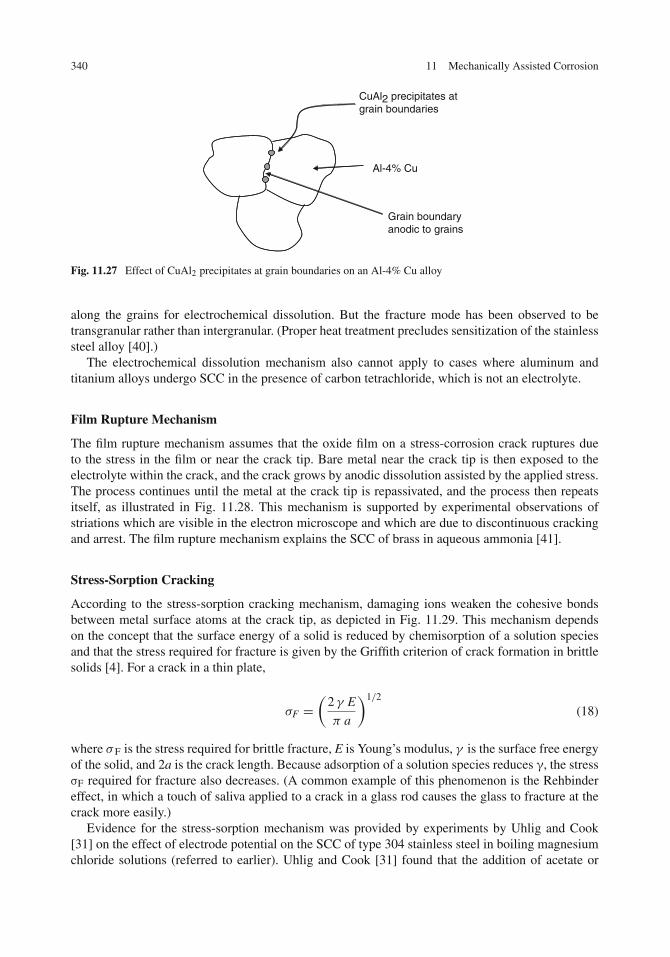
340 11 Mechanically Assisted Corrosion
CuAl2 precipitates atgrain boundaries
Al-4% Cu
Grain boundaryanodic to grains
Fig. 11.27 Effect of CuAl2 precipitates at grain boundaries on an Al-4% Cu alloy
along the grains for electrochemical dissolution. But the fracture mode has been observed to betransgranular rather than intergranular. (Proper heat treatment precludes sensitization of the stainlesssteel alloy [40].)
The electrochemical dissolution mechanism also cannot apply to cases where aluminum andtitanium alloys undergo SCC in the presence of carbon tetrachloride, which is not an electrolyte.
Film Rupture Mechanism
The film rupture mechanism assumes that the oxide film on a stress-corrosion crack ruptures dueto the stress in the film or near the crack tip. Bare metal near the crack tip is then exposed to theelectrolyte within the crack, and the crack grows by anodic dissolution assisted by the applied stress.The process continues until the metal at the crack tip is repassivated, and the process then repeatsitself, as illustrated in Fig. 11.28. This mechanism is supported by experimental observations ofstriations which are visible in the electron microscope and which are due to discontinuous crackingand arrest. The film rupture mechanism explains the SCC of brass in aqueous ammonia [41].
Stress-Sorption Cracking
According to the stress-sorption cracking mechanism, damaging ions weaken the cohesive bondsbetween metal surface atoms at the crack tip, as depicted in Fig. 11.29. This mechanism dependson the concept that the surface energy of a solid is reduced by chemisorption of a solution speciesand that the stress required for fracture is given by the Griffith criterion of crack formation in brittlesolids [4]. For a crack in a thin plate,
σF =(
2 γ E
π a
)1/2
(18)
where σ F is the stress required for brittle fracture, E is Young’s modulus, γ is the surface free energyof the solid, and 2a is the crack length. Because adsorption of a solution species reduces γ, the stressσF required for fracture also decreases. (A common example of this phenomenon is the Rehbindereffect, in which a touch of saliva applied to a crack in a glass rod causes the glass to fracture at thecrack more easily.)
Evidence for the stress-sorption mechanism was provided by experiments by Uhlig and Cook[31] on the effect of electrode potential on the SCC of type 304 stainless steel in boiling magnesiumchloride solutions (referred to earlier). Uhlig and Cook [31] found that the addition of acetate or

Stress-Corrosion Cracking 341
Brittle crackGrain boundaryAq.NH3
Brass
(a)
Oxidation
Preferentialpenetration
(b) (c)
Slip
(d) (e) (f)
Fracture surface
.
Brass
Fig. 11.28 Schematic illustration of the film rupture mechanism for stress-corrosion cracking. (a) The oxide filmis considered to grow preferentially along a grain boundary (b) until it undergoes brittle fracture (c). The crack isarrested by slip in the substrate exposing metal to the environment (d). Further intergranular penetration then occurs(e) leading to further limited fracture (f). Crack propagation proceeds by repeated the cycles, and the resulting fracturesurface shows evidence of discontinuous fracture [1, 41]
Direction of crack growth
ion adsorbingat a crack tip
Metal
Solution
Metal atoms
Cl–Cl–
Cl–
Fig. 11.29 Schematic diagram of the stress-sorption mechanism of SCC. An aggressive anion, such as Cl–, adsorbsat or near the crack tip to weaken the metal–metal bond at the crack tip (this figure is drawn using 1.24 Å (0.124 nm)as the radius of a metal (Fe) atom and 1.81 Å (0.181 nm) as the radius of a chloride ion)
nitrate ions raised the critical potential for SCC, as shown in Table 11.6. These authors proposed thatthere is competitive adsorption between the inhibitive species (acetate or nitrate) and the aggressivespecies (chloride). Adsorption of the inhibitive species prevails when its concentration is sufficientlyhigh. For 5% NaNO3, for example, the corrosion potential lies below the critical potential for SCC,so that SCC does not occur at the open-circuit corrosion potential in this solution.

342 11 Mechanically Assisted Corrosion
Table 11.6 Corrosion and critical potentials for cold-rolled type 304 stainless steel in MgCl2 boiling at 130◦C [31]
Anion additionCorrosion potentialEcorr(V vs. SHE)
Critical potentialEcrit(V vs. SHE) Ecorr < Ecrit? SCC at Ecorr?
None –0.11 –0.145 No Yes0.1% sodium acetate –0.12 –0.132 No Yes2% sodium acetate –0.12 –0.116 Yes NoNone –0.11 –0.145 No Yes2% sodium nitrate –0.06 –0.090 No Yes5% sodium nitrate –0.08 –0.070 Yes No
The stress-sorption model also explains the SCC of alloys in non-electrolytes, such as aluminumalloys in carbon tetrachloride solutions.
Hydrogen Embrittlement
Hydrogen embrittlement refers to the loss of ductility or to the cracking in a metal caused by theentrance of hydrogen atoms into the metal lattice. (Hydrogen embrittlement is also called hydrogen-assisted cracking.) Hydrogen is a culprit due to several reasons. These include its small atomic size,its solubility in most metals, and its mobility (hydrogen atoms diffuse through most metals). In addi-tion, hydrogen atoms can be present at the metal surface from several different sources. Hydrogenatoms arise from corrosion reactions or from various metal processing steps, such as melting orrolling, cleaning in acid solutions (“pickling”), or in electroplating from acid solutions.
Hydrogen atoms are produced by the reduction of hydrogen ions enroute to the evolution ofhydrogen gas. The first step is
2 H+ + 2 e− → 2 Hads (19)
followed by either
2 Hads → H2 (20)
orHads + H+ e− → H2 (21)
Equation (19) followed by Eq. (20) is called the combination mechanism of hydrogen evolution,while Eq. (19) together with Eq. (21) is called the electrochemical mechanism of hydrogen evolution[42]. Either mechanism involves the adsorption of hydrogen atoms, and some of these adsorbed Hatoms can enter the metal rather than participating in Eqs. (20) or (21) (see also Chapter 7).
As shown by Brown and co-workers (Table 11.3), the electrolyte near the crack tip becomesacidified, so that hydrogen reduction and the production of hydrogen atoms is possible within the tipof the stress-corrosion crack. This possibility has been shown dramatically by Peterson et al. [10]for type 4340 steel using the experimental setup shown in Fig. 11.8. Potential–pH data for cracktip electrolytes formed in a 3.5% NaCl solution are superimposed on the partial Pourbaix diagramshown in Fig. 11.30. It can be seen that all data points lie below the “a” line for hydrogen evolution,so that it is possible for the reduction of hydrogen ions to occur within the crack tip.
The actual mechanism by which hydrogen embrittlement occurs is not entirely clear but may bedue to several different effects. These are as follows:

Stress-Corrosion Cracking 343
–1500
–1000
–500
0
500
1000
1500
0 4 8 12 16
Cathodic control
Freely corroding
Anodic control
E in
mV
vs.
S.C
.E.
pH
b
a
Fe+2
Fe3O4
Fe2O3
Fe
Fig. 11.30 Electrochemical conditions at a propagating stress-corrosion crack in type 4340 steel and superimposedon a Pourbaix diagram for Fe [7, 10]. Note that all experimental data lie below the “a” line for hydrogen evolution,so that the reduction of hydrogen ions is possible within the stress-corrosion crack. • Freely corroding, � externalsample anodically polarized, ◦ external sample cathodically polarized. (The experimental data were obtained usingthe device shown in Figure 11.8.) Reproduced by permission of © NACE International 1970
(1) An internal pressure is caused by the release of interstitial hydrogen atoms as molecularhydrogen gas within voids or flaws.
(2) Brittle metal hydrides are formed at the crack tip, and these brittle hydrides can be fractured toallow the crack to grow.
(3) Hydrogen diffuses to and adsorbs at the crack tip, reducing the surface free energy. (This is aform of stress-sorption cracking.)
(4) Hydrogen diffuses ahead of the crack tip and aids in plastic deformation of the metal in advanceof the crack.
Experimental evidence for the plastic deformation mechanism has been provided by Beachem[43], who used the electron microscope to examine in detail the fracture surfaces on various carbonsteels subjected to SCC in aqueous NaCl or charged with hydrogen gas. The appearance of regions ofplastic-deformed metal ahead of the crack tip suggested that the presence of sufficiently concentratedhydrogen dissolved in the metal just ahead of the crack tip assisted the fracture process.
Anodic Dissolution vs. Hydrogen Embrittlement
It is possible to distinguish between anodic dissolution and hydrogen embrittlement by observingthe effect of the electrode potential on the time to failure. Figure 11.31 compares schematically themechanisms of anodic dissolution and hydrogen embrittlement [44] and also illustrates the expectedeffect of the electrode potential on the susceptibility to SCC. For the anodic dissolution mechanism,polarization in the anodic direction increases the rate of anodic dissolution and thus decreases thetime to failure. For the hydrogen embrittlement mechanism, polarization in the cathodic directionincreasingly generates more hydrogen atoms for penetration into the metal, and thus decreases thetime to failure.

344 11 Mechanically Assisted Corrosion
Fe Fe+3Fe+3
Fe+3Fe
Fe
Applied Current Density
Time to failure
Cathodic Anodic
(a) Anodic dissolution
Applied Current Density
Time to failure
Cathodic Anodic
(b) Hydrogen embrittlement
H+H+
H+Hads
Hads
Hads
(a)
Fig. 11.31 Schematic comparison of the anodic dissolution mechanism (active path corrosion) of SCC and thehydrogen embrittlement mechanism of SCC. Adapted from Brown [44]
Figure 11.32 illustrates the effect of small impressed currents on the time to failure of a marten-sitic steel in an aqueous solution containing (NH4)2S and acetic acid [44]. A small cathodic currentdecreases the time to fracture, while small anodic currents increase the fracture time. This behaviorindicates that in the case of zero impressed current, the failure occurs by hydrogen embrittlement.
0
5
10
15
20
25
–40 –20 0 20 40
Tim
e to
Fra
ctur
e in
Hou
rs
Impressed Current Density in µA/cm2
AnodicCathodic
Fig. 11.32 Effect of impressed current on time to fracture of a martensitic steel in 5% acetic acid plus 0.1% ammo-nium sulfide. Redrawn from Brown [44]. This figure shows that the mechanism of stress-corrosion cracking washydrogen embrittlement

Stress-Corrosion Cracking 345
0
1
2
3
4
5
6
7
8
–20 –10 0 10 20
Tim
e to
Fra
ctur
e in
Hou
rs
Impressed Current Density in µA/cm2
AnodicCathodic
Fig. 11.33 Effect of impressed current on time to fracture of a martensitic steel in distilled water containing H2S.Redrawn from Brown [44]. This figure shows that the mechanism of stress-corrosion cracking was anodic dissolution
Figure 11.33 shows the effect of small impressed currents on the same steel but in a differentsolution (H2S in distilled water) [44]. Here a small cathodic current increases the time to failure, buta small anodic current decreases the time to failure, indicating that the SCC mechanism is anodicdissolution. (Not shown in the figure is that hydrogen embrittlement occurs at larger impressedcathodic currents.)
If it is suspected that hydrogen embrittlement is the cause of SCC, then hydrogen permeationmeasurements should be made. Hydrogen permeation can be determined by an electrochemical tech-nique described elsewhere [45], and such experiments provide information as to hydrogen uptake asa function of electrode potential. Using such measurements, Wilde [46] showed that the SCC of ahigh-strength Fe-12 Cr-1 Mo steel in sodium chloride solutions was due to hydrogen embrittlement.
On a Universal Mechanism of SCC
Each of the different SCC mechanisms discussed in the previous sections has its own shortcom-ings. Some of these are listed in Table 11.7, which illustrate the point made earlier that no singlemechanism of SCC can apply to all cases of SCC.
Protection Against Stress-Corrosion Cracking
Methods of preventing SCC are based upon our knowledge of the mechanisms of SCC and uponengineering experience. Preventative measures include the following [47]:
(1) Lowering the stress below the threshold stress for fracture or maintaining KI below values ofKIscc.

346 11 Mechanically Assisted Corrosion
Table 11.7 Shortcomings in the various mechanisms of stress-corrosion cracking
Mechanism Comment
Anodic dissolution SCC of sensitized type 304 stainless steel often occurs transgranularly eventhough possible active paths may exist at grain boundaries
Film rupture Requires extremely high local corrosion rates to explain crack growth ratesStress sorption Local plastic deformation would blunt a crack tip and eliminate the sharp tip
required for this mechanism to apply. In addition, there is a competition forthe bare metal surface between the adsorption of solution species andoxide film formation
Hydrogen embrittlement The rate of hydrogen penetration cannot always be related to SCCsusceptibility
(2) Eliminating the critical environmental species (if possible).(3) Applying cathodic protection, but not if the mechanism of SCC is hydrogen embrittlement.(4) Adding inhibitors to the solution.(5) Materials selection. (For example, Ni additions to Fe-18 Cr stainless steels increase the time to
failure in boiling magnesium chloride solutions [20] and Mo additions to Fe–Cr–Ni alloys raisethe KIscc values in sodium chloride solutions, as shown in Fig. 11.18.)
(6) Short peening of the metal surface to put the surface in a state of compressive stress (ratherthan tensile stress) can improve the resistance to SCC [48]. (Shot peening is the controlledimpingement on a metal surface of particles of steel, glass, or ceramics.)
Corrosion Fatigue
Environmental cracking under a cyclic load, as shown in Fig. 11.34 [49], is referred to as corrosionfatigue. Corrosion fatigue fracture surfaces often have characteristic striations due to the intermittentnature of crack growth. Environmental effects are not as specific as in SCC, and the crack growthis usual transgranular, whereas stress-corrosion cracks can be either transgranular or intergranular.The mechanism of corrosion fatigue is not well understood but involves the local slip of metal
Stress range
Maximum stress
Minimum stress
One loadcycle
Fig. 11.34 Load cycling in a corrosion fatigue experiment

Corrosion Fatigue 347
atoms within grains assisted by the corrosion process. The same mechanisms which apply to SCCalso apply to corrosion fatigue [50] with the added complexity that the interaction between theenvironment and mechanical properties is more complicated in the presence of a cyclic load.
Corrosion Fatigue Data
Corrosion fatigue is characterized by plots of tensile stress (S) versus the number of cycles (N) tofailure, as in Fig. 11.35, which are called S–N curves [51, 52]. The stress S is the maximum stress inthe cycle. The definition of cycles to failure varies with individual researcher and can either be theinitiation of a small visible macrocrack or final failure of the test specimen [52].
0
50
100
150
200
250
300
350
Number of Cycles to Failure
Endurancelimitin air
Endurance limit in 3% NaCl
Air
3 % NaCl
10 4 10 5 10 6 10 7 10 8
Alte
rnat
ing
Stre
ss in
MPa
Fig. 11.35 S–N fatigue curves for a 0.21% C steel in air and in 3% NaCl [51]
Figure 11.35 shows S–N curves for a 0.21% C steel in air and in 3% NaCl [51]. In a givenenvironment, failure does not occur if the stress is held below a critical value called the endurancelimit. The effect of the environment is to lower the endurance limit and thus make failure easier. TheS–N curves are not usually frequency dependent in air but are frequency dependent in a corrosiveenvironment. Corrosion fatigue is more pronounced at lower frequencies because the crack spendsmore time in the local environment before the local electrolyte with its changes in solution chemistryis replaced due to the pumping action of the opening and closing of the crack.
A second way of presenting corrosion fatigue data is in a plot of the crack growth per cycle,da/dN, versus the range of the stress intensity factor, �K, where �K = Kmax – Kmin. This type ofplot is shown schematically in Fig. 11.36 [52]. This figure shows that the effect of the corrosiveenvironment is to increase the crack growth rate. In addition, the effect of the environment is mostprominent at the low �K values and is least effective at high �K values where mechanics is dominantand where fast fracture occurs. Plots of da/dN vs. �K display a linear region:
da
dN= C(�K)n (22)

348 11 Mechanically Assisted Corrosion
Corrosiveenvironment
Non-corrosiveenvironment
Region of Paris law
Log Stress Intensity Factor Range, ΔK
Log
Cra
ck G
row
th R
ate,
da/
dn
--
Fig. 11.36 Schematic plot of the fatigue crack growth per cycle, da/dN, vs. the range of the stress intensity factor,�K, where �K = Kmax – Kmin [52]
where C and n are constants to be determined experimentally. Equation (22) is called the Parislaw [53]. The parameter n is a positive number and is usually between 2 and 4. For example, forthe corrosion fatigue of several precipitation-hardened stainless steels in seawater, n has a value ofapproximately 2 [54].
Figure 11.37 shows experimental da/dN vs. �K curves in flowing seawater [55] for Al alloy 7475(Al-5 Zn-2 Mg-1.5 Cu), 17-4 precipitation-hardened (PH) steel (Fe-16 Cr-4 Ni-3 Cu), and a high-strength steel HY-130 (Fe-4 Ni with minor amounts of Cr, Mo, and Mn). As shown in Fig. 11.37, atany given value of �K, the aluminum alloy has the greatest crack growth rate of the three alloys inflowing seawater.
Protection Against Corrosion Fatigue
Preventative measures are similar to those for stress-corrosion cracking. These include [47] reducingthe stress on the component or annealing to relieve residual stress. Because corrosion fatigue is asurface phenomenon, surface finish is of major importance, and procedures such as polishing tosmooth the surface eliminates stress concentration sites. As in the case of SCC, shot peening of thesurface is also useful for protection against corrosion fatigue because the surface is left in a state ofresidual compression [52].
Corrosion fatigue resistance can also be improved by using corrosion inhibitors or coatings suchas nitride coatings. Steels containing chromium and molybdenum (which form nitrides) can betreated by anhydrous ammonia to produce nitride surface layers having improved corrosion fatigueresistance. Ion implantation of nitrogen into titanium surgical implants has been found to increasethe resistance to corrosion fatigue in simulated body fluids [56]. (Ion implantation as a surfacemodification technique is discussed in Chapter 16 on “Special Topics in Corrosion Science”.)

Cavitation Corrosion 349
10 –4
10 –3
10 –2
10 –1
10 100
Cra
ck G
row
th r
Rat
e d
a/dN
in m
m/c
ycle
ΔK in MPa m1/2
50 20020
17-4 PH steelAl alloy 7475
High strength steel(HY-130)
Fig. 11.37 Corrosion fatigue data for three different alloys in flowing seawater (see the text for alloy compositions).Redrawn from Ref. [55] by permission from ASTM International, 100 Barr Harbor Drive, West Coshohocken, PA19428
Corrosion fatigue can also be minimized by design considerations such as eliminating creviceswhere corrosion can be initiated.
Cavitation Corrosion
Cavitation corrosion occurs when the flow of a corrosive liquid produces a localized low pressurewhich leads to the formation of bubbles in the liquid. These low pressures necessary to form bubblescan be caused by fluid flow across curved interfaces. The force of the collapse of these bubblesinvolves creation of shock waves and high-velocity microjects [57, 58]. The impact of these wavesand jets against the metal surface causes a mechanical damage, which is intensified by the corrosiveeffect of the liquid.
The mechanical damage is caused by continuous and local bombardment of the vapor bub-bles against the metal surface, as depicted in Fig. 11.38. The collapse of the bubbles against themetal surface destroys the passive film and removes underlying metal, as shown schematically inFig. 11.38(a) – (c). The metal surface may repassivate, but the process is repeated as inFig. 11.38(d)–(f). The appearance of cavitation is similar to pitting, but the pitted areas are closelyspaced and the surface is roughened considerably.
The pressure �P required to maintain a spherical bubble of radius r in a liquid having a surfacetension γ is given by the Young and Laplace equation [59]:
�P = 2γ
r(23)

350 11 Mechanically Assisted Corrosion
Oxide film
Cavitatingbubble
Metala b c
d e f
Cavitatingbubble
Fig. 11.38 Schematic drawing of cavitation damage. A cavitation bubble in (a) collapses and destroys the oxide filmin (b) and the oxide film is reformed in (c). The process is repeated in steps (d)–(f). Redrawn from Ref. [47] with thepermission of The McGraw-Hill Companies
The magnitude of this pressure is given in the following calculation.
Example 11.2: A laboratory vibrating device used to study cavitation corrosion produces sphericalbubbles which are 20 μm in diameter [57]. Calculate the pressure difference across these bubbles.Solution: The surface tension of water is 72 mJ/m2. Thus,
�P = 2(72 × 10−3J/m2)
10 × 10−6 m
�P = 14,400J
m3
But 1 J = 1 N m, so that
�P = 14,400N
m2= 14,400 Pa = 0.0144 MPa
A small pressure of the order of 0.01 MPa is not sufficient to cause local deformation in a metalas, for example, in a typical aluminum alloy, where the yield stress is 460 MPa (Fig. 11.21). Thus,most of the mechanical damage to the alloy is produced by the hydrodynamic effects of the liquiddue to shock and microjets rather than by the simple collapse of the bubbles. The total pressureinside a bubble is thus
P = Pexternal + 2γ
r(24)
where Pexternal includes all the external effects on the bubble such as hydrodynamic effects plus theeffect of atmospheric pressure.
Cavitation corrosion is studied using a device which vibrates at high frequencies to produce cavi-tating bubbles on the surface of a metal which is immersed in a liquid [60]. Engleberg and Yahalom[61] were among the earliest to demonstrate that there is an electrochemical component to cavita-tion damage. Figure 11.39 shows the effect of cavitation on the anodic polarization curve of a carbonsteel in a potassium hydrogen phthalate buffer of pH 4.0. Cavitation had no effect on the active region

Cavitation Corrosion 351
0.001
0.01
0.1
1
10
–0.5 0 0.5 1 1.5
Cur
ren
t den
sity
in m
A/c
m2
E in V vs. S.C.E.
With vibration
Without vibration
Fig. 11.39 Effect of cavitation on the anodic behavior of a carbon steel in a phthalate buffer of pH 4.0 [61].Reproduced by permission of Elsevier Ltd
0
20
40
60
80
1000 10 20 30 40 50 60 70 80
0 10 20 30 40 50 60 70 80
Wei
ght L
oss
in m
g/(h
r cm
2 ) x
10–2
Wei
ght L
oss
in m
g/(h
r cm
2 ) ×
10–2
Time in Days
0.02
Time in Hours
0
0.01
Cavitation
Cavitation withcathodic protection
Stagnant
Fig. 11.40 Weight loss data for a nickel aluminum bronze alloy in seawater with and without cavitation [62]. Cathodicprotection reduces the weight loss for the cavitating solution. Reproduced by permission of NACE International
of the polarization curve but increased the current density in the passive region by a factor of 30.Figure 11.40 shows rate loss data for a nickel aluminum bronze (80% Cu-9% Al-4.9% Fe-4.9% Ni-1.2% Mn) in seawater with and without cavitation [62]. The effect of cavitation is to increase therate of metal loss, but this rate can be decreased by cathodic protection. Some investigators suggestthat the role of cathodic protection is to provide hydrogen bubbles which cushion the shock waveproduced by the cavitating bubbles [58].
Cavitation corrosion, like corrosion fatigue, is usually transgranular in nature [63]. In this regardthe metallurgical microstructure of the alloy is important because cracks can be initiated by the

352 11 Mechanically Assisted Corrosion
pile-up of dislocations. To prevent or delay this process, it is necessary to produce a large number ofvery fine homogeneously dispersed obstacles, such as precipitates, grain boundaries, or needle-likephases. Therefore surfaces containing a fine dispersion of a hard particle in a more ductile matrixshould improve the cavitation resistance. The high cavitation resistance of martensitic stainless steelshas been attributed to the limitation of dislocation motion by the fine platelets of the martensiticphase [58, 63]. (Martensite is a hard and brittle carbon-containing solid phase found in certain steels.)
Cavitation corrosion can be minimized by several approaches [47, 58] including a change indesign to minimize hydrodynamic flow conditions, by providing smooth surfaces to preclude sitesfor bubble initiation, by cathodic protection, and by alloy selection. Titanium alloys and Ni–Cr–Moalloys which form stable passive films exhibit good resistance to cavitation corrosion [58]. Variouscompilations of cavitation corrosion data are available [47, 57, 64].
Erosion Corrosion and Fretting Corrosion
Erosion corrosion is the attack of a metal caused by the movement of a corrosive liquid against themetal surface. The velocity of the fluid plays an important role in erosion corrosion and increasesin velocity generally lead to increases in erosion corrosion. Turbulent flow results in an increasedcontact of the liquid with the metal surface compared to laminar flow, as depicted in Fig. 11.41, andcauses more damage than laminar flow. For instance, increased corrosion at the inlet ends of tubingis due to turbulent flow at the inlet side (as compared to laminar flow further down the pipe.)
Laminar Turbulent
Fig. 11.41 Schematic diagram of laminar flow vs. turbulent flow in a pipe (The direction of flow is from left to right)
Protective measures [47] include design considerations, materials selection, or the addition ofinhibitors. Design considerations include reduction of surface velocity and turbulence by measuressuch as larger radius elbows, larger pipe diameters, or gradual changes in flow channel dimensions.Materials selection involves the use of passive alloys, such as stainless steel or titanium, which haveincreased resistance to erosion corrosion relative to plain carbon steels [47].
Fretting corrosion is caused by the slight periodic motion of two surfaces rubbing against eachother and is due to the combined effects of wear and corrosion. The mechanical damage is causedby the abrasive rupture of the oxide film and dislodgement of metal particles which themselves areeventually turned into oxide particles that accumulate between the two moving metal surfaces. Theseoxide debris particles act as abrasives which continue to add to the mechanical wear. With continuingmechanical motion, the passive film again breaks down, and the process repeats itself.
Fretting corrosion can be reduced by various measures [40, 47]. These include the use of lubri-cants which reduce friction and also act as corrosion inhibitors, reducing the load between frettingsurfaces, the use of elastomer gaskets between the abrading surfaces, and the use of wear-resistantalloys (such as cobalt-based alloys).

Problems 353
The key scientific issues for both erosion corrosion and fretting corrosion involve passive filmbreakdown and repassivation (or lack thereof) in the presence of the mechanical disruption causedby either fluid flow or wear.
Problems
1. Explain why the parameter KIscc, which arises from fracture mechanics, can vary with theelectrode potential.
2. Calculate the stress intensity factor KI for a high-strength steel having a yield stress of1,470 MPa and a thumbnail-shaped crack of depth a =1.0 mm when the depth of the crackis one-quarter the crack length and the alloy is loaded to one-half of its yield stress.
3. Show that KI for a cantilever beam specimen as given in Fig. 11.16 has the units of MPa√m.4. If a high-strength steel has a critical stress intensity factor of 20 ksi√in. in seawater, what is the
longest crack length that can be tolerated if the structure is loaded to a stress of 50 ksi. Assumea center crack in an infinite sheet.
5. The following data are for the stress-corrosion cracking of a titanium alloy in 3.5% NaCl [16].The alloy had a yield stress of 104 ksi.
Time to fracture (min) Stress intensity factor KI(ksi√in.)
0.1 1282.0 552.5 713.7 528.1 56150 53655 49No break in 1,380 min 47
(a) Plot these data to graphically determine the critical stress-intensity factor, KIscc.(b) For an edge crack which is 0.20 in. long (a = 0.20 in.) in a plate of the alloy which is
10.0 in. wide, what is the maximum external stress which can be applied without causingfracture in the 3.5% NaCl solution?
(c) Suppose that the value of the external stress found in Part (b) above is applied to a specimencontaining a thumbnail-shaped crack where the crack length is the same as in Part (b) above(2b = 0.20 in.). The crack depth a is given by a/b = 0.5. Will fracture occur in this case?
6. Calculate the safe-zone plot for an aluminum alloy in a corrosive environment when the criticalstress intensity factor is 13 MPa √m, the threshold value for fracture (for smooth specimens)is 48 MPa, and the yield stress of the alloy is 410 MPa. Assume a center crack in an infinitespecimen. Indicate regions on the diagram where smooth specimens are immune to fracture,where cracked specimens are immune to fracture, and the overall fracture-safe zone.
7. Based on the effect of electrode potential on KIscc for HY-130 steel as given in Table 11.5,suggest a possible mechanism for stress-corrosion cracking in 3.5% NaCl.
8. The rate of crack growth (v) of a titanium alloy in 0.6 M NaCl at –300 mV SCE was observed tobe 0.010 cm/s [34]. The crack had the geometry shown below [66]. Calculate the current densityrequired for this crack growth rate if the crack growth is due to anodic dissolution. Assume that

354 11 Mechanically Assisted Corrosion
the anodic current is due to the reaction:
Ti→ Ti3+ + 3e−
The density of Ti is 4.5 g/cm3 and the atomic weight is 47.87 g/mol.
l
l'h
θ1o
w
v
'
9. If the effect of an applied current on the time to failure in stress-corrosion cracking is as shownbelow, what can you say about the mechanism of SCC at the open-circuit potential (zero appliedcurrent)?
Applied Current
Cathodic Anodic
Time to Failure
0
10. In what ways is corrosion fatigue similar to stress-corrosion cracking? In what ways do thesetwo forms of localized corrosion differ?
11. For a precipitation-hardened stainless steel in seawater, the constants in the Paris Law, i.e., Eq.(22), are C = 1.6 × 10⁻⁹ (MPa)–2 and n = 2 [54]. How many cycles will it take for a crack togrow by 1.0 mm if �K = 20 MPa√m?
12. How are cavitation corrosion, erosion corrosion, and fretting corrosion similar to each other?How do they differ from each other?
13. Suppose that you have access to a high-velocity flume of a liquid which enables you to studyerosion corrosion. Devise an experiment or test which will determine the effect of electrodepotential on the total erosion-corrosion damage.
References
1. B. F. Brown, “Stress Corrosion Cracking Control Measures”, U. S. Government Printing Office, Washington, DC(1977).
2. R. W. Staehle in “Fundamental Aspects of Stress Corrosion Cracking”, R. W. Staehle, A. J. Forty, and D. vanRooyen, Eds., p. 3, NACE, Houston, TX (1969).

References 355
3. J. H. Brunton and M. C. Rochester in “Treatise on Materials Science and Technology”, Vol. 16, C. M. Preece,Ed., p. 185, Academic Press, New York, NY (1979).
4. A. S. Tetelman and A. J. McEvily, Jr., “Fracture of Structural Materials”, Chapters 1 and 2, John Wiley, NewYork, NY (1967).
5. B. F. Brown in “Stress Corrosion Cracking of Metals – A State of the Art”, ASTM STP 518, p. 3, ASTM,Philadelphia, PA (1972).
6. B. F. Brown in “Stress-Corrosion Cracking in High Strength Steels and in Titanium and Titanium Alloys”,B. F. Brown, Ed., p. 2, U. S. Government Printing Office, Washington, DC (1972).
7. B. F. Brown in “The Theory of Stress Corrosion Cracking in Alloys”, J. C. Scully, Ed., p. 186, NATO, Brussels,Belgium (1971).
8. B. F. Brown, C. T. Fujii, and E. P. Dahlberg, J. Electrochem. Soc., 116, 218 (1969).9. G. Sandoz, C. T. Fujii, and B. F. Brown, Corros. Sci., 10, 839 (1970).
10. J. A. Smith, M. H. Peterson, and B. F. Brown, Corrosion, 26, 539 (1970).11. J. C. Scully, “The Fundamentals of Corrosion”, p. 177, Pergamon Press, Oxford (1990).12. M. Kowaka and T. Kudo, Trans. JIM, 16, 385 (1975).13. G. R. Irwin and A. A. Wells, Met. Revs., 10, 223 (1965).14. B. F. Brown, Met. Revs., 13, 171, (1968).15. B. F. Brown and C. D. Beachem, Corros. Sci., 5, 745 (1965).16. M. H. Peterson, B. F. Brown, R. L. Newbegin, and R. E. Groover, Corrosion, 23, 142 (1967).17. P. C. Paris and G. C. Sigh in “Fracture Toughness Testing and Its Applications”, ASTM STP 381, p. 30, ASTM,
Philadelphia, PA (1965).18. H. Tada, P. C. Paris, and G. R. Irwin, “The Stress Analysis of Cracks Handbook”, Del Research Corporation,
St. Louis, MO (1973).19. S. A. Meguid, “Engineering Fracture Mechanics”, p. 134, Elsevier Applied Science, London (1989).20. A. J. Sedriks, “Corrosion of Stainless Steels”, Chapter 7, Wiley-Interscience, New York, NY (1996).21. R. W. Judy, Jr. and R. J. Goode, “Stress-Corrosion Cracking Characteristics of Alloys of Titanium in Salt Water”,
NRL Report 6564, Naval Research Laboratory, Washington, DC, July 21 (1967).22. R. W. Schutz in “Stress-Corrosion Cracking”, R. H. Jones, Ed., p. 265, ASM International, Materials Park, OH
(1992).23. A. J. Sedriks, ”Stress Corrosion Cracking Test Methods”, NACE, Houston, TX (1990).24. M. V. Hyatt and M. O. Speidel in “Stress-Corrosion Cracking in High Strength Steels and in Titanium and
Titanium Alloys”, B. F. Brown, Ed., p. 147, U. S. Government Printing Office, Washington, DC (1972).25. D. O. Sprowls and R. H. Brown in “Fundamental Aspects of Stress Corrosion Cracking”, R. W. Staehle,
A. J. Forty, and D. van Rooyen, Eds., p. 466, NACE, Houston, TX (1969).26. S. W. Ciaraldi in “Stress-Corrosion Cracking”, R. H. Jones, Ed., p. 41, ASM International, Materials Park, OH
(1992).27. E. N. Pugh, J. V. Craig, and A. J. Sedriks in “Fundamental Aspects of Stress Corrosion Cracking”, R. W. Staehle,
A. J. Forty, and D. van Rooyen, Eds., p. 118, NACE, Houston, TX (1969).28. R. M. Latanision and R. W. Staehle in “Fundamental Aspects of Stress Corrosion Cracking”, R. W. Staehle,
A. J. Forty, and D. van Rooyen, Eds., p. 214, NACE, Houston, TX (1969).29. R. N. Parkins in “Fundamental Aspects of Stress Corrosion Cracking”, R. W. Staehle, A. J. Forty, and D. van
Rooyen, Eds., p. 361, NACE, Houston, TX (1969).30. R. W. Hertzberg, “Deformation and Fracture Mechanics of Engineering Materials”, p. 129, John Wiley & Sons,
New York, NY (1996).31. H. H. Uhlig and E. W. Cook, Jr, J, Electrochem. Soc., 116, 173 (1969).32. N. Sridhar and G. Cragnolino in “Stress-Corrosion Cracking”, R. H. Jones, Ed., p. 131, ASM International,
Materials Park, OH (1992).33. G. Sandoz in “Stress-Corrosion Cracking in High Strength Steels and in Titanium and Titanium Alloys”,
B. F. Brown, Ed., p. 79, U. S. Government Printing Office, Washington, DC (1972).34. T. R. Beck in “The Theory of Stress Corrosion Cracking in Alloys”, J. C. Scully, Ed., p. 64, NATO, Brussels,
Belgium (1971).35. C. T. Fujii and E. A. Metzbower “Stress-Corrosion Cracking in the HY-130 System”, NRL Memorandum Report
2814, Naval Research Laboratory, Washington, DC, June (1974).36. P. G. Marsh and W. W. Gerberich in “Stress-Corrosion Cracking”, R. H. Jones, Ed., p. 64, ASM International,
Materials Park, OH (1992).37. M. J. Blackburn, W. H. Smyrl, and J. A. Feeny in “Stress-Corrosion Cracking in High Strength Steels and in
Titanium and Titanium Alloys”, B. F. Brown, Ed., p. 245, U. S. Government Printing Office, Washington, DC(1972).

356 11 Mechanically Assisted Corrosion
38. J. A. Beavers in “Stress-Corrosion Cracking”, R. H. Jones, Ed., p. 211, ASM International, Materials Park, OH(1992).
39. W. K. Miller in “Stress-Corrosion Cracking”, R. H. Jones, Ed., p. 251, ASM International, Materials Park, OH(1992).
40. H. H. Uhlig and R. W. Revie, “Corrosion and Corrosion Control”, Chapter 7, John Wiley, New York, NY (1985).41. E. N. Pugh in “The Theory of Stress Corrosion Cracking in Alloys”, J. C. Scully, Ed., p. 418, NATO, Brussels,
Belgium (1971).42. J. O’M. Bockris and A. K. N. Reddy, “Modern Electrochemistry”, Vol. 2, p. 1233, Plenum Press, New York, NY
(1977).43. C. D. Beachem, Metall. Trans., 3, 437 (1972).44. B. F. Brown, “Stress-Corrosion Cracking and Related Phenomena in High-Strength Steels”, NRL Report 6041,
Naval Research Laboratory, Washington, DC, November 6 (1963).45. M. A. Devanathan and Z. Stachurski, J. Electrochem. Soc., 111, 619 (1964).46. B. E. Wilde, Corrosion, 27, 326 (1971).47. M. G. Fontana and N. D. Greene, “Corrosion Engineering”, pp. 72, 88–115, McGraw-Hill, New York, NY
(1978).48. C. P. Dieport in “Impact Surface Treatment”, S. A. Meguid, Ed., p. 86, Elsevier Applied Science, London, (1986).49. D. W. Hoeppner in “Corrosion Fatigue: Chemistry, Mechanics, and Microstructure”, A. J. McEvily and
R. W. Staehle, Eds., p. 3, NACE, Houston, TX (1972).50. D. J. Duquette in “Corrosion Mechanisms”, F. Mansfeld, Ed., p. 367, Marcel Dekker, New York, NY (1987).51. V. I. Pokhmurskii and A. M. Krohmalnyi in “Corrosion Fatigue”, R. M. Parkins and Y. M. Kolotrykin, Eds.,
p. 54, The Metals Society, London (1983).52. T. W. Crooker “Basic Concepts for Design Against Structural Failure by Fatigue Crack Propagation”, NRL Report
7347, Naval Research Laboratory, Washington, DC, January 13 (1972).53. P. Paris and F. Erdogan, Trans. ASME, J. Basic Engineering, Series D, 85, 528 (1963).54. A. J. Sedriks, “Corrosion of Stainless Steels”, Chapter 8, Wiley-Interscience, New York, NY (1996).55. F. D. Bogar and T. W. Crooker, J. Testing Evaluation, 7, 155 (1979).56. J. Yu, Z. J. Zhao, and L. X. Li, Corrros. Sci., 35, 587 (1993).57. C. M. Preece in “Treatise on Materials Science and Technology”, Vol. 16, C. M. Preece, Ed., p. 249, Academic
Press, New York, NY (1979).58. A. Karimi and J. L. Martin, Inter. Metal Revs., 31, 1 (1986).59. A. W. Adamson, “Physical Chemistry of Surfaces”, 3rd edition, p. 2, John Wiley, New York, NY (1976).60. “Standard Test Method for Cavitation Erosion Using Vibratory Apparatus”, ASTM Test Method G32-92, “1998
Annual Book of ASTM Standards”, Volume 3.02, p. 103, ASTM, West Conshohocken, PA (1998).61. G. Engelberg and J. Yahalom, Corros. Sci., 12, 649 (1972).62. A. Al-Hashem, P. G. Caceres, W. T. Riad, and H. M. Shalaby, Corrosion, 51, 331 (1995).63. W. W. Hu, C. R. Clayton, and H. Herman, Mater. Sci. Eng, 45, 263 (1980).64. N. D. Tomashov, “Theory of Corrosion and Protection of Metals”, p. 465, MacMillan Company, New York, NY
(1966).65. W. F. Czyrkalis and M. Levy, “Stress Corrosion Cracking of Uranium Alloys”, AMMRC Report TR 73-54, Army
Materials and Mechanics Research Center, Watertown, MA, December (1973).66. T. R. Beck, J. Electrochem. Soc., 115, 890 (1968).67. R. A. Bayles and D. A. Meyn in “Corrosion Cracking”, V. S. Goel, Ed., p. 241, American Society of Metals,
Metals Park, OH (1986).68. W. H. Smyrl and M. J. Blackburn, J. Mater. Sci., 9, 777 (1974).

Chapter 12Corrosion Inhibitors
Introduction
Several different methods of corrosion protection have been considered so far in this text. Thesemethods can be classified as ones of changing the electrode potential of the metal surface or ofchanging the nature of the metal itself. Cathodic protection and anodic protection are two methodsof corrosion control by changing the electrode potential. The nature of the metal can be changedthrough the use of metallic coatings (sacrificial or noble) or by material selection in which acorrosion-resistant alloy is chosen over a less corrosion-resistant one. Very often, however, mate-rial selection is not an option due to the requirements of retaining some other desirable property(such as mechanical strength), or is prohibited by cost. In such cases, altering the environment bythe use of corrosion inhibitors then becomes a possible means of corrosion control.
A corrosion inhibitor is any chemical substance which when added to a solution (usually in smallamounts) increases the corrosion resistance. Corrosion inhibitors modify electrochemical reactionsby their action from the solution side of the metal/solution interface, and the increase in corrosionresistance can be measured by various parameters. In uniform corrosion, the rate of general corrosiondecreases from some value io (without the inhibitor) to an inhibited value i, and the percent inhibition(% I) is given by
%I = io − i
io× 100 (1)
In pitting, the use of inhibitors raises the pitting potential but may also decrease the pit growthrate and the number of corrosion pits per unit area. In crevice corrosion, inhibitors usually decreasethe propagation rate of crevice corrosion. In stress-corrosion cracking, inhibitors can increase thetime to failure by increasing the time to crack initiation and/or by decreasing crack growth rates.
Corrosion inhibitors are used in various industrial applications, including potable (drinking)water, cooling water systems, automobile engine coolants, acid pickling (cleaning) solutions, toprotect reinforcing steel bars in concrete, and in oil recovery and storage. Various applications andthe inhibitors used are listed in Table 12.1. Inhibitors are also used in the surface treatment of met-als to improve the corrosion resistance (chromates on aluminum alloys or galvanized steel) or toimprove their paint adhesion (phosphates on autobody steel sheet). Corrosion inhibitors can also beincorporated into paints or organic coatings.
A growing interest in corrosion inhibitors is illustrated by the increasing number of publishedarticles in the corrosion literature. Hackerman [5] noted the following:
357E. McCafferty, Introduction to Corrosion Science, DOI 10.1007/978-1-4419-0455-3_12,C© Springer Science+Business Media, LLC 2010

358 12 Corrosion Inhibitors
Table 12.1 Some industrial applications of corrosion inhibitors [1–4]
Application Inhibitors
Potable (drinking) water CaCO3 depositionSilicatesPolyphosphates
Recirculating cooling water ChromatesNitratesPolyphosphatesSilicatesZinc saltsBenzotriazole (for copper)
Automotive engine coolant systems(ethylene glycol/water)
Borax–nitrite mixturesSodium mercaptobenzothiazoleBenzotriazole
High-chloride solutions (seawater,refrigerating brines)
ChromatesSodium nitriteChromate–phosphate mixtures
Acid pickling (cleaning mixtures) Various aminesPyridineQuinolineMercaptansPhenylthiourea
Oil recovery Primary, secondary, tertiary aminesDiaminesAmidesPolyethoxylated amines
Steel-reinforced concrete Calcium nitriteSodium benzoate
Surface treatment of metalsAluminum aircraft components and
galvanized steelChromates
Autobody steel sheet Phosphates
• The first issue of Chemical Abstracts (published in 1907) contained no references to corrosioninhibition.
• The first such reference appeared in 1909 followed by a handful of references in each of the nextfew issues.
• The number of references on corrosion inhibition had grown to 280 by the 50th Edition (1956)and in 1990, the number of entries was voluminous.
This trend can be seen in Fig. 12.1, which records the number of listings for a computerizedsearch using the ISI Web of Science R© and the keywords “corrosion and (inhibition or inhibitor)”.As can be seen in Fig. 12.1, there is an explosion of entries for the time frame 1990–1999, and thenumber of entries for the 9 years from 2000 to 2008 is double that for the previous 10 years.
This chapter will draw on selective examples from the vast amount of work which has been donebut will focus primarily on the fundamental aspects of corrosion inhibition.
The mechanisms of corrosion inhibition are different for acidic and neutral solutions. In acid solu-tions, natural oxide films initially present on the metal surface are dissolved away so that inhibitorsthen interact directly with the metal surface. In neutral solutions, the system is more complex because

Types of Inhibitors 359
0
1000
2000
3000
4000
Num
ber
of E
ntrie
s
1945-1959
1960-1969
1970-1979
1980-1989
1990-1999
2000-2008
Fig. 12.1 Results for a computerized literature search for “corrosion inhibition” or “corrosion inhibitor”
the metal surface is oxide covered and also because dissolved oxygen may participate in the elec-trode reaction. Both types of solutions are addressed in this chapter. Most of this chapter deals withcorrosion inhibition in aqueous solutions, although vapor-phase inhibitors are also considered.
Types of Inhibitors
Inhibitors can be classified in several different ways. The two main types are (i) adsorption inhibitorsand (ii) film-forming inhibitors.
Adsorption inhibitors form a chemisorptive bond with the metal surface and impede ongoingelectrochemical dissolution reactions. Most organic inhibitors are chemisorption-type inhibitors. Forexample, Fig. 12.2(a) shows schematically that an aliphatic organic amine has an electron pair on thenitrogen atom which is available for donation to the metal surface. In addition, the hydrocarbon tailsof the molecule are oriented away from the interface toward the solution so that further protectionis provided by the formation of an array of hydrophobic hydrocarbon tails located on adjacentlyadsorbed amines. This hydrophobic network serves to keep water molecules and aggressive anions,such as Cl−, away from the metal surface, as shown in Fig. 12.2(b)
There are two types of film-forming inhibitors: (i) passivating inhibitors and (ii) precipitationinhibitors. As implied by their name, passivating inhibitors function by promoting the formationof a passive film on the surface. Passivating inhibitors may be oxidizing or non-oxidizing agents.(Oxidizing agents themselves are reduced in the process of oxidizing another molecule). Chromatesare typical oxidizing inhibitors, and with iron or steels, the chromate ion is reduced to Cr2O3 orCr(OH)3 on the metal surface to produce a protective mixed oxide of chromium and iron oxides[6]. Adsorption is also important with oxidizing inhibitors because they are usually adsorbed onthe metal surface prior to their reduction and formation of the passive film. Non-oxidizing passi-vators like benzoates, azelates, and phosphates also first adsorb on the surface before forming thepassive film.

360 12 Corrosion Inhibitors
Metal
Atomic number of N = 7Filled shells : 2, 8, 18, … electrons
Solution
(b)
(a)
H
Hydrocarbon tail Electronsavailablefor bonding
C
HX
X
X
N
H
H
N
NN
N
Metal
Atomic number of N = 7Filled shells : 2, 8, 18, … electrons
Solution
(b)
(a)
H
Hydrocarbon tail Electronsavailablefor bonding
CC
HX
X
X
N
H
H
N
NN
NN
NN
N
Fig. 12.2 (a) Chemisorption of amines at a metal surface. The solid black dots denote electrons belonging to the Natom, whereas the Xs refer to electrons from H or C atoms. (The size of the nitrogen atom is exaggerated relative tothe rest of the molecule.) (b) Formation of a close-packed monolayer on the metal surface
With precipitation inhibitors, a precipitation reaction between cations of the corroding metal andthe inhibitor deposits a three-dimensional barrier film on the metal surface. Such a film is formedwhen the solubility product is exceeded for the salt formed between the cations of the metal and theanions of the inhibitor. Phosphates and silicates are examples of precipitation-type inhibitors.
From another point of view, inhibitors can be classified as anodic, cathodic, or mixed inhibitors,depending on which partial electrochemical reaction is affected. As examples, chromates areanodic inhibitors, some phosphates are cathodic inhibitors, and most organic compounds are mixedinhibitors.
Acidic Solutions
Much of the information about the mechanisms of corrosion inhibitors has evolved from the studyof acidic solutions. The reason is that the dissolution of air-formed surface films allows focus on thedirect interaction between the inhibitor and the cleaned metal surface. Another simplification oftenmade in mechanistic studies is that the solution is de-aerated so that oxygen does not participate inthe electrode reaction and the cathodic reaction is restricted to hydrogen evolution. However, theeffect of dissolved oxygen in acidic solutions does not appear to be important until the pH is as highas 2–4 [7].
Despite these simplifications, the general results for acidic solutions have considerable practicalapplication. Corrosion inhibitors are used in a variety of acidic environments, including commercialpickling (cleaning) processes, in the storage and transport of acids, in oil and gas production, in thepulp and paper industry, and in the cleaning of corroded metal artifacts. In addition, corrosion inhi-bition in de-aerated acidic solutions serves as a scaled-up model for the inhibition of the propagation

Acidic Solutions 361
of localized corrosion processes, such as crevice corrosion, pitting, and stress-corrosion cracking,where the internal local electrolyte becomes both acidic and depleted in oxygen.
The most important act of the inhibitor in acid solutions is to chemisorb on the metal surface. Theprocess of chemisorption and factors which affect it are discussed below.
Chemisorption of Inhibitors
Chemisorption involves an actual charge transfer or charge sharing between the inhibitor moleculeand the metal surface. By interacting with metal surface atoms, the chemisorbed inhibitor inter-feres with metallic dissolution. The simplest picture is one of a blockage of active surface sites,but this view is not quite complete. Like all adsorbed species, chemisorbed molecules have a cer-tain residence time at the surface and thus play a dynamic role by participating in a number ofadsorption–desorption steps.
The main characteristics of chemisorption are the high heats of adsorption, persistence, andspecificity. Table 12.2 compares the process of chemisorption with physisorption (i.e., physicaladsorption), a more general type of adsorption but one involving weaker interactions.
Table 12.2 Comparison of chemical adsorption (chemisorption) and physical adsorption (physisorption) [8]
Physisorption Chemisorption
Type of electronicinteraction
Van der Waals orelectrostatic forces
Charge transfer or charge sharing
Reversibility Adsorbed species readilyremoved by solventwashing
Adsorption is irreversible, morepersistent
Energetics Low heat of adsorption,<10 kcal/mol(40 kJ/mol)
Higher heat of adsorption,>10 kcal/mol (40 kJ/mol)
Kinetics Rapid adsorption Slow adsorptionSpecificity Adsorbed species
relatively indifferent toidentity of surface
Specific interaction, strongdependence on identity ofsurface
Chemisorption-type inhibitors usually contain N, S, or O atoms; and chemisorption occursthrough the donation of electrons from these atoms to the metal surface, as shown in Fig. 12.2for a primary amine. In a homologous series differing in the identity of the donor atom, the order ofcorrosion inhibition is
-Se > -S > -N > -O
Increasing inhibition
Increasing electronegativity
The order of corrosion inhibition is the reverse order of the electronegativity of these atoms. Forinstance, sulfur compounds are usually better corrosion inhibitors than are their nitrogen analogsbecause a S atom is less electronegative than a N atom (is less effective in drawing electrons to itself),so S is a better electron donor than is N. (It should be noted that sulfur and selenium compounds areless soluble than the corresponding nitrogen compounds).

362 12 Corrosion Inhibitors
Direct evidence for the chemisorption of corrosion inhibitors has been gained through many stud-ies which have utilized various techniques such as radiotracer measurements, infrared spectroscopy,and modern surface analytical techniques such as X-ray photoelectron spectroscopy (XPS), amongothers.
Effect of Inhibitor Concentration
The inhibitor efficiency (% I) increases as the concentration of the dissolved inhibitor increases.Figure 12.3 shows polarization curves for iron in 6 M HCl containing various amounts of the diamineNH2(CH2)3NH2 [9, 10]. It can be seen in Fig. 12.3, as well as in Fig. 12.4, that the corrosion ratedecreases (and % I increases) with increasing concentration of the diamine.
Fig. 12.3 Polarization curves for iron in 6 M HCl with NH2-(CH2)3-NH2 inhibitor. The numbers on the figure referto the concentration of the diamine [9, 10]. Reproduced by permission of ECS – The Electrochemical Society
With increased concentration of inhibitor, the corrosion rate decreases because the adsorptionof the inhibitor also increases, as shown in Fig. 12.5(a). Figure 12.5(a) illustrates schematicallyan adsorption isotherm, which relates the concentration of the inhibitor in solution to the amountof inhibitor taken up by the surface. For chemisorption-type inhibitors, the maximum fraction ofthe surface able to be covered is one monolayer (i.e., one molecular layer). When this coverage isreached, the corrosion rate attains its minimum value, and further increases in inhibitor concentrationdo not produce any further decrease in the corrosion rate, as shown in Fig. 12.5(b).
There are several different types of adsorption isotherms, and these are discussed later in thischapter.

Acidic Solutions 363
0
500
1000
1500
2000
20
40
60
80
100
0 0.01 0.10
Cor
rosi
on R
ate
in μ
A/c
m2
Concentration of NH2(CH2)3NH2 in M/l
Per
cent
Inhi
bitio
n
Uninhibited Rate
1
Fig. 12.4 Corrosion rate or percent inhibition for iron in 6 M HCl containing NH2(CH2)3NH2 [9, 10]
Amount Adsorbed
(a)
Concentration of InhibitorConcentration of Inhibitor
Concentration of Inhibitor
CorrosionRate
(b)
Fig. 12.5 Schematic diagram showing the correlation between (a) the adsorption isotherm of an inhibitor and (b) thecorrosion rate
Chemical Factors in the Effectiveness of Chemisorbed Inhibitors
The chemisorption of organic molecules, and accordingly their effectiveness as corrosion inhibitors,is influenced by three principal chemical factors. These are (i) the electron donor ability of themolecule, (ii) the size of the molecule, and (iii) its solubility [9–13].

364 12 Corrosion Inhibitors
A first estimate of the ability of a molecule to act as an electron donor is given by its base strength.(Stronger bases are better electron donors than are weak bases). Organic bases are protonated inacidic solutions:
RNH2 + H+ → RNH+3 (2)
but as the amine approaches the metal surface, the molecule loses its proton so that the lone pair ofelectrons on the nitrogen atom can interact with the metal surface. The base strength is usually givenin terms of the acid dissociation constant Ka for the reverse of Eq. (2):
Ka = [RNH2][H+]
[RNH+3 ](3)
or by
pKa = log1
Ka(4)
The greater the value of pKa, the greater the base strength, as shown in Appendix G. A greaterbase strength, in turn, means that there is a greater tendency for electron donation and chemisorption.
Figure 12.6 shows pKa values for a series of aliphatic (straight chain) carboxylic acids andaliphatic amines. The pKa values for the amines are much higher than those for the carboxylic acids.Thus, an aliphatic amine is a better Lewis base (electron donor) than is the corresponding carboxylicacid and accordingly is a better adsorption-type corrosion inhibitor.
0
2
4
6
8
10
12
14
0 2 4 6 8 10
Aci
d D
isso
ciat
ion
Con
stan
t pK
a
Number of Carbon Atoms, n
Carboxylic acids
Bases
CnH2n+1NH2
Cn –1H2n –1COOH
Increasingbase strength
Fig. 12.6 The acid dissociation constant pKa for a homologous series of amines and carboxylic acids. (Larger valuesof pKa indicate a greater base strength)
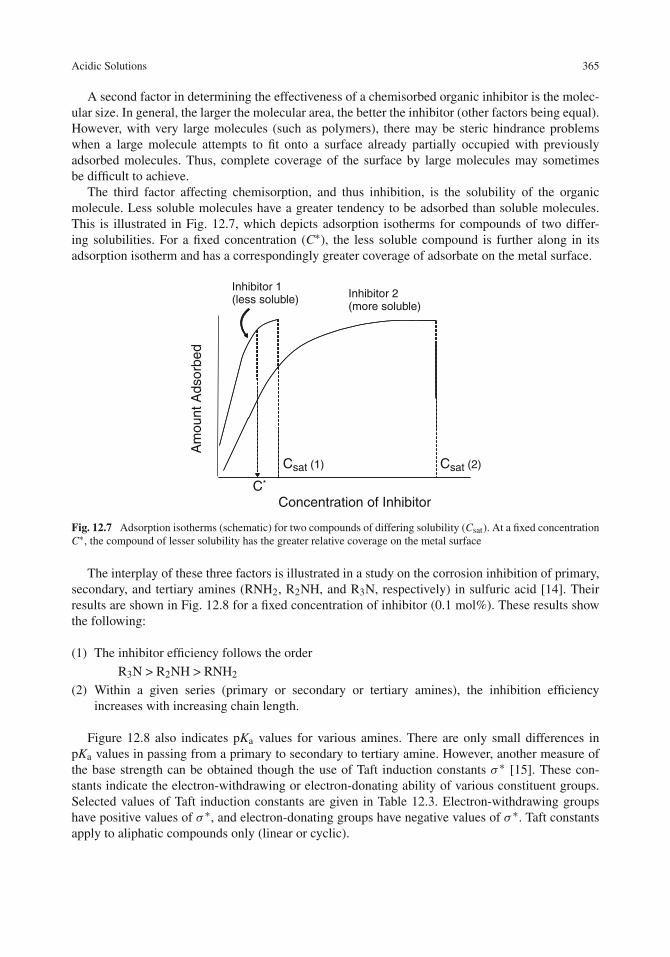
Acidic Solutions 365
A second factor in determining the effectiveness of a chemisorbed organic inhibitor is the molec-ular size. In general, the larger the molecular area, the better the inhibitor (other factors being equal).However, with very large molecules (such as polymers), there may be steric hindrance problemswhen a large molecule attempts to fit onto a surface already partially occupied with previouslyadsorbed molecules. Thus, complete coverage of the surface by large molecules may sometimesbe difficult to achieve.
The third factor affecting chemisorption, and thus inhibition, is the solubility of the organicmolecule. Less soluble molecules have a greater tendency to be adsorbed than soluble molecules.This is illustrated in Fig. 12.7, which depicts adsorption isotherms for compounds of two differ-ing solubilities. For a fixed concentration (C∗), the less soluble compound is further along in itsadsorption isotherm and has a correspondingly greater coverage of adsorbate on the metal surface.
Inhibitor 2(more soluble)
Inhibitor 1(less soluble)
Am
ount
Ads
orbe
d
Concentration of InhibitorC*
Csat (1) Csat (2)
Fig. 12.7 Adsorption isotherms (schematic) for two compounds of differing solubility (Csat). At a fixed concentrationC∗, the compound of lesser solubility has the greater relative coverage on the metal surface
The interplay of these three factors is illustrated in a study on the corrosion inhibition of primary,secondary, and tertiary amines (RNH2, R2NH, and R3N, respectively) in sulfuric acid [14]. Theirresults are shown in Fig. 12.8 for a fixed concentration of inhibitor (0.1 mol%). These results showthe following:
(1) The inhibitor efficiency follows the order
R3N > R2NH > RNH2
(2) Within a given series (primary or secondary or tertiary amines), the inhibition efficiencyincreases with increasing chain length.
Figure 12.8 also indicates pKa values for various amines. There are only small differences inpKa values in passing from a primary to secondary to tertiary amine. However, another measure ofthe base strength can be obtained though the use of Taft induction constants σ ∗ [15]. These con-stants indicate the electron-withdrawing or electron-donating ability of various constituent groups.Selected values of Taft induction constants are given in Table 12.3. Electron-withdrawing groupshave positive values of σ ∗, and electron-donating groups have negative values of σ ∗. Taft constantsapply to aliphatic compounds only (linear or cyclic).

366 12 Corrosion Inhibitors
0
20
40
60
80
100
0 1 2 3 4 5 6
Perc
ent In
hib
ition (
%I)
Number of Carbons in R
Primary Amines RNH2
Tertiary AminesR3N
Secondary AminesR2NH
10.63
10.73
9.80
10.75
10.84
11.05
11.25
10.65
10.54
10.60
10.63
Fig. 12.8 The corrosion inhibition of primary (RNH2), secondary (R2NH), and tertiary amines (R3N) in 1N sulfuricacid. (The numbers on the figure refer to pKa values)
Table 12.3 Values of someTaft substituent constants σ ∗[15]
Substituent Taft σ ∗
NO2 +4.0Cl +2.96COOH +2.08CONH2 +1.68SH +1.68CH3CO +1.65OH +1.34NH2 +0.62C6H5 +0.60H +0.49ClCH2CH2 +0.38C6H5CH2 +0.22CH3 0.00C2H5 −0.10n-C3H7 −0.12n-C4H9 −0.13Cyclohexyl −0.15n-C5H11 −0.25(CH3)3C −0.30
Example 12.1: Use the Taft induction constants in Table 12.3 to compare the electron-donatingproperties of C2H5NH2, (C2H5)2NH, and (C2H5)3N
Solution: For C2H5NH2:
�σ ∗ = σ ∗(C2H5)+ 2σ ∗(H)�σ ∗ = −0.10+ 2(0.49) = 0.88

Acidic Solutions 367
For (C2H5)2NH:
�σ ∗ = 2σ ∗(C2H5)+ σ ∗(H)�σ ∗ = 2(− 0.10)+ 0.49 = 0.29
For (C2H5)3N:
�σ ∗ = 3σ ∗(C2H5)�σ ∗ = 3(− 0.10) = −0.30
Thus, the electron-donating ability increases in the order
(C2H5)3N > (C2H5)2NH > C2H5NH2
and the tertiary amine is the strongest base of the three.
Figure 12.9 shows the data in Fig. 12.8 re-plotted in terms of the summed Taft constants �σ ∗for each amine. It can be seen clearly that for a given homologous series (given n), the inhibi-tion efficiency is greatest for the tertiary amine, which also has the greatest tendency to donateelectrons.
0
20
40
60
80
100
-0.5 0 0.5 1
n = number of carbons in R
Per
cent
Inhi
bitio
n
Sum of Taft Induction Constants, Σσ*
n = 5
n = 5n = 5
n = 3
n = 3
n = 3
n = 1
n = 1
n = 1
R2NH
R3N RNH2
n = 2 n = 4
n = 2 n = 4
Fig. 12.9 Data in Fig. 12.8 re-plotted in terms of the summed Taft constants �σ ∗. Drawn from data in [14] bypermission of Plenum Press (Springer)
Within a given series (primary or secondary or tertiary amine), the inhibitor efficiency increaseswith increasing size of the molecule. The larger molecules cover a larger portion of the surface andalso have decreased solubility as the molecular weight increases.
Involvement of Water
When a metal is immersed into an aqueous solution, the metal surface becomes covered with watermolecules. In order to adsorb onto the metal surface, the organic molecule must first displace these
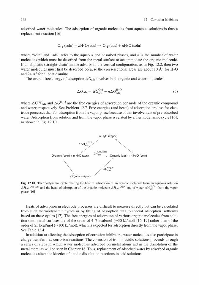
368 12 Corrosion Inhibitors
adsorbed water molecules. The adsorption of organic molecules from aqueous solutions is thus areplacement reaction [16].
Org (soln)+ nH2O (ads)→ Org (ads)+ nH2O (soln)
where “soln” and “ads” refer to the aqueous and adsorbed phases, and n is the number of watermolecules which must be desorbed from the metal surface to accommodate the organic molecule.If an aliphatic (straight-chain) amine adsorbs in the vertical configuration, as in Fig. 12.2, then twowater molecules must first be desorbed because the cross-sectional areas are about 10 Å2 for H2Oand 24 Å2 for aliphatic amine.
The overall free energy of adsorption �Gads involves both organic and water molecules:
�Gads = �GOrgads − n�GH2O
ads (5)
where �Gorgads and �GH2O are the free energies of adsorption per mole of the organic compound
and water, respectively. See Problem 12.7. Free energies (and heats) of adsorption are less for elec-trode processes than for adsorption from the vapor phase because of this involvement of pre-adsorbedwater. Adsorption from solution and from the vapor phase is related by a thermodynamic cycle [16],as shown in Fig. 12.10.
Organic (soln) + n H2O (ads) Organic (ads) + n H2O (soln)
n H2O (vapor)
Organic (vapor)
Hads
Org, v
n Hads
H2
O, v
ΔHadsOrg, soln
Δ
Δ
Fig. 12.10 Thermodynamic cycle relating the heat of adsorption of an organic molecule from an aqueous solution�Hads
Org, soln and the heats of adsorption of the organic molecule �HadsOrg,v and of water �HH2O,v
ads from the vaporphase [16]
Heats of adsorption in electrode processes are difficult to measure directly but can be calculatedfrom such thermodynamic cycles or by fitting of adsorption data to special adsorption isothermsbased on these cycles [17]. The free energies of adsorption of various organic molecules from solu-tion onto metal surfaces are of the order of 4–7 kcal/mol (∼30 kJ/mol) [16–19] rather than of theorder of 25 kcal/mol (∼100 kJ/mol), which is expected for adsorption directly from the vapor phase.See Table 12.4.
In addition to affecting the adsorption of corrosion inhibitors, water molecules also participate incharge transfer, i.e., corrosion reactions. The corrosion of iron in acidic solutions proceeds througha series of steps in which water molecules adsorbed on metal atoms aid in the dissolution of themetal atom, as will be seen in Chapter 16. Thus, replacement of adsorbed water by adsorbed organicmolecules alters the kinetics of anodic dissolution reactions in acid solutions.
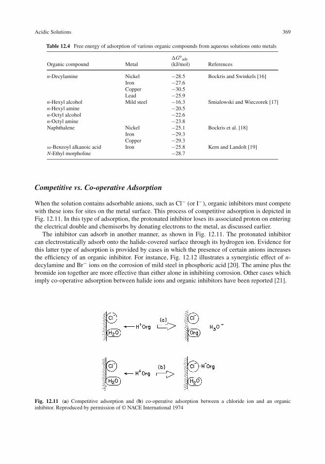
Acidic Solutions 369
Table 12.4 Free energy of adsorption of various organic compounds from aqueous solutions onto metals
Organic compound Metal�Go
ads(kJ/mol) References
n-Decylamine Nickel −28.5 Bockris and Swinkels [16]Iron −27.6Copper −30.5Lead −25.9
n-Hexyl alcohol Mild steel −16.3 Smialowski and Wieczorek [17]n-Hexyl amine −20.5n-Octyl alcohol −22.6n-Octyl amine −23.8Naphthalene Nickel −25.1 Bockris et al. [18]
Iron −29.3Copper −29.3
ω-Benzoyl alkanoic acid Iron −25.8 Kern and Landolt [19]N-Ethyl morpholine −28.7
Competitive vs. Co-operative Adsorption
When the solution contains adsorbable anions, such as Cl− (or I−), organic inhibitors must competewith these ions for sites on the metal surface. This process of competitive adsorption is depicted inFig. 12.11. In this type of adsorption, the protonated inhibitor loses its associated proton on enteringthe electrical double and chemisorbs by donating electrons to the metal, as discussed earlier.
The inhibitor can adsorb in another manner, as shown in Fig. 12.11. The protonated inhibitorcan electrostatically adsorb onto the halide-covered surface through its hydrogen ion. Evidence forthis latter type of adsorption is provided by cases in which the presence of certain anions increasesthe efficiency of an organic inhibitor. For instance, Fig. 12.12 illustrates a synergistic effect of n-decylamine and Br− ions on the corrosion of mild steel in phosphoric acid [20]. The amine plus thebromide ion together are more effective than either alone in inhibiting corrosion. Other cases whichimply co-operative adsorption between halide ions and organic inhibitors have been reported [21].
Fig. 12.11 (a) Competitive adsorption and (b) co-operative adsorption between a chloride ion and an organicinhibitor. Reproduced by permission of © NACE International 1974

370 12 Corrosion Inhibitors
0.0
0.5
1.0
1.5
0 50 100 150 200 250 300
cm3
H2
Evo
lved
/cm
2 m
ild s
teel
Time in Minutes
Uninhibited
0.0064 M n-decyl amine
0.0064 M n-decylamine
+ 0.064 M Br –
0.064 M Br –
Fig. 12.12 Synergistic effect of Br− ions and n-decylamine on the corrosion inhibition of mild steel in 3 M phosphoricacid [20]. Reproduced by permission of ECS – The Electrochemical Society
Effect of the Electrical Double Layer
The electrical double layer (edl), which was introduced in Chapter 3, is important in corrosion inhibi-tion because it plays a role in the adsorption of organic molecules. Organic molecules must enter theelectrical double layer to adsorb at the metal surface (for both competitive and co-operative adsorp-tion). Intrusion of organic molecules into the edl changes both its composition and its structure. SeeFig. 12.13. The adsorption of a long-chain organic molecule increases the thickness l of the edl andthe presence of an organic molecule in the edl also decreases the effective dielectric constant ε ofthe edl. Thus the capacitance of the edl per unit area Cdl given by
Cdl = ε
l(6)
decreases with the adsorption of the organic molecule. In measuring Cdl, the faradaic processes, e.g.,metal corrosion reactions, must be separated from the double layer properties. This can be done byusing an experimental technique called the single current pulse method, in which the electrical dou-ble layer is charged quickly before the response due to slower faradaic processes is observed. Moredetails as to this method are given in Fig. 12.14. The single pulse technique is effective in measur-ing the double layer capacitance, although double layer capacitances are frequently measured usingAC impedance techniques. AC impedance techniques and their applications are treated separately inChapter 14.
Figure 12.15 shows double layer capacitance–potential plots for iron in 6 M HCl with and with-out added NH2(CH2)11NH2 [9, 10]. The decrease in Cdl upon addition of the inhibitor shows thatthe diamine is adsorbed. Moreover, addition of the inhibitor leads to a general decrease in Cdl forpotentials in both anodic and cathodic directions. Thus, the diamine is a mixed inhibitor because

Acidic Solutions 371
Fig. 12.13 The electrical double layer at the metal/solution interface showing the adsorption of an organic molecule.IHP refers to the inner Helmholtz plane and OHP refers to the outer Helmholtz plane
INPUT OUTPUT
C = i x 1slope
Time
(a)
1i
Time
E
1–10 μsecii
Oscilloscope(b)
TESTELECTRODE
COUNTERELECTRODE
1CMEAS
= 1CTEST
+ 1CCOUNTER
Fig. 12.14 (a) The single current pulse technique for measuring double layer capacitance. (b) The experimental setup

372 12 Corrosion Inhibitors
0
10
20
30
40
50
60
70
–700–600–500–400–300–200
C dl in
μF/
cm2
E in mV vs. S.C.E.
Uninhibited7.84 x 10–4
1.96 x 10⁻³
1.96 x 10⁻²
Fig. 12.15 Double layer capacitance of iron in 6 M HCl with NH2(CH2)11NH2 inhibitor. The numbers on the fig-ure refer to the concentration of the diamine, and the arrows indicate the open-circuit corrosion potentials [9, 10].Reproduced by permission of ECS – The Electrochemical Society
it affects both anodic and cathodic partial reactions. At cathodic overvoltages, Cdl rises due to theadsorption of H+ ions, and at anodic overvoltages, it rises due to the adsorption of Cl− ions.
The Potential of Zero Charge
As discussed in Chapter 3, the metal side of the metal/solution interface can have an excess or adeficiency of electrons. Thus, the metal surface can have a negative or a positive charge, respectively.In the former instance, positive charges are attracted to the surface and in the latter instance, negativecharges will be favored. Between these two cases, there is an electrode potential at which the surfacehas zero charge, and this potential is called the potential of zero charge (pzc). The closer a metalis to its pzc, the easier it is for neutral organic molecules to adsorb onto the metal surface. Thisis especially true for those organic molecules which do not chemisorb strongly and would not befavored in competitive adsorption with other surface-active solution species, such as Cl− ions.
Table 12.5 lists pzc values for various metals [22, 23]. These values are not always invariantquantities for any given metal and vary somewhat with the nature of the solution, especially if thesolution contains adsorbable anions. But the idea is that above (more positive than) the pzc, theadsorption of negatively charged species is favored, and below (more negative than) the pzc, theadsorption of positively charged species is favored.
From Table 12.5, the pzc for iron is −0.40 V vs. SHE or −0.64 V vs. SCE. The open-circuit cor-rosion potential of iron in the HCl solutions containing the C11-diamine is approximately −0.46 Vvs. SCE (Fig. 12.15). Thus, the open-circuit corrosion potential for iron is more positive than the pzc
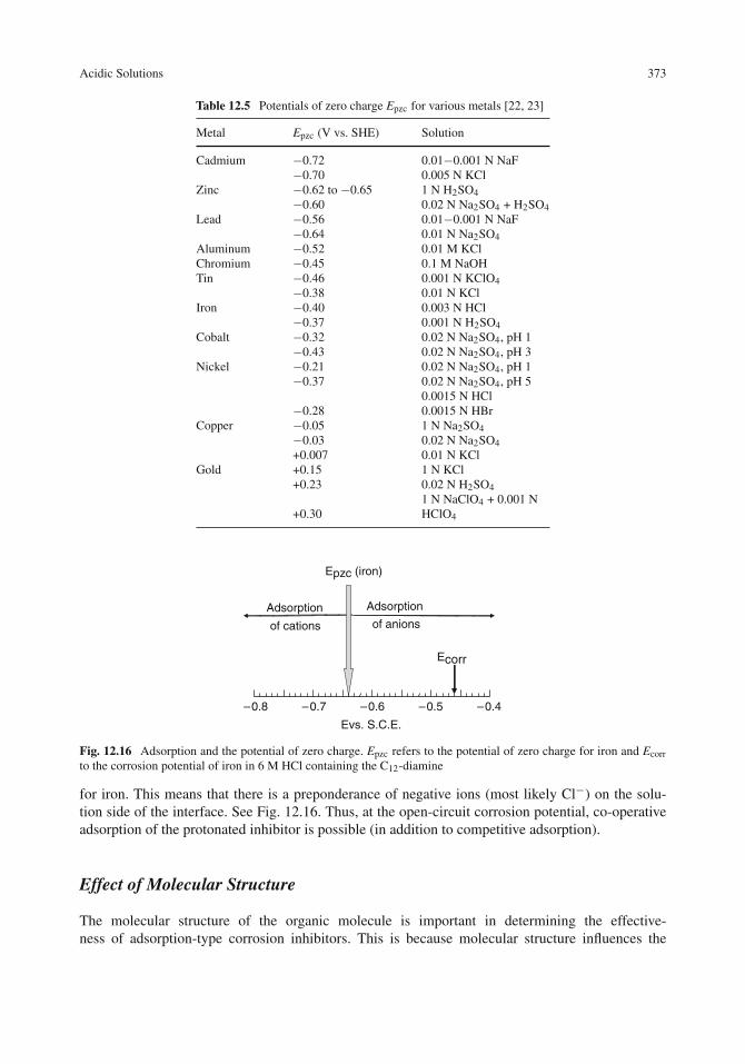
Acidic Solutions 373
Table 12.5 Potentials of zero charge Epzc for various metals [22, 23]
Metal Epzc (V vs. SHE) Solution
Cadmium −0.72 0.01−0.001 N NaF−0.70 0.005 N KCl
Zinc −0.62 to −0.65 1 N H2SO4−0.60 0.02 N Na2SO4 + H2SO4
Lead −0.56 0.01−0.001 N NaF−0.64 0.01 N Na2SO4
Aluminum −0.52 0.01 M KClChromium −0.45 0.1 M NaOHTin −0.46 0.001 N KClO4
−0.38 0.01 N KClIron −0.40 0.003 N HCl
−0.37 0.001 N H2SO4Cobalt −0.32 0.02 N Na2SO4, pH 1
−0.43 0.02 N Na2SO4, pH 3Nickel −0.21 0.02 N Na2SO4, pH 1
−0.37 0.02 N Na2SO4, pH 50.0015 N HCl
−0.28 0.0015 N HBrCopper −0.05 1 N Na2SO4
−0.03 0.02 N Na2SO4+0.007 0.01 N KCl
Gold +0.15 1 N KCl+0.23 0.02 N H2SO4
1 N NaClO4 + 0.001 N+0.30 HClO4
– 0.7 – 0.6 – 0.4
Epzc (iron)
Ecorr
Evs. S.C.E.
Adsorption Adsorption
of cations of anions
– 0.8 – 0.5
Fig. 12.16 Adsorption and the potential of zero charge. Epzc refers to the potential of zero charge for iron and Ecorrto the corrosion potential of iron in 6 M HCl containing the C12-diamine
for iron. This means that there is a preponderance of negative ions (most likely Cl−) on the solu-tion side of the interface. See Fig. 12.16. Thus, at the open-circuit corrosion potential, co-operativeadsorption of the protonated inhibitor is possible (in addition to competitive adsorption).
Effect of Molecular Structure
The molecular structure of the organic molecule is important in determining the effective-ness of adsorption-type corrosion inhibitors. This is because molecular structure influences the
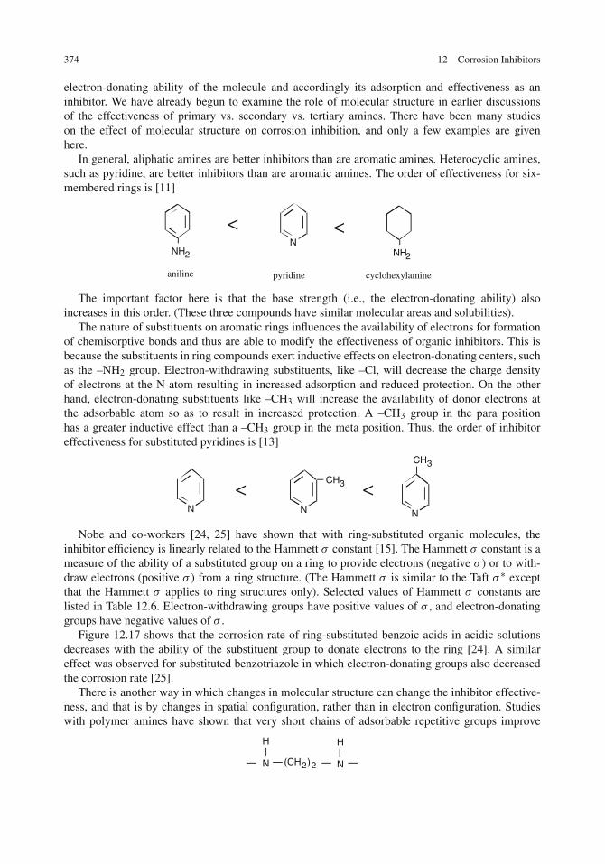
374 12 Corrosion Inhibitors
electron-donating ability of the molecule and accordingly its adsorption and effectiveness as aninhibitor. We have already begun to examine the role of molecular structure in earlier discussionsof the effectiveness of primary vs. secondary vs. tertiary amines. There have been many studieson the effect of molecular structure on corrosion inhibition, and only a few examples are givenhere.
In general, aliphatic amines are better inhibitors than are aromatic amines. Heterocyclic amines,such as pyridine, are better inhibitors than are aromatic amines. The order of effectiveness for six-membered rings is [11]
NH2NH2N
aniline pyridine cyclohexylamine
< <
The important factor here is that the base strength (i.e., the electron-donating ability) alsoincreases in this order. (These three compounds have similar molecular areas and solubilities).
The nature of substituents on aromatic rings influences the availability of electrons for formationof chemisorptive bonds and thus are able to modify the effectiveness of organic inhibitors. This isbecause the substituents in ring compounds exert inductive effects on electron-donating centers, suchas the –NH2 group. Electron-withdrawing substituents, like –Cl, will decrease the charge densityof electrons at the N atom resulting in increased adsorption and reduced protection. On the otherhand, electron-donating substituents like –CH3 will increase the availability of donor electrons atthe adsorbable atom so as to result in increased protection. A –CH3 group in the para positionhas a greater inductive effect than a –CH3 group in the meta position. Thus, the order of inhibitoreffectiveness for substituted pyridines is [13]
N N
CH3
N
CH3
< <
Nobe and co-workers [24, 25] have shown that with ring-substituted organic molecules, theinhibitor efficiency is linearly related to the Hammett σ constant [15]. The Hammett σ constant is ameasure of the ability of a substituted group on a ring to provide electrons (negative σ ) or to with-draw electrons (positive σ ) from a ring structure. (The Hammett σ is similar to the Taft σ ∗ exceptthat the Hammett σ applies to ring structures only). Selected values of Hammett σ constants arelisted in Table 12.6. Electron-withdrawing groups have positive values of σ , and electron-donatinggroups have negative values of σ .
Figure 12.17 shows that the corrosion rate of ring-substituted benzoic acids in acidic solutionsdecreases with the ability of the substituent group to donate electrons to the ring [24]. A similareffect was observed for substituted benzotriazole in which electron-donating groups also decreasedthe corrosion rate [25].
There is another way in which changes in molecular structure can change the inhibitor effective-ness, and that is by changes in spatial configuration, rather than in electron configuration. Studieswith polymer amines have shown that very short chains of adsorbable repetitive groups improve
(CH2)2 NN
HH
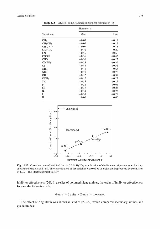
Acidic Solutions 375
Table 12.6 Values of some Hammett substituent constants σ [15]
Hammett σ
Substituent Meta Para
CH3 −0.07 −0.17CH2CH3 −0.07 −0.15CH(CH3)2 −0.07 −0.15C(CH3)3 −0.10 −0.20CN +0.56 +0.66COOH +0.36 +0.43CHO +0.36 +0.22CONH2 +0.28 +0.36CF3 +0.43 +0.54NH2 −0.16 −0.66NO2 +0.71 +0.78OH +0.12 −0.37OCH3 +0.12 −0.27SH +0.25 +0.15F +0.34 +0.06Cl +0.37 +0.23Br +0.39 +0.23I +0.35 +0.28H 0.00 0.00
20
30
40
50
60
–0.8 –0.6 –0.4 –0.2 0 0.2
Corr
osio
n Cu
rren
t Den
sity
in μ
A/c
m2
Hammett Substituent Constant, σ
p–OH–
m–OH–
m–NH2–
p–NH2–
Uninhibited
Benzoic acid
Fig. 12.17 Corrosion rates of inhibited iron in 0.5 M H2SO4 as a function of the Hammett sigma constant for ring-substituted benzoic acid [24]. The concentration of the inhibitor was 0.02 M in each case. Reproduced by permissionof ECS – The Electrochemical Society
inhibitor effectiveness [26]. In a series of polymethylene amines, the order of inhibitor effectivenessfollows the following order:
4 units > 3 units > 2 units > monomer
The effect of ring strain was shown in studies [27–29] which compared secondary amines andcyclic imines:

376 12 Corrosion Inhibitors
NH
(CH2)m
CH2
CH2
(CH2)m
CH2
CH2
(CH2)m
CH3
CH2
(CH2)m
CH3
CH2
NH
ring
closure
Both sets of compounds are secondary amines, have similar molecular weights (within 2 massunits), and similar molecular areas. Yet, the closed ring structures are more effective corrosioninhibitors than are their branched chain analogs. This structure effect is most pronounced for ringswith 9–12 carbon atoms. This higher efficiency is due to the large strain in these rings, which isrelieved with the formation of a strong chemisorptive bond with the metal surface.
Adsorption Isotherms
As discussed earlier, an adsorption isotherm relates the concentration of the inhibitor in solution tothe amount of inhibitor taken up by the surface. The surface coverage of the inhibitor, in turn, isimportant for chemisorption-type inhibitors, as shown in Fig. 12.5.
There are several types of adsorption isotherms, but the two most important ones which pertainto corrosion inhibition are the Langmuir isotherm and the Temkin isotherm. The Langmuir isothermis given by
θ
1− θ= KC (7)
where θ is the fraction of the surface covered by the inhibitor of concentration C, and K is a con-stant (which includes the heat of adsorption of the inhibitor). The derivation of Eq. (7) is givenin Appendix H. The Langmuir adsorption isotherm results if the adsorbent is energetically homoge-neous (all adsorption sites are equivalent) so that the heat of adsorption of the inhibitor is independentof coverage. The test of the Langmuir isotherm is that plots of θ /(1−θ ) vs. C produce a straight line.(Equivalently, plots of the logarithm of θ /(1−θ ) vs. the logarithm of C also produce a straight line,as shown in Fig. 12.18 [30]).
Another test of the Langmuir adsorption isotherm follows from rearranging Eq. (7) as
C
θ= 1
K+ C (8)
A plot of C/θ vs. C will produce a straight line of unit slope if the Langmuir isotherm applies[31, 32].
As stated above, the Langmuir adsorption isotherm assumes that the heat of adsorption of thecorrosion inhibitor �Hads is independent of fractional coverage of the inhibitor. Often this relation-ship is not obeyed, but instead �Hads decreases with increasing coverage, as shown schematicallyin Fig. 12.19. This decrease in �Hads arises from two sources. First, the corroding metal is energet-ically heterogeneous due to its polycrystalline nature and to the presence of grain boundaries anddefects (See Fig. 2.5). Thus, the most active sites are the first ones to interact with the inhibitor andare those which produce the greatest �Hads. Less active sites interact at higher coverages and with

Acidic Solutions 377
n – buty
l T.A
.B.
n – decy
l T.A
.B.
n – `exa
decy
l T.A
.B.
log
θ1
– θ
–0.5
0.0
0.5
1.0
1.5
– 6 –5 –4 –3 –2 –1 0
Log C oncentration of Inhibitor
Fig. 12.18 Test of the Langmuir isotherm for various trimethylammonium bromides (TAB) compounds adsorbed onmild steel from 0.5 M H2SO4 [30]. Reproduced by permission of John Wiley & Sons Ltd
Langmuir
Temkin
Often observedexperimentally
Surface Coverage
Hea
t of A
dsor
ptio
n, Δ
Had
s
Fig. 12.19 Schematic diagram showing the heat of adsorption vs. coverage for Langmuir and Temkin adsorptionisotherms
lesser values of �Hads. Second, lateral repulsive interactions between adsorbed molecules (or ions)result in a decrease in �Hads with increasing coverage.
The second major adsorption isotherm, the Temkin adsorption isotherm, allows for a lineardecrease in the heat of adsorption with coverage.
�Hads = �Hoads − rθ (9)
where �Hoads is the heat of adsorption at near-zero coverages and r is the Temkin parameter. When
Eq. (9) is inserted into the Langmuir model in Eq. (7), the result is
θ
1− θ= K′Ce−rθ/RT (10)

378 12 Corrosion Inhibitors
Table 12.7 Comparison of Langmuir and Temkin adsorption isotherms
Langmuir Temkin
Assumption Homogeneous surface Heterogeneous surfaceHeat of adsorption Independent of coverage Decreases linearly with coverageEquation θ
1−θ= KC
Cθ= 1
K + C
θ = 2.303RTr log C
+ 2.303RTr log K′
Test of isotherm Linear plot of θ/(1−θ) vs. C Plot of θ vs. log C gives a linear portionLinear plot of θ /C vs. C
where K′ is a constant. At intermediate coverages (0.3 < θ < 0.7), Eq. (10) gives
θ = 2.303 RT
rlog C + 2.303 RT
rlog K′ (11)
as shown in Appendix I. Thus, a test of the Temkin adsorption isotherm is that a plot of coverageθ vs. the logarithm of inhibitor concentration C gives a straight line over a portion of the plot, asshown in Fig. 12.20. Table 12.7 compares Langmuir and Temkin adsorption isotherms.
Direct experimental determination of adsorption isotherms during the actual corrosion inhibi-tion process is difficult to determine but can be done using radiotracer, infrared, or quartz crystalmicrobalance techniques. Alternately, the amount of adsorbed inhibitor can be inferred from doublelayer capacitance measurements or from corrosion current densities. These indirect methods yieldrelative, but not absolute, adsorption isotherms. The electrode surface can be modeled as being com-posed of two parallel capacitors for the inhibitor-bare and inhibitor-covered portions added on acoverage basis. The capacitance C is then
C = Co(1− θ )+ Csatθ (12)
0.0
0.2
0.4
0.6
0.8
1.0
1.2
0.0001 0.001 0.01 0.1 1
Capacitance
Corrosion rates
Sur
face
Cov
erag
e of
C11
-dia
min
e
Concentration of C11-diamine in M/l
Fig. 12.20 Experimental adsorption isotherms for NH2(CH2)11NH2 onto iron in 6 M HCl [9, 10]
Nearly Neutral Solutions 379
where Co and Csat are the capacitances (per unit area) of the inhibitor-free and inhibitor-coveredsurface, respectively, and θ is the coverage of the inhibitor. The value for Csat is that for whichfurther addition of the inhibitor causes no further decrease in capacitance. (While there is maximumadsorption at such a concentration, there may not be complete monolayer coverage, and this must bedetermined by other experimental methods). From Eq. (12)
θ = Co − C
Co − Csat(13)
Similarly, the corrosion rate (i) can be given by the corrosion rates of two parallel reactions forthe uninhibited (io) and inhibitor-covered (isat) surfaces. That is
i = io(1− θ )+ isatθ (14)
or
θ = io − i
io − isat(15)
Adsorption isotherms given in Fig. 12.20 were determined using Eqs. (13) and (15). Many sys-tems of organic inhibitors have been observed to obey Temkin isotherms [9, 10, 21, 26, 33–35], andnot surprisingly so, given the heterogeneous nature of the surface of a corroding metal.
Nearly Neutral Solutions
The corrosion of metals in nearly neutral solutions (and open to the air) differs from that inacidic solutions for two reasons. First, in acid solutions, the metal surface is oxide free, but inneutral solutions, the surface is oxide covered. Second, in acid solutions, the main cathodic reac-tion is hydrogen evolution, but in air-saturated neutral solutions, the cathodic reaction is oxygenreduction.
Effect of Oxide Films
Corrosion inhibitors can interact strongly with a surface even if it is oxide covered. Table 12.8compares the heats of adsorption �Hads for several small organic molecules onto the surfaces ofmetals, oxides, or oxide films. The heats of adsorption are from the vapor phase so as to con-sider the energy of interaction between the adsorbate and the surface without the complicatingeffect of the solvent. The heats of adsorption in Table 12.8 are for near-zero coverages, so val-ues of �Hads are those which pertain before �Hads begins to decrease with increasing coverage.It can be seen that in some cases, the heats of adsorption onto the oxide or oxide-covered sur-face are well within the range expected for a chemisorptive process. This strong interaction isdue to the interaction of dipoles in the organic molecule with cations or anions present in theoxide surface. In addition, pi-bonding is also possible between benzene rings and the metal orits oxides.
Table 12.8 also shows that water molecules are strongly adsorbed onto oxide surfaces or oxidefilms. Thus, for oxide-covered surfaces, corrosion inhibitors in neutral solutions must also competewith water molecules for adsorption sites, just as in the case for bare metal surfaces in acid solutions.

380 12 Corrosion Inhibitors
Table 12.8 Heats of adsorption from the vapor phase at near-zero coverages for various small organic molecules orwater on metals, oxides, or oxide-covered metal surfaces
Adsorbate �Hads on metal (kJ/mol)�Hads on metal oxide oroxide film (kJ/mol) References
n-C3H7NH2 −226 (on nickel) −84 (on oxidized nickel) Yu et al. [36]−105 (on copper) −96 (on oxidized copper)
n-C3H7OH −347 (on nickel) −138 (on oxidized nickel) Yu et al. [36]−105 (on copper) −67 (on oxidized copper)
−200 (on Al2O3) Rossi et al. [37]n-C3H7NH2 −138 (on iron) −188 (on oxidized iron) Yu Yao [38]n-C4H9NH2 −144 (on iron) −186 (on oxidized iron)n-C5H11NH2 −165 (on iron) −192 (on oxidized iron)n-C6H13NH2 −172 (on iron) −213 (on oxidized iron)(n-C3H7)2NH −128 (on iron) −183 (on oxidized iron)(C2H5)3N −156 (on iron) −207 (on oxidized iron)φ-CH3
a − −69 to −77 (on ZnO) Nakazawa [39]−83 (on FeO)
φ-OHa − −131 (on ZnO) Nakazawa [39]−140 (on FeO)
H2O −113 (on oxidized iron) Yu Yao [38, 40]−134 (on α-Fe2O3)−134 (on α-Al2O3)−80 to −90 (on NiO) Matsuda [41]
D2O −89 (on ZnO) Nakazawa [39]−65(on FeO)
aThe symbol φ denotes the benzene ring.
Because the metal surface is oxide-covered, the role of the inhibitor in neutral solutions is to makeoxide films protective and to keep them so. Oxidizing inhibitors, like chromates, react with the oxide-covered surface and are incorporated into the passive film. With non-oxidizing inhibitors, however,such chemical reactions do not occur. Phosphates, for example, are incorporated into the passive filmby exchange with surface oxide or hydroxide ions [42]. Other inhibitors, such as sodium azelate, arenot taken up as uniformly but instead function by repairing pores in oxide films by reacting therewith dissolved cations to form insoluble local precipitates [43].
Chelating Compounds as Corrosion Inhibitors
Chelating compounds are organic molecules with at least two polar functional groups capable of ringclosure with a metal cation. The functional groups may either be basic groups, such as –NH2, whichcan form bonds by electron donation, or acidic groups, such as –COOH, which can co-ordinate afterthe loss of a proton. An example of a chelate is shown in Fig. 12.21. The chelating molecule mayinteract with metal ions which exist in the oxide film, or they may react with metal cations whichare first produced by metallic dissolution. In the latter case, a complex of high molecular weight andlow solubility is precipitated near the metal surface, and a barrier film is formed. Other chelatingagents include mercaptoacetic acids, 8-hydroxyquinoline, and ethylenediaminetetraacetic acid. Ineach case, surface chelates are formed involving bonding between a surface cation and an oxygen, asulfur, or a nitrogen atom in the chelating molecule, as in Fig. 12.21 [44].

Nearly Neutral Solutions 381
H3C
H3C
–N –CH2 –C
OC=O
C11H23 C11H23
C11H23
OH.. H3C –N –CH2 –C
OC=O
O–+ H+..
M+n
CH2 HC
OC=O
ON–
Metal
– – – C
=
– –
=
– –
=
– –
=
– – –
O=
– – –– – –– – –
=
–
=
–
Fig. 12.21 A sarcosine-type surface chelate [44]. Reproduced by permission of NACE International
It is well known that in bulk solutions, five-membered chelate rings are the most stable [45], andit appears that this effect carries over to surface chelates as well. Steric requirements for surfacechelation are more restrictive than those for the bulk solution. Not all compounds which are capableof forming chelates in the bulk solution are effective inhibitors. As an example, 2,2-bipyridine and1,10-phenanthroline are classical chelating agents for ferrous ions in solution [45]. However, incooling water studies, the former provided no protection, while the latter did [44]. The differencesin corrosion inhibition are because the trans-2,2-bipyridine resists surface chelation, but the rigidstructure of the 1,10-phenanthroline is favorable for surface chelation, as shown in Fig.12.22 [44].
No inhibition
N
2-2' bipyridine
N N
1,10 phenanthroline
Inhibition
N
M+n
Fig. 12.22 Steric effects in surface chelation [44]. Reproduced by permission of NACE International
Chelating compounds have been studied as corrosion inhibitors for steel in industrial coolingwaters [44, 46] and for zinc [47, 48] and aluminum [49, 50] in various environments. A currentinterest in chelate inhibitors has been prompted by the search to replace chromate inhibitors withcompounds which are less toxic and less polluting.
Chromates and Chromate Replacements
Chromates (CrO42−) are excellent corrosion inhibitors when added to aqueous solution or if used to
treat metals to form corrosion-resistant “conversion” coatings. However, Cr6+ is a known carcinogen

382 12 Corrosion Inhibitors
(the oxidation state of Cr is +6 in chromates). In addition, other toxic chemicals, such as cyanidesand fluorides, are used in chromate conversion solutions. Thus, environmental concerns have beenraised over the use of chromates and the disposal of their processing baths, and, accordingly, thereis an increased interest in finding or developing replacements for chromate inhibitors. However, alack of detailed fundamental understanding as to why chromates are such effective inhibitors hascomplicated the search for chromate replacements.
As mentioned in Chapter 6, chromates are passivating-type inhibitors and are reduced to formCr2O3, which is incorporated into the passive film on the metal surface. The search for chromatereplacements has taken several directions. These include studies on
• compounds which are analogous to chromates, such as molybdates (MoO42−), tungstates
(WO42−), and vanadates (VO4
3− or VO3− ) [51–55]
• phosphates (PO43−) [56, 57]
• cerium salts [58]• “environment-friendly” inorganic coatings, such as hydrotalcite coatings (lithium aluminum
hydroxylated carbonate) [59]• diamond-like coatings [60]• ion beam surface modification [61] (see Chapter 16)• natural products as corrosion inhibitors [62, 63]
The use of natural products (biological molecules) as corrosion inhibitors is discussed later in thischapter.
Inhibition of Localized Corrosion
Pitting, crevice corrosion, and stress-corrosion cracking can all be mitigated by the use of corrosioninhibitors. In pitting corrosion, the use of an inhibitor usually raises the pitting potential, whereas increvice corrosion, the inhibitor usually affects the propagation stage and reduces the current betweenthe crevice metal and the component of the metal outside the crevice. In stress-corrosion cracking,inhibitors can increase the time to failure by increasing the time to initiation of cracks and/or bydecreasing the crack growth rate. Inhibitors can also increase the value of KIscc so as to increase theresistance of specimens containing inherent flaws to SCC.
Examples of the inhibition of these various forms of localized corrosion are given below.
Pitting Corrosion
The effect of a corrosion inhibitor on pitting is usually to increase the pitting potential. This effecthas been shown previously in Fig. 10.22, where it was seen that increasing additions of sulfate ionincrease the pitting potential of 304 stainless steel in a chloride solution.
Two additional examples on the effect of capronate and chromate inhibitors on the pitting poten-tial of iron are shown in Figs. 12.23 and 12.24 [64, 65]. For each inhibitor, the pitting potentialincreases linearly with the logarithm of the inhibitor concentration. That is:
(∂Epit
∂ log [I]
)[A]= constant (16)

Inhibition of Localized Corrosion 383
–0.2
–0.1
0.0
0.1
0.2
0.3
0.4
0.001 0.01 0.1 1 10
Pitt
ing
Pot
entia
l in
V v
s. S
.H.E
.
Concentration of Capronate in M/l
Borate buffer, pH 8.0
plus 0.1 M Cl–
(a)
–0.3
–0.2
–0.1
0.0
0.001 0.01 0.1 1 10
Pitt
ing
Pot
entia
l in
V v
s. S
.H.E
.
Concentration of Cl– in M/l
Borate buffer, pH = 8.0(No capronate)
(b)
Fig. 12.23 (a) Pitting potential of iron as a function of capronate concentration (at a constant chloride concentration).(b) Pitting potential of iron as a function of chloride concentration (no inhibitor present). Redrawn from [64] bypermission of Elsevier Ltd
where [I] refers to the concentration of inhibitive ion (capronate or chromate) and [A] refers to theconcentration of the aggressive ion (chloride). Figures 12.23 and 12.24 also show that at a con-stant concentration of inhibitive ion (capronate or chromate), the pitting potential decreases withincreasing concentration of aggressive ion (chloride), according to the following equation:
(∂Epit
∂ log [A]
)[I]= constant ′ (17)

384 12 Corrosion Inhibitors
– 0.4
– 0.2
0.0
0.2
0.4
0.0001 0.001 0.01 0.1
Pitt
ing
Pot
entia
l in
V. v
s. A
g/A
gCl
Concentration of CrO4–2 in M/l
0.006 M Cl–
(a)
–0.4
–0.2
0.0
0.2
0.4
0.0001 0.001 0.01 0.1
Pitt
ing
Pot
entia
l in
V v
s. A
g/A
gCl
Concentration of Cl– in M / l
0.003 M CrO4–2
(b)
Fig. 12.24 (a) Effect of CrO42− concentration on the pitting potential of iron (at constant Cl− concentration).
(b) Effect of Cl− concentration on the pitting potential of iron (at constant CrO42− concentration) [65]
The relationship in Eq. (17) is similar to that seen previously in Fig. 10.21 for aluminum or type304 stainless steel in chloride solutions but in the absence of a corrosion inhibitor.
Equations (16) and (17) can be explained on the basis of competitive adsorption between theaggressive and the inhibitive ions [64–67]. That is, the aggressive and inhibitive ions compete foradsorption sites on the oxide-covered metal surface. If adsorption of the inhibitive ion prevails, thenpassive film formation ensues, the pit initiation process is stifled, and the surface must be polarizedto a higher electrode potential to initiate passive film breakdown and pitting. (That is, the pittingpotential is increased.)
The adsorption of either the inhibitive or the aggressive ions can each be described by Temkinadsorption isotherms, but Eq. (11) must first be modified to take into account the fact that theadsorbates are charged species. See Appendix J. For the aggressive ion:
Inhibition of Localized Corrosion 385
θA = 2.303 RT
rAlog [A]+ 2.303 RT
rAlog K′A +
zA FE
rA(18)
where E is the electrode potential and zA is the charge on the aggressive ion. Similarly for theinhibitive ion
θI = 2.303 RT
rIlog [I]+ 2.303 RT
rIlog K′I +
zI FE
rI(19)
where zI is the charge on the inhibitive ion. Equations (18) and (19) combine to give
[(θA
θI
)zI
rI− zA
rA
]FE
2.303RT= 1
rAlog [A]−
(θA
θI
)1
rIlog [I]
+ 1
rAlog K′A −
(θA
θI
)1
rIlog K′I
(20)
According to the competitive adsorption model of Uhlig and co-workers [66, 67], pitting initiatesat sites on the oxide-covered metal surface at some critical ratio of θA/θ I = θcrit. This does not meanthat adsorption of the aggressive ion (usually chloride) is sufficient to cause pitting but that theensuing processes of film breakdown and pit initiation occur when some critical amount of Cl− hasbeen taken up by the surface. Using a scanning Cl−-sensitive micro-electrode, Lin et al. [68] foundthat chloride ions accumulated in Cl−-rich islands on the surface of 18-8 stainless steel. Recall thatin the pitting of aluminum, the amount of chloride taken up by the surface increases as the pittingpotential is approached, as was discussed in Chapter 10. Thus, when θA/θ I = θcrit, the electrodepotential is the pitting potential Epit:
θA
θI= θcrit at E = Epit (21)
Taking differentials in Eq. (20) at a constant concentration of aggressive ion and subject toEq. (21) gives:
(∂Epit
∂ log [I]
)[A]= −2.303 RT
F
θcrit
(rArI
)
θcrit
(rArI
)zI − zA
= constant ′ (22)
The right-hand side of Eq. (22) is a constant so that Eq. (22) has the form of Eq. (16) and explainsthe straight line observed experimentally in Figs. 12.23(a) and 12.24(a).
Taking differentials in Eq. (20) at a constant concentration of inhibitor ion gives:
(∂Epit
∂ log [A]
)[I]= 2.303RT
F
1
θcrit
(rArI
)zI − zA
= constant (23)
The right-hand side of Eq. (23) is also a constant so that Eq. (23) has the form of Eq. (17) andexplains the straight lines observed experimentally in Figs. 12.23(b) and 12.24(b).
Moreover, the slopes in Fig. 12.23(a) and (b) have opposite signs, as predicted by Eqs. (22) and(23). The same holds for Fig. 12.24(a) and (b).
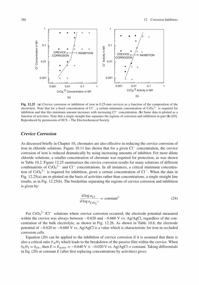
386 12 Corrosion Inhibitors
(a) (b)
0.001
0.01
0.1
1
0.001 0.01 0.1 1
Cl- C
once
ntra
tion
in M
/l
Cl- A
ctiv
ity in
M/l
CrO4-2 Concentration in M/l
INHIBITION CREVICECORROSION
0.001
0.01
0.1
1
0.001 0.01 0.1 1
CrO4-2 Activity in M/l
INHIBITION CREVICECORROSION
Fig. 12.25 (a) Crevice corrosion or inhibition of iron in 0.25-mm crevices as a function of the composition of theelectrolyte. Note that for a fixed concentration of Cl−, a certain minimum concentration of CrO4
2− is required forinhibition and that this minimum amount increases with increasing Cl− concentration. (b) Same data re-plotted as afunction of activities. Note that a single straight line separates the regions of corrosion and inhibition in part (b) [65].Reproduced by permission of ECS – The Electrochemical Society
Crevice Corrosion
As discussed briefly in Chapter 10, chromates are also effective in reducing the crevice corrosion ofiron in chloride solutions. Figure 10.11 has shown that for a given Cl− concentration, the crevicecorrosion of iron is reduced dramatically by using increasing amounts of inhibitor. For more dilutechloride solutions, a smaller concentration of chromate was required for protection, as was shownin Table 10.2. Figure 12.25 summarizes the crevice corrosion results for many solutions of differentcombinations of CrO4
2− and Cl− concentrations. In all instances, a critical minimum concentra-tion of CrO4
2− is required for inhibition, given a certain concentration of Cl−. When the data inFig. 12.25(a) are re-plotted on the basis of activities rather than concentrations, a single straight lineresults, as in Fig. 12.25(b). The borderline separating the regions of crevice corrosion and inhibitionis given by:
d log aCl−
d log aCrO−24
= constant′′ (24)
For CrO42−/Cl− solutions where crevice corrosion occurred, the electrode potential measured
within the crevice was always between −0.620 and −0.660 V vs. Ag/AgCl, regardless of the con-centration of the bulk electrolyte, as shown in Fig. 12.26. As shown in Table 10.6, the electrodepotential of −0.620 to −0.660 V vs. Ag/AgCl is a value which is characteristic for iron in occludedcorrosion cells.
Equation (20) can be applied to the inhibition of crevice corrosion if it is assumed that there isalso a critical ratio θA/θ I which leads to the breakdown of the passive film within the crevice. WhenθA/θ I = θcrit , then E= Eactive =−0.640 V±−0.020 V vs. Ag/AgCl= constant. Taking differentialsin Eq. (20) at constant E (after first replacing concentrations by activities) gives:

Inhibition of Localized Corrosion 387
Fig. 12.26 Crevice corrosion of iron in chromate/chloride solutions always occurred when the electrode potentialwithin the crevice was more negative than −0.62 V vs. Ag/AgCl. Crevice corrosion was inhibited at more positiveinternal electrode potentials [65]. Reproduced by permission of ECS – The Electrochemical Society
(∂ log aA
∂ log aI
)Eactive
= θcritrA
rI= constant′′ (25)
which has the form of Eq. (24) and describes the borderline between regions of crevice corrosion andinhibition in Fig. 12.25(b). Details regarding derivation of Eq. (25) are left as an exercise in Problem12.11.
Thus, inhibition of two forms of localized corrosion (pitting and crevice corrosion) is similarin that if a critical surface ratio of aggressive to inhibitive ion is exceeded, pitting ensues on opensurfaces and active corrosion occurs within crevices.
Stress-Corrosion Cracking and Corrosion Fatigue
An interesting example on the inhibition of SCC is given by the effect of benzotriazole (BTA) ontype 304 stainless steel in 1 M HCl [69].
Figure 12.27 shows that increasing amounts of BTA increase the KIscc values for single-edgenotched specimens in 1 M HCl. Recall from Chapter 11 that
KI = σ√
πa · (geometrical factor) (26)
so that increases in KI mean that a larger flaw size (a) can be tolerated for a given stress σ .In the same study [69], it was also shown that additions of BTA increased the time to failure
for smooth tensile specimens, as shown in Fig. 12.28. Thus, additions of BTA were able to protectagainst SCC for either smooth specimens or pre-cracked specimens of type 304 stainless steel in 1 MHCl.
As stated earlier, corrosion inhibitors can reduce stress-corrosion cracking in various ways.Inhibitors can increase the time to failure by increasing the time to initiation of cracks and/or by

388 12 Corrosion Inhibitors
50
100
150
200
250
0.001 0.01 0.1 1
Kis
cc o
r K
ic in
Mpa
m1/
2
Concentration of Benzotriazole in M/l
KIscc (1 M HCl without inhibitor)
KIc (in air)
Single edgenotched specimens
Fig. 12.27 Effect of benzotriazole on the stress intensity factor of type 304 stainless steel in 1 M HCl for single-edgenotched specimens. Drawn from data in [69]
50
100
150
200
250
0.001 0.01 0.1 1
Tim
e to
Fai
lure
in H
ours
Concentration of Benzotriazole in M/l
1 M HCl without inhibitor
Smooth specimens
Fig. 12.28 Effect of benzotriazole on the time to fracture of type 304 stainless steel in 1 M HCl for smooth specimensnot containing an intentional defect. Drawn from data in [69]

New Approaches to Corrosion Inhibition 389
decreasing the crack growth rate. Inhibitors can also increase the value of KIscc so as to increase theresistance of specimens containing inherent flaws to SCC.
Corrosion inhibitors can also reduce corrosion fatigue damage. An example is given by the use ofvarious inhibitors applied to the corrosion fatigue of a high-strength steel [70]. The environment wasair of 90% relative humidity (maintained in an environmental chamber surrounding the crack). Thus,water vapor adsorbs and condenses within the crack tip to form an electrolyte. Various inhibitorswere dissolved in appropriate solvents and were applied as droplets near the crack tip. Figure 12.29shows corrosion fatigue plots of da/dN vs. �K. It can be seen that several inhibitors were effectivein reducing the crack growth rate.
10–4
10–3
10–2
20 30 40 50 60
Cra
ck G
row
th R
ate
in m
m/c
ycle
ΔK in MPa m1/2
90 % relative humidity
Na2MoO4
Na2Cr2O7
Na2Cr2O7 + NaNO2
+ Na2B4O7
Fig. 12.29 Effect of various inhibitors on the corrosion fatigue crack growth rate of a high-strength steel in a humidenvironment [70]. Reproduced by permission of © NACE International 1980
In both stress-corrosion cracking and in corrosion fatigue (as well as in crevice corrosion), for thecorrosion inhibitor to be effective it is essential that the inhibitor reaches the inside of the occludedcorrosion cell (i.e., the crack tip or the crevice interior). This is accomplished most easily in thecase of corrosion fatigue because the cyclic load causes the crack to open and close. This, in turn,produces a pumping action in the electrolyte which serves to assist the inhibitors to move from thebulk solution inward toward the crack tip.
New Approaches to Corrosion Inhibition
New approaches to corrosion inhibition have been spurred in part by the desire for environmen-tally acceptable corrosion inhibitors and in part by recent advances in surface modification by

390 12 Corrosion Inhibitors
monomolecular films. The first of these two approaches, which is discussed below, is the use ofnatural products or biological molecules as non-toxic, biodegradable corrosion inhibitors.
Biological Molecules
The use of natural products as corrosion inhibitors is not new. Inhibitors of acid corrosion wereknown as far back as the Middle Ages by metal-working craftsmen, who used flour, bran, and yeastas pickling inhibitors [71]. In the early 1900s, molasses, vegetable oils, starch, tars, and oils werealso used [71].
In recent years, attention has turned to various organic molecules, such as α-amino acids, whichare components of natural products, and thus are environmentally acceptable. Amino acids are themolecular units that make up proteins, which in turn are the building blocks of biological systems.The formulas of some particular α-amino acids are shown in Fig. 12.30 [72]. All proteins are derivedfrom 20 specific naturally occurring amino acids. In addition to their non-polluting properties, aminoacids are attractive candidates as corrosion inhibitors because they contain adsorbable amino andcarboxyl functional groups for attachment to metal surfaces. Amino acids and other natural prod-ucts, such as peptides, catechols, vitamins, and siderophores (isolated from bacteria), have all beenexamined recently as corrosion inhibitors for different metals in various solutions [62, 63, 73–80].
R-CH-COOH
NH2
The αcarbon
Carboxyl group
Amino group
NH2-CH2-COOHGlycine
CH3-CH-COOH
NH2
Alanine
CH-CH2-CH-COOH
NH2
CH3
CH3
Leucine
-CH2-CH-COOH
NH2
HOTyrosine
CH2-CH-COOH
NH2N
Tryptophan
HOOC-CH2-CH-COOH
NH2
Aspartic acid
Amino acid Molecular Formula
Fig. 12.30 Molecular formulas of several α-amino acids [72]

New Approaches to Corrosion Inhibition 391
The application of natural products has been taken a step beyond the use of constituent moleculesby using actual extracts from plant systems, such as tannins or tree barks [78–80], or from animalsystems. An example of the latter is provided by the work of Hansen and co-workers [63, 76] onthe properties of the adhesive protein of the common blue mussel Mytilus edulis L. The blue mus-sel is shown suspended by byssal threads from a glass plate in Fig. 12.31. These byssal threadsterminate in adhesive plaques with which the mussel attaches itself to surfaces. The mussel adhe-sive protein (MAP), which has a molecular weight greater than 10,000, has been found to contain arepeating decapeptide that provides a variety of functional groups for attachment to bare or oxide-covered metal surfaces. These attachment possibilities include coulombic interactions, dipole–dipoleinteractions, hydrogen bonding through catechol groups, as well as co-ordination and chelation ofmetal ions or surface hydroxyls by the catecholic functional groups. These possibilities are shown inFig. 12.32.
Fig. 12.31 The common blue mussel (M. edulis) suspended by its byssal threads from a glass plate. Courtesy of Prof.J. H. Waite, University of California at Santa Barbara
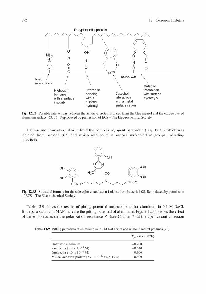
392 12 Corrosion Inhibitors
O O
M+n
O
O
C
H
=
NH3+
-
O O
OH
OH
OH
O
H
Ionicinteractions
Hydrogen bondingwith a surfaceimpurity
Hydrogen bondingwith a surfacehydroxyl
Catechol interactionwith surfacehydroxyls
Catechol interactionwith a metal surface cation
SURFACE
Polyphenolic protein
Fig. 12.32 Possible interactions between the adhesive protein isolated from the blue mussel and the oxide-coveredaluminum surface [63, 76]. Reproduced by permission of ECS – The Electrochemical Society
Hansen and co-workers also utilized the complexing agent parabactin (Fig. 12.33) which wasisolated from bacteria [62] and which also contains various surface-active groups, includingcatechols.
CONHN
COH3C
NO
OH
NHCO
OH
OH
OH
OH
Fig. 12.33 Structural formula for the siderophore parabactin isolated from bacteria [62]. Reproduced by permissionof ECS – The Electrochemical Society
Table 12.9 shows the results of pitting potential measurements for aluminum in 0.1 M NaCl.Both parabactin and MAP increase the pitting potential of aluminum. Figure 12.34 shows the effectof these molecules on the polarization resistance Rp (see Chapter 7) at the open-circuit corrosion
Table 12.9 Pitting potentials of aluminum in 0.1 M NaCl with and without natural products [76]
Epit (V vs. SCE)
Untreated aluminum −0.700Parabactin (1.3 × 10⁻⁵ M) −0.640Parabactin (1.0 × 10⁻⁴ M) −0.600Mussel adhesive protein (7.7 × 10⁻⁶ M, pH 2.5) −0.600

New Approaches to Corrosion Inhibition 393
102
103
104
105
106
107
108
0 50 100 150 200 250 300
Pol
ariz
atio
n R
esis
tanc
e R
p in
ohm
cm
2
Time in Hours
Mussel adhesive proteinplus tyrosinase
Mussel adhesive protein
Parabactin
Untreated
Fig. 12.34 Polarization resistance for aluminum samples treated with the mussel adhesive protein, the mussel adhe-sive protein plus tyrosinase, and the bacterial siderophore parabactin [63, 76]. Reproduced by permission of ECS –The Electrochemical Society
potentials. Parabactin and MAP with an enzyme added to cross-link the adhesive polymer weremost effective in increasing Rp. These experiments are representative of the emerging possibilitieson the use of natural products as new and novel corrosion inhibitors.
Langmuir–Blodgett Films and Self-assembled Monolayers
There are two novel approaches to corrosion inhibition which have attracted much recent interest.These are (i) Langmuir–Blodgett films and (ii) self-assembled monolayers. These approaches, whichare related to each other, are borrowed from the field of surface chemistry. Both methods involvepre-treatment of the metal surface prior to its use in the corrosive electrolyte. The thickness of theinhibitor films is only one monolayer for self-assembled films and is one to several monolayers forLangmuir–Blodgett films.
Langmuir–Blodgett films are oriented insoluble monomolecular films of a substance like stearicacid, CH3(CH2)16COOH, which contains a surface-active polar group, –COOH, and a non-polarhydrocarbon tail, CH3(CH2)16–. The film is formed by first dissolving the compound in a suitablesolvent and then casting it on a clean surface of water. After evaporation of the solvent, the polar endgroup of stearic acid resides in the water surface, and the hydrocarbon tail is oriented outward, asshown schematically in Fig. 12.35. The film is contained on a trough called a Langmuir film balance,which is fixed at one end and has a moveable barrier at the other end. By moving the adjustablebarrier, the film can be compressed and force–area curves determined, as shown in Fig. 12.36. Asthe area available to the surface film is progressively decreased, the molecules in the film come into
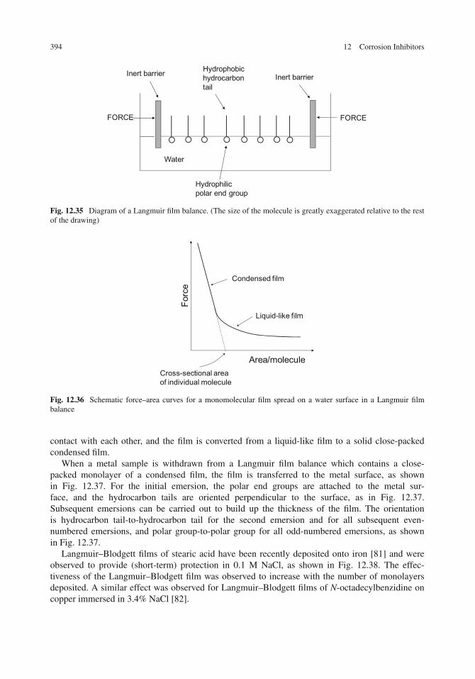
394 12 Corrosion Inhibitors
Inert barrierInert barrier
Water
FORCEFORCE
Hydrophilicpolar end group
Hydrophobichydrocarbontail
Fig. 12.35 Diagram of a Langmuir film balance. (The size of the molecule is greatly exaggerated relative to the restof the drawing)
Area/molecule
Forc
e
Condensed film
Liquid-like film
Cross-sectional areaof individual molecule
Fig. 12.36 Schematic force–area curves for a monomolecular film spread on a water surface in a Langmuir filmbalance
contact with each other, and the film is converted from a liquid-like film to a solid close-packedcondensed film.
When a metal sample is withdrawn from a Langmuir film balance which contains a close-packed monolayer of a condensed film, the film is transferred to the metal surface, as shownin Fig. 12.37. For the initial emersion, the polar end groups are attached to the metal sur-face, and the hydrocarbon tails are oriented perpendicular to the surface, as in Fig. 12.37.Subsequent emersions can be carried out to build up the thickness of the film. The orientationis hydrocarbon tail-to-hydrocarbon tail for the second emersion and for all subsequent even-numbered emersions, and polar group-to-polar group for all odd-numbered emersions, as shownin Fig. 12.37.
Langmuir–Blodgett films of stearic acid have been recently deposited onto iron [81] and wereobserved to provide (short-term) protection in 0.1 M NaCl, as shown in Fig. 12.38. The effec-tiveness of the Langmuir–Blodgett film was observed to increase with the number of monolayersdeposited. A similar effect was observed for Langmuir–Blodgett films of N-octadecylbenzidine oncopper immersed in 3.4% NaCl [82].

New Approaches to Corrosion Inhibition 395
FORCEFORCE
Metal
Water
(a)
1st emersion2nd emersion
3rd emersion
(b)
Fig. 12.37 (a) Transfer of a Langmuir–Blodgett film onto a metal surface by withdrawal of the metal specimenthrough a monomolecular film spread on a water surface. (b) Formation of multimolecular layers by successivewithdrawals
0
20
40
60
80
100
0 2 4 6 8 100
2
4
6
8
10
Per
cent
Inhi
bitio
n
Number of Monolayers
Rp
in k
ohm
-cm
2
Fig. 12.38 Effect of the number of Langmuir–Blodgett layers on the percent inhibition and polarization resistanceRp of iron in 0.1 M NaCl after 30 min of exposure. Redrawn from [81] by permission of © NACE International1995
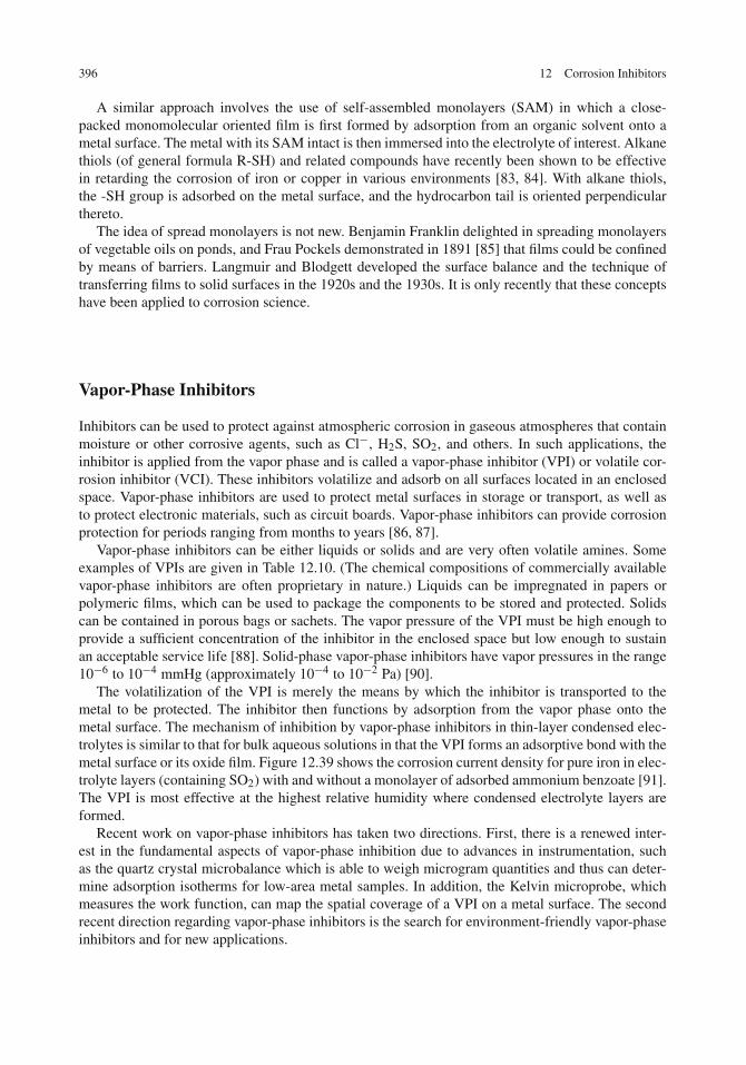
396 12 Corrosion Inhibitors
A similar approach involves the use of self-assembled monolayers (SAM) in which a close-packed monomolecular oriented film is first formed by adsorption from an organic solvent onto ametal surface. The metal with its SAM intact is then immersed into the electrolyte of interest. Alkanethiols (of general formula R-SH) and related compounds have recently been shown to be effectivein retarding the corrosion of iron or copper in various environments [83, 84]. With alkane thiols,the -SH group is adsorbed on the metal surface, and the hydrocarbon tail is oriented perpendicularthereto.
The idea of spread monolayers is not new. Benjamin Franklin delighted in spreading monolayersof vegetable oils on ponds, and Frau Pockels demonstrated in 1891 [85] that films could be confinedby means of barriers. Langmuir and Blodgett developed the surface balance and the technique oftransferring films to solid surfaces in the 1920s and the 1930s. It is only recently that these conceptshave been applied to corrosion science.
Vapor-Phase Inhibitors
Inhibitors can be used to protect against atmospheric corrosion in gaseous atmospheres that containmoisture or other corrosive agents, such as Cl−, H2S, SO2, and others. In such applications, theinhibitor is applied from the vapor phase and is called a vapor-phase inhibitor (VPI) or volatile cor-rosion inhibitor (VCI). These inhibitors volatilize and adsorb on all surfaces located in an enclosedspace. Vapor-phase inhibitors are used to protect metal surfaces in storage or transport, as well asto protect electronic materials, such as circuit boards. Vapor-phase inhibitors can provide corrosionprotection for periods ranging from months to years [86, 87].
Vapor-phase inhibitors can be either liquids or solids and are very often volatile amines. Someexamples of VPIs are given in Table 12.10. (The chemical compositions of commercially availablevapor-phase inhibitors are often proprietary in nature.) Liquids can be impregnated in papers orpolymeric films, which can be used to package the components to be stored and protected. Solidscan be contained in porous bags or sachets. The vapor pressure of the VPI must be high enough toprovide a sufficient concentration of the inhibitor in the enclosed space but low enough to sustainan acceptable service life [88]. Solid-phase vapor-phase inhibitors have vapor pressures in the range10−6 to 10−4 mmHg (approximately 10−4 to 10−2 Pa) [90].
The volatilization of the VPI is merely the means by which the inhibitor is transported to themetal to be protected. The inhibitor then functions by adsorption from the vapor phase onto themetal surface. The mechanism of inhibition by vapor-phase inhibitors in thin-layer condensed elec-trolytes is similar to that for bulk aqueous solutions in that the VPI forms an adsorptive bond with themetal surface or its oxide film. Figure 12.39 shows the corrosion current density for pure iron in elec-trolyte layers (containing SO2) with and without a monolayer of adsorbed ammonium benzoate [91].The VPI is most effective at the highest relative humidity where condensed electrolyte layers areformed.
Recent work on vapor-phase inhibitors has taken two directions. First, there is a renewed inter-est in the fundamental aspects of vapor-phase inhibition due to advances in instrumentation, suchas the quartz crystal microbalance which is able to weigh microgram quantities and thus can deter-mine adsorption isotherms for low-area metal samples. In addition, the Kelvin microprobe, whichmeasures the work function, can map the spatial coverage of a VPI on a metal surface. The secondrecent direction regarding vapor-phase inhibitors is the search for environment-friendly vapor-phaseinhibitors and for new applications.

Vapor-Phase Inhibitors 397
Table 12.10 Some examples of vapor-phase inhibitors
Compound Structure Melting point (◦C) Metals protected
Cyclohexylamine NH2 −17.7 Mild steel [88]
MorpholineCH2- CH2
CH2- CH2
NHO −4.9 Mild steel [88]
BenzotriazoleN
NNH
98.5 Copper, aluminum,zinc [86]
Dicyclohexylammoniumnitrate
NH2+ NO2
–154 Mild steel and
aluminum [87]
n-Decylamine CH3-(CH2)9 -NH2 15Mild steel and
zinc [89]
0.0
0.5
1.0
1.5
2.0
2.5
70 75 80 85 90 95 100
Cur
rent
Den
sity
in μ
A/c
m2
Relative Humidity in %
Pure iron only
Pure iron plusmonolayer ofammonium benzoate
Fig. 12.39 Effect of a monomolecular layer of ammonium benzoate on the corrosion rate of iron in a humidatmosphere. Redrawn from [91] by permission of Elsevier Ltd

398 12 Corrosion Inhibitors
Problems
1. What type of tests or experiments would you set up to screen a set of several com-pounds for their effectiveness as corrosion inhibitors? What parameters should you attempt tomeasure?
2. The corrosion weight loss of mild steel immersed in a hydrochloric acid solution for 124 hwas 1,229 mg/dm2 for 1 M HCl and 7,066 mg/dm2 for 4 M HCl [92]. In the pres-ence of an aldehyde inhibitor, the weight losses over the same period were 153 mg/dm2
for 1 M HCl and 2,860 mg/dm2 for 4 M HCl. What was the percent inhibition in eachcase?
3. The following data were taken by measurement of double layer capacitances for benzotriazoleon iron in sulfuric acid solution [31]. Show that these data obey a Langmuir adsorption isotherm.
Inhibitor concentration (mM) Surface coverage, θ
0.21 0.690.42 0.842.08 0.974.16 1.00
4. The following data were taken [93] for the corrosion of mild steel in 0.5 M sulfuric acid contain-ing various amounts of 5-hydroxyindole inhibitor. Calculate the fractional coverage of inhibitorfor each concentration given below. Do the data better fit a Langmuir adsorption isotherm or aTemkin adsorption isotherm?
Concentration of inhibitor Corrosion rate (μA/cm2)
0 1,0721.0 × 10−4 8795.0 × 10−4 8007.5 × 10−4 7721.0 × 10−3 7182.5 × 10−3 5685.0 × 10−3 4297.5 × 10−3 354
5. Use the model of parallel reactions to show that if the minimum corrosion rate of an inhib-ited surface (isat) is much less than the corrosion rate of the uninhibited surface (io), then thefractional coverage of inhibitor is given by θ = (% I)/100.
6. In the following pairs of compounds, which compound in each group of two is expected to bethe better inhibitor in acid solutions? Explain why in each case.
(a) CH3(CH2)4NH2 or CH3(CH2)4SH?(b) CH3(CH2)5COOH or CH3(CH2)16COOH?(c) CH3(CH2)4NH2 or H2N(CH2)5NH2?
The pKa values are 10.63 for the monoamine and 10.25 for the first ionization of thediamine.

Problems 399
(d)
N
Cl CH3
N
or ?
(e)
N
CH3
N
CH3
orCH3
?
7. For the adsorption of an organic molecule by replacement of previously adsorbed watermolecules
Org (soln)+ nH2O (ads)→ Org (ads)+ nH2O (soln)
show that
�Gads = �Gorgads − n�GH2O
ads
where �Gorgads and �GH2O
ads refer to the free energy of adsorption per mole of the organiccompound and water, respectively.
8. Chromate inhibitors are reduced to Cr2O3 on iron surfaces by the following reaction:
2Fe+ 2CrO2−4 + 4H+ → Fe2O3 + Cr2O3 + 2H2O
for which the Nernst equation is
E = 1.437+ 0.0197 log [CrO−24 ]− 0.0394 pH
The analogous reaction and the Nernst equation for tungstates are
2Fe+ 6WO−24 + 12H+ → Fe2O3 + 3W2O5 + 6H2O
E = 0.852+ 0.0591 log [WO−24 ]− 0.182 pH
(a) Calculate the electrode potentials for each of these two reactions at pH 7.0 and CrO42− or
WO42− concentrations of 1.0 × 10⁻³ M.
(b) What do the electrode potentials tell you about the spontaneity of each reaction under thegiven conditions and about the possibility of using tungstates as chromate replacements?
9. What are the similarities between the mechanisms of corrosion inhibition in acid solutions andin neutral solutions? What are the differences in mechanisms for these two types of solutions?
10. In some instances, very low concentrations of would-be corrosion inhibitors actually functionas accelerators of corrosion until a larger surface coverage of the inhibitor is attained. Provide apossible explanation for this accelerating effect.

400 12 Corrosion Inhibitors
11. Show that the straight line in Fig. 12.25(b) which separates regions of crevice corrosion fromregions of inhibition can be obtained from Eq. (20).
HINT: Replace concentrations in Eq. (20) with activities and then take differentials at constantE (E = Eactive) to get
(∂ log aA
∂ log aI
)Eactive
= θcritrA
rI= constant′′′
References
1. A. D. Mercer in “Corrosion”, L. L. Shreier, Ed., Vol. 2, p. 18.1, Newnes-Butterworths, London (1976).2. C. C. Nathan, Ed., “Corrosion Inhibitors”, pp. 114, 126, 173, 196, NACE, Houston, TX (1974).3. G. Butler and H. C. K. Ison, “Corrosion and Its Prevention in Waters”, p. 157, Reinhold Publishing Company,
New York (1966).4. J. M. Gaidis and A. Rosenberg, Mater. Perform., 43 (1), 48 (2004).5. N. Hackerman, Mater. Perform., 29 (2), 44 (1990).6. E. McCafferty, M. K. Bernett, and J. S. Murday, Corros. Sci., 28, 559 (1988).7. Z. Zembura, W. Ziolkowska, and H. Kolny, Bull. Acad. Polon. Sci., 13 (7), 487 (1965).8. N. Hackerman, Corrosion, 18, 332t (1962).9. E. McCafferty and N. Hackerman, J. Electrochem. Soc., 119, 146 (1972).
10. N. Hackerman and E. McCafferty in “Proceedings of the Fifth International Congress on Metallic Corosion”,p. 542, NACE, Houston, TX (1974).
11. N. Hackerman and A. C. Makrides, Ind. Eng. Chem., 46, 523 (1954).12. H. F. Finley and N. Hackerman, J. Electrochem. Soc., 107, 259 (1960).13. R. C. Ayers, Jr. and N. Hackerman, J. Electrochem. Soc., 110, 507 (1963).14. A. I. Altsybeeva, A. P. Dorokhov, and S. Z. Levin, Protect. Metals, 7, 422 (1971)15. J. A. Dean, Ed., “Lange’s Handbook of Chemistry”, p. 9.2, McGraw-Hill, New York (1999).16. J. O’M. Bockris and D. A. J. Swinkels, J. Electrochem. Soc., 111, 736 (1964).17. Z. Szklarska-Smialowska and G. Wieczorek, Corros. Sci., 11, 843 (1971).18. J. O’M. Bockris, M. Green, and D. A. J. Swinkels, J. Electrochem. Soc., 111, 743 (1964).19. P. Kern and D. Landolt, Electrochim. Acta, 47, 589 (2001).20. N. Hackerman, E. S. Snavely, Jr., and J. S. Payne, Jr., J. Electrochem. Soc., 113, 677 (1966).21. Z. A. Iofa, Y. A. Nikorova, and V. V. Batrakov, “Proceedings of the Third International Congress on Metallic
Corrosion”, Vol. 2, p. 40, Moscow (1969).22. I. L. Rozenfeld, “Corrosion Inhibitors”, p. 115, McGraw-Hill, New York (1981).23. R. S. Perkins and T. N. Andersen in “Modern Aspects of Electrochemistry”, J. O′M. Bockris and B. E. Conway,
Eds., Vol. 5, p. 203, Plenum Press, New York (1969).24. A. Akiyama and K. Nobe, J. Electrochem. Soc., 117, 999 (1970).25. N. Eldakar and K. Nobe, Corrosion, 33, 128 (1977).26. R. R. Annand, R. M. Hurd, and N. Hackerman, J. Electrochem. Soc., 112, 144 (1965).27. N. Hackerman, R. M. Hurd, and R. R. Annand, Corrosion, 18t, 37 (1962).28. K. Aramaki and N. Hackerman, J. Electrochem. Soc., 115, 1007 (1968).29. K. Aramaki, J. Electrochem. Soc., 118, 1553 (1971).30. R. J. Meakins, J. Appl. Chem., 13, 339 (1963).31. R. J. Chin and K. Nobe, J. Electrochem. Soc., 118, 545 (1971).32. N. Eldakar and K. Nobe, Corrosion, 32, 238 (1976).33. M. A. Quraishi, J. Rawat, and M. Ajmal, Corrosion, 54, 996 (1998).34. A. E. Stoyanova, E. I. Sokolova, and S. N. Raicheva, Corros. Sci., 39, 1595 (1997).35. M. S. A. Aal, S. Radwan, and A. El-Saied, Br. Corros. J., 18, 102 (1983).36. Y.-F. Yu, J. J. Chessick, and A. C. Zettlemoyer, J. Phys. Chem., 63, 1626 (1959).37. P. F. Rossi, M. Bassoli, G. Olivera, and F. Guzzo, J. Therm. Anal., 41, 1227 (1994).38. Y.-F. Yu Yao, J. Phys. Chem., 67, 2055 (1963).39. M. Nakazawa and G. A. Somorjai, Appl. Surf. Sci., 84, 309 (1995).

References 401
40. Y.-F. Yu Yao, J. Phys. Chem., 69, 3930 (1965).41. T. Matsuda, T. Taguchi, and M. Nagao, J. Therm. Anal., 38, 1835 (1992).42. J. G. N. Thomas, Br. Corros. J., 5, 41 (1970).43. J. E. O. Mayne and C. L. Page, Br. Corros. J., 7, 115 (1972).44. A. Weisstuch, D. A. Carter, and C. C. Nathan, Mater. Prot. Perf., 10 (4), 11 (1971).45. F. P. Dwyer and D. D. Mellor “Chelating Agents and Metal Chelates”, Academic Press, New York (1964).46. D. C. Zecher, Mater. Perf., 15 (4), 33 (1976).47. R. L. LeRoy, Corrosion, 34, 98 (1978).48. B. Müller, W. Kläger, and G. Kubitzki, Corros. Sci., 39, 1481 (1997).49. F. Tirbonod and C. Fiaud, Corros. Sci., 18, 139 (1978).50. Y. I. Kuznetsov and T. I. Bardasheva, Russ J. Appl. Chem., 66, 905 (1993).51. B. D. Chambers, S. R. Taylor, and M. W. Kendig, Corrosion, 61, 480 (2005).52. C. B. Breslin, G. Treacy, and W. M. Carroll, Corros. Sci., 36, 1143 (1994).53. A. A. O. Magalhaes, I. C. P. Margarit, and O. R. Mattos, J. Electroanal. Chem., 572, 433 (2004).54. S. Z. El Abedin, J. Appl. Electrochem., 31, 711 (2001).55. H. Guan and R. G. Buuchheit, Corrosion, 60, 284 (2004).56. V. F. Vetere and R. Romagnoli, Br. Corros. J., 29, 115 (1994).57. S. M. Cohen, Corrosion, 51, 71 (1995).58. B. R. W. Hinton, D. R. Arnott, and N. E. Ryan, Mater. Forum, 9, 162 (1986).59. R. G. Buchheit, M. D. Bode, and G. E. Stoner, Corrosion, 50, 205 (1994).60. P. M. Natishan, E. McCafferty, J. W. Glesener, and A. A. Morrish in “Proceedings of the Fourth International
Symposium on Diamond Materials”, K. V. Ravi and J. P. Dismukes, Eds., p. 607, The Electrochemical Society,Pennington, NJ (1995).
61. E. McCafferty, P. M. Natishan, and G. K. Hubler, Corros. Sci., 35, 239 (1993).62. E. McCafferty and J. V. McArdle, J. Electrochem. Soc., 142, 1447 (1995).63. D. C. Hansen and E. McCafferty, J. Electrochem. Soc., 143, 115 (1996).64. H.-H. Strehblow and B. Titze, Corros. Sci., 17, 461 (1977).65. E. McCafferty, J. Electrochem. Soc., 137, 3731 (1990).66. S. Matsuda and H. H. Uhlig, J. Electrochem. Soc., 111, 156 (1964).67. H. H. Uhlig and J. R. Gilman, Corrosion, 20, 289t (1964)68. C.-J. Lin, R.-G. Du, and T. Nguyen, Corrosion, 56, 41 (2000).69. A. Devasenapathi and V. S. Raja, J. Mater. Sci., 33, 3345 (1998).70. V. S. Argawala and J. J. De Luccia, Corrosion, 36, 208 (1980).71. I. M. Putilova, S. A. Balezin, and V. P. Barannik, “Metallic Corrosion Inhibitors”, p. 1, Pergamon Press, New
York (1960).72. J. W. Hill and R. H. Petrucci, “General Chemistry”, 2nd Edition, p. 980, Prentice Hall, Upper Saddle River,
NJ (1999).73. H. Ashassi-Sorkhabi, M. R. Majidi, and K. Seyyedi, Appl. Surf. Sci., 225, 176 (2004).74. J. Telegdi, E. Kalman, and F. H. Karman, Corros. Sci., 33, 1099 (1992).75. E. Mueller, C. S. Sikes, and B. J. Little, Corrosion, 49, 829 (1993).76. D. C. Hansen and E. McCafferty in “Environmentally Acceptable Inhibitors and Coatings”, S. R. Taylor,
H. S. Isaacs, and E. W. Brooman, Eds., p. 234, The Electrochemical Society, Pennington, NJ (1995).77. I. Sekine, Y. Nakahata, and H. Tanabe, Corros. Sci., 28, 987 (1988).78. G. D. Davis and J. A. Von Fraunhofer, Mater. Perform., 42 (2), 56 (2003).79. J. A. Von Fraunhofer and G. D. Davis, Mater. Perform., 42 (12), 38 (2003).80. G. Matamala, W. Smeltzer, and G. Droguett, Corros. Sci., 42, 1351 (2000).81. W. Xing, Y. Shan, D. Guo, T. Lu, and S. Xi, Corrosion, 51, 45 (1995).82. A. Jaiswal, R. A. Singh, and R. S. Dubey, Corrosion, 57, 307 (2001).83. G. Grundmeier, C. Reinartz, M. Rohwerder, and M. Stratmann, Electrochim. Acta, 43, 165 (1997).84. Y. Yamamoto, H. Nishihari, and K. Aramaki, J. Electrochem. Soc., 140, 436 (1993).85. W. A. Adamson, “Physical Chemistry of Surfaces”, p. 99, John Wiley & Sons, New York (1976).86. A. Subramananian, M. Natesan, V. S. Muralidharan, K. Balakrishnan, and T. Vasudevan, Corrosion, 56, 144
(2000).87. A. Wachter, T. Skei, and N. Stillman, Corrosion, 7, 284 (1951).88. E. Vuorinen, P. Ngobeni, G. H. van der Klashorst, W. Skinner, E. de Wet, and W. S. Ernst, Br. Corros. J., 29, 120
(1994).

402 12 Corrosion Inhibitors
89. E. M. Mora and J. M. Bastidas, Corros. Prevent. Control, 34 (6), 143 (1987).90. I. L. Rozenfeld, “Corrosion Inhibitors”, p. 302, McGraw-Hill, New York (1981).91. A. Leng and M. Stratmann, Corros. Sci., 34, 1657 (1993).92. M. N. Desai and M. B. Desai, Corros. Sci., 24, 649 (1984).93. G. Moretti, G. Quartarone, A. Tassan, and A. Zingales, Br. Corros. J., 31, 49 (1996).
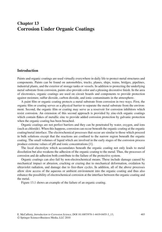
Chapter 13Corrosion Under Organic Coatings
Introduction
Paints and organic coatings are used virtually everywhere in daily life to protect metal structures andcomponents. Paints can be found on automobiles, trucks, planes, ships, trains, bridges, pipelines,industrial plants, and the exterior of storage tanks or vessels. In addition to protecting the underlyingmetal substrate from corrosion, paints also provide color and a pleasing decorative finish. In the areaof electronics, organic coatings are used on circuit boards and components to provide protectionagainst moisture, sulfur dioxide, carbon dioxide, and ionic contaminants in the atmosphere.
A paint film or organic coating protects a metal substrate from corrosion in two ways. First, theorganic film or coating serves as a physical barrier to separate the metal substrate from the environ-ment. Second, the organic film or coating may serve as a reservoir for corrosion inhibitors whichresist corrosion. An extension of this second approach is provided by zinc-rich organic coatingswhich contain flakes of metallic zinc to provide added corrosion protection by galvanic protectionwhen the organic coating has been breached.
Organic coatings are not perfect barriers and they can be penetrated by water, oxygen, and ions(such as chloride). When this happens, corrosion can occur beneath the organic coating at the organiccoating/metal interface. The electrochemical processes that occur are similar to those which proceedin bulk solutions except that the reactions are confined to the narrow region beneath the organiccoating. The small volumes of liquid which are involved in the early stages of the corrosion processproduce extreme values of pH and ionic concentrations [1].
The local electrolyte which accumulates beneath the organic coating not only leads to metaldissolution but also weakens the adhesion of the organic coating to the metal. Thus, the processes ofcorrosion and de-adhesion both contribute to the failure of the protective system.
Organic coatings can also fail by non-electrochemical means. These include damage caused bymechanical impact or abrasion, cracking or crazing due to mechanical deformation, oxidation byultraviolet radiation, and damage due to free-thaw cycles. In addition, all of the above processesallow slow access of the aqueous or ambient environment into the organic coating and thus alsoenhance the possibility of electrochemical corrosion at the interface between the organic coating andthe metal.
Figure 13.1 shows an example of the failure of an organic coating.
403E. McCafferty, Introduction to Corrosion Science, DOI 10.1007/978-1-4419-0455-3_13,C© Springer Science+Business Media, LLC 2010

404 13 Corrosion Under Organic Coatings
Fig. 13.1 An example of a paint failure leading to corrosion of the underlying substrate
Paints and Organic Coatings
A paint is an organic coating applied to a surface as a liquid, which subsequently dries or cures toform a protective film. Paint coatings are generally 25–1,000 μm in thickness [2].
A paint consists of at least three components [2–4]: (i) a vehicle or binder, (ii) a pigment sus-pended in the binder, and (iii) a solvent. In addition, there may be a fourth component, specialadditives, which have very specific purposes and are typically added to the paint in very smallamounts. When the paint is applied and the solvent evaporates, the paint film forms the structureshown schematically in Fig. 13.2.
Metal substrate
PaintFilm
Pigment
Binder
Environment
Fig. 13.2 Structure of a paint film upon drying of the solvent
Vehicles or binders are of various types, as listed in Table 13.1. The vehicle or binder is the film-forming agent in the paint and is the continuous polymeric phase in which all the other componentsare incorporated.
Pigments may be used to provide color to the paint film (e.g., Fe2O3 for red or TiO2 for white)or to act as a corrosion inhibitor (e.g., ZnCrO4). Pigments also include zinc powders or flakes (zinc-rich paints) which provide cathodic protection to the metal substrate when the paint film becomespermeated with water. Other pigments include fillers such as mica, which reinforce the paint filmand present a more torturous path for the penetration of water and ions through the film.

Underfilm Corrosion 405
Table 13.1 Some typical constituents of paints [2–4]
Vehicles Pigments
Epoxy Iron oxidesUrethane Titanium dioxideAcrylic ClaysVinyl SilicatesAlkyd ChromatesSilicones Mica
Zinc powder
Solvents Special additives
Xylene UV absorbersGlycol ethers Dispersing agentsKetones Mildew inhibitorsMineral spirits Fire-retarding agentsWater Biocides for anti-fouling paints
Abrasives for anti-slip paints
Solvents for paints are either volatile organic liquids or water. Oil-based paints require the use oforganic solvents for thinning and cleanup of brushes or other applicators, so that the use of oil-basedpaints is being phased out due to environmental considerations.
Paint films often consist of various layers, as shown schematically in Fig. 13.3. The metal surfacemay first be treated with chromates or phosphates to form a conversion coating for improved corro-sion resistance or paint adhesion. A primer may also be used prior to the application of the topcoat,with the topcoat itself having the structure in Fig. 13.2.
Metal
Conversion coatingOxide film
Primer
Topcoat(s)
25 to1000 μm
Fig. 13.3 Schematic diagram showing the various layers which may be present in a paint film
Paints are not generally used for protection below ground or in applications where mechanicaldamage may be a problem. Various types of organic coatings used in such applications includepolyvinyl chloride, epoxies, urethanes, and polyesters; and the structural formulas of various organiccompounds used in coatings are given in Fig. 13.4.
The primary purpose of a paint film or organic coating is to form a barrier between the metalsubstrate and its environment. However, an organic coating is not a perfect barrier but instead is likea membrane which can be penetrated by water, oxygen, and ions, as discussed below.
Underfilm Corrosion
Corrosion beneath an organic coating can occur only if an electrolyte exists at the organic coat-ing/substrate interface. This electrolyte is provided by the penetration of water into the organic

406 13 Corrosion Under Organic Coatings
H
C
H
H
C
Cln
poly (vinyl chloride)
H
C
H
H
Cn
C
H
H
H
C
cis 1,4-polybutadiene
a urethane
C
O
N
H
O R’RCH CH
O
R’R
an epoxy
C
H
HC
H
nR R’ polystyrene
O
n
O
C
O
C
a polyesterpoly (ethylene terephthalate)
C
H
H
C
H
H
O O
Fig. 13.4 Formulas of various organic compounds utilized in organic coatings for metals
coating and its subsequent accumulation beneath the coating. The presence of ions (such as chlo-rides) is also necessary in order to provide sufficient conductivity in the aqueous phase beneath thecoating to allow local electrochemical reactions to occur.
Water Permeation into an Organic Coating
Water permeation into an organic coating occurs due to three effects [4]:
(1) Water diffuses into the coating due to a concentration gradient formed by immersion into anaqueous solution or exposure to a humid atmosphere.
(2) Water penetrates the film by osmosis due to an ionic concentration gradient which exists betweenthe film (which may contain ionic impurities) and the environment.
(3) Water enters the film by capillary action through voids, pores, or cracks in the organic coating.

Underfilm Corrosion 407
Penetration rates of water or gases into an organic coating are given in terms of a permeabilitycoefficient P, which is the product of the usual diffusion coefficient D and the Henry’s law constantKH (also called the solubility coefficient). As shown in Chapter 8, the diffusion coefficient D pertainsto Fick’s first law:
J=−DdC
dx(1)
where J is the flux past a plane and dC/dx the concentration gradient. For gases, it is easier todetermine the partial pressure of the gas (Pgas) on each side of the polymer film (rather than itsconcentration) so that
J=−Pdpgas
dx(2)
where P is the permeability coefficient. The concentration of a gas in the polymer film and its vaporpressure in the vapor phase are related by Henry’s law:
C=KH pgas (3)
where KH is the Henry’s law constant (see Chapter 8). For a linear concentration (or pressure)gradient, Eqs. (1)–(3) combine to give
P=DKH (4)
(See Problem 13.3). The permeability coefficient P should be independent of the coating thickness(for a homogeneous coating) because both D and KH are independent of thickness. Permeabilitycoefficients have the following units:
P = (quantity of permeant)× (film thickness)
(area)× (time)× (pressure drop across the film)(5)
(See Problem 13.4). However, permeability data are often expressed as transmission rates for agiven thickness of coating. Experimentally determined transmission rates for water through variouspolymers or paint films are given in Table 13.2. It can be seen that all the polymers listed in Table 13.2are permeable to water vapor and that the permeability coefficients vary greatly with the nature ofthe polymer. The flux of water through a free polymer film is typically of the order of 1–10 mg/cm2
day for many classes of polymers [1, 5].The transmission rate of a molecule through an organic coating depends on the thickness of the
coating. If the transmission rate is J1 through a coating of thickness L1, then the transmission rate J2through a coating of the same material but having a different thickness L2 is given by
J2
J1= L1
L2(6)
as shown in Appendix K; that is, the transmission rate through a 100 μm coating is theoretically50% of that through a 50 μm coating.
The transmission rate of water necessary to sustain the corrosion of steel at the base of the organiccoating can be calculated as follows. The corrosion rate of unpainted steel in neutral electrolytes is1–10 mils per year (mpy) [7, 8]. From the density of iron, a penetration rate of 10 mpy corresponds

408 13 Corrosion Under Organic Coatings
Table 13.2 Transmission rates of water through organic coatings [5, 6]
CoatingTransmission rate inmg/cm2 day Film thickness in μm
Organic coatingEpoxy/polyamide 15.5 10Chlorinated rubber (plasticized) 9.5 10Styrene acrylic latex 230 10Vinyl chloride–vinylidene chloride copolymer 2.8 10Polybutadiene 3 25Polytetrafluoroethylene 0.48 25Cellulose nitrate 63 25
Paint filmsVinyl chloride–vinylidene chloride copolymerlatex
6.8 10
Chlorinated rubber, unmodified 5.0 10Coal tar epoxy 7.5 10Acrylic water-borne primer 180 10TiO2-pigmented alkyd 65 10Red lead-oil-based primer 54 10Alkyd resin 2.3 100Polyurethane 1.4 100Phenolic resin 1.1 100
to a weight loss for iron of 9.8 × 10⁻⁶ moles/cm2 day. The half-cell reactions in neutral electrolytes(see Chapter 2) are:
Anodic: 2 Fe → 2 Fe2+ + 4 e−
Cathodic: O2 + 2H2O+ 4 e− → 4 OH−
Overall: 2 Fe+O2 + 2 H2O→ 2 Fe2+ + 4 OH−
From simple stoichiometry, the reaction of 9.8 × 10⁻⁶ moles/cm2 day of Fe requires the samenumber of moles of H2O, which in turn amounts to 0.18 mg H2O/cm2 day. (The transmission rateof H2O needed to sustain the corrosion rate of 1 mpy is accordingly 0.018 mg H2O/cm2 day.)
As seen in Table 13.2, the transmission rate of water through various polymer films is sev-eral orders of magnitude higher than the transmission rate required for the corrosion of iron; seeTable 13.3. This fact was first established by Mayne [9] and has been verified subsequently by otherinvestigators [10, 11]. Thus, the permeation rate of H2O through an organic coating or paint film isnot the rate-determining step in the underfilm corrosion of steel substrates. However, the transmis-sion of water is important in providing the electrolyte, in facilitating the diffusion of ions throughthe coating, and in contributing to the loss of adhesion of the organic coating, as is discussed later.
The data in Table 13.2 apply to free-standing films rather than to films attached to metal sub-strates. (That is, the polymer films were formed on a substrate such as glass and were then detached.)Thus, some reservation must be taken in applying permeability data for free films to films which areintact on metal substrates. However, Nguyen and co-workers [12] have more recently developed atechnique based on Fourier transform infrared-multiple internal reflection (FTIR-MIR) for measur-ing in-situ water beneath organic coatings cast on metal substrates. This technique is able to detectmolecular water which accumulates at the organic coating/metal interface. Results are shown inFig. 13.5 for an epoxy coating applied to a silicon substrate. It can be seen that approximately 15 nm

Underfilm Corrosion 409
Tabl
e13
.3C
ompa
riso
nof
requ
ired
and
oper
ativ
epe
rmea
tion
rate
sfo
rco
rros
ion
tooc
cur
bene
ath
coat
edir
onsp
ecim
ens
Cor
rosi
onra
teof
open
unco
ated
stee
lin
neut
ral
elec
trol
ytes
[7,8
]R
equi
red
rate
ofsu
pply
ofH
2O
tosu
stai
nth
eco
rros
ion
rate
aPe
rmea
tion
rate
ofH
2O
thro
ugh
orga
nic
coat
ings
bR
equi
red
rate
ofsu
pply
ofO
2to
sust
ain
the
corr
osio
nra
tea
Perm
eatio
nra
teof
O2
thro
ugh
orga
nic
coat
ings
c
1m
il/ye
ar0.
018
mg
H2O
cm2
day
0.5
to23
0m
gH
2O
cm2
day
0.01
6m
gO
2
cm2
day
0.00
2to
0.00
8m
gO
2
cm2
day
(one
valu
eat
0.11
mg
O2
cm2
day
)
10m
ils/y
ear
0.18
mg
H2O
cm2
day
0.16
mg
O2
cm2
day
a Bas
edon
the
follo
win
gre
actio
n:2
Fe+
O2+
2H
2O→
2Fe
2++
4O
H−
bFr
omTa
ble
13.2
.c Fr
omTa
ble
13.4
.

410 13 Corrosion Under Organic Coatings
–5
0
5
10
15
20
25
30
0
2
4
6
8
0 50 100 150 200
Thi
cnes
s in
nm
Time in Hours
Wei
ght i
n μg
Clear epoxy on silicon
Clear epoxy on
silane-treated silicon
Fig. 13.5 Thickness and amount of water at the coating/substrate interface for clear epoxy coatings on silicon andon silane-treated silicon. The epoxy coating thickness was 130–140 μm. Redrawn from Nguyen et al. [12] with thepermission of Elsevier Ltd
of water accumulates at the interface (corresponding to approximately 50 monolayers of water).Thus, this later evidence confirms the idea that electrolyte layers can be readily formed beneathorganic coatings.
Nguyen and co-workers also found that the amount of water formed at the interface was muchless for a silane-treated interface, as shown in Fig. 13.5. (Silanes are Si-containing molecules usedto treat metals to produce hydrophobic surfaces.)
As mentioned earlier, the accumulation of water layers beneath a polymer film not only servesto provide an electrolyte for the operation of localized corrosion cells but also promotes the loss ofadhesion of the organic coating. Silane-treated specimens displayed a greater adhesion strength thanuntreated samples after more than 600 h exposure to water [12].
Permeation of Oxygen and Ions into an Organic Coating
The rates of oxygen penetration through organic coatings are generally very much less than the ratesfor water, as shown in Table 13.4.
The transmission rate of O2 necessary to support the corrosion of unpainted steel is calculated tobe 0.016–0.16 mg O2/cm2 day. This value results from the earlier calculation that a corrosion rateof 10 mpy consumes 9.8 × 10⁻⁶ moles/cm2 day of iron and thus requires half that amount of O2(from stoichiometry) or 4.9 × 10⁻⁶ moles/cm2 day or 0.16 mg O2/cm2 day. (A corrosion rate of 1mpy thus requires only 1/10 of that amount.) Most polymers in Table 13.4 have transmission ratesof O2 lower than that required for corrosion, as seen in Table 13.3. This observation has led some

Underfilm Corrosion 411
Table 13.4 Transmission rates of oxygen through organic coatings [5, 10, 11]
Coating Transmission rate in mg/cm2 day Film thickness in μm
Cellulose nitrate 0.106 100Epoxy resin 7.3 × 10⁻³ 100Vinyl chloride/vinyl acetate copolymer 7.5 × 10⁻³ 100Chlorinated rubber 2.2 × 10⁻³ 100Alkyd 15% poly (vinyl chloride) 6.8 × 10⁻³ 87Epoxy/coal tar 4.1 × 10⁻³ 33Epoxy/polyamide 6.4 × 10⁻³ 38Polybutadiene 2.5 × 10⁻³ 25
investigators to suggest that the rate-determining step in underfilm corrosion is the slow permeationof O2 through the organic coating [10, 11].
The rate of permeation of Cl− ions is even less than the permeation rates for O2, as seen inTable 13.5 [13]. The role of Cl− ions in underfilm corrosion appears to be that of providing sufficientelectrolyte conductivity for the operation of localized corrosion cells and to accelerate the anodichalf-cell reaction when it has been initiated.
Table 13.5 Transmission rates of chloride through organic coatings [13]
Organic coating Transmission rate in mg/cm2 day Film thickness in μm
Chlorinated rubber 6.00 × 10⁻³ 59Vinyl 0.31 × 10⁻³ 63Epoxy 0.90 × 10⁻³ 19Alkyd/iron oxide 0.52 × 10⁻³ 62Alkyd/red lead 0.20 × 10⁻³ 75Epoxy/polyamide 0.21 × 10⁻³ 100
Breakdown of an Organic Coating
The sequence of events which occurs in the breakdown of an organic coating in the subcoatingmicro-environment is illustrated by the work of Ritter and Rodriguez [14]; see Figs. 13.6 and 13.7.These authors studied the corrosion of iron covered with a transparent cellulose nitrate coating, acoating selected for its ease of breakdown and observation. The sequence of events is as follows[14, 35]:
(1) The organic coating first becomes penetrated by water and oxygen molecules, as discussedabove.
(2) Corrosion is initiated due to several possible causes, such as defects in the coating, mechani-cal rupture of the coating, or chemical rupture though generation of osmotic pressure at sitescontaining soluble salts.
(3) The substrate iron then goes into solution at a local anodic site:
Fe→ Fe2+ + 2 e−

412 13 Corrosion Under Organic Coatings
H2O H2OO2 O2
OH–
Fe
Fe+2
2 e–
H2O H2OO2 O2
Fe substrate
Paint
1). Diffusion of H2O and O2 through the paint film.
2). Initiation of corrosion beneath the paint.
Fig. 13.6 The first two steps in the deterioration of an organic coating. After Ritter and Rodriguez [14] and reproducedby permission of NACE International
Acidic hydrolysis occurs so that the anodic site becomes locally acidic, as in the case ofcrevice corrosion and pitting (Chapter 10). Chloride ions then migrate into the local acidicenvironment, again as with crevice corrosion and pitting.
(4) A localized cathodic site is generated at a different location and the operation of the cathodichalf-cell is fueled by O2 and H2O molecules which have previously permeated the organiccoating.
O2 + 2 H2O+4 e− → 4 OH−
The cathodic site becomes locally basic (alkaline) due to the production of these OH− ions.(5) The organic coating suffers disbonding from the metal substrate in the local alkaline environ-
ment. This disbonding and removal of the organic coating from the metal surface is calledcathodic delamination and is discussed in more detail later.
(6) As the coating system continues to deteriorate, a breakthrough occurs between adjacent anodicand cathodic areas, and there is a catastrophic failure of the organic coating.
Cathodic delamination, as in step (5), is also a problem in coated systems which are protected byapplied cathodic potential (cathodic protection). Areas on the metal adjacent to defects in the organiccoating can suffer delamination in the presence of the applied cathodic potential.
Adhesion of Organic Coatings
The adhesion properties and corrosion behavior of an organic coating are related. If corrosion occursbeneath the organic coating, a loss of adhesion of the coating will ensue. On the other hand, if thecoating does not possess good adhesion to the metal substrate, then undermining of the coating willlead to localized pockets of electrolyte which promote corrosion.
The relationship between adhesion and corrosion is seen schematically in Fig. 13.8.

Underfilm Corrosion 413
5) and 6). Cathodic disbonding and breakthrough of anodic and cathodic areas.
Cl–Fe+2
Fe+2
H+H+OH–
OH–OH–OH–
Fe+2+ 2 H2O Fe(OH)2+2 H+
3) and 4). Local cell operation.
Fe+2
Cl–
OH– OH–OH–
Cl–
Cathodicdelaminationof the coating
High pH Low pH
H+
Ironcorrosionproducts
O2+ 4 H2O + 4e– 4OH–
Cathodic region
Fe Fe+2+ 2e–
Anodic region
Fig. 13.7 Continued deterioration of an organic coating, according to Ritter and Rodriguez [14]. Reproduced bypermission of NACE International
Corrosion and delamination
Poor adhesion Corrosion
Corrosion Poor adhesion
Fig. 13.8 Schematic illustration showing the relationship between poor adhesion and poor corrosion resistance of acoating

414 13 Corrosion Under Organic Coatings
There are several fundamental theories of metal/polymer adhesion. These are as follows [15]:
(1) The adsorption theory (physical and chemical adsorption), in which the adhesive bond dependson adsorption forces between the two interfaces being joined
(2) The chemical reaction theory, in which a chemical reaction occurs between the polymer and themetal
(3) The mechanical interlocking theory, in which adhesion is due to the mechanical interlocking orkeying of the polymer into cavities and pores of the metal surface
(4) The electrostatic theory, in which adhesion depends on the existence of an electrostatic chargebetween the two surfaces
Each of these last three mechanisms can operate under certain conditions, but the most pervasivemechanism is the first, in which the polymer adheres to the metal substrate (or, more properly, itsoxide) because of interatomic and intermolecular bonds which are formed. These adsorption forcesthat exist across all boundaries include Lewis acid/Lewis base forces.
All metal surfaces to be coated with an organic polymer contain either the incipient air-formedoxide film or an oxide produced by a surface treatment (such as chromates). Thus, it is appropriateto consider the interaction of organic polymers with oxide films.
In Chapter 12 it was seen that many corrosion inhibitors are Lewis bases, which function bydonation of electrons to the metal surface. Organic polymers can also be classified as Lewis bases(electron donors) or Lewis acids (electron acceptors). Poly(methyl methacrylate) (PMMA) is a typ-ical basic polymer, as can be reasoned from its molecular structure, as shown in Fig. 13.9. Thecarbonyl oxygens of esters are basic (electron-donating) sites, which can form acid/base bonds withelectron-accepting sites of Lewis acids.
Poly(vinyl chloride) (PVC) is an example of a polymer which is a Lewis acid. For PVC, it is thepartially positive –CH portion of the vinyl group which is the electron-accepting site [16] and whichcan form acid/base bonds with electron-donating sites of Lewis bases; see Fig. 13.10.
Oxide films on metal surfaces have, in fact, acid/base properties, which will be discussed in moredetail in Chapter 16, and the acidic or basic character of the oxide varies with the nature of the metal.
Figure 13.11 shows adhesion results for two organic polymers on a series of oxide-covered metalsfor which the oxide films have differing degrees of acidity (or basicity) [17]. Figure 13.11 showsthat the adhesion strength of an acidic polymer (as measured by the peel strength) increases withincreasing basicity of the oxide film. Conversely, the adhesion strength of the basic polymer PMMA(as measured by a pull-off test) increases with increasing acidity of the oxide film. These resultsillustrate the importance of Lewis acid/Lewis base interactions in the adhesion of organic polymersto metal surfaces.
However, the situation becomes more complicated when water molecules accumulate beneaththe organic coating because water interferes with the adhesion between the organic coating and themetal substrate. The extent of adhesion in the presence of a liquid (usually water) is referred to as wetadhesion and is considered by Funke [18] to be the most important property of the organic coating.Two different reasons have been proposed for the loss of adhesion in the presence of water [4, 19].These are as follows:
(1) Chemical disbonding due to the interaction of water molecules with covalent, hydrogen, or polarbonds between the organic polymer and the oxide film
(2) Mechanical disbonding due to forces caused by accumulation of water and osmoticpressure

Underfilm Corrosion 415
C
H
C
H
H
C=O..
.. O
CH3
.. npoly (vinyl acetate)
..
C
H
H
C
H
Hn
..
..O polyethyene oxide
C
CH3
C
H
H C=O..O
CH3
....
n
Electron donor groups
poly (methyl methacrylate)..
Fig. 13.9 Some examples of basic polymers. Electrons on the oxygen atom available for donation are indicated byblack solid dots
C
H
C
H
H Fn
poly (vinyl fluoride)
poly (vinylidene fluoride)C
F
C
H
H Fn
C
H
C
H
H Cln
poly (vinyl chloride)
δ-
δ+Can interact withelectron-rich donor groups
Fig. 13.10 Some examples of acidic polymers. Partial charges are denoted by δ+ and δ−

416 13 Corrosion Under Organic Coatings
100
150
200
250
300
350
400
450
0.0
0.2
0.4
0.6
0.8
1.0
1.2
-2 0 2 4 6 8 10
Pe
el E
nerg
y G
c in
J/m
2
Pul
l-off
For
ce in
MN
/m2
Isoelectric Point of O xide F ilm
P eel energyfor P S A(ac idic polyme r)
P ull-off forcefor P MMA(bas ic polyme r)
Ta S i Cr AlZr
B as ic oxide sAcidic oxides
Fig. 13.11 Adhesion strength on various metals (indicated at top) of an acidic pressure-sensitive adhesive (PSA) andof a basic polymer, poly(methyl methacrylate) (PMMA) vs. the isoelectric point of the oxide film. For the PSA, theadhesion strength is measured by the peel energy, Gc, and for PMMA, the adhesion strength is measured by the pull-off force. The peel energy is shown for the various contact times prior to peel measurement: ◦ 1 h, � 10 h, � 24 h[17]. Reproduced by permission of ECS – The Electrochemical Society
At present the mechanisms of wet adhesion (and its loss) are not understood very well andconstitute a fertile area for further research and study.
Improved Corrosion Prevention by Coatings
Based on a mechanistic understanding of the breakdown of organic coatings, as discussed earlier,the following guidelines may be suggested to improve the durability of organic coatings. Most of thefollowing guidelines are due to Leidheiser and Kendig [6]:
(1) Reduce penetration by H2O, O2, and ions. This can be achieved through the development ofcoatings with reduced permeability or by overcoating with another material.
(2) Prevent electrons from reaching the reaction site. This can be accomplished by providing asurface film between the metal and the organic coating which is a poor electron conductor.
(3) Inhibit the anodic reaction by pre-treatment of the surface or by including an anodic inhibitor inthe coating.
(4) Inhibit the cathodic reaction by pre-treatment of the surface or by including a cathodic inhibitorin the coating.
(5) Control the pH at anodic or cathodic sites by including buffering agents in the coating.
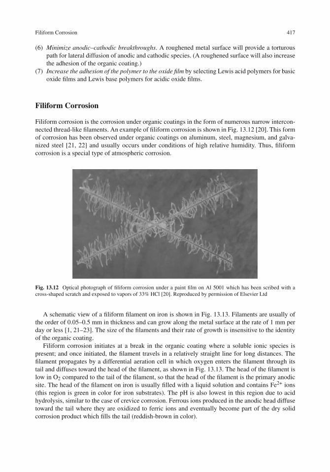
Filiform Corrosion 417
(6) Minimize anodic–cathodic breakthroughs. A roughened metal surface will provide a torturouspath for lateral diffusion of anodic and cathodic species. (A roughened surface will also increasethe adhesion of the organic coating.)
(7) Increase the adhesion of the polymer to the oxide film by selecting Lewis acid polymers for basicoxide films and Lewis base polymers for acidic oxide films.
Filiform Corrosion
Filiform corrosion is the corrosion under organic coatings in the form of numerous narrow intercon-nected thread-like filaments. An example of filiform corrosion is shown in Fig. 13.12 [20]. This formof corrosion has been observed under organic coatings on aluminum, steel, magnesium, and galva-nized steel [21, 22] and usually occurs under conditions of high relative humidity. Thus, filiformcorrosion is a special type of atmospheric corrosion.
Fig. 13.12 Optical photograph of filiform corrosion under a paint film on Al 5001 which has been scribed with across-shaped scratch and exposed to vapors of 33% HCl [20]. Reproduced by permission of Elsevier Ltd
A schematic view of a filiform filament on iron is shown in Fig. 13.13. Filaments are usually ofthe order of 0.05–0.5 mm in thickness and can grow along the metal surface at the rate of 1 mm perday or less [1, 21–23]. The size of the filaments and their rate of growth is insensitive to the identityof the organic coating.
Filiform corrosion initiates at a break in the organic coating where a soluble ionic species ispresent; and once initiated, the filament travels in a relatively straight line for long distances. Thefilament propagates by a differential aeration cell in which oxygen enters the filament through itstail and diffuses toward the head of the filament, as shown in Fig. 13.13. The head of the filament islow in O2 compared to the tail of the filament, so that the head of the filament is the primary anodicsite. The head of the filament on iron is usually filled with a liquid solution and contains Fe2+ ions(this region is green in color for iron substrates). The pH is also lowest in this region due to acidhydrolysis, similar to the case of crevice corrosion. Ferrous ions produced in the anodic head diffusetoward the tail where they are oxidized to ferric ions and eventually become part of the dry solidcorrosion product which fills the tail (reddish-brown in color).

418 13 Corrosion Under Organic Coatings
Direction ofgrowth
Fe2O3
Primary cathodic site
Primary anodicsite
Top view
Side view
Fe+2
Fe+3 Cl-
H2OOH-H+
Organic coating
O2
Fe+2
H+Cl-
H2O
OH-
Fe+3
O2
H2OO2
0.05 to0.5 mm
O2
Fig. 13.13 Schematic illustration of filiform corrosion on steel. Redrawn from Ruggeri and Beck [23]. The filamentpropagates by a differential aeration cell in which oxygen enters the filament through its tail and diffuses toward thehead of the filament. The head of the filament is low in O2 compared to the tail of the filament, so that the head of thefilament is the primary anodic site. Ferrous ions produced in the anodic head diffuse toward the tail where they areoxidized to ferric ions and precipitate as Fe(OH)3, eventually becoming Fe2O3. Reproduced by permission of NACEInternational
Ruggeri and Beck [23] showed that oxygen diffuses through the filament tail in a set ofexperiments involving filament tails:
• The growth of a filament was stopped by cutting a filament tail across its width, peeling back theorganic coating, and applying epoxy to the open portion of the tail so as to seal off its supply ofoxygen.
• In control experiments, the filament continued to grow if epoxy was only applied to the tail(without cutting) or if the tail was only cut (but not sealed with epoxy).
• A filament which had been de-activated by sealing off the supply of oxygen could be re-activatedby cutting open the tail to the atmosphere.
A characteristic of filament growth is that filaments rarely cross each other, although filamentsmay merge or divide [24]. Ruggeri and Beck [23] suggest that the reason filaments do not cross isthat a growing head would encounter a new source of oxygen if it crossed another filament. Thiswould cause changes in the positions of anodic and cathodic sites and would therefore change thedirection of growth.
A more recent and finer scale investigation on filiform corrosion has been conducted by Leblancand Frankel [25] using atomic force microscopy (for topographical measurements) and scanningKelvin probe microscopy (for maps of the Volta potential distribution). (More about the scanningKelvin probe is given later in this chapter.) This study generally supported the mechanism discussedabove but with two new interesting observations. For a 300 nm thick epoxy coating on carbon steel,in addition to the predominantly cathodic region, local microscopic cathodes were also found in the

Corrosion Tests for Organic Coatings 419
nearby periphery of the filament head, suggesting that the organic coating in the filament head isdisbonded by cathodic delamination.
In addition, Leblanc and Frankel [25] also observed voids at the edges of the tail beneath theorganic coating. The authors suggest that these voids are caused by cathodic disbondment aided bymechanical prying of the epoxy film by the voluminous solid corrosion product. Leblanc and Frankelalso suggest that such voids are involved in the filament growth process. That is, they provide fastchannels for O2 diffusion relative to transport through the solid tail and thus explain the fact thatfilaments deflect off tails without actually touching. When an active head approaches the tail ofanother filament, the advancing filament is exposed to a new source of oxygen contained in the voidand the advancing filament changes the direction. The new direction responds to the sum of the twocombined oxygen fluxes. This explanation supports the earlier ideas of Ruggeri and Beck [23] onfilament crossing.
Corrosion Tests for Organic Coatings
There are a variety of test methods and measurements which can be used to assess or study thecorrosion behavior of organic coatings [26, 27]. These methods include both accelerated standard-ized tests and experimental electrochemical measurements, but only a few methods are discussedhere.
Accelerated Tests
The salt-fog test [28] is an accelerated exposure test (not limited to coatings) in which samples areexposed to a continuous spray of salt water in an enclosed high-humidity chamber. The sample sizeis typically 4 in. × 6 in., and organic coatings (with cut edges protected) are usually scribed with alarge “X” and the performance of the coating is evaluated by its resistance to attack and de-adhesionalong the scribe marks.
Other accelerated tests include alternate immersion cycles or exposure to various conditions ofrelative humidity, temperature, and ultraviolet light in a “weatherometer” [29]. Such tests, alongwith the salt-fog test, are useful in comparing or rating various organic coating systems but yield nomechanistic information.
Cathodic Delamination
The process of disbonding at cathodic sites is illustrated schematically in Fig. 13.14. Leidheiser andco-workers [30, 31] made extensive use of cathodic delamination tests under conditions of controlledelectrode potential. In the cathodic delamination test, a small defect of the order of 1 mm diameter ispunched into an organic coating, and the coated metal specimen is immersed into an electrolytic cellcontaining an ionic solution. The specimen is held at a constant electrode potential in the cathodicregion, and replicate samples are removed at various times to determine the area of the coatingwhich has been detached during the period of immersion. Typical experimental results are shownin Fig. 13.15 for the cathodic delamination of an alkyd coating at –0.8 V vs. SCE in aerated 0.5 MNaCl. After an initial delay time, the delamination rate is constant with time over the duration of thetest.

420 13 Corrosion Under Organic Coatings
Fe+2
OH- OH-OH-OH-
O2
O2
O2H2O
H2O
H2O
O2 + 2 H2O + 4e- 4OH-
Solution
Defect
SubstrateFe
Organic coating
(High pH beneath
organic coating)
Fig. 13.14 Schematic illustration of cathodic delamination. When a defect triggers an anodic event, the cathodicreaction at other sites beneath the organic coating produces OH− ions, which cause delamination of the coating
0.0
0.1
0.2
0.3
0.4
0.5
0.6
0.7
0.8
0 20 40 60 80 100 120 140
De
lam
inat
ed A
rea
in c
m2
Time in Hours
Fig. 13.15 The cathodic delamination at –0.8 V of a 142 μm thickness alkyd coating in aerated 0.5 M NaCl [31].Reproduced by permission of Elsevier Ltd
Rates of cathodic delamination can be used to compare different coating systems because thedelamination rate is sensitive to the nature of the organic polymer, the nature of the metal substrate,and the surface pre-treatment used prior to application of the organic coating. For a given system,the rate of cathodic delamination increases as follows [32]:

Corrosion Tests for Organic Coatings 421
(1) the coating thickness decreases,(2) the temperature increases,(3) the electrode potential becomes more negative.
Delamination rates also depend on environmental factors, such as the nature of the cation in solu-tion [30–32]. Delamination rates of polybutadiene coatings on steel in solutions of 0.5 M chloridesincrease in the order
CaCl2 < LiCl < NaCl < KCl < CsCl
Leidheiser and Wang [30] have correlated this latter effect to the diffusion coefficients of thevarious 0.5 M chloride solutions, as shown in Fig. 13.16. A similar effect has been observed byStratmann et al. [33], who have suggested that delamination depends on the galvanic current betweenlocal anodes and cathodes and is possible only if cations are transferred from the cathode to theanode.
0.0
1.0
2.0
3.0
4.0
5.0
6.0
1.0 1.2 1.4 1.6 1.8 2.0
Del
am
ina
tion
Rat
e in
cm
2 /cou
lom
b
Diffusion Coefficient for 0.5 M Cl - x105 cm2/sec
CaC l2 LiCl
NaCl
K Cl
Cs Cl
Fig. 13.16 The relationship between the cathodic delamination of polybutadiene coatings in various chloride solu-tions and the diffusion coefficient of the electrolyte. Reprinted from Ref. [30] by permission of the Federation ofSocieties for Coatings Technology
The mechanism of cathodic delamination is not completely understood at the microscopic level,but it is recognized that there are three possible modes of failure. These are (i) dissolution of the oxidefilm in the local alkaline environment which is formed, (ii) degradation of the polymer in the localalkaline environment, and (iii) loss of adhesion at the organic coating/oxide-coated metal interface[34, 35]. That is, the failure can occur within the oxide, within the polymer, or at the oxide/polymerinterface, respectively.
Figure 13.17 shows five different planes along which delamination of the organic coating fromthe metal substrate can occur [1, 35]. Planes 3, 4, and 5 in Fig. 13.17 correspond to the three modesof cathodic delamination listed above.
Planes 1 and 2 in Fig. 13.17 are operative in cases of anodic undermining, which occurs whenthe major separation process is an anodic dissolution reaction occurring beneath the coating. Anodicundermining occurs beneath organic coatings on tin or aluminum [35].

422 13 Corrosion Under Organic Coatings
Organic coating
Interfacial oxide orsurface treatment
Cathodic delamination
Anodic underminingMetal substrate 1
2
3
4
5
Environment
Fig. 13.17 Planes along which undermining of an organic coating may occur. After Leidheiser [35] and reproducedby permission of NACE International
AC Impedance Techniques – A Brief Comment
Alternating current (AC) impedance techniques have become more prevalent in studying the intru-sion of water and ions into organic coatings and in comparing the performance of various organiccoatings or surface treatments. In addition, AC impedance techniques can produce models of thesolution/organic coating/metal system and thus yield mechanistic information about the protectivesystem. The theory of AC impedance techniques and their application to various problems, includingcorrosion protection by organic coatings, is discussed in Chapter 14.
Recent Directions and New Challenges
Recent work in the area of paints and organic coatings has taken two directions. One is drivenby industrial needs and the second direction is due to advanced instrumental techniques which areavailable to study the corrosion behavior of organic coatings.
Just as the search for new corrosion inhibitors has been triggered by environmental consider-ations, so too is there a similar effort regarding paint coatings [36]. Much recent work has beendirected toward reducing the volatile organic content (VOC) level of paint systems. For example,studies at the Naval Research Laboratory have shown that zero- or low-VOC variants of epoxies,polyurea, and polyurethanes have promise as protective coatings [37].
A second current active research direction involves the development of organic coating systemswhich can be applied with minimum surface preparation over partially corroded metal surfaces.It is generally recognized that the most important factor affecting the lifetime of a paint is properpreparation of the metal surface prior to application of the paint film. Ideally, paints should be appliedto bright metal surfaces and in the absence of condensed moisture. However, there is much interestin developing coating systems which are tolerant to partially corroded or contaminated surfaces. Thepresence of rust itself is not the major problem, but nests of aggressive ions (chloride or sulfate)contained in the rust near the interface promote corrosion if a paint film is applied over such anarea [38]. Adhesion between a paint coating and rust is generally good, and failure is likely tooccur within the brittle rust layer [39]. There is currently considerable research and development onchemical treatments for the removal of chloride ions from rusted surfaces and for the conversion ofsurface rust into a coherent protective layer over which additional paint coatings may be applied.
A recent experimental thrust in the study of corrosion behavior of organic coatings has madeextensive use of the scanning Kelvin probe (SKP) [25, 33, 40] (mentioned earlier in this chapter).

Problems 423
The SKP measures the work function of a sample using a vibrating condenser [40] so that portionsof the sample which have an intact organic coating display a different response than for areas wherethere is coating defect or breakthrough. By scanning across the surface, a two-dimensional map isobtained with a lateral resolution of approximately 1 μm or less. Figure 13.18 shows a scanningKelvin probe analysis of a defect on an organic coating on Al alloy 2024-T3 [41]. The specimen wasclad with a conversion coating, a primer, and a polyurethane coating. The specimen was scribed andexposed to 12 M HCl for 1 h and then to a salt fog before SKP analysis.
Anodic area
Fig. 13.18 Scanning Kelvin probe analysis of a defect on an organic coating on Al alloy 2024-T3 [41]. The specimenwas scribed and exposed to 12 M HCl and to a salt fog before SKP analysis. Reproduced by permission of NACEInternational
There has also been much recent interest in the development of smart coatings, i.e., coatingswhich can detect the presence of a breakthrough and, in response, release a corrosion inhibitor atthe required site. For example, Kendig and co-workers [42] have shown that conducting polyanilinefilms containing inhibitors for oxygen reduction are able to release the inhibitor at defects in theorganic coating. The authors state that the inhibitor is released when there is a galvanic currentbetween the conducting polymer and the bare metal surface.
In the future, improved and novel organic coatings will arise from increased environmental orperformance demands, as well as from new mechanistic information gained from the continueduse of advanced experimental techniques. It is also anticipated that the coatings field will draw onopportunities arising from the emerging areas of nanotechnology to develop a wide variety of smartorganic coatings which can sense and repair corrosion damage.
Problems
1. How is the underfilm corrosion of an organic coating similar to crevice corrosion? How do thesetwo forms of localized corrosion differ?
2. Filiform corrosion is a special type of underfilm corrosion. Would you expect the mechanismof detachment of the organic coating to be similar on a microscopic basis for both filiformcorrosion and underfilm corrosion? Explain your answer.

424 13 Corrosion Under Organic Coatings
3. When there is a linear concentration gradient across an organic coating, show that the perme-ability coefficient P is given by P = DKH, where D is the diffusion coefficient and KH is theHenry’s law constant.
4. Show that the permeability coefficient P can have the units:
P = (mol)× (cm)
(cm2)× (s)× (atm)
5. As shown in Table 13.2, a 100 μm thick polyurethane film has a water transmission rate of1.4 mg/cm2 day:
(a) Calculate the number of molecular layers of water which would be formed at the base ofthe organic coating after 1 day if all the water transmitted after 1 day accumulates there.The diameter of a water molecule is 0.30 nm.
(b) Under the conditions of part (a), compare the thickness of the water layer to the thicknessof the organic coating.
6. The transmission rate of through a 25 μm coating of polybutadiene was reported to be3.0 mg/cm2 day for water and 2.5 × 10⁻³ mg/cm2 day for oxygen (5):
(a) What is the limiting reactant for the cathodic reduction of oxygen on the underlying metalsubstrate?
(b) What corrosion current density (in μA/cm2) be sustained by these transmission rates if theunderlying substrate is aluminum and the corrosion reaction is the following?
4 Al+ 3 O2 + 6 H2O −→ 4 Al+3 + 12 OH−
7. Several investigators have measured the pH to be 14 at the front of a delaminating polymer.Leidheiser and Wang (30) conducted delamination experiments for polybutadiene on aluminumin 0.5 M NaCl solutions at an applied electrode potential of −1.35 V vs. SCE. (a) Is the oxidefilm on aluminum subject to dissolution under these conditions? Explain your answer. (b) Whatdoes your answer in part (a) mean in regard to the possible mechanism of delamination ofpolybutadiene on aluminum?
8. The transmission rate of water though a 10 μm thick coating of styrene acrylic latex is230 mg/cm2 day. What is the transmission rate of water through a 25 μm thick coating ofthe same material?
9. The oxide film on tantalum is acidic in nature. Which polymer would you expect to exhibit agreater (dry) adhesion to oxide-covered tantalum, poly (vinyl acetate) or poly (vinyl fluoride)?Explain your answer.
10. As shown in Table 13.2, polytetrafluoroethylene (PTFE) has a very low rate of water trans-mission. (a) Search the scientific literature or the Internet and list several other properties offluoropolymers which make them attractive as organic coatings. (b) What is a drawback in theuse of fluoropolymers as organic coatings?
11. (a) Would measuring the electrode potential of an underground pipeline protected by an organiccoating be useful in monitoring the integrity of the coating? Explain your answer. (b) Wouldmeasuring the polarization resistance of a section the coated pipeline be useful for the samepurpose? Explain your answer.

References 425
References
1. H. Leidheiser, Jr. in “Corrosion Mechanisms”, F. Mansfeld, Ed., p. 165, Marcel Dekker, New York (1987).2. K. B. Tator in “Corrosion and Corrosion Protection Handbook”, P. A. Schweitzer, Ed., p. 355, Marcel Dekker,
New York (1983).3. C. H. Hare in “Uhlig’s Corrosion Handbook”, 2nd edition, R. W. Revie, Ed., p. 1023, John Wiley, New York
(2000).4. J. H. W. de Wit in “Corrosion Mechanisms in Theory and Practice”, P. Marcus and J. Oudar, Eds., p. 581, Marcel
Dekker, New York (1995).5. N. L. Thomas, Prog. Org. Coat., 19, 101 (1991).6. H. Leidheiser, Jr. and M. W. Kendig, Corrosion, 32, 69 (1976).7. S. C. Dexter, “Handbook of Oceanographic Engineering Materials”, p. 38, John Wiley, New York (1979).8. H. H. Uhlig and W. R. Revie, “Corrosion and Corrosion Control”, p. 96, John Wiley, New York (1985).9. J. E. O. Mayne, Corros. Technol., 1, 286 (1954).
10. S. Guruviah, J. Oil Col. Chem. Assoc., 53, 669 (1970).11. T. Haagen and W. Funke, J. Oil Col. Chem. Assoc., 58, 359 (1975).12. N. Nguyen, E. Byrd, D. Bentz, and C. Lin, Prog. Org. Coat., 27, 181 (1996).13. L. S. Hernandez, J. M. Miranda, and G. Garcia, Corros. Prevention Control, 45 (6), 181 (1998).14. J. J. Ritter and M. J. Rodriguez, Corrosion, 38, 223 (1982).15. J. Schultz and M. Nardin in “Adhesion Promotion Techniques”, K. L. Mittal and A. Pizzi, Eds., p. 1, Marcel
Dekker, New York (1999).16. F. M. Fowkes, D. O. Tischler, J. A. Wolfe, L. A. Lannigan, C. M. Ademu-John and M. J. Halliwell, J. Polym.
Sci., Polm. Chem. Ed., 22, 547 (1984).17. E. McCafferty, J. Electrochem. Soc., 150, B342 (2003).18. W. Funke, Prog. Org. Coat., 31, 5 (1997).19. H. Leidheiser, Jr. and W. Funke, J. Oil Col. Chem. Assoc., 70 (5), 121 (1987).20. J. L. Delplancke, S. Berger, X. Lefèbvre, D. Maetens, A. Pourbaix, and N. Heymans, Prog. Org. Coat., 43, 64
(2001).21. G. M. Hoch in “Localized Corrosion”, B. F. Brown, J. Kruger, and R. W. Staehle, Eds., p. 134, NACE, Houston,
TX (1974).22. W. H. Slabaugh, W. Dejager, S. E. Hoover, and L. L. Hutchison, J. Paint Technol., 44, 76 (1972).23. R. T. Ruggeri and T. R. Beck, Corrosion, 39, 452 (1983).24. M. G. Fontana and N. D. Greene, “Corrosion Engineering”, p. 46, McGraw-Hill Book Co., New York, NY
(1978).25. P. P. Leblanc and G. S. Frankel, J. Electrochem. Soc., 151, B105 (2004).26. G. W. Walter, Corros. Sci., 26, 39 (1986).27. J. N. Murray, Prog. Org. Coat., 31, 375 (1997).28. ASTM Test B 117–97, “Standard Practice for Operating Salt Spray (Fog) Apparatus”, “1998 Annual Book of
ASTM Standards”, Volume 3.02, p. 1, ASTM, West Conshohocken, PA (1998).29. ASTM Active Standard G 154–06, “Standard Practice for Operating Fluorescent Light Apparatus for UV
Exposure of Nonmetallic Materials”, ASTM, West Conshohocken, PA (2006).30. H. Leidheiser, Jr. and W. Wang, J. Coatings Technol., 53 (672), 77 (1981).31. H. Leidheiser, Jr., W. Wang, and L. Igetoft, Prog. Org. Coat., 11, 19 (1983).32. U. Steinsmo and J. I. Skar, Corrosion, 50, 934 (1994).33. M. Stratmann, A. Leng, W. Fürbeth, H. Streckel, H. Gehmecker, and K.-H. Grosse-Brinkhaus, Prog. Org. Coat.,
27, 261 (1996).34. J. F. Watts. J. Adhesion, 31, 73 (1989).35. H. Leidheiser, Jr., Corrosion, 38, 374 (1982).36. “Environmentally Acceptable Inhibitors and Coatings”, S. R. Taylor, H. S. Isaacs, and E. W. Broomen, Eds., The
Electrochemical society, Pennington, NJ (1997).37. M. V. Veazey, Mater. Perfor., 42 (10), 22 (2003).38. N. L. Thomas, J. Oil Col. Chem. Assoc., 74(3) 83 (1991).39. N. L. Thomas, J. Prot. Coat. Linings, 6 (12) 63 (1989).40. G. Grundmeier, W. Schmidt, and M. Stratmann, Electrochim. Acta, 45, 2515 (2000).41. D.C. Hansen, G.E. Grecsek and R.O. Roberts, “A Scanning Kelvin Probe Analysis of Aluminum and Aluminum
Alloys”, paper presented at NACE International 54th Annual Conference & Exposition, San Antonio, TX, April25–30, 1999.
42. M. W. Kendig, M. Hon, and L. Warren, Prog. Org. Coat., 47, 183 (2003).

Chapter 14AC Impedance
Introduction
The electrochemical techniques which have been considered so far in this text have been direct cur-rent techniques. This chapter describes a powerful technique [1, 2] which uses alternating current(AC). AC impedance techniques are not new, but prior to about 1980, AC measurements were gen-erally made with a Schering bridge which requires manual balancing to null the bridge in orderto measure the equivalent parallel resistance and capacitance. This method is tedious and time-consuming. With the advent of improved instrumentation under computer control and acquisition,AC impedance techniques have become an important method of making electrochemical measure-ments. AC impedance has been used to study the metal/solution interface, oxide films and surfacetreatments, and the corrosion behavior of organic coatings on metals. Each of these three applicationsis considered in this chapter.
In essence, the method consists of superimposing a small (10–20 mV) AC signal on the electro-chemical system of interest and measuring the response of the system to this perturbation. Whenan electrochemical system is perturbed by an applied AC signal, the system relaxes to a new steadystate; and the time τ required for this relation is known as the time constant. Sometimes τ is calledthe relaxation time by analogy to the process by which dipoles orient and relax in response to analternating field [3, 4].
Relaxation Processes
Suppose that a liquid contains polar molecules which possess permanent dipoles, such as watermolecules. In the absence of an external field, individual dipoles are oriented randomly in all direc-tions, as shown in Fig. 14.1(a). However, in the presence of an alternating field, the dipoles will tendto orient themselves in the direction of the applied electric field, as illustrated in Fig. 14.1(b) and(c). With an alternating field, these water molecules must therefore turn back and forth in responseto the changing direction of the electric field. The rotation of these dipoles, however, cannot respondperfectly to the electric field. This delayed response of a system to a change in external force istermed relaxation. Even if there are no permanent dipoles in the material, the presence of an electricfield can induce a dipole, which then can respond to the alternating field and display a relaxationeffect.
The AC impedance technique is also called electrochemical impedance spectroscopy (EIS). Thisis by analogy to conventional spectroscopy, in which the system displays a response at a character-istic frequency to an applied perturbation. In EIS, as will be seen later, plots of the imaginary part of
427E. McCafferty, Introduction to Corrosion Science, DOI 10.1007/978-1-4419-0455-3_14,C© Springer Science+Business Media, LLC 2010

428 14 AC Impedance
Electric field
+-
+-
+- +-
+-
+-+-
+-
+-+- +-
+-
+-
+
++
+
++
-
--
-
--
Electric field
+ -
+ -
+ - + -
+ -
+ -+ -
+ -
+ -+ - + -
+ -
+ -
-
--
-
--
+
++
+
++
+ -
+- + -
+-
+ -
+-
+ -
+-
+ -
+- +-
+ -
+-
(a)
(b)
(c)
+-
+-
+- +-
+-
+-+-
+-
+-+- +-
+-
+-
+
++
+
++
-
--
-
--
Electric field
+ -
+ -
+ - + -
+ -
+ -+ -
+ -
+ -+ - + -
+ -
+ -
-
--
-
--
+
++
+
++
+ -
+- + -
+-
+ -
+-
+ -
+-
+ -
+- +-
+ -
+-
+-
+-
+- +-
+-
+-+-
+-
+-+- +-
+-
+-
+
++
+
++
-
--
-
--
+-
+-
+- +-
+-
+-+-
+-
+-+- +-
+-
+-
+
++
+
++
-
--
-
--
+- +-
+- +-
+- +- +- +-
+- +-
+- +-+- +-
+- +-
+- +-+- +- +- +-
+- +-
+- +-
+
+++
++
+
+++
++
-
---
--
-
---
--
+ -
+ -
+ - + -
+ -
+ -+ -
+ -
+ -+ - + -
+ -
+ -
-
--
-
--
+
++
+
++
+ -+ -
+ -+ -
+ -+ - + -+ -
+ -+ -
+ -+ -+ -+ -
+ -+ -
+ -+ -+ -+ - + -+ -
+ -+ -
+ -+ -
-
---
--
-
---
--
+
+++
++
+
+++
++
+ -
+- + -
+-
+ -
+-
+ -
+-
+ -
+- +-
+ -
+-
+ -+ -
+-
+- + -+ -
+- +-
+ -+ -
+- +-
+ -+ -
+- +-
+ -+ -
+-
+- +- +-
+ -+ -
+- +-
Fig. 14.1 (a) Random orientation of dipoles in the absence of an electric field. (b) and (c) Alignment of dipoles withthe direction of an electric field
the impedance vs. the logarithm of the frequency produce a peak, analogous to usual observations inother types of spectroscopy .
Some types of spectroscopy and the characteristic frequencies involved are listed in Table 14.1.
Table 14.1 Several types of relaxation processes [5]
Type of relaxation Frequency (Hz) Portion of spectrum
Electronic transitions 1014–1016 Visible and ultravioletVibrations of flexible bonds 1013–1014 InfraredRotation of small molecules 1011–1013 Far infraredRotation of polyatomic molecules 109–1011 MicrowaveRotation of dipoles
Liquid H2O at 25◦C [3, p. 128] 1010 MicrowaveIce at 0◦C [6] 103 RadiofrequenciesPhysically adsorbed H2O
on α-Fe2O3 at 25◦C [4]10–104 Radiofrequencies
Electrochemical interfaces 10–2–105 Radiofrequencies

Introduction 429
In electrochemical systems, the relaxation time (in seconds) is given by
τ = RC (1)
where R is the resistance (in ohms) and C is the capacitance (in farads) of the system. The impedanceis the resistance to the flow of an AC current:
Z = E
I(2)
Both resistors and capacitors possess an impedance, as will be seen shortly.
Example 14.1: Show that the product RC has the units of seconds.
Solution:
RC = ohms× coulombs
voltsor
RC = ohms× (amps) (seconds)
voltsThen use E = IR, or
volts = (amps) (ohms)
so that
amps
volts= 1
ohms
Use this in the expression above for RC to get
RC = ohms × 1
ohms× seconds
or
RC = seconds
Experimental Setup
A block diagram of the experimental setup is shown in Fig. 14.2. The apparatus consists of anelectrochemical cell, frequency generator, a frequency response analyzer (FRA), and a computer tocontrol the experiment and to store the data. The electrode potential is controlled as usual with apotentiostat. The heart of the system is the FRA, which can measure the real and imaginary parts ofthe complex impedance. (The concept of a complex impedance is addressed below.) AC impedancemeasurements are usually made in the frequency range of 0.01–100,000 Hz (cycles/s), although thisrange can be extended. More detail on the experimental aspects of AC impedance techniques is givenelsewhere [7, 8].

430 14 AC Impedance
Potentiostat
Computer
Monitor
Printer
Frequency Generatorand
Frequency Response Analyzer
Sample
Fig. 14.2 A simple block diagram for the measurement of AC impedance by application of a sine wave and the useof a frequency response analyzer
Complex Numbers and AC Circuit Analysis
The analysis of AC electrical circuits utilizes complex numbers so it is useful to review some of theirbasic properties. A complex number z consists of an ordered pair of numbers, a and b, which arerelated by
z = a+ j b (3)
where j = √−1 (and is used here to avoid confusion with the current density i). The number ais called the real part of the complex number z and b is called the imaginary part (although both aand b themselves are real numbers). A complex number can be represented in the complex plane, asshown in Fig. 14.3. The absolute value of the complex number |z| is given by its distance from theorigin in the complex plane. Thus
xReal axis
Imaginaryaxis
y
|z|z = a + j b
a
b
|z| = a2 +b2
Fig. 14.3 Geometrical representation of a complex number

The Metal/Solution Interface 431
|z| = (a2 + b2)1/2 (4)
The absolute value |z| is sometimes called the modulus of z.A useful identity in complex variables is Euler’s equation:
ejx = cos x+ j sin x (5)
and it is this equation which introduces complex variables into AC circuit analysis. The alternatingvoltage of an AC signal can be represented by a cosine (or sine) wave. We can write
E = E0 ejωt (6)
where E0 is the amplitude of the voltage, t is the time, and ω = 2π f is the angular frequency, with fthe frequency of the AC signal. Then from Eq. (5),
E = E0 ( cos ωt + j sin ωt) (7)
It is understood that to get the actual voltage, it is necessary to take the real part of Eq. (7):
E = Re {E0( cos ωt + j sin ωt) = E0( cos ωt) (8)
Similarly, the current may also have a complex form:
I = I0 ejω(t−s) (9)
where δ is the phase angle. Because both the voltage and current can be written as complex numbers,it follows that the impedance Z given by
Z(ω) = E(ω,t)
I(ω,t)(10)
may also be a complex number. The impedance of a resistor R is simply the resistance itself:
ZR = R (11)
but the impedance of a capacitor is an imaginary number:
ZC = 1
j ω C(12)
where C is the value of the capacitance. Equation (12) is not obvious, so that its origin is given inAppendix L. Impedances in series or parallel follow the same rules as for resistances.
The Metal/Solution Interface
In Chapter 3 (Fig. 3.14), we discussed an equivalent circuit model for the metal/solution interface.This equivalent circuit, shown again in Fig. 14.4, contains a double-layer capacitance Cdl in parallel
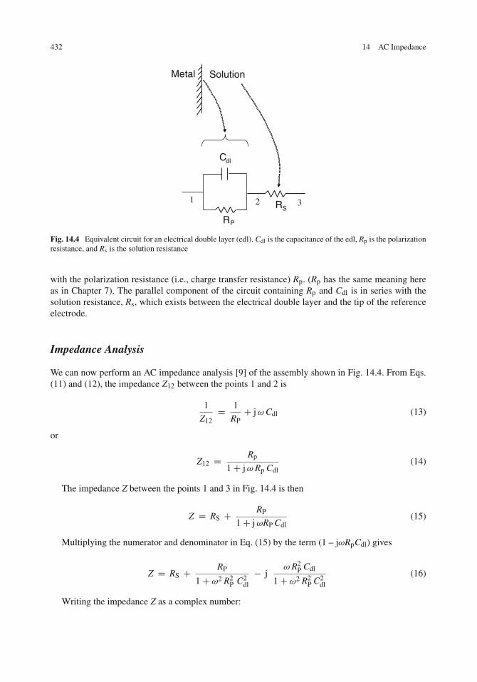
432 14 AC Impedance
Metal Solution
Cdl
RP
RS1 2 3
Fig. 14.4 Equivalent circuit for an electrical double layer (edl). Cdl is the capacitance of the edl, Rp is the polarizationresistance, and Rs is the solution resistance
with the polarization resistance (i.e., charge transfer resistance) Rp. (Rp has the same meaning hereas in Chapter 7). The parallel component of the circuit containing Rp and Cdl is in series with thesolution resistance, Rs, which exists between the electrical double layer and the tip of the referenceelectrode.
Impedance Analysis
We can now perform an AC impedance analysis [9] of the assembly shown in Fig. 14.4. From Eqs.(11) and (12), the impedance Z12 between the points 1 and 2 is
1
Z12= 1
RP+ j ω Cdl (13)
or
Z12 = Rp
1+ j ω Rp Cdl(14)
The impedance Z between the points 1 and 3 in Fig. 14.4 is then
Z = RS + RP
1+ j ωRP Cdl(15)
Multiplying the numerator and denominator in Eq. (15) by the term (1 – jωRpCdl) gives
Z = RS + RP
1+ ω2 R2P C2
dl
− jω R2
P Cdl
1+ ω2 R2P C2
dl
(16)
Writing the impedance Z as a complex number:

The Metal/Solution Interface 433
Z = Z′ + j Z′′ (17)
gives the real (Z ′) and imaginary (Z ′′) parts of the impedance to be
Z′ = RS + RP
1+ ω2 R2P C2
dl
(18)
and
Z′′ = − ω R2P Cdl
1+ ω2 R2p C2
dl
(19)
These last two equations can be combined by the elimination of ω. The result (after a littlealgebra) is
[Z′ −
(RS + RP
2
)]2
+ (Z′′)2 =(
RP
2
)2
(20)
Equation (20) is the equation of a semi-circle centered at (Rs + (Rp/2), 0), as shown in Fig. 14.5.The semi-circle intersects the Z ′-axis at the values Rs and (Rs + Rp). The value of ω at the apex ofthe semi-circle is given by
ωmax = 1
RP Cdl(21)
Imag
inar
y, -
Z”
Real, Z ’
RS RS + RP
RP2
RPCdl
1ωmax =
RSRP2
+
’
22
= =
2+
22+
Fig. 14.5 Schematic diagram of complex-plane plot of the imaginary part of the impedance, Z ′′, vs. the real part ofthe impedance, Z ′
The result in Eq. (21) follows from taking dZ ′′/dω = 0. See Problem 14.1. Then Cdl can bedetermined from Eq. (21) once Rp is known.
Thus, all three unknown quantities Rp, Rs, and Cdl can be determined from Fig. 14.5. Plots suchas Fig. 14.5 are referred to by various workers as complex-plane plots, Argand diagrams, Nyquistplots, or Cole–Cole plots.
If the value of Rp is known, then the value of Cdl can also be determined from a linear plot of Z ′vs. Z ′′/ω. The relationship is

434 14 AC Impedance
Z′ = Rs − Z ′′
ω RP Cdl(22)
The slope of the plot is –1/(RpCdl) and the intercept is Rs. The origin of Eq. (22) is left as anexercise in Problem 14.2.
Additional Methods of Plotting Impedance Data
One of the disadvantages of the semi-circular plots in Fig. 14.5 is that the frequency dependence ofthe impedance does not appear on the diagram. In addition, the points are often distributed unevenlyalong the arc of the semi-circle. Finally, the maximum value of Z ′′ on the semi-circle and its corre-sponding frequency (used to obtain Cdl) may not actually correspond to a data point. These problemsare illustrated in Fig. 14.6, which is the complex-plane plot for an interface for which Rp = 1,000 �,Rs = 100 �, and Cdl = 10 μF/cm2.
–1200
–1000
–800
–600
–400
–200
00 200 400 600 800 1000 1200
Im
agin
ary,
- Z
", in
ohm
- cm
2
Real, Z', in ohm-cm2
Cdl
R s
R p
f = 10
ωmax = 1/(RP Cdl)
2030
50
100f = 1.0 X 10⁵
7
5
1
0.01
Fig. 14.6 Calculated complex-plane plot for the equivalent circuit shown in Fig. 14.4 with Rp = 1,000 �, Rs = 100�, and Cdl = 10 μF/cm2 (frequencies in hertz are indicated on the figure)
(It should be noted that when C is expressed as a capacitance per unit area, i.e., as F/cm2, thenvalues of resistances and impedances are actually in �-cm2 rather than in ohms. See Problems 14.3and 14.4.)
An alternate method of displaying impedance data is a Bode plot, in which log |Z| is plotted vs.log ω. The absolute value of the impedance Z follows from Eq. (4) as
|Z| = (Z′2 + Z′′2)12 (23)
Equations (18), (19), and (23) combine to give

The Metal/Solution Interface 435
10
100
1000
10–2 10–1 100 101 101 103 104 105 106
|Z| i
n oh
m-c
m2
Angular Frequency, 2πf
Rs+Rp
Rs
Fig. 14.7 Calculated Bode plot corresponding to the complex-plane plot in Fig. 14.6
|Z | =
⎧⎪⎨⎪⎩(
RS + RP
1+ ω2 R2P C2
dl
)2
+(
ω R2P Cdl
1+ ω2 R2P C2
dl
)2⎫⎬⎭
1/2
(24)
The Bode plot corresponding to the complex-plane plot in Fig. 14.6 is given in Fig. 14.7.Resistances appear as horizontal lines in a Bode plot, and capacitances appear as slanted lines. Itcan be seen from Eq. (24) that for small values of ω
|Z| → (RS + RP) as ω→ 0 (25)
For large values of ω
|Z| → RS as ω→∞ (26)
To see this last result it is necessary to use L’Hospital’s rule on Eq. (24). See Appendix M. Theportion of the curve where the impedance is due largely to the capacitance Cdl has a slope equal to–1. See Problem 14.5.
Other methods of plotting impedance data include graphs of Z ′ or Z ′′ vs. ω, as shown inFig. 14.8 for the equivalent circuit shown in Fig. 14.4. In addition, the phase angle δ can be plottedversus ω, where the phase angle δ is given by
tan δ = Z′′
Z′(27)
The most useful plot, however, has generally proven to be the Bode plot, and applicationsinvolving Bode plots are given in this chapter.

436 14 AC Impedance
–400
0
400
800
1200
10 –2 10–1 100 101 102 103 104 105 106
Real, Z'
Angular Frequency, 2 πf
Imaginary, Z"
Rs + Rp
Rs
–1/(Rp Cdl)
Fig. 14.8 Real and imaginary components of the complex impedance corresponding to the complex-plane plot inFig. 14.6 and the Bode plot in Fig. 14.7
RS RS + RP1 RS + RP1 + RP2
ω
Imag
inar
y, -
Z ”
Real, Z’
Fig. 14.9 Schematic diagram of a complex-plane plot for a system having two time constants
Multiple Time Constants and the Effect of Diffusion
An electrochemical system may contain more than one relaxation process and thus may have morethan a single time constant. In such a case, the complex-plane plot will display more than onesemi-circle, as shown schematically in Fig. 14.9 for the case of two time constants. (The Bodeplot corresponding to Fig. 14.9 will contain three plateaus).
In addition, an electrochemical system may contain a component which is under diffusion control,for which [8]
Z = σ
ω1/2− j σ
ω1/2(28)
where σ is the conductivity. The effect of diffusion appears at low frequencies in the complex-plane plot as a straight line 45◦ to the real axis, as shown schematically in Fig. 14.10. The effect of
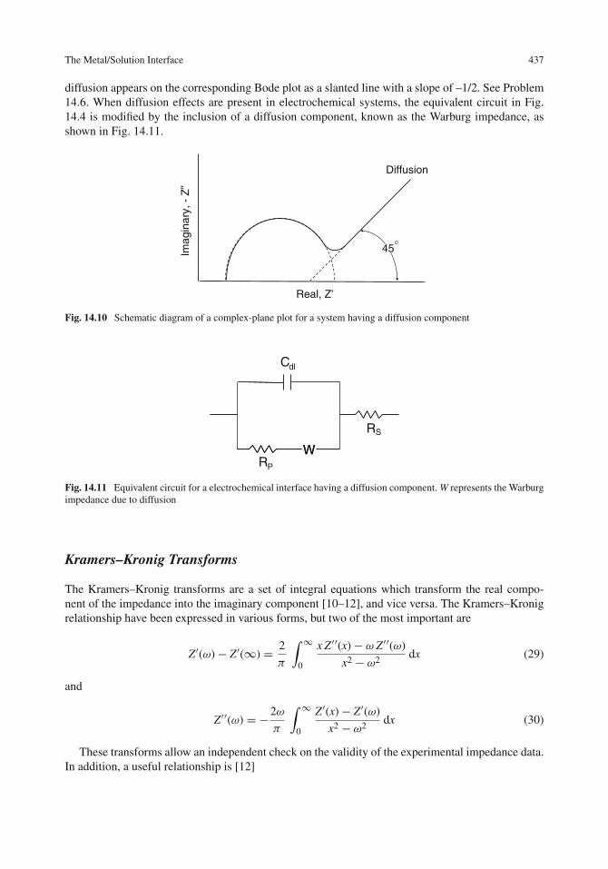
The Metal/Solution Interface 437
diffusion appears on the corresponding Bode plot as a slanted line with a slope of –1/2. See Problem14.6. When diffusion effects are present in electrochemical systems, the equivalent circuit in Fig.14.4 is modified by the inclusion of a diffusion component, known as the Warburg impedance, asshown in Fig. 14.11.
Imag
inar
y, -
Z”
Real, Z’
Diffusion
45°
Fig. 14.10 Schematic diagram of a complex-plane plot for a system having a diffusion component
Cdl
RP
RS
WW
Fig. 14.11 Equivalent circuit for a electrochemical interface having a diffusion component. W represents the Warburgimpedance due to diffusion
Kramers–Kronig Transforms
The Kramers–Kronig transforms are a set of integral equations which transform the real compo-nent of the impedance into the imaginary component [10–12], and vice versa. The Kramers–Kronigrelationship have been expressed in various forms, but two of the most important are
Z′(ω)− Z′(∞) = 2
π
∫ ∞0
x Z′′(x)− ω Z′′(ω)
x2 − ω2dx (29)
and
Z′′(ω) = −2ω
π
∫ ∞0
Z′(x)− Z′(ω)
x2 − ω2dx (30)
These transforms allow an independent check on the validity of the experimental impedance data.In addition, a useful relationship is [12]
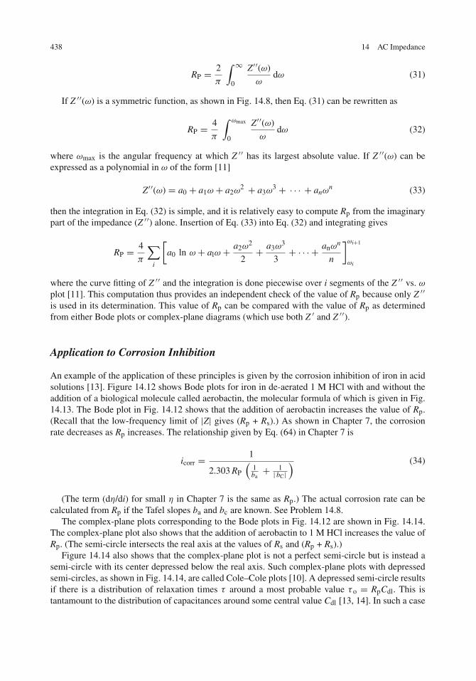
438 14 AC Impedance
RP = 2
π
∫ ∞0
Z′′(ω)
ωdω (31)
If Z ′′(ω) is a symmetric function, as shown in Fig. 14.8, then Eq. (31) can be rewritten as
RP = 4
π
∫ ωmax
0
Z′′(ω)
ωdω (32)
where ωmax is the angular frequency at which Z ′′ has its largest absolute value. If Z ′′(ω) can beexpressed as a polynomial in ω of the form [11]
Z′′(ω) = a0 + a1ω + a2ω2 + a3ω
3 + · · · + anωn (33)
then the integration in Eq. (32) is simple, and it is relatively easy to compute Rp from the imaginarypart of the impedance (Z ′′) alone. Insertion of Eq. (33) into Eq. (32) and integrating gives
RP = 4
π
∑i
[a0 ln ω + alω + a2ω
2
2+ a3ω
3
3+ · · · + anω
n
n
]ωi+1
ωi
where the curve fitting of Z ′′ and the integration is done piecewise over i segments of the Z ′′ vs. ω
plot [11]. This computation thus provides an independent check of the value of Rp because only Z ′′is used in its determination. This value of Rp can be compared with the value of Rp as determinedfrom either Bode plots or complex-plane diagrams (which use both Z ′ and Z ′′).
Application to Corrosion Inhibition
An example of the application of these principles is given by the corrosion inhibition of iron in acidsolutions [13]. Figure 14.12 shows Bode plots for iron in de-aerated 1 M HCl with and without theaddition of a biological molecule called aerobactin, the molecular formula of which is given in Fig.14.13. The Bode plot in Fig. 14.12 shows that the addition of aerobactin increases the value of Rp.(Recall that the low-frequency limit of |Z| gives (Rp + Rs).) As shown in Chapter 7, the corrosionrate decreases as Rp increases. The relationship given by Eq. (64) in Chapter 7 is
icorr = 1
2.303 RP
(1ba+ 1| bC|
) (34)
(The term (dη/di) for small η in Chapter 7 is the same as Rp.) The actual corrosion rate can becalculated from Rp if the Tafel slopes ba and bc are known. See Problem 14.8.
The complex-plane plots corresponding to the Bode plots in Fig. 14.12 are shown in Fig. 14.14.The complex-plane plot also shows that the addition of aerobactin to 1 M HCl increases the value ofRp. (The semi-circle intersects the real axis at the values of Rs and (Rp + Rs).)
Figure 14.14 also shows that the complex-plane plot is not a perfect semi-circle but is instead asemi-circle with its center depressed below the real axis. Such complex-plane plots with depressedsemi-circles, as shown in Fig. 14.14, are called Cole–Cole plots [10]. A depressed semi-circle resultsif there is a distribution of relaxation times τ around a most probable value τ o = RpCdl. This istantamount to the distribution of capacitances around some central value Cdl [13, 14]. In such a case

The Metal/Solution Interface 439
0.1
1
10
100
1000
1000001000010001001010 0.10.01
|Z| i
n oh
ms
Frequency in c/s
3 x 10⁻³ M/l aerobactin
Uninhibited
Iron in 1 M HCl
Fig. 14.12 Experimental Bode plots for iron in de-aerated 1 M HCl with and without the inhibitor aerobactin [13].Sample area = 5.0 cm2. Reproduced by permission of ECS – The Electrochemical Society
CH N
(CH2)4
N OH
C O
HOOC H
C
O
CH C
COOH
OH
CH
C HN
(CH )4
NHO
CO
H
C
O
CH
COOH
CH N
HOOC H
C CH2 C
OH
CH3
C HN
(CH )4
NHO
CO
H
C
O
CH
COOH
CHCHCH3CH
C HN
(CH )4
N
CO
H
C
O
CH
COOH
C HN
2)
H
CCH2
COOH
Fig. 14.13 Molecular formula for the inhibitor aerobactin [13]
Eq. (15) is replaced by [10]:
Z = RS + RP
1+ (j ω RP Cdl)l−α(35)
where α is a measure of the departure from ideality. The parameter α ranges from 0 to 1 and is zerofor ideal behavior. The capacitance Cdl and the parameter α can be determined from the various arcchords U and V shown in Fig. 14.15. By calculating the ratio |V/U| for each frequency, we obtain[4, 10, 13]:
log
∣∣∣∣ V
U
∣∣∣∣ = (α − 1) log (2π f )+ (α − 1) log (Cdl RP) (36)
The derivation of Eq. (36) is given in Appendix N. The value of Cdl follows from Eq. (36) and isgiven by

440 14 AC Impedance
–200
–150
–100
–50
0400300 350200150100500 250
Real, Z', in ohms
Imag
inar
y, Z
", in
ohm
s
Uninhibited
iron
3 x 10⁻³ M/l
aerobactin
Iron in 1 M HCl
Fig. 14.14 Experimental complex-plane plot for iron in de-aerated 1 M HCl with and without the inhibitor aerobactin[13]. Sample area = 5.0 cm2. Reproduced by permission of ECS – The Electrochemical Society
Ideal (semicircle)
Depressed semicircle(Cole-Cole)
*z*
VU
Imag
inar
y, Z
”
VU
RS RS + RP Real, Z’
Fig. 14.15 Schematic complex-plane diagram for the impedance showing arc chords U and V for a given frequency[13]. The notation z∗ indicates that z is a complex number. Reproduced by permission of ECS – The ElectrochemicalSociety
Cdl = 10I/S
RP(37)
where I and S are the intercept and slope, respectively, of the plot of log |V/U| vs. log ω.Figure 14.16 shows the plot of Eq. (36) for iron in 1 M HCl containing 3 × 10⁻³ M aerobactin.
The calculated value of Cdl was 56 μF/cm2, and the value for uninhibited iron was 89 μF/cm2, sothat the double-layer capacitance decreased with adsorption of the inhibitor, as has been discussedin Chapter 12. The slope of the plot in Fig. 14.16 is (α–1) = –0.86, or α = 0.14.
In addition, polarization resistances were determined from Kramer–Kronig relations in Eqs.(31) and (34) for iron in 1 M HCl in the presence of various biological molecules. As shown inTable 14.2, there is good agreement between Rp values determined using the Kramers–Kronigrelation and Rp values determined from Bode plots or complex-plane plots.

Organic Coatings 441
–4
–3
–2
–1
0
0 1 2 3 4 5
1
Log Angular Frequency, 2 πf
log
|V/U
|
3 x 10⁻³ M/l aerobactin
R = 0.99989
Iron in 1 M HCl
Slope = (α − 1)
Intercept = (α − 1) log(CdlRp)
Fig. 14.16 A typical experimental arc chord plot used to determine the capacitance of the electrical double layer [13].Reproduced by permission of ECS – The Electrochemical Society
Table 14.2 Polarization resistance (Rp) values determined by three different methods for iron in 1 M HCl with andwithout the addition of various biological molecules [13]
Rp in �cm2
Kramers–Kronig Bode plot Complex-plane plot
Uninhibited 20.4 20.3 20.4Aerobactin
3.0 × 10⁻³ M71.5 73.5 74.4
Rhodotorulic acid1.2 × 10–3 M
75.5 71.6 71.4
Enterobactin3.1 × 10–4 M
113 104 107
Parabactin1.4 × 10–4 M
476 449 466
Organic Coatings
One of the most powerful applications of AC impedance techniques has been to assess the durabilityof organic coatings in aqueous media [1, 2, 15–17]. In this regard, AC impedance techniques havebeen used in two ways:
(1) to monitor the ingress of water (or ions) into the organic coating and(2) to develop an equivalent circuit for the coating/substrate system and to relate the corrosion
behavior to the properties of the elements of the equivalent circuit.
Kendig and Leidheiser [18] were among the earliest to use AC measurements to follow the changein capacitance and resistance of a coated metal in an aqueous solution (0.5 M NaCl). As time pro-gressed, the capacitance of a polybutadiene coating increased and the resistance decreased due to
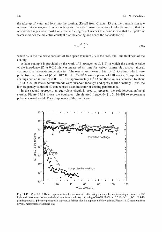
442 14 AC Impedance
the take-up of water and ions into the coating. (Recall from Chapter 13 that the transmission rateof water into an organic film is much greater than the transmission rate of chloride ions, so that theobserved changes were most likely due to the ingress of water.) The basic idea is that the uptake ofwater modifies the dielectric constant ε of the coating and hence the capacitance C:
C = ε0 ε A
l(38)
where εo is the dielectric constant of free space (vacuum), A is the area, and l the thickness of thecoating.
A later example is provided by the work of Bierwagen et al. [19] in which the absolute valueof the impedance |Z| at 0.012 Hz was measured vs. time for various primer plus topcoat aircraftcoatings in an alternate immersion test. The results are shown in Fig. 14.17. Coatings which wereprotective had values of |Z| at 0.012 Hz of 108–109 � over a period of 110 weeks. Non-protectivecoatings had an initial |Z| at 0.012 Hz of approximately 106 � and these values decreased to about103 � in 20–40 weeks. Similar trends were observed for alkyd and epoxy marine coatings. Thus, thelow-frequency values of |Z| can be used as an indicator of coating performance.
In the second approach, an equivalent circuit is used to represent the solution/coating/metalsystem. Figure 14.18 shows the equivalent circuit used frequently [1, 2, 16–19] to represent apolymer-coated metal. The components of the circuit are:
109
1010
107
108
Protective coatings
106
104
105
|Z|
at 0
.012
c/s
in O
hms
102
103
Non-protective coatings
100 20 40 60 80 100 120
Time in Weeks
Fig. 14.17 |Z| at 0.012 Hz vs. exposure time for various aircraft coatings in a cyclic test involving exposure to UVlight and alternate exposure and withdrawal from a salt fog consisting of 0.05% NaCl and 0.35% (NH4)2SO4. � Self-priming topcoat, � Primer plus glossy topcoat, � Primer plus flat topcoat • Yellow primer. Figure 14.17 redrawn from[19] by permission of Elsevier Ltd

Organic Coatings 443
Organic coating
Metal Solution
Cc
Cdl
RS
RP
Rcp
Fig. 14.18 Equivalent circuit for an organic coating on a metal substrate [1]. Rp is the polarization resistance at themetal/solution interface and Cdl is the capacitance of the electrical double layer at the metal solution interface. Rcp isthe pore resistance of the coating and Cc the capacitance of the coating. Rs is the solution resistance.
Cc = coating capacitanceCdl = double-layer capacitance at the metal/solution interfaceRp = polarization resistance at the metal/solution interfaceRcp = pore resistance of the coatingRs = solution resistance
The pore resistance of the coating Rcp is of particular interest because it contains informationregarding degradation of the protective properties of the coating.
By combining the impedances of the components of the equivalent circuit, the real and imaginaryparts of the impedance are seen to be (after considerable algebra):
Z′ = RS + RP + Rcp + ω2 (RP Cdl)2 Rcp(
1− ω2RPCdlRcpCc)2 + ω2
(RpCdl + RP Cc + RcpCc
)2 (39)
and:
Z′′ = −ω[R2
P Cdl
(1+ ω2 R2
cp Cdl Cc
)+ Cc
(Rp + Rcp
)2](1− ω2 Rp Cdl Rcp Cc
)2 + ω2(Rp Cdl + Rp Cc + Rcp Cc
)2 (40)
The absolute value of the impedance |Z| then follows from inserting Eqs. (39) and (40) into Eq.(23). It can be seen that as ω ⇒ 0, |Z| ⇒ Rs + Rp + Rcp. As ω⇒ ∞, |Z| ⇒ Rs. The latter resultrequires successive use of L’Hospital’s rule.

444 14 AC Impedance
Rp Rcp Cdl C C
10 8 10 4 25x10 –11 10x10 –10
107
109 . .
10 6 10 3 2.5 x 10 –9 1.0 x 10 –10
10 4 10 2 2.5 x 10⁻⁵ 1.0 x 10 –9
105
103R
Rp + Rcp + Rs
Rcp + Rs
Cdl
101
RP
Increasingdegradation
10–1
103
101
101
103
105 107 10
910
11
CC
– –
Angular Frequency, 2
|Z| i
n oh
m-c
m2
Rs
Rcp
Rs
Cdl
CC
Fig. 14.19 Calculated Bode plots for the equivalent circuit in Fig. 14.18 for various input parameters. R is in � andC in F/cm2
A typical Bode plot for an organic coating can be constructed by evaluating Z ′ and Z ′′ for rep-resentative values of the components of the equivalent circuit. If the organic coating has undergonelittle degradation, we can take Rp = 108 �, Rcp = 104 �, and Cdl = 2.5 × 10⁻¹¹ F/cm2 [1]. We canestimate Cc as in Example 14.2.
Example 14.2: What is the capacitance of a 35-μm thick organic coating having a dielectric constantof 4.0? (This example is taken from Mansfeld [1]).
Solution: The organic coating is considered to be a parallel plate capacitor, for which the capacitanceis given by
C = ε0 ε A
1
where ε0 is the dielectric constant of free space (8.85 × 10⁻¹⁴ F/cm), A the area, and l the thicknessof the coating. Thus,
C
A=(8.85× 10⁻¹⁴F cm−1
)(4.0)(
35× 10−6 m) (
100 cmm
) = 1.0× 10⁻¹⁰ F/cm2
Then, we can use Cc = 1.0 × 10⁻¹⁰ F/cm2 and Rs = 1 � along with the values of the othercomponents of the equivalent circuit to calculate Z ′, Z ′′, and |Z| from Eqs. (39), (40), and (23).These calculations produce the Bode plot in Fig. 14.19 (topmost curve).

Organic Coatings 445
If there is significant delamination of the coating and concomitant electrochemical activitybeneath the organic coating, then Rp decreases and Cdl increases. The pore resistance of the coatingRcp also decreases. In addition Cc increases due to absorption of water which causes an increasein the effective dielectric constant of the organic coating. Figure 14.19 also shows the calculatedBode plot for the following set of parameters: Rp = 104 �, Rcp = 102 �, Cc = 1.0 × 10⁻⁹ F/cm2,Cdl = 2.5 × 10⁻⁵ F/cm2, and Rs = 1 � (lowermost curve). The effect of coating degradation is toshift the Bode plot downward (and also to reveal more features in the plot). The Bode plot for anintermediate set of equivalent circuit parameters is also given in Fig. 14.19 (middle curve).
The low-frequency portion of Bode plots can be used to rate or compare the corrosion behaviorof various organic coatings because the low-frequency limit contains the values (Rcp + Rp) whichreflect the properties of the coating (Rcp) and of the polarization resistance (Rp). Actually, the lowfrequency limit also contains the value of the solution resistance, Rs, but this is constant for a giventest solution and is also much less than (Rcp + Rp).
Figure 14.20 shows experimentally determined Bode plots [20] for three different epoxy coatingsafter 9 days immersion in an electrolyte used in atmospheric corrosion studies (8.5 mM (NH4)2SO4plus 26 mM NaCl). The Bode plots show that the electrocoat epoxy has the best corrosion resistanceof the three coatings after the 9-day immersion period. The Bode plots in Fig. 14.20 also have thesame general shapes shown in Fig. 14.19.
108
109
Electro-coat
107
105
106 Water borne
10
104
Solvent borne
102
103
10–3
10–2
10–1
100
101
102
103
104
105
Log Frequency
Impe
danc
e |Z
|
Fig. 14.20 Experimental Bode plots for three different epoxy coatings immersed 9 days in a solution containing8.5 mM (NH4)2SO4 and 26 mM NaCl. Redrawn from [20] with the permission of the American Chemical Society
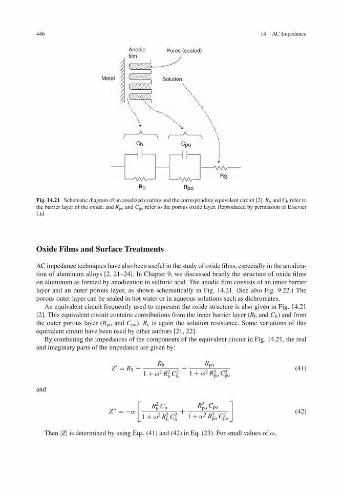
446 14 AC Impedance
Pores (sealed)Anodicfilm
Metal Solution
Cb Cpo
R
RS
RRb Rpo
Fig. 14.21 Schematic diagram of an anodized coating and the corresponding equivalent circuit [2]. Rb and Cb refer tothe barrier layer of the oxide, and Rpo and Cpo refer to the porous oxide layer. Reproduced by permission of ElsevierLtd
Oxide Films and Surface Treatments
AC impedance techniques have also been useful in the study of oxide films, especially in the anodiza-tion of aluminum alloys [2, 21–24]. In Chapter 9, we discussed briefly the structure of oxide filmson aluminum as formed by anodization in sulfuric acid. The anodic film consists of an inner barrierlayer and an outer porous layer, as shown schematically in Fig. 14.21. (See also Fig. 9.22.) Theporous outer layer can be sealed in hot water or in aqueous solutions such as dichromates.
An equivalent circuit frequently used to represent the oxide structure is also given in Fig. 14.21[2]. This equivalent circuit contains contributions from the inner barrier layer (Rb and Cb) and fromthe outer porous layer (Rpo and Cpo). Rs is again the solution resistance. Some variations of thisequivalent circuit have been used by other authors [21, 22].
By combining the impedances of the components of the equivalent circuit in Fig. 14.21, the realand imaginary parts of the impedance are given by:
Z′ = RS + Rb
1+ ω2 R2b C2
b
+ Rpo
1+ ω2 R2po C2
po(41)
and
Z′′ = −ω
[R2
b Cb
1+ ω2 R2b C2
b
+ R2po Cpo
1+ ω2 R2po C2
po
](42)
Then |Z| is determined by using Eqs. (41) and (42) in Eq. (23). For small values of ω,

Oxide Films and Surface Treatments 447
109
Rb + R po + R s
107
R +R
105
Rpo+ s
101
103
|Z| i
n oh
m-c
m2
Approximate range
of exptl. frequencies
10–1
–6 –4 –2 0 2 4 6 8 10
Rs
10 10 10 10 10 10 10 10 10Frequency in c/s
Rb = 10 9 ohms, C b = 5x10 –7 F/cm 2
Rpo = 10 5 ohms, C po = 1x10 –9 F/cm 2
R = 1 ohms
Fig. 14.22 Calculated Bode plot for the equivalent circuit in Fig. 14.21 with input parameters indicated on the figure
∣∣Z| → Rs + Rb + Rpo as ω→ 0 (43)
For large values of ω,
|Z| → Rs as ω→∞ (44)
This last result again requires the use of L’Hospital’s rule. Note that the low-frequency portionof the Bode plot is of particular interest because it contains information about the resistances of thetwo layers which comprise the anodic oxide film.
Figure 14.22 shows a Bode plot for representative values of the circuit components, as given byMansfeld and Kendig [23]: Rb = 109 �, Cb = 5× 10⁻⁷ F/cm2, Rpo = 105 �, Cpo = 10–9 F/cm2, andRs = 1 �. The exact shape of the curve, of course, depends on the values of the input parameters.Note that some features of the calculated Bode plot in Fig. 14.22 lie outside the range of appliedexperimental frequencies.
Figure 14.23 shows experimental Bode plots for aluminum alloy 2024 anodized in sulfuric acidwith and without a dichromate seal [24]. It can be seen that the dichromate seal is effective inincreasing the impedance |Z| of the oxide film.
In order to compare the effectiveness of various anodization procedures and sealing treatments,Mansfeld and Kendig [24] defined a damage function D as
D = log
( |Z|0|Z|t
)0.1 Hz
(45)
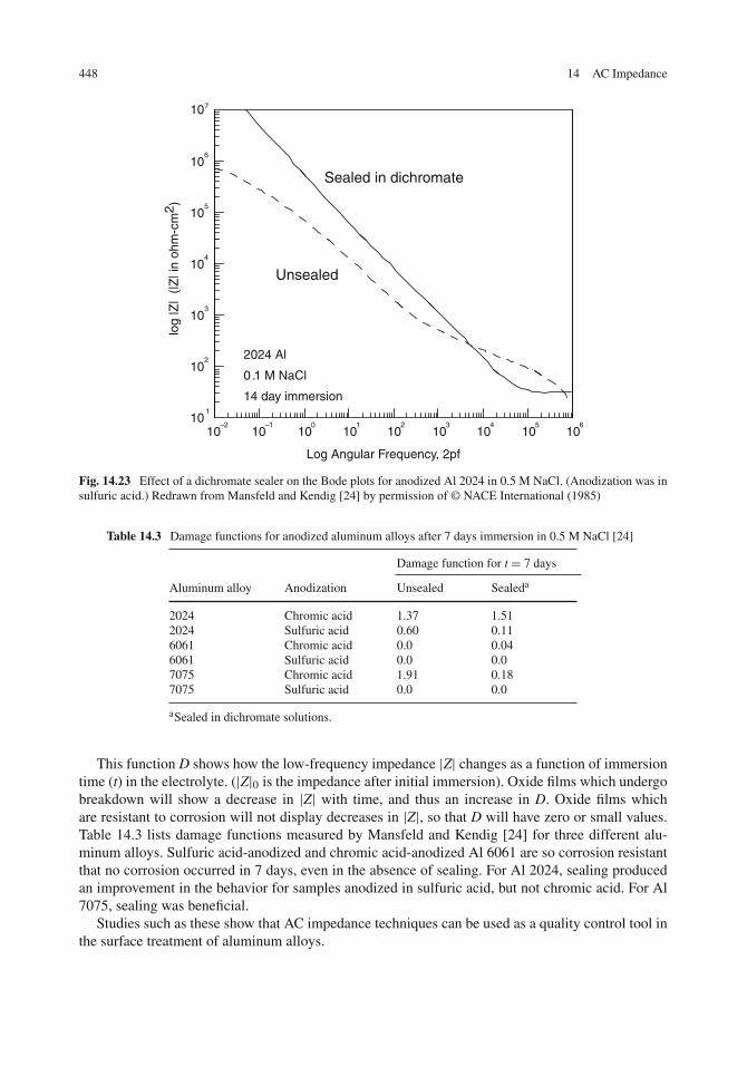
448 14 AC Impedance
106
107
105
Sealed in dichromate
104
Unsealed
102
103
log
|Z|
(|Z
| in
ohm
-cm
2 )
2024 Al
0 1 M NaCl
101
10–2
10–1
100
101
102
103
104
105
106
.
14 day immersion
Log Angular Frequency, 2pf
Fig. 14.23 Effect of a dichromate sealer on the Bode plots for anodized Al 2024 in 0.5 M NaCl. (Anodization was insulfuric acid.) Redrawn from Mansfeld and Kendig [24] by permission of © NACE International (1985)
Table 14.3 Damage functions for anodized aluminum alloys after 7 days immersion in 0.5 M NaCl [24]
Damage function for t = 7 days
Aluminum alloy Anodization Unsealed Sealeda
2024 Chromic acid 1.37 1.512024 Sulfuric acid 0.60 0.116061 Chromic acid 0.0 0.046061 Sulfuric acid 0.0 0.07075 Chromic acid 1.91 0.187075 Sulfuric acid 0.0 0.0
aSealed in dichromate solutions.
This function D shows how the low-frequency impedance |Z| changes as a function of immersiontime (t) in the electrolyte. (|Z|0 is the impedance after initial immersion). Oxide films which undergobreakdown will show a decrease in |Z| with time, and thus an increase in D. Oxide films whichare resistant to corrosion will not display decreases in |Z|, so that D will have zero or small values.Table 14.3 lists damage functions measured by Mansfeld and Kendig [24] for three different alu-minum alloys. Sulfuric acid-anodized and chromic acid-anodized Al 6061 are so corrosion resistantthat no corrosion occurred in 7 days, even in the absence of sealing. For Al 2024, sealing producedan improvement in the behavior for samples anodized in sulfuric acid, but not chromic acid. For Al7075, sealing was beneficial.
Studies such as these show that AC impedance techniques can be used as a quality control tool inthe surface treatment of aluminum alloys.

Problems 449
Concluding Remarks
As seen above, extensive use has been made of equivalent electrical circuits to characterize corrosionprotection by inhibitors, by organic coatings, or by surface treatments such as anodization. Suchequivalent circuits are based on best estimates of the physico-chemical properties of the system.However, a given equivalent circuit is not necessarily unique; and other possible equivalent circuitscan be used. But if a given equivalent circuit is modified to take into account additional details, thenew equivalent circuit can instead become unnecessarily complicated and unwieldy for analysis.
AC impedance instrumentation is a standard tool in the modern corrosion laboratory. Not onlyare these systems fully automated by computer control, but appropriate software is also available fordata analysis. AC impedance has been successfully applied to problems involving the metal/solutioninterface, corrosion inhibition, anodization and surface treatments, and the corrosion behavior oforganic coatings.
Problems
1. Show that Eq. (19) can be differentiated and dZ ′′/dω set equal to zero to give
ωmax = 1
Rp Cdl
where ωmax is the frequency at which Z ′′ has its maximum absolute value.2. In the text it was stated that for the equivalent circuit shown in Fig. 14.4, the term 1/(CdlRp) can
be determined from a linear plot of Z ′ vs. Z ′′/ω. Show that
Z′ = Rs − Z′′
ω Cdl Rp
Hint: Combine Eqs. (18) and (19).3. Show that the term ωRC is dimensionless when R is in ohms and C is in F.4. (a) Use the fact that ωRC is dimensionless if R is in ohms and C is in F to show that the units of
Z ′ and Z ′′ in Eqs. (18) and (19) are then each in ohms. (b) If C is in F/cm2, show that Rs, Rp,Z ′, and Z ′′ are then each in � cm2 for Eqs. (18) and (19).
5. Show that on a Bode plot of log |Z| vs. log ω the slope for the impedance of a capacitor is –1.6. (a) Show that a Warburg diffusion element appears on a complex-plane plot of –Z ′′ vs. Z ′ as a
straight line 45◦ to the real axis. (b) Show that on a Bode plot of log |Z| vs. log ω, the Warburgimpedance gives a straight line with slope –1/2.
7. (a) Derive an expression for |Z| for the following equivalent circuit. (b) Draw the Bode plot andcomplex-plane plot for R = 1,000 � and C = 1.0 × 10⁻⁵ F/cm2.
CR
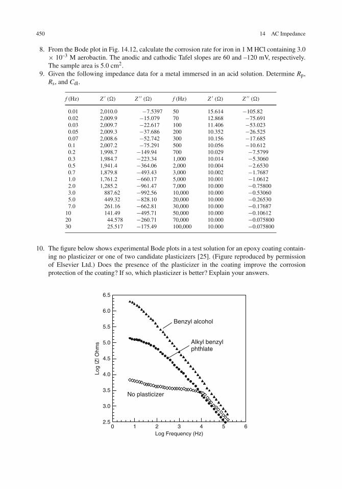
450 14 AC Impedance
8. From the Bode plot in Fig. 14.12, calculate the corrosion rate for iron in 1 M HCl containing 3.0× 10⁻³ M aerobactin. The anodic and cathodic Tafel slopes are 60 and –120 mV, respectively.The sample area is 5.0 cm2.
9. Given the following impedance data for a metal immersed in an acid solution. Determine Rp,Rs, and Cdl.
f (Hz) Z ′ (�) Z ′′ (�) f (Hz) Z ′ (�) Z ′′ (�)
0.01 2,010.0 −7.5397 50 15.614 −105.820.02 2,009.9 −15.079 70 12.868 −75.6910.03 2,009.7 −22.617 100 11.406 −53.0230.05 2,009.3 −37.686 200 10.352 −26.5250.07 2,008.6 −52.742 300 10.156 −17.6850.1 2,007.2 −75.291 500 10.056 −10.6120.2 1,998.7 −149.94 700 10.029 −7.57990.3 1,984.7 −223.34 1,000 10.014 −5.30600.5 1,941.4 −364.06 2,000 10.004 −2.65300.7 1,879.8 −493.43 3,000 10.002 −1.76871.0 1,761.2 −660.17 5,000 10.001 −1.06122.0 1,285.2 −961.47 7,000 10.000 −0.758003.0 887.62 −992.56 10,000 10.000 −0.530605.0 449.32 −828.10 20,000 10.000 −0.265307.0 261.16 −662.81 30,000 10.000 −0.17687
10 141.49 −495.71 50,000 10.000 −0.1061220 44.578 −260.71 70,000 10.000 −0.07580030 25.517 −175.49 100,000 10.000 −0.075800
10. The figure below shows experimental Bode plots in a test solution for an epoxy coating contain-ing no plasticizer or one of two candidate plasticizers [25]. (Figure reproduced by permissionof Elsevier Ltd.) Does the presence of the plasticizer in the coating improve the corrosionprotection of the coating? If so, which plasticizer is better? Explain your answers.
2.5
3.0
3.5
4.0
4.5
5.0
5.5
6.0
6.5
0 1 2 3 4 5 6
Log
|Z| O
hms
Log Frequency (Hz)
Benzyl alcohol
Alkyl benzyl phthlate
No plasticizer

References 451
11. Calculate the capacitance per unit area of a barrier layer oxide film which is 200 Å thick andhas a dielectric constant of 10.
References
1. F. Mansfeld, J. Appl. Electrochemistry, 25, 187 (1995).2. F. Mansfeld, Electrochim. Acta, 38, 1891 (1993).3. C. P. Smyth, “Dielectric Behavior and Structure”, Chapters 1 and 2, McGraw-Hill, New York, NY (1955).4. E. McCafferty, V. H. Pravdic, and A. C. Zettlemoyer, Trans. Faraday Soc., 66, 1720 (1970).5. D. A. McQuarrie and J. D. Simon, “Physical Chemistry”, p. 496, University Science Books, Sausalito, CA (1997).6. R. P. Auty and R. H. Cole, J. Chem. Phys., 20, 1309 (1952).7. J. R. Macdonald, Ed., “Impedance Spectroscopy”, John Wiley & Sons, New York (1987).8. A. J. Bard and L. R. Faulkner, “Electrochemical Methods”, 2nd edition, p. 368, John Wiley & Sons, New York
(2001).9. F. Mansfeld, Corrosion, 36, 301 (1981).
10. K. S. Cole and R. H. Cole, J. Chem. Phys., 9, 341 (1941).11. D. D. Macdonald and M. Urquidi-Macdonald, J. Electrochem. Soc., 132, 2316 (1985).12. M. Urquidi-Macdonald, S. Real, and D. D. Macdonald, J. Electrochem. Soc., 133, 2018 (1986).13. E. McCafferty and J. V. McArdle, J. Electrochem. Soc., 142, 1447 (1995).14. E. McCafferty, Corros. Sci., 39, 243 (1997).15. A. Amirudin and D. Thierry, Prog. Org. Coat., 26, 1 (1995).16. J. N. Murray, Prog. Org. Coat., 31, 375 (1997).17. H. P. Hack and J. R. Scully, J. Electrochem. Soc. 138, 33 (1991).18. M. W. Kendig and H. Leidheiser, Jr., J. Electrochem. Soc., 123, 982 (1976).19. G. Bierwagen, D. Tallman, J. Li, L. He, and C. Jeffcoat, Prog. Org. Coat., 46, 148 (2003).20. R. L. Twite and G. P. Bierwagen in “Organic Coatings for Corrosion Control”, ACS Symposium Series 689,
G. P. Bierwagen, Ed., p. 308, American Chemical Society, Washington, DC (1998).21. T. P. Hoar and G. C. Wood, Electrochim. Acta., 7, 333 (1962).22. J. Hitzig, K. Jüttner, W. J. Lorentz, and W. Paatsch, Corros. Sci., 24, 945 (1984).23. F. Mansfeld and M. W. Kendig, J. Electrochem. Soc., 135, 828 (1988).24. F. Mansfeld and M. W. Kendig, Corrosion, 41, 490 (1985).25. J. M. McIntyre and H. Q. Pham, Prog. Org. Coat., 27, 201 (1996).

Chapter 15High-Temperature Gaseous Oxidation
Introduction
So far this text has considered the corrosion of metals or alloys in aqueous environments. However,when a metal or alloy is exposed to an oxidizing gas, corrosion may occur in the absence of anelectrolyte, especially at high temperatures. This phenomenon is sometimes called “dry corrosion”as opposed to “wet corrosion” which occurs in the presence of an aqueous electrolyte. Oxidizinggases include O2, SO2, H2S, H2O, and CO2 but the most common oxidant is O2.
High-temperature gaseous oxidation is important in many applications, such as in gas turbines,aircraft engines, petrochemical and power plants, and the extraction of metals from their ores. High-temperature oxidation usually concerns the temperature range of several hundred degrees centigradeto about 1,100◦C or so. (The transition metals Cr, Fe, Ni, and Co melt at 1,890, 1,535, 1,453, and1,495◦C, respectively, but their oxides melt at higher temperatures. Aluminum melts at 660◦C andaluminum oxide melts at about 2,000◦C.) The oxide films formed in high-temperature oxidationreactions are much thicker than ordinary passive films and are often referred to as oxide layers orscales. The term “hot corrosion” is generally reserved for the attack of metals and alloys by moltensalts or slags, but is not considered here.
Because this book is primarily concerned with aqueous corrosion, only a brief introduction tohigh-temperature oxidation is given here. For a more extensive treatment, specialized texts on high-temperature oxidation should be consulted [1–4].
Thermodynamics of High-Temperature Oxidation
The oxidation of a metal in air by oxygen proceeds by a chemical reaction such as
2 Cu(s)+ 1
2O2 (g) → Cu2O (s) (1)
The standard free energy change for this reaction as written above is given by the standard freeenergy of formation, �Gf
0, of Cu2O because 1 mole of Cu2O is formed from its elements. Tabulatedvalues of �Gf
0 exist as a function of temperature for various oxides [5, 6]. For instance, at 1,000 K,the free energy of formation of Cu2O is −95.52 kJ/mole Cu2O, so that at 1,000 K the oxidationreaction in Eq. (1) is spontaneous because the free energy change is negative. To compare the ther-modynamic behavior of various oxides, it is useful to calculate their free energy change per mole ofO2. Thus, Eq. (1) can be rewritten as
453E. McCafferty, Introduction to Corrosion Science, DOI 10.1007/978-1-4419-0455-3_15,C© Springer Science+Business Media, LLC 2010

454 15 High-Temperature Gaseous Oxidation
–1200
–1000
–800
–600
–400
–200
0
200
0 500 1000 1500 2000 2500 3000 3500
ΔGo in
kJ
per
mol
e O
2
Temperature in oK
Ag2O
Cu2O
NiOFe3O4
Cr2O3
SiO2
TiO2
Al2O3
Fig. 15.1 Ellingham diagrams for various bulk oxides
4 Cu(s)+O2 (g) → 2 Cu2O (s) (2)
and the free energy change for Eq. (2) at 1,000 K is 2(−95.52 kJ/mole Cu2O)=−191.04 kJ/mole O2.Figure 15.1 shows the free energy change of Cu2O in Eq. (2) as a function of temperature. The
oxidation reaction is spontaneous at all temperatures shown, as indicated by the negative values forthe change in free energy. The slope of the line of �G0 vs. T gives the standard entropy change � S0
from Eq. (8) in Chapter 4. That is
�G0 = �H0 − T �S0 (3)
so that d�G0/dT = −�S0. The slope of �G0 vs. T has a positive value, so that �S0 is negativefor the oxidation reaction. This means that the entropy decreases and the degree of order in themetal/oxygen system increases for the formation of a solid oxide from the metal and O2 gas.
Ellingham Diagrams
Figure 15.1 also shows standard free energy changes for other oxides, with each case being cal-culated on the basis of 1 mole of O2. For example, the oxidation of iron to Fe3O4 is written as

Thermodynamics of High-Temperature Oxidation 455
3
2Fe(s)+O2 (g) → 1
2Fe3O4 (s) (4)
It can be seen that of the oxides given in Fig. 15.1, Al2O3 is the most stable because it has thelargest decrease in free energy (at any given temperature) and Ag2O is the least stable because ithas the smallest decrease in free energy (at any given temperature). In fact, the oxidation of silver toAg2O is not spontaneous above 450 K where �G0 for the oxidation reaction becomes positive.
Figure 15.1 also shows that the oxides of Fe and Ni (which are major components of engineeringalloys) are less stable than the oxides of Cr, Al, and Si, which are often added as alloying elementsfor protection against high-temperature oxidation.
Diagrams as in Fig. 15.1 are called Ellingham diagrams [7, 8], and they have the same limitationsas do Pourbaix diagrams in aqueous corrosion. That is, they contain information about the tendencyof reactions to occur but do not take into account the kinetics of reactions. Ellingham diagrams canalso be constructed for high-temperature reactions which form sulfides or carbides.
Although not shown in Fig. 15.1, there can be changes in the slope of a given curve if there is aphase change due to melting or a change in the structure of the oxide.
Equilibrium Pressure of Oxygen
The pressure of oxygen in equilibrium with solid can be calculated from an expression given inChapter 4. That is
�G0=−RT In K (5)
For Eq. (2), for example,
K= a2 (Cu2O)
a4 (Cu) P (O2)(6)
where a(Cu2O) and a(Cu) are the activities of Cu2O and Cu, respectively, and P(O2) is the pressureof O2 gas. But recall from Chapter 4 that the activities of solids are unity, so that Eq. (6) becomes
K= 1
P (O2)(7)
and Eq. (7) then becomes
�G0=RT In P(O2) (8)
Using �G0 =−191.04 kJ/mole in Eq. (8) gives P(O2)= 1.1× 10⁻¹⁰ atm at 1,000 K. At 1,000 K,pressures of O2 below this value will not be sufficient to oxidize copper, whereas pressures greaterthan 1.1 × 10⁻¹⁰ atm will support oxidation.
Note that Eq. (5) can also be applied to Eq. (1), in which case a different K would be written, butthe calculated value of P(O2) is the same as from Eq. (1); see Problem 15.2.
Table 15.1 gives equilibrium oxygen pressures for the oxidation of various metals at differenttemperatures. For each metal, the equilibrium pressure needed to support oxidation increases withtemperature. All the equilibrium pressures are very low, except in the case of silver. For the oxidationof silver at 400 K, an oxygen pressure of 0.10 atm is required for oxidation; and this value is less

456 15 High-Temperature Gaseous Oxidation
than the partial pressure of oxygen in air (0.2) atm so that the oxidation of silver in air is thermo-dynamically favored in air at 400 K. However, at 500 K an oxygen pressure of 3.3 atm is requiredfor oxidation so that the oxidation of silver in air is not thermodynamically favored at 500 K (or athigher temperatures). (Note that this argument pertains only to the tendency of oxidation to occurand not to the rate of oxidation.) There is a thermodynamic tendency for all the other metals inTable 15.1 to oxidize in air because the required oxygen pressures are very low.
Table 15.1 Equilibrium pressures of oxygen required for the oxidation of various metals at different temperatures
O2 pressure in atmospheres
Oxidation reaction 400 K 500 K 1,000 K 1,500 K 2,000 K
2Ag + 1/2O2→ Ag2O 0.10 3.3 2,320 – a – a
2Cu + 1/2O2→ Cu2O 2.6 × 10–37 2.1 × 10⁻²⁸ 1.1 × 10⁻¹⁰ 1.0 × 10⁻⁴ – a
Ni + 1/2 O2→ NiO – b 4.6 × 10–41 4.6 × 10⁻¹⁶ 8.5 × 10⁻⁸ 1.4 × 10⁻³
3Fe + 2O2→ Fe3O4 – b – b 2.0 × 10⁻²¹ 6.8 × 10⁻¹² 4.3 × 10⁻⁷
2Cr + 3/2O2→ Cr2O3 – b – b 5.4 × 10⁻³¹ 5.8 × 10⁻¹⁸ 1.9 × 10⁻¹¹
Si + O2→ SiO2 – b – b 7.2 × 10–39 3.9 × 10⁻²³ 4.5 × 10⁻¹⁵
Ti + O2→ TiO2 – b – b 1.5 × 10–40 3.4 × 10⁻²⁴ 5.1 × 10⁻¹⁶
2Al+ 3/2O2→ Al2O3 – b – b – b 1.7 × 10⁻²⁸ 9.9 × 10⁻¹⁹
aThe oxide is molten at this temperature.bThe value of the O2 pressure is very low and is lower than in the entry to the right in the table.
Theory of High-Temperature Oxidation
The initial stages of oxidation involve the chemisorption of oxygen as O−2 ions on a clean metalsurface to generate an electrical field at the surface. This electrical field then promotes the intrusion ofoxidized metal atoms (cations) into the plane of adsorbed oxygen ions to produce a two-dimensionalstructure, which grows into an oxide film. These processes have been studied in detail at lowertemperatures [4, 9] but at higher temperatures the initial stages of oxidation proceed very rapidly, sothat it is the continued growth of the oxide film which is of paramount importance.
The growth of thicker oxide layers is described by the Wagner theory of oxidation [1−4, 10].According to this model, oxide layers grow both from the metal substrate outward and from theouter oxide layer inward. Metal atoms are oxidized to metal cations at the metal substrate, andthe cations which are produced diffuse outward through the oxide film, along with a concomitantoutward migration of electrons produced by the oxidation reaction. At the outermost surface of theoxide film, O2 gas is reduced to O−2 ions, which then diffuse inward through the oxide film. Thussituation is depicted in Fig. 15.2.
For the growth of an oxide of composition MO, the reactions are thus:
M → M2+ + 2e− at the metal/oxide Interface
1/2 O2+ 2e− → O2− at the metal/oxide Interface
M+ 1/2 O2 → MO (overall reaction)
Thus, the oxide layer must possess both an ionic and electronic conductivity for the oxide film togrow. The oxide layer serves as (i) an ionic conductor, (ii) an electronic conductor, (iii) an electrodefor the reduction of oxygen (at the outer surface of the oxide), and (iv) a diffusion barrier throughwhich metal cations and oxygen anions diffuse.

Oxidation Rate Laws 457
M+2 O–2
2 e
Metal Oxide Oxygen
Ionicresistance
Electronicresistance
O2M
–
Ano
de
Cat
hode
Fig. 15.2 The Wagner mechanism of high-temperature oxidation [10]. The oxide layer contains both an ionic andelectronic resistance
The electronic resistivity of the oxide film is much higher than its ionic resistivity so that the ionicpath is usually rate determining. Cations and anions do not diffuse with equal ease, and the diffusionof one or the other may be rate controlling. For the common base metals Fe, Ni, Cu, Cr, and Co, therate-controlling step is the diffusion of cations outward but for the refractory metals Ta, Nb, Hf, Ti,and Zr, the rate-controlling step is the diffusion of O2– anions inward [11]
Because the oxide layer grows by movement of ions (not atoms) through the film, the oxidefilm may be considered to be a solid electrolyte. This raises an interesting comparison betweenhigh-temperature oxidation and aqueous corrosion, as shown in Table 15.2.
The Wagner mechanism is not only applicable for high temperatures but also for lower temper-ature processes, such as the growth of rust layers in the natural atmosphere; see Problem 15.4.
Table 15.2 Comparison between electrochemical aspects of high temperature oxidation and aqueous corrosion [11]
Method of corrosion control
Avoid contact between fixedanodes and fixed cathodes in agalvanic cell
Increase electrolyte resistance
Aqueous corrosion Often possible, e.g., by insertingan inert barrier between anodeand cathode
Often impossible because of fixedconditions
High-temperature oxidation Impossible because metal andoxide are in contact
Possible, by alloying to reduce theionic diffusivity
Oxidation Rate Laws
The kinetics of high temperature oxidation are usually studied in experiments which measure thegain in weight of a metal sample when an oxide is formed on the metal sample. The gain in weight isproportional to the thickness of the oxide which is formed. These measurements are made continu-ously using a microbalance assembly, with the sample placed in a furnace fitted with a thermocoupleand temperature control.
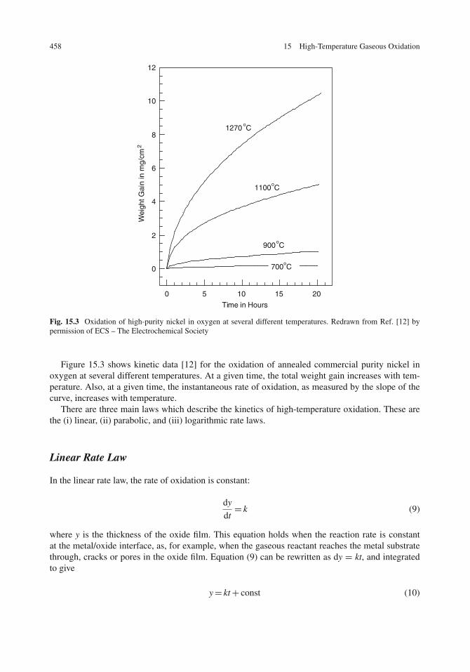
458 15 High-Temperature Gaseous Oxidation
0
2
4
6
8
10
12
0 5 10 15 20
Wei
ght G
ain
in m
g/cm
2
Time in Hours
900 oC
700 oC
1100 oC
1270 oC
Fig. 15.3 Oxidation of high-purity nickel in oxygen at several different temperatures. Redrawn from Ref. [12] bypermission of ECS – The Electrochemical Society
Figure 15.3 shows kinetic data [12] for the oxidation of annealed commercial purity nickel inoxygen at several different temperatures. At a given time, the total weight gain increases with tem-perature. Also, at a given time, the instantaneous rate of oxidation, as measured by the slope of thecurve, increases with temperature.
There are three main laws which describe the kinetics of high-temperature oxidation. These arethe (i) linear, (ii) parabolic, and (iii) logarithmic rate laws.
Linear Rate Law
In the linear rate law, the rate of oxidation is constant:
dy
dt= k (9)
where y is the thickness of the oxide film. This equation holds when the reaction rate is constantat the metal/oxide interface, as, for example, when the gaseous reactant reaches the metal substratethrough, cracks or pores in the oxide film. Equation (9) can be rewritten as dy = kt, and integratedto give
y= kt+ const (10)

Oxidation Rate Laws 459
where “const” is the constant of integration and can be determined from the initial conditions. If aclean metal surface is used in the rate study, then y = 0 at t = 0, so that const = 0. Otherwise, constis the initial thickness of the oxide film prior to high-temperature oxidation.
Metals which obey the linear rate law do not form protective oxides. An example is the oxidationof niobium in air at 1 atm between 600 and 1,200◦C [13].
The oxide thickness in Eq. (10) can be replaced by the gain in weight per unit area, because theweight gain is proportional to the oxide thickness. (The constant in Eq. (10) will accordingly bedifferent.) See Example 15.1. The same is true for the other two rate laws which follow.
Example 15.1: Show that for the linear rate law, the gain in weight per unit area, w, has the sameform as in Eq. (10).
Solution: The weight gain per unit area, w, is related to the oxide thickness y by
w= ρ y( g
cm2= g
cm3× cm
)
where ρ is the oxide density. Thus, y = w/ρ, and substitution into Eq. (9) gives
1
ρ
dw
dt= k
or
dw
dt= kρ= k′
Thus, dw = k ′dt, and integration gives
w= k′t+ const
which has the same form as Eq. (10).
Parabolic Rate Law
In the parabolic rate law, the diffusion of ions or electrons through the oxide is rate controlling, asillustrated in Fig. 15.2. The rate of oxidation is inversely proportional to the oxide thickness:
dy
dt= k′
y(11)
Rewriting Eq. (11) as ydy = k ′dt and integrating gives
y2= 2k′t+ const= kpt+ const (12)
where kp is the parabolic rate constant. This rate law holds for protective oxides and is applicable tothe high-temperature oxidation of many metals, including copper, nickel, iron, chromium, and cobalt[14]. The data in Fig. 15.3 follow the parabolic rate law.

460 15 High-Temperature Gaseous Oxidation
Logarithmic Rate Law
At lower temperatures and for oxide films of 1,000 Å or less, the oxidation rate often follows alogarithmic law:
y= k" log(ct+ 1) (13)
where c is a constant to be determined from the experimental data. This rate law is semi-empirical,but is generally thought to result if the rate of oxidation is controlled by the transfer of electronsacross the oxide film. The transfer of electrons can be rate controlling because of the thinner oxidefilms involved. The logarithmic rate law is obeyed for the initial oxidation of many metals, includingcopper, iron, zinc, nickel, and others [14].
Comparison of Rate Laws
The three main rate laws for oxidation are compared in Table 15.3. These three rate laws are alsocompared in Fig. 15.4, which is plotted with arbitrary values of k = k ′ = k ′′ =1, c = 100, andthe constants of integration taken as zero. Figure 15.4 shows that the linear rate law leads to anon-protective oxide whereas the parabolic and logarithmic rate laws pertain to protective oxides inwhich the rate of growth (and hence the rate of weight gain) decreases with time. The oxide filmapproaches a limiting thickness in the case of the logarithmic rate law.
Table 15.3 The three main rate laws for high-temperature oxidation
Rate law Equation Test for fit
Linear y = kt + const y vs. t is linearParabolic y2 = 2k ′t + const y2 vs. t is linearLogarithmic y = k ′′ log (ct + 1) y vs. log t is linear (for ct > 1)
The Wagner Mechanism and the Parabolic Rate Law
The Wagner mechanism of oxidation shown in Fig. 15.2 gives rise to a parabolic rate law [15–17].This rate law results from assuming that the growth of the oxide film is proportional to a current Iwhich flows through the oxide film:
dy
dt=BI (14)
where B is a proportionality constant given by
B= M
A doxideF(15)
where M is the gram-equivalent weight of the oxide, A is the area of the oxide, doxide the oxidedensity, and F is the Faraday. (B has the units of cm/C, and accordingly, dy/dt has the units of cm/s.)The corrosion current is given by
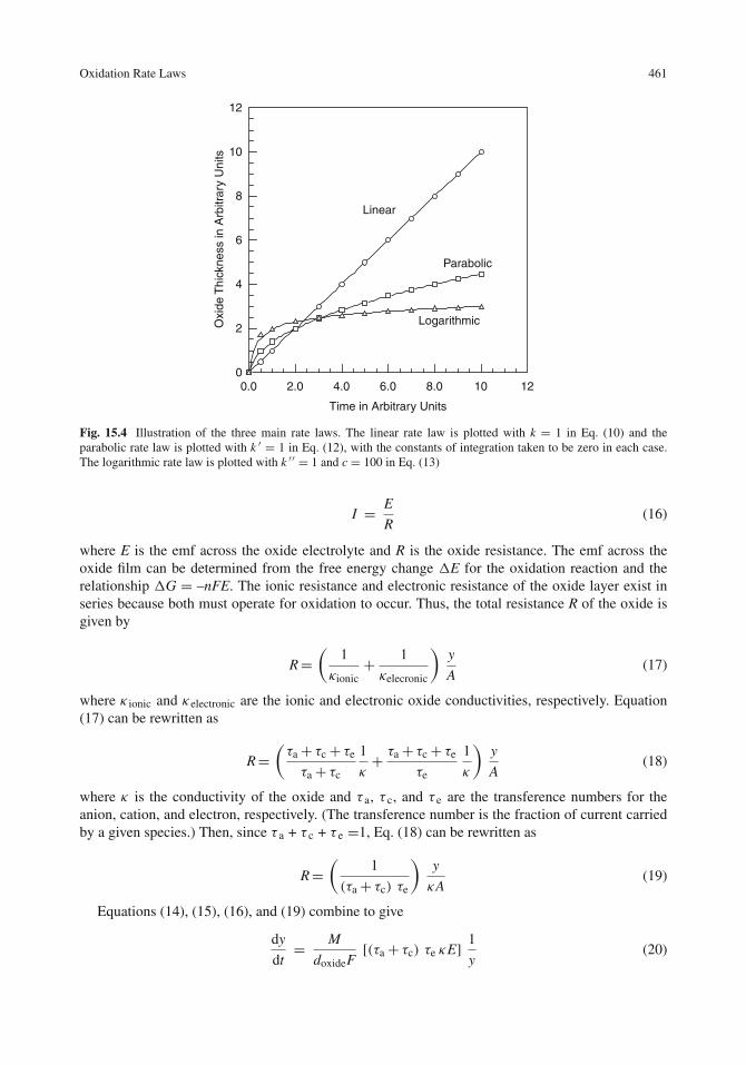
Oxidation Rate Laws 461
0
2
4
6
8
10
12
0.0 2.0 4.0 6.0 8.0 10 12
Oxi
de T
hick
ness
in A
rbitr
ary
Uni
ts
Time in Arbitrary Units
Linear
Parabolic
Logarithmic
Fig. 15.4 Illustration of the three main rate laws. The linear rate law is plotted with k = 1 in Eq. (10) and theparabolic rate law is plotted with k ′ = 1 in Eq. (12), with the constants of integration taken to be zero in each case.The logarithmic rate law is plotted with k ′′ = 1 and c = 100 in Eq. (13)
I = E
R(16)
where E is the emf across the oxide electrolyte and R is the oxide resistance. The emf across theoxide film can be determined from the free energy change �E for the oxidation reaction and therelationship �G = –nFE. The ionic resistance and electronic resistance of the oxide layer exist inseries because both must operate for oxidation to occur. Thus, the total resistance R of the oxide isgiven by
R=(
1
κionic+ 1
κelecronic
)y
A(17)
where κ ionic and κelectronic are the ionic and electronic oxide conductivities, respectively. Equation(17) can be rewritten as
R=(
τa+ τc+ τe
τa+ τc
1
κ+ τa+ τc+ τe
τe
1
κ
)y
A(18)
where κ is the conductivity of the oxide and τ a, τ c, and τ e are the transference numbers for theanion, cation, and electron, respectively. (The transference number is the fraction of current carriedby a given species.) Then, since τ a + τ c + τ e =1, Eq. (18) can be rewritten as
R=(
1
(τa+ τc) τe
)y
κA(19)
Equations (14), (15), (16), and (19) combine to give
dy
dt= M
doxideF[(τa+ τc) τe κE]
1
y(20)

462 15 High-Temperature Gaseous Oxidation
or
y dy = M
doxideF[(τa+ τc) τe κE] dt (21)
After integration,
y2 = 2 M
doxideF[(τa+ τc) τe κE] t + const (22)
which has the form of a parabolic expression:
y2= kpt+ const (23)
where
kp = 2 M
doxideF[(τa+ τc) τe κE] (24)
The parabolic rate constant can also be expressed as a normalized rate constant by dividing y2 by2M/doxide. Then Eq. (22) becomes
y2
2 Mdoxide
= 1
F[(τa+ τc) τe κE] t + const′ (25)
or
y2
2 Mdoxide
= krational t + const′ (26)
where krational is called the rational rate constant and is given by
krational = 1
F[(τa+ τc) τe κE] (27)
The rational rate constant has the units equiv cm−1 s−1.Equations (24) or (27) provide a means for calculating parabolic rate constants from oxide param-
eters. Some calculated values compiled by Kubachewski and Hopkins [1] are listed in Table 15.4.
Table 15.4 Calculated and measured rational rate constants for high-temperature oxidation [1]
Rational rate constant (equiv/cm/s)
Metal OxidantTemperature in◦C Calculated Experimental
Cu I2 (gas) 195 3.8 × 10⁻¹⁰ 3.4 × 10⁻¹⁰
Ag Br2 (gas) 200 2.7 × 10⁻¹¹ 3.8 × 10⁻¹¹
Cu O2, P = 8.3 × 10⁻² atm 1,000 6.6 × 10⁻⁹ 6.2 × 10⁻⁹
Cu O2, P = 3.0 × 10⁻⁴ atm 1,000 2.1 × 10⁻⁹ 2.2 × 10⁻⁹
Co O2, P = 1 atm 1,000 1.25 × 10⁻⁹ 1.05 × 10⁻⁹
Co O2, P = 1 atm 1,350 3.15 × 10⁻⁸ 3.65 × 10⁻⁸
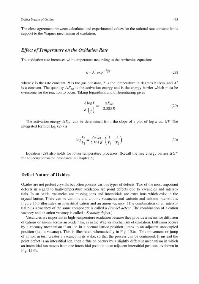
Defect Nature of Oxides 463
The close agreement between calculated and experimental values for the rational rate constant lendssupport to the Wagner mechanism of oxidation.
Effect of Temperature on the Oxidation Rate
The oxidation rate increases with temperature according to the Arrhenius equation:
k=A′ exp−�Eact
RT (28)
where k is the rate constant, R is the gas constant, T is the temperature in degrees Kelvin, and A ′is a constant. The quantity �Eact is the activation energy and is the energy barrier which must beovercome for the reaction to occur. Taking logarithms and differentiating gives
d log k
d(
lT
) =− �Eact
2.303 R(29)
The activation energy �Eact can be determined from the slope of a plot of log k vs. 1/T. Theintegrated form of Eq. (29) is
logk2
k2= �Eact
2.303 R
(1
T1− 1
T2
)(30)
Equation (29) also holds for lower temperature processes. (Recall the free energy barrier �G�=for aqueous corrosion processes in Chapter 7.)
Defect Nature of Oxides
Oxides are not perfect crystals but often possess various types of defects. Two of the most importantdefects in regard to high-temperature oxidation are point defects due to vacancies and intersti-tials. In an oxide, vacancies are missing ions and interstitials are extra ions which exist in thecrystal lattice. There can be cationic and anionic vacancies and cationic and anionic interstitials.Figure 15.5 illustrates an interstitial cation and an anion vacancy. (The combination of an intersti-tial plus a vacancy of the same component is called a Frenkel defect. The combination of a cationvacancy and an anion vacancy is called a Schottky defect.)
Vacancies are important in high-temperature oxidation because they provide a means for diffusionof cations or anions across an oxide film, as in the Wagner mechanism of oxidation. Diffusion occursby a vacancy mechanism if an ion in a normal lattice position jumps to an adjacent unoccupiedposition (i.e., a vacancy). This is illustrated schematically in Fig. 15.6a. This movement or jumpof an ion in turn creates a vacancy in its wake, so that the process can be continued. If instead thepoint defect is an interstitial ion, then diffusion occurs by a slightly different mechanism in whichan interstitial ion moves from one interstitial position to an adjacent interstitial position, as shown inFig. 15.6b.

464 15 High-Temperature Gaseous Oxidation
-2-2O-2
-2-2O-2
-2-2O-2
Interstitialcation
Anionvacancy
M+2
M+2
M+2
Fig. 15.5 Illustration of an interstitial cation and an anion vacancy
O–
M+2
M+2
(a)
O
O
M+2(b)
–
M+2
M+2
–2
–2
–2
M+2
M+2
M+2M+2
M+2M+2
M+2M+2
Fig. 15.6 Schematic illustration of ionic diffusion by (a) anion diffusion by means of vacancies and (b) cationdiffusion by movement of interstitial cations

Defect Nature of Oxides 465
Semiconductor Nature of Oxides
The existence of point defects gives rise to the semiconductor nature of oxides. for example, supposethat ZnO contains interstitial Zn2+ ions, as illustrated in Fig. 15.7. Then for charge neutrality, twoextra electrons must be added to the oxide structure (from the metal) for each interstitial Zn2+ cation.Thus, the current in the oxide film is carried by electrons, so that ZnO is an n-type semiconductor.Ionic transport occurs by interstitial diffusion.
Zn+2 O–2
O–2
O–2
O–2
O–2
O–2
O–2
O–2
O–2
O–2
O–2
O–2Zn+2 Zn+2
Zn+2 Zn+2 Zn+2
Zn+2 Zn+2 Zn+2
Zn+2 Zn+2 Zn+2
Zn+2
Interstitial Zn+2
e–
e–
2 electrons required for charge neutrality
Fig. 15.7 Schematic illustration of an n-type oxide semiconductor containing interstitial cations
If instead the point defect is a cation vacancy, as illustrated in Fig. 15.8 for NiO, then the oxidecontains a deficiency of positive charges (due to the missing Ni2+ ions). Then for charge neutrality,two electron holes must be added to the oxide structure for each Ni2+ vacancy. Thus, the current inthe oxide film is carried by electron holes, so that NiO is a p-type semiconductor and ionic transportoccurs by diffusion of vacancies.
Ni+2
vacancy
2 electron holes requiredfor charge neutrality
Ni+2 Ni+2
Ni+2 O–2
O–2O–2O–2
O–2O–2O–2
O–2O–2O–2
O–2O–2Ni+2 Ni+2
Ni+2 Ni+2 Ni+2
Ni+2Ni+2 Ni+2
h+
h+
Fig. 15.8 Schematic illustration of a p-type oxide semiconductor containing cation vacancies

466 15 High-Temperature Gaseous Oxidation
By similar arguments it can be seen that O2− vacancies produce a deficiency of negative charges,so that electrons must be added for electroneutrality, thus producing an n-type semiconductor.Figure 15.9 shows schematically that oxygen vacancies can be formed at high temperatures by theloss of oxide ions to the gaseous phase.
O2
O-2
O-2O2
Metal Oxide Gas Metal Oxide Gas
Oxygenvacancies
2
-2
-22
-2
-22
Fig. 15.9 Schematic illustration showing the loss of two oxide ions (O2–) to the gas phase to form two oxygenvacancies in the oxide layer
The last possibility, i.e., interstitial anions, produces an excess of negative charges which arebalanced by electron holes, thus giving a p-type semiconductor. However, examples of interstitialanions, e.g. O2–, are not common due to the large size of the anion. These concepts are summarizedin Table 15.5.
Table 15.5 Types of oxide semiconductors
Type of oxidesemi-conductor Defect
Requirement forcharge neutrality Charge carriers Ionic transport Examples [4, 18]
n-Type Interstitialcations [extra(+) charge]
Add electrons Electrons Interstitial ZnO, CdO
n-Type Anion vacancies[missing (−)charge]
Add electrons Electrons Vacancies Al2O3, TiO2,Fe2O3, ZrO2
p-Type Cation vacancies[missing (+)charge]
Add holes Holes Vacancies NiO, FeO,Cr2O3, Fe3O4
p-Type Interstitial anions[extra (−)charge]
Add holes Holes Interstitial UO2
Hauffe Rules for Oxidation
The effect of various foreign ions on the rates of high-temperature oxidation can be explained onthe basis of the semiconductor nature of the oxide layer. The effects of various solute ions on high-temperature oxidation rates are called the Hauffe rules for oxidation.
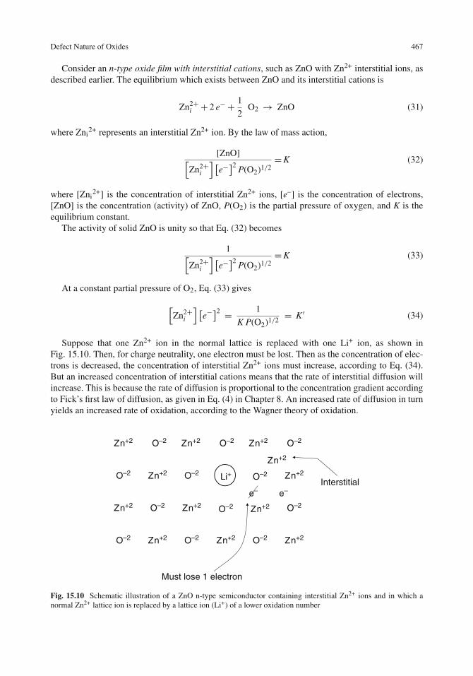
Defect Nature of Oxides 467
Consider an n-type oxide film with interstitial cations, such as ZnO with Zn2+ interstitial ions, asdescribed earlier. The equilibrium which exists between ZnO and its interstitial cations is
Zn2+i + 2 e− + 1
2O2 → ZnO (31)
where Zni2+ represents an interstitial Zn2+ ion. By the law of mass action,
[ZnO][Zn2+
i
] [e−]2
P(O2)1/2=K (32)
where [Zni2+] is the concentration of interstitial Zn2+ ions, [e–] is the concentration of electrons,
[ZnO] is the concentration (activity) of ZnO, P(O2) is the partial pressure of oxygen, and K is theequilibrium constant.
The activity of solid ZnO is unity so that Eq. (32) becomes
1[Zn2+
i
] [e−]2
P(O2)1/2=K (33)
At a constant partial pressure of O2, Eq. (33) gives
[Zn2+
i
] [e−]2 = 1
K P(O2)1/2= K′ (34)
Suppose that one Zn2+ ion in the normal lattice is replaced with one Li+ ion, as shown inFig. 15.10. Then, for charge neutrality, one electron must be lost. Then as the concentration of elec-trons is decreased, the concentration of interstitial Zn2+ ions must increase, according to Eq. (34).But an increased concentration of interstitial cations means that the rate of interstitial diffusion willincrease. This is because the rate of diffusion is proportional to the concentration gradient accordingto Fick’s first law of diffusion, as given in Eq. (4) in Chapter 8. An increased rate of diffusion in turnyields an increased rate of oxidation, according to the Wagner theory of oxidation.
Interstitial
Must lose 1 electron
e– e–
Zn+2
Zn+2Zn+2 Zn+2
Zn+2Zn+2Zn+2
Zn+2
Zn+2Zn+2
Zn+2Zn+2
O–2O–2
O–2O–2O–2
O–2O–2O–2
O–2O–2O–2
O–2
Li+
Fig. 15.10 Schematic illustration of a ZnO n-type semiconductor containing interstitial Zn2+ ions and in which anormal Zn2+ lattice ion is replaced by a lattice ion (Li+) of a lower oxidation number

468 15 High-Temperature Gaseous Oxidation
Al+3Interstitial
Must add 1 more electron
Zn+2 Zn+2 Zn+2
Zn+2 Zn+2
Zn+2
Zn+2 Zn+2 Zn+2
Zn+2Zn+2Zn+2
O–2 O–2 O–2
O–2 O–2 O–2
O–2 O–2 O–2
O–2 O–2 O–2
Fig. 15.11 Schematic illustration of a ZnO n-type semiconductor containing interstitial Zn2+ ions and in which anormal Zn2+ lattice ion is replaced by a lattice ion (Al3+) of a higher oxidation number
If the ZnO film contains a solute ion of oxidation number greater than +2, e.g., Al3+ as shown inFig. 15.11, then for charge neutrality one electron must be added for each Al3+ solute ion. Accordingto Eq. (34), as the concentration of electrons increases, the concentration of interstitial Zn2+ ionsdecreases. This means that there is a decreased rate of ionic diffusion, and accordingly a decreasedoxidation rate. See Table 15.6 for a compilation of these trends.
Table 15.6 Hauffe rules for oxidation
Type of oxidesemiconductor Defect Example
Oxidationnumber of soluteion relative tooxide cation
Change in defectconcentrationand ionicdiffusion
Change inoxidation rate
n-Type Interstitial cations ZnO Lower Increase IncreaseHigher Decrease Decrease
Anion vacancies ZrO2 Lower Increase IncreaseHigher Decrease Decrease
p-Type Cation vacancies NiO Lower Decrease DecreaseHigher Increase Increase
Interstitial anions UO2 Lower Decrease DecreaseHigher Increase Increase
If instead of interstitial cations, as in n-type semiconductors as described above, suppose that weconsider a p-type oxide semiconductor (e.g., NiO) in which the point defects are cationic vacancies.The equilibrium which exists between the nickel ion vacancies and the NiO lattice is given by
NiO+VNi′′ + 2 h+ → 1
2O2 (35)
where VNi′′ represents a nickel ion vacancy of effective charge –2 (the prime refers to an effective
negative charge) and h+ refers to an electron hole. By the law of mass action
P(O2)1/2
[NiO][V"
Ni
] [h+]2 =K (36)

Defect Nature of Oxides 469
or
[V"
Ni
] [h+]2 = P(O2)1/2
K=K′ (37)
at a constant partial pressure of oxygen.Suppose next that one Ni2+ ion in the normal lattice position is replaced by one Li+ ion, as shown
schematically in Fig. 15.12. Then for charge neutrality, one electron must be lost, or equivalently, oneelectron hole must be added. As the concentration of electron holes increases, then the concentrationof metal ion vacancies decreases, as per Eq. (37). This decrease produces a decrease in the rate ofionic diffusion and hence a decrease in the oxidation rate.
Ni+2 Ni+2
Ni+2 Ni+2
Ni+2
Ni+2
Ni+2Ni+2Ni+2
Ni+2
Ni+2
Li+
h+ h+h+
O–2 O–2 O–2
O–2O–2O–2
O–2 O–2 O–2
O–2 O–2O–2
vacancy
Must add 1 more electron hole
Fig. 15.12 Schematic illustration of a NiO p-type semiconductor containing oxygen vacancies and in which a normalNi2+ lattice ion is replaced by a lattice ion (Li+) of a lower oxidation number
If the NiO lattice contains a substitutional solute ion having an oxidation number higher thanthat of Ni2+, e.g., Cr3+, then by a similar argument as just given, for each Cr3+ ion substituted fora Ni2+ ion, one electron must be added (or one h+ is lost). According to Eq. (37), a decrease in theconcentration of electron holes yields an increase in the concentration of metal ion vacancies andhence an increase in the rate of ionic diffusion and an increase in the oxidation rate.
This trend has been observed for the oxidation of Cr–Ni alloys in which chromium is addedprogressively to nickel. Table 15.7 lists parabolic rate constants as compiled by Uhlig [14] for thehigh-temperature oxidation of Ni-Cr alloys. For dilute alloys, the increased addition of Cr to Niresults in an increase in the oxidation rate. This can be explained on the basis that increased alloyingwith Cr results in increased concentrations of Cr3+ in the oxide film which, according to the argu-ments above, leads to an increase in the oxidation rate. For higher alloying amounts of Cr, however,the oxidation rate decreases as the oxide becomes predominantly Cr2O3 instead of NiO. (Recall fromthe Ellingham diagram in Fig. 15.1 that Cr2O3 is more stable than NiO.)
So far we have considered only cation defects in regard to the Hauffe rules for oxidation. Considernext an n-type oxide having anion vacancies, such as ZrO2. The equilibrium between an oxygen atomin the lattice and an oxygen vacancy is:
V ′′O+ 2 e− + 1
2O2 → Olattice (38)

470 15 High-Temperature Gaseous Oxidation
Table 15.7 Oxidation ofnickel alloyed with chromiumat 1,000◦C and 1 atm O2 [14] Wt% Cr
Parabolic rate constant(g2/cm4/s3)
0 3.1 × 10⁻¹⁰
0.3 14 × 10−10
1.0 26 × 10−10
3.0 31 × 10−10
10.0 1.5 × 10⁻¹⁰
where V′′O represents an oxygen vacancy of effective charge +2. (The dots in V′′O represent effectivepositive charges). Thus,
[Olattice][V ′′O] [
e−]2
P(O2)1/2=K (39)
or,
[V ′′O] [
e−]2 = 1
K P(O2)1/2=K′ (40)
at a constant partial pressure of O2.If one Zr4+ ion in the normal lattice is replaced by an ion of lower oxidation state, say Al+3, then
one electron must be lost for charge neutrality; see Fig. 15.13. According to Eq. (40), a decrease inthe concentration of electrons produces an increase in the concentration of oxygen vacancies, whichin turn leads to an increase in the rate of diffusion and an increase in the oxidation rate. If Zr4+ ionsare replaced by ions of a higher oxidation state, the opposite trend results.
Must add 1 more electron
e–
e–
e–
Zr+4 Zr+4 Zr+4
Zr+4 Zr+4
Zr+4 Zr+4 Zr+4
Al+3
Anion vacancy
O–2
O–2
O–2 O–2 O–2 O–2 O–2 O–2
O–2 O–2 O–2 O–2
O–2 O–2 O–2 O–2O–2
Fig. 15.13 Schematic illustration of a ZrO2 n-type semiconductor containing oxygen vacancies and in which a normalZr4+ lattice ion is replaced by a lattice ion (Al3+) of a lower oxidation number
The last case to be considered is a p-type oxide semiconductor with interstitial anions. Theequilibrium between an interstitial oxygen ion Oi
2− and the lattice is
O−2i + 2 h+ = 1
2O2 (41)

Defect Nature of Oxides 471
The effect of solute ions is left as an exercise in Problem 15.11.Table 15.6 compiles the effects of various solute ions on the high-temperature oxidation rates of
the different types of oxide semiconductors.
Effect of Oxygen Pressure on Parabolic Rate Constants
The rate of parabolic oxidation is a function of the O2 partial pressure. The general relationship, aswill be seen below, is
kp=A P (O2)1/n (42)
where kp is the parabolic rate constant and A is a constant, and n is negative for an n-type oxideand positive for a p-type oxide. The case of an n-type oxide containing interstitial cations is shownbelow.
For an n-type oxide MO with interstial cations, the equilibrium between the oxide and itsinterstitial cations is given by
M+2i + 2 e− + 1
2O2 → MO (43)
which is a generalization of Eq. (31). Thus,
1[M+2
i
] [e−]2
P(O2)1/2=K (44)
But [Mi+2] = 2 [e–], so that substituting for [e–] into Eq. (44) gives the result
[M+2
i
]=K′ P(O2)−1/6 (45)
For n-type oxides with interstitial cations, the rate of ionic diffusion is proportional to the con-centration of interstitial cations (see Table 15.5). The rate of oxidation is in turn proportional to therate of diffusion, so that the result is
kp α P(O2)−1/6 (46)
If an electron associates itself with an interstitial cation, then Eq. (43) is modified to
M+i + e− + 1
2O2 → MO (47)
and by a similar argument it can be shown that
kp α P(O2)−1/4 (48)
Similar arguments can be made for n-type oxides with anion vacancies by using Eq. (38), forp-type oxides with cation vacancies by using Eq. (35), and for p-type oxides with interstitial anionsby using Eq. (41). The results are given in Table 15.8.

472 15 High-Temperature Gaseous Oxidation
Table 15.8 Effect of oxygen pressure on the parabolic rate constant
Type of oxide semiconductor EquilibriumMechanism ofdiffusion
Dependence ofparabolic rate constanton P(O2)
n-Type with interstitial cations Eq. (31) or (43) Interstitial cations P(O2)−1/6 or P(O2)−1/4
n-Type with anion vacancies Eq. (38) Anion vacancies P(O2)−1/6
p-Type with cation vacancies Eq. (35) Cation vacancies P(O2)1/6 or P(O2)1/4
p-Type with interstitial anions Eq. (41) Interstitial anions P(O2)1/6
Non-uniformity of Oxide Films
Oxide films formed at high temperature are often not uniformly homogeneous in composition orstructure. (That is, the solid electrolyte is not always homogeneous as are the usual electrolytesin aqueous corrosion.) An example is provided by the oxidation of iron, which possesses multipleoxidation states. As shown in Fig. 15.14, the oxide film consists of three distinct layers, FeO, Fe3O4,and Fe2O3 [11]. The phase richest in iron (FeO) exists nearest the metal surface and the phase richestin oxygen (Fe2O3) exists nearest the source of oxygen. The various voids in the oxide phase inFig. 15.13 are attributed to the collapse of cation vacancies.
Fe2O3
Fe
FeO
Fe3O4
Fig. 15.14 Oxide layers formed on iron exposed to air at high temperatures [11]. Original photomicrograph byC.T. Fujii of the Naval Research Laboratory, Washington, DC and reproduced by permission of The McGraw-HillCompanies
Voids have also been observed in other instances, such as in the high-temperature oxidation ofniobium [11]. (Nb2O5 has a Pilling–Bedworth ratio of 2.66.) These voids result in a non-protectiveoxide in which oxygen can diffuse through the voids to locations closer to the metal surface wherethe oxygen reduction reaction can occur. Thus, the effective thickness of the oxide film is reducedby the presence of the voids.

Protective vs. Non-protective Oxides 473
Protective vs. Non-protective Oxides
Based on the various factors which affect high temperature oxidation and on the properties of oxides,several generalizations may be drawn regarding the protective nature of oxide films.
Pilling–Bedworth Ratio
The Pilling–Bedworth ratio R given by
R= Molecular volume of oxide
Molecular volume of metal(49)
as was discussed in Chapter 9 on passivity. It was seen that the Pilling–Bedworth ratio is one factor indetermining whether or not an oxide forms a protective passive film. These considerations especiallyapply to high-temperature oxidation because the thickness of the oxide layer is much greater thanthat for ambient temperatures. This means that Pilling–Bedworth ratios taken from values for bulkoxides are more reliable for high-temperature oxide layers than for the thinner passive oxide filmsformed at lower temperatures.
A value of R < 1 once again means that the metal produces insufficient oxide to cover the metalsurface, and the oxide is not protective. A value of R equal to or slightly greater than 1 is the optimalPilling–Bedworth ratio for producing a protective oxide film. Values much greater than 1 intro-duce compressive strengths which lead to fracture and spalling of the oxide layer. However, thePilling–Bedworth ratio is only one factor in determining the oxidation resistance of metals at hightemperatures, as seen below.
Properties of Protective High-Temperature Oxides
To be protective against high-temperature oxidation, an oxide should have the followingproperties [11]:
(1) a coefficient of expansion approximately equal to that of the metal substrate,(2) a good adherence to the metal substrate,(3) a high melting point,(4) a low vapor pressure,(5) good high-temperature plasticity so as to resist fracture,(6) low electrical conductivity or low diffusion coefficients for metal cations or oxygen anions,(7) a Pilling–Bedworth ratio of approximately 1.
The actual behavior of metals and alloys must be measured experimentally. As in the case ofpassive films at ambient temperatures, it is not possible to predict the exact behavior of alloys frombulk oxide properties. Alloying additions of Cr, Al, and Si, however, have been generally found tobe effective in forming high-temperature protective oxides.
Most high-temperature engineering alloys form chromia (Cr2O3) or alumina (Al2O3) scales. Fe-Cr, Ni-Cr, and Co-Cr alloys exhibit low oxidation rates when the Cr concentration is 15–30 wt.% [4].Alloy 625 is another example of an alloy which provides a chromia-forming oxide. Alloy 625 hasa nominal composition of 60 Ni-20 Cr-10 Mo-5 Fe (Table 9.11) and is used frequently in aqueous

474 15 High-Temperature Gaseous Oxidation
corrosion applications but was originally developed as an alloy for high-temperature applications.Alumina-forming oxides arise from alloys containing 5–7 wt.% Al and greater than 10 wt.% Cr [4].A compilation of various high-temperature alloys is given by Khanna [4].
Problems
1. Based on thermodynamic considerations alone, what would be the effect on the stability of theoxide film formed by high-temperature oxidation if iron was alloyed with aluminum?
2. For the following reaction:
4Cu (s) +O2 (g) → 2 Cu2O (s)
(a) Write an expression for the equilibrium constant.(b) Calculate the equilibrium pressure of O2 from the equilibrium constant given that �G0 is
–191.04 kJ/mole at 1,000 K for the reaction as written above.(c) How does this pressure of O2 compare with that calculated in the text for the reaction:
2Cu (s) + 1
2O2 (g) → Cu2O (s)
3. The free energy of formation of MgO is –469.888 kJ/mole at 1,200 K. Calculate the equilibriumpressure of O2 required for the oxidation of Mg to MgO at this temperature. Is oxidation possiblein air at this temperature?
4. In a study on the long-term growth of rust layers formed on a high tensile steel in the naturalatmosphere, Horton et al. [19] found that atmospheric dusts become deposited on the air surfaceof the rust and then become enveloped within the rust layer. What does this observation suggestabout the mechanism of growth of rust layers at ambient temperatures in the natural atmosphere?
5. (a) Show that for logarithmic oxidation, the rate of oxide growth dy/dt is inversely proportionalto the time for large reaction times. (b) Then show that the oxidation rate approaches 0 for alarge reaction time.
6. Smeltzer et al. [20] found that the oxidation rate for Ni–Al alloys at 1,298 K increases with anincrease in the amount of Al (between 0.1 and 3.0 wt.%).
(a) Is this increase in the oxidation rate for Ni-Al alloys with increasing Al content consistentwith the thermodynamic trends in the Ellingham diagram?
(b) Is this increase in oxidation rate consistent with the Hauffe rules for oxidation?
7. The parabolic rate constant in the preceding problem was determined to be 3.5 × 10⁻¹⁰
g2 cm−4 s−1 for a Ni-0.1 wt% Al alloy at 1,298 K.
(a) Calculate the weight gain at 1,298 K after 20 h of oxidation.(b) Calculate the oxide thickness (in μm) after 20 h oxidation assuming that the oxide is
predominantly NiO having a density of 6.67 g/cm3.
8. Lithium-aluminum alloys are used in aerospace applications where a reduction in weight isdesired. On the basis of the Hauffe rules for oxidation, what would be the effect of solute Li+
ions on the parabolic oxidation rate of aluminum?

References 475
9. The following data are taken from a study [21] on a Co-10% Cr alloy oxidized in 100 torr O2 at1,100◦C. Which one of the three major rate laws best fits these data?
Exposure time (h) Weight gain (mg/cm2)
1.0 14.02.0 20.13.0 24.94.0 28.7
10. In a study [21] on the high-temperature oxidation of cobalt, the activation energy was deter-mined to be 146 kJ/mole for the oxidation of pure cobalt at 100 torr O2 pressure. The parabolicrate constant at 950◦C was determined to be 25 mg2 cm−4 h−1. What is the weight gain of thecobalt sample in mg/cm2 after 5 h of oxidation at 1,200◦C?
11. Uranium dioxide, UO2, is a p-type oxide with interstitial anions. Explain the effect of Al3+
solute ions on the rate of high-temperature oxidation. Explain the effect of Ta5+ solute ions onthe oxidation rate.
12. For the oxidation of Cu to Cu2O at a temperature of 1,000◦C and a pressure of 100 mmHg, theoxide conductivity is 4.8 �/cm, the transference numbers are τa + τc = 4 × 10⁻⁴, and the cellemf is E = 0.337 V [1]. Calculate the rational rate constant for parabolic oxidation. How doesyour answer compare with the experimentally determined value of 7 × 10⁻⁹ equiv cm−1s−1
References
1. O. Kubaschewski and B. E. Hopkins, “Oxidation of Metals and Alloys”, Butterworths, London (1962).2. K. Hauffe, “Oxidation of Metals”, Plenum Press, New York (1965).3. P. Kofstad, “High Temperature Corrosion”, Elsevier Applied Science, London (1988).4. A. S. Khanna, “Introduction to High Temperature Oxidation and Corrosion”, ASM International, Materials Park,
OH (2002).5. M. W. Chase, Jr., Ed., “NIST-JANAF Thermochemical Tables”, National Institute of Standards and Technology,
Gaithersburg, MD (1998).6. J. P. Coughlin, “Contributions to the Data on Theoretical Metallurgy”, Vol. XII, US Government Printing Office,
Washington, DC (1954).7. D. R. Gaskell, “Introduction to Metallurgical Thermodynamics”, p. 272, Hemisphere Publishing Corp.,
Washington, DC (1981).8. F. D. Richardson and J. H. Jeffes, J. Iron Steel. Inst., 160, 261 (1948).9. D. F. Mitchell and M. J. Graham in “High Temperature Corrosion”, R. A. Rapp, Ed., p. 18, National Association
of Corrosion Engineers, Houston, TX (1983).10. C. Wagner, Z. Physik. Chem., B21, 25 (1933).11. M. G. Fontana and N. D. Greene, “Corrosion Engineering”, Chapter 11, McGraw-Hill, New York (1978).12. D. Caplan, M. J. Graham, and M. Cohen, J. Electrochem. Soc., 119, 1205 (1972).13. K. Hauffe, “Oxidation of Metals”, p. 237, Plenum Press, New York (1965).14. H. H. Uhlig and W. R. Revie, “Corrosion and Corrosion Control”, Chapter 10, John Wiley, New York (1985).15. O. Kubaschewski and B. E. Hopkins, “Oxidation of Metals and Alloys”, p. 82, Butterworths, London (1962).16. T. P. Hoar and L. E. Price, Trans. Faraday Soc., 34, 867 (1938).17. N. D. Tomashov, “Theory of Corrosion and Protection of Metals”, p. 74, MacMillan Co., New York (1966).18. G. Wranglen, “An Introduction to Corrosion and Protection of Metals”, Chapter 11, Chapman and Hall, London
(1985).

476 15 High-Temperature Gaseous Oxidation
19. J. B. Horton, W. C. Hahn, and J. F. Libsch, “Proceedings of the Third International Congress on MetallicCorrosion”, Vol. IV, p. 401, Moscow (1969).
20. W. W. Smeltzer, H. M. Hindam, and F. A. Elrefaie in “High Temperature Corrosion”, R. A. Rapp, Ed., p. 251,NACE, Houston, TX (1983).
21. P. K. Kofstad and A. Z. Hed, “Proceedings of the Fourth International Congress on Metallic Corrosion”, p. 196,NACE, Houston, TX (1972).

Chapter 16Selected Topics in Corrosion Science
Introduction
This chapter addresses selected topics in corrosion science. These topics can each form the basisfor more extended treatments, but in large part they complement the body of material included inprevious chapters. These special topics include (i) the application of electrode kinetics to corrosionprocesses, (ii) potential and current distribution, (iii) large structures and scaling rules, (iv) acid–base properties of oxide films, and (v) surface modification by directed energy beams (i.e., by ionimplantation or laser-surface techniques).
Electrode Kinetics of Iron Dissolution in Acids
Throughout this text, for the dissolution of iron, we have written
Fe→ Fe2+ + 2e− (1)
This equation pertains to the overall dissolution reaction but does not describe the mechanism bywhich the reaction proceeds. In acid solutions, there are two experimental variable parameters whichcontrol the anodic current density, ia. These are the pH (i.e., the concentration of hydrogen ions) andthe electrode potential, E. Thus
ia = f([
H+]
, E)
(2)
where [H+] is the concentration of hydrogen ions in solution. Accordingly, we can experimen-tally observe two parameters which describe how ia varies with changes in either [H+] or E. Theseparameters are
zH+ =(
∂ log ia∂ log
[H+])
E
(3)
and
b−1a =
(∂ log ia∂ log E
)[H+]
(4)
where zH+ is called the reaction order with respect to the H+ ions and ba is the usual Tafel slope (seeChapter 7).
477E. McCafferty, Introduction to Corrosion Science, DOI 10.1007/978-1-4419-0455-3_16,C© Springer Science+Business Media, LLC 2010

478 16 Selected Topics in Corrosion Science
Various investigators have reported two different sets of kinetic data for the steady-state disso-lution of iron in sulfuric or perchloric acids, as shown in Table 16.1. One group of investigators[1, 2] reports anodic Tafel slopes of 40 mV while a second group [3, 4] reports values of 30 mV.In addition, two different values of zH+ have been observed, i.e., −1 vs. −2. Both groups of inves-tigators have observed that dissolved ferrous ions do not affect the anodic dissolution of iron, i.e.,zFe
2+ = 0.
Table 16.1 Kinetic data for the anodic dissolution of iron in acid solutions
Solution Investigator ba (mV) zH+ zCl–
Sulfuric acid Bockris [1] 40 −1 −Kelly [2] 40 −1 −Heusler [3, 4] 30 −2 −
Hydrochloric acid Lorenz [7, 8] 60 −1 −1McCafferty [9] 60 −1 −1
Concentrated acidicchloride solutions
McCafferty [9] 60 +1.8 +1Lorenz [8] 100 +1 +0.6Nobe [10] 100 +1 +1
The observation that zH+ is a negative number (−1 or −2) is at first glance an astonishing result.This means that at constant electrode potential, the H+ ion does not catalyze the anodic reaction,but instead, it is the OH− ion which promotes anodic dissolution. The concentration of OH− ionsis very small in acid solutions ([OH−] = 10−13 M at pH 1.0), but OH− ions are generated by thedissociation of adsorbed water molecules, as shown in the following mechanisms.
Bockris–Kelly Mechanism
Bockris et al. [1] and Kelly [2] proposed the following mechanism to explain their experimentalresults:
Fe+ H2O1�−1
Fe(H2O)ads (5)
Fe(H2O)ads2�−2
Fe(OH−)ads + H+ (6)
Fe(OH−)ads3�−3
Fe(OH)ads + e− (7)
Fe (OH)ads4−→ (FeOH)+ + e− (RDS) (8)
(FeOH)+ + H+ 5−→ Fe2+ (aq)+ H2O (9)
The overall reaction in steps 1–5 is Fe −→ Fe2++2e−. The mechanism above takes into accountthat the electrode surface contains adsorbed water molecules, adsorbed hydroxyl ions, and the sur-face intermediate FeOHads. The anodic reaction thus proceeds by two consecutive one-electrontransfer reactions. The rate-determining step (RDS) occurs in step 4.
In the steady state, the rate of appearance of each surface intermediate is equal to its rate ofconsumption. That is,

Electrode Kinetics of Iron Dissolution in Acids 479
βdθi
dt= 0 (10)
where β is a proportionality constant which relates the surface coverage θ to the surface concentra-tion in mol/cm2. Thus
βdθ1
dt= k1 (1− θT)− k−1βθ1 − k2βθ1 + k−2
[H+]βθ2 = 0 (11)
βdθ2
dt= k2βθ1 − k−2
[H+]βθ2 − k3βθ2 + k−3βθ3 = 0 (12)
βdθ3
dt= k3βθ2 − k−3βθ3 − k4βθ3 = 0 (13)
where ki are the electrochemical rate constants and θ1, θ2, and θ3 are the surface coverages ofFe(H2O)ads, FeOH−ads, and FeOHads, respectively; and θT = θ1 + θ2 + θ3. The current densityis carried in steps 3 and 4. Thus
iaF= k3βθ2 − k−3βθ3 + k4βθ3 (14)
where F is the Faraday. Each rate constant ki (bar) is related to the electrode potential E by
ki = kie±niFE/2RT (15)
where ni is the number of electrons transferred in the ith step. (The plus and minus signs refer to theanodic and cathodic directions, respectively.) In addition, in Eq. (15) it is assumed that the transfercoefficient α = 1/2 (see Chapter 7).
The solution to Eqs. (11) – (15) subject to (1 – θT) ≈ (1 – θ1) and k−3>>k4 is (after considerablealgebra) [2]
ia = 2Fk2k3k4β
k−2k−3[H+](
k1
k1 + k−1β
)e3FE/2RT (16)
Thus,
log ia = log (constants)− log[H+]+ 3FE
2.303 (2RT)(17)
Taking appropriate partial derivatives gives
zH+ =(
∂ log ia∂log
[H+])
E
= −1 (18)
and
ba =(
∂E
∂ log ia
)[H+]= 2
3
(2.303RT
F
)= 0.040 V (19)
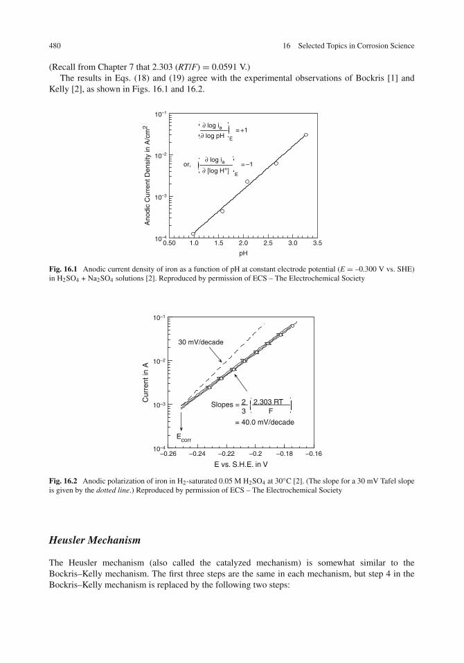
480 16 Selected Topics in Corrosion Science
(Recall from Chapter 7 that 2.303 (RT/F) = 0.0591 V.)The results in Eqs. (18) and (19) agree with the experimental observations of Bockris [1] and
Kelly [2], as shown in Figs. 16.1 and 16.2.
10–2
10–3
10–4
10–1
0.50 1.0 1.5 2.0 2.5 3.0 3.5
Ano
dic
Cur
rent
Den
sity
in A
/cm
2
pH
or, ∂ log ia
∂ [log H+] E
= –1
∂ log ia∂ log pH E
= +1
Fig. 16.1 Anodic current density of iron as a function of pH at constant electrode potential (E = –0.300 V vs. SHE)in H2SO4 + Na2SO4 solutions [2]. Reproduced by permission of ECS – The Electrochemical Society
10–1
10–2
10–3
10–4–0.26 –0.24 –0.22 –0.2 –0.18 –0.16
Cur
rent
in A
30 mV/decade
Ecorr
= 40.0 mV/decade
Slopes = 23
2.303 RTF
E vs. S.H.E. in V
Fig. 16.2 Anodic polarization of iron in H2-saturated 0.05 M H2SO4 at 30◦C [2]. (The slope for a 30 mV Tafel slopeis given by the dotted line.) Reproduced by permission of ECS – The Electrochemical Society
Heusler Mechanism
The Heusler mechanism (also called the catalyzed mechanism) is somewhat similar to theBockris–Kelly mechanism. The first three steps are the same in each mechanism, but step 4 in theBockris–Kelly mechanism is replaced by the following two steps:

Electrode Kinetics of Iron Dissolution in Acids 481
Fe+ Fe(OH)ads3a�−3a
[Fe(FeOH)ads] = catalyst (20)
and
[Fe(FeOH)ads]+ OH−4�−4
(FeOH)+ + (FeOH)ads + 2e− (21)
The reaction then continues as in step 5 of the Bockris–Kelly mechanism. The surface speciesFe(FeOH)ads serves simply as a catalyst for step 4. In the Heusler mechanism it is assumed thatmost of the anodic reaction is carried out by step 4. With this assumption, then the overall reactionis again- Fe→ Fe2+ + 2e−, and
ia = 2Fk4βθcatalyst [OH]− (22)
By setting up a system of steady-state equations as was done for the Bockris–Kelly mechanism,it can be shown that
ia = 2F
(k1
k1 + k−1β
)k2k3k4
k−2k−3
(KKw[H+]2)
e2FE/RT (23)
where K is the equilibrium constant for the formation of the catalyst in step 3a, i.e., Eq. (20), and Kwis the dissociation constant for water. Equation (23) leads to
zH+ =(
∂ log ia∂log
[H+])
E
= −2 (24)
and
ba =(
∂E
∂ log ia
)[H+]= 1
2
(2.303RT
F
)= 0.030 V (25)
One of the criticisms of the Heusler mechanism is that a simultaneous two-electron transfer instep 4 is less likely than two consecutive one-electron transfers, as in the Bockris–Kelly mechanism.However, Eqs. (24) and (25) explain the experimental results observed by Heusler.
Reconciliation of the Two Mechanisms
Lorenz and co-workers [5, 6] have shown that either mechanism is possible depending on themicrostructure of the iron surface. On iron surfaces having a high density of active sites such ascrystal planes, grain boundaries, and dislocations, the Heusler mechanism occurs. But on an elec-tropolished and smooth iron surfaces having a low-surface activity, the Bockris–Kelly mechanismis favored. The Heusler mechanism (30 mV) can be induced on smooth surfaces (40 mV) by coldworking to increase the density of surface sites. In addition, the Bockris–Kelly mechanism (40 mV)

482 16 Selected Topics in Corrosion Science
can occur on iron initially having a high density of active sites (30 mV) if the iron is first annealedto relieve high energy sites.
In addition, the adsorption of an organic molecule on an iron surface having a low density ofactive sites (a 40 mV surface) can transform the surface into one with a high density of active sites(a 30 mV surface). But the opposite effect does not occur.
These various relationships are illustrated schematically in Fig. 16.3.
Anneal
Organicadsorption
X
Active sites Less active surface
Cold work
60 mV 60 mV
Fe+2
(HCl)
40 mV(Bockris-Kelly)
30 mV(Heusler)
(H2SO4, HClO4)Fe+2
Fig. 16.3 Summary of anodic Tafel slopes (given on the figure) for the dissolution of iron in sulfuric acid, perchloricacid, or hydrochloric acid solutions
Additional Work on Electrode Kinetics
The mechanism of iron dissolution changes slightly in acidic chloride solutions, in which Cl− ionscompete with water molecules for surface sites. Details are given elsewhere [7–9], but it is generallyfound that zH+ = −1 (as in chloride-free solutions), ba is usually 60 mV, and zCl– = −1. This lastresult means that at constant electrode potential, Cl− ions inhibit the anodic dissolution of iron(rather than promoting anodic dissolution).
In highly concentrated acidic chloride solutions, however, both zH+ and zCl– are positive [8–10]indicative of a dramatic change in the mechanism of dissolution. These positive values mean thatthe H+ and Cl− ions act co-operatively to promote iron dissolution. (Recall co-operative adsorptionfrom Chapter 12). See Table 16.1 for a compilation of these kinetic parameters for iron in acidsolutions.
Detailed electrode kinetic studies have also been carried out for the dissolution of various othermetals in acid solutions, including nickel, cobalt [11], indium [12], and titanium [13]. In addition,electrode kinetics have been applied to the dissolution of iron and other metals in neutral or basicsolutions. But when oxide films are formed, the electrode kinetic approach finds limited utility, andelectrode kinetic studies should be complemented by other electrochemical measurements (such asAC impedance) and by surface analysis of the oxide films.

Distribution of Current and Potential 483
Distribution of Current and Potential
In many electrochemical systems, the corrosion current and electrode potential are not distributeduniformly over the metal surface. Instances where there is instead a non-uniform distribution ofcurrent and potential include galvanic couples, cathodic protection systems, atmospheric corrosionunder thin layers of electrolyte, and localized corrosion in pits, crevices, and stress-corrosion cracks.Two examples involving current and potential distribution [14] are given here.
Laplace’s Equation
The concept of the electrostatic potential φ was introduced in Chapter 3. Recall that φ is defined atany point in the electrolyte, including “just outside” the electrode surface. The electrostatic potentialφ obeys Laplace’s equation [15]:
∇2φ = 0 (26)
where ∇ is the differential operator (∂ /∂x + ∂ /∂y + ∂ /∂z). Equation (26) applies if the solution iselectroneutral (the usual situation), if there are no chemical reactions in the bulk electrolyte whichproduce or consume ions, and if there are no concentration gradients in the bulk of the solution. Thederivation of Laplace’s equation is given in Appendix O.
Circular Corrosion Cells
Many corrosion systems can be modeled by a co-planar circular geometry, as shown in Fig. 16.4.Examples include galvanic corrosion between dissimilar metals, pitting, crevice corrosion underO-rings or washers, corrosion under barnacles, or corrosion under dust particles in atmosphericcorrosion.
z
0 a c r
z = b
Cathode Anode
Electrolyte
Fig. 16.4 Coplanar concentric geometry in a corrosion cell. Reproduced by permission of ECS – The ElectrochemicalSociety
In cylindrical co-ordinates, Laplace’s equation is
∂2φ (r, z)
∂r2+ 1
r
∂φ (r, z)
∂r+ ∂2φ (r, z)
∂z2= 0 (27)
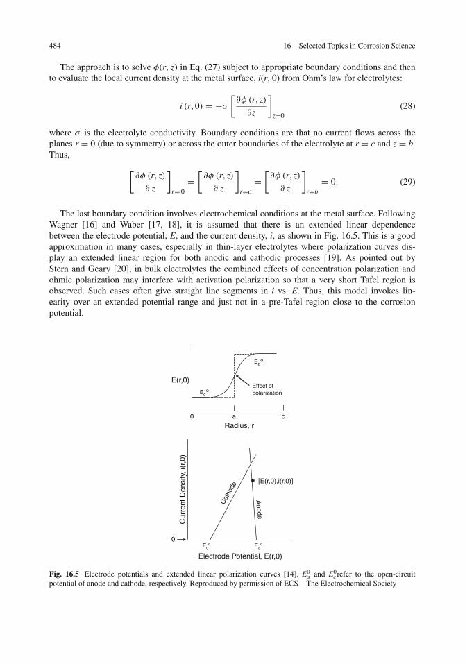
484 16 Selected Topics in Corrosion Science
The approach is to solve φ(r, z) in Eq. (27) subject to appropriate boundary conditions and thento evaluate the local current density at the metal surface, i(r, 0) from Ohm’s law for electrolytes:
i (r, 0) = −σ
[∂φ (r, z)
∂z
]z=0
(28)
where σ is the electrolyte conductivity. Boundary conditions are that no current flows across theplanes r = 0 (due to symmetry) or across the outer boundaries of the electrolyte at r = c and z = b.Thus,
[∂φ (r, z)
∂ z
]r= 0=[∂φ (r, z)
∂ z
]r=c=[∂φ (r, z)
∂ z
]z=b= 0 (29)
The last boundary condition involves electrochemical conditions at the metal surface. FollowingWagner [16] and Waber [17, 18], it is assumed that there is an extended linear dependencebetween the electrode potential, E, and the current density, i, as shown in Fig. 16.5. This is a goodapproximation in many cases, especially in thin-layer electrolytes where polarization curves dis-play an extended linear region for both anodic and cathodic processes [19]. As pointed out byStern and Geary [20], in bulk electrolytes the combined effects of concentration polarization andohmic polarization may interfere with activation polarization so that a very short Tafel region isobserved. Such cases often give straight line segments in i vs. E. Thus, this model invokes lin-earity over an extended potential range and just not in a pre-Tafel region close to the corrosionpotential.
o
Ec
Ea
o
a0 cRadius, r
E(r,0)Effect ofpolarization
Cur
rent
Den
sity
, i(r
,0)
Electrode Potential, E(r,0)
Eco Ea
o
Cat
hode
Anode
[E(r,0),i(r,0)]
0
Fig. 16.5 Electrode potentials and extended linear polarization curves [14]. E0a and E0
c refer to the open-circuitpotential of anode and cathode, respectively. Reproduced by permission of ECS – The Electrochemical Society

Distribution of Current and Potential 485
Thus, the Wagner polarization parameters are defined as
La = σ
∣∣∣∣dE
di
∣∣∣∣a
for the anode (30a)
and
Lc = σ
∣∣∣∣dE
di
∣∣∣∣c
for the cathode (30b)
where σ is the conductivity of the electrolyte. Just outside the electrode surface,
E (r, 0) = V ′ − φ (r, 0) (31)
where V ′ is a constant which includes all the various differences in electrostatic potential across theextra interfaces which are introduced in the measurement of an electrode potential, E, as discussedin Chapter 3. From Fig. 16.5,
di
dE= i (r, 0)
E (r, 0)− E0a
(32)
Equations (28), (30a), (31), and (32) combine to give
φ (r, 0)− La
[∂φ (r, z)
∂ z
]z=0= V ′ − E0
a (33)
Similarly for the cathode,
φ (r, 0)− Lc
[∂φ (r, z)
∂ z
]z=0= V ′ − E0
c (34)
Equations (33) and (34) thus complete the boundary conditions. The solution of Laplace’sequation, i.e., Eq. (27) subject to the boundary conditions in Eqs. (29), (33), and (34) is [14]:
E (r, 0) =(a
c
)2E0
a +(
c2 − a2
c2
)E0
c
+ 2a
c2 (La − Lc)
∞∑n=1
Cn sinh
(xn
b
c
)J1
(xn
a
c
)
−∞∑
n=1
Cn cosh
(xn
b
c
)J0
(xn
r
c
)(35)
where sinh and cosh are the hyperbolic functions given by sinh x = (ex – e−x)/2 and cosh x =(ex + e−x)/2, Jo and J1 are Bessel functions of order 0 and 1, respectively, and xn are the values whereJ1(x)= 0. (Note that the parameter V′ in Eqs. (33) and (34) has vanished enroute to the solution givenby Eq. (35).) The coefficients Cn are generated by a series of n equations, the form of which is givenelsewhere [14]; but in brief, these equations contain the cell dimensions, the Wagner polarizationparameters La and Lc, the quantities E0
a and E0c , and Bessel functions.

486 16 Selected Topics in Corrosion Science
The derivation of Eq. (35) is too detailed to include in this text but is given elsewhere [14]. Themajor point to be taken here is that the potential distribution in Eq. (35) depends both on geometricalfactors (a, b, and c) and on electrochemical factors (La, Lc, E0
a and E0c ). The current distribution
follows from applying Eq. (28) to Eq. (35). The result is [14]
i (r, 0)
σ= 1
c
∞∑n=1
Cnxn sinh
(xn
h
c
)J0
(xn
r
c
)(36)
The total anodic current is obtained from the local anodic current density i(r, 0) by
Ia =∫ a
r=0
∫ 2π
θ=0i (r, 0) r dr dθ (37)
The result is [14]
Ia
σ= 2π a
∞∑n=1
Cn sinh
(xn
b
c
)J1
(xn
a
c
)(38)
Parametric Study
Figure 16.6 shows the electrode potential E(r, 0) for La = 1 cm and Lc = 10 cm for a corrosion cellwith different electrolyte thicknesses. The coefficients Cn were computed up to Cn = 100. It can be
Fig. 16.6 Distribution of electrode potential in a concentric circular cell for La = 1 cm and Lc = 10 cm for differentelectrolyte thicknesses b [14]. (Anode radius a= 0.5 cm, cathode radius c=1.0 cm, Ea
0 = 0.00 V, and Ec0 = 1.00 V.)
Reproduced by permission of ECS – The Electrochemical Society

Distribution of Current and Potential 487
Fig. 16.7 Current distribution corresponding to the potential distribution given in Fig. 16.6 [14]. (Anode radius a =0.5 cm, cathode radius c =1.0 cm, E0
a = 0.00 V, and E0c = 1.00 V.) The electrolyte thickness b in centimeters is given
on the figure. Reproduced by permission of ECS – The Electrochemical Society
seen that the electrode potential is distributed almost uniformly for the bulk electrolyte (large valuesof b), but the potential distribution becomes increasingly non-uniform with decreasing thickness ofthe electrolyte layer.
The corresponding current distributions are shown in Fig. 16.7. The local current densities werecalculated from Eq. (36) with n = 100–125. For the thin layers of electrolyte, there is a pronouncedgeometry effect in which the corrosion attack is concentrated near the anode/cathode juncture.
Figure 16.8 shows the total anodic current calculated from Eq. (38) for two different combina-tions of La and Lc. In both cases, the total current approaches values for the bulk electrolyte for an

488 16 Selected Topics in Corrosion Science
Fig. 16.8 Total anode current computed as a function of electrolyte thickness b for two different combinations of Laand Lc [14]. (Anode radius a = 0.5 cm, cathode radius c =1.0 cm, E0
a = 0.00 V, and E0c = 1.00 V.) Reproduced by
permission of ECS – The Electrochemical Society
electrolyte thickness of about 0.1 cm (or about 1,000 μm). This value is consistent with experimentalresults for iron in thin-layer electrolytes open to the air where the corrosion reaction is under cathodiccontrol. For atmospheric corrosion under thin layers of 0.1 M NaCl, the cathodic polarization curvefor iron was similar to that for the bulk electrolyte for an electrolyte thickness greater than 330 μm[19]; see Fig. 16.9. For iron in 0.6 M NaCl, the thickness of the diffusion layer for oxygen reductionwas calculated in Chapter 8 to be 0.065 cm (650 μm). Thus, the cathodic polarization curve for ironin 0.6 M NaCl will be the same as in the bulk electrolyte for an electrolyte thickness of 650 μm orgreater.
Application to the Experiments of Rozenfeld and Pavlutskaya
Rozenfeld and Pavlutskaya [19] have measured the potential distribution across an iron circularanode in contact with a copper disc in 0.1 M NaCl for both bulk and 165 μm thickness electrolytes.Their experimental results, which are shown in Figs. 16.10 and 16.11, provide an experimentalcomparison for calculations made using the model described above. Figure 16.12 shows cathodicpolarization curves as measured by Rozenfeld [19] for copper in 0.1 M NaCl. For copper in bulk0.1 M NaCl, the cathodic curve is nearly linear over an overvoltage of about 1 V, after which thecurve shifts considerably, as the reaction moves from the region of oxygen reduction into that ofhydrogen evolution. A tangent approximation was drawn to the linear portion of the curve, and thevalue of E0
c was replaced by the value Ec′, which is given by the intersection of the tangent approx-
imation and the potential axis. A similar treatment was done for the polarization curve for copperin 165 μm 0.1 M NaCl, which also displays an extended linear range. Values of Lc were calculatedfrom Eq. (30b) using the slopes of the cathodic polarization curves and handbook values for the

Large Structures and Scaling Rules 489
–100
0
100
200
300
400
–1000–800–600–400–2000
Cur
rent
Den
sity
in μ
A/c
m2
E in mV
Bulk
100 μm
165 μm
330 μm
Fig. 16.9 Cathodic polarization curves of iron in 0.1 M NaCl for different electrolyte thicknesses (electrolyte thick-nesses are shown on the figure). Redrawn from Rozenfeld [19] by permission of © NACE International (1972)
Fig. 16.10 Comparison of the calculated potential distribution [14] and experimental data of Rozenfeld [19] forcircular electrodes in bulk 0.1 M NaCl. Reproduced by permission of ECS – The Electrochemical Society
electrolyte conductivity. The anodic polarization curves for iron in bulk and 165 μm 0.1 M NaClwere analyzed similarly, and Wagner polarization parameters are listed in Table 16.2.
The potential distributions calculated from Eq. (35) for the bulk and 165 mm electrolytes aregiven in Figs. 16.10 and 16.11. It can be seen that there is good agreement between the calculationsand experimental data.
Large Structures and Scaling Rules
The previous examples of systems where there is a non-uniform distribution of electrode potentialand current have concerned electrochemical cells of small size, but there are many practical cases

490 16 Selected Topics in Corrosion Science
Fig. 16.11 Comparison of the calculated potential distribution [14] and experimental data of Rozenfeld [19] forcircular electrodes in 165 μm 0.1 M NaCl. Reproduced by permission of ECS – The Electrochemical Society
0
50
100
150
200
250
300
350
–1200–1000–800–600–400–2000200
Cur
rent
Den
sity
in μ
A/c
m2
E in mV
Bulk
165 μm
Fig. 16.12 Cathodic polarization of copper in 0.1 M NaCl at two different electrolyte film thicknesses [19].Reproduced by permission of © NACE International (1972)
Table 16.2 Experimental parameters from Rozenfeld data [19] used to calculate the potential distribution for an irondisc in a copper annulus
Electrolyte thickness La (iron) cm Lc (copper) (cm) Ea′ (V) Ec
′ (V)
Bulk 0 73 −0.19 0.00165 μm 0 46 −0.15 +0.10
where much larger sizes are involved. These include the cathodic protection of ships, bridges, off-shore platforms, or buried pipelines, as well as galvanic corrosion problems in large-scale structures,such as between a ship’s propeller and hull.
With such complicated geometries, analytical solutions of the type discussed above are difficultif not impossible. Instead, numerical solutions of Laplace’s equation are employed using techniquessuch as the boundary element method, the finite element method, or the finite difference method.

Large Structures and Scaling Rules 491
Standard texts on numerical analysis techniques should be consulted for a description of these meth-ods. The application of the boundary element method to corrosion studies has been discussed byvarious authors [21, 22].
Modeling of the Cathodic Protection System of a Ship
An example of computer modeling of the potential distribution on a large structure is provided bythe work of Lucas et al. [23], who analyzed the performance of a cathodic protection system on thehull of an aircraft carrier hull. The overall length of this type of vessel is 317 m (approximately 1,000ft), and the geometry modeled has the shape shown in Fig. 16.13. Additional corrosion protectionfor the painted hull is provided by an impressed cathodic current protection (ICCP) system, in whichan electrical current is provided to anodes by external power supplies (rather than by the sacrificialaction of zinc anodes).
Z
Y
X
X
Z
Fig. 16.13 The shape of the hull of a vessel for modeling of potential distribution [23]. Figure courtesy of VirginiaG. DeGiorgi, Naval Research Laboratory, Washington D.C., and reproduced by permission of Elsevier Ltd
The ICCP system for the hull consisted of 17 anodes (platinum), placed as follows. Two pairs(four anodes) were located in the fore region of the hull, four anode pairs (eight anodes) were locatedin the mid-region, and two anode pairs and a single mid-line anode (five anodes) were located in thestern region. A certain degree of damaged paint was assumed (either 2.8% or 15%) of the hullsurface.
Laplace’s equation, i.e., Eq. (26) was solved using the boundary element method, using experi-mental electrochemical polarization parameters determined in previous studies. The computationalresults are given in Fig. 16.14, which shows the potential profile along the hull centerline. Potentialvalues of –1.0 V vs. Ag/AgCl (or more negative values) indicate that the ICCP system is operatingproperly.
Figure 16.14 also shows experimentally measured electrode potentials at various locations alonga physical scale model of the hull. These results were obtained after first constructing a scale modelof the carrier hull. Then, zinc anodes were placed on the scale model at positions analogous tothose in the actual full-sized hull, and electrode potentials of the immersed hull were measured vs. aAg/AgCl reference electrode at precise fixed locations on the model hull.

492 16 Selected Topics in Corrosion Science
–3.5
–3.0
–2.5
–2.0
–1.5
–1.0
–0.50 50 100 150 200 250 300
ExperimentalComputational
Pot
entia
l in
V v
s. A
g/A
Cl
Relative Position Along Hull
Fig. 16.14 Potential profiles along the centerline of the hull of a US Navy CVN aircraft carrier for a paint damage of15% of the hull surface. Redrawn from Ref. [23] by permission of Elsevier Ltd
In order to construct a successful scale model, it is necessary not only to scale down the physicaldimensions of the original object but also to scale down the conductivity of the electrolyte, as isdiscussed below.
Scaling Rules
It is often desirable to scale large structures down to a smaller size in order to conduct experimentsin the laboratory (either at bench-top or at a pilot plant scale). However, when scaling down thegeometrical size of an electrolytic cell, the current distribution in the scale model is not accuratelyreproduced unless the electrolyte conductivity is also scaled, as described below.
A suitable scaling parameter is the Wagner number, Wa, given by [24]
Wa = Ract
Rohm(39)
where Ract is the activation resistance and Rohm is the ohmic resistance. The Wa number indicateswhether the current density is under kinetic control and therefore relatively uniform, or whether it isunder ohmic control and therefore more non-uniform, being dependent on the cell configuration.
The ohmic resistance is given by
Rohm = �
σA(40)
where σ is the conductivity of the electrolyte, A is the area, and � is a characteristic length whichdepends on the cell configuration. (For parallel plate electrodes, for example, � is the distancebetween electrodes.)
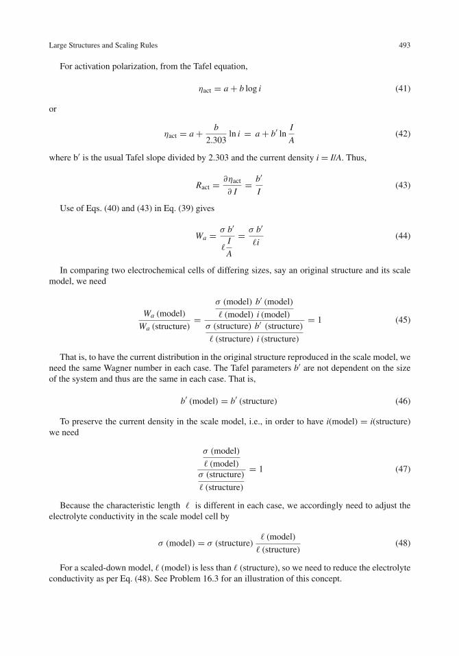
Large Structures and Scaling Rules 493
For activation polarization, from the Tafel equation,
ηact = a+ b log i (41)
or
ηact = a+ b
2.303ln i = a+ b′ ln I
A(42)
where b′ is the usual Tafel slope divided by 2.303 and the current density i = I/A. Thus,
Ract = ∂ηact
∂ I= b′
I(43)
Use of Eqs. (40) and (43) in Eq. (39) gives
Wa = σ b′
�I
A
= σ b′
�i(44)
In comparing two electrochemical cells of differing sizes, say an original structure and its scalemodel, we need
Wa (model)
Wa (structure)=
σ (model) b′ (model)
� (model) i (model)σ (structure) b′ (structure)
� (structure) i (structure)
= 1 (45)
That is, to have the current distribution in the original structure reproduced in the scale model, weneed the same Wagner number in each case. The Tafel parameters b′ are not dependent on the sizeof the system and thus are the same in each case. That is,
b′ (model) = b′ (structure) (46)
To preserve the current density in the scale model, i.e., in order to have i(model) = i(structure)we need
σ (model)
� (model)σ (structure)
� (structure)
= 1 (47)
Because the characteristic length � is different in each case, we accordingly need to adjust theelectrolyte conductivity in the scale model cell by
σ (model) = σ (structure)� (model)
� (structure)(48)
For a scaled-down model, � (model) is less than � (structure), so we need to reduce the electrolyteconductivity as per Eq. (48). See Problem 16.3 for an illustration of this concept.

494 16 Selected Topics in Corrosion Science
Acid–Base Properties of Oxide Films
The properties of oxide films are important in a number of corrosion phenomena, including passivityand its breakdown, corrosion inhibition by organic molecules, and the adhesion of organic coatings.In previous chapters, we have briefly mentioned that the acid–base properties of oxide film areimportant in the pitting of passive films (Chapter 10) and in the adhesion of an organic coating ontoan oxide-covered metal surface (Chapter 13).
Surface Hydroxyl Groups
It is well known that oxide surfaces or oxide-covered metals exposed to either the ambient environ-ment or immersed in aqueous solutions terminate in an outermost layer of hydroxyl groups due totheir interaction with water molecules [25, 26]. The reaction of a surface oxide with a water moleculeis shown in Fig. 16.15. Using quantitative X-ray photoelectron spectroscopy, the concentration ofsurface hydroxyls in the air-formed oxide films on various metals has been found to be 6–20 OHgroups/nm2 [27]. The depth of the hydroxylated region extends 5–8 Å into the oxide. Although thesurface hydroxyl layer is quite thin, it nonetheless has a large influence on the properties of the oxidefilm, especially on its surface charge.
M
O
M
O
M
O
M
O
H2O
H
OH
Oxide
Metal
Oxide
Metal
M M
O
OHOH
Oxide
Metal
Fig. 16.15 Interaction of a water molecule with the oxide film on a metal
In aqueous solutions, the surface hydroxyl groups may remain undissociated. In such an instance,the oxide surface is said to be at its isoelectric point (IEP) and will have a net surface charge of zero.This will occur only if the pH of the aqueous solution has the same value as the isoelectric point ofthe oxide. It is more likely, however, that the oxide film will be charged. If the pH is less than theisoelectric point, the surface will acquire a positive charge:
−MOHsurf + H+(aq)�−MOH+2 surf (49)
where M denotes a surface site occupied by a metal cation. If the pH is greater than the isoelectricpoint, the surface will acquire a negative charge:
−MOHsurf + OH− � −MO−surf+H2O
or
−MOHsurf � −MO−surf+H+ (aq) (50)

Acid–Base Properties of Oxide Films 495
In the above reactions the surface species –MOH2+ is a Bronsted acid because it is a proton donor
(in the reverse direction of Eq. (49)), and –MO− is a Bronsted base in Eq. (50) (reverse direction)because it is a proton acceptor. The surface species -MOH is amphoteric, being a Bronsted base inEq. (49) (forward direction) and a Bronsted acid in Eq. (50) (forward direction).
Nature of Acidic and Basic Surface Sites
A broadened view of acids and bases has been given by G.N. Lewis, in which a Lewis acid is anelectron acceptor and a Lewis base is an electron donor [28, 29]. This definition allows a wide varietyof molecules, ions, and compounds to be classified as Lewis acids or Lewis bases. With this in mind,the following lists the types of acid sites on metal oxide surfaces:
(1) unhydroxylated metal ions, M+δS
(2) protonated surface hydroxyls, −MOH2+
surf
−MOH+2 surf →−MOHsurf + H+ (aq)
(3) surface hydroxyls, -MOHsurf
−MOHsurf →−MO−surf + H+(aq)
where δs is the partial charge on a metal surface ion. The first of these acid sites above is a Lewisacid because the metal ion M+δS can accept electrons [30,31].
The basic sites on metal oxides are [30, 31]
(4) unhydroxylated oxygen anions, O−γS
(5) dissociated surface hydroxyls, –MO−surf
−MO−surf + H+(aq)→−MOHsurf
(6) surface hydroxyls, –MOHsurf
−MOHsurf + H+(aq)→−MOH+2 surf
where γs is the partial charge a surface oxygen anion. The first of these basic sites above is a Lewisbase because the oxygen anion O−γS can be an electron donor.
While all these different types of acid or basic sites are possible, the acid–base properties of theoxide are usually dominated by the behavior of the hydroxyl groups.
Isoelectric Points of Oxides
The isoelectric point of an oxide or oxide film can be measured in several different ways. Onemethod is to measure the zeta potential, i.e., the potential drop across the diffuse part of the electrical

496 16 Selected Topics in Corrosion Science
double layer, as a function of the pH of the electrolyte. This can be done by streaming potentialmeasurements [32, 33], in which the aqueous phase is forced to flow across a fixed solid. The zetapotential goes through zero at the isoelectric point of the solid surface.
Another method is to measure contact angles of aqueous droplets on the oxide-covered metalsurface [34–37]. In this approach, contact angles are measured at the hexadecane/aqueous solutioninterface, as shown in Fig. 16.16. The pH of the aqueous phase is varied, and the contact angle isobserved to go through a maximum at the isoelectric point of the oxide film, as shown in Fig. 16.17.Details are given elsewhere [35–37].
Liquid θθ
Hexadecane
Aqueoussolution
Metal
Oxide film
Hexadecane
Fig. 16.16 Schematic diagram showing the contact angle of an aqueous droplet in a two-liquid–solid system. Theisoelectric point of the oxide film is determined by measuring the contact angle as a function of the pH of the aqueousdroplet
0
5
10
15
20
25
–2 0 2 4 6 8 10 12 14
Con
tact
Ang
le in
Deg
rees
pH of Aqueous Phase
I.E.P.
Fig. 16.17 Contact angles for a chromium-plated steel (ferrotype) at the hexadecane/aqueous solution interface, as afunction of the pH of the aqueous phase [35, 36]. The maximum in the contact angle gives the isoelectric point (IEP)of the solid surface, i.e., of the oxide film on chromium. Reproduced by permission of Elsevier Ltd
Table 16.3 lists the isoelectric points (IEP) for various bulk oxides and oxide films. The isoelectricpoint is a function of the identity of the individual cation in the M-OH bond. Oxides with an IEP lessthan 7 are acidic oxides and oxides with an IEP greater than 7 are basic oxides. It can be seen thatthere is a wide range in the IEP values for metals. For instance, tantalum which is a passive metalhas an oxide which is acidic and aluminum which is used in many applications in neutral solutionshas an oxide which is basic. Much more data are available on bulk oxides than on intact oxide films,but in general, the IEP of an oxide film is similar to that for the stand-alone bulk oxide [37, 38].

Acid–Base Properties of Oxide Films 497
Table 16.3 Isoelectric points of oxides and oxide films
Oxide Isoelectric point References
Oxide film on Ta −0.7 McCafferty and Wightman[36, 37]
IrO2 0.5 Ardizzone and Trasatti [56]MoO3 1.8−2.1 Compiled by Natishan [49]SiO2 1.8–2.2 Compiled by Natishan [49]Ta2O5 2.8 Compiled by Natishan [49]Oxide film on 316
stainless steel4.2–5.2 Kallay et al. [57]
MnO2 4.7–4.8 Tamura et al. [58]Oxide film on Ti 2
4.2 (revised value)Kallay et al. [59]McCafferty et al. [60]
TiO2 5.0–6.5 Ardizzone and Trasatti [56]SnO2 5–6 Arai et al. [61]Oxide film on Cr 5.2–5.3 McCafferty and Wightman
[36, 37]CeO2 5.2–6.1 Hsu et al. [62]ZrO2 5.5–6.3 Compiled by Natishan [49]Cr2O3 6.2–6.3 Compiled by Natishan [49]NiO 7.3
8.2–8.6Moriwaki et al. [63]Kokarev et al. [64]
Fe2O3 7.58.7
Yates and Healy [65]Moriwaki et al. [63]Smith and Salman [66]
CuO 8.5–9.5 Compiled by Kosmulski [67]Al2O3 9.0–9.4 Compiled by Natishan [49]Oxide film on Al 9.5 McCafferty and Wightman
[36, 37]ZnO 9.2–10.3 Compiled by Natishan [49]Oxide film on iron 9.8
10.0Kurbatov [68]Simmins and Beard [69]
CdO 10.3 Janusz [70]MgO 12.4 Compiled by Natishan [49]
Surface Charge and Pitting
Figure 16.18 illustrates the surface charge character of several oxides. As seen in the diagram, in asolution of pH 7, the surface of aluminum oxide (and oxide-covered aluminum) consists of acidicgroups (positively charged =AlOH2
+) onto which Cl– ions will adsorb. As discussed in Chapter10, aluminum is susceptible to pitting corrosion; and the adsorption of Cl− ions is the first step inthe pitting process. However, for other oxides, such as tantalum oxide, the surface consists of basicgroups (negatively charged TaO−), so that Cl− adsorption and its subsequent penetration through theoxide film is less favored. Thus, it is necessary to polarize tantalum further in the positive directionto initiate the pitting process. Hence, tantalum has a higher (more positive) pitting potential thanaluminum.
Figure 16.19 shows pitting potentials as a function of the isoelectric point of the oxide for variousmetals in 1 M NaCl [38]. It can be seen that the pitting potential increases as the oxide IEP decreases,in accordance with the surface charge character of the various oxides.
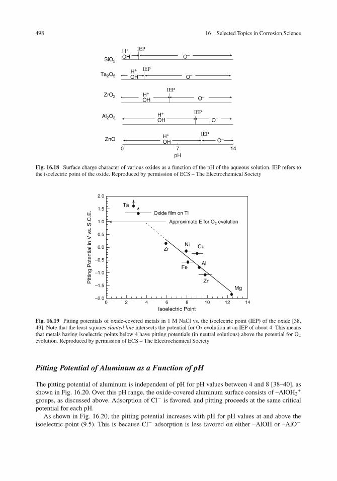
498 16 Selected Topics in Corrosion Science
SiO2
Ta2O5
IEP
O–
O–
O–
O–
O–
Al2O3
pH
IEPZrO2
O
ZnOIEP
0 147O
IEP
O
O
IEP
OHH+
H+
H+
H+
H+
H
H
H
H
Fig. 16.18 Surface charge character of various oxides as a function of the pH of the aqueous solution. IEP refers tothe isoelectric point of the oxide. Reproduced by permission of ECS – The Electrochemical Society
–2.0
–1.5
–1.0
–0.5
0.0
0.5
1.0
1.5
2.0
0 2 4 6 8 10 12 14
Pitt
ing
Pot
entia
l in
V v
s. S
.C.E
.
Isoelectric Point
Mg
Al
Zn
Cu
Fe
NiZr
Approximate E for O2 evolution
Oxide film on Ti
Ta
Fig. 16.19 Pitting potentials of oxide-covered metals in 1 M NaCl vs. the isoelectric point (IEP) of the oxide [38,49]. Note that the least-squares slanted line intersects the potential for O2 evolution at an IEP of about 4. This meansthat metals having isoelectric points below 4 have pitting potentials (in neutral solutions) above the potential for O2evolution. Reproduced by permission of ECS – The Electrochemical Society
Pitting Potential of Aluminum as a Function of pH
The pitting potential of aluminum is independent of pH for pH values between 4 and 8 [38–40], asshown in Fig. 16.20. Over this pH range, the oxide-covered aluminum surface consists of –AlOH2
+
groups, as discussed above. Adsorption of Cl− is favored, and pitting proceeds at the same criticalpotential for each pH.
As shown in Fig. 16.20, the pitting potential increases with pH for pH values at and above theisoelectric point (9.5). This is because Cl− adsorption is less favored on either –AlOH or –AlO−
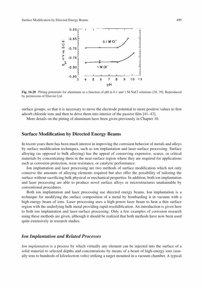
Surface Modification by Directed Energy Beams 499
Fig. 16.20 Pitting potentials for aluminum as a function of pH in 0.1 and 1 M NaCl solutions [38, 39]. Reproducedby permission of Elsevier Ltd
surface groups, so that it is necessary to move the electrode potential to more positive values to firstadsorb chloride ions and then to drive them into interior of the passive film [41–43].
More details on the pitting of aluminum have been given previously in Chapter 10.
Surface Modification by Directed Energy Beams
In recent years there has been much interest in improving the corrosion behavior of metals and alloysby surface modification techniques, such as ion implantation and laser-surface processing. Surfacealloying (as opposed to bulk alloying) has the appeal of conserving expensive, scarce, or criticalmaterials by concentrating them in the near-surface region where they are required for applicationssuch as corrosion protection, wear resistance, or catalytic performance.
Ion implantation and laser processing are two methods of surface modification which not onlyconserve the amounts of alloying elements required but also offer the possibility of tailoring thesurface without sacrificing bulk physical or mechanical properties. In addition, both ion implantationand laser processing are able to produce novel surface alloys or microstructures unattainable byconventional procedures.
Both ion implantation and laser processing use directed energy beams. Ion implantation is atechnique for modifying the surface composition of a metal by bombarding it in vacuum with ahigh-energy beam of ions. Laser processing uses a high-power laser beam to heat a thin surfaceregion with the underlying bulk metal providing rapid resolidification. An introduction is given hereto both ion implantation and laser-surface processing. Only a few examples of corrosion researchusing these methods are given, although it should be realized that both methods have now been usedquite extensively in research studies.
Ion Implantation and Related Processes
Ion implantation is a process by which virtually any element can be injected into the surface of asolid material to selected depths and concentrations by means of a beam of high-energy ions (usu-ally tens to hundreds of kiloelectron volts) striking a target mounted in a vacuum chamber. A typical

500 16 Selected Topics in Corrosion Science
Fig. 16.21 A typical ion implantation apparatus. Ions of a chemical species are obtained by bombarding an appro-priate material with an electron beam to create a plasma. An electric field at the extraction electrode extracts the ionsfrom the plasma. The ions are then focused and accelerated with magnetic and electric fields before bombarding thematerial to be surface modified [44]
ion implantation system is shown schematically in Fig. 16.21 [44]. Atoms of a selected chemicalelement are ionized by collisions with electrons in an electrical discharge in a gas at a low pres-sure in the ion source. The ions are electrostatically extracted though an orifice into a high-vacuumregion to a moderate energy, are further separated by isotope mass, are accelerated to the desiredenergy, and are focused. Farther down the line the beam is rastered to ensure that a uniform distribu-tion of ions is implanted laterally into the target metal surface. Areas to be implanted are typicallyseveral square inches, although larger areas can be implanted by rotation of the sample through theion beam.
The bombarding ions lose energy in collisions with substrate electrons and atoms. Penetrationdepths of tens to thousands of angströms are achieved before incident ions lose all their energyand come to a rest in the solid. The depth of penetration depends on the accelerating voltage, themass of the ion, and the atomic mass of the substrate. The maximum concentration of implantedions is generally located beneath the substrate surface, and the depth–concentration profile follows aGaussian distribution. The surface concentration of implanted ions that can be achieved ranges fromextremely dilute alloys to 50 at.% alloys.
Table 16.4 summarizes the various characteristics of the ion implantation process and Table 16.5lists advantages of the ion implantation approach. One of the major disadvantages of ion implantationis in the shallow depth of the surface-modified region.
Two related extensions of ion implantation are ion beam mixing and ion beam-assisted deposition,each of which can extend the depth of the modified region.
In ion beam mixing, a sputter-deposited or sputter-evaporated thin film of thickness several hun-dreds to thousands of angströms is induced to intermix with the substrate using collisional cascadesgenerated by an implanted ion, which may be either an inert ion (e.g., a noble gas) or may be an

Surface Modification by Directed Energy Beams 501
Table 16.4 Ion implantation parameters
Implanted elements Virtually any element can be implantedIon energy Normally 2–200 keVImplantation depth Varies with ion energy, ion species, and host
material. Ranges from 100 to 1,000 ÅRange distribution Approximately Gaussian. Choice of energies
allow tailored depth distributionConcentration From trace amounts up to 50 at.%Host material Any solid material can be implanted
Table 16.5 Advantages of ion implantation
1. No sacrifice of bulk properties2. Rare, expensive, or critical materials can be conserved by concentrating them in the surface3. Solid solubility limit can be exceeded4. Metastable phases and amorphous phases can be produced which are often unattainable by
conventional alloying techniques5. No change in sample dimensions or grain sizes6. Depth–concentration distribution is controllable (within limits)
ion of one of the desired constituents of the surface alloy. Ion beam mixing retains all the advan-tages of ion implantation (provided that complete mixing can be achieved) and in addition allowsthe possibility of producing a thicker surface alloy than can be provided by ion implantation alone.
Ion beam-assisted deposition (IBAD) is a process which combines physical vapor deposition(PVD) and ion implantation. The result is to produce coatings which are much thicker (of the orderof microns) than the surface alloys produced by ion implantation. In addition, IBAD coatings havea greater adhesion than PVD coatings due to the partial mixing of the coating with the substrate bythe energetic ion source.
Applications of Ion Implantation
Modification of the corrosion behavior of metal surfaces by ion implantation using accelerated ionbeams was first achieved in the 1970s in England in collaborative efforts between scientists at theUniversity of Manchester Institute of Science and Technology and Salford University. Concertedefforts were also established about the same time at various research institutions, notably the HarwellLaboratory in England, the University of Heidelberg in Germany, and the Naval Research Laboratoryin the United States. The use of ion implantation to improve the corrosion behavior of iron andsteel, stainless steels, and aluminum for the period 1985–2000 has been treated in a review article[45]. Between 1985 and 2000, 35 different elements were implanted into iron, stainless steels, oraluminum in regard to corrosion studies, as shown in Fig. 16.22.
Ion implantation can be used to alter either the anodic or cathodic half-cell reaction. A goodexample of the first approach is given by the early implantation studies of Ashworth et al. [46]who were the first to show that the ion implantation of chromium into iron produced passive Fe–Crsurface alloys similar to the corresponding conventional bulk alloys. Cr-implantation decreased thecritical anodic current density for passivation in an acetate buffer but had little or no effect on thecathodic polarization curves.

502 16 Selected Topics in Corrosion Science
I AII
A
III A
IV
AV A
VI A
VII A
VII
I
A2 H
e3 Li
5 B6 C
7 N8 O
10 Ne
12 Mg
III B
IV
BV B
VI B
VII B
VII
IB
VII
IB
VII
IB
I BII B
13 Al
14 Si
15 P16 S
18 Ar
22 Ti
24 Cr
27 Co
28 Ni
29 Cu
30 Zn
33 As
36 Kr
39 Y40 Z
r41 N
b42 M
o46 P
d47 A
g51 S
b54 X
e73 Ta
74 W79 A
u
58 Ce
68 Er
70 Yb
Fig. 16.22 Elements which have been implanted into iron, low alloy steels, stainless steels, or aluminum (1985–2000) and their locations on the periodic table (group numbers and atomic numbers are also shown). Reproduced bypermission of © NACE International
One of the earliest examples which used ion implantation to modify corrosion behavior by alter-ation of the cathodic process is provided by work [47, 48] on the corrosion of titanium in hot acids.Ion implantation of Pd into titanium produced surface alloys which decreased the corrosion rate ina manner similar to that for Pd–Ti bulk alloys.

Surface Modification by Directed Energy Beams 503
0.1
1
10
100
1000
10000
–1.5–1–0.500.5
Titanium
Ion beam mixed Pd-Ti
Pd-implantedtitanium
E in V vs. Hg2SO4
Anodic
Cur
rent
Den
sity
in μ
A/c
m2
0
0.1
1
10
100
1000
10000
–1.5–1–0.500.5
Cur
rent
Den
sity
in μ
A/c
m2 Anodic curve
for Ti
Cathodic curve for Pd
Ecorr
Pd-TiAnodic Cathodic
Fig. 16.23 (Top): Experimental anodic polarization curve for titanium in boiling 1 M H2SO4 and the cathodic polar-ization curve for palladium. The corrosion potential for a Pd–Ti alloy is indicated on the figure for alloy having equalareas of Pd and Ti. (Bottom): Anodic polarization curves for titanium, ion-beam mixed Pd–Ti, and for Pd-implantedtitanium [47, 48]. Reproduced by permission of Elsevier Ltd
Figure 16.23 shows anodic polarization curves for titanium, Pd–implanted titanium, and ionbeam mixed Pd-Ti surface alloys in boiling 1 M H2SO4. It can be seen that titanium can be pas-sivated but only after extensive anodic polarization before undergoing an active/passive transition.(Enroute to the passive state, the titanium surface suffers considerable corrosion damage). By con-trast, each of the two Pd–Ti surface alloys self-passivates, and each displays low anodic currentdensities.
This behavior is similar to that for Pd–Ti bulk alloys, as has been discussed in Chapter 9 in thesection “Passivity by Alloying with Noble Metals”; see Figs. 9.45 and 9.46. Hydrogen reductionpredominates on palladium sites rather than on titanium so that the resulting mixed potential for thesurface alloy (or bulk alloy) occurs in the passive region for titanium rather than in its active region.
Ion implantation has also been used to increase the pitting resistance of aluminum. As shownin Fig. 16.24, implantation of Mo or Si into aluminum resulted in increases in the pitting poten-tial in 0.1 M NaCl [49]. (Implantation of Al into aluminum had no effect on the pitting potential,

504 16 Selected Topics in Corrosion Science
0
0
0.1
1
10
100
1000
–1.20 –1.00 –0.80 –0.60 –0.40 –0.20 0.00
Cur
rent
Den
sity
in μ
A /c
m2
E in V vs. S.C.E.
Zn into Al
Si into Al
Mo into AlAluminum
Anodic
Fig. 16.24 Anodic polarization curves in de-aerated 0.1 M NaCl for unimplanted aluminum and for aluminumimplanted with various ions [49]. Reproduced by permission of ECS – The Electrochemical Society
thus showing that the changes in pitting potential are chemical effects rather than physical effectsintroduced by the damage of the implantation process.)
XPS surface analysis has shown that the implanted ions are contained in the oxide film as wellas in the underlying metal. This means that some of the aluminum–oxygen ionic bonds in the oxidefilm have been replaced with bonds formed between oxygen ions and the implanted cation. That is,the properties of the oxide film are modified by the ion implantation process.
Increases (or decreases) in pitting potential by ion implantation can be explained by two effects[37–39, 49, 50]. Ion implantation can change (i) the surface charge on the oxide film and (ii) theconcentration of oxygen vacancies in the film. The first effect is related to the adsorption of Cl− ionson the oxide surface and the second effect to the transport of Cl− ions through the oxide film. Eachof these two effects is discussed below.
Figure 16.25 shows the pitting potential of ion-implanted aluminum as a function of the isoelectricpoint (IEP) of the oxide of the implanted ions. (There is some scatter in the data because the varioussamples did not all receive the same dose of implanted ions.) Implantation into aluminum of metalssuch as Mo, Si, Nb, Ta, Cr, and Zr (all with oxides having a isoelectric point lower than that ofAl2O3) resulted in an increase in the pitting potential, i.e., an increase in the resistance to pittingattack. Conversely, implantation with Zn or Li (whose oxides have a higher isoelectric point thanthat of Al2O3) decreased the pitting potential.
Ion implantation changes the surface charge of the oxide, as has been shown elsewhere [36, 37]. Ithas been shown that the IEP of aluminum is 9.5, of tantalum is –0.7, and of Ta-implanted aluminumis 5.0 [36, 37]. In each case the metals are actually oxide-covered so that the IEP values refer to theoxide films. Thus, the effect of implantation of Ta into aluminum is to change the surface charge atpH 7 from positive AlOH2
+ groups to negative AlO− or TaO− surface groups, as per Fig. 16.18, sothat the adsorption of Cl− ions is less favored on the Ta-implanted surface.
Once initiated, corrosion pits were observed to propagate through the thickness of the ion-implanted region. Thus, the role of the implanted ion appears to be that of modifying the surfacechemistry of the oxide film rather than providing an underlying substrate which is resistant topropagation in the occluded cell environment.
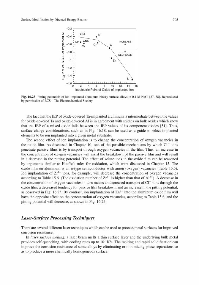
Surface Modification by Directed Energy Beams 505
–1.6
–1.4
–1.2
–1
–0.8
–0.6
–0.4
–0.2
0 2 4 6 8 10 12 14 16
Isoelectric Point of Oxide of Implanted Ion
Epi
t in
V v
s. S
.C.E
. of I
mpl
ante
d A
lZn
Li
AlCr
Si Zr
Ta
NbMo INCREASE
DECREASE
Fig. 16.25 Pitting potentials of ion-implanted aluminum binary surface alloys in 0.1 M NaCl [37, 38]. Reproducedby permission of ECS – The Electrochemical Society
The fact that the IEP of oxide-covered Ta-implanted aluminum is intermediate between the valuesfor oxide-covered Ta and oxide-covered Al is in agreement with studies on bulk oxides which showthat the IEP of a mixed oxide falls between the IEP values of its component oxides [51]. Thus,surface charge considerations, such as in Fig. 16.18, can be used as a guide to select implantedelements to be ion implanted into a given metal substrate.
The second effect of ion implantation is to change the concentration of oxygen vacancies inthe oxide film. As discussed in Chapter 10, one of the possible mechanisms by which Cl− ionspenetrate passive films is by transport through oxygen vacancies in the film. Thus, an increase inthe concentration of oxygen vacancies will assist the breakdown of the passive film and will resultin a decrease in the pitting potential. The effect of solute ions in the oxide film can be reasonedby arguments similar to Hauffe’s rules for oxidation, which were discussed in Chapter 15. Theoxide film on aluminum is an n-type semiconductor with anion (oxygen) vacancies (Table 15.5).Ion implantation of Zr4+ ions, for example, will decrease the concentration of oxygen vacanciesaccording to Table 15.6. (The oxidation number of Zr4+ is higher than that of Al3+). A decrease inthe concentration of oxygen vacancies in turn means an decreased transport of Cl− ions through theoxide film, a decreased tendency for passive film breakdown, and an increase in the pitting potential,as observed in Fig. 16.25. By contrast, ion implantation of Zn2+ into the aluminum oxide film willhave the opposite effect on the concentration of oxygen vacancies, according to Table 15.6, and thepitting potential will decrease, as shown in Fig. 16.25.
Laser-Surface Processing Techniques
There are several different laser techniques which can be used to process metal surfaces for improvedcorrosion resistance.
In laser surface melting, a laser beam melts a thin surface layer and the underlying bulk metalprovides self-quenching, with cooling rates up to 107 K/s. The melting and rapid solidification canimprove the corrosion resistance of some alloys by eliminating or minimizing phase separations soas to produce a more chemically homogeneous surface.

506 16 Selected Topics in Corrosion Science
Laser surface alloying consists of melting the surface of a metal, adding known amounts ofother metals, mixing these components, and alloying them to resolidify. This process producesa surface layer with chemical composition and properties which are different from the substratematerial. The surface alloy is also metallurgically bonded to the substrate and has a high degree ofadhesion.
Laser melt–particle injection consists of melting a shallow pool on the surface of a metal whichis translated under the laser beam and of blowing particles into the melt pool from a nearby finenozzle. The injected particles may melt completely to form a surface alloy upon resolidification orthey may melt only partially so as to be built up as a coating.
In laser consolidation of coatings, a coating previously applied by a process such as flame spray-ing or plasma spraying is laser remelted to remove residual porosity. (The corrosion behavior oflaser-melted titanium coatings has been discussed in Chapter 5.)
A typical experimental apparatus used for surface processing using kilowatt power continuouslasers is shown in Fig. 16.26 [52]. The focusing element is a single spherical mirror which is usedto obtain a sharply focused laser beam. Test specimens are mounted on a rotating turntable, swept
Turningmirror
Focusingmirror
Specimen
Protective gas shield
Turntable
Motor
Laser beam
Fig. 16.26 (Top): Schematic diagram of a continuous-wave high-power laser-processing apparatus [52]. (Bottom):Schematic diagram showing melt stripes, surface ripples, and chevron marks in the laser-surface-melted regionReproduced by permission of ECS – The Electrochemical Society

Surface Modification by Directed Energy Beams 507
though the focused beam, and protected during the processing by a flowing helium gas shield. Thelaser beam rapidly melts a small volume of metal, which subsequently rapidly solidifies by con-duction of heat to the bulk specimen. Each pass results in the processing of a ribbon of material,typically 0.25 mm wide and 0.1 mm deep. The width and depth of such a ribbon is varied by changingthe processing conditions, such as sweep speed, laser power, or spot diameter. Complete coverageof a large surface is obtained by using successive passes spaced a fraction of a pass width fromone another. Table 16.6 lists typical processing conditions for surface modification for corrosionapplications [53].
Table 16.6 Typicallaser-processing conditionsusing a high-powercontinuous-wave laser forsurface modification forcorrosion applications [53]
Output power 7.5 kWSpot diameter 0.15 mmAverage power
density4 × 107 W/cm2
Sweep speed 50 cm/sInteraction time 0.6 msTime metal is molten 1 msMelt depth 50 μmMelt width 260 μmCooling rate 107 K/s
Applications of Laser-Surface Processing
Only two examples of corrosion research are given here, one involving laser surface melting and asecond involving laser surface alloying. (Chapter 5 has already considered an additional applicationon laser consolidation of coatings.)
Figure 16.27 shows a cross section of laser-melted 304 stainless steel sample. The overlappingmelt stripes can be clearly seen in the figure, which also shows that the growth in the resolidified meltis epitaxial, extending from grains in the base metal. Table 16.7 shows the effect of laser-processing
Fig. 16.27 Cross section of a laser-surface-melted 304 stainless steel showing the overlapping melt stripes and char-acteristic surface ripples due to laser processing. The epitaxial resolidification of the laser-melted region can also beseen [52]. Reproduced by permission of ECS – The Electrochemical Society

508 16 Selected Topics in Corrosion Science
Table 16.7 Pitting potentials for 304 stainless steel in 0.1 M NaCl at various anodic sweep rates [52]
Pitting potential in V vs. SCEa
1 mV/min 10 mV/min 100 mV/min
Type 304stainless steel
+0.28 +0.28 +0.28
Laser-processedtype 304stainless steel
+0.50+0.58+0.80
+0.48+0.50+0.80+0.80
+0.80
aEach entry in the table represents a separate experiment.
on pitting potentials obtained in 0.1 M NaCl [52]. For the laser processed stainless steels, sampleswere polished past the surface ripples but only partially through the melt zone to provide a smoothfinish. There is some scatter in the pitting potentials of the laser-processed stainless steel, but theeffect of laser processing is clearly to increase the pitting potential by 200–500 mV.
The reason for the increase in pitting potential is due to the redistribution or possible eliminationof sulfide inclusions from the stainless steel. The role of sulfide inclusions in contributing to thebreakdown of passivity on stainless steels has been discussed in Chapter 10, and an SEM micrographof a typical sulfide inclusion on type 304 stainless steel has been shown previously in Fig. 10.36.These MnS particles were not detected after laser processing, and sulfur levels were reduced, asdetermined by electron microprobe analysis. Thus, the sulfide inclusions were melted during laserprocessing and are either eliminated or are redistributed into a larger number of smaller particles[52].
The preparation and characterization of laser-alloyed stainless steels was first carried out bygroups at the Naval Research Laboratory [52, 53] and at Rockwell International [54, 55]. McCaffertyand Moore [52, 53] laser alloyed Mo into 304 stainless steel to produce Fe–Cr–Ni–Mo surfacealloys. Two types of alloys were prepared: Fe-18 Cr-10 Ni-3 Mo, which is within the specifica-tions for bulk 316 stainless steel (which is often used instead of 304 stainless steel when improvedresistance to pitting is needed), and Fe-19 Cr-12 Ni-9 Mo. These surface alloys were produced bysputter depositing up to 30 alternating layers of pure Mo and Ni–Cr alloys on a type 304 stainlesssubstrate. (The Ni–Cr layers were provided to maintain the Ni and Cr levels in the surface alloyupon melting and mixing.) Details are given elsewhere [52, 53]. These specimens were laser sur-face melted to an initial depth of 150 μm followed by a second laser processing at a shallowerdepth of 100 μm two or more times to further homogenize the composition of the resulting surfacealloy.
Figure 16.28 shows a cross section through the 3% Mo surface alloy. (The sample had beenetched to bring out its structure.) The outlines of the various melt passes can be shown in thefigure. Figure 16.29 shows electron microprobe traces taken across the 3% Mo surface alloy.It can be seen that Mo is distributed evenly throughout the surface alloy, except at the bottomof the laser-melted region. Molybdenum was also distributed uniformly throughout the 9% Moalloy.
The anodic behavior of the two surface alloys in 0.1 M NaCl is shown in Fig. 16.30. The pittingpotential of the 3% Mo surface alloy is similar to that for bulk 316 stainless steel (which contains2–3% Mo). The 9% Mo surface alloy did not undergo pitting up to potentials of oxygen evolution.The compositions and the pitting potentials are summarized in Table 16.8.

Surface Modification by Directed Energy Beams 509
Fig. 16.28 Cross section of 3% Mo laser-surface alloy showing overlapping sets of melt passes due to deep alloyingand shallower homogenization [52]. Reproduced by permission of ECS – The Electrochemical Society
Fig. 16.29 Electron microprobe traces across the 3% Mo surface alloy. The inset to the right shows the outline of thelaser-surface alloy [52]. Reproduced by permission of ECS – The Electrochemical Society
Thus, the 3% Mo surface alloy prepared by laser surface alloying exhibits both a surface compo-sition and a pitting potential equivalent to type 316 stainless steel, but conserves the amount of Morequired by restricting its presence to the near-surface region. The rapid solidification feature of laseralloying enables production of a surface stainless steel containing 9% Mo, an amount in excess ofthat attainable by conventional alloying techniques. The improved pitting resistance of the 9% Mosurface alloy is comparable to that normally obtained with higher alloys containing larger amountsof Cr and Ni. Thus, the use of 9% Mo surface alloy also minimizes the amount of Cr and Ni required,thus conserving these alloying elements in addition to conserving Mo.
Comparison of Ion Implantation and Laser–Surface Processing
These two surface modification techniques are complementary in nature. The depth of the surface–modified region is greater with laser processing, but the surface is roughened with characteristic

510 16 Selected Topics in Corrosion Science
0.01
0.1
1
10
100
1000
104
–0.50 0.00 0.50 1.00 1.50
Cur
rent
Den
sity
in μ
A /c
m2
E in V vs. S.C.E.
9% Mo Surface alloy
3% MoSurface alloy
EpitEpit
316 Stainless steel(2-3% Mo) Anodic
Fig. 16.30 Anodic polarization curves of Fe–Cr–Ni–Mo alloys in de-aerated 0.1 M NaCl [52]. Reproduced bypermission of ECS – The Electrochemical Society
Table 16.8 Summary of composition of Fe–Ni–Cr–Mo alloys and pitting potentials in 0.1 M NaCl [52]
Alloy Cr Ni Mo Epit in V vs. SCE
304 stainless steel 18–20 8–10 0 +0.300316 stainless steel 16–18 10–14 2–3 +0.5503% Mo surface alloy 18.9 9.1 3.7 +0.5009% Mo surface alloy 19.2 11.7 9.6 Did not pit
surface ripples. With ion beam processing, there is no effect on surface topography, although themodified region is much shallower. Ion implantation, its related techniques, and laser surface pro-cessing are still primarily research techniques, but each offers the possibility of a new approach tocorrosion protection.
Problems
Electrode kinetics
1. Given the following corrosion mechanism for a univalent metal ion
M+ H2O1�−1
M (H2O)ads
M (H2O)ads2�−2
M(OH−
)ads+ H+
M(OH−
)ads
3→ M (OH)ads + e− (slow step)
M (OH)ads+H+ 4→ M+ (aq)+ H2O
(a) write an expression for the anodic current density ia in terms of θ (OH−), where θ (OH−) isthe surface coverage of the species M(OH−)ads

Problems 511
(b) Set up a system of steady-state equations for each intermediate species and solve for θ (OH−)in terms of the individual rate constants Assume that most of the surface is covered byadsorbed water molecules
(c) What is the Tafel slope ba for this mechanism?(d) What is the reaction order zH+ for this mechanism?
Current and potential distribution
2. Suppose that a zinc-coated metal fastener is screwed flush into a nickel sheet and that a 300 μmthick layer of electrolyte condenses from a marine atmosphere in a circular droplet, as shownbelow:
(Top view)
Water droplet(2 cm. diameter)
Zinc screwhead(1 cm. diameter)
Nickel sheet
(Cross-section) Nickel sheet
Zinc screw
Water droplet
The anodic polarization curve for zinc in the thin-layer electrolyte gives an extended linearregion with |dE/di| = 20 � cm2 and the intercept of the linear region with the zero current axisis Ea
′ = 0.0 V. Similarly, the cathodic polarization curve for nickel in the thin-layer electrolyte givesan extended linear region with |dE/di| = 200 � cm2 and intercept Ec
′ = 1.0 V. The conductivity ofthe electrolyte is 0.05 �−1 cm−1. What is the approximate local current density at the center of thescrew head?
Hint: Use Fig. 16.7.
Scaling effects
3. Lucas and co-workers [23] constructed a physical scale model of an aircraft carrier using a scaleof 1/100 in a study of the distribution of the electrode potential at various points along the hull ofthe model. The conductivity of seawater in which the aircraft carrier operates is 0.05 �−1 cm−1.What conductivity of chloride solution should be used in the scaled-down model system?
Acid–base properties of oxide films
4. Given the isoelectric points in Table 16.3, what is the surface charge (positive or negative) of eachof the following oxides when immersed in a solution of pH 7.0?
Molybdenum (Mo)Zirconium (Zr)Cadmium (Cd)

512 16 Selected Topics in Corrosion Science
5. Repeat the above problem for pH 11.0.6. Would a negatively charge corrosion inhibitor be electrostatically adsorbed onto an oxide-covered
surface of zinc at a solution pH of 8.0?
Ion implantation
7 In ion implantation, a typical dose of the implanted ions is 1.0 × 10¹⁶ ions/cm2. The implantedions are distributed into the host metal substrate throughout a depth of approximately 100 Å in aGaussian distribution. Suppose that Cr is implanted as Cr3+ ions into an iron substrate and that10% of the dose of 1 × 10¹⁶ Cr3+ ions/cm2 is retained in the outermost iron surface. Assumethat the metal surface contains only implanted Cr3+ ions and Fe host atoms. The radius of an Featom is 1.24 Å (124 pm).
(a) What is the surface concentration of Cr3+ in atomic percent if all of the implanted ionsreside in the outermost iron surface?
(b) How does this surface concentration of Cr3+ compare with the critical composition neededin Fe-Cr alloys for passivity?
8. Based on the data in Table 16.3, name one ion which could be implanted into pure copper toimprove its pitting potential in a chloride solution of pH 6.0? Explain why? What assumption(s)are you making?
9. (a) Based on a surface charge argument, what is the expected effect on the pitting potential ina neutral chloride solution if Si is implanted into iron?
(b) Based on a defect concentration argument, what is the expected effect on the pittingpotential in a neutral chloride solution if Si is implanted into iron?
(c) What conclusion can be drawn?
10. Name and discuss one drawback of the ion implantation approach as a method of corrosionprotection.
Laser-surface modification
11. Laser-surface melting and the resulting local rapid resolidification impart a compressive stressesto the near-surface region. What is the effect of this local stress on corrosion fatigue?
12. Name and discuss one drawback of the laser-processing approach in regard to corrosionprotection.
References
1. J. O’M. Bockris, D. Drazic, and A. R. Despic, Electrochim. Acta, 4, 325 (1961).2. E. J. Kelly, J. Electrochem. Soc., 112, 124 (1965).3. K. E. Heusler, Z. Elektrochem., 62, 582 (1958).4. K. F. Bonhoeffer and K. E. Heusler, Z. Elektrochem., 61, 122 (1957).5. G. Eichkorn, W. J. Lorenz, L. Albert, and H. Fischer, Electrochim. Acta, 13, 183 (1968).6. F. Hilbert, Y. Miyoshi, G. Eichkorn, and W. J. Lorenz, J. Electrochem. Soc., 118, 1919 (1971).7. W. J. Lorenz, Corros. Sci., 5, 121 (1965).8. N. A. Darwish, F. Hilbert, W. J. Lorenz, and H. Rosswag, Electrochim. Acta, 18, 421 (1973).9. E. McCafferty and N. Hackerman, J. Electrochem. Soc., 119, 999 (1972).
10. H. C. Kuo and K. Nobe, J. Electrochem. Soc., 125, 853 (1978).11. W. J. Lorenz in “ Corrosion Mechanisms”, F. Mansfeld, Ed., p. 1, Marcel Dekker, New York, NY (1987).

References 513
12. B. Miller and R. E. Visco, J. Electrochem. Soc., 115, 251 (1968).13. E. J. Kelly in “Proceedings of the Fifth International Congress on Metallic Corrosion”, p. 137, NACE, Houston,
TX (1974).14. E. McCafferty, J. Electrochem. Soc., 124, 1869 (1977).15. J. Newman in “Advances in Electrochemistry and Electrochemical Engineering”, Vol. 5, C. W. Tobias, Ed., p. 87,
Interscience, New York, NY (1967).16. C. Wagner, J. Electrochem. Soc., 98, 116 (1951).17. J. T. Waber, J. Electrochem. Soc., 101, 271 (1954).18. J. T. Waber and B. Fagan, J. Electrochem. Soc., 103, 64 (1956).19. I. L. Rozenfeld, “Atmospheric Corrosion of Metals”, pp. 60–90, NACE, Houston, TX (1972).20. M. Stern and A. L. Geary, J. Electrochem. Soc., 104, 56 (1957).21. R. S. Munn in “Computer Modeling in Corrosion”, ASTM STP 1154, R. S. Munn, Ed., p. 215, ASTM,
Philadelphia, PA (1992).22. V. G. DeGeorgi, E. D. Thomas II, and A. I. Kaznoff in Reference 21, p. 265.23. V. G. DeGiorgi, E. D. Thomas II, and K. E. Lucas, Engr. Anal. with Boundary Elements, 22, 41 (1998).24. U. Landau, Lecture Notes, “Workshop on Electrochemical Engineering”, Chapter 12, Case Western University,
Cleveland, OH (2004).25. W. Stumm, “Chemistry of the Solid-Water Interface”, Chapter 2, John Wiley, New York (1992).26. J. C. Bolger in “Adhesion Aspects of Polymeric Coatings”, p. 3, K. L. Mittal, Ed., Plenum Press, New York
(1983).27. E. McCafferty and J. P. Wightman, Surface Interface Anal., 26, 549 (1998).28. W. F. Luder, Chem. Revs., 27, 547 (1940).29. G. N. Lewis, J. Franklin Inst., 226, 293 (1938).30. K. Aramaki, Corrosion Engineering, 45, 733 (1996).31. T. Yamanaka and K. Tanabe, J. Phys. Chem., 80, 1723 (1976).32. D. Fairhurst and V. Ribitsch in “Particle Size Distribution II”, ACS Symposium Series No, 472, T. Provder, Ed.,
p. 337, American Chemical Society, Washington, DC (1991).33. C. Bellmann, A. Opfermann, H.-J. Jacobasch, and H.-J. Adler, Fresnius J. Anal. Chem., 358, 255 (1997).34. L.-K. Chau and M. D. Porter, J. Colloid Interface Sci., 145, 283 (1995).35. E. McCafferty and J. P. Wightman, J. Colloid Interface Sci., 194, 344 (1997).36. E. McCafferty and J. P. Wightman, J. Adhesion Sci. Technol., 13, 1415 (1999).37. E. McCafferty, J. Electrochem. Soc., 146, 2863 (1999).38. E. McCafferty, J. Electrochem. Soc., 150, B342 (2003).39. E. McCafferty, Corros. Sci., 37, 481 (1995).40. W. M. Carroll and C. B. Breslin, Br. Corros. J., 26, 255 (1991).41. A. Kolics, A. S. Besing, P. Baradlai, R. Haasch, and A. Wieckowski, J. Electrochem. Soc., 148, B251 (2001).42. P. M. Natishan, W. E. O’Grady, E. McCafferty, D. E. Ramaker, K. Pandya, and A. Russell, J. Electrochem. Soc.,
146, 1737 (1999).43. S. Y. Yu, W. E. O’Grady, D. E. Ramaker, and P. M. Natishan, J. Electrochem. Soc., 147, 2952 (2000).44. G. K. Hubler, “Ion Beam Processing”, NRL Memorandum Report 5928, Naval Research Laboratory, Washington,
DC (1987).45. E. McCafferty, Corrosion, 57, 1011 (2001).46. V. Ashworth, D. Baxter, W. A. Grant, and R. P. M. Proctor, Corrosion Sci., 16, 775 (1976).47. G. K. Hubler and E. McCafferty, Corros. Sci., 20, 103 (1980).48. E. McCafferty, P. M. Natishan, and G. K. Hubler, Corros. Sci., 30, 209 (1990).49. P. M. Natishan, E. McCafferty, and G. K. Hubler, J. Electrochem. Soc., 135, 321 (1988).50. E. McCafferty, Corros. Sci., 45, 1421 (2003).51. P. Roy and D. W. Fuerstenau, Surf. Sci., 30, 487 (1972).52. E. McCafferty and P. G. Moore, J. Electrochem. Soc., 133, 1090 (1986).53. E. McCafferty and P. G. Moore in “Laser Surface Treatment of Metals”, C. W. Draper and P. Mazzoldi, Eds.,
p. 263, Martinus Nijhoff Publishers, The Netherlands (1986).54. J. B. Lumsden, D. S. Gnanamuthu, and R. J. Moores in “Corrosion of Metals Processed by Directed Energy
Beams”, C. R. Clayton and C. M. Preece, Eds., p. 129, AIME, Warrendale, PA (1982).55. J. B. Lumsden, D. S. Gnanamuthu, and R. J. Moores in “Fundamental Aspects of Corrosion Protection by
Surface Modification”, E. McCafferty, C. R. Clayton, and J. Oudar, Eds., p. 122, The Electrochemical Society,Pennington, NJ (1984).
56. S. Ardizzone and S. Trasatti, Adv. in Colloid Interface Sci., 64, 173 (1996).

514 16 Selected Topics in Corrosion Science
57. N. Kallay, D. Kovacevic, I. Dedic, and V. Tomasic, Corrosion, 50, 598 (1994).58. H. Tamura, T. Oda, M. Nagayama, and R. Furuichi, J. Electrochem. Soc., 136, 2782 (1989).59. N. Kallay, Z. Torbic, M. Golic, and E. Matijevic, J. Phys. Chem., 95, 7028 (1991).60. E. McCafferty, J. P. Wightman, and T. F. Cromer, J. Electrochem. Soc., 146, 2849 (1999).61. T. Arai, D. Aoki, Y. Okaba, and M. Fujihara, Thin Solid Films, 273, 322 (1996).62. W. P. Hsu, L. Rönnquist, and E. Matijevic, Langmuir, 4, 31 (1988).63. H. Moriwaki, Y. Yoshikawa, and T. Morimoto, Langmuir, 6, 847 (1990).64. G. A. Kokarev, V. A. Kolesnikov, A. F. Gubin, and A. A. Korabonav, Soviet Electrochem., 18, 407 (1982).65. D. E. Yates and T. W. Healy, J. Colloid Interface Sci., 52, 222 (1975).66. G. W. Smith and T. Salman, Canadian Met. Quart., 5 (2), 93 (1966).67. M. Kosmulski, Langmuir, 13, 1615 (1997).68. G. Kurbatov, E. Darque-Ceretti, and M. Aucouturier, Surf. Interface Anal., 18, 811 (1992).69. G. W. Simmons and B. C. Beard, J. Phys. Chem., 91, 1143 (1987).70. W. Janusz, J. Colloid Interface Sci., 145, 119 (1991).

Chapter 17Beneficial Aspects of Corrosion
Introduction
Throughout this text we have considered corrosion to be a troublesome or dangerous process. Andindeed it is! Chapter 1 has discussed the impact of corrosion on health and safety, on wastage ofmaterials, and on economic loss.
Figure 17.1 shows a humorous look at the forces of corrosion. Table 17.1 lists some quotationsabout corrosion [1–3]. As seen in the table, corrosion (rusting) does not fare well and has been com-pared to disease, stagnancy, obsession with material wealth, and even to envy. Personal degradationby tribological forces is deemed to be preferred over corrosion.
But there can also be some advantageous aspects to corrosion if corrosion is managed in acontrolled manner [4, 5]. Some benefits of corrosion include the following:
Rust Is Beautiful
Rust layers possess an attractive reddish-brown hue. Recall Fig. 1.6, which shows a picture of theattractive rust-colored giant watering can, which graces an outdoor garden center near Alexandria,Virginia.
“Weathering” steels have this same general appearance. Weathering steels are low alloy steelswhich form attractive-looking rust layers upon exposure in the natural atmosphere. More impor-tantly, these rust layers are also tightly adherent and provide corrosion protection. An example hasalready been given in Fig. 7.2.
The chemical composition of a typical weathering steel is given in Table 17.2.Weathering steels have been used in the construction of buildings, bridges, and utility towers.
Because of their low corrosion rate, which is established after about 1 year, and with their pleasingappearance, weathering steels have been touted as requiring no painting.
Copper Patinas Are Also Beautiful
The beautiful blue-green patinas which form on copper roofs and statues are due to the initialcorrosion of copper to form an oxide film, which then provides further corrosion protection tothe underlying copper. Example can be found in the blue-green roofs of hotels, public buildings,churches, and private homes (usually porch roofs), as well as on copper or bronze statues.
515E. McCafferty, Introduction to Corrosion Science, DOI 10.1007/978-1-4419-0455-3_17,C© Springer Science+Business Media, LLC 2010

516 17 Beneficial Aspects of Corrosion
Fig. 17.1 A humorous look at the forces of corrosion. Reprinted with permission from the comic strip “Hagar theHorrible” by Chis Browne, Washington Post, August 15, 2006. By permission of Hagar © King Features Syndicate
Table 17.1 Some quotations regarding corrosion [1–3]
“Time will rust the sharpest sword”.Sir Walter Scott (1771–1832)
“It is better to wear out than to rust out”.Richard Cumberland (1631–1792)
“When I rest, I rust”.German proverb
“Iron rusts from disuse, stagnant water loses its purity, even so does inaction sap the vigor of the mind”.Leonardo da Vinci (1452–1519)
“Keep up your bright swords, for the dew will rust them”.William Shakespeare (1564–1616)
“Where moth and rust doth corrupt and where thieves break through to steal”.Matthew, New Testament, 6:19–20
“As iron is eaten with rust, so are the envious consumed by envy”.Antistenes (c. 455 BC to c. 365 BC)
“Usura∗ rusteth the chiselIt rusteth the craft and craftsman”.Ezra Pound (1885–1972)
“Rust Never Sleeps”Album recorded in 1979 by Neil Young, North American folk-rock artist
∗Pound’s use of the word usura (usury) refers to the obsession with wealth or money.
Table 17.2 Composition of weathering steels compared to two other structural steels [6]
Composition (%)
Type of steel C Mn P S Si Cu Ni Cr
Structural carbon steel 0.17 0.57 0.019 0.050 0.043 0.05 0.02 0.02Structural copper steel 0.18 0.49 0.024 0.034 0.025 0.32 0.02 0.02Early Cor-Ten steel 0.09 0.30 0.16 0.035 0.93 0.42 0.03 1.1Later Cor-Ten steel 0.06 0.48 0.11 0.030 0.54 0.41 0.51 1.0

Introduction 517
Cathodic Protection
Cathodic protection by a sacrificial anode is another example of beneficial corrosion. When a zincanode is electrically connected to an iron structure, as in Fig. 5.5, the zinc, which has the morenegative open-circuit potential, becomes the anode in the iron/zinc couple. Thus, the sacrificial zincanode is allowed to intentionally corrode, but in so doing, it provides protection to the more valuablestructure iron (or steel), which may be a bridge, a pipeline, or a ship.
Electrochemical Machining
Electrochemical machining utilizes controlled anodic dissolution (i.e., corrosion) between a work-piece (anode) and a “tool” (cathode) in an electrolytic cell. The shape of the machined work piece iscontrolled by moving the tool electrode through the electrolyte in a prescribed path.
Metal Cleaning
Scale-covered or rusted metals can be cleaned prior to surface treatment by immersing them in acidsolutions (“pickling”).
Etching
In studies on the metallography of metals or alloys, specimens are etched in appropriate solutions(often acids) to allow the specimen to corrode in a controlled manner in order to bring out the grainboundary structure.
Batteries
Batteries physically separate the anode and cathode in order to provide an electromotive forcebetween the two electrodes. In lead acid batteries (automobile batteries), the reactions are as follows:
Anode: Pb+ H2SO4 → PbSO4 + 2H+ + 2e−
Cathode: PbO2 + H2SO4 + 2H+ + 2e− → PbSO4 + 2H2O
Overall: Pb+ PbO2 + 2H2SO4 → 2PbSO4 + 2H2O
Thus, in order for this battery to operate, the lead anode must undergo oxidation (corrosion). Sixcells are used in series to produce a total cell voltage of approximately 12 V. (This battery can berecharged, a process which reverses the half-cell reactions above.)
Passivity
Chapter 9 has discussed in much detail the protection of metals or alloys by passive films. Thesepassive films arise from the controlled corrosion of the substrate metal to form a protective oxidefilm.

518 17 Beneficial Aspects of Corrosion
Anodizing
Anodizing is a special form of passivation in which an oxide film of tens to hundreds of micronsin thickness is formed anodically in an electrochemical cell. Such anodized oxide coatings provideimproved corrosion protection, increased abrasion, or enhanced adhesion of paints or other organiccoatings.
Titanium Jewelry and Art
Titanium is a gray-colored metal, but it is often used in jewelry and art pieces. This is because tita-nium can be colored by the process of anodizing to produce oxide films of various beautiful colors,including yellow, blue, green, and violet. The color of the oxide film depends on the applied voltageand on the thickness of the film. Specimens can be anodized by immersion into an electrochemicalcell, or selected areas can be anodized with a brush which brings the electrolyte and the cell to themetal. In this case, a brush tip or sponge is saturated with the electrolyte, and the wetted brush orsponge is in contact with a metal cathode (which is insulated). The desired pattern and color is then“painted” onto the titanium surface; see Fig. 17.2.
+ –
Anode
Cathode(insulated from user)
Power supply
Sponge or brush tipsaturated withelectrolyte
Fig. 17.2 Schematic diagramof the anodizing of a titaniumearring using a brush tip
Caution to Inexperienced Artisans:
There is a real danger of getting an electric shock. Be careful, and don’t let corrosion throw you fora loop!
References
1. “Familiar Quotations: John Bartlett”, 16th edition, J. Kaplan, Ed., Little, Brown, and Company, Boston, MA(1992).
2. “Dictionary of Quotations”, B. Evans, Delacorte Press, New York (1968)3. Canto XLV in “Selected Poems of Ezra Pound”, A New Directions Paperback, New York (1957).

References 519
4. H. Leidheiser, Jr., “Corrosion: sometimes good is mostly bad”, C. & E. News, April 5, p. 78 (1965).5. P. F. King in “Corrosion and Corrosion Protection”, R. P. Frankenthal and F. Mansfeld, Eds., p. 285, The
Electrochemical Society, Pennington, NJ (1981).6. C. P. Larrabee and S. K. Coburn, “First International Congress on Metallic Corrosion”, p. 276, Butterworths,
London (1962).

Answers to Selected Problems
Chapter 2
1. (a) Physical; (b) – (d) physical plus environmentally assisted.2. Anodic: Zn (s)→ Zn2+ (aq) + 2e−
Cathodic: 2H+ (aq) + 2e− → H2 (g)and: O2 (g) + 2H2O (l) + 4e− → 4OH−
3. Anodic: Fe (s)→ Fe2+ (aq) + 2e−and: Cr(s)→ Cr3+ (aq) + 3e−Cathodic: O2 (g) + 2H2O (l) + 4e− → 4OH−
4. (a) Anodic: Cu (s)→ Cu2+ (aq) + 2e−Cathodic: O2 (g) + 2H2O (l) + 4e− → 4OH−
(b) Precipitation occurs.(c) Decreasing the pH increases the concentration of H+ ions and decreases the concentration
of OH− ions so that the equilibrium is shifted to the left.6. 93.1 mA/cm2.7. (a) 3.97 × 10⁻⁴ g/(cm2 h); (b) 0.363 mA/cm2.8. (a) 7.40 × 10⁻³ A/m2; (b) 8.23 × 10⁻³ mm/year; (c) 61 years.9. 5.9 mils thickness required.
10. 0.664 mA/cm2.11. Hf has the larger atomic weight and thus the larger weight loss.12. The final pH is 14.4. Figure 2.11 shows that this will cause an increase in the corrosion rate of
Al.13. (a) Anodic areas usually appear near the point of the nail. (b) The bent part of the nail is an
anodic area because straining the metal perturbs metal atoms from their equilibrium latticepositions.
Chapter 3
1. The number of water molecules involved in primary hydration is 0.86% of the total watermolecules.
2. 2.5 × 10⁷ V/cm.3. (a) 75 μF/cm2; (b) 56 μF/cm2; (c) 30 μF/cm2.4. V = PD M1/S − PD ref/S.6. (a) E = −0.380 V vs. SCE; E = −0.360 V vs. Ag/AgCl; (c) E = −0.454 V vs. Cu/CuSO4.
521E. McCafferty, Introduction to Corrosion Science, DOI 10.1007/978-1-4419-0455-3,C© Springer Science+Business Media, LLC 2010

522 Answers to Selected Problems
8. (a) False; (b) True; (c) True.9. (a) False; (b) True; (c) False.
10. The double-layer capacitance Cdl decreases as the corrosion rate decreases, and thus can be usedto monitor the corrosion rate.
11. The double-layer capacitance per unit area Cdl is given by Cdl = ε/d. As an organic moleculeadsorbs, ε decreases and the thickness d of the edl increases, so that Cdl decreases.
Chapter 4
2. (a) 1364 cal/mol; 5708 J/mol.3. (a) E = +0.235 V vs. SHE. (b) The electrode potential for the SCE electrode is + 0.242 V vs.
SHE, so there is only 7 mV difference between the two.4. E = −0.337 V vs. SHE.5. E = +0.209 V vs. SHE.6. The reaction is spontaneous.7. (a) The overall reaction is spontaneous in the standard state; (b) E0 = +0.656 V vs. SHE; (c)
E = 0.656 + 0.0295 log [MoO42−] − 0.0.0591 pH; (d) the overall reaction to form MoO2 is
spontaneous, under the given conditions; and (e) Spontaneity of forming MoO2 depends on theexperimental conditions, i.e., pH and MoO4
2− concentration.8. μ0 (Sn2+ (aq)) = − 26,634 J/mol = −6365 cal/mol.9. E = −2.394 V vs. SHE.
10. [Pb+2] = 0.036 M.11. We cannot add the two given values of E0. We must write �G0 =−nFE0 =�(νiμi
0 (products))− �(νiμi
0 (reactants)) for each of the two given half-cell reactions to calculate μ0(Fe2+) andμ0(Fe3+) for use in calculating E0 (Fe3+/Fe). The result is E0 (Fe+3/Fe) = −0.041 V vs. SHE.
12. In the solid metal, a metal atom is confined to a certain lattice position. In the aqueous solution,the metal cation can move through the solution, so the disorder increases. Thus, the entropyincreases.
Chapter 5
1. (a) The nickel electrode is the anode and will corrode; (b) cell emf is +0.570 V; (c) Ni (s) + Cu2+
(aq)→ Cu (s) + Ni2+ (aq).2. (a) The aluminum electrode is the anode and will corrode; (b) cell emf is +1.391 V; (c) 2Al (s)
+ 3Ni2+ (aq)→ 2Al3+ (aq) + 3Ni (s).3. [Cd2+]/[Fe2+] = 0.032.4. (a) Pb in contact with 0.01 M Pb2+ is the anode. (b) Cell emf is +0.05 V.5. (a) Zn is more negative in the emf series and in the galvanic series for seawater. (b) Sn is more
negative than Cu in the emf series, but both have approximately the same potential in seawater.(c) Ni is more negative than Ag in the emf series, but both have approximately the same potentialin seawater. (d) Ti is more negative than Fe in the emf series, but is more positive in the galvanicseries for seawater.
6. (a) Mg can be used to cathodically protect steel in seawater. (b) Al can be used to cathodicallyprotect steel in seawater. (c) Either Be or Cd can be used to cathodically protect steel in seawater.
7. Tin will be the anode and will corrode to protect the underlying steel substrate.
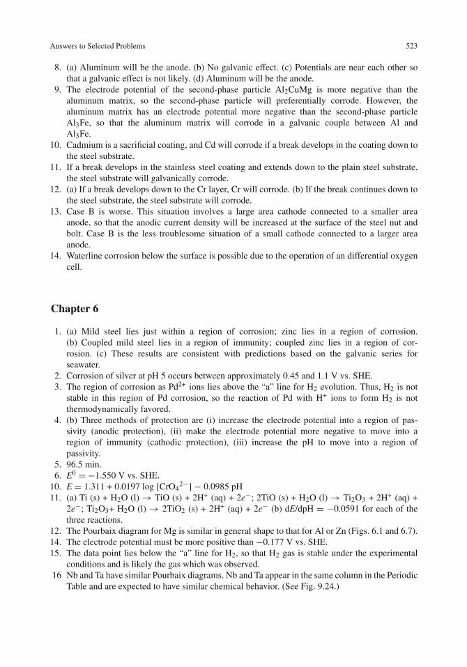
Answers to Selected Problems 523
8. (a) Aluminum will be the anode. (b) No galvanic effect. (c) Potentials are near each other sothat a galvanic effect is not likely. (d) Aluminum will be the anode.
9. The electrode potential of the second-phase particle Al2CuMg is more negative than thealuminum matrix, so the second-phase particle will preferentially corrode. However, thealuminum matrix has an electrode potential more negative than the second-phase particleAl3Fe, so that the aluminum matrix will corrode in a galvanic couple between Al andAl3Fe.
10. Cadmium is a sacrificial coating, and Cd will corrode if a break develops in the coating down tothe steel substrate.
11. If a break develops in the stainless steel coating and extends down to the plain steel substrate,the steel substrate will galvanically corrode.
12. (a) If a break develops down to the Cr layer, Cr will corrode. (b) If the break continues down tothe steel substrate, the steel substrate will corrode.
13. Case B is worse. This situation involves a large area cathode connected to a smaller areaanode, so that the anodic current density will be increased at the surface of the steel nut andbolt. Case B is the less troublesome situation of a small cathode connected to a larger areaanode.
14. Waterline corrosion below the surface is possible due to the operation of an differential oxygencell.
Chapter 6
1. (a) Mild steel lies just within a region of corrosion; zinc lies in a region of corrosion.(b) Coupled mild steel lies in a region of immunity; coupled zinc lies in a region of cor-rosion. (c) These results are consistent with predictions based on the galvanic series forseawater.
2. Corrosion of silver at pH 5 occurs between approximately 0.45 and 1.1 V vs. SHE.3. The region of corrosion as Pd2+ ions lies above the “a” line for H2 evolution. Thus, H2 is not
stable in this region of Pd corrosion, so the reaction of Pd with H+ ions to form H2 is notthermodynamically favored.
4. (b) Three methods of protection are (i) increase the electrode potential into a region of pas-sivity (anodic protection), (ii) make the electrode potential more negative to move into aregion of immunity (cathodic protection), (iii) increase the pH to move into a region ofpassivity.
5. 96.5 min.6. E0 = −1.550 V vs. SHE.
10. E = 1.311 + 0.0197 log [CrO42−] − 0.0985 pH
11. (a) Ti (s) + H2O (l)→ TiO (s) + 2H+ (aq) + 2e−; 2TiO (s) + H2O (l)→ Ti2O3 + 2H+ (aq) +2e−; Ti2O3+ H2O (l)→ 2TiO2 (s) + 2H+ (aq) + 2e− (b) dE/dpH = −0.0591 for each of thethree reactions.
12. The Pourbaix diagram for Mg is similar in general shape to that for Al or Zn (Figs. 6.1 and 6.7).14. The electrode potential must be more positive than −0.177 V vs. SHE.15. The data point lies below the “a” line for H2, so that H2 gas is stable under the experimental
conditions and is likely the gas which was observed.16 Nb and Ta have similar Pourbaix diagrams. Nb and Ta appear in the same column in the Periodic
Table and are expected to have similar chemical behavior. (See Fig. 9.24.)

524 Answers to Selected Problems
Chapter 7
1. (a) 0.411 g/cm2 h; (b) 123 mA/cm2.2. (a) 71.3 mg/cm2 year. (b) The corrosion rate decreases with time. (c) The rust layer becomes
more protective with time.3. (a) 7.5 × 10⁻³ M/L; (b) 0.10 g/cm2; (c) 41.9 mL (STP)/cm2.4. 3.6 mg/cm2 h.5. The weight fractions of metals in the alloy are Fe 0.058, Cr 0.162, Mo 0.153, Ni 0.546. Their
cation fractions in solution are Fe 0.057, Cr 0.100, Mo 0.130, Ni 0.712. Thus, Ni is preferentiallycorroded, while the others are not.
6. ba = 0.0591 V.8. (a) Ecorr = −0.459 V vs. SCE. (b) icorr = 24 μA/cm2.9. (a) The overvoltage is given by η = 0.0591/n (in V), where n is the number of electrons trans-
ferred. If n = 1, η = 0.0591 V. If n = 2, η = 0.0296 V. (b) η = 0.118/n (in V), where n is thenumber of electrons transferred. If n = 1, η = 0.118 V. If n = 2, η = 0.0591 V.
10. log icorr = (1/2) log (Ac/Aa) + constant.11. (a) icorr = 1.2 × 10⁻⁵ A/cm2 (b) Ecorr = −0.03 V12. 1.6 μA/cm2.13. ba = 0.073 V.
Chapter 8
1. (a) 0.0173 cm; (b) 2005 jumps/s.2. 3.7 h.3. 5.6 h.4. 35 s (using 0.065 cm as the thickness δ of the diffusion layer from Example 8.2).5. For δ = 0.05 cm, iL = 3.9 × 10⁻⁵ A/cm2. For δ =0.1 cm, iL = 1.9 × 10⁻⁵ A/cm2. (Using D =
2.0 × 10⁻⁶ cm2/s and the concentration of dissolved O2 = 8.0 mg/L from Fig. 8.5.)6. (b) Increasing the flow velocity increases the limiting cathodic current density iL for the reduc-
tion of oxygen and hence increases the corrosion rate. (c) The concentration of dissolved O2decreases, so iL decreases and so does the corrosion rate.
7. The following assumptions must hold: (i) the only cathodic reaction is the reduction of O2,(ii) the O2 reduction reaction is under diffusion control, and (iii) the anodic and cathodicpolarization curves intersect in the region of the limiting cathodic current density.
8. (b) Ecorr = −0.070 V vs. SHE = −0.31 V vs. SCE. (c) From the galvanic series for seawater,Ecorr = −0.1 to −0.2 V vs. SCE.
9. (a) 11 μA/cm2; (b) 3.1 g/m2 day.10. The electrolyte in contact with the hotter end of the metal will contain less dissolved O2
(Fig. 8.4). Thus, an oxygen concentration cell will be set up, with the hotter end of the metalbecoming the anode.
11. 238 μA/cm2.
Chapter 9
1. 0.94−1.91 monolayers of O−2.2. The calculated potential for the reduction of γ-Fe2O3 to Fe2+ is −0.214 V vs. SHE., in good
agreement with the experimental value for the first plateau. The calculated potential for the

Answers to Selected Problems 525
reduction of Fe3O4 to Fe is −0.534 V vs. SHE., in good agreement with the experimental valuefor the second plateau.
3. Tantalum. Based on the Pourbaix diagrams in Fig. 9.24, tantalum is either passive or immuneover a large range of pH and electrode potential.
4. E = −0.672 V vs. SHE; not in agreement with the experimentally observed Flade potential.6. 15.9 at.% Ni. The electron configuration theory is based on the concept of an adsorbed film and
does not take into account the properties of the oxide film.7. The effective molecular weight of the oxide is 136.17 g/mol. The effective atomic weight
of the metal is 55.27 g/mol. The effective value of n = 1.74. The density of the oxide is6.67 g/cm3. The density of the metal is 7.0 g/cm3 (given). R = 1.49, so that the oxide film isprotective.
8. The addition of Mo to Fe–Ni alloys is predicted to be detrimental. This trend is in agreementwith the text, which states that Mo is beneficial only when Cr is present.
9. (a) icorr ≈ 400 μA/cm2; (b) 0 to +0.3 V vs. SCE; (c) 30 μA/cm2; (d) 9.5× 10⁻⁴ cm penetration;(e) at −0.7 V vs. SCE, ianodic ≈ 30 μA/cm2.
10. (a) The anodic and cathodic polarization curves intersect in a region of active corrosion. (b) Theanodic and cathodic curves intersect in a region of passivity. (c) The situation is unstable andthe system oscillates between a state of active corrosion and one of passivity.
Chapter 10
1. Pitting and crevice corrosion are similar in their propagation stages. Each of these two formsof localized corrosion results in the formation of an internal solution of low pH and concen-trated in Cl− ions and in metal cations. Pitting and crevice corrosion differ in their initiationstages. Crevice corrosion initiates by means of a differential O2 cell, whereas pitting involvesthe localized breakdown of an oxide film (by one of several different mechanisms).
3. (c) Both the 1.0 cm2 crevice and the 2.0 cm2 crevice have the same weight loss, but the smallersample has the greater weight loss per unit area.
6. The pitting potential is Epit = −0.70 V vs. S.C.E.7. The current density within the pit is approximately 1,900 A/cm2.8. (a) The pitting potential for pure Al in 0.6 M Cl− is−0.74 V vs. S.C.E.=−0.72 V vs. Ag/AgCl.
(b) The pitting potential of Al alloys in seawater from Table 10.5 is −0.88 V vs. Ag/AgCl.(c) Agreement is fair. Differences may be caused by the following reasons: (i) Use of 0.6 M Cl−does not satisfactorily simulate seawater, which contains other ions as well as organic matter.(ii) Short-term laboratory tests do not represent data obtained over a much longer period ofimmersion. (iii) We have considered laboratory data for pure Al rather than for the Al alloy ofinterest.
9. (b) Safe ranges are more negative than −0.7 V vs. SCE (immunity) or between −0.35 V and−0.58 V vs. SCE. (perfect passivity).
10. Alloy B (but not alloy A) can be used instead of 304 stainless steel. Alloy B has ahigher pitting potential in 1 M HCl than does the other two alloys and has a critical cur-rent density for passivation similar to that for 304 stainless steel and lower than that ofalloy A.
11. With increased temperature the rate increases for all individual steps which lead to pitting. Thisincludes the rate of Cl− transfer within the oxide film, the rate of oxide thinning, and the rate ofelectrochemical reactions at the metal/oxide interface. Thus, the metal can be driven to a lowerelectrode potential to cause pitting to occur.

526 Answers to Selected Problems
Chapter 11
2. KI = 38 MPa√
m.4. Crack length 2a = 0.10 in. = 2.5 mm.5. (a) KIscc = 45 ksi
√in.; (b) σ = 51 ksi; (c) KI = 19 ksi
√in. is less than KIscc so that fracture
does not occur.6. Smooth specimens do not fracture below the threshold yield stress σ th = 48 MPa. For pre-
cracked specimens, the stress is given by σ = 3.103/√
a. Pre-cracked specimens do not fracturebelow the intersection of this line and the yield stress, σY = 410 MPa. The safe-zone region liesbelow the intersection of the lines σ = 3.103/
√a and σ th = 48 MPa.
7. Making the electrode potential more negative decreases KIscc (or increases the susceptibility tostress-corrosion cracking). (If KIscc decreases, the critical flaw size also decreases for the sameapplied stress σ .) Hydrogen embrittlement is a possible mechanism of stress-corrosion crackingbecause the alloy is more susceptibile with increasing negative potentials, where more cathodiccharging with hydrogen gas can occur.
8. 1.2 A/cm2.9. The time to failure decreases for both cathodic and anodic currents. Thus, the mechanism
for stress-corrosion cracking must be a mixed-mode mechanism, involving both hydrogenembrittlement and anodic dissolution within the crack.
11. 1,563 cycles.
Chapter 12
2. For 1 M HCl, %I = 88%; for 4 M HCl, %I = 60%.3. A plot of C/θ vs. C gives a straight line of unit slope.4. Calculate θ from θ = (i0 − i)/(i0 − isat). Then, a plot of θ vs. log C gives a straight line over
a portion of the plot, indicative of a Temkin isotherm. Various tests for the Langmuir isothermfail.
6. (a) The S-containing compound is better because the S atom is a better electron donor than the Natom. (b) CH3(CH2)16COOH is better because it has the longer chain length and thus presentsa greater barrier to the aqueous solution when a close-packed monolayer is formed on the metalsurface. (c) Both compounds have similar base strengths, but the diamine (second compound)is better because it offers more attachment possibilities to the metal surface. Either of the two-NH2 groups can adsorb with the molecule in the vertical configuration or both -NH2 groupscan adsorb with the molecule being in the flat configuration. (d) The -CH3 compound (secondcompound) is better. This is because the p-CH3 group is an electron donor and provides electronsto the ring. The Hammet sigma value σ(p-CH3) = −0.17. The Cl-containing compound is anelectron acceptor and withdraws electrons from the ring. The Hammet sigma value for the Clgroup is σ(p-Cl) = +0.23. (e) The second compound is better. It contains two electron-donatinggroups, so that the electron density on the N atom is higher for the second compound.
8. (a) For the conditions given, E = +1.103 V vs. SHE for chromate reduction, and E =−0.153 V vs. SHE For tungstate reduction, (b) under the given conditions, chromate reductionis spontaneous, but tungstate reduction is not, by �G = −nFE.
9. The corrosion of metals in nearly neutral solutions differs from that in acidic solutions for tworeasons. (1) In acid solutions, the metal surface is oxide-free, but in neutral solutions, the sur-face is oxide-covered. (2) In acid solutions the main cathodic reaction is hydrogen evolution,

Answers to Selected Problems 527
but in air-saturated neutral solutions, the cathodic reaction is oxygen reduction. In each case theinhibitor must interact with the metal or oxide-covered metal surface. For acid solutions, adsorp-tion alone may be sufficient to cause inhibition. But in nearly neutral solutions, the inhibitormust be able to enhance the protective properties of the oxide film. Possibilities include (i) for-mation of surface chelates, (ii) incorporation into the film of an oxidizing inhibitor (such asCrO4
2−), which itself is reduced to Cr2O3, (iii) incorporation of the inhibitor into the oxide filmor into its pores, (iv) formation of a precipitate on the oxide film.
10. If the inhibitor does not completely cover the metal surface, there can be a difference inpotential between the covered sites and the uncovered sites. This difference can cause a gal-vanic effect, so that the uncovered sites act as local anodes, and thus localized corrosion mayoccur.
Chapter 13
1. When an anodic site is activated beneath an organic coating, the local solution becomes acidifiedand chloride ions migrate into the vicinity of the site, as in crevice corrosion. The cathodic reac-tion (O2 reduction) also occurs beneath the organic coating. This is different than the usual caseof crevice corrosion, in which the principal cathodic reaction takes place outside the crevice.The major damage to the organic coating is caused in alkaline regions (cathodic) rather than inthe acidic region (anodic). This is different than the usual case of crevice corrosion where themain corrosion damage occurs within the crevice (anodic region).
2. Filiform corrosion is different in its geometric appearance than the usual type of underfilmcorrosion, but the mechanism of detachment is similar in both cases. Cathodic regions beneaththe coating exist in each case and can give rise to cathodic delamination.
5. (a) 33,000 layers of H2O molecules, (b) 9.9% of the thickness of the organic coating containsH2O molecules.
6. (a) In 1 day the coating will transmit 1.67× 10⁻⁴ mol H2O, as compared to 7.81× 10⁻⁸ mol O2.To use up all the H2O, we would need 8.4 × 10⁻⁵ moles O2, but we have much less. Thus, O2is the limiting reactant. (b) 0.35 μA/cm2.
7. (a) The data point lies in the region of the Pourbaix diagram for aluminum where Al goes intosolution as AlO2
−. (b) Thus, the oxide film is not stable so that dissolution of the oxide isa possible mechanism of delamination. However cathodic delamination due to failure of thepolymer in the alkaline environment cannot be ruled out.
8. 92 mg/cm2 day.9. From Figs. 13.9 and 13.10, poly(vinyl acetate) is a basic polymer and poly(vinyl fluoride) is
an acidic polymer. Thus, the basic polymer, poly(vinyl acetate), would be expected to have thegreater adhesion to the acidic oxide.
10. (a) Desirable properties are that polytetrafluoroethylene (PTFE) has good corrosion resistancein most solutions and is also a hydrophobic polymer which is not wetted by aqueous solutions.In addition, PTFE has a low coefficient of friction and is a good electrical insulator. (b) Anundesirable property is that when drastically overheated, PTFE can release toxic gases. In addi-tion, perfluorooctanoic acid, which is used to make PFTE, is a carcinogen. It is also difficult toget PTFE to adhere to the metal substrate without using certain adhesion promoters. (Adhesionpromoters are often bifunctional chemical agents which act as molecular bridges between twochemically different materials. Adhesion promoters improve adhesion by chemically bondingto both types of materials simultaneously.)

528 Answers to Selected Problems
11. (a) Measuring the electrode potential of an underground coated system would be useful in find-ing holidays (breakthroughs) in the coating. (b) Similarly, measuring the polarization resistanceof specimens of the coated metal could give information on the integrity of the coating. Valuesof Rp would decrease if there is a breakthrough in the coating.
Chapter 14
7. |Z| = [R2 + 1/(ω2C2)]1/2.8. 12 μA/cm2.9. Rp = 1,910 �; Rs = 10 �, Cdl = 3.1 × 10⁻⁵ F.
10. The low-frequency value of |Z| is the parameter of interest because it contains the values of thepolarization resistance Rp and the pore resistance Rcp of the coating. |Z| → Rp + Rcp + Rs asω → 0. At low frequencies, |Z| is larger when either plasticizer is contained in the organiccoating. Benzyl alcohol is the better of the two plasticizers.
11. 4.4 × 10⁻⁷ F/cm2.
Chapter 15
1. Based on thermodynamics, there will be an increase in the stability of the oxide. When iron isalloyed with aluminum, the oxide will be a mixed oxide consisting of Fe2O3 and Al2O3, withAl2O3 being more stable than Fe2O3, per the Ellingham diagram.
2. (a) K = 1/PO2 ; (b) PO2 = 1.0 × 10⁻¹⁰;(c) the two results are the same.3. PO2 = 1.2 × 10−41 atm, so that oxidation is possible in air at 1,200 K.4. The observation that dust particles become enveloped within the rust layer means that the rust
layer grows both from the outside oxide surface inward and from the metal surface outward.This is similar to the Wagner mechanism of high-temperature oxidation.
6. (a) According to the Ellingham diagram, the addition of Al to Ni should result in a more stablealloy. But the oxidation rate increases with Al content, in disagreement with the Ellinghamdiagram. (b) From Table 15.5, NiO is a p-type oxide with cation vacancies. From the Haufferules in Table 15.6, a solute of higher oxidation number (Al3+) results in an increase in oxidationrate, in agreement with the Hauffe rules.
7. (a) 5.0 × 10⁻³ g/cm2 after 20 h; (b) 7.5 μm.8. According to Table 15.5, Al2O3 is an n-type oxide with anion vacancies. The addition of a solute
like Li+ with an oxidation number lower than that of Al3+ causes an increase in the oxidationrate, according to the Hauffe rules in Table 15.6.
9. The parabolic rate law gives the best fit.10. 37.7 mg/cm2.11. (a) Replacing U4+ with Al3+ reduces the oxidation rate. (b) Replacing U+4 with Ta+5 increases
the oxidation rate.12. krational = 6.7 × 10⁻⁹ equiv cm−1s−1.
Chapter 16
1. (a) ia/F = k3θOH−;(b) k1k2/{(k1 + k−1β) (k−2[H+])};(c) ba = 0.118 V; (d) zH+ = −1.2. 2.5 mA/cm2.

Answers to Selected Problems 529
3. 5.0 × 10⁻⁴�−1cm−1.4. Surface charges at pH 7.0 are MoO3 negative, ZrO2 negative, CdO positive.5. Surface charges at pH 11.0 are MoO3 negative, ZrO2 negative, CdO negative.6. At pH 8.0, the oxide-covered surface has a positive charge. Thus, a negatively charged corrosion
inhibitor can be adsorbed at pH 8.0.7. (a) The concentration of implanted Cr3+ ions at the surface is 33 at.%. (b) This concentration is
higher than the critical concentration of 13 at.% Cr required for passivity in Fe–Cr binary alloys.8. (a) At pH 6.0, the surface of oxide-covered copper has a positive charge. We want to implant
copper with a metal whose oxide will have a negative charge at pH 6.0 in order to replace aportion of the positively charge surface with negative charges (to minimize Cl−uptake). Thus,any oxide having an isoelectric point less than 6.0 will do. Possibilities are Ce, Ti, Ta, Si, andMo. (b) We are assuming that the implanted ion is contained in the oxide film and that theisoelectric point for an oxide film is similar to that for bulk oxides.
9. (a) In neutral solutions, the surface of oxide-covered Fe is positively charged, and surface ofoxide-covered Si is negatively charged. Thus implantation of Si into Fe will convert a portionof the positively charged surface into negative charges. The uptake of Cl− will be reduced, soprotection against pitting will be increased. (b) Fe2O3 is an n-type semiconductor with anionvacancies (Table 15.6). Insertion of Si4+ ions will decrease the concentration of anion vacancies(Table 15.6). This reduces ionic diffusion through the oxide film so that protection against pit-ting will be increased. (c) Each argument is consistent with the other, so we can conclude thatimplantation of Si into Fe provides increased resistance to pitting.
10. Ion implantation has the following limitations: (i) the depth of the modified region is shallow(hundreds to thousands of angstroms); (ii) ion implantation is a line-of-sight process so thatrecesses in the sample geometry cannot be easily ion implanted; (iii) large-sized samples cannotbe processed readily.
11. The resulting stress is a compressive stress which is beneficial to protection against corrosionfatigue.
12 Laser processing produces a rough surface containing surface ripples which must be machinedif a smoother surface finish is desired. The depth of modified region is thicker than in the caseof ion implantation, but is still limited to the near-surface of the order of hundreds of micronsdeep.

Appendix ASome Properties of Various Elemental Metals
Oxidation number of mostcommon aqueous ionsb, c
Element SymbolAtomicnumber
Atomicweight(g/mol)a
Density(g/cm3)a Mono-atomic Oxyions
Lithium Li 3 6.941 0.534 +1Beryllium Be 4 9.012 1.85 +2Boron B 5 10.811 2.34 +3 (BO3
3−)+3 (B4O7
2−)Sodium Na 11 22.990 0.97 +1Magnesium Mg 12 24.305 1.74 +2Aluminum Al 13 26.982 2.70 +3 +3 (AlO2
−)Silicon Si 14 28.086 2.3296 +4 (SiO3
2−)Potassium K 19 39.098 0.89 +1Calcium Ca 20 40.078 1.54 +2Scandium Sc 21 44.956 2.99 +3Titanium Ti 22 47.867 4.506 +2, +3, +4 +4 (TiO3
2−)Vanadium V 23 50.942 6.0 +2, +3 +5 (VO4
3−)Chromium Cr 24 51.996 7.15 +2, +3 +6 (CrO4
2−)Manganese Mn 25 54.938 7.3 +2, +3 +7 (MnO4
−)Iron Fe 26 55.845 7.87 +2, +3 +2 (FeO2
2−)Cobalt Co 27 58.933 8.86 +2, +3 +2 (CoO2
2−)Nickel Ni 28 58.693 8.90 +2 +2 (NiO2
2−)Copper Cu 29 63.546 8.96 +1, +2 +2 (CuO2
2−)Zinc Zn 30 65.409 7.134 +2 +2 (ZnO2
2−)Gallium Ga 31 69.723 5.91 +2, +3 +3 (GaO3
3−)Germanium Ge 32 72.64 5.3234 +2, +4 +4 (GeO3
2−)Rubidium Rb 37 85.468 1.53 +1Strontium Sr 38 87.62 2.64 +2Yttrium Y 39 88.906 4.47 +3Zirconium Zr 40 91.224 6.52 +4 +4 (ZrO3
2−)Niobium Nb 41 92.906 8.57 +3Molybdenum Mo 42 95.94 10.2 +3 +6 (MoO4
2−)Technetium Tc 43 98 11 +2 +7 (TcO4
−)Ruthenium Ru 44 101.07 12.1 +2, +3 +6 (RuO4
2−)Rhodium Rh 45 102.906 12.4 +1, +2, +3 +6 (RuO4
2−)
531

532 Appendix A
Oxidation number of mostcommon aqueous ionsb, c
Element SymbolAtomicnumber
Atomicweight(g/mol)a
Density(g/cm3)a Mono-atomic Oxyions
Palladium Pd 46 106.42 12.0 +2 +2 (PdO22−)
Silver Ag 47 107.868 10.5 +1, +2Cadmium Cd 48 112.411 8.69 +2 +2 (CdO2
2−)Indium In 49 114.818 7.31 +1, +2, +3 +3 (InO2
−)Tin Sn 50 118.710 7.287 +2, +4 +4 (SnO3
2−)Antimony Sb 51 121.760 6.68 +3 (SbO2
−)+5 (SbO3
−)Cesium Cs 55 132.905 1.93 +1Barium Ba 56 137.327 3.62 +2Lanthanum La 57 138.905 6.15 +3Cerium Ce 58 140.116 6.770 +3, +4Hafnium Hf 72 178.49 13.3 +4Tantalum Ta 73 180.948 16.4 +3 +5 (TaO3
−)Tungsten W 74 183.84 19.3 +6 (WO4
2−)Rhenium Re 75 186.207 20.8 +3 +6 (ReO4
2−)+7 (ReO4
−)Osmium Os 76 190.23 22.587 +6 (OsO4
2−)Iridium Ir 77 192.217 22.562 +3 +6 (IrO4
2−)Platinum Pt 78 195.084 21.5 +2 +6 (PtO4
2−)Gold Au 79 196.967 19.3 +1, +3 +3 (AuO3
3−)Mercury Hg 80 200.59 13.534 +1, +2Thallium Tl 81 204.383 11.8 +1, +3Lead Pb 82 207.2 11.3 +2, +4 +2 (PbO2
2−)+4 (PbO3
2−)Bismuth Bi 83 208.980 9.79 +3Polonium Po 84 209 9.20 +2 +4 (PoO3
2−)Radium Ra 88 226 5 +2
a“Handbook of Chemistry and Physics”, CRC Press (online Edition) (2002).bM. Pourbaix, “Atlas of Electrochemical Equilibrium”, National Association of Corrosion Engineers, Houston,TX (1974).cP. Vanysek, “Electrochemical Series” in “Handbook of Chemistry and Physics”, CRC Press (online Edition)(2002).
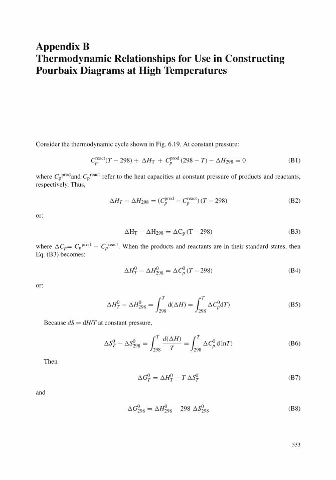
Appendix BThermodynamic Relationships for Use in ConstructingPourbaix Diagrams at High Temperatures
Consider the thermodynamic cycle shown in Fig. 6.19. At constant pressure:
Creactp (T − 298)+ �HT + Cprod
p (298− T)−�H298 = 0 (B1)
where Cpprodand Cp
react refer to the heat capacities at constant pressure of products and reactants,respectively. Thus,
�HT −�H298 = (Cprodp − Creact
p ) (T − 298) (B2)
or:
�HT −�H298 = �Cp (T− 298) (B3)
where �Cp= Cpprod − Cp
react. When the products and reactants are in their standard states, thenEq. (B3) becomes:
�H0T −�H0
298 = �C0p (T − 298) (B4)
or:
�H0T −�H0
298 =∫ T
298d(�H) =
∫ T
298�C0
pdT) (B5)
Because dS = dH/T at constant pressure,
�S0T −�S0
298 =∫ T
298
d(�H)
T=∫ T
298�C0
p d lnT) (B6)
Then
�G0T = �H0
T − T �S0T (B7)
and
�G0298 = �H0
298 − 298 �S0298 (B8)
533

534 Appendix B
combine to give:
�G0T −�G0
298 = (�H0T −�H0
298)− T(�S0T −�S0
298)− (�T)�S0298) (B9)
where �T = T − 298. Use of Eqs. (B5) and (B6) in Eq. (B9) gives the result:
�G0T = �G0
298 +∫ T
298�C0
P dT − T∫ T
298�C0
P d lnT − (�T)�S0298 (B10)
Equation (B10) is the expression for relating the standard free energy change at some elevatedtemperature T to the standard free energy change at 25◦C. Equation (B10) is the same as Eq. (30) inChapter 6. The heat capacities required in Eq. (B10) are either measured or estimated. Ionic entropiesare usually estimated by the empirical correlation method of Criss and Cobble [B1, B2] which relatesentropies at elevated temperatures to entropies at 298 K.
References
B1. C. M. Criss and J. W. Cobble., J. Am. Chem. Soc., 86, 5385 (1964).B2. J. W. Cobble, J. Am. Chem. Soc., 86, 5394 (1964).
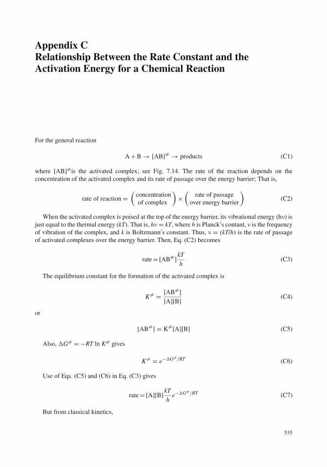
Appendix CRelationship Between the Rate Constant and theActivation Energy for a Chemical Reaction
For the general reaction
A+B→ [AB] �= → products (C1)
where [AB] �=is the activated complex; see Fig. 7.14. The rate of the reaction depends on theconcentration of the activated complex and its rate of passage over the energy barrier; That is,
rate of reaction =(
concentrationof complex
)×(
rate of passageover energy barrier
)(C2)
When the activated complex is poised at the top of the energy barrier, its vibrational energy (hν) isjust equal to the thermal energy (kT). That is, hν = kT, where h is Planck’s contant, ν is the frequencyof vibration of the complex, and k is Boltzmann′s constant. Thus, ν = (kT/h) is the rate of passageof activated complexes over the energy barrier. Then, Eq. (C2) becomes
rate= [AB�=]kT
h(C3)
The equilibrium constant for the formation of the activated complex is
K �= = [AB�=]
[A][B](C4)
or
[AB �=] = K�=[A][B] (C5)
Also, �G�= = −RT ln K�= gives
K �= = e−�G�=/RT (C6)
Use of Eqs. (C5) and (C6) in Eq. (C3) gives
rate= [A][B]kT
he−�G�=/RT (C7)
But from classical kinetics,
535

536 Appendix C
rate= (rate constant) [A] [B] (C8)
Comparison of Eqs. (C7) and (C8) gives the result
rate constant = kT
he−�G�=/RT (C9)
which is the same as Eq. (6) in Chapter 7.

Appendix DRandom Walks in Two Dimensions
We want to calculate the root mean square distance√
< d2 > which a particle can move after Ntwo-dimensional steps. Suppose that after N−1 jumps, an atom or ion has the co-ordinates xN−1 andyN−1, as shown in Fig. D.1. As described in Chapter 8, let the jump distance be l units and supposethat the particle can jump in any of the eight discrete directions shown in Fig. D.2.
yN–1
xN–1
dN–1
(xN, yN)
(xN–1, yN–1)
Fig. D.1 A particle jumps from a given site to a new site one jump distance in the North direction
N
NE
E
SE
S
NW
SW
W
Fig. D.2 Diagram showing the possible jump directions considered in this example of a two-dimensional walk
537

538 Appendix D
Suppose that the particle jumps from co-ordinates (xN−1, yN−1) in the north direction (N), asshown in Fig. D.1. Then,
xN = xN−1 (D1)
and
yN = yN−1 + l (D2)
Squaring both sides of these two equations gives
X2N = X2
N−1 (D3)
and
Y2N = Y2
N−1 + 2 l yN−1 + l2 (D4)
Adding Eqs. (D3) and (D4) gives
x2N + y2
N = x2N−1 + y2
N−1 + 2lyN−1 + l2 (D5)
Equation (D5) can be written as
d2N = d2
N−1 + w2 (D6)
where
d2N−1 = x2
N−1 + y2N−1 (D7)
and
w2 = 2 l yN−1 + l2 (D8)
Instead of jumping from co-ordinates (xN−1, yN−1) in the north direction (N), suppose thatthe particle jumps in the northeast direction (NE). Then, from simple geometry, as shown inFig. D.3:
xN = xN−1 + l√2
(D9)
yN = yN−1 + l√2
(D10)
Squaring both sides in Eqs. (D9) and (D10) and adding gives
x2N + y2
N = x2N−1 + y2
N−1 +2 l√
2(xN−1 + yN−1)+ l2 (D11)
which again has the form of Eq. (D6), except now that

Appendix D 539
xN–1
yN–1
dN–1
(xN, yN)
(xN–1, yN–1)
/
2
2
Fig. D.3 The particle jumps from the second location in Fig. D.1 to a new site one jump distance in the Northeastdirection
w2 = 2 l√2
(xN−1 + yN−1) + l2 (D12)
Thus, we can continue around the compass in Fig. D.2 and generate a set of equations (as perEq. (D6)), where w2 has the form for each case as given in Table D.1.
Table D.1 Forms for w2 in d2N = d2
N−1+ w2
Direction of jump w2
N w2 = 2 lyN−1 + l2
NE w2 = 2 l√2
(xN−1 + yN−1)+ l2
E w2 = 2 lxN−1 + l2
SE w2 = 2 l√2
(xN−1 − yN−1)+ l2
S w2 = −2 lyN−1 + l2
SW w2 = 2 l√2
(− xN−1 − yN−1)+ l2
W w2 = −2 lxN−1 + l2
NW w2 = 2 l√2
(− xN−1 + yN−1)+ l2
The average value of w2 should be l2. From Table D.1, it can be seen that adding up the variousvalues of w2 and dividing by 8 gives
w2 = 8 l2
8= l2 (D13)
Thus, starting at the origin and making one jump gives
d21 = d2
0 + l2 = l2 (D14)
After the second jump

540 Appendix D
d22 = d2
1 + l2 = 2 l2 (D15)
After the third jump
d23 = d2
2 + l2 = 3 l2 (D16)
Thus, in general,
d2N = Nl2 (D17)
or, the expected root-mean square value of d is
< d2 >= Nl2 (D18)
which is Eq. (5) in Chapter 8. Thus,
√< d2 > =
√Nl2 (D19)
It can be seen that if the jump direction is considered for a larger number of jump directions thatin turn approach a continuum, the result will be the same as in Eq. (D19).

Appendix EUhlig’s Explanation for the Flade Potential on Iron
Uhlig assumed that the following surface reaction was responsible for the passivation of iron:
Fe(s)+ 3H2O (1)→ Fe(O2 ·O)ads + 6H+(aq)+ 6e− (E1)
where Fe(O2·O)ads refers to the chemisorbed monolayer with a second layer of adsorbed O2molecules. The approach is to calculate the standard free energy change �G0 for Eq. (E1), andthen to get E0 from �G0 = −nFE0. The standard free energy change for Eq. (E1) is
�G0 = μ0 (Fe(O2 ·O)ads)+ 6μ0(H+(aq))− μ0((Fe(s))− 3μ0((H2O(1)) (E2)
Recall that μ0(H+(aq)) = 0 and μ0((Fe(s)) = 0. The value for μ0((H2O (l)) has been tabu-lated, but the value for μ0(Fe(O2.O)ads) is not available and must be calculated. Uhlig calculatedμ0(Fe(O2.O)ads) by considering the following surface reaction:
Fe (s)+ 3
2O2 → Fe (O2 ·O)ads (E3)
Uhlig then used
�G0S = �H0
S − T�S0S (E4)
where the subscripts refer to the surface reaction in Eq. (E3). With experimental data reported inthe surface chemistry literature for the heat of adsorption �Hs
0 and entropy of adsorption �Ss0 of
oxygen on iron, Eq. (E4) gives
�G0S =
(−75,000 cal
mol O2
)(3
2mol O2
)− 298◦
( −46.2 cal
deg mol O2
) (3
2mol O2
)(E5)
or, �Gs0 =− 91,848 cal per mole of Fe(O2·O)ads. This is also the value for μ0(Fe(O2.O)ads) because
Eq. (E3) involves the formation of Fe(O2·O)ads from its elements.Use of ΔGs
0 = − 91,848 cal for Fe(O2.O)ads in Eq. (E2) along with the value of−56,690 cal/mole for liquid water gives
�G0 = (1 mol Fe(O2 ·O)ads)
(−91,848 cal
mol
)− (3 mol H2O)
(−56,690 cal
mol
)
or, �G0 = 78,222 cal mol in Eq. (E1). Then,
541

542 Appendix E
�G0 = −nFE0 (E6)
gives
(78,222 cal)
(4.184 J
cal
)= −(6 equiv)
(96,500 coul
equiv
)E0 (E7)
or, E0 = − 0.57 V vs. SHE. But this value is for the oxidation reaction and the standard electrodepotential is for the reduction reaction, so that E0 = + 0.57 V vs. SHE. This value is in good agreementwith the Flade potential of +0.58 V for Franck’s data for iron in sulfuric acid.

Appendix FCalculation of the Randic Index X(G) for the Passive Filmon Fe–Cr Alloys
From Chapter 9, we begin with a hexagonal graph of Cr2O3 which contains Fe3+ ions substitutedfor some Cr3+ ions to form a mixed oxide, xFe2O3·(1−x) Cr2O3. The original hexagonal graph G0for Cr2O3 contains N vertices (Cr3+ ions) and (3/2) N edges (O2− ions). In the new graph G for themixed oxide D edges have been deleted one Fe3+ substituted per edge deletion. From Eq. (18) inChapter 9:
D
N= x
1− x(F1)
where x is the mole fraction of Fe2O3 in the mixed oxide.To calculate X(G), we would need to know which edges have been deleted from G0. However,
the process of edge deletion is random, so we follow the procedure used by Meghirditchian [F1] inanalyzing the network of a silica glass. For X(G), we use its expected value E[X(G)] given by
E[X(G)] =∑
i,j
(ij)−0.5E[A(G)ij ] (F2)
where A(G)ij is the number of edges in G connecting vertices of degrees i and j. We calculate the
expected value of E[A(G)ij ] following Meghirditchian [F1].
Edge deletion in the hexagonal network G0 can be treated by considering two adjacent verticesk and l in G0 and the connecting edge (kl), as shown in Fig. F.1. Suppose that after edge deletion,the edge (kl) remains undeleted, but the degrees of vertices k and l become i and j, as also shown inFig. F.1. To do this, we
(1) delete (3 − i) edges incident with the vertex k,(2) delete (3 − j) edges incident with vertex l, and(3) delete (D − 6 + i + j) edges from the remaining (3/2)N − 5 edges (See Table F.1).
k l i j
Fig. F.1 Edge deletion in a hexagonal network. After edge deletion, the vertices of degree k and l become i and j(shown here for the case where i and j are both two)
543
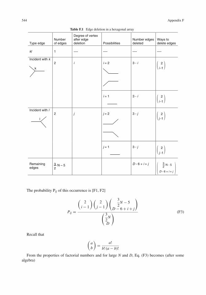
544 Appendix F
Table F.1 Edge deletion in a hexagonal array
Type edge Number of edges
Degree of vertex after edge deletion Possibilities
Number edges deleted
Ways to delete edges
kl 1 ---- ---- ---- ----
Incident with k
Incident with l
k
2 i i = 2 3 - i 2
i -1
i -1
j -1
i = 1 3 - i 2
l
2 j j = 2 3 - j 2
2
j -1
j = 1 3 - j
Remaining edges
32
N – 5 D - 6 + i + j
D - 6 + i + j
32
N - 5
The probability Pij of this occurrence is [F1, F2]
Pij =
(2
i− 1
)(2
j− 1
)( 3
2N − 5
D− 6+ i+ j
)
( 3
2N
D
) (F3)
Recall that(
ab
)= a!
b! (a− b)!From the properties of factorial numbers and for large N and D, Eq. (F3) becomes (after some
algebra)

References 545
Pij =
(2
i− 1
)(2
j− 1
)⎛⎜⎝3
2N−D
D
⎞⎟⎠
i+j−1
⎛⎜⎝
3
2N
D
⎞⎟⎠
5(F4)
which is the probability of any single edge (kl) in G0 becoming an edge of G joining vertices ofdegrees i and j. Then the expected value for the total number of edges in G joining vertices ofdegrees i and j is
E[A(G)ij ] = A(G0)Pij (F5)
where A(G0) is the number of edges in G. Thus
E[X(G)] = A(G0)3∑
j=1
3∑i=1
(ij)−0.5Pij (F6)
or
E[X(G)] = A(G0)3∑
j=i
3∑i=1
(ij)−0.5αijPij (F7)
where
αij ={
2 if i �=j1 if i = j
Use of Eqs. (F1) and (F4) in Eq. (F7) with A(G0) = (3/2)N gives
E[X(G)] =
(1
3
)5
N
(1− x)5(3− 5x) {24 x4 + 24
√2 x3(3− 5x)+ 4(
√3 + 3) x2 (3− 5x)2
+2√
6 × (3− 5x) 3 + 12 (3− 5x)4
}(F8)
References
F1. J. J. Meghirditchian, J. Am. Chem. Soc., 113, 395 (1991).F2. E. McCafferty, Electrochem. and Solid State Lett. 3, 28 (2000).

Appendix GAcid Dissociation Constants pKa of Bases and the Base Strength
Organic bases are protonated in acid solutions. For a secondary amine, for instance,
R2NH+ � R2N+H+ (G1)
where R2N denotes the depronated amine and R2NH+ its conjugate acid, with R referring to anorganic substituent. (If one of the R′s is an H atom, then the amine is a primary amine). The aciddissociation constant for Eq. (G1) is
Ka = [R2N] [H+]
[R2NH+](G2)
and
pKa = log1
Ka(G3)
The stronger the conjugate acid, the greater its tendency to produce protons. Thus, the strongerthe acid, the larger the ratio [R2N]/[R2NH+], and the larger the value of Ka. Large values of Kacorrespond to small values of pKa.
Thus, the smaller the pKa, the greater the acid strength. Conversely, the greater the pKa, thestronger base and greater the tendency to donate electrons.
547

Appendix HThe Langmuir Adsorption Isotherm
Suppose that a species A adsorbs from the aqueous phase onto a metal surface
A (aqueous)k1�
k−1A (adsorbed) (H1)
where k1 and k−1 refer to the rate constants in the forward (adsorption) and reverse (desorption)directions.
The process is represented by the free energy diagram in Fig. H.1(also see Chapter 7). In Fig. H.1,�G�=1 is the height of the free energy barrier in the forward direction, �G�=−1 is the correspondingheight in the reverse direction, and �Gads is the change in free energy due to adsorption of thespecies A.
A (adsorbed)
A (liquid)
ΔG1≠
ΔG-1≠
ΔGads
Extent of reaction
Free
ene
rgy
Fig. H.1 Free energy diagram for the adsorption of a species A from the aqueous phase onto a metal surface. �G �=1 is
the height of the free energy barrier in the forward direction, �G�=−1 is the corresponding height in the reverse direction,and �Gads is the change in free energy due to adsorption of the species A
The process of adsorption requires a vacant site on the metal surface (i.e., a site not already occu-pied by an adsorbed molecule or ion). From absolute reaction rate theory, as discussed in Chapter 7,the rate of adsorption (the forward direction) is
549

550 Appendix H
rate forward = k1 (1− θ ) Ce−�G�=−1/RT (H2)
where θ is the surface coverage of the adsorbed species and C is the concentration of species A inthe liquid phase. The rate of desorption (the reverse direction) is given by
rate reverse = k−1θe−�G�=−1/RT (H3)
At equilibrium the two rates are equal so that
k−1 θ e− �G�=−1/RT = k1 (1− θ ) Ce− �G�=−1/RT (H4)
Thus,
θ
1− θ= k1
k1Ce (�G�=−1−�G�=1 )/RT (H5)
But from Fig. H.1,
�G�=−1 −�G�=1 = �Gads (H6)
Use of Eq. (H6) in Eq. (H5) gives
θ
1− θ= k1
k−1e �Gads/RTC (H7)
Then we can write �Gads = �Hads − T �Sads, so that Eq. (H7) becomes
θ
1− θ= k1
k−1e−�Sads/Re �Hads/RTC (H8)
or
θ
1− θ= K1 e�Hads/RTC (H9)
where e−�Sads/R has been incorporated into the constant K1.In the Langmuir model, the metal surface is assumed to be homogeneous everywhere. In addition,
it is assumed that there are no lateral interactions between adsorbed molecules. (If there were lateralinteractions, then the heat of adsorption would vary with the surface coverage θ .) Thus, �Hads isindependent of the surface coverage θ . Then Eq. (H9) becomes
θ
1− θ= KC (H10)
where
K = K1 e�Hads/RT (H11)
Equation (H10) is the same as Eq. (7) in Chapter 12.
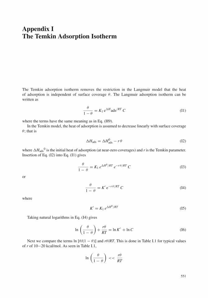
Appendix IThe Temkin Adsorption Isotherm
The Temkin adsorption isotherm removes the restriction in the Langmuir model that the heatof adsorption is independent of surface coverage θ . The Langmuir adsorption isotherm can bewritten as
θ
1− θ= K1 e�Hads/RT C (I1)
where the terms have the same meaning as in Eq. (H9).In the Temkin model, the heat of adsorption is assumed to decrease linearly with surface coverage
θ ; that is
�Hads = �H0ads − r θ (I2)
where �Hads0 is the initial heat of adsorption (at near-zero coverages) and r is the Temkin parameter.
Insertion of Eq. (I2) into Eq. (I1) gives
θ
1− θ= K1 e�H0/RT e−r θ/RT C (I3)
or
θ
1− θ= K′ e−r θ/RT C (I4)
where
K′ = K1 e�H0/RT (I5)
Taking natural logarithms in Eq. (I4) gives
ln
(θ
1− θ
)+ rθ
RT= ln K′ + ln C (I6)
Next we compare the terms ln [θ /(1 − θ )] and rθ /RT. This is done in Table I.1 for typical valuesof r of 10−20 kcal/mol. As seen in Table I.1,
ln
(θ
1− θ
)<<
rθ
RT
551

552 Appendix I
for 0.3 < θ < 0.7. Then Eq. (I6) simplifies to
rθ
RT= ln K′ + ln C (I7)
or
θ = 2.303 RT
rlog C + 2.303 RT
rlog K′ (I8)
which is Eq. (11) in Chapter 12.
Table I.1 Comparison of the terms ln [θ /(1 − θ)] and rθ /RT in the derivation of the Temkin adsorption isotherm
r θ
RT
θ lnθ
1− θr = 10 kcal/mole r = 20 kcal/mole
0.1 −2.198 1.69 3.380.2 −1.386 3.38 6.760.3 −0.847 5.08 10.10.4 −0.405 6.78 13.60.5 0.000 8.47 16.90.6 0.405 10.0 20.20.7 0.847 11.9 23.80.8 1.386 13.6 27.20.9 2.198 15.3 30.6
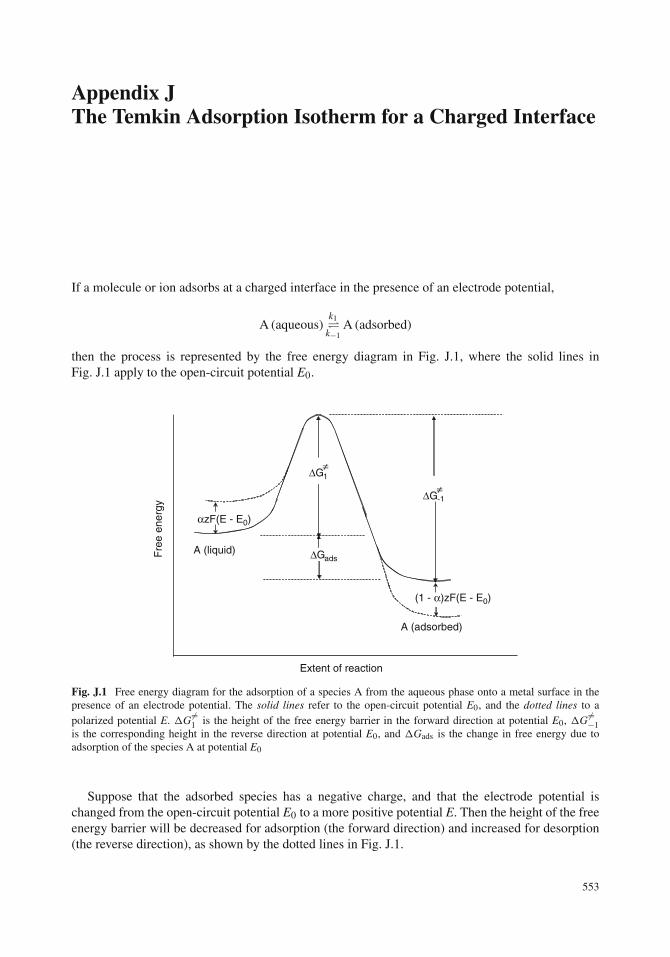
Appendix JThe Temkin Adsorption Isotherm for a Charged Interface
If a molecule or ion adsorbs at a charged interface in the presence of an electrode potential,
A (aqueous)k1�
k−1A (adsorbed)
then the process is represented by the free energy diagram in Fig. J.1, where the solid lines inFig. J.1 apply to the open-circuit potential E0.
A (adsorbed)
A (liquid)
ΔG1≠
ΔG-1≠
ΔGads
Extent of reaction
Fre
e en
ergy
αzF(E - E0)
(1 - α)zF(E - E0)
Fig. J.1 Free energy diagram for the adsorption of a species A from the aqueous phase onto a metal surface in thepresence of an electrode potential. The solid lines refer to the open-circuit potential E0, and the dotted lines to apolarized potential E. �G�=1 is the height of the free energy barrier in the forward direction at potential E0, �G�=−1is the corresponding height in the reverse direction at potential E0, and �Gads is the change in free energy due toadsorption of the species A at potential E0
Suppose that the adsorbed species has a negative charge, and that the electrode potential ischanged from the open-circuit potential E0 to a more positive potential E. Then the height of the freeenergy barrier will be decreased for adsorption (the forward direction) and increased for desorption(the reverse direction), as shown by the dotted lines in Fig. J.1.
553

554 Appendix J
The rate of adsorption in the forward direction at the open-circuit potential E0 is
rate forward = k1 (1− θ )[A] e−�G1�=/RT (J1)
(see Eq. (H2) in Appendix H). Under the new applied potential E, the rate of adsorption in theforward direction is
rate forward = k1 (1− θ ) [A] e−[�G�=−αzF(E−E0)
]/RT (J2)
where z is the charge on the adsorbing species, α is the symmetry factor, and αZF(E− E0) representsthe coulombic interaction of the charge with the electric field. (If the decrease in the free energybarrier in the forward direction is equal to the increase in the free energy barrier in the reversedirection, then α = 0.5.)
Similarly, the rate of desorption in the reverse direction under potential E is
rate reverse = k−1 θ e−[�G�=−1+ (1−α)zF(E−E0)
]/RT
(J3)
At equilibrium under the potential E, the rate in the forward direction is equal to the rate in thereverse direction, or
k−1 θ e−[�G�=−1+ (1−α)zF(E−E0)
]/RT = k1 (1− θ ) [A] e
−[�G�=1 −αZF(E− E0)
]/RT
(J4)
Thus,
θ
1− θ= k1
k−1[A] e(�G�=−1−�G�=1 )/RT e−zFE0/RT ezFE/RT (J5)
As in Appendix H,
�G�=−1 −�G�=−1 = �Gads (J6)
and writing �Gads = �Hads − T �Sads gives
θ
1− θ= k1
k−1[A] e�Hads/RTe−�Sads/R e−zFEo/RT ezFE/RT (J7)
As in Appendix I, we write
�Hads = �H0ads − r θ (J8)
where �Hads0 is the initial heat of adsorption (at near-zero coverages) and r is the Temkin parameter.
Then
θ
1− θ= k1
k−1[A] e�H0
ads/RTe−rθ/RT e−�Sads/R e−ZFEo/RT ezFE/RT (J9)
θ
1− θ= K2 [A] e−rθ/RT ezFE/RT (J10)

Appendix J 555
where
K2 = k1
k−1e�H0
ads/RTe−�Sads/R e−zF E0/RT (J11)
Equation (J10) has a form similar to that of Eq. (I4) in Appendix I, and the remainder of thetreatment is similar to that in Appendix I. Taking logarithms in Eq. (J10) gives
ln
(θ
1− θ
)+ rθ
RT= ln K2 + ln [A]+ zFE
RT(J12)
As shown in Appendix I,
ln
(θ
1− θ
)<<
rθ
RT
for 0.3 < θ < 0.7. Then Eq. (J12) becomes
θ = 2.303 RT
rlog [A]+ 2.303 RT
rlog K2 + zFE
r(J13)
which is Eq. (18) in Chapter 12.

Appendix KEffect of Coating Thickness on the Transmission Rateof a Molecule Permeating Through a Free-StandingOrganic Coating
Consider the case where the exterior of the coating is in contact with concentration C0 of permeatingmolecule. The concentration profiles with time within an organic coating of thickness L1 are givenin Fig. K.1. The concentration of permeating molecule at the underside boundary of the organic filmis zero because the permeating molecules exit the film at that distance.
Distance from surface
t1 t2t3
Concentrationof permeant in coating
Distance from surface
t1 t2t3 t4
L1
L2
t5
C0
C0
Concentrationof permeant in coating
Fig. K.1 Concentration profiles (at different times) for a permeating molecule in free-standing organic films ofthickness L1 (top) and L2 (bottom)
From Ficks first law of diffusion, the transmission rate J1 of the permeating molecule in thecoating of thickness L1 is
J1 = −DdC
dx(K1)
or
J1 = −D
(0− C0
L1
)(K2)
557

558 Appendix K
For a second coating of identical material but of a different thickness L2,
J2 = −D
(0− C0
L2
)(K3)
Equations (K2) and (K3) combine to give:
J2
J1= L1
L2(K4)

Appendix LThe Impedance for a Capacitor
The voltage across a capacitor C is
E(t) = 1
CQ(t) (L1)
where Q(t) is the charge given by
Q(t) = I(t)t (L2)
Use of Eq. (L2) in Eq. (L1) gives
E(t) = 1
CI(t)t (L3)
so that
d E(t)
d t= 1
CI(t) (L4)
and
I(t) = Cd E(t)
d t(L5)
The impedance is given by
ZC = E(t)
I(t)= E(t)
Cd E(t)
dt
(L6)
The voltage E(t) is given by Eq. (6) in Chapter 14, that is
E = E0 ejωt (L7)
Use of Eq. (L7) in Eq. (L6) gives
ZC = E(t)
I(t)= E0ejωt
CjωEjωt0
(L8)
or
ZC = 1
jωC(L9)
Reference
L1. G. H. Hostetter, “Fundamentals of Network Analysis”, p. 162, Harper & Row, New York, NY (1980).
559

Appendix MUse of L’Hospital’s Rule to Evaluate |Z| for theMetal/Solution Interface for Large Values of AngularFrequency ω
For the model of the electrical double layer shown in Fig. 14.4, we have
|Z| =⎧⎨⎩(
RS + Rp
1+ ω2R2p C2
dl
)2
+(
ωR2p Cdl
1+ ω2R2p C2
dl
)2⎫⎬⎭
1/2
(M1)
which is Eq. (24) in Chapter 14. For ω → ∞, the first term in the parentheses on the right-handside of Eq. (M1) approaches (Rs)2, but we need to apply L’Hospital’s rule to the second term on theright-hand side of Eq. (M1). Thus,
limω→∞
(ω R2
p Cdl
1+ ω2R2p C2
dl
)= lim
ω→∞
⎛⎜⎝
d
dω
(ωR2
p Cdl
)d
dω
(1 + ω2R2
p C2dl
)⎞⎟⎠ (M2)
limω→∞
(ω R2
p Cdl
1+ ω2R2p C2
dl
)= lim
ω→∞
(R2
p Cdl
2ωR2p Cdl
)(M3)
or
limω→∞
(ω R2
p Cdl
1+ ω2R2p C2
dl
)= 0 (M4)
Thus,
limω→∞ |Z| = |R
2S|1/2 = RS (M5)
561
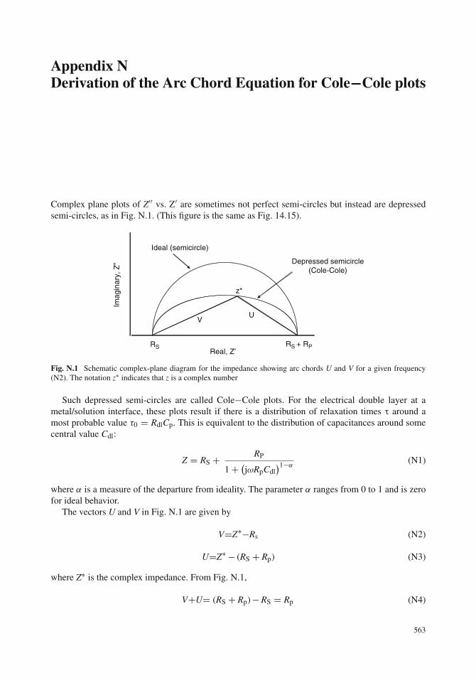
Appendix NDerivation of the Arc Chord Equation for Cole−Cole plots
Complex plane plots of Z′′ vs. Z′ are sometimes not perfect semi-circles but instead are depressedsemi-circles, as in Fig. N.1. (This figure is the same as Fig. 14.15).
Depressed semicircle(Cole-Cole)
z*
VU
Imag
inar
y, Z
”
Real, Z’
Ideal (semicircle)
RS RS + RP
Fig. N.1 Schematic complex-plane diagram for the impedance showing arc chords U and V for a given frequency(N2). The notation z∗ indicates that z is a complex number
Such depressed semi-circles are called Cole−Cole plots. For the electrical double layer at ametal/solution interface, these plots result if there is a distribution of relaxation times τ around amost probable value τ0 = RdlCp. This is equivalent to the distribution of capacitances around somecentral value Cdl:
Z = RS + RP
1+ (jωRpCdl)1−α
(N1)
where α is a measure of the departure from ideality. The parameter α ranges from 0 to 1 and is zerofor ideal behavior.
The vectors U and V in Fig. N.1 are given by
V=Z∗−Rs (N2)
U=Z∗ − (RS + Rp) (N3)
where Z∗ is the complex impedance. From Fig. N.1,
V+U= (RS + Rp)−RS = Rp (N4)
563

564 Appendix N
Then Eq. (N1) becomes
V + U = V + U
1+ (jωRpCdl)1−α(N5)
or
V + V(jωRpCdl)1−α = V + U (N6)
so that
V
U= 1
(jωRpCdl)1−α(N7)
or
V
U= (jωRpCdl)
α−1 (N8)
Taking absolute values on each side
∣∣∣∣VU∣∣∣∣ = |j (α−1)
∣∣∣ (ωRpCdl)α−1 (N9)
Then use is made of the property that any complex number can be written in polar form:
z = a+ jb = r ejθ (N10)
For the special case where z = j,
j = 1·ej π2 (N11)
j(α−1) = e(j π2 )(α−1) (N12)
or
j(α−1) = cosπ
2(α − 1)+ j sin
π
2(α − 1) (N13)
With
| z| =√
a2 + b2 (N14)
∣∣∣j(α−1)∣∣∣ =
√cos2
[π2
(α − 1)]+ sin2
[π2
(α − 1)]= 1 (N15)
Use of this result in Eq. (N9) gives
∣∣∣∣VU∣∣∣∣ = (ωRpCdl)
α−1 (N16)

References 565
and
log
∣∣∣∣VU∣∣∣∣ = (α − 1) log ω + (α − 1) log (CdlRp) (N17)
which is the desired result.
References
N1. E. McCafferty, V. H. Pravdic, and A. C. Zettlemoyer, Trans. Faraday Soc., 66, 1720 (1970).N2. K. S. Cole and R. H. Cole, J. Chem. Phys., 9, 341 (1941).N3. E. McCafferty and J. V. McArdle, J. Electrochem. Soc., 142, 1447 (1995).

Appendix OLaplace’s Equation
The flux Ni of each dissolved species in an electrolyte arises from three effects. These are: (a)the motion of charged species in an electric field (migration), (b) diffusion due to a concentrationgradient, and (c) convection due to bulk motion of the fluid. These three contributions give [O1]
Ni = -zi μ i F Ci ∇φ - Di ∇ Ci + Ci v
migration diffusion convection (O1)
whereNi = ionic flux of species izi = charge of species iμi = mobility of species iF = Faraday’s constantCi = concentration of species iφ = electrostatic potentialDi = diffusion coefficient of species iv = fluid velocity∇ = differential operator (∂ /∂x + ∂ /∂y + ∂ /∂z)
The current density i is given by
i = F∑
i
ziNi (O2)
The material balance of each species is
∂Ci
∂t= −∇ Ni + Ri (O3)
where Ri is the rate of production of species i due to chemical reactions in the bulk of the electrolyte.If ions are not generated in the bulk, then Ri = 0.
The condition of electroneutrality in the solution is
∑i
zi Ci = 0 (O4)
567

568 Appendix O
Multiplying Eq. (O3) by zi gives
∂(ziCi)
∂t= −∇ ziNi (O5)
(with Ri = 0). Then, summing over all species gives
∂
∂t
∑i
zi Ci = −∇∑
i
ziNi (O6)
But from Eq. (04),∑
izi Ci = 0, so that Eq.(06) gives
∇∑
i
ziNi = 0 (O7)
Then, Eq. (O2) can be written as
∇i = ∇(
F∑
i
ziNi
)= F
∑i
ziNi (O8)
Using Eq. (O7) in Eq. (O8) gives
∇i = 0 (O9)
This result will be used below. Use of Eq. (O1) in Eq. (O2) gives
i = F∑
i
zi (−zi μiFCi∇φ − Di∇Ci + Civ)
or
i = −F2∇φ∑
i
z2i μiCi − F
∑i
zi Di∇Ci + Fv∑
i
ziCi (O10)
By virtue of electroneutrality, the last term is zero. If there are no concentration gradients in thebulk of the solution, ∇Ci = 0. Thus, Eq. (O10) becomes
i = −σ ∇φ (O11)
where σ is the electrolyte conductivity given by
σ = −F2∑
i
z2i μiCi (O12)
We can operate on Eq. (O11) as follows:
∇i = −σ ∇2φ (O13)

Reference 569
But ∇i = 0 by Eq. (O9), so that Eq. (O13) gives
∇2φ = 0 (O14)
which is Laplace’s equation.
Reference
O1. J. Newman, in “Advances in Electrochemistry and Electrochemical Engineering”, C. W. Tobias, Ed., Vol. 5,p. 87, Interscience Publishers, New York, NY (1967).
Index
AAbsolute reaction rate theory, 131–132, 136, 549AC circuit analysis, 430–431Acid–base properties of oxides, 477, 494–499, 511–512Acidic solutions and inhibitors, 360–379Acidification within crevices, 322Acidification within pits, 321–322Acid solutions and concentration polarization, 148,
177–178, 200–202Acid solutions, metals in, 146–148AC impedance
anodization, 446, 448–449corrosion inhibition, 370, 449effect of diffusion, 436–437experimental set-up, 370, 429–430, 441, 450organic coatings, 370, 422, 427, 441–446, 449surface treatment, 422, 427, 446–448, 449
Activation polarization, 127–146, 177–179, 202–203, 484
Active/passive transition, 168, 211–212, 237, 254–255,290–291, 503
Adhesion of organic coatings, 232, 412–416, 494Adsorption inhibitors, 359Adsorption theory of passivity, 217, 238Aging infrastructure, 3Aluminum, 1, 6, 8, 13, 21–23, 77–79, 96–101, 122–124,
209–211, 230–235, 280–283, 297–300, 305,334, 351, 373, 385, 397, 446–448, 496–499,501–505
Aluminum, corrosion rate vs. pH, 78, 101Anodic control, 158–159, 343Anodic dissolution and stress-corrosion cracking, 339,
343–345, 353Anodic polarization, 128–130, 136, 149, 159, 168–169,
171, 179, 193, 211–215, 237–238, 250, 254,274, 277–280, 288–289
Anodic protection, 105, 255–257, 357Anodic reactions, 15–16Anodization, 211, 232, 446–449Anodization and AC impedance, 446, 448–449Anodizing, 211, 233, 518Applications of mixed potential theory, 146–159Area effects, 83, 199, 274–275
BBase strength and inhibition, 365, 374Batteries, 517Beneficial aspects of corrosion, 6, 515–518Binary alloys, 111–112, 151, 216–218, 237–248,
252, 271Biological molecules as inhibitors, 382, 390Bockris–Devanathan–Muller model of the electrical
double layerinner Helmholtz plane, 42Bockris–Kelly mechanism, 478–481Bode plots, 434–441, 444–445, 447–448, 450Body implants, 2, 278, 315–316, 348Breakdown of organic coatings, 416
CCapacitance of electrical double layer,
441, 443Cathode area, 82–83, 154, 200, 309Cathodic control, 158–159, 192, 343, 488Cathodic delamination, 412–413, 419–422Cathodic polarization, 127–129, 137, 143, 148, 159,
171, 173, 179, 191, 193, 199, 200, 254, 258,266, 308, 337
Cathodic protection, 79–81, 105, 150–153, 197–199,209, 255–258, 276, 337, 346, 351–352, 404,412, 490
Cathodic protection in acids, 150, 153, 199, 255–256,337, 357, 412, 517
Cathodic reactions, 16–17, 19–21, 149, 156, 203secondary effects, 19–21
Cavitation, 13–14, 315, 317, 349–352, 354Cavitation corrosion, 14, 315, 349–352Challenges, 9–10, 422–423Chemical potential, 63–66, 71–72, 97, 100,
114, 209Chemisorption of inhibitors, 361–362Chloride and stress-corrosion cracking, 3, 9, 14, 26, 211,
263, 277, 301, 320, 336, 345, 382Chromate, 3, 9, 65, 71, 106, 109–110, 115, 158,
212–213, 229, 237, 255, 273, 276, 306, 357,360, 380–382, 405, 414, 446–448
Chromate replacements, 71, 381–382, 399Cole–Cole plots, 433, 438
571

572 Index
Concentration polarization, 127–131, 148, 162, 167,177–208
kinetics, 131, 177, 186–192limiting current density, 191, 193polarization curves, 139, 144, 149, 177, 279,
292, 362Conservation of materials, 1, 5–6, 9Copper, pitting of, 278Corrosion
beneficial aspects, 6, 515–518definition, 13, 16quotations about, 515
Corrosion fatigue, 7–9, 14, 315, 346–349, 354,387–389
Corrosion inhibition and AC impedance, 370,438–441, 449
Corrosion inhibitors, 4, 9, 109, 163, 173, 209, 276, 283,348, 352, 357–400, 414, 422
Corrosion rates, 24–25, 48, 78, 101, 111, 119, 150–151,154, 162, 164, 170, 196, 200, 209, 236–237,240, 255, 346, 375, 378–379
methods, 119–127Corrosion science vs. engineering, 8–9Corrosion testing of organic coatings, 419–423Corrosion of works of art, 6Cost of corrosion, 1, 4, 10Coupled reactions, 17–18, 19, 60Crevice corrosion, 27, 89, 211, 249, 263–277, 322, 357,
361, 382, 386–387, 412, 417, 483area effects, 83, 199, 274–275effect of temperature, 196–197, 294–296initiation, 26, 263–265, 272, 280, 300, 307, 320, 357local acidification, 321oxygen depletion, 186propagation, 269–272, 274, 286, 357protection against, 83–84, 263testing, 264, 272–274
Critical relative humidity, 18–20Current distribution, 130, 167, 306, 477, 486–487, 493
DDealloying, 27–28Defect nature of oxides, 463–472Detection of pits, 307Differential concentration cells, 84–89Differential oxygen cell, 86, 89, 264Diffusion, 111, 159, 177–208, 264, 266, 269, 273, 282,
290, 300, 302, 407–408, 412, 417, 419, 421,436–437, 449, 456–457, 459, 463, 464
Diffusion and AC impedance, 449Diffusion and high temperature oxidation, 456–457, 459,
463, 469, 471–473Diffusion layer, 188–189, 194, 206, 266,
269, 488Diffusion and random walks, 183–185Distribution
circular corrosion cells, 483–486
of current, 306, 483–489of potential, 307
Drinking water problems, 3–4, 71, 178, 357–358
EEffect of O2 concentration on corrosion, 193Effect of O2 pressure on high temperature oxidation,
453–457, 462, 466, 469, 472–474Effect of temperature on corrosion, 196–197, 294, 296,
338–339, 463Effect of temperature on oxidation, 463Effect of velocity on corrosion, 194–196Eight forms of corrosion, 27–28Einstein–Smoluchowski equation, 185Electrical double layer, 37, 39–44, 52, 129, 189,
370–372, 432, 441, 443, 556–557Bockris–Devanathan–Muller, 42capacitance and, 43, 370–372, 378, 398Guoy–Chapman layer, 42inner Helmholtz plane, 41–42, 44, 371outer Helmholtz plane, 42, 371Stern mode, 41–42
Electrochemical cells, 67, 73–92, 167–168, 489, 493on the same surface, 75–76
Electrode kinetics, 131–146, 186–192, 477–482Electrode potential, 43–53, 65–66, 68–70, 75–87, 90–92,
95–99, 102–106, 111–112, 114, 127–128,131, 134–141, 150, 179, 185, 189–191
factors affecting, 69–70measurement of, 52–53sign, 68–70standard, 45–48, 65–66, 68–69, 76, 115, 127, 139,
147, 185, 189–191, 216, 257, 541Electrolytes, 18, 21, 30, 33–35, 53, 169, 181, 185, 199,
206, 232, 269–270, 273–274, 290–291, 300,322, 330–332, 409, 484, 488–489
Electromotive force series, 46–48limitations of, 111–112
Electron configuration theory of binary alloys, 238–241,257–258
Electrostatic potential, 40–41, 44, 65, 483, 485, 560Ellingham diagrams, 454–455Erosion, 13–14, 27–28, 315–316, 321, 352–354Erosion–corrosion, 28, 354Evans diagrams, 143, 150, 152, 154, 157–158, 171,
190–192, 194, 196, 198, 200, 206, 267,269, 275
Evans water drop experiment, 88Exchange current density, 133, 138–139, 142–147, 150,
154–155, 254Experimental Pourbaix diagrams, 111, 291–293, 310Experimental techniques, 165–169, 423
FFaraday’s Law, 23–25, 150Fatigue, 2, 7, 9, 13–14, 315, 321, 329–330, 346–349,
351, 354, 387–389

Index 573
Fermi sea of electrons, 38–39Fick’s first law, 181–182, 187, 407, 467Filiform corrosion, 417–419Film-forming inhibitors, 359Film sequence theory of passivity, 215, 218Flade potential, 211–213, 216, 237, 239, 257, 541–542Fracture, 8–9, 13–14, 28, 234–235, 316, 318–320,
323–324, 335, 340–341, 343–347Fracture mechanics, 323–331, 334, 353Fracture-safe diagrams, 334, 353Fretting corrosion, 14, 315–316, 352–354
GGalvanic corrosion, 27, 57, 73–92, 154–156, 199,
483, 490protection against, 83–84
Galvanic series, 76–79, 83, 89–91, 150, 199, 207Gaseous oxidation, 453–475Graph theory of Fe–Cr alloys, 243–248Guoy–Chapman layer, 42
HHarsh environment, 1–2Hauffe rules of oxidation, 466–471Henry’s law, 180, 197, 208, 407Heusler mechanism, 480–481High temperature oxidation, 9, 235, 453–460, 462–463,
469, 471–473High temperature oxide films
defect nature, 463–464layers on pure iron, 233, 395properties of protective films, 210semiconductor nature, 465–466
Hydration of ions, 35, 38–39, 42, 229–230, 235, 285Hydrogen embrittlement, 21, 103, 321, 339,
342–346
IInhibition of crevice corrosion, 302, 386Inhibition of pitting, 382–387Inhibition of stress-corrosion cracking, 341, 361,
382–389Inhibitors
adsorption inhibitors, 359acidic solutions, 360, 363–368, 373, 375, 379base strength effects, 364–365, 374concentration effects, 128, 150crevice corrosion, 273, 276, 283, 294, 296, 302,
357–399film-forming inhibitors, 359localized corrosion, 25–28, 109, 111, 293, 361,
382–389molecular size effects, 373–376molecular structure effects, 373–376, 414neutral solutions, 109, 358passivating inhibitors, 359pitting, 9, 263–311, 387
precipitation inhibitors, 359stress-corrosion cracking, 357, 382
Interfaces, 33–55, 316, 349, 414, 428, 485Intergranular corrosion, 27–28, 335Ion implantation, 124–125, 301, 348, 477, 499–505,
509–510Iron
–chromium alloys, 237dissolution, 141, 150, 190, 192–194, 477–482
microstructure, effect of, 335, 351nail experiment, 30–31
Irreversible potentials, 139–140Isoelectric point of oxides, 416, 505
KKI, 319, 325–329, 333–334, 345, 353, 387, 479KIscc, 329–337, 345, 353, 387–389Kramer–Kronig transforms, 440
LLangmuir–Blodgett films, 393–396Laplace’s equation, 483, 485, 490–491Laser-surface alloying, 509Laser-surface melting, 512Levich equation, 202, 204Limiting diffusion current, 187–188, 192–194, 196, 199,
201–203, 206Linear polarization, 159–165, 199–200, 484Localized corrosion
crevice corrosion, 25–27, 111, 211, 249, 263inhibition of, 382–389pitting, 25, 27, 211, 235, 263, 277–297stress-corrosion cracking, 25–27, 211, 263, 315–316
Luggin–Haber capillary, 53–54, 130–131, 167–168
MMagnesium–graphite couple, 78Mechanical metallurgy, 318–319Mechanism of pit initiation, 283–286Mechanism of pit propagation, 286–288Mechanisms of stress-corrosion cracking, 346Metallic coatings
galvanized steel, 4, 13, 29, 80–81titanium, 82–83zinc–aluminum, 81
Metals-based society, 1Metal/solution interface, 16, 23, 33, 36–42, 44–45, 65,
227, 357, 371–372, 427, 431–441, 443, 449,496, 556
Metastable pits, 290–291Mixed control, 158–159Mixed potential theory, 140–144, 146–159Mo effect on pitting, 293–294Molecular structure and inhibition, 373–376, 414Monolayers, 225, 393–396, 410Multiple oxidation–reduction reactions, 156–158

574 Index
NNernst equation, 66–68, 75, 77, 85, 87, 97–101, 112,
139, 141, 189, 191, 216, 265, 399Noble metal alloying, 256Non-uniform oxide layers on iron in high temperature
oxidation, 472Nuclear waste disposal, 3Nyquist plots, 433
OOccluded corrosion cells, 300–306, 386Ohmic polarization, 127, 130–131, 484Organic coatings, 8, 10, 83, 209, 232, 357, 382, 403–424,
441–446, 449Organic coatings and AC impedance, 422, 427, 441,
444, 449Outer Helmholtz plane, 42, 371Overvoltage, 127, 136, 138–139, 142, 148, 150,
157–158, 161, 172, 178, 190–191, 202, 268,372, 488
Oxidation rate laws, 457–463Oxide film properties of Fe–Cr alloys, 241–242Oxide film theory of passivity, 218Oxygen reduction, 87, 177–178, 179, 186, 188, 191–194,
197, 199, 205–207, 264, 269, 274, 379, 423,472, 488, 527
Oxygen scavengers, 193
PPaint, 10, 78, 80, 357, 403–405, 407–408, 412, 417, 422Parabolic rate law, 459, 460–463Passivating inhibitors, 359Passive films
aluminum, 210–211, 217, 230, 233–235, 278, 283,285–286, 297–300
properties, 110, 210, 215, 217–218, 228–229,234–235, 241–242, 473, 494–499
structure, 219, 227, 229–230, 233, 235, 241, 353,359, 499
surface analysis, 253thickness, 210–211, 215, 217–218, 228, 230, 233,
235, 257, 285, 473Passivity, 9, 95–96, 101, 103–110, 209–259, 263, 278,
288, 290, 292–293, 305, 310alloying and, 509aluminum, 95–96, 101–103, 209–211, 217, 230–232,
283, 286, 297, 298–300, 305, 351, 384, 499bilayer model for iron, 224–227binary alloys, 112, 216–218, 237–238, 240–241,
243, 246, 529bipolar model, 229, 253definition, 210effect of Mo, 258electrochemical basis, 211–215Fe–Cr, 112, 217–218, 229, 237–243, 248, 250, 252,
289, 293, 331history, 210
hydrous model for iron, 227–228models for iron, 222, 224–230spinel defect model, 224–225, 229–230stainless steel, 9, 158, 214, 217, 228, 230, 234, 238,
248–253, 278–279, 283, 289–291, 294, 297,320, 331, 352, 508
theories, 215–218Percolation theory of Fe–Cr alloys, 242–243Permeation of Cl− into organic coatings, 411Permeation of H2O into organic coatings, 406–410Permeation of O2 into organic coatings, 410–411pH and stress-corrosion cracking, 338Physical degradation, 13–14Pilling–Bedworth ratio, 234–236, 472–473Pitting, 263–311, 382–386, 497–499
of aluminum, 283, 286, 297–300, 385, 499chloride ions, 9, 214, 235, 263, 277, 287, 291, 293,
297, 412, 499detection of, 306–308inhibition, 302, 357, 361, 382–397, 494local acidification, 321metastable, 290–291propagation, 263, 280, 283, 286–290, 298–299, 322,
357, 382protection against, 296–297, 529stainless steel, 9, 27, 214–215, 249, 278, 289–290,
294, 297, 320, 384, 497Pitting potential
effect of chloride, 282inhibition, 283
Polarization, 127–146, 159–169, 177–208curves, 136–138, 143, 147–151, 160, 165–169,
191–192, 197–205, 212–215, 236–238, 250,266, 268, 274, 279–280, 288
Potential difference, 33, 40–41, 43–45, 54Potential distribution, 418–419, 483–491, 511Potential of zero charge, 372–373Pourbaix diagrams
aluminum, 96, 234chromium, 106–107, 110copper, 111–112experimental, 57, 67, 95–116, 214–215, 233–234,
291–293, 301, 342–343iron, 103–106water, 95, 98, 101–103, 112, 114zinc, 103
Precipitation inhibitors, 360Properties of protective high temperature oxides,
473–474Protection against corrosion fatigue,
348–349Protection against pitting, 296–297Protection potential, 288–293
RRandom walks, 183–185Rate laws in oxidation, 457–463

Index 575
Reference electrodestable of, 50copper/copper sulfate, 50–51saturated calomel, 48, 50, 52, 70, 77in seawater, 49–50silver/silver chloride, 49standard hydrogen electrode, 48, 50
Relative electrode potential, 45–46Relaxation processes, 427–429Rotating disc electrode, 202–205Rotating ring disc electrode (RRDE), 205Rust, 5, 7, 13–14, 18, 60, 83, 88, 170, 205, 240, 249,
315–316, 422, 457, 474, 515–516
SSafety, 1–4, 515Scaling rules, 477, 489–493Scanning tunneling microscopy (STM), 219, 223–224,
229, 244Seawater corrosion, 78–79Self-assembled monolayers, 393–396Semiconductor nature of oxides, 465–466Sensitization, 27, 339Smart coatings, 423Solubility and diffusion, 179–185Solubility product, 22, 29, 71, 290, 360Solution/air interface, 33, 35–37Spontaneity, 47, 60, 399Stainless steels, 1, 6, 8–9, 14, 158, 217, 229, 249–253,
274, 289, 293–294, 320–321, 348, 352Stainless steels passivity, 249–253Standard hydrogen electrode (SHE), 45–48, 50–51, 54,
64–65, 77, 85, 96–98, 100Stern–Geary, 159–165, 199, 484Stern model of the electrical double layer, 41Strain, 235, 318–319, 325, 375–376Stress, 1, 3, 7–9, 14, 20, 70, 103, 211, 277, 300–303,
315–348, 361, 382, 387–389, 483Stress-corrosion cracking, 7–9, 14, 20, 25–27, 103,
211, 263, 277, 301, 305, 315–324, 330, 333,335–337, 345–346, 353–354
effect of Cl− concentration, 338–339, 384effect of electrode potential, 336–338, 340, 353effect of pH, 212, 338effect of temperature, 196–197, 338–339flaws and, 320–321, 382, 389initiation, 264–269mechanisms, 8–9, 230, 263, 286, 293, 300, 337, 339metallurgical effects, 335–336modes of, 322propagation, 26–27, 263, 320, 338, 357properties, 319–320, 339protection against, 83–84, 263, 275, 296,
348–349, 455stages, 264, 320–323tests, 329, 419–423
Stress intensity factor, 319, 325–329, 328–333, 335–336,338, 347–348, 353, 388
Sulfides, effect on pitting, 294, 344, 508Surface-active species, 36Surface alloys, 501, 503, 506, 508–510Surface analysis techniques, 217–224Surface charge and pitting, 497–498Surface hydroxyls, 231, 391–392, 494–495Surface modification, 348, 382, 389, 477, 499–510Surface treatment and AC impedance, 422, 427, 446,
448–449
TTafel equation, 138–139, 141, 493Tafel extrapolation, 148–151, 159, 170, 179, 211Tafel slopes, 136, 139, 143, 145–148, 152, 160, 162,
438, 450, 478, 482Taft induction constants, 365–367Thermodynamics, 57–72, 73–92, 95–116, 453–456Thermodynamics of high temperature oxidation,
453–456Thickness of passive films, 233Titanium jewelry, 518Transpassive dissolution, 106
alloys, 111–112applications, 108–111copper–nickel, 112elevated temperature, 112–114iron–chromium, 109–111limitations, 111and localized corrosion, 111palladium, 107–108silver, 108tantalum, 109titanium, 126
UUniform corrosion, 18, 24–27, 30, 109, 119–120, 357
VVapor phase inhibitors, 359, 396–397
WWagner mechanism of high temperature oxidation, 457Wagner–Traud, 140–144, 156, 191–192Waterline corrosion, 88–89, 92Water molecules, 33–36, 38, 42, 189, 221, 228, 285,
359, 367–368, 379, 399, 414, 427, 478, 482,494, 511
Water permeation and organic coatings, 406–410Wear, 8–9, 13–14, 316, 352–353, 499, 516
XX-ray absorption spectroscopy (XAS), 219, 222–223,
283, 299X-ray photoelectron spectroscopy (XPS), 217, 219,
220–222, 248, 252–253, 283, 285, 298–300,362, 494, 504