Intrinsic subdivision with smooth limits for graphics and animation

Intrinsic Subdivision with Smooth Limits for Graphics andAnimation

Johannes Wallner and Helmut Pottmann

This paper demonstrates the definition of subdivision processes in nonlinear geometries such thatsmoothness of limits can be proved. We deal with curve subdivision in the presence of obstacles,

in surfaces, in Riemannian manifolds, and in the Euclidean motion group. We show how to model

kinematic surfaces and motions in the presence of obstacles via subdivision. As to numerics, weconsider the sensitivity of the limit’s smoothness to sloppy computing.

Categories and Subject Descriptors: I.3.5 [Computer Graphics]: Computational Geometry and Object Modeling

General Terms: Algorithms

Additional Key Words and Phrases: nonlinear subdivision, geodesic subdivision, subdivision in

surfaces, motion design, obstacles, smoothness, computing in nonlinear geometries.

1. INTRODUCTION

1.1 Background and previous work

Subdivision is an appealing way of defining a continuous object by a discrete approximation, and a curve orsurface generated by subdivision has many desirable properties. It is therefore not surprising that subdivisionhas been extended to nonlinear spaces.

Spheres have been considered by [Kim et al. 1995; Ramamoorthi and Barr 1997; Juttler and Wagner 2002],always having in mind that the points of the quaternion unit sphere represent the matrix parts of rigid bodymotions. Also with a view toward motion design, Sprott and Ravani [1997] extended B-spline algorithmsto Lie groups. Nonlinear interpolatory schemes in Lie groups were constructed from linear schemes by[Donoho 2001], and used in various applications such as in smoothly interpolating a motion given at discreteinstances. This material is also contained in [Ur Rahman et al. 2005], which gives a comprehensive treatmentof multiscale representation for Lie-valued data and the corresponding nonlinear subdivision rules employed.We would also like to mention the nonlinear median-interpolating subdivision schemes and their extensions[Xie and Yu 2005; Oswald 2004], interpolatory schemes based on the idea of essential non-oscillation [Cohenet al. 2003], and nonlinear geometry driven schemes [Marinov et al. 2004], whose construction and analysisis different from the schemes used in this paper.

When subdividing in inherently nonlinear environments, the following problems arise:— The definition of many linear subdivision rules employs affine combination of points. It is necessary tofind a replacement for this basic way of creating new points.— Results guaranteeing certain desirable properties (smoothness, for example) of the limits generated bynonlinear rules are harder to come by. Numerical evidence however says that they must be there.— Computing in curved geometries often requires discretization, and sometimes also iterative processes tootime-consuming to be pursued ‘until they converge’, as it is sometimes put. Quantitative information on theconsequences of inaccuracies introduced by incomplete computation is usually not available.

It is the aim of this paper to demonstrate how certain ways of mimicking linear subdivision rules in

Authors’ address: Institute of Discrete Mathematics and Geometry, Vienna University of Technology.Email {wallner,pottmann}@geometrie. tuwien.ac.at

ACM Transactions on Graphics, Vol. V, No. N, Month 20YY, Pages 1–18.

2 · J. Wallner and H. Pottmann

nonlinear geometries leads to nonlinear subdivision schemes with provably smooth limits.For linear subdivision, the smoothness analysis in many cases can be considered complete. We do not

attempt to review the existing literature here, but refer to the surveys [Dyn 1992; Warren and Weimer2001; Kobbelt 2002; Sabin 2002]. Smoothness results for nonlinear subdivision schemes have been shown byL. Noakes [1997; 1998; 1999]: the geodesic analogues of the 2nd and 3rd degree Lane-Riesenfeld algorithmin Riemannian manifolds possess smooth limit curves with Lipschitz derivative. Recently some generalsmoothness results have been given for a wide class of nonlinear schemes which arise as perturbations oflinear schemes [Wallner and Dyn 2005; Wallner 2006a]. It is that work which serves as a theoretical basisof this paper. Some examples are briefly mentioned already in [Wallner and Dyn 2005] in order to illustratethe theory. They are mentioned again in the present paper, whose contributions to nonlinear subdivisionare a long list of examples where nonlinear subdivision schemes are useful in Computer Graphics; obstaclesubdivision; intrinsic shape properties of geodesic subdivision; the use of configuration spaces for subdividingposes and the treatment of obstacles. A theoretical result contained in the present paper concerns verificationof smoothness for sloppy computations.

1.2 Overview

This paper is organized as follows: Section 2 gives a long list of examples of nonlinear subdivision schemeswhich are constructed in analogy to linear schemes by the means available in various nonlinear geometries.The nonlinear schemes constructed in this way can be seen as perturbations of linear ones. In a few caseswe also discuss numerical issues.

Section 3 verifies that the available theory applies to the subdivision rules defined in the previous sec-tion. We invoke general results concerning the proximity of subdivision rules and verify that the proximityconditions are fulfilled, so that the limits are C1 and in some cases even C2. A proof of convergence fromproximity is also included.

Section 4 deals with the problem of incomplete computation of geodesics in surfaces. It turns out that awide class of iterative algorithms used for evaluating certain nonlinear subdivision rules is quite resistant tosloppy usage.

As we emphasize the smoothness of limits, we mostly speak about smooth geometries like parametrizedsurfaces or level sets. After discretization (e.g. when using triangulated surfaces) the question of smoothnessdoes no longer make sense in the strict mathematical sense. Even so, it is important to know that whencomputing approximately by means of a triangulation, the ideal geometric object one tries to approximate issmooth. On the other hand, there are geometries which are not discretized at all, e.g. the Euclidean motiongroup, and for which smoothness has the precise mathematical meaning.

1.3 Notation

We use the symbol p for a polygon, which may be either closed or open, and is a synonym for ‘list ofvertices’. We write pi for the i-th vertex. A binary subdivision scheme S maps a polygon p to the polygonSp, consisting of the points (Sp)i, or Spi for short. The result of two rounds of subdivision applied to p isdenoted by S2p, and so on. The symbol S∞p means the limit curve. We express linear subdivision rules interms of the affine average operator

avt(a,b) = a + t(b− a). (1)

For instance, the n-th degree B-spline subdivision rule Bn (n ≥ 2) is recursively defined by

B2p2i = av1/4(pi,pi+1), B2p2i+1 = av3/4(pi,pi+1), Bnpi = av1/2(Bn−1pi, Bn−1pi+1). (2)

B2 is Chaikin’s rule. For an illustration of B2 and B3, see Fig. 7. The polygons (Bn)jp converge to then-th degree B-spline curve for which the polygon p and, indeed, any polygon (Bn)jp, is a control polygon.ACM Transactions on Graphics, Vol. V, No. N, Month 20YY.

Intrinsic Subdivision with Smooth Limits for Graphics and Animation · 3

1. 2. 3.

4. 5. 6.

7. 8. 9.

10. 11. 12.

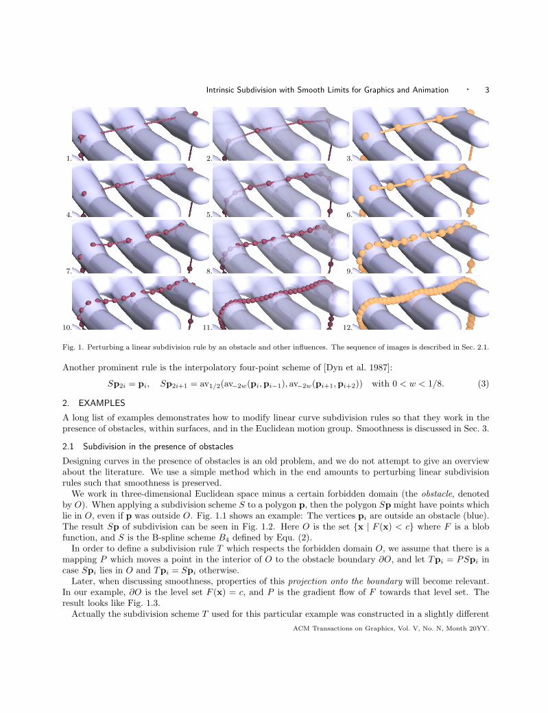
Fig. 1. Perturbing a linear subdivision rule by an obstacle and other influences. The sequence of images is described in Sec. 2.1.

Another prominent rule is the interpolatory four-point scheme of [Dyn et al. 1987]:

Sp2i = pi, Sp2i+1 = av1/2(av−2w(pi,pi−1), av−2w(pi+1,pi+2)) with 0 < w < 1/8. (3)

2. EXAMPLES

A long list of examples demonstrates how to modify linear curve subdivision rules so that they work in thepresence of obstacles, within surfaces, and in the Euclidean motion group. Smoothness is discussed in Sec. 3.

2.1 Subdivision in the presence of obstacles

Designing curves in the presence of obstacles is an old problem, and we do not attempt to give an overviewabout the literature. We use a simple method which in the end amounts to perturbing linear subdivisionrules such that smoothness is preserved.

We work in three-dimensional Euclidean space minus a certain forbidden domain (the obstacle, denotedby O). When applying a subdivision scheme S to a polygon p, then the polygon Sp might have points whichlie in O, even if p was outside O. Fig. 1.1 shows an example: The vertices pi are outside an obstacle (blue).The result Sp of subdivision can be seen in Fig. 1.2. Here O is the set {x | F (x) < c} where F is a blobfunction, and S is the B-spline scheme B4 defined by Equ. (2).

In order to define a subdivision rule T which respects the forbidden domain O, we assume that there is amapping P which moves a point in the interior of O to the obstacle boundary ∂O, and let Tpi = PSpi incase Spi lies in O and Tpi = Spi otherwise.

Later, when discussing smoothness, properties of this projection onto the boundary will become relevant.In our example, ∂O is the level set F (x) = c, and P is the gradient flow of F towards that level set. Theresult looks like Fig. 1.3.

Actually the subdivision scheme T used for this particular example was constructed in a slightly differentACM Transactions on Graphics, Vol. V, No. N, Month 20YY.


Fig. 2. The left hand

image shows the con-

trol polygon of provablysmooth spaghetti. The

right hand figure illus-

trates this smooth limitby depicting the result of

5 rounds of nonlinear B-

spline subdivision avoid-ing the interior of the

hand, with added gravity.For details, see Sec. 2.1.

way: In the recursive definition of B4 given by Equ. (2) every averaging is immediately followed by aprojection onto the boundary of the obstacle, should the result of averaging lie in O. It turns out that bothways of perturbing a linear scheme lead to smooth limit curves.

We want to show that for applications one might want to modify a given subdivision scheme for a varietyof reasons and in many different ways. In our case we produce an image of a handful of spaghetti, whichin the real world is under the influence of gravity. Thus we add the following perturbation: Before againsubdividing with B4, we decrease the z-coordinate of each point by a small amount. Here we choose

pi → pi − C · ‖pi+1 − pi‖2 · (0, 0, 1). (4)

This small movement of vertices is hardly visible. The result is shown by Fig. 1.4.The sequence of images of Fig. 1.1–12 documents several rounds of this iterative process – an orange

polygon first experiences a gravity-like perturbation, is further subdivided linearly for illustration (shownwith transparent obstacle), and nonlinearly (shown again in orange). Subdivision of a longer polygon p isshown in Fig. 2. Note that this procedure neither simulates the actual statics of pasta, nor does it takeself-intersections into account. It intends to demonstrate two possible perturbations which may be inflictedon a linear subdivision rule.

2.2 Geodesic Subdivision

If the vertices pi of a polygon are contained in a surface M , it is in general not true that after subdivisionwith a linear scheme S, the vertices Spi are also contained in M . It is therefore impossible to use suchsubdivision schemes directly if one wants to work entirely in M . One way of dealing with this problem is toemploy geodesic analogues of linear rules, which are the topic of the next paragraphs.

2.2.1 Curve Subdivision within Surfaces. An idea which occurs naturally when looking for an intrinsicequivalent of linear subdivision rules is to replace straight lines by geodesic lines, which are the shortest pathsbetween points on the surface [do Carmo 1992]. Because of the computational difficulties involved, geodesicsubdivision defined in this way is useful only in special circumstances. The idea however is important and isexplained now in more detail: If c(t) is a constant speed parametrization of a geodesic line emanating froma and ending in b, then a geodesic average is defined by

c(0) = a, c(1) = b =⇒ g-avt(a,b) = c(t). (5)

Because of the symmetry relation g-avt(a,b) = g-av1−t(b,a), “g-av” is a a satisfactory intrinsic replacementof “av”. We replace “av” by “g-av” in the definition the B-spline rule Bn in Equ. (2) and thus get a geodesicACM Transactions on Graphics, Vol. V, No. N, Month 20YY.


1. 2. 3.

Fig. 3. Geodesic Subdivision. 1–3: Subdivision by the geodesic analogue T2 of Chaikin’s rule B2. The polygon p is shown in

red and, from left to right, T2p, T 22 p, T∞2 p in yellow. The variation diminishing property of geodesic B-splines is illustrated

by means of a grey geodesic line.

1 round

q = T2p

2 rounds

q = T 22 p

4 rounds

q = T 42 p

8 rounds

q = T 82 p

1 round

q = T3p

2 rounds

q = T 23 p

4 rounds

q = T 43 p

8 rounds

q = T 83 p

polylineq

1st derivative∆q/h

2nd derivative∆2q/h2

3rd derivative∆3q/h3

Fig. 4. Visualization of smoothness of the geodesic Chaikin rule “T2” in the wriggly surface of Fig. 3 (left) and of the cubic

geodesic B-spline rule “T3” (right). The figures illustrate numerical smoothness after several rounds of subdivision. Eachsmall figure depicts a diagram of the first coordinate of the points under consideration, the diagrams for the second and third

coordinate being similar. Scaling in each figure depends only on the order of differentiation, so that derivatives of different

polylines are comparable. From the blue figures it is obvious that for the Chaikin rule T2, the second numerical derivativeno longer appears to be continuous, while for the cubic rule, the third numerical derivative (green) is the first to show this

behaviour.

B-spline rule of degree n, which is illustrated in Fig. 3

Generically, the shortest geodesic which contains two given points a, b is unique, and for a given surfacethere is always a certain positive distance δ such that uniquenes holds in case ‖a−b‖ < δ. Another problemwhich might arise is that in a non-complete surface it can happen that there is no unbroken geodesic whichjoins two given points a, b. These problems are unlikely to occur at all, as we usually subdivide polygonswhose vertices are close together.

ACM Transactions on Graphics, Vol. V, No. N, Month 20YY.


Fig. 5. Hyperbolic swordfish (Geodesic analogue of B-Spline subdivision B3

with C2 limit curves). One hyperbolic control polygon is also shown.

2.2.2 Subdivision in Riemannianmanifolds. The word Riemannianmanifold means a manifold (which forthe purposes of Computer Graphicsis realized as a piece of Rd or aparametrized surface or a triangula-tion), where the way of computingthe scalar product of two tangentvectors attached to the same point isnot the one of ambient space, but isallowed to change smoothly with thepoint quite independent of the waythe manifold lies in some other space.Of course we might as well use thescalar product of ambient space, soevery surface in the ordinary senseis a Riemannian manifold. It turnsout that the theory dealing withsmoothness of limits extends easily toRiemannian manifolds, so for the sakeof completeness we give an exampleof subdivision in terms of geodesics ofa Riemannian manifold.

The Poincare disk model of hyperbolic geometry (here thought to be contained in the unit disk of R2,see Fig. 5) is a fascinating geometry which appears in Computer Graphics e.g. because it is suitable forvisualization of surface-like data which will not fit well into the Euclidean plane. Geodesics are easilycomputable [Alekseevskij et al. 1993] – they appear as circles which intersect the boundary of the hyperbolicdisk orthogonally. The geodesic midpoint g-av1/2(a,b) of points a, b is computed by

g-av1/2(a,b) = ψ( φ(a) + φ(b)|||φ(a) + φ(b)|||

), where |||x|||2 = x2

1 − x22 − x2

3, (6)

φ(x) = 11−x2

(1 + x2, 2x1, 2x2

), ψ(x) = 1

1+x1

(x2, x3

).

Equ. (6) is sufficient for defining hyperbolic B-spline subdivision analogous to Equ. (2). because

g-av1/4(a,b) = g-av1/2(a, g-av1/2(a,b)), g-av3/4(a,b) = g-av1/4(b,a). (7)

The curves which appear in Fig. 5 are the result of hyperbolic B-spline subdivision analogous to B3.

2.2.3 Intrinsic shape properties of geodesic schemes. If a planar subdivision rule S works by corner cutting(the B-spline schemes do), then it enjoys the variation diminishing property: A straight line intersects theedges of each polygon Sip at least as often as it intersects the edges of the polygon Sjp, if j > i (j = ∞ andi = 0 are allowed). This follows directly from the fact that two line segments have at most one intersectionpoint.

Therefore geodesic subdivision rules in a 2-dimensional surface or manifold have the same property, pro-vided geodesic segments intersect in one point only. This is not the case in general, but can be guaranteedfor any compact surface if the shorter of the two segments in question is not longer than a certain constant,which depends on the intrinsic curvature of the surface [do Carmo 1992]. This geodesic variation diminishingproperty is illustrated by Fig. 3.ACM Transactions on Graphics, Vol. V, No. N, Month 20YY.


2.2.4 Numerics of geodesic lines. Here we discuss some issues related to discretization and computationof geodesics in surfaces. Fast computation of geodesics is a topic of its own (see e.g. [Memoli and Sapiro2001; 2005; Surazhsky et al. 2005]). We show how geodesics can be computed in principle, and we collectfacts which in Section 4 help to analyze the results of incomplete computation.

In the following we discuss a well known infinitesimal characterization of geodesic lines “(i)” and a char-acterization of arc length minimizing geodesics in terms of energy “(ii)”: (i) If a geodesic c(t) in a surfaceM is traversed with constant speed, the vector c′′(t) is orthogonal to M ; (ii) minimal geodesics traversedwith constant speed are precisely the minimizers of the energy functional

∫‖c′(t)‖2dt. When representing

the curve c(t) by a polygon p0,p1, . . . ,pk, a classical discretization of this is as follows: (i): the secondforward difference ∆2pi−1 = pi+1 − 2pi + pi−1 is orthogonal to M in the point pi; (ii): the discrete energy∑‖pi+1 − pi‖2 is minimal. It is well known that polygons with property (ii) also satisfy (i).Discretization (i) is suitable for solving the initial value problem, i.e., computing a discrete geodesic with

given endpoint a and tangent vector v: We choose p0 = a, determine p1 as close as possible to a + v, andrecursively find pi+1 such that the condition on ∆2pi−1 is fulfilled, which means that pi+1 is the intersectionpoint of the given surface with a line orthogonal to the surface at pi and and passing through the pointpi + (pi − pi−1). This is a numerical “Euler polygon” method for solving an ODE, so the discretizationerror, i.e., the difference between the point pi and an actual geodesic, is bounded by a constant times thestep size squared. The precise inequality is given in Section 4.2, Equation (17).

Discretization of type (ii) is suitable for solving the boundary value problem, i.e., computing a discretegeodesic with given endpoints a and b. We let p0 = a, pk = b, and choose the remaining points somehowin between. It is elementary that moving the points pi (0 < i < k) in direction ∆2pi−1 decreases energy,so it is easy to set up a gradient descent or conjugate gradient method for minimization. If k is a powerof two, the multigrid idea accelerates this procedure. The discretization error is the same as it was for theinitial value problem. This is because property (ii) implies (i), so a polygon found with (ii) occurs amongthe polygons found using criterion (i).

2.3 Projection Subdivision

Often projections onto surfaces are computable. Here projection does not necessarily mean orthogonal pro-jection, but any smooth mapping which maps onto the surface and which leaves the points of the surfacefixed. Especially if the surface in question is a level set F (x) = c, a projection is provided by any procedurewhich moves a point towards the level set and whose output depends smoothly on the input.

If a projection P is given, we modify a given subdivision scheme S as follows: An analogous projectionscheme “T” is defined by Tpi = PSpi. In fact in our detailed discussion of subdivision in the presence ofobstacles we already encountered such a projection. The difference to the obstacle setting is that here theprojection is applied to all points, not only those inside a forbidden domain.

If a subdivision scheme happens to be defined by a certain number of averaging steps, we might apply theprojection onto the surface every time after averaging. This leads to a different kind of analogous projectionscheme. The idea of projection subdivision is especially important in the next section, which deals withmotion design.

2.4 Subdivision in the Euclidean motion group

Like previous sections, Sec. 2.4 describes ways of defining intrinsic subdivision rules in a nonlinear environ-ment. Here we work with Euclidean positions of a rigid body.

The position of a rigid body in space is described by a 3×3 orthogonal matrix A with positive determinantand a vector of a ∈ R3. If x is the coordinate vector of a point with respect to a coordinate system attachedto the rigid body, then its position in space is Ax + a. The set of all such matrix-vector pairs is calledthe Euclidean motion group SE3. Subdividing a sequence “p” of positions of a rigid body should lead to



1. 2.

3.

(A,a)(B,b)

Fig. 6. 1. Group-midpoint (C( 12), c( 1

2)) of positions

(A,a), (B,b). 2. Positions (A,a) and (B,b) togetherwith averages avt((A,a), (B,b)). 3. Projection of aver-

ages onto SE3.

ever denser sequences Sp, S2p of positions and, in the limit, to a continuous motion S∞p. There are twostraightforward ways of defining subdivision in the set of positions – one similar to geodesic subdivision in asurface, the other one being a kind of projection subdivision. They are described also in [Wallner and Dyn2005] – here we briefly repeat the constructions in Sections 2.4.2 and 2.4.1. We subsequently extend themethod to motions in the presence of obstacles, kinematic surfaces, and multibody kinematic chains.

2.4.1 Helical subdivision. We consider a uniform helical motion (C(t), c(t)) which moves position (A,a) =(C(0), c(0)) of a rigid body into position (B,b) = (C(1), c(1)). It is illustrated in Fig. 6.1 and can beinterpreted as a curve in the motion group SE3. The helical motion which joins given positions (A,a) and(B,b) is not unique, but it is tacitly understood that we always choose one with the smallest possible angleof rotation. Then the group average of (A, a) and (B, b) is given by

g-avt((A,a), (B,b)) = (C(t), c(t)). (8)

Any subdivision rule expressible by the av operator has an analogous group rule, where “av” is replaced by“g-av”. We now illustrate this concept by means of the B-spline rule B3 defined by Equ. (2):

We start with a planar polygon p whose edges are shown in red and whose vertices are shown in blue (Fig.7.1). We insert the vertices of B2p (which lie on the edges of p, Fig. 7.2) and draw an image of edges andvertices of B2p (Fig. 7.3). On the edges of B2p, we draw the vertices of B3p (Fig. 7.4). Fig. 7.5 shows ptogether with B3p, and Fig. 7.6 has p and B2

3p. The group analogues of these constructions are indicatedwith a polygon “q” of positions and the group subdivision rules T2 and T3 which are analogous to B2 andB3 (Fig. 8.1–6). Instead of the edges of a polygon we show the helical motions which connect the vertices.The blue positions are scaled by a factor of 1.2 for better visibility.

2.4.2 Projection subdivision in the motion group. The helical way is not the only one how subdivisionin the motion group can be defined. The matrix/vector pairs (A,a) with A ∈ R3×3 and a ∈ R3 withoutany restriction imposed on A comprise the space of affine positions, which is a vector space of dimension3× 3 + 3 = 12 and which contains the Euclidean motion group as a surface of dimension six. Applying theaffine average operator to Euclidean positions usually yields affine positions which are not Euclidean (Fig.6.2), but by projecting them onto the group we get Euclidean positions again (cf. Fig. 6.3). Thus we maydefine projection subdivision in SE3.

It remains to define a projection onto the Euclidean motion group. This is a so-called matrix nearnessproblem [Higham 1989]. We follow Belta and Kumar [2002], who define a distance between affine positions:Assume that points x1, . . . ,xr in which are not co-planar represent a rigid body and points yi = Axi + aand zi = Bxi = b represent two different positions α = (A,a) and β = (B,b), resp., of that body. Weassume that

∑xi = o, which means that the barycenter of the points xi is the origin of the coordinate

system attached to the rigid body in question. Then dist(α, β)2 :=∑r

i=1 ‖yi − zi‖2. For given (A,a), weask for the Euclidean position (B,b) nearest to (A,a).ACM Transactions on Graphics, Vol. V, No. N, Month 20YY.


Fig. 7. Linear B-spline subdivision rules B2

and B3. The various combinations of a poly-gon p and the subdivided polygons B2p and

B3p correspond to the images in Fig. 8.1–8,

which show analogous B-spline subdivisionin the Euclidean motion group.

p, p, B2p,p B2p B2p1. 2. 3.

B2p, p, p, p, p,

B3p B3p B23p B3

3p B∞3 p

4. 5. 6. 7. 8.

1. q, q 2. q, T2q 3. T2q, T2q 4. T2q, T3q

5. q, T3q 6. q, T 23 q 7. q, T 3

3 q 8. q, T∞3 q

Fig. 8. 1–8: Helical subdivision T2, T3 in the Euclidean motion group analogous to Chaikin’s Rule B2 and the cubic Lane-Riesenfeld rule B3. The images correspond to Fig. 7.1–8.

The answer to this question in the case detA > 0 requires computation of the matrix J =∑r

i=1 xi · xTi

and is given by b := a and B := PQ, if AJ = PDQ is the singular value decomposition of AJ . Thedefinition b := a means that “a”, the position of the barycenter of the given rigid body, is not affected bythe projection. In the case detA < 0, we have B := PD′Q, where D′ = diag(−1, 1, 1), under the assumptionthat the singular values are sorted by size, smallest first. The distance defined above is compatible with ascalar product in R3×3+3 and the projection used here is the corresponding orthogonal projection onto SE3.Thus this construction is a special case of projection subdivision (see Sec. 2.3), where the surface we projecton is given by SE3.

Kinematic surfaces, such as surfaces of revolution, are traced out by the motion of a curve. Previous workon subdivision in relation to kinematic surfaces includes pp. 216–220 of [Warren and Weimer 2001], which



1. 3. 5.

2. 4. 6.

Fig. 9. Projection subdivision in the Euclidean motion group. 1–2: Kinematic surface produced by a projection scheme based

on the interpolatory rule (3) and a projection onto the motion group. (1 round of subdivision and limit surface). 3–5: Avoiding

the interior of a solid without gliding constraint: Control Positions of a coffee pot are shown in blue. We see 1, 2, and 4 roundsof subdivision derived from the Chaikin rule. Positions which had to be modified in the last round because they intersect with

the teapot are in a different colour. 6: Kinematic surface with gliding constraint (subdivision scheme derived from the DGL

rule (3)).

describe subdivision schemes converging to surfaces of revolution. We interactively design kinematic surfacesby choosing control positions of the generator curve and apply subdivision to these positions, which in thelimit yields a smooth kinematic surface generated by the original curve, provided the motion generated bysubdivision is smooth (Fig. 9.1–2). After the design process we might want to convert the surface into a splinerepresentation – this benefits from the evenly spaced discrete parametrization furnished by the subdivisionprocess.

2.4.3 Comparison and limitations of the two methods of subdivision. If subdividing a dense sequenceof positions it hardly matters whether we use helical subdivision (Section 2.4.1) or projection subdivision(Section 2.4.2). A difference is noticeable only if the positions to be subdivided are wide apart.

It is always possible to construct helical motions which connect two given positions, but the shortest suchmotion is possibly not unique. This happens exactly if the rotation angle from the first position to thesecond equals π. This situation is comparable to finding the shortest arc of a great circle which connectstwo antipodal points on a sphere.

As to projection subdivision, the only place where the computation of averages in the nonlinear way canfail is where the computation a singular value decomposition is not unique the average ((1− t)A+ tB)J ofACM Transactions on Graphics, Vol. V, No. N, Month 20YY.


Fig. 10. Kinematic chain con-

sisting of three bodies and two

spherical joints, which suddenlycease to exist.

matrices A,B is singular. It is easy to convince oneself that this happens only if the rotation described bythe matrix A−1B is about an angle of 180 degrees, and t = 1/2. So apparently both methods have aboutthe same limitations.

2.4.4 Motions generated by subdivision which avoid obstacles. There are several ways of dealing withmotions which are to avoid a forbidden domain O. Suppose that we start with a sequence q of positions.Suppose further that for each position (A,a) of the rigid body under consideration we can find another one,denoted by PO(A,a), which is as close as possible to the original, such that the body does not enter O,but touches the obstacle boundary ∂O. A subdivision scheme T acting on positions may be modified in thefollowing way: If the body at position Tqi intersects O, let Tqi := PO(Tqi). Otherwise, let Tqi := Tqi.Then the subdivision scheme T produces motions where the given rigid body avoids the interior of O (seeFig. 9.3–5). If a body is to glide on ∂O, we let Tqi := PO(Tqi) in all cases. Then T is a subdivision schemewhich produces a tangential gliding motion along the obstacle boundary ∂O (see Fig. 9.6). We don’t go intothe computational issues involved in computing PO. In fact, “as close as possible” may well be replaced by“close enough for the purpose we have in mind”. We return to PO when discussing smoothness in Sec. 3.

2.4.5 Kinematic chains. We may use subdivision for the modeling of motions of several rigid bodiesinteracting with each other. This is done by subdividing polygons in the so-called configuration space, apoint of which represents the positions of the bodies in question [Latombe 2001]. Here we consider only thesimple case of two bodies connected by a spherical joint: Assume that the joint is located at coordinates xand y in respective local coordinate systems attached to the two bodies. The two bodies can assume onlysuch positions (A,a) and (B,b), where Ax + a = By + b. This is the equation of the configuration space Cof this two-element kinematic chain:

C = {(A,a, B,b) | Ax+a = By+b, (A,a) ∈ SE3, (B,b) ∈ SE3} ⊂ Rd, d = 3×3+3+3×3+3 = 24. (9)

C is a smooth surface in Rd. A way of projecting a general element (A,a, B,b) of R24 onto the configurationspace is to first project both (A,a) and (B,b) onto elements (A′,a′) and (B′,b′) contained in the Euclideanmotion group, and then to modify a′ and b′ such that the side condition is fulfilled. We may choose e.g. a′′ :=a′+n and b′′ := b′−n with n = (B′y +b′−A′x− a′)/2. Then the mapping (A,a, B,b) 7→ (A′,a′′, B′,b′′)is a smooth projection onto the configuration space, and we can do projection subdivision (see Fig. 10).

2.5 Tensor product rules

There is an obvious extension of the concept of curve subdivision scheme to higher dimensions – it is thetensor product rule S ⊗ S′ of curve subdivision rules S, S′ which does not operate on polygons, but onregular grids which, combinatorially, are products of polygons. One round of subdivision by S ⊗ S′ meanssubdividing the columns of the grid with S, and then subdividing the rows of the resulting refined grid with



Fig. 11. Both images show a tensor product surface together with its cylindrical control grid defined by an obstacle modification

of the linear scheme B5 ⊗B5.

S′. A picture of an obstacle modification of such a tensor product rule is shown in Fig. 11.

2.6 A note on implementation

Any existing implementation of a subdivision scheme based on affine averages can be “perturbed” in order tobecome an implementation of one of the nonlinear schemes described in the present paper. The perturbationeither consists of projecting the affine average, or of replacing the affine average with a group or geodesicaverage. It is usually not hard to implement projections, and for group-midpoints explicit formulae areavailable. The computation of geodesics, however, is a topic of much previous and current research, andmany solutions are available [Memoli and Sapiro 2001; 2005; Surazhsky et al. 2005].

3. THEORY: NONLINEAR PERTURBATIONS OF LINEAR SCHEMES

This section first describes the concept of proximity of subdivision schemes and the smoothness results whichare available from [Wallner and Dyn 2005] and [Wallner 2006a]. Afterwards we verify that the various waysof perturbing linear schemes introduced in Section 2 fulfill the requirements of the theory. This turns out tobe easy for the surface and motion cases, because general results already exist.

3.1 Notation and general results

We use the symbol ∆p for the forward difference sequence of a polygon: ∆pi = pi+1 − pi, and alsothe notation δ(p) = supi ‖pi − pi+1‖. Following [Wallner and Dyn 2005; Wallner 2006a], we define thatsubdivision schemes S and T are in 0-proximity, if if there is a constant C such that

supi‖Spi − Tpi‖ < Cδ(p)2, (10)

whenever δ(p) is small enough. Similarly, S and T are said to be in 1-proximity, if they are in 0-proximity,and in addition for small enough δ(p),

supi‖∆Spi −∆Tpi‖ < C(δ(∆p)δ(p) + δ(p)3). (11)

The following is a result of [Wallner and Dyn 2005]: Suppose that S and T are subdivision schemes in0-proximity, and that S is an affinely invariant linear scheme, which has certain technical properties (theACM Transactions on Graphics, Vol. V, No. N, Month 20YY.


B-spline schemes Bn for n ≥ 2 and also the interpolatory four-point scheme of Equ. (3) have them). ThenT∞p exists for all polygons p with δ(p) small enough, and T∞p is a C1 curve for all polygons p wheresubdivision converges. According to [Wallner 2006a], if S = Bn with n ≥ 3 and S, T are in 1-proximity,then T∞p is a C2 curve for all polygons p where subdivision converges.

3.2 Overview of the convergence proof

For the convenience of the reader, we repeat the proof of the convergence theorem as presented in [Wallnerand Dyn 2005]. Recall that convergence of a linear subdivision scheme “S” is essentially equivalent to theexistence of µ < 1 such that

δ(Slp) ≤ µlδ(p) for all l,p. (12)

There are linear schemes which are convergent without fulfilling (12). In that case, several rounds of S haveto be taken as one round of a new linear scheme, which then fulfills (12), see [Dyn 1992].

For the precise formulation of convergence, we have to assign a polyline to a sequence of vertices. For anN -ary subdivision scheme, this is done as follows: For points pi, the piecewise linear function “t 7→ Fj(p)(t)”assumes the value pi exactly for t = i/N j , and is assumed to be linear in each interval [i/N j , (i+ 1)/N j ]. Itis obvious by construction that for all j,

supi ‖pi − qi‖ = ‖Fj(p)−Fj(q)‖∞, where ‖f‖∞ := supt ‖f(t)‖. (13)

If subdivision is applied to p, we get sequences Tp, T 2p, . . . We consider the polylines F0(p), F1(Tp),F2(T 2p), . . . and ask for the limit of this sequence of functions. Now the subdivision scheme S is said toconverge when applied to p, if the limit of the functions Fj(T jp) exists for j → ∞ in the sense of thesup-norm defined by (13).

For a linear convergent scheme S with finite mask the rate of convergence towards its limit is well known(cf. Equations (3.8)–(3.10) of [Dyn 1992]): There is a constant γ, depending only on S, such that

‖Fl+1(Sq)−Fl(q)‖∞ ≤ γ δ(q), for all q, l. (14)

We are now ready to formulate and prove a theorem on convergence of nonlinear subdivision schemes whichare in proximity with linear ones.

Theorem 1. Assume that S, T are in 0-proximity, i.e., there is ε > 0 such that (10) holds true wheneverδ(p) < ε. Further assume that the linear scheme S fulfills (12). Then there is ε′ > 0 and µ < 1 such thanan inequality analogous to(12) is fulfilled:

δ(T lp) ≤ µlδ(p) for all l,p with δ(p) < ε′. (15)

In that case, the sequence T lp converges to a continuous curve.

Proof. We let dl := δ(T lp). By the triangle inequality, we have the implication supi ‖pi − qi‖ ≤ K =⇒δ(p) ≤ δ(q)+2K . This together with (10) shows that dl ≤ δ(ST l−1p)+2Cδ(T l−1p)2. We use (12) and thedefinition of dl to get the recursion dl ≤ µdl−1 + 2Cd2

l−1. Now we choose ε′ > 0 such that µ := µ+ 2Cε′ < 1.It is our aim to show that dl+1 ≤ µdl, for all l. This property is referred to as “R(l)”, and if it holdstrue for all l, we obviously have shown (15). “R(0)” follows immediately from our choice of ε′: We haved1 ≤ d0(µ+ 2Cd0) ≤ (µ+ 2Cε′)d0 = µ0d0. In order to show “R(l)” in general, we use induction. Assumingthe truth of “R(l−1)”, we compute dl ≤ µdl−1+2Cd2

l−1 ≤ µl−1δ(p)(µ+2Cµl−1δ(p)) ≤ µl−1δ(p)(µ+2Cε′) ≤µlδ(p). Thus we have “R(l)” and (15).

We now use (14) and (10) together with (13) to compute ‖Fj+1(T j+1p)− Fj(T jp)‖∞ ≤ ‖Fj+1(T j+1p)−Fj+1(ST jp)‖∞ + ‖Fj+1(ST jp)− Fj(T jp)‖∞ ≤ Cδ(T jp)2 + γ δ(T jp). By (15), this expression is bounded



by a factor times µj , with µ < 1. It follows that Fj(T jp) is a Cauchy sequence with respect to the sup-norm,i.e., the limit curve exists and is continuous.

3.3 The proof of the smoothness results

The proofs of the smoothness results in [Wallner and Dyn 2005] and [Wallner 2006a] are along the lines of§ 3.2, but considerably more complicated. For an N -ary subdivision scheme T , they aim at inequalities ofthe following form, which for k = 0 is similar to (12):

δ(N jl∆jSlp) ≤ µljPj(l)δ(p), j = 1, . . . , k, (16)

for some k, where Pj is a nonnegative polynomial. This inequality is the key ingredient in showing Ck

smoothness of the limit curves limj→∞ Fj(T jp). For details, the interested reader is referred to the papersmentioned above.

3.4 Verifying proximity

We apply the general results of the previous paragraphs to the nonlinear schemes encountered in Section 2.In each case we have to show that a nonlinear scheme T and a linear scheme S fulfill the proximity inequality(10) for C1 smoothness and in addition the inequality (11) for C2 smoothness.

While it is usually not difficult to show (10) in the various cases where it holds true, the currently availableproofs of (11) for both geodesic and projection subdivision occupy 13 densely written pages in [Wallner 2006a].

Geodesic subdivision. It is shown in [Wallner and Dyn 2005] that a geodesic subdivision scheme T is alwaysin 0-proximity with the linear scheme S it is derived from; provided the surfaces and manifolds involved areC2. Together with the results of Sec. 3.1, this means that the geodesic subdivision rules in surfaces andRiemannian manifolds produce C1 limits. Wallner and Dyn [2006a] show that for the B-spline schemes Bn

with n ≥ 3 we have even 1-proximity (provided the surfaces and manifolds involved are C3), and thereforegeodesic B-spline subdivision has C2 limit curves.

Helical subdivision. According to [Wallner and Dyn 2005; Wallner 2006a] the results concerning C1 andC2 smoothness of geodesic subdivision extend to helical subdivision in SE3.

Projection subdivision. Again according to [Wallner and Dyn 2005; Wallner 2006a] the results concerningC1 and C2 smoothness of geodesic subdivision extend to nonlinear schemes defined in terms of a projectiononto a surface; provided after some rounds of subdivision all edges of polygons do not leave a neighbourhoodof the surface where the projection is smooth and has bounded derivatives up to second order (for C1

smoothness) or third order (for C2 smoothness). These conditions are fulfilled for the projection onto SE3

employed in Section 2.4.2.

Obstacle rules for curves. An obstacle rule is a kind of one-sided projection rule. Consider an obstacle O,its boundary surface ∂O, and the projection P onto ∂O. Suppose that S is a linear rule, T is the projectionrule, and T is the obstacle rule corresponding to S. By the previous discussion, S and T are in 0-proximity.As Tpi either equals Tpi or Spi, it is trivial that also S and T are in 0-proximity. It follows that the resultsconcerning C1 smoothness of projection rules extend to obstacle rules.

“Arbitrary” perturbations. This title refers to perturbations like the one described by (5) in Sec. 2.1, whichare not entailed by the underlying geometry.

0-proximity is obviously transitive in the following sense: If S and T are in 0-proximity, and so are Tand U , then also the schemes S and U are in 0-proximity. This means that further perturbing a nonlinearscheme such that the magnitude of perturbation is bounded by a constant times ‖pi+1 − pi‖2 does notACM Transactions on Graphics, Vol. V, No. N, Month 20YY.


destroy 0-proximity, and therefore does not influence C1 smoothness. The gravitational effect introduced by(4) is an example of this.

Subdivision rules which generate motions in the presence of obstacles. Using the concept of configurationspace, we are able to reduce these cases to the previous ones. The set of positions of a rigid body such thatit intersects a given obstacle O, is a subset of SE3 denoted by O (SE3 minus O then is the configurationspace of moving outside the obstacle). Its boundary ∂O consists of the set of positions such that the givenrigid body touches ∂O without intersecting the interior of O (∂O is the configuration space of gliding on O).Computing PO(A,a) means projecting (A,a) onto ∂O. Thus the subdivision process under consideration isnothing but an obstacle scheme (if we don’t have a gliding constraint) or a projection scheme (if we considergliding on O). The smoothness results apply, if PO is smooth enough. The smoothness of PO depends onthe surfaces involved and on the exact definition of PO. We do not deal with this topic here, as it would leadtoo far. The obstacle in Fig. 9.3–5 is only piecewise smooth – and so are both PO and the limit motion.

Tensor product rules. The smoothness of nonlinear tensor product rules does not follow in a straightforwardway from the results of on curve subdivision and is the topic of [Wallner 2006b]. There it is shown thatthe tensor product rules, if some technical conditions are fulfilled, have essentially the same smoothnessproperties as curve subdivision rules. The surfaces shown in Fig. 11 are C1.

4. PERTURBATION BY COMPUTATION

The very aim of Computer Graphics – visualization – often makes speed of computations more importantthan their accuracy. It is therefore important to know that smoothness of a limit is stable with respect tosloppiness in computations.

Suppose that a linear subdivision scheme S and a nonlinear scheme T satisfy the requirements cited abovewhich ensure that T ’s limit curves are C1, but T is cumbersome to compute and therefore is replaced byan approximation T . The limit curves of T are C1 also, if T and T are in 0-proximity, because then so areS and T . This section shows that this principle applies to the discretization of the concept of geodesic lineand the incomplete computation of such discrete geodesics. It can be seen as a model for the treatment ofother differential equations.

4.1 Computation of discrete geodesics

Section 2.2.4 discusses how to compute a discrete geodesic p0, . . . ,pk with given endpoints a = p0 andb = pk. For the use in subdivision, we suggest that k is even (e.g. k = 2 or k = 4), because then pk/2

serves as discrete geodesic midpoint. For evaluating the Chaikin rule, we have to discretize both g-av1/4 andg-av3/4: We choose k as a multiple of four, and use the points pk/4 and p3k/4, respectively.

Minimizing the discrete energy mentioned in Sec. 2.2.4 can be done by the numerical optimization algo-rithm of your choice. Usually such an algorithm works by first finding an initial guess, which is improvediteratively. We are interested in the order of accuracy of such a method. For simplicity, we consider onlythe case that k is even, and we assume that the subdivision algorithm is defined solely using geodesic mid-points (because of Equ. (7), this includes all B-spline rules.). We assume that pk/2 is the exact discretegeodesic midpoint, and that qk/2 is the point computed by some algorithm which we don’t want to specify,but which is required to meet two conditions. The first one is as follows: Assume that the given surfaceis parametrized by some function f(u), where u is a list of surface parameters (e.g. u = (u, v)), and thata = f(u0), b = f(u1). With ri := f(u0 + i(u1 − u0)/k), we use r0, . . . , rk as initial polygon of our iteration.

The second condition which our iterative algorithm has to satisfy is that its result qk/2 of computationmust not be far from both the initial value rk/2 and the exact result pk/2. So we assume that there is aconstant D with ‖rk/2 − qk/2‖ ≤ D‖rk/2 − pk/2‖. This assumption is reasonable and rather weak. It will



certainly be fulfilled for iterative procedures where qk/2 actually converges to pk/2.

4.2 General remarks on the discretization of ordinary differential equations

The numerical theory of ODEs has been a standard topic of numerical analysis for a long time. As thispaper needs only the differential equation of geodesics, we here consider second order ODEs which havethe implicit form F (t, y(t), y(t)) = 0 with y and F as smooth vector-valued functions. The function F isgiven, and y(t) is unknown except for y(t0) and y(t0). We choose a time step ∆t, so that tj = t0 + j∆t(j = 0, 1, 2, . . .) and discretize this ODE by the definitions y0 = y(t0), y1 = y0 + ∆ty(t0), and lettingF (tj , yj , (yj+1 − 2yj + yj−1)/∆t2) = 0 for j = 2, 3, . . . Thus solving the ODE is reduced to the (possiblynumerically hard) solution of a finite system of equations. This is a so-called implicit Euler method. Theerror we make in a fixed number “k” of steps is bounded as follows:

‖y(t0 + j∆t)− yj‖ ≤ C ·∆t2, j = 0, . . . , k, where C depends on F , y(t0), y(t0), and k. (17)

The constant C depends on y(t0), y(t0) in a continuous way. Thus for any compact set where those valuesare picked from, there is a global constant C. When discretizing the differential equation of geodesics wemake use of this fact: We require that geodesic lines are traversed with unit speed, i.e., the initial conditions“c(0) = p, c(0) = v” are always such that ‖v‖ = 1. As long as we pick p from a compact set, the total setof pairs (p,v) is compact, and there is a global upper bound C for the discretization error in (17).

4.3 Error estimates

We consider a linear subdivision rule expressible in terms of midpoints. Its geodesic analogue employsgeodesic midpoints. As this rule is discretized, we use a discrete geodesic midpoint instead (the point pk/2

from above). As we don’t want to spend too much time computing that point, we use qk/2 instead of pk/2.Our aim is to establish that the resulting subdivision scheme is in 0-proximity with the original one, so thatwe still have C1 smoothness.

Theorem 2. A linear subdivision rule expressible via midpoints is in 0-proximity with its geodesic/dis-crete/numerical analogue as described above.

Proof. Part 1: We have to show that for any a and b, the distance ‖qk/2 − av1/2(a,b)‖ is bounded bya constant times ‖a− b‖2 =: δ2, provided δ is small enough. According to [Wallner and Dyn 2005], such aconstant C exists for the distance of the actual geodesic midpoint g-av1/2(a,b) from av1/2(a,b) – this is thefact that a linear subdivision scheme is in 0-proximity with its geodesic analogue. We are going to establishthat such a constant C ′ exists also for the distance of g-av1/2(a,b) from pk/2 – this is the discretizationerror (Part 2 of the proof). Part 3 below shows that there is an analogous constant C ′′ for the distance‖av1/2(a,b)−rk/2‖. We now assume that the constants C,C ′, C ′′ at our disposal. Then each of the distances

rk/2 —— av1/2(a,b) —— g-av1/2(a,b) —— pk/2

has a known bound, implying that ‖rk/2 − pk/2‖ ≤ δ2 · (C + C ′ + C ′′). It follows that ‖rk/2 − qk/2‖ ≤δ2D(C + C ′ + C ′′). The known bounds for the distances

qk/2 —— rk/2 —— av1/2(a,b)

show that ‖qk/2 − av1/2(a,b)‖ ≤ δ2 · (D(C + C ′ + C ′′) + C ′′), which concludes the proof of 0-proximity.Part 2: Section 2.2.4, which describes discrete geodesic lines, is actually the application of the general

concept of Section 4.2 to the differential equation of geodesics. We therefore have the error estimate of(17). Unfortunately (17) is formulated in terms of the discretization time step ∆t rather than in termsof ‖a − b‖ as required in our proof. This problem is resolved as follows: The curvature radius ρ(s) ofACM Transactions on Graphics, Vol. V, No. N, Month 20YY.


a geodesic line c(s) is at least ρmin = 1/κ, where κ is an upper bound for the normal curvatures of thesurface in question [do Carmo 1992]. It is an elementary fact that for any such geodesic arc of length L,we have the inequality L ≥ ‖c(0) − c(L)‖ ≥ L/π, provided L ≤ πρmin (for a semicircle of radius ρmin,the second inequality is sharp). As geodesics are traversed by unit velocity, the length L of the geodesicequals k∆t, and we have ∆t ≤ π‖a − b‖/k. This allows to re-formulate the error term of (17) in the form‖g-av1/2(a,b)− pk/2‖ ≤ C ′‖a− b‖2, as required.

Part 3: As to the existence of C ′′, we consider the curve d(t) = f(u0 + t(u1 − u0)). By construction,a = d(0), rk/2 = d(1/2), b = d(1), av1/2(a,b) = (d(0) + d(1))/2. By Taylor’s theorem, d(t) = d(0) +td′(0) + t2d′′(θt)/2, where 0 ≤ θt ≤ t. We plug Taylor’s formula into the previous expressions and find that

rk/2 − av1/2(a,b) = d′′(θ1/2)/8− d′′(θ1)/4.

We easily verify that the i-th component of d′′(t) is computed by d′′i (t) = (u1−u0)T ·Hi(t) ·(u1−u0), whereHi(t) is the matrix of second derivatives of the i-th component fi of the given surface parametrization in thepoint d(t). Those are bounded for a compact piece of surface, so it follows that d′′(t), and therefore also‖rk/2 − av1/2(a,b)‖ is bounded by a constant times ‖u1 − u0‖2. This is almost what we wanted to show.Actually we need a constant times ‖a−b‖2. So it remains to find D′ such that ‖u1−u0‖ ≤ D′‖a−b‖. Themeaning of this inequality is that if points of a surface are close together, so are their respective parametervalues. We rephrase the last condition to ‖u1 − u0‖/‖f(u1) − f(u0)‖ ≤ D′ and show that the left handexpression has a maximum, then equal to D′. This follows (by compactness of the surface) from continuityof that expression: Continuity is trivial for u1 6= u2 and follows from smoothness of f if u1 approaches u2.The proof is complete.

5. CONCLUSION

We have shown several natural analogues of curve subdivision rules in nonlinear geometries. All of themare perturbations of linear rules, but still close enough so that smoothness can be shown. The types ofperturbation range from geodesic instead of affine subdivision, moving points out of obstacles, projectingpoints onto fixed surfaces, and perturbation by sloppy computation. The available theory shows that manyways of intuitively placing control handles and subdividing actually leads to smooth limits.

ACKNOWLEDGMENTS

The authors would like to express their thanks to Nira Dyn for many fruitful discussions.

REFERENCES

Alekseevskij, D. V., Vinberg, E. B., and Solodovnikov, A. S. 1993. Geometry of spaces of constant curvature. In Geometry,II. Encyclopaedia Math. Sci., vol. 29. Springer, Berlin, 1–138.

Belta, C. and Kumar, V. 2002. An SVD-based projection method for interpolation on SE(3). IEEE Trans. RoboticsAutomation 18, 334–345.

Cohen, A., Dyn, N., and Matei, B. 2003. Quasilinear subdivision schemes with applications to ENO interpolation. Appl.Comput. Harmon. Anal. 15, 89–116.

do Carmo, M. P. 1992. Riemannian Geometry. Birkhauser Verlag, Boston Basel Berlin.

Donoho, D. L. 2001. Wavelet-type representation of Lie-valued data. Talk at the IMI “Approximation and Computation”meeting, May 12–17, 2001, Charleston, South Carolina.

Dyn, N. 1992. Subdivision schemes in CAGD. In Advances in Numerical Analysis Vol. II, W. A. Light, Ed. Oxford UniversityPress, Oxford, 36–104.

Dyn, N., Gregory, J., and Levin, D. 1987. A four-point interpolatory subdivision scheme for curve design. Computer Aided

Geometric Design 4, 257–268.

Higham, N. J. 1989. Matrix nearness problems and applications. In Applications of matrix theory (Bradford, 1988). Inst.

Math. Appl. Conf. Ser. New Ser., vol. 22. Oxford Univ. Press, New York, 1–27.



Juttler, B. and Wagner, M. 2002. Kinematics and animation. In Handbook of Computer Aided Geometric Design, G. Farin,J. Hoschek, and M.-S. Kim, Eds. North Holland, Amsterdam, 723–748.

Kim, M.-J., Kim, M.-S., and Shin, S. 1995. A general construction scheme for unit quaternion curves with simple high order

derivatives. In Proceedings of SIGGRAPH 95. Computer Graphics Proceedings, Annual Conference Series. ACM, ACMPress/ACM SIGGRAPH, New York, 369–376.

Kobbelt, L. 2002. Multiresolution techniques. In Handbook of Computer Aided Geometric Design, G. Farin, J. Hoschek, and

M.-S. Kim, Eds. North-Holland, Amsterdam, 343–361.

Latombe, J. C. 2001. Robot Motion Planning. Kluwer, Boston.

Marinov, M., Dyn, N., and Levin, D. 2004. Geometrically controlled 4-point interpolatory schemes. In Advances in Mul-tiresolution for Geometric Modelling, N. Dodgson, M. S. Floater, and M. Sabin, Eds. Springer, Berlin, 301–317.

Memoli, F. and Sapiro, G. 2001. Fast computation of weighted distance functions and geodesics on implicit hyper-surfaces.

J. Comput. Phys. 173, 2, 730–764.

Memoli, F. and Sapiro, G. 2005. Distance functions and geodesics on submanifolds of Rd and point clouds. SIAM J. Appl.

Math. 65, 4, 1227–1260.

Noakes, L. 1997. Riemannian quadratics. In Curves and Surfaces with Applications in CAGD. Vol. 1. Vanderbilt University

Press, Nashville and London, 319–328.

Noakes, L. 1998. Non-linear corner cutting. Advances Comp. Math. 8, 165–177.

Noakes, L. 1999. Accelerations of Riemannian quadratics. Proc. American Math. Soc. 127, 1827–1836.

Oswald, P. 2004. Smoothness of nonlinear median-interpolation subdivision. Advances Comput. Math. 20, 401–423.

Ramamoorthi, R. and Barr, A. 1997. Fast construction of accurate quaternion splines. In Proceedings of ACM SIGGRAPH97. Computer Graphics Proceedings, Annual Conference Series. ACM, New York, 287–292.

Sabin, M. A. 2002. Interrogation of subdivision surfaces. In Handbook of Computer Aided Geometric Design, G. Farin,

J. Hoschek, and M.-S. Kim, Eds. North-Holland, Amsterdam, 327–341.

Sprott, K. and Ravani, B. 1997. Ruled surfaces, Lie groups and mesh generation. In Proc. ASME Design Eng. Techn. Conf.1997. ASME, New York, No. DETC97/DAC–3966.

Surazhsky, V., Surazhsky, T., Kirsanov, D., Gortler, S. J., and Hoppe, H. 2005. Fast exact and approximate geodesics

on meshes. ACM Trans. Graphics 24, 3, 553–560. (Proceedings of ACM SIGGRAPH 2005).

Ur Rahman, I., Drori, I., Stodden, V. C., Donoho, D. L., and Schroder, P. 2005. Multiscale representations for manifold-valued data. Multiscale Modeling and Simulation 4, 4, 1201–1232.

Wallner, J. 2006a. Smoothness analysis of subdivision schemes by proximity. Constr. Approx.. to appear.

Wallner, J. 2006b. Smoothness of nonlinear tensor product subdivision schemes. forthcoming paper.

Wallner, J. and Dyn, N. 2005. Convergence and C1 analysis of subdivision schemes on manifolds by proximity. Comput.

Aided Geom. Design 22, 7, 593–622.

Warren, J. and Weimer, H. 2001. Subdivision Methods for Geometric Design: A Constructive Approach. Morgan KaufmannSeries in Computer Graphics. Morgan Kaufmann, San Francisco.

Xie, G. and Yu, T. P.-Y. 2005. Smoothness analysis of nonlinear subdivision schemes of homogeneous and affine invariant

type. Constr. Approx. 22, 2, 219–254.


Intrinsic subdivision with smooth limits for graphics and animation

Documents

Transcript of Intrinsic subdivision with smooth limits for graphics and animation