Intracluster Planetary Nebulae in the Virgo Cluster III: Luminosity of the Intracluster Light and...

INTRACLUSTER PLANETARY NEBULAE IN THE VIRGO CLUSTER. II. IMAGING CATALOG

John J. Feldmeier1,2

and Robin Ciardullo1

Department of Astronomy andAstrophysics, Penn State University, 525 Davey Lab, University Park, PA 16802;[email protected], [email protected]

George H. Jacoby

WIYNObservatory, P.O. Box 26732, Tucson, AZ 85726; [email protected]

and

Patrick R. Durrell

Department of Astronomy andAstrophysics, Penn State University, 525Davey Lab, University Park, PA 16802; [email protected] 2002 August 22; accepted 2002 October 25

ABSTRACT

Intracluster stars—stars outside of individual galaxies—are a sensitive measure of the poorly understoodprocesses of galactic mergers, cluster accretion, and tidal stripping that occur in galaxy clusters. In particular,intracluster planetary nebulae are a useful probe of intracluster light as a whole. We present a catalog of 318intracluster planetary nebula candidates in the nearby Virgo Cluster of galaxies, taken with the Kitt PeakNational Observatory 4 m telescope. We detail the automated detection routines developed to search forthese candidates and discuss the routines’ strengths and weaknesses. We discuss the importance ofcontamination in the catalog, and the likely causes. We present magnitudes and positions of these candidates,suitable for spectroscopic follow-up observations. Analyses of these candidates are presented in other papersof this series.

Subject headings: galaxies: clusters: general — galaxies: clusters: individual (Virgo) —galaxies: interactions — galaxies: kinematics and dynamics — planetary nebulae: general

On-line material:machine-readable table

1. INTRODUCTION

The concept of intracluster starlight was first proposed byZwicky (1951), who claimed to detect excess light betweenthe galaxies of the Coma cluster. Follow-up photographicsearches for intracluster luminosity in Coma and other richclusters (e.g., Welch & Sastry 1971; Melnick, White, &Hoessel 1977; see Vıchez-Gomez 1999 and Feldmeier 2000for reviews) produced mixed results, and it was not until theadvent of CCDs that more precise estimates of the amountof intracluster starlight were made (e.g., Uson, Boughn, &Kuhn 1991; Vılchez-Gomez, Pello, & Sanahuja 1994;Bernstein et al. 1995; Gonzalez et al. 2000). These observa-tions are extremely difficult to perform and interpret due tothe low surface brightness of the phenomenon: typically, thesurface brightness of intracluster light is less than 1% of thebrightness of the night sky. Measurements of this luminos-ity must also contend with the problems presented by scat-tered light from nearby bright objects and the contributionof discrete sources.

Despite these difficulties, intracluster light (ICL) is ofgreat interest to studies of galaxy and galaxy cluster evolu-tion. The dynamical evolution of cluster galaxies is complex,involving poorly understood processes such as galacticencounters, cluster accretion, and tidal stripping (Dressler

1984). The ICL provides a direct way to constrain theimportance of these mechanisms. Various studies have sug-gested that anywhere between 10% and 70% of a cluster’stotal stellar mass may be contained in the ICL (Richstone &Malumuth 1983; Miller 1983), depending on the dynamicalstate of the cluster. Moreover, the properties of the ICLmay be a sensitive probe of the distribution of dark matterin cluster galaxies. Simulations have shown that the struc-ture of dark matter halos in galaxies plays a central role inthe formation and evolution of tidal debris (Dubinski,Mihos, & Hernquist 1996, 1999). Therefore, the ICL mayact as a sensitive probe of the mechanics of tidal stripping,the distribution of dark matter around galaxies, and clusterevolution in general.

A complementary way to study the ICL phenomenon innearby galaxy clusters is through the direct observation andmeasurement of luminous individual intracluster stars. Byobserving such stars, much more detailed information onthe spatial distribution, metallicity, and kinematics of theintracluster stellar population can be obtained.

In particular, intracluster planetary nebulae (IPNe) haveseveral unique features that make them ideal for probingintracluster starlight. In the light of [O iii] �5007, planetarynebulae (PNe) are extremely luminous and can be observedout to distances of �25 Mpc with present day telescopes.Planetary nebulae also trace stellar luminosity extremelywell (Ciardullo, Jacoby, & Ford 1989; Ciardullo et al. 1989)and therefore provide an estimate of the total amount ofintracluster starlight. In addition, through the [O iii] �5007planetary nebula luminosity function (PNLF), PNe areexcellent distance indicators (Jacoby et al. 1992; Ciardullo2003); therefore, the observed shape of the PNLF provides

1 Visiting Astronomer, Kitt Peak National Observatory, NationalOptical Astronomy Observatory, which is operated by the Association ofUniversities for Research in Astronomy, Inc. (AURA), under cooperativeagreement with the National Science Foundation.

2 Present address: Department of Astronomy, Case Western ReserveUniversity, 10900 Euclid Avenue, Cleveland, OH 44106.

The Astrophysical Journal Supplement Series, 145:65–81, 2003March

# 2003. The American Astronomical Society. All rights reserved. Printed in U.S.A.

E

65

information on the line-of-sight distribution of the intra-cluster starlight. Finally, since PNe emit a large fraction(�10%) of their flux in a single narrow emission line at 5007A, their velocities can be determined via moderate(�=D� � 5000) resolution spectroscopy, making kinemati-cal studies of the ICL possible.

One way to understand the properties of intracluster starsand their contribution to galaxy clusters is to study IPNe ina nearby system. The well-studied Virgo Cluster (e.g.,Richter & Binggeli 1985) is perhaps the best place for such asurvey. Five years ago, we began surveying the Virgo Clus-ter for IPNe (Feldmeier, Ciardullo, & Jacoby 1998, here-after Paper I) with the goal of measuring their density anddistribution on the sky. Here, we describe our survey indetail, give the methods used to detect IPNe, and present acatalog of 318 IPNe candidates found over 1.46 deg2 of sky.To make full use of this survey, spectroscopic follow-upobservations are needed to determine the velocities of theIPNe and to separate them from contaminating sources,which are themselves of significant scientific interest. Weencourage spectroscopic follow-up of these sources.

2. FIELD SELECTION

The most straightforward way to survey the VirgoCluster for IPNe would be to observe the entire cluster to auniform limiting magnitude. Unfortunately, this is notfeasible with current CCD imagers. Classically, the VirgoCluster is defined as a circular region 6� in radius from thegalaxy M87 (Shapley & Ames 1926). Using a wide-field36<0� 36<0 CCD mosaic imager, over 300 fields and 1500hours of 4 m telescope time would be required to completelycover the cluster. Therefore, the goal of this survey wasmore modest: to gather a representative sample of IPNe inthe Virgo Cluster to outline their basic properties and toprepare for targeted follow-up observations. A total of eightfields (displayed in Fig. 1) were observed for this purpose;their locations were chosen as follows.

The first priority of the survey was to confirm the pres-ence of IPNe in the Virgo Cluster (Arnaboldi et al. 1996;Mendez et al. 1997; Ciardullo et al. 1998) and obtain a largenumber of candidates for spectroscopic follow-up observa-tions. This led us to observe near the isopleth center of thecluster and near the large central elliptical galaxy M87(Paper I). Since Virgo is well known to have complex sub-structure (Binggeli, Tammann, & Sandage 1987), with atleast three large subclusters (A, B, and C), we also made aneffort to survey portions of subcluster B, to see if the proper-ties of IPNe varied from subcluster to subcluster.

Once the presence of IPNe was confirmed (Paper I), thefocus of our observations shifted to confirming our initialmeasurements, comparing our results with those obtainedfrom Hubble Space Telescope observations of intraclusterred giants (IRGs) (Ferguson, Tanvir, & von Hippel 1998;Durrell et al. 2002a), and observing IPNe at different clusterradii. Since IRG stars should derive from the same stellarpopulation as IPNe, the IRG/IPNe comparison allowed usto improve our estimate of the number, age, and metallicityof intracluster stars, while the IPNe data at different radiienabled us to compare our intracluster star results withthose obtained from surface brightness ICL observations ofmore distant clusters (e.g., Gonzalez et al. 2000; Feldmeieret al. 2002).

6

HST

subclump B

16’

subclump A8

RCN1

3

5

FTV

M87

M86

HST Virgo A 7

1

4

LPF

2

Fig. 1.—A 2=5 by 5=7 region of the Virgo Cluster drawn from theDigitized Sky Survey. North is up, and east is to the left. The six PFCCDfields are indicated by the small squares 160 on a side. The twoMosaic fieldsare the large 360 squares. The subclumps A and B defined by Binggeli et al.(1987) are indicated. Other detections of Virgo’s intracluster stars are dis-played for reference. These include the IPNe survey fields of Mendez et al.(1997) and Arnaboldi et al. (2002) (marked as LPF and RCN1, respec-tively), M86 (from the spectroscopic IPNe identification of Arnaboldi et al.1996), M87 (from the PNLF analysis of Ciardullo et al. 1998), and theHSTintracluster red giant survey fields of Ferguson et al. (1998; FTV) andDurrell et al. (2002a; Virgo A).

66 FELDMEIER ET AL. Vol. 145

https://www.researchgate.net/publication/1844880_More_Evidence_for_a_Population_of_Intracluster_Planetary_Nebulae_in_the_Virgo_Cluster?el=1_x_8&enrichId=rgreq-e16c8280f6639dff5266dd068da6d967-XXX&enrichSource=Y292ZXJQYWdlOzIzMDkxNDUwNjtBUzoxNDcxNzAzMjU5NjI3NTNAMTQxMjA5OTU0ODU0MQ==



In choosing our fields, we took care to avoid luminousgalaxies as much as possible. Large galaxies have substan-tial PN populations of their own (e.g., Jacoby, Ciardullo, &Ford 1990; Ciardullo et al. 1998), and separating thesebound objects from the population of IPNe is difficult, evenwith time-consuming spectroscopy. Unfortunately, since weare surveying in the dense regions of a galaxy cluster, thisrequirement is extremely difficult to satisfy. We often hadto compromise between our desire to exclude luminous gal-axies from or adjacent to our survey fields, and achievingthe survey’s goals.

3. OBSERVATIONS

The imaging data for this survey were taken over thecourse of three observing runs from 1997 March to 1999March at the Kitt Peak National Observatory (KPNO) 4 mtelescope, using the Prime Focus CCD camera for runs 1and 2 (PFCCD) and the NOAO MOSAIC I imager(MOSAIC; Muller et al. 1998) for run 3. In run 1, thePFCCD detector (T2KB), provided a field of view of 16<2by 16<2, and a plate scale of 0>47 pixel�1. With the replace-ment of the 4 m prime focus corrector in the spring of 1998(Jacoby et al. 1998), this same CCD and telescope produceda field of view of 14<3 and a corresponding plate scale of0>42 pixel�1 in run 2. The MOSAIC consists of eight CCDdetectors, providing a total field of view of 36<0 and a platescale of 0>26 per pixel. The default gains for each instrumentwere used for all runs.

Virgo Cluster Fields 1–3 were observed in run 1, Fields 4–6 were observed in run 2, and Fields 7–8 were observed inrun 3. The field centers and details of the exposures are givenin Table 1, and an image showing the locations of all thefields is given in Figure 1. The sky conditions during eachobservation varied greatly in seeing and transparency, withthe seeing ranging from 1>1 to 1>6.

The exposures consisted of observations through an[O iii] �5007 narrowband filter (hereafter the on-band), anda medium band filter that rejects the [O iii] �5007 emissionline (hereafter the off-band). On photometric nights, on-band exposures were also taken of spectrophotometric stan-dard stars from the list of Massey et al. (1988) and Stone(1977) to place the data on the AB79 magnitude system (Oke&Gunn 1983). We took care so that at least one exposure ofeach field was made under photometric conditions. The fil-ter properties for each run are given in Table 2, and the on-band filter bandpasses are displayed in Figure 2. Thesecurves take into account the f/3 converging beam of the

KPNO 4 m telescope and the bandpass shift due to ambienttemperature (Jacoby et al. 1989). If we assume that thevelocity histogram of IPNe follows that of the Virgo Clustergalaxies (vmean ¼ 1064 km s�1, � ¼ 699 km s�1; Binggeli,Popescu, & Tammann 1993), 92% of the IPNe fall withinthe full width at half-maximum (FWHM) bandpass of thePFCCD filter and 96% of the IPNe are within the FWHMof theMOSAIC on-band filter.

Our PFCCD observations alternated between the on-band and off-band filters in the following pattern: on, off,off, on. This allowed us to better correct for time dependentchanges in seeing and transparency during the night. Expo-sure times were typically one hour in each on-band image,and 600–900 s in each off-band image. These images weredithered by a few pixels between each exposure to reduceany flat-fielding error, since each object will be observed bymultiple pixels. For the MOSAIC data, we followed thestandard five sequence dither pattern to fill in the gapsbetween the individual CCDs, with exposure times of 1800–2700 s in the on-band images, and 900 s in the off-bandimages. An important goal of both the PFCCD andMOSAIC surveys was to have the off-band exposures reachat least 0.2 mag deeper than their on-band counterparts, asis customary in extragalactic PN surveys (e.g., Ciardullo etal. 2002a). This was achieved in all cases but the notableexception of Field 1 (discussed in x 11). However, as the sur-vey progressed, we realized that even deeper off-band expo-sures were preferred, in order to better separate IPNe fromother objects. We therefore increased our exposure times inthe off-band filter in the later fields.

In order to correct for the temperature-specific effectsassociated with the narrowband filters (Jacoby et al. 1989),we recorded the instrument temperature approximatelyevery hour. Once the initial cool-down after sunset ended,this temperature generally varied by less than 1�C over theentire night. For narrowband filters such as the ones used inthis survey, the shift in mean wavelength due to temperatureis about 0.2 A per degree Celsius (e.g., Pogge 1992).

4. DATA REDUCTION

All our data were reduced using the IRAF3 data reduc-tion package. For the PFCCD data, the procedures of

TABLE 1

Summary of Imaging Observations

Run Date Field

�(2000)

(Field Center)

�(2000)

(Field Center)

Total On-Band

Exposure Time

(s)

Total Off-Band

Exposure Time

(s)

Mean

Transparency

(%)

Mean Seeing

(FWHM)

(arcsec)

1................... 1997March 1 12 27 27.51 +12 42 24.3 10800 3000 78 1.1

1................... 1997March 2 12 29 49.54 +08 34 22.4 18000 5750 100 1.5

1................... 1997March 3 12 30 47.50 +12 30 47.5 18000 6000 98 1.4

2................... 1998March 4 12 27 47.47 +12 27 24.2 16200 4500 94 1.3

2................... 1998March 5 12 33 52.46 +12 21 34.3 18000 5400 85 1.6

2................... 1998March 6 12 31 00.49 +07 55 34.3 14400 3600 100 1.4

3................... 1999March 7 12 28 25.02 +12 49 26.6 22500 9000 94 1.4

3................... 1999March 8 12 27 30.22 +11 28 47.7 16200 6300 97 1.1

Note.—Units of right ascension are hours, minutes, and seconds, and units of declination are degrees, arcminutes, and arcseconds.

3 IRAF is distributed by the National Optical Astronomy Observatory,which is operated by the Association of Universities for Research inAstronomy, Inc., under cooperative agreement with the National ScienceFoundation.

No. 1, 2003 INTRACLUSTER PLANETARY NEBULAE IN VIRGO. II. 67

https://www.researchgate.net/publication/23584859_Secondary_standard_stars_for_absolute_spectrophotometry?el=1_x_8&enrichId=rgreq-e16c8280f6639dff5266dd068da6d967-XXX&enrichSource=Y292ZXJQYWdlOzIzMDkxNDUwNjtBUzoxNDcxNzAzMjU5NjI3NTNAMTQxMjA5OTU0ODU0MQ==


P. Massey4 were generally followed. The data were firsttrimmed, then overscan corrected and bias subtracted usinga series of 10 averaged bias frames. The data were then flat-fielded using a series of dome flat fields. After the reductionwas complete, the individual on-band and off-band frameswere spatially aligned to a common system, using the tasksGEOMAP and GEOTRAN within IRAF. Typically, about30 stars were used to obtain this transformation. After theimages were aligned, they were combined using theIMCOMBINE task, with a sigma clip of 4 � used to removeradiation events. Note that this cutoff value removes most,but not all, radiation events (see x 5.2).

For theMOSAIC data of run 3, the large sizes of the indi-vidual images, and a number of complicating factors madethe data reduction more complex. The data were reducedvia the IRAF package MSCRED (v3.2) using the recom-mended procedures of Valdes.5 The processes of overscancorrection, bias subtraction, and trimming were done in thesame way as with the PFCCD fields. However, the

MOSAIC has a nonzero amount of cross-talk between thepairs of CCD chips that share common electronics, so anadditional correction for the cross-talk was needed beforeoverscan correction and bias subtraction. Flat-fielding theMOSAIC data also had some unusual challenges. In thecenter of each MOSAIC image is a reflection of the tele-scope pupil off the optical elements of the prime-focus cor-rector (Massey 1997). This reflection is an additive lighteffect, and must be removed from each individual flat-fieldexposure before the data can be flat-fielded. Figure 3 showsan image of this scattered light pupil for theMOSAIC [O iii]�5007 filter at the time of our observations (spring 1998).The typical strength of the pupil image is about 4% of theaverage sky flux in the on-band image, and less than 1% ofthe average sky flux in the off-band images. Since this pupilpattern varies over time due to the total illumination of thescene, it must be measured empirically. Following the rec-ommendations of Valdes (see footnote 5), the pupil wasextracted from the flat-field data using the IRAF taskMSCPUPIL, then scaled and subtracted from each flat-fieldimage. The pupil-removed flats were then averaged, andused to flat-field the program images. These dome flats wereadequate for our purpose: since all our data were takenthrough narrow and medium bandpass filters, CCD colorterms were relatively unimportant, and sky flats were notneeded. Finally, the telescope pupil was subtracted fromeach object frame using the RMPUPIL task. Although thissubtraction left a small residual in each individual image(most notably in the on-band frames), the final averaging ofthe dithered images minimized the importance of thisproblem.

With the basic reductions completed, the next task was toalign the images. This was done using the MSCZERO andMSCCMATCH tasks within MSCRED; approximately120 stars were used in this image alignment step. Next, ageometric correction was made to the data. The MOSAICat the KPNO 4 m has some distortion, with pixels at theedges of the field being up to 8% smaller in effective areathan those in the center (as in Valdes 1998, see footnote 5).If this effect is not taken into account, the result would be aposition-dependent term in the frame’s photometric zeropoint, which can be up to �0.08 mag in amplitude. There-fore, we remapped all our observations (program fields andstandard star images) onto the tangent plane using IRAF’sMSCIMAGE task. The images were then combined usingthe MSCSTACK task, with a sigma clip of 4 � used toremove radiation events. Finally, as the images were over-sampled spatially (�5 pixels FWHM), the data were binnedup 2� 2 pixels. This is known to improve the signal-to-noiseratio of stellar detection and photometry (Harris 1990) andgreatly reduces the sizes of the images for further analysis.

5. AUTOMATED SEARCH FOR INTRACLUSTERPLANETARY NEBULAE

The Virgo IPNe survey, like most other extragalacticplanetary nebulae surveys, detects planetary nebulae by acombination of imaging through on-band and off-band fil-ters (e.g., Jacoby et al. 1989; Magrini et al. 2001; Mendez etal. 2001; Arnaboldi et al. 2002; Ciardullo et al. 2002a).Extragalactic planetary nebulae will appear as point sourceson the on-band images but will be completely invisible inthe off-band images. In Paper I, the IPNe candidates weredetected manually by ‘‘ blinking ’’ the on-band and off-band

TABLE 2

Filter Properties

Name RunsUsed

�peak

(A)

�FWHM

(A)

CS 5044............................... 1, 2 5026 44

Mosaic [O iii] no. 2 .............. 3 5021 55

KP1443............................... 1 5312 267

KP1582............................... 2 5289 256

Mosaic [O iii] +29 ............... 3 5305 241

Fig. 2.—Transmission curves of the two [O iii] �5007 filters used in thissurvey. The dashed line indicates the filter used in the PFCCD camera,while the solid curve indicates theMOSAIC filter. Both curves were derivedfrom a series of Lambda 9 Spectrophotometer measurements of the filterstaken at different tilts and reproduce the bandpass at ambient temperaturein the converging beam of the telescope (Jacoby et al. 1989). The solid verti-cal line indicates the corresponding wavelength of the [O iii] �5007 emissionline at the mean redshift of the Virgo Cluster (�1064 km s�1; Binggeli et al.1993).

5 Valdes, F. 1998, Guide to the Mosaic Data Handling Software, 1998September version, available athttp://iraf.noao.edu/scripts/irafhelp?mscguide.

4 A User’s Guide to CCD Reductions with IRAF, available at ftp://iraf.noao.edu/iraf/docs/ccduser.ps.Z.


images, and noting which objects disappeared in the off-band. However, with the large quantity of data from theMOSAIC detector, this approach is much less practical.More importantly, the gains in uniformity and repeatabilityproduced by an automated detection algorithm are substan-tial. Therefore, we developed a set of routines designed tofind IPNe candidates.

The main goal of our detection software is to automatethe search for IPNe candidates and perform some rudimen-tary screening. These tasks take up the majority of thesearch time and are the most prone to human error. Ourautomated search routines are composed of nearly 30 sepa-rate IRAF command language scripts and FORTRAN pro-grams. Source code is available from the lead author onrequest.

Two factors influenced the design of our algorithms.First, we wished to make the routines as simple as possi-ble, to enable reliable detections over a variety of differ-ent data sets. This led us to divide each task into severaldistinct subunits, so that each component could be rigor-ously tested and improved upon when necessary. Second,we desired our detection routines to err on the side ofpermissiveness; that is, to accept more ‘‘ false positives ’’than ‘‘ true negatives.’’ The reason for this is that weexpect that only a few IPNe will be present in eachimage. Thus, losing even a small fraction of objects isunacceptable. A conscious choice was therefore made to

detect all potential candidates and then scrutinize the listby eye to exclude obvious interlopers.

It should be noted that the detection of stellar ‘‘ drop-out ’’ sources by automated means is not unique to this sur-vey. Other examples of automated and semiautomatedmethods similar to ours include surveys for Lyman breakgalaxies (e.g., Steidel & Hamilton 1993), Ly� galaxy surveys(e.g., Rhoads et al. 2000), supernovae surveys (e.g., Schmidtet al. 1998; Perlmutter et al. 1999), and asteroid surveys(Millis et al. 2002 and references therein).

5.1. Details of theMethods

Two independent algorithms were used to find IPNe can-didates. The first method, which employed a color-magni-tude diagram, is similar to the algorithm described byTheuns & Warren (1997). In the method, point sources areidentified on the on-band frame using IRAF’s version ofDAOFIND (Stetson 1987, 1992). To do this efficiently, weexperimented with DAOFIND to find the algorithm’s opti-mal set of parameters; to detect our faint IPNe candidates,we adjusted the routine’s ‘‘ threshold ’’ parameter to 3 timesthe standard deviation of the sky, the ‘‘ nsigma ’’ parameterto 2.5, and the lower and upper ‘‘ sharpness ’’ limits to 0.2and 1.2, respectively. All other DAOFIND parameters wereleft at their default settings. Once found, the objects werethen measured photometrically on both the on-band andoff-band frames using simple aperture photometry. If a

Fig. 3.—Image of the pupil reflection pattern from the KPNO MOSAIC in the light of [O iii] �5007 at the time of our observations (Spring 1998). Thispattern was derived from the [O iii] dome flats using the MSCPUPIL task within IRAF. The pattern must be removed from all MOSAIC images before thereduction can be completed.


photometric measurement fell below the sky noise, itsinstrumental magnitude was set equal to that of the skynoise; hereafter, we refer this value as the faint magnitudecutoff. With this algorithm IPNe are identified via theirlarge negative colors with respect to the stellar locus.

For a normal continuum source, the flux per unit wave-length will be approximately constant over the small wave-length range covered by the on-band and off-band filters(�300 A). Similarly, the transmission of the telescope andthe detector will also be roughly constant over this wave-length range. Therefore, the instrumental color of a contin-uum source will be approximately

color ¼ �2:5 logTon

Toff

� �; ð1Þ

where Ton and Toff are the integrated area under the respec-tive filter transmission curves. Planetary nebulae, on theother hand, will have no detectable off-band flux, and there-fore their colors will be extremely negative. A schematic ofthis behavior is shown in Figure 4.

To test our identification algorithm, we used the ADD-STAR task within DAOPHOT to add 100,000 artificialstars (in groups of 500) to our on-band (but not our off-band) images, taking care not to place any objects in ourexcluded regions around bad pixels or saturated stars. Theseartificial stars spanned a large range of magnitudes, fromminst ¼ 26:0 to 31.0, and therefore effectively mimicked thebehavior of IPNe on our frames. After each simulation, weran our color-magnitude code on the data, in an attempt torecover the objects and determine their positions in color-magnitude space. We stress that the faintest artificial candi-dates should not be detected: they were added to the imagesto estimate the amount of false detections by the software.

Figure 5 displays the results of our simulation. It is imme-diately obvious that most of our artificial IPNe do, indeed,have an extreme color: the two solid lines, which denote

where 90% and 95% of the fake objects are located, lie com-fortably close to the line which defines our adopted fluxlimit. Objects below these lines would easily be identified asIPNe candidates. However, a significant number of artificialstars scatter far from the theoretical locus and are evenfound above the line which defines the locus of stars. Thereason for this scatter is blending: approximately 5% of ourartificial stars lie on or near a continuum source, which con-taminates the photometry. This blending issue also explainsthe number of objects found with m < 26, as no artificialstars were assigned a magnitude this bright. Note that theimages used in this survey are relatively uncrowded; in adenser environment, the fraction of blends would be consid-erably larger.

The filled dots in Figure 5 define the photometric errorfunction of flat-spectrum continuum objects. As the fig-ure illustrates, the photometric errors of faint continuumsources with minst > 27:5 are substantial, and theseobjects can be scattered into the same region of the dia-gram as the IPNe. Fortunately, the situation in reality issomewhat better than this. Most faint field stars and gal-axies are red, with on-band/off-band colors that are �0.5mag redder than the dashed line of Figure 5. This prop-erty causes the vast majority of continuum sources to bescattered away from the IPNe region of the diagram.Conversely, those blue objects which may be confusedwith IPNe are relatively rare (see Table 3). As a result,this color-magnitude technique is an excellent way ofidentifying IPNe candidates.

Based on the simulations displayed in Figure 5, weapplied the following criteria (displayed graphically inFig. 6) to discriminate IPNe candidates from continuumsources. In order to be classified as an IPN candidate anobject had to have the following qualities:

1. An on-band magnitude fainter than mbright. Thisexcluded all bright objects with negative colors. Since

Fig. 4.—Schematic demonstrating the color-magnitude diagrammethod. The x-axis plots the instrumental on-band [O iii] �5007magnitude;the y-axis gives the on-band minus off-band instrumental color. The solidline at y ¼ 2 denotes the expected stellar locus for objects of neutral color.Continuum sources, such as stars and galaxies, will have similar fluxes inthe two filters, so their instrumental magnitudes are given by the ratio ofthe filter widths. PNe, however, are visible only on the on-band image, sotheir ‘‘ measured ’’ off-band magnitude is an upper limit, defined by the cut-off magnitude for the off-band. PNe will therefore fall along a line of unitslope in this diagram. This is depicted by the set of open circles.

TABLE 3

Scatter in Instrumental Color as a Function of Object Typea

Object Type

Color Correction

(mag)

Main-Sequence Stars

O5 V ....................................................................... �0.23

A1 V ....................................................................... �0.17

F2 V........................................................................ �0.03

G2 V ....................................................................... 0.06

K4 V ....................................................................... 0.43

M6V....................................................................... 0.91

Supergiant Stars

F0 I ......................................................................... �0.14

G5 I ........................................................................ 0.19

M2 I........................................................................ 0.98

Other Sources

White dwarf ............................................................ �0.24

Elliptical galaxy (z ¼ 0)........................................... 0.25

Spiral galaxy (z ¼ 0)................................................ 0.06

a The color correction is defined as �2:5 logðf5007=f5305Þ, where the fluxis units of ergs cm�2 s�1 A�1. The stellar models came from the Kurucz1993 stellar atmospheres database, and the other models came from theSpace Telescope Imaging Spectrograph exposure time calculator and areavailable at http://garnet.stsci.edu/STIS/ETC/stis_models.html.


extragalactic planetary nebulae have faint magnitudes, notrue sources can be lost with this criterion.2. An on-band magnitude brighter thanmfaint. This crite-

rion removed the faintest objects, whose colors were souncertain as to be useless. Generally, mfaint was about 0.2mag brighter than the faint magnitude cutoff.3. An on-band minus off-band color more negative than

the median of the stellar locus minus s times the local scatterof the photometric error function. This step ensured that allIPN candidates had an instrumental color significantlymore negative than that of continuum sources. The parame-ter s was usually set to 1, i.e., IPN candidates had to be atleast 1 � away from the median of the stellar locus. Notethat the photometric error function used in this step wasdetermined empirically, by binning the measured uncertain-ties and spline-fitting the results.4. An off-band magnitude fainter than mlimit. Note that

mlimit is usually larger than the faintest magnitude mea-sured: even when the flux is zero, small uncertainties in thebackground sky can cause the off-band magnitude to be sig-nificantly brighter than the cutoff value. To be as conserva-tive as possible, we generally set mlimit to the instrumentalmagnitude of a source detected with a signal-to-noise of 5.

If an object passed all of these criteria, it was included as apotential IPN candidate.

The second detection method, hereafter referred to as thedifference method, is comparatively straightforward. Amul-

tiplicative scaling factor is found by measuring the fluxes ofseveral bright, uncrowded stars on both the on-band andoff-band frames. The off-band image is then scaled to,and then subtracted from the on-band image to produce adifference image, consisting of positive counts (from

Fig. 5.—Simulated color-magnitude diagram of IPNe, where the on-band instrumental magnitude is the x-axis, and the instrumental color (mon�moff) is they-axis. The simulated instrumental magnitudes vary betweenminst ¼ 26:0 andminst ¼ 31:0; a total of 100,000 objects are displayed. The dashed line at y ¼ 2:0denotes the average color of continuum sources, and the filled dots represent the one � errors in the color as a function of magnitude. The solid lines runningdiagonally across the frame indicate the limits below which 90% and 95% of the simulated objects lie. Although the vast majority of the simulated IPNe followthe expected relation, a significant fraction are scattered away from the unit line. This is due to blending from continuum sources. See the text for further dis-cussion.

Fig. 6.—Schematic showing the color-magnitude selection criteria,where the on-band instrumental magnitude is the x-axis, and the instru-mental color (mon�moff) is the y-axis. All IPN candidates must be (1) fainterthan mbright in the on-band, (2) brighter than mfaint in the on-band, (3)fainter than mlimit in the off-band, and (4) have an on-band minus off-bandcolor less than the median stellar color minus s times the local photometricerror function. The region of selection is illustrated by the filled space.


emission-line sources) and subtraction residuals. Once thisframe has been created, a constant value is added to it, toensure that the background ‘‘ sky ’’ value is positive, and thestandard deviation of the sky background of the differenceimage is measured. The difference frame is then searched forpositive residuals using the DAOFIND algorithm. Since theon-band and off-band images were interspersed in ourobservations, the PSFs of the final averaged image were sim-ilar, and the residuals were generally small. In the future, weplan to improve our subtraction by using automated PSF-matching techniques (i.e., Alard & Lupton 1998).

A complication of this method is that, despite the remea-surement of the background, the number of false detectionsproduced by DAOFIND on the difference frame is signifi-cantly greater than DAOFIND performed on the on-bandframe alone. This is partially due to the original frames’non-Gaussian pixels (i.e., bad columns and radiationevents) which propagate into the difference image, and par-tially due to the locally increased noise in regions of brightstellar subtractions. Increasing the DAOFIND ‘‘ thresh-old ’’ parameter to 4 times the standard deviation of thebackground sky suppresses these false detections.

How well do both methods do at detecting IPNe?Although most IPN candidates are detected by both meth-ods, the techniques have complementary strengths andweaknesses. Because the color-magnitude method is suscep-tible to confusion by superposed continuum sources, thistype of analysis misses �5% of emission-line sources, evenat bright magnitudes. Conversely, while the differencemethod detects virtually all bright IPN candidates, theincreased noise caused by the frame subtraction limitssource detections at the faintest magnitudes.

To quantify the detection efficiency of both algorithms,we again added artificial stars to the on-band image (but notthe off-band image) and determined the fraction of objectsrecovered by each method as a function of magnitude. Theresults of these simulations are displayed in Figures 7 and 8.Since both methods rely on the DAOFIND algorithm, inFigure 8, we compare the fraction recovered by eachmethod as a function of magnitude to the DAOFINDresults. As expected, the difference method is slightly moreefficient at bright magnitudes, but the color-magnitudemethod is needed to detect the faintest sources. Because ofthe complementary nature of the techniques, both methodswere used to identify IPN candidates. Duplicate detectionswere then dealt with in the screening process, discussed inthe next section.

5.2. Automated Screening of Candidates

After applying both automated detection methods,approximately 5000 candidates per PFCCD field and10,000 candidates per MOSAIC field remained. Althoughthis is a great reduction over the total number of objects in aframe, about 20,000 for the PFCCD fields, and 50,000 forthe MOSAIC fields, there are still far too many to inspectmanually.

We therefore screened the list of IPN candidates toremove the obvious interlopers using an automated process.First, any object that had coordinates within �1 pixel ofanother object was removed; this eliminates almost allduplicate objects and crowded sources from the two lists.Next, objects in regions of the CCDs that contained badpixels, or signal from saturated stars, were excluded from

consideration. This was done by comparing the coordinatesof the candidate objects against a user-generated regionsfile; if a candidate’s position fell within a bad region, it wasdiscarded from the list. Next, the candidate list was searchedfor cosmic rays and other radiation events (Nichollian &Brews 1982; Mackay 1986). Although most of the high-amplitude events were automatically eliminated during theIMCOMBINE stage of the reduction (see x 4), some low-amplitude events remained and often mimicked the proper-ties of a extremely faint IPN candidate.

To remove these low-level radiation events, aperturephotometry was performed on each IPN candidate on eachindividual on-band frame which comprised the averagedon-band image. The resulting measurements were then cor-rected for sky transparency effects by scaling the magnitudesto those of a set of field stars. Candidate IPNe were thenrejected if (1) they had greater than a 5 � variation in thecount rate of one on-band image compared to the other on-band images, and (2) the mean flux of the other images wasless than a particularly small value (typically �100 ADU).The latter criterion guarded against the case of a radiationevent striking one image of a legitimate IPN candidate.After rejecting radiation events, the signal-to-noise valuesof candidate IPNe were estimated. It has been shown previ-ously by Ciardullo et al. (1987) and Hui et al. (1993) that asample of on-band/off-band recoveries is essentially 100%complete when the measured signal-to-noise ratio of theobjects is nine, and the completeness goes to zero as the sig-nal-to-noise approaches 4. Therefore, any object that had ameasured signal-to-noise of less than 4 was removed fromthe sample. As the common signal-to-noise formula actuallyoverestimates the true signal-to-noise by 10%–20% at faintmagnitudes (i.e., Merline & Howell 1995), it is unlikely thata real object will be rejected.

Once the automated screening was complete, approxi-mately 100 candidates remained in the PFCCD Fields 1–6,and about 500 candidates remained in the MOSAIC Fields7–8. These remaining objects were visually inspected on theindividual on-band images, and on the averaged on-band,off-band, and difference frames to confirm their properties.An example of this manual inspection is shown in Figure 9.Only objects that passed this test made our final list of IPNcandidates.

To test our screening process, we used the ADDSTARcommand within DAOPHOT in the identical manner dis-cussed above. In addition, the automated candidate lists forFields 1–6 and for a blank control field (Ciardullo et al.2002b) were compared with the results of a manual search.There was good agreement between the automated andmanually compiled lists. All of the sources above the com-pleteness limit were found by both the automated detectionmethods, and manual inspection, and 92% of the objectsoverall that were detected manually were recovered with thesoftware. Of the sources that were not recovered, most hada signal-to-noise less than 4 and were screened out by oursignal-to-noise cutoff. Since these objects were well belowthe threshold of completeness, their loss is not crucial, andtheir actual validity may be suspect.

6. REMOVAL OF EXTRAGALACTICPLANETARY NEBULAE

With the list of PN-like candidates established, we mustmake an important correction to our IPNe survey catalog.


Many of our survey fields either contain, or are adjacent to,large, luminous galaxies. These galaxies have substantialnumbers of bound PNe, which may be mistaken for intra-cluster objects. Here we detail our efforts to remove suchobjects from our survey. We note that this process may

actually remove some genuine IPN candidates from oursample; Arnaboldi et al. (1996) and Ciardullo et al. (1998)have both found evidence for IPNe in front of two luminousVirgo galaxies. However, without more definitive evidence,we have chosen to be conservative and exclude any

Fig. 7.—Sample of six artificial IPN candidates that illustrate different cases encountered by our automated detection routines. The first column is a smallregion of the unaltered on-band image, the second is the same on-band region with an artificial star added, the third is the identical off-band region, and thefinal column is the artificial on-band image minus the off-band image. The first two rows from the top show objects that were detected with both detectionmethods. The next two rows show objects that were detected by the color-magnitude method but not the difference method. The final two rows have sourcesthat were not detected by the color-magnitude diagram but were detected with the differencemethod.


suspicious objects. Corrections were made to Fields 1, 3, 7,and 8 as follows.

For Field 1, NGC 4425, a relatively bright (0:2L�) lentic-ular galaxy, is present on the extreme western edge of the

field. From numerous observations (examples includeJacoby et al. 1990 and Ciardullo et al. 1989), the spatial dis-tribution of PNe closely follows the distribution of galaxystarlight. Therefore, surface photometry measurements canbe used to statistically remove the galaxy’s bound PNe.Seven IPNe candidates fell within 2<4 of NGC 4425’snucleus and were excluded. From the B-band surfacephotometry of Bothun & Gregg (1990), this distance corre-sponds to approximately five effective radii or seven diskscale lengths.

Field 3 contains a combination of intracluster PNe andPNe bound to the halo of the central elliptical M87. Ouranalysis of the PN luminosity function suggests that at least10 of the 75 PN candidates are intracluster in nature, andthe true number may be substantially higher (Paper I).

The northwest corner of Field 7 is dominated by NGC4438 and NGC 4435, an interacting galaxy pair. NGC 4438is highly distorted, and it is difficult to determine whereexactly the galaxy ends and the intracluster environmentbegins. A further complication comes from the evidence forgas and stellar outflows associated with the NGC 4438/NGC 4435 system (Kenney et al. 1995; Katsiyannis et al.1998). To estimate the contamination from these galaxies,the optical extent of the system was determined from the off-band frames, and a total of 10 objects were removed fromthe survey sample. NGC 4425 is also in Field 7, and the PNesurrounding it were removed in the same manner as forField 1. A total of four objects were excluded in this way.

Finally, Field 8 contains the small galaxies IC 3358, IC3356, NGC 4452, and VCC 0936. Five stellar emission-linesources were identified near these systems (most near IC3358) and were removed from the list of IPN candidates.

A final concern is that some of our IPN candidates mightactually be bound to low surface-brightness dwarf galaxies,rather than the cluster as a whole. Because PNe are

26 27 28

.4.6

.81

Instrumental Magnitude

Fra

ctio

n of

obj

ects

rec

over

ed

Fig. 8.—Fraction of artificial IPNe recovered from our on-band CCDframes as a function of instrumental magnitude. The open circles representthe efficiency of the DAOFIND detection algorithm alone, the solidsquares plot the fraction of recoveries from the color-magnitude method,and the solid triangles show the efficiency of detections on the differenceimage. The curves are spline fits through the data and are for illustrationonly. The solid vertical line denotes the 90% completeness limit atminst ¼ 27:88, while the dashed line shows the 50% completeness limit atminst ¼ 28:26. The simulations show that the color-magnitude method isthe most efficient way of detecting faint emission-line sources, but it fails torecover �5% of objects at all magnitudes. Conversely, the differencemethod detects all objects at the brighter end but is not as effective atfinding the faintest sources.

Fig. 9.—Example of the manual inspection process for a faint IPNe candidate within Field 3. The figure consists of portions from many images, all at anidentical location. The top row, from left to right, contains the averaged on-band, off-band and difference images. The second row contains the five individualon-band images, and the bottom row contains the five individual off-band images. The source is centered on all of the subimages and shows the characteristicsof a bona fide intracluster planetary nebula candidate: present in all of the on-band images, and absent in all of the off-band images. The small bright sourcesnear the center of the second and fifth off-band images are radiation events.


short-lived, and therefore relatively rare objects, this sourceof contamination is unimportant for the numerous, butlow-luminosity, dwarf galaxies that are scattered through-out the Virgo Cluster. In their survey of Local Group dwarfgalaxies, Jacoby & Lesser (1981) found that most LocalGroup dwarfs contain at most one or two bright PNe. Fur-thermore, because of the depth of the off-band survey expo-sures, most of Virgo’s dwarf galaxies are easily detectableon our frames. For example, a visual inspection of our off-band frame of Field 7 demonstrates that the MB � �11dwarfs of Binggeli, Sandage, & Tammann (1985) VirgoCluster galaxy catalog are clearly detected. Moreover, evenlow-surface brightness objects, such as V8L18 (Impey,Bothun, & Malin 1988) are visible on our frames. Thus, thebulk of our IPN candidates are unlikely to be associatedwith faint, undetected dwarf galaxies.

7. PHOTOMETRY OF CANDIDATE INTRACLUSTERPLANETARY NEBULAE

Once the list of IPN candidates was compiled, the [O iii]�5007 magnitudes of the candidates were found using acombination of aperture and point spread function fittingphotometry. The photometric zero point for the [O iii]�5007 filter was determined from large-radius aperturephotometry of spectrophotometric standard stars definedby Stone (1977) andMassey et al. (1988). The residuals fromthe standard stars averaged �0.04 mag; this fixes the ulti-mate accuracy of our measurements.

Next, in order to place the data frames on the same pho-tometric system as the standard stars, large-radius aperturephotometry was performed on several bright isolated starson a photometric exposure of each field. Typically, at least20 stars were used to create this transformation. Instrumen-tal magnitudes for the IPN candidates were then found byrunning the point-spread function (PSF) photometry pro-gram DAOPHOT (Stetson 1987) for the PFCCD images.Since problems with PSF photometry have been reportedon stacked MOSAIC images,6 we chose to use aperturephotometry on these frames using the IRAF APPHOTpackage. The DAOPHOT/APPHOTmagnitudes were thenconverted to the standard system by matching the instru-mental magnitudes of the bright field stars.

The last step in the photometric reduction is the conver-sion of IPN AB magnitudes to monochromatic flux. Inorder to compare the flux of an emission-line object withthat of a continuum source (i.e., a standard star), the trans-mission of the filter at the wavelength of the emission linemust be known relative to the filter’s total integrated trans-mission (Jacoby, Quigley, &Africano 1987). Unfortunately,there is an intrinsic uncertainty regarding the former quan-tity. The velocity dispersion of galaxies in the Virgo Clusteris �700 km s�1 (Binggeli et al. 1993); if the IPNe have thesame dispersion, then there is a � � 11 A uncertainty con-cerning where the [O iii] �5007 emission line of any individ-ual PN falls along the filter transmission curve. While it ispossible in principle (and practice) to measure the velocitiesof the IPNe, this information is not currently available.Thus, a statistical method is needed to correct for themotions of the IPNe within the cluster.

When observing planetary nebulae within galaxies, thisstatistical filter correction is straightforward: a ‘‘ mean ’’ fil-ter transmission is used, whereby the filter throughput isweighted by the Gaussian representation of the stellar veloc-ity dispersion (Jacoby et al. 1989). In the case of intraclusterPNe, however, the filter correction is more uncertain. If thevelocity dispersion of intracluster stars is indeed �700 kms�1, then a nonnegligible fraction of IPNe have their [O iii]�5007 emission lines velocity-shifted onto the wings of ourfilter. Since these objects are less likely to be detected in oursurvey (because of the lower filter throughput), ideally theyshould not contribute to the calculation of the mean filtertransmission. Instead, we would construct a revised filtercorrection, taking into account the detectability of eachIPN as a function of velocity.

However, both the original and any revised filter correc-tion are very dependent on the exact values assumed for thecluster’s mean velocity and velocity dispersion. By varyingthese parameters by as little as�200 km s�1 from the valuesof Binggeli et al. (1993), the filter corrections can vary by asmuch as �0.08 mag in some cases. It is also quite plausiblethat the velocity distribution of the IPNe could vary as afunction of position in the cluster, making it necessary tocorrect this filter correction on each field. If we had morecomplete knowledge of the IPNe kinematics, we could makesuch corrections, but currently they are premature.

Therefore, we have adopted the standard correction forthe mean filter transmission assuming that the IPNe have avelocity distribution identical to Binggeli et al. (1993), butwe stress that individual IPNe magnitudes with extremevelocities can have up to a 0.08 mag offset from this meancorrection. We stress that once the velocities of the IPNecandidate are known, this effect can be corrected exactly.

The use of a filter correction allows us to then immedi-ately derive monochromatic [O iii] �5007 fluxes for our IPNcandidates. We can then write these values as magnitudes,using the system originally defined by Jacoby (1989):

m5007 ¼ �2:5 logF5007 � 13:74 ; ð2Þ

where F5007 is in ergs cm�2 s�1.Before leaving the topic of photometric reductions, there

is one last topic that must be addressed: the effect of [O iii]�4959 on the IPNe photometry. PN observations of normalgalaxies are usually performed through filters withFWHM < 50 A. Such observations are not affected by thisweaker line; in order to be redshifted into the filter band-pass, a PN would have to have a velocity of �1400 km s�1

relative to its parent galaxy. Galactic stars do not have suchvelocities, and even if they did, [O iii] �4959 and 5007 couldnot simultaneously fall within the filter’s bandpass. Conse-quently, any PNe detectable via [O iii] �4959 would appearextremely faint, e1 mag down the luminosity function(Arnaboldi et al. 1996). These would be of limited conse-quence for a PNLF analysis.

The same is not true for PN observations in the intraclus-ter environment. If the velocity dispersion of Virgo’s IPNeis the same as that of its galaxies, then some objects will have[O iii] �4959 included within the [O iii] �5007 bandpass. Inthe case of our PFCCD observations, this is not a majorconcern, since the on-band filter has a FWHMof only 44 A.However, the MOSAIC camera’s [O iii] �5007 filter is 56 Awide, so IPNe with velocities between 2000 and 2300 km s�1

will have their flux boosted as a result of both [O iii] lines6 Massey, P. 1998, NOAO internal memo, available at

http://www.physics.nau.edu/�pmassey/Mosaicphot.html.


being with the filter. Although the number of IPNe in thisvelocity range is small (�5% of the total population, assum-ing the IPNe velocity distribution matches that of the gal-axies), the effect can cause the magnitudes of theseparticular objects to be overestimated by as much as�0.2 mag.

Again, without follow-up spectroscopy, it is impossible tocorrect individual photometric measurements for the contri-bution of [O iii] �4959. However, it is relatively easy toinclude the effect statistically. The observed planetary neb-ula luminosity function of any system is the convolution ofthe true PNLF with another function which represents thephotometric errors of the observation. The inclusion of[O iii] �4959 in the [O iii] �5007 filter acts like a photometricerror with an asymmetrical kernel. In the case where [O iii]�5007 remains in the filter, the [O iii] �4959 kernel is strictlypositive, as objects may only be scattered toward brightermagnitudes. If [O iii] �5007 shifts out of the filter when[O iii] �4959 shifts in, then the kernel is strongly negative.

8. ASTROMETRY OF CANDIDATE INTRACLUSTERPLANETARY NEBULAE

Equatorial coordinates were obtained for each intraclus-ter planetary nebula candidate by comparing its position tothose of USNO-A 2.0 astrometric stars (Monet 1998;Monet et al. 1996) on the same frame. To calculate the platecoefficients, the FINDER astrometric package within IRAFwas used. Typically, the final fit used approximately 80USNO-A 2.0 stars for the PFCCD frames, and 400 stars fortheMOSAIC fields.

For the PFCCD fields, the positions were fitted by a fifth-order polynomial, with cross terms of fourth-order. Sincethe MOSAIC data were already mapped onto a tangentplane, the astrometric positions could be well fitted by a sec-ond-order polynomial, with cross terms of first-order. Theastrometric residuals for each final fit are listed in Table 4and should approximate the errors in position for eachobject. The external errors from the USNO-A 2.0 catalogare believed to be less than 0>25 (Monet 1998; Monet et al.1996), and the fits are generally consistent with this uncer-tainty. All coordinates are J2000 epoch.

9. DETERMINING THE MAGNITUDE LIMITOF THE SURVEY

A critical task in any photometric survey is to determineto what limiting magnitude (or flux level) the survey is com-plete. In normal extragalactic PN surveys, this is done byinspection of the final luminosity function. Since the plane-tary nebulae luminosity function is exponentially increasingat the faint end, any deviation due to incompleteness will bereadily apparent (see Ciardullo et al. 2002a for some exam-ples). However, in the intracluster environment, PNe will beless common. Hence, the IPNe luminosity function will besparsely sampled, and the method above may be unreliable.

Another method for determining the level of complete-ness is to use the IPN signal-to-noise ratio: according toCiardullo et al. (1987) and Hui et al. (1993), incompletenesssets in at a signal-to-noise of 9. In principle, the requisiteinformation for this analysis is available from our photom-etry. In practice, however, the method is more useful as asanity check. As mentioned above, the signal-to-noise givenby DAOPHOT overestimates the true signal-to-noise by up

to 20% at faint magnitudes (Merline & Howell 1995).Applying this approach would therefore cause the true com-pleteness limit to also be overestimated.

Rather than use either of these techniques, we employedanother method commonly used in photometric surveys(e.g., Stetson 1987; Bolte 1989; Harris 1990). Using theADDSTAR algorithm, we once again added artificial starsto the on-band frame and calculated the recovery fractionas a function of instrumental magnitude. We then binnedthe data as a function of instrumental magnitude and fitteda spline to the results. The advantage of this process is thatit is solely empirical, and uses the exact DAOFIND algo-rithm used in the automated search routines. An example ofsuch a calculation is plotted in Figure 8. By comparing ourartificial star experiments to previous PN surveys in gal-axies, we find that the point where the PN luminosity func-tion begins to drop is equivalent to the 90% completenesslevel. Note that other authors (e.g., Harris 1990) define thelimiting magnitude as the magnitude where 50% of artificialstars are recovered. In order to be conservative, the 90%completeness level is adopted as the limiting magnitude forthis survey. The results for each field are given in Table 5,with the field number in column (1), the total angular areaof each field, taking into account regions excluded by thescreening process in column (2), and the photometric com-pleteness limit in column (3). In column (4), the number ofIPNe candidates above the completeness limit are given,and the total number of candidates are given in column (5).Due to the differing transparency, seeing, and exposuretimes of the observations, the limiting magnitudes vary sig-nificantly from field to field.

10. BACKGROUND CONTAMINATION

Any stellar object that appears in the on-band image, butdisappears in the off-band image, will be flagged as a poten-tial IPNe candidate by the automated detection software.But can other objects mimic the properties of IPNe,and if so, how do they compare in number to our targetpopulation?

The only definitive way to answer these questions isthrough follow-up spectroscopy. If the candidate is a genu-ine IPNe, it will also emit the other lines common to high-excitation planetary nebulae, of which the most detectableare [O iii] � 4959 and the Balmer lines. Unfortunately, at thistime, fewer than 30 objects of our candidates have any spec-troscopy at all (Kudritzki et al. 2000; Freeman et al. 2000),and in most of these objects, only the brightest emission linewas detected. When the Freeman et al. (2000) spectra of

TABLE 4

Astrometric Residuals for Intracluster Planetary

Nebula Fields

Field

�(2000) rms Residuals

(arcsec)

�(2000) rms Residuals

(arcsec)

1............. 0.30 0.22

2............. 0.39 0.40

3............. 0.37 0.41

4............. 0.36 0.27

5............. 0.37 0.36

6............. 0.39 0.48

7............. 0.33 0.32

8............. 0.33 0.29


https://www.researchgate.net/publication/252751107_A_Catalog_of_Astrometric_Standards?el=1_x_8&enrichId=rgreq-e16c8280f6639dff5266dd068da6d967-XXX&enrichSource=Y292ZXJQYWdlOzIzMDkxNDUwNjtBUzoxNDcxNzAzMjU5NjI3NTNAMTQxMjA5OTU0ODU0MQ==



IPNe were averaged together, however, the [O iii] �4959 linewas clearly visible, indicating that the majority of theseobjects are genuine IPNe.

Instead, we turn to a statistical method of correction,described in detail in Ciardullo et al. (2002b). Briefly, weobserved a series of blank control fields, located far awayfrom any nearby galaxy or galaxy cluster. We then ran ourautomated detection methods and found the number of can-didates that resembled IPNe. In a 0.13 deg2 region of thesky, we found a total of nine sources brighter thanm5007 ¼ 27:0. We adopt this as the surface density of con-taminating sources in our survey.

Unfortunately, most of Virgo fields do not reachm5007 ¼ 27:0. Therefore, we must either extrapolate ourVirgo Cluster results to the photometric depth of the back-ground field or truncate our background field counts to theVirgo Cluster limits. Due to the very small number ofobjects in the background field, we have chosen the formeroption. We assume that the observed luminosity function ofIPNe is the convolution of the photometric error function(and the [O iii] �4959 added flux function) with the empiri-cally determined [O iii] �5007 planetary nebulae luminosityfunction:

NðMÞ / e0:307M ½1� e3ðM��MÞ� ; ð3Þ

where the luminosity function is defined in the standardmanner (Ciardullo et al. 1989). We then extrapolated ourresults to a m5007 magnitude of 27.0. This extrapolation isa lower limit to the true number of IPNe candidates: ifthe IPNe have any line-of-sight structure, as has beenobserved in Paper I and in Arnaboldi et al. (2002), thesenumbers will underestimate the true number of IPNe ineach field. This extrapolated density, denoted as N27.0, isgiven in column (6) of Table 5. We then compare thesesurface densities to the adopted density of backgroundsources, which are given for each field in column (7) ofTable 5. There is a clear excess of IPN candidates inFields 2–7, but in Field 8, the expected number of con-taminants is (within the errors) equal to the number ofobjects observed. Our final IPN densities, derived by sub-tracting the expected number of contaminants from theobservations, are presented in column (8) of Table 5. Theerrors on this surface density are the Poisson uncertain-ties of the IPN densities, added in quadrature to thePoisson uncertainty of the background field results

(33%). These densities are given in terms of the numberof candidates brighter than m5007 ¼ 27:0 deg�2.

There are a number of uncertainties associated with ourresults. First, the Poisson errors, denoted by the error barsin columns (6) and (8) are substantial due to the small num-bers of objects in both in Virgo and the control field. Thereis also the possibility of systematic changes in the surfacedensity of background sources due to large-scale structure.It is reassuring to note that our contamination rates are sim-ilar to the �26% value found by Freeman et al. (2000)through follow-up spectroscopy of a limited sample ofIPNe. Unfortunately, without additional backgroundobservations and/or new spectroscopic observations ofthese sources, we cannot improve the accuracies of thesedensities. The implications of these densities, and theamount of intracluster starlight implied by them will bediscussed in future papers (J. J. Feldmeier et al. 2003, inpreparation).

What are the contaminating objects? In order for anobject to masquerade as an IPNe, it must have a very highobserved emission equivalent width (200 A), because werequire IPN candidates to be completely absent in our off-band exposures. From their equivalent widths, the majorityof contaminants are probably Ly� emission galaxies nearz � 3:1 (where Ly� is redshifted into the [O iii] �5007 filterbandpass). Spectroscopy by Kudritzki et al. (2000) confirmsthis hypothesis, but other possible contaminants do exist.For example, type II quasars at high redshift (e.g., Normanet al. 2002) and very rare high-equivalent-width [O ii] �3727emitters at z � 0:3 (Stern et al. 2000) could be picked up inour survey. These objects are of significant scientific interestin their own right and deserve further study (e.g., Kudritzkiet al. 2000; Rhoads et al. 2000; Stern et al. 2000).

If the vast majority of the contaminating objects areindeed Ly� galaxies, and Ly� and Lyman break galaxies atredshifts of z � 3 follow similar density contrasts, as sug-gested by Steidel et al. (2000), we could, in principle, makean approximate estimate of the fluctuations of our back-ground due to large scale structure. From observations of268 (z � 3) Lyman break galaxies in six 90 � 90 fields, Adel-berger et al. (1998) found that the variance of Lyman breakgalaxy counts had a value of �2

gal ¼ 1:3� 0:4, in units of themean counts squared. If this variance is also appropriate toLy� galaxies, then the variations due to large-scale structurewill dominate the uncertainties in our background subtrac-tion. However, at this time, the density comparisons

TABLE 5

Catalog Summary

Field

(1)

Area

(arcmin2)

(2)

Completeness

Limitm5007

(3)

Ncomplete

(4)

Ntotal

(5)

N27.0

(Extrapolated)a

(6)

Estimated Number

of Contaminantsb

(7)

Surface

Densityc

(8)

1.................... 244 26.4 (44) (69)

2.................... 252 26.8 9 16 18� 6.0 4.8 190� 90

3.................... 241 27.0 10 (47) (75) 21� 6.6 4.6 250� 100

4.................... 158 26.6 4 12 21� 10 3.0 410� 240

5.................... 200 26.1 3 7 30� 17 3.8 470� 300

6.................... 204 26.8 9 16 14� 5 3.9 178� 90

7.................... 1098 26.8 32 77 44� 8 21 75� 34

8.................... 1086 26.9 20 46 22� 5 21 4� 27

a See the text for the definition of this quantity.b We adopt the contaminating density found by Ciardullo et al. 2002b, andmultiply by the survey area of each field.c In units of number of extrapolated IPNe to a limiting magnitude ofm5007 ¼ 27:0 deg�2. See the text for discussion.


between Ly� galaxies and Lyman break galaxies at theseredshifts comes solely from the SSA22A field of Steidel et al.(2000), which is believed to be significantly overdense, andtherefore may be an atypical environment. Additional Ly�observations of blank fields, especially fields with knownLyman break galaxies, will be needed to confirm this result.

11. COMMENTS ON SPECIFIC FIELDS

Field 1.—A reexamination of the Field 1 images revealedthat, due to sudden changes in the seeing and transparency,the off-band limiting magnitude was significantly brighterthan intended. The Field 1 data originally consisted of three3600 s on-band and five 600 s off-band exposures. The addi-tional off-band frames were intended to compensate for thetransparency, which was decreasing at the time of the expo-sures. Unfortunately, although these additional exposuresdid partially compensate for the change in transparency, thepoorer seeing on these frames limited their depth, and there-fore the mean off-band exposure is not deep enough. As aresult, a large portion of the IPNe candidates in Field 1 arecontinuum sources (Kudritzki et al. 2000). Specifically,objects 1-4, 1-6, 1-16, 1-21, 1-26, 1-27, and 1-42 were foundto be continuum in nature. Though some of the IPNe candi-dates in Field 1 have been confirmed as bona fide IPNe(Freeman et al. 2000), until reobserved, all the candidates inthis field must be considered suspect. The coordinates aregiven primarily for historic completeness (Paper I). No sci-entific results are given for these objects.

Field 4.—On the night of 1998March 20, when the obser-vations of Field 4 began, two out-of-focus images of thetelescope pupil, one with a radius of 3<5, and the other witha radius of 1<1 appeared on the southern edge of the CCDarray. The features had an average strength of �100 ADU,but the pixel-to-pixel variations (�20 ADU) in these regionswere twice as large as the rest of the frame. These featuresare not associated with bright stars, in or near the frame,not present in the data of Field 4 taken on other nights, andnot present in the data of other fields taken during the sameobserving run. Furthermore, since the features appear inboth the [O iii] and off-band exposures of the night, theycannot be a property of a particular filter. At the time of theMarch 20 exposures, the last quarter moon was rising, andit seems likely that the moonlight entered the newly installed4 m telescope dome vents (Massey et al. 1997), and afterreflecting off of the telescope, entered the light path of thedetector. On the following nights, the telescope’s domevents were closed as the moon rose, and the anomaly didnot reappear. Therefore, it is highly likely that these featuresare not due to an instrumental problem, but instead causedby the unique sky conditions at the time of the exposures.Rather than sacrifice the entire data frame, we decided tocompletely exclude the two roughly circular regions fromthe analysis. In so doing, an area of 42.2 arcmin2, or 21.6%of the total area in Field 4, was lost.

12. SUMMARY

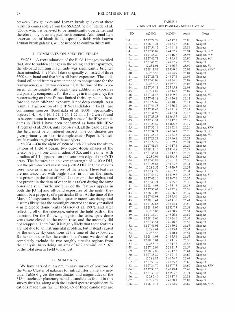
We have carried out a preliminary survey of portions ofthe Virgo Cluster of galaxies for intracluster planetary neb-ulae. Table 6 gives the coordinates and magnitudes of the318 intracluster planetary nebulae candidates found in thissurvey thus far, along with the limited spectroscopic identifi-cations made thus far. Of these, 69 of these candidates are

TABLE 6

Virgo Intracluster Planetary Nebula Catalog

ID �(2000) �(2000) m5007 Notes

1-1......... 12 27 27.79 12 42 42.1 25.80 Suspect, SLa

1-2......... 12 28 13.24 12 41 53.8 25.80 Suspect1-3......... 12 27 54.12 12 40 41.1 25.84 Suspect1-4......... 12 27 36.07 12 44 52.7 25.94 Suspect, SCb

1-5......... 12 27 38.20 12 40 16.6 25.95 Suspect, SOc

1-6......... 12 27 42.71 12 43 55.5 25.96 Suspect, SC1-7......... 12 27 46.95 12 49 27.7 25.98 Suspect1-8......... 12 28 1.01 12 44 36.7 25.99 Suspect, SL1-9......... 12 28 11.83 12 45 0.5 26.02 Suspect, SPNd

1-10....... 12 28 8.56 12 47 24.9 26.04 Suspect1-11....... 12 27 21.71 12 46 27.4 26.06 Suspect1-12....... 12 27 45.08 12 41 24.5 26.07 Suspect1-13....... 12 28 3.36 12 39 7.2 26.08 Suspect1-14....... 12 27 39.11 12 35 45.8 26.08 Suspect1-15....... 12 28 4.87 12 42 44.3 26.09 Suspect1-16....... 12 27 31.56 12 44 9.2 26.11 Suspect, SC1-17....... 12 27 41.18 12 40 36.1 26.11 Suspect1-18....... 12 27 27.69 12 48 40.6 26.11 Suspect1-19....... 12 27 44.53 12 42 36.2 26.14 Suspect1-20....... 12 27 57.45 12 40 41.8 26.14 Suspect1-21....... 12 27 34.92 12 44 37.4 26.15 Suspect, SC1-22....... 12 27 23.23 12 46 5.7 26.17 Suspect1-23....... 12 27 50.31 12 39 12.5 26.18 Suspect1-24....... 12 27 23.49 12 46 5.3 26.19 Suspect1-25....... 12 27 32.19 12 36 58.6 26.20 Suspect, SPN1-26....... 12 27 34.21 12 43 34.1 26.20 Suspect, SC1-27....... 12 27 38.33 12 39 33.3 26.22 Suspect, SC1-28....... 12 27 23.23 12 39 46.1 26.23 Suspect1-29....... 12 27 22.29 12 36 59.1 26.24 Suspect1-30....... 12 27 41.56 12 40 17.4 26.26 Suspect1-31....... 12 28 11.15 12 41 4.8 26.27 Suspect1-32....... 12 27 36.41 12 40 12.8 26.28 Suspect1-33....... 12 28 0.06 12 40 3.3 26.29 Suspect1-34....... 12 27 45.82 12 36 51.2 26.30 Suspect1-35....... 12 27 26.84 12 44 23.3 26.31 Suspect1-36....... 12 28 5.52 12 43 39.7 26.33 Suspect1-37....... 12 27 30.27 12 45 52.3 26.34 Suspect1-38....... 12 27 54.59 12 43 9.8 26.35 Suspect, SL1-39....... 12 27 43.10 12 36 7.6 26.35 Suspect1-40....... 12 27 43.24 12 37 25.2 26.36 Suspect1-41....... 12 28 14.98 12 47 31.6 26.38 Suspect1-42....... 12 27 36.62 12 45 22.8 26.39 Suspect, SC1-43....... 12 28 19.03 12 46 36.8 26.39 Suspect1-44....... 12 27 49.98 12 35 55.0 26.40 Suspect1-45....... 12 28 10.41 12 42 41.0 26.41 Suspect1-46....... 12 27 29.85 12 45 44.4 26.50 Suspect1-47....... 12 28 13.05 12 42 7.3 26.51 Suspect1-48....... 12 28 6.03 12 49 50.7 26.51 Suspect1-49....... 12 27 33.30 12 45 26.1 26.52 Suspect1-50....... 12 28 13.65 12 39 24.5 26.53 Suspect1-51....... 12 27 38.54 12 46 48.3 26.53 Suspect1-52....... 12 27 46.01 12 34 59.2 26.53 Suspect1-53....... 12 28 7.61 12 40 43.4 26.54 Suspect1-54....... 12 28 8.56 12 39 40.4 26.54 Suspect1-55....... 12 28 14.08 12 41 55.1 26.55 Suspect1-56....... 12 28 15.01 12 39 11.8 26.55 Suspect1-57....... 12 28 8.76 12 42 17.8 26.56 Suspect1-58....... 12 27 15.94 12 36 31.7 26.59 Suspect1-59....... 12 28 17.88 12 46 12.3 26.61 Suspect1-60....... 12 27 38.29 12 49 21.2 26.62 Suspect1-61....... 12 28 8.82 12 40 54.5 26.64 Suspect1-62....... 12 27 58.39 12 40 55.3 26.66 Suspect1-63....... 12 27 34.70 12 47 7.5 26.69 Suspect, SPN1-64....... 12 27 30.26 12 45 49.4 26.69 Suspect1-65....... 12 27 30.32 12 35 3.2 26.71 Suspect1-66....... 12 28 2.46 12 36 17.9 26.81 Suspect1-67....... 12 28 7.77 12 40 58.1 26.82 Suspect1-68....... 12 28 13.14 12 39 32.9 26.82 Suspect, SPN

78 FELDMEIER ET AL.

TABLE 6—Continued

ID �(2000) �(2000) m5007 Notes

1-69....... 12 28 11.09 12 47 59.2 26.87 Suspect

2-1......... 12 29 24.29 8 31 17.6 26.36 Ce

2-2......... 12 29 32.16 8 37 16.7 26.41 C2-3......... 12 29 35.44 8 39 29.6 26.47 C2-4......... 12 30 2.48 8 36 26.2 26.51 C2-5......... 12 29 49.79 8 37 51.8 26.62 C2-6......... 12 29 22.21 8 33 43.4 26.73 C2-7......... 12 29 54.22 8 34 22.8 26.74 C2-8......... 12 29 19.45 8 37 37.9 26.74 C2-9......... 12 29 53.94 8 36 3.0 26.75 C2-10....... 12 29 41.08 8 40 30.4 26.902-11....... 12 29 49.52 8 36 55.1 26.972-12....... 12 29 45.40 8 37 59.4 26.982-13....... 12 30 2.39 8 39 25.1 27.032-14....... 12 29 54.24 8 41 1.0 27.132-15....... 12 30 2.09 8 33 33.5 27.182-16....... 12 29 17.76 8 36 36.8 27.46

3-1......... 12 30 33.12 12 38 13.3 25.79 C3-2......... 12 30 27.74 12 35 48.2 25.99 C3-3......... 12 30 52.72 12 34 59.6 26.11 C3-4......... 12 30 23.30 12 33 58.0 26.19 C3-5......... 12 30 59.29 12 35 58.5 26.24 C, SPN3-6......... 12 30 16.04 12 36 56.8 26.25 C3-7......... 12 30 59.57 12 37 24.8 26.34 C, SPN3-8......... 12 31 01.15 12 34 33.6 26.35 C, SPN3-9......... 12 30 41.33 12 32 26.3 26.42 C3-10....... 12 30 24.38 12 33 03.2 26.47 C3-11....... 12 30 56.29 12 42 28.8 26.47 C, SPN3-12....... 12 30 19.47 12 38 33.3 26.48 C3-13....... 12 30 49.16 12 39 21.8 26.51 C3-14....... 12 30 52.31 12 32 31.1 26.55 C, SPN3-15....... 12 30 48.22 12 31 45.7 26.56 C, SPN3-16....... 12 30 55.22 12 36 04.8 26.57 C, SPN3-17....... 12 30 27.01 12 31 28.8 26.58 C3-18....... 12 30 18.62 12 32 37.8 26.62 C3-19....... 12 31 05.88 12 32 50.0 26.65 C, SPN3-20....... 12 30 36.76 12 40 59.7 26.67 C3-21....... 12 30 24.14 12 40 58.3 26.68 C3-22....... 12 30 27.35 12 31 16.6 26.68 C3-23....... 12 30 31.62 12 36 04.9 26.69 C, SL3-24....... 12 30 34.24 12 43 58.5 26.69 C3-25....... 12 30 53.78 12 38 26.8 26.69 C, SPN3-26....... 12 30 46.03 12 38 31.7 26.72 C3-27....... 12 30 33.98 12 30 50.2 26.73 C3-28....... 12 30 55.21 12 36 38.3 26.75 C3-29....... 12 30 41.58 12 38 37.6 26.78 C3-30....... 12 30 45.87 12 38 33.9 26.79 C3-31....... 12 30 20.51 12 33 41.6 26.80 C3-32....... 12 30 23.99 12 37 36.2 26.80 C3-33....... 12 30 31.37 12 30 04.4 26.84 C3-34....... 12 30 37.59 12 29 54.7 26.86 C3-35....... 12 30 20.62 12 31 26.0 26.87 C, SPN3-36....... 12 30 25.40 12 30 34.5 26.87 C, SPN3-37....... 12 30 22.07 12 43 30.5 26.88 C3-38....... 12 30 29.79 12 39 18.8 26.88 C3-39....... 12 30 36.19 12 41 55.8 26.90 C3-40....... 12 31 01.59 12 39 58.1 26.91 C3-41....... 12 30 31.77 12 30 40.0 26.91 C, SPN3-42....... 12 31 09.43 12 45 06.6 26.93 C, SL3-43....... 12 30 21.50 12 41 54.5 26.93 C3-44....... 12 30 23.56 12 42 45.6 26.94 C3-45....... 12 30 53.88 12 42 12.6 26.97 C3-46....... 12 30 41.40 12 35 21.0 26.97 C3-47....... 12 30 37.18 12 33 06.5 27.00 C3-48....... 12 31 09.54 12 33 43.2 27.013-49....... 12 30 41.39 12 32 58.4 27.013-50....... 12 30 36.57 12 33 56.6 27.02

TABLE 6—Continued

ID �(2000) �(2000) m5007 Notes

3-51....... 12 31 01.16 12 44 51.2 27.023-52....... 12 30 38.52 12 35 14.8 27.033-53....... 12 31 13.30 12 33 19.0 27.043-54....... 12 30 57.97 12 30 32.0 27.073-55....... 12 30 42.66 12 37 37.8 27.073-56....... 12 30 38.67 12 36 57.1 27.083-57....... 12 30 31.20 12 38 54.1 27.083-58....... 12 30 30.53 12 35 38.8 27.093-59....... 12 30 43.05 12 39 18.8 27.103-60....... 12 30 51.24 12 34 44.6 27.173-61....... 12 30 50.11 12 38 30.9 27.183-62....... 12 31 14.79 12 36 39.3 27.183-63....... 12 30 26.33 12 35 54.5 27.193-64....... 12 30 49.31 12 36 56.4 27.203-65....... 12 30 49.28 12 41 49.0 27.223-66....... 12 30 15.07 12 37 39.4 27.243-67....... 12 31 03.75 12 41 08.1 27.243-68....... 12 30 39.18 12 44 02.1 27.273-69....... 12 31 09.06 12 37 01.8 27.30 SPN3-70....... 12 30 28.94 12 29 59.3 27.373-71....... 12 30 22.16 12 41 07.9 27.473-72....... 12 30 50.87 12 33 22.4 27.473-73....... 12 31 10.34 12 30 42.0 27.503-74....... 12 30 27.65 12 41 07.5 27.613-75....... 12 31 12.39 12 31 32.1 27.97

4-1......... 12 27 44.91 12 27 44.9 25.55 C, SL4-2......... 12 27 16.12 12 25 25.9 26.42 C, SL4-3......... 12 27 53.50 12 26 48.6 26.46 C4-4......... 12 27 16.16 12 23 18.0 26.52 C, SPN4-5......... 12 27 27.53 12 31 06.7 26.77 SL4-6......... 12 27 22.78 12 34 07.0 26.784-7......... 12 27 19.73 12 33 39.2 26.834-8......... 12 27 25.99 12 30 27.6 26.884-9......... 12 27 43.53 12 29 12.5 26.93 SPN4-10....... 12 27 21.25 12 34 05.7 26.964-11....... 12 28 03.37 12 32 12.5 27.074-12....... 12 27 40.35 12 27 57.6 27.07

5-1......... 12 34 07.48 12 14 49.0 25.80 C5-2......... 12 33 52.61 12 20 51.0 25.95 C5-3......... 12 33 40.23 12 25 07.1 25.99 C5-4......... 12 33 32.47 12 17 08.3 26.105-5......... 12 34 05.34 12 24 06.2 26.235-6......... 12 34 11.42 12 20 41.7 26.255-7......... 12 33 56.13 12 16 41.9 26.29

6-1......... 12 31 05.08 07 54 15.1 26.13 C6-2......... 12 30 46.31 07 56 12.0 26.31 C6-3......... 12 30 48.06 07 58 06.9 26.38 C6-4......... 12 30 28.94 07 58 22.3 26.40 C6-5......... 12 30 36.60 07 50 36.4 26.53 C6-6......... 12 30 35.72 08 02 14.4 26.62 C6-7......... 12 31 01.87 07 54 40.3 26.62 C6-8......... 12 31 14.03 07 51 55.5 26.66 C6-9......... 12 31 14.94 07 53 10.7 26.74 C6-10....... 12 30 56.51 08 02 14.9 26.906-11....... 12 30 44.10 07 59 04.9 26.946-12....... 12 30 38.64 07 52 21.5 26.956-13....... 12 30 28.97 07 55 59.9 27.106-14....... 12 31 00.79 07 57 48.5 27.116-15....... 12 31 17.36 07 49 10.4 27.176-16....... 12 31 02.77 07 49 15.0 27.31

7-1......... 12 29 27.15 12 57 1.7 25.92 C7-2......... 12 27 13.85 12 34 13.1 26.10 C7-3......... 12 27 22.41 12 56 24.4 26.18 C7-4......... 12 27 27.78 12 42 42.6 26.20 C7-5......... 12 28 42.77 12 38 39.5 26.21 C

TABLE 6—Continued

ID �(2000) �(2000) m5007 Notes

7-6......... 12 27 15.26 12 57 58.4 26.26 C7-7......... 12 28 26.60 12 46 40.8 26.30 C7-8......... 12 28 58.82 12 46 53.0 26.35 C7-9......... 12 29 29.25 13 5 16.0 26.41 C7-10....... 12 28 3.25 12 38 18.7 26.41 C7-11....... 12 28 57.25 12 40 12.8 26.43 C7-12....... 12 28 52.00 12 44 43.3 26.43 C7-13....... 12 28 1.12 13 2 40.7 26.47 C7-14....... 12 29 33.84 13 4 15.6 26.47 C7-15....... 12 28 16.97 13 5 15.0 26.48 C7-16....... 12 29 2.23 12 58 36.2 26.49 C7-17....... 12 28 56.24 12 36 32.0 26.49 C7-18....... 12 29 32.40 13 4 43.6 26.51 C7-19....... 12 28 9.55 12 56 34.4 26.52 C7-20....... 12 28 10.76 13 3 11.8 26.52 C7-21....... 12 27 50.14 12 41 16.1 26.57 C7-22....... 12 28 15.94 13 3 37.1 26.58 C7-23....... 12 29 28.42 12 56 45.6 26.66 C7-24....... 12 29 17.02 12 52 3.8 26.67 C7-25....... 12 29 7.32 12 50 43.2 26.70 C7-26....... 12 27 27.28 12 47 29.6 26.70 C7-27....... 12 27 40.86 12 34 35.4 26.71 C7-28....... 12 27 55.70 12 54 26.5 26.72 C7-29....... 12 28 0.21 13 3 46.1 26.73 C7-30....... 12 29 4.34 12 46 31.1 26.74 C7-31....... 12 28 50.78 12 37 60.0 26.77 C7-32....... 12 29 19.89 13 2 13.6 26.79 C7-33....... 12 29 5.83 12 39 4.5 26.817-34....... 12 28 58.59 12 46 11.9 26.817-35....... 12 29 27.36 12 53 26.7 26.847-36....... 12 27 40.01 12 56 16.4 26.857-37....... 12 27 30.63 12 38 30.2 26.877-38....... 12 29 30.19 13 0 13.0 26.877-39....... 12 27 30.50 12 57 56.4 26.887-40....... 12 29 6.27 12 39 31.0 26.897-41....... 12 27 15.47 12 41 34.2 26.917-42....... 12 28 8.86 12 56 53.1 26.937-43....... 12 28 47.28 12 35 27.2 26.947-44....... 12 27 16.71 12 59 53.7 26.957-45....... 12 29 4.17 12 40 34.2 26.987-46....... 12 28 1.53 12 39 10.2 26.987-47....... 12 27 15.12 12 39 47.0 26.987-48....... 12 27 50.84 12 52 26.2 26.997-49....... 12 28 3.49 13 0 42.5 27.037-50....... 12 27 27.55 13 5 26.7 27.067-51....... 12 29 21.48 13 0 37.0 27.067-52....... 12 28 53.42 12 57 28.3 27.097-53....... 12 29 13.84 13 3 54.5 27.107-54....... 12 28 21.14 12 47 59.8 27.107-55....... 12 28 4.01 12 59 10.3 27.117-56....... 12 28 35.70 12 35 54.5 27.147-57....... 12 29 21.42 12 38 41.9 27.147-58....... 12 29 3.27 12 56 31.8 27.157-59....... 12 29 34.46 13 3 54.3 27.187-60....... 12 29 32.35 13 4 57.3 27.197-61....... 12 27 18.09 12 42 29.1 27.217-62....... 12 27 28.92 12 33 19.6 27.217-63....... 12 27 23.11 12 39 22.2 27.237-64....... 12 28 18.20 13 1 32.6 27.247-65....... 12 29 3.05 13 2 50.5 27.247-66....... 12 28 5.09 12 55 19.2 27.257-67....... 12 28 14.19 12 54 52.6 27.267-68....... 12 28 49.11 12 58 12.6 27.297-69....... 12 29 32.05 12 44 53.3 27.307-70....... 12 28 25.89 13 0 43.9 27.317-71....... 12 29 34.82 13 6 29.3 27.347-72....... 12 27 50.86 12 57 36.5 27.347-73....... 12 28 15.15 13 3 48.8 27.447-74....... 12 27 20.14 12 54 55.5 27.44

TABLE 6—Continued

ID �(2000) �(2000) m5007 Notes

7-75....... 12 27 25.99 12 36 51.3 27.487-76....... 12 29 11.54 12 51 31.4 27.527-77....... 12 29 2.32 12 36 17.6 27.59

8-1......... 12 28 25.86 11 21 33.2 25.38 C8-2......... 12 27 28.51 11 39 50.6 25.52 C8-3......... 12 28 31.31 11 19 33.3 26.17 C8-4......... 12 28 13.45 11 21 30.6 26.21 C8-5......... 12 28 12.22 11 25 43.2 26.23 C8-6......... 12 27 21.86 11 42 38.8 26.24 C8-7......... 12 27 5.44 11 15 38.0 26.35 C8-8......... 12 28 24.75 11 24 4.9 26.35 C8-9......... 12 28 2.81 11 30 15.1 26.43 C8-10....... 12 27 29.79 11 35 34.6 26.48 C8-11....... 12 26 28.13 11 39 42.7 26.49 C8-12....... 12 28 19.99 11 43 34.2 26.53 C8-13....... 12 27 11.17 11 36 20.5 26.57 C8-14....... 12 27 59.18 11 32 42.8 26.66 C8-15....... 12 27 6.58 11 32 34.1 26.70 C8-16....... 12 28 31.29 11 11 41.8 26.71 C8-17....... 12 27 46.85 11 13 22.4 26.73 C8-18....... 12 27 0.64 11 31 52.2 26.82 C8-19....... 12 28 21.86 11 28 41.1 26.86 C8-20....... 12 28 27.84 11 17 43.3 26.89 C8-21....... 12 27 58.98 11 37 33.4 26.938-22....... 12 28 28.14 11 13 30.6 26.958-23....... 12 27 11.35 11 41 40.6 26.978-24....... 12 28 32.12 11 43 8.8 26.998-25....... 12 26 41.41 11 38 2.5 27.018-26....... 12 27 50.30 11 29 54.9 27.058-27....... 12 28 13.49 11 28 12.0 27.058-28....... 12 27 23.43 11 11 39.9 27.118-29....... 12 27 59.13 11 15 0.8 27.118-30....... 12 26 40.33 11 40 34.5 27.128-31....... 12 27 57.01 11 30 42.2 27.148-32....... 12 27 51.67 11 45 10.4 27.158-33....... 12 27 14.14 11 20 34.4 27.238-34....... 12 27 19.69 11 44 2.3 27.248-35....... 12 26 46.22 11 36 42.7 27.248-36....... 12 27 39.96 11 19 38.8 27.258-37....... 12 28 5.98 11 42 47.5 27.268-38....... 12 27 29.07 11 30 10.0 27.278-39....... 12 28 40.58 11 26 14.6 27.308-40....... 12 27 45.43 11 34 2.9 27.308-41....... 12 27 11.21 11 32 49.0 27.318-42....... 12 26 39.94 11 19 29.7 27.348-43....... 12 27 38.50 11 20 29.8 27.378-44....... 12 27 19.55 11 16 6.7 27.398-45....... 12 28 20.48 11 13 22.7 27.418-46....... 12 27 5.66 11 26 56.5 27.53

Note.—Units of right ascension are hours, minutes, and seconds,and units of declination are degrees, arcminutes, and arcseconds.Table 6 is also available in machine-readable form in the electronicedition of theAstrophysical Journal Supplement. .

a SL: object was detected spectroscopically by Freeman et al. 2000,or Kudritzki et al. 2000 and found to be a Ly� galaxy candidate.

b SC: object was detected spectroscopically by Kudritzki et al.2000 and found to be a continuum source.

c SO: object was detected spectroscopically by Kudritzki et al.2000 and found to be an [O ii] emitter at a redshift of�0.35.

d SPN: object was detected spectroscopically by Freeman et al.2000 and found to be a IPN.

e C: object is part of photometrically complete subsample.

from Field 1 and are suspect. The vast majority of theremainder are likely to be genuine IPNe. From control-fieldexperiments and limited spectroscopic follow-up observa-tions, we believe approximately 20% of the candidates willbe background objects of significant scientific interest. Con-sequently, we estimate that �200 of the candidates in Table6 are genuine IPNe. To conclude, we note that despite allour efforts, less than a percent of the Virgo Cluster has beensurveyed for intracluster planetary nebulae, and those areashave been shallowly surveyed. Thousands more IPNe waitto be discovered.

We thank M. Arnaboldi, K. Freeman, R. Kudritzki, andR.Mendez for useful discussions, and their infinite patience.We thank P. Harding and B. Jannuzi for useful discussionsconcerning MOSAIC photometry issues. We thank C.McBride for assistance with adapting Figure 9 for publica-tion.We also thank an anonymous referee for useful sugges-tions that improved the presentation of this paper. J.Feldmeier acknowledges salary support from J. C. Mihosunder grant AST-9876143. This work was also partiallysupported by NSF grant AST 0071238 and NASA grantNAG 5-9377.

REFERENCES

Adelberger, K. L., Steidel, C. C., Giavalisco, M., Dickinson, M., Pettini,M., &Kellogg,M. 1998, ApJ, 505, 18

Alard, C., & Lupton, R. H. 1998, ApJ, 503, 325Arnaboldi, M., et al. 1996, ApJ, 472, 145———. 2002, AJ, 123, 760Bernstein, G.M., Nichol, R. C., Tyson, J. A., Ulmer,M. P., &Wittman, D.1995, AJ, 110, 1507

Binggeli, B., Popescu, C. C., & Tammann, G. A. 1993, A&AS, 98, 275Binggeli, B., Sandage, A., & Tammann, G. A. 1985, AJ, 90, 1681Binggeli, B., Tammann, G. A., & Sandage, A. 1987, AJ, 94, 251Bolte,M. 1989, ApJ, 341, 168Bothun, G. D., &Gregg,M. D. 1990, ApJ, 350, 7Ciardullo, R. 2003, in IAU Symp. 209, Planetary Nebulae: Their EvolutionandRole in the Universe, in press

Ciardullo, R., Feldmeier, J. J., Jacoby, G. H., Kuzio, R., Laychak, M. B.,&Durrell, P. R. 2002a, ApJ, 577, 31

Ciardullo, R., Feldmeier, J. J., Krelove, K., Jacoby, G. H., & Gronwall, C.2002b, ApJ, 566, 784

Ciardullo, R., Ford, H. C., Neill, J. D., Jacoby, G. H., & Shafter, A. W.1987, ApJ, 318, 520

Ciardullo, R., Jacoby, G. H., Feldmeier, J. J., & Bartlett, R. E. 1998, ApJ,492, 62

Ciardullo, R., Jacoby, G. H., & Ford, H. C. 1989, ApJ, 344, 715Ciardullo, R., Jacoby, G. H., Ford, H. C., &Neill, J. D. 1989, ApJ, 339, 53Dressler, A. 1984, ARA&A, 22, 185Dubinski, J., Mihos, J. C., &Hernquist, L. 1996, ApJ, 462, 576———. 1999, ApJ, 526, 607Durrell, P., Ciardullo, R., Feldmeier, J. J., Jacoby, G. H., & Sigurdsson, S.2002a, ApJ, 570, 119

Durrell, P., Mihos, J. C. M., Feldmeier, J. J., Jacoby, G. H., & Ciardullo,R. 2002b, ApJ,582, 170

Feldmeier, J. J. 2000, Ph.D. thesis, Penn State Univ.Feldmeier, J. J., Ciardullo, R., & Jacoby, G. H. 1998, ApJ, 503, 109(Paper I)

Feldmeier, J. J., Mihos, J. C. M., Morrison, H. L., Rodney, S. A., &Harding, P. 2002, ApJ, 575, 779

Ferguson, H. C., Tanvir, N. R., & vonHippel, T. 1998, Nature, 391, 461Freeman, K. C., et al. 2000, ASP Conf. Ser. 197: Dynamics of Galaxies:from the Early Universe to the Present, ed. F. Combes, G. A. Mamon, &V. Charmandaris (San Francisco: ASP) 389.

Gonzalez, A. H., Zabludoff, A. I., Zaritsky, D., & Dalcanton, J. J. 2000,ApJ, 536, 561

Harris,W. E. 1990, PASP, 102, 949Hui, X., Ford, H., Ciardullo, R., & Jacoby, G. 1993, ApJ, 414, 463Impey, C., Bothun, G., &Malin, D. 1988, ApJ, 330, 634Jacoby, G. H. 1989, ApJ, 339, 39Jacoby, G. H., Ciardullo, R., & Ford, H. C. 1990, ApJ, 356, 332Jacoby, G. H., Ciardullo, R., Ford, H. C., & Booth, J. 1989, ApJ, 344,70

Jacoby, G. H., & Lesser,M. P. 1981, AJ, 86, 185Jacoby, G. H., Liang, M., Vaughnn, D., Reed, R., & Armandroff, T. 1998,Proc. SPIE, 3355, 721

Jacoby, G. H., Quigley, R. J., & Africano, J. L. 1987, PASP, 99, 672Jacoby, G. H., et al. 1992, PASP, 104, 599Katsiyannis, A. C., Kemp, S. N., Berry, D. S., &Meaburn, J. 1998, A&AS,132, 387

Kenney, J. D. P., Rubin, V. C., Planesas, P., & Young, J. S. 1995, ApJ, 438,135

Kudritzki, R.-P., et al. 2000, ApJ, 536, 19Mackay, C. D. 1986, ARA&A, 24, 255Magrini, L., Perinotto,M., Corradi, R. L.M., &Mampaso, A. 2001, A&A,379, 90

Massey, P. 1997, NOAONewsletter 52Massey, P., Strobel, K., Barnes, J. V., & Anderson, E. 1988, ApJ, 328,315

Melnick, J., White, S. D.M., &Hoessel, J. 1977,MNRAS, 180, 207Mendez, R. H., Guerrero, M. A., Freeman, K. C., Arnaboldi, M.,Kudritzki, R. P., Hopp, U., Capaccioli, M., & Ford, H. 1997, ApJ, 491,23

Mendez, R. H., Riffeser, A., Kudritzki, R.-P., Matthias, M., Freeman,K. C., Arnaboldi, M., Capaccioli, M., & Gerhard, O. E. 2001, ApJ, 563,135

Merline,W. J., &Howell, S. B. 1995, Exp. Astron., 6, 163Miller, G. E. 1983, ApJ, 268, 495Millis, R. L., Buie, M. W., Wasserman, L. H., Elliot, J. L., Kern, S. D., &Wagner, R.M. 2002, AJ, 123, 2083

Monet, D. 1998, BAAS, 30, 1427Monet, D., et al. 1996, USNO A-1.0: A Catalog of Astrometric Standards(Washington: USNaval Obs)

Muller, G. P., Reed, R., Armandroff, T., Boroson, T. A., & Jacoby, G. H.1998, Proc. SPIE, 3355, 577

Nichollian, E. H., & Brews, J. R. 1982,Metal Oxide Semiconductor Physicsand Technology (NewYork:Wiley), 549

Norman, C., et al. 2002, ApJ, 571, 218Oke, J. B., &Gunn, J. E. 1983, ApJ, 266, 713Perlmutter, S., et al. 1999, ApJ, 517, 565Pogge, R. W. 1992, in ASP Conf. Ser. 23, Astronomical CCD ObservingandReduction Techniques, ed. S. Howell (San Francisco: ASP), 195

Rhoads, J. E., Malhotra, S., Dey, A., Stern, D., Spinrad, H., & Jannuzi,B. T. 2000, ApJ, 545, L85

Richstone, D. O., &Malumuth, E.M. 1983, ApJ, 268, 30Richter, O.-G., & Binggeli, B., eds. 1985, ESO Workshop on the VirgoCluster of Galaxies (Garching: ESO)

Schmidt, B. P., et al. 1998, ApJ, 507, 46Shapley, H., &Ames, A. 1926, Harvard Circ. 294Steidel, C. C., Adelberger, K. L., Shapley, A. E., Pettini, M., Dickinson,M., &Giavalisco, M. 2000, ApJ, 532, 170

Steidel, C. C., &Hamilton, D. 1993, AJ, 105, 2017Stern, D., Bunker, A., Spinrad, H., &Dey, A. 2000, ApJ, 537, 73Stetson, P. B. 1987, PASP, 99, 191———. 1992, JRASC, 86, 71Stone, R. P. S. 1977, ApJ, 218, 767Theuns, T., &Warren, S. J. 1997,MNRAS, 284, L11Uson, J.M., Boughn, S. P., &Kuhn, J. R. 1991, ApJ, 369, 46Vılchez-Gomez, R. 1999, ASP Conf. Ser. 170: The Low Surface BrightnessUniverse, ed. J. I. Davies, C. Impey, & S. Phillips (San Francisco: ASP),349

Vıchez-Gomez, R., Pello, R., & Sanahuja, B. 1994, A&A, 283, 37Welch, G. A., & Sastry, G. N. 1971, ApJ, 169, L3Zwicky, F. 1951, PASP, 63, 61

INTRACLUSTER PLANETARY NEBULAE IN VIRGO. II. 81







Intracluster Planetary Nebulae in the Virgo Cluster III: Luminosity of the Intracluster Light and...

Documents

Transcript of Intracluster Planetary Nebulae in the Virgo Cluster III: Luminosity of the Intracluster Light and...