
Intra-host HIV-1 evolution and the co-receptor switch - TUprints
188
Intra-host HIV-1 evolution and the co-receptor switch !" #$% &’ () *’ ’ +, - .’ () *’ ’ ) ./’&0’.0&1 % *%) &2’&.’.0&1 .0&3 &4
-
Upload
khangminh22 -
Category
Documents
-
view
1 -
download
0
Transcript of Intra-host HIV-1 evolution and the co-receptor switch - TUprints

Intra-host HIV-1 evolution and the co-receptor switch
������������� ����������������������������������������������������������������������������
���������������������� �������������������������
�
���� ���� ���������������!����"�����������#$��%����
�
&'�( ���)�*�� '���'�+�,�-�������
.'�( ���)�*�� '���'�������������
�
�����������������)��./'&0'.0&1�
��������%��������*�% ���)��&2'&.'.0&1�
�
����������.0&3�
�&4


Ehrenwortliche Erklarung
Ich erklare hiermit ehrenwortlich, dass ich die vorliegende Arbeit entsprechend den Regelnguter wissenschaftlicher Praxis selbststandig und ohne unzulassige Hilfe Dritter angefertigthabe.
Samtliche aus fremden Quellen direkt oder indirekt ubernommene Gedanken sowiesamtliche von Anderen direkt oder indirekt ubernommenen Daten, Techniken und Ma-terialien sind als solche kenntlich gemacht. Die Arbeit wurde bisher bei keiner anderenHochschule zu Prufungszwecken eingereicht.
Darmstadt, den 25. Oktober 2013


Abstract
The course of an infection with the human immunodeficiency virus type 1 (HIV-1) ischaracterised by three phases: primary infection, chronic infection and acquired immun-odeficiency syndrome (AIDS). These stages are defined based on levels of the number ofCD4-positive T-helper cells (CD4+). This characteristic three-staged classification is alsoreflected in the course of the viral divergence and in the emergence of viral diversity.It is known that the V3 loop, a region encoded in the HIV envelope gene, is important forT cell infection. The CD4 receptor of the cells is used as primary receptor for viral cellentry, and the CCR5 or CXCR4 are the most important co-receptors that are necessary forcell entry. In about half of all patients, HIV switches from CCR5 towards CXCR4 usageduring the late stage of infection, which hints at the onset of AIDS. Since the co-receptortropism is determined by the V3 loop sequence, an understanding of the mechanisms ofits evolution and of the circumstances leading to the co-receptor switch is of high interest.In the first part of the present work, we analysed longitudinal patient data, compris-ing information on CD4+ cell count, viral load, medication, coinfections and V3 loopsequences. We examined the correlations among the clinical and evolutionary data as wellas the co-receptor usage over time, guided by different questions: Is the course of diseaseone-directional? Can successful drug therapy influence co-receptor usage? What are thegenetic differences between CCR5- and CXCR4-tropic viruses?Due to the weak statistical support of our data, we only found few indications thatsuccessful HAART therapy influences the course of disease and the direction of the co-receptor switch. We hypothesise that successful therapy can pause or roll back the courseof infection, enabling the CD4+ cells to recover to high levels of immune pressure. Asuppression of the viral load further can displace X4-tropic viral variants in the viralpopulation in favour of R5-tropic variants.In the second part of this work, we derived a fitness function to approximate the replicationcapacity of R5 and X4-tropic viruses. Based on a set of V3 loop sequences gathered fromthe Los Alamos HIV data base, the fitness function is composed of two components: themain fitness term describes the amino acid preferences found in the R5 and the X4 consen-sus sequence, and the additional epistatic term describes the effects of double mutations.While the impact of the main and epistatic fitness contribution can be influenced by aweighting parameter, an additional parameter controls the importance of available CCR5and CXCR4 positive target cells. The fitness function enabled us to observe the differencesof the underlying R5 and X4 fitness landscapes.A comparison of the sequence data set showed that the R5-tropic viral sequences werehighly conserved, in contrast to the X4 sequences. Network analyses confirmed the highersequence variability of the X4 sequences, which we found to be distributed over a largersequence space. Interestingly, our analyses revealed that the most weakly conserved se-quence positions of the X4 data set were very sensible to mutations. Upon an alteration ofthe most weakly conserved nt positions, the X4 sequences showed an increased probabilityto acquire stop condons and to loose their replicative capacity.The last part of the work describes an in silico approach of the V3 loop evolution basedon the R5 and X4 fitness function. Simulations enable us to mimic the sequence evolutionin silico, and to monitor the course of the viral diversity and divergence as well as themean fitness of the simulated viral population over time.
I

First results indicated that our simulation is able to imitate the evolutionary course ofthe viral diversity and divergence of an HIV infection. In our simulations, the sequenceevolution followed a chemically sensible course. Amino acids that differed from the favouredchemical properties were first replaced by amino acids belonging to the favourable chemicalclass and finally converged into the dominant amino acid in the specific sequence position.The present project was designed to prepare the ground for deeper insights into the evolu-tionary dynamics of the HIV V3 loop. Our work enabled us to gain broader knowledge ofthe properties of R5- and X4-tropic viral sequences.
II

Zusammenfassung
Eine Infektion mit dem humanen Immundefizienz-Virus (HIV) verlauft in drei charak-teristischen Krankheitsphasen. Die Phasen konnen einerseits an Hand der Anzahl derCD4-Zellen unterschieden werden, andererseits kann eine Unterscheidung auf der Grund-lage der viralen Diversitat und Divergenz statt finden.Fur die Infektion der Wirtszellen durch das Virus ist die V3-Region, ein Abschnitt, derim Hullprotein von HIV kodiert ist, von zentraler Bedeutung. Nach der Bindung vonHIV an den CD4-Rezeptor der Zielzellen erfolgt eine Bindung der V3-Region an einenzellularen Korezeptor, welches in den meisten Fallen ein CCR5- bzw. CXCR4-Rezeptorist. Im Verlauf der Infektion kann man bei etwa der Halfte aller Patienten einen Wechseldes benutzten Korezeptors beobachten. Dieser findet im allgemeinen in einer spatenKrankheitsphase statt und kundigt ein rasches Fortschreiten der Infektion an. Bisher ist esnicht gelungen, die Hintergrunde und Mechanismen, welche zu diesem Korezeptor-Wechselfuhren, komplett aufzuklaren.Die vorliegende Arbeit untersucht die Sequenzevolution von HIV-1 mit besonderem Au-genmerk auf die Unterschiede zwischen R5-trophen und X4-trophen Viren. Der erste Teilberuht auf Daten von HIV-1-infizierten Patienten, die uber mehrere Jahre beobachtet wur-den. Basierend auf Publikationen aus der Zeit der beginnenden HIV-Forschung verglichenwir die Daten von akuellen Patienten mit den fruheren Beobachtungen, um Unterschiedeim Verlauf der Infektion zu untersuchen zwischen nahezu untherapierten Patienten undPatienten, die mit moderner Kombinationstherapie behandelt wurden. Wir fanden dabeierste Hinweise, dass die grundsatzlichen Beobachtungen der fruhen Studien auch fur Patien-ten mit modernen Therapieansatzen Bestand haben, wobei die Daten einen Unterschiedim zeitlichen Verlauf der Infektion zwischen HAART-therapierten und therapie-naıven Pa-tientengruppen andeuten. Unsere Untersuchungen lassen die Vermutung zu, dass aktuelleTherapien den Krankheitsverlauf verlangsamen und fur begrenzte Zeit sogar stoppen oderzuruck setzen konnen. Diese Hypothese konnte im Rahmen der vorliegenden Arbeit aufGrund der unzureichenden Datenlage allerdings nicht besttigt werden.Im zweiten Teil der Arbeit untersuchten wir die Unterschiede zwischen den R5-trophen undX4-trophen Viren an einem umfangreichen frei verfugbaren Sequenzdatensatz. Nach derKlassifizierung der Sequenzen in R5- und X4-trophe Varianten untersuchten wir zunachstdie Unterschiede der R5 und X4 Konsensussequenz. Wir konnten fruhere Ergebnissebestatigen, nach denen die R5-trophen Viren starker konserviert sind, und nach denenbei X4-trophen Viren eine Dominanz von positiv geladenen Aminosauren in den Korezep-tor bestimmenden Sequenzpositionen 11 und 25 vorliegt. Auf Basis des R5- und desX4-Datensatzes entwickelten wir zwei unabhangige Fitnessfunktionen, die die Replika-tionsfahigkeit der R5- beziehungsweise der X4-trophen Viren mathematisch beschreiben.Die Fitnessfunktionen bestehen jeweils aus zwei Beitragen. Der erste Fitnessterm beschreibtdie Fitness der Aminosaureabfolge der V3-Region der HIV-1 Sequenz, wohingegen derzweite Teil die Auswirkung von epistatischen Wechselwirkungen von Paaren von Sequenz-mutationen auf die replikative Fitness berechnet.Auf der Grundlage dieser Fitnessfunktionen waren wir in der Lage, die Fitnesslandschaftender R5- und X4-trophen Viren zu vergleichen. Wir stellten dabei fest, dass sich die starkkonservierten Sequenzen der R5-trophen Viren in direkter Nachbarschaft im Sequenzraumbefinden, wahrend sich die Sequenzen der X4-trophen Viren uber einen großeren Bereich
III

des Sequenzraumes erstrecken. Unsere Ergebnisse stimmten mit den Beobachtungenanderer Forschungsgruppen uberein.Die beiden Fitnessfunktionen bildeten das Herz einer sequenzbasierten Simulation derEvolution der V3-Region, die wir im dritten Teil dieser Arbeit beschreiben. Wir kon-nten zeigen, dass unsere Simulation die Evolution von zufalligen Sequenzen hin zur R5-bzw. zur X4-Konsensussequenz ermoglicht. Daruber hinaus folgen die Simulationenchemisch sinnvollen Pfaden. Wir konnten beobachten, dass sich anfanglich nicht op-timierte, mutierte Sequenzpositionen zunachst in Richtung der korrekten chemischenGruppe (z.B. positiv geladene Aminosaure) und in folgenden Replikationen weiter zurkorrekten Konsensusaminosaure entwickelten. Unsere Simulationen ermoglichen daherModelluntersuchungen der Evolution von artifiziellen Sequenzen der V3-Region, die nichtden Restriktionen einer groß angelegten Patientenstudie unterliegen.
IV
Contents
Abstract . . . . . . . . . . . . . . . . . . . . . . . . . . . . . . . . . . . . . . . . IZusammenfassung . . . . . . . . . . . . . . . . . . . . . . . . . . . . . . . . . . . III
1. Motivation 1
1.1. Motivation . . . . . . . . . . . . . . . . . . . . . . . . . . . . . . . . . . . . 11.1.1. Relevance of the work . . . . . . . . . . . . . . . . . . . . . . . . . 11.1.2. Aim of the Project . . . . . . . . . . . . . . . . . . . . . . . . . . . 2
2. Introduction 4
2.1. Structure of the project . . . . . . . . . . . . . . . . . . . . . . . . . . . . . 42.1.1. Project I: Correlation between clinical and evolutionary parameters
of patients under HAART . . . . . . . . . . . . . . . . . . . . . . . 42.1.2. Project II: Fitness function of HIV-1 V3 loop . . . . . . . . . . . . 52.1.3. Project III: Simulation of HIV-1 V3 loop evolution . . . . . . . . . 52.1.4. Previous work within the project . . . . . . . . . . . . . . . . . . . 5
Biological assay for in vitro co-receptor prediction . . . . . . . . . . 6Case study of stem cell treated patient . . . . . . . . . . . . . . . . 6
3. Correlations between clinical and evolutionary parameters 7
3.1. Introduction . . . . . . . . . . . . . . . . . . . . . . . . . . . . . . . . . . . 73.1.1. HIV-1 infection and the human immune system . . . . . . . . . . . 7
The human immune system . . . . . . . . . . . . . . . . . . . . . . 7Innate immune system . . . . . . . . . . . . . . . . . . . . . 8Adaptive immune system . . . . . . . . . . . . . . . . . . . . 8
3.1.2. The influence of the HIV-1 infection on the immune system . . . . . 8Characteristics of HIV-1 . . . . . . . . . . . . . . . . . . . . . . . . 9The HIV-1 infection cycle . . . . . . . . . . . . . . . . . . . . . . . 10
Step 1: Receptor binding, membrane fusion and cell entry . . 11Step 2: Reverse transcriptase . . . . . . . . . . . . . . . . . . 12Step 3: Integration into host genome . . . . . . . . . . . . . 12Step 4: Replication . . . . . . . . . . . . . . . . . . . . . . . 13Step 5: Viral assembly and budding . . . . . . . . . . . . . . 13
Co-receptor usage of HIV-1 . . . . . . . . . . . . . . . . . . . . . . 133.1.3. Phases of an untreated HIV-1 infection . . . . . . . . . . . . . . . . 15
Clinical classification . . . . . . . . . . . . . . . . . . . . . . . . . . 16Evolutionary classification . . . . . . . . . . . . . . . . . . . . . . . 18
3.2. Methods . . . . . . . . . . . . . . . . . . . . . . . . . . . . . . . . . . . . . 203.2.1. Evolutionary and mathematical definitions . . . . . . . . . . . . . . 20
Phylogenetics and phylogeny . . . . . . . . . . . . . . . . . . . . . . 20Coalescence and coalescence time . . . . . . . . . . . . . . . . . . . 20
V

Contents
Effective population size Ne . . . . . . . . . . . . . . . . . . . . . . 20Bayesian skyline . . . . . . . . . . . . . . . . . . . . . . . . . . . . . 20Hamming distance . . . . . . . . . . . . . . . . . . . . . . . . . . . 20Diversity and Divergence . . . . . . . . . . . . . . . . . . . . . . . . 21Bayes factor . . . . . . . . . . . . . . . . . . . . . . . . . . . . . . . 22Mathematical correlations . . . . . . . . . . . . . . . . . . . . . . . 23Statistical significance . . . . . . . . . . . . . . . . . . . . . . . . . 23Confidence interval . . . . . . . . . . . . . . . . . . . . . . . . . . . 23Correlation coefficients . . . . . . . . . . . . . . . . . . . . . . . . . 24
Pearson correlation coefficient . . . . . . . . . . . . . . . . . 24Spearman rank correlation coefficient . . . . . . . . . . . . . 24Kendall rank correlation coefficient . . . . . . . . . . . . . . 24
3.2.2. Software tools and programming languages . . . . . . . . . . . . . . 25R scripting . . . . . . . . . . . . . . . . . . . . . . . . . . . . . . . 25Perl scripting . . . . . . . . . . . . . . . . . . . . . . . . . . . . . . 25BALLView software suite . . . . . . . . . . . . . . . . . . . . . . . . 25geno2pheno[coreceptor] . . . . . . . . . . . . . . . . . . . . . . . . . 25FSSM . . . . . . . . . . . . . . . . . . . . . . . . . . . . . . . . . . 26Clustal software family . . . . . . . . . . . . . . . . . . . . . . . . . 26MEGA software . . . . . . . . . . . . . . . . . . . . . . . . . . . . . 27BEAST software package . . . . . . . . . . . . . . . . . . . . . . . . 27
BEAST workflow . . . . . . . . . . . . . . . . . . . . . . . . 28RAxML . . . . . . . . . . . . . . . . . . . . . . . . . . . . . . . . . 28
3.3. Data . . . . . . . . . . . . . . . . . . . . . . . . . . . . . . . . . . . . . . . 293.3.1. Patient records . . . . . . . . . . . . . . . . . . . . . . . . . . . . . 293.3.2. Blood samples . . . . . . . . . . . . . . . . . . . . . . . . . . . . . . 293.3.3. In silico processing of sequence data . . . . . . . . . . . . . . . . . 30
In silico co-receptor determination . . . . . . . . . . . . . . . . . . 313.3.4. Data processing of clinical measurements . . . . . . . . . . . . . . . 34
3.4. Results . . . . . . . . . . . . . . . . . . . . . . . . . . . . . . . . . . . . . . 353.4.1. Model selection using Bayes factor analysis . . . . . . . . . . . . . . 35
Parameter setting . . . . . . . . . . . . . . . . . . . . . . . . . . . . 383.4.2. BEAST phylogenetic reconstruction . . . . . . . . . . . . . . . . . . 383.4.3. RAxML phylogenetic reconstruction . . . . . . . . . . . . . . . . . 383.4.4. Associations between clinical parameters . . . . . . . . . . . . . . . 39
Association of HAART and the viral load . . . . . . . . . . . . . . 39Viral load and the number of CD4+ cells . . . . . . . . . . . . . . . 42
3.4.5. Associations between evolutionary parameters . . . . . . . . . . . . 43Diversity and the effective population size Ne . . . . . . . . . . . . 43Diversity and divergence . . . . . . . . . . . . . . . . . . . . . . . . 46
3.4.6. Analyses of the correlation between evolutionary and clinical pa-rameters . . . . . . . . . . . . . . . . . . . . . . . . . . . . . . . . . 48The course of the co-receptor tropism over time . . . . . . . . . . . 49
3.5. Discussion . . . . . . . . . . . . . . . . . . . . . . . . . . . . . . . . . . . . 513.6. Outlook . . . . . . . . . . . . . . . . . . . . . . . . . . . . . . . . . . . . . 52
VI
Contents
4. Fitness function and fitness landscape 53
4.1. Introduction . . . . . . . . . . . . . . . . . . . . . . . . . . . . . . . . . . . 534.2. Methods . . . . . . . . . . . . . . . . . . . . . . . . . . . . . . . . . . . . . 55
4.2.1. Additional Notation and Measures . . . . . . . . . . . . . . . . . . 55Fitness . . . . . . . . . . . . . . . . . . . . . . . . . . . . . . . . . . 55Fitness landscape . . . . . . . . . . . . . . . . . . . . . . . . . . . . 55Mutation . . . . . . . . . . . . . . . . . . . . . . . . . . . . . . . . 55Selection . . . . . . . . . . . . . . . . . . . . . . . . . . . . . . . . . 56Quasispecies model . . . . . . . . . . . . . . . . . . . . . . . . . . . 56Mutual information . . . . . . . . . . . . . . . . . . . . . . . . . . . 56
ORMI . . . . . . . . . . . . . . . . . . . . . . . . . . . . . . 57SUMI . . . . . . . . . . . . . . . . . . . . . . . . . . . . . . . 57ESMI . . . . . . . . . . . . . . . . . . . . . . . . . . . . . . . 58DEMI . . . . . . . . . . . . . . . . . . . . . . . . . . . . . . 58Normalisation and significance of MI values . . . . . . . . . . 58
Structural coupling . . . . . . . . . . . . . . . . . . . . . . . . . . . 59Cross correlation . . . . . . . . . . . . . . . . . . . . . . . . . . . . 60
Validation and noise reduction of the cross correlation . . . . 60Biological networks . . . . . . . . . . . . . . . . . . . . . . . . . . . 61
Basic network terms . . . . . . . . . . . . . . . . . . . . . . . 61Adjacency . . . . . . . . . . . . . . . . . . . . . . . . . . . . 62Paths . . . . . . . . . . . . . . . . . . . . . . . . . . . . . . . 62Node degree . . . . . . . . . . . . . . . . . . . . . . . . . . . 62Connectedness . . . . . . . . . . . . . . . . . . . . . . . . . . 62Reachability . . . . . . . . . . . . . . . . . . . . . . . . . . . 63Betweenness . . . . . . . . . . . . . . . . . . . . . . . . . . . 63Closeness . . . . . . . . . . . . . . . . . . . . . . . . . . . . . 63
4.3. Data . . . . . . . . . . . . . . . . . . . . . . . . . . . . . . . . . . . . . . . 644.3.1. Sequence collection . . . . . . . . . . . . . . . . . . . . . . . . . . . 654.3.2. Separation into R5 and X4 subset . . . . . . . . . . . . . . . . . . . 67
R5 and X4 sequence subsets . . . . . . . . . . . . . . . . . . . . . . 67Intra-sample duplicates . . . . . . . . . . . . . . . . . . . . . 67US versus non-US samples . . . . . . . . . . . . . . . . . . . 69R5-only samples versus mixed-tropic samples . . . . . . . . . 71Consistent FSSM and geno2pheno co-receptor prediction . . 72Final R5 and X4 data set . . . . . . . . . . . . . . . . . . . . 72
4.4. Results . . . . . . . . . . . . . . . . . . . . . . . . . . . . . . . . . . . . . . 774.4.1. Determination of R5 and X4 fitness function . . . . . . . . . . . . . 774.4.2. Position specific amino acid counts . . . . . . . . . . . . . . . . . . 774.4.3. Main fitness contribution fitmain . . . . . . . . . . . . . . . . . . . 804.4.4. Counts of pairs of coupled mutations . . . . . . . . . . . . . . . . . 83
Structural coupling . . . . . . . . . . . . . . . . . . . . . . . . . . . 83Mutual Information . . . . . . . . . . . . . . . . . . . . . . . . . . . 86Cross correlation . . . . . . . . . . . . . . . . . . . . . . . . . . . . 88Cross correlation of the R5 and X4 data set . . . . . . . . . . . . . 88
4.4.5. Epistatic fitness contribution fitepi . . . . . . . . . . . . . . . . . . 91
VII

Contents
4.4.6. Complete R5 and X4 fitness function . . . . . . . . . . . . . . . . . 924.4.7. Structure of modelled fitness landscape . . . . . . . . . . . . . . . . 95
Local fitness landscape . . . . . . . . . . . . . . . . . . . . . . . . . 95Definition of a graph representation of the fitness landscapes . . . . 104
Fitness landscape of four-point mutants . . . . . . . . . . . . 105Fitness landscape of six-point mutants . . . . . . . . . . . . 110
Definition of evolutionary networks . . . . . . . . . . . . . . . . . . 113Evolutionary networks of four-point mutants . . . . . . . . . 113Evolutionary networks of six-point mutants . . . . . . . . . . 116Evolutionary networks of eight- and ten-point mutants . . . 117
Definition of neutral networks . . . . . . . . . . . . . . . . . . . . . 1194.5. Discussion . . . . . . . . . . . . . . . . . . . . . . . . . . . . . . . . . . . . 1254.6. Outlook . . . . . . . . . . . . . . . . . . . . . . . . . . . . . . . . . . . . . 127
5. Simulation of evolution of HIV-1 V3 loop 128
5.1. Introduction . . . . . . . . . . . . . . . . . . . . . . . . . . . . . . . . . . . 1285.2. Methods . . . . . . . . . . . . . . . . . . . . . . . . . . . . . . . . . . . . . 129
5.2.1. Moran model . . . . . . . . . . . . . . . . . . . . . . . . . . . . . . 129Basic Moran model . . . . . . . . . . . . . . . . . . . . . . . . . . . 129Adaptation of the Moran model for simulation . . . . . . . . . . . . 129
5.2.2. Simulation . . . . . . . . . . . . . . . . . . . . . . . . . . . . . . . . 129Initialisation of the simulation . . . . . . . . . . . . . . . . . . . . . 130Simulation turns . . . . . . . . . . . . . . . . . . . . . . . . . . . . 132
Replication . . . . . . . . . . . . . . . . . . . . . . . . . . . . 132Mutation . . . . . . . . . . . . . . . . . . . . . . . . . . . . . 133Death . . . . . . . . . . . . . . . . . . . . . . . . . . . . . . 133
5.2.3. Save simulation results . . . . . . . . . . . . . . . . . . . . . . . . . 1335.3. Results . . . . . . . . . . . . . . . . . . . . . . . . . . . . . . . . . . . . . . 134
5.3.1. Parameter analysis . . . . . . . . . . . . . . . . . . . . . . . . . . . 134Population size and mutation rate . . . . . . . . . . . . . . . . . . . 134Sampling . . . . . . . . . . . . . . . . . . . . . . . . . . . . . . . . 137Additive versus multiplicative fitness . . . . . . . . . . . . . . . . . 138
5.3.2. Results of the default model . . . . . . . . . . . . . . . . . . . . . . 139Evolution of the diversity and the divergence . . . . . . . . . . . . . 139Hamming distances of the final population . . . . . . . . . . . . . . 141Evolution of position specific amino acids over time . . . . . . . . . 143
5.4. Discussion . . . . . . . . . . . . . . . . . . . . . . . . . . . . . . . . . . . . 1455.5. Outlook . . . . . . . . . . . . . . . . . . . . . . . . . . . . . . . . . . . . . 146
6. Discussion 147
6.1. Discussion . . . . . . . . . . . . . . . . . . . . . . . . . . . . . . . . . . . . 147References . . . . . . . . . . . . . . . . . . . . . . . . . . . . . . . . . . . . . . . 149
A. Appendix 162
A.1. Supplementary results . . . . . . . . . . . . . . . . . . . . . . . . . . . . . 162A.1.1. Pearson correlation coefficient . . . . . . . . . . . . . . . . . . . . . 162
A.2. Amino acid code and chemical properties . . . . . . . . . . . . . . . . . . . 168
VIII

Contents
A.3. Analytical determination of the mutation rate . . . . . . . . . . . . . . . . 169A.4. Alphabetical list of frequently used abbreviations . . . . . . . . . . . . . . 170Acknowledgements . . . . . . . . . . . . . . . . . . . . . . . . . . . . . . . . . . 171Curriculum Vitae . . . . . . . . . . . . . . . . . . . . . . . . . . . . . . . . . . . 172
IX
List of Figures
3.1. Complete HIV genome . . . . . . . . . . . . . . . . . . . . . . . . . . . . . 93.2. Illustration of a mature HI virion . . . . . . . . . . . . . . . . . . . . . . . 103.3. HIV infection cycle . . . . . . . . . . . . . . . . . . . . . . . . . . . . . . . 113.4. Binding and cell entry of HIV . . . . . . . . . . . . . . . . . . . . . . . . . 123.5. Clinical phases of an untreated HIV-1 infection . . . . . . . . . . . . . . . 173.6. Phases of an HIV-1 infection, evolutionary classification . . . . . . . . . . . 193.7. Distribution of the number of sequences per patient . . . . . . . . . . . . . 313.8. Distribution of the number of sequences per blood sample . . . . . . . . . . 313.9. Sequence logos of patient sequences with predicted R5 and X4 phenotype . 323.10. Hamming distances of sequences of selected patients . . . . . . . . . . . . . 333.11. Course of the disease of 20 patients . . . . . . . . . . . . . . . . . . . . . . 403.12. Course of the disease of 16 patients . . . . . . . . . . . . . . . . . . . . . . 413.13. Course of Ne and diversity of 20 study patients . . . . . . . . . . . . . . . 443.14. Course of Ne and diversity of 16 study patients . . . . . . . . . . . . . . . 45
4.1. Sequence of steps to derive main fitness and epistatic interactions . . . . . 644.2. Statistics of Los Alamos V3 loop sequences: country of sample . . . . . . . 654.3. Statistics of Los Alamos V3 loop sequences: year of sample . . . . . . . . . 664.4. Statistics of Los Alamos V3 loop sequences: sequences per patient . . . . . 664.5. Differences in position specific amino acid counts of the full and reduced
data set . . . . . . . . . . . . . . . . . . . . . . . . . . . . . . . . . . . . . 694.6. Differences in position specific amino acid counts of the US and non-US
data subset . . . . . . . . . . . . . . . . . . . . . . . . . . . . . . . . . . . 704.7. Sequence logo of X4 predicted sequences of US and non-US subsets . . . . 714.8. Differences in sequence conservation of R5 and X4 data set . . . . . . . . . 734.9. Amino acid sequence logo of R5 and X4 subset . . . . . . . . . . . . . . . . 744.10. Nucleotide sequence logo of R5 and X4 subset . . . . . . . . . . . . . . . . 754.11. Position specific amino acid counts in the R5 data set . . . . . . . . . . . . 784.12. Position specific amino acid counts in the X4 data set . . . . . . . . . . . . 794.13. Selected V3 loop structures . . . . . . . . . . . . . . . . . . . . . . . . . . 844.14. Optimal match of selected V3 loop structures . . . . . . . . . . . . . . . . 854.15. Mutual information of R5 and X4 sequence alignment . . . . . . . . . . . . 864.16. Z-scores of mutual information of R5 and X4 sequence alignment . . . . . . 874.17. Cross correlation of R5 and X4 sequence alignment . . . . . . . . . . . . . 884.18. Eigenvalues of R5 and X4 CC matrices . . . . . . . . . . . . . . . . . . . . 904.19. Noise-reduced CC matrices of R5 and X4 MSA . . . . . . . . . . . . . . . 914.20. Histograms of amino acid Hamming distances . . . . . . . . . . . . . . . . 964.21. Cumulative statistics of amino acid Hamming distances . . . . . . . . . . . 974.22. Genetic distance to stop codons . . . . . . . . . . . . . . . . . . . . . . . . 100
X

List of Figures
4.23. Histograms of population fitness . . . . . . . . . . . . . . . . . . . . . . . . 1024.24. Cumulative statistics of fitness . . . . . . . . . . . . . . . . . . . . . . . . . 1034.25. Number of edges in the R5 and X4 network of four-point-mutants . . . . . 1054.26. Maximal node degree in R5 and X4 network of four-point-mutants . . . . . 1064.27. Number of components in R5 and X4 network of four-point-mutants . . . . 1074.28. Degree of the consensus sequence in R5 and X4 network of four-point mutants1094.29. Degree of least fit sequences in R5 and X4 network of four-point mutants . 1104.30. Number of edges in R5 and X4 network of six-point-mutants . . . . . . . . 1114.31. Maximal node degree in R5 and X4 network of six-point-mutants . . . . . 1124.32. Minimal node fitness of R5 and X4 network . . . . . . . . . . . . . . . . . 1214.33. Maximal node betweenness of R5 and X4 network . . . . . . . . . . . . . . 1224.34. Maximal node closeness of R5 and X4 network . . . . . . . . . . . . . . . . 1234.35. Shortest path length of R5 and X4 network . . . . . . . . . . . . . . . . . . 124
5.1. Graphical description of the workflow of the simulation . . . . . . . . . . . 1305.2. Parameter scan for simulation using roulette selection . . . . . . . . . . . . 1355.3. Parameter scan for simulation using tournament selection . . . . . . . . . . 1365.4. Parameter scan for sampling rate . . . . . . . . . . . . . . . . . . . . . . . 1375.5. Parameter scan for sampling rate . . . . . . . . . . . . . . . . . . . . . . . 1385.6. Evolution of diversity in the default model . . . . . . . . . . . . . . . . . . 1405.7. Evolution of divergence in the default model . . . . . . . . . . . . . . . . . 1415.8. Hamming distances of the final population of the default model . . . . . . 1425.9. Evolution of chemical properties . . . . . . . . . . . . . . . . . . . . . . . . 144
XI
List of Tables
3.1. Classification of the HIV-1 infection stage by the CDC . . . . . . . . . . . 173.2. Bayes factor of four phylogenetic models and three patients . . . . . . . . . 363.3. Bayes factor of four phylogenetic models and 14 patients . . . . . . . . . . 373.4. Pearson correlation of the CD4+ cell count and the viral load . . . . . . . . 423.5. Pearson correlation of Ne and diversity . . . . . . . . . . . . . . . . . . . . 463.6. Pearson correlation of diversity and divergence . . . . . . . . . . . . . . . . 47
4.1. Graph size . . . . . . . . . . . . . . . . . . . . . . . . . . . . . . . . . . . . 1044.2. Network measures of R5 and X4 mutant network . . . . . . . . . . . . . . 1164.3. Graph size using minimal fitness constraint . . . . . . . . . . . . . . . . . . 120
A.1. Pearson correlation of diversity and CD4+ cell count . . . . . . . . . . . . 162A.2. Pearson correlation of divergence and CD4+ cell count . . . . . . . . . . . 163A.3. Pearson correlation of viral load and diversity . . . . . . . . . . . . . . . . 164A.4. Pearson correlation of viral load and Ne . . . . . . . . . . . . . . . . . . . 165A.5. Graph measures of 6-point mutant networks . . . . . . . . . . . . . . . . . 166A.6. Graph measures of 8-point mutant networks . . . . . . . . . . . . . . . . . 167A.7. Amino acid code and chemical properties . . . . . . . . . . . . . . . . . . . 168A.8. Nucleotide code . . . . . . . . . . . . . . . . . . . . . . . . . . . . . . . . . 168
XII

1. Motivation
1.1. Motivation
In May 1983, the Science magazine published an article by Luc Montagnier and FrancoiseBarre-Sinoussi [9] describing a new virus isolated from the blood of a Caucasian patientwith signs and symptoms of the acquired immune deficiency syndrome (AIDS). Thevirus, that was first termed human T-cell leukemia virus II (HTLV-II) and later namedlymphadenopathy associated virus (LAV), today is known as human immunodeficiencyvirus (HIV). The discovery of the virus was granted with the Nobel Prize in Physiology orMedicine in 2008.Since the discovery of HIV, the virus caused a global pandemic, with 33.4 million peopleworldwide living with an HIV infection [84]. Despite more than 30 years of research, HIVis still of major concern for public health. Neither a vaccine nor a curative therapy forHIV-infected patients exists and there are a number of open questions that hinder thedevelopment of therapy schemes.The goal of the present work is to gain insight into the progression of the infection andto understand the factors that drive the dynamics of the viral evolution. We put specialemphasise on the co-receptor tropism, since a change in cell tropism of the virus is observedin about 50 % of all patients [35] and is associated with a disease progression and a worseprognosis for the patients.In our work, we combine biological approaches with in silico methods to seek new knowl-edge to support the ongoing combat against HIV.
1.1.1. Relevance of the work
According to the World Health Organisation, 2.2 million adults and 330,000 childrenacquired a new HIV infection in 2011, while 1.7 million people died from AIDS. At theend of the year, 34.0 million people worldwide were living with the virus [84].HIV-infected patients are in constant need of HIV therapy to control the viral load. Inhighly active antiretroviral therapy (HAART), at least three drugs from different drugclasses are combined to avoid or delay the occurrence of resistance mutations of the fastevolving virus.Due to intensive research, an increasing number of anti-HIV drugs is available that enabletherapy changes to cope with the occurrence of resistance mutations. The drugs belong todifferent classes, depending on the mode of action: nucleosidic and non- nucleosidic reversetranscriptase inhibitors (NRTI, NNRTI), protease inhibitors (PI), integrase inhibitors(II) and entry inhibitors. The drug Maraviroc [49, 67], a CCR5 co-receptor blocker andmember of the drug class of entry-inhibitors, is one of the latest anti-HIV drugs.Though the problem of resistance mutations became less severe due to the increasing
1

1. Motivation
number of effective drugs, the frequent uptake of drugs often leads to a number of sideeffects, especially in long term therapy.Therefore, new approaches to avoid infections have been developed, for example post-exposure prophylaxis (PEP) and pre-exposure prophylaxis (PrEP). First evidence for thesuccess of PEP was described by Cardo et al. in 1997 [19], finding a 81% reduction of HIVseroconversion in health care workers after percutaneous exposure to the virus. Two yearslater, Guay et al. [66] reported a 47% reduction of PEP in mother to child transmission.In a review of Okwundu et al. [112], PrEP was described to reduce the incidence of HIVby 44% [63] to 62 % [148].Despite these promising first reports, the clinical effectiveness of PEP and PrEP to avoidHIV infections is compromised. On the one hand, some trials were not able to show aprotective effect in large scale use, and on the other hand the outcome of the therapyheavily depends on the compliance of the (uninfected) people taking the drugs.Further preventive strategies, including gene therapy methods and approaches to elicitHIV-specific antibodies, so far were not effective.In contrast, two recent publications reported success in a functional cure or functionalhealing of HIV-infected patients. At the 20th Conference of Retroviruses and OpportunisticInfections in March 2013, a group of researchers [116] presented a case of a newborn whowas infected by mother to child transmission. The baby was treated with ART starting30 hours after birth. Despite ART discontinuation at the age of 18 months, the plasmaviral load of the child remained below the detection limit until the age of 26 month. Usingultra-sensitive methods, only a few single copies of HIV RNA could be detected. Thestudy is still ongoing.A few days after these exciting news, researchers from the Institut Pasteur [131] publishedthe data of 14 HIV-infected patients with long-term virological remission after earlyinitiated ART, so-called post-treatment controllers. During therapy of these patients, ARTwas initiated early post infection and continued for approximately three years. When thetherapy was interrupted after that time, the patients were able to control the infection forat least 89 month without anti-HIV therapy. The study is still ongoing.Despite these promising reports, a vaccine or a curative therapy for most of the 34.0million HIV-infected people worldwide is still lacking and ongoing HIV research is of highdemand.
1.1.2. Aim of the Project
The project was designed to reveal new insights into the evolution of HIV-1 within itshost. An important aspect that guided our analyses is the central question about theoccurrence of the co-receptor switch: Is the switch from CCR5- towards CXCR4-tropicviruses a cause or a consequence of the disease progression towards AIDS?We examined the interrelations of clinical and evolutionary parameters from longitudinaldata of HIV-infected patients. This enabled us to study more general evolutionary patternsin patients under antiretroviral therapy and to compare our findings to the one-directionalevolution of mainly therapy naive patients described in the past [51, 138].This biological view was supplemented by in silico studies of viral sequences of the V3 loopregion of the HIV envelope protein. We derived a fitness function to describe the replicativefitness of the V3 loop and to study the fitness landscape of CCR5- and CXCR4-tropic HI
2

1. Motivation
viruses. Based on the fitness function we furthermore developed a phylodynamic model tosimulate the viral evolution in silico.
3

2. Introduction
2.1. Structure of the project
The present project addresses the properties of the HIV evolution and the co-receptortropism by three associated approaches. Part one of this work is based on a clinical studyobserving the course of an HIV-1 infection over time. In part two, we developed a fitnessfunction to describe the replicative fitness of the V3 loop, and to study the topology ofthe corresponding fitness landscape. The fitness function is the heart of the simulationsthat are presented in part three of this work.In the following lines we give a short summary of the three parts of the project.
2.1.1. Project I: Correlation between clinical and evolutionary
parameters of patients under HAART
In the early days of HIV research, most patients were treated with single antiretroviraldrugs or did not receive any HIV specific therapy. The illustration of the clinical course ofan HIV-1 infection of Pantaleo et al. and the description of the evolutionary course ofthe disease of Shankarappa date back to these early times, and the studies relied on dataof untreated patients or patients with HIV mono-therapy. The early therapies did onlyslightly influence the course of infection and were only successful for short periods of timedue to quickly upcoming drug-resistance mutations.In recent HIV-1 therapy, antiretroviral drugs from different drug classes with differentmodes of action are combined into a highly active antiretroviral therapy, coined HAART.The combination therapies mainly comprise non-nucleosidic (NNRTI) and nucleosidic(NRTI) reverse transcriptase inhibitors, integrase (II) and protease (PI) inhibitors, andmost recently co-receptor blockers. Due to the different modes of action and the differenttarget sites of the drugs, combination therapy avoids drug-resistance mutations over longperiods of time. Successful HAART therapy is defined as almost complete suppression ofplasma viremia, with a level viral load below the limit of detection. In contrast to earlytherapy forms, recent HAART influences the course of the disease remarkably.In the first part of the project, we ask whether the well-known illustrations of Pantaleoet al. [64] and Shankarappa [138] et al. introduced in the early 1990th are still suitableto describe the course of the infection of recent patients. We hypothesise that successfulHAART therapy slows down or pauses the progression of the disease. In consequence,we expect the one-directional course of the disease described by Pantaleo et al. andShankarappa to be turned into a bi-directional course. The success of the administeredtherapy could be reflected as a delay or eventually as a roll-back of the infection by steppingforward and backwards in the disease progression.To address this question, we analysed correlations between clinical and evolutionary dataof HIV-1-infected patients undergoing long-term HAART treatment. The analysis of the
4

2. Introduction
longitudinal clinical and evolutionary data set is described in detail in the first part of thiswork.
2.1.2. Project II: Fitness function of HIV-1 V3 loop
In the second part of the project, we addressed the genetic differences between viral R5 andX4 populations and analysed deviations in the underlying fitness landscapes by utilisingnetwork theory. We selected a data set of eighty thousand HIV-1 V3 loop sequences fromthe Los Alamos HIV data base [100]. After data analyses and an in silico co-receptorprediction of the sequences, we discriminated a set of CCR5-tropic (R5) and a set ofCXCR4-tropic (X4) V3 loop sequences.Based on these two data sets, we derived a fitness function to describe the replicativefitness of the V3 loop sequence of HIV-1. We used the newly established fitness functionto evaluate networks of V3 loop sequences and to analyse the fitness landscapes that aredescribed by the fitness function.We hypothesised that R5 sequences are favoured early in HIV infection due to a worseimmune recognition, while the X4 sequences outnumber R5 strains in the late phase, as aconsequence of the decreased immune pressure and due to a higher sequence variability ofthe X4 population.
2.1.3. Project III: Simulation of HIV-1 V3 loop evolution
In the third part of the project, we developed a software tool to simulate the course of anHIV-1 infection in silico. The fitness function we derived in the second part prepared theground to estimate the replicative fitness of the simulated sequences. We examined theinterplay of different biological parameters used in the simulation, e.g. the mutation rateand the population size. Furthermore, we balanced the strength of the main and epistaticfitness contributions and explored the influence of the R5 and X4 fitness term.The simulated sequence data was used to monitor the in silico evolution with respect tothe course of the diversity and the divergence of the viral quasispecies over time and thecourse of the position specific chemical properties over time.
2.1.4. Previous work within the project
The present work is part of the joint project Monitoring of resistant HIV in newly andchronically infected HIV patients in Germany - Evolution of HIV-genotype and phenotypesduring antiretroviral therapy. The project was initiated in 1999 by Albrecht Werner at thePaul-Ehrlich-Institut and Hans-Reinhard Brodt at the Universitatsklinikum Frankfurt amMain.When we started to work on this project in 2010, the study run for ten years and twoprevious research projects had been finished. In the first project, Binninger-Schinzel et al.[14] established a cell-based biological assay for in vitro co-receptor prediction (see thefollowing Section 2.1.4).The second research project addressed the peculiarities of HIV evolution of a patientwho discontinued HAART to underwent stem cell therapy. The respective case studiespublished by Wolf et al. [162] and by Kamp et al. [85] built the basis for the correlationanalyses in Chapter 3.
5

2. Introduction
Biological assay for in vitro co-receptor prediction
The first in silico co-receptor prediction tools lacked sensitivity to detect X4 variants,a fact that became critical with the marketing authorization of Maravirioc [49, 67], thefirst CCR5 co-receptor blocker. The problem of a decreased X4 sensitivity is even harderto tackle in patients with a viral load level at or below the limit of detection, since theisolation of viral RNA sequences from the blood of those patients is often impossible.Binninger-Schinzel et al. [14] addressed this problem by the development of a highlysensitive assay for in vitro co-receptor determination. They isolated peripheral bloodmono-nuclear cells (PBMCs) from a homozygous CCR5 negative healthy donor. By aco-cultivation of the donor PBMCs with gamma-irradiated human leukaemia T-cells, theyestablished an immortal CD4-positive cell line that was CCR5 receptor negative and hencenon-permissive for R5-tropic strains. Due to this property, the cell line was named isnoR5.Infection of the isnoR5 cells with a dilution series of virus-containing supernatant proofedthat the assay is highly sensitive for the detection of low amounts of X4 viruses in a viralpopulation. As a marker to quantify the viral replication, a p24 antigen assay of thecontent of viral Gag protein was used.Werner et al. [159] could show successful breeding of virus on the isnoR5 cell line in 87%of the experiments, independent of the therapy or the CDC state of the patients, whichthey stated to be a high rate in comparison to other labs.In the course of this project, the isnoR5 cell line was used for the in vitro co-receptordetermination and for the validation of the in silico co-receptor predictions generated bythe bioinformatics tools geno2pheno [97] and FSSM [82, 81, 118], which are described inSection 3.3.3.
Case study of stem cell treated patient
Wolf et al. [162] described the course of the disease of an HIV-1-infected patient thatunderwent allogeneic stem cell transplantation due to severe aplastic anemia. Afterradiation and deletion of his own bone marrow cells, the patient got blood stem cells of ahealthy donor. In contrast to the therapy of Thimothy Brown, better known as BerlinerPatient [80, 3], who was treated with blood stem cells from a CCR5∆32 donor, the bloodstem cells for this patient originate from a donor without CCR5 deficiency.The clinical perspective of this case study was complemented by Kamp et al. [85], whoanalysed the evolution of the viral V3 loop sequences of this patient using phylogeneticmethods. A detailed analysis of the viral sequences of the patient, taken at six subsequenttime points, showed that the stem cell therapy led to a decreased viral diversity, thoughHAART was disrupted during the period of the stem cell transplantation. Radiationand stem cell transplantation suppressed the patients immune system and simultaneouslyslowed down the course of the viral evolution.
6

3. Correlations between clinical and
evolutionary parameters of patients
under HAART
3.1. Introduction
In the first section of this chapter, we introduce some relevant details of the human immunesystem and describe the peculiarities of the human immunodeficiency virus type 1 (HIV-1),with special emphasise on its influence on the human immune system. The knowledgeabout the special properties of the virus and its interplay with the CD4-positive (CD4+)immune cells is crucial to understand the relevance of the subsequent analyses. Afterthe introduction of the biological background, we define some important biological andmathematical terms and explain the methods we used for the data analysis.Central to this chapter is the description and the analysis of the longitudinal patient dataset established in the course of this study. We examine the course of the disease of HIV-1-infected patients under HAART, with special emphasis on the clinical and evolutionaryparameters of the infection.We compare our findings with the well-known descriptions of the course of the diseaseof Pantaleo et al. [64] and Shankarappa et al. [138], which were established in the early1990th.
3.1.1. HIV-1 infection and the human immune system
In the following lines, we give an overview over the role of CD4+ in the immune systemand the consequences of an HIV-1 infection. A more detailed description can be found inthe article of Weber [157] or the book review of Levy [98], which are the main sources forthe presented summary.
The human immune system
The human immune system is a complex interplay of innate and adaptive mechanisms,consisting of physical barriers and cell mediated responses, that protect us against diseases.An infection with the HI virus has large impact on the immune defence, since it alters thecell balance and disturbs the cell interactions of the human immune system.The central aspect of an HIV-1 infection is a steady decline of immune cells bearingthe CD4 receptor on the surface (CD4+ cells) [98, 157]. While healthy young adultshave ∼ 2 · 1011 mature CD4+ cells, the CD4+ cell count of HIV-infected patients in aprogressed state of the disease often drops below 200 cells per microlitre (which meets
7

3. Correlations between clinical and evolutionary parameters
approximately a bisection of the amount of cells) [68]. This threshold is commonly knownas the AIDS-defining threshold [21, 160].
Innate immune system The first layer of immune protection is the innate immunesystem. The innate defence consists of a combination of physical barriers and cell-mediatedimmunity. The mucosa in the genital tract, populated by CD4+ dendritic cells (DC), isone of these barriers.DCs orchestrate the immune system via a signalling to T cells and B cells and stimulateresting T cells. Furthermore, DCs are important antigen presenting cells (APC) - theypresent foreign proteins to T cells via the major histocompatibility complex (MHC) ontheir surface. Efficient antigen-presentation is essential for an effective innate and adaptiveimmune response, since T cells can only recognise antigens that are presented on MHCmolecules of APCs (e.g. DCs and macrophages).The DCs in the mucosa of the genital tract are often the first cells that are infected by theHI virions. These early infected cells can transport the virus to the lymphoid tissue andenable the infection of other immune cells [98, 99].
Adaptive immune system The major component of the adaptive immune system arelymphocytes [98], a variant of white blood cells. The lymphocytes can be further discrimi-nated into the thymus-derived T cells, the bursa-derived B cells, and the natural killer(NK) cells. While B cells are important for the humoral immunity, T cells are indispensablefor the cell-mediated immunity. In contrast to B cells and T cells, NK cells are a part ofthe innate immune system.The group of T cells can be further divided into precursor, effector, helper, and suppressorT cells, based on their specialised function within the immune system. T helper cellsdirect and regulate both humoral and cell-mediated immune responses via interactionwith precursor and suppressor T cells, B cells, and monocytes. They orchestrate theimmune defence by the secretion of cytokines, stimulate the antibody production of Bcells, direct phagocytes, and activate other immune cells. Though T helper cells have nodirect cytotoxic activity, they bear a central role in the human immune system.
3.1.2. The influence of the HIV-1 infection on the immune system
The CD4+ T cells and the macrophages are the major target of the HI virions. NK cellscan also be infected by HIV-1, since ∼ 50% express CD4, and a lower percentage inaddition bear CCR5 and CXCR4 receptors [98, 99].In the course of an HIV-1 infection, the CD4+ cells are reduced in function, prior to anobserved reduction in number [27]. The reasons for the reduced number of CD4+ cellsare manifold and comprise an increased cell death (e.g. due to apoptosis, necrosis, andbystander effects from the formation of syncytia (i.e. multi-nucleated cells) that induce thedeath of uninfected CD4+ cells), and a decreased proliferation, life span, and regeneration(due to the cytokine release from the infected cells) [89, 98].Furthermore, the rate of the remaining immune cells is altered [98, 157]. While the numberof the long-term memory T cells is decreased, the number of short-lived naive effector T
8

3. Correlations between clinical and evolutionary parameters
cells is increased. This leads to a shift in the rate of CD4+ to CD8+ cells.In advanced stages of the disease, different forms of anemia, leukopenia, and throm-bocytopenia are observed in the HIV-1-infected patients (e.g. due to a bone marrowdysfunction), but it is still not understood in detail how HIV-1 disorders the immunesystem.Finally, the HIV-1-infected patients develop immune deficiencies, which lead to the ac-quired immunodeficiency syndrome (AIDS) in the late stage of disease. Due to thisproperty of the virus, an international virus taxonomy consortium coined the name humanimmunodeficiency virus (HIV) [28].
Characteristics of HIV-1
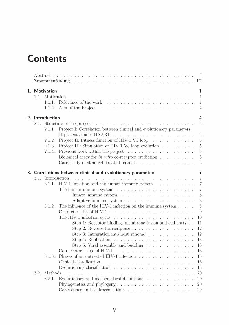
HIV is a positive single-stranded RNA (ribonucleic acid) virus of the genus of lentiviridaebelonging to the retrovirus family. The complete HIV-1 genome has a length of 9,181basepairs (bp) [58] and consists mainly of the genes gag, pol, and env, flanked by two longterminal repeats (LTR) of about 600 nucleotides (nt) with a 5′-cap and a 3′ poly-A tail.Figure 3.1 illustrates the sequence of genes of the HIV genome.The Gag polyprotein is cleaved into three proteins: matrix, capsid, and nucleocapsid.The cleavage of the Pol polyprotein results in additional viral reverse transcriptase (RT),protease, and integrase molecules. The envelope gene (env) of HIV has a length of 2,571bp. The gene product of env is a precursor glycoprotein (gp) 160, which is cleaved intothe membrane proteins gp41 and gp120 as well as the HIV accessory proteins Vif, Vpu,Vpr, and Nef, and the regulatory proteins Rev and Tat. Central to the present project is aspecific 105 bp nucleotide region of gp120, termed V3 loop region.
Figure 3.1.: Complete HIV genomeThe figure illustrates the sequence of genes of the HIV-1 genome and the location of the V3loop within the env gene.(image source: image adapted from [5])
Upon the creation of virions, two (usually identical) strands of the full-length HIV RNA,together with the proteins RT, protease, and integrase, and the accessory proteins Nef,Vif, and Vpr are packed together into the cone-shaped viral core formed by the p24 Gagcapsid protein. The viral core is coated by a lipid membrane, carrying 10 to 15 proteinspikes. Each spike consists of a heterodimeric trimer of the external surface glycoprotein(gp) gp120 and the transmembrane protein gp41. These membrane-protruding spikes playan important role in the cell entry of HIV (see Section 3.1.2).Mature HI virions are roughly spherical with a diameter of 100 − 120 nm. Figure 3.2illustrates the organisation of the viral components of a mature particle.
9

3. Correlations between clinical and evolutionary parameters
(a) (b)
Figure 3.2.: Illustration of a mature HI viriona) A schematic sketch of a mature HI virion (www.niaid.nih.gov/SiteCollectionImages/
topics/hivaids).b) Electron microscopic image of a mature HI virion (Yu et al. [166]).
The HIV-1 infection cycle
The HIV-1 infection cycle can be distinguished into five coarse-grained phases that aredepicted in Figure 3.3. In the following description, we will focus on some key aspects ofHIV biology [55] which are relevant for this work.An HIV-1 infection is initiated by the process of receptor binding and cell entry (step 1 inFigure 3.3). After the release of the viral core into the host cell, the viral proteins and theRNA are distributed within the cell. The RT transcribes the viral RNA into cDNA (step2), which becomes integrated into the host cell DNA by the integrase (step 3). Initiatedby some start signals, the replication of the integrated pro-viral DNA starts (step 4). Theviral transcripts are translated and processed into viral proteins. They assemble with twofull-length viral RNA molecules and form immature virions, which maturate upon buddingfrom the infected cell (step 5). The mature virus particles start a new infection cycle.In the following paragraphs, the main aspects of these five phases are described. If noother references are given, the content of the following paragraphs is based on the work ofFrankel et al. [55].
10

3. Correlations between clinical and evolutionary parameters
Figure 3.3.: HIV infection cycleThe image depicts the sequence of steps of the viral infection cycle. (image adapted from[128])
1. Receptor binding and cell entry2. Reverse transcription3. DNA integration4. Replication5. Translation, assembly and budding
Step 1: Receptor binding, membrane fusion and cell entry In 2000, Doms and Trono[37] described and illustrated the process of receptor binding and cell entry (see Figure3.4). The surface protein gp120 and the transmembrane protein gp41 are the most impor-tant HIV proteins that are involved into the virus-to-cell contact. Heterotrimers of bothproteins are non-covalently associated to form membrane protruding spikes. These spikesare anchored in the lipid membrane of the virion by the gp41 domain, and the tip of thespikes is formed by the gp120 moieties.When the viral and the cellular membrane proteins are in close proximity, the gp120region at the tip of the spikes binds to the primary CD4 receptor on the host cell surface.This interaction is a necessary prerequisite for viral cell entry since it initiates the firststructural rearrangements of the gp120 moiety and the CD4 receptor. The conformationalchanges lead to an exposure of the third variable loop (V3 loop), a part of the gp120subunit, to the host cell [37, 98].Revealed at the tip of the spike, the V3 loop structure is a high affinity binding site thatinteracts with a chemokine co-receptor on the target host cell surface. Different chemokinereceptors from a seven-transmembrane G-protein-coupled receptor family are known toserve as co-receptors for HIV binding and cell entry, for example the receptors CCR1 toCCR5, CCR8, CXCR4, BOB, or Bonzo [16, 44]. Of those, the chemokine receptors CCR5and CXCR4 (prior known as fusin) are the most important co-receptors to facilitate HIVcell entry [36, 38, 167].The co-receptor tropism has been shown to influence significantly the disease progression
11

3. Correlations between clinical and evolutionary parameters
[29, 62, 125]. More details on the co-receptor usage are given in Section 3.1.2.Upon binding of the V3 loop to the cellular co-receptor, further structural rearrange-ments of the spike are induced. These conformational changes occur predominantly inthe gp41 moiety and lead to the formation of a hairpin structure which is exposed tothe host cell membrane. This hairpin structure of gp41 triggers the fusion of the mem-branes of the virus particle and the host cell (possibly including an interaction withanother specific host cell receptor) [37, 98]. As a result of the fusion process, the viralnucleocapsid is released into the target cell. In the cytoplasm, the capsid is uncoatedand the complex of the viral RNA and the viral proteins is transported into the cell nucleus.
Figure 3.4.: Binding and cell entry of HIVThe image describes the sequence of steps of HIV cell entry, from CD4 binding to membranefusion and the release of the viral nucleocapsid into the host cell.(image adapted from Doms et al. [37])
Step 2: Reverse transcriptase Once the complex of the viral RNA and protein moleculesreaches the nucleus, the viral reverse transcriptase (RT) molecules start to transcribethe viral RNA into proviral DNA. The transcription needs specific tRNA primers forinitiation. Usually, one Lysin tRNA is packed into the viral capsid and this molecule isused to start the transcription on one of the two RNA strands. During the formationof the first minus-strand of HIV DNA, the viral plus-strand RNA template is degraded.After completion of the minus-strand DNA copy, the RT jumps onto this newly producedDNA strand and uses it as template to transcribe a complementary plus-strand. The twonewly synthesised DNA strands hybridise into a double-stranded viral copy DNA (cDNA).It is important to note that the HIV RT lacks an editing function and thus the transcriptionof the viral RNA into DNA is highly error prone. Estimates of the error rate vary inthe range of 5.0 · 10−4 [126] to 3.4 · 10−5 [102]. Typically, one error in every 1,000 bp isassumed. Applied to an HIV genome of ∼10,000 bp, this results in ten nucleotide changesin every round of reverse transcription.This high mutation rate of the HIV RT is the main obstacle to HIV therapy as well asdrug and vaccine development.
Step 3: Integration into host genome After reverse transcription, the viral integraseprocesses the newly formed viral cDNA. By detaching two nucleotides to both sides ofthe blunt, double-stranded ends, it creates so-called sticky ends, single-stranded DNAextensions at both ends of the viral DNA genome. Such prepared, the viral cDNA isintegrated into the host genome, being site specific only with respect to the sticky endextensions.
12

3. Correlations between clinical and evolutionary parameters
Upon cleavage of the host DNA, the integrase joins the sticky ends of the cDNA to thehost cell DNA and ligates them. Upon DNA repair after ligation, host cell enzymes createshort repeats at the flanking ends of the integrated cDNA.
Step 4: Replication After integration into the host cell genome, the hosts RNA poly-merase II transcribes the provirus and produces HIV RNA and mRNA whenever the DNAof the infected host cells is transcribed. The transcription is regulated by the binding ofhost factors and viral proteins to the long terminal repeat. The viral proteins Tat and Revare important for transcription control. While the Tat protein stimulates transcriptionand facilitates elongation of the transcript, Rev controls the splicing of the transcriptand mediates the transport of the fully and partially spliced messenger RNA (mRNA)from the nucleus into the cytoplasm [86]. In the cytoplasm, some of the mRNAs aredirectly translated into HIV proteins or into chains of multiple protein precursors, whichare further processed by the viral protease. Other mRNAs are delivered to different celllocations for translation and processing − the env mRNA for example is translated at theendoplasmatic reticulum.In contrast to the productive state of activated infected host cells, infected cells can alsogo to resting state. Then the infection becomes latent and non-productive until the cell isre-activated again [142].
Step 5: Viral assembly and budding After the translation and the processing of theviral proteins, the viral components assemble to form new virions. The structural proteinsderived from the gag gene form the new viral cores. Each viral core comprises a complexof two full-length RNA transcripts, some host tRNAs, the viral proteins RT, protease, andintegrase, and the accessory proteins Nef, Vif, and Vpr.Upon budding of the new viral particles from the host cell, the cores are coated witha lipid bilayer taken off the cell membrane. This newly formed lipid envelope becomesspiked with complexes of the viral Env proteins gp41 and gp120. Shortly after budding,the maturation of the new viral particles is completed and the released virions can infectnew host cells and restart the transcription cycle.
Co-receptor usage of HIV-1
The binding of the V3 loop to the cellular co-receptor is an important step in cell entry.The co-receptor usage is highly specific and mainly depends on the protein sequence ofthe V3 loop [24]. Visualisations of the loop structure are given in part two of the work(Figure 4.13).The amino acid sequence of the V3 loop determines the cell tropism and thereby influencesthe progression of the disease [29, 62, 125].As stated earlier, the chemokine receptors CCR5 and CXCR4 are the most abundantco-receptors for cell entry [36, 38]. While the CCR5 receptor is predominately used inearly HIV infection, about 50 % of all patients face a co-receptor switch from CCR5towards CXCR4 in later stages of the disease [35]. The co-receptor switch is associatedwith disease progression and with a worse prognosis for the patient. CXCR4-tropicstrains show an increased growth rate in vitro and induce the formation of multi-nucleatedcells (syncytia), which have a cytopathic effect on uninfected cells (bystander effect).
13

3. Correlations between clinical and evolutionary parameters
The occurrence of CXCR4-tropic strains often marks the manifestation of AIDS relatedsymptoms [29, 135, 138].Amino acid changes due to non-synonymous mutations in the nucleotide sequence of theV3 loop region are the reason for the switch of the co-receptor tropism from CCR5 towardsCXCR4. Xiao et al. [165] explored these sequence changes and found conserved unchargedamino acids at position 11 of the V3 loop, mostly serine and glycine, and the negativelycharged amino acids glutamic acid and aspartic acid at position 25 of CCR5-tropic strains.Mutational studies showed that a substitution with the positive amino acids arginine orglutamine at both positions altered the co-receptor usage in favour of the CXCR4 receptor.From this observation they derived the amino acid consensus motif S/GXXXGPGXXXXXXXE/D
for positions 11 to 25 of the V3 loop as a determinant of CCR5 tropism. The notationS/G and E/D indicates the alternatives of the dominant amino acids at positions 11 and 25of CCR5-tropic sequences.Based on these observations, the first sequence derived decision rule to determine theco-receptor phenotype of a V3 loop sequence was established, the so-called 11/25 rule.The 11/25 rule still is an important determinant of recent in silico co-receptor predictiontools. In Section 3.3.3 we describe two co-receptor prediction tools that are used asvaluable instruments in scientific research and in therapy optimisation.The reasons that lead to the co-receptor switch in about 50% of all patients are stillunclear, but a number of hypotheses tries to explain the change in cell tropism. The mostprominent hypotheses were discussed by Regoes and Bonnhoefer in 2005 [123]. A shortdescription is given in the following paragraphs.
Transmission mutation hypothesis According to Regoes and Bonnhoefer [123], thetransmission mutation hypothesis relies on the as-sumption that CCR5-tropic strains are favouredupon virus transmission. In consequence, CCR5using viruses are found more often in early stagesof disease. This hypothesis further states that theco-receptor switch happens by chance at some timeduring infection as a result of the high mutationrate of the reverse transcriptase of HIV.
Target cell life time hypothesis Rodrigo [127] attributes the co-receptor switch toa competition of CXCR4- and CCR5-tropic strains.He argues that the more cytopathic CXCR4 virusesare outcompeted since they destroy their replicationreservoirs faster than the CCR5-tropic viruses. Thisdisadvantage leads to a shorter life time of CXCR4-infected host cells and thus CCR5-tropic strainspersist longer and dominate the infection.
Target cell based hypothesis The target cell based hypothesis formulated by Dav-enport et al. [34] and modelled by Ribeiro et al.[124] argues that the co-receptor switch is a conse-quence of the different rates of available CCR5 andCXCR4 positive cells within the host.Following this hypothesis, the number of activated
14

3. Correlations between clinical and evolutionary parameters
CCR5 positive memory T cells is increased earlyduring the infection as a result of the hosts immunedefence. The availability of activated CCR5 cellsfavours CCR5-tropic viral strains early in the in-fection. In the late stage of the disease, when thememory T cells are mainly depleted, the rate ofthe naıve CXCR4 positive T cells increases, andthus the CXCR4-tropic strains dominate in the latestage of the infection.
Immune-control hypothesis The immune-control hypothesis of Pastore et al.[113] explains the predominance of CCR5-tropicviruses in early stages of the disease with a reducedreplicative fitness of CXCR4-tropic strains on theone hand and a better immune recognition andcontrol of CXCR4 strains by the human immunesystem on the other hand. They state that CXCR4-tropic strains are successfully fought by the immunesystem and are not able to replicate efficiently earlyin infection, when the number of immune cells ishigh and the immune system is strong.With advanced T cell depletion due to continuousinfection of T cells by HIV, the immune systemis weakened and the immune pressure fades. Inthe late stage of disease, the exhausted immunesystem is no longer able to effectively fight HIVand under this condition the CXCR4 strains areable to sustain and become prevalent.
So far, none of the hypotheses could be confirmed or disproved and an explanation for theco-receptor switch is still missing. Since the occurrence of CXCR4-tropic strains marks anadvanced stage of the infection and an accelerated disease progression, an understandingof the mechanisms of the co-receptor switch is essential to prevent the disease progressionand the development of AIDS.The knowledge is also necessary in the field of rational drug design to develop new drugsand to avoid unwanted side effects, for example regarding the new drug class of co-receptorblockers, with Maraviroc as the first licensed drug [49, 67]. Since Maraviroc impedesthe usage of the CCR5 receptor, it was suspected to accelerate the co-receptor switch byestablishing an additional pressure to HIV towards CXCR4 co-receptor usage.These aspects indicate the relevance of the co-receptor usage and pronounce the importanceof an understanding of the mechanisms of HIV evolution.
3.1.3. Phases of an untreated HIV-1 infection
The course of an untreated HIV-1 infection can be separated into three phases, either basedon clinical observations or on evolutionary sequence parameters. In both classificationsystems, the co-receptor switch occurs in an progressed stage of infection.
15

3. Correlations between clinical and evolutionary parameters
In this section we describe the three phases of the disease and the different classificationmethods.
Clinical classification
At the Clinical Staff Conference held on the 27th of June 1990, Anthony S. Fauci andGiuseppe Pantaleo et al. [51] for the first time showed an illustration summarising thetypical clinical course of an HIV-1 infection. Fauci and Pantaleo et al. refined the imagein their subsequent publications [64, 50]. This image, shown in Figure 3.5, describes thegeneral course of the CD4+ cells and of the viral load (VL) during the three phases of thedisease in untreated patients.During the initial phase of infection (phase 1), the viral load rapidly increases, leadingto an acute retroviral syndrome three to six weeks after primary infection [64]. Duringthis phase, the symptoms are described like the symptoms of an acute seasonal influenzainfection. Clinically, a pronounced drop of the number of CD4+ cells to about 500 cellsper microlitre of plasma is described.After one week to three months of high level viremia, the immune system is capable toeffectively chase the virus [64]. The viral load remarkably decreases and stabilises at apatient specific virus level known as the viral set point. The viral set point is an individualamount of virus that can be controlled by the hosts immune system. This level of viralload is quite stable throughout the chronic phase of the HIV infection (phase 2). Thoughthe immune system is able to control the level of the virus during the chronic phase, thenumber of CD4+ cells decreases slowly but permanently due to a continuous infection ofthe activated cells by the replicating virus.In most patients, the number of CD4+ cells drops below 200 cells per microlitre of plasmaduring the infection (phase 3). The time span to this clinical observation varies betweenpatients and averages to about ten years [51]. At that time, the immune system of thepatients is exhausted and the CD4+ cells are widely depleted. Clinically, a dramatic weightloss is described for the majority of the patients and they suffer from various opportunisticinfections. Characteristic examples are respiratory tract infections, herpes, hepatitis, andcancer. This third stage of disease is known as acquired immunodeficiency syndrome(AIDS). The patients die due to multiple opportunistic infections which the immune systemno longer can control.
16

3. Correlations between clinical and evolutionary parameters
CD4+
cells/ l
1,000
500
200
0
0 6 12 1 5 10
weeks years
primary infection clinical latency AIDS
1 2 3 VL/ml
plasma
106
105
104
103
102
opportunistic diseases
Figure 3.5.: Clinical phases of an untreated HIV-1 infectionThe illustration describes the clinical course of an HIV-1 infection in a patient without therapy.The blue curve marks the number of CD4+ cells and the red curve describes the course of theviral load.(image based on Fauci and Pantaleo et al. [51, 50, 64])
In 1986, the Centers for Disease Control and Prevention (CDC) [21], Atlanta, USAintroduced a classification system for HIV-1 infections. The classification is based on alaboratory category, which is the lowest documented CD4+ cell count of the patient, callednadir, and a clinical category based on the presence or absence of specific HIV-relatedconditions. This staging system is still used in hospital. The most recent version wasrevised by the CDC in 2008 [133] and is presented in Table 3.1
Table 3.1.: Classification of the HIV-1 infection stage by the CDC [133]
CD4+ cell count Clinical categoriescategories
category A: category B: category C:Asymptomatic, Symptomatic AIDS-acute HIV, or conditions, indicator
persistent generalised not A or C conditionslymphadenopathy
stage 1: ≥ 500 cells/µL A1 B1 C1stage 2: 200 - 499 cells/µL A2 B2 C2stage 3: < 200 cells/µL A3 B3 C3
17

3. Correlations between clinical and evolutionary parameters
Besides the nadir of the patient, which defines the coarse-grained numerical classifica-tion of the disease stage, the CDC provides a list [133] of symptomatic conditions andAIDS-indicator conditions to assist the physicians to determine the disease stage.In the case of a missing diagnosis, the classification system is supplemented by stageunknown (e.g. Ax) and category unknown (e.g. x2).
Evolutionary classification
In 1999, nine years after Fauci and Pantaleo et al. [51, 50, 64] presented their illustrationof the clinical course of the disease, Shankarappa et al. [138] described the course of anuntreated HIV-1 infection based on evolutionary parameters. They originally discriminatedfive different phases of the infection, which can be consolidated into three phases comparableto the phases observed by Fauci and Pantaleo et al. (compare Figure 3.6).They found that during the acute initial phase of the disease the genetic diversity within theviral population and the evolutionary distance (termed divergence) of the viral populationto the founder strain steadily increase. Furthermore, the transition from acute to chronicphase is marked by the emergence of CXCR4-tropic strains.During the following chronic stage of disease, the error-prone reverse transcriptase stillgenerates escape mutants and the viral population further diverges from the founder strain.In parallel, the level of diversity stabilises, since the diminishing number of CD4+ cellsresults in a decreasing immune pressure and an increasing amount of the virus.In patients with a co-receptor switch, a peak of the CXCR4-tropic viral population marksthe breakdown of the immune system and the begin of the last stage of the disease. Inthat phase, also the viral divergence stabilises. The immune system is exhausted and thedepleted population of immune cells is no longer able to fight the virus. High amounts ofvirus particles are produced.During the present work we recognised that the description by Fauci and Pantaleo et al.[51, 50, 64] mainly coincides with the findings by Shankarappa et al. [138]. Both groupsdistinguished three phases of the disease in the course of an HIV-1 infection. While theolder illustration of Fauci and Pantaleo et al. focussed on the clinical parameters that weredetermined routinely by physicians during the regular visits of the patients, Shankarappaet al. described the evolutionary measures that were available as a result of the beginningsequencing approaches in later days of biological research.For the evaluation of the clinical and evolutionary patient data presented in this work, wehave to keep in mind that both the publications by Fauci and Pantaleo et al. [51, 50, 64]from the 1990th and the publication by Shankarappa et al. [138] from 1999 are based ondata from the early days of HIV research. The participating patients were therapy naıveor treated only by a single reverse transcriptase inhibitor. In contrast, the present studyanalysed data from HAART treated patients.
18

3. Correlations between clinical and evolutionary parameters
Figure 3.6.: Phases of an untreated HIV-1 infection The illustration describes the course of an un-treated HIV-1 infection over time (x-axis), based on evolutionary parameters. The divergenceof the population from the founder strain is described by the hight of the curve (y-axis),whereas the diversity of the sequences within a sample is described by the size of the circles.(image adapted from Shankarappa et al. [138])
19

3. Correlations between clinical and evolutionary parameters
3.2. Methods
In this section we introduce necessary terms and definitions as well as mathematical mea-sures and software that were used to describe and analyse the evolutionary interrelations.
3.2.1. Evolutionary and mathematical definitions
Phylogenetics and phylogeny
The study of evolutionary relationships of populations is termed phylogenetics. Basedon sequencing data and by the computation of multiple sequence alignments (MSA),evolutionary relations are reconstructed. A phylogenetic study yields a hypothesis aboutthe evolutionary history of the population, which is in general described by a genealogictree, termed phylogeny of the population [20].
Coalescence and coalescence time
The term coalescence describes the merging of genetic lineages backwards in time towardsthe most recent common ancestor (MRCA). In this context, the coalescence time is thepredicted amount of time that passed between the introduction of a mutation and theobservation of a particular distribution of the mutation in a population [91].
Effective population size Ne
Following Sewall Wright [164, 163], the effective population size Ne is ”the number ofbreeding individuals in an idealised population that would show the same amount of disper-
sion of allele frequencies under random genetic drift or the same amount of inbreeding
as the population under consideration”. The concept is used to determine the rate of theevolutionary change that results from the effect of sampling in a finite population [23]. Ne
is estimated empirically with respect to the coalescence time.In real populations, Ne is neither constant nor undergoes a regular (e.g. linear or expo-nential) change [155]. Therefore models developed to estimate the Ne of real populationsbased on predictions from artificial evolutionary models assuming a regular change haveto be used with care.
Bayesian skyline
The Bayesian skyline [42] estimates the effective population size Ne over time. It describesa possible course of the number of individuals over time that would result in the observedphylogeny, reflecting the allele frequencies over time. The details of the Bayesian skylinereconstruction we used in the present work are described in the recent BEAST publications[40, 42, 43].
Hamming distance
The Hamming distance is a distance measure for strings that was introduced by Hamming[71, 72]. For two sequences of symbols of equal length, the Hamming distance is defined
20

3. Correlations between clinical and evolutionary parameters
as the number of differing sequence positions.In biological terms, the Hamming distance is the least number of point mutations that arenecessary to transform one nucleotide sequence into another. For the analysis of aminoacid sequences, it is defined as the number of differing amino acids between two sequences.For two sequences X = x1, ..., xn and Y = y1, ..., yn of equal length n, the Hammingdistance H(X, Y ) is the sum of the different sequence positions i, e.g. for two identicalpositions xi == yi, hi(xi, yi) = 0, and for two differing positions xi Ó= yi, hi(xi, yi) = 1:
H(X, Y ) =n∑
i=1
hi(xi, yi) (3.1)
Example:Sequence X = ATGCATGCSequence Y = ATGGATCC
h1(x1, y1) = h2(x2, y2) = h3(x3, y3) = h5(x5, y5) = h6(x6, y6) = h8(x8, y8) = 0h4(x4, y4) = h7(x7, y7) = 1
H(X, Y ) =n∑
i=1hi(xi, yi) = 2
Diversity and Divergence
Diversity and divergence are two measures that describe the genetic distance within orbetween samples of sequences. According to Shankarappa et al. [138], the genetic diversitywithin a group of sequences can be estimated as the mean and the standard deviation ofthe pairwise nucleotide distances between all pairs of sequences from that group.The divergence determines the evolutionary distance between two groups of sequencesat different time points. In terms of viral infection, the viral sequences from the earliertime point are supposed to be the founder sequence or the founder population (i.e. thepopulation of the first virus-positive sample). The second sample is a more recent sampleobtained at a later time point. To determine the viral divergence, all pairwise Hammingdistances between the founder sequence and every sequence of the later sample are calcu-lated. The divergence of the later sample from the founder strain is then calculated as themean and standard deviation of all pairwise distances.In biological samples, a single founder sequence can often not be determined. In the caseof a founder population of differing sequences, Shankarappa et al. [138] either definedone random sequence from the first virus-positive sample as the founder sequence orapproximated the founder sequence by a consensus sequence of all sequences of the founderpopulation.In the present work, we adapted the definitions of Shankarappa et al. [138] to fit our needs.We computed the diversity of any pair of sequences as the pairwise nucleotide distance, i.e.the Hamming distance, of this pair of sequences. We defined the diversity of a sample S
of m sequences as the average of the Hamming distance of all m(m − 1) pairs of sequences
21

3. Correlations between clinical and evolutionary parameters
(Xj, Xk), (k Ó= j) of that sample.
diversity(S) =1
m(m − 1)
m∑
j=1
m∑
k=1k Ó=j
H(Xj, Xk) (3.2)
with H(Xj, Xk) being the Hamming distance of sequence Xj and sequence Xk.The divergence estimates the genetic distance of a sample of sequences taken at time t
(t > 0) to the viral founder strain (at time t0). Since many of the patients of our studywere in a progressed state of the disease, we were not able to determine the founder strainof the viral population or to estimate it as Shankarappa et al. [138] did. Thus, we adaptedthe definition of the divergence. We defined the divergence of the first HIV-positive bloodsample E of each patient, consisting of l sequences Yo, to be zero. The divergence of anymore recent sample S of m sequences Xj is defined as the average Hamming distance ofall ml pairs of a sequence Xj of S to a sequence Yo of E of that patient.
divergence(E) = 0
divergence(S) =1
ml
m∑
j=1
l∑
o=1
H(Xj, Yo)(3.3)
with H(Xj, Yo) being the Hamming distance of sequence Xj and sequence Yo.
Bayes factor
The Bayes factor (BF) [87, 110, 61] is a method for hypothesis testing. The test is amodification of the classical likelihood ratio test described by Neyman and Pearson [111]and can be used to decide between two alternative models M1 (e.g. the null model) andM2 (an alternative model) to describe some observed data X. To decide whether modelM1 with parameters θ1 or model M2 with parameters θ2 fits the data X best, the BF [40]is calculated:
BF =p(X|M1)
p(X|M2)=
∫p(X|θ1, M1)p(θ1|M1) dθ1∫p(X|θ2, M2)p(θ2|M2) dθ2
(3.4)
where the conditional probability p(X|Mi) is called the marginal likelihood for model i
and the θi are vectors of the model parameters. Since the Bayesian model comparisonintegrates over all parameters θi in each model Mi, the method does not depend on asingle set of model parameters.A problem of model fitting is the danger of overfitting. In general, a model can be adaptedto reproduce any data set by an increase of the number of model parameters, but with anincreasing number of parameters, the model loses the ability to describe new, unknowndata. The difficulty is to find the best trade-off between the model complexity and thequality of the data fitting.According to Kass et al. [87], the problem of overfitting is avoided by the Bayesian modelcomparison, since the usage of large numbers of parameters is intrinsically penalised duringthe calculation of the BF.In this work, the BF was used for the evaluation and the selection of the best phylogeneticmodel. The exact implementation of the BF is described in the recent BEAST literature
22

3. Correlations between clinical and evolutionary parameters
[40, 42, 43].
Mathematical correlations
In general, correlations or dependencies are mathematical relations between two or morefeatures of a data set or between two or more random variables. By definition, mathe-matical correlations are in the range of [−1, 1]. While a positive correlation value of twovariables x and y describes a the more of x, the more of y relation (e.g. the more CD4+
cells, the higher the immune pressure), a negative correlation of x and y means a the moreof x, the less of y association (e.g. the higher the viral load, the less CD4+ cells survive).The absence of a significant correlation between two sets of observations does not neces-sarily mean that there is no causal relation. This was formulated by Carl Sagan, an USastronomer and popularizer of astronomy (1934 - 1996), in the famous and often citedexpression ”The absence of evidence is not the evidence of absence.”For example the application of a weak or wrong method of analysis or an inadequatesample size could be reasons for a missing significant correlation [4]. On the other hand,the presence of a significant correlation does not guarantee a causal interrelation of therespective data [2]. The causation has to be ensured by the design of the experiment.
Statistical significance
In statistical hypothesis testing it is indispensable to check for the statistical significance ofa correlation [53]. A test on the statistical significance analyses whether an observation isonly a rare event that arose by chance (null hypothesis) or whether an observation reflectsa real pattern among the observed data (alternative hypothesis).The p-value describes the level of significance. A p-value of 0.05 states that the probabilityto gain the observed result (or an even extremer one) by chance is 5.0%. If the p-value ofa correlation is smaller than the defined significance level, than the observed pattern isdefined to be statistically significant with respect to the selected significance level.To avoid misinterpretations, the desired significance level has to be defined prior to testing.In general it is not admissible to adjust the level afterwards when the result is alreadyknown.In the present work, we used a threshold for the p-value of 0.05, if not stated otherwise.
Confidence interval
Closely related to the statistical significance is the confidence interval (CI). The CI iscalculated from the observed data and estimates an interval that contains an unknownparameter of interest with a given probability.Similar to the significance level, the level of confidence describes the reliability of a model,or to be more concise, it describes the probability that the estimated parameter of interestis comprised in the calculated interval. A CI of 95% states that one is 95% confident thatthe true value of the parameter of interest can be found within the interval (i.e. we face arisk of 5.0% that we have made the wrong decision). A CI of 95% defines a significance
23

3. Correlations between clinical and evolutionary parameters
level of α = 5%.If not stated otherwise, we used a CI of 95% throughout this work.
Correlation coefficients
Many tests on mathematical relations are parametric tests that rely on specific assumptionsabout the data of interest, for example the assumption that the data follow a specificdistribution. It is important to know and to be aware of the underlying assumptions of anapplied test method and it is crucial to critically check whether the assumptions suit thespecific data that are analysed.In the following paragraphs we describe the parametric Pearson correlation coefficient thatrelies on the assumption that the observed data follow intrinsically a linear dependenceand the non-parametric rank correlation coefficients of Spearman and Kendall.
Pearson correlation coefficient The parametric Pearson correlation coefficient r canbe used to measure the strength of the linear dependence of samples of paired values xi
and yi. Thus, the Pearson correlation coefficient relies on the assumption that the dataintrinsically follow a linear dependence.A perfectly positive correlation results in a value of r = 1, e.g. for the correlation x andy = 2x, while a perfectly negative linear relation results in r = −1, e.g. the correlationbetween x and y = −2x. A value r = 0 indicates that the two variables are not linearlydependent.
Spearman rank correlation coefficient The non-parametric Spearman rank correlationcoefficient ρ estimates how well the relation between samples of paired values xi and yi
can be described by a monotonic function. The Spearman rank correlation coefficient isrelated to the Pearson correlation coefficient and is mathematically defined as the Pearsoncorrelation between the ranked values. For the computation of ρ, the xi and yi values areranked and the coefficient of the ranks is calculated.A Spearman rank correlation coefficient ρ = 1 states that the association between the xi
and yi values is a monotonically increasing function, and ρ = −1 states that the associationis monotonically decreasing.If the samples contain many identical values, so called tied values, the computation of ρ
has to be performed with care. Identical values within a sample are ranked as the mean ofall their ranks, e.g. if xk == xl occupy both rank 2 and 3, than xk and xl are both rankedas 2.5.
Kendall rank correlation coefficient The Kendall rank correlation coefficient τ is a thirdmeasure to quantify the extent of the statistical dependence between pairs of observationsxi and yi. Similar as the Spearman rank correlation coefficient ρ, τ is a non-parametricrank correlation measure. The value of τ describes how well the rankings of the xi’s andyi’s coincide given that the spacing is non-equidistant. If xk > xl and yk > yl, the ranks ofboth variables are said to be concordant, if xk > xl and yk < yl, the ranks are discordant,and if xk == xl and yk == yl they are neither concordant nor discordant.
24

3. Correlations between clinical and evolutionary parameters
Since the Kendall rank correlation coefficient relies on the counts of concordant anddiscordant data pairs, pairs that are neither concordant nor discordant weaken the method,comparable to the difficulties caused by tied values upon computation of the Spearmanrank correlation coefficient.Details on the described mathematical concepts can be found in the classical textbooks ofCramer [30] and Bronstein et al. [17].
3.2.2. Software tools and programming languages
R scripting
We used the freely available R [121] software environment and the R package MASS [152]for standard statistics, e.g. to compute the Pearson, Kendall, and Spearman correlationcoefficients and to provide significance testing. In the second part of the project, we usedthe BioPhysConnectoR [77] package of R for the calculation of the mutual informationand for the structural coupling analysis.
Perl scripting
In addition to the Perl [26] standard routines, we used the BioPerl [56] package and thePerl Statistics [105] package. BioPerl is a developers project that comprises routines andcode snippets that are useful for biological applications, and the Statistics package is acollection of a number of basic statistics methods.Based on these packages, we developed a number of Perl scripts for sequence collectionand handling, data renaming and statistics calculations.
BALLView software suite
BALLView [107, 106] is a Bioinformatics software designed for molecular modelling andvisualisation. BALLView supplements the functionality of the Biochemical AlgorithmsLibrary (BALL) [73] with an integrated graphical user interface. In combination, BALL andBALLView provide tools and methods for the visualisation and manipulation of molecularstructures, e.g methods for energy minimisation and molecular dynamics simulations withdifferent force fields or the calculation and visualisation of the electrostatic properties ofmolecules.We used the software for the modification and visualisation of different 3D crystal structuresof the V3 loop of HIV.
geno2pheno[coreceptor]
Due to a prior cooperation with the scientific research group at the Max Planck In-stitute for Computer Science, Saarbrucken, we decided to use the Bioinformatics toolgeno2pheno[coreceptor] [97] for the in silico predictions. geno2pheno is a classification toolbased on a machine learning approach using so-called support vector machines (SVM) fortwo-class decisions.Prosperi et al. [119] validated the geno2pheno[coreceptor] predictions in 2010. They found
25
3. Correlations between clinical and evolutionary parameters
a prediction accuracy of 71.4% for plasma RNA and of 70.6% for whole-blood DNA [151].
FSSM
We used FSSM [82, 81, 118] as an additional co-receptor prediction tool. Similar togeno2pheno, the tool first aligns the amino acid sequence of a V3 loop against a referencesequence. In the next step, the co-receptor tropism of a specific sequence is calculatedbased on a prediction score derived from position specific scoring matrices (PSSM) of theamino acid content of the FSSM R5 and X4 reference data set.We used the HIV-1 subtype B X4/R5 scoring matrix for our predictions and selected theoption to exclude degenerated sequences from the analysis. Regarding the publicationof Low et al. [101], we predicted sequences with a sequence score above −8.12 as X4- ordual-tropic, while scores equal or below −8.12 indicate the use of the R5 co-receptor. TheFSSM web server allows the upload of datasets of up to 200kb in size, which conforms toa maximum of 1,300 V3 loop sequences in .fasta format.
Clustal software family
Clustal [25, 149] is a software family that comprises a number of widely used tools for thecomputation of multiple sequence alignments (MSA). In MSAs, biologically related aminoacid sequences (or less frequent nucleotide sequences) are organised in sequence tables in away such that corresponding sequence positions of the individual sequences are containedin the same alignment column. The Clustal software suite is designed to handle large setsof sequences.The Clustal software family consists of ClustalX, ClustalW, and most recently ClustalO.We used ClustalW with a command line interface. For our data, the most importantalignment parameters were the gap associated parameters. We chose a gap opening penaltyof 10 and a gap extension penalty of 0.1 for the pairwise alignments. During the extensionof the pairwise alignments into an MSA, the gap extension penalty was increased to 0.2,since a value of 0.1 introduced several large gaps that massively prolonged the sequencelength of the resulting MSA.In detail, we used the following parameter settings for the computation of the multiplesequence alignments:
• Gap opening penalty: 10• Gap extension penalty: 0.2 (0.1 for pairwise alignments)• Protein Weight Matrix: BLOSUM• Residue specific penalties: ON• Hydrophilic penalties: ON• Gap Separation distance: 4• End gap separation: OFF• Use negative matrix: OFF• Delay divergent cutoff: 30%• Keep predefined Gaps: NO
26

3. Correlations between clinical and evolutionary parameters
MEGA software
For the illustration and the visual inspection of the sequences, we used ClusalW [149] in theMEGA [95] (Molecular Evolutionary Genetics Analysis) environment. MEGA comprises acollection of tools for DNA and protein sequence analyses. We used the software versionMEGA 4.0 [147] which was released in 2007. Among other applications, MEGA 4.0 enablesthe user to calculate multiple sequence alignments, to reconstruct phylogenetic trees, andto estimate rates of molecular evolution.We chose the MEGA environment mainly due to the nice MSA illustration and thegraphical sequence modification properties, which enabled us to do visual checks andexperimental modifications of our sequence alignments.
BEAST software package
The BEAST [40] (Bayesian Evolutionary Analysis by Sampling Trees) cross-platformsoftware package is a Bioinformatics tool that can be used for a number of phylogeneticinferences, for example for the reconstruction of evolutionary trees and for estimates ofpopulation measures. Mandatory input for the calculations are files containing MSAs.The BEAST software family comprises a number of integrated tools with multiple functions.We only give a short impression of those properties of BEAST that we used to analyse ourdata. For details on the variety of possibilities provided by the BEAST software package,we recommend to consult the BEAST literature [40, 39, 42, 41, 43].BEAST provides methods for the reconstruction of phylogenetic trees. The computationsare not restricted to the reconstruction of single phylogenetic trees, but create a forest ofindependently calculated trees. The number of trees can be predefined by the user. Theresult is a cross-section of the most frequently created tree topologies.BEAST uses Markov Chain Monte Carlo (MCMC) [10] as core algorithm. MCMC isused to average over tree space and thus weights each tree proportional to its posteriorprobability.Based on the reconstructed phylogenetic trees, BEAST enables the calculation of importantevolutionary measures, e.g. the coalescent time and the effective population size Ne. Theuser can decide between different molecular clock models and different options for theprior distribution and the integration of a priori knowledge.We used the following tools of the BEAST software distribution (version 1.6.1):
BEAUti (Bayesian Evolutionary Analysis Utility) provides a graphical user inter-face to prepare .xml input files for BEAST based on sequence alignmentfiles in .nex format.
BEAST reconstructs phylogenies using an MCMC algorithm based on a treeweighting process [40, 39].
LogCombiner combines the output log and tree files from different BEAST reconstruc-tion runs.
LogAnalyser enables analyses of the result and the quality of the reconstruction runs.
Tracer allows a visual inspection of the BEAST log files, especially of thereconstruction traces created by the MCMC calculations, and enablesthe calculation of an estimated time course of Ne [42, 41].
27
3. Correlations between clinical and evolutionary parameters
TreeAnnotator consolidates the information of a forest of phylogenetic trees into oneconsensus tree [43].
Figtree enables the visualisation and the modification of the reconstructedphylogenetic trees [122].
BEAST workflow We combined the BEAST tools to a sequential workflow to performphylogenetic reconstructions of the viral sequences of the study patients. Using ClustalWin the MEGA environment, we translated the available nucleotide (nt) sequences of theV3 loop into amino acid (aa) sequences, calculated the aa MSA for each patient, andback-translated the aa MSAs into nt MSAs. The resulting patient specific nt MSAs wereconverted into .nex file format and separately uploaded into BEAUTi to create the .xmlinput files for the phylogenetic calculations of BEAST.After a predefined number of BEAST reconstruction runs, LogCombiner was used tocombine the multiple .log files into one summary file. The combined result was inspectedwith LogAnalyser and Tracer to evaluate the reconstruction quality and to decide about theso called burn-in, the number of initial BEAST runs necessary to calibrate the parametersfor each specific data set. In general, the burn-in comprised the first ten percent of theruns, the exact value for each data set was individually determined.Excluding the burn-in, Tracer was then used to the determine the effective populationsize Ne over time, also known as Bayesian Skyline reconstruction. In parallel, the forest ofreconstructed phylogenetic trees was consolidated into one summary tree by TreeAnnotator.Finally, FigTree was used to illustrate and inspect the consensus trees.Due to the close association with the study data, the model and parameter selection isdescribed in detail in Subsection 3.4.1 within the data Section 3.3.
RAxML
In addition to the BEAST software family, we used the RAxML-VI-HPC [144, 145] soft-ware package for the reconstruction of evolutionary phylogenies. RAxML-VI-HPC is anacronym for Randomized Axelerated Maximum Likelihood for High Performance Com-puting, version VI. The software was developed to enable fast and parallel calculations ofmultiple runs on distinct starting trees. Details can be found in the RAxML publications[144, 145].Using a bootstrapping approach, RAxML creates a set of independent random startingtrees for the phylogenetic reconstruction. After the independent reconstruction runs, thebootstrapping results are summarised on the tree with the best likelihood. In the last step,the pairwise distances are extracted.RAxML can directly be operated from the command line, is less complex than the bundleof BEAST tools, and enables fast phylogenetic reconstructions, thus we used the softwareto get a fast estimate of the viral phylogenies and to cross-check the BEAST results.
28

3. Correlations between clinical and evolutionary parameters
3.3. Data
The first part of our project is based on longitudinal patient data that were collectedin the course of the joint project Monitoring of resistant HIV in newly and chronicallyinfected HIV patients in Germany - Evolution of HIV-genotype and phenotypes duringantiretroviral therapy. Starting in 1999, it was initially planned to collect sequential bloodsamples of HIV-1-infected patients at the Universitatsklinikum Frankfurt am Main duringregular visits of the patients at the hospital to monitor the intra-host evolution of the HIVgenome during infection. In addition, we received selected information from the patientrecords of the participants of the study.The study was authorized by an ethical commission and informed consent was obtainedfrom all participants before they were included in the study.
3.3.1. Patient records
Our cooperating physicians at the hospital provided us with a data base of selected datafrom the patient records. Among others, the files comprised the sex, the date of thefirst HIV positive test, and the putative way of infection. In some rare cases also thedate of the last HIV negative test was given. The patients were identified by an unique,patient-specific number.During the sequential visits of the patients at the hospital, the number of CD4+ cellsand the viral load were documented. Occasionally, also the number of CD8+ cells wasdetermined. Based on these data, the stage of the disease with respect to the CDCclassification system [21, 133] was regularly ascertained. In addition, the drug therapy andthe reason for an eventual therapy change was reported in most cases. Less frequently, thedrug related side effects or patient-induced therapy discontinuations were documented inthe patient records.These general disease-related data were complemented by information on occasional testsof the patients for co-infections (e.g. human cytomegalo virus, syphilis, and hepatitis A,B, and C). In the case of stationary visits of the patients at the hospital, the reason andthe duration of the stay at the hospital are also noted in the patient records.
3.3.2. Blood samples
According to the study protocol, it was planned to include 300 patients into the studyand to collect blood samples of the participants every three to six month up to ten years.Without further preparation, the refrigerated full blood samples were directly sent to thePaul-Ehrlich-Institut in Langen, where the blood samples were processed for sequencing.The elaborative isolation of the virus from the blood was performed in the wet lab of thedivision of Virology in the section AIDS, New and Emerging Pathogens of the institute.During the process of virus isolation, it is important to ensure the absence of a selectivepressure on the virus. Therefore, a multi-step protocol was developed for sequenceextraction. According to Werner et al. [159] breeding was successful in about 87 % of allcases. For a detailed description of the sequencing process we recommend the respectivepublication [159].
29

3. Correlations between clinical and evolutionary parameters
3.3.3. In silico processing of sequence data
We were provided with the nucleotide (nt) V3 loop sequences of 106 patients. Collectedduring more than years of research, the digital data were organised in multiple directoriesand stored in hundreds of files of different data types. Unfortunately, neither a uniformsystem of file and folder naming or folder structure was used, nor a unified file (.doc, .txt,.xls) and sequence (.ab1, .seq) format or consistent information content of the files. Thesequencing protocols contained the nt sequences as well as some additional informationnot relevant for this study. It was very challenging to ensure an automated data analysisof the complete data.We developed a Perl script and searched all directories and folders for sequence data. Upondata collection, an unique identifier was created for every sequence, consisting of:
• the unique patient number,• the number of the blood sample,• an enumerator counting the sequences within one blood sample,• the number of days that passed since the first HIV-positive test of the patient
As an example, the identifier 004 P411 01 d5 describes sequence 01 of patient 004 fromsample P411 that has been collected five days after the first HIV-1 positive test. Theidentifiers were later supplemented by the predicted co-receptor (compare Section 3.3.3).In the first approach, we extracted all sequences available in any kind of text format (.txt,.doc, .xls) and ended up with 2,349 nucleotide sequences, on average 42 sequences of fourvisits at the hospital. Some of the sequences contained stop codons or were extremelyshortened (in the range of 100 nt instead of 300 nt). A further inspection of the datarevealed that the sequences covered only half of all blood samples that were documentedto be collected in the course of the project. Therefore, we decided to go one step back inthe protocol and to have a closer look onto the raw sequencing data.We checked all directories for .seq and .ab1 files, manually inspected the data, and exportedthe nt sequences. In a subsequent refinement step, fragmented sequences of a length ofless than 200 nt (i.e. less then two thirds of the target region) were removed. On average,the remaining sequences consisted of 300 to 330 nt. Using ClustalW [149] in the MEGAenvironment [95], the nt sequences were translated into amino acid (aa) sequences and anMSA was calculated. Finally, we excluded aa sequences that contained stop codons orlarge gaps within the V3 loop.This extended data collection resulted in a data set of 3,132 sequences, about 800 sequencesricher than the original set of 2,349 sequences. The sequences were extracted from theblood of 47 male and eight female patients.Since we planned to examine the sequence evolution over time, we determined a subset ofall patients with at least four sequential blood samples and remained with 2,224 sequencesof 34 male and two female patients - the final data set contained an average of 60 sequencesper six visits per patient. Figures 3.7 and 3.8 illustrate the distribution of sequences foreach patient and for each blood sample.
30

3. Correlations between clinical and evolutionary parameters
0
1
2
3
4
30 40 50 60 70 80 90 100 110 120
counts
sequences per patient
Figure 3.7.: Distribution of the number of sequences per patientThe illustration shows the number of sequences per patient. 30 to 120 sequences per patientwere extracted during the course of the study.
0
20
40
60
80
100
120
140
0 5 10 15 20 25
counts
sequences per sample
Figure 3.8.: Distribution of the number of sequences per blood sampleThe distribution of sequences per blood sample shows that the intended number of tensequences per sample could be achieved for the majority of samples. Operating the sequencingprocess at full capacity resulted in more than the envisaged ten sequences for some samples.
In silico co-receptor determination
We started the data analyses with an in silico determination of the co-receptor. Usinggeno2pheno[coreceptor] [97] for the classification, we applied a FPR of 10% according tothe recommendations of the European Consensus Group on clinical management of HIV-1tropism testing [151] (i.e. sequences for which the geno2pheno classifier reported a FPR< 10% were labelled as X4- or dual-tropic, while sequences with a reported FPR of theclassifier ≥ 10% were labelled as R5-tropic). Of the 2,224 viral sequences, 1,557 sequences
31
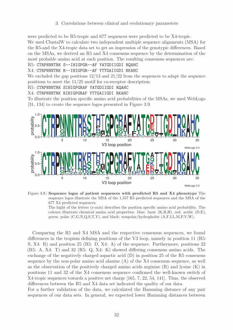
3. Correlations between clinical and evolutionary parameters
were predicted to be R5-tropic and 677 sequences were predicted to be X4-tropic.We used ClustalW to calculate two independent multiple sequence alignments (MSA) forthe R5-and the X4-tropic data set to get an impression of the genotypic differences. Basedon the MSAs, we derived an R5 and X4 consensus sequence by the determination of themost probable amino acid at each position. The resulting consensus sequences are:R5: CTRPNNNTRK S--IHIGPGR--AF YATGDIIGDI RQAHC
X4: CTRPNNNTRK R--IHIGPGR--AF YTTGAIIGDI RKAHC
We excluded the gap positions 12/13 and 21/22 from the sequences to adapt the sequencepositions to meet the 11/25 motif for co-receptor description:R5: CTRPNNNTRK SIHIGPGRAF YATGDIIGDI RQAHC
X4: CTRPNNNTRK RIHIGPGRAF YTTGAIIGDI RKAHC
To illustrate the position specific amino acid probabilities of the MSAs, we used WebLogo[31, 134] to create the sequence logos presented in Figure 3.9.
V3 loop positionWebLogo 3.3
0.0
0.5
1.0
pro
babili
ty
CA
I
S
V
TRLHP5
SGNNNTIR
10
TRKGSVIQ
T
SNRPHV
LMI
15
A
GT
PGH
AK
QSRM
VTA
20
M
L
I
A
FEFYF
G
RTAA
H
TD
G25
K
S
A
G
QEDVIS
TIG
Q
ND
30
P
IRE
RKQAYH
35
C
V3 loop positionWebLogo 3.3
0.0
0.5
1.0
pro
babili
ty
CITRP5
F
SGHNK
E
S
H
PNP
YKHINQ
R
P
KITK
VSINR
10
TRKHGSR
M
FIP
SNTRH
V
H
TLMI
15
GT
ALPR
GQ
H
KRLTVA
20
L
V
YWFRHYI
KGATH
SRTR
DEG
25
N
GRDEKQA
GVIM
R
VTIE
GND30
L
VIKRRQKAYH
35
CFigure 3.9.: Sequence logos of patient sequences with predicted R5 and X4 phenotype The
sequence logos illustrate the MSA of the 1,557 R5 predicted sequences and the MSA of the677 X4 predicted sequences.The hight of the letters (y-axis) describes the position specific amino acid probability. Thecolours illustrate chemical amino acid properties: blue: basic (K,R,H), red: acidic (D,E),green: polar (C,G,N,Q,S,T,Y), and black: nonpolar/hydrophobic (A,F,I,L,M,P,V,W).
Comparing the R5 and X4 MSA and the respective consensus sequences, we founddifferences in the tropism defining positions of the V3 loop, namely in position 11 (R5:S, X4: R) and position 25 (R5: D, X4: A) of the sequence. Furthermore, positions 22(R5: A, X4: T) and 32 (R5: Q, X4: K) showed differing consensus amino acids. Theexchange of the negatively charged aspartic acid (D) in position 25 of the R5 consensussequence by the non-polar amino acid alanine (A) of the X4 consensus sequence, as wellas the observation of the positively charged amino acids arginine (R) and lysine (K) inpositions 11 and 32 of the X4 consensus sequence confirmed the well-known switch ofX4-tropic sequences towards a positive net charge [165, 7, 22, 54, 141]. Thus, the observeddifferences between the R5 and X4 data set indicated the quality of our data.For a further validation of the data, we calculated the Hamming distance of any pairsequences of our data sets. In general, we expected lower Hamming distances between
32

3. Correlations between clinical and evolutionary parameters
any two sequences of the more conserved R5 population (R5-R5), and higher Hammingdistances for sequence pairs of the more heterogeneous X4 population (X4-X4). A calcula-tion of the Hamming distances of mixed sequence pairs (X4-R5 or R5-X4) was expectedto result in Hamming distances in between the two regimes. Figure 3.10 depicts thefrequencies of the respective Hamming distances. The curves confirmed our expectations.While most R5-R5 sequence pairs showed an amino acid distance of nine, the most frequentX4-X4 distance was 13, and most mixed R5-X4 pairs differed 12 by amino acids.
0
50000
100000
150000
200000
250000
300000
350000
400000
0 5 10 15 20 25
frequency
hamming distance
R5 <-> R5X4 <-> X4R5 <-> X4
Figure 3.10.: Hamming distances of sequences of selected patientsThe figure illustrates the Hamming distance distribution of all R5-R5, X4-X4, and R5-X4sequence pairs of the patient sequence data.Both the Kolmogorow-Smirnov [92, 143] and the χ2 [114] test confirmed that the Hammingdistance distributions of the data sets were significantly different:R5 vs. X4 pairs: p − value =< 0.0001, R5 vs. mixed pairs:p − value < 0.0001, X4 vs. mixedpairs: p − value < 0.0001.
Interestingly, the illustration of the X4 distances indicated a second peak at a Hammingdistance of 16. Upon literature search, we found a publication of Bozek et al. [15](belonging to the group of geno2pheno developers) that also showed this double peak.Bozek et al. analysed the distribution of Blosum62 distances of an R5 and X4 population,but they did not further address this phenomenon in their study.A closer inspection of our data showed that the second peak resulted from three sequencepositions of the X4 MSA that were occupied by more than two predominant amino acids,namely positions 11, 13, and 32. The increase in the Hamming distance from 13 to 16resulted from these three positions.Thus, the observed Hamming distance distribution of our data was in good agreement with
33

3. Correlations between clinical and evolutionary parameters
the prior described V3 sequence population study of Bozek et al. [15] and gave furtherevidence for the validity of our R5 and X4 patient data set.
3.3.4. Data processing of clinical measurements
Subsequent to the processing and the phenotypic classification of the sequence data, weinspected the electronic patient records. We found that the data of one male patient wasmissing, thus we excluded this patient from further studies. In addition, we correctedsome entries of the clinical measurements and some data on therapy and co-infections formisspellings (i.e. the format of the date and the use of the wrong line separator), andremoved duplicated entries.To build a better basis for the following analyses, all dates of the samples, of the clinicalmeasurements, and of the drug therapy were uniformly transformed into days since thefirst HIV-positive test.
34

3. Correlations between clinical and evolutionary parameters
3.4. Results
In this section we first present the phylogenetic reconstructions of the patients sequencedata. Since the process of model selection and parameter fitting strongly influences theresult of the phylogenetic reconstructions, we describe the search for a suitable phylogeneticmodel in this section.Based on the phylogenetic reconstructions, we determined the correlations between theevolutionary data and the clinical measurements. An analysis of the course of the infectionof the patients under successful HAART and the possibility of a back-switch of the viralpopulation from X4 towards R5 tropism are addressed at the end of this section.
3.4.1. Model selection using Bayes factor analysis
The reconstruction of phylogenies and the estimation of population sizes were performedwith the BEAST software package [40, 39, 42, 41, 43]. The the initial model selectionprocess and the parameter setting were tied up to the prior study of Kamp et al. [85] inthe course of the project. Based on their work, we did not consider the HKY or TN93nucleotide substitution model for the phylogenetic reconstructions, but restricted ouranalyses to the general time-reversible (GTR) models [96, 130].Furthermore, we applied coalescent models [91, 90], since the coalescent approach ingeneral relies on the assumption that only a limited sample of a population is studied,instead of the whole population, which is valid for our data. For the reconstruction of theviral phylogenies, the empirical base frequencies, the gamma distribution of among-siterate variation, and the rate of invariant sites (+I) [65, 154] were derived from the sequencedata. The analyses were initiated from randomly generated starting trees.We started the model selection process from the following subset of evolutionary models:
• Site heterogeneity model
– gamma– gamma+I
• Molecular Clock Model
– Relaxed uncorrelated exponential– Relaxed uncorrelated lognormal– Strict Clock
• Tree prior
– Coalescent: Constant Size– Coalescent: Exponential Growth– Coalescent: Logistic Growth– Coalescent: Expansion Growth– Coalescent: Bayesian Skyline– Coalescent: Extended Bayesian Skyline
In addition to the data of patient 265 that was analysed extensively by Kamp et al. [85]in an earlier study, comprehensive reconstructions of three additional patients served asa decision basis to test a variety of model parameters. The patients 041, 107, and 132
35

3. Correlations between clinical and evolutionary parameters
were selected since their data resembled different courses of disease. We used Bayes Factorstatistics [87, 110] to analyse the suitability of the different phylogenetic models and tomeasure their capability to perform phylogenetic reconstructions. The Bayes factors (BF)of the different models for the selected patients are summarised in Table 3.2.
Table 3.2.: Bayes factor of four phylogenetic models and three patientsThe table summarises the Bayes factor of four general time-reversible (GTR) Bayesian skylinecoalescence models (BSC) for three different data sets and 106 reconstruction steps. Theempirical base frequencies, the gamma distribution of among-site rate variation, and the rateof invariant sites (+I) were derived from the sequence data.
patient 041 ln p(model|data)
GTR gamma+I constant BSC -822,04
GTR gamma+I linear BSC -824,85
GTR gamma linear BSC -829,23
GTR gamma BSC expansion -829,56
GTR gamma extended linear BSC -831,27
GTR gamma constant BSC -831,83
GTR gamma extended exponential BSC -832,37
GTR gamma constant BSC -905,43
GTR gamma extended exponential BSC -907,73
GTR gamma BSC expansion -4707,58
patient 107
GTR gamma+I linear BSC -1211,86
GTR gamma linear BSC -1214,44
GTR gamma+I constant BSC -1214,52
GTR gamma+I extended linear BSC -1215,59
GTR gamma extended linear BSC -1216,41
GTR gamma extended exponential BSC -1216,80
GTR gamma constant BSC -1217,03
GTR gamma+I extended exponential BSC -1251,60
patient 132
GTR gamma linear BSC -1533,88
GTR gamma+I constant BSC -1536,35
GTR gamma constant BSC -1539,95
GTR gamma+I linear BSC -1545,88
GTR gamma BSC expansion -1546,88
GTR gamma+I extended exponential BSC -1550,45
GTR gamma+I extended linear BSC -1554,92
GTR gamma extended exponential BSC -1556,44
GTR gamma extended linear BSC -1559,63
GTR gamma+I BSC expansion -1573,95
During these first analyses, we found some of the models to be less suitable to reconstructour sequence data. The Bayesian skyline expansion model as well as the extended linearand exponential models did not fit our data well. Furthermore, the reconstruction runs forsome data sets finished without being able to calculate any phylogenetic reconstruction.
36

3. Correlations between clinical and evolutionary parameters
Thus we reduced the analyses to the four best-ranked models: the GTR Bayesian skylinemodel with constant or linear coalescence and with gamma distribution of among-site ratevariation, with (+I) or without invariant sites.Since we recognised a danger of overfitting of the models to the individual patient data, weincluded further patients into the model selection process. The decision about the suitableevolutionary model for the phylogenetic reconstruction finally was based on reconstructionruns results of the four preselected models for 14 different patient data sets. The rankedBF are listed in Table 3.3 (with best model ranked 1, least model ranked 4).
Table 3.3.: Bayes factor of four phylogenetic models and 14 patientsComparison of the Bayes factor of four general time-reversible (GTR) Bayesian skylinecoalescence models (BSC) for 14 patients (ID):(top) 1 · 106 reconstruction steps, (bottom) 2 · 108 reconstruction steps.The empirical base frequencies, the gamma distribution of among-site rate variation, and therate of invariant sites (+I) were derived from the sequence data. The number in parenthesesgives the rank of the respective model among the four analysed models.
ID linear model + I constant model + I linear model constant model
041 -824,85 (2) -822,04 (1) -829,23 (3) -831,83 (4)
107 -1211,86 (1) -1214,52 (3) -1214,44 (2) -1217,03 (4)
132 -1545,88 (4) -1536,35 (2) -1533,88 (1) -1539,95 (3)
005 -1220,86 (1) -1223,85 (2) -1229,43 (4) -1226,47 (3)
007 -1571,46 (4) -1571,12 (3) -1569,10 (2) -1559,84 (1)
013 -709,44 (2) -707,91 (1) -710,26 (3) -712,32 (4)
040 -776,82 (2) -776,71 (1) -780,62 (4) -779,49 (3)
085 -1621,86 (4) -1621,32 (3) -1613,31 (2) -1610,40 (1)
127 -1266,96 (1) -1269,40 (4) -1267,68 (2) -1268,31 (3)
180 -1289,11 (4) -1285,82 (2) -1286,08 (3) -1284,01 (1)
190 -1078,23 (1) -1083,53 (3) -1084,18 (4) -1078,26 (2)
194 -1043,69 (2) -1043,50 (1) -1051,83 (4) -1050,29 (3)
196 -771,34 (1) -772,35 (2) -775,96 (4) -775,03 (3)
265 -687,83 (4) -686,49 (3) -683,72 (2) -682,29 (1)
41 -823,56 (3) -822,99 (1) -823,12 (2) -830,29 (4)
107 -1216,00 (4) -1215,62 (2) -1215,94 (3) -1215,09 (1)
132 -1554,20 (4) -1545,02 (1) -1551,22 (2) -1553,33 (3)
190 -1075,83 (1) -1084,01 (4) -1083,60 (3) -1078,06 (2)
Considering the BF, we preferred the performance of the linear or constant Bayesianskyline model with codon handling using the GTR Gamma model with invariant sites(+I), but we were aware that the differences of the best rankings were very small.To gain further information about the suitability of the preferred model, we increased thenumber of calculations to 2 · 108 reconstruction steps per data set, and reduced the numberof data sets again to the four patients resembling a different course of the disease. Therespective BF and rankings, subsumed in the lower part of Table 3.3, showed only subtledifferences in the BF statistics, but the analyses again confirmed the danger of overfittingwhen using a proportion of invariant sites.We decided to perform the phylogenetic reconstructions of all patient data sets with one
37

3. Correlations between clinical and evolutionary parameters
single model and parameter set. A fixation of the reconstruction parameters yielded atleast some comparability of the results, since the data of the individual patients alreadyshowed a broad variability. We finally selected the linear GTR Bayesian skyline modelwith relaxed clock coalescence and uncorrelated lognormal distribution of among-site ratevariation for the reconstruction of the phylogenies of the study patients. To decrease thedanger of overfitting, we restricted the use of invariant sites.
Parameter setting
Following the model selection process, we determined the parameters for the phylogeneticreconstruction. Using the empirical base frequencies of the MSA, we selected four gammacategories (A,G,T,C) and three unlinked codon positions, thus substitution rate parameters,rate heterogeneity, and base frequencies were set to be unlinked across codon positions.Using the relaxed clock coalescence model with uncorrelated lognormal distribution andlinear Bayesian skyline estimate, we started the calculations from randomly generatedstarting trees.Since BEAST can integrate information about the timely course of sequences, we includedthe age of the sequences, defined as the number of days since the first HIV-positive test.According to the study of Kamp et al. [85], we mainly stuck to the default BEAST modelpriors and exclusively adjusted the following parameters:
• CPx.mu
– start 0.5– min 0– max 1,000
• ucld.mean
– start 0.5– min 0– max 1,000
With these parameters, we performed 109 reconstruction steps for each set of sequences.Saving the trees to file every 50,000 steps yielded 20,000 phylogenetic trees per patient.We selected a posterior probability limit of 0.5 with maximum clade credibility and medianheights to summarise the trees with TreeAnnotator [43]. For the skyline reconstructionwith Tracer [41], the date of the latest sample served as starting point. All other Tracerparameters were extracted from the BEAUTi .xml files.
3.4.2. BEAST phylogenetic reconstruction
After the determination of the reconstruction model and the phylogenetic parameters, weperformed the reconstruction runs for the sequence data of each individual patient. TheNe was extracted from the Bayesian skyline reconstructions and is presented in Section3.4.5.
3.4.3. RAxML phylogenetic reconstruction
RAxML was used to form a second view on the phylogenetic reconstructions. The re-construction model and the parameter settings were adopted from the BEAST selectionprocess. We found that RAxML in general yielded comparable phylogenetic reconstructions
38

3. Correlations between clinical and evolutionary parameters
and successfully confirmed the BEAST results.
3.4.4. Associations between clinical parameters
We started the data analysis with a determination of the correlations between the clinicalparameters HAART, viral load, CD4+ cell count, and co-receptor usage.
Association of HAART and the viral load
Analysing the correlations between the clinical measurements, we focussed on the questionwhether the early illustration of the clinical course of an HIV-1 infection presented byPantaleo et al. [51] fits the data of recent HAART treated patients.To get a first impression of the clinical course of disease of the study patients, we illustratedthe clinical data in Figures 3.11 and 3.12. While most patients were under long termtherapy, 8 patients (013, 040, 051, 062, 100, 127, 197, and 212) were included into thestudy upon HAART initiation. HAART treatment of patient 004 was initiated at the dayof the last clinical measurement.As the illustrations indicate, the HIV therapy in general successfully suppressed the viralgrowth. The rare cases of therapy failure (patients 005, 010, 026, 041, 072, 107, and196) showed a dramatical increase of the viral load within a short period of time, witha beginning decline of the number of CD4+ cells. In most cases, a subsequent change oftherapy immediately suppressed the viral load again below the limit of detection (comparedata of patients 041, 072, 107, and 196).Only five patients (005, 010, 026, 109, and 180), all of them therapy experienced, showeda high viral load persisting for more than a few days. Patient 005 had a transient increasein viral load due to therapy discontinuation, while patient 010 was documented to takethe drugs irregularly. For patient 026, a therapy failure in the late stage of the diseasewas documented, and for patient 109, the uptake of several drugs in parallel led to druginteractions. The therapy changes of patient 180 mainly were a consequence of side effectsand of frequent co-infections.Despite these patient specific exceptions, the clinical data reported an immediate decreaseof the viral load upon a therapy initiation or a therapy change, in most cases suppressingthe viral load below the detection limit within a few days. Contemporaneously with theinitiation of the (new) therapy, the number of CD4+ cells started to recover, but at a lowerspeed than the observed drop of the viral load.In summary, the visual inspection of the clinical data gave first evidence for a negativecorrelation between the viral load and the number of CD4+ cells in HAART treatedpatients — a fact, that is already known for untreated patients [50, 64, 104]. In addition,the data indicated that successful HAART might be able to pause the course of theinfection or to even turn back the disease progression in time.
39

3. Correlations between clinical and evolutionary parameters
Figure 3.11.: Course of the disease of 20 patientsThe figure illustrates the course of the CD4+ cells (green) and the viral load (red) of 20study patients on an uniform time interval of seven years (starting at the time of the firstpatient specific measurement). Blue triangles along the x-axis indicate the time points ofthe sequenced blood samples, and the HIV therapy is depicted as horizontal lines in theupper part of each plot. Blue lines mark nucleosidic (NRTI) and violet lines non-nucleosidic(NNRTI) reverse transcriptase inhibitors, cyan lines mark protease inhibitors (PI) and redlines mark integrase inhibitors (II). An arrow on the therapy lines indicates the initiation ofthe respective therapy.
40

3. Correlations between clinical and evolutionary parameters
Figure 3.12.: Course of the disease of 16 patientsThe figure illustrates the course of the CD4+ cells (green) and the viral load (red) of 16study patients on an uniform time interval of seven years (starting at the time of the firstpatient specific measurement). Blue triangles along the x-axis indicate the time points ofthe sequenced blood samples, and the HIV therapy is depicted as horizontal lines in theupper part of each plot. Blue lines mark nucleosidic (NRTI) and violet lines non-nucleosidic(NNRTI) reverse transcriptase inhibitors, cyan lines mark protease inhibitors (PI) and redlines mark integrase inhibitors (II). An arrow on the therapy lines indicates the initiation ofthe respective therapy.
41

3. Correlations between clinical and evolutionary parameters
Viral load and the number of CD4+ cells
Based on the indications derived from the visual inspection of the clinical data, we hy-pothesised to find negative correlation between the number of the CD4+ cells and theviral load of HAART treated patients. We observed that successful therapy suppressedviral load and enabled the number of CD4+ cells to recover, while therapy discontinuationor failure facilitated an increase in viral growth and a decrease of the number of CD4+
cells. From these findings, we expected the course of the disease to step forth and back inprogression, in contrast to the linear course of the disease described by Pantaleo et al. foruntreated patients [51, 50, 64].To address this question, we computed the correlations between the clinical measurements.We extracted the numbers of CD4+ cells and the viral load from the patient records anddetermined the Pearson correlation coefficient separately for the data of each patient(compare Table 3.4).
Table 3.4.: Pearson correlation of the CD4+ cell count and the viral loadThe table lists the Pearson correlation coefficient r and the respective p-values for the association
of the of the CD4+ cell count and the viral load. ’ID’ is the unique patient identifier and the
column ’obs.’ gives the number of observations.
ID obs. r p-value ID obs. r p-value
004 41 0.290 0.066 098 33 -0.348 0.047
005 44 -0.397 0.008 100 33 0.467 0.006
007 28 0.064 0.745 107 42 -0.488 0.001
010 9 -0.780 0.013 109 29 -0.417 0.024
013 20 -0.840 <0.001 127 29 0.103 0.595
024 43 -0.606 <0.001 132 15 -0.632 0.011
026 13 0.298 0.323 143 38 -0.225 0.174
032 41 -0.441 0.004 166 35 -0.530 0.001
040 25 -0.355 0.082 178 21 -0.484 0.026
041 26 -0.192 0.348 180 68 -0.497 <0.001
043 11 0.123 0.718 190 12 -0.540 0.070
049 36 -0.475 0.003 194 40 -0.144 0.375
051 34 -0.143 0.418 196 44 -0.162 0.293
062 45 -0.461 0.001 197 22 -0.254 0.254
068 45 -0.381 0.010 212 21 -0.812 <0.001
072 33 -0.061 0.737 222 12 -0.200 0.533
085 38 -0.600 <0.001 265 44 -0.552 <0.001
097 40 -0.839 <0.001 268 11 -0.872 <0.001
We found negative correlations between the number of CD4+ cells and the viral load for30 of 36 the patients, with a p-value <0.05 in 20 data sets. In contrast, 6 of 36 patientsshowed a positive Pearson correlation (p-value <0.05 only for patient 100).Though the Figures 3.11 and 3.12 indicated a negative association of the observed data,the totality of all correlations could not support our hypothesis. An additional calculationof the Spearman and Kendal correlation neither could confirm our idea (data not shown).Thus, based on the present study data, we could not decide whether Patients under
42

3. Correlations between clinical and evolutionary parameters
HAART treatment show a comparable association between the number of CD4+ cells andthe viral load as therapy naıve patients.
3.4.5. Associations between evolutionary parameters
Following the correlation analyses of the clinical data, we analysed the correlations betweenthe evolutionary measures diversity, divergence, and the effective population size Ne.
Diversity and the effective population size Ne
The internal Bayesian skyline reconstruction method of BEAST estimates the putativecourse of the effective population size Ne over time that would result in the reconstructedphylogeny of sequences. Ne describes the genetic range of sequences within a population,thus the Ne estimates are comparable to the course of the population diversity over timeas defined in Section 3.2.1. Following this idea, we hypothesised to find a positive linearcorrelation of Ne and the population diversity.We illustrated the Ne and the diversity of each patient to get a first visual impressionof the data (compare Figures 3.13 and 3.14). For ease of computation, we scaled bothmeasures onto the interval [0, 1].In the next step, we computed the Pearson correlation coefficient r of Ne and the viraldiversity for a statistical evaluation. The Pearson correlation values are listed in Table3.5. We found a positive correlation in 28 of 36 patients, ranging from almost zero (0.02)to strong (0.9) positive correlations. Due to the small number of observations (i.e. fourto 12 sequenced blood samples), the level of significance of the results was poor. Theenvisaged p-value <0.05 was missed in all but one data set (patient 107). Eight of 36samples showed negative Pearson correlation values ranging from -0.02 to -0.57, but noneof the correlations was significant.A repetitive analysis using the Spearman and Kendal rank coefficients confirmed thesefindings. We calculated a positive correlation for 28 respective 26 data sets, yieldingsignificant results (p-value <0.05) only for patients 010, 196, and 265 with the Spearmanrank coefficient and for patients 010 and 265 with the Kendal rank coefficient (data notshown).In summary, the we were not able to confirm our hypothesis of a positive linear correlationbetween Ne and the viral diversity due to missing empirical evidence.
43

3. Correlations between clinical and evolutionary parameters
Figure 3.13.: Course of Ne and diversity of 20 study patientsThe figure illustrates the course of the estimated effective population size Ne (blue line)with 95% confidence interval and the course of diversity (red line) of 20 study patients onan uniform time interval of seven years (starting at the time of the first patient specificmeasurement).
44

3. Correlations between clinical and evolutionary parameters
Figure 3.14.: Course of Ne and diversity of 16 study patientsThe figure illustrates the course of the estimated effective population size Ne (blue line)with 95% confidence interval and the course of diversity (red line) of 16 study patients onan uniform time interval of seven years (starting at the time of the first patient specificmeasurement).
45

3. Correlations between clinical and evolutionary parameters
Table 3.5.: Pearson correlation of Ne and diversityThe table lists the Pearson correlation values r and the respective p-values for the associationbetween Ne and the diversity. ’ID’ is the unique patient identifier and the column ’obs.’ givesthe number of observations.
ID obs. r p-value ID obs. r p-value
004 8 0.609 0.109 098 6 0.587 0.221
005 6 0.795 0.058 100 4 0.765 0.235
007 5 0.172 0.783 107 9 0.686 0.041
010 5 0.754 0.141 109 4 0.783 0.217
013 6 0.788 0.062 127 8 -0.510 0.197
024 4 -0.567 0.433 132 12 0.025 0.939
026 4 -0.545 0.455 143 4 0.827 0.173
032 6 0.629 0.181 166 5 -0.017 0.978
040 6 0.246 0.639 178 4 0.501 0.499
041 7 0.251 0.587 180 12 0.490 0.106
043 3 0.251 0.838 190 6 0.324 0.530
049 4 0.769 0.231 194 7 0.672 0.098
051 5 0.080 0.899 196 7 0.474 0.282
062 5 -0.247 0.689 197 6 0.509 0.302
068 4 0.552 0.448 212 5 -0.366 0.544
072 7 0.276 0.549 222 4 0.782 0.218
085 7 -0.261 0.572 265 9 0.518 0.153
097 4 0.901 0.099 268 7 -0.220 0.636
Diversity and divergence
From the illustration of the evolutionary course of the HIV-1 infection of Shankarappaet al. [138], we derived a hypothesis about the sequence evolution. The observation ofthe parallel increase of the viral diversity and the divergence in the initial phase of theinfection and the simultaneous stabilisation of both measures in the third phase led us tothe assumption of a positive linear correlation between the measures. Therefore we nextanalysed the Pearson correlation coefficient r of the viral diversity and the divergence.We found a positive correlation for 24 of 36 patients, with a p-value <0.05 for eight datasets. The data on the diversity and the divergence showed an almost perfect positive linearcorrelation (r >0.95 ) for patients 049, 100, 127, and 222, confirmed by an significancelevel of 0.05 in all four cases. In contrast, 12 patients showed negative correlation values,being significant for patients 041 and 043.A closer inspection of the data revealed a difficulty regarding the definition of the diver-gence of the sample at the first time point. The genetic distance of a sample to itself iszero, thus the divergence of the first sample of each patient was defined to be zero. Sincethe first sample of our patient data does not equal the founder sample, we excluded thistime point from the analyses.A repetitive analysis, excluding the first sample, resulted in 24 of 36 positive and 11 of 36negative correlations. We could not calculate a correlation for patient 043, since only twodata points remained in the respective data set. Three of the four data sets with initialpositive correlations r >0.95 (patients 049, 127, and 222) increased to significant corre-lations r >0.99, while three additional data sets yielded significant positive correlations
46

3. Correlations between clinical and evolutionary parameters
r >0.95 (patient 040, 166, and 265). In summary, we only found a significant positivecorrelation for six patients (040, 049, 127, 166, 222, and 265), while none of the negativecorrelations was significant.All Pearson correlation values for the association of the diversity and the divergence aregiven in Table 3.6. A calculation of the respective Spearman and Kendal rank correlationcoefficients could not improve the results (data not shown).
Table 3.6.: Pearson correlation of diversity and divergenceThe table lists the Pearson correlation values r and the respective p-values for the associationof the diversity and the divergence. ’ID’ is the unique patient identifier and the column ’o.’gives the number of observations. The numbers in parentheses resemble the correlation valuescalculated upon the exclusion of the first data point.
ID o. r p-val. ID o. r p-val.
004 8 -0.247 (-0.488) 0.556 (0.267) 098 6 0.648 (0.585) 0.164 (0.300)
005 6 0.576 (0.691) 0.231 (0.196) 100 4 0.977 (0.993) 0.023 (0.073)
007 5 0.075 (-0.255) 0.905 (0.745) 107 9 -0.082 (-0.143) 0.834 (0.735)
010 5 -0.342 (0.739) 0.573 (0.261) 109 4 0.794 (0.987) 0.206 (0.104)
013 6 0.524 (0.259) 0.285 (0.674) 127 8 0.994 (0.994) <0.001 (<0.001)
024 4 0.725 (0.940) 0.275 (0.221) 132 12 -0.406 (-0.372) 0.191 (0.260)
026 4 -0.825 (0.571) 0.175 (0.613) 143 4 0.724 (0.884) 0.276 (0.309)
032 6 0.315 (0.212) 0.543 (0.733) 166 5 0.774 (0.988) 0.124 (0.012)
040 6 0.839 (0.976) 0.037 (0.004) 178 4 0.342 (0.397) 0.658 (0.740)
041 7 -0.756 (-0.572) 0.049 (0.235) 180 12 0.383 (0.324) 0.219 (0.330)
043 3 -0.998 (-) 0.038 (-) 190 6 -0.251 (-0.773) 0.632 (0.125)
049 4 0.997 (1.000) 0.003 (0.002) 194 7 -0.067 (-0.061) 0.887 (0.909)
051 5 0.887 (0.576) 0.045 (0.424) 196 7 0.016 (-0.163) 0.973 (0.758)
062 5 0.894 (0.926) 0.041 (0.074) 197 6 0.041 (-0.587) 0.939 (0.298)
068 4 -0.480 (0.955) 0.520 (0.193) 212 4 0.805 (0.856) 0.195 (0.346)
072 7 0.198 (0.011) 0.671 (0.983) 222 4 0.999 (0.999) 0.001 (0.026)
085 7 0.457 (0.505) 0.302 (0.307) 265 9 0.893 (0.994) 0.001 (<0.001)
097 4 -0.648 (-0.816) 0.352 (0.392) 268 7 -0.532 (-0.475) 0.219 (0.341)
An further inspection of the data of the 11 patients with a non-significant negativecorrelation revealed that 8 of these patients were clinically classified as CDC stage A3 orBx patients, presumably situated in the intermediate phase of the infection. Thereforethe observed negative correlations hint towards a discordant course of the diversity andthe divergence, as described by Shankarappa et al. [138] for the intermediate phase of theinfection. Due to the non-significant statistics, we could not confirm this idea.In summary, the hypothesis about the evolutionary data could not be confirmed. Ourdata did not enable us to decide whether the evolutionary correlations of HAART treatedpatients coincided with the observations of Shankarappa et al. due to insufficient statisticalsupport.
47

3. Correlations between clinical and evolutionary parameters
3.4.6. Analyses of the correlation between evolutionary and clinical
parameters
So far, the analyses of the associations between the clinical as well as between the evo-lutionary parameters in general gave no statistical support to our hypothesis about thecourse of the disease in HAART treated patients. In the next step, we determined thecorrelations between the evolutionary data on the one hand and the clinical data on theother hand.Since we hypothesised the immune system to drive the speed of evolution, we supposedto find an interrelation between the strength of the immune system and the speed of thesequence evolution. In evolutionary terms, we expected to find a positive associationbetween the diversity and the number of CD4+ cells as well as between the divergenceand the number of CD4+ cells.The computation of the Pearson correlation coefficient did not support our idea. Thoughwe found a weak trend for a positive correlation between the viral diversity and the numberof CD4+ cells (positive r for 22 and negative r for 12 of 36 patients), only two of thepositive and one of the negative correlations were significant (p-value <0.05). In two cases,the calculation of the correlation failed due to missing measurements.The analysis of the divergence and the number of CD4+ cells yielded comparable results.24 of 36 correlations were positive, 10 of 36 correlations were negative and for two patients,no correlation could be calculated. Only one positive and one negative correlation weresignificant (p-value <0.05). The complete list of the Pearson correlation coefficients of allpatients is given in the supplementary material in Section A.1.1.Thus, our idea of the immune system as driving force of the viral evolution could not beconfirmed. Our data gave no statistical support for our hypothesis.We further examined the association of the size of the viral population and the viral diver-sity. Formulating an idea of a survival of the fastest we expected a large viral populationto be more homogeneous.A negative Pearson correlation coefficient between the viral load and the diversity for 18patients (p-value <0.05 for one patient) and a positive correlation coefficient for 14 patients(p-value <0.05 for one patient) confuted our idea. The calculation of a correlation for fourdata sets failed due to a lack of data. Thus, the data did not support our hypothesis of adominance of the fastest replicating sequence.A number of additional analyses also failed due to missing statistical support (e.g. theanalysis of the association between the slope of the clinical and evolutionary measurementsor an approach using a joined data set of all patients). Correlations with the putativeway of infection, the medication as well as the occurrence of co-infections could not beobserved.Additional calculations using the Kendall and Spearman rank correlation coefficientsencountered further difficulties, for example the existence of identical viral load measure-ments in the data sets (e.g. the value of 50 viral RNA copies per millilitre was multiplyobserved, indicating a viral load below the detection limit). Therefore, including a rankingof the data points into the calculation of the correlations did not improve the power of theanalyses.Summarising the data analysis, we can not conclude that the illustrations of Pantaleo et al.[51] and Shankarappa et al. [138] derived in times before HAART resemble the correlations
48
3. Correlations between clinical and evolutionary parameters
of patients under modern HIV combination therapy. Due to the weak statistical support,the analyses have to be repeated by a larger data set.
The course of the co-receptor tropism over time
Analysing Figures 3.11 and 3.12 we supposed that the course of disease of patients withsuccessful HAART does not develop one-directional, but can be paused or reverted bysuccessful therapy. Following this idea, we finally asked whether the therapy could invertan X4- or R5/X4-tropic population to use exclusively the R5 co-receptor. We hypothesisedthat the reversion of the course of infection entails the reversion of the co-receptor usage.Jensen and Shankarappa et al. [82] reported the observation of transient X4 strains in aco-receptor prediction study, describing two possible reasons for the back-switch. On theone hand, they observed a switch in the viral production through a shift in the latencyand a repression of X4-tropic by viruses by R5-tropic viruses, while on the other hand,they monitored a possible sequence of back-mutations from X4-tropic sequences towardsR5-tropic sequences.Upon the analyses of the clinical course of the infection (compare Figures 3.11 and 3.12),we selected five patients for an extended co-receptor analysis: 007, 051, 062, 098, and 197.Using geno2pheno and FSSM for in silico co-receptor predictions, we found the followingcourse of tropism:
• 007: mixed → X4 → mixed → X4 → X4• 051: R5 → mixed → mixed → mixed → mixed
• 062: X4 → R5 → X4 → X4 → X4• 098: X4 → mixed → mixed → X4 → mixed → mixed
• 197: R5 → X4 → X4 → X4 → X4 → mixed
This result was very surprising and did not support our idea in any of the five patients.In fact, the observed co-receptor evolution over time seemed to be almost random andprovoked a further inspection of the sequence data.An investigation of the sequencing method and the laboratory records as well as personaldiscussions with laboratory assistants and biologists revealed an important fact about thesequence data. For patients with viral load below the limit of detection it was in generalnot possible to extract viral RNA sequences. Therefore pro-viral DNA of the infected hostcells was sequenced.This knowledge led to the realisation that our evolutionary data did not show the recentpopulation at the time of sampling, but constituted a view back into the past of the viralmemory of the patient. We will discuss this observation extensively at the end of thechapter, since it has major impact on the presented evolutionary data.With respect to the co-receptor analysis, we looked for a way to solve this problem and togain information about the recent viral population at the time point of sampling. Thepreviously described in vitro co-receptor prediction method of Binninger-Schinzel et al.[14] provided a solution. The researchers predicted the co-receptor usage of some of thestudy patients based on the isnoR5 cell line.The isnoR5 reporter cells are highly sensitive for the existence of X4-tropic viruses, asthe researchers could show in their study [14]. The cell culture exclusively facilitates thegrowth of HIV populations that contain at least some replicative-competent X4 virions.Mere R5-tropic populations are not able to infect the cell line due to the absence of the
49

3. Correlations between clinical and evolutionary parameters
CCR5 receptor on isnoR5 cells. To avoid misclassification and to confirm the existenceof replicative competent HIV virions in the absence of viral growth, control experimentswere performed.Assessing the in vitro co-receptor prediction data of Binninger-Schinzel et al., we gainedexperimental data for four of the five patients. The co-receptor usage of patient 062 wasnot examined in vitro and one sample of patient 197 could not be analysed. We found thefollowing course of co-receptor usage:
• 007: X4 → X4 → X4 → R5 → R5• 051: X4 → X4 → X4 → R5 → R5• 098: X4 → X4 → R5 → R5 → R5 → R5• 197: X4 → X4 → R5 → R5 → not possible → R5
The in vitro co-receptor analyses finally confirmed our hypothesis. The experiments showedthat all patients harboured at least some X4-tropic virions at the beginning of the studyperiod. The observed early X4-tropic strains vanished under successful therapy, leavingmere R5-tropic samples during subsequent in vitro analyses. In the case of the patients098 and 197, the X4-tropic strains were completely lost one year after the introductionof HAART, and in the case of the patients 007 and 051, the X4-tropic subpopulationdispersed about one year after a successful change in therapy.For clarification we want to stress that the isnoR5 cell line is highly sensitive for theexistence of X4-tropic virons in the viral population. Discussions with our cooperationpartners revealed that the presence of at least one replicative competent X4 virion sufficesto induce viral growth on the isnoR5 cell line. Therefore we can rule out the presenceof X4-tropic strains in the case of an absence of viral growth. Due to this property, themethod is not feasible to determine the co-receptor usage of the dominant viral strain,since as few as one X4-tropic minority strain induces viral growth on isnoR5 cells.Thus it is save to say that at least a subpopulation of X4-tropic virions was present underphases of high viral load, and this subpopulation completely vanished from the activepopulation under successful HAART.Summarising this last part of the analysis, we can say that the emergence of an X4-tropicstrain during the course of the infection is no final state of the population We observedthat successful therapy can obliterate sequences with X4 phenotype from the populationand facilitate the outgrowth of mere R5-tropic populations from populations harbouringat least some X4-tropic strains.
50

3. Correlations between clinical and evolutionary parameters
3.5. Discussion
In the first part of this section, we analysed correlations between clinical and evolutionarydata of HAART treated patients. Unfortunately, our study data were neither feasibleto confirm the well-known negative correlation between the number of CD4+ cells andviral load, nor to find the expected positive correlation between the diversity and thedivergence.At most, the data of some patients suggested a difference in the timely course of the diseasebetween HAART treated HIV-1 infections and infections in the early days of HIV therapy.We suppose that the linear course of the disease that was observed in therapy naıve patientends with the initiation of HAART. For some patients, we found weak indications thatthe infection under HAART does not develop linearly from phase one towards phase three,but describes a steady forth-and-back course, in which either the virus or the therapydominates the infection and determines the speed and the direction of evolution.Due to the weak statistical support resulting from mainly non-significant correlations, theidea has to be confirmed by further studies.In the last part of the section we analysed the co-receptor usage over time. Our resultsindicated that the emergence of X4-tropic strains during an HIV infection is no one-waystreet towards disease progression. An approach using the isnoR5 cell line [14] for in vitroco-receptor predictions showed that successful HAART suppressed an initially observedX4-tropic viral subpopulation and facilitated the subsequent outgrowth of an R5-onlypopulation in the analysed patients. Thus, X4-tropic strains can be displaced by R5-tropicstrains upon successful therapy.During the analyses we revealed a weakness of the applied sequencing method and thereforea problem of the sequence data. For patients with a viral load below the detection limit, itwas not possible to obtain viral RNA from the blood samples. Therefore, pro-viral DNAsequences were extracted from the infected host cells. In consequence, the evolutionarydata does not reflect the recent population at the day of sampling, but comprises a viewinto the history of the viral evolution of the patient.Therefore, the analysis of a correlation between evolutionary and clinical measurements isnot possible due to the insecure timing of the pro-viral sequences. This finding explainsthe observation of mainly non-significant and contradictory correlations of our data set.
51

3. Correlations between clinical and evolutionary parameters
3.6. Outlook
The presented study is based on longitudinal blood samples of HIV-infected patients thathave been collected beginning in the year 1999. During the last ten to 15 years, thesensitivity of the clinical measurement methods as well as the sequencing techniques havewidely improved. Due to the progress in the field of sequencing, a recent study using adeep sequencing approach could provide the whole viral population instead of a reducedsample that is mainly restricted to the dominant subpopulation. Also the pro-viral DNAcould be examined in detail and could provide a complete history of the infection.An interesting extension of the present work would be an analysis of the frozen longitudinalblood samples of some patients with modern sequencing methods, with special emphasison a complete picture of both the active viral population and the viral reservoir. Suchan analysis could presumably answer the question whether the viral reservoir contains amore complete image of the evolutionary pathways of the viral sequences by presentingsequences that are normally swept off the population by selection. Furthermore, we couldgain insight into the time delay between the active and the latent viral population.For the design of a new, consecutive study, special attention should be paid to sound andconsistent sampling intervals, e.g. in the range of three to six months. As a consequenceof successful HAART, the viral population evolves at very low levels of viral load. Due tothe small population size, presumably less mutations accumulate among the individuals ofthe population. Thus, the follow-up times per patient should be increased.Last but not least, the responsible physicians should seek to include patients in an earlystage of the infection to gain a view of the complete viral evolution, since the presentstudy was dominated by patients in CDC stage C3.
52

4. Fitness function and fitnesslandscape
4.1. Introduction
In the second part of the work, we used two large datasets of R5- and X4-tropic sequencesto derive to fitness functions that enabled us to analyse the differences of the R5 and X4fitness landscape.In modern theoretical population genetics, the concept of fitness landscapes was introducedby Sewall Wright [164]. The basic idea of the concept is to use a suitable mathematicalfunction, termed fitness function, to translate the genotype of an individual into a fitnessvalue. The fitness value of an individual for example measures its capability to createoffspring.For means of visualisation, Wright used the method of fitness landscapes to reduce a multi-dimensional field of possible gene combinations of a population onto a two-dimensionallandscape map, which he compared to a geological landscape with contour lines that arebuild around peaks and valleys in the landscape. Sequences with high fitness values towerabove their neighbourhood and create peaks in the fitness landscape, similar to mountains.Sequences with low fitness create valleys that pass through the landscape, and sequenceswith zero replicative fitness are represented by holes in the fitness landscape.In general, two types of fitness landscapes are used. Dynamic fitness landscapes [161] adaptto changing environmental conditions. These might be internal population properties, forexample the competition of the individuals for limited resources (e.g. available host cells),as well as external influences, for example the immune pressure or the administration ofdrugs.Dynamic landscapes are difficult to handle. It is not only challenging to determine allrelevant environmental factors and to measure their individual influence on the fitnessof the population, but also to formulate the correct mathematical representation and tocompute the solution for a complete dynamic fitness landscape.In contrast, static landscapes [57] are a good approximation to describe the fitnessof individuals on a fixed population background, e.g. an environmental scenario thatconverged into a steady state. Furthermore, static fitness landscapes can be used toapproximate the fast evolution of a population that evolves on a background of long-termchanges.In our work, we used static fitness landscapes to analyse the fitness landscapes of R5-and X4-tropic V3 loop sequences. We hypothesised that the cross section of data banksequences we obtained from the Los Alamos database [100] represented a kind of steadystate of the viral population. Dissociated from their genetic background and withoutknowledge of the immune status or the therapy scheme of the individual patients, the
53

4. Fitness function and fitness landscape
database population served as a tool to describe an average V3 loop population. Therefore,static fitness landscapes are a suitable approximation for our approach.
54

4. Fitness function and fitness landscape
4.2. Methods
In the first part of this section, evolutionary terms and mathematical methods are explainedto describe and examine fitness landscapes and sequence networks. In the second part weintroduce software and bioinformatics tools that we used to derive our fitness functionsand to analyse the resulting fitness landscapes.
4.2.1. Additional Notation and Measures
Fitness
The term fitness describes a trait of an individual of a population in a defined environment.All individuals of a population contribute to the mean fitness of the population. Thefitness of an individual measures for example its probability of survival, its growth rate, orits contribution to the next generation in general [57, 33, 47].In the present work, we defined fitness as the replicative capacity of an individual, in termsof the probability to create offspring. The fitness is determined based on the amino acidsequence (i.e. the phenotype) of the individual.
Fitness landscape
Wright [164] described a fitness landscape as a ”representation of the field of gene combi-nations in two dimensions instead of many thousands.” By translating a genotype into afitness value, he created a rugged field of fitness peaks, surrounded by contours built ofindividuals with similar gene combinations, and separated by fitness valleys.We used the concept of fitness landscapes to describe the replicative capacity of popula-tions of V3 loop sequences. By a translation of the fitness landscape into a network ofsequences, we analysed the underlying properties of the landscape and of the respectiveviral population.
Mutation
A mutation is a change in the nucleotide sequence of a gene that is passed on to descendentgenerations. Mutations are the basis for genetic variability. In HIV, the main source ofmutations are replication errors introduced into the viral genome by the reverse transcrip-tase.The majority of all mutations are point mutations [75, 156] that exchange one nucleotide ofa codon triplet for another. Due to the redundancy of the genetic code, a point mutationcan have three possible outcomes upon translation: 1) the amino acid sequence remainsunchanged (i.e. a silent or synonymous mutation), 2) the amino acid is replaced byanother amino acid (i.e. non-synonymous mutation), or 3) the amino acid is replacedby a stop codon. While silent mutations in general do not alter the protein function,non-synonymous mutations, might lead to sensible protein changes. The introductionof a stop codon often has a deleterious effect on the protein function, since it leads to atermination of the translation and results in a shortened protein [109, 132].In addition to point mutations that conserve the open reading frame of the nucleotidesequence, frameshift mutations can occur. A frameshift mutation or indel inserts or deletesa number of n nucleotides from the nucleotide sequence (n not evenly divisible by three).
55

4. Fitness function and fitness landscape
Indels change the reading frame by prolonging or shortening the sequence by lengths n
different from the codon length. Starting at the position of the indel, a frameshift mutationalters all subsequent amino acids downstream of the indel upon translation of the shiftedcodons. A second indel further downstream of the first could shift the displaced readingframe back into the correct frame. Indels are often deleterious for the protein [156].
Selection
The idea of natural selection was formulated by Charles Darwin [33] in 1859: ”Thispreservation of favourable variations and the rejection of injurious variations, I callNatural Selection.”In general, a mutation that changes the amino acid sequence also alters the fitness ofan individual. If the individual carrying the mutation has a fitness benefit (i.e. a higherfitness than the parent), it is more capable to reproduce. Thus, mutations that increasethe replicative fitness have a selective advantage and the mutated individuals dominatethe population. Individuals with a lower fitness create less offspring and are outcompetedby number.Since individuals with higher fitness are favoured upon replication, the process of selectionincreases the mean fitness of the population.Silent nucleotide mutations do not alter the amino acid sequence, thus they do not grantany fitness benefit or disadvantage. They are selectively neutral with respect to thereplicative fitness and are not affected by selection.
Quasispecies model
The concept of quasispecies was introduced by Eigen [45] and put forward in subsequentpublications; among others, also Schuster [47, 46, 136] contributed to the idea. A quasis-pecies represents a stationary distribution of self-replicating individuals with error-pronereplication, e.g. a population of RNA or DNA molecules.The quasispecies model describes the dynamic of an individual or sequence i in an infinitepopulation by the following equation:
xi =n∑
j=1
fjxjµji − φxi (4.1)
xi is the concentration of i, resulting from a specified replicative fitness fi and a mutationrate µji (i.e. parent j producing offspring i). The model forms a population of n
genetically diverse but closely related sequence variants, the so-called quasispecies. Theterm φ =
∑i fixi describes the average fitness of the population and is used as a regulator
to keep the population size constant.
Mutual information
The mutual information (MI) is a non-parametric measure that is used to describe theinformation content one data set provides about another data set. The method is trans-ferred from information theory and is also known under the older term of transinformation.
56

4. Fitness function and fitness landscape
Derived from the Shannon entropy [139], the MI measures the expected informationcontent of a message by estimating the content of information that can be derived fromone random variable X about a second random variable Y , and vice versa.Korber et al. [93] were the first to use the MI in biological context to examine the co-evolution of sequence positions by an analysis of the information content of two columns i
and j of a multiple sequence alignment (MSA). Further approaches to reveal co-evolutionaryeffects were, among others, described by Gloor and Martin et al. [59, 103].Using the probabilities p(xi) and p(x′
j) of the amino acids x at position i and x′ at positionj, the MI of the columns i and j can be defined based on the Shannon entropy H(i) andH(j) that measures the amino acid variability at position i and j of the alignment [93]:
H(i) = −20∑
x=1
p(xi) log p(xi)
H(j) = −20∑
x′=1
p(x′j) log p(x′
j)
H(i, j) = −20∑
x=1
20∑
x′=1
p(xi, x′j) log p(xi, x′
j)
MI(i, j) = H(i) + H(j) − H(i, j)
(4.2)
with H(i, j) being the joint entropy of columns i and j of the alignment and p(xi, x′j)
describing the joint probability to find xi in column i while observing x′j in column j.
Alternatively, the mutual information can be expressed by [93]:
MI(i, j) = −20∑
x=1
20∑
x′=1
p(xi, x′j) log(
p(xi, x′j)
p(xi), p(x′j)) (4.3)
The MI values of two columns i and j of an MSA are positive real numbers in the interval[0, log(20)] (20 being the size of the amino acid alphabet), describing the magnitude ofthe mutual dependence of columns i and j.In our work, we applied the MI to identify potentially co-evolving positions in the MSAsof the V3 loop data sets. We used the R package BioPhysConnectoR [77] developedby Hoffgaard and Weil et al. which provides an easy-to-use tool to compute the MI ofMSAs. The package comprises four alternative approaches to handle gaps in the MSA.The occurrence of gaps in alignments can cause problems upon the calculation and inter-pretation of the MI values, e.g. by overestimating the information content of the remainingamino acid symbols in columns with frequent gaps. The different methods provided bythe BioPhysConnectoR package are described in the following paragraphs.
ORMI The ORriginal MI intuitively defines gaps as an additional 21th letter of theamino acid alphabet and calculates the MI values following Equation 4.3.
SUMI The SUbset MI excludes position pairs (xi, yi) with gaps and computes the MIof the reduced alignment subset following Equation 4.3, i.e. if one of the selected columnsx or y contains a gap, the respective row i is omitted from the computation of the MI
57

4. Fitness function and fitness landscape
of the columns x and y. By the exclusion of gaps, the SUMI maximises the informationcontent carried by the amino acid symbols.
ESMI The Enhanced Sampling MI computes the mutual dependence of two columns i
and j using their position specific amino acid probabilities (compare Equation 4.3). Gapcharacters are omitted upon the calculation of the respective probabilities, but in contrastto the SUMI approach, the gap frequency is regarded for the computation of the columnprobabilities.The ESMI calculation can lead to artificial results. In columns x with many gap charactersand reduced amino acid content, the gap handling process results in very small probabilitiesp(x) in the denominator. Thus, the resulting ESMI values are very large, overestimatingthe impact of the low amino acid content in the observed column x.
DEMI The gap handling of the Delta Entropy MI is related to the calculation of theSUMI. The method is based on the entropy definition of the MI (Equation 4.2) andcalculates the entropy H(i) and H(j) of two columns i and j upon the exclusion of gapcharacters only in the actual column. In consequence, all rows i with gap characters ineither position xi or yi are excluded from the computation of the joint entropy H(i, j).Due to this mode of calculation, the DEMI values can become negative, i.e. H(i, j) ≥H(i) + H(j).A detailed description and analysis of the MI and the different gap handling algorithms
is presented by Weil et al. [158]. Based on their observations and on first evaluations ofour data sets, we decided to use the SUMI method to treat gap characters. We omitted theESMI from our analyses because the method can result in artificially large ESMI values incolumns with many gaps and therefore might price positions with few information withhigh MI values. The DEMI was excluded because it can violate the general definition ofthe MI by taking negative values.
Normalisation and significance of MI values For MI normalisation, we also consultedthe work of Weil et al. [158]. They described different methods to normalise the MI valuesand to determine the significance of the results.The MI is capable to estimate the mutual dependence between two random variables, butthe mere MI values can not be used to discriminate significant results from random effectsof the underlying data or to detect so-called finite size effects caused by insufficiently largedata sets.To cope with this problem, Weil et al. developed a method to normalise the MI values, theso-called shuffle null model of the MI. The idea of the shuffle null model is to randomlyshuffle the intra-column letters of an MSA to destroy the dependencies between thesequence positions, but to conserve the amino acid content in the column.Since this shuffling method does not change the amino acid probabilities within a column,it enables an exact estimation of the random dependencies.After the column shuffling, the MI of the shuffled MSA is calculated. The process ofshuffling and the subsequent calculation of the MI is done n times. The average of then runs gives an estimation of the random dependencies or basic noise of the observedcolumns.
58

4. Fitness function and fitness landscape
Following the noise estimation, the concept of Z-scores is used to decide about thesignificance of the MI values. A Z-score counts the number of standard deviations a valuediffers from the sample mean. Weil et al. calculate the respective Z-scores of the MI fortwo columns i and j as follows:
Z(i, j) =MI(i, j) − MI(i, j)√
var(MI(i, j))(4.4)
with MI(i, j) being the mean MI value of the shuffled columns i and j and var(MI(i, j))being the respective variance.Significant and non-significant MI values can be discriminated by the a priori definition ofa threshold. If the Z-score of the MI value of a specific pair of columns i and j surpassesthe defined threshold, the respective MI value is significant, else it is discarded as noise.
Structural coupling
In addition to the computation of the MI, the R BioPhysConnectoR [77] package providesan algorithm to analyse the co-evolution of sequence and structure, termed structuralcoupling. The idea of the method is to combine the knowledge about the sequenceconservation analysed by the MI with information on the structural conservation of therespective positions of the protein structure.The structural coupling approach is based on the work of Brooks et al. [18] and Go et al.[60] who introduced a method to describe the spatial fluctuations of atoms in molecules.They define the coordinates of an atom in a protein structure as the mean position of thereal atom fluctuations. Structural coupling combines this idea with an elastic networkmodels approach described by Bahar et al. [6].Using the structural coupling analysis, the spatial protein representation is reduced to theCα atoms of the amino acid residues. Neighbouring Cα’s of the original protein structureare connected by springs. The result of this reduction process is a simplified representationof the contacts of the original protein structure p0, which can be represented as a matrixm0. An entry m0ij
in this matrix represents the presence or absence of a contact of theCα atoms i and j. During analysis, the contacts are switched off one after the other andthe protein rearranges, resulting in a modified structure p1 and the respective matrixrepresentation m1. In the next step, the spatial differences of the original and the alteredstructure are compared by the calculation of the Frobenius norm of the contact matricesm0 and m1. Large values of the Frobenius norm represent large deviations of the structuresp0 and p1, and thus the causative contact in the original protein structure is supposed tobe highly conserved.The idea behind the coupling of the amino acid sequence and the protein structure statesthat an amino acid contact that both shows a high MI value and is essential to conservethe protein structure is biologically highly important in terms of protein function.A detailed description of the theory was published in [77, 76, 158].
59

4. Fitness function and fitness landscape
Cross correlation
By definition, MI values are always positive. Though the method is highly suitable toreveal the co-evolving positions, is fails to discriminate positive and negative epistaticeffects of the coupled positions. To cope with this problem, we used the measure of crosscorrelation (CC). The method was recently described by Kouyos et al. [94] and Dahirelet al. [32]. Both groups used a formulation of the cross correlation to analyse epistaticinteractions of an MSA of HIV sequences. While Kouyous et al. determined propertiesof the fitness landscape of the HIV protease and the partial reverse transcriptase gene,Dahirel et al. analysed the gag, nef, and rt gene to detect coupled regions, so-called sectorsof immunological vulnerability, which they hypothesised to suppress the viral reproductionupon simultaneous targeting by anti-HIV drugs.Dahirel et al. [32] formulated the following equation to compute the cross correlation cij
of a pair of sequence positions i and j:
cij =< xi, xj > − < xi >< xj >√
(< x2i > − < xi >2)(< x2
j > − < xj >2)(4.5)
The values xi and xj indicate the presence or absence of the consensus amino acid atposition i and j. Thus, < xi > and < xi > describe the counts of a mutation in position i
and j in all sequences of the MSA, while < xi, xj > describes the number of the mutualoccurrences of mutations in both positions. A higher frequency of the mutual occurrencecompared to the single mutations is indicative of positive epistasis, while a lower frequencyis indicative of negative epistasis. The observed difference of the mutual and single muta-tions is divided by the variance of the observed mutations.The evaluation of positions i and j is commutative, thus cij and cji are identical, and theresulting cross correlation matrix C is symmetric. Since all entries of C are real-valued, C
can be diagonalized and all eigenvalues of C are real.
Validation and noise reduction of the cross correlation Kouyous et al. [94] validatedthe method using measurements of in vitro fitness of 70,081 virus samples of HIV-infectedpatients [74]. They compared the predicted values with the in vitro replicative capacity ofHIV protease and reverse transcriptase mutants. They found a Spearman rank correlationof 0.33 (p ≤ 10−16) between the in vitro replicative fitness and the in silco results.In contrast to the biological validation of Kouyos et al. [94], Dahirel et al. [32] focussedon a mathematical method to discriminate significant correlations from background noise.Furthermore, they addressed the problem of finite size effects due to the limited numberof sequences.In detail, Dahirel et al. determined the eigenvalues λC and the corresponding eigenvec-tors kC of the cross correlation matrix C, which entries are defined by Equation 4.5.Subsequently, they randomised the underlying MSA by randomly shuffling each columnof the sequence alignment independently, analogue to the shuffle null model Weil et al.[158] developed for the noise-reduction of the MI. The column shuffling removed thedependencies between two columns i and j in the original alignment, but conserved theamino acid composition and thus the phylogenetical and statistical properties within eachcolumn.
60

4. Fitness function and fitness landscape
Subsequent to the shuffling, the authors computed the cross correlation matrix Cshuff
based on Equation 4.5 and determined the eigenvalues λshuff and the eigenvectors kshuff ofthe shuffled matrix. This process was done 1,000 times, resulting in 1,000 cross correlationmatrices Cshuff and their corresponding eigenvalues and eigenvectors.They determined the largest eigenvalue λshuffmax
across all 1,000 random matrices andreduced the original cross correlation matrix C to the eigenvalues λC>
= λC > λshuffmax
that are larger than the largest eigenvalue λshuffmax.
A matrix reconstruction using the significant eigenvalues λC>and corresponding eigenvec-
tors k> yielded the matrix Cclean, which represented the original cross correlation matrix,cleared from noise and random correlations, but preserving the significant correlations ofthe underlying MSA.So far, we found the approach to be closely related to the idea of principal componentanalysis (PCA) first presented by Pearson [115] and recently reviewed by Abdi et al. [1]. Intheir approach, Dahirel et al. stated further, that the contribution of the largest eigenvalueλCmax
of C is a result of the phylogenetic history of the related sequences in the MSA.They claimed that the contribution of λCmax
merely resembles phylogeny, but contains norelevant co-evolutionary information. Thus, they removed the largest eigenvalue λCmax
andcorresponding eigenvector kCmax
from C and recomputed the eigenspectrum of C, sincethey state that the largest eigenvalue λCmax
influences the remaining eigenvalues. Finally,they reconstruct Ccleanphyl
from the recomputed eigenvalues.The details and the derivation of this argument are described in the supplementary materialof the publication by Dahirel et al. [32].
Biological networks
Graph or network theory is in wide-spread use throughout different research areas, since itprovides comfortable and well-studied methods to analyse properties of complex interrelateddata. The basics were coined by Euler [48] formulating the Konigsberger bridge problem inthe eighteenth century. Since then, almost any kind of data was transferred onto networkstructures for analysis. Kauffman [88] was one of the first to present interaction networksto analyse aggregated nets of chemical reactions and the method is used until today todescribe the dynamic interactions of cellular metabolic processes [83].In our work, we used network theory to analyse the fitness landscapes of populations ofV3 loop sequences. The analyses were performed using the Python Networkx [120, 69]package, which provides a number of fast routines for the calculation of basic networkmeasures.
Basic network terms A simple graph G is mathematically described as a tuple (V, E),where V is the non-empty set of all vertices (or nodes) and E ⊆ V ×V the set of unorderedpairs of vertices, the edges of G. In a directed graph, the set of edges E consists of orderedpairs of vertices.The number of all vertices |V (G)| is called the order n(G) of the graph, while the numberof all edges |E(G)| determines the size e(G) of the graph.Based on these definitions, we introduce a number of measures from graph theory thatwe used to analyse the networks of the V3 loop sequences. The definitions in this section
61

4. Fitness function and fitness landscape
are based on Rosens book of Discrete Mathematics and its applications [129], if no othersource is given.
Adjacency Two vertices vi and vj are called adjacent (or neighbours) in G if there existsan edge eij in G. The edge eij is called incident with the vertices vi and vj. While eij issaid to connect vi and vj, vi and vj are endpoints of eij.If a directed graph G contains the edge eij, vi is adjacent to vj and vj is adjacent from vj,while vi is the initial and vj the terminal vertex of eij.Two edges exi and eix of an undirected graph are adjacent or consecutive if they areincident with the same vertex vi. In a directed graph, two edges or arrows eij and ejk arecalled adjacent or consecutive if the terminal vertex of the first edge eij is the start vertexof the succeeding second edge ejk.
Paths A path is a sequence of adjacent edges in a graph. The length n of the path in anunweighted graph is the number of edges traversed. A path of length n connecting v0 andvn can be described by listing the vertex sequence v0, v1, ..., vn.The shortest path between two nodes vi and vj is the path with the least number of edgesstarting in vi and ending in vj or vice versa. In a graph G, the average shortest path l(G)is the average of all shortest paths between any possible pair of vertices in the graph.
Node degree In an undirected graph, the degree kG(vi) of a vertex vi is the number ofall vertices incident with vi in G.In a directed graph, the degree of a vertex vi is discriminated into an in-degree k−
G(vi) andan out-degree k+
G(vi). While the in-degree is the number of all edges with vi as final vertex,the out-degree is the number of all edges with vi as initial vertex. Incoming edges on avertex of a directed graph G are represented by an arrow head, while outgoing edges arerepresented as an arrow tail.To describe a network or to compare the structure of two networks, we can determine theaverage, minimal, and maximal (in- or out-)degree of all vertices, as well as the degreedistribution of all vertices of the networks.
in-degree k+G(vi) =
n(G)∑
j=1
eji
out-degree k−G(vi) =
n(G)∑
j=1
eij
degree kG(vi) = k+G(vi) + k−
G(vi)
(4.6)
with eij being an edge directed from vertex i towards vertex j.
Connectedness Two vertices vi and vj are called connected, if there exists a path vi, ..., vj
between them in the graph.A graph is called connected, if such a path can be found for every pair of vertices. Adirected graph is strongly connected if there is a path from vi to vj and from vj to vi foreach pair vi and vj of the graph, and it is weakly connected, if the underlying undirectedgraph is connected.
62

4. Fitness function and fitness landscape
If the graph is not connected, then it can be divided into at least two connected components,which are disjoint and disjunct connected subgraphs of the original graph.A vertex vi of a graph G is isolated, if the degree kG(vi) = 0.
Reachability In a graph G, a vertex vj is reachable from vi in G, if there exists a pathfrom vi to vj. Each vertex is reachable from any other vertex, if an undirected graph isconnected or a directed graph is strongly connected.
Betweenness The betweenness bvi, or betweenness centrality, of a vertex vi in a graph
G is calculated as the fraction of the number of all shortest paths pvj ,vi,vkin the network
that pass through vi.
bvi=
∑
j,k
pvj ,vi,vk
pvj ,vk
(4.7)
for vj Ó= vi, vi Ó= vk, and vk Ó= vj.The betweenness of an edge eij can be defined correspondingly as the fraction of all shortestpaths that contain eij.
Closeness The closeness cviof a vertex vi is the reciprocal of the average path length
of all shortest paths to all other vertices vj of a graph G. If G consists of n vertices, thecloseness cvi
of a vertex vi is computed as follows:
cvi=
11n
∑ni=1 pvi,vj
(4.8)
for vi Ó= vj.
63

4. Fitness function and fitness landscape
4.3. Data
The second part of the present work focusses on the determination of two fitness functionsto describe the replicative fitness of R5and X4-tropic sequences of the V3 loop of HIV-1.We developed the multi-step approach presented in Figure 4.1 to derive the fitness functions.The detailed description of each task is given in the following sections.
Los Alamos sequences
co-receptor prediction
multiple sequence alignment
consensus sequence
co-evolving positions
noise correction
fitepi
fitmain
data sets
Figure 4.1.: Sequence of steps to derive main fitness and epistatic interactionsThe figure presents an overview over the sequence of tasks to derive the fitness functions. Weseparated the Los Alamos V3 loop sequences into an R5 and X4 data set and calculated therespective MSAs. Based on the MSAs, we derived position specific aa frequencies and consensussequences. The results were used to determine the main and the epistatic contributions of thefitness functions.
64

4. Fitness function and fitness landscape
4.3.1. Sequence collection
In the first step, we retrieved all HIV-1 subtype B V3 loop sequences from the Los AlamosHIV database [100] that were accessible until 10.05.2012. We used the following parametersfor the database search:
• Virus: HIV-1• Subtype: B• Genomic Region: V3
All other categories were set to default.Nucleotide sequences of the V3 loop were the largest group of all HIV-1 sequences in thedata base, providing 81,651 loop sequences. For reasons we could not clarify, the databasesearch labelled 1,963 sequences as being problematic. We removed those from the searchresult and requested the remaining 79,688 nucleotide sequences for download.44,656 (55%) of the sequences were extracted from blood samples of patients in theUnited States, whereas only 430 sequences from Germany were contained in the dataset. Detailed statistics of the sampling country of the sequences are presented in Figure 4.2.
0
5000
10000
15000
20000
25000
30000
35000
40000
45000
US
CH
NL
FR
GB
IT ES
BE
SE
TT
BR
JP
CA
AU
PR
CN
DK
DE
VE
AR
DO
KR
TW
PT
oth
er
no.
of
sequences
country
Figure 4.2.: Statistics of Los Alamos V3 loop sequences: country of sample The figure distin-guishes the sequences based on the sampling country.(US: United States of America, CH: Switzerland, NL: Netherlands, FR: France, GB: GreatBritain, IT: Italy, ES: Spain, BE: Belgium, SE: Sweden, TT: Trinidad and Tobago, BR: Brazil,JP: Japan, CA: Canada, AU: Australia, PR: Puerto Rico, CN: China, DK: Denmark, DE:Germany, VE: Bolivarian Republic of Venezuela, AR: Argentina, DO: Dominican Republic,KR: Republic of Korea, TW: Taiwan, Province of China, PT: Portugal)
The sequences were collected in the years from 1978 to 2011, for 24,415 sequences theyear of sampling was missing. Figure 4.3 describes the distribution of sequences over time.
65

4. Fitness function and fitness landscape
0
500
1000
1500
2000
2500
3000
3500
4000
4500
1980 1985 1990 1995 2000 2005 2010
no.
of
sequences
year
Figure 4.3.: Statistics of Los Alamos V3 loop sequences: year of sample The figure distinguishesthe sequences based on the sampling year.
For 2,768 patients, at least one sequence was available. Of those, 2,096 patients con-tributed at least five sequences to the data set. For 7,324 sequences, a patient identificationcode was missing. More detailed statistics on the sequence distribution per patient aredepicted in Figure 4.4.
0
500
1000
1500
2000
2500
3000
at least 1 seq.
at least 5 seq.
at least 10 seq.
at least 20 seq.
at least 50 seq.
at least 100 seq.
at least 200 seq.
no.
of
patients
with least
sequences
Figure 4.4.: Statistics of Los Alamos V3 loop sequences: sequences per patient The figuredescribes how many patients with at least 1/5/10/20/50/100/200 sequences are included inthe data set.
In addition to the sampling country, the sampling year and the unique patient identifier,the database provided a co-receptor phenotype for 4,160 of the 79,688 sequences. Of those,3,301 sequences were annotated with R5 label, 199 with X4 label, and 500 sequences withboth R5 and X4. The remaining 160 sequences were annotated with other known HIVco-receptors.
66

4. Fitness function and fitness landscape
4.3.2. Separation into R5 and X4 subset
The Los Alamos sequence data served as a basis to determine fitness functions to describethe replicative capacity of R5- and X4-tropic sequences. Since a high quality of the data setis indispensable for the derivation of the fitness functions, we performed several analysesof the sequence data set.
R5 and X4 sequence subsets
Starting from the 79,688 V3 loop sequences, we first performed an in silico co-receptorprediction to separate the sequences into an R5 and an X4 sequence subset. Due to theupload restriction of geno2pheno [97] to ≤ 50 sequences, we used FSSM [82, 81, 118] forthe first phenotypic predictions.Following the analyses of Poveda et al. [118] and Low et al. [101], we used a predictioncutoff value of −8.12: sequences with scores ≤ −8.12 were classified as R5-tropic andsequences with scores > −8.12 were classified as X4- or dual-tropic.Upon prediction, FSSM highlighted problematic sequences, either due to alignment errorsor due to prediction values that lay outside the 95% CI of the distribution. We excludedthese sequences from further analyses. FSSM provided valid classifications of 67,770sequences of 6,403 patients: 47,036 sequences of 4,410 patients were predicted to beR5-tropic and 20,734 sequences of 1,993 patients to be X4-tropic.
Intra-sample duplicates Intra-sample duplicates are known to be rather a result of thesequencing technique used in former days than a result of the replicative fitness of thesequence [146], therefore we next removed sequence duplicates within a patient specificsample from the data set. In consequence, we had to remove also sequences with missingpatient identifier. This process removed about two thirds of both the R5 and X4 sequencesfrom the data set, reducing the R5 data set to 15,626 sequences (of 4,410 patients) andthe X4 data set to 7,053 sequences (of 1,993 patients). The rate of about one third ofall sequences being unique could be confirmed by an analysis of the sequences from theclinical study presented in part one of this work (compare Section 3.3), of which we knowthe exact sequencing protocol that was used.It has to be clarified that the reduced R5 and X4 data sets still span the same sequencespace as the data set including the intra-sample duplicates, but the data sets miss theinformation of the frequency of the sequences within a sample. Since the sequence countsare a determinant of the replicative fitness, the exclusion of intra-sample duplicates reducedthe sequencing bias at cost of a loss of fitness information. Despite, we expect to findsequences with high fitness not only within one sample but within multiple samples, ofthe same or of different patients. Therefore the loss of information on replicative fitnesswas rated less severe in comparison to the estimated sequencing bias.To evaluate the effect of the exclusion on the position specific aa counts of our datasets, we performed a comparison of the R5 and X4 data set before and after exclusion.Using ClustalW [149], we created MSAs of the reduced and the full R5 and X4 datasets. During the alignment process we observed that no gap columns were introducedinto the R5 alignment, it maintained the length of 35 aa. In the case of the X4 dataset, eight gap-dominated columns were introduced into the MSA, due to insertions found
67

4. Fitness function and fitness landscape
in single V3 loop sequences of the X4 data subset. Varying alignment parameters didnot further reduce the number of gaps, since some of the unaligned X4-tropic sequencesalready contained 43 instead of 35 amino acids. Length polymorphisms of X4 sequenceshave already been observed in earlier studies (e.g. [137]).Due to a better comparability of the R5 and X4 sequences, we reduced the X4 alignmentto a sequence length of 35. Therefore, we aligned the complete MSA of the X4 data set tofour V3 template sequences, one being the standard HIV-1 B consensus sequence HXB2[70] and the others being the V3 loop sequences of the .pdb structures presented in Section4.4.4. As expected, this step introduced eight gaps into the four V3 template sequences.The supernumerary gap columns of the MSA were marked by the introduction of gapsinto the four template sequences. By the removal of those gap-dominated columns, wetrimmed the X4 MSA to a sequence length of 35 aa.After the computation of the MSAs, we created heat maps of the differences of the positionspecific aa counts (left illustration in Figure 4.5). In the case of the R5 MSA, the exclusionof intra-sample duplicates resulted in small deviations of the position specific conservationvalues. The maximal change of the aa counts was as small as 2.06% and was observed inposition 29 for aspartic acid (D). Though the frequency deviations were more pronouncedin the X4 MSA, most changes affected the frequency of position specific gaps, a fact thatis also reflected in the maximal deviation of 13.50% for the deviation of the gap count inposition 24 (compare right image in Figure 4.5).
68

4. Fitness function and fitness landscape
1 5 10 15 20 25 30 35
sequence position
-ACDEFGHI
KLMNPQRSTVWY
am
ino a
cid
-0.03
-0.02
-0.01
0
0.01
0.02
0.03
1 5 10 15 20 25 30 35
sequence position
-ACDEFGHI
KLMNPQRSTVWY
-0.1
-0.05
0
0.05
0.1
Figure 4.5.: Differences in position specific amino acid counts of the full and reduced datasetThe heatmaps illustrate the rate of the frequency difference between the full minus the reduceddata set.left: The exclusion of intra-sample duplicates from the R5 data set resulted in small deviationsof the position specific aa frequencies.right: In the X4 data set, the exclusion of intra-sample duplicates resulted in more pronounceddeviations of the position specific aa frequencies, but most changes affected the counts of theposition specific gaps.
US versus non-US samples Following the exclusion of intra-sample duplicates, weperformed additional subset analyses to gain deeper insights into the structure of our datasets. Using Perl scripts we selected subsets based on different parameters, for examplesampling country, sampling year, or the number of patient specific sequences in the dataset.We already revealed that 55% of all sequences originate from the US. Therefore we analysedthe differences between the US (7,877 R5 and 3,596 X4) and non-US sequences (7,739 R5and 3,450 X4).For the R5 predicted sequences, we could hardly find any differences in the positionspecific aa preferences of the US and non-US data set (compare left image in Figure 4.6).The maximal frequency deviation of 5.46% was observed in positions 13 for amino acidasparagine (N).
69

4. Fitness function and fitness landscape
1 5 10 15 20 25 30 35
sequence position
-ACDEFGHI
KLMNPQRSTVWY
am
ino a
cid
-0.04
-0.02
0
0.02
0.04
1 5 10 15 20 25 30 35
sequence position
-ACDEFGHI
KLMNPQRSTVWY
-0.1
-0.05
0
0.05
0.1
Figure 4.6.: Differences in position specific amino acid counts of the US and non-US datasubsetThe heatmaps illustrate the rate of the frequency differences of the US minus the non-USdata subset.left: In the R5 data set, the maximal deviation of the position specific aa counts was 0.0546(5.46%), observed in position 13 for asparagine.right: Positions 13, 14, and 23 of the X4 MSA showed deviations of the position specific aacounts of the US data set compared to the non-US data set, with a maximal deviation of19.19% for threonine (T) in position 23 in the US subset.
In the case of the X4 data set, the analysis showed increased deviations between theUS and non-US sequences (compare right image in Figure 4.6). The largest deviationoccurred in position 23, with a frequency shift of 19.19% between the amount of threonine(T) and alanine (A). The other positions showed only marginal differences in the positionspecific aa probabilities.For an additional representation of the differences, we created sequence logos of theX4-tropic US and non-US sequences compare Figure 4.7). The deviations of the sequencelogos did not alter the aa dominance of the consensus sequence, and only marginallymodified the position specific aa probabilities. The largest deviations were found for theless frequent aa in positions 13 (S,P,R,N) and 24 (T,E,D,R), but histidine (H) in position13 and glycine (G) in position 24 were still dominant in both data sets. The differences inthe other sequence positions were even smaller, as we have already seen in Figure 4.6.
70

4. Fitness function and fitness landscape
V3 loop positionWebLogo 3.3
0.0
0.5
1.0pro
babili
ty
CA
V
E
ITRHLP
5
H
Y
GSNT
S
NT
H
K
Y
NI
K
R
TG
KI
SR
10
T
Q
RKK
D
RGSL
M
VIA
YRNSPTHT
F
V
LMI
15
A
R
GL
PR
GG
SKRS
TVA
20
YVIWLFI
R
V
HFYM
V
G
TAR
S
G
AT
Q
TKRDEG
25
T
S
A
NGRKQED
VITVIR
GG
K
ND
30
V
IK
RL
E
RKQAFYH
35
C
V3 loop positionWebLogo 3.3
0.0
0.5
1.0
pro
babili
ty
CS
M
V
E
ITRLP
5
H
GSNS
NY
K
NI
TG
I
KSR
10
T
E
Q
RKD
RGSM
VIQ
A
YNRPSTHF
V
LMI
15
R
A
GL
A
Q
PR
GG
A
Q
SKRR
S
TVA
20
Y
I
VWLFI
HFYG
V
TAS
R
GATK
DRETG
25
T
S
N
AGRKQED
VITVIR
GG
ND
30
V
IK
RE
RKQAYH
35
CFigure 4.7.: Sequence logo of X4 predicted sequences of US and non-US subsets (without du-
plicates)The hight of the letters (y-axis) describes the position specific aa probability. Thecolours illustrate chemical properties: blue: basic (K,R,H), red: acidic (D,E), green: po-lar (C,G,N,Q,S,T,Y), and black: non-polar/hydrophobic (A,F,I,L,M,P,V,W).The upper sequence logo describes the position specific aa probability of the 3,596 X4 se-quences from US, while the lower sequence logo describes the position specific aa probabilityof the 3,450 non-US X4 sequences. The sequence logos revealed no differences in the dominantposition specific aa.
Since the position specific aa counts differed in only a few positions between the USand non-US data set, the respective consensus sequences were not altered by the dataseparation. Thus, we did not further consider a separation of our sequences into an USand a non-US data set.
R5-only samples versus mixed-tropic samples In another subanalysis, we asked fordifferences between sequences of patients in early and progressed state of disease. There-fore we discriminated patients with exclusively R5-tropic sequences from patients withX4-tropic sequences. We created an R5 sequence subset consisting solely of sequencesof patients without X4 sequences (R5-only). A second data set contained sequences ofthose patients with both X4 and R5 predicted sequences, but without sequences fromR5-only patients (mixed X4/R5). A subset of X4-only patients is difficult to gather, sinceX4 patients in general also harbour R5 sequences. Thus, we could only perform this weakseparation to get an X4 subset of a reliable size.The comparison of the sequences of R5-only patients and of mixed X4/R5 patients showedno significant differences. Similar to the previous analyses, we mainly observed a slighttendency towards a higher sequence conservation within the R5-only subset, in parallel witha marginal decrease of the conservation within the mixed X4/R5 subset. The differenceswere even smaller than those observed for the US and non-US sequences (data not shown).Due to the marginal differences between the analysed subsets, we regarded the observeddifferences as minor random data fluctuations. Therefore we decided to reduce the se-quencing bias by the exclusion of the intra-sample duplicates, but to perform no further
71

4. Fitness function and fitness landscape
subset separation.
Consistent FSSM and geno2pheno co-receptor prediction A correct separation ofR5- and X4-tropic sequences is essential for our data sets. Therefore, we used geno2pheno[97] for confirmative predictions of the FSSM [82, 81, 118] co-receptor classification. Wefirst compared the predictions of FSSM (using the HIV-1 subtype B X4/R5 scoring matrixand a threshold of −8.12, compare Section 3.2.2) with the geno2pheno predictions (usinga threshold for the FPR of 10%) for a subset of randomly selected V3 loop sequences toget an idea of the concordance of both tools.Based on geno2pheno predictions of the Los Alamos data set, we selected 580 randomR5 and 580 random X4 predicted sequences. Using FSSM, we performed a subsequentprediction of those 1.060 sequences.Three sequences could not be classified by FSSM due to problems in the alignment process.Of the remaining 1.057 test sequences, FSSM gave concordant predictions for 477 of the580 R5 sequences (82.24%) and for 399 of the 580 X4 sequences (68.79%). In summary, 281R5 and X4 predictions (24.29%) were discordant between the tools. The rate of discordantpredictions of the random test set was confirmed during the analyses of the complete dataset.Based on discussions with A. Thielen and an additional search in the published literature,we could address this problem mainly to the observed length polymorphism of the X4 data.This phenomenon was earlier analysed in a study by Poveda et al. [137]. For sequencesof uniform length of 35, the researchers found a concordance up to 88% between theposition-specific scoring matrix and geno2pheno algorithms. For V3 loop sequences ofother lengths, the concordance was as low as 55%. These numbers were confirmed in ouranalysis.The discordance is further influence by the design of geno2pheno, which is aimed tomaximize the X4 sensitivity, and by deviations in the underlying consensus sequences ofboth prediction tools.In consequence, a restriction to those sequences consistently predicted by FSSM andgeno2pheno reduced the 15,626 R5 sequences to 14,008 (89.65%) and the 7,053 X4sequences to 3,409 (48.33%) sequences.
Final R5 and X4 data set In summary, the final data sets consisted of 14,008 R5 and3,409 X4 sequences, consistently classified by FSSM and geno2pheno to minimize theprediction bias, and without intra-sample duplicates to reduce the frequency bias resultingfrom the sequencing method. Based on four template sequences, the length of the X4sequences was trimmed to a length of 35 aa (as described in Section 4.3.2). We did notuse any other restriction.
72
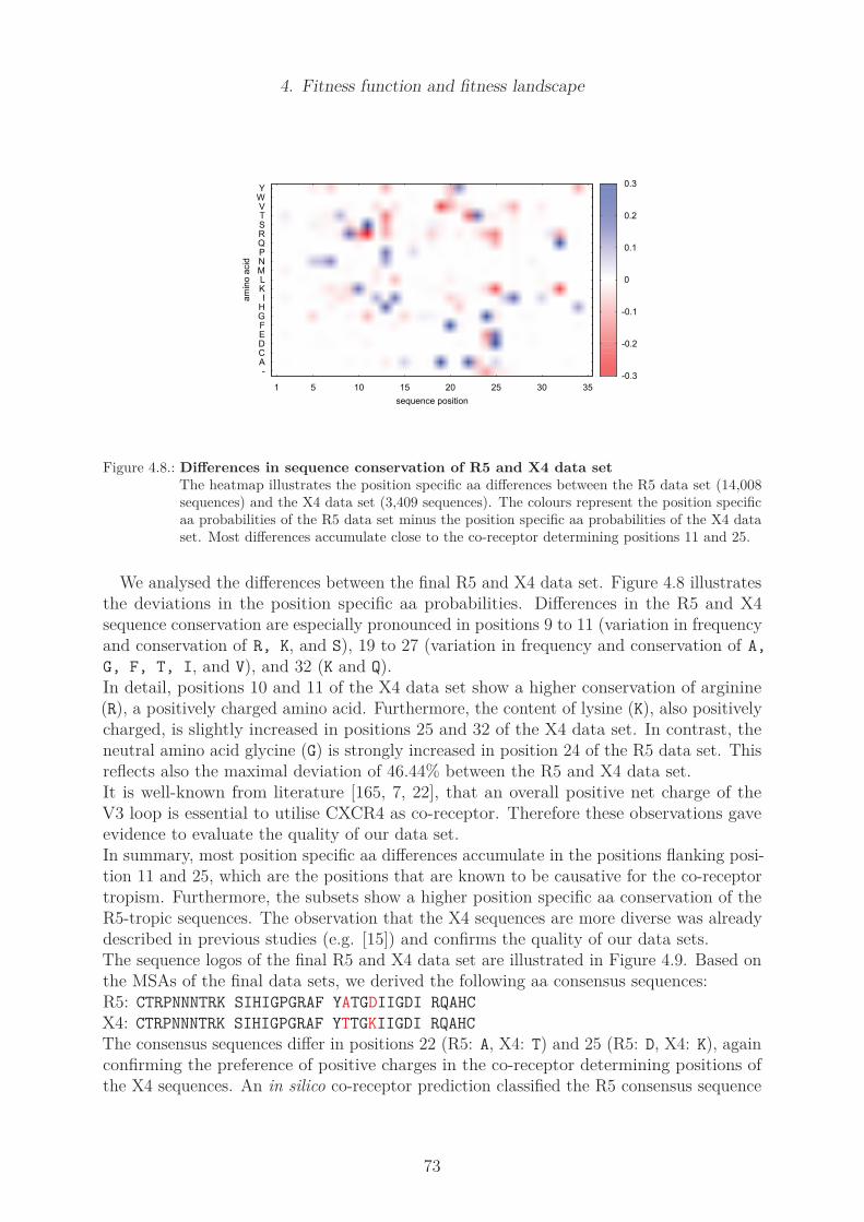
4. Fitness function and fitness landscape
1 5 10 15 20 25 30 35
sequence position
-ACDEFGHI
KLMNPQRSTVWY
am
ino a
cid
-0.3
-0.2
-0.1
0
0.1
0.2
0.3
Figure 4.8.: Differences in sequence conservation of R5 and X4 data setThe heatmap illustrates the position specific aa differences between the R5 data set (14,008sequences) and the X4 data set (3,409 sequences). The colours represent the position specificaa probabilities of the R5 data set minus the position specific aa probabilities of the X4 dataset. Most differences accumulate close to the co-receptor determining positions 11 and 25.
We analysed the differences between the final R5 and X4 data set. Figure 4.8 illustratesthe deviations in the position specific aa probabilities. Differences in the R5 and X4sequence conservation are especially pronounced in positions 9 to 11 (variation in frequencyand conservation of R, K, and S), 19 to 27 (variation in frequency and conservation of A,
G, F, T, I, and V), and 32 (K and Q).In detail, positions 10 and 11 of the X4 data set show a higher conservation of arginine(R), a positively charged amino acid. Furthermore, the content of lysine (K), also positivelycharged, is slightly increased in positions 25 and 32 of the X4 data set. In contrast, theneutral amino acid glycine (G) is strongly increased in position 24 of the R5 data set. Thisreflects also the maximal deviation of 46.44% between the R5 and X4 data set.It is well-known from literature [165, 7, 22], that an overall positive net charge of theV3 loop is essential to utilise CXCR4 as co-receptor. Therefore these observations gaveevidence to evaluate the quality of our data set.In summary, most position specific aa differences accumulate in the positions flanking posi-tion 11 and 25, which are the positions that are known to be causative for the co-receptortropism. Furthermore, the subsets show a higher position specific aa conservation of theR5-tropic sequences. The observation that the X4 sequences are more diverse was alreadydescribed in previous studies (e.g. [15]) and confirms the quality of our data sets.The sequence logos of the final R5 and X4 data set are illustrated in Figure 4.9. Based onthe MSAs of the final data sets, we derived the following aa consensus sequences:R5: CTRPNNNTRK SIHIGPGRAF YATGDIIGDI RQAHC
X4: CTRPNNNTRK SIHIGPGRAF YTTGKIIGDI RQAHC
The consensus sequences differ in positions 22 (R5: A, X4: T) and 25 (R5: D, X4: K), againconfirming the preference of positive charges in the co-receptor determining positions ofthe X4 sequences. An in silico co-receptor prediction classified the R5 consensus sequence
73

4. Fitness function and fitness landscape
as R5-tropic and the X4 consensus sequence as X4-tropic.
V3 loop positionWebLogo 3.3
0.0
0.5
1.0
pro
babili
ty
CA
V
ITRLP
5
H
GSNNNTSR
10
RKGSV
IQ
TSNPHLMI
15
A
GW
L
PGQ
G
SKRV
TA
20
I
WLFFYTAATEG
25
N
G
AQED
VIV
TIGND
30
IRRKQAYH35
C
V3 loop positionWebLogo 3.3
0.0
0.5
1.0
pro
babili
ty
CA
V
S
E
M
ITRLP
5
H
Y
SGND
K
T
S
NS
T
H
K
YNK
R
I
TM
A
G
I
KSR
10
T
E
Q
RKD
K
GRS
L
M
VIA
N
PYRSTH
R
T
F
VLMI
15
A
GL
Q
PR
GG
SKRK
R
S
TVA
20
YLIVWFR
I
V
FHYS
Y
V
ATS
R
ATQ
T
KDREG
25
S
T
N
A
GDRQEK
VIS
K
TVIG
G
ND
30
T
L
V
IK
RRKQAFYH35
CFigure 4.9.: Amino acid sequence logo of R5 and X4 subset
The figure illustrates the position specific aa probabilities of(top) 14,008 R5-tropic sequences, and(bottom) 3,409 X4-tropic sequences (adjusted to a length of 35 aa).The consensus sequences differ in positions 22 (R5: A, X4: T) and 25 (R5: D, X4: K).The hight of the letters (y-axis) describes the position specific aa probability. Thecolours illustrate chemical properties: blue: basic (K,R,H), red: acidic (D,E), green: po-lar (C,G,N,Q,S,T,Y), and black: non-polar/hydrophobic (A,F,I,L,M,P,V,W).
In addition to the amino acid consensus sequences, also the corresponding nucleotide (nt)consensus sequences were determined. Using the original nt sequences as templates, the R5and X4 aa MSA were back-translated into nt sequences. The dominant nucleotide letter ateach sequence position determined the nt consensus sequence. Due to the length adaptationof the X4 MSA, the nucleotide consensus sequences are both of length 105. The sequencelogos in Figure 4.10 illustrate the position specific nt probabilities of the R5 and X4 nt MSA.
74
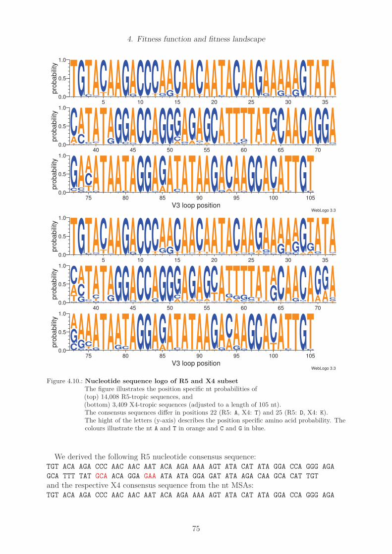
4. Fitness function and fitness landscape
V3 loop positionWebLogo 3.3
0.0
0.5
1.0p
rob
ab
ility
TGCTGA5
T
CC
AAGGA10
CT
CA
T
CC
GAGA
15
T
CAATCA20
ACTACCGA25
AGGAAGA30
GAGAGCTGA
35
TTCA
0.0
0.5
1.0
pro
ba
bili
ty
T
ACG
CAG
CT
40
T
CATTGAGCG
45
G
AT
CG
T
CGAG
50
GACGC
GAA
GC
T
GA
55
A
GT
CG
C
AC
ATGT
60
A
CGTC
TTACTAG65
CG
AG
ACG
A70
GA
GT
G
A
0.0
0.5
1.0
pro
ba
bili
ty
A
C
GG
CA
75
G
TCAGATAGA
80
CTAGGGA
85
AGACTAT
90
AAGGAG
A
C95
G
AG
AGCT
C
G
A100
T
CACTTG105
CT
V3 loop positionWebLogo 3.3
0.0
0.5
1.0
pro
ba
bili
ty
TGCTTGA5
A
T
CG
AAGGA10
CT
CA
T
CC
T
GAC
GA
15
T
CG
AC
G
AA
T
CC
TA
20
G
C
AG
C
TAA
G
T
CC
T
G
A25
GAC
TA
GT
C
GAG
C
AC
GA
30
GAC
GAA
GC
AGTT
C
GA
35
TC
T
G
A
0.0
0.5
1.0
pro
ba
bili
ty
G
TACGCAA
G
C
T40
G
TCAG
C
TC
T
GAA
GC
G45
T
GAG
T
CG
A
T
CGAA
G50
GAC
GG
C
AA
GC
T
G
A55
T
A
GA
G
TCG
C
ACAGTC
AGT
60
A
C
GTA
G
CTG
TAC
TC
T
GA
65
A
T
CG
T
C
AT
GAA
T
G
CG
A70
C
AGC
AGT
G
CA
0.0
0.5
1.0
pro
ba
bili
ty
CGA
C
GA
75
G
TCAGATA
C
T
GA
80
A
CTAGGGA
85
AGG
ACTGACT90
C
AAAGGAAC95
GAGAGC
G
A100
TCT
ACTTG105
C
TFigure 4.10.: Nucleotide sequence logo of R5 and X4 subset
The figure illustrates the position specific nt probabilities of(top) 14,008 R5-tropic sequences, and(bottom) 3,409 X4-tropic sequences (adjusted to a length of 105 nt).The consensus sequences differ in positions 22 (R5: A, X4: T) and 25 (R5: D, X4: K).The hight of the letters (y-axis) describes the position specific amino acid probability. Thecolours illustrate the nt A and T in orange and C and G in blue.
We derived the following R5 nucleotide consensus sequence:TGT ACA AGA CCC AAC AAC AAT ACA AGA AAA AGT ATA CAT ATA GGA CCA GGG AGA
GCA TTT TAT GCA ACA GGA GAA ATA ATA GGA GAT ATA AGA CAA GCA CAT TGT
and the respective X4 consensus sequence from the nt MSAs:TGT ACA AGA CCC AAC AAC AAT ACA AGA AAA AGT ATA CAT ATA GGA CCA GGG AGA
75

4. Fitness function and fitness landscape
GCA TTT TAT ACA ACA GGA AAA ATA ATA GGA GAT ATA AGA CAA GCA CAT TGT
Analogue to the aa consensus sequences, the R5 and X4 nt consensus sequences differedonly in codons 22 (R5: GCA, X4: ACA, nt positions 64 to 66) and 25 (R5: GAA, X4: AAA, ntpositions 73 to 75).During this analysis, we observed a peculiarity about the nt and aa consensus sequence ofthe R5 data set. The aa translation of the nt consensus sequence of R5 did not exactlymatch the aa consensus sequence. Codon 25 (GAA) translates into glutamic acid (E), whilewe found aspartic acid (D) in the respective aa position 25, which would be encoded bycodon GAC.An examination of our data showed that this peculiarity was not an error in our consensussequences, but a result of the most weakly conserved nucleotide position 75, the thirdposition in the differing codon. In position 75 of the nucleotide MSA, the nucleotidesadenine (A) and cytosine (C) occurred with almost similar probability, but with a slightpreference towards nucleotide A, while amino acid D was slightly more frequent in thecorresponding position 25 of the aa sequence.
76

4. Fitness function and fitness landscape
4.4. Results
Based on the previously described R5 and X4 sequence data sets, we give a detaileddescription of the determination of the R5 and X4 fitness function. Additive and multi-plicative terms for the fitness functions are introduced and discussed. In the second partof the section, the underlying R5 and X4 fitness landscapes are analysed.
4.4.1. Determination of R5 and X4 fitness function
We derived an independent R5 and X4 fitness functions from the respective R5 and X4MSA of the V3 loop. Both fitness functions were built of a main fitness term, evaluatingthe one-dimensional aa sequence, and an epistatic term, accounting for the effects ofevolutionary coupled pairs of mutations.
4.4.2. Position specific amino acid counts
Following the sequence of steps presented in Figure 4.1, we first determined the frequencyof each aa at each alignment position, separately for the R5 and X4 data set.Figure 4.11 illustrates the position specific aa counts of the 14,008 R5 sequences as aheatmap, and Table 4.11 contains the respective numerical values. Since the sequencespace of R5 was highly conserved, only one amino acid was dominant in most sequencepositions. The few positions with ambiguous aa preferences were found in the regionsflanking positions 11 and 25. For example histidine (H) is dominant in position 13, butonly in half of the sequences (7,888 of 14,008). The remaining sequences mainly containproline (P, 2,723), asparagine (N, 1,926), serine (S, 658), and threonine (T, 546).A heatmap of the position specific aa counts of the 3,409 X4 sequences is given in Figure4.12. Though we adapted the X4 MSA to a length of 35 amino acids, it still contained 679gaps that were scattered throughout the sequences and positions, with most of the gapsaccumulated in position 24.In contrast to the R5 data set, a number of sequence positions of the X4 data set didnot show a clear dominance of any aa, an observation that applied in particular for theco-receptor determining positions 11 and 25. Table 4.12, presents the exact positionspecific aa frequencies and clarifies this observation. In position 11, arginine (R) and serine(S) showed almost balanced counts of 1,086 and 1,184. This applied also for threonine (T,1,754) and alanine (A, 1,381) in position 22. Most pronounced is the diversity for sequenceposition 25, with comparable frequencies for the four aa lysine (K, 700), glutamic acid (E,661), glutamine (Q, 563), and arginine (R, 513).
77

4. Fitness function and fitness landscape
1 5 10 15 20 25 30 35
sequence position
-ACDEFGHI
KLMNPQRSTVWY
am
ino a
cid
0
0.2
0.4
0.6
0.8
1
1 2 3 4 5 6 7 8 9 10 11 12 13 14 15 16 17 18
Y 0 1 0 0 15 7 7 0 0 0 0 0 5 1 0 0 0 0
W 0 0 0 0 0 0 0 0 0 0 0 0 0 0 1 138 4 0
V 0 200 0 42 0 0 0 0 2 0 0 297 0 128 21 12 0 0
T 0 12049 0 8 31 24 6 13958 2 125 2 12 546 26 37 10 0 21
S 0 90 0 0 1446 64 36 9 139 6 11248 0 658 1 3 18 0 793
R 0 3 14008 0 3 0 0 5 13698 2210 0 1 66 4 62 1 40 11133
Q 0 3 0 0 2 2 0 0 1 67 0 0 159 0 36 71 0 245
P 0 12 0 13629 1 0 0 2 0 0 1 0 2723 0 1 13490 0 1
N 0 1 0 0 11177 13835 13925 0 0 29 12 0 1926 1 0 0 8 2
M 0 12 0 0 0 0 0 2 31 3 0 53 0 2151 0 9 2 0
L 0 34 0 292 1 0 0 1 4 3 0 9 9 943 1 188 1 0
K 0 3 0 0 1 2 0 1 25 11475 0 2 1 2 1 0 1 1168
I 0 1407 0 0 5 3 3 2 36 9 0 13633 4 10674 1 0 0 6
H 0 1 0 37 236 21 4 0 0 0 0 0 7888 0 0 0 0 5
G 0 0 0 0 1030 1 0 0 61 10 2717 0 1 0 12910 9 13910 514
F 0 3 0 0 4 0 0 0 0 0 0 1 3 76 0 32 13 0
E 0 55 0 0 0 0 0 0 0 49 0 0 0 0 27 0 21 26
D 0 1 0 0 49 49 27 0 0 20 28 0 8 0 0 0 3 1
C 14008 0 0 0 1 0 0 0 0 0 0 0 0 0 0 1 0 0
A 0 133 0 0 6 0 0 28 9 2 0 0 11 1 907 29 5 93
- 0 0 0 0 0 0 0 0 0 0 0 0 0 0 0 0 0 0
19 20 21 22 23 24 25 26 27 28 29 30 31 32 33 34 35
Y 0 65 12798 5 0 1 0 0 0 0 3 0 0 0 0 1365 0
W 0 738 61 0 0 0 0 0 0 1 0 0 0 0 0 0 0
V 160 83 17 55 2 2 6 598 371 1 2 54 0 5 21 0 0
T 714 0 0 4805 13590 24 34 26 652 0 0 46 3 2 20 1 0
S 81 24 9 19 18 1 107 0 3 0 13 0 9 1 7 28 0
R 8 1 3 9 25 27 101 3 4 32 6 1 13883 302 0 49 1
Q 11 0 16 2 11 7 1127 0 0 0 14 0 0 12184 0 60 0
P 6 0 0 13 24 0 0 0 0 0 8 21 0 13 2 7 0
N 0 0 2 1 7 10 280 2 0 0 2429 0 0 5 0 6 0
M 6 126 0 24 39 0 0 37 42 0 0 32 0 0 0 0 0
L 0 832 7 2 1 1 1 12 32 0 0 2 0 80 0 2 0
K 1 0 0 0 0 20 25 4 1 3 85 0 50 1219 0 1 0
I 3 435 10 14 48 2 2 13325 12896 0 1 13852 7 5 0 0 0
H 0 2 112 0 11 0 5 0 0 0 7 0 0 36 0 12437 0
G 4 0 0 21 1 13701 494 0 1 13928 38 0 56 1 6 11 0
F 0 11700 947 0 0 0 0 0 2 0 1 0 0 0 0 30 0
E 5 0 1 5 1 151 5008 0 1 41 90 0 0 131 6 1 0
D 0 0 7 0 0 56 5706 1 0 0 11302 0 0 9 1 7 0
C 0 2 18 0 0 0 0 0 0 0 0 0 0 2 0 3 14007
A 13009 0 0 9033 230 5 1112 0 3 2 9 0 0 13 13945 0 0
- 0 0 0 0 0 0 0 0 0 0 0 0 0 0 0 0 0
Figure 4.11.: Position specific amino acid counts in the R5 data setThe figure presents the position specific aa counts of the 14,008 R5 sequences and the tablelists the respective numerical values. In general, one aa was dominant in each positions ofthe R5 MSA, but we found a few ambiguous positions in the regions flanking positions 11and 25.
78

4. Fitness function and fitness landscape
1 5 10 15 20 25 30 35
sequence position
-ACDEFGHI
KLMNPQRSTVWY
am
ino a
cid
0
0.2
0.4
0.6
0.8
1
1 2 3 4 5 6 7 8 9 10 11 12 13 14 15 16 17 18
Y 0 0 0 0 77 20 176 0 0 0 0 3 294 9 0 0 0 1
W 0 0 0 0 0 0 0 0 0 0 2 1 1 0 0 12 2 0
V 0 43 0 5 0 1 1 19 29 0 3 204 3 138 1 0 1 1
T 0 2850 0 7 16 48 56 3100 9 34 12 24 640 59 16 13 1 9
S 0 46 0 0 288 59 41 8 193 5 1184 0 514 1 16 32 3 127
R 0 3 3409 0 3 25 4 74 2748 946 1086 3 330 41 16 15 37 2891
Q 0 2 0 0 0 3 1 1 7 88 0 0 27 0 6 76 0 9
P 0 8 0 3339 0 3 0 4 4 0 6 0 125 0 0 3130 6 2
N 0 0 0 0 2504 3108 2914 0 12 20 8 0 106 0 0 0 0 3
M 0 60 0 0 0 1 0 17 33 0 1 94 0 518 0 1 5 7
L 0 3 0 48 1 15 0 3 12 2 3 80 5 501 0 68 14 0
K 0 6 0 0 4 46 109 61 158 2248 59 0 0 3 0 0 17 259
I 0 287 0 0 10 13 28 110 87 1 8 2986 1 2062 0 3 0 10
H 0 0 0 10 58 4 59 1 0 3 29 0 1260 2 11 1 0 7
G 0 2 0 0 420 14 0 0 57 22 947 0 9 1 3301 23 3316 76
F 0 4 0 0 0 0 2 0 0 0 0 13 10 69 0 10 0 0
E 0 53 0 0 0 14 0 0 20 34 0 0 0 0 5 0 6 1
D 0 0 0 0 23 34 18 0 0 1 49 0 0 0 3 0 0 0
C 3409 0 0 0 2 0 0 0 0 0 3 0 2 0 1 0 0 0
A 0 42 0 0 3 1 0 11 40 5 9 1 82 5 33 25 1 6
- 0 0 0 0 0 0 0 0 0 0 0 0 0 0 0 0 0 0
19 20 21 22 23 24 25 26 27 28 29 30 31 32 33 34 35
Y 11 249 2674 38 1 0 1 0 2 0 9 0 0 0 0 645 0
W 1 358 14 0 0 0 0 0 0 0 0 0 0 1 0 0 0
V 784 355 88 87 13 1 4 253 406 1 2 88 0 1 7 0 0
T 152 4 0 1754 2706 70 60 10 252 5 14 36 5 2 10 2 0
S 70 10 10 34 51 8 57 1 33 0 18 0 10 0 8 12 0
R 52 7 66 6 101 300 513 23 18 19 0 13 3264 418 2 20 0
Q 6 0 1 14 2 53 563 0 18 0 0 0 0 1908 0 26 0
P 10 0 1 16 12 1 0 0 9 0 0 4 0 1 7 3 0
N 4 0 5 1 3 2 90 2 8 0 529 1 0 3 0 2 0
M 0 14 1 7 16 8 0 16 21 0 0 26 0 0 0 0 0
L 0 268 25 12 5 0 0 7 17 0 1 37 0 15 1 6 0
K 37 0 0 9 25 166 700 7 33 5 17 12 94 1001 0 0 0
I 8 274 86 20 25 3 3 3028 2543 0 0 3186 9 8 0 0 0
H 2 3 222 1 2 1 26 0 0 0 0 0 0 15 0 2654 0
G 21 0 0 19 20 1751 220 0 1 3361 33 0 17 1 7 0 0
F 0 1845 175 1 0 0 0 0 0 0 0 0 0 0 0 37 0
E 4 1 1 1 4 464 661 0 14 13 5 0 4 28 0 0 0
D 1 1 31 2 1 233 310 2 5 0 2775 0 0 0 0 0 0
C 1 0 4 1 0 0 0 0 0 0 0 0 0 0 0 2 3409
A 2228 20 3 1381 300 7 107 3 9 2 6 0 0 1 3367 0 0
- 17 0 2 5 122 341 94 57 20 3 0 6 6 6 0 0 0
Figure 4.12.: Position specific amino acid counts in the X4 data setThe figure presents the position specific aa counts of the 3,409 X4 sequences and the tablelists the respective numerical values. Many sequence positions are highly diverse, somedominated by two aa at similar rates (e.g. R and S in position 11), others by three to fouraa (e.g. position 25).In some positions, no clear dominance of any aa could be observed, in particular for theco-receptor determining positions 11 and 25.
79
4. Fitness function and fitness landscape
The derivation of the position specific aa frequencies started from 79,688 V3 loopsequences. During data analysis we concluded that our data reduction method did notlead to relevant changes in the position specific aa probabilities. Despite this fact, we areaware that our data set is not infinite and does not cover the complete V3 loop sequencespace. We presumably missed V3 loop sequences with further position specific aa that arenot represented in our finite data sets.This kind of problems, known as regularisation problems, was described by Tikhonov [150].The method of regularisation tries to find suitable approximations to solve ill-conditionedmathematical problems that arose from finite data or noise contributions.We addressed the finite size effect of our data by the use of a regularisation parameter γ
and adapted the observed aa frequencies using the following equation:
freqnewij= freqorigij
+ γ (4.9)
By an addition of γ = 1 to any frequency value freqorigijof any amino acid j at any
sequence position i, we accounted for amino acids that we possibly have not seen atposition i in our data set. This regularisation equation explicitly includes positions withamino acid counts of zero.The selection of a small γ value guaranteed only marginal alterations of the real aminoacid frequencies of our data.
4.4.3. Main fitness contribution fitmain
The position specific aa counts of the R5 and X4 data set are the basis for the computationof the main fitness contribution fitmain. Given a specific V3 loop sequence, we computetwo independent fitness contributions fitmainR5
and fitmainX4, using the respective R5 or
X4 frequency table (compare Figures 4.11 and 4.12). Based on the frequencies freqijc, we
calculated the position specific aa probabilities pijc= freqijc
Nc, with c being the respective
co-receptor and NR5 = 14,008 and NX4 = 3,409 being the number of R5 and X4 sequences.
80

4. Fitness function and fitness landscape
We considered two possible formulations to calculate the replicative fitness, an additiveand a multiplicative fitness function:
addF itmainR5=
35∑
i=1
20∑
j=1
pijR5rij ;
addF itmainX4=
35∑
i=1
20∑
j=1
pijX4rij ;
multF itmainR5=
35∏
i=1
20∑
j=1
pijR5rij ;
multF itmainX4=
35∏
i=1
20∑
j=1
pijX4rij
with rij =
1 if aa j is at position i
0 else
(4.10)
and the probability pijR5of aa j at position i in the R5 data set and the probability pijX4
of aa j at position i in the X4 data set.For any sequence, rij = 0 for all but amino acid j at position i, and thus the inner sum∑
pijrij = 0.0 for all but one amino acid.Using the additive fitness function defined in Equation 4.10, we summed up the respectiveaa 35 probabilities in each position. Maximal fitness values addF itmainR5
= 31.26 andaddF itmainX4
= 27.26 were assigned to the respective R5 and X4 consensus sequence. Thedeviations of the additive main fitness contribution from the absolute maximum of 35.0reflected the deviations in the conservation of the sequence positions.To observe the impact of an aa mutation on the replicative fitness, we analysed a numberof random sequence examples. For clarification, a small example of two shortened V3 loopsequences a and b (V3 loop positions one to 11) is presented. Sequence a is composedof the consensus amino acids, while position seven of sequence b carries a biologicallyunfavourable mutation (E) that was not observed at this position in both data sets.We computed the fitness of the example sequences based on the aa frequencies freqijR5
and freqijX4shown in Tables 4.11 and 4.12, altered by the regularisation Equation 4.9:
sequence a: CTRPNNNTRKS
addF itmainR5(a) = 14009+12050+14009+13630+11178+13836+13926+13958+13699+11476+11249
14008+20·γ= 10.20
addF itmainX4(a) = 3410+2851+3410+3340+2505+3109+2915+3101+2749+2247+1185
3409+20·γ= 8.99
sequence b: CTRPNNETRKS
addF itmainR5(b) = 14009+12050+14009+13630+11178+13836+1+13958+13699+11476+11249
14008+20·γ= 9.20
81
4. Fitness function and fitness landscape
addF itmainX4(b) = 3410+2851+3410+3340+2505+3109+1+3101+2749+2247+1185
3409+20·γ= 8.14
The examples showed deviations of the additive replicative fitness of ≈ 1.0 for the R5fitness function and of 0.85 for the X4 fitness function, reflecting the reduced replicativefitness of the mutated aa in position seven. Thus, the mutation of a highly conserved aainto an aa not observed in that sequence position of the underlying MSA leads to a fitnessreduction of ≈ 1.0.The regularisation Equation 4.9 with γ = 1 changed the additive fitness of the consensussequences in two decimal points (data not shown).In the alternative formulation of the main fitness contributions, we multiplied the positionspecific aa probabilities. In this case, maximal fitness values multF itmainR5
= 1.149 · 10−2
and multF itmainX4= 2.779 · 10−5 were calculated for the consensus R5 and X4 sequence.
The consensus sequence maxima differed remarkably from the theoretic fitness maximum of1.0 (1.035), which would be assigned to a completely conserved data set. These deviationsreflected the variability in the position specific conservation of the aa sequences.We again demonstrate the calculation of the replicative fitness for sequences a and b,carrying the aa mutation E in position seven.
sequence a: CTRPNNNTRKS
multF itmainR5(a) = 14009·12050·14009·13630·11178·13836·13926·13959·13699·11476·11249
(14008+γ)11 = 0.42
multF itmainX4(a) = 3410·2851·3410·3340·2505·3109·2915·3101·2749·2249·1185
(3409+γ)11 = 0.08
sequence b: CTRPNNETRKS
multF itmainR5(b) = 14009·12050·14009·13630·11178·13836·1·13959·13699·11476·11249
(14008+γ)11 = 3.02 · 10−5
multF itmainX4(b) = 3410·2851·3410·3340·2505·3109·1·3101·2749·2249·1185
(3409+γ)11 = 2.70 · 10−5
In case of the multiplicative fitness function, the mutation of a conserved aa was highlypronounced and resulted in a maximal fitness reduction of 1
(14008+γ)≈ 104 for the multi-
plicative R5 fitness function and in a maximal fitness reduction of 1(3409+γ)
≈ 103 for the
multiplicative X4 fitness function. This variation of the replicative fitness was in a rangewe would expect from an aa that is biologically and chemically unfavourable.An analysis of the influence of the regularisation Equation 4.9 with γ = 1 revealed that theregularisation altered the fitness value of the consensus sequences in five (R5) respectivefour (X4) decimal points (data not shown), except for the case when a frequency of 0 isreplaced by a frequency of γ = 1. In that case, the regularisation Equation 4.9 with γ = 1avoids the multiplication of a zero probability and restricts a resulting zero fitness.Based on these observations, in combination with the simulation results we present inSection 5.3.1, we decided to use the multiplicative formulation of the fitness function.
82

4. Fitness function and fitness landscape
4.4.4. Counts of pairs of coupled mutations
The second part of the fitness function is an epistatic fitness contribution. Epistaticpositions are characterised by a coupled evolution, meaning that mutations of the aminoacids at two (or more) positions of the V3 loop are linked and the occurrence of an aamutation in one position influences the aa in the other position.For the replicative capacity of an individual, the epistatic fitness effect can either bepositive or negative. If the mutual occurrence of two aa mutations mi and mj in twocoupled positions i and j leads to a fitness benefit compared to the fitness effects of bothsingle mutations (e.g. two cysteine residues that build a disulfide bridge), we speak ofpositive epistasis. In the case of a negative epistatic effect, two contemporary aa mutationslead to a decreased replicative fitness compared to the sole occurrence, for example due tosteric hindrance in the case of two large aa in close proximity.We discriminated positions of positive and negative epistatic based on the sign of theentries of the cross correlation matrix described in Section 4.2.1.
Structural coupling
There are different methods to detect co-evolving positions in sequences. We first usedthe measure of mutual information complemented by the structural coupling analysis asprovided by the R Bioconductor [121, 77] package to determine pairs of co-evolutionarycoupled positions in the R5 and X4 MSA.The structural coupling analysis is based on an MSA and an additional crystal structureof the respective molecule. To obtain a crystal structure of the V3 loop, we used the PDBdata base [12, 11], an archive of macromolecular structures. A search for ’env HIV’ inthe database resulted in 104 structure hits, a search for ’gp120’ delivered 153 hits andsearching for ’V3’ we found 86 structures. The different search results were mainly subsetsof each other.A close inspection of the files revealed that most of the structures contained incompleteV3 loop sequences. Especially the gp120 residues 300 to 320 (V3 loop positions five to 25)were missing in almost all .pdb structure files.At the date of our search, only the following three .pdb files contained complete HIV-1 V3loops:
1CE4.pdb The file [153] contained a conformational model for the consensus V3 loop ofthe HIV-1 envelope protein gp120 published in 1997. The authors presentedno unique crystal structure, but described a summary of observations fromseveral structures, and combined them into one consensus model. Theresolution of the structure thus could not be determined. In the 1CE4.pdbstructure, a synthetically disulfide bridge between cys296 (loop position 1)and cys331 (loop position 35) has been introduced due to crystallisationissues. In consequence, we did not consider this contact during the structuralcoupling analysis.We extracted the following aa sequence of the V3 loop from the file:CTRPNNNTRK SIHIGPGRAF YTTGEIIGDI RQAHC
2QAD.pdb In 2007, the group of Kwong et al. [78] published the structure file 2QAD.pdb.The file contained the spatial structure of a tyrosine-sulfated antibody,
83

4. Fitness function and fitness landscape
complexed with the complete HIV-1 envelope protein gp120 and the CD4receptor. The resolution of the file was 3.3 A.We trimmed the molecule to the V3 loop and extracted the following aasequence:CTRPNNNTRK SINIGPGRAL YTTGEIIGDI RQAHC
2B4C.pdb The third structure was also published from the group of Kwong [79]. Thefile 2B4C.pdb contained a crystal structure of the gp120 core protein ofHIV-1, complexed with CD4 and an X5 antibody. The resolution of the filewas specified as 3.3 A.We extracted the following sequence, restricted to the V3 loop residues, fromthe file:CTRPNQNTRK SIHIGPGRAF YTTGEIIGDI RQAHC
Though the research groups of Zolla-Pazner et al. and Kwong et al. did excessive researchin the field of V3 loop structure, no further V3 loop structures were available. The majorityof the envelope structures was lacking the V3 region or missed at least the central residuesof the loop due to problems upon the crystallisation.We used the BALLView [107, 106] package to visually inspect the crystal structures andto restrict the sequence to fit the V3 loop region. Figure 4.13 illustrates the three V3 loopstructures we extracted from the files.
(a) (b) (c)
Figure 4.13.: Selected V3 loop structuresThe illustration presents the V3 loop structures extracted from the files 1CE4.pdb (left),2QAD.pdb (center), and 2B4C.pdb (right). The co-receptor determining position 11 iscoloured in blue and position 25 in yellow.
The BALLView software package furthermore enabled us to calculate the root meansquare deviation (RMSD), a measure used to determine spatial deviations between proteinstructures. The best match of the Cα atoms of the protein backbone of the three V3 loop
84
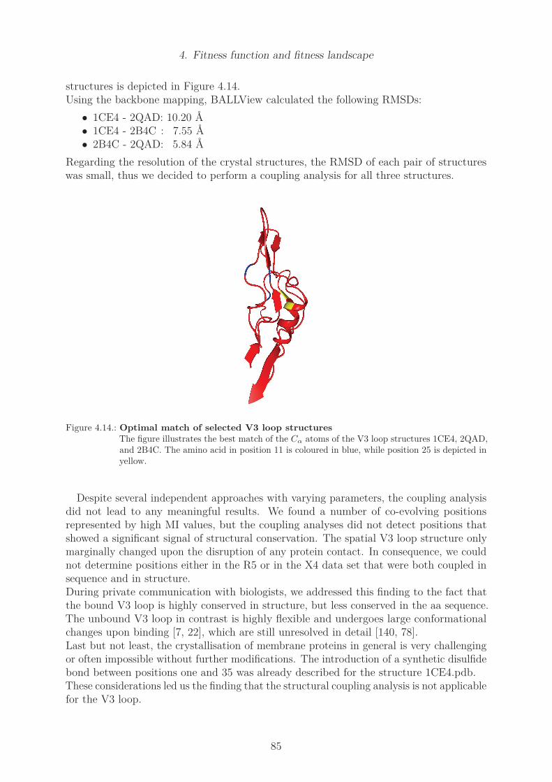
4. Fitness function and fitness landscape
structures is depicted in Figure 4.14.Using the backbone mapping, BALLView calculated the following RMSDs:
• 1CE4 - 2QAD: 10.20 A• 1CE4 - 2B4C : 7.55 A• 2B4C - 2QAD: 5.84 A
Regarding the resolution of the crystal structures, the RMSD of each pair of structureswas small, thus we decided to perform a coupling analysis for all three structures.
Figure 4.14.: Optimal match of selected V3 loop structuresThe figure illustrates the best match of the Cα atoms of the V3 loop structures 1CE4, 2QAD,and 2B4C. The amino acid in position 11 is coloured in blue, while position 25 is depicted inyellow.
Despite several independent approaches with varying parameters, the coupling analysisdid not lead to any meaningful results. We found a number of co-evolving positionsrepresented by high MI values, but the coupling analyses did not detect positions thatshowed a significant signal of structural conservation. The spatial V3 loop structure onlymarginally changed upon the disruption of any protein contact. In consequence, we couldnot determine positions either in the R5 or in the X4 data set that were both coupled insequence and in structure.During private communication with biologists, we addressed this finding to the fact thatthe bound V3 loop is highly conserved in structure, but less conserved in the aa sequence.The unbound V3 loop in contrast is highly flexible and undergoes large conformationalchanges upon binding [7, 22], which are still unresolved in detail [140, 78].Last but not least, the crystallisation of membrane proteins in general is very challengingor often impossible without further modifications. The introduction of a synthetic disulfidebond between positions one and 35 was already described for the structure 1CE4.pdb.These considerations led us the finding that the structural coupling analysis is not applicablefor the V3 loop.
85

4. Fitness function and fitness landscape
Mutual Information
We next concentrated on methods that are solely sequence based. We used the RBioconductor [121, 77] package to calculate the mutual information and to detect pairs ofco-evolving sequence positions in the MSAs. For an optimal handling of the 679 gaps weobserved in the X4 MSA, we used the subset mutual information (SUMI) described inSection 4.2.1. We further applied the shuffle null model of Weil et al. [158] to discriminatesignificant co-evolution signals from background noise.The SUMI values of the sequence positions pairs are depicted in Figure 4.15. The matrixof the R5 SUMI values showed co-evolutionary signals in positions 13 to 14 linked topositions 18 and 20. Furthermore, positions five and 25 were weakly coupled to a numberof additional positions, indicated by the increased SUMI values in column 25.The X4 data set contained an increased number of coupled positions and also higherSUMI values compared to the R5 data set, but in general, the same regions were detected.The co-evolutionary X4 signal extended from positions 11 to 14, coupled to positions19 to 25. In addition, positions 19 to 25 of the X4 data set are evolutionary coupledintra-sequentially, indicated by the increased SUMI values in positions 19 to 25.In summary we found increased co-evolutionary signals for the co-receptor determiningpositions 11 and 25 and the flanking amino acids.
1 5 10 15 20 25 30 35
sequence position
1
5
10
15
20
25
30
35
sequence p
ositio
n
0
0.01
0.02
0.03
0.04
0.05
1 5 10 15 20 25 30 35
sequence position
1
5
10
15
20
25
30
35
0
0.05
0.1
0.15
0.2
Figure 4.15.: Mutual information of R5 and X4 sequence alignmentThe heat maps illustrate the R5 SUMI values (left) and the X4 SUMI values (right). Ingeneral, both data sets contain a number of coupled positions in the co-receptor determiningregions, but the coupling is more pronounced in the X4 data set.
86
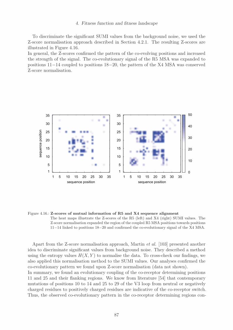
4. Fitness function and fitness landscape
To discriminate the significant SUMI values from the background noise, we used theZ-score normalisation approach described in Section 4.2.1. The resulting Z-scores areillustrated in Figure 4.16.In general, the Z-scores confirmed the pattern of the co-evolving positions and increasedthe strength of the signal. The co-evolutionary signal of the R5 MSA was expanded topositions 11−14 coupled to positions 18−20, the pattern of the X4 MSA was conservedZ-score normalisation.
1 5 10 15 20 25 30 35
sequence position
1
5
10
15
20
25
30
35
sequence p
ositio
n
1 5 10 15 20 25 30 35
sequence position
1
5
10
15
20
25
30
35
0
10
20
30
40
50
Figure 4.16.: Z-scores of mutual information of R5 and X4 sequence alignmentThe heat maps illustrate the Z-scores of the R5 (left) and X4 (right) SUMI values. TheZ-score normalisation expanded the region of the coupled R5 MSA positions towards positions11−14 linked to positions 18−20 and confirmed the co-evolutionary signal of the X4 MSA.
Apart from the Z-score normalisation approach, Martin et al. [103] presented anotheridea to discriminate significant values from background noise. They described a methodusing the entropy values H(X, Y ) to normalise the data. To cross-check our findings, wealso applied this normalisation method to the SUMI values. Our analyses confirmed theco-evolutionary pattern we found upon Z-score normalisation (data not shown).In summary, we found an evolutionary coupling of the co-receptor determining positions11 and 25 and their flanking regions. We know from literature [54] that contemporarymutations of positions 10 to 14 and 25 to 29 of the V3 loop from neutral or negativelycharged residues to positively charged residues are indicative of the co-receptor switch.Thus, the observed co-evolutionary pattern in the co-receptor determining regions con-
87

4. Fitness function and fitness landscape
firmed our expectations about the data and indicated that we found relevant epistaticpositions that were cross-linked during evolution.
Cross correlation
Mutual information values are defined to be positive. Though the SUMI was highlysuitable to reveal the co-evolving positions, the measure failed to discriminate positive andnegative epistatic effects of the coupled positions. To cope with this problem, we appliedthe cross correlation method described in Section 4.2.1.
Cross correlation of the R5 and X4 data set
Using Perl [26] and additional content of the packages List [8] and Math::MatrixReal [13],we computed the cross correlation (CC) matrices of the R5 and X4 MSA using Equation4.5. The resulting matrices CR5 and CX4 are illustrated in figure 4.17.
1 5 10 15 20 25 30 35
sequence position
1
5
10
15
20
25
30
35
sequence p
ositio
n
1 5 10 15 20 25 30 35
sequence position
1
5
10
15
20
25
30
35
-0.4
-0.3
-0.2
-0.1
0
0.1
0.2
0.3
0.4
Figure 4.17.: Cross correlation of R5 and X4 sequence alignmentThe left heatmap illustrates CR5. While pairs (13,18) and (13,20) were highly positivelycorrelated, the matrix showed a strong negative correlation for the pair (11,13).CX4 (right) contained more and increased signals. The pattern of positions 11−14 correlatedto positions 19−24 contained the largest positive values of CX4 for pairs (13,19) and (14,19),and comprised highly negative correlations. The largest negative correlation was observedfor pair (19,24).
88

4. Fitness function and fitness landscape
Positively correlated positions dominated CR5. The correlations of position 14 coupledto positions 18−20 were pronounced. In contrast, the pair (11,13) showed the largestnegative correlation.Similar to the MI approach, CX4 contained a higher frequency of cross linked positions.Furthermore, the CC analysis revealed a high number of negatively correlated pairs inCX4 compared to CR5.In detail, positions 11−14 were positively correlated with positions 19−20, and negativelycorrelated with positions 22−24. This pattern contained the largest positive values of CX4
for pairs (13,19) and (14,19), and also the highly negatively correlated pair (14, 24). Thelargest negative correlation was calculated for the pair (19,24).The correlations of positions 1, 3, and 35 were ∼ 0.0 in both matrices, since the positionsof the respective MSAs were highly conserved.Next, we applied the noise reduction method to the CC matrices. After a column shufflingof both the R5 and the X4 MSA, we calculated the matrices CR5shuff
and CX4shuffand
performed eigenvalue decompositions. We found the largest eigenvalue in the sixth shufflingrun for the R5 MSA and the 13th for the X4 MSA, therefore we stopped the shufflingafter 500 runs for each alignment.The resulting eigenvalues of the real and column-shuffled MSAs are illustrated in Figure4.18. We can clearly see the differences between the eigenvalues of the shuffled alignments,which concentrate in the range from 0.7 to 1.2 for both data sets, and the eigenvaluesλR5 and λX4 of the original MSAs that are spread over a range of 0.3 to 2.8. The largesteigenvalues of the shuffled MSAs were λR5shuffmax
= 1.177 and λX4shuffmax= 1.221.
The thresholds that we used for separation were determined as half the distance of thelargest real eigenvalue that was smaller and the smallest real eigenvalue that was largerthan the largest random eigenvalue. Based on these thresholds, we kept four eigenvalues ofthe R5 MSA and six eigenvalues of the X4 MSA. From these eigenvalues and correspondingeigenvectors, we reconstructed the noise-reduced CC matrices for both data sets. Thereconstructed matrices are depicted in Figure 4.19.An analysis of the differences of the original CC CR5 and CX4 in Figure 4.17 and thenoise-corrected matrices CR5clean
and CX4cleanin Figure 4.19 revealed that the method of
noise-reduction worked as intended. While the previously identified cross-linked pairs wereconserved by the method, the signals increased and became more pronounced.
89
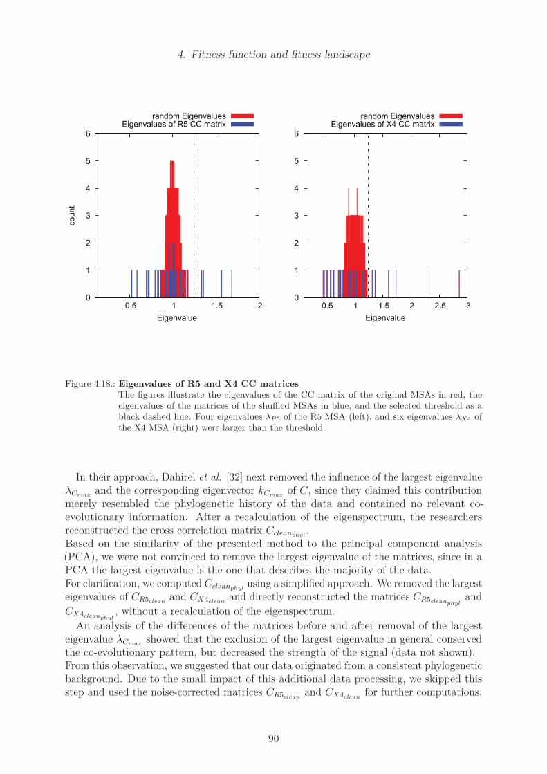
4. Fitness function and fitness landscape
0
1
2
3
4
5
6
0.5 1 1.5 2
count
Eigenvalue
random EigenvaluesEigenvalues of R5 CC matrix
0
1
2
3
4
5
6
0.5 1 1.5 2 2.5 3
count
Eigenvalue
random EigenvaluesEigenvalues of X4 CC matrix
Figure 4.18.: Eigenvalues of R5 and X4 CC matricesThe figures illustrate the eigenvalues of the CC matrix of the original MSAs in red, theeigenvalues of the matrices of the shuffled MSAs in blue, and the selected threshold as ablack dashed line. Four eigenvalues λR5 of the R5 MSA (left), and six eigenvalues λX4 ofthe X4 MSA (right) were larger than the threshold.
In their approach, Dahirel et al. [32] next removed the influence of the largest eigenvalueλCmax
and the corresponding eigenvector kCmaxof C, since they claimed this contribution
merely resembled the phylogenetic history of the data and contained no relevant co-evolutionary information. After a recalculation of the eigenspectrum, the researchersreconstructed the cross correlation matrix Ccleanphyl
.Based on the similarity of the presented method to the principal component analysis(PCA), we were not convinced to remove the largest eigenvalue of the matrices, since in aPCA the largest eigenvalue is the one that describes the majority of the data.For clarification, we computed Ccleanphyl
using a simplified approach. We removed the largesteigenvalues of CR5clean
and CX4cleanand directly reconstructed the matrices CR5cleanphyl
and
CX4cleanphyl, without a recalculation of the eigenspectrum.
An analysis of the differences of the matrices before and after removal of the largesteigenvalue λCmax
showed that the exclusion of the largest eigenvalue in general conservedthe co-evolutionary pattern, but decreased the strength of the signal (data not shown).From this observation, we suggested that our data originated from a consistent phylogeneticbackground. Due to the small impact of this additional data processing, we skipped thisstep and used the noise-corrected matrices CR5clean
and CX4cleanfor further computations.
90

4. Fitness function and fitness landscape
1 5 10 15 20 25 30 35
sequence position
1
5
10
15
20
25
30
35
sequence p
ositio
n
1 5 10 15 20 25 30 35
sequence position
1
5
10
15
20
25
30
35
-0.4
-0.3
-0.2
-0.1
0
0.1
0.2
0.3
0.4
Figure 4.19.: Noise-reduced CC matrices of R5 and X4 MSA:The left figure illustrates the reconstructed matrix CR5clean
, and the right figure the matrixCX4clean
. Noise-reduction conserved and pronounced the co-evolutionary signals.
A comparison of the CC matrices depicted in Figure 4.19 on the one hand and the MIZ-score matrices presented in Figure 4.16 on the other hand revealed, that both the CC andthe MI method found mainly the same co-evolution pattern. Thus, the well-established andfrequently applied MI method confirmed the validity of the recent CC approach for our data.
4.4.5. Epistatic fitness contribution fitepi
The noise-corrected CC matrices CR5cleanand CX4clean
build the basis for the computationof the epistatic fitness term fitepi. The epistatic fitness contribution is defined by the
91

4. Fitness function and fitness landscape
following equations:
fitepiR5=
35∏
i,k=1
20∑
j,l=1
cikR5sijskl
fitepiX4=
35∏
i,k=1
20∑
j,l=1
cikX4sijskl
with sij =
1 if aa j at position i is mutated
0 else
and skl =
1 if aa l at position k is mutated
0 else
(4.11)
and cikR5and cikX4
being the CC values of position pair (i, k) of the corresponding R5 orX4 MSA.If both amino acids j and l at the observed positions i and k are mutated, sijskl = 1, elsesijskl = 0. Thus, for each pair (i, k) the inner sum contributes exactly once.On basis of the epistasis equations, we used a bootstrapping approach to determine therange of the epistatic fitness values. From the set of all possible aa sequences of length 35,we randomly picked two times 1.6 · 106 sequences and calculated the respective fitepiR5
andfitepiX4
values. The distributions of the fitness values of both runs were mainly concordant.Thus, we could derive reliable estimates for the range of the epistatic fitness values (datanot shown).Though the main fitness contribution of R5-tropic sequences is generally higher, due tothe higher sequence conservation of the R5 data set (compare Section 4.4.3), we observeda larger epistatic fitness contribution for the X4-tropic sequences. A retrospect of the CCmatrices revealed that this finding was result of the more frequent epistatic positions andthe increased epistatic signals of CX4clean
.
4.4.6. Complete R5 and X4 fitness function
Based on the R5 and X4 MSA, we determined the position specific aa probabilities tocompute the main fitness term fitmain (compare Equation 4.10), and we calculated CCmatrices to compute the epistatic fitness term fitepi (compare Equation 4.11). We decidedto use a multiplicative fitness formulation to ensure fitness values close to zero for sequenceswith biologically unlikely aa mutations.First analyses revealed that a combination of the main and epistatic fitness terms resultedin small fitness values, even in the case of the consensus sequences, with a fitness of1.149 ·10−2 for the R5 consensus sequence and of 2.779 ·10−5 for the X4 consensus sequence.Test sequences that deviated in one aa decreased the resulting R5 fitness by a factor of10−4 and the X4 fitness by a factor of 10−3 (compare Section 4.4.3). Further tests of theepistatic Equation 4.11 revealed that the fitness of sequences that accumulated mutationscould become negative due the multiplication of an odd number of negative epistatic terms.Negative replicative fitness values are biologically contradictory and very small numbers
92

4. Fitness function and fitness landscape
can lead to numerical instabilities. We resolved these difficulties by the usage of anexponential fitness function. While negative fitness values in the exponent of e resulted insmall positive fitness values, the multiplication of the aa probabilities was converted intoan addition and thus numerical inconsistencies due to the multiplication of 35 probabilityvalues < 1.0 were avoided. The usage of the exponential fitness function was paired withthe usage of the inverse logarithmic function. The Taylor expansions of a logarithmicfunction:
ln(x) = (x − 1)−(x − 1)2
2+(x − 1)3
3− · · ·
reduces to ln(x) ≈ (x − 1) for small x. Since we used a normalisation of our fitness valuesto an interval of [0, 1], the expression could be reduced further to ln(x) ≈ x. Based onthese considerations, we used an exponential expression without an inverse logarithmicoperation. A subsequent normalisation of the fitness values to the interval of [0, 1] wasused to perform the the balancing of the main and epistatic fitness terms.Since we applied different methods to derive the single fitness contributions from our data,the ratio of the main and the epistatic fitness contribution had to be derived in a sequenceof independent steps. In a first step, we approximated the task by scaling both main andepistatic fitness to the interval of [0, 1]. Therefore, we determined the maximal fitnessvalues for the main and epistatic term for both the R5 and X4 contribution. The maximaof the main fitness terms equal the main fitness of the consensus sequence, since theconsensus sequence is computed based on the most frequent amino acid in each sequenceposition. The determination of the maxima of the epistatic terms was more challenging.We performed a bootstrapping approach, creating two times 5% of all possible sequences,and determined their epistatic fitness. A comparison of the distribution of the two sets ofepistatic fitness values showed similar fitness distributions. Therefore, we could estimatethe maximal fitness values by the use of the maximal fitness of the independent randomsequence subsets.Based on the maximal main and epistatic fitness values of both the R5 and X4 data set,we performed a normalisation of each single fitness contribution to the interval [0, 1] bythe division of the fitness values by the respective maximal value.Using a weighting factor β enabled us to further balance the influence of the main andepistatic fitness contribution. Large values of β represent a strong influence of the epistaticcontribution, while small values of β decrease the epistatic contribution to the replicativefitness of a sequence. Finally, we combined the individual R5 and X4 fitness functions byan additional weighting factor α. A value α = 1 restricted the calculation of the replicativefitness to the R5 fitness term, and α = 0 restricted the calculation to the X4 fitness term.A variation of α could for example be used to mimic the availability of CCR5 or CXCR4positive target cells.
93

4. Fitness function and fitness landscape
The complete exponential fitness function eF it is defined as follows:
eF it = αeFitR5 + (1 − α)eF itX4
with eF itR5 = e
35∑i=1
20∑j=1
pijR5rij
+ βe
35∑i,k=1
35∑j,l=1
cikR5sijskl
and eF itX4 = e
35∑i=1
20∑j=1
pijX4rij
+ βe
35∑i,k=1
35∑j,l=1
cikX4sijskl
and rij =
1 if aa j is at position i
0 else
and sij =
1 if aa j at position i is mutated
0 else
and skl =
1 if aa l at position k is mutated
0 else
(4.12)
and pijR5being the probability of aa j at position i in the R5 data set and pijX4
being therespective probability in the X4 data set. cikR5
is the cross correlation of position i andposition k in the R5 data set and cikX4
the cross correlation of position i and position k inthe X4 data set. While α determines the R5 fitness contribution, and 1− α the respectiveX4 fitness contribution, β balances the influence of the epistatic effect on the joined fitness.The normalisation of the main and epistatic term for the R5 and X4, performed by thedivision by the respective maximal values, is not expressed in the equation for reasons ofclarity. When we used Equation 4.12 during subsequent analyses, we used the normalisedexpression of the exponential fitness equation.The normalised exponential fitness equation assigns the maximal fitness value of 1.0 tothe R5 consensus sequence for α = 1.0, while α = 0.0 assigns the maximal value of 1.0to the X4 consensus sequence. The selection of a weighting parameter β < 1.0 reducesthe influence of the epistasis and thus assigns a fitness value smaller than the maximalvalue to any sequence that deviates from the consensus sequence. A selection of β > 1.0pronounces the epistatic effect. Analyses showed that this results in the accumulation ofrandom sequence mutations and destabilises the conservation of the V3 loop sequence.Thus, a selection of β < 1.0 in Equation 4.12 is recommended.Mutations that introduce stop codons into the V3 loop typically terminate the proteintranslation and result in truncated, non-functional proteins. Since the functionality of theloop is essential to HIV, truncated sequences would not enable the process of co-receptorbinding and cell entry and inhibit viral replication. Therefore the replicative fitness ofsequence variants carrying stop codons was defined to be zero.It has to be noted that the absolute fitness values defined by Equation 4.12 are only soundfor an intra-R5 or intra-X4 population ranking, since the fitness contributions were derivedfrom two independent MSA and we lacked a method to compare the replicative fitness
94

4. Fitness function and fitness landscape
of the R5 and X4 sequences. Thus, an inter-population comparison of an R5 and an X4fitness value is not possible with the presented fitness function.
4.4.7. Structure of modelled fitness landscape
We derived fitness functions to describe the replicative fitness V3 loop sequences. Ourmain concern were the differences between the R5 and X4 population, as well as theevolutionary pathways that transform R5-tropic viruses into X4-tropic viruses. Our fitnessfunctions built the basis to analyse the structural differences of the R5 and X4 fitnesslandscape.
Local fitness landscape
We created two populations of unique nucleotide (nt) sequences, derived from the R5 andX4 nt consensus sequence by the introduction of a predefined number of mutations. Thecomplete sequence space of the V3 loop covers 4105 = 1.6 · 1063 sequences. Due to thismultitude of sequences, it is not possible to analyse the complete sequence space.A limitation to all five-point mutants of a V3 loop consensus sequences still results in4
(1055
)≈ 3.9 · 108 sequences. First analyses of two random samples of five-point mutants
showed that many of the sequences contained stop codons or yielded very low fitnessvalues due to mutations in highly conserved positions. Following these observations, westopped the respective analyses and performed a local approach - local in the sense thatwe analysed a reduced fitness landscape of sequences that are evolutionary close to theR5 and X4 consensus sequence. We introduced mutations only in the ten least conservedsequence positions of the R5 and X4 nt MSA.The following ten nt positions of the R5 and X4 MSA are the weakest conserved positionsand were thus selected for mutation (sorted from least to most conserved nt position):
• R5: 75, 64, 38, 37, 51, 31, 85, 14, 42, 29• X4: 73, 38, 37, 64, 71, 31, 94, 33, 74, 29
Mutations in these positions of the R5 and the X4 MSA were most frequently observedand are thus assumed be biologically most relevant.We performed analyses of the R5 and X4 populations, consisting of all possible four-,six-, eight-, and ten-point mutants, but with the mutations restricted to the most weaklyconserved nt positions, i.e. each of the selected least conserved nt positions was mutatedtowards every possible nucleotide. This approach built populations of the size n = 4m, withm being the number of mutated sequence positions and 4 being the number of differentnucleotides.
• m = 4 : n = 44 = 256 sequences• m = 6 : n = 46 = 4, 096 sequences• m = 8 : n = 48 = 65, 536 sequences• m = 10 : n = 410 = 1, 048, 576 sequences
The mutated nucleotide sequences were translated into the corresponding amino acidsequences and their fitness was determined based on Equation 4.12.
95
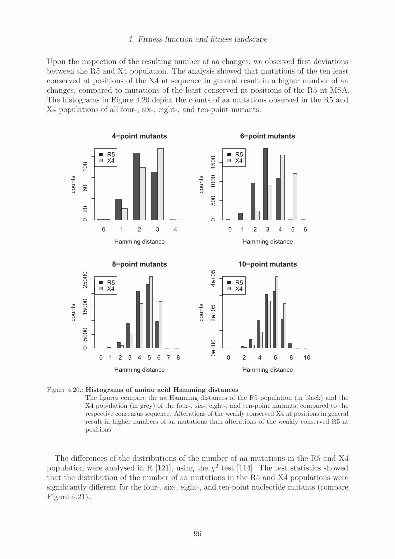
4. Fitness function and fitness landscape
Upon the inspection of the resulting number of aa changes, we observed first deviationsbetween the R5 and X4 population. The analysis showed that mutations of the ten leastconserved nt positions of the X4 nt sequence in general result in a higher number of aachanges, compared to mutations of the least conserved nt positions of the R5 nt MSA.The histograms in Figure 4.20 depict the counts of aa mutations observed in the R5 andX4 populations of all four-, six-, eight-, and ten-point mutants.
0 1 2 3 4
4−point mutants
Hamming distance
counts
020
60
100
R5X4
0 1 2 3 4 5 6
6−point mutants
Hamming distance
counts
0500
1000
1500 R5
X4
0 1 2 3 4 5 6 7 8
8−point mutants
Hamming distance
counts
05000
15000
25000
R5X4
0 2 4 6 8 10
10−point mutants
Hamming distance
counts
0e+
00
2e+
05
4e+
05
R5X4
Figure 4.20.: Histograms of amino acid Hamming distancesThe figures compare the aa Hamming distances of the R5 population (in black) and theX4 population (in grey) of the four-, six-, eight-, and ten-point mutants, compared to therespective consensus sequence. Alterations of the weakly conserved X4 nt positions in generalresult in higher numbers of aa mutations than alterations of the weakly conserved R5 ntpositions.
The differences of the distributions of the number of aa mutations in the R5 and X4population were analysed in R [121], using the χ2 test [114]. The test statistics showedthat the distribution of the number of aa mutations in the R5 and X4 populations weresignificantly different for the four-, six-, eight-, and ten-point nucleotide mutants (compareFigure 4.21).
96

4. Fitness function and fitness landscape
0.0 0.5 1.0 1.5 2.0 2.5 3.0
0.0
0.4
0.8
4−point mutants
Hamming distance
CD
F
●
●
●
●
●
●
●
●
R5X4
0 1 2 3 4 5
0.0
0.4
0.8
6−point mutants
Hamming distance
CD
F
●
●
●
●
●
● ●
●
●
●
●
R5X4
0 1 2 3 4 5 6
0.0
0.4
0.8
8−point mutants
Hamming distance
CD
F
● ●●
●
●
●
●
● ● ●
●
●
●
●
R5X4
0 2 4 6 8
0.0
0.4
0.8
10−point mutants
Hamming distance
CD
F
● ● ●
●
●
●
●
●●
● ● ●●
●
●
●
●
R5X4
Figure 4.21.: Cumulative statistics of amino acid Hamming distancesThe figures illustrate the analyses of the differences of the aa Hamming distances of the R5and X4 sequences. The distributions of the Hamming distances were significantly different,χ2 tests [114] resulted in the following statistics:4-point mutants: p − value = 0.0002, 6-point mutants: p − value < 0.0001,8-point mutants: p − value < 0.0001, 10-point mutants: p − value < 0.0001,CDF: cumulative distribution function, x ∼ f(x),
∫x
0f(y) dy
The differing numbers of aa mutations were a consequence of the differences of theweakly conserved nt sequence positions, resulting in different mutated codon positions.Though 50% of the less conserved nt positions were concordant between the R5 and X4MSA (29, 31, 37, 38, 64), a detailed inspection of the remaining discordant positions ledus to an interesting finding. Our analyses revealed that the first codon position dominatedthe ten weakly conserved positions of the X4 MSA, but not of the R5 MSA. The followingweakly conserved nt positions occurred at the first codon position (positions sorted byweakness of conservation):
• R5: 64, 31, 85• X4: 73, 37, 64, 31, 94
97
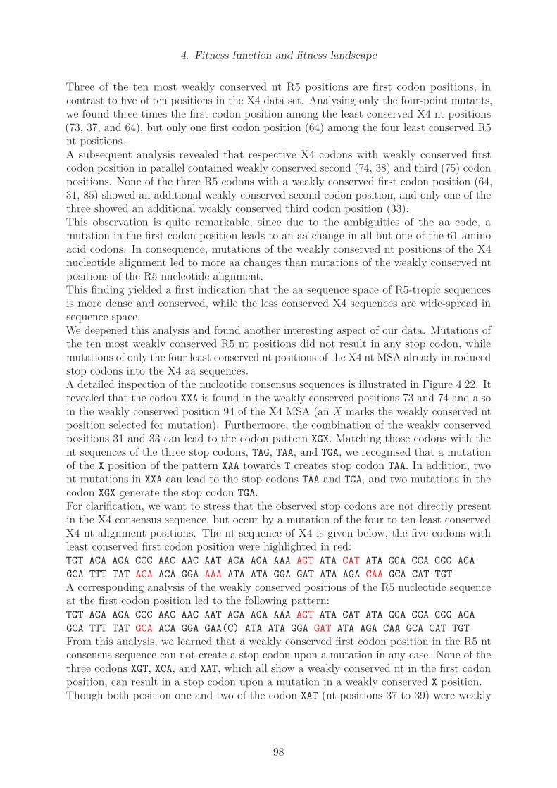
4. Fitness function and fitness landscape
Three of the ten most weakly conserved nt R5 positions are first codon positions, incontrast to five of ten positions in the X4 data set. Analysing only the four-point mutants,we found three times the first codon position among the least conserved X4 nt positions(73, 37, and 64), but only one first codon position (64) among the four least conserved R5nt positions.A subsequent analysis revealed that respective X4 codons with weakly conserved firstcodon position in parallel contained weakly conserved second (74, 38) and third (75) codonpositions. None of the three R5 codons with a weakly conserved first codon position (64,31, 85) showed an additional weakly conserved second codon position, and only one of thethree showed an additional weakly conserved third codon position (33).This observation is quite remarkable, since due to the ambiguities of the aa code, amutation in the first codon position leads to an aa change in all but one of the 61 aminoacid codons. In consequence, mutations of the weakly conserved nt positions of the X4nucleotide alignment led to more aa changes than mutations of the weakly conserved ntpositions of the R5 nucleotide alignment.This finding yielded a first indication that the aa sequence space of R5-tropic sequencesis more dense and conserved, while the less conserved X4 sequences are wide-spread insequence space.We deepened this analysis and found another interesting aspect of our data. Mutations ofthe ten most weakly conserved R5 nt positions did not result in any stop codon, whilemutations of only the four least conserved nt positions of the X4 nt MSA already introducedstop codons into the X4 aa sequences.A detailed inspection of the nucleotide consensus sequences is illustrated in Figure 4.22. Itrevealed that the codon XXA is found in the weakly conserved positions 73 and 74 and alsoin the weakly conserved position 94 of the X4 MSA (an X marks the weakly conserved ntposition selected for mutation). Furthermore, the combination of the weakly conservedpositions 31 and 33 can lead to the codon pattern XGX. Matching those codons with thent sequences of the three stop codons, TAG, TAA, and TGA, we recognised that a mutationof the X position of the pattern XAA towards T creates stop codon TAA. In addition, twont mutations in XXA can lead to the stop codons TAA and TGA, and two mutations in thecodon XGX generate the stop codon TGA.For clarification, we want to stress that the observed stop codons are not directly presentin the X4 consensus sequence, but occur by a mutation of the four to ten least conservedX4 nt alignment positions. The nt sequence of X4 is given below, the five codons withleast conserved first codon position were highlighted in red:TGT ACA AGA CCC AAC AAC AAT ACA AGA AAA AGT ATA CAT ATA GGA CCA GGG AGA
GCA TTT TAT ACA ACA GGA AAA ATA ATA GGA GAT ATA AGA CAA GCA CAT TGT
A corresponding analysis of the weakly conserved positions of the R5 nucleotide sequenceat the first codon position led to the following pattern:TGT ACA AGA CCC AAC AAC AAT ACA AGA AAA AGT ATA CAT ATA GGA CCA GGG AGA
GCA TTT TAT GCA ACA GGA GAA(C) ATA ATA GGA GAT ATA AGA CAA GCA CAT TGT
From this analysis, we learned that a weakly conserved first codon position in the R5 ntconsensus sequence can not create a stop codon upon a mutation in any case. None of thethree codons XGT, XCA, and XAT, which all show a weakly conserved nt in the first codonposition, can result in a stop codon upon a mutation in a weakly conserved X position.Though both position one and two of the codon XAT (nt positions 37 to 39) were weakly
98

4. Fitness function and fitness landscape
conserved, the nt in the third position, T, restricted the mutation of the codon into a stopcodon, since a stop codon with T in the third position does not exists. No other codon ofthe R5 MSA comprised two weakly conserved nt positions.Thus, mutations of the least conserved sequence positions frequently create stop codons insequences derived from the X4 nt consensus sequence, but not in R5 derived sequences.
For a further validation of these results, we made a similar analysis, including all 105sequence positions instead of focussing on the weakly conserved ones. We previouslydescribed in Section 4.3.2 that the R5 and X4 nt consensus sequences differ only in codon22 (nt 64 to 66) and 25 (nt 73 to 75). Codon 22 of R5 is GCA, of X4 it is ACA. Since thereis no stop codon with either G or A in the first position and positions two and three areidentical, both codons yield the same probability to mutate into a stop codon. For codon25, we have GAA in case of R5 and AAA in case of X4. Again, only codon position onediffers, and there is no stop codon with either G or A in the first position. Following theseobservations, the distance to any stop codon is identical for both the R5 and X4 consensussequence (compare illustration (b) of Figure 4.22).In consequence, the complete consensus sequences of the R5 and X4 nt MSA did not givefurther indications whether the R5 or X4 sequence is more or less in danger to be mutatedinto a sequence with stop codon.Finally, we did an analogue analysis, but we started from the aa instead of the nt consensussequences. As described at the end of Section 4.3, a translation of the R5 nt consensussequence does not exactly match the R5 aa sequence. The codon 25, GAA, translatesinto glutamic acid (E), while we find aspartic acid (D) at position 25 in the aa consensussequence of R5, encoded by codon GAC. This differing sequence position is a result of themost weakly conserved nt position 75 (position three of codon 25). If we analyse the codonGAC instead of GAA, and compare the R5 codon GAC in position 25 to the correspondingcodon AAA of the X4 consensus sequence, at least two mutations for codon GAC in R5sequence are necessary to be translated into a stop codon (TAG or TAA), while the codonAAA in the X4 sequence needs only one mutation to be transformed into the stop codonTAA. The distance of both sequences to the third stop codon, TGA, is identical (compareillustration (c) of Figure 4.22).In summary, the mutation of GAC to TAG and TAA in R5 could occur with the probability2 · 1
4· 1
4= 1
8, while a mutation of the codon AAA into TAA in X4 occurs with twice the
probability (14).
Thus, the direct comparison of the complete nt consensus sequences showed no differences,but upon a back-translation of the aa consensus sequences into nt sequences, we foundthe genetic distance of the X4 consensus sequence to a stop codon to be closer than thedistance of the R5 consensus sequence.In summary, the analysis of the ten most weakly conserved nt sequence positions revealedthat the X4 codons are evolutionary closer to stop codons than the R5 sequences and arethus in higher danger to evolve into dead-end sequences. From the observed differencesin the intra-codon conservation, we expected to observe an accumulation of stop codonsin the X4 mutant population, resulting in many individuals with zero replicative fitness.Furthermore, we hypothesised that the X4 mutant sequences form a rugged and holeyfitness landscape. In contrast, we did not expect to see any individuals of zero fitness inthe R5 mutant population, provided that we mutate exclusively the ten least conserved
99
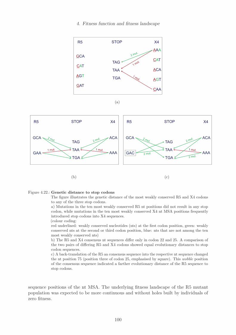
4. Fitness function and fitness landscape
GCA
AGT
GAT
AAA
CAT
ACA
AGT
CAA
TAG
TAA
TGA
R5 X4STOP
CAT
(a)
GCA
GAA AAA
ACATAG
TAA
TGA
R5 X4STOP
(b)
GCA
GAC AAA
ACATAG
TAA
TGA
R5 X4STOP
(c)
Figure 4.22.: Genetic distance to stop codonsThe figure illustrates the genetic distance of the most weakly conserved R5 and X4 codonsto any of the three stop codons.a) Mutations in the ten most weakly conserved R5 nt positions did not result in any stopcodon, while mutations in the ten most weakly conserved X4 nt MSA positions frequentlyintroduced stop codons into X4 sequences.(colour coding:red underlined: weakly conserved nucleotides (nts) at the first codon position, green: weaklyconserved nts at the second or third codon position, blue: nts that are not among the tenmost weakly conserved nts)b) The R5 and X4 consensus nt sequences differ only in codon 22 and 25. A comparison ofthe two pairs of differing R5 and X4 codons showed equal evolutionary distances to stopcodon sequences.c) A back-translation of the R5 aa consensus sequence into the respective nt sequence changedthe nt position 75 (position three of codon 25, emphasised by square). This wobble positionof the consensus sequence indicated a farther evolutionary distance of the R5 sequence tostop codons.
sequence positions of the nt MSA. The underlying fitness landscape of the R5 mutantpopulation was expected to be more continuous and without holes built by individuals ofzero fitness.
100

4. Fitness function and fitness landscape
An inspection of the fitness values of the R5 and X4 populations of four-, six-, eight-, andten-point mutants gave a first hint to confirm our idea. We translated each nt sequenceinto an aa sequence and determined the corresponding fitness based on Equation 4.12.The fitness values were in the range of [0.0, 1.0], with 0.0 representing sequences with stopcodons and 1.0 representing the most fit consensus sequence of each population.Figure 4.23 depicts histograms of the resulting fitness values of the R5 and X4 mutantpopulations. The figures show that aa changes decreased the fitness of the R5 mutantsto a larger extend than the fitness of the X4 mutants. This was already observed inthe sequence examples presented in Section 4.4.3. Due to the larger position specific aaprobabilities of the R5 MSA and the higher conservation of the R5 consensus sequence,the R5 sequences are more sensitive to aa changes than the less conserved X4 sequence. Achange in the highly conserved R5 consensus sequence decreases the fitness of the mutantto a larger extend.This effect can also be seen by a direct comparison of the Figure 4.23 to the previouspresented distribution of the aa Hamming distances (see Figure 4.20). Though the X4mutant populations tend to accumulate a higher number of aa mutations upon mutationof the weakly conserved nt positions, the distribution of the fitness values indicates a shiftof the X4 mutant fitness towards higher fitness values.The X4 sequences showed a broader range of fitness values. The fitness values of the X4four-point mutants for example extended to the complete interval [0.0, 1.0], while the R5four-point mutants did not drop below a fitness threshold of 0.28. The Figure 4.23 showedfurther the accumulation of stop codons upon mutations of the most weakly conserved X4nt positions, resulting in high counts of individuals with zero fitness. The populations ofeight- and ten-point mutants furthermore showed that mutations in the less conservedX4 consensus sequence in general lead to a decreased fitness reduction, except in the casethat a stop codon is generated.Using the Kolmogorow-Smirnov test [92, 143], we compared the distributions of the fitnessvalues of the R5 and X4 mutant populations. Our analyses showed that the distributionsof the fitness values are significantly different for the four-, six-, eight-, or ten-point mutantpopulations (see Figure 4.24).It has to be noted that the absolute fitness values can only be used for a ranking ofthe replicative capacity within the respective R5 or X4 population, i.e. the deviationsbetween the fitness values are only sound for an intra-population ranking. Since we lackedan in vitro method to compare the replicative fitness of the R5 and X4 sequences, aninter-population comparison of the fitness values is not possible with the presented method.The numerical deviations between the R5 fitness values eF itR5 and the X4 fitness valueseF itX4 need a further validation.
101

4. Fitness function and fitness landscape
0.025 0.28 0.48 0.68 0.88
4−point mutants
fitness
counts
020
40
60
80 R5
X4
0.025 0.28 0.48 0.68 0.88
6−point mutants
fitness
counts
0200
600
1000
R5X4
0.025 0.28 0.48 0.68 0.88
8−point mutants
fitness
counts
010000
20000
30000
R5X4
0.025 0.28 0.48 0.68 0.88
10−point mutants
fitness
counts
0e+
00
3e+
05
6e+
05
R5X4
Figure 4.23.: Histograms of population fitnessThe figures compare the replicative fitness of the R5 population (in black) and the X4population (in grey) of the four-, six-, eight-, and ten-point mutants. Mutations in theconserved R5 consensus sequence decreased the fitness of the individuals to a larger extendthan mutations in the less conserved X4 consensus sequence.
102
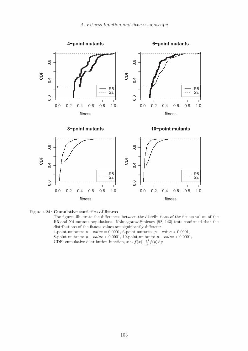
4. Fitness function and fitness landscape
0.0 0.2 0.4 0.6 0.8 1.0
0.0
0.4
0.8
4−point mutants
fitness
CD
F
●●●●●●●●●●●●●●●●●●●●●●●●●●●●●●●●●●●●●●●●●●●●●●●●
●●●●●●●●●●●●●●●●●●●●●●●
●●●●●●●●●●●●●●●●●●●●●●●●●●●●●●●●
●●● ● ●
● ●●●●●●●●●●●●●●●●●●●●●●●●●●●●●●●●●●●●●●●●●●●●●●●●●●●●●●●●●●●●●●●●●●●●●●●●●●●●●●●●●●
●●●●●●●●●●●●●●●●●●●●●●●●●●●●●●●●●●●●●●●●●●●●●●●●●●●●●●●●●●●●●●●●●●●●●●●●●●●●●●●●●●●●●
●●●●●●●● ●●●
R5X4
0.0 0.2 0.4 0.6 0.8 1.0
0.0
0.4
0.8
6−point mutants
fitness
CD
F
●●●●●●●●●●●●●●●●●●●●●●●●●●●●●●●●●●●●●●●●●●●●●●●●●●●●●●●●●●●●●●●●●●●●●●●●●●●●●●●●●●●●●●●●●●●●●●●●●●●●●●●●●●●●●●●●●●●●●●●●●●●●●●●●●●●●●●●●●●●●●●●●●●●●●●●●●●●●●●●●●●●●●●●●●●●●●●●●●●●●●●●●●●●●●●●●●●●●●●●●●●●●●●●●●●●●●●●●●●●●●●●●●●●●●●●●●●●●●●●●●●●●●●●●●●●●●●●●●●●
●●●●●●●●●●●●●●●●●●●●●●●●●●●●●●
●●●●●●●●●●●●●●●●●●●●●●●●●● ●● ● ● ●
R5X4
0.0 0.2 0.4 0.6 0.8 1.0
0.0
0.4
0.8
8−point mutants
fitness
CD
F
R5X4
0.0 0.2 0.4 0.6 0.8 1.0
0.0
0.4
0.8
10−point mutants
fitness
CD
F
R5X4
Figure 4.24.: Cumulative statistics of fitnessThe figures illustrate the differences between the distributions of the fitness values of theR5 and X4 mutant populations. Kolmogorow-Smirnov [92, 143] tests confirmed that thedistributions of the fitness values are significantly different:4-point mutants: p − value = 0.0001, 6-point mutants: p − value < 0.0001,8-point mutants: p − value < 0.0001, 10-point mutants: p − value < 0.0001,CDF: cumulative distribution function, x ∼ f(x),
∫x
0f(y) dy
103

4. Fitness function and fitness landscape
Definition of a graph representation of the fitness landscapes
Analysing the aa Hamming distances and the distribution of the fitness values of thepopulations of four-, six-, eight-, and ten-point mutants, we found some first evidence forstructural differences between the R5 and the X4 fitness landscape. We next examinedthe underlying local R5 and X4 fitness landscapes. Therefore, we used the Python graphanalysis package networkx [120, 69] to translate the populations of four-, six-, eight-, andten-point mutants into a graph representation of the R5 and X4 fitness landscape. Thefitness values of the four-, six-, eight-, and ten-point mutants were determined based onequation 4.12.The mutant networks were created based on the following rules:
• define a maximal nt Hamming distance threshold maxHamming
• define a maximal fitness deviation maxfitDev
• create a vertex vi for each sequence i
• add an edge between two vertices vi and vj if
• H(vi, vj) ≤ maxHamming and• |vi − vj| ≤ maxfitDev and• eF itvi
Ó= 0.0 or eF itvjÓ= 0.0
Thus, two mutant sequences i and j were connected by an edge, if both the Hammingdistance of the two nt sequences and the fitness deviation of the corresponding aa transla-tions did not exceed a given threshold maxfitDev. The approach restricted to create anedge between two sequences i and j with zero replicative fitness, since mutants with zeroreplicative fitness by definition can not produce offspring and thus can not be mutatedone into the other. In contrast, a link between a sequence eF iti Ó= 0.0 and a sequenceeF itj = 0.0 is allowed, since a replicative-competent sequence can be mutated into asequence of zero fitness.The size of the resulting networks can be calculated based on the number of sequencesrespective vertices of the network, n = 4m (again m being the number of mutated sequence
positions). The maximal number of edges e of each network is n(n−1)2
. The term n − 1addresses the fact that we do not allow self loops and the denominator of 2 is a consequenceof the graphs being undirected. Table 4.1 presents the number of vertices and the maximalnumber of edges of the graph representations of the four-, six-, eight-, and ten-point mutantpopulations.
Table 4.1.: Graph sizeThe table gives a overview over the number of nodes and the maximal number of edges of thenetworks of four-, six-, eight-, and ten-point mutants.
m n = 4m en(n−1)
2
4 256 3.3 · 104
6 4,096 8.4 · 106
8 65,536 2.1 · 109
10 1,048,576 5.5 · 1011
104

4. Fitness function and fitness landscape
Fitness landscape of four-point mutants In the following paragraphs, we analysed thelocal networks of the R5 and X4 mutants with fitness values based on Equation 4.12. Themutated nt positions resembled the four, six, eight, or ten weakest conserved nt sequencepositions of the respective data set. We started with a comparison of the R5 and the X4network of all four-point mutants, using the network definition in Section 4.4.7.Figure 4.25 illustrates the number of edges that were realised in the R5 and X4 networkof four-point mutants. The distinct lines in the illustration represent four nt Hammingdistance thresholds. The selected fitness deviation threshold, describing the fitness devi-ation between connected nodes, is represented on the x-axis. We used the following 28fitness deviation thresholds: 10−5, 10−4, 10−3, 10−2, 2.5 ·10−2, seven subsequent equidistantintervals of 2.5·10−2 up to a maximal fitness deviation of 0.2, and 16 subsequent equidistantintervals of 0.05 up to a fitness deviation of 1.0. Thus, the illustration presented in Figure4.25 summarises the results of 4 · 28 = 112 different R5 respective X4 networks. The imagepresents the number of the realised edges. The maximal possible number of edges (32,640,compare Table 4.3) was realised only in the R5 network with a nt Hamming distancethreshold of four and the maximal fitness deviation of 1.0. A Hamming distance of fourand a maximal fitness deviation of 0.3 realised the majority of all possible edges in the R5network (29,876). Using the same same definition, the X4 network contained about half ofall possible edges (16,033). Even using the maximal fitness deviation threshold of 1.0 at amaximal Hamming distance of four, the X4 network only contained 30,624 of 32,640 edges.A detailed analysis showed that this is a consequence of the sequences with zero fitness,which were by definition not allowed to interconnect to each other.
0
5000
10000
15000
20000
25000
30000
35000
0 0.2 0.4 0.6 0.8 1
no.
of
edges
fitness deviation
R5 X4
hamming 1 hamming 2 hamming 3 hamming 4
Figure 4.25.: Number of edges in the R5 and X4 network of four-point-mutantsThe graphic depicts the number of realised edges in the R5 and the X4 network of thefour-point-mutants. The distinct lines represent four nt Hamming distance thresholds. Theselected fitness deviation threshold, describing the fitness deviation between connected nodes,is represented on the x-axis.Identical nt Hamming distance and fitness deviation thresholds enabled more connectingedges in the R5 network than in the corresponding X4 network.
105

4. Fitness function and fitness landscape
Thus, the same number of nt changes created a population of X4 mutants that weremore isolated, while the R5 sequences created densely connected regions of homogeneousfitness. The last edges, that were only created upon the definition of the maximal fitnessdeviation, connected the most fit R5 consensus sequence to the least fit mutants of thepopulation.We next determined the maximal node degree of the networks. Since self-loops were re-stricted, the maximal possible node degree was 255. In the R5 network, a fitness deviationof 0.20 and an nt Hamming distance of four almost resulted in the maximal node degree(245). We observed a comparable maximal node degree of 244 in the X4 network at afitness threshold of 0.4. The corresponding fitness deviation of 0.2 restricted the numberof edges in the X4 network to two thirds of all possible edges (180). The exact maximaldegree was reached almost in parallel for a fitness deviation of 0.4 for R5 and 0.5 for X4.Using a fitness deviation >0.4 and a consistent nt Hamming distance for both the R5 andX4 network, the R5 and X4 networks had an almost identical maximal degree.Though mutations of the less conserved X4 consensus sequence in general lead to smallerfitness deviations than mutations of the R5 consensus sequence, the X4 population showeda broader range of fitness values. The X4 fitness values spread along the complete interval[0.0, 1.0], while the fitness of the R5 four-point mutants did not drop below a fitnessthreshold of 0.28 (though the fitness Equation 4.12 enabled R5 fitness values along thecomplete interval [0.0, 1.0] as presented in Figure 4.23).
0
50
100
150
200
250
300
0 0.2 0.4 0.6 0.8 1
degre
e
fitness deviation
R5 X4
hamming 1 hamming 2 hamming 3 hamming 4
Figure 4.26.: Maximal node degree in R5 and X4 network of four-point-mutantsThe graphic depicts the maximal node degree that was found in both the R5 and the X4network of the four-point mutants. The distinct lines represent four nt Hamming distancethresholds. The selected fitness deviation threshold, describing the fitness deviation betweenconnected nodes, is represented on the x-axis.At low fitness deviations, the maximal node degree of the R5 network was always higherthan the maximal node degree of the X4 network at the same Hamming distance. A fitnessdeviation >0.4 approximated an equal maximal node degree for the R5 and X4 networks.
106

4. Fitness function and fitness landscape
Further investigations showed that this difference between the R5 and the X4 fitnessvalues was a consequence of the sequences with zero replicative fitness in the X4 populationof four-point mutants. An exclusion of those sequences would limit the range of the X4fitness values to the interval [0.39, 1.0].An analysis of the number of network components fit into the line of observations (compareFigure 4.27). The maximal number of network components is the number of nodes inthe network, which was 256 for the four-point mutants. Independent of the selected ntHamming distance threshold, the R5 network merged fast into one component. At a fitnessdeviation of 0.1, one large and one small component were formed. Increasing the fitnessdeviation threshold to 0.25 joined the small component and the large network component.At the same time, the X4 network consisted of ≥ 65 separated components, and thecomponents were stable until a fitness deviation of 0.35. For fitness deviations >0.35, newedges were created and at an nt Hamming distance ≥ 3, the networks merged into onecomponent. At an nt Hamming distance of two, a fitness deviation of ≥ 0.6 was requiredto merge the components. Finally, at an nt Hamming distance of one, the maximal fitnessdeviation of 1.0 (i.e. no fitness restriction) was obligatory to merge the components intoone large network.We already discussed this peculiarity of the X4 network to be a result of the mutantsequences with zero replicative fitness. In the case of the R5 population, the mergingnetwork structures again indicated a homogeneous distribution of the R5 fitness values.
0
50
100
150
200
250
0 0.2 0.4 0.6 0.8 1
no.
of
com
ponents
fitness deviation
R5 X4
hamming 1 hamming 2 hamming 3 hamming 4
Figure 4.27.: Number of components in R5 and X4 network of four-point-mutantsThe graphic depicts the number of network components created from the R5 and X4population of four-point-mutants. Independent of the nt Hamming distance threshold, theR5 networks converged into one large component at low fitness deviations, while the X4networks stably formed ≥ 65 independent components. For a fitness deviation >0.35, theX4 components started to merge into one component.
The number of network components is highly correlated with the number of isolatednodes of the respective network. A corresponding analysis showed almost identical results(data not shown).
107

4. Fitness function and fitness landscape
In Figure 4.28, we analysed the degree of the vertex representing the consensus sequence.For an nt Hamming distance of one and for a fitness deviation ≥ 0.75, the R5 consensussequence connected to all sequences of the population (represented by a node degreeof 255). This fitness threshold is consistent for the nt Hamming distances of two andthree. The steep increase of the node degree for fitness deviations of 0.4 to 0.75 showedthat mutations in the highly conserved R5 consensus sequence remarkably decreased thereplicative fitness of the mutant sequences.In comparison to the previous analysis of the number of network components (compareFigure 4.27), this observation confirmed that the most fit consensus sequence was onlyconnected to a few sequences of similar fitness and was clearly marked off from the majorityof the mutated individuals. Thus, the consensus sequence builds a peak in the fitnesslandscape, while the mutated sequences build a plateau or cloud of sequences of lowerfitness. This plateau of sequences of lower fitness is also indicated by Figure 4.26, whichshowed that a high node degree of 245 in the R5 network was reached at a low fitnessdeviation of 0.20. Thus, many sequences reside in a region of comparable fitness, separatedby fitness deviations ≤ 0.20.In the X4 network, the drop of the node degree of the consensus sequence was lesspronounced, presumably due to the weaker sequence conservation in general. In addition,the X4 sequences of high fitness are more interconnected than the R5 sequences of highfitness and thus have a higher node degree. A close inspection of the X4 MSA showed thatthis was a consequence of the observed wobble positions of the MSA, populated by almostidentical counts of two (positions 11 and 22) or four (position 25) different aa (compare aacounts presented in Section 4.4.2).In contrast to the higher node degree of the X4 consensus sequence, resulting from amultitude of edges to the neighbouring X4 mutants of high fitness, a biologically unsuitablefitness deviation threshold of 1.0 was required to achieve a maximal node degree of theconsensus sequence. The fitness threshold of 1.0 represents a connection of the X4 fitnesspeak to all sequences of the population, including the holes of zero fitness. A comparisonof the average node degree of the R5 and X4 network with the degree of the consensussequences showed a lower degree than the average node degree for the consensus sequences.This difference in the degree was especially pronounced for fitness deviations ≤ 0.75 forthe R5 network and ≤ 0.6 for the X4 network (data not shown). This result confirmed theobservation that the fitness peaks are weakly connected to the majority of the sequencesof the mutant population.
108
4. Fitness function and fitness landscape
0
50
100
150
200
250
0 0.2 0.4 0.6 0.8 1
degre
e o
f consensus
fitness deviation
R5 X4
hamming 1 hamming 2 hamming 3 hamming 4
Figure 4.28.: Degree of the consensus sequence in R5 and X4 network of four-point mutantsFor fitness deviations of ≤ 0.4, the R5 consensus sequence showed a low node degree andwas connected to only a few high fit sequences. A fitness threshold of 0.75 connected the R5consensus sequence to all mutated individuals.In the case of the X4 consensus sequence, the degree of the consensus sequence was higherat smaller fitness thresholds, but the X4 consensus sequence could only reach the maximaldegree at a fitness deviation of 1.0.
In the final analysis of the networks of all four-point mutants, we determined the nodedegree of the sequences of minimal fitness. In general, we found a higher degree for theleast fit R5 sequences and than for the least X4 sequences (compare Figure 4.29. Atthe maximal nt Hamming distance of four and a fitness deviation of 0.4, the least fit R5sequences were connected to 245 of 256 sequences of the network. In contrast, the 64 X4mutants with zero fitness were still isolated at this level of fitness deviation. A transitionthat was comparable to the increase in the node degree observed for the R5 network at afitness deviation of 0.4 could be observed at a fitness deviation threshold of ≥ 0.75 for theX4 network. Using this threshold, the node degree increased to 174. Since our networkdefinition restricted sequence mutants of zero fitness to interconnect, the degree of thenodes of minimal fitness in the X4 networks was lower.The comparison of the R5 and the X4 fitness landscape of four-point mutants revealedthat the R5 fitness landscape contains a few sequences of high fitness, that result in asteep fitness decay upon the introduction of mutations, levelling off into a non-zero fitnessplateau built by a set of least fit (but Ó= 0.0) sequences. In contrast, the X4 consensussequence fitness peak is surrounded by a number of mutated variants with small fitnessdeviations and the fitness decrease close to the peak is less steep. On the other hand, theX4 fitness landscape contains fitness holes built by 64 sequences of zero fitness.
109

4. Fitness function and fitness landscape
0
50
100
150
200
250
300
0 0.2 0.4 0.6 0.8 1
degre
e
fitness deviation
R5 X4
hamming 1 hamming 2 hamming 3 hamming 4
Figure 4.29.: Degree of least fit sequences in R5 and X4 network of four-point mutantsAt an nt Hamming distance of four and a fitness deviation of 0.4, the R5 sequences ofminimal fitness achieved a node degree of 245. The least fit X4 mutants were still isolatedat this level of fitness deviation and were connected to the central X4 network at a fitnessthreshold ≥ 0.75.
Fitness landscape of six-point mutants After a detailed analysis of the fitness land-scapes built by the four-point mutants, we examined the fitness landscapes described bythe populations of six-point mutants. Corresponding analyses of the R5 and X4 mutantsconfirmed the previous observations of the fitness landscapes of the four-point mutantsand did not reveal additional findings. Thus, we only discuss two exemplary analyses.According to Table 4.3, the networks contained 4,096 vertices and at most 8,386,560 edges.Figure 4.30 illustrates the number of edges that were realised in the networks, dependingon the selected nt Hamming distance and the fitness deviation threshold. The maximalnumber of edges was created only in the R5 network (of an nt Hamming distance ofsix), with the majority of all possible edges (7,455,424) already being realised at a fitnessdeviation ≥ 0.3. Our findings confirmed the observation of a majority of homogeneousfitness values on the one hand, and the distinct separation of a few highly fit R5 sequenceson the other hand, which were completely connected to all sequences only at fitnessdeviations ≥ 0.9.In contrast to the R5 network, the X4 network contained approximately two thirds ofall possible edges (5,384,534) at a fitness deviation level of 0.3 and at an nt Hammingdistance of six. Furthermore, 523,776 edges (∼ 6% of the possible edges) were not realisedin any X4 network, which was again a result of the restriction to connect two vertices thatboth carry sequences of zero replicative fitness.
110

4. Fitness function and fitness landscape
0
2e+06
4e+06
6e+06
8e+06
1e+07
0 0.2 0.4 0.6 0.8 1
no.
of
edges
fitness deviation
R5 X4
hamming 1 hamming 2 hamming 3 hamming 4
hamming 5 hamming 6
Figure 4.30.: Number of edges in R5 and X4 network of six-point-mutantsThe graphic depicts the number of realised edges in the R5 and the X4 networks of six-point-mutants, depending on the selected nt Hamming distance (different lines) and the fitnessdeviation threshold (x-axis).Most of the edges of the R5 network are already created at a fitness deviation ≥ 0.3; themaximum number of edges was realised at a fitness deviation ≥ 0.9 at an nt Hammingdistance of six. In contrast, the X4 network realised at most two-thirds of all possible edges.
Figure 4.31 illustrates the maximal node degree that was observed in the networks ofsix-point mutant. In the case of the R5 network, a fitness deviation of 0.15 resulted in amaximal node degree of 3,679 (∼ 90% of all possible edges), while a comparable transitionin the X4 network was observed at a fitness threshold of 0.25 (3,670). A fitness deviationof 0.15 restricted the number of edges of the X4 network to 2,517 (∼ 61.5%). The maximalnode degree of 4,095 was reached almost in parallel for a fitness deviation of 0.45 in theR5 network and a fitness deviation of 0.55 in the X4 network.
111
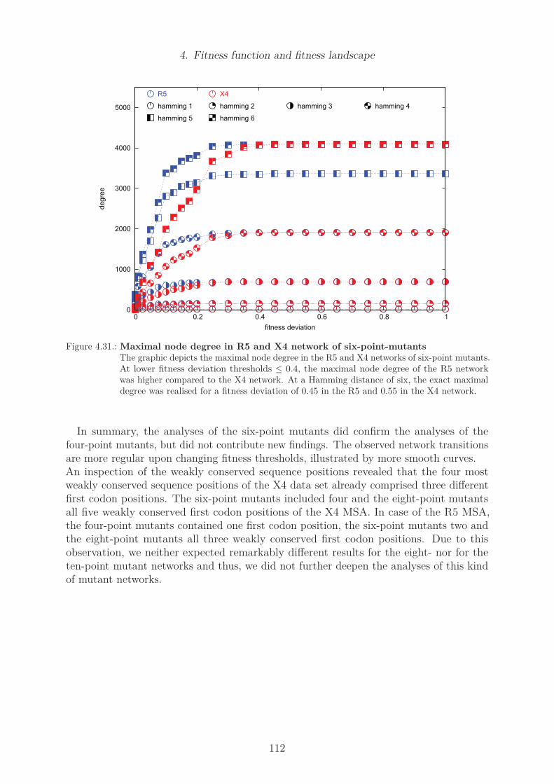
4. Fitness function and fitness landscape
0
1000
2000
3000
4000
5000
0 0.2 0.4 0.6 0.8 1
degre
e
fitness deviation
R5 X4
hamming 1 hamming 2 hamming 3 hamming 4
hamming 5 hamming 6
Figure 4.31.: Maximal node degree in R5 and X4 network of six-point-mutantsThe graphic depicts the maximal node degree in the R5 and X4 networks of six-point mutants.At lower fitness deviation thresholds ≤ 0.4, the maximal node degree of the R5 networkwas higher compared to the X4 network. At a Hamming distance of six, the exact maximaldegree was realised for a fitness deviation of 0.45 in the R5 and 0.55 in the X4 network.
In summary, the analyses of the six-point mutants did confirm the analyses of thefour-point mutants, but did not contribute new findings. The observed network transitionsare more regular upon changing fitness thresholds, illustrated by more smooth curves.An inspection of the weakly conserved sequence positions revealed that the four mostweakly conserved sequence positions of the X4 data set already comprised three differentfirst codon positions. The six-point mutants included four and the eight-point mutantsall five weakly conserved first codon positions of the X4 MSA. In case of the R5 MSA,the four-point mutants contained one first codon position, the six-point mutants two andthe eight-point mutants all three weakly conserved first codon positions. Due to thisobservation, we neither expected remarkably different results for the eight- nor for theten-point mutant networks and thus, we did not further deepen the analyses of this kindof mutant networks.
112

4. Fitness function and fitness landscape
Definition of evolutionary networks
In the first network approach, we observed the influence of the nt Hamming distanceand of a range of fitness deviation thresholds on the structure of the R5 and X4 mutantnetworks. In this section, we used an alternative definition for the construction of thenetworks of four-, six-, eight-, and ten-point mutants. We intended to analyse beneficialpaths of evolution, and thus we applied directed networks. The networks were constructedas follows: for every individual of the population, we created one vertex, containinginformation about the nt sequence and the replicative fitness of the individual (based onEquation 4.12). Two vertices were connected by a directed edge, if the Hamming distanceof the nt sequences was one (since the mutant sequences in each population were unique,no two sequences had a Hamming distance of zero). Furthermore, the edges were definedto start at the node with the lower fitness and point towards the node with the higherfitness. If both nodes had the same fitness, two parallel edges pointing into oppositedirections were created to connect the nodes.In summary, the evolutionary networks were defined in the following way:
• create a vertex vi for each sequence i
• add a directed edge pointing from vertex vi to vertex vj if
• H(vi, vj) == 1 and• eF itvi
≤ eF itvjand
• eF itviÓ= 0.0
This approach again restricted the construction of links between two vertices representingsequences with zero replicative fitness. Links pointing from a sequence of non-zero fitnessto a sequence of zero fitness are allowed, since sequences with replicative fitness Ó= 0.0could replicate and generate offspring with zero fitness, but not vice versa.Using this definition, we created finite directed cyclic graphs of the R5 and the X4 mutantpopulation. Cycles can only contain nodes that represent sequences with identical replica-tive fitness (i.e. different nt sequences that were translated into the same aa sequence).Self-loops did not contribute additional information to this analysis, thus, they wererestricted to keep the graphs more simple. In contrast to the previous approach, thisdefinition created only one network for each R5 and X4 mutant population.The resulting graphs enabled us to follow paths of beneficial or neutral evolution, repre-sented by an increasing or steady fitness along any path through the network. Analyses ofthe network structure enabled us to determine difference between the underlying fitnesslandscapes of the R5 and X4 mutant population and to find deviations in the length ofthe evolutionary pathways. Table 4.2 summarises the analyses of the R5 and X4 networksfor the four-, six-, eight-, and ten-point mutant populations.
Evolutionary networks of four-point mutants We started with an analysis of the evo-lutionary networks of the R5 and X4 four-point mutants. The directed networks wereboth very sparse. In the case of R5, 1,664 edges were realised, representing 2.549% of allpossible edges. The average node degree was 13, which was also the degree of each of the256 nodes. Both the average in- and out-degree of the R5 network were 6.5.The R5 network comprised two nodes of the maximal fitness of 1.0, representing the
113

4. Fitness function and fitness landscape
consensus master sequence and an alternative nt mutant that consistently was translatedinto the aa consensus sequence. The in-degree of both R5 nodes of maximal fitness wasone, representing the possible mutational pathway from one node to the other, exchangingonly one nucleotide. The out degree was 12 for both nodes, resembling the four mutatednt positions and the three alternative nucleotides at each position.As we expected, the R5 population did not contain any sequence of zero fitness. Theleast fitness value was 0.285 and represented four different nt sequences that all translatedinto the same aa sequence. The evolutionary network of the X4 mutants contained 1,248edges, which represents a fraction of 1.911% of the theoretic maximum. The average nodedegree was 9.75, with an average in-degree of 4.875 and an average out-degree of 4.875. Amaximal degree of 12 could be observed for 192 nodes, and the remaining 64 nodes hadan (in-)degree of only three. The X4 network comprised only one node of the maximalfitness of 1.0, which in consequence had an in-degree of zero and an out-degree of 12. Nosilent nt mutation was possible for the X4 consensus master sequence.We found 64 sequences of zero fitness among the X4 mutants, all containing at least onestop codon in the translated aa sequence. Only three directed paths led into each of thesenodes and stopped there. The three pathways represented the three alternative nt at therespective sequence position.This first analysis showed that the R5 network contained more edges than the X4 network,an observation that was already made for the previously described networks. An inspectionof the underlying populations revealed that the differences between the R5 and the X4network resulted from the 64 sequences of zero replicative fitness in the X4 population.We next analysed the shortest paths in the networks. In the R5 network, the averagelength of all 35,928 reachable shortest paths (of length 1.0 to 6.0) was 2.676. In contrast,the number and average shortest path length in the X4 network was slightly decreased.We found 24,144 reachable shortest paths of length 1.0 to 5.0, with an average length of2.583. Though the R5 network in general had a higher node degree than the X4 network,the shortest paths in the R5 network were longer. Analyses of single shortest paths ofthe R5 network showed that difficult mutational pathways were evolutionary reachablevia detour and thus increased the shortest path length. In contrast, difficult evolutionarypaths in the X4 network showed a tendency to become disconnected at some vertex. Thus,the shortest paths lengths in the X4 network were shorter (since long shortest paths moreoften were not reachable).We next focussed the shortest paths analyses to those paths that connected a sequence ofminimal fitness to a sequence of maximal fitness (min-max path), following the shortestmutational pathway to evolve from the least to the most fit sequence (or vice versa). TheR5 network contained eight possible min-max paths, each of a length of 4.0, connectingany of the four nodes of minimal fitness to the two nodes of maximal fitness. In theX4 network, with one sequence of maximal fitness and 64 sequences of minimal fitness,we found 52 possible shortest paths of length 1.0 to 4.0. The network restriction to ntHamming distances of one blocked 12 of the possible min-max pathways. The averageshortest path length of 4.0 for the min-max paths was higher in the R5 network, than theaverage shortest path length of 3.135 for the 52 min-max paths in the X4 network.Though the general shortest path length of the R5 and X4 network only varied by 3.6%(R5: 2.676 vs. X4: 2.583), the length of the shortest min-max paths connecting sequencesof minimal to sequences of maximal fitness varied by ∼ 27.6% (R5: 4.0 vs. X4: 3.135)
114
4. Fitness function and fitness landscape
between the R5 and X4 population.This observation indicated a faster evolution of sequences of minimal fitness into sequencesof maximal fitness in the X4 population, and gave further evidence to our hypothesis thatthe X4 population is evolutionary closer to sequences with minimal fitness than the R5population.This idea gained further support by an analysis of the maximal and minimal node be-tweenness, a value that represents the rate of all shortest paths that pass through a node.The measure describes the importance of the central nodes of a network as well as thenetwork extension (i.e. for a network of sequences the extension in sequence space).The maximal betweenness was 2.5 · 10−3 for the R5 network and 2.1 · 10−3 for the X4network. These numbers indicated a slightly reduced importance of the central nodes ofthe X4 network as well as a larger expansion in sequence space. This observation wasconfirmed by the minimal betweenness of 2.9 · 10−4 for the R5 and 0.0 for the X4 network.Thus, the R5 network was more central and dense and contained more evolutionary pathsthat traversed through the central nodes, while the X4 network was further extended insequence space.An analysis of the network closeness, which is an alternative measure of node centrality,further stressed this point. The maximal closeness of 0.332 in the R5 network was higherthan the maximal closeness of 0.315 in the X4 network, and also the minimal closeness ofthe R5 network was higher than the minimal closeness of the X4 network 4.0 · 10−3 vs.0.0). In summary we found that the R5 network of all four-point mutants was more denseand concentrated in a smaller region in sequence space. The betweenness and closenessof the R5 network was higher, indicating more important central nodes. Evolutionarypathways between the R5 mutants in general were short (avg. length of 2.676), but pathsthat connected sequences of maximal fitness to sequences of minimal fitness were as longas 4.0.In contrast, the network of the X4 mutant population was more sparse and extendedin a larger region of sequence space. The X4 network enabled less evolutionary pathsconnecting the sequences of the population, and the possible pathways in general wereslightly shorter (average length of 2.583), presumably due an interruption or blocking oflonger evolutionary paths. Pathways from sequences of minimal to sequences of maximalfitness traversed on average 3.135 edges. A comparison of the average shortest path lengthand the shortest min-max path length indicated a reduced shortest min-max path lengthin the X4 network. Thus, a direct comparison of the fitness landscapes of the R5 andX4 four-point mutants supported our hypothesis that the pathways between sequencesof maximal fitness and sequences of minimal fitness are evolutionary shorter in the X4network than in the R5 network.
115

4. Fitness function and fitness landscape
Table 4.2.: Network measures of R5 and X4 mutant networkThe table gives a summary of the network analyses. The number of the sequences of minimaland maximal fitness is given in parenthesis (obs.).
network measure R5 (obs.) X4 (obs.)
4-p. mut. no. of edges 1,664 1,248
6-p. mut. no. of edges 46,112 29,184
8-p. mut. no. of edges 934,264 495,360
4-p. mut. avg. degree 13.00 9.75
6-p. mut. avg. degree 22.52 14.25
8-p. mut. avg. degree 28.51 16.54
4-p. mut. min. fit 2.8 · 10−1 (4) 0.00 (64)
6-p. mut. min. fit 1.3 · 10−1 (48) 0.00 (1,024)
8-p. mut. min. fit 2.56 · 10−2 (32) 0.00 (30,976)
4-p. mut. avg. shortest path 2.68 2.58
6-p. mut. avg. shortest path 4.03 3.74
8-p. mut. avg. shortest path 5.26 5.12
4-p. mut. avg. shortest min - max path 4.00 3.14
6-p. mut. avg. shortest min - max path 5.75 4.64
8-p. mut. avg. shortest min - max path 7.75 6.04
4-p. mut. not reachable min - max paths 0 12
6-p. mut. not reachable min - max paths 0 192
8-p. mut. not reachable min - max paths 0 9,504
4-p. mut. max. betweenness 2.49 · 10−3 2.10 · 10−3
6-p. mut. max. betweenness 1.83 · 10−4 9.43 · 10−5
8-p. mut. max. betweenness 1.93 · 10−5 9.36 · 10−6
4-p. mut. min. betweenness 2.92 · 10−3 0.00
6-p. mut. min. betweenness 5.93 · 10−5 0.00
8-p. mut. min. betweenness 2.29 · 10−6 0.00
4-p. mut. max. closeness 3.32 · 10−1 3.15 · 10−1
6-p. mut. max. closeness 2.22 · 10−1 2.10 · 10−1
8-p. mut. max. closeness 1.67 · 10−1 1.58 · 10−1
4-p. mut. min. closeness 3.92 · 10−3 0.00
6-p. mut. min. closeness 4.09 · 10−3 0.00
8-p. mut. min. closeness 1.23 · 10−4 0.00
Evolutionary networks of six-point mutants Analogue to the networks of four-pointmutants, we analysed the R5 and X4 network of all six-point mutants. A summary of thenetwork measures is given in Table 4.2.The networks consisted of 46 = 4, 096 nodes. While 46,112 edges were realised in theR5 network, the X4 network only contained 29,184 edges. The higher density of the R5network was reflected in a higher average node degree of 22.52, compared to 14.25 in theX4 network.The average shortest path length was 4.03 (path length 1.0 to 8.0) in the R5 network,and 3.74 in the X4 network (paths length 1.0 to 7.0). Thus, the shortest paths in the X4
116

4. Fitness function and fitness landscape
network are 7.75% shorter than in the R5 network, though the R5 network contains moreedges and a higher average node degree.An analysis of the sequences of minimal and maximal fitness showed that the R5 populationcontained eight individuals of maximal fitness (1.0), and 48 individuals of a minimal fitnessof 0.13. The X4 population contained only one sequence of maximal fitness (1.0), but1,024 individuals of a minimal replicative fitness of 0.0. Thus, the highly fit R5 sequencescan integrate a number of different neutral nt mutations without a fitness loss. While theX4 population still contains only one sequences of maximal fitness, it accumulated furthersequences of zero fitness, compared to the X4 population of four-point mutants.All 384 possible shortest pathways between the eight sequences of maximal fitness andthe 48 sequences of minimal fitness were reachable in the R5 network, while 192 of thepossible 1,024 shortest pathways between the sequence of maximal and a sequence ofminimal fitness in the X4 network could not be realised. The resulting shortest min-maxpath length varied between 6.0 and 7.0 in the R5 network and between 1.0 and 6.0 inthe X4 network. On average, the shortest mutational pathway between a sequence ofmaximal and a sequence of minimal fitness was 5.75 in the R5 and 4.64 in the X4 network.Though the general shortest paths length only varied by 7.75% between the R5 and X4network, the shortest min-max paths showed in a length difference of 23.92% and wereagain significantly shorter in the X4 network than in the R5 network.The comparison of the centrality measures indicated a more condensed R5 network with ahigher importance of the central nodes (maximal betweenness of 1.83 · 10−4 and maximalcloseness of 0.22), in contrast to a less central X4 network (maximal betweenness of 9.43 ·10−5 and maximal closeness of 0.21.Thus, the results of the R5 and X4 network of the six-point mutants again confirmed thatthe R5 network is more central, while the decreased centrality measures of the X4 networkindicate a less concentrated around its centre. Furthermore, the shortest paths analysesof all shortest paths in comparison to the min-max shortest paths further confirmed ourhypothesis of a closer proximity of sequences of maximal fitness to sequences of minimalfitness in the X4 sequence population.
Evolutionary networks of eight- and ten-point mutants Analyses of the evolutionarynetworks of the eight-point mutants revealed that the observed differences that we foundfor the networks of four- and six points mutants of the R5 and the X4 population werealso present in the population of all eight-point mutants. The R5 population containedeight sequences of maximal fitness and the X4 population two individuals. We observed aminimal fitness of 0.0256 for 32 R5 mutants, while the minimal fitness in the X4 populationwas again zero, representing 30,976 mutants with stop codons.Our analyses indicated a more dense R5 network, containing almost twice as many edgesas the X4 network (934,264 edges versus 495,360 edges). Despite this difference, thegeneral shortest path length of 5.26 edges in the R5 network and of 5.12 in the X4 networkwere comparable. In contrast, the length of the shortest evolutionary pathways between asequence of minimal fitness and a sequence of maximal fitness differed remarkably fromthese numbers. An average shortest min-max pathway traversed 7.75 edges in the R5network, but only 6.04 edges in the X4 network. Thus, the evolutionary distance of asequence of maximal fitness to sequence of minimal fitness was in general 28.31% closer inthe X4 network than in the R5 network. In addition, 9,504 (15,34%) of the 61,952 possible
117

4. Fitness function and fitness landscape
evolutionary pathways between a sequence of minimal and a sequence of maximal fitnessin the X4 network were not reachable, while each of the 256 corresponding pathways inthe R5 network were reachable.A final comparison of the network centrality measures of both networks showed that boththe maximal betweenness (R5: 1.93 · 10−5, X4: 9.36 · 10−6) and the maximal closeness (R5:0.17, X4: 0.16) of the R5 network were higher, which was also true for the correspondingminimal values.Thus, the R5 network of all eight-point mutants was more central and concentrated on aspecific region of the sequence space, and many paths traversed the central nodes of thenetwork. In contrast, the central nodes of the X4 network were less important for thenetwork structure. This finding again indicated a larger extension of the X4 network.The detailed results are given in the summary in Table 4.2.First analyses of the R5 and X4 population of the ten-point mutants showed a similartendency. The inclusion of the ninth and tenth weakly conserved nucleotide position didnot add a new first codon position to the mutated sequences, neither in the R5 nor theX4 data set, therefore we did not expect contradictory observations upon further analysisof the R5 and X4 network of ten-point mutants. On basis of the results for the previousnetwork approaches and the different mutant networks, we decided to discontinue theanalysis of the ten-point mutants and to omit the time-consuming analyses of shortestpaths and centrality measures.In summary, this part of the network analyses showed that the R5 networks concentratedin a condensed region of the sequence space. Central nodes of the network are an importantcomponent of many shortest evolutionary paths. The R5 networks contained no sequencesof zero fitness, and pathways between nodes of maximal fitness and nodes of minimal fitnesswere longer than the average shortest path length. In comparison, the centrality valuesof the X4 networks showed that the networks were less concentrated. The central nodeswere less important for the network structure, since they were less frequent integratedinto the shortest network paths. Though the shortest min-max paths were also longerthan the average shortest network pathways, the length difference was less pronounced. Acomparison of the shortest min-max pathways in the R5 and X4 networks showed that theevolutionary distance of the sequences of minimal fitness and the sequences of maximalfitness was shorter in the X4 than in the R5 network. We assume that the X4 sequencesyield an increased tendency to mutate towards low fit sequences that are no longer able toreplicate efficiently.
118

4. Fitness function and fitness landscape
Definition of neutral networks
In the two previous network approaches, we observed the structure of the R5 and X4mutant networks using all available mutant sequences and enabling edges under differentconditions (undirected edges at variable nt Hamming distances and different fitnessdeviation thresholds as well as evolutionary networks of directed edges from low to highfitness at a fixed nt Hamming distance of one). In the last part of the network analysis,we combined the fixed Hamming distance with a fitness constraint. Upon the networkconstruction, we limited the sequences to a fraction of the R5 and the X4 sequences thatsurpassed a defined fitness threshold eF itmin. From the remaining sequences, we createdan R5 respectively an X4 network based on two conditions. First, the nt Hamming distancebetween two sequences was one, and second, the representing vertices were connected viaa directed edge, starting at the node with lower fitness and pointing towards the nodewith higher fitness. If both sequences had the same replicative fitness, two directed edgeswith an opposite orientation were created.
• create a vertex vi if eF itvj≥ eF itmin
• add a directed edge pointing from vertex vi to vertex vj if
• H(vi, vj) == 1 and• eF itvi
≤ eF itvj
The fitness eF it was determined based on Equation 4.12.The idea behind the definition of a fitness restriction for the inclusion of the nodes re-spectively sequences into the networks was to reduce the networks to sequences of a highreplicative fitness, since we presume those sequences to be biologically relevant for thecourse of the infection and the evolution of the sequences. Sequences with low or even zeroreplicative fitness are supposed to build a less relevant minority. The resulting networksshould only contain sequences that are evolutionary neutral with respect to the replicativefitness of the underlying sequences.Based on these definitions, we repeatedly analysed the structural differences between theR5 and X4 mutant networks. Depending on the selected fitness threshold eF itmin, wefound a significant deviation in the size of the corresponding R5 and X4 networks, aspresented in Table 4.3. The reason for the different network sizes are the deviations in theunderlying fitness distributions discussed and presented in Figure 4.23.The observed differences in size were largest in the networks of eight-point mutants usingfitness constraints of 0.5 and 0.6. The definition of a fitness threshold led to networksthat varied up to a factor of ten in size, making it less sensible to compare the resultingnetworks and to interpret the results. Clearly, the numbers of edges were smaller and alsothe paths lengths were remarkably shorter in the small networks.
119
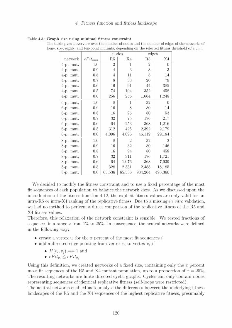
4. Fitness function and fitness landscape
Table 4.3.: Graph size using minimal fitness constraintThe table gives a overview over the number of nodes and the number of edges of the networks offour-, six-, eight-, and ten-point mutants, depending on the selected fitness threshold eF itmin.
nodes edgesnetwork eF itmin R5 X4 R5 X4
4-p. mut. 1.0 2 1 2 04-p. mut. 0.9 4 3 8 34-p. mut. 0.8 4 11 8 144-p. mut. 0.7 8 33 20 794-p. mut. 0.6 16 91 44 3854-p. mut. 0.5 74 104 352 4584-p. mut. 0.0 256 256 1,664 1,248
6-p. mut. 1.0 8 1 32 06-p. mut. 0.9 16 8 80 146-p. mut. 0.8 16 25 80 536-p. mut. 0.7 32 75 176 2176-p. mut. 0.6 64 253 368 1,2166-p. mut. 0.5 312 425 2,392 2,1796-p. mut. 0.0 4,096 4,096 46,112 29,184
8-p. mut. 1.0 8 2 32 28-p. mut. 0.9 16 32 80 1468-p. mut. 0.8 16 94 80 4588-p. mut. 0.7 32 311 176 1,7218-p. mut. 0.6 64 1,076 368 7,9398-p. mut. 0.5 328 2,331 2,488 18,1858-p. mut. 0.0 65,536 65,536 934,264 495,360
We decided to modify the fitness constraint and to use a fixed percentage of the mostfit sequences of each population to balance the network sizes. As we discussed upon theintroduction of the fitness function 4.12, the explicit fitness values are only valid for anintra-R5 or intra-X4 ranking of the replicative fitness. Due to a missing in vitro validation,we had no method to perform a direct comparison of the replicative fitness of the R5 andX4 fitness values.Therefore, this relaxation of the network constraint is sensible. We tested fractions ofsequences in a range x from 1% to 25%. In consequence, the neutral networks were definedin the following way:
• create a vertex vi for the x percent of the most fit sequences i
• add a directed edge pointing from vertex vi to vertex vj if
• H(vi, vj) == 1 and• eF itvi
≤ eF itvj
Using this definition, we created networks of a fixed size, containing only the x percentmost fit sequences of the R5 and X4 mutant population, up to a proportion of x = 25%.The resulting networks are finite directed cyclic graphs. Cycles can only contain nodesrepresenting sequences of identical replicative fitness (self-loops were restricted).The neutral networks enabled us to analyse the differences between the underlying fitnesslandscapes of the R5 and the X4 sequences of the highest replicative fitness, presumably
120

4. Fitness function and fitness landscape
representing the dominant sequences in an HIV infection.We excluded the population of the four-point mutants from this analysis, since it containedonly 256 sequences and resulted in very small networks. First analyses of these smallnetworks showed that it was less informing to analyse and compare the network measuresof these networks.The restriction to use the 1 - 25% most fit sequences created R5 and X4 networks of equalsize, but with differing least fitness values. These differences resulted from the deviationsbetween the R5 and X4 fitness distribution we already described in Figure 4.23. Therefore,the least fit sequences that were included into the X4 network showed a higher fitnessvalue than the least fit sequences that were included into the R5 network.Using the 1% most fit sequences of the R5 population of all 6-point mutants for examplecomprised the sequence with fitness eF itR5 = 0.69 as least fit node. In the correspondingX4 network, the node with minimal fitness had a fitness of eF itX4 = 0.75. Correspond-ingly, the 1% most fit sequences of the 8-point mutants resulted in least fitness values ofeF itR5 = 0.40 in the R5 network and of eF itX4 = 0.66 in the X4 network.As stated above, we had no in vitro method to calibrate this pure numerical fitness valuesin terms of replicative capacity. Therefore, the numerical fitness value are valid for aranking of the replicative capacity within the R5 or within the X4 population, but notacross the populations. The numerical deviation of two fitness values, e.g. eF itR5 = 0.40and eF itX4 = 0.66, could only be an artefact of our computational method and in vitroresult in the same replicative fitness.The minimal numerical fitness values of the six- and eight-point mutant sequences thatwere included into the R5 and X4 networks are compared in Figure 4.32, depending on theused proportion x of the most fit sequences. An overview over the fitness values and theadditional network measures presented in the following lines are given in the Appendix inTable A.5 for the six-point mutants and in Table A.6 for the eight-point mutants.
0
0.05
0.1
0.15
0.2
0.25
0.2 0.3 0.4 0.5 0.6 0.7 0.8
thre
shold
minimal fitness
minimal R5 fitnessminimal X4 fitness
(a)
0
0.05
0.1
0.15
0.2
0.25
0.1 0.2 0.3 0.4 0.5 0.6 0.7
thre
shold
minimal fitness
minimal R5 fitnessminimal X4 fitness
(b)
Figure 4.32.: Minimal node fitness of R5 and X4 networkThe illustrations compare the minimal node fitness included into the R5 (blue) and X4 (red)network, depending on the selected threshold x. Figure (a) shows the minimal fitness for thesix-point mutant networks, and Figure (b) for the eight-point mutant networks.
121

4. Fitness function and fitness landscape
The analyses of the network measures of the neutral R5 and X4 networks of varyingsize confirmed our previous findings. A comparison of the maximal node betweenness ofthe R5 and the X4 networks of the most fit six- and eight-point mutants revealed thatthe maximal node betweenness of the R5 networks was always higher than the maximalnode betweenness observed in the corresponding X4 networks (see Figure 4.33). Furthercomparisons of the average node betweenness as well as the minimal node betweennesswitnessed this finding. Comparable to the evolutionary networks analysed before, theminimal node betweenness in the X4 networks was zero, but in general differed from zerofor the R5 networks (data not shown).The higher node betweenness of the nodes of the R5 network confirmed that the R5networks are more centralised and that the central nodes are more often traversed bythe shortest paths than the central vertices of the X4 networks. This result consolidatesthe idea that the R5 population is more condensed and centralised in sequence space, incontrast to the X4 sequences that are farther extended in sequence space.
0
0.05
0.1
0.15
0.2
0.25
0 0.002 0.004 0.006 0.008 0.01 0.012 0.014
thre
shold
maximal betweenness
maximal R5 betweennessmaximal X4 betweenness
(a)
0
0.05
0.1
0.15
0.2
0.25
0 0.0002 0.0004 0.0006 0.0008 0.001 0.0012
thre
shold
maximal betweenness
maximal R5 betweennessmaximal X4 betweenness
(b)
Figure 4.33.: Maximal node betweenness of R5 and X4 networkThe illustrations compare the maximal node betweenness of the R5 (blue) and X4 (red)network, depending on the selected threshold x. Figure (a) shows the maximal betweennessof the six-point mutant networks, and Figure (b) of the eight-point mutant networks.
We found the same result upon the computation of the node closeness as an alternativecentrality measure. The maximal node closeness for any threshold x in the range of 1 -25% was higher for the R5 network than for the X4 network (compare Figure 4.34), andthis observation was confirmed by additional analyses of the average and the minimalnode closeness of the respective networks (data not shown). In agreement to the findingsfrom the previous network analyses (see Table 4.2), the minimal node closeness in any ofthe X4 networks was zero, while the minimal closeness in the respective R5 networks ingeneral differed from zero. The analyses of the node centrality measures coincided withthe findings for the previous R5 and X4 network definitions.
A subsequent analysis of the maximal and the average node degree showed that thenode degree in the R5 was higher (data not shown).
122

4. Fitness function and fitness landscape
0
0.05
0.1
0.15
0.2
0.25
0.2 0.25 0.3 0.35 0.4 0.45 0.5
thre
shold
maximal closeness
maximal R5 closenessmaximal X4 closeness
(a)
0
0.05
0.1
0.15
0.2
0.25
0.15 0.2 0.25 0.3 0.35
thre
shold
maximal closeness
maximal R5 closenessmaximal X4 closeness
(b)
Figure 4.34.: Maximal node closeness of R5 and X4 networkThe illustrations compare the maximal node closeness of the R5 (blue) and X4 (red) network,depending on the selected threshold x. Figure (a) shows the maximal closeness of thesix-point mutant networks, and Figure (b) of the eight-point mutant networks.
Further computations showed that the shortest paths in the X4 networks were in generallonger than in the corresponding R5 networks (compare Figure 4.35. This finding differedfrom the previous shortest path analysis 4.2, in which we found comparable averageshortest path lengths in the R5 and the X4 networks. The deviation in the path lengthsbetween the neutral networks and the evolutionary networks presumably resulted from theexclusion of the sequences of low fitness. In the previous evolutionary network definition,the low fit X4 sequences often led to an interruption of network paths in the more sparseand extended X4 network. Starting at a sequence of maximal fitness, a fraction of the leastfit sequences was not reachable in each X4 network (compare number of not reachablemin-max paths in Table 4.2). Using the present neutral network definition, the shortestpath length of the X4 network increased, since less fit mutants were excluded and thusless frequently led to an interruption of the paths.In summary, the analyses of the neutral networks of sequences of similar replicative
fitness agreed with the findings for the previous network types. Thus, our results areindependent of the details of the network definition. We conclude that the highly conservedR5-tropic viral sequences are evolutionary close and condensed in sequence space, whilethe more variable sequences of the X4-tropic viral populations extend farther to moredistant regions of the V3 loop sequence space.
123
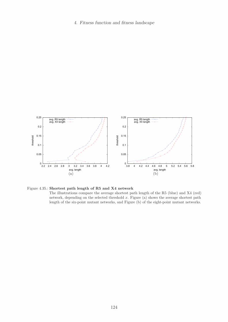
4. Fitness function and fitness landscape
0
0.05
0.1
0.15
0.2
0.25
2.2 2.4 2.6 2.8 3 3.2 3.4 3.6 3.8 4 4.2
thre
shold
avg. length
avg. R5 lengthavg. X4 length
(a)
0
0.05
0.1
0.15
0.2
0.25
3.8 4 4.2 4.4 4.6 4.8 5 5.2 5.4 5.6 5.8
thre
shold
avg. length
avg. R5 lengthavg. X4 length
(b)
Figure 4.35.: Shortest path length of R5 and X4 networkThe illustrations compare the average shortest path length of the R5 (blue) and X4 (red)network, depending on the selected threshold x. Figure (a) shows the average shortest pathlength of the six-point mutant networks, and Figure (b) of the eight-point mutant networks.
124
4. Fitness function and fitness landscape
4.5. Discussion
In the second part of the work, we used the Los Alamos database [100] to collect a large V3loop data set. We separated the sequences into two independent R5- and X4-tropic datasets, calculated multiple sequence alignments (MSA) of the R5- and X4-tropic sequences,and analysed the differences of the MSAs and the resulting consensus sequences. Wefurther used the MSA to derive two fitness functions to describe the replicative fitness ofR5- and X4-tropic V3 loop sequences. Finally, we studied evolutionary pathways definedby the fitness landscapes using methods from network theory to compare the underlyingR5 and X4 fitness landscape.We found deviations in the sequence conservation of the nucleotide (nt) and amino acid(aa) MSAs of the R5 and X4 data set. In general, the X4-tropic viral sequences are lessconserved than the R5-tropic sequences. In consequence, random mutations of the morevariable X4 consensus sequence altered the replicative fitness less than the introduction ofrandom mutations into the highly conserved R5 consensus sequence.During our analyses, we further revealed a putative fitness deficit of the X4-tropic strains.Upon analyses of the conservation of the MSAs with respect to the codon position, weobserved a preference of the most weakly conserved X4 nt to occur in the first codonposition. Among the ten most weakly conserved X4 consensus sequence positions, wefound five times a first codon position. Though mutations in the ten least conserved X4consensus sequence positions in general had a small impact on the X4 fitness, alterations inthe five weakly conserved first codon positions frequently introduced stop codons into themutant sequences of the X4 population. Based on the definition of our fitness functions,these stop mutations inhibit the replication of the respective X4 mutants.In contrast to the five first codon positions among the ten most weakly conserved X4sequence positions, we observed three first codon positions among the ten most weaklyconserved R5 sequence positions. We further showed that no point mutation in theten most weakly conserved R5 nt positions of our MSA (including the three first codonpositions) could introduce a stop codon into any individual of the R5 mutant population.We formulate the hypothesis that a random mutation in general has a more negativeimpact on the replicative fitness of the R5 sequences, due the higher sequence conservationof the R5 consensus sequence, but a complete loss of the replicative fitness upon theintroduction of a stop codon might occur in the less conserved X4 sequences at a higherprobability.Subsequent network analyses of the R5 and X4 mutant populations showed that the centralnodes of the R5 network were part of many shortest paths and that the R5 sequencesconcentrated in a small region in sequence space, while the sparse and less centralised X4network extended into a farther regions of the sequence space.Furthermore, we found that the average shortest path length of the R5 and X4 networkswas comparable, but the shortest evolutionary pathways between a sequence of maximalfitness and a sequence of minimal fitness were approximately one fourth shorter in the X4network than in the R5 sequence network. These observations again indicated that themore variable sequences of the X4 population are evolutionary closer to sequences withlow replicative fitness than the conserved sequences of the R5 population.Based on our observations and on additional knowledge from literature, we hypothesisethe following explanation for the co-receptor switch:
125

4. Fitness function and fitness landscape
The fast replication of the HIV sequences and the high error rate of the reverse transcriptaseresult in the accumulation of replication errors. Since the R5 and X4 sequences are in closeproximity in the sequence space, the accumulation of mutations frequently transforms R5sequences into X4 and vice versa, and creates both R5- and X4-tropic HIV sequences.In early stages of the disease, the immune system is strong. Due to a preference to detectX4-tropic viruses, X4 sequences are the major target of the immune system and theremaining R5-tropic sequences dominate the infection. In later stages of the disease, thedecreasing immune pressure results in a diminishing immune selection, and the continuouslyhigh error rate of the reverse transcriptase creates a high sequence variability, which enablesa dominance of the more variable X4-tropic sequences.Thus, our hypothesis of the co-receptor switch merges the idea of the immune controlhypothesis with our observation of a less conserved X4 population.
126

4. Fitness function and fitness landscape
4.6. Outlook
Upon the comparison of local R5 and X4 mutant populations, our work revealed differencesin the most weakly conserved sequence positions. In further studies, it is essential to extendour local studies onto larger populations of V3 loop sequences. To increase the observedsequence space, the next analyses should compare populations that carry mutations atthe identical sequence positions, for example we could combine the weakly conserved R5and X4 nucleotide positions and mutate both consensus sequences at the same sequencepositions.Furthermore, the replicative fitness of the V3 loop sequences should be confirmed ex-perimentally in in vitro experiments. Above all, it would be very interesting to directlycompare the replicative capacity of the R5 and the X4 consensus sequence. Though ourdata analyses indicated a higher replicative fitness of the highly conserved R5 consensussequence, this observation is presumably an artefact of our computational method, thatrewarded the higher sequence conservation with a higher replicative fitness.In our work, we derived a fitness function that is composed of an amino acid based mainfitness contribution and a second term that evaluates epistatic interactions between pairsof coupled amino acid mutations. In further studies, it would be challenging to includehigher dimensions of amino acid interactions into the fitness function.Our analyses were based on a cross section of data bank sequences that we assumedto represent a steady state of the V3 loop population. For further studies, it would beinteresting to further increase the data set. One could include viral populations from deepsequencing approaches, and in addition gain fitness information based on the number ofsequence duplicates found within the patient-specific viral populations.Last but not least, our approach presumed static fitness landscapes. It would be interestingto transform the static fitness landscapes into dynamic fitness landscapes, and to modelfor example changes in the immune pressure, the cell availability, and in the administeredtherapy. The increasing availability of high-throughput sequencing techniques could enablean approach to formulate a dynamic fitness landscape based on the longitudinal deepsequencing information of a single patient, for example at different time points during theinfection, supplemented by the additional clinical information as presented in the first partof this work.
127

5. Simulation of evolution of HIV-1 V3loop
5.1. Introduction
In the last part of this work, we developed a model to simulate the evolution of HIV V3loop populations in an artificial in silico setting.The observation of a patients complete viral population is time consuming, costly anddepends on the compliance of the patient. Our model enables us to create a multitude ofdifferent viral populations, starting from varying founder sequences or founder populations,and to observe their evolution in detail. Using this simulation tool, we are not limitedby the restrictions of a clinical study, neither by the compliance of the patient and thephysician, by the sensitivity of the sequencing method, by the observation time, or by thecosts.The only restriction we face in an in silico approach is the availability of sufficient compu-tation time and hardware to perform the simulations, to store the data, and to analysethe simulated populations, but these are restrictions we also face upon the analysis of realsequencing data, for example from a high-throughput sequencing approach.
128

5. Simulation of evolution of HIV-1 V3 loop
5.2. Methods
In the following sections, we describe the established evolutionary model of Moran [108] onwhich our simulation of the V3 loop evolution is based. We first introduce the basic conceptof the model, then we describe some model extensions and introduce the adaptations weused in our simulation.
5.2.1. Moran model
The basic idea of the Moran model was introduced by Moran [108] in 1958. In general,the model describes the evolution of a population of N individuals over time.
Basic Moran model
In the standard Moran model, two representations, a and A, build a population of N
individuals. In each time step, one random individual x is replaced by another randomindividual which is selected from the whole population (including x). Thus, the allelefrequencies of A and a can change by 1 in each time step.Starting from k individuals A and N − k individuals a, with the birth process b and deathprocess d, the frequency of A changes following these equations:
k → k + 1 : bk = (N − k) ·k
N
k → k − 1 : dk = kN − k
N
(5.1)
Note that the birth and death rate, bi and di, are identical.
Adaptation of the Moran model for simulation
Our simulations are based on the Moran model. In contrast to the classical model, in whichone individual is replaced in every time step, our simulation tool replaces ten individualsin every time step. This modification was introduced to decrease the computation time ofthe simulation runs.In test simulations, the modification did not influence the evolutionary course of thesimulated sequences, but changes of the default population size of the model could alterthe impact of this adaptation.
5.2.2. Simulation
We used the Perl programming language to develop the simulation tool. Each run of thesimulation is divided into three phases:
• model initialisation• simulation turns• sampling and computation of mean population fitness
A graphical description of the simplified model workflow is given in Figure 5.1.During initialisation (1), the user defines the evolutionary parameters of the model. These
129
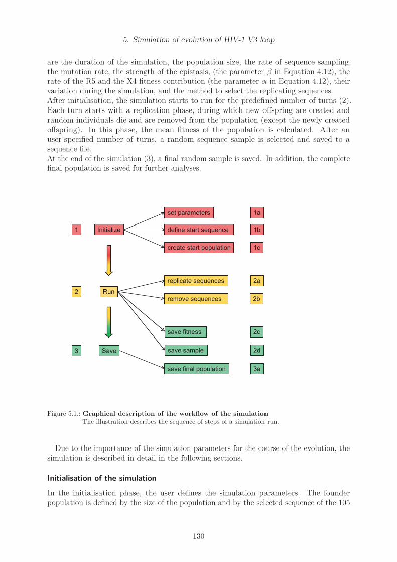
5. Simulation of evolution of HIV-1 V3 loop
are the duration of the simulation, the population size, the rate of sequence sampling,the mutation rate, the strength of the epistasis, (the parameter β in Equation 4.12), therate of the R5 and the X4 fitness contribution (the parameter α in Equation 4.12), theirvariation during the simulation, and the method to select the replicating sequences.After initialisation, the simulation starts to run for the predefined number of turns (2).Each turn starts with a replication phase, during which new offspring are created andrandom individuals die and are removed from the population (except the newly createdoffspring). In this phase, the mean fitness of the population is calculated. After anuser-specified number of turns, a random sequence sample is selected and saved to asequence file.At the end of the simulation (3), a final random sample is saved. In addition, the completefinal population is saved for further analyses.
Initialize
set parameters
define start sequence
create start population
replicate sequences
remove sequences
save fitness
save sample
save final population
Run
Save
1a
1 1b
1c
2a
2b
2c
2d
3a
2
3
Figure 5.1.: Graphical description of the workflow of the simulationThe illustration describes the sequence of steps of a simulation run.
Due to the importance of the simulation parameters for the course of the evolution, thesimulation is described in detail in the following sections.
Initialisation of the simulation
In the initialisation phase, the user defines the simulation parameters. The founderpopulation is defined by the size of the population and by the selected sequence of the 105
130

5. Simulation of evolution of HIV-1 V3 loop
nucleotides (nt) that build the V3 loop. The user can decide whether to use a constantpopulation size or to allow the population to vary in size. In general, we use a populationof a constant size of 3,000 sequences for our simulations. This is based on the knowledgethat the virus population in the blood of a successful treated patient is almost constantover time, with an estimate of 3,000 cells infected. A population of variable size willincrease or decrease, depending on the replicative fitness of the sequences of the population.The fitter the population, the more sequences are by chance selected for replication.In addition to the size of the population, the user also decides whether the start populationis homogeneous or heterogeneous. Choosing a uniform start population enables the user todecide about the exact nt start sequence. The simulation will then start with the definednumber of identical, predefined nt sequences.In the default setting, our simulation generates a homogeneous initial population ofidentical V3 loop sequences, based on the knowledge that an in vivo HIV infection typicallyis seeded by only one viral founder strain [52]. The homogeneous population consists ofidentical copies of a random ten-point mutant of a modified V3 loop consensus sequence.We previously analysed that the original R5 and X4 consensus sequences only differedin the nt positions 64 (R5: G, X4: A) and 73 (R5: G, X4: A). To minimise the risk tointroduce a co-receptor bias by the founder population of the simulation, the R5 and X4consensus sequence was modified into a neutral sequence with respect to the co-receptorusage. Thus, both position 64 and 73 the nt was altered manually into the alternative ntT, mutating the aa from A (R5) and T (X4) into S, respectively from D (R5) and K (X4)into Y.The resulting co-receptor neutral sequence is then mutated in ten random nt positions tocreate a start sequence for the simulations. For additional variability, a back-switch of therandomly selected nt position into the consensus nt symbol is not restricted. Therefore,the resulting start sequence has a nt Hamming distance in the range of two to twelve withrespect to the R5 and X4 nt consensus sequence.It is also possible to start from a heterogeneous population of nt sequences of length 105,with the nt sequences randomly created from the letters of the DNA alphabet (G, C, A, T).The simulation ensures a founder population of nt sequences without stop codons. Randomsequences with stop codons are created again until they are replaced by a sequence withoutany stop codon.The duration of the simulation is measured in replication cycles (termed turns). Thedefault duration of the simulation was set to 30,000 turns and can be modified by theuser upon the simulation start. Using the default parameters, a simulation of 30,000 turnsensured the convergence of the population towards the consensus sequence.Next, the user can define the mutation rate. We determined a default mutation rate of0.016 to result in an average of one amino acid mutation per replication. The averagenumber of mutations is based on an analysis of 1,000 simulation runs. In parallel, wedetermined the mutation rate of 0.016 analytically A.3. This mutation rate is set as defaultmutation rate for the simulation. Note that higher mutation rates increase and lower ratesdecrease the speed of evolution, leaving the course of the evolution in general unaffected.The user can further decide between roulette and tournament selection to select a sequencefor replication (see next Section), and between an additive or a multiplicative fitnessfunction to calculate the replicative fitness of the sequences. The roulette selection methodbased on a multiplicative fitness function is defined as the default setting.
131

5. Simulation of evolution of HIV-1 V3 loop
Finally, the user can define the sampling rate and the sampling time. The sampling ratedetermines the number of sequences that are saved and the sampling time determines afterwhich number of turns a sample is saved to the result file.An overview over the simulation parameters is given in the following enumeration. Thedefault values are given in parenthesis.
• number of turns (30,000)• initial population size (3,000)• homogeneous or heterogeneous starting population (homogeneous)• start sequence (ten-point mutant of consensus sequence)• constant or variable population size (constant)• mutation rate (µ = 0.016)• roulette or tournament selection (roulette)• fitness function: additive/multiplicative (multiplicative (see Equation 4.12)• epistatic strength (β = 0.8)• R5 fitness contribution (α = 0.5)• X4 fitness contribution 1 − α
• sampling time: every t turns (t = 100)• fraction of sampling: r (r = 0.05)
In addition, the user can decide to change the influence of the R5 or the X4 fitness functionduring the simulation. Therefore, an optional parameter x can be defined which determinesthe number of turns after which the parameter α is altered. In general, x = numberofturns
10.
Using this setting, α is increased every 10% of the turns by 0.1. Also this value can bemodified upon simulation initialisation.Apart from this expansion, the user can decide to use only the main or only the epistaticfitness term by an alteration of the parameter β, as described in Equation 4.12.Optionally, the user can initialise the random number generator of the simulation with arandom seed to get reproducible simulation results.
Simulation turns
After the initialisation, the simulation of the sequence evolution is started. During eachturn of the simulation, ten sequences of the population are selected for replication and tensequences are removed from the population.
Replication During the replication step, parental sequences are selected to create offspringbased on their fitness. The underlying selection algorithm is either roulette or tournamentselection. In general, all sequences have a chance to get selected by both methods, butsequences with a larger replicative fitness are selected for replication at a higher frequency.Upon roulette selection, a sequence is selected proportional to its fitness. Sequences witha higher replicative fitness get selected with a higher probability, and sequences with afitness of zero (i.e. sequences that carry at least one stop codon) are selected with aprobability of zero , thus they are excluded from the selection process.If tournament selection is used to select a parental sequence, the selection is a two-stepprocess. First, two sequences are randomly picked from the population (i.e. not depending
132

5. Simulation of evolution of HIV-1 V3 loop
on their fitness). In the second step, the two individuals compete and only the sequencewith the higher fitness is replicated.In contrast to the classical Moran model, an average of ten parental sequences is selectedto replicate per turn.
Mutation The simulation performs the sequence replication with a chance for a mutation(i.e. error-prone replication). Applying the defined mutation rate µ, each of the 105 ntpositions is checked for a possible mutation upon replication. The resulting nt sequenceof the offspring is translated into an aa sequence and the fitness of the newly createdoffspring is calculated based on the selected fitness function.
Death After replication, an number of sequences equal to the number of newly createdoffspring is randomly selected and removed from the population. Since the classical Moranmodel assumes a parallel birth and death process, those offspring that were produced inthe same turn are excluded from the death selection process.
5.2.3. Save simulation results
During the simulation run, the results are saved to a result file at equidistant time points.The distance of the time points can be defined by the user. The saved results comprisethe nt and aa sequences of the individuals of the population, their individual replicativefitness as well as the mean replicative fitness of the population.For large populations, the user can decide to save only a fraction of all sequences, i.e. alimited sequence sample, instead of the complete population. The sampling rate can beselected upon the initialisation of the simulation.Independent of the defined sampling rate, the complete final population is saved at theend of the simulation.
133
5. Simulation of evolution of HIV-1 V3 loop
5.3. Results
In the following section, we analyse a number of simulation properties and evaluate thecapability to reproduce the course of the V3 loop evolution. We start with an analysis ofthe influence of the simulation parameters. Subsequently, we compare the effect of thedifferent definitions of the underlying fitness functions and finally, we present selectedsimulation results using the default simulation parameters given in Section 5.2.2.
5.3.1. Parameter analysis
During the design of the simulation tool, we tested a variety of different simulationparameters and a range of parameter values. The main purpose was to get a firstimpression of the features of our model simulation.Some of the parameter settings had no biologically meaningful equivalent and were excludedfrom further considerations (e.g. simulations of the viral evolution merely based on epistaticinteractions, constant and very small viral populations, a random selection of replicatingparental sequences, simulations with heterogeneous random starting populations, or withunrealistic viral start sequences as for example mere poly-A sequences).The parameter analyses that were relevant to mimic a biologically sensible V3 loop sequenceevolution are described in the following lines.
Population size and mutation rate
We performed a parameter scan for both roulette and tournament selection to determinebiologically meaningful parameters for the simulations. Therefore, homogeneous testpopulations were simulated for 50,000 turns and tested in ten simulations. We analysedthe influence of the mutation rate µ in the range of 0.001 to 0.032 and of the populationsize in the range of 50 to 3,000 individuals.The parameters of a simulation were defined to be appropriate, if the simulated sequencesevolved towards the most fit consensus sequence, represented by a fitness value of 1.0(based on Equation 4.12), at some time point during the simulation (termed timed toconvergence). This definition relies on the observation that the consensus sequence ingeneral spreads fast throughout the population shortly after its first occurrence.Using the roulette selection method, the time to convergence was closely related with thepopulation size (compare Figure 5.2). The larger the population, the earlier we observed asequence that evolved towards the consensus sequence. While the largest mutation rate of0.032 only converged for simulated populations of more than 500 sequences, the smallestmutation rate of 0.001 evolved towards the consensus sequence only in populations largerthan 1,000, (using a simulation duration of 50,000 turns). Additional simulations of aduration of up to 500,000 turns showed only slightly improved result.A detailed inspection of the populations during the simulations revealed that the sequencesdo not persist long enough in small populations to enable their replication, since theprobability that they become removed from the population is higher. To avoid sequencewith increased fitness to be swept out before they create offspring, we either had to increasethe population size or the life span of the sequences in our simulations.In a further analysis of the simulated populations, we found that small mutation rates(e.g. 0.001) increased the mean population fitness, while large mutation rates (e.g. 0.032)
134

5. Simulation of evolution of HIV-1 V3 loop
decreased the mean fitness (data not shown). The simulated data indicated that largemutation rates tend to overshoot the mark. Once the simulated sequences reached theconsensus sequence, simulation runs with large mutation rates continued to alter multiplenucleotides within one round of replication and thus failed to stabilise the population atthe fitness optimum. We observed that large populations could cope with this problem.Though the sequences spread wide in sequences space, a proportion of the simulatedsequences in a large population conserved the maximal fit consensus sequence. In the caseof small mutation rates, the majority of the sequences exactly hit the most fit consensussequence, since only rare mutations were introduced into the offspring upon replication.
0
0.1
0.2
0.3
0.4
0.5
0.6
0.7
0.8
0.9
1
0 500 1000 1500 2000 2500 3000
fitn
ess
population size
mut 0.001mut 0.008mut 0.016mut 0.024mut 0.032
Figure 5.2.: Parameter scan for simulation using roulette selectionThe figure illustrates the association of the population size, the mutation rate µ, and themaximal fitness of the simulated population upon roulette selection. A fitness of 1.0 isindicative of an evolution towards the consensus sequence.A mutation rate of 0.032 converged for population sizes larger than 500, and a mutation rateof 0.001 converged for population sizes larger than 1,000.
We performed the same parameter test for the tournament selection method (compareFigure 5.3). The simulations showed that the method was very sensitive to the selectedmutation rate. Mutation rates µ > 0.008 (i.e. on average one aa mutation in everysecond turn) restricted the population to evolve towards the consensus sequence duringsimulations of 50,000 turns. A five- to tenfold duration of the simulations (i.e. up to500,000 turns) increased the success, but still some simulations failed to evolve to theconsensus sequence.
135

5. Simulation of evolution of HIV-1 V3 loop
We found that this was mainly a consequence of the first step of the tournament selectionmethod. As log as there are many sequences of low fitness and only a few sequence of highfitness in the population, the random selection picks sequences of high fitness at a lowprobability. Therefore, the fitness-dependent second step can only decide between two lessfit sequences. Only if there are enough high fit sequences in the population, the highly fitsequences are selected steadily for replication. In consequence, the time to convergence islonger upon the usage of tournament selection.
0
0.1
0.2
0.3
0.4
0.5
0.6
0.7
0.8
0.9
1
0 500 1000 1500 2000 2500 3000
fitn
ess
population size
mut 0.001mut 0.008mut 0.016mut 0.024mut 0.032
Figure 5.3.: Parameter scan for simulation using tournament selectionThe figure illustrates the association of the population size, the mutation rate µ, and themaximal fitness of the simulated population upon tournament selection. A fitness of 1.0 isindicative of an evolution towards the consensus sequence.The use of the tournament selection method in our simulations was very sensitive to themutation rate. Mutation rates larger than 0.008 often failed to evolve towards the consensussequence during simulations of 50,000 turns.
Due the increased computation time, the simulations based on tournament selectionwere less useful to observe the evolution of many populations in parallel. Thus, we decidedto use roulette selection. We used populations ≥ 1, 000 sequences, since populations ofthat size were quite robust to any of the tested mutation rates, as analysed in Figure 5.2.Higher mutation rates resulted in shorter convergence times, but introduced more sequencediversity, while simulations with lower mutation rates required a longer simulation duration,but resulted in populations of less sequence diversity. Thus, we selected a fast defaultmutation rate of 0.016 for roulette selection (on average one aa mutation per replication).
136

5. Simulation of evolution of HIV-1 V3 loop
Sampling
During a simulation run, a user-defined fraction of sequences is written to a result file.Given enough memory space, the user can decide to save all intermediate sequences of eachgeneration. The subsequent analyses of the full sequence data of the default simulationwith 3,000 sequences and 30,000 turns would then comprise 90,000,000 sequences. In testsimulations, this amount of data required more computational time for the determination ofthe pairwise nt Hamming distances and the calculation of the diversity and the divergencethan the simulations themselves.For practical reasons, we found a sampling process in predefined timely intervals (e.g.every 100 turns) more suitable. Furthermore, limited sequence samples with intervals ofunknown populations in between mimic the conditions of our longitudinal patient study,during which sparse samples were taken in variable time intervals.To analyse the effect of sampling and to find an optimal sampling rate, we performeda parameter scan for the sampling rate. Figures 5.4 and 5.5 illustrate the influence ofthe sampling rate on the population diversity and divergence over time, as defined inSection 3.2.1. For a population of 3,000 sequences, we tested sampling rates of 100%, 10%,5%, and 2% , i.e. all 3,000 sequences and 300, 150, and 60 randomly drawn sequences.The sampling rate of 100% represents the real sequence diversity and divergence of thesimulated population.
0
1
2
3
4
5
6
7
8
0 5000 10000 15000 20000 25000 30000
div
ers
ity
time
Influence of sampling rate on diversity
sampling rate 2%sampling rate 5%sampling rate 10%sampling rate 100%
Figure 5.4.: Parameter scan for sampling rateThe figure illustrates the influence of the sampling rate on the evolution of the populationdiversity over time. The red curve (100% of all sequences saved) equals the real sequencediversity of the simulated population and served as a standard to test sampling rates of 10%,5%, and 2% for a population of 3,000 sequences.
137
5. Simulation of evolution of HIV-1 V3 loop
0
2
4
6
8
10
12
14
0 5000 10000 15000 20000 25000 30000
div
erg
ence
time
Influence of sampling rate on divergence
sampling rate 2%sampling rate 5%sampling rate 10%sampling rate 100%
Figure 5.5.: Parameter scan for sampling rateThe figure illustrates the influence of the sampling rate on the evolution of the populationdivergence over time. The red curve (100% of all sequences saved) equals the real sequencedivergence of the simulated population and served as a standard to test sampling rates of10%, 5%, and 2% for a population of 3,000 sequences.
As expected, the comparison showed an increasing deviation of the real measures fromthe sample estimates with decreasing sampling rate. The required memory space for theanalyses scaled with the same rate, while the computation time scaled quadratically withthe sampling rate, due to the calculation of the Hamming distance of each sequence pairupon the computation of the diversity. Based on these observations and with respect tothe consumption of memory space and computation time, we used a default sampling rateof five percent, i.e. a sampling parameter of 1
20for the simulations.
Additive versus multiplicative fitness
In our model, two fitness contributions influence the fitness value of a sequence. Thefitness is composed of the main fitness term, based on the aa sequence, and of theepistatic fitness term, describing the effect of pairs of interacting mutations. Resolvingthe mathematical description of the fitness terms in more detail, both the main and theepistatic fitness contribution are composed of multiple individual fitness contributions.The exact definitions were described in Sections 4.4.3 and 4.4.5.We considered different possibilities to join the single fitness contributions: the summationof all single fitness contributions, the multiplication of all single fitness contributions(as described in Equation 4.10 and analysed in Section 4.4.3), and a combination of thesummation and the multiplication (i.e. the summation of the single position specificcontributions, and the multiplication of the resulting main and epistatic term).
138

5. Simulation of evolution of HIV-1 V3 loop
We tested the different methods and analysed the effect on the resulting replicative fitnessas well as on the course and the outcome of the simulations. The test simulations confirmedour theoretical considerations presented in Section 4.4.3 (results not shown). Simulationsbased on the multiplicative fitness function sifted the less fit sequences out fast and soundly,due to an increased chance to select sequences of high fitness for replication. In the caseof the additive fitness function, the simulations run approximately the tenfold numberof turns to evolve towards the consensus sequence and the resulting final populationswere more heterogeneous and showed a decreased mean population fitness, compared tosimulations that were based on the multiplicative fitness function. The rational behind thisobservation is that the multiplicative fitness function has a distinct and steep fitness peak,representing the optimal consensus sequence, while the additive fitness function creates afitness landscape which is more flat and has a less pronounced consensus sequence peak.Piganeau et al. [117] described that additive selective effects are not effective when thenumber of selected sites is larger than the effective population size, an assumption theystate to be realistic for current molecular data.Based on these results and the previous considerations (compare Section 4.4.3 ), we decidedto use a the multiplicative formulation of the fitness function for the default simulationmodel, as presented in Equation 4.12. The resulting values were normalised to the interval[0.0, 1.0] as described upon the introduction of the fitness function.
5.3.2. Results of the default model
We used the default parameter settings described in Section 5.2.2 to perform multiplesimulations of the evolution of the V3 loop, starting from homogeneous populations of ran-dom ten-point mutants of the R5 and X4 nt consensus sequences presented in Section 4.3.2.
Evolution of the diversity and the divergence
Based on the default simulations, we analysed the course of the diversity and the divergence(defined by Equation 3.2.1). Figure 5.6 illustrates the course of the diversity, using thedefault simulation parameters (see Section 5.2.2) and the fitness function presented inEquation 4.12. The simulations started from homogeneous populations with zero diversity,and the diversity increased during the first 2,000 turns, representing approximately 20,000replications. Around this time, one of the newly created offspring mutated into the mostfit consensus sequence. In the subsequent simulation turns, the consensus sequence becamedominant and spread throughout the population. As a consequence, the diversity of thepopulation decreased and finally stabilised at an average diversity level depending on themutation rate.A comparison of the simulation results with the results of Shankarappa et al. [138]showed that the course of diversity created by our simulations nicely coincided with thethree-staged pattern of viral evolution published in 1999.
139

5. Simulation of evolution of HIV-1 V3 loop
0
1
2
3
4
5
6
7
8
0 5000 10000 15000 20000 25000 30000
div
ers
ity
time
Evolution of diversity
diversity
Figure 5.6.: Evolution of diversity in the default modelThe figure illustrates the course of the diversity of 15 example runs, using the default simulationparameters.The diversity showed a three-staged pattern: an increase during the first 2,000 turns, adecreasing diversity while the consensus sequence became dominant, and a final stabilisationat an average diversity level.
The corresponding analysis of the course of the divergence is shown in Figure 5.7. Afteran initial increase of the divergence during the first 2,000 turns, the divergence of thepopulation stabilised at a specific nt Hamming distance, representing the genetic distancebetween the initial sequence and the consensus sequence. The extend of the final divergenceof the population depends on the exact number of mutations of the founder strain.Using the default weighting parameter α = 0.5, we observed a closer genetic distance ofthe simulated sequences to the R5 consensus sequence in the majority of all simulations.A temporarily increase or decrease of the divergence during the course of evolution wasobserved in single simulation runs. Detailed analyses showed that this was a result of atransient dominance of the X4 consensus sequence. The closer genetic distance of thesimulated sequences to the R5 consensus sequence could so far not be completely resolved.The reduced epistatic interactions in intermediate sequences seem to be one cause. Wefurther presume that the R5 dominance is at least partially a consequence of the finitepopulation size and the limited simulation time.A comparison of the simulated course of divergence with the evolutionary course of anHIV-1 infection described by Shankarappa et al. [138] showed similar patterns. Afteran initial increase of the divergence during the acute phase of the infection, the geneticdistance stabilised at some time point during the disease and stayed at that level until theend of the simulations.
140

5. Simulation of evolution of HIV-1 V3 loop
0
2
4
6
8
10
12
14
0 5000 10000 15000 20000 25000 30000
div
erg
ence
time
Evolution of divergence
divergence
Figure 5.7.: Evolution of divergence in the default modelThe figure illustrates the course of divergence of 15 example runs, using the default simulationparameters.The divergence increased during the first 2,000 turns, until one of the offspring evolvedtowards the most fit consensus sequence. While the consensus sequence became dominant,the divergence of the population stabilised.
Thus, regarding the viral diversity and divergence, our simulation tool is capable tomimic the evolutionary course of an HIV-1 infection as described in early biological studiesof Shankarappa et al. [138]
Hamming distances of the final population
Subsequent to the analyses of the viral diversity and divergence, we analysed the geneticdistance between the simulated populations and the consensus sequences. Therefore, wecalculated the aa Hamming distance of each sequence of the final population to both theR5 and the X4 aa consensus sequence. All default simulations resulted in comparable finalpopulations.Figure 5.8 shows the distribution of the resulting aa Hamming distances. As previouslydescribed, the R5-tropic sequences dominated the population at the end of the simulationruns, despite an equal weight for both the R5 and X4 fitness contribution (α = 0.5). Thedefinition of our fitness function (defined in Equation 4.12) favoured the R5 sequence dueto less epistatic interactions in intermediate sequences. Using α = 0.5, a population infavour of the X4 consensus sequence was only observed transiently in intermediate timesteps during the simulation.In the default simulations, about 1
6of the 3,000 sequences of the final population of each
simulation exactly matched the R5 consensus sequence, i.e. the aa Hamming distance to
141

5. Simulation of evolution of HIV-1 V3 loop
the R5 consensus sequence was zero for about 500 sequences per run. The majority ofthe sequences (∼ 1, 000 sequences) accumulated at a Hamming distance of one. We foundthis to be a result of the continuous replication and mutation process. Once the consensussequence is present in the population, it is most likely selected for replication due to themaximal fitness value. Upon the following replication, the default mutation rate of 0.016introduces on average one aa mutation into the newly created offspring. This phenomenonis further discussed at the end of the section.
0 1 2 3 4 5 6 7 8 9 10
Histogram of Hamming distances
Hamming distance
counts
02000
4000
6000
8000
10000
14000
R5X4
Figure 5.8.: Hamming distances of the final population of the default modelThe figure illustrates the distribution of the aa Hamming distances of the sequences of thefinal population to the R5 and the X4 consensus sequence.Both the Kolmogorow-Smirnov [92, 143] and the χ2 [114] test showed that the distributionsof aa the Hamming distances were significantly different (p − value =< 0.0001 for both tests).
In additional simulation runs, we found that an alteration of the weighting parameterα in favour of the X4 fitness function (i.e. α < 0.5) directed the viral evolution eithertowards mixed R5- and X4-tropic or mere X4-tropic final populations, depending on theexact parameter value (data not shown).
142

5. Simulation of evolution of HIV-1 V3 loop
Evolution of position specific amino acids over time
Following the analyses of the course of the diversity and divergence and of the Hammingdistances of the final populations, we next asked whether the course of evolution ischemically sensible. Therefore, we classified the amino acids into four chemical groups:basic (K, R, H), acidic (E, D), polar (Y, T, Q, G, S, C, N), and non-polar (A, V, M, L, I,P, W, F) (compare Table A.7).During the simulations, the sampled sequences were translated into a chemical score withrespect to the target consensus sequence, regarding the following scheme: amino acidsmatching the consensus sequence amino acid were scored as 1.0, differing amino acidsbelonging to the same chemical group as the consensus amino acid were scored as 0.0and differing amino acids of a differing chemical group were scored as -1.0. We scored allsequences of each sample and calculated the position-specific sample average.Figure 5.9 depicts the position-specific average of the samples compared to the respectiveR5 (a) or X4 (b) consensus sequence. The illustrations show that evolution of the mutatedpositions follows a meaningful chemical course. In general, mutated positions first met thecorrect chemical group and finally evolved towards the correct amino acid. This effect isespecially pronounced in figure (a) for the R5 sequence position one, 22, and 25.A comparison of the chemical evolution with respect to the R5 and the X4 consensussequence confirmed the finding, that the X4 consensus sequence dominated the populationonly transiently. In the illustrated example in Figure 5.9, this can be seen for the first 5,000to 10,000 turns in the positions 22 and 25 of the simulation. During this time, the correctchemical group with respect to the X4 sequence dominated both positions, represented bythe blue colour in the X4 (b) plot. In consequence, the chemical group in the positions22 and 25 differed from the R5 consensus sequence during that time, represented by thered colour in the R5 plot (a). After approximately 12,000 turns, the R5 consensus aadominated, leading to a switch of the chemical property, represented by the positive score(blue colour) in the R5 plot (a) and the negative score (red colour) in the X4 plot (b).Figure 5.9 also nicely visualises the fluctuating character of the position-specific aa ofthe population. Once the correct aa in a sequence positions occurred, it dominated thatposition, but some individuals of the population continuously acquired new mutationsduring later rounds of replication (illustrated by the change between dark and light bluein position 25 beginning from turn 25,000).From the analyses of the chemical course of the evolution we found that our model wasable to simulate chemically meaningful evolutionary pathways.
143
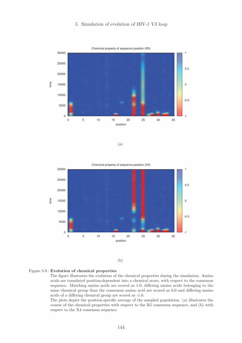
5. Simulation of evolution of HIV-1 V3 loop
Chemical property of sequence position (R5)
0 5 10 15 20 25 30 35
position
0
5000
10000
15000
20000
25000
30000tim
e
-1
-0.5
0
0.5
1
(a)
Chemical property of sequence position (X4)
0 5 10 15 20 25 30 35
position
0
5000
10000
15000
20000
25000
30000
tim
e
-1
-0.5
0
0.5
1
(b)
Figure 5.9.: Evolution of chemical propertiesThe figure illustrates the evolution of the chemical properties during the simulation. Aminoacids are translated position-dependent into a chemical score, with respect to the consensussequence. Matching amino acids are scored as 1.0, differing amino acids belonging to thesame chemical group than the consensus amino acid are scored as 0.0 and differing aminoacids of a differing chemical group are scored as -1.0.The plots depict the position-specific average of the sampled population. (a) illustrates thecourse of the chemical properties with respect to the R5 consensus sequence, and (b) withrespect to the X4 consensus sequence.
144

5. Simulation of evolution of HIV-1 V3 loop
5.4. Discussion
In the third part of the work we developed a model to simulate the sequence evolution ofthe HIV-1 V3 loop. The simulation tool is based on the findings from the previous parts ofthe project, i.e. the sequence analyses, the observed evolutionary course of the evolution,and the fitness function to describe the replicative fitness of the simulated sequences.The model is flexible and enables the user to examine the influence of changing simulationparameters on the timely course of the evolution, for example the impact of the mutationrate, of the simulation time, of the population size, or the effect of different homogeneousor heterogeneous founder populations.We determined a set of parameters that serve as a default model to simulate the evolutionof the V3 loop over time. Our analyses showed that the default model is able to evolvea population of sequences towards the observed R5 and/or X4 consensus sequence. Theevolutionary speed of the simulation depends on the composition of the founder population,the mutation rate, and the size of the population.We further found that the model is capable to reproduce the evolutionary course ofthe viral diversity and divergence over time, as it was described by Shankarappa et al.[138]. Further analyses confirmed that the simulated evolutionary pathways follow sensiblechemical paths, first accumulating amino acids with correct chemical properties and finallyconverging into the correct position specific consensus amino acid.Upon the inspection of the final steady state populations of the default model, we detectedthat the majority of the sequences resided at an amino acid Hamming distance of oneto the consensus sequence. The exact distance is defined by the underlying mutationrate (default 0.016). We found that the final Hamming distance is a consequence of thecontinuous mutation process. The sequences are driven by the selection process towardsthe fitness optimum, which is the consensus sequence. Once the fitness peak is reached,the sequences slide down on the fitness landscape to positions of lower fitness. From thelower level of the fitness landscape, they again step uphill towards the optimum, creatinga continuous exchange of the sequences at the top of the fitness peak and the sequences atthe observed Hamming distance.Based on our observations we state that our in silico simulation model is a useful toolto study V3 loop evolution. The model is able to cope with the restrictions of in vivo orin vitro studies, e.g. the decreasing patient compliance during the years of a longitudinalstudy, the high costs of the deep sequencing approaches to enable analyses of completeviral populations, or the sensitivity of the sequencing methods.
145
5. Simulation of evolution of HIV-1 V3 loop
5.5. Outlook
In further studies, we would like to focus on the simulation of the co-receptor switch andto evaluate the neutral networks generated by our simulation tool. We want to analysethe network changes that happen during the simulated evolution. By a variation of thesimulation parameters during a running simulation, analyses of dynamic fitness landscapescould be possible. This property has already been implemented into the simulation. Lastbut not least, a combination of the simulation tool with a co-receptor prediction methodis also highly recommended to enable co-receptor predictions during the simulation.We would further like to combine the simulation data with longitudinal studies of in vivoHIV evolution. First, it would be very interesting to study HIV evolution in humanisedmice. Humanised mice are mice in which the mouse-specific immune system (in parts)is replaced by a human immune system or at least a couple of human immune cells.These studies would enable us to decide whether the simulated evolutionary pathways arecomparable with the viral evolution in a model organism. We could further imagine tocompare the intra-host evolution of a longitudinal study of HIV-infected patients with thesimulated evolution.To do so, the simulation should be supplemented with a cell dynamics model, mimickingthe availability of CCR5 and CXCR4 positive T cells as well as the level of viral load.This extension of the model was used in early version of the simulation tool and we werealready able to reproduce the dynamics of susceptible and infected (SI) cells.A further extension could model the adaptation of the immune system to the viral se-quences via the integration of a death or clearance process based on adapted immune cells.The presented model is further prepared to utilise ageing information of virions. Some veryfirst test were made to distinguish between productively and latently infected cells and tointroduce compartmentalisation into the model (i.e. to compare the viral populations indifferent body compartments). Last but not least, the model could be extended to mimicHAART treatment, for example by the introduction of a fitness benefit for drug specificamino acid mutations during the course of simulation.
146

6. Discussion
6.1. Discussion
The present PhD project is a composed of three intertwined parts. While the first part isbased directly on longitudinal data of 36 HIV-infected patients, the second part utilised across-section of biological sequence data from 2,768 patients comprised in the Los AlamosHIV data base. In the third part, the findings were combined to develop an in silico toolto describe intra-host HIV evolution.Though the general clinical and evolutionary course of an HIV-1 infection was known fromthe early days of HIV research, so far it was not analysed whether the course of infectionof HAART treated patients is comparable to the course of untreated patients or patientswith antiretroviral monotherapy. We found some first indications that the course of theinfection of treated and untreated patients is highly related, but the timely course of theinfection varies, depending on the success of the administered therapy.In vitro co-receptor studies further revealed that intermediate blinks of X4-tropic viralstrains can be suppressed by successful HAART therapy. Thus, we hypothesise that boththe course of infection and the co-receptor switch are not one- but bi-directional. Our firstfindings should be confirmed in further longitudinal studies.Based on approximately 80,000 Los Alamos V3 loop sequences we next analysed thegenetic differences between the R5- and the X4-tropic strains, since the conditions thatlead to a co-receptor switch in about 50% of all patients are still obscure. Therefore wederived two independent fitness functions to describe the replicative fitness of R5- andX4-tropic V3 loop sequences. Based on the fitness functions, we used methods from graphtheory to analyse the underlying fitness landscapes.With our studies, we were able to confirm the differences between the R5 and the X4sequence space of the V3 loop, that were described in prior publications, e.g. by Bozeket al. [15]. Analysing the sequence conservation of our data set, we could show that theR5-tropic sequences are more conserved than the X4-tropic sequences, a fact that was alsodescribed earlier.In addition, we found that the weakest conserved sequence positions deviate between theR5 and the X4 sequences, leading to far-reaching consequences. Detailed studies of theweakest conserved sequence positions and the respective nucleotide codons showed thatthe most weakly conserved X4 sequence codons are evolutionary close to stop codons. Inseveral of the weakest conserved codons, only one nucleotide mutation suffices to introducea stop codon into the respective X4-tropic V3 loop sequence. In contrast, none of theweakest conserved nucleotides of the R5 consensus sequence enables a mutation thatintroduced a stop codon into the R5 sequence.Following these observations we hypothesise that the less conserved X4 sequences havea fitness disadvantage in a setting with high immune pressure. The better immunerecognition of X4-tropic sequences yields an additional disadvantage. Based on these ideas,
147

6. Discussion
the R5-tropic sequences dominate early in the infection due to a mutational robustness anda worse immune recognition, while a weak immune pressure is a prerequisite to enable theoccurrence and replication of X4-tropic sequences. Thus, we suppose that the co-receptorswitch can be explained by the immune control hypothesis, in combination with theobservation of a weakly conserved X4 population.We comprised our observations in the third part of this work by the development of anin silico tool to simulate the sequence evolution of the HIV V3 loop. The heart of thesimulation is the fitness function derived in the second part of the work. The method is at aearly state and is still missing some important factors that influence in vivo viral evolution(e.g. strength of immune pressure, availability of R5 and X4 target cells, drug-virusinteractions). Therefore we were not able to reproduce the course of the viral evolutionof our study patients. So far, the simulations enabled us to analyse some evolutionaryprocesses of simulated viral populations in fast time and at low costs. With our in silicomodel we were able to mimic the course of the evolution of HIV populations with respectto the viral diversity and the divergence. Further analyses showed that the simulated viralevolution followed a chemically sensible course.In summary, the present project gave us some clues regarding the mechanisms of theco-receptor switch and was successful to gain a number of new and interesting insights intothe aspects of viral intra-host HIV-1 evolution and into the genetic differences betweenthe R5-tropic and the X4-tropic viral strains.
148

Bibliography
[1] H. Abdi and L. J. Williams. Principal component analysis. CompStats, 2(4):433–459,Jul 2010.
[2] J. Aldrich. Correlations Genuine and Spurious in Pearson and Yule. StatisticalScience, 10(4):364–376, 1995.
[3] K. Allers, G. Hutter, J. Hofmann, C. Loddenkemper, K. Rieger, E. Thiel, andT. Schneider. Evidence for the cure of HIV infection by CCR5∆32/∆32 stem celltransplantation. Blood, 117(10):2791–2799, Mar 2011.
[4] D. G. Altman and J. M. Bland. Absence of evidence is not evidence of absence.BMJ, 311(7003):485, Aug 1995.
[5] P. Artimo, M. Jonnalagedda, K. Arnold, D. Baratin, G. Csardi, E. de Castro, S. Du-vaud, V. Flegel, A. Fortier, E. Gasteiger, A. Grosdidier, C. Hernandez, V. Ioannidis,D. Kuznetsov, R. Liechti, S. Moretti, K. Mostaguir, N. Redaschi, G. Rossier, I. Xe-narios, and H. Stockinger. ExPASy: SIB bioinformatics resource portal. NucleicAcids Res., 40(Web Server issue):597–603, Jul 2012.
[6] I. Bahar, A. R. Atilgan, and B. Erman. Direct evaluation of thermal fluctuations inproteins using a single-parameter harmonic potential. Fold Des, 2(3):173–181, 1997.
[7] C. Balasubramanian, G. Chillemi, I. Abbate, M. R. Capobianchi, G. Rozera, andA. Desideri. Importance of V3 Loop Flexibility and Net Charge in the Context ofCo-Receptor Recognition. A Molecular Dynamics Study on HIV gp120. J. Biomol.Struct. Dyn., 29(5):1–13, Apr 2012.
[8] G. Barr. Perl ’List::Util’ Package, 1997–2007. Licensed under the LGPL version 2.
[9] F. Barre-Sinoussi, J. C. Chermann, F. Rey, M. T. Nugeyre, S. Chamaret, J. Gruest,C. Dauguet, C. Axler-Blin, F. Vezinet-Brun, C. Rouzioux, W. Rozenbaum, andL. Montagnier. Isolation of a T-lymphotropic retrovirus from a patient at risk foracquired immune deficiency syndrome (AIDS). Science, 220(4599):868–871, May1983.
[10] J. E. Bennett, A. Racine-Poon, J. C. Wakefield, W. R. eds. Gilks, S. Richardson,and D. J. Spiegelhalter. Markov Chain Monte Carlo in Practice. Chapman and Hall,London, 1996. ISBN 0 412 05551 1.
[11] H. M. Berman, J. Westbrook, Z. Feng, G. Gilliland, T. N. Bhat, H. Weissig, I. N.Shindyalov, and P. E. Bourne. The Protein Data Bank. Nucleic Acids Res., 28(1):235–242, Jan 2000. http://www.pdb.org.
149

Bibliography
[12] F. C. Bernstein, T. F. Koetzle, G. J. Williams, E. F. Meyer, M. D. Brice, J. R.Rodgers, O. Kennard, T. Shimanouchi, and M. Tasumi. The Protein Data Bank: acomputer-based archival file for macromolecular structures. J. Mol. Biol., 112(3):535–542, May 1977.
[13] S. Beyer, R. Ortalo, and J. Leto. Perl ’Math::MatrixReal’ Package, 1996-2002.Licensed under the LGPL version 2.
[14] D. Binninger-Schinzel, D. Muller, T. Wolf, B. Krause, B. Meye, G. Winskowsky,S. Raupp, S. Norley, R. Brodt, and A. Werner. Characterization of a chemokine re-ceptor CCR5-negative T cell line and its use in determining human immunodeficiencyvirus type 1 phenotype. J. Med. Virol., 80:192–200, Feb 2008.
[15] K. Bozek, A. Thielen, S. Sierra, R. Kaiser, and T. Lengauer. V3 loop sequence spaceanalysis suggests different evolutionary patterns of CCR5- and CXCR4-tropic HIV.PLoS ONE, 4(10):e7387, 2009.
[16] R. Bron, P. J. Klasse, D. Wilkinson, P. R. Clapham, A. Pelchen-Matthews, C. Power,T. N. Wells, J. Kim, S. C. Peiper, J. A. Hoxie, and M. Marsh. Promiscuous useof CC and CXC chemokine receptors in cell-to-cell fusion mediated by a humanimmunodeficiency virus type 2 envelope protein. J. Virol., 71(11):8405–8415, Nov1997.
[17] I. N. Bronstein. Taschenbuch der Mathematik. Verlag Harri Deutsch. ISBN 3-80-855670-6.
[18] B. Brooks and M. Karplus. Harmonic dynamics of proteins: normal modes andfluctuations in bovine pancreatic trypsin inhibitor. Proc. Natl. Acad. Sci. U.S.A.,80(21):6571–6575, Nov 1983.
[19] D. M. Cardo, D. H. Culver, C. A. Ciesielski, P. U. Srivastava, R. Marcus, D. Abiteboul,J. Heptonstall, G. Ippolito, F. Lot, P. S. McKibben, and D. M. Bell. A case-controlstudy of HIV seroconversion in health care workers after percutaneous exposure.Centers for Disease Control and Prevention Needlestick Surveillance Group. N. Engl.J. Med., 337(21):1485–1490, Nov 1997.
[20] L. L. Cavalli-Sforza and A. W. Edwards. Phylogenetic analysis. Models and estimationprocedures. Am. J. Hum. Genet., 19(3 Pt 1):233–257, May 1967.
[21] Centers for Disease Control and Prevention, Atlanta, USA. Current Trends HumanT-Lymphotropic Virus Type III / Lymphadenopathy-Associated Virus: AgentSummary Statement. Morbidity and Mortality Weekly Report, 35(34):540–542, 547–549, Aug 1986.
[22] B. Chandramouli, G. Chillemi, I. Abbate, M. R. Capobianchi, G. Rozera, andA. Desideri. Importance of V3 loop flexibility and net charge in the context ofco-receptor recognition. A molecular dynamics study on HIV gp120. J. Biomol.Struct. Dyn., 29(5):879–891, 2012.
150
Bibliography
[23] B. Charlesworth. Fundamental concepts in genetics: effective population size andpatterns of molecular evolution and variation. Nat. Rev. Genet., 10(3):195–205, Mar2009.
[24] C. Cheng-Mayer, M. Quiroga, J. W. Tung, D. Dina, and J. A. Levy. Viral deter-minants of human immunodeficiency virus type 1 T-cell or macrophage tropism,cytopathogenicity, and CD4 antigen modulation. J. Virol., 64(9):4390–4398, Sep1990.
[25] R. Chenna, H. Sugawara, T. Koike, R. Lopez, T. J. Gibson, D. G. Higgins, andJ. D. Thompson. Multiple sequence alignment with the Clustal series of programs.Nucleic Acids Res., 31(13):3497–3500, Jul 2003.
[26] T. Christiansen, B. D. Foy, L. Wall, and J. Orwant. Programming Perl. O’ReillyMedia, 4th edition, 2012. ISBN 978-0596004927.
[27] M. Clerici, N. I. Stocks, R. A. Zajac, R. N. Boswell, D. R. Lucey, C. S. Via, andG. M. Shearer. Detection of three distinct patterns of T helper cell dysfunction inasymptomatic, human immunodeficiency virus-seropositive patients. Independenceof CD4+ cell numbers and clinical staging. J. Clin. Invest., 84(6):1892–1899, Dec1989.
[28] J. Coffin, A. Haase, J. A. Levy, L. Montagnier, S. Oroszlan, N. Teich, H. Temin,K. Toyoshima, H. Varmus, and P. Vogt. What to call the AIDS virus? Nature,321(6065):10, 1986.
[29] R. I. Connor, K. E. Sheridan, D. Ceradini, S. Choe, and N. R. Landau. Change incoreceptor use correlates with disease progression in HIV-1–infected individuals. J.Exp. Med., 185(4):621–628, Feb 1997.
[30] H. Cramer. Mathematical Methods of Statistics. Princeton University Press, Prince-ton, 1999. ISBN 0-69-100547-8.
[31] G. E. Crooks, G. Hon, J. M. Chandonia, and S. E. Brenner. WebLogo: a sequencelogo generator. Genome Res., 14(6):1188–1190, Jun 2004.
[32] V. Dahirel, K. Shekhar, F. Pereyra, T. Miura, M. Artyomov, S. Talsania, T. M.Allen, M. Altfeld, M. Carrington, D. J. Irvine, B. D. Walker, and A. K. Chakraborty.Coordinate linkage of HIV evolution reveals regions of immunological vulnerability.Proc. Natl. Acad. Sci. U.S.A., 108(28):11530–11535, Jul 2011.
[33] C. R. Darwin. On the origin of species by means of natural selection, or thepreservation of favoured races in the struggle for life. John Murray, London, firstedition, 1859. John van Wyhe, ed. 2002-. The Complete Work of Charles DarwinOnline.
[34] M. P. Davenport, J. J. Zaunders, M. D. Hazenberg, H. Schuitemaker, and R. P.van Rij. Cell turnover and cell tropism in HIV-1 infection. Trends Microbiol.,10(6):275–278, Jun 2002.
151

Bibliography
[35] P. Delobel, K. Sandres-Saune, M. Cazabat, C. Pasquier, B. Marchou, P. Massip,and J. Izopet. R5 to X4 switch of the predominant HIV-1 population in cellularreservoirs during effective highly active antiretroviral therapy. J. Acquir. ImmuneDefic. Syndr., 38(4):382–392, Apr 2005.
[36] H. Deng, R. Liu, W. Ellmeier, S. Choe, D. Unutmaz, M. Burkhart, P. Di Marzio,S. Marmon, R. E. Sutton, C. M. Hill, C. B. Davis, S. C. Peiper, T. J. Schall, D. R.Littman, and N. R. Landau. Identification of a major co-receptor for primary isolatesof HIV-1. Nature, 381(6584):661–666, Jun 1996.
[37] R. W. Doms and D. Trono. The plasma membrane as a combat zone in the HIVbattlefield. Genes Dev., 14(21):2677–2688, Nov 2000.
[38] B. J. Doranz, J. Rucker, Y. Yi, R. J. Smyth, M. Samson, S. C. Peiper, M. Parmentier,R. G. Collman, and R. W. Doms. A dual-tropic primary HIV-1 isolate that uses fusinand the beta-chemokine receptors CKR-5, CKR-3, and CKR-2b as fusion cofactors.Cell, 85(7):1149–1158, Jun 1996.
[39] A. J. Drummond, G. K. Nicholls, A. G. Rodrigo, and W. Solomon. Estimating mu-tation parameters, population history and genealogy simultaneously from temporallyspaced sequence data. Genetics, 161(3):1307–1320, Jul 2002.
[40] A. J. Drummond and A. Rambaut. BEAST: Bayesian evolutionary analysis bysampling trees. BMC Evol. Biol., 7:214, 2007.
[41] A. J. Drummond and A. Rambaut. Tracer, version 1.4, 2007. [Online; accessed19-December-2011].
[42] A. J. Drummond, A. Rambaut, B. Shapiro, and O. G. Pybus. Bayesian coalescentinference of past population dynamics from molecular sequences. Mol. Biol. Evol.,22(5):1185–1192, May 2005.
[43] A. J. Drummond, A. Rambaut, and M. Suchard. BEASTWiki. [Online; accessed19-December-2011].
[44] M. P. D’Souza and V. A. Harden. Chemokines and HIV-1 second receptors. Conflu-ence of two fields generates optimism in AIDS research. Nat. Med., 2(12):1293–1300,Dec 1996.
[45] M. Eigen. Selforganization of matter and the evolution of biological macromolecules.Naturwissenschaften, 58(10):465–523, Oct 1971.
[46] M. Eigen. The origin of genetic information: viruses as models. Gene, 135(1-2):37–47,Dec 1993.
[47] M. Eigen, J. McCaskill, and P. Schuster. Molecular Quasi-Species. J. Phys. Chem.,92:6881–6891, Jun 1988.
[48] L. Euler. Solutio problematis ad geometriam situs pertinentis. CommentariiAcademiae Scientiarum Imperialis Petropolitanae, 8:128–140, 1736. Opera Om-nia (1) 7 (1911-56), 1-10.
152

Bibliography
[49] G. Fatkenheuer and et al. Subgroup analyses of maraviroc in previously treated R5HIV-1 infection. N. Engl. J. Med., 359(14):1442–1455, Oct 2008.
[50] A. S. Fauci, G. Pantaleo, S. Stanley, and D. Weissman. Immunopathogenic mecha-nisms of HIV infection. Ann. Intern. Med., 124(7):654–663, Apr 1996.
[51] A. S. Fauci, S. M. Schnittman, G. Poli, S. Koenig, and G. Pantaleo. NIH conference.Immunopathogenic mechanisms in human immunodeficiency virus (HIV) infection.Ann. Intern. Med., 114(8):678–693, Apr 1991.
[52] W. Fischer, V. V. Ganusov, E. E. Giorgi, P. T. Hraber, B. F. Keele, T. Leitner,C. S. Han, C. D. Gleasner, L. Green, C. C. Lo, A. Nag, T. C. Wallstrom, S. Wang,A. J. McMichael, B. F. Haynes, B. H. Hahn, A. S. Perelson, P. Borrow, G. M. Shaw,T. Bhattacharya, and B. T. Korber. Transmission of single HIV-1 genomes anddynamics of early immune escape revealed by ultra-deep sequencing. PLoS ONE,5(8):e12303, 2010.
[53] R. A. Fisher. The Design of Experiments. Macmillan Pub Co, 9 edition, 1971. ISBN0-028-44690-9.
[54] R. A. Fouchier, M. Groenink, N. A. Kootstra, M. Tersmette, H. G. Huisman,F. Miedema, and H. Schuitemaker. Phenotype-associated sequence variation in thethird variable domain of the human immunodeficiency virus type 1 gp120 molecule.J. Virol., 66(5):3183–3187, May 1992.
[55] A. D. Frankel and J. A. Young. HIV-1: fifteen proteins and an RNA. Annu. Rev.Biochem., 67:1–25, 1998.
[56] G. Fuellen, R. Resnick, S. E. Brenner, C. Dagdigian, S. Chervitz, E. Birney, J. Gilbert,and E. o. Stupka. Perl ’Bioperl’ Package, 1996-2009.
[57] S. Gavrilets. Evolution and speciation on holey adaptive landscapes. Trends Ecol.Evol. (Amst.), 12(8):307–312, Aug 1997.
[58] L. Y. Geer, A. Marchler-Bauer, R. C. Geer, L. Han, J. He, S. He, C. Liu, W. Shi,and S. H. Bryant. The NCBI BioSystems database. Nucleic Acids Res., 38(Databaseissue):D492–496, Jan 2010.
[59] G. B. Gloor, L. C. Martin, L. M. Wahl, and S. D. Dunn. Mutual information inprotein multiple sequence alignments reveals two classes of coevolving positions.Biochemistry, 44(19):7156–7165, May 2005.
[60] N. Go, T. Noguti, and T. Nishikawa. Dynamics of a small globular protein in termsof low-frequency vibrational modes. Proc. Natl. Acad. Sci. U.S.A., 80(12):3696–3700,Jun 1983.
[61] S. N. Goodman. Toward evidence-based medical statistics. 2: The Bayes factor.Ann. Intern. Med., 130(12):1005–1013, Jun 1999.
[62] P. R. Gorry and P. Ancuta. Coreceptors and HIV-1 pathogenesis. Curr HIV/AIDSRep, 8(1):45–53, Mar 2011.
153

Bibliography
[63] R. Grant and . co workers. Preexposure chemoprophylaxis forHIV prevention inmen who have sex with men. N. Engl. J. Med., 363(27):2587–99, Dec 2010.
[64] C. Graziosi, G. Pantaleo, J. F. Demarest, O. J. Cohen, M. Vaccarezza, L. Butini,M. Montroni, and A. S. Fauci. HIV-1 infection in the lymphoid organs. AIDS, 7Suppl 2:S53–58, Nov 1993.
[65] X. Gu, Y. X. Fu, and W. H. Li. Maximum likelihood estimation of the heterogeneityof substitution rate among nucleotide sites. Mol. Biol. Evol., 12(4):546–557, Jul1995.
[66] L. A. Guay, P. Musoke, T. Fleming, D. Bagenda, M. Allen, C. Nakabiito, J. Sherman,P. Bakaki, C. Ducar, M. Deseyve, L. Emel, M. Mirochnick, M. G. Fowler, L. Mofenson,P. Miotti, K. Dransfield, D. Bray, F. Mmiro, and J. B. Jackson. Intrapartum andneonatal single-dose nevirapine compared with zidovudine for prevention of mother-to-child transmission of HIV-1 in Kampala, Uganda: HIVNET 012 randomised trial.Lancet, 354(9181):795–802, Sep 1999.
[67] R. M. Gulick and et al. Maraviroc for previously treated patients with R5 HIV-1infection. N. Engl. J. Med., 359(14):1429–1441, Oct 2008.
[68] A. T. Haase. Population biology of HIV-1 infection: viral and CD4+ T cell de-mographics and dynamics in lymphatic tissues. Annu. Rev. Immunol., 17:625–656,1999.
[69] A. A. Hagberg, D. A. Schult, and P. J. Swart. Exploring network structure, dynamics,and function using NetworkX. In Proceedings of the 7th Python in Science Conference(SciPy2008), pages 11–15, Pasadena, CA USA, Aug. 2008.
[70] B. H. Hahn, G. M. Shaw, S. K. Arya, M. Popovic, R. C. Gallo, and F. Wong-Staal.Molecular cloning and characterization of the HTLV-III virus associated with AIDS.Nature, 312(5990):166–169, 1984.
[71] R. W. Hamming. Error Detecting and Error Correcting Codes. The Bell SystemTechnical Journal, 29(2):147–160, Apr 1950.
[72] R. W. Hamming. Coding and Information Theory. Prentice Hall, second edition,2002. ISBN 0131390724.
[73] A. Hildebrandt, A. K. Dehof, A. Rurainski, A. Bertsch, M. Schumann, N. C. Tous-saint, A. Moll, D. Stockel, S. Nickels, S. C. Mueller, H. P. Lenhof, and O. Kohlbacher.BALL–biochemical algorithms library 1.3. BMC Bioinformatics, 11:531, 2010.
[74] T. Hinkley, J. Martins, C. Chappey, M. Haddad, E. Stawiski, J. M. Whitcomb, C. J.Petropoulos, and S. Bonhoeffer. A systems analysis of mutational effects in HIV-1protease and reverse transcriptase. Nat. Genet., 43(5):487–489, May 2011.
[75] A. Hodgkinson and A. Eyre-Walker. Variation in the mutation rate across mammaliangenomes. Nat. Rev. Genet., 12(11):756–766, Nov 2011.
154

Bibliography
[76] F. Hoffgaard. Biomolecular Correlation in Physical and Sequence Space. TechnischeUniversitat Darmstadt, 2011. PhD thesis.
[77] F. Hoffgaard, P. Weil, and K. Hamacher. BioPhysConnectoR: Connecting sequenceinformation and biophysical models. BMC Bioinformatics, 11:199, 2010.
[78] C. C. Huang, S. N. Lam, P. Acharya, M. Tang, S. H. Xiang, S. S. Hussan, R. L.Stanfield, J. Robinson, J. Sodroski, I. A. Wilson, R. Wyatt, C. A. Bewley, and P. D.Kwong. Structures of the CCR5 N terminus and of a tyrosine-sulfated antibodywith HIV-1 gp120 and CD4. Science, 317(5846):1930–1934, Sep 2007.
[79] C. C. Huang, M. Tang, M. Y. Zhang, S. Majeed, E. Montabana, R. L. Stanfield,D. S. Dimitrov, B. Korber, J. Sodroski, I. A. Wilson, R. Wyatt, and P. D. Kwong.Structure of a V3-containing HIV-1 gp120 core. Science, 310(5750):1025–1028, Nov2005.
[80] G. Hutter, D. Nowak, M. Mossner, S. Ganepola, A. Mussig, K. Allers, T. Schneider,J. Hofmann, C. Kucherer, O. Blau, I. W. Blau, W. K. Hofmann, and E. Thiel.Long-term control of HIV by CCR5 Delta32/Delta32 stem-cell transplantation. N.Engl. J. Med., 360(7):692–698, Feb 2009.
[81] M. A. Jensen, M. Coetzer, A. B. van ’t Wout, L. Morris, and J. I. Mullins. A reliablephenotype predictor for human immunodeficiency virus type 1 subtype C based onenvelope V3 sequences. J. Virol., 80(10):4698–4704, May 2006.
[82] M. A. Jensen, F. S. Li, A. B. van’t Wout, D. C. Nickle, D. Shriner, H. X. He,S. McLaughlin, R. Shankarappa, J. B. Margolick, and J. I. Mullins. Improvedcoreceptor usage prediction and genotypic monitoring of R5-to-X4 transition bymotif analysis of human immunodeficiency virus type 1 env V3 loop sequences. J.Virol., 77(24):13376–13388, Dec 2003.
[83] H. Jeong, B. Tombor, R. Albert, Z. N. Oltvai, and A. L. Barabasi. The large-scaleorganization of metabolic networks. Nature, 407(6804):651–654, Oct 2000.
[84] Joint United Nations Programme on HIV/AIDS (UNAIDS). UNAIDS Report on theglobal AIDS epidemic. WHO Library Cataloguing-in-Publication Data, 20 AvenueAppia, CH-1211 Geneva 27, Switzerland, 2012. ISBN 978-92-9173-996-7.
[85] C. Kamp, T. Wolf, I. G. Bravo, B. Kraus, B. Krause, B. Neumann, G. Winskowsky,A. Thielen, A. Werner, and B. S. Schnierle. Decreased HIV diversity after allogeneicstem cell transplantation of an HIV-1 infected patient: a case report. Virol. J., 7:55,2010.
[86] J. Karn and C. M. Stoltzfus. Transcriptional and posttranscriptional regulation ofHIV-1 gene expression. Cold Spring Harb Perspect Med, 2(2):a006916, Feb 2012.
[87] R. E. Kass and A. E. Raftery. Bayes Factors. J Am Stat Asoc., 90(430):773–795,Jun 1995.
[88] S. A. Kauffman. Metabolic stability and epigenesis in randomly constructed geneticnets. J. Theor. Biol., 22(3):437–467, Mar 1969.
155
Bibliography
[89] M. S. Killian and J. A. Levy. HIV/AIDS: 30 years of progress and future challenges.Eur. J. Immunol., 41(12):3401–3411, Dec 2011.
[90] J. Kingman. The coalescent. Stochastic Processes and their Applications, 13(3):235 –248, 1982.
[91] J. F. Kingman. Origins of the coalescent. 1974-1982. Genetics, 156(4):1461–1463,Dec 2000.
[92] A. Kolmogorov. Sulla determinazione empirica di una legge di distribuzione. G. Ist.Ital. Attuari, 4:83, 1933.
[93] B. T. Korber, R. M. Farber, D. H. Wolpert, and A. S. Lapedes. Covariation ofmutations in the V3 loop of human immunodeficiency virus type 1 envelope protein:an information theoretic analysis. Proc. Natl. Acad. Sci. U.S.A., 90(15):7176–7180,Aug 1993.
[94] R. D. Kouyos, G. E. Leventhal, T. Hinkley, M. Haddad, J. M. Whitcomb, C. J.Petropoulos, and S. Bonhoeffer. Exploring the complexity of the HIV-1 fitnesslandscape. PLoS Genet., 8(3):e1002551, 2012.
[95] S. Kumar, K. Tamura, and M. Nei. MEGA: Molecular Evolutionary GeneticsAnalysis software for microcomputers. Comput. Appl. Biosci., 10(2):189–191, Apr1994.
[96] C. Lanave, G. Preparata, C. Saccone, and G. Serio. A new method for calculatingevolutionary substitution rates. J. Mol. Evol., 20(1):86–93, 1984.
[97] T. Lengauer, O. Sander, S. Sierra, A. Thielen, and R. Kaiser. Bioinformaticsprediction of HIV coreceptor usage. Nat. Biotechnol., 25:1407–1410, Dec 2007.
[98] J. Levy. HIV and the Pathogenesis of AIDS. ASM Press, Washington, DC, thirdedition, 2007. ISBN 1-55581-393-3.
[99] J. A. Levy. HIV pathogenesis: 25 years of progress and persistent challenges. AIDS,23(2):147–160, Jan 2009.
[100] Los Alamos National Laboratory, Los Alamos, NM 87545. Los Alamos database.[Online; accessed 15-May-2012].
[101] A. J. Low, W. Dong, D. Chan, T. Sing, R. Swanstrom, M. Jensen, S. Pillai, B. Good,and P. R. Harrigan. Current V3 genotyping algorithms are inadequate for predictingX4 co-receptor usage in clinical isolates. AIDS, 21(14):17–24, Sep 2007.
[102] L. M. Mansky and H. M. Temin. Lower in vivo mutation rate of human immun-odeficiency virus type 1 than that predicted from the fidelity of purified reversetranscriptase. J. Virol., 69(8):5087–5094, Aug 1995.
[103] L. C. Martin, G. B. Gloor, S. D. Dunn, and L. M. Wahl. Using information theoryto search for co-evolving residues in proteins. Bioinformatics, 21(22):4116–4124, Nov2005.
156
Bibliography
[104] J. W. Mellors, A. Munoz, J. V. Giorgi, J. B. Margolick, C. J. Tassoni, P. Gupta,L. A. Kingsley, J. A. Todd, A. J. Saah, R. Detels, J. P. Phair, and C. R. Rinaldo.Plasma viral load and CD4+ lymphocytes as prognostic markers of HIV-1 infection.Ann. Intern. Med., 126(12):946–954, Jun 1997.
[105] P. Miller. Perl ’Statistics::Basic’ Package, 2012. Licensed under the LGPL version2.
[106] A. Moll, A. Hildebrandt, H. P. Lenhof, and O. Kohlbacher. BALLView: an object-oriented molecular visualization and modeling framework. J. Comput. Aided Mol.Des., 19(11):791–800, Nov 2005.
[107] A. Moll, A. Hildebrandt, H. P. Lenhof, and O. Kohlbacher. BALLView: a tool forresearch and education in molecular modeling. Bioinformatics, 22(3):365–366, Feb2006.
[108] P. Moran. Random processes in genetics. Mathematical Proceedings of the CambridgePhilosophical Society, 54:60–71, Jan 1958.
[109] H. J. Muller. Further studies on the nature and causes of gene mutations. Proceedingsof the 6th International Congress of Genetics, pages 213–255, 1932.
[110] M. Newton and A. Raftery. Approximate Bayesian inference by the weightedlikelihood bootstrap (with Discussion). J R Stat Soc Series B, 56:3–48, 1994.
[111] J. Neyman and E. S. Pearson. On the Problem of the Most Efficient Tests of StatisticalHypotheses. Philosophical Transactions of The Royal Society A: Mathematical,Physical and Engineering Sciences, 231:289–337, 1933.
[112] O. A. Okwundu, C. I.and Uthman and O. C. A. Antiretroviral pre-exposureprophylaxis (PrEP) for preventing HIV in high-risk individuals. J Evid Based Med,5(3):186, Aug 2012.
[113] C. Pastore, A. Ramos, and D. E. Mosier. Intrinsic obstacles to human immun-odeficiency virus type 1 coreceptor switching. J. Virol., 78(14):7565–7574, Jul2004.
[114] K. Pearson. On the criterion that a given system of deviations from the probablein the case of a correlated system of variables is such that it can be reasonablysupposed to have arisen from random sampling. Phil. Mag., 50(302):157–175, 1900.
[115] K. Pearson. On lines and planes of closest fit to systems of points in space. Phil.Mag., 2:559–572, 1901.
[116] D. Persaud, H. Gay, C. Ziemniak, Y. H. Chen, M. Piatak, T.-W. Chun, M. Strain,D. Richman, and K. Luzuriaga. Functional HIV cure after very early ART of aninfected infant. Program and abstracts of the 20th Conference on Retroviruses andOpportunistic Infections, Mar 2013. Abstract 48LB.
157

Bibliography
[117] G. Piganeau, R. Westrelin, B. Tourancheau, and C. Gautier. Multiplicative versusadditive selection in relation to genome evolution: a simulation study. Genet. Res.,78(2):171–175, Oct 2001.
[118] E. Poveda, E. Seclen, M. d. e. l. M. Gonzalez, F. Garcia, N. Chueca, A. Aguilera,J. J. Rodriguez, J. Gonzalez-Lahoz, and V. Soriano. Design and validation of newgenotypic tools for easy and reliable estimation of HIV tropism before using CCR5antagonists. J. Antimicrob. Chemother., 63(5):1006–1010, May 2009.
[119] M. C. Prosperi, L. Bracciale, M. Fabbiani, S. Di Giambenedetto, F. Razzolini,G. Meini, M. Colafigli, A. Marzocchetti, R. Cauda, M. Zazzi, and A. De Luca.Comparative determination of HIV-1 co-receptor tropism by Enhanced SensitivityTrofile, gp120 V3-loop RNA and DNA genotyping. Retrovirology, 7:56, 2010.
[120] Python Software Foundation. The Python Language Reference, 2010. Version 2.7.
[121] R Development Core Team. R: A Language and Environment for Statistical Com-puting. R Foundation for Statistical Computing, Vienna, Austria, 2011. ISBN3-900051-07-0, [Online; accessed 19-December-2011].
[122] A. Rambaut. FigTree, 2009. version 1.2.3.
[123] R. R. Regoes and S. Bonhoeffer. The HIV coreceptor switch: a population dynamicalperspective. Trends Microbiol., 13(6):269–277, Jun 2005.
[124] R. M. Ribeiro, M. D. Hazenberg, A. S. Perelson, and M. P. Davenport. NaÃŕveand memory cell turnover as drivers of CCR5-to-CXCR4 tropism switch in humanimmunodeficiency virus type 1: implications for therapy. J. Virol., 80(2):802–809,Jan 2006.
[125] N. E. Riddick, E. A. Hermann, L. M. Loftin, S. T. Elliott, W. C. Wey, B. Cervasi,J. Taaffe, J. C. Engram, B. Li, J. G. Else, Y. Li, B. H. Hahn, C. A. Derdeyn,D. L. Sodora, C. Apetrei, M. Paiardini, G. Silvestri, and R. G. Collman. A novelCCR5 mutation common in sooty mangabeys reveals SIVsmm infection of CCR5-null natural hosts and efficient alternative coreceptor use in vivo. PLoS Pathog.,6(8):e1001064, 2010.
[126] J. D. Roberts, K. Bebenek, and T. A. Kunkel. The accuracy of reverse transcriptasefrom HIV-1. Science, 242(4882):1171–1173, Nov 1988.
[127] A. G. Rodrigo. Dynamics of syncytium-inducing and non-syncytium-inducing type1 human immunodeficiency viruses during primary infection. AIDS Res. Hum.Retroviruses, 13(17):1447–1451, Nov 1997.
[128] Rohrer. Aids-Therapie aus dem Computer. MaxPlanck- Forschung, 3:22, Mar 2005.http://www.mpg.de/979037/MPF_2005_3.
[129] K. H. Rosen. Discrete Mathematics and its Applications. McGraw-Hill, New York,fifth edition, 2003. ISBN 0-07-242434-6.
158

Bibliography
[130] T. S. Some probabilistic and statisical problems on the analysis of DNA sequences.Lect Math Life Sci, 17:57–86, 1986.
[131] A. Saez-Cirion, C. Bacchus, L. Hocqueloux, V. Avettand-Fenoel, I. Girault,C. Lecuroux, V. Potard, P. Versmisse, A. Melard, T. Prazuck, B. Descours,J. Guergnon, J.-P. Viard, F. Boufassa, O. Lambotte, C. Goujard, L. Meyer,D. Costagliola, A. Venet, G. Pancino, B. Autran, C. Rouzioux, and the ANRSVISCONTI Study Group. Post-Treatment HIV-1 Controllers with a Long-TermVirological Remission after the Interruption of Early Initiated Antiretroviral TherapyANRS VISCONTI Study. PLoS Pathog., 9(3):e1003211, 2013.
[132] S. A. Sawyer, J. Parsch, Z. Zhang, and D. L. Hartl. Prevalence of positive selectionamong nearly neutral amino acid replacements in Drosophila. Proc. Natl. Acad. Sci.U.S.A., 104(16):6504–6510, Apr 2007.
[133] E. Schneider, S. Whitmore, K. M. Glynn, K. Dominguez, A. Mitsch, and M. T.McKenna. Revised surveillance case definitions for HIV infection among adults,adolescents, and children aged ¡18 months and for HIV infection and AIDS amongchildren aged 18 months to ¡13 years–United States, 2008. MMWR Recomm Rep,57(RR-10):1–12, Dec 2008.
[134] T. D. Schneider and R. M. Stephens. Sequence logos: a new way to display consensussequences. Nucleic Acids Res., 18(20):6097–6100, Oct 1990.
[135] H. Schuitemaker, M. Koot, N. A. Kootstra, M. W. Dercksen, R. E. de Goede, R. P. vanSteenwijk, J. M. Lange, J. K. Schattenkerk, F. Miedema, and M. Tersmette. Biologicalphenotype of human immunodeficiency virus type 1 clones at different stages ofinfection: progression of disease is associated with a shift from monocytotropic toT-cell-tropic virus population. J. Virol., 66(3):1354–1360, Mar 1992.
[136] P. Schuster and J. Swetina. Stationary mutant distributions and evolutionaryoptimization. Bull. Math. Biol., 50(6):635–660, 1988.
[137] E. Seclen, V. Soriano, M. M. Gonzalez, S. Gomez, A. Thielen, and E. Poveda. Highconcordance between the position-specific scoring matrix and geno2pheno algorithmsfor genotypic interpretation of HIV-1 tropism: V3 length as the major cause ofdisagreement. J. Clin. Microbiol., 49(9):3380–3382, Sep 2011.
[138] R. Shankarappa, J. B. Margolick, S. J. Gange, A. G. Rodrigo, D. Upchurch,H. Farzadegan, P. Gupta, C. R. Rinaldo, G. H. Learn, X. He, X. L. Huang, andJ. I. Mullins. Consistent viral evolutionary changes associated with the progressionof human immunodeficiency virus type 1 infection. J. Virol., 73:10489–10502, Dec1999.
[139] C. E. Shannon. The mathematical theory of communication. Bell Syst. Tech. J.,27(3):379–423, Jul 1948.
[140] M. Sharon, N. Kessler, R. Levy, S. Zolla-Pazner, M. Gorlach, and J. Anglister.Alternative conformations of HIV-1 V3 loops mimic beta hairpins in chemokines,
159

Bibliography
suggesting a mechanism for coreceptor selectivity. Structure, 11(2):225–236, Feb2003.
[141] T. Shioda, J. A. Levy, and C. Cheng-Mayer. Small amino acid changes in the V3hypervariable region of gp120 can affect the T-cell-line and macrophage tropism ofhuman immunodeficiency virus type 1. Proc. Natl. Acad. Sci. U.S.A., 89(20):9434–9438, Oct 1992.
[142] R. F. Siliciano and W. C. Greene. HIV latency. Cold Spring Harb Perspect Med,1(1):a007096, Sep 2011.
[143] N. V. Smirnov. Tables for estimating the goodness of fit of empirical distributions.Ann. Math. Stat., 19:279, 1948.
[144] A. Stamatakis. RAxML-VI-HPC: maximum likelihood-based phylogenetic analyseswith thousands of taxa and mixed models. Bioinformatics, 22(21):2688–2690, Nov2006.
[145] A. Stamatakis, P. Hoover, and J. Rougemont. A Fast Bootstrapping Algorithm forthe RAxML Web-Servers. Systematic Biology, 57(5):758–771, 2008.
[146] T. Strachan and A. P. Read. Human Molecular Genetics. Wiley-Liss, Bios ScientificPublishers, New York, 2. edition, 1999. ISBN 1859962025.
[147] K. Tamura, J. Dudley, M. Nei, and S. Kumar. MEGA4: Molecular EvolutionaryGenetics Analysis (MEGA) software version 4.0. Mol. Biol. Evol., 24:1596–1599,Aug 2007.
[148] M. C. Thigpen and et al. Antiretroviral preexposure prophylaxis for heterosexualHIV transmission in Botswana. N. Engl. J. Med., 367(5):423–434, Aug 2012.
[149] J. D. Thompson, D. G. Higgins, and T. J. Gibson. CLUSTAL W: improving thesensitivity of progressive multiple sequence alignment through sequence weight-ing, position-specific gap penalties and weight matrix choice. Nucleic Acids Res.,22(22):4673–4680, Nov 1994.
[150] A. N. Tikhonov. Solution of incorrectly formulated problems and the regularizationmethod. Soviet Math., 4:1035–1038, 1963.
[151] L. P. Vandekerckhove and et al. European guidelines on the clinical management ofHIV-1 tropism testing. Lancet Infect Dis, 11(5):394–407, May 2011.
[152] W. N. Venables and B. D. Ripley. Modern Applied Statistics with S. Springer, NewYork, fourth edition, 2002. ISBN 0-387-95457-0.
[153] W. F. Vranken, M. Budesinsky, F. Fant, K. Boulez, and F. A. Borremans. Thecomplete Consensus V3 loop peptide of the envelope protein gp120 of HIV-1 showspronounced helical character in solution. FEBS Lett., 374(1):117–121, Oct 1995.
[154] P. J. Waddell and M. A. Steel. General time-reversible distances with unequal ratesacross sites: mixing gamma and inverse Gaussian distributions with invariant sites.Mol. Phylogenet. Evol., 8(3):398–414, Dec 1997.
160
Bibliography
[155] R. S. Waples. Genetic methods for estimating the effective size of cetacean popula-tions. Report of the international whaling commision, 13:279–300, 1991.
[156] J. D. Watson. Molecular Biology of the Gene. Cold Spring Harbor Laboratory Press,6 edition, 2007. ISBN 080539592X.
[157] J. Weber. The pathogenesis of HIV-1 infection. Br. Med. Bull., 58:61–72, 2001.
[158] P. Weil. Koevolution in molekularen Komplexen. Technische Universitat Darmstadt,2012. PhD thesis.
[159] A. Werner, D. Binninger-Schinzel, D. Muller, B. Krause, B. Meye, G. Winskowsky,T. Wolf, R. Brodt, and B. Schnierle. Evolution of HIV Geno- and Phenotypes duringAnti-Retroviral Therapy. European Journal of Medical Research, 12:12–13, Aug2007.
[160] WHO. WHO Case Definitions of HIV for Surveillance and Revised Clinical Stagingand Immunological Classification of HIV-Related Disease in Adults and Children.WHO Library Cataloguing-in-Publication Data, Geneva, Switzerland, 2007. ISBN978 92 4 159562 9.
[161] C. O. Wilke, C. Ronnewinkel, and T. Martinetz. Dynamic fitness landscapes inmolecular evolution. Phys. Rep., 349(5):395–446, Aug 2001.
[162] T. Wolf, V. Rickerts, S. Staszewski, S. Kriener, B. Wassmann, G. Bug, M. Bickel,P. Gute, H. R. Brodt, and H. Martin. First case of successful allogeneic stem cell trans-plantation in an HIV-patient who acquired severe aplastic anemia. Haematologica,92:e56–58, Apr 2007.
[163] S. Wright. Evolution in Mendelian Populations. Genetics, 16(2):97–159, Mar 1931.
[164] S. Wright. The roles of mutation, inbreeding, crossbreeding and selection in evolution.Proc. of the VI International Congress of Genetrics:, 1:356–366, 1932.
[165] L. Xiao, S. M. Owen, I. Goldman, A. A. Lal, J. J. deJong, J. Goudsmit, and R. B. Lal.CCR5 coreceptor usage of non-syncytium-inducing primary HIV-1 is independent ofphylogenetically distinct global HIV-1 isolates: delineation of consensus motif in theV3 domain that predicts CCR-5 usage. J. Virol., 240(1):83–92, Jan 1998.
[166] Z. Yu, M. J. Dobro, C. L. Woodward, A. Levandovsky, C. M. Danielson, V. Sandrin,J. Shi, C. Aiken, R. Zandi, T. J. Hope, and G. J. Jensen. Unclosed hiv-1 capsidssuggest a curled sheet model of assembly. Journal of Molecular Biology, 425(1):112 –123, 2013.
[167] L. Zhang, T. He, Y. Huang, Z. Chen, Y. Guo, S. Wu, K. J. Kunstman, R. C. Brown,J. P. Phair, A. U. Neumann, D. D. Ho, and S. M. Wolinsky. Chemokine coreceptorusage by diverse primary isolates of human immunodeficiency virus type 1. J. Virol.,72(11):9307–9312, Nov 1998.
161

A. Appendix
A.1. Supplementary results
A.1.1. Pearson correlation coefficient
Table A.1.: Pearson correlation of diversity and CD4+ cell count The table lists the Pearsoncorrelation values r and the respective p-values for the association of the diversity and theCD4+ cell count. ’ID’ is the unique patient identifier and the column ’obs.’ gives the numberof observations.
ID obs. r p-value ID obs. r p-value
4 8 -0.168 0.691 98 7 0.183 0.694
5 6 -0.363 0.479 100 4 -0.967 0.033
7 4 -0.419 0.581 107 8 0.025 0.952
10 5 - - 109 3 0.023 0.985
13 6 0.855 0.030 127 7 0.845 0.017
24 4 -0.501 0.499 132 4 0.109 0.891
26 3 0.978 0.133 143 3 0.322 0.791
32 6 0.135 0.799 166 5 -0.145 0.816
40 5 -0.022 0.973 178 3 0.816 0.393
41 6 0.081 0.879 180 12 0.356 0.256
43 3 - - 190 5 0.665 0.220
49 5 0.851 0.067 194 7 0.307 0.504
51 5 0.299 0.624 196 4 -0.377 0.623
62 5 -0.082 0.895 197 5 0.517 0.373
68 4 -0.748 0.252 212 5 0.342 0.573
72 7 0.252 0.585 222 3 -0.530 0.644
85 3 -0.975 0.141 265 11 0.031 0.927
97 3 0.863 0.337 268 7 0.015 0.975
162

A. Appendix
Table A.2.: Pearson correlation of divergence and CD4+ cell count The table lists the Pearsoncorrelation values r and the respective p-values for the association of the divergence and theCD4+ cell count. ’ID’ is the unique patient identifier and the column ’obs.’ gives the numberof observations.
ID obs. r p-value ID obs. r p-value
4 8 -0.725 0.042 98 7 -0.010 0.983
5 6 0.519 0.291 100 4 -0.893 0.107
7 4 0.545 0.455 107 8 0.343 0.405
10 5 - - 109 3 0.185 0.881
13 6 0.564 0.244 127 7 0.837 0.019
24 4 0.111 0.889 132 4 -0.741 0.259
26 3 -0.983 0.119 143 3 0.727 0.482
32 6 0.465 0.353 166 5 0.194 0.755
40 5 0.099 0.874 178 3 0.925 0.247
41 6 0.058 0.913 180 12 0.443 0.149
43 3 - - 190 5 -0.273 0.657
49 5 0.840 0.075 194 7 0.160 0.732
51 5 0.602 0.283 196 4 -0.836 0.164
62 5 -0.358 0.554 197 5 0.705 0.184
68 4 0.939 0.061 212 5 0.577 0.309
72 7 0.286 0.535 222 3 -0.496 0.670
85 3 0.459 0.696 265 11 -0.015 0.966
97 3 0.629 0.567 268 7 0.470 0.287
163

A. Appendix
Table A.3.: Pearson correlation of viral load and diversity The table lists the Pearson correlationvalues r and the respective p-values for the association of the viral load and the diversity. ’ID’is the unique patient identifier and the column ’obs.’ gives the number of observations.
ID obs. r p-value ID obs. r p-value
4 7 -0.203 0.663 98 7 -0.445 0.317
5 5 -0.586 0.299 100 4 0.748 0.252
7 3 1.000 0.015 107 8 0.377 0.357
10 5 - - 109 3 -0.390 0.745
13 6 -0.742 0.092 127 7 -0.133 0.776
24 4 -0.068 0.932 132 6 0.261 0.617
26 3 -0.233 0.850 143 3 0.744 0.466
32 6 -0.158 0.765 166 5 0.357 0.555
40 3 0.861 0.340 178 4 -0.260 0.740
41 5 0.339 0.577 180 9 -0.089 0.820
43 3 - - 190 5 0.305 0.618
49 5 -0.439 0.459 194 7 -0.026 0.956
51 5 -0.938 0.019 196 5 0.060 0.924
62 5 -0.533 0.355 197 6 0.262 0.616
68 3 0.993 0.074 212 5 0.259 0.674
72 6 -0.379 0.459 222 4 - -
85 7 - - 265 9 0.143 0.713
97 4 -0.162 0.838 268 6 -0.457 0.362
164
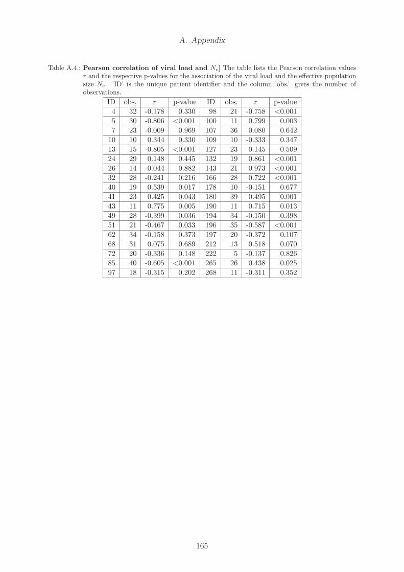
A. Appendix
Table A.4.: Pearson correlation of viral load and Ne] The table lists the Pearson correlation valuesr and the respective p-values for the association of the viral load and the effective populationsize Ne. ’ID’ is the unique patient identifier and the column ’obs.’ gives the number ofobservations.
ID obs. r p-value ID obs. r p-value
4 32 -0.178 0.330 98 21 -0.758 <0.001
5 30 -0.806 <0.001 100 11 0.799 0.003
7 23 -0.009 0.969 107 36 0.080 0.642
10 10 0.344 0.330 109 10 -0.333 0.347
13 15 -0.805 <0.001 127 23 0.145 0.509
24 29 0.148 0.445 132 19 0.861 <0.001
26 14 -0.044 0.882 143 21 0.973 <0.001
32 28 -0.241 0.216 166 28 0.722 <0.001
40 19 0.539 0.017 178 10 -0.151 0.677
41 23 0.425 0.043 180 39 0.495 0.001
43 11 0.775 0.005 190 11 0.715 0.013
49 28 -0.399 0.036 194 34 -0.150 0.398
51 21 -0.467 0.033 196 35 -0.587 <0.001
62 34 -0.158 0.373 197 20 -0.372 0.107
68 31 0.075 0.689 212 13 0.518 0.070
72 20 -0.336 0.148 222 5 -0.137 0.826
85 40 -0.605 <0.001 265 26 0.438 0.025
97 18 -0.315 0.202 268 11 -0.311 0.352
165

A. Appendix
Table A.5.: Graph measures of 6-point mutant networks. The table lists the minimal node fitness,the maximal node betweenness, the maximal node closeness and the average shortest pathlength of the respective R5 and X4 six-point mutant networks, depending on the percentageof the most fit nodes (%) included into the six-point mutant networks.
min. fit. max. bet. max. close. avg. length% R5 X4 R5 X4 R5 X4 R5 X4
1 0.692 0.750 1.2 · 102 2.9 · 103 0.476 0.283 2.349 3.5192 0.592 0.697 6.9 · 103 1.9 · 103 0.404 0.317 3.008 3.2313 0.570 0.672 6.4 · 103 1.8 · 103 0.397 0.320 2.973 3.1944 0.569 0.653 6.4 · 103 1.6 · 103 0.376 0.307 3.043 3.2505 0.544 0.630 4.1 · 103 1.4 · 103 0.356 0.294 3.120 3.3096 0.542 0.604 4.0 · 103 1.3 · 103 0.352 0.282 3.153 3.3897 0.525 0.587 3.3 · 103 1.1 · 103 0.340 0.276 3.193 3.4568 0.500 0.568 2.5 · 103 9.6 · 104 0.343 0.270 3.340 3.5179 0.448 0.537 2.0 · 103 7.9 · 104 0.341 0.262 3.446 3.61210 0.423 0.507 1.6 · 103 6.4 · 104 0.333 0.252 3.542 3.71211 0.421 0.489 1.7 · 103 5.6 · 104 0.328 0.245 3.591 3.77712 0.420 0.481 1.6 · 103 5.0 · 104 0.318 0.251 3.641 3.81713 0.401 0.472 1.4 · 103 4.5 · 104 0.309 0.254 3.684 3.87314 0.401 0.466 1.3 · 103 4.3 · 104 0.303 0.256 3.690 3.90715 0.376 0.457 1.2 · 103 3.8 · 104 0.300 0.256 3.725 3.94216 0.346 0.451 1.1 · 103 3.6 · 104 0.296 0.256 3.773 3.96217 0.331 0.444 9.6 · 104 3.3 · 104 0.296 0.256 3.812 3.99018 0.322 0.438 8.5 · 104 3.1 · 104 0.294 0.254 3.860 4.00919 0.314 0.432 7.6 · 104 2.9 · 104 0.291 0.252 3.903 4.02920 0.310 0.426 7.3 · 104 2.7 · 104 0.288 0.252 3.927 4.04921 0.310 0.422 7.3 · 104 2.7 · 104 0.288 0.251 3.965 4.06422 0.310 0.418 7.2 · 104 2.6 · 104 0.286 0.249 4.005 4.08223 0.301 0.414 6.6 · 104 2.6 · 104 0.283 0.251 4.027 4.09824 0.299 0.411 7.2 · 104 2.5 · 104 0.283 0.250 4.036 4.11125 0.299 0.408 7.1 · 104 2.5 · 104 0.282 0.249 4.045 4.122
166
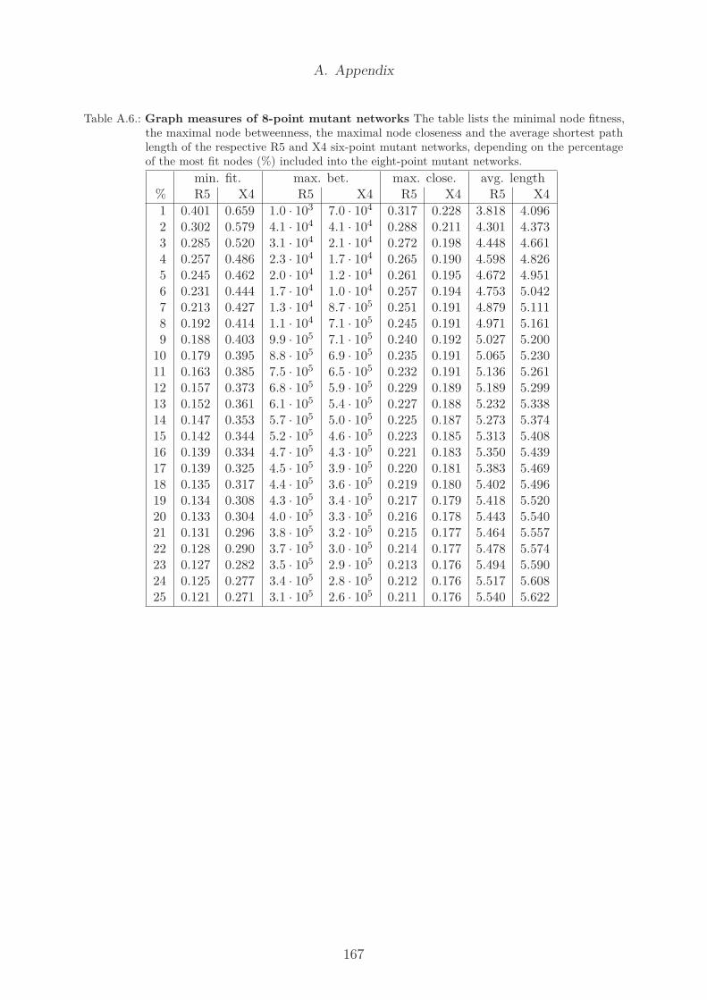
A. Appendix
Table A.6.: Graph measures of 8-point mutant networks The table lists the minimal node fitness,the maximal node betweenness, the maximal node closeness and the average shortest pathlength of the respective R5 and X4 six-point mutant networks, depending on the percentageof the most fit nodes (%) included into the eight-point mutant networks.
min. fit. max. bet. max. close. avg. length% R5 X4 R5 X4 R5 X4 R5 X4
1 0.401 0.659 1.0 · 103 7.0 · 104 0.317 0.228 3.818 4.0962 0.302 0.579 4.1 · 104 4.1 · 104 0.288 0.211 4.301 4.3733 0.285 0.520 3.1 · 104 2.1 · 104 0.272 0.198 4.448 4.6614 0.257 0.486 2.3 · 104 1.7 · 104 0.265 0.190 4.598 4.8265 0.245 0.462 2.0 · 104 1.2 · 104 0.261 0.195 4.672 4.9516 0.231 0.444 1.7 · 104 1.0 · 104 0.257 0.194 4.753 5.0427 0.213 0.427 1.3 · 104 8.7 · 105 0.251 0.191 4.879 5.1118 0.192 0.414 1.1 · 104 7.1 · 105 0.245 0.191 4.971 5.1619 0.188 0.403 9.9 · 105 7.1 · 105 0.240 0.192 5.027 5.20010 0.179 0.395 8.8 · 105 6.9 · 105 0.235 0.191 5.065 5.23011 0.163 0.385 7.5 · 105 6.5 · 105 0.232 0.191 5.136 5.26112 0.157 0.373 6.8 · 105 5.9 · 105 0.229 0.189 5.189 5.29913 0.152 0.361 6.1 · 105 5.4 · 105 0.227 0.188 5.232 5.33814 0.147 0.353 5.7 · 105 5.0 · 105 0.225 0.187 5.273 5.37415 0.142 0.344 5.2 · 105 4.6 · 105 0.223 0.185 5.313 5.40816 0.139 0.334 4.7 · 105 4.3 · 105 0.221 0.183 5.350 5.43917 0.139 0.325 4.5 · 105 3.9 · 105 0.220 0.181 5.383 5.46918 0.135 0.317 4.4 · 105 3.6 · 105 0.219 0.180 5.402 5.49619 0.134 0.308 4.3 · 105 3.4 · 105 0.217 0.179 5.418 5.52020 0.133 0.304 4.0 · 105 3.3 · 105 0.216 0.178 5.443 5.54021 0.131 0.296 3.8 · 105 3.2 · 105 0.215 0.177 5.464 5.55722 0.128 0.290 3.7 · 105 3.0 · 105 0.214 0.177 5.478 5.57423 0.127 0.282 3.5 · 105 2.9 · 105 0.213 0.176 5.494 5.59024 0.125 0.277 3.4 · 105 2.8 · 105 0.212 0.176 5.517 5.60825 0.121 0.271 3.1 · 105 2.6 · 105 0.211 0.176 5.540 5.622
167

A. Appendix
A.2. Amino acid code and chemical properties
Table A.7.: Amino acid code and chemical properties
A ALA Alanine non-polarC CYS Cysteine polarD ASP Aspartic Acid acidicE GLU Glutamic Acid acidicF PHE Phenylalanine non-polarG GLY Glycine polarH HIS Histidine basicI ILE Isoleucine non-polarK LYS Lysine basicL LEU Leucine non-polarM MET Methionine non-polarN ASN Asparagine polarP PRO Proline non-polarQ GLN Glutamine polarR ARG Arginine basicS SER Serine polarT THR Threonine polarV VAL Valine non-polarW TRP Tryptophan non-polarY TYR Tyrosine polar
Table A.8.: Nucleotide code
A Adenine T ThymineC Cytosine G Guanine
168

A. Appendix
A.3. Analytical determination of the mutation rate
The 64 codons are translated into 21 different symbols, 20 amino acids and 3 stop codons.First codon position:19 symbols are altered into a differing symbol upon any nt mutation in the first codon po-sition (19 · 3
4), two symbols are altered due to a mutation into two of four possible nts (2 · 2
4).
19 ·3
4+ 2 ·
2
4=61
4
Second codon position:19 symbols are altered into a differing symbol upon any nt mutation in the second codon po-sition (19 · 3
4), two symbols are altered due to a mutation into two of four possible nts (2 · 2
4).
19 ·3
4+ 2 ·
2
4=61
4
Third codon position: two symbols are altered into a differing symbol upon any nt mu-tation in the third codon position (2 · 3
4), ten symbols are altered due to a mutation
into two of four possible nts (10 · 24), one symbol is altered only upon one specific nt
(1· 14), and eight symbols are not altered by any nt mutation in the third codon position (8· 0
4).
2 ·3
4+ 10 ·
2
4+ 1 ·
1
4+ 8 ·
0
4=27
4
In summary, these considerations result in:
61
4+61
4+27
4=149
4
Based on 21 symbols, the result is divided by 21, resulting in a value of 1.7738. Thisnumber describes, that a mutation in the first, second, and third codon position in parallelalters on average 1.7738 symbols.In consequence, we need on average 3 · 1
1.7738= 1.69 nucleotide mutations to produce an
average of one amino acid mutation per replication. Adapted to a nt sequence length of105, this consideration results in a mutation rate of 1.69
105= 0.016.
169

A. Appendix
A.4. Alphabetical list of frequently used abbreviations
aa amino acid
ART antiretroviral therapy
bp basepair
CCR5 one of the two predominant HIV-1 co-receptors, often used in the early tolatent phase of infection
CXCR4 one of the two predominant HIV-1 co-receptors, in about 50% of patientsused in latent to late phase of infection
CC cross correlation
CD4+ T-cell bearing CD4 receptor
CDC United States Centers for Disease Control and Prevention
DNA deoxyribonucleic acid
FPR false positive rate
HAART highly active antiretroviral therapy
nt nucleotide
MI mutual information
MSA multiple sequence alignment
MRCA most recent common ancestor
mRNA messenger RNA
PBMC peripheral blood mononuclear cell
PCR polymerase chain reaction
R5 short form of the CCR5 co-receptor
RNA ribonucleic acid
SUMI subset mutual information
X4 short form of the CXCR4 co-receptor
V3 third variable loop, a specific region of the HIV-1 envelope gene, which iscrucial in co-receptor binding and cell entry
HIV (HIV-1) human immunodeficiency virus (type 1)
AIDS acquired immunodeficiency syndrome
env envelope gene of HIV-1
gp glycoprotein
RT reverse transcriptase, a central HIV protein
WHO World Health Organization
170

A. Appendix
Last but not least ...
Vielen Dank an alle, die mich durch meine Promotionszeit begleitet haben!
Der erste Dank gebuhrt Christel, Barbara und Peter, die mir die Chance gaben, unter
ihrer Anleitung an einem tollen Thema zu arbeiten und die meine Doktorarbeit stets mit
Interesse und zahlreichen guten Ideen und Ratschlagen unterstutzt haben.
Danke an Kay, der mich als externe Doktorandin in seine Gruppe aufgenommen hat,
obwohl er meist alle Hande voll zu tun hat. Die Diskussionen in der AG Hamacher haben
mir so manches mal eine neue Perspektive auf meine Arbeit eroffnet. Nicht zu vergessen
der wochentliche Brunch, fur den ich sogar ab und an ein Mittagessen mit Kollegen am PEI
hab’ sausen lassen. Aber nicht nur die Zeit mit euch, sondern auch mit euren zahlreichen
Gaste war immer eine Bereicherung, und allzu oft musste ich die Runde verlassen, wenn
ich gerne noch geblieben ware.
Auch meinen Kollegen hier am PEI mochte ich herzlich fur die gemeinsame Zeit danken.
Trotz vieler Umzuge war ich in der Nachbarschaft jedes meiner wechselnden Buros stets
willkommen und wurde mit offenen Armen empfangen. Auch wenn uns thematisch
meist wenig verband, haben wir beim Mittagessen oder auf dem Flur am Drucker viele
interessante Gesprache gefuhrt.
Danke an Barbaras Gruppe, und insbesondere an Sarah, die meine Kenntnisse uber die
Methoden im Labor und die mit den Analysen verbundenen Schwierigkeiten erweitert
haben. Danke an Jan, der sich jederzeit bereit erklart hat, mit mir mathematische
Fragestellungen zu erortern oder zur rechten Zeit gemeinsam eine Pause von der Arbeit
einzulegen. Danke an Kay fur die Unterstutzung bei den statistischen Auswertungen.
Auch Susanne mochte ich auf diesem Weg nochmal danke sagen fur die gemeinsamen
Monate im Buro.
Ein besonderer Dank geht an die liebste Saarlanderin im fernen Hessen. Es ist sehr schade,
dass wir uns erst so spat beim Joggen im Wald begegnet sind. Auf die gemeinsamen
Runden habe ich mich immer den ganzen Tag gefreut. Und auch Barbara hat uns so
maches Mal begleitet, wenn es ihre Zeit und das Wetter zugelassen haben.
Meinen Freunden zu hause danke ich, dass sie trotz der wenigen gemeinsamen Zeit den
Kontakt nicht haben einschlafen lassen. Ich hoffe sehr, dass wir in Zukunft wieder mehr Zeit
miteinander verbringen konnen und dass der abgesagte gemeinsame Urlaub im nachsten
Jahr statt findet.
Auch meine Familie und insbesondere mein Mann mussten viele Stunden wahrend der
letzten Jahre ohne mich verbringen. Danke, dass ihr auch uber viele Kilometer Entfernung
stets fur mich da wart, euch gemeinsam mit mir gefreut und mir in schwierigen Zeiten
Kraft gegeben habt - auch dann, wenn ich selbst manchmal nicht fur euch da sein konnte,
wenn ich es gerne gewesen ware.
Danke auch an all die, die bisher unerwahnt geblieben sind. An Alexander Thielen fur
die Durchfuhrung der Korezeptor Vorhersagen, an die projektverantwortlichen fur die
finanzielle Unterstutzung dieser wichtigen Forschung, an meine Doktorandenkollegen hier
am PEI, die mir die drei Jahre zu einer angenehmen Zeit gemacht haben.
171

Curriculum Vitae
Personal
Name Miriam Carbon-Mangels
Date of Birth 24.09.1977
Place of Birth Zweibrücken
Career
1984 - 1988 Grundschule Sechsmorgen, Zweibrücken
1988 - 1997 Helmholtz-Gymnasium, Zweibrücken
1997 - 2000 training on the job, Tax consultant assistant, Dr. Meyer und Partner, Pirmasens
2000 - 2005 Tax consultant assistant, StB Kämmerer, Kaiserslautern
2005 - 2010 study of Bioinformatics at the University of Saarland, Saarbrücken,
BA-Thesis In Silico Models for the Prediction of Metabolism by Cytochrome P450 Enzymes, MA-Thesis TNF alpha Antibody Design
2010 - 2013 PhD at Paul-Ehrlich-Institut, Langen, and TU Darmstadt, Intra-host HIV-1 evolution and the co-receptor switch
Presentations
2010 3. HIV-Resistenz-Workshop, Berlin, Oral Presentation, Ausblick HIV-Projekt
5th PEI Retreat, Kröckelbach, Oral Presentation, Tracing intra-host HIV evolution by phylogenetic analysis
2011 AREVIR-Meeting, Bonn, Oral Presentation, Comparative study of intra-host HIV evolution: Emergence of viral diversity
12th International Conference on Systems Biology (ICSB), Mannheim, Poster Presentation, Tracing intra-host HIV evolution by phylogenetic analysis
2012 6th PEI Retreat, Tagungsstätte Löwenstein, Poster Presentation, Correlating clinical and evolutionary parameters in intra-patient HIV evolution
2013 7th PEI Retreat, Tagungsstätte Löwenstein, Oral Presentation, Development of a fitness function for the V3 loop of HIV-1