Interplay between dividend rate and business constraints for a ...

arX

iv:m

ath/

0503

541v

1 [

mat

h.PR

] 2

4 M

ar 2

005

The Annals of Applied Probability

2004, Vol. 14, No. 4, 1810–1837DOI: 10.1214/105051604000000909c© Institute of Mathematical Statistics, 2004

INTERPLAY BETWEEN DIVIDEND RATE AND BUSINESS

CONSTRAINTS FOR A FINANCIAL CORPORATION

By Tahir Choulli1, Michael Taksar2 and Xun Yu Zhou3

University of Alberta, University of Missouri

and Chinese University of Hong Kong

We study a model of a corporation which has the possibility tochoose various production/business policies with different expectedprofits and risks. In the model there are restrictions on the dividenddistribution rates as well as restrictions on the risk the company canundertake. The objective is to maximize the expected present valueof the total dividend distributions. We outline the correspondingHamilton–Jacobi–Bellman equation, compute explicitly the optimalreturn function and determine the optimal policy. As a consequenceof these results, the way the dividend rate and business constraintsaffect the optimal policy is revealed. In particular, we show that un-der certain relationships between the constraints and the exogenousparameters of the random processes that govern the returns, somebusiness activities might be redundant, that is, under the optimalpolicy they will never be used in any scenario.

1. Introduction. In recent years we have seen a lot of new results inthe application of diffusion optimization models to financial mathematics.Together with portfolio optimization models, dividend distribution and riskcontrol models have undergone major development.

In typical models of this type (see [[2], [3], [8]–[11], [13], [14], [16]]), the liq-uid assets of the company are governed by a Brownian motion with constantdrift and diffusion coefficients. The drift term corresponds to the expected(potential) profit per unit time, while the diffusion term is interpreted asrisk. The decrease of risk from business activities corresponds to a decrease

Received December 2002; revised March 2003.1Supported by the Department of Systems Engineering and Engineering Management

at the Chinese University of Hong Kong and NSERC Grant 121210818.2Supported by NSF Grant DMS-00-72388.3Supported by RGC Earmarked Grant CUHK 4054/98E.AMS 2000 subject classifications. 91B70, 93E20.Key words and phrases. Diffusion model, dividend distribution, business constraints,

risk control, optimal stochastic control, HJB equation.

This is an electronic reprint of the original article published by theInstitute of Mathematical Statistics in The Annals of Applied Probability,2004, Vol. 14, No. 4, 1810–1837. This reprint differs from the original inpagination and typographic detail.

1

http://arxiv.org/abs/math/0503541v1

http://www.imstat.org/aap/

http://dx.doi.org/10.1214/105051604000000909

http://www.imstat.org

http://www.ams.org/msc/

http://www.imstat.org

http://www.imstat.org/aap/

http://dx.doi.org/10.1214/105051604000000909

2 T. CHOULLI, M. TAKSAR AND X. Y. ZHOU

in potential profits. Different business activities in these models correspondto changing the drift and the diffusion coefficients of the underlying processsimultaneously. This sets the scene for an optimal stochastic control modelwhere the controls affect not only the drift, but also the diffusion part of thedynamic of the system.

In this article we study a model with an explicit restriction on risk controland on the rate at which the dividends are paid out. In addition, the companymay have liability which it has to pay out at a constant rate no matter whatthe business plan is.

The controls are described by two functionals at and ct. The first rep-resents the degree of business activity which the company assumes. Theprocess at takes on values in the interval [α,β], 0< α< β ≤+∞. The risk,which in our model is associated with the diffusion coefficient, and the poten-tial profit, which is associated with the drift coefficient of the correspondingprocess, are both proportional to at. The constraints on the values of at re-flect institutional or statutory restrictions (e.g., for a public company) thatthe risk it can assume cannot exceed a certain level or that its businessactivities cannot be reduced to zero unless the company goes bankrupt.

The value ct of the second control functional shows the rate at whichdividends are paid out at time t. The dividends are paid out from the liquidreserve and are distributed to shareholders. This corresponds to ct enteringthe drift coefficient of the reserve process with a negative sign. The dividendrate is bounded by a constant M given a priori.

In our model we also assume the existence of a constant rate liabilitypayment, such as a mortgage payment on a property or amortization ofbonds. The results of this model can be viewed as an extension of the resultsof Choulli, Taksar and Zhou [4]. The presence of dividend rate constraints,however, adds a whole new dimension to the analysis as well as to thequalitative structure of the results obtained.

What is the most interesting is the interplay between the constraints andthe exogenous parameters that govern the process of returns. Depending onthe relationship between these parameters, we get several distinct cases ofqualitative behavior of the company under the optimal policy.

This article is structured as follows. In the next section we present a rigor-ous mathematical formulation of the problem and state general properties ofthe optimal return or the value function. We also write the Hamilton–Jacobi–Bellman (HJB) equation this function must satisfy. In Section 3 we find abounded smooth solution to the HJB equation. In Section 4 we constructthe optimal policy and present our main findings in table form. Finally, inSection 5 we describe some economic interpretation of the results and stateconclusions.

DIVIDEND RATE AND BUSINESS CONSTRAINTS 3

2. Mathematical model. We start with a filtered probability space (Ω,F ,Ft, P )and a one-dimensional standard Brownian motion Wt (with W0 = 0) on it,adapted to the filtration Ft. We denote by Rπ

t the reserve of the companyat time t under a control policy π = (aπt , c

πt ; t≥ 0) (to be specified below).

The dynamic of the reserve process Rπt is described by

dRπt = (aπt µ− δ)dt+ aπt σ dWt − cπt dt, Rπ

0 = x,(2.1)

where µ is the expected profit per unit time (profit rate), σ is the volatilityrate of the reserve process (in the absence of any risk control), δ representsthe amount of money the company has to pay per unit time (the debt rate)irrespective of what business activities it chooses and x is the initial reserve.

The control in this model is described by a pair of Ft-adapted processesπ = (aπt , c

πt ; t ≥ 0). A control π = (aπt , c

πt ; t ≥ 0) is admissible if α ≤ aπt ≤

β and 0 ≤ cπt ≤ M ∀ t ≥ 0, where 0 < α < β < +∞ and 0 < M < +∞ aregiven scalars. We denote the set of all admissible controls by A. The controlcomponent aπt represents one of the possible business activities available forthe company at time t, and the component cπt corresponds to the dividendpayout rate at time t.

Given a control policy π, the time of bankruptcy is defined as

τπ = inft≥ 0 :Rπt = 0.(2.2)

The performance functional associated with each control π is

Jx(π) =E

(∫ τπ

0e−γtcπt dt

)

,(2.3)

where γ > 0 is an a priori given discount factor (used to calculate the presentvalue of the future dividends), and the subscript x denotes the initial statex. The objective is to find

v(x) = supπ∈A

Jx(π)(2.4)

and the optimal policy π∗ such that

Jx(π∗) = v(x).(2.5)

The exogenous parameters of the problem are µ, σ, δ, α, β and γ. The aimof this article is to obtain the optimal return function v and the optimalpolicy explicitly in terms of these parameters.

The main tools for solving the problem are the dynamic programmingand HJB equation (see [[6], [7] and [17]] as well as relevant discussions in[[2], [9] and [16]]). We start by stating the following properties of the optimalreturn function v.


Proposition 2.1. The optimal return function v is a concave, nonde-

creasing function subject to v(0) = 0 and

0≤ v(x)≤ M

γ∀x> 0.(2.6)

Proof. The proof of the concavity and the monotonicity as well as theboundary condition, v(0) = 0, is similar to the one in [4]. To show (2.6),consider

0≤E

(∫ τπ

0e−γtcπt dt

)

≤M

∫ ∞

0e−γt dt=

M

γ.

If the optimal return function v is twice continuously differentiable, thenit must be a solution to the HJB equation

0 = maxα≤a≤β,0≤c≤M

( 12σ2a2V ′′(x) + (aµ− δ− c)V ′(x)− γV (x) + c)

≡ maxα≤a≤β

( 12σ2a2V ′′(x) + (aµ− δ)V ′(x)− γV (x) +M(1− V ′(x))+)(2.7)

V (0) = 0,

where x+ =max(x,0). This equation is rather standard and its derivationcan be found in [[6], [7], and [17]]; see also [9] and [10].

Note that we do not know a priori whether the HJB equation has any so-lution other than the optimal return function. However, the following verifi-cation theorem, which says that any concave solution V to the HJB equation(2.7) whose derivative is finite at 0 majorizes the performance functional forany policy π, is sufficient for us to identify optimal policies.

Theorem 2.2. Let V be a concave, twice continuously differentiable so-

lution of (2.7), such that V ′(0)<+∞. Then, for any policy π = (aπt , cπt ; t≥

0),

V (x)≥ Jx(π).(2.8)

Proof. Let Rπt be the reserve process given by (2.1). Denote the oper-

ator

La =1

2σ2a2

d2

dx2+ (aµ− δ)

d

dx− γ.

Then by applying Ito’s formula (see [5], Theorem VIII.27) to the processe−γtV (Rπ

t ), we get

e−γ(t∧τ)V (Rπt∧τ ) = V (x) +

∫ t∧τ

0e−γsσaπsV

′(Rπs )dWs

(2.9)

+

∫ t∧τ

0e−γsLaπs V (Rπ

s )ds−∫ t∧τ

0e−γsV ′(Rπ

s )cπs ds.


Since V is nondecreasing, concave with finite derivative at the origin, V ′(x) isbounded and the stochastic integral in (2.9) is a square integrable martingalewhose expectation vanishes. In view of the HJB equation (2.7) and theinequality cπs ≤M , we have

Laπs V (Rπs )≤−cπs (1− V ′(Rπ

s ))+.(2.10)

Taking expectations of both sides of (2.9), in view of (2.10) we get

E(e−γ(t∧τ)V (Rπt∧τ ))

(2.11)

≤ V (x)−E

∫ t∧τ

0e−γscπs [V

′(Rπs ) + (1− V ′(Rπ

s ))+]ds.

Combining (2.11) with the fact that y+ (1− y)+ ≥ 1, we get

E(e−γ(t∧τ)V (Rπt∧τ )) +E

∫ t∧τ

0e−γscπs ds≤ V (x).(2.12)

Note that in view of the boundedness of V ′,

e−γ(t∧τ)V (Rπt∧τ )≤ e−γtK(1 +Rπ

t∧τ )≤ e−γtK(1 + |Rπt |)

for some constant K. Since Rπt is a diffusion process with uniformly bounded

drift and diffusion coefficient, standard arguments yield E|Rπt | ≤ x+K1t for

some constant K1. Therefore,

Ee−γ(t∧τ)V (Rπt∧τ )→ 0(2.13)

as t→∞. Thus taking the limit in (2.12) as t→∞, we arrive at

V (x)≥E

∫ τ

0e−γscπs ds= Jπ(x).

The idea of solving the original optimization problem is first to find aconcave, smooth function to the HJB equation (2.7) and then to construct acontrol policy [by solving a stochastic differential equation (SDE); for detailssee Section 4] whose performance functional can be shown to coincide withthe solution to (2.7). Then, the above verification theorem establishes theoptimality of the constructed control policy. As a by-product, there is noother concave solution to (2.7) than the optimal return function.

3. A smooth solution to the HJB equation. In this section, we are look-ing for a concave, smooth solution to (2.7). Assume that such a solution Vhas been found. Let

x1 = infx≥ 0 :V ′(x)≤ 1.(3.1)

Then, for 0≤ x < x1, (2.7) becomes

0 = maxα≤a≤β

(12σ2a2V ′′(x) + (aµ− δ)V ′(x)− γV (x)),(3.2)


while for x≥ x1, (2.7) can be rewritten as

0 = maxα≤a≤β

(12σ2a2V ′′(x) + (aµ− δ −M)V ′(x)− γV (x) +M).(3.3)

We start by seeking a smooth solution to (3.3). Obviously if V ′(0)≤ 1, thenx1 = 0 and (2.7) is equivalent to (3.3) for all x≥ 0.

Proposition 3.1. If βµ≤ δ, then V ′(0)< 1.

Proof. It follows from (2.7) that there exist a ∈ [α,β] such that

0 = 12σ

2a2V ′′(0) + (aµ− δ)V ′(0) +M(1− V ′(0))+.(3.4)

If βµ < δ, then each of the first two terms on the right-hand side of (3.4) isnonpositive with the second being strictly negative. Therefore,M(1− V ′(0))+ > 0,which implies V ′(0)< 1. The same argument goes if βµ= δ and V ′′(0)< 0.In this case, either the first or the second term on the right-hand side of (3.4)is strictly negative. If βµ= δ and V ′′(0) = 0, then the maximizer of the right-hand side of (2.7) is equal to β for all x in a right neighborhood of 0 [recallthat V ′(0)> 0]. Substituting a= β either into (3.2) or into (3.3) and solvingthe resulting linear ordinary differential equation (ODE) with constant co-efficients, we get a function V whose second derivative at 0 does not vanish,which is a contradiction.

Remark 3.2. When the dividend rates are unrestricted, the conditionβµ≤ δ makes the problem trivial (see [4], Theorem 4.1). This is not the casewhen the dividend rates are bounded. Even if βµ≤ δ, the second derivativeof V at 0 is strictly negative, which makes the problem nontrivial in contrastto a similar situation in the case of unrestricted dividends.

Now we analyze the solution to (3.3) under the condition βµ > δ. As we seelater, the qualitative nature of this solution depends on whether a(x1)< αor α≤ a(x1)< β or a(x1)≥ β, where

a(x)≡− µV ′(x)

σ2V ′′(x)> 0, x < x1.(3.5)

To this end, we need the following proposition:

Proposition 3.3. (i) If a(x1)≥ α, then, for each x≥ x1,

a(x)≥ α.(3.6)

(ii) If a(x1)≥ β, then, for each x≥ x1,


a(x)≥ β.(3.7)

Proof. (i) Suppose there exists x0 >x1 such that a(x0)< α. Then thereexists ε > 0 such that a(x)<α for each x with |x−x0|< ε. Let x′ = supx1 ≤x < x0 :a(x) = α. Then x1 ≤ x′ < x0 < x0 + ε and a(x′) = α. Since a(x)≤ αfor all x ∈ [x′, x0+ε), the function V satisfies (3.3) with the maximum thereattained at a= α. Therefore,

V (x) =M

γ+K1 exp(r+(α)(x− x′)) +K2 exp(r−(α)(x− x′))

(3.8)∀x∈ [x′, x0 + ε).

Here

r+(z)≡−(zµ− δ−M) +

√(zµ− δ −M)2 +2γσ2z2

z2σ2,(3.9)

r−(z)≡−(zµ− δ−M)−

√(zµ− δ −M)2 +2γσ2z2

z2σ2, z > 0.(3.10)

From (3.8) and (3.5), the equation a(x′) = α can be rewritten as

K1r+(α) =−K2r−(α)µ+ ασ2r−(α)

µ+ ασ2r+(α),

which establishes a relationship between the constants K1 and K2. Usingthis relationship, we calculate

a(x) =−µV ′(x)

σ2V ′′(x)

=

(

−µ

(

exp((r+(α)− r−(α))(x− x′))− µ+ασ2r+(α)

µ+ασ2r−(α)

))

×(

σ2(

r+(α) exp((r+(α)− r−(α))(x− x′))(3.11)

− r−(α)µ+ασ2r+(α)

µ+ασ2r−(α)

))−1

∀x∈ [x′, x0 + ε).

However, we have a(x)< α for x > x′, which after a simple algebraic trans-formation of (3.11) is equivalent to exp((r+(α)− r−(α))(x − x′))< 1. Thisleads to a contradiction. Therefore (3.6) holds.


(ii) By virtue of the assertion (i), a(x)≥ α for all x≥ x1. Suppose thereexists x′ >x1 such that a(x′)< β. Then there exists ε > 0 such that a(x)< βfor all x< x′ + ε. Let x= supx1 ≤ x < x′ :a(x) = β. Then x1 ≤ x < x′ anda(x) = β. In addition α≤ a(x)< β for all x < x≤ x′. Substituting a≡ a(x)and V ′′(x) =−(µV ′(x))/(σ2a(x)) into (3.3), we get

0 =µa(x)

2V ′(x)− (δ +M)V ′(x)− γV (x) +M.(3.12)

Differentiating (3.12) and again substituting V ′′(x) = −(µV ′(x))/(σ2a(x))into the resulting equation, we obtain

a(x)a′(x) = (a(x)− c)µ2 +2σ2γ

µσ2.(3.13)

Then integrating (3.13) we get

a(x)− a(x) + c log

(

a(x)− c

a(x)− c

)

= (x− x)µ2 +2σ2γ

µσ2> 0

(3.14)∀ x < x < x′,

which is a contradiction. Hence (3.7) holds and this completes the proof ofthe proposition.

First suppose that a(x1) ≥ β. In view of Proposition 3.3(i), we deducethat a(x)≥ β for each x≥ x1. Substituting a= β into (3.3) and solving theresulting equation, we get

V (x) =M

γ+Kβ exp(r−(β)(x− x1)) ∀x≥ x1.

Here Kβ is a constant which takes on either the value −Mγ or 1/(r−(β))

depending, respectively, on whether x1 in (3.1) is zero or not. Then straight-forward calculations show that a(x) = −µ/(σ2r−(β)). Thus, the conditiona(x1)≥ β is equivalent to

c≡ 2µ(δ +M)

µ2 + 2γσ2≥ β.(3.15)

Next suppose α≤ a(x1)< β. By virtue of Proposition 3.3(i), a(x)≥ α for allx≥ x1. As a result, α≤ a(x)< β in a right neighborhood of x1. Substitutinga ≡ a(x) and V ′′(x) = −(µV ′(x))/(σ2a(x)) into (3.3), we deduce that a(x)satisfies (3.12). Then, following the same analysis there, we derive equation(3.13) for a(x).

Suppose there exists x′ ≥ x1 such that a(x′) < c [resp., a(x′) > c]. Thenfrom (3.13) we deduce that a(x)< c [resp., a(x)> c] for each x≥ x′. Thus,


by integrating (3.13) we derive (3.14) for all x≥ x′, with x replaced by x′.

From (3.12) and (2.6), we see that a(x) ≤ 2(δ+M)µ ∀x≥ x1. Therefore, the

left-hand side of (3.14) is bounded. This is a contradiction and we concludethat a(x) = c for each x ≥ x1. In view of the above results, the conditionα ≤ a(x1) < β can be rewritten as α ≤ c < β. Now, substituting a= c into(3.3) and solving the resulting equation [noting that r−(c) = −σ2c/µ], weget

V (x) =M

γ+ K exp

(

−σ2c

µ(x− x1)

)

∀x≥ x1,

where K is a constant which takes on either the value of −Mγ or −µ/(σ2c)

depending, respectively, on whether x1 = 0 or x1 > 0.Finally, suppose that a(x1) < α. Then it follows from the above results

that c < α. Therefore a(x) < α for all x in a right neighborhood of x1.Substituting a = α into (3.3) and solving the resulting linear differentialequation, we get

V (x) =M

γ+K1(α) exp(r+(α)(x−x1))+K2(α) exp(r−(α)(x−x1)),(3.16)

where K1(α) and K2(α) are free constants. If K1(α) > 0, then the right-hand side of (3.16) is unbounded on [x1,∞), which contradicts (2.6). IfK1(α) < 0, then the right-hand side of (3.16) becomes negative for x largeenough, which again is a contradiction. Hence K1(α) = 0. On the other hand,we have K2(α)< 0 in view of V ′′(0)< 0. Therefore,

V (x) =M

γ+Kα exp(r−(α)(x− x1)),

where Kα is a constant that takes on the value either −Mγ or 1/(r−(α))

depending on whether x1 is zero or not. Combining the above results, wecan formulate the following theorem.

Theorem 3.4. Let r−(α), r−(β) and c be the constants given by (3.10)and (3.15), respectively. Let x1 be defined by (3.1). Then for x1 = 0 (resp.,for x1 > 0) the following assertions hold.

(i) If c≥ β, then

V (x) =M

γ+Kβ exp(r−(β)(x− x1)), x≥ x1,(3.17)

is a concave, twice differentiable solution of the HJB equation (3.3) on

[x1,∞), where Kβ is equal to −Mγ [resp., to 1/(r−(β))].


(ii) If α≤ c < β, then,

V (x) =M

γ+ K exp

(−µ

σ2c(x− x1)

)

, x≥ x1,(3.18)


[x1,∞), where K is equal to −Mγ [resp., to −µ/(σ2c)].

(iii) If c < α, then,

V (x) =M

γ+Kα exp(r−(α)(x− x1)), x≥ x1,(3.19)


[x1,∞), where Kα is a constant equal to −Mγ [resp., to 1/(r−(α))].

Corollary 3.5. If x1 = 0, then the solution to (2.7) subject to (2.6) isgiven by

V (x) =

M

γ(1− exp(r−(β)x)), if c≥ β,

M

γ

(

1− exp

(−µ

σ2cx

))

, if α≤ c < β, ∀x≥ 0,

M

γ(1− exp(r−(α)x)), if c < α.

Corollary 3.5 shows that the qualitative nature of the solution depends onthe relationship between 2δ

µ , α and β. Accordingly, we consider three cases.However, in contrast to the situation with unbounded dividend rates, eachcase here will consist of several subcases, each subcase being associated witha different range for the value of M .

Remark 3.6. If neither −Mγ r−(β)≤ 1 when c≤ β nor M

γ (µ/(σ2c))≤ 1

when α≤ c < β nor −Mγ r−(α)≤ 1 when c < α is satisfied, then the solution

to (2.7) satisfies

V ′(0)> 1.

The main purpose of the remaining part is to derive the solution to (3.2)and then to combine the latter with Theorem 3.4. The solution to (3.2) isbased mainly on the value of a(0). Thus, first of all, we present an analysisof a(0).

Proposition 3.7. Suppose the assumptions of Remark 3.6 hold. Then:

(i) 2δµ < α if and only if a(0)< α. In this case a(0) = (µα2)/(2(µα− δ)).

(ii) α≤ 2δµ < β if and only if α≤ a(0)< β. In this case a(0) = 2 δ

µ .


(iii) β ≤ 2δµ if and only if a(0)≥ β. In this case a(0) = (µβ2)/(2(µβ− δ)).

Proof. In view of the assumption of Remark 3.6, assume that x1 ispositive. Let a ∈ [α,β] be such that

0 = maxα≤a≤β

( 12σ2a2V ′′(0) + (aµ− δ)V ′(0))

(3.20)= 1

2σ2a2V ′′(0) + (aµ− δ)V ′(0).

Comparing (3.20) to (3.5) we obtain

a2 − 2a(0)a+2δ

µa(0) = 0.(3.21)

From (3.21), it follows that a(0)≥ 2δµ . Moreover, by definition, a(0) ∈ [α, β]

is equivalent to a= a(0), which is further equivalent to a(0) = 2δµ ∈ [α, β].

Thus we conclude:

(i) If a(0)< α, then 2δµ ≤ a(0)< α. Conversely, suppose 2δ

µ < α. If a(0) ∈[α,β], then by the above results a(0) = 2δ

µ < α, which is a contradiction.

Thus either a(0) < α or a(0) > β. Suppose a(0) > β. Then a = β and by(3.21), a(0) = (µβ2)/(2(µβ − δ)) < β (due to 2δ

µ < α < β). This is again a

contradiction. Hence we have a(0) < α. Then a= α, and in view of (3.21),we get a(0) = (µα2)/(2(αµ− δ)).

(ii) Suppose α ≤ 2δµ < β. Then due to (i) we have a(0) ≥ α. Now we

proceed to prove that a(0)≤ 2δµ < β. Suppose a(0)> 2δ

µ . Then a(0)> β ≡ a.

On the other hand, in view of (3.21), we have a(0) = (µβ2)/(2(βµ − δ));thus (µβ2)/(2(βµ− δ)) ≥ β, which is equivalent to 2 δ

µ ≥ β. This, however, is

a contradiction and therefore a(0) = 2δµ ∈ [α,β). Conversely, if a(0) ∈ [α,β),

then a(0) = 2δµ ∈ [α,β).

(iii) Suppose β ≤ 2δµ . Then a(0) ≥ 2δ

µ ≥ β, leading to a = β and a(0) =

(µβ2)/(2(βµ−δ))≥ β. Conversely, if a(0)≥ β, then a= β and a(0) = (µβ2)/(2(µβ−δ))≥ β, which is equivalent to 2δ

µ ≥ β.

3.1. Case of 2δµ < α. To resolve equation (3.2), we begin our analysis

with an observation that in this case, in view of Proposition 3.7(i), a(x)< αfor all x in the right neighborhood of 0. We also suppose that a(x1) > β.This assumption is not a restriction, but gives us the solution of (3.2) thatcorresponds to the maximal interval [0, x1). Substituting a≡ α in (3.2) andsolving the resulting second-order linear ODE, we obtain

V (x) = k1(α,β)(exp(r+(α)x)− exp(r−(α)x)),(3.22)


where k1(α,β) is a free constant to be determined and

r+(z) =−(zµ− δ) + [(zµ− δ)2 + 2σ2z2γ]1/2

σ2z2,

(3.23)

r−(z) =−(zµ− δ)− [(zµ− δ)2 + 2σ2z2γ]1/2

σ2z2, z > 0.

Due to (3.5) and (3.22),

a′(x) =−µ

σ2

(V ′′(x))2 − V ′(x)V (3)(x)

(V ′′(x))2

=−µr+(α)r−(α) exp((r+(α) + r−(α))x)(r+(α)− r−(α))

2

σ2(V ′′(x))2> 0

for each x in the right neighborhood of 0. Therefore a(x) increases andreaches α at the point xα given by

xα =1

r+(α)− r−(α)log

(

r−(α)(µ+ασ2r−(α))

r+(α)(µ+ασ2r+(α))

)

> 0.(3.24)

By virtue of Proposition 3.3(i), α ≤ a(x) < β in the right neighborhood ofxα. In this case we substitute a≡ a(x) and

V ′′(x) =−µV ′(x)

σ2a(x)(3.25)

into (3.2), differentiating the resulting equation and substituting

V ′′(x) =−µV ′(x)

σ2a(x)

once more, we arrive at

µa′(x)

2+

µδ

σ2a(x)=

µ2 +2γσ2

2σ2.

As a result,

a′(x) =µ2 + 2γσ2

µσ2

(

1− c

a(x)

)

(3.26)

with

c≡ 2δµ

µ2 +2γσ2.(3.27)

Integrating (3.26), we get G(a(x)) ≡ ((µ2 + 2γσ2)/(µσ2))(x − xα) +G(α),where

G(u) = u+ c log(u− c).(3.28)


Therefore,

a(x) =G−1(

µ2 +2γσ2

µσ2(x− xα) +G(α)

)

.(3.29)

Thus a(x) is increasing and a(xβ) = β for

xβ ≡ µσ2

µ2 +2γσ2[G(β)−G(α)] + xα

(3.30)

=µσ2

µ2 +2γσ2(β − α) +

µσ2c

µ2 + 2γσ2log

(

β − c

α− c

)

.

Solving (3.25) we obtain

V (x) = V (xα) + V ′(xα)

∫ x

xα

exp

(

− µ

σ2

∫ y

xα

du

a(u)

)

dy, xα ≤ x < xβ,(3.31)

where V (xα) and V ′(xα) are free constants. Choosing V (xα) and V ′(xα) asthe value and the derivative, respectively, of the right-hand side of (3.22)at xα, we can ensure that the function V given by (3.22) and (3.31) iscontinuous with its first and second derivatives at the point xα no matterwhat the choice of k(α,β) is. (Note that due to the HJB equation, continuityof V and its first derivative at xα automatically implies continuity of thesecond derivative as well.) Next we simplify (3.31). First, changing variablesa(u) = θ we get

∫ x

xα

exp

(

− µ

σ2

∫ y

xα

du

a(u)dy

)

=µσ2

µ2 + 2γσ2

∫ a(x)

α

(

1 +c

θ− c

)(

θ− c

α− c

)−Γ

dθ, xα ≤ x < xβ.

On the other hand, relationships (3.24) and (3.22) imply

V (xα) =αµ− 2δ

2γV ′(xα).

Simple algebraic transformations yield(

µσ2

µ2 +2γσ2

)(

c

Γ− z − c

1− Γ

)

=zµ− 2δ

2γ∀ z > 0,(3.32)

where c is given by (3.27) and

Γ =µ2

µ2 + 2γσ2.(3.33)

Therefore,

V (x) = V ′(xα)µa(x)− 2δ

2γ

(

a(x)− c

α− c

)−Γ

, xα ≤ x < xβ.(3.34)


The same arguments as in Proposition 3.3(ii) show that a(x) ≥ β for eachx≥ xβ . Thus, substituting a≡ β into (3.2) and solving the resulting ODE,we get

V (x) = k1(β) exp(r+(β)(x− x1)) + k2(β) exp(r−(β)(x− x1)),(3.35)

xβ ≤ x < x1,

where k1(β) and k2(β) are two free constants to be determined. The continu-ity of (3.31) at xβ , together with simple but tedious algebraic transformation[similar to those used above to simplify (3.31) to (3.34)] lead to

V ′(xα) = V ′(xβ)

(

β − c

α− c

)Γ

.(3.36)

Let c be given by (3.15) and

Mz =

(

z − 2δµ

µ2 +2σ2γ

)

µ2 + 2σ2γ

2µ, z > 0.(3.37)

Then c≥ β (resp., c= β ) is equivalent to M ≥Mβ (resp., M =Mβ). Thisis the first subcase we consider.

3.1.1. Case of M >Mβ . Our assumptions imply that in this case, a(x1)> β,which is equivalent to x1 >xβ . Combining (3.22), (3.34) and (3.35) and The-orem 3.4(i) we can write a general form of the solution to (2.7) and (2.6),

V (x) =

K1(α,β)(exp(r+(α)x)− exp(r−(α)x)), 0≤ x < xα,

V ′(xα)µa(x)− 2δ

2γ

(

a(x)− c

α− c

)−Γ

, xα ≤ x < xβ,

K1(β) exp(r+(β)(x− x1))+K2(β) exp(r−(β)(x− x1)), xβ ≤ x < x1,

M

γ+

1

r−(β)exp(r−(β)(x− x1)), x≥ x1,

(3.38)

where r+(α), r−(α), r+(β) and r−(β), xα and xβ are given by (3.23),(3.24) and (3.30), respectively, and K1(β), K2(β), K1(α,β) and x1 are un-known constants to be determined. Continuity of the first and the secondderivatives at x1 results in

V ′(x1) = 1, V ′′(x1) = r−(β).

This gives us two equations,

1 =K1(β)r+(β) +K2(β)r−(β),

r−(β) =K1(β)r2+(β) +K2(β)r

2−(β),


whose solutions are

K1(β) =r−(β)− r−(β)

r+(β)(r+(β)− r−(β)),

(3.39)

K2(β) =r+(β)− r−(β)

r−(β)(r+(β)− r−(β)).

Put ∆= xβ − x1. As before, using the principle of smooth fit at xβ , we get

xβ − x1 =∆=1

(r+(β)− r−(β))(3.40)

× log

(

−(r+(β)− r−(β))(µ+ βσ2r−(β))

(r−(β)− r−(β))(µ+ βσ2r+(β))

)

.

The expression on the right-hand side of (3.40) is negative due to c > β. Inview of (3.40) and (3.39) we can derive a simplified expression for V ′(xβ):

V ′(xβ) = βσ2 exp(r−(β)∆)r+(β)− r−(β)

µ+ βσ2r+(β).

The continuity of V ′ at xα yields V ′(xα) =K1(α,β)(r+(α) exp(r+(α)xα)−r−(α) exp(r−(α)xα)). Combining this equality with (3.36), we get

K1(α,β) =V ′(xβ)((β − c)/(α− c))Γ

r+(α) exp(r+(α)xα)− r−(α) exp(r−(α)xα).(3.41)

Theorem 3.8. Let a(x) be a function given by (3.29) and let r+(α),r−(α), r+(β), r−(β), xα, xβ , c, Γ, r−(β), K1(β), K2(β), K1(α,β) and x1be given by (3.23), (3.24), (3.30), (3.27), (3.33), (3.10), (3.39), (3.41) and

(3.40), respectively. If 2δµ < α and M > Mβ , then V given by (3.38) is a

concave, twice differentiable solution of the HJB equation (2.7), subject to(2.6).

Proof. From the way we constructed V , it is a twice continuously dif-ferentiable solution to the HJB equation (3.2). What remains to show is theconcavity. From (3.38), we deduce that

V ′′′(x) = k1(α,β)(r3+(α) exp(r+(α)x)− r3−(α) exp(r−(α)x))> 0

∀0≤ x < xα,

due to r−(α)< 0< k1(α,β). Hence on this interval V ′′ is increasing and

V ′′(x)< V ′′(xα) = k1(α,β)(r2+(α) exp(r+(α)xα)− r2−(α) exp(r−(α)xα))< 0,

due to (r−(α))/(r+(α)) = exp((r+(α)− r−(α))xα) and |r−(α)|> r+(α).


For xα ≤ x < xβ , V′′(x) = (−µV ′(x))/(σ2a(x))< 0. For xβ ≤ x < x1,

V ′′′(x) = k1(β)r3+(β) exp(r+(β)(x−x1))+k2(β)r

3−(β) exp(r−(β)(x−x1))> 0,

since k2(β) and r−(β) are of the same sign. Thus V ′′(x)< V ′′(x1)< 0 ∀xβ ≤x < x1. Finally, V

′′(x) < 0 ∀x ≥ x1. This establishes the concavity of V .Since V ′(x)> 1 for x < x1 and V ′(x)≤ 1 for x≥ x1, it is clear that V satisfies(2.7).

3.1.2. Case of Mα <M ≤Mβ . Expression (3.37) shows that β ≥ c > α ifand only if Mβ ≥M >Mα. From (3.29) we see that the condition β ≥ c > αis equivalent to β ≥ a(x1)>α. In view of Theorem 3.4, a(x)≤ a(x1)≤ β forall x≥ 0. This also implies V ′(x1) = 1. As a result K =−σ2c/µ. Taking intoaccount (3.22), (3.34) and (3.18), we can write the expression for V as

V (x) =

K1(α,β)(exp(r+(α)x)− exp(r−(α)x)), 0≤ x < xα,

V ′(xα)µa(x)− 2δ

2γ

(

a(x)− c

2δ/µ− c

)−Γ

, xα ≤ x < x1,

M

γ− σ2c

µexp

(

− µ

σ2c(x− x1)

)

, x≥ x1.

For a(x) given by (3.29), the root of the equation a(x1) = c can be writtenas

x1 =µσ2

µ2 +2σ2γ

∫ c

2δ/µ

udu

u− c(3.42)

=µσ2(c− 2δ/µ)

µ2 +2σ2γ+

µσ2

µ2 +2σ2γlog

(

c− c

2δ/µ− c

)

.

The continuity of V ′ at x1 leads to V ′(xα) = ( c−c2δ/µ−c )

Γ. Consequently,

K1(α,β) =((c− c)/(2δ/µ− c))Γ

r+(α) exp(r+(α)xα)− r−(α) exp(r−(α)xα).(3.43)

Theorem 3.9. Let a(x) be a function given by (3.29) and let r+(α),r−(α), K1(α,β), xα, x1, c, Γ and c be given by (3.23), (3.43), (3.24), (3.42),(3.27), (3.33) and (3.15), respectively. If 2δ

µ < α and Mα <M ≤Mβ , then

V (x) =

K1(α,β)(exp(r+(α)x)− exp(r−(α)x)), 0≤ x < xα,µa(x)− 2δ

2γ

(

a(x)− c

c− c

)−Γ

, xα ≤ x < x1,

M

γ− σ2c

µexp

(

− µ

σ2c(x− x1)

)

, x≥ x1

(3.44)

is a concave, twice differentiable solution of the HJB equation (2.7) subject

to (2.6).


Proof. The proof of this theorem follows the same lines as that ofTheorem 3.8.

Now suppose that M ≤Mα. Then a(x)≤ a(x1)≤ α for each x≥ 0 [sincea(x) is increasing on [0, x1) and is constant for x≥ x1; see Theorem 3.4]. IfV ′(0)> 1, then x1 > 0 and V ′(x1) = 1. As a result, Kα = 1/(r−(α)). In viewof (3.22) and (3.19), the function V is given by

V (x) =

k1(α,β)(exp(r+(α)x)− exp(r−(α)x)), 0≤ x < x1,M

γ+

1

r−(α)exp(r−(α)(x− x1)), x≥ x1.

(3.45)

The smoothness of V requires

V ′(x1−) = 1, V ′′(x1−) = r−(α),

which translates into

k1(α,β)(r+(α) exp(r+(α)x1)− r−(α) exp(r−(α)x1)) = 1,(3.46)

k1(α,β)(r2+(α) exp(r+(α)x1)− r2−(α) exp(r−(α)x1)) = r−(α).

Excluding k1(α,β), we get an equation for x1:

exp((r+(α)− r−(α))x1) =r−(α)(r−(α)− r−(α))

r+(α)(r+(α)− r−(α)).(3.47)

This equation has a positive solution if and only if

M >M0(α)≡α2σ2γ

2(αµ− δ).(3.48)

This proves the following statement.

Proposition 3.10. If 2δµ < α, then

V ′(0)> 1 iff M >α2σ2γ

2(αµ− δ).

Let Mz be given by (3.37) and

M0(z)≡z2σ2γ

2(zµ− δ), z >

δ

µ.

A simple analysis shows that f(z)≡M0(z)−Mz is a decreasing function ofz and f(2δµ ) = 0. Similarly, we claim that M0(z) is decreasing for z ≤ 2δ

µ and


increasing for z ≥ 2δµ . Thus, we derive the inequalities

M0

(

2δ

µ

)

<M0(α)<Mα <Mβ if2δ

µ< α,(3.49)

Mα ≤M0(α)≤M0

(

2δ

µ

)

<Mβ if α≤ 2δ

µ< β,(3.50)

Mα <Mβ ≤M0

(

2δ

µ

)

≤M0(β)<M0(α) if β ≤ 2δ

µ.(3.51)

Since the qualitative behavior of the solution to (3.2) [resp., to (3.3)] dependson the value of a(0) [resp., of a(x1)], in accordance with (3.49) we distinguishand study the remaining subcases in the following sections.

3.1.3. Case of M0(α) < M ≤ Mα. This is the case when (3.47) has apositive solution x1 given by

x1 =1

r+(α)− r−(α)log

(

r−(α)(r−(α)− r−(α))

r+(α)(r+(α)− r−(α))

)

.(3.52)

Theorem 3.11. Let r+(α), r−(α), r−(α) and x1 be given by (3.23),(3.10) and (3.52), respectively, and let k1(α,β) be determined by (3.46). If2δµ < α and M0(α) <M ≤Mα, then V given by (3.45) is a concave, twice

continuously differentiable solution of (2.7) subject to (2.6).

Proof. The proof of this theorem follows from that of Theorem 3.9.

3.1.4. Case of M ≤M0(α). By virtue of Proposition 3.10, this assump-tion results in V ′(0) ≤ 1. As a consequence, x1 = 0. As shown in Theorem3.4, this leads to a(x) = a(0) for each x ≥ 0. Since Mα > M0(α), we canapply Corollary 3.5 to deduce a(0)< α.

Theorem 3.12. Let r−(α) be a constant given by (3.10). If 2δµ < α and

M ≤M0(α), then

V (x) =M

γ(1− exp(r−(α)x)), x≥ 0,(3.53)

is a concave, twice continuously differentiable solution of (2.7) subject to

(2.6).

Proof. See Corollary 3.5.


3.2. Case of α≤ 2δµ < β. In this section, we investigate the second main

case of α ≤ a(0) < β. As in the preceding section, if we assume a(x1) > β,then (3.2) admits the solution

V (x) =

V ′(0)µa(x)− 2δ

2γ

(

a(x)− c

2δ/µ− c

)−Γ

, 0≤ x < xβ,

K1(β) exp(r+(β)(x− x1))+K2(β) exp(r−(β)(x− x1)), xβ ≤ x < x1.

(3.54)

Here

xβ =µσ2

µ2 +2γσ2

[

G(β)−G

(

2δ

µ

)]

(3.55)

=µσ2

µ2 +2γσ2

(

β − 2δ

µ

)

+2δµc

µ2 +2γσ2log

(

β − c

2δ/µ− c

)

and the function a(x) is defined by

a(x) =G−1(

µ2 +2γσ2

µσ2x+G

(

2δ

µ

))

∈[

2δ

µ,∞

)

,(3.56)

where G is given by (3.28).As before, the solution to (2.7) is derived by combining (3.54) and (3.3),

by distinguishing subcases as follows.

3.2.1. Case of M >Mβ . As in Section 3.1.1, consider the case of x1 > xβ .This case is characterized by M >Mβ , which is also equivalent to c > β. As a

result, we get V ′(x1) = 1. This leads to Kβ = 1/(r−(β)) [see Theorem 3.4(i)].Then using (3.54) and Theorem 3.4(i), V can be represented in the form

V (x) =

V ′(0)µa(x)− 2δ

2γ

(

a(x)− c

2δ/µ− c

)−Γ

, 0≤ x < xβ,

K1(β) exp(r+(β)(x− x1))+K2(β) exp(r−(β)(x− x1)), xβ ≤ x < x1,

M

γ+

1

r−(β)exp(r−(β)(x− x1)), x≥ x1,

(3.57)

where a(x), K1(β), K2(β) and x1 are given by (3.56), (3.39) and (3.40),respectively. Let ∆ = xβ − x1 be given by (3.30). Continuity of V at xβyields

V ′(0) =

(

2γ

µβ − 2δ

(

β − c

2δ/µ− c

)Γ)

(3.58)× (K1(β) exp(r+(β)∆) +K2(β) exp(r−(β)∆)).


Theorem 3.13. Let V ′(0), a(x), c, Γ, K1(β), K2(β), x1 and c be given

by (3.58), (3.56), (3.27), (3.33), (3.39), (3.40) and (3.15), respectively. If

α≤ 2δµ < β and M ≥ Mβ , then V (x) given by (3.57) is a concave, twice

continuously differentiable solution of (2.7) subject to (2.6).

Proof. The proof results from combining (3.54) and Theorem 3.4(ii).

To classify the remaining cases, suppose M ≤Mβ . Let V′(0)> 1. In this

case, x1 defined by (3.1) is positive. Therefore, using (3.54) and Theorem3.4(ii), we can represent V as

V (x) =

V ′(0)µa(x)− 2δ

2γ

(

a(x)− c

2δ/µ− c

)−Γ

, 0≤ x < x1,

V (x1) +σ2c

µ− σ2c

µexp

(

− µ

σ2c(x− x1)

)

, x≥ x1,

(3.59)

where a(x) and c are given by (3.56) and (3.15), respectively. As a conse-quence, we get

a(x1) = c.(3.60)

Continuity of V ′(x) at x= x1 [see (3.26) for the expression of the derivativesof a(x)] along with (3.60) results in

V ′(0) =

(

c− c

2δ/µ− c

)Γ

.(3.61)

Substituting (3.61), (3.60) and (3.37) into (3.59), we obtain

V (x1) =M

γ− σ2c

µ.(3.62)

The unknown constant x1 is the root of (3.60). Recalling (3.56), we see that(3.60) admits a positive solution if and only if

M >M0

(

2δ

µ

)

=2δ2σ2γ

µ2.(3.63)

Proposition 3.14. Suppose α≤ 2δµ < β. Then

V ′(0)> 1 iff M >M0

(

2δ

µ

)

.

In view of this proposition, we distinguish the remaining subcases as fol-lows.


3.2.2. Case of M0(2δµ )<M ≤Mβ . Substituting (3.56) into (3.60), we ob-

tain

x1 =µσ2

µ2 +2σ2γ

∫ c

2δ/µ

udu

u− c(3.64)

=µσ2(c− 2δ/µ)

µ2 +2σ2γ+

µσ2

µ2 +2σ2γlog

(

c− c

2δ/µ− c

)

.

Theorem 3.15. Let a(x), c, Γ, c and x1 be given by (3.56), (3.27),(3.33), (3.15) and (3.64), respectively. If α≤ 2δ

µ < β and M0(2δµ )<M ≤Mβ ,

then

V (x) =

µa(x)− 2δ

2γ

(

a(x)− c

c− c

)−Γ

, 0≤ x< x1,

M

γ− σ2c

µexp

(

− µ

σ2c(x− x1)

)

, x≥ x1,

(3.65)


(2.6).

Proof. The proof of this theorem follows from that of (3.54).

3.2.3. Case of M ≤ M0(2δµ ). Note that in this case, V ′(0) ≤ 1 due to

Proposition 3.14. From (3.50), it follows that a(0) = c < β.

Theorem 3.16. Suppose α≤ 2δµ < b and M ≤M0(

2δµ ). Let c and r−(α)

be given by (3.15) and (3.10), respectively.

(i) If α< 2δµ and α≤ c, then

V (x) =M

γ

(

1− exp

(

− µ

σ2cx

))

, x≥ 0,(3.66)


(2.6).(ii) If α= 2δ

µ or c < α, then

V (x) =M

γ(1− exp(r−(α)x)), x≥ 0,(3.67)


(2.6).

Proof. See Corollary 3.5.


3.3. Case of δµ < β ≤ 2δ

µ . We now investigate the final main case, δµ <

β ≤ 2δµ . Suppose V ′(0)> 1. Then x1 defined by (3.1) is positive. In view of

Proposition 3.7(iii) and Proposition 3.3(i), a(x)≥ β for all x≥ 0. Therefore,using (3.62) and Theorem 3.4(i), V can be represented as

V (x) =

K(exp(r+(β)x)− exp(r−(β)x)), 0≤ x < x1,M

γ+

1

r−(β)exp(r−(β)(x− x1)), x≥ x1.

(3.68)

The principle of smooth fit for V at x1 yields

V ′(x1−) =K(r+(β) exp(r+(β)x1)− r−(β) exp(r−(β)x1)) = 1,(3.69)

V ′′(x1−) = r−(β).

Thus

exp((r+(β)− r−(β))x1) =r−(β)(r−(β)− r−(β))

r+(β)(r+(β)− r−(β)),(3.70)

which admits a positive solution x1 iff

M >M0(β) =σ2β2γ

2(βµ− δ).(3.71)

Proposition 3.17. If δµ < β ≤ 2δ

µ , then

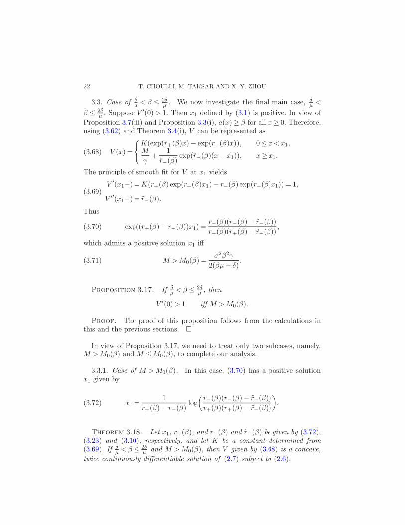
V ′(0)> 1 iff M >M0(β).

Proof. The proof of this proposition follows from the calculations inthis and the previous sections.

In view of Proposition 3.17, we need to treat only two subcases, namely,M >M0(β) and M ≤M0(β), to complete our analysis.

3.3.1. Case of M >M0(β). In this case, (3.70) has a positive solutionx1 given by

x1 =1

r+(β)− r−(β)log

(

r−(β)(r−(β)− r−(β))

r+(β)(r+(β)− r−(β))

)

.(3.72)

Theorem 3.18. Let x1, r+(β), and r−(β) and r−(β) be given by (3.72),(3.23) and (3.10), respectively, and let K be a constant determined from

(3.69). If δµ < β ≤ 2δ

µ and M >M0(β), then V given by (3.68) is a concave,

twice continuously differentiable solution of (2.7) subject to (2.6).


Proof. By differentiating the expression (3.68), we obtain

V (3)(x) =K(r3+(β) exp(r+(β)x)− r3−(β) exp(r−(β)x))> 0, 0≤ x < x1.

As a result, V ′′(x) < V ′′(x1) = 0 and V ′(x) > V ′(x1) = 1. This proves thatV is concave.

3.3.2. Case of M ≤M0(β). In this case, in view of Proposition 3.17,V ′(0)≤ 1. Therefore, x1 defined by (3.1) equals zero.

Theorem 3.19. Suppose that either β ≤ δµ or δ

µ < β ≤ 2δµ and M ≤

M0(β). Let r−(β), r−(α) and c be given by (3.10) and (3.15), respectively.

(i) If M ≥Mβ , then

V (x) =M

γ(1− exp(r−(β)x)), x≥ 0,(3.73)


(2.6).(ii) If Mα ≤M <Mβ , then

V (x) =M

γ

(

1− exp

(

− µ

σ2cx

))

, x≥ 0,


(2.6).(iii) If M <Mα, then

V (x) =M

γ(1− exp(r−(α)x)), x≥ 0,


(2.6).

Proof. In the case of β ≤ δµ , the inequality V ′(0) ≤ 1 holds due to

Proposition 3.17. Then by applying Corollary 3.5, the desired result follows.On the other hand, if δ

µ < β ≤ 2δµ and M ≤ M0(β), then V ′(0) ≤ 1 (see

Proposition 3.1). Thus, in view of (3.51), Corollary 3.5 can be applied againto obtain the results.

4. Optimal policies. In this section we construct the optimal control poli-cies based on the solutions to the HJB equations obtained in the previoussection. The derivation of the results of this section is simpler than the cor-responding one in [4], in view of the fact that no Skorohod problem has tobe involved in this case.


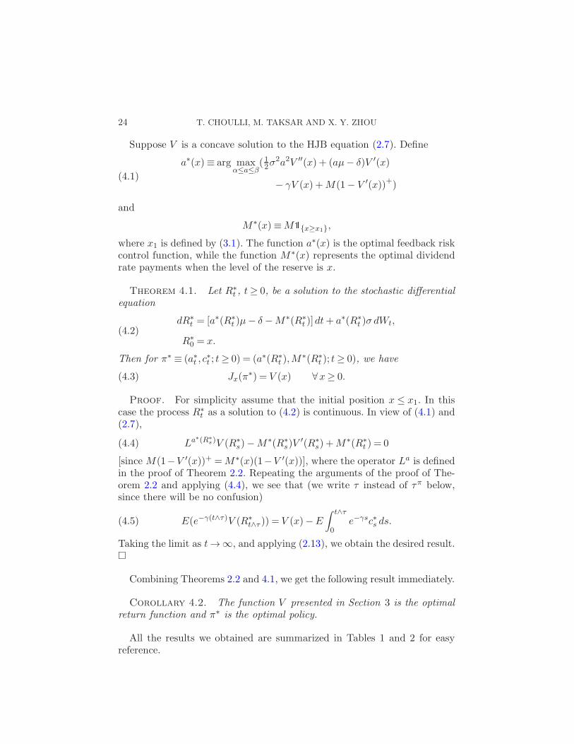
Suppose V is a concave solution to the HJB equation (2.7). Define

a∗(x)≡ arg maxα≤a≤β

( 12σ2a2V ′′(x) + (aµ− δ)V ′(x)

(4.1)− γV (x) +M(1− V ′(x))+)

and

M∗(x)≡M1x≥x1,

where x1 is defined by (3.1). The function a∗(x) is the optimal feedback riskcontrol function, while the function M∗(x) represents the optimal dividendrate payments when the level of the reserve is x.

Theorem 4.1. Let R∗t , t≥ 0, be a solution to the stochastic differential

equation

dR∗t = [a∗(R∗

t )µ− δ −M∗(R∗t )]dt+ a∗(R∗

t )σ dWt,(4.2)

R∗0 = x.

Then for π∗ ≡ (a∗t , c∗t ; t≥ 0) = (a∗(R∗

t ),M∗(R∗

t ); t≥ 0), we have

Jx(π∗) = V (x) ∀x≥ 0.(4.3)

Proof. For simplicity assume that the initial position x ≤ x1. In thiscase the process R∗

t as a solution to (4.2) is continuous. In view of (4.1) and(2.7),

La∗(R∗s)V (R∗

s)−M∗(R∗s)V

′(R∗s) +M∗(R∗

t ) = 0(4.4)

[since M(1−V ′(x))+ =M∗(x)(1−V ′(x))], where the operator La is definedin the proof of Theorem 2.2. Repeating the arguments of the proof of The-orem 2.2 and applying (4.4), we see that (we write τ instead of τπ below,since there will be no confusion)

E(e−γ(t∧τ)V (R∗t∧τ )) = V (x)−E

∫ t∧τ

0e−γsc∗s ds.(4.5)

Taking the limit as t→∞, and applying (2.13), we obtain the desired result.

Combining Theorems 2.2 and 4.1, we get the following result immediately.

Corollary 4.2. The function V presented in Section 3 is the optimal

return function and π∗ is the optimal policy.

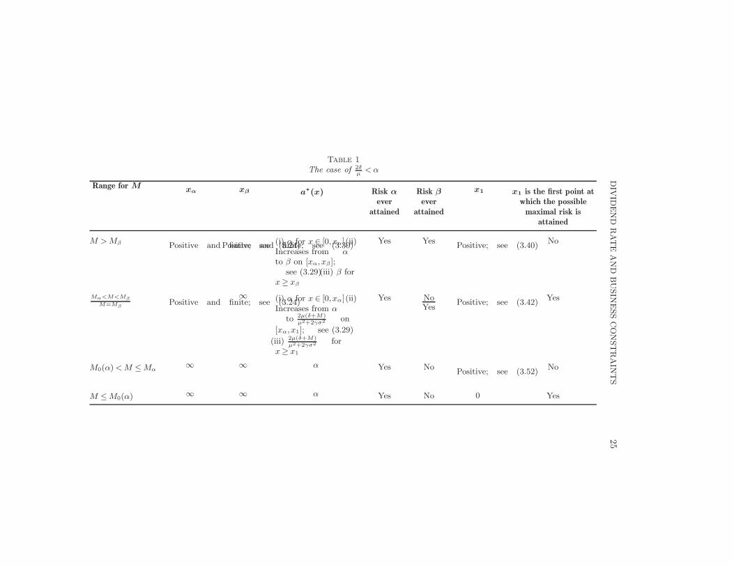
All the results we obtained are summarized in Tables 1 and 2 for easyreference.

DIV

IDEND

RATE

AND

BUSIN

ESSCONSTRAIN

TS

25

Table 1

The case of 2δµ

<α

Range for M xα xβ a∗(x) Risk α

ever

attained

Risk β

ever

attained

x1 x1 is the first point at

which the possible

maximal risk is

attained

M >Mβ Positive and finite; see (3.24)Positive and finite; see (3.30)(i) α for x ∈ [0, xα](ii)Increases from α

to β on [xα, xβ];see (3.29)(iii) β for

x≥ xβ

Yes YesPositive; see (3.40)

No

Mα<M<Mβ

M=MβPositive and finite; see (3.24)

∞ (i) α for x ∈ [0, xα](ii)Increases from α

to 2µ(δ+M)

µ2+2γσ2 on

[xα, x1]; see (3.29)

(iii) 2µ(δ+M)

µ2+2γσ2 forx≥ x1

Yes NoYes

Positive; see (3.42)Yes

M0(α)<M ≤Mα∞ ∞ α Yes No

Positive; see (3.52)No

M ≤M0(α) ∞ ∞ α Yes No 0 Yes

26

T.CHOULLI,M.TAKSAR

AND

X.Y.ZHOU

Table 2

Range for Mxα xβ a∗(x) Risk α ever

attained

Risk β

ever

attained

x1 x1 is the first point at

which the possible

maximal risk is

attained

The case of α ≤ 2δµ

< β

M >Mβ 0Positive and finite; see (3.55)(i) Increases

from 2δµ

to β on[0, xβ]; see (3.56);(ii) β for x > xβ

Yes if α=2δµ; no

if α> 2δµ

YesPositive; see (3.40)

No

M0(2δ/µ)<M<Mβ

M=Mβ

0 ∞ (i) Increases from2δµ

to 2µ(δ+M)

µ2+2γσ2 on

[0, x1]; see (3.56)(ii)2µ(δ+M)

µ2+2γσ2 for x≥ x1

Yes if α=2δµ; no

if α> 2δµ

NoYes

Positive; see (3.64)Yes

Mα <M ≤M0(2δµ) 0 ∞ 2µ(δ+M)

µ2+2γσ2No No 0 Yes

M ≤Mα 0 ∞ α Yes No 0 Yes

The case of δµ< β ≤ 2δ

µ

M >M0(β) 0 0 β No YesPositive; see (3.72)

No

Mβ ≤M ≤M0(β) 0 0 β No Yes 0 Yes

Mα<M<Mβ

M=Mα

0 ∞ 2µ(δ+M)

µ2+2γσ2

NoYes

No 0 Yes

M <Mα∞ ∞ α No No 0 Yes


5. Economic interpretation and conclusions. The optimal policies ob-tained in the previous sections have clear economic meaning and are veryeasy to implement. Let us now elaborate.

The risk control policy is characterized by two critical reserve levels:xα and xβ . The values of these two levels are further determined by four pa-rameters: the minimum risk allowed (α), the maximum risk allowed (β), theratio between the debt rate and profit rate ( δµ), and the maximum dividend

rate allowed (M ). Specifically, there are three different cases to consider.The first case is when the company has very little debt compared to the

potential profit (so that 2δµ <α). In this case, if the maximum dividend rate

M is large enough (M >Mβ), then both critical reserve levels, xα and xβ ,are positive and finite. In other words, the company will minimize businessactivity (i.e., take the minimum risk α) when the reserve is below level xα,then gradually increase business activity when the reserve is between xαand xβ , and then maximize business activity (i.e., take the maximum riskβ) when the reserve reaches or goes beyond level xβ . This policy is the sameas that obtained in [4] for the case of unbounded dividend rate. Next, ifthe maximum dividend rate M is at a medium level (Mα <M <Mβ), thenxα remains positive and finite while xβ becomes infinite. This implies thatthe company will become less aggressive; in particular, it will never takethe maximum risk, due to a more restrictive dividend payout upper bound.Finally, if M is so small that M ≤Mα, then both xα and xβ turn out to beinfinite, meaning that business activities will be carried out at the minimumlevel or those business activities are redundant.

The second case is when the company has a higher debt–profit ratio (sothat α≤ 2δ

µ < β). In this case, xα = 0. This means that no matter how smallthe reserve is the company will never take the minimum risk; rather it willstart with a bit higher risk level and gradually increase it. On the other hand,whether it will ever increase to the maximum possible risk (i.e., whether xβis finite or infinite) depends on the value of the maximum possible dividendrate M , in the same way as in the first case discussed above. Therefore, inthe second case the company overall has to be a bit more aggressive thanin the first case. This can be explained by the fact that when the debtrate is high, one needs to gamble on higher potential profits to get out ofthe “bankruptcy zone” as fast as possible, even at the expense of assuminghigher risk.

The company becomes even more aggressive in the third case when thedebt–profit ratio is even higher (precisely when δ

µ < β ≤ 2δµ ). In this case,

when the maximum dividend rate M is large enough (M ≥Mβ), the max-imum allowable risk β is taken throughout, while the two critical levelsxα and xβ are both zero. On the other hand, when M is small enough sothat M <Mα, business activities are carried out at the minimum level αthroughout.


On the other hand, the optimal dividend policy is always of a thresholdtype here the threshold is x1 (which is positive or zero). Namely, the dividenddistribution takes place only when the reserve exceeds the critical level x1,in which case the dividend payout rate is M .

It is interesting to note that in the case of unbounded dividend rate,the maximum business activity is always taken before dividend distributionsever take place; see [4]. However, in the present case of bounded dividendrate, the company may need to pay dividends before the maximum risklevel β is ever taken; refer to Tables 1 and 2 for details. This represents astriking difference between the cases of unbounded and bounded dividendrate. The economic reason for such behavior is the following. When there isa significant constraint on the dividend rate, there may be no necessity topursue business aggressively because the accumulated liquid assets cannotbe paid out as dividends fast enough anyway.

In conclusion, we point out an intricate interplay between the restrictionon the dividend distribution rate and that on the risk control of a finan-cial company. The sheer number of qualitatively different optimal policies,which appears due to different possible relationships between exogenous pa-rameters, shows the multiplicity of different economic environments which afinancial company faces depending on the size of the debt, on the constrainton the dividend rate, and on the size of available business activity.

REFERENCES

[1] Asmussen, S., Højgaard, B. and Taksar, M. (2000). Optimal risk control anddividend distribution policies. Example of excess-of-loss reinsurance. Finance

Stoch. 4 299–324. MR1779581[2] Asmussen, S. and Taksar, M. (1997). Controlled diffusion models for optimal div-

idend pay-out. Insurance Math. Econom. 20 1–15. MR1466852[3] Boyle, P., Elliott, R. J. and Yang, H. (1998). Controlled diffusion model for an

insurance company. Preprint, Dept. Statistics, Univ. Hong Kong.[4] Choulli, T., Taksar, M. and Zhou, X. Y. (2003). An optimal diffusion model of

a company with constraints on risk control. SIAM J. Control Optim. 41 1946–1979. MR1972542

[5] Dellacherie, C. and Meyer, P. A. (1980). Probabilite et Potentiels: Theorie des

Martingales. Hermann, Paris. MR566768[6] Fleming, W. H. and Rishel, R. W. (1975). Deterministic and Stochastic Optimal

Control. Springer, New York. MR454768[7] Fleming, W. H. and Soner, H. M. (1993). Controlled Markov Processes and Vis-

cosity Solutions. Springer, New York. MR1199811[8] Højgaard, B. and Taksar, M. (1998). Optimal proportional reinsurance policies

for diffusion models with transaction costs. Insurance Math. Econom. 22 41–51.MR1625815

[9] Højgaard, B. and Taksar, M. (1998). Optimal proportional reinsurance policiesfor diffusion models. Scand. Actuar. J. 2 166–168. MR1659297

[10] Højgaard, B. and Taksar, M. (1999). Controlling risk exposure and dividendspay–out schemes: Insurance company example. Math. Finance 2 153–182.MR1849002

http://www.ams.org/mathscinet-getitem?mr=1779581










[11] Jeanblanc-Picque, M. and Shiryaev, A. N. (1995). Optimization of the flow ofdividends. Russian Math. Surveys 50 257–277. MR1339263

[12] Lions, P. -L. and Sznitman, A.-S. (1984). Stochastic differential equations withreflecting boundary conditions. Comm. Pure Appl. Math. 37 511–537. MR745330

[13] Paulsen, J. and Gjessing, H. K. (1997). Optimal choice of dividend barriers for arisk process with stochastic return on investments. Insurance Math. Econom. 20

215–223. MR1491295[14] Radner, R. and Shepp, L. (1996). Risk vs. profit potential: A model for corporate

strategy. J. Econom. Dynam. Control 20 1373–1393.[15] Taksar, M. (2000). Optimal risk and dividend distribution control models for an

insurance company. Math. Methods Oper. Res. 51 1–42. MR1742395[16] Taksar, M. and Zhou, X. Y. (1998). Optimal risk and dividend control for a com-

pany with a debt liability. Insurance Math. Econom. 22 105–122. MR1625795[17] Yong, J. and Zhou, X. Y. (1999). Stochastic Controls: Hamiltonian Systems and

HJB Equations. Springer, New York. MR1696772

T. Choulli

Mathematical and

Statistical Sciences Department

University of Alberta

Edmonton, Alberta

Canada T6G 2G1

M. Taksar

Department of Mathematics

University of Missouri

Columbia, Missouri 65211

USA

e-mail: [email protected]

X. Y. Zhou

Department of Systems Engineering

and Engineering Management

Chinese University of Hong Kong

Shatin, Hong Kong

Peoples Republic of China

e-mail: [email protected]







mailto:[email protected]

mailto:[email protected]

Interplay between dividend rate and business constraints for a ...

Documents

Transcript of Interplay between dividend rate and business constraints for a ...