Internship Program for Minority Students - OpenSky

NCAR/TN-1 19+PROCNCAR TECHNICAL NOTE

March 1977

Fellowship Program inScientific Computing;Internship Program for Minority Students

Computing FacilitySummer 1976

Editors: Jeanne C. AdamsRussell K. Rew

ATMOSPHERIC TECHNOLOGY DIVISION_ ,, - --

-e 1

8

NATIONAL CENTER FOR ATMOSPHERIC RESEARCHBOULDER, COLORADC

hi

IlP Ab

as b�I - :i

iii

PREFACE

The papers contained in the 1976 Technical Note NCAR/TN-119+PROC represent

the research and programming carried out by 12 students in the Computing

Facility summer programs during the summer of 1976. The papers were

written by the students, and reviewed by the scientific and programming

staff who worked with them. A wide variety of topics are included,

since the students were assigned to many different projects according

to their interests and their academic

background. Many staff members part-

icipated--scientists, programmers and

technical staff--supervising students, .

consulting, giving lectures and courses

for the students.

The Computing Facility Staff

Summer Fellowship Program

Russell Rew, the Computing Facility

Librarian, was co-director of theJeanne Adams

program. Linda Besen was administrative Program Dixector

assistant for the program as well as

editorial assistant for the collection

of papers presented in this report.

Internship Program

Richard Valent, Jo Walsh and Fred Glare

supervised the interns in their work

assignments. Richard Valent monitored y ii

the course credit hours for which the

students had registered under a cooperative >7education arrangement with their univ-

ersities.

Russell RewProgram Co-Director

iv

Left to right: Eric Barron, JimThrasher, Kerry EmanueZ, Camp Tones

Student

Jon Ahlquist

Eric Barron

Kerry Emanuel

Lynn Hubbard (UCAR Fellow)

Iluei-Iin Lu

Curtis Mobley

Gary Newman

Joelee Normand

James Thrasher

The Students

Two groups of students participated,

one group of nine in the Summer

Fellowship Program in Scientific

Computing; the other group of

three in the Internship Program

for minority students. The

Summer Fellowship students were:

University

University of Wisconsin at Madison

University of Miami

Massachusetts Institute of Technology

University of California at Riverside

Florida State University

University of Maryland

Pennsylvania State University

University of Oklahoma

University of California at Davis

The three students listed below were selected to participate in the

Internship Program.

Karen Kendrick

Arleen Kimble

Campanella Tones

Atlanta University

Prairie View A & M University

Prairie View A & M University

v

Summer Fellowship Program

The students arrived at NCAR around June 14. These students, most of whom

are graduate students, are chosen on the basis of their interest in the

atmospheric sciences, as well as their academic background. A committee

of three staff members at NCAR examined the applications and made the

selections. The students spent the first two and a half weeks in an

intensive programming review, so that they would have an introduction to

the most unfamiliar features of the NCAR operating system before work was

begun on the scientific projects. The topics covered during this first

part of the summer were varied: Russell Rew conducted seminars that

reviewed FORTRAN and the NCAR operating system for half a day; the other

half day covered topics in input/output, which I presented. The students

all wrote and designed a program which required the buffering techniques

usually needed for a large simulation model that is not core-contained.

An introduction to direct access was presented as an alternate approach

to complicated problems with out-of-core data arrays. The topics in the

first two and a half week review are listed.

Marie Working lectures on "Terminal Command Language; John Gary 's talkis on "Numerical Solution of Hyperbolic Equations."

vi

FORTRAN Review

NCAR System Orientation

FORTRAN Review

Programming StyleUse of Graphics

Input/Output

I/O and Control CardsI/O--Word Formats, ComputerArithmetic, Core DumpsPhysical Characteristics ofI/O Devices and Tapes

Files and Sequential AccessBlocking and Use of LCMDatasets and Direct Access I/OOverlays

SAVE and RESTARTSpecial Routines for Usein I/OAccess Time and Transfer Rates

Computing Facility Summer Seminar Series

For the remainder of the summer there were two lecture series given

weekly. One series introduced simulation models that have been designed

and implemented at NCAR. The other series included special topics of

general interest to users, as well

as a discussion of Computing Facility

:;::: ......... ... ....... supporting university visitors.

*.. r :... ............... .. _. ..... ... . .

These lectures, the Computing Facility

0000iiis~ ~ Summer Seminar Series, were primarily

for the students in the Fellowship

program; however, the lectures were

announced weekly in NCAR Staff Notes

and other visitors and NCAR staff

.....li....I.................Summer Se were invited to attend .

.... ...... ,~ l-........

Russell Rew gives the students anintroduction to the NCAR System

1st Week

2nd Week

3rd Week

vii

Cicely Ridley explains how to apply for computer time in a lecture givenby her and Jeanne Adams, "Applications for CRU and Site Initiation. "Left to right are Gary Newman, Joelee Normand, Curt Mob ley, Cicely Ridley,Camp Tones and Eric Barron.

Tuesday Series - Special Topics

Topic

Overview of Communications Hardware and SoftwareMass Storage System Hardware and Software

Special Routines for Use in I/OFORTPAN Standards and Program PortabilityThe Status of Mathematical SoftwareTLIB and NEWVOLInitial Boundary-Value Problems in Fluid DynamicsThe FRED PreprocessorSorting on Vector ComputersRandom File I/O in Higher Level Language-A ComparisonTerminal Command LanguageApplications for CRU and Site Initiation

Data ArchivingMaking Mini Computers Look Like RJE Terminals

Speaker

Gary AitkenJeanne Adams andBernie O'LearWill SpanglerJeanne AdamsAlan ClineWill SpanglerJoe OligerDave KennisonHarold S. StoneGary AitkenMarie WorkingJeanne Adams andCicely RidleyPaul MulderDave Robertson

viii

Thursday Series- Computing in the Atmospheric Sciences

Speaker

Introduction to Computing in the Physical SciencesData Structures for Large ModelsProcessing Results from Large ModelsThe NCAR GCMNumerical Solution of One-Dimensional Non-Linear

Parabolic EquationsNumerical Solution of Hyperbolic EquationsNumerical Solution of Elliptical EquationsFast Fourier TransformationsA Coronal Magnetic Field ModelNumerical Solution of Integral Equations

Cecil LeithDick SatoDave FulkerWarren WashingtonJordan Hastings

John GaryRoland SweetPaul SwarztrauberJohn AdamsBen Domenico

Rob Gerritsen, consultant to the Advanced Methods Group of the Computing

Facility, gave a course that met three times a week on Data Management.

The students also attended other lectures offered at NCAR in scientific

topics by a variety of visitors and staff.

En g i efe i e ng (e ft) and WarrenWashington of NCAR were among

;i:-l-j , i ithe speake2rs in- ,he seminarseries eat tZed "Com auting in

'i the Atmospheric Scinces."

Topic

ix

Participating Scientists

The participating scientists supervised the theoretical aspects of

the research projects of the students. Without the support and co-

operation of these scientists, the program could not use real projects

for study. I want to acknowledge and thank the scientists for their

participation in the program and their interest in the students. They

provided many hours of consultation and scientific support.

Scientist Student

Grant Branstator

Jim Deardorff

Tzvi Gal-Chen

Jack Herring

Akira Kasahara

C. S. Kiang

Stephen Schneider

Roland Sweet

Ed Zipser

Joelee Normand

Jim Thrasher

Eric Barron

Gary Newman

Huei-Iin Lu

Lynn Hubbard

Jon Ahlquist

Curt Mobley

Kerry Emanuel

Foreground, left to right: Joelee Normand and Jon AhZquist, SummerFellowship students; background, Mary Trembour, NCAR.

x

Clyde Christopher

provided consulting for the students

Summer Internship Program

The interns arrived at NCAR on

June 1. There were two under-

graduates from the Computer Science

Education department of Prairie

View A & M University and one

undergraduate from the Computation

Center of Atlanta University.

Clyde Christopher, Director of

Computer Science Education at

Prairie View A & M University, was

a guest lecturer during the first

week of the program. Grover Simmons,

Director of the Computation Center

at Atlanta University, lectured and

during the latter part of the program.

Internship Courses

During the first few weeks of the program, Jo Walsh taught Beginning FORTRAN

for the Computing Facility Interns and the student interns active in the

Advanced Study Program. This class was essentially a review for the interns

since they already had programming experience through their course work.

During this same period, I taught a course in "Computer Organization" for

which the three Computing Facility Interns received 3 credit hours.

The second credit course

was offered during the

later part of the summer.

The following Computing

Facility Staff gave lectures

in Numerical Calculus;

Richard Valent organized

the course as well as

lectured.

Grover Simmons

xi

Topic Speaker

Error DiscussionDerivativesMatrix and Linear Simultaneous EquationsPolynomial ApproximationRoots of EquationsIntegralsEuler's Method

Jo WalshBen DomenicoBen DomenicoFred ClareDick ValentRuss RewJo Walsh

The interns attended a number of the sessions in the lecture series

as w.ell as their courses and the testing project meetings throughout

the summer.

.............. r

The Computing Facility staff have enjoyed the student visitors over the

Jeanne Adams ans a inProgram Director

(ASP Student) and Karen Kendrick (Intern)attend a lecture.

years. They have contributed many fresh ideas and new ways of solving

problems. They bring with them an enthusiasm for their research. Many

very hard and learning new things.

Jeanne AdamsProgram Director

xiii

TABLE OF CONTENTS

CLIMAT: A Simple Zonally Averaged Energy Balance

Climate Model .. .. ...... * * 1

by Jon Ahlquist (University of Wisconsin at Madison)

Stephen Schneider, Scientist

Experimentation with Meridional Heat Transport

Formulations in the Schneider and Gal-Chen

Energy Balance Climate Model ...... .. ........ 25

by Eric J. Barron (University of Miami)

Tzvi Gal-Chen, Scientist

Preliminary Investigation of a Tropical Squall

Mesosystem as Observed by Aircraft During Gate ........ 39

by Kerry Emanuel (Massachusetts Institute of Technology)

Ed Zipser, Scientist

Numerical Simulation of Photochemical Processes

in the Troposphere ... ......... o . 73

by Lynn M. Hubbard (University of California at Riverside)

C. S. Kiang, Scientist

Testing NSSL Routines KURV and RTNI at the Demonstration

Driver Level . . . . . . . . . 97

by Karen Kendrick (Atlanta University)

Dick Valent, Scientist

The NCAR Scientific Subroutine Library and

Computer Solutions to Linear Systems .......... 107

by Arleen Kimble (Prairie View A&M University)

Fred Clare, Scientist

On the Balance Assumption of Zonally Averaged

Dynamical Model for the Annulus ......e ........ 115

by Huei-Iin Lu (Florida State University)

Akira Kasahara, Scientist

Investigation of Algorithms for the Solution

of the Nonseparable Helmholtz Equation .......... 133

by Curtis D. Mobley (University of Maryland)

Roland Sweet, Scientist

A Test Field Model Study of a Passive Scalar

in Isotropic Turbulence . 157

by Gary R. Newman (Pennsylvania State University)

Jack Herring, Scientist

XlV

TABLE OF CONTENTS (Cont'd.)

Processing, Display, and the Use of theResults of a Numerical Model .. *.... .. 203

by Joelee Normand (University of Oklahoma)Grant Branstator, Scientist

An Adapted One-Layer Model of the ConvectivelyMixed Planetary Boundary Layer ... 2 .. . ...... 217

by James Thrasher (University of California at Davis)Jim Deardorff, Scientist

Testing NSSL Routines ADQUAD and SIMPSN ... ..... . 243by Campanella Tones (Prairie View A&M University)Jo Walsh, Scientist

1

CLIMAT: A SIMPLE ZONALLY AVERAGED

ENERGY BALANCE CLIMATE MODEL

by

Jon AhlquistUniversity of Wisconsin at Madison

Stephen Schneider, Scientist

ABSTRACT

This report is a description of and a users' guide for CLIMAT, a re-

written version of the simple zonally averaged energy balance climate

model described in Schneider and Gal-Chen (1973) and Gal-Chen and Schneider

(1976). This model is highly modular and should run on almost any FORTRAN

compiler without modification. Procedures for acquiring a copy of CLIMAT

are described in the conclusion of this report.

INTRODUCTION

Modeling is important in climate research because it enables count-

less impossible and/or undesirable experiments to be simulated. We can

further state that small simple climate models have a place in climate

research. Simple climate models have at least two advantages over com-

plicated general circulation models (GCM's). One, they are much cheaper

to run, being perhaps a million or more times faster than a big GCM.

Two, they are more useful in gaining insights into physical processes,

since cause and effect can often be easily isolated. The results of

GCM's are frequently almost as difficult to interpret as the processes

active in the Earth's real climate.

Small models have disadvantages, though. Bluntly, their results

may be wrong, because parameterizations are often based on semi-empirical

formulations rather than on rigorous physics. (What exacerbates this

problem is that, since there is seldom any way to check the predictions

of any climate model, one cannot know for certain when predictions are

wrong.) Also, one will never discover anything very subtle from small

models because of their simplicity.

At least at present, though, many very basic questions about our

climate have not yet been answered, and the subtle questions can wait.

As for the first disadvantage, one can try a number of different

2

CLIMAT: A Simple Zonally Averaged Energy Balance Climate Model ..

parameterizations and sensitivity tests for any particular quantity in a

climate model. If the model's predictions are similar and not too

sensitive to the exact values of parameterization coefficients, one can

have some confidence in the predictions even if one cannot know positively

that they are correct.

This report describes a rewritten version of the simple zonally

averaged climate model originally written by Schneider, Gal-Chen and

others. See Schneider and Gal-Chen (1973) and Gal-Chen and Schneider

(1976) for information on the original model and its results. The rewritten

version, named CLIMAT, was designed to be easy to understand and modify.

This report, along with a program listing, should contain sufficient

information for the reader to use and modify this model. The Appendices

to this report contain some of the details needed to understand CLIMAT.

THE BASIC EQUATION FOR CLIMAT

In CLIMAT, the Earth is divided into eighteen zonal bands, each ten

degrees of latitude wide. The bands are 900 North to 80° North, 800 North

to 70° North, etc. The only prognostically evaluated quantity is the

average surface temperature for each zonal band. The prognostic equation

is the zonally averaged, vertically integrated, thermodynamic equation

for the Earth - atmosphere system. Specifically, we have for each zonal

band:

DTR = (1-a)Q - F. - div(FA + F + F )3t ir A q o

where R = thermal inertia coefficient (J/K/m2)

T = surface temperature (Kelvin)

t = time (seconds)

a = albedo

Q = incoming solar flux (W/m2)

F. = outgoing infared flux (W/m2)ir

3

. .. * * * .ee.. .. . ... ... e .0 0 0 * * J. Ahlquist

and div(FA + F + F ) is the vertically integrated divergence of atmos-

pheric sensible heat flux (FA), latent heat flux (F ), and oceanic sensibleq

heat flux (Fo). (Units are W/m2 for div(FA + F + Fo).)

In the present version of CLIMAT, R is constant, Q is a specified

function of time, and the remaining variables are all parameterized as

functions of temperature. The reader is urged to study Budyko (1969),

Sellers (1969), Schneider and Gal-Chen (1973), and Gal-Chen and Schneider

(1976). These articles describe various parameterizations which are

applicable to CLIMAT. In its basic form, CLIMAT is a time dependent

version of the Sellers model, but the Budyko parameterizations and other

parameterizations can be used with equal ease. The reader should be

told that Schneider and Gal-Chen in their two articles have some canceling

sign errors in their definitions of fluxes and divergence.

GENERAL ASPECTS OF CLIMAT

CLIMAT is written in nearly standard FORTRAN and should run on almost

any FORTRAN compiler without modification. The program is structured, and

subroutines are extensively used in order to isolate the various stages of

computation and to improve the readability of the FORTRAN code; modularity

and clarity were deemed more important than operational efficiency and

speed.

CLIMAT offers few frills. This was done since modifications are more

simply performed by changing an occasional card or subroutine rather than

by redirecting program flow through a mass of IF statements. Thus, a

knowledge of standard FORTRAN is necessary to work with CLIMAT. If the

user is familiar with the articles cited in the previous section, especially

those of Sellers, and Schneider and Gal-Chen (1973), CLIMAT should be

fairly easy to understand, use, and modify. Every variable in CLIMAT is

either a mnemonic or corresponds to notation used in the literature.

Throughout the program, the MKS system of units is used without exception,

and all the temperatures are in Kelvin.

4

CLIMAT: A Simple Zonally Averaged Energy Balance Climate Model ..

SEQUENCE OF EVENTS IN THE EXECUTION OF CLIMAT

There are four main sections in CLIMAT. (A more detailed breakdown

of the steps in CLIMAT appears in Appendix A.) In the order in which these

four sections occur:

1. read in values for parameters which control the integration of

the model

2. tune the model to the Earth's present climate

3. read in an array of initial temperatures (optional)

4. integrate the eighteen zonally averaged thermodynamic equations

and compute and print average statistics which are generated as

the model is integrated.

We shall now look at each one of these points in more detail.

1. Read values for the integration parameters. The user must supply

values for six parameters which CLIMAT requires when integrating any model.

In this section, we shall list these parameters using CLIMAT's FORTRAN

names for them, describe each one, and look at the READ and FORMAT state-

ments through which they enter CLIMAT. The six parameters are:

PRNTYR an integer greater than or equal to one, specifying how often,

in years, the user wants CLIMAT to print a summary of its

current calculations. For example, if PRNTYR = 50, then CLIMAT

will print information regarding every fiftieth year of model

integration time. Setting PRNTYR equal to 50 or to MAXYRS

(one of the upcoming parameters) is generally a good choice.

NSEASN an integer between one and twelve, inclusive, which specifies

the number of periods per year (loosly, the number of "seasons")

into which the user wants the year divided. CLIMAT knows nothing

about months, so NSEASN need not be a divisor of 12. Given

PRNTYR and NSEASN, CLIMAT will compute and print average

statistics for each period during each of the years designated

by PRNTYR. For a model using annual average solar fluxes, one

would set NSEASN = 1, since "seasonal" averages would be iden-

tical with one another. For a seasonal model (i.e., one in

which solar fluxes vary during the year), CLIMAT's year begins

5

.. . . . . . . . . e . . .e e o e ... . . . . . . . . J. Ahlquist

on 1 December. (This date is set by a data card in the seasonal

version of subroutine SOLAR.) This way, if the user specifies

NSEASN = 4, the four periods will roughly correspond with winter,

spring, summer, and fall. As a specific example, if PRNTYR = 50

and NSEASN = 6, CLIMAT will compute and print bimonthly average

temperatures, albedos, heat transports, etc. for model years

50, 100, 150, etc. Whatever the value of NSEASN, CLIMAT will

also compute and print annual average temperatures, etc., for

the years designated by PRINTYR. Setting NSEASN = 4 is generally

a good choice for a seasonal model.

NSTEPS an integer greater than or equal to one, specifying the desired

number of integration time steps per "season." For stability,

there should be at least eighty time steps per year. So, if

NSEASN = 4, one might set NSTEPS = 20.

MAXYRS an integer greater than or equal to one, specifying the maximum

number of years over which CLIMAT will integrate before stopping.

Setting MAXYRS = 300 is often a good choice.

EPSILN a real number which CLIMAT will use in testing the integrated

model for convergence to steady state. Although CLIMAT computes

average statistics for most variables only every PRNTYR years,

it computes seasonally averaged temperatures every season of

every year for its own use. CLIMAT will signal convergence to

steady state as soon as all the zonally averaged temperatures

for any season in any year differ by less than EPSILN degrees

Kelvin from those for the same season in the previous year.

Symbolically, let Tij k represent the zonally and seasonallyijk

averaged temperature for the i-th zonal band during the j-th

season of the k-th year. CLIMAT will signal convergence as

soon as

max T< -T < EILNilax Tijk ij(k-1) I <EPSILN

for any j and k. Once convergence has been reached, CLIMAT

will integrate the model for one more complete year in order

6

CLIMAT: A Simple Zonally Averaged Energy Balance Climate Model ...

to gather and print steady state zonal temperatures, etc.;

then CLIMAT will shut itself off. If the climate model does

not converge after CLIMAT has integrated through MAXYRS years,

CLIMAT will shut itself off. Setting EPSILN = 0.001 is often

a good choice.

CSOLAR a real number specifying the ratio of the solar constant to

be used when integrating the thermodynamic equation to the

Earth's present solar constant. For example, if CSOLAR = 1.01,

CLIMAT will multiply the Earth's present solar constant by

1.01 to obtain a new solar constant which will be used when

integrating the model. (CLIMAT always uses CSOLAR = 1.00

when tuning the model.) Because of the infrared flux "consistency

factor" which is computed when tuning the model,* the value

which CLIMAT uses for the Earth's present solar constant is not

too critical. (CLIMAT uses a solar constant of 1358 W/m2 .

This value is fixed by a DATA statement in subroutine SOLAR.)

However, once the model is tuned, CLIMAT is very sensitive to

the value of the solar constant. If the user specifies

CSOLAR = 0.97 when running the time dependent Sellers (1969)

model, the entire Earth will glaciate in less than two centuries.

These, then are all six parameters required as user input to CLIMAT.

They are read by the main program in CLIMAT by the following READ state-

ments:

READ 110,PRNTYR,NSEASN, NSTEPS

110 FORMAT (I3,7X,I2,8X,I3)

READ 120,MAXYRS,EPSILN

120 FORMAT (I4,6X,F10.5)

READ 130, CSOLAR

130 FORMAT (F10.3)

If the user is interested only in steady state results, he can set PRNTYR

equal to the same integer which he chooses for MAXYRS. This way, CLIMAT

* See Schneider and Gal-Chen (1973) for more information about the infraredflux "consistency factor."

7

. . . . . . . .. . . . . . .o * . ... o c * e J. Ahlquis t

will print only when the model has reached steady state or MAXYRS years.

This saves computer paper. If EPSILN = 0.001, most models will converge

in a century or two.

2. Tune the model. Data statements in the main program of CLIMAT

contain experimentally measured temperatures, time rates of change of

temperature, meridional winds, and energy fluxes. Using these values,

CLIMAT computes parameterization coefficients which are tuned to the

Earth's present climate. Once these parameterization coefficients have

been initially computed, they are held constant for the remainder of the

program. Details of this tuning operation appear in Appendix B.

3. Initial conditions. Because our thermodynamic equation is an

ordinary differential equation, we need only initial conditions with our

thermodynamic equation to complete closure of the problem. CLIMAT does

not use the polar boundary condition discussed in Schneider and Gal-Chen

(1973).

See Schneider and Gal-Chen (1973) regarding sensitivity of the model

to initial conditions. If the Earth's present annual average zonal temp-

eratures are close enough to the desired initial temperatures, the user

need do nothing since CLIMAT knows the Earth's current temperature from

the tuning operation. If different initial conditions are desired, the

user can easily enter them by deleting the "C"s from column one of the

READ and FORMAT statements in the "Read initial temperatures" section

of CLIMAT's main program. Then type the eighteen desired temperatures

onto data cards with the most northern temperature first and the most

southern temperature last. See the "Read initial temperatures" section

in CLIMAT for specifics.

4. Integration and computation of average statistics. The method

of integrating the thermodynamic equation is crucial because of the

sensitivity of this equation. The author has tried the following explicit

methods of integration: leapfrog, fourth order Adams-Bashforth multistep,

fourth order Adams-Moulton predictor-corrector, fourth order Runge-Kutta,

and two fancy "canned" integration schemes from the NCAR computer library

(which automatically adjust the integration time step). Of these, the

8

CLIMAT: A Simple Zonally Averaged Energy Balance Climate Model. .

author found the Runge-Kutta method to be the fastest for reasonable

accuracy. No implicit integration schemes were tried. (The implicit

Crank-Nicholson method is used in the original Gal-Chen and Schneider

model.) If the reader wishes to try his own integration method, he should

bear three points in mind. First, different integration schemes are not

too hard to plug into CLIMAT. Second, the integration time step must be

an unvarying constant because of calls to two subroutines within CLIMAT's

integration loop. These subroutines compute average statistics and check

for convergence of the climate to steady state. Third, the equations in

CLIMAT are very touchy as to stability with respect to time step size.*

The author became an expert on the error message "FLOATING POINT OVERFLOW"

in his experiments with integration methods and time step sizes. When

instability occurs, the explosion in temperature takes place near the

equator. This sensitivity is apparently due to the large sensible and

latent heat fluxes in the subtropics, the fluxes being sensitive functions

of the very small temperature gradient. Certainly, improved parameterization

for fluxes near the equator would make a noble modification to CLIMAT.

GETTING STARTED WITH CLIMAT

The basic time dependent Sellers model requires the following four-

teen subroutines:

ALBED FSENAT

AVGVAL FSENOC

CONVER OUT

DERIVV SOLAR

DIVERG TEMADJ

FLATEN VPRESS

FLUXIR WINDD

* For example, on a Control Data 7600, the model suggested in the nextsection, "Getting Started with CLIMAT," goes unstable in less than tenyears of model time if NSEASN = 1 and NSTEPS = 75, but seems quitestable if NSEASN = 1 and NSTEPS = 80. The temperatures predicted whenNSTEPS = 80 coincide with those predicted when NSTEPS = 90 or 120 toat least five significant digits, which is all the accuracy that isprinted.

9

.. . . . . . . . . . . .e .. . . . . .. J. Ahlquist

A brief summary of each subroutine as well as flow charts for CLIMAT

appear in Appendices C and D. Several versions are available for some

of the subroutines. For instance, Sellers and Budyko versions of DIVERG

and FLUXIR exist. DIVERG computes the vertically integrated, zonally

averaged divergence of sensible and latent heat fluxes, and FLUXIR the

outgoing infrared flux. The Sellers version of DIVERG requires subroutines

FLATEN, FSENAT, FSENOC, VPRESS, and WINDD to compute the various fluxes.

Because of the simplicity of Budyko's parameterization for divergence, the

Budyko version of DIVERG uses none of the five subroutines required by

the Sellers version of DIVERG. In general, two CLIMAT subroutines with the same

name represent different parameterizations for the same quantity. Such

subroutines always have exactly identical parameter lists, so that one

or the other can be used without having to modify CLIMAT in any way. A

glance at the first few comment cards of any CLIMAT subroutine will tell

the user the purpose of that subroutine and the parameterization form.

For the user's first run of CLIMAT, the author suggests assembling

the fourteen subroutines listed above, using the annual average version

of SOLAR, the Sellers version of DIVERG, and the linearized Sellers

version of FLUXIR. Set:

PRNTYR = 25

NSEASN = 1

NSTEPS = 90

MAXYRS = 200

EPSILN 0.001

CSOLAR = 1.01

The resulting climate generated by this run should converge to steady

state in about three-quarters of a century.* On a Control Data 6600,

this model compiles and executes in about eighty seconds.

After the user has run this model and received his output, he should

sit down in a comfortable chair and take a long look at the output and

program listing for CLIMAT. Hopefully, CLIMAT does not contain too many

* A copy of the results produced by a run using this set of values appears

in Appendix G.

10

CLIMAT: A Simple Zonally Averaged Energy Balance Climate Model ...

constructions where the user reacts by thinking, "What on Earth does this

do?" or "Why did that crazy programmer do it that way?"

CONCLUSION

The original Schneider and Gal-Chen model was developed, modified,

and remodified over a period of several years by a number of people. The

result was a model which operated fairly well and formed the basis for

the Schneider and Gal-Chen, and Gal-Chen and Schneider papers previously

cited. However, this model takes literally weeks and weeks for the user

to understand because of its monolithic structure and length (over 2000

FORTRAN cards). Little program bugs also kept popping up.

Faced with this situation, the author decided that this climate

model should be rewritten from scratch. The primary goal for the new

model (CLIMAT) was modularity, both for ease of understanding and for

ease of modification. This reduces operational efficiency, but efficiency

is not too important for a small model which will be frequently modified.

The run suggested in "Getting Started with CLIMAT" is about 1000 FORTRAN

cards long, including hundreds of comment cards. On a Control Data 7600,

it compiles in less than 0.8 seconds, fits in about 20K of core, and

executes in 16.2 seconds. If the seasonal version of SOLAR is used

instead of the annual average version, compilation and execution take

only a second longer; this includes three extra years of integration

required by the seasonal model to reach steady state.

To obtain a copy of CLIMAT, contact the NCAR Computing Facility and

ask for a Software Request Form. Complete this form, requesting a taped

copy of the PLIB file named CLIMAT which is on project number 03010017.

Then return this form to NCAR along with a blank tape on which a source

image version of the CLIMAT file will be written. This file contains

several subroutines which have the same name.

The user is certainly encouraged to modify CLIMAT but to do so by

modifying subroutines which are as low on the structure tree as possible.

That is, keep the main program and subroutines ignorant of as much as

possible. This makes the various stages of the program easier to under-

stand. The author is open to any questions or comments regarding CLIMAT.

11

... . .. . . . . . . . . . . . . . . . . . . . . . . . .. J . Ahlquist

APPENDIX A: STRUCTURE OF THE CLIMAT MAIN PROGRAM

The main program in CLIMAT performs the following tasks (in order):

1. Start.

2. Dimension arrays and establish common blocks.

3. Using DATA statements, define all the constants which are used

in the main program.

4. Using DATA statements, load observed annually averaged climatic

data into arrays. This data will be used in tuning the model.

5. Compute the areas of the eighteen zonal bands and the lengths of

the latitude circles which bound them. Load these values into arrays.

6. Read in values for the six integration parameters.

7. Tune the model so that it can reproduce the Earth's current

annual average temperatures. (See Appendix B for details.)

8. (Optional) Read in an array of temperatures to be used as

initial conditions for the thermodynamic equation.

9. Print parameterization coefficients and a summary of the specified

climate at time zero.

10. Integrate the thermodynamic equation. Compute and print seasonal

averages as the integration progresses, and check to see if the simulated

climate has reached a steady state.

11. Stop.

APPENDIX B: TUNING THE MODEL

Tuning the model consists of adjusting parameterization coefficients

so that the model can reproduce the Earth's present annually and zonally

averaged temperature field in perpetuity if the solar "constant" were to

remain fixed at its present value. The comments below assume familiarity

with Budyko (1969), Sellers (1969), and Schneider and Gal-Chen (1973).

Subroutines which are mentioned are briefly explained in Appendix C.

If the Budyko version of subroutine DIVERG is used in CLIMAT, the

tuning operation is very simple. Only the infrared flux consistency factors

are computed, since they are the only free parameters.

12

CLIMAT: A Simple Zonally Averaged Energy Balance Climate Model . ..

If the Sellers version of DIVERG is used, the first step is to

adjust Sellers' wind coefficients, "a," and the three diffusity co-

efficients, KH , Kw , and K , so that the observed annual average sensible

and latent heat transports are obtained. In order to perform this oper-

ation, subroutines SOLAR, WINDD, FLATEN, FSENAT, and FSENOC have special

sections which are executed only the first time they are called. Then

energy balance is achieved by computing the infrared flux consistency

factors. Refer to CLIMAT's main program and to the subroutines in

question for specifics.

If the seasonal version of subroutine SOLAR is used, an additional

step occurs within SOLAR the first time it is called (which is during

the tuning stage). Since seasonally varying solar fluxes are time

consuming to compute, they are computed only once, during the first call

to SOLAR, and stored in an array for future reference.

APPENDIX C: SUBROUTINE SUMMARY

Subroutine Purpose

ALBED Computes albedo using the Sellers formulation. Called once in

AVGVAL

CONVER

DERIVV

DIVERG

the main program during model tuning and subsequently by DERIVV.

Computes seasonal and annual average values of all time depend-

ent quantities except temperature. Called by the main program.

Computes seasonal and annual average temperatures and checks

for convergence of climate to steady state. Called by the

main program.

Computes the right hand side of

DT 1 (at_ R1 (l-a)Q - Fr - div(FA + F + F)t R (1ir A q 0)

Called by the main program during integration. Calls TEMADJ,

ALBED, SOLAR, FLUXIR, and DIVERG.

Computes div(FA + F + F ). Two versions of DIVERG are avail-

able, the Budyko version and the Sellers version. The Sellers

version calls WINDD, FSENAT, FLATEN, and FSENOC. DIVERG is

called once in the main program during model tuning and sub-

sequently by DERIVV.

L

13

. . . . . . . .. . . . . . .e o v . . . . . . . . J. Ahlquist

FLATEN Computes vertically integrated flux of latent heat using the

Sellers formulation. Called by the Sellers version of DIVERG;

calls VPRESS.

FLUXIR Computes emitted infrared flux. Three versions of FLUXIR are

available: Budyko, Sellers, and linearized Sellers versions.

The linearized Sellers formulation agrees with the complicated

original Sellers formulation to within 1% between 200 and 300

Kelvin. Called by DERIVV.

FSENAT Computes vertically integrated flux of sensible heat carried

by the atmosphere using the Sellers formulation. Called by

the Sellers version of DIVERG.

FSENOC Computes vertically integrated flux of sensible heat carried

by the oceans using the Sellers formulation. Called by the

Sellers version of DIVERG.

OUT Prints values of all time varying quantities for all zones and

latitude circles. Called by the main program.

SOLAR Computes incoming solar flux. Two versions of SOLAR are avail-

able. One version returns only the annual average solar flux

for each zonal band, while the other version returns a seasonally

varying solar flux. Called once by the main program during

model tuning and subsequently by DERIVV.

TEMADJ The Sellers climate model uses "sea level" temperatures (T )

for some calculations and "ground level" temperatures (T ) for

other calculations. Sellers related these two temperatures by

the formula T = T - 0.0065(Z), where Z is the average elevationg s

in meters of the zonal band in question. TEMADJ performs this

transformation between T and T , i.e., it "adjusts" the temp-

eratures. TEMADJ is called twice in DERIVV.

VPRESS Computes the vapor pressure in each zonal band as a function

of temperature using the Clausius-Clapeyron equation and an

assumed relative humidity of 75%. Called by FLATEN.

WINDD Computes the northward wind using the Sellers formulation.

Called by the Sellers version of DIVERG.

14

CLIMAT: A Simple Zonally Averaged Energy Balance Climate Model .....

APPENDIX D: SUBROUTINE NESTING

The largest structure tree in CLIMAT stems from the integration loop

in climate, which computest dTf a- dto

for each zonal band. The integration loop calls DERIVV to compute the

right hand side of

FT Fat =R (l-a)Q- Fi - div(FA + F + F).

DERIVV calls:

1. TEMADJ to adjust temperatures to sea and ground levels as needed;

2. ALBED to compute albedos;

3. SOLAR to compute solar fluxes;

4. FLUXIR to compute infrared fluxes; and

5. DIVERG to compute div(FA + F + F ).

If the Sellers version of DIVERG is used, DIVERG calls:

1. WINDD to compute northward winds;

2. FLATEN to compute vertically integrated fluxes of latent heat;

(FLATEN calls VPRESS to compute vapor pressures.)

3. FSENAT to compute vertically integrated fluxes of sensible heat

carried by the atmosphere; and

4. FSENOC to compute vertically integrated fluxes of sensible heat

carried by the oceans.

APPENDIX E: COMMON BLOCKS

CLIMAT uses four labeled common blocks. Blank common is not used.

The names of these common blocks and the subroutines which access them

appear below. All common blocks are also accessed by the main program.

Common Block Accessed by subroutine

AVRAGE AVGVAL

DIFFUS WINDD, FLATEN, FSENAT, FSENOC

INFO AVGVAL, DERIVV, DIVERG

LEVEL TEMADJ, OUT

15

* * * * * * . . . . . . . . . . . . ... . . . . . . . . . .. . J. Ahlquist

AVRAGE holds average values of quantities; DIFFUS holds diffusion and

wind constants; INFO holds general information on what is going on within

CLIMAT; and LEVEL holds a variable which remembers whether the temperatures

at any particular moment are at ground or sea level.

APPENDIX F: SELLERS' "FLUXES"

The Sellers (1969) definitions of atmospheric and oceanic "fluxes"

technically are not fluxes. Strictly speaking, a flux is a vector, and

a flux, F, of any extensive variable, W, points in the direction of the

flow of W and has a magnitude equal to the quantity of W per unit time

which passes through a unit area which is perpendicular to the flow of

W. In contradistinction, Sellers' definition of "flux," F', is

27T Hf | F(4,X,z) dz a cos ( dX

F'() .... 2TrS a cos 4 dX

where F(A,X,z) = northward component of the true flux

a = radius of the Earth

= latitude

X = longitude

H = depth of the atmospheric or oceanic layer

through which the flux is passing.

For example, Sellers' definition of oceanic sensible heat "flux"

across latitude 4 is the total amount of oceanic sensible heat crossing

latitude 4 per second divided by the length of the latitude circle at

latitude (, i.e., 27T a cos 4.* The MKS units for Sellers' "fluxes" are

Watts per second.

* There is an error in Sellers (1969) formula for oceanic sensible heat

"flux." Equation (13) should read

F = -Ko Az (M'/ki) (AT/Ay) cw p

where cw is the specific heat of sea water, and p is the density of sea

water. The other two "flux" formulae are correct.

16

CLIMAT: A Simple Zonally Averaged Energy Balance Climate Model . ..

For simplicity, this author chose to have his subroutines compute

Sellers-type "fluxes," which are actually quasi vertically integrated

fluxes. However, CLIMAT's output labels these "fluxes" as "transports"

to avoid confusion.

APPENDIX G: SAMPLE OUTPUT FROM CLIMAT

The following pages form the complete printed output from the run

of CLIMAT suggested in the section "Getting Started with CLIMAT." This

run was made on the Control Data 7600 at NCAR.

*._- -- -------- ----------------- - .- --- --- . -- -- -I~---- ----- ----.-- ---- ---------- ----- ------------------------- ----------------------- - --------- --- - --- -----

PARAMETERIZATION COEFFICIENTS _0

LAT 80- 70 60 50 40 -33 2- li -1 -20 -3C -- 40 -50 -60 -70 -80

A .010 .0084 .0092 .0117 .0133 .271 .0325 .G301 .G299 .03?9 .0603 .0331 .0424 .0113 .0113 .0051 .0054 _

KH 1E+ E+06 2E+06 1E,06 9E+05 iE+06 E E+JE 7E+07 3E+? 7E+06 2E0+6 2E+06 2E+06 1E406 9E+05 4E+05

KI 4E+05 2E+05 1E+05 7+05 7E+05 4E+.5 3E+05 3E+36 6E+05 -4F+^5 4E+04 6E+05 2E+06 _E+06 tE+06 5E+05 2E+05 O

KC 6E+01 7E+02 9E+02 9E+02 7E+02 t1E+3 2E+'3 E+07 3 !E+02 2E+C3 8E+C2 5E+C2 4E-32 9E+ui 3E+01 1E+01 0

C .98 1.02 .98 .94 i.04 .95 .97 .94 .9 .9_ .93 .97 1.00_ 1.0 ..91 .12 .9_ ._97.

LAT"LATITUOE --'A -SELLERS WINO COEFFICIENT (M/S/K)KHM =IFFUSIVITY COEFFICIENT FOR ATMOSPHERIC SENSIBLE HEAT FLUX (MKS UNITS) .KW =DIFFUSIVITY COEFFICIENT FOR LATENT HEAT FLUX (MKS tNITS)KO =OIFFUSIVITY COEFFICIENT FOR OCEANIC SENSIBLE HEAT FLUX (MKS UNITS)

4* '"C sCONSISTENCY FACTOR FOR INFRARED FLUX

C =CONSISTE____ _______CY FACTOR FOR NFRARD FLUX ----------------------- ---------------------------------------

N UMlER OF AVERAGING PERI03S PER YEAR =__ _

NUMIER -OF TIME STEPS PER AVERAGING PERIOD = 90

NAXt#UM NUMBER OF YEARS FOR WHICH MODEL WILL RUN =200"COIERGENCE CRITERION FOR TEMPERATURE CHANGE = .0010 KELVIN

, 8_ _,_ ___________________ ____________ ------------- - --- - ---- ------ ----- __----------------------------------- - _

SCALI N FACTOR FOR SOLAR CONSTANT = 1.CIG

K, _______------------ -- ----- -----

,--------- --- ------------------------- - - --- ----------- -----

--------------

e------------------------------- ----

- -- -- ----- ---------------------- ----- --------

* ' -

:;' ' '. ,

;;,ii_--------__---- -------------------------------------------------------------------- _-------------------------_ _ __-- - ------------ _ _-------

,f : t -^-------------------------- ------------------------------------------------------------- _-__ -_ _- -------- -_- __

*. ·

::~~~~~~~~~~-1··~~~~~~~~~~~~~~~4~~~~~~~~~~ C~~~~~~~~~

::~;....: :~.:~ .... .za~~~~~~~~~~~~~~~~~~~~~~~~~~~~~~~~~~~~~~~~~~~~~~~~~e

AVERAGING PERIOD NO.

· It.R Vr'UK* L AT LEVEL) OTEMP/OT PRESS

90* 252.60 1.9E-09 74

80- 25B.60 2.3E-0g9 t29

0 70'- -50-- 7T0----3-m -5-9-4-----ZiE

- -

* "---- - -275.0 --- E-0-9--- 3-50

OI Jl1U OeUt-U"J

* 40~-------7I- . .-7- ' 5' E-O

30* I2 ----

2012-

29. EU* 10

0

1 ---0 2--10

4'o1-UU

-9-1- TF

"~~L~~-

SOULAR I K 1RKIU

AL9EDO FLUX FLUX 9 IV (F) WIND

c.000.6593 174 173 -115

. SQ1

.612

"4Z9

I I I .271

. 3 -7

----

e-15(i'

--2-vcr

- 97o20 9.E6-09 2781-- w -420

i 2 li klC-----~-~~T--~TTI - 30* -'7----- f 2y---2-5-- -'

401.7 · n r r ru · ~ZO<*UU b!lt"U"

9 '50'9 T- ----27 .-3-----vr.E--.

-60* 20

--- ''7---- -

-7021 Z-- 5 2.8U . L-U9* -80

2------8- N^---gE_-1---

-90023---------------------

O-)t

---2-3-

__vgE_

~-698

* 26751

-* 317

a -3 -. .. - . 1- I 9 =# -Z a 1. 4 - _.464

1 5b

260

'34 q

381

-4LU 4-

16i.4iT

-..185-

--,- -s5-3 '-

31

25T-

22-2-

(5--- .dU -1 4

---2~8--- ~8~45 10'--' 831~'

LA I LAIMIUt l UtGKLt(~ASJ

=TEMPERATURE (KELVIN)

191

2t2'"-i-

-120

-5-* - --5X_

C 2' 'r

-244

441

246

252

23P-

2316

-5-7-

57-

41

3-

1-95

--rI-

. '33

.330

.03 0

.030

. C30

-. 06j

- 143

1 30

.110

.C045

-. C15

-. -15-.121

-. C3

-. C5

-. 351 /5 -15 4

-. .25-55 ---- 7-2..7--- .

_~~~~~~a cc7 _ _

3 .-- , A,.·, 9 ·C-\ * -~~-- ~ ~~C· C A·CIr & e. d, A u A tf% n LIMI A 0 Irm u El 0T 1-1 IlUA AYiri UeUN LMFt i

T iMU StNHT TRANS

0.0

6. COE+C7

1.20E+C8

1.50E+08

1.30E+08

1.20E+C 8

1.GOE+08

9.00+C 7

7. OOE+07

-3. (OE+C7

-S.00E+O7

-. QOE+08

-1.30E+C8

-1.30E+C8

-1.60E+08-i.60E+C 8-1. 80C+08

-1.40E+ 8

-7.00E+C7

C C

LA i N

HT TRANS

_0.0_

2.C0E+06

3. OCE+06

4. OOE+06

3.00E+07

5.00E+07

3.00E+07

-4.00E+06

-3.OOE+07

4. 0CE+07

5.00E+07

1.OOE+G7--1.00E+G7

-7.0OE+07

-5 00E+C7

-3.00DE+07

-8.00E+06

UIN atNHT TRANS

0.0

2.0OE+06

_1.00E+07

2.OOE+07

3.00E+07

4.00E+07

5.OOE+075. 00E07

5. 00E+ 07

3.00 E+ C7

-6.00E+06

-3.00E+C7

-4.G0E+07

-3.00E+07

-3.00E+07

-1.00F+07

-4. OE+06

-1.00Eo06

-1.0OE+06 -0.0

0.0 0.0

"'TE-E7oT --- T--- -- T EINE--EaUVM F uF- - -- P--TF--PTURE--11KELVT -PE'--SFr -------- ---------------------------VAPQR PRESS =WATER VAPOR PRESSURE (N/M+*2)

26 BEfOLBEO ----------- ------ --------------------------------------------------------------

SO.AR FLUX =SOLAR FLUX (W/M+*

2)1"%RK rlunj-- rU =UIbUtlb NG NIRAFt- FUX (H"M-U --- )rI

* OV(F) =VERTICALLY INTEGRATED FLUX OIVERGENCE (W/M*+2)WERIEIUD WINUH ---- ~ERT WRTHRWARD T rr-----------------------------------------------------------------------------------------ATMQ SEN HT TRANS=ATNOSPHERIC SENSIBLE HEAT TRANSPORT (W/M)

* RtATENT Tr TEW M -H-T TMRTSPTJT --- -------------------------------------------------------------------- -----------------OCM SEN HT TRANS =OCEANIC SENSIBLE HEAT TRANSPORT (W/M)

YEAR =0

* 2- -

C3

*-

* *

En

rM

rn

? H

C' Oo (DN

o 0M 09

PHH H

rD

(D

CD

09

r'

CD

O

0d

CDH

0F-

1

'CO

11 -. - - - II

9 n~~~~~~C--nV n In 7l -rM- .. . .; Z 1 I

2 - -. -.. .- -".. --. 1 .~ 1 -1.

1¢ ---19

- . .

- --1. . -1. - --

-44

0 T

,YEAR= 25 ANNUAL _AVERAGE VALUES

T (SEA VAPORI* LAT LEVEL) OTEMP/OT PRESS____ A

90*, c-- 2 56. 20 i.9E-09

262.13 1.8E-09-»- 70

270.55 - .6E-0960

'- 278.66 1.4E-0950

1 .4 4 C '

* . 29 402-92.78

300 " 2- 98.15

20

leltC-U

9.2E-10

-?.8E-10

103

178

369

678

1109- :--r ---- 7ir1109

1732

-- 30i.25 -7.1E-10 29i5..

301.64 7.0E-10 29840

300.96 7T2E-10 2864-10

71

7 5-- 299.29 7.5E-10 2590

0 -20295.11 8.6E-i0 20.5

-30* '

7 - ~289.81 .- 0-T E-09 - 1433

-40'-- 284.66 1.2E-09 102

277.37 1.4E-09 620-60

* - T268.13 1.7E-09 301- 70

21- 256.55 2.1E-09 10o7

· -6o22-----0 2-47 .06 --.-3-E--39--

- -- - -. 43-90

03

- ---- .ArriT npu cr 1SOLAR IR MERID

iLBEDO FLUX FLUX uL

V (F) WINO

0.000.6?6 174-i7 1...... ---8 --- --115 ----

. 01.581 -- ,

.581

.455: ~d '

SbU �U b 242*5bO

,322

*.278

*263

;256

.267

.441

..... '9

185

262

.1U

343

381

416

417

385

353

267

222

183

-T~1--

i'$Z-

197

203

207

232

256-

255

....... ...--.....

242

240- .

.--- 7---

-87

-52

eU-. e 1. _.TL a a I, C & , · ,, ...... rt--i--

.v1 5 0

.030

.3$0._ ..

- ,,m ;m-

.£274

.£14- ; C-- - - -

-. --c7

C/3

M

NTMT S TN LAtNI UTM TRAn S-HT TRANS

0.0

5.96E+C?7

1.20E+08

1.49E+C8

I -P P~c

loiiE+08

9.50E+07

6. 89EF4C7

HT TRANS

2.638E+06

3.90E+06

4.81E+06

.; .t3F +*.r7

5.46E.07

3.26E+C7

-4.26E+06

HT TRANS

0.0

1.98E+06

9,79E+06

1.95E+07

7 V.F8f6E 7

3. 77E+07

4.80E+07

4.85E+07

13 E --------------------------------------------- 3E

.1325 -37.E+07 .3426E+07 -25.9E+07

56.135 -8.56E+C7 5.42E+07 -2.95E,07

.341 -1.12E+08 1.04E+07 -3.88E+0743

-. C15 -1.26E+08 -4.40E407 -2.89E407. . . . . . . . -.....-.- _.-.... . . . ...- - - --

-. 013 -1.20E+C8 -7,74E+07 -2.86E+C744 1 ~

-44

-51

1-ft64

-. r27

-. C49_.C~

-. 025

0.200

-1. 50E+C8

-1.74E+C8

-1.38E+C8

-6.99E+07

0.0

-5.64E+07

-3.50E+07

-1.05E+07

-1.39E+06

0.0

-9.46E+06

-3. 85E+ 06

-9.74E+05

0.0

0.0

LA =LIIUO UJ4KE"24T . .T- =LATITUIE {DEGREE) »* T =TEMPERATURE (KELVIN)

"'OTEJg7W r----- ^TT 'RE RArTE CHA8 OF-o T81PE^AT rrE<€LViTN PErT 'StOa

VAPOR PRESS =WATER VAPOR PRESSURE (N/M4*2)

SOLAR FLUX =SOLAR FLUX (W/M' 2)

='IR FLUX --- =OUTGOING INFRARED FLUX (W/M *2)

a OIV(F) =VERTICALLY INTEGRATED FLUX OIVERGENCE (W/M44 2)

" RWDIM -------- IDrlaNKL (OTTHWAR)'iN ( )ATNQ SEN HT TRANS=ATMOSPHERIC SENSIBLE HEAT TRANSPORT (W/M)

* M AENf-HTRNS ----=--ATENT-ET-TRN-RT -( w/ )

OCN SEN HT TRANS =OCEANIC SENSIBLE HEAT TRANSPORT (W/I)

--4P-3c::2

0--.d

r_H'

(A

I -- . -1

-A I I.

-, -J.

3^-- -- I-

II

0

III0u

..- AN L A E E

,, I (tA VrAUR

* i. LAT LEVEL) OTEMP/OT PRESS

r 90 _

80256.7 - i.8E-lO

Z6Z66 1.7E-100* 710.7

-- :- 271.03 -rwiB------60,

279.f08 1-3E-1050

151

*3V8L4---

Z~b*Z4 lolt-lU 1 -55

I 29---X 3.R- 06 C-~PC7--8--T7 iy r

30* "t--Tq1T T.Ear

20

IVc

.a'.* 1 30 J 7 6 7 E T -

- 10

30-

*I " 2 q w T q T7sf l

* 50Z9 -c,77 .513 1 ITWE;- 10 WT~-~----- -- F39-

-608"--270 7 Z GO ------ f5-0170.

- Z- 1.- 18a Z auE- Ou 11.

* --80.22- z 4 r e7 - Z-s-T~z-IT------- IW6-90 .

0 -- .. -----

...=--L A UR 1 UuC tulcl=TEMPERATURE (KELVIN)

.. . .. 4 I-..I . I~~~~~~~~~L~~ P

SOULA I ntKl.u

ALREDO FLUX FLUX OIV (F) WINO

0 . 00~~~.521 1~~7V4 l l -11i-5 ---- ----

.C a I

.576 1B5

.397 260

-2-0%-

208

.32J 3'irB

.27-~~ 381-- --34-a-

-,2T3 "' '- 38Y~~

a 2 b1 '- 4-U--4 4

.2 -4 1.6 -

--07 -- G- 4 i T-

.,267' 3' &"J5-.757T--- -3953-

-242-

-2z4-

-119

--- 5T-

-51-

-S4

.40

----I

.C30

.028

,C27

.154

-. 056

- 133

124

.104

. G41

-. 15

-. 012

-.1227

- . C48*5 9W 22T W 5-- ----- W2-2-;-- -I -B -- ITT -

-.034

AM l U SEtNHT TRANS

_0.C_

5.93E+C7

1.1 9EC+C8

1 .48E+08

1.22F+08

1. 10E+C8

9.46E+C7

S. 89EiC7

7, 14F+C7

-3.51E+07

-8 .58E+07

-1.12E+C8

-1.25E+C8

-1.19E+03

-1.48E+08

-1.73E+C8

-1.37E+C8

HT TRANS

0-0.-

2.79E+06

4.04E0+06

4.91E+06

3.47E+07

5.51E407

3.28E+07

-4.21E006

-3.27E+07

4.35E+07

5.45E+07

1.04E+07

-4.44E0C7

-7.81E+07

-5.71E+C7

-3.56E+07

-1.09E+07. 7bi 194 1. -1.54

-. C25 -6.95E+07 -1.46E+06-.-8[3

-0- 3 -- .-3

--T7- -------------

C.C03 C.O 0.0

2 aP7D pP/DI -- =T IM AI E I NF-TUAN-O'- 1 .TFT PERAT iUREtKEVTrI- PEt-SE TUOT-VAPIR PRESS =WATER VAPOR PRESSURE (N/M*+2)

* e A i.BE-------- -ALB------------------- ----. .^ ftUX =SOLAR FLUX (W/H+M2)

;? *'Jf:~.o =uO..X-.------- UIUl INFRARLD FLUX (M,*"- --

'' =VERTICALLY INTEGRATED FLUX -IVERGENCE (W/M*-2)7,71 MIIR !Bnimr--- ~.,-.Eu Ro.A- HAOR Tlrn--w0:?-r~7^r----------

.: t~ TSEN HT TRANS=ATMOSPHERIC SENSIBLE HEAT TRANSPORT (W/M)ri * .::i Tw TRNF "=LAtENE TRfENNU---rS- H T T---1. ..-------------: i0 S- ^i* TRANS =OCEANIC SENSIBLE HEAT TRANSPORT (W/M)

1 '. . o &- 0

uG m NtNrHT TRANS

10.09

1.97E+06

9. 72E+06

1.94E+*07

2.83E+07

3. 74E07

4.76E+07

4.81E+07

2.91E+07

-5.85E+06

-2.93E+07

-3.85E+07

-2.87E+07

-2.84E+07

-9.35E+406

-3. 1E+06

-9.65E+05

0, 0

0.0

H n ** 1-3

0

N

c: 0

H r<'13

oQ(F-'

H-

CD

N0

CDH'(D

(D

rt(D

z00

I -___ - I - _ I I

-. r 2 . 1E- n 4 W . -,0 I r , ? ,7 - .G I

- r: . I ., a I . I I I .I_- - I .

- 7 0 -K-1 7 -4 - V 7 F -7 F-il -WT 7 7 -, i ul

7 7. ~ 41-C L " -7.1

. I. I. ~ ~~~~~~~~~ -- I-~~~~-

~~~~- --- I - - . ...--.

------ ------------------------------------------------------------------

-ZO.ifC -.' * .3t-1l CtCO

, . - ------------------------

YAeRt 73 A__ANNURALAVERAGE VALUES

* CLZMATE HAS REACHED STEADY STATE

(SEA VAPOQLAT LEVEL) OTEMP/OT PRESS

* 90256.82 21.E-11 110

-so262.72 2.0E-ll __188

271.07 i.8E-11 386

279.12 1.6E-i1 700

SOLAR IRALEDO FLUX FLUX

ICt4ERIO~~~~~~~~~~~~~~~~~~~~~~~~~~~~~r

MFRI33IV(F) WIND

_ 4 rl

ATHO SENHT TRANS

0.0

LATENTHT TRANS

O.0

OCN SENHT TRANS

0.0

. 6 2 IT4 1 t5I - !).b-1 '1fl4 ci Q lSFl2 7 2.RfF406 1.96E+06 Ilt

.575

.450

frtc- I

18 5

214

,3. _

* 286.27 1 *3E-11 1137 .363 3363"40

293.08 1.OE-lt 1766 __ 322 348

298.41 8.8E-12 2456 .278 381

20301.49 8.OE-12 2957 .261

4 3410

13-10-------------------------------- --- ' - -- - -

301.88 7.9E-12 3026 .260 416-- 4 -- _---------------------------------------

301.19 8.1E-12 2905 .253 417

16-O------------------------------------* ___ _299.54 __8.5E-12 2630 .2.5 4U6- 20

295.40 9.7E-12 2041 .267 385

0-30290.14 1.IE-11 1464 .317 353

-40* 285.04 _ 1.3E-11 1348 .374 33...

- 50277.85 1.6E-11 641 .437 267

* 60268.72 2.0E-11 316 .593 222

"- ?B- ---* 257.24 2.4E-11 114 .763 194

247.84 2.7E-11 46 .902 18323- ----------------- - ----

198

204

?rfR

242

232

248

245

250

255

238

242

4.n

241

200

208

186

163

-119

-86

-...

-. 3

C30

-6 27 i.2iF Gs 3 .4E 1M0 7 2.32E+07

2 73 nil. e

54

58

56

67

40

1a

-44

-50

-113

-. 33

.124

.104

. .41

I-ll r5

* J. If

--. 27

-. £4

-* LE 4

-134.. _. _ ....... . ........ -n-2'. -

-127---- ---- - ......- -'

1. 19E+C C

1.48E+08

4. 05E+06

4.92E+06

9.72E+06

1 T94Ea40

1 09E+08

9. 46E+076. 8E+7V

7. 89E+C7

-3.SIE+07S-5. 50Lg~i.c r

-1. 2f4- -8"-i.Si-+C B

-16.-48+0

--1- -72 E+ -

- 3 77r~ 2 - -0 --1' 0 r_ u o

-: ;--6 .E-0: 7- -

u- ...E..

TT-J-.O ffuO

5.51E+07

3.28E+07

-4.2CE+Ob

-3.27E+*7

4. 35E+07

~.404E+c0

-4-44E + 7

-. 5B-tE+U I

--3 57Et+7

3 .73E+7

4.76E+07

2.9i1Es 07

-5. 84E'06~ -2.93E+076 ea

-2.93F+-07

-3.85E+07

-2.~87E+07

-. b3E40UI

-3.81E a06

-- i .47VrEr 6

~-~-------

L ,LAT =LATITUOE (OEGREES)25-T- -t; ------ R TURE 0KELVT

1 )OTEWP/OT =TIME RATE OF CHANGE OF TEMPERATURE(KELVIN PER SECOND)

* APOTER FESS V----POR -PRESUR- (N/M -- -- -----

ALBEDO =ALBEDO"S2lR FLUX =SOLAR FLUX (W/M*2)

l IR FLUX =OUTGOING INFRARED FLUX (W/M**2)28 l--YTUEVtTLLY TNRTZrrE BTLUX V RN--F C 1/

4 --------

HERPO NIND =MERIDIONAL (NORTHWARD) WINO (M/S)

* '11 i SEN HT TRg- TOHER -ERSILE- ET NSP-T-T-T T( -------------i- LATNT HT TRANS =LATENT HEAT TRANSPORT (W/M)

:-. UCn SE HT TRANS =UCEANIC SENSIBLE HEAT IRANSP'UT (HW)

0

H

i-3

t4

M

C-4

::rH'

Ft-

·*0 .' t u

_ - - - DOA r z 7

V .4v.ts .- - -

·- m -- . 7P

I ~ --- ~ ~ -- 17 -1307r-A&. '" U ,.t

f_ n 7,.------~~- U-.

A S A ' ~~~~~~~---

-

I-D-4

I I4 4 71. 4 I

I

--D-6-2-- --- '

22

CLIMAT: A Simple Zonally Averaged Energy Balance Climate Model .....

REFERENCES

Budyko, M. I., 1969: The Effect of Solar Radiation Variations on theClimate of the Earth. TeZZus (21), 611-619.

Gal-Chen, T., and S. H. Schneider, 1976: Energy Balance Climate Modeling:Comparison of Radiative and Dynamic Feedback Mechanisms. TeZZus (28),108-121.

Schneider, S. H., and T. Gal-Chen, 1973: Numerical Experiments in ClimateStability. J. Geophys. Res. (78), 6182-6194.

Sellers, W. D., 1969: A Global Climate Model Based on the Energy Balanceof the Earth-Atmosphere System. J. AppZ. Meterorl. (8), 392-400.

23

· · · ·O a · 0 a It a J. Ahlquist

25

EXPERIMENTATION WITH MERIDIONAL HEAT TRANSPORT

FORMULATIONS IN THE SCHNEIDER AND GAL-CHEN

ENERGY BALANCE CLIMATE MODEL

by

Eric J. BarronUniversity of Miami

Tzvi Gal-Chen, Scientist

ABSTRACT

Simple energy-balance climate models of the Budyko and Sellers type

are extremely sensitive to variations in solar radiation. A decrease in

solar input of %2.0 percent results in a catastrophic ice-covered Earth

solution. During geological time glaciations have repeatedly advanced

extremely close to the critical latitude of the catastrophic solution,

yet the ice-covered state has never been realized. This suggests three

possibilities; the solar input has varied less than 2.0 percent during

geologic time or the radiation balance was different as a result of

variations in atmospheric composition or oceanic circulation patterns,

or the model is overly sensitive to variations in solar input. The

model's sensitivity is strongly influenced by the formation of the ice-

albedo positive feedback. The purpose of the modifications presented is

to examine the model sensitivity to changes in solar scaling with dif-

ferent physical interpretations of heat transport. The modifications

are a first attempt at formulating the meridional heat transport such

that the transport is a function of 1) tropical sea surface temperature

and 2) the average temperature structure of the atmosphere.

INTRODUCTION

A major purpose of climate models is to examine the sensitivity of

the climate system to various external and internal perturbations.

Simple, global energy balance climate models (Budyko (1969); Sellers

(1969); Schneider and Gal-Chen (1973); and Gal-Chen and Schneider (1976)

are in particular useful to examine cause and effect processes and to

experiment with different parametric representations.

The relationship between climatic variations and scaling of the solar

constant is an especially interesting aspect of these models. A decrease

26

Experimentation with Meridional Heat Transport Formulations .. ...

between 1.6 and 2.0 percent in solar input results in a catastrophic ice-

covered Earth solution. During the Pleistocene and Permian glacial

periods, despite the repetitive nature of glacial cycles, an ice-covered

earth state was never realized. This fact suggests either the solar

input is rather invariant with respect to geologic time, or more than a

2.0 percent decrease is required to reach the catastrophic state.

Alternatively, one of the many other theories proposed to explain cli-

matic changes could be more valid.

The present study is based on experimentation with the eddy heat

flux parameterization and examination of the functional relationship of

heat transport and glaciation in the Schneider and Gal-Chen model. In

particular, the purpose is to examine the relationship of different

parameterizations to the solar scaling required for an ice-covered Earth

solution, and to examine the continuity of this relationship. Essentially,

experiments with two types of variations were performed: 1) the poleward

heat transport was determined as a function of changes in equatorial

temperature and 2) the eddy heat transport was related to the equator to

pole gradient of average potential temperature in the troposphere rather

than using the surface temperature gradient.

SUMMARY OF MODEL ASSUMPTIONS

A complete summary of the model characteristics is presented by

Schneider and Gal-Chen (1973) and Gal-Chen and Schneider (1976). The

following description is presented only for continuity of discussion.

The basic modeling assumption is the long time scale equality of

incoming solar radiation with outgoing infrared radiation. A time

dependent version of the zonally averaged vertically integrated energy

equation is

R = Qsc -)F (1-a) - F + F) (1)t sc ir sinO 3y o a q

27

· * · · · · · ·· ·· · · · · · ·· ·· · · ·* · · ·e · * E. Barron

where R

t

T

Qsc(

F.F .

is the thermal inertia of the ocean

= time

= sea level temperature

= yearly average, zonally averaged value of solar input at

latitude ¢

= albedo

is the outgoing infrared radiation flux to spaceiL

and F , F and F are respectively the zonal heat fluxes due to oceano a q

currents, atmospheric motion and the transport of latent heat.

F. = c (q) T4 {l-mtanh(19T6 x 10 16)}ir

(2)

where c(Q) is a consistency factor designed to make the present climate

an exact steady state solution of the finite difference analogue to

eq.(l) when no perturbations are present.

b () - CT x T T < TFg

(3)

b() - CT x TF Tg > TF

where T = ground temperaturegT = albedo feedback temperature (282.39)

b(c) = empirical coefficients designed to fit (3) to present

albedos

CT = feedback rate parameter (0.009)

It is assumed that a change in temperature instantaneously results

in a change in albedo with the restriction: 0.25 < a < 0.85 regardless

of -TI

The zonal heat fluxes are3T

F =Ko o 3y

DTF =K -

a a by

F =K q(T)q q 3y

(4)

=

28

Experimentation with Meridional Heat Transport Formulations.. . .

where K's: are non-linear eddy diffusion coefficients as suggested by

Stone (1973) and q(T) is the water vapor mixing ratio .

In experiment (1) an effective eddy diffusion coefficient D* is

used where D* is present day zonally averaged transport.

A boundary condition is: applied such that there is no heat trans-

ference across the poles (i.e., T gradient vanishes).

The consistency constraint

Qs(l ) - Fr = -div(F) (5)SC ir.

is applied at the initial time. Consistency is achieved by varying

c(j) or by varying the largest divergence term.

The convergence criteria for equilibrium is reached when the- energy

storage terms on the left hand side of equation (1) are smaller in-

absolute value than the largest transport term by a factor of 10- 4

(i.e., the storage term is. less than 10 9).

The model is: not a real time dependent approach to equilibrium and

is- based on how long the upper- 100 meters of the oceans adjust to an

imbalance in the zonal energy balance.

THE CATASTROPHIC SOLUTION

Analytical. analysis of simple. climate models of the Budyko and

Sellers type (Chylek and Coakley (1975) and North (1975a,b)) indicate the

present climate and: the ice-covered earth climate are stable under, small

perturbations. However, the intermediate solution is unstable, and- only

a few percent drop in solar input- leads to the ice-covered earth solution..

These .models are characterized:by a critical latitude- of ice- cap penetra-

tion at which point an abrupt transition to an ice-covere-d Earth occurs.

The Budyko model predicts the catastrophic solution at a latitude of 500

and a decrease of the solar constant by 1.6. percent. The abrupt transi-

tion occurs because of the functional. relationship of: albedo and

temperature. This feedback mechanism is important because of the large

albedo contrast between ice andX ice-free areas..

The two branch analytical solution- graphed as a control axis (solar

constant scaling) versus a behavior axis (the latitude of ice-- penetration)

29

.· * * ·· · · e ··· · e e*·* *· e ** * ·* e . ..... E. Barron

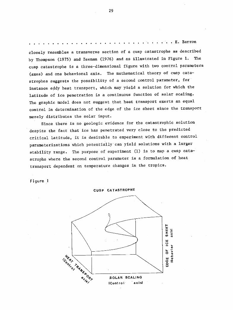
closely resembles a transverse section of a cusp catastrophe as described

by Thompson (1975) and Zeeman (1976) and as illustrated in Figure 1. The

cusp catastrophe is a three-dimensional figure with two control parameters

(axes) and one behavioral axis. The mathematical theory of cusp cata-

strophes suggests the possibility of a second control parameter, for

instance eddy heat transport, which may yield a solution for which the

latitude of ice penetration is a continuous function of solar scaling.

The graphic model does not suggest that heat transport exerts an equal

control in determination of the edge of the ice sheet since the transport

merely distributes the solar input.

Since there is no geologic evidence for the catastrophic solution

despite the fact that ice has penetrated very close to the predicted

critical latitude, it is desirable to experiment with different control

parameterizations which potentially can yield solutions with a larger

stability range. The purpose of experiment (1) is to map a cusp cata-

strophe where the second control parameter is a formulation of heat

transport dependent on temperature changes in the tropics.

Figure 1

CUSP CATASTROPHE

, I, =

w '\

LU

30

Experimentation with Meridional Heat Transport Formulations . . . .

EXPERIMENT 1

During a glacial period sea ice covers a larger portion of the oceans.

Consequently poleward heat transport by surface ocean currents and in the

form of latent heat will be inhibited in northern latitudes. This argu-

ment suggests meridional transport decreases during a glacial period.

The arguments of Kraus (1975) suggest tropical temperatures are the

controlling factor of climatic change because small reductions of

tropical sea surface temperatures are associated with large reductions

in latent heat release and in the temperature of the upper tropical

troposphere, and consequently, in the meridional heat transport.

Other arguments suggest that increased baroclinic activity during an

ice age would increase the meridional transport. In this experiment,

a constant, present day eddy coefficient, D*, which is a function of

latitude is used during the simulation. The transport is related to

equatorial temperature by the expression

Transport = D* x e ( To * - 1) (6)

where 3 is an arbitrary constant used for experimentation with the degree

of tropical dependence, T is the model derived equatorial temperature

and T * is the initial, present day, equatorial temperature.

For present tropical temperature the transport is equal to D*, the

present day transport. A decrease in solar scaling decreases transport

as a function of the difference between perturbed and initial equatorial

temperature. The 1 determines the degree of dependence on the temperature

in the tropics. Consequently, the larger the solar scaling decrease,

the smaller the poleward heat transport. Consider an extreme example of

no heat transport across latitude zones for present day solar scaling.

The result would be an extremely warm equator and an extremely cold

polar region.

A heat transport model with strong equatorial temperature dependence

potentially could maintain a non-frozen climate in the tropics if heat

transport decreases with decreasing solar input. The major purpose of

31

e l * * * * * * * * * * * * * * E. Barron

this simulation is to fit a B such that the ice-covered Earth solution

occurs at a much lower solar constant and, ideally, such that the

latitude of ice penetration is a continuous function of solar scaling

rather than a catastrophic one.

Results. A solar scaling of .99 and B equal to 20 resulted in the

catastrophic ice covered Earth solution. The decrease in solar constant

lowered equatorial temperature and therefore, decreased the meridional

heat transport. The decreased heat transport resulted in ice formation

in northern latitudes and positive ice-albedo feedback. The formulation

accentuated the feedback and consequently the critical latitude of ice

penetration was reached for only a one percent decrease in solar input.

The solution is the opposite predicted by the theoretical model. Clearly,

the model prediction is dependent on the critical latitude of the pene-

tration rather than the temperature in the tropics.

This result suggests increased meridional heat transport would

reduce the significance of the ice-albedo feedback in the Schneider

and Gal-Chen model. In order to experiment with increased heat transport

the ration To/T * was inverted. Consequently as the ice covers more of0 0

the Earth's surface the transport from the tropics is increased (despite

the fact that the equatorial temperature is also decreasing).

For a B of 20, the solar constant could be reduced to .94 before

an ice covered Earth solution occurred. The critical latitude was ap-

proximately 35 . For larger B's a cool equator and slightly warmer polar

region results and for B's larger than 40 the model became numerically

unstable. There did not exist a B such that the latitude of the edge

of the ice sheet was a continuous function of solar scaling.

A similar result was derived using Budyko's formulation of D* where

D* = y (T - Tp) (7)

where y = 2.61

T = annual mean temperature at a given latitude

T = planetary mean temperature

32

Experimentation with Meridional Heat Transport Formulations ....

The formulation of increased heat transport during a glacial period

damped the positive ice-albedo feedback, however the physical reasoning

for this type of parameterization is not readily apparent. The result

is useful for examining the relationship of solar input, heat transport

and glaciation.

If glacial cycles are indeed caused by fluctuations in solar input,

three possible conclusions are apparent from this model:

1) the climate is extremely sensitive to variations in the solar

input and the model is therefore an accurate description or

2) if the theoretical model of decreased meridional heat transport

is accurate, then the model's physics must be incomplete or overly

simplified or

3) increased heat transport is in fact reasonable, although the

physical reasoning is debatable (i.e., there is a negative feedback

represented in the model).

EXPERIMENT 2

The present Schneider and Gal-Chen model formulates F , F and Fo a q

an an eddy coefficient multiplied by the zonally averaged surface temp-

erature gradient. The zonally averaged potential temperature integrated

over the troposphere is substituted in the calculation of F , F and F.o a q

Logically, meridional heat transport is, more accurately, a function of

the temperature structure of the atmosphere rather than simply the surface

temperature gradient. O/by was used in the calculation of F in order0

to prevent numerical instability in the present finite-difference scheme.

Given the potential temperature at the surface

p R (To) g (8)

where R(T) = r + r1T + r2T 2 + r3T3

r = 2.83471 x 103o

rl = -2.92257 x 101

r2 = 1.00547 x 10- 1

33

. . . . . . .. . . . . . . . . . . . . . . . . . . . . E. Barron

r3. = -1.153817 x 10 4

and gs = aP (saturated at To).s = r

ipQ sat- [ __f _+ ~ T (9)ap sat p- pg (

surface

1000where = RT

o

T = surface temperature

R = universal gas constant divided by the molecular

weight of water

g = acceleration of gravity

and C = specific heat capacity

From Hess (1959)

l+ _WsRd T

P 1 P 2CpRd T

where L = latent heat phase change

Rd = gas constant for dry air

W = saturation mixing ratios

and e = ratio of molecular weights of water and dry air.

The potential temperature, 0 at the tropopause is

1000

(p) = 0 + P dp (11)o p

where P = 1856.26 - 5.71 T , PT is the height of the tropopause in mb,T 0o T

T Oo o

34

Experimentation with Meridional Heat Transport Formulation ...

The average potential temperature 0 is1000

11000 - PT 0O(p)dp (12)

The calculated average potential temperature very closely matches

the observed values.

Based on this derivation of 0, the average potential temperature in

the troposphere, the heat transport formulations Fa, F and F area o q

modified to the form

Transport = K - (13)°y

The average potential temperature model resulted in an ice-covered

Earth solution at a solar scaling of .972, approximately .7% lower than

previous models using surface temperature.

Initially, the gradient is less than the -- gradient and conse-

quently the heat transport would be expected to be smaller. Based on

experiment (1) the decreased heat transport should enhance the ice-

albedo feedback mechanism and result in a more rapid glaciation. The

model result is again the opposite solution. For a temperature decrease,

the moist pseudoadiabatic lapse rate decreased (larger negative number)

but is much more sensitive to temperature changes in the tropics than at

the poles. This tendency also reduces the equator to pole temperature

gradient. The level of the tropopause, PT' is also a function of the~T

temperature and since aZ is more sensitive to a temperature change in

the tropics, both these factors reduce the equator to pole temperature

gradient. However, the formulation for R(T ), a factor used to match

the calculated potential temperature to present day observed temperatures,

changes in the opposite sense. In other words, in the formulation ofa0- where

= R(T )gs,

R(T ) changes in the opposite sense as gs and actually cancels at the equator.0

35

.··. · · e' e · e ·e ··· e · * * * * * · .E. Barron

R(T ) is calculated based on the observed seasonal changes which in a

way is a mini-climatic change. However, the equator to pole gradient

actually increased. If R(To) is maintained as a constant, a similar

result as part (1) of experiment (1) occurs (i.e., enhancement of the

ice-albedo feedback). The R(T ) formulation may be less reasonable for0larger climatic variations such as Pleistocene climates.

CONCLUSIONS

The theoretical considerations presented by Kraus (1975) and dis-

cussed in this paper suggest the meridional heat transport during a

glacial period should decrease. Oceanic surface currents and latent

heat transport decrease because of increased extent of ice over the ocean.

Secondly, the temperature of the upper tropical troposphere decreases

substantially with small decreases in sea surface temperature in contrast

with the polar regions. In both experiments, a decreased meridional

heat transport results in a more rapid glaciation. From a geologic

standpoint, this result is even less reasonable. Three possible conclu-

sions may be reached:

1) the latitudinal extent of the ice sheet is extremely sensitive

to changes in the solar constant and/or reductions of tropical sea surface

temperature and consequently, these factors have been relatively stable

throughout geologic time or

2) the model physics are oversimplified and do not give the correct

response for a decreased temperature gradient or

3) a negative feedback mechanism is not taken into account which

may oppose the ice-albedo positive feedback.

Obviously, the modifications used in these experiments are only

simple attempts to examine the functional relationship of meridional

heat transport and glaciation. The results are encouraging even though

contradictory. The problematic nature of the solutions are an incentive

for formulation of a more sophisticated parameterization of heat trans-

port during glacial periods, particularly as concerns latent and oceanic

heat transport as the ice sheet advances.

36

Experimentation with Meridional Heat Transport Formulation ......

REFERENCES

Budyko, M. I., 1969: The Effect of Solar Radiation Variations on theClimate of the Earth. TeZZus (21), 611-619.

Chylek, P. and J. Coakley, 1975: Analytical Analysis of a Budyko-typeClimate Model. J. Atmos. Sci. (32), 675-679.

Gal-Chen, T., and S. H. Schneider, 1976: Energy Balance Climate Modeling:Comparison of Radiative and Dynamic Feedback Mechanisms. Tellus (28),108-121.

Hess, S., 1959: Introduction to Theoretical Meteorology. Holt, Rinehartand Winston, New York.

Kraus, E., 1973: Comparison Between Ice Age and Present General Circulations.Nature (245), 129-133.

North, G., 1975a: Analytical Solution to a Simple Climate Model withDiffusive Heat Transport. J. Atmos. Sci. (32), 1301-1307.

____ , 1975b: Theory of Energy-Balance Climate Models. J. Atmos. Sci.(32), 2033-2043.

Schneider, S. and T. Gal-Chen, 1973: Numerical Experiments in ClimateStability. J. Geophys. Res. (78), 6182-6194.

Sellers, W. D., 1969: A Global Climatic Model Based on the Energy Balanceof the Earth-Atmosphere System. J. AppZ. Meteorl. (8), 392-400.

Stone, P., 1973: The Effect of Large-Scale Eddies on Climatic Change.J. Atmos. Sci. (30), 521-529.

Thompson, J., 1975: Experiments in Catastrophe. Nature (254), 392-400.

Zeeman, E., 1976: Catastrophe Theory. Sci. American (234), 65-83.

37

†.................. .......... . E. Barron

39

PRELIMINARY INVESTIGATION

OF A TROPICAL SQUALL MESOSYSTEM

AS OBSERVED BY AIRCRAFT DURING GATE

by

Kerry EmanuelMassachusetts Institute of Technology

Ed Zipser, Scientist

ABSTRACT

A squall line mesosystem is investigated using measurements obtained

by aircraft during phase III of the GATE project. A preliminary analysis

of the fields of motion, temperature, and moisture reveals that a) two

important updraft maxima occur, one corresponding to forced ascent ahead

of a surface gust front, and a second, more elevated updraft related to

buoyant ascent or forcing by mesoscale heating; b) vorticity is generated

in the updraft region and reaches maximum intensity in the middle tropo-

sphere, and c) the movement of the system is characterized by eastward

propagation upshear and against the mean momentum field on a time scale

of several hours, while it is strongly evident that the individual cells,

with a lifetime of 1/2 to 1 hour, are advected northwestward with the

mean flow.

INTRODUCTION

A well organized, north-south oriented cumulonimbus line and associ-

ated mesosystem formed during the late morning of 14 September 1974, and

propagated slowly eastward through the dense B- and C-scale ship arrays

operated during phase III of the GATE project. The mesosystem was

extensively surveyed by rawinsondes launched from the ship arrays, and

by five aircraft operating between 990 and 190 mb. Each aircraft con-

ducted between 4 and 12 passes through the system, flying in line patterns

roughly transverse to the observed squall line orientation. The aircraft

measurements permit a reconstruction of the meteorological fields for

successive passes, from which certain aspects of the temporal evolution

of the system may be deduced. The analysis is, however, limited to two

dimensions. In the reduction of the aircraft data, it is found that the

most problematic data interpretations involve the location of the aircraft

with sufficient accuracy to resolve the convective scale features.

40

Preliminary Investigation of a Tropical Squall Mesosystem .......

CHARACTERISTICS OF AIRCRAFT AND MEASUREMENT SYSTEMS

A summary of the aircraft missions flown on 14 September is provided

in Table 1. Unfortunately, data from the UK C-130 was unavailable at

the time this research was conducted, and only limited data from the

Sabreliner could be obtained. Thus, the analysis relies heavily on data

collected by the DC-6, Electra, and US C-130.

Each aircraft carried equipment for measuring inertial latitude and

longitude, radar altitude, various aircraft control parameters, pressure,

temperature, dew point temperature, apparent surface temperature, short-

wave and longwave radiation, and liquid water content. In addition, the

US C-130 measured the C02 temperature, and the total water content via

a Lyman-Alpha instrument; and the US L-188 (Electra) measured vertical

wind and boom ambient temperature. The specific quantities measured, as

well as the characteristics of the measurement systems, are listed for

each of the three aircraft used in the Appendix.

In general, the various quantities were sampled several times per

second, and in most cases were averaged over 1 second in the final output.

A second of flying time corresponds to about 100 meters flying distance

for the DC-6 and Electra flying at low levels, 120 meters for the C-130

at 700 mb., and 150 meters for the C-130 at 500 mb.

AIRCRAFT MISSION OF 14 SEPTEMBER

The large scale flight plan for 14 September 1974, including the

general area in which the flight pattern was conducted, is shown in

Figure 1. Commonly, the aircraft left Dakar at about 09:00 local time,

and in this instance, all aircraft had reached the pattern area by 1232Z

(except for the Sabreliner, which started the flight pattern at 1311Z).

Figure 1 also shows the 1200Z SMS satellite cloud outlines. The meso-

system was in range of the radars aboard the Quadra and the Oceanographer;

however, data from the former has not yet been received, and the latter

instrument was not operated prior to 15:50 on this day. The radar scan

at this time (Figure 2) shows several banded echoes oriented SSW- NNE,

moving slowly eastward.

DATE: 14 September 1974

TTTT TAN TAV ?i7

MissionNumber

257-1

257-1

257-1

257-1

257-1

MissionType

P=Prim.A=Alter.

Aircraftand

AircraftScientist

MISSION SCIENTIST(S): Hoeber AIRBORNE MISSION

SCIENTIST(S):

257-1 Zipser (US-C130)257-lb Mazin (IL-18C)

IULIN X_ t..- Lw ,I

Time ofTake Off

andLanding

(CMT

Lat. andLong. ( )of IP andTime ofArrival

Pattern

Flown andNumber ofCircuits

PatternAltitude

(feet)

intercom-parison withor Calibration,and number ofeach

Down

Systems

I I4- , I 1'I I I I I - -- I - -~Lin (12 5,0 Sel (1) -- t- -. - '-t~d u-C n

1C2(P)

1C2(P)

1C2(P)

1C2(P)

1C2(P)

UK-C130Butler

US-C130Daivs

DC-6Emmanuel

L-188LeMone

SabrelinsSimpson,

eJ.

11112000

08421655

08401810

09561640

11551519

lOOON1000N

2200W1232Z

100UN2200W1017Z

1000N2200W1030Z

1000N

2200W1121Z

0835N2230W1311Z

Line (12)

Line (9)

Line (4)

L's (2)

Line (8)

Line (4)

5,0005,0005,0005,0005,0005,0002,0002,000

500500500500

15,00015,00017,00017,00010,00010,00010,00017,00017,000

1,0001,0001,000

500300

50

2,0002,0002,0002,0002,0002,0002,0002,000

39,00039,00039,00039,000

Self (4)

Self (3)

Self (7)

.efractomer inop. trom

.310 to 1317Z, 1333 to

.340Z, 1604 to 1620Z, andfrom 1855 to 2000Z.

weather Encountreau

in Route and in Pattern

In route: Broken trace mu, as F*LU

Ac.

In pattern: Extensive rain mainlyfrom As and Ac. Cloud system de-cayed rapidly with time.

IR radiometer questionabl In route: TCu, broken As and Cs.

throughout. In pattern: Line of Cbs scatteredCu, overcast Ac and As.

Beta vane inop. through-out. Computer inop. aftes1755Z.

Vertical field mill inop.throughout. Data systeminop. from 1601 to 1626Z.

IR radiometer inop.throughout.

In route: Scattered Cu and Ci.Very hazy, poor visibility.In pattern: Line of showers markedwith wind shifts. Light turbulence.Intensity of line did not changeat the lower levels. Some heavyrain.

In route: Broken Cu, As, Ac and

overcast Ci.In pattern: Line of convection wasgrowing, and persisted throughoutmission. Line was narrow and well-organized with observed convergenceFirst line dissipated while newlines formed to the E and W.

In route: Fair weather.In pattern: Line of Cb towers to40,000 ft, oriented N-S line.

257-2 Lazanoff (P-3A)257-3 Reiff (WC-135)

Summary and

Evaluation

Planned to do a 6B add-on mis-sion, but this was cancelleddue to extensive heavy rain inthe area.

Very successful mission, 6½hours of continuous crossingsof band of Cbs in the C-arraywith good coordination withships. Life cycle of a strongconvective band should havebeen well-documented.

Considerable convective activitthroughout the mission. Activeevaporation regions found.Very successful flight.

Repeated penetrations of aroughly N-S squall line. Suc-cessful mission.

This pattern was well-coordina-

ted with five other aircraft inthe stack. Flight was success-ful. Right altitude for cloudtops; right pattern, correctlylocated. Analysis should bevery valuable.

--a)

Cr0-

O -'

_ * _

3

- 0CD DQC

icn

3

_CD -

-- CD

--hO-

re £

<0

C-t

l< >

CD:

(D U)

- O:

D) CD

CD

v 3

0)

D 0

h -L

CD

_0r,^ ..

_ _ I _ __ I _ __ I I__ I _ _ _ 2 I__ _ 2 _ _ _ _ _- I 4

Eg

C(P

!R11f

I

I!

I

II

F-

_

iJr-

!I Self (1)

42


Visual observations of the squall line, by personnel aboard the air-

craft, indicate a continuous band of cumulonimbus (Table 1). Apparently,

the new growing cells were located near the eastern edge of the band,

which was the more sharply defined in several respects, while older,

decaying cells comprised the ill-defined west edge of the system. Photo-

graphs reveal these characteristics, and also show anvils trailing behind

the system, toward the west (Figure 3).

The flight patterns were flown transverse to this system, near the

southern end of the line. An attempt was made to keep the aircraft

flight tracks vertically stacked, but at a given time, the individual

aircraft tracks may have deviated in the horizontal up to about 10

nautical miles in the direction tangent to the squall line. The Sabreliner,

flying at 39,000 feet (X198 mb.), was close to the cloud tops.* Figure 4

details the flight tracks of the DC-6 and Electra between 14:00 and 14:30;

the DC-6 flying at about 980 mb., and the Electra at 940 mb. The flight

tracks of the C-130 between 14:00 and 15:00 are also shown; during the

first half-hour the aircraft flew at %694 mb., while during the second

it operated at %522 mb. The DC-6 and Electra intercepted the gust front

during these passages at 14:21, while the C-130 penetrated deep cloud at

14:13, flying at 694 mb., and again at 14:36, this time at 522 mb.

CORRECTIONS TO NAVIGATION SYSTEMS,

AND LOCATION OF AIRCRAFT WITH RESPECT TO SQUALL LINE

As the width of the cloud band was apparently on the order of 25

nautical miles, it is important to locate the aircraft with 1 or 2

nautical mile accuracy. The inertial systems suffered from various errors,

including a systematic error which increased with time, and a "Schuler

Oscillation," peculiar to inertial systems, with a period of 84.4 minutes

(Kayton, 1969). The amplitude and phase of such oscillations were unknown

in most instances, and thus no attempt could be made to correct for them.

The total inertial position error, on landing, was as great as ten nautical

miles, so that extensive attempts to correct the navigation were necessary.

* From direct observation by Joanne Simpson, aircraft scientist.

43

· ·Is · · · · · e · · ··· -·· ·· . · e. K. Emanuel

Flight Plan of 14 September (from "Report on the Field Phase

of GATE - Aircraft Mission Summary," Gate Report No. 18, World

Meteorological Organization)

25° 20° 15°

..... -- '1.------.-..- ' ..... -...,:..: >- -. __. - - .sAL----.---

-. -- " -- '-.- .......:T" ,-4--'-AKAR_ _ -_ - ^_ *I. -_

'.. . .,. .. ,___t,

· - 1

, :- ^ ''' '"""~ '" '-::~:'' '' r '¥:'-! ... .. ' ,E % .-

' ' ' e e eeeel~ eeeeeo i' · ' s~~le " t~t'~:" ···· 1 ··r l ·

~~~~~~~~~~~~~~~~~~· .. ... . .....

· ~~~~~~~~~ !': ':::'''::. '"~,"-~'__, " )........ ..

_ _ _ _ _ _~~~~~~,____ _ _ __,,!.;_ _,_ _, ..

....... __ _ _ _ _ __ --------- 0

ale ~ ~ ~ ~ ~ ~ ~ ~ ~ ~ ~ ~~~~~~~......... . . . , . . . ,.,,..-,. .,.....~,..

_~~~·0 ,

· ,e·~~~~~~~~~~~~~~ o ~ ~ ~ ~ _a~~ ..... ~·r\ \.... . ,--- ........,,...~_ _

25° 2U" I!

I

14 SEPT 1974(EXCLUDING TRANS-ATLANTIC FLIGHT 257-3)

Figure 1:

30o

5'

C30°

I g

11

I

#a

I__LI __ _ __ _I� �

50

0O

44


Figure 2: Oceanographer Radar Scan at 15:02Z. Range markers are at25 km. intervals, except the first is at 10 km.

. t m -..

\P ,

The US Electra carried a VLF system, with an accuracy of about 1 nautical

mile, enabling a more precise determination of position in this case.

In addition, the C-130 was equipped with Omega navigation, which was used

to continuously update the inertial positions, to an accuracy of about

a nautical mile.

On occasion, aircraft that carry only inertial navigation systems

can be located fairly accurately by comparing handwritten navigator's

notes with the inertial data. (E.g., the aircraft will often fly over a

ship with an accurately known position.) On this day, however, such notes

were very incomplete and corrections to inertial systems of the DC-6 and

Sabreliner were not possible. Fortunately, the inertial errors on landing

of both these aircraft were less than .5 nautical mile, so that inertial

positions were assumed correct throughout the flight.positions were assumed correct throughout the flight.

45

. . . .. . e. . . . . . .... . . . . ...9 . . . . .. . .* e** K. Emanuel

Figure 3: Top, Photograph from US C-130, panning SW - W at the east edgeof the squall line. Aircraft was at 530 mb. in the top photographand 694 mb in the bottom photograph. Bottom, looking east towardwest edge of system. Note anvils overhead, sheared toward west.Photos courtesy of Dr. Edward Zipser.

46

Preliminary Investigation of a Tropical Squall Mesosystem ......

The movement of the squall line and the positioning of aircraft

relative to the latter were determined in several ways, depending on the

aircraft. It was found that the gust front was very well defined below

900 mb., so that this feature could be used to define the movement of

the system as measured by the DC-6 and Electra. Figure 5 shows the normal

velocity profile of the squall line as measured by the DC-6 and Electra

during one pass each of the system.

It was found that the Lyman-Alpha total water measurement device

provided the most consistent method for locating the C-130 with respect

to the eastern cloud edge, and that the radiation instruments aboard the

Sabreliner were most useful in the same connection.

As the aircraft flew at slightly different latitudes, and in directions

not exactly normal to the squall line, it is necessary to project the air-

craft positions onto a reference plane normal to the squall line. This

reference plane is oriented in a 110 - 290 degree direction, intersecting

the east edge of the squall line at all times at 8.16 degrees latitude.

Thus the reference plane crosses the line at different points in the

transverse direction, depending on the time. Hereafter, all aircraft

positions will refer to this coordinate system.

The projected longitude of the squall line east edge is plotted as

a function of time, for each aircraft, in Figure 6. The correlation

between the line movement, as measured by each aircraft, is quite good,

especially after 13:30. Apparently, there were two line propagation

regimes, one before and one after 13:00. The eastward propagation

velocity during the latter was about 2.7 m sec 1 .

It is apparent, in Figure 6, that the east edge of the line slopes

westward with altitude. If the slopes of the regression lines are

averaged for the four aircraft, during the period after 13:00, and the

resulting slope is fitted to each aircraft line position set, the vertical

slope of the line may be determined from the four intercepts. This slope

is plotted in Figure 7. The line appears to slope about 52 degrees west-

ward from the vertical, probably as a result of moderate easterly shear,

at least below 500 mb.

47

. . . . .. . . . . . . . . . . . e o ... . . . . . .o . . K, Emanuel

Figure 4: Flight Tracks of Aircraft, 14 September. Upper left, DC-6 at

980 mb. between 14:00 and 14:30. Upper right, Electra at940 mb. between 14:00 and 14:30. Lower left, C-130 at 694 mb.

between 14:00 and 14:30. Lower right, C-130 at 522 mb. between14:30 and 15:00.

DAY 257 N595KR

-25.0 -Z.5 -'z. u -,. * -4.,J ... -.

LONGITUDE (DEG) P= 3 LONGITUDE (DEG) P- 17

DA'' 257 -55L 1 CIO192 I "

10.0

(\,

N

9.5 h

-

I

i: e c : - 5: I 1:- I i I I I I I

.* ** I " * I i ! ' ! i9.0 .* .- . ! ' ' , '

8.5 -- --- t- t ---i t I :

-2 .0 -23.5 -23.0 -22.5 -22.

LONGITUDE (DEG) P= 3 LONGITUDE (DEG)

N6539C10.0

(l

c£

DAY 257

9.5

9.0

B 8.5

.,c

-23i.5

N6541 CJA', 25-

-71 A

P= 3

48

Preliminary Investigation of a Tropical Squall Mesosystem ...

The horizontal wind components are computed, also using the aircraft

inertial systems, and projected onto the aforementioned reference plane.

It is observed that, in general, such measurements of wind velocity are

subject to two errors: Heading-dependent errors, and errors inherent in

the inertial system (including Schuler oscillation). An estimate was

made of the former by examining the measured wind components just before,

and just after a 180 degree turn. The results of this analysis are pre-

sented in Figure 8. No attempt could be made to correct for the Schuler

oscillation in the inertial system.*

Figure 5: Left, Example of Normal Velocity Profile for DC-6. Wind shiftis at zero nm, east is on the right. Velocity is in msec- .Right, Example of Normal Velocity Profile for Electra.

:. r -TT r T-T-r- -TrT-T-r i i [ I -rr-r- TTI ' f T-17-T 7 T-- T- 'T- I r I | I I rn

-i-4

-i

-

-i

iC

.:C-

-14 -35

19i_

-3.s

-Xa i,,

-4v 3

I I I I I I I I I I I I I I I I I , i I I I I . .I I I I I II l

-30 -25 -20 -15 -10 -5 uX (N.M.)

I I t I,, I , I LLI I J

5 1 15 I

1.-5 -I - TT T I, I I I I I I , I I " l I i I I I I I I

1-

I

-1.5

Z

-3. -

-3.5

-5.0-40 -35 -30 -25 -20 -15 -10 -5

X (N.M.)

* The period of the Schuler oscillation was, unfortunately, nearly equalto the time needed for one complete aircraft cycle through the system.There is no reason to suspect, a priori, that the phase of this oscil-lation is correlated between aircraft. Smooth vertical trends in themeasured horizontal velocity components in the regions removed fromthe squall line, as viewed in the composites involving all aircraft,would tend to support the conclusion that the amplitude of the oscil-lation is small.

0 5 10 15 2. .Iu

49

* ............... * e* e*.....* e-...*@** K. Emanuel

Figure 6: Longitude of Squall Line Eastern Edge vs. Time. Line definedby wind shift for DC-6 and Electra, otherwise by evidence ofcloud penetration. Inertial systems corrected for landingerror by linear interpolation; and all longitudes are correctedto 8.6 degrees latitude, since line is skewed from north-southdirection.

wo 23.1

3-

z0

23.00lUw

LL

o 22.90

40 13:0020 40 14:00 2 40 15:00

TIME

Day 257: Westward Slope of Squall Mesosystem as Determinedby Wind-shift Line Measured by DC-6 and Electra and CloudPenetration by C-130 and Sabreliner.

12000 H

9000 -

6000 -

3000 F

0

11 10 9 8 7 6 5 4 3 2 1 0 - -2-3-4(n.m.)

Figure 7:

E

-r

lLI

0

1TT71__~Y ~ .; I v II

Sabre linere. Sabreliner

C-1304(694)

Electra \ C-6I I I I I I I I I I I I

_I

I I - I i I I , ! . -- -J

I I I ---

50

Preliminary Investigation of a Tropical Squall Mesosystem . ..... .

Figure 8: Heading-Dependent Velocity Error vs. Time. Correction to East-bound Aircraft Track. Top to bottom, DC-6, Electra, C-130.

0 -

-I40

I. I I I

REGRESSION DATA

NORMALSLOPE = -0.006INTERCEPT=0.3705

TANGENTIALSLOPE =0.2094INTERCEPT=-2.4137

(0.33)

(0.20)

(0.50)X

0(0.1 1)

I I I

X-NORMALCOMPONENT

O-TANGENTIALCOMPONENT

(0.50) (0.60)0 0

xX (0.29)

(0.17)

I I I

12:00 20 40

2

m/sec I

0

-I

13:00 20

TIME

14:00 2014:0040

TIME

2

m/sec I

0

-I

2

m/sec I -

15:00

TIME

I Il I X . - -

! I I

51

e e * * e * * * * * * * e e o * o o . . .* K. Emanuel

SCALAR MEASUREMENTS, AND AVERAGING OF DATA

Direct measurements of temperature, pressure, and dew point permit

analysis of the thermodynamic and moisture fields associated with the

mesosystem. The measurement of pressure was, in general, quite good,

although in some cases there was apparently a constant or near constant

bias in the observation.* Where determinable, this was removed--in no

case was it greater than two millibars.

The measurement of temperature and dew point both suffered a great

deal from the effects of liquid water in cloud, even though much effort

had been made to keep the instruments dry. Since the air stream is

brought to stagnation before the temperature is registered, it is always

subsaturated at this point--permitting liquid water to evaporate from the

temperature element. This results in a low bias in the temperature,

after a factor related to the stagnation effect is subtracted from the

raw measurement. Liquid water in contact with the reflecting surface of

the dew point instrument causes the latter to heat up in an attempt to

evaporate the water. Because of this, the dew point is probably warm

biased in cloud regions. As a result of these two effects, the measured

temperature is sometimes lower than the dew point; in such cases, the

temperature is set equal to the dew point. This is essentially the only

correction made to the scalar measurements; it is felt that further mod-

ifications would become too arbitrary.

Rather than compositing the data by using several aircraft passes

through the system, the fields measured during single passes are used to

construct a two-dimensional cross-section normal to the line. For this

purpose, the four passes shown in Figure 4 were examined. Each of these

passes were very close in time; in no case was one observation removed

from another by more than 35 minutes. The data are averaged over 20

second periods (corresponding to about 1 nautical mile flying distance)

for each pass, and the 4 resulting .data levels are plotted and subjectively

interpolated onto a grid with 2 n.m. spacing in the horizontal, and 100 mb.

in the vertical.

* Personal communication with Alan Miller, NCAR.

52

Preliminary Investigation of a Tropical Squall Mesosystem . . ...

Figure 9: Top, Component of Normal Velocity Relative to Moving SquallLine. Velocity is in msec- 1 Bottom, same as above, but fortangential component. Positive values indicate westerly andsoutherly flow respectively.

a. a. /

s * °

.

a a -,

# .

_ # lb

0 *

S C s

I I

I '

I I I .1 I I *'

30

a ~ ~ ~ ~ ~ ~ ~ ~ I -. a~~~~~~~~~~~~

-7.2D. Sila e

a ~ ~ ~ ~ ~ ~ -. a~~~~~~~

a a a -a - a a ~o f-& %

a a a a ~ ~ ~ ~ ~ ~ ~ * a a * , * -~~~~~~la E0 ag

0a. a ~ ~ ~ ~ . , , ~ ~ ~ , a 1 , a~~I

- a a a~~~~~~'t~~ a,,a a a~~~a a a EG a, aaa~~~~~~~~A'a aa

a - a a a'arlaaa'a' c~~~~~~~aa, a a a a~t- a a a a E a . M~a.Ia ,.',

a a 5 a a aa' ~~~~~~~~~~~~~~Ar g 'Va.',* faab~~ D a a I a~ ~

a a a' aa~,aa a a aG a

a, S

a a s%t ~ ~ ,% %lb~~~~~~~~~~~a

% % ~ ~ ~ ~ a t ~ a ,a lviba

- L aC I a &. a a LL a . - .- -- - -

10(N.M.)

U -1U

(N.M.)

500

600

700

(MB)

800

900

1000

500

600

700

(MB)

800

900

1000

_. 1 r. ·. 0· --C - · L n-I -.a - ·I

rl

f

-LU

53

***..**** **** ... *.. * ... K. Emanuel

FIELD OF MOTION

The tangential wind component, and the normal component relative to

the moving surface wind shift line, are shown in Figure 9. It is immedi-

ately evident that the squall line, in its entirety, is not being advected

westward with the mean flow, nor, in fact, are there many regions of west

relative wind. Strong convergence is apparent just ahead of the surface

wind shift, and also at the 700 mb. level several nautical miles to the

rear. Weak convergence predominates in the area ahead of the wind shift

line, and weak divergence covers the area to the west of the mesosystem.

A stronger area of divergence is evident near 500 mb. about 5 n.m. behind

the wind shift.

The profile of tangential velocity reveals a remarkable area of neg-

ative relative vorticity sloping back from the wind shift line, and

increasing in magnitude with altitude. Minimum relative vorticities of

-1 x 10 3sec 1 occur near 500 mb. at +9 n.m. These values indicate

generation of negative absolute vorticity, which can only be accomplished

by twisting of horizontal vorticity tubes. This view is supported by

Figure 10: Stream Function Corresponding to Figure 9 (top), in mb msec-

for same cross-section as in Figure 9.

500

600

700

:MB)

800

900 - -

1000, I'. I I I] 00 i , n , n n -ininn in - ?N

(N.M.)

54


-1Figure 11: Vertical Motion in mb. sec

600

- -r(; (e ijTrt ,

C3~is· , ,:';

9000 a

1000 f ile ofI and 7 and shw i so I a I. T II t aim

i1000 40 30 20 10 0 -10 -20(N.M.)

a comparison of the unperterbed environmental tangential velocity (near

the right-hand edge of Figure 9 (bottom)) with the streamlines and the

w field. The latter are defined via the continuity equation integrated

over the reference plane:

J 100 v dp with i0ooo 0

and = _'-' with - =0 at x = -24 n.m.and x =+42 n.m.

Profiles of 4 and w and shown in Figures 10 and 11. Two updraft maxima

occur, one just above the gust front location, and a second at higher

levels somewhat to the west. Weak upward motion prevails in the general

region east of the wind shift, and downward motion are evident, one on

either side of the area of strong updraft at 500 mb. A comparison of

the vertical motion field with the observed distribution of tangential

velocity indicates that the latter is being redistributed, to a certain

degree, by the former. Note that the vertical shear of tangential velo-

city is far less to the rear of the system than ahead of it; apparently

the meso-circulation acts to decrease the shear in this direction.

(POMI~~~e~Ii Iq

the m-so-ircuationactsto dcreas thesheare inth"'"~'"Jion

55

v..... eX........ .... ee.....e. ..... * K. Emanuel

Figure 12: Relative Vorticity in sec - 1 x 10" 5

5 0 0 ' r ·,

6000 " // "'

( OOM.l

8 wa00

0 0 C ··:30 20 -20

'waves.

!~ ~ q~9-~~·r ICc:;~ ~ ~ ~ ~ ~~·~,0 ~

mc u pa wat h il fveria oo s.get ha h p

56

Preliminary Investigation of a Tropical Squall Mesosystem . . ..

1" 1 v -2 in sec 2Figure 13: - in sec 2 x 10 8.9x ap

500

600

700

(MB)

800

900

I000

(N.M.

Figure 14: Equivalent Potential Temperature in degrees Kelvin.

500

600

700

1MB)

800

900

1000

(N.M.)

57

·e * † e * ··e ··· * ** K. Emanuel

THERMODYNAMIC VARIABLES

An attempt is made to define the thermodynamic properties of the

mesosystem, using the direct measurements of temperature and moisture.

It is felt that a calculation of equivalent potential temperature has

the greatest potential usefulness, as the cold bias in temperature and

warm bias of dew point in cloud tend to be compensatory. The field of

o is presented in Figure 14. It should be kept strongly in mind thate

a) errors of measurement are likely in cloud (roughly between 0 and 15

nm.), and that b) measurements by different aircraft are likely to give

different values. Therefore, the gradients of 0E between 1000 and 700

mb are not entirely dependable, but those between 700 and 500 mb. are,

as both these levels were surveyed by a single aircraft. The values of

equivalent potential temperature shown here are also uniformly too low

by about 6 degrees Centigrade, since specific humidity rather than mixing

ratio was unintentially used in the calculation.

Although relatively high 0 air is being transported upward by the

vertical motion, no values characteristic of boundary layer air (as

measured by the DC-6) are found at middle levels in the updraft region.

The low 0 air near the 700 mb. level, exterior to the immediate squalle

circulation, is highly typical of mean tropical surroundings (Aspliden,

1976). Figure 15 (top) shows the 0 field superposed on the streamlines

relative to the moving wind shift line. If the effects of mixing are,

for the moment, neglected, it is apparent that large local temporal

changes of e occur, especially in the region of upward motion, in assoc-

iation with strong horizontal advections. Evidently, the updraft region

does not appear to retain a quasi-steady position with respect to the

surface wind shift. If, on the other hand, the 0 field is compared with

streamlines in a coordinate system moving westward with the mean momentum

field* (Figure 15 (bottom)), a different pattern emerges. Strong hori-

zontal transports of 0 do not occur, and apparently, the mean circulation

acts to advect the 0 field upward ahead of the squall line, and downwarde

behind it. Comparison of the two streamline fields would appear to indi-

cate that the main updraft center is drifting westward with the mean flow,

but that the region of upward motion immediately above the gust front

maintains a relatively stationary position with respect to the latter.

*as defined by vertical average at x = 24 n.m

58

Preliminary Investigation of a Tropical Squall Mesosystem . ... .

Figure 15: Top, Oe in Degrees Kelvin, and Streamfunction Relative toSurface Wind Shift Line in mb. msec- 1. Bottom, Oe in DegreesKelvin, and Streamfunction Relative to Coordinate SystemMoving with the Mean Momentum Field.

(N.M.)

(N.M.)

500

600

700

'MB)

800

900

1000

500

600

700

(MB)

800

900

1000

59

* l * e * e e 0 * .. * * o K. Emanuel

No strong upward advections of 0e occur in the updraft at high levels

behind the windshift; rather, upward transports appear to occur in

conjunction with the smaller updraft above the wind shift line. Strong

downward transports take place behind the west updraft cell.

The existence of two individual updraft - downdraft doublets is

implied during the time of these observations. A newly initiated updraft

cell is present over the wind shift line, while an older, more elevated

cell is observed about 12 n.m. behind the line. The latter is accom-

panied by a downdraft of greater extent, but smaller intensity, and has

ceased to transport equivalent potential temperature upward, at least

through the mean flow. The younger cell, however, is actively advecting

higher 0e values toward greater altitudes. Evidence of a still younger

updraft cell may be seen at low levels near -12 n.m., while what may be

the remains of a very old doublet is observed at 500 mb. and near +35 n.m.,

in both the vertical motion and 0e fields. Quite possibly, we are looking

at an evolution of individual cumulonimbus, each with a lifetime of

1% hour, spaced roughly 10 n.m. apart. The individual cells intensify

and dissipate, while being advected along by the mean flow, but the

sequence itself drifts slowly eastward against both the mean flow and

the shear direction. The new cells grow up along and move with the

surface gust front, and evidence of both newer and older gust fronts may

be seen in the profile of normal velocity near the surface. These corre-

spond with negative perturbations in the tangential velocity field, and

are also spaced about 10 n.m. apart, lagging 2 or 3 n.m. behind the

updraft cells. In fact, the two gust front velocity regimes, apparent

in Figure 6, may represent a new, vigorous gust front overtaking an

older, decaying wind shift line.

The sequence of individual cells is also evident in the profile of

relative humidity, shown in Figure 16. (Bear in mind that the humidities

are questionable in cloudy areas, and are probably low biased in these

regions due to temperature errors.) High relative humidities occur in

both the important updraft regions, and also in areas corresponding to

very young and very old updraft cells.

60

Preliminary Investigation of a Tropical Squall Mesosystem.. ..

Figure 16: Relative Humidity, in percent.

500

600

700

800

900

1000 4000 L 1 30 20 lO II0 0 -10 -20(N.M.)

Further evidence of discrete propagation of the mesosystem may be

seen, to some degree, in the sequence of individual aircraft passes

through the system. If, indeed, individual cumulus towers are

advected by the mean flow, then they should also have a large tangential

component of motion as they are transported across the line. It is there-

fore improbable that an individual cell can be tracked by the aircraft

(unless these cells are also elongated in the same direction as the main

line). Nevertheless, some evidence of westward advection of individual

features may be seen in certain aircraft sequences. An example of such

a sequence, in the mixing ratio field, is shown in Figure 17.

The phenomenon of discrete propagation of convective mesosystems

has been discussed in connection with previous tropical experiments

(Zipser, 1969), and has recently been observed on radar (Houze, 1976;

Sanders and Emanuel, 1976). In the latter case, new echoes were observed

to form in the middle troposphere upshear of mature echoes, and propagate

downward while drifting with the mean flow. In both instances, the

squall line--defined as an entity with a lifetime of %6 hours--propagated

· · · · ·* · ·· · · · ·· · ·e . · · · ·e · · ·. · · K Emanuel

generally upshear. The mechanism by which such propagation occurs

remains a mystery, and should provide an interesting area for further

investigation.

CONCLUSIONS

The measurement of meteorological variables in a tropical meso-

system on small time and space scales has been accomplished, essentially

for the first time, by the GATE project. It is now possible to resolve

individual convective elements on a time scale of %1/2 hour and space

scale of 1% nautical mile, and, to a certain degree, follow their tempo-

ral evolution over the span of several hours. A preliminary analysis

of the aircraft data, for this case, has revealed the existence of

several previously unsuspected features, including regions of large

vorticity, generation of negative absolute vorticity over substantial

areas, and descretization of the squall line propagation. Further

investigation of such mesosystems, using GATE data, should reveal common

properties of these convective systems. Additional analysis of this and

other cases, including detailed heat, momentum, and moisture budgets and

inspection of turbulent fluxes and mixing, will greatly increase the

understanding of the dynamics of convection.

62

Preliminary Investigation of a Tropical Squall Mesosystem ......

Figure 17: Profile of Mixing Ratio, in gm Kg-, for two passes of theDC-6 %1 hour apart.

MIXING RATI0 DC-61 -r' r-. --r- -F1-TT I I ! I--F-rT I I AF i mT T 1 r1 1 T r rT- r-

I T-TT-rT

LDL1- .4

I 2 1- V5

16.0-

15 .8 L I I I a I I | I I I I I I I I I i I I I I I I I I a I A I I I I ' '

-40 -35 -30 -25 -20 -15 -10 -5 0 5 10 15 20X (N.M.)

.I

I4

I

t4

iI

63

*. . . . *. . . . .... .e o * ! e. .e. . . e .. 0 -. . K. Emanuel

Figure 17, continued.

MIXING RRTI0 DC-63.5 -r--T--' - r-T-r-- I '"' ' 1I' r ' I v -T-r-T--rT Tr-TT- r-- T-Tr -T ' I T-1

1-/4i A A.~~~~~~~~~~~~~~~~~~~~~~~~~~~~~~~~~~~~~~·

-1

rI-

i-..5 H

t-

i

II

Ii

I -Y.

15.5

15.0 L"--25

I-Ck

0

-

-20 -15 -10 -5 0 5 10 15 20X (N.M.)

1

I -. wv

64

Preliminary Investigation of a Tropical Squall Mesosystem . ...

APPENDIX: AIRCRAFT MEASUREMENTS AND INSTRUMENTATION

NOAA DC-6 N6539C

Ins trwnent Used Operating Procedures of Instrument

Crystal Oscillator. Time CodeGenerator

Delco Carousel Inertial NavigationSystem

RadarAltitude

StaticPressure

Stewart Warner APN 159A

Garret Pressure Transducer

Dew Point Cambridge Systems 137-C3-S3-PTemperature Hygrometer

ApparentSurfaceTemperature

SideslipAngle

True Airspeed

Liquid WaterContent

Barnes PRT-5 IR Radiometer

Conventional pulsed radar utilizing"leading edge-time of flight" timing(measuring) techniques.

470 MHz Quartz crystal oscillator whosefrequency is pressure dependent.

Formation of dew or frost on an electri-cally-cooled mirror is determined bydiffusion of light. Temperature measuredby platinum resistance element.

Incoming 8-13p radiation is chopped withreflective blade so that alternatelyincoming radiation and radiation fromthe internal cavity is measured by animmersed thermistor which is comparedagainst another thermistor at cavitytemperature.

Lockheed Gust Probe System

Calculated

Johnson Williams Hot Wire Flowmeter

Temperature Rosemont 102E2 Platinum ResistanceThermometer

Changes in resistance of heated wireperpendicular to the airstream due toimpingment of cloud droplets <50p dia-meter is compared to that of a wireparallel to the air stream which is notin contact with the cloud droplets.

A platinum resistance wire shielded fromthe impingment of water drops and otherparticles in a boundary layer controlledhousing is one leg of a linearized bridgecircuit.

Parameter

Time

Latitude

Longitude

Heading

Pitch Angle

Roll Angle

N-S GroundSpeed

E-W GroundSpeed

II

65

.. .. .......................... K. Emanuel

NOAA DC-6 N6539C (continued)

Instrument Used Operating Procedures of Instrument

Calculated

Calculated

Epply PIR Pyrgrometer (3-50p) A multijunction thermopile with anabsolute reference at the focal point ofa filtered hemispheric lens whose outputis a 4th power of hemispheric flux of I.R.

Epply 2 Spectral Pyranometer (.3-3p)

Epply PIR Pyrgeometer (3-50p)


A hemispheric filtered thermopilereferenced to the instrument basetemperature.

Same as Longwave Radiation above.

Same as Shortwave Radiation above.

Parameter

U WindComponent

V WindComponent

LongwaveOutgoingRadiation

ShortwaveOutgoingRadiation

LongwaveIncomingRadiation

ShortwaveIncomingRadiation

66

Preliminary Investigation of a Tropical Squall Mesosystem .

NCAR Electra L-188 N595KR

In trument' Used

Gulton Time Code GeneratorModel DST-930

Operating Procedures of Instrument

NCAR Electra Data Management System (EDMS)records at 5 samples per second, withaperature times 500 microseconds forsyncro to digital channels, 75 micro-seconds for analog to digital channels.

Altitude Litton LTN-51 Inertial NavigationSystem

Longitude " "

INS TrueHeading

Sideslip Angle NCAR Gust Probe System

Attack Angle " "

N-S Ground Litton LTN-51 Inertial NavigationSpeed System

E-W GroundSpeed

True Airspeed Rosemont 1301-B Pressure Transducer

Litton LTN-51 Inertial NavigationSystem

INS Roll Angle

Calculated

Calculated

Calculated

Rosemont 1301-A Pressure Transducer

Sperry Rand Model AA-220

Ambient Rosemont 102E2AL Platinum ResistanceTemperature Thermometer

The transducer is a variable capacitancedevice. Pressure is constant on one sideof diaphragm; open to ambient on theother. Pressure changes capacitance whichis electrically part of an oscillaticcircuit.

FM-CW radar altimeter receivable to 20 cm.The device sweeps a fixed frequency bandlinearly and compares that sent to thatreturned.

Platinum resistance wire shielded fromimpingment of aerosols in a boundary layercontrolled housing one leg of a linearizedbridge circuit.

Parameter

Time

INS PitchAngle

U WindComponent

V WindComponent

W WindComponent

StaticPressure

RadarAltitude

,t

67

a . . . . . . . . . . a . . . . . . ..a lK... .. .o K. Emanuel

NCAR Electra L-188 N595KR (continued)

Instrument Used

Rosemont 102E2AL Platinum ResistanceThermometer

Cambridge Systems 137-C3-S3 Hygrometer

Barnes PRT-5 Bolometric Radiometer.

Johnson Williams LV/H Hot WireFlowmeter

Barnes IT-3 Bolometric Radiometer

Epply 2 Spectral Pyranometers(3 sensors)


Eppley Spectra Pyranometers(3 sensors)



Same as sensor for Ambient Temperature.


Incoming 8-13p radiation is chopped withreflective blade so that alternatelyincoming radiation and radiation fromthe internal cavity is measured by animmersed thermistor which is comparedagainst another thermistor in the cavity.

Changes in resistance of heated wireperpendicular to the air stream due toimpingment of cloud droplets <50p dia-meter is compared to that of a wireparallel to the air stream which is notin contact with the cloud droplets.

An early version of a type I.R. radio-meter, e.g., PRT downward-lookingradiometer.

A hemispheric filtered thermopilereferenced to the instrument basetemperature.

A multijunction thermopile with anabsolute reference at the focal point ofa filtered hemispheric lens whose outputis o 4th power of hemispheric flux of I.R.



Parameter

Boom AmbientTemperature

Dew PointTemperature


Liquid WaterContent

IncomingRadiationTemperature





68


NOAA C-130 N6541C

Instrument Used Operating Procedures of Instrument

Crystal Oscillator Time Code Generator

Northrop AN/ARN99V (Omega Bound)Inertial Navigation System

Longitude

INS TrueHeading

Sideslip Angle

Attack Angle

Rosemont Model 858 Angle of Attack andSideslip Sensor

I! It

N-S Ground Northrop AN/ARN99V (Omega Bound)Speed Inertial Navigation System

E-W GroundSpeed

INS PitchAngle

INS Roll Angle

Radar Altitude Stewart Warner APN 159A

Static Kollsman A4533-000001 PressurePressure Transducer

Temperature Rosemont 102CH2AF Platinum ResistanceThermometer

Conventional pulsed radar utilizing"leading edge-time of flight" timingtechniques.

The change of the natural frequency of ananeroid capsule is a function of thepressure differential between the interiorand exterior of the capsule.

A platinum resistance wire shielded from

impingment of water drops and other part-icles in a boundary layer controlledhousing is one leg of a linearized bridgecircuit.

True Airspeed

U WindComponent

V WindComponent

Dew PointTemperature


Rosemont 1301DB 13B Pressure Transducer

Calculated

Calculated

Cambridge Systems 137 Hygrometer

Barnes PRT-5 IR Radiometer


Incoming 8-13p radiation is chopped withreflective blade so that alternately,incoming radiation and radiation from the

internal cavity is measured by an immersedthermistor which is compared against thethermistor in the cavity.

Parameter

Time

Latitude

II

..

69

......... o . * .. . K. Emanuel

NOAA C-130 N6541C (continued)

Instrument Used

Barnes PRT-5 Filtered IR Radiometer


Same as radiometer used to sense surfacetemperature with the exception of a14.7-15.7u bandwidth and the addition ofan optical pass band filter.

Kalman Filtered Output from InertialAccelerometer

Epply PIR Prygeometer (3-50p)




A multijunction thermopile with anabsolute reference at the focal point ofa filtered hemispheric lens whose outputis c 4th power of hemispheric flux of I.R.

A hemispheric filtered thermopilereference to the instrument basetemperature.



Parameter

CO2Temperature

AircraftVerticalVelocity





70


REFERENCES

Aspliden, C. I., 1976: A Classification of the Structure of the TropicalAtmosphere and Related Energy Fluxes. J. AppZ. MeteorZ. 15(7), 692-697.

Houze, R. A., 1976: GATE Radar Observation of a Tropical Squall Line.Paper presented at the 17th Radar Meteorology Conference, AmericanMeteorological Society.

Kayton, M. and F. Fried, 1969: Inertial Navigation, Avionics NavagationsSystems, J. Wiley and Sons, New York.

Lemone, M. and W. Pennel, 1976: The Relationship of Trade Wind CumulusDistribution to Subcloud Layer Fluxes and Structure. Monthly WeatherReview 104(5), 524-539.

Riehl, H. and J. Malkus, 1958: On the Heat Balance in the EquatorialTrough Zone. Geophysica 6(3-4), 503-507.

Sanders, F. and K. Emanuel, 1976 (expected publication date): TheMomentum Budget and Temporal Evolution of a Mesoscale Convective System.J. Atmos. Sci.

Zipser, E., 1969: The Role of Organized Unsaturated Convective Downdraftsin the Structure and Rapid Decay of an Equatorial Disturbance. J. AppZ.MeteorZ. 8(5), 799-814.

71

.. , . . . . . . . .†a. . . .. . . .*. * * * * K. Emanuel

73

NUMERICAL SIMULATION OF PHOTOCHEMICAL

PROCESSES IN THE TROPOSPHERE

by

Lynn M. Hubbard

University of California at RiversideC. S. Kiang, Scientist

INTRODUCTION

The chemical evolution of a polluted troposphere is dependent on

the flux of primary pollutants, intensity of solar radiation, meteoro-

logical conditions and chemical kinetics of the dynamic system. The

photochemical process initiated by radiation absorbing molecules is

often a driving force for chains of reactions resulting in the production

of secondary 1 pollutants, some of which adversely affect life. An under-

standing of the kinetics of the chemical system is a necessary component

in evaluating the total impact of source pollutants on the environment.

Chemical modeling is a straightforward and useful approach for

understanding the interactions of the molecular species present in the

atmosphere. The biggest limitation is the availability of measured rate

constants, the verification of proposed reactions and the wide variability

of meteorological conditions making it difficult to test the model. The

following is a discussion of a gas phase photochemical model which

includes the nitrogen, oxygen, hydrogen, methane and sulfur chemistry

as shown in Table 1 . The zero dimensional time dependent model includes3

diurnally changing photochemical coefficients for summer solstice and

40° North latitude.

1 A primary pollutant is injected directly into the atmosphere and a

secondary pollutant is produced in the atmosphere through chemical

2processes.The choice of reactions was governed by the existing literature, model

tests of the impact of certain reactions, comments from Doug Davis

and discussions with Jack Fishman of NCAR.

3 Photochemical coefficients determine the rate of photolysis and are

dependent on the molecules' absorption cross section, the direct

irradiance, scattered irradiance, solar zenith angle and density of

air column above the height at which the coefficient is being calculated.

74

Numerical Simulation of Tropospheric Photochemical Processes .

Table 1: Chemical Reactions and Reaction Rates

NO2 + hv J l > NO + O(3P) jl = 5.5 x 10-3 * Leighton (1961)

03 + hv -2- O(3P) + 02 J2 = 3.3 x 10- 4 * Hampson & Garvin

NO3 + hv _ NO2 + 0(3P) j3 = 5.5 x 10- 2 * .

0(3P) + 02 + M k 03 + M k = 6.6 x 10-35exp( 5 0 )

k2 3 -1200)03kexpl2 0 0)03 + NO - N02 + 02 k= 9.0 x 10 l

k3 k-=.X 3 -2 4 5 0 .03 + NO2 NO3 + 02 k3 1.1 x 10T3exp(- 2 4 5 )

NO + N03 - 2N02 k4 = 8.7 x 10 12

ks -10 , 0 0 0 ,NO2 + NO3 5 > NO + NO2 + 02 ks = 23 x 1013exp(100

CH4 + OH k6 CH3 + H20 k6= 2.36 x 10 1exp(1) "T

M -12CH3 + 02 -- CH302 k7 = 1.2 x 10 1 2

k7

CH302 + NO C30 + N2 ks = 3.0 x 10N2exp(500) "

k = 3.0x 10-exp(-00CH30 + 02 k9- CH20 + H02 kg 3.0 x 10-18

HO2 + NO k--- NO2 + OH ko 2.0 x 10 1 3

CH20 + hv 34 > CO + H2 j4 = 1.9 x 10- 5 CAES (1975)

CH20 + hv -5 H + HCO js = 7.2 x 10 - 5

H + 02 + NM ~ ~J-t_ M + HO 2 .Jsa = 6.7 x 10exp(-) HampsonT -.

HCO + 02 5 b > H02 + CO jsb =5.7 x 102

CO + OH(+02) kl- CO + H02 kl = 1.4 x 1013

CH4 + O('D) -k- CH3 + OH k12 = 3.6 x 1010

03 + hv J 6 >- 02 + O('D) j6 = 7.4 x 10 8* Griggs

O('D) + H 20 - k 3 20H kl3 = 3.5 x 10-10 Hampsor

Rate Constant Units: photolysis (j) - secbimolecular - cm 3molecule1 sec 1

termolecular - cm6 molecule -sec* Noon Time Values

Gtarv /

it

(1968)

1 & Garvin (1974)

(1974)

&I r."/.'\

75

Table 1: Chemical Reactions and Reaction Rates (continued)

CH20 + OH HCO + H20 k =4 = 1.4 x 1011 Hampson

2H02 k l 5 H202 + 02

H202 + OH - k H20 + H02

H202 + hv J 7 t 20H

20H ks-; H20 + O(3P)

k19OH + H02 --I H20 + 02

k2003 + OH k20 H02 + 02

k2a10 3 + H02 ---- OH + 202

MO('D) - + O(P)

k22

HN03 + hv s > N02 + OH

N02 + OH - k 2 3-- HN03

HN03 + OH -2 4 NO3 + H20

OH + NO - k 2 5 HONO

HONO + hv --- ' OH + NO

NO + N02 + H20 - 6 2HONO

NO2 + HO2 k 2 7 HONO + 02

k 28S02 + OH - - HS03

S02 + 0(3P) + M _' S03 + M

S02 + 03 3 S03 + 02

k31S02 + HO2 -3 S03 + OH

H20 + S03 k 3 2 H2S04

S02 + CH302 3 3 S03 + CH30

kl5 = 3.0 x

kl6 = 1.7

j7 = 1.23

ki8 = 1.0

kl9 = 1.6

k20 = 1.6

k2 1 = 1.0

k22 = 5.0

j8 = 4.83

k23 =

k24 =

k25 =

j9 = 2

k26 =

k27 =

k28 =

k29 =

k 30 =

k3 1 =

k32 =

k33 =

x

x

x

L. Hubbard

& Garvin (1974)

10- exp( T

T10-l1exp(0)

10- 6* Schumb et al (1955)

-55010 1 exp(- T5) Hampson &

Garvin (1974)

x 10 11.

*- .-1 000)x 10- 1exp(-000)

x 10 13exp(125 0 )

x 10 - l l Griggs (1968)

x 10- 6* Johnston & Graham (1973)

4.89 x 10-12 Hampson

1.3 x 1013

2.0 x 1012

e.752 x 10 3*

3 86.04 x 10 3 8 Chan et

3.0 x 10-14 Hampson

9.0 x 10-13

3.4 x 10- 32exp( T)3

2.0 x 1022

9.0 x 1016

9.0 x 10-12

1.0 x 10-12 Bell et

1.0 x 10-15 Davis &

& Garvin (1974)

if

t'

it

al (1976)

& Garvin (1974)

11

ti

al (1975)

Klauber (1975)

* Noon Time Values

76

Numerical Simulation of Tropospheric Photochemical Processes .....

THE MODEL

The model utilizes a coupled fourth order Runge-Kutta, Predictor-

Corrector numerical scheme to solve the system of first order time

dependent differential equations (See Table 2, Rate Equations) of the

form

d[C] = k i][B] - [C]k.[D ]4dt i j j

where the sum over i are the production terms and the sum over j are

the destruction terms for the chemical species C. Runge-Kutta is a

self starting method which generates the initial seven points after

which the Predictor-Corrector (not self starting) scheme is activated.

The variable time step is initialized and remains constant until error

checks (tests for negative distribution, single step error, and time

step check) require an increase or decrease in the time step. At each

change in the time step Runge-Kutta restarts the calculations with seven

new points.

Some of the molecules in the chemical scheme have photochemical

lifetimes, T, small in comparison to the long-lived species. 5 These

short-lived species (Table 3) can be considered in stationary states

(Leighton, 1961) and their time derivative set equal to zero.

d[C] [C] = i idt k[DI

jj J

The time derivative of the stationary state concentrations has been set

equal to zero; however, the concentrations still vary as a result of

dependence on time varying concentrations. A lifetime of less than

1 second was chosen as criterion for the stationary state assumption so

[C] = The concentration of C.5 1

T -k [D

77

. .. . . . . . . . . . . . . . . . . . . . . . . . . . . . L. Hubbard

Table 2: Rate Equations

1. d[N] = [NO2]{jl + ks[N03]} + jg[HN02] - [NO]{k2[03] - k4[N03]dt

- k8[CH302] - klo[H02] - k2s[OH] - k26[NO2][H20]}

2. d [N01 = j3[NO 3] + [N0]{k2[03] + k4[N03] + k[CH302] + klo[H02]}dt

+ js[HN03] - [NO2]{jl + k3[N03] + k23[OH] + k2 7[H02]

+ k26[NO][H20]}

3. d[03 = kl[0( 3P)][02][M] [03]{k2[NO] + j2 + k3[NO2] + j6 + k2o[OH]dt

+ k2l[H02] + k30 [S02]}

. d[H202 = ki5[H02]2 - [H202]{k 1 6[OH] + j2 + Aerosol}

dt

5. d[ = k9[0 2][CH30] - [CH20]{j4 + j5 + kl 4 [CH2 ]}dt

6. d[HN3] = k23[N02][OH] - [HNO3]{j8 + k24[OH]}dt

d [so] = - [S2]{k 28[OH] + k29[03P)][] + k3 0[03 + k[3[3H0 2 ]

dt

+ k33[CH302]}

8. d[HNo 2 = [NO]{k2s[OH] + 2k26[N02][H20]} + k27[NO2][H02] - j9[HNO2]dt

d[H2S0 = k28[OH][S02] + k3 2[H20][S03]dt

that the model's time step could be kept on the order of seconds.

Table 4 shows the chemical species and their lifetimes at 12:00, maximum

solar intensity, and at 24:00 when no photochemical reaction can be

initiated. The lifetimes are approximate since they depend on time

varying concentrations.

The following observation (Table 4),

T(N03) < At during the day

T(NO3) > At during the night

where At is the time step, implies there could be error associated with

78

Numerical Simulation of Tropospheric Photochemical Processes

Table 3: Stationary State Equations

k3[NO2] [03] + k24[HN03] [OH]1. N03] =:1. [NO3 ] j3 + k4[NO] + k 5[N02]

[CH4]{k 6 [OH] + kl2[0('D)]}2. [CH3021 ]2. [CH3

02 ] = ks[NO] + k33[S02]

[CH302]{k 8 [NO] + k33[S02]}3. [CH30] = k[0 2 ]

k9 [02]

jl[N02 ] + j 2 [03] + J3[NO3 ] + k3 2 [M][O('D)] + k1 8 [OH] 2

4. O(3p)1 =

4* [( 3P)] = kl1[02][M] + k29[S02][M]

j6 [ 3]5. [o('D)] -

5 [O('D] kl 3 [H20] + k2 [CtI4] + k22[M]

[S0 2 ]{k2 9 (3P)] [M] + k30[03] + k3 1 [H02] + k3 3 [CH 3 02]}6. [S03] =- k3 2[I20]...6. IS031

k32 [H20]

7. [IH] = [OH + H02 + HCO + H]

-B + /BZ-4ACG[H] =-B +

2A

A = Destruction of two H

B = Destruction of one H

C = Production of H

-(2){kl 5 [HO212 /[OH] 2 + kl9 [1H 2 ]/[OH] + k1 8 }A =

(1 + [H02]/[OH]) 2

B = -[NO]{k1 o+k2 5 } - [N0 2 ]{k23+k27} - k 6[CH4 ] - k24[HN03] - k2 8 [S02]

(1 + [HO2]/[OH])

C = [O('D)] k1 2 [CH4] + 2k 1 3[H20] + 2j 7 [H202] + 2j 5 [CH20] + k [CH 30][02]

+ j 8 [HN03] + js[HN02]

79

a....... .. ... L. Hubbard

Table 4: Approximate Photochemicalcase 5 values.

* No gas phase removal mechanism isby aerosol formation.

Lifetimes T, calculated with day 1,

included in the model; removal is

keeping N03 in a stationary state at night. The model was tested with

-t[N03] # 0 at night for just the nitrogen chemistry (reactions jl-j 3,dtkl-ks) and the noontime values for [N03] differed from those generated

by the model with d[N03 0 by .01% on day 1 and .05% on day 2. Thesedt

errors are smaller than most of the uncertainties in the rate constants

and thus NO3 was left in a stationary state during the night.6

6 One reason the error is so low is that the time step at night, when

the rates are slow, approaches 30 seconds.

Species T(1200) (sec) T(2400) (sec)

NO 60 4. x 10 2

N02 180 5. x 10 5

03 90 1. x 104

H202 6. x 105 no removal mechanism at night

CH20 1. x 104 no removal mechanism at night

HNO 3 2. x 105no removal mechanism at night

S02 2. x 106 7. x 1010

HONO 3.5 x 102 no removal mechanism at night

HSO3 *

H2S04 *

0( 3P) 2. x 10 - 5 0.0

O('D) 7. x 10- 0 0.0

NO3 2. x 10- 1 32

CH302 3. x 10- 1 0.0

CH30 6.5 x 10-2 0.0

S03 4. x 10- 6 4. x 10- 6

H=OH+H02 9 x 10 - 2 0.0

·+HCO+H__

- -- - -II--- -- �'- -- -- C

80

Numerical Simulation of Tropospheric Photochemical Processes . . . .

Table 5

Reaction Production Term for the Reaction(Values for 1200 hours, day 2,case 1-A)

1. NO2 + hv j3_ NO + 0(3P)

2. 03 + hv - j 2 02 + 0(3P)

3. NO 3 + hv J 3 N02 + O(3P)

4. O(3) + 02 + M k > 03 + M

5. 03 + NO -2 N02 + 02

k36. 03 + N02 N03 + 02

7. NO + NO3 k4 2N02

8. N02 + N03 - 5- N02 + NO + 02

jl[N02] = 1.043 x 10lo moleculescc-sec.

j2[03] = 2.649 x 108

j3[N03] = 3.484 x 105

kl[O(3P)][0 2][M] = 1.070 x 1010 "

k2[03][NO] = 1.039 x 10'"

k3[03][N02] = 4.492 x 107

k4[N03][NO] = 4.448 x 107

ks[N03][N02] = 9.629 x 104

It is assumed the change in the following concentrations due to

chemical and photochemical reactions is negligible and therefore that

their concentrations are held constant.

M(density of air @ 298°K) = 2.458 x 10' 9 molecules/cc 7

H20(30% relative humidity and 298°K) = 2.32 x 1017 molecules/cc7

02 = 5.15 x 1018 molecules/cc 7

CH4 = 3.44 x 1013 molecules/cc (1.4 ppm. Ehhalt, 1974)

= 9.832 x 101 3 molecules/cc (4 ppm)8CO = 9.832 x 1013 molecules/cc (4 ppm)

7Calculated values.Typical value for a polluted troposphere.

81

.............................. L. Hubbard

Table 6

Figure Case Chemistry Reactions : Specifications

Nitrogen

Nitrogen

Nitrogen-Methane

Nitrogen-Methane

Nitrogen-Methane

Nitrogen-Methane

Nitrogen-Methane

Nitrogen-Methane

Nitrogen-MethaneNitric Acid

Nitrogen-MethaneNitric andNitrous Acids

Nitrogen-MethaneNitric Acid

Nitrogen-MethaneSulphur-Acids






I._ .. .. . * .I ... .

J1-iJ3

jl-j3,

il-i 7,

J 1-J7,

il-i 7,

il-i 7,J1-J7,

J i1-J7,

J1-J8,

kl-ks

kl-k5

kl-k 1 6

kl-kl 6

kl-k22

kl-k22

kl-k22

kl-k22

kl-k24

J1-j9, kl-k 2 7

ji-j8, kl-k24

jl-j9, kl-k 3 3

1i-j9, kl-k33

J1-j9, kl-k 3 3

J1-j9, kl-k 3 3

ji-js, kl-k 3 3

jl-j9, kl-k33

day

day

day

day

day

day

day

day

day

3

3

3

3

3

3

3

3

1

day 1

day 1, [CH20] =6 ppb constant


day 1, [CH20] =6 ppb initially



day 1, [CH20] =

6 ppb constant

day 1, [CH20] =6 ppb constant,

k22 = C

A implies [NOx] = 110 ppb; B implies [NO ] = 55 ppb.

* Concentration curves of [OH] and/or [H02j: All others are concentration

curves of [NO],[NO2] and [03].

1

2

3

4*

5

6*

7

8*

9

10

11

12

13

14

15*

16

17

1At

lBt

2A

2A

3A

3A

3B

3B

4A1

4A2

4A3

5A1

5A2

5As

5As

5A3

5As

82


RESULTS AND DISCUSSION

One of the primary pollutants emitted from exhaust systems in signif-

icant quantities in an urban atmosphere is NO and NO2(NOx = NO + NO2).

The basic chemical cycle associated with NOx is shown by reactions 1-8,

Table 1, and Figures 1 and 2.

The photolysis of N02 (reaction j ) is the dominant reaction for

generation of ozone. Ozone (03) is a secondary pollutant which is

harmful to life when the concentration is consistently of a significant

level. The EPA standard for clean air is a maximum total oxidant of

80 ppb for 1 hour.

The intermediate species, 0(3P), in the sequence

N02 + hv j NO + O(3P)

0(3P) + 02 + M kl + 03 + M

has a photochemical lifetime (Table 4) on the order of 10- 5 seconds

indicating the rate determining step on 03 formation is the photolysis

of N02. That is, each 0(3P) formed "immediately" reacts to give 03.

The equilibrium between the dominant reactions in Table 5 is evident.

N02 + hv + 02 + M j1 > NO + 03 + M

03 + hv + 02 + M 32 _ 02 + 03 + Mk2

NO + 03 - NO 2 + 02

with the diurnal pattern (Figures 1 and 2) due to the diurnal change

in the photolysis rates with any perturbation in the equilibrium due to

reactions j3, k3, k4 and ks.

Throughout a 24 hour period reactions 1 through 8 give:

d[NO] _ d[N02]dt dt

Equating expressions 1 and 2, Table 2 (making the appropriate sign change),

yields:

k5[NO2][N0 3] + k4[NO][NO 3 ] + j3[NO 3] = k3[N02 ][0 3]

83

. . . . . . O 0 . . . .0 . . . . . . . . . . . . . . . . . . . . L. Hubbard

Figure 1 Figure 2

NO(R),N02(B),AND 03(C) CONCS

; /0-

5 10 15 20 25 30 55 40 :5 5:t(HRS»=(X-l)/2

Figure 3

N0(A),N02(B),RND 03(C) C0NCS

5 10 15 20 25 30 35 4' 45 5:T(HRS)=(X-l)/2

Figure 4

N0(R),N02(B),RND 03(C) C0NCS

21

lC

(_)

z

^./ \

0 5 10 15 20 25 30 35 40 45 50T(HRS)=(X-1)/2

C0NC 0H(R)XIOO RND H02(B) VS.TIME.298K

12:

133

43

20

0

84

Numerical Simulation of Tropospheric Photochemical Processes . .

The rate of reactions j3, k4 and ks equals the rate of reaction k3 with

k4 dominant (Table 5) and therefore very nearly equal to the rate of k3.

k3[O3][N02] ~ k4[NO][N03]

Assuming the rates are equal gives

[03] = k [No][NO3]k3 LN0 2]

Ozone is proportional to [NO] and inversely proportional to [NO 2]. When

this expression is checked by a calculation using values of [NO], [NO2]

and [NO 3] generated from the model, the value for [03] matches the model

generated value within 2% throughout the daylit hours and within 10%

during the night. This result is interesting but cannot necessarily be

generalized since this involves only eight (important) reactions repre-

senting the nitrogen cycle and in the troposphere there are many more

interactions which affect the concentrations of NO, NO2 and 03.

In the field measurements of [NO], [NO2] and [03] an anti-correlation

between [03] and [NO] has been observed.9 This is reasonable if one

considers the magnitude of reaction k2 (Table 5). Where there exists a

large source of NO, such as an urban plume or a power plant plume, one

would expect to find ozone depletion near the source due to the reaction

(Davis and Klauber (1975)):

k2NO + 03 --k> NO2 + 02

One possible cause of the ozone buildup downwind of a plume source due

to chemistry is the initial oxidation of NO to N02 (reactions 5 and 7 in

the nitrogen cycle), the transport of N02 downwind and the subsequent

photolysis of NO2 to yield 03. Any chemical species present within the

plume that will oxidize NO to NO2 without destruction of O3 (such as H02

and CH302, reactions of ks and kio) may be important in the buildup of 03.

9Data collected in both the Brown Cloud I (7/6/76-7/8/76) and BrownCloud II (8/23/76-8/24/76) field experiment conducted by the AerosolProject, NCAR, showed a consistant anti-correlation between [03] and[NO].

85

* 0 .. . . . . . . . . . . . . . . . . * L. Hubbard

There is an unsettled question concerning the products of reaction j3:

NO3 + hv -- _+ NO2 + O(3P)

or NO3 + hv - NO + 02

The first reaction would initiate 03 formation through both the NO2

photolysis and the addition of O( 3P) and 02 (reaction kl). The second

reaction would cause ozone destruction by reaction k2. The first reaction

is believed to dominate and has been chosen for use in this study (Hampson

and Garvin (1975), page 108).

Table 6 shows the five different cases for which the model was run

in order to compare the effects of the different sets of reactions on

the diurnal changes in [NO], [NO2], [03], [OH] and [H02]. The concentra-'

tion of OH and H02 (OH and H02 are assumed in equlibirium) are monitored

since the effect of the methane oxidation chain on the concentration of

03 depends on these concentrations, as will be discussed below. Figures 1

through 17 represent this comparison graphically.

Case I (reactions ji - j3, ki - ks) and Case III (reactions ji - j7,

kl - k22) were run for three days 0 with [NOx] = 110 ppb and again with

[NOx] = 55 ppb. The noontime peaks for [03] of 33 ppb (Figure 1) and

22 ppb (Figure 2) show a 33% decrease in [03] with the 50% reduction in

[NOx]. The addition of the methane chemistry (Case III) generated peak

values of [03] (at 1700 hours) of 75 ppb (Figure 5) and 51 ppb (Figure 7),

a 32% decrease in [03] with the 50% reduction in NOx corresponding to the

above observation. Comparison of Figures 6 and 8 show a decrease in [OH]

and [HO 2] with the 50% reduction in [NOx] due to the following dependence

of [OH] and [H02] on [NO]:

CH202 + NO -k8 CH30 + N02k9

CH30 + 02 9 CH20 + H02

CH20 + hv(+202) i 5j > 2H02 + 02

H02 + NO kl OH + NO2

1A diurnal equilibrium is reached and the day 3 initial values equalthe final values.

86

Numerical Simulation of Tropospheric Photochemical Processes . ..

Figure 5 Figure 6

N0 (R),N02 B ), RND 03(C): C0NCS

,8: -

20/

Z;2" \

Figure 7

C0NC 0H(,R )X1OO RND H02 (B)' VS'. T ME 298K..25

5 10 15 2Q 25 30Tn HRS).- (X- I.1/2

Figure 8

N0 ( R.), N02 (B') ,.RND 03(C) C0NCS C0NC 0HI(AIXI00. AOND H022(B): VS..TI ME,,298K

.:'e ,

.: t L-

··0`

.:F2- 'r

Z; . It.

aW.-rr .9

I. 11·6

0.00010 5 10 15 20 25 30 35' 40

T(HRS)=(X-11/2

55

5:

:5

4

35

_-)a:

U.

2S

15

10

T(HRSI=(X-D/2

87

* . e * .. . . .. . .. .. . . .. . .. ... . ...... - L. Hubbard

Case II differed from Case III by exclusion of reactions kl -k22.

The relaxation of O(1D) to O(3P) (reaction k22) is the dominant removal

mechanism for O(1D) and exclusion of this reaction cannot be considered

realistic when modelling tropospheric chemistry. Case II, however, was

included for the purpose of comparing the effect of the five neglected

reactions on the concentrations of 03 and OH. The peak [03] decreased

by 50% (Figures 4 and 6) in Case III indicating the significance of

these five reactions. Inclusion of the relaxation of O(1D) to its ground

state O(3P) decreased O(1D) by two orders of magnitude therefore decreasing

ozone production through the methane oxidation chain (reactions k6-k2 2 ,

j4-j7). [O(1D)] affects [03] through the following:

CH4 + 0(1D) k- CH3 + OH

H2O + O(1D) k13 20H

CH4 + OH 6 CH3 + H20

A direct comparison of the effect of [O(1D)] on [03] is shown in Figures 16

(k22 0 0) and 17 (k22 = 0) with a 12% decrease in [03] with inclusion of

the O(1D) relaxation to 0(3P). Addition of the methane chemistry shifted

the peak [03] from 1200 hours to 1700 hours.

With addition of nitric acid (HN03), Figure 9, and nitrous acid

(HNO2), Figure 10, chemistry came reversion of the diurnal changes in the

concentrations to curves similar to the nitrogen chemistry (Figure 1).

This is due to the dominance of reaction k2 3 which causes a decrease in

[OH] from 106 molecules/cc in the above cases to 104 molecules/cc. Such

a low OH number density cancels the effect of the methane oxidation chain

by lowering the yield of one of the chain initiating reactions

k6CH4 + OH k6- CH3 + H2 0

to a quantity which produces insignificant consequences. That is, addition

of HN03 and HNO2 chemistry nullifies the methane chemistry by reducing

[OH]. This implies that if the methane oxidation chain is significant

on 03 generation some other mechanism(s) must be present. In particular,

it is likely that the hydrocarbon chemistry associated with a polluted

88


urban troposphere increases the concentration of formaldehyde (CH20) and

aldehydes of higher order. The importance of reaction J5 for generation

of odd H radicals (H = OH + HO2 + HCO + H) becomes evident:

CH20 + hv --- ÷ HCO + H

H + 02 + M -J 5 H02 + M

HCO + 02 - HJh H02 + CO

In the cases mentioned above the concentration of CH20 was determined

through a rate equation in which the only production term was due to the

reaction

kgCH30 + 02 -- CH20 + H02

where the only source of CH30 was through the oxidation of methane

(reactions k6,kl 2,k7,ks). This reaction alone generated a value for

[CH20] of % lppb throughout a 24 hour period. Figure 11 is the same

chemistry as Figure 9 except CH20 is held constant at 6ppb, a reasonable

value for a polluted troposphere (Graedel, 1975). With CH20 held constant

the concentration curves again show the effect of the methane oxidation

chain. Figures 12 through 15 represent the total chemistry included to

date in the model with variations on the concentration of CH20. In all

runs a critical value for [OH] of %l. x 106 molecules/cc is necessary

for the methane oxidation to have an effect on [03] (Crutzen, 1974).

The SO2-H2S04 chemistry (reactions k28-k3 3, Figures 12-15) generates

considerable quantities of HSO3 and H2S04 but does not substantially

affect the other concentrations. The chemistry represented by Figure 14

(Day 3, CH20 = 6ppb constant) produced concentrations of HSO3 = 3.2 x 1010

molecules/cc and H2SO4 = 1.3 x 1010 molecules/cc.

The production of H202 (hydrogen peroxide) by

2H02 k15_ H202 + 02

is dominant over the destruction reactions:

k1 6H202 + OH k l 6- H20 + H02

H202 + hv -Jl 20H

89

0 * * .. .... e* e a o. L. Hubbard

Figure 9 Figure 10


:-- ---

2

1: L- \ r

_i s

20 /

12.

I ̂

8C

-60z

0

20

20

0 5 10 15 20 25 30 35 4 45 50T(HRS):(X-11/2

Figure 11


9: -

8 : :,-

C-

2-- I

2:


Figure 12

N0(R),N02(B),RND 03(C) C0NCS12' -

- --- --- B-

8 ;a

L ,.

Z

20

15 20 25 30 35 40T(HRSI=(X-1)/2 T(HRS)=(X-11/2

90

Numerical Simulation of Tropospheric Photochemical Processes

Figure 13 Figure 14

N0(R),N02(B).RND 03(C) C0NCS N0(R),N02(B),RND 03(C) C0NCS1;:: - 90 -

:- \ X

0 ip 80

70

60

L

Figure 15Figure 16

1.20E-04 -, \ 2 \

2.00E-0 - F 16F~~~..

10 R

0 5 10 15 20 25 30 35 40 , 5 50 0 5 10 15 20 25 30 35 40 45 50T(HRSI=(X-'I/Z T (HRSr=(X- 1/2

Figure 15 Figure 16

OH NPVN02(B)PNDND 03(C) C0NCS1.40E-O -,

1.20E-34

1.00E-05

0-

~8.00E-05Ca..

LiQ~~ .

o6. 00E-05 L

4.00E-05 I

202.00E-05

0 5 10 15 20 25 30 35 40 45 5;T(HRS)=(X-I)/2

91

* 0 s 0 e * e*.. . . . . . . . . . . . . . . . . . . . . . . . . . . . .** L. Hubbard

After running the model three days the concentration of H202 builds up

to %L101 molecules/cc. An approximation of the removal of H202 to aerosols

was added to the rate equation:

d[H202] = Z[Ai][B] - [H20o2]Ek[Dj] - [H2O ]A kT }dt =k[ j jj 2TmH20 2

where

= probability of the gas sticking to aerosol

A = surface area of aerosol/volume of air

kTJ27Tr - = thermal speed of particlesH 202

Figures 18 through 21 show the comparison between a = 0 (no removal to

aerosol) and a = .033. The difference in the concentrations of the other

chemical species changed only within 2 - 10% while [H202] changed by 3

orders of magnitude. That is, [H202] has little effect on the other

gas phase chemistry in the model.

A comparison of the Runge-Kutta, Predictor Corrector numerical

scheme with the Euler-Backward finite difference (Matsuno, 1966) scheme

(approximately 4 times faster) was done in order to evaluate the

difference between the respective fourth order and first order approx-

imations. The relative computer concentrations differ most strongly at

sunrise (20% difference) when the rates change the fastest. At other

times the deviation in values ranges from 0 - 4% with the maximum values

(peak concentrations) being equal, indicating that for the closed box

chemical model presently developed the rates are changing slow enough

to justify using the Euler-Backward numerical technique.

1 The comparison was conducted with Jack Fishman of NCAR.

92

Numerical Simulation of Tropospheric Photochemical Processes ...

Figure 17 Figure 18*

N0(),N02 (B).RND 03(C) C0NCS3.OOE+s0

2.50E+08

2.00oE+o0

50

Figure 19

H20277~-ir~ i k , I i i ] 1 X !'',rT'-'T-¥r-r-r-r r ' -

a = .033

/I

\

1 I L .L J.I LI LIL 1.A L I -.L J .

0 5 10 15 20 25 30 L5 40 45 50X

Figure 20

03I.80E+12 - F-r-T -TF-FT. ' i , , , 1

- -- -1-- '

1.6CE+12

a = .0331.40E+12 /

/ \.20E+12

.O-12-/ \

8.00E+12 /

4.oo£+ r/ \6.0o0E+, I

6 1t~l / \

2.00.E+ 1 /I

A A L -. . . . .. ... .

0 5 10 15 ZO 25X

30 35 40.1

45 50

2.95E+11 I I , , I , I T- --T-

2.94E+ I

2.930+1l -

a = 0.0

2.92E+1I1

- 2.91E+tI

2.90E+11

2.89E*11

2.88E+11

2.8T+15 11 15 2C 25

X

*In figures 18-21, the units of the x-coordinate are T(HRS)=(X-1)/2,

and the units of the Y-coordinate are CONC(molecules/cm3 ).

8:

0-

60

40

20

H202I o I , .I I I ? I 1 v I F I .I

-4

5 I , . j 35 I . - I ̂: s, I II :-.iL

30 35 , I 5 57:. I . . . . . . I . . I . I . . .I . . . I I - -u .

93

... *. .. . . . . . . . . . . . . . . . . . . . . . . . . . . .e e*e 6* *L. Hubbard

Figure 21 CONCLUSION

The model is to be used as the

03 gas phase component in C. S. Kiang

21 ' ' ' ' *-and Paulette Middleton's gas to part-

2 a = 0, 0~ icle (or aerosol) model. The diurnally= 0.0

12 ' / \- changing concentrations of the gas

12- / \ -phase species will be a refined compo-

12/ \ nent in the existing aerosol model

which uses fixed values. Another

application of the model will be its

combination with Dennis Deavon's urban

scale dispersion model for both research'1

purposes and the possibility of use on

a predictive basis for both an urban

5: : 15 2 25 3: -35 .: and power plant plume.x

The existing model is a foundation

upon which new chemistry will be added. As noted earlier, the importance

of hydrocarbon chemistry in the polluted troposphere becomes evident in

Cases IV and V. However, a chemical model of an isolated power plant

plume (coal burning) need not include hydrocarbon chemistry since the

efficiency of most existing plants is high and emissions of hydrocarbons

are insignificant. It has been suggested that S02 plays a significant

role in ozone formation in the power plant plume (Davis & Klauber, 1975;

Graedel, 1976) and the proposed mechanisms can be tested in the model.

The addition of the loss to aerosols of these chemical species (in12

particular, the radicals ) relevant to aerosol growth is another subject

of future work.

12A radical is a molecule with one unpaired electron and is generallyhighly reactive.

2.00FOE

94

Numerical Simulation of Tropospheric Photochemical Processes .

REFERENCES

Bell, J., A. W. CastlemAn, Jr., R. Davis and I. N. Tang, 1975: AssociationReactions Involved in H2SO4 Aerosol Formation. Paper presented at the68th Annual Meeting of the Air Pollution Control Assoc., Massachusetts.

Center for Air Environment Studies, 1975: Publication Series. ThePennsylvania State University, Pennsylvania.

Chan, Walter H., Robert J. Nordstrom, Jack G. Calvert, John H. Shaw,1976: Kinetic Study of HONO Formation and Decay Reactions in GaseousMixtures of HONO, NO, NO2, H20, AND N2. Env. Sci. & Tech. (10), 675.

Crutzen, Paul J., 1974: Photochemical Reactions Initiated by andInfluencing Ozone in Unpolluted Tropospheric Air. Tellus (26), 47-57.

Davis, D. D. and G. Klauber, 1975: Atmospheric Gas Phase OxidationMechanisms for the Molecule SO2. Int. J. Chem. Kinetics Symp. (1),543-556.

Ehhalt, D. H., 1974: The Atmospheric Cycle of Methane. Tellus (26),58-70.

Graedel, T. E., 1976: Sulfur Dioxide, Sulfate Aerosol, and Urban Ozone.Geo. Res. Letters 3(3), 181-184.

__ , L. A. Farrow and T. A. Weber, (1976, expected publication date):Kinetic Studies of the Photochemistry of the Urban Troposphere.Atmospheric Environment.

Griggs, M., 1968: Absorption Coefficients of Ozone in the Ultravioletand Visible Region. J. Chem. Phys. (49), 857-859.

Hampson, R. F. and D. Garvin, 1974: Chemical Kinetic and PhotochemicalData for Modelling Atmospheric Chemistry. NBS Technical Note 866, 112 pp.

Johnston, H. S., and R. W. Graham, 1973: Gas-phase Ultraviolet AbsorptionSpectrum of Nitric Acid Vapor. J. Phys. Chem. (77), 62-63.

Leighton, P. A., 1961: Photochemistry of Air Pollution, Academic Press,New York, 217 pp.

Matsuno, T., 1966: Numerical Integrations of the Primitive Equations bya Simulated Backward Difference Method. J. Met. Soc. Japan (44).

Schumb, W. C., C. N. Satterfield and R. L. Wentworth, 1955: HydrogenPeroxide, Reinhold, New York, 266-291.

95

. * o e 0 . . . . . . . . . . . . . . . . . . . . .. L. Hubbard

97

TESTING NSSL ROUTINES KURV AND RTNI

AT THE DEMONSTRATION DRIVER LEVEL

by

Karen KendrickAtlanta University

Dick Valent, Scientist

There are many mathematical algorithms which are used by National

Center for Atmospheric Research (NCAR) scientists on a regular basis

for solving complex problems on the computer. The function and sub-

routine subprograms performing these algorithms are invaluable tools

necessary for the jobs which must be completed. In order to avoid du-

plication of effort and increase availability of these routines, the

NCAR Software Support Library (NSSL) was created in March, 1974. The

NSSL is a collection of some one hundred ten mathematical and input/

output functions and subroutines. They are stored on the User Library

(ULIB) and are available for use by all. These routines include many

of the algorithms frequently used in scientific computation. They fall

under the following categories:

1) Solutions of Non-Linear Systems/Determination of Roots of a

Polynomial

2) Interpolation

3) Solution of Linear Systems and Eigenvalue/Eigenvector Analysis

4) Numerical Integration

5) Solutions of Ordinary/Partial Differential Equations

6) Evaluation of Special Mathematical Functions

7) Fast Fourier Analysis

8) Statistical Analysis and Random Number Generators

9) Special Purpose Input/Output Routines

10) Data Processing Utility Routines

11) Computer Graphics

12) File Manipulation, Text Editing, Program Preprocessing and

Debugging

The purpose of the NSSL Testing Project is to insure that the

library routines are dependable and do what is expected of them. The

98

Testing NSSL Routines KURV and RTNI . . . ....

actual testing effort is divided into two categories:

1) demonstration drivers

2) extensive test decks.

More specifically, given a particular routine in the NSSL library, two

test programs are written for it: a demonstration driver and an exten-

sive test deck.

The demonstration drivers are simple routines which are designed

to give the user an example of how an NSSL routine is to be used. It

also includes a small test for accuracy and dependability. The examples

used in the demonstration drivers are usually very simple, and the

routine being tested is expected to work well on it. (All examples

used were furnished by Alan K. Cline, Numerical Analyst, NCAR.) At

present, there are some 18 demonstration drivers. The extensive

test deck, on the other hand, is a more rigorous testing effort designed

to point out the strengths and weaknesses of the particular routine

being tested. The examples used in this deck may be complicated and

are expected to push the routines to their limits in order to see how

well they perform under extreme conditions. The author's part in the

overall testing project was primarily to write demonstration drivers

for the subroutine RTNI and the subroutine package KURV, both found in

the NSSL library. A general description of the work follows:

The routine RTNI is essentially a mathematical algorithm for the

Newton-Raphson method of root approximation. This is an iterative

method which generally has quadratic convergence. The only requirement

for use of this method is that the function (F(x)) to be used must be

differentiable (i.e., Fl(x) must exist). At the outset, an initial

approximation (x ) of a root is made. The function is evaluated at xo oand the tangent line to the function at the point F(x ) is constructed.

The x-intercept (x1) of that tangent line is used as the next approxi-

mation to a root. This process is repeated until the desired degree of

accuracy is met or the allotted number of iterations has been exceeded.

99

·· e · e · e s ·e o e - ·e * K. Kendrick

A tolerance factor (EPS) is specified in the subroutine RTNI which

allows a comparison to be made between the new and the old x-values

(Xn-, xn) and the closeness of f(xn) to zero. The iteration formula

for the Newton-Raphson method is:

F(x )nXn+1 = Xn F- ()

The demonstration driver for RTNI is called TRTNI. The test func-

tion used for the demonstration was F(x) = x2 -1. This function was

chosen primarily for two reasons:

1) The polynomial is relatively simple and of low order; there-

fore, RTNI was expected to work well.

2) The actual roots of the function are not exactly zero (a case

which may cause some convergence problems).

The subroutine TRTNI specifies an initial root guess (XST), the number

of iterations to be performed (IEND) and a machine epsilon (EPS). The

function is supplied externally. RTNI is called and returns an appro-

ximation (x) to one of the roots {+1., -1.} of the function F(x) = x2-1.

Since F is convex upward to the right of positive one, and since the

initial guess was taken to be greater than positive one, it was ex-

pected that the root RTNI would converge to would be positive one. The

absolute value of (x-l.) is tested against EPS in order to make sure

that x is a good approximation to 1., and IER (the error parameter) is

checked to see if it is zero. If those two conditions are met, then

the message 'RTNI TEST SUCCESSFUL' is printed, and IER is set to zero.

If those two conditions are not met, then the message 'RTNI TEST UN-

SUCCESSFUL' is printed, and IER is set to one.

Upon completion of the demonstration driver TRTNI, several other

test cases were fed to RTNI to see how it performed under different

circumstances. The following is a brief account of the results:

Normally Newton's method has quadratic convergence i.e., the

error term, eK+ = eK. This can be seen quite clearly from the

100

Testing NSSL Routines KURV and RTNI ........ ......

output results below of RTNI using the function F(x) = x 2 .

Te:fAT ION 1t25:CE+0~ .A--i -6250 -FU'N TO VLUE 01 1.250.0000E+00 5.625000S00E-O1

3 1i*CCt0UC489E+0l14 -QO7 S fI-

S~~~~~~~~~~~~~-. .! .mi00 c!0E+ an6. C984+9C,48E-34

0.0

In the case where a double zero exists, however, the convergence is no

longer quadratic but in fact linear. For the function F(x) = x2 , the

error term eK+1 = 1/4 eK as can be seen by the output below.

ITERATIONS

2345

678

.... .................. .

910111213141516171819202122

ROOT APPROXIMATION2.0'- o 0 o000 a E +o 02.OOOOOOOOOE+O2.0000000C3E+-05 5. 0 3 0 0 03 F- O1- 1

1 250000 03E-316.25 00 O 33E-023 1 25 0 0 GE-021.56250:300E-3 27.8125 iE0 E-3 33.9-062503OE-031.95312503E-039,76562533E-044.88281250E-342.44140625E- 41.2207 313E-3 46.10351563E- 053,.051 75731E-0 51.52587891E- 57. 62939453.E-063,81469727E-0 6i.9C7348633E-0 69.53674316E-0 7

FUNCTION VALUE

1..000GOOO'E+QC

6.2500GOCQ0E-26 25G0'C00E-02' .56'25-C 00 !'E'- - 2'3.696&25.0'E-039. 7656 25.0.- 4 ....2 44140 625E-0 4

1.5258739iE-C53, 81i469" q727-' 69.53674316-0 72. 3 84i8579E -;C75. 9 6 644E- 8

3.725 29030E-CC99.3 32 t 57'5E i32.328 35644E-13.53 907660'9£-' '11

1 455 19152-11.3,.6'3' 7 39r8'ie- it"2 .""9.09494702E-13

Another case tested was when the function (F) was a linear function.

RTNI was expected to calculate the root in exactly one iteration. The

function used was F(x) = x and it did, in fact, converge in one step.

The function F(x) = 4(x-3) 3 + b presented a different sort of

problem when x = 3. is used as the initial guess. This is so because

101

. * 5*** e , K. Kendrick

when x = 3. the derivative of F (Fl(x)) = 0. . Since the iteration for-

mula includes division by the derivative (which in this case is zero)

it is impossible to carry on any further. RTNI contains an error para-

meter (IER) that will detect such an occurrence and will return to the

main program the message IER = 34, which indicates that at some point

the derivative of the function became zero, and the calculations were

thus terminated.

When a function that is concave in one direction everywhere (i.e.

either upward or downward) is used, then RTNI is expected to obtain

convergence from one side only, depending on the values of the initial

guess. This was true in the case where the function used was

F(x) = eX-l.. Specifying the initial guess at 5., the convergence was

from the right, and it obtained convergence in ten iterations.

In the case of two closely spaced roots, it was found that RTNI

again gives linear convergence rather than quadratic convergence. The-14

function used as an example was F(x) = x(x - 10 ), and as shown by

the output below, RTNI did in fact converge linearly for the function

F(x) = x(x - 10-0 ), where the roots are spaced a little farther apart

than previously.

102

Testing NSSL Routines KURV and RTNI ....

ITERATIONSI23456789

1011121314L5161718192321222324252627

ROOT APPROXIMATION5 0000000 E-01

2...250000E-011.25000000E-02

1 56250000E-027.812500 E-033*9062500OE- 3.195312500E- 39. 7656250EE- 0 44.88281250E-042 4414L 625E-041.22070313E-046. 10351563E-053.5 -5175781E- 51.52587891E-057.62939454E-0 63.81469727E-0 61.90734864E-069. 536 74321E-074.76837i63E-0 72 3 8418584E-. 7119209295E-0 75.96046498E-082.98023274E-0 81.49011662E-0 87.45058560E-09

FUNCTION VALUE2.50000000E-016.25 60C 0 -E02i.. i5625 0 i - 0 23.9062500OE-0 39.76562500E-042.4414L 625E-046. i351562E-051. 52587891E-053 .81469727E-069 536 74316E-0 72.384i8579E -075 .96046448E-08:1.490 116i2E-083.72529030E-0 99.*3 3 22575E-102. 3283 644E-105.820 76609E-111 i455£9152E -1i3.63797881E-129.09494702E-132.27373675E-135. 6434189E-141. 42108547E-143.55271368E-158. 8817842OE-162. 22J44605E-165.55ii15i2E-17

The interpolation package KURV contains two subroutines KURV1

and KURV2. The entire package performs the mapping of points on the

interval (0., 1.) using splines under tension. This package differs

from the package CURV in that KURV generates two splines under tension

while CURV only generates one. KURV is also more complicated than

CURV in that it handles parametric curves whereas CURV treats function

curves only.

Subroutine KURV1 takes on the task of generating the splines

under tension to be used for interpolation. These splines are developed

from a set of differential equations which involve second derivative

values of the splines. Although these values are unknown at the outset,

103

*e********e*.............................. K. Kendrick

the solution of the differential equations introduces two tridiagonal

linear systems of equations which when solved yields the solution

vectors (XP and YP) containing those second derivative values. These

second derivative values give valuable information about the curvature

of the curve; furthermore, subroutine KURV2 uses the solution vectors

XP and YP which were returned from KURV1. The X and Y-splines are

parametrized over Sn (the polygonal are length of the curve). (See

Figures 1, 2 and 3.) A value (T) is supplied to KURV2 such that

ITI <1. . T is multiplied by S after which a linear search is con-

ducted to find which two values of S the value T * S lies between.

When these values are found, the function value of (T * S) is mapped

on the X and Y-splines. After mapping this value onto the two para-

metrized functions, this information is used to map the point T onto

the interpolated curve on the interval (0., 1.).

The demonstration driver for KURV is called TKURV. The arrays

X, Y, XP, YP, and TEMP are dimensioned at ten and are used both in

KURV1 and KURV2. The endpoint slopes (SLP1, SLPN) are set at zero,

and the tension factor (SIGMA) is set at one. KURV1 is then called

and returns the arrays XP and YP (which contain the second derivative

values of the X and Y splines), and S (the polygonal arc length of the

curve). The XP values are compared with zero (the actual second deriva-

tive value of the X-spline), and the YP values are compared with the

actual second derivative (plus or minus formula) of the Y-spline. If

the comparison is successful, the message 'KURV1 TEST SUCCESSFUL' is

printed, and IER is set to zero. If the comparison is unsuccessful,

the message 'KURV1 TEST UNSUCCESSFUL' is printed, and IER is set to

one. Next, T (the value at which interpolation is desired) is speci-

fied; afterward, KURV2 is called. KURV2 returns the interpolated

point (XS, YS). XS is then compared with 5.5 and YS is compared with

0.5 to see if they are reasonably close. If the values are close

enough and the test criteria are met, the message 'KURV2 TEST SUCCESS-

FUL' is printed, and IER is set to zero. If the criteria are not met,

the message 'KURV2 TEST UNSUCCESSFUL' is printed, and IER is set to one.

104

Testing NSSL Routines KURV and RTNI .... ... ..........

1. s C ^ A A^

0.0

Figure 1:

1 w I

2. 30.0 4.0 5.0 6.0 7.0 8.0 9.0 10.0

Plot of Interpolating Curve (solid) and Polygonal Arc Length.(dotted).

L-0-0-71- I '00,0007-- L^"C. .2 .3 3.5 .i 5.8 6.9 8.1 93 4 1 1 ; 11 12.

Figure 2: Plot of X-Coordinate of the Curve XS vs. Polygonal Arc Length.

, , CR A A A

. 1 V I 5. * . . e _.'1 i5 9 9! Ic 1 1. 1

Figure 3: Plot of Y-Coordinate of the Curve YS vs. Polygonal Arc Length.

105

†* ................. ee eeeee............. e K. Kendrick

The demonstration drivers TRTNI and TKURV have been very helpful

in testing the reliability of the two NSSL routines RTNI and KURV.

TRTNI introduced the possibility that there was a need for two test

factors (EPS1, EPS2), so that the closeness of F(xn) to zero might be

tested independently of the closeness of x 2 to xn. Furthermore,

TKURV disclosed two actual omissions in the code for KURV which inhi-

bited its ability to return the correct values. This shows that the

NSSL Testing Project is of immeasurable value in ensuring that the

routines therein are reliable enough for use everywhere.

107

THE NCAR SCIENTIFIC SUBROUTINE LIBRARY

AND COMPUTER SOLUTIONS TO LINEAR SYSTEMS

by

Arleen KimblePrairie View A&M University

Fred Clare, Scientist

The NCAR Computing Facility maintains a library of software sub-

routines available to all computer users. This collection of subroutines

is kept on disk storage and is called the NCAR Scientific Subroutine

Library (NSSL). These routines are in the public domain, and are

available to anyone upon request.

For the purpose of maintenance and verification of the NSSL,

there is a library testing project at NCAR which requires two phases:

demonstration drivers, which give examples of how the routines should

be used, and extensive test decks, which perform exhaustive tests on

the routines. Part of the NCAR library is devoted to the solution of

linear systems. Below we discuss some !of the techniques employed in

this area.

The systematic elimination methods of C.F. Gauss have proven to

be better in time or accuracy than any other class of solution algor-

ithms. Let us suppose that we have n linear equations relating n

variables. They can be written:

all x + * * * * + alnx n bl '

(1)

a lx + . + a x = bnl 1 nn n n

or

(2)Ax = b (2)

when Eq. (1) is written in matrix form. When A is a non-singular

matrix, the equations (1) and (2) have a unique solution, vector x.

The algebraic basis of Gaussian elimination is the following theorem.

108

Computer Solutions to Linear Systems . ......... .

LU Theorem. Given a square matrix of order N let Ak denote the princi-

pal minor matrix made from the first k rows and columns. Assume that

det(Ak) # 0 for k = 1, 2, ... n-l. Then there exist a unique lower tri-

angular matrix L = (m), with ml 1 = m.... =1, and a uniquemij 1,1 2,2 n,n

upper triangular matrix U = (u. .) so that LU = A.

We will motivate the proof of this theorem by considering the 4 x 4

case.

all a12 13 a14

Let A =a21 2 a23 a24

31 a32 33 34

a41 42 43 44

Assume this matrix can be factored in the form

1

1

a31 a32 1

4 1 "42 : 4 3

¥11 Y12 Y13 Y14

Y22 '23 Y24

Y33 Y34

Y441

Y 13

'2 1 Y13 +

31 Y13 +

C4 1 Y13 +

++ Y24

+ 32 ¥24

+ 42 Y24

Y23

C32 Y23 + ¥33

42 Y23 + a 43 y33

+ Y34

+ "43 Y34 + ¥44

A = LU -

c2 1 Y11LU =

31 y11

a2 1 y12

c31 Y12

a4 1 y 12a41 Y11

+ Y22

+ a3 2

+ a4 2

Y 14

a2 1

a3 1

a 4 1

Y14

Y 14

Y 14

a21

Y12

Y22

Y22

109

* A ... . . . . .. . . . . . . . . . . . . . . . . . . .A. .Kimble

Hence, each a and y can be written in terms of the elements of A. The

general equation for ij being (3)

Hence, each a and y can be written in terms of the elements of A. The

general equation for a.. being (3)13

jaij= Z CZikaij k= l

j-1

a.. = Zk=13k=l

¥kj when i > j

aik Ykj + 7i j when i > j

j-1

ij k= 1 ik Ykja. -

13 Yjjwhen i > j (3)

The equation for yij was similarly derived by setting

i

aij = Eik -kjk= 1

From equation (4)

i-1

aij = k ik Ykj + a°ii

i-1

aij k= 1 aik ¥kj + Yij

*^ jj. -i-i

121ij iji k kkj'ij =aij ~ ak=1

where a 1

for i < j

for i < j

for i < j (4)

110

Computer Solutions to Linear Systems ................

Thus, the factorization of A as the product LU is the basic idea of all

Gaussian elimination schemes, for then the system Ax = b can be written

LUx = b.

This represents two triangular systems

Ly = b and Jx = y

which are very easily solved. The components of the intermediate solu-

tion y can be obtained directly from the first system since the first

equation involves only yl, the second only yl and Y2,, and so on. Then

the components of x can be similarly obtained from the second system

in the order xn, x n 1 ... x1" The calculation of L and U together with

the solution of Ly = b are usually called the forward elimination, and

the solution of Ux = y is the back substitution.

The various methods differ in the order in which the operations are

carried out in the forward elimination. Also, sometimes the matrix L

is stored, and sometimes it is not, but the importance of saving L can

be demonstrated easily if A is a general stored matrix. The diagonal

of L need not be stored since it is known to be all l's. The below

diagonal part of L together with U can occupy the space originally taken

by A. No intermediate storage is needed since elements of L are created

at the same time that elements A are zeroed. About 60% of the computer

time required to solve Ax = b is spent finding L and U. Hence, if one

might later need to solve another system with the same matrix A but

with a new right-hand side b, there is every reason to retain L and U

and thereby avoid repeating the triangular decomposition.

The above matrix discussion can be related to ordinary elimination.

Given a matrix A and a vector b, one uses elementary row operations to

put zeroes below the main diagonal of A. Assume all 0, a22 ° 0,

a3 3 O. If any of the numbers vanish, we cannot continue the elimina-

tion. For example, suppose the pivot (element in the first column

which is largest in absolute value) all were zero. Since det(A) # 0,we know that ail # 0 for some i > 1. If we interchange any such i-th

1ll

._ e. . ·· .. . .· . .·. ·. · ·. . . · A. Kimble

row of A and b with the first row of A and b, we will obtain an equiva-

lent equation system with all # 0.

Unless a pivot is exactly zero, this interchange is unnecessary in

theory. Working with a zero pivot all is impossible, but working with

a pivot all that is close to zero is inaccurate. To see this, consider

the following.

Example. Assuming three-decimal floating arithmetic, we shall solve the

system

.000100 xl + 1.00 x2 = 1.00

1.00 x1 + 1.00 x2 = 2.00

The true solution, rounded to the decimals shown, is:

10,000 -. 9998 991 = 1.0001.0 x2 0.99999 0l 9999 9999

Solution by Gaussian elimination without interchange is:

.000100 xl + 1.00 x 2 = 1.00

-10,000 x2 = -10,000

X2 = 1.00

x1 = 0.00 (awful)

Solution by Gaussian elimination with interchange:

1.00 x1 + 1.00 x = 2.00

1.00 x = 1.00

x = 1.002

x1 = 1.00 (perfect)

112

Computer Solutions to Linear Systems . . .. . ..... .

Pivots a(r) which are small in absolute value must be avoided;rr

therefore, one should choose as a pivot the largest in absolute value(r)of the numbers a. (i > r). This is accomplished at each stage byi,r -

interchanging the corresponding equations in the original system.

The solution of linear equations can be a long and tedious process

because there are no methods which reduce the work substantially, but

large systems of equations can be handled quite easily by electronic

computers.

The NCAR library subroutines TRIPIV and BDSLV compute the solutions

of linear systems of equations. TRIPIV computes A(K) * X(I-l) + B(I)

* X(I) + C(I) * X(I+1) = Y(I) for I = 1, 2, 3, ... N, where A(1) =

C(N) = 0, using Gaussian elimination with partial pivoting. The solu-

tion of the tridiagonal system is computed by factoring the coefficient

matrix as the product of a unit lower triangular matrix and an upper

triangular matrix. For example, given the matrix

2 1 0 0 0 0 0 0 0 0

3 2 1 00 0 0 0 0 0

0 3 2 1 0 0 0 0 0 0

0 0 3 2 1 0 0 0 0 0

0 0 0 3 2 1 0 0 0 0

A= 0 0 0 0 3 2 1 0 0 0

0 0 O 0 0 3 2 1 0 0

0 0 0 0 0 0 3 2 1 0O O O O O 2 3 2 1

0 0 0 0 0 0 0 3 2 1

0 0 0 0 0 0 0 0 3 2

and the vector

113

. . . . . . .. . . . . . . . . . . . . . . . . . . . . . .* A. Kimble

3

6

6

6

6B6

6

6

6

5

TRIPIV can solve the matrix equation Ax = b for x.

The routine BDSLV solves the matrix equation Ax = b, where A is a

matrix of band width 2M+1, i.e., A(I,J) = 0 whenever II-JI.GT. M. BDSLV

also uses Gaussian elimination with partial pivoting to solve the system

of equations.

115

ON THE BALANCE ASSUMPTION OF ZONALLY AVERAGED

DYNAMICAL MODEL FOR THE ANNULUS

by

Huei-Iin LuFlorida State University

Akira Kasahara, Scientist

ABSTRACT

A diagnostic equation of mean meridional circulation of rotating,

differentially heated fluid is derived under a quasi-geostrophic assumption.

The numerical solution is obtained using the forcing functions prescribed

by a three-dimensional distribution of fluid variables obtained from a time

integration of Quon's numerical model (1976). The meridional circulation

obtained by solving the diagnostic equation is almost identical with that

originally given by Quon's time-dependent model. It proves that the fluid

system in the rotating annulus has a spontaneous balance of hydrostatic

and geostrophic as the state of fluid changes.

INTRODUCTION

In the current of research on climatic problems, it has been popular

to theorize that most climatic fluctuations are a result of changes in the

external conditions. However, it is also possible for climatic change to

be brought about by natural time variations of the entire climate system

without any external influence. Some scale of climate change could be

just the natural fluctuations arising solely from the complex nonlinear

interaction among land, oceans, atmosphere and polar ice. It is our post-

ulation that the interaction between zonal flow and eddies must be one of

the most important internal mechanisms which cause climatic variability on

the time scale of 10 days. This type of fluctuation is sometimes called

index cycle. The idea of an index cycle has been criticized as an over-

idealization since the variation of the circulation of the atmosphere is

more random than cyclic. Nevertheless, in the laboratory experiments of

rotating annulus, it has been well documented that under certain external

parameters, waves form and undergo periodic vacillation which transfers

energies to and from zonal basic state (Pfeffer et al., 1974). Within a

hierarchy of climate models (Schneider and Dickinson, 1974) we propose a

116

Kuo-Eliassen Equation for the Annulus ........

zonally symmetric dynamic model to predict the characteristic structure of

the zonally averaged state with emphasis on the feedback mechanism between

zonal state and eddy processes. Dynamically, this type of model involves

two fundamental problems. One is related to the closure problem of eddies.

Another is the balance requirement between zonal velocity and temperature

fields. Prediction of eddy transport processes has been one of the most

difficult problems in hydrodynamics. One has to make certain assumptions

to close the system of equations. The balance means that any redistribution

of heat and momentum by eddy fluxes of heat and momentum or heating and

dissipation in the fluid shall be in such a way that zonal flow, pressure,

and temperature fields evolve while maintaining a hydrostatic and geo-

strophic balance. In order to achieve such spontaneous balance, the

adiabatic heating (cooling) and the coriolis force must act to create mean

meridional circulation. The balance assumption enables us to predict

change of mean vertical and meridional flow without using their prognostic

equations.

This summer as a project of the Scientific Computing Fellowship I have

investigated the above stated balance in a rotating annulus fluid. I plan

to extend the present result to formulate a zonally symmetrical climate

model, eventually.

DERIVATION OF THE KUO-ELIASSEN EQUATION

We shall derive a diagnostic equation of mean meridional circulation

which arises from the balance assumption as originally formulated by Kuo

(1956) and Eliassen (1952). I have simplified the derivation considerably

by assuming that the fluid system is quasi-geostrophic. The quasi-

geostrophic assumption enables us to derive the Kuo-Eliassen equation

into an elliptic partial differential equation solvable by numerical

subprograms available at NCAR.

117

** * * * ** Huei-Iin Lu

First, partition the horizontal velocity into the rotational

and divergent components. Denote all variables related to the rotational

part of flow by the subscript 2 and those related to the divergent part of

flow by the subscript 3. Then

V = V2 + V3

4. /

V2= k x VW2

V3 = VX3

where i2 and X3 are horizontal stream function and velocity potential,

respectively. Hence,

vorticity E2 = kVxV = V2 2

aw3

divergence 63 = V-V = V2 3 = -

by virtue of the continuity equation.

Also specify those variables which are determined by the equation

of state and hydrostatic equation by the subscript 1. We can write the

quasi-geostrophic system in cylindrical coordinates as follows.

au 2 u2 DU2U 2u 2v2 2U2V2

rt + r+ + + fv3 + = 0 (1)Dt rDX Dr r Po r

2 2av2 au2v2 av2v2 v2 u2 1 pli

+ + + -- fu3 + - V2v2 0 (2)at rrX Dr r r Po Dr

DT1 Du2T1 Dv2T1 v2T1 DT1

t -rD ar +w 3 ( ) - kV2Tl = O (3)at -raX r r r z

1 P( 4 )

fu2 Po r(4)

api1 o (5)

fv2 = - r (5)

118

Kuo-Eliassen Equation for the Annulus .... .....

au3 av3 V3 aW3-T +SF^+y+T- =0 (6)r3' +r ++ -0

api-=-pig (7)

P1 = Po [1 - P(T 1-To)] (8)

where r is radial distance from the origin, X is azimuthal angle, f is

twice the rotation rate along the vertical axis, v and k are kinematic

viscosity and thermal diffusivity, respectively. po is the fluid density

at a reference (mean) temperature; To, 3 being the volume expansion rate

of fluid and g, the gravity. Notice that in the quasi-geostrophic system

the pressure gradient terms in Eqs. (1) and (2) are one order of magni-aT1tude less than those in Eqs. (4) and (5). The static stability (_

is assumed independent of r and X. We also assume that viscous

dissipation is applicable to the quasi-geostrophic flow.

We now partition every dependent variable as a sum of the zonal

average and its departure; i.e.,

q = q+ q'

where

q = 2 r q dX

Then take the zonal average on the above system of equations. We obtain:

au2 _ u2V2 2u52 _+ f V 3 + Vr + - V2 U2 = (1)Dt + fv3 + r r

7Ti _ U-T? Dv5Tj v2T]

W3 (--)o + r+ -r -kV 2T =0 (3')Dt at Dr r

fu2 = -- (4)Pfu2 (4')Oo or

119

. .. - o 0 0* -0 - aece Huei-Iin Lu

v2 = 5

aV3 V3 3W3+ - - = (6 )

ar r az

apl(7')= -p g

Pi = Po[l- (T-T)] 8 )

f,,~(l') _(3')We now eliminate time derivatives of u2 and T1 by taking f ~ - g-" -Dr

which is actually the balance assumption stated in the previous section.

We obtain

av3 aT 1 aw 3 v 2uv 2-f2 - )B( - + f--+ - v

f z ar + z0 ar rav2Ti V2T1 _2-

g- r Dr + --- kV2 T1 0 (9)

Equation (6') allows introduction of a stream function ~ such that

- = A ad W3 = 1 - By substituting them into (9) wev3- rz and W3 r = r

obtain the Kuo-Eliassen equation.

+g - fr ff2 2r 2+ g gx Ps ar a=r u2v2 2u 2v2 + V2

g~r_ a { _ }2T_ -r kr r

aT1 az2 ar2

( - )

%-f-z O°

-- +r +---- - k'V2T1

aT,

(z o

120

Kuo-Eliassen Equation for the Annulus .................

The boundary condition is 0 = 0 on the closed boundary of the r-z

plane because of non-slip conditions on the two side walls and bottom

lid and free stress on the top surface. Equation (10) is elliptic if

aT,

(--z)> 0. It states that under the quasi-geostrophic and quasi-static

balance assumption, the mechanism of creating a mean meridional circula-

tion is due to viscous force, heat conduction, and the convergence of

geostrophic eddy fluxes of heat and momentum.

DATA SOURCE

For given heat and momentum distributions (eddy statistics and

basic state) in the fluid, the stream function 1 can be solved from the

Kuo-Eliassen equation with prescribed boundary conditions. In this

study, we simply take the three-dimensional distribution of fluid

variables obtained from a time integration of Quon's numerical model

(1976) as a set of source data. Quon solved complete equations of

momentum and heat by employing a spectral method in the azimuthal direc-

tion and a finite difference method in radial and vertical directions.

The results of each 50 time-integrations were stored in a series of

standard 7-track 800 bpi tapes. The information is unformatted and

binary coded. Our task is to read an appropriate portion of data from

the tapes, convert them into dimensional quantities, and interpolate their

values to the grid points for difference approximation. We then obtain

a numerical solution of the Kuo-Eliassen equation and compare it with

the stream function inferred by v or w fields of Quon's model.

THE NET AND FINITE DIFFERENCE FORMULATION

As in Quon's model, the grid network is set up with a variable grid

increment. The variable grids give higher resolution near the boundary.

Let I and K represent transformed coordinates of grid points in r- and

z-directions, respectively. We introduce the coordinate transformations

r -+ I(r), z + K(z), together with the transformation of differential

121

* e Huei-Iin Lu

operators ) (Ir K ), where Ir = and Kz = are cal-'r r z Mz

culated at each grid point in the I-K plane.

In addition to variable grids we employ staggered coordinates. The

net is depicted in Fig. 1. The cross section of the annulus is divided

into uniform square cells on the I-K plane. At the center of the cells

the variables v2T1 and u2v2 are defined, at the middle points of the cell

walls the u2 and Ti are prescribed, at the four corners of the cell stream

function i is defined. We shall represent the space locations at which

4 are evaluated by I = iAI and K = kAK, where I and K are integer,

AI = AK = 1 are spatial grid intervals. By applying a two-point stencil

for the first derivative, a three-point stencil for the second derivative,

and five points for the third derivative, we can put the Kuo-Eliassen

equation into the following finite difference form.

AN(K)*@I(I,K-1) + AM(I)*i(I-l,K) + (BN(K)+BM(I))*p(I,K) + CN(K)*4(I,K+l)

+ CM(I)*p(I+1,K) = F(I,K) (11)

where2Kf ,K

AN(K) =

(TK+- TK½)

AM(I) = gIr I(I I-+ 1)

f2 (K +Kz, K+l+Kz,K )

BN(K) = -fir T )

BM(I) = -gBIr I(Ir,I+I -r,-)

122

Kuo-Eliassen Equation for the Annulus .................2f2K

z K+lCN(K) = -z

(TK+-TK_)K+-- K-i

CM(I)= gIr I(Ir, - 2r)

where T is radially averaged temperature on each level. F(I,K) is a

finite difference approximation of forcing function which appears on the

right-hand side of equation (10).

Eq. (11) is solvable by the numerical subroutine BLKTRI developed by

Swarztrauber and Sweet (1975).

It is important to note that in order to use the BLKTRI subroutine,

the number of unknowns in the K-direction must be of the form 2 -l where

n is an integer greater than one. In our grid net the number of unknowns

(excluding known boundary conditions) in the K-direction is 35, which

clearly doesn't satisfy the required condition. Fortunately, Dr. Swarztrauber

kindly provided for me his new generalized BLKTRI subroutine which solves

the same type of elliptic equation with an arbitrary number of unknowns

in the K-direction. The new version of BLKTRI is expected to appear in

the new edition of the NCAR Technical Note (Swarztrauber and Sweet, 1975).

DISCUSSION OF RESULTS

Solution of the Kuo-Eliassen equation was obtained at each 50 time

steps of Quon's numerical integration. In the mean time the stream function

was computed directly from either v or w field originally solved by Quon's

model. Results are plotted on the r-z plane by using a contour subroutine

developed by Mr. Zarichny who was a computer programmer of Quon's model.

The two results show good agreement even in the detailed structures (Fig. 2

and Fig. 3). This may lead to the conclusion that the balance between

changing zonal flow and temperature fields exists and the motions can be

approximated by quasi-geostrophic assumption.

123

.. ... .. . . .. . . .. ... . . ... . .... Huei-Iin LuFigure * : Relative Posiions of the V les on S gered Huei-Iin Lu

Figure 1: Relative Positions of the Variables on Staggered Grids.

k-35 ;,, __,

Q/< X 0 X 0 )/ -_

Ak x x

Tk =x2x

I

/ x

( x

( xx

K x

"^"l

2V2v , 2 T

0 U2 , T.

kS l 7//77/7rm /

- 4AI Ki=l i=2 i=23

Since the Kuo-Eliassen equation is linear we can further partition

the solution as a sum of solutions from each individual term of forcing

function. Fig. 4 to Fig. 11 illustrate how each forcing contributes to

produce the mean meridional circulation. It clearly shows that friction

and heating near the side wall boundary are responsible for the direct

circulation (Hadley cell) while the convergences of eddy heat and momen-

tum fluxes are responsible for the formation of the indirect cell (Ferrel

cell). The curvature effects of eddy fluxes are negligible. The dynamics

of the mean meridional circulation in the annulus are analogous to that

found in the atmosphere (Kuo, 1956).

Quon's model has simulated some features of vacillation observed

in the laboratory experiment. It is interesting to compare the structure

and intensity of the mean meridional circulation at two extreme time

stages of wave activity. Fig. 12 is at the state when baroclinic eddies

are fully intensified while Fig. 13 is a result at weak eddy activities.

This is one of the features we hope to be able to predict in the zonally

symmetrical prognostic model.

124

Kuo-Eliassen Equation for the Annulus . ..........

Figure 2: Contour of StreamFunction i(r,z) solved from wField of guon's Model. The unitis cm3sec 1 .

Figure 3: Contour of Stream Functionp(r,z) solved from Kuo-Eliassen equation.

The unit is cm3sec 1 .

FUTURE IMPROVEMENT

Using NCAR software to solve the elliptic equation for this type of

problem can save significant amounts of computation time over the con-

ventional relaxation method. Yet, it will still be very expensive if one

applies it in the zonally symmetrical model without taking the most im-

portant advantage of that subroutine. One important feature of BLKTRI

is that it initializes computation by computing the quantities AN, BN,

and CN in equation (11) first and storing them in a work array. Then in

the computation stage the quantities AN, BN, and CN that were computed

in the initialization are used to obtain the solution i. Since initial-

ization takes approximately twice as much computation as the computation

stage it need not be repeated unless the quantities AN, BN, and CN change.

125

. . . . . . . .. . . . . . . . .e . . . . . . . . . . . . Huei-Iin-Lu

Now as in Eq. (11), coefficients AN, BN, and CN appear to be a

function of time in the zonally symmetrical model. It looks like initial-

ization has to be recalculated at each time step. However, since AM, BM,

and CM are independent of time we can rotate the coordinates by 90° in

the finite differencing procedure so that the coefficient arrays AM, BM,

and CM replace AN, BN, and CN. They only need to be calculated once in

the entire time integration of the zonally symmetrical model. Consequently

two-thirds of the computation involved in solving the elliptic equation

can be saved.

Figure 4: Stream Function Figure 5: Stream Function

contributed by - 2 contributed by - 2 2

contributed by - contributed b

126

Kuo-Eliassen Equation for the Annulus . . ...............

Figure 6: Stream Function

contributed by vV2 -u.


contributed by -- V 2 u V + vV2u3r r

127

· · . . · · ·· ··· 0 o o ·· o · · -· ·o · · · · ·· Huei-Iin Lu


v2d b rcontributed by -Dr

Figure 9: Stream Functionc b7V2"Tlc

contributed by

128

Kuo-Eliassen Equation for the Annulus ..................


contributed by -kV2T1

Figure .1: Stream Function

contributed by V' + vT - kV2TlDr r r

129

.............................. Huei-Iin Lu

Figure 12: Mean meridionalcirculation of the annulus wheneddy processes are very strong.

Figure 13: Mean meridional circulationof the annulus when eddy processes arevery weak.

130

Kuo-Eliassen Equation for the Annulus .. .......

REFERENCES

Eliassen, A. (1952): Slow thermally or frictionally controlled meridionalcirculations in a circular vortex. Astrophys. Norv., 5, 19-60.

Kuo, H-L. (1956): Forced and free meridional circulations in the atmosphere.J. Meteorol., 13, 561-568.

Pfeffer, R.L., G. Buzyna, and W.W. Fowlis (1974): Synoptic features andenergetics of wave-amplitude vacillation in a rotating, differen-tially-heated fluid. J. Atmos. Sci., 31, 622-645.

Quon, C. (1976): A mixed spectral and finite difference model to studybaroclinic annulus waves. J. Comp. Physics, 20, 442-479.

Schneider, S.H. and R.E. Dickinson (1974): Climate modeling. Reviews ofgeophysics and space physics, 12, 447-493.

Swarztrauber, P. and R. Sweet (1975): Efficient FORTRAN subprograms forthe solution of elliptic partial differential equations, TechnicalNote NCAR TN/IA-109, Boulder, Colorado, 139 pages.

131

. .. . . . . .a . . . . .0 0 ..0 .,. * * * * . . Huei-Iin Lu

133

INVESTIGATION OF ALGORITHMS FOR THE SOLUTION

OF THE NONSEPARABLE HELMHOLTZ EQUATION

by

Curtis D. MobleyUniversity of MarylandRoland Sweet, Scientist

INTRODUCTION

There is frequent necessity in the atmospheric sciences for

solving the two dimensional Helmholtz equation

(V2 + X)4 = f. (1)

Here V2 is the two dimensional Laplacian operator, X is a nonpositive

constant, f is a known function of position, and ( is the unknown

function of position being sought.

A simple example is the time integration of the barotropic vor-

ticity equation

( + f) = 0.dt

Here t is the time, C is the vorticity of the fluid relative to the

earth, and f is the vorticity due to the earth's rotation (the Coriolis

parameter). With 3 - af/ay, a known constant, this equation is

3C = _ -3- 3v9t "tx Vy y

Introducing a stream function i via

u - and v =

yields

~~~aS. ^M -MM-r, afi8^ at; ~(2)at y= a ax y xx x

and

(3)v 2 9 = C.

134

Nonseparable Helmholtz Equation ....................

Suppose C is known at some initial time t = t . Then if one can

solve (3) for i, one can evaluate 3a/at at t = t from equation (2).

The vorticity at some later time t = to + At can then be approximated

by

%(t + At = C(t ) + (8) At . (4)

This process can now be repeated, so that by cycling through equations

(2) - (4) one can find the vorticity at any time t>t .

In problems of this type the solution of a Helmholtz equation at

each time step of a numerical integration can account for a significant

portion of the total computer time required. For example, in a primi-

tive equation model used by the author, (Caponi, 1974), in which the

nonhydrostatic part of the pressure field is obtained from a Helmholtz

equation, the solution requires up to 30% of the total run time.

Furthermore, if the solution of (1) is required on a domain whose

boundaries are irregular, many of the available solution techniques

are inapplicable, and others which are in principle applicable may fail

to provide accurate numerical results.

It is not surprising then, that the development of efficient

numerical techniques for solving this equation has received considerable

attention from applied mathematicians. Continuing this development,

this paper numerically compares a recently developed algorithm (Paige,

1974) with algorithms using successive over-relaxation and cyclic re-

duction. The Paige algorithm is applicable, in principle at least,

to the solution of (1) on domains of arbitrary shape.

A PARTICULAR PROBLEM

In order to carry out the intended numerical study, a suitable

example of (1) and associated initial and boundary conditions must be

formulated. The problem stated here arises in certain oceanographic

studies and was suggested by Dr. J. McWilliams (personal conversation).

135

. . . . .. . . . . . . . . . . . . . . . . . . . . . .. C. Mobley

Let x and y be cartesian coordinates, and let 3 and K be given

constants. Then a particular Helmholtz equation is

V2 (-a) = - -KV2 f(x,y) (5)V2 _KV2 f(xy)

where u represents the quantity of interest in some domain Q.

Now consider the coordinate transformation

x = r(l + a cos kG) cos 9(6)

y = r(l + a cos k6) sin e

with the inverse transformation

2

r = (x2 + y2 )

1 + a cos[k tan -l()] (7)

0 = tan 1(x) .

If the parameter a is zero, equations (6) and (7) reduce to those

defining polar coordinates. For nonzero a this transformation modulates

a circle of radius r with a sinusoid of amplitude a and wavenumber k.

By varying a and k one can study the efficiency of a solution algorithm

as the domain Q becomes more and more distorted from a simple annulus.

(See figure 1.)

Using (6) and (7) it is straightforward but tedious to transform

the Laplacian

V2 +2 + 2

Since X = 0, (5) can be referred to as a Poisson equation. If

the right hand side of (5) were also zero, one would have a La-

place equation.

136

Nonseparable Helmholtz Equation ... ........

into (r,0) coordinates. The result is

V2 = all() - 2 + a 1 (r,) - + a 1 2 (r,9) r + a (r,) (8)

where

al,1 () = Y2 [1 + (yka sin k8) 2 ]

2al (r,G) = - [1 + 2 (ykasin k8) 2 + yak 2 cos kO]

al 2(r,) = 1 3 k a sin ke (9)

2

a22(r,e) =

and

y = (1 + a cos kG)-l

Likewise,

-- (y Os e -y kosin sin k) . - sine-X (y cos e - Y2 ks sin 6 sin kD)er r g. (10)

It is to be noted that (5) is not separable when expressed in

(r,e) coordinates. One also notes that there is a singularity at the

origin, r = 0. In order to obviate the need for developing a special

equation valid at r = 0, the domain Q is taken to exclude the origin:

O < R < r < R < oo0 -1

0 < < 2 Tr

And as stated previously, u(r,6, t = 0) is known throughout Q. In

order to have a mathematically well posed problem, only the boundary

137

C. Mobley

conditions remain to be specified. These are chosen to be

at (R° oet) = t (R 1,e,t) = o

Duand -t is periodic of period 2 fr in e for all t>0.

Figure 1 shows the initial field u for R = .2, R1 = 1, and for

the cases a = 0 (an annulus) and a = .5, k = 3. u is expressed in

nondimensional units.

a = 0

Figure 1:

a = 0.5 k = 3

The Initial Conditions u(r,e,t=0) for various a and k.

FINITE DIFFERENCING

After (5) is rewritten using (8)-(10), standard finite differencing

formulas can be applied.

Impose a computational grid on Q by choosing integers M and N and

defining

138

Nonseparable Helmholtz Equation . . ........

Ar ER-R _A -M+1 ' N+l

Then let

r. - R + iAr,1 o

ej jAe ,

i = 0, 1, 2, ... , M + 1

j = 0, 1, 2, ..., N + 1

Examples of the grid for various values of a, k, M, and N are shown

in Figure 2 on the following page.

Now let v.. = v(ri,.j,t), where vis either u or the tendency

9uT - . The derivatives in (8) and (10) can be approximated by the

centered differences

-r (ri, e) =

^ 1 J

~- (ri ,S) =

ae (riSj) =

2aV

~z riaj ) =

Vi+l,j i-lj2Ar

Vl+l,j + Vi-,j - 2vi1,J

(Ar) .

v - v ii,j+l i .j-l

2Ae

vi,j+l + v i j- - 2v.i(Ae)1

ar2 1 J+l 1 + +ara (ri j 4AAe (V l+lj+l l-lj-

(11)

and

139

* 0 . e 0. * - 0 C * · 0 0. * a * e * * e e e a * e 0 e * C. Mobley

a = 0 a = .1, k = 4

20 x 30 grid 20 x 30 arid

a = .4, k = 5

20 x 30 grid 25 x 55 grid

Figure 2: Examples of the Computational Grid.

140

Nonseparable Helmholtz Equation ...........

Substitution of (8)-(11) into (5) and collection of common terms

gives the finite difference form of (5):

C1(i,J) Ti, + C2 (ij) Til + C3 (ij) (Ti+l j+l - T

-Ti+lj + Tilj ) + C( (Tij+ + T l +

C 5(i,j) Ti = fi (1

The left hand side; of (.12) is the finite difference representation

of V2T at grid point (i,j). The forcing function f. has a corres-

ponding structure in u.

The coefficients Ci, which are functions of position, are

a aC - 1 = 2 _L 1G1l (Ar) 2 2Ar

a:,.12

3. 4ArA9

and

2a 2a11. 22

5s (_Ar) > (Ae)

al1l al

2 (Ar) 2- 2Ar

a212C4 (Ae) 2

wherein the functions. of po&sition a1 ., etc., are evaluated at (ri, .)

via equation (9).

This section is closed with a. remark about computational stability.

The use of centered spacial differences forces the use of a centered

time difference- as well. Thus the u field is updated by

u. .(t+At) = u.. (:t-At) + 2At T. .1,J 1J 1 ,

141

* e * e. * *-Ise** * e *-* * le* C. *Mobley

Only the first time step is made by a forward time difference as in

(4), since this scheme causes computational instability in the parti-

cular problem stated above. The time step is limited by the usual

Courant-Friedrichs-Levy condition

ArAt < Ar

as well as by a viscous condition

At < (Ar)2K

METHODS OF SOLUTION OF THE FINITE DIFFERENCE EQUATIONS

As mentioned in the introduction, many different algorithms exist

for the solution of the Helmholtz equation. Two of these, successive

over-relaxation and cyclic reduction, are briefly discussed here. Then

a more detailed discussion of the less well known Lanczos-Paige-Saunders

algorithm follows.

In the next section of this paper, these three methods are applied

to the problem stated in the previous section.

Successive Over-Relaxation (SOR)

SOR is certainly the best known technique for solving (1), and it

serves as the standard to which the other methods are compared in this

paper. For the development of this method, the reader is referred to

any standard reference on finite difference equations, for example,

Varga (1962). Suffice it to say that if T() denotes the mth guess of

the value Tij, then (12) can be written

(m) () T(m) (m) T +T ) +C1Ti+ij i-lj 3 i+lj+l i-lj+l i+lj-l i-lj-l

() (mi) (+ (m)C (T , + T m ) + C T f T R - (13)4(i,j+i ij 5 i,j m~j

142

Nonseparable Helmholtz Equation....................

(mi) thEquation (13) is the definition of the residual, R.. If the m guess

at each grid point were the correct one, the residual would be zero for

all (i,j) and a solution would have been found. In general, however,(m)R ( 0 at each grid point. If the (i,j) value of T is updated in

such a manner as to make the residual at (i,j) zero, while the sur-

rounding T's are held fixed, (13) becomes

(m) (m) (m) (m) (m) (m)1Ti+j + i-lj + 3 ( i+lj+l- i-lj+l Ti+lj-1 Ti-l,jl

(m) (m) (m+H)+ C (T (in + T( + CT ) fC . = 04 ij+l + j 1 5i,j -i ,j

Subtracting this equation from (13) yields the relaxation equation

R(m)(m+1) (m) Ri.

T ( j ) = T ( -T.- (14)i,j 1, Cj 5 (ij)

The relaxation parameter w has been arbitrarily inserted; its value

is determined experimentally to give the fastest convergence for a

given problem.

(0)Starting with an initial guess, say T. . = 0 for all (i,j), one

can pass through the grid computing R. . from (13) and then immediately(o) (1) im a

updating T( to T( via (14). The most recent update of T is used

whenever possible, rather than using all T values at the same m value

as shown in (13). One continues to pass through the grid using (13)

and (14) to improve the guess field until a convergence criteria

max T(m+l) T(m) <

ij j iT Ji,j 1'3 z,

is met; c is some small number.

143

.. . . . . .. . . . . . . ..-.. . . . . . . . ... . .aC. Mobley

SOR is clearly an iterative method which provides only an approximate

solution. However, it is applicable, in principle at least, to domains

of arbitrary geometry, and it is quite simple to code.

Cyclic Reduction

The finite difference equation (12) represents a large system of

linear equations for the Ti j , there being one such equation for each

grid point (i,j). Thus the problem of finding the solution field of (12)

can be put into matrix form

Ax = f (15)

where f is a vector whose elements are the known values of the forcing

at the grid points, x is a vector whose elements are the unknowns

T. ., and A is a matrix whose elements are determined by the particulari,j'finite differencing scheme used. The dimensions of x and f are of

order MNxl for a grid of M by N cells, and A is of order MNxMN.

However, the fact that equation (12) for Ti j involves only those

unknowns at adjacent grid points, Ti+lj+' means that A contains

nonzero elements only on and near the main diagonal. (For an explicit

but simple example of such a matrix, see Sweet, 1972). Indeed, A has

a block tridiagonal structure. Thus the solution of the linear system

(12) is not as formidable a task as it might seem, since the regular

structure and sparseness of A can be exploited.

The method of cyclic reduction (Sweet, 1974) is a direct method

based upon the block tridiagonal structure of A, and is quite econom-

ical in both storage and running time. Furthermore, it is amenable to

rigorous error analysis, and the solutions provided are quite accurate.

The method is limited, however, to certain simple geometries for Q

and is tedious to code.

The Lanczos-Paige-Saunders Algorithm

Since this algorithm is not as well known as SOR or cyclic reduction,

it is described in some detail in this section. The LPS algorithm

144

Nonseparable Helmholtz Equation .. . . . . . . .

has greater generality than will be evident from the following discussion,,

and proofs are omitted here. The reader desiring a rigorous development

is referred to the previously cited work by Paige (1974).

Let our problem be formulated as in (15):

Ax = f

where x and f are nxl and A is nxn, but no assumption about the struc-

ture of A need be made.

Motivation. Suppose A can be written as

A = ULVT

where U and V are both

bidiagonal nxn matrix,

orthogonal

i.e.

nxn matrices and where L is a lower

c 1 0 0 0

62 02 0 0

0 53 (o 3 0

0 3

'. .a,

Cn- 1

o 0 5n

The a i andi

S. are chosen to be non-negative.

Then

Ax = f

becomes

Tx= fULV x = f

or

Tx= UTfLV x = U f

But this system is easily solvable due to the bidiagonal structure of L.

0

0

an,

145

* .C. Mobley

TDevelopment. From A = ULV one gets

AV = UL

T T Tand from A = VL U one gets

T TA U = VL

Now let U and V be composed of nxl column vectors u. and v.

U = [u1,u2 ,..,un] and V = [vv 2,. ..,vn]

Thus from A U = VL by comparing columns one sees that

AT = aG v1 (16)A = alV1

and

TA u av + v- l<i<n (17)

and from AV = UL

Avi = aiui + ui+lu+l (18)

To begin, choose some ul of unit euclidean norm, |ull =1. (A

common choice is u = f/||f|l.) Then from (16)

T TA u1 A u

vl= "1 IIATul I

Thus al and v1 are determined. Now from (18) with i=l,

A1 ll = Avl - a lUl

=2 2 JIAv -cau 1 I

And now a2 and v2 can be obtained from (17):

A -2 vAu- 2 2 v11ATu2- B2v 1 - I

v2 2 I IATU - 2V 111

146

Nonseparable Helmholtz Equation ..........

One can obviously continue alternating between (17) and (18) until U, V,

and L have been constructed.

Storage Requirements. It might appear from the above development that

one needs to store the U, V, and L matrices. This is emphatically not

the case. Recall the form

T TL(V x) = U f

or

Lz - c

TNow ul known implies that al' vl, and cl = u1 f are known. From

Oa 0 0 zI ci

Lz = B2 2 Z2 = C2

* ' a z cg n n n

n

one gets z = c /a . But

nx = Vz = Z v.z..

i=l

So the vector v.z. can be formed and stored in x. Now al', 1' ul, and

v. need be saved only until a2, 82 u2, and v2 have been computed, at

which time z2 is obtained from

^^+a =c~ Tf.2Z1 + 2 z2 = c2

= u2 f.

Then v2z2 can be added to x. At the last step this accumulated x is

just the desired solution vector. Thus one need store only a few nxl

vectors and no nxn matrices. Not even A need be stored if its elements

are easily computed.

147

e * * .* * * * * * * * * C * C. Mobley

Indeed, if subroutines are written to compute A ui and Av. for each

particular problem to be solved, then a general routine requiring only

these subroutines and the known f vector can be written to implement

the LPS algorithm.

Convergence. From the analytical development it appears that this

method provides a direct solution to Ax=f. In reality though, the

numerically generated sequences of vectors u. and vi are only appro-

ximately orthogonal, and thus only an approximate solution vector x is

obtained. If y1 denotes the approximate solution for x obtained from

solving Ax=f, then

R1E f - Ay

is some residual vector which would be zero if yl were the true solu-

tion. Now if the system

Ay2 = R1

could be solved exactly, then x = yl + Y2 would be the desired solu-

tion since A(y1 + Y2) = f-Ri+R = f. But of course Ay2 = R1 cannot

be solved exactly either. Thus a series of solutions of Ay i = Ri.1

where R. E f-AYi is made. Iteration ceases when I RI |<E for some

small E. The solution is then taken to be

Ix = y..

i=1

COMPARISON OF ALGORITHMS

A driver FORTRAN program for solution of the stated problem was

written by the author. This program then called the appropriate sub-

routine to obtain the solution by either SOR, cyclic reduction, or the

LPS algorithm. A routine was available for the solution by cyclic re-

duction (Swarztrauber and Sweet, 1975). A routine to perform the LPS

calculations was kindly provided the author by Dr. Alan Cline of the

University of Texas at Austin. The SOR routine was coded by the author.

148

Nonseparable Helmholtz Equation ....................

The runs described below were made on the NCAR Control Data 7600

computer. The tabulated times show only the times required by the solu-

tion routines and none of the time required to set up the coefficient

matrix A or to perform other calculations such as the time stepping,.

In all cases, the runs were for five time steps with average solution

times being shown. The parameter values shown in equation (5) and 8=1.

and K=0.25.

Figure 3 shows the number of SOR iterations required for a given

accuracy in T.. for different values of a and for different grids. It13

is clear that the optimum w is a function of the geometry of Q and of

the resolution of the grid for a given geometry. However, it seems that

a value of w=1.7 does not greatly slow down convergence of the SOR

routine for any of the cases shown. This value was therefore used in

all SOR runs.

--- 20 by 30 gridU) x--x 25 by 55 gridz 60o S

:50 - a=0.5, k=4

H X-/ / X. /

LL20 --

40 a=0.5, k=40::

D30Z

201.6 1.7 1.8

RELAXATION PARAMETER w

Figure 3: Determi nation of the Relaxation Parameter w.

149

. . . . .. . . . . . .** . . .* .*.*.* e e . . . . . . C. Mobley

A series of comparison runs was then made using the initial u field

shown in Figure 1 and grids of 20 x 30 cells as shown in Figure 2. The

results are collected in Table 1.

Cyclic

l OR _SOR _LPS Reduction

0. 128 msec. 3800 msec. 21 msec.

.01 128 4000 not applicablfor aOO.

.05 131 4400

.1 133 failed toconverge in

.5 138 30000. msec.

ccuracy agrees with agrees with 9 significant

cyclic red. cyclic red. digits

to better to about 0.1%

than 0.1%

for accuracycomparable tocyclic red.need 3 timesas long.

TABLE 1. Comparison of solution methods for k=4 and

variable a. The times shown are the times

required to obtain solutions of the indicated

accuracy.

From the case of a=0 (Q an annulus), for which each method is appli-

cable, one sees that cyclic reduction is superior to SOR, and either

method is vastly superior to the LPS algorithm. The solution times are

in the ratio 1 to 6 to 181. Furthermore, the LPS algorithm fails to

provide a solution for a >.1; a value which does not cause much dis-

tortion of Q away from an annulus (see Figure 2).

The accuracy provided by either SOR or LPS is much less than that

provided by cyclic reduction. The results of Table 1 agree with those

of Sweet (1972) who found that SOR requires about 25 times as long as

150

Nonseparable Helmholtz Equation ..........

cyclic reduction to produce results of the same accuracy.

An accuracy study of the SOR routine was made by comparing its output

to that of the cyclic reduction routine which is known to provide solu-

tions of at least nine significant digits. This study used a "symmetric"

initial u field similar to the "asymmetric" field shown in Figure 1, and

the optimum value of w=1.745 was used. The SOR routine used an initial

guess of T ( ) = 0 for the first time step, and thereafter used the solu-ij (o)

tion field from the previous time step as the initial guess T(. (this

procedure was used in all SOR runs). The number of SOR iterations re-

quired to get a given maximum relative error compared to cyclic reduction,

max. rel. error = maxTi (SOR) - T..(cyc.red.)I,ij

131,]

is shown in Figure 4. Clearly, doubling

tion requires doubling the run time.

Figure 4: Accuracy Studyof SOR Compared toCyclic Reduction. 1 2

...AI-An . . I .

120 -

0w

Or

CD

Z(I)

0

Oc

IJ

0

wm

z

I110

100 -

90-

80-

70

60s-

50-

40

30C2

the accuracy of an SOR solu-

APPROXIMATE NUMBEROF SIGNIFICANT DIGITS3 4 5 6 7 8 9

3 4 5 6 7 8 9 10n

MAXIMUM RELATIVE ERROR COMPAREDTO CYCLIC REDUCTION IS 10- n

I I I --- -I I

Time Step IInitial Guess is 0

Time Steps 2-5 InitialGuess is Solution from-Previous Step

I I I I I I . II . . . . .

IIVI

151

* * **.. . .. . . . . . . . . . . . . . . . .* * *v *e . . . .. C. Mobley

Since only SOR is capable of providing a solution in a greatly

distorted domain, its behavior as a function of a and k was investigated.

Table 2 shows average solution times as a function of a for k=4,-6

w=1.7, and a convergence criterion of c =10 (agreement with cyclic

reduction to better than 0.1% for the a=0 case). The initial field of

Figure 1 was used.

a 0 .01 .05 .1 .5 .6 .7 .8 .9

TIME IN 128 128 131 133 139 142 145 143 141MSEC.

Table 2. Solution times of SOR as a function of O for k = 4.

SOR is able to provide a solution even for the extremely distorted do-

main given by a =.9, k=4 (see Figure 5). The time required for solution

is nearly independent of a.

Figure 5: The Initial Conditions u(r,9,t=0) for a = 0.5, k = 4.

152

Nonseparable Helmholtz Equation ..... .. . . . .....

Table 3 shows the SOR times as a function of k for a=0.5. Two grids

were used, one of 20 by 30 cells and one of 25 by 55 cells (see Figure 2).

Other parameters are as in Table 2.

20 by 30 Grid

k 0 1 2 3 4 5 6

TIME INTIMECN 128 135 143 143 138 blowup blowupMSEC

25 by 55 Grid

k 0 1 2 3 4 5 6

TIME IN 395 384 blowupMSEC (50 for

cyclicreduction)

Table 3. Solution times of SOR as a function of k and gridresolution for a=0.5.

Once again, the solution time seems to be nearly independent of the

distortion of Q, until a certain number of "lobes" in Q is reached.

At this point the relaxation procedure becomes numerically unstable,

which soon leads to numbers too large to represent in the computer. The

nature of this instability is not understood, but comparison of the k=5

runs for the two grids indicates that it is related to the resolution

of the grid. A further run with the 20 by 30 grid and a=0.2 found that

a solution could be found quickly for k=5 and k=6, but for this a the

k=7 case blows up.

CONCLUSIONS

It is clear from Table 1 that the Lanczos-Paige-Saunders algorithm

is not competitive even with relaxation, at least for the particular

153

. . . . . . . . . . . ...C. Mobley

problem studied here. Whether or not the poor performance of this method

is a consequence of the algorithm itself or of the problem to which it

was applied can be determined only with further study. The obvious

desirability of solution techniques which are applicable to arbitrary

geometries and also competitive with direct methods (which depend upon

simple geometries) makes such study imperative.

The sudden, catastrophic failure of successive over-relaxation for

the more distorted geometries was unexpected esand begs further investi-

gation. An understanding of why SOR failed for these particular cases

might yield insight into the nature of the relaxation process itself.

154

Nonseparable Helmholtz Equation ... . . ............

REFERENCES

Caponi, E.A., 1974: A Three-Dimensional Model for the Numerical Simula-lation of Estuaries, Ph.D. Dissertation, Tech. Note BN-800, Inst.Fluid Dynamics and Appl. Math., Univ. of Maryland, College Park, Md.,215 pp. To appear in Advances in Geophysics, ed. by H.E. Landsberg,Academic Press, 1976.

Paige, C.C., 1974: Bidiagonalization of Matrices and Solution of LinearEquations, SIAM J. Numer. Anal., Vol. II, No. 1, pp. 197-209.

Swarztrauber, P. and Sweet, R., 1975: Efficient FORTRAN Subprogramsfor the Solution of Elliptic Partial Differential Equations, TechnicalNote NCAR-TN/1A-109, subroutine PWSPLR.

Sweet, R., 1972: A Direct Method for Solving Poisson's Equation, Faci-lities for Atmospheric Research, No. 22, pp. 10-13.

Sweet, R., 1974: A Generalized Cyclic Reduction Algorithm, SIAM J.Numer. Anal., Vol. II, No. 3, pp. 506-520.

Varga, R.S., 1962: Matrix Iterative Analysis, Prentice Hall, pp. 322.

155

l.. . . . . . . . . . . . . . . . . . . . l I.. . . . . . ...D C . Mobley

157

A TEST FIELD MODEL STUDY

OF A PASSIVE SCALAR IN ISOTROPIC TURBULENCE

by

Gary R. NewmanPennsylvania State University

Jack Herring, Scientist

ABSTRACT

A Test Field Model representation of an isotropic, passive scalar

field in an isotropic, turbulent velocity field is developed. The model

is shown to exhibit required consistency properties. Numerical simulation

of heated grid turbulence data using the model is shown to compare well

with existing experimental data. Results of model simulations are also

compared with second-order modeling parameterizations of isotropic

turbulence.

INTRODUCTION

In a laminar flow, molecular diffusion acts to homogenize the spatial

distribution of an admixture. In a turbulent flow, on the other hand, a

contaminant diffuses at a rate much in excess of the molecular diffusion

rate because of the additional stirring character of the stochastic

velocity field. Consequently, turbulence profoundly influences, for

example, both chemical reactions and pollutant dispersal in the atmosphere

and in water bodies.

In this paper, we address a stochastic flow which comprises an iso-

tropic, passive, scalar-contaminant field imbedded in an isotropic,

turbulent velocity field, and hence we do not treat the physics of the

interactions between fluctuating and mean scalar and velocity fields

(inhomogeneous fields). We may consider that isotropic turbulence con-

tains features which are fundamental to all turbulence flows, and so a

study of this case of turbulence is certainly of value. Additionally,

practical consequence of such a study may derive from the fact that the

smaller-scales of turbulence are thought to be locally isotropic. In

isotropic turbulence which contains a passive scalar, the scalar and

velocity variances decay with time if no external forcing is applied to

the system. The large-scale eddies of the velocity field generally

158

A Test Field Model Study .....................

contribute a major portion of the velocity variance; and, under the

decay process, variance energy is cascaded as a result of non-linear,

eddy-eddy interactions down into the smallest scales where it is

destroyed by viscous dissipation. The distribution and decay of scalar

variance is generally similar to that of the velocity variance, although

the scalar-variance cascade is driven solely (for the case of a passive

contaminant) by the stirring action of the velocity field. In our work

here, we investigate the simultaneous evolution of both isotropic scalar

and velocity fields through numerical simulations with a statistical

model representation, the Test Field Model, of the two fields.

We develop in Section 2 the Test Field Model equations for an iso-

tropic scalar field. The Test Field Model equations appropriate for an

isotropic velocity field are given by Kraichnan (1971). Our scalar

Test Field Model is developed from a Langevin representation for the

scalar equation of motion. The scalar Test Field Model equations are

invariant under random Galilean transformations as are the corresponding

velocity equations, and this property is exhibited in truncated-wave-

number representations of the scalar and velocity equations of motion.

In addition, the scalar Test Field Model exhibits required consistency

properties which we also describe.

In Section 3, we discuss the numerical techniques employed in

the simulations.

In Section 4, we first evaluate our simulation results through

comparisons with existing heated, grid turbulence data. There, we

compare both spectral quantities and quantities evaluated in configura-

tion space. Then we compare our simulation results with second-order

modeling parameterizations of Lumley and Newman (1976) and Newman,

Launder and Lumley (1976), where the second-order models are formulated

in configuration space and comprise closed sets of equations for various

statistical quantities.

159

. . . . .· a · ·. · ·* * G. Newman

2. Construction of the Model Equations

In this section we shall obtain the Test Field Model for the

scalar field from a Langevin model equation for the scalar equation of

motion. The Direct Interaction Approximation for isotropic turbulence

will serve as a reference closure for our Langevin model. The forced

equation of motion for a passive scalar contaminant may be written in

fourier space as:

(at +i K u ( t) (P, t) = f(K,t) (2.1)

K=P+

where y is the scalar molecular diffusivity, f(K,t) is a stochastic

driving force and where ui(K,t) and 4(K,t) are the fourier representa-

tions of the Eulerian velocity and scalar fields respectively and are

given by the transforms:

u i (x,t) = ui(K,t)e- , i(x,t) = Z (K,t)e i' -K K

where the wave-vectors assume all possible values in a large cyclic

box with sides of length L. The convolution sum in (2.1) is defined

for any function F(K,P,q,t) as:

A 00

F(K,P,q,t) 6= (K-P-q)F(K,P,q,t)dPdq as L + oo (2.2)

K=P+q

We shall consider only the case of an isotropic scalar field imbedded

in isotropic turbulence. Thus, we may write the velocity and scalar

time-displaced covariance functions in the following form where the

brackets denote ensemble averages:K.K.

<ui(K,t)uj(P,t')>= 1 P (K)U(K,t,t')6(K+P) P. (K)-i. -i- j _ ij ij K-

(2.3)

(K(K,t)i(Pt' )> = y(Ktt')6(K+P) K -

We shall develop our model from a closure of the equations governing

the temporal evolution of the velocity and scalar covariances.

160

A Test Field Model Study ......................

We may form the Direct Interaction Approximation equations for

the scalar field in the following manner (where we shall denote the

Approximation as the DIA hereafter and where the DIA equations for

the velocity field are given by Kraichnan (1964)). Equation (2.1) is

linear in i(K,t) so that we may form a Green's function solution for

the equation in terms of the forcing function f(K,t). In keeping with

the usage in the literature, we refer to the Green's function, g(K,t,S),

as the response Green's function for the system. C(K,t,S) represents

the reponse of~ (K,t) to a unit perturbation (given by f(K,s)) in wave

mode K at time s. The equations for the ensemble averaged response

Green's function and scalar covariance may be written as:

' y 2) K A(t + YK )<(Kt)(K,t ')>+i Km <u m (q,t)(P,t) i (K,t')> =

K=P+q

<f(K,t) K*(K,t')> (2.4)

A(3t + YK2 ) f(Ktt')>+i E Km <Um(q t) g(Pt,t )> =

K=P+q

6(t-t') , f (K,t,t') = <f(K,t,t')) (2.5)

where these equations are obtained from the equations for ik(K,t) and

and (K,t,t'). Now to effect closure under the DIA (as in Leslie (1973))

we: associate a small perturbation parameter, p, with the non-linear

terms in (2.4) and (2.5); expand u., k and f in a series of powers of p;

assume that the lowest order quantities in the expansions for u. and i

are Gaussian; terminate the expansion in (2.4) and (2.5) at the lowest

non-zero order after ensemble averaging and finally replace the retained

expansion quantities for ui,4 and Sby the exact functions u.,,i and C.

Upon applying this procedure we obtain:

dS = 0 t > t(- + yK2) 9(K,t,t')+ T n(K,t,S) g(K,S,t' )dS = 0 t > t' (2.6)t-

w (K,t,t') = 0 t <t'with W(K,t't') = 1

161

* * * * * * G. Newman

2 t(-t+ YK (Ktt + yK ) (Kt,t) t+ (K ,S,t')dS =

" w(t , ,< f(K,t)f (K,S) > (K,t',S)dS + rK dS ffqp sin2 (q,K(KtS)U(qtS)(P,t,S)dqdP

t >t' (2.7)

( + 2YK 2 )(K,t,t) + 2 tl(K, t, S)Y(K, S,t)dS =(+ t t) AA2t <f(K,t)f*(KS)>¶(KtS)dS + 2TrKt dSj qP sin2 (q,K>(K, t,S)U(q,t, S)Y(P,t,S)dqdP

(2.8)

with r(K,t,S) -KJ Pq sin2 (q,K:;(P,t,S) U(q,t, )dqdP (2.9)

where we have transformed the bipolar integrals (z ) using~~~~~A A ~~~~K=P+qA A __

F(K, P, q, t, S) = 2_P F (K, P q, t, S)dPdqK=P+q

which holds for any suitably integrable function, F(K,P,q,t,S), and

where the integration domain ( i dPdq) spans allowed K,P,q values

subject to IK - PI <q < K + P. (2.10)

The set (2.6)-(2.9) constitute the Eulerian DIA equations which

describe the temporal evolution of the modal scalar covariances, \(K,t,t')

and T(Kt,t), in isotropic turbulence assuming that the time displaced

velocity correlation and modal velocity energy function (U(K,t,S),

U(K,t,t)) are known. The latter correlations may be determined for

example by the DIA equations for the velocity fierd. The DIA equations

account in a fundamental way for both non-linear scrambling of energy

and for stochastic relaxation, which is the relaxation of ensemble

averages toward equilibrium due to the effects of cumulants of all

orders, where both of the properties are exhibited in real turbulence

(see Orszag (1974) for further description of the statistical mechanics

of turbulence). Further, a number of desirable consistency properties

are exhibited by the DIA model for turbulence as shown by Kraichnan

(1961) through consideration of a random-coupling modal system for the

Navier-Stokes equations. We do not present here a random-coupling

modal for the scalar DIA system. The velocity field DIA equations pro-

vide fairly good predictions of low Reynolds number turbulence (as

162

A Test Field Model Study ...........

shown for example by Herring and Kraichnan (1972)). However, the DIA

equations yield unfaithful predictions of the intertial range of large

Reynolds number turbulence. This inadequacy of the DIA model results

from a divergence of the DIA response integral at low wave numbers-5/3(see Leslie (1973)) if and only if one takes E(k)a k 5 /3 This impro-

per behavior of DIA has been attributed by Kraichnan (1964) to the fact

that the DIA equations are not invariant to random Galilean transforma-

tions. Kraichnan (1965) rectified the intertial range problem of DIA

by developing his Galilean invariant Lagrangian History Direct Interac-

tion model. This model provides good agreement with inertial range

data. However, the model is extremely complex, requiring significant

amounts of computer time for computations, and thus we have chosen not

to use this statistical model for our predictions. Instead, as men-

tioned previously, we have utilized a Test Field Model (referred to

hereafter as TFM) for isotropic scalar transport which we discuss now.

We have employed Kraichnan's (1971) velocity field TFM to simulate the

evolution of turbulence in our predictions. The Test Field Models ex-

hibit the Galilean invariance property, and additionally, the TFM equa-

tions do not contain the integration over time, which is computationally

costly, which is exhibited in our DIA equations above.

We shall develop our scalar TFM from a Langevin representation of

the scalar equation of motion. The philosophy of this approach is that

we replace the original system which is too complex to solve exactly

with one which we can solve (from a statistical point of view). However,

the modal system is developed to reproduce as closely as possible the

statistical evolution of the original system. We adopt the following

Langevin equation as a model of the scalar equation of motion where

the random forcing is now specified to be white noise in time:

[-a + yK ++ (K,t)] (K,t) = q(K,t) + f(K,t) (2.11)

n(K,t) = rK ffpq sin2(q,K) K(t)dPdq (2.12)

q(K,t) = w(t) p i K * (q) §(P,t) pr (t) (2.13)K=P+q PKq

163

a a* G* e * * * * e * e * * * * * * . . . . . . * *. N G. Newman

where(<w(t)w(t'> = 6(t-t')

< ni () nj(P) > = Pi (q) 6 (P + q)

(f(K,t)f (K,t')> = Z(K,t)6(t - t')

<E(P,t)E(q,t')>= <((P,t)_(q,t')> = Y(P,,tt')6(P + q)

where w(t) is white noise in time as shown and where n(q) is a random,

isotropic solenoidal vector. We assume that n(q), E, w and f are all

statistically independent of each other and of the initial scalar field,

i(K,O). (KP (t) is a "memory" quantity which is related to the time

scale for dynamic interactions among the wave numbers K, P, q. We shall

define KPq (t) more explicitly below.KPq

From (2.11) we find that the Green's function and time displaced

scalar covariance function satisfy:

[t + yK2 + p(K,t)] G(K,t,t') = 0 t> t' (2.14)

[t + YK2 + n(K,t)] Y(K,t,t') = 0 t>t' (2.15)

with G(K,t',t') = 1 (2.16)

We obtain (2.15) because of the white noise quality of q and f.

Y(K,t,t') and G(K,t,t') obey the same differential equation and hence

must be proportional to one another. This is a statement of Fluctua-

tion-Dissipation Theory. Using (2.16) we obtain for our model system:

T(K,t,t') = G(K,t,t')T(K,t,t'). (2.17)

We may also obtain the equation for l(K,t,t). From (2.14) we find:

,(Kt) - o(KO)H(tO) = 3 [q(K,S) + f(K,S)]H(t,S)dS (2.18)

where H(t,S) = exp - jt [YK 2 + P(K,v)]dvj is a non-stochastic function.

Now, using (2.18) we obtain:

(- + 2YK2 ) Y(K,t,t) + 2n(K,t)Y(K,t,t) = 2S(K,t) +

2TTK Pq sin2 (q,K) p (t)T(P,t,t)dPdq. (2.19)V<J~~~~~~~~~~~ · l

164

A Test Field Model Study .......... .............

If we conpare (2.19) with the DIA equation (2.8) (where we now set the

initial time in (2.8) to zero and where we employ the Langevin model

white noise form for the forcing function which transforms the integral

forcing term in (2.8 to the term 29(K,t)) we see that we reproduce

exactly the 'form' of the DIA equation (2.8) with our model scalar

variance equation if we define:

t U(qtS)G(KtS) (PtS) dS (2.20)0PKq(t) =j o T(Pt,t)

We use the term 'form' because the Green's function for our model

system will in general not be equal to the DIA Green's function. We

may employ (2.17) and an analogous Langevin model relation for the

isotropic velocity field (obtained by Kraichnan (1971)) which is

U(K,t,t') = G (K,t,t')U(K,tt't) (2.21)v

to rewrite (2.20) as:

PKq(t) = U(q,tt) G ( t,t,S)G,(K,t,S)GUq(P,t,S) U )

where we denote the velocity and scalar response Green's functions by

G and GT respectively to avoid confusion.

TWe define 0 (t) (symmetric in P and K) as:

PKq

e K(t) = Gv(q,t,S)G(K,t,S)GT(P,t,S)dS (2.22)PKq o

where the superscript "T" denotes the scalar field and where we noteT

that eT (t) has the dimension of time. We now form a modified equationPKq

for T(K,t,t) as:

(at+ 2yK2)(K,t,t) = 29(K,t) + 2rK:'Pq sin2 (q,K) e (t) U(q,tt)

LT(P,t,t) - T(K,t,t) dPdq (2.23)

Equation (2.23) reproduces exactly the form of the DIA equation (2.8)

for the case of statistically steady scalar and velocity fields. Con-

sequently, this Langevin scalar covariance equation reproduces the

form of the steady-state scalar-variance transfer which is exhibited by

the DIA equations. We shall adopt (2.23) as the basis for our TFM

closure, although we shall change the current choice of Green's functions

165

*. .. · a a · a * * * a * ** * * GC. Newman

which appear in the definition of K(t). Our equations (2.22) andPKq

(2.23) are analogous to the equations for U(K,t,t) and the correspond-

ing velocity memory function which Kraichnan (1971) obtained from his

velocity Langevin system. eK (t) serves as a characteristic timeKPq T

scale for interactions between the wave modes K, P, q. 0 pq (t) repre-

sents approximate memory effects inherent in the DIA equations as a

result of the explicit integrations over past history.

Our Langevin model equations are not yet invariant under random

Galilean transformations. To insure invariance we must alter some-

what the forms for G and GT in (2.27), and we must insure that the

corresponding velocity field model exhibits the desired invariance

property.

We shall employ Kraichnan's (1971) Galilean invariant TFM for the

description of the evolution of the isotropic velocity field. The

velocity TFM equations we shall utilize for our scalar transport simu-

lations are:

a-t v + 2VK2 + 2n(K,t) U(K,t,t) = 2 (K,t) +

2rK aK Pqe (t)U(q,tt)U(P,t,t)PqdPdq (2.24)Kp qKP q

where v is the kinematic viscosity

n (K,t) = K q qK(t)U(qt,t)PqdPdq (2.25)v KPq PqK

bKp (XY + 2) , bp =(l )( 2 )KP K ' KPq

q

aKPq = (bKp + KqaKPq q bKqP

where X, Y and Z are the angles opposite K, P and q

5 2'P G vG26)r (K,t) = TKg2 bp pG (t)U(q,t,t)PqdPdq (2.26)v KPq PKq

c 2 G vG(Kt) = 2TKg 2 bKq eKq (t)U(q,t,t)PqdPdq (2.27)

v =2 vg bKPq Kqp

where g is a dimensionless scaling parameter which we discuss in

a later section

166

A Test Field Model Study . . ..........

dt vG (t) = 1 - tV(K 2 + p2 + q2 ) + nC(Kt) + fn(Pt) +dt KPq v v '

s vrn (qtj t Kp(t) (2.28)

KPq KPqdenote velocity field quantities. The differential equations (2.28)

and (2.29) are obtained from:

ev (t) = G (K,tS)G P,t,S)G (q,t,S)dSKPq otv v v

T1V (q~t K~q W (2.30)

ejPq(t) = (G(KtS)Gs(qts)Gs(PtS)dS

where G and G are respectively the response Green's functions forv v

the solenoidal and compressive parts of the velocity test field in

IKraichnan's TFM formulation. The details of the velocity TFM deriva-

tion and of the consistency properties of the velocity TFM are given

in Kraichnan (1971). However, it is instructive to discuss them briefly

here.

The Galilean non-invariance of the Eulerian DIA derives from the

fact that the memory times inherent in the DIA are not built up along

Lagrangian trajectories of the fluid particles. The memory times of

the Lagrangian History DIA (which is formulated using mixed Lagrangian

and Eulerian fluid mechanics) are developed along particle trajectories

so that Galilean invariance is achieved The velocity Langevin model

was formulated by Kraichnan in an Eulerian framework, and Kraichnan

devised a scheme whereby Galilean invariance could be achieved in the

model in an Eulerian frame.

Internal fluid distortions, as observed from an Eulerian frame,

are caused by both inertial interactions due to pressure forces and

by advection, where the latter effect may be construed as a pseudo-

167

* e * * * v· · * 'e e * * * * *v * * * * ** G. Newman

distortion (see Leslie (1973)). Kraichnan (1971) achieved a Galilean

invariant formulation by removing "self advection" effects in the

model Eulerian Langevin system. In order to assess the effects of

pressure forces in an Eulerian frame, Kraichnan simply turned off

pressure interactions by considering the advection of a passive (pres-

sure-less) velocity field (labeled a test field) which contained both

compressive and solenoidal parts by a purely solenoidal velocity

field. He set up the equations of motion for this mixed velocity sys-

tem and insured Galilean invariance of both fields by eliminating the

self-advection term in the motion equation for the solenoidal and com-

pressive parts of the test field. Kraichnan then developed Langevin

model equations which represented the two test field motion equations,

and then he formulated Green's function equations from the Langevin

equations. These Green's functions (Gs and Gc in equation (2.30) above)v v

were shown to be free from Galilean non-invariance effects. Kraichnan

then made a correspondence between the Green's function of his original

Langevin system and the solenoidal Green's function, Gv, of the test

field system. This Green's function correspondence implies that Gs is

a measure of the inherent internal distortions which govern the growth

of the triple correlations. Finally, he made correspondence between

the modal velocity variance of the original Langevin system and the

velocity variance of the solenoidal part of the test field. The final

Galilean invariant set of equations have been given above. Herring and

Kraichnan (1972) have shown that the velocity TFM predictions compare

favorably with those of the Lagrangian History DIA. Further, with the

Galilean invariance problem eliminated, the velocity TFM has been shown

to behave properly in the intertial range (Kraichnan (1971-a)) giving

reasonable values for the Kolmogorov constant which scales the three

dimensional energy spectrum in the inertial range.

Now, to effect our TFM closure for the scalar field, we shall

employ an idea proposed by Kraichnan (1971). We note that the scalar-

gradient field is identically a compressive field since

168

A Test Field Model Study ..... . . ..............

£ijK iKj (xt) E 0, Vx(VW ) = 0 V (x,t).

Consequently, we shall assume that the compressive Green's function,c

Gv, of the velocity TFM may be associated with the Green's function for

the scalar-gradient field. Further, we shall assume that Gc may alsov

be associated with the scalar Green's function (GT) in our scalarT

Langevin model equation (equation (2.22)) for K (t). That is, weKPq

assume that the response Green's function for the compressive test field

is a measure of the distortions which limit the growth of the triple

correlations which are responsible for the non-linear transfer of scalar

variance among wave-number triads. We then complete our scalar TFM by

replacing the velocity Green's function in equation (2.22), Gv, with the

solenoidal Green's function, G , of the velocity TFM.

If we apply the above reasoning to equation (2.22) we obtain:

ep (t) = GS(q,t,S)G (K,t,S)G (P,t,S)dS (2.31)

Kq T v 'vwhere pq(t) is now symmetric in K and P. We may differentiate (2.31)q sand use (2.14) and an analogous equation for Gs (equation (4.6) of

vTKraichnan (1971)) to obtain a rate equation for e (t) which is:

KPq

d T (t) = 1 - [2 +y (K2 + p2) + c(K,t) + c(P,t) +dt KPq

r%(q,t)J ep(t) (2.32)

where pq(0) = 0 because of (2.31).

Our final scalar TFM comprises equations (2.23) and (2.32) which

we solve in conjunction with the velocity TFM which comprises equations

(2.24)-(2.29). The total system consists of a set of prognostic equa-

tions for the velocity and scalar modal variances and the memory functions

coupled with diagnostic equations for n and n. Our development of

the scalar TFM involved a number of intuitive steps which we cannot

justify on a rigorous basis. However, we may examine the self-consis-

tency of the scalar TFM system as set out below.

169

. .. e e.*. .** ********..* G. Newman

The scalar TFM equations satisfy invariance to random Galilean

transformations because of the replacement of Gv and GT in (2.22)

s c s cwith G and Gv. Further Gv and Gv are positive, monotonic-decreasing

functions of t (see Kraichnan (1971)) so that equation (2.31) insures

that 6 (t) > OVt which is essential in view of our defining LangevinKPq -

model equation (2.13). We may show that our scalar TFM satisfies con-

servation of scalar variance by examining the model's scalar variance

transfer function. For isotropic scalar and velocity fields the equa-

tions for the three dimensional velocity and scalar spectra may be

written as:

+K2! =(2.33)[-a + 2yK2 E(K,t) = T(K,t) (2.33)

r a 27 (2.34)at + 2vK2 E(K,t) = T(K,t) (2.34)

where E(k,t) and E6(K,t) are the three dimensional velocity and scalar

spectra respectively and are defined as:

E (K,t) = 27K2 Y(K,t,t) (2.35)

E(K,t) = 2rK 2 U(K,t,t) (2.36)

with

'- 2 _ h (X,t)$(xt)) = i E(K,t)dK (2.37)

00

i2 - <ui(x,.t)u i (x,t)> = E(K,t)dK. (2.38)

62 and q2/2 represent the scalar variance and mechanical energy

in configuration space. The quantities T(K,t) and T6(K,t) represent

the transfer of energy and scalar variance respectively to wave number

K from all other wave numbers and are defined as:

T(K,t) = 4TK 2F(K,t) (2.39)

Te(K,t) = 4TK2Fe(K,t) (2.40)

where F and Fg are defined from the velocity and scalar variance

equations as:

(i a + vK2)U(K,t,t) = F(K,t) (2.41)

+ K,t,t = F(K,t) (242)

29 + YKTl(mKct) = Fe(Kt) (2. 4 2 )

170

A Test Field Model Study . ...........

Thus, F and Fe represent the non-linear interaction terms which we

have modeled using the Test Field Models. Conservation of scalar

variance by non-linear interaction refers to the relation:

T (Kt)dK = 0 (2.43)

and we note that condition (2.43) is satisfied by the transfer term

formed from a truncated-wave-number representation of the scalar field

equation of motion. The relation (2.43) can be shown to be satisfied

by our scalar TFM by forming T (K,t) from equation (2.23) (by multiply-

ing the right hand side by 2TrK 2) and then utilizing both the sylnmetry

in K and P of KP(t) and the symmetry of the integration aS /dPdq

specified in (2.43). The symmetric integration region for K, P, q is

shown in figure 1 and is derived from the triangle relation (2.10)

which is also illustrated in figure 1 for one K-P-q triad set. The

figures show the truncated-wave-number system (0<K<K ) which we have- - max

employed in our numerical simulations.

The existence of the model scalar Langevin system insures that

the scalar TFM additionally yields realizability of the modal scalar

variance, T(K,t,t). We may see this alternatively from equation (2.23).

If we assume that Y(K,t,t)> 0 V K, Vt < tl and consider the condition

T(K,tl,t1) = 0 for some K = K, then (2.23) shows that a-Y(K,t,t)lt

> 0 insuring T(K,t,t) > 0 for t = t1 + 0+. We note that this reali-

zability property is satisfied for any definition of ET (t) which givesT KJ 1P qe (t) > OVt. Orszag (1974) presents a similar argument verifyingKPq

realizability of U(K,t,t) for the velocity TFM.

The scalar TFM is also consistent with the equi partitioning

behavior which can be exhibited from the truncated-wave-number scalar

equation of motion. In (inviscid) absolute statistical equilibrium

the modal variance, T(K,t,t), of the truncated motion equation becomes

constant independent of K and t. We see from equation (2.23) that,

with zerio forcing and with y=O, if our TFM system achieves T(K,t,t) =

constant vK at some tl, then (2.23) insures T(K,t,t) = constant vt>tl

171

.a. ·. . .* .. . . .. .. .. . .. . . ... . ...... G. Newman

P

k

p

kmax

k

1k:maxq

Fo-i re 1. ToTs: Truncated!-wave-nu.rmber intesration region.Bottom: Cross section of the top figure for a fixed k val..ueillstsratin-.; the re.gion sranned by the triangle relation (2,10)arnon. k,,p and q.

172

A Test Field Model Study .........................

providing the velocity field has also achieved equipartition equilibrium.

Additionally, the scalar TFM also satisfies the fluctuation-dissipation

theorem (Kraichnan (1959)) as can be seen from equation (2.21) (this

theorem is valid for the truncated motion equation system only in abso-

lute statistical equilibrium). We note further that the forms of the

'input' and 'drain' terms of the TFM modal variance equation, (2.23),

are consistent with a tendency for equipartitioning. The terms act to

drain modal variance from wave number regions with excess variance and

input variance into wave numbers exhibiting modal variance deficiencies.

We note finally that numerical studies (see Orszag (1974)) of isotropic

turbulence with the eddy-damped Markovian equations have shown that the

velocity field tends toward modal-energy equipartion. Since the scalar

TFM equation for T(K,t,t) has exactly the 'input' and 'drain' forms of

the Markovian equation for U(K,t,t), we infer that the scalar TFM sys-

tem would exhibit similar equipartitioning behavior. We now discuss

the numerical procedures employed in our scalar transport calculations.

3. Numerical Techniques and Procedures

As noted, we must solve prognostic equations for U(K,t,t),e q(t),and vG s

e6 (t) and vG (t) along with diagnostic equations for rn(K,t) andKPq 2 KPq v

nv(K,t). The time stepping for Y, U, e , e and e is performed

with two-step predictor corrector marching. This numerical procedure

has been determined to be sufficiently accurate for our simulations.

We illustrate here the marching scheme for T(K,t,t) where we represent

the equation for T(K,t,t), equation (2.23), simply as:

(1 a + 2yK 2 )YK(t) = 2F(t) (3.1)

The predictor, for a time step increment of A, is generated with

(1 - e-2yK2 A2y A e yKA

TK(t + A) = e 2K K(t) + (1 F(t). (3.2)

F*(t + A) is next computed from T*(t + A) and then the corrector formula6 .K-2yK2AK-2K(t A) -2K2 T(t) + i (1 - e- 2Y K 2 A ) (F (t) + Fl(t + A)) (3.3)

is obtained. The wave number integrations in the scalar and velocity

TFM equations are performed in the following manner. We discreetize

173

* G. Newman

35

the wave number domain into an interpolating set, {Kii which spans

the range of K=O to K=100. The set {K } are distributed with maximum

point density at the low wave numbers so as to provide good representa-

tions of velocity and scalar spectra. We now evaluate the continuous

TFM equations on this discreet set, {Ki}, and perform the time marching

on the {Ki}. To effect the P-q integrations we interpolate values of

the functions in the integrands using cubic splines and perform the

integration using Gaussian integrations. As mentioned, the integration

domain for the P-q integration is illustrated in the lower part of

figure 1. Herring and Kraichnan (1972) note that the wave number trun-

cation scheme depicted in figure 1 guarantees energy-conserving wave

number integrations.

The initial state of the scalar and velocity fields are represented

by chosen forms for the three dimensional spectra, E(K,O) and Ee(K,O).

In our simulations we have employed the following forms for the initial

spectra (where H(K,O) represents either E(K,O) or Ee(K,0)):

-K/BH(K,O) = AKe , A and B = constant (3.4)

AKH(K,O) = K 8/3 (3.5)

We note that H(K,O) peaks at K=B for the function (3.4) whereas it

peaks at approximately .826B for the form (3.5). These initial spectral

shapes evolved rapidly into spectra which are very nearly identically

self preserving. We determine the accuracy of our numerical scheme by

examining the energy balance equations for the velocity and scalar

fields. These equations may be obtained by integrating (2.33) and

(2.34) over the entire range of K values and are given as:

dq 2(t) = -2E(t) (3.6)

d_ 2 (t) = -2

3(t)

dt

where q2 and 82 are the velocity and scalar variances given in (2.37)

and (2.38), where £ is the mechanical dissipation rate given by:

174

A Test Field Model Study ........................

£(t) = 2V 0K2E(K,t)dK = Viji j (3.8)

and where £g is the scalar dissipation rate which represents the rate

of molecular smearing of scalar fluctuations and is given by:

ge(t) = 2yJoK2E (K,t)dK = y ji (3.9)

By numerically differentiating the data from our simulations we find

that the error quantities

dq 1 and d2 1 -dq 2- 1- |and de 2 1 1|(3.10)dt 2C dt 28 -

-3 0are less than lx10 at each time step for all of our simulations. Our

simulations cover a dimensional time range from 0.0 to a maximum of 3.0.

Thus, with the results (3.10) we deduce that the cumulative error growth

in the balance equations is small. We now present the results of our

scalar transport simulations.

4. Results and Discussion

In this section we present and discuss the results of our scalar

decay simulations with two objectives. First, we compare two of our

simulations with existing experimental data which pertain to scalar

decay in isotropic turbulence. Then, we evaluate the second-order

modeling parameterizations which we discussed in the introduction. We

note that some of our statements regarding the results of the velocity

TFM simply reinforce the findings of Herring and Kraichnan (1972). They

serve here to provide a touchstone with which the scalar TFM results

may be evaluated. Before addressing the objectives, however, we will

present the initial conditions and parameter values for the simulations

discussed below.

s cWe noted in section (2) that the TFM equations for Tv and nV V

(equations (2.26) and (2.27)) were augmented by the factor g2. The

inclusion of this factor provides a means of tuning the characteristic

memory times which control the build-up of the triple moments. In his

development of the velocity TFM, Kraichnan (1971) determined the value

g = 1.064 by requiring that the TFM reproduce the results of the DIA

175

* * * * * G. Newman

for a case which the DIA model is expected to predict satisfactorily.

Kraichnan fit the TFM to the DIA model for the case of small perturba-

tions about the equilibrium state in a thin spherical shell of wave

numbers. On the other hand, Herring and Krachnan (1972) determined

an 'optimal' value of g = 1.5 by comparing predictions of the TFM with

predictions of the Lagrangian History DIA. This value of g yields a

value for the Kolmogorov constant which is in excellent agreement with the

value obtained from the Lagrangian History DIA. We have utilized both

g = 1.5 and g = 1.0 (negligibly different from 1.064) in our simu-

lations.

We present in Table 1 the initial conditions and parameters of

the simulations which we shall consider. We define the quantities

R (the turbulence Reynolds number) and PX which are given in the table

as:u1X _ u'j =/2

R=X , uP =- ( 3 = q2 (4.1)\IV X Y

where X and XA are the velocity and scalar Taylor microscales and

are given by:

-2 ~ r E (K,t)dK 1X = i = 5 (4.2)

% 0E [9 - 0 K6E (K,t)dK

9 e~ye"' = fEe e(K,t)dK12 I/KZE (K, t)dXe = [6 - K d J (4.3)

The RX and P% values given represent asymptotic values from the various

simulations, but we note that both RX and PX change very slowly with

time in any simulation after self preservation is attained.

We now compare two predictions with the heated grid turbulence

decay data of Yeh and Van Atta (1973) and in part with the data of

Mills, Kistler O'Brien and Corrsin (1958). The scalar contaminant in

each of these experiments was temperature, and the thermal fluctuations

were input into both of these laboratory flows by heating the grids

which were employed to generate the turbulent flow fields. The thermal

fluctuations were relatively small in both flows so that buoyancy effects

were negligible and hence the temperature contaminant behaved passively.

176

A Test Field Model Study ........ .. . . ... . ...

TABLE 1

Initial InitialR% @ Prandtl t

Run Spectrum Spectral Peak Wave tina g Final { l @Shape r Final Number Final

Shape Number

E b* 3.31 .- .- i -.-. 34.9 1.0 1.0 0.6 36.7

E e b 2.5

E a 9.12 -. .. a . 37.2 1.0 1.5 1.0 39.8

E a 9.1__._.__.__ 0 ..

E b 3.33 ..| .b - 61.5 1.0 1. 0.8 56.8

E_ b 6.6

E a 9.14 - .a . - 24.1 1.0 1.0 3.0 25.4

E· a 18.2

E a 18.25 .. I 22.0 1.0 1.0 3.0 24.3

E___ a 9.1

E a 9.16 - .. a . 52.8 0.1 1.5 0.5 17.7

E I a 9.1

E a 9.17 - 36.9 4.0 1.5 0.6 74.9

Eg a 9.16 , , , ... _ _ , _ _ ..

* a = form (3.4), b = form (3.5)

177

· · ·· · ·e ·* * · * e · · · c · a e * **** G. Newman

Decaying grid turbulence is known to exhibit approximate isotropy of the

flow field, i.e. near equipartition of the turbulence energy among the

lateral and longitudinal component energies (u2-u2 u2) and to exhibit1 2 3

approximate self preservation of various turbulence quantities when the

quantities are non-dimensionalized (normalized) with appropriate local

variables (see Monin and Yaglom (1975) for further details of the proper-

ties of grid turbulence). These qualities suggest that heated, grid

turbulence data may be employed for comparison with our isotropic turbu-

lence simulations which are very nearly identically self preserving.

However, after Herring and Kraichnan (1972), we note additionally that

it is difficult to assess to what extent the period of temporal evolution

predicted in our simulations corresponds to that of the experiments. Our

simulations march forward in time from chosen initial spectral forms and

achieve self preservation, whereas the grid turbulence fields evolve from

coalescing heated wakes (which initiate behind the grid bars) and hence

have markedly different initial spectra. On the other hand, we compare

self preserving forms of the simulations results and the data, and these

results may well be fairly universal in nature.

To effect simulation of the experimental data we have simply closely

matched the values RX = 35.2 and P% = 32.5 which were exhibited in the

Yeh and Van Atta (1973) flow at the midpoint downstream tunnel position

x/M = 35 (where M is the grid mesh size). We label our two comparison

simulations as Runs 1 and 2, and as shown in Table 1 above, the RX values

for Runs 1 and 2 are well matched with that of Yeh and Van Atta, while

the PA values exceed their value by about 15%. The PX discrepancies

derive from the fact that these two computer Runs were performed with

unity Prandtl numbers (where the Prandtl number is y ,the Prandtl

number of the experiments for which air was the working fluid was approxi-

mately .72 so that we had slightly less control over the level of Pi.

We hope to run a comparison simulation with Prandtl number = .72 soon,

however, it is unlikely that the results shall differ significantly from

those of the two simulations discussed here. The values of RX and PX

178

A Test Field Model Study ..........

exhibited in the Mills et al flow at the midpoint downstream position

(x/M = 50) were 31.5 and 24.1 respectively.

We present two comparison simulations in order to illustrate the

sensitivity of the predictions to changes in the value of the scaling

factor 9. As seen from Table 1, the factor 9 = 1.0 in Run 1 while

g = 1.5 in Run 2. Further, the initial spectral shape for Run 1 is

the algebraic form given in equation (3.5) whereas the initial spectrum

in Run 2 is the exponential form (3.4). We have performed an independent

simulation which shows that the differences between the results of Runs

1 and 2 are attributable to the disparity between the values of g rather

than to the differences in the initial spectra.

In figures 2 - 11 we compare predictions with the experimental

data for the following quantities (where we now drop explicit time

dependence): E(k), T(k), K2E(k) - the velocity dissipation spectrum,

R(u,u) - the double velocity correlation, R(uu,u) - the triple velocity

correlation, Ee(k), Te(k), K2E (k) - the scalar dissipation spectrum,e

R(0,0) - the double scalar correlation and R(u0,0)- the triple velocity-

scalar correlation. The defining relations for the double and triple

correlations are given below. The simulation profiles presented (eg.

E(k) = E(k,t)) are for dimensional times of t = .6 for Run 1 and t = 1.0

for Run 2; however, they represent nearly universal shapes for all t such

that self preservation is closely maintained. The corresponding figure

numbers for the various plotted quantities are given in Table 2.

TABLE 2Figure # Ordinate Abscissa

2 E(k) k/k

3 Ee(k) k/k4 -T(k)kk5 Te(k) t k/k e5T(k) " k/kk6 K2E(k)k/k

? 7 K2E0 (k) k/ka 8 ' R(9,0) r/X j

B 9 9| R(u,u) r/ A10 R(uf.Lf) Yr/(72^, ./3

11 I R(uu,u) r/Xi~~~~~~~~~~ri !0

- \ , L, i /i... \-- ~ v, j

179

.. . . . .... G. Newman

In Table 2 above, the variable r represents the spatial separation

distance in the correlation quantities while ks is the inverse of the

Kolmogorov microscale and is defined as k = (E/v3)¼ . We utilize local

values of k and v = (Ev)¼ (where v is the Kolmogorov velocity scale)s s s

to scale the plotted statistical quantities into nearly self preserving

forms. The normalization of scalar spectral quantities with the velocity

quantities k and v follows Yeh and Van Atta (1973). However, we note

that this scaling is strictly valid only for the case of unity Prandtl

number. For cases with significant departures from unity Prandtl number,

scalar spectra must be normalized with scales relevant to the contaminant

field. We have employed such scaling in our presentation of the scalar

correlation quantities where both X and Xe are used to scale r. Further,

the small-scale normalization presented in our comparison figures should

enhance agreement between predictions and empirical data at the higher

wave numbers since isotropy is more nearly achieved at the smaller scales

in real turbulence flows (see Yeh and Van Atta for a discussion of

observed departures from isotropy at low wave numbers in grid turbulence).

As shown in figures 2 and 3, the predicted energy spectra E(k) and

Ee(k) agree well with the corresponding empirical spectra, although Run 2

shows somewhat better agreement than Run 1 over the central range of

k/k values. We see that the computed spectra and the empirical spectra

exhibit the quality that E (k) peaks at a lower wave number than E(k).

The disparity of approximately 9% in the peak values of E (k) between

the simulations and the experimental data may be attributable to the

difference in P% values.

Agreement between simulation and data profiles of Te(k) and T(k)

is seen from figures 4 and 5 to be good at the high wave numbers and

not as good at the low wave numbers. We note, however, as indicated

in figures 4 and 5, that Yeh and Van Atta could not accurately map the

entire negative regions of T(k) and T(k) by direct measurements. We

have included in figures 4 and 5 for comparison the profiles of Te(k)

and T(k) which they determined indirectly using thnde spectral balance

equations (2.33) and (2.34). Additionally, we note that Yeh and Van

180


Figure 2140.- ll---.-l-l-l120.4oIII I

120. -

100. - /

E(k)ks

v2s

80.

6o.

20.

0.0

k/ks0.3

140.

120.

100.

Ee(k) kN

80.

60.

20.

0.0

Figure 3

0.,

Figure 2. Normalized three dimensional velocity spectra.-- - , Run 1; -, Run 2; * , Yeh and Van Atta.

Figure 3. Normalized three dimensional temperature spectra.--- -- , Run 1; -- , Run 2; · , Yeh and Van Atta.

k,/k

181

· O · · · · · a · ··· * · · ·0 · · · ··e* G. Newman

Figure 4. Normalized three dimensional transfer spectra of kinetic energy.

_ _ Run 1; , Run 2; - - - - -, Yeh and Van Atta directly

measured; - --- , Yeh and Van Atta spectral balance (2.34).

CE U)

H-

182

A Test Field Model Study ................. ..... ..

Figure 5

Figure 5. Normalized three dimensional transfer spectra of temperaturefluctuations. --- , Run 1; , Run 2; - - - - - -Yehand Van Atta directly measured; -- - -, Yeh and Van Atta spectralbalance (2.33).

<,.

0.0

Cy-, U)

lslcYEw

w-

-2.0

-400

-6.0

-8.0

f

183

* ·* * * * * * * * * *e * * e * * * e ·· * ··· e G. Newman

Atta indicate that the energy conservation property (2.43) and the ana-

logous property for T(k) (foT(k,t)dk = 0) are not satisfied identically

by their directly measured data curves with positive area contributions

exceeding negative area ones by 50% for Te(k) and 10% for T(k). The

absence of definitive empirical data in the regions of negative transfer

may account in part for the less faithful agreement in these regions

between experiment and simulation. Finally, we see from Figures 4 and 5

that the negative peak values of T(k) and Te(k) are larger for Run 1

than Run 2. The cited differences between the Run 1 and Run 2 profiles

for E(k), E0(k), T(k) and Te(k) are consistent with greater scalar and

velocity energy transfer efficiencies in Run 1 than in Run 2. Indeed,

as indicated by Herring and Kraichnan (1972), the efficiency of spectral

energy transfer in the TFM increases as the parameter "g" decreases,

because a decrease in g causes an increase in the decay time for G (k,t,s).

The dissipation spectra are presented in Figures 6 and 7, and we

observe that the results of Run 2 are in somewhat better agreement with

the empirical data than those of Run 1. Differences between these

spectral curves of Runs 1 and 2 are again consistent with the increased

transfer efficiency in Run 1. The agreement between simulation and

data for either Run, however, is not exceptional with the greatest dis-

parities occurring in the region of the spectral peaks. On the other

hand, we note that Yeh and Van Atta compare their velocity dissipation

spectrum with spectra of Uberoi (1963) (with Rx70) and Van Atta and

Chen (1969) (with Rx335). It can be seen from their comparison figure

that the Uberoi (1963) spectral values agree well with those of Yeh and

Van Atta (1973) while the values of Van Atta and Chen (1969) are lower

than those of Yeth and Van Atta over the entire spectrum. In fact,

the peak value of the Van Atta and Chen (1969) dissipation spectrum

(where their turbulence Reynolds number is almost identical with that

of Yeh and Van Atta (1973)) is nearly equal to ours.

Finally, we compare in Figures (8 and 9) and (10 and 11) longi-

tudinal second-order and third-order correlations respectively. We

define the longitudinal second-order correlations as:

184

A Test Field Model Study . .... ................

R(uu) <u)u( + _r)> <0(x) (x + r)>R (u u) R(e, ) = <e(<u 2()> , <e2(x)>

and we further define the longitudinal third-order correlations as:

<u 2 t > < ( ).(xx)u(x + r) + _r)>R(uu,u) <U2(X)> 3 / 2 - , R(ue,) ' <u2(x))>½ <2(x)>

For isotropic turbulence all four correlations are functions only of

the separation distance magnitude r, r = (ri r i ) . We assume here that

the direction of r points along the direction of the velocity component

"u". The empirical data are presented in the original papers as functions

of a temporal separation variable, whereas we present them as functions

of r by making recourse to Taylor's hypothesis. The correlation curves

for the simulations are determined with the following formulae which

are valid for isotropic turbulence (see Monin and Yaglom (1975) for

derivations of these expressions):

R(u,u)(r) = 2 - C kr) + sin(kr) E(k)dk (4.6)R( (kr) 2 (kr)3

R(,e)(r)= 23 [sin(kr)]E 0(k)dk (4.7)' _ 1 T(k)

R(uuu)(r) 2 o sin(kr) + 3 cos(kr) 3 sin(kr) T(k) (4 8)R(uu,u)(r)= -2 + (k)S 7kr)4 ] d2 (+).[(kr )2 (kr) (kr) 4 dk

Ru )() - w cos(kr) sin(kr)1 TO(k)dR(u6,6O)(r) = + k 2 ( (4 I 9)RluGE3(kr) (kr) = J k

We see from the correlation formulae that R(u,u) and R(0,0) are even

functions of the separation r while R(uu,u) and r(u0,0) are odd

functions of r. The integrations in (4.8) - (4.11) are evaluated in

the same manner as all other integral quantities by application of

Simpson's method to cubic spline representations of the integrands.

From figures 8 and 9 we see that the predicted second-order cor-

relations agree reasonably well with the empirical data. Here, only

one simulation curve is presented in either figure because the R(0,0)

and R(u,u) results for Runs 1 and 2 are virtually indistinguishable

on the scale of the graphs. We observe that R(0,0) is negative at the

higher wave numbers in both the Yeh and Van Atta data and the simulations,

although the negative peak in the data is of larger magnitude than in

185

a . . 0 . . . . . . . . * .. . .... . . . G. Newman

3.0

2*0

2k2 E(k)

vks1.0

0.0

3.

2.0

2k 2 Ee(k)vs

N v

0.0

Figure 6

k/ks

Figure ?

1.0

k/ks

Figure 6. Normalized three dimensional velocity dissipation spectra.

, Run 1; -- , Run 2; o , Yeh and Van Atta.

Figure 7. Normalized three dimensional temperature dissipation spectra.

-- -- , Run 1; -- , Run 2; o , Yeh and Van Atta.

186

A Test Field Model Study ...................

Figure 8

10.0

.1 A

Figure 9

Longitudinal second-order temperature correlations.Runs 1&2; - - - - , Yeh and Van Atta; --- , Mills et al.

Figure 9. Longitudinal second-order velocity correlations.------ , Runs 1&2; - - , Yeh and Van Atta; -- - -, Mills et al.

1.

0.

0.

R(e,e) 0.

0.2

0.0

-1 .0

1

0

0

R(u,u)

0

0.0

Figure 8..

187

0.08

o0o4

0.0

-0o.04

* . . . .. .. .... . . o .* * * G ; Newmanl F0 igure 10NewmanFigure 10

/ \/

I/

/

/

-0.08 I0 o 5.0 o0o 1 5.0 20.0 25.0

. r / (;\

Figure 11

Figure 10. Longitudinal third-order mixed velocity-temperature

correlations. R(uG,6): -, Run 1; -- , Run 2;

--- , Yeh and Van Atta; - -, Mills et al. R(e8,):

-- -- , Yeh and Van Atta.

Figure 11. Longitudinal third-order velocity correlations. R(uu,u):

, Run 1; - , Run 2; ----- , Yeh and Van Atta.

R(u,uu): ---- , Yeh and Van Atta.

R(ue,e)&

R(9,ue)

R(uu,u)&

R(uuu)

I _U __ I_ _ ~~ _ · __IIII_* s__li I

I

188


the simulations and it occurs at a lower wave number.

Finally, we compare in figures 10 and 11 the simulation and data

profiles of R(ue,e) and R(uu,u). The R(uO,e) and R(0,u6) curves from

Van Atta and Yeh exhibit near antisymmetry (modulus the region near

zero separation); however, the peak values of these curves are seen

to be approximately 80% larger than the peak values of the computed

curves and the peak value of the Mills et al (1958) data. On the other

hand, the R(uu,u) and R(u,uu) profiles of Van Atta and Yeh are not

antisymmetrical, and our simulation curves more nearly reproduce their

R(uu,u) curve. Indeed, the peak value of the Run 1 curve agrees well

with that of their R(uu,u) curve although their peak occurs further to

the right. We see for both the velocity and the mixed velocity-tempera-

ture triple correlations that the results of Run 1 concur more closely

with the data than the results of Run 2. This fact, of course, again

reflects the difference in energy transfer efficiencies between the two

simulations.

We infer from the above observations that the comparisons between

the TFM predictions and the heated grid turbulence data are not unfavor-

able to the scalar TFM, and we propose that the scalar TFM may well pro-

vide useful information in future studies of scalars in turbulence. In

addition, we note that there is room for further developmental work with

the model particularly with regard to optimization of the scale parameter

g in the scalar equations. Our results described above indicate that

the larger value of g is preferable to the smaller one for prediction of

most of the spectral quantities, although the smaller value appears to

yield better results for the triple moment. However, we cannot deduce

an 'optimal' value for g from our investigations to date. One possible

method for determining an optimal scalar g value would be to compare

scalar TFM predictions with those of direct spectral simulations and of

Lagrangian History DIA predictions in the same manner that Herring and

Kraichnan (1972) compared various velocity-field statistical models.

Additionally, it would be valuable to make comparisons with any existing

large Reynolds number, scalar trnasport data such as atmospheric turbu-

189

. . .. . . . . . . . . .. . . . . . . .... . ... . G. Newman

lence data. In this manner the intertial range behavior of the scalar

TFM could be evaluated. We now discuss the implications of various of

our TFM simulation results for the second-order modeling parameteriza-

tions which are relevant to isotropic turbulence.

As noted in the introduction, the second-order modeling approach

involves flow description through utilization of ensemble averaged

transport equations, where the various statistical quantities in the

equations are evaluated for zero spatial separation in configuration

space. The second-order model system (written in configuration space)

appropriate for isotropic turbulence which contains a passive scalar is:

q -2 292aq 2 = -2£ , = -2£-

(4.10)

t£ = '-2/q2 -o 2 -/

where Wand bJ represent second-order parameterizations and where

q2 , and 2 , E and e have been defined above and are functions of time

only in light of the assume isotropy. We observe that if we represent

i and in terms of q2 , c2, £ and c£ (as is done in second-order

modeling), then the system (4.10) forms a closed, predictive set.

Lumley and Newman (1976) formulate a second-order closure model

for anisotropic, homogeneous turbulence using the invariant modeling

techniques developed by Lumley (1970). The forms for their parameterized

closures are determined in part from existing homogeneous turbulence

decay data and in part from consideration of various analytical results

for limiting states of homogeneous turbulence. If we specialize their

representation for t to the case of isotropic turbulence we obtain:

14 r 2.83 (4.11)

= + 0.980 exp - (4.11)

where Ro is the turbulence Reynolds number based on the integral length

scale, Z, (which is a scale representative of the large eddy size) and

is defined by:

R (q) - ( q42) (4.12)Rl = 9£v V

190


We note (as is shown in Tennekes and Lumley (1973)) that R - R2 for

large Reynolds numbers. We shall evaluate i from our simulation results

below; however, we note that our TFM results for the velocity field

have been obtained previously by Herring (1976).

Newman, Launder and Lumley (1976) formulate a second-order repre-

sentation for he from a homogeneous scalar field in a manner analogous

to the development of the form for i by Lumley and Newman (1976). The

form which Newman et al. (1976) propose which is appropriate for iso-

tropic turbulence is:

10 6.2 ]d = 3 + 0.447 exp - 6 (4.13)

The expressions for l and he are equivalent for large values of R£,

but they diverge for smaller values asymptoting to their respective

'final period' values as R tends to zero. On the other hand, Newman

et al (1976) note that the existing isotropic (heated grid turbulence)

scalar decay data are somewhat inconsistent. They define a convenient

parameter representing the evolution of the scalar and velocity fields

(which we shall utilize to illustrate the inconsistencies) as:

-- 2R = (q /E)/(e/E) (4.14)

where R is the ratio of the mechanical to scalar time scales. We

may view the scales q 2 / and 2/£c as the time scales for significant

evolutionary changes in the large-scale (i.e. energy containing) velocity

and scalar eddies respectively (see Tennekes and Lumley (1972) for a

detailed discussion of the physical interpretation of the scale q /£).

The levels of R in the existing data are scattered about a value of

unity. However, the data values range from .6 to 2.0, and this degree

of scatter among the data is difficult to rationalize physically.

Indeed, from a physical viewpoint it would seem that a value of R nearly

unity should be appropriate for 'equilibrium' decay situations. That

is, it is physically reasonable to propose that the energetic, large-

scale velocity eddies should most profoundly affect the large-scale

scalar eddies, physically distorting them on the scale of the velocity

eddies. Thus, the ratio R, viewed as the ratio of time scales relevant

191

· * * · e e * * * * * ·a a e e ··* · * * · a e * * * · * G. Newman

to the large eddies, should be nearly unity in decaying 'equilibrium'

flow regimes (i.e. in flow regions which are not significantly influenced

by initial or boundary conditions). The expression given above for 9

has been in part formulated to concur with this premise. Isotropic decay

calculations using the above closure models exhibit the trend of R-.6

(the final period value) as the Reynolds number tends to zero. We

note that data for q2 and 92 from the initial period of decay in iso-

tropic, heated grid turbulence are generally well represented by power

law expressions with constant exponents. This decay behavior is closely

reproduced by the above closure model over temporal periods comparable

to those in the experiments. We note finally that i and Ae reduce to

the following simple forms for the case of power law decay for q2 (t) and

2 (t):

-2 = -2 (1 +( ) (4.15)

where n and ne are the q2 and 82 power law exponents respectivelyq

and where these forms are valid independent of possible non-zero virtual

origins for q2 and @2. We now discuss our simulations.

We have performed a number of TFM simulations of scalar decay in

isotropic turbulence, and we have varied the Reynolds number, Prandtl

number and initial spectral shapes in the varius simulations. The

Reynolds number range spanned in the Runs is RX = 3.2 to RX = 62.5,

whereas the Prandtl number varies from 0.01 to 10.0. We shall discuss

the results regarding i, ie and R from five of the simulations. However,

these results are representative of those for the entire set of simula-

tions, because as we discuss below, the asymptotic behaviors of i, ie

and R are very similar for the entire prediction set. The initial con-

ditions and parameter values for the five Runs are given above in Table 1,

and the Runs are denoted as Runs 3-7. Before considering the results of

these Runs, however, we discuss briefly some general evolutionary behaviors

exhibited in the predictions.

Our simulations depict the evolution toward self preservation of

scalar and velocity fields which are given initially by specifying profiles

192


10.0

8.0

6.0

4.0

2.0

R 1.0

0.8

0.6

0.2

0.1O.C

Figure 12*~~ ~ ~~~ ~ ~ I I I - I -

i Ii I II

\ -/

.

/~~~~~~

\_ .

/~~~_//

! i I , I I

0.03 0.06 0.1 0.3 0.6 1.0

t

Figure 12. Time scale ratio. , Run 3; -- , Run 4;-- - , R -- ,Ri Run 5; , Run 6;----- , Run 7.

3.0I I --I- . __

)1

193

e e e eG. Newman

for E(k) and E6(k). The initial spectral profiles are distinguishable

in terms of the positions of their peaks. The wave numbers correspond-

ing to the peaks of the initial spectra are included in Table 1, and we

see from the Table that the initial E(k) and E 6(k) curves peak at dif-

ferent wave numbers in some of the runs. For the 'well behaved' spectra

considered in our simulations, we may infer that the wave number corres-

ponding to a spectral peak is inversely proportional to the size of the

energetic, large-scale eddies in the corresponding configuration space

(see Tennekes and Lumley (1973) for a discussion of the distinctions

between waves and eddies). Thus, we may view the relation between the

wave numbers of the peaks in E(k) and E0(k) as depicting the inverse

relation between the sizes of the large-scale velocity and scalar eddies.

Additionally, the evolution of the velocity and scalar spectra exhibit

(qualitatively) universal characters in all of the simulations after self

preservation is approximately achieved. In the self preserving mode,

all of our simulations predict that both E(k) and E0(k) peak at successively

lower wave numbers as time increases, and additionally, in all of the

simulations the Ee(k) spectra peak at somewhat lower wave numbers than

the E(k) spectra. We note that both of these characteristics are

exhibited in the heated grid turbulence data of Van Atta and Yeh (1973).

In real turbulence, the former characteristic reflects the fact that

although eddy energy is cascaded toward the higher wave numbers, the

smaller eddies decay more rapidly than the larger ones. We now consider

the second-order parameterizations.

In figure 12 we present the results for R from Runs 3-7, while in

figures 13 and 14 we give the results for k and fi from these Runs. In

these figures the quantities are given as functions of the dimensional

simulation time. The striking feature of these plots is that the curves

for the time scale ratio appear to be asymptoting to values in the

neighborhood of Rl, whereas the curves for both i and Aip appear to be

asymptoting to values in the neighborhood of 4, ie ~ 4. Further, these

asymptotic behaviors seem independent of the level of Rk and of the value

of the Prandtl number over the ranges of these two quantities spanned by

194

A Test Field Model Study .. .................Figure 13

3.00.03 0.06 0.1 0.3 0.6 1.0

Figure 14

0,.3L0.0)1 0.03 o. 06 0.1

Figure 13 Second-order parameterizationequat ion. , Run 3;-- - -- Run..... Run 6;--- --- , Run 7.

0.3 0.6 1.o 3.0t.

for the velocity dissipation4;- -- - , Run 5;

Figure 14. Second-order paranmeterization for the temperaturedissipation equation.- , Run 3;- - Run 5;

------- , Run 6;-------, Run 7.

5.0

4.0

3.0

2.0

ut1.0

0,3 L0.c

5.04.0

3.0

2.0

1.0

I i

/ -/

-. <~~~~~~~~~~

7

- - ----- --- -~- ---- -- - I I I I

- -- -- I ·- --· 4 - -

_ _ _ I JI I -- - I ,I I I

)1

|! .

I I

195

e. . . . .. . . . . . . . . . . * e · * - e e e * a G. Newxman

the simulations. In fact, we find similar asymptotic results fort ,'P

and R from all of our simulations. We observe that changes in the

levels of RX and PA only influence the rate at which predictions

evolve to self preservation. Additionally, in all of our simulation

results, the decays of q2 and 62 asymptote nearly to power law decays

where the decay exponents are nearly unity for both quantities. These

decay trends are consistent with the asymptotic approach of 4 and i

toward values in the region of 4.0 as can be seen by setting n and n

equal to 1.0 in equations (4.15).

The apparent insensitivity of the asymptotic values of R, 4 and

B to changes in R. and P, implies that these quantities are not influenced

by changes in the levels of the scalar and mechanical molecular diffusi-

vities in the TFM model. This phenomenon should probably be exhibited

in real turbulence only for the case of large Reynolds and Peclet numbers,

although lack of large Reynolds number data precludes direct evaluation

of this premise. The velocity field large-eddy structure in high Reynolds

number turbulence (which contains several decades of eddy sizes) is

thought to lose only a negligible amount of eddy energy as a result of

direct viscous dissipaton. Instead, the energy of the large scales is

said to be depleted predominantly through non-linear exchange of energy

with slightly smaller eddies as a result of vortex stretching, and the

energy in the large-scales is 'cascaded' down to the smallest scales

by numerous non-linear exchanges of this form among eddies of slightly

differing sizes. In addition, the evolution of the energy containing

portion of the scalar spectrum is undoubtedly influenced mainly by the

large-scale velocity eddies for the case of large Reynolds and Peclet

numbers; and consequently, for this case of turbulence, the dissipation

rates of both q2 and 62 may be considered to be approximately independent

of the values of the molecular diffusivities. Thus, we may propose that

the levels of R, k and Be should be fairly insensitive to changes in RX

and P. for large Reynolds and Peclet numbers. Indeed, the form for i,

(4.11), indicates that ' changes by about only 6% over the range R-10

to R2-o, although we note that the asymptotic value, p = 3.78 as R+oo,

196

A Test Field Model Study ............

is extrapolated from existing isotropic turbulence data which span R

values only up to R-40.

The asymptotic value, P=4.0, exhibited in the simulations is in

fair agreement with the range of i values observed from the data over

a fairly wide range of Reynolds numbers. This characteristic of the

velocity TFM predictions suggests that our scalar TFM predictions for

1) and R may be fairly realistic, and hence they may serve to augment

the existing (somewhat inconsistent) data. Thus, the single value of

l=4.0 evidenced in the simulations may be indicative of the value

appropriate for large Reynolds and Peclet numbers, and it may correspond

fairly well with real turbulence at moderate RX and PX. Indeed, the

value, l==4.0, agrees with most of the scalar-decay data to the extent

that the predicted value for i agrees with the corresponding velocity-

decay data. Additionally, the prediction that R=l from the simulations

makes sense physically and also concurs with most of the empirical data.

On the other hand, we acknowledge the need for further investigative

study with the TFM regarding the second-order parameterizations. In

particular, the TFM characteristic that R, Ad and i appear insensitive

to changes in RA and P% deserves further attention. It is possible,

for example, that TFM simulations would be dependent on the levels of

RX and PX (at moderate RX, PX) at much larger integration times than

those employed in our study, although the temporal period in our simu-

lations provides for relative decreases in q and2 which equal those

in the empirical data. On the other hand, the insensitivity quality of

the TFM simulations may derive from a characteristic inherent within

the Test Field Model equations. This possibility is being investigated

analytically, but the work has not been completed to date.

We shall close with one final comment. Second-order closure models

have proven to be good predictors of various complex, turbulence flow

situations. For example, Zeman and Lumley (1976) present successful

predictions of the rise of an inversion in the mixed layer of the atmos-

phere. In the second-order modeling approach, closure is effected by

parameterizing higher-order moment quantities (in a hierarchy of moment

197

· ·· · · * *** G. Newman

equations) in terms of lower-order quantities. Rational closure para-

meterizations are then developed through consideration of a hierarchy

of increasingly-complex documented flows. In this manner, the numerous

physical phenomena which may be evidenced in turbulence may be considered

individually, and hence good parameterizations for the higher-order terms

associated with these phenomena may be developed. It is noted in both

Lumley and Newman (1976) and Newman et al. (1976) that the second-order

models developed in those papers could undoubtedly be improved in the

light of further information regarding homogeneous turbulence. Since

models for homogeneous turbulence serve as the basis closure from which

more complicated closures are developed, it is desirable that homogeneous

turbulence models describe accurately the physics of homogeneous turbu-

lence. In the latter part of this section we have evaluated the second-

order parameterizations appropriate for isotropic turbulence containing

a passive scalar; and, although our results are not entirely conclusive,

they do perhaps in part augment the existing information regarding the

second-order representations for this case of turbulence. Statistical

theory models (such as the Test Field Model) may be employed for simu-

lating other homogeneous turbulence flows, and we suggest that future

investigation regarding the implications of statistical theory predic-

tions for second-order modeling might well prove to be fruitful endea-

vors.

198

A Test Field Model Study . ... . . . .. . ....... . . . . . . . . .

FOOTNOTES

1. Our Langevin equation representation of the scalar equation ofmotion is modeled after a Gradient-Based, Markovian, LagrangianHistory Direct Interaction scalar field representation given byKraichnan (1970).

2. The velocity field TFM equations were solved with a code developedby Dr. J. R. Herring, and the equations of the scalar TFM wereimbedded into this code and solved concomitantly. Further, theconvolution sums in the scalar and velocity TFM equations wereevaluated by implementing a second code developed by Doctor Herring.The availability of these codes is gratefully acknowledged.

3. Recent experimental work by Warhaft (1976) provides further indi-cation that R=l in decaying, heated grid turbulence; and additionally,the work explains in part some of the disparities in the existingliterature.

199

·* · · · · . G. Newman

REFERENCES

Batchelor, G. K. (1956) The Theoty of Homogeneous TuAbulen ce

(The University Press, Cambridge).

Herring, J. R. (1976) Private Communication of Unpublished Work.

Herring, J. R. and Kraichnan, R. H. (1972) Comparison of Some

Approximations for Isotropic Turbulence, Statistical Models andTutbueQnce, 148-194. Springer-Verlag.

Kraichnan, R. H. (1958) Irreversible Statistical Mechanics of

Incompressible Hydromagnetic Turbulence, Phyz. Rev. Vol. 109,

1407-1422.

Kraichnan, R. H. (1961) Dynamics of Nonlinear Stochastic Systems,

J. Math. Phys. Vol. 2, 124-148.

Kraichnan, R. H. (1964) Decay of Isotropic Turbulence in the Direct

Interaction Approximation, Phy4. Fluids, Vol. 7, 1030-1048.

Kraichnan, R. H. (1965) Lagrangian History Closure Approximation for

Turbulence, Phy4. Fuids, Vol. 8, 575-598.

Kraichnan, R. H. (1970) Notes on Lagrangian History Amplitude Models,

Communicated by J. R. Herring.

Kraichnan, R. H. (1971) An Almost-Markovian Galilean-invariant

Burbulence Model, J. F£uid Mech., Vol. 47, 513-524.

Kraichnan, R. H. (1971-a) Intertial-range Transfer in two-and-three

Dimensional Turbulence, J. Fuid Mech., Vol. 47, 525-535.

Leslie, D. C. (1973) Development/s in the The.oy of TuAbutence

(Clarendon Press, Oxford).

Lumley, J. L. (1970) Toward a Turbulent Constitutive Relation,

J. FruLd Mech., Vol. 41, 413-434.

Lumley, J. L. and Newman, G. R. (1976) The Return to Isotropy of

Homogeneous Turbulence, Submitted to J. Fluid Mech.

Mills, R. R., Kistler, A. L., O'Brien, V. and Corrsin, S. (1958)

Turbulence and Temperature Fluctuations Behind a Heated Grid,

NACA Tech. Note, No. 4288

Monin, A. S. and Yaglom, A. M. (1975) Stati6ttical Fuid Mechanics

Vol. II (J. Lumley, ed., M.I.T. Press, Cambridge).

200

A Test Field Model Study ...... . . . . . .......

Newman, G. R., Launder, B. L. and Lumley, J. L. (1976) ModelingThe Decay of Temperature Fluctuations in a Homogeneous Turbulence,To be Submitted for Publication.

Orszag, S. A. (1974) Lectures on the Statistical Theory of Turbulence,Flow RaeQcach Repo.t, No. 31.

Tennekes, H. and Lumley, J. L. (1973) A FiUAt Course in Tuabutence(M.I.T. Press, Cambridge).

Uberoi, M. S. (1963) Energy Transfer in Isotropic Turbulence,Phys. FluLids , Vol. 6, 1048-1056.

Van Atta, C. W. and Chen, W. Y. (1969) Measurements of SpectralEnergy Transfer in Grid Turbulence, J. Ftui.d Mech., Vol. 38, 743-763.

Van Atta, C. W. and Yeh, T. T. (1973) Spectral Transfer of Scalarand Velocity Fields in Heated-Grid Turbulence, J. Flutid Mech.,Vol. 58, 233-261.

Warhaft, Z. (1976) Private Communication of Unpublished Work at thePennsylvania State University.

Zeman, 0. and Lumley, J. L. (1976) Modeling Buoyancy Driven MixedLayers, To Appear in J. Atmo4. Sci., Vol. 33, No. 10.

201

. .a. . . . . . ..0 0 0 6 0 0 a a . 0 lbG. Newman

203

PROCESSING, DISPLAY, AND THE USE

OF THE RESULTS OF A NUMERICAL MODEL

by

Joelee NormandUniversity of Oklahoma

Grant Branstator, Scientist

INTRODUCTION

In order to interpret data output from large numerical models,

such as those models used to simulate the earth's climate, an effective

method of presentation is needed. If carefully designed, a graphical

display of model output can help the scientist, as well as the unsophis-

ticated observer, easily assimilate large quantities of data. The

project reported on in this paper involved the preparation of a processor

for data output by a new numerical model at NCAR.

DESCRIPTION OF THE MODEL

The advantages of representing fields in a model of the atmosphere

in terms of coefficients of a set of orthogonal functions instead of

as grid point values has been recognized for years (Platzman, 1960).

However, not until the work of Eliasen, et al. (1970) and Orszag (1970)

have methods been developed which allow these so-called spectral models

to be efficient. A global spectral multi-level primitive equation

model patterned after Bourke (1974) which takes advantages of these new

methods has recently been developed at NCAR.

Set in sigma coordinates in the vertical, the momentum, thermo-

dynamic, continuity and hydrostatic equations in this model are as

follows:

204

Processing the Results of a Numerical Model ..............

dVdt -fk x V- V - RTVlnp* + F

dT RT v( a)- Vv)dt Cp v a o

d lnp,= -V -

dt

and RTRT

9a ar

Here V is the horizontal wind, f is the Coriolis parameter, k is

the vertical unit vector, 0 is geopotential height, R is the gas con-

stant for dry air, T is temperature, p* is surface pressure, F is the

horizontal frictional force, C is the specific heat at constant pressure

for dry air, a = where p is pressure, a = and V is the horizontal

gradient operator.

In the model these equations are reformulated in spherical coordi-

nates and then expanded in the horizontal in terms of surface spherical

harmonics

i Xmyn (,X) = pm (sin()em n

where ( is latitude, X is longitude and P (sink) is an associatedn

Legendre function of the first kind normalized to unity. The vertical

coordinate is handled discretely.

The model is advanced forward in time by using an extension of

the semi-implicit time integration scheme of Robert (1969) with all

linear terms being handled implicitly.

205

* .,·... 0 · c * · · *· e · ·. * * ·· · .· e * a · * · J. Normand

Figure 1.

ZONRL MERN OF ZONRL WIND

.OQ

.2s

.o

.6

.I

0 LN*1 0o "et a -. LRTITUE

LRTITUOE

ITERRTIIN= 30 DRY 5 nWUR 0 MINUTE 0

CASE NL. S009 10 LEVELS

FECAST Fft12ZIOEC67. FIRECAST RUN IN 06/23/76

206

Processing the Results of a Numerical Model . . .... .

To date the model has been used as a short range prediction model

with only a few physical processes parameterized. The processor des-

cribed in this report is for use in possible future climate simulation

runs.

THE PROCESSOR'S USES

A means of looking at fields produced by numerical models of the

atmosphere which scientists have found useful is to examine north-south

cross-sections of these fields. A processor was written that could

read the output from the NCAR spectral model and produce cross-sections

of various fields.

In its initial state, the processor was coded specifically for

retrieving and displaying the u-component of the wind at a given time

in the model integration. It was found to be a simple matter, however,

to generalize the code so that it could read temperature data, the v-

components of the wind, or other variables output by the model, and to

produce cross-sections of these fields either at a particular instant

in the model run or time-averaged over any desired interval in the

simulation.

Though first written to produce a cross-section at any given lati-

tude, in most cases a zonal average of the fields is desired in order

to compare simulation efforts with observed conditions, and this exten-

sion of the code was easily implemented.

For use in long term simulation of the atmosphere (e.g., 30, 60 or

90 day forecasts), the time mean produced by the model and displayed by

the processor can be compared to long-term observed means. Examination

of differences between observed and simulated means facilitates improve-

ments in the model. For example, the value of the surface drag coefficient

or the parameterization of diffusion can be altered to see if such changes

make the simulated atmosphere more closely resemble the real atmosphere.

Simulated conditions which can be compared to observational data

in the display of the ional mean of the al u-component of the wind (see

Figure 1) include the location and intensity of the subtropical jet and

207

..................... · · ·......... . * .............. * a la J. Normand

Figure 2.

Z0NRL MERN OF TEMPERRTURE

en

,,

/ \\i v\ 291

#.1» \ .t 1 .I t.11 - .I

.66

.65.* *S. Wee ge .5e~

LATITUOE

ITERRTIBN = 360 AY 5 mBUR 0 MINUTE 0

,CISE N 4 S009 10 LEVELS

FBIECAST FRIZ1ZI40EC67. FIRECAST RUN BN 06/23/76 .

-60. I -91*0

208

Processing the Results of a Numerical Model .......

polar night jet and the simulated strength and shape of the tropical

easterlies. In the cross-section of the time averaged v-component of

the wind, it is apparent whether the location of the Hadley Cell approxi-

mates reality. In comparing temperature data from the model to observed

data, the position of the tropopause can be checked as well as the

overall static stability of the simulated atmosphere (see Figure 2).

At times it is useful to look at a cross-section through a parti-

cular longitude instead of at zonally averaged quantities (see Figures

3 and 4). From such a display one can examine the affects of local condi-

tions such as orography or land-sea contrasts.

DESIGN OF THE PROCESSOR

The goals in writing the processor were primarily ease of use and

reliability. Input is therefore free-format and by name, and the pro-

cessor makes sure input is valid before attempting to plot the data.

Another feature of the processor is that if an error is discovered, it

will go on to the next plot requested by the input rather than simply

stopping.

Efficiency was given a lower priority since the processing time

required for each plot is not large. For example, the central pro-

cessing time required to produce one frame is approximately .8 seconds

on NCAR's Control Data 7600.

The processor reads the history tape containing the data at time

intervals specified by the programmer. By reading information off the

first record the program proceeds to locate the file which contains

the desired time period in the series. Since the input data is arranged

as east-west cross-sections, the processor must reorder the data into

north-south cross-sections. The plotting routines used are contained

in the NCAR Software Support Library as described in the Library

Routines Manual and Vol. 3 of the NSSL manuals. These routines are

used to produce labeled contour maps of cross-sections in the vertical

through a single longitude or of a zonal average of all longitudes for

a desired field. Information for the labels on the plots produced is

209

* * · · · · · · · · ·e ·· ·* o o * · · · e · · ·* J. Normand

Figure 3.

N0RTH-S0UTH CR0SS-SECT IN OF TEMPERRTURE

THROUGH -100.0 DEGREES

S.,0

.11

.a

.S

.o

._

#.0-9,.,0M., MS.I SoS *HeO

LATITUDE

ITERATIIN 360 OY 5 NMBU 0 MINUTE 0

CSE NO. S009 10 LEVELS

FIECAST FRI121Z40EC67. FORECST R BUSN 06/23/76

210

Processing the Results of a Numerical Model ........ ..... .

Figure 4.

N0RTH-S0UTH CR0SS-SECTION 0F Z0NRL WIND

THROUGH -100.0 DEGREES

.05

.4S

Ln m

.0

.l

".0 *90.0.I so.IO I. -50.0

LATITUDE

TERATION 360 DRY 5

CASE N24 I

F RECAST FRB12Z14EC67. I

HOUR 0 MINUTE 0

10 LEVELS

FBOICRST RUN ON 06/23/76

211

·* s · · · ·· e · ·· · ·· e *·*-*e * · e J. Normand

extracted from the header record of the model output.

In addition to producing plots, a one-minute movie was produced

of the time evolution of the zonally averaged u-components of the wind.

Data on the model output tape were recorded at twenty-four hour inter-

vals, so that linear interpolation was required in order to produce a

more smoothly moving time sequence. Complete with titles, the movie

presents a unique display of how the model atmosphere evolves with time.

INTERDISCIPLINARY JUSTIFICATION FOR PARTICIPATION IN THIS PROGRAM

One of the reasons for my desire to learn this display technique

at NCAR was because I have seen the successful use of a 3-dimensional

computer movie in which the output from an air pollution diffusion

model was displayed (Shannon, 1976) using the EPA required emission

data from Tulsa, Oklahoma. This movie was well received by a municipal

planning group from that city. The success of this demonstration

convinced me of the use of this type of presentation technique. It is

possible that an interdisciplinary student could perform a great service

for the urban planner by learning to apply this presentation technique

to output from other scientist-engineer produced models which the non-

scientific planner is currently using and is having difficulty under-

standing. Some models of current interest are hydrology/flood plain

models, transportation models, urban demographic models, and a host of

urban geographic analyses (e.g., socioeconomic and demographic configu-

rations).

As an interdisciplinary student I was encouraged to attempt a pro-

ject in the Summer Fellowship for Scientific Computing at NCAR. I was

told the object of the program was to facilitate my use of the computer

for future research efforts. However, when I arrived I discovered that

I was expected to be experienced in programming techniques and be pre-

pared to engage in scientific research using the computing facilities

at NCAR. Notwithstanding the many people who were patient with my

limitations, I found a distinct problem of communication in my efforts

212

Processing the Results of a Numerical Model .............

to learn how to use the computer and in questions concerning research

done at NCAR on problems which concern the outside world, e.g., how to

solve problems of depleted grain stocks, polluted environment and

urbanization techniques which have created artificial climates in our

cities. One question which began to haunt me was: what has atmospheric

science to do with real problems in the world, and why at this marvelous

facility with all the latest in research capabilities do I get the

impression that people still cannot communicate their needs to one

another, no matter what the level of education and technology?

Speaking of the "interface" needed between the English language

and machine language, and technical jargon in general, a professor of

English has stated:

"To prevent extreme loss of information at the boundary be-tween two social environments requires not only the fulluse of the powers of [English], but something more difficultto attain..." "The something more is for the sender ofmessages to take into account the receiver's circumstances,basic assumptions, ignorance and knowledge. The main reasonfor poor transmission across environmental boundaries isfailure to translate beforehand into the terms of existenceholding sway at the other end." (B.R. Schneider, 1974).

This author goes on to say that what we need to bridge the gap

is imagination. I would add, a real interest in the good of our own

individual existence is needed. Schneider's efforts at cataloguing a

large literary work on the computer produced a book of some 240 pages

of frustrations during his experiences as a layman in "Computerland".

The conclusion he reached was that man can now talk to his machines

better than to his own species.

My experience in the Computing Facility at NCAR has also brought

about some questions as to the need for perpetuation and multiplication

of specialized occupations which, in turn, multiply the difficulties

already existing in man's communication with his fellow man. The re-

search and effort put forth in the atmospheric science work at NCAR

are admirable, and the efforts are awesome even to the unsophisticated

213

. . . . . . ·. · · * ·· o a * ·e a J. Normand

observer and student. However, the question keeps returning: How will

all the marvelous research be applied to problems which have rapidly

become critical in the past decade? How does all the technology get

transferred to aid in solving the imminent food shortage we hear about?

Where are the people who are willing to transmit the science needed to

solve problems of the environment to the agencies who have to deal with

the problems from day to day? Why are there no programs designed to

teach interdisciplinary students how to bridge the gap between the

scientist and the policy maker and make obvious the application of the

research being done to problems which affect all of us? How can con-

cientious scientists continue to ignore the facts of the energy crisis

and depletion of our resources? Journals abound with articles arguing

on how effectively we are destroying our atmosphere, and yet arguments

are continuing on whether or not there really is a crisis anywhere of

such proportion critical enough to warrant concern.

At a research facility such as NCAR, I expected to find discussion

of which problems should receive top priority, one of which should be

the transfer of information. There is a need for the efforts devoted

to pure research done at NCAR. My concern is that there is no apparent

facility for the transfer of the results of such research to be used

in practical applications. I expected, at least, productive efforts

to cooperate with other disciplines to determine priorities and solu-

tions, and programs designed to educate the student who will become

a user of the facilities of NCAR on the most effective means of com-

municating his efforts to those who make decisions and have to deal

with their social impact. There are certainly those individuals at

NCAR and elsewhere who have struggled for such a cause. But so far,

I have not seen any concentrated effort to show how the research con-

ducted at a national institute of the sciences produces results which

directly aid the man who has to foot the bill and help in solving his

most urgent problems.

214

Processing the Results of a Numerical Model ...............

REFERENCES

Bourke, W., "A multi-level spectral model. I. Formulation and hemis-pheric integrations," Monthly Weather Review, 102, pp. 687-701.

Eliasen, E., Machenhauer, B. and Rasmussen, E., "On a numerical methodfor integration of the hydro-dynamical equations with a spectralrepresentation of the horizontal fields," Institut for TeoretiskMeteorologi, Kobenhavns Universitet. Report No. 2.

Library Routines Manual, NCAR TN/IA-67, Atmospheric Technology Division,National Center for Atmospheric Research, March, 1975.

NCAR Software Support Library, Vol. 3, NCAR TN/IA-105, AtmosphericTechnology Division, National Center for Atmospheric Research,March, 1975.

Orszag, S., "Transform method for calculation of vector-coupled sums;application to the spectral form of the vorticity equation," J.Atmos. Sci., 27, pp. 890-895.

Platzman, G., "The spectral form of the vorticity equation," Journalof Meteorology, 17, pp. 635-644.

Robert, A., "Integration of a spectral model of the atmosphere by theimplicit method," Proc. WMO/IUGG Symposium on Numerical WeatherPrediction, Tokyo, 26 November - 4 December 1968. Japan Meteorolo-gical Agency, Tokyo.

Schneider, B. R., Travels in Computer Land, Addison-Wesley Publ.,Phillipines, 1974.

Shannon, J., "Tulsa Air Pollution," Computer Movie, Ph.D. Dissertation,Dept. of Meteorology, The University of Oklahoma, Norman, Oklahoma,1976.

215

0 0 0 0 ·0 0 .e * e e e0 a e e 0 e 0 0 a * e a 0 e e e J. Normand

217

AN ADAPTED ONE-LAYER MODEL OF THE

CONVECTIVELY MIXED PLANETARY BOUNDARY LAYER

by

James ThrasherUniversity of California at Davis

Jim Deardorff, Scientist

ABSTRACT

A steady state mesoscale numerical model which was developed by

Ronald Lavoie (1972) to simulate lake effect storms near the Great Lakes

in winter is extended to allow the representation of time dependent

phenomena. An explicit, "leapfrog" numerical integration scheme with

second-order spatial differencing is employed. A simple filter elimi-

nates time splitting of solutions at successive time steps. Entrainment

processes at the top of the mixed layer are parameterized in the present

model, as well as horizontal eddy mixing. Although these effects are

relatively minor at any instant, their time integrated effects may be

important. Some preliminary results of a one-dimensional version of

the present model illustrate how it handles the more important terms

in the governing equations.

INTRODUCTION

The model to be presented here is an adaptation of a one-layer

simulation of the PBL associated with "lake-effect" storms. The

original model was developed by Ronald Lavoie (1972), and was shown

to model the gross dynamics of the neutral to unstable PBL accurately.

His primary objective was to model a pseudo-steady state weather pattern

by starting with relatively simple initial conditions and integrating

the prognostic equations with inflow characteristics and internal

forcing terms held constant until subsequent time steps showed little

change. His model reflects the influence of relatively minor variations

in surface terrain on the characteristics of an overlying mixed layer

of air. Intermediate results are invalid as actual prognoses from the

initial conditions. Here we wish to develop a suitable adaptation to

this model whereby one can simulate temporal evolution of the PBL with

some validity.

218

An Adapted One-Layer Model ...... . .. .. . . .

THE PHENOMENON

The type of system we wish to model is in most respects very much

like the Lake-effect storms, except that condensation of water vapor.

and precipitation will not be considered. The- structure of the lower

atmosphere is divided into three distinct strata. The lowest layer,

commonly referred to as the surface layer, or friction layer;, is pre-

scribed to be 50 meters thick. It is the stratum of the atmosphere

in which surface- characteristics almost completely dominate the dyna-.

mics. The mixed-layer is driven from below by the surface layer. All'

fluxes into or out of the mixed layer from below depend upon the speci-

fied characteristics of the surface layer. The second stratum is the

mixed layer itself. It is characterized by strong mixing and :neutral

stratification, uniform horizontal wind speed and direction with depth,

and a sudden discontinuity of potential temperature at its top. This.

is the part of the atmosphere which accounts: for by far the majority

of surface-based pollutant transport by horizontal winds. The upper

level is characterized by constant geostrophic wind shear and constant-

potential temperature gradient. A schematic of this situation is showni

in Fig. 1.

We hypothesize that this atmospheric structure is quite common,

especially during the daytime hours in- spring and summer in many places.

Figure 2 shows. atmospheric radiosonde data; taken at:Davis, California,

during April and May, 1967. Note that there appears to be a definite

unstable layer near the surface- overlain by a more or less neutral'.

layer with slowly varying wind speed and direction. Above. the "hneutralT.

layer, there is a thin, very stable or inverted temperature. gradient;

followed by air of relatively constant static stability.

Lavoie's. model assumptions are chosen for this research because

only one level is involved with the, prognostic variables, instead of

many levels in the vertical as is the case - with most primitive equation

PBL models. Thus, we may increase horizontal resolution many times.

while sacrificing relatively little by the vertical homogeneity assump-

AC o f l 6~~~ , c w i t

/ =

a con-vri i

df Ltet i *tuyn top o-tkt osstOr6A uvd ~ Ot 7> f Qhfe Ic8

-the iovey siov

e Oc- oH (.Sh9 CI~ C3a

.......j .-~ FL-F LrN0EL~VtflOI~'?2, -

Tbr C l V 05 c~~

CBovis-irw LV7 #o Eurvoo

VstalAu tyg i

\run~iSt~s~-ec% e~e"- - I., ur - -

Je- .W

Figure 1. Schematic representat ion o the tmodel PBL.P3cn

PDY

_~~~~~~~~~~~~~~~~~~~~~~~~~~~~~~~~~~~~~~~~~

I

I

I

r

]

II -

A

220

An Adapted One-Layer Model .. ............. ......

Figure 2: Radiosonde temperature data taken at Davis, California.

6 /\A , s' -

-Z-117 I 7- ,'/f -A 2'ftI'/ /5( -

/

X/ A XV~~~'S~,j

Q'~~~~~~~~~~

W~~~~~38

50,XXI~~~~~~

-2 ~~; .,,, f~A X",,

-c~-~j-~.[~:c-L~(~\ t: ·-V/ A; L/x~~~~~

Z5 30 35 40 45 50 55 60 65 70 75

FAHRENHEIT TEMPERATURE SCALE

I

221

e J. Thrasher

tion for a given amount of computer time. Such a model will give an

economical means to assess horizontal pollutant transport in mesoscale

systems.

GOVERNING EQUATIONS

We now follow Lavoie's development of the governing equations as

applied to an air parcel within the mixed layer with mention given to

adaptations resulting from the present work. The Lagrangian time deri-

vatives of the prognostic variables are as follows (with the exception

of water substance):

dv- = k x fv - aVP + V Kv(1)dt

dO -cO a ^ + V - KV6 (2)dt C T aZ

p

1 d = V . v + (3)a dt $Z

where v is the horizontal velocity vector.

The hydrostatic assumption is made:

a U P g (4)

and we include the definition of potential temperature used in

subsequent analysis:

= a p/DK-1 (5)

Note the inclusion of horizontal eddy mixing terms. Lavoie neglected

these because his numerical integration scheme (upstream, forward-time)

introduced artificial viscosity amounting to about two orders of mag-

nitude larger than physically realistic values sought in the present

effort. The symbols K, T, and Q are respectively, horizontal eddy

diffusivity coefficient, vertical flux of horizontal momentum, and

vertical flux of thermal energy. The other symbols are standard and

are defined in the symbol table in the appendix.

Assuming vertical homogeneity of wind velocity and potential

temperature in the mixed layer, the parcel equations may be easily

222

An Adapted One-Layer Model ......................

integrated over its entire depth. Having done this, we will have a set

of equations which describes the behavior of the mixed layer as a whole.

A. Horizontal Momentum Equation

This is the most difficult equation to average vertically and the

final result is perhaps the weakest theoretically. Letting Z represents

the height of the top of the surface layer above sea level and denoting

the height of the inversion by h, we obtain the mixed layer horizontal

momentum equation upon integration between these two levels.

dv _ k x fvh-h'dt k fvZ aVPdZ - a(Th - )] (6)

We will assume a linear decrease in vertical momentum flux from its

surface value to Z to 0 at z = h. That is to say that there is nos

transfer of momentum through the inversion from the mixed layer as a

result of surface friction. In certain cases this may be a weak

assumption because it is not uncommon to see a very sharp change in

momentum immediately above a strong inversion, however, that may pos-

sibly be considered in a later study. The surface value of momentum

flux is derived using the bulk aerodynamic method due to Priestley

(1959). T = CDrhos vlv. The drag coefficient, CD, is a function of

surface roughness only in Lavoie's work, and it will be here also.

In order to evaluate the horizontal pressure gradient integral,

consider the pressure to be known at a level H above the top of the

mixed layer. Integrate from this point down to a level z within. This

gives pressure as a function of height within the mixed layer. Using

the hydrostatic equation and the definition of potential temperature to

eliminate a, the vertical gradient of pressure may be expressed in terms

of the potential temperature.

K

tP = - gCp0 (7)-t P -

H- h OH z- , a /KP(z) = H - - o iH-n H- + - , where -- Oh. (8)o H c H-en O

223

. ··· · · · e*** o - e J. Thrasher

Approximating ln(eH/Oh) by the first two terms in its Taylor Series

expansion and substituting for alpha from (5) gives the horizontal

pressure gradient as a function of height without explicit reference

to P except PH which is prescribed.

-aVP(z) = - (aVP) + 29g(H-h)v(H+h) + - Oh+ H Vh +(oP)H + 0 +e

°H H H h 2 h 2

g(h-z) . (9)g (9)

This expression is easily integrated through the mixed layer and to-

gether with the definitions

F - (aVP) (10)H H H

and 0 +0- - h +H3 E HJ 2 (11)

yields

dv k x fv - F H ) + g V + (0-)Vh + g (h-s)dt eH 0 h

CD(h-Z )Ivv + V KVv. (12)

(h-Zs)

In this equation, it is evident that the choice of H strongly

affects the magnitude of the third term. It is argued that mesoscale

disturbances, while being felt to great heights, tilt upward with

height in such a manner that pressure perturbations which would be

large from vertically-aligned disturbances turn out to cancel each other.

Consequently, pressure disturbances near the ground are probably small.

Therefore, H need not be a great deal higher than h. Note the

thermal wind equation in the following form:

3v av (13)V-0e = fk x -a f - f(1

Here v is the geostrophic wind in the layer above the inversion and

i represents the rotated shear vector. If one assumes i to be prac-

tically constant in the stable layer, then applying the definition (10)

at the initial height of the inversion, hi, we have

224

An Adapted One-Layer Model ...........

FH F = -(H -hi)fi (14)

or

FH + (H-h)fl = Fi + (hi-h) (15)

Substituting this expression into (12) eliminates all reference

to H except in the fourth term which represents the restoring force

due to the deformation of the inversion surface. Here for the purpose

of defining 0, Lavoie defines:

H -½(hi + h ). (16)1 m

This expression used for the mean effective potential temperature

in the overlying stable layer is:

6 = (0h + 0H )/2 = h + (h - h).

Here r is the vertical gradient of potential temperature above the

inversion. This has no rigorous physical basis, but it is not

unreasonable. Equation (12) is now rewritten in its final form:

v = v ' Vv k x fv - Fi - (hi-h)f + -f- h (h -h h +3t I i h 4 m ih

-(h- Zs)v - i vv + V KVv. (17)(h-Zs)

The prognostic variables are v, h, hm, 6 and h (not included in

the earlier work as such).

B. Potential Temperature Equation for the Mixed Layer

Vertical averaging of (2) through the mixed layer yields

_ __-- 1 W +

at -CV ve -Cp T (h-Z) (Qh-Qs)S KV(18)

(K' = 1.3K). (18)

Lavoie takes Qh to be negligible, but here we will parameterize it

through some empirical results obtained from mesoscale observations in

convective boundary layers. We shall take Qh = -20% Qs Qs in turn is

parameterized by the same method as that for momentum. We will express

the vertical heat flux out of the surface layer as:

225

* -**** * J. Thrasher

Qs = c psCD iv (e- ),= p spC V o 0) (19)

D D

The heat flux at the inversion represents that due to entrainment of

warmer air from above the inversion. We obtain as the final form of

the prognostic equation for potential temperature the following:

e = v Ve + 2 CD ivli (e-e0) + V KVe (20)Dt oh-Z

where the horizontal diffusion term is additional to Lavoie's original

model.

C. The Mass Continuity Equation

Averaging (3) through the mixed layer yields:

-1 d Wh-W1 da = V * v + hs 21)a dt h-Zs

s

On the mesoscale, the second term is dominant, so we are justified in

using the approximation (Haltiner, 1971):

1 da 9 w (22)adt W C,

where C is the local speed of sound.

This yields, upon vertical averaging through the mixed layer,

dc1 da ' - (W + W) (23)

Where W is defined as v -VZ,. Solving for Wh, we get

Wh = W 1 + g(h-Zs)/2c 2 - (h-Z)V v (24)h 1 g(h-Zs)

2c

At this point we depart from Lavoie's analysis by considering the

effect of frictional entrainment of stable air aloft into the mixed

layer. (James Deardorff, private discussion, July, 1976) suggests the

following parameterizations for entrainment into the top of the mixed

layer, depending upon whether a zero- or first-order discontinuity in

potential temperature exists at that level:

W .25W s (25)e - A

z=h

226

An Adapted One-Layer Model .....................

for cases in which a zero-order discontinuity exists, and

W = 8'sWe h (26)

hp

for cases in which only a discontinuity in the slope of the potential

temperature graph exists at the inversion. The latter condition

implies encroachment. Lavoie did not use (25), and used (26) only

when A9= h <0. The prognostic equation for the height of the mixed-=h -layer may now be written:

Dh= - v V h + Wh + W + V KVh. (27)

Dt h e

D. The Potential Temperature Immediately Above the Inversion, 9

In Lavoie's development, Oh was either held constant or else was allowed to

go up as the potential temperature in the mixed layer increased once

the two became equal due to heating from below reducing the magnitude

of the inversion. Since we have included entrainment as a mechanism

for heat transport and mass transport through the inversion, h may

change even though there is a zero-order discontinuity in potential

temperature at that level. We obtain for the 8h forecast equation

the following:

h = _ v . V9h + W r + V KVh (28)t h e h(

This completes the set of equations used in this simulation study.

Now the finite-difference discretization of these equations will be

presented.

FINITE DIFFERENCE ANALYSIS OF THE GOVERNING EQUATIONS

A. Discussion

In order to arrive at solutions of the equations which suitably

represent the physical processes of interest, it is necessary to choose

a numerical integration scheme which preserves quantities that are

invariant in the analytical problem. For example, a numerical integra-

tion scheme which causes spurious perturbations on the inversion surface

but nevertheless preserves the total momentum of the system would be very

useful if all one wishes to model is the net horizontal transport without

regard to the topography of the inversion surface. It would fail,

227

v · · ··· · c a e * I e e e * · .** J. Thrasher

however, to describe accurately the characteristics of gravity waves

which form at the fluid density interface. It is important to choose a

numerical scheme which represents the physical phenomenon of greatest

interest with the highest accuracy.

Lavoie's objective is to model a steady-state phenomenon. Although

his numerical integration scheme includes a very large numerical damping

effect, the mesoscale disturbance he models is one which is continually

reinforced by surface forcing functions. He does not mind that the

intermediate transient features are inaccurately represented. If one

wishes to model a diurnally varying sea breeze or mountain-valley wind

systems, the realistic representation of transient features is highly

desirable if not essential. In the present study, this is our aim.

Therefore, we use a different numerical integration scheme than

Lavoie. The grid used here has spatially staggered variables at the

grid points. It is illustrated in Figure 3. None of the variables are

staggered in the time frame. The integration scheme is second order

accurate both in time and in space. The time integration is carried

out using a leap-frog scheme. Because of the time splitting of solu-

tions, which occurs with this scheme, a three-level filter due to

A. Robert (1966) is applied every time step in order to eliminate waves

of period 26t. The expression is as follows:

u*n = un + (un+l _ 2un + u*n-l (29)

where the starred value is the smoothed or filtered value. c is held as

small as possible, usually about .05 in the present study. Since the

method used in the integration is explicit, the Courant-Friedrichs-

Lewy stability criterion must be strictly satisfied at all points on

the grid. That is 6t< , where C is the maximum phase propagationgC g

speed. In the model equations used here, sound waves in the horizontal

are not allowed, so the maximum phase speed occurs with gravity waves.

In a test run with an inversion height of 100 meters and a density

difference of 3% between the mixed layer and the air above the inversion,

the model produces stable results using three-minute time steps. The

results become rapidly unstable if the mixed layer depth is 600 meters

228

An Adapted One-Layer Model . .. ................

Figure 3: The staggered finite difference grid.

o + h,e,ehWhW ,k

A u

+÷ V

+ - v

I Ji I I-> 0------ A-- --+-- p I -

t ; J t '1 - s at el,tI

.... 4. -0

A-0- A--o--"A--'--O....

229

a * * ·* * e · * · * e ·· * ·· * e e lb · e · e e* J. Thrasher

with other parameters unchanged. This is because gravity waves propagate

faster in a deep layer than in a shallow one. The other important

stability criterion which must be satisfied in leap frog time integra-

tions is the diffusion time step limit,

6t < K

In the mesoscale systems which are of interest to the present effort,

this criterion is more easily met than the C-F-L restriction.

The space-differencing scheme used in the model is second order

centered differencing. This formulation applied to advective terms

as opposed to the upwind differencing method employed by Lavoie, and

also by Pielke (1973), has the disadvantage of producing computational

solution modes which travel upstream from their point of origin. For-

tunately, these disturbances are of considerably shorter wavelength and am-

plitude than the physical modes which produce them and most of the computa-

tional noise is removed by the low pass filter mentioned earlier. The relia-

bility of the model's representation of a physically induced disturbance

in the computational results is relatively good for wavelengths greater

than 4Ax. It should be mentioned here that forcing fields such as

terrain and initial potential temperature are smoothed using a spatial

filter corresponding to the temporal one. This filter was also used by

Lavoie, namely

(½, ¼, ½) * )The leapfrog differencing scheme, if unfiltered, is shown by the

Von Neumann stability analysis to be free of spurious computational

damping such as occurs in upstream differencing schemes. This allows

us to include horizontal diffusion effects in a physically realistic

manner. Lavoie does not include this term in his set of governing

equations because the numerical diffusion resulting from the upwind

differencing scheme is one to two orders of magnitude larger than

what is physically realistic for the mixed layer. In the present model

we want to model the diffusion realistically, using a form suggested

by Deardorff (personal discussion, 1976) where the horizontal exchange

230


coefficient for momentum, K, is of the following form:

K =(g(W)s (h-z ) + V,13/) * 12(h-Zs) (30)

The second term in the brackets is just the friction velocity cubed

3(u*).

B. The Finite Difference Equations Which Apply to Points Interiorto the Numerical Grid.

The governing equations for the prognostic variables in the

interior of the finite difference grid are easily put into discretized

form. It should be noted that the frictional terms are lagged by one

time increment relative to the other terms in the equations because

the leapfrog integration scheme is unconditionally unstable if those

terms are used at the same time level. The finite difference forms

used in this study are as follows:n n n n

~n+l n-l ~(U )2- u )2 u. Uu+1 n-= l ( +26t. +lj i- n j+l ij-l=uiJ 45x - \vMi, j 2y

v - (F i+j + -Fxl, ) / 2 + (hi,+ hi+lj h.-M i6lj -jJ '

(31 a,b)

hn f 3vgi+l,j)2 aZ

(31 c,d,e)

n n -n -n+ g 0ij+ 0i+lj' e.ij i+lj

eh + hij i+lj

n n _Z _zi+ j+ i+lj- sij si+l,j

n nei,j + i+lji~~~~j ~

i+l, j- hi.6x

n nei+l.j - ei,

x

, 1 fn n-l n n-1+ (U i- Ui - K (Ui U 1 1 (31 h)

1 0. n n-l1(K. +K +K K )(UU46y2 [ i i+l i j+l + Ki+l, l j+l -( , jn-l

(Ki, j+ K j+ Ki j K j-)(U j+l ijn- 1 } ( 3 1 i )(uj3-u, j )1

(31 f)

(31 g)

- I

231

* * e * ·* *J. Thrasher

The subscript M in terms b and c refers to the mean value of v

taken over the four nearest points at which it is defined.

VM =-¼(v4 +v +v +v .. )

VM = ( j+ i+l j+ i,j-l+ i+l,j-1

This is the value of v which applies at the location of uij. In the

prognostic equation for v, an analogous uM is defined.

M = (i-lj+l+ Uij+l+ Ui-l j+ i-l ,j-l)

The terms F and Fy in (31) and (32) are the x and y components of

the large scale pressure gradient force, Fi, defined in (14) and (15).

The y-momentum finite difference equation is: nvn vn (v n 2_ (v 1 2

v. V. + 26t -U 1 (32 a,b)

n - 0 - n n f nug 3 df- - (Fyi,j+l+ Fyij)/ 2 - (hi j+ hi h hi (32 cde)

e. .+ - 1 1 h. -hi j + i ij ijlgn + (32 f)

hi, j hi, j+l 6

hi j+ hi,j+l- Zi x- iZji, .. . __ (32 g)+ g I+i i.! (32 g)

n + en y+ij ij+l

rh( n-l+ x2 (k, j i+l,+ Ki, j+l+ Ki j+l i+l j (32 h)

46x2 5i i+lj i j

(Ki,j + K ij -l++ K Ki-l j+l n(vi+- +Vi i n- l J

+ L- [K( - vi )n1 Ki- v v n-v1 (32 i)Ly ,j+l ij+l ij 3 i j i(3

In the computer program, mneumonics for the terms a through i are:

a. ADVXb. ADVYc. COTERMd. pGRADe. SHEARf. HPRTRBg. TMPFRCh. DIFFXi. DIFFY.

232

An Adapted One-Layer Model .......................

The forecast equation for h is:

n+l n-1 I 2 n _ u n n )+n nij = + 2 6 t ~ i i+l i- hij) + Uil, j h -hil C33 a)

n (hn n n (33 b)-CD. . .- U Vj V

1i J

+ ( j (Z+l j Z i) + U (Zl,jZ j- Z1 n n

V26 . (Z Z,- i (+v.)

26y Lj i,j+l ) ,j-1 Z l) (33 d)

X 1 + CD.1 -CD.

1,j

( n-)+ We. + V * KVh (33 e,f)

1i,j

Here Di . represents the depth of the mixed layer, h. .- Z. where Z

represents the level of the top of the surface layer. C is the constant

g/2c2. The eddy mixing term, (33f) is formulated as follows for the

x-component.

D 2h 1- K 7(- + K.)(h - h.

ax ax 26x 2 i+l j+ i i+l J i j)

-(K j + K.-l j )(h i i-lij i-l,j LJ 1 i, j)

The term - K is formulated in a completely analogous fashion. The

horizontal eddy diffusion terms for the 6 and eh equations are computed

the same way as V * K h. In the program, these terms are calculated by

a call to DIFFUS(A,K). The eddy coefficient terms are updated each

time step in a call to EDDYK(CDIJ,K).

Potential temperature within the mixed layer is forecast using

the finite difference analog of (20), which is:

en+ = enl + 26t same form as 33 a, b (34 ab)

233

..... *** J. Thrasher

1.2C' n- 1 n-1 n- 1 '2+ l.2GD ¼(u +U + ) + ( + vi,

,j i,jn(hn-z 1

( - en-1) (34 c)

0i, j 1,

+ V · KVe-} (34 d)

Finally, the potential temperature at the bottom of the stable air

above the inversion is calculated in the following manner:

8n+l = en-1 + same form as 33 a,b (35 a)

1,j hi,j

+We n r + V KVh (35 b,c)

This completes the set of discretized prognostic equations for the

grid interior.

C. Boundary Conditions

The boundary conditions in the problem are handled through calls

to the subroutines LWRUPR and LFTRGT. These cause the boundary condi-

tions on the prognostic variables to be met at both the lower and

upper boundaries (J=l, J=N) and the left and right boundaries (I=1,

I=M), respectively. At the suggestion of J. Klemp (Private discussion,

NCAR, 1976), boundary conditions on u, v, and h are handled as follows:

Let c be the wave propagation velocity of a disturbance approaching theg

boundary. If the feature is approaching the boundary (c > u, v), then

it is allowed to exist. If the disturbance is moving away from the

boundary, then u, v and h are set to either constant values or a pres-

cribed function which defines the variable at an inflow boundary.

Figure 4 illustrates the conditions under which the waves are allowed

to exit through a boundary. This procedure will be illustrated for the

case in which a disturbance in u approaches the right hand boundary and

u + c > 0.g

234


Figure 4:

Nh)

rY

h0

The Finite Difference Grid. Conditions under which disturbancesare allowed to exit through the boundaries.

Oh.Z~"WA/

0

II

H

0

Figure 5: Variablesboundary.

v and h surrounding a value of u on the right hand

I

-i,j -- h,^.j -

r.

hm-L.

II

235

J. Thrasher

n+lUM 1 j is calculated according to

n n,n+l .n- _ (n_ + n n -U

-=2 J( UM-1,J) + Cgx-l, d- (36)M.1j - lj L:J -2j m ) Cgj .4L6 M (36)

Cg M1i corresponds to the wave speed calculated from variables located

at the position of hMl j . This represents an "upstream" differencing

method at the boundary when disturbances approach it. If the disturbance

is moving toward the interior of the region, away from the boundary,

the following form is used:

U- 1 = u (t). (specified inflow velocity)M-lj M-l,j

A similar equation to (36) is used for boundary values of h.

h+1 n-l [-n + CL(n +,j = h M ,j M-, CgM-i,j + CgM,M~j MJ M-1 9i M-19i MJ (37)

6x

The other prognostic variables 0 and 0h on the outflow boundaries are

set to their values one grid point interior to the boundary. Other-

wise they are set to prescribed inflow values.

PRELIMINARY MODEL RESULTS

Although the two-dimensional computer program has been written,

extensive testing is yet to be done. The boundary conditions have been

the most influential in determining the overall success of a test run.

The two-dimensional problem has been rewritten as a one-dimensional

channel problem in order to economize on computer time and allow test-

ing various formulations of boundary conditions.

236

An Adapted One-Layer Model .......... .............

This approach has given encouraging results. The boundary formu-

lations presented in the previous section are working well for the

channel flow problem. In this problem, the momentum equations alone

are considered. Only terms involving the horizontal velocity and inver-

sion height are evaluated, because a dimensional analysis of the equa-

tions of motion shows that amplification of small perturbations at the

boundaries is greatest for these variables, if improper boundary-

condition formulations are used.

The equations solved are a version of the shallow water wave

equations (with no friction).

u _ u2 Ae h (38)at ax 2 8° x a

and

ah (= a (uh)9)

Initial conditions are u.=5, h.=100, I-1,2,...,11 (i6).

6 = 2.5, h6 = 200

Relevant parameters are: .04, -S= .25.6x e

The integration remains stable beyond 50 6t with no signs of

boundary-originating errors. Apparently because of the low-pass

time filter (29), a slight decrease in the overall momentum of the

system is observed. The results of this test case are illustrated in

figure 6.

Notice that an apparent "wake" in both u and h forms and widens

with time. The upstream propagating crest in both u and h moves more

slowly than the downstream propagating crest as would be expected in

a physical channel. When the initial depth is 600 meters, the waves

are unstable. This is probably because the greater depth allows faster

moving waves which cause the courant number to exceed unity. The time

step for a typical mesoscale problem with an inversion height of one

kilometer, an inversion magnitude of 3K, and a horizontal grid spacing

of 1 km, is about 30 seconds to one minute, not unreasonable for a

model using explicit equations.

237

· · · 0 @ @ · @ @ @ · · · · ··· @ @ · @ · · ·· * e ·· J. Thrasher

Figure 6: Numerical solutions of the shallow water wave equations withinitial perturbations of +100 meters in the h-field and

-2.5 m/sec in the u-field both at point 1=6.

/2<0 ./~--~ t--~---- 50 tr _------_

10R000\

BoO

kI Io N-1

3100

31000 -

238

An Adapted One-Layer Model . ..........

CONCLUSIONS

The mesoscale model developed by Ronald Lavoie has been written

in modified form and discretized through an explicit numerical scheme

which allows transient features as well as standing features of meso-

scale flows to be simulated with reasonable accuracy, at least in one

dimension. Extension of the model to two dimensions will be achieved

by merely inserting slightly modified boundary condition formulations

in the existing two-dimensional code. It appears that this model may

be nondimensionalized by appropriate scaling parameters and applied

to a wide variety of problems.

239

*.......e.e .. **** ***** 0 J. Thrasher

SYMBOL TABLE

CDICD Drag coefficients for momentum and heat

C Ratio of gravity to 1 the speed of sound in air squared

c The speed of sound in dry air at 293K.

C Specific heat for dry air at constant pressure.

f Coriolis parameter.

g Acceleration due to gravity.

H "Undisturbed height," also subscript referring to this level.

h Height of the inversion, also subscript referring to the top

of the inversion.

h. Initial height of the inversion.

h Maximum disturbed height of the inversionm

i,j,n Spatial and temporal indices.

k Unit vector along z axis.

K Horizontal eddy coefficient for momentum and heat

M,N Maximum i and j subscripts in the finite difference grid.

o Subscript referring to the ground surface

P Atmospheric pressure.

Po Standard-level pressure, 1000 mb.

Q Vertical heat flux.

R Gas constant for dry air

s Subscript referring to the top of the surface layer.

t Time

T Kelvin temperature

u,v,w Three-dimensional wind components along x, y and z axes.

240


We Entrainment velocity at inversion height.

V Horizontal component of velocity vector.

x,y Mutually perpendicular coordinate axes in the horizontalplane.

z Vertical coordinate distances.

Zo Height of ground surface.

~a Specific volume.

r Vertical gradient of potential temperature above the inversion.

~6 Finite increment operator.

V Horizontal vector gradient operator.

K R/Cp

6o,9,'h Potential temperature at the ground surface, within the mixedlayer, and immediately above the inversion, respectively.

p Atmospheric density.

T Eddy stress vector.

1( ~ Rotated shear vector of the geostrophic wind in the upper,stable layer.

241

. ·. ·. e.. . . . . . .. . . . . . .. . J. Thrasher

REFERENCES

Haltiner, G. J., NumeZcato WeuthQe Ptedicton, John Wiley & Sons,

Inc., 1971, 317 pp.

Haltiner, C. J., and R. J. Williams, Some Recent Advances in Numerical

Weather Prediction, Month¾y Weathe Reviw, V. 103, (1975), 571-590.

Lavoie, Ronald, A Mesoscale Numerical Model of Lake-Effect Storms,

Journae od the Atmozpheric Science, V. 29, (1972), 1025-1039.

Pielke, Roger A., A Three-Dimensional Numerical Model of the Sea

Breezes over South Florida, NOAA Technical Memo, ERL/WMPO-2, (1973),

136.

Priestley, C. H. B., TuwbuRent Tmavlnse in the LoweA Atmosphete, The

Univ. of Chicago Press, Chicago, Ill, (1959), 130 pp.

Roache, Patrick, ComputacionoaL FuiLd Dynamic, Hermosa Publishers,

Albuquerque, N.Mex. (1972), 434 pp.

Robert, A. J., The Integration of a Low Order Spectral Form of the

Primitive Meteorological Equations, J.Meteat.Soc.Japan, Vol. 44

(1966), 237-245.

Tapp, M. C. and P. W. White, A Non-hydrostatic Mesoscale Model,

Quat.tJout.Roy.Met.Soc., Vol. 102 (1976), 277-296.

243

TESTING NSSL ROUTINES ADQUAD AND SIMPSN

by

Campanella TonesPrairie View A&M University

Jo Walsh, Scientist

The NCAR Software Support Library (NSSL) is a collection of routines

available to users from the system file library called ULIB. The

mathematical routines include many of the algorithms frequently used in

scientific computations. There are also utility routines and special

purpose routines to facilitate program input/output. The graphics

routines provide easy access to a variety of on-line graphical tech-

niques including contouring.

The NSSL testing program at NCAR consists mainly of writing two

programs for each of the NSSL files being tested. These programs are

called the demonstration driver and extensive test deck, respectively.

A short description of the purpose of these programs follows in the

next two paragraphs.

A demonstration driver is a sample execution program. The tester

should design a sample mathematical problem which the routine is designed

to solve. This problem should be simple and well-conditioned, but yet

it should exercise a good portion of the code. For this problem, a test

is designed which can determine whether or not the routine is executing

properly. The demonstration driver must be portable and commented.

The demonstration drivers have one argument parameter, IERROR. If

everything was computed correctly, IERROR is set to 0; otherwise, it

is set to 1. My main program printed the message IERROR=O or IERROR=1.

The demonstration driver must print whether or not a certain test was

successful or not.

The tester should also develop a program and data which extensively

exercise the routine being tested and which provide evidence for timing

and accuracy statements in the documentation. This extensive test deck

will generally not need to be portable, since it will be used only as

a basis for certification of NCAR's implementation of routines and as

a library maintenance aid. When changes are required to library rou-

tines, the compiler, the operating system, or hardware, the extensive

244

Testing NSSL Routines ADQUAD and SIMPSN ................

test decks may be rerun to discover whether the changes significantly

affect the timing or accuracy of the routine.

This summer at NCAR I wrote two demonstration drivers for two

routines, ADQUAD and SIMPSN. Both routines do numerical quadrature.

For ADQUAD and SIMPSN certain values for input arguments in both rou-

tines were tested, and the true value of the integral was compared

with the machine value or computed value of the integral with a tole-

rance of error called epsilon. Epsilon was set to a very small number.

To compute the integrand of a function, I just simply called ADQUAD or

SIMPSN in my subroutine.

ADQUAD is a routine written to do a method of integration called

Gaussian Quadrature. (See Figure 1.)

Gauss developed his method of integration from the trapezoidal

method. Using Gaussian quadrature, two different points, instead of

the points A and B at the ends of the interval, are chosen to determine

the trapezoid. These are two points C and D which are inside the

interval (a,b). A straight line is drawn through these points and

extended out to the ends of the interval to complete the shaded trape-

zoid (Figure 1). Part of the trapezoid lies outside the curve (the

upper corners), while part of the curve lies outside the trapezoid.

By properly choosing the points C and D, the two areas can be balanced

so that the area in the trapezoid' equals the area under the curve. The

resulting approximation then gives the exact integral. Gauss' method

essentially consists of a simple way of choosing C and D to get as good

an answer as possible. Another note is the fact that Gauss' method can

be extended to three and more points.

Automatic quadrature is an iterative method of integration. A

function is needed. The subintervals are always evenly spaced across

the intervals (a,b). The value of the interval of the first spacing

is compared to the value of the interval of the second and third spacing.

When the value of the interval of any two spacings are almost identical,

then the computer stops integration.

The algorithm for ADQUAD is an adaptive quadrature scheme. This

245

· · a a ·e · ·e o e * · e · * · · · · · · · ·e · ·* C. Tones

Figure 1

A

f(X)

xa b

TRAPEZOIDAL METHOD

y

f(X)

a b

GAUSS METHOD WITH TWO POINTS

X

246

Testing NSSL Routines ADQUAD and SIMPSN . ..... ... ... ...

means that the routine divides up the interval of integration according

to the complexity of the function. That is, ADQUAD does not have

equally-spaced abscissae and ordinate values where the function is more

complex.

SIMPSN is a routine that does integration by using Simpson's rule

and Lagrange interpolation. In Simpson's method the integral is

approximated by a series of parabolic segments, with the idea that the

parabola will more closely match a given curve, f(x), than would the

straight line determined by the trapezoidal method.

Figure 2

YAPARABOLA

\ y=aX2+x+r II

I~~~~~~\ I~~~~~~\ I

\- I

) BI

f(X)

a cb

247

v v v * * e * * * * * * * * * * C. Tones

To integrate the function, f(x), between the limits of a and b as

shown in Figure 2, a point c = (a+b)/2 midway between a and b is chosen

and the function values, A, B, and C, which have the coordinates:

A: (a,f(a))

B: (b,f(b))

C: (c,f(c))

are computed. These three points define a unique parabola, y = ax2 +

Bx + y which passes through all three points. It is now hoped that the

area under the parabola is easier to find than the area under the curve

f(x) and that the two areas are approximately equal. Simpson's method

should give exact answers for any function which is either constant, or

a straight line, or a parabola, since a parabola can match any of these

exactly. The general formula for Simpson's rule is:

bjf(x) dx ~ x[f(xo) + 4f(xl) + 2f(x2) + 4f(x 3) + 2f(x4) +...

a

+ 2f(22 + 4f(X2nl + f(2)]

where Ax = (b-a)/2n, and x. = a + i-Ax, i=0,...,2n.

SIMPSN provides the capability of accepting unequally-spaced data

through entry point, SIMPSE. In this case Lagrangian interpolation is

used to create a set of equally-spaced data. The interpolation is

three-point Lagrangian interpolation.

The following table summarizes some of the results obtained for

SIMPSN and ADQUAD.

SIMPSN ADQUAD

FUNCTION INTEGRAL TRUE VALUE CALCULATED VALUE ERROR CALCULATED VALUE ERROR

21. x 9 0 to 2.5 2.50738455 2.473050E+00 .034334 2.5073846E+00 3.213184E-07

2. x2-3x+2 0 to 3 1.5 1.499999C+00 -.0000006666 1.499999E+00 9.4739031E-15

3. -1.5 to 2.5 FAILED FAILED2

4. eX 0 to 1 1.718281 1.718445E+00 .0000936188 1.7182818E+00 4.795991E-07

[~ ~ ~ ~~~~~ i i mi ' llml Imil ] i i l i · ~

IH(D

rt

0

OI

En

Ctl(D

z

CO

C.-I

No00

Internship Program for Minority Students - OpenSky

Documents

Transcript of Internship Program for Minority Students - OpenSky