
International diversification, growth, and welfare with non-traded income risk and incomplete...
29
WORKING PAPER SERIES No. 17/2002 INTERNATIONAL DIVERSIFICATION, GROWTH, AND WELFARE WITH NON-TRADED INCOME RISK AND INCOMPLETE MARKETS Egil Matsen Department of Economics N-7491 Trondheim, Norway www.svt.ntnu.no/iso/wp/wp.htm
Transcript of International diversification, growth, and welfare with non-traded income risk and incomplete...

WORKING PAPER SERIES
No. 17/2002
INTERNATIONAL DIVERSIFICATION,
GROWTH, AND WELFARE WITH NON-TRADED INCOME RISK AND
INCOMPLETE MARKETS
Egil Matsen
Department of Economics
N-7491 Trondheim, Norway www.svt.ntnu.no/iso/wp/wp.htm
OysteinR
ISSN 1503-299X

International Diversification, Growth, and Welfare with
Non-Traded Income Risk and Incomplete Markets
Egil Matsen* [email protected]
Abstract
We ask how the potential benefits from cross-border asset trade are affected by the
presence of non-traded income risk in incomplete markets. We show that the mean
consumption growth may be lower with full integration than in financial autarky. This
can occur because: the hedging demand for risky high-return projects may fall as the
investment opportunity set increases, and precautionary savings may fall as the
unhedgeable non-traded income variance decreases upon financial integration. We also
show that international asset trade increases welfare if it increases the risk-adjusted
growth rate. This is always the case in our model, but the effect may be close to
negligible. The welfare gain is smaller the higher the correlation between the domestic
non-traded income process and foreign asset returns.
JEL Classification: E44, F36, G15
Keywords: Incomplete markets, financial integration, growth, welfare
* I have benefited from comments provided by seminar-/workshop participants at Copenhagen University,
the Norwegian School of Economics & Business Administration, the Norwegian School of Management,
the Norwegian University of Science & Technology, the Stockholm School of Economics, and the
University of Oslo. Special thanks to Steinar Ekern, Diderik Lund, Erling Steigum, and Ragnar Torvik for
detailed suggestions and criticism. The usual disclaimer applies.

2
1. Introduction
The turmoil in worldwide financial markets during 1997 and 1998 has lead to
renewed discussions on the costs and benefits of free international capital mobility (see
e.g. Obstfeld, 1998; Rogoff, 1999). Some economists point to the crisis as evidence on
the risks of global financial trading, arguing for restraints on capital flows (Bhagwati,
1998; Krugman, 1998). On the other hand, economic theory predicts potential important
advantages of international financial integration. The benefits are associated with
consumption smoothing (across time and different states of nature) and the allocation of
resources that the international financial markets facilitate. (See Obstfeld and Rogoff,
1996 for a comprehensive introduction.) The largest potential gains from international
asset trade have been demonstrated in models where the ability to diversify risk increases
the long-term growth rate by inducing producers to undertake riskier high-return projects
(e.g. Obstfeld, 1994; Dumas and Uppal, 1999).1
This paper adds to the debate on capital mobility by asking how the growth and
welfare effects of cross-border asset trade are affected by the presence of non-traded
income risk. Earlier literature has ignored such income components despite its probable
real-world importance. This would not be a problem if markets where complete, but some
non-traded income risk (e.g. labor income) would be hard to diversify even under full
capital mobility (Rodrik, 1997). Furthermore, income from non-traded assets will affect
portfolio choice and savings decisions, exactly the channels through which financial
integration may impact growth, growth-variability, and welfare.
Several recent papers have explored how free asset trade affects growth and
welfare. Devereux and Smith (1994) show that increased ability to diversify risk can
reduce the precautionary motive for saving, and this would lower growth with financial
integration. While their analysis assume that agents have access to one technology only,
Obstfeld (1994) analyses this issues in a model where investors can choose between a
low-return risk-free and a high-return risky technology. Financial integration allows
agents to lay off nation-specific risks in international markets, giving incentives to
1 See also Acemoglu and Zilibotti (1997) on the link between the ability to diversify, risk-taking, and
growth. Related research can be found in the financial development literature; see Pagano (1993) and
Levine (1997) for useful surveys.

3
increase risk-taking. In Obstfeld’s complete markets model, this leads to huge gains in
terms of both growth and welfare. Dumas and Uppal (1999) introduce goods-market
frictions in the same type of model. They show that goods-market imperfections reduce
the gains from free asset trade, but not by much.2
This paper extends this research to the case where some income risk can not be
traded and financial markets are incomplete. We study a two-country simple linear
continuos-time stochastic growth model, along the lines of Cox et al. (1985) akin to
several of the papers referred to above. Each country has a set of traded assets associated
with constant-returns-to-scale no-adjustment-cost production technologies. In addition,
we follow Svensson and Werner (1993) and include stochastic income that corresponds
to income from non-traded assets. Such assets could be due to asset-market
imperfections like transaction costs, moral hazard, capital controls, etc. We do not
attempt to model the reason(s) for the (partially) missing insurance markets, but treat this
absence as an exogenous constraint. In our context we may think of the market for
claims on GDP, proposed by Shiller (1993), as an example of such missing markets.
Throughout, we compare our results with the all-assets-tradable, complete-
markets models of Obstfeld (1994) and Dumas and Uppal (1999). Several interesting
differences from these models emerge from our analysis: First, growth rates may be
different across countries with full financial integration, even if preferences are equal.
This happens because different countries choose different resource allocations depending
on the covariance of their non-traded income process with the set of internationally traded
assets.
Second, the equilibrium consumption growth rate may be lower with free asset
trade than under financial autarky. This occurs when extending the set of available
marketable assets leads to lower hedging demand for risky high-return projects, and/or
when the increase in the hedgeable non-traded income variance that follows from
integration gives lower precautionary savings.
Third, the welfare gain from international asset trade is always positive, but can
approach zero in our model. The positive welfare effect is common with the Obstfeld
and Dumas-Uppal models. However, we show by the means of numerical simulations 2 Devereux and Saito (1997) study the effects of restricted asset trade, in the sense that agents can trade in
non-contingent bonds only. In this case, some countries may experience both higher growth and welfare

4
that for certain parameter combinations, our model predicts a negligible welfare gain
from cross-border asset trade while a model ignoring non-traded income risk would
imply substantial gains. A key parameter in evaluating the size of the welfare gain is the
correlation between the domestic non-traded income process and the return on foreign
risky assets. The higher the correlation the lower is the welfare gain. This is because the
risk-return benefits from diversifying into foreign assets are counteracted by reduced
hedging ability of the risky asset portfolio when the correlation between domestic non-
traded income and foreign assets is high.
The rest of this paper is organized in the following manner. In the next section we
go through the basic model elements and assumptions that we build on. In section 3 we
derive the equilibrium consumption growth rate, and its variance, for an economy in
financial autarky. Section 4 contains the paper’s central results on the link between asset
trade, growth and welfare. Finally, in section 5 we present some numerical illustrations
of the model, before concluding in section 6. The appendix contains the derivations of
the optimal decision rules under autarky and integration.
2. Basic Model Elements
We will consider a world consisting of two countries, indexed by i = H,F. A large
number of identical infinitely lived households populate each country. Time is
continuous, and at time t the household in country i maximizes the intertemporal
objective:
1 1 ( )( ) (1 ) ( ) ti t i
t
U t E c e d∞
− −γ −δ τ− = −γ τ τ
∫ , (1)
where Et is the conditional expectations operator, ci(τ) the consumption level prevailing
in country i at time τ, and γ and δ are the common constant coefficients of relative risk
aversion and rate of time preference, respectively. Notice that Et is independent of
nationality, so that we assume homogenous expectations across countries.
In each country, there are two distinct constant-returns-to-scale production
technologies for the production of the single consumption/investment good. One of the
technologies is assumed to be risky while the other is risk-free. Adjustments in the under complete financial autarky.
5
allocation of capital to the different technologies are costless and instantaneous. Let Ki
and Bi denote the quantity of the good invested in country i’s risky and risk-free
technology, respectively. Geometric Brownian motions drives all investment processes:
( ) ( ), ,( )i
i i ii
dK t dt dz t i H FK t
= α + σ = , (2)
( ) , ,( )i
i
dB t rdt i H FB t
= = . (3)
Here, αi and r are the constant instantaneous expected rates of return (it is assumed that αi
> r, i = H,F), σi the constant instantaneous standard deviation of returns, and dzi(t) a
standard wiener process. As can be seen from equation (3), we assume that the returns on
investment in risk-free technologies are equal across countries. The cross-country
correlation of technology shocks are represented by the structure dzHdzF = κdt, where κ is
the correlation coefficient.
In addition to the return on their portfolio of traded assets, households in both
countries receive an exogenous stochastic income from a non-traded asset. We can
interpret this as income from some production factor in fixed supply (e.g. labor or land).
Non-traded income are driven by the processes:
,( ) ( ), ,( )
ii y i i
i
dy t dt d t i H FW t
= µ + σ ζ = . (4)
In (4) Wi(t) is aggregate marketable wealth in country i at time t, µi a constant drift
coefficient, σy,i the constant instantaneous standard deviation and dζ i,(t) another wiener
process. (We will often refer to (4) as simply the non-traded income process. It
implicitly understood that this refers to the process of non-traded income to marketable
wealth.)
The assumption made in (4) implies that non-traded income is proportional to
marketable wealth. It follows Losq (1978), whom adopts it to study consumption
behavior in this setting. He does not, however, study the growth and welfare properties of
the model. These properties are the focus of our paper. The analysis is greatly simplified
by imposing this assumption and does not loose its illustrative power. Indeed, the
process in (4) allows us to solve the model in closed form, given the assumed CRRA-
preferences. Svensson and Werner (1993) demonstrate that the consumption/ asset-
allocation problem considered below can be analytically solved in more general cases

6
with CARA-preferences, but such preferences would prevent us from deriving closed-
form solutions of the growth rates that are very central to our analysis.3
3. Financial Autarky
Let us first imagine that the two economies can not trade its (marketable) assets
with each other. This experiment provides a benchmark upon which we evaluate the
gains from cross-border asset trade in the next section.
3.1 Individual Behavior
In the absence of international asset trade, the wealth of a representative
household will evolve according to (country subscripts are ignored in this section):
[ ]( ) ( ) (1 ( )) ( ) ( ) ( ) ( ) ( ) ( ) ,dW t t t r W t dt t W t dz t dy t c t dt= ω α + − ω + ω σ + − (5)
where ω(t) denotes the fraction of wealth invested in the domestic risky technology at
time t. We will assume that negative allocations are non-feasible; 0 ≤ ω(t) ≤ 1.4 The
change in wealth is determined by (i) the return on the investment in the risky asset, (ii)
the return on the (composite) risk-free asset, (iii) exogenous income growth and (iv) the
instantaneous consumption rate.
The representative household in the closed economy chooses a consumption path
( )t
c ∞
τ=τ and a portfolio path ( )
t
∞
τ=ω τ , to maximize (1) subject to (4), (5) and the current
3 Losq (1978) interprets the non-traded income process as dividends on human wealth. He argues that it is
plausible to assume that the ratio of human wealth income to financial wealth stays relatively constant
through time, in which case (4) is a reasonable representation of the labor income process. 4 This restriction is imposed to ensure consistency with the assumption of a constant risk-free interest rate.
As such, it is an innocuous restriction in the closed economy of this section. Since domestic agents are
homogenous, we could easily have introduced a market for an instantaneous risk-free bond and showed that
the endogenously determined interest rate on this bond would be constant in the closed economy
equilibrium. In the open version of the model studied in the next section agents are heterogeneous across
countries. Then, allowing non-positive allocations would imply that the equilibrium risk-free interest rate
would be a time varying process, as would be the optimal consumption policy and the asset demand
function. It is in general very difficult to calculate the equilibrium path with heterogeneous agents (Den
Haan, 1994). We wish to make the model tractable and hence impose the above restrictions on the
portfolio weights.

7
level of wealth. This problem is solved in the appendix.5 Here, we summarize the
solution as follows:
Lifetime utility evaluated at time t is given by (time indexes are ignored from now
on when they are unnecessary): 1 1( ) (1 ) ,J W A W− −γ −γ= − γ (6)
where
( )2 2 212
1 (1 ) ( ) ( 2 Ky yA r r ≡ δ − − γ + µ + ω α − − γ ω σ + ωσ + σ γ (6a)
is a constant assumed to be positive. In (6a), σKy is the instantaneous covariance between
the ratio of non-traded income to marketable wealth and the traded risky asset. The
consumption policy and asset demand of the household in the closed economy is
c AW
= , (7)
and
0 if 0if 0 1
1 if 1,
ϖ <ω = ϖ ≤ ϖ ≤ ϖ >
(8)
respectively, where
2 2Kyr σα −ϖ = −
γσ σ. (8a)
Equation (7) shows that the optimal consumption-wealth ratio is constant. For interior
solutions, equation (8a) tells that the optimal portfolio is a combination of the tangency
portfolio, corresponding to the first term on the right-hand-side of the equality, and a
hedge portfolio given by the second term. Without non-traded income risk, the tangency
portfolio would have been the only part of the household’s asset demand. In our model,
the household wishes to hedge against fluctuations in non-traded income and thus adjusts
their portfolio holdings. The hedge portfolio is the portfolio that has the maximum
negative correlation with non-traded income (see Ingersoll, 1987 for a general discussion
of the tangency and hedge portfolios).
The result that both optimal consumption and asset-allocation are constant
fractions of wealth replicates the standard model where all assets are marketable (Merton,
5 Losq (1978) also consider this problem, deriving equations (6) and (7) below.

8
1969). We have obtained this replication by using the special process in equation (4).
Still non-traded income risk gives rise to important differences from the standard model.
The following two observations underline this:
First, the existence of a non-traded income component affects the equilibrium,
even if this income is uncorrelated with the return on the traded assets (i.e., σKy = 0). The
asset demand would be identical to the standard model, but both the consumption
function and welfare are affected by the non-traded income component.
Second, non-traded income affects consumption and asset allocation decisions
even if the domestic financial market is complete. Complete markets in this closed
economy mean that the non-traded income risk is spanned by the risky technology.
Formally, it implies that the unhedgeable variance of the ratio of non-traded income to
marketable wealth conditional upon the set of traded assets, denoted σy|K, is 0. In the
closed economy: 2
2 2 22 (1 ) 0,Ky
y y Kyy K
σσ = σ − = σ −ρ =
σ (9)
where ρKy is the instantaneous correlation coefficient between returns on the risky
technology and the growth rate of the ratio non-traded income to marketable wealth.
Obviously, spanning in the closed economy requires 1Kyρ = . Still, equations (6)-(8)
would be different from the corresponding ones without non-traded income. It may thus
be misleading to ignore non-traded income components even if one believe that financial
markets are complete.
3.2 Equilibrium
We have three possible equilibria in the closed economy: one where both types of
technology are demanded, and one for each of the corner solutions with zero investment
in either risk-free or risky capital.
3.2.1 Investments in Both Types of Technology
Consider first the case when the representative household wishes to incur positive
investments in both assets. Notice that, since there are no adjustment costs, asset supply
always accommodate the equilibrium asset demand, given by equation (8a). By

9
substituting equations (4) and (7) into (5), wealth accumulation in the closed economy
can be written as
[ ] ( )( ) (1 ) ( ) ( ) ( ) ( )ydW t r A W t dt dz t d t W t= ωα + − ω + µ − + ωσ + σ ζ . (10)
Using this expression in (7), we obtain the stochastic process for per capita consumption:
[ ] ( )( ) (1 ) ( ) ( ) ( ) ( )ydc t r A c t dt dz t d t c t= ωα + − ω + µ − + ωσ + σ ζ . (11)
By defining g as the instantaneous expected per capita consumption growth rate, we find
from equation (11): [ ( ) / ]
( ) (1 )tE dc t dtc t g r A≡ = ωα + − ω +µ − . (12)
That is, g is endogenously determined as the expected return on the traded assets, plus the
instantaneous expected non-traded income growth, minus the consumption-wealth ratio.
The growth rate can be expressed in closed-form by substituting for ω from (8a)
in (6a) and (12):
,g m n= + (13)
where 2
2 2
(1 )( ) ,2
r rm − δ + γ α −≡ +γ γ σ
(13a)
and
12 |2
1 ( ) (1 ) .Kyy Kn r
σ ≡ µ − α − − γ − γ σ γ σ
(13b)
We have split the components of (13) in two, because m is the consumption growth rate
that would prevail if only the traded assets were present. With the non-traded income
process (4) the growth rate needs to be adjusted by the term n. In (13b), we see that the
growth adjustment is expected non-traded income plus the expected excess return on the
hedge portfolio less the (risk-aversion weighted) unhedgeable variance σy|K. All this is
multiplied by the elasticity of intertemporal substitution (1/γ). We notice that non-traded
income affects the growth rate of the economy also in the cases where there is spanning
(σy|K = 0) and when the return on the traded assets is uncorrelated with non-traded income
(σKy = 0).
The instantaneous variance of the mean growth rate can be derived from equation
(11):

10
[ ] 22 2 2 2
|2 2
var / ( )2 Ky y y K
dc c rsdt
α −≡ = ω σ + ωσ + σ = + σγ σ
, (14)
where the last equality follows upon substitution from (8a). The consumption growth
variance is simply the sum of the instantaneous variances of the return on the traded
assets and the non-traded income. Notice that the first term after the last equality is the
consumption variance that would prevail without the non-traded income component.
Unless markets are complete, consumption growth becomes more volatile when we add
non-traded income.
We can obtain insight into how international asset trade may affect the
equilibrium growth rates of this model, by considering the growth impacts of a fall in σ.
Imagine that the households hold both types of assets also after the parameter shift. In an
economy without non-traded income risk, we would then have ∂g/∂σ = ∂n/∂σ < 0; lower
rate-of-return risk stimulates consumption growth. This clear prediction arises because a
lower σ unambiguously shift investments towards the high-productive, risky technology,
dominating a possible fall in saving (Obstfeld 1994).
The direction of the portfolio shift is ambiguous when there is non-traded income
risk, as can be seen from equation (8a). Resembling the economy where all income risks
are traded, the fraction of wealth invested in the tangency portfolio will increase.
However, lower rate-of-return risk has an ambiguous effect on the fraction of wealth
invested in the hedge portfolio. This fraction can be written as Ky yρ σσ− . Holding ρKy fixed,
a fall in σ will decrease the optimal investment in the hedge portfolio if ρKy > 0,
contributing to lower overall risk-taking. More precisely, it will increase further the
absolute value of the negative amount invested in the hedge portfolio.6 Whether the
increase in the amount invested in the tangency portfolio will dominate this effect is
theoretically undetermined. A similar ambiguity is present in the relationship between σ
and the consumption-wealth ratio (equation (7)). Ultimately, this implies a theoretically
6 The effect is similar if we hold the covariance fixed. Higher ρKy and lower σ both contribute to lower
hedging demand (given that ρKy < 0). I thank Diderik Lund for this point.

11
undetermined sign on the term ∂m/∂σ in equation (13), so there is an uncertain impact on
the growth rate from lower rate-of-return risk.7
3.2.2 Investment in One Type Only
In the equilibrium where all investments are in the risky technology the
instantaneous expected growth rate would be g = α + µ − A. By (6a), the consumption-
wealth ratio is
( )2 212
1 (1 ) ( 2 )K Ky yA = δ − − γ α + µ − γ σ + σ + σ γ
when ω is forced to 1. Then the consumption growth rate can be written as
' ',g m n= + (15)
where
212' (1 ) ,Km α − δ≡ − −γ σ
γ (15a)
and
( )212' (1 ) 2 .Ky yn µ≡ − −γ σ + σ
γ (15b)
Here, m’ is the growth rate that would prevail without non-traded income risk. Again, the
equilibrium per capita consumption growth rate could be higher or lower than in an
economy with only traded income risk, depending on the covariance between the traded
asset return and non-traded income growth. The instantaneous variance of the growth
rate is simply σ + 2σKy + σy when all marketable assets held are of the risky form.
The growth impact of lower technological uncertainty is ambiguous in this case as
well, depending on the effect on σKy and on whether γ is smaller than or larger than 1.
The latter point is valid also if we ignore non-marketable assets, as can be seen from
(15a) and as shown earlier by Devereux and Smith (1994) and Obstfeld (1994). Since the
portfolio allocation is fixed in this case, the ambiguous effect on the growth rate from a
fall in σ is due to a undetermined impact on the consumption-wealth ratio (confer
equation (12)).
7 A similar argument for the parameter α gives parallel conclusions. Without non-traded income risk, the
equilibrium growth rate increases in α, while the link is theoretically ambiguous in the model with non-
traded income.

12
The last possible equilibrium in the closed economy is one where there is
investment in risk-free technology only. By (12), the consumption growth rate in this
case is simply g = r + µ − A. This can be expressed in closed form by observing that the
definition of A simplifies to
( )212
1 (1 ) yA r = δ − − γ + µ − γσ γ,
whenever ω = 0. Hence, the consumption growth rate is 21 1
2( ) (1 ) yg rγ= +µ − δ − −γ σ . (16)
It is noteworthy that higher non-traded income variance increases saving (lowers the
consumption-wealth ratio), and thus growth, only when the elasticity of intertemporal
substitution (1/γ) is smaller than 1. This resembles the classic analysis of uncertainty and
saving in Sandmo (1970).
4. Integrated Capital Markets
4.1 Trade in Marketable Assets
Assume now that the marketable assets can be traded internationally. Given the
setup in section 2, wealth dynamics in the two countries are:
,( ) , ,F F
j ji i j i i i i j j y i i i
j H j HdW r r W c dt dz d W i H F
= =
= ω α − + + µ − + ω σ + σ ζ =
∑ ∑ (17)
where ωij is the fraction of country i’s wealth invested in the risky asset of country j, i,j =
H,F. To ensure consistency with the assumption of a constant risk-free interest rate we
need to impose the short sale constraints: 0 ≤ ωij ≤ 1 i,j = H,F, and 1j
ij ω ≤∑ , i = H,F.
The problem solved by the representative households is as in the closed economy, with
the budget constraint (17) replacing (5). We show how to proceed in the appendix.
Maximal utility is given by Ji(Wi) = (1−γ)-1(Ai*)-γWi, where
( )* 12 ,
1 (1 ) ' ( ) ( ' 2 ' ) , ,i i i i i i i y iA r r i H F = δ − − γ + µ + − − γ Ω + + σ = γw a 1 w w w V . (18)
In this expression wi ≡ [ωiH ωi
F]´ is the portfolio weight vector, a ≡ [αH αF]´, 1 ≡ [1 1]´,
Ω Ω Ω Ω ≡ [σH σF κ] is an invertible 2 x 2 variance-covariance matrix, and Vi ≡ [σHy,i σFy,i]´ is the

13
vector of the covariance of each of the traded risky assets with the ratio of non-traded
income. The optimal consumption policies are * , ,i i ic A W i H F= = , (19)
Due to the constraints on the portfolio weights, the asset allocation policy is somewhat
complicated:
[ ]
[ ]
ˆ ˆ0,0 if 0 and 0
ˆ ˆ0, if 0 and 0 1
ˆ0,1 if 0 and 1
ˆ ˆ,0 if 0 1 and 0
, if 0 1, 0 1 and 1
, if H Fi i
H F H Fi i i i
H Fi i
F H Fi i i
H Fi i
H H FH F i i i
i i iH F H H H Fi i i i i i
Hi
ϖ ϖϖ +ϖ ϖ +ϖ
ω < ω <
ω ω < ≤ ω ≤ ω < ω >
ω ≤ ω ≤ ω <′ = ω ω ≡ ϖ ϖ ≤ ϖ ≤ ≤ ϖ ≤ ϖ + ϖ ≤ ϖ
w
!
"!
[ ]0, 0 and 1
ˆ1,0 if 1 and 0
F H Fi H H
H Fi i
> ϖ > ϖ + ϖ > ω > ω < "
(20)
i = H,F, where
,2 2
ˆ , , ,j jy iji
j j
ri j H F
α − σω ≡ − =
γσ σ,
,2 2 2 , , ,j jy ij HF
ij j j
ri j H F
α − σ σω = − − =γσ σ σ
" ,
, ,2 2 2 2 2 2
( ) , ,Hy i Fy i FHH H F HFi
j H F H H F
r r i H Fσ σ σα − α − σω ≡ − − + =
γσ γσ σ σ σ σ! ,
, ,2 2 2 2 2 2
( ) , ,Fy i Hy i FHF F H HFi
F H F F H F
r r i H Fσ σ σα − α − σω ≡ − − + =
γσ γσ σ σ σ σ! ,
and
1,( ) , , ,
F Fji jk k jk jy i
k H k Hr i j H F−
= =
ϖ = γ ν α − − ν σ =∑ ∑ , (21)
In (21), νjk are the elements of ΩΩΩΩ−1.
In comparing the asset allocation policy above to a world with only tradable
assets, we restrict attention to the case where none of the short-sale constraints bind; that
is, case 5 in equation (20). Equation (21) gives the asset demand functions in this case. It
is instructive to rewrite it in matrix form: 1 1 1( ) , ,i ir i H F− − −= γ Ω − − Ω =w a 1 V . (22)
Define the scalars D ≡ γ[1´ΩΩΩΩ-1(a − r1)] and Hi ≡ −1´ΩΩΩΩ-1Vi, so that (22) can be written as

14
11
1 1
( ), , , ,' ( ) '
ii i i i i
i
rD H i H Fr
−−
− −
ΩΩ −= + ≡ = =Ω − Ω
Va 1w t h t h1 a 1 1 V
. (23)
The two portfolios t and hi are the tangency and hedge portfolio respectively (Ingersoll,
1987), and these are independent of preferences. A household from country i form a
portfolio of risky assets by buying shares in the two mutual funds t and hi. The
construction of the tangency portfolio is identical across nations, while the composition
of the hedge portfolio depends on the covariance between non-traded income in country i
and the (global) set of traded risky assets. Hence, the portfolio of risky assets will be
different across nations. This contrasts the case where all assets are marketable, in which
all households would construct an identical mutual fund regardless of nationality,
consisting of the tangency portfolio only (Obstfeld, 1994).
The optimal fraction of wealth invested in risky assets is given by the scalar 1´wi,
while the composition of the risky asset portfolio can be found from the 2 x 1 vector qi ≡≡≡≡
wi/1'wi, i = H,F.8 Because of the short-sale constraints, the optimal asset allocation is
time-invariant. This enables us to derive closed-form solutions of the mean growth rates,
as will shown below.
4.2 Equilibrium
Let us now characterize the equilibrium in which the two economies above can
trade marketable assets. The absence of adjustment costs has the convenient implication
that the price of marketable assets relative to each other will be unchanged upon
integration. We fix these relative prices at 1. Accordingly, given a, ΩΩΩΩ, r, VH and VF, it is
quantities that adjust to balance the demands given by (20). The equilibrium conditions
are thus simply
, ,F
ii j j
j HK W i H F
=
= ω =∑ .
To derive the mean consumption growth rates we can proceed as in subsection
3.2, obtaining * *' ( ) , ,i i i ig r r A i H F= − + + µ − =w a 1 . (24)
8 The composition is undetermined in the first case of equation (20) when the households hold no risky
assets.

15
We thus have seven possible mean growth rates for each country, depending on the short-
sale constraints (see equation (20)). Again we concentrate on the case where no
constraint is binding (case 5 in equation (20)).9 Using (22) in (18), we find that the
consumption-wealth ratios are
1* 11 ( ) ' ( ) 1(1 ) ( ) ' (1 )
2 2i i ir rA r r V
−− − Ω −= δ − −γ +µ + − − Ω + −γ γ γ
a 1 a 1 a 1 V ,
i = H,F, where 2 1, 'i y i i iV −= σ − ΩV V is the unhedgeable variance of the process (4)
conditional upon the set of internationally traded assets. Using this in (24), the expected
growth rate can be written as
gi* = m* + ni
*, (25)
where
* 12
(1 ) ( ) ' ( )2
rm r r−− δ +γ= + − Ω −γ γ
a 1 a 1 , (25a)
and
* 1 12
1 ( ) ' (1 )i i i in r V− = µ − − Ω − γ − γ γa 1 V . (25b)
A model without non-traded income would predict a common world growth rate, given
by m*, in a financially integrated equilibrium. This may no longer be the case when we
include non-traded income, since different countries choose different resource allocations
depending on the covariance of their non-traded income process with the set of traded
assets. This is reflected in the growth adjustment term (25b) above.
Equation (25) corresponds to (13) in autarky. From Obstfeld’s (1994) work we
know that m* > m, whenever there is investment in both risk-free and risky technologies
both prior to and after trade has been opened. Such an unambiguous ranking is not
present for ni and ni*. The second term in the square brackets of (25b) is the expected
excess return on the hedge portfolio under financial integration. This may be higher or
lower than the corresponding return under financial autarky. As for last term in the
square brackets, Vi is a decreasing function of available marketable assets and will
accordingly decrease upon integration. Hence, when γ > 1 this term contributes to lower
growth under integration, while the opposite is true for γ < 1. This reflects precautionary
9 We can derive the mean consumption growth rates for the other asset demand policies in equation (20) in
the same manner as below.

16
savings behavior: With CRRA-utility lower unhedgeable income risk reduce (increase)
savings when γ > 1 (γ < 1), slowing (spurring) growth in this model.
Now since ni* can be higher or lower than its autarky counterpart, we have an
ambiguous effect on growth from financial integration. Underlying this indeterminacy is
the uncertain effect that the increase in the investment opportunity set has on the hedging
demand for the high-return risky technologies, and the ambiguous savings response to
lower unhedgeable income risk.
The instantaneous variance of the consumption growth rates with financial
integration are given by * 2 2
,( ) ' 2 ' , ,i i i i i y is i H F= Ω + + σ =w w w V . (26)
This can be expressed in terms of the parameters of the model simply by plugging in the
relevant optimal portfolio allocation from equation (20).
4.3 The Effect of Integration on Welfare
A convenient measure for evaluating the welfare effects of financial integration in
this type of models is equivalent variation. This gives the percentage change in wealth
under autarky necessary to make the households as well off as with integrated markets.
That is, we wish to compute EVi, which is implicitly defined as
[ ]1 11 * 1(1 ) (1 ) ( ) (1 )i i i i iA W EV A W−γ −γ−γ − −γ −− γ + = − γ . (27)
The left hand-side of (27) corresponds to (6), while the right hand-side is maximal utility
with financial integration (equation (18)). Solving for EVi, we obtain
* 11i
ii
AEVA
γγ−
= −
. (28)
To interpret (28), it is instructive to notice that Ai can be written as
( )212(1 ) , ,i i iA g s i H F= δ − − γ − γ = , (29)
by substituting from (12) and (14) into (6a). The term in the last parenthesis of (29) is the
risk-adjusted (or certainty equivalent) growth rate in country i. There is a similar
expression for the consumption-wealth ratio under financial integration. Then, it follows
from (28) that financial integration has a positive welfare effect for country i if, and only
if, its risk-adjusted expected consumption growth rate is higher under financial
integration than under financial autarky.

17
By choosing the same resource allocations under both autarky and integration, the
households can always obtain the same expected risk-adjusted growth rate. Utility-
maximizing agents will never choose an allocation that implies lower welfare, so we can
conclude that the risk-adjusted growth rate is non-decreasing upon integration and that
financial integration improves welfare.
This qualitative result is common with the all-assets-tradable, complete-markets
models of Obstfeld (1994) and Dumas and Uppal (1999). To investigate whether there
may be significant quantitative differences between the welfare gains in those models and
ours, we rewrite the autarky risk-adjusted growth rates in full:10 21
2
2
2
12 |2
,
( ) ,2
( ),
i i i i
ii
i
i Kyii y K
i
g s m nrrm
rn
− γ = +
α −− δ≡ +γ γσ
α − σµ≡ − − σγ γσ
" "
"
"
(30)
for i = H,F. The risk-adjusted growth rate that would prevail if we ignored non-traded
income risk is given by im" . Since welfare would be increasing upon financial integration
in that case, this term must increase. This comes through as an increase in the expected
excess return on the tangency portfolio (the last term in the definition of im" ). As
explained earlier, the unhedgeable non-traded income variance is decreasing in available
assets so that the last term in the definition of in" reinforces the welfare gain. What may
counteract this, is the expected excess return on the hedge portfolio. That is, the second
term in the definition of in" may be lower with asset trade than in autarky, contributing to
lower welfare. This happens when the expected excess return on the optimal portfolio of
risky assets is lower with full integration, and/or when the covariance between the non-
traded income process and the portfolio of risky assets is higher with free asset trade.
Although this can never dominate the combined effect of increased expected excess
return on the tangency portfolio and lower unhedgeable income risk, the numerical
examples constructed in the next section show that it could be important.
10 We discuss only the case when all short-sale constraints are slack both under autarky and integration.
Equation (30) is derived by using (13) and (14).

18
5. Numerical Illustrations
The preceding subsection has demonstrated that the growth-stimulus of
international asset trade, implied by a complete market model, might be overturned when
one introduces non-traded income components, while the positive welfare effect is
retained. In this section we construct a few simple examples to demonstrate that non-
traded income may significantly amplify the gains from cross-country asset trade in some
cases, while it practically removes the gains in other instances.
Example 1: Consider a situation where r = 0.02, αH = αF = 0.08, σH = σF = 0.20,
and κ = 0.554. These numbers are used by Dumas and Uppal (1999) in calibrating a
friction-free version of their model, and are (roughly) based on stock-market data from
the US and Germany presented by Obstfeld (1994). Let us also adapt Dumas and
Uppal’s preference parameters, setting δ = 0.02 and γ = 4. To this, we add some
imaginary parameters for the non-traded income processes. We assume that µH = µF =
0.02, σy,H = σy,F = 0.05, ρHy,H = ρFy,F = 0.5, and ρHy,F = ρFy,H = 0. That is, we start by using a
fairly high domestic correlation between risky (marketable) asset return and non-traded
income growth, while the domestic risky assets and foreign non-traded income growth
are uncorrelated.
Under autarky, equation (8a) implies that both countries invest ω = 25 % of their
marketable wealth in the risky asset. This is the sum of investing long 37.5 % of wealth
in the tangency portfolio and shorting 12.5 % of wealth in a hedge portfolio. Since there
are investments in both types of technologies, we use equation (13) to find that the mean
consumption growth rate is g = m + n = 1.41 % + 0.59 % = 2.00 %. By equation (14) the
instantaneous standard deviation of the growth rate is s = 8.66 %, giving a risk-adjusted
mean growth rate of 0.5 %.
In the integrated equilibrium we use equations (20)-(22) to calculate that 1´wH =
1´wF = 0.402. Risk-taking increases upon integration. This is the result of increasing the
fraction of wealth invested in the tangency portfolio to 48.2 % and reducing the short
hedge position to 8 % of wealth. In both countries, the portfolio of risky assets consists
of 15 % invested in the domestic risky technology and 85 % in the foreign. This
symmetric investment behavior occurs because we assume that the two countries are

19
identical. From (25) we find that the growth rate increases to g* = m* + n* = 1.81 % +
0.62 % = 2.43 % in both countries upon integration. The standard deviation of the
consumption growth rates is also higher however. Equation (26) gives si* = 9.40 %, i =
H,F. Still, the risk-adjusted mean growth rates increase to 0.66 %.
By (28) we can then calculate that households in both nations requires an increase
in marketable wealth of 18.9 % in autarky to obtain the same level of life-time utility as
with financial integration. This is a large welfare gain; it is more than 40 % higher than
Dumas and Uppal (1999) find in their frictions-free calibration. Hence, the covariance
structure between marketable assets and non-traded income assumed above amplify the
gains from international asset trade.
Example 2: Consider a second example where ρHy,F = ρFy,H = 0.7, while the other
parameters are left unchanged. The foreign risky technology is less attractive in this
example, leading to an increase in the fraction of wealth invested in risky assets to 29 %
only. This allocation to tangency portfolio is still 48.2 %, but the non-traded
income/risky assets covariance structure now imply a short hedge position of 19.3 % of
wealth. The risky asset portfolio composition is 69.4 % in the domestic asset and 30.6 %
in the foreign.
Since risk-taking increases less than in example 1 the impact on the mean growth
rate is also smaller. It is still substantial though, increasing to g* = m* + n* = 1.81 % +
0.39 % = 2.20 % in both countries. We notice that the growth-adjustment term n
contributes to lowering growth upon integration in this situation, but this is dominated by
the increase in m. The instantaneous standard deviation of the growth rate increases to s
= 9.20 %, giving a slightly higher expected risk-adjusted growth rate of 0.51 %. The
implied welfare gain from integration is accordingly quite small, with EV = 1.25 % in
both nations. This demonstrates that the gain from international asset trade need not be
very large, even though the positive impact on the growth rate is significant. An
equivalent-variation gain of 1.25 % is less than a tenth of what this example would yield
if we ignored non-traded income risk.
Examples 1 and 2 illustrate that the gains from asset trade are sensitive to the
hedging ability of foreign marketable assets relative to the domestic ones. In figure 1 we
represent the gains from trade for country H, varying ρHy,F between –0.3 and 0.9 (the other
20
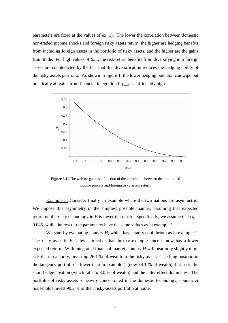
parameters are fixed at the values of ex. 1). The lower the correlation between domestic
non-traded income shocks and foreign risky assets return, the higher are hedging benefits
from including foreign assets in the portfolio of risky assets, and the higher are the gains
from trade. For high values of ρHy,F, the risk-return benefits from diversifying into foreign
assets are counteracted by the fact that this diversification reduces the hedging ability of
the risky-assets portfolio. As shown in figure 1, the lower hedging potential can wipe out
practically all gains from financial integration if ρHy,F is sufficiently high.
Figure 3.1: The welfare gain as a function of the correlation between the non-traded
income process and foreign risky assets return.
Example 3: Consider finally an example where the two nations are asymmetric.
We impose this asymmetry in the simplest possible manner, assuming that expected
return on the risky technology in F is lower than in H. Specifically, we assume that αF =
0.045, while the rest of the parameters have the same values as in example 1.
We start by evaluating country H, which has autarky equilibrium as in example 1.
The risky asset in F is less attractive than in that example since it now has a lower
expected return. With integrated financial market, country H will bear only slightly more
risk than in autarky, investing 26.1 % of wealth in the risky assets. The long position in
the tangency portfolio is lower than in example 1 (now 34.1 % of wealth), but so is the
short hedge position (which falls to 8.0 % of wealth) and the latter effect dominates. The
portfolio of risky assets is heavily concentrated in the domestic technology; country H
households invest 90.2 % of their risky-assets portfolio at home.
0
0.05
0.1
0.15
0.2
0.25
0.3
0.35
-0.3 -0.2 -0.1 0 0.1 0.2 0.3 0.4 0.5 0.6 0.7 0.8 0.9
ρFy,H
EV

21
Even though there is a small increase in fraction of wealth invested in risky assets,
the mean consumption growth rate falls to 1.97 % in this case. This arises because the
expected return on the portfolio held with integrated markets gives a lower expected
return than under autarky. Households choose a portfolio with lower expected return
because it provides a better hedge against non-traded income risk.
The instantaneous standard deviation of consumption growth would decrease to sH
= 8.59 % in country H upon integration. This ensures a tiny increase in the risk-adjusted
growth rate to 0.501 %. The welfare gain from financial integration is accordingly very
small; the equivalent-variation gain is only 0.1 % of wealth. Even moderate trading costs
would thus swamp the gains from trade in country H.
Turning to country F, we have an autarky equilibrium characterized by ωF = 0.03,
gF = mF + nF = 0.24 % + 0.70 % = 0.94 %, sF = 5.34 %, and a risk-adjusted growth rate of
0.38 %. The low expected return on the risky asset in F implies little investment in this
asset, and low consumption growth. With free asset trade between the two countries the
short-sale constraints binds for country F. It wish to short its own risky technology and
invest the proceedings in H’s risky asset, since the latter provides both a better risk-return
tradeoff and a better hedge against non-traded income risk. The short-sale constraints
prohibit such allocations, however. By inspection it turns out that case 4 in equation (20)
gives the optimal constrained asset allocation for country F, implying an investment of
37.5 % of wealth in the foreign risky asset while nothing is invested in the domestic
counterpart. Using equations (24) and (26), we find that this allocation implies gF* = 2.84
% and sF* = 10.89 %, giving a risk-adjusted growth rate equal to 0.47 %. The equivalent
variation measure of the welfare gain from financial integration is 11.9 % of initial
wealth. Hence, country F derives large benefits from cross-country asset trade even with
a binding short-sale constraint.
6. Conclusions
Our starting point was the debate on the costs and benefits of free capital mobility.
This paper has dealt with the possible benefits, an asked how these might be affected by
non-traded income risk when financial markets are incomplete.

22
We have shown that non-traded income risk can substantially alter the conclusions
found in earlier research on the gains from cross-border asset trade. In our model,
extending the set of available marketable assets may imply lower hedging demand for
risky high-return projects, and lower precautionary savings as the unhedgeable non-
traded income variance is reduced. These effects counteract the growth stimulus that all-
assets-traded complete-markets models predict from international asset trade. It also
implies that the welfare gains from financial integration may be negligible.
These results will typically occur if the non-traded income process has a higher
correlation with foreign risky asset returns than the domestic equivalent. If, on the other
hand, the non-traded income process has a lower correlation with the returns on foreign
assets than with the domestic ones, the gains from asset trade would typically be
amplified compared to a complete markets model.
Labor income fluctuations are probably the most important non-traded income
risk in reality. Baxter and Jermann (1997) presents evidence from Germany, Japan, UK
and US, where the pattern is that both (a synthetically computed) return on human capital
and labor income growth is more highly correlated with domestic capital returns than
foreign. This points to the conclusion that labor income risk strengthens the case for
trade in financial assets. Bottazzi et al. (1996) concludes different, however. Using data
for a large set of OECD-countries and taking into consideration redistributive shocks
between capital and labor, they find that foreign assets generally are less attractive than
domestic assets for hedging labor income uncertainty. Whether the presence of non-
traded income risk strengthens or weakens the arguments in favor of international asset
trade is therefore an empirical question that seems open.
Appendix
A.1 Individual Choice in the Closed Economy
We want to derive lifetime utility, asset demand, and the consumption policy of
the households in the closed economy of section 2. The consumption path tc ∞
τ τ= and
portfolio path t
∞τ τ=
ω are chosen to maximize (1) subject to (4), (5), the current level of
wealth W(t). Let J(W) denote the implied indirect utility function. The Hamilton-Jacobi-
Bellman equation for this problem is

23
( ) 1 2 2 2 21
1 2,0 max (1 ) 2c
W WW Ky ycJ J W r c J W−γ
−γω = − δ + ωα + − ω + µ − + ω σ + ωσ + σ (A.1)
where subscripts on J denotes partial derivatives. The implied first order conditions with
respect to the instantaneous consumption rate can be written as:
Wc J−γ = . (A.2)
Substituting this back into (A.1), we find that the differential equation for the value
function J is
[ ]1 2 2 2 211 20 (1 ) 2W W WW Ky yJ J J W r J W
γ−γγ
−γ = − δ + ωα + − ω +µ + ω σ + ωσ + σ , (A.3)
where the portfolio weights are optimized under the constraint that they must lie between
0 and 1:
0 if 0if 0 1
1 if 1,
ϖ <ω = ϖ ≤ ϖ ≤ ϖ >
(A.4)
where
2 2KyW
WW
J rJ W
σα −ϖ = − −σ σ
. (A.5)
Whenever there is an interior solution, (A.5) tells us that the optimal portfolio is a
combination of the tangency portfolio, corresponding to the first term on the right-hand-
side, and a hedge portfolio given by the second term.
Preferences of the CRRA-form leads to the conjecture that the indirect utility
function is of the form J(W) = A-γ(1 − γ)−1W1−γ for some constant A. Plugging the
conjectured function into (A.3) confirms that it is indeed correct, and that A is given by
equation (6a) in the main text. Finally, using (6) in (A.2) and (A.5) gives the
consumption policy (equation (7)) and asset demand (equation (8)) for the representative
household in the closed economy.
A.2 Behavior with International Asset Trade
We can follow the same methodology, as above to derive the optimal policies
when there is financial integration. Let us start by considering the problem without
restrictions on the portfolio weights. The Hamilton-Jacobi-Bellman equations are

24
1
, , 2 21
2 , ,
( )1
0 max , ,
2
i
H Fi i i
i i
Fji
W i i j i ij H
c F F Fj k j
W W i i i jk y i i jy ij H k H j H
c J J W r r ci H F
J W
−γ
=
ω ω
= = =
+ δ + ϖ α − + + µ − − γ = =
+ ϖ ϖ σ + σ + ϖ σ
∑
∑ ∑ ∑ (A.6)
In (A.6) the ϖij’s are the unconstrained portfolio weights, σjk is the instantaneous
variance/covariance of risky asset returns, and σjy,i is the instantaneous covariance
between non-traded income in i and the return on the risky asset in country j, j = H,F.
From this, we find that the optimal consumption policy is as in the closed economy:
, ,ii Wc J i H F−γ = = .
The optimal unconstrained portfolio weights satisfy
2,0 ( ) , , , .
i i i
Fk
W i j W W i i jk jy ik H
J W r J W i j H F=
= α − + ϖ σ + σ = ∑ (A.7)
This condition can conveniently be rewritten in matrix form as
( )( ) , ,i i iW W W i i iJ r J W i H F= − + Ω − =0 a 1 w V , (A.8)
where iw = [ϖiH ϖi
F]´. (The other notation is explained in the main text.) Solving for iw ,
we obtain:
1 1( ) , ,i
i i
Wi i
W W i
Jr i H F
J W− −= − Ω − − Ω =w a 1 V , (A.9)
which implies that
,( ) , , ,i
i i
F FWj
i jk k jk jy ik H k HW W i
Jr i j H F
J W = =
ϖ = − ν α − − ν σ =∑ ∑ . (A.10)
In (A.10), νjk are the elements of ΩΩΩΩ−1. We notice that the tangency and hedge portfolio is
given by the first and second term, respectively, on the right hand side of (A.9).
Taking into account the short sale constraints 0 ≤ ωij ≤ 1, i,j = H,F, and 1j
j iω ≤∑ ,
i = H,F, the asset allocation policies are considerably more complicated. The Hamilton-
Jacobi-Bellman equation is as (A.6), with the unconstrained portfolio weights ϖij replaced
by the constrained ones ωij. The first order conditions with respect to ωi
H and ωiF are:
,2 2 2 , ,i
i i
W Hy iH FH HFi i
W W i H H H
J r i H FJ W
σα − σω = − − − ω =σ σ σ
(A.11)

25
,2 2 2 , ,i
i i
W Fy iF HF HFi i
W W i F F F
J r i H FJ W
σα − σω = − − − ω =σ σ σ
. (A.12)
Next, define the following subsets of (A.11) and (A.12):
,2 2
ˆ , , ,i
i i
W j jy iji
W W i j j
J ri j H F
J Wα − σ
ω ≡ − − =σ σ
, (A.13)
,2 2 2 , , ,i
i i
W j jy ij HFi
W W i j j j
J ri j H F
J Wα − σ σω = − − − =
σ σ σ" , (A.14)
and
, ,2 2 2 2 2 2
( ) , ,i
i i
W Hy i Fy i FHH H F HFi
W W i j H F H H F
J r r i H FJ W
σ σ σα − α − σω ≡ − − − + = σ σ σ σ σ σ
! , (A.15)
where there is an analogous expression for Fiω! . Together with (A.10) and (A.13)-(A.15),
equations (A.11) and (A.12) gives us the following constrained asset allocation policies:
[ ]
[ ]
ˆ ˆ0,0 if 0 and 0
ˆ ˆ0, if 0 and 0 1
ˆ0,1 if 0 and 1
ˆ ˆ,0 if 0 1 and 0,, if 0 1, 0 1 and 1
, if H Fi i
H F H Fi i i i
H Fi i
F H Fi i i
H Fi i
H H FH F i i i
i i iH F H H H Fi i i i i i
iϖ ϖ
ϖ +ϖ ϖ +ϖ
ω < ω <
ω ω < ≤ ω ≤ ω < ω >
ω ≤ ω ≤ ω <′ = ω ω ≡ ϖ ϖ ≤ ϖ ≤ ≤ ϖ ≤ ϖ + ϖ ≤ ϖ
w
!
"!
[ ]0, 0 and 1
ˆ1,0 if 1 and 0
H H H Fi H H
H Fi i
> ϖ > ϖ + ϖ > ω > ω < "
(A.16)
for i = H,F.
Substituting the optimal consumption policy into the constrained Hamilton-
Jacobi-Bellman equation gives the differential equations for the value functions Ji(Wi):
[ ]1 2 21, ,1 20 ' ( ) ' 2 '
i i i iW i W i i i W W i i i i y i y iJ J J W r r J Wγ−
γγ−γ = + δ + − + + µ + Ω + + σ w a 1 w w w V ,
where w’i are given by (A.16), and i = H, F. The functional form of the intertemporal
indirect utility function does not change upon financial integration. For country i it is still 11 *( ) (1 ) ( ) i i
i i i iJ W A W−γ −γ−= − γ , for some constant Ai*. Using this in (A.8) we find that Ai
*
is given by (18) in the main text and that the optimal asset allocation is given by (20) and
(21).

26
References
Acemoglu, D. and F. Zilibotti, (1997). “Was Promotheus unbound by chance? Risk, diversification and
growth”, Journal of Political Economy, 105, 709-751.
Baxter, M. and U. J. Jermann, (1997). “The international diversification puzzle is worse than you think”,
American Economic Review, 87, 170-180.
Bhagwati, J., (1998). “The capital myth: The difference between trade in widgets and dollars”, Foreign
Affairs, 77, 7-12.
Bottazzi, L., P. Pesenti and E. van Wincoop, (1996). “Wages, profits and the international portfolio
puzzle”, European Economic Review, 40, 219-254.
Cox, J.C., J.E. Ingersoll and S.A. Ross, (1985). “An intertemporal general equilibrium model of asset
prices”, Econometrica, 53, 363-384.
Den Haan, W.J., (1994). “Heterogeneity, aggregate uncertainty and the short term interest rate: A case
study of two solution techniques”, mimeo, University of California at San Diego.
Devereux, M. and M. Saito, (1997). “Growth and risk-sharing with incomplete international asset markets”,
Journal of International Economics, 42, 453-481.
Devereux, M. and G.W. Smith, (1994). “International risk sharing and economic growth”, International
Economic Review, 35, 535-550.
Dumas, B. and R. Uppal, (1999). “Global diversification, growth and welfare with imperfectly integrated
markets for goods”, NBER working paper no. 6994.
Ingersoll, J.E., (1987). Theory of Financial Decision Making, (Rowman & Littlefield, New Jersey).
Levine, R., (1997). “Financial development and economic growth: Views and agenda”, Journal of
Economic Literature, 35, 688-726.
Krugman, P., (1998). “Saving Asia: It’s time to get radical”, Fortune.
Losq, E., (1978). “A note on consumption, human wealth and uncertainty”, mimeo, McGill University,
Montreal.
27
Merton, R.C., (1969). “Lifetime portfolio selection under uncertainty: The continuous time case”, Review
of Economics and Statistics, 51, 247-257.
Obstfeld, M., (1994). “Risk-taking, global diversification, and growth”, American Economic Review, 84,
1310-1329.
Obstfeld, M., (1998). “The global capital market: Benefactor or menace?”, Journal of Economic
Perspectives, 12, 9-30.
Obstfeld, M. and K. Rogoff, (1996). Foundations of International Macroeconomics, (MIT Press,
Cambridge).
Pagano, M., (1993). “Financial markets and growth: An overview”, European Economic Review, 37, 613-
622.
Rodrik, D., (1997). Has Globalization Gone too Far?, (The Institute of International Economics,
Washington).
Rogoff, K., (1999). “International institutions for reducing global financial instability”, NBER working
paper no. 7265.
Sandmo, A., (1970). “The effect of uncertainty on savings decisions”, Review of Economic Studies, 37,
353-360.
Shiller, R., (1993). Macro Markets: Creating Institutions to Manage Society’s Largest Economic Risks,
(Clarendon Press, Oxford).
Svensson, L. and I. Werner, (1993). “Nontraded assets in incomplete markets: Pricing and portfolio
choice”, European Economic Review, 37, 1149-1168.

28