Hydrol. Earth Syst. Sci., 14, 2443–2453, 2010www.hydrol-earth-syst-sci.net/14/2443/2010/doi:10.5194/hess-14-2443-2010© Author(s) 2010. CC Attribution 3.0 License.

Hydrology andEarth System

Sciences

Interannual variations of the terrestrial water storagein the Lower Ob’ Basin from a multisatellite approach

F. Frappart 1, F. Papa2, A. Guntner3, S. Werth3, G. Ramillien1,4, C. Prigent5, W. B. Rossow2, and M.-P. Bonnet1,6

1Universite de Toulouse, OMP, GET, UMR 5563, Toulouse, France2NOAA Cooperative Remote Sensing Science and Technology Center, City College of New York, New York, USA3GFZ, Telegrafenberg, Potsdam, Germany4CNRS, OMP, GET, UMR 5563, Toulouse, France5Laboratoire d’Etudes du Rayonnement et de la Matiere en Astrophysique, Observatoire de Paris, CNRS, Paris, France6IRD,OMP, GET, UR 154, Toulouse, France

Received: 23 July 2010 – Published in Hydrol. Earth Syst. Sci. Discuss.: 1 September 2010Revised: 24 November 2010 – Accepted: 1 December 2010 – Published: 6 December 2010

Abstract. Temporal variations of surface water volume overinundated areas of the Lower Ob’ Basin in Siberia, one of thelargest contributor of freshwater to the Arctic Ocean, are esti-mated using combined observations from a multisatellite in-undation dataset and water levels over rivers and floodplainsderived from the TOPEX/POSEIDON (T/P) radar altimetry.We computed time-series of monthly maps of surface watervolume over the common period of available T/P and mul-tisatellite data (1993–2004). The results exhibit interannualvariabilities similar to precipitation estimates and river dis-charge observations. This study also presents monthly esti-mates of groundwater and permafrost mass anomalies dur-ing 2003–2004 based on a synergistic analysis of multisatel-lite observations and hydrological models. Water stored inthe soil is isolated from the total water storage measured byGRACE when removing the contributions of both the surfacereservoir, derived from satellite imagery and radar altimetry,and the snow estimated by inversion of GRACE measure-ments. The time variations of groundwater and permafrostare then obtained when removing the water content of theroot zone reservoir simulated by hydrological models.

1 Introduction

All climate scenarios agree on the high sensitivity of thenorthern regions to global change, with a stronger warm-ing at these latitudes than globally. Average annual Arctic

Correspondence to:F. Frappart(frederic.frappart@lmtg.obs-mip.fr)

temperatures have increased at almost twice the global rateover recent decades and are predicted to increase by an addi-tional 4–7◦C by the end of the 20th century (Serreze et al.,2000). Continued warming of the Arctic regions will likelyhave profound consequences, many of which may have re-gional and global implications (Peterson et al., 2002). Forinstance, an increase in air temperature is expected to inten-sify the Arctic hydrological cycle (Stocker and Raible, 2005;Wu et al., 2005) and important modifications of the terrestrialwater cycle have been already observed in these northern lat-itudes. One observable change that attracted considerablescientific attention is the increase over the last century by 7%in the average annual discharge of fresh water from the sixlargest Eurasian rivers to the Arctic Ocean (Peterson et al.,2002; Yang et al., 2002). Other recent evidences of changein the Arctic hydrology were revealed with the analysis ofoptical remote sensing images by Smith et al. (2005) whichshowed a reduction between 1975 and 1997 in the numberof lakes in West Siberia that could be related to permafrostthawing. These modifications could lead to significant reper-cussions on both the biogeochemical and hydrological cyclesof northern high latitude systems, with further influence onthe global climate.

Among the various reservoirs in which fresh water on landis stored (e.g., ice caps, glaciers, snowpack, soil moisture andgroundwater), surface waters (rivers, lakes, reservoirs, wet-lands and inundated areas) play a crucial role in the globalbiogeochemical and the hydrological cycles (de Marsily etal., 2005). Although wetlands and floodplains cover only 6%of the Earth surface (OECD, 1996), they have a substantialimpact on flood flow alteration, sediment stabilization, waterquality, groundwater recharge and discharge (Maltby, 1991;

Published by Copernicus Publications on behalf of the European Geosciences Union.

2444 F. Frappart et al.: Interannual variations of the terrestrial water storage in the Lower Ob’ Basin

Bullock and Acreman, 2003). Moreover, floodplain inunda-tion is an important regulator of river hydrology owing tostorage effects along channel reaches. Reliable and timelyinformation about the extent, spatial distribution, and tempo-ral variation of wetlands and floods as well as the amount ofwater stored is crucial to better understand their relationshipwith river discharges, and also their influence on regional hy-drology and climate.

Remote sensing techniques have been very useful forstudying cold region climate and hydrology (Massom, 1995;Smith, 1997; Seidel and Martinec, 2004) as they providea unique mean to observe large regions. Good capabili-ties for monitoring snow extent and depth using passive mi-crowave measurements (Yang et al., 2002; Grippa et al.,2005) or multispectral images (Hall et al., 2002; Robinsonand Frei, 2000), water levels and discharges using radar al-timetry (Kouraev et al., 2005), and inundation extent com-bining multisatellite information (Papa et al., 2007, 2008a)have already been demonstrated. The Gravity Recovery AndClimate Experiment (GRACE) mission, launched in 2002,detects tiny changes in the Earth’s gravity field which can berelated to the spatio-temporal variations of the terrestrial wa-ter storage (TWS) at monthly or 10-day time-scales (Tapleyet al., 2004). Previous studies provide important informationon changes in TWS and snow mass at high latitudes (Muskettand Romanovsky, 2009; Frappart et al., 2010). TWS, repre-senting an integrated measurement of the water stored in thedifferent hydrological reservoirs, and consequently, the sumof the surface water, water stored in the root zone, snowpackand groundwater, can be considered as a good indicator of thechanges that occur in the hydrological conditions globally,and at basin-scale. Nevertheless, TWS is difficult to measuredue to the lack of a complete network of in situ observa-tions of the terrestrial hydrological components. The hydro-logic regime of rivers is strongly influenced by the presenceof permafrost at high latitudes. The river basins with highpermafrost coverage have lower subsurface storage capacity,which causes a lower winter baseflow and a higher summerpeak flow, than basins with low coverage (Woo, 1986; Kane,1997; Smith et al., 2007).

Variations in the groundwater storage can be extractedfrom the TWS measured by GRACE using external infor-mation on the other hydrological reservoirs such as in situobservations (Yeh et al., 2006), model outputs (Rodell et al.,2009), or both (Leblanc et al., 2009). No similar studies havebeen yet undertaken for large river basins characterized byextensive wetlands or floodplains in high latitude regions.

In this study, we demonstrate that remote sensing and hy-drological modelling can be combined to estimate water stor-age changes in the Lower Ob’ Basin by combining high-resolution imagery-derived inundation extents, altimetry-derived water level measurements and gravimetry from spaceproducts, and soil water outputs from hydrological models.We first present the analysis of twelve years of surface waterstorage variations. Then, water storage anomalies of surface

22

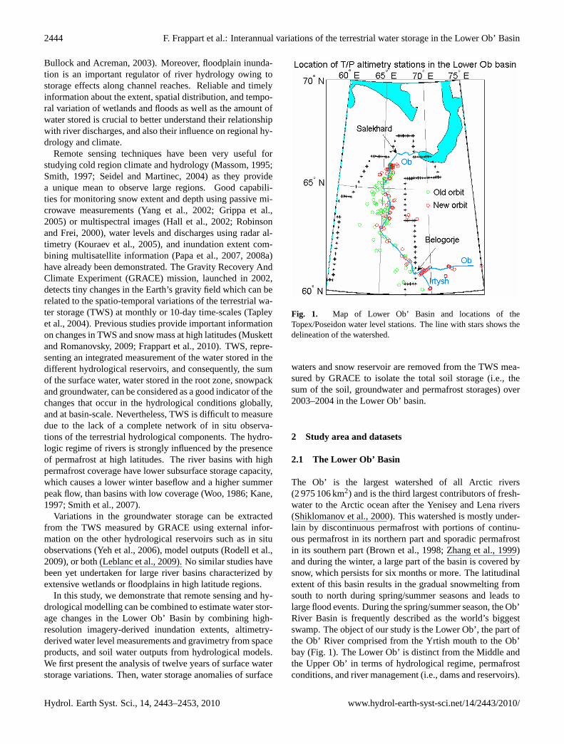
Figure 1. Map of Lower Ob’ basin and locations of the Topex/Poseidon water level stations. 1

The line with stars shows the delineation of the watershed. 2

Fig. 1. Map of Lower Ob’ Basin and locations of theTopex/Poseidon water level stations. The line with stars shows thedelineation of the watershed.

waters and snow reservoir are removed from the TWS mea-sured by GRACE to isolate the total soil storage (i.e., thesum of the soil, groundwater and permafrost storages) over2003–2004 in the Lower Ob’ basin.

2 Study area and datasets

2.1 The Lower Ob’ Basin

The Ob’ is the largest watershed of all Arctic rivers(2 975 106 km2) and is the third largest contributors of fresh-water to the Arctic ocean after the Yenisey and Lena rivers(Shiklomanov et al., 2000). This watershed is mostly under-lain by discontinuous permafrost with portions of continu-ous permafrost in its northern part and sporadic permafrostin its southern part (Brown et al., 1998; Zhang et al., 1999)and during the winter, a large part of the basin is covered bysnow, which persists for six months or more. The latitudinalextent of this basin results in the gradual snowmelting fromsouth to north during spring/summer seasons and leads tolarge flood events. During the spring/summer season, the Ob’River Basin is frequently described as the world’s biggestswamp. The object of our study is the Lower Ob’, the part ofthe Ob’ River comprised from the Yrtish mouth to the Ob’bay (Fig. 1). The Lower Ob’ is distinct from the Middle andthe Upper Ob’ in terms of hydrological regime, permafrostconditions, and river management (i.e., dams and reservoirs).

Hydrol. Earth Syst. Sci., 14, 2443–2453, 2010 www.hydrol-earth-syst-sci.net/14/2443/2010/

F. Frappart et al.: Interannual variations of the terrestrial water storage in the Lower Ob’ Basin 2445

2.2 The multisatellite inundation dataset

The multisatellite inundation dataset quantifies at globalscale the monthly distribution of surface water extent and itsvariations at∼25 km of resolution. The methodology whichcaptures the extent (with an accuracy of∼10%) of episodicand seasonal inundations, wetlands, rivers, lakes, and irri-gated agriculture over more than a decade, 1993–2004, isbased on a clustering analysis of a suite of complementarysatellites observations, including passive (SSM/I) and ac-tive (ERS) microwaves, visible and near-IR (AVHRR) ob-servations (Papa et al., 2007, 2008a,b, 2010; Prigent et al.,2007). As the microwave measurements are also sensitiveto snow cover, snow masks are used to edit the results andavoid any confusion with snow-covered pixels. The weeklyNorth Hemisphere and South Hemisphere snow mask fromthe National Snow and Ice Data Center (University of Col-orado; NSIDC) is adopted and averaged on a monthly basis(Armstrong and Brodzik, 2005).

This dataset has been intensively used for climatologi-cal and hydrological analyses, such as the evaluation of themethane surface emission models (Ringeval et al., 2010) orthe validation of the river flooding scheme in land surfacemodels (Decharme et al., 2008). In high latitudes regions,Papa et al. (2007) evaluated the consistency of the spatial andtemporal variations of this inundation dataset over the Ob’basin using in situ snow depth and river runoff, and Papa etal. (2008) investigated the response of river discharge to sea-sonal flood extent change in the large Siberian watersheds.

2.3 T/P-derived water levels

First devoted to ocean studies, radar altimetry is now com-monly used to monitor water levels over lakes, rivers andfloodplains (Calmant et al., 2008). In this study, we built analtimetry-based hydrological network of 90 (old orbit: 1993–2002) and 92 (new orbit: 2002–2005) time series of waterlevels derived from T/P measurements over the Lower Ob’drainage basin (see Fig. 1 for their locations), following themethodology previously proposed by Frappart et al. (2006a),for the period 1993–2004. All relevant environmental andgeophysical corrections of the altimeter range measurementswere applied. They include ionospheric, dry and wet tropo-spheric, solid Earth tide and pole tide corrections and correc-tion for the satellite’s centre of gravity. Following Kouraev etal. (2005), corrections specific to open ocean environmentssuch as ocean tides, ocean tide loading, inverted barometereffect and sea state bias were neglected. For each intersec-tion between the river (or the floodplain) and the satelliteground track, we define a so-called “altimetry station”, repre-sented by a rectangular window. Outliers are deleted using a3-σ criterion over the whole time span of analysis. For each10 day cycle, the water level at a given altimetry station isobtained by computing the median of all the high-rate data(10 Hz) included in the rectangular window. This process,

repeated for each cycle, allows the construction of a waterlevel time-series at the altimetry station. All the water lev-els are expressed with respect to the static GGM02C geoidmodel (Tapley et al., 2005). The uncertainty associated withthe water level height ranges between 5–25 cm for high wa-ter season to 15–50 cm during low water season. Note thatin high latitudes regions, the presence of ice and snow per-turbs the altimetric signal during a large portion of the year(Kouraev et al., 2005).

2.4 GRACE – derived land water and snow masssolutions

The Gravity Recovery And Climate Experiment (GRACE)mission, launched in March 2002, provides measurements ofthe spatio-temporal changes in Earth’s gravity field. Severalrecent studies have shown that GRACE data over the conti-nents can be used to derive the monthly changes of the to-tal land water storage (Ramillien et al., 2005, 2008; Schmittet al., 2008) with an accuracy of∼1.5 cm of water equiva-lent thickness when averaged over regions of a few hundredssquare-kilometres. The Level-2 GRACE solutions consist ofmonthly estimates of geo-potential coefficients adjusted foreach 30-day period from raw along-track GRACE measure-ments by different research groups (i.e., CSR, GFZ and JPL).These coefficients are developed up to a degree 60 (or spa-tial resolution of 333 km) and corrected for oceanic and at-mospheric effects (Bettadpur, 2007) to obtain residual globalgrids of ocean and land signals corrupted by a strong noise.These data are available at:ftp://podaac.jpl.nasa.gov/grace/.Here we used the three latest land water solutions (RL04)produced by GFZ, JPL (for these two first products, Jan-uary 2003, June 2003 and January 2004 are missing), andCSR (June 2003 and January 2004 are missing) and the de-rived snow solutions (Frappart et al., 2006b, 2010).

2.5 Water in the root zone from hydrological models

2.5.1 The LaD model

The LaD model provides monthly 1◦× 1◦ gridded time se-

ries of surface parameters. For each cell of the model, thetotal water storage is composed of three stores: a snowpackstore, a root-zone store and a groundwater store and the to-tal energy storage is equal to the sum of latent heat of fusionof the snowpack and the glacier and sensible heat content(Milly and Schmakin, 2002). Unfortunately, it contains norepresentation of the permafrost.

2.5.2 The WGHM model

The Water GAP Global Hydrology Model (WGHM) wasspecifically designed to estimate river discharge for wa-ter resources assessments. It computes 0.5◦

× 0.5◦ griddedtime series of monthly runoff and river discharge and istuned against time series of annual river discharges measured

www.hydrol-earth-syst-sci.net/14/2443/2010/ Hydrol. Earth Syst. Sci., 14, 2443–2453, 2010

2446 F. Frappart et al.: Interannual variations of the terrestrial water storage in the Lower Ob’ Basin

at 724 globally distributed stations. The soil water bal-ance takes into account the water content of the soil withinthe effective root zone, the effective precipitation as thesum of throughfall and snowmelt, the actual evapotranspi-ration and the surface runoff. Surface runoff is computedfrom the water balance equation that takes the water con-tent within the effective root zone, the effective precipita-tion and the evapotranspiration into account (Doll et al.,2003). This model employs a minimization function includ-ing a permafrost/glacier-related factor for the recharge of theaquifer described in Doll and Fiedler (2008).

We use the water content within the root zone from thesetwo models to simulate the soil moisture reservoir. It is im-portant to note that WGHM takes into account the occurrenceof permafrost in a grid cell for the groundwater recharge butLaD does not, and to keep in mind that these two models areunable to reproduce the complex mechanisms that occurredin the permafrost, active-layer, and talik, as described, forinstance, in MacKay (1995).

2.6 Precipitation estimates from GPCP

These data quantify the distribution of precipitation over theglobal land surface (Adler et al., 2003). We use the monthlySatellite-Gauge Combined Precipitation Data product Ver-sion 2 data, available from January 1997 to present with aspatial resolution of 1◦ of latitude and longitude. Over landsurfaces, the uncertainty in the rate estimates from GPCP isgenerally lower than over the oceans due to the in situ gaugeinput (in addition to satellite) from the GPCC (Global Pre-cipitation Climatology Center). Over land, validation exper-iments have been conducted in a variety of location world-wide and suggest that while there are known problems in re-gions of persistent convective precipitation, non precipitatingcirrus or regions of complex terrain, the estimates uncertain-ties range between 10%–30% (Adler et al., 2003).

2.7 In situ hydrological data from ArcticRIMS

Daily water levels from the Salekhard station between Febru-ary 2000 and December 2004, and monthly river dischargesfrom Salekhard station between January 1993 and Decem-ber 2004, and Belogorje station (see Fig. 1 for the location ofthese two stations) between January 1993 and October 1999(but with missing data over long time periods for Belogorjestation) were obtained from the ArcticRIMS web site (Arcti-cRIMS, 2003).

3 Methodology

3.1 Monthly maps of water levels

Monthly maps of water levels over the floodplains of theLower Ob’ Basin have been determined using combined ob-servations from the multi-satellite inundation dataset and the

T/P derived water levels at the altimetry stations. For a givenmonth during the flood season, water levels were linearly in-terpolated over the flooded zones of the Lower Ob’ Basin.A pixel of 25 km× 25 km is considered inundated when itspercentage of inundated area is greater than 0. Maps of inter-polated surface water levels with 25 km resolution have beenconstructed for each month between January 1993 and De-cember 2004. The elevation of each pixel of the water levelmaps is given with reference to its minimum computed overthe 1993–2004 period. This minimum elevation representseither the bathymetry or very low water stage of the flood-plain. More details about the methodology can be found inFrappart et al. (2005, 2006c, 2008).

3.2 Rescaling of the GRACE data

The GRACE solutions suffer from the presence of impor-tant high-frequency noise (i.e., north-south striping) causedby orbit resonance in spherical harmonics determination andaliasing of short-time phenomena which are geophysicallyunrealistic. An optimum filter method was determined byanalyzing the correspondance of GRACE basin-average wa-ter storage to the ensemble mean of hydrological models(WGHM, LaD) and by analyzing the error budgets (satel-lite/leakage errors) and amplitude and phase biases for thediffferent filter types. For the Lower Ob’ Basin, the simpleGaussian filter with 500 km radius was the best filter. Onlya very small bias in the seasonal phase of storage changesresulted due to filtering for the selected optimum filter meth-ods. The GRACE products have been rescaled with a factorof 0.98 to account for amplitude smoothing due to filteringdetermined from smoothed and unsmoothed basin-averagemodel ensemble time series of water storage (Werth et al.,2009).

3.3 Total soil and groundwater storages estimates

The time variations in Terrestrial Water Storage (TWS)are the sum of the contributions of the different reservoirspresent in a drainage basin:

1 TWS = 1 SW + 1 SN + 1 TSS (1)

with 1 TSS = 1 RZ + 1 GW + 1 P (2)

where SW represents the total surface water storage includ-ing lakes, reservoirs, in-channel and floodplains water, SN isthe snow storage, TSS is the total soil storage including RZthe water contained in the root zone of the soil (represent-ing a depth of 1 or 2 m), GW the groundwater storage in theaquifers, and P the permafrost storage. These terms are gen-erally expressed in volume (km3) or mm of equivalent-waterheight.

The sum of GW and P anomalies over 2003–2004 isobtained in Eq. (1) by calculating the difference betweenthe TWS anomaly estimated by GRACE and the SW level

Hydrol. Earth Syst. Sci., 14, 2443–2453, 2010 www.hydrol-earth-syst-sci.net/14/2443/2010/

F. Frappart et al.: Interannual variations of the terrestrial water storage in the Lower Ob’ Basin 2447

anomaly maps previously derived from remote sensing andthe RZ anomaly derived from hydrological models outputs.The TWS and RZ monthly anomalies are the average anoma-lies of respectively the Level-2 GRACE CSR, GFZ and JPLdestriped and smoothed solutions at 300 km of averaging ra-dius, and the outputs from LaD and WGHM.

3.4 Water volume variations

For a given montht , the regional water volume of TWS, SW,TSS, SN, RZ or GW + P storageδV (t) in a basin with sur-face areaS, is simply computed from the water heightsδhj ,with j = 1, 2, ... (expressed in mm of equivalent water height)insideS, and the elementary surfaceR2

esinθj δλδθ (and thepercentage of inundationPj for SW):

δ V (t) = R2e

∑j∈S

Pj δ hj

(θj , λj , t

)sin θj δ λ δ θ (3)

whereλj andθj are co-latitude and longitude respectively,δλ and δθ are the grid steps in longitude and latitude(generallyδλ = δθ ), and Re the mean radius of the Earth(∼6371 km). The surface and total water volume variationsare consequently expressed in km3.

3.5 Annual cycle of water volumes

From the series of TWS, SW, TSS, SN, RZ and GW + Panomaly grids, the temporal trend, seasonal and semi-annualamplitude were simultaneously fitted by least-square adjust-ment at each grid point. We assumed that, at 1st order,the changesδq(t) at each grid point are the sum of a lin-ear trend, an annual sinusoid (with frequencyωann=

2πTann

,with Tann∼ 1 year), a semi-annual sinusoid (with frequencyωsemi−ann=

2πTsemi−ann

, with Tsemi−ann∼ 6 months) and water

mass residualsδqRES(t):

δ q(t) = At + B + C cos (ωann t + ϕann) (4)

+ D cos (ωsemi−ann t + ϕsemi−ann) + δ qRES

The parameters which we adjusted for each grid point (θ ,λ) are the linear trend (i.e. slopeA and y-interceptB), theannual cycle (i.e. amplitudeC and phaseϕann) and the semi-annual cycle (i.e. amplitudeD and phaseϕsemi−ann). For thispurpose, we merely used a error-free least-square fitting tosolve the system:

δ Q = 8.X (5)

where the vectorδQ is the list of the SWE values,8 andX are the configuration matrix and the parameter vector, re-spectively. The latter two terms are:{8j

}=

[tj 1 cos

(ωann tj

)sin

(ωann tj

)(6)

cos(ωsemi−ann tj

)sin

(ωsemi−ann tj

)]X =

[α β ξann cosϕann − ξann sin ϕann ξsemi−ann (7)

cosϕsemi−ann − ξsemi−ann sin ϕsemi−ann]

23

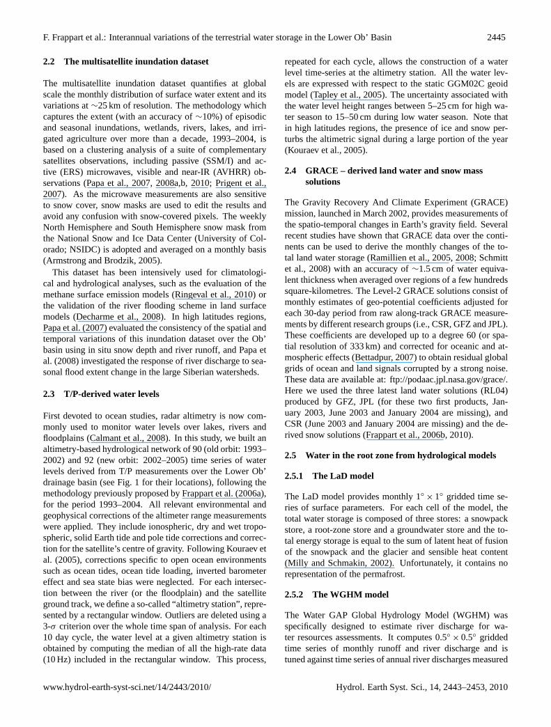
Figure 2. Monthly time variations of the inundated areas (km2) in the Lower Ob’ River Basin 1

from 1993 to 2004. 2 Fig. 2. Monthly time variations of the inundated areas (km2) in theLower Ob’ River Basin from 1993 to 2004.

for adjusting the temporal trend and for fitting the annual andsemi-annual amplitude and phase.

According to the least-squares criteria, the solution vectorof the linear system (Eq. 5) is:

XSOL=

(8T 8

)−18T δ Q (8)

4 Results and discussion

4.1 Monthly inundation extent

The inundated area fractions for the Lower Ob’ watershedwere extracted from the multisatellite inundation dataset.The temporal evolution of the total inundated extent (km2)over the lower Ob’ River Basin for the period 1993–2004 ispresented in Fig. 2. The mean extent during the snow-freemonths is only of 29× 103 km2. The inundation extent al-ways reaches its maximum in July, except for 1996, 1998,and 1999 where the maximum occurred in August. The in-undation exhibits a strong seasonal cycle, with the floodsgenerally starting in June and lasting until October. It alsopresents an important interannual variability. For example, in1993, the maximum inundated extent reached 67× 103 km2

whereas in 1995, it only reached 32× 103 km2.The spatial pattern of the inundation over the Lower Ob’

Basin is shown in Fig. 3. Figure 3a displays maps ofthe annual maximum of fractional inundation extent (in %,100% of inundations equals to a total area of 773 km2) fromsatellite estimates for each year of the period 1993–2004.Figure 3b shows the corresponding month during whichthe maximum inundation occurs. The inundation extent isclearly delineated over the river channel and the associatedfloodplains. The pixels with a very high percentage of inun-dation (greater than 50%) are located along the river chan-nel. A large inundation area is present downstream the junc-tion between the Ob’ and the Irtysh Rivers around 60◦ N and65◦ E.

www.hydrol-earth-syst-sci.net/14/2443/2010/ Hydrol. Earth Syst. Sci., 14, 2443–2453, 2010

2448 F. Frappart et al.: Interannual variations of the terrestrial water storage in the Lower Ob’ Basin

24

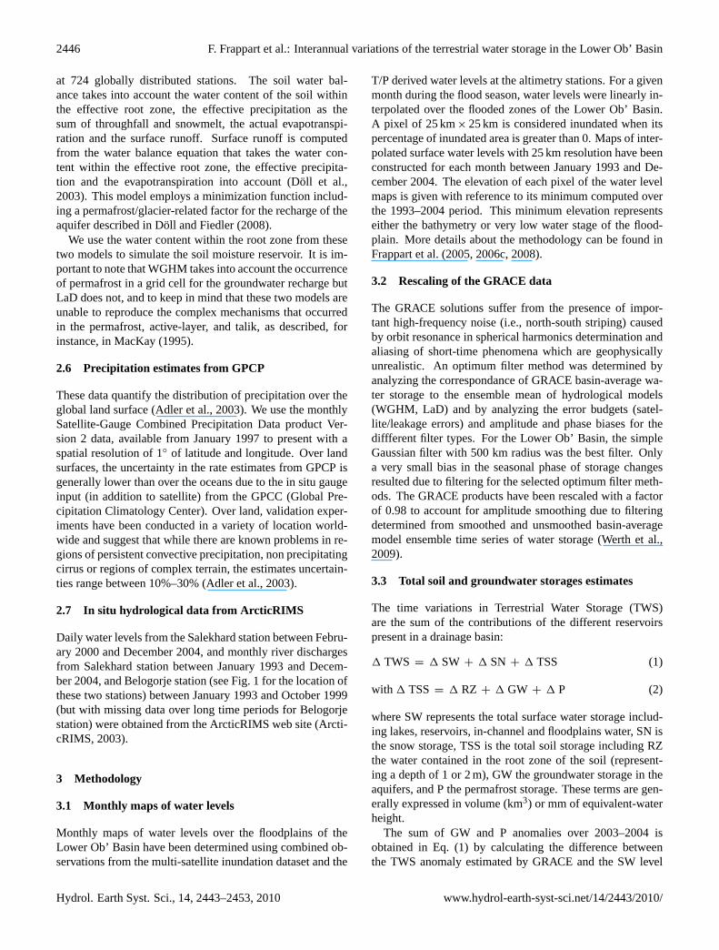
Figure 3. a) the 1993–2004 mean fractional inundation at yearly maximum (%) b) the average 1

month of the year (1993-2004) when the fractional inundation is maximum (in month).2

a)

b)

Fig. 3. (a) The 1993–2004 mean fractional inundation at yearlymaximum (%); (b) the average month of the year (1993–2004)when the fractional inundation is maximum (in month).

Figure 3b presents a map of the month during which oc-curred the maximum inundation extent. As seen in the resultsfrom Papa et al. (2008), this map clearly shows a propagationfrom south to north resulting from the latitudinal dependenceof the snow melting. The maximum inundation extent occursfrom May to June in the southern part of the basin and fromJuly to August on the northern region. The propagation ofthe maximum inundation extent from south to north gener-ally takes two to three months (this rough estimate is limitedby the monthly temporal resolution of the dataset).

4.2 Altimetry-derived water levels time series

The T/P altimetry stations where water level time seriescan be constructed are unevenly distributed across the basin(Fig. 1). An important point to notice is that this dataset givesvaluable information on water levels especially for unmoni-tored regions of the Lower Ob’ watershed, in particular overthe floodplains.

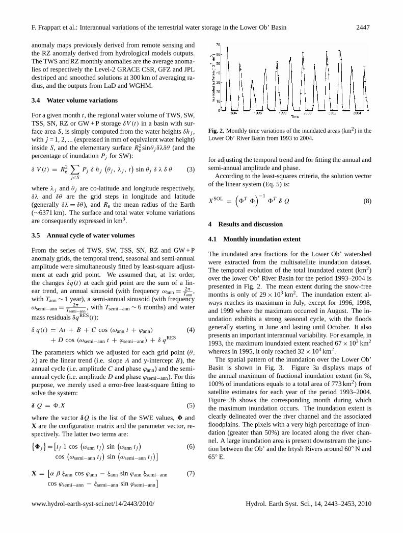
The water level time series derived from radar altimetry forthe stations close to Salekhard are presented in Fig. 4 alongwith in situ river heights time series. Comparisons have been

25

-3

-1

1

3

5

7

9

07/01/1992 06/01/1994 06/01/1996 05/01/1998 05/01/2000 04/01/2002 04/01/2004

Date

Wa

ter

Le

vels

(m

)

In situ

T/P 187

T/P 112

T/P 214

Figure 4. Time series of water levels at Salekhard from in situ gauge (black), T/P altimetry 1

stations. 2 Fig. 4. Time series of water levels at Salekhard from in situ gauge(black), T/P altimetry stations.

Table 1. Comparisons between the gauge records from Salekhardand the water levels derived from T/P measurements.

RMS (m) Correlation

In situ/TP 112 (old orbit) 0.89 0.89In situ/TP 187 (old orbit) 1.32 0.84In situ/TP 214 (new orbit) 1.34 0.69

made between the in situ gauge station of Salekhard at themouth of the Ob’ River and the closest altimetry stations onthe river channel for both the old and the new orbit of T/P(Table 1). For the old orbit, two altimetry stations can be de-fined at locations around 65 km at the South of Salekhard. Aspreviously observed by Kouraev et al. (2004), a good agree-ment between altimetry-derived and in situ water levels isfound with a correlation of 0.89 and a RMS of 0.89 m forT/P track 112 (old orbit). For the new orbit, the closest al-timetry station is located around 100 km from Salekhard. Asa consequence, the derived water levels do not agree as wellas the ones from the old orbit with a correlation of 0.69 anda RMS of 1.34 m.

4.3 Monthly maps of water levels

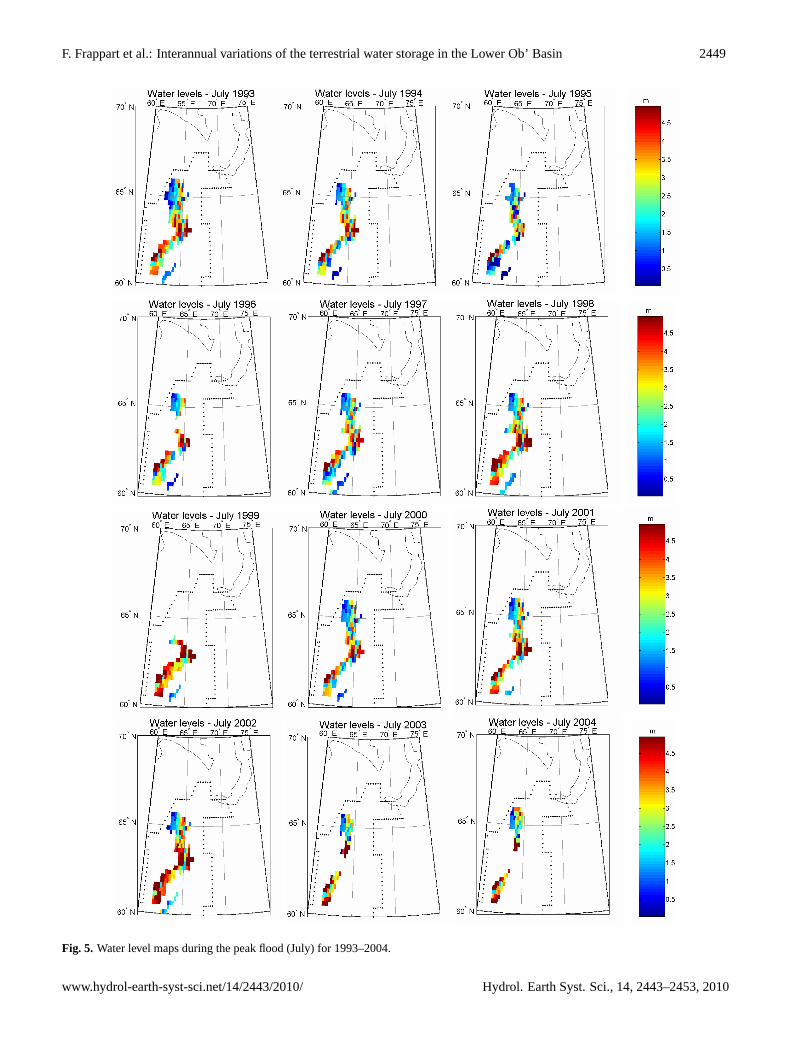
The monthly flood maps indicate that the flood period in theLower Ob’ generally ranges from June to October, whereaslow-water period ranges from December to April, during thewinter with a maximum occurring generally in July due tothe snowmelt. Figure 5 shows a series of maps of interpo-lated water levels over the floodplains at the maximum ofinundation for the period 1993–2004. The maximum differ-ence of water levels between high and low waters is lowerthan 6 m in the Lower Ob’ Basin. Maximum differences ofwater levels between high and low stages are observed alongthe river stream. Large spatial and temporal variabilities arealso revealed by the series of maps.

Hydrol. Earth Syst. Sci., 14, 2443–2453, 2010 www.hydrol-earth-syst-sci.net/14/2443/2010/

F. Frappart et al.: Interannual variations of the terrestrial water storage in the Lower Ob’ Basin 2449

26 Figure 5. Water level maps during the peak flood (July) for 1993–2004.1 Fig. 5. Water level maps during the peak flood (July) for 1993–2004.

www.hydrol-earth-syst-sci.net/14/2443/2010/ Hydrol. Earth Syst. Sci., 14, 2443–2453, 2010

2450 F. Frappart et al.: Interannual variations of the terrestrial water storage in the Lower Ob’ Basin

27

Figure 6. Time series of annual maximum of surface water storage volume (light green), 1

annual water volume flown in the Lower Ob’ basin (blue), and annual water volume of 2

precipitation. 3

0

20

40

60

80

100

120

140

160

180

1993 1994 1995 1996 1997 1998 1999 2000 2001 2002 2003 2004

Year

Wa

ter

vo

lum

e (

km

3)

Annual flown

Maximum storage

Average precipitation

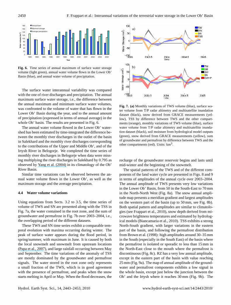
Fig. 6. Time series of annual maximum of surface water storagevolume (light green), annual water volume flown in the Lower Ob’Basin (blue), and annual water volume of precipitation.

The surface water interannual variability was comparedwith the one of river discharges and precipitation. The annualmaximum surface water storage, i.e., the difference betweenthe annual maximum and minimum surface water volumes,was confronted to the volume of water that has flown in theLower Ob’ Basin during the year, and to the annual amountof precipitation (expressed in terms of annual average) in thewhole Ob’ basin. The results are presented in Fig. 6.

The annual water volume flowed in the Lower Ob’ water-shed has been estimated by time-integrated the difference be-tween the monthly river discharges in the outlet of the basinin Salekhard and the monthly river discharges correspondingto the contributions of the Upper and Middle Ob’, and of theIrtysh River in Belogorje. We completed the time series ofmonthly river discharges in Belogorje when data were miss-ing multiplying the river discharges in Salekhard by 0.795 asobserved by Yang et al. (2004) in its climatology of the Ob’River Basin.

Similar time variations can be observed between the an-nual water volume flown in the Lower Ob’, as well as themaximum storage and the average precipitation.

4.4 Water volume variations

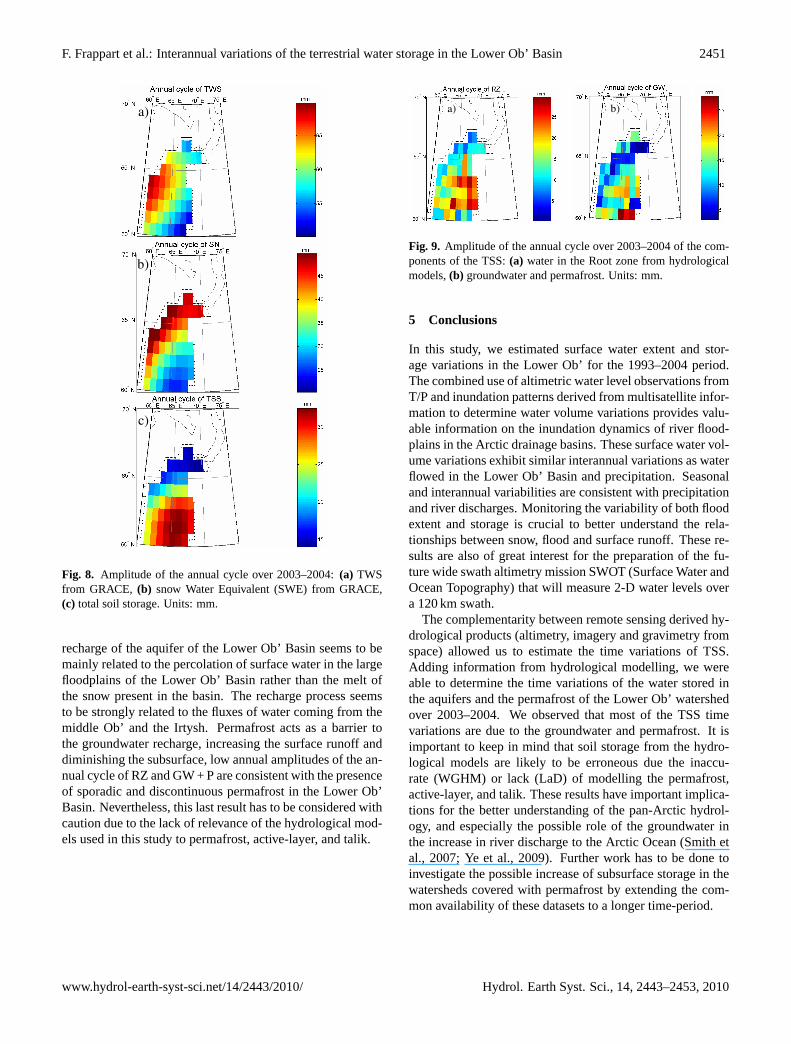
Using equations from Sects. 3.2 to 3.5, the time series ofvolume of TWS and SN are presented along with the TSS inFig. 7a, the water contained in the root zone, and the sum ofgroundwater and permafrost in Fig. 7b over 2003–2004, i.e.,the overlapping period of the different datasets.

These TWS and SN time series exhibit a comparable tem-poral evolution with maxima occurring during winter. Thepeak of surface water appears during the flood period, inspring/summer, with maximum in June. It is caused by boththe local snowmelt and snowmelt from upstream locations(Papa et al., 2007), and large rainfall occurring between Mayand September. The time variations of the anomaly of TSSare mostly dominated by the groundwater and permafrostsignals. The water stored in the root zone only representsa small fraction of the TWS, which is in good agreementwith the presence of permafrost, and peaks when the snowstarts melting in April or May. When the flood decreases, the

28

Figure 7. a) Monthly variations of TWS volume (blue), surface water volume from T/P radar 11

altimetry and multisatellite inundation dataset (black), snow derived from GRACE 12

measurements (yellow), TSS by difference between TWS and the other compartments 13

(orange), Monthly variations of TWS volume (blue), surface water volume from T/P radar 14

altimetry and multisatellite inundation dataset (black), soil moisture from hydrological model 15

outputs (green), snow derived from GRACE measurements (yellow), sum of groundwater and 16

permafrost by difference between TWS and the other compartments (red). Units: km3. 17

a)

b)

Fig. 7. (a)Monthly variations of TWS volume (blue), surface wa-ter volume from T/P radar altimetry and multisatellite inundationdataset (black), snow derived from GRACE measurements (yel-low), TSS by difference between TWS and the other compart-ments (orange), monthly variations of TWS volume (blue), surfacewater volume from T/P radar altimetry and multisatellite inunda-tion dataset (black), soil moisture from hydrological model outputs(green), snow derived from GRACE measurements (yellow), sumof groundwater and permafrost by difference between TWS and theother compartments (red). Units: km3.

recharge of the groundwater reservoir begins and lasts untilmid-winter and the beginning of the snowmelt.

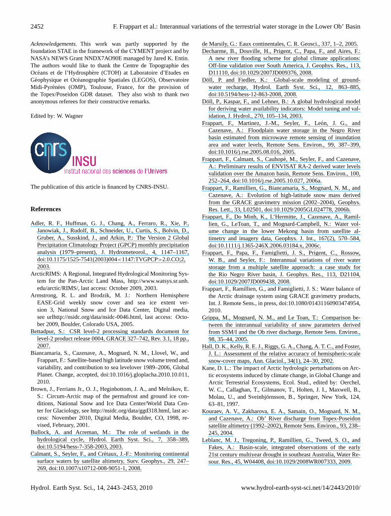
The spatial patterns of the TWS and of the different com-ponents of the land water cycle are presented in Figs. 8 and 9in terms of amplitudes of the annual cycle over 2003–2004.The annual amplitude of TWS presents very low variationsin the Lower Ob’ Basin, from 50 in the South-East to 70 mmin the North-North West (Fig. 8a). The snow annual ampli-tude map presents a meridian gradient and largest amplitudeson the western part of the basin (up to 50 mm, see Fig. 8b).Both spatial pattern and amplitudes are similar to climatolo-gies (see Frappart et al., 2010), snow depth derived from mi-crowave brightness temperatures and estimated by hydrolog-ical models (Biancamaria et al., 2010). TSS exhibits a strongNorth-South gradient, with larger variations in the easternpart of the basin, and following the permafrost distributionfrom Brown et al. (1998): high amplitudes around 30–35 mmin the South (especially in the South East) of the basin wherethe permafrost is isolated or sporadic to less than 15 mm inthe North-East close to the mouth where the permafrost isdiscontinuous (Fig. 8c). RZ has a very low annual amplitude,except in the eastern part of the basin with value reaching25 mm (Fig. 9a). The map of annual amplitude of the ground-water and permafrost components exhibits a low signal inthe whole basin, except just below the junction between theOb’ and the Irtysh where it reaches 30 mm (Fig. 9b). The

Hydrol. Earth Syst. Sci., 14, 2443–2453, 2010 www.hydrol-earth-syst-sci.net/14/2443/2010/

F. Frappart et al.: Interannual variations of the terrestrial water storage in the Lower Ob’ Basin 2451

29

1

2

3

4

5

6

7

8

9

10

11

12

13

14

15

16

17

18

19

20

21

22

23

Figure 8. Amplitude of the annual cycle over 2003-2004: a) TWS from GRACE, b) Snow 24

Water Equivalent (SWE) from GRACE, c) Total Soil Storage. Units: mm. 25

26

a)

b)

c)

Fig. 8. Amplitude of the annual cycle over 2003–2004:(a) TWSfrom GRACE, (b) snow Water Equivalent (SWE) from GRACE,(c) total soil storage. Units: mm.

recharge of the aquifer of the Lower Ob’ Basin seems to bemainly related to the percolation of surface water in the largefloodplains of the Lower Ob’ Basin rather than the melt ofthe snow present in the basin. The recharge process seemsto be strongly related to the fluxes of water coming from themiddle Ob’ and the Irtysh. Permafrost acts as a barrier tothe groundwater recharge, increasing the surface runoff anddiminishing the subsurface, low annual amplitudes of the an-nual cycle of RZ and GW + P are consistent with the presenceof sporadic and discontinuous permafrost in the Lower Ob’Basin. Nevertheless, this last result has to be considered withcaution due to the lack of relevance of the hydrological mod-els used in this study to permafrost, active-layer, and talik.

30

Figure 9. Amplitude of the annual cycle over 2003-2004 of the components of the TSS: a) 1

Water in the Root zone from hydrological models, b) Groundwater and permafrost. Units: 2

mm. 3

a) b)

Fig. 9. Amplitude of the annual cycle over 2003–2004 of the com-ponents of the TSS:(a) water in the Root zone from hydrologicalmodels,(b) groundwater and permafrost. Units: mm.

5 Conclusions

In this study, we estimated surface water extent and stor-age variations in the Lower Ob’ for the 1993–2004 period.The combined use of altimetric water level observations fromT/P and inundation patterns derived from multisatellite infor-mation to determine water volume variations provides valu-able information on the inundation dynamics of river flood-plains in the Arctic drainage basins. These surface water vol-ume variations exhibit similar interannual variations as waterflowed in the Lower Ob’ Basin and precipitation. Seasonaland interannual variabilities are consistent with precipitationand river discharges. Monitoring the variability of both floodextent and storage is crucial to better understand the rela-tionships between snow, flood and surface runoff. These re-sults are also of great interest for the preparation of the fu-ture wide swath altimetry mission SWOT (Surface Water andOcean Topography) that will measure 2-D water levels overa 120 km swath.

The complementarity between remote sensing derived hy-drological products (altimetry, imagery and gravimetry fromspace) allowed us to estimate the time variations of TSS.Adding information from hydrological modelling, we wereable to determine the time variations of the water stored inthe aquifers and the permafrost of the Lower Ob’ watershedover 2003–2004. We observed that most of the TSS timevariations are due to the groundwater and permafrost. It isimportant to keep in mind that soil storage from the hydro-logical models are likely to be erroneous due the inaccu-rate (WGHM) or lack (LaD) of modelling the permafrost,active-layer, and talik. These results have important implica-tions for the better understanding of the pan-Arctic hydrol-ogy, and especially the possible role of the groundwater inthe increase in river discharge to the Arctic Ocean (Smith etal., 2007; Ye et al., 2009). Further work has to be done toinvestigate the possible increase of subsurface storage in thewatersheds covered with permafrost by extending the com-mon availability of these datasets to a longer time-period.

www.hydrol-earth-syst-sci.net/14/2443/2010/ Hydrol. Earth Syst. Sci., 14, 2443–2453, 2010

2452 F. Frappart et al.: Interannual variations of the terrestrial water storage in the Lower Ob’ Basin

Acknowledgements.This work was partly supported by thefoundation STAE in the framework of the CYMENT project and byNASA’s NEWS Grant NNDX7AO90E managed by Jared K. Entin.The authors would like to thank the Centre de Topographie desOceans et de l’Hydrosphere (CTOH) at Laboratoire d’Etudes enGeophysique et Oceanographie Spatiales (LEGOS), ObservatoireMidi-Pyrenees (OMP), Toulouse, France, for the provision ofthe Topex/Poseidon GDR dataset. They also wish to thank twoanonymous referees for their constructive remarks.

Edited by: W. Wagner

The publication of this article is financed by CNRS-INSU.

References

Adler, R. F., Huffman, G. J., Chang, A., Ferraro, R., Xie, P.,Janowiak, J., Rudolf, B., Schneider, U., Curtis, S., Bolvin, D.,Gruber, A., Susskind, J., and Arkin, P.: The Version 2 GlobalPrecipitation Climatology Project (GPCP) monthly precipitationanalysis (1979–present), J. Hydrometeorol., 4, 1147–1167,doi:10.1175/1525-7541(2003)004<1147:TVGPCP>2.0.CO;2,2003.

ArcticRIMS: A Regional, Integrated Hydrological Monitoring Sys-tem for the Pan-Arctic Land Mass,http://www.watsys.sr.unh.edu/arctic/RIMS/, last access: October 2009, 2003.

Armstrong, R. L. and Brodzik, M. J.: Northern HemisphereEASE-Grid weekly snow cover and sea ice extent ver-sion 3, National Snow and Ice Data Center, Digital media,see urlhttp://nsidc.org/data/nsidc-0046.html, last access: Octo-ber 2009, Boulder, Colorado USA, 2005.

Bettadpur, S.: CSR level-2 processing standards document forlevel-2 product release 0004, GRACE 327–742, Rev. 3.1, 18 pp.,2007.

Biancamaria, S., Cazenave, A., Mognard, N. M., Llovel, W., andFrappart, F.: Satellite-based high latitude snow volume trend and,variability, and contribution to sea levelover 1989–2006, GlobalPlanet. Change, accepted, doi:10.1016/j.gloplacha.2010.10.011,2010.

Brown, J., Ferrians Jr., O. J., Heginbottom, J. A., and Melnikov, E.S.: Circum-Arctic map of the permafrost and ground ice con-ditions, National Snow and Ice Data Center/World Data Cen-ter for Glaciology, seehttp://nsidc.org/data/ggd318.html, last ac-cess: November 2010, Digital Media, Boulder, CO, 1998, re-vised, February, 2001.

Bullock, A. and Acreman, M.: The role of wetlands in thehydrological cycle, Hydrol. Earth Syst. Sci., 7, 358–389,doi:10.5194/hess-7-358-2003, 2003.

Calmant, S., Seyler, F., and Cretaux, J.-F.: Monitoring continentalsurface waters by satellite altimetry, Surv. Geophys., 29, 247–269, doi:10.1007/s10712-008-9051-1, 2008.

de Marsily, G.: Eaux continentales, C. R. Geosci., 337, 1–2, 2005.Decharme, B., Douville, H., Prigent, C., Papa, F., and Aires, F.:

A new river flooding scheme for global climate applications:Off-line validation over South America, J. Geophys. Res., 113,D11110, doi:10.1029/2007JD009376, 2008.

Doll, P. and Fiedler, K.: Global-scale modeling of ground-water recharge, Hydrol. Earth Syst. Sci., 12, 863–885,doi:10.5194/hess-12-863-2008, 2008.

Doll, P., Kaspar, F., and Lehner, B.: A global hydrological modelfor deriving water availability indicators: Model tuning and val-idation, J. Hydrol., 270, 105–134, 2003.

Frappart, F., Martinez, J.-M., Seyler, F., Leon, J. G., andCazenave, A.: Floodplain water storage in the Negro Riverbasin estimated from microwave remote sensing of inundationarea and water levels, Remote Sens. Environ., 99, 387–399,doi:10.1016/j.rse.2005.08.016, 2005.

Frappart, F., Calmant, S., Cauhope, M., Seyler, F., and Cazenave,A.: Preliminary results of ENVISAT RA-2 derived water levelsvalidation over the Amazon basin, Remote Sens. Environ., 100,252–264, doi:10.1016/j.rse.2005.10.027, 2006a.

Frappart, F., Ramillien, G., Biancamaria, S., Mognard, N. M., andCazenave, A.: Evolution of high-latitude snow mass derivedfrom the GRACE gravimetry mission (2002–2004), Geophys.Res. Lett., 33, L02501, doi:10.1029/2005GL024778, 2006b.

Frappart, F., Do Minh, K., L’Hermitte, J., Cazenave, A., Ramil-lien, G., LeToan, T., and Mognard-Campbell, N.: Water vol-ume change in the lower Mekong basin from satellite al-timetry and imagery data, Geophys. J. Int., 167(2), 570–584,doi:10.1111/j.1365-246X.2006.03184.x, 2006c.

Frappart, F., Papa, F., Famiglietti, J. S., Prigent, C., Rossow,W. B., and Seyler, F.: Interannual variations of river waterstorage from a multiple satellite approach: a case study forthe Rio Negro River basin, J. Geophys. Res., 113, D21104,doi:10.1029/2007JD009438, 2008.

Frappart, F., Ramillien, G., and Famiglietti, J. S.: Water balance ofthe Arctic drainage system using GRACE gravimetry products,Int. J. Remote Sens., in press, doi:10.1080/01431160903474954,2010.

Grippa, M., Mognard, N. M., and Le Toan, T.: Comparison be-tween the interannual variability of snow parameters derivedfrom SSM/I and the Ob river discharge, Remote Sens. Environ.,98, 35–44, 2005.

Hall, D. K., Kelly, R. E. J., Riggs, G. A., Chang, A. T. C., and Foster,J. L.: Assessment of the relative accuracy of hemispheric-scalesnow-cover maps, Ann. Glaciol., 34(1), 24–30, 2002.

Kane, D. L.: The impact of Arctic hydrologic perturbations on Arc-tic ecosystems induced by climate change, in Global Change andArctic Terrestrial Ecosystems, Ecol. Stud., edited by: Oerchel,W. C., Callaghan, T., Gilmanov, T., Holten, J. I., Maxwell, B.,Molau, U., and Sveinbjornsson, B., Springer, New York, 124,63–81, 1997.

Kouraev, A. V., Zakharova, E. A., Samain, O., Mognard, N. M.,and Cazenave, A.: Ob’ River discharge from Topex-Poseidonsatellite altimetry (1992–2002), Remote Sens. Environ., 93, 238–245, 2004.

Leblanc, M. J., Tregoning, P., Ramillien, G., Tweed, S. O., andFakes, A.: Basin-scale, integrated observations of the early21st century multiyear drought in southeast Australia, Water Re-sour. Res., 45, W04408, doi:10.1029/2008WR007333, 2009.

Hydrol. Earth Syst. Sci., 14, 2443–2453, 2010 www.hydrol-earth-syst-sci.net/14/2443/2010/

F. Frappart et al.: Interannual variations of the terrestrial water storage in the Lower Ob’ Basin 2453

MacKay, J. R.: Active Layer Changes (1968 to 1993) followingthe Forest-Tundra Fire, Inuvik, N. W. T., Canada, Arctic AlpineRes., 27(3), 323–336, 1995.

Maltby, E.: Wetland management goals: Wise use and conservation,Landscape Urban Plan., 20, 9–18, 1991.

Massom, R: Satellite remote sensing of polar snow and ice: presentstatus and future directions, Polar Res., 31(1), 99–114, 1995.

Milly, P. C. D. and Shmakin, A. B.: Global modeling of land waterand energy balances: 1. The Land Dynamics (LaD) model, J.Hydrometeorol., 3, 283–299, 2002.

Muskett, R. R. and Romanovsky, V. E.: Groundwater storagechanges in arctic permafrost watersheds from GRACE and in situmeasurements, Environ. Res. Lett., 4(3), 045009, 2009.

Organisation for Economic Cooperation and Development: Guide-lines for Aid Agencies for Improved Conservation and Sustain-able Use of Tropical and Sub-tropical Wetlands, Guidelines AidEnviron., 9, Paris, France, 69 pp., 1996.

Papa, F., Prigent, C., and Rossow, W. B.: Ob’ River flood inunda-tions from satellite observations: a relationship with winter snowparameters and river runoff, J. Geophys. Res., 112, D18103,doi:10.1029/2007JD008451, 2007.

Papa, F., Prigent, C., and Rossow, W. B.: Monitoring Flood andDischarge Variations in the Large Siberian Rivers From a Multi-Satellite Technique, Surv. Geophys., 29, 297–317, 2008a.

Papa, F., Guntner, A., Frappart, F., Prigent, C., and Rossow, W. B.:Variations of surface water extent and water storage in large riverbasins: A comparison of different global data sources, Geophys.Res. Lett., 35, L11401, doi:10.1029/2008GL033857, 2008b.

Papa, F., Prigent, C., Aires, F., Jimenez, C., Rossow, W. B.,and Matthews, E.: Interannual variability of surface wa-ter extent at global scale, J. Geophys. Res., 115, D12111,doi:10.1029/2009JD012674, 2010.

Peterson, B. J., Holmes, R. M., McClelland, J. W., Vorosmarty,C. J., Lammers, R. B., and Shiklomanov, A. I.: Increasing riverdischarge to the Artic Ocean, Science, 298, 2171–2173, 2002.

Prigent, C., Papa, F., Aires, F., Rossow, W. B., and Matthews,E.: Global inundation dynamics inferred from multiple satel-lite observations, 1993–2000, J. Geophys. Res., 112, D12107,doi:10.1029/2006JD007847, 2007.

Ramillien, G., Frappart, F., Cazenave, A., and Guntner, A.: Timevariations of the land water storage from an inversion of 2 yearsof GRACE geoids, Earth Planet. Sc. Lett., 235, 283–301,doi:10.1016/j.epsl.2005.04.005, 2005.

Ramillien, G., Famiglietti, J. S., and Wahr, J.: Detection of con-tinental hydrology and glaciology signals from GRACE: A re-view, Surv. Geophys., 29(4–5), 361–374, doi:10.1007/s10712-008-9048-9, 2008.

Ringeval, B., de Noblet-Ducoudre, N., Ciais, P., Bousquet, P., Pri-gent, C., Papa, F., and Rossow, W. B.: An attempt to quantifythe impact of changes in wetland extent on methane emissionson the seasonal and interannual time scales, Global Biogeochem.Cy., 24, GB2003, doi:10.1029/2008GB003354, 2010.

Robinson, D. A. and Frei, A.: Seasonal variability of northern hemi-sphere snow extent using visible data, Prof. Geogr., 52(2), 307–315, 2000.

Roddel, M., Velicogna, I., and Famiglietti, J. S.: Satellite-basedestimates of groundwater depletion in India, Nature, 460, 999–1003, doi:10.1038/nature08238, 2009.

Schmidt, R., Flechtner, F., Meyer, U., Neumayer, K.-H., Dahle,Ch., Koenig, R., and Kusche, J.: Hydrological Signals Ob-served by the GRACE Satellites, Surv. Geophys., 29, 319–334,doi:10.1007/s10712-008-9033-3, 2008.

Seidel, K. and Martinec, J.: Remote sensing in snow hydrol-ogy: runoff modelling, effect of climate change, Springer Praxisbooks – Geophysical Sciences, Berlin, 150 pp., 2004.

Serreze, M. C., Walsh, J. E., Chapin III, F. S., Osterkamp, T., Dyurg-erov, M., Romanovsky, V., Oechel, W. C., Morison, J., Zhang, T.,and Barry, R. G.: Observational evidence of recent change in thenorthern high-latitude environment, Climatic Change, 46, 159–207, 2000.

Shiklomanov, I. A., Lammers, R. B., Peterson, B. J., andVorosmarty, C. J.: The dynamics of river water inflow to the Arc-tic Ocean. In the freshwater budget of the Arctic Ocean, proc. ofthe NATO advanced research workshop, Kluwer Academic Pub-lishers, Norwell, 281–296, 2000.

Smith, L. C.: Satellite remote sensing of river inundation area, stageand processes: a review, Hydrol. Process., 11, 1427–1439, 1997.

Smith, L. C., Sheng, Y., MacDonald, G. M., and Hinz-man, L. D.: Disapearing Arctic lakes, Science, 308, 1429,doi:10.1126/science.1108142, 2005.

Smith, L. C., Pavelsky, T. M., MacDonald, G. M., Shiklomanov, A.I., and Lammers, R. B.: Rising minimum daily flows in north-ern Eurasian rivers: a growing influence of groundwater in thehigh-latitude hydrologic cycle, J. Geophys. Res., 112, G04S47,doi:10.1029/2006JG000327, 2007.

Stocker, T. F. and Raible, C. C.: Water cycle shifts gear, Nature,434, 1560–1563, 2005.

Tapley, B., Ries, J., Bettadpur, S., Chambers, D., Cheng, M.,Condi, F., Gunter, B., Kang, Z., Nagel, P., Pastor, R., Pekker,T., Poole, S., and Wang, F.: GGM02 – an improved Earthgravity field model from GRACE, J. Geodesy, 79, 467–478,doi:10.1007/s00190-005-0480-z, 2005.

Werth, S., Guntner, A., Schmidt, R., and Kusche, J.: Evaluation ofGRACE filter tools from a hydrological perspective, Geophys.J. Int., 179, 1499–1515, doi:10.1111/j.1365-246X.2009.04355.x,2009.

Woo, M.-K.: Permafrost hydrology in North America, Atmos.Ocean, 24(2), 201–234, 1986.

Wu, P., Wood, R., and Stott, P.: Human influence on increas-ing Arctic river discharges, Geophys. Res. Lett., 32, L02703,doi:10.1029/2004GL0215, 2005.

Yang, D., Kane, D. L., Hinzman, L. D., Zhang, X., Zhang, T., andYe, H.: Siberian Lena river hydrologic regime and recent change,J. Geophys. Res., 107(D23), 4694, 2002.

Yang, D., Ye, B., and Shiklomanov, A.: Discharge characteristicsand changes over the Ob’ River watershed in Siberia, J. Hydrom-eteorol., 5, 595–610, 2004.

Ye, B., Yang, D., Zhang, Z., and Kane, D. L.: Variation of hydrolog-ical regime with permafrost coverage over Lena basin in Siberia,J. Geophys. Res., 114, D07102, doi:10.1029/2008JD010537,2009.

Zhang, T., Barry, R. G., Knowles, K., Heginbottom, J. A., andBrown, J.: Statistics and characteristics of permafrost andground-ice distribution in the Northern Hemisphere, Polar Ge-ogr., 23(2), 132–154, 1999.

www.hydrol-earth-syst-sci.net/14/2443/2010/ Hydrol. Earth Syst. Sci., 14, 2443–2453, 2010