Interactive response surface approaches using computationally intensive models for multiobjective...

Interactive response surface approaches using computationallyintensive models for multiobjective planning of lake water qualityremediation

A. Castelletti,1,2 J. P. Antenucci,2 D. Limosani,1 X. Quach Thi,1 and R. Soncini-Sessa1

Received 16 February 2011; revised 3 August 2011; accepted 4 August 2011; published 30 September 2011.

[1] Recent work has demonstrated the utility of interactive response surfaces in integratingdecision making and complex process-based modeling of environmental systems.Specifically, we focus on problems that require computationally expensive dynamic modelswhere a limited number of simulations are possible and so traditional meta-modeling mightbe not an option for the optimization process. Within this constraint, the interactive globalresponse surface method aims to develop a complete picture of how the system responds toa planning decision on the basis of a restricted number of simulations. The interactive localresponse surface method utilizes the current best alternative to determine improvements onthe basis of relatively small changes in the current decision. We outline the use of bothmethods to a real example of remediation in a water supply reservoir, demonstrating the keyadvantages and disadvantages of each method and describe a new, interactive cascadeapproach that provides an improved solution to the problem.

Citation: Castelletti, A., J. P. Antenucci, D. Limosani, X. Quach Thi, and R. Soncini-Sessa (2011), Interactive response surface

approaches using computationally intensive models for multiobjective planning of lake water quality remediation, Water Resour. Res.,47, W09534, doi:10.1029/2011WR010552.

1. Introduction[2] Inland waters are under increasing stress from changes

in land use, rainfall and runoff patterns, and increasing tem-peratures. In many cases, this is leading to an increasingprevalence of cyanobacteria [Jönk et al., 2008], and thus del-eterious impacts on water quality.

[3] Remediation of lakes and reservoirs has traditionallybeen associated with reducing external nutrient loads bycatchment management of point and nonpoint sources [Schin-dler et al., 2008], however, in-lake strategies can complementthese approaches for certain objectives. In-lake strategies usu-ally involve the installation of some mechanical device toincrease hypolimnetic oxygen concentrations [Singleton andLittle, 2006], increase vertical mixing [Schladow, 1993], orincrease horizontal transport [Morillo et al., 2009]. Hypo-limnetic oxygenation aims to reduce internal nutrient load-ing by changing the redox conditions at the sediment/waterinterface so that the sediments are no longer a source ofnutrients. Artificial destratification has a similar aim, how-ever, it also breaks down the seasonal thermocline and thuspotentially impacts the light regime experienced by the phy-toplankton in a lake environment [Huisman et al., 2004].

[4] The scientific basis and engineering design aspectsof these interventions are thus well known, however, theproliferation of available technologies now makes the

efficient assessment of the best alternative a complex task.We define an alternative as a combination of different tech-nological interventions, and it is the potential for combin-ing technologies across various spatial scales that makesthe number of feasible alternatives large. In addition, thereis the need to demonstrate the preferred alternative is opti-mal in some sense, and so multiobjective optimization addsan additional layer of complexity to the problem.

[5] An assessment of remediation options typicallyassumes a dynamic, process-based model is available to sim-ulate the system behavior under each possible alternative.The traditional approach to this problem is the ‘‘what-if’’analysis, where the model is directly used to evaluate thealternatives and to choose the most preferred by compari-son with other feasible alternatives. Alternatively, the deci-sion criteria for remediation can be formalized as a set ofindicators to be optimized using some multiobjective tech-nique. Indicators are much less informative than the fullmodel output, yet they have the clear advantage of allowingfor a rational and effective evaluation of the alternatives. Inprinciple, by solving this multiobjective optimization prob-lem one obtains the Pareto frontier and the associated set ofPareto-efficient alternatives, wherein the decision-maker(DM) can eventually choose the best compromise alterna-tive (BCA) [see Castelletti and Soncini-Sessa, 2006; Cas-telletti et al., 2008].

[6] Existing multiobjective optimization approacheswork well when the computational costs of the dynamicmodel are relatively small [e.g., see Rodriguez et al., 2011].Where the computational costs are excessive, a commonapproach is to replace the process-based model with a fast-to-run surrogate (or meta-model) [e.g., Broad et al., 2005].To improve the efficiency of traditional meta-modeling

1Dipartimento di Elettronica e Informazione, Politecnico di Milan,Milan, Italy.

2Centre for Water Research, University of Western Australia, Crawley,Western Australia.

Copyright 2011 by the American Geophysical Union.0043-1397/11/2011WR010552

W09534 1 of 15

WATER RESOURCES RESEARCH, VOL. 47, W09534, doi:10.1029/2011WR010552, 2011

http://dx.doi.org/10.1029/2011WR010552

approaches, off-line sampling of the decision space has beenreplaced by more sophisticated techniques, such as sequen-tial sampling [e.g., see Yan and Minsker, 2006; Espinozaand Minsker, 2006; Jamshid Mousavi and Shourian, 2010],that iteratively sample the decision space exploiting the in-formation progressively gained during the optimization pro-cess. In most of these approaches the sampling strategy isdriven by particular features of the structure of the approxi-mate function (e.g., Kriging models) and/or of the optimiza-tion algorithm (e.g., genetic algorithms). While all theseapproaches ensure a good balance among efficiency, effec-tiveness, and reliability (e.g., they allow uncertainty analysis[Kourakos and Mantoglou, 2008]), they still require a re-markable number, in the order of thousands, of simulationsof the process-based model. For our problem, this option isnot available as the computational expense is extremelyhigh, since the real-to-run ratio of the process-based modelis in the order of 1:30. Hence, we require a multiobjectiveoptimization procedure that must contend with a process-based model with extremely large computational cost, whereless than 50 simulations are possible in total.

[7] Given the limited number of simulation runs possi-ble, we must efficiently allocate these runs in the decisionspace in order to maximize the information they provideabout the unknown Pareto frontier. Moreover, given thepotential complexity of the decision space, resulting fromthe large variety of engineering options available and thestrong nonlinearities characterized in the process-basedmodel, we want to minimize the a priori assumptions onthe regularities of the problem. To address this, a new aposteriori and interactive procedural approach was pro-posed by Castelletti et al. [2010a, 2010b]. This procedureiteratively computes an approximation of the Paretofrontier by combining the response surface methodology[Myers and Montgomery, 1995] and the interactive deci-sion map technique [e.g., Lotov et al., 2005 and referencestherein]. The first is used to obtain an approximation of theresponse surface (RS), which maps the alternatives into theindicator values; the second is to visualize the associatedfrontier and support the DM in his choice of the most‘‘interesting’’ alternatives and, correspondingly, the newsample points in the decision space. A major differencewith respect to the improved meta-modeling approachesmentioned above, is thus that the sampling strategy is notdriven by a particular feature of the approximation schemeand/or the optimization algorithm but by the DM’s throughan interactive approach. Interactive approaches have beenused for genetic algorithm approaches in water managementproblems previously [Babbar-Sebens and Mukhopadhyay,2009; Singh et al., 2010], however, the particular issuesfaced in those cases such as user fatigue are not consideredhere because of the restriction of the relatively few simula-tion runs possible.

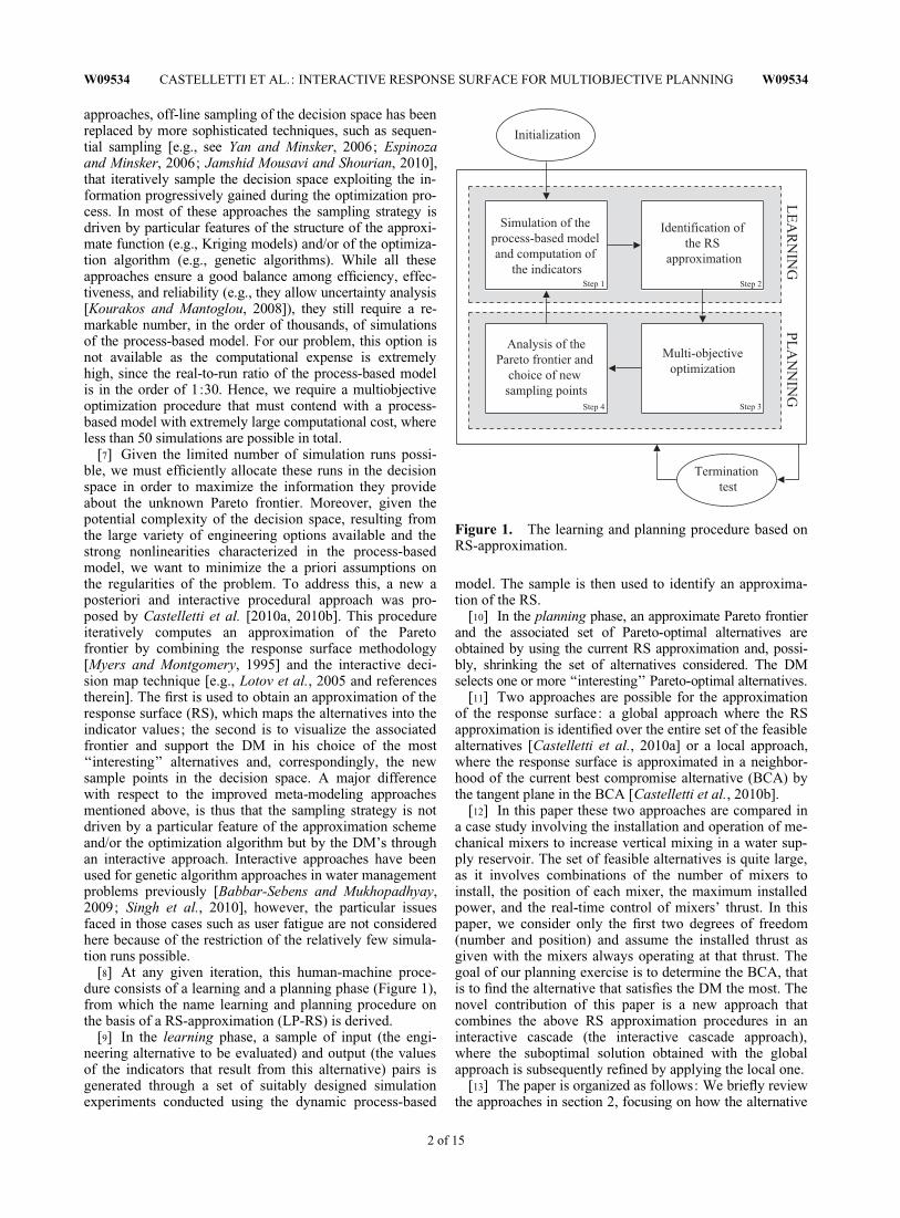
[8] At any given iteration, this human-machine proce-dure consists of a learning and a planning phase (Figure 1),from which the name learning and planning procedure onthe basis of a RS-approximation (LP-RS) is derived.

[9] In the learning phase, a sample of input (the engi-neering alternative to be evaluated) and output (the valuesof the indicators that result from this alternative) pairs isgenerated through a set of suitably designed simulationexperiments conducted using the dynamic process-based

model. The sample is then used to identify an approxima-tion of the RS.

[10] In the planning phase, an approximate Pareto frontierand the associated set of Pareto-optimal alternatives areobtained by using the current RS approximation and, possi-bly, shrinking the set of alternatives considered. The DMselects one or more ‘‘interesting’’ Pareto-optimal alternatives.

[11] Two approaches are possible for the approximationof the response surface: a global approach where the RSapproximation is identified over the entire set of the feasiblealternatives [Castelletti et al., 2010a] or a local approach,where the response surface is approximated in a neighbor-hood of the current best compromise alternative (BCA) bythe tangent plane in the BCA [Castelletti et al., 2010b].

[12] In this paper these two approaches are compared ina case study involving the installation and operation of me-chanical mixers to increase vertical mixing in a water sup-ply reservoir. The set of feasible alternatives is quite large,as it involves combinations of the number of mixers toinstall, the position of each mixer, the maximum installedpower, and the real-time control of mixers’ thrust. In thispaper, we consider only the first two degrees of freedom(number and position) and assume the installed thrust asgiven with the mixers always operating at that thrust. Thegoal of our planning exercise is to determine the BCA, thatis to find the alternative that satisfies the DM the most. Thenovel contribution of this paper is a new approach thatcombines the above RS approximation procedures in aninteractive cascade (the interactive cascade approach),where the suboptimal solution obtained with the globalapproach is subsequently refined by applying the local one.

[13] The paper is organized as follows: We briefly reviewthe approaches in section 2, focusing on how the alternative

Figure 1. The learning and planning procedure based onRS-approximation.

W09534 CASTELLETTI ET AL.: INTERACTIVE RESPONSE SURFACE FOR MULTIOBJECTIVE PLANNING W09534

2 of 15

definitions of the decision vector affect the problem formula-tion, and outline the case study to which they were applied.Each of the approaches is then applied to the case study toelucidate the key advantages and disadvantages, which arethen discussed.

2. Methods2.1. Global and Local RS Approximation

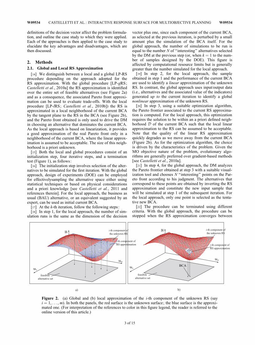
[14] We distinguish between a local and a global LP-RSprocedure depending on the approach adopted for theRS approximation. With the global procedure [LP-gRS;Castelletti et al., 2010a] the RS approximation is identifiedover the entire set of feasible alternatives (see Figure 2a)and as a consequence, the associated Pareto front approxi-mation can be used to evaluate trade-offs. With the localprocedure [LP-lRS; Castelletti et al., 2010b]) the RS isapproximated in a local neighborhood of the current BCAby the tangent plane to the RS in the BCA (see Figure 2b),and the Pareto front obtained is only used to drive the DMin choosing an alternative that dominates the current BCA.As the local approach is based on linearization, it providesa good approximation of the real Pareto front only in aneighborhood of the current BCA, where the linear approx-imation is assumed to be acceptable. The size of this neigh-borhood is a priori unknown.

[15] Both the local and global procedures consist of aninitialization step, four iterative steps, and a terminationtest (Figure 1), as follows:

[16] The initialization step involves selection of the alter-natives to be simulated for the first iteration. With the globalapproach, design of experiments (DOE) can be employedfor effectivelysampling the alternative space either usingstatistical techniques or based on physical considerationsand a priori knowledge [see Castelletti et al., 2011 andreferences therein]. For the local approach, the business asusual (BAU) alternative, or an equivalent suggested by anexpert, can be used as initial current BCA.

[17] At the k-th iteration, follow the following steps:[18] In step 1, for the local approach, the number of sim-

ulation runs is the same as the dimension of the decision

vector plus one, since each component of the current BCA,as selected at the previous iteration, is perturbed by a smallamount plus the simulation of the BCA itself. For theglobal approach, the number of simulations to be run isequal to the number N of ‘‘interesting’’ alternatives selectedby the DM at the previous step (or, when k ¼ 1 to the num-ber of samples designed by the DOE). This figure isaffected by computational resource limits but is generallygreater than the number simulated for the local approach.

[19] In step 2, for the local approach, the sampleobtained in step 1 and the performance of the current BCAare used to identify a linear approximation of the unknownRS. In contrast, the global approach uses input/output data(i.e., alternatives and the associated value of the indicators)generated up to the current iteration to identify a globalnonlinear approximation of the unknown RS.

[20] In step 3, using a suitable optimization algorithm,the Pareto frontier associated to the current RS approxima-tion is computed. For the local approach, this optimizationrequires the solution to be within an a priori defined neigh-borhood D of the current BCA such that the local linearapproximation to the RS can be assumed to be acceptable.Note that the quality of the linear RS approximationquickly degrades as we move away from the current BCA(Figure 2b). As for the optimization algorithm, the choiceis driven by the characteristics of the problem. Given theMO objective nature of the problem, evolutionary algo-rithms are generally preferred over gradient-based methods[see Castelletti et al., 2010a].

[21] In step 4, for the global approach, the DM analyzesthe Pareto frontier obtained at step 3 with a suitable visual-ization tool and chooses N ‘‘interesting’’ points on the Par-eto front according to his judgment. The alternatives thatcorrespond to these points are obtained by inverting the RSapproximation and constitute the new input sample thatwill be simulated at step 1 of the subsequent iteration. Forthe local approach, only one point is selected as the tenta-tive new BCA.

[22] The procedure can be terminated using differentcriteria. With the global approach, the procedure can bestopped when the RS approximation converges between

Figure 2. (a) Global and (b) local approximation of the i-th component of the unknown RS (sayi ¼ 1, . . . , m). In both the panels, the red surface is the unknown surface; the blue surface is the approxi-mated one. (For interpretation of the references to color in this figure legend, the reader is referred to theonline version of this article.)


3 of 15

two iterations. Alternatively, the procedure can be termi-nated when the average distance between the available out-put vectors simulated via the numerical model and thecorresponding output computed through the RS approxima-tion is below a given threshold. When the procedure is over,the DM is provided with an approximation of the Paretofrontier that includes the ‘‘interesting’’ alternatives lastlychosen and among which the final BCA will be selected. Byconstruction, this approximation is more accurate in theregion corresponding to the ‘‘interesting’’ alternatives.

[23] For the local approach, if the performance obtainedvia simulation of the tentative new BCA is preferred overthe performance of the current BCA, then the tentativeBCA becomes the current BCA for the subsequent itera-tion. The procedure then continues from step 1 and termi-nates when either the DM is not able to find a point thatimproves the current BCA or is satisfied with it.

[24] At each iteration, the local procedure approximatesthe RS locally and linearly in a neighborhood of the cur-rent BCA. Therefore, the set of alternatives explored ateach iteration is not the whole feasible set as in the globalprocedure, but a subset D centered in the current BCA.The size of D is key to the effectiveness of the procedure:too small might require a large number of iterations beforegetting to a Pareto-efficient alternative; too large mightprevent us from determining an efficient alternative whenthe unknown RS is far from being linear within the neigh-borhood defined.

2.2. Interactive Decision Maps[25] As for the effective representation of the multidi-

mensional Pareto frontier in step 4 and the associated setof Pareto-efficient alternatives, there are an increasingnumber of studies [see Lotov et al., 2005; Kollat andReed, 2007; Madetoja et al., 2008, and the review inchapters 8 and 9 of Branke et al. 2008] demonstrating thatvisualization tools can provide DMs with a graphical rep-resentation of the Pareto frontier in problems with three toseven objectives. Interactive decision maps (IDMs) [seeLotov, 1989 and references therein] are particularly effec-tive and are used in this paper. IDMs are based on theapproximation of the feasible set in the objective spaceand on displaying various decision maps, i.e., collectionsof bi-objective slices of the approximated frontier (anexample is shown in Figure 9). For three objectives, theIDM is a prepared collection of several bi-objective trade-off curves, while the value of the third objective changes.The tradeoff curves are the frontiers of the slices. Formore than three objectives various three-objective decisionmaps are constructed and displayed on request of the DMfor different values of the fourth through the seventhobjectives.

2.3. Problem Formulation and SuboptimalApproaches

[26] The optimal formulation of the problem wouldallow us to determine the optimal number and the locationsof mixers (the original multiobjective problem). There are,however, operational difficulties in the resolution of thisproblem [see Castelletti et al., 2010a], and thus we areforced to take a suboptimal approach and solve either oneor the other of the following problems: we fix the number r

of mixers and determine their best location (problem P1),or we determine the best number �r� of mixers with the loca-tion decided a priori by a suitable positioning rule (problemP2). From these two problems, a third option emerges: Wefirst solve problem P2 and subsequently a problem (prob-lem P3), which is problem P1, where �r is assumed equal tothe optimal number �r� of mixers determined from problemP2. In other words, problem P3 optimally reallocates the�r� mixers.

[27] In detail, a planning alternative is described by thedecision vector u ¼ jr;Z1; . . . ;Zrj 2 U, whose componentsare the number r of mixers and the n-component vectorsZ1, . . . , Z defining their positions, where n is the dimensionof the set L of feasible positions, obtained by consideringthe existing physical or technical constraints on the mixerpositioning (e.g., minimum lake depth, minimum distancebetween mixers, distance from recreational or navigationalzones). Assuming the maximum feasible number of mixersis R, the feasibility set U is

U ¼ fu : u 2 Rnrþ1; r < R and Zi 2 L; i ¼ 1; . . . ; rg: ð1Þ

[28] A dynamic, process-based model M is available tosimulate the system behavior under each alternative. Mtransforms an alternative u into a collection B of trajecto-ries of spatially distributed outputs, i.e., B ¼MðuÞ.

[29] The DM’s decision criteria can be formalized interms of m quantitative indicators y1, . . . , ym and the set ofPareto-optimal alternatives is obtained by solving the fol-lowing multiobjective optimization problem:

minu

y1ðB;uÞ; . . . ; ymðB; uÞ½ �; ð2aÞ

subject to

u ¼ jr;Z1; . . . ;Zrj 2 U; ð2bÞ

B ¼ MðuÞ; ð2cÞ

Within this set the DM selects the best compromise alterna-tive (BCA).

[30] Since the output B can be computed for each alter-native u 2 U via simulation, the indicator yiðB; uÞ can beseen as a function fi(u) of u, which encompasses both directrelations between u and yi and relations mediated by themodel M though B. Since U � R

nrþ1, the functions fi(�),with i ¼ 1, . . . , m, constitute the components of a vectorfunction f : R

nrþ1 ! Rm called the response surface (RS).

Equation (2) can be rewritten as

minu

f1ðuÞ; . . . ; fmðuÞ½ �; ð3aÞ

subject to (2b) and (2c).[31] The definition of u is an implicit formulation since

the vector dimension nr þ 1 depends on the value r of itsfirst component. This is logically consistent, but the result-ing definition of the feasible decision set U � R

nrþ1, aswell as the definition of the RS f : R

nrþ1 ! Rm, become

particularly tricky. To overcome this difficulty, we considerseparately the decision r concerning the number of mixers


4 of 15

and the decisions Z1, . . . , Zr about the positioning. Twoalternative formulations can be considered: (1) the number�r of mixers to be installed is a priori fixed and only themixer positions are to be decided; and (2) the positionsZ1, . . . , Zr of mixers are empirically defined by an a priorigiven function Z(�) of r, i.e., jZ1, . . . , Zrj ¼ Z(�), and thenumber r is the unique decision variable. Formally, equa-tion (3) can be reformulated by substituting (2b) for one ofthe following expressions:

[32] Formulation F1: u ¼ jZ1; . . . ;Z�rj with �r given;[33] Formulation F2: u ¼ r with jZ1, . . . , Zrj ¼ Z(�),

where Z(�) is an a priori given function.[34] We refer to the associated problems as problems P1

and P2.[35] Neither one nor the other of these problems is equiv-

alent to equation (3) and therefore they yield a suboptimalsolution. However, when formulation F1 is adopted, byrepeatedly solving the associated problem P1 for�r ¼ 1; . . . ;R and considering the nondominated points ofthe union set of the Pareto frontiers, one obtains the solu-tion to equation (3). To improve the approximationobtained using formulation F2, the lake bathymetry is di-vided into a fixed number p of macro areas and decides thenumber of mixers ri(i ¼ 1, . . . , p) to install in each area,i.e., u ¼ r. The quality of the approximation improves withthe number of macro areas considered (i.e., with the reduc-tion of the surface of each macro area).

[36] The suboptimal solution (r�, Z(r*)) to equation (3),obtained by solving problem P2, can be refined by subse-

quently solving problem P1 for �r ¼Ppi¼1

r�i , that is problem

P3. Therefore, an improved approximate solution to equa-tion (3) can be computed with the following steps.2.3.1. Cascade Approach

[37] Step 1. Solve problem P2 over p macro areas usingthe global approach, thus obtaining the set of Pareto-optimal alternatives. The DM choses the BCA among thesealternatives, which is specified by the optimal number r�i ofmixers in each macro area and the associated positionsZiðr�i Þi ¼ 1, . . . , p.

[38] Step 2. Solve problem P1 with the local approach,starting from the BCA obtained in step 1 and assuming

�r ¼Ppi¼1

r�i .

2.4. Problem Formulation Versus RS Approximation[39] Depending on whether the problem is formulated as

P1, P2, or P3, one of the two RS approaches seems to beintuitively more appropriate. The local approach exploresthe feasible alternative set starting from a given alternative(usually the BCA alternative) and follows a path iterativelyconstructed in the neighborhood of the alternative currentlypreferred by the DM. When the feasible set is large and/or agood starting alternative is not available, the relative sim-plicity of the linear approximation is overwhelmed by thecomputational cost of the many iterations required forexploring the alternative set and hence the global approachseems to be more appropriate. This might be the case withproblem P1. With problem P2 there is no a priori reason toprefer one approach over the other, while for problem P3 thelocal approach is most suitable since the starting alternative

is generated by solving an optimization problem (i.e., prob-lem P1), and thus it should represent a ‘‘good’’ starting point.To verify these a priori conjectures, the two RS approacheswere comparatively tested using a real world application.

3. Case Study3.1. Study Site

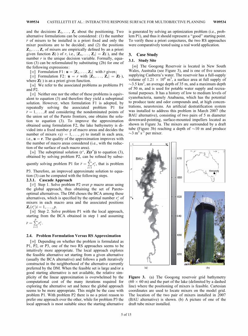
[40] The Googong Reservoir is located in New SouthWales, Australia (see Figure 3), and is one of five sourcessupplying Canberra’s water. The reservoir has a full-supplyvolume of 1.21 � 106 m3, a surface area at full supply of�3.5 km2, an average depth of 35 m, and a maximum depthof 50 m, and is used for potable water supply and recrea-tional purposes. It has a history of low to medium levels ofcyanobacteria, namely Anabaena, which has the potentialto produce taste and odor compounds and, at high concen-trations, neurotoxins. An artificial destratification systemwas installed to address this problem in March 2007 (theBAU alternative), consisting of two pairs of 5 m diameterdownward-pointing, surface-mounted impellers located asshown in Figure 3a. The mixers are surrounded by a drafttube (Figure 3b) reaching a depth of �10 m and produce�3 m3 s–1 per mixer.

Figure 3. (a) The Googong reservoir grid bathymetry(60 � 60 m) and the part of the lake (delimited by a dashedline) where the positioning of mixers is feasible. Cartesiancoordinates are used to locate mixers on the model grid.The location of the two pair of mixers installed in 2007(BAU alternative) is shown. (b) A picture of one of thedraft tube mixer installed.


5 of 15

3.2. The Indicators[41] The management concern relates to Anabaena and

manganese concentrations exceeding some reference value.We will consider the average annual number of days inwhich the concentration of chlorophyll-a associated withAnabaena in the epilimnion exceeds a given threshold, i.e.,

yA ¼365h

Xh

t¼1

�t; �t ¼1 if At > �A

0 otherwise

�; ð4Þ

where At is the average concentration of chlorophyll-a inthe epilimnion (temporal mean on day t) and �A is the criti-cal threshold (2 �g chlorophyll-a/L as stated in the Austra-lian Drinking Water Guidelines) and h is the total numberof days in the simulation horizon.

[42] As for manganese, any increase in its concentrationin the hypolimnion can be either because of poor (or null)oxygenation in the hypolimnion and/or driven by theinflow. We will consider the average annual number ofdays in which the concentration of manganese in the layerjust above the sediments exceeds a given threshold, i.e.,

yM ¼365h

Xh

t¼1

�t; �t ¼1 if Mnt > Mn

0 otherwise

�; ð5Þ

where Mnt is the average concentration of manganese inthe benthic layer (temporal mean on day t) and Mn is thecritical threshold (0.065 mg L�1 as stated in the AustralianDrinking Water Guidelines).

[43] Finally, the installation cost should be taken intoproper consideration. Assuming such cost is linearly pro-portional to the number of mixers installed, we may con-sider the total number of mixers as a proxy of the monetaryindicator, that is

yC ¼ r; ð6Þ

where r is the number of mixers installed.

3.3. The Process-Based Model[44] The 3-D coupled hydrodynamic-ecological model

ELCOM-CAEDYM [Hodges et al., 2000; Hipsey et al.,2007] has been used to simulate the seasonal cycles in theGoogong reservoir and event driven dynamics (wind andinflow). The Estuary and Lake Computer Model (ELCOM)is a three-dimensional hydrodynamics model used for pre-dicting the velocity, temperature, and salinity distributionin natural water bodies, subjected to external environmentalforcing such as wind stress and surface fluxes. The hydro-dynamic simulation method solves the unsteady, viscousNavier-Stokes equations for incompressible flow, using thehydrostatic assumption for pressure. Simulated processesinclude baroclinic and barotropic responses, rotationaleffects, wind stresses, surface thermal forcing, inflows, out-flows, and transport of salt, heat, and passive scalars. Thehydrodynamic algorithms in ELCOM are based on theEuler-Lagrange method for advection of momentum with aconjugate-gradient solution for the free-surface height. TheComputational Aquatic Ecosystem DYnamics Model (CAE-DYM) was configured to simulate the major biogeochemical

processes influencing water quality, including primaryproduction, nutrient and metal cycling, and oxygen dynam-ics. The ELCOM-CAEDYM model (simply model M inwhat follows) was calibrated and validated against avail-able field data for temperature, dissolved oxygen, nutrients,metals and chlorophyll-a, with results reported by Hillmeret al. [2008].

[45] For the purpose of producing sample data for RSapproximation, the coupled ELCOM-CAEDYM modelwas run on a 60 m � 60 m grid bathymetry with 1 m verti-cal grid resolution (Figure 3a) using a simulation time stepof 2 min. One-year long simulation on a AMD Athlon(tm)64 3.5 MHz required �7 d. The output required by the indi-cators has been sampled with two different time steps,every 12 h for the manganese and every 3 h for cyanobacte-ria which are much more sensitive to daylight variations.

4. Results[46] The two response surface approaches were both

tested for problems P1 and P2, while for problem P3 thelocal approach seemed the natural choice. With bothapproaches, the feasible goal method [Lotov et al., 2004]was adopted to solve the optimization problem. Given theacademic nature of the study, when necessary, the role ofthe DM was played by a limnologist from CWR.

4.1. Problem P1: Optimizing the Location of a FixedNumber of Mixers

[47] Two mixers, as in the BAU alternative (Figure 3a),were considered with the purpose of verifying if anyimprovement of the BAU alternative was possible at noadditional cost. Because of the irregular shape of the lake, itis convenient to describe mixer positions in curvilinear coor-dinates along the riverbed (the dark gray cells in Figure 4),giving a set of 121 options for the two mixers positions (u1and u2) on the basis of the model spatial resolution. To avoidmutual mixer interference, the locations of the two mixerswere made to differ by more than one grid point.4.1.1. Global Approach

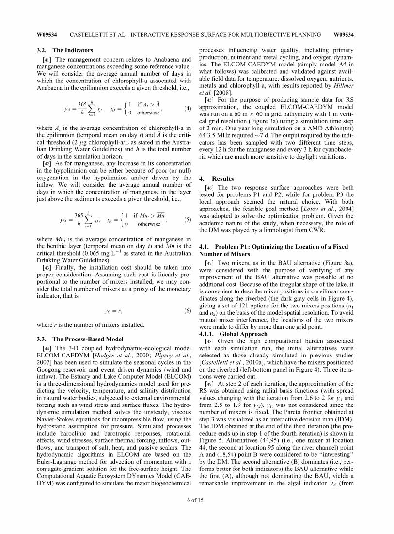
[48] Given the high computational burden associatedwith each simulation run, the initial alternatives wereselected as those already simulated in previous studies[Castelletti et al., 2010a], which have the mixers positionedon the riverbed (left-bottom panel in Figure 4). Three itera-tions were carried out.

[49] At step 2 of each iteration, the approximation of theRS was obtained using radial basis functions (with spreadvalues changing with the iteration from 2.6 to 2 for yA andfrom 2.5 to 1.9 for yM). yC was not considered since thenumber of mixers is fixed. The Pareto frontier obtained atstep 3 was visualized as an interactive decision map (IDM).The IDM obtained at the end of the third iteration (the pro-cedure ends up in step 1 of the fourth iteration) is shown inFigure 5. Alternatives (44,95) (i.e., one mixer at location44, the second at location 95 along the river channel) pointA and (18,54) point B were considered to be ‘‘interesting’’by the DM. The second alternative (B) dominates (i.e., per-forms better for both indicators) the BAU alternative whilethe first (A), although not dominating the BAU, yields aremarkable improvement in the algal indicator yA (from


6 of 15

180 to 48 d yr�1) at the price of a small worsening of man-ganese indicator yM (from 100 to 108 d yr�1).4.1.2. Local Approach

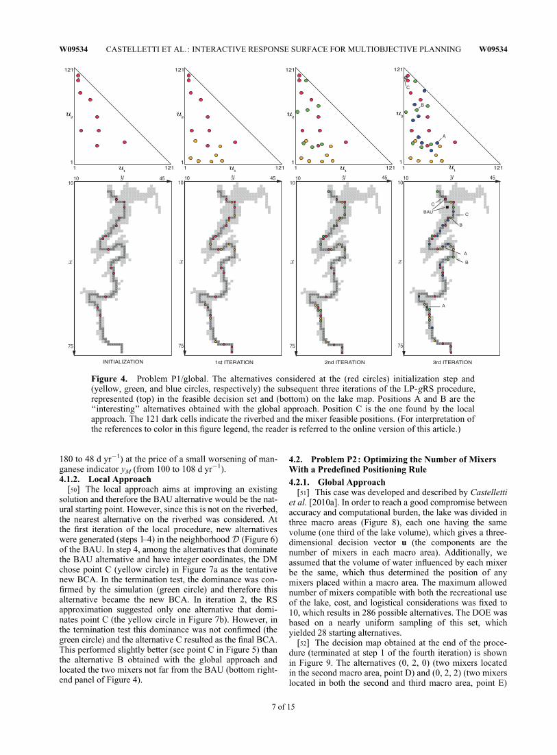
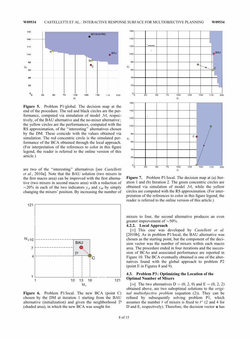
[50] The local approach aims at improving an existingsolution and therefore the BAU alternative would be the nat-ural starting point. However, since this is not on the riverbed,the nearest alternative on the riverbed was considered. Atthe first iteration of the local procedure, new alternativeswere generated (steps 1–4) in the neighborhood D (Figure 6)of the BAU. In step 4, among the alternatives that dominatethe BAU alternative and have integer coordinates, the DMchose point C (yellow circle) in Figure 7a as the tentativenew BCA. In the termination test, the dominance was con-firmed by the simulation (green circle) and therefore thisalternative became the new BCA. In iteration 2, the RSapproximation suggested only one alternative that domi-nates point C (the yellow circle in Figure 7b). However, inthe termination test this dominance was not confirmed (thegreen circle) and the alternative C resulted as the final BCA.This performed slightly better (see point C in Figure 5) thanthe alternative B obtained with the global approach andlocated the two mixers not far from the BAU (bottom right-end panel of Figure 4).

4.2. Problem P2: Optimizing the Number of MixersWith a Predefined Positioning Rule4.2.1. Global Approach

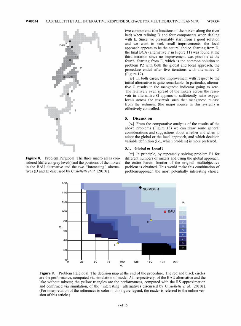
[51] This case was developed and described by Castellettiet al. [2010a]. In order to reach a good compromise betweenaccuracy and computational burden, the lake was divided inthree macro areas (Figure 8), each one having the samevolume (one third of the lake volume), which gives a three-dimensional decision vector u (the components are thenumber of mixers in each macro area). Additionally, weassumed that the volume of water influenced by each mixerbe the same, which thus determined the position of anymixers placed within a macro area. The maximum allowednumber of mixers compatible with both the recreational useof the lake, cost, and logistical considerations was fixed to10, which results in 286 possible alternatives. The DOE wasbased on a nearly uniform sampling of this set, whichyielded 28 starting alternatives.

[52] The decision map obtained at the end of the proce-dure (terminated at step 1 of the fourth iteration) is shownin Figure 9. The alternatives (0, 2, 0) (two mixers locatedin the second macro area, point D) and (0, 2, 2) (two mixerslocated in both the second and third macro area, point E)

Figure 4. Problem P1/global. The alternatives considered at the (red circles) initialization step and(yellow, green, and blue circles, respectively) the subsequent three iterations of the LP-gRS procedure,represented (top) in the feasible decision set and (bottom) on the lake map. Positions A and B are the‘‘interesting’’ alternatives obtained with the global approach. Position C is the one found by the localapproach. The 121 dark cells indicate the riverbed and the mixer feasible positions. (For interpretation ofthe references to color in this figure legend, the reader is referred to the online version of this article.)


7 of 15

are two of the ‘‘interesting’’ alternatives [see Castellettiet al., 2010a]. Note that the BAU solution (two mixers inthe first macro area) can be improved with the first alterna-tive (two mixers in second macro area) with a reduction of�20% in each of the two indicators yA and yM by simplychanging the mixers’ position. By increasing the number of

mixers to four, the second alternative produces an evengreater improvement of �50%.4.2.2. Local Approach

[53] This case was developed by Castelletti et al.[2010b]. As in problem P1/local, the BAU alternative waschosen as the starting point, but the component of the deci-sion vector was the number of mixers within each macroarea. The procedure ended in four iterations and the succes-sion of BCAs and associated performance are reported inFigure 10. The BCA eventually obtained is one of the alter-natives found with the global approach to problem P2(point E in Figures 8 and 9).

4.3. Problem P3: Optimizing the Location of theOptimal Number of Mixers

[54] The two alternatives D ¼ (0, 2, 0) and E ¼ (0, 2, 2)obtained above, are two suboptimal solutions to the origi-nal multiobjective problem (equation (2)). They can berefined by subsequently solving problem P1, whichassumes the number �r of mixers is fixed to �r� (2 and 4 forD and E, respectively). Therefore, the decision vector u has

Figure 5. Problem P1/global. The decision map at theend of the procedure. The red and black circles are the per-formance, computed via simulation of model M, respec-tively, of the BAU alternative and the no-mixer alternative;the yellow circles are the performances, computed with theRS approximation, of the ‘‘interesting’’ alternatives chosenby the DM. These coincide with the values obtained viasimulation. The red concentric circle is the simulated per-formance of the BCA obtained through the local approach.(For interpretation of the references to color in this figurelegend, the reader is referred to the online version of thisarticle.)

Figure 6. Problem P1/local. The new BCA (point C)chosen by the DM at iteration 1 starting from the BAUalternative (initialization) and given the neighborhood D(shaded area), in which the new BCA was sought for.

Figure 7. Problem P1/local. The decision map at (a) Iter-ation 1 and (b) Iteration 2. The green concentric circles areobtained via simulation of model M, while the yellowcircles are computed with the RS approximation. (For inter-pretation of the references to color in this figure legend, thereader is referred to the online version of this article.)


8 of 15

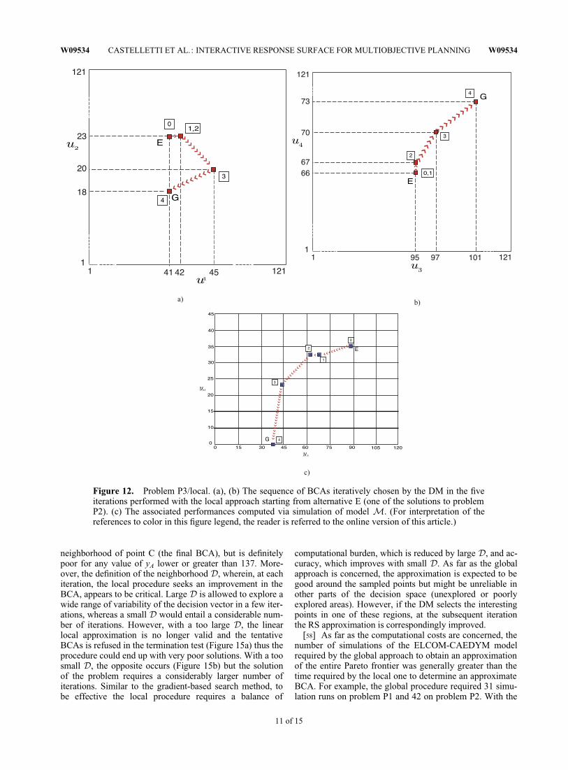
two components (the locations of the mixers along the riverbed) when refining D and four components when dealingwith E. Since we presumably start from a good solutionand we want to seek small improvements, the localapproach appears to be the natural choice. Starting from D,the final BCA (alternative F in Figure 11) was found at thethird iteration since no improvement was possible at thefourth. Starting from E, which is the common solution toproblem P2 with both the global and local approach, theprocedure ended after five iterations with alternative G(Figure 12).

[55] In both cases, the improvement with respect to theinitial alternative is quite remarkable. In particular, alterna-tive G results in the manganese indicator going to zero.The relatively even spread of the mixers across the reser-voir in alternative G appears to sufficiently raise oxygenlevels across the reservoir such that manganese releasefrom the sediment (the major source in this system) iseffectively controlled.

5. Discussion[56] From the comparative analysis of the results of the

above problems (Figure 13) we can draw some generalconsiderations and suggestions about whether and when toadopt the global or the local approach, and which decisionvariable definition (i.e., which problem) is more preferred.

5.1. Global or Local?[57] In principle, by repeatedly solving problem P1 for

different numbers of mixers and using the global approach,the entire Pareto frontier of the original multiobjectiveproblem is obtained. This would make this combination ofproblem/approach the most potentially interesting choice.

Figure 9. Problem P2/global. The decision map at the end of the procedure. The red and black circlesare the performance, computed via simulation of model M, respectively, of the BAU alternative and thelake without mixers; the yellow triangles are the performances, computed with the RS approximationand confirmed via simulation, of the ‘‘interesting’’ alternatives discussed by Castelletti et al. [2010a].(For interpretation of the references to color in this figure legend, the reader is referred to the online ver-sion of this article.)

Figure 8. Problem P2/global. The three macro areas con-sidered (different gray levels) and the positions of the mixersin the BAU alternative and the two ‘‘interesting’’ alterna-tives (D and E) discussed by Castelletti et al. [2010a].


9 of 15

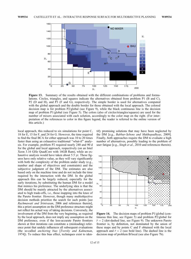
However, numerical results do not seem to support this apriori guess (Figure 13). In fact, the approximate Paretofrontier (black continuous line) obtained from problemP1/global is partly dominated, at least for the two mixercase, by points C and F calculated with the LP-lRS proce-dure. Second, the recursive resolution of problem P1 withthe global procedure for different numbers of mixers �r is acomputational challenge as the number of feasible alterna-tives grows slightly less than exponentially with �r, and thusthe number of simulation runs necessary to generate an ac-ceptable frontier approximation also grows quite rapidly.Generally, when the number of mixers is the same, the alter-natives determined by the local approach always performbetter than those obtained with the global approach, exceptfor solution A (Figure 13). This should be expected as the

local procedure is always initialized with a ‘‘good’’ alterna-tive. The local approach is clearly sensitive to the quality ofthe initial alternative, as proved by its different behaviorwhile starting from E rather than D. However, a good start-ing alternative is, at least in principle, always obtainable ata relatively low cost either by running an expert-based‘‘what-if’’ analysis or by few iterations of the global proce-dure. On the other hand, the global approach has the clearadvantage of providing an approximation of the entire Par-eto frontier of the original problem, while the local approxi-mation is reliable only in a small neighborhood of the finalBCA. This can be easily seen in Figure 14, where the deci-sion map of problem P2 solved through the LP-lRS proce-dure (dashed line) provides an acceptable approximation ofthe Pareto frontier of the original problem only in a small

Figure 11. Problem P3/local. (a) The sequence of BCAs iteratively chosen by the DM in the four itera-tions performed with the local approach starting from alternative D (one of the solutions to problem P2).(b) The associated performances computed via simulation of model M. (For interpretation of the refer-ences to color in this figure legend, the reader is referred to the online version of this article.)

Figure 10. Problem P2/local. (a) The sequence of BCAs (red triangles) iteratively chosen by the DMin the three iterations performed with the local approach starting from the BAU. (b) The associatedperformance computed via simulation of model M. (For interpretation of the references to color in thisfigure legend, the reader is referred to the online version of this article.)


10 of 15

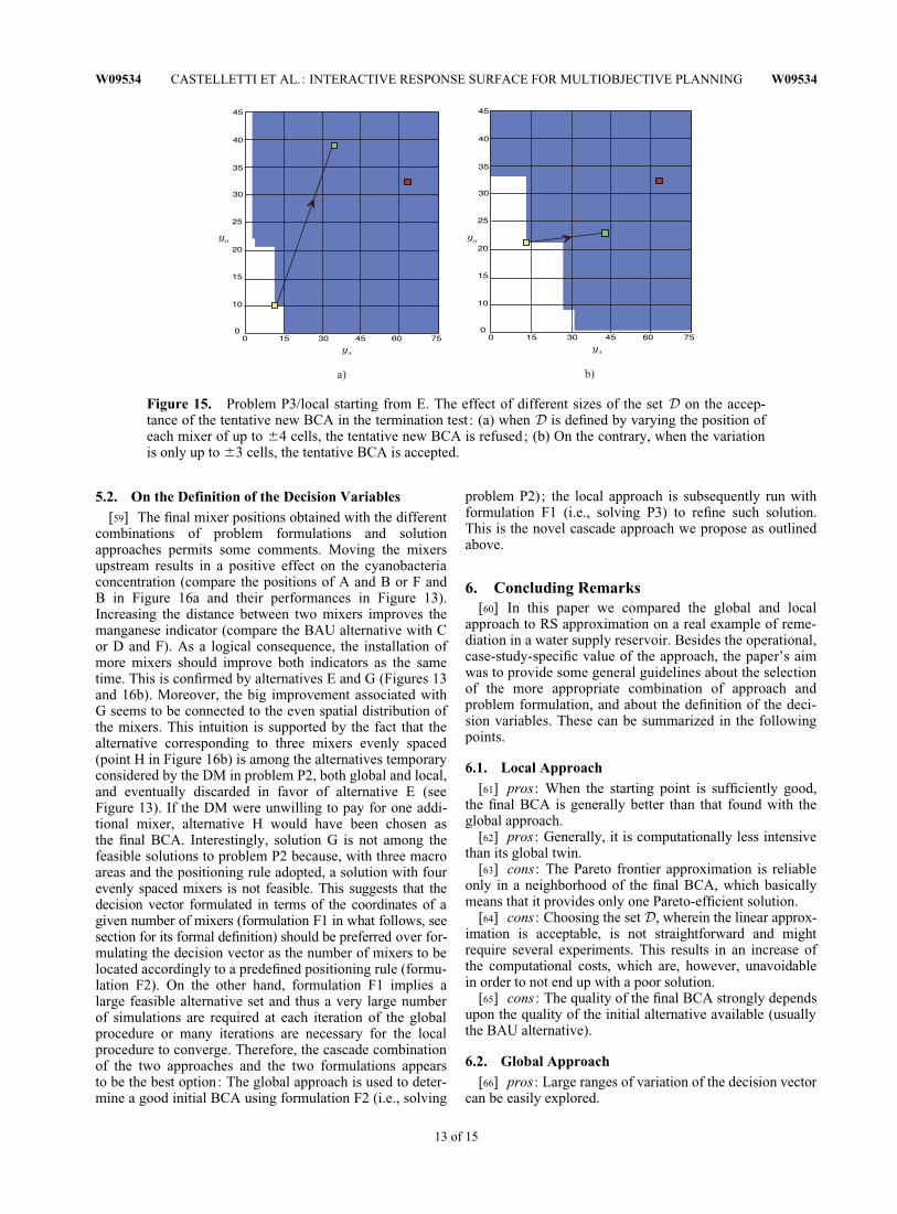
neighborhood of point C (the final BCA), but is definitelypoor for any value of yA lower or greater than 137. More-over, the definition of the neighborhood D, wherein, at eachiteration, the local procedure seeks an improvement in theBCA, appears to be critical. Large D is allowed to explore awide range of variability of the decision vector in a few iter-ations, whereas a small D would entail a considerable num-ber of iterations. However, with a too large D, the linearlocal approximation is no longer valid and the tentativeBCAs is refused in the termination test (Figure 15a) thus theprocedure could end up with very poor solutions. With a toosmall D, the opposite occurs (Figure 15b) but the solutionof the problem requires a considerably larger number ofiterations. Similar to the gradient-based search method, tobe effective the local procedure requires a balance of

computational burden, which is reduced by large D, and ac-curacy, which improves with small D. As far as the globalapproach is concerned, the approximation is expected to begood around the sampled points but might be unreliable inother parts of the decision space (unexplored or poorlyexplored areas). However, if the DM selects the interestingpoints in one of these regions, at the subsequent iterationthe RS approximation is correspondingly improved.

[58] As far as the computational costs are concerned, thenumber of simulations of the ELCOM-CAEDYM modelrequired by the global approach to obtain an approximationof the entire Pareto frontier was generally greater than thetime required by the local one to determine an approximateBCA. For example, the global procedure required 31 simu-lation runs on problem P1 and 42 on problem P2. With the

Figure 12. Problem P3/local. (a), (b) The sequence of BCAs iteratively chosen by the DM in the fiveiterations performed with the local approach starting from alternative E (one of the solutions to problemP2). (c) The associated performances computed via simulation of model M. (For interpretation of thereferences to color in this figure legend, the reader is referred to the online version of this article.)


11 of 15

local approach, this reduced to six simulations for point C,18 for E, 15 for F, and 24 for G. However, the time requiredto find the final BCA for either approach was 10 to 20 timesfaster than using an exhaustive traditional ‘‘what-if’’ analy-sis. For example, problem P2 required nearly 240 and 90 dfor the global and local approach, respectively (on an IntelXeon 3.16 GHz QuadCore with 16GB Ram), while an ex-haustive analysis would have taken about 5.5 yr. These fig-ures have only relative value, as they will vary significantlywith both the complexity of the problem under study (e.g.,number and shape of objectives and constraints) and thesubjective judgment of the DM. The estimates are alsobased only on the machine time and do not include the timerequired by the interaction with the DM. In the globalapproach this can be largely reduced, especially for theearly iterations, by substituting the human DM for a modelthat mimics his preference. The underlying idea is that theDM should be mainly attracted by the alternatives associ-ated to high trade-offs, i.e., those mapping into the knee ofthe Pareto frontier. However, though many multiobjectivedecision methods prioritize the search for such points [seeRachmawati and Srinivasan, 2006 and references therein],this a priori assumption on the DM preference structure mightnot reflect his actual way of taking decisions. Conversely, theinvolvement of the DM from the very beginning, as requiredby the local approach, does not imply any assumption on theDM preference, even if the less-accurate Pareto frontiersshown at first iterations can constitute a (misleading) refer-ence point that unduly influences all subsequent evaluations(the so-called anchoring bias [Tversky and Kahneman,1974]). To reduce this bias effect, techniques exist to iden-

tify promising solutions that may have been neglected bythe DM [e.g., Babbar-Sebens and Mukhopadhyay, 2009].Finally, both approaches require the DM to evaluate a highnumber of alternatives, possibly leading to the problem ofuser fatigue [e.g., Singh et al., 2010 and references therein).

Figure 13. Summary of the results obtained with the different combinations of problems and formu-lations. Circles, triangles, and squares indicate the alternatives obtained from problem P1 (B and C),P2 (D and H), and P3 (F and G), respectively. The simple border is used for alternatives computedwith the global approach and the double border for those obtained with the local approach. The coloreddecision map is for problem P2/global (see Figure 9), while the black continuous line is the decisionmap of problem P1/global (see Figure 5). The colors (also of circles/triangles/squares) are used for thenumber of mixers associated with each solution, accordingly to the color map on the right. (For inter-pretation of the references to color in this figure legend, the reader is referred to the online version ofthis article.)

Figure 14. The decision maps of problem P1/global (con-tinuous thin line, see Figure 5) and problem P2/global for�r ¼ 2 (dot-dashed line, see Figure 9). The unknown Paretofrontier is, by definition, not dominated by the union ofthese maps and by points C and F obtained with the localapproach and �r ¼ 2 (see bold line). The dashed line is thedecision map of problem B/local (see also Figure 7b).


12 of 15

5.2. On the Definition of the Decision Variables[59] The final mixer positions obtained with the different

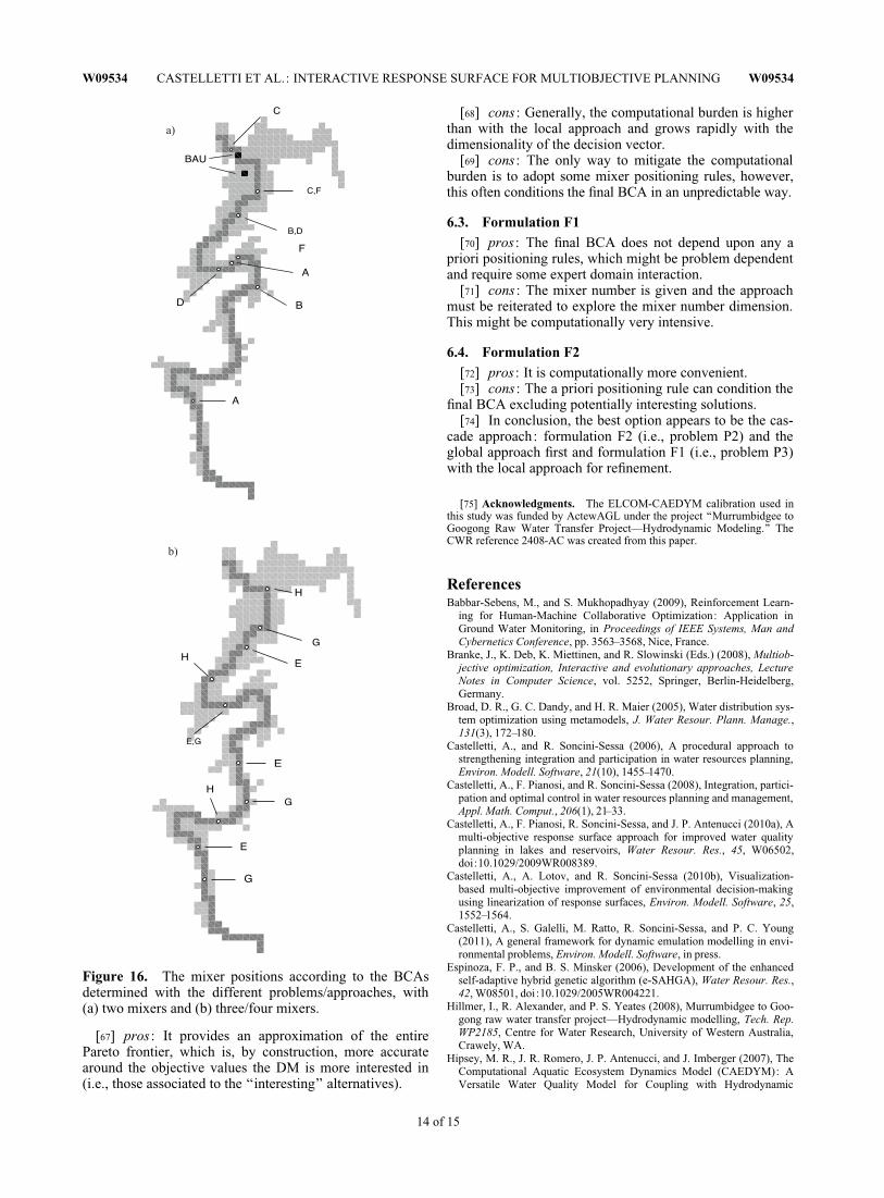
combinations of problem formulations and solutionapproaches permits some comments. Moving the mixersupstream results in a positive effect on the cyanobacteriaconcentration (compare the positions of A and B or F andB in Figure 16a and their performances in Figure 13).Increasing the distance between two mixers improves themanganese indicator (compare the BAU alternative with Cor D and F). As a logical consequence, the installation ofmore mixers should improve both indicators as the sametime. This is confirmed by alternatives E and G (Figures 13and 16b). Moreover, the big improvement associated withG seems to be connected to the even spatial distribution ofthe mixers. This intuition is supported by the fact that thealternative corresponding to three mixers evenly spaced(point H in Figure 16b) is among the alternatives temporaryconsidered by the DM in problem P2, both global and local,and eventually discarded in favor of alternative E (seeFigure 13). If the DM were unwilling to pay for one addi-tional mixer, alternative H would have been chosen asthe final BCA. Interestingly, solution G is not among thefeasible solutions to problem P2 because, with three macroareas and the positioning rule adopted, a solution with fourevenly spaced mixers is not feasible. This suggests that thedecision vector formulated in terms of the coordinates of agiven number of mixers (formulation F1 in what follows, seesection for its formal definition) should be preferred over for-mulating the decision vector as the number of mixers to belocated accordingly to a predefined positioning rule (formu-lation F2). On the other hand, formulation F1 implies alarge feasible alternative set and thus a very large numberof simulations are required at each iteration of the globalprocedure or many iterations are necessary for the localprocedure to converge. Therefore, the cascade combinationof the two approaches and the two formulations appearsto be the best option: The global approach is used to deter-mine a good initial BCA using formulation F2 (i.e., solving

problem P2); the local approach is subsequently run withformulation F1 (i.e., solving P3) to refine such solution.This is the novel cascade approach we propose as outlinedabove.

6. Concluding Remarks[60] In this paper we compared the global and local

approach to RS approximation on a real example of reme-diation in a water supply reservoir. Besides the operational,case-study-specific value of the approach, the paper’s aimwas to provide some general guidelines about the selectionof the more appropriate combination of approach andproblem formulation, and about the definition of the deci-sion variables. These can be summarized in the followingpoints.

6.1. Local Approach[61] pros : When the starting point is sufficiently good,

the final BCA is generally better than that found with theglobal approach.

[62] pros : Generally, it is computationally less intensivethan its global twin.

[63] cons : The Pareto frontier approximation is reliableonly in a neighborhood of the final BCA, which basicallymeans that it provides only one Pareto-efficient solution.

[64] cons : Choosing the set D, wherein the linear approx-imation is acceptable, is not straightforward and mightrequire several experiments. This results in an increase ofthe computational costs, which are, however, unavoidablein order to not end up with a poor solution.

[65] cons : The quality of the final BCA strongly dependsupon the quality of the initial alternative available (usuallythe BAU alternative).

6.2. Global Approach[66] pros: Large ranges of variation of the decision vector

can be easily explored.

Figure 15. Problem P3/local starting from E. The effect of different sizes of the set D on the accep-tance of the tentative new BCA in the termination test : (a) when D is defined by varying the position ofeach mixer of up to 64 cells, the tentative new BCA is refused; (b) On the contrary, when the variationis only up to 63 cells, the tentative BCA is accepted.


13 of 15

[67] pros : It provides an approximation of the entirePareto frontier, which is, by construction, more accuratearound the objective values the DM is more interested in(i.e., those associated to the ‘‘interesting’’ alternatives).

[68] cons : Generally, the computational burden is higherthan with the local approach and grows rapidly with thedimensionality of the decision vector.

[69] cons : The only way to mitigate the computationalburden is to adopt some mixer positioning rules, however,this often conditions the final BCA in an unpredictable way.

6.3. Formulation F1[70] pros : The final BCA does not depend upon any a

priori positioning rules, which might be problem dependentand require some expert domain interaction.

[71] cons : The mixer number is given and the approachmust be reiterated to explore the mixer number dimension.This might be computationally very intensive.

6.4. Formulation F2[72] pros : It is computationally more convenient.[73] cons : The a priori positioning rule can condition the

final BCA excluding potentially interesting solutions.[74] In conclusion, the best option appears to be the cas-

cade approach: formulation F2 (i.e., problem P2) and theglobal approach first and formulation F1 (i.e., problem P3)with the local approach for refinement.

[75] Acknowledgments. The ELCOM-CAEDYM calibration used inthis study was funded by ActewAGL under the project ‘‘Murrumbidgee toGoogong Raw Water Transfer Project––Hydrodynamic Modeling.’’ TheCWR reference 2408-AC was created from this paper.

ReferencesBabbar-Sebens, M., and S. Mukhopadhyay (2009), Reinforcement Learn-

ing for Human-Machine Collaborative Optimization: Application inGround Water Monitoring, in Proceedings of IEEE Systems, Man andCybernetics Conference, pp. 3563–3568, Nice, France.

Branke, J., K. Deb, K. Miettinen, and R. Slowinski (Eds.) (2008), Multiob-jective optimization, Interactive and evolutionary approaches, LectureNotes in Computer Science, vol. 5252, Springer, Berlin-Heidelberg,Germany.

Broad, D. R., G. C. Dandy, and H. R. Maier (2005), Water distribution sys-tem optimization using metamodels, J. Water Resour. Plann. Manage.,131(3), 172–180.

Castelletti, A., and R. Soncini-Sessa (2006), A procedural approach tostrengthening integration and participation in water resources planning,Environ. Modell. Software, 21(10), 1455–1470.

Castelletti, A., F. Pianosi, and R. Soncini-Sessa (2008), Integration, partici-pation and optimal control in water resources planning and management,Appl. Math. Comput., 206(1), 21–33.

Castelletti, A., F. Pianosi, R. Soncini-Sessa, and J. P. Antenucci (2010a), Amulti-objective response surface approach for improved water qualityplanning in lakes and reservoirs, Water Resour. Res., 45, W06502,doi:10.1029/2009WR008389.

Castelletti, A., A. Lotov, and R. Soncini-Sessa (2010b), Visualization-based multi-objective improvement of environmental decision-makingusing linearization of response surfaces, Environ. Modell. Software, 25,1552–1564.

Castelletti, A., S. Galelli, M. Ratto, R. Soncini-Sessa, and P. C. Young(2011), A general framework for dynamic emulation modelling in envi-ronmental problems, Environ. Modell. Software, in press.

Espinoza, F. P., and B. S. Minsker (2006), Development of the enhancedself-adaptive hybrid genetic algorithm (e-SAHGA), Water Resour. Res.,42, W08501, doi:10.1029/2005WR004221.

Hillmer, I., R. Alexander, and P. S. Yeates (2008), Murrumbidgee to Goo-gong raw water transfer project––Hydrodynamic modelling, Tech. Rep.WP2185, Centre for Water Research, University of Western Australia,Crawely, WA.

Hipsey, M. R., J. R. Romero, J. P. Antenucci, and J. Imberger (2007), TheComputational Aquatic Ecosystem Dynamics Model (CAEDYM): AVersatile Water Quality Model for Coupling with Hydrodynamic

Figure 16. The mixer positions according to the BCAsdetermined with the different problems/approaches, with(a) two mixers and (b) three/four mixers.


14 of 15

Drivers, in Proceedings of the 7th International Conference on Hydroin-formatics, pp. 526–533, Nice, France.

Hodges, B. R., J. Imberger, A. Saggio, and K. B. Winters (2000), Modelingbasin-scale internal waves in a stratified lake, Limnol. Oceanogr., 45(7),1603–1620.

Huisman, J., J. Sharples, J. M. Stroom, P. M. Visser, W. E. A. Kardinaal,J. M. H. Verspagen, and B. Sommeijer (2004), Changes in turbulent mix-ing shift competition for light between phytoplankton species, Ecology,85(11), 2960–2970.

Jamshid Mousavi, S., and M. Shourian (2010), Adaptive sequentially space-filling metamodeling applied in optimal water quantity allocation at basinscale, Water Resour. Res., 46, W03520, doi:10.1029/2008WR007076.

Jönk, K. D., J. Huisman, J. Sharples, B. Sommeijer, P. M. Visser, and J. M.Stroom (2008), Summer heatwaves promote blooms of harmful cyano-bacteria, Global Change Biol., 14(3), 1365–2486.

Kollat, J. B., and P. Reed (2007), A framework for visually interactive deci-sion-making and design using evolutionary multi-objective optimization(VIDEO), Environ. Modell. Software, 22(12), 1691–1704.

Kourakos, G., and A. Mantoglou (2008), Remediation of heterogeneousaquifers based on multiobjective optimization and adaptive determina-tion of critical realizations, Water Resour. Res., 44, W12408,doi:10.1029/2008WR007108.

Lotov, A. V. (1989), Methodology and software for interactive decisionsupport, Lecture Notes in Economics and Mathematical Systems, vol.337, Generalized reachable sets method in multiple criteria problems,pp. 65–73, Springer,Berlin, Germany.

Lotov, A., V. A. Bushenkov, and G. K. Kamenev (2004), Interactive Deci-sion Maps: Approximation and Visualization of Pareto Frontier, 336pp., Kluwer, Boston, MA.

Lotov, A. V., L. V. Bourmistrova, R. V. Efremov, V. A. Bushenkov, A. L.Buber, and N. B. Brainin (2005), Experience of model integration andpareto frontier visualization in the search for preferable water qualitystrategies, Environ. Modell. Software, 20(2), 243–260.

Madetoja, E., H. Ruotsalainen, V.-M. Monkkonen, J. Hamalainen, and K.Deb (2008), Visualizing multi-dimensional Pareto-optimal fronts with a3D virtual reality system, in Proceedings of the International Multicon-ference on Computer Science and Information Technology, pp. 907–913,Wisla, Poland.

Morillo, S., J. Imberger, J. P. Antenucci, and D. Copetti (2009), Usingimpellers to distribute local nutrient loadings in a stratified lake: LakeComo, Italy, J. Hydraul. Eng., 135(7), 564–574.

Myers, R., and D. Montgomery (1995), Response Surface Methodology:Process and Product Optimization Using Designed Experiments, 728pp., John Wiley & Sons, NY.

Rachmawati, L., and D. Srinivasan (2006), A multi-objective genetic algo-rithm with controllable convergence on knee regions, in Proceedings ofIEEE Congress on Evolutionary Computation, pp. 1916–1923, Vancouver,Canada.

Rodriguez, H. G., J. Popp, C. Maringanti, and I. Chaubey (2011), Selectionand placement of best management practices used to reduce water qualitydegradation in Lincoln Lake watershed, Water Resour. Res., 47,W01507, doi:10.1029/2009WR008549.

Schindler, D. W., R. E. Hecky, D. L. Findlay, M. P. Stainton, B. R. Parker,M. J. Paterson, K. G. Beaty, M. Lyng, and S. E. M. Kasian (2008), Eutro-phication of lakes cannot be controlled by reducing nitrogen input:Results of a 37-year whole-ecosystem experiment, Proc. Natl. Acad. Sci.U. S. A., 105(32), 11:254–11:258.

Schladow, S. G. (1993), Lake destratification by bubble-plume systems:Design methodology, J. Hydraul. Eng., 119(3), 350–368.

Singleton, V. L., and J. C. Little (2006), Designing hypolimnetic aeration andoxygenation systems: A review, Environ. Sci. Technol., 40(24), 7512–7520.

Singh, A., B. S. Minsker, and P. Bajcsy (2010), Image-based machine learn-ing for reduction of user-fatigue in an interactive model calibration sys-tem, J. Comput. Civil Eng., 24(3), 241–251.

Tversky, A., and D. Kahneman (1974), Judgment under uncertainty: Heuri-sitcs and biases, Science, 185, 1124–1130.

Yan, S., and B. Minsker (2006), Optimal groundwater remediation designusing an adaptive neural network genetic algorithm, Water Resour. Res.,42, W05407, doi:10.1029/2005WR004303.

J. P. Antenucci, Centre for Water Research, University of WesternAustralia M023, 35 Stirling Highway, Crawley, 6009 Western Australia,Australia.

A. Castelletti, D. Limosani, X. Quach Thi, and R. Soncini-Sessa, Dipar-timento di Elettronica e Informazione, Politecnico di Milano, PiazzaLeonardo da Vinci, 32, 20133 Milano, Italy. ([email protected])


15 of 15

Interactive response surface approaches using computationally intensive models for multiobjective...

Documents

Transcript of Interactive response surface approaches using computationally intensive models for multiobjective...