Commodity cluster-based parallel processing of hyperspectral imagery
Upload
khangminh22Category
view
3download
0
Institut für Höchstleistungsrechnen
Florian Niebling
INTERACTIVE PARALLEL POST-PROCESSING OF SIMULATION RESULTS ON UNSTRUCTURED GRIDS
FORSCHUNGS -- UND ENTWICKLUNGSBERICHTE
ISSN 0941 - 4665 Januar 2014 HLRS-11


INTERACTIVE PARALLEL POST-PROCESSING OF SIMULATION RESULTS ON UNSTRUCTURED GRIDS
Höchstleistungsrechenzentrum Universität Stuttgart
Prof. Dr.-Ing. Dr. h.c. Dr. h.c. M. ReschNobelstrasse 19 - 70569 Stuttgart
Institut für Höchstleistungsrechnen
von der Fakultät Energie-, Verfahrens- und Biotechnik der Universität Stuttgart zur Erlangung der Würde eines Doktor-Ingenieurs (Dr.-Ing.) genehmigte Abhandlung
vorgelegt von
Florian Nieblingaus Waiblingen
Hauptberichter: Prof. Dr.-Ing. Dr. h.c. Dr. h.c. Michael ReschMItberichter: Prof. Dr.-Ing. Eberhard GödeTag der Einreichung: 16. Juli 2012Tag der mündlichen Prüfung: 26. August 2013CR-Klassifikation: I.3.2, I.6.6
ISSN 0941 - 4665 Januar 2014 HLRS-11
D93


Contents
List of Figures . . . . . . . . . . . . . . . . . . . . . . . . . . . . . . viiiList of Listings . . . . . . . . . . . . . . . . . . . . . . . . . . . . . ixList of Abbreviations . . . . . . . . . . . . . . . . . . . . . . . . . . xChapter Outline . . . . . . . . . . . . . . . . . . . . . . . . . . . . . xiiiAbstract . . . . . . . . . . . . . . . . . . . . . . . . . . . . . . . . . xivDeutsche Zusammenfassung . . . . . . . . . . . . . . . . . . . . . . xv
1. Introduction 11.1. Contribution . . . . . . . . . . . . . . . . . . . . . . . . . . . . 4
2. State of the Art and Technological Background 52.1. Post-processing Workflow . . . . . . . . . . . . . . . . . . . . 5
2.1.1. Visualization Pipeline . . . . . . . . . . . . . . . . . . 52.1.2. Rendering Pipeline . . . . . . . . . . . . . . . . . . . . 6
2.2. Flow Simulation Data . . . . . . . . . . . . . . . . . . . . . . . 72.2.1. Grid Types . . . . . . . . . . . . . . . . . . . . . . . . 72.2.2. Data Types . . . . . . . . . . . . . . . . . . . . . . . . 9
2.3. Flow Visualization . . . . . . . . . . . . . . . . . . . . . . . . 92.3.1. Surface Extraction . . . . . . . . . . . . . . . . . . . . 102.3.2. Particle Tracing . . . . . . . . . . . . . . . . . . . . . . 112.3.3. Commonly Used Data Structures for Unstructured Grids 12
2.4. Post-processing Resources . . . . . . . . . . . . . . . . . . . . 142.4.1. Levels of Parallelism . . . . . . . . . . . . . . . . . . . 152.4.2. GPGPU Hardware . . . . . . . . . . . . . . . . . . . . 152.4.3. Performance Considerations in GPGPU Computing . . . 162.4.4. Parallel Rendering in Scientific Computing . . . . . . . 17
3. Related Work 233.1. Parallel Post-processing Infrastructure . . . . . . . . . . . . . . 23
3.1.1. ParaView . . . . . . . . . . . . . . . . . . . . . . . . . 243.1.2. VisIt . . . . . . . . . . . . . . . . . . . . . . . . . . . . 253.1.3. Viracocha . . . . . . . . . . . . . . . . . . . . . . . . . 26
3.2. Parallel Post-processing Algorithms . . . . . . . . . . . . . . . 273.2.1. Surface Extraction . . . . . . . . . . . . . . . . . . . . 27
iii
Contents
3.2.2. Particle Tracing . . . . . . . . . . . . . . . . . . . . . . 293.2.3. Texture-based Dense Flow Visualization . . . . . . . . . 30
4. Interactive Post-Processing in Parallel Manycore Environ-ments 334.1. Utilizing Visualization Clusters . . . . . . . . . . . . . . . . . . 334.2. Interactive Post-Processing in Hybrid Manycore Systems . . . . 34
4.2.1. Simulation Datasets . . . . . . . . . . . . . . . . . . . 354.2.2. Distributed Data Objects . . . . . . . . . . . . . . . . . 364.2.3. Dataflow Architecture . . . . . . . . . . . . . . . . . . 364.2.4. Hybrid Parallel Post-Processing Algorithms . . . . . . . 38
4.3. A Dataflow oriented, Parallel Post-Processing Environment . . . 394.3.1. Employing Different Levels of Parallelism . . . . . . . 404.3.2. Parallel Runtime Environment . . . . . . . . . . . . . . 414.3.3. Components of the Post-Processing Environment . . . . 44
5. Particle Tracing 495.1. Introduction . . . . . . . . . . . . . . . . . . . . . . . . . . . . 495.2. Parallel Particle Tracing on GPGPUs . . . . . . . . . . . . . . . 50
5.2.1. Initial Cell Location . . . . . . . . . . . . . . . . . . . 515.2.2. Tetrahedral Decomposition . . . . . . . . . . . . . . . . 515.2.3. Numerical Integration . . . . . . . . . . . . . . . . . . 525.2.4. Neighbor Search . . . . . . . . . . . . . . . . . . . . . 535.2.5. Parallelization . . . . . . . . . . . . . . . . . . . . . . 535.2.6. Particle Rendering . . . . . . . . . . . . . . . . . . . . 54
5.3. Massive Particle Tracing for Erosion Prediction in Turboma-chinery . . . . . . . . . . . . . . . . . . . . . . . . . . . . . . 565.3.1. Tracking Massive Particles in Unstructured Grids . . . . 565.3.2. Collision Detection . . . . . . . . . . . . . . . . . . . . 595.3.3. Tabakoff and Grant Erosion Model . . . . . . . . . . . . 595.3.4. Visualization of Erosion . . . . . . . . . . . . . . . . . 61
5.4. Performance . . . . . . . . . . . . . . . . . . . . . . . . . . . . 62
6. Surface Extraction 636.1. Extraction of Surfaces from Unstructured Grids . . . . . . . . . 63
6.1.1. Surface Extraction Algorithm . . . . . . . . . . . . . . 646.1.2. Parallel Manycore Implementation . . . . . . . . . . . . 65
6.2. Texture-based Feature Visualization . . . . . . . . . . . . . . . 706.2.1. Parallel Line Integral Convolution on Manycore De-
vices: FragmentLIC . . . . . . . . . . . . . . . . . . . 706.2.2. Performance Considerations on GPGPUs . . . . . . . . 74
iv

Contents
7. Summary and Conclusion 777.1. Contributions . . . . . . . . . . . . . . . . . . . . . . . . . . . 777.2. Conclusions . . . . . . . . . . . . . . . . . . . . . . . . . . . . 787.3. Outlook . . . . . . . . . . . . . . . . . . . . . . . . . . . . . . 79
7.3.1. Massively Parallel Post-Processing Algorithms . . . . . 797.3.2. Reliability and Fault Tolerance in HPC Algorithms . . . 807.3.3. Massively Parallel Rendering of Large Post-Processing
Results . . . . . . . . . . . . . . . . . . . . . . . . . . 80
A. Unstructured Grids 81A.1. Data Structures . . . . . . . . . . . . . . . . . . . . . . . . . . 81A.2. Decomposition of Grid Elements into Tetrahedra . . . . . . . . 82A.3. Marching Elements for Surface Extraction . . . . . . . . . . . . 82
B. GLSL Shaders 85B.1. LIC on GPU . . . . . . . . . . . . . . . . . . . . . . . . . . . . 85B.2. Particle Rendering . . . . . . . . . . . . . . . . . . . . . . . . 86
C. Datasets 87C.1. Francis Turbine Runner . . . . . . . . . . . . . . . . . . . . . . 87C.2. Coal Combustion Chamber . . . . . . . . . . . . . . . . . . . . 88C.3. Data center . . . . . . . . . . . . . . . . . . . . . . . . . . . . 89
Bibliography 91
Index 103
v


List of Figures
1. Virtual Product Development (VPD) workflow . . . . . . . . . . 12. Visualization of radial water turbine runner CFD simulation data 2
3. Visualization Pipeline . . . . . . . . . . . . . . . . . . . . . . . 64. Simplified rendering pipeline . . . . . . . . . . . . . . . . . . . 75. Structured grid types . . . . . . . . . . . . . . . . . . . . . . . 86. Unstructured grid types . . . . . . . . . . . . . . . . . . . . . . 97. Marching tetrahedra triangle lookup table . . . . . . . . . . . . 118. Space partitioning using Cell-Tree . . . . . . . . . . . . . . . . 139. Comparison of isosurface extraction performance using Cell
Tree, Interval Tree and traditional implementation . . . . . . . . 1410. NVIDIA GPU thread hierarchy and memory layout . . . . . . . 1611. Coalesced memory access patterns on different NVIDIA GPU
generations . . . . . . . . . . . . . . . . . . . . . . . . . . . . 1712. Performance of global memory access patterns on different
NVIDIA GPU generations . . . . . . . . . . . . . . . . . . . . 1813. Sort-last rendering . . . . . . . . . . . . . . . . . . . . . . . . 2014. Binary Swap parallel composition process . . . . . . . . . . . . 21
15. Architecture of a parallel post-processing environment. . . . . . 3916. Different levels of parallelism. . . . . . . . . . . . . . . . . . . 4217. Sequence diagram of the creation of a shared memory object
during execution of a module partition . . . . . . . . . . . . . . 4518. Description of the vistle file format header . . . . . . . . . . . . 4719. Performance of sort-last rendering on 1024 nodes of CRAY XE6
HERMIT . . . . . . . . . . . . . . . . . . . . . . . . . . . . . 48
20. Decomposition of neighboring hexahedral cells . . . . . . . . . 5221. GLSL particle rendering using GL_POINTS . . . . . . . . . . . 5422. Massively parallel particle rendering on the GPU using GLSL
shaders . . . . . . . . . . . . . . . . . . . . . . . . . . . . . . 5523. Erosion in a radial water turbine runner . . . . . . . . . . . . . 5624. Erosion model of Tabakoff/Grant . . . . . . . . . . . . . . . . . 60
vii

List of Figures
25. Particle paths and isosurfaces of particle density for severaleroded segments . . . . . . . . . . . . . . . . . . . . . . . . . . 61
26. Performance of CPU and GPU implementation of tracing ofmassless and massive particles . . . . . . . . . . . . . . . . . . 62
27. Extracted surfaces showing pressure distribution in a radial wa-ter turbine CFD simulation . . . . . . . . . . . . . . . . . . . . 64
28. Performance of isosurface computation on CPU/GPU . . . . . . 6529. Parallel GPGPU surface extraction . . . . . . . . . . . . . . . . 6630. Comparison between face- and vertex normals . . . . . . . . . . 6731. Surface extraction runtime performance on different generation
GPUs . . . . . . . . . . . . . . . . . . . . . . . . . . . . . . . 6832. Visualization of temperature distribution in a coal combustion
chamber simulation using surface extraction methods . . . . . . 6933. Visualization of vortices in data center air cooling, including
additional background geometry . . . . . . . . . . . . . . . . . 7134. First LIC render pass showing triangle boundaries, world coor-
dinates of fragments and USG element index per fragment . . . 7235. Second LIC pass: CUDA-based image post-processing apply-
ing tracing of streamlines to compute convolution integrals perfragment . . . . . . . . . . . . . . . . . . . . . . . . . . . . . . 73
36. Visualization of flow at the inlet of a radial water turbine . . . . 7437. Performance of FragmentLIC depending on the size of the gen-
erated image, using a fixed number of triangles extracted fromthe datacenter dataset . . . . . . . . . . . . . . . . . . . . . . . 75
38. Performance of FragmentLIC depending on the number of trian-gles extracted from the datacenter dataset, using a fixed numberof fragments (1.048.576) . . . . . . . . . . . . . . . . . . . . . 75
39. Data structures allowing for coordinate-sharing in USGs . . . . 8140. Decomposition of USG elements into tetrahedra . . . . . . . . . 8241. Marching tetrahedra triangle lookup table . . . . . . . . . . . . 8342. Marching pyramids triangle lookup table . . . . . . . . . . . . . 8343. Marching prisms triangle lookup table . . . . . . . . . . . . . . 8344. Original marching cubes triangle lookup table . . . . . . . . . . 83
45. Geometry of the radial water turbine runner . . . . . . . . . . . 8746. Surface grid of the high resolution CFD model . . . . . . . . . . 8847. Numerical simulation of combustion in a coal power plant . . . 8848. Numerical simulation of airflow in a data center . . . . . . . . . 89
viii

Listings
B.1. GLSL vertex shader for first LIC render pass . . . . . . . . . . . 85B.2. GLSL fragment shader for first LIC render pass . . . . . . . . . 85B.3. GLSL vertex shader for particle rendering using GL_POINTS . 86B.4. GLSL fragment shader for particle rendering using GL_POINTS 86
ix

Listings
List of Abbreviations
AABB Axis-aligned Bounding Box
API Application Programming Interface
AUFLIC Accelerated Unsteady Flow LIC
BSP Block-synchronous Parallel Program
CAD Computer Aided Design
CFD Computational Fluid Dynamics
CPU Central Processing Unit
CUDA Compute Unified Device Architecture
DDA Digital Differential Analyzer
FBU Frequency Based Replacement
GLSL OpenGL Shading Language
GPGPU General Purpose Computing on Graphics Processing Units
GPU Graphics Processing Unit
GUI Graphical User Interface
HPC High Performance Computing
IBFV Image-based Flow Visualization
IBFVS Image-based Flow Visualization for Surfaces
ISA Image Space Advection
KD tree K-Dimensional tree
LIC Line Integral Convolution
LFU Least Frequently Used
LRU Least Recently Used
MIMD Multiple Instruction, Multiple Data
MPI Message Passing Interface
ms millisecond(s)
ODE Ordinary Differential Equation
x

Listings
OpenMP Open Multi-Processing
PDE Partial Differential Equation
PGAS Partitioned Global Address Space
PVM Parallel Virtual Machine
RGB Red-Green-Blue
RGBA Red-Green-Blue-Alpha
RK4 Runge-Kutta of 4-th order
RK5 Runge-Kutta of 5-th order
SDK Software Development Kit
SIMD Single Instruction, Multiple Data
SIMT Single Instruction, Multiple Threads
SMT Simultaneous Multithreading
TCL Tool Command Language
TCP Transmission Control Protocol
TLT Triangle Lookup Table
UFLIC Unsteady Flow LIC
USG Unstructured Grid
VBO Vertex Buffer Object
VPD Virtual Product Development
VTK Visualization Toolkit
xi


Abstract and Chapter Outline
Chapter Outline
This thesis is structured as follows. Chapter 1 states the purpose and contextof this work. Chapter 2 describes the foundations and technologies on whichthis work is built. Chapter 3 reviews the state of the art and work related toparallel post-processing of fluid simulation data in the field of High PerformanceComputing (HPC).
Chapter 4 states the analysis of the problem statement and introduces a frame-work that allows for interactive parallel post-processing of simulation data con-taining large unstructured grids.
Chapter 5 presents methods for the tracing of both massless and massive par-ticles using the software architecture described in chapter 4. Chapter 6 dis-cusses techniques for massively parallel surface extraction from unstructuredgrids (USGs). Texture-based visualization methods are proposed that benefitfrom accelerators such as GPGPU devices in parallel environments.
Chapter 7 concludes this thesis by giving a summary of the work as well as anoutlook on future developments. The appendices give additional information ondatastructures, shader programs and the simulation datasets that have been usedto evaluate the methods developed during the establishment of this work.
xiii

Listings
Abstract
Numerical simulations and the assessment of their results are constantly gain-ing importance in product design and optimization workflows in many differentfields of engineering. The availability of massively parallel manycore comput-ing resources enables simulations to be executed with accuracies posing veryhigh requirements on the methods for interactive post-processing of the simula-tion results. A traditional post-processing of such large-scale simulation datasetson single workstations is often no longer possible due to the limited resourcessuch as main memory, the low number of compute cores and the available net-work bandwidth to the simulation cluster.
In this work, concepts and solutions are presented that enable interactive post-processing of large-scale datasets generated by fluid dynamic simulations on un-structured grids through the use of parallel manycore environments. A softwarearchitecture the parallel post-processing and visualization, as well as specific op-timizations of frequently used methods for post-processing are introduced thatenable the interactive use of parallel manycore resources.
The implementation of the methods and algorithms is based on existing many-core devices in the form of programmable graphics hardware, which are nolonger solemnly usable for computer graphics applications, but are getting in-creasingly interesting for general purpose computing. It will be shown, thatmethods for visualization of fluid simulation data such as the interactive com-putation of cut-surfaces or particle traces is made possible even for large-scaleunstructured data. Additionally, an algorithm for the dense texture-based visu-alization of flow fields will be introduced that combines the presented methodsfor the extraction of cut-surfaces, isosurfaces and particle tracing. This algo-rithm for line integral convolution enables the interactive post-processing offlow fields on partitioned and distributed unstructured grids.
The methods introduced in this thesis are evaluated using several large-scalesimulation datasets from different fields of engineering in scientific and indus-trial applications.
xiv

Abstract
Deutsche Zusammenfassung
Numerische Simulationen und deren Auswertung gewinnen in Produktdesignund Produktoptimierung im ingenieurwissenschaftlichen Umfeld stetig an Be-deutung. Durch die Verfügbarkeit massiv paralleler Manycore Rechenressour-cen werden diese Simulationen in einer Genauigkeit ermöglicht, welche sehrhohe Anforderungen an die Methoden der interaktiven Nachbearbeitung der je-weiligen Ergebnisse stellt. So ist wegen des hohen Datenaufkommens oft eineherkömmliche Nachbearbeitung auf einzelnen Workstations, aufgrund der dortvorhandenen Ressourcen wie Speichermenge, Anzahl an Prozessorkernen so-wie der verfügbaren Netzwerkbandbreite zum Simulationscluster, nicht mehrmöglich.
In dieser Arbeit werden Konzepte und Lösungen vorgestellt, mit denen eineinteraktive Nachbearbeitung großer Datenmengen aus Strömungssimulationenauf unstrukturierten Gittern durch den Einsatz paralleler Manycore Rechenres-sourcen ermöglicht wird. Hierbei wird sowohl eine Softwarearchitektur für dieparallele Nachbearbeitung und Visualisierung vorgestellt, als auch konkrete Op-timierungen häufig genutzter Methoden der Nachbearbeitung für den interakti-ven Einsatz in parallelen Manycore Umgebungen beschrieben.
Für die Implementierung und Evaluation der verwendeten Methoden und Algo-rithmen kommt programmierbare Graphikhardware, die nicht mehr ausschließ-lich für computergraphische Anwendungen, sondern zunehmend auch für gene-relle Berechnungen eingesetzt wird, als aktuell verfügbare parallele ManycoreRessource zum Einsatz. Es wird gezeigt, dass durch die Verwendung parallelerGraphikhardware Auswertungsmethoden für Strömungssimulationsdaten, wiedie Berechnung von Schnitten und Partikelbahnen, auch für sehr große Daten-sätze auf unstrukturierten Gittern mit interaktivem Antwortzeitverhalten ausge-führt werden können. Außerdem wird ein Verfahren für die texturbasierte Vi-sualisierung von Strömungsfeldern vorgestellt, welches die gezeigten Verfahrenzur Schnitt- und Partikelberechnung kombiniert. Dieses Verfahren zur Linienin-tegralfaltung ermöglicht erstmalig eine interaktive Nachbearbeitung auf verteil-ten unstrukturierten Gittern.
xv
Listings
Die Evaluierung der vorgestellten Verfahren erfolgt mittels der Nachbearbei-tung großer Simulationsdatensätze aus Forschnung und industrieller Nutzung inverschiedenen ingenieurwissenschaftlichen Anwendungsgebieten.
xvi

Chapter 1.
Introduction
The purpose of computing is insight,not numbers.
(Richard Hamming)
Numerical simulations executed on high performance computing (HPC) re-sources have become an integral part of scientific engineering workflows. Theyreplace or add to model tests that may be infeasible due to their high costs,prohibitive time requirements or even health hazards. In virtual product devel-opment (VPD) and digital prototyping, simulations enable engineers to carryout more product revisions during the development cycle, offering potential forcost reductions, faster product development and product improvement.
Design /Optimization
Simulationon HPC
Resources
Volume GridGeneration /
DomainDecomposition
AssessmentPost-Processing
Rendering
Surface GridGeneration
Surface
SurfaceGrid
DistributedCFD Mesh
CFDResults
Insight
ParametersBoundary Conditions
Figure 1.: Virtual Product Development (VPD) workflow
1

Chapter 1. Introduction
To interpret results from large scale numerical simulations, methods supportingextensive analysis of the data are indispensable. Exploration of datasets in thedomain of scientific engineering, used for feasibility studies, early identificationof errors or design optimization, is a highly interactive process. As a directevaluation of numerical datasets is impracticable, methods for post-processingof simulation results are essential. During post-processing, multi-dimensionalraw data is transformed into visual information. Many different methods havebeen developed to allow for the analysis of characteristics of data generated bycomputational fluid dynamics (CFD) simulations.
Indirect visualization, the focus of this work, relies upon the construction or ex-traction of geometric primitives such as points, lines or triangular meshes, andthe mapping of simulation data to these primitives using glyphs or colors. Of-ten used indirect visualization approaches include the extraction of isosurfaces,slices and geometry created by particle tracing methods. Using a combinationof multiple post-processing algorithms on a single dataset allows for differentrepresentations of characteristics of the underlying data.
Figure 2.: Visualization of radial water turbine runner CFD simulation data (seeDataset C.1)
The exploration of multi-dimensional datasets is massively enhanced by lowlatency, interactive post-processing algorithms. Direct manipulation requiresthat the user have some immediate visual feedback reflecting the user’s con-trol motions, i.e. a delay of less than 100ms [8]. This can be achieved through
2

employing massively parallel compute resources not only for running the CFDsimulation itself, but also for interactive post-processing during analysis of thedata. Such a post-processing cluster typically consists of multiple nodes con-taining several multi-core CPUs and one or more graphics processing units(GPUs) each. Current generation GPUs themselves are highly parallel devicesconsisting of hundreds comparably simple processor cores that can be used forrendering as well as for general purpose processing.
A software architecture used for interactive post-processing of large amounts ofsimulation data on parallel hybrid visualization clusters has to consider severalnecessities:
1. Memory architecture: Simulation data and data-structures used for post-processing have to be shared between different CPU- and GPU processorsand between different algorithms. Data has to be decomposed to reducethe number of data elements to be processed by each of the processorcores during execution of a post-processing algorithm allowing for inter-active response times.
2. Preserving locality of data: Moving data between different hosts or be-tween host and GPU device memory has to be avoided during interactivepost-processing of the dataset.
3. GPGPU computing: To reduce latency and to address bandwidth limi-tations between host and device memory, GPGPU computing, i.e. post-processing of simulation data on general purpose graphics processingunits, has to be used to prepare the final data for rendering.
4. Parallel rendering: For large amounts of post-processed data, copyingof graphics primitives to a single GPU for rendering limits the speed ofthe post-processing environment. Parallel rendering methods have to beused to employ multiple GPUs in the cluster for rendering of graphicsprimitives and composition of the resulting images.
3

Chapter 1. Introduction
1.1. Contribution
1. A model and a framework for parallel post-processing allowing for theexecution of interactive post-processing algorithms on massively parallelvisualization clusters.
2. Parallel surface extraction methods for unstructured grids (USGs) and themapping of flow fields to these surfaces without resampling or surface-projection of the flow field using line integral convolution (LIC).
3. Massless/massive parallel GPGPU particle-tracing methods for visualiza-tion of flow fields and computation of erosion in CFD simulations of tur-bomachinery components based on USGs.
4

Chapter 2.
State of the Art andTechnological Background
The data represent an abstraction ofreality in the sense that certainproperties and characteristics of thereal objects are ignored because theyare peripheral and irrelevant to theparticular problem. An abstraction isthereby also a simplification of thefacts.
(Niklaus Wirth)
2.1. Post-processing Workflow
Workflows describing the post-processing of simulation data are used to formal-ize knowledge about the extraction of information from these datasets. Albeitworkflows used in the analysis of Computational Fluid Dynamics (CFD) simu-lations are usually dependant on the type of simulation performed.
2.1.1. Visualization Pipeline
The Visualization Pipeline describes an abstraction to post-processing work-flows from data acquisition to the display of extracted information in the form
5

Chapter 2. State of the Art and Technological Background
of images. The goal of the transformations on the simulation data, is “to convertthe information (...) to a format amenable to understanding by the human per-ceptual system while maintaining the integrity of the information” [30]. For the
ImageData
Raw Data PreparedData
FocusData
GeometricData
FilteringDataAnalysis
DataAcquisition Mapping Rendering
highlyinteractiveusually non-interactive
Data Space Visualization Space Image Space
Figure 3.: Visualization pipeline (adapted from Haber et al. [30])
purpose of interactive post-processing of simulation data, operations in the Vi-sualization Pipeline can be grouped regarding the user interactions they permit.While data acquisition and analysis, acquiring simulation data and smoothing,interpolating or correcting require very few interactions to be performed by thepost-processing engineer, the filtering and mapping of data depend on expertknowledge and is highly interactive as shown in Figure 3. Filtering, the selec-tion of portions of data to be visualized, and mapping, the forming of geometricprimitives from focus data, therefor are interesting targets for optimization ofthroughput and latency in an interactive system.
2.1.2. Rendering Pipeline
The rendering pipeline closely resembles the operations implemented by GPUhardware for the generation of images from primitives by using rasterization.Over the last years, the fixed-function rendering pipeline shown in Figure 4has been largely replaced by the possibility for the programmer to implementspecific portions of the rendering pipeline using programmable operations calledshaders.
In addition to effects such as per fragment lighting that have not been imple-mented in the fixed function pipeline, shaders provide the basic possibility touse the GPU for computations other than rendering. Being replaced in recent
6

2.2. Flow Simulation Data
ImageData
VerticesTransformed Primitives Fragments SamplesVertices
RasterizationGeometryProcessing
VertexProcessing
FragmentProcessing
Tests&
Blending
Programmable Shaders
Figure 4.: Simplified rendering pipeline
years by APIs for general purpose computing on GPUs such as CUDA, shaders
still play an important role in GPGPU programming for interfacing computa-tions and rendering of resulting data.
2.2. Flow Simulation Data
Fluid flows are controlled by conservation laws for mass, momentum and en-ergy, which can be represented by a set of partial differential equations (PDE).Fluid dynamic simulations replace these systems of PDEs with a set of alge-braic equations which allows the solution to these PDEs to be approximatednumerically. Numerical fluid simulation data are the solution to these algebraicequations.
Flow simulation data are represented by data elements mapped to specificlocations x within an n-dimensional spatial domain D ⊆ Rn at timestepst ∈ I ⊆ R.
The topology of a dataset is considered to be the relationship of discrete datasamples that are invariant with respect to geometric transformations, whereasthe geometry is a specification of the topology in space [41].
2.2.1. Grid Types
Depending on the topology of the data elements in a flow field computed bya CFD solver, the results can be categorized into mesh-less, structured, andunstructured data.
7

Chapter 2. State of the Art and Technological Background
2.2.1.1. Structured Grids
Structured grids have an implicit structure given by the location of the data inmemory. Their structure is expressed as multi dimensional arrays. In practicalapplications, cells in structured grids are limited to quadrilaterals in 2D andhexahedra in 3D.
(a) Cartesian (b) Rectilinear (c) Curvilinear
Figure 5.: Structured grid types
Structured grids can be further categorized according to specific characteristics.Cartesian grids are equidistant and orthogonal in every dimension, whereas gen-eral rectilinear grids do not have to be equidistant. Curvilinear grids can betransformed from curvilinear physical space (P-space) to a rectilinear grid incomputational space (C-space).
2.2.1.2. Unstructured Grids
In unstructured grids (USGs), each vertex position has to be stored separately,The topology, i.e. the connectivity between these vertices must be explicitlydefined. In transient simulations, locations of vertices as well as the topologyneed not be static between different timesteps. In contrast to simulation dataon structured grids, proximity of data in world coordinates generally does nothave to correlate with proximity in memory in neither dimension, which makesoptimization of memory accesses difficult for the general case. Since there is noimplicit structure inherent in the topology, neighbor relationship between cellshas to be explicitly stored. USGs typically consist of an array of elements, anarray specifying connectivity, and an array of points (see Figure 39). Using
8

2.3. Flow Visualization
the information stored in the connectivity array, cells are built from points as2D or 3D elements such as lines, triangles, tetrahedra or hexahedra. Indirectaddressing can be used to allow for the sharing of vertices between neighboringcells. One of the significant advantages of using unstructured grids in numerical
(a) Single elementtype
(b) Multipleelement types
Figure 6.: Unstructured grid types
simulations is the possibility to perform local refinements in a certain region,without affecting the grid point distribution outside that region [34].
2.2.2. Data Types
Data generated by CFD simulations normally is given at discrete locations eitherper vertex or per cell of the computational grid. The reconstruction of continu-ous functions that are examined in this work is performed by linear interpolationof the available surrounding data elements, effectively producing piecewise lin-ear functions. The dimensionality of the data ranges from scalar values such aspressure or temperature, 1st order tensor data such as velocity of the flow field,to higher order tensor data such as stress and momentum.
2.3. Flow Visualization
The principal idea in flow visualization is that data has a natural spatial repre-sentation. Interactive flow visualization techniques are designed to aid the user
9

Chapter 2. State of the Art and Technological Background
in the exploration and analysis of information contained in a dataset, and to pro-vide a basis for confirmation and presentation of results. Visualization is usuallyan iterative process and a user may generate additional data through interactiveexploration of visualised data to gain better understanding of the nature of theinformation [63].
2.3.1. Surface Extraction
Surface extraction techniques to generate cut-surfaces or isosurfaces are one ofthe most commonly used post-processing techniques [25]. The extraction ofmeaningful surfaces from large-scale datasets allows for a substantial reductionin the number of data elements to be displayed and comprehended. The visu-alization of scalar values on extracted surfaces is easily done by using color-coding techniques. Vector values such as flow fields are therefor often reducedto scalar values, e.g. the magnitude of velocity vectors. The most common tech-niques for the extraction of surfaces from structured and unstructured data arebased on the marching cubes family of algorithms.
2.3.1.1. Marching Cubes
Marching cubes has originally been created for the extraction of surfaces fromstructured grids [54]. The basic idea of the marching cubes algorithm is thatfor a surface to be located inside a cell of a grid, at least two of the verticesof a cell have to be on opposing sides of the surface. The first step in surfaceextraction in a single cell is a classification of vertices to be either on the inside
or on the outside of the surface to be extracted. For isosurfaces, i.e. surfacesthrough points of equal value regarding a given data field, this classification ofvertices happens by comparing the data mapped at these vertices to a certainreference value, called isovalue. When extracting geometric cut-surfaces suchas cut-planes, cut-cylinders or cut-spheres, the vertices are classified accordingto their distance to the specified surface. The classification of all vertices ina cell is then used to extract a number of triangles approximating the surfaceinside the cell by consulting a triangle lookup table (TLT). Due to symmetry,
10
2.3. Flow Visualization
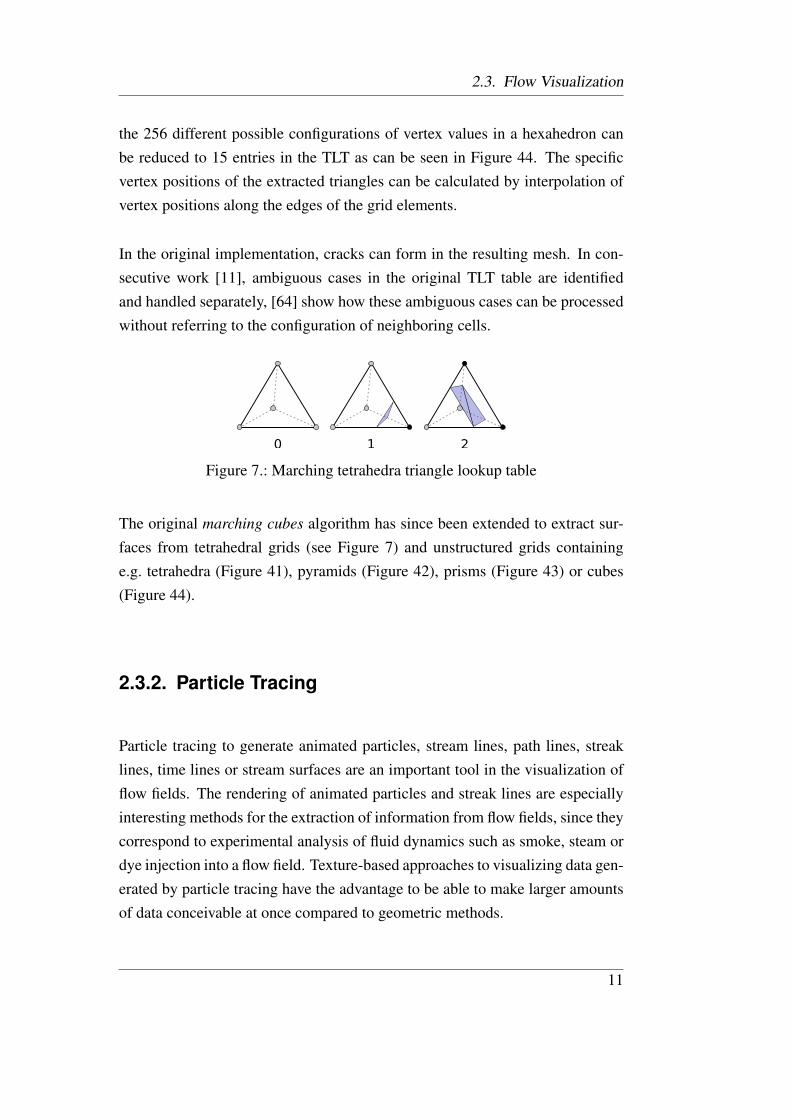
the 256 different possible configurations of vertex values in a hexahedron canbe reduced to 15 entries in the TLT as can be seen in Figure 44. The specificvertex positions of the extracted triangles can be calculated by interpolation ofvertex positions along the edges of the grid elements.
In the original implementation, cracks can form in the resulting mesh. In con-secutive work [11], ambiguous cases in the original TLT table are identifiedand handled separately, [64] show how these ambiguous cases can be processedwithout referring to the configuration of neighboring cells.
0 1 2
Figure 7.: Marching tetrahedra triangle lookup table
The original marching cubes algorithm has since been extended to extract sur-faces from tetrahedral grids (see Figure 7) and unstructured grids containinge.g. tetrahedra (Figure 41), pyramids (Figure 42), prisms (Figure 43) or cubes(Figure 44).
2.3.2. Particle Tracing
Particle tracing to generate animated particles, stream lines, path lines, streaklines, time lines or stream surfaces are an important tool in the visualization offlow fields. The rendering of animated particles and streak lines are especiallyinteresting methods for the extraction of information from flow fields, since theycorrespond to experimental analysis of fluid dynamics such as smoke, steam ordye injection into a flow field. Texture-based approaches to visualizing data gen-erated by particle tracing have the advantage to be able to make larger amountsof data conceivable at once compared to geometric methods.
11

Chapter 2. State of the Art and Technological Background
2.3.3. Commonly Used Data Structures forUnstructured Grids
From a post-processing point of view, structured grids have many advantagesregarding the complexities of the algorithms used to handle their datastructures.Problems that are easily solvable in structured grids, e.g. finding a cell given alocation in the spatial domain or finding neighboring elements given a specificcell, are computationally much harder to solve in unstructured grids. Since manypost-processing algorithms need to solve these problems repeatedly, additionaldata structures have to be used that speed up the computation of these tasks.
2.3.3.1. Indexing and Vertex Sharing
In unstructured grids, topology and vertex locations have to be explicitly stored.Since most vertices belong to more than one grid element, the storage size ofan USG can be vastly reduced if these vertex locations are stored once and arethen referenced instead of having to be stored multiple times as can be seen inFigure 39. Unfortunately, this reduction in storage size does not automaticallylead to a decrease in processing time. Even if an algorithm has to access fewerdata items because of coordinate sharing, the memory access patterns of theseindexed data structures are not beneficial for the streaming multiprocessors oftoday’s manycore hardware due to repeated indirect addressing.
2.3.3.2. Neighbor Lists
A mapping from grid cells to neighbors is necessary to vastly decrease thecomputational complexity of advection in particle tracing algorithms. As thereis no implicit neighbor information in USGs, these information has to be re-ceived from the numerical solver, or if that is not available, pre-computed foreach USG. Either way, these neighbor lists use up large amounts of memoryand increase the number of data accesses needed during the execution of post-processing algorithms.
12

2.3. Flow Visualization
2.3.3.3. Space Partitioning Trees
Space partitioning trees can be used to accelerate the finding of a cell containinga certain coordinate in the mesh. Commonly, KD trees [22] are used to storespatial subdivisions of coordinates in K-dimensional space. Since CFD cellsspan a certain extend in the computational mesh, not all points inside a certaincell can be assumed to be located in the same leaf of a space partitioning ofvertices based on axis-aligned splitting planes. To efficiently locate a CFD cellgiven a certain point in 3D space, the KD tree datastructure has to be extendedto be able to store a bounding interval hierarchy.
Figure 8.: Space partitioning using Cell-Tree
This extension is called Cell-Tree [23], storing bounding boxes of elements atthe leafs of the tree instead of vertices as can be seen in Figure 8. As boundingboxes of elements in an unstructured grid generally overlap, leafs in a Cell-Tree may contain more than a single grid element. This leads to additionalstorage and runtime overhead depending on the depth of the subdivision, i.e. themaximum number of elements that are allowed to be contained in the leafs.
2.3.3.4. Data Partitioning Trees
Instead of spatial subdivisions, post-processing algorithms such as isosurfacecomputation can also benefit from data partitioning trees, e.g. Interval-Trees.Data partitioning trees partition computational meshes according to the data val-
13

Chapter 2. State of the Art and Technological Background
ues at the vertices or cells, which means a separate partitioning of the mesh isneeded for each parameter array.
0
100
200
300
400
500
600
700
800
0 100000 200000 300000 400000 500000 600000 700000 800000 900000
Tim
e (
ms)
Generated triangles
Isosurface, unstructured grid (11626484 elements)
Isosurface 4x CPU XEON E5472 3.00GHz 8x OpenMP 2x MPIIsosurface 4x CPU XEON E5472 3.00GHz 8x OpenMP 2x MPI Interval Tree
Isosurface 4x CPU XEON E5472 3.00GHz 8x OpenMP 2x MPI Cell Tree
Figure 9.: Comparison of isosurface extraction performance using Cell Tree, In-terval Tree and traditional implementation
Analysis of the runtime performance of isosurface extraction in a real-worlddataset shows vast improvements when extracting small surfaces as shown inFigure 9. When more elements are sliced by the surface, at some point the over-head from processing the tree datastructure outweighs the performance gainedfrom reducing the number of elements that need to be processed.
2.4. Post-processing Resources
Workstations have been largely replaced by clusters for interactive post-processing and rendering of large-scale simulation results. Nowadays, simu-lation datasets are getting event too large to be moved to a remote cluster aftersimulation. This is the reason why integrated simulation and post-processingclusters that share the same application network and filesystems are being in-creasingly necessary. Post-processing clusters immensely benefit from the hugeprocessing power and high memory bandwidth of manycore devices such asGPGPUs.
14

2.4. Post-processing Resources
2.4.1. Levels of Parallelism
In High Performance Computing (HPC), different levels of parallelism are dis-tinguished concerning both software and hardware architectures.
• Instruction level parallelism: CPUs can issue several instructions in par-allel to different execution units inside a single CPU.
• Loop- or data level parallelism: Software method of issuing several blocksof data to to different compute cores or shared memory processors in par-allel. On CPUs, this is often implemented using OpenMP.
• Function- or task level parallelism: Distributed compute processes on dif-ferent compute nodes. Message passing between different partitions, typ-ically implemented using MPI or PVM.
Interactive parallel applications often try to leverage parallelism on multiplelevels to achieve scalable low-latency, high throughput computations.
2.4.2. GPGPU Hardware
The rendering pipeline was extended by programmable shaders to provide morerealistic rendering than what was possible using the fixed-function pipeline. Pro-grammable fragment shader units especially enabled the development of per-pixel lighting instead of per-vertex lighting. The GPU’s shader units developedinto multi-purpose, high throughput compute cores that were also usable forgeneral purpose computing.
The compute elements in current generation GPGPU are built from streamingmultiprocessors1. These multiprocessors contain compute cores that work in aSIMD fashion. Aside from the local memory of the compute cores, multipro-cessors contain shared memory that gives compute cores collaborative access todata. Compute cores in separate multiprocessors may exchange data by usingthe global memory area of the device. NVIDIA represents the GPGPU hardwarearchitecture in their CUDA API (see Figure 10).
1NVIDIA terminology
15

Chapter 2. State of the Art and Technological Background
Block
ThreadLocal
Memory
SharedMemory
GlobalMemory
Block (0, 0) Block (1, 0) Block (2, 0)
Block (0, 1) Block (1, 1) Block (2, 1)
Grid
Figure 10.: NVIDIA GPU thread hierarchy and memory layout [67]
A thread represents a single chain of execution in a compute core. Blocks com-bine multiple threads inside a streaming multiprocessor that share a single exe-cution unit and are able to communicate via shared memory. Blocks are sched-uled to free streaming multiprocessors independently and thus are only allowedto communicate by using global memory. A compute kernel is represented by agrid that is forming a 1D or 2D organization of thread blocks.
2.4.3. Performance Considerations in GPGPUComputing
2.4.3.1. Diverging Threads
Since compute cores in a streaming multiprocessor share a single execution unit,the SIMD programming model has to be followed. Diverging threads are imple-mented by executing both branches serially, while disabling the compute coresthat do not participate in the particular branch. This serialization of threadsconsiderably limits the performance of kernels containing diverging executionpaths.
16

2.4. Post-processing Resources
2.4.3.2. Memory Throughput
In GPGPU stream programming devices, high global memory throughput isenabled by coalesced memory access. In current generation NVIDIA GPUs,global memory loads and stores by threads of a warp2 can be coalesced intoone memory transaction if certain access requirements are met [66] (see Figure11).
0 1 2 3 4 5 6 7 8 9 11 12 13 1410 15
0 4 8 12 16 20 24 28 32 36 44 48 52 5640 60
0 4 8 12 16 20 24 28 32 36 44 48 52 5640 60
0 1 2 3 4 5 6 7 8 9 11 12 13 1410 15
0 1 2 3 4 5 6 7 8 9 11 12 13 1410 15
0 4 8 12 16 20 24 28 32 36 44 48 52 5640 60 64
Thread ID
MemoryAddress
Thread ID
MemoryAddress
Thread ID
MemoryAddress
Coalesced memory access pattern
Coalesced for Compute Capability >= 1.2
Coalesced for Compute Capability >= 1.2
64B Segment
Figure 11.: Coalesced memory access patterns on different NVIDIA GPU gen-erations [67]
In practical post-processing applications, the design of datastructures such asvertices as structures of arrays (SoA) or arrays of structures (AoS) [83], canlead to vast differences in performance of algorithms performing large amountsof memory accesses (see Figure 12).
2.4.4. Parallel Rendering in Scientific Computing
Data obtained from post-processing of numerical simulation results typicallyconsist of a large number of geometric primitives. These primitives, gener-ally huge amounts of triangle data, can be rendered by GPUs using either thefixed function pipeline or programmable shaders. Because of memory limita-tions of single workstations or cluster nodes as well as the complexity of the
2A group of threads inside a block being concurrently executed by a streaming multiprocessor
17

Chapter 2. State of the Art and Technological Background
Quadro FX 5800UVW UVW UVW
Quadro FX 5800UUU VVV WWW
Quadro FX 6000UVW UVW UVW
Quadro FX 6000UUU VVV WWW
0 1 2 3 41e+09 scalar products / second
U V W U V W U V Wa
U U U
V V V
W W W
b
Global memory performance using different memory access patterns on differentNVIDIA GPU generations.
x
Figure 12.: Performance of global memory access patterns on different NVIDIAGPU generations
computations that need to be performed, efficient parallel post-processing oflarge scale simulation data is essential. To reduce latency of user interactionswithin the visualization environment, post-processing and rendering have to betightly integrated and able to exploit locality of data. Parallel rendering of dis-tributed graphics primitives offers the possibility to maintain interactive render-ing speeds when visualizing these large-scale, partitioned simulation data.
2.4.4.1. Display Hardware
There are different rendering environments that make it possible for individualsor small teams of engineers to collaborate on exploring large-scale numericalsimulation data. These environments have different requirements for the remoterendering system. In general, it should be possible to combine various render-ing environments, even of different types, to allow sharing of a post-processingsession by multiple, geographically separated users.
An immersive digital environment is an artificial, interactive, computer-createdscene within which users can immerse themselves. Because of cost-efficiency,these installations are often a central resource in the company, university or re-search institution, in many cases featuring a high bandwidth and low latency net-work connection to the data center. Virtual Reality environments such as largetiled display walls [61] or CAVEs [15] need to make high-resolution, very low
18

2.4. Post-processing Resources
latency, high bandwidth stereo image renderings available to the users. Sincethese installations also often feature tracking equipment for user interactions aswell as viewpoint changing, the rendering needs to be updated much more oftencompared to desktop environments, often continuously.
2.4.4.2. Parallel Rendering Paradigms
Parallel rendering techniques can be categorized based on at which point in therendering pipeline graphics primitives are distributed or assigned to the parallelrendering clients. Molnar et al. [59] identify three classes of parallel renderingalgorithms:
• Sort-first algorithms sort graphics primitives during geometry process-ing. Renderer partitions are responsible for a specific rectangle in screen-space. Graphics primitives can be assigned to renderer partitions by eval-uating the screen-projection of the graphics primitives’ bounding box.
• Sort-middle algorithms redistribute graphics primitives between geometryprocessing and rasterization. After geometry processing, primitives trans-formed to screen coordinates are distributed to the partition responsiblefor rasterization of the particular primitive.
• Sort-last algorithms assign arbitrary geometry to each partition as seenin Figure 13. Rendered pixels are then combined by one or more com-
positors. The composition is done by sorting pixels according to theirdistance from the screen projection plane by consulting the depth buffersof the rendered images.
Sort-first parallel rendering is a suitable strategy when either the bandwidth re-quirements for redistribution of geometric primitives is relatively small, or whenrendering times are dominated by the limited fill-rate of the GPUs (e.g. for vol-ume rendering).
The most simple sort-last composition solution is the serial approach whichcombines and merges all intermediate images on the destination rendering unit
19

Chapter 2. State of the Art and Technological Background
responsible for the final display. Several other parallelization schemes for soft-ware composition have been proposed. Most notably, these include Direct Send
[82], Binary Tree [79], Binary Swap [53] and Parallel Pipeline [50], amongwhich Binary Swap is the most commonly used algorithm [20].
(a) Renderer 1 (b) Renderer 2 (c) Renderer 3 (d) Renderer 4
(e) Result
Figure 13.: Sort-last rendering
Binary Swap algorithms distribute the composition of parts of images to allnodes in the cluster. A naïve approach for parallel merging of the partial imagesis to do binary composition. By pairing up processors in order of composition,each disjoint pair produces a new subimage. Thus after the first stage, the taskis reduced to composition n/2 subimages. Using half the number of originalprocessors they are then paired up for the next level of composition. Continuingsimilarly, after log2 n stages, the final image is obtained. One problem with theabove method is that during the composition process many processors becomeidle. At the top of the tree, only one processor is active.
To exploit the compute power of all nodes in the cluster, the key idea in Binary
Swap is that, at each composition stage, the two processors involved in a com-posite operation split the image plane into two pieces and each processor takesresponsibility for one of the two pieces. In the early phases of the Binary Swap
algorithm, each processor is responsible for a large portion of the image areaas can be seen in Figure 14. In later phases of the algorithm, the processors
20

2.4. Post-processing Resources
Communication between partitions
Step 1
Step 2
Step 31 2 3 4
Step 1
Step 2
Step 3
Composition of subimages on partitions
1 2 3 4
1 2 3 4
Figure 14.: Binary Swap parallel composition process (adapted from Ma et al.[53])
are responsible for a smaller and smaller portion of the image area. At the topof the tree, all processors have complete information for a small rectangle ofthe image. The final image can be constructed by sending the subimage tilesto the display node or a remote workstation. The bandwidth requirements forBinary Swap composition are similar to the Direct Send algorithm. Fortunately,the communication patterns are much more suitable for cluster networks thatare not fully connected, since larger image tiles are distributed in early stagesof the composition tree where directly neighbouring cluster nodes communi-cate. There are further developments of Binary Swap such as 2-3 Swap [97]that eliminate the need to use power-of-two number of nodes. 2-3 Swap alongwith enhancements such as improved scanline methods, Sorted Pipeline ImageComposition [71], RLE encoding and the use of bounding boxes [84], make fora promising approach towards even very large numbers of rendering nodes infuture high performance cluster systems.
21

Chapter 2. State of the Art and Technological Background
2.4.4.3. Parallel Rendering Software Systems
In addition to WireGL [36] [37], its successor Chromium [38] [39] and theCGLX library [18] that were mainly developed to accelerate existing softwareby using distributed rendering, complex frameworks such as Equalizer [19]have been developed to simplify the development of parallel graphical appli-cations.
Several post-processing environments feature their own parallel rendering in-frastructure such as AVS/Express [51] or ParaView, which contains the IceTlibrary [60].
22
Chapter 3.
Related Work
A huge gap exists between what weknow is possible with today’s machinesand what we have so far been able tofinish.
(Donald Knuth)
In this chapter, the state of the art in parallel post-processing environments aswell as parallel algorithms for the visualization of flow fields are reviewed.The review shows parallel methods for surface extraction, particle tracing andtexture-based dense flow visualization with a focus on execution on parallelmanycore devices such as programmable GPUs.
3.1. Parallel Post-processing Infrastructure
Modular dataflow architectures dominate today’s general purpose post-processing and visualization software environments. Traditional, mostly serialpackages such as IRIS Explorer [92], Data Explorer (now OpenDX) and CO-VISE [94] aim at allowing the user to specify their post-processing workflowby providing configurable, combinable and thus reusable modules. For the in-teractive processing of large-scale datasets however, distributed data access andparallel processing mechanisms are needed.
23

Chapter 3. Related Work
Many of the existing parallel post-processing architectures are based on the Vi-sualization ToolKit (VTK) [77]. VTK provides methods that allow for the im-plementation of parallel algorithms using message passing over MPI, sharedmemory and socket connections. VTK also allows for the definition of paralleldataflow pipelines.
3.1.1. ParaView
ParaView is a dataflow-oriented post-processing and visualization system basedon VTK. ParaView uses VTK’s data-parallel mode, where identical pipelinesare created in every process, and each process is assigned a different piece ofthe data set [49]. Parallel algorithms operate on VTK objects each containingparts of the distributed simulation data.
The ParaView software architecture is split into several parts. A client processproviding a graphical user interface (GUI) and several server processes that areable to exploit remote parallel processing resources. The server processes areseparated into a root process and optional slave processes running on attachedcluster nodes. User interactions are performed by sending commands from theclient to the root process, which are then broadcast to the slave processes. Thesecommands are implemented as TCL scripts which are interpreted by the serverprocesses. Commands are also used to build visualization pipelines called theprogramme graph. Modules in the programme graph receive partitioned dataobjects for collaborative parallel processing.
Modules can be classified into sources, filters and mappers [77]. Data stor-age and rendering of post-processed simulation data is separated into multiplecomponents. This allows for the usage of ParaView in heterogeneous clusterenvironments where not all compute nodes also contain GPUs [32]. Since post-processing operations most often result in a vast reduction of datasize, the num-ber of rendering servers typically needs to be much smaller than those used forpost-processing. ParaView supports server side rendering as well as the transferof geometry from the servers to the client containing the GUI.
24

3.1. Parallel Post-processing Infrastructure
3.1.1.1. Parallelism at the Task Level
ParaView achieves parallelism at the task level by executing identical pipelinesin parallel, and merging the distributed results in the renderer using vtkParallel-
RenderManager.
3.1.1.2. Parallelism at the Algorithm Level
Many VTK filters support loop-level parallelism using OpenMP. VTK itself isnot thread-safe, so data objects have to be created in the main thread. Changingdata using multiple threads has to be protected by mutual exclusion, addingcommunication overhead to parallel computations at the algorithm level.
3.1.2. VisIt
VisIt is a parallel data-flow oriented visualization systems that makes heavy useof VTK functionality in its components, but is independent of VTK’s data flownetwork.
The VisIt data flow network consists of two different types: data objects andcomponents [12]. Components can be categorized into sources, e.g. file read-ers, filters that transform input data into output data, and sinks such as rendercomponents that consume data objects.
The pipeline, a collection of components, is executed in a demand-driven fash-ion that starts with a pull operation at the end of the dataflow graph. A sinkgenerates an update request that propagates through the pipeline to the source.The data generated by the source is then processed by filter components andfinally consumed by the sink. Parallelism is achieved by executing identicalflow networks on different cluster nodes, distinguished only by the differentchunks of data that are generated or processed during the different stages in thepipeline.
25

Chapter 3. Related Work
One main distinctive feature of VisIt is its notion of contracts that enable com-ponents to perform optimizations dependent on the properties of the pipelinecomponents [13]. These contracts allow components to specify how they im-pact a pipeline, serving as a interface for communication between componentsdetached from the processing of data objects. A contract is created at a sinkand travels upwards through the pipeline along with update requests, allowingcomponents to change or augment a given contract along the way. In a con-tract, components can then react to requirements requested by consumers oftheir output objects, as well as demand that their input objects will fulfill certaincharacteristics. Contracts can also be used to limit the amount of data that hasto be read from disk, e.g. when spatial extends are communicated by a filtercomponent to the reader component.
VisIt supports different models for execution of parallel processing. Stream-
ing can be used for out of core processing where only one domain is processedper execution of the pipeline, given post-processing algorithms that do not haveto employ collective communication. In grouping mode, the pipeline is exe-cuted once with each component processing all domains before proceeding tothe next one. This means that using streaming, adaptive load-balancing can beperformed since domains can be dynamically assigned to processor cores orpost-processing nodes.
VisIt supports both rendering at the client for small numbers of polygons, aswell as remote parallel rendering based on the sort-last algorithm (see Section2.4.4).
3.1.3. Viracocha
Viracocha is a parallel extension to the visualization library ViSTA FlowLib[76]. Its main focus lies on the interactive post-processing of large-scale CFDdatasets in virtual environments [25]. Viracocha employs a master/workermodel to distribute computations to parallel post-processing nodes. Interactionsare sent from ViSTA to the Viracocha scheduler which uses worker processes to
26
3.2. Parallel Post-processing Algorithms
do parallel post-processing. After completion, the master worker collects par-tial results and sends the complete result back to ViSTA FlowLib. Partial resultsgenerated by worker processes can also be streamed directly to the renderingcomponent.
Throughout the system, an optional streaming multi-resolution approach canbe followed that allows for the extraction of base data from the lowest reso-lution dataset available [74]. The approximate data is then being refined byprogressively streaming results generated from post-processing on higher reso-lution grids. Due to the generated overhead by generating multiple results ondifferent scales, the total computation time will be increased when streaming isenabled.
The parallel processing is based on an MPI enabled processing backend, thatis coupled to the ViSTA rendering frontend by using a single TCP connection.The hybrid parallel processing backend relies on distributed processing of de-composed multi-block datasets [95]. The usage of a single TCP connectionbetween the Viracocha and ViSTA FlowLib components lead to interruptionswhere the visualization system may be stalled by newly generated data, nega-tively affecting real-time rendering [24].
Viracocha relies upon a central data manager at the scheduler node that co-ordinates data proxies at the compute nodes. The data management supportshierarchical cache levels employing different caching strategies such as LRU,LFU and FBU. These data caches can be filled using prefetching [26].
3.2. Parallel Post-processing Algorithms
3.2.1. Surface Extraction
Surface extraction methods based on the marching cubes family of algorithmshave been optimized for parallel computers very early after the publication ofthe original algorithm. Paul Mackerras’ implementation for the experimental
27

Chapter 3. Related Work
distributed memory MIMD computer Fujitsu AP1000 uses domain decompo-sition of cartesian grids to distribute the work between the parallel processors[57]. To correctly compute normal vectors at the borders between partitionswhile avoiding the communication overhead between processors, halo elements
of size 1 in each dimension are employed. To achieve primitive load-balancing,an interleaved assignment of blocks containing a low number of cells to theprocessors is performed.
Pascucci [68] and Reck et al. [69] use the vertex shading unit of programmableGPUs to extract isosurfaces from unstructured tetrahedral meshes. To createa quadrilateral surface patch from each tetrahedron, they send four numberedvertices through the vertex pipeline, with the actual vertex positions and functionvalues stored as vertex attributes. The tables used for the marching tetrahedra
algorithm that is computed by the vertex shader are supplied in constant GPUregisters. The output generated by the vertex shader is always a quadrilateral.Degenerate quadrilaterals are used when the actual surface inside an individualtetrahedron is actually a triangle or when the isosurface does not intersect thetetrahedron at all. Degenerate primitives with zero area are then ignored by therasterizer.
Buatois et al. [9] extend on this work by storing data in GPU texture memoryinstead of GPU registers to be able to defeat the memory limitations of theformer approach. They also use indexing to support the sharing of verticesbetween multiple tetrahedra and thus avoiding data redundancy. Although, thisapproach achieves a relatively low performance because of expensive texturelookups in the vertex shader.
Klein et al. [45] follow a different approach to also make use of the fragmentshaders and to be able to read back generated surface patches from the GPU.The fragment shader is used to render a single quadrilateral per tetrahedron intoa floating point render target using ATI’s SuperBuffer extension. After applyingmarching tetrahedra in the fragment shader, the SuperBuffer is then bound as avertex buffer array to render the resulting isosurface.
Martin et al. present a load-balancing method for isosurface extraction on multi-GPU clusters [58]. They suggest applying cost heuristics in a pre-processing
28

3.2. Parallel Post-processing Algorithms
step to pairs of isovalue and partition in a multi-block grid. Triangle count fora range of isosurfaces in each block in the grid. During runtime, blocks arescheduled to GPUs in the system according to the estimated runtime for loadbalancing. They show that triangle count is a legitimate heuristic for expectedruntime performance of isosurface extraction using marching cubes.
Gerndt et al. present view-dependent sorting for progressive streaming duringisosurface extraction [25]. They use view-dependent BSP trees to sort blocks inpartitioned grids from front to back with respect to the viewing position.
NVIDIA provide a CUDA-based marching cubes implementation for rectilineargrids with their CUDA SDK samples [65]. Their implementation uses texturesto store the lookup tables. CUDA kernels are used to classify voxels based onthe number of vertices that will be generated per voxel. Stream compactionis used to skip voxels that are not cut by the isosurface. Triangles are cre-ated using marching cubes and per voxel normals are interpolated from the fieldfunction.
3.2.2. Particle Tracing
The advancement of GPU technology greatly enhanced the usability of ren-dering hardware as general computing devices. Newly developed GPU fea-tures made it possible to implement particle tracing algorithms directly on pro-grammable GPUs:
• Floating point textures and floating point render targets can be employedto generate floating point output from fragment shader programs.
• Texture maps are made available in the vertex units allowing for the ran-dom access of GPU memory in vertex shader programs.
• Buffers can be interpreted both as texture maps and as vertex arrays. Thisenables the passing of render targets as vertex inputs to subsequent ren-dering passes.
29

Chapter 3. Related Work
These features enable Kruger et al. to achieve interactive particle tracing on uni-form grids [46] by performing particle advection, geometry generation and ren-dering completely on the GPU without any readback to CPU accessible mem-ory. They use floating point textures to store and access the initial seed points ofparticles in the RGB channels, leaving the alpha channel to designate individualparticle lifetimes. A floating point texture render target is employed to storeadvected particle positions in the fragment shader. In the second pass, vertextexture fetches are executed for displacing particle geometry according to thepositions stored in the render target of the previous pass.
Schirski et al. adapt this technique for particle tracing in unstructured tetrahedralgrids [74] [75]. In their tracer, the locating of cells is implemented in two phases.A broad phase where a KD tree [5] is used on the CPU to locate a vertex closeto the particle position, followed by a tetrahedral walk [44] on the GPU usingbarycentric coordinates. As in Kruger’s approach, particle positions are storedin the RGB channels of floating point textures, the alpha channel is used todesignate the cell index in the unstructured tetrahedral mesh.
Yu et al. provide methods for scalable pathline construction on very large time-varying cartesian grids [96]. In a pre-processing step, they construct hierarchi-cal meshes by merging neighboring cells with similar vector data into largerclusters. The larger clusters on higher levels can then be assigned to the indi-vidual compute nodes in a parallel cluster system. During particle tracing, thisminimizes communication between partitions since clusters are built along theprincipal flow direction and streamlines can thus be expected to cross partitionboundaries very infrequently.
3.2.3. Texture-based Dense Flow Visualization
In the visualization of CFD simulation data, lines and animated particles areused to provide insight into the local flow field. Arrow plots have been used asthe standard method to visualize the global flow directions in dense flow fields,although it is hard for the user to reconstruct the flow from discrete samples.To provide a global, contiguous visualization of dense flow fields, texture-based
30
3.2. Parallel Post-processing Algorithms
methods such as Digital Differential Analyzer (DDA), Spot Noise and Line In-tegral Convolution (LIC) have been developed. The basic idea of these flow vi-sualization techniques is to blur textures containing noise along the local vectorsin a flow fields. As opposed to DDA convolution where complete streamlinesare approximated by the tangent of the vector field, LIC [10] computes locallyexact streamline advection.
FastLIC [81] improves on the original algorithm by making two observations:First, streamlines cover multiple texels, and thus large parts of streamlines arerecomputed for multiple texels. Second, for a constant filter kernel similar con-volution integrals occur for texels covered by the same streamline.
Parallel LIC [99] is a parallelization of FastLIC that exploits both spatial andtemporal coherence. The parallelization is done in image space by subdivisionof the image into several subdomains assigned to different processors. To avoidcommunication between partitions, the vector field data is replicated in neigh-boring domains.
Teitzel et al. perform LIC on unstructured triangulated 2D surfaces [85]. Toavoid the mapping of complex surfaces to flat texture space, one texture pertriangle of the surface mesh with a fixed number of texels per triangle are em-ployed. After projecting the vector field to the triangular mesh, streamline com-putation and traditional LIC for the projected vector field is performed. Severalmethods for the generation of the input texture are evaluated: First, using thesame white noise for each texture. Second, texture interpolation by vertex usingone intensity value per vertex. Third, triangle subdivision with a fixed numberof subdivision steps and a single intensity value per triangle.
Unsteady Flow LIC (UFLIC) [93] and Accelerated Unsteady Flow LIC (AU-FLIC) [52] extend LIC for the visualization of unsteady flow fields. Sincethe traditional streamline approach supports no coherence between animationframes, they use scattering of pixel values following pathlines and combinationof image values at pixels from pathlines matching the timestep in the anima-tion. AUFLIC increases performance of UFLIC to near interactive frameratesby sparse seeding of pathlines and the reuse of known pathlines. The spatialreuse is performed by correcting already computed pathlines that travel through
31

Chapter 3. Related Work
the pixel containing the seed point of a new pathline. Temporal flexibility al-lows for pathline seeds to not be released at exactly integer timesteps, but somefractional time shortly after the scattering process.
Bachthaler et al. accelerate LIC by combining hybrid parallelization strategieson GPU cluster computers [4]. After using Sort-first for image space decom-position and Sort-last for object space partitioning of the vector field, LIC isperformed on projected flow fields using GPU shader programs in image space.The flow field is replicated using ghost cells at partition border for efficientparticle tracing. Traditional z-sorting and blending of subimages is performedduring image composition in the Sort-last phase.
Image-based Flow Visualization (IBFV) [88] and Image-based Flow Visualiza-tion for Surfaces (IBFVS) [89] is an alternative to traditional LIC-based ap-proaches for unsteady flow. Each image is the result of warping the previousimage along the flow direction, blended with background images containingwhite noise. Van Wijk uses CPU-based a projection of the velocity vectorsat mesh vertices to image space. The texture is then advected over the meshaccording to the velocity vectors stored at the projected mesh vertices. The dis-torted texture coordinates computed by the mesh advection are then mapped tothe original 3D surface mesh vertices.
Image Space Advection (ISA) [48] distorts a regular, rectilinear mesh definedin 2D image space. The vectors in a flow field at the vertices are encoded in theRGB channels of a texture and rendered using Gouraud shading to interpolatethe vectors resulting in a velocity image. The velocity vectors projected onto theimage plane are then used for image-space advection of the local flow field.
32

Chapter 4.
Interactive Post-Processing inParallel Manycore Environments
The secret of getting ahead is gettingstarted. The secret of getting started isbreaking your complex, overwhelmingtasks into small manageable tasks, andthen starting on the first one.
(Mark Twain)
4.1. Utilizing Visualization Clusters
Workstations that have been used traditionally to post-process simulationdatasets are no longer able to process the huge amount of data produced bylarge-scale simulations. The limiting factors are the resources available in asingle workstation, e.g. the amount of memory that can be installed in a singlesystem or the number of compute cores available. Another factor is the networkbandwidth between the compute cluster and workstations of post-processingengineers. The size of raw simulation data of large-scale simulations is pro-hibitively large to be copied off the compute cluster to an outgoing network.
This makes it necessary for post-processing and visualization of simulation datato be performed either during runtime of the simulation on the cluster nodesthemselves (in-situ visualization [56]), or on dedicated visualization nodes in
33

Chapter 4. Interactive Post-Processing in Parallel Manycore Environments
the cluster that can be utilized for interactive tasks. These visualization nodesoften share a common network and parallel filesystem with the compute nodes,which eliminates the need to move data off the cluster. Although the visual-ization cluster nodes typically use the same general processing architecture asthe compute nodes, they additionally offer manycore accelerators such as pro-grammable GPUs to support post-processing and rendering.
4.2. Interactive Post-Processing in Hybrid
Manycore Systems
To be able to execute interactive post-processing algorithms on visualizationclusters, the post-processing software environment has to able to make optimaluse of the available resources.
• Supporting distributed memory environments. Subsets of data have to beable to be distributed to nodes in the visualization cluster. A given de-composition of data generated during pre-processing must be allowed tobe used by the post-processing environment. Data might be needed tobe replicated from one cluster node to another or even between multipleinterconnected clusters. Shared access to data must be possible for con-currently executing post-processing algorithms.
• Executing parallel algorithms on distributed simulation data. Algorithmsshould be allowed to process data both on individual partitions indepen-dently, as well as collaboratively across multiple nodes in the cluster.Post-processing algorithms need to be parametrizable for the user of thesystem to be able to influence various aspects of the workflow interac-tively, such as iso-values or normal vectors of surface extraction algo-rithms.
• Accessing manycore accelerators such as GPGPUs to achieve interac-tivity. Programmable GPUs feature high memory bandwidth and high
34

4.2. Interactive Post-Processing in Hybrid Manycore Systems
processing power which makes them an ideal target for interactive post-processing algorithms. Using GPUs for post-processing also allows forimmediate rendering of processed data, avoiding the latency introducedby copying data between host and accelerator device. Parallel render-ing techniques (2.4.4) and composition methods have to be supported tominimize network bandwidth requirements between the post-processinginfrastructure and user workstations.
• Making the visualization cluster resources as well as individual post-processing workflows available to multiple remote workstations simul-taneously allowing for collaborative distributed working.
To achieve interactivity, i.e. a delay of less than 100 ms [8] from user interac-tion to visual feedback, close attention has to be payed to software architecturedesign decisions that introduce latency.
4.2.1. Simulation Datasets
Datasets that are generated by large-scale CFD simulations on unstructuredgrids consist of multiple different kinds of data. First, one or more partitionedunstructured meshes containing 1D, 2D and 3D elements of various types, suchas points, lines, polygons, tetrahedra, prisms or hexahedra. Second, one or morearrays of data of potentially different dimensionality that map to faces, cells orvertices of the unstructured mesh(es). These data include computed pressure,temperature and velocity values at the distinct positions in the mesh, as well asdata initially set as boundary conditions for the numerical solver. Additionally,there might be geometry specifying boundaries or components that are not partof the actual simulation run but are helpful or necessary for efficient analysis ofthe resulting dataset.
4.2.1.1. Domain Decomposition
In large-scale simulations on distributed memory clusters, the simulation do-main is partitioned spatially into chunks of data, which will be referred to as
35

Chapter 4. Interactive Post-Processing in Parallel Manycore Environments
blocks, that are processed by different compute nodes. Since the processing ofdata at the boundary of a block requires data from neighboring cells that mightbe located in a different block, the contents of these cells have to be commu-nicated between the compute nodes participating in the simulation. To reducecommunication overhead from exchanging individual data elements betweenpartitions during access, these data elements are replicated inside the block,allowing for efficient transfer of all out-of-block neighbors at once. These out-of-block elements are called halo elements or ghost cells. The size of data perblock in today’s HPC CFD simulations typically varies from several thousandelements to several million elements per core.
4.2.2. Distributed Data Objects
Without loss of generality, both the memory as well as the computational com-plexity of the CFD simulation solver will be higher than that of the post-processing algorithms. This allows for an existing partitioning of the data to bereused for the execution of parallel post-processing algorithms in a distributedmemory cluster, even combining multiple smaller blocks in a single partitionof the post-processing environment, avoiding computationally expensive repar-titioning of the data.
To be able to execute collaborative parallel algorithms on distributed data ob-jects, these objects need to contain information about which block and timestepthey belong to, and which blocks are their neighbors. To limit the amount ofmemory needed to represent unstructured grids, data structures can be used toseparate geometry from topology (see Appendix 39).
4.2.3. Dataflow Architecture
Post-processing environments allow for interactive analysis of simulation databy making modular algorithms applicable to operate on these datasets. Popularsystems such as IRIS Explorer [21], IBM data explorer [55] and its successor
36

4.2. Interactive Post-Processing in Hybrid Manycore Systems
OpenDX [1], COVISE [94] and ParaView [77] employ data-centric views ofpost-processing workflows.
A dataflow graph is a directed graph in which nodes represent post-processingmodules and vertices correspond to the data dependencies. Modules in thedataflow graph implement functions of one or more arguments that are repre-sented by data connected as input streams to a given node. Post-processingmodules typically produce data from their input streams that is then made avail-able as one or more output streams. A given module may execute when data isavailable at all its required input ports. This strategy introduces sequencing be-tween modules that depend on each other and allows for independent modulesto execute in parallel.
Algorithms that can be instantiated as modules operate on a portion of data andtransform these data to a different representation. The transformation mightalso be parametrized by the user to allow for an interactive analysis of the un-derlying data. A typical classification of post-processing algorithms follows thevisualization pipeline [2.1.1]:
1. Data acquisition: Modules that allow for input of simulation data fromdifferent sources. These sources include databases, files and simulationsthat are coupled to the post-processing environment during runtime forin-situ visualization [56] of simulation data.
2. Data analysis: Interpolation of data to e.g. different types of grids forfaster post-processing and visualization of a dataset.
3. Filtering: Selection of a subset of data that is of particular interest to thescientist (focus data), this typically includes cropping of data to drasticallyreduce the amount of data to be visualized and analysed.
4. Mapping: Mapping of focus data to geometric primitives such as linesand triangles. Several different mapping techniques exist according tothe dimensionality of the data values, e.g. color coding for scalar data orrendering of glyphs to represent vector data.
37

Chapter 4. Interactive Post-Processing in Parallel Manycore Environments
5. Rendering: Rendering of post-processed data in the form of geometricprimitives suitable for a given environment, e.g. powerwalls, CAVEs ordesktop workstations. A renderer typically includes the possibility ofuser-interaction with the post-processing system, adapted to the possibil-ities of interaction in the given environment.
Dataflow architectures are well established for post-processing of simulationdata because they offer a great deal of flexibility through the ability to arrangecomplex workflows by composition of smaller, relatively simple algorithms[70]. Their modularized nature also allows for ad-hoc extension by adding ad-ditional algorithms needed for advanced, sometimes domain-specific, tasks.
4.2.4. Hybrid Parallel Post-Processing Algorithms
Hybrid parallelization describes exploiting different levels of parallelism or par-allelism on several different kinds of hardware architectures at the same time aswill be described later on in section 4.3.1. Typically, this refers to algorithmsworking in a distributed shared memory environments such as today’s clusters,which consist of a large amount of shared memory multiprocessors. In thiswork, the term hybrid parallelism in the scope of post-processing clusters isextended to include exploiting manycore accelerator cards such as GPGPUs.
Parallel post-processing algorithms can be categorized according to the amountof communication that is necessary between the parallel partitions during exe-cution.
• Pleasantly parallel algorithms require no communication with other par-titions during runtime. This group of algorithms include simple surfaceextraction where the extracted surface, in particular the normal of the sur-face at each vertex in the USG, is known to every partition as will beelaborated in section 6.
• Semi-independent algorithms require the exchange of data with neighbor-ing cells. This group contains e,g. more sophisticated surface extraction
38

4.3. A Dataflow oriented, Parallel Post-Processing Environment
techniques such as isosurface extraction when accurate, per-vertex nor-mals are needed in the post-processed result as will be seen in section 6.Often, communication can be avoided or performed more efficiently byusing halo cells.
• Collaborative algorithms require dynamic data exchange. This may be thecase when communication between partitions depends on the data valueswhich might not be possible to predict before execution of the algorithm.This group includes particle tracing methods that will be discussed in sec-tion 5.2.5.
This categorization also extends to data-parallel post-processing algorithms.
4.3. Software Architecture of vistle1: A
Dataflow oriented, Parallel
Post-Processing Environment
MPI Renderer
Module 2
Module 1 Module 1
ControllerData Manager
Shared Memory
GPU
Module 2
Module 1 Module 1
Renderer
ControllerData Manager
Shared Memory
GPU
MPI Transport Layer
Renderer
ControllerData Manager
Shared Memory
TCP Transport Layer
Start
Spawn
Remote Rendering
Control
Workstation HPC Cluster
Module
Resource
Transport
MPI
MPI
MPI
Cluster Node Cluster Node Cluster Node
Figure 15.: Architecture of a parallel post-processing environment.
vistle is a dataflow-oriented parallel post-processing architecture that has beenbuilt during the creation of this work. The software architecture is based uponcollaborative hybrid parallel processes (see Figure 15). There are multiple pos-sibilities to map tasks in a dataflow system to operating system primitives. The
1Visualization Testing Laboratory for Exascale Computing
39

Chapter 4. Interactive Post-Processing in Parallel Manycore Environments
choice which task abstraction to use influences the techniques employed to im-plement other integral components, such as communication and data manage-ment. The rationale for the choice of task abstraction is also influenced byconsiderations about performance, ease of programmability and fault isolation.In this section, decisions in the design of the vistle software architecture and itscomponents will be presented.
4.3.1. Employing Different Levels of Parallelism
4.3.1.1. Task Parallelism
In this work, a post-processing task is defined as an independent algorithm thattakes a stream of input data and executes specific instructions to produce one ormore streams of output data. Task parallelism can then be defined as the con-current execution of more than one post-processing task on different processorcores. Therefore, the ability to execute a given post-processing task dependsonly on the availability of its input streams. A runtime system for the executionof post-processing tasks can be modeled to contain a directed dataflow graphwhere the vertices are represented by tasks, and the edges are represented bydata streams (see Figure 16). Due to the explicit modeling of the interdepen-dence of tasks in the dataflow graph, the runtime system can determine whichtasks may be executed according to the state of their input streams.
A post-processing task itself can be implemented to contain various subtasksthat can be parallelized explicitly by the programmer without support of theunderlying dataflow runtime system.
4.3.1.2. Data Parallelism
Data parallelism is the parallelization of an algorithm by distributing data acrossmultiple processor cores and applying the same function to single data elementsor subsets of data elements in parallel. This allows the algorithm to scale with
40

4.3. A Dataflow oriented, Parallel Post-Processing Environment
the number of data elements and processors [2]. Data parallelism can be ex-ploited on various different scales:
• Loop level parallelism: On shared memory multiprocessors, a single setof operations can be executed on multiple data elements simultaneously(SIMD). Accelerators such as GPGPU devices expose methods both sim-ilar to SIMD and SMT, where the processing of each data element can beinterpreted as being executed in a separate thread (SIMT).
• Domain decomposition refers to decomposing a data structure and solvinga specific problem for the smaller subdomains. In parallel computing,subdomains can be processed simultaneously on different compute nodes.The performance of the parallel algorithm is often limited by the amountof communication that is necessary when elements in different domainscannot be processed individually. For post-processing of simulation data,the existing decomposition used by the numerical solver usually can bereused.
4.3.2. Parallel Runtime Environment
A runtime environment used to execute parallel post-processing algorithms mustallow for both independent and collaborative processing of subdomains of data.For collaborative parallel execution, a method for communication between par-allel partitions on distributed memory systems has to be supported.
Message Passing Interface (MPI): MPI is a standard message passing interfacefor distributed memory concurrent computers [91]. MPI provides an execu-tion environment for parallel processes as well as methods for communicationbetween these processes. With MPI 2, a dynamic process model has been intro-duced. This allows for the spawning of new processes by a running applicationand connecting to existing processes to support client / server applications [28].Several modes of communication between partitions of a parallel program aresupported. Point-to-point communications can be executed both blocking andnon-blocking. As of MPI 2, collective operations can only be performed by
41

Chapter 4. Interactive Post-Processing in Parallel Manycore Environments
Task AInput Input
OutputOutput
Task BTask BInput InputInput
OutputOutput
(a) Task level parallelism
1 2 3Parallel Task BInput
Output
Parallel Task AOutput
Parallel data stream
Partition 0 1 2 3
Partition 0
(1) Domain decomposition
float output[SIZE];float input[SIZE];
#pragma omp parallel forfor (i = 0; i < SIZE; i++){ output[i] = compute(input[i]);}
(2) Loop-level parallelism
...
...
(b) Data level parallelism
Figure 16.: Different levels of parallelism.
blocking communication, severely limiting their use, since non-blocking com-munication can be used to implement overlapping of communication and com-putation. MPI supports the definition of process groups and intercommunicationbetween these groups.
Enhancements to support manycore architectures are still an active researchtopic:
• Current implementations are not able to scale to very high numbers ofcores. This is hindered e.g. by communication buffers limiting the numberof connections that are possible between partitions.
• Employing very high numbers of cores reduces the time to failure due tohardware defects of the whole system. Fault tolerance in MPI will haveto be improved upon the simple checkpointing / restore that is no longerapplicable in large-scale applications [40].
42

4.3. A Dataflow oriented, Parallel Post-Processing Environment
MPI provided easy integration with shared memory parallel programming meth-ods such as OpenMP [16].
Parallel Virtual Machine (PVM): Focused on portability over performance, dy-namic processes in heterogeneous environments [29]. Low-level message pass-ing. Some support for fault tolerance and recovery.
Partitioned global address space (PGAS): PGAS languages allow for partition-ing of data while controlling locality. Current implementations, e.g. UnifiedParallel C (UPC) or Co-Array Fortran are based on active messages [90] im-plemented on top of GASNet [7]. Implementations of GASNet for high perfor-mance networks either already exist or are currently being developed. A hugebenefit of PGAS languages is the ease of programming due to globally accessi-ble data structures and implicit communication. However, PGAS languages stillhave not been widely adopted in the HPC community. According to Shan et al.this is mainly due to “lack of direct hardware support, a mature developer en-vironment and lack of convincing performance results that they are superior toMPI” [78]. Another factor is the poor interoperability between PGAS languagesand existing high performance numerical libraries written using OpenMP andMPI [42].
The major reasons why MPI has been chosen as parallel runtime and commu-nication framework for vistle are its wide deployment on clusters, the supportfor all major communication networks, high performance implementations bycluster vendors, easy integration with OpenMP, and the availability of numeri-cal libraries and of implementations of various different post-processing algo-rithms.
43

Chapter 4. Interactive Post-Processing in Parallel Manycore Environments
4.3.3. Components of the Post-ProcessingEnvironment
4.3.3.1. Controller
The controller handles dataflow between different post-processing modules, andis responsible for distributed memory communication between the various com-ponents in the system. To be able to control the workflow by executing runnablemodule partitions, it is responsible for managing the workflow graph containingconnections between the modules currently running in the system. The execu-tion of modules where objects are available on input ports can be performedaccording to different modes that can be specified by the post-processing mod-ule:
• Single timestep, single block. A partition of the module may be executedat any time a new data object partition is available. The module partitionis not allowed to do blocking communication with other partitions duringthe processing of the input object. This mode is applicable when all com-putations performed by a module partition can be executed independentof the computation of the other partitions. This is the case e.g. for theextraction of surfaces from unstructured grids when generating per-facenormals.
• Single timestep, all blocks. Execution of a module partition may not startuntil all blocks in a given timestep are currently available as input objectsat the different partitions of this module. This mode is applicable formodules that have to perform global communication between the differentpartitions participating in the post-processing of a dataset. Particle tracingmodules are an example that have to track particles between the differentpartitions of the computational grid.
• All timesteps, all blocks. Processing of input data by executing the mod-ule may only start if all timesteps and all blocks of the input dataset areavailable. The computation of pathlines are an example for a modulespecifying this execution mode.
44

4.3. A Dataflow oriented, Parallel Post-Processing Environment
The type of execution needs to be registered for any given module at startuptime.
Controller Partition
compute()
publish()
vistle::Object::create()
Object ID
addObject(Object ID, Port)
Module Partition Shm Partition
Figure 17.: Sequence diagram of the creation of a shared memory object duringexecution of a module partition
4.3.3.2. Data Management
Data in parallel applications has to be made accessible to the partitions partic-ipating in the data processing. For shared memory systems such as nodes in acompute cluster containing multiple processors and compute cores, many dif-ferent APIs exist to provide shared access to data. In vistle, a system to create,access and identify objects in shared memory (Shm) based on the Boost [17]interprocess library has been developed, providing an abstraction of SysV andPOSIX shared memory and memory mapped files.
Supported object types in shared memory are unstructured grids, points, lines,triangles, polygons, textures, and arrays of floating point or integer values ofdifferent dimensionality. In addition, user defined types can be stored in sharedmemory by the developer of post-processing modules for easy extensibility.
To avoid global communication when creating or accessing shared memory ob-jects, every cluster node contains an independent partition of the data manager.Access to data by partitions of post-processing modules is always performedby contacting the local data manager (see Figure 17). Data objects are thenreplicated from other data manager partitions when necessary.
45

Chapter 4. Interactive Post-Processing in Parallel Manycore Environments
4.3.3.3. GPU Data
To be able to share data on limited GPU memory resources by different post-processing algorithms, vistle contains a memory manager for GPU objects. Thismemory manager is used to replicate objects from host memory to GPU mem-ory, automatically transforming datastructures to a memory layout that is op-timal for parallel access by post-processing algorithms executed on streamingmultiprocessors.
Due to the implementation of data management in today’s GPU drivers, CPUobjects such as textures, VBOs or Renderobjects, can only be accessed with-out difficulty from the operating system process in which they were allocated.Therefore, GPU data management and post-processing algorithms in vistle areimplemented and executed inside the local partition of the renderer.
4.3.3.4. Parallel Modules
Modules implement operations on data, post-processing algorithms and render-ing. These modules can employ different levels of parallelism making use ofshared memory multiprocessing (OpenMP) and distributed memory using mes-sage passing (MPI). Module contain input ports and output ports that can beconnected to ports of other modules in the dataflow graph. When a modulegenerates a data object at one of its output ports, the controller will send a mes-sage to the connected modules depending on the module’s execution mode (seeSection 4.3.3.1).
According to the execution mode, different forms of communication may beused inside a module:
• Single timestep, single block. The module partition is not allowed to doblocking communication with other partitions during the processing ofthe input object, since computation on other partitions may or may not beexecuted at the same time.
46

4.3. A Dataflow oriented, Parallel Post-Processing Environment
• Single timestep, all blocks and All timesteps, all blocks. Global commu-nication may be performed, since the other partitions are guaranteed to beexecuted in the same sequence.
I/O I/O modules function as sources or sinks in the dataflow graph, perform-ing reading or writing of simulation datasets from or to filesystems. To be ef-ficient in a distributed environment, I/O modules have to support simultaneous,communication-free parallel input and output of blocks of data on different com-pute nodes.
Catalogue uint64_t infosize uint64_t itemsize uint64_t numItems
ItemInfo uint64_t infosize uint64_t itemsize uint64_t offset uint64_t type uint64_t block uint64_t timestep...
Item data
...
SET | POLYGONS | ...
ItemInfo uint64_t type = SET uint64_t numItems
...
...
ItemInfo
...
ItemInfo
ItemInfo
Figure 18.: Description of the vistle file format header
The vistle file format (see Figure 18) enables the I/O of parallel regions of databy supplying meta-data linked to the objects in a file. The object-oriented meta-data in the file header serves both as a specification of the layout of the file,as well as a description of the stored objects. Utilizing information about thedataflow network obtained from the controller, an I/O module is enabled to readdistinct partial objects from the specified file in different partitions of the mod-ule. This decomposition of objects then provides a distribution of work amongstthe various post-processing modules in the dataflow graph.
Post-Processing Post-processing modules act as filters for data objects,transforming their input objects into output objects according to a given post-processing algorithm. The available post-processing modules are implementa-tions of the cut- and isosurface algorithms presented in Section 6, as well as the
47

Chapter 4. Interactive Post-Processing in Parallel Manycore Environments
particle tracing methods introduced in Section 5. These implementations bothtest independent execution of different domains in the dataflow graph for sur-face extraction, and collaborative processing for the tracing of particles throughdifferent domains in the CFD grid.
Parallel Rendering Renderer modules provide a user interface for interac-tion with data or post-processed results in a given graphical environment. Theparallel rendering module currently implemented in vistle supports sort-last ren-dering for desktop computers on remote clusters. Along with transformationof the viewer position, control over the visualized timesteps is provided usingmouse input. The performance of the renderer based on the parallel rendering li-brary IceT [60] has been evaluated on the CRAY XE6 installation at HLRS (seeFigure 19). Normally, in sort-last based algorithms, the performance should besimilar inside a section ranging from 2n + 1 to 2n+1 nodes. The observable vari-ations in the measurements stem from the node allocation that is not guaranteedto be consecutive in the testing phase of the HERMIT installation.
0
5
10
15
20
25
30
35
40
32 64 128 256 512 1024
Tim
e (
ms)
Number of rendering nodes
Sort last, binary swap compositing on HERMIT
Compositing time
Figure 19.: Performance of sort-last rendering on 1024 nodes of CRAY XE6HERMIT
48

Chapter 5.
Particle Tracing
When you put together the science ofthe motions of water, remember toinclude under each proposition itsapplication and use, in order that thisscience may not be useless.
(Leonardo da Vinci)
Particle tracing is an established visualization method for the analysis of CFDdata. By releasing particles into a computational domain and computing thepaths of the particles as they are advected by the flow field, particle tracingalgorithms are able to reproduce experimental results created in wind tunnels orturbomachinery testbeds.
5.1. Introduction
Time-varying flow fields are defined as vector-valued functions defined on agiven domain:
v(x, t) : D × I → Rn (5.1)
where x ∈ D ⊆ Rn defines spatial positions in an n-dimensional flow domainand t ∈ I ⊆ R represents time in transient flow fields. Particle paths can becomputed by the integration of the ordinary differential equation (ODE)
dx(t)
dt= v(x(t), t) (5.2)
49

Chapter 5. Particle Tracing
where x(t) denotes the position of the particle at time t, and v(x, t) denotes thevelocity-vector of the flow field at position x at time t. The starting position x0
of the particle provides the initial condition
x(t0) = x0 (5.3)
Reformulation of equation 5.2 leads to its integral form
x(t+ ∆t) = x(t) +
∫ t+∆t
t
v(x(t), t) dt (5.4)
While equation 5.4 cannot be analytically solved in general, a solution can beapproximated using numerical integration. Although in CFD simulation datavector fields are given in discrete form over a computational mesh, numericalintegrators treat the flow field v as a continuous function. As flow data is givenwith respect to individual grid cells or vertices, there is a need for interpola-tion to evaluate the flow field at arbitrary positions inside the computationaldomain.
5.2. Parallel Particle Tracing on GPGPUs
Algorithms for the tracing of particles by numerical integration in discretemeshes perform multiple steps. First, the cell that contains the particle at itsinitial position has to be determined. The velocity of the flow field at this po-sition has to be determined by interpolating the velocity field at the vertices ofthe cell. Then, an integration step calculates the next position of the particlein the flow field according to the, either constant or adaptive, step size. If theparticle has left the mesh element, the cell containing the new particle positionhas to be determined. The algorithm continues until either the particle leavesthe computational mesh, or another break condition, such as a total number ofintegration steps, is reached.
50
5.2. Parallel Particle Tracing on GPGPUs
5.2.1. Initial Cell Location
The finding of cells for the location of particle positions can be accelerated byutilizing binary space partitioning data structures such as KD trees [22] (see alsosection 2.3.3.3). There are different ways KD trees can be used to help in initialcell location. First, vertices potentially close to a given coordinate can be foundby traversing the vertex partitioning tree and then continuing the search by vis-iting the cell the vertex is in and its neighbors until the correct cell is found.Second, a KD tree can also be used to quickly constrain the number of cells aspecific coordinate may be located in. For this purpose, leaves in the KD treestore axis-aligned bounding boxes (AABBs) of the elements in the computa-tional mesh. The element(s) containing a specific coordinate can then be foundby traversing the KD tree until a leaf is reached. Considering mesh elementscover an extent in space and are generally neither axis-aligned nor aligned toother mesh elements, splitting planes of the KD tree may slice elements, lead-ing to the requirement for elements to be located in more than one branch ofthe tree. These observations motivate an extension of the KD tree datastruc-ture called Cell-Tree [23]. Since AABBs of unstructured mesh elements cangenerally overlap, the leaves in the Cell-Tree are not limited to containing onlya single mesh element. To limit the amount of memory a Cell-Tree uses, it isbeneficial for the leaves in the tree to contain a certain maximum number ofelements, and then use exact point location methods in these cells to find theparticular coordinate. KD trees can be constructed on graphics hardware in re-altime [98].
5.2.2. Tetrahedral Decomposition
There are multiple possibilities for interpolation in unstructured mesh elements.The first method is the transformation of irregular elements into regular elementsto carry out the interpolation in transformed space. Although, the transforma-tion of irregular element using Jacobian matrices is only an approximation andcan lead to discontinuities in the flow field [43]. The second method is the de-composition of elements such as hexahedra, prisms and pyramids into multiple
51

Chapter 5. Particle Tracing
(a) Incongruent decomposition (b) Continuous decomposition
Figure 20.: Decomposition of neighboring hexahedral cells
tetrahedra and computing natural coordinates for interpolation of the flow fieldinside these tetrahedra [44].
It has to be noted that in general, a given decomposition of complex elementsinto tetrahedra is not unique. To be able to create consistent results, the de-composition of these elements has to be performed the same way every time.Because faces of complex elements may not be planar, neighboring faces withincongruent edges can create gaps between elements and will prohibit consistentvelocity interpolation (see Figure 20).
The method for decomposition of complex elements into tetrahedra describedby Kenwright et al. [44] can be used to do on-the fly decomposition duringparticle tracing. The advantage of using runtime decomposition compared tooffline decomposition is that the memory requirements for an USG containingcomplex cells is much lower than for a tetrahedral mesh.
5.2.3. Numerical Integration
Hull et al. compare various numerical integration methods and recommend us-ing fourth or fifth order Runge-Kutta method for calculations in which the func-tion evaluations are simple [35]. Bogacki et al. describe an embedded Runge-Kutta 4,5 pair [6] that can be used for efficient particle tracing with adaptivestepsize by using the error between RK4 and RK5 as an indicator for stepsizedoubling.
52

5.2. Parallel Particle Tracing on GPGPUs
5.2.4. Neighbor Search
To avoid computationally expensive cell location testing during particle advec-tion, particles leaving individual cells can be detected as part of the tetrahedraldecomposition method described in section 5.2.2. Neighbor search [31] canthen be applied to locate the new cell that the particle traveled to. This standardmethod has also been implemented on the GPU e.g. by Schirski to trace parti-cles through unstructured tetrahedral grids [74]. More recently, algorithms thatdo not require face to cell data [72] to locate the next cell in the particle pathhave been developed.
5.2.5. Parallelization
Acceleration of particle tracing in HPC can be performed by parallelization overdata, parallelization over the particles, or hybrid approaches. Parallelizationstrategies depend on the amount of data to be visualized:
• For large numbers of particles and relatively small size of the dataset fit-ting in memory of a shared memory node or an accelerator, a paralleliza-tion over the number of particles allows for pleasantly parallel implemen-tation achieving good scalability.
• Although for large data sets that do not fit into memory, parallel tracing inpartitioned datasets has to be employed. Particles leaving a domain haveto be transferred to different partitions, adding communication overhead.The scalability then depends on the smart partitioning of the data, thathas to ensure that particles stay inside a single partition for long periodsof time. The approach described by Yu et al. [96] employing hierarchi-cal clustering methods to partition the flow field is an effective methodtowards this goal.
53

Chapter 5. Particle Tracing
[0..1]
[0..1]GL_POINT
automatically generatedtexture coordinates
Fragments
D D
DD
discardedfragments
Figure 21.: GLSL particle rendering using GL_POINTS
5.2.6. Particle Rendering
To be able to render large number of particles for the visualization of flow fields,standard methods include the rendering of billboards or textured point-sprites.Using billboards, as well as simple geometry such as quads, has the disadvan-tage that large numbers of vertices have to be passed through the vertex pipelineof the GPU, seriously affecting rendering performance for large numbers of par-ticles.
Point-sprites define an alternative, where only a single vertex has to be processedfor each particle. Although, texture accesses needed to render dynamically lit,rounded points that appear to be spheres viewed from the front, are expensivein terms of rendering performance. To eliminate texture accesses, shader pro-grams can be used rendering dynamically lit “spheres” using point sprites (seeFigure 21 and Appendix B.2). This is made possible by automatic genera-tion of texture coordinates on OpenGL’s GL_POINTS during rendering usingGL_COORD_REPLACE as a texture environment for the point. These texturecoordinates can be used to detect the position of a fragment inside the particle tocalculate appropriate lighting per fragment, or simply discarding the fragmentson the outside to provide the notion of circular points. The size of the particlecan be set according to the z position of the fragment, possibly augmented withan additional particle size passed as a vertex attribute when different particlesizes have to be supported.
54

5.2. Parallel Particle Tracing on GPGPUs
(a) Visualization of vortices in data center air cooling (particles)
(b) Vortex rope in a radial water turbine runner
Figure 22.: Massively parallel particle rendering on the GPU using GLSLshaders
55

Chapter 5. Particle Tracing
(a) Erosion at inlet (b) Erosion at outlet
Figure 23.: Erosion in a radial water turbine runner1
5.3. Massive Particle Tracing for Erosion
Prediction in Turbomachinery
Erosion is a major component causing material removal in hydraulic machinery[86]. The effects of erosion are abrasive and erosive wear caused by massiveparticles contained in the water flow that impact on the surface of the machinery.The erosion intensity depends on the sediment type and its characteristics suchas shape, size and hardness [62]. Erosion effects may also be combined withwear caused by cavitation [87]. An optimal geometry of turbomachinery has tobe developed to minimize these issues.
In this section, methods are presented that allow the engineer to interactivelyanalyze the cause and effect of erosion during computational optimization ofturbomachinery components. The implementations are realized to exploit paral-lel manycore devices such as GPUs, to be able to efficiently augment traditionalmethods for visualization of cavitation (also see Figure 27c) with the visualiza-tion of abrasive and erosive wear.
5.3.1. Tracking Massive Particles in Unstructured Grids
The advection of sediment such as quartz sand is based on the methods presentedin Section 5. To be able to efficiently compute erosion caused by massive par-
1Images courtesy of Stellba Hydro GmbH & Co KG, Heidenheim
56
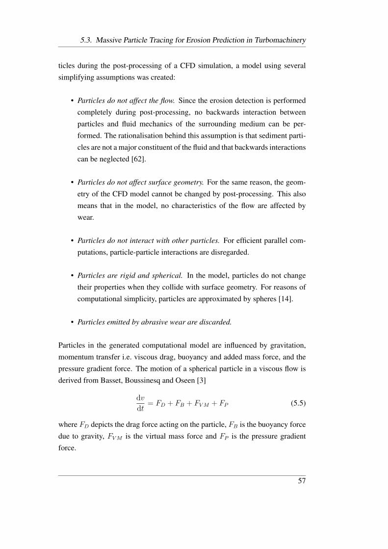
5.3. Massive Particle Tracing for Erosion Prediction in Turbomachinery
ticles during the post-processing of a CFD simulation, a model using severalsimplifying assumptions was created:
• Particles do not affect the flow. Since the erosion detection is performedcompletely during post-processing, no backwards interaction betweenparticles and fluid mechanics of the surrounding medium can be per-formed. The rationalisation behind this assumption is that sediment parti-cles are not a major constituent of the fluid and that backwards interactionscan be neglected [62].
• Particles do not affect surface geometry. For the same reason, the geom-etry of the CFD model cannot be changed by post-processing. This alsomeans that in the model, no characteristics of the flow are affected bywear.
• Particles do not interact with other particles. For efficient parallel com-putations, particle-particle interactions are disregarded.
• Particles are rigid and spherical. In the model, particles do not changetheir properties when they collide with surface geometry. For reasons ofcomputational simplicity, particles are approximated by spheres [14].
• Particles emitted by abrasive wear are discarded.
Particles in the generated computational model are influenced by gravitation,momentum transfer i.e. viscous drag, buoyancy and added mass force, and thepressure gradient force. The motion of a spherical particle in a viscous flow isderived from Basset, Boussinesq and Oseen [3]
dv
dt= FD + FB + FVM + FP (5.5)
where FD depicts the drag force acting on the particle, FB is the buoyancy forcedue to gravity, FVM is the virtual mass force and FP is the pressure gradientforce.
57
Chapter 5. Particle Tracing
The drag force FD is proportional to the relative fluid flow velocity between theparticle and the fluid. It is defined by
FD =1
2CD ρF AF |UF − UP |(UF − UP ) (5.6)
where CD is the drag coefficient, AF is the effective cross section of the particle,and UF and UP are the velocities of the fluid and of the particle respectively.
The drag coefficient is a term determined by experimental data used to quantifythe drag of an object in a vicious fluid [33] [73]. It is defined by
CD =
24Re
if Re ≤ 1
24Re
(1 + 0.15 Re0.687) if 1 < Re ≤ 1000
0.44 if 1000 < Re ≤ 2.5× 10⁵
(5.7)
in which the first case depicts the Stokes Region, the second case is a transi-tional region, and the third case represents Newton’s Law Region where the dragcoefficient is constant.
The buoyancy force FB on a particle is equal to the weight of the fluid that isdisplaced by the particle. It is defined by
FB = (mP −mF ) g (5.8)
with g being the gravity vector, mP and mF depicting the mass of the particleand of the displaced fluid respectively.
The virtual mass force FVM is an additional drag force on the particle, repre-senting the kinetic energy gained by the surrounding fluid due to an acceleratedparticle. It is defined by
FVM =CVM
2·mF · (
dUF
dt− dUP
dt) (5.9)
where CVM = 0.5 is a non-dimensional mass coefficient for inviscid flowaround an isolated sphere [3], mF the mass of the displaced fluid, and UF andUP the velocity vectors of the fluid and the particle respectively.
58

5.3. Massive Particle Tracing for Erosion Prediction in Turbomachinery
According to [3], the pressure gradient force is only important if large fluidspressure gradients exist and if the particle density is smaller than or similar tothe fluid density. Since particle density will be much higher in this application2,the pressure gradient force will be ignored.
5.3.2. Collision Detection
To compute collision detection, the algorithm for cell traversal presented in Sec-tion 5.2 and [43] is extended using walls generated from the CAD model of thewater turbine. Whenever a particle leaves a CFD cell, the face of the element inthe direction of the worst violator in terms of natural coordinates of the particleis checked. If the face that has to be intersected by the path of the particle ismarked as as wall, the particle is reflected from the wall instead, impacting thesurface geometry at the intersection point, adding erosive wear according to aerosion model.
5.3.3. Tabakoff and Grant Erosion Model
Given the velocity of a particle, the angle between the path of the particle and thesurface normal of the struck geometry, as well as the material of the particle andthe surface, the erosion model of Tabakoff and Grant [27] reproduces empiricalerosive wear of the surface.
As implemented in ANSYS CFX-12 [3], the dimensionless erosion rate E iscomputed by
E = f(γ)(VPV1
)2cos2γ(1−R2T ) + f(VPN) (5.10)
where VP is the particle impact velocity and γ is the impact angle. The impactangle function f(γ) is computed by
f(γ) = [1 + k2k12sin(γπ
2γ0
)]2 (5.11)
2the density of quartz is 2.650
59

Chapter 5. Particle Tracing
0.0000
0.0001
0.0002
0.0003
0.0004
0.0005
0 10 20 30 40 50 60 70 80 90
Ero
ded
mas
s pe
r pa
rtic
le m
ass
Angle of collision between particle and wall
Erosion quartz particles / steel walls
Particle speed m/s
1
2
3
4
5
6
7
8
9
10
(a) Erosion caused by quartz particles on steelwalls
0.0000
0.0001
0.0002
0.0003
0.0004
0.0005
0 10 20 30 40 50 60 70 80 90
Ero
ded
mas
s pe
r pa
rtic
le m
ass
Angle of collision between particle and wall
Erosion quartz particles / aluminum walls
Particle speed m/s
1
2
3
4
5
6
7
8
9
10
(b) Erosion caused by quartz particles on alu-minum walls
Figure 24.: Eroded mass depending on particle mass, angle of collision, speedof particle and wall material (erosion model of Tabakoff/Grant [27])
with γo depicting the angle of maximum erosion. The other model constantk12 and the reference velocities V1, V2 and V3 are used to configure the modeldependent on the materials used.
RT = 1− VPV3
sinγ (5.12)
f(VPN) = (VPV2
sinγ)4 (5.13)
k2 =
1.0 if γ ≤ 2γ0
0.0 if γ > 2γ0
(5.14)
Figure 24 shows a visualization of erosive wear of quartz particles on steel andaluminum walls with respect to different velocities and impact angles accordingto the Tabakoff and Grant erosion model.
60

5.3. Massive Particle Tracing for Erosion Prediction in Turbomachinery
Figure 25.: Particle paths and isosurfaces of particle density for several erodedsegments
5.3.4. Visualization of Erosion
The visualization of erosive wear combines massive particle tracing methodsand the surface extraction methods introduced in Chapter 6. Using a statisticaldistribution of sand particles at the inlet elements of a turbomachinery simu-lation (also see C.1), massive particles are traced to the outlet elements of thecomputational mesh. When colliding with surface geometry, the eroded massis added to the affected surface polygons accordingly. The eroded mass that iscomputed by the introduced erosion model can then be visualized as color codedregions mapped to the surface polygons of the CAD model.
Additional information about the origin of particles contributing to erosion of aparticular segment can be visualized as boundary surfaces of particle paths ascan be seen in Figure 25. Efficient extraction of the boundary surface of multipleparticle paths is implemented by generating an additional particle density fieldin the CFD model during particle tracing. The density field can then be usedto extract an isosurface containing all CFD elements through which particlescontributing to erosion of an interactively indicated segment have travelled, al-lowing for deeper analysis of potential for optimization regarding the durabilityof turbomachinery components.
61

Chapter 5. Particle Tracing
0
10000
20000
30000
40000
50000
60000
70000
80000
90000
100000
Dual Xeon 8 threads Quadro FX 6000
inte
gra
tions/m
s
masslessmassive
Figure 26.: Performance of CPU and GPU implementation of tracing of mass-less and massive particles
5.4. Performance
As can be seen in Figure 26, tracing of massive particles adds much less com-putational overhead on GPUs than on CPUs. Where massive particle tracing onthe CPU yields about half the performance of massless particle tracing, the GPUachieves about 74% of the performance compared to tracing massless particlesusing the same dataset. Even though particle tracing in USGs is not a primediscipline of GPUs since memory accesses cannot be coalesced and code pathsdiverge frequently between the different threads, there is an overall speedup.The reason why massive particle tracing is able to perform much better thanin the CPU implementation, is that the additional computations necessary areovershadowed by memory accesses.
62

Chapter 6.
Surface Extraction
Measure twice, cut once.
(Proverb)
6.1. Extraction of Surfaces from Unstructured
Grids
Direct visualization of a complete, large scale simulation dataset is often im-practical because of the occlusion of interesting flow features by other data.Providing tools for interactive reduction of datasets to extract meaningful datavia filtering helps users to analyze large-scale flow fields. Displaying extractedsurfaces is such an effective way to visualize various characteristics of fluid dy-namic simulation results. Scalar fields such as pressure, or scalar data derivedfrom fields of higher dimensionality such as the magnitude of a velocity field,can be efficiently displayed on these surfaces via color coding. To allow usersfor dynamic probing of data fields, low latency surface extraction and mappingmechanism have to be developed that provide immediate visual feedback to theusers control motions, i.e. with a delay of less than 100 ms [8].
In this chapter, GPGPU methods for creating interactive cross-sections of dataon USGs and accompanying mapping techniques for scalar and vector data areshown. These methods can be used to extract surfaces both using implicit spatial
63

Chapter 6. Surface Extraction
functions such as planes or cylinders, and contour surfaces defined by the datavalues such as isosurfaces.
(a) Cut-Plane (b) Cut-Cylinder
(c) Isosurface of pressure at outlet (magni-tude of velocity color coded)
Figure 27.: Extracted surfaces showing pressure distribution in a radial waterturbine CFD simulation (see also Appendix C.1)
6.1.1. Surface Extraction Algorithm
Marching cubes was created to construct isosurfaces from 3-dimensional recti-linear grids, originally intended to be used for the visualization of medical data[54]. Although, the enhanced family of algorithms can also be applied to the ex-traction of arbitrary surfaces from structured and unstructured datasets (see alsoSection 2.3.1.1). The basic marching cubes algorithm can be accelerated usingeither geometric decomposition such as KD trees, value decomposition such
64

6.1. Extraction of Surfaces from Unstructured Grids
as Cell-Trees (see also Section 2.3.3.3), or employing the sweeping simplicesalgorithm [80]).
Parallelization is usually achieved by employing a divide and conquer approachto locate the surface within each cell of the grid. Collaboration between the par-titions participating in the parallel extraction is needed to achieve results similarto the serial algorithm:
• The combination of extracted partial surfaces from the distinct partitionsto form the complete surface.
• The calculation of per-vertex normals for the complete surface.
0
25
50
75
100
125
150
0 200000 400000 600000 800000
Tim
e (
ms)
Generated Triangles
Isosurface, Unstructured Grid (11626484 elements)
16x CPU XEON E5472 3.00GHz OpenMP/MPI hybrid1x GPU (NVIDIA Quadro FX 5800)
4x GPU (NVIDIA Quadro FX 5800) MPI1x GPU (NVIDIA Quadro FX 6000)
Figure 28.: Performance of isosurface computation on CPU/GPU
6.1.2. Parallel Manycore Implementation
In this section, a method for efficient hybrid manycore extraction of surfaces onUSGs is provided that is based on NVIDIA’s implementation for cartesian grids[65]. The algorithm treats unstructured grids as a stream of individual cellsthat can be processed independently in parallel. Given an input stream of cells,
65

Chapter 6. Surface Extraction
output streams of triangles, normals and mapped data elements are provided forimmediate rendering or further post-processing on the parallel GPU.
Output
InputA B C D E F G
Classification
Mesh elements
9 12 9 3Number of generated vertices 0 0 0
Output
Input
Stream compaction index computation
0 9 21 309 30 30Exclusive prefix sum (vertices)
9 12 9 3Number of generated vertices 000
Output
Input
Output vertices
Scatter triangle vertices to output stream
0 9 21 309 30 30Exclusive prefix sum (vertices)Element index 0 2 3 6
Output
Input
Element index
Compact Elements
0 1 2 31 3 3Exclusive prefix sum (classification)
Number of generated vertices 9 12 9 3000
1 1 1 1Classification 0 0 0
1 1 1 1Classification 000
0 1 2 31 3 3Exclusive prefix sum (classification)
0 2 3 6
Figure 29.: Parallel GPGPU surface extraction
The algorithm is split into multiple steps (see also Figure 29):
• Classification: All cells in the USG are classified according to how manyvertices are generated by surface extraction in the individual cell. Twooutput stream are generated as input for the following stages. First, astream containing the number of vertices generated in the cell, second, aclassification of boolean values (0/1) if any vertices in the cell are gener-ated at all.
• Index computation for stream compaction: Since it is likely that there arecells in the USG that are not cut by the surface, the output streams have tobe compacted. To be able to leave out empty cells, exclusive prefix sumsfor the aforementioned output streams are computed to be used in the nextstage.
• Stream compaction: Using the stream containing the number of generatedvertices per cell, along with the stream containing the exclusive prefix sum
66
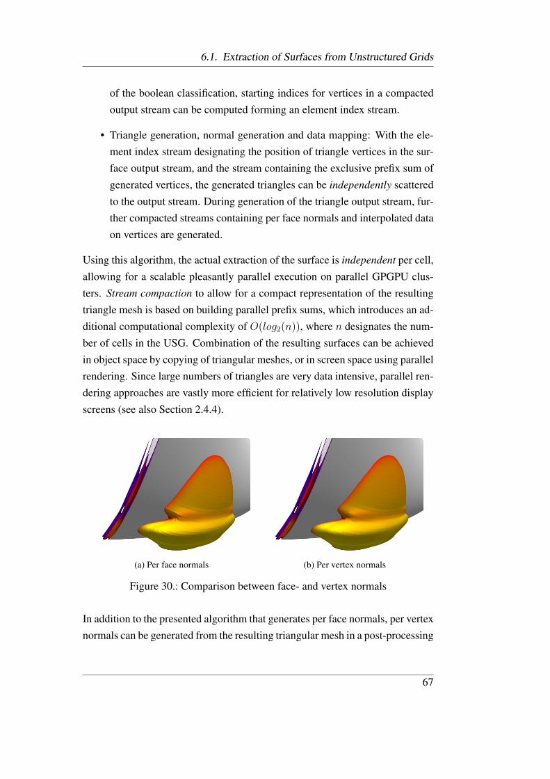
6.1. Extraction of Surfaces from Unstructured Grids
of the boolean classification, starting indices for vertices in a compactedoutput stream can be computed forming an element index stream.
• Triangle generation, normal generation and data mapping: With the ele-ment index stream designating the position of triangle vertices in the sur-face output stream, and the stream containing the exclusive prefix sum ofgenerated vertices, the generated triangles can be independently scatteredto the output stream. During generation of the triangle output stream, fur-ther compacted streams containing per face normals and interpolated dataon vertices are generated.
Using this algorithm, the actual extraction of the surface is independent per cell,allowing for a scalable pleasantly parallel execution on parallel GPGPU clus-ters. Stream compaction to allow for a compact representation of the resultingtriangle mesh is based on building parallel prefix sums, which introduces an ad-ditional computational complexity of O(log2(n)), where n designates the num-ber of cells in the USG. Combination of the resulting surfaces can be achievedin object space by copying of triangular meshes, or in screen space using parallelrendering. Since large numbers of triangles are very data intensive, parallel ren-dering approaches are vastly more efficient for relatively low resolution displayscreens (see also Section 2.4.4).
(a) Per face normals (b) Per vertex normals
Figure 30.: Comparison between face- and vertex normals
In addition to the presented algorithm that generates per face normals, per vertexnormals can be generated from the resulting triangular mesh in a post-processing
67

Chapter 6. Surface Extraction
step (see Figure 30). Using neighbor information in the USG, the vertex normalscan be interpolated from the face normals by revisiting cell neighbors based onthe element index stream. This process is computationally expensive and can bevery time consuming depending on the number of generated triangles.
Since memory on existing manycore devices is scarce compared to the host-memory of current compute cluster nodes, data has to be constantly copiedto the device when applying surface extraction on transient datasets. Usingdouble-buffering, communication and computation can be overlaid as can beseen in Figure 31 without any additional overhead in the coal combustion cham-
ber dataset.
memcpyHtoDasync
classifyElements
scan4
vectorAddUniform4
memcpyDtoH
compactElements
generateTrianglesQuadro FX 6000
Quadro FX 5800
ScanClassify & Asynchronous Memcopy
0 21639 μs20000
VerticesGenerate
71244 μs20000 40000 60000
Figure 31.: Surface extraction runtime performance on different generationGPUs 1
Performance analysis of the parallel manycore implementation using streamcomputing show various interesting results on different generation NVIDIAGPUs (see Figures 28 and 31).
• A single previous generation Quadro FX 5800 is about as fast as 16 In-tel XEON CPUs applying isosurface extraction on the medium-size coal
combustion chamber dataset.
• The speedup using multiple GPUs connected via MPI over a high-speedInfiniband interconnect is decreasing when more triangles are extractedbecause of the overhead of combining the resulting triangle meshes overthe network.
• The memory intensive classification of cells where every cell and all thevertices in each cell have to be accessed is much faster on newer genera-
1Quadro FX 5800 chipset GT200, Quadro FX 6000 chipset GF100
68

6.1. Extraction of Surfaces from Unstructured Grids
tion GPUs. Although these highly irregular memory accesses needed inthe processing of USGs still are a bottleneck for parallel manycore algo-rithms.
• Transfers of memory from host to device e.g. for the preparation of thenext timestep in transient datasets is not much faster on the newer gener-ation devices, but still can be hidden by overlaying communication andcommunication.
• The performance of surface extraction on manycore devices allows forinteractive feedback to user interactions. Due to the mostly pleasantlyparallel nature of the algorithm, meshes can be distributed to the nodes inthe post-processing cluster for scalable parallel execution.
Figure 32.: Visualization of temperature distribution in a coal combustion cham-ber simulation (see Dataset C.2) using surface extraction methods
69
Chapter 6. Surface Extraction
6.2. Texture-based Feature Visualization
Dense, texture-based visualization techniques have been introduced in Section3.2.3. In contrast to geometric, indirect visualization methods, these techniquescan be used to provide a complete coverage of large-scale vector fields [47].
Given streamlines σ parametrized by arclength s that are defined by
d
dsσ(s) = v(σ(s), t) (6.1)
and the initial conditionσ(0) = σ0 (6.2)
the LIC algorithm computes intensities for each texel located at x0 = σ(s0) byevaluating the convolution integral
I(x0) =
∫ s0+L
s0−L
k(s− s0)T (σ(s))ds (6.3)
where σ is the streamline through the center of the texel, k is a given filter kernelwith length L, and T is a texture filled with white noise [81].
In this section, a method for parallel LIC is introduced, that provides fast, inter-active visualizations of flow on surfaces extracted from USGs.
6.2.1. Parallel Line Integral Convolution on ManycoreDevices: FragmentLIC
The presented algorithm is able to calculate convolution integrals on surfacesextracted from USGs using parallel manycore devices. It avoids several short-comings of previous developments:
• The unstructured grid does not need to be resampled to a structured gridat any time of the algorithm. This avoids artifacts introduced by interpo-lation.
70

6.2. Texture-based Feature Visualization
Figure 33.: Visualization of vortices in data center air cooling, including addi-tional background geometry
• The flow field does not have to be projected to the surface where LICis applied. Instead, particle advection is performed on the original CFDgrid. Projection of the vector field is only appropriate for surfaces that areclose approximations of the local flow field, i.e. stream surfaces. Other-wise, aliasing artifacts are added to the visualization, possibly leading toerroneous conclusions about the underlying flow.
• Streamline computation is performed per fragment of the generated im-age, providing a decoupling of image resolution and object space. There-fore, both coarse visualizations stemming from large triangles, and dupli-cate computations for small objects are eliminated.
• Readback of rendered images from the GPU to CPU-accessible memory isnot required, unless parallel or remote rendering is performed and copyingof image data to remote hosts is essential.
The algorithm provides integrated surface extraction and computation of line in-tegral convolution on these surfaces using multiple rendering and computationphases. The surface extraction methods described in section 6.1.2 and the par-ticle tracing technique shown in section 5.2 are combined to provide generationof LIC visualizations at interactive framerates using programmable GPUs.
71
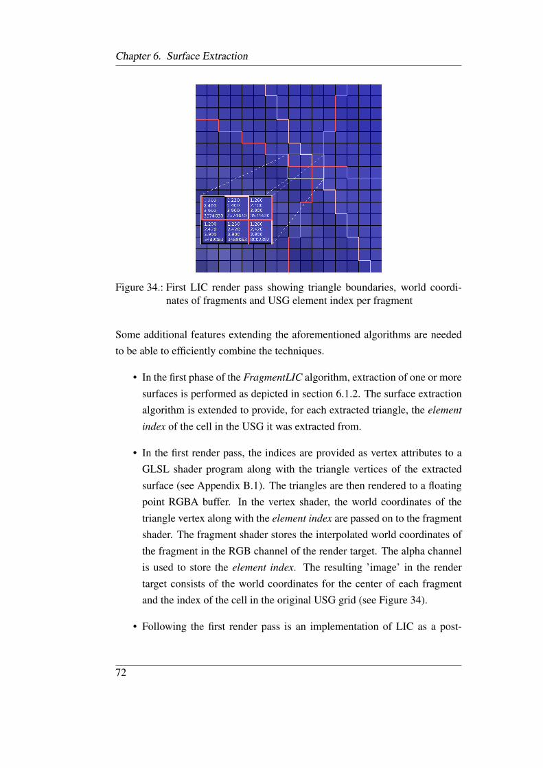
Chapter 6. Surface Extraction
Figure 34.: First LIC render pass showing triangle boundaries, world coordi-nates of fragments and USG element index per fragment
Some additional features extending the aforementioned algorithms are neededto be able to efficiently combine the techniques.
• In the first phase of the FragmentLIC algorithm, extraction of one or moresurfaces is performed as depicted in section 6.1.2. The surface extractionalgorithm is extended to provide, for each extracted triangle, the element
index of the cell in the USG it was extracted from.
• In the first render pass, the indices are provided as vertex attributes to aGLSL shader program along with the triangle vertices of the extractedsurface (see Appendix B.1). The triangles are then rendered to a floatingpoint RGBA buffer. In the vertex shader, the world coordinates of thetriangle vertex along with the element index are passed on to the fragmentshader. The fragment shader stores the interpolated world coordinates ofthe fragment in the RGB channel of the render target. The alpha channelis used to store the element index. The resulting ’image’ in the rendertarget consists of the world coordinates for the center of each fragmentand the index of the cell in the original USG grid (see Figure 34).
• Following the first render pass is an implementation of LIC as a post-
72

6.2. Texture-based Feature Visualization
1.1102.3803.9003489093
1.1402.3803.9003574630
1.1702.3803.9003574630
1.2002.3803.9003574630
1.2302.3803.9003574630
1.2602.3803.9003574630
1.2902.3803.9003574632
1.3202.3803.9003574632
1.3202.4003.9003574632
1.2902.4003.9003574632
1.2602.4203.9009002392
1.2902.4203.9009002392
1.3202.4203.9009002392
1.2602.4403.9009002392
1.2902.4403.9009002392
1.3202.4403.9009002392
1.2302.4003.9003574630
1.2602.4003.9003574630
1.2002.4003.9003574630
1.1102.4003.9003489093
1.1402.4003.9003489093
1.1702.4003.9003489093
1.1102.4203.9003489093
1.1402.4203.9003489093
1.1702.4203.9003489093
1.2002.4203.9003489093
1.2302.4203.9003489093
1.1402.4403.9003489093
1.1102.4403.9003489093
1.1702.4403.9003489093
1.2002.4403.9003489093
1.2302.4403.9003489093
Figure 35.: Second LIC pass: CUDA-based image post-processing applyingtracing of streamlines to compute convolution integrals per fragment
processing of the generated floating point RGBA image using CUDA ker-nels. For every fragment in the ’image’ containing an alpha value that isa valid cell in the USG, computation of the convolution integral throughthe center of this fragment is performed (see Figure 35 The starting pointof the streamline computation is known to be in the grid cell referencedin the alpha buffer. Therefore, the computationally expensive point lo-cation operations described in section 5.2 can be avoided. The output ofthe post-processing kernels is an image where the fragments containingthe rendered surface have been replaced by the intensity values resultingfrom the computation of the convolution integral, merged with colors des-ignating scalar properties of the flow, e.g. the magnitude of the local flowfield. Fragments containing image background, e.g. additional geometryaccompanying the LIC visualization, can be copied from the floating pointRGBA image. Geometry that contains transparent elements has to be ren-dered in an additional render pass and blended with the image generatedin the post-processing pass.
73

Chapter 6. Surface Extraction
Figure 36.: Visualization of flow at the inlet of a radial water turbine
6.2.2. Performance Considerations on GPGPUs
As the performance of the presented algorithm mainly depends on the numberof fragments used for post-processing of the image (see Figure 37), it bene-fits enormously from sort-first parallelization by partitioning the image space,allowing multiple GPUs to process parts of the dataset in parallel.
Although no reuse of calculated streamlines is performed (since the GPGPUparticle tracing implementation does not support it), the combined surface ex-traction and particle tracing benefits from current GPGPU architectures. Espe-cially at close viewing distances, partitioning of the image space into 2D blocksfor processing using CUDA kernels, makes it probable that fragments processedinside the same block are part of the same USG cell. The individual threads par-ticipating in the computation of streamlines in a single block are then able toexploit cached access to USG datastructures on the GPU, considerably increas-ing performance (see Figure 38).
74

6.2. Texture-based Feature Visualization
0
20
40
60
80
100
120
0 100000 200000 300000 400000 500000 600000 700000 800000 900000 1e+06 1.1e+06
Tim
e (
ms)
Number of fragments
Total LIC computation time on extracted triangles
Figure 37.: Performance of FragmentLIC depending on the size of the generatedimage, using a fixed number of triangles extracted from the datacen-ter dataset
0
20
40
60
80
100
120
140
0 50000 100000 150000 200000 250000
Tim
e (
ms)
Number of triangles
Total LIC computation time on extracted triangles
Figure 38.: Performance of FragmentLIC depending on the number of trianglesextracted from the datacenter dataset, using a fixed number of frag-ments (1.048.576)
75


Chapter 7.
Summary and Conclusion
We can only see a short distanceahead, but we can see plenty therethat needs to be done.
(Alan Turing)
The analysis of simulation data during the virtual product development cycleis alleviated tremendously by interactive post-processing. Traditionally, post-processing algorithms used to examine flow features in simulation data havebeen executed on special purpose workstations. With remarkably detailed sim-ulation results generated on today’s highly parallel HPC clusters, even sepa-rate post-processing clusters are inadequate for interactive analysis, since thesedatasets frequently are even too large to be transferred between the computecluster and the post-processing cluster in adequate time. Engineers presentlyoften have to settle for exploration of temporal or spacial subsets of simulationdata, data sampled to coarser grids, or non-interactive post-processing meth-ods.
7.1. Contributions
To be able to interactively analyze complete, unmodified large-scale simulationdata, post-processing environments have to be able to take advantage of highlyparallel cluster resources.
77

Chapter 7. Summary and Conclusion
In this work, a framework was introduced for the execution of post-processingalgorithms in parallel manycore environments. The main focus was put onachieving interactive framerates during evaluation of large simulation data onunstructured grids, without the need for resampling of data to structured gridsor coarser unstructured grids. vistle, a dataflow-oriented software infrastructurefor a parallel post-processing system based on HPC mechanisms was presented,that was designed and developed during the preparation of this work. vistle isusing a distributed data model to make use of a given domain decompositionobtained from the partitioning created during pre-processing or simulation bythe numerical solver. It allows for parallel modules, implementations of post-processing algorithms, to access distributed data objects either for independentor collaborative parallel processing.
The parallel runtime environment enables vistle modules to utilize the variouslevels of parallelism existent in modern HPC cluster systems. The interac-tive post-processing algorithms that have been developed using the vistle ar-chitecture demonstrate the usage of different parallelization techniques. Parallelsurface extraction algorithms have been designed and implemented using dis-tributed stream-processing capabilities, supported on current HPC hardware us-ing either GPGPU manycore devices or alternative accelerators. Parallel particletracing methods using hybrid parallelization methods have been implementedboth for the interactive assessment of flow fields, as well as for the detection ofareas vulnerable to erosion due to sand-particles in turbomachinery. Combina-tions of parallel surface extraction and particle tracing to enable dense, texture-based visualization of fluid simulation data, has been shown to generate interac-tive framerates without the need for projection of the flow field to the extractedsurface used in competing methods. The algorithms have been evaluated usingseveral real-world datasets.
7.2. Conclusions
Surface extraction techniques, as well as visualization methods based on par-ticle tracing and combinations thereof, still play a highly important role in the
78

7.3. Outlook
analysis of fluid dynamic simulation results. Since parallel rendering and com-position is achieving interactive framerates even on massively parallel clustersystems, interactive parallel post-processing is becoming feasible for the analy-sis of very large partitioned simulation data.
Future manycore CPUs developed for HPC systems will likely combine fea-tures found today in programmable graphics hardware, relatively simple com-pute cores allowing for high-throughput computations, with general purposeprocessing units. The availability of manycore computing resources in the formof GPGPUs makes integrated post-processing and rendering feasible even today,avoiding or hiding expensive copying of data between the different memoriesand address-spaces of CPUs and GPUs and thus further decreasing latency.
The applicability of exploiting large scale manycore HPC compute resourcesfor remote post-processing while maintaining interactivity was shown. Thisenables engineers to analyze full-scale fluid dynamic simulation results withoutsacrificing accuracy due to the usage of sampling or coarsening methods.
7.3. Outlook
7.3.1. Massively Parallel Post-Processing Algorithms
Interactive parallel post-processing using domain-decomposition techniqueshave been demonstrated to be attainable for different algorithms required forthe exploration of fluid dynamic simulation data. Stream computing on many-core devices has been shown to be a useful technique even for algorithms thatnecessitate reduction of data, as is often the case in post-processing methods.The approaches that have been presented might also proof to be highly benefi-cial for three-dimensional feature-based visualization methods that rely on theadvection of massive number of particles.
79

Chapter 7. Summary and Conclusion
7.3.2. Reliability and Fault Tolerance in HPC Algorithms
The probability of hardware malfunctions during large-scale computations risesin combination with the ever increasing number of compute cores involved.Prospective generations of HPC middleware libraries such as MPI and PVM willhave to provide features to support recovering from process failure. The prevail-ing method of checkpointing and restarting of failed computations will likelybe replaced by application focused, Algorithm Based Fault Tolerance (ABFT)techniques [40], which will allow recovery with minimum overhead. Regardingmassively parallel post-processing systems, replication features currently usedto support load balancing might be able to provide means for maintaining inter-activity even during process deterioration or breakdown.
7.3.3. Massively Parallel Rendering of LargePost-Processing Results
Most of the current parallel post-processing and visualization systems depend onremote parallel rendering using scanline rendering, preferably hardware accel-erated using dedicated GPUs. Future manycore HPC systems without special-ized rasterization hardware might make rendering methods such as CPU-basedray-casting appear far more attractive. Of course, this brings up other interest-ing possibilities e.g. for direct rendering of isosurfaces and cut-surfaces even inUSG-based simulation datasets, bypassing the need for the very expensive priorextraction of large numbers of triangles.
80

Appendix A.
Unstructured Grids
A.1. Data Structures
0
8
0
1
2
3
4
5
0.0
0.0
1.0
1.0
1.0
1.0
0.0
0.0
6
7 0.0
1.0
1.0
0.0
0.0
1.0
0.0
0.0
1.0
1.0
0.0
0.0
1.0
1.0
1.5
1.5 1.0
0.00.7
0.78
1
2
5
9
1.0
0.0
6
7
6
Hexahedron
Prism
Type List Element List Vertex List Point Listzyx
Figure 39.: Data structures allowing for coordinate-sharing in USGs
Element lists allow for the reuse of vertices in the vertex list within neighbor-ing grid elements. Since vertex coordinates are data intensive, this sharing ofcoordinates drastically reduces the amount of memory needed to store an USG.In some algorithms, memory access times can be reduced since less data ele-ments have to be accessed compared to using data structures where coordinates
81

Appendix A. Unstructured Grids
are replicated. Although in other algorithms, the indirection introduced by theelement list drastically decreases performance.
A.2. Decomposition of Grid Elements into
Tetrahedra
(a) Decomposition of a pyramid (b) Decomposition of a prism
(c) Decomposition of a hexahedron
Figure 40.: Decomposition of USG elements into tetrahedra
Complex elements in USGs can be efficiently decomposed into tetrahedra toperform robust particle tracing techniques. Continuity between decompositionof neighboring grid elements has to be taken into account as is shown in Figure20 on page 52.
A.3. Marching Elements for Surface
Extraction
82
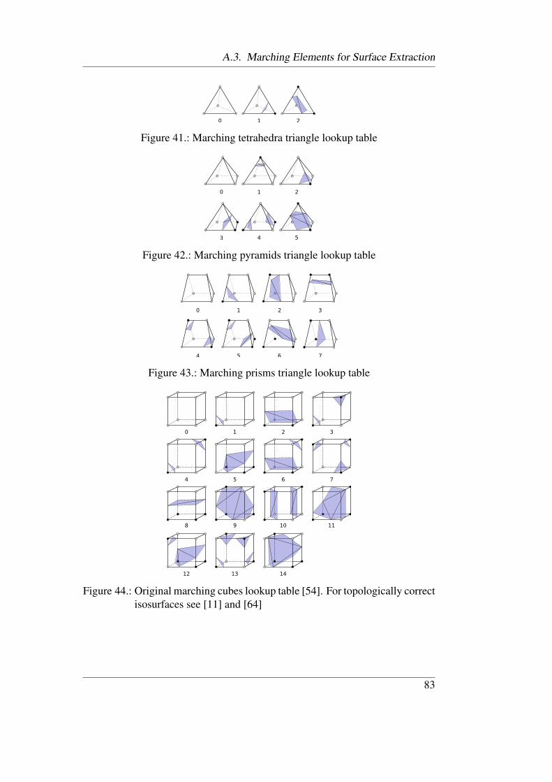
A.3. Marching Elements for Surface Extraction
0 1 2
Figure 41.: Marching tetrahedra triangle lookup table
0 1 2
3 4 5
Figure 42.: Marching pyramids triangle lookup table
0 1 2 3
764 5
Figure 43.: Marching prisms triangle lookup table
0 1 2 3
7654
8 9 10 11
12 13 14
Figure 44.: Original marching cubes lookup table [54]. For topologically correctisosurfaces see [11] and [64]
83


Appendix B.
GLSL Shaders
B.1. LIC on GPU
Listing B.1: GLSL vertex shader for first LIC render pass1 #version 1302 #extension GL_EXT_gpu_shader4 : enable3 attribute int elem; // index of CFD element from VBO4 flat out int element; // index of CFD element to pass to fragment shader5 out vec3 position; // world coordinates of vertex to pass to fragment shader
7 void main(void) {8 gl_Position = gl_ModelViewProjectionMatrix * gl_Vertex;9 position = gl_Vertex.xyz; // pass world coordinates of vertex to
10 // fragment shader11 element = elem; // pass CFD element index of vertex to12 // fragment shader13 }
Listing B.2: GLSL fragment shader for first LIC render pass1 #version 1302 #extension GL_EXT_gpu_shader4 : enable3 flat in int element; // index of CFD element4 in vec3 position; // interpolated world coordinates of fragment
6 void main() {7 // set RGB to interpolated world coordinates, alpha to CFD element index8 gl_FragData[0] = vec4(position, element);9 };
85
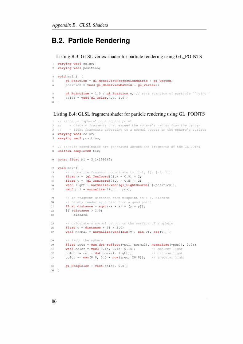
Appendix B. GLSL Shaders
B.2. Particle Rendering
Listing B.3: GLSL vertex shader for particle rendering using GL_POINTS1 varying vec4 color;2 varying vec3 position;
4 void main() {5 gl_Position = gl_ModelViewProjectionMatrix * gl_Vertex;6 position = vec3(gl_ModelViewMatrix * gl_Vertex);
8 gl_PointSize = 1.0 / gl_Position.w; // size adaption of particle ‘‘point’’9 color = vec4(gl_Color.xyz, 1.0);
10 }
Listing B.4: GLSL fragment shader for particle rendering using GL_POINTS1 // render a ’sphere’ on a square point2 // - discard fragments that exceed the sphere’s radius from the center3 // - light fragments according to a normal vector on the sphere’s surface4 varying vec4 color;5 varying vec3 position;
7 // texture coordinates are generated across the fragments of the GL_POINT8 uniform sampler2D tex;
10 const float PI = 3.14159265;
12 void main() {13 // normalize fragment coordinate to ([-1, 1], [-1, 1])14 float x = (gl_TexCoord[0].x - 0.5) * 2;15 float y = (gl_TexCoord[0].y - 0.5) * 2;16 vec3 light = normalize(vec3(gl_LightSource[0].position));17 vec3 ptl = normalize(light - pos);
19 // if fragment distance from midpoint is > 1, discard20 // hereby rendering a disc from a quad point21 float distance = sqrt((x * x) + (y * y));22 if (distance > 1.0)23 discard;
25 // calculate a normal vector on the surface of a sphere26 float v = distance * PI / 2.0;27 vec3 normal = normalize(vec3(sin(v), sin(v), cos(v)));
29 // light the sphere30 float spec = max(dot(reflect(-ptl, normal), normalize(-pos)), 0.0);31 vec3 color = vec3(0.15, 0.15, 0.15); // ambient light32 color += col * dot(normal, light); // diffuse light33 color += max(0.0, 0.3 * pow(spec, 20.0)); // specular light
35 gl_FragColor = vec4(color, 0.0);36 }
86

Appendix C.
Datasets
C.1. Francis Turbine Runner1
The francis turbine runner dataset uses an USG consisting of 11 channels con-taining 15.215.488 elements and 15.490.831 vertices each, resulting in a totalamount of 167.370.368 volume elements and 170.399.141 vertices. The sim-ulation results include per-vertex pressure and velocity data. The numericalsolver used to simulate the turbine is ANSYS CFX.
(a) Francis turbine runner, CADmodel
(b) Parts in one channel of the CFDmodel: inlet (green), interface(yellow), outlet (red), blades /walls (gray)
Figure 45.: Geometry of the radial water turbine runner
1Dataset courtesy of Stellba Hydro GmbH & Co KG, Heidenheim
87

Appendix C. Datasets
Figure 46.: Surface grid of the high resolution CFD model
C.2. Coal Combustion Chamber2
This coal combustion chamber simulation dataset uses an USG split into 32parts. It contains 11.626.484 elements and 12.431.626 vertices in total. Thesimulation results include per vertex temperature, velocity and various speciesconcentrations such as CO2, O2, NOx, coke, coal and ash. The numerical solverused for the simulation of coal combustion is RECOM AIOLOS.
(a) Different parts in the CFDmodel of the coal combustionchamber
(b) Partial surface grid ofthe CFD model
Figure 47.: Numerical simulation of combustion in a coal power plant
2Dataset courtesy of RECOM Services GmbH, Stuttgart
88

C.3. Data center
C.3. Data center3
(a) Data center of the High Per-formance Computing CenterStuttgart, planning stage NECSX9
(b) Texture-based flow visualiza-tion
Figure 48.: Numerical simulation of airflow in a data center
This airflow simulation is one of various different design possibilities analyzedduring the optimization of the data center for the installation of the NEC SX9supercomputer at HLRS. The dataset consists of an USG containing 5.575.896elements and 5.836.713 vertices. It contains per-vertex temperature and velocitydata. The numerical solver used to simulate the air conditioning is ANSYSCFX.
3Dataset courtesy of High Performance Computing Center Stuttgart (HLRS)
89


Bibliography
[1] ABRAM, G., AND TREINISH, L. An Extended Data-Flow Architecturefor Data Analysis and Visualization. SIGGRAPH Computer Graphics 29
(May 1995), 17–21.
[2] ALVERSON, G. A., GRISWOLD, W. G., LIN, C., NOTKIN, D., AND
SNYDER, L. Abstractions for Portable, Scalable Parallel Programming.IEEE Transactions Parallel and Distributed Systems 9 (January 1998), 71–86.
[3] ANSYS. ANSYS CFX-Solver Theory Guide Release 12.0, April 2009.
[4] BACHTHALER, S., STRENGERT, M., WEISKOPF, D., AND ERTL, T. Par-allel Texture-Based Vector Field Visualization on Curved Surfaces UsingGPU Cluster Computers. In Eurographics Symposium on Parallel Graph-
ics and Visualization (2006), Eurographics Association, pp. 75–82.
[5] BENTLEY, J. L. Multidimensional Binary Search Trees Used for Asso-ciative Searching. Communications of the ACM 18, 9 (1975), 509–517.
[6] BOGACKI, P., AND SHAMPINE, L. F. An Efficient Runge-Kutta (4,5)Pair. Computers & Mathematics with Applications 32, 6 (1996), 15–28.
[7] BONACHEA, D. GASNet Specification, v1.1. Tech. rep., Berkeley, CA,USA, 2002.
[8] BRYSON, S., AND JOHAN, S. Time Management, Simultaneity and Time-Critical Computation in Interactive Unsteady Visualization Environments.In Proceedings of the 7th conference on Visualization ’96 (Los Alamitos,CA, USA, 1996), VIS ’96, IEEE Computer Society Press, pp. 255–ff.
91
Bibliography
[9] BUATOIS, L., CAUMON, G., AND LÉVY, B. GPU Accelerated IsosurfaceExtraction on Tetrahedral Grids. In ISVC (1)’06 (2006), pp. 383–392.
[10] CABRAL, B., AND LEEDOM, L. C. Imaging Vector Fields Using Line In-tegral Convolution. In Proceedings of the 20th annual conference on Com-
puter graphics and interactive techniques (New York, NY, USA, 1993),SIGGRAPH ’93, ACM, pp. 263–270.
[11] CHERNYAEV, E. V. Marching Cubes 33: Construction of Topo-logically Correct Isosurfaces. Tech. Rep. CN/95-17, CERN, 1995.http://wwwinfo.cern.ch/asdoc/psdir/mc.ps.gz.
[12] CHILDS, H., BRUGGER, E. S., BONNELL, K. S., MEREDITH, J. S.,MILLER, M., WHITLOCK, B. J., AND MAX, N. A contract-based systemfor large data visualization. In Proceedings of IEEE Visualization 2005
(2005), pp. 190–198.
[13] CHILDS, H., AND MILLER, M. Beyond meat grinders: An analysisframework addressing the scale and complexity of large data sets. InSpringSim High Performance Computing Symposium (HPC 2006) (2006),pp. 181–186.
[14] CLIFT, R., GRACE, J. R., AND WEBER, M. E. Bubbles, Drops and
Particles. Academic Press, New York, 1978.
[15] CRUZ-NEIRA, C., SANDIN, D. J., AND DEFANTI, T. A. Surround-Screen Projection-Based Virtual Reality: The Design and Implementationof the CAVE. In Proceedings of the 20th annual conference on Computer
graphics and interactive techniques (New York, NY, USA, 1993), SIG-GRAPH ’93, ACM, pp. 135–142.
[16] DAGUM, L., AND MENON, R. OpenMP: An Industry-Standard API forShared-Memory Programming. IEEE Computational Science and Engi-
neering 5 (January 1998), 46–55.
[17] DEMMING, R., AND DUFFY, D. J. Introduction to the Boost C++ Li-
braries: Volume II - Advanced Libraries. Datasim Education, 2012.
92

Bibliography
[18] DOERR, K.-U., AND KUESTER, F. CGLX: A Scalable, High-Performance Visualization Framework for Networked Display Environ-ments. IEEE Transactions on Visualization and Computer Graphics 17
(May 2011), 320–332.
[19] EILEMANN, S., MAKHINYA, M., AND PAJAROLA, R. Equalizer: a scal-able parallel rendering framework. In ACM SIGGRAPH Asia 2008 courses
(New York, NY, USA, 2008), SIGGRAPH Asia ’08, ACM, pp. 44:1–44:14.
[20] EILEMANN, S., AND PAJAROLA, R. Direct Send Compositing for ParallelSort-Last Rendering. In ACM SIGGRAPH Asia 2008 courses (New York,NY, USA, 2008), SIGGRAPH Asia ’08, ACM, pp. 39:1–39:8.
[21] FOULSER, D. IRIS Explorer: A Framework for Investigation. SIGGRAPH
Computer Graphics 29 (May 1995), 13–16.
[22] FRIEDMAN, J. H., BENTLEY, J. L., AND FINKEL, R. A. An Algorithmfor Finding Best Matches in Logarithmic Expected Time. ACM Transac-
tions on Mathematics Software 3, 3 (September 1977), 209–226.
[23] GARTH, C., AND JOY, K. Fast, Memory-Efficient Cell Location in Un-structured Grids for Visualization. IEEE Transactions on Visualization and
Computer Graphics 16, 6 (Nov. 2010), 1541–1550.
[24] GERNDT, A. Methoden des parallelen Postprocessing numerischer Strö-
mungssimulationsdaten für die echtzeitfähige Visualisierung und Interak-
tion in VR-basierten Arbeitsumgebungen. PhD thesis, Fakultät für Math-ematik, Informatik und Naturwissenschaften der Rheinisch-WestfälischenTechnischen Hochschule Aachen, 2006.
[25] GERNDT, A., HENTSCHEL, B., WOLTER, M., KUHLEN, T., AND
BISCHOF, C. VIRACOCHA: An Efficient Parallelization Framework forLarge-Scale CFD Post-Processing in Virtual Environments. In Proceed-
ings of the 2004 ACM/IEEE conference on Supercomputing (Washington,DC, USA, 2004), SC ’04, IEEE Computer Society, pp. 50–.
93

Bibliography
[26] GERNDT, A., VAN REIMERSDAHL, T., KUHLEN, T., BISCHOF, C.,HÖRSCHLER, I., MEINKE, M., AND SCHRÖDER, W. Large Scale CFDData Handling in a VR-based Otorhinolaryngological CAS-System usinga Linux-Cluster. The Journal of Supercomputing 25, 3 (June 2003), 143–154.
[27] GRANT, G., AND TABAKOFF, W. Erosion Prediction in TurbomachineryResulting from Environmental Solid Particles. Journal of Aircraft 12, 5(1975), 471–478.
[28] GROPP, W., AND LUSK, E. Dynamic process management in an MPI set-ting. In Parallel and Distributed Processing, 1995. Proceedings. Seventh
IEEE Symposium on (oct 1995), pp. 530–533.
[29] GROPP, W., AND LUSK, E. Goals guiding design: PVM and MPI. InCluster Computing, 2002. Proceedings. 2002 IEEE International Confer-
ence on (2002), pp. 257–265.
[30] HABER, R., AND MCNABB, D. Visualization Idioms: A ConceptualModel for Scientific Visualization Systems. In Visualization in Scientific
Computing (1990), G. Nielson, B. Shriver, and L. Rosenblum, Eds., IEEEComputer Society Press, pp. 74–92.
[31] HASELBACHER, A., NAJJAR, F. M., AND FERRY, J. P. An efficient androbust particle-localization algorithm for unstructured grids. Journal of
Computational Physics 225 (August 2007), 2198–2213.
[32] HEIRICH, A., RAFFIN, B., (EDITORS, L. P. D. S., CEDILNIK, A.,GEVECI, B., MOREL, K., AHRENS, J., AND FAVRE, J. Remote LargeData Visualization in the ParaView Framework. In Eurographics Sympo-
sium on Parallel Graphics and Visualization (2006).
[33] HINDS, W. C. Aerosol Technology : Properties, Behavior, and Measure-
ment of Airborne Particles, 2nd ed. John Wiley and Sons, 1999.
[34] HIRSCH, C., Ed. Numerical computation of internal & external flows:
fundamentals of numerical discretization. John Wiley & Sons, Inc., NewYork, NY, USA, 1988.
94

Bibliography
[35] HULL, T. E., ENRIGHT, W. H., FELLEN, B. M., AND SEDGWICK, A. E.Comparing numerical methods for ordinary differential equations. SIAM
Journal on Numerical Analysis 9, 4 (1972), pp. 603–637.
[36] HUMPHREYS, G., BUCK, I., ELDRIDGE, M., AND HANRAHAN, P.Distributed rendering for scalable displays. In Proceedings of the 2000
ACM/IEEE conference on Supercomputing (Washington, DC, USA, 2000),Supercomputing ’00, IEEE Computer Society.
[37] HUMPHREYS, G., ELDRIDGE, M., BUCK, I., STOLL, G., EVERETT, M.,AND HANRAHAN, P. Wiregl: A scalable graphics system for clusters. InSIGGRAPH Computer Graphics (2001).
[38] HUMPHREYS, G., HOUSTON, M., NG, R., FRANK, R., AHERN, S.,KIRCHNER, P., AND KLOSOWSKI, J. T. Chromium: A stream process-ing framework for interactive rendering on clusters of workstations. InACM Transactions on Graphics, Special Issue: Proceedings of ACM SIG-
GRAPH 2002 (2002), vol. 21, pp. 693–702.
[39] HUMPHREYS, G., HOUSTON, M., NG, R., FRANK, R., AHERN, S.,KIRCHNER, P. D., AND KLOSOWSKI, J. T. Chromium: a stream-processing framework for interactive rendering on clusters. In Proceed-
ings of the 29th annual conference on Computer graphics and interactive
techniques (New York, NY, USA, 2002), SIGGRAPH ’02, ACM, pp. 693–702.
[40] HURSEY, J., AND GRAHAM, R. L. Preserving collective performanceacross process failure for a fault tolerant MPI. In Proceedings of the
2011 IEEE International Symposium on Parallel and Distributed Process-
ing Workshops and PhD Forum (Washington, DC, USA, 2011), IPDPSW’11, IEEE Computer Society, pp. 1208–1215.
[41] JOHNSON, C., AND HANSEN, C. Visualization Handbook. AcademicPress, Inc., Orlando, FL, USA, 2004.
[42] JOSE, J., LUO, M., SUR, S., AND PANDA, D. K. Unifying upc and mpiruntimes: experience with mvapich. In Proceedings of the Fourth Con-
95

Bibliography
ference on Partitioned Global Address Space Programming Model (NewYork, NY, USA, 2010), PGAS ’10, ACM, pp. 5:1–5:10.
[43] KENWRIGHT, D., AND LANE, D. Interactive time-dependent particletracing using tetrahedral decomposition. IEEE Transactions on Visual-
ization and Computer Graphics 2, 2 (jun 1996), 120–129.
[44] KENWRIGHT, D. N., AND LANE, D. A. Optimization of time-dependentparticle tracing using tetrahedral decomposition. In Proceedings of the 6th
conference on Visualization ’95 (Washington, DC, USA, 1995), VIS ’95,IEEE Computer Society, pp. 321–.
[45] KLEIN, T., STEGMAIER, S., AND ERTL, T. Hardware-accelerated recon-struction of polygonal isosurface representations on unstructured grids. InIn Proceedings of Pacific Graphics ’04 (2004), pp. 186–195.
[46] KRUGER, J., KIPFER, P., KONDRATIEVA, P., AND WESTERMANN, R.A Particle System for Interactive Visualization of 3D Flows. IEEE Trans-
actions on Visualization and Computer Graphics 11 (November 2005),744–756.
[47] LARAMEE, R. S., ERLEBACHER, G., GARTH, C., SCHAFHITZEL, T.,THEISEL, H., TRICOCHE, X., WEINKAUF, T., AND WEISKOPF, D. Ap-plications of texture-based flow visualization. Engineering Applications of
Computational Fluid Mechanics 2 (2008), 264–274.
[48] LARAMEE, R. S., JOBARD, B., AND HAUSER, H. Image space basedvisualization of unsteady flow on surfaces. In IEEE Visualization (2003),IEEE Computer Society, pp. 131–138.
[49] LAW, C. C., HENDERSON, A., AND AHRENS, J. An application ar-chitecture for large data visualization: a case study. In Proceedings of the
IEEE 2001 symposium on parallel and large-data visualization and graph-
ics (Piscataway, NJ, USA, 2001), PVG ’01, IEEE Press, pp. 125–128.
[50] LEE, T.-Y., RAGHAVENDRA, C. S., AND NICHOLAS, J. B. Image com-position schemes for sort-last polygon rendering on 2D mesh multicom-
96

Bibliography
puters. IEEE Transactions on Visualization and Computer Graphics 2, 3(Sept. 1996), 202–217.
[51] LEVER, L. M., AND PERRIN, J. S. Integrated parallel rendering for AVS/-Express. CSAR Focus, 14 (2005).
[52] LIU, Z., AND II, R. J. M. Accelerated Unsteady Flow Line Integral Con-volution. IEEE Transactions on Visualization and Computer Graphics 11
(March/April 2005), 113–125.
[53] LIU MA, K., PAINTER, J. S., AND HANSEN, C. D. Parallel volumerendering using binary-swap compositing. IEEE Computer Graphics and
Applications 14 (1994), 59–68.
[54] LORENSEN, W. E., AND CLINE, H. E. Marching cubes: A high resolu-tion 3D surface construction algorithm. SIGGRAPH Computer Graphics
21 (August 1987), 163–169.
[55] LUCAS, B., ABRAM, G. D., COLLINS, N. S., EPSTEIN, D. A., GRESH,D. L., AND MCAULIFFE, K. P. An architecture for a scientific visual-ization system. In Proceedings of the 3rd conference on Visualization ’92
(Los Alamitos, CA, USA, 1992), VIS ’92, IEEE Computer Society Press,pp. 107–114.
[56] MA, K.-L. In situ visualization at extreme scale: Challenges and opportu-nities. IEEE Computer Graphics and Applications 29, 6 (nov.-dec. 2009),14–19.
[57] MACKERRAS, P., AND MACKERRAS, P. A fast parallel marching-cubesimplementation on the Fujitsu AP1000. Tech. rep., 1992.
[58] MARTIN, S., SHEN, H.-W., AND MCCORMICK, P. Load-Balanced Iso-surfacing on Multi-GPU Clusters. In Eurographics Symposium on Parallel
Graphics and Visualization (May 2010), pp. 91–100.
[59] MOLNAR, S., COX, M., ELLSWORTH, D., AND FUCHS, H. A sortingclassification of parallel rendering. In IEEE Computer Graphics and Ap-
plications (1994), vol. 14, pp. 23–32.
97

Bibliography
[60] MORELAND, K., KENDALL, W., PETERKA, T., AND HUANG, J. Animage compositing solution at scale. In Proceedings of 2011 International
Conference for High Performance Computing, Networking, Storage and
Analysis (New York, NY, USA, 2011), SC ’11, ACM, pp. 25:1–25:10.
[61] NAVRÁTIL, P. A., WESTING, B., JOHNSON, G. P., ATHALYE, A., CAR-RENO, J., AND ROJAS, F. A Practical Guide to Large Tiled Displays.Springer-Verlag, 2009, pp. 970–981.
[62] NEOPANE, H. P. Sediment Erosion in Hydro Turbines. PhD thesis, Facultyof Engineering Science and Technology, Norwegian University of Scienceand Technology, Trondheim, 2010.
[63] NIEBLING, F., KOPECKI, A., AND BECKER, M. Collaborative steeringand post-processing of simulations on HPC resources: everyone, anytime,anywhere. In Proceedings of the 15th International Conference on Web 3D
Technology (New York, NY, USA, 2010), Web3D ’10, ACM, pp. 101–108.
[64] NIELSON, G. M. On marching cubes. IEEE Transactions on Visualization
and Computer Graphics 9 (2004), 283–297.
[65] NVIDIA. CUDA C/C++ SDK Code Samples, 2008. http://
developer.nvidia.com/cuda-cc-sdk-code-samples.
[66] NVIDIA. CUDA C Best Practices Guide. NVIDIA Corporation Version
3., 3.2 (2010), 1–64.
[67] NVIDIA. CUDA programming guide 2.0. NVIDIA Corporation Version
3., 2.3.1 (2010), 1–111.
[68] PASCUCCI, V. Isosurface computation made simple: Hardware accelera-tion, adaptive refinement and tetrahedral stripping. In In Joint Eurograph-
ics - IEEE TVCG Symposium on Visualization (VisSym (2004), pp. 293–300.
[69] RECK, F., DACHSBACHER, C., GROSSO, R., GREINER, G., AND STAM-MINGER, M. Realtime Isosurface Extraction with Graphics Hardware. InEurographics 2004, Short Presentations and Interactive Demos (2004),Eurographics Association.
98

Bibliography
[70] RIBARSKY, W., BROWN, B., MYERSON, T., FELDMANN, R., SMITH,S., AND TREINISH, L. Object-oriented, dataflow visualization systems: aparadigm shift? In Proceedings of the 3rd conference on Visualization ’92
(Los Alamitos, CA, USA, 1992), VIS ’92, IEEE Computer Society Press,pp. 384–388.
[71] ROTH, M., AND REINERS, D. Sorted pipeline image composition. InEurographics Symposium on Parallel Graphics and Visualization (2006).
[72] SANI, M., AND SAIDI, M. A set of particle locating algorithms not re-quiring face belonging to cell connectivity data. Journal of Computational
Physics 228, 19 (2009), 7357–7367.
[73] SCHILLER, L., AND NAUMANN, Z. A drag coefficient correlation.Zeitschrift Verein Deutscher Ingenieure, 77 (1935), 318–320.
[74] SCHIRSKI, M. Interactive Particle Tracing for the Exploration of Flow
Fields in Virtual Environments. PhD thesis, Fakultät für Mathematik, In-formatik und Naturwissenschaften der Rheinisch-Westfälischen Technis-chen Hochschule Aachen, 2008.
[75] SCHIRSKI, M., BISCHOF, C., AND KUHLEN, T. Interactive Particle Trac-ing on Tetrahedral Grids Using the GPU. In Proceedings of Vision, Mod-
eling, and Visualization (VMV) 2006 (2006), pp. 153–160.
[76] SCHIRSKI, M., GERNDT, A., VAN REIMERSDAHL, T., KUHLEN, T.,ADOMEIT, P., LANG, O., PISCHINGER, S., AND BISCHOF, C. ViSTAFlowLib - framework for interactive visualization and exploration of un-steady flows in virtual environments. In Proceedings of the workshop on
Virtual environments 2003 (New York, NY, USA, 2003), EGVE ’03, ACM,pp. 77–85.
[77] SCHROEDER, W. J., MARTIN, K. M., AND LORENSEN, W. E. The de-sign and implementation of an object-oriented toolkit for 3D graphics andvisualization. IEEE Visualization 0 (1996), 93.
[78] SHAN, H., WRIGHT, N. J., SHALF, J., YELICK, K., WAGNER, M., AND
WICHMANN, N. A preliminary evaluation of the hardware acceleration
99

Bibliography
of the cray gemini interconnect for PGAS languages and comparison withMPI. In Proceedings of the second international workshop on Perfor-
mance modeling, benchmarking and simulation of high performance com-
puting systems (New York, NY, USA, 2011), PMBS ’11, ACM, pp. 13–14.
[79] SHAW, C. D., GREEN, M., AND SCHAEFFER, J. A VLSI architecturefor image composition. In Advances in Computer Graphics Hardware III
(Eurographics’88 Workshop) (London, UK, UK, 1991), Springer-Verlag,pp. 183–200.
[80] SHEN, H.-W., AND JOHNSON, C. Sweeping simplices: a fast iso-surfaceextraction algorithm for unstructured grids. In IEEE Visualization (oct-3nov 1995), pp. 143–150, 447.
[81] STALLING, D., AND HEGE, H.-C. Fast and resolution independentline integral convolution. In Proceedings of the 22nd annual conference
on Computer graphics and interactive techniques (New York, NY, USA,1995), SIGGRAPH ’95, ACM, pp. 249–256.
[82] STOMPEL, A., MA, K.-L., LUM, E. B., AHRENS, J., AND PATCHETT, J.Slic: Scheduled linear image compositing for parallel volume rendering. InProceedings of the 2003 IEEE Symposium on Parallel and Large-Data Vi-
sualization and Graphics (Washington, DC, USA, 2003), PVG ’03, IEEEComputer Society, pp. 6–.
[83] STONE, C. P., DUQUE, E. P. N., ZHANG, Y., CAR, D., OWENS, J. D.,AND DAVIS, R. L. GPGPU parallel algorithms for structured-grid CFDcodes. In Proceedings of the 20th AIAA Computational Fluid Dynamics
Conference (June 2011), no. 2011-3221.
[84] TAKEUCHI, A., INO, F., AND HAGIHARA, K. An improved binary-swapcompositing for sort-last parallel rendering on distributed memory multi-processors. Parallel Computing 29 (November 2003), 1745–1762.
[85] TEITZEL, C., GROSSO, R., AND ERTL, T. Line integral convolution ontriangulated surfaces. In In WSCG 1997 Conference Proceedings (1997),Press, pp. 572–581.
100

Bibliography
[86] THAPA, B. Sand Erosion in Hydraulic Machinery. PhD thesis, Facultyof Engineering Science and Technology, Norwegian University of Scienceand Technology, Trondheim, 2004.
[87] THAPA, B., CHAUDHARY, P., DAHLHAUG, O. G., AND UPADHYAY,P. Study of combined effect of sand erosion and cavitation in hydraulicturbines. In International Conference on Small Hydropower, Kandy, Sri
Lanka (2007).
[88] VAN WIJK, J. J. Image Based Flow Visualization. In ACM Transactions
on Graphics (2002), vol. 21, pp. 745–754.
[89] VAN WIJK, J. J. Image based flow visualization for curved surfaces. InIEEE Visualization (2003), IEEE Computer Society, pp. 123–130.
[90] VON EICKEN, T., CULLER, D. E., GOLDSTEIN, S. C., AND SCHAUSER,K. E. Active messages: a mechanism for integrated communication andcomputation. In Proceedings of the 19th annual international symposium
on Computer architecture (New York, NY, USA, 1992), ISCA ’92, ACM,pp. 256–266.
[91] WALKER, D. W. The design of a standard message passing interface fordistributed memory concurrent computers. Parallel Computing 20 (1994),657–673.
[92] WALTON, J. NAG’s IRIS Explorer. Tech. rep., 2003. http://www.
nag.co.uk/doc/TechRep/Pdf/tr2_03.pdf.
[93] WEI SHEN, H., AND KAO, D. L. A new line integral convolution algo-rithm for visualizing time-varying flow fields. In In Proceedings Visual-
ization ’97 (1998), IEEE Computer Society Press, pp. 317–322.
[94] WIERSE, A., LANG, U., AND RÜHLE, R. Architectures of distributed vi-sualization system and their enhancements. In 4th Eurographics Workshop
on Visualization in Scientific Computing (1993).
[95] WOLTER, M., SCHIRSKI, M., AND KUHLEN, T. Hybrid parallelizationfor interactive exploration in virtual environments. Advances in Parallel
Computing 15 (2008).
101

Bibliography
[96] YU, H., WANG, C., AND MA, K.-L. Parallel Hierarchical Visualiza-tion of Large Time-Varying 3D Vector Fields. In Proceedings of the 2007
ACM/IEEE conference on Supercomputing (New York, NY, USA, 2007),SC ’07, ACM, pp. 24:1–24:12.
[97] YU, H., WANG, C., AND MA, K.-L. Massively parallel volume ren-dering using 2-3 swap image compositing. In Proceedings of the 2008
ACM/IEEE conference on Supercomputing (Piscataway, NJ, USA, 2008),SC ’08, IEEE Press, pp. 48:1–48:11.
[98] ZHOU, K., HOU, Q., WANG, R., AND GUO, B. Real-time KD-tree con-struction on graphics hardware. In ACM SIGGRAPH Asia 2008 papers
(New York, NY, USA, 2008), SIGGRAPH Asia ’08, ACM, pp. 126:1–126:11.
[99] ZÖCKLER, M., STALLING, D., AND HEGE, H.-C. Parallel line integralconvolution. Parallel Computing 23, 7 (1997), 975–989.
102

Index
BSP-Tree, 13
Cell-Tree, 13, 51Cut-Cylinder, 10, 64Cut-Plane, 10, 64, 69
Erosion, 56, 61
GPGPU, 2, 15, 16, 47, 66, 78
Interval-Tree, 13Isosurface, 10, 64, 65
KD-Tree, 13, 51
Line Integral Convolution, 30, 70
Manycore, 33, 34, 66, 79Marching Cubes, 10, 64MPI, 15, 65, 68
Octree, 13OpenMP, 15, 65
Parallel Rendering, 17, 19, 22, 48Parallelism, 15, 27, 38, 65Particle Rendering, 54Particle Tracing, 11, 29, 49, 56, 61,
78
Post-Processing, 5, 23, 27, 34, 47,79
PVM, 15
Stream Compaction, 65, 66Stream Processing, 37, 65Structured Grid, 8Surface Extraction, 10, 63, 78, 79
Tabakoff and Grant, 59Triangle Lookup Table, 10, 82
Unstructured Grid, 8, 35, 36, 51, 56,63, 65, 77, 81
Visualization Pipeline, 5, 24, 36
103
Copyright © 2022 FDOKUMEN