Interaction of plant cell wall building blocks: towards a bio
246
THESIS Pour obtenir le grade de DOCTEUR DE L'UNIVERSITE GRENOBLE ALPES préparée dans le cadre d’une cotutelle entre la Communauté Université Grenoble Alpes et Ben-Gurion University of the Negev Spécialité : Chimie Physique Moléculaire et Structurale Arrêté ministériel : le 6 janvier 2005 – 25 mai 2016 Présentée par Yotam NAVON Thèse dirigée par Laurent HEUX et Anne BERNHEIM préparée au sein du Centre de Recherche sur les Macromolécules Végétales dans les Écoles Doctorales: Chimie et Science du Vivant et Kreitmann School for Advanced Graduate Studies Interaction of plant cell wall building blocks: towards a bio- inspired model system Thèse soutenue publiquement le 29 Avril 2020 Devant le jury composé de : M. Eric MARECHAL Directeur de recherche, Grenoble, Examinateur, Président M. Jean-François BERRET Directeur de recherche, Paris, Rapporteur M me Karine GLINEL Prof./Maître de recherche FNRS Lauvain-la Neuve, Rapporteur M. Alexis PEAUCELLE Directeur de Recherche, Paris, Examinateur M Laurent HEUX Directeur de recherche, Grenoble, Directeur de thèse M me Anne BERNHEIM Professeure, Ben-Gurion University of the Negev, Israël, Directrice de thèse
-
Upload
khangminh22 -
Category
Documents
-
view
0 -
download
0
Transcript of Interaction of plant cell wall building blocks: towards a bio
THESIS
Pour obtenir le grade de
DOCTEUR DE L'UNIVERSITE GRENOBLE ALPES
préparée dans le cadre d’une cotutelle entre la Communauté Université Grenoble Alpes et Ben-Gurion University of the Negev
Spécialité : Chimie Physique Moléculaire et StructuraleArrêté ministériel : le 6 janvier 2005 – 25 mai 2016
Présentée par
Yotam NAVON
Thèse dirigée par Laurent HEUX et Anne BERNHEIM
préparée au sein du Centre de Recherche sur les Macromolécules Végétales dans les Écoles Doctorales: Chimie et Science du Vivant et Kreitmann School for Advanced Graduate Studies
Interaction of plant cell wall building blocks: towards a bio-inspired model system
Thèse soutenue publiquement le 29 Avril 2020 Devant le jury composé de :
M. Eric MARECHAL Directeur de recherche, Grenoble, Examinateur, Président
M. Jean-François BERRET Directeur de recherche, Paris, Rapporteur
Mme Karine GLINEL Prof./Maître de recherche FNRS Lauvain-la Neuve, Rapporteur
M. Alexis PEAUCELLE Directeur de Recherche, Paris, Examinateur
M Laurent HEUX Directeur de recherche, Grenoble, Directeur de thèse Mme Anne BERNHEIM Professeure, Ben-Gurion University of the Negev, Israël,
Directrice de thèse

i
Table of contents
Chapter 1. Introduction ................................................................................................ 1
1.1. The primary plant cell wall (PCW): composition structure and function ........... 1 1.2. Plant cell wall building blocks .............................................................................................. 3
1.2.1. From cellulose fibers to cellulose nano crystals ................................................... 3 1.2.2. From Hemicellulose to Xyloglucan (XG) ............................................................... 11 1.2.3. From Pectin to Homogalacturonan ........................................................................ 14 1.2.4. From lipids to membranes to vesicles ................................................................... 17
1.2.4.1. Chemical structure of lipids .............................................................................. 17 1.2.4.2. Self-assembly of lipids......................................................................................... 18 1.2.4.3. Physical states of lipid membranes ............................................................... 19 1.2.4.4. Permeability ............................................................................................................ 20 1.2.4.5. Lipids of the plant plasma membrane .......................................................... 22 1.2.4.6. Lipid membrane model systems ..................................................................... 24
1.3. Plant cell wall architecture ................................................................................................. 27 1.4. Growth and expansion ......................................................................................................... 32 1.5. Cell wall mechanical properties........................................................................................ 33 1.6. Biomimetic models in 3D and 2D ..................................................................................... 40
1.6.1. General aspects of layer by layer (LbL) ................................................................ 40 1.6.2. Multilayer biomimetic films – plant cell wall analogues ................................ 42 1.6.3. Biomimetic capsules ..................................................................................................... 44
1.6.3.1. Solid core systems ................................................................................................ 44 1.6.3.2. Liquid core systems-emulsions ....................................................................... 46
Chapter 2. Characterization techniques ............................................................... 51
2.1. Dynamic light scattering (DLS) ......................................................................................... 51 2.2. 𝜉-potential ................................................................................................................................. 53 2.3. Isothermal titration calorimetry (ITC) .......................................................................... 54 2.4. Quartz Crystal Microbalance with Dissipation monitoring (QCM-D) ................ 55 2.5. Optical microscopy ................................................................................................................ 56 2.6. Atomic-force microscopy (AFM) ...................................................................................... 61
Chapter 3. Preparation of building blocks .......................................................... 63
3.1. Building blocks characterization ...................................................................................... 63 3.1.1. Lipids and lipid vesicles .............................................................................................. 63 3.1.2. CNCs .................................................................................................................................... 66 3.1.3. Xyloglucan (XG) .............................................................................................................. 69 3.1.4. Pectin .................................................................................................................................. 71 3.1.5. Grafting of Fluorophores on CNC, XG and Pectin .............................................. 72
3.2. Summary .................................................................................................................................... 76
ii
Chapter 4. Interaction studies ................................................................................. 77
4.1. Theoretical background- intermolecular forces ........................................................ 78 4.1.1. Intermolecular forces ................................................................................................... 78 4.1.2. Derjaguin, Landau, Verwey, and Overbeek (DLVO) theory .......................... 79 4.1.3. The electrical double layer (DL) .............................................................................. 82 4.1.4. Adsorption of polymers on surfaces ...................................................................... 84
4.2. CNC-Lipids ................................................................................................................................. 85 4.2.1. Interaction of CNCs with lipid vesicles .................................................................. 85
4.2.1.1. Materials and methods ....................................................................................... 86 Dynamic Light Scattering (DLS) and ζ-potential ........................................................ 87 Isothermal Titration Calorimetry (ITC) ........................................................................ 88 Transmission Electron Microscopy (TEM) .................................................................. 88
4.2.1.2. Size and Morphology of CNC-lipid Complexes ........................................... 89 Characterization of the Individual Constituents ........................................................ 89 Addition of CNCs to DOPC vesicle suspensions .......................................................... 91
4.2.1.3. Electron microscopy observations of CNC-liposome complexes ....... 94 4.2.1.4. Thermodynamic characterization of CNC-liposome interaction........ 96
Heat flow measurements using ITC ................................................................................ 96 Interaction Modeling and Thermodynamic Parameters ......................................... 99
4.2.1.5. Summary- CNC-liposome interaction. ........................................................107 4.2.2. Interaction of CNCs with supported lipid membranes- 2D .........................107
4.2.2.1. Materials and Methods .....................................................................................108 Materials ..................................................................................................................................108 CNCs preparation .................................................................................................................109 Dynamic Light Scattering (DLS) and ζ-Potential......................................................109 Quartz crystal microbalance with dissipation monitoring (QCM-D) ...............110 Substrate preparation ........................................................................................................110 QCM-D data analysis ...........................................................................................................111 Scanning Force Microscopy (SFM) ................................................................................112 Total Internal Reflection Fluorescence microscopy (TIRF) ................................113 TIRF observation flow cell preparation .......................................................................113
4.2.2.2. Formation of the CNCs/SLBs construct ......................................................114 4.2.2.3. QCM-D monitoring of film deposition .........................................................115 4.2.2.4. CNCs water content using D2O/H2O solvent exchange ........................119 4.2.2.5. Microscopic visualization of the constructs using TIRF ......................121 4.2.2.6. Constructs probed at the nanoscale by SFM ............................................124 4.2.2.8. Summary ................................................................................................................131
4.3. CNC-XG study .........................................................................................................................132 4.3.1. CNC-XG interaction in (3D) .....................................................................................133
4.3.1.1. Materials and methods .....................................................................................133 4.3.1.2. Addition of XG into a CNC suspension by ITC ..........................................134 4.3.1.3. Adsorption isotherm studied by liquid state NMR ................................138 4.3.1.4. Light scattering experiments on CNC-XG complexes ............................141 4.3.1.5. TEM enables the visualization of the formed complexes ....................145
iii
4.3.1.6. Surface covered by XG at R = 0.05 from atomistic modeling ............146 4.3.1.7. CNC-XG complexes -steric stabilization .....................................................148 4.3.1.8. Summary and conclusions ...............................................................................150
4.3.2. CNC-XG interaction in 2D .........................................................................................151 4.4. Pectin-CNC interaction .......................................................................................................154
4.4.1. Screening experiments ..............................................................................................155 4.4.2. DLS and ζ-potential measurements ......................................................................157 4.4.3. Summary .........................................................................................................................159
4.5. Summary of the interaction studies ..............................................................................161
Chapter 5. Biomimetic constructs: assembly and characterization ......... 162
5.1. 2D configuration ...................................................................................................................163 5.1.1. 2D assemblies: multilayered films ........................................................................163 5.1.2. Characterization of layer thickness using AFM................................................164
5.2. 3D assemblies: bare and decorated vesicles..............................................................174 5.2.1. GUV preparation ..........................................................................................................174 5.2.2. Observation of GUVs in optical microscopy ......................................................175 5.2.3. Decoration protocol ....................................................................................................177 5.2.4. Bare vesicles ..................................................................................................................178 5.2.5. Decorated vesicles .......................................................................................................179
5.3. Vesicles under osmotic Shocks .......................................................................................182 5.3.1. Observation of GUVs for osmotic shocks ............................................................182 5.3.2. Bare vesicles ..................................................................................................................183
5.3.2.1. Glucose shocks .....................................................................................................183 6.3.2.2. NaCl and CaCl2 shocks .............................................................................................186
5.3.3. GUV-(CNC) ......................................................................................................................188 5.3.4. GUV-(CNC/XG)1.5 .........................................................................................................191 5.3.5. GUV-(CNC/)5.5 and GUV (CNC/XG)10.5 .................................................................193 5.3.7. Decorated vesicles under CaCl2 shocks ...............................................................197
5.4. Permeability analysis ..........................................................................................................198 5.5. Conclusions .............................................................................................................................201
Chapter 6. Mechanical properties of biomimetic constructs ...................... 202
6.1. Mechanical properties of 3D constructs ......................................................................204 6.2. Mechanical properties of 2D constructs ......................................................................206
Chapter 7. Summary and outlook ......................................................................... 213
References ............................................................................................................................................... 218 ANNEX I .................................................................................................................................................... 231 ANNEX II ................................................................................................................................................... 232 Abstract..................................................................................................................................................... 235 General abstract .................................................................................................................................... 236
iv
Acknowledgments
Many people took part in this journey yet, I would like to begin by thanking the plant
cell wall for offering a perfect landscape for me to observe nature in a deeper level.
○○○
My sincere gratitude to the jury for accepting to evaluate this work: Jean-François
Berret, Karine Glinel, Alexis Peaucelle and Eric Marechal. Additional appreciations to
Emily Cranston, Liliane Guerente, Raz Jelinek and Dganit Danino for accepting to
participate in the following committee and evaluate this work in its early stages.
To my thesis supervisor, Dr. Laurent Heux, thank you for including me in your
biomimetic quest towards an artificial cell wall. For your support, guidance and ideas
during these years. It is thanks to you that I could have this enriching experience.
My BGU thesis director, Prof. Anne Bernheim, overcoming the distance challenge, you
have supported me scientifically and morally from the beginning to the end and I thank
you for that.
I wish to express my sincere gratitude to Bruno Jean for the fruitful exchanges,
manuscript corrections and the encouragement along the way, always more than just a
colleague. A special gratitude to Mr. Henri Chanzy for the proof reading of my
manuscripts. His wise advices and kind generosity truly enlightened this path.
I would like to express my gratitude to the cermav lab for the warm hospitality and
pleasant atmosphere. Particularly the team 'structure and properties of
glycomaterials': Pierre Sailler, Stephanie Pardeau and Christine Lancelon-Pin for the
technical support, Jean-Luc Putaux, for the contribution to the TEM experiments and
the active participation in the proof reading of my manuscripts. Karim Mazeau for the
modelling and insights on CNC-XG interaction. Franck Dahlem, for the numerous great
moments of scientific joy around the AFM and for the friendly advices.

v
I would like to acknowledge the following people for their direct and indirect
contributions to this work: Isabelle Caldera and Sandrine Coindet from cermav, Magali
Pourtier from UGA and Sima Korem from BGU for the administrative aspects.
Oren Regev, Moshe Gottlieb and Rachel Yerushalmi-Rozen from the chemical
engineering department at BGU, for their encouragement through numerous
discussions and exchanges over the years, both scientific and beyond.
Anne Imberty and Émilie Gillon for their formation and advices with the ITC, Christophe
Travelet for the DLS experiments and the good humour, Liliane Guerente for her
professional guidance through the QCMD analysis and Hugues Bonnet for the technical
part of the trials. Giovanna Fragneto and Yuri Gerelli for their support with the neutron
reflectometry studies at ILL. Sébastien Mongrand and Adiilah Mamod-Kassim for the
work around the plant lipids, Thomas Podgorski from LiPhy for the EF cells, Simone
Bovio from the team of Arezki Boudaoud for the AFM analysis and great adventure at
ENS Lyon. Anna Szarpak and Sonia Ortega for the nice exchanges around the optical
microscope and Walaa El-Mokdad for her contribution on pectin CNC interaction.
The friends from cermav: Julien, Lauric, Marlène, Lea, Robin, Harisoa, Agustin, Maëva,
Françoise, Axel, Emilie, Maud, Marie-Alix and Fabien; thank you guys for the super
moments at the lab, in the nature and down-town.
The folks from BGU, particularly Sam, Shachar and Dina for their friendly welcome
when I came to work in Israel. Special thanks to Guy for the random walks and to the
Negev desert for the great moments of inspiration.
Big thank you to my family from the French and Israeli sides for their endless support
and thoughtfulness over these years and a special thought to my grandfather Sason.
○○○
Finally, merci Eléna, this thesis is dedicated to you.

vi
vii
Outline
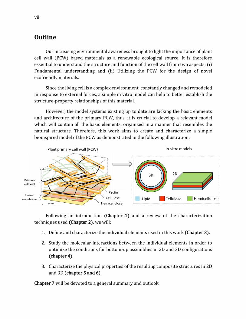
Our increasing environmental awareness brought to light the importance of plant
cell wall (PCW) based materials as a renewable ecological source. It is therefore
essential to understand the structure and function of the cell wall from two aspects: (i)
Fundamental understanding and (ii) Utilizing the PCW for the design of novel
ecofriendly materials.
Since the living cell is a complex environment, constantly changed and remodeled
in response to external forces, a simple in vitro model can help to better establish the
structure-property relationships of this material.
However, the model systems existing up to date are lacking the basic elements
and architecture of the primary PCW, thus, it is crucial to develop a relevant model
which will contain all the basic elements, organized in a manner that resembles the
natural structure. Therefore, this work aims to create and characterize a simple
bioinspired model of the PCW as demonstrated in the following illustration:
Following an introduction (Chapter 1) and a review of the characterization
techniques used (Chapter 2), we will:
1. Define and characterize the individual elements used in this work (Chapter 3).
2. Study the molecular interactions between the individual elements in order to
optimize the conditions for bottom-up assemblies in 2D and 3D configurations
(chapter 4).
3. Characterize the physical properties of the resulting composite structures in 2D
and 3D (chapter 5 and 6).
Chapter 7 will be devoted to a general summary and outlook.

1
Chapter 1
Introduction
1. Introduction
1.1. The primary plant cell wall (PCW): composition structure and
function
Composed of a complex network of polysaccharides and proteins, the plant cell
wall (PCW) is the layer encapsulating the plant cell, designed to provide structural
support, defense and protection, while enabling cell growth and expansion.
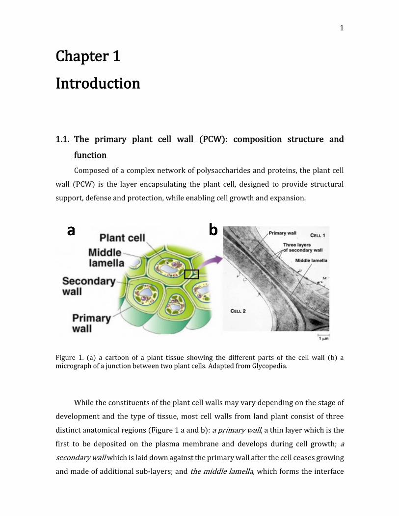
Figure 1. (a) a cartoon of a plant tissue showing the different parts of the cell wall (b) a micrograph of a junction between two plant cells. Adapted from Glycopedia.
While the constituents of the plant cell walls may vary depending on the stage of
development and the type of tissue, most cell walls from land plant consist of three
distinct anatomical regions (Figure 1 a and b): a primary wall, a thin layer which is the
first to be deposited on the plasma membrane and develops during cell growth; a
secondary wall which is laid down against the primary wall after the cell ceases growing
and made of additional sub-layers; and the middle lamella, which forms the interface
2 CHAPTER 1. INTRODUCTION
between the primary walls of neighboring cells. While all plant cells do not have a
secondary wall, all have a primary wall and middle lamella.(Albersheim, et al. 2011,
Cosgrove 2005, Somerville, et al. 2004)
The primary cell wall, which is the focus and inspiration of this study, is
deposited while the cell is still growing, providing both the rigid structural support of
plant cells and the adjustable elasticity needed for cell expansion. In order to perform
these seemingly contradictory tasks, the primary cell wall displays a composite-like
structure with cellulose microfibrils embedded in a matrix of soluble polysaccharides
called hemicelluloses and pectins.
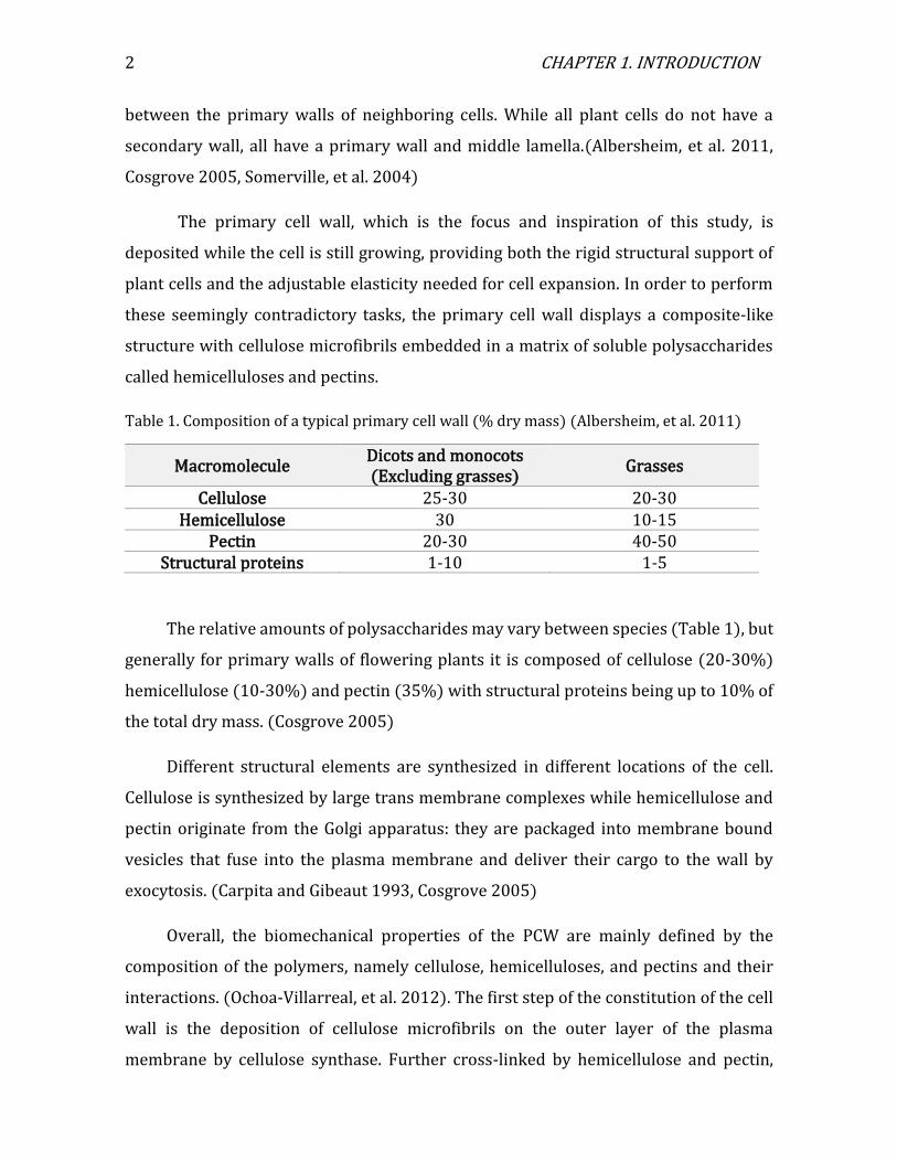
Table 1. Composition of a typical primary cell wall (% dry mass) (Albersheim, et al. 2011)
Macromolecule Dicots and monocots (Excluding grasses)
Grasses
Cellulose 25-30 20-30 Hemicellulose 30 10-15
Pectin 20-30 40-50 Structural proteins 1-10 1-5
The relative amounts of polysaccharides may vary between species (Table 1), but
generally for primary walls of flowering plants it is composed of cellulose (20-30%)
hemicellulose (10-30%) and pectin (35%) with structural proteins being up to 10% of
the total dry mass. (Cosgrove 2005)
Different structural elements are synthesized in different locations of the cell.
Cellulose is synthesized by large trans membrane complexes while hemicellulose and
pectin originate from the Golgi apparatus: they are packaged into membrane bound
vesicles that fuse into the plasma membrane and deliver their cargo to the wall by
exocytosis. (Carpita and Gibeaut 1993, Cosgrove 2005)
Overall, the biomechanical properties of the PCW are mainly defined by the
composition of the polymers, namely cellulose, hemicelluloses, and pectins and their
interactions. (Ochoa-Villarreal, et al. 2012). The first step of the constitution of the cell
wall is the deposition of cellulose microfibrils on the outer layer of the plasma
membrane by cellulose synthase. Further cross-linked by hemicellulose and pectin,

3
cellulose is the main bear loading component of the cell wall, while proteins perform
enzymatic, defensive signaling, and structural functions.
In the following sections, we will describe in more detail the basic elements of the
PCW and the way they are represented in a bottom-up approach for PCW model
systems.
1.2. Plant cell wall building blocks
1.2.1. From cellulose fibers to cellulose nano crystals
Cellulose (Figure 2), the poly −(1→4) anhydro D glucopyranose (AGU), is a
natural homo-polysaccharide that is produced by a wide variety of living creatures:
from higher and lower plants, to some sea animals, bacteria, fungi, and amoebas.
Figure 2. Molecular structure of cellulose with the numbering of carbons.
In the cellulose producing bacteria, the mechanism of cellulose biosynthesis has
been recently deciphered at the molecular level (McNamara, et al. 2015, Morgan, et al.
2013, Morgan, et al. 2016).
Even if the biosynthetic mechanism of cellulose synthesis in plant cell has not
been resolved with a precision similar to that in bacteria, a detailed 3D atomistic model
of the plant cellulose synthase, has been established, using a molecular modeling
approach (Sethaphong, et al. 2013). This model presents a close agreement with the
core region of bacterial cellulose synthesis complex, implying that the molecular
mechanism of cellulose biosynthesis is very similar in plants and in bacteria.
4 CHAPTER 1. INTRODUCTION
In the native state, cellulose systematically occurs as microfibrils, this
particularity being due to its mode of biosynthesis (Nishiyama 2009). Indeed, in the
plant plasma membrane, the cellulose biosynthesis takes place within a cluster of a
well-defined number of cellulose synthases, organized into a tridimensional
architecture commonly called terminal complex (TC). Within a TC, all the cellulose
synthases produce cellulose chains simultaneously (figure 3). These chains, which are
insoluble in the surrounding medium, readily coalesce and cluster together with precise
Van der Waals (VdW) and hydrogen bonding interactions. In higher plants, TCs,
observed by freeze-fracture electron microscopy, consist of 6-lobed rosettes tightly
packed in a ring of outside diameter of the order of 20 to 30 nm depending on the
species. (Giddings, et al. 1980, Mueller and Brown 1980, Nixon, et al. 2016)
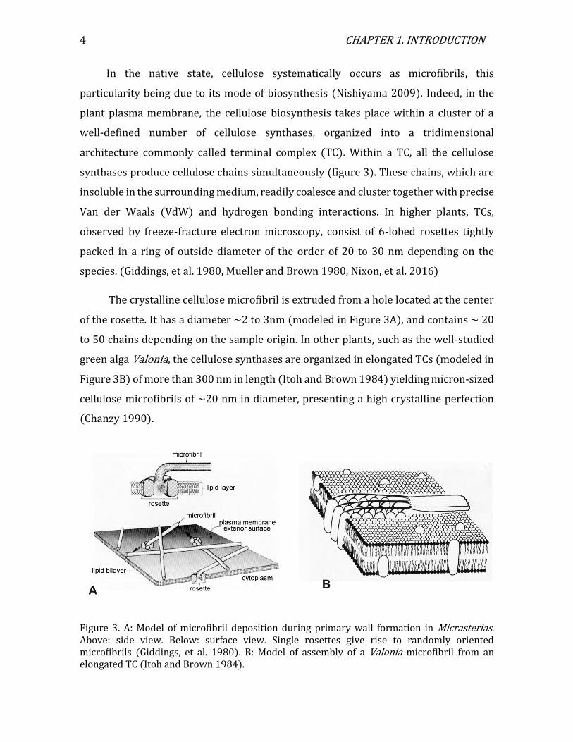
The crystalline cellulose microfibril is extruded from a hole located at the center
of the rosette. It has a diameter ~2 to 3nm (modeled in Figure 3A), and contains ~ 20
to 50 chains depending on the sample origin. In other plants, such as the well-studied
green alga Valonia, the cellulose synthases are organized in elongated TCs (modeled in
Figure 3B) of more than 300 nm in length (Itoh and Brown 1984) yielding micron-sized
cellulose microfibrils of ~20 nm in diameter, presenting a high crystalline perfection
(Chanzy 1990).
Figure 3. A: Model of microfibril deposition during primary wall formation in Micrasterias. Above: side view. Below: surface view. Single rosettes give rise to randomly oriented microfibrils (Giddings, et al. 1980). B: Model of assembly of a Valonia microfibril from an elongated TC (Itoh and Brown 1984).

5
Examples of the diversity of the cellulose microfibril dimensions are presented in
Figures 4A and 4B. In both micrographs, the microfibrils have lengths of many microns,
but in 4A those from primary wall cellulose have no more than 2-3 nm in diameter as
opposed to those in Figure 4B, which have diameters 10 times wider.
Obviously, the number of cellulose chains within one microfibril is substantially
different, ranging from about 20 to 30 in the primary wall cellulose such as observed in
Figure 4A as opposed to more than 1000 in the sample shown in Figure 4B.
Figure 4. Negatively stained electron micrographs of: A. Thin microfibrils from protoplast cell wall, typical of primary wall cellulose. B. Wide microfibrils from Valonia cell wall. Taken from the CERMAV images collection.
Between these two extremes, one finds a variety of microfibril sizes, depending on the
sample origin, exemplified in Figure 5.

6 CHAPTER 1. INTRODUCTION
Figure 5. Typical sizes of cellulose microfibrils depending on the sample origin. For Valonia, Halocynthia and Micrasterias, the sections were observed by cross-sectioning and electron microscopy. For cotton, wood and parenchyma, the shape of the cross-section is hypothetical.
The association of cellulose microfibrils in PCW shows two type of organization,
illustrated in Figures 6A and 6B. Figure 6A is typical of the cellulose organization in
primary wall, where the microfibrils as in Figure 5 are organized in a loose net, without
any preferred orientation allowing the expansion of the living cell, while maintaining
its strength. On the other hand, in the thicker secondary wall, occurring when the cells
have stopped their growth, the microfibrils are organized in thick sheets where the
microfibrils point roughly to the same direction (Figure 6B). This wall is not extensible,
but provides strength and rigidity to the plant (Cosgrove 2012).
7
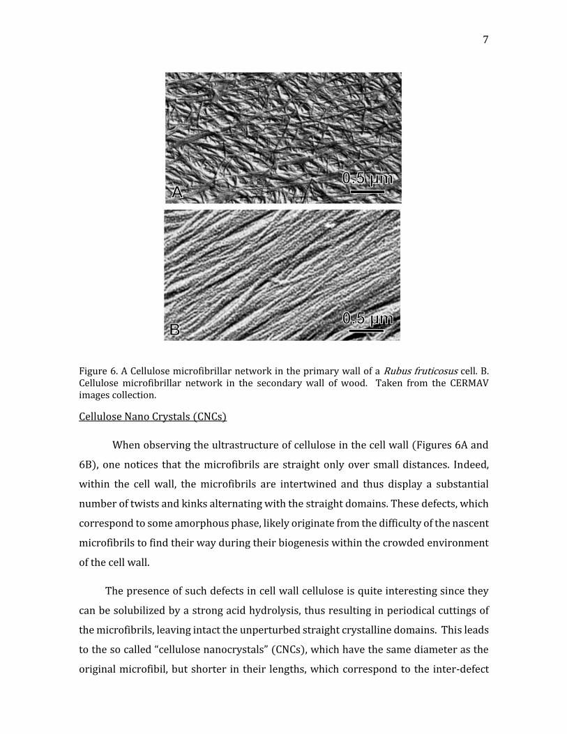
Figure 6. A Cellulose microfibrillar network in the primary wall of a Rubus fruticosus cell. B. Cellulose microfibrillar network in the secondary wall of wood. Taken from the CERMAV images collection.
Cellulose Nano Crystals (CNCs)
When observing the ultrastructure of cellulose in the cell wall (Figures 6A and
6B), one notices that the microfibrils are straight only over small distances. Indeed,
within the cell wall, the microfibrils are intertwined and thus display a substantial
number of twists and kinks alternating with the straight domains. These defects, which
correspond to some amorphous phase, likely originate from the difficulty of the nascent
microfibrils to find their way during their biogenesis within the crowded environment
of the cell wall.
The presence of such defects in cell wall cellulose is quite interesting since they
can be solubilized by a strong acid hydrolysis, thus resulting in periodical cuttings of
the microfibrils, leaving intact the unperturbed straight crystalline domains. This leads
to the so called “cellulose nanocrystals” (CNCs), which have the same diameter as the
original microfibil, but shorter in their lengths, which correspond to the inter-defect
8 CHAPTER 1. INTRODUCTION
distances of the parent microfibrils. Remarkably, cellulose microfibrils grown in vitro
in dilute suspension cannot be cut in similar acid treatment as they are free to grow
without defects, being not perturbed by their neighbors (Lai-Kee-Him, et al. 2002).
The acid hydrolytic conversion of cellulose fibers into CNCs was already reported
in the early 40s at Freiburg in Germany (Husemann 1943) and developed further at
Uppsala in Sweden, as illustrated by improved electron micrographs (Rånby 1949,
Rånby and Ribi 1950).
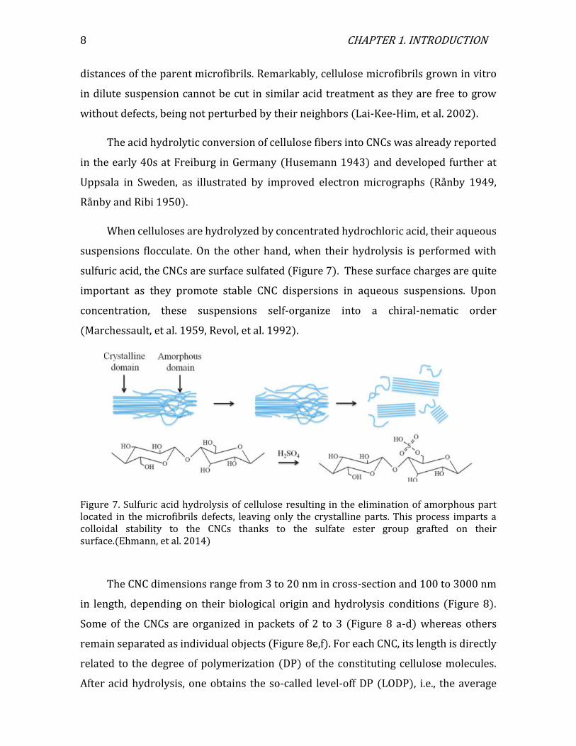
When celluloses are hydrolyzed by concentrated hydrochloric acid, their aqueous
suspensions flocculate. On the other hand, when their hydrolysis is performed with
sulfuric acid, the CNCs are surface sulfated (Figure 7). These surface charges are quite
important as they promote stable CNC dispersions in aqueous suspensions. Upon
concentration, these suspensions self-organize into a chiral-nematic order
(Marchessault, et al. 1959, Revol, et al. 1992).
Figure 7. Sulfuric acid hydrolysis of cellulose resulting in the elimination of amorphous part located in the microfibrils defects, leaving only the crystalline parts. This process imparts a colloidal stability to the CNCs thanks to the sulfate ester group grafted on their surface.(Ehmann, et al. 2014)
The CNC dimensions range from 3 to 20 nm in cross-section and 100 to 3000 nm
in length, depending on their biological origin and hydrolysis conditions (Figure 8).
Some of the CNCs are organized in packets of 2 to 3 (Figure 8 a-d) whereas others
remain separated as individual objects (Figure 8e,f). For each CNC, its length is directly
related to the degree of polymerization (DP) of the constituting cellulose molecules.
After acid hydrolysis, one obtains the so-called level-off DP (LODP), i.e., the average

9
inter-defect DP in the initial microfibrils. Since each AGU has a length of ~ 0.5 nm and
since the cellulose chains are perfectly aligned along the CNC, the cellulose LODP can
be easily deduced from the CNC length. Overall, the LODP is a constant for each cellulose
origin (Battista, et al. 1956, Nishiyama, et al. 2003).
Figure 8. TEM images of negatively stained preparations of CNCs of various origins: a) wood b) cotton c) bamboo d) Gluconacetobacter xylinus e) Glaucocystis f) Halocynthia papillosa (Kaushik, et al. 2015). From the CERMAV image collection.
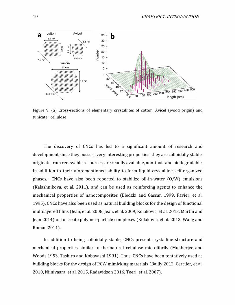
Like the overall morphology of cellulose microfibrils, the cross-section
dimensions of the individual CNCs also depend on the cellulose origin (Elazzouzi-
Hafraoui, et al. 2007). Figure 9a shows the cross-section dimensions of cellulose from
wood, cotton, and tunicin (the cellulose from tunicate mantle), corresponding to
Figures 8a, b, and f, respectively. Figure 9b shows a two-dimensional histogram
obtained for the width length and height of CNCs prepared by acid hydrolysis of cotton
linters (Elazzouzi-Hafraoui, et al. 2007).
10 CHAPTER 1. INTRODUCTION
Figure 9. (a) Cross-sections of elementary crystallites of cotton, Avicel (wood origin) and
tunicate cellulose particles. (b) Two-dimensional histogram of CNCs from cotton (Elazzouzi-Hafraoui, et al. 2007).
The discovery of CNCs has led to a significant amount of research and
development since they possess very interesting properties: they are colloidally stable,
originate from renewable resources, are readily available, non-toxic and biodegradable.
In addition to their aforementioned ability to form liquid-crystalline self-organized
phases, CNCs have also been reported to stabilize oil-in-water (O/W) emulsions
(Kalashnikova, et al. 2011), and can be used as reinforcing agents to enhance the
mechanical properties of nanocomposites (Bledzki and Gassan 1999, Favier, et al.
1995). CNCs have also been used as natural building blocks for the design of functional
multilayered films (Jean, et al. 2008, Jean, et al. 2009, Kolakovic, et al. 2013, Martin and
Jean 2014) or to create polymer-particle complexes (Kolakovic, et al. 2013, Wang and
Roman 2011).
In addition to being colloidally stable, CNCs present crystalline structure and
mechanical properties similar to the natural cellulose microfibrils (Mukherjee and
Woods 1953, Tashiro and Kobayashi 1991). Thus, CNCs have been tentatively used as
building blocks for the design of PCW mimicking materials (Bailly 2012, Cerclier, et al.
2010, Niinivaara, et al. 2015, Radavidson 2016, Teeri, et al. 2007).
11
From the above-mentioned reasons, in the present work we intend to use
cellulose nanocrystals in order to mimic the role of cellulose microfibrils in the cell wall.
1.2.2. From Hemicellulose to Xyloglucan (XG)
Hemicelluloses are a group of heterogeneous polysaccharides, including
Xyloglucans (XG), Glucuronoxylans, Glucomannans, Galactoglucomannans that are
synthesized in the Golgi apparatus and secreted to the PCW by endocytosis (Cosgrove
1997, Fry 1989, Hayashi 1989). They bind to the surface of cellulose and have a
backbone made up of (1→4)-β-D-glycans that resembles cellulose (Fry 1989, Scheller
and Ulvskov 2010). Unlike cellulose, hemicelluloses contain branches and other
modifications in their structure, preventing them from crystallizing by themselves into
microfibrils, but increasing their water solubility. In the PCW, hemicellulose play a
major role in the mechanical properties by cross linking cellulose microfibrils (Hayashi,
et al. 1987, Park and Cosgrove 2015). This interaction will be discussed in more detail
in chapter 4.3.
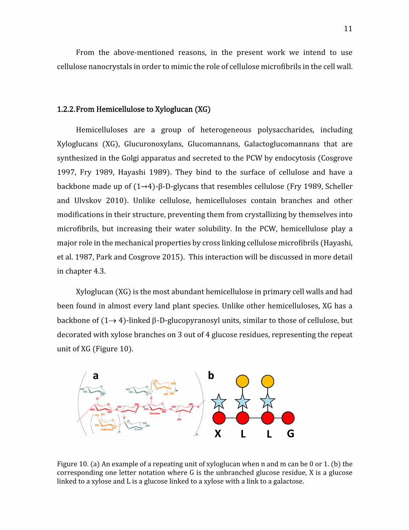
Xyloglucan (XG) is the most abundant hemicellulose in primary cell walls and had
been found in almost every land plant species. Unlike other hemicelluloses, XG has a
backbone of (1→ 4)-linked -D-glucopyranosyl units, similar to those of cellulose, but
decorated with xylose branches on 3 out of 4 glucose residues, representing the repeat
unit of XG (Figure 10).
Figure 10. (a) An example of a repeating unit of xyloglucan when n and m can be 0 or 1. (b) the corresponding one letter notation where G is the unbranched glucose residue, X is a glucose linked to a xylose and L is a glucose linked to a xylose with a link to a galactose.

12 CHAPTER 1. INTRODUCTION
A common one letter notation is used to code the different side chains,(Fry, et al.
1993) where G denotes unbranched glucose residue, X denotes α-D-Xylp-(1→6)-β-D-
Glcp segment and L denotes a β-D-Galp-(1→2)-α-D-Xylp- (1→6)-β-D-Glcp segment
(figure 10b). The side chains of XG can vary depending on its source. In several species,
an additional Fucose (F) residue is connected to the Galactose unit.(Fry, et al. 1993,
Scheller and Ulvskov 2010)
Sugar analysis on xyloglucan from tamarind seeds revealed that the majority of
oligosaccharides repeat units are XLLG (50.6%) where XXLG, XXXG and XLXG represent
28, 13 and 9% respectively (Faïk, et al. 1997).
Being a hydro-soluble polymer, XG adopts a semiflexible conformation in solution.
Muller et al. characterized the solution properties of XG using SEC-MALLS and small
angle neutron scattering (SANS). They found that XG behaved as a semiflexible
polymer, with a Mark-Houwink-Sakurada parameter of 0.67 and a Flory exponent
ν=0.588 in water, describing a polymer in a good solvent with excluded volume
interactions as demonstrated in figure 11.(Muller, et al. 2011) The persistence length
(lp), which quantify the bending rigidity of the polymer, was found to be 80Å.
Figure 11. Schematic representation of an isolated XG chain in water, showing a self-avoiding chain with a persistence length of lp=80Å (Muller, et al. 2011).
The behavior of XG in solution depends greatly on its molecular weight and
concentration. In another work, Muller et al. (Muller, et al. 2013) used SLS, DLS and

13
viscosity measurements to study aqueous solutions of neutral xyloglucan extracted
from tamarind seed. They found out that even at very low concentration, XG chains
became associated to form swollen aggregates. (Figure 12)
Figure 12. Schematic picture of the behavior of XG chains from tamarind seeds upon dilution (Muller, et al. 2013).
These associations, inherent to the nature of XG chains, are forming and
reforming, tending towards larger structures with time. It is therefore essential to take
into account not only the structural parameters, but also the physical characteristics of
XG when studying its interactions with other components or incorporating it into
biomimetic constructs (Kishani, et al. 2019, Park and Cosgrove 2015).
XG have been widely used to represent the role of hemicellulose with in silico
(Hanus and Mazeau 2006, Zhao, et al. 2014) and in vitro models (Chambat, et al. 2005,
Hayashi and Maclachlan 1984, Hayashi, et al. 1994, Jean, et al. 2009, Villares, et al.
2017).
In this work XG will be used as a representative hemicellulose in the biomimetic
constructs.

14 CHAPTER 1. INTRODUCTION
1.2.3. From Pectin to Homogalacturonan
Pectins represent another diverse family of linear and branched polysaccharides,
found throughout the primary wall. They are present in high concentration in the
middle lamella and act as cell adhesion agent and a matrix embedding the CNC-XG
network (Sharma, et al. 2006). Pectin has functions in plant growth, morphology,
development, cell–cell adhesion, wall structure, and expansion (Caffall and Mohnen
2009, Mohnen 2008).
Within the plant walls pectins, several groups can be distinguished, as shown in
figure 13: Homogalacturonans (HG), linear polymers of galacturonic acid;
Xylogalacturonans (XGA); Rhamnogalacturonanes type I and II (RGI and RGII).
Figure 13. Pectin general structure (Burton, et al. 2010).
The linear part of pectin, homogalacturonan or HG, is the simplest and most
abundant pectic structural domain, usually accounting for approximately 65% of the
pectin macromolecule. It consists of a linear backbone of 85–320 (1→4) linked α-d-GalA
residues, partly methyl-esterified at C-6 position. It may also be O-acetylated at O-2 or
O-3 position (Figure 14a).(Burton, et al. 2010) In solution, the non-methylated carboxyl
groups will dissociate depending on the pH, leaving a negative charge on the GalA
monomers, resulting in typical features of an anionic polyelectrolyte. The degree of

15
methyl esterification (DE, in %) of the glucuronic acid backbone, have a profound
impact on pectin interaction and properties in vitro and in planta.(O'Neill, et al. 1990)
In this work we focus on HG since it the most abundant pectin, believed to play a
major role in the interaction and properties, and therefore its physical chemistry has
been relatively well studied.
Isolated HG rich pectins exhibits two different gelation mechanisms that are
influenced by the degree of methyl esterification. High methoxylated pectin (HM
pectin) can form a gel in acidic medium (pH < 3.5) in presence of a co-solute, typically
sucrose at high concentrations (Thakur, et al. 1997, Thibault and Ralet 2003). Such gels
are often referred to as ‘‘acid gels’’. The high sugar concentration decreases the water
activity, promoting hydrophobic interactions between methoxyl groups, while the low
pH is required to reduce dissociation of carboxyl groups, thus diminish electrostatic
repulsions.
Figure 14. (a) Structure of HG showing the methyl esterified- and the O-acetyl esterified groups. (b) A suggested egg-box model of calcium crosslinking in HG.
16 CHAPTER 1. INTRODUCTION
Low methoxylated pectin (LM pectin) forms a gel in the presence of divalent metal
ions such as calcium (Figure 14b). In this case, ionic linkages are formed via calcium
bridges between dissociated carboxyl groups (Thibault and Ralet 2003). However, in
case of pectin, the most favorable association is better described as a ‘‘shifted’’ egg-box,
since one of the chains is slightly shifted with respect to the other (Braccini and Pérez
2001). Egg-boxes formed between two neighboring chains are stabilized by VdW
interactions and hydrogen bonds in addition to electrostatic interactions (Braccini and
Pérez 2001, Thibault and Rinaudo 1986).
Furthermore, it was found that a minimum number of 6-14 non-methyl esterified
GalA units residues is required for the formation of egg-box pattern (Fraeye, et al.
2010).
Gelation of LM pectins has been found to be influenced by several parameters
which can be denoted as intrinsic and extrinsic parameters. Intrinsic parameters refer
to pectin structural characteristics, such as the amount and distribution of methyl
esters (also called degree of blockiness), chain length, pectin side chains, and
substitution with acetyl groups. The term extrinsic parameters refer to environmental
conditions, such as Ca2+ and pectin concentration, pH, and temperature (Fraeye, et al.
2010, Mohnen 2008).
In addition, the biosynthesis and modification of homogalacturonan have recently
emerged as key determinants of plant growth, controlling cell adhesion and organ
development (Pelloux, et al. 2007). De-methyl-esterification of homogalacturonan
occurs through the action of the ubiquitous enzyme ‘pectin methyl-esterase’ and have
an important effect on the mechanical properties of the growing plant (Wolf, et al.
2009).

17
1.2.4. From lipids to membranes to vesicles
1.2.4.1. Chemical structure of lipids
Lipids are part of the large family of amphiphilic molecules which consist of a
hydrocarbon chain (tail) and a polar group (head). Several groups of lipids exist in
plants and they are classified by their chemical structure: glycerophospholipids,
cholesterol, and sphingolipids. In this study, we focus mainly on glycerophospholipids
which contain two hydrophobic tails connected by a glycerol to a hydrophilic head
composed of a phosphate group and a polar group. (Figure 15)
The chemical nature of the polar group determines the net charge of the lipid.
Phosphatidylcholine (PC) and phosphatidylethanolamine (PE) carry both positive and
negative charges on the hydrophilic head while phosphatidic acid (PA),
phosphatidylglycerol (PG), and phosphatidylserine (PS) are negatively charged.
Figure 15. General chemical structure of phospholipids, showing the hydrophobic tail region connected with a glycerol group (light blue) to the hydrophilic head, a phosphate group (grey) and a polar group (R), which determine the net charge of the lipid.
18 CHAPTER 1. INTRODUCTION
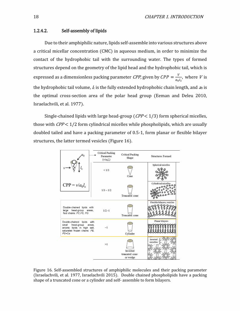
1.2.4.2. Self-assembly of lipids
Due to their amphiphilic nature, lipids self-assemble into various structures above
a critical micellar concentration (CMC) in aqueous medium, in order to minimize the
contact of the hydrophobic tail with the surrounding water. The types of formed
structures depend on the geometry of the lipid head and the hydrophobic tail, which is
expressed as a dimensionless packing parameter CPP, given by 𝐶𝑃𝑃 =𝑉
𝑎0𝑙𝑐, where V is
the hydrophobic tail volume, lc is the fully extended hydrophobic chain length, and a0 is
the optimal cross-section area of the polar head group (Eeman and Deleu 2010,
Israelachvili, et al. 1977).
Single-chained lipids with large head-group (CPP < 1/3) form spherical micelles,
those with CPP < 1/2 form cylindrical micelles while phospholipids, which are usually
doubled tailed and have a packing parameter of 0.5-1, form planar or flexible bilayer
structures, the latter termed vesicles (Figure 16).
Figure 16. Self-assembled structures of amphiphilic molecules and their packing parameter (Israelachvili, et al. 1977, Israelachvili 2015). Double chained phospholipids have a packing shape of a truncated cone or a cylinder and self- assemble to form bilayers.
19
In the present study, we will mainly focus on bilayers (yellow frame in figure 16),
which are the main form of biological membranes.
1.2.4.3. Physical states of lipid membranes
In aqueous medium, lipid bilayers can occur under different physical states,
characterized by the lateral organization, the molecular order and the mobility of the
lipid molecules within the bilayer. Physicochemical parameters such as ionic strength,
pH and temperature, among other factors such as the chemical nature of the lipid
components and the presence of sterols, can strongly affect the nature of the phases
and the transitions between them. Differential scanning calorimetry (DSC) and X-ray
diffraction (XRD) studies have shown that several main phases of lipid membrane
exists (Eeman and Deleu 2010, Janiak, et al. 1979) as well as characteristic phase
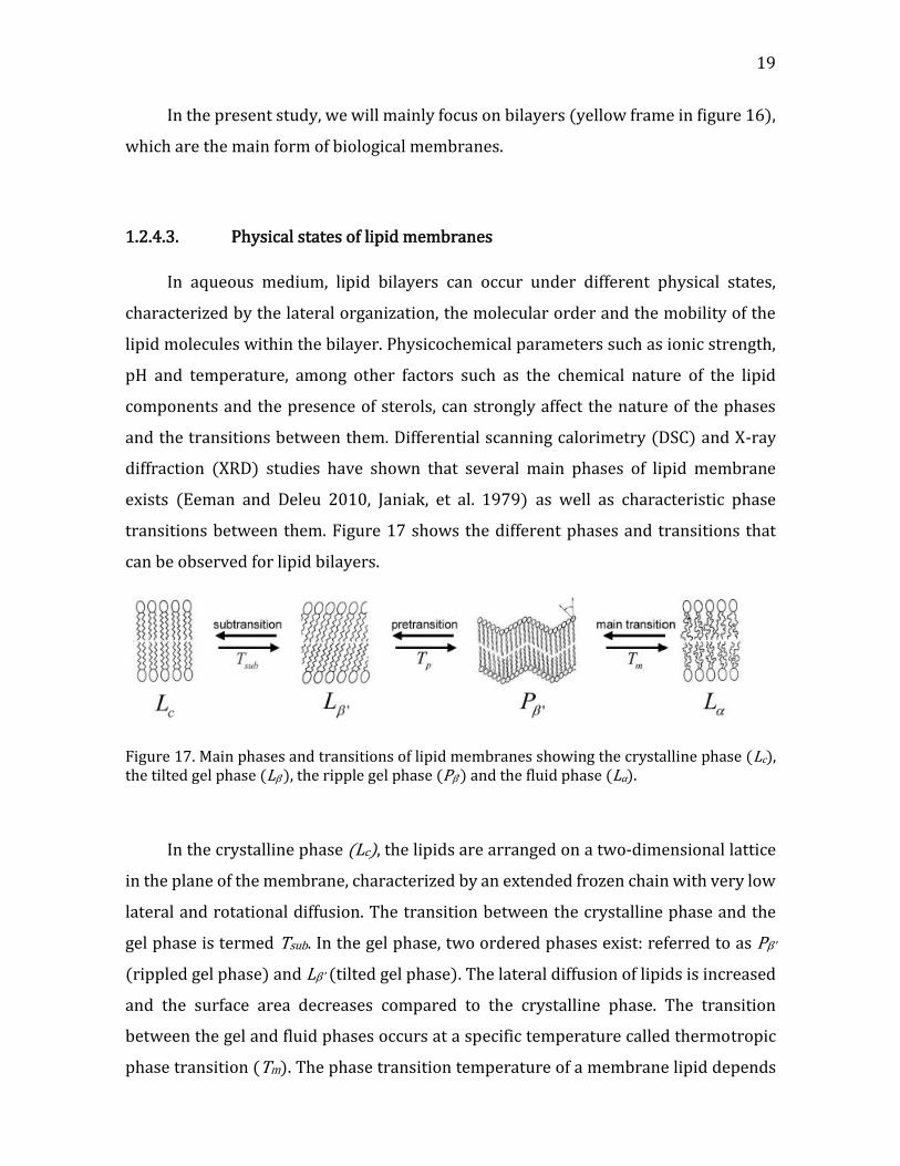
transitions between them. Figure 17 shows the different phases and transitions that
can be observed for lipid bilayers.
Figure 17. Main phases and transitions of lipid membranes showing the crystalline phase (Lc), the tilted gel phase (Lβ'), the ripple gel phase (Pβ') and the fluid phase (Lα).
In the crystalline phase (Lc), the lipids are arranged on a two-dimensional lattice
in the plane of the membrane, characterized by an extended frozen chain with very low
lateral and rotational diffusion. The transition between the crystalline phase and the
gel phase is termed Tsub. In the gel phase, two ordered phases exist: referred to as Pβ'
(rippled gel phase) and Lβ' (tilted gel phase). The lateral diffusion of lipids is increased
and the surface area decreases compared to the crystalline phase. The transition
between the gel and fluid phases occurs at a specific temperature called thermotropic
phase transition (Tm). The phase transition temperature of a membrane lipid depends
20 CHAPTER 1. INTRODUCTION
on the nature of its hydrophobic moiety such as chain length and degree of
unsaturation. In the fluid phase, also called liquid-disordered phase (Lα, sometimes
noted as Ld), the hydrophobic chains are less extended and a free to the move.
The lateral and the rotational diffusion modes are more common in fluid lipid
bilayers than in the crystalline or gel phase. In the presence of cholesterol, the fluid
phase can increase its order and transform to liquid ordered phase (Lo) which shares
the characteristics of both gel and fluid phases.
1.2.4.4. Permeability
The transport of substances across a lipid membrane can be classified into two
categories: active and passive transport. While active transport requires input of
energy that transports the target molecules in the direction opposed to the
concentration gradient, passive transport occurs via an entropy-driven, nonspecific
diffusion process of the molecule across the membrane.
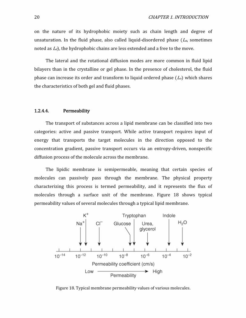
The lipidic membrane is semipermeable, meaning that certain species of
molecules can passively pass through the membrane. The physical property
characterizing this process is termed permeability, and it represents the flux of
molecules through a surface unit of the membrane. Figure 18 shows typical
permeability values of several molecules through a typical lipid membrane.
Figure 18. Typical membrane permeability values of various molecules.

21
In addition to the type of molecule, membrane permeability to a given substance
can be influenced by several parameters such as temperature, lipid type, and physical
state (liquid or gel) as well as the presence of cholesterol. Permeability can be
determined using osmotic shock experiments(Bernard, et al. 2002, Boroske, et al. 1981,
Mathai, et al. 2008).
Since large solute molecules such as glucose and sucrose cannot passively cross
the membrane, a difference in the solute concentration creates a difference in the
osmotic pressure, Π, between the interior and exterior of the membrane, according to
the following equation:
(Eq. 1) Π = 𝑅𝑇 ln𝐶𝑖𝑛
𝐶𝑜𝑢𝑡
Where 𝐶𝑖𝑛 and 𝐶𝑜𝑢𝑡 are the solute concentration in and out of the membrane
respectively, R is the ideal gas constant, and T is the temperature. Due to the difference
in concentration, water molecules will migrate, in (hypotonic solution) or out
(hypertonic solution) of the membrane until a new equilibrium is reached, a process
that is called osmotic shock.
Table 2. Permeability values from osmotic shock experiments
Lipid Permeability, µm s-1 Reference
Egg lecithin 17-47 (Boroske, et al.
1981)
Egg lechithin +cholesterol 10 % 5-10 (Bernard, et al.
2002)
DOPC 150 (Mathai, et al.
2008) DOPC+Chol 10 % 145
DOPC +Chol 20% 115
DOPC + chol 40% 68
22 CHAPTER 1. INTRODUCTION
This property can be exploited to study the transport of water across the lipidic
membrane by applying a difference in the solute concentration between the interior
and exterior of the membrane. Permeability can be thus determined experimentally
using osmotic shock experiments, by directly measuring the radius, or by using
fluorescence of encapsulated molecules, or chromatography (Taupin, et al. 1975). Table
2 shows typical permeability values for water across different membranes obtained
with osmotic shocks experiments.
The reported permeability values were evaluated from osmotic shock
experiments by directly measuring changes in vesicle diameter (Bernard, et al. 2002,
Boroske, et al. 1981) or by measuring the self-quenching of entrapped
carboxyfluorescein.(Mathai, et al. 2008) The variation in the reported values may
emerge from the variation in experimental methods used to quantitively determine the
permeability.
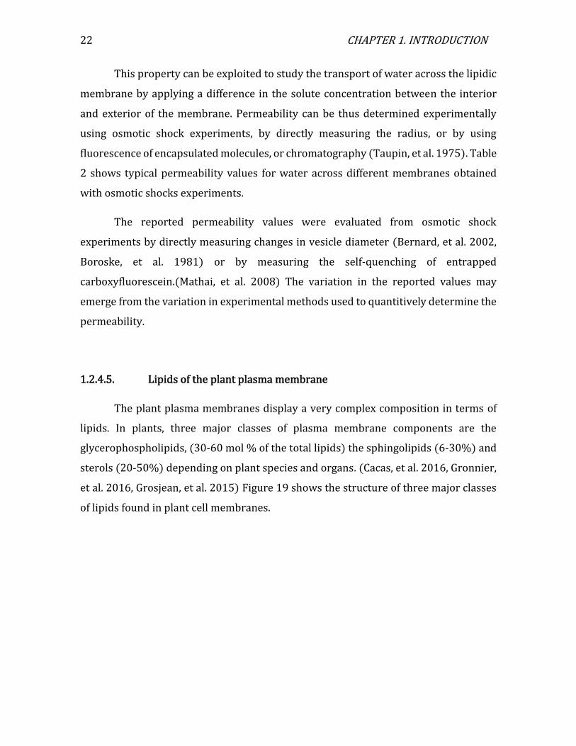
1.2.4.5. Lipids of the plant plasma membrane
The plant plasma membranes display a very complex composition in terms of
lipids. In plants, three major classes of plasma membrane components are the
glycerophospholipids, (30-60 mol % of the total lipids) the sphingolipids (6-30%) and
sterols (20-50%) depending on plant species and organs. (Cacas, et al. 2016, Gronnier,
et al. 2016, Grosjean, et al. 2015) Figure 19 shows the structure of three major classes
of lipids found in plant cell membranes.
23
Figure 19. (a) Chemical features of the three major classes of plant plasma membrane lipids. The polar heads are highlighted in yellow. (b) A drawing of the plasma membrane composition.
Glycerophospholipids are composed of a glycerol backbone on which two fatty
acid chains are esterified. The third carbon atom of the glycerol backbone supports the
phospholipid polar head group, which is composed of an alcohol molecule (choline,
ethanolamine, serine, glycerol or inositol) linked to a negatively charged phosphate
group. Sphingolipids are composed of a sphingosine (or phytosphingosine) base, on
which is linked a relatively long (up to 24 carbon atoms) saturated fatty acid chain.
Acylated sphingosines are referred to as ceramides. Sphingomyelin and
glycosphingolipids result from the attachment of a choline molecule and an
oligosaccharide to the hydroxyl group of ceramides, respectively. Sterols are a
particular class of membrane components. While the hydrophobic moiety of most
membrane lipids is constituted of relatively long aliphatic chains, the one of sterols is
composed of polycyclic structures (Eeman and Deleu 2010).
To overcome the complexity of the biological membranes, 2D and 3D model
membranes, containing both natural and synthetic lipids, offer a good in vitro model for
the study and potential use of the plant plasma membranes (Castellana and Cremer
2006, Eeman and Deleu 2010, Fenz and Sengupta 2012). Let us revise the main
characteristics of such models.
24 CHAPTER 1. INTRODUCTION
1.2.4.6. Lipid membrane model systems
Supported lipid bilayers
Supported Lipid Bilayers (SLBs) are lipid bilayers supported onto a solid surface
which can be curved (beads)(Mornet, et al. 2005) or flat (mica, glass, or silicon oxide
wafers) (Richter and Brisson 2005, Richter, et al. 2006), depending on the desired
geometry. Supported lipid membranes confined to the surface of a flat solid support can
be characterized using a variety of surface sensitive techniques such as atomic force
microscopy (AFM), optical ellipsometry, quartz-crystal microbalance (QCM-D), and
neutron reflectivity (NR) (Castellana and Cremer 2006, Richter, et al. 2003, Richter and
Brisson 2005, Richter, et al. 2006).
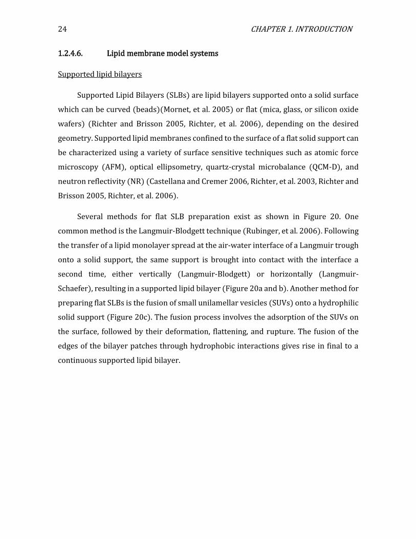
Several methods for flat SLB preparation exist as shown in Figure 20. One
common method is the Langmuir-Blodgett technique (Rubinger, et al. 2006). Following
the transfer of a lipid monolayer spread at the air-water interface of a Langmuir trough
onto a solid support, the same support is brought into contact with the interface a
second time, either vertically (Langmuir-Blodgett) or horizontally (Langmuir-
Schaefer), resulting in a supported lipid bilayer (Figure 20a and b). Another method for
preparing flat SLBs is the fusion of small unilamellar vesicles (SUVs) onto a hydrophilic
solid support (Figure 20c). The fusion process involves the adsorption of the SUVs on
the surface, followed by their deformation, flattening, and rupture. The fusion of the
edges of the bilayer patches through hydrophobic interactions gives rise in final to a
continuous supported lipid bilayer.
25
Figure 20. (a) Scheme of Langmuir–Blodgett (b) Langmuir–Schaefer experimental setups, showing the water lower phase (w), the lipids on the air/water interface (bold line) and the substrates during the transfers. (c) Vesicle fusion scheme.
Due to their versatile properties and relative ease of preparation and
characterization, SLBs are commonly used as biomimetic models to study biological
phenomena (Castellana and Cremer 2006, Migliorini, et al. 2014, Sandrin, et al. 2010).
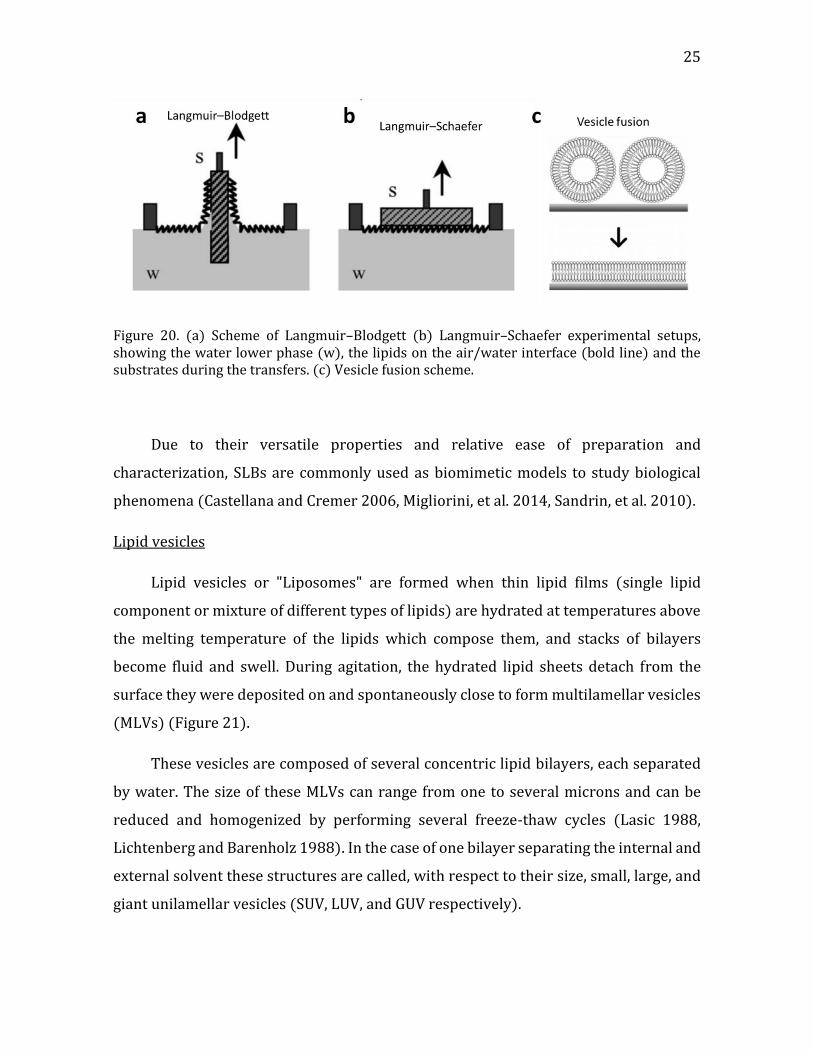
Lipid vesicles
Lipid vesicles or "Liposomes" are formed when thin lipid films (single lipid
component or mixture of different types of lipids) are hydrated at temperatures above
the melting temperature of the lipids which compose them, and stacks of bilayers
become fluid and swell. During agitation, the hydrated lipid sheets detach from the
surface they were deposited on and spontaneously close to form multilamellar vesicles
(MLVs) (Figure 21).
These vesicles are composed of several concentric lipid bilayers, each separated
by water. The size of these MLVs can range from one to several microns and can be
reduced and homogenized by performing several freeze-thaw cycles (Lasic 1988,
Lichtenberg and Barenholz 1988). In the case of one bilayer separating the internal and
external solvent these structures are called, with respect to their size, small, large, and
giant unilamellar vesicles (SUV, LUV, and GUV respectively).

26 CHAPTER 1. INTRODUCTION
Figure 21. General scheme showing the main methods of vesicle preparation starting from a dry lipid film. Following the spontaneous or induced swelling, different types of vesicles can be formed. They are defined by the number of bilayers separating the interior and the exterior of the vesicle (multi or unilamellar), and their size (Giant, Large, and Small Unilamellar vesicles, referred to as GUV, LUV, and SUV, respectively).
According to the method of preparation, different types of vesicles can be
obtained (Reeves and Dowben 1969, Szoka Jr and Papahadjopoulos 1980, Walde, et al.
2010)(Figure 21). The homogenization and extrusion of MLVs through an extruder
equipped with a polycarbonate membrane with nano-sized pores gives rise to the
formation of large unilamellar vesicles (LUVs) with a mean diameter of 50-500 nm,
corresponding to the mesh size of the polycarbonate membrane. Small unilamellar
vesicles (SUVs) are formed by sonicating the MLVs or LUVs in a classical bath sonicator
or using a probe sonicator. The SUVs usually exhibit a mean diameter of 10 to 50 nm
and due to their high membrane tension, they are not stable and generally tend to fuse
to create larger vesicles.
GUVs can be obtained by hydrating a dried lipid film at temperatures above the
crystalline to liquid-like lipid phase transition either for a long period of time (up to 36
27
h) (i.e. gentle hydration method) or in presence of an external electrical field (i.e.
electroformation technique) (Rodriguez, et al. 2005, Walde, et al. 2010). The size of the
GUVs allows their visualization by optical microscopy such as fluorescence and phase
contrast microscopy, as well as their micromanipulation.
Besides their application in the fields of drug delivery (Peetla, et al. 2009) and
gene therapy (Lasic and Templeton 1996), lipid vesicles are versatile biomimetic model
of membranes and they commonly used for studying biological environments at the
nanometric and micrometric scales (Eeman and Deleu 2010, Szoka Jr and
Papahadjopoulos 1980).
After revising the main building blocks of the PCW and some typical analogues
used in biomimetic models, we will now focus on the way these building blocks organize
to form the multinetwork architecture of the PCW.
1.3. Plant cell wall architecture
Plant cell walls have been in use for thousands of years by humans for food,
construction, and tools. Nevertheless, understanding of how polysaccharides and
structural proteins are organized into plant cell walls is important for elucidating the
structure-property relationships of such a complex system. It is only in the last few
decades, with the improvement of characterization techniques, such as microscopy and
spectroscopy, that the PCW structure and composition could be investigated. From
these studies, different models have emerged, showing how the different
polysaccharides are organized in the plant cell wall.
One of the first models suggested by Albersheim and carrying his name (Keegstra,
et al. 1973) was deduced from the degradation of the cell wall by enzymes, followed by
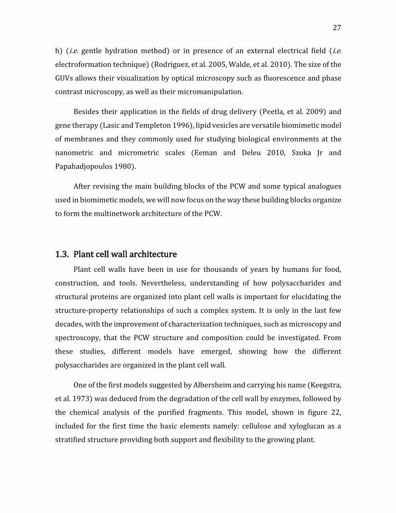
the chemical analysis of the purified fragments. This model, shown in figure 22,
included for the first time the basic elements namely: cellulose and xyloglucan as a
stratified structure providing both support and flexibility to the growing plant.
28 CHAPTER 1. INTRODUCTION
Figure 22. The Albersheim early model of primary plant cell wall. (Keegstra, et al. 1973)
In this early model, the matrix polymers were all covalently linked to one another
and connected to the cellulose microfibrils. However, elaborated studies on the
interactions between the basic components were still lacking. Advances in the
determination of polymer structure and the preservation of its structure for electron
microscopy in the following two decades led to the “tethered network” model of
Hayashi (Hayashi 1989) and Fry (Fry 1989) where single xyloglucan chains spanned
the gap between microfibrils and tethered them together. These models, further
developed by Carpita and Gibeaut (Carpita and Gibeaut 1993) provided a more
comprehensive view of how polysaccharides and structural proteins were organized
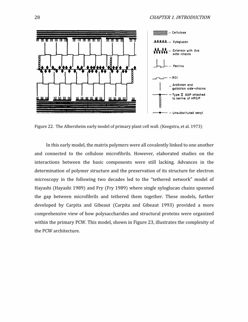
within the primary PCW. This model, shown in Figure 23, illustrates the complexity of
the PCW architecture.
29
Figure 23. The model of primary plant cell wall proposed by Carpita and Gibeaut (Carpita and Gibeaut 1993).
Figure 23 shows the model proposed by Carpita and Gibeaut. According to their
revised and still more elaborated model, cellulose microfibrils contain non crystalline
regions that may be formed by entrapment of hemicelluloses such as xyloglucan in the
early stages of cellulose synthesis. Xyloglucan can also bind to the surface of cellulose
and may link two microfibrils together. Although the side chains of xyloglucan interfere
with bonding of one glucan backbone to other glucans, they may twist such that short
regions of the backbone form a planar configuration suitable for bonding to cellulose.
In this model, pectins form a space-filled hydrophilic gel between microfibrils.
In 2001, Cosgrove published a review which describes the models obtained so far
and in 2004 Somerville showed a scaled model based on NMR and electron microscopy.

30 CHAPTER 1. INTRODUCTION
Figure 24. Scale model of the polysaccharides in an Arabidopsis leaf cell. The figure is an elaboration of a model originally presented by McCann and Roberts (Somerville, et al. 2004).
A recent paper by Cosgrove puts forward a model that introduces the concept of
biomechanical hotspots (Cosgrove 2014). His model is based on recent developments
in enzyme activity assays together with advanced characterization techniques such as
AFM and solid-state NMR. According to this model, cellulose fibrils are linked via direct
load-bearing junctions, mediated via physical bonding by xyloglucan. This idea is in
accordance with common depictions of primary cell walls which show well-spaced
microfibrils kept apart by matrix polysaccharides, using never-dried walls under water.
Images obtained by Zhang et al. (Zhang, et al. 2014) (figure 25a) contribute to the
development of the current model (figure 25b).
31
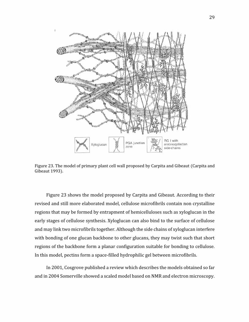
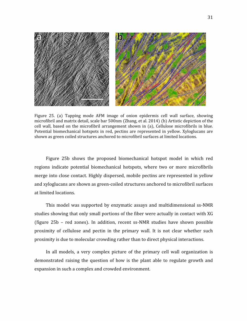
Figure 25. (a) Tapping mode AFM image of onion epidermis cell wall surface, showing microfibril and matrix detail, scale bar 500nm (Zhang, et al. 2014) (b) Artistic depiction of the cell wall, based on the microfibril arrangement shown in (a), Cellulose microfibrils in blue. Potential biomechanical hotspots in red, pectins are represented in yellow. Xyloglucans are shown as green coiled structures anchored to microfibril surfaces at limited locations.
Figure 25b shows the proposed biomechanical hotspot model in which red
regions indicate potential biomechanical hotspots, where two or more microfibrils
merge into close contact. Highly dispersed, mobile pectins are represented in yellow
and xyloglucans are shown as green-coiled structures anchored to microfibril surfaces
at limited locations.
This model was supported by enzymatic assays and multidimensional ss-NMR
studies showing that only small portions of the fiber were actually in contact with XG
(figure 25b – red zones). In addition, recent ss-NMR studies have shown possible
proximity of cellulose and pectin in the primary wall. It is not clear whether such
proximity is due to molecular crowding rather than to direct physical interactions.
In all models, a very complex picture of the primary cell wall organization is
demonstrated raising the question of how is the plant able to regulate growth and
expansion in such a complex and crowded environment.

32 CHAPTER 1. INTRODUCTION
Several growth regulation mechanisms exist, each targeting a different component or
network, each with its own loosening enzymes. These mechanisms will be further
discussed in the following section.
1.4. Growth and expansion
The growing cell wall in plants has the conflicting requirements of being strong
enough to withstand the high tensile forces generated by cell turgor pressure while
selectively yielding to forces inducing wall stress relaxation, leading to water uptake
and polymer movements underlying cell wall expansion. The wall loosening
mechanisms can be divided into three main groups, as summarized in the following
table:
Table 3. Wall loosening mechanisms
Enzyme Activity Reference
Expansin
Break bonds between
cellulose and
hemicellulose
(McQueen-Mason, et al.
1992)
Endoglucanase Hydrolyses
hemicelluloses (Levy, et al. 2002)
Pectin methyl esterase
Homogalactouronase
Demethylation
Shortening the HG chain (Peaucelle, et al. 2011)
The cell wall extensibility permits an irreversible expansion of its surface area by
10 to 1000-fold between its initial state and the cessation of growth at maturity. Such
expansion involves selective wall loosening to enable irreversible extension.
33
Summary
As can be seen from this short review, our understanding of the structure and
composition of the plant cell wall did not change much since the 70s, however the
structure function relationships are still not clear. This is due to the lack of a simple
model for the plant cell wall, which emphasizes the advantage of in vitro model systems.
These systems enable to avoid the complexity of the biological living environment,
thereby allowing to study a given process, or effect, in a direct and simplified manner.
1.5. Cell wall mechanical properties
The growing plant cell wall has to adapt to two conflicting requirements: on the
one hand, the wall must be strong enough to resist hydrostatic pressure extracted by
the cytoplasm (turgor pressure), and on the other hand, it needs to be flexible enough
to allow cell growth and expansion. As we've seen previously in this chapter, the wall
accommodates these requirements through its composite and dynamic structure,
presenting stiff structural elements, such as the cellulose microfibrils, embedded in a
softer matrix of polysaccharides. While the main components of the cell wall are well
identified (Albersheim, et al. 2011, Ochoa-Villarreal, et al. 2012), their individual
contribution to its mechanical properties is not completely understood (Bidhendi and
Geitmann 2015, Hamant and Moulia 2016).
The remarkable features of plant cells and tissues have drawn interest in recent
years, among biologists and biophysicists studying plant morphogenesis and
development, as well as among engineers and medical scientists who regard plants as
smart materials, that can be utilized as scaffold or inspire biomimetic design
(Hambardzumyan, et al. 2011, Singh, et al. 2012). For all those communities a
quantitative understanding of plant cell mechanical properties is essential.
Experimental techniques to study PCW mechanical properties in planta, typically
involves the application of a deforming force on the cell/tissue and measuring the
response to that force. The deformations can be in the form of stretching, compression,
bending, or shear of the material. Depending on the studied structure and the property
34 CHAPTER 1. INTRODUCTION
one wishes to probe, different approaches have been employed to deform individual
cells or cellular structures and measure their response to that deformation. The
resulting deformations can be either local or global, and they can address either the
properties of an individual cellular component such as the wall or the membrane, or the
cell as a whole.
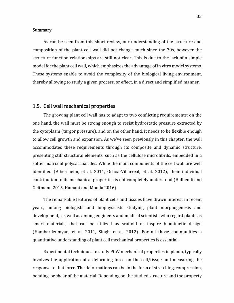
Figure 26. Schematic drawings of cell mechanical measurement techniques. The plasma membrane is shown in red, the cell cytoskeleton in blue, and the cell walls in green. (a) Micropipette aspiration- a microcapillary is placed on the cells surface, and a suction pressure is applied to force the cell into the micropipette. (b) Cell compression - a single cell is compressed between two surfaces. (c) Micro indentation - a diamond tip is used to locally deform a material with a calibrated force. (d) AFM nano-indentation - the deflection of a cantilever in contact with a sample is recorded and the mechanical properties are extracted with the help of fitting the force-deformation curve with empiric physical models. Adapted from (Geitmann 2006).
Figure 26 shows several characterization methods. In the following part, we
briefly describe each of these methods.
Micropipette aspiration
This technique is based on measuring the suction pressure necessary to partially
or wholly draw a single cell into a micropipette (Fig. 26a). The diameter of the pipette
may range from less than 1 µm to 10 µm and the applied pressures are as small as 0.1-
0.2 pN µm-2 (Hochmuth 2000). While widely used to determine viscoelastic properties
of mammalian cells, this technique has not been used systematically for assessing plant
cells mechanics. This is due to either technical difficulties or to the inability to produce
forces strong enough to act against the cell wall and the turgor pressure (Bidhendi and
Geitmann 2019).

35
Compression of single cells
Another way to measure the mechanical properties of plant cells is to directly
compress an isolated cell between two flat surfaces (Figure 26b). In cases of simple cell
geometries, such as a sphere or an ellipsoid, force-deformation curves can be predicted
from an analytical model and then fitted to the experimental data.
In such experiment, the deformation is global rather than local and thus includes
contributions from the turgor pressure as well as from the cell wall mechanical
properties. (Geitmann 2006, Routier-Kierzkowska and Smith 2013).
Indentation techniques
Indentation techniques involve indenting a sample using a tip with known
geometry and recording force-indentation data, from which the mechanical properties,
such as Young's modulus or stiffness, can be extracted (Figure 26c). Micro indentation
is sensitive to the turgor pressure, cell wall elasticity, the tip geometry and the
indentation angle. When large indenters are used, the deformation of the cell is global
and modeled as an elastic shell. When smaller indenters are used, both local and global
deformations influence the results (Routier-Kierzkowska and Smith 2013).
Nano indentation is used to deform cells wall locally and to determine its young's
modulus in the direction normal to the surface by using an atomic force microscope
(AFM) tip as a probe. Besides being a topographical imaging tool, AFM can probe local
mechanical properties by applying a controlled force and measuring the deflection of a
calibrated cantilever providing information on the mechanical response of the sample.
AFM-based studies of mechanical properties are performed by collecting force-
indentation curves at various cell-surface points. Each curve comprises the approach
and retraction of the AFM cantilever from the surface, while recording its deformation
(Figure 26d). The resulting approach-retract curve is often compared to a reference
curve and, following the determination of the contact point, the data is fitted to a
mathematical model. Several models are available that are commonly used to extract
the apparent Young’s modulus, or bulk elastic modulus E, of the sample from the
36 CHAPTER 1. INTRODUCTION
loading–unloading curves. The modulus obtained using these methods is sometimes
termed 'indentation modulus'.
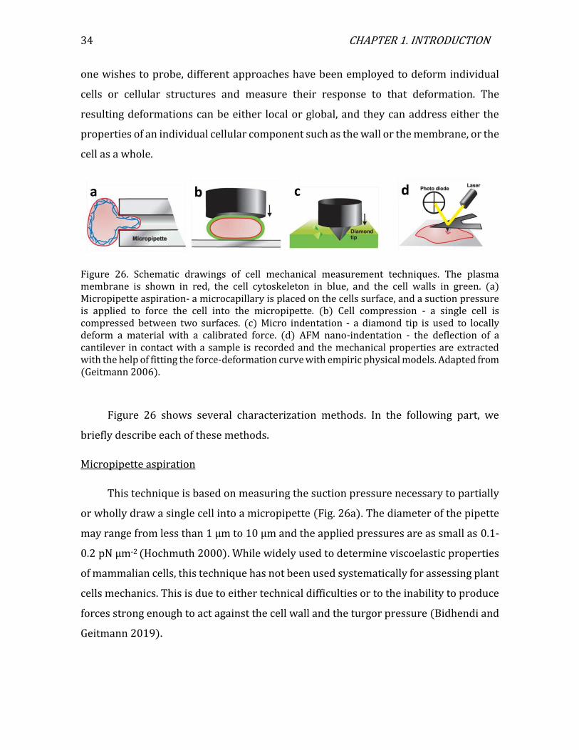
A significant variation of probing tips exists in terms of shape and size (Fig. 27a).
Knowledge of the tip geometry is crucial for data analysis as it directly determines the
contact surface between the tip and the probed sample. If the indentation depth is small
compared to the sample thickness, the measurement is believed to probe only the
properties of the thin upper layer. In the case of the PCW, which is composed of many
layers, this means that one only probes the thin upper layer composing the cell wall
(figure 27d).
Figure 27. AFM indentation schematics. (a) Typical tip geometries used in AFM indentation experiments. (b) In a typical indentation experiment, the deflection of a flexible cantilever due to the contact with the sample is recorded. Changes in direction of the laser beam reflected off the surface of the cantilever allow measurement of applied force, and based on the measured cantilever bending spring constant (k), the mechanical properties of the sample can be extracted by fitting the data to a model. (c) A typical deflection curve obtained from primary cell wall of A. Thaliana. The 0 position on this axis is determined empirically by the user, and corresponds to the bending of the cantilever. In blue, a similar curve is obtained when approaching the cantilever on mica, a flat and stiff material that serves as a maximal stiffness reference (Milani, et al. 2011). (d) Nano indentation experiments of a plant cell. The depth of the indentation determines to what extent the turgor pressure (or the substrate in the case of 2D thin films) contribute to the measured forces (Bidhendi and Geitmann 2019, Geitmann 2006, Milani, et al. 2011).
37
Another important parameter is the cantilever spring constant, with values
between 0.01-42 N m-1 being commonly used. The effect of the geometry on the data, in
terms of probe dimensions, sample shape and wall thickness must be carefully
considered. The modulus measured by indentation of anisotropic material is commonly
thought to be an average of stiffness in different directions and often reported as the
Indentation modulus or Young's modulus. Under the condition of indentation
significantly smaller than the shell thickness, the Hertz or Sneddon models can be used
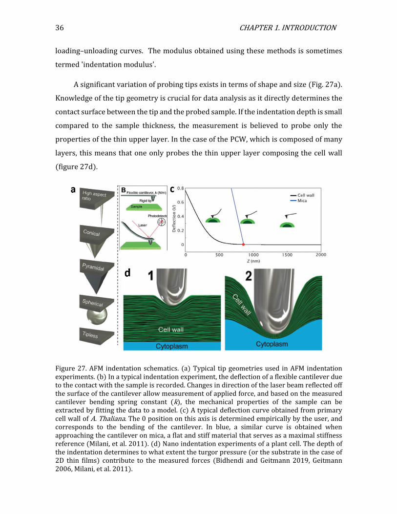
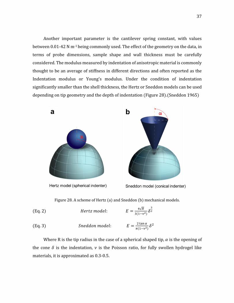
depending on tip geometry and the depth of indentation (Figure 28).(Sneddon 1965)
Figure 28. A scheme of Hertz (a) and Sneddon (b) mechanical models.
(Eq. 2) 𝐻𝑒𝑟𝑡𝑧 𝑚𝑜𝑑𝑒𝑙: 𝐸 =4√𝑅
3(1−𝜈2)𝛿
3
2
(Eq. 3) 𝑆𝑛𝑒𝑑𝑑𝑜𝑛 𝑚𝑜𝑑𝑒𝑙: 𝐸 =2 tan 𝛼
𝜋(1−𝜈2)𝛿2
Where R is the tip radius in the case of a spherical shaped tip, 𝛼 is the opening of
the cone 𝛿 is the indentation, 𝜈 is the Poisson ratio, for fully swollen hydrogel like
materials, it is approximated as 0.3-0.5.
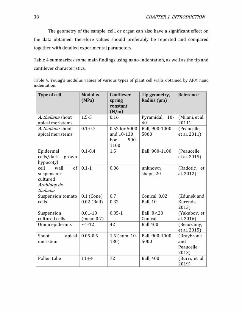
38 CHAPTER 1. INTRODUCTION
The geometry of the sample, cell, or organ can also have a significant effect on
the data obtained, therefore values should preferably be reported and compared
together with detailed experimental parameters.
Table 4 summarizes some main findings using nano-indentation, as well as the tip and
cantilever characteristics.
Table 4. Young's modulus values of various types of plant cell walls obtained by AFM nano indentation.
Type of cell Modulus (MPa)
Cantilever spring constant (N/m)
Tip geometry, Radius (µm)
Reference
A. thaliana shoot apical meristems
1.5-5 0.16 Pyramidal, 10-40
(Milani, et al. 2011)
A. thaliana shoot apical meristems
0.1-0.7 0.52 for 5000 and 10-130 For 900-1100
Ball, 900-1000 5000
(Peaucelle, et al. 2011)
Epidermal cells/dark grown hypocotyl
0.1-0.4 1.5 Ball, 900-1100 (Peaucelle, et al. 2015)
cell wall of suspension-cultured Arabidopsis thaliana
0.1-1 0.06 unknown shape, 20
(Radotić, et al. 2012)
Suspension tomato cells
0.1 (Cone) 0.02 (Ball)
0.7 0.32
Conical, 0.02 Ball, 10
(Zdunek and Kurenda 2013)
Suspension cultured cells
0.01-10 (mean 0.7)
0.05-1 Ball, R<20 Conical
(Yakubov, et al. 2016)
Onion epidermis ~1-12 42 Ball 400 (Beauzamy, et al. 2015)
Shoot apical meristem
0.05-0.5 1.5 (nom. 10-130)
Ball, 900-1000 5000
(Braybrook and Peaucelle 2013)
Pollen tube 11±4 72 Ball, 400 (Burri, et al. 2019)
39
As can be seen from this summary, the Young's modulus values can span over
several orders of magnitude. This is due to the diversity of experimental parameters
and the different types of samples used for the different studies. In terms of probe
characteristics, Zdunek et al. found different modulus for the same sample by using
different cantilever spring constant and tip radius. For a ball shaped tip with a radius
of 10 µm mounted on cantilever with a spring constant of 0.32 N m-1 the modulus was
20 kPa. This value was 5 times lower than for the modulus measured on the same
sample using a cone shaped tip with diameter of 20 nm mounted on a cantilever with a
spring constant of 0.7 N m-1. Moreover, large variability regarding elastic properties
(>100%) among cells sampled from the same region in the sample was observed
(Zdunek and Kurenda 2013).
In addition, different organs/cell types may have different stiffnesses. It was
shown that modulus can vary even for the same type of cells during different stages of
plant development (Radotić, et al. 2012).
Finally, we note several important parameters that needs to be considered when
interpreting the results of an indentation experiment:
(i) The Young's modulus is defined in the regions where the deformation is elastic
and no residual deformation is observed. However, the polymeric matrix of the
PCW could also contain regions where plastic deformation takes place. For
example, by forcing two objects to a particle-particle separation where short
range interaction takes place, the structure could collapse to a local energetic
minimum, creating irreversible deformations that will not be retrieved when the
force is removed.
(ii) The cell wall is often considered mechanically as a homogenous material, when in
fact it is a composite material similar to a fiber-reinforced gel. As such, varying
indenter size, shape, and depth of indentation may reveal different properties of
the composite. Small, shallow indentations may be more likely to reveal
properties of the gel matrix, whereas larger deformations would involve the
bending of cellulose fibers and cellulose-hemicellulose interactions.
40 CHAPTER 1. INTRODUCTION
(iii) The Hertzian contact model and its variations, which are used to extract Young’s
moduli, is valid only for the indentation of homogenous, isotropic materials with
infinite depth. This is rarely the case, in particular for plant cell walls. Moreover,
due to the heterogeneity in properties within a given sample, extensive statistical
data processing is required to obtain meaningful data.
Despite these limitations, indentation methods are still commonly used to qualitatively
estimate the elastic modulus of plant cells wall.
These points also emphasize the need for developing in vitro model systems that
can help relating the structure-property relationships in plant cells wall without the
complexity of the biological environment. The next part will revise some of the existing
in vitro PCW model systems.
1.6. Biomimetic models in 3D and 2D
PCW analogues can be roughly divided in two groups:
(i) 2D constructs: These are multilayered films of polymers, particles or their
combinations, deposited in a consecutive fashion on a solid substrate.
(ii) 3D constructs: These are multilayered shells deposited on a spherical solid
(particles) or liquid (emulsion/membrane) support.
2D constructs can provide a simple model in terms of the composition of cell wall,
while 3D constructs include also the spherical geometry of real cells. In both cases, the
Layer by Layer (LbL) technique is commonly used to create the structures.
1.6.1. General aspects of layer by layer (LbL)
Pioneered by Decher in the 90s, the LbL technique is used to create multilayer
films on solid supports, by taking advantage of the electrostatic interactions between
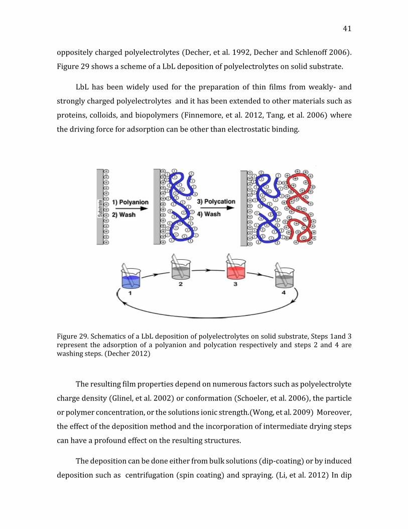
41
oppositely charged polyelectrolytes (Decher, et al. 1992, Decher and Schlenoff 2006).
Figure 29 shows a scheme of a LbL deposition of polyelectrolytes on solid substrate.
LbL has been widely used for the preparation of thin films from weakly- and
strongly charged polyelectrolytes and it has been extended to other materials such as
proteins, colloids, and biopolymers (Finnemore, et al. 2012, Tang, et al. 2006) where
the driving force for adsorption can be other than electrostatic binding.
Figure 29. Schematics of a LbL deposition of polyelectrolytes on solid substrate, Steps 1and 3 represent the adsorption of a polyanion and polycation respectively and steps 2 and 4 are washing steps. (Decher 2012)
The resulting film properties depend on numerous factors such as polyelectrolyte
charge density (Glinel, et al. 2002) or conformation (Schoeler, et al. 2006), the particle
or polymer concentration, or the solutions ionic strength.(Wong, et al. 2009) Moreover,
the effect of the deposition method and the incorporation of intermediate drying steps
can have a profound effect on the resulting structures.
The deposition can be done either from bulk solutions (dip-coating) or by induced
deposition such as centrifugation (spin coating) and spraying. (Li, et al. 2012) In dip
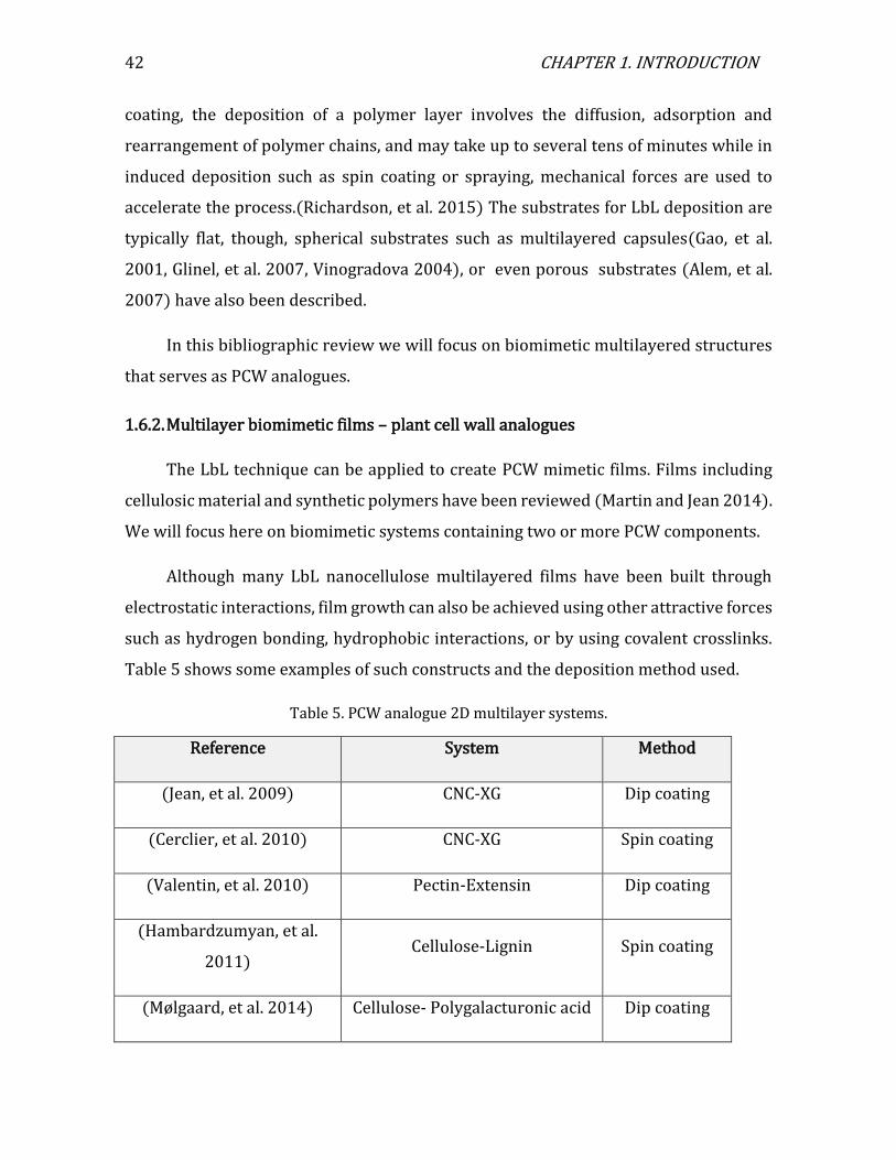
42 CHAPTER 1. INTRODUCTION
coating, the deposition of a polymer layer involves the diffusion, adsorption and
rearrangement of polymer chains, and may take up to several tens of minutes while in
induced deposition such as spin coating or spraying, mechanical forces are used to
accelerate the process.(Richardson, et al. 2015) The substrates for LbL deposition are
typically flat, though, spherical substrates such as multilayered capsules(Gao, et al.
2001, Glinel, et al. 2007, Vinogradova 2004), or even porous substrates (Alem, et al.
2007) have also been described.
In this bibliographic review we will focus on biomimetic multilayered structures
that serves as PCW analogues.
1.6.2. Multilayer biomimetic films – plant cell wall analogues
The LbL technique can be applied to create PCW mimetic films. Films including
cellulosic material and synthetic polymers have been reviewed (Martin and Jean 2014).
We will focus here on biomimetic systems containing two or more PCW components.
Although many LbL nanocellulose multilayered films have been built through
electrostatic interactions, film growth can also be achieved using other attractive forces
such as hydrogen bonding, hydrophobic interactions, or by using covalent crosslinks.
Table 5 shows some examples of such constructs and the deposition method used.
Table 5. PCW analogue 2D multilayer systems.
Reference System Method
(Jean, et al. 2009) CNC-XG Dip coating
(Cerclier, et al. 2010) CNC-XG Spin coating
(Valentin, et al. 2010) Pectin-Extensin Dip coating
(Hambardzumyan, et al.
2011) Cellulose-Lignin Spin coating
(Mølgaard, et al. 2014) Cellulose- Polygalacturonic acid Dip coating
43
The naturally occurring affinity between cellulose and XG, was exploited in few
cases to create all biobased multilayered films. Jean et al. used dip coating do deposit
multilayer consisting of the periodic repetition of a single layer of CNC and a thin layer
of xyloglucan, up to 5 bilayers (Jean, et al. 2009). The resulting film architecture was
studied with AFM and neutron reflectivity, and a linear film growth was observed with
approximately 9 nm per bilayer. This stands in agreement with the thickness value of a
single crystal of 7 nm,(Elazzouzi-Hafraoui, et al. 2007) with an additional thin XG layer.
Cerclier et al. used spin coating to create multilayered CNC/XG films, up to 8
bilayers.(Cerclier, et al. 2010). The growth of the film in their case depended on XG
concentration. At high XG concentrations (5 and 10 g L-1) the XG chains were entangled
resulting in nonlinear film growth with a plateau after 4 bilayers, where at low XG
concentration the growth was linear. They attributed this difference to the
conformation of XG in the different concentrations. Multilayered films reminiscent of
primary wall may provide a good in vitro model to study the degradation of cell wall
polymers and relaxation mechanisms linked to specific enzymes. Further studies, dealt
with a single CNC/XG bilayer and the investigation of enzymatic hydrolysis and the
effect of XG chain length on the adsorption onto CNCs (Villares, et al. 2015, Villares, et
al. 2017).
Whereas pectins have already been used to create multilayered films with
polycations such as polylysine or chitosan, very little literature covers their
combination with other plant cell wall components. Valentin et al. used Extensin and
de-esterified pectin from citrus to construct multilayer structures by LbL techniques
taking advantage of the opposite charge of the components. The film growth was non-
uniform and involved swelling/deswelling process (Valentin, et al. 2010). In another
work, Mølgaard et al. (Mølgaard, et al. 2014) used cationic cellulose fibers and
polygalacturonic acid to create multilayered films up to 8 bilayers. When the films were
exposed to pectin degrading enzymes, they showed a significant reduction in mass.
The LbL technique can be modified and transferred to create 3D architecture. In
the following sections, we will review some examples of multilayered biomimetic
capsules prepared by LbL technique.
44 CHAPTER 1. INTRODUCTION
1.6.3. Biomimetic capsules
The LbL technique was successfully transferred to spherical geometries where
the flat substrate is replaced by spherical objects (Donath, et al. 1998). Similar to the
2D case, these structures rely on intermolecular interactions to successively deposit
alternating layers of various components. Generally, two types of systems exist (i)
liquid cores, where emulsions or aqueous phase are occupying the capsule interior and
(ii) solid cores, where colloidal particles are used as a template for component
deposition. In the latter case, the solid core can be removed leaving a hollow polymeric
shell. The rinsing step, essential for removal of non-adsorbed material, is replaced here
with sedimentation of the decorated objects, removal of the supernatant and
redispersion into a new solution. Let us review some examples for each system.
1.6.3.1. Solid core systems
This type of systems is based on the deposition of polymer layers on a solid
colloidal template, which can be later removed to create hollow shells (Figure 30a).
This method can be used to prepare synthetic polymer multilayer capsules based on
electrostatic interactions. The templates include silicon dioxide (SiO2) or carbonate
(MnCO3, CaCO3, CdCO3) microparticles, or crosslinked polymer (polystyrene). Among
the shell forming polymers one can point polyelectrolytes like poly(allylamine
hydrochloride) (PAH), poly(styrenesulfonate)(PSS) and polyethylenimine (PEI)
(Vinogradova 2004).
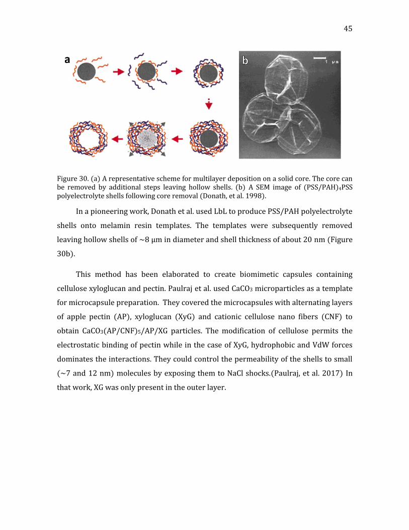
45
Figure 30. (a) A representative scheme for multilayer deposition on a solid core. The core can be removed by additional steps leaving hollow shells. (b) A SEM image of (PSS/PAH)4PSS polyelectrolyte shells following core removal (Donath, et al. 1998).
In a pioneering work, Donath et al. used LbL to produce PSS/PAH polyelectrolyte
shells onto melamin resin templates. The templates were subsequently removed
leaving hollow shells of ~8 µm in diameter and shell thickness of about 20 nm (Figure
30b).
This method has been elaborated to create biomimetic capsules containing
cellulose xyloglucan and pectin. Paulraj et al. used CaCO3 microparticles as a template
for microcapsule preparation. They covered the microcapsules with alternating layers
of apple pectin (AP), xyloglucan (XyG) and cationic cellulose nano fibers (CNF) to
obtain CaCO3(AP/CNF)5/AP/XG particles. The modification of cellulose permits the
electrostatic binding of pectin while in the case of XyG, hydrophobic and VdW forces
dominates the interactions. They could control the permeability of the shells to small
(~7 and 12 nm) molecules by exposing them to NaCl shocks.(Paulraj, et al. 2017) In
that work, XG was only present in the outer layer.

46 CHAPTER 1. INTRODUCTION
Figure 31. (a) Simplified overview of LbL microcapsule fabrication process. Between each adsorption step, a washing step was included. (b) SEM image and of (AP/CNF)5AP/XyG microcapsules after core removal.(Paulraj, et al. 2018)
They have further elaborated the system to create (CNF/XG/CNF/AP)2CNF/XG
and (CNF/XG)5 systems (figure 31). The capsules were partially permeable to 2000
kDa FITC dextrans (hydrodynamic diameter of ca. 54 nm) in water, but in saline
conditions (250 mM NaCl), the microcapsules permeability dropped. They attributed
the change in permeability to the microcapsule wall composition, i.e. the presence of XG
and small amount of charged molecules such as pectins. (Paulraj, et al. 2018).
1.6.3.2. Liquid core systems-emulsions
An emulsion is a system of dispersed droplets of one immiscible liquid in another
stabilized by emulsifiers. If solid colloidal particles are adsorbed at the fluid interfaces
they are called “Pickering emulsions” (Pickering 1907). Kalashnikova et al. created oil
in water Pickering emulsions stabilized by bacterial cellulose nanocrystals. The
resulting solid particles, formed a highly stable colloidal suspension in water
(Kalashnikova, et al. 2011) (Figure 32).
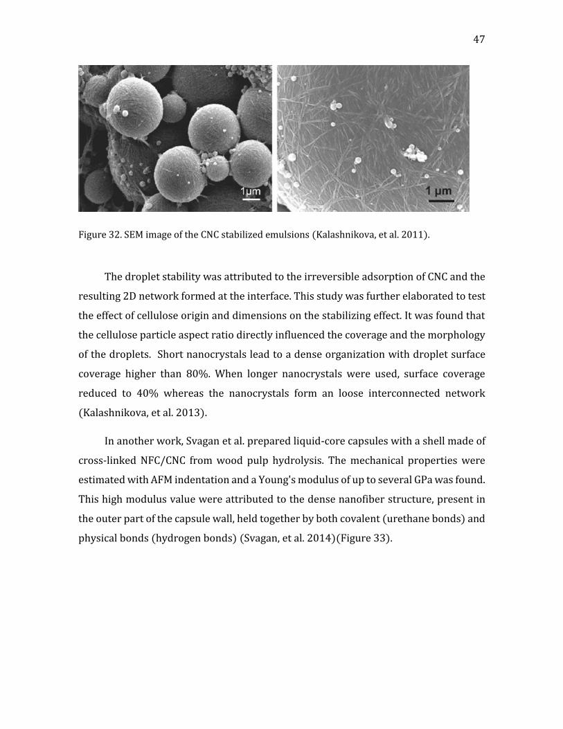
47
Figure 32. SEM image of the CNC stabilized emulsions (Kalashnikova, et al. 2011).
The droplet stability was attributed to the irreversible adsorption of CNC and the
resulting 2D network formed at the interface. This study was further elaborated to test
the effect of cellulose origin and dimensions on the stabilizing effect. It was found that
the cellulose particle aspect ratio directly influenced the coverage and the morphology
of the droplets. Short nanocrystals lead to a dense organization with droplet surface
coverage higher than 80%. When longer nanocrystals were used, surface coverage
reduced to 40% whereas the nanocrystals form an loose interconnected network
(Kalashnikova, et al. 2013).
In another work, Svagan et al. prepared liquid-core capsules with a shell made of
cross-linked NFC/CNC from wood pulp hydrolysis. The mechanical properties were
estimated with AFM indentation and a Young's modulus of up to several GPa was found.
This high modulus value were attributed to the dense nanofiber structure, present in
the outer part of the capsule wall, held together by both covalent (urethane bonds) and
physical bonds (hydrogen bonds) (Svagan, et al. 2014)(Figure 33).

48 CHAPTER 1. INTRODUCTION
Figure 33. NFC/CNC liquid core capsules (Svagan, et al. 2014).
These studies showed the possibility of stabilizing emulsion using cellulose nano
crystals, and put forward the potential use of emulsions to create biomimetic
constructs. In a work done previously in the group by Bailly (Bailly 2012), oil in water
emulsions were prepared and the liquid core was decorated with alternating layers of
CNC and XG serving as a simplified model of plant cell wall. Octamethyl cyclotetra
siloxane was used as a starting material for the emulsion and Cetylpyridinium chloride
(CPC) as surfactant, up to 15 bilayers were obtained. Figure 34 shows a scheme of the
preparation protocol (a) and the resulting decorated capsules (b and c).
Figure 34. Biomimetic multilayered capsules from CNC and XG. (a) Deposition scheme, (b) SEM image of the covered capsule, and (c) SEM image of the capsule shell (Bailly 2012).
One drawback of emulsion systems is that they are difficult to characterize in
terms of shell mechanical properties, such as bending rigidity or Young's modulus.
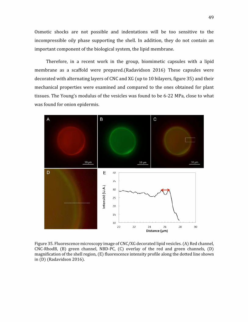
49
Osmotic shocks are not possible and indentations will be too sensitive to the
incompressible oily phase supporting the shell. In addition, they do not contain an
important component of the biological system, the lipid membrane.
Therefore, in a recent work in the group, biomimetic capsules with a lipid
membrane as a scaffold were prepared.(Radavidson 2016) These capsules were
decorated with alternating layers of CNC and XG (up to 10 bilayers, figure 35) and their
mechanical properties were examined and compared to the ones obtained for plant
tissues. The Young's modulus of the vesicles was found to be 6-22 MPa, close to what
was found for onion epidermis.
Figure 35. Fluorescence microscopy image of CNC/XG decorated lipid vesicles. (A) Red channel, CNC-RhodB, (B) green channel, NBD-PC, (C) overlay of the red and green channels, (D) magnification of the shell region, (E) fluorescence intensity profile along the dotted line shown in (D) (Radavidson 2016).
50 CHAPTER 1. INTRODUCTION
This pioneering work paved the way for the creation of new class of biomimetic
constructs composed of a lipid membrane and plant polysaccharides. However, the
factors governing the interaction between the building blocks were not yet studied in
depth.
The proposed work aims to further elaborate the above-mentioned system, first
by deciphering the underlying mechanisms governing the interactions between the
different components, and second, by exploring additional bio-based building blocks.

CHAPTER 2. CHARACTERIZATION TECHNIQUES 51
Chapter 2
Characterization techniques
2. Characterization techniques
2.1. Dynamic light scattering (DLS)
Dynamic Light Scattering (sometimes named Photon Correlation Spectroscopy or
Quasi-Elastic Light Scattering) is a technique used for extracting the mean
hydrodynamics diameter of particles in the sub-micron scale. In dynamic light
scattering, the speed at which the particles are diffusing, due to Brownian motion, is
measured by determining the rate at which the intensity of the scattered light fluctuates
(Rayleigh scattering). From the intensity fluctuation signals, calculated between time t
and t+δt, one can determine the first order autocorrelation function (g1):
(Eq. 4) 𝑔1(𝑞, 𝑡) = exp(−Γ𝜏)
Where Γ is the decay rate, 𝜏 the delay time, and q is the wave vector given by:
(Eq. 5) 𝑞 =4𝜋𝑛0
𝜆sin (𝜃 2)⁄
Where 𝑛0 is the refractive index of the sample, 𝜆 is the wavelength and 𝜃 is the angle at
which the detector is located with respect to the sample cell. For a spherical object, the
decay rate relates to the translational self-diffusion coefficient D using the following
equation:
(Eq. 6) Γ = 𝑞2𝐷
The stocks-Einstein relationship is then used to convert the self-diffusion coefficient of
a perfect sphere to its size by:
(Eq. 7) 𝐷ℎ =𝑘𝐵𝑇
3𝜋𝜂𝑠𝐷
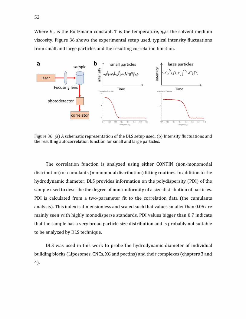
52
Where 𝑘𝐵 is the Boltzmann constant, T is the temperature, 𝜂𝑠is the solvent medium
viscosity. Figure 36 shows the experimental setup used, typical intensity fluctuations
from small and large particles and the resulting correlation function.
Figure 36. (a) A schematic representation of the DLS setup used. (b) Intensity fluctuations and the resulting autocorrelation function for small and large particles.
The correlation function is analyzed using either CONTIN (non-monomodal
distribution) or cumulants (monomodal distribution) fitting routines. In addition to the
hydrodynamic diameter, DLS provides information on the polydispersity (PDI) of the
sample used to describe the degree of non-uniformity of a size distribution of particles.
PDI is calculated from a two-parameter fit to the correlation data (the cumulants
analysis). This index is dimensionless and scaled such that values smaller than 0.05 are
mainly seen with highly monodisperse standards. PDI values bigger than 0.7 indicate
that the sample has a very broad particle size distribution and is probably not suitable
to be analyzed by DLS technique.
DLS was used in this work to probe the hydrodynamic diameter of individual
building blocks (Liposomes, CNCs, XG and pectins) and their complexes (chapters 3 and
4).
CHAPTER 2. CHARACTERIZATION TECHNIQUES 53
2.2. 𝝃-potential
𝜉-potential is a physical property which is exhibited by any charged particle in
suspension. It can be used to predict the stability of colloidal suspensions and is based
on the electrokinetic effect.
The development of a net charge at a particle surface affects the distribution of
ions in its surrounding region. Specifically, there is an increased concentration of
counter ions, namely, ions of opposite charge to that of the particle, close to the particle
surface with a thickness that corresponds to the Debye screening length 𝜆𝐷 (see figure
53 section 4.1.3 for a more detailed description). When the particle moves, ions within
this boundary move with it, while the ions beyond the boundary stay with the bulk
dispersant. The net potential at this boundary (surface of hydrodynamic shear) is the 𝜉
potential.
The 𝜉-potential can be estimated from electrophoresis experiments, where the
movement of a charged particle relative to the liquid it is suspended in, is measured
under the influence of an applied electric field E. When an electric field is applied, the
charged particles are attracted to the electrode of opposite sign while viscous forces
acting on the particles tend to oppose this movement. When steady state is reached
between these two opposing forces, the particles move with constant velocity v. The
electrophoretic mobility, Ue, defined as v/E, can be related to the 𝜉 -potential by the
Henry equation:
(Eq. 8) 𝑈𝑒 =2 𝑟 0𝜉
3𝜂𝑓(𝑎 𝜆𝐷)⁄
Where 휀𝑟 and 휀0 are the permittivities of the solution and the vacuum respectively, a is
the particle radius, 𝜂 is the viscosity of the medium and 𝜆𝐷 is the Debye length which
refers to the thickness of the electrical double layer. The term 𝑓(𝑎 𝜆𝐷)⁄ is called the
Henry function and it ranges for a sphere from 1 for 𝑎 𝜆𝐷 ≪ 1⁄ (Huckel limit) to 3/2 for
𝑎 𝜆𝐷 ≫ 1⁄ (Smoluchowski limit)(Hunter 2013). In the case where 𝑎 ≫ 𝜆𝐷, eq. 8 then
becomes the Smoluchowski relationship:
(Eq. 9) 𝑈𝑒 = 𝑟 0𝜉
𝜂
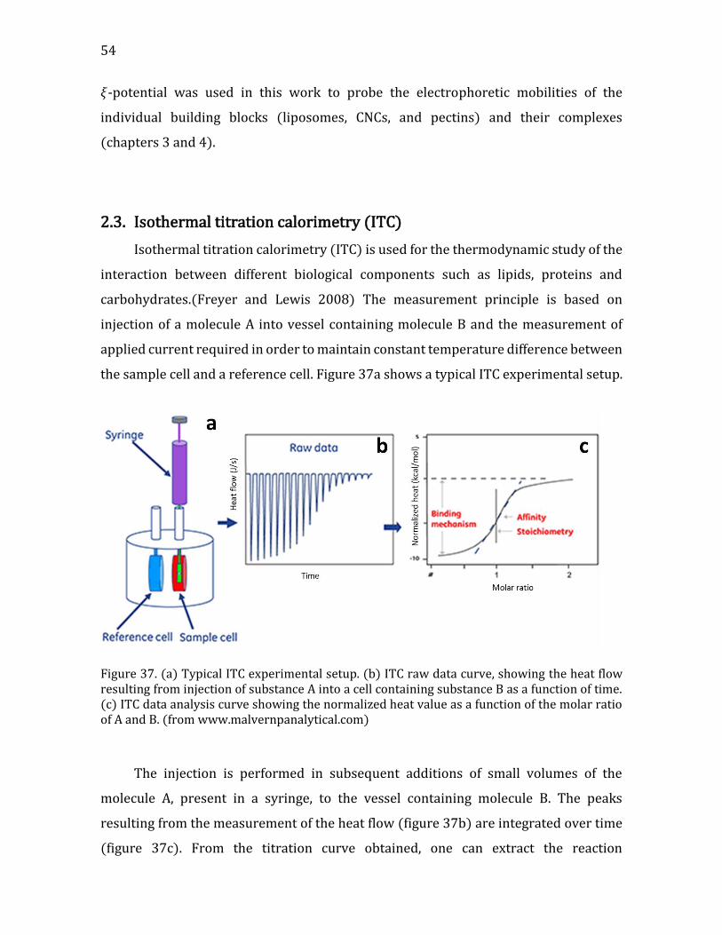
54
𝜉-potential was used in this work to probe the electrophoretic mobilities of the
individual building blocks (liposomes, CNCs, and pectins) and their complexes
(chapters 3 and 4).
2.3. Isothermal titration calorimetry (ITC)
Isothermal titration calorimetry (ITC) is used for the thermodynamic study of the
interaction between different biological components such as lipids, proteins and
carbohydrates.(Freyer and Lewis 2008) The measurement principle is based on
injection of a molecule A into vessel containing molecule B and the measurement of
applied current required in order to maintain constant temperature difference between
the sample cell and a reference cell. Figure 37a shows a typical ITC experimental setup.
Figure 37. (a) Typical ITC experimental setup. (b) ITC raw data curve, showing the heat flow resulting from injection of substance A into a cell containing substance B as a function of time. (c) ITC data analysis curve showing the normalized heat value as a function of the molar ratio of A and B. (from www.malvernpanalytical.com)
The injection is performed in subsequent additions of small volumes of the
molecule A, present in a syringe, to the vessel containing molecule B. The peaks
resulting from the measurement of the heat flow (figure 37b) are integrated over time
(figure 37c). From the titration curve obtained, one can extract the reaction
CHAPTER 2. CHARACTERIZATION TECHNIQUES 55
stoichiometry as well as valuable thermodynamic parameters such as enthalpy (ΔH)
entropy (ΔS) Gibbs free energy (ΔG), and association constant (Ka) by applying an
adequate model.
ITC was used in this work to probe the interaction between CNC and liposomes (chapter
4.2.1) and between CNC and XG (chapter 4.3.1).
2.4. Quartz crystal microbalance with dissipation monitoring (QCM-D)
Quartz crystal microbalance (QCM or QCM-D) is a versatile tool for investigating
soft and solvated interfaces between solid surfaces and bulk liquids because it can
provide a wealth of information about key structural and functional parameters of
these interfaces.(Reviakine, et al. 2011) QCM is based on the inverse piezoelectric effect
discovered by the Curies in the late 19th century: application of voltage results in
mechanical deformation of the material (Ward and Buttry 1990). In the QCM-D method,
the external driving voltage is turned off intermittently and the oscillations are left to
decay freely. Given that quartz is piezoelectric, a voltage is generated during these
decaying mechanical oscillations (figure 38). This signal is recorded, yielding two
parameters, the resonance frequency fn and the dissipation Dn (figure 38c) from which
the adsorbed mass as well as the viscoelastic properties of the layer can be extracted.
Bandwidth and dissipation are equivalent, with Dn = 2Γn/fn (figure 38d). The use of
QCM-D is based on the linear relationship between changes in the resonator (crystal)
mass and in the resonance frequency, derived by Sauerbrey:
(Eq. 10) ∆𝑓𝑛 = −𝑛
𝐶𝑚𝑓 = −
𝑛
𝐶𝜌𝑓ℎ𝑓
where fn is the resonance frequency, 𝑚𝑓 is the areal mass density of the adsorbed film
(mass per unit area), and 𝜌𝑓 and ℎ𝑓 are the density and the thickness of the adsorbed
film, respectively. The mass sensitivity constant C depends solely on the fundamental
resonance frequency fF and the material properties of the quartz crystal. For typically
used crystals with fF = 5 MHz, it is 18 ng cm-2 Hz-1.(Johannsmann 1999, Johannsmann
2008)
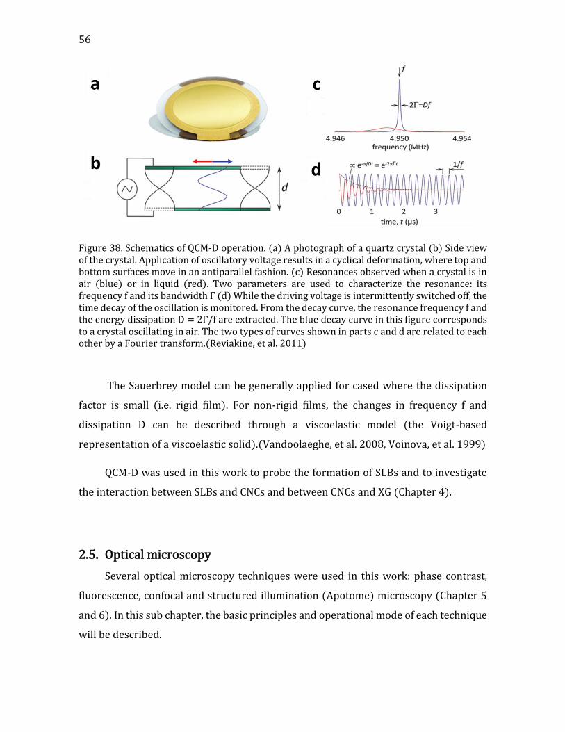
56
Figure 38. Schematics of QCM-D operation. (a) A photograph of a quartz crystal (b) Side view of the crystal. Application of oscillatory voltage results in a cyclical deformation, where top and bottom surfaces move in an antiparallel fashion. (c) Resonances observed when a crystal is in air (blue) or in liquid (red). Two parameters are used to characterize the resonance: its frequency f and its bandwidth Γ (d) While the driving voltage is intermittently switched off, the time decay of the oscillation is monitored. From the decay curve, the resonance frequency f and the energy dissipation D = 2Γ/f are extracted. The blue decay curve in this figure corresponds to a crystal oscillating in air. The two types of curves shown in parts c and d are related to each other by a Fourier transform.(Reviakine, et al. 2011)
The Sauerbrey model can be generally applied for cased where the dissipation
factor is small (i.e. rigid film). For non-rigid films, the changes in frequency f and
dissipation D can be described through a viscoelastic model (the Voigt-based
representation of a viscoelastic solid).(Vandoolaeghe, et al. 2008, Voinova, et al. 1999)
QCM-D was used in this work to probe the formation of SLBs and to investigate
the interaction between SLBs and CNCs and between CNCs and XG (Chapter 4).
2.5. Optical microscopy
Several optical microscopy techniques were used in this work: phase contrast,
fluorescence, confocal and structured illumination (Apotome) microscopy (Chapter 5
and 6). In this sub chapter, the basic principles and operational mode of each technique
will be described.
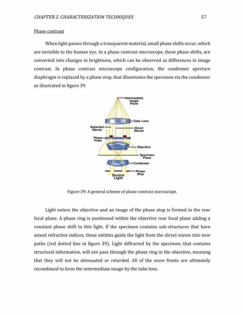
CHAPTER 2. CHARACTERIZATION TECHNIQUES 57
Phase contrast
When light passes through a transparent material, small phase shifts occur, which
are invisible to the human eye. In a phase contrast microscope, these phase shifts, are
converted into changes in brightness, which can be observed as differences in image
contrast. In phase contrast microscope configuration, the condenser aperture
diaphragm is replaced by a phase stop, that illuminates the specimen via the condenser
as illustrated in figure 39.
Figure 39: A general scheme of phase contrast microscope.
Light enters the objective and an image of the phase stop is formed in the rear
focal plane. A phase ring is positioned within the objective rear focal plane adding a
constant phase shift to this light. If the specimen contains sub-structures that have
mixed refractive indices, these entities guide the light from the direct waves into new
paths (red dotted line in figure 39). Light diffracted by the specimen, that contains
structural information, will not pass through the phase ring in the objective, meaning
that they will not be attenuated or retarded. All of the wave fronts are ultimately
recombined to form the intermediate image by the tube lens.
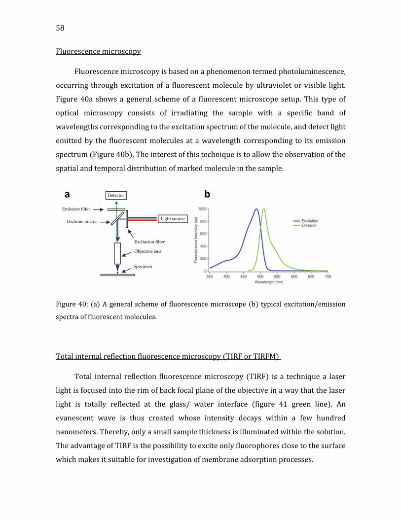
58
Fluorescence microscopy
Fluorescence microscopy is based on a phenomenon termed photoluminescence,
occurring through excitation of a fluorescent molecule by ultraviolet or visible light.
Figure 40a shows a general scheme of a fluorescent microscope setup. This type of
optical microscopy consists of irradiating the sample with a specific band of
wavelengths corresponding to the excitation spectrum of the molecule, and detect light
emitted by the fluorescent molecules at a wavelength corresponding to its emission
spectrum (Figure 40b). The interest of this technique is to allow the observation of the
spatial and temporal distribution of marked molecule in the sample.
Figure 40: (a) A general scheme of fluorescence microscope (b) typical excitation/emission
spectra of fluorescent molecules.
Total internal reflection fluorescence microscopy (TIRF or TIRFM)
Total internal reflection fluorescence microscopy (TIRF) is a technique a laser
light is focused into the rim of back focal plane of the objective in a way that the laser
light is totally reflected at the glass/ water interface (figure 41 green line). An
evanescent wave is thus created whose intensity decays within a few hundred
nanometers. Thereby, only a small sample thickness is illuminated within the solution.
The advantage of TIRF is the possibility to excite only fluorophores close to the surface
which makes it suitable for investigation of membrane adsorption processes.
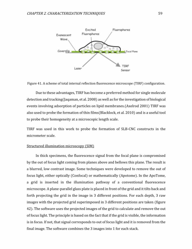
CHAPTER 2. CHARACTERIZATION TECHNIQUES 59
Figure 41. A scheme of total internal reflection fluorescence microscope (TIRF) configuration.
Due to these advantages, TIRF has become a preferred method for single molecule
detection and tracking(Jaqaman, et al. 2008) as well as for the investigation of biological
events involving adsorption of particles on lipid membranes.(Axelrod 2001) TIRF was
also used to probe the formation of thin films(Blacklock, et al. 2010) and is a useful tool
to probe their homogeneity at a microscopic length scale.
TIRF was used in this work to probe the formation of SLB-CNC constructs in the
micrometer scale.
Structured illumination microscopy (SIM)
In thick specimens, the fluorescence signal from the focal plane is compromised
by the out of focus light coming from planes above and bellows this plane. The result is
a blurred, low contrast image. Some techniques were developed to remove the out of
focus light, either optically (Confocal) or mathematically (Apotome). In the ApoTome,
a grid is inserted in the illumination pathway of a conventional fluorescence
microscope. A plane-parallel glass plate is placed in front of the grid and it tilts back and
forth projecting the grid in the image in 3 different positions. For each depth, 3 raw
images with the projected grid superimposed in 3 different positions are taken (figure
42). The software uses the projected images of the grid to calculate and remove the out
of focus light. The principle is based on the fact that if the grid is visible, the information
is in focus. If not, that signal corresponds to out of focus light and it is removed from the
final image. The software combines the 3 images into 1 for each stack.
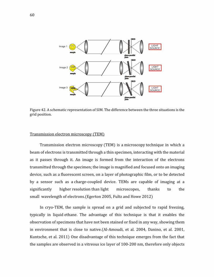
60
Figure 42. A schematic representation of SIM. The difference between the three situations is the grid position.
Transmission electron microscopy (TEM)
Transmission electron microscopy (TEM) is a microscopy technique in which a
beam of electrons is transmitted through a thin specimen, interacting with the material
as it passes through it. An image is formed from the interaction of the electrons
transmitted through the specimen; the image is magnified and focused onto an imaging
device, such as a fluorescent screen, on a layer of photographic film, or to be detected
by a sensor such as a charge-coupled device. TEMs are capable of imaging at a
significantly higher resolution than light microscopes, thanks to the
small wavelength of electrons.(Egerton 2005, Fultz and Howe 2012)
In cryo-TEM, the sample is spread on a grid and subjected to rapid freezing,
typically in liquid ethane. The advantage of this technique is that it enables the
observation of specimens that have not been stained or fixed in any way, showing them
in environment that is close to native.(Al-Amoudi, et al. 2004, Danino, et al. 2001,
Kuntsche, et al. 2011) One disadvantage of this technique emerges from the fact that
the samples are observed in a vitreous ice layer of 100-200 nm, therefore only objects
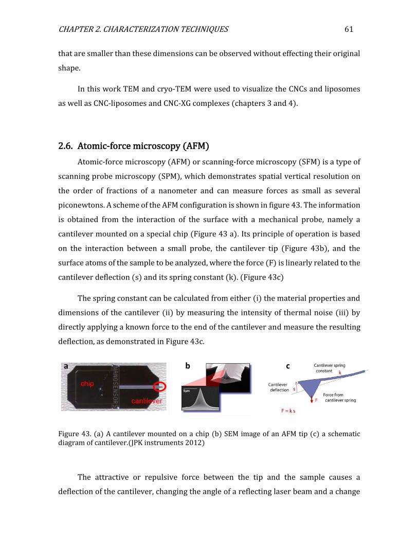
CHAPTER 2. CHARACTERIZATION TECHNIQUES 61
that are smaller than these dimensions can be observed without effecting their original
shape.
In this work TEM and cryo-TEM were used to visualize the CNCs and liposomes
as well as CNC-liposomes and CNC-XG complexes (chapters 3 and 4).
2.6. Atomic-force microscopy (AFM)
Atomic-force microscopy (AFM) or scanning-force microscopy (SFM) is a type of
scanning probe microscopy (SPM), which demonstrates spatial vertical resolution on
the order of fractions of a nanometer and can measure forces as small as several
piconewtons. A scheme of the AFM configuration is shown in figure 43. The information
is obtained from the interaction of the surface with a mechanical probe, namely a
cantilever mounted on a special chip (Figure 43 a). Its principle of operation is based
on the interaction between a small probe, the cantilever tip (Figure 43b), and the
surface atoms of the sample to be analyzed, where the force (F) is linearly related to the
cantilever deflection (s) and its spring constant (k). (Figure 43c)
The spring constant can be calculated from either (i) the material properties and
dimensions of the cantilever (ii) by measuring the intensity of thermal noise (iii) by
directly applying a known force to the end of the cantilever and measure the resulting
deflection, as demonstrated in Figure 43c.
Figure 43. (a) A cantilever mounted on a chip (b) SEM image of an AFM tip (c) a schematic diagram of cantilever.(JPK instruments 2012)
The attractive or repulsive force between the tip and the sample causes a
deflection of the cantilever, changing the angle of a reflecting laser beam and a change
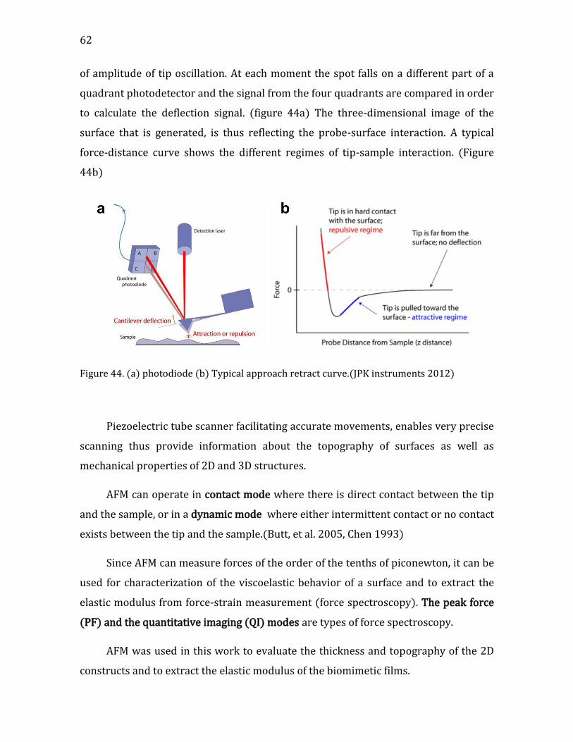
62
of amplitude of tip oscillation. At each moment the spot falls on a different part of a
quadrant photodetector and the signal from the four quadrants are compared in order
to calculate the deflection signal. (figure 44a) The three-dimensional image of the
surface that is generated, is thus reflecting the probe-surface interaction. A typical
force-distance curve shows the different regimes of tip-sample interaction. (Figure
44b)
Figure 44. (a) photodiode (b) Typical approach retract curve.(JPK instruments 2012)
Piezoelectric tube scanner facilitating accurate movements, enables very precise
scanning thus provide information about the topography of surfaces as well as
mechanical properties of 2D and 3D structures.
AFM can operate in contact mode where there is direct contact between the tip
and the sample, or in a dynamic mode where either intermittent contact or no contact
exists between the tip and the sample.(Butt, et al. 2005, Chen 1993)
Since AFM can measure forces of the order of the tenths of piconewton, it can be
used for characterization of the viscoelastic behavior of a surface and to extract the
elastic modulus from force-strain measurement (force spectroscopy). The peak force
(PF) and the quantitative imaging (QI) modes are types of force spectroscopy.
AFM was used in this work to evaluate the thickness and topography of the 2D
constructs and to extract the elastic modulus of the biomimetic films.

63
Chapter 3
Preparation of building blocks
3. Preparation of building blocks
In this part, we will deal with the characterization of the building blocks chosen
to represent the PCW architecture, namely, lipid membranes, CNCs, XG and pectin.
3.1. Building blocks characterization
3.1.1. Lipids and lipid vesicles
Lipids used
Table 6. Structure and physical properties of the Lipids used.
Chemical structure Tm
[°C]
Mw
g/mol Lipid
-18 786.1 DOPC 1,2-dioleoyl-sn-glycero-3-phosphocholine
41 734.0 DPPC 1,2-dipalmitoyl-sn-glycero-3-phosphocholine
-2 760.1 POPC (1-palmitoyl-2-oleoyl-glycero-3-phosphocholine)
~0 698.5
DOTAP 1,2-dioleoyl-3-trimethylammonium-propane (chloride salt)
136 414.7
SS Β-Sitosterol 22,23-dihydrostigmasterol

64 CHAPTER 3. BUILDING BLOCKS
Phospholipids and sterols were purchased from Avanti Polar Lipids Inc.
(Birmingham, U.S.A.) and dissolved without further purification in a
chloroform/methanol mixture (9/1 %V/%V) to a total concentration of 10 mg mL−1.
The solutions were stored at −20 °C until used.
Liposomes
Lipid solutions in chloroform/methanol mixture were transferred into a round-
bottom flask and the organic solvent was removed by evaporation under high vacuum
pumping for 2-4 h, until complete evaporation of the solvent. The lipid film was then
hydrated in an appropriate amount of buffer solution at room temperature above the
melting point of the lipids. Multilamellar vesicles were then obtained by vortexing for
30 min. The resulting suspensions were then successively extruded 20 times through
200 and 100 nm polycarbonate membranes using a miniextruder (Avanti Polar Lipids).
(Figure 45)
Figure 45. Liposome preparation with extrusion through polycarbonate membranes with defined sizes.
The liposomes were finally characterized by cryo-TEM, DLS and ζ-potential. Typical
characterization of DOPC and DOPC/DOTAP liposomes is shown in figure 46.
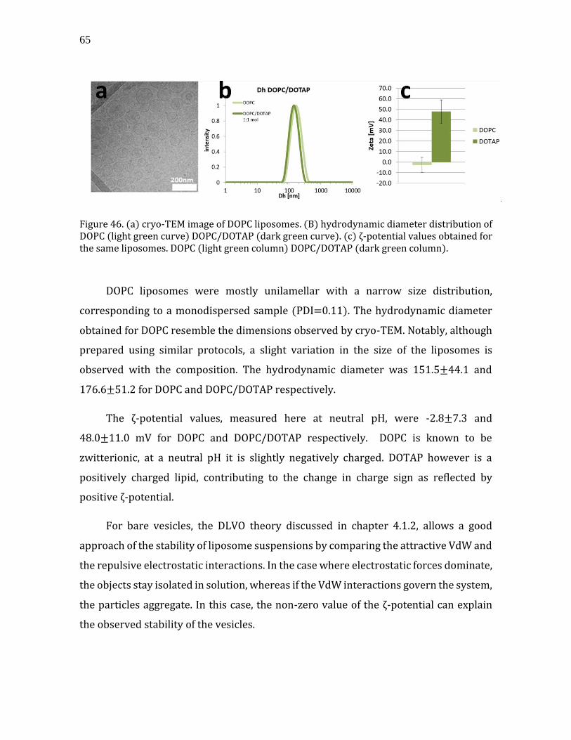
65
Figure 46. (a) cryo-TEM image of DOPC liposomes. (B) hydrodynamic diameter distribution of DOPC (light green curve) DOPC/DOTAP (dark green curve). (c) ζ-potential values obtained for the same liposomes. DOPC (light green column) DOPC/DOTAP (dark green column).
DOPC liposomes were mostly unilamellar with a narrow size distribution,
corresponding to a monodispersed sample (PDI=0.11). The hydrodynamic diameter
obtained for DOPC resemble the dimensions observed by cryo-TEM. Notably, although
prepared using similar protocols, a slight variation in the size of the liposomes is
observed with the composition. The hydrodynamic diameter was 151.5±44.1 and
176.6±51.2 for DOPC and DOPC/DOTAP respectively.
The ζ-potential values, measured here at neutral pH, were -2.8±7.3 and
48.0±11.0 mV for DOPC and DOPC/DOTAP respectively. DOPC is known to be
zwitterionic, at a neutral pH it is slightly negatively charged. DOTAP however is a
positively charged lipid, contributing to the change in charge sign as reflected by
positive ζ-potential.
For bare vesicles, the DLVO theory discussed in chapter 4.1.2, allows a good
approach of the stability of liposome suspensions by comparing the attractive VdW and
the repulsive electrostatic interactions. In the case where electrostatic forces dominate,
the objects stay isolated in solution, whereas if the VdW interactions govern the system,
the particles aggregate. In this case, the non-zero value of the ζ-potential can explain
the observed stability of the vesicles.
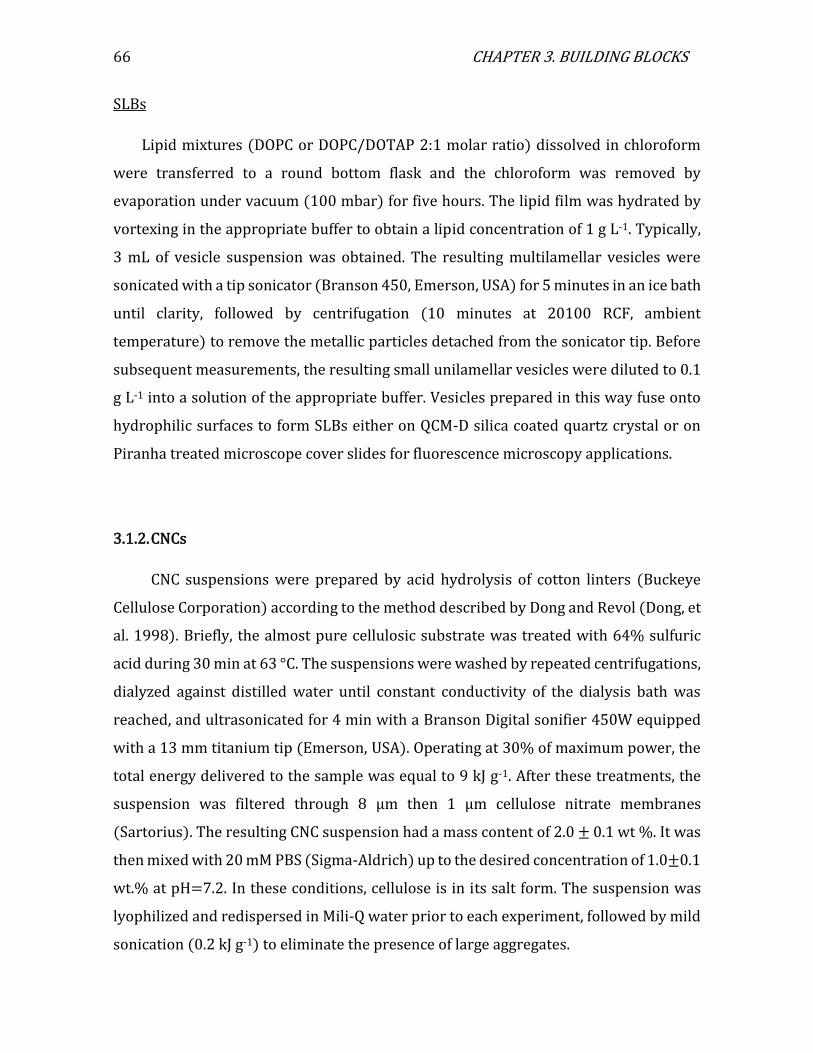
66 CHAPTER 3. BUILDING BLOCKS
SLBs
Lipid mixtures (DOPC or DOPC/DOTAP 2:1 molar ratio) dissolved in chloroform
were transferred to a round bottom flask and the chloroform was removed by
evaporation under vacuum (100 mbar) for five hours. The lipid film was hydrated by
vortexing in the appropriate buffer to obtain a lipid concentration of 1 g L-1. Typically,
3 mL of vesicle suspension was obtained. The resulting multilamellar vesicles were
sonicated with a tip sonicator (Branson 450, Emerson, USA) for 5 minutes in an ice bath
until clarity, followed by centrifugation (10 minutes at 20100 RCF, ambient
temperature) to remove the metallic particles detached from the sonicator tip. Before
subsequent measurements, the resulting small unilamellar vesicles were diluted to 0.1
g L-1 into a solution of the appropriate buffer. Vesicles prepared in this way fuse onto
hydrophilic surfaces to form SLBs either on QCM-D silica coated quartz crystal or on
Piranha treated microscope cover slides for fluorescence microscopy applications.
3.1.2. CNCs
CNC suspensions were prepared by acid hydrolysis of cotton linters (Buckeye
Cellulose Corporation) according to the method described by Dong and Revol (Dong, et
al. 1998). Briefly, the almost pure cellulosic substrate was treated with 64% sulfuric
acid during 30 min at 63 °C. The suspensions were washed by repeated centrifugations,
dialyzed against distilled water until constant conductivity of the dialysis bath was
reached, and ultrasonicated for 4 min with a Branson Digital sonifier 450W equipped
with a 13 mm titanium tip (Emerson, USA). Operating at 30% of maximum power, the
total energy delivered to the sample was equal to 9 kJ g-1. After these treatments, the
suspension was filtered through 8 μm then 1 μm cellulose nitrate membranes
(Sartorius). The resulting CNC suspension had a mass content of 2.0 ± 0.1 wt %. It was
then mixed with 20 mM PBS (Sigma-Aldrich) up to the desired concentration of 1.0±0.1
wt.% at pH=7.2. In these conditions, cellulose is in its salt form. The suspension was
lyophilized and redispersed in Mili-Q water prior to each experiment, followed by mild
sonication (0.2 kJ g-1) to eliminate the presence of large aggregates.

67
TEM DLS and ζ-potential
Figures 47a and 47b show a TEM image and hydrodynamic diameter distribution
profile respectively, of CNCs prepared according to the described protocol.
Figure 47. (a) TEM image of negatively stained CNCs prepared by cotton hydrolysis, scale bar: 100 nm (b) DLS profile showing the hydrodynamic diameter of CNCs. (TEM image taken by Jean-Luc Putaux, CERMAV)
The TEM images reveal needle-shaped particles which are, in fact, bundles of 3-5
individual crystallites, in agreement with previous studies on CNCs prepared with the
same protocol.(Elazzouzi-Hafraoui, et al. 2007, Jean, et al. 2009) The corresponding
DLS curve shows a hydrodynamic diameter of 90.2 and PDI of 0.17. Although the
interpretation of DLS analysis using Stokes-Einstein relationship is limited to spherical
objects, it gives a reasonable assessment for the overall size of the objects.(Foster, et al.
2018)
Conductometric titration
The surface charge density of CNCs can be determined using conductometric
titration of the H3O+ ions, the counterions of the sulfate half-ester groups left after acid
hydrolysis. By following the conductivity of CNC suspension during titration with a

68 CHAPTER 3. BUILDING BLOCKS
strong base, NaOH in this case, we can determine the equivalent point from which the
surface charge density can be determined.
The titration is done under stirring with a conductometer CDM 210 (Thermoscientific,
USA) equipped with an electrode CDM 614T. Figure 48 shows the conductivity as a
function of added NaOH volume.
Figure 48. Conductometric titration: conductivity as a function of NaOH volume. The charge density can be determined from the equivalent point.
The equivalent point is determined from the inflection point and related to the
amount of half sulfate ester groups by the following relationship (Dong, et al. 1998):
(Eq. 11) 𝐶𝑁𝑎𝑂𝐻𝑉𝑒𝑞 = 𝑛𝑠𝑜3−
Where 𝐶𝑁𝑎𝑂𝐻 is the concentration of NaOH used for titration, 𝑛𝑠𝑜3− is the number of
moles of sulfate ester groups in the sample and Veq is the volume at the equivalent point.
The degree of substitution is defined as:
(Eq. 12) 𝑑𝑠 =𝑛𝑠𝑜3
−
𝑚𝑐𝑒𝑙𝑙𝑢𝑙𝑜𝑒 𝑚𝑚𝑜𝑙
𝑘𝑔
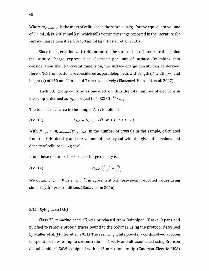
69
Where 𝑚𝑐𝑒𝑙𝑙𝑢𝑙𝑜𝑠𝑒 is the mass of cellulose in the sample in kg. For the equivalent volume
of 2.4 mL, ds is 240 mmol kg-1 which falls within the range reported in the literature for
surface charge densities: 80-350 mmol kg-1.(Foster, et al. 2018)
Since the interaction with CNCs occurs on the surface, it is of interest to determine
the surface charge expressed in electrons per unit of surface. By taking into
consideration the CNC crystal dimension, the surface charge density can be derived.
Here, CNCs from cotton are considered as parallelepipeds with length (l) width (w) and
height (t) of 150 nm 21 nm and 7 nm respectively.(Elazzouzi-Hafraoui, et al. 2007)
Each SO3- group contributes one electron, thus the total number of electrons in
the sample, defined as 𝑛𝑒 , is equal to 6.022 ∙ 1023 ∙ 𝑛𝑠𝑜3− .
The total surface area in the sample, Atot , is defined as:
(Eq. 13) 𝐴𝑡𝑜𝑡 = 𝑁𝑐𝑟𝑦𝑠 ∙ 2(𝑙 ∙ 𝑤 + 𝑙 ∙ 𝑡 + 𝑡 ∙ 𝑤)
With 𝑁𝑐𝑟𝑦𝑠 = 𝑚𝑐𝑒𝑙𝑙𝑢𝑙𝑜𝑠𝑒/𝑚𝑐𝑟𝑦𝑠𝑡𝑎𝑙 is the number of crystals in the sample, calculated
from the CNC density and the volume of one crystal with the given dimensions and
density of cellulose 1.6 g cm-3.
From these relations, the surface charge density is:
(Eq. 14) 𝜎𝐶𝑁𝐶 [𝑒−
𝑛𝑚2] =𝑛𝑒
𝐴𝑡𝑜𝑡
We obtain 𝜎𝐶𝑁𝐶 = 0.52 𝑒− 𝑛𝑚−2, in agreement with previously reported values using
similar hydrolysis conditions.(Radavidson 2016)
3.1.3. Xyloglucan (XG)
Class 3A tamarind seed XG was purchased from Dainnipon (Osaka, Japan) and
purified to remove protein traces bound to the polymer using the protocol described
by Muller et al.(Muller, et al. 2011) The resulting white powder was dissolved at room
temperature in water up to concentration of 1 wt.% and ultrasonicated using Branson
digital sonifier 450W, equipped with a 13 mm titanium tip (Emerson Electric, USA)

70 CHAPTER 3. BUILDING BLOCKS
operating at 30% of maximum power. Sonication was carried out on a 20 mL sample in
a cylinder glass vial which was placed in an ice bath to avoid over heating of the sample.
The sonication was performed in cycles of 1 min each with 4 min rest periods between
cycles to allow the cooling of the solution, providing 405 kJ g-1 per cycle. A total of 10
cycles were performed, the total energy delivered to the sample was equal to 4·103 kJ
g-1. The sonication was followed by centrifugation 13.4·103 rpm for 10 min (Eppendorf,
Germany) to remove metal particles from the sonicator tip. The suspension was then
ultrafiltrated using a 10 kDa membrane and then lyophilized and kept in a sealed glass
vial. Samples were prepared by dissolving the lyophilized XG in the appropriate buffer
up to the desired concentration. The samples were filtered prior to measurement with
a 0.2 µM syringe filter to eliminate the presence of dust and aggregates. Figure 49 shows
the number averaged (Mn) and weight averaged (Mw) molecular weights as a function
of the energy provided to the sample from GPC measurements
Figure 49. Molar mass of sonicated XG as a function of the energy provided to the sample. Inset: PDI as a function of the energy provided to the sample. The sonication of XG was carried out as detailed in the experimental section.
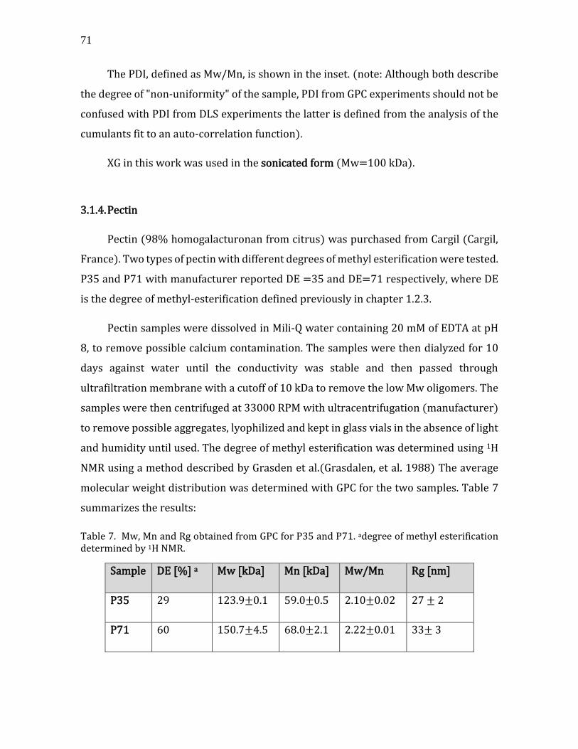
71
The PDI, defined as Mw/Mn, is shown in the inset. (note: Although both describe
the degree of "non-uniformity" of the sample, PDI from GPC experiments should not be
confused with PDI from DLS experiments the latter is defined from the analysis of the
cumulants fit to an auto-correlation function).
XG in this work was used in the sonicated form (Mw=100 kDa).
3.1.4. Pectin
Pectin (98% homogalacturonan from citrus) was purchased from Cargil (Cargil,
France). Two types of pectin with different degrees of methyl esterification were tested.
P35 and P71 with manufacturer reported DE =35 and DE=71 respectively, where DE
is the degree of methyl-esterification defined previously in chapter 1.2.3.
Pectin samples were dissolved in Mili-Q water containing 20 mM of EDTA at pH
8, to remove possible calcium contamination. The samples were then dialyzed for 10
days against water until the conductivity was stable and then passed through
ultrafiltration membrane with a cutoff of 10 kDa to remove the low Mw oligomers. The
samples were then centrifuged at 33000 RPM with ultracentrifugation (manufacturer)
to remove possible aggregates, lyophilized and kept in glass vials in the absence of light
and humidity until used. The degree of methyl esterification was determined using 1H
NMR using a method described by Grasden et al.(Grasdalen, et al. 1988) The average
molecular weight distribution was determined with GPC for the two samples. Table 7
summarizes the results:
Table 7. Mw, Mn and Rg obtained from GPC for P35 and P71. adegree of methyl esterification determined by 1H NMR.
Sample DE [%] a Mw [kDa] Mn [kDa] Mw/Mn Rg [nm]
P35 29 123.9±0.1 59.0±0.5 2.10±0.02 27 ± 2
P71 60 150.7±4.5 68.0±2.1 2.22±0.01 33± 3

72 CHAPTER 3. BUILDING BLOCKS
Taking the average molecular weight of galacturonic acid monomer and the methyl
esterified monomer to be 194.1 and 253.1 g mol-1 respectively, we can calculate the
average theoretical molecular weight 𝑀𝑎𝑣:
(Eq. 15) 𝑀𝑎𝑣 = 194.1 ∙ (1 − 𝐷𝐸) + (253.1 ∙ 𝐷𝐸)
and obtain the degree of polymerization:
(Eq. 16) 𝐷𝑃 =𝑚𝑛
𝑚𝑎𝑣
The calculated DP were 278 and 289 for P35 and P71 respectively.
3.1.5. Grafting of Fluorophores on CNC, XG and Pectin
CNCs, XG and pectin were fluorescently labeled in order to enable their
visualization via fluorescence microscopy. The fluorophores used were Rhodamine-B
Isothiocyanate (RBITC) for the CNCs and Fluorescein isothiocyanate (FITC) for the
soluble polysaccharides- XG and Pectin (P35). Table 8 shows the chemical structure,
molecular weight and the excitation/ emission wavelength of each fluorophore.
Table 8. Chemical structure, Mw and Excitation/Emission wavelengths of the fluorophores used for this study.
Rhodamine B FITC
Chemical structure
Mw [g mol-1] 536.1 389.4
Excitation/Emission λex=540nm/λem=580nm λex=490 nm/ λem=520 nm

73
The following equations were used in order to calculate the required mass of
fluorophore with respect to polysaccharide.(Dong and Roman 2007, Nielsen, et al.
2010)
(Eq. 17) 𝑚𝑅𝐵𝐼𝑇𝐶 = 0.032 ∙ 𝑚𝑐𝑛𝑐 ∙ 𝑚𝑤,𝑅𝐵𝐼𝑇𝐶
(Eq. 18) 𝑚𝐹𝐼𝑇𝐶 = 0.32 ∙ 𝑚𝑋𝐺 𝑜𝑟 𝑃𝑒𝑐𝑡𝑖𝑛 ∙ 𝑚𝑤,𝐹𝐼𝑇𝐶
Where 𝑚𝑤,𝑅𝐵𝐼𝑇𝐶 and 𝑚𝑤,𝐹𝐼𝑇𝐶 are the molar masses of Rhod-B and FITC respectively. In
the case of CNCs, the mass was divided by 10 in order to avoid excess substitution which
may alternate the interaction with the other polysaccharides.(Radavidson 2016)
CNC labeling
CNCs were labeled according to previously described protocols by Nielsen and
Dong(Dong and Roman 2007, Nielsen, et al. 2010) with slight modifications. Cellulose
nanocrystals (250 mg) were suspended in 25 mL of 0.1 M NaOH together with 7.5 mg
of RBITC (Sigma-Aldrich) and stirred for 4.5 days in the dark at ambient temperature.
The suspension was centrifuged for 20 min and 20000 g and the orange supernatant
removed. The precipitate was redispersed in water and dialyzed using a 10 kDa
membrane against deionized water for 10 days until the pH was stable, and then freeze
dried. The obtained pink powder was stored in a sealed vile and kept in the dark. Prior
to use, the powder was dissolved into to the desired buffer and sonicated using tip
sonicator for 60 seconds to break any formed aggregates.
XG and pectin labeling
Polysaccharides (xyloglucan and pectin) were labeled using a similar protocol to
the one used for CNC labeling. 25 mL of polymer solution (1% wt.) was mixed with
NaOH 0.2M and 75 mg of FITC (Sigma-Aldrich). The mixture was stirred for 4 days in
the dark at ambient temperature and the resulting solution was dialyzed against water
until the pH was stable. The solution was then transferred to an ultrafiltration cell and
passed through a cellulose nitrate membrane (Amicon) with a 10 kDa cutoff for 24

74 CHAPTER 3. BUILDING BLOCKS
hours under constant water flow, to remove the excess of unbound fluorophores. The
resulting solution was lyophilized and kept in sealed vials in the absence of light.
Calibration curves
In order to calculate the number of grafted groups, a calibration curve was
generated for the two types of fluorophores using UV-vis spectrometer. RBITC and FITC
solutions with known fluorophore concentrations were prepared, and the absorbance
value was recorded with a specific excitation wavelength for each type of fluorophore,
according to their characteristic excitation/emission spectrum (see table 8).
Figure 50 shows the calibration curves and the linear fits.
Figure 50. Calibration curves for RBITC (red circles) and FITC (green circles) with the linear fits (dashed lines)
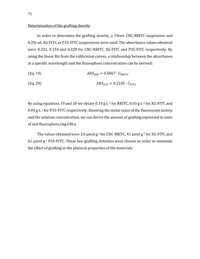
75
Determination of the grafting density
In order to determine the grafting density, a 1%wt. CNC-RBITC suspension and
0.2% wt. XG-FITC or P35-FITC suspensions were used. The absorbance values obtained
were 0.332, 0.154 and 0.228 for CNC-RBITC, XG-FITC and P35-FITC respectively. By
using the linear fits from the calibration curves, a relationship between the absorbance
at a specific wavelength and the fluorophore concentration can be derived:
(Eq. 19) 𝐴𝐵𝑆580 = 0.5867 ∙ 𝐶𝑅𝐵𝐼𝑇𝐶
(Eq. 20) 𝐴𝐵𝑆520 = 0.2105 ∙ 𝐶𝐹𝐼𝑇𝐶
By using equations 19 and 20 we obtain 0.19 g L-1 for RBITC, 0.03 g L-1 for XG-FITC and
0.04 g L-1 for P35-FITC respectively. Knowing the molar mass of the fluorescent moiety
and the solution concentration, we can derive the amount of grafting expressed in units
of mol fluorophore/mg CNCs.
The values obtained were 3.6 µmol g-1 for CNC-RBITC, 41 µmol g-1 for XG-FITC and
61 µmol g-1 P35-FITC. These low grafting densities were chosen in order to minimize
the effect of grafting in the physical properties of the materials.
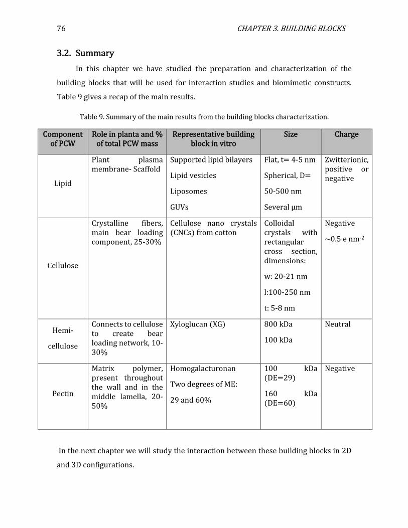
76 CHAPTER 3. BUILDING BLOCKS
3.2. Summary
In this chapter we have studied the preparation and characterization of the
building blocks that will be used for interaction studies and biomimetic constructs.
Table 9 gives a recap of the main results.
Table 9. Summary of the main results from the building blocks characterization.
Component of PCW
Role in planta and % of total PCW mass
Representative building block in vitro
Size Charge
Lipid
Plant plasma membrane- Scaffold
Supported lipid bilayers
Lipid vesicles
Liposomes
GUVs
Flat, t= 4-5 nm
Spherical, D=
50-500 nm
Several µm
Zwitterionic, positive or negative
Cellulose
Crystalline fibers, main bear loading component, 25-30%
Cellulose nano crystals (CNCs) from cotton
Colloidal crystals with rectangular cross section, dimensions:
w: 20-21 nm
l:100-250 nm
t: 5-8 nm
Negative
~0.5 e nm-2
Hemi-
cellulose
Connects to cellulose to create bear loading network, 10-30%
Xyloglucan (XG) 800 kDa
100 kDa
Neutral
Pectin
Matrix polymer, present throughout the wall and in the middle lamella, 20-50%
Homogalacturonan
Two degrees of ME:
29 and 60%
100 kDa (DE=29)
160 kDa (DE=60)
Negative
In the next chapter we will study the interaction between these building blocks in 2D
and 3D configurations.
77 CHAPTER 4. INTERACTION STUDIES
Chapter 4
Interaction studies
4. Interaction studies
The interaction between PCW components plays an important role in cell
biosynthesis and growth. Understanding these interactions is important for developing
new strategies to design biomimetic constructs, which can serve as simplified PCW
models (Cosgrove 1997, Ochoa-Villarreal, et al. 2012, Somerville, et al. 2004). Thus,
identifying the factors governing the interaction between the building blocks is an
essential strategic step towards the creation of biomimetic constructs.
In the previous chapters we have introduced the building blocks. In this section,
following a short introduction on intermolecular forces, we will focus on the study of
the interactions between pairs of building blocks, namely, CNC-Lipid, CNC-XG, and CNC-
Pectin, in 2D and 3D systems.
In the 3D systems, the measurements are carried in the bulk solution, meaning
that the individual components are mixed and the interactions between them are
studied with various experimental techniques such as light scattering, ITC, NMR, and
TEM. For the 2D systems, the interactions take place in the vicinity of a surface, thus, in
this case we use surface sensitive techniques such as AFM, TIRF, NR, and QCM-D.
Note: chapter 4.2.1 and chapter 4.2.2 were published in peer reviewed journals, see
annex I.
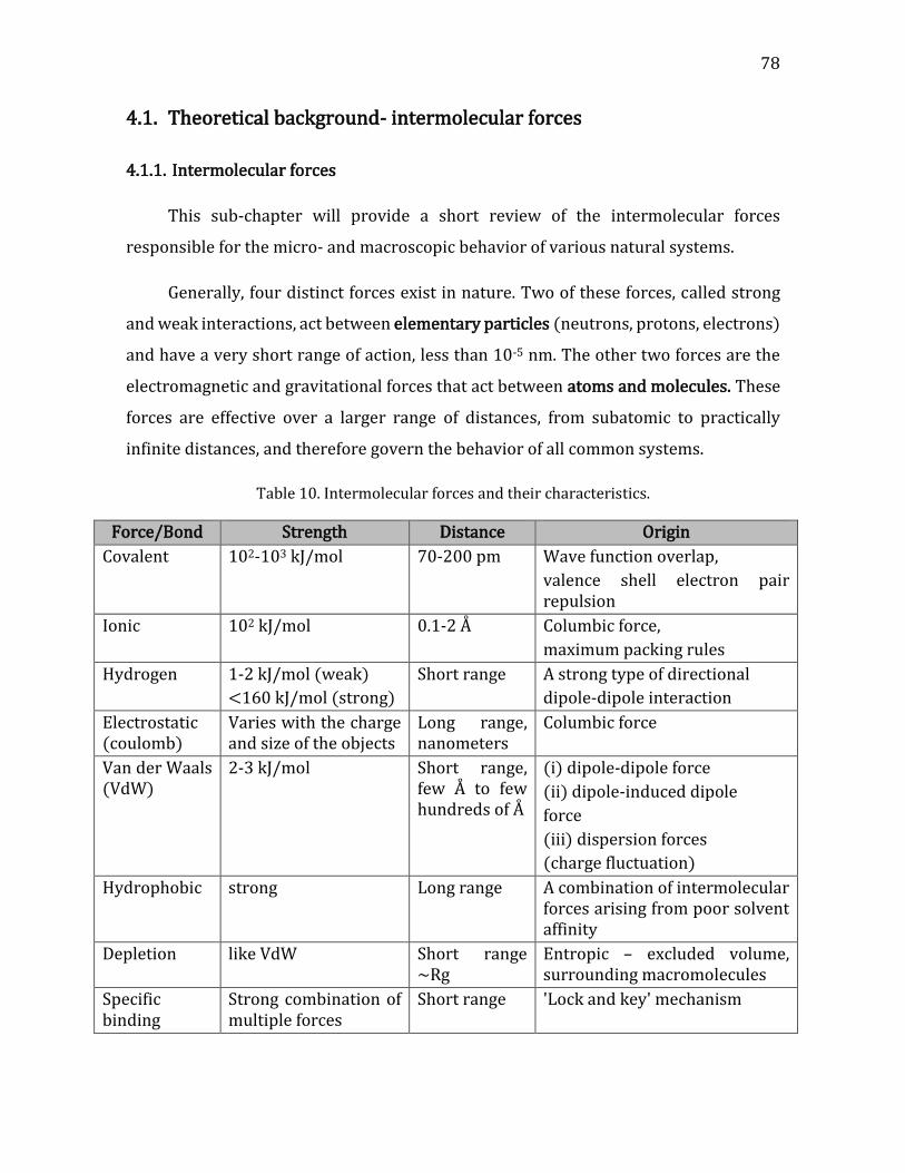
78
4.1. Theoretical background- intermolecular forces
4.1.1. Intermolecular forces
This sub-chapter will provide a short review of the intermolecular forces
responsible for the micro- and macroscopic behavior of various natural systems.
Generally, four distinct forces exist in nature. Two of these forces, called strong
and weak interactions, act between elementary particles (neutrons, protons, electrons)
and have a very short range of action, less than 10-5 nm. The other two forces are the
electromagnetic and gravitational forces that act between atoms and molecules. These
forces are effective over a larger range of distances, from subatomic to practically
infinite distances, and therefore govern the behavior of all common systems.
Table 10. Intermolecular forces and their characteristics.
Force/Bond Strength Distance Origin
Covalent 102-103 kJ/mol 70-200 pm Wave function overlap,
valence shell electron pair repulsion
Ionic 102 kJ/mol 0.1-2 Å Columbic force,
maximum packing rules
Hydrogen 1-2 kJ/mol (weak)
<160 kJ/mol (strong)
Short range A strong type of directional
dipole-dipole interaction
Electrostatic (coulomb)
Varies with the charge and size of the objects
Long range, nanometers
Columbic force
Van der Waals (VdW)
2-3 kJ/mol Short range, few Å to few hundreds of Å
(i) dipole-dipole force
(ii) dipole-induced dipole
force
(iii) dispersion forces
(charge fluctuation)
Hydrophobic strong Long range A combination of intermolecular forces arising from poor solvent affinity
Depletion like VdW Short range ~Rg
Entropic – excluded volume, surrounding macromolecules
Specific binding
Strong combination of multiple forces
Short range 'Lock and key' mechanism
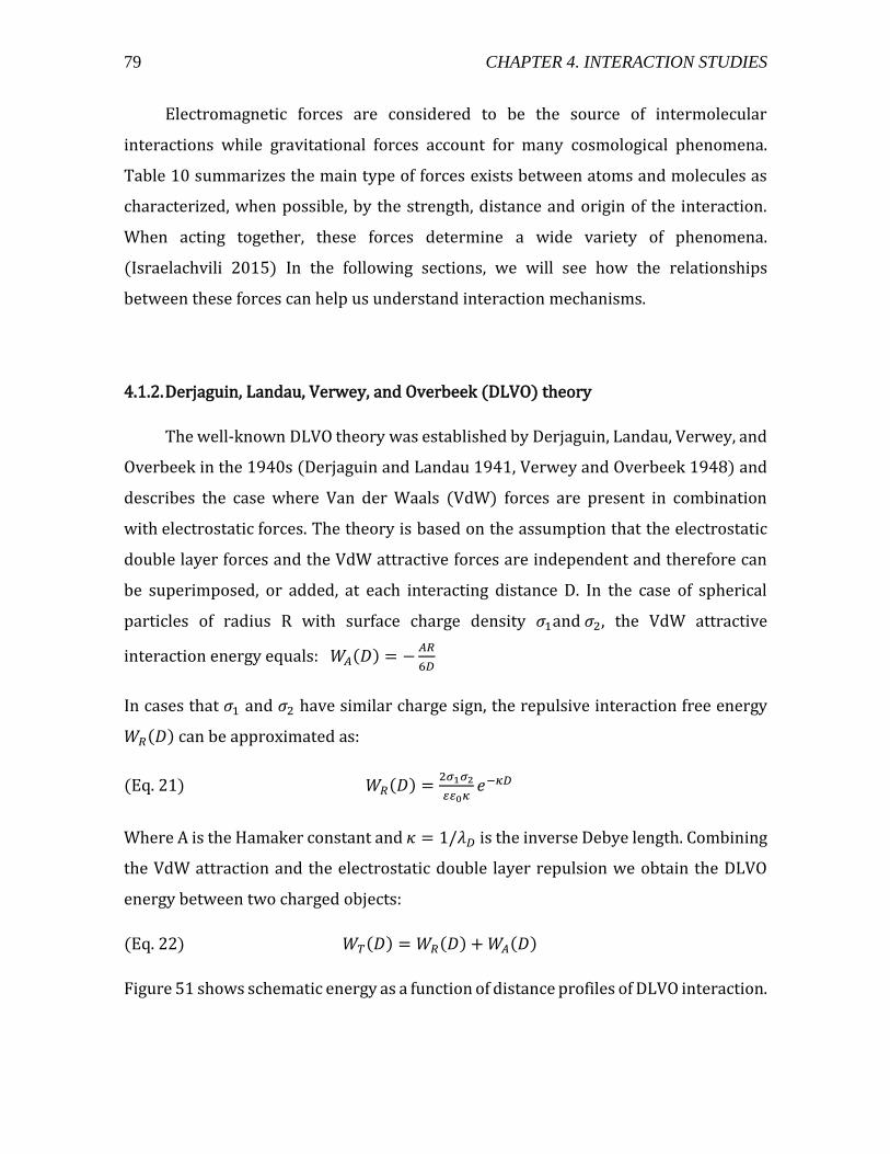
79 CHAPTER 4. INTERACTION STUDIES
Electromagnetic forces are considered to be the source of intermolecular
interactions while gravitational forces account for many cosmological phenomena.
Table 10 summarizes the main type of forces exists between atoms and molecules as
characterized, when possible, by the strength, distance and origin of the interaction.
When acting together, these forces determine a wide variety of phenomena.
(Israelachvili 2015) In the following sections, we will see how the relationships
between these forces can help us understand interaction mechanisms.
4.1.2. Derjaguin, Landau, Verwey, and Overbeek (DLVO) theory
The well-known DLVO theory was established by Derjaguin, Landau, Verwey, and
Overbeek in the 1940s (Derjaguin and Landau 1941, Verwey and Overbeek 1948) and
describes the case where Van der Waals (VdW) forces are present in combination
with electrostatic forces. The theory is based on the assumption that the electrostatic
double layer forces and the VdW attractive forces are independent and therefore can
be superimposed, or added, at each interacting distance D. In the case of spherical
particles of radius R with surface charge density 𝜎1and 𝜎2, the VdW attractive
interaction energy equals: 𝑊𝐴(𝐷) = −𝐴𝑅
6𝐷
In cases that 𝜎1 and 𝜎2 have similar charge sign, the repulsive interaction free energy
𝑊𝑅(𝐷) can be approximated as:
(Eq. 21) 𝑊𝑅(𝐷) =2𝜎1𝜎2
0𝜅𝑒−𝜅𝐷
Where A is the Hamaker constant and 𝜅 = 1/𝜆𝐷 is the inverse Debye length. Combining
the VdW attraction and the electrostatic double layer repulsion we obtain the DLVO
energy between two charged objects:
(Eq. 22) 𝑊𝑇(𝐷) = 𝑊𝑅(𝐷) + 𝑊𝐴(𝐷)
Figure 51 shows schematic energy as a function of distance profiles of DLVO interaction.
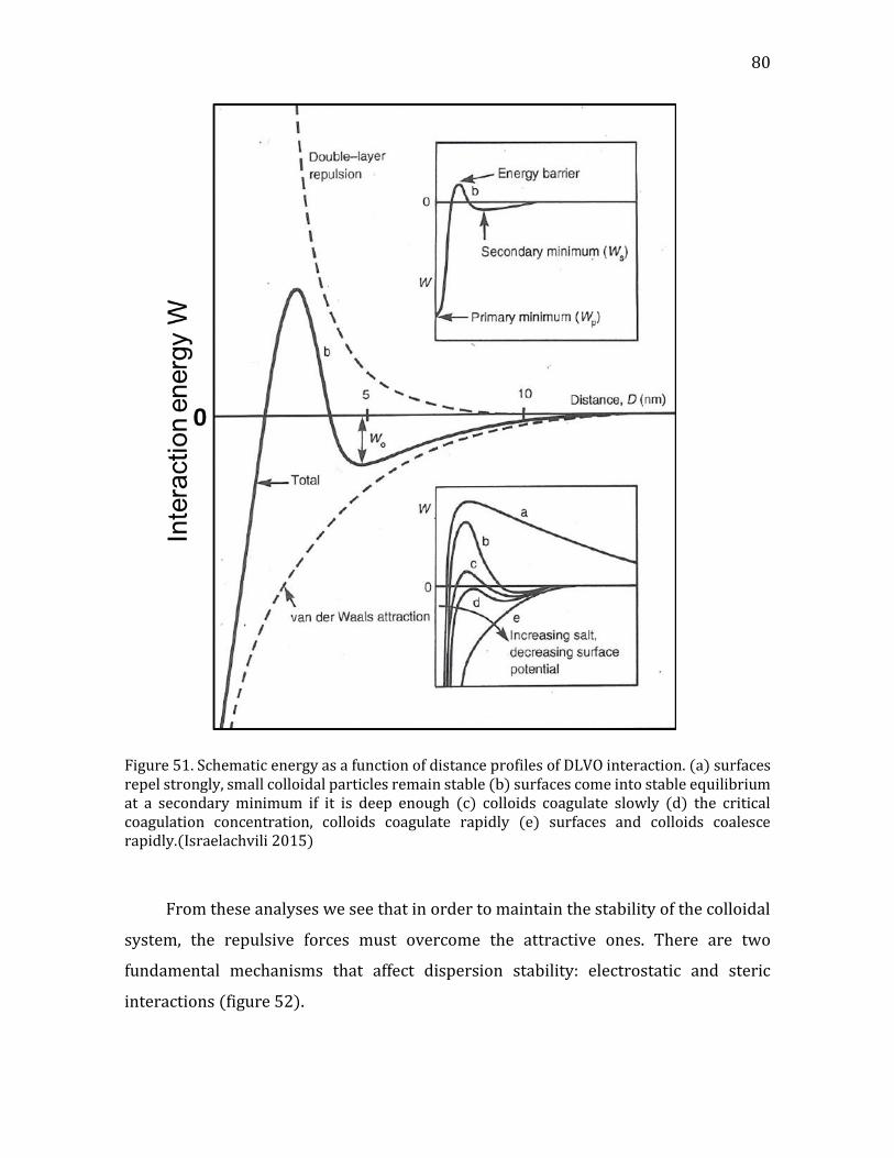
80
Figure 51. Schematic energy as a function of distance profiles of DLVO interaction. (a) surfaces repel strongly, small colloidal particles remain stable (b) surfaces come into stable equilibrium at a secondary minimum if it is deep enough (c) colloids coagulate slowly (d) the critical coagulation concentration, colloids coagulate rapidly (e) surfaces and colloids coalesce rapidly.(Israelachvili 2015)
From these analyses we see that in order to maintain the stability of the colloidal
system, the repulsive forces must overcome the attractive ones. There are two
fundamental mechanisms that affect dispersion stability: electrostatic and steric
interactions (figure 52).

81 CHAPTER 4. INTERACTION STUDIES
Figure 52. Steric (a) Vs electrostatic (b) colloidal stabilization mechanisms.
(i) Steric repulsion - involves polymers added to the system adsorbing onto the
particle surface and preventing the particle surfaces coming into close contact. If
enough polymer adsorbs, the thickness of the coating will be sufficient to keep
particles separated by steric repulsions (excluded volume) between the polymer
layers, and at those separations the VdW forces are too weak to cause the particles
to adhere.
(ii) Electrostatic or charge stabilization - this is the effect on particle interaction due
to the distribution of charged species in the system and greatly affected by the
charge and size of the particle and the ionic strength of the medium.
DLVO theory gained appreciation in the scientific community thanks to its intuitive
nature and the successful match to experimental results. However, it fails at high salt
concentrations, and other forces beyond the DLVO construct (e.g., hydrogen bonding
and the hydrophobic effect, hydration pressure, charge transfer, Lewis acid base
interactions, and steric interactions) have been reported to also play a major role in
determining colloid stability.(Hesselink, et al. 1971)
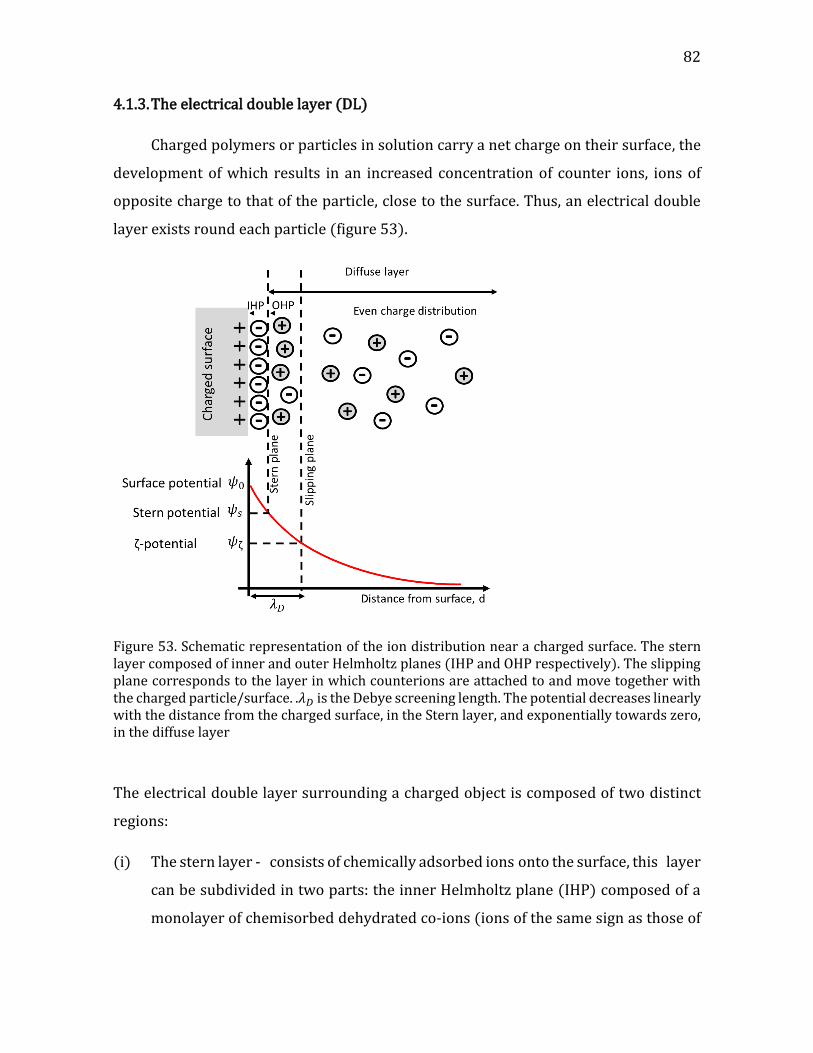
82
4.1.3. The electrical double layer (DL)
Charged polymers or particles in solution carry a net charge on their surface, the
development of which results in an increased concentration of counter ions, ions of
opposite charge to that of the particle, close to the surface. Thus, an electrical double
layer exists round each particle (figure 53).
Figure 53. Schematic representation of the ion distribution near a charged surface. The stern layer composed of inner and outer Helmholtz planes (IHP and OHP respectively). The slipping plane corresponds to the layer in which counterions are attached to and move together with the charged particle/surface. .𝜆𝐷 is the Debye screening length. The potential decreases linearly with the distance from the charged surface, in the Stern layer, and exponentially towards zero, in the diffuse layer
The electrical double layer surrounding a charged object is composed of two distinct
regions:
(i) The stern layer - consists of chemically adsorbed ions onto the surface, this layer
can be subdivided in two parts: the inner Helmholtz plane (IHP) composed of a
monolayer of chemisorbed dehydrated co-ions (ions of the same sign as those of
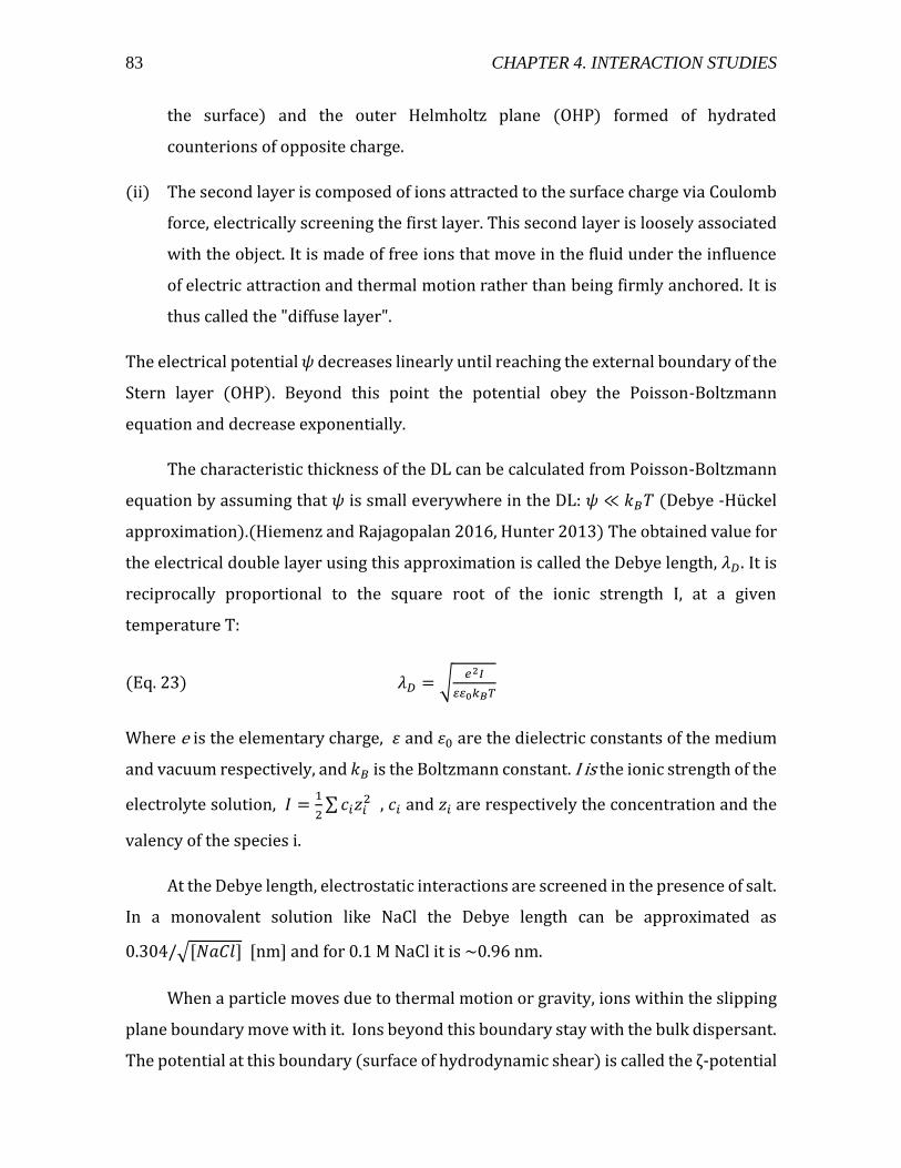
83 CHAPTER 4. INTERACTION STUDIES
the surface) and the outer Helmholtz plane (OHP) formed of hydrated
counterions of opposite charge.
(ii) The second layer is composed of ions attracted to the surface charge via Coulomb
force, electrically screening the first layer. This second layer is loosely associated
with the object. It is made of free ions that move in the fluid under the influence
of electric attraction and thermal motion rather than being firmly anchored. It is
thus called the "diffuse layer".
The electrical potential 𝜓 decreases linearly until reaching the external boundary of the
Stern layer (OHP). Beyond this point the potential obey the Poisson-Boltzmann
equation and decrease exponentially.
The characteristic thickness of the DL can be calculated from Poisson-Boltzmann
equation by assuming that 𝜓 is small everywhere in the DL: 𝜓 ≪ 𝑘𝐵𝑇 (Debye -Hückel
approximation).(Hiemenz and Rajagopalan 2016, Hunter 2013) The obtained value for
the electrical double layer using this approximation is called the Debye length, 𝜆𝐷. It is
reciprocally proportional to the square root of the ionic strength I, at a given
temperature T:
(Eq. 23) 𝜆𝐷 = √𝑒2𝐼
0𝑘𝐵𝑇
Where e is the elementary charge, 휀 and 휀0 are the dielectric constants of the medium
and vacuum respectively, and 𝑘𝐵 is the Boltzmann constant. I is the ionic strength of the
electrolyte solution, 𝐼 =1
2∑ 𝑐𝑖𝑧𝑖
2 , 𝑐𝑖 and 𝑧𝑖 are respectively the concentration and the
valency of the species i.
At the Debye length, electrostatic interactions are screened in the presence of salt.
In a monovalent solution like NaCl the Debye length can be approximated as
0.304/√[𝑁𝑎𝐶𝑙] [nm] and for 0.1 M NaCl it is ~0.96 nm.
When a particle moves due to thermal motion or gravity, ions within the slipping
plane boundary move with it. Ions beyond this boundary stay with the bulk dispersant.
The potential at this boundary (surface of hydrodynamic shear) is called the ζ-potential
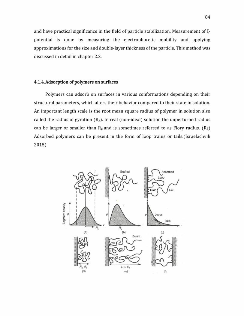
84
and have practical significance in the field of particle stabilization. Measurement of ζ-
potential is done by measuring the electrophoretic mobility and applying
approximations for the size and double-layer thickness of the particle. This method was
discussed in detail in chapter 2.2.
4.1.4. Adsorption of polymers on surfaces
Polymers can adsorb on surfaces in various conformations depending on their
structural parameters, which alters their behavior compared to their state in solution.
An important length scale is the root mean square radius of polymer in solution also
called the radius of gyration (Rg). In real (non-ideal) solution the unperturbed radius
can be larger or smaller than Rg and is sometimes referred to as Flory radius. (RF)
Adsorbed polymers can be present in the form of loop trains or tails.(Israelachvili
2015)
85 CHAPTER 4. INTERACTION STUDIES
Figure 54. (a) Polymer in solution (b) chemisorbed (end-grafted) copolymer (c) physiosorbed homopolymer (d) adsorption at low surface coverage with no nearest neighbor overlap (e) adsorption at high coverage (brush) (f) bridging.(Israelachvili 2015)
Figure 54 shows schematic representation of the behavior of polymers near
surfaces. The segment density, ρ , as a function of the distance, r, from a surface is shown
in figure 54 a b and c, for a free, grafted and adsorbed polymers respectively, the radius
of gyration, Rg, is also indicated.
The conformation of the polymer, often depends on the concentration and
solvent, can determine the nature of adsorption as well as the surface coverage. In
addition, when additional surface is added, like in the case of layered structures,
bridging forces come into play, presenting an additional mechanism of interaction.
These features are characteristic for polyelectrolytes as well as for non-charged
polymers and can determine the structural properties of biomimetic constructs.
After revising the importance of intermolecular forces in governing interaction
phenomena, we will now present the main results from the interaction studies between
the selected building blocks.
4.2. CNC-Lipids
4.2.1. Interaction of CNCs with lipid vesicles
In this study, we used CNCs and liposomes made from the zwitterionic lipid 1,2-
dioleoyl-sn-glycero-3-phosphocholine (DOPC), from the phospholipid family, the main
group of lipids in the plasma membrane (up to 60% of the lipids in plasma membrane
are phospholipids (Furt, et al. 2011, Liu, et al. 2015)), with the purpose of studying the
interaction between these two representative components of PCWs.
As shown in chapter 3.1.2, CNC are negatively charged, regardless of the pH due
to sulfate half-ester groups on their surface. However, DOPC is zwitterionic, meaning
that its charge is dependent on the pH of the solution in which it is dissolved. We
86
therefore combined several characterization techniques in order to test the effect of pH
on the interaction between DOPC liposomes and cotton CNCs. Dynamic light scattering
(DLS) and electrophoretic mobility measurements respectively provided the size and
ζ-potential values for both CNCs and liposomes. ITC was used to obtain the
thermodynamic parameters of the interaction, and cryo-transmission electron
microscopy (cryo-TEM) was used to directly visualize the CNC/liposome complexes.
4.2.1.1. Materials and methods
Materials
Acetic acid, sodium hydroxide, sodium acetate, sodium chloride (99% pure or
higher) were purchased from Sigma Aldrich (Germany). Phosphate buffered saline
(PBS) tablets were purchased from Sigma Aldrich and dissolved in 200 mL of deionized
water followed by dilution to the desired concentration and ionic strength. 1,2-dioleoyl-
sn-glycero-3-phosphatidylcholine (DOPC) and 1,2-dioleoyl-3-trimethylammonium-
propane (DOTAP) was purchased from Avanti Polar Lipids Inc. (Birmingham, USA) and
dissolved without further purification in a chloroform/methanol mixture (9/1 v/v) to
a total concentration of 10 mg mL-1. The solutions were stored at -20 °C until use. All
other reagents were of analytical grade. All solutions were prepared using deionized
water from Milli-Q Millipore system with a resistivity of 18.2 Ω cm. Aqueous acetic
acid/sodium acetate buffer was prepared at a total concentration of 100 mM to obtain
a solution with pH 3. 120 mM PBS buffer adjusted with small amounts of 0.1 M
HCl/NaOH was used to prepare a pH 7 buffer.
Preparation of LUVs
The lipid solution (DOPC or 70/30 mol % / mol % DOPC/DOTAP) in 9/1 v/v
chloroform/methanol mixture was transferred into a round-bottom flask and the
organic solvent was removed by evaporation under high vacuum pumping for 2 h, until
complete evaporation of the solvent. The lipid film was then hydrated in an appropriate
amount of buffer solution at room temperature well above the melting point of the
lipids to yield suspensions with concentrations of 0.5 – 2.8 mM. Multilamellar vesicles
87 CHAPTER 4. INTERACTION STUDIES
were then obtained by vortexing for 30 min. The resulting suspensions were then
successively extruded 20 times through 200 and 100 nm polycarbonate membranes
using a miniextruder (Avanti Polar Lipids). The vesicle size distribution was finally
characterized by dynamic light scattering measurements.
Preparation of CNCs
According to the method described by Revol et al., (Revol, et al. 1992) CNC
suspensions were prepared by acid hydrolysis of cotton linters (Buckeye Cellulose
Corporation, USA). The almost pure cellulosic substrate was treated with 65 % sulfuric
acid during 30 min at 63 °C. The suspensions were washed by repeated centrifugations,
dialyzed against distilled water until constant conductivity of the dialysis bath and
ultrasonicated for 4 min with a Branson Digital sonifier (Emerson, USA) After these
treatments, the suspensions were filtered through 8 μm then 1 μm cellulose nitrate
membranes (Sartorius). The resulting CNC suspensions had a dry mass content of 2.0
± 0.1 wt. %. They were then mixed with the appropriate buffer solution to reach a total
ionic strength of 100 mM and the pH (2, 3, 5 or 7) was adjusted using small amounts of
0.1 M HCl/NaOH. The final CNC concentration was 1.0 ± 0.1 wt. %.
Dynamic Light Scattering (DLS) and ζ-potential
DLS measurements were performed with a Malvern NanoZS instrument operating
with a 2 mW HeNe laser at a wavelength of 632.8 nm and detection at an angle of 173°.
All measurements were performed in a temperature-controlled chamber at 20 °C
(±0.05 °C). Three measurements of 15 runs each were usually averaged. The intensity
size distribution was obtained from the analysis of the correlation function using the
multiple narrow mode algorithm of the Malvern DTS software. The electrophoretic
mobility of vesicles and CNCs was measured by using the same Malvern NanoZS
apparatus performing at 17° from which the ζ-potential values are determined by
applying the Henry equation. The ζ-potential values and the ζ-deviation were averaged
over at least 3 measurements with at least 30 runs per measurement was expressed as
mean ± SD (n≥3).
88
Isothermal Titration Calorimetry (ITC)
ITC measurements were performed with a VP-ITC microcalorimeter from
MicroCal Inc. (Northampton, MA). All samples were degassed using an apparatus
provided by MicroCal for 10 min shortly before starting the measurements in order to
avoid the presence of air bubbles. The working cell (1.447 mL in volume) was filled
with the liposome suspension (0.5 – 2.8 mM initial concentrations) at a given pH. One
aliquot of 5 μL followed by 28 aliquots of 10 μL of a 0.5 – 1 wt. % CNC suspension (at
the same pH as the liposome suspension) were injected stepwise with 300 s intervals
into the working cell filled with the vesicle suspension. During the measurement, the
sample cell was constantly stirred at a rate of 307 rpm and the measurements were
performed at 25 °C. The data analyses were carried out using the Origin software
provided by MicroCal.(MicroCal 2004) The heat of dilution, ∆𝐻𝑑 ,was determined in
control experiments by injecting the CNC suspension into the corresponding buffer
solution. The heats of dilution were subtracted from the heats determined in the
corresponding CNC-lipid binding experiments noted as ∆𝐻𝑖. The quantitative
evaluation of ΔH from the experimental data was thus based on the relationship:
(Eq. 24) ∆𝐻 = ∆𝐻𝑖 − ∆𝐻𝑑
Transmission Electron Microscopy (TEM)
Drops of ca. 0.001 wt.% CNC or CNC / liposomes suspensions were deposited onto
carbon-coated TEM grids freshly glow-discharged in an easiGlow plasma cleaning
system (Pelco). After 2 min, the liquid in excess was blotted away with filter paper and
a drop of 2 wt.% uranyl acetate negative stain was deposited before complete drying.
After 2 min, the stain in excess was blotted and the remaining thin liquid film was
allowed to dry. Cryo-TEM specimens were prepared by quench-freezing thin films of
ca. 0.1 wt. % CNC / liposome suspensions formed on NetMesh lacy carbon films (Pelco)
into liquid ethane, using a Leica EM-GP fast-freezing workstation equipped with a
temperature- and humidity-controlled chamber. The specimens were mounted in a
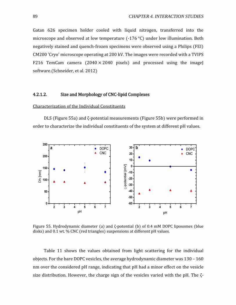
89 CHAPTER 4. INTERACTION STUDIES
Gatan 626 specimen holder cooled with liquid nitrogen, transferred into the
microscope and observed at low temperature (-176 °C) under low illumination. Both
negatively stained and quench-frozen specimens were observed using a Philips (FEI)
CM200 'Cryo' microscope operating at 200 kV. The images were recorded with a TVIPS
F216 TemCam camera (2040 × 2040 pixels) and processed using the imageJ
software.(Schneider, et al. 2012)
4.2.1.2. Size and Morphology of CNC-lipid Complexes
Characterization of the Individual Constituents
DLS (Figure 55a) and ζ-potential measurements (Figure 55b) were performed in
order to characterize the individual constituents of the system at different pH values.
Figure 55. Hydrodynamic diameter (a) and ζ-potential (b) of 0.4 mM DOPC liposomes (blue disks) and 0.1 wt. % CNC (red triangles) suspensions at different pH values.
Table 11 shows the values obtained from light scattering for the individual
objects. For the bare DOPC vesicles, the average hydrodynamic diameter was 130 – 160
nm over the considered pH range, indicating that pH had a minor effect on the vesicle
size distribution. However, the charge sign of the vesicles varied with the pH. The ζ-
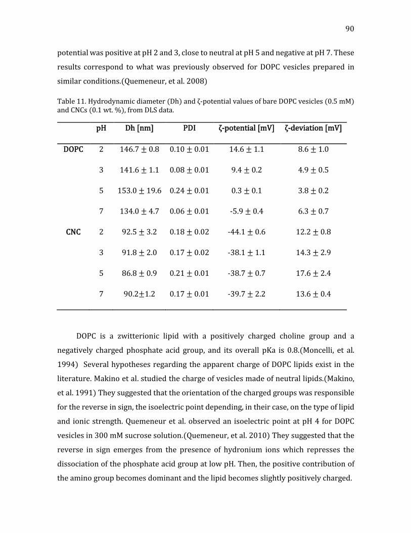
90
potential was positive at pH 2 and 3, close to neutral at pH 5 and negative at pH 7. These
results correspond to what was previously observed for DOPC vesicles prepared in
similar conditions.(Quemeneur, et al. 2008)
Table 11. Hydrodynamic diameter (Dh) and ζ-potential values of bare DOPC vesicles (0.5 mM) and CNCs (0.1 wt. %), from DLS data.
pH Dh [nm] PDI ζ-potential [mV] ζ-deviation [mV]
DOPC 2 146.7 ± 0.8 0.10 ± 0.01 14.6 ± 1.1 8.6 ± 1.0
3 141.6 ± 1.1 0.08 ± 0.01 9.4 ± 0.2 4.9 ± 0.5
5 153.0 ± 19.6 0.24 ± 0.01 0.3 ± 0.1 3.8 ± 0.2
7 134.0 ± 4.7 0.06 ± 0.01 -5.9 ± 0.4 6.3 ± 0.7
CNC 2 92.5 ± 3.2 0.18 ± 0.02 -44.1 ± 0.6 12.2 ± 0.8
3 91.8 ± 2.0 0.17 ± 0.02 -38.1 ± 1.1 14.3 ± 2.9
5 86.8 ± 0.9 0.21 ± 0.01 -38.7 ± 0.7 17.6 ± 2.4
7 90.2±1.2 0.17 ± 0.01 -39.7 ± 2.2 13.6 ± 0.4
DOPC is a zwitterionic lipid with a positively charged choline group and a
negatively charged phosphate acid group, and its overall pKa is 0.8.(Moncelli, et al.
1994) Several hypotheses regarding the apparent charge of DOPC lipids exist in the
literature. Makino et al. studied the charge of vesicles made of neutral lipids.(Makino,
et al. 1991) They suggested that the orientation of the charged groups was responsible
for the reverse in sign, the isoelectric point depending, in their case, on the type of lipid
and ionic strength. Quemeneur et al. observed an isoelectric point at pH 4 for DOPC
vesicles in 300 mM sucrose solution.(Quemeneur, et al. 2010) They suggested that the
reverse in sign emerges from the presence of hydronium ions which represses the
dissociation of the phosphate acid group at low pH. Then, the positive contribution of
the amino group becomes dominant and the lipid becomes slightly positively charged.
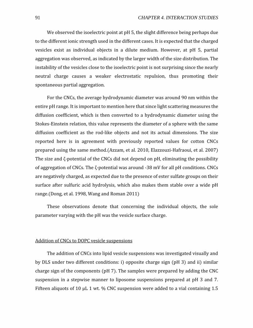
91 CHAPTER 4. INTERACTION STUDIES
We observed the isoelectric point at pH 5, the slight difference being perhaps due
to the different ionic strength used in the different cases. It is expected that the charged
vesicles exist as individual objects in a dilute medium. However, at pH 5, partial
aggregation was observed, as indicated by the larger width of the size distribution. The
instability of the vesicles close to the isoelectric point is not surprising since the nearly
neutral charge causes a weaker electrostatic repulsion, thus promoting their
spontaneous partial aggregation.
For the CNCs, the average hydrodynamic diameter was around 90 nm within the
entire pH range. It is important to mention here that since light scattering measures the
diffusion coefficient, which is then converted to a hydrodynamic diameter using the
Stokes-Einstein relation, this value represents the diameter of a sphere with the same
diffusion coefficient as the rod-like objects and not its actual dimensions. The size
reported here is in agreement with previously reported values for cotton CNCs
prepared using the same method.(Azzam, et al. 2010, Elazzouzi-Hafraoui, et al. 2007)
The size and ζ-potential of the CNCs did not depend on pH, eliminating the possibility
of aggregation of CNCs. The ζ-potential was around -38 mV for all pH conditions. CNCs
are negatively charged, as expected due to the presence of ester sulfate groups on their
surface after sulfuric acid hydrolysis, which also makes them stable over a wide pH
range.(Dong, et al. 1998, Wang and Roman 2011)
These observations denote that concerning the individual objects, the sole
parameter varying with the pH was the vesicle surface charge.
Addition of CNCs to DOPC vesicle suspensions
The addition of CNCs into lipid vesicle suspensions was investigated visually and
by DLS under two different conditions: i) opposite charge sign (pH 3) and ii) similar
charge sign of the components (pH 7). The samples were prepared by adding the CNC
suspension in a stepwise manner to liposome suspensions prepared at pH 3 and 7.
Fifteen aliquots of 10 μL 1 wt. % CNC suspension were added to a vial containing 1.5
92
mL of 0.5 mM lipid vesicles. Mixtures of DOPC vesicles with 0.01, 0.05, and 0.1 wt. %
CNCs were transferred to the NanoZS chamber for inspection.
Table 12 and figure 56 shows the variation of the average hydrodynamic diameter
obtained by the titration of a vesicle suspension (0.5 mM DOPC) with different amounts
of a 1 wt. % CNC suspension at two different pH values. At pH 3, with the addition of
CNCs, the average size of the objects in the medium increases and the distribution
becomes wider
Table 12. Hydrodynamic diameter (Dh) of DOPC+CNC complexes at pH 3 and 7.
pH CCNC [wt. %] Dh [nm] PDI
3 0.001 428.6 ± 33.1 0.25 ± 0.01
0.01 1808.7 ± 161.1 0.27 ± 0.15
0.1 2140.3 ± 351.7 0.29 ± 0.06
7 0.001 133.7 ± 5.6 0.09 ± 0.03
0.01 131.3 ± 3.4 0.14 ± 0.01
0.1 126.0 ± 4.2 0.16 ± 0.01
The results demonstrate the formation of large complexes at pH 3. At pH 7, no
particles larger than the initial objects were detected upon addition of CNCs, implying
that no aggregation occurred at this pH.

93 CHAPTER 4. INTERACTION STUDIES
Figure 56. Hydrodynamic diameter variations upon addition of CNCs into a DOPC vesicle suspension (CDOPC = 0.5 mM) at pH 3 (blue disks) and pH 7 (orange triangles) at a constant ionic strength of 100 mM. Insets are photographs of the mixtures, taken 24 h after mixing, corresponding to the addition of 0.1 wt. % CNC at the two different pH values.
As shown in the insets of Figure 56, a clear difference between mixtures prepared
at pH 3 and 7 was observed for the addition of CNCs into a suspension of lipid vesicles.
At pH 3, aggregation, indicated by the immediate increase in turbidity, was detected
with the addition of negatively charged CNCs to positively charged vesicles. However,
at pH 7, no such aggregation was observed and the suspension was stable over a period
of several weeks. It is suggested that the stability of the suspension at pH 7 arises from
CNC-CNC, vesicle-vesicle and vesicle-CNC electrostatic repulsions due to the similar
charge of the components.
Similar observations were made for the interaction of CNCs with cationic double
tailed (Oikonomou, et al. 2017, Oikonomou, et al. 2018) and single tailed (Dhar, et al.
2012) surfactants, where addition of oppositely charged amphiphiles resulted in CNC
aggregation.
Furthermore, this also demonstrates the efficiency of light scattering to probe, in
more detail, the formation of complexes, as previously shown by Berret et al. for
94
electrostatic polymer-particle (Berret 2007) and lipid-nanoparticle (Mousseau and
Berret 2018, Mousseau, et al. 2018) interactions.
In order to gain further information on the system, we investigated the interaction
at different pH using TEM.
4.2.1.3. Electron microscopy observations of CNC-liposome complexes
The addition of CNCs into liposome suspensions was monitored by TEM. First,
each component was imaged individually for reference. Figure 57a is a micrograph of
CNCs dried from an aqueous suspension at pH 3. Negative staining was used to provide
more contrast. The rod-like particles have a length of 50 - 200 nm and a width of 10 - 20
nm, which are typical dimensions for cotton CNCs. These CNCs are made of
3 - 5 elementary crystallites that were not separated during the acid hydrolysis and
subsequent sonication treatment.(Elazzouzi-Hafraoui, et al. 2007) The particles are
well dispersed due to the electrostatic repulsion from the charged sulfate groups on the
particle surface, as previously explained.
Figures 57b and 57c show cryo-TEM micrographs of bare DOPC vesicles
embedded in a film of vitreous ice at pH 3 and 7, respectively. At pH 3, the vesicles were
mostly unilamellar and spherical with a diameter ranging from 100 to 200 nm, in fair
agreement with the dimensions measured by DLS. A small number of multilamellar and
elongated vesicles were also observed. At pH 7, the vesicles were mostly multilamellar
with a diameter ranging from 100 to 200 nm. The vesicles were mostly spherical but
several elongated objects were observed.
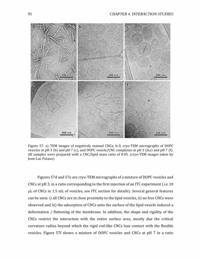
95 CHAPTER 4. INTERACTION STUDIES
Figure 57. a) TEM images of negatively stained CNCs; b-f) cryo-TEM micrographs of DOPC vesicles at pH 3 (b) and pH 7 (c), and DOPC vesicle/CNC complexes at pH 3 (d,e) and pH 7 (f). All samples were prepared with a CNC/lipid mass ratio of 0.05. (cryo-TEM images taken by Jean-Luc Putaux)
Figures 57d and 57e are cryo-TEM micrographs of a mixture of DOPC vesicles and
CNCs at pH 3, in a ratio corresponding to the first injection of an ITC experiment (i.e. 10
μL of CNCs in 1.5 mL of vesicles, see ITC section for details). Several general features
can be seen: i) all CNCs are in close proximity to the lipid vesicles, ii) no free CNCs were
observed and iii) the adsorption of CNCs onto the surface of the lipid vesicle induced a
deformation / flattening of the membrane. In addition, the shape and rigidity of the
CNCs restrict the interaction with the entire surface area, mostly due the critical
curvature radius beyond which the rigid rod-like CNCs lose contact with the flexible
vesicles. Figure 57f shows a mixture of DOPC vesicles and CNCs at pH 7 in a ratio
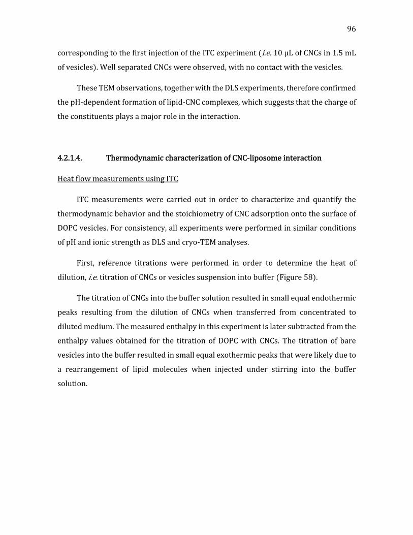
96
corresponding to the first injection of the ITC experiment (i.e. 10 μL of CNCs in 1.5 mL
of vesicles). Well separated CNCs were observed, with no contact with the vesicles.
These TEM observations, together with the DLS experiments, therefore confirmed
the pH-dependent formation of lipid-CNC complexes, which suggests that the charge of
the constituents plays a major role in the interaction.
4.2.1.4. Thermodynamic characterization of CNC-liposome interaction
Heat flow measurements using ITC
ITC measurements were carried out in order to characterize and quantify the
thermodynamic behavior and the stoichiometry of CNC adsorption onto the surface of
DOPC vesicles. For consistency, all experiments were performed in similar conditions
of pH and ionic strength as DLS and cryo-TEM analyses.
First, reference titrations were performed in order to determine the heat of
dilution, i.e. titration of CNCs or vesicles suspension into buffer (Figure 58).
The titration of CNCs into the buffer solution resulted in small equal endothermic
peaks resulting from the dilution of CNCs when transferred from concentrated to
diluted medium. The measured enthalpy in this experiment is later subtracted from the
enthalpy values obtained for the titration of DOPC with CNCs. The titration of bare
vesicles into the buffer resulted in small equal exothermic peaks that were likely due to
a rearrangement of lipid molecules when injected under stirring into the buffer
solution.
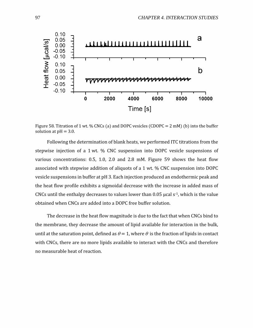
97 CHAPTER 4. INTERACTION STUDIES
Figure 58. Titration of 1 wt. % CNCs (a) and DOPC vesicles (CDOPC = 2 mM) (b) into the buffer solution at pH = 3.0.
Following the determination of blank heats, we performed ITC titrations from the
stepwise injection of a 1 wt. % CNC suspension into DOPC vesicle suspensions of
various concentrations: 0.5, 1.0, 2.0 and 2.8 mM. Figure 59 shows the heat flow
associated with stepwise addition of aliquots of a 1 wt. % CNC suspension into DOPC
vesicle suspensions in buffer at pH 3. Each injection produced an endothermic peak and
the heat flow profile exhibits a sigmoidal decrease with the increase in added mass of
CNCs until the enthalpy decreases to values lower than 0.05 µcal s-1, which is the value
obtained when CNCs are added into a DOPC free buffer solution.
The decrease in the heat flow magnitude is due to the fact that when CNCs bind to
the membrane, they decrease the amount of lipid available for interaction in the bulk,
until at the saturation point, defined as = 1, where is the fraction of lipids in contact
with CNCs, there are no more lipids available to interact with the CNCs and therefore
no measurable heat of reaction.
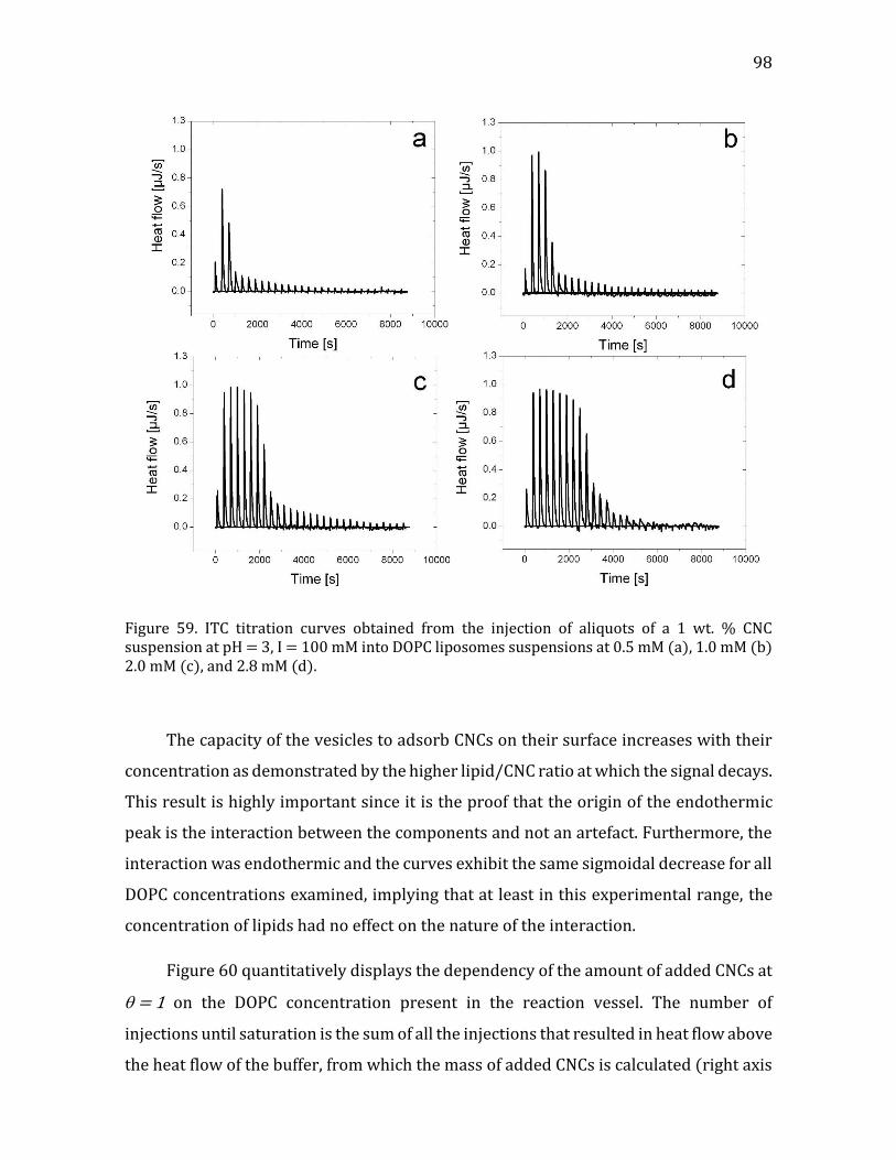
98
Figure 59. ITC titration curves obtained from the injection of aliquots of a 1 wt. % CNC suspension at pH = 3, I = 100 mM into DOPC liposomes suspensions at 0.5 mM (a), 1.0 mM (b) 2.0 mM (c), and 2.8 mM (d).
The capacity of the vesicles to adsorb CNCs on their surface increases with their
concentration as demonstrated by the higher lipid/CNC ratio at which the signal decays.
This result is highly important since it is the proof that the origin of the endothermic
peak is the interaction between the components and not an artefact. Furthermore, the
interaction was endothermic and the curves exhibit the same sigmoidal decrease for all
DOPC concentrations examined, implying that at least in this experimental range, the
concentration of lipids had no effect on the nature of the interaction.
Figure 60 quantitatively displays the dependency of the amount of added CNCs at
= 1 on the DOPC concentration present in the reaction vessel. The number of
injections until saturation is the sum of all the injections that resulted in heat flow above
the heat flow of the buffer, from which the mass of added CNCs is calculated (right axis
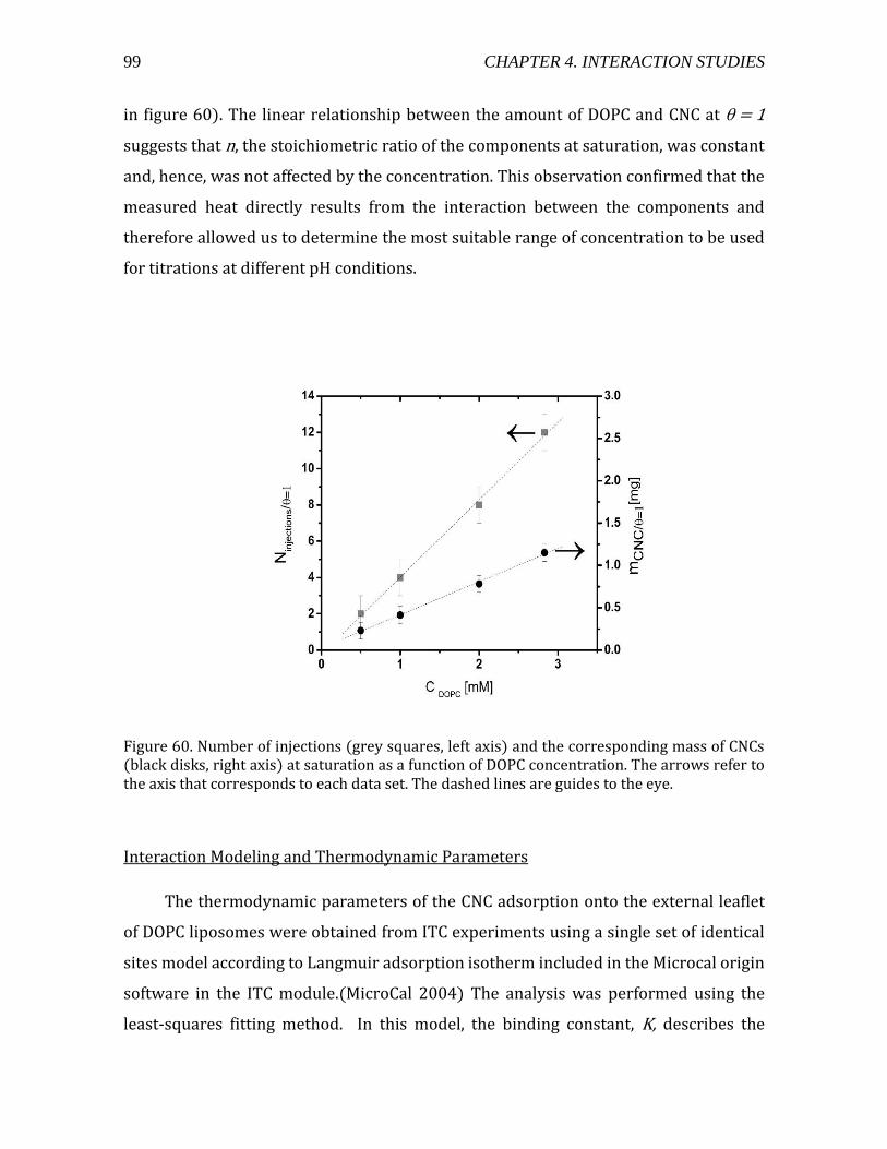
99 CHAPTER 4. INTERACTION STUDIES
in figure 60). The linear relationship between the amount of DOPC and CNC at = 1
suggests that n, the stoichiometric ratio of the components at saturation, was constant
and, hence, was not affected by the concentration. This observation confirmed that the
measured heat directly results from the interaction between the components and
therefore allowed us to determine the most suitable range of concentration to be used
for titrations at different pH conditions.
Figure 60. Number of injections (grey squares, left axis) and the corresponding mass of CNCs (black disks, right axis) at saturation as a function of DOPC concentration. The arrows refer to the axis that corresponds to each data set. The dashed lines are guides to the eye.
Interaction Modeling and Thermodynamic Parameters
The thermodynamic parameters of the CNC adsorption onto the external leaflet
of DOPC liposomes were obtained from ITC experiments using a single set of identical
sites model according to Langmuir adsorption isotherm included in the Microcal origin
software in the ITC module.(MicroCal 2004) The analysis was performed using the
least-squares fitting method. In this model, the binding constant, K, describes the

100
equilibrium between the concentration of the lipid-CNC complex and the
concentrations of the free constituents can be expressed as:
(Eq. 25) K =θ
(1−θ)[X]
where is the mass fraction of lipid occupied by CNC and [X] is the concentration of
free CNCs which can be expressed as:
(Eq. 26) [X] = Xt − nθMt
where Xt and Mt are the bulk concentrations of CNC and DOPC, respectively, and n
represents the number of binding sites. In our case, since the concentration are
expressed as mass ratios, n no longer represent the number of binding sites but the
exact mass ratio as derived from the fitting procedure.
Substituting the expression for [X] given in eq. 26 into eq. 25 yields a quadratic
equation for the surface fraction θ. Solving this equation provides an expression for
as a function of the lipid concentration. Then, the total heat content, Q, of the solution
contained in the experimental volume Vo at a given is:
(Eq. 27) Q = nθMtΔHV0
where ΔH is the enthalpy of CNC binding to a unit of mass on the membrane. Fitting the
experimentally measured heat release for each step of injection with the expression in
eq. 27 provides the fitting parameters n, K and ΔH.
Figure 61 shows ITC curves of titration of DOPC vesicles (CDOPC = 2 mM) with ~1 wt. %
CNC suspensions at pH 2, 3, 5, and 7.
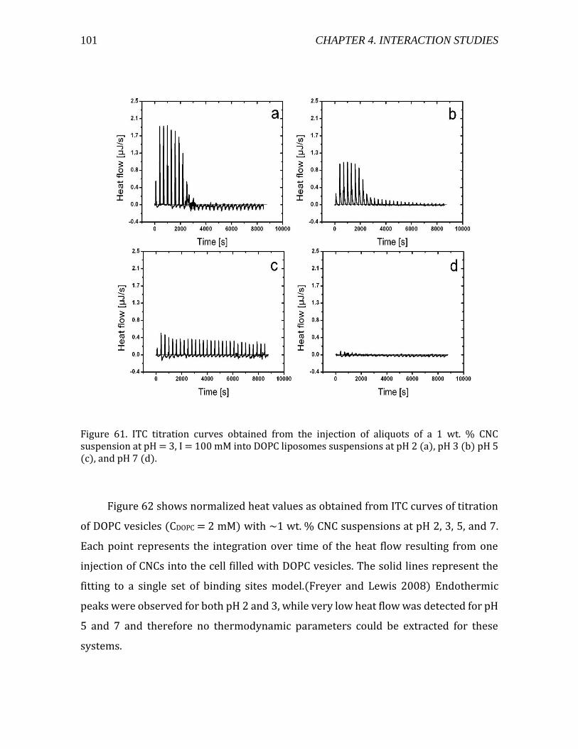
101 CHAPTER 4. INTERACTION STUDIES
Figure 61. ITC titration curves obtained from the injection of aliquots of a 1 wt. % CNC suspension at pH = 3, I = 100 mM into DOPC liposomes suspensions at pH 2 (a), pH 3 (b) pH 5 (c), and pH 7 (d).
Figure 62 shows normalized heat values as obtained from ITC curves of titration
of DOPC vesicles (CDOPC = 2 mM) with ~1 wt. % CNC suspensions at pH 2, 3, 5, and 7.
Each point represents the integration over time of the heat flow resulting from one
injection of CNCs into the cell filled with DOPC vesicles. The solid lines represent the
fitting to a single set of binding sites model.(Freyer and Lewis 2008) Endothermic
peaks were observed for both pH 2 and 3, while very low heat flow was detected for pH
5 and 7 and therefore no thermodynamic parameters could be extracted for these
systems.

102
Figure 62. Total heat for the titration of DOPC liposomes (CDOPC = 2 mM) by CNCs (1 wt. %) extracted from the modeling of ITC data at pH 2 (red), 3 (blue), 5 (green) and 7 (orange).
The values of the thermodynamic parameters normalized to the mass of CNCs are
presented in Table 13. Since the exact number of CNC particles is unknown, we could
only obtain the stoichiometric ratio, n, the enthalpy of the process, ΔH and the binding
constant, Ka. The amount of heat adsorbed per unit of mass of CNCs was larger at pH 2
than at pH 3 and no heat flow was detected as a result from titrations at pH 5 and 7
where the components possess a similar negative charge sign.
At pH 2 and 3, where the charge sign of the components is opposite, an
endothermic interaction was detected with larger values of enthalpy and association
constant at pH 2. The enthalpy values were 1.36 ± 0.08 and 0.70 ± 0.16 J g-1 at pH 2 and
3, respectively. The association constant, Ka, is a measure of the affinity of the objects
under inspection, the higher Ka, the stronger the association. Ka was 475 and 48 L g-1 at
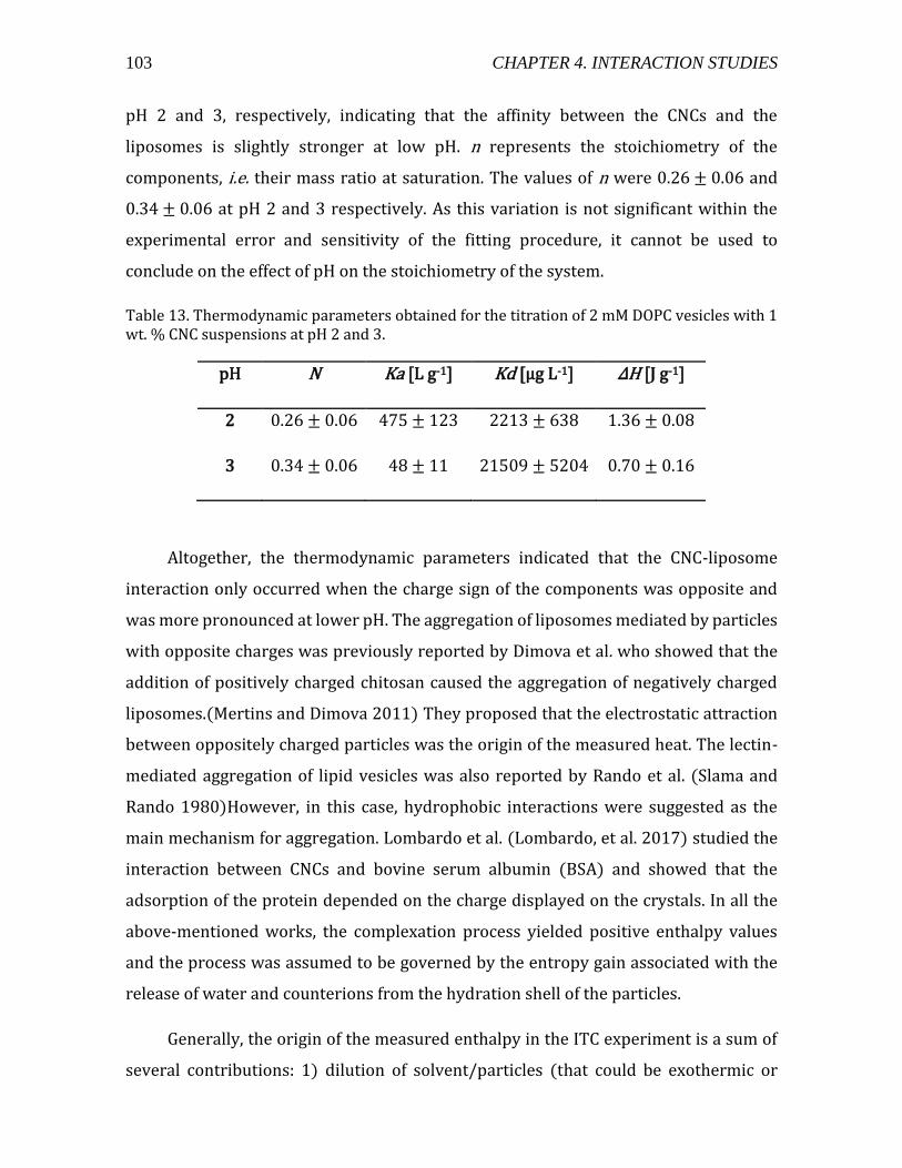
103 CHAPTER 4. INTERACTION STUDIES
pH 2 and 3, respectively, indicating that the affinity between the CNCs and the
liposomes is slightly stronger at low pH. n represents the stoichiometry of the
components, i.e. their mass ratio at saturation. The values of n were 0.26 ± 0.06 and
0.34 ± 0.06 at pH 2 and 3 respectively. As this variation is not significant within the
experimental error and sensitivity of the fitting procedure, it cannot be used to
conclude on the effect of pH on the stoichiometry of the system.
Table 13. Thermodynamic parameters obtained for the titration of 2 mM DOPC vesicles with 1 wt. % CNC suspensions at pH 2 and 3.
pH N Ka [L g-1] Kd [µg L-1] ΔH [J g-1]
2 0.26 ± 0.06 475 ± 123 2213 ± 638 1.36 ± 0.08
3 0.34 ± 0.06 48 ± 11 21509 ± 5204 0.70 ± 0.16
Altogether, the thermodynamic parameters indicated that the CNC-liposome
interaction only occurred when the charge sign of the components was opposite and
was more pronounced at lower pH. The aggregation of liposomes mediated by particles
with opposite charges was previously reported by Dimova et al. who showed that the
addition of positively charged chitosan caused the aggregation of negatively charged
liposomes.(Mertins and Dimova 2011) They proposed that the electrostatic attraction
between oppositely charged particles was the origin of the measured heat. The lectin-
mediated aggregation of lipid vesicles was also reported by Rando et al. (Slama and
Rando 1980)However, in this case, hydrophobic interactions were suggested as the
main mechanism for aggregation. Lombardo et al. (Lombardo, et al. 2017) studied the
interaction between CNCs and bovine serum albumin (BSA) and showed that the
adsorption of the protein depended on the charge displayed on the crystals. In all the
above-mentioned works, the complexation process yielded positive enthalpy values
and the process was assumed to be governed by the entropy gain associated with the
release of water and counterions from the hydration shell of the particles.
Generally, the origin of the measured enthalpy in the ITC experiment is a sum of
several contributions: 1) dilution of solvent/particles (that could be exothermic or
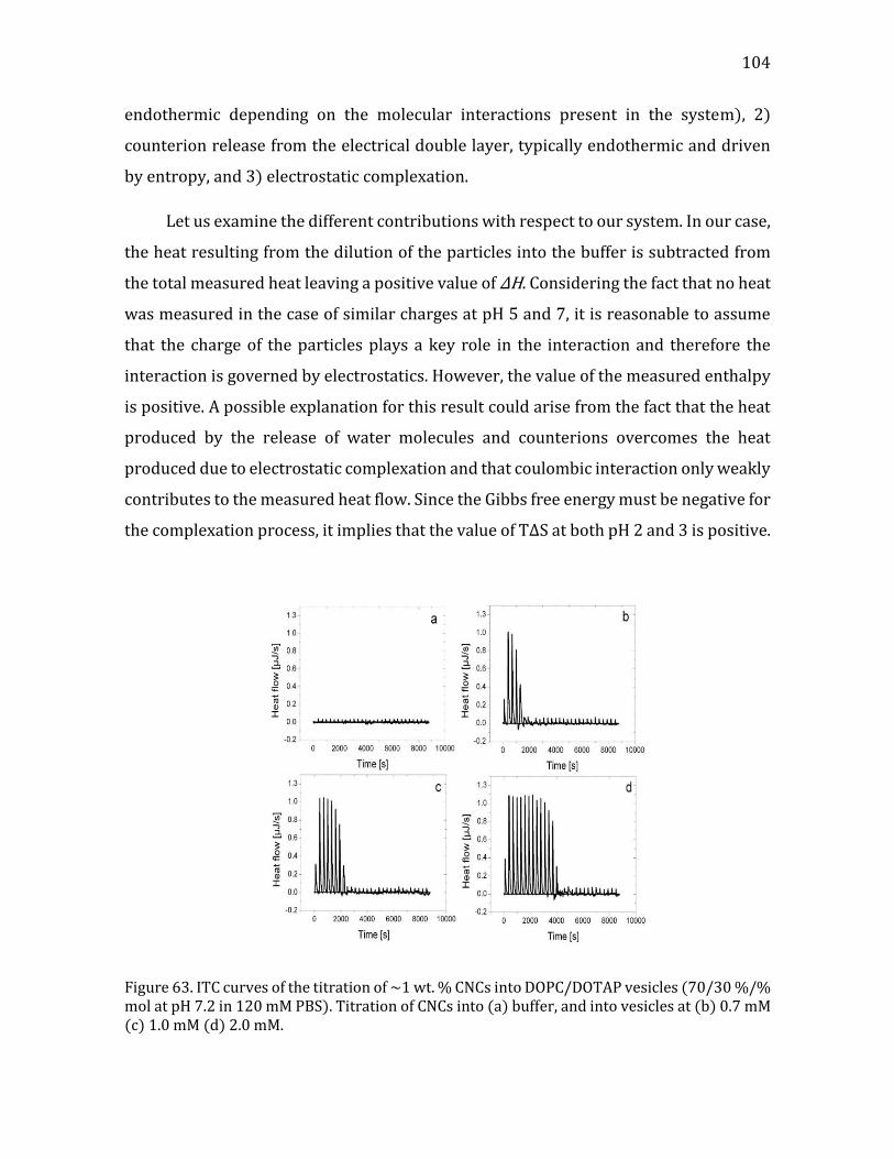
104
endothermic depending on the molecular interactions present in the system), 2)
counterion release from the electrical double layer, typically endothermic and driven
by entropy, and 3) electrostatic complexation.
Let us examine the different contributions with respect to our system. In our case,
the heat resulting from the dilution of the particles into the buffer is subtracted from
the total measured heat leaving a positive value of ΔH. Considering the fact that no heat
was measured in the case of similar charges at pH 5 and 7, it is reasonable to assume
that the charge of the particles plays a key role in the interaction and therefore the
interaction is governed by electrostatics. However, the value of the measured enthalpy
is positive. A possible explanation for this result could arise from the fact that the heat
produced by the release of water molecules and counterions overcomes the heat
produced due to electrostatic complexation and that coulombic interaction only weakly
contributes to the measured heat flow. Since the Gibbs free energy must be negative for
the complexation process, it implies that the value of TΔS at both pH 2 and 3 is positive.
Figure 63. ITC curves of the titration of ~1 wt. % CNCs into DOPC/DOTAP vesicles (70/30 %/% mol at pH 7.2 in 120 mM PBS). Titration of CNCs into (a) buffer, and into vesicles at (b) 0.7 mM (c) 1.0 mM (d) 2.0 mM.

105 CHAPTER 4. INTERACTION STUDIES
In addition, experiments were performed on DOPC/DOTAP formulations, where
the charge sign of the vesicles was positive at pH 7. The interaction profile was similar
to the one of DOPC at pH 3, yielding thermodynamic values in the same order of
magnitude as the experiments performed on pure DOPC at pH 2 and 3, in agreement
with the previous results, as shown in figure 63 and table 14.
Table 14: Hydrodynamic diameter (Dh) and ζ-potential values and thermodynamic parameters of DOPC/DOTAP vesicles as obtained from light scattering and ITC measurements respectively.
Dh [nm] ζ-potential [mV] n Ka [L g-1] Kd [µg L-1] ΔH [J g-1]
151.5±1.7 48.0±1.2a 0.39 ± 0.01 401 ± 330 3676±2238 0.99±0.02
The effective positive charge on the surface of DOPC liposomes was slightly larger
at pH 2 than at pH 3 as indicated by the ζ-potential measurements. Although the initial
concentration of lipids in the cell is the same for pH 2 and 3, perhaps due to the presence
of larger amount of multilamellar vesicles fewer lipids are available to interact, affecting
the apparent CNC/Lipid ratio required to reach saturation. However, as previously
discussed, it was not possible to obtain clear conclusion regarding the pH effect on the
stoichiometry.
We have estimated the available surface for interaction of both DOPC vesicles and
CNCs based on their average dimensions and their surface area. For 2 mM DOPC
vesicles with a lipid head area of about 0.7 nm2, assuming an interaction on the external
leaflet only, the available surface area per 1 mL is 0.42 m2. CNCs are rod like objects and
their average dimensions are 150 × 20 × 7 nm3 giving surface area of 8380 nm2. The
approximate mass of one unit, with density of 1.6 g cm-3 is 3.36∙10-17 g. Thus,
approximately 1.69 g is required to saturate the total available lipid surface, giving a
ratio at saturation of 1.07. Considering the fact that the presence of multilamellar
vesicles causes a significant reduction of the available surface area, this ratio is lower
than what is observed from the ITC analysis. Since the association clearly takes place
on the surface of the objects, the surface charge distribution is a key parameter.
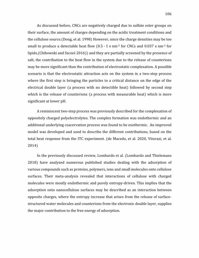
106
As discussed before, CNCs are negatively charged due to sulfate ester groups on
their surface, the amount of charges depending on the acidic treatment conditions and
the cellulose source.(Dong, et al. 1998) However, since the charge densities may be too
small to produce a detectable heat flow (0.5 - 1 e nm-2 for CNCs and 0.037 e nm-2 for
lipids,(Chibowski and Szcześ 2016)) and they are partially screened by the presence of
salt, the contribution to the heat flow in the system due to the release of counterions
may be more significant than the contribution of electrostatic complexation. A possible
scenario is that the electrostatic attraction acts on the system in a two-step process
where the first step is bringing the particles to a critical distance on the edge of the
electrical double layer (a process with no detectible heat) followed by second step
which is the release of counterions (a process with measurable heat) which is more
significant at lower pH.
A reminiscent two-step process was previously described for the complexation of
oppositely charged polyelectrolytes. The complex formation was endothermic and an
additional underlying coacervation process was found to be exothermic. An improved
model was developed and used to describe the different contributions, based on the
total heat response from the ITC experiment. (de Macedo, et al. 2020, Vitorazi, et al.
2014)
In the previously discussed review, Lombardo et al. (Lombardo and Thielemans
2018) have analyzed numerous published studies dealing with the adsorption of
various compounds such as proteins, polymers, ions and small molecules onto cellulose
surfaces. Their meta-analysis revealed that interactions of cellulose with charged
molecules were mostly endothermic and purely entropy-driven. This implies that the
adsorption onto nanocellulose surfaces may be described as an interaction between
opposite charges, where the entropy increase that arises from the release of surface-
structured water molecules and counterions from the electronic double layer, supplies
the major contribution to the free energy of adsorption.
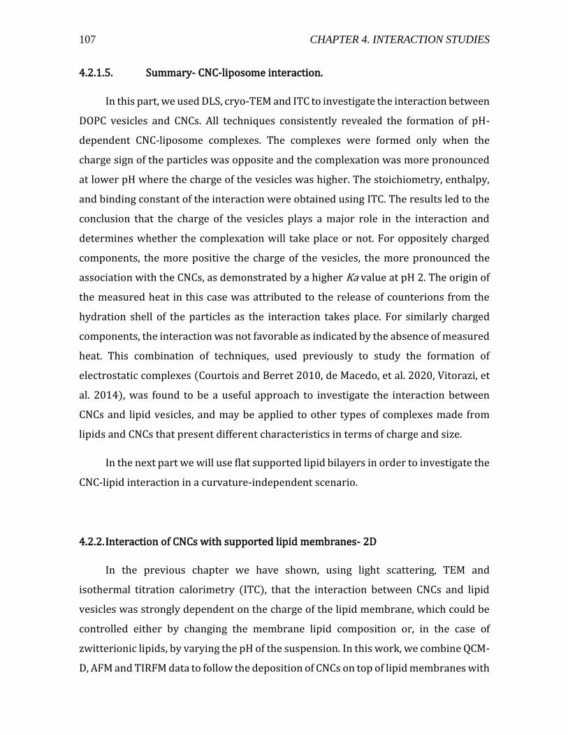
107 CHAPTER 4. INTERACTION STUDIES
4.2.1.5. Summary- CNC-liposome interaction.
In this part, we used DLS, cryo-TEM and ITC to investigate the interaction between
DOPC vesicles and CNCs. All techniques consistently revealed the formation of pH-
dependent CNC-liposome complexes. The complexes were formed only when the
charge sign of the particles was opposite and the complexation was more pronounced
at lower pH where the charge of the vesicles was higher. The stoichiometry, enthalpy,
and binding constant of the interaction were obtained using ITC. The results led to the
conclusion that the charge of the vesicles plays a major role in the interaction and
determines whether the complexation will take place or not. For oppositely charged
components, the more positive the charge of the vesicles, the more pronounced the
association with the CNCs, as demonstrated by a higher Ka value at pH 2. The origin of
the measured heat in this case was attributed to the release of counterions from the
hydration shell of the particles as the interaction takes place. For similarly charged
components, the interaction was not favorable as indicated by the absence of measured
heat. This combination of techniques, used previously to study the formation of
electrostatic complexes (Courtois and Berret 2010, de Macedo, et al. 2020, Vitorazi, et
al. 2014), was found to be a useful approach to investigate the interaction between
CNCs and lipid vesicles, and may be applied to other types of complexes made from
lipids and CNCs that present different characteristics in terms of charge and size.
In the next part we will use flat supported lipid bilayers in order to investigate the
CNC-lipid interaction in a curvature-independent scenario.
4.2.2. Interaction of CNCs with supported lipid membranes- 2D
In the previous chapter we have shown, using light scattering, TEM and
isothermal titration calorimetry (ITC), that the interaction between CNCs and lipid
vesicles was strongly dependent on the charge of the lipid membrane, which could be
controlled either by changing the membrane lipid composition or, in the case of
zwitterionic lipids, by varying the pH of the suspension. In this work, we combine QCM-
D, AFM and TIRFM data to follow the deposition of CNCs on top of lipid membranes with
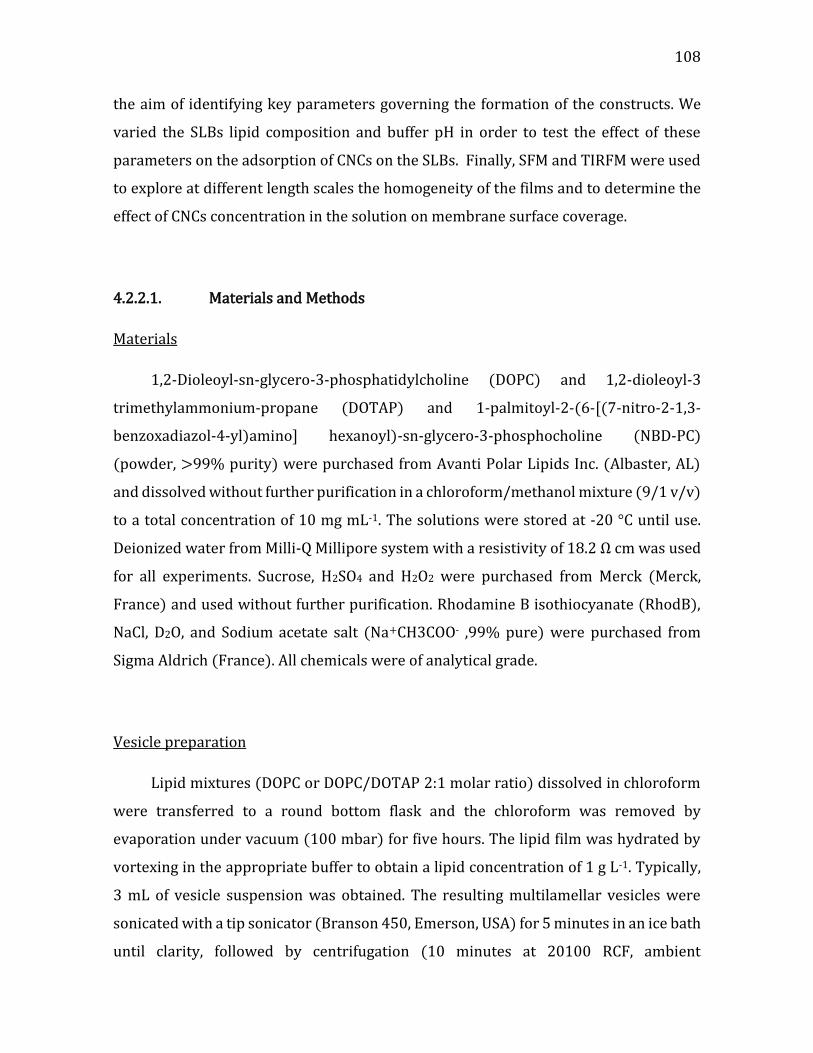
108
the aim of identifying key parameters governing the formation of the constructs. We
varied the SLBs lipid composition and buffer pH in order to test the effect of these
parameters on the adsorption of CNCs on the SLBs. Finally, SFM and TIRFM were used
to explore at different length scales the homogeneity of the films and to determine the
effect of CNCs concentration in the solution on membrane surface coverage.
4.2.2.1. Materials and Methods
Materials
1,2-Dioleoyl-sn-glycero-3-phosphatidylcholine (DOPC) and 1,2-dioleoyl-3
trimethylammonium-propane (DOTAP) and 1-palmitoyl-2-(6-[(7-nitro-2-1,3-
benzoxadiazol-4-yl)amino] hexanoyl)-sn-glycero-3-phosphocholine (NBD-PC)
(powder, >99% purity) were purchased from Avanti Polar Lipids Inc. (Albaster, AL)
and dissolved without further purification in a chloroform/methanol mixture (9/1 v/v)
to a total concentration of 10 mg mL-1. The solutions were stored at -20 °C until use.
Deionized water from Milli-Q Millipore system with a resistivity of 18.2 Ω cm was used
for all experiments. Sucrose, H2SO4 and H2O2 were purchased from Merck (Merck,
France) and used without further purification. Rhodamine B isothiocyanate (RhodB),
NaCl, D2O, and Sodium acetate salt (Na+CH3COO- ,99% pure) were purchased from
Sigma Aldrich (France). All chemicals were of analytical grade.
Vesicle preparation
Lipid mixtures (DOPC or DOPC/DOTAP 2:1 molar ratio) dissolved in chloroform
were transferred to a round bottom flask and the chloroform was removed by
evaporation under vacuum (100 mbar) for five hours. The lipid film was hydrated by
vortexing in the appropriate buffer to obtain a lipid concentration of 1 g L-1. Typically,
3 mL of vesicle suspension was obtained. The resulting multilamellar vesicles were
sonicated with a tip sonicator (Branson 450, Emerson, USA) for 5 minutes in an ice bath
until clarity, followed by centrifugation (10 minutes at 20100 RCF, ambient
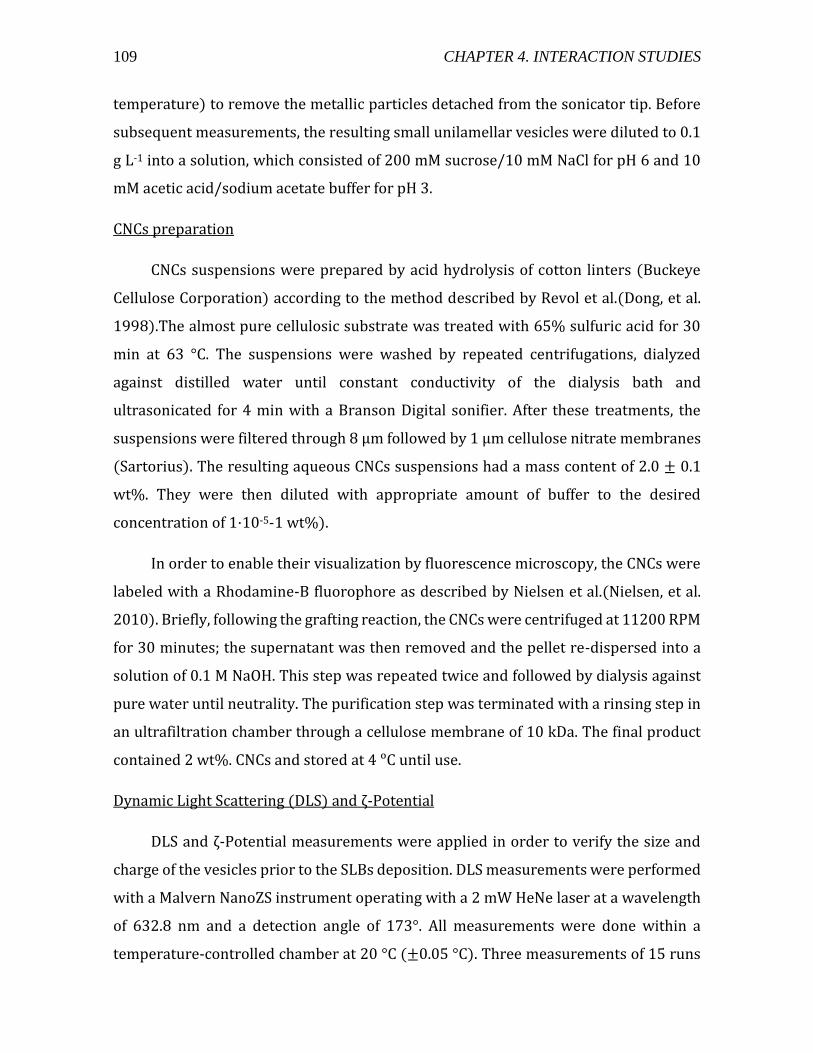
109 CHAPTER 4. INTERACTION STUDIES
temperature) to remove the metallic particles detached from the sonicator tip. Before
subsequent measurements, the resulting small unilamellar vesicles were diluted to 0.1
g L-1 into a solution, which consisted of 200 mM sucrose/10 mM NaCl for pH 6 and 10
mM acetic acid/sodium acetate buffer for pH 3.
CNCs preparation
CNCs suspensions were prepared by acid hydrolysis of cotton linters (Buckeye
Cellulose Corporation) according to the method described by Revol et al.(Dong, et al.
1998).The almost pure cellulosic substrate was treated with 65% sulfuric acid for 30
min at 63 °C. The suspensions were washed by repeated centrifugations, dialyzed
against distilled water until constant conductivity of the dialysis bath and
ultrasonicated for 4 min with a Branson Digital sonifier. After these treatments, the
suspensions were filtered through 8 μm followed by 1 μm cellulose nitrate membranes
(Sartorius). The resulting aqueous CNCs suspensions had a mass content of 2.0 ± 0.1
wt%. They were then diluted with appropriate amount of buffer to the desired
concentration of 1·10-5-1 wt%).
In order to enable their visualization by fluorescence microscopy, the CNCs were
labeled with a Rhodamine-B fluorophore as described by Nielsen et al.(Nielsen, et al.
2010). Briefly, following the grafting reaction, the CNCs were centrifuged at 11200 RPM
for 30 minutes; the supernatant was then removed and the pellet re-dispersed into a
solution of 0.1 M NaOH. This step was repeated twice and followed by dialysis against
pure water until neutrality. The purification step was terminated with a rinsing step in
an ultrafiltration chamber through a cellulose membrane of 10 kDa. The final product
contained 2 wt%. CNCs and stored at 4 ᵒC until use.
Dynamic Light Scattering (DLS) and ζ-Potential
DLS and ζ-Potential measurements were applied in order to verify the size and
charge of the vesicles prior to the SLBs deposition. DLS measurements were performed
with a Malvern NanoZS instrument operating with a 2 mW HeNe laser at a wavelength
of 632.8 nm and a detection angle of 173°. All measurements were done within a
temperature-controlled chamber at 20 °C (±0.05 °C). Three measurements of 15 runs
110
each were usually averaged. The intensity size distribution was obtained from the
analysis of the correlation function using the multiple narrow mode algorithm of the
Malvern DTS software. The electrophoretic mobility of vesicles and CNCs was measured
by using the same Malvern NanoZS apparatus performing at 17° from which the ζ-
potential values are determined by applying the Henry equation. The ζ-potential values
and the ζ-deviation were averaged over at least three measurements with at least 30
runs per measurement. They were expressed as mean ± SD (n≥3).
Quartz crystal microbalance with dissipation monitoring (QCM-D)
QCM-D experiments were performed using a Q-Sense E4 instrument (Q-sense,
Gothenburg, Sweden) equipped with one to four flow modules. Experiments were
conducted under continuous liquid flow of liquid with a rate of 50µL/min, using a
multichannel peristaltic pump (ISM 935C Ismatec, Switzerland). The temperature of
the solutions was stabilized using a temperature control chamber (Eppendorf,
Germany) operated at 24 °C. A clean quartz crystal sensor was placed in the
measurement chamber of the flow module; the resonance frequency and the
dissipation factor were monitored in air and then in liquid for the fundamental 4.95
MHz as well as for the six odd overtones (n=3-13). Suspensions of small unilamellar
vesicles (SUVs) or CNCs were injected into the measurement chamber until a stable
baseline was reached (ΔF<1 Hz over 10 min and ΔD<0.1 10-6 over 10 min). The
changes in dissipation and frequency presented here were normalized by the overtone
number and reported only for the 7th overtone.
Substrate preparation
Silicon coated AT-cut quartz crystals (QSX 303) were purchased from Biolin
Scientific (Stockholm, Sweden). The silicon coated disk shaped had a diameter of 14
mm, a surface roughness<1 nm with a fundamental frequency of 4.95 MHz ± 50 kHz.
The sensors were rinsed with a 2 wt% SDS aqueous solution followed by abundant
water rinsing and dried under a nitrogen stream. The sensors were then exposed to a
UV/ozone lamp for 10 minutes prior to the measurements.

111 CHAPTER 4. INTERACTION STUDIES
QCM-D data analysis
In the case of homogeneous, quasi-rigid films (for which ΔD/-Δf << 4 10-7 Hz-1),
the frequency shifts are proportional to the mass uptake per unit area (mQCM), which
can be deduced from the Sauerbrey relationship:(Johannsmann 1999, Reviakine, et al.
2011)
(Eq. 28) 𝑚𝑄𝐶𝑀 = −𝐶∆𝑓
where C is the mass sensitivity of the crystal (17.7 ng cm-2 Hz-1 at f1 = 4.95 MHz). In
the case of soft films , the adsorbed film was modeled as a homogeneous viscoelastic
layer of acoustic thickness dQCM, density ρ, and a complex shear modulus G(f) with a
storage modulus G’(f) and loss modulus G’’(f) The frequency dependence of the
viscoelastic properties was approximated by power laws with exponents α' and α'':
(Eq. 29) 𝐺′(𝑓) = 𝐺𝑜′ (𝑓
𝑓𝑜)
𝛼′
(Eq. 30) 𝐺′′(𝑓) = 𝐺𝑜′′ (𝑓
𝑓𝑜)
𝛼′′
Where G0' and G0'' are the shear storage and loss moduli at a reference frequency, f0=
35 MHz, dQCM is the film thickness with a density of ρ. ρdQCM, ρ G0', ρ G0', α', and α'' were
adjustable fitting parameters. The semi-infinite bulk solution was taken as water and
was assumed to be Newtonian with a viscosity ηl = 0.89 mPa·s at T= 25ᵒC and a density
of ρl = 1.0 g cm-3. Initially the CNCs film density ρ was fixed to 1.0 g cm-3. Details of the
fitting procedure have been described previously (Eisele, et al. 2012) and the specified
errors represent a confidence level of one standard deviation (68%). The viscoelastic
model contains exclusively the product terms mQCM = ρdQCM, ρ G0', and ρ G0'', and the
fitting will therefore provide correct results for these product terms irrespective of the
exact choice of ρ. The 5th, 7th, 9th, 11th and 13th overtones were used for the calculation.
Determination of coupled water with D2O/H2O solvent exchange
The water content of the film was determined by using a procedure described by
Craig et al and by Kittle et al.(Craig and Plunkett 2003, Kittle, et al. 2011) by changing
the water to deuterium oxide and comparing the scaled QCM-D frequency shifts. Water
112
was introduced to the flow cell at a flow rate of 0.1 mL min-1 on a bare crystal and on a
lipid/CNC film. After reaching a stable base line, D2O was introduced to the cell for few
minutes until a stable baseline was obtained, and the frequency changes was recorded
for the bare crystal (Δfbare) and the lipid-CNC film (Δfn,film). The cells were then rinsed
with water until the frequency reached back to the initial value. The reported value is
the areal mass of water in ng cm-2.
Scanning Force Microscopy (SFM)
The SFM measurements were performed with a Dimension ICON instrument from
Bruker Company. The surface topography was investigated via a pulsed force
(PeakForce) mode, whereas the nano-shaving process was done under contact mode.
Both modes were applied in situ in liquid medium to avoid the drying of the SLB layer,
which could lead to the CNCs layer disassembly. Imaging was performed with an open
liquid-cell and a ScanAsyst liquid cantilever-tip having a radius of around 20-30 nm and
a spring constant of 0.7 N/m. (manufactory data).
In order to control all probing parameters and better adjust the tip to sample
interaction, the SFM data was acquired without ScanAsyst technique. A 50 nm
Peakforce amplitude was selected due to the actual low adhesion level and in order to
minimize the hydrodynamic forces, which can hinder the measurements. For the same
reason, a 1 kHz z-modulation was selected. The PeakForce set-point was kept below the
SLB breaking force (i.e. 1 nN for the tip used here). Depending on the density of the
CNCs in the film, this setpoint force was adjusted to limit the deformation of the fluid-
like SLB below. A force of less than 150 pN was used in the case of a dispersed CNCs
layer since the tip pressure is transferred to the SLB via a single cellulose nanocrystal
thereby promoting the SLB deformation and in rare cases its disruption. On a contrary,
in the case of a dense CNCs layer, a sharp image could be obtained by applying a force
of 750 pN. This large force distributes over many CNCs within the layer, thereby
promoting less deformation of the fluid-like SLB.
SFM images plotting and their data analysis were achieved with the Gwyddion
free software.(Nečas and Klapetek 2012) To extract the thickness of the CNCs layer
113 CHAPTER 4. INTERACTION STUDIES
after nanoshaving, a careful method needed to be followed since the sample surface was
rough. A data leveling was first achieved in the well bottom, i.e. the flattest area, by
fitting a plane through three points. After plane removing, different line profiles were
plotted to control the plane subtraction. Finally, the step height was determined via
averaging a maximum of scan lines passing through the well.
Total Internal Reflection Fluorescence microscopy (TIRF)
Total internal reflection fluorescence microscopy (TIRFM) experiments were
carried out with a Leica DMI6000 B microscope. Samples were excited by total internal
reflection illumination at 488 and 568 nm and images were captured with an Andor
back-illuminated DU-897 EMCCD camera (512X512 pixels) controlled by Leica
software (LAS-AF-6000, Leica Microsystems CMS GmbH, Germany). The fluorescence
intensity values were evaluated by the Leica LASX software. A region of 50X50 µm2
(220X220 pixels) was selected and the values were obtained for at least 10 different
regions. Error bars indicate the standard deviations for the experimental values
(n≥10).
TIRF observation flow cell preparation
The CNCs/SLBs constructs were generated in an observation cell consisting of a
microscope glass slide 2X5 cm with parafilm spacers and sealed with a cover slip,
creating observation channels with volume of 50 µL and surface of about 1 cm2 (see
figure 64a). The slides and cover slips were cleaned with piranha solution (H2SO4
/H2O2 70/30 V%), rinsed with ethanol and stored in milli-Q water until used. Prior to
the deposition of the layers, the slides were dried under a nitrogen gas flow. The
preparation protocol of sample for observation was the following: on a clean cell, a drop
of the suspension was deposited on one side of the channel and pulled in due to
capillary forces to the other side of the channel. Excess liquid was wicked off using a
filter paper placed on the other side of the channel. The flow in the channel was laminar
114
so that exchange of material could be easily performed. During the filling process, care
was taken to avoid the formation of bubbles during the flowing.
4.2.2.2. Formation of the CNCs/SLBs construct
The deposition of the vesicles was achieved in the following way: first, the channel
was rinsed four times with a buffer composed of 200 mM Sucrose and 10 mM NaCl
(pH~6). Then a vesicle suspension (DOPC/DOTAP 70/30 %/% mol., 1 gr L-1) was
deposited in the cell and incubated for 15 minutes at room temperature. The cell was
then rinsed again with 4 volumes of suspension buffer. The SLBs was excited at 488 nm,
close to the excitation spectrum maxima of the DOPC-NBD (461 nm). In the second step,
a drop of 50 µL of CNCs at the desired concentration (0-1·10-1 wt%) was loaded into
the flow cell and incubated for 15 minutes at room temperature and rinsed with four
volumes of a 200 mM sucrose solution. We have chosen not to measure higher
concentration of CNCs in order to ensure that the system is in the semi-dilute regime
and to avoid influence of particle-particle interaction or a change in rheological
properties, on the deposition process.
The deposition of the CNCs on top of the lipid bilayer was visualized by
fluorescence, at an excitation wavelength of 561 nm, which is close to maximum in the
excitation spectrum of Rhod-B (556 nm). Figure 64 shows the measurement
configuration in TIRF and QCM-D modules.
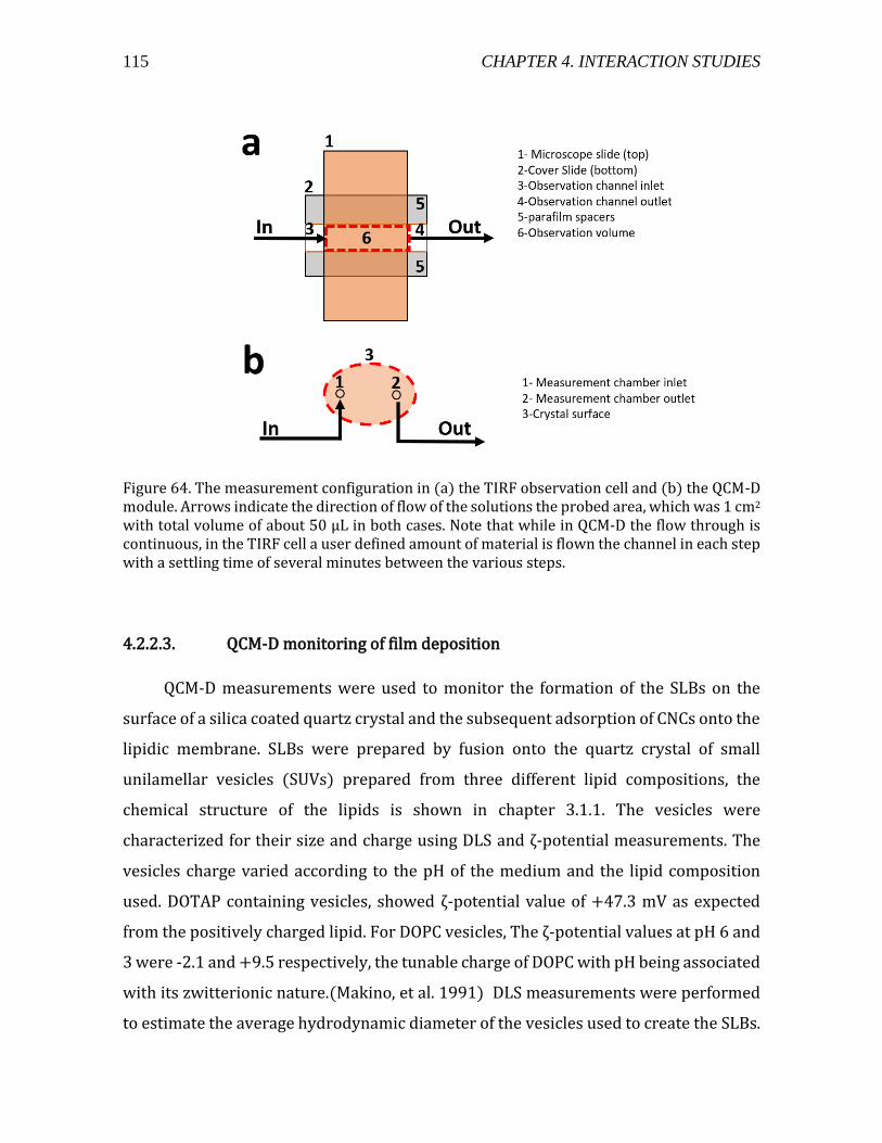
115 CHAPTER 4. INTERACTION STUDIES
Figure 64. The measurement configuration in (a) the TIRF observation cell and (b) the QCM-D module. Arrows indicate the direction of flow of the solutions the probed area, which was 1 cm2 with total volume of about 50 µL in both cases. Note that while in QCM-D the flow through is continuous, in the TIRF cell a user defined amount of material is flown the channel in each step with a settling time of several minutes between the various steps.
4.2.2.3. QCM-D monitoring of film deposition
QCM-D measurements were used to monitor the formation of the SLBs on the
surface of a silica coated quartz crystal and the subsequent adsorption of CNCs onto the
lipidic membrane. SLBs were prepared by fusion onto the quartz crystal of small
unilamellar vesicles (SUVs) prepared from three different lipid compositions, the
chemical structure of the lipids is shown in chapter 3.1.1. The vesicles were
characterized for their size and charge using DLS and ζ-potential measurements. The
vesicles charge varied according to the pH of the medium and the lipid composition
used. DOTAP containing vesicles, showed ζ-potential value of +47.3 mV as expected
from the positively charged lipid. For DOPC vesicles, The ζ-potential values at pH 6 and
3 were -2.1 and +9.5 respectively, the tunable charge of DOPC with pH being associated
with its zwitterionic nature.(Makino, et al. 1991) DLS measurements were performed
to estimate the average hydrodynamic diameter of the vesicles used to create the SLBs.
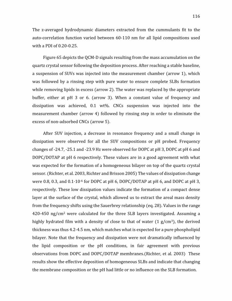
116
The z-averaged hydrodynamic diameters extracted from the cummulants fit to the
auto-correlation function varied between 60-110 nm for all lipid compositions used
with a PDI of 0.20-0.25.
Figure 65 depicts the QCM-D signals resulting from the mass accumulation on the
quartz crystal sensor following the deposition process. After reaching a stable baseline,
a suspension of SUVs was injected into the measurement chamber (arrow 1), which
was followed by a rinsing step with pure water to ensure complete SLBs formation
while removing lipids in excess (arrow 2). The water was replaced by the appropriate
buffer, either at pH 3 or 6. (arrow 3). When a constant value of frequency and
dissipation was achieved, 0.1 wt%. CNCs suspension was injected into the
measurement chamber (arrow 4) followed by rinsing step in order to eliminate the
excess of non-adsorbed CNCs (arrow 5).
After SUV injection, a decrease in resonance frequency and a small change in
dissipation were observed for all the SUV compositions or pH probed. Frequency
changes of -24.7, -25.1 and -23.9 Hz were observed for DOPC at pH 3, DOPC at pH 6 and
DOPC/DOTAP at pH 6 respectively. These values are in a good agreement with what
was expected for the formation of a homogeneous bilayer on top of the quartz crystal
sensor. (Richter, et al. 2003, Richter and Brisson 2005) The values of dissipation change
were 0.8, 0.3, and 0.1·10-6 for DOPC at pH 6, DOPC/DOTAP at pH 6, and DOPC at pH 3,
respectively. These low dissipation values indicate the formation of a compact dense
layer at the surface of the crystal, which allowed us to extract the areal mass density
from the frequency shifts using the Sauerbrey relationship (eq. 28). Values in the range
420-450 ng/cm2 were calculated for the three SLB layers investigated. Assuming a
highly hydrated film with a density of close to that of water (1 g/cm3), the derived
thickness was thus 4.2-4.5 nm, which matches what is expected for a pure phospholipid
bilayer. Note that the frequency and dissipation were not dramatically influenced by
the lipid composition or the pH conditions, in fair agreement with previous
observations from DOPC and DOPC/DOTAP membranes.(Richter, et al. 2003) These
results show the effective deposition of homogeneous SLBs and indicate that changing
the membrane composition or the pH had little or no influence on the SLB formation.
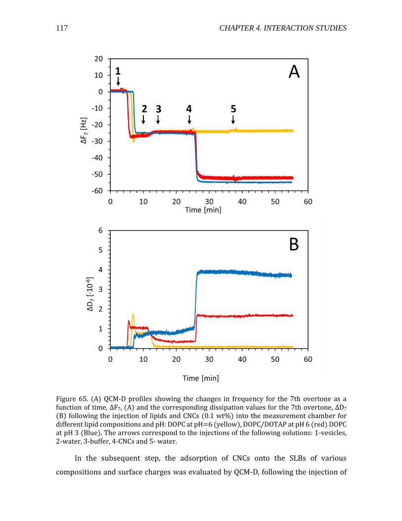
117 CHAPTER 4. INTERACTION STUDIES
Figure 65. (A) QCM-D profiles showing the changes in frequency for the 7th overtone as a function of time, ΔF7, (A) and the corresponding dissipation values for the 7th overtone, ΔD7 (B) following the injection of lipids and CNCs (0.1 wt%) into the measurement chamber for different lipid compositions and pH: DOPC at pH=6 (yellow), DOPC/DOTAP at pH 6 (red) DOPC at pH 3 (Blue). The arrows correspond to the injections of the following solutions: 1-vesicles, 2-water, 3-buffer, 4-CNCs and 5- water.
In the subsequent step, the adsorption of CNCs onto the SLBs of various
compositions and surface charges was evaluated by QCM-D, following the injection of
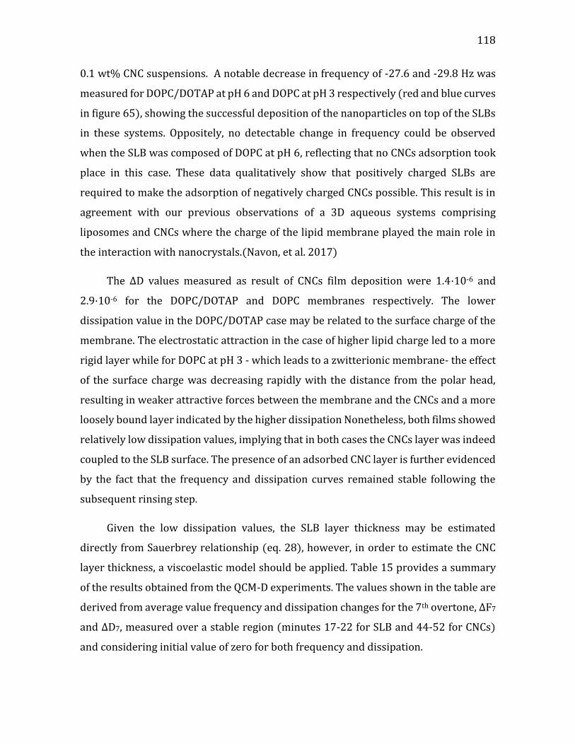
118
0.1 wt% CNC suspensions. A notable decrease in frequency of -27.6 and -29.8 Hz was
measured for DOPC/DOTAP at pH 6 and DOPC at pH 3 respectively (red and blue curves
in figure 65), showing the successful deposition of the nanoparticles on top of the SLBs
in these systems. Oppositely, no detectable change in frequency could be observed
when the SLB was composed of DOPC at pH 6, reflecting that no CNCs adsorption took
place in this case. These data qualitatively show that positively charged SLBs are
required to make the adsorption of negatively charged CNCs possible. This result is in
agreement with our previous observations of a 3D aqueous systems comprising
liposomes and CNCs where the charge of the lipid membrane played the main role in
the interaction with nanocrystals.(Navon, et al. 2017)
The ΔD values measured as result of CNCs film deposition were 1.4·10-6 and
2.9·10-6 for the DOPC/DOTAP and DOPC membranes respectively. The lower
dissipation value in the DOPC/DOTAP case may be related to the surface charge of the
membrane. The electrostatic attraction in the case of higher lipid charge led to a more
rigid layer while for DOPC at pH 3 - which leads to a zwitterionic membrane- the effect
of the surface charge was decreasing rapidly with the distance from the polar head,
resulting in weaker attractive forces between the membrane and the CNCs and a more
loosely bound layer indicated by the higher dissipation Nonetheless, both films showed
relatively low dissipation values, implying that in both cases the CNCs layer was indeed
coupled to the SLB surface. The presence of an adsorbed CNC layer is further evidenced
by the fact that the frequency and dissipation curves remained stable following the
subsequent rinsing step.
Given the low dissipation values, the SLB layer thickness may be estimated
directly from Sauerbrey relationship (eq. 28), however, in order to estimate the CNC
layer thickness, a viscoelastic model should be applied. Table 15 provides a summary
of the results obtained from the QCM-D experiments. The values shown in the table are
derived from average value frequency and dissipation changes for the 7th overtone, ΔF7
and ΔD7, measured over a stable region (minutes 17-22 for SLB and 44-52 for CNCs)
and considering initial value of zero for both frequency and dissipation.
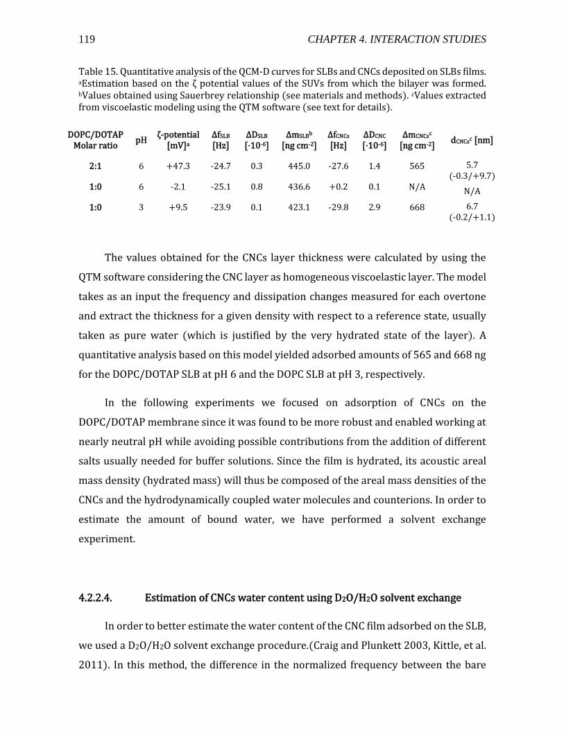
119 CHAPTER 4. INTERACTION STUDIES
Table 15. Quantitative analysis of the QCM-D curves for SLBs and CNCs deposited on SLBs films. aEstimation based on the ζ potential values of the SUVs from which the bilayer was formed. bValues obtained using Sauerbrey relationship (see materials and methods). cValues extracted from viscoelastic modeling using the QTM software (see text for details).
The values obtained for the CNCs layer thickness were calculated by using the
QTM software considering the CNC layer as homogeneous viscoelastic layer. The model
takes as an input the frequency and dissipation changes measured for each overtone
and extract the thickness for a given density with respect to a reference state, usually
taken as pure water (which is justified by the very hydrated state of the layer). A
quantitative analysis based on this model yielded adsorbed amounts of 565 and 668 ng
for the DOPC/DOTAP SLB at pH 6 and the DOPC SLB at pH 3, respectively.
In the following experiments we focused on adsorption of CNCs on the
DOPC/DOTAP membrane since it was found to be more robust and enabled working at
nearly neutral pH while avoiding possible contributions from the addition of different
salts usually needed for buffer solutions. Since the film is hydrated, its acoustic areal
mass density (hydrated mass) will thus be composed of the areal mass densities of the
CNCs and the hydrodynamically coupled water molecules and counterions. In order to
estimate the amount of bound water, we have performed a solvent exchange
experiment.
4.2.2.4. Estimation of CNCs water content using D2O/H2O solvent exchange
In order to better estimate the water content of the CNC film adsorbed on the SLB,
we used a D2O/H2O solvent exchange procedure.(Craig and Plunkett 2003, Kittle, et al.
2011). In this method, the difference in the normalized frequency between the bare
DOPC/DOTAPMolar ratio
pH ζ-potential
[mV]a ΔfSLB [Hz]
ΔDSLB [·10-6]
ΔmSLBb [ng cm-2]
ΔfCNCs [Hz]
ΔDCNC
[·10-6] ΔmCNCsc
[ng cm-2] dCNCsc [nm]
2:1 6 +47.3 -24.7 0.3 445.0 -27.6 1.4 565 5.7 (-0.3/+9.7)
1:0 6 -2.1 -25.1 0.8 436.6 +0.2 0.1 N/A N/A
1:0 3 +9.5 -23.9 0.1 423.1 -29.8 2.9 668 6.7 (-0.2/+1.1)
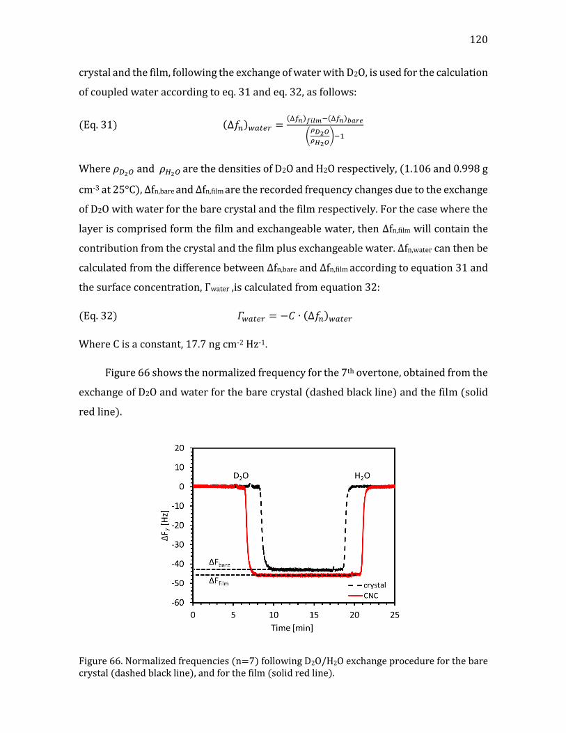
120
crystal and the film, following the exchange of water with D2O, is used for the calculation
of coupled water according to eq. 31 and eq. 32, as follows:
(Eq. 31) (∆𝑓𝑛)𝑤𝑎𝑡𝑒𝑟 =(∆𝑓𝑛)𝑓𝑖𝑙𝑚−(∆𝑓𝑛)𝑏𝑎𝑟𝑒
(𝜌𝐷2𝑂
𝜌𝐻2𝑂)−1
Where 𝜌𝐷2𝑂 and 𝜌𝐻2𝑂 are the densities of D2O and H2O respectively, (1.106 and 0.998 g
cm-3 at 25°C), Δfn,bare and Δfn,film are the recorded frequency changes due to the exchange
of D2O with water for the bare crystal and the film respectively. For the case where the
layer is comprised form the film and exchangeable water, then Δfn,film will contain the
contribution from the crystal and the film plus exchangeable water. Δfn,water can then be
calculated from the difference between Δfn,bare and Δfn,film according to equation 31 and
the surface concentration, Γwater ,is calculated from equation 32:
(Eq. 32) 𝛤𝑤𝑎𝑡𝑒𝑟 = −𝐶 ∙ (∆𝑓𝑛)𝑤𝑎𝑡𝑒𝑟
Where C is a constant, 17.7 ng cm-2 Hz-1.
Figure 66 shows the normalized frequency for the 7th overtone, obtained from the
exchange of D2O and water for the bare crystal (dashed black line) and the film (solid
red line).
Figure 66. Normalized frequencies (n=7) following D2O/H2O exchange procedure for the bare crystal (dashed black line), and for the film (solid red line).
121 CHAPTER 4. INTERACTION STUDIES
The experiment was done for DOPC/DOTAP SLB composition, where CNC
adsorption is possible in pure water. The normalized frequencies at the 7th overtone
were recorded and found to be -45.6±1.1 Hz and -43.3±0.6 Hz (mean±SD, n≥3) for the
film and the bare crystal respectively. Γwater was then calculated for the film according
to equations 31 and 32 and was found to be 380±90 ng cm-2. The hydrated mass
obtained for the same type of film was 565 ng cm-2, resulting in dry mass of 185 ng cm-
2. The amount of water in the film may be directly derived from the hydrated and water
masses, and it was found to be 67 ± 15%.
4.2.2.5. Microscopic visualization of the constructs using TIRF
In order to investigate the structural properties of the CNCs/SLB constructs at
tens of micrometers length scale, TIRF microscopy was used to directly image the
formation of the lipid bilayer and the deposition of the CNCs on top of it. Especially, the
effect of CNCs concentration on the formation and homogeneity of CNCs/SLBs films was
investigated. CNCs samples were prepared from dilution of a 1% CNCs aqueous
suspension at pH 6 and the resulting sample concentration varied from 0 to 0.1 wt%.
We did not use 1 wt% sample in order to avoid viscosity variation which can influence
the flow in the cell.
The experiments were performed in a flow chamber described in the
experimental section, which is commonly used for biophysical studies (Gilboa, et al.
2009). In order to visualize the SLBs and CNCs simultaneously, two fluorescent probes
were used: lipidic membranes were labeled using NBD-PC and CNCs using Rhodamine
B (see experimental section for details). Figure 67 depicts the impact of CNCs
concentration using 4545 µm2 top view images of the films in the case of SLB-only
visualization (top row), CNCs-only visualization (middle row) and co-visualization
(bottom row).
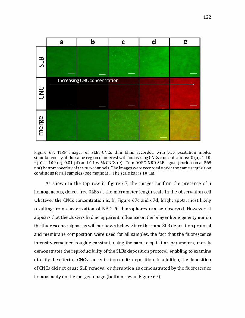
122
Figure 67. TIRF images of SLBs-CNCs thin films recorded with two excitation modes simultaneously at the same region of interest with increasing CNCs concentrations: 0 (a), 1·10-
4 (b), 1·10-3 (c), 0.01 (d) and 0.1 wt% CNCs (e). Top: DOPC-NBD SLB signal (excitation at 568 nm) bottom: overlay of the two channels. The images were recorded under the same acquisition conditions for all samples (see methods). The scale bar is 10 µm.
As shown in the top row in figure 67, the images confirm the presence of a
homogeneous, defect-free SLBs at the micrometer length scale in the observation cell
whatever the CNCs concentration is. In Figure 67c and 67d, bright spots, most likely
resulting from clusterization of NBD-PC fluorophores can be observed. However, it
appears that the clusters had no apparent influence on the bilayer homogeneity nor on
the fluorescence signal, as will be shown below. Since the same SLB deposition protocol
and membrane composition were used for all samples, the fact that the fluorescence
intensity remained roughly constant, using the same acquisition parameters, merely
demonstrates the reproducibility of the SLBs deposition protocol, enabling to examine
directly the effect of CNCs concentration on its deposition. In addition, the deposition
of CNCs did not cause SLB removal or disruption as demonstrated by the fluorescence
homogeneity on the merged image (bottom row in Figure 67).

123 CHAPTER 4. INTERACTION STUDIES
In order to quantify the variation in fluorescence intensity and the homogeneity
of the lipid bilayer we have performed a statistical analysis of fluorescence intensity on
a series of TIRF images. It is important to mention here, that quantification of
fluorescence signal should be carried out and interpreted carefully due to number and
experimental sensitivity of the parameters that can influence the signal. To ensure the
proportionality of the measured signal to the amount of fluorophore in the sample, we
have kept the acquisition parameters (i.e. laser intensity, exposure time and camera
gain) constant while varying only the CNCs concentration. Figure 68 shows the average
fluorescence values obtained from statistical analysis of the images using the green
(SLBs visualization) and red (CNCs visualization) channels for each CNCs concentration
for a given region of interest. Typically, 10 regions were averaged and the errors were
expressed as the standard deviation from this population (n±SD).
Figure 68. Average fluorescence intensity as a function of CNCs weight percent for the SLBs (green triangles) and CNCs layer (red triangles). Values correspond to mean ± SD (n=10).
While the average fluorescence intensity of the SLBs remained roughly constant
within measurement error 5070±320 AU, the fluorescence intensity of the CNCs layer
increased with the increase in CNCs concentration tending to a plateau around 0.01
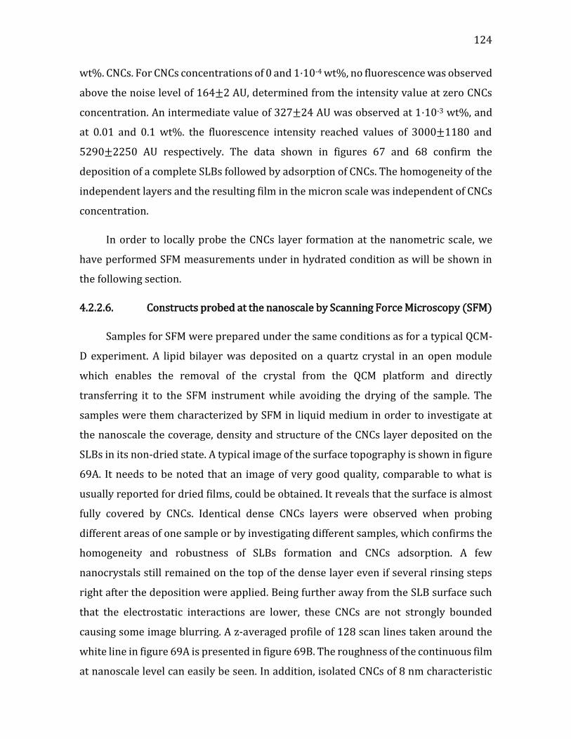
124
wt%. CNCs. For CNCs concentrations of 0 and 1·10-4 wt%, no fluorescence was observed
above the noise level of 164±2 AU, determined from the intensity value at zero CNCs
concentration. An intermediate value of 327±24 AU was observed at 1·10-3 wt%, and
at 0.01 and 0.1 wt%. the fluorescence intensity reached values of 3000±1180 and
5290±2250 AU respectively. The data shown in figures 67 and 68 confirm the
deposition of a complete SLBs followed by adsorption of CNCs. The homogeneity of the
independent layers and the resulting film in the micron scale was independent of CNCs
concentration.
In order to locally probe the CNCs layer formation at the nanometric scale, we
have performed SFM measurements under in hydrated condition as will be shown in
the following section.
4.2.2.6. Constructs probed at the nanoscale by Scanning Force Microscopy (SFM)
Samples for SFM were prepared under the same conditions as for a typical QCM-
D experiment. A lipid bilayer was deposited on a quartz crystal in an open module
which enables the removal of the crystal from the QCM platform and directly
transferring it to the SFM instrument while avoiding the drying of the sample. The
samples were them characterized by SFM in liquid medium in order to investigate at
the nanoscale the coverage, density and structure of the CNCs layer deposited on the
SLBs in its non-dried state. A typical image of the surface topography is shown in figure
69A. It needs to be noted that an image of very good quality, comparable to what is
usually reported for dried films, could be obtained. It reveals that the surface is almost
fully covered by CNCs. Identical dense CNCs layers were observed when probing
different areas of one sample or by investigating different samples, which confirms the
homogeneity and robustness of SLBs formation and CNCs adsorption. A few
nanocrystals still remained on the top of the dense layer even if several rinsing steps
right after the deposition were applied. Being further away from the SLB surface such
that the electrostatic interactions are lower, these CNCs are not strongly bounded
causing some image blurring. A z-averaged profile of 128 scan lines taken around the
white line in figure 69A is presented in figure 69B. The roughness of the continuous film
at nanoscale level can easily be seen. In addition, isolated CNCs of 8 nm characteristic

125 CHAPTER 4. INTERACTION STUDIES
height can be detected. Data therefore show that the adsorption of CNCs onto the SLBs
occurred as a dense monolayer on top of which scarcely distributed CNCs were
detected. This result is in full agreement with QCM-D data showing that the thickness
of the adsorbed CNCs layer is intermediate between a monolayer and a double layer.
Figure 69. (A) Topography of SLBs/CNCs layer made from DOPC/DOTAP 70/30 %mol. at pH 6, on quartz substrate obtained by SFM in Peakforce mode in Milli-Q water. The PeakForce setpoint was 100 pN. Image is plotted after removing polynomial background, aligning rows and correcting horizontal scars. (B) Z-profile averaged over the 128 lines marked by the white line and its borders in figure 69A. Colored rectangles with 8 nm in height were added as an indication for the CNCs height. Few isolated CNCs lying on top of the construct are also clearly visible.
A nanoshaving of SLBs/CNCs film was applied in order to precisely determine the
construct thickness. This procedure was performed in contact mode. In order to
determine the working conditions, different tip loadings, i.e. friction forces, were first
tested.
Figure 70A and B shows SFM image in contact mode made of 256 scanning lines
and by changing every 25 lines the force load, expressed as cantilever-tip deflection in
Volt. The change in z is due to the modification of the piezo tube position to obtain the
required cantilever deflection. Three zones are distinguished. Between 0 and 0.3V, the
construct is just slightly deformed. Starting around 0.3V, few CNCs were removed and
above 0.7V deflection the whole film was peeled off. The granular surface of the
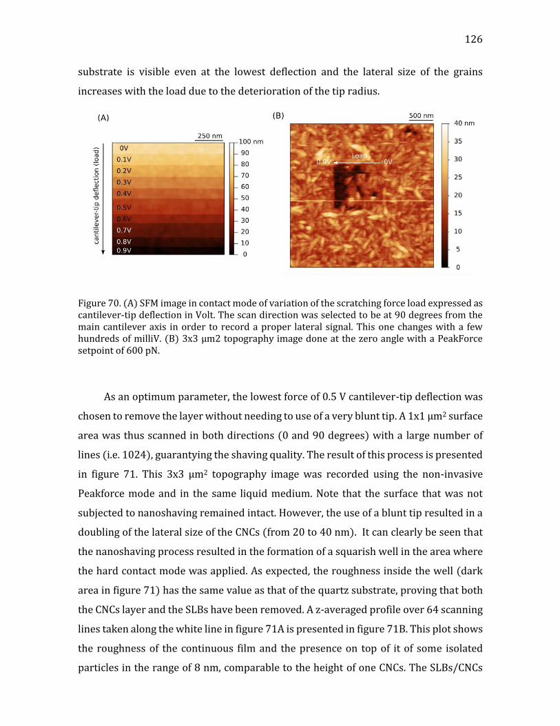
126
substrate is visible even at the lowest deflection and the lateral size of the grains
increases with the load due to the deterioration of the tip radius.
Figure 70. (A) SFM image in contact mode of variation of the scratching force load expressed as cantilever-tip deflection in Volt. The scan direction was selected to be at 90 degrees from the main cantilever axis in order to record a proper lateral signal. This one changes with a few hundreds of milliV. (B) 3x3 µm2 topography image done at the zero angle with a PeakForce setpoint of 600 pN.
As an optimum parameter, the lowest force of 0.5 V cantilever-tip deflection was
chosen to remove the layer without needing to use of a very blunt tip. A 1x1 µm2 surface
area was thus scanned in both directions (0 and 90 degrees) with a large number of
lines (i.e. 1024), guarantying the shaving quality. The result of this process is presented
in figure 71. This 3x3 µm2 topography image was recorded using the non-invasive
Peakforce mode and in the same liquid medium. Note that the surface that was not
subjected to nanoshaving remained intact. However, the use of a blunt tip resulted in a
doubling of the lateral size of the CNCs (from 20 to 40 nm). It can clearly be seen that
the nanoshaving process resulted in the formation of a squarish well in the area where
the hard contact mode was applied. As expected, the roughness inside the well (dark
area in figure 71) has the same value as that of the quartz substrate, proving that both
the CNCs layer and the SLBs have been removed. A z-averaged profile over 64 scanning
lines taken along the white line in figure 71A is presented in figure 71B. This plot shows
the roughness of the continuous film and the presence on top of it of some isolated
particles in the range of 8 nm, comparable to the height of one CNCs. The SLBs/CNCs

127 CHAPTER 4. INTERACTION STUDIES
construct thickness appears to be 13 nm ± 3 nm. These data are consistent with the
deposited film being composed of a 4-5 nm thick SLBs covered by a dense monolayer
of CNCs, with some isolated crystals on top. These values are in good agreement with
the values obtained from QCM-D data when taking the total resonance frequency shift
(i.e SLB + CNCs layers). Similar nanoshaving measurements were performed using a
much higher 5V cantilever-tip deflection and the same step height was obtained,
confirming the validity of the results.
Figure 71. (A) Topography image of a SLBs/CNCs layer made from DOPC/DOTAP 70/30 mol.% at pH 6, obtained by SPM in Peakforce mode in Milli-Q after nanoshaving (see text). The PeakForce setpoint was 750 pN. The detail of the data treatment can be found in the supporting information. (B) Averaged step height showing the thickness of the whole construct. Color shade (5nm thickness for SLBs and 8nm for CNCs) were added as a visual guide. A typical roughness of the quartz substrate is found in the well, whereas a larger roughness on the surface corresponds to the CNCs layers organization.
The results obtained from the SFM experiments were compared to the QCM-D
observations and the derived layer thickness calculation thereafter. Several aspects
emerge from this comparison. The estimation of layer thickness, water content and
homogeneity will be discussed in the following section.
4.2.2.7. Discussion
Several studies have shown that cellulose based films are swollen in aqueous
medium, with the amount of water being dependent on the nature of the cellulose
(native, regenerated, etc.) and mode of deposition (spin coating, dipping, etc.). In an
128
early study, Aulin et al. estimated the water content of cellulose films prepared in
different conditions and measured 26% for spin coated CNC films by evaluating a
normalized adsorbed mass measured by QCM-D and thicknesses by ellipsometry after
exposure to a buffer solution.(Aulin, et al. 2009) Later on, Niinivarra et al. found values
of water by mass ranging from 28% for the thicker films to 79% for the thinner ones
from QCM-D and ellipsometry experiments on CNC films obtained by spin coating and
exposed to a relative humidity of 97%.(Niinivaara, et al. 2015) It is worth mentioning
that since the case of relative humidity is different from the case of swelling in liquid
water, different behavior is expected. Reid et al. found that swollen CNC films, also
prepared by spin coating, contained 35% wt water.(Reid, et al. 2016) It has to be noted
that all these results are obtained on films that have been prepared by spin coating
followed by a drying step that enhances the cohesion of the CNCs in the film, ensuring
its integrity.
Values of 74% wt water by mass have been measured by Kittle et al. for
nanocrystalline cellulose films with various thicknesses as measured by ellipsometry,
deposited by electrospinning at different concentration, dried, and then
rehydrated.(Kittle, et al. 2011) They have estimated the water content using H2O/D2O
solvent replacement on the CNC films deposited on a QCM-D crystal. These results are
significantly different from the one evaluated from combined QCM-D and ellipsometry
measurements, that evaluate lower amounts of water.
It has to be noticed that, in addition, neutron reflectometry measurements on
phospholipid bilayers revealed a bound water layer between the substrate and the
hydrophilic head: up to 7% of water by volume in the hydrophobic tails region and up
to 35% in the headgroup region.(Montis, et al. 2016, Wacklin 2010) This should account
for additional adsorbed water molecules, which can also contribute to the total mass
fraction of water in our film, but to a limited extent.
In our case, by knowing these masses we may calculate a corrected film density
by using equation 33:

129 CHAPTER 4. INTERACTION STUDIES
(Eq. 33) 𝜌𝑓𝑖𝑙𝑚 =𝑚𝑄𝐶𝑀𝐷
𝑚𝑑𝑟𝑦
𝜌𝐶𝑁𝐶+
𝑚𝑤𝑎𝑡𝑒𝑟𝜌𝑤𝑎𝑡𝑒𝑟
Where 𝜌𝑓𝑖𝑙𝑚 is the film density, 𝑚𝑄𝐶𝑀𝐷 is the hydrated mass, 𝑚𝑑𝑟𝑦 and 𝑚𝑤𝑎𝑡𝑒𝑟 are the
dry and water mass respectively and 𝜌𝐶𝑁𝐶 and 𝜌𝑤𝑎𝑡𝑒𝑟 are the densities of cellulose and
water respectively. The film density obtained from this calculation was 1.14 g cm-3.
By using the calculated density value as the input value in the viscoelastic model,
assuming the same water uptake for both films, we obtain thicknesses of 5.7 and 6.7 nm
for the DOPC/DOTAP and DOPC films, respectively. The best fit of QTM modeling of
QCM-D data for the CNC layer thickness from the model in the case of DOPC/DOTAP
system (5.7 nm) is slightly lower compared to the known dimensions of CNCs from
cotton prepared under the same conditions (7.5 ± 1 nm) and compared to the thickness
measured by us using SFM (8.0 ± 2 nm). Indeed, the value given for the thickness
represents the minimum solution, yet thickness with 1 standard deviation (0.683) is in
the range of 5.4−14.2 and 6.5−7.5 nm for the DOPC/DOTAP and DOPC system,
respectively.
The Χ2 landscape, representing the difference between the theoretically predicted
and the experimental values, is calculated for both systems as shown in figure 72:
Figure 72. X2 landscape for the CNCs layer deposited on DOPC/DOTAP (a) and DOPC (b) systems. The red point indicates the minimal solution and the extreme points represents the solution boundaries for confidence interval of 0.683 or one standard deviation.
130
For the DOPC case the X2 landscape comprises a skewed bell shape distribution,
where for the DOPC/DOTAP system, a single sharp minimum appears around d=5.6 nm
followed by a secondary smeared minimum around d=8 nm. The values of thicknesses
fall in the range of the estimated layer thickness from SFM, 13±3 for the total film
thickness SLB+CNC.
It can therefore be estimated that the positively charged SLB surfaces were
covered by a monolayer of CNCs, on average, with some loosely bound isolated crystals
on top of it. This situation is reminiscent of the case of the adsorption of double layers
of CNCs onto positively charged poly(allylamine hydrochloride) (PAH) polymer layers,
which was ascribed to charge complexation and counterions release effects.(Jean, et al.
2008) In the case of CNCs adsorbed onto PAH, it was further shown that the second
layer was twice less dense that the first one.
Theoretically, if all the surface is covered with one layer of cellulosic material, the
areal mass is equal to the mass of a cylinder with thickness of 7 nm multiplied by the
cellulose density, 1.6 g cm-3. This calculation gives 1050 ng cm-2, representing the
maximum dry mass in case of perfect packing. The adsorbed dry mass in our case was
185 ng cm-2 for the DOPC/DOTAP, which infers a lower surface coverage compared to
the ideal case. The SFM images support this observation, showing that the CNCs are
randomly distributed, leading to a porous network of entangled rods. Taking the
average film thickness from SFM measurements, the water content from D2O/H2O
exchange experiment and the maximum estimation from QTM model for DOPC/DOTAP
system, we converge to a CNC hydrated layer composed of 70−80% wt water with a
total thickness of 6−8 nm.
In summary, our results showed that the water content of our deposited layers
account for more than 2/3 of the total mass, in agreement with the results of Kittle et
al.(Kittle, et al. 2011) but in fair contrast with other estimation from combined
ellipsometric and QCM-D measurements, which lead to values closer to 1/4 water
content. However, evaluation of random packing of rods in the case of sedimentation of
colloids or compaction of anisotropic powders leads to volume fraction at maximum
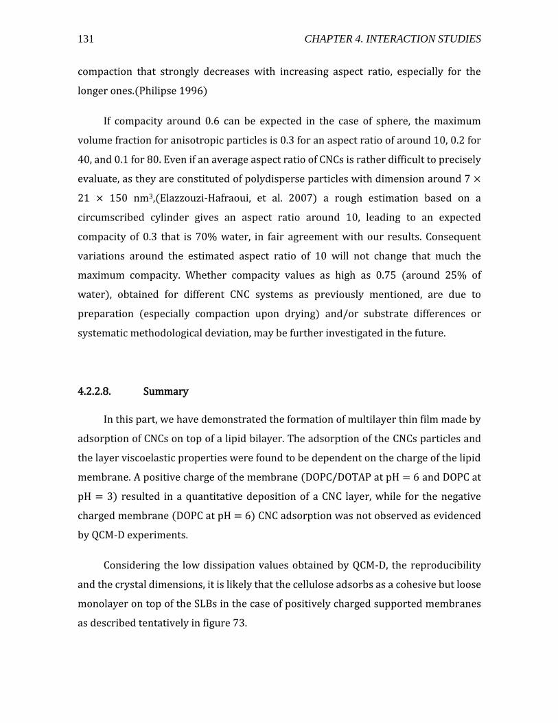
131 CHAPTER 4. INTERACTION STUDIES
compaction that strongly decreases with increasing aspect ratio, especially for the
longer ones.(Philipse 1996)
If compacity around 0.6 can be expected in the case of sphere, the maximum
volume fraction for anisotropic particles is 0.3 for an aspect ratio of around 10, 0.2 for
40, and 0.1 for 80. Even if an average aspect ratio of CNCs is rather difficult to precisely
evaluate, as they are constituted of polydisperse particles with dimension around 7 ×
21 × 150 nm3,(Elazzouzi-Hafraoui, et al. 2007) a rough estimation based on a
circumscribed cylinder gives an aspect ratio around 10, leading to an expected
compacity of 0.3 that is 70% water, in fair agreement with our results. Consequent
variations around the estimated aspect ratio of 10 will not change that much the
maximum compacity. Whether compacity values as high as 0.75 (around 25% of
water), obtained for different CNC systems as previously mentioned, are due to
preparation (especially compaction upon drying) and/or substrate differences or
systematic methodological deviation, may be further investigated in the future.
4.2.2.8. Summary
In this part, we have demonstrated the formation of multilayer thin film made by
adsorption of CNCs on top of a lipid bilayer. The adsorption of the CNCs particles and
the layer viscoelastic properties were found to be dependent on the charge of the lipid
membrane. A positive charge of the membrane (DOPC/DOTAP at pH = 6 and DOPC at
pH = 3) resulted in a quantitative deposition of a CNC layer, while for the negative
charged membrane (DOPC at pH = 6) CNC adsorption was not observed as evidenced
by QCM-D experiments.
Considering the low dissipation values obtained by QCM-D, the reproducibility
and the crystal dimensions, it is likely that the cellulose adsorbs as a cohesive but loose
monolayer on top of the SLBs in the case of positively charged supported membranes
as described tentatively in figure 73.
132
Figure 73. A schematic description of CNC deposited on a supported lipid bilayer.
SFM and TIRF images confirmed the formation of SLBs and of homogenous CNCs
coverage at the micrometer scale, while QCM-D measurements were used to extract the
value of the adsorbed CNCs mass at saturation of about 600±70 ng and an
approximated height of 6-8 nm. This height was confirmed via SFM nanoshaving. QCM-
D experiments using solvent exchange with D2O demonstrate the formation of a
continuous monolayer of CNCs on top a lipid membrane with a compacity around 0.3.
Altogether, the results demonstrate a formation of a continuous monolayer of CNCs on
top a lipid membrane and shed light on the key factors governing the interactions of
these two bio-based building blocks.
Notably, QCM-D, SFM, and TIRF proved to be a useful combination of methods to
probe the formation of multilayer 2D constructs from the nanometric to the
micrometric length scale. This information will serve us in the following parts for the
construction of biomimetic capsules in chapter 5.
4.3. CNC-XG study
Xyloglucans (XG) interact with cellulose microfibrils via hydrogen bonds, VdW
interactions, and polar interactions.(Hayashi and Maclachlan 1984, Lopez, et al. 2010,
Mazeau and Charlier 2012)These interactions lead to the formation of a flexible
network, which is a key factor in maintaining cell wall integrity. In this part, we were
interested in studying and optimizing the interaction between CNC and XG building
blocks, with the aim to utilize these elements for the construction of synthetic PCW.

133 CHAPTER 4. INTERACTION STUDIES
4.3.1. CNC-XG interaction in (3D)
CNCs were used in this case as a model of the naturally-occurring cellulose
nanofibrils, but with improved colloidal stability thanks to charged sulfate ester groups
which are grafted on their surface as previously discussed. Since XG is a neutral
polysaccharide, we expect the electrostatic interaction between the CNCs and XG to be
negligible compared to the other intermolecular forces present in this system. In the
following sections, we will describe our observations on CNCs and sonicated XG system
using complementary data from dynamic light scattering (DLS), nuclear magnetic
resonance (NMR) spectroscopy, isothermal titration calorimetry (ITC) and
transmission electron microscopy (TEM).
4.3.1.1. Materials and methods
Nuclear magnetic resonance (NMR). Proton NMR spectra were recorded with a
Bruker Avance 400 spectrometer (Bruker, Germany) operating at a frequency of
400.13 MHz for 1 h. Samples were solubilized in D2O at a temperature of 25 °C. Residual
signal of the solvent was used as the internal standard at 4.80 ppm at 25 °C. Proton
spectra were recorded using 90° pulses with a 4006 Hz spectral width, 32768 data
points, 4.089 s acquisition times, 10 s relaxation delays, and 32 scans.
The samples were prepared in the same way as for the DLS and ITC, i.e. stepwise
addition of 10 µL aliquots 1 wt % XG100 into a vessel containing 1 mL of 1 wt % CNCs
where both XG and CNCs in D2O. 1.1·10-4 wt % dimethyl sulfoxide (DMSO) was added
to each sample for integral normalization.
Transmission electron microscopy (TEM). Droplet of ca. 0.001 wt.% CNC or XG-
CNC complex suspension were deposited onto freshly glow-discharged carbon-coated
copper grids and negatively stained with 2 wt % uranyl acetate. The specimens were
observed with a Philips (FEI) CM200 microscope operating at 200 kV and equipped
with a TVIPS TemCam F216 digital camera.
134
Atomistic modeling. We have considered a molecular model of the (100) surface
of cellulose Iβ(Mazeau 2011). Periodic boundary conditions were applied in order to
general an infinite surface. We have also considered a typical repeat unit of tamarind
XG, XXLG, whose initial coordinates were extracted from a previous study (Hanus and
Mazeau 2006). Modeling strategy and simulation conditions are fully described
elsewhere(Mazeau and Charlier 2012). Briefly, the XG molecule was placed above the
cellulose surface and molecular dynamics (5 ns at constant number of particles, volume
and temperature) was used to search for the most stable organization of the complex.
At the end of the molecular dynamics trajectory, the total energy of the system was
constant and the XG was stabilized on the surface as its location and orientation with
respect to the cellulose surface remained stable. Several snapshots taken at the
equilibrium stage were extracted from the trajectory to estimate the area of the
cellulose surface covered by the XG fragment.
4.3.1.2. Heat response from the addition of XG into a CNC suspension by ITC
ITC was used to evaluate the thermodynamic parameters of the interaction
between CNCs and XG with high and low Mw. The experimental setup is described in the
method section. Briefly, aliquots of 1 wt.% XG solution were added dropwise to a 1 wt
% CNC suspension and the heat response was measured. For both XG800 and XG100, a
pronounced heat flow was observed, with an overall exothermic behavior. The addition
of non-sonicated XG into a CNC suspension resulted in broad peaks of increasing
magnitude. In a typical ITC experiment, the heat values resulting from the integration
of the heat flow over time are decreasing in magnitude with the addition of titrant. In
the case of XG800 (high Mw), the peaks continuously increased during the experiment.
No return to the baseline was observed and thus a clear ITC profile could not be
obtained and no valuable data could be extracted. This observation may imply that the
timescale of interaction, and therefore heat flow, is longer than the timescale of an ITC
experiment.

135 CHAPTER 4. INTERACTION STUDIES
A possible explanation for this phenomenon may emerge from the rearrangement
of XG chains, a process that influence the heat flow and has characteristic time of up to
several hours in the case of high-Mw XG (Villares, et al. 2015). We have tried to enable
a clear return of the heat signal to the baseline after each injection by increasing the
time between injections up to 3000 s, 10 times higher than the interval used a typical
ITC experiment. However, in the timescale of the experiment, we did not achieve robust
response and reproducibility and, therefore, no conclusive data could be obtained for
the stoichiometry and thermodynamic parameters of XG800, apart from the exothermic
nature of the interaction.
In the case of XG100, the peaks could be distinguished. The kinetics was faster
enabling the return to the baseline and identification of the stoichiometric point where
no additional heat flow was observed above the baseline. Figure 74 shows the variation
of the normalized heat value as a function of the mass ratio of XG to CNC which will be
noted R, from the titration of a 1 wt % CNC suspension with 1 wt % XG100. Each injection
resulted in an exothermic peak and the integration of the peak over time yielded the
heat release during a single injection.
The heat flow due to the injection increased until reaching a maximum point at
the fifth injection corresponding to a mass ratio R = 0.03 and heat value of -2.2 kcal mol-
1 XG. After reaching this value, further addition of XG resulted in a decrease in the heat
value until after 8 injections, corresponding to a mass ratio of R = 0.05, no heat flow
was observed with further addition of XG. Similar results were obtained for lower initial
XG concentrations, as well as for larger time intervals between injections. Since ITC
provides the overall heat release due to the interaction, it is rather difficult to
unambiguously determine which type of interaction dominates the complexation
process. The heat response is in fact a sum of the enthalpy changes due to several
origins among them the dilution of the polymer, formation of hydrogen bonds, release
of water molecules and counterions from both polymer and crystal surfaces and finally,
rearrangement of XG on the surface of cellulose.
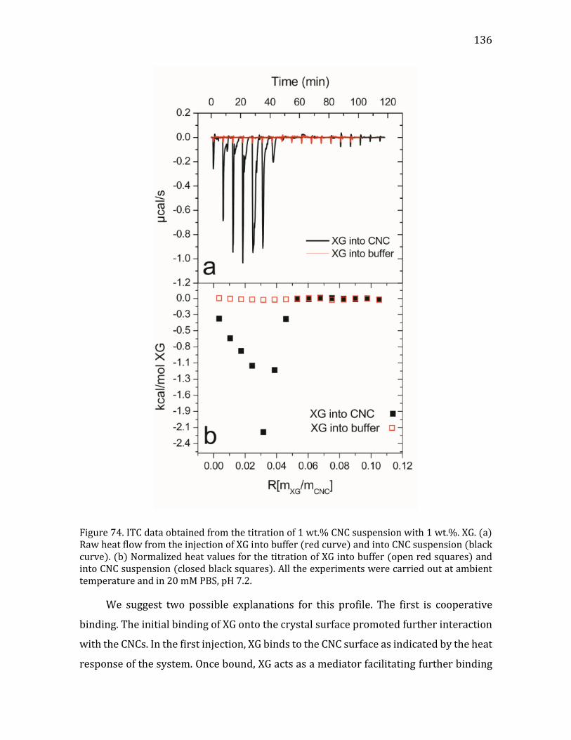
136
Figure 74. ITC data obtained from the titration of 1 wt.% CNC suspension with 1 wt.%. XG. (a) Raw heat flow from the injection of XG into buffer (red curve) and into CNC suspension (black curve). (b) Normalized heat values for the titration of XG into buffer (open red squares) and into CNC suspension (closed black squares). All the experiments were carried out at ambient temperature and in 20 mM PBS, pH 7.2.
We suggest two possible explanations for this profile. The first is cooperative
binding. The initial binding of XG onto the crystal surface promoted further interaction
with the CNCs. In the first injection, XG binds to the CNC surface as indicated by the heat
response of the system. Once bound, XG acts as a mediator facilitating further binding
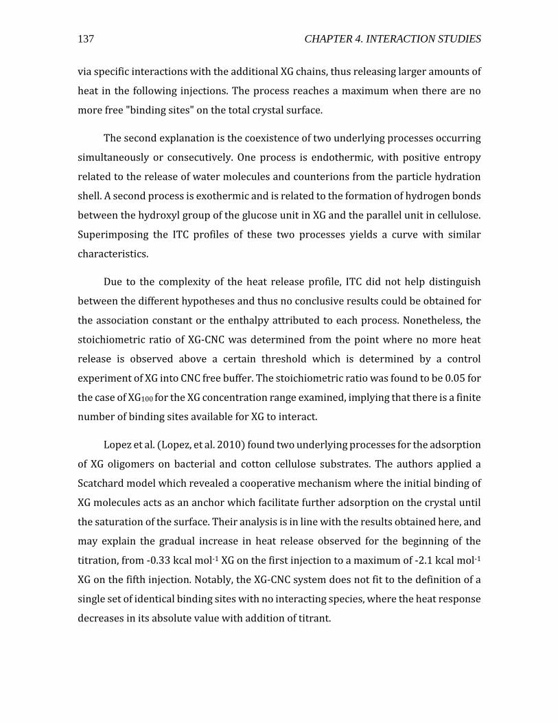
137 CHAPTER 4. INTERACTION STUDIES
via specific interactions with the additional XG chains, thus releasing larger amounts of
heat in the following injections. The process reaches a maximum when there are no
more free "binding sites" on the total crystal surface.
The second explanation is the coexistence of two underlying processes occurring
simultaneously or consecutively. One process is endothermic, with positive entropy
related to the release of water molecules and counterions from the particle hydration
shell. A second process is exothermic and is related to the formation of hydrogen bonds
between the hydroxyl group of the glucose unit in XG and the parallel unit in cellulose.
Superimposing the ITC profiles of these two processes yields a curve with similar
characteristics.
Due to the complexity of the heat release profile, ITC did not help distinguish
between the different hypotheses and thus no conclusive results could be obtained for
the association constant or the enthalpy attributed to each process. Nonetheless, the
stoichiometric ratio of XG-CNC was determined from the point where no more heat
release is observed above a certain threshold which is determined by a control
experiment of XG into CNC free buffer. The stoichiometric ratio was found to be 0.05 for
the case of XG100 for the XG concentration range examined, implying that there is a finite
number of binding sites available for XG to interact.
Lopez et al. (Lopez, et al. 2010) found two underlying processes for the adsorption
of XG oligomers on bacterial and cotton cellulose substrates. The authors applied a
Scatchard model which revealed a cooperative mechanism where the initial binding of
XG molecules acts as an anchor which facilitate further adsorption on the crystal until
the saturation of the surface. Their analysis is in line with the results obtained here, and
may explain the gradual increase in heat release observed for the beginning of the
titration, from -0.33 kcal mol-1 XG on the first injection to a maximum of -2.1 kcal mol-1
XG on the fifth injection. Notably, the XG-CNC system does not fit to the definition of a
single set of identical binding sites with no interacting species, where the heat response
decreases in its absolute value with addition of titrant.
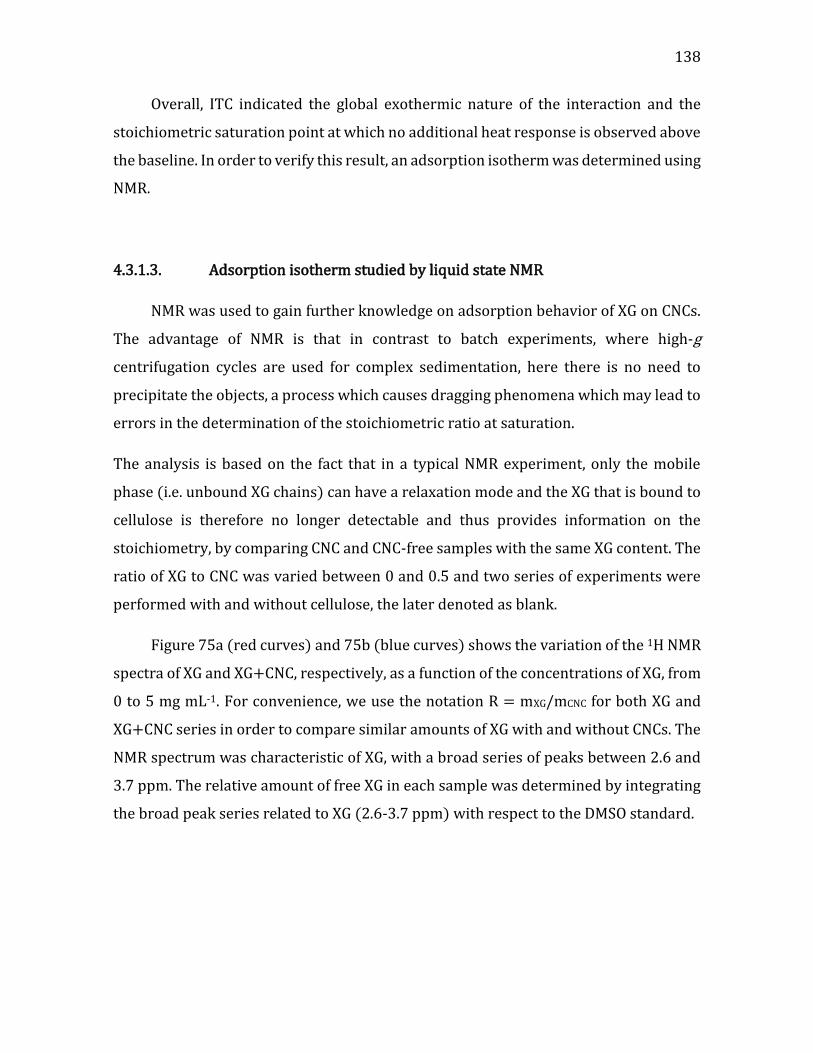
138
Overall, ITC indicated the global exothermic nature of the interaction and the
stoichiometric saturation point at which no additional heat response is observed above
the baseline. In order to verify this result, an adsorption isotherm was determined using
NMR.
4.3.1.3. Adsorption isotherm studied by liquid state NMR
NMR was used to gain further knowledge on adsorption behavior of XG on CNCs.
The advantage of NMR is that in contrast to batch experiments, where high-g
centrifugation cycles are used for complex sedimentation, here there is no need to
precipitate the objects, a process which causes dragging phenomena which may lead to
errors in the determination of the stoichiometric ratio at saturation.
The analysis is based on the fact that in a typical NMR experiment, only the mobile
phase (i.e. unbound XG chains) can have a relaxation mode and the XG that is bound to
cellulose is therefore no longer detectable and thus provides information on the
stoichiometry, by comparing CNC and CNC-free samples with the same XG content. The
ratio of XG to CNC was varied between 0 and 0.5 and two series of experiments were
performed with and without cellulose, the later denoted as blank.
Figure 75a (red curves) and 75b (blue curves) shows the variation of the 1H NMR
spectra of XG and XG+CNC, respectively, as a function of the concentrations of XG, from
0 to 5 mg mL-1. For convenience, we use the notation R = mXG/mCNC for both XG and
XG+CNC series in order to compare similar amounts of XG with and without CNCs. The
NMR spectrum was characteristic of XG, with a broad series of peaks between 2.6 and
3.7 ppm. The relative amount of free XG in each sample was determined by integrating
the broad peak series related to XG (2.6-3.7 ppm) with respect to the DMSO standard.
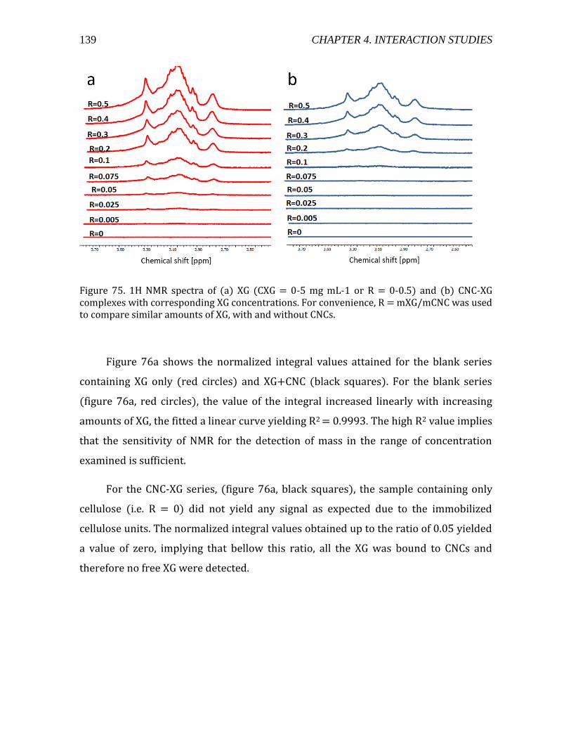
139 CHAPTER 4. INTERACTION STUDIES
Figure 75. 1H NMR spectra of (a) XG (CXG = 0-5 mg mL-1 or R = 0-0.5) and (b) CNC-XG complexes with corresponding XG concentrations. For convenience, R = mXG/mCNC was used to compare similar amounts of XG, with and without CNCs.
Figure 76a shows the normalized integral values attained for the blank series
containing XG only (red circles) and XG+CNC (black squares). For the blank series
(figure 76a, red circles), the value of the integral increased linearly with increasing
amounts of XG, the fitted a linear curve yielding R2 = 0.9993. The high R2 value implies
that the sensitivity of NMR for the detection of mass in the range of concentration
examined is sufficient.
For the CNC-XG series, (figure 76a, black squares), the sample containing only
cellulose (i.e. R = 0) did not yield any signal as expected due to the immobilized
cellulose units. The normalized integral values obtained up to the ratio of 0.05 yielded
a value of zero, implying that bellow this ratio, all the XG was bound to CNCs and
therefore no free XG were detected.

140
Figure 76. (a) Normalized integral values obtained from integration of the XG peak between 3.7 and 2.6 ppm as a function of XG-CNC ratio for XG (red circles) and XG+CNC (black squares). The red line represents a linear fit to the data. (b) Subtracted integral as a function of XG-CNC ratio. The red line is a guide to the eye.
Above R = 0.05, a signal was detected, and from a value of about R = 0.1, a linear
increase in the integral values was observed with the increase in XG/CNC mass ratio for
the series containing cellulose, and the slope in that case was similar to the slope of the
blank series, indicating the accumulation of non-adsorbed XG in the bulk.
Figure 76b shows the difference between the integral values for the XG and the
XG-CNC series as a function of R. This difference reached a nearly constant value,
implying a saturation of the available binding sites and thus no further adsorption was
observed. However, it should be mentioned that the value at which the system reaches
saturation cannot be estimated from the plateau of this curve. We did not attempt to fit
the result to the classical Langmuir model since the assumptions used in this model (i.e.
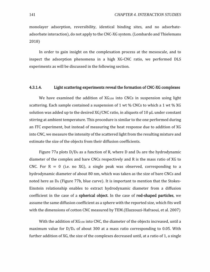
141 CHAPTER 4. INTERACTION STUDIES
monolayer adsorption, reversibility, identical binding sites, and no adsorbate-
adsorbate interaction), do not apply to the CNC-XG system. (Lombardo and Thielemans
2018)
In order to gain insight on the complexation process at the mesoscale, and to
inspect the adsorption phenomena in a high XG-CNC ratio, we performed DLS
experiments as will be discussed in the following section.
4.3.1.4. Light scattering experiments reveal the formation of CNC-XG complexes
We have examined the addition of XG100 into CNCs in suspension using light
scattering. Each sample contained a suspension of 1 wt % CNCs to which a 1 wt % XG
solution was added up to the desired XG/CNC ratio, in aliquots of 10 µL under constant
stirring at ambient temperature. This procedure is similar to the one performed during
an ITC experiment, but instead of measuring the heat response due to addition of XG
into CNC, we measure the intensity of the scattered light from the resulting mixture and
estimate the size of the objects from their diffusion coefficients.
Figure 77a plots D/D0 as a function of R, where D and D0 are the hydrodynamic
diameter of the complex and bare CNCs respectively and R is the mass ratio of XG to
CNC. For R = 0 (i.e. no XG), a single peak was observed, corresponding to a
hydrodynamic diameter of about 80 nm, which was taken as the size of bare CNCs and
noted here as D0 (Figure 77b, blue curve). It is important to mention that the Stokes-
Einstein relationship enables to extract hydrodynamic diameter from a diffusion
coefficient in the case of a spherical object. In the case of rod-shaped particles, we
assume the same diffusion coefficient as a sphere with the reported size, which fits well
with the dimensions of cotton CNC measured by TEM.(Elazzouzi-Hafraoui, et al. 2007)
With the addition of XG100 into CNC, the diameter of the objects increased, until a
maximum value for D/Do of about 300 at a mass ratio corresponding to 0.05. With
further addition of XG, the size of the complexes decreased until, at a ratio of 1, a single

142
peak was observed, corresponding to a diameter of about 140 nm or D/Do of 1.7,
(Figure 77b, red curve).
Figure 77: (a) Z-average hydrodynamic diameter as a function of XG/CNC mass ratio as obtained from DLS following the sequential addition of 1 wt % XG into 1 wt %. CNC suspension. The grey line is a guide to the eye and has no physical meaning. The yellow shading represents the aggregation zone (see text for details) (b) normalized intensity and (c) ζ-potential values for bare CNCs (blue curve and column) and decorated CNCs (red curve and column). The corresponding points in graph (a) are labeled in blue (R=0) and red (R=1).
The maximum diameter observed by light scattering was 300 times the initial
diameter at a mass ratio of 0.05, a size which is beyond the detection limit of the
apparatus used (~4-5 µm). In fact, all values obtained for 0.045 > R > 0.065 (yellow
shading in figure 77a) were beyond the detection limit of the apparatus in the actual
working conditions, and consequently have no real physical meaning. Therefore, we do
not conclude for a definite size in this region but merely note the trend observed, and
define the stoichiometric point as the middle point in this region.

143 CHAPTER 4. INTERACTION STUDIES
Since the scattering from XG alone, at this concentration range, has little to no
effect on the overall scattering intensity and it is negligible compared to the scattering
from the CNCs, we can assimilate the increase in hydrodynamic diameter of the objects
to the adsorbed polymer on the crystal surface which slows down the movement of the
objects causing the decrease in measured diffusion coefficient.
Figure 77c shows ζ-potential values of bare CNC (R = 0) and XG decorated CNCs
(R = 1). The ζ-potential value for R=0 and R=1 were -36.6 and -5.0 mV respectively.
Being negatively charged colloids, CNCs carry an electrical double layer containing ions
and water molecules which are present close to the crystal surface and moves in similar
speed. Any adsorption of another object, whether it is a surfactant or a polymer, will
enforce a rearrangement of the double layer and will change the electrical properties of
the surface. Since electrophoretic mobility is closely related to surface charge, and is
relatively easy to measure, it may be used as a method to confirm adsorption of
polymers and other molecules onto cellulose. (Oikonomou, et al. 2017, Stana, et al.
1995)
Figure 78. The reduction of measured ζ-Potential is attributed to the displacement of the shear plane upon adsorption of polymer on a surface.(Quemeneur 2010)

144
Taken together with the value of hydrodynamic diameter of the complexes at R =
1, we attribute the change in electrophoretic mobility to the presence of the adsorbed
polymer on the surface of the CNCs. In fact, the ζ- potential is the potential at the shear
plane, which is displaced due to adsorption of a polymer on a surface (figure 78), in our
case XG on the CNCs.
Unlike salt mediated aggregation, where the aggregates continue to grow with
addition of salt, in the case of XG-CNC complexes, beyond a critical ratio, the aggregates
separate, leading to a decrease in apparent diameter.
From the ITC, NMR and light scattering experiments, several characteristic
adsorption regimes can be identified, defined by the XG/CNC mass ratio R. At R = 0 (no
XG), CNCs are colloidally stable due to electrostatic repulsion. At 0 > R > 0.05, an
adsorption of XG leads to the formation of CNC-XG complexes by bridging of adjacent
crystals, causing a gradual increase in aggregate size. At 0.05 < R < 1 a gradual decrease
in aggregate size and separation of large bundles is observed. At this regime, the CNCs
are covered by a polymer layer, as indicated by the DLS and ζ-potential values at R = 1.
In order to gain further information regarding the organization of the CNC-XG
complexes in the nanoscale, we observed the samples by TEM in these representative
adsorption regimes, as will be discussed in the following section.
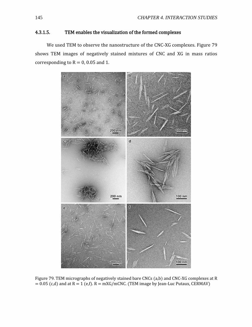
145 CHAPTER 4. INTERACTION STUDIES
4.3.1.5. TEM enables the visualization of the formed complexes
We used TEM to observe the nanostructure of the CNC-XG complexes. Figure 79
shows TEM images of negatively stained mixtures of CNC and XG in mass ratios
corresponding to R = 0, 0.05 and 1.
Figure 79. TEM micrographs of negatively stained bare CNCs (a,b) and CNC-XG complexes at R = 0.05 (c,d) and at R = 1 (e,f). R = mXG/mCNC. (TEM image by Jean-Luc Putaux, CERMAV)
146
Figure 79a and b corresponds to the bare CNCs (R=0). CNCs appear as bundles of
3-5 elementary crystallites, with average length of 150 nm, width of 20 nm and height
of 7 nm, in agreement with previous observations (Elazzouzi-Hafraoui, 2007). The
objects are separated due to electrostatic repulsion, as previously discussed.
At a ratio of 0.05, (Figure 79c and d) the distance between the crystals
dramatically decreased and the CNCs appeared to be aggregated. It is reasonable to
assume that the aggregates observed in the case of R = 0.05 are, in fact, fragments of
the large aggregates detected by light scattering, as shown in the previous section,
having an approximate diameter from few hundred nanometers up to several microns.
At R = 1 (figure 79 e and f), the separation between crystals increased compared to R
= 0.05 and resembles the separation between crystal bundles in the case of bare CNCs.
There was no direct evidence of the presence of XG in the TEM images. XG is non-
crystalline and in a non-aggregated molecular state, it is likely that negative staining is
not sufficient to reveal the polysaccharide. Therefore, it is not possible to conclude, at
this resolution, on the spatial distribution of XG.
These results are in agreement with the ones obtained by Dammak et al.
(Dammak, et al. 2015) who studied the adsorption of XG onto cellulose in different
adsorption regimes by enzymatic degradation. The authors have identified two main
adsorption regimes in which, at low XG/CNC ratio, XG tightly adsorbed on cellulose,
inducing aggregation of CNCs, and at high XG/CNC ratio, the crystals were separated.
4.3.1.6. Surface covered by XG at R = 0.05 from atomistic modeling
We have complemented the experimental results by atomistic simulations in
order to estimate the cellulose surface covered by XG at R = 0.05. 1 g of cellulose
contains 3·1016 nanocrystals. Each nanocrystal exhibits a usable area for XG adsorption
of 6000 nm2 estimated from its measured dimensions: 150 × 20 × 7 nm3 (Elazzouzi-
Hafraoui, et al. 2007) so the total surface area of 1 g of cellulose is 1.8·1020 nm2.

147 CHAPTER 4. INTERACTION STUDIES
For the polymer adsorption, 0.05 g of XG contains 2.2·1019 repeat units,
considering that the molar mass of one unit of XG (4 glucose units, 3 xylose, and 1
galactose) is 1350 g mol-1. The projected dimensions of the XG repeat unit in the
molecular model at equilibrium are 2.1 and 2.2 nm (Figure 80). XG repeat thus covers
a surface of 4.6 nm2. Assuming the ideal flat conformation with maximal coverage
identical to that observed in the simulation, 0.05 g of XG would theoretically covers a
total surface area of 1.0·1020 nm2.
Comparing the two values, the cellulose area of 1.8·1020 nm2 estimated from
experimentally measured dimensions versus the theoretical area that XG can covers
from modeling of 1.0·1020 nm2, suggests that R = 0.05 is slightly below the monolayer
regime.
However, for the calculation of the theoretical crystal surface, we have used a
single value for the length which was 150 nm. Bearing in mind the shape polydispersity
of the 50-250-nm-long CNCs, as also evident from the TEM images, the values obtained
from theoretical calculation suggest that sonicated XG adsorbed in a flat conformation
referred to as "trains" on the surface. These results support those of Villares et al. who
found that sonicated XG (low Mw) tended to adsorb in a flat conformation on the
surface of CNCs while non-sonicated XG (high Mw) tended to form "loops" and
"tails".(Villares, et al. 2015, Villares, et al. 2017)
Figure 80. Simulated XG repeat unit adsorbed on the (100) cellulose crystal surface. (a) top view, (b) side view. (By Karim Mazeau, CERMAV)
a b
148
4.3.1.7. The addition of salt to CNC-XG complexes confirms steric stabilization
In order to verify the presence of a XG layer which presents a steric barrier
between the CNCs, salt was added to the CNC-XG complex at R = 1. In order to eliminate
the effect of unbound polymer molecules, the excess XG was removed by centrifugation
of the complex and redispersion in aqueous medium. For comparison, salt was added
to bare CNC and XG-decorated CNCs. Figures 81a and 80b shows images of bare and
decorated CNCs respectively, with addition of NaCl. At NaCl concentrations of 0.1, 0.5
and 1.0 M, the bare CNC suspensions became turbid and the turbidity slightly increased
with increasing salt concentration. We attribute this apparent turbidity to the
formation of large aggregates, indicating the screening of electrostatic repulsion
between the CNCs.
In contrast, addition of salt to decorated CNCs did not result in the increase of
apparent turbidity, for the NaCl concentration range examined. In order to get a clearer
view of the objects size with the addition of salt, we have estimated the mean
hydrodynamic diameter of the objects as a function of NaCl concentration for bare and
decorated CNCs using DLS (Figure 81c).
The mean hydrodynamic diameter obtained for the bare CNCs dramatically
increased from about 80 nm with no salt to few hundred nanometers for 0.1, 0.5 and
1.0 M NaCl. It must be mentioned that the addition of salt in the case of bare CNCs
resulted in a multimodal distribution. Thus, the calculated average size obtained by the
fit to the correlation function merely emphasizes the increase in aggregate size rather
than providing an accurate measure for the hydrodynamic diameter of the objects.
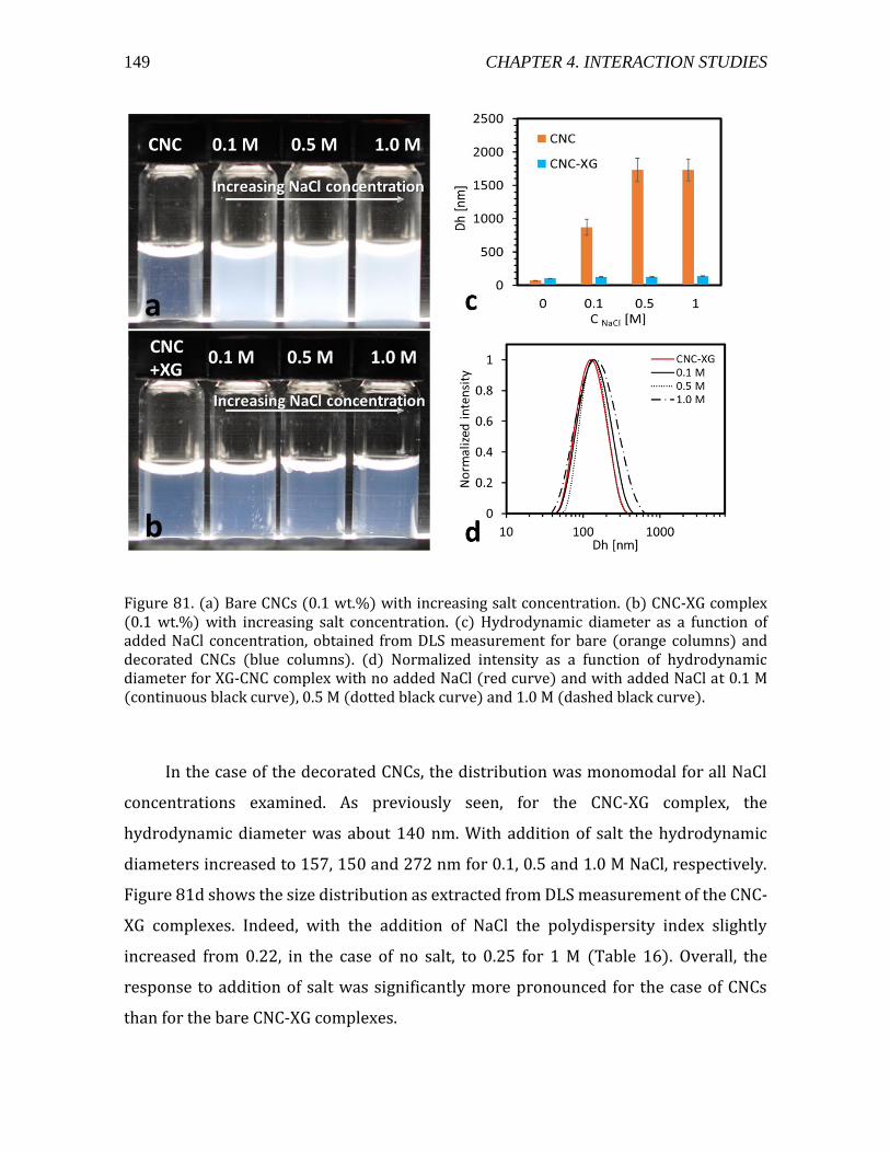
149 CHAPTER 4. INTERACTION STUDIES
Figure 81. (a) Bare CNCs (0.1 wt.%) with increasing salt concentration. (b) CNC-XG complex (0.1 wt.%) with increasing salt concentration. (c) Hydrodynamic diameter as a function of added NaCl concentration, obtained from DLS measurement for bare (orange columns) and decorated CNCs (blue columns). (d) Normalized intensity as a function of hydrodynamic diameter for XG-CNC complex with no added NaCl (red curve) and with added NaCl at 0.1 M (continuous black curve), 0.5 M (dotted black curve) and 1.0 M (dashed black curve).
In the case of the decorated CNCs, the distribution was monomodal for all NaCl
concentrations examined. As previously seen, for the CNC-XG complex, the
hydrodynamic diameter was about 140 nm. With addition of salt the hydrodynamic
diameters increased to 157, 150 and 272 nm for 0.1, 0.5 and 1.0 M NaCl, respectively.
Figure 81d shows the size distribution as extracted from DLS measurement of the CNC-
XG complexes. Indeed, with the addition of NaCl the polydispersity index slightly
increased from 0.22, in the case of no salt, to 0.25 for 1 M (Table 16). Overall, the
response to addition of salt was significantly more pronounced for the case of CNCs
than for the bare CNC-XG complexes.

150
Table 16: Hydrodynamic diameter and PDI values obtained from CONTIN (CON) and cumulants (CUM) analyses of the autocorrelation function measured by DLS for bare and decorated CNCs with the addition of salt (expressed in M). PDI is the polydispersity index.
Sample Dh [nm, CUM] PDI Dh [nm, CON]
CNC 74 ± 1 0.18 ± 0.02 91 ± 3
CNC+ (0.1 M) 874 ± 120 1.00 1428 ± 351
CNC+ (0.5 M) 1732 ± 179 1.00 383 ± 66
CNC+ (1.0 M) 1731 ± 166 1.00 400 ± 72
CNC-XG 107 ± 1 0.22 ± 0.01 137 ± 1
CNC-XG+ (0.1 M) 124 ± 4 0.21 ± 0.01 157 ± 4
CNC-XG+ (0.5 M) 124 ± 4 0.18 ± 0.02 150 ± 4
CNC-XG+ (1.0 M) 134 ± 6 0.25 ± 0.03 272 ± 104
Taken together with the ζ-potential measurements, these results suggest that the
electrostatic stabilization in the case of bare CNCs, was replaced by a steric stabilization
in the case of CNC-XG complexes. Moreover, the removal of unbound XG from the
system did not alter the decorated crystal shape, leading us to the conclusion that at
high XG/CNC ratio, a CNC-XG core-shell particle was formed, stabilized by steric
repulsion in place of the original electrostatic repulsion of the bare CNCs.
4.3.1.8. Summary and conclusions
In this part we have followed the formation of CNC-XG complexes using multiple
techniques. The data confirms the presence of a complex adsorption process with a
specific stoichiometry. The adsorption process seems to include two main steps: (i) The
rapid adsorption of XG onto the CNC surface, a physical process which leads to the
occupation of most binding sites and creates a diffusion barrier for the next XG
molecules, while bridging two or more adjacent crystal bundles to form large
aggregates. (ii) Slower adsorption, rearrangement and entanglements with other XG
molecules, and finally separation of the formed CNC-XG aggregates.
151 CHAPTER 4. INTERACTION STUDIES
The results also suggest that the aggregation and formation of bundles may be
reversed with further addition of XG molecules. Possibly, the addition of XG molecules
changes the solution properties in a way that favors the dissolution of the loosely bound
XG layer back to the solution, reducing the diameter of the observed complexes until, at
a XG/CNC mass ratio of 1, only the irreversible tightly bound first layer of XG is
remained.
From this study, we conclude that the following points:
• XG will be used in its sonicated form in order to promote tighter and faster
adsorption.
• The ratio between the mass of CNC and the mass of XG in the biomimetic
constructs will be tuned to be 0.1, slightly above the saturation ratio to ensure
complete adsorption and optimal surface coverage.
• Addition of salt can promote the adsorption, therefore 1-10 mM of NaCl will be
added in the biomimetic constructs.
To gain further information, in the following chapter we will examine the
interaction between CNC and XG using a 2D configuration.
4.3.2. CNC-XG interaction in 2D
The interaction of CNC with XG was examined in 2D with QCM-D. The limitations
of this method regarding this system are (1) long rearrangement times of XG chains on
the CNC surface (already shown in the 3D experiments) (2) loss of signal after the 2nd
layer of CNC due to high dissipation leading to low accuracy. We therefore focus on the
first CNC-XG layer, deposited in this case on SLB from DOPC/DOTAP 70/30 %
mol./%mol. in 0.2M sucrose at pH 6. We used 0.1 %wt. CNCs and 0.01 %wt. XG
suspensions dissolved in 0.2 M glucose solutions, to mimic as close as possible the
conditions in which the biomimetic constructs will be prepared. Figure 82 shows QCM-
D profile from the deposition of SLB, CNC and XG layers.

152
Figure 82. QCM-D profile showing the deposition of SLB, CNC and XG. The frequency (black line) and the dissipation (grey line) for the 7th overtone, are plotted on the left and right axes respectively. The different steps are labeled with a colored star (blue=SLB, red=CNC, green=XG) and arrows (rinsing steps).
The adsorption profile shows fast, almost immediate adsorption of SLB on the
quartz crystal followed by fast adsorption of CNCs. The adsorption of XG was slower
(~20 min), yet resulted in a final stable baseline, implying that the adsorption process
was completed within the time scale of the measurement. In addition, the rinsing steps
(black arrows) did not result in removal of mass as indicated by the stable frequency
value for all deposition steps.
Given the low dissipation values, Sauerbrey relationship was used for the
calculation of adsorbed mass, taking the film density as the one of water. Table 17
shows the values obtained for the frequency, dissipation, mass and calculated thickness
of the SLB CNC and XG layers composing the film.
The values of frequency and dissipation for the SLB were -25.2 Hz and 0.8·10-6
respectively, resulting in SLB thickness of of 4.5 nm. values of frequency and dissipation
for the CNC layer were -29.7 Hz and 2.9·10-6 respectively, resulting in CNC thickness of
5.3 nm, in agreement with the previous results obtained for SLB-CNC system (chapter
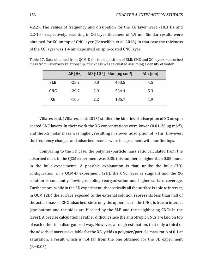
153 CHAPTER 4. INTERACTION STUDIES
4.2.2). The values of frequency and dissipation for the XG layer were -10.3 Hz and
2.2·10-6 respectively, resulting in XG layer thickness of 1.9 nm. Similar results were
obtained for XG on top of CNC layer.(Benselfelt, et al. 2016) in that case the thickness
of the XG layer was 1.4 nm deposited on spin-coated CNC layer.
Table 17. Data obtained from QCM-D for the deposition of SLB, CNC and XG layers. aadsorbed mass from Sauerbrey relationship. tthickness was calculated assuming a density of water.
ΔF [Hz] ΔD [·10-6] aΔm [ng cm-2] bΔh [nm]
SLB -25.2 0.8 453.5 4.5
CNC -29.7 2.9 534.4 5.3
XG -10.3 2.2 185.7 1.9
Villares et al. (Villares, et al. 2015) studied the kinetics of adsorption of XG on spin
coated CNC layers. In their work the XG concentrations were lower (0.01-20 µg mL-1),
and the XG molar mass was higher, resulting in slower adsorption of ~1hr. However,
the frequency changes and adsorbed masses were in agreement with our findings.
Comparing to the 3D case, the polymer/particle mass ratio calculated from the
adsorbed mass in the QCM experiment was 0.35. this number is higher than 0.05 found
in the bulk experiments. A possible explanation is that, unlike the bulk (3D)
configuration, in a QCM-D experiment (2D), the CNC layer is stagnant and the XG
solution is constantly flowing enabling reorganization and higher surface coverage.
Furthermore, while in the 3D experiment- theoretically all the surface is able to interact,
in QCM (2D) the surface exposed to the external solution represents less than half of
the actual mass of CNC adsorbed, since only the upper face of the CNCs is free to interact
(the bottom and the sides are blocked by the SLB and the neighboring CNCs in the
layer). A precise calculation is rather difficult since the anisotropic CNCs are laid on top
of each other in a disorganized way. However, a rough estimation, that only a third of
the adsorbed mass is available for the XG, yields a polymer/particle mass ratio of 0.1 at
saturation, a result which is not far from the one obtained for the 3D experiment
(R=0.05).
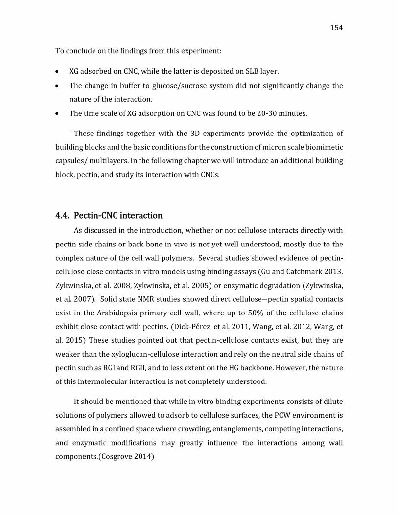
154
To conclude on the findings from this experiment:
• XG adsorbed on CNC, while the latter is deposited on SLB layer.
• The change in buffer to glucose/sucrose system did not significantly change the
nature of the interaction.
• The time scale of XG adsorption on CNC was found to be 20-30 minutes.
These findings together with the 3D experiments provide the optimization of
building blocks and the basic conditions for the construction of micron scale biomimetic
capsules/ multilayers. In the following chapter we will introduce an additional building
block, pectin, and study its interaction with CNCs.
4.4. Pectin-CNC interaction
As discussed in the introduction, whether or not cellulose interacts directly with
pectin side chains or back bone in vivo is not yet well understood, mostly due to the
complex nature of the cell wall polymers. Several studies showed evidence of pectin-
cellulose close contacts in vitro models using binding assays (Gu and Catchmark 2013,
Zykwinska, et al. 2008, Zykwinska, et al. 2005) or enzymatic degradation (Zykwinska,
et al. 2007). Solid state NMR studies showed direct cellulose−pectin spatial contacts
exist in the Arabidopsis primary cell wall, where up to 50% of the cellulose chains
exhibit close contact with pectins. (Dick-Pérez, et al. 2011, Wang, et al. 2012, Wang, et
al. 2015) These studies pointed out that pectin-cellulose contacts exist, but they are
weaker than the xyloglucan-cellulose interaction and rely on the neutral side chains of
pectin such as RGI and RGII, and to less extent on the HG backbone. However, the nature
of this intermolecular interaction is not completely understood.
It should be mentioned that while in vitro binding experiments consists of dilute
solutions of polymers allowed to adsorb to cellulose surfaces, the PCW environment is
assembled in a confined space where crowding, entanglements, competing interactions,
and enzymatic modifications may greatly influence the interactions among wall
components.(Cosgrove 2014)

155 CHAPTER 4. INTERACTION STUDIES
Regardless if cellulose-pectin links exist in vivo, understanding of its interaction
with the other components of the system is essential for their incorporation in our
biomimetic constructs. Since XG and pectin are not believed to be interacting directly
in vivo, we rely on possible interaction between CNCs and pectin. Both CNC and pectin
being negatively charged, one as a colloid and the other as a polyelectrolyte,
electrostatic repulsion has to be overcome in order to promote the adsorption of pectin
on the crystal surface. Three possible mechanisms may be taken into account:
1. Screening the electrostatic repulsion using monovalent electrolyte.
2. Creating coordinative binding through calcium mediated interaction.
3. Gelation of the pectic chain via egg-box type or entanglement mechanism
followed by entrapment of cellulose aggregates in the network.
In order address these points, a series of experiments was performed. First, CNCs
were simply mixed with pectin at constant CNC concentration and increasing pectin
concentration for two types of pectin: P35 and P71, and 3 types of medium: water, NaCl
10 mM and CaCl2 3.3 mM representing similar ionic strength of 10 mM. The mixtures
were left under stirring overnight for equilibrium, then observed or measured with
DLS.
4.4.1. Screening experiments
Figure 83 shows mixtures of CNC (1 %wt.) and pectins (1% wt., P35 and P71) at
increasing polymer/particle ratio. The first point, at R=0 corresponds to pure CNCs.
The mixing was performed dropwise under stirring and the order of addition was CNC,
pectin and electrolyte solutions consecutively with 10 minutes delay between pectin
and electrolyte solution, to ensure proper mixing of the two first components.
156
Figure 83: Mixtures of CNC-pectin in water (a,b) NaCl 10mM (c,d) and CaCl2 3.3 mM. for tow degrees of methyl esterification: P35 DE=0.35 (a,c,e,) and P71 DE=70 (b,d,f)
The first evident observation is that with the increase in polymer/particle ratio, a
minor increase in the turbidity of the mixtures is observed, with a sharp increase in
turbidity for R=1. This phenomenon is observed for both P35 and P71 even without the
presence of salt, suggesting that depletion forces exist at high ratio due to the presence
of high amount of polymer and reduction of the available free volume. Such phenomena
was observed for other particle/polymer systems carrying similar charge
sign.(Toyotama, et al. 2016) Noticeably, the sum of electrostatic, depletion and VdW
forces needs to be taken into account. At high polyelectrolyte concentration, the
contribution of depletion to the total sum of forces reduces the separation distance
between two components enabling contact and eventual aggregation.
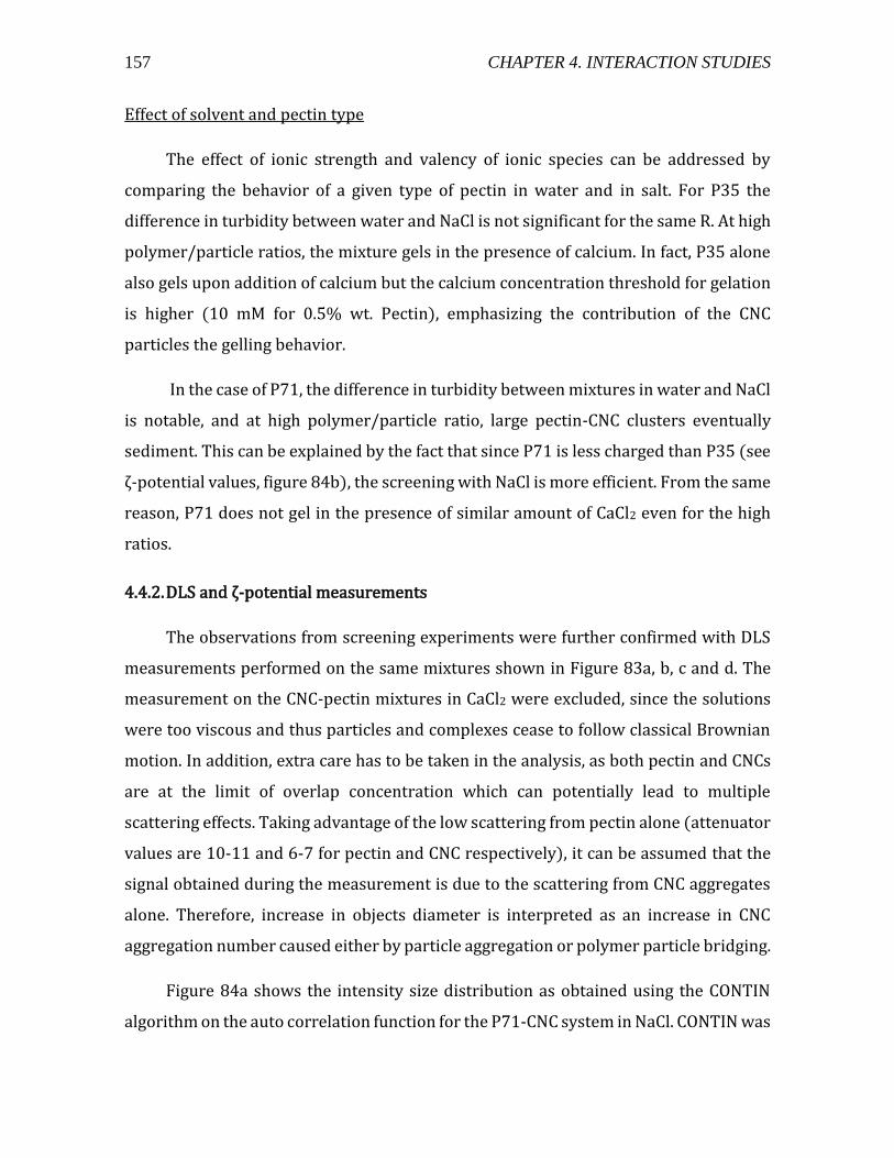
157 CHAPTER 4. INTERACTION STUDIES
Effect of solvent and pectin type
The effect of ionic strength and valency of ionic species can be addressed by
comparing the behavior of a given type of pectin in water and in salt. For P35 the
difference in turbidity between water and NaCl is not significant for the same R. At high
polymer/particle ratios, the mixture gels in the presence of calcium. In fact, P35 alone
also gels upon addition of calcium but the calcium concentration threshold for gelation
is higher (10 mM for 0.5% wt. Pectin), emphasizing the contribution of the CNC
particles the gelling behavior.
In the case of P71, the difference in turbidity between mixtures in water and NaCl
is notable, and at high polymer/particle ratio, large pectin-CNC clusters eventually
sediment. This can be explained by the fact that since P71 is less charged than P35 (see
ζ-potential values, figure 84b), the screening with NaCl is more efficient. From the same
reason, P71 does not gel in the presence of similar amount of CaCl2 even for the high
ratios.
4.4.2. DLS and ζ-potential measurements
The observations from screening experiments were further confirmed with DLS
measurements performed on the same mixtures shown in Figure 83a, b, c and d. The
measurement on the CNC-pectin mixtures in CaCl2 were excluded, since the solutions
were too viscous and thus particles and complexes cease to follow classical Brownian
motion. In addition, extra care has to be taken in the analysis, as both pectin and CNCs
are at the limit of overlap concentration which can potentially lead to multiple
scattering effects. Taking advantage of the low scattering from pectin alone (attenuator
values are 10-11 and 6-7 for pectin and CNC respectively), it can be assumed that the
signal obtained during the measurement is due to the scattering from CNC aggregates
alone. Therefore, increase in objects diameter is interpreted as an increase in CNC
aggregation number caused either by particle aggregation or polymer particle bridging.
Figure 84a shows the intensity size distribution as obtained using the CONTIN
algorithm on the auto correlation function for the P71-CNC system in NaCl. CONTIN was
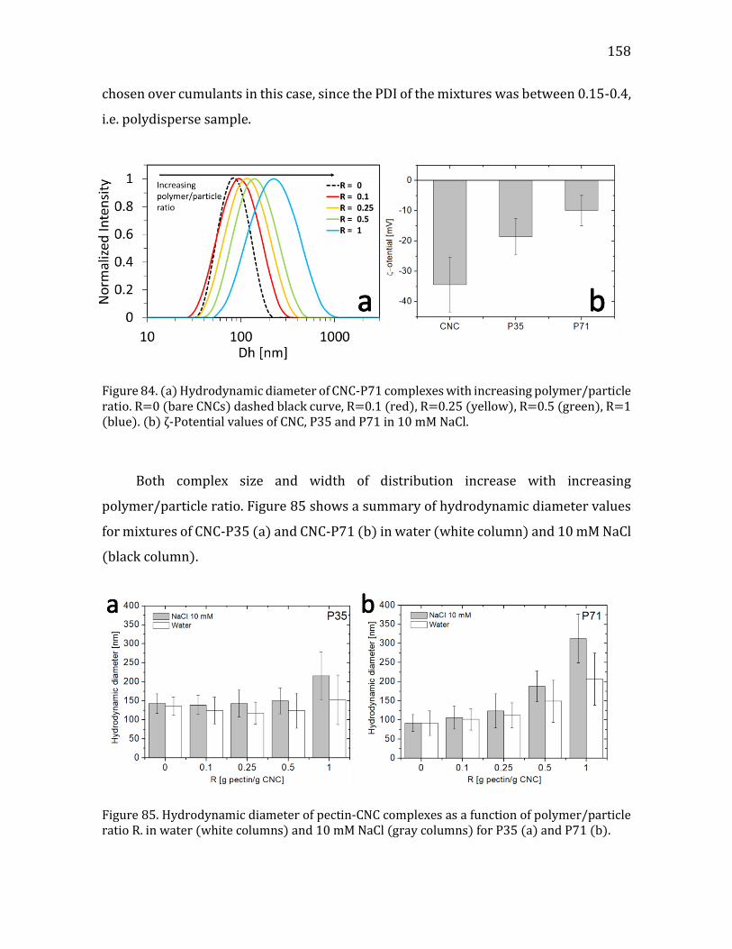
158
chosen over cumulants in this case, since the PDI of the mixtures was between 0.15-0.4,
i.e. polydisperse sample.
Figure 84. (a) Hydrodynamic diameter of CNC-P71 complexes with increasing polymer/particle ratio. R=0 (bare CNCs) dashed black curve, R=0.1 (red), R=0.25 (yellow), R=0.5 (green), R=1 (blue). (b) ζ-Potential values of CNC, P35 and P71 in 10 mM NaCl.
Both complex size and width of distribution increase with increasing
polymer/particle ratio. Figure 85 shows a summary of hydrodynamic diameter values
for mixtures of CNC-P35 (a) and CNC-P71 (b) in water (white column) and 10 mM NaCl
(black column).
Figure 85. Hydrodynamic diameter of pectin-CNC complexes as a function of polymer/particle ratio R. in water (white columns) and 10 mM NaCl (gray columns) for P35 (a) and P71 (b).
159 CHAPTER 4. INTERACTION STUDIES
A notable increase in hydrodynamic diameter is observed for the highest
polymer/particle ratios in all conditions. The difference in Dh between water and NaCl
for the same ratios was higher for P71 than for P35. This is backed up by the
observation of the complexes in naked eye (Figure 83).
4.4.3. Summary
• The interaction between CNCs and pectin depended on polymer/particle ratio,
pectin charge, the ionic strength of the medium and the valency of the electrolyte
solution.
• At high polymer/particle ratios, depletion forces could be overcome the
electrostatic repulsion, causing CNC aggregation.
• In the presence of monovalent salt, screening effect takes place at higher ratios,
effect that is more pronounced in the case of P71 due to the lower DE and thus
lower negative charge.
• In the presence of divalent salt, P35 gels at high polymer/particle ratios.
These conclusions are summarized in table 18.
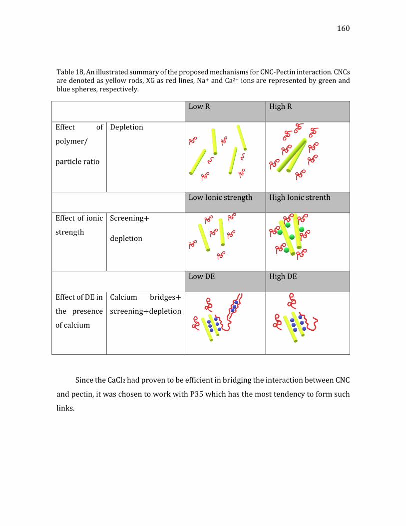
160
Table 18, An illustrated summary of the proposed mechanisms for CNC-Pectin interaction. CNCs are denoted as yellow rods, XG as red lines, Na+ and Ca2+ ions are represented by green and blue spheres, respectively.
Low R High R
Effect of
polymer/
particle ratio
Depletion
Low Ionic strength High Ionic strenth
Effect of ionic
strength
Screening+
depletion
Low DE High DE
Effect of DE in
the presence
of calcium
Calcium bridges+
screening+depletion
Since the CaCl2 had proven to be efficient in bridging the interaction between CNC
and pectin, it was chosen to work with P35 which has the most tendency to form such
links.
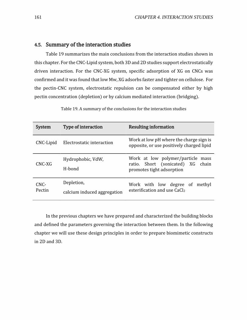
161 CHAPTER 4. INTERACTION STUDIES
4.5. Summary of the interaction studies
Table 19 summarizes the main conclusions from the interaction studies shown in
this chapter. For the CNC-Lipid system, both 3D and 2D studies support electrostatically
driven interaction. For the CNC-XG system, specific adsorption of XG on CNCs was
confirmed and it was found that low Mw, XG adsorbs faster and tighter on cellulose. For
the pectin-CNC system, electrostatic repulsion can be compensated either by high
pectin concentration (depletion) or by calcium mediated interaction (bridging).
Table 19. A summary of the conclusions for the interaction studies
In the previous chapters we have prepared and characterized the building blocks
and defined the parameters governing the interaction between them. In the following
chapter we will use these design principles in order to prepare biomimetic constructs
in 2D and 3D.
System Type of interaction Resulting information
CNC-Lipid Electrostatic interaction Work at low pH where the charge sign is opposite, or use positively charged lipid
CNC-XG Hydrophobic, VdW,
H-bond
Work at low polymer/particle mass ratio. Short (sonicated) XG chain promotes tight adsorption
CNC-Pectin
Depletion,
calcium induced aggregation
Work with low degree of methyl esterification and use CaCl2
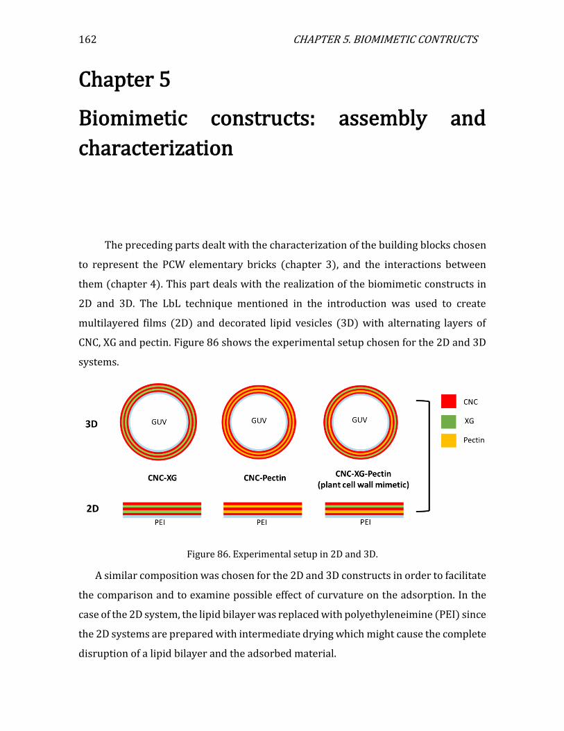
162 CHAPTER 5. BIOMIMETIC CONTRUCTS
Chapter 5
Biomimetic constructs: assembly and
characterization
5. Biomimetic constructs: assembly and characterization
The preceding parts dealt with the characterization of the building blocks chosen
to represent the PCW elementary bricks (chapter 3), and the interactions between
them (chapter 4). This part deals with the realization of the biomimetic constructs in
2D and 3D. The LbL technique mentioned in the introduction was used to create
multilayered films (2D) and decorated lipid vesicles (3D) with alternating layers of
CNC, XG and pectin. Figure 86 shows the experimental setup chosen for the 2D and 3D
systems.
Figure 86. Experimental setup in 2D and 3D.
A similar composition was chosen for the 2D and 3D constructs in order to facilitate
the comparison and to examine possible effect of curvature on the adsorption. In the
case of the 2D system, the lipid bilayer was replaced with polyethyleneimine (PEI) since
the 2D systems are prepared with intermediate drying which might cause the complete
disruption of a lipid bilayer and the adsorbed material.
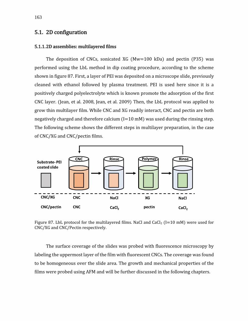
163
5.1. 2D configuration
5.1.1. 2D assemblies: multilayered films
The deposition of CNCs, sonicated XG (Mw=100 kDa) and pectin (P35) was
performed using the LbL method in dip coating procedure, according to the scheme
shown in figure 87. First, a layer of PEI was deposited on a microscope slide, previously
cleaned with ethanol followed by plasma treatment. PEI is used here since it is a
positively charged polyelectrolyte which is known promote the adsorption of the first
CNC layer. (Jean, et al. 2008, Jean, et al. 2009) Then, the LbL protocol was applied to
grow thin multilayer film. While CNC and XG readily interact, CNC and pectin are both
negatively charged and therefore calcium (I=10 mM) was used during the rinsing step.
The following scheme shows the different steps in multilayer preparation, in the case
of CNC/XG and CNC/pectin films.
Figure 87. LbL protocol for the multilayered films. NaCl and CaCl2 (I=10 mM) were used for CNC/XG and CNC/Pectin respectively.
The surface coverage of the slides was probed with fluorescence microscopy by
labeling the uppermost layer of the film with fluorescent CNCs. The coverage was found
to be homogeneous over the slide area. The growth and mechanical properties of the
films were probed using AFM and will be further discussed in the following chapters.
164 CHAPTER 5. BIOMIMETIC CONTRUCTS
5.1.2. Characterization of layer thickness using AFM
Prior to obtaining force curves, it is highly important to have a priori knowledge
on the film thickness and topography. In order to obtain this information, an AFM tip
(RTESPA-300, Bruker, USA) mounted on a cantilever (k=40 N/m ,Bruker, USA) was
used in two modes: QI mode was used for imaging, while contact mode was used to
generate a square shaped well, also referred to as 'groove', in the film by scratching the
surface, in order to measure its thickness. This process, previously termed "nano-
shaving" was similar to the one used in chapter 4.2.
First, a 1010 µm² (150150 pixel) scan was performed in QI mode. A set point
of 0.1 V and z-length of 500 nm were typically used. After obtaining the image, a smaller
area of 33 µm² was chosen in the center of the previous scan, where the material was
removed. To this purpose, AFM was operated in contact mode setting a large set point
(8V) and virtually switching off the feedback loop (by using typically P gain = 0.0001
and I gain = 0.1). The scan was repeated 3 times and then a new topographic map,
acquired on the original 1010 µm² area, was used for the thickness analysis. Typically,
1-3 scratches were performed for each sample.
As can be seen in figure 88, a square shaped groove was obtained following the
scratching process, indicating efficient removal of material. The material removed from
the film accumulated on the edges of the square and in several cases some of the
material fell back to the bottom of the formed well. Figure 88a shows a 3D image of the
scanned area after scratching.
In order to obtain thickness values, Gwyddion (V 2.54) software was used. First,
a mask was applied on the scratched area in order to exclude it and plane leveling
procedure was performed in order to remove offset and tilt from height values and set
the mean height to zero. Then, a new mask was applied, this time on the scratch edges
in order to exclude them from the analysis. A histogram of the height was calculated
using the 1D statistical function toolbox, yielding two peaks corresponding to the top of
the layer and the exposed substrate (the microscope slide). Each peak may be fitted
with a Gaussian function (Figure 88b). The Gaussian peak represents the mean height

165
for the bottom and the top planes of the image, the distance between the peaks is the
average height.
Figure 88.(a) A typical height profile obtained following the scratching process, the inset shows a side profile of the same image (b) A gauss fit to the two main peaks found using image analysis. Height distribution (black line), a fit to the bottom plane- groove (red dashed line) and a fit to the upper plane sample surface (green dashed line) the z distance between the two peaks is the calculated sample thickness.
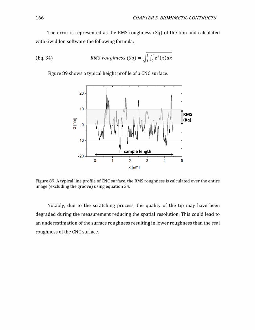
166 CHAPTER 5. BIOMIMETIC CONTRUCTS
The error is represented as the RMS roughness (Sq) of the film and calculated
with Gwiddon software the following formula:
(Eq. 34) 𝑅𝑀𝑆 𝑟𝑜𝑢𝑔ℎ𝑛𝑒𝑠𝑠 (𝑆𝑞) = √1
𝑙∫ 𝑧2(𝑥)𝑑𝑥
𝑙
0
Figure 89 shows a typical height profile of a CNC surface:
Figure 89. A typical line profile of CNC surface. the RMS roughness is calculated over the entire image (excluding the groove) using equation 34.
Notably, due to the scratching process, the quality of the tip may have been
degraded during the measurement reducing the spatial resolution. This could lead to
an underestimation of the surface roughness resulting in lower roughness than the real
roughness of the CNC surface.

167
Figure 90: From the left in columns: AFM topography image of CNC/XG film after scratch, (a,e,i,m) Gaussian fit to the height distribution (b,f,j,n,), line profiles used to calculate the film thickness (c,g,k,o), height profiles obtained from the lines (d,h,l,p) and an illustration of the multilayered films. Results are shown for varying number of layers: PEI/CNC (a-d), 10.5 Layers (e-h), 15.5 Layers (i-j), 20.5 Layers (m-p). One layer corresponds to a CNC/XG section.
This technique was used in order to probe 3 types of systems: (i) CNC/XG, (ii)
CNC/pectin and (iii) CNC/XG/pectin. For the XG system, a simple LbL process was
performed with NaCl rinse (I=10 mM) between each deposition step. When pectin was
present (systems ii and iii) the sample was rinsed with CaCl2 (I=10 mM) between CNC
and pectin layers. The deposition was done with and without intermediate drying. A
summary of the calculated heights for the different systems is shown in table 20:
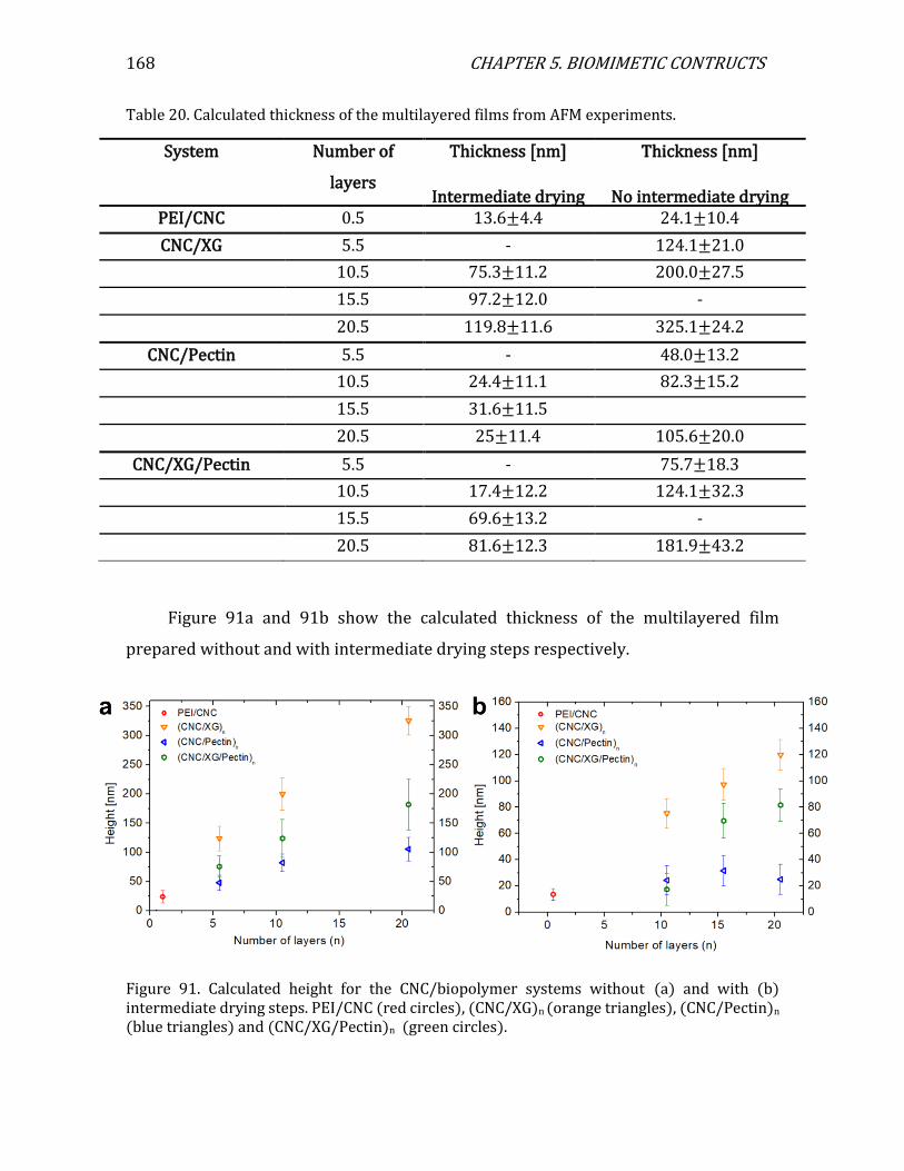
168 CHAPTER 5. BIOMIMETIC CONTRUCTS
Table 20. Calculated thickness of the multilayered films from AFM experiments.
System Number of
layers
Thickness [nm]
Intermediate drying
Thickness [nm]
No intermediate drying PEI/CNC 0.5 13.6±4.4 24.1±10.4
CNC/XG 5.5 - 124.1±21.0
10.5 75.3±11.2 200.0±27.5
15.5 97.2±12.0 -
20.5 119.8±11.6 325.1±24.2
CNC/Pectin 5.5 - 48.0±13.2
10.5 24.4±11.1 82.3±15.2
15.5 31.6±11.5
20.5 25±11.4 105.6±20.0
CNC/XG/Pectin 5.5 - 75.7±18.3
10.5 17.4±12.2 124.1±32.3
15.5 69.6±13.2 -
20.5 81.6±12.3 181.9±43.2
Figure 91a and 91b show the calculated thickness of the multilayered film
prepared without and with intermediate drying steps respectively.
Figure 91. Calculated height for the CNC/biopolymer systems without (a) and with (b) intermediate drying steps. PEI/CNC (red circles), (CNC/XG)n (orange triangles), (CNC/Pectin)n (blue triangles) and (CNC/XG/Pectin)n (green circles).

169
Let us discuss the result with respect to the different parameters.
Effect of intermediate drying
Comparing figures, 91a and b for systems with similar composition, notably,
including intermediate drying steps resulted in thinner films. This applies for all the
systems investigated, regardless of composition. This effect may be further visualized
when comparing a system with similar composition, in this case CNC/XG system, with
and without intermediate drying steps (figure 92).
Figure 92. Multilayer thickness for CNC/XG system as a function of number of layers. With (grey columns) and without (orange columns) intermediate drying steps.
This observation could be attributed to the collapse of the polymer and the
particles upon drying. When water is removed from the layer, individual CNCs
approach closer towards the short range VdW attraction regime, resulting in tighter
arrangement and reduction of the thickness.

170 CHAPTER 5. BIOMIMETIC CONTRUCTS
Figure 93 shows the proposed structure based on the thickness of the film
prepared with and without intermediate drying steps.
Figure 93. A scheme showing the proposed film structure prepared with and without intermediate drying steps. PEI (purple line), CNCs (red rectangles) and XG (green lines) are deposited in alternative manner on a flat substrate (grey rectangle). The image is not to scale.
In order to estimate the volume fraction of water in the films, an AFM nanoshaving
experiment was done on the same multilayered sample, in air. An estimation of the
difference in the volume fraction of water 𝜙𝑣 can be obtained, considering similar
surface area, by subtracting the thickness of the system prepared without intermediate
drying measured under liquid (𝑡ℎ) and in air (𝑡𝑑) according to the following equation:
(Eq. 35) 𝜙𝑣 =Δ𝑣𝑖
𝑣𝑡𝑜𝑡=
Δ𝑡𝑖
𝑡𝑡𝑜𝑡=
𝑡ℎ−𝑡𝑑
𝑡ℎ
This results in the volume fraction of water in the film due to hydration. 𝜙𝑣 was 0.67,
measured on the same sample (XG/CNC)5.5. This result, showing high water content in
the film, is in fair agreement with the results obtained in chapter 4.2, where water
content of up to 70% was found in the CNC layer adsorbed on SLBs.
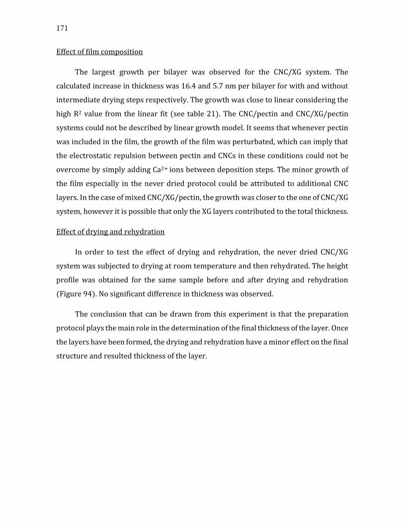
171
Effect of film composition
The largest growth per bilayer was observed for the CNC/XG system. The
calculated increase in thickness was 16.4 and 5.7 nm per bilayer for with and without
intermediate drying steps respectively. The growth was close to linear considering the
high R2 value from the linear fit (see table 21). The CNC/pectin and CNC/XG/pectin
systems could not be described by linear growth model. It seems that whenever pectin
was included in the film, the growth of the film was perturbated, which can imply that
the electrostatic repulsion between pectin and CNCs in these conditions could not be
overcome by simply adding Ca2+ ions between deposition steps. The minor growth of
the film especially in the never dried protocol could be attributed to additional CNC
layers. In the case of mixed CNC/XG/pectin, the growth was closer to the one of CNC/XG
system, however it is possible that only the XG layers contributed to the total thickness.
Effect of drying and rehydration
In order to test the effect of drying and rehydration, the never dried CNC/XG
system was subjected to drying at room temperature and then rehydrated. The height
profile was obtained for the same sample before and after drying and rehydration
(Figure 94). No significant difference in thickness was observed.
The conclusion that can be drawn from this experiment is that the preparation
protocol plays the main role in the determination of the final thickness of the layer. Once
the layers have been formed, the drying and rehydration have a minor effect on the final
structure and resulted thickness of the layer.
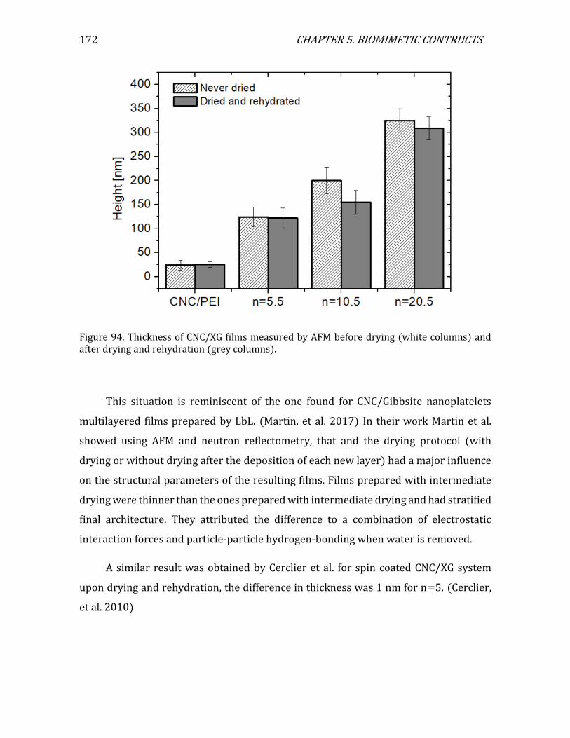
172 CHAPTER 5. BIOMIMETIC CONTRUCTS
Figure 94. Thickness of CNC/XG films measured by AFM before drying (white columns) and after drying and rehydration (grey columns).
This situation is reminiscent of the one found for CNC/Gibbsite nanoplatelets
multilayered films prepared by LbL. (Martin, et al. 2017) In their work Martin et al.
showed using AFM and neutron reflectometry, that and the drying protocol (with
drying or without drying after the deposition of each new layer) had a major influence
on the structural parameters of the resulting films. Films prepared with intermediate
drying were thinner than the ones prepared with intermediate drying and had stratified
final architecture. They attributed the difference to a combination of electrostatic
interaction forces and particle-particle hydrogen-bonding when water is removed.
A similar result was obtained by Cerclier et al. for spin coated CNC/XG system
upon drying and rehydration, the difference in thickness was 1 nm for n=5. (Cerclier,
et al. 2010)
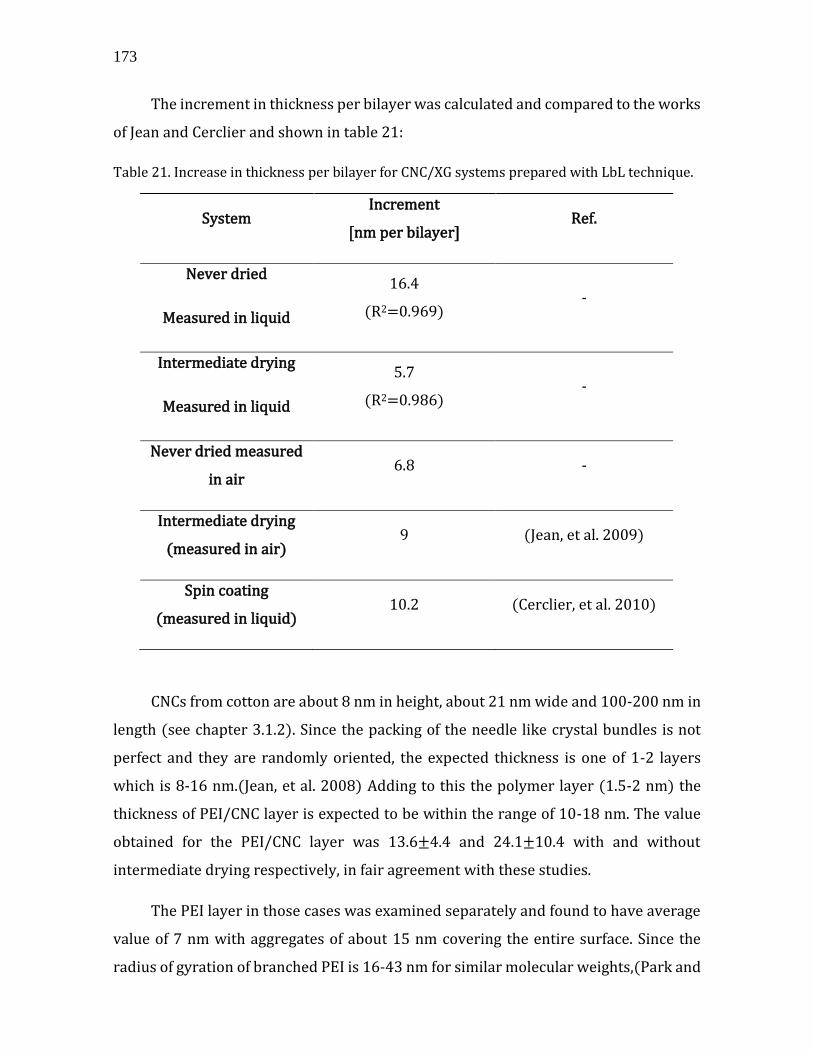
173
The increment in thickness per bilayer was calculated and compared to the works
of Jean and Cerclier and shown in table 21:
Table 21. Increase in thickness per bilayer for CNC/XG systems prepared with LbL technique.
CNCs from cotton are about 8 nm in height, about 21 nm wide and 100-200 nm in
length (see chapter 3.1.2). Since the packing of the needle like crystal bundles is not
perfect and they are randomly oriented, the expected thickness is one of 1-2 layers
which is 8-16 nm.(Jean, et al. 2008) Adding to this the polymer layer (1.5-2 nm) the
thickness of PEI/CNC layer is expected to be within the range of 10-18 nm. The value
obtained for the PEI/CNC layer was 13.6±4.4 and 24.1±10.4 with and without
intermediate drying respectively, in fair agreement with these studies.
The PEI layer in those cases was examined separately and found to have average
value of 7 nm with aggregates of about 15 nm covering the entire surface. Since the
radius of gyration of branched PEI is 16-43 nm for similar molecular weights,(Park and
System Increment
[nm per bilayer] Ref.
Never dried
Measured in liquid
16.4
(R2=0.969) -
Intermediate drying
Measured in liquid
5.7
(R2=0.986) -
Never dried measured
in air 6.8 -
Intermediate drying
(measured in air) 9 (Jean, et al. 2009)
Spin coating
(measured in liquid) 10.2 (Cerclier, et al. 2010)
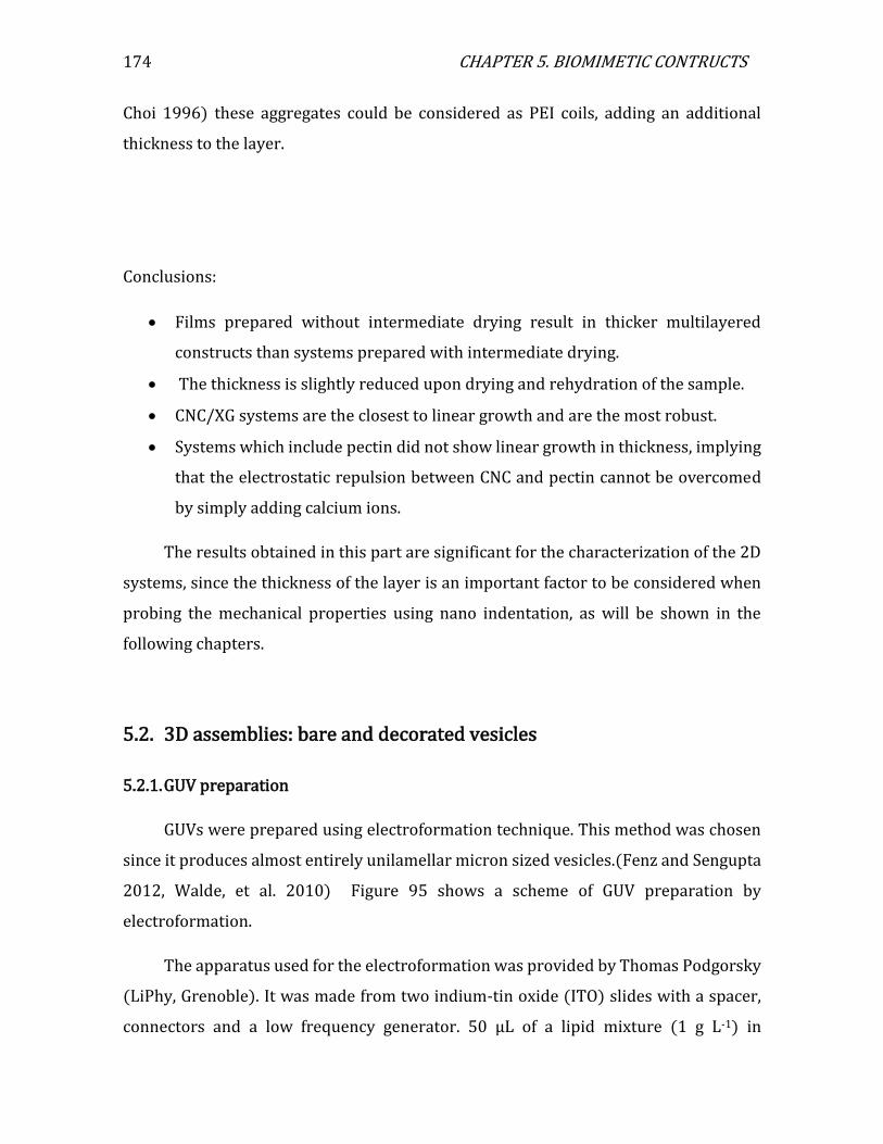
174 CHAPTER 5. BIOMIMETIC CONTRUCTS
Choi 1996) these aggregates could be considered as PEI coils, adding an additional
thickness to the layer.
Conclusions:
• Films prepared without intermediate drying result in thicker multilayered
constructs than systems prepared with intermediate drying.
• The thickness is slightly reduced upon drying and rehydration of the sample.
• CNC/XG systems are the closest to linear growth and are the most robust.
• Systems which include pectin did not show linear growth in thickness, implying
that the electrostatic repulsion between CNC and pectin cannot be overcomed
by simply adding calcium ions.
The results obtained in this part are significant for the characterization of the 2D
systems, since the thickness of the layer is an important factor to be considered when
probing the mechanical properties using nano indentation, as will be shown in the
following chapters.
5.2. 3D assemblies: bare and decorated vesicles
5.2.1. GUV preparation
GUVs were prepared using electroformation technique. This method was chosen
since it produces almost entirely unilamellar micron sized vesicles.(Fenz and Sengupta
2012, Walde, et al. 2010) Figure 95 shows a scheme of GUV preparation by
electroformation.
The apparatus used for the electroformation was provided by Thomas Podgorsky
(LiPhy, Grenoble). It was made from two indium-tin oxide (ITO) slides with a spacer,
connectors and a low frequency generator. 50 µL of a lipid mixture (1 g L-1) in
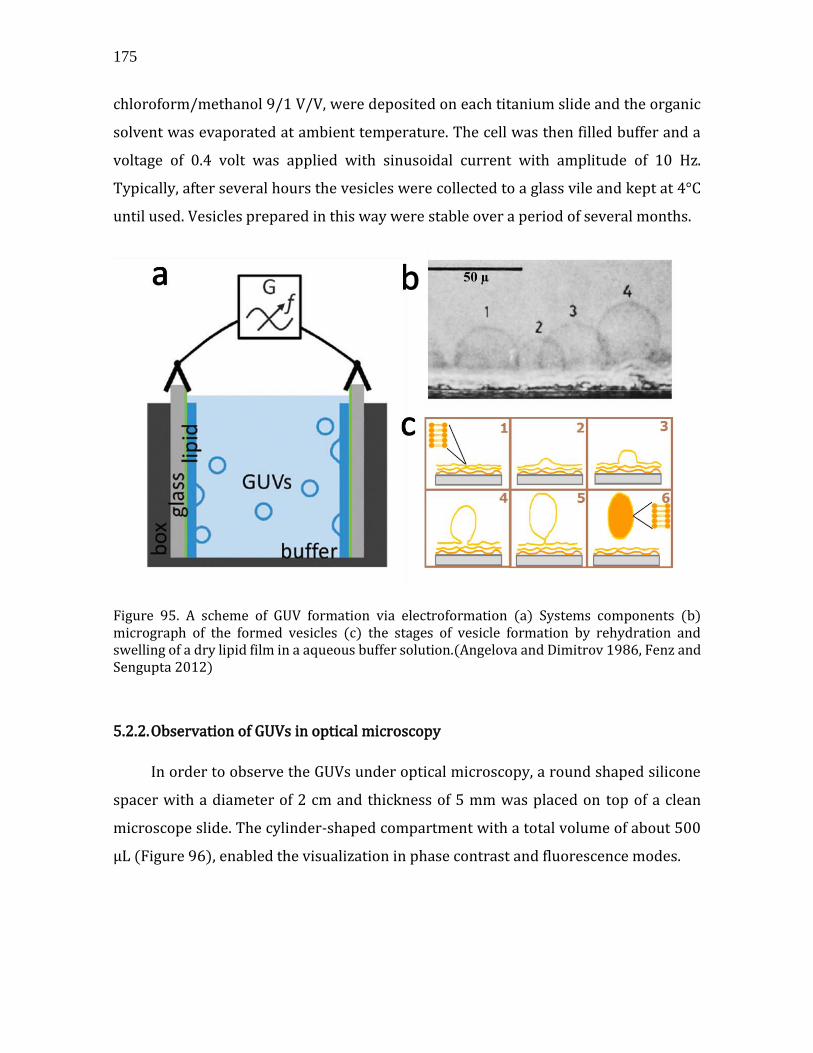
175
chloroform/methanol 9/1 V/V, were deposited on each titanium slide and the organic
solvent was evaporated at ambient temperature. The cell was then filled buffer and a
voltage of 0.4 volt was applied with sinusoidal current with amplitude of 10 Hz.
Typically, after several hours the vesicles were collected to a glass vile and kept at 4°C
until used. Vesicles prepared in this way were stable over a period of several months.
Figure 95. A scheme of GUV formation via electroformation (a) Systems components (b) micrograph of the formed vesicles (c) the stages of vesicle formation by rehydration and swelling of a dry lipid film in a aqueous buffer solution.(Angelova and Dimitrov 1986, Fenz and Sengupta 2012)
5.2.2. Observation of GUVs in optical microscopy
In order to observe the GUVs under optical microscopy, a round shaped silicone
spacer with a diameter of 2 cm and thickness of 5 mm was placed on top of a clean
microscope slide. The cylinder-shaped compartment with a total volume of about 500
µL (Figure 96), enabled the visualization in phase contrast and fluorescence modes.
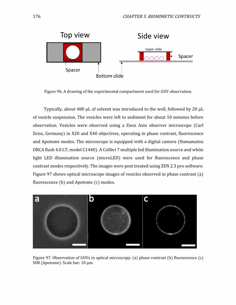
176 CHAPTER 5. BIOMIMETIC CONTRUCTS
Figure 96. A drawing of the experimental compartment used for GUV observation.
Typically, about 480 µL of solvent was introduced to the well, followed by 20 µL
of vesicle suspension. The vesicles were left to sediment for about 10 minutes before
observation. Vesicles were observed using a Ziess Axio observer microscope (Carl
Zeiss, Germany) in X20 and X40 objectives, operating in phase contrast, fluorescence
and Apotome modes. The microscope is equipped with a digital camera (Hamamatsu
ORCA flash 4.0 LT, model C1440). A Colibri 7 multiple led illumination source and white
light LED illumination source (microLED) were used for fluorescence and phase
contrast modes respectively. The images were post treated using ZEN 2.3 pro software.
Figure 97 shows optical microscope images of vesicles observed in phase contrast (a)
fluorescence (b) and Apotome (c) modes.
Figure 97. Observation of GUVs in optical microscopy. (a) phase contrast (b) fluorescence (c) SIM (Apotome). Scale bar: 10 µm.

177
These operational modes will be used in the following sections to characterize
bare and decorated vesicles and explore their behavior under external stresses.
5.2.3. Decoration protocol
Inspired by the LbL technique, GUVs were decorated with alternating layers of
CNC/polymer by incubating a suspension of GUVs with the desired component. Figure
98 shows a scheme demonstrating the decoration and rinsing process.
Figure 98. A scheme of the decoration procedure. Instep 1- bare GUVs are mixed with CNC suspension. Step 2- Sedimentation. Step 3- Supernatant removal. step 4- redispersion in either solvent for rinsing (200 mM Glucose, 1 mM NaCl) or in a polymer solution for decoration.
CNCs, XG and pectin in powder form were dissolved in 0.2 M glucose solution and
1mM NaCl, a solute concentration similar to the one of sucrose present in the GUVs, in
order to avoid an osmotic pressure difference that will lead to a mechanical stress on
the vesicle. The pH was adjusted to 3 to give a slightly positively charged GUVs which
promote the adsorption of CNCs, according to the results obtained in chapter 4.2.
100 µL of GUV suspension were mixed with 300 µL 0.1% wt CNC suspension (step
1) A stirring wheel operating at 10 RPM for 60 seconds was used to ensure proper
mixing. The Eppendorf was then removed from the stirring wheel and the vesicles were
left to sediment. Due to the difference in density, the GUVs tend to sediment to the
bottom phase after 20-30 minutes. (step 2) An additional centrifugation step was
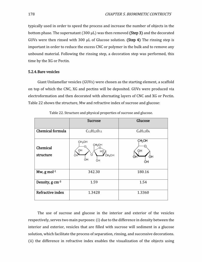
178 CHAPTER 5. BIOMIMETIC CONTRUCTS
typically used in order to speed the process and increase the number of objects in the
bottom phase. The supernatant (300 µL) was then removed (Step 3) and the decorated
GUVs were then rinsed with 300 µL of Glucose solution. (Step 4) The rinsing step is
important in order to reduce the excess CNC or polymer in the bulk and to remove any
unbound material. Following the rinsing step, a decoration step was performed, this
time by the XG or Pectin.
5.2.4. Bare vesicles
Giant Unilamellar vesicles (GUVs) were chosen as the starting element, a scaffold
on top of which the CNC, XG and pectins will be deposited. GUVs were produced via
electroformation and then decorated with alternating layers of CNC and XG or Pectin.
Table 22 shows the structure, Mw and refractive index of sucrose and glucose:
Table 22. Structure and physical properties of sucrose and glucose.
Sucrose Glucose
Chemical formula C12H22O11 C6H12O6
Chemical
structure
Mw, g mol-1 342.30 180.16
Density, g cm-3 1.59 1.54
Refractive index 1.3428 1.3360
The use of sucrose and glucose in the interior and exterior of the vesicles
respectively, serves two main purposes: (i) due to the difference in density between the
interior and exterior, vesicles that are filled with sucrose will sediment in a glucose
solution, which facilitate the process of separation, rinsing, and successive decorations.
(ii) the difference in refractive index enables the visualization of the objects using
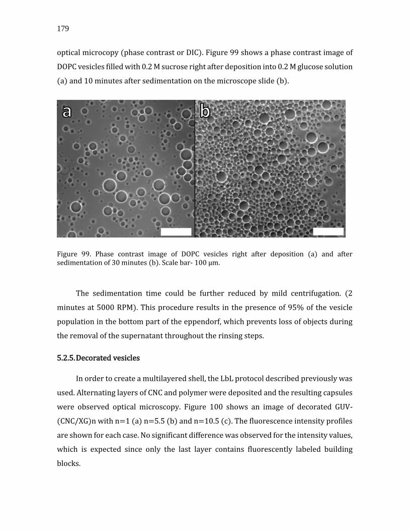
179
optical microcopy (phase contrast or DIC). Figure 99 shows a phase contrast image of
DOPC vesicles filled with 0.2 M sucrose right after deposition into 0.2 M glucose solution
(a) and 10 minutes after sedimentation on the microscope slide (b).
Figure 99. Phase contrast image of DOPC vesicles right after deposition (a) and after sedimentation of 30 minutes (b). Scale bar- 100 µm.
The sedimentation time could be further reduced by mild centrifugation. (2
minutes at 5000 RPM). This procedure results in the presence of 95% of the vesicle
population in the bottom part of the eppendorf, which prevents loss of objects during
the removal of the supernatant throughout the rinsing steps.
5.2.5. Decorated vesicles
In order to create a multilayered shell, the LbL protocol described previously was
used. Alternating layers of CNC and polymer were deposited and the resulting capsules
were observed optical microscopy. Figure 100 shows an image of decorated GUV-
(CNC/XG)n with n=1 (a) n=5.5 (b) and n=10.5 (c). The fluorescence intensity profiles
are shown for each case. No significant difference was observed for the intensity values,
which is expected since only the last layer contains fluorescently labeled building
blocks.
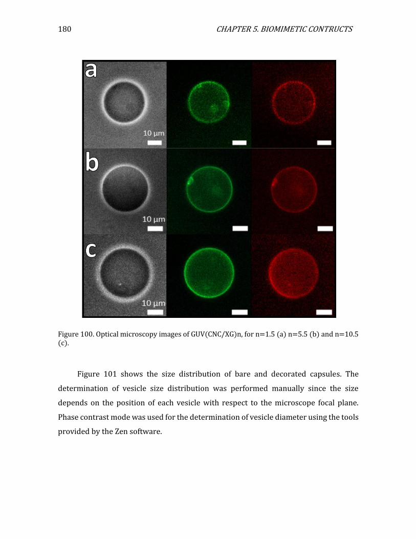
180 CHAPTER 5. BIOMIMETIC CONTRUCTS
Figure 100. Optical microscopy images of GUV(CNC/XG)n, for n=1.5 (a) n=5.5 (b) and n=10.5 (c).
Figure 101 shows the size distribution of bare and decorated capsules. The
determination of vesicle size distribution was performed manually since the size
depends on the position of each vesicle with respect to the microscope focal plane.
Phase contrast mode was used for the determination of vesicle diameter using the tools
provided by the Zen software.

181
Figure 101. Size distribution (diameter) of bare and decorated GUVs.
Table 23 shows the average diameters of the vesicles obtained for bare and
decorated vesicles with 1.5, 5.5 and 10.5 layers.
Table 23.Average diameter of bare and decorated vesicles.
Sample Number of layers Average diameter [µm]
GUV 0 22.3±12.2
GUV (CNC/XG)1.5 1.5 25.3±9.5
GUV (CNC/XG)5.5 5.5 24.6±10.6
GUV (CNC/XG)10.5 10.5 25.2±10.2
The size distribution of the vesicles is in agreement with previous work on CNC/XG
decorated vesicles.(Radavidson 2016)
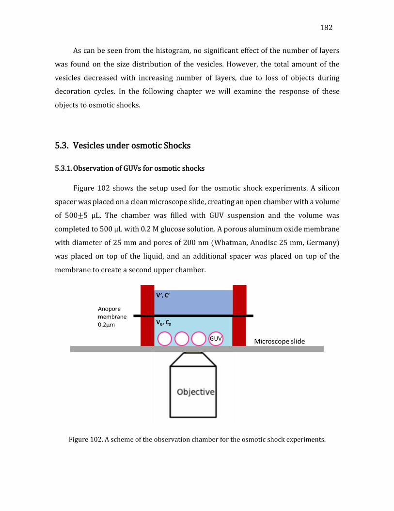
182
As can be seen from the histogram, no significant effect of the number of layers
was found on the size distribution of the vesicles. However, the total amount of the
vesicles decreased with increasing number of layers, due to loss of objects during
decoration cycles. In the following chapter we will examine the response of these
objects to osmotic shocks.
5.3. Vesicles under osmotic Shocks
5.3.1. Observation of GUVs for osmotic shocks
Figure 102 shows the setup used for the osmotic shock experiments. A silicon
spacer was placed on a clean microscope slide, creating an open chamber with a volume
of 500±5 µL. The chamber was filled with GUV suspension and the volume was
completed to 500 µL with 0.2 M glucose solution. A porous aluminum oxide membrane
with diameter of 25 mm and pores of 200 nm (Whatman, Anodisc 25 mm, Germany)
was placed on top of the liquid, and an additional spacer was placed on top of the
membrane to create a second upper chamber.
Figure 102. A scheme of the observation chamber for the osmotic shock experiments.
183 CHAPTER 5. BIOMIMETIC CONSTRUCTS
The presence of the porous membrane between the lower and upper
compartment prevents the movement of the liquid of the liquid in the lower
compartments upon addition of liquid, thus facilitating the observation of a single
vesicle upon osmotic shock.
The upper chamber was then filled with desired solution by addition of
concentrated glucose solution or electrolyte (hypertonic) or water (hypotonic). The
difference in concentration due to the addition ΔC is then:
(Eq. 36) ∆𝐶 = 𝐶0 − 𝐶𝑓 = 𝐶0 − (𝐶0𝑉0+𝐶′𝑉′
𝑉0+𝑉′)
For hypertonic solution ∆𝐶 > 0 and for hypotonic solution ∆𝐶 < 0.
5.3.2. Bare vesicles
As shown in chapter 1.2.4, lipid vesicles deform when subjected to osmotic shock,
due to transport of water molecules in or out of the membrane. This can be visualized
in optical microscopy by imposing a difference in osmolarity between the interior and
the exterior of the vesicles and measuring the variation in diameter with time. The tools
provided with the ZEN software (Zen Blue, V. 2012, Carl Zeiss) enables determination
of the vesicle's diameter, assuming a circular geometry.
5.3.2.1. Glucose shocks
Figure 103 shows a series of images of bare DOPC GUVs taken at different times,
following the addition of a concentrated glucose solution to the upper compartment of
the observation cell.

184
Figure 103. Variation of DOPC vesicles diameter with time upon osmotic shock (glucose, ΔC=100mM). Scale bar= 10 µm.
The vesicle deflated equally in all directions (isotropic deflation) upon addition of
glucose with ΔC=100 mM. The decrease in diameter while maintaining a spherical
shape is possible thanks to the fluid nature of the DOPC membrane which is in the liquid
disordered phase at room temperature. Additionally, due to the elastic nature of the
membrane, the deformation is reversible. In order to verify the reversibility, a
consecutive deflation/inflation experiment was performed. After the addition of
glucose and reaching state of equilibrium, the upper compartment was emptied and
filled with water instead of glucose. This caused a decrease in the total glucose
concentration, and thus osmotic shock of ΔC=Cf-C0=-100 mM where C0 is the glucose
concentration before the shocks and Cf is the final glucose concentration (figure 104).

185 CHAPTER 5. BIOMIMETIC CONSTRUCTS
Figure 104. Vesicle diameter as a function of time, due to the addition of hypertonic solution (filled circles, 0-2500 sec) followed by addition of hypotonic solution (hollow circles, 2500-5500 sec). A reversible and isotropic (in plane) deformation is observed while maintaining membrane integrity (corresponding insets).
In fact, this type of deformation implies a reduction of the vesicle surface area,
∆𝑆 = 4𝜋(𝑟12 − 𝑟2
2) where r1 and r2 are the radii before and after the osmotic shock. This
change in surface can be compensated either by a more compact packing of the lipids
in the membrane (Kummrow and Helfrich 1996) or by the formation of tubes
(Quemeneur 2010) or daughter vesicles connected to the original vesicle. (Bernard, et
al. 2002, Boroske, et al. 1981)
In our case, no visible tubes or daughter vesicles were found upon glucose shocks
of bare vesicles. While possibly existing, these type of membrane deformations are
below the resolution of the microscope in this setup. Whatever the mechanism of size
reduction, the deformation was isotropic, which enabled the determination of
permeability values as will be shown in chapter 5.4.
186
6.3.2.2. NaCl and CaCl2 shocks
Mono and divalent ions such as sodium and calcium are important ionic species
that play a key role in many internal and external cellular processes such as energy and
charge transfer, osmotic pressure regulation and modulation the mechanical properties
of the cell wall.(Hepler and Winship 2010) Since the lipid membrane has very poor
permeability to these ions, as discussed in chapter 1.2.4, they are transported in vivo
across the plasma membrane via trans membranal proteins that facilitate their passage.
In our system, ions are typically used to promote adsorption of components by
screening of electrostatic interactions and bridging, according to the theoretical
considerations discussed in chapter 4.1. It is therefore important to evaluate the
response of our biomimetic capsules to addition of these types of salts.
Hence, we will explore the behavior of bare and decorated vesicles in response to
salt shocks, beginning with the bare vesicles, as a reference. Upon addition of NaCl,
vesicles exhibit osmotic shock, where the concentration difference is two times the
electrolyte concentration in the case of NaCl, since both Na+ and Cl- ionic species
contribute to the osmotic pressure. An isotropic deflation was observed, similarly to the
case of glucose shock, and permeability values calculated show a slight increase in
membrane permeability. This is not surprising, since charged ions are known to
interact readily with the lipid polar head and enhance membrane tension as well as
membrane porosity, promoting the transport of water through the membrane or even
invagination.(Contini, et al. 2018, Montis, et al. 2014, Wang, et al. 2008)
Upon calcium shock, (ΔC=5 mM) bare vesicles exhibit a dramatic change in their
size and morphology. Figure 105 shows time evolution of bare DOPC vesicles upon
exposure to CaCl2 shock.
Approximately one minute after addition of CaCl2 solution in the upper
compartment of the cell, an apparent decrease in diameter was observed and small
micron size vesicles started to appear in the interior of the GUVs (Figure 105a and b).

187 CHAPTER 5. BIOMIMETIC CONSTRUCTS
Figure 105. DOPC GUVs uppon calcium shock. ΔC=5 mM. (a) time evolution following the addition of CaCl2, scale bar=100 µm. (B) a closeup on the square area framed in red dashed line (c) reverse shock by addition of water ΔC= -100 mM. The scale bar for (b) and (c) is 20 µm.
The appearance of daughter vesicles was visualized using under focus conditions,
because the focal plane of the daughter vesicles is not similar to the focal plane of the
mother GUV. Formation of daughter vesicles was previously observed for egg-PC
vesicles upon osmotic shock of NaCl (Boroske, et al. 1981) as well as glucose (Bernard,
et al. 2002) Since the cohesion energy of lipid molecules is lower than the bending
energy, the lipid membrane is able to detach a daughter vesicle while maintaining the
favorable spherical shape. In order to examine the reversibility of the daughter vesicle
formation, hypotonic solution was consecutively added to the upper compartment,
similarly to the procedure described earlier for the glucose shocks.
Figure 105c shows a series of images taken after addition of water into the upper
compartment of the cell (hypotonic solution). Two phenomena were observed: (i) the
daughter vesicles disappeared and (ii) the mother vesicle diameter increased. This
shows that upon exposure to hypotonic solution, daughter vesicles can fuse back into
the GUV membrane in order to compensate the new imposed difference in chemical
potential, or in other words, the process is reversible. It also implies that the material
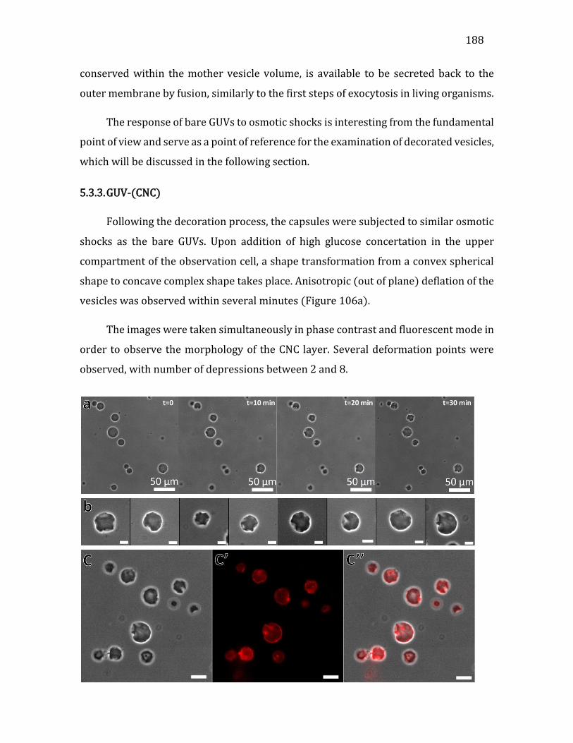
188
conserved within the mother vesicle volume, is available to be secreted back to the
outer membrane by fusion, similarly to the first steps of exocytosis in living organisms.
The response of bare GUVs to osmotic shocks is interesting from the fundamental
point of view and serve as a point of reference for the examination of decorated vesicles,
which will be discussed in the following section.
5.3.3. GUV-(CNC)
Following the decoration process, the capsules were subjected to similar osmotic
shocks as the bare GUVs. Upon addition of high glucose concertation in the upper
compartment of the observation cell, a shape transformation from a convex spherical
shape to concave complex shape takes place. Anisotropic (out of plane) deflation of the
vesicles was observed within several minutes (Figure 106a).
The images were taken simultaneously in phase contrast and fluorescent mode in
order to observe the morphology of the CNC layer. Several deformation points were
observed, with number of depressions between 2 and 8.
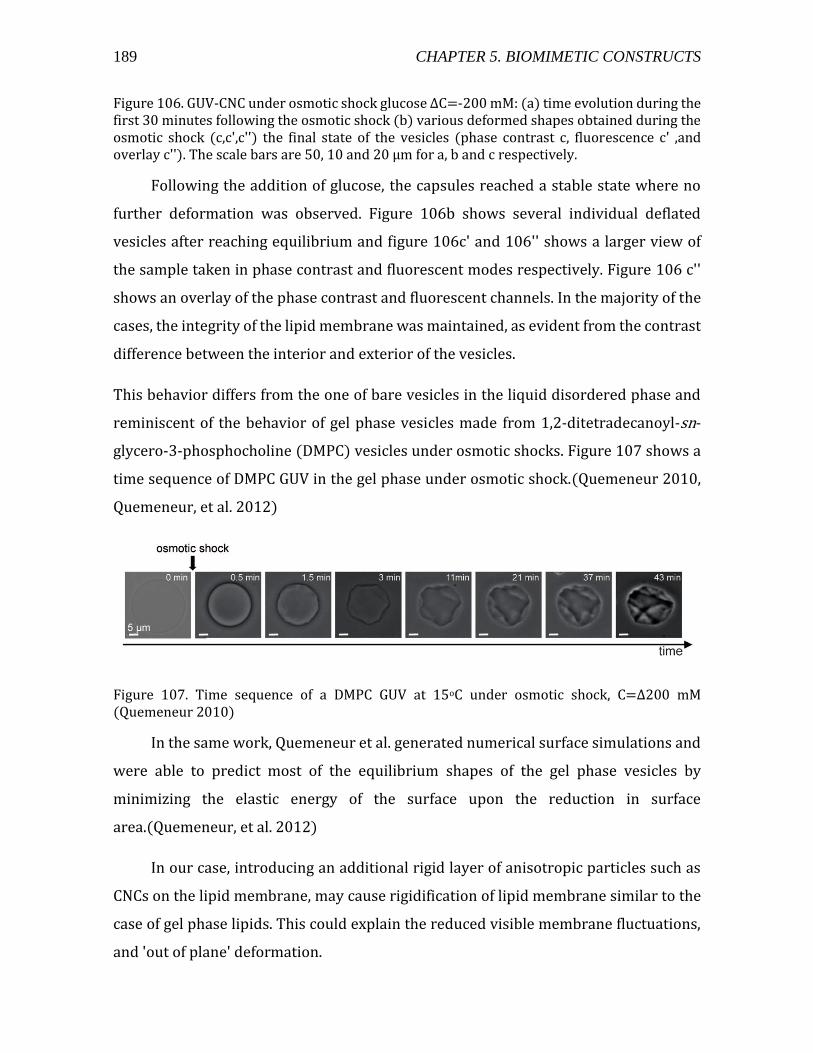
189 CHAPTER 5. BIOMIMETIC CONSTRUCTS
Figure 106. GUV-CNC under osmotic shock glucose ΔC=-200 mM: (a) time evolution during the first 30 minutes following the osmotic shock (b) various deformed shapes obtained during the osmotic shock (c,c',c'') the final state of the vesicles (phase contrast c, fluorescence c' ,and overlay c''). The scale bars are 50, 10 and 20 µm for a, b and c respectively.
Following the addition of glucose, the capsules reached a stable state where no
further deformation was observed. Figure 106b shows several individual deflated
vesicles after reaching equilibrium and figure 106c' and 106'' shows a larger view of
the sample taken in phase contrast and fluorescent modes respectively. Figure 106 c''
shows an overlay of the phase contrast and fluorescent channels. In the majority of the
cases, the integrity of the lipid membrane was maintained, as evident from the contrast
difference between the interior and exterior of the vesicles.
This behavior differs from the one of bare vesicles in the liquid disordered phase and
reminiscent of the behavior of gel phase vesicles made from 1,2-ditetradecanoyl-sn-
glycero-3-phosphocholine (DMPC) vesicles under osmotic shocks. Figure 107 shows a
time sequence of DMPC GUV in the gel phase under osmotic shock.(Quemeneur 2010,
Quemeneur, et al. 2012)
Figure 107. Time sequence of a DMPC GUV at 15oC under osmotic shock, C=Δ200 mM (Quemeneur 2010)
In the same work, Quemeneur et al. generated numerical surface simulations and
were able to predict most of the equilibrium shapes of the gel phase vesicles by
minimizing the elastic energy of the surface upon the reduction in surface
area.(Quemeneur, et al. 2012)
In our case, introducing an additional rigid layer of anisotropic particles such as
CNCs on the lipid membrane, may cause rigidification of lipid membrane similar to the
case of gel phase lipids. This could explain the reduced visible membrane fluctuations,
and 'out of plane' deformation.
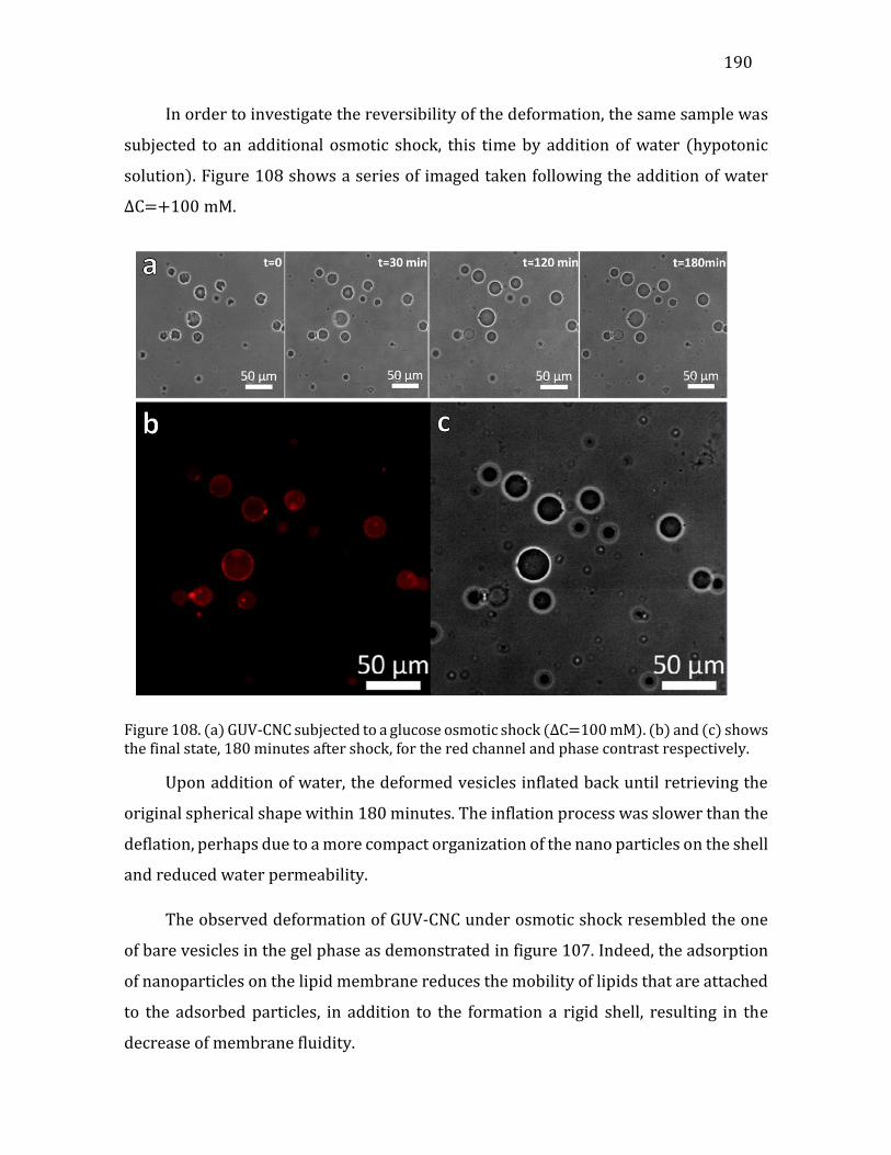
190
In order to investigate the reversibility of the deformation, the same sample was
subjected to an additional osmotic shock, this time by addition of water (hypotonic
solution). Figure 108 shows a series of imaged taken following the addition of water
ΔC=+100 mM.
Figure 108. (a) GUV-CNC subjected to a glucose osmotic shock (ΔC=100 mM). (b) and (c) shows the final state, 180 minutes after shock, for the red channel and phase contrast respectively.
Upon addition of water, the deformed vesicles inflated back until retrieving the
original spherical shape within 180 minutes. The inflation process was slower than the
deflation, perhaps due to a more compact organization of the nano particles on the shell
and reduced water permeability.
The observed deformation of GUV-CNC under osmotic shock resembled the one
of bare vesicles in the gel phase as demonstrated in figure 107. Indeed, the adsorption
of nanoparticles on the lipid membrane reduces the mobility of lipids that are attached
to the adsorbed particles, in addition to the formation a rigid shell, resulting in the
decrease of membrane fluidity.
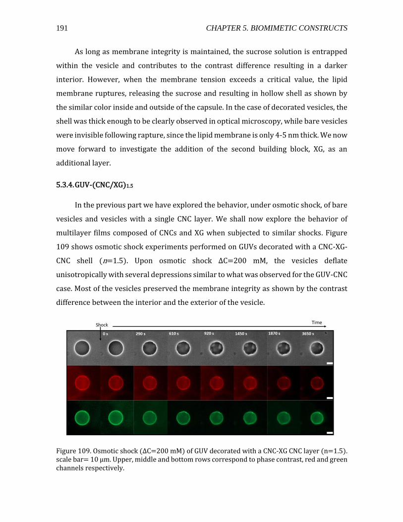
191 CHAPTER 5. BIOMIMETIC CONSTRUCTS
As long as membrane integrity is maintained, the sucrose solution is entrapped
within the vesicle and contributes to the contrast difference resulting in a darker
interior. However, when the membrane tension exceeds a critical value, the lipid
membrane ruptures, releasing the sucrose and resulting in hollow shell as shown by
the similar color inside and outside of the capsule. In the case of decorated vesicles, the
shell was thick enough to be clearly observed in optical microscopy, while bare vesicles
were invisible following rapture, since the lipid membrane is only 4-5 nm thick. We now
move forward to investigate the addition of the second building block, XG, as an
additional layer.
5.3.4. GUV-(CNC/XG)1.5
In the previous part we have explored the behavior, under osmotic shock, of bare
vesicles and vesicles with a single CNC layer. We shall now explore the behavior of
multilayer films composed of CNCs and XG when subjected to similar shocks. Figure
109 shows osmotic shock experiments performed on GUVs decorated with a CNC-XG-
CNC shell (n=1.5). Upon osmotic shock ΔC=200 mM, the vesicles deflate
unisotropically with several depressions similar to what was observed for the GUV-CNC
case. Most of the vesicles preserved the membrane integrity as shown by the contrast
difference between the interior and the exterior of the vesicle.
Figure 109. Osmotic shock (ΔC=200 mM) of GUV decorated with a CNC-XG CNC layer (n=1.5). scale bar= 10 µm. Upper, middle and bottom rows correspond to phase contrast, red and green channels respectively.

192
The onset of visible deformation occurs after several minutes, a bit longer than for
the bare vesicles and similar to the vesicle-CNC system.
The reversibility of the process was investigated by adding hypotonic solution.
Figure 110 shows a decorated vesicle after deflation, upon addition of water into the
upper compartment of the cell.
Figure 110. Reversible deformation of GUV-CNC-XG-CNC (n=1.5) upon osmotic shock in water. ΔC=200 mM, scale bar=5 µm. Upper, middle and bottom rows correspond to phase contrast, red and green channels respectively.
As can be seen from figure 110, the deformation is reversible. However larger
number of vesicles explode during the deflation/inflation cycles, leaving only the
hollow shell. As shown in the previous sections, the interaction between the CNCs and
XG promote the formation of crosslinks between CNC layers, making the shell more
resistant to shock, similarly to what is observed for electrostatically driven
multilayers.(Quemeneur 2010)
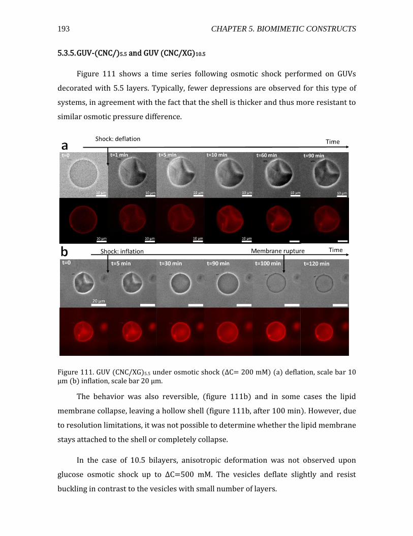
193 CHAPTER 5. BIOMIMETIC CONSTRUCTS
5.3.5. GUV-(CNC/)5.5 and GUV (CNC/XG)10.5
Figure 111 shows a time series following osmotic shock performed on GUVs
decorated with 5.5 layers. Typically, fewer depressions are observed for this type of
systems, in agreement with the fact that the shell is thicker and thus more resistant to
similar osmotic pressure difference.
Figure 111. GUV (CNC/XG)5.5 under osmotic shock (ΔC= 200 mM) (a) deflation, scale bar 10 µm (b) inflation, scale bar 20 µm.
The behavior was also reversible, (figure 111b) and in some cases the lipid
membrane collapse, leaving a hollow shell (figure 111b, after 100 min). However, due
to resolution limitations, it was not possible to determine whether the lipid membrane
stays attached to the shell or completely collapse.
In the case of 10.5 bilayers, anisotropic deformation was not observed upon
glucose osmotic shock up to ΔC=500 mM. The vesicles deflate slightly and resist
buckling in contrast to the vesicles with small number of layers.
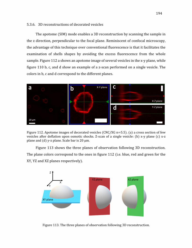
194
5.3.6. 3D reconstructions of decorated vesicles
The apotome (SIM) mode enables a 3D reconstruction by scanning the sample in
the z direction, perpendicular to the focal plane. Reminiscent of confocal microscopy,
the advantage of this technique over conventional fluorescence is that it facilitates the
examination of shells shapes by avoiding the excess fluorescence from the whole
sample. Figure 112 a shows an apotome image of several vesicles in the x-y plane, while
figure 110 b, c, and d show an example of a z-scan performed on a single vesicle. The
colors in b, c and d correspond to the different planes.
Figure 112. Apotome images of decorated vesicles (CNC/XG n=5.5). (a) a cross section of few vesicles after deflation upon osmotic shocks. Z-scan of a single vesicle: (b) x-y plane (c) x-z plane and (d) y-z plane. Scale bar is 20 µm.
Figure 113 shows the three planes of observation following 3D reconstruction.
The plane colors correspond to the ones in figure 112 (i.e. blue, red and green for the
XY, YZ and XZ planes respectively).
Figure 113. The three planes of observation following 3D reconstruction.
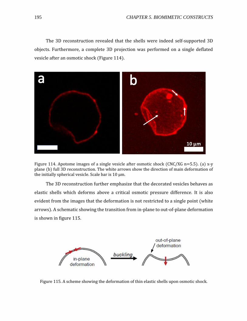
195 CHAPTER 5. BIOMIMETIC CONSTRUCTS
The 3D reconstruction revealed that the shells were indeed self-supported 3D
objects. Furthermore, a complete 3D projection was performed on a single deflated
vesicle after an osmotic shock (Figure 114).
Figure 114. Apotome images of a single vesicle after osmotic shock (CNC/XG n=5.5). (a) x-y plane (b) full 3D reconstruction. The white arrows show the direction of main deformation of the initially spherical vesicle. Scale bar is 10 µm.
The 3D reconstruction further emphasize that the decorated vesicles behaves as
elastic shells which deforms above a critical osmotic pressure difference. It is also
evident from the images that the deformation is not restricted to a single point (white
arrows). A schematic showing the transition from in-plane to out-of-plane deformation
is shown in figure 115.
Figure 115. A scheme showing the deformation of thin elastic shells upon osmotic shock.
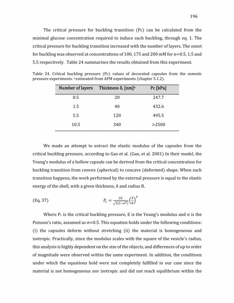
196
The critical pressure for buckling transition (Pc) can be calculated from the
minimal glucose concentration required to induce such buckling, through eq. 1. The
critical pressure for buckling transition increased with the number of layers. The onset
for buckling was observed at concentrations of 100, 175 and 200 mM for n=0.5, 1.5 and
5.5 respectively. Table 24 summarizes the results obtained from this experiment.
Table 24. Critical buckling pressure (Pc) values of decorated capsules from the osmotic pressure experiments. a estimated from AFM experiments (chapter 5.1.2).
Number of layers Thickness δ, [nm]a Pc [kPa]
0.5 20 247.7
1.5 40 432.6
5.5 120 495.5
10.5 340 >2500
We made an attempt to extract the elastic modulus of the capsules from the
critical buckling pressure, according to Gao et al. (Gao, et al. 2001) In their model, the
Young's modulus of a hollow capsule can be derived from the critical concentration for
buckling transition from convex (spherical) to concave (deformed) shape. When such
transition happens, the work performed by the external pressure is equal to the elastic
energy of the shell, with a given thickness, δ and radius R.
(Eq. 37) 𝑃𝑐 =2𝐸
√3(1−𝜎2)(
𝛿
𝑅)
2
Where Pc is the critical buckling pressure, E is the Young's modulus and σ is the
Poisson's ratio, assumed as σ=0.5. This equation holds under the following conditions:
(i) the capsules deform without stretching (ii) the material is homogeneous and
isotropic. Practically, since the modulus scales with the square of the vesicle's radius,
this analysis is highly dependent on the size of the objects, and differences of up to order
of magnitude were observed within the same experiment. In addition, the conditions
under which the equations hold were not completely fulfilled in our case since the
material is not homogeneous nor isotropic and did not reach equilibrium within the

197 CHAPTER 5. BIOMIMETIC CONSTRUCTS
time scale of the experiment. We therefore could not conclude on the elastic modulus
of the vesicles using this analysis, reflecting the need of a more direct measurement in
order to access the mechanical properties of the objects.
5.3.7. Decorated vesicles under CaCl2 shocks
Unlike bare vesicles, exposure of decorated vesicles to mild calcium shocks does
not result in the formation of visible daughter vesicles, but to aggregation of the objects.
The aggregation was found to be related to the surface coverage of vesicles on the
microscope slide. In the case of high initial surface coverage (Figure 116a) vesicles can
coalesce to a tissue like structure. Figure 116 shows the formation of tissue like
structure upon calcium shock ΔC=5 mM for high (a,b) and low (c) initial surface
coverage.
Figure 116. A phase contrast images showing the evolution of GUV(CNC/Pectin)5.5 during calcium osmotic shock. In high initial coverage (a and b) and low initial coverage (c). the numbers in (b) demonstrate the cluster formation by following individual vesicles.
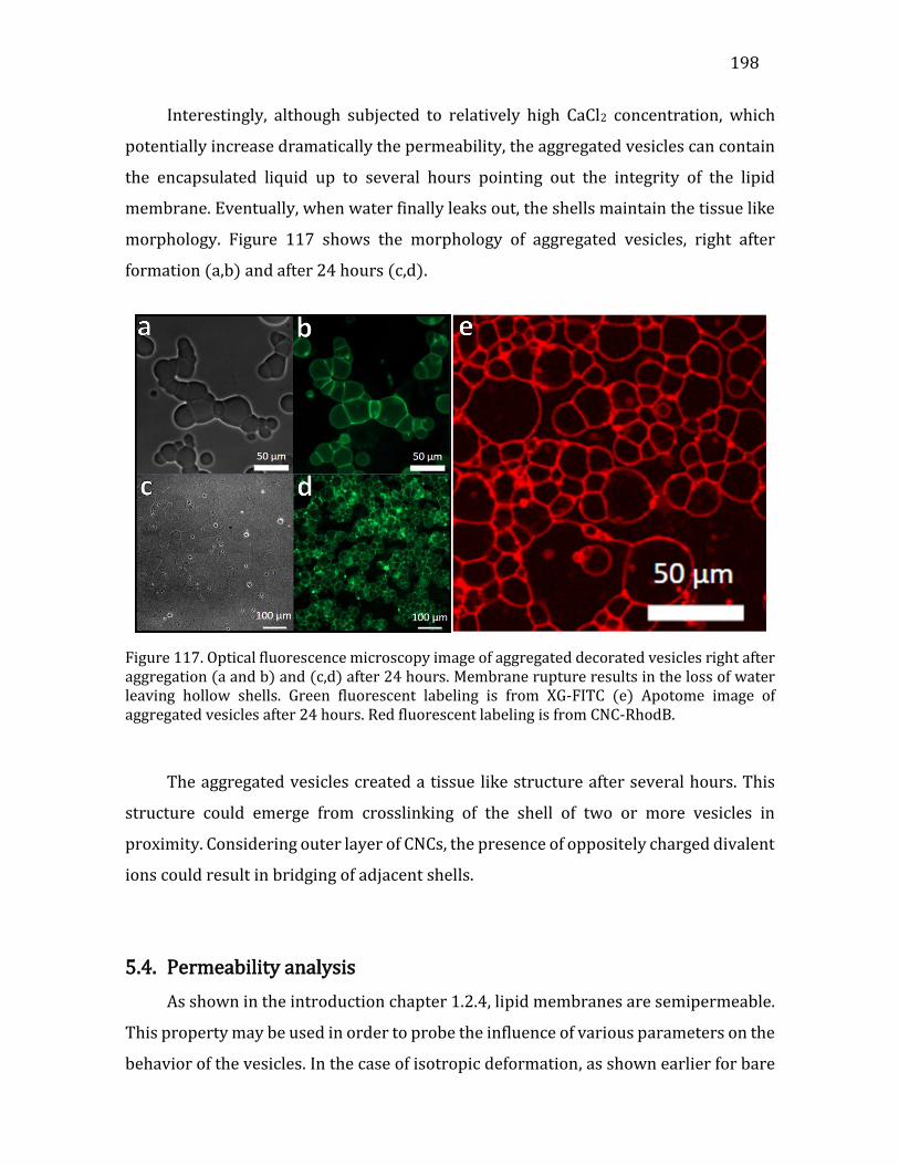
198
Interestingly, although subjected to relatively high CaCl2 concentration, which
potentially increase dramatically the permeability, the aggregated vesicles can contain
the encapsulated liquid up to several hours pointing out the integrity of the lipid
membrane. Eventually, when water finally leaks out, the shells maintain the tissue like
morphology. Figure 117 shows the morphology of aggregated vesicles, right after
formation (a,b) and after 24 hours (c,d).
Figure 117. Optical fluorescence microscopy image of aggregated decorated vesicles right after aggregation (a and b) and (c,d) after 24 hours. Membrane rupture results in the loss of water leaving hollow shells. Green fluorescent labeling is from XG-FITC (e) Apotome image of aggregated vesicles after 24 hours. Red fluorescent labeling is from CNC-RhodB.
The aggregated vesicles created a tissue like structure after several hours. This
structure could emerge from crosslinking of the shell of two or more vesicles in
proximity. Considering outer layer of CNCs, the presence of oppositely charged divalent
ions could result in bridging of adjacent shells.
5.4. Permeability analysis
As shown in the introduction chapter 1.2.4, lipid membranes are semipermeable.
This property may be used in order to probe the influence of various parameters on the
behavior of the vesicles. In the case of isotropic deformation, as shown earlier for bare
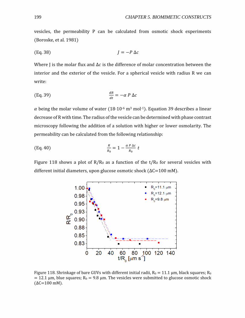
199 CHAPTER 5. BIOMIMETIC CONSTRUCTS
vesicles, the permeability P can be calculated from osmotic shock experiments
(Boroske, et al. 1981)
(Eq. 38) 𝐽 = −𝑃 ∆𝑐
Where J is the molar flux and ∆𝑐 is the difference of molar concentration between the
interior and the exterior of the vesicle. For a spherical vesicle with radius R we can
write:
(Eq. 39) 𝑑𝑅
𝑑𝑡= −𝛼 𝑃 ∆𝑐
𝛼 being the molar volume of water (18·10-6 m3 mol-1). Equation 39 describes a linear
decrease of R with time. The radius of the vesicle can be determined with phase contrast
microscopy following the addition of a solution with higher or lower osmolarity. The
permeability can be calculated from the following relationship:
(Eq. 40) 𝑅
𝑅0= 1 −
𝛼 𝑃 ∆𝑐
𝑅0 𝑡
Figure 118 shows a plot of R/R0 as a function of the t/R0 for several vesicles with
different initial diameters, upon glucose osmotic shock (ΔC=100 mM).
Figure 118. Shrinkage of bare GUVs with different initial radii, R0 = 11.1 µm, black squares; R0 = 12.1 µm, blue squares; R0 = 9.8 µm. The vesicles were submitted to glucose osmotic shock (ΔC=100 mM).
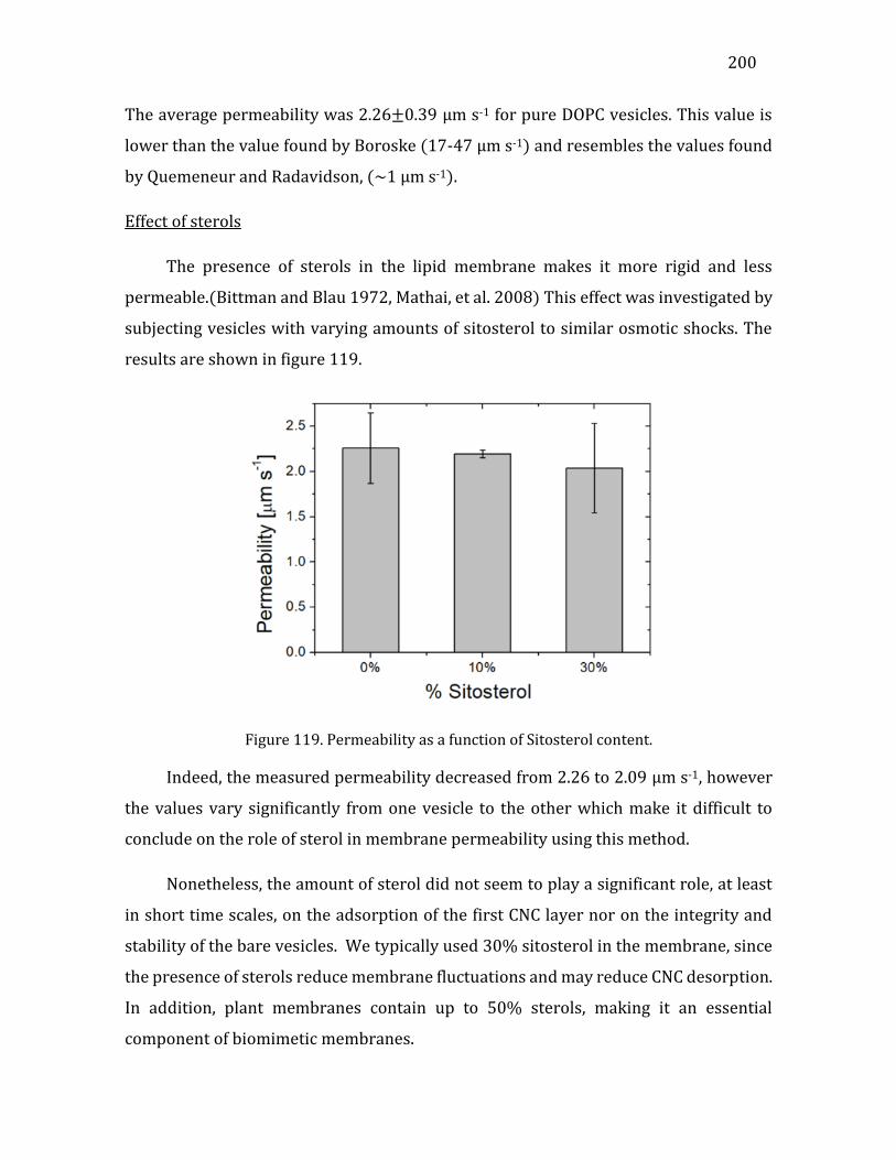
200
The average permeability was 2.26±0.39 µm s-1 for pure DOPC vesicles. This value is
lower than the value found by Boroske (17-47 µm s-1) and resembles the values found
by Quemeneur and Radavidson, (~1 µm s-1).
Effect of sterols
The presence of sterols in the lipid membrane makes it more rigid and less
permeable.(Bittman and Blau 1972, Mathai, et al. 2008) This effect was investigated by
subjecting vesicles with varying amounts of sitosterol to similar osmotic shocks. The
results are shown in figure 119.
Figure 119. Permeability as a function of Sitosterol content.
Indeed, the measured permeability decreased from 2.26 to 2.09 µm s-1, however
the values vary significantly from one vesicle to the other which make it difficult to
conclude on the role of sterol in membrane permeability using this method.
Nonetheless, the amount of sterol did not seem to play a significant role, at least
in short time scales, on the adsorption of the first CNC layer nor on the integrity and
stability of the bare vesicles. We typically used 30% sitosterol in the membrane, since
the presence of sterols reduce membrane fluctuations and may reduce CNC desorption.
In addition, plant membranes contain up to 50% sterols, making it an essential
component of biomimetic membranes.
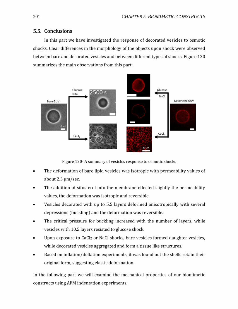
201 CHAPTER 5. BIOMIMETIC CONSTRUCTS
5.5. Conclusions
In this part we have investigated the response of decorated vesicles to osmotic
shocks. Clear differences in the morphology of the objects upon shock were observed
between bare and decorated vesicles and between different types of shocks. Figure 120
summarizes the main observations from this part:
Figure 120- A summary of vesicles response to osmotic shocks
• The deformation of bare lipid vesicles was isotropic with permeability values of
about 2.3 µm/sec.
• The addition of sitosterol into the membrane effected slightly the permeability
values, the deformation was isotropic and reversible.
• Vesicles decorated with up to 5.5 layers deformed anisotropically with several
depressions (buckling) and the deformation was reversible.
• The critical pressure for buckling increased with the number of layers, while
vesicles with 10.5 layers resisted to glucose shock.
• Upon exposure to CaCl2 or NaCl shocks, bare vesicles formed daughter vesicles,
while decorated vesicles aggregated and form a tissue like structures.
• Based on inflation/deflation experiments, it was found out the shells retain their
original form, suggesting elastic deformation.
In the following part we will examine the mechanical properties of our biomimetic
constructs using AFM indentation experiments.
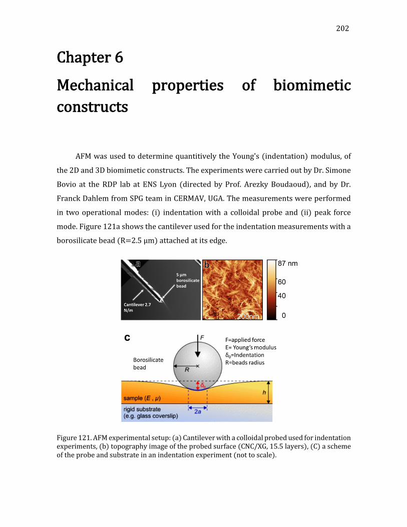
202
Chapter 6
Mechanical properties of biomimetic
constructs
6. Mechanical properties of biomimetic constructs
AFM was used to determine quantitively the Young's (indentation) modulus, of
the 2D and 3D biomimetic constructs. The experiments were carried out by Dr. Simone
Bovio at the RDP lab at ENS Lyon (directed by Prof. Arezky Boudaoud), and by Dr.
Franck Dahlem from SPG team in CERMAV, UGA. The measurements were performed
in two operational modes: (i) indentation with a colloidal probe and (ii) peak force
mode. Figure 121a shows the cantilever used for the indentation measurements with a
borosilicate bead (R=2.5 µm) attached at its edge.
Figure 121. AFM experimental setup: (a) Cantilever with a colloidal probed used for indentation experiments, (b) topography image of the probed surface (CNC/XG, 15.5 layers), (C) a scheme of the probe and substrate in an indentation experiment (not to scale).

203 CHAPTER 6. MECHANICAL PROPERTIES
Figure 121b shows a typical topography image of the probed surface (CNC/XG,
15.5 layers), taken with MLCT tip in contact mode. The CNC layer deposited on the
polymers (either PEI or XG) showing isotopically scattered CNC particles, with some
larger aggregates. Figure 121c shows a scheme of the indentation experiment with a
spherical probe. Let us discuss some important aspects of the AFM indentation method.
General considerations
• A good sample adhesion is required in order to extract reliable data.
• The sample should be thick enough to avoid contributions from the substrate to the
overall measured properties.
• The material under study is considered homogeneous and isotropic.
Given that these conditions are fulfilled, a model (Hertz or Sneddon for sphere or
cone shape tip, respectively) may be fitted to the approach retract curves obtained from
tip sample interaction.
Influence of the medium on tip sample interaction
In order to evaluate the mechanical properties of the sample, the contribution of
the electrostatic interaction to the force curve needs to be reduced to the minimum.
This can be done by changing the ionic strength of the medium.
In the case of ionic solution, the presence of salt can partially eliminate the
positive shift in vertical deflection and thus affects the calculation of the contact point.
Since the Hertz model was fitted only to the initial part of the curve, such shift in vertical
deflection in the case of high ionic strength leads to an increase in the initial slope,
resulting in higher Young's modulus.
This effect have been demonstrated by Cranston et al. who have shown the
dependence of adhesion on the ionic strength in PEI/CNC nanocomposite
films.(Cranston, et al. 2010) In their case the forces were attractive, therefore, with the
decrease in ionic strength, these interactions become more pronounced. For the
repulsive force in approach, it was shown that upon changing the charge of both tip and
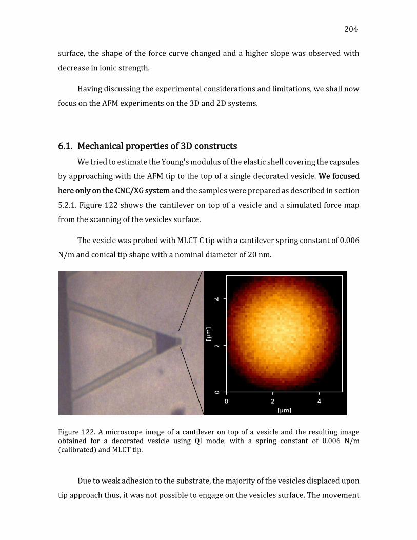
204
surface, the shape of the force curve changed and a higher slope was observed with
decrease in ionic strength.
Having discussing the experimental considerations and limitations, we shall now
focus on the AFM experiments on the 3D and 2D systems.
6.1. Mechanical properties of 3D constructs
We tried to estimate the Young's modulus of the elastic shell covering the capsules
by approaching with the AFM tip to the top of a single decorated vesicle. We focused
here only on the CNC/XG system and the samples were prepared as described in section
5.2.1. Figure 122 shows the cantilever on top of a vesicle and a simulated force map
from the scanning of the vesicles surface.
The vesicle was probed with MLCT C tip with a cantilever spring constant of 0.006
N/m and conical tip shape with a nominal diameter of 20 nm.
Figure 122. A microscope image of a cantilever on top of a vesicle and the resulting image obtained for a decorated vesicle using QI mode, with a spring constant of 0.006 N/m (calibrated) and MLCT tip.
Due to weak adhesion to the substrate, the majority of the vesicles displaced upon
tip approach thus, it was not possible to engage on the vesicles surface. The movement
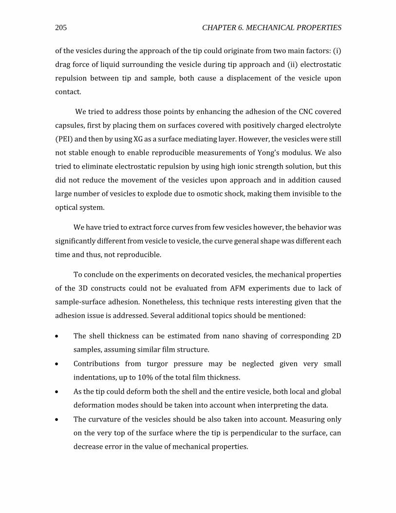
205 CHAPTER 6. MECHANICAL PROPERTIES
of the vesicles during the approach of the tip could originate from two main factors: (i)
drag force of liquid surrounding the vesicle during tip approach and (ii) electrostatic
repulsion between tip and sample, both cause a displacement of the vesicle upon
contact.
We tried to address those points by enhancing the adhesion of the CNC covered
capsules, first by placing them on surfaces covered with positively charged electrolyte
(PEI) and then by using XG as a surface mediating layer. However, the vesicles were still
not stable enough to enable reproducible measurements of Yong's modulus. We also
tried to eliminate electrostatic repulsion by using high ionic strength solution, but this
did not reduce the movement of the vesicles upon approach and in addition caused
large number of vesicles to explode due to osmotic shock, making them invisible to the
optical system.
We have tried to extract force curves from few vesicles however, the behavior was
significantly different from vesicle to vesicle, the curve general shape was different each
time and thus, not reproducible.
To conclude on the experiments on decorated vesicles, the mechanical properties
of the 3D constructs could not be evaluated from AFM experiments due to lack of
sample-surface adhesion. Nonetheless, this technique rests interesting given that the
adhesion issue is addressed. Several additional topics should be mentioned:
• The shell thickness can be estimated from nano shaving of corresponding 2D
samples, assuming similar film structure.
• Contributions from turgor pressure may be neglected given very small
indentations, up to 10% of the total film thickness.
• As the tip could deform both the shell and the entire vesicle, both local and global
deformation modes should be taken into account when interpreting the data.
• The curvature of the vesicles should be also taken into account. Measuring only
on the very top of the surface where the tip is perpendicular to the surface, can
decrease error in the value of mechanical properties.

206
In the following section we will focus on evaluating the mechanical properties of the 2D
constructs- the multilayer films.
6.2. Mechanical properties of 2D constructs
The samples were prepared as described in chapter 5.1. The force curves were
obtained using 2 methods:
(i) Indentation with spherical borosilicate ball with radius of 2.5 µm (figure 121a)
and an analysis of the approach retract curves using Hertz model (Eq. 2, Ch.1.5).
(ii) Using a conical tip with radius of 20 nm in peak-force mode to produce approach
retract curves fitted with Sneddon model (Eq. 3, Ch. 1.5).
The advantage of the 2D system (multilayered films) over the 3D system (decorated
GUVs) is the inherent adhesion to the substrate and the absence of curvature which
could possibly affect the results.
Indentation experiment
Indentation experiments were typically done with spherical probe mounted on a
cantilever. An analysis process was then systematically launched on each curve of a
force map, yielding average values from about 20-50 measurements. Typically, three
force maps were performed and analyzed for each sample.
The analysis included several steps: tip calibration, baseline subtraction, contact
point determination and calculation of the vertical tip position axis (calculated as piezo
displacement – cantilever deflection). The Hertz model was fitted to 2-50% of the curve
and the indentation at 0.1 of the force (i.e. ~10 nN) was calculated. Since it was seen
that only the thickest films are thick enough to be measured, we focused the analysis
on the samples with 20.5 and 15.5.
Peak force mode
Elastic modulus values were calculated from the Sneddon model fit to the peak
force curves at each point in the sample. A mechanical properties map is then generated
over the whole sample area and a statistical averaging is performed using the Gwyddion
software to yield average value of Young's modulus (see annex II for details).
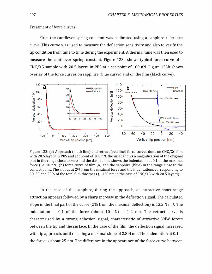
207 CHAPTER 6. MECHANICAL PROPERTIES
Treatment of force curves
First, the cantilever spring constant was calibrated using a sapphire reference
curve. This curve was used to measure the deflection sensitivity and also to verify the
tip condition from time to time during the experiment. A thermal tune was then used to
measure the cantilever spring constant. Figure 123a shows typical force curve of a
CNC/XG sample with 20.5 layers in PBS at a set point of 100 nN. Figure 123b shows
overlay of the force curves on sapphire (blue curve) and on the film (black curve).
Figure 123: (a) Approach (black line) and retract (red line) force curves done on CNC/XG film with 20.5 layers in PBS and set point of 100 nN. the inset shows a magnification of the original plot in the range close to zero and the dashed line shows the indentation at 0.1 of the maximal force (i.e. 10 nN) (b) force curve of film (a) and the sapphire (blue) in the range close to the contact point. The slopes at 2% from the maximal force and the indentations corresponding to 50, 30 and 20% of the total film thickness (~120 nm in the case of CNC/XG with 20.5 layers).
In the case of the sapphire, during the approach, an attractive short-range
attraction appears followed by a sharp increase in the deflection signal. The calculated
slope in the final part of the curve (2% from the maximal deflection) is 13.3 N m-1. The
indentation at 0.1 of the force (about 10 nN) is 1-2 nm. The retract curve is
characterized by a strong adhesion signal, characteristic of attractive VdW forces
between the tip and the surface. In the case of the film, the deflection signal increased
with tip approach, until reaching a maximal slope of 2.8 N m-1. The indentation at 0.1 of
the force is about 25 nm. The difference in the appearance of the force curve between
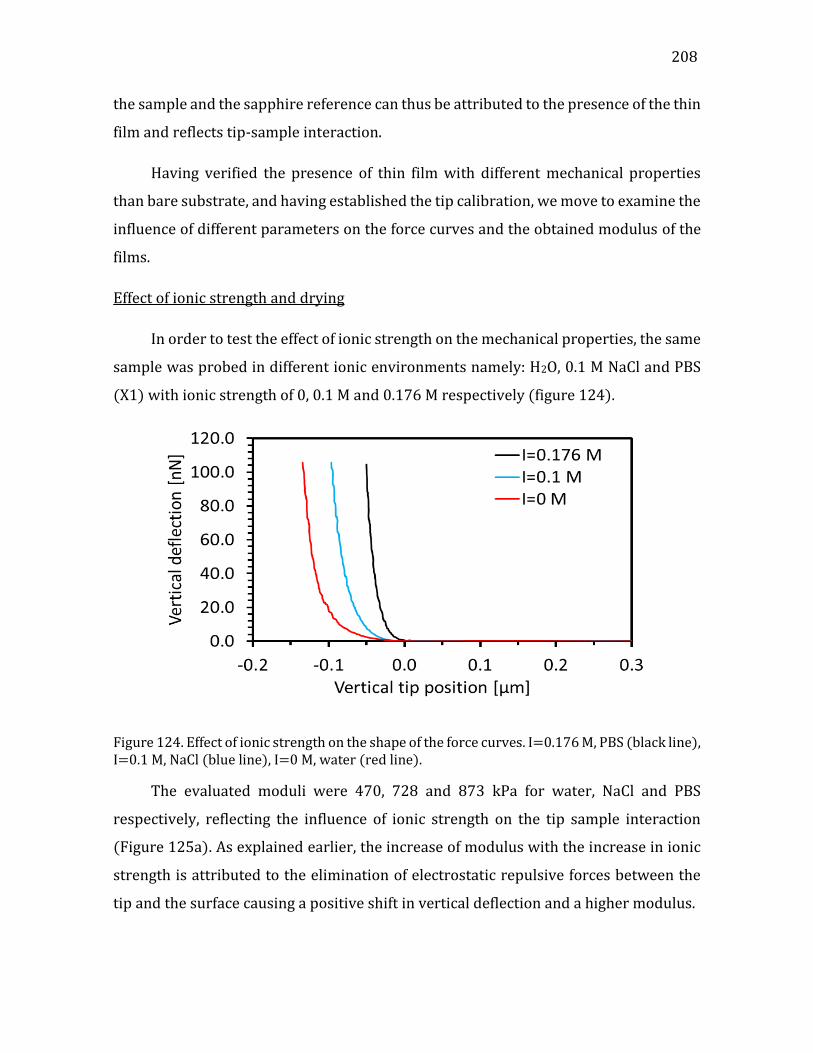
208
the sample and the sapphire reference can thus be attributed to the presence of the thin
film and reflects tip-sample interaction.
Having verified the presence of thin film with different mechanical properties
than bare substrate, and having established the tip calibration, we move to examine the
influence of different parameters on the force curves and the obtained modulus of the
films.
Effect of ionic strength and drying
In order to test the effect of ionic strength on the mechanical properties, the same
sample was probed in different ionic environments namely: H2O, 0.1 M NaCl and PBS
(X1) with ionic strength of 0, 0.1 M and 0.176 M respectively (figure 124).
Figure 124. Effect of ionic strength on the shape of the force curves. I=0.176 M, PBS (black line), I=0.1 M, NaCl (blue line), I=0 M, water (red line).
The evaluated moduli were 470, 728 and 873 kPa for water, NaCl and PBS
respectively, reflecting the influence of ionic strength on the tip sample interaction
(Figure 125a). As explained earlier, the increase of modulus with the increase in ionic
strength is attributed to the elimination of electrostatic repulsive forces between the
tip and the surface causing a positive shift in vertical deflection and a higher modulus.
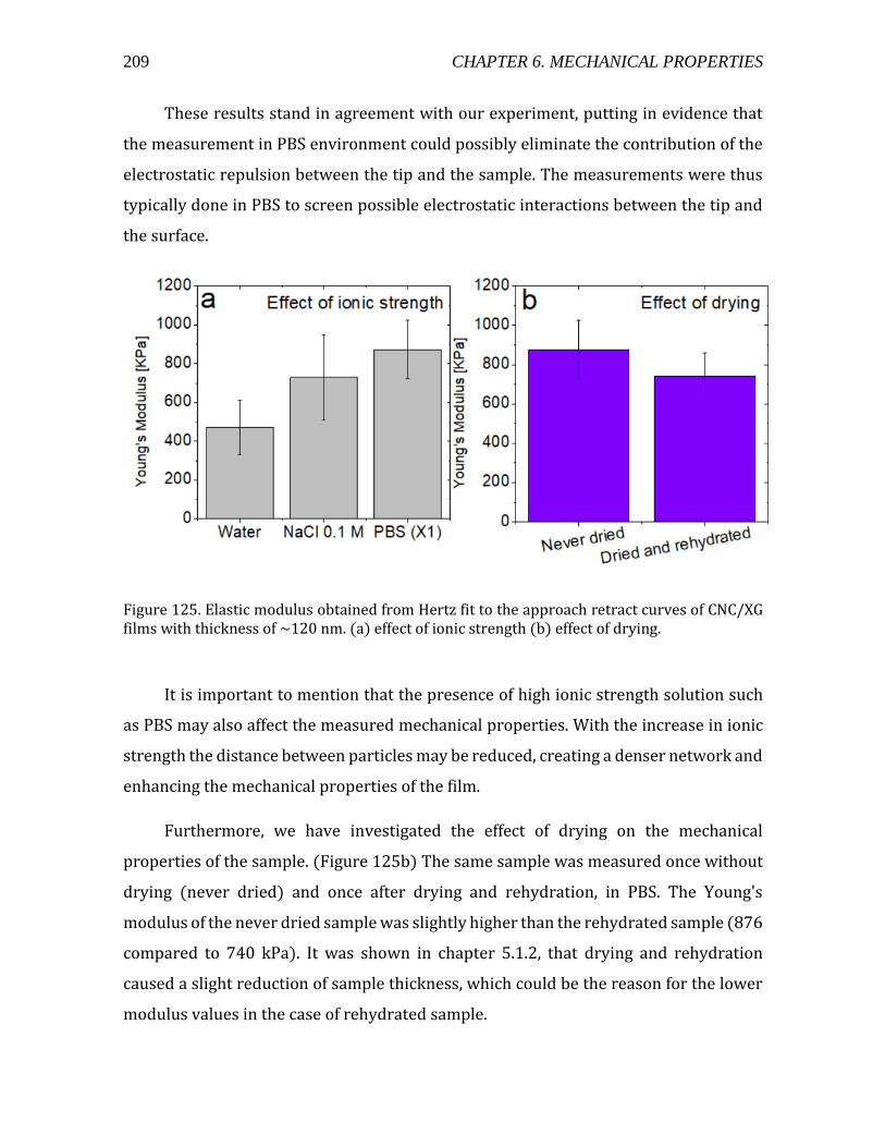
209 CHAPTER 6. MECHANICAL PROPERTIES
These results stand in agreement with our experiment, putting in evidence that
the measurement in PBS environment could possibly eliminate the contribution of the
electrostatic repulsion between the tip and the sample. The measurements were thus
typically done in PBS to screen possible electrostatic interactions between the tip and
the surface.
Figure 125. Elastic modulus obtained from Hertz fit to the approach retract curves of CNC/XG films with thickness of ~120 nm. (a) effect of ionic strength (b) effect of drying.
It is important to mention that the presence of high ionic strength solution such
as PBS may also affect the measured mechanical properties. With the increase in ionic
strength the distance between particles may be reduced, creating a denser network and
enhancing the mechanical properties of the film.
Furthermore, we have investigated the effect of drying on the mechanical
properties of the sample. (Figure 125b) The same sample was measured once without
drying (never dried) and once after drying and rehydration, in PBS. The Young's
modulus of the never dried sample was slightly higher than the rehydrated sample (876
compared to 740 kPa). It was shown in chapter 5.1.2, that drying and rehydration
caused a slight reduction of sample thickness, which could be the reason for the lower
modulus values in the case of rehydrated sample.
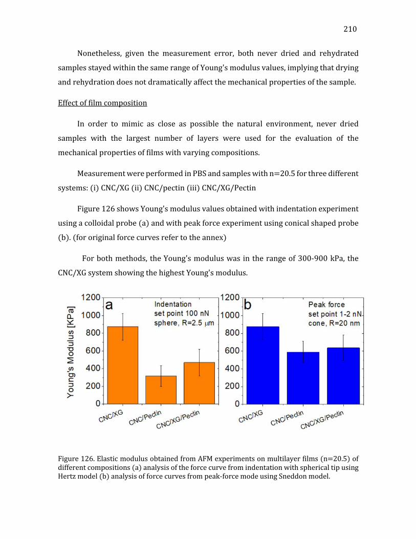
210
Nonetheless, given the measurement error, both never dried and rehydrated
samples stayed within the same range of Young's modulus values, implying that drying
and rehydration does not dramatically affect the mechanical properties of the sample.
Effect of film composition
In order to mimic as close as possible the natural environment, never dried
samples with the largest number of layers were used for the evaluation of the
mechanical properties of films with varying compositions.
Measurement were performed in PBS and samples with n=20.5 for three different
systems: (i) CNC/XG (ii) CNC/pectin (iii) CNC/XG/Pectin
Figure 126 shows Young's modulus values obtained with indentation experiment
using a colloidal probe (a) and with peak force experiment using conical shaped probe
(b). (for original force curves refer to the annex)
For both methods, the Young's modulus was in the range of 300-900 kPa, the
CNC/XG system showing the highest Young's modulus.
Figure 126. Elastic modulus obtained from AFM experiments on multilayer films (n=20.5) of different compositions (a) analysis of the force curve from indentation with spherical tip using Hertz model (b) analysis of force curves from peak-force mode using Sneddon model.
211 CHAPTER 6. MECHANICAL PROPERTIES
For the CNC/pectin sample, the modulus was lower than for the CNC/XG sample
in both indentation and peak force experiments. This could be the result of a weak
contact between CNC and pectin resulting in softer films. It should be pointed out that
the growth of CNC/pectin film was not linear and resulted in thinner and less
homogeneous films, possibly affecting the mechanical properties.
The obtained values, in the range of several hundred kPa, correspond to what was
obtained with AFM indentation, with colloidal probe and small cantilever spring
constants up to 2.7 N/m, for plant cell walls of Arabidopsis thaliana shoot apical
meristem (Peaucelle, 2011, Braybrook and Peucelle, 2013) and epidermal cells/dark
grown hypocotyl (Peaucelle, 2015). These values are lower than the ones found for
onion epidermis (Beauzamy 2015) or for pollen tubes (Burri, 2019), however the other
studies used stiffer cantilevers of 42 and 72 N/m (see table 4).
It is important to mention the fact that our in vitro system contains the basic
elements however, it cannot represent their diversity in terms of architecture
(colloidal cellulose nano-crystals in vitro versus micron sized fibers in planta),
composition (only one type of polysaccharide from each representative group) and
absence of specific interactions related to structural proteins.
Nonetheless, the results obtained on our simplified model system are in fair
agreement with the results obtained for various types of cell walls measured in planta,
using similar probing techniques, emphasizing the importance of those key
components in constructing plant cell wall mimetic models.
212
Summary
➢ Measurement on 2D constructs were achieved using AFM indentation and peak
force modes.
➢ The measurement conditions were optimized: thick layers n>15.5 or h>120 nm
and measurement in PBS to minimize tip-sample interaction.
➢ The indentation (Young's) modulus was in the range of 300-900 kPa.
➢ The effect of film composition was investigated and it was found that CNC/XG
films had higher Yong's modulus than the films that included pectin, perhaps due
to week CNC-pectin interaction.
Outlook
o The adhesion of GUVs to the substrate should be further addressed.
o Investigate more deeply the effect of composition on the mechanical properties
after tuning CNC-pectin interaction.
o Measurement of free-standing films prepared by casting and comparison with
LbL films. This comparison could resolve the question of film thickness
dependence of the mechanical properties, since free standing films are prepared
with casting and generally have thickness of few hundred microns.
213 CHAPTER 7. SUMMARY AND OUTLOOK
Chapter 7
Summary and outlook
7. Summary and outlook
This work was aimed to present a bottom up approach for the rational design of
biomimetic constructs inspired from the PCW. To do this it was divided to three main
parts: (i) building block characterization (ii) interaction studies (iii) realization and
characterization of 2D and 3D plant cell wall mimetic constructs. In this overview we
will describe the main findings from each part and propose some future outlook.
Initially, the building blocks of the system were identified and chosen to represent
the naturally occurring components of the PCW. The lipid membrane served as a
scaffold for LbL assembly while cellulose nano crystals were used to mimic the
naturally occurring cellulose fibers. Xyloglucan and homogalacturonan represented the
hemicellulose and pectin families respectively.
In the first part of the work we have characterized the structural parameters and
physical properties of the individual building blocks. Interaction studies were carried
out in the second part (ii), in order to optimize the conditions for assembly of
biomimetic constructs. Characterization of the constructs using optical microscopy and
AFM was finally established in the third part (iii).
Lipid-CNC interaction was probed in 2D (thin films) and 3D (bulk) experiments.
In both configurations, it was found that the main factor governing the interaction was
electrostatic attraction between positively charged membrane and negatively charged
CNCs. (Navon, et al. 2017) 2D experiments revealed that CNCs adsorb on flat supported
bilayers as highly hydrated film comprised of 1-2 layers of particles, with an average
thickness of 6-8 nm.(Navon, et al. 2020) It should be mentioned that adsorption of CNC
could be visualized by optical microscopy also for pH 5.5, however the highest
adsorption was indeed observed for pH<4. Hence, further experiments should include
a more quantitative study, by for example gradually changing the charge of CNCs and
214
measuring the interaction stoichiometry and thermodynamic parameters. In addition,
molecular dynamic simulations could be used to predict the contribution of other
intermolecular forces like VdW and hydrogen bonding, on the interaction of lipids and
CNCs.
We then proceed for the study of CNC-XG interaction. The molar mass of XG was
reduced by sonication, and it was shown using TEM, ITC, DLS and NMR that the
stoichiometric mass ratio of XG/CNC at saturation was 0.05 mg XG to 1 mg CNC. ITC
experiments suggest that the interaction of the XG chains with the CNC surface is of
exothermic nature and consists of slow rearrangement of chains on the surface. With
further addition of XG, at high XG/CNC ratio, the CNC-XG aggregates separate, resulting
in CNC particles covered by XG, the particles were stabilized by steric repulsion.
2D experiments on lipid-CNC-XG system with QCM-D, revealed that the XG layer
covering the CNCs is about 2 nm thick and composed from highly swollen XG chains.
Important factors, that could be further investigated quantitatively, are the effect of size
and solubility of XG on the adsorption on CNC surfaces.
The interaction between CNCs and homogalacturonan representing the pectin
family, was investigated in the presence of monovalent and divalent ions. It was found
that electrostatic repulsion between the two negatively charged species prevented the
interaction of pectin with CNCs. However, this repulsion could be compensated with
attractive depletion forces at high polymer concentration and high polymer/CNC ratio.
In addition, it was found that divalent ions promoted the formation of a gel at high
polymer/particle ratios and low degree of methyl esterification. A more comprehensive
study on pectin CNC interaction may include adsorption of pectins on model CNC
surfaces of different charges, and characterization of the interaction, as well as the
structural parameters of the resulting films with surface sensitive techniques such as
QCM-D or AFM. In addition, a physical characterization of pectin, is required to better
understand the effect of structural parameters such degree of ME, degree of blockiness
and solubility on the adsorption onto cellulose surfaces.
After studying the factors governing the interaction between the PCW building
blocks, we used the optimized parameters to build 2D and 3D constructs using LbL
deposition on spherical (GUVs) and flat (multilayered films) surfaces.
215 CHAPTER 7. SUMMARY AND OUTLOOK
For the 3D constructs, we examined the effect of layer thickness and composition
on the response to osmotic shocks of decorated vesicles and evaluated permeability
values for bare vesicles.
A clear difference in the response to osmotic shocks was observed between bare
and decorated vesicles. While bare vesicles deflated spherically upon osmotic shock,
decorated vesicles tended to buckle into deformed shapes, similarly to what is observed
for polyelectrolyte decorated capsules and gel phase vesicles. (Gao, et al. 2001,
Quemeneur, et al. 2012)
At high number of layers (n>10.5), decorated vesicles resisted osmotic shock and
ceased to deform. The critical glucose concentration required to induce buckling
increased with the increasing number of layers, confirming the increase in layer
thickness due to successive deposition cycles.
The theoretical relations and the derived equations should be refined using
theoretical simulations that will take into account the anisotropy of the material and
the contribution from both z (bending) and x-y (stretching) moduli. In addition, the
osmotic pressure can be generated using uncharged polymers such as polyethylene
glycol (PEG) instead of glucose. By doing so, a larger osmotic pressure difference could
be generated, possibly deflating the shells with large number of layers, helping to better
understand the effect of shell thickness and composition on the mechanical properties.
Additional experiments should be performed on larger number of objects to ensure
statistical reproducibility.
Upon addition of divalent ions, decorated vesicles aggregated to form tissue like
structures. The resulting structures resemble the composition and morphology of real
plant tissue thus, could be useful to investigate biological phenomena such as enzyme
activity or modulation of the mechanical properties, similarly to what was done with
natural plant tissues.(Beauzamy, et al. 2015, Bidhendi and Geitmann 2019, Milani, et al.
2011)
Due to weak adhesion between the vesicle and the substrate, the mechanical
properties of 3D vesicles could not be extracted. Future experiments should therefore
focus on developing the experimental conditions required for sufficient adhesion of the
vesicles to the substrate.

216
The structural features and mechanical properties of the 2D structures could be
evaluated using AFM experiments on flat multilayered films prepared via LbL method.
Films were prepared from CNC/XG, CNC/pectin and a mixed system of CNC/XG/pectin,
with different number of layers (n=5.5,10.5,15.5 and 20.5). It was found that the
preparation protocol had a striking influence on the resulting film thickness. Film
prepared with intermediate drying were thinner than the ones prepared without
intermediate drying, for the same number of layers and composition. This suggests that
the intermediate drying enables the closer contacts between CNCs and themselves and
between CNC and polymer, creating an irreversible shrinkage of the CNC-polymer
matrix. Upon rehydration, the sample slightly decreased in thickness, which could
result from closer packing of the CNCs and the polysaccharides upon drying.
The mechanical properties of the multilayered films were probed using both
peak-force and indentation experiments. It was found that the Young's modulus of the
films was 200-900 kPa, lower for what was found for CNC/XG decorated vesicles
(Radavidson 2016) and resembles the one found for Arabidopsis thaliana cell walls.
(Peaucelle, et al. 2011, Radotić, et al. 2012) The methodology could be further
developed, following tuning the interaction between CNC and pectin, to include
measurements on films with different composition.
The work presented here provides a platform for the rational design of PCW
mimetic materials. This type of biomimetic structures, designed as multilayered films
or decorated lipid vesicles, could serve for drug delivery, biodegradable coatings, food
packaging as well as serving as a simplified model of the primary wall for the study of
biological phenomena, such as transport of molecules or regulation of mechanical
properties by enzymes.
217
References Al-Amoudi, A.; Norlen, L. P.; Dubochet, J., Cryo-electron microscopy of vitreous sections of native biological cells and tissues. Journal of structural biology 2004, 148 (1), 131-135. Albersheim, P.; Darvill, A.; Roberts, K.; Sederoff, R.; Staehelin, A., Plant Cell Walls. Garland Science, Taylor and Francis Group: New York, 2011. Alem, H.; Blondeau, F.; Glinel, K.; Demoustier-Champagne, S.; Jonas, A. M., Layer-by-layer assembly of polyelectrolytes in nanopores. Macromolecules 2007, 40 (9), 3366-3372. Angelova, M. I.; Dimitrov, D. S., Liposome electroformation. Faraday discussions of the Chemical Society 1986, 81, 303-311. Aulin, C.; Ahola, S.; Josefsson, P.; Nishino, T.; Hirose, Y.; Osterberg, M.; Wagberg, L., Nanoscale Cellulose Films with Different Crystallinities and Mesostructures-Their Surface Properties and Interaction with Water. Langmuir 2009, 25 (13), 7675-7685. Axelrod, D., Total internal reflection fluorescence microscopy in cell biology. Traffic 2001, 2 (11), 764-774. Azzam, F.; Heux, L.; Putaux, J.-L.; Jean, B., Preparation by grafting onto, characterization, and properties of thermally responsive polymer-decorated cellulose nanocrystals. Biomacromolecules 2010, 11 (12), 3652-3659. Bailly, A. Elaboration and deformability of biomimetic systems. Université Grenoble Alpes, 2012. Battista, O.; Coppick, S.; Howsmon, J.; Morehead, F.; Sisson, W. A., Level-off degree of polymerization. Industrial & Engineering Chemistry 1956, 48 (2), 333-335. Beauzamy, L.; Derr, J.; Boudaoud, A., Quantifying hydrostatic pressure in plant cells by using indentation with an atomic force microscope. Biophysical journal 2015, 108 (10), 2448-2456. Benselfelt, T.; Cranston, E. D.; Ondaral, S.; Johansson, E.; Brumer, H.; Rutland, M. W.; Wagberg, L., Adsorption of xyloglucan onto cellulose surfaces of different morphologies: an entropy-driven process. Biomacromolecules 2016, 17 (9), 2801-2811. Bernard, A.-L.; Guedeau-Boudeville, M.-A.; Jullien, L.; di Meglio, J.-M., Raspberry vesicles. Biochimica et Biophysica Acta (BBA)-Biomembranes 2002, 1567, 1-5. Berret, J.-F., Stoichiometry of electrostatic complexes determined by light scattering. Macromolecules 2007, 40 (12), 4260-4266. Bidhendi, A. J.; Geitmann, A., Relating the mechanics of the primary plant cell wall to morphogenesis. Journal of Experimental Botany 2015, 67 (2), 449-461. Bidhendi, A. J.; Geitmann, A., Methods to quantify primary plant cell wall mechanics. Journal of Experimental Botany 2019, 70 (14), 3615-3648. Bittman, R.; Blau, L., Phospholipid-cholesterol interaction. Kinetics of water permeability in liposomes. Biochemistry 1972, 11 (25), 4831-4839. Blacklock, J.; Vetter, A.; Lankenau, A.; Oupický, D.; Möhwald, H., Tuning the mechanical properties of bioreducible multilayer films for improved cell adhesion and transfection activity. Biomaterials 2010, 31 (27), 7167-7174.
REFERENCES 218
Bledzki, A.; Gassan, J., Composites reinforced with cellulose based fibres. Progress in Polymer Science 1999, 24 (2), 221-274. Boroske, E.; Elwenspoek, M.; Helfrich, W., Osmotic shrinkage of giant egg-lecithin vesicles. Biophysical journal 1981, 34 (1), 95-109. Braccini, I.; Pérez, S., Molecular basis of Ca2+-induced gelation in alginates and pectins: the egg-box model revisited. Biomacromolecules 2001, 2 (4), 1089-1096. Braybrook, S. A.; Peaucelle, A., Mechano-chemical aspects of organ formation in Arabidopsis thaliana: the relationship between auxin and pectin. PloS one 2013, 8 (3), e57813. Burri, J. T.; Vogler, H.; Munglani, G.; Läubli, N. F.; Grossniklaus, U.; Nelson, B. J., A Microrobotic System for Simultaneous Measurement of Turgor Pressure and Cell-Wall Elasticity of Individual Growing Plant Cells. IEEE Robotics and Automation Letters 2019, 4 (2), 641-646. Burton, R. A.; Gidley, M. J.; Fincher, G. B., Heterogeneity in the chemistry, structure and function of plant cell walls. Nature chemical biology 2010, 6 (10), 724–732. Butt, H.-J.; Cappella, B.; Kappl, M., Force measurements with the atomic force microscope: Technique, interpretation and applications. Surface Science Reports 2005, 59 (1-6), 1-152. Cacas, J.-L.; Buré, C.; Grosjean, K.; Gerbeau-Pissot, P.; Lherminier, J.; Rombouts, Y.; Maes, E.; Bossard, C.; Gronnier, J.; Furt, F., Revisiting plant plasma membrane lipids in tobacco: a focus on sphingolipids. Plant Physiology 2016, 170 (1), 367-384. Caffall, K. H.; Mohnen, D., The structure, function, and biosynthesis of plant cell wall pectic polysaccharides. Carbohydrate research 2009, 344 (14), 1879-1900. Carpita, N. C.; Gibeaut, D. M., Structural models of primary cell walls in flowering plants: consistency of molecular structure with the physical properties of the walls during growth. The Plant Journal 1993, 3 (1), 1-30. Castellana, E. T.; Cremer, P. S., Solid supported lipid bilayers: From biophysical studies to sensor design. Surface Science Reports 2006, 61 (10), 429-444. Cerclier, C.; Cousin, F.; Bizot, H.; Moreau, C. l.; Cathala, B., Elaboration of spin-coated cellulose-xyloglucan multilayered thin films. Langmuir 2010, 26 (22), 17248-17255. Chambat, G.; Karmous, M.; Costes, M.; Picard, M.; Joseleau, J.-P., Variation of xyloglucan substitution pattern affects the sorption on celluloses with different degrees of crystallinity. Cellulose 2005, 12 (2), 117-125. Chanzy, H., Aspect of cellulose structure. In Cellulose Sources and Exploitation. Industrial Utilization, Biotechnology and Physico-Chemical Properties. , Kennedy, J. F.; Phillips, G. O.; Williams, P. A., Eds. Ellis Horwood Ltd. : Chichester, 1990; pp 3-12. Chen, C. J., Introduction to scanning tunneling microscopy. Oxford University Press: 1993; Vol. 4. Chibowski, E.; Szcześ, A., Zeta potential and surface charge of DPPC and DOPC liposomes in the presence of PLC enzyme. Adsorption 2016, 22 (4-6), 755-765. Contini, C.; Schneemilch, M.; Gaisford, S.; Quirke, N., Nanoparticle–membrane interactions. Journal of Experimental Nanoscience 2018, 13 (1), 62-81.
219
Cosgrove, D. C., Comparative structure and biomechanics of plant primary and secondary cell walls. Frontiers in plant science 2012, 3, 204. Cosgrove, D. J., Assembly and enlargement of the primary cell wall in plants. Annual review of cell and developmental biology 1997, 13 (1), 171-201. Cosgrove, D. J., Growth of the plant cell wall. Nature reviews molecular cell biology 2005, 6 (11), 850-861. Cosgrove, D. J., Re-constructing our models of cellulose and primary cell wall assembly. Current opinion in plant biology 2014, 22, 122-131. Courtois, J.; Berret, J.-F., Probing oppositely charged surfactant and copolymer interactions by isothermal titration microcalorimetry. Langmuir 2010, 26 (14), 11750-11758. Craig, V. S.; Plunkett, M., Determination of coupled solvent mass in quartz crystal microbalance measurements using deuterated solvents. Journal of colloid and interface science 2003, 262 (1), 126-129. Cranston, E. D.; Gray, D. G.; Rutland, M. W., Direct surface force measurements of polyelectrolyte multilayer films containing nanocrystalline cellulose. Langmuir 2010, 26 (22), 17190-17197. Dammak, A.; Quemener, B.; Bonnin, E.; Alvarado, C.; Bouchet, B.; Villares, A.; Moreau, C. l.; Cathala, B., Exploring architecture of xyloglucan cellulose nanocrystal complexes through enzyme susceptibility at different adsorption regimes. Biomacromolecules 2015, 16 (2), 589-596. Danino, D.; Bernheim-Groswasser, A.; Talmon, Y., Digital cryogenic transmission electron microscopy: an advanced tool for direct imaging of complex fluids. Colloids and Surfaces A: Physicochemical and Engineering Aspects 2001, 183, 113-122. de Macedo, B. d. S.; Almeida, T. d.; Cruz, R. d. C.; Netto, A. D. P.; Silva, L. d.; Berret, J.-F.; Vitorazi, L., Effect of pH on the complex coacervation and on the formation of layers of sodium alginate and PDADMAC. Langmuir 2020. Decher, G.; Hong, J.; Schmitt, J., Buildup of ultrathin multilayer films by a self-assembly process: III. Consecutively alternating adsorption of anionic and cationic polyelectrolytes on charged surfaces. Thin solid films 1992, 210, 831-835. Decher, G.; Schlenoff, J. B., Multilayer thin films: sequential assembly of nanocomposite materials. John Wiley & Sons: 2006. Decher, G., Layer-by-layer assembly (putting molecules to work). Multilayer thin films 2012, 1, 1-21. Dhar, N.; Au, D.; Berry, R. C.; Tam, K. C., Interactions of nanocrystalline cellulose with an oppositely charged surfactant in aqueous medium. Colloids and Surfaces A: Physicochemical and Engineering Aspects 2012, 415, 310-319. Dick-Pérez, M.; Zhang, Y.; Hayes, J.; Salazar, A.; Zabotina, O. A.; Hong, M., Structure and interactions of plant cell-wall polysaccharides by two-and three-dimensional magic-angle-spinning solid-state NMR. Biochemistry 2011, 50 (6), 989-1000. Donath, E.; Sukhorukov, G. B.; Caruso, F.; Davis, S. A.; Möhwald, H., Novel hollow polymer shells by colloid‐templated assembly of polyelectrolytes. Angewandte Chemie International Edition 1998, 37 (16), 2201-2205.
REFERENCES 220
Dong, S.; Roman, M., Fluorescently labeled cellulose nanocrystals for bioimaging applications. Journal of the American Chemical Society 2007, 129 (45), 13810-13811. Dong, X. M.; Revol, J.-F.; Gray, D. G., Effect of microcrystallite preparation conditions on the formation of colloid crystals of cellulose. Cellulose 1998, 5 (1), 19-32. Eeman, M.; Deleu, M., From biological membranes to biomimetic model membranes. Biotechnologie, Agronomie, Société et Environnement 2010, 14 (4), 719-736. Egerton, R. F., Physical principles of electron microscopy. Springer: 2005; Vol. 56. Ehmann, H. M.; Mohan, T.; Koshanskaya, M.; Scheicher, S.; Breitwieser, D.; Ribitsch, V.; Stana-Kleinschek, K.; Spirk, S., Design of anticoagulant surfaces based on cellulose nanocrystals. Chemical Communications 2014, 50 (86), 13070-13072. Eisele, N. B.; Andersson, F. I.; Frey, S.; Richter, R. P., Viscoelasticity of thin biomolecular films: a case study on nucleoporin phenylalanine-glycine repeats grafted to a histidine-tag capturing QCM-D sensor. Biomacromolecules 2012, 13 (8), 2322-2332. Elazzouzi-Hafraoui, S.; Nishiyama, Y.; Putaux, J.-L.; Heux, L.; Dubreuil, F.; Rochas, C., The shape and size distribution of crystalline nanoparticles prepared by acid hydrolysis of native cellulose. Biomacromolecules 2007, 9 (1), 57-65. Faïk, A.; Chileshe, C.; Sterling, J.; Maclachlan, G., Xyloglucan galactosyl-and fucosyltransferase activities from pea epicotyl microsomes. Plant Physiology 1997, 114 (1), 245-254. Favier, V.; Chanzy, H.; Cavaillé, J., Polymer nanocomposites reinforced by cellulose whiskers. Macromolecules 1995, 28 (18), 6365-6367. Fenz, S. F.; Sengupta, K., Giant vesicles as cell models. Integrative Biology 2012, 4 (9), 982-995. Finnemore, A.; Cunha, P.; Shean, T.; Vignolini, S.; Guldin, S.; Oyen, M.; Steiner, U., Biomimetic layer-by-layer assembly of artificial nacre. Nature communications 2012, 3, 966. Foster, E. J.; Moon, R. J.; Agarwal, U. P.; Bortner, M. J.; Bras, J.; Camarero-Espinosa, S.; Chan, K. J.; Clift, M. J.; Cranston, E. D.; Eichhorn, S. J., Current characterization methods for cellulose nanomaterials. Chemical Society Reviews 2018, 47 (8), 2609-2679. Fraeye, I.; Duvetter, T.; Doungla, E.; Van Loey, A.; Hendrickx, M., Fine-tuning the properties of pectin–calcium gels by control of pectin fine structure, gel composition and environmental conditions. Trends in Food Science & Technology 2010, 21 (5), 219-228. Freyer, M. W.; Lewis, E. A., Isothermal titration calorimetry: experimental design, data analysis, and probing macromolecule/ligand binding and kinetic interactions. Methods in cell biology 2008, 84, 79-113. Fry, S. C., Cellulases, hemicelluloses and auxin‐stimulated growth: a possible relationship. Physiologia Plantarum 1989, 75 (4), 532-536. Fry, S. C., The structure and functions of xyloglucan. Journal of Experimental Botany 1989, 40 (1), 1-11. Fry, S. C.; York, W. S.; Albersheim, P.; Darvill, A.; Hayashi, T.; Joseleau, J. P.; Kato, Y.; Lorences, E. P.; Maclachlan, G. A.; McNeil, M., An unambiguous nomenclature for xyloglucan‐derived oligosaccharides. Physiologia Plantarum 1993, 89 (1), 1-3.

221
Fultz, B.; Howe, J. M., Transmission electron microscopy and diffractometry of materials. Springer Science & Business Media: 2012. Furt, F.; Simon-Plas, F.; Mongrand, S., Lipids of the plant plasma membrane. In The plant plasma membrane, Springer: 2011; pp 3-30. Gao, C.; Donath, E.; Moya, S.; Dudnik, V.; Möhwald, H., Elasticity of hollow polyelectrolyte capsules prepared by the layer-by-layer technique. The European Physical Journal E 2001, 5 (1), 21-27. Geitmann, A., Experimental approaches used to quantify physical parameters at cellular and subcellular levels. American Journal of Botany 2006, 93 (10), 1380-1390. Giddings, T. H.; Brower, D. L.; Staehelin, L. A., Visualization of particle complexes in the plasma membrane of Micrasterias denticulata associated with the formation of cellulose fibrils in primary and secondary cell walls. The Journal of cell biology 1980, 84 (2), 327-339. Gilboa, B.; Gillo, D.; Farago, O.; Bernheim-Groswasser, A., Bidirectional cooperative motion of myosin-II motors on actin tracks with randomly alternating polarities. Soft Matter 2009, 5 (11), 2223-2231. Glinel, K.; Moussa, A.; Jonas, A. M.; Laschewsky, A., Influence of polyelectrolyte charge density on the formation of multilayers of strong polyelectrolytes at low ionic strength. Langmuir 2002, 18 (4), 1408-1412. Glinel, K.; Déjugnat, C.; Prevot, M.; Schöler, B.; Schönhoff, M.; Klitzing, R. v., Responsive polyelectrolyte multilayers. Colloids and Surfaces A: Physicochemical and Engineering Aspects 2007, 303 (1-2), 3-13. Grasdalen, H.; Bakøy, O. E.; Larsen, B., Determination of the degree of esterification and the distribution of methylated and free carboxyl groups in pectins by 1H-NMR spectroscopy. Carbohydrate research 1988, 184, 183-191. Gronnier, J.; Germain, V.; Gouguet, P.; Cacas, J.-L.; Mongrand, S., GIPC: Glycosyl Inositol Phospho Ceramides, the major sphingolipids on earth. Plant signaling & behavior 2016, 11 (4), 1-6. Grosjean, K.; Mongrand, S.; Beney, L.; Simon-Plas, F.; Gerbeau-Pissot, P., Differential effect of plant lipids on membrane organization specificities of phytosphingolipids and phytosterols. Journal of Biological Chemistry 2015, 290 (9), 5810-5825. Gu, J.; Catchmark, J. M., The impact of cellulose structure on binding interactions with hemicellulose and pectin. Cellulose 2013, 20 (4), 1613-1627. Hamant, O.; Moulia, B., How do plants read their own shapes? New Phytologist 2016, 212 (2), 333-337. Hambardzumyan, A.; Molinari, M.; Dumelie, N.; Foulon, L.; Habrant, A.; Chabbert, B.; Aguié-Béghin, V., Structure and optical properties of plant cell wall bio-inspired materials: cellulose–lignin multilayer nanocomposites. Comptes rendus biologies 2011, 334 (11), 839-850. Hanus, J.; Mazeau, K., The xyloglucan–cellulose assembly at the atomic scale. Biopolymers: Original Research on Biomolecules 2006, 82 (1), 59-73. Hayashi, T.; Maclachlan, G., Pea xyloglucan and cellulose: I. Macromolecular organization. Plant Physiology 1984, 75 (3), 596-604. Hayashi, T.; Marsden, M. P.; Delmer, D. P., Pea xyloglucan and cellulose: VI. Xyloglucan-cellulose interactions in vitro and in vivo. Plant Physiology 1987, 83 (2), 384-389. Hayashi, T., Xyloglucans in the primary cell wall. Annual review of plant biology 1989, 40 (1), 139-168.
REFERENCES 222
Hayashi, T.; Takeda, T.; Ogawa, K.; Mitsuishi, Y., Effects of the degree of polymerization on the binding of xyloglucans to cellulose. Plant and Cell Physiology 1994, 35 (6), 893-899. Hepler, P. K.; Winship, L. J., Calcium at the cell wall‐cytoplast interface. Journal of integrative plant biology 2010, 52 (2), 147-160. Hesselink, F. T.; Vrij, A.; Overbeek, J. T. G., Theory of the stabilization of dispersions by adsorbed macromolecules. II. Interaction between two flat particles. The Journal of Physical Chemistry 1971, 75 (14), 2094-2103. Hiemenz, P. C.; Rajagopalan, R., Principles of Colloid and Surface Chemistry, revised and expanded. CRC press: 2016. Hochmuth, R. M., Micropipette aspiration of living cells. Journal of biomechanics 2000, 33 (1), 15-22. Hunter, R. J., Zeta Potential in Colloid Science: Principles and Applications. Academic Press: London, 2013; Vol. 2. Husemann, E., Übermikroskopische Untersuchungen an hydrolytisch abgebauten Fasern. Mitteilung über makromolekulare Verbindungen. Journal für Praktische Chemie 1943, 1 (1‐6), 16-27. Israelachvili, J. N.; Mitchell, D. J.; Ninham, B. W., Theory of self-assembly of lipid bilayers and vesicles. Biochimica et Biophysica Acta (BBA)-Biomembranes 1977, 470 (2), 185-201. Israelachvili, J. N., Intermolecular and Surface Forces. Academic Press: New York, 2015. Itoh, T.; Brown, R. M., The assembly of cellulose microfibrils in Valonia macrophysa Kütz. Planta 1984, 160 (4), 372-381. Iwamoto, S.; Kai, W.; Isogai, A.; Iwata, T., Elastic modulus of single cellulose microfibrils from tunicate measured by atomic force microscopy. Biomacromolecules 2009, 10 (9), 2571-2576. Janiak, M. J.; Small, D. M.; Shipley, G. G., Temperature and compositional dependence of the structure of hydrated dimyristoyl lecithin. Journal of Biological Chemistry 1979, 254 (13), 6068-6078. Jaqaman, K.; Loerke, D.; Mettlen, M.; Kuwata, H.; Grinstein, S.; Schmid, S. L.; Danuser, G., Robust single-particle tracking in live-cell time-lapse sequences. Nature methods 2008, 5 (8), 695–702. Jean, B.; Dubreuil, F.; Heux, L.; Cousin, F., Structural details of cellulose nanocrystals/polyelectrolytes multilayers probed by neutron reflectivity and AFM. Langmuir 2008, 24 (7), 3452-3458. Jean, B.; Heux, L.; Dubreuil, F.; Chambat, G.; Cousin, F., Non-electrostatic building of biomimetic cellulose− xyloglucan multilayers. Langmuir 2009, 25 (7), 3920-3923. Johannsmann, D., Feature Article Viscoelastic analysis of organic thin films on quartz resonators. Macromol. Chem. Phys 1999, 200, 501-516. Johannsmann, D., Viscoelastic, mechanical, and dielectric measurements on complex samples with the quartz crystal microbalance. Physical Chemistry Chemical Physics 2008, 10 (31), 4516-4534. JPK instruments, NanoWizard Handbook. JPK instruments AG: Berlin Germany, 2012; Vol. Version 2.2, pp 4-5. Kalashnikova, I.; Bizot, H.; Cathala, B.; Capron, I., New Pickering emulsions stabilized by bacterial cellulose nanocrystals. Langmuir 2011, 27 (12), 7471-7479.
223
Kalashnikova, I.; Bizot, H.; Bertoncini, P.; Cathala, B.; Capron, I., Cellulosic nanorods of various aspect ratios for oil in water Pickering emulsions. Soft Matter 2013, 9 (3), 952-959. Kaushik, M.; Fraschini, C.; Chauve, G.; Putaux, J.-L.; Moores, A., Transmission electron microscopy for the characterization of cellulose nanocrystals. In Transmission Electron Microscopy - Theory and Applications, Maaz, K., Ed. InTech: Rijeka, Croatia, 2015; pp 130-156. Keegstra, K.; Talmadge, K. W.; Bauer, W.; Albersheim, P., The structure of plant cell walls: III. A model of the walls of suspension-cultured sycamore cells based on the interconnections of the macromolecular components. Plant Physiology 1973, 51 (1), 188-197. Kishani, S.; Vilaplana, F.; Ruda, M.; Hansson, P.; Wågberg, L., The influence of solubility on the adsorption of different Xyloglucan fractions at Cellulose Water Interfaces. Biomacromolecules 2019. Kittle, J. D.; Du, X.; Jiang, F.; Qian, C.; Heinze, T.; Roman, M.; Esker, A. R., Equilibrium water contents of cellulose films determined via solvent exchange and quartz crystal microbalance with dissipation monitoring. Biomacromolecules 2011, 12 (8), 2881-2887. Kolakovic, R.; Peltonen, L.; Laukkanen, A.; Hellman, M.; Laaksonen, P.; Linder, M. B.; Hirvonen, J.; Laaksonen, T., Evaluation of drug interactions with nanofibrillar cellulose. European journal of pharmaceutics and biopharmaceutics 2013, 85 (3), 1238-1244. Kummrow, M.; Helfrich, W., Collapse of giant phosphatidylcholine vesicles. Chemistry and physics of lipids 1996, 79 (2), 147-156. Kuntsche, J.; Horst, J. C.; Bunjes, H., Cryogenic transmission electron microscopy (cryo-TEM) for studying the morphology of colloidal drug delivery systems. International journal of pharmaceutics 2011, 417 (1-2), 120-137. Lai-Kee-Him, J.; Chanzy, H.; Müller, M.; Putaux, J.-L.; Imai, T.; Bulone, V., In vitro versus in vivocellulose microfibrils from plant primary wall synthases: Structural differences. Journal of Biological Chemistry 2002, 277 (40), 36931-36939. Lasic, D. D., The mechanism of vesicle formation. Biochemical Journal 1988, 256 (1), 1-11. Lasic, D. D.; Templeton, N., Liposomes in gene therapy. Advanced Drug Delivery Reviews 1996, 20 (2-3), 221-266. Levy, I.; Shani, Z.; Shoseyov, O., Modification of polysaccharides and plant cell wall by endo-1, 4-β-glucanase and cellulose-binding domains. Biomolecular engineering 2002, 19 (1), 17-30. Li, Y.; Wang, X.; Sun, J., Layer-by-layer assembly for rapid fabrication of thick polymeric films. Chemical Society Reviews 2012, 41 (18), 5998-6009. Lichtenberg, D.; Barenholz, Y., Liposomes: preparation, characterization, and preservation. Methods Biochem. Anal 1988, 33, 337-462. Liu, Z.; Persson, S.; Sánchez-Rodríguez, C., At the border: the plasma membrane–cell wall continuum. Journal of Experimental Botany 2015, 66 (6), 1553-1563. Lombardo, S.; Eyley, S.; Schutz, C.; Van Gorp, H.; Rosenfeldt, S.; Van den Mooter, G.; Thielemans, W., Thermodynamic study of the interaction of bovine serum albumin and amino acids with cellulose nanocrystals. Langmuir 2017, 33 (22), 5473-5481.

REFERENCES 224
Lombardo, S.; Thielemans, W., Thermodynamics of adsorption on nanocellulose surfaces. Cellulose 2018, 1-31. Lopez, M.; Bizot, H.; Chambat, G.; Marais, M.-F.; Zykwinska, A.; Ralet, M.-C.; Driguez, H.; Buléon, A., Enthalpic studies of xyloglucan− cellulose interactions. Biomacromolecules 2010, 11 (6), 1417-1428. Makino, K.; Yamada, T.; Kimura, M.; Oka, T.; Ohshima, H.; Kondo, T., Temperature-and ionic strength-induced conformational changes in the lipid head group region of liposomes as suggested by zeta potential data. Biophysical chemistry 1991, 41 (2), 175-183. Marchessault, R. H.; Morehead, F.; Walter, N., Liquid crystal systems from fibrillar polysaccharides. Nature 1959, 184 (4686), 632-633. Martin, C.; Jean, B., Nanocellulose/polymer multilayered thin films: tunable architectures towards tailored physical properties. Nordic Pulp & Paper Research Journal 2014, 29 (1), 19-30. Martin, C.; Barker, R.; Watkins, E. B.; Dubreuil, F. d. r.; Cranston, E. D.; Heux, L.; Jean, B., Structural variations in hybrid all-nanoparticle gibbsite nanoplatelet/cellulose nanocrystal multilayered films. Langmuir 2017, 33 (32), 7896-7907. Mathai, J. C.; Tristram-Nagle, S.; Nagle, J. F.; Zeidel, M. L., Structural determinants of water permeability through the lipid membrane. The Journal of general physiology 2008, 131 (1), 69-76. Mazeau, K., On the external morphology of native cellulose microfibrils. Carbohydrate Polymers 2011, 84 (1), 524-532. Mazeau, K.; Charlier, L., The molecular basis of the adsorption of xylans on cellulose surface. Cellulose 2012, 19 (2), 337-349. McNamara, J. T.; Morgan, J. L.; Zimmer, J., A molecular description of cellulose biosynthesis. Annual review of biochemistry 2015, 84, 895-921. McQueen-Mason, S.; Durachko, D. M.; Cosgrove, D. J., Two endogenous proteins that induce cell wall extension in plants. The Plant Cell 1992, 4 (11), 1425-1433. Mertins, O.; Dimova, R., Binding of chitosan to phospholipid vesicles studied with isothermal titration calorimetry. Langmuir 2011, 27 (9), 5506-5515. MicroCal, ITC data analysis in Origin: Tutorial Guide. In MicroCal, LLC, Northampton, MA, 2004. Migliorini, E.; Thakar, D.; Sadir, R.; Pleiner, T.; Baleux, F.; Lortat-Jacob, H.; Coche-Guerente, L.; Richter, R. P., Well-defined biomimetic surfaces to characterize glycosaminoglycan-mediated interactions on the molecular, supramolecular and cellular levels. Biomaterials 2014, 35 (32), 8903-8915. Milani, P.; Gholamirad, M.; Traas, J.; Arnéodo, A.; Boudaoud, A.; Argoul, F.; Hamant, O., In vivo analysis of local wall stiffness at the shoot apical meristem in Arabidopsis using atomic force microscopy. The Plant Journal 2011, 67 (6), 1116-1123. Mohnen, D., Pectin structure and biosynthesis. Current opinion in plant biology 2008, 11 (3), 266-277. Mølgaard, S. L.; Henriksson, M.; Cárdenas, M.; Svagan, A. J., Cellulose-nanofiber/polygalacturonic acid coatings with high oxygen barrier and targeted release properties. Carbohydrate Polymers 2014, 114, 179-182.
225
Moncelli, M. R.; Becucci, L.; Guidelli, R., The intrinsic pKa values for phosphatidylcholine, phosphatidylethanolamine, and phosphatidylserine in monolayers deposited on mercury electrodes. Biophysical journal 1994, 66 (6), 1969-1980. Montis, C.; Maiolo, D.; Alessandri, I.; Bergese, P.; Berti, D., Interaction of nanoparticles with lipid membranes: a multiscale perspective. Nanoscale 2014, 6 (12), 6452-6457. Montis, C.; Gerelli, Y.; Fragneto, G.; Nylander, T.; Baglioni, P.; Berti, D., Nucleolipid bilayers: A quartz crystal microbalance and neutron reflectometry study. Colloids and Surfaces B: Biointerfaces 2016, 137, 203-213. Morgan, J. L. W.; Strumillo, J.; Zimmer, J., Crystallographic snapshot of cellulose synthesis and membrane translocation. Nature 2013, 493 (7431), 181-186. Morgan, J. L. W.; McNamara, J. T.; Fischer, M.; Rich, J.; Chen, H.-M.; Withers, S. G.; Zimmer, J., Observing cellulose biosynthesis and membrane translocation in crystallo. Nature 2016, 531 (7594), 329-334. Mornet, S.; Lambert, O.; Duguet, E.; Brisson, A., The formation of supported lipid bilayers on silica nanoparticles revealed by cryoelectron microscopy. Nano letters 2005, 5 (2), 281-285. Mousseau, F.; Berret, J.-F., The role of surface charge in the interaction of nanoparticles with model pulmonary surfactants. Soft Matter 2018, 14 (28), 5764-5774. Mousseau, F.; Oikonomou, E. K.; Baldim, V.; Mornet, S.; Berret, J.-F., Nanoparticle-lipid interaction: Job scattering plots to differentiate vesicle aggregation from supported lipid bilayer formation. Colloids and Interfaces 2018, 2 (4), 50. Mueller, S. C.; Brown, R. M., Evidence for an intramembrane component associated with a cellulose microfibril-synthesizing complex in higher plants. The Journal of cell biology 1980, 84 (2), 315-326. Mukherjee, S.; Woods, H., X-ray and electron microscope studies of the degradation of cellulose by sulphuric acid. Biochimica et biophysica acta 1953, 10, 499-511. Muller, F. O.; Jean, B.; Perrin, P.; Heux, L.; Boué, F.; Cousin, F., Mechanism of associations of neutral semiflexible biopolymers in water: the xyloglucan case reveals inherent links. Macromolecular Chemistry and Physics 2013, 214 (20), 2312-2323. Muller, F. o. O.; Manet, S.; Jean, B.; Chambat, G.; Boue, F. o.; Heux, L.; Cousin, F., SANS measurements of semiflexible xyloglucan polysaccharide chains in water reveal their self-avoiding statistics. Biomacromolecules 2011, 12 (9), 3330-3336. Navon, Y.; Radavidson, H.; Putaux, J.-L.; Jean, B.; Heux, L., pH-Sensitive Interactions between Cellulose Nanocrystals and DOPC Liposomes. Biomacromolecules 2017, 18 (9), 2918-2927. Navon, Y.; Jean, B.; Coche-Guerente, L.; Dahlem, F.; Bernheim-Groswasser, A.; Heux, L., Deposition of cellulose nanocrystals onto biomimetic lipid membranes. Langmuir 2020. Nečas, D.; Klapetek, P., Gwyddion: an open-source software for SPM data analysis. Open Physics 2012, 10 (1), 181-188. Nielsen, L. J.; Eyley, S.; Thielemans, W.; Aylott, J. W., Dual fluorescent labelling of cellulose nanocrystals for pH sensing. Chemical Communications 2010, 46 (47), 8929-8931. Niinivaara, E.; Faustini, M.; Tammelin, T.; Kontturi, E., Water vapor uptake of ultrathin films of biologically derived nanocrystals: quantitative assessment with quartz crystal microbalance and spectroscopic ellipsometry. Langmuir 2015, 31 (44), 12170-12176.
REFERENCES 226
Nishiyama, Y.; Kim, U.-J.; Kim, D.-Y.; Katsumata, K. S.; May, R. P.; Langan, P., Periodic disorder along ramie cellulose microfibrils. Biomacromolecules 2003, 4 (4), 1013-1017. Nishiyama, Y., Structure and properties of the cellulose microfibril. Journal of wood science 2009, 55 (4), 241-249. Nixon, B. T.; Mansouri, K.; Singh, A.; Du, J.; Davis, J. K.; Lee, J.-G.; Slabaugh, E.; Vandavasi, V. G.; O’Neill, H.; Roberts, E. M., Comparative structural and computational analysis supports eighteen cellulose synthases in the plant cellulose synthesis complex. Scientific reports 2016, 6, 28696. O'Neill, M.; Albersheim, P.; Darvill, A., The pectic polysaccharides of primary cell walls. In Methods in plant biochemistry, Elsevier: 1990; Vol. 2, pp 415-441. Ochoa-Villarreal, M.; Aispuro-Hernández, E.; Vargas-Arispuro, I.; Martínez-Téllez, M. Á., Plant cell wall polymers: function, structure and biological activity of their derivatives. In Polymerization, edit., A. D. S. G., Ed. Intech: Rijeka, Croatia 2012; pp 63-86. Oikonomou, E.; Mousseau, F.; Christov, N.; Cristobal, G.; Vacher, A.; Airiau, M.; Bourgaux, C.; Heux, L.; Berret, J.-F., Fabric Softener–Cellulose Nanocrystal Interaction: A Model for Assessing Surfactant Deposition on Cotton. The Journal of Physical Chemistry B 2017, 121 (10), 2299-2307. Oikonomou, E.; Christov, N.; Cristobal, G.; Bourgaux, C.; Heux, L.; Boucenna, I.; Berret, J.-F., Design of eco-friendly fabric softeners: Structure, rheology and interaction with cellulose nanocrystals. Journal of colloid and interface science 2018, 525, 206-215. Park, I. H.; Choi, E.-J., Characterization of branched polyethyleneimine by laser light scattering and viscometry. Polymer 1996, 37 (2), 313-319. Park, Y. B.; Cosgrove, D. J., Xyloglucan and its interactions with other components of the growing cell wall. Plant and Cell Physiology 2015, 56 (2), 180-194. Paulraj, T.; Riazanova, A. V.; Yao, K.; Andersson, R. L.; Mullertz, A.; Svagan, A. J., Bioinspired layer-by-layer microcapsules based on cellulose nanofibers with switchable permeability. Biomacromolecules 2017, 18 (4), 1401-1410. Paulraj, T.; Riazanova, A.; Svagan, A., Bioinspired capsules based on nanocellulose, xyloglucan and pectin–The influence of capsule wall composition on permeability properties. Acta biomaterialia 2018, 69, 196-205. Peaucelle, A.; Braybrook, S. A.; Le Guillou, L.; Bron, E.; Kuhlemeier, C.; Höfte, H., Pectin-induced changes in cell wall mechanics underlie organ initiation in Arabidopsis. Current biology 2011, 21 (20), 1720-1726. Peaucelle, A.; Wightman, R.; Höfte, H., The control of growth symmetry breaking in the Arabidopsis hypocotyl. Current biology 2015, 25 (13), 1746-1752. Peetla, C.; Stine, A.; Labhasetwar, V., Biophysical interactions with model lipid membranes: applications in drug discovery and drug delivery. Molecular pharmaceutics 2009, 6 (5), 1264-1276. Pelloux, J.; Rusterucci, C.; Mellerowicz, E. J., New insights into pectin methylesterase structure and function. Trends in plant science 2007, 12 (6), 267-277. Philipse, A. P., The random contact equation and its implications for (colloidal) rods in packings, suspensions, and anisotropic powders. Langmuir 1996, 12 (5), 1127-1133.
227
Pickering, S. U., Emulsions. Journal of the Chemical Society, Transactions 1907, 91, 2001-2021. Quemeneur, F.; Rinaudo, M.; Pépin-Donat, B., Influence of polyelectrolyte chemical structure on their interaction with lipid membrane of zwitterionic liposomes. Biomacromolecules 2008, 9 (8), 2237-2243. Quemeneur, F. Relationship between mechanical parameters and behaviour under external stresses in lipid vesicles with modified membranes. University of Grenoble, Grenoble, 2010. Quemeneur, F.; Rinaudo, M.; Maret, G.; Pépin-Donat, B., Decoration of lipid vesicles by polyelectrolytes: mechanism and structure. Soft Matter 2010, 6 (18), 4471-4481. Quemeneur, F.; Quilliet, C.; Faivre, M.; Viallat, A.; Pépin-Donat, B., Gel phase vesicles buckle into specific shapes. Physical review letters 2012, 108 (10), 108303. Radavidson, H. Vésicules lipidiques biomimétiques décorées par un assemblage multicouche nanocristaux decellulose/xyloglucane : élaboration et caractérisation mécanique. University of Grenoble Alpes, 2016. Radotić, K.; Roduit, C.; Simonović, J.; Hornitschek, P.; Fankhauser, C.; Mutavdžić, D.; Steinbach, G.; Dietler, G.; Kasas, S., Atomic force microscopy stiffness tomography on living Arabidopsis thaliana cells reveals the mechanical properties of surface and deep cell-wall layers during growth. Biophysical journal 2012, 103 (3), 386-394. Rånby, B. G., Aqueous colloidal solutions of cellulose micelles. Acta Chemica Scandinavica 1949, 3 (5), 649-650. Rånby, B. G.; Ribi, E., Über den Feinbau der Zellulose. Experientia 1950, 6 (1), 12-14. Reeves, J. P.; Dowben, R. M., Formation and properties of thin‐walled phospholipid vesicles. Journal of cellular physiology 1969, 73 (1), 49-60. Reid, M. S.; Villalobos, M.; Cranston, E. D., Cellulose nanocrystal interactions probed by thin film swelling to predict dispersibility. Nanoscale 2016, 8 (24), 12247-12257. Reviakine, I.; Johannsmann, D.; Richter, R. P., Hearing What You Cannot See and Visualizing What You Hear: Interpreting Quartz Crystal Microbalance Data from Solvated Interfaces. Analytical Chemistry 2011, 83 (23), 8838-8848. Revol, J.-F.; Bradford, H.; Giasson, J.; Marchessault, R. H.; Gray, D., Helicoidal self-ordering of cellulose microfibrils in aqueous suspension. International journal of biological macromolecules 1992, 14 (3), 170-172. Richardson, J. J.; Björnmalm, M.; Caruso, F., Technology-driven layer-by-layer assembly of nanofilms. Science 2015, 348 (6233), aaa2491. Richter, R.; Mukhopadhyay, A.; Brisson, A., Pathways of lipid vesicle deposition on solid surfaces: a combined QCM-D and AFM study. Biophysical journal 2003, 85 (5), 3035-3047. Richter, R. P.; Brisson, A. R., Following the formation of supported lipid bilayers on mica: a study combining AFM, QCM-D, and ellipsometry. Biophysical journal 2005, 88 (5), 3422-3433. Richter, R. P.; Bérat, R.; Brisson, A. R., Formation of solid-supported lipid bilayers: an integrated view. Langmuir 2006, 22 (8), 3497-3505. Rodriguez, N.; Pincet, F.; Cribier, S., Giant vesicles formed by gentle hydration and electroformation: a comparison by fluorescence microscopy. Colloids and Surfaces B: Biointerfaces 2005, 42 (2), 125-130.
REFERENCES 228
Routier-Kierzkowska, A.-L.; Smith, R. S., Measuring the mechanics of morphogenesis. Current opinion in plant biology 2013, 16 (1), 25-32. Rubinger, C.; Moreira, R.; Cury, L.; Fontes, G.; Neves, B.; Meneguzzi, A.; Ferreira, C., Langmuir–Blodgett and Langmuir–Schaefer films of poly (5-amino-1-naphthol) conjugated polymer. Applied Surface Science 2006, 253 (2), 543-548. Sandrin, L.; Coche-Guérente, L.; Bernstein, A.; Basit, H.; Labbé, P.; Dumy, P.; Boturyn, D., Cell adhesion through clustered ligand on fluid supported lipid bilayers. Organic & biomolecular chemistry 2010, 8 (7), 1531-1534. Sapkota, J.; Shirole, A.; Foster, E. J.; Garcia, J. C. M.; Lattuada, M.; Weder, C., Polymer nanocomposites with nanorods having different length distributions. Polymer 2017, 110, 284-291. Scheller, H. V.; Ulvskov, P., Hemicelluloses. Annual review of plant biology 2010, 61 (1), 263-289. Schneider, C. A.; Rasband, W. S.; Eliceiri, K. W., NIH Image to ImageJ: 25 years of image analysis. Nature methods 2012, 9 (7), 671-675. Schoeler, B.; Delorme, N.; Doench, I.; Sukhorukov, G. B.; Fery, A.; Glinel, K., Polyelectrolyte films based on polysaccharides of different conformations: Effects on multilayer structure and mechanical properties. Biomacromolecules 2006, 7 (6), 2065-2071. Sethaphong, L.; Haigler, C. H.; Kubicki, J. D.; Zimmer, J.; Bonetta, D.; DeBolt, S.; Yingling, Y. G., Tertiary model of a plant cellulose synthase. Proceedings of the National Academy of Sciences 2013, 110 (18), 7512-7517. Sharma, B.; Naresh, L.; Dhuldhoya, N.; Merchant, S.; Merchant, U., An overview on pectins. Times Food Processing Journal 2006, 23 (2), 44-51. Singh, A. V.; Rahman, A.; Kumar, N. S.; Aditi, A.; Galluzzi, M.; Bovio, S.; Barozzi, S.; Montani, E.; Parazzoli, D., Bio-inspired approaches to design smart fabrics. Materials & Design (1980-2015) 2012, 36, 829-839. Slama, J. S.; Rando, R. R., Lectin-mediated aggregation of liposomes containing glycolipids with variable hydrophilic spacer arms. Biochemistry 1980, 19 (20), 4595-4600. Sneddon, I. N., The relation between load and penetration in the axisymmetric Boussinesq problem for a punch of arbitrary profile. International journal of engineering science 1965, 3 (1), 47-57. Somerville, C.; Bauer, S.; Brininstool, G.; Facette, M.; Hamann, T.; Milne, J.; Osborne, E.; Paredez, A.; Persson, S.; Raab, T., Toward a systems approach to understanding plant cell walls. Science 2004, 306 (5705), 2206-2211. Stana, K.; Pohar, C.; Ribitsch, V., Adsorption of whitening agents on cellulose fibers—Monitored by streaming potential measurements, calorimetry and fluorescence. Colloid and Polymer Science 1995, 273 (12), 1174-1178. Svagan, A. J.; Musyanovych, A.; Kappl, M.; Bernhardt, M.; Glasser, G.; Wohnhaas, C.; Berglund, L. A.; Risbo, J.; Landfester, K., Cellulose nanofiber/nanocrystal reinforced capsules: A fast and facile approach toward assembly of liquid-core capsules with high mechanical stability. Biomacromolecules 2014, 15 (5), 1852-1859. Szoka Jr, F.; Papahadjopoulos, D., Comparative properties and methods of preparation of lipid vesicles (liposomes). Annual review of biophysics and bioengineering 1980, 9 (1), 467-508.
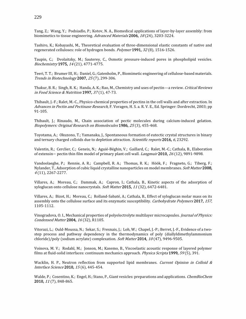
229
Tang, Z.; Wang, Y.; Podsiadlo, P.; Kotov, N. A., Biomedical applications of layer‐by‐layer assembly: from biomimetics to tissue engineering. Advanced Materials 2006, 18 (24), 3203-3224. Tashiro, K.; Kobayashi, M., Theoretical evaluation of three-dimensional elastic constants of native and regenerated celluloses: role of hydrogen bonds. Polymer 1991, 32 (8), 1516-1526. Taupin, C.; Dvolaitzky, M.; Sauterey, C., Osmotic pressure-induced pores in phospholipid vesicles. Biochemistry 1975, 14 (21), 4771-4775. Teeri, T. T.; Brumer III, H.; Daniel, G.; Gatenholm, P., Biomimetic engineering of cellulose-based materials. Trends in Biotechnology 2007, 25 (7), 299-306. Thakur, B. R.; Singh, R. K.; Handa, A. K.; Rao, M., Chemistry and uses of pectin—a review. Critical Reviews in Food Science & Nutrition 1997, 37 (1), 47-73. Thibault, J.-F.; Ralet, M.-C., Physico-chemical properties of pectins in the cell walls and after extraction. In Advances in Pectin and Pectinase Research, F. Voragen, H. S. a. R. V. E., Ed. Springer: Dordrecht, 2003; pp 91-105. Thibault, J.; Rinaudo, M., Chain association of pectic molecules during calcium‐induced gelation. Biopolymers: Original Research on Biomolecules 1986, 25 (3), 455-468. Toyotama, A.; Okuzono, T.; Yamanaka, J., Spontaneous formation of eutectic crystal structures in binary and ternary charged colloids due to depletion attraction. Scientific reports 2016, 6, 23292. Valentin, R.; Cerclier, C.; Geneix, N.; Aguié-Béghin, V.; Gaillard, C.; Ralet, M.-C.; Cathala, B., Elaboration of extensin− pectin thin film model of primary plant cell wall. Langmuir 2010, 26 (12), 9891-9898. Vandoolaeghe, P.; Rennie, A. R.; Campbell, R. A.; Thomas, R. K.; Höök, F.; Fragneto, G.; Tiberg, F.; Nylander, T., Adsorption of cubic liquid crystalline nanoparticles on model membranes. Soft Matter 2008, 4 (11), 2267-2277. Villares, A.; Moreau, C.; Dammak, A.; Capron, I.; Cathala, B., Kinetic aspects of the adsorption of xyloglucan onto cellulose nanocrystals. Soft Matter 2015, 11 (32), 6472-6481. Villares, A.; Bizot, H.; Moreau, C.; Rolland-Sabaté, A.; Cathala, B., Effect of xyloglucan molar mass on its assembly onto the cellulose surface and its enzymatic susceptibility. Carbohydrate Polymers 2017, 157, 1105-1112. Vinogradova, O. I., Mechanical properties of polyelectrolyte multilayer microcapsules. Journal of Physics: Condensed Matter 2004, 16 (32), R1105. Vitorazi, L.; Ould-Moussa, N.; Sekar, S.; Fresnais, J.; Loh, W.; Chapel, J.-P.; Berret, J.-F., Evidence of a two-step process and pathway dependency in the thermodynamics of poly (diallyldimethylammonium chloride)/poly (sodium acrylate) complexation. Soft Matter 2014, 10 (47), 9496-9505. Voinova, M. V.; Rodahl, M.; Jonson, M.; Kasemo, B., Viscoelastic acoustic response of layered polymer films at fluid-solid interfaces: continuum mechanics approach. Physica Scripta 1999, 59 (5), 391. Wacklin, H. P., Neutron reflection from supported lipid membranes. Current Opinion in Colloid & Interface Science 2010, 15 (6), 445-454. Walde, P.; Cosentino, K.; Engel, H.; Stano, P., Giant vesicles: preparations and applications. ChemBioChem 2010, 11 (7), 848-865.
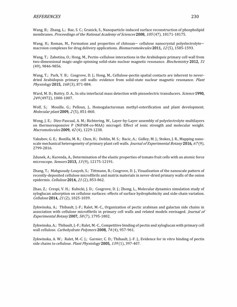
REFERENCES 230
Wang, B.; Zhang, L.; Bae, S. C.; Granick, S., Nanoparticle-induced surface reconstruction of phospholipid membranes. Proceedings of the National Academy of Sciences 2008, 105 (47), 18171-18175. Wang, H.; Roman, M., Formation and properties of chitosan− cellulose nanocrystal polyelectrolyte− macroion complexes for drug delivery applications. Biomacromolecules 2011, 12 (5), 1585-1593. Wang, T.; Zabotina, O.; Hong, M., Pectin–cellulose interactions in the Arabidopsis primary cell wall from two-dimensional magic-angle-spinning solid-state nuclear magnetic resonance. Biochemistry 2012, 51 (49), 9846-9856. Wang, T.; Park, Y. B.; Cosgrove, D. J.; Hong, M., Cellulose-pectin spatial contacts are inherent to never-dried Arabidopsis primary cell walls: evidence from solid-state nuclear magnetic resonance. Plant Physiology 2015, 168 (3), 871-884. Ward, M. D.; Buttry, D. A., In situ interfacial mass detection with piezoelectric transducers. Science 1990, 249 (4972), 1000-1007. Wolf, S.; Mouille, G.; Pelloux, J., Homogalacturonan methyl-esterification and plant development. Molecular plant 2009, 2 (5), 851-860. Wong, J. E.; Diez-Pascual, A. M.; Richtering, W., Layer-by-Layer assembly of polyelectrolyte multilayers on thermoresponsive P (NiPAM-co-MAA) microgel: Effect of ionic strength and molecular weight. Macromolecules 2009, 42 (4), 1229-1238. Yakubov, G. E.; Bonilla, M. R.; Chen, H.; Doblin, M. S.; Bacic, A.; Gidley, M. J.; Stokes, J. R., Mapping nano-scale mechanical heterogeneity of primary plant cell walls. Journal of Experimental Botany 2016, 67 (9), 2799-2816. Zdunek, A.; Kurenda, A., Determination of the elastic properties of tomato fruit cells with an atomic force microscope. Sensors 2013, 13 (9), 12175-12191. Zhang, T.; Mahgsoudy-Louyeh, S.; Tittmann, B.; Cosgrove, D. J., Visualization of the nanoscale pattern of recently-deposited cellulose microfibrils and matrix materials in never-dried primary walls of the onion epidermis. Cellulose 2014, 21 (2), 853-862. Zhao, Z.; Crespi, V. H.; Kubicki, J. D.; Cosgrove, D. J.; Zhong, L., Molecular dynamics simulation study of xyloglucan adsorption on cellulose surfaces: effects of surface hydrophobicity and side-chain variation. Cellulose 2014, 21 (2), 1025-1039. Zykwinska, A.; Thibault, J.-F.; Ralet, M.-C., Organization of pectic arabinan and galactan side chains in association with cellulose microfibrils in primary cell walls and related models envisaged. Journal of Experimental Botany 2007, 58 (7), 1795-1802. Zykwinska, A.; Thibault, J.-F.; Ralet, M.-C., Competitive binding of pectin and xyloglucan with primary cell wall cellulose. Carbohydrate Polymers 2008, 74 (4), 957-961. Zykwinska, A. W.; Ralet, M.-C. J.; Garnier, C. D.; Thibault, J.-F. J., Evidence for in vitro binding of pectin side chains to cellulose. Plant Physiology 2005, 139 (1), 397-407.

231
ANNEX I

232
ANNEX II
Figure 127. Force curves obtained with a colloidal probe on multilayered systems. Approach (light blue) and retract (dark blue) curves of (a) CNC/XG (b) CNC/Pectin (c) (CNC/XG/CNC/Pectin films with 20 deposition cycles. The green curve is a fit to the Hertz model. The limits are adjusted to fit the part of the curve corresponding to an indentation of 10% of the total film thickness as measured by AFM height profile on a scratched area. This is done in order to avoid contribution from the substrate.
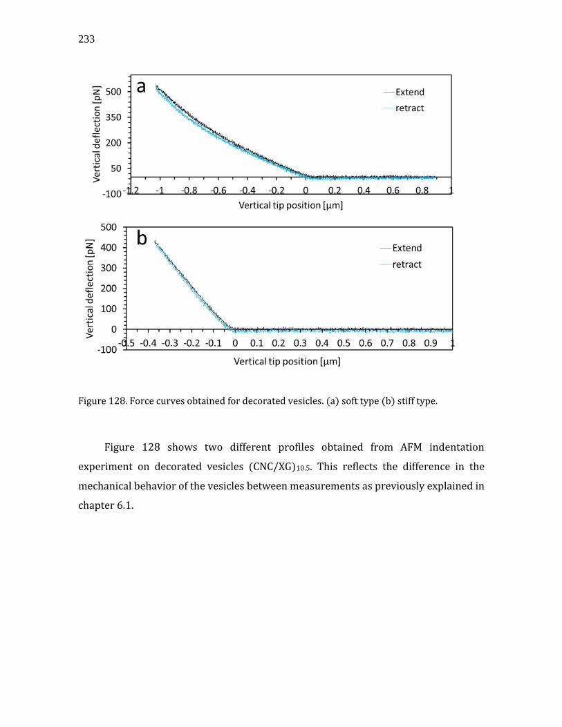
233
Figure 128. Force curves obtained for decorated vesicles. (a) soft type (b) stiff type.
Figure 128 shows two different profiles obtained from AFM indentation
experiment on decorated vesicles (CNC/XG)10.5. This reflects the difference in the
mechanical behavior of the vesicles between measurements as previously explained in
chapter 6.1.
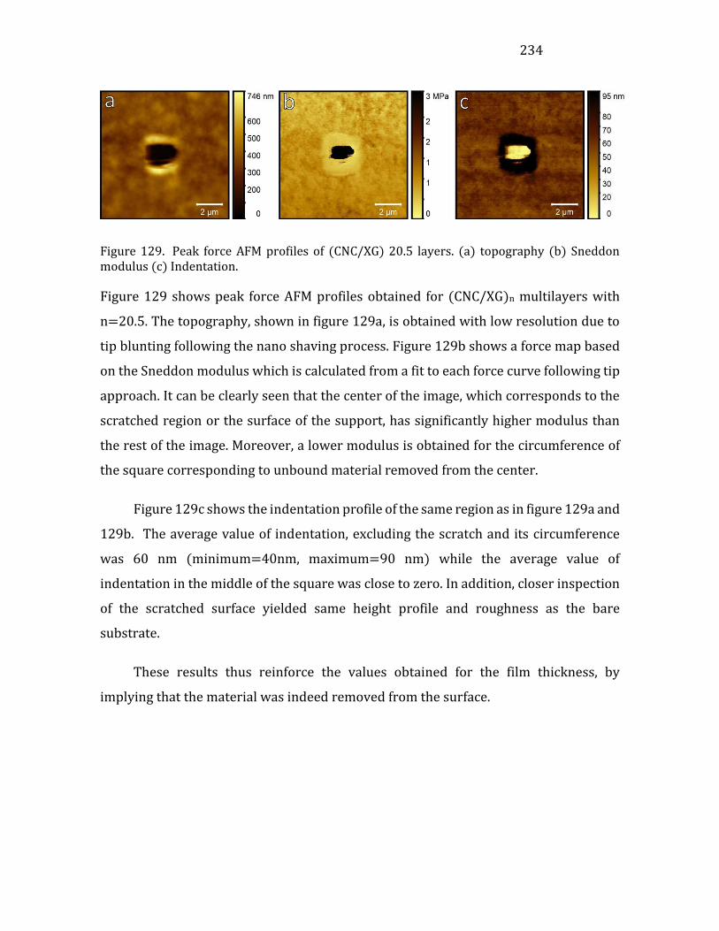
234
Figure 129. Peak force AFM profiles of (CNC/XG) 20.5 layers. (a) topography (b) Sneddon modulus (c) Indentation.
Figure 129 shows peak force AFM profiles obtained for (CNC/XG)n multilayers with
n=20.5. The topography, shown in figure 129a, is obtained with low resolution due to
tip blunting following the nano shaving process. Figure 129b shows a force map based
on the Sneddon modulus which is calculated from a fit to each force curve following tip
approach. It can be clearly seen that the center of the image, which corresponds to the
scratched region or the surface of the support, has significantly higher modulus than
the rest of the image. Moreover, a lower modulus is obtained for the circumference of
the square corresponding to unbound material removed from the center.
Figure 129c shows the indentation profile of the same region as in figure 129a and
129b. The average value of indentation, excluding the scratch and its circumference
was 60 nm (minimum=40nm, maximum=90 nm) while the average value of
indentation in the middle of the square was close to zero. In addition, closer inspection
of the scratched surface yielded same height profile and roughness as the bare
substrate.
These results thus reinforce the values obtained for the film thickness, by
implying that the material was indeed removed from the surface.
235
Abstract
The goal of this work was to develop an in vitro model of the plant primary cell wall. A
bottom up approach was chosen for the rational design of 2D and 3D constructs made
of a lipid membrane, cellulose nano crystals (CNCs) and xyloglucan (XG). First, the
interaction between the building blocks was probed using light scattering, isothermal
titration calorimetry, quartz crystal microbalance and electron microscopy, revealing
firstly the electrostatic nature of the interaction between CNCs and a lipidic membrane
and secondly, specific interaction between CNCs and XG in a precise stoichiometric
ratio. Then, the optimal parameters from the interaction studies were used to obtain
2D and 3D structures by depositing alternating layers of CNCs and XG on flat substrates
(multilayered films) and giant unilamellar vesicles (GUVs). A linear growth of the films
was revealed by atomic force microscopy (AFM) experiments while the response of
decorated vesicles to osmotic shocks lead to their buckling due to the rigidification of
the lipid membrane. Finally, the mechanical properties of the constructs were
characterized using AFM indentation, revealing a Young's modulus of few hundred kPa,
similarly to what is observed for real plant cell walls.
Key words: primary cell wall, lipid membranes, cellulose, interaction, biomimetics
************************************************************************************
L'objectif de ce travail était de développer un modèle in vitro de la paroi primaire des
plantes. Une approche ascendante a été choisie pour la conception rationnelle de
constructions 2D et 3D faites d'une membrane lipidique, de nanocristaux de cellulose
(CNC) et de xyloglucane (XG). Tout d'abord, l'interaction entre les blocs de base a été
examinée à l'aide de la diffusion de la lumière, la calorimétrie de titrage isotherme, la
microbalance à quartz et la microscopie électronique, révélant tout d'abord la nature
électrostatique de l'interaction entre les CNC et une membrane lipidique ainsi qu'une
interaction spécifique entre les CNC et XG dans un rapport stœchiometrique précis. Par
la suite, les paramètres optimisés des études d'interaction ont été utilisés pour obtenir
des structures 2D et 3D en déposant des couches alternées de CNC et XG sur des
substrats plats (films multicouches) et des vésicules unilamellaires géantes (GUV). Une
croissance linéaire des films a été révélée par les expériences de microscopie à force
atomique (AFM), tandis que la réponse des vésicules décorées aux chocs osmotiques
conduit à leur flambage en raison de la rigidification de la membrane lipidique. Enfin,
les proprietes mecaniques des constructions ont ete caracterisees en utilisant l’AFM par
indentation, révélant un module d'Young de quelques centaines de kPa, similaire à celui
observé pour de vraies parois cellulaires végétales.
Mots-clés : paroi primaire, membranes lipidiques, cellulose, interaction, biomimétique

236
General bstract
Our increasing environmental awareness brought to light the importance of materials
made from plants as a renewable ecological source. It is therefore essential to
understand the structure and function of plant cell walls, from both fundamental and
applicative aspects, in order to utilize them for the design of novel eco-friendly
materials. However, since the living cell is a very complex system, a simple model can
help to better understand the behavior of this material. The model systems existing up
to date are lacking the basic elements and architecture of the plant cell wall, thus, it is
necessary to develop a relevant model which will contain all the basic elements,
organized in a manner that resembles the natural structure. Thus, this work was aimed
to create and characterize a simple bioinspired model of the plant cell wall by studying
the interactions between the basic elements composing this structure. Thanks to these
studies, we were able to construct a simple model system which represents the plant
cell wall in terms of structure and properties, paving the way for the design of a new
class of bio-based materials.
********************************************************************
Notre conscience environnementale croissante a mis en évidence l'importance des
matériaux à base de plantes comme source écologique renouvelable. Il est donc
essentiel de comprendre la structure et la fonction de la paroi cellulaire, à la fois ses
aspects fondamentaux mais aussi applicatifs, afin de les utiliser pour la conception de
nouveaux matériaux respectueux de l'environnement. Cependant, comme la cellule
vivante est très complexe, un modèle simple peut aider à mieux comprendre le
comportement de ce matériau. Les systèmes modèles existants ne disposent, pourtant,
pas des éléments de base ni de l'architecture de la paroi cellulaire végétale. Il est donc
nécessaire de développer un modèle pertinent qui contiendra tous les éléments de
base, organisés d'une manière qui ressemble aux structures naturelles. Ainsi, ce travail
visait à créer et caractériser un modèle simple de la paroi, en étudiant les interactions
entre ses éléments constitutifs. Grâce à ces études, nous avons pu construire un système
modèle bio inspiré de la paroi, reproduisant sa structure et ses propriétés, ouvrant la
voie à la conception d'une nouvelle classe de matériaux biosourcés.