Intelligent Scheduling for Yarn - DiVA Portal

IN DEGREE PROJECT INFORMATION AND COMMUNICATION TECHNOLOGY,SECOND CYCLE, 30 CREDITS

, STOCKHOLM SWEDEN 2017

Intelligent Scheduling for YarnUsing Online Machine Learning

ZAHIN AZHER RASHID

KTH ROYAL INSTITUTE OF TECHNOLOGYSCHOOL OF INFORMATION AND COMMUNICATION TECHNOLOGY

Abstract

Many big companies who provide cloud infrastructure, platforms and serviceshave to face a lot of challenges in dealing with big data and execution ofthousands of tasks that run on servers. Thousands of servers running in cloudconsume a large amount of energy which increases operating cost to a great extentfor companies hosting infrastructures and platforms as services. Hundreds ofthousands of applications are submitted every day on these servers by users. Onsubmission of applications, somehow the total resources are not properly utilizedwhich cause the overall operating cost to increase.

A distribution of Apache Hadoop called HOPS is developed at SICS SwedishICT and efforts are made to make it a better platform for institutions andcompanies. Yarn is used as the resource management and scheduling frameworkwhich is responsible for allocating resources such as memory and CPU coresto submitted applications. Yarn simply allocate resources based on the defaultset of values or what user has demanded. Yarn has no prior information aboutthe submitted applications so it is very much possible that allocated resourcesare more or less than required. Energy is being wasted if fewer resources arerequired or application will probably not succeed if required more. In this researchproject, different techniques and methods are looked into for the collection ofuseful metrics related to applications and resources from Yarn, Spark and othersources.

Machine Learning is becoming a very popular technique nowadays for theoptimization of systems dealing with big data in a cloud environment. Thegoal is to collect these vital metrics and build a machine learning model tocommission smart allocation of resources to submitted applications. This canhelp to increase the efficiency of the servers in the cloud and reduce the operatingcost. Finally, a machine learning model was developed and memory and vCoreswere successfully predicted to be allocated to applications.

i

Sammanfattning

Manga stora foretag som tillhandahaller molninfrastruktur, plattformar och tjanstermaste mota manga utmaningar nar det handlar om stora data och utforandeav tusentals uppgifter som kors pa servrar. Tusentals servrar som kor i molnetforbrukar en stor mangd energi vilket i hog grad okar driftskostnaden for foretagsom tillhandahaller infrastrukturer och plattformar som tjanster. Hundratusentalsapplikationer skickas varje dag pa dessa servrar av anvandare. Vid inlamning avansokningar pa nagot satt utnyttjas inte de totala resurserna korrekt, vilket medforatt de totala driftskostnaderna okar.

En distribution av Apache Hadoop, kallad HOPS, ar utvecklad hos SICSSwedish ICT, och det gors anstrangningar for att gora den till en battre plattformfor institutioner och foretag. Garn anvands som resurshanterings- och schemalagg-ningsramen som ar ansvarig for att allokera resurser som minne och CPU-karnor till inlamnade applikationer. Garn fordelar helt enkelt resurser utifranstandardvardet av varden eller vilken anvandare som har kravt. Garn har ingentidigare information om de inlamnade ansokningarna sa det ar mycket mojligtatt tilldelade resurser ar mer eller mindre an vad som kravs. Energi slosas bortom farre resurser kravs eller ansokan kommer sannolikt inte att lyckas om detbehovs mer. I detta forskningsprojekt undersoks olika tekniker och metoder forinsamling av anvandbara matvarden relaterade till applikationer och resurser franGarn, Spark och andra kallor.

Machine Learning blir idag en mycket popular teknik for optimering av systemsom hanterar stora data i en molnmiljo. Malet ar att samla in dessa viktigamatvarden och bygga en maskininlarningsmodell for att bestalla smart fordelningav resurser till inlamnade applikationer. Detta kan hjalpa till att oka effektivitetenhos servrarna i molnet och minska driftskostnaden. Slutligen utvecklades enmaskininlarningsmodell och minnet och vCores hade framgangsrikt forutsagt atttilldelas applikationer.

iii

Acknowledgements

I would like to acknowledge my examiner Jim Dowling, supervisor at SICSGautier Berthou, supervisor at KTH Seif Haridi for providing the informationto get going with my thesis project. I am also thankful to my colleagues at SICSfor helping me out for resolving issues and explaining HOPS project. I trulyappreciate the constant support and feedback they provided me throughout, tillthe completion of this thesis project.

v

Contents

1 Introduction 11.1 Problem description . . . . . . . . . . . . . . . . . . . . . . . . . 31.2 Problem context . . . . . . . . . . . . . . . . . . . . . . . . . . . 31.3 Structure of this thesis . . . . . . . . . . . . . . . . . . . . . . . 3

2 Background 52.1 Hops . . . . . . . . . . . . . . . . . . . . . . . . . . . . . . . . . 52.2 Yarn . . . . . . . . . . . . . . . . . . . . . . . . . . . . . . . . . 52.3 Resource Manager . . . . . . . . . . . . . . . . . . . . . . . . . 62.4 Node Manager . . . . . . . . . . . . . . . . . . . . . . . . . . . 7

2.4.1 Container Manager . . . . . . . . . . . . . . . . . . . . . 82.4.2 Application Master . . . . . . . . . . . . . . . . . . . . . 9

2.5 Related work . . . . . . . . . . . . . . . . . . . . . . . . . . . . 102.5.1 Dr Elephant . . . . . . . . . . . . . . . . . . . . . . . . . 102.5.2 PepperData . . . . . . . . . . . . . . . . . . . . . . . . . 102.5.3 CASK Data Application Platform . . . . . . . . . . . . . 122.5.4 Sztaki (Hungary Project) . . . . . . . . . . . . . . . . . . 122.5.5 Peloton . . . . . . . . . . . . . . . . . . . . . . . . . . . 132.5.6 Ottertune . . . . . . . . . . . . . . . . . . . . . . . . . . 14

3 Method 173.1 Resource Manager . . . . . . . . . . . . . . . . . . . . . . . . . 183.2 Node Manager . . . . . . . . . . . . . . . . . . . . . . . . . . . 193.3 Yarn Timeline Series . . . . . . . . . . . . . . . . . . . . . . . . 213.4 Collection of Metrics . . . . . . . . . . . . . . . . . . . . . . . . 21

3.4.1 Map Java thread IDs to application ids . . . . . . . . . . . 213.4.2 Influxdb . . . . . . . . . . . . . . . . . . . . . . . . . . . 233.4.3 Graphite . . . . . . . . . . . . . . . . . . . . . . . . . . . 24

3.4.3.1 Collect Hadoop Metrics . . . . . . . . . . . . . 253.4.3.2 Collect Spark metrics into InfluxDB . . . . . . 26

3.4.4 Telegraf . . . . . . . . . . . . . . . . . . . . . . . . . . . 27

vii

viii CONTENTS

3.4.5 MySQL Cluster . . . . . . . . . . . . . . . . . . . . . . . 283.5 Tensorflow . . . . . . . . . . . . . . . . . . . . . . . . . . . . . 283.6 Machine Learning Model . . . . . . . . . . . . . . . . . . . . . . 29

3.6.1 Read Metrics from InfluxDB . . . . . . . . . . . . . . . . 293.6.2 Data Preparation and Cleansing . . . . . . . . . . . . . . 313.6.3 Fully Connected Feedforward Neural Network . . . . . . 31

3.6.3.1 Batch Normalization . . . . . . . . . . . . . . . 313.6.3.2 Rectified Linear Unit (ReLU) . . . . . . . . . . 323.6.3.3 Dropout . . . . . . . . . . . . . . . . . . . . . 323.6.3.4 Cross Entropy . . . . . . . . . . . . . . . . . . 333.6.3.5 Optimizer . . . . . . . . . . . . . . . . . . . . 333.6.3.6 Prediction . . . . . . . . . . . . . . . . . . . . 34

4 Analysis and Evaluation 354.1 Performance Evaluation In Terms Of Scaling . . . . . . . . . . . 38

5 Conclusions 415.1 Reflections on Ethics, Sustainability and Economics . . . . . . . . 415.2 Conclusion . . . . . . . . . . . . . . . . . . . . . . . . . . . . . 415.3 Future work . . . . . . . . . . . . . . . . . . . . . . . . . . . . . 42

5.3.1 Use Tfrecords instead of feed dict Input Method . . . . . 425.3.2 Distributed Tensorflow . . . . . . . . . . . . . . . . . . . 435.3.3 Use Kapacitor For Processing Data . . . . . . . . . . . . 435.3.4 Make Yarn Use The Predictions . . . . . . . . . . . . . . 44

Bibliography 45

A Insensible Approximation 49

List of Figures

1.1 Apache Hadoop Ecosystem . . . . . . . . . . . . . . . . . . . . . 2

2.1 Yarn Architecture . . . . . . . . . . . . . . . . . . . . . . . . . . 62.2 Yarn Application Startup . . . . . . . . . . . . . . . . . . . . . . 82.3 Pepperdata Architecture . . . . . . . . . . . . . . . . . . . . . . . 11

3.1 Metrics Collection Architecture . . . . . . . . . . . . . . . . . . 233.2 Machine Learning Model . . . . . . . . . . . . . . . . . . . . . . 29

4.1 Cross Entropy Vs iterations . . . . . . . . . . . . . . . . . . . . . 364.2 Initialized Bias Values comparison . . . . . . . . . . . . . . . . . 374.3 Two labels Prediction . . . . . . . . . . . . . . . . . . . . . . . . 384.4 Available memory vs iterations . . . . . . . . . . . . . . . . . . 39

ix

List of Tables

3.1 Features available from Resource Manager . . . . . . . . . . . . . 193.2 Features available from Node Manager . . . . . . . . . . . . . . . 20

xi

List of Listings

3.1 Get Java Threads IDs . . . . . . . . . . . . . . . . . . . . . . . . 223.2 Thread IDs using jstack . . . . . . . . . . . . . . . . . . . . . . . 223.3 Get Resources consumed using pidstat . . . . . . . . . . . . . . . 223.4 InfluxDB settings for metrics . . . . . . . . . . . . . . . . . . . . 243.5 Yarn metrics settings for Graphite . . . . . . . . . . . . . . . . . 253.6 container metrics period settings . . . . . . . . . . . . . . . . . . 263.7 Spark metrics settings . . . . . . . . . . . . . . . . . . . . . . . . 263.8 Telegraf Metrics Settings . . . . . . . . . . . . . . . . . . . . . . 273.9 Database Query for Metrics . . . . . . . . . . . . . . . . . . . . . 30

xiii

List of Acronyms and Abbreviations

This document requires readers to be familiar with terms and concepts describedin RFC 1235. For clarity, summary of terms and short description of them areaddressed before presenting them in next sections.

AM Application Master

API Application programming interface

CPU Central Processing Unit

DBMS Database Management System

DN Data Node

ETC Et cetera

GPU Graphics Processing Unit

GUI Graphical User Interface

HDFS Hadoop Distributed File System

HOPS Hadoop Open Platform-as-a-Service

HTAP Hybrid Transaction Analytical Processing

JDBC Java Database Connectivity

JMX Java Management Extensions

JSON JavaScript Object Notation

NDB Network Database

NM Node Manager

NN Name Node

xv

xvi LIST OF ACRONYMS AND ABBREVIATIONS

OLAP Online Analytical Processing

OLTP Online Transaction Processing

RDD Resilient Distributed Dataset

ReLU Rectified Linear Unit

RM Resource Manager

S3 Simple Storage Service

URL Uniform Resource Locator

VCORE Virtual Core

Yarn Yet Another Resource Negotiator

Chapter 1

Introduction

Apache Hadoop [1] is an open source and the most popular cloud framework tostore and process a large amount of data and metadata. The Hadoop ecosystem ismainly divided into three main sections as shown in figure 1.1. The first partconsists of data processing, analyzing and serving tools. Second is resourcemanagement framework and third is data and metadata storage system. Thewhole framework is used for distributed storage on computer clusters using aMapReduce [2] programming model and also handles all batch and streamingjobs. A MapReduce job splits data into smaller chunks and process map tasks inparallel in a distributed fashion. Spark [3] and flink [4] modules both can processbatch and streaming data and provide high throughput compared to conventionalMapReduce jobs. This platform can quickly and reliably store, manage andanalyze a large amount of structured and unstructured data with the help of manyservers in the cluster.

Improving existing algorithms or techniques and introducing new modulesto the existing framework can be of great help to the cloud hosting companiesand their customers. YARN [5] has effectively become a scheduler and resourcemanagement tool for many data centers and even small improvements in Yarn canlead to increased cluster utilization, which can mean large energy and monetarysavings for organizations that run on large Hadoop farms. One downside of Yarn[5] is that it does not allocate resources to the applications in a smart way.

Big companies like Facebook use tens of thousands of servers [6]. Consideringthe amount of energy being saved on one server and then comparing it with theamount of energy that can be saved on thousands of servers, so it’s huge. Thisclearly shows that the motivation and demand behind doing such this project thatwill allow organizations to save both energy and money. The ability to predict thebehaviour of applications, users, hosts, and networks would enable it to improveits scheduling decision making and will eventually improve cluster utilization.Improvement in utilization is achieved by predicting the resources using machine

1

2 CHAPTER 1. INTRODUCTION

Figure 1.1: Apache Hadoop Ecosystem

learning to allocate to the submitted applications. Machine learning and deeplearning are promising approaches for improving the scheduling capabilities ofYARN which is supported by related work study mentioned in section 2.5. Therelated work includes projects namely Dr Elephant [7], PepperData [8], CDAP[9], Sztaki, Peleton [10] and Ottertune [11]. The choice for using the machinelearning tool Tensorflow [12] is also inspired by ideas from related work becauseit was used in several of those projects as well.

There are some open source machine learning tools in the Hadoop ecosystemsuch as Mahout, MLlib, SAMOA that can be used by the users or applications [13]but none of those available tools are designed to improve the resource allocationtechniques of the resource management framework. As the number of applicationsubmitted to the cloud cluster is growing, the size of the data is also growing.Various modules such as Graphite [14] and Telegraf [15] are used to collectmetrics and store in a time series database called InfluxDB [16]. This is a greatdeal and creates a demand for such a project that can collect necessary metrics tobuild a machine or deep learning model to enhance the performance of resourcemanagement framework.

1.1. PROBLEM DESCRIPTION 3

1.1 Problem descriptionAs previously mentioned in section 1, Yarn [5] does not allocate resources smartlyand allocates based on what is requested or simply uses the default values. Thisraise issues like under and over-provisioning of resources to the applications. Ifmore resources are provided to the applications than resources are being wastedand on the contrary, if fewer resources are provided than those applications willfail to complete their execution. Also, currently Hadoop ecosystem [17] doesnot have a machine learning tool that improves its resource management andscheduling techniques.

YARN includes extensive metrics, and including both host and networkperformance metrics. The signals for evaluating the success or otherwise ofscheduling decisions can be fed back to a machine learning system to improvea scheduling policy for a given environment. First, it is required to determine themetrics that can help to predict the memory and vCores to allocate to applications.Next step is to find the sources and components from where we can collectthese metrics. After that, the collected data has to be processed and cleansedto make it easier for the machine learning model to learn better. Finally, be able tosuccessfully build the machine learning model and perform a scaling performancetest for the server on which the model is run on.

1.2 Problem contextThere is a much need for a machine learning tool for the resource manager andscheduler framework in Apache Hadoop to allow the cloud hosting companies toworry less about the wastage of resources. Efforts will be made to find answers tothe following Research Questions.

• Determine the important metrics for the machine learning model?

• Can we get resources consumption information for each container?

• Can we predict two labels in the same machine learning session?

• How can Yarn make use of the predictions?

1.3 Structure of this thesisChapter 1 gives an overview of Apache Hadoop and Yarn and addresses themain problem. Description about the Apache Hadoop and Yarn components isexplained in Chapter 2 and details about the related work is included in this

4 CHAPTER 1. INTRODUCTION

section. The next chapter 3 describes, how to get metrics using resource and nodemanager, spark etc. Also, it includes details about the use of graphite and telegrafmodules to provide a means to collect and store metrics into InfluxDB [18]. Theanalysis and evaluation in explained in Chapter 4. The last chapter 5 coversethics, sustainability and economics aspect of the project and then proceeded byconclusions and some suggestions for future work.

Chapter 2

Background

This section covers some basic understanding about the HOPS project that isdeveloped at RISE SICS and information about the working of the resourcemanagement framework Yarn, followed by all the related work that helped to getgoing with the project.

2.1 HopsHOPS [19] is a distribution of open source Apache Hadoop project whichis managed by a Distributed Research Group at RISE SICS. It uses its ownFilesystem called HopsFS which consists of MySQL cluster [20] and networkdatabase (ndb) [20] and do not use HDFS [21]. It has a new distributedarchitecture for managing metadata in MySQL cluster. This distribution relieson Yarn for scheduling jobs and allocation of resources to applications. It doesnot rely on a zookeeper [1] which is a centralized service built on limited serversof maintaining configuration information, allowing writes and reads. HOPS [19]used Yarn as the resource management and scheduling framework and the plan isto make YARN more intelligent so wastage of resources can be avoided.

2.2 YarnYarn [5] is a resource management for Apache Hadoop that helps to scheduleand monitor jobs submitted by clients. It consists of two components namelythe Resource Manager (RM) and Node Manager (NM). This framework is ableto process multiple data engines to handle stored data in the system. Suchengines include interactive SQL, real-time streaming and batch processing. Italso provides the functionality of abstraction between resource management andjob scheduling by splitting the services into separate daemons. A cluster is a

5

6 CHAPTER 2. BACKGROUND

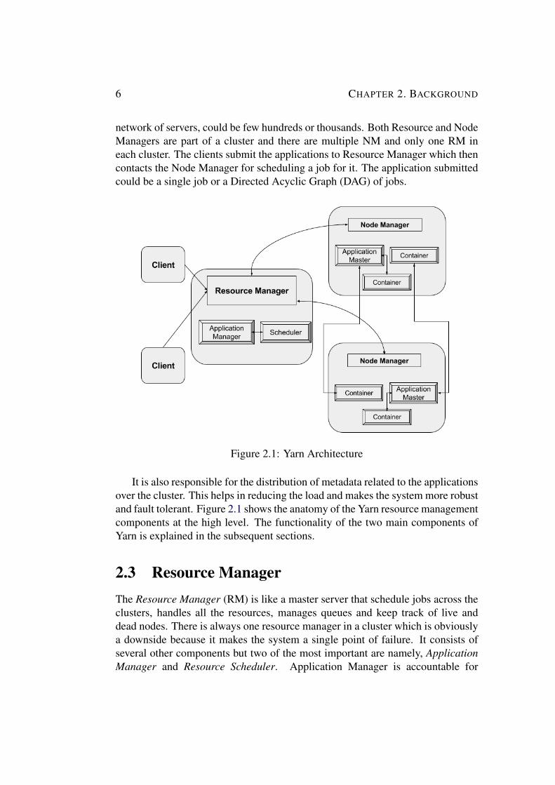
network of servers, could be few hundreds or thousands. Both Resource and NodeManagers are part of a cluster and there are multiple NM and only one RM ineach cluster. The clients submit the applications to Resource Manager which thencontacts the Node Manager for scheduling a job for it. The application submittedcould be a single job or a Directed Acyclic Graph (DAG) of jobs.

Figure 2.1: Yarn Architecture

It is also responsible for the distribution of metadata related to the applicationsover the cluster. This helps in reducing the load and makes the system more robustand fault tolerant. Figure 2.1 shows the anatomy of the Yarn resource managementcomponents at the high level. The functionality of the two main components ofYarn is explained in the subsequent sections.

2.3 Resource ManagerThe Resource Manager (RM) is like a master server that schedule jobs across theclusters, handles all the resources, manages queues and keep track of live anddead nodes. There is always one resource manager in a cluster which is obviouslya downside because it makes the system a single point of failure. It consists ofseveral other components but two of the most important are namely, ApplicationManager and Resource Scheduler. Application Manager is accountable for

2.4. NODE MANAGER 7

submitting jobs to the Node Manager and asks the Application Master for oneor more containers for running an application specific task. It maintains alist of all the submitted applications, the cache of the completed applicationsand the ones that are in queues. The Application Scheduler allocate resourcesto numerous submitted applications depending on how much resources can beprovided at that time. If there are not enough resources in the cluster then thosejobs are added to queues. When an application is submitted to the ResourceManager it requests the scheduler for available resources on nodes. On gettingthis information, it asks the Node Manager, to be more specific Application Master(AM), for available resources to allocate to application tasks. The functionalityof Application Master and containers is discussed in the following section 2.4,which is part of Node Manager. It is quite possible that multiple tasks for the sameapplication are submitted on different Node Managers because it is a distributedsystem. Moreover, the RM can ask NM at any time to kill a running container forany obvious reason.

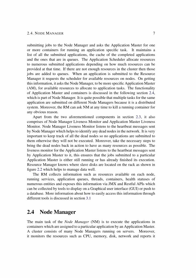
Apart from the two aforementioned components in section 2.3, it alsocomprises of Node Manager Liveness Monitor and Application Master LivenessMonitor. Node Manager Liveness Monitor listens to the heartbeat messages sentby Node Manager which helps to identify any dead nodes in the network. It is veryimportant to keep track of all the dead nodes so no applications are submitted tothem otherwise they will not be executed. Moreover, take the necessary steps tobring the dead nodes back in action to have as many resources as possible. Theliveness monitor for the Application Master listens to the heartbeat messages sentby Application Master to it, this ensures that the jobs submitted to a particularApplication Master is either still running or has already finished its execution.Resource Manager knows where slave disks are located on the rack as shown infigure 2.2 which helps to manage data well.

The RM collects information such as resources available on each node,running services, application queues, threads, containers, health statuses ofnumerous entities and exposes this information via JMX and Restful APIs whichcan be collected by tools to display on a Graphical user interface (GUI) or push toa database. More information about how to easily access this information throughdifferent tools is discussed in section 3.1

2.4 Node ManagerThe main task of the Node Manager (NM) is to execute the applications incontainers which are assigned to a particular application by an Application Master.A cluster consists of many Node Managers running on servers. Moreover,it monitors the resources such as CPU, memory, disk, network and reports it


Figure 2.2: Yarn Application Startup

to Resource Manager as well, hence it has much significance in our work.Furthermore, it sends node status to the RM, shares data information, manageslogs and health statuses. The structure of the NM is designed so that they caneasily be scaled out. When any NM becomes live, it sends information to the RMabout the resources available on the nodes. NM consists of several componentsbut the most important ones are Application Master, Container Manager. Each ofthe components is discussed in a separate heading below.

2.4.1 Container ManagerContainer Manager is the core component of the NM that itself comprisesof different sub-components including a Remote Procedure call (RPC) server,container launcher, container monitor, log handler etc. A container is an isolatedenvironment for running independent tasks. Unlike virtual machines that needtheir own operating system, containers use kernels functionality and separatenamespaces and isolate the resources for tasks and applications. A containerlauncher handles a pool of threads for the execution of containers. It can alsokill a container process if any such command comes from Resource Manageror Application Master. This manager monitors the resources being used by acontainer during its execution. As mentioned previously, each container runs in an

2.4. NODE MANAGER 9

isolated environment which is launched by a container-executor and furthermorefair allocation is ensured among them by the Resource Manager. During theexecution of a container, if it exceeds the limit of allocated resources then thisspecific container might be killed.

2.4.2 Application MasterOn submission of an application to the Resource Manager, it communicates withApplication Master (AM) for the allocation of resources and number of containersto launch jobs. Application Master negotiates the resources with the RM to beallocated to the submitted application in question. It will assign containers andother resources such as memory, CPU, disk etc to application-specific tasks andsends this information to the Resource Manager. On top of this, it also sendsheartbeat messages to the RM which ensures that those tasks are still in processand will complete their execution. One Application Master is responsible for onlyone application. The information held by AM is spread over the cluster in theform of metadata. It sends requests to the Container Manager to start or stopcontainers. It is well aware of the application logic and knowledge about theMapReduce framework.

Here it would be worth mentioning about the anatomy of the MapReduce Jobso this tells exactly how tasks are distributed and assigned in the cluster. AMhandles all the map and reduce tasks. When Map phase is discussed, it refers toall the map tasks that are executed in a cluster and same goes for reduce tasks.Applications are mostly submitted in the form of a jar file. Let’s talk about thisin terms of only one application and see what does an AM do with the input.The AM needs to make a decision on how many map tasks should it start for asubmitted job and this decision depends on some key factors. Along with a jar file,the user also submits a configurable file, input directory where to read input datafrom and the output directory where to store the results to. The configuration filecontains information about the type of type (spark, flink, etc), initial memory,vcores, executed cores to allocate and some other parameters. The input andoutput directories could be a path on HDFS, S3 storage etc. HDFS has two maincomponents namely Data Node (DN) and Name Node (NN) are responsible forhandling data and metadata respectively. The jar file contains information abouthow to implement the map phase, combiner or shuffle phase, how to combinethe results and finally the reduce phase implementation, on how to aggregate theintermediate results to get the final output. The number of map tasks to executefor a job depends on the size and number of files in the input directory. AM willlaunch only one map task for each map split. If there are multiple map splits, letsay 10, then it will launch 10 map tasks for it. Usually, a split happens when theinput file is bigger than the HDFS block size.


2.5 Related workFew research projects were identified which can provide some ideas and help forthis thesis project.

2.5.1 Dr ElephantDr Elephant [7] is a tool that measures and monitors the performance ofApache Hadoop and Spark which is developed by LinkedIn. The major goalof this product is to automatically gather all the necessary metrics to run theperformance analysis on them. The results of the analysis are then presented in anunderstandable way to the users so they can easily evaluate the performance of thecluster and the statuses of all nodes. This helps to ensure that all the components ina cluster are performing optimally. All this information can be viewed on a nicegraphical user interface. It helps to go through the history of all executed jobs,resources used by all processes and jobs and also how well a job performed. Apartfrom this it also provides comparison performance between different jobs usingsome rule-based heuristics. Finally, it uses the results to suggest for improvementin the overall performance of jobs. The core idea is to optimize cluster efficiencyand let the user tune the job easily. It gets data mainly through JMX metrics whichis one of the ways to collect metrics some of them might be interesting for thisproject. The graphical interface gives information and statistics about every Sparkand MapReduce job including the job history server. The job history allows to doa comparison with all the previous execution of the specific job. As it is clear thatthe similar information can also be got from Yarn Metrics and Rest API so we candecide what method to choose on doing some more extensive research.

2.5.2 PepperDataPepperdata [8] is a software product and the company behind the product is namedafter the product itself. The company highlights the shortcomings of the Yarn andits lack of ability to utilize the resources in a proper way. In response to thatthen they have proposed and implemented a solution to increase utilization ofresources in a cluster. Firstly, they stated that Yarn gives us the information aboutthe upper and lower bound of the utilization of resources and does not providethe actual runtime metrics. Secondly, they claim that there is no such platformavailable at that time which can provide detailed information at job and task levelof the computing resources. Moreover, they also mentioned yarn cannot predictby itself that how much resources should be allocated to submitted applicationsand cannot optimize to varying load. Let me discuss now what exactly did theydo to optimize the resource utilization. They added more module to Yarn by

2.5. RELATED WORK 11

monitoring resources such as CPU, memory, disk I/O and network, HDFS and tryto dynamically adjust resources consumption in a cluster. This enables them toexecute jobs with a variable load on the same cluster and allows to increase thejob success rate. That is the reason for them to claim to guarantee the quality ofservice.

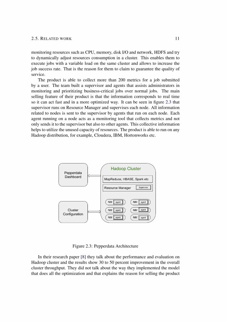
The product is able to collect more than 200 metrics for a job submittedby a user. The team built a supervisor and agents that assists administrators inmonitoring and prioritizing business-critical jobs over normal jobs. The mainselling feature of their product is that the information corresponds to real timeso it can act fast and in a more optimized way. It can be seen in figure 2.3 thatsupervisor runs on Resource Manager and supervises each node. All informationrelated to nodes is sent to the supervisor by agents that run on each node. Eachagent running on a node acts as a monitoring tool that collects metrics and notonly sends it to the supervisor but also to other agents. This collective informationhelps to utilize the unused capacity of resources. The product is able to run on anyHadoop distribution, for example, Cloudera, IBM, Hortonworks etc.

Figure 2.3: Pepperdata Architecture

In their research paper [8] they talk about the performance and evaluation onHadoop cluster and the results show 30 to 50 percent improvement in the overallcluster throughput. They did not talk about the way they implemented the modelthat does all the optimization and that explains the reason for selling the product


for few thousands of dollars. Some part of the code is available on Github and ongoing through the code, it was figured out that some metrics are being collectedthrough Restful API’s. Using Restful API’s for metrics collection is one wayto do this and is obvious from the literature study section 2.3. For this project,either partial metrics can be collected through these API’s available from Resourceand Node Manager or else to find an easier way to collect the metrics which weconsider to be important for our machine learning model.

2.5.3 CASK Data Application PlatformCASK is another cloud platform developed by Cask Data, Inc to providebetter services with unified integrated modules and high level of abstraction ismaintained among them. The product mostly focuses on providing desirableinformation via a graphical user interface. All the services on nodes are monitoredusing a central server. Information regarding the progress of each application andamount of resources used along with core services is available through an API.It supports almost all the Apache Hadoop distributions available in the marketincluding Cloudera, Hortonworks etc. The information is coming from Hadoop,HDFS, HBase, Hive, Spark along with and some other modules and collected andis made accessible on a GUI for the users in a way that can be understood easily.We are interested in what metrics did they collect and how did they collect thembecause we are not interested in the way, information is displayed. MBeanServerinterface is used to collect the operational statistics that are reported as JMXmetrics. In respect to the Cask product, they named the server as CDAP masterprocess.

The first key feature of the product is that it is compatible with other softwarethat runs in the Hadoop ecosystem. The second one is 3rd party monitoring toolscan also be used alongside their own monitoring tool.The use of JMX metricswas also verified through the implementation available in the source code of theproduct. Hadoop provides separate Restful APIs to collect information such asResource and Node Manager API and also via JMX metrics. Hence metrics canbe collected using different methods. On the other hand, Cask tool itself providesone Restful API to allow users to fetch whole statistical information using theirplatform. If an easier way cannot be found to get metrics then we have the optionto collect them using either Restful APIs or via JMX interface.

2.5.4 Sztaki (Hungary Project)It is very interesting to know that a team in Hungary working at HungarianAcademy of Sciences (Computer and Automation Research Institute) who werecontributing to a project that was intended to collect necessary application metrics


to improve cluster utilization. We were also given access to the Github repositorybut unfortunately, while the development of the project was still in the beginningphase, they stopped it’s development and access to the repository was alsorevoked. Therefore, not much information could be extracted from that project.

2.5.5 PelotonPeloton [10] is a self-driving relational database management system for all typesof workloads that uses deep learning to predict future workload trends and renderthe required action to be taken for autonomous optimization without humanassistance. Lets first start with the problem they want to tackle and what do theywant to achieve in the end. Two of the commonly used transactions nowadays areOnline Transaction Processing (OLTP) and Online Analytical Processing (OLAP)[22] and the first one constitute is used most of the time. OLTP mainly deals withtransaction-oriented application such as retrieving or pushing information intothe database using Update, Insert, Delete commands for instance. On the otherhand, OLAP is used in data mining techniques, analyzing and aggregation. Thereis another type of transaction called Hybrid Transaction Analytical Processing(HTAP) which is a combination of both OLTP and OLAP which is seldomused. The main idea is to successfully determine the type of optimization actionsneeded for the respective transaction for different databases. In order to renderthe optimization on the type of actions for modern database deployments, itshould be able to support indexes, materialized views, storage layout, locationpartitioning, configuration tuning and query optimization. For indexes, it shouldbe capable of add, drop, rebuild and convert indexes. For materialized views, itshould be capable of adding and dropping them. Switch from row to column-oriented storage and vice versa should be supported along with compression.Data migration should be achievable, moving it up or down the tier. Replicationand repartition of tables should be possible and self-controllable. Furthermore, itshould set the knobs automatically for best possible configuration settings. Thiswill eventually help to take the necessary steps automatically before a problemoccurs.

Three major components of this database management system are 1) workloadclassification, 2) workload forecasting 3) action planning followed by execution.For query clustering, it uses DBSCAN [23] algorithm. All collected informationis stored as a time series data which means all features correspond to a particulartimestamp. We are interested in the machine learning model they used foroptimization. They used Long Short-Term Memory (LSTM) [24] by combiningmultiple Recurrent Neural Network (RNN) [25]. They integrated Tensorflow [12]with their Peloton system which was basically used for building the machinelearning model. A total of fifty two million queries were trained on two RNNs


for analysis and the workload used was TPC-C. Moreover, through optimizedconfigurations, they were able to achieve 4 million transactions, a high throughputtransaction performance, which is indeed a great procurement. They also statedfew things that cannot be automated such as security and access control. Thingswe can learn from this Research Paper is, know what to learn, know what toautomate and what features would be needed for our machine learning model.Secondly, Tensorflow is a very good choice as a machine learning library for ouranalysis. Thirdly, LSTM Model can also be a good choice because it is based onrewards given back to the system in a loopback fashion.

2.5.6 OttertuneThis related work also contains information about machine learning as Pelotonproject. Ottertune [11] is an automatic database management system that usesmachine learning on database related information to find the optimal configurationfor databases. They performed the experiment on 3 different databases namelyMySQL, Postgres and OLAP DBMS vector. The machine learning was performedon Tensorflow [12] and Python’s scikit-learn [26] and performance was evaluatedon both of them. The purpose of the tool is to produce a configuration forthe workloads on any system and reduce the overhead and latency so millionsof requests could be entertained optimally and data can be stored in the bestpossible way. The core components of the tool are client-side controller andtuning manager. The controller communicates with the DBMS via an APIcalled Java database connectivity (JDBC) to install new configuration and collectmeasurements that determine the performance. The collected measurementsare sent to tuning manager which mostly consists of knobs configurations andperformance data in a repository and then the Machine learning internal modelis used to refine the configurations without user interaction. Furthermore, themodel works in such a fashion that it first selects the knobs that can have themost impact on the performance, then it tries to map prior database workloadsto familiar workloads and finally, it will suggest the best knob settings. We willfocus on the machine learning model of this project to get an idea on how we canbuild a similar model for Yarn.

In the research, they mentioned that all the statistics are collected at runtimeand the tool uses a combination of supervised and unsupervised learning. In thelearning phase, it starts off with dimensionality reduction method called factoranalysis to remove the noise, followed by k-means clustering to group data intomeaningful output. Next, it uses linear regression technique called Lasso forfeature selection. Lastly, it uses Gaussian Process regression to suggest and tunethe configuration for the database. We looked at the source code available onGithub repository as well and found out that they are they train the model by


executing several sessions and each time adding more information to the feedbackloop which helps to tune the output in a better way. Looping the feedback tothe input is a technique for the model to learn in an iterative way and has beenobserved to be used in several machine learning model. Looping the feedbackwill also a good approach for our machine learning model as well.

Chapter 3

Method

Behind every research work, there is a goal to be achieved. Similarly, the purposeof this research is to use a machine learning model to predict memory and CPUconsumption to allow us to efficiently allocate resources to submitted applicationsin the cloud platform. As mentioned in section 2.5, there are few firms or privateresearch groups that did something similar using machine learning for allocationof resources but as this new technique is significant, it can enable companies togenerate money out of it by providing this novel platform to users. RISE SICSalso want to design and implement an intelligent framework for Yarn so that theycan contribute to the Apache Hadoop platform, which will enable numerous bigcompanies to integrate this new machine learning tool to help them save a hugeamount of energy and money. At the moment, machine learning module is notavailable in Hadoop project. This part of the report will focus more on the sourcesfrom where to get metrics and useful data from, followed by how we can collectthose metrics easily, next finding intermediate modules to improve the overall flowof the model, then some research on the machine learning models that can possiblybe used for better prediction and finally finding ways and various techniques totune the machine learning model by changing hyper-parameters. These are theparameters that we set during the start of training and do not change during arunning session.

This section covers the possible sources where we can get the required dataand determine what metrics will be useful for our analysis. In section 2.5,we looked more into what metrics were collected by other groups and throughwhat sources. Every machine learning model is dependant on some key featuresor metrics that assist to make better predictions. Choice of features are veryimportant, poor choice of metrics can lead to bad predictions. We will start bydiscussing the sources and modules in Hadoop to collect the data and if the samedata can be collected from different sources, in that case, we will choose the optionwhere we can get the data easily. If any metrics, we believe would be important for

17

18 CHAPTER 3. METHOD

our analysis and cannot be collected from the available sources, then will developour own code to get those important metrics where necessary.

As we went through the research work, we identified that metrics can becollected from at least five different sources mentioned below.

• Resource Manager

• Node Manager

• Yarn Timeline series

• HDFS

• Spark

• Host machine

We also identified some tools that made simpler for us to collect metrics

• Graphite

• Telegraf

Below, we will discuss the aforementioned sources and tools in details.

3.1 Resource ManagerAs already discussed in section 2.2, Yarn consists of two modules namelyResource Manager (RM) and Node Manager (NM), therefore there are twodifferent sources for the collection of metrics in Yarn. First, we will talk aboutthe metrics collection from Resource Manager in this section and from NodeManager in the subsequent section. Lets first talk about the ways we can fetch datafrom RM. It reports information as JMX metrics which can be collected using anyutility like JMX console, MBean Server and other similar tools. The second wayto collect metrics reported by RM is via HTTPRestful APIs. There are some toolsthat collect this information for us and can be stored in the database which wewill see in the later sections. The API has URLs for clusters nodes, applications,scheduler, nodes and many others. The information we are looking for is availablefrom applications and nodes URLs. It is very simple to get the metrics in a JSONformat using the URLs which look like the following.

• http://<rm http address:port>/ws/v1/cluster/metrics

3.2. NODE MANAGER 19

• http://<rm http address:port>/ws/v1/cluster/apps/appid

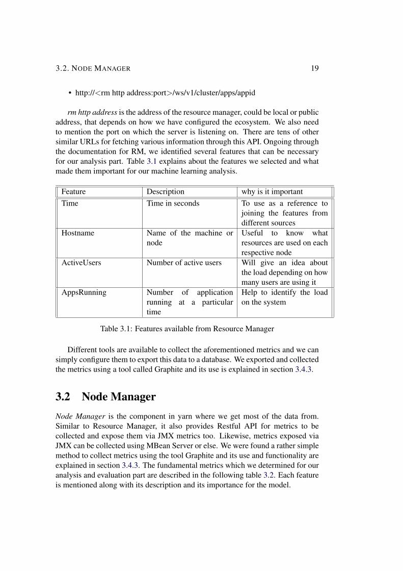
rm http address is the address of the resource manager, could be local or publicaddress, that depends on how we have configured the ecosystem. We also needto mention the port on which the server is listening on. There are tens of othersimilar URLs for fetching various information through this API. Ongoing throughthe documentation for RM, we identified several features that can be necessaryfor our analysis part. Table 3.1 explains about the features we selected and whatmade them important for our machine learning analysis.

Feature Description why is it importantTime Time in seconds To use as a reference to

joining the features fromdifferent sources

Hostname Name of the machine ornode

Useful to know whatresources are used on eachrespective node

ActiveUsers Number of active users Will give an idea aboutthe load depending on howmany users are using it

AppsRunning Number of applicationrunning at a particulartime

Help to identify the loadon the system

Table 3.1: Features available from Resource Manager

Different tools are available to collect the aforementioned metrics and we cansimply configure them to export this data to a database. We exported and collectedthe metrics using a tool called Graphite and its use is explained in section 3.4.3.

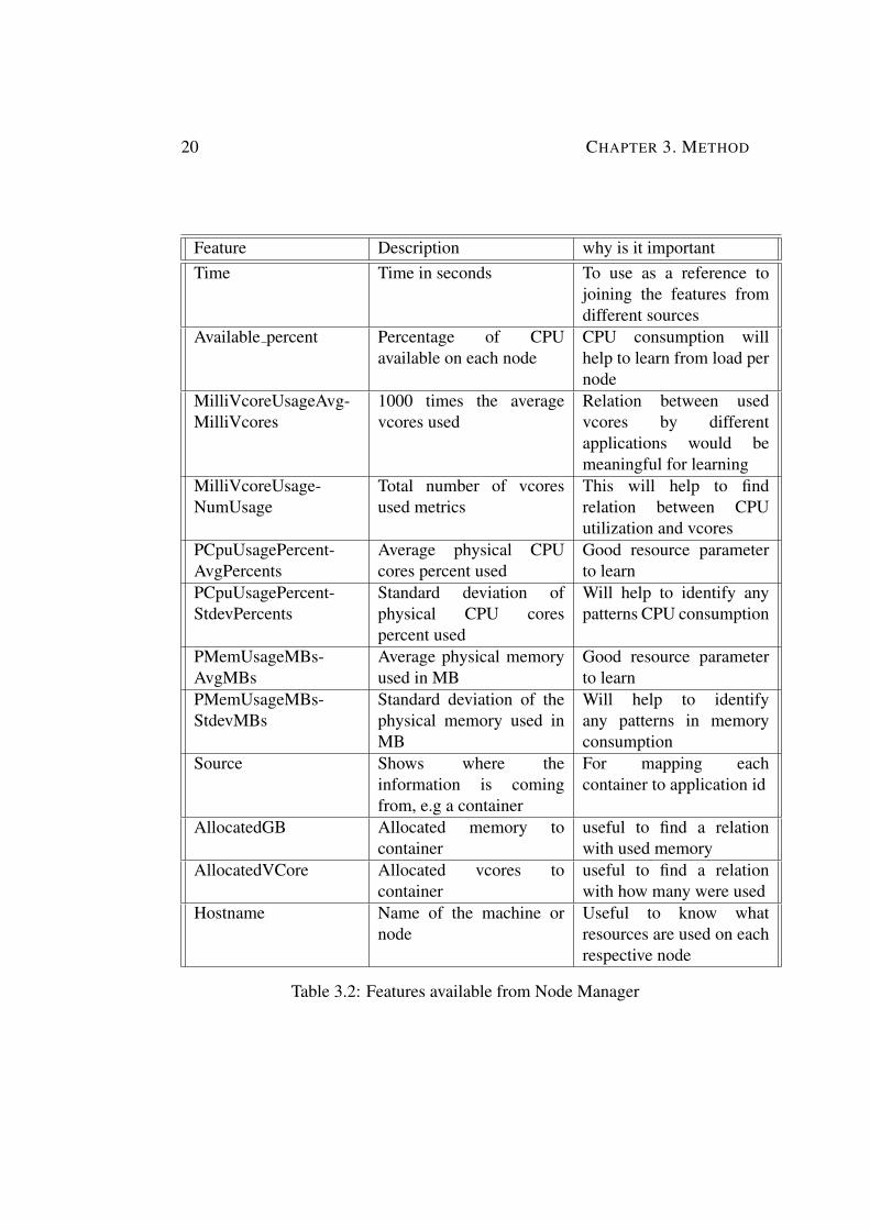
3.2 Node ManagerNode Manager is the component in yarn where we get most of the data from.Similar to Resource Manager, it also provides Restful API for metrics to becollected and expose them via JMX metrics too. Likewise, metrics exposed viaJMX can be collected using MBean Server or else. We were found a rather simplemethod to collect metrics using the tool Graphite and its use and functionality areexplained in section 3.4.3. The fundamental metrics which we determined for ouranalysis and evaluation part are described in the following table 3.2. Each featureis mentioned along with its description and its importance for the model.


Feature Description why is it importantTime Time in seconds To use as a reference to

joining the features fromdifferent sources

Available percent Percentage of CPUavailable on each node

CPU consumption willhelp to learn from load pernode

MilliVcoreUsageAvg-MilliVcores

1000 times the averagevcores used

Relation between usedvcores by differentapplications would bemeaningful for learning

MilliVcoreUsage-NumUsage

Total number of vcoresused metrics

This will help to findrelation between CPUutilization and vcores

PCpuUsagePercent-AvgPercents

Average physical CPUcores percent used

Good resource parameterto learn

PCpuUsagePercent-StdevPercents

Standard deviation ofphysical CPU corespercent used

Will help to identify anypatterns CPU consumption

PMemUsageMBs-AvgMBs

Average physical memoryused in MB

Good resource parameterto learn

PMemUsageMBs-StdevMBs

Standard deviation of thephysical memory used inMB

Will help to identifyany patterns in memoryconsumption

Source Shows where theinformation is comingfrom, e.g a container

For mapping eachcontainer to application id

AllocatedGB Allocated memory tocontainer

useful to find a relationwith used memory

AllocatedVCore Allocated vcores tocontainer

useful to find a relationwith how many were used

Hostname Name of the machine ornode

Useful to know whatresources are used on eachrespective node

Table 3.2: Features available from Node Manager

3.3. YARN TIMELINE SERIES 21

The source features represent the container id that belongs to each applicationin the cluster. The metrics coming from Node Manager do not contain theapplication ID explicitly but rather some part of the container id itself containsthe application id. Hence, application id is extracted from the container ID. Thecontainer id has a specific format which looks like this ContainerResource contain-er e05 1493038364816 0001 01 000001, and the application id that can beinferred from this is application 1493038364816 0001. Node Manager providesus with the per container information and it is collected per second.

3.3 Yarn Timeline SeriesYarn Timeline Series [27] is a server daemon that export metrics via RestfulAPI. It can deployed on Resource Manager or any standalone node. It providesgeneral information about the submitted applications such as queue-name, userinformation, application start and finish time, progress, status, pending tasks in thequeue, container information and more. Progress shows the estimated percentageof execution time before the applications complete their execution. Status defineswhether an application is in running, finished or failed state. It allows the historyof events to be stored in memory or data store. Most of the information is alsoavailable through Resource Manager API as well so there we have the option tochoose any one of these. We did not use Restful API rather the graphite tool toget all the necessary metrics.

3.4 Collection of MetricsIn this section, we will talk about the ways to collect the metrics using availabletools and its storage for further processing.

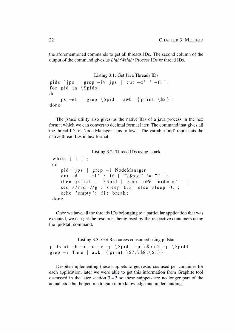
3.4.1 Map Java thread IDs to application idsInitially, during the research phase of the project, we were not sure of whereto get container-specific information so we also looked into java threads for theresources being used by the containers. The idea was to get CPU consumption andmemory used for each container which is launched as java threads and then theycan be mapped to each application ID by tracking child processes. All the threadsbelonging to a Process have the same parent process ID but different threads IDs.A simple command like ”ps -eLf” can give us this information and simply outputsall the processes and afterwards we can search for the required processes. The’jps’ command gives us all the current java processes. We used a combination of


the aforementioned commands to get all threads IDs. The second column of theoutput of the command gives us LightWeight Process IDs or thread IDs.

Listing 3.1: Get Java Threads IDsp i d s = ` j p s | g rep −i v j p s | c u t −d ' ' −f1 ` ;f o r p i d i n \ $ p i d s ;do

ps −eL | g rep \ $p id | awk '{ p r i n t \$2 } ' ;done

The jstack utility also gives us the native IDs of a java process in the hexformat which we can convert to decimal format later. The command that gives allthe thread IDs of Node Manager is as follows. The variable ’nid’ represents thenative thread IDs in hex format.

Listing 3.2: Thread IDs using jstackw h i l e [ 1 ] ;do

p i d = ` j p s | g rep − i NodeManager |c u t −d ' ' −f1 ` ; i f [ ”\ $p id ” != ”” ] ;t h e n j s t a c k − l \ $p id | g rep −oPe ' n i d = . * ? ' |sed s / n i d = / / g ; s l e e p 0 . 3 ; e l s e s l e e p 0 . 1 ;echo ' empty ' ; f i ; b r e a k ;

done

Once we have all the threads IDs belonging to a particular application that wasexecuted, we can get the resources being used by the respective containers usingthe ’pidstat’ command.

Listing 3.3: Get Resources consumed using pidstatp i d s t a t −h −r −u −v −p \ $p id1 −p \ $p id2 −p \ $p id3 |g rep −v Time | awk '{ p r i n t \$7 , \ $8 , \ $13 } '

Despite implementing these snippets to get resources used per container foreach application, later we were able to get this information from Graphite tooldiscussed in the later section 3.4.3 so these snippets are no longer part of theactual code but helped me to gain more knowledge and understanding.

3.4. COLLECTION OF METRICS 23

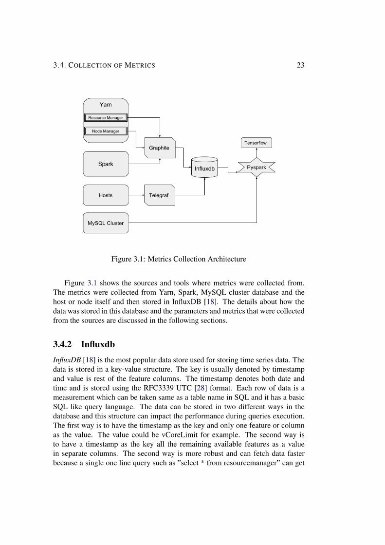
Figure 3.1: Metrics Collection Architecture

Figure 3.1 shows the sources and tools where metrics were collected from.The metrics were collected from Yarn, Spark, MySQL cluster database and thehost or node itself and then stored in InfluxDB [18]. The details about how thedata was stored in this database and the parameters and metrics that were collectedfrom the sources are discussed in the following sections.

3.4.2 InfluxdbInfluxDB [18] is the most popular data store used for storing time series data. Thedata is stored in a key-value structure. The key is usually denoted by timestampand value is rest of the feature columns. The timestamp denotes both date andtime and is stored using the RFC3339 UTC [28] format. Each row of data is ameasurement which can be taken same as a table name in SQL and it has a basicSQL like query language. The data can be stored in two different ways in thedatabase and this structure can impact the performance during queries execution.The first way is to have the timestamp as the key and only one feature or columnas the value. The value could be vCoreLimit for example. The second way isto have a timestamp as the key all the remaining available features as a valuein separate columns. The second way is more robust and can fetch data fasterbecause a single one line query such as ”select * from resourcemanager” can get


all the information and we would not require to aggregate results with respect totimestamp like in the first case, which will probably take longer time.

As already stated that we will use the second method of storing data intothe database, for that we need to add some instructions as a template in the/srv/hops/influxdb/conf/influxdb.conf file. We also changed the separator from a”.” to ” ” and added required templates for proper formatting of the measurementsand get the features in a normalized form. It means that all the features belongingto a particular service will be shown against each timestamp.

Listing 3.4: InfluxDB settings for metricss e p a r a t o r = ” ”Templa t e s = [” s p a r k . * measurement . a p p i d . s e r v i c e . s o u r c e . f i e l d *” ,” r e s o u r c e m a n a g e r . * measurement . s e r v i c e . s o u r c e . d e t a i l s .

c o n t e x t . hos tname . f i e l d *” ,” nodemanager . * measurement . s e r v i c e . s o u r c e . d e t a i l s .

c o n t e x t . hos tname . f i e l d *” ,” measurement *”]

InlfuxDB provides a support of column indexing which is referred to as tags.Search queries on tags speed up the data extraction process. Tags consist of tagkeys and tag values. Only few of the field are indexed in a table. The index allowsto quickly search the data by looking through only those indexes where searcheddata exists and this is achieved by skipping rows where data cannot be found. InResource Manager table, the fields that are indexed are hostname, service, source,context, details and on the contrary, fields that are indexed in the Node Managertable are hostname, service and source. For Resource Manager, we are using theservice tag for filtering the data and they are filtered by all yarn services. ForNode Manager, we are using source tag and is filtered by container services. Thenames of the databases in InfluxDB [18] are Graphite and Telegraf.

3.4.3 GraphiteGraphite [14] is a tool designed to monitor and store time series numerical datain database and helps to build graphs. It does not fetch data by itself but someconfigurations let us to forward the metrics to Graphite and then it can easilycollect it. The metrics exposed by Resource and Node Manager including thespark jobs data are collected by this tool and stored in InfluxDB database [18].The general architecture is that it consists of 3 main components namely Carbon,Whisper, Webbapp. Carbon is a daemon based on Twisted Requests library tolistens all time series data. Whisper is a database library that stores this data and


a web application for rendering graphs. For our part, we do not need to visualizethe data so we will not be using the webapp. As we are using InfluxDB for storingdata hence Whisper database library is also not used. There are some changesin the configuration files which we did to receive metrics through Graphite andpushed the data to InfluxBD.

3.4.3.1 Collect Hadoop Metrics

Hadoop metrics can be exposed to Graphite by making the add the followinginstructions in the file

/srv/hops/hadoop-2.7.3/etc/hadoop/hadoop-metrics2.properties

Listing 3.5: Yarn metrics settings for Graphite

* . s i n k . g r a p h i t e . c l a s s = org . apache . hadoop . m e t r i c s 2 .s i n k . G r a p h i t e S i n k

* . p e r i o d =1

r e s o u r c e m a n a g e r . s i n k . g r a p h i t e . s e r v e r h o s t = 1 0 . 0 . 2 . 1 5r e s o u r c e m a n a g e r . s i n k . g r a p h i t e . s e r v e r p o r t =2003r e s o u r c e m a n a g e r . s i n k . g r a p h i t e . m e t r i c s p r e f i x =rm

nodemanager . s i n k . g r a p h i t e . s e r v e r h o s t = 1 0 . 0 . 2 . 1 5nodemanager . s i n k . g r a p h i t e . s e r v e r p o r t =2003nodemanager . s i n k . g r a p h i t e . m e t r i c s p r e f i x =nm

The instruction starting with *sink enables sinking of the metrics into Graphiteof all the identities. As we want to get metrics for Resource and Node Managertherefore, we specified only these two in the file. All we need to do is to specifythe hostname, port and prefix of the identity or source we want to get metrics of.After adding all the required sources, we also need to restart their service as well.The commands to restart the services for Resource and Node are:

sudo s e r v i c e r e s o u r e m a n a g e r r e s t a r tsudo s e r v i c e nodemanager r e s t a r t

When we change the value of period in the hadoop-metrics2.properties file, wealso need to change two more parameters in /srv/hops/hadoop/etc/hadoop/yarn-site.xml file which are Yarn.nodemanager.container-metrics.period-ms and yarn.n-odemanager.container-monitor.interval-ms. The period parameter will only betaken into account if is less than or equal to monitor parameter. Secondly, theperiod parameter in metrics2.properties file has higher precedence than the othertwo parameters therefore, it has be less than or equal to them. The period inmetrics2.properties file applies to all the services stated in this file. If we want


to change the period settings for individual services then the respective parametershould be changed in the yarn-site.xml file.

Listing 3.6: container metrics period settings<p r o p e r t y ><name>ya rn . nodemanager . c o n t a i n e r−m o n i t o r .

i n t e r v a l −ms</name><va lue >1000</ va lue><d e s c r i p t i o n >How o f t e n t o m o n i t o r c o n t a i n e r s .</ d e s c r i p t i o n ></ p r o p e r t y >

<p r o p e r t y ><name>ya rn . nodemanager . c o n t a i n e r−m e t r i c s .

p e r i o d−ms</name><va lue >1000</ va lue><d e s c r i p t i o n >C o n t a i n e r m e t r i c s f l u s h p e r i o d i n ms .

S e t t o −1 f o r f l u s h on c o m p l e t i o n . < / d e s c r i p t i o n ></ p r o p e r t y >

3.4.3.2 Collect Spark metrics into InfluxDB

In order to collect Spark metrics into InlfuxDB, we need to add the followingsettings in spark configuration file i.e metrics.properties. The file is located onHops at the location

/srv/hops/hadoop/bin/hadoop fs -cat /user/glassfish/metrics.properties

Listing 3.7: Spark metrics settings

* . s i n k . g r a p h i t e . c l a s s = org . apache . s p a r k . m e t r i c s .s i n k . G r a p h i t e S i n k

* . s i n k . g r a p h i t e . h o s t = 1 0 . 0 . 2 . 1 5* . s i n k . g r a p h i t e . p o r t =2003* . s i n k . g r a p h i t e . p e r i o d =1* . s i n k . g r a p h i t e . p r e f i x = s p a r k

The host and port are the IP and port of the server on which graphite serviceis running and period is the time, how often the metrics should be pushed to thedatabase. On changing this file, we also need to restart InfluxDB, which can bedone using the command.

sudo s e r v i c e i n f l u x d b r e s t a r t


On restart, database service will be in operation and metrics will be pushedwhenever any spark application is executed.

3.4.4 TelegrafYarn metrics only contain information about the resources used by containersand applications but for our machine learning, we would also need resourcesused per node. For that, we came across a tool Telegraf which is a part of abigger project known as TICK [16] that consists Telegraf [15], InlfuxDB [18],Chronograf [29] and Kapacitor [30] components. We can choose to use all or justa few of the components. Telegraf consists of several plugins that collectively iscalled an agent which is responsible for collecting metrics from operating system,databases, network, message queues, events and applications. It has integrationwith 3rd party plugins and APIs as well. For Example, it can pull data fromStatsD and Kafka consumer services. It also provides the functionality to senddata to various components such as Graphite, InfluxDB, DataDog (monitoringservice), OpenTSDB (scalable distributed monitoring system), collectd (systemstatistics collection daemon) and few more. The good part is that it can bebuilt using a standalone library and does not have any dependencies on otherpackages. Telegraf tool is easy to handle with easy configuration settingsfor metrics collection and therefore, also used in our project. To collect themetrics every second we have to change the value of interval parameter in the/srv/hops/telegraf/conf/telegraf.conf file.

Listing 3.8: Telegraf Metrics Settings[ a g e n t ]

I n t e r v a l = ”1 s ”

When the changes has been made, we also we need to restart it service forchanges to take into effect which can be done by the following command.

sudo s e r v i c e t e l e g r a f r e s t a r t

All the components are to some extent interesting for us except Chronografbecause it provides a dashboard and interface for visualizing information and wedo not need that for our project. The collected metrics can be exported to InfluxDBand also to Kapacitor. Kapacitor is a real-time batch and stream data processingengine. There can be two ways process these metrics. First is to export them toKapacitor and then load onto Machine Learning module or second way is to pushthe data into InfluxDB and then fetch it for processing and machine learning. Inthe first case, as nothing will be pushed to database this can save a lot of disk spaceby loading all the incoming data into memory and for further processing. Thiscan be challenging when we have a huge amount of metrics loaded in memory


for processing and how to handle more incoming data. Furthermore, Kapacitorcomponent is mostly used for alerting and notification. We also tried to use itif possible for feeding the incoming data to our machine learning module butthat did not work out mainly because it does not have any integration with othermodules except the ones mentioned above. Moreover, as we cannot export datafrom Graphite to Kapacitor which also makes it less likely to use component foronly data coming from Telegraf. Hence, we implemented the second techniqueand pushed metrics into InfluxDB first.

3.4.5 MySQL Cluster

When an application is submitted multiple times to Resource Manager, sameapplication ID is assigned to it. Hence, our machine learning model would beunable to distinguish between them. HOPS platform is able to distinguish theseapplications by assigning a unique job id no matter that particular applicationhas been submitted before or not. Job id is stored in the hopsworks database inMySQL Cluster [31] and the table that contains this information is jobs history.Apart from job id we also collected the maximum vCores and memory allocatedto the Application Master. In order to get this information from the database, weneed to know the username, password, port and hostname of the MySQL Cluster.While implementing the code, this information was read from a text file but canbe changed according to user’s need.

3.5 Tensorflow

Tensorflow [12] has become a quick a popular open source tool for machinelearning over the past years and it uses data flow graphs to process numericalcomputation. It can be used both with CPUs and GPUs. The input data isfirst converted into tensors which are basically multidimensional data arrays andrepresented by graph edges. While mathematical operations are represented bynodes in the graph. The library can be used on desktops and mobile devices.Other available tools for machine intelligence are Theono [32], Karas [33], Caffeon spark [33] and Torch [34]. As from the study of related work, we saw thatPeloton and Ottertune also used Tensorflow for optimization therefore, we thinkthat it will be a good choice for our project. This library uses random seeds tocreate some randomness in the algorithm. Random seed parameter can be set toa particular value according to the requirement so every time we run the session,we get the same results.

3.6. MACHINE LEARNING MODEL 29

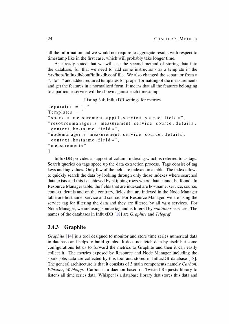
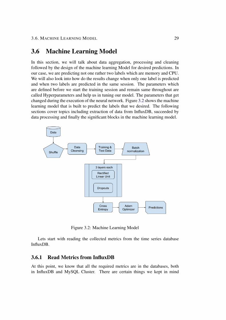
3.6 Machine Learning ModelIn this section, we will talk about data aggregation, processing and cleaningfollowed by the design of the machine learning Model for desired predictions. Inour case, we are predicting not one rather two labels which are memory and CPU.We will also look into how do the results change when only one label is predictedand when two labels are predicted in the same session. The parameters whichare defined before we start the training session and remain same throughout arecalled Hyperparameters and help us in tuning our model. The parameters that getchanged during the execution of the neural network. Figure 3.2 shows the machinelearning model that is built to predict the labels that we desired. The followingsections cover topics including extraction of data from InfluxDB, succeeded bydata processing and finally the significant blocks in the machine learning model.

Figure 3.2: Machine Learning Model

Lets start with reading the collected metrics from the time series databaseInfluxDB.

3.6.1 Read Metrics from InfluxDBAt this point, we know that all the required metrics are in the databases, bothin InfluxDB and MySQL Cluster. There are certain things we kept in mind


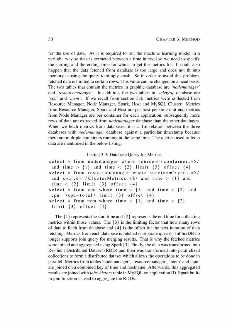
for the use of data. As it is required to run the machine learning model in aperiodic way so data is extracted between a time interval so we need to specifythe starting and the ending time for which to get the metrics for. It could alsohappen that the data fetched from database is too large and does not fit intomemory causing the query to simply crash. So in order to avoid this problem,fetched data is limited to certain rows. This value can be changed on a need basis.The two tables that contain the metrics in graphite database are ’nodemanager’and ’resourcemanager’. In addition, the two tables in telegraf database are’cpu’ and ’mem’. If we recall from section 3.4, metrics were collected fromResource Manager, Node Manager, Spark, Host and MySQL Cluster. Metricsfrom Resource Manager, Spark and Host are per host per time unit and metricsfrom Node Manager are per container for each application, subsequently morerows of data are extracted from nodemanager database than the other databases.When we fetch metrics from databases, it is a 1:n relation between the threedatabases with nodemanager database against a particular timestamp becausethere are multiple containers running at the same time. The queries used to fetchdata are mentioned in the below listing.

Listing 3.9: Database Query for Metricss e l e c t * from nodemanager where s o u r c e = ˜ / c o n t a i n e r . * $ /and t ime > {1} and t ime < {2} l i m i t {3} o f f s e t {4}

s e l e c t * from r e s o u r c e m a n a g e r where s e r v i c e = ˜ / ya rn . * $ /and s o u r c e = ˜ / C l u s t e r M e t r i c s . * $ / and t ime > {1} andt ime < {2} l i m i t {3} o f f s e t {4}

s e l e c t * from cpu where t ime > {1} and t ime < {2} andcpu = ˜ / cpu− t o t a l / l i m i t {3} o f f s e t {4}

s e l e c t * from mem where t ime > {1} and t ime < {2}l i m i t {3} o f f s e t {4}

The {1} represents the start time and {2} represents the end time for collectingmetrics within those values. The {3} is the limiting factor that how many rowsof data to fetch from database and {4} is the offset for the next iteration of datafetching. Metrics from each database is fetched is separate queries. InlfluxDB nolonger supports join query for merging results. That is why the fetched metricswere joined and aggregated using Spark [3]. Firstly, the data was transformed intoResilient Distributed Dataset (RDD) and then was transformed into parallelizedcollections to form a distributed dataset which allows the operations to be done inparallel. Metrics from tables ’nodemanager’, ’resourcemanager’, ’mem’ and ’cpu’are joined on a combined key of time and hostname. Afterwards, this aggregatedresults are joined with jobs history table in MySQL on application ID. Spark built-in join function is used to aggregate the RDDs.


3.6.2 Data Preparation and CleansingIn Machine learning, 80% of the time is spent on cleaning the data because datais in raw form and will contain null, missing, inconsistent and irregular values oroutliers, which can be considered as a bad input. For instance, if we use this datafor machine learning without cleansing then probably it will give poor predictionsand results. This process ensures good quality of data and is a prerequisite forevery Model. Some of the feature columns contained None as values so werereplaced with an integer with value -1. The features containing the containerand application id also contained strings ’ContainerResource container e’ and’application ’ respectively and were removed. The hostnames and users featurecolumns also contained strings and therefore one hot encoding was applied to mapthem to integer values. This part is necessary because Tensorflow library cannotprocess features containing strings.

As the metrics were recorded per second so there is very high chance that thefeatures in the subsequent rows have similar values which is probably not goodfor machine learning. Hence, the data is shuffled first to create some randomnessin order which will allow us to get better predictions for memory and CPUutilization.

3.6.3 Fully Connected Feedforward Neural NetworkFeedforward Neural Networks [35] are the ones where the neurons informationflows through the intermediate hidden layers and reaches the output. Noinformation is fed back to the system, but if fed back then it is called a RecurrentNeural Network [36]. We can have multiple hidden layers in our network.

3.6.3.1 Batch Normalization

Once the data is prepared, it is fed to Tensorflow [12] and it starts by doing somebatch normalization [37]. This step is very important for our model because thefeatures values have some closeness among themselves normalization will help tospace correlate with mean values and makes them more distinguishable. It helpsto increase the learning rate and improves the accuracy of the model. The generalformula to calculation normalization is:

γ(x−u)σ

+β (3.1)

The batch normalization function takes the following parameters.

b a t c h n o r m a l i z a t i o n (x ,


mean ,v a r i a n c e ,o f f s e t ,s c a l e ,v a r i a n c e e p s i l o n ,

)

The parameter x is the input tensor to the function that contains all the featureswhich to apply normalization on. The parameters mean (u) and variance σ are thevalues for mean and variance for the features. The parameter scale γ is the scalingfactor for all feature columns and β is the offset.Furthermore, variance epsilon isa small float value to ensure no division by 0. Normalization definitely helps tospeed up the learning process when the training was done with more iterations.

3.6.3.2 Rectified Linear Unit (ReLU)

A neural network normally consists of some hidden layers where weights ’W’are multiplied with neurons, followed by addition of biases (b) to the resultantproduct. This method is called affine transformation, z = W*x + b. The weightare usually initialized with small values and biases are also kept small. Theweights keep on adjusting as it moves flows through the network. After theaffine transformation, an activation function is typically used on top of it andthe popular ones are ReLU, Sigmoid and tanh. Sigmoid is a type of logisticfunction and is usually used in recurrent networks where the model has moresensitive requirements because it also take negative values into account. The tanhfunction will normally give better results compared to Sigmoid and also learnsfrom negative values. One major problem with it is that it saturates the valuesclose to 1 or 0 and that causes the gradient to vanish. ReLU is a suitable activationfunction for Feedforward Neural Network. The negative values are mapped tozero and weights are adjusted using the positive values. We used ReLU for ourmodel as it fulfils our needs better. We started with one layer of ReLU andincreased to 5 layers to improve the prediction results.

3.6.3.3 Dropout

This is a technique to avoid the problem of overfitting the data too much. Thefunction randomly drops some of the features and the remaining ones are used forlearning. We have to define the keeping probability for the columns, for example,if keep probability is 0.8, then eighty percent of the features will be kept forlearning and the rest twenty percent will be dropped out. The variable ’x’ in thebelow function is the input tensor. The noise shape is a 1D tensor and randomlygenerates flags for keeping and dropping. Dropout is used after every ReLU layer


and assigning a different keeping probability each time. The parameter seed whenset, creates randomness in features drop. In our case, operation seed was notused but rather a global graph level seed played its role. Just for information, ifneither operation nor global seed is set then a random seed is used for this dropoutfunction.

d r o p o u t (x ,keep prob ,n o i s e s h a p e =None ,s eed =None ,

)

3.6.3.4 Cross Entropy

The standard for evaluating a model is done by calculating the loss function whichis termed as cross entropy. It compares the predicted labels with the true labelsand evaluates it. The loss is usually calculated as the absolute or squared loss.

3.6.3.4.1 Choice for L1 or L2 Regularization

Regularization is a technique to adjust the values that are measured on a differentscale to a more common scale. Normally there are two types of techniques usedto normalize the loss function namely L1 [38] and L2 regularization [39]. Eachtechnique has its own perks. L1 calculates the least absolute regression loss andL2 calculates least mean square loss. Despite L1 being more robust but the outputis not very stable and L2 is more commonly used in practical life. L1 is used inthe cases where we have sparse feature spaces. Here, it is also good to explainthe difference between the sparse and dense representation of data. Data that alsoshows zero values such as [0,0,6,7,0] is referred to as dense representation. Sparserepresentation of the same data will look like this, [(2,3),(3,5)] which representsthat values 6 and 7 are stored at index 2 and 3 respectively. In my case, I havea dense representation of data so I used L2 regularization. L2 is mostly usedbecause it normalizes better than the other and it was also used for this project aswell.

3.6.3.5 Optimizer

Optimization is a fundamental part of machine learning. The Optimizer isa function that is used to improve the learning in each iteration. Learningrates should be kept same for all the parameters. Gradient Descent [40] andAdam Optimizer [41] are good techniques for optimizing learning model. These


functions help to find the coefficients and parameters of a function that reducesthe overall loss. We just have to set a learning rate which often has a low valueto avoid overfitting of data and automatically determines the step size based onthe rate. There is an option to use exponential decaying rate as well. Global step,decay steps and decay rate have to provided to determine the decaying rate. If thestep size is small, it will longer time to converge and if the step size is too largethen it can even diverge and optimal step size has to be determined. It makes moresense to use a decreasing learning rate when dealing with a larger dataset, so themodel does not overfit too much.

3.6.3.5.1 Gradient Descent Vs Adam Optimizer

Both optimizers are first order Gradient Descent algorithms to determine theminimum of the loss function and then update the parameters for the machinelearning in an iterative way which allows to decreasing the error rate. They areused to stop large errors to propagate through the iterations. Gradient Descent runsthrough all the parameters in the training data and does a single improvement in aniteration for specific parameters. On the other hand, Adam Optimizer determinesthe local minimum by calculating moving averages of the parameters. It doesmore computation for each parameter to calculate the scaled gradient to deal withmoving averages and variance, making the model bigger in size. For larger data,Adam Optimizer takes more time compared to gradient descent. The output wastested with both optimizers and resulted in a similar loss. For the analysis, AdamOptimizer is used. For real-world data, it is better to use Adam Optimizer as it hasproven to provide better results on other machine learning projects.

3.6.3.6 Prediction

Input can be loaded into Tensorflow session using two methods. The first one isby using feed dict and the second one is by using tfrecords. We used feed dict asto feed data into Tensorflow but later it was figured out that it has latency issuesso the use of tfrecords has been suggested as a future work. Tensorflow acceptsthe data and labels as inputs. The collected data also contained the labels as wellwhich is the average memory and CPU used per container between one secondtime interval. These features were extracted and separated from the original dataand were used as labels. Both data and labels were fed to the neural networkmodel to predict memory and CPU utilization.

Chapter 4

Analysis and Evaluation

In this chapter, we will talk about the analysis and performance of machinelearning model and some approaches that can be used to optimize and avoid over-fitting of the data. Usually, simple models are not good at the generalizationof data and on the other hand complex models do not perform well on testdata and may lead to over-fitting. Regularization helps us to resolve this issueby reducing the generalization error by making some changes in the learningalgorithm. There are various approaches and strategies are used to regularize theoutput loss. The first one is early stopping. The second method is to use either L1or L2 regularization which is used to normalize the loss as discussed in section3.6.3.4.1. Another good technique to regularize the output is dropout which hasbeen used and discussed in section 3.6.3.3 and finally data augmentation can beused to introduce regularity if needed. Augmentation is a technique to generatemore data from existing data. In the end, analysis of performance scaling testswill be conducted.

The model was tested and evaluated on data generated from sample applicationsby changing the vCores and memory to be allocated to containers or to applications.Seventy different combinations of input parameters were used for generating moremetrics with a sample spark application. In the start of the project, there was apossibility of data acquisition from Spotify company or from any other sourcebut unfortunately, no real-world applications could be acquired from any source.This was also one of the main limitations of the project, not getting real-worldapplications to test the machine learning model on. This made a bit hard totune the model because sample data did not have much variance and diversityin its features. One of the requirements for good machine learning models is thatmetrics values in other rows much not be close enough to each otherwise modeldoes not learn any useful thing from it and instead, it will lead to poor predictions.

The data fetched from Influxdb contained a total of 8904 rows. This datawas divided into training and testing set and both with equal proportion, 4452

35

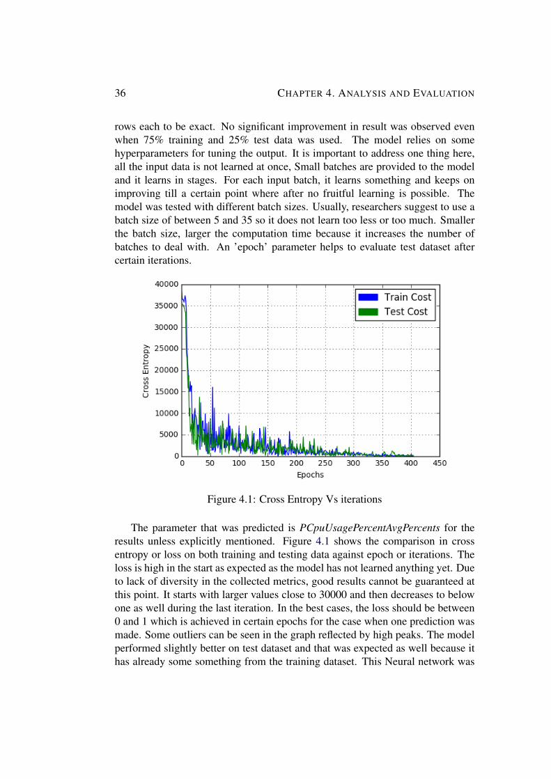
36 CHAPTER 4. ANALYSIS AND EVALUATION

rows each to be exact. No significant improvement in result was observed evenwhen 75% training and 25% test data was used. The model relies on somehyperparameters for tuning the output. It is important to address one thing here,all the input data is not learned at once, Small batches are provided to the modeland it learns in stages. For each input batch, it learns something and keeps onimproving till a certain point where after no fruitful learning is possible. Themodel was tested with different batch sizes. Usually, researchers suggest to use abatch size of between 5 and 35 so it does not learn too less or too much. Smallerthe batch size, larger the computation time because it increases the number ofbatches to deal with. An ’epoch’ parameter helps to evaluate test dataset aftercertain iterations.

Figure 4.1: Cross Entropy Vs iterations

The parameter that was predicted is PCpuUsagePercentAvgPercents for theresults unless explicitly mentioned. Figure 4.1 shows the comparison in crossentropy or loss on both training and testing data against epoch or iterations. Theloss is high in the start as expected as the model has not learned anything yet. Dueto lack of diversity in the collected metrics, good results cannot be guaranteed atthis point. It starts with larger values close to 30000 and then decreases to belowone as well during the last iteration. In the best cases, the loss should be between0 and 1 which is achieved in certain epochs for the case when one prediction wasmade. Some outliers can be seen in the graph reflected by high peaks. The modelperformed slightly better on test dataset and that was expected as well because ithas already some something from the training dataset. This Neural network was

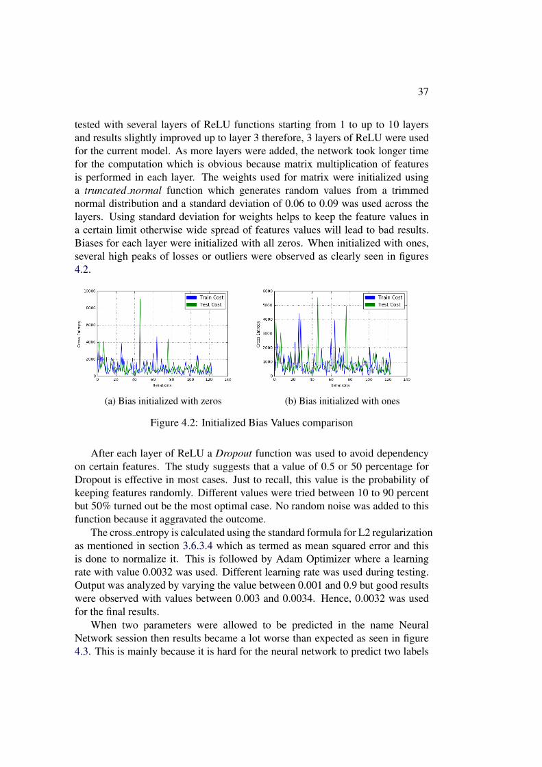
37

tested with several layers of ReLU functions starting from 1 to up to 10 layersand results slightly improved up to layer 3 therefore, 3 layers of ReLU were usedfor the current model. As more layers were added, the network took longer timefor the computation which is obvious because matrix multiplication of featuresis performed in each layer. The weights used for matrix were initialized usinga truncated normal function which generates random values from a trimmednormal distribution and a standard deviation of 0.06 to 0.09 was used across thelayers. Using standard deviation for weights helps to keep the feature values ina certain limit otherwise wide spread of features values will lead to bad results.Biases for each layer were initialized with all zeros. When initialized with ones,several high peaks of losses or outliers were observed as clearly seen in figures4.2.

(a) Bias initialized with zeros (b) Bias initialized with ones

Figure 4.2: Initialized Bias Values comparison

After each layer of ReLU a Dropout function was used to avoid dependencyon certain features. The study suggests that a value of 0.5 or 50 percentage forDropout is effective in most cases. Just to recall, this value is the probability ofkeeping features randomly. Different values were tried between 10 to 90 percentbut 50% turned out be the most optimal case. No random noise was added to thisfunction because it aggravated the outcome.

The cross entropy is calculated using the standard formula for L2 regularizationas mentioned in section 3.6.3.4 which as termed as mean squared error and thisis done to normalize it. This is followed by Adam Optimizer where a learningrate with value 0.0032 was used. Different learning rate was used during testing.Output was analyzed by varying the value between 0.001 and 0.9 but good resultswere observed with values between 0.003 and 0.0034. Hence, 0.0032 was usedfor the final results.

When two parameters were allowed to be predicted in the name NeuralNetwork session then results became a lot worse than expected as seen in figure4.3. This is mainly because it is hard for the neural network to predict two labels

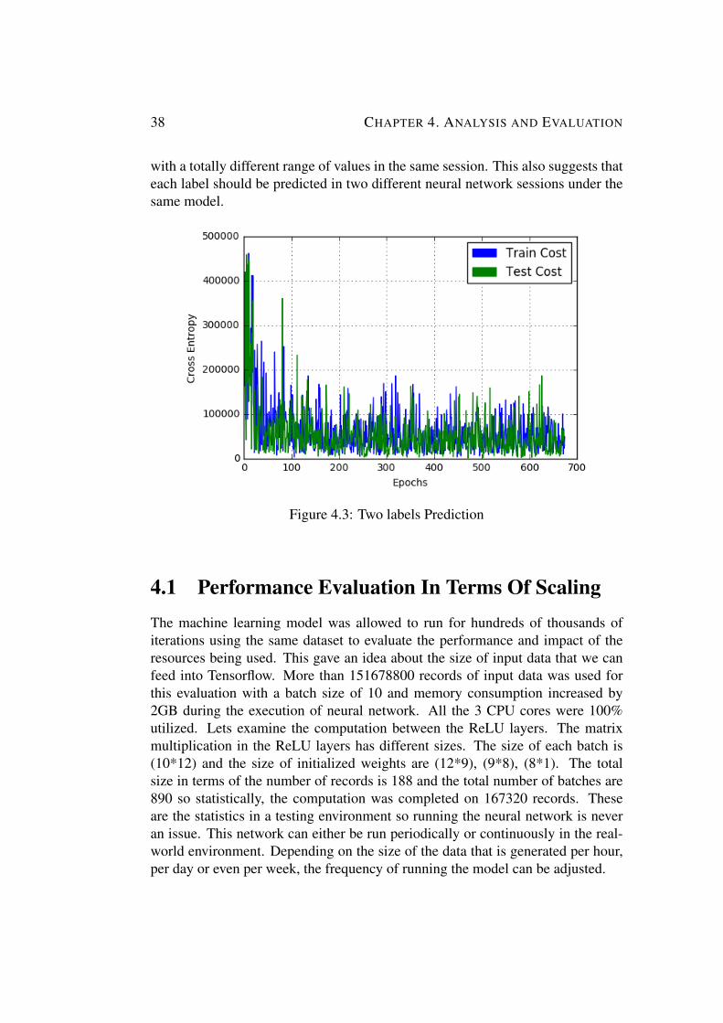
38 CHAPTER 4. ANALYSIS AND EVALUATION

with a totally different range of values in the same session. This also suggests thateach label should be predicted in two different neural network sessions under thesame model.

Figure 4.3: Two labels Prediction

4.1 Performance Evaluation In Terms Of ScalingThe machine learning model was allowed to run for hundreds of thousands ofiterations using the same dataset to evaluate the performance and impact of theresources being used. This gave an idea about the size of input data that we canfeed into Tensorflow. More than 151678800 records of input data was used forthis evaluation with a batch size of 10 and memory consumption increased by2GB during the execution of neural network. All the 3 CPU cores were 100%utilized. Lets examine the computation between the ReLU layers. The matrixmultiplication in the ReLU layers has different sizes. The size of each batch is(10*12) and the size of initialized weights are (12*9), (9*8), (8*1). The totalsize in terms of the number of records is 188 and the total number of batches are890 so statistically, the computation was completed on 167320 records. Theseare the statistics in a testing environment so running the neural network is neveran issue. This network can either be run periodically or continuously in the real-world environment. Depending on the size of the data that is generated per hour,per day or even per week, the frequency of running the model can be adjusted.

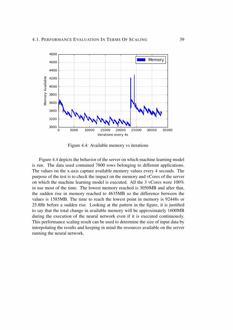
4.1. PERFORMANCE EVALUATION IN TERMS OF SCALING 39

Figure 4.4: Available memory vs iterations

Figure 4.4 depicts the behavior of the server on which machine learning modelis run. The data used contained 7800 rows belonging to different applications.The values on the x-axis capture available memory values every 4 seconds. Thepurpose of the test is to check the impact on the memory and vCores of the serveron which the machine learning model is executed. All the 3 vCores were 100%in use most of the time. The lowest memory reached is 3050MB and after that,the sudden rise in memory reached to 4635MB so the difference between thevalues is 1585MB. The time to reach the lowest point in memory is 92448s or25.8Hr before a sudden rise. Looking at the pattern in the figure, it is justifiedto say that the total change in available memory will be approximately 1600MBduring the execution of the neural network even if it is executed continuously.This performance scaling result can be used to determine the size of input data byinterpolating the results and keeping in mind the resources available on the serverrunning the neural network.

Chapter 5

Conclusions

This section includes ethics and sustainability concern of the project, followed bydiscussion and conclusion and in the end some suggestion for future work to makethis project better.

5.1 Reflections on Ethics, Sustainability and EconomicsThe implementation and contribution is made to an open source Apache HadoopDistribution HOPS so there is no issue of security of privacy. The whole code isopen to public and anyone is allowed to do useful contribution to HOPS by addingmore functionality to their fork and rendering a pull request on Github. Manyresearchers are contributing to several distributions of Apache Hadoop and areinvolved in extensive research. Big data is not only a problem of few companiesbut every company from medium-sized to large-scale are directly or indirectly partof it. The clients using the cloud platforms would prefer to wait less when theysubmitted applications.

This project keeps in mind the sustainable aspect of it and aims to save energyin the environment. Moreover, it can be scaled easily without any high costbecause neural network is only required to run on one server and can be easilyvertically scaled by adding more resources to that server. The provided solutionwill not only save energy and resources but also execute more applications duringany specific time period.

5.2 ConclusionWe started with an idea to make resource management and scheduling frameworkmore intelligent in order to avoid the waste of resources and one of the biggestchallenges was to get the metrics at the container level. We have been successful

41

42 CHAPTER 5. CONCLUSIONS

in getting this information and all the other important metrics that were identifiedin section 3. Moreover, more than 200 metrics were collected from resourcemanager, node manager, spark and MySQL Cluster but we reduced the number offeatures to 19 to be able to do better predictions. This is also very importantotherwise, more features will make it hard for the neural network model tolearn. InfluxDB deprecated the use of join query from different tables so the dataaggregation and further processing were done as spark jobs using their mappingfunction which is quite fast for computation. In addition to this, we were also ableto find the common parameter to keep track of any application that is submittedmultiple times. That was done by mapping the application ID to the job ID as thisis unique for all submitted applications.

Besides this, tools like Graphite and Telegraf made a lot easier to collect themetrics from the desired sources and store into the time series InfluxDB insteadusing implementing Restful APIs or using JMX metrics collection tool. On topof that, this was achieved by making changes in the respective configuration files.Tensorflow turned out to be a good choice for building the neural network as itprovides numerous functions for optimizing results. Use of batch normalization,Dropout and Adam Optimizer slightly improved the results on data generatedfrom sample applications. Definitely, when it will be used on data generatedfrom real-world applications then significant improvement could be observable.Lastly, our major goal was to predict memory and CPU utilization at containerand application level and we have been successful in doing that by building afully connected feed-forward network. Using this neural network for real-worldapplications might need a slight tuning of the hyperparameters but that should notbe trivial. Eventually, it will save resources and energy of the running servers thatare part of a cluster.

5.3 Future workIn most thesis project, there is always a possibility of extension of work and addmore modules to make it an even better project. On doing some research, thefollowing information is suggested as future work.

5.3.1 Use Tfrecords instead of feed dict Input MethodFeed dict input method has to copy an abundant of values in the feed holder asit has to convert the numpy arrays to tensor’s proto byte and copy to anothermemory location. Feeding data with python variables is not a good approachwhen we think in terms of scalability. On the contrary, tfrecords input methodis the recommended method to feed data to Tensorflow. The features in this

5.3. FUTURE WORK 43

format are stored as fields and it mixing and matching of features and datasetsis simple and easy in tfrecords compared to feed dict method. After all, feed dictis more memory hungry since all python arrays are copied to memory to changeit to tensor. Data can be simply stored into and read from a tfrecords file using’tf.python io.TFRecordWriter’ and ’tf.TFRecordReader’ functions respectively.

5.3.2 Distributed TensorflowOnline machine learning is computation intensive and it should be performed ona distributed system. Tensorflow does this by distributing the computation graphto the servers that are part of the cluster. Each task in the Tensorflow cluster isassociated with servers. Tensorflow cluster provides a master service and severalworker services. It constitutes of one master and numerous worker servers. Thejob of the master service is to provide remote access to devices for distribution ofwork across worker services. Some segment of the Tensorflow graph is executedby the worker services. Master and worker services are implemented in all theservers. A program is regarded as the chief worker which is responsible forinitialization of model, setting checkpoints, collection of results from non chiefworkers. The non-chief workers wait for the chief worker to initialize the modelto render their tasks. It is important to note that the chief worker or program has tobe explicitly specified for this role. If there is only a single program then it marksitself as the chief. In case, a non-chief worker crashes and needs re-initializationof the model then chief worker handles that.

A cluster can run many computation jobs and further a job can be divided intonumerous tasks. Normally every task tends to be executed on a different server butseveral tasks can be run on the same machine as well. This might be the case whenmultiples are executed on a server with GPU devices so those can be configuredand controlled. The details about the tasks and processes distribution are specifiedin the ClusterSpec function, including the worker hostname and port. Distributionof tasks is made easy by using indexes for each task. A tool called Kuberneteswhich acts a cluster manager can be used to programmatically launching thetasks instead of manually specifying cluster specifications. Distributed Tensorflowgives us more power and flexibility to use CPUs and GPUs where online machinelearning has to be performed on very large datasets. Lastly, implementationof queues using ’queuerunner’ function would also be a good approach to runiteration jobs in a multi-threading fashion.

5.3.3 Use Kapacitor For Processing DataKapacitor is a real-time streaming processing engine that can remove the dependencyof storing data into InfluxDB and minimize large overheads. At the moment, data

44 CHAPTER 5. CONCLUSIONS

is first stored in InfluxDB [18] and then fetched for processing and causing anincrease in the size of the database. Kapacitor provides the functionality to collectdata from Telegraf but not Graphite and Spark. If somehow, it is able to collectdata from all the required sources and feed it to Tensorflow would be a good optionto do.

5.3.4 Make Yarn Use The PredictionsIn the future, it will be good to see an implementation in Yarn code to makeit use the predictions and automatically suggest the resources to be allocated toapplications. This can be done if the same application is submitted twice. If it is anew application then we don’t have a base or any other measuring criteria how theapplication would react. One way to do this would by compare the predicted CPUwith the vCores initially allocated and then finding a suitable generic relation thatworks all applications. For new applications, minimum resources are providedand for long-running applications, we can use predictions at runtime to providemore resources if needed.

Bibliography

[1] A. Hadoop, “Apache hadoop,” 2011.

[2] J. Dean and S. Ghemawat, “Mapreduce: simplified data processing on largeclusters,” Communications of the ACM, vol. 51, no. 1, pp. 107–113, 2008.

[3] J. G. Shanahan and L. Dai, “Large scale distributed data science usingapache spark,” in Proceedings of the 21th ACM SIGKDD InternationalConference on Knowledge Discovery and Data Mining. ACM, 2015, pp.2323–2324.

[4] P. Carbone, A. Katsifodimos, S. Ewen, V. Markl, S. Haridi, and K. Tzoumas,“Apache flink: Stream and batch processing in a single engine,” Bulletinof the IEEE Computer Society Technical Committee on Data Engineering,vol. 36, no. 4, 2015.

[5] V. K. Vavilapalli, A. C. Murthy, C. Douglas, S. Agarwal, M. Konar,R. Evans, T. Graves, J. Lowe, H. Shah, S. Seth et al., “Apache hadoopyarn: Yet another resource negotiator,” in Proceedings of the 4th annualSymposium on Cloud Computing. ACM, 2013, p. 5.

[6] J. Leber, “Mit technology review,” https://www.technologyreview.com/s/427941/the-biggest-cost-of-facebooks-growth/, August 26, 2017.

[7] ——, “Open sourcing dr. elephant,” https://engineering.linkedin.com/blog/2016/04/dr-elephant-open-source-self-serve-performance-tuning-hadoop-spark,August 26, 2017.

[8] S. A. Suchter, C. C. Carson Jr, K. Kim, C. Chang, S. A. Banachowski, andJ. A. Hay, “Systems, methods, and devices for dynamic resource monitoringand allocation in a cluster system,” May 9 2017, uS Patent 9,647,955.

[9] “Cask data application platform (cdap),”https://docs.cask.co/collateral/current/cdap-whitepaper-1.1.0.pdf, 2015.

45

46 BIBLIOGRAPHY

[10] A. Pavlo, G. Angulo, J. Arulraj, H. Lin, J. Lin, L. Ma, P. Menon, T. C.Mowry, M. Perron, I. Quah et al., “Self-driving database managementsystems.” in CIDR, 2017.

[11] D. Van Aken, A. Pavlo, G. J. Gordon, and B. Zhang, “Automatic databasemanagement system tuning through large-scale machine learning,” inProceedings of the 2017 ACM International Conference on Management ofData. ACM, 2017, pp. 1009–1024.

[12] M. Abadi, A. Agarwal, P. Barham, E. Brevdo, Z. Chen, C. Citro, G. S.Corrado, A. Davis, J. Dean, M. Devin et al., “Tensorflow: Large-scalemachine learning on heterogeneous distributed systems,” arXiv preprintarXiv:1603.04467, 2016.

[13] S. Landset, T. M. Khoshgoftaar, A. N. Richter, and T. Hasanin, “A surveyof open source tools for machine learning with big data in the hadoopecosystem,” Journal of Big Data, vol. 2, no. 1, p. 24, 2015.

[14] V. Sharma, “Graphite monitoring and graphs,” in Beginning Elastic Stack.Springer, 2016, pp. 73–94.

[15] “Telegraf - agent for collecting reporting metrics data,”https://www.influxdata.com/time-series-platform/telegraf/, August 26,2017.

[16] M. Brattstrom and P. Morreale, “Scalable agentless cloud networkmonitoring,” in Cyber Security and Cloud Computing (CSCloud), 2017IEEE 4th International Conference on. IEEE, 2017, pp. 171–176.

[17] J. Y. Monteith, J. D. McGregor, and J. E. Ingram, “Hadoop and itsevolving ecosystem,” in 5th International Workshop on Software Ecosystems(IWSECO 2013), 2013, p. 50.

[18] S. Beckett, “Influxdb-archive/rollup/precision tuning feature, 2015,”https://github.com/influxdb/influxdb, no. 1884, p. 38, 2015.

[19] M. R. Hasan, “Quota based access-control for hops: Improving clusterutilization with hops-yarn,” 2016.

[20] A. Davies and H. Fisk, MySQL clustering. Sams Publishing, 2006.

[21] D. Borthakur et al., “Hdfs architecture guide,” Hadoop Apache Project,vol. 53, 2008.

BIBLIOGRAPHY 47

[22] J. Arulraj, “Rethinking database systems for real-time analytics and next-generation storage technologies,” Carnegie Mellon University Libraries,2015.

[23] D. Birant and A. Kut, “St-dbscan: An algorithm for clustering spatial–temporal data,” Data & Knowledge Engineering, vol. 60, no. 1, pp. 208–221,2007.

[24] M. Sundermeyer, R. Schluter, and H. Ney, “Lstm neural networks forlanguage modeling,” in Thirteenth Annual Conference of the InternationalSpeech Communication Association, 2012.

[25] T. Mikolov, M. Karafiat, L. Burget, J. Cernocky, and S. Khudanpur,“Recurrent neural network based language model.” in Interspeech, vol. 2,2010, p. 3.

[26] F. Pedregosa, G. Varoquaux, A. Gramfort, V. Michel, B. Thirion, O. Grisel,M. Blondel, P. Prettenhofer, R. Weiss, V. Dubourg et al., “Scikit-learn:Machine learning in python,” Journal of Machine Learning Research,vol. 12, no. Oct, pp. 2825–2830, 2011.

[27] A. Arora and S. Mehrotra, Learning YARN. Packt Publishing Ltd, 2015.

[28] G. Klyne and C. Newman, “Rfc 3339: Date and time on the internet:Timestamps,” The Internet Society, Request for Comments Jul, 2002.

[29] B. Erb, D. Meißner, J. Pietron, and F. Kargl, “Chronograph: A distributedprocessing platform for online and batch computations on event-sourcedgraphs,” in Proceedings of the 11th ACM International Conference onDistributed and Event-based Systems. ACM, 2017, pp. 78–87.

[30] “Kapacitor, real-time streaming data processing engine,”https://www.influxdata.com/time-series-platform/kapacitor/, August 26,2017.

[31] M. Ronstrom and L. Thalmann, “Mysql cluster architecture overview,”MySQL Technical White Paper, 2004.

[32] J. Bergstra, O. Breuleux, F. Bastien, P. Lamblin, R. Pascanu, G. Desjardins,J. Turian, D. Warde-Farley, and Y. Bengio, “Theano: A cpu and gpu mathcompiler in python,” in Proc. 9th Python in Science Conf, 2010, pp. 1–7.

[33] I. H. Witten, E. Frank, M. A. Hall, and C. J. Pal, Data Mining: Practicalmachine learning tools and techniques. Morgan Kaufmann, 2016.

48 BIBLIOGRAPHY

[34] R. Collobert, S. Bengio, and J. Mariethoz, “Torch: a modular machinelearning software library,” Idiap, Tech. Rep., 2002.

[35] G. Bebis and M. Georgiopoulos, “Feed-forward neural networks,” IEEEPotentials, vol. 13, no. 4, pp. 27–31, 1994.

[36] L. Medsker and L. Jain, “Recurrent neural networks,” Design andApplications, vol. 5, 2001.

[37] S. Ioffe and C. Szegedy, “Batch normalization: Accelerating deep networktraining by reducing internal covariate shift,” in International Conference onMachine Learning, 2015, pp. 448–456.

[38] M. Y. Park and T. Hastie, “L1-regularization path algorithm for generalizedlinear models,” Journal of the Royal Statistical Society: Series B (StatisticalMethodology), vol. 69, no. 4, pp. 659–677, 2007.

[39] A. Y. Ng, “Feature selection, l 1 vs. l 2 regularization, and rotationalinvariance,” in Proceedings of the twenty-first international conference onMachine learning. ACM, 2004, p. 78.

[40] C. Burges, T. Shaked, E. Renshaw, A. Lazier, M. Deeds, N. Hamilton, andG. Hullender, “Learning to rank using gradient descent,” in Proceedings ofthe 22nd international conference on Machine learning. ACM, 2005, pp.89–96.

[41] D. Kingma and J. Ba, “Adam: A method for stochastic optimization,” arXivpreprint arXiv:1412.6980, 2014.

Appendix A

Insensible Approximation

49

TRITA -ICT-EX-2017-148

www.kth.se

Intelligent Scheduling for Yarn - DiVA Portal

Documents

Transcript of Intelligent Scheduling for Yarn - DiVA Portal