Geoderma xxx (2010) xxx–xxx

GEODER-10520; No of Pages 14

Contents lists available at ScienceDirect

Geoderma

j ourna l homepage: www.e lsev ie r.com/ locate /geoderma

Integration of mid-infrared spectroscopy and geostatistics in the assessment of soilspatial variability at landscape level

Juan Guillermo Cobo a,b, Gerd Dercon a,1, Tsitsi Yekeye c, Lazarus Chapungu c, Chengetai Kadzere b,Amon Murwira c, Robert Delve b,2, Georg Cadisch a,⁎a University of Hohenheim, Institute of Plant Production and Agroecology in the Tropics and Subtropics, 70593 Stuttgart, Germanyb Tropical Soil Biology and Fertility Institute of the International Center for Tropical Agriculture (TSBF-CIAT), MP 228, Harare, Zimbabwec University of Zimbabwe, Department of Geography and Environmental Science, MP 167, Harare, Zimbabwe

⁎ Corresponding author. Tel.: +49 711 459 22438; faE-mail address: georg.cadisch@uni-hohenheim.de (G

1 Present address: Soil and Water Management and CJoint FAO/IAEA Division of Nuclear Techniques in Food aNuclear Sciences and Applications, International AWagramerstrasse 5, A-1400, Vienna, Austria.

2 Present address: Catholic Relief Services, P.O. Box 4

0016-7061/$ – see front matter © 2010 Elsevier B.V. Aldoi:10.1016/j.geoderma.2010.06.013

Please cite this article as: Cobo, J.G., et alvariability at landscape level, Geoderma (2

a b s t r a c t

a r t i c l e i n f o

Article history:Received 7 January 2010Received in revised form 16 May 2010Accepted 21 June 2010Available online xxxx

Keywords:DRIFTMIRSSampling designsSoil fertilitySpatial patternsZimbabwe

Knowledge of soil spatial variability is important in natural resource management, interpolation and soilsampling design, but requires a considerable amount of geo-referenced data. In this study, mid-infraredspectroscopy in combination with spatial analyses tools is being proposed to facilitate landscape evaluationand monitoring. Mid-infrared spectroscopy (MIRS) and geostatistics were integrated for evaluating soilspatial structures of three land settlement schemes in Zimbabwe (i.e. communal area, old resettlement andnew resettlement; on loamy-sand, sandy-loam and clay soils, respectively). A nested non-aligned designwith hierarchical grids of 750, 150 and 30 m resulted in 432 sampling points across all three villages (730–1360 ha). At each point, a composite topsoil sample was taken and analyzed by MIRS. Conventionallaboratory analyses on 25–38% of the samples were used for the prediction of concentration values on theremaining samples through the application of MIRS–partial least squares regression models. These modelswere successful (R2≥0.89) for sand, clay, pH, total C and N, exchangeable Ca, Mg and effective CEC; but notfor silt, available P and exchangeable K and Al (R2≤0.82). Minimum sample sizes required to accuratelyestimate the mean of each soil property in each village were calculated. With regard to locations, fewersamples were needed in the new resettlement area than in the other two areas (e.g. 66 versus 133–473samples for estimating soil C at 10% error, respectively); regarding parameters, less samples were needed forestimating pH and sand (i.e. 3–52 versus 27–504 samples for the remaining properties, at same errormargin). Spatial analyses of soil properties in each village were assessed by constructing standardizedisotropic semivariograms, which were usually well described by spherical models. Spatial autocorrelation ofmost variables was displayed over ranges of 250–695 m. Nugget-to-sill ratios showed that, in general, spatialdependence of soil properties was: new resettlementNold resettlementNcommunal area; which waspotentially attributed to both intrinsic (e.g. texture) and extrinsic (e.g. management) factors. As a newapproach, geostatistical analysis was performed using MIRS data directly, after principal componentanalyses, where the first three components explained 70% of the overall variability. Semivariograms based onthese components showed that spatial dependence per village was similar to overall dependence identifiedfrom individual soil properties in each area. In fact, the first component (explaining 49% of variation) relatedwell with all soil properties of reference samples (absolute correlation values of 0.55–0.96). This showed thatMIRS data could be directly linked to geostatistics for a broad and quick evaluation of soil spatial variability. Itis concluded that integrating MIRS with geostatistical analyses is a cost-effective promising approach, i.e. forsoil fertility and carbon sequestration assessments, mapping and monitoring at landscape level.

x: +49 711 459 22304.. Cadisch).rop Nutrition Subprogramme,nd Agriculture, Department oftomic Energy Agency, IAEA,

9675-00100, Nairobi, Kenya.

l rights reserved.

., Integration of mid-infrared spectroscopy a010), doi:10.1016/j.geoderma.2010.06.013

© 2010 Elsevier B.V. All rights reserved.

1. Introduction

Soil properties are inherently variable in nature mainly due topedogenetical factors (e.g. parental material, vegetation, climate), butheterogeneity can be also induced by farmers' management (Derconet al., 2003; Samake et al., 2005; Yemefack et al., 2005; Giller et al.,2006; Wei et al., 2008). Soil spatial variability can occur over multiplespatial scales, ranging from micro-level (millimeters), to plot level(meters), up to the landscape (kilometers) (Garten et al., 2007). Thus,

nd geostatistics in the assessment of soil spatial

2 J.G. Cobo et al. / Geoderma xxx (2010) xxx–xxx

soil spatial variability is a function of the different driving factors andspatial scale (in terms of size and resolution), but also of the specificsoil property (or process) under evaluation and the spatial domain(location), among others factors (Lin et al., 2005). Recognizing spatialpatterns in soils is important as this knowledge can be used forenhancing natural resource management (e.g. Liu et al., 2004;Borůvka et al., 2007; Wang et al., 2009), predicting soil properties atunsampled locations (e.g. Wei et al., 2008; Liu et al., 2009) andimproving sampling designs in future agro-ecological studies (e.g. Yanand Cai, 2008; Rossi et al., 2009). In fact, the identification of spatialpatterns is the first step to understanding processes in natural and/ormanaged systems, which are usually characterized by spatialstructures due to spatial autocorrelation: i.e. where closer observa-tions are more likely to be similar than by random chance (Fortin etal., 2002). Conventional statistical analyses are not appropriate toidentify spatial patterns, as these analyses require the assumption ofindependence among samples, which is violated when autocorrelated(spatially dependent) data are present (Fortin et al., 2002; Liebholdand Gurevitch, 2002). Thus, since 1950s, alternative methods, so-called spatial statistics, have been developed for dealing with spatialautocorrelation (Fortin et al., 2002). Today several methods for spatialanalyses exist (e.g. Geostatistics, Mantel tests, Moran's I, Fractalanalyses), while the reasons for the different studies carried out todate on spatial assessments are also diverse (e.g. hypotheses testing,spatial estimation, uncertainty assessment, stochastic simulation,modeling) (Goovaerts, 1999; Liebhold and Gurevitch, 2002). Howev-er, a common characteristic is that all methods intent to capture andquantify in one way or another underlying spatial patterns of aspecific spatial domain (Liebhold and Gurevitch, 2002; Olea, 2006).

Geostatistics is one of the most used and powerful approaches forevaluating spatial variability of natural resources such as soils (Saueret al., 2006). However, construction of stable semivariograms (themain tool on which geostatistics is based) requires considerableamount of geo-referenced data (Davidson and Csillag, 2003). Infraredspectroscopy (IRS) has been suggested as a viable option to facilitateaccess to the extensive soil data required (Shepherd andWalsh, 2007;Cécillon et al., 2009). IRS is able to detect the different molecularvibrations due to the stretching and binding of the differentcompounds of a sample when illuminated by an infrared beam inthe near, NIRS (0.7–2.5 μm), or mid, MIRS (2.5–25 μm) ranges. Theresult of the measurements is summarized in one spectrum (e.g.wavelength versus absorbance), which is later related by multivariatecalibration to known concentration values of the properties of interest(e.g. carbon content, texture) from reference samples. Thus, amathematical model is created and used later for the prediction ofconcentration values of these properties in other samples from whichIRS data is also available (Conzen, 2003). IRS measurements aretherefore not destructive, take few minutes, and one spectra can berelated to multiple physical, chemical and biological soil properties(Janik et al., 1998; McBratney et al., 2006). Hence the technique ismore rapid and cheaper than conventional laboratory analysis,especially when a large number of samples must be analyzed(Viscarra-Rossel et al., 2006). IRS has the additional advantage thatspectral information can be used as an integrative measure of soilquality, and therefore employed as a screening tool of soil conditions(Shepherd and Walsh, 2007). The few existing initiatives in thisregard are, however, limited to NIRS. For example, a visible-NIRS

Table 1Main characteristics of the villages under study.

Village name Settlement type Settlement time Location (district, w

Kanyera Communal area 1948 Shamva, 6Chomutomora Old resettlement 1987 Shamva, 15Hereford Farm New resettlement 2002 Bindura, 8

a According to FAO soil classification.

Please cite this article as: Cobo, J.G., et al., Integration of mid-infrarevariability at landscape level, Geoderma (2010), doi:10.1016/j.geoderm

(VNIRS) soil fertility index based on ten common soil properties hasbeen developed and applied in Madagascar (Vågen et al., 2006);ordinal logistic regression and classification trees were used todiscriminate soil ecological conditions by using biogeochemical dataand VNIRS in the USA (Cohen et al., 2006); and in Kenya, Awiti et al.(2008) developed an odds logistic model based on principalcomponents from NIRS for soil fertility classification. Nevertheless,despite its multiple applications, to date IRS has not been widely used,especially for wide-scale purposes and in developing countries(Shepherd and Walsh, 2007).

African regions are usually characterized by food insecurity andpoverty, which have been extensively attributed to low soil fertilityand soil mining (Sanchez and Leakey, 1997; Vitousek et al., 2009).Therefore, to boost land productivity in the continent, there is anincreasing need to develop and apply reliable indicators of landquality at different spatial scales (Cobo et al., 2010). In fact, Shepherdand Walsh (2007) proposed that the successful “combination ofinfrared spectroscopy and geographic positioning systems willprovide one of the most powerful modern tools for agricultural andenvironmental monitoring and analysis” in the next decade. Thepresent study aims to contribute to this goal, and follows up a studyfrom Cobo et al. (2009), in which three villages as typical cases ofthree settlement schemes in north-east Zimbabwe (i.e. communalarea, old resettlement and new resettlement) were evaluated todetermine specific cropping strategies, soil fertility investments andland management practices at each site. The assessment, however,was done at plot and farm level, and did not take into account spatialstructures of soil properties. Hence, the same three villages of Cobo etal. (2009) were systematically sampled, soils characterized by MIRS,and data subsequently analyzed using conventional statistics andgeostatistics tools. The main objectives of this study were: i) toevaluate advantages and disadvantages of using MIRS and geostatis-tics in the assessment of spatial variability of soils, ii) to test if MIRScan be directly integrated with geostatistics for landscape analyses,and iii) to present recommendations for guiding future samplingdesigns.

2. Materials and methods

2.1. Description of study sites

The study sites consisted of three villages, selected as typical casesof three small-holder settlement schemes, in the districts of Binduraand Shamva, north-east Zimbabwe (Table 1). The first village,Kanyera, is located in a communal area, covers 730 ha, and is mainlycharacterized with loamy-sand soils of low fertility. The secondvillage, Chomutomora, is located in an old resettlement area (from1987), covers 780 ha and mostly presents sandy-loam soils of lowquality. The third village, Hereford farm, is located in a newresettlement area (from 2002), covers 1360 ha and is predominantlycharacterized by clay soils of relatively higher fertility. All villages arelocated in natural region II, which covers a region with altitudes of1000 to 1800 m a.s.l. and unimodal rainfall (April to October) with750–1000 mm per annum (FAO, 2006). Maize (Zea maiz L.) is themain crop planted in the three areas, and farmers have free access tocommunal grazing areas andwoodlands. A full description of the sites'selection and characteristics is provided in Cobo et al. (2009).

ard) Dominant soil typea Mean soil textural class Village area (ha)

Chromic Luvisols Loamy sand 730Chromic Luvisols Sandy loam 780Rhodic Ferrasols Clay 1360

d spectroscopy and geostatistics in the assessment of soil spatiala.2010.06.013

3J.G. Cobo et al. / Geoderma xxx (2010) xxx–xxx

2.2. Soil sampling design

A non-aligned block sampling designwas used in the three villagesto capture both small and large variation over large areas (Urban,2002). It started with the delineation of the villages' boundaries byusing a hand-held GPS. Coordinates were later overlaid in ArcView(www.esri.com) to a Landsat TM image of the zone acquired on 12June 2006. A buffer of 30 m inside each village boundary was createdand later a grid of 750×750 m was drawn for each village in ILWIS(www.ilwis.org) (Fig. 1A). Next, each main cell of 750×750 m wasdivided in 25 sub-cells of 150×150 m, which were subsequentlydivided once again in 25 micro-cells of 30×30 m. All grids were latertransferred to ArcView, where 3 sub-cells from each main cell and 3micro-cells from each sub-cell were randomly selected. This yielded acluster of 9 micro-cells per main cell (Fig. 1B). Finally, the centroids ofeach selectedmicro-cells were estimated and included into the GPS tolocate these points in the field (Fig. 1C). However, as some pointswere found in unsuitable places for sampling (e.g. road, water way,household) they were re-located (if possible) to alternate locationswithin cropping fields, grasslands or woodlands, mostly inside aradius of 30 m. In the same way, in cropping fields maize waspreferentially chosen for future comparison purposes. At Herefordfarm, a part of the woodlands in the southern border was consideredto be sacred by the villagers, hence this sector was excluded. 432points were successfully sampled in the three villages: 159 points incropping fields (105 in maize, 32 in fallow and 22 in other crops), 163in woodlands and 110 in grasslands. Maximum sampling distancebetween points was 5.2 (communal area), 3.8 (old resettlement) and4.6 km (new resettlement); while minimum sampling distance was

Fig. 1. Soil sampling design. Hereford farm is used here as illustration: (A) representation of th750×750 mwhere grids of 150×150 and 30×30m, and selected sub-cells andmicro-cells (wi(D) schematic representation of the radial arm for each sampling point, where central circle in

Please cite this article as: Cobo, J.G., et al., Integration of mid-infrarevariability at landscape level, Geoderma (2010), doi:10.1016/j.geoderm

30 m (for all three villages). Sample collection was carried out at theend of the 2006–2007 cropping season.

Each sampling point consisted of a radial arm containing foursampling plots: one central and other three located at 12.2 m indirections north, south-west and south-east (Fig. 1D), which weredesigned to represent the internal characteristics and variations ineach 30×30 m micro-cell (K. Shepherd and T. Vågen, personalcommunication, 2006). Once plots were established, they were fullycharacterized by using the FAO land cover classification system (FAO,2005). Soils were sampled (0–20 cm depth) in each plot and all soilsamples per point (4 plots) were thoroughly mixed to account forshort-range (b30 m) spatial variability, and a composite sub-sample(∼250 g) was taken from the field. Composite soil sub-samples wereair-dried, sieved (b2 mm) and a sub-sub-sample sent to Germany forlaboratory analyses.

2.3. Conventional and MIRS analyses of soil samples

Soil texture, pH, total carbon (C) and nitrogen (N), availablephosphorus (Pav), exchangeable potassium (K), calcium (Ca), magne-sium (Mg) and aluminum (Al), and effective cation exchange capacity(CEC)were analyzed on 25% (texture) to 38% (other soil properties) ofall collected samples (referred in this study as “reference samples”) forthe calibration and validation of the MIRS models. Soil texture wasdetermined by Bouyucos (Anderson and Ingram, 1993), pH by CaCl2(Anderson and Ingram, 1993), total C and N by combustion using anauto-analyzer (EL, Elementar Analysensysteme, Germany), Pav by themolybdenum blue complex reactionmethod of Bray and Kurtz (1945)

e overlay of a village boundary with main grid of 750×750 m; (B) zooming into a cell ofth respective centroids), are shown; (C) final distribution of sampling points in the village;dicates the centroid of each micro-cell (N: north, SW: south-west; SE: south-east).

d spectroscopy and geostatistics in the assessment of soil spatiala.2010.06.013

4 J.G. Cobo et al. / Geoderma xxx (2010) xxx–xxx

and exchangeable cations and effective CEC by extraction withammonium chloride (Schöning and Brümmer, 2008).

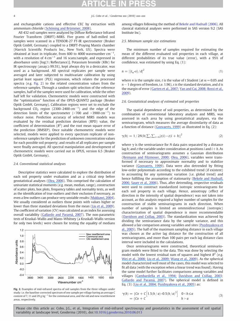
All 432 soil samples were analyzed by Diffuse Reflectance InfraredFourier Transform (DRIFT)-MIRS. Five grams of ball-milled soilsamples were scanned in a TENSOR-27 FT-IR spectrometer (BrukerOptik GmbH, Germany) coupled to a DRIFT-Praying Mantis chamber(Harrick Scientific Products Inc., New York, US). Spectra wereobtained at least in triplicate, from 600 to 4000 wavenumber cm−1,with a resolution of 4 cm−1 and 16 scans/sample, and expressed inabsorbance units [log(1/Reflectance)]. Potassium bromide (KBr) forIR spectroscopy (assay≥99.5%), kept always dry in a desiccator, wasused as a background. All spectral replicates per sample wereaveraged and later subjected to multivariate calibration by usingpartial least square (PLS) regression, which relates the processedspectra (e.g. Fig. 2) to the related concentration values from thereference samples. Through a random split selection of the referencesamples, half of the samples were used for calibration, while the otherhalf left for validation. Chemometric models were constructed withthe “optimization” function of the OPUS-QUANT2 package (BrukerOptik GmbH, Germany). Calibration regions were set to exclude thebackground CO2 region (2300–2400 cm−1) and the edge of thedetection limits of the spectrometer (b700 and N3900 cm−1) toreduce noise. Prediction accuracy of selected MIRS models wasevaluated by the residual prediction deviation (RPD) value, thecoefficient of determination (R2) and the root mean square error ofthe prediction (RMSEP). Once suitable chemometric models wereselected, models were applied to every spectrum replicate of non-reference samples for the prediction of unknown concentration valuesfor each possible soil property; and results of all replicates per samplewere finally averaged. All spectral manipulation and development ofchemometric models were carried out in OPUS, version 6.5 (BrukerOptik GmbH, Germany).

2.4. Conventional statistical analyses

Descriptive statistics were calculated to explore the distribution ofeach soil property under evaluation and as a critical step beforegeostatistical analyses (Olea, 2006). This comprised the calculation ofunivariate statistical moments (e.g. mean, median, range), constructionof scatter plots, box plots, frequency tables and normality tests, as wellas the identification of true outliers and their exclusion if necessary, aseven a few outliers can produce very unstable results (Makkawi, 2004).We usually considered as outliers those points with values higher orlower than three standard deviations from the mean (Liu et al., 2009).The coefficient of variation (CV)was calculated as an index for assessingoverall variability (Gallardo and Paramá, 2007). The non-parametrictests of Kruskal–Wallis and Mann–Whitney (a Kruskall–Wallis versionfor only two levels) were chosen for testing the equality of medians

Fig. 2. Examples of mid-infrared spectra of soil samples from the three villages understudy: i.e. the baseline-corrected spectrumof one sample per village having an average Ccontent of 7, 11 and 29 g kg−1 for the communal area, and the old and new resettlementareas, respectively.

Please cite this article as: Cobo, J.G., et al., Integration of mid-infrarevariability at landscape level, Geoderma (2010), doi:10.1016/j.geoderm

among villages following the method of Bekele and Hudnall (2006). Allclassical statistical analyses were performed in SAS version 9.2 (SASInstitute Inc).

2.5. Minimum sample size estimations

The minimum number of samples required for estimating themean of the different evaluated soil properties in each village, atdifferent probabilities of its true value (error), with a 95% ofconfidence, was estimated by using Eq. (1):

n = ½ tα*s� �

=d�2 ð1Þ

where n is the sample size, t is the value of t Student (at α=0.05 andn−1 degrees of freedom, i.e. 1.96), s is the standard deviation, and d isthe margin of error (Garten et al., 2007; Yan and Cai, 2008; Rossi et al.,2009).

2.6. Geostatistical analyses of estimated soil properties

The spatial dependence of soil properties, as determined by thecombination of conventional laboratory analyses and MIRS, wasassessed in each area by using geostatistical analyses, via thesemivariogram, which measures the average dissimilarity of data asa function of distance (Goovaerts, 1999) as illustrated in Eq. (2):

γðhÞ = 1 = 2N hð Þ∑i∑i+h½z ið Þ−z i + hð Þ�2 ð2Þ

where γ is the semivariance for N data pairs separated by a distancelag h; and z the variable under consideration at positions i and i+h. Asconstruction of semivariograms assumes a Gaussian distribution(Reimann and Filzmoser, 2000; Olea, 2006), variables were trans-formed if necessary to approximate normality and to stabilizevariance (Goovaerts, 1999). Data were also detrended by fittinglow-order polynomials according to the exhibited trend (if existent)to accounting for any systematic variation (i.e. global trend) andhence fulfilling the assumption of stationarity (Bekele and Hudnall,2006; Sauer et al., 2006). Thus, after detrending, respective residualswere used to construct standardized isotropic semivariograms foreach soil property in each village. Hence, anisotropy (effect ofdirection in the intensity of spatial dependence) was not taken intoaccount, as this analysis required a higher number of samples for theconstruction of stable semivariograms in each direction. Whennumber of samples is limited an ommnidirectional (isotropic)characterization of spatial dependence is more recommendable(Davidson and Csillag, 2003). The standardization was achieved bydividing the semivariance data by the sample variance, and thisallowed a fair comparison among variables and sites (Pozdnyakova etal., 2005). The half of the maximum sampling distance in each villagewas chosen as the active lag distance for the construction of allsemivariograms, and more than 100 pairs per each lag distance classinterval were included in the calculations.

Once semivariograms were constructed, theoretical semivario-gram models were fitted to the data. This was done by selecting themodel with the lowest residual sum of squares and highest R2 (e.g.Wei et al., 2008; Liu et al., 2009; Wang et al., 2009). As the sphericalmodel characterized well most of the cases, this model was selected tofit all data (with the exceptionwhen a linear trendwas found). Havingthe same model further facilitates comparisons among variables andvillages (Cambardella et al., 1994; Davidson and Csillag, 2003;Gallardo and Paramá, 2007). The spherical model is defined inEq. (3) (Liu et al., 2004; Pozdnyakova et al., 2005) as:

γ hð Þ = fCo + C 1:5 h= að Þ–0:5 h=að Þ3h i

0 b h≤a

= fCo + C h N að3Þ

d spectroscopy and geostatistics in the assessment of soil spatiala.2010.06.013

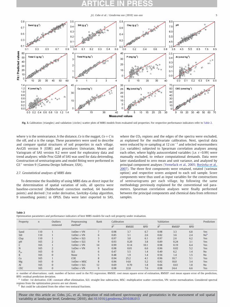
Fig. 3. Calibration (triangles) and validation (circles) scatter plots of MIRS models from evaluated soil properties. For respective performance indicators refer to Table 2.

5J.G. Cobo et al. / Geoderma xxx (2010) xxx–xxx

where γ is the semivariance, h the distance, Co is the nugget, Co+C isthe sill, and a is the range. These parameters were used to describeand compare spatial structures of soil properties in each village.ArcGIS version 9 (ESRI) and procedures Univariate, Means andVariogram of SAS version 9.2 were used for exploratory data andtrend analyses; while Proc GLM of SAS was used for data detrending.Construction of semivariograms and model fitting were performed inGS+ version 9 (Gamma Design Software, USA).

2.7. Geostatistical analyses of MIRS data

To determine the feasibility of using MIRS data as direct input forthe determination of spatial variation of soils, all spectra werebaseline-corrected (Rubberband correction method, 64 baselinepoints) and derived (1st order derivative, Savitzky–Golay algorithm,9 smoothing points) in OPUS. Data were later exported to SAS,

Table 2Optimization parameters and performance indicators of best MIRS models for each soil pro

Property n Outliersremoved

Preprocessingmethoda

Rank Calibra

R2

Sand 110 1 1stDer+VN 7 0.98Silt 110 1 1stDer+VN 6 0.85Clay 110 1 1stDer+SLS 3 0.97pH 165 2 1stDer+SLS 9 0.93C 165 1 1stDer+VN 14 0.99N 165 2 1stDer+VN 9 0.98Pav 165 0 SLS 6 0.47K 165 0 None 5 0.48Ca 165 1 COE 8 0.94Mg 165 0 1stDer+MSC 8 0.96Al 165 0 1stDer+SLS 12 0.69CEC 165 0 1stDer+VN 9 0.98

n: number of observations; rank: number of factors used in the PLS regression; RMSEE: roRPD: residual prediction deviation.

a 1stDer: 1st derivative, COE: constant offset elimination, SLS: straight line subtraction,regions from the optimization process are not shown.

b But could be calculated from the other two textural fractions.

Please cite this article as: Cobo, J.G., et al., Integration of mid-infrarevariability at landscape level, Geoderma (2010), doi:10.1016/j.geoderm

where the CO2 regions and the edges of the spectra were excluded,as explained for the multivariate calibration. Next, spectral datawere reduced by re-sampling at 12 cm−1 and selected wavenumbers(i.e. variables) subjected to Spearman correlation analyses amongeach other, where highly autocorrelated variables (i.e. rN0.99) weremanually excluded, to reduce computational demands. Data werelater standardized to zero mean and unit variance, and analyzed byprincipal component analyses (Yemefack et al., 2005; Borůvka et al.,2007). The three first components were retained, rotated (varimaxoption) and respective scores assigned to each soil sample. Scorecomponents were thus used as input variables for the constructionsof semivariograms per each village, by following the samemethodology previously explained for the conventional soil para-meters. Spearman correlation analyses were finally performedbetween the principal components and chemical data from referencesamples.

perty under evaluation.

tion Validation Prediction

RMSEE RPD R2 RMSEP RPD

3.7 6.7 0.98 3.3 6.8 Yes3.1 2.6 0.82 3.6 2.4 Nob

3.0 6.1 0.97 2.6 6.2 Yes0.20 3.8 0.89 0.24 3.1 Yes0.14 10.1 0.98 0.19 6.4 Yes0.01 6.6 0.96 0.02 5.2 Yes5.5 1.4 0.49 6.2 1.4 No1.9 1.4 0.56 1.4 1.5 No

25.2 4.1 0.96 18.7 5.1 Yes14.8 5.2 0.92 18.0 3.4 Yes0.70 1.8 0.66 0.61 1.8 No

22.8 7.6 0.98 24.4 6.6 Yes

ot mean square error of estimation, RMSEP: root mean square error of the prediction,

MSC: multiplicative scatter correction, VN: vector normalization. Considered spectral

d spectroscopy and geostatistics in the assessment of soil spatiala.2010.06.013

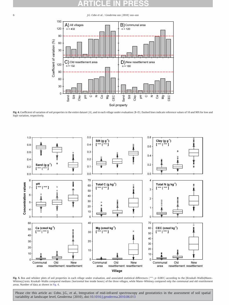
Fig. 4. Coefficient of variation of soil properties in the entire dataset (A), and in each village under evaluation (B–D). Dashed lines indicate reference values of 10 and 90% for low andhigh variation, respectively.

Fig. 5. Box and whisker plots of soil properties in each village under evaluation, and associated statistical differences (***: pb0.001) according to the [Kruskall–Wallis|Mann–Whitney] tests. Kruskall–Wallis compared medians (horizontal line inside boxes) of the three villages, while Mann–Whitney compared only the communal and old resettlementareas. Number of data as shown in Fig. 4.

6 J.G. Cobo et al. / Geoderma xxx (2010) xxx–xxx

Please cite this article as: Cobo, J.G., et al., Integration of mid-infrared spectroscopy and geostatistics in the assessment of soil spatialvariability at landscape level, Geoderma (2010), doi:10.1016/j.geoderma.2010.06.013

7J.G. Cobo et al. / Geoderma xxx (2010) xxx–xxx

3. Results

3.1. MIRS models and prediction

A good representation across the different concentration rangesfor most of the soil properties was obtained by the selection of thesamples, as shown in Fig. 3. Calibration and validation models alsoshowed that predictability potential of MIRS varied with the specificsoil property under evaluation and location, as indicated by thedifferent model fit and performance indicators (Fig. 3, Table 2). Forexample, in agricultural applications RPD values higher than 5indicate that predictions models are excellent; RPD values greaterthan 3 are considered acceptable; while values less than 3 indicatepoor prediction power (Pirie et al., 2005). Besides, R2 values near 1typically indicate good models (Conzen, 2003), in particular whenbias is minimal and regression line follows the 1:1 line. Hence,excellent models (5bRPD≤6.8, 0.96≤R2≤0.98) were obtained forsand, clay, C, N, Ca and CEC; acceptable models (3bRPDb5,0.89≤R2≤0.92) were obtained for pH and Mg; while unsuitablemodels (RPDb3, R2≤0.82) were obtained for silt, Pav, K and Al. Poorvalidation for these last variables (especially Pav, K and Al) was theresult of a deficient calibration, as indicated by their model fit (Fig. 3)and parameters (Table 2). Mid-infrared spectroscopymodels for thesevariables were thus not used for prediction, and hence these datawere dropped from any further analyses. Silt fraction, however, couldbe calculated from the other two fractions (silt=100 — sand–clay).Therefore, by using the selected MIRS models shown in Table 2 for theprediction of soil parameters in non-reference samples, the entiredataset of sand, silt, clay, pH, C, N, Ca, Mg and CEC could be completed.

3.2. Exploratory data analysis and differences among villages

Exploratory data analyses in the entire dataset indicated that mostsoil properties presented skewed and kurtic distributions (data not

Fig. 6. Minimum sample sizes required for estimating the mean of different evaluated soilconfidence in: communal area (closed triangles), old resettlement (closed circles) and newfor calculations and units as shown in Fig. 4.

Please cite this article as: Cobo, J.G., et al., Integration of mid-infrarevariability at landscape level, Geoderma (2010), doi:10.1016/j.geoderm

shown). For example, texture fractions showed clearly a bimodaldistribution, which suggested the presence of different populations, asit was in fact the case (i.e. different villages presenting differenttextural classes). Descriptive statistics and histograms were thereforealso obtained by village. In this case, although texture fractions oftenapproximated normality, the other soil properties still exhibited non-normal distributions (data not shown). Non-normality is usually therule and not the exception when dealing with geostatistical andenvironmental data (Reimann and Filzmoser, 2000). This is why themedian (instead of the mean) and non-parametric approaches werepreferably used for classical statistical analyses, in spite of datatransformation of skewed variables usually helped to approximatenormality.

Overall variability of soil properties in each area was evaluated byits coefficient of variation. According to Wei et al. (2008), a CV lessthan 10% indicates that variability of a considered property is low;while a CV higher than 90% indicates high variation. Thus, calculatedCVs in the entire dataset (Fig. 4A) showed that Ca, Mg and CEC werethe properties with the highest overall variability (N90%); while onlypH presented a relative low variation (∼10%). Other evaluated soilproperties showed intermediate variability (CV=10–90%). Whencalculations were performed by village (Fig. 4B–D), CVs of all soilproperties reduced considerably, as expected. Data showed that Mgvaried the most in the three villages, while pH (in all villages) andsand (in the communal and old resettlement area) presented thelowest variation. With the particular exception of sand and pH,variability of all soil properties in the new resettlement was lowerthan in the other two areas.

Differences in medians among villages for all soil properties weresignificant at pb0.001 (Fig. 5). Differences were especially evidentwhen the communal and old resettlement areas were compared tothe new resettlement area, mainly due to divergent soil textural types(Table 1). In fact, the new resettlement area presented the lowestvalues for sand and the highest for the remaining properties. This is

properties at different probabilities of its true value (margin of error), with a 95% ofresettlement (open circles). Notice that Y-axes are in logarithmic scale. Number of data

d spectroscopy and geostatistics in the assessment of soil spatiala.2010.06.013

8 J.G. Cobo et al. / Geoderma xxx (2010) xxx–xxx

why a Mann–Whitney test was also performed to compare onlybetween the communal and old resettlement area. This analysisshowed highly significant differences (pb0.001) in medians betweenthese two villages for all evaluated soil properties (Fig. 5).

3.3. Minimum sample size requirements

Estimated minimum sample sizes, for all evaluated parameters,exhibited a negative exponential trend by increasing the margin of error(Fig. 6). Taking soil C as an example, aminimumof 473 sampleswould berequired in the communal area to estimate the mean at 5% of its truevalue;while aminimumof118, 53, 30and19sampleswouldbenecessaryatmargins errors of 10, 15, 20 and25%, respectively.With the exceptionofsandandpH, the requirednumberof sampleswas found tobe lower in thenew resettlement area than in the other villages. In general, a highernumber of sampleswould be required forMg, CEC andCa,while relativelyfewer samples would be necessary for pH, silt and sand.

3.4. Geostatistical analyses of generated soil data

Geostatistical analyses require data following Gaussian distribu-tion. Thus, transformation of variables was necessary in most of thecases (see Table 3) and this generally allowed to approximatenormality. However, for Mg in the communal and old resettlementareas any transformations used could shift the highly skeweddistribution of this variable. This was attributed to the low concentra-tions measured (Fig. 5), where a high proportion of samples had null

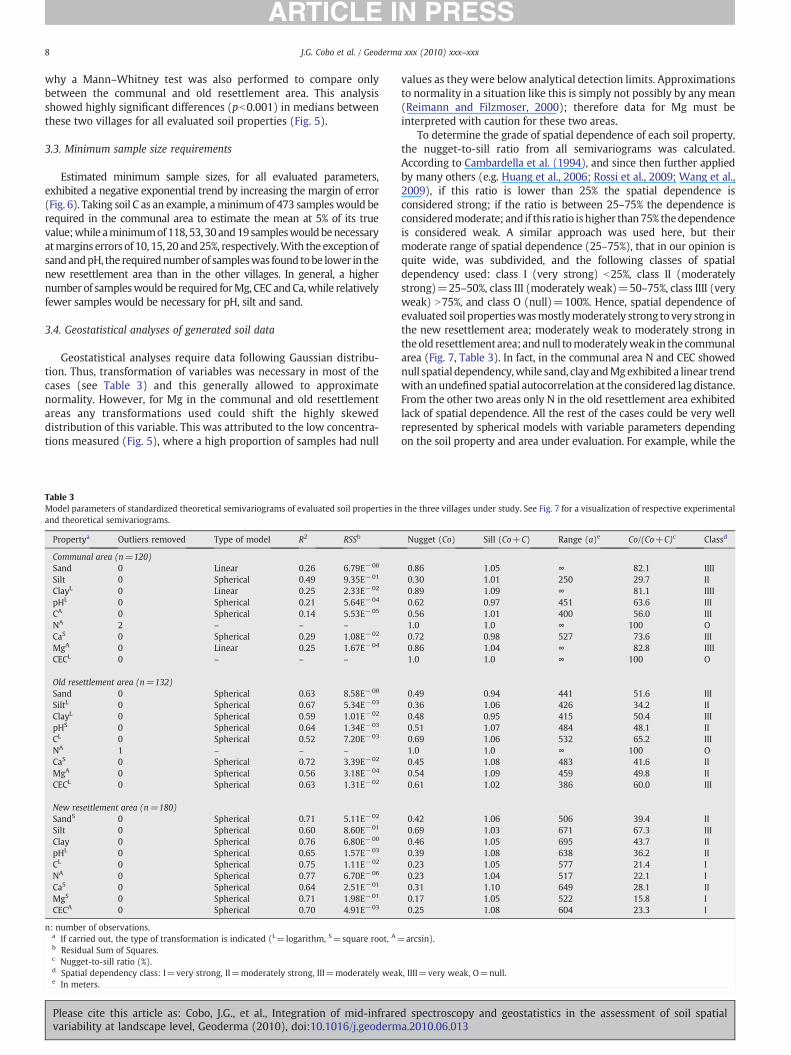
Table 3Model parameters of standardized theoretical semivariograms of evaluated soil properties inand theoretical semivariograms.

Propertya Outliers removed Type of model R2 RSSb

Communal area (n=120)Sand 0 Linear 0.26 6.79E−00

Silt 0 Spherical 0.49 9.35E−01

ClayL 0 Linear 0.25 2.33E−02

pHL 0 Spherical 0.21 5.64E−04

CA 0 Spherical 0.14 5.53E−05

NA 2 – – –

CaS 0 Spherical 0.29 1.08E−02

MgA 0 Linear 0.25 1.67E−04

CECL 0 – – –

Old resettlement area (n=132)Sand 0 Spherical 0.63 8.58E−00

SiltL 0 Spherical 0.67 5.34E−03

ClayL 0 Spherical 0.59 1.01E−02

pHS 0 Spherical 0.64 1.34E−03

CL 0 Spherical 0.52 7.20E−03

NA 1 – – –

CaS 0 Spherical 0.72 3.39E−02

MgA 0 Spherical 0.56 3.18E−04

CECL 0 Spherical 0.63 1.31E−02

New resettlement area (n=180)SandS 0 Spherical 0.71 5.11E−02

Silt 0 Spherical 0.60 8.60E−01

Clay 0 Spherical 0.76 6.80E−00

pHL 0 Spherical 0.65 1.57E−03

CL 0 Spherical 0.75 1.11E−02

NA 0 Spherical 0.77 6.70E−06

CaS 0 Spherical 0.64 2.51E−01

MgS 0 Spherical 0.71 1.98E−01

CECA 0 Spherical 0.70 4.91E−03

n: number of observations.a If carried out, the type of transformation is indicated (L=logarithm, S=square root, A=b Residual Sum of Squares.c Nugget-to-sill ratio (%).d Spatial dependency class: I=very strong, II=moderately strong, III=moderately weae In meters.

Please cite this article as: Cobo, J.G., et al., Integration of mid-infrarevariability at landscape level, Geoderma (2010), doi:10.1016/j.geoderm

values as they were below analytical detection limits. Approximationsto normality in a situation like this is simply not possibly by any mean(Reimann and Filzmoser, 2000); therefore data for Mg must beinterpreted with caution for these two areas.

To determine the grade of spatial dependence of each soil property,the nugget-to-sill ratio from all semivariograms was calculated.According to Cambardella et al. (1994), and since then further appliedby many others (e.g. Huang et al., 2006; Rossi et al., 2009; Wang et al.,2009), if this ratio is lower than 25% the spatial dependence isconsidered strong; if the ratio is between 25–75% the dependence isconsideredmoderate; and if this ratio ishigher than75% thedependenceis considered weak. A similar approach was used here, but theirmoderate range of spatial dependence (25–75%), that in our opinion isquite wide, was subdivided, and the following classes of spatialdependency used: class I (very strong) b25%, class II (moderatelystrong)=25–50%, class III (moderately weak)=50–75%, class IIII (veryweak) N75%, and class O (null)=100%. Hence, spatial dependence ofevaluated soil propertieswasmostlymoderately strong tovery strong inthe new resettlement area; moderately weak to moderately strong intheold resettlement area; andnull tomoderatelyweak in the communalarea (Fig. 7, Table 3). In fact, in the communal area N and CEC showednull spatial dependency,while sand, clayandMgexhibited a linear trendwith anundefined spatial autocorrelation at the considered lag distance.From the other two areas only N in the old resettlement area exhibitedlack of spatial dependence. All the rest of the cases could be very wellrepresented by spherical models with variable parameters dependingon the soil property and area under evaluation. For example, while the

the three villages under study. See Fig. 7 for a visualization of respective experimental

Nugget (Co) Sill (Co+C) Range (a)e Co/(Co+C)c Classd

0.86 1.05 ∞ 82.1 IIII0.30 1.01 250 29.7 II0.89 1.09 ∞ 81.1 IIII0.62 0.97 451 63.6 III0.56 1.01 400 56.0 III1.0 1.0 ∞ 100 O0.72 0.98 527 73.6 III0.86 1.04 ∞ 82.8 IIII1.0 1.0 ∞ 100 O

0.49 0.94 441 51.6 III0.36 1.06 426 34.2 II0.48 0.95 415 50.4 III0.51 1.07 484 48.1 II0.69 1.06 532 65.2 III1.0 1.0 ∞ 100 O0.45 1.08 483 41.6 II0.54 1.09 459 49.8 II0.61 1.02 386 60.0 III

0.42 1.06 506 39.4 II0.69 1.03 671 67.3 III0.46 1.05 695 43.7 II0.39 1.08 638 36.2 II0.23 1.05 577 21.4 I0.23 1.04 517 22.1 I0.31 1.10 649 28.1 II0.17 1.05 522 15.8 I0.25 1.08 604 23.3 I

arcsin).

k, IIII=very weak, O=null.

d spectroscopy and geostatistics in the assessment of soil spatiala.2010.06.013

9J.G. Cobo et al. / Geoderma xxx (2010) xxx–xxx

nugget-to-sill ratio for Ca was 74% in the communal area (moderatelyweak dependency), in the old and new resettlement areas this ratioreduced to 42 and 28% (moderately strong dependency), respectively.This contrasted with silt, as the nugget-to-sill ratio increased from 30and 34% in the communal and old resettlement area, respectively, up to67% in the new resettlement area. Ranges of the semivariograms for allsoil properties and sites ranged from 250 m (silt in the communal area)to 695 m (clay in the new resettlement). With the exception of Ca,estimated ranges were lowest in the communal area and highest in thenew resettlement.

Fig. 7. Standardized experimental (circles) and theoretical (line) semivariograms for evaluaTable 3.

Please cite this article as: Cobo, J.G., et al., Integration of mid-infrarevariability at landscape level, Geoderma (2010), doi:10.1016/j.geoderm

3.5. Principal components and geostatistical analyses of MIRS data

Forty nine percent (49%) of overall variability of MIRS data couldbe explained by the first principal component (PC1), while 11, 10, 6, 4and 4% could be explained by PC2, PC3, PC4, PC5 and PC6 respectively.Therefore, only the first three components, accounting for 70% ofoverall variability, were retained. Scores of the first three componentswere next correlated to concentration values of reference samples. Ingeneral, PC1 related very well to texture fractions, C, N, Ca and Mg(absolute Spearman coefficient values of 0.55–0.96, Fig. 8); while

ted soil properties in the three areas under study. For model parameters please refer to

d spectroscopy and geostatistics in the assessment of soil spatiala.2010.06.013

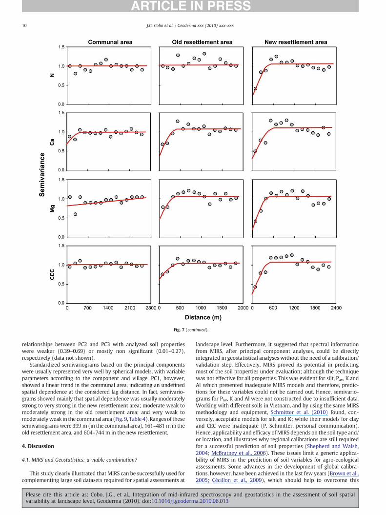
Fig. 7 (continued).

10 J.G. Cobo et al. / Geoderma xxx (2010) xxx–xxx

relationships between PC2 and PC3 with analyzed soil propertieswere weaker (0.39–0.69) or mostly non significant (0.01–0.27),respectively (data not shown).

Standardized semivariograms based on the principal componentswere usually represented very well by spherical models, with variableparameters according to the component and village. PC1, however,showed a linear trend in the communal area, indicating an undefinedspatial dependence at the considered lag distance. In fact, semivario-grams showed mainly that spatial dependence was usually moderatelystrong to very strong in the new resettlement area; moderate weak tomoderately strong in the old resettlement area; and very weak tomoderatelyweak in the communal area (Fig. 9, Table 4). Ranges of thesesemivariogramswere 399 m (in the communal area), 161–481 m in theold resettlement area, and 604–744 m in the new resettlement.

4. Discussion

4.1. MIRS and Geostatistics: a viable combination?

This study clearly illustrated that MIRS can be successfully used forcomplementing large soil datasets required for spatial assessments at

Please cite this article as: Cobo, J.G., et al., Integration of mid-infrarevariability at landscape level, Geoderma (2010), doi:10.1016/j.geoderm

landscape level. Furthermore, it suggested that spectral informationfrom MIRS, after principal component analyses, could be directlyintegrated in geostatistical analyses without the need of a calibration/validation step. Effectively, MIRS proved its potential in predictingmost of the soil properties under evaluation; although the techniquewas not effective for all properties. This was evident for silt, Pav, K andAl which presented inadequate MIRS models and therefore, predic-tions for these variables could not be carried out. Hence, semivario-grams for Pav, K and Al were not constructed due to insufficient data.Working with different soils in Vietnam, and by using the same MIRSmethodology and equipment, Schmitter et al. (2010) found, con-versely, acceptable models for silt and K; while their models for clayand CEC were inadequate (P. Schmitter, personal communication).Hence, applicability and efficacy of MIRS depends on the soil type and/or location, and illustrates why regional calibrations are still requiredfor a successful prediction of soil properties (Shepherd and Walsh,2004; McBratney et al., 2006). These issues limit a generic applica-bility of MIRS in the prediction of soil variables for agro-ecologicalassessments. Some advances in the development of global calibra-tions, however, have been achieved in the last few years (Brown et al.,2005; Cécillon et al., 2009), which should help to overcome this

d spectroscopy and geostatistics in the assessment of soil spatiala.2010.06.013

Fig. 8. Scatter plots and Spearman correlation coefficients for the relationships between soil properties from reference samples (i.e. analyzed by conventional laboratory procedures)and respective component scores of the first principal component (PC1) based on MIRS data. ***: pb0.001.

11J.G. Cobo et al. / Geoderma xxx (2010) xxx–xxx

limitation in the near future. Alternative solutions could be the use ofMIRS-based predictions models to estimate through pedotransferfunctions those soil properties that cannot be predicted accurately bysole MIRS (McBratney et al., 2006), or the utilization of auxiliarypredictors (i.e. simple and inexpensive conventional soil parameters,like pH and sand; or from complementary sensors, like NIRS) that canimprove the prediction of other soil properties (Brown et al., 2005).Thus, all data could be later used in spatial analyses withoutrestriction.

Semivariograms based on the soil dataset clearly showed thatspatial autocorrelation of most soil properties in the villages followedthe order: communal areabold resettlementbnew resettlement.Variography analyses based on the principal components from MIRSdata showed comparable spatial patterns (i.e., nugget-to-sill ratios andranges of semivariograms, Fig. 10). This implies important savings interms of analytical costs and time, as it creates the possibility of a broadand quick assessment of soil spatial variability at landscape scale basedonly on MIRS, confirming previous suggestions by Shepherd andWalsh (2007) and complementing studies based on NIRS (i.e. byCohen et al., 2006; Vågen et al., 2006; Awiti et al., 2008). A relatedapproach to our study, but at plot level and by using NIRS, was carriedout by Odlare et al. (2005). However, they found out that spatialdependence from principal components (based on spectral informa-tion) was not related to the spatial dependence from considered soilproperties (i.e. C, clay and pH). Hence, although spatial variation basedon NIRS could be identified, the authors did not know what thevariation represented. Thus, to properly understand the meaning ofthe spatial structures from the principal components it is necessary tolink the component scores to soil parameters of reference samples. Inour case, this was possible for the first principal component (PC1),which was well related to textural fractions, C, N, Ca, Mg and CEC.Therefore, PC1 was clearly associated to soil fertility, and thus, derived

Please cite this article as: Cobo, J.G., et al., Integration of mid-infrarevariability at landscape level, Geoderma (2010), doi:10.1016/j.geoderm

spatial results could be used for distinguishing areas of different soilquality. However, for PC2 and PC3 simple relationshipswithmeasuredvariables were not evident. A reason for this may be related to theexplained variance in each component, where PC1 accounted for 49%of the overall variability, while the other two components eachexplained a lower proportion (10–11%). The unexplained variance andlack of relationships for the other components would indicate thatMIRS could be either generating noise or capturing additionalcharacteristics of soils that this study did not take into account (e.g.carbonates, lime requirements, dissolved organic C, phosphatase andurease activity, among others). In fact, MIRS can be related to a widerange of physical, chemical and biological soil characteristics (forfurther details please refer to Shepherd andWalsh, 2007; andViscarra-Rossel et al., 2006). All this would further suggest that MIRS maypresent great potential as an integrative measurement of soil statusand, hence, could be a valuable tool for characterizing spatial variationof soils.

4.2. Analyses of spatial patterns

Nearly all experimental semivariograms of soil properties werevery well described by the spherical model, with a reachable sill,which clearly indicates the presence of spatial autocorrelation.However, some of the semivariograms in the communal area (forsand, clay, Mg and PC1), could only be described by a linear modelwith an undefined spatial dependence. If there is no reachable sill thiscould indicate that spatial dependence may exist beyond theconsidered lag distance (Huang et al., 2006). Semivariograms for Nand CEC in the communal area, and N in the old resettlement showedinstead pure nugget effect. Pure nugget effect can represent eitherextreme homogeneity (all points have similar values) or extremeheterogeneity (values are very different, in a random way). However,

d spectroscopy and geostatistics in the assessment of soil spatiala.2010.06.013

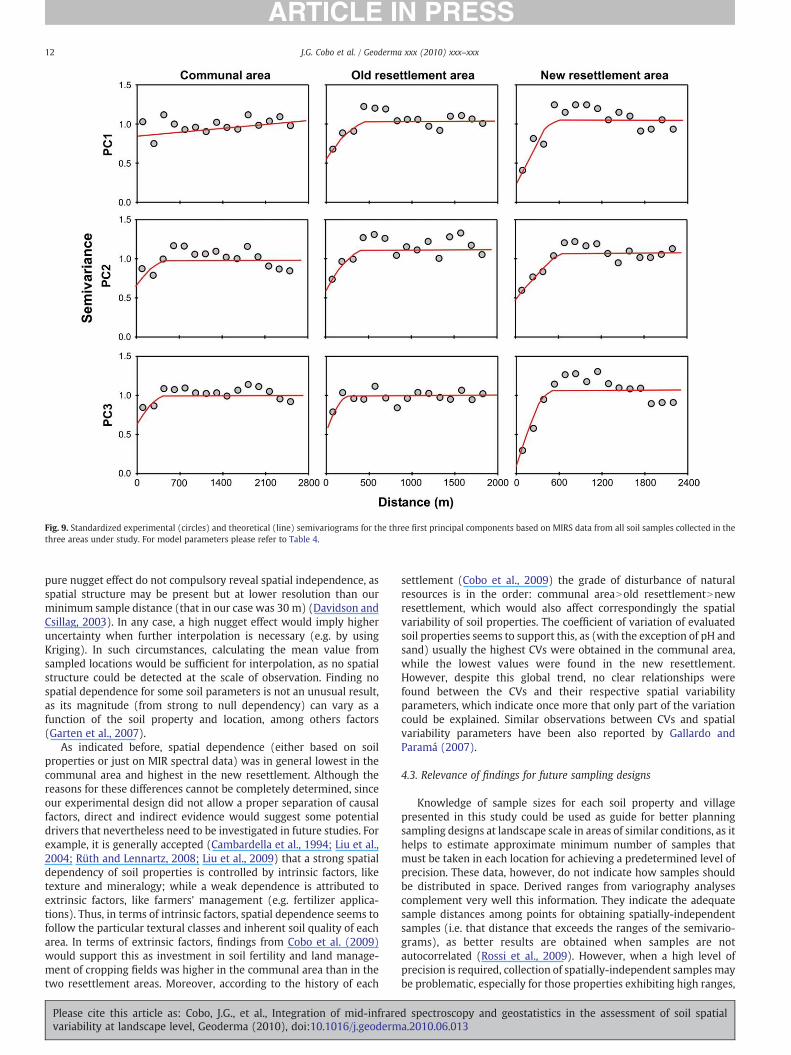
Fig. 9. Standardized experimental (circles) and theoretical (line) semivariograms for the three first principal components based on MIRS data from all soil samples collected in thethree areas under study. For model parameters please refer to Table 4.

12 J.G. Cobo et al. / Geoderma xxx (2010) xxx–xxx

pure nugget effect do not compulsory reveal spatial independence, asspatial structure may be present but at lower resolution than ourminimum sample distance (that in our case was 30 m) (Davidson andCsillag, 2003). In any case, a high nugget effect would imply higheruncertainty when further interpolation is necessary (e.g. by usingKriging). In such circumstances, calculating the mean value fromsampled locations would be sufficient for interpolation, as no spatialstructure could be detected at the scale of observation. Finding nospatial dependence for some soil parameters is not an unusual result,as its magnitude (from strong to null dependency) can vary as afunction of the soil property and location, among others factors(Garten et al., 2007).

As indicated before, spatial dependence (either based on soilproperties or just on MIR spectral data) was in general lowest in thecommunal area and highest in the new resettlement. Although thereasons for these differences cannot be completely determined, sinceour experimental design did not allow a proper separation of causalfactors, direct and indirect evidence would suggest some potentialdrivers that nevertheless need to be investigated in future studies. Forexample, it is generally accepted (Cambardella et al., 1994; Liu et al.,2004; Rüth and Lennartz, 2008; Liu et al., 2009) that a strong spatialdependency of soil properties is controlled by intrinsic factors, liketexture and mineralogy; while a weak dependence is attributed toextrinsic factors, like farmers' management (e.g. fertilizer applica-tions). Thus, in terms of intrinsic factors, spatial dependence seems tofollow the particular textural classes and inherent soil quality of eacharea. In terms of extrinsic factors, findings from Cobo et al. (2009)would support this as investment in soil fertility and land manage-ment of cropping fields was higher in the communal area than in thetwo resettlement areas. Moreover, according to the history of each

Please cite this article as: Cobo, J.G., et al., Integration of mid-infrarevariability at landscape level, Geoderma (2010), doi:10.1016/j.geoderm

settlement (Cobo et al., 2009) the grade of disturbance of naturalresources is in the order: communal areaNold resettlementNnewresettlement, which would also affect correspondingly the spatialvariability of soil properties. The coefficient of variation of evaluatedsoil properties seems to support this, as (with the exception of pH andsand) usually the highest CVs were obtained in the communal area,while the lowest values were found in the new resettlement.However, despite this global trend, no clear relationships werefound between the CVs and their respective spatial variabilityparameters, which indicate once more that only part of the variationcould be explained. Similar observations between CVs and spatialvariability parameters have been also reported by Gallardo andParamá (2007).

4.3. Relevance of findings for future sampling designs

Knowledge of sample sizes for each soil property and villagepresented in this study could be used as guide for better planningsampling designs at landscape scale in areas of similar conditions, as ithelps to estimate approximate minimum number of samples thatmust be taken in each location for achieving a predetermined level ofprecision. These data, however, do not indicate how samples shouldbe distributed in space. Derived ranges from variography analysescomplement very well this information. They indicate the adequatesample distances among points for obtaining spatially-independentsamples (i.e. that distance that exceeds the ranges of the semivario-grams), as better results are obtained when samples are notautocorrelated (Rossi et al., 2009). However, when a high level ofprecision is required, collection of spatially-independent samples maybe problematic, especially for those properties exhibiting high ranges,

d spectroscopy and geostatistics in the assessment of soil spatiala.2010.06.013

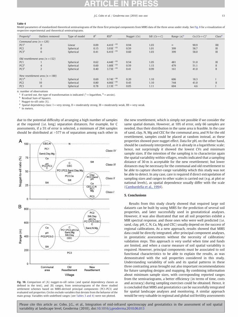
Table 4Model parameters of standardized theoretical semivariograms of the three first principal components from MIRS data of the three areas under study. See Fig. 8 for a visualization ofrespective experimental and theoretical semivariograms.

Propertya Outliers removed Type of model R2 RSSb Nugget (Co) Sill (Co+C) Range (a)e Co/(Co+C)c Classd

Communal area (n=120)PC1L 0 Linear 0.09 4.41E−03 0.94 1.03 ∞ 90.9 IIIIPC2 0 Spherical 0.15 3.93E−03 0.59 1.01 399 58.7 IIIPC3L 0 Spherical 0.41 6.41E−03 0.60 1.03 399 58.0 III

Old resettlement area (n=132)PC1 1 Spherical 0.62 4.44E−03 0.54 1.05 481 51.0 IIIPC2L 4 Spherical 0.60 1.60E−03 0.59 1.15 479 51.1 IIPC3L 2 Spherical 0.40 3.73E−03 0.41 0.99 161 41.0 II

New resettlement area (n=180)PC1A 1 Spherical 0.69 9.74E−06 0.20 1.10 606 18.3 IPC2 10 Spherical 0.80 4.66E−05 0.45 1.10 744 41.0 IIPC3 0 Spherical 0.78 2.13E−01 0.05 1.11 604 4.6 I

n: number of observationsa If carried out, the type of transformation is indicated (L=logarithm, A=arcsin).b Residual Sum of Squares.c Nugget-to-sill ratio (%).d Spatial dependency class: I=very strong, II=moderately strong, III=moderately weak, IIII=very weak.e In meters.

13J.G. Cobo et al. / Geoderma xxx (2010) xxx–xxx

due to the potential difficulty of arranging a high number of samplesat the required (i.e. long) separation distances. For example, for Cassessments, if a 5% of error is selected, a minimum of 264 samplesshould be distributed at N577 m of separation among each other in

Fig. 10. Comparison of (A) nugget-to-sill ratios (and spatial dependency classes asdefined in the text), and (B) ranges, from semivariograms of the three studiedsettlement schemes based on MIRS-derived principal components (PC1-PC3) andevaluated soil properties. Circles exclude variables that deviate from the behavior of themain group. Variables with undefined ranges (see Tables 3 and 4) were not plotted.

Please cite this article as: Cobo, J.G., et al., Integration of mid-infrarevariability at landscape level, Geoderma (2010), doi:10.1016/j.geoderm

the new resettlement, which is simply not possible if we consider thesame spatial domain. However, at 10% of error, only 66 samples areneeded, thus their distribution in the same area is feasible. In the caseof sand, clay, N, Mg and CEC for the communal area, and N for the oldresettlement, samples could be placed at random instead, as theseproperties showed pure nugget effect. Data for pH, on the other hand,should be cautiously interpreted, as it is already in a logarithmic scale;hence, not surprisingly it showed the lowest CVs and minimumsample sizes. If the intention of the sampling is to characterize againthe spatial variability within villages, results indicated that a samplingdistance of 30 m is acceptable for the new resettlement; but lowerdistances may be necessary for the communal and old resettlement tobe able to capture shorter-range variability which this study was notbe able to detect. In any case, care is required if direct extrapolation ofsampling sizes and ranges to other scales is carried out (e.g. at plot ornational levels), as spatial dependence usually differ with the scale(Cambardella et al., 1994).

5. Conclusions

Results from this study clearly showed that required large soildatasets can be built by using MIRS for the prediction of several soilproperties, and later successfully used in geostatistical analyses.However, it was also illustrated that not all soil properties exhibit aMIR spectral response, and those ones who were well predicted (i.e.sand, clay, pH, C, N, Ca, Mg and CEC) usually depend on the success ofregional calibrations. As a new approach, results showed that MIRSdata could be directly integrated, after principal component analyses,in geostatistic assessments without the necessity of calibration/validation steps. This approach is very useful when time and fundsare limited, and when a coarse measure of soil spatial variability isrequired. However, principal components must be associated to soilfunctional characteristics to be able to explain the results, as wasdemonstrated with the soil properties considered in this study.Understanding variability of soils and its spatial patterns in thesethree contrasting areas brought out also important recommendationsfor future sampling designs and mapping. By combining informationabout minimum sample sizes, with corresponding reported rangesfrom the semivariograms, a better efficiency (in terms of time, costsand accuracy) during sampling exercises could be obtained. Hence, itis concluded that MIRS and geostatistics can be successfully integratedfor spatial landscape analyses and monitoring. A similar approachwould be very valuable in regional and global soil fertility assessments

d spectroscopy and geostatistics in the assessment of soil spatiala.2010.06.013

14 J.G. Cobo et al. / Geoderma xxx (2010) xxx–xxx

and mapping (e.g. Sanchez et al., 2009) and carbon sequestrationcampaigns (e.g. Goidts et al., 2009), where large soil sample sizes arerequired and uncertainty about sampling designs prevail.

Acknowledgments

The authors are grateful to all farmers in the three villages whosupported this study. Many thanks also go to: the extension officers inthe region for their collaboration; to Stefan Becker, Cheryl Batistel andthe staff of Landesanstalt für Landwirtschaftliche Chemie in theUniversity of Hohenheim for laboratory analyses; to Irene Chukwu-mah for her support during MIRS readings; and to Hans-Peter Piephofor assistance during statistical analyses. Thanks also to AndreaSchmidt (Bruker Optik GmbH) for her useful help during the analysesof MIRS data. The methodology development of this study is linked tothe DFG-funded project PAK 346 (“Structure and functions ofagricultural landscapes under global climate change”), subproject P3.

References

Anderson, J.M., Ingram, J.S.I., 1993. Tropical Soil Biology and Fertility: A Handbook ofMethods. CAB International, Wallingford, Oxon. 221 pp.

Awiti, A.O., Walsh, M.G., Shepherd, K.D., Kinyamario, J., 2008. Soil conditionclassification using infrared spectroscopy: a proposition for assessment of soilcondition along a tropical forest-cropland chronosequence. Geoderma 143, 73–84.

Bekele, A., Hudnall, W.H., 2006. Spatial variability of soil chemical properties of aprairie–forest transition in Louisiana. Plant and Soil 280, 7–21.

Borůvka, L., Mládková, L., Penížek, V., Drábek, O., Vašát, R., 2007. Forest soil acidificationassessment using principal component analysis and geostatistics. Geoderma 140,374–382.

Bray, R.H., Kurtz, L.T., 1945. Determination of total, organic, and available forms ofphosphorus in soils. Soil Science 59, 39–45.

Brown, D.J., Shepherd, K.D., Walsh, M.G., Mays, M.D., Reinsch, T.G., 2005. Global soilcharacterization with VNIR diffuse reflectance spectroscopy. Geoderma 132 (3–4),273–290.

Cambardella, C.A., Moorman, T.B., Novak, J.M., Parkin, T.B., Karlen, D.L., Turco, R.F.,Konopka, A.E., 1994. Field-scale variability of soil properties in Central Iowa soils.Soil Science Society of America Journal 58, 1501–1511.

Cécillon, L., Barthès, B.G., Gomez, C., Ertlen, D., Genot, V., Hedde, M., Stevens, A., Brun, J.J.,2009. Assessment and monitoring of soil quality using near-infrared reflectancespectroscopy (NIRS). European Journal of Soil Science 60, 770–784.

Cobo, J.G., Dercon, G., Monje, C., Mahembe, P., Gotosa, T., Nyamangara, J., Delve, R.,Cadisch, G., 2009. Cropping strategies, soil fertility investment and landmanagement practices by smallholder farmers in communal and resettlementareas in Zimbabwe. Land Degradation & Development 20 (5), 492–508.

Cobo, J.G., Dercon, G., Cadisch, G., 2010. Nutrient balances in African land use systemsacross different spatial scales: a review of approaches, challenges and progress.Agriculture, Ecosystem and Environment 136 (1–2), 1–15.

Cohen, M., Dabral, S., Graham, W., Prenger, J., Debusk, W., 2006. Evaluating ecologicalcondition using soil biogeochemical parameters and near infrared reflectancespectra. Environmental Monitoring and Assessment 116, 427–457.

Conzen, J.-P., 2003. Multivariate Calibration: A Practical Guide for the MethodDevelopment in the Analytical Chemistry. Bruker Optik GmbH. 92 pp.

Davidson, A., Csillag, F., 2003. A comparison of nested analysis of variance (ANOVA) andvariograms for characterizing grassland spatial structure under a limited samplingbudget. Canadian Journal of Remote Sensing 29, 43–56.

Dercon, G., Deckers, J., Govers, G., Poesen, J., Sanchez, H., Vanegas, R., Ramirez, M., Loaiz,G., 2003. Spatial variability in soil properties on slow-forming terraces in the Andesregion of Ecuador. Soil and Tillage Research 72, 31–41.

FAO, 2005. Land Cover Classification System. Classification Concepts and User Manual,Software Version 2. Environment and Natural Resources Series 8. FAO, Rome, Italy.

FAO, 2006. Fertilizer use by crop in Zimbabwe. Food and Agriculture Organization of theUnited Nations, Land and Plant Nutrition Management Service, Land and WaterDevelopment Division, Rome, Italy.

Fortin, M.-J., Dale, M.R.T., Hoef, J.v., 2002. Spatial analysis in ecology. In: El-Shaarawi, A.H.,Piegorsch, W.W. (Eds.), Encyclopedia of Environmetrics. John Wiley & Sons, Ltd,Chichester, pp. 2051–2058.

Gallardo, A., Paramá, R., 2007. Spatial variability of soil elements in two plantcommunities of NW Spain. Geoderma 139, 199–208.

Garten Jr., C.T., Kanga, S., Bricea, D.J., Schadta, C.W., Zho, J., 2007. Variability in soilproperties at different spatial scales (1 m–1 km) in a deciduous forest ecosystem.Soil Biology & Biochemistry 39, 2621–2627.

Giller, K.E., Rowe, E.C., De Ridder, N., Van Keulen, H., 2006. Resource use dynamics andinteractions in the tropics: scaling up in space and time.Agricultural Systems88, 8–27.

Goidts, E., Wesemael, B.V., Crucifix, M., 2009. Magnitude and sources of uncertainties insoil organic carbon (SOC) stock assessments at various scales. European Journal ofSoil Science 60, 723–739.

Goovaerts, P., 1999. Geostatistics in soil science: state-of-the-art and perspectives.Geoderma 89, 1–45.

Please cite this article as: Cobo, J.G., et al., Integration of mid-infrarevariability at landscape level, Geoderma (2010), doi:10.1016/j.geodermAll in-text references underlined in blue are linked to publications on Re

Huang, S.-W., Jin, J.-Y., Yang, L.-P., Bai, Y.-L., 2006. Spatial variability of soil nutrients andinfluencing factors in a vegetable production area of Hebei Province in China.Nutrient Cycling in Agroecosystems 75, 201–212.

Janik, L.J., Merry, R.H., Skjemstad, J.O., 1998. Can mid infrared diffuse reflectanceanalysis replace soil extractions? Australian Journal of Experimental Agriculture 38,681–696.

Liebhold, A.M., Gurevitch, J., 2002. Integrating the statistical analysis of spatial data inecology. Ecography 25, 553–557.

Lin, H., Wheeler, D., Bell, J., Wilding, L., 2005. Assessment of soil spatial variability atmultiple scales. Ecological Modelling 182, 271–272.

Liu, X., Xu, J., Zhang, M., Zhou, B., 2004. Effects of land management change on spatialvariability of organic matter and nutrients in paddy field: a case study of Pinghu,China. Environmental Management 34, 691–700.

Liu, X., Zhang, W., Zhang, M., Ficklin, D.L., Wang, F., 2009. Spatio-temporal variations ofsoil nutrients influenced by an altered land tenure system in China. Geoderma 152,23–34.

Makkawi, M.H., 2004. Integrating GPR and geostatistical techniques to map the spatialextent of a shallow groundwater system. Journal of Geophysics and Engineering 1,56–62.

McBratney, A.B., Minasny, B., Rossel, R.V., 2006. Spectral soil analysis and inferencesystems: a powerful combination for solving the soil data crisis. Geoderma 136,272–278.

Odlare, M., Svensson, K., Pell, M., 2005. Near infrared reflectance spectroscopy forassessment of spatial soil variation in an agricultural field. Geoderma 126, 193–202.

Olea, R.A., 2006. A six-step practical approach to semivariogram modeling. StochasticEnvironmental Research and Risk Assessment 20, 307–318.

Pirie, A., Singh, B., Islam, K., 2005. Ultra-violet, visible, near-infrared, and mid-infrareddiffuse reflectance spectroscopic techniques to predict several soil properties.Australian journal of soil research 43, 713–721.

Pozdnyakova, L., Gimenez, D., Oudemans, P.V., 2005. Spatial analysis of Cranberry yieldat three scales. Agronomy Journal 97, 49–57.

Reimann, C., Filzmoser, P., 2000. Normal and lognormal data distribution ingeochemistry: death of a myth. Consequences for the statistical treatment ofgeochemical and environmental data. Environmental geology 39, 1001–1014.

Rossi, J., Govaerts, A., Vos, B.D., Verbist, B., Vervoort, A., Poesen, J., Muys, B., Deckers, J.,2009. Spatial structures of soil organic carbon in tropical forests — a case study ofSoutheastern Tanzania. Catena 77, 19–27.

Rüth, B., Lennartz, B., 2008. Spatial variability of soil properties and rice yield along twocatenas in Southeast China. Pedosphere 18, 409–420.

Samake, O., Smaling, E.M.A., Kropff, M.J., Stomph, T.J., Kodio, A., 2005. Effects ofcultivation practices on spatial variation of soil fertility and millet yields in theSahel of Mali. Agriculture, Ecosystems and Environment 109, 335–345.

Sanchez, P.A., Leakey, R.R.B., 1997. Land use transformation in Africa: threedeterminants for balancing food security with natural resource utilization.European Journal of Agronomy 7, 15–23.

Sanchez, P.A., et al., 2009. Digital soil map of the world. Science 325, 680–681.Sauer, T.J., Cambardella, C.A., Meek, D.W., 2006. Spatial variation of soil properties

relating to vegetation changes. Plant and Soil 280, 1–5.Schmitter, P., Dercon, G., Hilger, T., Le Ha, T., Thanh, N.H., Vien, T.D., Lam, N.T., Cadisch,

G., 2010. Sediment induced soil spatial variation in paddy fields of NorthwestVietnam. Geoderma 155 (3–4), 298–307.

Schöning, A., Brümmer, G.W., 2008. Extraction of mobile element fractions in forestsoils using ammonium nitrate and ammonium chloride. Journal of Plant Nutritionand Soil Science 171, 392–398.

Shepherd, K.D., Walsh, M.G., 2004. Diffuse reflectance spectroscopy for rapid soilanalysis. In: Lal, R. (Ed.), Encyclopedia of Soil Science. Marcel Dekker, Inc.

Shepherd, K.D., Walsh, M.G., 2007. Infrared spectroscopy— enabling an evidence-baseddiagnostic surveillance approach to agricultural and environmental managementin developing countries. Journal of Near Infrared Spectroscopy 15, 1–20.

Urban, D.L., 2002. Tactical monitoring of landscapes. In: Liu, J., Taylor, W.W. (Eds.),Integrating Landscape Ecology into Natural Resource Management. CambridgeUniversity Press, Cambridge, pp. 294–311.

Vågen, T.-G., Shepherd, K.D., Walsh, M.G., 2006. Sensing landscape level change in soilfertility following deforestation and conversion in the highlands of Madagascarusing Vis-NIR spectroscopy. Geoderma 133, 281–294.

Viscarra-Rossel, R.A., T, D.J.J.W., McBratney, A.B., Janik, L.J., Skjemstad, J.O., 2006. Visible,near infrared, mid infrared or combined diffuse reflectance spectroscopy forsimultaneous assessment of various soil properties. Geoderma 131, 59–75.

Vitousek, P.M., et al., 2009. Nutrient imbalances in agricultural development. Science324, 1519–1520.

Wang, Y., Zhang, X., Huang, C., 2009. Spatial variability of soil total nitrogen and soiltotal phosphorus under different land uses in a small watershed on the LoessPlateau, China. Geoderma 150, 141–149.

Wei, J.-B., Xiao, D.-N., Zeng, H., Fu, Y.-K., 2008. Spatial variability of soil properties inrelation to land use and topography in a typical small watershed of the black soilregion, northeastern China. Environmental Geology 53, 1663–1672.

Yan, X., Cai, Z., 2008. Number of soil profiles needed to give a reliable overall estimate ofsoil organic carbon storage using profile carbon density data. Soil Science and PlantNutrition 54, 819–825.

Yemefack, M., Rossiter, D.G., Njomgang, R., 2005. Multi-scale characterization of soilvariability within an agricultural landscape mosaic system in southern Cameroon.Geoderma 125, 117–143.

d spectroscopy and geostatistics in the assessment of soil spatiala.2010.06.013searchGate, letting you access and read them immediately.