Applied Mathematical Modelling 33 (2009) 2737–2747

Contents lists available at ScienceDirect

Applied Mathematical Modelling

journal homepage: www.elsevier .com/locate /apm

Integral equation of optimal replacement: Analysis and algorithms

Natali Hritonenko a, Yuri Yatsenko b,*

a Department of Mathematics, Prairie View A&M University, Prairie View, TX 77446, USAb College of Business and Economics, Houston Baptist University, Houston, TX 77074, USA, and Center for Operations Research and Econometrics,Université Catholique de Louvain, B-1348 Louvain-la-Neuve, Belgium

a r t i c l e i n f o

Article history:Received 2 July 2007Received in revised form 10 August 2008Accepted 15 August 2008Available online 22 August 2008

Keywords:Nonlinear optimizationIntegral equationsState-dependent delayOptimal equipment lifetimeVintage capital models

0307-904X/$ - see front matter � 2008 Elsevier Incdoi:10.1016/j.apm.2008.08.007

* Corresponding author. Tel.: +1 281 649 3000.E-mail address: yyatsenko@hbu.edu (Y. Yatsenko

a b s t r a c t

The paper is devoted to theoretic and numeric investigation of a nonlinear integral equa-tion with an unknown function in the upper limit of integration. This equation appearsin optimal replacement problems of engineering and production economics. Its solutionis essential for finding the optimal policy of equipment replacement under technologicaladvances. Solvability and qualitative dynamics of the solution are analyzed. Computationalalgorithm for solving the equation is constructed. A numeric example illustrates theobtained results.

� 2008 Elsevier Inc. All rights reserved.

1. Introduction

The optimal replacement of machines (equipment, productive capital) is one of the fundamental issues of engineering eco-nomics, operations research, and management sciences. The paper considers a simple process of the optimal replacement ofone machine in continuous time t. To keep the machine indefinitely, a firm periodically sells the old machine and buys a newone. The machine is characterized by the purchase price p(t) and the efficiency bðt;uÞ of the machine bought at time t andused at time u, t 6 u. In the presence of technological change, newer machines are more efficient (productive) than the olderones. The optimal replacement process can be characterized by the installation time xðtÞ < t of the machine that is beingreplaced at time t (known in [1,2] as the scrapping time). Then, t � xðtÞ is the machine lifetime. In this paper, we show thatthe optimal replacement is described by the following nonlinear integral equation

Z x�1ðtÞ

te�ru½bðt; uÞ � bðxðuÞ;uÞ�du ¼ e�rtpðtÞ; t 2 ð�1;1Þ; ð1Þ

with respect to x. The constant r > 0 is the industry-wide discount rate. The unknown x in the integrand and the upper limitof integration essentially complicates the analysis of Eq. (1). The major theoretic result of this paper is the existence andqualitative dynamics of a unique solution x in the case of exponential b and p.

The integral Eq. (1) also arises in more complex parallel replacement of many machines [3,4]. Equations of type (1) werefirst obtained in [5] for a parallel replacement equipment problem. It was shown that, under simplifying assumptions, thisequation produced simple optimal replacement formulas stated in engineering economics textbooks. Although someeconomic analysis of the equation was provided, no analytical investigation was performed in [5]. Such integral equationshave later appeared in the vintage capital models of mathematical economics, which describe economic growth under

. All rights reserved.

).

2738 N. Hritonenko, Y. Yatsenko / Applied Mathematical Modelling 33 (2009) 2737–2747

technological change [1,2,6,7,4,8–10]. As stressed in [2], ‘‘. . .dynamic general equilibrium models with vintage technologyoften collapse into a mixed delay differential equation system, which cannot be in general solved either mathematicallyor numerically”.

Mathematical investigation of (1) and similar integral equations was started in [3,11] where the solvability was proved insimple cases only, including Case A of Theorem 2 below. These early results were summarized in monograph [4]. The paper[12] developed a systematic investigation technique for equations of type (1) and applied it to a simpler equation arising inthe expense minimization problem (rather than the output maximization as in the present paper). The qualitative picture isdifferent in these alternative optimization problems. Optimization analysis of some more complex replacement problems[9,13,14] also involves dual integral equations of type (1). In particular, [9] investigates the output maximization problemin a model with a two-factor production function and generates a system of two equations of type (1) with an additional un-known variable. A hierarchical vintage capital replacement model of paper [14] takes into account network effects and in-volves the expense minimization with a two-factor production function. The paper [13] investigates an optimization modelwith a three-factor production function that depends on capital, labour, and energy consumption. The corresponding systemof equations possesses two additional unknowns as compared with (1). The existence results are obtained in [9,13,14] only incases when the optimal lifetime is constant.

The present paper explains the origin of Eq. (1), provides its rigorous analysis, and develops an efficient numeric algo-rithm for its solution. A new outcome is that, in general case, the solution of (1) exists only on the semi-infinite intervalsðtcr;1Þ or ð�1; tcr; Þ depending on the comparative dynamics of the given b and p.

The obtained results are relevant for the theory of continuous vintage capital models. On the other hand, a number ofreplacement models in operations research [15–22] use the discrete time and lead to integer programming problems thatare difficult to investigate analytically and numerically. The most recent contributions to replacement theory assume con-tinuous time stochastic environment with no technological change [23,24] or use discrete models and mostly numeric ap-proach to model the technological change [18,25]. Considering the replacement process in continuous time, we reducecorresponding optimization problems to integral equations for the optimal capital lifetime. Thus, the paper also demon-strates new perspectives that continuous analysis can bring into the analysis of discrete equipment replacement models.

The structure of the paper is as follows. The next section introduces the optimization problem for the single-machinereplacement, derives its extremum conditions, and shows that the optimal replacement policy follows the solution of Eq.(1). In Section 3, the solvability of (1) is analyzed and qualitative properties of its solutions are established. An applied inter-pretation of obtained results is provided. Numerical algorithm and simulation example are presented in Section 4. The algo-rithm is tested on data about a typical US manufacturing plant and shows a good resemblance with engineering practice andliterature sources. The simulation example confirms analytical results of the paper. The last section summarizes the results.

2. Integral equation for optimal replacement time

Let us formalize a mathematical model for the single-machine replacement problem mentioned in Introduction. Our goalis to find the optimal sequence L ¼ fLk; k ¼ 1;2; . . . ; g of the lifetimes Lk of sequentially replaced machines. The sequence Lcan be either (a) an infinite series fLkg, k = 1,. . .,1, of finite lifetimes or (2) N replacements fLkg, k = 1,. . .,N, N P 0, withthe infinite last lifetime LN ¼ 1. Assuming that the first machine was purchased at the known time s0 6 0, the replacementtimes are

skþ1 ¼ sk þ Lkþ1; k ¼ 0;1;2; . . . : ð2Þ

Two common criteria of optimal machine replacement are the maximization of profit and the minimization of expenses [18].Here we consider the problem of finding the optimal policy p� ¼ fL�k; k ¼ 1;2; . . .g, that maximizes the discounted firm’s netprofit over the infinite horizon ½s0;1Þ,

maximizeLj ;j¼1;...;1

JðpÞ; ð3Þ

JðpÞ ¼X1i¼0

Z siþ1

si

e�rubðsi; uÞdu�X1i¼1

e�rsi pðsiÞ; ð4Þ

siþ1 ¼ si þ Liþ1. The first term of (4) is the discounted total product output and the second term is the discounted total cost ofpurchased machines (capital). The discount rate r, r > 0, is given. The efficiency bðt;uÞ increases in t because of the TC (for afixed machine age u� t), while physical deterioration decreases bðt;uÞ when the machine age u� t increases. Specific casesof bðt;uÞ will be considered in Section 3.

Analogous machine replacement models in the discrete time [26–28,25, and others] are subjected to the additional restric-tion on the integer-valued unknowns L�k, which essentially complicates their analysis. Our continuous model (3) and (4) isnot restricted to the integer-valued L�k and allows us to obtain deeper mathematical results.

2.1. Derivation of integral equation

Let us assume that the given functions p(t) and b(t,u) are continuously differentiable in t and continuous in u. Applying thestandard optimization technique to problem (3) and (4), we obtain

N. Hritonenko, Y. Yatsenko / Applied Mathematical Modelling 33 (2009) 2737–2747 2739

Lemma 1. (the necessary condition for an extremum). If an optimal policy p� ¼ fL�k; k ¼ 1;2; . . .g exists, then L�k > 0, k ¼ 1;2; . . .,and every finite component L�k satisfies the condition

oJ=osi ¼ 0; k ¼ 1;2; . . . ; ð5Þ

where

oJ=osi ¼Z siþ1

si

e�ru obðsi; uÞosi

duÞ � e�rsi ½p0ðsiÞ � rpðsiÞ þ bðsi; siÞ � bðsi�1; siÞ� ð6Þ

Proof. Rewriting (4) as

J ¼Z s1

s0

e�rubðs0;uÞduþZ s2

s1

e�rubðs1;uÞduþ . . .

Z si

si�1

e�rubðsi�1;uÞdu

þZ siþ1

si

e�rubðsi; uÞduþ . . .� e�rs1 pðs1Þ � . . .� e�rsi pðsiÞ � . . . ;

and differentiating it,

oJosi¼ e�rsi bðsi�1; siÞ � e�rsi bðsi; siÞ þ

Z siþ1

si

e�ru obðsi; uÞosi

duþ re�rsi pðsiÞ � e�rsi p0ðsiÞ;

we obtain (6). h

It is easy to see that oJ=os1 < 0 and the optimal policy is trivial L�1 ¼ 1 (no replacement) in the case with no TC that occursat b(t,u) = const and p(t) = const. The next statement derives the integral Eq. (1) for the optimal replacement times.

Theorem 1. Let e�rtpðtÞ ! 0 andR1

t e�rubðt;uÞdu! 0 at t !1. If the optimal policy p� ¼ fL�k; k ¼ 1;2; . . .g exists, then it isdetermined as

L�k ¼ sk � sk�1; sk ¼ x�1ðsk�1Þ; k ¼ 1;2; . . . ; ð7Þ

where x(t), t 2 ½s0;1Þ, is the solution of the nonlinear integral equation

Z x�1ðtÞ

te�ru½bðt; uÞ � bðxðuÞ;uÞ�du ¼ e�rtpðtÞ; t 2 ½s0;1Þ; ð8Þ

and function x�1 is the inverse of x.

Proof. Let us rewrite Eq. (8) as FðtÞ ¼ 0; t 2 ½s0;1Þ, where

FðtÞ ¼Z x�1ðtÞ

te�ru½bðt; uÞ � bðxðuÞ;uÞ�du� e�rtpðtÞ:

Differentiating it, we obtain

F 0ðtÞ ¼Z x�1ðtÞ

te�ru obðt;uÞ

otduþ e�rx�1ðtÞ½bðt; x�1ðtÞÞ � bðxðx�1ðtÞÞ; x�1ðtÞÞ�dx�1ðtÞ

dt� e�rt ½bðt; tÞ � bðxðtÞ; tÞ� þ re�rtpðtÞ � e�rtp0ðtÞ ¼ 0

The second term is zero because xðx�1ðtÞÞ ¼ t, hence,

F 0ðtÞ ¼Z x�1ðtÞ

te�ru obðt;uÞ

otdu� e�rt ½p0ðtÞ � rpðtÞ þ bðt; tÞ � bðxðtÞ; tÞ� ¼ 0; ð9Þ

t 2 ½s0;1Þ. Since FðtÞ ! 0 at t !1 under the theorem conditions, equality (9) is equivalent to the integral Eq. (8) (see Re-mark 1 below).

Now, let us compare equality (9) and conditions (5) and (6). Let t ¼ si in (9), then xðsiÞ ¼ si � LðsiÞ ¼ si�1 andx�1ðsiÞ ¼ siþ1 by (2). Therefore, equality (9) coincides with conditions (5) and (6) at t ¼ sk, k = 1,2,. . .. By Lemma 1, condition(5) holds true for the optimal policy at t ¼ sk, k = 1,2,. . .. Hence, (9) also holds at t ¼ sk, k = 1,2,. . .. The theorem is proven. h

Theorem 1 states that the optimal sequences fL�kg and fskg, k = 1,2,. . ., at given s0 are uniquely determined via the solutionof (8). We will be interested in the continuously differentiable monotonic solutions x(t) of Eq. (8), t 2 ð�1;1Þ, such thatxðtÞ < t and x0ðtÞP 0. Then the inverse x�1ðtÞ > t because of the properties of the inverses (a function and its inverse are sym-metric about the 45� line). Both x(t) and x�1ðtÞ are shown in Fig. 1. The vertical axis y is measured in the same time units asthe horizontal axis t.

By (7), the machine installed at instant t ¼ sk�1 will be replaced at time x�1ðtÞ. Since t is any time in Eq. (8), let us considerthe instant t ¼ xðuÞ. Then, the machine installed at x(u) will be replaced at time x�1ðxðuÞÞ ¼ u (see Fig. 1). The function t-x(t) is

1(t)

x 1 (t) (t)

x(t)

0 x(x(u)) x(u) u x (u)1 t

y=t

ξ

ξ

_

_

_

Fig. 1. The structure of the solution of Eq. (12) in the case B ðcb > cpÞ. The dashed lines are the initial function nðtÞ and its inverse n�1ðtÞ, the solid lines arex(t) and its inverse x�1ðtÞ, and the dotted straight 45� line highlights the symmetry between x(t) and x�1ðtÞ.

2740 N. Hritonenko, Y. Yatsenko / Applied Mathematical Modelling 33 (2009) 2737–2747

the lifetime of the machine installed at instant x(t) and replaced at time t (it is the vertical segment between the straight liney ¼ t and function y ¼ xðtÞ in Fig. 1). Correspondingly, x�1ðtÞ � t is the ‘future’ lifetime of a ‘new’ machine installed at t andreplaced at time x�1ðtÞ. Both lifetimes t–x(t) and x�1ðtÞ � t are unknown and can be expressed one through the other. Theconnection between x(t) and x�1ðtÞ is investigated in details in Section 3 (the proof of Theorem 2) and Section 4.1.1(algorithms).

Remark 1. We investigate both Eqs. (8) and (9) depending which one is easier and clearer in every specific case. There areseveral historical, methodological, and computational reasons for analyzing Eqs. (8) and (9) together:

� In multi-machine parallel replacement problems, Eq. (8) arises directly as the result of applying necessary optimality con-ditions [3,4,11]. Since the parallel problems were investigated starting 1975 [5], integral equations of type (8) were thefirst to analyze. On the other hand, the original integral equations were differentiated in [3,5,12] to obtain simpler recur-rent formulas for optimal trajectories.

� The integral Eq. (8) possesses a clear economic interpretation [4]. The left-hand side of (8) describes the differencebetween the discounted future total O&M costs of a new machine and the total O&M costs of the existing machine. Equal-ity (8) states that, in the rational policy of machine replacement, this difference should be equal to the discounted price ofthe new machine.

� As demonstrated in Section 4, Eq. (9) is computationally simpler. So, it is profitable to start with the initial approximationof the solution to the integral Eq. (8) on some initial interval and after use its differentiated version (9) for continuing thetrajectory to the entire interval (what is done in Section 4.1.1).

3. Theoretic analysis

By Theorem 1, Eq. (8) delivers the optimal replacement policy in the single-machine replacement problem (3) and (4). Italso plays an essential role in multi-machine replacement [29,12] and some more general optimization problems of the eco-nomic growth theory [1–3,9,13].

In this section, we investigate the existence and dynamics of solutions to Eq. (8). We restrict ourselves with the exponen-tial TC and exponential capital deterioration:

bðs; tÞ ¼ b0ecbs�cdðt�sÞ; pðtÞ ¼ p0ecpt ; ð10Þb0 > 0; p0 > 0; cb þ cd > 0; cb < r; cp < r; b0ðr � cbÞ > p0ðr þ cdÞðr � cpÞeðcp�cbÞt0 : ð11Þ

Case (10) is important in applications and common in the replacement literature, see [26–28,25, and the references therein].The coefficient cb reflects the influence of TC on the productivity. Because of advances in science and technology, the newer

N. Hritonenko, Y. Yatsenko / Applied Mathematical Modelling 33 (2009) 2737–2747 2741

capital (equipment) is more efficient, although it can be more expensive. The coefficient cp shows the rate of change in theprice of new equipment. By (11), the efficiency and cost rates are smaller than the discount rate r. The coefficient cd describesthe impact of the age t � s of capital on its efficiency (deterioration and learning-by-doing effects). The last inequality of (11)requires the initial efficiency b0 to be superior in some sense to the initial equipment price p0 (used in Case B of the belowTheorem 2).

Then, Eq. (8) has the following form:

b0

Z x�1ðtÞ

te�ðrþcdÞðu�tÞ½eðcbþcdÞt � eðcbþcdÞxðuÞ�du ¼ p0eðcpþcdÞt ; t 2 ½t0;1Þ: ð12Þ

Theorem 2. Let conditions (10) and (11) hold. Then:

(A) If cb ¼ cp ¼ c, then Eq. (12) has a unique solution xðtÞ ¼ t � L, t 2 �1;1Þ, where the constant L > 0 is determined from thefollowing nonlinear equation:

ðr þ cdÞe�ðcþcdÞL � ðc þ cdÞe�ðrþcdÞL ¼ ðr � cÞ 1� ðr þ cdÞp0

b0

� �ð13Þ

In particular, L ¼ffiffiffiffiffiffiffiffiffiffiffiffiffiffiffiffiffiffiffiffiffiffiffiffiffiffiffiffiffiffiffiffiffiffi2p0=b0=ðc þ cdÞ

pþ oðrÞ at r � 1.

(B) If cb > cp, then Eq. (12) has a unique solution x(t), xðtÞ < t, x0ðtÞ > 0, t 2 ½t0;1Þ, such that LðtÞ ¼ t � xðtÞ monotonicallydecreases and xðtÞ ! t at t !1.

(C) If cb < cp, then Eq. (12) has a unique solution xðtÞ; xðtÞ < t, on an interval ð�1; tcrÞ, tcr > t0, such that t � xðtÞ increases,x0ðtÞP 0 at �1 < t 6 td < tcr, x�1ðtÞ ¼ 1 and x0ðtÞ < 0 at td < t < tcr, xðtÞ ! �1 at t ! tcr � 0 and xðtÞ ! t att ! �1. The critical time is tcr ¼ 1

cp�cbln b0ðr�cbÞ

p0ðrþcdÞðr�cpÞ :

Remark 2. Theorem 2 covers the behavior of a solution to (8) on the interval ð�1;1Þ. Although it is enough in practice tosolve the equation on the interval ½t0;1Þ, it is interesting from a mathematical viewpoint to analyze the problem on a largerinterval (when possible).

Remark 3. Case C involves a decreasing part of the trajectory x(t) on the interval ½td; tcrÞ, where the time td will be definedduring the proof below. From the economic point of view, this part of trajectory has a little practical sense, because thenthere is no future replacement (since x�1ðtÞ ¼ 1) and the optimal strategy is bringing back older and older machines (sincetrajectory x(t) is decreasing). We analyzed this part of trajectory mostly for mathematical completeness.

Proof. The investigation technique for another integral equation with simpler properties was developed in [10]. Here weextend this technique. For convenience, we transform Eq. (12) to the following form

b0

Z x�1ðtÞ

te�~rðu�tÞ½ec1t � ec1xðuÞ�du ¼ p0ec2t ; t 2 ½t0;1Þ: ð14Þ

using the notations c1 ¼ cb þ cd, c2 ¼ cp þ cd, ~r ¼ r þ cd.The differentiation of (14) leads to

~re�c1LðtÞ � c1e�~rLðx�1ðtÞÞ ¼ ~r � c1 � ~rp0

b0ð~r � c2Þeðc2�c1Þt ð15Þ

with respect to the unknown function LðtÞ ¼ t � xðtÞ > 0. So, if a solution of (14) exists, it satisfies (15). Depending on therelation between c1 and c2, the solution has distinct dynamics and we investigate different cases separately.

Case A: c2 ¼ c1. The existence of the unique solution xðtÞ ¼ t � L, L = const, on the infinite interval ð�1;1Þ was proved in[3] and (13) is easily verified by direct substitution of x(t) into (15).

Let us show that, at c2–c1, (14) does have a solution on the entire infinite interval ð�1;1Þ but can have a solution on itsinfinite subintervals. It is easy to see that the left-hand side of (15) satisfies �c1 < ~re�c1LðtÞ � c1e�~rLðx�1ðtÞÞ < ~r. Its right-hand

side ~r � c1 � ~r p0b0ð~r � c2Þeðc2�c1Þt < �c1 at

t 6 tf if c1 > c2t P tf if c1 < c2

�, where tf ¼ 1

c2�c1ln b0

p0ð~r�c2Þ. That is, Eq. (15) does not have a

solution on ð�1;1Þ in these cases.Case B: c1 > c2. Let us investigate the behavior of a solution to (15) on the interval ½t0;1Þ. Because of the last inequality of

(11),

t0 >1

c2 � c1ln

b0ð~r � c1Þp0~rð~r � c2Þ

>1

c2 � c1ln

b0

p0ð~r � c2Þ¼ tf

and the right-hand side of (15) is 0 < ~r � c1 � ~r p0b0ð~r � c2Þeðc2�c1Þt < ~r � c1, t 2 ½t0;1Þ. Hence, a positive solution L(t) of (15) is

possible. To prove the existence of the solution, let us provide the following steps:

2742 N. Hritonenko, Y. Yatsenko / Applied Mathematical Modelling 33 (2009) 2737–2747

Step 1. A recurrent formula for x(t). The delay Eq. (15) connects LðtÞ ¼ t � xðtÞ and Lðx�1ðtÞÞ ¼ x�1ðtÞ � t. It can be iterativelysolved forward or backward. Let us consider its backward solution and rewrite (15) in the recurrent form

t � xðtÞ ¼ � 1c1

ln 1� p0

b0ð~r � c2Þeðc2�c1Þt þ c1

~r½e�~rðx�1ðtÞ�tÞ � 1�

� �: ð16Þ

Step 2. A suitable initial function on a finite subinterval of ½t0;1Þ. As other delay equations, Eq. (14) can be solved with aninitial condition xðtÞ ¼ nðtÞ given on an interval of a finite length. Let us consider a fixed instant u > t0. To satisfy(14) at t ¼ u, the initial function xðtÞ ¼ nðtÞ; nðtÞ < t, should be given on an interval ½u; x�1ðuÞ�, shown in Fig. 1. ByFig. 1, the interval length x�1ðuÞ � u depends on the unknown function xðtÞ itself. The continuously differentiableinitial function xðtÞ ¼ nðtÞ can be constructed on ½u; n1ðuÞ� in a non-unique way. In the simplest case, the functionnðtÞ can be chosen as linear, then

n0ðtÞ > 1; t 2 ½u; x�1ðuÞ�: ð17Þ

A specific technique of constructing the initial function xðtÞ ¼ nðtÞ; t 2 ½u; n1ðuÞ�, is illustrated in Section 4.1, where anumeric algorithm is constructed.

Step 3. A solution x(t) on ½t0;uÞ. We will solve Eq. (15) from the right to the left. By xðtÞ < t, if we know xðtÞ ¼ nðtÞ att 2 ½u; x�1ðuÞ�, we also know n�1ðtÞ for t 2 ½xðuÞ;u� (see Fig. 1). Then, applying (16), we obtain a continuous solutionxðtÞ for t 2 ½xðuÞ;u�. By (11), xðtÞ < t at t 2 ½xðuÞ; u�. The differentiation of (16) leads to

1� x0ðtÞ ¼ e�~rðx�1ðtÞ�tÞ½1=x0ðx�1ðtÞÞ � 1� � ~rp0=ðc1b0Þð~r � c2Þðc2 � c1Þeðc2�c1Þt

~r � ~rp0=b0ðr � c2Þeðc2�c1Þt þ c1½e�~rðx�1ðtÞ�tÞ � 1�: ð18Þ

The denominator of (18) is positive by (8) and its numerator is negative by (17). Hence, x0ðtÞ > 1 at t 2 ðxðuÞ;uÞ andcondition (17) is now satisfied for the function x(t), t 2 ½xðuÞ;u�. So, x(t) can be taken as nðtÞ on the new interval (x(u), u) and the recurrent process (16) can be repeated to produce the solution x(t) on [x(x(u)), x(u)], then on[x(x(x(u))), x(x(u))], and so on. The solution is illustrated in Fig. 1.

Step 4. The convergence of the iteration process (16). To prove the convergence, we give a small variation dxðtÞ to the solutionx(t) of (15) and the corresponding d/ðtÞ to x�1ðtÞ. By the property of inverses, x�1ðxðtÞÞ ¼ 1 and x�1ðxþ dxÞ þ d/ðxþ dxÞ ¼ 1. Applying the Taylor series to the last expression, we obtain x�1ðxðtÞÞ þ dx�1ðxðtÞÞ

dt dxðtÞ þ d/ðxðtÞÞ ¼1þ oðdx; d/Þ, from which, using the implicit function theorem, we find the following relation between d/ and dx:

d/ðxðtÞÞ � � dxðtÞdt

� ��1

dxðtÞ: ð19Þ

Giving xþ dx and the corresponding x�1 þ d/ to (15) and subtracting (15) from the resulting expression, we have

~re�c1ðt�xðtÞ�dxðtÞÞ � c1e�~rðx�1ðtÞþd/ðtÞÞ�tÞ � ~re�c1ðt�xðtÞÞ þ c1e�~rðx�1ðtÞ�tÞ ¼ 0:

Using (19) and the Taylor series approximations

~re�c1ðt�xðtÞÞðe�c1dxðtÞ � 1Þ ¼ c1e�~rðx�1ðtÞ�tÞðe�~rd/ðtÞ � 1Þ;~rc1e�c1ðt�xðtÞÞdxðtÞ � c1~re�~rðx�1ðtÞ�tÞd/ðtÞ;

we finally obtain that

jdxðtÞj � ec1ðxðtÞ�tÞ�~rðx�1ðtÞ�tÞ½x0ðx�1ðtÞÞ��1jdxðx�1ðtÞÞj for jdxðtÞj � 1: ð20Þ

Now, using jx0j > 1 from (17), we conclude that the iterations (16) converge, jdxðtÞj < jdxðx�1ðtÞÞj, when c1ðxðtÞ � tÞ�~rðx�1ðtÞ � tÞ < 0, that is, when

LðtÞ < Lðx�1ðtÞÞ~r=c1: ð21Þ

It means that, when we solve (15) using iterations (16) from right to left, the small variation of x will decrease andthe process converges if (21) holds. We justify (21) in the next step.

Step 5. The solution on the infinite interval ½t0;1Þ. The idea is to extend the solution obtained in Step 2 to an infiniteinterval. Let us first consider the infinite interval ½tr ;1Þ, where tr � 1. By (18), L0ðtÞ ¼ 1� x0ðtÞ ! 0 as t !1, i.e.,L(t) ? const at t !1, hence, the convergence condition (21) holds true on ½tr ;1Þ. Therefore, the unique solutionx(t) on ½tr ;1Þ is obtained by the recurrent process (16) with the initial function n on ½u; x�1ðuÞ� by letting utend to 1. Finally, the solution x(t) on the remaining finite interval ½t0; trÞ is uniquely determined from (16) as inStep 2.

Case C: c1 < c2. Although the dynamics of the solution in this case is different from the previous one, we use some steps ofCase B. First of all, from (11) and (14)

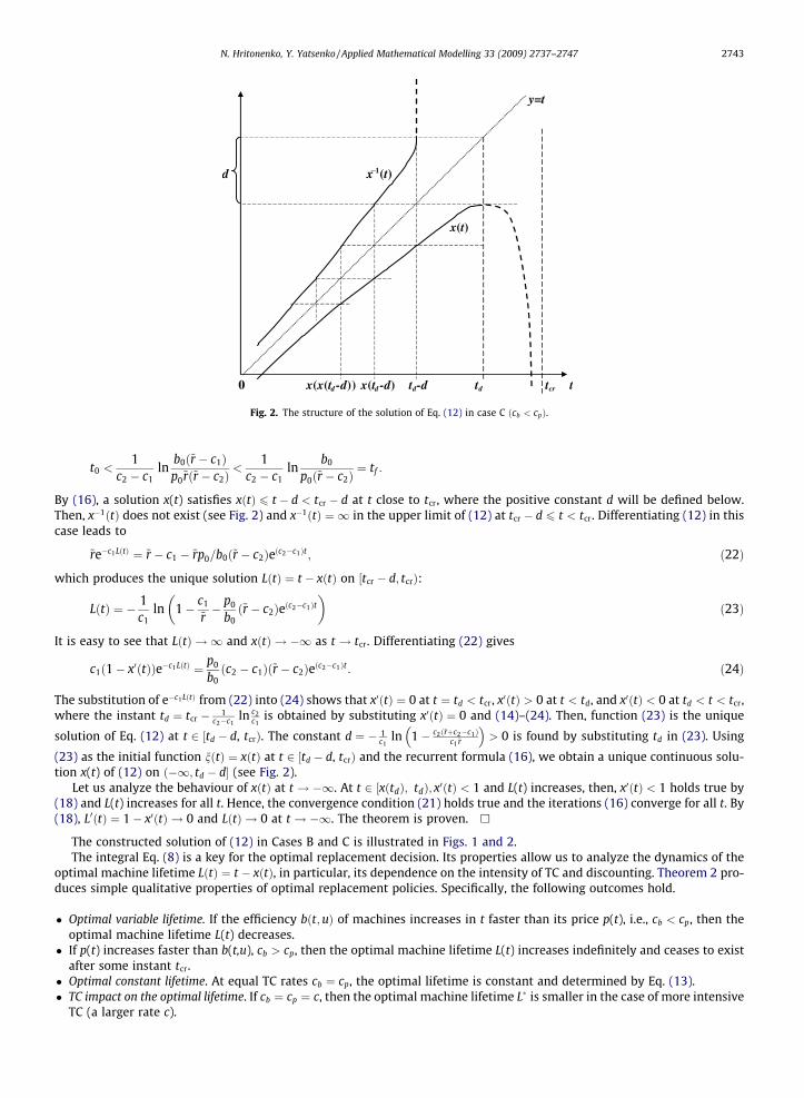
d x (t)1

x(t)

0 x(x(td -d)) x(td -d) td-d td tcr t

y=t

_

Fig. 2. The structure of the solution of Eq. (12) in case C ðcb < cpÞ.

N. Hritonenko, Y. Yatsenko / Applied Mathematical Modelling 33 (2009) 2737–2747 2743

t0 <1

c2 � c1ln

b0ð~r � c1Þp0~rð~r � c2Þ

<1

c2 � c1ln

b0

p0ð~r � c2Þ¼ tf :

By (16), a solution x(t) satisfies xðtÞ 6 t � d < tcr � d at t close to tcr, where the positive constant d will be defined below.Then, x�1ðtÞ does not exist (see Fig. 2) and x�1ðtÞ ¼ 1 in the upper limit of (12) at tcr � d 6 t < tcr. Differentiating (12) in thiscase leads to

~re�c1LðtÞ ¼ ~r � c1 � ~rp0=b0ð~r � c2Þeðc2�c1Þt ; ð22Þ

which produces the unique solution LðtÞ ¼ t � xðtÞ on ½tcr � d; tcrÞ:

LðtÞ ¼ � 1c1

ln 1� c1

~r� p0

b0ð~r � c2Þeðc2�c1Þt

� �ð23Þ

It is easy to see that LðtÞ ! 1 and xðtÞ ! �1 as t ! tcr. Differentiating (22) gives

c1ð1� x0ðtÞÞe�c1LðtÞ ¼ p0

b0ðc2 � c1Þð~r � c2Þeðc2�c1Þt: ð24Þ

The substitution of e�c1LðtÞ from (22) into (24) shows that x0ðtÞ ¼ 0 at t ¼ td < tcr, x0ðtÞ > 0 at t < td, and x0ðtÞ < 0 at td < t < tcr,where the instant td ¼ tcr � 1

c2�c1ln c2

c1is obtained by substituting x0ðtÞ ¼ 0 and (14)–(24). Then, function (23) is the unique

solution of Eq. (12) at t 2 ½td � d, tcrÞ. The constant d ¼ � 1c1

ln 1� c2ð~rþc2�c1Þc1~r

> 0 is found by substituting td in (23). Using

(23) as the initial function nðtÞ ¼ xðtÞ at t 2 ½td � d, tcrÞ and the recurrent formula (16), we obtain a unique continuous solu-tion x(t) of (12) on ð�1; td � d� (see Fig. 2).

Let us analyze the behaviour of xðtÞ at t ! �1. At t 2 ½xðtdÞ; tdÞ; x0ðtÞ < 1 and L(t) increases, then, x0ðtÞ < 1 holds true by(18) and L(t) increases for all t. Hence, the convergence condition (21) holds true and the iterations (16) converge for all t. By(18), L0ðtÞ ¼ 1� x0ðtÞ ! 0 and LðtÞ ! 0 at t ! �1. The theorem is proven. h

The constructed solution of (12) in Cases B and C is illustrated in Figs. 1 and 2.The integral Eq. (8) is a key for the optimal replacement decision. Its properties allow us to analyze the dynamics of the

optimal machine lifetime LðtÞ ¼ t � xðtÞ, in particular, its dependence on the intensity of TC and discounting. Theorem 2 pro-duces simple qualitative properties of optimal replacement policies. Specifically, the following outcomes hold.

� Optimal variable lifetime. If the efficiency bðt;uÞ of machines increases in t faster than its price p(t), i.e., cb < cp, then theoptimal machine lifetime L(t) decreases.

� If p(t) increases faster than b(t,u), cb > cp, then the optimal machine lifetime L(t) increases indefinitely and ceases to existafter some instant tcr.

� Optimal constant lifetime. At equal TC rates cb ¼ cp, the optimal lifetime is constant and determined by Eq. (13).� TC impact on the optimal lifetime. If cb ¼ cp ¼ c, then the optimal machine lifetime L� is smaller in the case of more intensive

TC (a larger rate c).

2744 N. Hritonenko, Y. Yatsenko / Applied Mathematical Modelling 33 (2009) 2737–2747

4. Numeric simulation

At our knowledge, there are no results on the numeric solution of integral equations of type (8) in literature. This paper isthe first attempt to formalize corresponding algorithms. We construct algorithms for solving Eq. (8) on finite and infiniteintervals. The first problem is an initial problem for the delay Eq. (8) with a given ‘‘initial function”. The second problem esti-mates the unique solution on the infinite interval ½t0;1Þ (if it exists, see Theorem 1) without an initial function.

4.1. Approximate algorithms

We will consider numeric solution of Eq. (8) in a more general situation than the exponential case (10). The only neces-sary assumption is the strict monotonicity of b(t,u) in t (i.e., the presence of TC). The functions p(t) and b(t,u) are assumed tobe continuously differentiable. We construct algorithms for solving the initial problem for Eq. (8) (Problem A) and for findinga unique infinite interval solution (Problem B). At the same time, Problem A is an auxiliary step for Problem B.

4.1.1. The initial problem AThe problem consists of finding a solution x(t) of the delay Eq. (8) on ½t1; t0Þ; t1 < t0, or ½t0; t1Þ, t1 > t0, at the given initial

monotonic function xðtÞ ¼ nðtÞ < t at t 2 ½t0; x�1ðt0Þ�. A general numeric approach to initial problems for delay equations isthe method of steps. It allows computing exact solutions of constant delay equations and has been recently developed forsolving the equations with variable delay and the functional delay differential equations with state dependent delays (itis known as the ‘‘standard approach” in [30,31]). Comparing to the case of constant delay equations, the novelty of Eq. (8)is that the length of the initial interval ½t0; n

�1ðt0Þ� itself depends on the initial function.Applying the method of steps to problem A is straightforward. The algorithm is based on the recurrent formula

bðt; tÞ � bðxðtÞ; tÞ ¼Z x�1ðtÞ

te�rðu�tÞ obðt; uÞ

otduþ rpðtÞ � p0ðtÞ; ð25Þ

obtained from (6). The only nonstandard step is to invert the implicit function b(x,t) in x for each fixed t (for backward solu-tion) or

R xt f ðt;uÞdu (for forward solution), which can be done using a polynomial interpolation.

For definiteness, let us assume that t1 < t0 (backward solution) and the initial function xðtÞ ¼ nðtÞ, t 2 ½t0; x�1ðt0Þ�, satisfies(8) at t ¼ t0. Then, by the definition of the inverse, the function x�1ðtÞ is known at t 2 ½xðt0Þ; t0� and the inversion of b(x,t) informula (25) produces the solution xðtÞ < t of (8) on the first-step interval ½xðt0Þ; t0�. In a similar manner, we obtain x(t) on thesecond-step interval ½xðxðt0ÞÞ; xðt0Þ�, and so on. If x(t) becomes non-monotonic at some point t0, then the inverse x�1ðt0Þ doesnot exist at the point t ¼ xðt0Þ of the next step interval and the algorithm stops after finding the solution x(t) on ½xðt0Þ; t0Þ.

The dynamics of the constructed solution x(t) heavily depends on the given functions n, p, and q. In the general case, x(t)has discontinuities at the instants xkðt0Þ, k = 0, ±1, ±2, ±3, . . . (unless the function n is specially adjusted). Also, x(t) may havediscontinuities at instants, where the derivatives of p and b in (25) possess jumps. As shown in [31], the presence of discon-tinuity points leads to serious challenges in solving state-dependent delay equations, which are out of our scope. Instead, wefocus on solving Eq. (8) on an infinite interval. By Theorem 1, the Eq. (8) has the unique solution ~x on an infinite interval, atleast, for exponential b and p. Therefore, the above constructed solution x(t) of Problem A may not exist in a general case(unless the initial function nðtÞ is a part of the unique solution ~x). The problem of finding the unique solution ~x is importantfor applications and is considered below.

4.1.2. The asymptotic problem Bconsists of finding (or, at least, estimating) the solution x(t) of Eq. (8) on the infinite interval ½t0;1Þ. In practice, this prob-

lem needs to be solved on a finite interval ½t0; t1� in the case when the given functions p and b are known on ½t0; t1� only (seean example in Section 4.2). Then, the additional assumption is made that the solution dynamics remains similar at t > t1.

The algorithm for the asymptotic problem B includes two steps:

Step 1. Constructing a proper initial function xðtÞ ¼ nðtÞ, t 2 ½xðt1Þ; t1�.Step 2. Applying the recurrent formula (25) to find x(t) on ½t0; xðt1Þ�.

During Step 1, an initial function xðtÞ ¼ nðtÞ needs to be constructed on ½xðt1Þ; t1�, such that (8) is satisfied and x(t) is con-tinuous at point t̂ ¼ xðt1Þ. One can see that it can be done in a non-unique manner. We implement this step by choosing thelinear

nðtÞ ¼ at � Lþ ð1� aÞt1 on ½nðt1Þ; t1�; ð26Þ

that depends on two parameters a and L ¼ t1 � nðt1Þ. If oqðt1 ;t1Þot > p0ðt1Þ, we select an initial value a > 1, otherwise 0 < a < 1.

Substituting n as x into (8), we obtain the equation rða; LÞ ¼ 0,

Uða; LÞ ¼Z t1

t1�Le�ru½bðt1 � L;uÞ � bðt1 � L� aðt1 � uÞ;uÞ�du� e�rðt1�LÞpðt1 � LÞ: ð27Þ

N. Hritonenko, Y. Yatsenko / Applied Mathematical Modelling 33 (2009) 2737–2747 2745

At the given a, we find the unique L > 0 and the point t̂ ¼ nðt1Þ ¼ t1 � L from (27). The uniqueness of L, follows from the factthat rða;0Þ < 0 and or=oL > 0.

Next, we find x(t) at t 6 t̂ close to t̂ from the recurrent formula (25). In a general case, xð̂tÞ differs from nð̂tÞ. If xð̂tÞ < nð̂tÞ,then we slightly decrease a in (26), which increases L obtained from (27) and decreases nð̂tÞ. Otherwise, we decrease a.Applying any numeric technique for solving a single nonlinear equation (e.g., bisection algorithm) and repeating the processof finding L and t̂ and calculating xð̂tÞ from (25), we get xð̂tÞ � nð̂tÞ. The corresponding values a and L deliver the initial func-tion (26) continuous at t̂ ¼ nðt1Þ. It completes Step 1.

Now we can implement Step 2, using the above constructed algorithm for Problem A. Iterating the recurrent formula (25)backward, we obtain a continuous function x(t) for ½t0; xðt1Þ�. When t1 � t0 becomes larger ðt1 � t0 !1Þ, the obtained x(t)tends to the unique solution ~xðtÞ of (11) on ½t0;1Þ (if it exists at the given p and b). This fact is established by the same argu-ments as in the proof of Theorem 2.

The constructed algorithms are implemented in Visual Basic/Excel and can be provided to all interested readers.

4.2. Numeric example

To approbate our algorithm on real economic data, let us consider modeling of the optimal equipment lifetime for a typ-ical US manufacturing plant. Then, the hypothesis about exponential technological change is commonly accepted[15,16,18,28,25] and we can use the assumptions (10). Under (10), the identification of Eq. (12) involves five parameters:the interest rater, the TC rates cb and cp, deterioration rate cd, and the initial productivity/cost ratio b0=p0. Following [1,6],we choose r ¼ 0:1 and cd ¼ 0. For the rest of the parameters, the identification is challenging. Various sources provide thebasic rate of technological change cb in the range of 3–17% for the years 1970–2000. We follow [32] and choosecb ¼ 0:08. The rate cp is even more difficult to find in literature and we provide a series of numeric experiments with differentcb. Finally, under given r, cb, cp, and cd, the identification parameter b0=p0 is adjusted to produce the current equipment life-time t1 � xðt1Þ of approximately 24 years at the initial modeling year t0 ¼ 0.

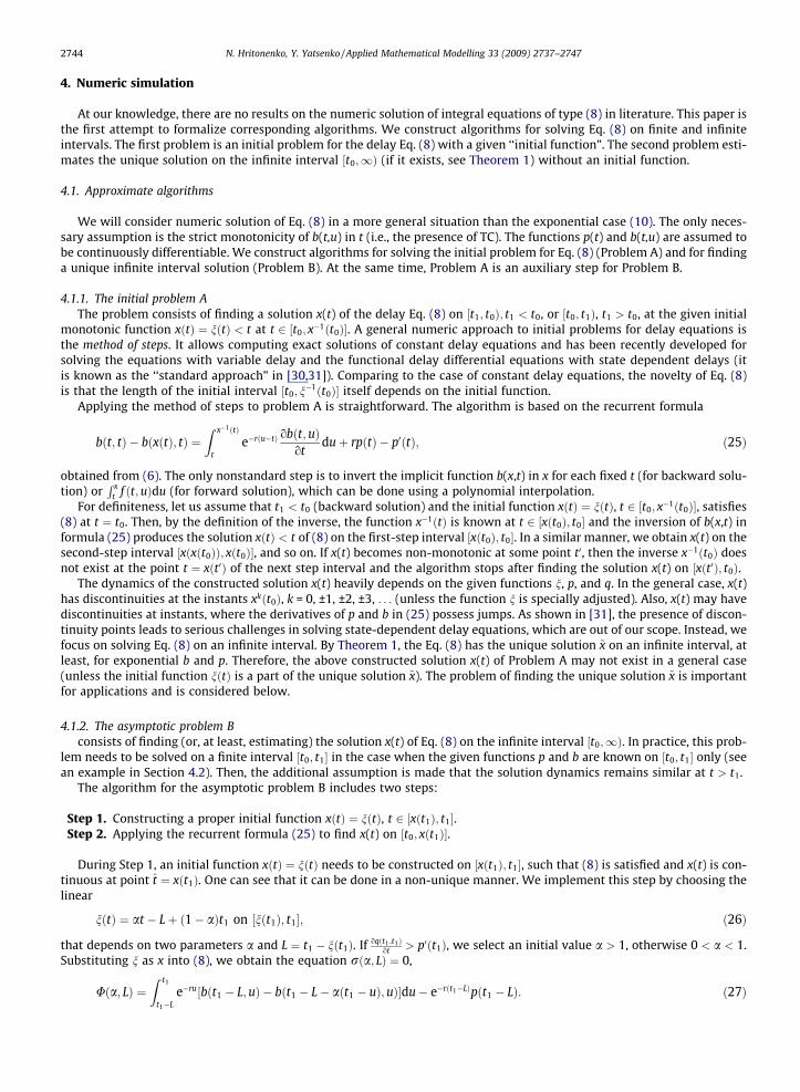
Next, we apply the algorithm of Section 4.1.2 for finding the unique infinite–horizon solution ~x at t0 < t < T . The basicsimulation run is shown in Fig. 3. The calculation parameters involve the horizon length T ¼ 100 years and the discretizationstep H ¼ 0:1. At the accepted parameter values, the algorithm does not require smaller steps and longer horizons [33]. Toanalyze the robustness of the algorithm, we have found the solution ~x of Eq. (12) for different algorithm parameters and val-ues of T. The results appear to be too close to show graphically. Some simulation results for different H of T are provided inthe Table 1. One can see that the 10% change of the horizon length T has no impact on the calculated value of the optimal

Variable lifetime at continuous TC b(t,u) and p(t)

0

10

20

30

40

50

60

70

80

90

100

0 10 20 30 40 50 60 70 80 90

Func

tions

x(t)

and

x-1

(t)

(years)

Fig. 3. Numeric solution of Eq. (12) at r ¼ 0:1, cb ¼ 0:08, and cp ¼ 0:05. The solid line is x, the dashed line is the inverse x�1 of x, and the straight linehighlights the symmetry between x and x�1.

Table 1Calculated results for different simulation periods and discretization steps

Horizon length T � t0 Step H Calculated Lðt0Þ

100 0.2 24.036100 0.1 24.10490 0.1 24.10250 0.1 23.523

Table 2Simulation results for different input data

Rate cb Rate cp Ratio b0=p0 Calculated a Calculated Lðt0Þ Calculated L(T)

0.08 0 0.5 1.11 22.3 0.40.08 0.01 0.5 1.03 24.10 0.690.08 0.05 1.1 1.07 22.83 3.870.08 0.08 1.65 1 23.10 23.020.08 0.085 1.7 0.76 24.34 39.550.08 0.087 1.78 0.62 23.14 46.86

Optimal lifetime for different TC rates

0

5

10

15

20

25

30

35

40

45

50

0 50 80 (years)

Opt

imal

L(t)

c=0.087

c=0.085

c=0.08

c=0.05c=0.01c=0

Fig. 4. The optimal machine lifetime LðtÞ ¼ t � xðtÞ for the efficiency rate cb ¼ 0:08 and different values of the capital cost rate c ¼ cp . The constant lifetime(solid line) corresponds to cp ¼ 0:08.

2746 N. Hritonenko, Y. Yatsenko / Applied Mathematical Modelling 33 (2009) 2737–2747

Lðt0Þ at the initial modeling year t0 ¼ 0, and even cutting T twice still causes only 0.3% relative change in Lðt0Þ. When weincrease T, the value of Lðt0Þ simply stays the same. So, as predicted theoretically in Theorem 2, the algorithm indeed deliversthe unique solution ~x (when the horizon length T � t0 is at least 4-5 times larger than max L(t)).

As follows from Theorem 1, the ratio cp=cb impacts the core dynamics of the optimal replacement. If the rates of TC in theoperating costs and machine price are different, cb ¼ cp in (12), then, by Theorem 2, the optimal machine lifetime decreasesat cb > cp and increases at cb < cp. The dynamics of the optimal replacement was analyzed for several scenarios cb > cp,cb ¼ cp, and cb < cp. The key input and output data are provided in the Table 2. Fig. 4 shows the variable optimal lifetimefor six different scenarios. The simulation results confirm the analytic conclusions of Theorem 2. In particular, at cb ¼ cp,the optimal lifetime appears to be constant (then it can be also found from Eq. (13)). Naturally, the sensitivity of solution~x to the difference cb � cp is higher when cb > cp (and ~x increases).

5. Conclusion

The paper develops new analytic and numeric techniques for finding optimal replacement policies. The techniques arebased on deriving and solving a nonlinear integral equation for the optimal lifetime of machines. The obtained theoretic re-sults lead to new insights into the qualitative dynamics of equipment replacement processes in manufacturing systems un-der the presence of technological change. In particular, the solution x of (1) exists on the infinite interval ð�1;1Þ only whenthe growth rates of the given bðt;uÞ and p(t) in t are the same (then x(t) = t-const). In more general cases, the solution x existsonly on the semi-infinite intervals ðtcr;1Þ or ð�1; tcr; Þ depending on the comparative dynamics of b and p (Figs. 1 and 2). Inthe alternative expense minimization problem [12], the optimal dynamics is qualitatively different and the solution exists onthe whole interval ð�1;1Þ. The numeric experiments on real industry data confirm the theoretical findings of the paper andthe robustness of the developed algorithm.

Acknowledgement

The authors are grateful to anonymous referees for their useful remarks.

References

[1] R. Boucekkine, M. Germain, O. Licandro, Replacement echoes in the vintage capital growth model, J. Econ. Theory 74 (1997) 333–348.[2] R. Boucekkine, O. Licandro, L. Puch, F. del Rio, Vintage capital and the dynamics of the AK model, J. Econ. Theory 120 (2005) 39–72.

N. Hritonenko, Y. Yatsenko / Applied Mathematical Modelling 33 (2009) 2737–2747 2747

[3] N. Hritonenko, Yu. Yatsenko, Integral-functional equations for optimal renovation problems, Optimization 36 (1996) 249–261.[4] N. Hritonenko, Yu. Yatsenko, Modeling and Optimization of the Lifetime of Technologies, Kluwer Academic Publishers, Dordrecht, 1996.[5] J.M. Malcomson, Replacement and the rental value of capital equipment subject to obsolescence, J. Econ. Theory 10 (1975) 24–41.[6] T. Cooley, J. Greenwood, M. Yorukoglu, The replacement problem, J. Monetary Econ. 40 (1997) 457–499.[7] O. Hilten, The optimal lifetime of capital equipment, J. Econ. Theory 55 (1991) 449–454.[8] N. Hritonenko, Yu. Yatsenko, Applied Mathematical Modeling of Engineering Problems, Kluwer Academic Publishers, Massachusetts, 2003.[9] N. Hritonenko, Yu. Yatsenko, Turnpike properties of optimal delay in integral dynamic models, J. Optim. Theory Appl. 127 (2005) 109–127.

[10] G. Silverberg, Modelling economic dynamics and technical change: Mathematical approaches to self-organization and evolution, in: Technical Changeand Economic Theory, Pinter, London, 1988, pp. 531–559.

[11] Yu. Yatsenko, Volterra integral equations with unknown delay time, Meth. Appl. Anal. 2 (1995) 408–419.[12] Yu. Yatsenko, N. Hritonenko, Optimization of the lifetime of capital equipment using integral models, J. Ind. Manage. Optim. 1 (2005) 415–432.[13] N. Hritonenko, Yu. Yatsenko, Optimization of financial and energy structure of productive capital, IMA J. Manage. Math. 17 (2006) 245–255.[14] Yu. Yatsenko, N. Hritonenko, Network economics and optimal replacement of age-structured IT capital, Mathematical Methods of Operations Research,

in press, doi:10.1007/s00186-006-0129-6.[15] J. Bean, J. Lohmann, J. Smith, Equipment replacement under technological change, Naval Res. Logist. 41 (1994) 117–128.[16] S. Chand, T. McClurg, J. Ward, A model for parallel machine replacement with capacity expansion, Eur. J. Operat. Res. 121 (2000) 519–531.[17] T. Cheevaprawatdomrong, R.L. Smith, A paradox in equipment replacement under technological improvement, Operat. Res. Lett. 31 (2003) 77–82.[18] J. Hartman, J. Rogers, Dynamic programming approaches for equipment replacement problems with continuous and discontinuous technological

change, IMA J. Manage. Math. 17 (2006) 143–158.[19] P. Jones, J. Zydiak, W. Hopp, Parallel machine replacement, Naval Res. Logist. 38 (1991) 351–365.[20] N. Karabakal, J. Lohmann, J. Bean, A Lagrangian algorithm for the parallel replacement problem with capital rationing constraints, Manage. Sci. 40

(1994) 305–319.[21] T. McClurg, S. Chand, A parallel machine replacement model, Naval Res. Logist. 49 (2002) 275–287.[22] S. Rajagopalan, M. Singh, T. Motron, Capacity expansion and replacement in growing markets with uncertain technological breakthroughs, Manage. Sci.

44 (1998) 12–30.[23] V. Makis, X. Jiang, Optimal replacement under partial observations, Math. Operat. Res. 28 (2003) 382–394.[24] V. Makis, X. Jiang, K. Cheng, Optimal preventive replacement under minimal repair and random repair cost, Math. Operat. Res. 25 (2000) 141–156.[25] J. Rogers, J. Hartman, Equipment replacement under continuous and discontinuous technological change, IMA J. Manage. Math. 16 (2005) 23–36.[26] G. Bethuyne, Optimal replacement under variable intensity of utilization and technological progress, Eng. Economist 43 (1998) 85–106.[27] P. Grinyer, The effects of technological change on the economic life of capital equipment, AIIE Trans. 5 (1973) 203–213.[28] E. Regnier, G. Sharp, C. Tovey, Replacement under ongoing technological progress, IIE Trans. 36 (2004) 497–508.[29] N. Hritonenko, Yu. Yatsenko, Optimal equipment replacement without paradoxes: a continuous analysis, Operat. Res. Lett. 35 (2007) 245–250.[30] A. Bellen, M. Zennaro, Numeric Methods for Delay Differential Equations, Oxford Science Publishers/Clarendon Press, Oxford, 2003.[31] F. Hartung, T. Krisztin, H.-O. Walther, J. Wu, Functional differential equations with state-dependent delay: theory and applications, Handbook of

Differential Equations, vol. 3, Elsevier, Amsterdam, 2006, pp. 435–545.[32] P. Sakellaris, D.J. Wilson, Quantifying embodied technological change, Rev. Econ. Dyn. 7 (2004) 1–26.[33] D. Aistrakhanov, Yu. Yatsenko, Approximate algorithm for modeling optimal renewal times in economic systems, Cybern. Syst. Anal. 28 (1992) 945–

949.