
Insights into machine learning:Data clustering and classification algorithms for astrophysical...
112
UNIVERSITY OF UDINE - ITALY Department of Mathematics and Computer Science Ph.D. Thesis INSIGHTS INTO MACHINE LEARNING: DATA CLUSTERING AND CLASSIFICATION ALGORITHMS FOR ASTROPHYSICAL EXPERIMENTS Supervisors: Candidate: Prof. ALESSANDRO DE ANGELIS PRAVEEN BOINEE Prof. GIAN LUCA FORESTI Doctorate of Philosophy in Computer Science XVIII cycle AY 2005/2006
-
Upload
independent -
Category
Documents
-
view
1 -
download
0
Transcript of Insights into machine learning:Data clustering and classification algorithms for astrophysical...

UNIVERSITY OF UDINE - ITALY
Department of Mathematics and Computer Science
Ph.D. Thesis
INSIGHTS INTO MACHINE
LEARNING: DATA CLUSTERING
AND CLASSIFICATION
ALGORITHMS FOR
ASTROPHYSICAL EXPERIMENTSSupervisors: Candidate:Prof. ALESSANDRO DE ANGELIS PRAVEEN BOINEE
Prof. GIAN LUCA FORESTI
Doctorate of Philosophy in Computer Science
XVIII cycle
AY 2005/2006

Abstract
Data analysis domain dealing with data exploration, clustering and classification isan important problem in many experiments of astrophysics, computer vision, bioin-formatics etc. The field of machine learning is increasingly becoming popular forperforming these tasks. In this thesis we deal with machine learning models based onunsupervised and supervised learning algorithms.
In unsupervised learning category, we deal with Self-Organizing Map (SOM) withnew kernel function. The data visualization/exploration and clustering capabilities ofSOM are experimented with real world data set problems for finding groups in data(cluster discovery) and visualisation of these clusters.
Next we discuss ensembling learning, a specialized technique within the supervisedlearning field. Ensemble learning algorithms such as AdaBoost and Bagging havebeen in active research and shown improvements in classification results for severalbenchmarking data sets. They grow multiple learner algorithms and combine themfor getting better accuracy results. Generally decision trees learning algorithm is usedas base classifiers to grow these ensembles. In this thesis we experiment with RandomForests (RF) and Back-Propagation Neural Networks (BPNN) as base classifiers formaking ensembles. Random Forests is a recent development in tree based classifiersand quickly proven to be one of the most important algorithms in the machine learningliterature. It has shown robust and improved results of classifications on standard datasets. We experiment the working of the ensembles of random forests on the standarddata sets available in University of California Irvine (UCI) data base. We comparethe original random forest algorithm with their ensemble counterparts and discussthe results.
Finally we deal the problem of image data classification with both supervised(ensemble) learning and unsupervised learning. We apply the algorithms developedin the thesis for this task. These image data are taken from the MAGIC telescopeexperiment, which collects the images of particle rays coming from the outer universe.We apply the ensembles of RF, BPNN for making a supervised classification of imagesand compare the performance results. Then we discuss a SOM system, developed formaking an automatic classification of images using the unsupervised techniques.

Acknowledgments
I sincerely thank Prof. Alessandro De Angelis for being so friendly guide and givingme lot of opportunities to see many beautiful places in Italy and Europe on myresearch work. He is a professor with different attitude who is always available,makes constructive remarks and makes things easy and fun. He is more a friend thana professor. Working with him was very motivating. Many thanks to Prof. GianLuca Foresti for his gigantic patience for listening to me and correcting me in manyways.
Special thanks to Udine University Chancellor Prof. Furio Honsell and BirlaScience Center Director Dr. Sidharth in India, because of whom the whole PhD ofmine has came into existence.
During my PhD I got lot of suggestions and help from many people. I take thisopportunity to thank them. Not in any particular order, I am very much greatful toMarco Frailis, Trieste Longo (Francesco), Abelardo Moralejo, Riccardo Giannitrapani,Fabrizio Barbarino, Oriana Mansutti , Barbara De Lotto, Massimo Pin, Alberto Forti,Reddy, Tiziano, Erica. I am greatful to Alessia Degano for helping me in many titanicburocratic issues.
I had a very special experience with my friends in the multinational - multi cul-tural, multi-lingual apartment. Many many thanks to my very special spain friendsMaria, Cristina, Edurne (for being so beautiful and making me so mad!), Andrea,Javier, Carlos.
Also I am thankful to other Indian students who are also fighting with their PhD’s.My friendship with Subbu has gone upto Mt.Blanc levels especially in the last monthsof my work. Also I am thankful to Reddy, Vijay, Rekha and beautiful Nirmala.
Many thanks to my family who were always with me both in the happy and toughtimes.
Last but not least a very special acknowledgment to GOOGLE without which itis almost impossible to do this job.


Contents
Introduction vii
1 Machine Learning System 11.1 System Design . . . . . . . . . . . . . . . . . . . . . . . . . . . . . . . 21.2 Learning modes . . . . . . . . . . . . . . . . . . . . . . . . . . . . . . . 51.3 Some learning algorithms . . . . . . . . . . . . . . . . . . . . . . . . . 7
1.3.1 Back-Propagation Neural Network (BPNN) . . . . . . . . . . . 71.3.2 k-nearest neighbors . . . . . . . . . . . . . . . . . . . . . . . . . 101.3.3 Decision Trees . . . . . . . . . . . . . . . . . . . . . . . . . . . 111.3.4 Support vector machines . . . . . . . . . . . . . . . . . . . . . . 12
2 Unsupervised Learning 152.1 Introduction . . . . . . . . . . . . . . . . . . . . . . . . . . . . . . . . . 152.2 Cluster Analysis . . . . . . . . . . . . . . . . . . . . . . . . . . . . . . 162.3 Cluster distance measures . . . . . . . . . . . . . . . . . . . . . . . . . 17
2.3.1 Proximity measures . . . . . . . . . . . . . . . . . . . . . . . . 172.3.2 Dissimilarities Based on Attributes . . . . . . . . . . . . . . . . 172.3.3 Object Dissimilarity . . . . . . . . . . . . . . . . . . . . . . . . 18
2.4 Clustering Algorithms . . . . . . . . . . . . . . . . . . . . . . . . . . . 19
3 Self-Organizing Maps 233.1 Introduction . . . . . . . . . . . . . . . . . . . . . . . . . . . . . . . . . 233.2 Algorithm . . . . . . . . . . . . . . . . . . . . . . . . . . . . . . . . . . 253.3 SOM as clustering technique . . . . . . . . . . . . . . . . . . . . . . . 273.4 SOM as visualization technique . . . . . . . . . . . . . . . . . . . . . . 30
3.4.1 U-matrix . . . . . . . . . . . . . . . . . . . . . . . . . . . . . . 313.4.2 Component plane visualisation . . . . . . . . . . . . . . . . . . 33
3.5 Case study on Astrophysical experiment: GRB Data Analysis . . . . . 34
4 Ensemble Learning 394.1 Introduction . . . . . . . . . . . . . . . . . . . . . . . . . . . . . . . . . 394.2 Ensemble Mechanics . . . . . . . . . . . . . . . . . . . . . . . . . . . . 414.3 Methods for constructing the ensembles . . . . . . . . . . . . . . . . . 43
4.3.1 Bagging . . . . . . . . . . . . . . . . . . . . . . . . . . . . . . . 444.3.2 Boosting . . . . . . . . . . . . . . . . . . . . . . . . . . . . . . . 454.3.3 Other techniques . . . . . . . . . . . . . . . . . . . . . . . . . . 49
ii Contents
5 Meta Random Forests 515.1 Introduction . . . . . . . . . . . . . . . . . . . . . . . . . . . . . . . . . 515.2 Random Forests . . . . . . . . . . . . . . . . . . . . . . . . . . . . . . 525.3 Error convergence in random forests . . . . . . . . . . . . . . . . . . . 555.4 Bagged Random Forests . . . . . . . . . . . . . . . . . . . . . . . . . . 565.5 Boosted Random Forests . . . . . . . . . . . . . . . . . . . . . . . . . . 575.6 Experiments on UCI data sets . . . . . . . . . . . . . . . . . . . . . . . 585.7 Discussion . . . . . . . . . . . . . . . . . . . . . . . . . . . . . . . . . . 60
6 MAGIC and its image classification 656.1 MAGIC Infrastructure . . . . . . . . . . . . . . . . . . . . . . . . . . . 666.2 Image collection in MAGIC . . . . . . . . . . . . . . . . . . . . . . . . 676.3 Image processing in MAGIC . . . . . . . . . . . . . . . . . . . . . . . . 686.4 Supervised classification . . . . . . . . . . . . . . . . . . . . . . . . . . 70
6.4.1 Random forests and its ensembles . . . . . . . . . . . . . . . . 716.4.2 BPNN and its ensembles . . . . . . . . . . . . . . . . . . . . . . 726.4.3 Classification results . . . . . . . . . . . . . . . . . . . . . . . . 746.4.4 Experiments with R.K. Bock et.al Monte-carlo data sets . . . . 75
6.5 Unsupervised classification . . . . . . . . . . . . . . . . . . . . . . . . . 76
Conclusions 85
Bibliography 87
List of Figures
1.1 Tabular representation of a data set . . . . . . . . . . . . . . . . . . . 21.2 Model for Machine learning System . . . . . . . . . . . . . . . . . . . 31.3 Backpropagation neural network architecture. . . . . . . . . . . . . . . 81.4 A decision tree with the tests on attributes X and Y . . . . . . . . . . 111.5 Linear separation problem with SVM . . . . . . . . . . . . . . . . . . 13
2.1 Interesting clusters may exist at several levels. In addition to A, B andC, also the cluster D, which is a combination of A and B, is interesting. 20
3.1 : Discrete neighborhoods (size 0, 1 and 2) of the centermost unit:a) hexagonal lattice, b) rectangular lattice. The innermost polygoncorresponds to 0-neighbourhood, the second to the 1-neighbourhoodand the biggest to the 2-neighbourhood . . . . . . . . . . . . . . . . . 24
3.2 Different map shapes. The default shape (a), and two shapes wherethe map topology accommodates circular data: cylinder (b) and toroid(c). . . . . . . . . . . . . . . . . . . . . . . . . . . . . . . . . . . . . . . 24
3.3 Updating the best matching unit (BMU) and its neighbors towardsthe input sample with x. The solid and dashed lines correspond tosituation before and after updating, respectively . . . . . . . . . . . . 26
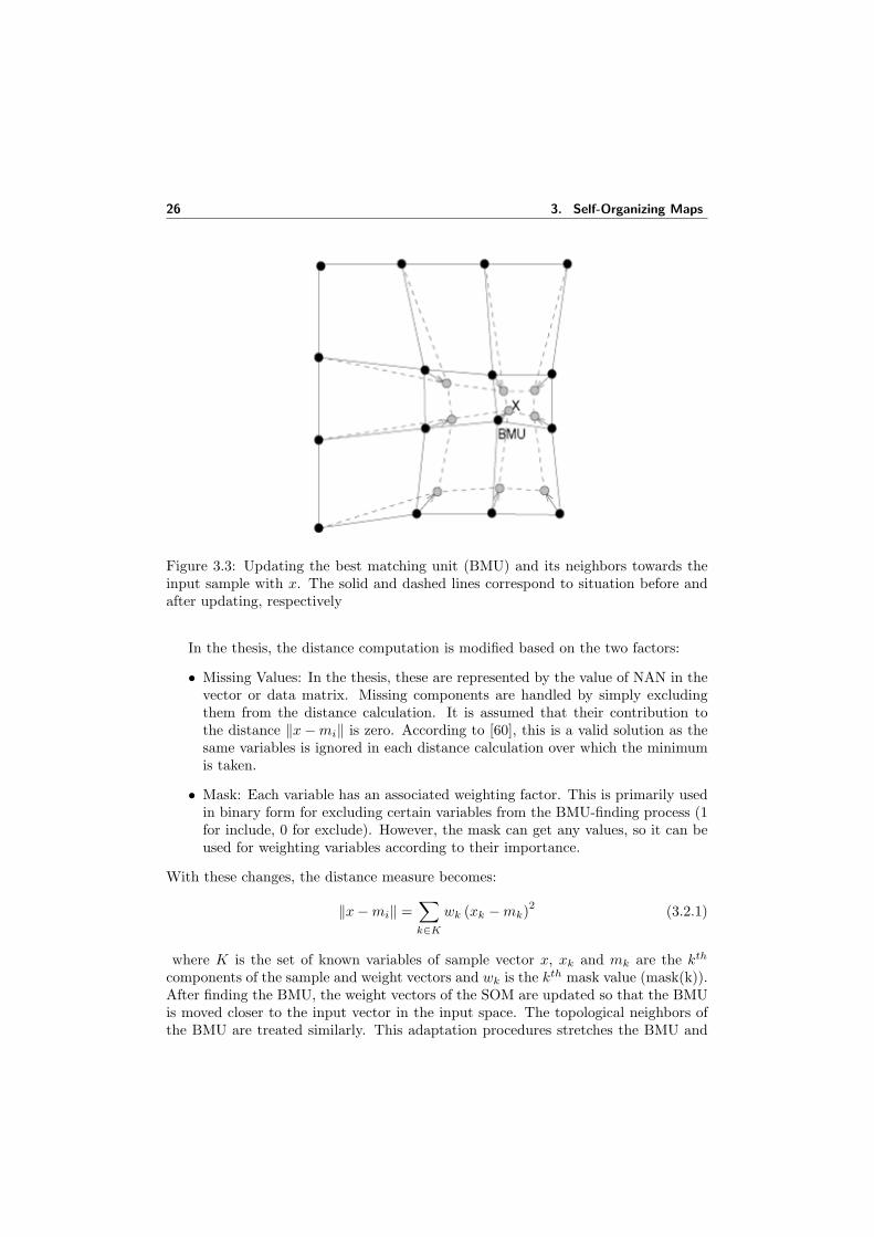
3.4 Different neighborhood functions. From the left ’bubble’ hci (t) =1 (σt − dci), ’gaussian’ hci (t) = e−d2
ci/2σ2t , ’cut-gauss’ hci (t) = e−d2
ci/2σ2t 1 (σt − dci),
and ’ep’ hci (t) = max
0, 1− (σt − dci)2
, dci = ‖rc − ri‖ is the dis-tance between map units c and i on the map grid and 1 (x) is the stepfunction: 1 (x) = 0 if x < 0 and 1 (x) = 1 if x ≥ 0. The top row showsthe function in 1-dimensional and the bottom row on a 2-dimensionalmap grid. The neighborhood radius used is σt = 2. . . . . . . . . . . . 27
3.5 Different learning rate functions: ′linear′ (solid line) α (t) = α0 (1− t/T ),′power′ (dot-dashed) α (t) = α0 (0.005/α0)
t/T and ′inv′ (dashed) α (t) =α0/ (1 + 100t/T ), where T is the training length and α0 is the initiallearning rate. . . . . . . . . . . . . . . . . . . . . . . . . . . . . . . . . 28
3.6 Two side effects caused by the neighborhood function: (a) border effectand (b) interpolating units. The + are the training data, and theconnected grid of circles is the map. . . . . . . . . . . . . . . . . . . . 29
3.7 SOM classification of points in threed space . . . . . . . . . . . . . . . 313.8 Component planes for the data points in 3-D space . . . . . . . . . . . 323.9 SOM based system for GRB Data Analysis . . . . . . . . . . . . . . . 343.10 GRB Classification models . . . . . . . . . . . . . . . . . . . . . . . . . 373.11 Component plane distribution for BATSE data . . . . . . . . . . . . . 38
iv List of Figures
3.12 BATSE data classification: SOM with cut-gaussian kernel, the twogroups are visually distinct[blue color codes] with a well separatedboundary . . . . . . . . . . . . . . . . . . . . . . . . . . . . . . . . . . 38
4.1 The basic architecture of an ensemble. . . . . . . . . . . . . . . . . . . 404.2 Loss functions of the margin for binary classification. Zero-one misclas-
sification loss (solid line), log-likelihood loss (dashed line), exponentialloss (dotted line), squared error loss (dashed/dotted). . . . . . . . . . 47
5.1 Schematic of AdaBoost random forests. . . . . . . . . . . . . . . . . . 595.2 Performance of random forests as function of number of trees . . . . . 605.3 ROC Comparison for various UCI data sets . . . . . . . . . . . . . . . 635.4 Classification accuracies for RF and its ensembles for various UCI data
sets . . . . . . . . . . . . . . . . . . . . . . . . . . . . . . . . . . . . . . 64
6.1 The MAGIC telescope . . . . . . . . . . . . . . . . . . . . . . . . . . . 656.2 Schematic view of 17mφ MAGIC telescope [111] . . . . . . . . . . . . . 666.3 A simulated MAGIC Camera . . . . . . . . . . . . . . . . . . . . . . . 676.4 Images of various particles recorded on the simulated camera of the
magic. . . . . . . . . . . . . . . . . . . . . . . . . . . . . . . . . . . . . 686.5 Image parameters. (x, y) are coordinates in the original camera system.
(x0, y0) is a reference point, for example the source position or thecenter of the camera. . . . . . . . . . . . . . . . . . . . . . . . . . . . 69
6.6 Fundamental BPNN used for ensembling to perform image classifica-tion in MAGIC . . . . . . . . . . . . . . . . . . . . . . . . . . . . . . . 72
6.7 A bagged BPNN ensemble. The ensemble is built by using bootstrap re-sampling to generate multiple training sets which are then used to trainan ensemble of BPNNs. The predictions generated by each network areaveraged to generate more stable bagged ANN ensemble predictions. . 74
6.8 Alpha distributions . . . . . . . . . . . . . . . . . . . . . . . . . . . . . 806.9 ROC curves for BPNN and its ensembles . . . . . . . . . . . . . . . . 816.10 ROC curves for RF and its ensembles . . . . . . . . . . . . . . . . . . 816.11 Classifier performances study: Bock et.al classifications, ensemble clas-
sifiers used in this thesis . . . . . . . . . . . . . . . . . . . . . . . . . . 826.12 The SOM based system for automatic separation of gamma events from
background events . . . . . . . . . . . . . . . . . . . . . . . . . . . . . 836.13 Data distributions for image parameters in crab on data set. . . . . . . 836.14 Classification using SOM . . . . . . . . . . . . . . . . . . . . . . . . . 846.15 QE of various cluster distances . . . . . . . . . . . . . . . . . . . . . . 84

List of Tables
1 Data explosion centers [2] . . . . . . . . . . . . . . . . . . . . . . . . . viii
3.1 Important Attributes of BATSE catalog used in GRB classification byvarious experiments . . . . . . . . . . . . . . . . . . . . . . . . . . . . 35
4.1 The exponential, binomial negative log-likelihood and squared errorloss functions for boosting. The miss classification plots are in figure 4.2 46
4.2 Some ensemble techniques . . . . . . . . . . . . . . . . . . . . . . . . . 50
5.1 Description of UCI data sets . . . . . . . . . . . . . . . . . . . . . . . 595.2 The Classification results for Random Forests (RF), Bagged RF, Boosted
RF on various UCI data sets. ( Notations % for classification accuracy,MAE for Mean Absolute Error, ROC for ROC area) . . . . . . . . . . 61
6.1 Comparative study of 2 classifiers and their ensembles . . . . . . . . . 756.2 SOM clustering results for different S (Qk) . . . . . . . . . . . . . . . . 79

vi List of Tables
Introduction
Nature has designed us as an advanced neural- cognitive system to learn, recognizeand make decisions. The ease, with which we recognize a face [especially of an op-posite sex], learn and understand the spoken languages and several other daily lifedecision makings are astoundingly complex tasks. These are internally performed bya sophisticated coordination between brain, eye, ear, hands, legs etc. Humans learnfrom experience, by mistakes or successes. By human nature, it is quite natural thatwe seek to design and build systems that can also learn to perform these learning,recognition and decision making tasks.
The field of machine learning is concerned with designing machines to learn fromexperience, learn from examples to make decisions. It deals with the formalizationof human learning and decision making. Thus the aim of the machine learning isto automate the process of solving problems, and thereby machine learning is rivalto what humans have considered their domain. It has a long history in engineeringand science applications. It is quite interdisciplinary and has roots in many disci-plines ranging from statistics, biology, philosophy to computational theory, artificialintelligence, data mining, cognitive science etc. It is also used interchangeably aspattern recognition and is used to describe the wide range of problems such as recog-nition, classification, grouping of patterns. These problems are important in variety ofapplications such as Signal processing, Physics experiments, Computer vision, Bioin-formatics, Genomics, Remote sensing, Financial forecasting etc [1].
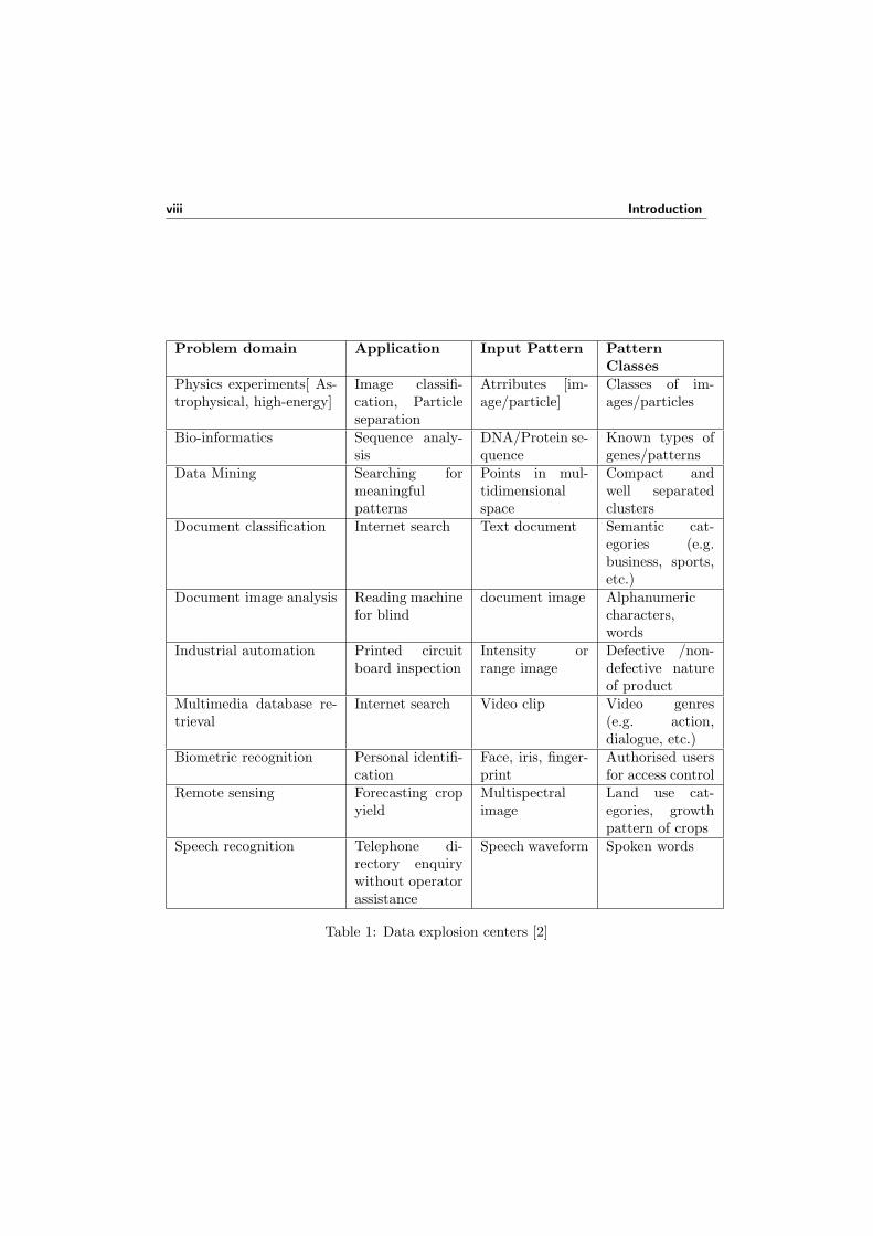
After seeing table 1 we can start thinking that our world is now a data-driven one.We are surrounded by very large collections of data from these applications, sometimeswith hundreds of millions of individual records stored in centralized data warehouses.This ever growing data requires to be classified or clustered to get analyzed. Machinelearning algorithms are proved to be powerful, comprehensive methods used for thispurpose. It is an important data mining step which assists in converting the datainto information that informs, instructs, answers, or otherwise aids understandingand decision-making. They learn by searching through an n-dimensional space ofa given data set to find an acceptable generalization to represent the analysis orknowledge from the data.
In recent years there has been a significant growth of methods in the machinelearning field for learning from raw data to classify/cluster them. The proliferation oflow-cost computers (for software implementation), low-cost sensors, communications,database technology (to collect and store data), and computer-literature applicationexperts who can pose “interesting” and “useful” application problems, all have con-tributed for its development.
viii Introduction
Problem domain Application Input Pattern PatternClasses
Physics experiments[ As-trophysical, high-energy]
Image classifi-cation, Particleseparation
Atrributes [im-age/particle]
Classes of im-ages/particles
Bio-informatics Sequence analy-sis
DNA/Protein se-quence
Known types ofgenes/patterns
Data Mining Searching formeaningfulpatterns
Points in mul-tidimensionalspace
Compact andwell separatedclusters
Document classification Internet search Text document Semantic cat-egories (e.g.business, sports,etc.)
Document image analysis Reading machinefor blind
document image Alphanumericcharacters,words
Industrial automation Printed circuitboard inspection
Intensity orrange image
Defective /non-defective natureof product
Multimedia database re-trieval
Internet search Video clip Video genres(e.g. action,dialogue, etc.)
Biometric recognition Personal identifi-cation
Face, iris, finger-print
Authorised usersfor access control
Remote sensing Forecasting cropyield
Multispectralimage
Land use cat-egories, growthpattern of crops
Speech recognition Telephone di-rectory enquirywithout operatorassistance
Speech waveform Spoken words
Table 1: Data explosion centers [2]

Introduction ix
Research Objectives
The research aims at developing new machine learning algorithms for data clusteringand classification. The developed algorithms are applied for data analysis tasks inMAGIC telescope experiment. It is an international effort with 17 institutes. Thetelescope collects image data at the rate of 432GB per day. At the end of year weacquired with 37800GB of data to be analyzed. The task is to classify the imagesbased on their properties. The work is performed by both supervised and unsupervisedclassification techniques. Also the algorithms are applied to Gamma ray burst datasets, UCI 1data sets.
The thesis is written in three parts. First we discuss Self-Organizing Maps (SOM)based on unsupervised learning. New kernel neighborhood functions are proposedand applied to the algorithm. A case study on Gamma Ray Burst (GRB) analysishas performed. In this experiment we use SOM for data exploration, visualsation andcluster discovery in the GRB data sets.
In the second part the work is carried out with supervised classification algorithms,especially of ensemble learning. The ensembles are applied to standard algorithmssuch as random forests and Back propagation neural nets. The ensembles of ran-dom forests are applied on standard UCI data sets to study the performance resultscompared to the original random forests algorithm.
Finally in the third part, we use the proposed algorithms for image classificationin MAGIC. The image classification has done with supervised techniques by usingthe ensembles of random forest and back propagation neural nets. Then we apply theself organizing map for the classification of images in an automatic way.
Thesis Organization
Chapter 1 discusses the machine learning system in general and introduces variouslearning modes and algorithms. Chapter 2 discusses the unsupervised learning givingspecial emphasis to partition clustering algorithms, the basis for SOM. Also variouscluster distance measurements are discussed . In chapter 3 Self-organizing maps arediscussed with various kernel neighborhood functions. The clustering (quantization)ability of SOM along with its visualization techniques such as U-matrix and compo-nent plane visualization are discussed. In this chapter we experiment with gammaray burst analysis using SOM. Next in chapter 4 ensemble learning techniques arediscussed. We especially concentrate on bagging and boosting techniques. In chapter5 we discuss tree classifier “Random forests” and discuss the making of its ensembleswith bagging and boosting. These algorithms are applied on UCI data sets. Theresults and comparative study are discussed with the original random forests algo-rithm. In chapter 6 MAGIC telescope project is introduced. We discuss the imagingtechnique used in MAGIC for image collection and image processing. We apply the
1University of California Irvine maintains the international machine learning database repository,an archive of over 100 databases used specifically for evaluating machine learning algorithms.

x Introduction
supervised and unsupervised algorithms that are proposed in the thesis for the imagedata classification for the MAGIC.
Thesis Contributions
- P. Boinee et.al, Meta Random Forests, In International Journal for Computa-tional Intelligence, Volume-II, pages: 138-147 (2005)
- P. Boinee et.al, Ensembling Classifiers: An application to image data classi-fication from chernkov telescope experiment. In Proceedings of InternationalConference on Signal Processing, Enformatika series, Prague (2005)
- P. Boinee et. al, Self-Organising Networks for Classification: developing Ap-plications to Science Analysis for Astroparticle Physics, CoRR cs.NE/0402014:(2004)
- P. Boinee et al., Neural Networks for MAGIC data analysis, In proceedings ofSixth International Conference on Foundations of Fundamental and Computa-tional Physics, Udine, Italy (2004)
- P. Boinee et al., Automatic Classification using Self-Organizing Neural Networksin Astrophysical Experiments, In Proc. of Science with the New Generation ofHigh Energy Gamma-ray Experiments, Perugia, Italy, (2003)

1Machine Learning System
Ever since computers were invented, we have wondered whether they might be madeto learn. If we could understand how to program them to learn-to improve automat-ically with experience-the impact would be dramatic. The field of machine learningis concerned with the question of how to construct computer programs that auto-matically improve with experience. According to [3], Machine learning is defined asa computer program which learns a problem from experience E with respect to someclass of tasks T and performance measure P . The performance at tasks in T , asmeasured by P , could improve with experience E.
We do not yet know how to make computers learn nearly as well as people learn.However, algorithms have been invented that are effective for certain types of learningtasks, and a theoretical understanding of learning is beginning to emerge. Manypractical computer programs have been developed to exhibit useful types of learning,and significant commercial applications have begun to appear.
It is possible to relate the problem of learning to the general notion of inference inclassical philosophy. Every predictive-learning process consists of two main phases:
• Learning or estimating unknown dependencies in the system from a given setof samples,
• Using estimated dependencies to predict new outputs for future input values ofthe system.
These two steps correspond to the two classical types of inference known as induc-tion (progressing from particular cases-training data-to a general mapping or model)and deduction (progressing from a general model and given input values to particularcases of output values). These processes may be described, formalized, and imple-mented using different learning methods [4].
A learning method (essentially an algorithm usually implemented in software)estimates an unknown mapping (dependency) between a system’s inputs and outputsfrom the available data set, namely, from known samples. Once such a dependency hasbeen accurately estimated, it can be used to predict the future outputs of the systemfrom the known input values. Learning from data has been traditionally explored insuch diverse fields as statistics, engineering, and computer science. In this chapter

2 1. Machine Learning System
Figure 1.1: Tabular representation of a data set
we discuss the design of the general machine learning system and introduce variouslearning modes and algorithms.
1.1 System Design
Machine learning system design have been inspired by the learning capabilities ofbiological systems and, in particular, those of humans. In fact, biological systemslearn to cope with the unknown, statistical nature of the environment in a data-driven fashion. Babies are not aware of the laws of mechanics when they learn howto walk, and most adults drive a car without knowledge of the underlying laws ofphysics. People are not born with such capabilities, but learn them through data-driven interaction with the environment.
Machine learning is also data-driven. The input for the system is taken from a database, which in general a collection of data sets. Each data set is again a collectionof data vectors also called as “patterns” representing a collection of measurementscalled as “features” of the learning problem. Thus a pattern can be viewed as arepresentation of set of n features in the form of a n−dimensional vector. Thesepatterns can have optional label, which tells the type of class, a pattern belongs to.Labeling of patterns depends on the type of learning used by the system in the trainingmode. Supervised learning algorithms uses labeled data sets as input, whereas theunsupervised learning algorithms directly operates on unlabeled patterns to adopt tothe underlying data distribution of the patterns.
The data set represents the standard model of structured data with the featuresuniformly measured over many cases. Usually the pattern vectors in the data setare represented in a tabular form, or in the form of a single relation (term used inrelational databases), where columns are features of objects stored in a table and rowsare values of these features for specific entities. A simplified graphical representationof a data set and its characteristics is given in Figure 1.1. Many different types offeatures (attributes or variables)-i.e., fields-in structured data records are common inmachine learning.
A machine learning system can be operated in two modes: training and testing
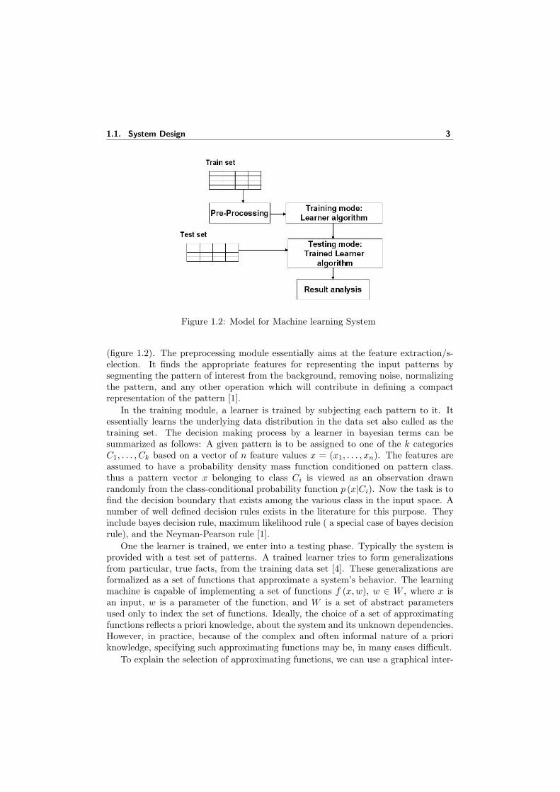
1.1. System Design 3
Figure 1.2: Model for Machine learning System
(figure 1.2). The preprocessing module essentially aims at the feature extraction/s-election. It finds the appropriate features for representing the input patterns bysegmenting the pattern of interest from the background, removing noise, normalizingthe pattern, and any other operation which will contribute in defining a compactrepresentation of the pattern [1].
In the training module, a learner is trained by subjecting each pattern to it. Itessentially learns the underlying data distribution in the data set also called as thetraining set. The decision making process by a learner in bayesian terms can besummarized as follows: A given pattern is to be assigned to one of the k categoriesC1, . . . , Ck based on a vector of n feature values x = (x1, . . . , xn). The features areassumed to have a probability density mass function conditioned on pattern class.thus a pattern vector x belonging to class Ci is viewed as an observation drawnrandomly from the class-conditional probability function p (x|Ci). Now the task is tofind the decision boundary that exists among the various class in the input space. Anumber of well defined decision rules exists in the literature for this purpose. Theyinclude bayes decision rule, maximum likelihood rule ( a special case of bayes decisionrule), and the Neyman-Pearson rule [1].
One the learner is trained, we enter into a testing phase. Typically the system isprovided with a test set of patterns. A trained learner tries to form generalizationsfrom particular, true facts, from the training data set [4]. These generalizations areformalized as a set of functions that approximate a system’s behavior. The learningmachine is capable of implementing a set of functions f (x, w), w ∈ W , where x isan input, w is a parameter of the function, and W is a set of abstract parametersused only to index the set of functions. Ideally, the choice of a set of approximatingfunctions reflects a priori knowledge, about the system and its unknown dependencies.However, in practice, because of the complex and often informal nature of a prioriknowledge, specifying such approximating functions may be, in many cases difficult.
To explain the selection of approximating functions, we can use a graphical inter-
4 1. Machine Learning System
pretation of the inductive-learning process. The task of inductive inference is this:given a collection of samples (xi, f (xi)), return a function h (x) that approximatesf (x). The function h (x) is often called a hypothesis.
The task of learning machine is to select a function from the set of functions,which best approximates the system’s responses. The learning machine is limited toobserving a finite number of samples n in order to make this selection. The finitenumber of samples, which we call a training data set, is denoted by (xi, yi), wherei = 1, . . . , n. The quality of an approximation produced by the learning machine ismeasured by the loss function L (y, f (x, w)) where
- y is the output produced by the system,
- x is a set of inputs,
- f (x, w) is the output produced by the learning machine for a selected approxi-mating function, and
- w is the set of parameters in the approximating functions.
L measures the difference between the outputs produced by the system yi and thatproduced by the learning machine f (xi, w) for every input point xi. By convention,the loss function is nonnegative, so that large positive values correspond to poorapproximation and small positive values close to zero show a good approximation.The expected value of the loss is called the risk functional R (w)
R (w) =∫ ∫
L (y, f (x,w)) p (x, y) dxdy
where L (y, f (x,w))is a loss function and p (x, y) is a probability distribution of sam-ples. The R (w) value, for a selected approximating functions, is dependent only on aset of parameters w. Inductive learning can be now defined as the process of estimat-ing the function f (x, wopt), which minimizes the risk functional R (w) over the set offunctions supported by the learning machine, using only the training data set, and notknowing the probability distribution p (x, y). With finite data, we cannot expect tofind f (x,wopt) exactly, so we denote f (x,wopt∗) as the estimate of parameters wopt∗
of the optimal solution wopt obtained with finite training data using some learningprocedure.
In a two-class classification problem, where the output of the system takes on onlytwo symbolic values, y = 0, 1, corresponding to the two classes, a commonly usedloss function measures the classification error.
L (y, f (x,w)) =
0 ify = f (x,w)1 ify 6= f (x,w)
Maximum accuracy will be obtained by minimizing the risk functional because, inthat case, the approximating function will describe the best set of given samples. Thetraining of the learning machine can be interpreted in terms of “inductive principle”.
1.2. Learning modes 5
An inductive principle is a general prescription for obtaining an estimate f (x, wopt∗)in the class of approximating functions from the available finite training data. Aninductive principle tells us what to do with the data, whereas the learning methodspecifies how to obtain an estimate. Hence a learning method or learning algorithm isa constructive implementation of an inductive principle. For a given inductive prin-ciple, there are many learning methods corresponding to a different set of functionsof a learning machine. The important issue here is to choose the candidate models(approximating functions of a learning machine) of the right complexity to describethe training data.
The result analysis is governed by many factors such as : learning mode, learneralgorithm, analysis requirements in the problem domain. For a supervised learningmode typically a learning algorithm outputs the probability of class assignment foreach pattern in the test row. These probabilities are inturn used to perform theresult analysis like classification accuracies rates (or error rates) of the learner. InUnsupervised learning mode the learner algorithm can be used to group the data setinto clusters. These clusters can be analyzed by various cluster analysis techniques(chapter 2). Also some specialized unsupervised learning algorithms such as Self-Organizing Maps (SOM) can be used for cluster visualization, data exploration tasks(Chapter 3).
1.2 Learning modes
In practice, the choice of a learner algorithm is a difficult task and driven by thelearning problem at the hand. The learning modes can be broadly classified in tothree types depending on the availability of a labeled training set.
Unsupervised learning
Unsupervised classification is a branch of machine learning designed to find naturalgroupings, or clusters, in multidimensional data, based on measured or perceived sim-ilarities among the patterns. It is used in a wide variety of fields under a wide varietyof names, the most common of which are cluster analysis. It has no explicit teacher,and the system forms [26] clusters or “natural groupings” of the input patterns. Inconceptual terms, we may think of the teacher as having knowledge of the environ-ment, with that knowledge being represented by a set of input-output examples. Theenvironment with its characteristics and model is, however, unknown to the learningsystem. It operates on unlabeled data sets to discover the natural groups in the dataset. “Natural” is always defined explicitly or implicitly in the clustering system itself,and given a particular set of patterns or cost function; different clustering algorithmslead to different clusters. Often the user will set the hypothesized number of differentclusters ahead of time. It is often suitable for real world problems as it is difficult toobtain the labeled data sets. We discuss more on unsupervised learning in chapter 2.
6 1. Machine Learning System
Supervised learning
Supervised learning is used to estimate an unknown dependency from known input-output samples. It assumes the existence of a teacher-fitness function or some otherexternal method of estimating the proposed model. The term “supervised” denotesthat the output values for training samples are known (i.e., provided by a “teacher”)[7]. In conceptual terms, we may think of the teacher as having knowledge of theenvironment, with that knowledge being represented by a set of input-output exam-ples. The environment with its characteristics and model is, however, unknown tothe learning system. The parameters of the learning system are adjusted under thecombined influence of the training samples and the error signal. The error signal isdefined as the difference between the desired response and the actual response of thelearning system.
Supervised learning algorithms work by searching through a space of possiblefunctions, called hypotheses, to find a function, h, that is the best approximationto the unknown function f . To determine which hypothesis h is best, a learningalgorithm can measure how well h matches f on the training data points, and it canalso assess how consistent h is with any available prior knowledge about the problem.
As a performance measure for the system, we may think in terms of the mean-square error or the sum of squared errors over the training samples. This functionmay be interpreted as a multidimensional error surface, with tile free parametersof the learning system as coordinate. Any learning operation under supervision isrepresented as a movement of a point on the error surface. For the system to improvethe performance over time and therefore learn from the teacher, the operating pointon an error surface has to move down successively toward a minimum of the surface[2]. An adequate set of input-output samples will move the operating point towardthe minimum, and a supervised learning system will be able to perform such tasks aspattern classification and function approximation. Different techniques support thiskind of learning, and some of them such as neural networks, support vector machines,decision trees etc. Supervised learning can be applied to many problems like signalprocessing, image classification, handwriting recognition, medical diagnosis, and part-of-speech tagging in language processing [3].
One of the most active areas of research in supervised learning has been to studymethods for constructing good ensembles of classifiers. Ensemble learning algorithmswork by running a “base learning algorithm” multiple times and forming a vote outof the resulting hypotheses [62]. This area is referred to by different names in theliterature - committees of learners, mixtures of experts, classifier ensembles, multipleclassifier systems. In general, an ensemble method is used to improve on the accuracyof a given learning algorithm. Practically it has proven that combining the predic-tions of ensembles of classifiers produces more accurate predictions than the singleclassifiers.
Ensembles or committee machines can be useful in many ways. The committeemight exhibit a test set performance unobtainable by an individual committee mem-ber on its own. The reason for this is that the errors of the individual committeemembers cancel out to some degree when their predictions are combined. The sur-
1.3. Some learning algorithms 7
prising discovery of this line of research is that even if the committee members weretrained on data derived from the same data set, the predictions of the individualcommittee members might be sufficiently different such that this combining processis beneficial in improving the classification accuracy. Ensemble learning is describedin more detail in chapter 4.
Reinforcement learning
The most typical way to train a classifier is to present an input, compute its tentativecategory label, and use the known target category label to improve the classifier. Inreinforcement learning or learning with a critic, no desired category signal is given;instead, the only teaching feedback is that the tentative category is right or wrong.This is analogous to a critic who merely states that something is right or wrong,but does not say specifically how it is wrong [26]. (Thus only binary feedback isgiven to the classifier; reinforcement learning also describes the case where a singlescalar signal, say some number between 0 and 1, is given by the teacher.) In patternclassification, it is most common that such reinforcement is binary either the tentativedecision is correct or it is not.
1.3 Some learning algorithms
In this section, we discuss some standard learning algorithms in the machine learningliterature. Here we mainly make the study based on learning modes, especially ofsupervised and unsupervised. In supervised we deal with 4 types of models. Firstwe discuss Back-propagation neural network (BPNN), a standard algorithm availableunder neural network category. In this thesis we develop the ensembles of BPNN forimage data classification for MAGIC telescope. Next we discuss k-nearest neighboralgorithm (K-NN) which performs an instant learning from pattern by pattern in thetraining set. Then we discuss decision trees a tree based classifier, which forms thebasis for making random forests a specialized trees based classifier. Finally we discusskernel based learners with support vector machines as an example.
Under unsupervised technique there exists a variety of algorithms like Self-OrganisingMaps (SOM) [33], Fixed weight competitive nets [15], Adaptive resonance theory mod-els [19]. Here we concentrate on SOM models that are discussed in detail in Chapter3.
1.3.1 Back-Propagation Neural Network (BPNN)
Neural networks has great advantages of adaptability, flexibility, and universal non-linear functional approximators [14]. One of the most popular algorithms in neuralnetworks category is the back-propagation algorithm [13]. The back-propagation al-gorithm performs supervised learning on a multilayer feed-forward neural network. Itis based on Perceptron algorithm introduced by Rosenblatt [11] that is consideredas one of the first machine learning algorithms. Perceptron algorithm express linear
8 1. Machine Learning System
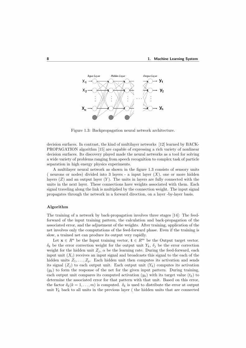
Figure 1.3: Backpropagation neural network architecture.
decision surfaces. In contrast, the kind of multilayer networks [12] learned by BACK-PROPAGATION algorithm [15] are capable of expressing a rich variety of nonlineardecision surfaces. Its discovery played made the neural networks as a tool for solvinga wide variety of problems ranging from speech recognition to complex task of particleseparation in high energy physics experiments.
A multilayer neural network as shown in the figure 1.3 consists of sensory units( neurons or nodes) divided into 3 layers - a input layer (X), one or more hiddenlayers (Z) and an output layer (Y ). The units in layers are fully connected with theunits in the next layer. These connections have weights associated with them. Eachsignal traveling along the link is multiplied by the connection weight. The input signalpropagates through the network in a forward direction, on a layer -by-layer basis.
Algorithm
The training of a network by back-propagation involves three stages [14]: The feed-forward of the input training pattern, the calculation and back-propagation of theassociated error, and the adjustment of the weights. After training, application of thenet involves only the computations of the feed-forward phase. Even if the training isslow, a trained net can produce its output very rapidly.
Let x ∈ Rn be the Input training vector, t ∈ Rm be the Output target vector.δk be the error correction weight for the output unit Yk, δj be the error correctionweight for the hidden unit Zj , α be the learning rate. During the feed-forward, eachinput unit (Xi) receives an input signal and broadcasts this signal to the each of thehidden units Z1, . . . , Zp. Each hidden unit then computes its activation and sendsits signal (Zj) to each output unit. Each output unit (Yk) computes its activation(yk) to form the response of the net for the given input pattern. During training,each output unit compares its computed activation (yk) with its target value (tk) todetermine the associated error for that pattern with that unit. Based on this error,the factor δk(k = 1, . . . ,m) is computed. δk is used to distribute the error at outputunit Yk back to all units in the previous layer ( the hidden units that are connected

1.3. Some learning algorithms 9
to Yk). It is also used later to update the weights between the hidden layer and theinput layer. Listing 1.1 shows the algorithm.
Listing 1.1: BPNN algorithm
Step 0 : I n t i a l i z e weights with smal l random va lue sStep 1 : While s topping cond i t i on i s f a l s e do s t ep s 2−9.Step 2 : for each t a r i n i n g pair , do s t ep s 3−8
FeedforwardStep 3 : Each input un i t (Xi, i = 1, . . . , n)
r e c e i v e s input s i g n a l xi and broadcas t st h i s s i g n a l to a l l un i t s to hidden l ay e r
Step 4 : Each hidden un i t (Zj , j = 1, . . . , p)sums i t s weighted input s i gna l s ,z − inj = v0j +
∑ni=1 xivij
app l i e s i t s a c t i v a t i o n func t i on tocompute i t s output s i g n a lzj = f (z − inj) ,and sends t h i s s i g n a l to a l l un i t sto the output un i t s .
Step 5 : Each output un i t (Yk, k = 1, . . . ,m)sums i t s weighted input s i gna l s ,y − ink = w0k +
∑pj=1 zjwjk
and app l i e s i t s a c t i v a t i o n func t i on to computei t s output s i gna l ,yk = f (y − ink) .
Back−propagat ion o f e r r o r :Step 6 : Each output un i t (Yk, k = 1, . . . ,m)
r e c e i v e s a t a r g e t pattern corre spond ing to the inputpattern , computes i t s e r r o r in fo rmat ion term ,δk = (tk − yk) f ′ (y − ink)c a l c u l a t e s i t s b i a s c o r e r c t i o n termused to update w 0k l a t e r ,∆w0k = αδk
and sends the δk to un i t s in the l ay e r below .Step 7 : Each hidden un i t (Zj , j = 1, . . . , p)
sums i t s d e l t a inputs from un i t s in l ay e r above .δ − inj =
∑mk=1 δkwjk
mu l t i p l i e s by the d e r i v a t i v e o f i t s a c t i v a t i o nfunc t i on to c a l c u l a t e i t s e r r o r in fo rmat ion term ,δj = δ − injf
′ (z − inj)c a l c u l a t e i t s weight c o r r e c t i o n termused to update vij l a t e r ,∆vij = αδjxi
and c a l c u l a t e s i t s b i a s c o r e r c t i o n termused to update v0j l a t e r ,
10 1. Machine Learning System
∆voj = αδj .Update weights and b i a s e s :Step 8 : Each output un i t (Yk, k = 1, . . . ,m)
updates i t s b i a s and weights (j = 0, . . . , p) :wjk (new) = wjk (old) + ∆wjk
Each hidden un i t (Zj , j = 1, . . . , p)updates i t s b i a s and weights (i = 0, . . . , n) :vij (new) = vij (old) + ∆vij
Step 9 : Test stopping cond i t i on .
After all of the δ factors that have been determined, the weights for all the layersare adjusted simultaneously [14]. The adjustment to the weight wjk from the hiddenunit Zj to the output unit Yk is based on the factor δk and the activation function zj ofthe hidden unit Zj . The adjustment to the weight vij form the input unit Xi to hiddenunit Zj is based on the factor δj and the activation xi of the input unit. An activationfunction for a backpropagation net should have several important characteristics: Itshould be continuous differentiable, and monotonically non-decreasing. Furthermore,for computational efficiency, it is desirable that its derivative be easy to compute.For the most commonly used activation functions, the value of the derivative can beexpressed in terms of the value of the function. Usually the function is expected tosaturate, i.e, approach finite maximum and minimum values asymptotically. In thisthesis the BPPNN network is developed using a hyperbolic tangent function, whichhas range of (-1, 1) and is defined as
tanh (x) =ex − e−x
ex + e−x
1.3.2 k-nearest neighbors
Instance-based learning methods such as nearest neighbor are conceptually straight-forward approaches to approximating real-valued or discrete-valued target functions.Learning in these algorithms consists of simply storing the presented training data[3]. When a new query instance is encountered, a set of similar related instances isretrieved from memory and used to classify the new query instance.
One important instance-based method is the k-nearest neighbors algorithm. Thisalgorithm assumes all instances correspond to points in the n-dimensional space Rn.The nearest neighbors of an instance are defined in terms of the standard euclideandistance. More precisely, let an arbitrary instance x be described by the feature vector(a1 (x) , . . . , an (x)), where ar (x) denotes the vaue of the rth atrribute of insyance x.Then the distance between two instances xi and xj is defined to be d (xi, xj) where
d (xi, xj) =√∑n
r=1 (ar (xi)− ar (xj))2
In nearest-neighbor learning the target function may be either discrete-valued orreal-valued. For learning discrete-valued target functions of the form f : Rn → V ,where V is the finite set v1, . . . , vs. The k-nearest neighbor algorithm returns f (xq)
1.3. Some learning algorithms 11
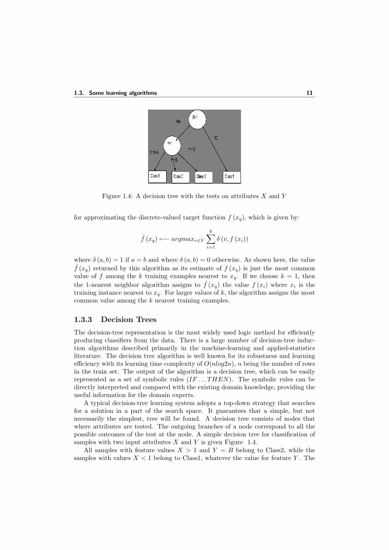
Figure 1.4: A decision tree with the tests on attributes X and Y
for approximating the discrete-valued target function f (xq), which is given by:
f (xq)←− argmaxv∈V
k∑i=1
δ (v, f (xi))
where δ (a, b) = 1 if a = b and where δ (a, b) = 0 otherwise. As shown here, the valuef (xq) returned by this algorithm as its estimate of f (xq) is just the most commonvalue of f among the k training examples nearest to xq. If we choose k = 1, thenthe 1-nearest neighbor algorithm assigns to f (xq) the value f (xi) where xi is thetraining instance nearest to xq. For larger values of k, the algorithm assigns the mostcommon value among the k nearest training examples.
1.3.3 Decision Trees
The decision-tree representation is the most widely used logic method for efficientlyproducing classifiers from the data. There is a large number of decision-tree induc-tion algorithms described primarily in the machine-learning and applied-statisticsliterature. The decision tree algorithm is well known for its robustness and learningefficiency with its learning time complexity of O(nlog2n), n being the number of rowsin the train set. The output of the algorithm is a decision tree, which can be easilyrepresented as a set of symbolic rules (IF . . . THEN). The symbolic rules can bedirectly interpreted and compared with the existing domain knowledge, providing theuseful information for the domain experts.
A typical decision-tree learning system adopts a top-down strategy that searchesfor a solution in a part of the search space. It guarantees that a simple, but notnecessarily the simplest, tree will be found. A decision tree consists of nodes thatwhere attributes are tested. The outgoing branches of a node correspond to all thepossible outcomes of the test at the node. A simple decision tree for classification ofsamples with two input attributes X and Y is given Figure 1.4.
All samples with feature values X > 1 and Y = B belong to Class2, while thesamples with values X < 1 belong to Class1, whatever the value for feature Y . The
12 1. Machine Learning System
samples, at a non leaf node in the tree structure, are thus partitioned along thebranches and each child node gets its corresponding subset of samples. Decision treesthat use univariate splits have a simple representational form, making it relativelyeasy for the user to understand the inferred model; at the same time, they representa restriction on the expressiveness of the model. In general, any restriction on aparticular tree representation can significantly restrict the functional form and thusthe approximation power of the model.
A well-known tree-growing algorithm for generating decision trees based on uni-variate splits is Quinlan’s ID3 with an extended version called C4.5, C5.0 [101].Greedy search methods, which involve growing and pruning decision-tree structures,are typically employed in these algorithms to explore the exponential space of possi-ble models and to remove unnecessary preconditions and duplication. They apply adivide and conquer strategy to construct the tree. The sets of instances are accom-panied by a set of properties. Each node in the tree performs a test on the values ofan attribute, and the leaves represent the class of an instance that satisfies the tests.The tree will return a ’yes’ or ’no’ decision when the sets of instances are tested onit. Rules can be derived from the tree by following a path from the root to a leafand using the nodes along the path as preconditions for the rule, to predict the classat the leaf. Random forests, an ensemble decision trees uses the trees that randomlychoose a subset of attributes at each mode. We discuss the random forest in chapter5 in more detail.
1.3.4 Support vector machines
SVMs are kernel based learning algorithms used in machine learning and computervision research communities. However, SVMs have two possible limitations in realworld applications. First, the training of SVMs is slow, especially for large datasets problems. Second, SVM training algorithms are complex, subtle, and sometimesdifficult to implement [17].
The basic training for SVMs involves finding a function which optimizes a boundon the generalization capability, i.e., performance on unseen data. We are guven Nobservations x(i) ∈ RL with associated labels y(i), i = 1, . . . , N . These set of trainingdata
(x(i), y(i)
)is linearly separable if there exists a hyperplane (wt, b) for which
the positive examples lie on one side and the negative examples on the other. Letus define the margin as twice the distance of the closest training example to thehyperplane (wt, b) (figure 1.5 (a)). The structural risk minimization principle [18]states that a hyperplane which classifies the training set accurately with the largestmargin will minimize a bound on the generalization error and will generalize best,regardless of the dimensionality of the input space.
Provided that all of the training examples are linearly separable, the goal is then tofind the optimal separating hyperplane (wt, b) in the sense of maximizing the margin.Let dw,b
(x(s)
)be the distance of the closest training example x(s) to a separating
hyperplane (wt, b):
dw,b
(x(s)
)=| wtx(s) + b |‖ w ‖
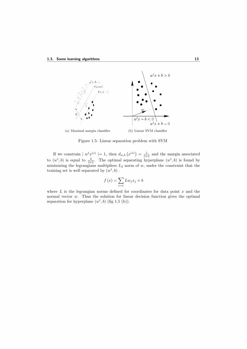
1.3. Some learning algorithms 13
(a) Maximal margin classifier (b) Linear SVM classifier
Figure 1.5: Linear separation problem with SVM
If we constrain | wtx(s) |= 1, then dw,b
(x(s)
)= 1
‖w‖ and the margin associatedto (wt, b) is equal to 2
‖w‖ . The optimal separating hyperplane (wt, b) is found byminimizing the legrangians multipliers L2 norm of w, under the constraint that thetraining set is well separated by (wt, b) .
f (x) =∑i=1
Lwjxj + b
where L is the legrangian norms defined for coordinates for data point x and thenormal vector w. Thus the solution for linear decision function gives the optimalseparation for hyperplane (wt, b) (fig 1.5 (b)).

14 1. Machine Learning System
2Unsupervised Learning
2.1 Introduction
Unsupervised learning refers to situations where the objective is to construct decisionboundaries based on unlabeled training data to find the natural groups or clustersthat exist in the data set[7]. Unsupervised classification or clustering is a very dif-ficult problem because data can reveal clusters with different shapes and sizes. Tocompound the problem further, the number of clusters in the data often depends onthe resolution with which we view the data.
In unsupervised learning a higher-order statistical model is learnt from a set ofexamples, with the aim of revealing hidden causes and density estimation. Appli-cations range from data visualization [21] to data mining and knowledge discovery[22]. These techniques are strongly related to the statistical field of cluster analysis,where over the years large number of clustering methods have been proposed [23] [24][25]. In cluster analysis observed data are organized into meaningful structures ortaxonomies. The objective is to sort samples into clusters or groups, so that the de-gree of association is strong between members of the same cluster and weak betweenmembers of different clusters. A fair amount of research has been done on clusteranalysis giving many ad hoc methods to search for these groupings, or clusters.
There are at least five basic reasons for interest in unsupervised Procedures. First,collecting and labeling a large set of sample patterns can be surprisingly costly. Forthe MAGIC telescope experiment discussed in chapter 6, particle image data collec-tion is virtually free, but accurately labeling the images of particles, i.e., marking theparticles with labels of gamma, hadrons, muons particle types is very expensive, timeconsuming and error pruned . If a classifier can be crudely designed on a small setof labeled samples, and then tuned up by allowing it to run without supervision ona large, unlabeled set, much time and trouble can be saved. Second, one might wishto proceed in the reverse direction: train with large amounts of (less expensive) unla-beled data, and only then use supervision to label the groupings found. This may beappropriate for large data mining applications where the contents of a large databaseare not known beforehand. Again this can be useful for the MAGIC telescope as wehave giga bytes of data to be classified. The possible way of working it out is to groupthe unlabeled data automatically by unsupervised technique, Self-Organizing Map

16 2. Unsupervised Learning
(SOM). The grouped data is then subjected to a supervised technique for identifyingthe labels. Third, in many applications the characteristics of the patterns can changeslowly with time, for example in automated food classification as the seasons change.If these changes can be tracked by a classifier running in an unsupervised mode, im-proved performance can be achieved. Fourth, we can use unsupervised methods to findfeatures that will then be useful for categorization. There are unsupervised methodsthat represent a form of data-dependent smart preprocessing or smart feature extrac-tion. Lastly, in the early stages of an investigation it may be valuable to gain someinsight into the nature or structure of the data. The discovery of distinct subclassesor similarities among patterns or of major departures from expected characteristicsmay suggest we significantly alter our approach to designing the classifier.
In this chapter we discuss some fundamental issues and state-of-art related tounsupervised learning. After discussing cluster analysis we describe the types ofclustering algorithms available in the literature with special emphasis on k-meansclustering, the basis for self-organizing map (SOM) discussed in next chapter.
2.2 Cluster Analysis
Cluster analysis is a very important and often required in real world problems. Thespeed, reliability, and consistency with which a clustering algorithm can organize largeamounts of data constitute overwhelming reasons to use it in applications such as datamining [2], information retrieval [9], image segmentation , signal processing [10]. Asa consequence, several clustering algorithms have been proposed in the literature andnew clustering algorithms continue to appear. Most of these algorithms are basedon a) iterative squared-error clustering or b) agglomerative hierarchical clustering.Hierarchical techniques organize data in a nested sequence of groups which can bedisplayed in the form of a dendogram or a tree. Squared-error partitional algorithmsattempt to obtain that partition which maximizes the between-cluster scatter.
It has a variety of goals. All relate to grouping or segmenting a collection ofobjects into subsets or clusters, such that those within each cluster are more closelyrelated to one another than objects assigned to different clusters. An object can bedescribed by a set of measurements, or by its relation to other objects. In addition,the goal is sometimes to arrange the clusters into a natural hierarchy. This involvessuccessively grouping the clusters themselves so that at each level of the hierarchy,clusters within the same group are more similar to each other than those in differentgroups. Cluster analysis is also used to form descriptive statistics to ascertain whetheror not the data consists of a set distinct subgroups, each group representing objectswith substantially different properties. This latter goal requires an assessment of thedegree of difference between the objects assigned to the respective clusters.
2.3. Cluster distance measures 17
2.3 Cluster distance measures
Central to all of the goals of cluster analysis algorithms is the notion of the degreeof similarity (or dissimilarity) between the individual objects being clustered. Aclustering method attempts to group the objects based on the definition of similaritysupplied to it. This can only come from subject matter under considerations [20]. Inthis section we discuss the variety of distance measures used in clustering algorithms.
2.3.1 Proximity measures
Sometimes the data is represented directly in terms of the proximity (alikeness oraffinity) between pairs of objects. These can be either similarities or dissimilarities(difference or lack of affinity). For example, in social science experiments, participantsare asked to judge by how much certain objects differ from one another. Dissimilari-ties can then be computed by averaging over the collection of such judgments. Thistype of data can be represented by an N × N matrix D, where N is the number ofobjects, and each element dii′ records the proximity between the ith and i′th objects.This matrix is then provided as input to the clustering algorithm. Most algorithmspresume a matrix of dissimilarities with non- negative entries and zero diagonal el-ements: dii = 0, i = 1, . . . , N . If the original data were collected as similarities, asuitable monotone-decreasing function can be used to convert them to dissimilarities.Also, most algorithms assume symmetric dissimilarity matrices, so if the original ma-trix D is not symmetric it must be replaced by
(D + DT
)/2. Subjectively judged
dissimilarities are seldom distances in the strict sense, since the triangle inequalitydii′ ≤ dik + di′k for all k ∈ 1, . . . , N does not hold. Thus, some algorithms thatassume distances cannot be used with such data.
2.3.2 Dissimilarities Based on Attributes
Most often we have measurements xij for patterns i = 1, . . . , N , on features j =1, . . . , p. Since most of the popular clustering algorithms take a dissimilarity matrix astheir input, we must first construct pairwise dissimilarities between the observations.In the most common case, we define a dissimilarity dj (xij , xi′j) between values of thejth variable, and then define
D (xi, x′i) =
p∑j=1
dj (xij , xi′j) (2.3.1)
as the dissimilarity between objects i and i′. By far the most common choice issquared distance
dj (xij , xi′j) = (xij − xi′j)2 (2.3.2)
However, other choices are possible, and can lead to potentially different results.For non quantitative attributes (e.g., categorical data), squared distance may not beappropriate. In addition, it is sometimes desirable to weigh attributes differently.Here we discuss alternatives in terms of the attribute type:
18 2. Unsupervised Learning
• Quantitative variables. Measurements of this type of features or variables orattributes are represented by continuous real-valued numbers. It is natural todefine the “error” between them as a monotone-increasing function of theirabsolute difference
d (xi, x′i) = l (| xi − x′i |) (2.3.3)
Besides squared error loss (xi − xi′)2, a common choice is the identity (absolute
error). The former places more emphasis on larger differences than smaller ones.Alternatively, clustering can be based on the correlation
ρ (xi, xi′) =
∑j (xij − xi) (xi′j − xi′)√∑
j (xij − xi)2∑
j (xi′j − xi′)2
(2.3.4)
with xi =∑
j xij/p. If the inputs are first standardized, then∑
j (xij − xi′j)2 =
2 (1− ρ (xi, xi′)) . Hence clustering based on correlation (similarity) is equivalentto that based on squared distance (dissimilarity).
• Ordinal variables: The values of this type of variable are often represented ascontiguous integers, and the realizable values are considered to be an orderedset. Examples are academic grades (A, B, C, D, F), degree of preference (can’tstand, dislike, OK, like, terrific). Rank data are a special kind of ordinal data.Error measures for ordinal variables are generally defined by replacing their Moriginal values with
i− 1/2M
, i = 1, . . . ,M (2.3.5)
in the prescribed order of their original values. They are then treated as quan-titative variables on this scale.
• Categorical variables: With unordered categorical (also called nominal) vari-ables, the degree-of-difference between pairs of values must be delineated ex-plicitly. If the variable assumes M distinct values, these can be arranged in asymmetric M ·M matrix with elements Lrr′ = Lr′r, Lrr = 0, Lrr′ ≥ 0. Themost common choices is Lrr′ = 1 for all r 6= r, while unequal losses can be usedto emphasize some errors more than others.
2.3.3 Object Dissimilarity
Next we define a procedure for combining the p-individual attribute dissimilaritiesdj (xij , xi′j) , j = 1, . . . , p into a single overall measure of dissimilarity D (xi, x
′i) be-
tween two objects or observations (xi, xi′) possessing the respective attribute values.This is nearly always done by means of a weighted average (convex combination)
D (xi, x′i) =
p∑j=1
wj .dj (xij , xi′j) (2.3.6)
2.4. Clustering Algorithms 19
Here wj is a weight assigned to the jth attribute regulating the relative influenceof that variable in determining the overall dissimilarity between objects. This choiceshould be based on subject matter considerations. If the goal is to discover naturalgroupings in the data, some attributes may exhibit more of a grouping tendency thanothers. Variables that are more relevant in separating the groups should be assigned ahigher influence in defining object dissimilarity. Giving all attributes equal influencein this case will tend to obscure the groups to the point where a clustering algorithmcannot uncover them.
Although simple generic prescriptions for choosing the individual attribute dissim-ilarities dj (xij , xi′j) and their weights wj can be comforting, there is no substitutefor careful thought in the context of each individual problem. Specifying an appropri-ate dissimilarity measure is far more important in obtaining success with clusteringthan choice of clustering algorithm. This aspect of the problem is emphasized less inthe clustering literature than the algorithms themselves, since it depends on domainknowledge specifics and is less amenable to general research. Finally, often obser-vations have missing values in one or more of the attributes. The most commonmethod of incorporating missing values in dissimilarity calculations as in equation2.3.6 is to omit each observation pair xij , xi′j having at least one value missing, whencomputing the dissimilarity between observations xi and x′i. This method can failin the circumstance when both observations have no measured values in common.In this case both observations could be deleted from the analysis. Alternatively, themissing values could be imputed using the mean or median of each attribute over thenon-missing data. For categorical variables, one could consider the value missing asjust another categorical value, if it were reasonable to consider two objects as beingsimilar if they both have missing values on the same variables.
2.4 Clustering Algorithms
Clustering algorithms divide, or partition, data into natural groups of objects. Bynatural it means that the objects in a cluster should be internally similar to eachother, but differ significantly from the objects in the other clusters. Most clusteringalgorithms produce crisp partitionings, where each data sample belongs to exactlyone cluster. To reflect the inherently vague nature of clusterings, there are also somealgorithms where each data object may belong to several clusters to a varying degree.Another way to deal with the complexity of real data sets is to construct a clusterhierarchy. Clustering may depend on the level of detail being observed, and thusa cluster hierarchy may, at least in principle, be better at revealing the inherentstructure of the data than a direct partitioning 2.4.
Thus clustering algorithms can be fundamentally divided into two types: hier-archical and partitional [24]. Hierarchical clustering algorithms find clusters one byone. The hierarchical methods can be further divided to agglomerative and divi-sive algorithms, corresponding to bottom-up and top-down strategies. Agglomerativeclustering algorithms merge clusters together one at a time to form a clustering treewhich finally consists of a single cluster, the whole data set. The algorithms consist

20 2. Unsupervised Learning
Figure 2.1: Interesting clusters may exist at several levels. In addition to A, B andC, also the cluster D, which is a combination of A and B, is interesting.
of the following steps, Listing 2.1:
Listing 2.1: hierarchical clustering
1 . i n i t i a l i z e : a s s i gn each vec to r to i t s own c l u s t e r , or usesome i n i t i a l p a r t i t i o n i n g provided by some other c l u s t e r i n g a lgor i thm2 . Compute d i s t an c e s d (Ci, Cj) between a l l c l u s t e r s3 . merge the two c l u s t e r s that are c l o s e s t to each other4 . return to s tep 2 un t i l the re i s only one c l u s t e r l e f t
The problem of partitional clustering can be formally stated as follows: Given Npatterns in a d-dimensional metric space, determine a partition of the patterns intok clusters, such that the patterns in a cluster are more similar to each other thanto patterns in different clusters [8]. Under partitional clustering we concentrate onK-means algorithm.
The K-means algorithm is intended for situations in which all variables are ofthe quantitative type, and squared Euclidean distance is chosen as the dissimilaritymeasure.
d (xi, xi′) =p∑
j=1
(xij − xi′j)2 =‖ xi − x′i ‖2 (2.4.1)
Since the goal is to assign close points to the same cluster, a natural loss (orenergy) function would be
W (C) =12
K∑k=1
∑C(i)=k
∑C(i′)=k
d (xi, x′i) (2.4.2)
The above equation characterizes the extent to which observations assigned to thesame cluster tend to be close to one another. The minimum value for the equationcan be obtained by assigning the N observations to the K clusters in such a waythat within each cluster the average dissimilarity of the observations from the clustermean, as defined by the points in that cluster, is minimized.
2.4. Clustering Algorithms 21
Listing 2.2: K-means clustering algorithm
1 . For a g iven c l u s t e r ass ignment C , the t o t a l c l u s t e r var i ancei s minimized with r e sp e c t to m1, . . . ,mK y i e l d i n gthe means o f the cu r r en t l y a s s i gned c l u s t e r s
2 . Given a cur rent s e t o f means m1, . . . ,mK , eqn 2 . 3 . 4i s minimized by a s s i gn i ng each obse rvat i on to the c l o s e s t c l u s t e r mean .That i s , C (i) = argmin1≤k≤K ‖ xi −mk ‖2
3 . F i r s t two s t ep s are i t e r a t e d un t i l the ass ignments do not change .
An iterative descent algorithm for solving
C∗ = minc
K∑k=1
∑C(i)=k
‖ xi − xk ‖2 (2.4.3)
can be obtained by noting that for any set of observations S
xS = argminm
∑i∈S
‖ xi −m ‖2 (2.4.4)
Hence we can obtain C∗ by solving the enlarged optimization problem
minC,mkK1
K∑k=1
∑C(i)=k
‖ xi −mk ‖2 (2.4.5)
This can be minimized by an alternating optimization procedure given by K-meansclustering algorithm in Listing 2.2. Each of steps 1 and 2 reduces the value of thecriterion (eqn 2.4.5, so that convergence is assured. However, the result may repre-sent a suboptimal local minimum. In addition one should start the algorithm withmany different random choices for the starting means, and choose the solution havingsmallest value of the objective function.
K-means algorithm can be extended to perform unsupervised learning using neuralnetworks. These networks will look for regularities, or trends in the input signals, andmake adaptations according to the function of the network. Even without being toldwhether it is right or wrong, the network still must have some information about howto organize itself. This information is built into the network topology and learningrules. Competition between processing elements could form a basis for learning.Training of competitive elements could amplify the responses of specific groups tospecific stimuli. As such, it would associate those groups with each other and witha specific appropriate response. Such a procedure was developed by Teuvo Kohonentermed as Self-Organizing Maps (SOM) neural networks, and was inspired by learningin biological systems [33].

22 2. Unsupervised Learning
3Self-Organizing Maps
3.1 Introduction
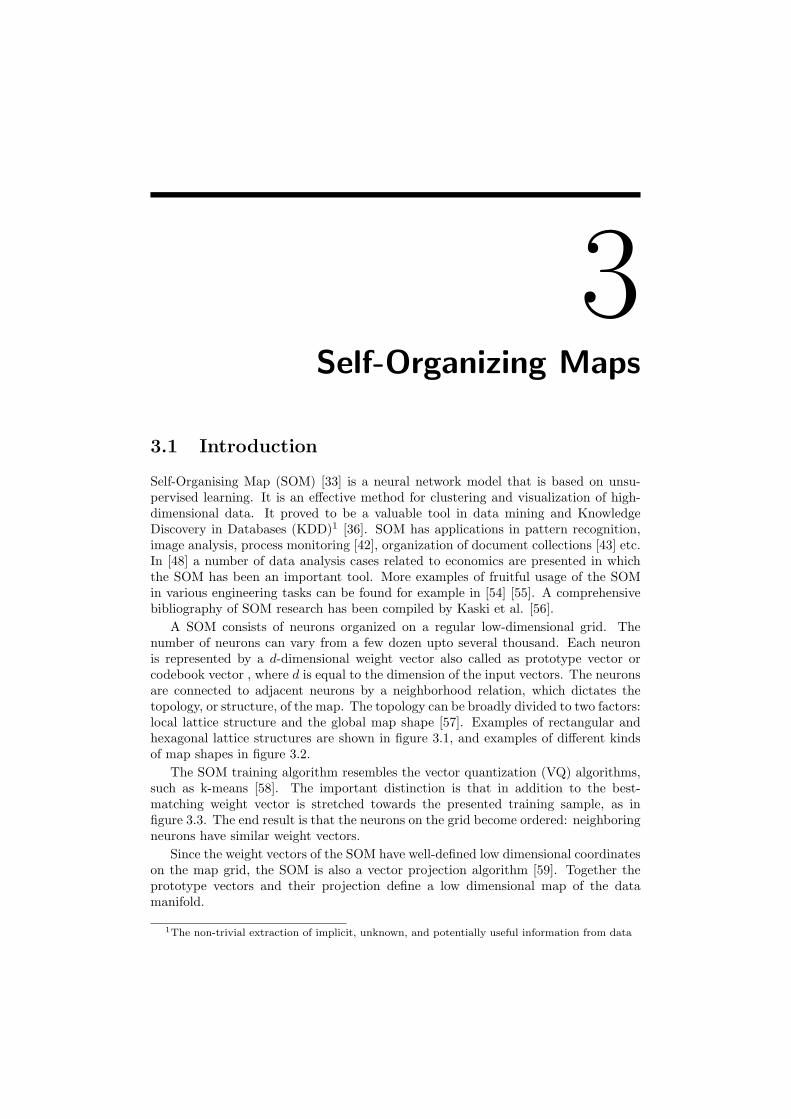
Self-Organising Map (SOM) [33] is a neural network model that is based on unsu-pervised learning. It is an effective method for clustering and visualization of high-dimensional data. It proved to be a valuable tool in data mining and KnowledgeDiscovery in Databases (KDD)1 [36]. SOM has applications in pattern recognition,image analysis, process monitoring [42], organization of document collections [43] etc.In [48] a number of data analysis cases related to economics are presented in whichthe SOM has been an important tool. More examples of fruitful usage of the SOMin various engineering tasks can be found for example in [54] [55]. A comprehensivebibliography of SOM research has been compiled by Kaski et al. [56].
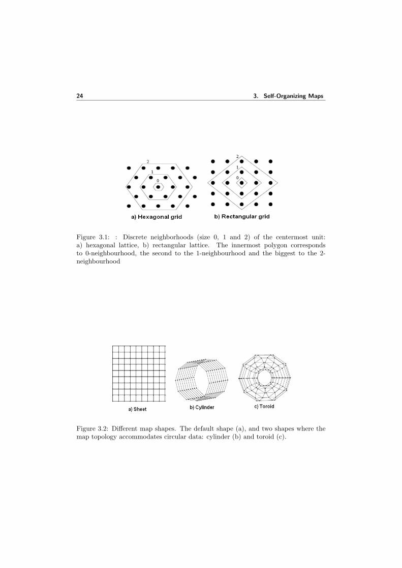
A SOM consists of neurons organized on a regular low-dimensional grid. Thenumber of neurons can vary from a few dozen upto several thousand. Each neuronis represented by a d-dimensional weight vector also called as prototype vector orcodebook vector , where d is equal to the dimension of the input vectors. The neuronsare connected to adjacent neurons by a neighborhood relation, which dictates thetopology, or structure, of the map. The topology can be broadly divided to two factors:local lattice structure and the global map shape [57]. Examples of rectangular andhexagonal lattice structures are shown in figure 3.1, and examples of different kindsof map shapes in figure 3.2.
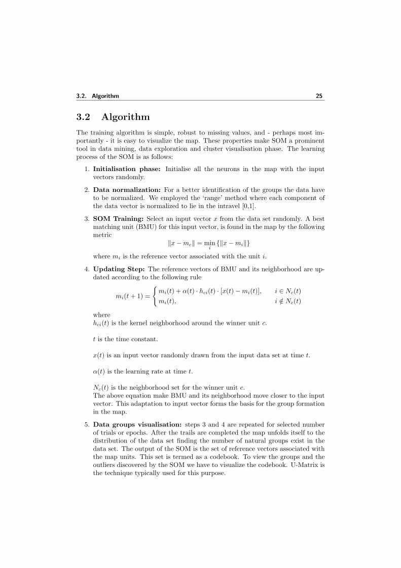
The SOM training algorithm resembles the vector quantization (VQ) algorithms,such as k-means [58]. The important distinction is that in addition to the best-matching weight vector is stretched towards the presented training sample, as infigure 3.3. The end result is that the neurons on the grid become ordered: neighboringneurons have similar weight vectors.
Since the weight vectors of the SOM have well-defined low dimensional coordinateson the map grid, the SOM is also a vector projection algorithm [59]. Together theprototype vectors and their projection define a low dimensional map of the datamanifold.
1The non-trivial extraction of implicit, unknown, and potentially useful information from data
24 3. Self-Organizing Maps
Figure 3.1: : Discrete neighborhoods (size 0, 1 and 2) of the centermost unit:a) hexagonal lattice, b) rectangular lattice. The innermost polygon correspondsto 0-neighbourhood, the second to the 1-neighbourhood and the biggest to the 2-neighbourhood
Figure 3.2: Different map shapes. The default shape (a), and two shapes where themap topology accommodates circular data: cylinder (b) and toroid (c).
3.2. Algorithm 25
3.2 Algorithm
The training algorithm is simple, robust to missing values, and - perhaps most im-portantly - it is easy to visualize the map. These properties make SOM a prominenttool in data mining, data exploration and cluster visualisation phase. The learningprocess of the SOM is as follows:
1. Initialisation phase: Initialise all the neurons in the map with the inputvectors randomly.
2. Data normalization: For a better identification of the groups the data haveto be normalized. We employed the ‘range’ method where each component ofthe data vector is normalized to lie in the intravel [0,1].
3. SOM Training: Select an input vector x from the data set randomly. A bestmatching unit (BMU) for this input vector, is found in the map by the followingmetric
‖x−mc‖ = mini‖x−mi‖
where mi is the reference vector associated with the unit i.
4. Updating Step: The reference vectors of BMU and its neighborhood are up-dated according to the following rule
mi(t + 1) =
mi(t) + α(t) · hci(t) · [x(t)−mi(t)], i ∈ Nc(t)mi(t), i /∈ Nc(t)
wherehci(t) is the kernel neighborhood around the winner unit c.
t is the time constant.
x(t) is an input vector randomly drawn from the input data set at time t.
α(t) is the learning rate at time t.
Nc(t) is the neighborhood set for the winner unit c.The above equation make BMU and its neighborhood move closer to the inputvector. This adaptation to input vector forms the basis for the group formationin the map.
5. Data groups visualisation: steps 3 and 4 are repeated for selected numberof trials or epochs. After the trails are completed the map unfolds itself to thedistribution of the data set finding the number of natural groups exist in thedata set. The output of the SOM is the set of reference vectors associated withthe map units. This set is termed as a codebook. To view the groups and theoutliers discovered by the SOM we have to visualize the codebook. U-Matrix isthe technique typically used for this purpose.
26 3. Self-Organizing Maps
Figure 3.3: Updating the best matching unit (BMU) and its neighbors towards theinput sample with x. The solid and dashed lines correspond to situation before andafter updating, respectively
In the thesis, the distance computation is modified based on the two factors:
• Missing Values: In the thesis, these are represented by the value of NAN in thevector or data matrix. Missing components are handled by simply excludingthem from the distance calculation. It is assumed that their contribution tothe distance ‖x−mi‖ is zero. According to [60], this is a valid solution as thesame variables is ignored in each distance calculation over which the minimumis taken.
• Mask: Each variable has an associated weighting factor. This is primarily usedin binary form for excluding certain variables from the BMU-finding process (1for include, 0 for exclude). However, the mask can get any values, so it can beused for weighting variables according to their importance.
With these changes, the distance measure becomes:
‖x−mi‖ =∑k∈K
wk (xk −mk)2 (3.2.1)
where K is the set of known variables of sample vector x, xk and mk are the kth
components of the sample and weight vectors and wk is the kth mask value (mask(k)).After finding the BMU, the weight vectors of the SOM are updated so that the BMUis moved closer to the input vector in the input space. The topological neighbors ofthe BMU are treated similarly. This adaptation procedures stretches the BMU and
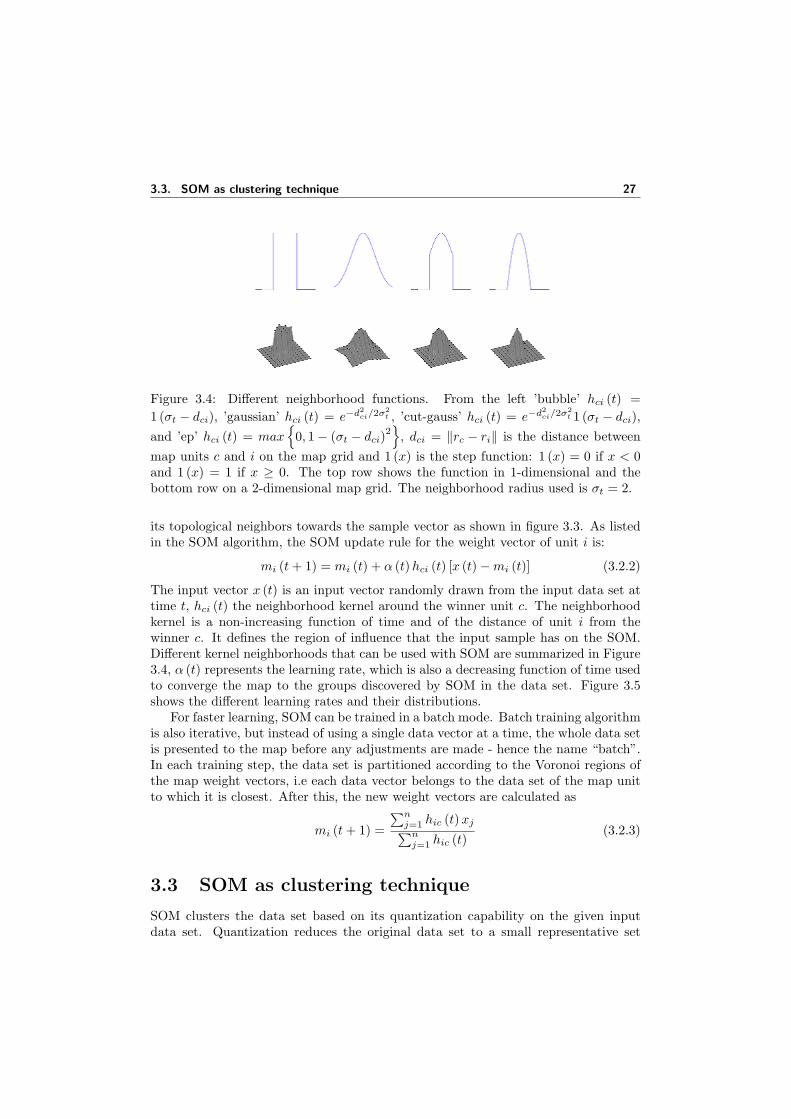
3.3. SOM as clustering technique 27
Figure 3.4: Different neighborhood functions. From the left ’bubble’ hci (t) =1 (σt − dci), ’gaussian’ hci (t) = e−d2
ci/2σ2t , ’cut-gauss’ hci (t) = e−d2
ci/2σ2t 1 (σt − dci),
and ’ep’ hci (t) = max
0, 1− (σt − dci)2
, dci = ‖rc − ri‖ is the distance betweenmap units c and i on the map grid and 1 (x) is the step function: 1 (x) = 0 if x < 0and 1 (x) = 1 if x ≥ 0. The top row shows the function in 1-dimensional and thebottom row on a 2-dimensional map grid. The neighborhood radius used is σt = 2.
its topological neighbors towards the sample vector as shown in figure 3.3. As listedin the SOM algorithm, the SOM update rule for the weight vector of unit i is:
mi (t + 1) = mi (t) + α (t) hci (t) [x (t)−mi (t)] (3.2.2)
The input vector x (t) is an input vector randomly drawn from the input data set attime t, hci (t) the neighborhood kernel around the winner unit c. The neighborhoodkernel is a non-increasing function of time and of the distance of unit i from thewinner c. It defines the region of influence that the input sample has on the SOM.Different kernel neighborhoods that can be used with SOM are summarized in Figure3.4, α (t) represents the learning rate, which is also a decreasing function of time usedto converge the map to the groups discovered by SOM in the data set. Figure 3.5shows the different learning rates and their distributions.
For faster learning, SOM can be trained in a batch mode. Batch training algorithmis also iterative, but instead of using a single data vector at a time, the whole data setis presented to the map before any adjustments are made - hence the name “batch”.In each training step, the data set is partitioned according to the Voronoi regions ofthe map weight vectors, i.e each data vector belongs to the data set of the map unitto which it is closest. After this, the new weight vectors are calculated as
mi (t + 1) =
∑nj=1 hic (t)xj∑n
j=1 hic (t)(3.2.3)
3.3 SOM as clustering technique
SOM clusters the data set based on its quantization capability on the given inputdata set. Quantization reduces the original data set to a small representative set
28 3. Self-Organizing Maps
Figure 3.5: Different learning rate functions: ′linear′ (solid line) α (t) =α0 (1− t/T ), ′power′ (dot-dashed) α (t) = α0 (0.005/α0)
t/T and ′inv′ (dashed)α (t) = α0/ (1 + 100t/T ), where T is the training length and α0 is the initial learningrate.
of prototypes to work with. The representative set of prototypes can be utilized incomputationally intensive tasks, like clustering or projection, to get approximativeresults with reduced computational cost [45]. This reduction is important especiallyin data exploration. In addition, since the prototypes are formed as averages of thedata samples, the effect of zero-mean noise as well as outliers are reduced [46].
Vector quantization algorithms, try to find a set of prototype vectors mi =1, . . . ,M which reproduce the original data set as well as possible. The best knownalgorithm to find these prototypes is the k-means alogorithm [53]. Quantization algo-rithms finds a set of M = k prototype vectors which minimize the quantixation errorEq, used to measure the quatization property of the algorithm.
Eq =1N
N∑i=1
d∑j=1
|xij −mbij |r (3.3.1)
where bi is the index of the best-matching prototype, r is the distance norm. The pointdensity of the prototypes follows the density of the training data. Asymptotically itholds that:
p (m) ∝ p (x)d
d+r (3.3.2)
where d is the dimension and p (x) and p (m) are the probability density functionsof the input data and the protoype vectors respectively.
The SOM is closely related to the k-means algorithm. If the neighborhood kernelvalue is one for the BMU and zero elsewhere ( hbij = δ (bi, j) in Eq. 3.2.2, the SOMreduces to the adaptive k-means algorithm. Also batch map reduces to batch k-means.
The difference between classical vector quantization and SOM is that the SOMperforms local smoothing in the neighborhood of each map unit. This smoothing cre-ates the ordering of the prototypes, but when the neighborhood radius σ is decreased

3.3. SOM as clustering technique 29
Figure 3.6: Two side effects caused by the neighborhood function: (a) border effectand (b) interpolating units. The + are the training data, and the connected grid ofcircles is the map.
during the the training, it also implements a simulated annealing type of learningscheme that makes the quantization process more robust. There are also two sideeffects (fig. 3.6).
• Border effect: The neighborhood definition is not symmetric on the bordersof the map. Therefore, the density estimation is different for the border unitsthan for the center units of the map [47]. In practice, the map is contracted onthe borders. This has the effect that the tails of the marginal distributions ofvariables are less well presented than their centers. In some cases, this may helpto reduce the effect of outliers, but in general, this is a weakness of the SOM.
• Interpolating units: When the data cloud is discontinuous, interpolating unitsare the data distribution. However, in case of some analysis tools, for examplesingle linkage clustering, these may give false cues of the shape of the datamanifold and may need to be deemphasized or completely left out of analysis.
If the input data set considered as the set of stochastic data variables x that isdistributed according to a probability density function p (x) then the SOM formsan approximation to this probability density function p (x), using a finite number ofcentroid vectors mi (i = 1, . . . , k). Now these point density of the prototypes followsroughly the probability density of the data. Once the centroid is chosen, the approx-imation of x means finding the centroid vector mc closest to x vector in the inputspace. The optimal solution of mi minimizes the average expected value Eavg of thequantization error Eq, defined as
Eavg =∫‖x−mc‖2 p (x) dx (3.3.3)
According to [61] , if the number of centroid vectors is large, the optimal selectionof mi values is such that their point density (Eq. 3.3.2) approximates to
p (m) ∝ p (x)23−
13σ2+3(σ+1)2 (3.3.4)
30 3. Self-Organizing Maps
Variables play an important role in quantization properties of the SOM. Theimportances of variables defines the viewpoint of the quantization. When quantizationhas a central role in data analysis, it is important to know what is this viewpoint,because any analysis based on the quantization will reflect how well the variablesare represented.By adding, removing, or rescaling variables, a different quantizationresult is acquired because the quantization error function Eq changes correspondingly.How well each variable is represented in the quantization depends on how stronglythe variable effects the total quantization error.
The quantization error Eq can be expressed in terms of variable-wise errors Ej :
Eq =d∑
j=1
1N
N∑i=1
|xij −mbij |2 =
1N
d∑j=1
Ej (3.3.5)
In order to measure the granularity of the quantization with respect to each variable,the errors Ej can be compared to quantizations performed on each variable separatelywith increasing number of quantization points Ej (k), k = 1, . . . , N . Depending onthe distribution characteristics of the variable, the quantization error decreases atdifferent rates. For example, for a uniformly distributed variable, the quantizationerror reduces according to formula Ej (k) = σ2
j k−2, where σj is the standard deviationof the variable. we use this SOM clustering capability to discover the groups ofGamma ray bursts data sets in the case study of GRB analysis described in thischapter. In chapter 6 we describe a SOM based system for automatic classification ofimages based on the clustering property of SOM
3.4 SOM as visualization technique
One of the most important property of the SOM is that it is an efficient methodfor visualization of high-dimensional data. The SOM is thus an excellent tool inexploratory data analysis [50]. Visualization methods try to find low-dimensionalcoordinates that preserve the distances (or the order of distances) between the orig-inally high-dimensional objects. A classical projection method is multi-dimensionalscaling (MDS) [49] which tries to preserve pairwise distances between all objects whilereducing the dimension. The error function to be minimized is:
Emds =N∑
i=1
N∑j=1
(dij − d′ij
)2 (3.4.1)
where dij is the distance between data samples i and j in the input space ‖xi − xj‖,and d′ij is the corresponding distance between the projection coordinates in the outputspace. There is also a non-metric version of MDS which tries to preserve the rankorder of the distances. other prominent projection techniques are sammons’ mapping[51], Curvilinear Component Analysis(CCA) [52]
sammons′mapping : Esam =N∑
i=1
N∑j=1
(dij − d′ij
)2/dij (3.4.2)

3.4. SOM as visualization technique 31
CCA : Ecca =N∑
i=1
N∑j=1
(dij − d′ij
)2e−d′ij (3.4.3)
For SOM the error function minimization is given by
Esom =N∑
i=1
M∑j=1
h(d′ij) (
d2ij
)(3.4.4)
where h (.) is the neighborhood kernel function. Since it is monotonically decreasingfunction of d′ij , small distances in the outer space are emphasized, also d′ij is dependenton the density distribution of the input data set. Thus, the definition of locality inSOM tunes to input data density. Rather than try to preserve the original distances,the SOM orders prototype vectors on a predefined map grid such that local neigh-borhood sets in the projection are preserved. SOM is especially good at maintainingthe trustworthiness of the projection: if two data samples are close to each other inthe visualization, they are more likely to be close in the original high-dimensionalspace as well. The visualization techniques which are mainly used in this thesis aredescribed below.
(a) Points in threed - space (b) SOM grouping with U-matrix
Figure 3.7: SOM classification of points in threed space
3.4.1 U-matrix
U-matrix (unified distance matrix) representation of the Self-Organizing Map visual-izes the distances between the map units or neurons. An U-Matrix displays the localdistance structure of the data set.It is a standard tool for the display of the distancestructures of the input data on SOM [50]. The distance between the adjacent neuronsis calculated and presented with different colorings between the adjacent nodes. InU-matrix color coding scale is used to distinguish various clusters. The clusters andtheir outliers, boundaries are represented by different colors. This can be a helpfulpresentation when one tries to find clusters in the input data without having anya priori information about the clusters. Teaching a SOM and representing it with
32 3. Self-Organizing Maps
Figure 3.8: Component planes for the data points in 3-D space
the U-matrix offers a fast way to get insight of the data distribution without humanintervention. The U-Matrix is constructed on top of the map. The color coding of amap unit is based on the factor “U-height”. The unified distance matrix (U-matrix)visualizes all distances between each map unit and its neighbors. This is possibledue to the regular structure of the map grid: it is easy to position a single visualmarker between a map unit and each of its neighbors. The map prototypes followthe probability density function of the data, the “u-height” distances are inverselyproportional to the density of the data. Thus, cluster borders can be identified asdifferent colors separating the map units of low distances that are with in the cluster.This interpretation can also be used in clustering. Let i be a unit on the map, NN (i)be the set of immediate neighbors on the map, m (i) the weight vector associated withneuron i, then
U − height (i) =∑
j∈NN(i)
d (m (i)−m (j)) (3.4.5)
where d (m (i)−m (j)) is the distance used in the SOM algorithm to construct themap. Thus U-Matrix is a display of the U-heights on top of the grid positions of theneurons on the map. Once the u-heights are determined contrast color coding areassigned to various clusters in the following way:
- U-height(i) = mean(U − heights) ⇒ (clustercenter)
- U-height(i) < mean(U − heights) ⇒ (intercluster)
- U-height(i) > mean(U − heights) ⇒ (intracluster)
- U-height(i) < min(U − heights) ⇒ U-height(i) = 0 (boundary)
Properties of the U-Matrix:
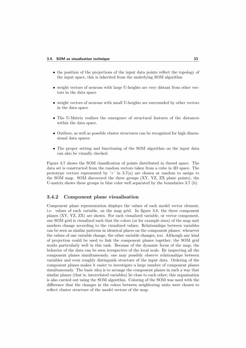
3.4. SOM as visualization technique 33
• the position of the projections of the input data points reflect the topology ofthe input space, this is inherited from the underlying SOM algorithm
• weight vectors of neurons with large U-heights are very distant from other vec-tors in the data space
• weight vectors of neurons with small U-heights are surrounded by other vectorsin the data space
• The U-Matrix realizes the emergence of structural features of the distanceswithin the data space.
• Outliers, as well as possible cluster structures can be recognized for high dimen-sional data spaces.
• The proper setting and functioning of the SOM algorithm on the input datacan also be visually checked.
Figure 3.7 shows the SOM classification of points distributed in threed space. Thedata set is constructed from the random vectors taken from a cube in 3D space. Theprototype vectors represented by ’+’ in 3.7(a) are chosen at random to assign tothe SOM map. SOM discovered the three groups (XY, YZ, ZX plane points), theU-matrix shows these groups in blue color well separated by the boundaries 3.7 (b).
3.4.2 Component plane visualisation
Component plane representation displays the values of each model vector element,i.e. values of each variable, on the map grid. In figure 3.8, the three componentplanes (XY, YZ, ZX) are shown. For each visualized variable, or vector component,one SOM grid is visualized such that the colors (or for example sizes) of the map unitmarkers change according to the visualized values. Relationships between variablescan be seen as similar patterns in identical places on the component planes: wheneverthe values of one variable change, the other variable changes, too. Although any kindof projection could be used to link the component planes together, the SOM gridworks particularly well in this task. Because of the dynamic focus of the map, thebehavior of the data can be seen irrespective of the local scale. By inspecting all thecomponent planes simultaneously, one may possibly observe relationships betweenvariables and even roughly distinguish structure of the input data. Ordering of thecomponent planes makes it easier to investigate a large number of component planessimultaneously. The basic idea is to arrange the component planes in such a way thatsimilar planes (that is, interrelated variables) lie close to each other; this organizationis also carried out using the SOM algorithm. Coloring of the SOM was used with thedifference that the changes in the colors between neighboring units were chosen toreflect cluster structure of the model vectors of the map.
34 3. Self-Organizing Maps
Figure 3.9: SOM based system for GRB Data Analysis
3.5 Case study on Astrophysical experiment: GRBData Analysis
Gamma ray bursts (GRBs) were arguably the biggest mystery in high-energy astron-omy. They’ve been the target of intense research and speculation by astronomers.Although 3 decades have passed since their discovery, very little is known about thefundamental physical mechanisms behind these phenomena [34]. They are consideredto be short-lived bursts of gamma-ray photons, the most energetic form of light. Atleast some of them are associated with a special type of supernovae, the explosionsmarking the deaths of especially massive stars. Lasting anywhere from a few millisec-onds to several minutes, gamma-ray bursts (GRBs) shine hundreds of times brighterthan a typical supernova and about a million trillion times as bright as the Sun, mak-ing them briefly the brightest source of cosmic gamma-ray photons in the observableUniverse. GRBs are detected roughly once per day from wholly random directions ofthe sky. GRBs exhibit great morphological diversity and complex temporal behavior:To analyze their properties it is beneficial to find the classes that exists in the GRBdata. Studies based on GRB bulk properties (such as burst duration and spectralhardness) have proved to be fruitful, and the discovery of distinct classes in the GRBpopulation might lead to some new astrophysical insight.
In 1991 NASA launched the Compton Gamma Ray Observatory carrying an in-strument called the Burst and Transient Source Experiment, or “BATSE” for short.BATSE was designed specifically for the study of the enigmatic gamma ray bursts andhas led to a new understanding of their origin and distribution in the universe. Forthe GRB analysis we used the data sets taken from the BATSE catalog data[35]. Thegamma ray burst data sets are organised in in a series of burst catalogs containing allburst data from the start of the mission. The catalogs follow the naming convention“BATSE nB Gamma Ray Burst Catalog”, where n is an integer beginning at 1. Thelatest published catalog as of 1999 March is the 4B Catalog. Each catalog containsall burst data from the start of the mission. For example, the 2B catalog contains
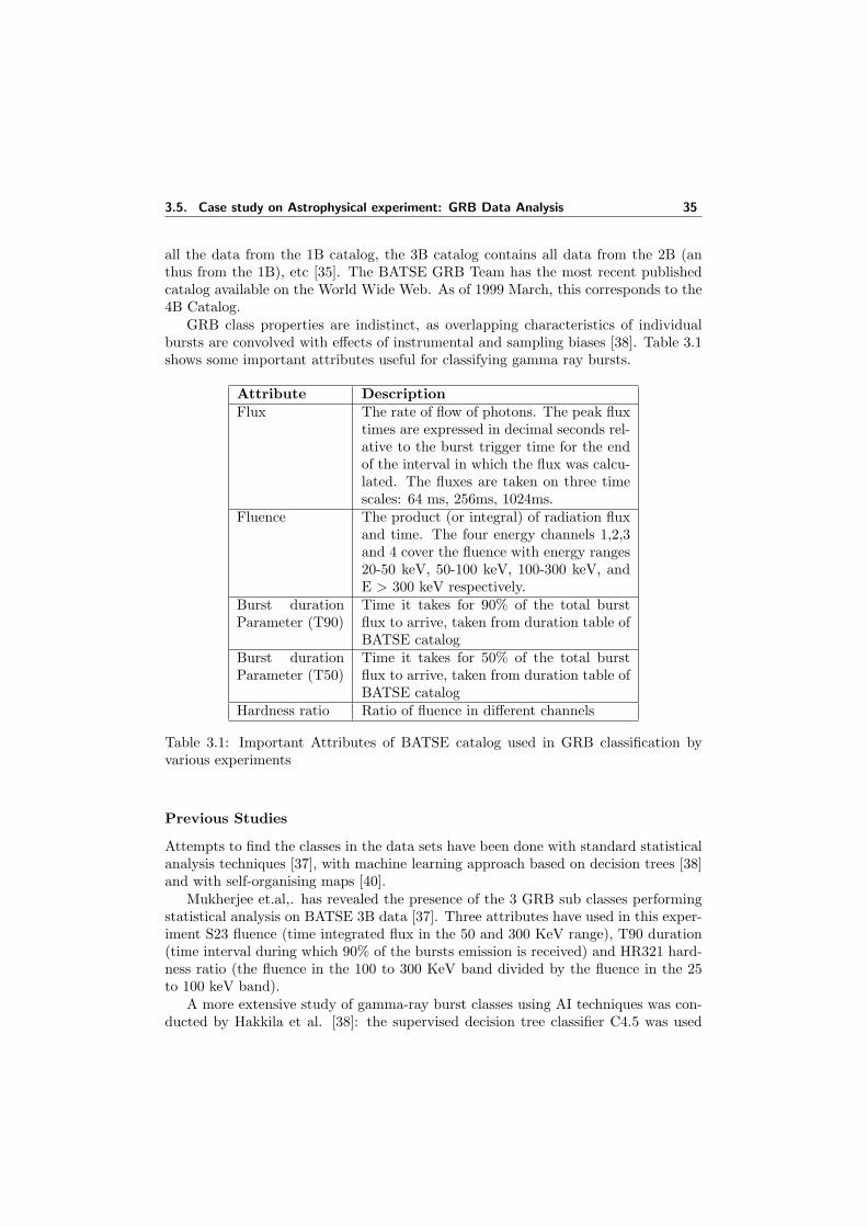
3.5. Case study on Astrophysical experiment: GRB Data Analysis 35
all the data from the 1B catalog, the 3B catalog contains all data from the 2B (anthus from the 1B), etc [35]. The BATSE GRB Team has the most recent publishedcatalog available on the World Wide Web. As of 1999 March, this corresponds to the4B Catalog.
GRB class properties are indistinct, as overlapping characteristics of individualbursts are convolved with effects of instrumental and sampling biases [38]. Table 3.1shows some important attributes useful for classifying gamma ray bursts.
Attribute DescriptionFlux The rate of flow of photons. The peak flux
times are expressed in decimal seconds rel-ative to the burst trigger time for the endof the interval in which the flux was calcu-lated. The fluxes are taken on three timescales: 64 ms, 256ms, 1024ms.
Fluence The product (or integral) of radiation fluxand time. The four energy channels 1,2,3and 4 cover the fluence with energy ranges20-50 keV, 50-100 keV, 100-300 keV, andE > 300 keV respectively.
Burst durationParameter (T90)
Time it takes for 90% of the total burstflux to arrive, taken from duration table ofBATSE catalog
Burst durationParameter (T50)
Time it takes for 50% of the total burstflux to arrive, taken from duration table ofBATSE catalog
Hardness ratio Ratio of fluence in different channels
Table 3.1: Important Attributes of BATSE catalog used in GRB classification byvarious experiments
Previous Studies
Attempts to find the classes in the data sets have been done with standard statisticalanalysis techniques [37], with machine learning approach based on decision trees [38]and with self-organising maps [40].
Mukherjee et.al,. has revealed the presence of the 3 GRB sub classes performingstatistical analysis on BATSE 3B data [37]. Three attributes have used in this exper-iment S23 fluence (time integrated flux in the 50 and 300 KeV range), T90 duration(time interval during which 90% of the bursts emission is received) and HR321 hard-ness ratio (the fluence in the 100 to 300 KeV band divided by the fluence in the 25to 100 keV band).
A more extensive study of gamma-ray burst classes using AI techniques was con-ducted by Hakkila et al. [38]: the supervised decision tree classifier C4.5 was used
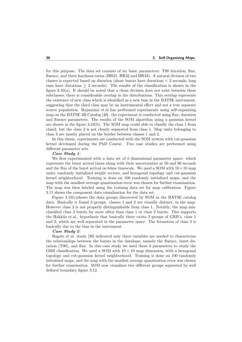
36 3. Self-Organizing Maps
for this purpose. The data set consists of six basic parameters: T90 duration, flux,fluence, and three hardness ratios (HR21, HR32 and HR43). A natural division of twoclasses is expected based on duration (short bursts have durations < 2 seconds; longones have durations ≥ 2 seconds). The results of the classification is shown in thefigure 3.10(a). It should be noted that a clean division does not exist between thesesubclasses; there is considerable overlap in the distributions. This overlap representsthe existence of new class which is identified as a new bias in the BATSE instrument,suggesting that the third class may be an instrumental effect and not a true separatesource population. Rajaneimi et.al has performed experiments using self-organisingmap on the BATSE 3B Catalog [40]. the experiment is conducted using flux, durationand fluence parameters. The results of the SOM algorithm using a gaussian kernelare shown in the figure 3.10(b). The SOM map could able to classify the class 1 fromclass2, but the class 3 is not clearly separated from class 1. Map units belonging toclass 3 are mostly placed on the border between classes 1 and 2.
In this thesis, experiments are conducted with the SOM system with cut-gaussiankernel developed during the PhD Course. Two case studies are performed usingdifferent parameter sets.
Case Study 1 :We first experimented with a data set of 5 dimensional parameter space: which
represents the burst arrival times along with their uncertainties at 50 and 90 secondsand the flux of the burst arrival on 64ms timescale. We used a SOM with 10×10 mapunits, randomly initialized weight vectors, and hexagonal topology and cut-gaussiankernel neighborhood. Training is done on 100 randomly initialized maps, and themap with the smallest average quantization error was chosen for further examination.The map was then labeled using the training data set for map calibration. Figure3.11 shows the component data visualisation for the data set.
Figure 3.10(c)shows the data groups discovered by SOM in the BATSE catalogdata. Basically it found 3 groups. classes 1 and 2 are visually distinct, in the map.However class 3 is not properly distinguishable from class 1. Notably, the map mis-classified class 3 bursts far more often than class 1 or class 2 bursts. This supportsthe Hakkila et.al., hypothesis that basically there exists 2 groups of GRB’s, class 1and 2, which are well separated in the parameter space. The formation of class 3 isbasically due to the bias in the instrument.
Case Study 2 :Bagoly et al. study [39] indicated only three variables are needed to characterize
the relationships between the bursts in the database, namely the fluence, burst du-ration (T90), and flux. In this case study we used these 3 parameters to study theGRB classification. We used a SOM with 10× 10 map dimension, with a hexagonaltopology and cut-gaussian kernel neighborhood. Training is done on 100 randomlyinitialized maps, and the map with the smallest average quantization error was chosenfor further examination. SOM now visualizes two different groups separated by welldefined boundary figure 3.12.
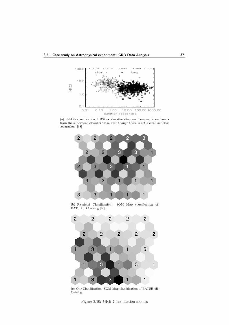
3.5. Case study on Astrophysical experiment: GRB Data Analysis 37
(a) Hakkila classification: HR32 vs. duration diagram. Long and short burststrain the supervised classifier C4.5, even though there is not a clean subclassseparation. [38]
(b) Rajniemi Classification: SOM Map classification ofBATSE 3B Catalog [40]
(c) Our Classification: SOM Map classification of BATSE 4BCatalog
Figure 3.10: GRB Classification models
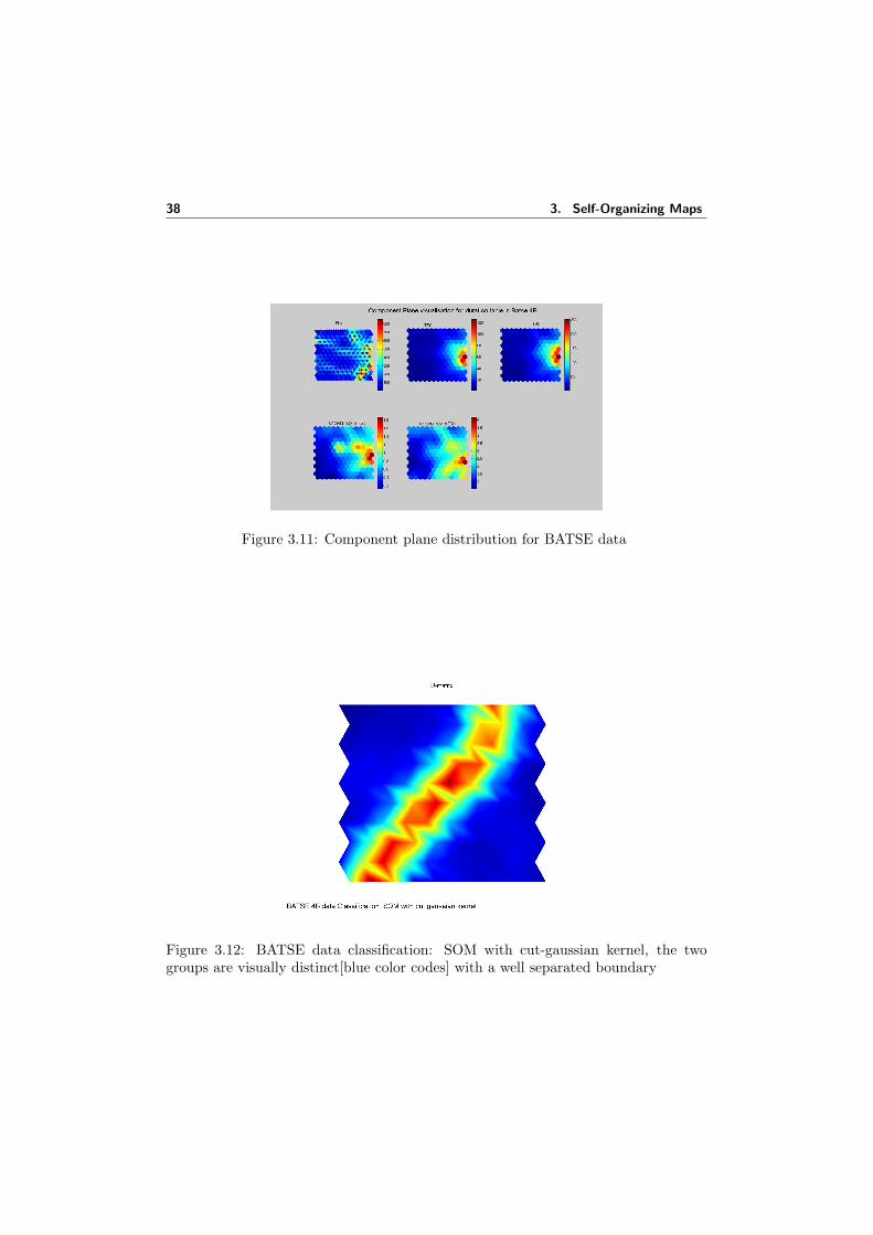
38 3. Self-Organizing Maps
Figure 3.11: Component plane distribution for BATSE data
Figure 3.12: BATSE data classification: SOM with cut-gaussian kernel, the twogroups are visually distinct[blue color codes] with a well separated boundary
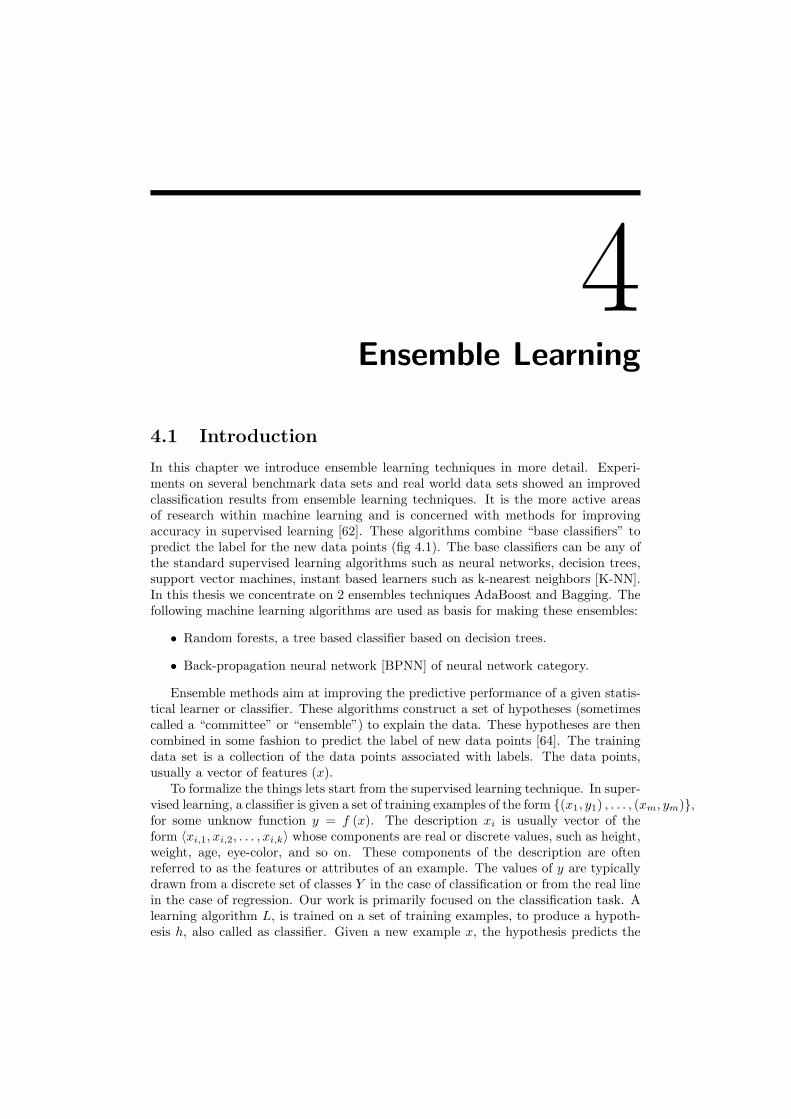
4Ensemble Learning
4.1 Introduction
In this chapter we introduce ensemble learning techniques in more detail. Experi-ments on several benchmark data sets and real world data sets showed an improvedclassification results from ensemble learning techniques. It is the more active areasof research within machine learning and is concerned with methods for improvingaccuracy in supervised learning [62]. These algorithms combine “base classifiers” topredict the label for the new data points (fig 4.1). The base classifiers can be any ofthe standard supervised learning algorithms such as neural networks, decision trees,support vector machines, instant based learners such as k-nearest neighbors [K-NN].In this thesis we concentrate on 2 ensembles techniques AdaBoost and Bagging. Thefollowing machine learning algorithms are used as basis for making these ensembles:
• Random forests, a tree based classifier based on decision trees.
• Back-propagation neural network [BPNN] of neural network category.
Ensemble methods aim at improving the predictive performance of a given statis-tical learner or classifier. These algorithms construct a set of hypotheses (sometimescalled a “committee” or “ensemble”) to explain the data. These hypotheses are thencombined in some fashion to predict the label of new data points [64]. The trainingdata set is a collection of the data points associated with labels. The data points,usually a vector of features (x).
To formalize the things lets start from the supervised learning technique. In super-vised learning, a classifier is given a set of training examples of the form (x1, y1) , . . . , (xm, ym),for some unknow function y = f (x). The description xi is usually vector of theform 〈xi,1, xi,2, . . . , xi,k〉 whose components are real or discrete values, such as height,weight, age, eye-color, and so on. These components of the description are oftenreferred to as the features or attributes of an example. The values of y are typicallydrawn from a discrete set of classes Y in the case of classification or from the real linein the case of regression. Our work is primarily focused on the classification task. Alearning algorithm L, is trained on a set of training examples, to produce a hypoth-esis h, also called as classifier. Given a new example x, the hypothesis predicts the
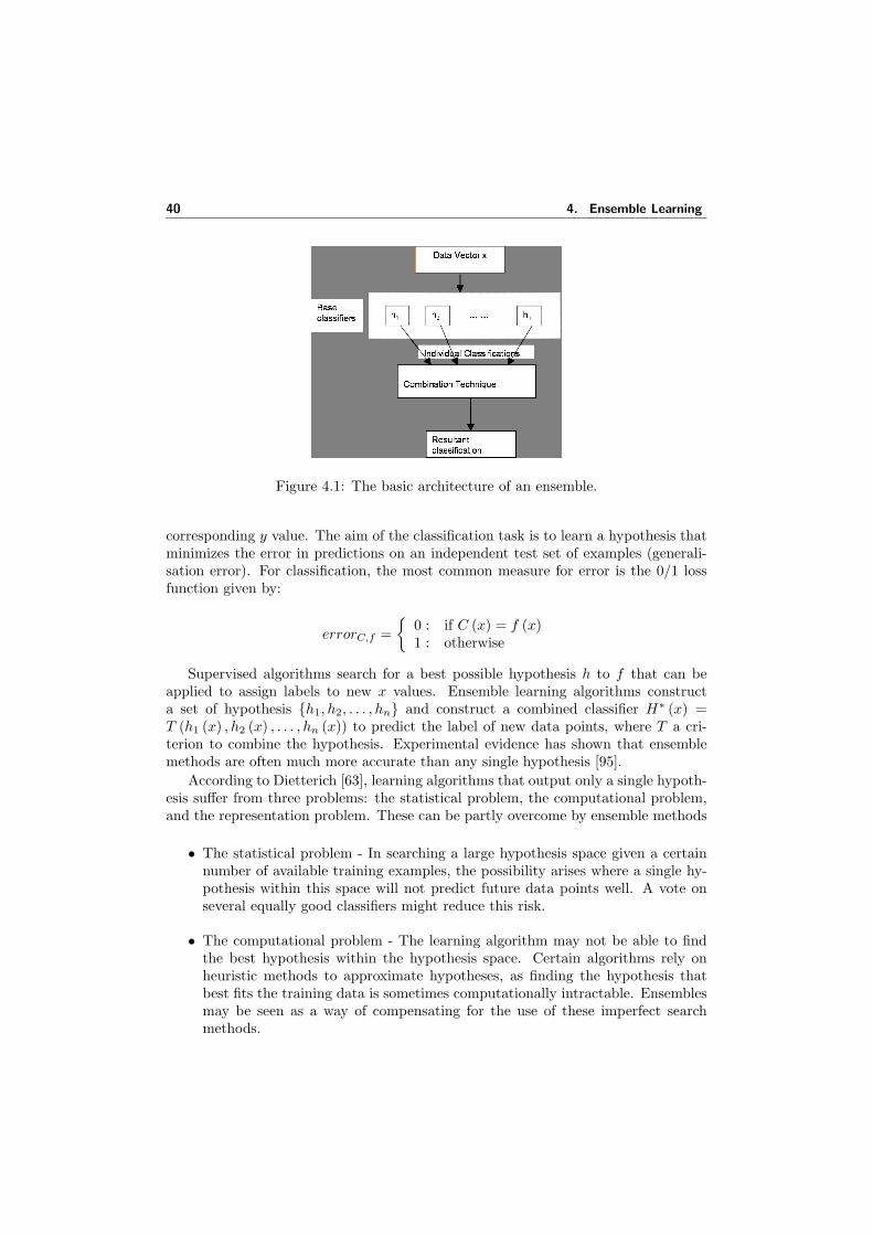
40 4. Ensemble Learning
Figure 4.1: The basic architecture of an ensemble.
corresponding y value. The aim of the classification task is to learn a hypothesis thatminimizes the error in predictions on an independent test set of examples (generali-sation error). For classification, the most common measure for error is the 0/1 lossfunction given by:
errorC,f =
0 : if C (x) = f (x)1 : otherwise
Supervised algorithms search for a best possible hypothesis h to f that can beapplied to assign labels to new x values. Ensemble learning algorithms constructa set of hypothesis h1, h2, . . . , hn and construct a combined classifier H∗ (x) =T (h1 (x) , h2 (x) , . . . , hn (x)) to predict the label of new data points, where T a cri-terion to combine the hypothesis. Experimental evidence has shown that ensemblemethods are often much more accurate than any single hypothesis [95].
According to Dietterich [63], learning algorithms that output only a single hypoth-esis suffer from three problems: the statistical problem, the computational problem,and the representation problem. These can be partly overcome by ensemble methods
• The statistical problem - In searching a large hypothesis space given a certainnumber of available training examples, the possibility arises where a single hy-pothesis within this space will not predict future data points well. A vote onseveral equally good classifiers might reduce this risk.
• The computational problem - The learning algorithm may not be able to findthe best hypothesis within the hypothesis space. Certain algorithms rely onheuristic methods to approximate hypotheses, as finding the hypothesis thatbest fits the training data is sometimes computationally intractable. Ensemblesmay be seen as a way of compensating for the use of these imperfect searchmethods.
4.2. Ensemble Mechanics 41
• The representation problem - The hypothesis space may not contain any hy-pothesis that are good approximations to the true target function that mapsany given training example Ai to its respective class Ci. Combining severalviable functions (that are only fair approximations) may expand the space offunctions and thus form a more accurate approximation to the true target func-tion.
A learning algorithm that suffers from the statistical problem is said to have high“variance”. An algorithm that exhibits the computational problem is sometimes de-scribed has having “computational variance”, and a learning algorithm that suffersfrom the representational problem is said to have high “bias”. Hence, ensemble meth-ods can reduce both the bias and the variance of learning algorithms.
4.2 Ensemble Mechanics
Ensembles can be generalized in various directions. In [67], ensembles are formalizedin terms of Bayesian learning theory. Bayesian learning theory is used for decisionmaking using the knowledge of prior events to predict future events. Bayes first pro-posed his theorem in his 1763 work (published two years after his death in 1761),An Essay Towards Solving a Problem in the Doctrine of Chances. Bayes’ theoremprovided, for the first time, a mathematical method that could be used to calculate,given occurrences in prior trials, the likelihood of a target occurrence in future trials.According to Bayesian logic, the only way to quantify a situation with an uncertainoutcome is through determining its probability. Bayes’ Theorem is a means of quanti-fying uncertainty. Based on probability theory, the theorem defines a rule for refiningan hypothesis by factoring in additional evidence and background information, andleads to a number representing the degree of probability that the hypothesis is true.
Bayesian theory stipulates that in order to maximize predictive accuracy, insteadof using just a single learning algorithm, one should ideally employ all hypothesesin the hypothesis space. Assume that a statistical model allows the inference aboutthe variable y in the form of the predictive probability density P (y|x), where x is avector of model parameters. Furthermore, assume that we have a data set D whichcontains information about the parameter vector x in the form of the probabilitydensity P (x|D). We then obtain
P (y|D) =∫
P (y|x) P (x|D) dx ≈ 1M
M∑i=1
P (y|xi)
where M samples xiMi=1 are generated from the distribution P (x|D). This approx-imation tells us that for Bayesian inference [68], one should average the predictionsof a committee of estimators.
The motivation for pursuing ensembles can be understood by analyzing the pre-diction error of the combined system, which is particularly simple if we use a squarederror cost function. The expected squared difference between the prediction of acommittee member hi and the unknown target t cab be written as

42 4. Ensemble Learning
E (hi − t)2 = E (hi −mi + mi − t)2
= E (hi −mi)2 + E (mi − t)2 + 2E ((hi −mi) (mi − t))
= vari + b2i
(4.2.1)
decomposes into the variance vari = E (hi −mi)2 and the square of the bias
bi = mi− t, with mi = E (hi). E (.) stands for the expected value, which is calculatedwith respect to different data sets of the same size and possible variations in thetraining procedure, parameters used for making the base classifier for ex: differentinitializations of the weights in the neural network. Now t can be estimated by forminga linear combination of the hi which can be given as:
t =M∑i=1
gihi = g′f
where f = (f1, . . . , fM )′ is the vector of the predictions of the committee membersand g = (g1, . . . , gM )′ is the vector of weights. The expected error of the combinedsystem is
E(t− t
)2= E (g′f − E (g′f))2 + E (E (g′f)− t)2
= E (g′ (f − E (f)))2 + E (g′m− t)2
= g′Ωg + (g′m− t)2(4.2.2)
where Ω is an M ×M covariance matrix with
Ωij = E [(fi −mi) (fj −mj)]
and m = (m1, . . . ,mM )′ is the vector of the expected values of the predictions of thecommittee members. Here g′Ωg is the variance of the committe and g′m − t is thebias of the committee. If we simply average the predictors, i.e., set gi = 1
M , the lastexpression simplifies to
E(t− t
)2=
1M2
M∑i=1
Ωii +1
M2
M∑i=1
M∑j=1,j 6=i
Ωij +1
M2
( M∑i=1
(mi − t))2
(4.2.3)
If we now assume that the mean mi = mean, the variance Ωii = var and the inter-member covariances Ωij = cov are identical for all members, we obtain
E(t− t
)2=
1M
var +M2 −M
M2cov + (mean− t)2 (4.2.4)
It is apparent that the bias of the combined system (mean− t) is identical tothe bias of each member and is not reduced. Therefore, estimators should be used
4.3. Methods for constructing the ensembles 43
which have low bias, and regularization 1- which introduces bias - should be avoided.Secondly, the estimators should have low covariance, since this term in the errorfunction cannot be reduced by increasing M . The good news is that the term whichresults from the variances of the committee members decreases as 1/M . Thus, if wehave estimators with low bias and low covariance between members, the expected errorof the combined system is significantly less than the expected errors of the individualmembers. Thus , a committee can be used to reduce both bias and variance: bias isreduced in the design of the members by using little regularization, and variance isreduced by the averaging process which takes place in the committee.
Finally, the generalization error statistic of a committee is a function of the averageerror of ensemble members and the average variance (or ambiguity) among them [69].Optiz and Shavlik [70] empirically verified this claim, showing that ensembles thatconsist of highly correct classifiers that disagree as much as possible generalize well.
The relationship between the error rate of the ensemble and the error rates of theindividual can be given by [71]
E (ensemble) =1 + ρ (N − 1)
NE (individual) + E (Bayes) (4.2.5)
where N is the number of classifiers, ρ is the correlation among the classifier errors,E (Bayes) is the error rate obtained using the Bayes rule assuming that all the condi-tional probabilities are known. E (ensemble) and E (individual) represent the errorrate of a classifier ensemble and the error rate of an individual component classifierrespectively. ρ = 0 means the error of the whole ensemble decreases proportionally tothe number of the component classifiers while ρ = 1 means the error of the ensemblearchitecture equals to the error of a single component classifier.
4.3 Methods for constructing the ensembles
Generally speaking, the classifier ensembles can be divided into parallel ensemblesand sequential ensembles. The categorization scheme can also be done according tothe combining strategies, e.g. the diversity of the classifier ensemble. Jain, Duin andMao ?? list a number of popular ensemble methods in their review paper on statisticalpattern recognition. Dietterich [63] describes the ensemble methods from the pointof view of machine learning and we review this categorization scheme in this thesis.According to him there are two main approaches for constructing ensembles.
• Methods for Independently Constructing Ensembles
• Methods for Coordinated Construction of Ensembles
In the first approach each hypothesis is constructed independently in such a waythat the resulting set of hypotheses is accurate and diverse that is, each individualhypothesis has a reasonably low error rate for making new predictions and yet the
1A numerical method to solve problems of deconvolution by introducing a priori informationabout the smoothness of the expected result [65].

44 4. Ensemble Learning
hypotheses disagree with each other in many of their predictions. If such an ensembleof hypotheses can be constructed, it is easy to see that it will be more accurate thanany of its component classifiers, because the disagreements will “cancel out.” Suchensembles can overcome both the statistical and computational problems. Bagging isthe popular technique belonging to this category.
The second approach to designing ensembles is to construct the hypotheses in acoupled fashion so that the weighted vote of the hypotheses gives a good fit to thedata. This approach directly addresses the representational problem discussed above.Boosting is the very popular technique belonging to this category. we experimentwith this technique in this thesis.
4.3.1 Bagging
Bagging is a statistical re-sample and combine technique used to improve the classifi-cation accuracies of a classifier. It based on bootstrapping and aggregating techniques.
The idea of the bootstrap is to generate more (pseudo) data using the informationof the original data. True underlying sample properties are reproduced as closelyas possible and unknown model characteristics are replaced by sample estimates.Bagging uses bootstrapping to generate multiple versions of a data set. Each of thesedata sets have their own classifier. Th predictions from these classifiers are thencombined to get the final classification result. In theory this combination shouldperform better than a single classifier built to solve the same problem.
Bootstrapping is based on random sampling with replacement. It generates thesamples more (pseudo) data using the information of the original data. True un-derlying sample properties are reproduced as closely as possible and unknown modelcharacteristics are replaced by sample estimates. Therefore, taking a bootstrap i.e.,(random selection with replacement) of the training set T, one can sometimes avoidor get less misleading training objects in the bootstrap training set. Consequently, aclassifier constructed on such a training set may have a better performance.
Aggregating actually means combining classifiers [74]. Often a combined classifiergives better results than individual classifiers, because of combining the advantages ofthe individual classifiers in the final solution. Therefore, bagging might be helpful tobuild a better classifier on training sample sets with misleaders. Breiman motivatedbagging as a variance reduction technique for a given base procedure, such as decisiontrees or methods that do variable selection and fitting in a linear model. It hasattracted much attention, probably due to its implementation simplicity and thepopularity of the bootstrap methodology. At the time of its invention, only heuristicarguments were presented why bagging would work. Later, it has been shown in ([90])that bagging is a smoothing operation which turns out to be advantageous whenaiming to improve the predictive performance of regression or classification trees.In case of decision trees, the theory in confirms Breiman’s intuition that bagging isa variance reduction technique, reducing also the mean squared error (MSE). Theempirical fact that bagging improves the predictive performance of regression andclassification trees is nowadays widely documented ( [90], [91], [92]. On average, whentaking a bootstrap sample of the training set, approximately 37% of the objects are
4.3. Methods for constructing the ensembles 45
not presented in the bootstrap sample, meaning that possible ’outliers’ in the trainingset sometimes do not show up in the bootstrap sample. Thus, better classifiers (with asmaller apparent error - classification error on the training data set) may be obtainedby the bootstrap sample than by the original training set. These classifiers will bepresented ’sharper’ in the apparent error than those obtained on the training setswith outliers. Therefore, they will be more decisive than other bootstrap versionsin the final judgment. Thus, aggregating classifiers in bagging can sometimes give abetter performance than individual classifiers. In Bagging [75] (short for BootstrapAggregation Learning) we randomly generate a new training set, based on the originalset, for each ensemble member. Given a training set of size N, from this we uniformlyat random sample N items with replacement, then train a new ensemble member withthis resample. We repeat this for any new ensemble members we wish to create. Theresampled sets are often termed bootstrap replicates [77]; Breiman showed that onaverage 63.2% of the original training set will present in each replicate. Listing 5.1gives the algorithm.
Listing 4.1: Bagging Algorithm
1 Let M be the f i n a l number o f p r e d i c t o r s r equ i r ed .2 Take a t r a i n i n g s e t T (x1, y1) , (x2, y2) , . . . , (xm, ym)3 for i=1 to M4 5 Make a new t r a i n i n g s e t Tbag by resampl ing T .6 Train a c l a s s i f i e r hi with t h i s s e t Tbag and add i t to the ensemble .7 8 For any new t e s t i n g pattern x , the bagged output i s :9 hbag = 1
M
∑i hi (x)
Bagging has proved to be a popular technique, applicable to many problems, butthe explanation for its success remains controversial. Friedman [78] suggests thatBagging succeeds by reducing the variance component of the error and leaving thebias unchanged;
while [79] shows evidence that Bagging can in fact converge without reducingvariance. Domingos [80] gives a Bayesian account, and investigates two hypotheses:Bagging succeeds because
1. it is an approximation to Bayesian Model Averaging [81], and
2. it shifts the prior distribution of the combined estimator to a more appropriateregion of the model space; the empirical results on 26 real and artificial datasetsall support the second hypothesis and contradict the first.
4.3.2 Boosting
Boosting algorithms have been proposed in the machine learning literature by Schapire([82]) and Freund ([83]). These first algorithms have been developed as ensemblemethods. Unlike bagging which is a parallel ensemble method, boosting methods are
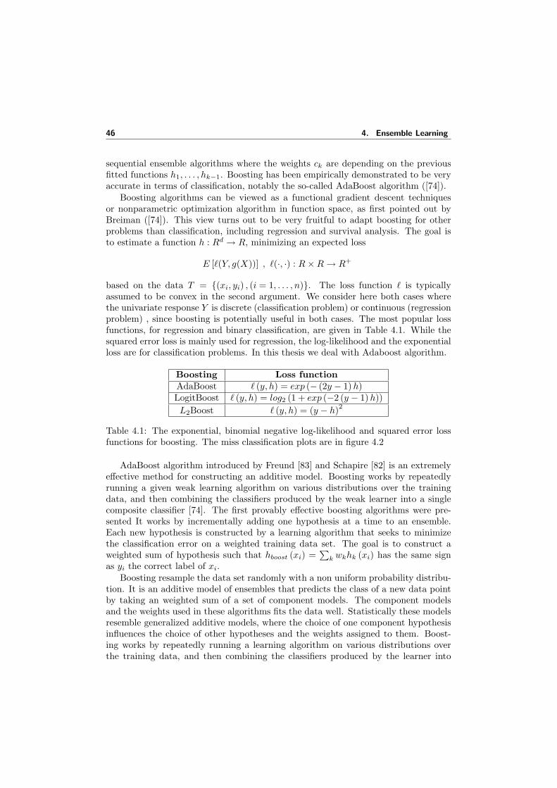
46 4. Ensemble Learning
sequential ensemble algorithms where the weights ck are depending on the previousfitted functions h1, . . . , hk−1. Boosting has been empirically demonstrated to be veryaccurate in terms of classification, notably the so-called AdaBoost algorithm ([74]).
Boosting algorithms can be viewed as a functional gradient descent techniquesor nonparametric optimization algorithm in function space, as first pointed out byBreiman ([74]). This view turns out to be very fruitful to adapt boosting for otherproblems than classification, including regression and survival analysis. The goal isto estimate a function h : Rd → R, minimizing an expected loss
E [`(Y, g(X))] , `(·, ·) : R×R→ R+
based on the data T = (xi, yi) , (i = 1, . . . , n). The loss function ` is typicallyassumed to be convex in the second argument. We consider here both cases wherethe univariate response Y is discrete (classification problem) or continuous (regressionproblem) , since boosting is potentially useful in both cases. The most popular lossfunctions, for regression and binary classification, are given in Table 4.1. While thesquared error loss is mainly used for regression, the log-likelihood and the exponentialloss are for classification problems. In this thesis we deal with Adaboost algorithm.
Boosting Loss functionAdaBoost ` (y, h) = exp (− (2y − 1) h)LogitBoost ` (y, h) = log2 (1 + exp (−2 (y − 1) h))L2Boost ` (y, h) = (y − h)2
Table 4.1: The exponential, binomial negative log-likelihood and squared error lossfunctions for boosting. The miss classification plots are in figure 4.2
AdaBoost algorithm introduced by Freund [83] and Schapire [82] is an extremelyeffective method for constructing an additive model. Boosting works by repeatedlyrunning a given weak learning algorithm on various distributions over the trainingdata, and then combining the classifiers produced by the weak learner into a singlecomposite classifier [74]. The first provably effective boosting algorithms were pre-sented It works by incrementally adding one hypothesis at a time to an ensemble.Each new hypothesis is constructed by a learning algorithm that seeks to minimizethe classification error on a weighted training data set. The goal is to construct aweighted sum of hypothesis such that hboost (xi) =
∑k wkhk (xi) has the same sign
as yi the correct label of xi.Boosting resample the data set randomly with a non uniform probability distribu-
tion. It is an additive model of ensembles that predicts the class of a new data pointby taking an weighted sum of a set of component models. The component modelsand the weights used in these algorithms fits the data well. Statistically these modelsresemble generalized additive models, where the choice of one component hypothesisinfluences the choice of other hypotheses and the weights assigned to them. Boost-ing works by repeatedly running a learning algorithm on various distributions overthe training data, and then combining the classifiers produced by the learner into
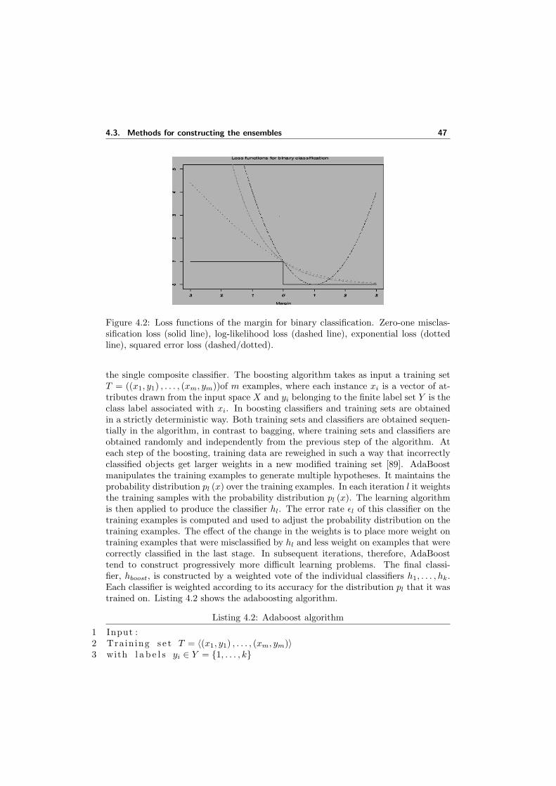
4.3. Methods for constructing the ensembles 47
Figure 4.2: Loss functions of the margin for binary classification. Zero-one misclas-sification loss (solid line), log-likelihood loss (dashed line), exponential loss (dottedline), squared error loss (dashed/dotted).
the single composite classifier. The boosting algorithm takes as input a training setT = ((x1, y1) , . . . , (xm, ym))of m examples, where each instance xi is a vector of at-tributes drawn from the input space X and yi belonging to the finite label set Y is theclass label associated with xi. In boosting classifiers and training sets are obtainedin a strictly deterministic way. Both training sets and classifiers are obtained sequen-tially in the algorithm, in contrast to bagging, where training sets and classifiers areobtained randomly and independently from the previous step of the algorithm. Ateach step of the boosting, training data are reweighed in such a way that incorrectlyclassified objects get larger weights in a new modified training set [89]. AdaBoostmanipulates the training examples to generate multiple hypotheses. It maintains theprobability distribution pl (x) over the training examples. In each iteration l it weightsthe training samples with the probability distribution pl (x). The learning algorithmis then applied to produce the classifier hl. The error rate εl of this classifier on thetraining examples is computed and used to adjust the probability distribution on thetraining examples. The effect of the change in the weights is to place more weight ontraining examples that were misclassified by hl and less weight on examples that werecorrectly classified in the last stage. In subsequent iterations, therefore, AdaBoosttend to construct progressively more difficult learning problems. The final classi-fier, hboost, is constructed by a weighted vote of the individual classifiers h1, . . . , hk.Each classifier is weighted according to its accuracy for the distribution pl that it wastrained on. Listing 4.2 shows the adaboosting algorithm.
Listing 4.2: Adaboost algorithm
1 Input :2 Train ing s e t T = 〈(x1, y1) , . . . , (xm, ym)〉3 with l a b e l s yi ∈ Y = 1, . . . , k
48 4. Ensemble Learning
4 ba s i c l e a rn a lgor i thm base−l e a r n e r5 i n t e g e r M s p e c i f y i n g number o f i t e r a t i o n s6 I n i t i a l i z e D1 (i) = 1
m for a l l i7 for t = 1, . . . ,M8 9 c a l l base−l e a rne r , prov id ing i t with d i s t r i b u t i o n Dt .
10 Get back a hypothes i s ht : X −→ Y11 Ca lcu la te the e r r o r o f ht : εt =
∑i:ht(xi) 6=yi
Dt (i)12 i f εt > 1/213 14 M = t− 115 e x i t16 17 βt = εt/ (1− εt)18 update d i s t r i b u t i o n Dt :19 i f (ht (xi) = yi)20 Dt+1 (i) = Dt(i)
Zt∗ βt
21 else22 Dt+1 (i) = Dt(i)
Zt
23 here Zt i s a norma l i za t i on constant24 25 Output :26 hboost (x) = argmaxy∈Y
∑t:ht(x)=y log 1
βt
There seem to be two separate reasons for the improvement in performance thatis achieved by boosting. The first and better understood effect of boosting is that itgenerates a hypothesis whose error on the training set is small by combining manyhypotheses whose error may be large (but still better than random guessing). Itseems that boosting may be helpful on learning problems having either of the fol-lowing two properties. The first property, which holds for many real-world problems,is that the observed examples tend to have varying degrees of hardness. For suchproblems, the boosting algorithm tends to generate distributions that concentrate onthe harder examples, thus challenging the weak learning algorithm to perform wellon these harder parts of the sample space. The second property is that the learn-ing algorithm be sensitive to changes in the training examples so that significantlydifferent hypotheses are generated for different training sets. In this sense, boostingis similar to Breiman’s bagging which performs best when the weak learner exhibitssuch ”unstable” behavior. However, unlike bagging, boosting tries actively to forcethe weak learning algorithm to change its hypotheses by changing the distributionover the training examples as a function of the errors made by previously generatedhypotheses.
Intuitively, taking a weighted majority over many hypotheses, all of which weretrained on different samples taken out of the same training set, has the effect ofreducing the random variability of the combined hypothesis. Thus, like bagging,
4.3. Methods for constructing the ensembles 49
boosting may have the effect of producing a combined hypothesis whose variance issignificantly lower than those produced by the weak learner. However, unlike bagging,boosting may also reduce the bias of the learning algorithm, as discussed above [84].
Drucker, Schapire and Simard [85] performed the first experiments using a boost-ing algorithm. They used Schapire’s [83] original boosting algorithm combined witha neural net for an OCR problem. Followup comparisons to other ensemble methodswere done by Drucker et al. [86]. In [87] used AdaBoost with a decision-tree algo-rithm for an OCR task. Jackson and Craven [88] used AdaBoost to learn classifiersrepresented by sparse perceptrons, and tested the algorithm on a set of benchmarks.
4.3.3 Other techniques
Sharkey [93] points out that a limiting factor in research on combining classifiers isdue to a lack of awareness of the full range of available modular structures. Onereason for this is that there is as yet little agreement on a means of describing andclassifying types of multiple classifier systems in the literature. One possible way ofliterature survey of ensembles is to study based on the outputs expected by ensemblesfrom individual classifiers [94]. These expectations can be grouped into three levels:a) measurement (or confidence), b) rank and c) abstract. At the confidence level, aclassifier outputs a numerical value for each class indicating the belief or probabilitythat the given patterns belong to that class. At the rank level, a classifier assigns arank to each class with the highest rank being the first choice. Rank value cannotbe used in the isolation because the highest rank does not necessarily mean a highconfidence in the classification. At the abstract level, a classifier only outputs a uniqueclass label or several class labels. The confidence level conveys the richest information,while the abstract level contains the least amount of information about the decisionbeing made. Following [1] here we summarize a number of popular ensemble methodsused in the machine learning literature (table 4.2). This is by no means an exhaustivelist.
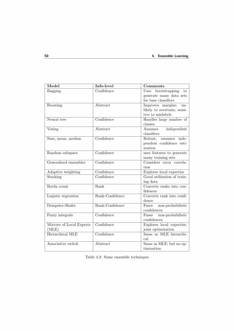
50 4. Ensemble Learning
Model Info-level CommentsBagging Confidence Uses bootstrapping to
generate many data setsfor base classifiers
Boosting Abstract Improves margins; un-likely to overtrain; sensi-tive to mislabels
Neural tree Confidence Handles large number ofclasses
Voting Abstract Assumes independentclassifiers
Sum, mean, median Confidence Robust, assumes inde-pendent confidence esti-mation
Random subspace Confidence uses features to generatemany training sets
Generalized ensembles Confidence Considers error correla-tion
Adaptive weighting Confidence Explores local expertiseStacking Confidence Good utilization of train-
ing dataBorda count Rank Converts ranks into con-
fidencesLogistic regression Rank-Confidence Converts rank into confi-
denceDempster-Shafer Rank-Confidence Fuses non-probabilistic
confidencesFuzzy integrals Confidence Fuses non-probabilistic
confidencesMixture of Local Experts(MLE)
Confidence Explores local expertise;joint optimization
Hierarchical MLE Confidence Same as MLE hierarchi-cal
Associative switch Abstract Same as MLE; but no op-timization
Table 4.2: Some ensemble techniques
5Meta Random Forests
5.1 Introduction
Leo Breimans Random Forests (RF) [96] is a recent development in tree based clas-sifiers and quickly proven to be one of the most important algorithms in the machinelearning literature. It has shown robust and improved results of classifications on stan-dard data sets. It is throwing very good competition to neural networks, ensembletechniques and support vector machines on various classification problems. Randomforest are considered to be special type of ensembles using bagging and random split-ting methods for growing multiple trees. In this chapter we experiment with therandom forests as themselves acting as the base classifiers for making ensembles withbagging and boosting. These meta random forests are then applied on UCI standarddata sets and compared the results with the original random forest algorithm.
The important properties of random forests can be summarized as follows [97]
• Random forests are computationally effective and offer good prediction perfor-mance.
• It has proved to be robust to noise,
• Offers possibilities for explanation and visualization of its output.
• It generates an internal unbiased estimate of the generalization error as theforest building progresses and thus does not overfit.
• It has an effective method for estimating missing data and maintains accuracywhen a large proportion of the data are missing.
• It can be extended to unlabeled data, leading to unsupervised clustering, dataviews and outlier detection.
In previous chapter we seen the construction of ensembling techniques of baggingand boosting. The success of these ensemble methods is usually explained with theerror convergence of base classifiers [108]. To have a good ensemble one needs baseclassifiers which are diverse (in a sense that they predict differently), yet accurate.

52 5. Meta Random Forests
The ensemble mechanism which operates on the top of base learners then ensureshighly accurate predictions. Here we discuss the possibilities of making ensembles ofrandom forests and how they perform on standard data sets. WEKA, a very nicemachine learning framework is used for this purpose [126]. It facilitates powerfulobject oriented programming framework for making ensembles. It provides facilitiesfor using various machine learning algorithms as base classifiers for ensembles. Inthis thesis the ensembles of random forests have been developed by using the WEKAsoftware framework.
The chapter is organised as follows. First we discuss the random forests in section5.2. Section 5.3 discuss the error convergence property for random forests. Section5.4, 5.5 discuss the making of meta random forests with bagging and boosting re-spectively. Section 5.6 shows the experiments with standard data sets from UCIrepository. Finally in section 5.7 a discussion on performance results on UCI datasets and comparative studies between meta random forests and the original randomforest are discussed.
5.2 Random Forests
Random forests construct a series of tree-based learners. Each base learner receivesdifferent training set which are drawn independently with replacement from the origi-nal learning set. Statistically speaking two elements serve to obtain a random forest -resampling and random split selection. Resampling is done here by sampling multipletimes with replacement from the original training data set. Thus in the resultingsamples, a certain event may appear several times, and other events not at all. About2/3rd of the data in the training sample are taken for each bootstrap sample and theremaining one-third of the cases are left out of the sample. This oob (out-of-bag)data is used to get a running unbiased estimate of the classification error as trees areadded to the forest. The design of random forests is to give the user a good deal ofinformation about the data besides an accurate prediction. Much of this informationcomes from using the oob cases in the training set that have been left out of thebootstrapped training set. Random split selection selects a subset of features to growthe nodes in the tree. It is also used to get estimates of variable importance. Thusrandom forests perform randomized selection in both rows (by random sampling) andin columns (by random splitting) for better classification results.
According to [96] the formal definition for random forests is as follows,A random forest is a classifier consisting of a collection of tree structured classifiersh (x,Θk) , k = 1, . . . where the Θk are independent identically distributed randomvectors and each tree casts a unit vote for the most popular class at input x.
Each tree is grown as follows:
• If the number of cases in the training set is n then sample n cases at randombut with replacement, from the original data. This sample will be the trainingset for growing the tree.
• If there are M input variables, a number m << M is specified such that at each

5.2. Random Forests 53
node, m variables are selected at random out of the M and the best split onthese m is used to split the node. The value of m is held constant during theforest growing.
• Each tree is grown to the largest extent possible. There is no pruning 1.
The overall forest error rate depends on two things:
- The correlation between any two trees in the forest. Increasing the correlationincreases the forest error rate.
- The strength of each individual tree in the forest. A tree with a low error rateis a strong classifier. Increasing the strength of the individual trees decreasesthe forest error rate.
The variable selection is an important criterion in classification problems for RF. Oneway of variable selection is to to estimate the importance of the mth variable, in theoob cases for the kth tree, randomly permute all values of the mth variable. Thesealtered oob x-values are put down the tree to get the classification results and newinternal error rate. The amount by which this new error exceeds the original test seterror is defined as the importance of the mth variable. The other measure criterioncould be dealing with the nth case in the data. This nth case data margin at theend of a run is the proportion of votes for its true class minus the maximum of theproportion of votes for each of the other class.
After each tree is built, all of the data are run down the tree, and proximities arecomputed for each pair of cases. If two cases occupy the same terminal node, theirproximity is increased by one. At the end of the run, the proximities are normalizedby dividing by the number of trees. Proximities are used in replacing missing data,locating outliers, and producing illuminating low-dimensional views of the data.
To formalize the working of the random forests, Let the forest contain K classi-fier trees h1 (x) , . . . , hK (x) and the joint classifier be h (x). Each training set of ninstances is drawn at random with replacement from the training set of n instances.Each learning instance is represented by an ordered pair (x, y), where each vector ofattributes x consists of individual attributes Ai, i = 1, . . . , d, (d is the number of at-tributes) and is labeled with the target value yj , j = 1, . . . , c(c is the number of classvalues). The correct class is denoted as y, without index. Each discrete attributeAi has values v1 through vmi (mi is the number of values of attribute Ai).We writep (vi,k) for the probability that the attribute Ai has value vk, p (yj) is the probabilityof the class yj and p (yj | vi,k) is the probability of the class yj conditioned by theattribute Ai having the value vk.
With this sampling of bootstrap replication, on average 36.8% of training in-stances are not used for building each tree. These out-of-bag instances come handyfor computing an internal estimate of the strength and correlation of the forest. Let
1The technique of removing parts of a decision tree that do not capture true features of theunderlying pattern. Decision Tree algorithms typically employ prunning to avoid overfitting of thedata.
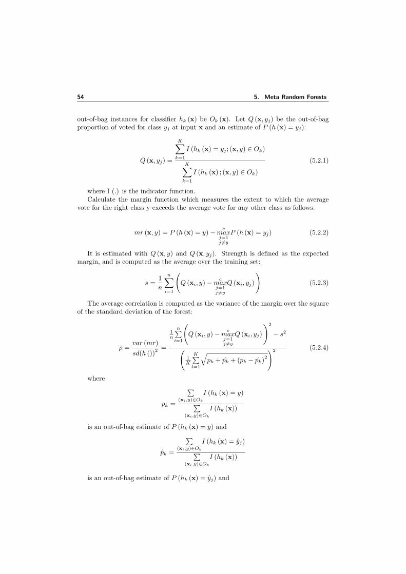
54 5. Meta Random Forests
out-of-bag instances for classifier hk (x) be Ok (x). Let Q (x, yj) be the out-of-bagproportion of voted for class yj at input x and an estimate of P (h (x) = yj):
Q (x, yj) =
K∑k=1
I (hk (x) = yj ; (x, y) ∈ Ok)
K∑k=1
I (hk (x) ; (x, y) ∈ Ok)
(5.2.1)
where I (.) is the indicator function.Calculate the margin function which measures the extent to which the average
vote for the right class y exceeds the average vote for any other class as follows.
mr (x, y) = P (h (x) = y)− cmaxj=1j 6=y
P (h (x) = yj) (5.2.2)
It is estimated with Q (x, y) and Q (x, yj). Strength is defined as the expectedmargin, and is computed as the average over the training set:
s =1n
n∑i=1
(Q (xi, y)− c
maxj=1j 6=y
Q (xi, yj)
)(5.2.3)
The average correlation is computed as the variance of the margin over the squareof the standard deviation of the forest:
ρ =var (mr)sd(h ())2
=
1n
n∑i=1
(Q (xi, y)− c
maxj=1j 6=y
Q (xi, yj)
)2
− s2
(1K
K∑t=1
√pk + pk + (pk − pk)2
)2 (5.2.4)
where
pk =
∑(xi,y)∈Ok
I (hk (x) = y)∑(xi,y)∈Ok
I (hk (x))
is an out-of-bag estimate of P (hk (x) = y) and
pk =
∑(xi,y)∈Ok
I (hk (x) = yj)∑(xi,y)∈Ok
I (hk (x))
is an out-of-bag estimate of P (hk (x) = yj) and

5.3. Error convergence in random forests 55
yj = argc
maxj=1j 6=y
Q (x, yj)
is estimated for every instance x in the training set with Q (x, yj).Breiman used unpruned decision tress as base classifiers and introduces additional
randomness into the trees [99]. The basic approach of the algorithm is to use asplitting criterion to determine the most suitable attribute to be used for splitting thenodes, to grow the tree. The algorithm continually perform this search for finding theattributes to build the branches of the tree until there is no more splits are necessary.Gini Index is the common splitting criterion used in the algorithm. It determines thebest attribute to be used for splitting the node, to grow the tree. The attribute withthe highest Gini index is chosen as split in that node. The gini index is given by theformula:
Gini (Ai) = −c∑
i=1
p(yi)2 +
mi∑j=1
p (vi,j)c∑
i=1
p(yi | vi,j)2
The other splitting criterion methods used in classification problems are Gain ratio[101], ReliefF [102], MDL [103], and KDM [104]. Random Forests uses the Giniindex taken from the CART learning system [105].
5.3 Error convergence in random forests
The generalization error is defined as the probability of margin function defined overthe training set space (X, Y ). It is given by
PE∗ = PX,Y (mg (X, Y ) < 0)
where PX,Y is the probability over the X, Y Space.The generalization error for random forests can be expressed in terms of two
parameters. One is how accurate the individual classifiers and the other is dependencebetween them. The interplay between them gives the insights of the working of therandom forests. Here we derive the convergence factor for generalization error ofrandom forest. This factor estimates the accuracy of the classifier.
Theorem 5.3.1 As the number of trees increases, for almost surely all sequencesΘ1, . . . generalization error PE∗ converges to
PX,Y (PΘ (h (Θ,X) = Y )−maxj 6=Y PΘ (h (Θ,X) = j) < 0)
Proof. The theorem can be proved by showing that there exists a set of probabilityzero C on the sequence space Θ1,Θ2, . . . such that outside of C, for all x,
1N
N∑n=1
I (h (Θn,x) = j)→ PΘ (h (Θ,x) = j)
56 5. Meta Random Forests
For a fixed training set and fixed Θ, the set of all x such that h (Θ,x) = j is a unionof hyper-rectangles. For all h (Θ,x) there is only a finite number K of such unions ofhyper-rectangles, denoted by S1, . . . , SK . Define ϕ (Θ) = k if x : h (Θ,x) = j = Sk.Let Nk be the number of times that ϕ (Θn) = k in the first N trials. Then
1N
N∑n=1
I (h (Θn,x) = j) =1N
∑k
NkI (x ∈ Sk)
By the law of large Numbers,
Nk =1N
N∑n=1
I (ϕ (Θn) = k)
converges as to PΘ (ϕ (Θn) = k). Taking unions of all the sets on which conver-gence does not occur for some value of k gives a set C of zero probability such thatoutside of C,
1N
N∑n=1
I (h (Θn,x) = j)→∑
k
PΘ (ϕ (Θ) = k) I (x ∈ Sk) .
Thus the theorem proves that as the number of trees grows in the RF the resultantclassifier converges to a probabilityPΘ (h (Θ,x) = j). This shows that when the RFitself used as a base classifier for ensembling, with many trees can produce betterconvergence factors.
5.4 Bagged Random Forests
In this section we discuss the application of bagging algorithm to grow the ensemblesof random forest. The random forest itself is considered to be the varied version ofbagged decision trees. Here we experiment with the growth of ensembles of randomforests with bagging in order to reduce the overall bias and variance of learning system.Listing 5.1 describes the bagged random forest algorithm.
Bagging could be used for enhancing the accuracy of random forests. It can be usedto give ongoing estimates of the generalization error (PE∗) of the combined ensembleof forests and the trees within the forests, along with the estimates for the strength and
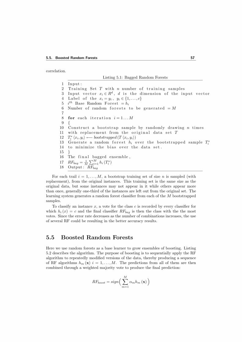
5.5. Boosted Random Forests 57
correlation.
Listing 5.1: Bagged Random Forests
1 Input :2 Train ing Set T with n number o f t r a i n i n g samples3 Input vec to r xi ∈ Rd , d i s the dimension o f the input vec to r4 Label o f the xi = yi , yi ∈ 1, . . . , c5 ith Base Random Forest = hi
6 Number o f random f o r e s t s to be generated = M78 for each i t e r a t i o n i = 1 . . .M9
10 Construct a boots t rap sample by randomly drawing n t imes11 with replacement from the o r i g i n a l data s e t T12 T ∗
i 〈xi, yi〉 ←− bootstrapped (T 〈xi, yi〉)13 Generate a random f o r e s t hi over the bootstrapped sample T ∗
i
14 to minimize the b ia s over the data s e t .15 16 The f i n a l bagged ensemble ,17 RFbag = 1
M
∑Mi=1 hi (T ∗
i )18 Output : RFbag
For each trail i = 1, . . . ,M , a bootstrap training set of size n is sampled (withreplacement), from the original instances. This training set is the same size as theoriginal data, but some instances may not appear in it while others appear morethan once, generally one-third of the instances are left out from the original set. Thelearning system generates a random forest classifier from each of the M bootstrappedsamples.
To classify an instance x, a vote for the class c is recorded by every classifier forwhich hi (x) = c and the final classifier RFbag is then the class with the the mostvotes. Since the error rate decreases as the number of combinations increases, the useof several RF could be resulting in the better accuracy results.
5.5 Boosted Random Forests
Here we use random forests as a base learner to grow ensembles of boosting. Listing5.2 describes the algorithm. The purpose of boosting is to sequentially apply the RFalgorithm to repeatedly modified versions of the data, thereby producing a sequenceof RF algorithms hm (x) i = 1, . . . ,M . The predictions from all of them are thencombined through a weighted majority vote to produce the final prediction:
RFboost = sign( M∑
m=1
αmhm (x))

58 5. Meta Random Forests
Listing 5.2: Boosted Random Forests
1 Input :2 Train ing Set T with n number o f t r a i n i n g samples .3 Input vec to r xi ∈ Rd , d i s the dimension o f the input vec to r4 Label o f the xi = yi , yi ∈ 1, . . . , c5 mth Base Random Forest = hm
6 M be the number o f Random f o r e s t s to grow7 I n i t i a l i z e the obse rvat i on weights :8 for a l l i = 1, . . . , n9 wi = 1/n
10 for m = 1 to M11 12 Fit a random f o r e s t hm (x) to t ra in ing−s e t T us ing weights wi
13 Compute e r r o r o f hm
14 errm =Pn
i=1 wiI(yi 6=hm(xi))Pni=1 wi
15 Compute r e l a t i v e importances o f hm
16 αm = log ((1− errm) /errm)17 Set wi ← wi · exp [αm · I (yi 6= hm (xi))] , i = 1, . . . , n .18 1920 Output :21 RFboost = sign
[∑Mm=1 αmhm (x)
]In the algorithm α1, α2, . . . , αM represent the relative importances, for are each
of the random forest classifier, computed by the boosting algorithm. Their effect isto give higher influence to the more accurate classifiers in the sequence. Figure 5.1shows a schematic of the AdaBoost procedure for random forests, here RF classifiersare trained on weighted versions of the dataset, and then combined to produce a finalprediction.
5.6 Experiments on UCI data sets
UCI machine learning repository [106] contains data sets that have been in use toevaluate learning algorithms. Each data file contains individual records described interms of attribute-value pairs. The ensembles of RF along with the original RF havebeen evaluated on several datasets from the UCI Machine learning Repository. Thedata sets used in the experiment are summarized in the table 5.1
For the original random forest algorithm, 20 decision trees have been grown forthese experiments. In all the experiments at an average a random forest with 20 treeshave shown significant improvements in the classification accuracies, further growth oftrees have not shown any significant improvements in classification accuracies (Figure5.6). The experiments are conducted with unpruned trees, and the variable yielding
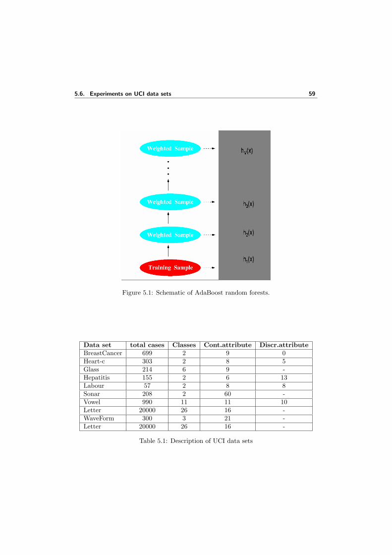
5.6. Experiments on UCI data sets 59
Figure 5.1: Schematic of AdaBoost random forests.
Data set total cases Classes Cont.attribute Discr.attributeBreastCancer 699 2 9 0Heart-c 303 2 8 5Glass 214 6 9 -Hepatitis 155 2 6 13Labour 57 2 8 8Sonar 208 2 60 -Vowel 990 11 11 10Letter 20000 26 16 -WaveForm 300 3 21 -Letter 20000 26 16 -
Table 5.1: Description of UCI data sets
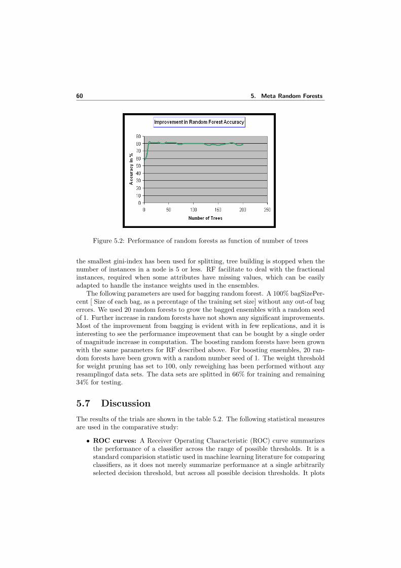
60 5. Meta Random Forests
Figure 5.2: Performance of random forests as function of number of trees
the smallest gini-index has been used for splitting, tree building is stopped when thenumber of instances in a node is 5 or less. RF facilitate to deal with the fractionalinstances, required when some attributes have missing values, which can be easilyadapted to handle the instance weights used in the ensembles.
The following parameters are used for bagging random forest. A 100% bagSizePer-cent [ Size of each bag, as a percentage of the training set size] without any out-of bagerrors. We used 20 random forests to grow the bagged ensembles with a random seedof 1. Further increase in random forests have not shown any significant improvements.Most of the improvement from bagging is evident with in few replications, and it isinteresting to see the performance improvement that can be bought by a single orderof magnitude increase in computation. The boosting random forests have been grownwith the same parameters for RF described above. For boosting ensembles, 20 ran-dom forests have been grown with a random number seed of 1. The weight thresholdfor weight pruning has set to 100, only reweighing has been performed without anyresamplingof data sets. The data sets are splitted in 66% for training and remaining34% for testing.
5.7 Discussion
The results of the trials are shown in the table 5.2. The following statistical measuresare used in the comparative study:
• ROC curves: A Receiver Operating Characteristic (ROC) curve summarizesthe performance of a classifier across the range of possible thresholds. It is astandard comparision statistic used in machine learning literature for comparingclassifiers, as it does not merely summarize performance at a single arbitrarilyselected decision threshold, but across all possible decision thresholds. It plots
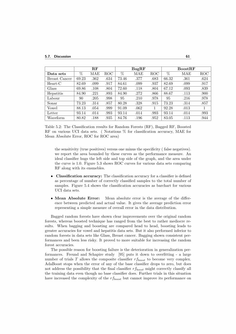
5.7. Discussion 61
RF BagRF BoostRFData sets % MAE ROC % MAE ROC % MAE ROCBreast Cancer 69.23 .362 .634 73.46 .377 .683 66.32 .361 .624Heart-C 82.69 .099 .917 84.61 .099 .937 82.69 .099 .917Glass 69.86 .108 .804 72.60 .118 .804 67.12 .093 .839Hepatitis 84.90 .221 .893 84.90 .272 .866 88.67 .113 .900Labour 90 .205 .998 95 .210 .978 95 .216 .978Sonar 73.23 .314 .857 80.28 .328 .915 73.23 .314 .857Vowel 88.13 .054 .999 91.09 .062 1 92.28 .013 1Letter 93.14 .014 .993 93.14 .014 .993 93.14 .014 .993Waveform 80.82 .188 .935 84.76 .196 .952 83.05 .113 .944
Table 5.2: The Classification results for Random Forests (RF), Bagged RF, BoostedRF on various UCI data sets. ( Notations % for classification accuracy, MAE forMean Absolute Error, ROC for ROC area)
the sensitivity (true positives) versus one minus the specificity ( false negatives).we report the area bounded by these curves as the performance measure. Anideal classifier hugs the left side and top side of the graph, and the area underthe curve is 1.0. Figure 5.3 shows ROC curves for various data sets comparingRF along with its ensmebles.
• Classification accuracy: The classification accuracy for a classifier is definedas percentage of number of correctly classified samples to the total number ofsamples. Figure 5.4 shows the classification accuracies as barchart for variousUCI data sets.
• Mean Absolute Error: Mean absolute error is the average of the differ-ence between predicted and actual value. It gives the average prediction errorrepresenting a simple measure of overall error in the data distribution.
Bagged random forests have shown clear improvements over the original randomforests, whereas boosted technique has ranged from the best to rather mediocre re-sults. When bagging and boosting are compared head to head, boosting leads togreater accuracies for vowel and hepatitis data sets. But it also performed inferior torandom forests in data sets like Glass, Breast cancer. Bagging shown consistent per-formances and been less risky. It proved to more suitable for increasing the randomforest accuracies.
The possible reason for boosting failure is the deterioration in generalization per-formances. Freund and Schapire study [95] puts it down to overfitting - a largenumber of trials T allows the composite classifier rfboost to become very complex.AdaBoost stops when the error of any of the base classifier drops to zero, but doesnot address the possibility that the final classifier rfboost might correctly classify allthe training data even though no base classifier does. Further trials in this situationhave increased the complexity of the rfboost but cannot improve its performance on
62 5. Meta Random Forests
the data sets. It also supports the hypothesis that over-fitting is a major factor inexplaining boosting’s failure on some data sets.
We investigated the possibilities of improving the random forests. Experimentsover diverse collection of data sets have confirmed that the ensembles of random foresthave improved the performance of classifications. Boosting and Bagging both have asound theoretical base and also have the advantage that the extra computation theyrequire is known in advance - if T classifiers are generated, then both require T timesthe computational effort of random forests. In these experiments, a little increase incomputation can buys a significant increase in the classification accuracies. In manyapplications, improvements of this magnitude would be well worth the computationalcost.
We use these random forest ensembles for the image data classification in MAGICtelescope experiment discussed in the next chapter. Also we discuss the developmentof BPNN ensembles for the application to MAGIC image data.
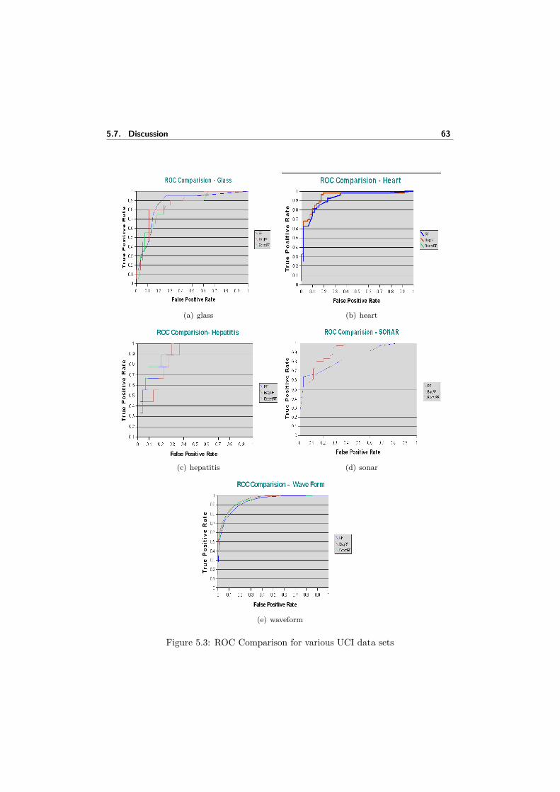
5.7. Discussion 63
(a) glass (b) heart
(c) hepatitis (d) sonar
(e) waveform
Figure 5.3: ROC Comparison for various UCI data sets

64 5. Meta Random Forests
Figure 5.4: Classification accuracies for RF and its ensembles for various UCI datasets

6MAGIC and its image
classification
Figure 6.1: The MAGIC telescope
MAGIC(Major Atmospheric Gamma Imaging Telescope) is the world’s largestimaging air Cherenkov telescope used for detecting the gamma signals from the outerspace [109]. It is an international collaboration project with more than 150 Physicists,Computer scientists from 17 institutions. It is designed to provide vital informationon several established gamma-ray sources, like Active Galactic Nuclei, SupernovaRemnants, Gamma Ray Bursts and Pulsars. It is located in La Palma one of thebeautiful Canary islands in Spain at the Roque de los Muchachos Observatory Cen-ter(28.8N, 17.9W), 2200 m above the sea level. The place is well known for its goodmeteorological features and its altitude allows to make observations of astronomicalsources, with an almost always clean night sky. The data taking by the telescopehas been started in april 2004, and since then several sources are being observed. Inthis chapter we discuss the classification of images collected by the MAGIC based on
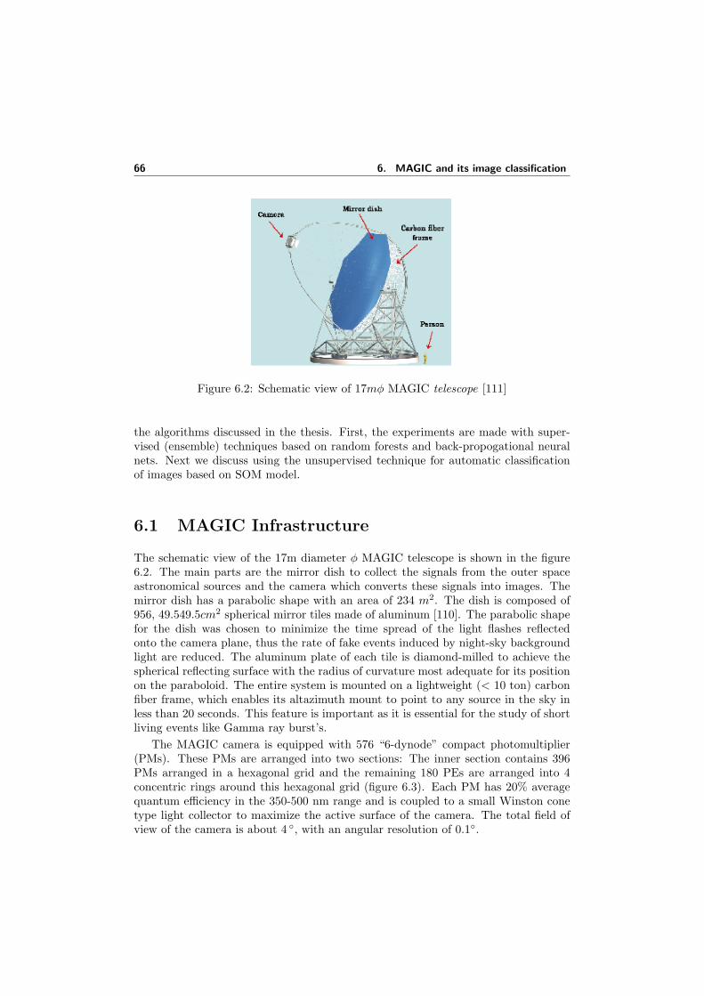
66 6. MAGIC and its image classification
Figure 6.2: Schematic view of 17mφ MAGIC telescope [111]
the algorithms discussed in the thesis. First, the experiments are made with super-vised (ensemble) techniques based on random forests and back-propogational neuralnets. Next we discuss using the unsupervised technique for automatic classificationof images based on SOM model.
6.1 MAGIC Infrastructure
The schematic view of the 17m diameter φ MAGIC telescope is shown in the figure6.2. The main parts are the mirror dish to collect the signals from the outer spaceastronomical sources and the camera which converts these signals into images. Themirror dish has a parabolic shape with an area of 234 m2. The dish is composed of956, 49.549.5cm2 spherical mirror tiles made of aluminum [110]. The parabolic shapefor the dish was chosen to minimize the time spread of the light flashes reflectedonto the camera plane, thus the rate of fake events induced by night-sky backgroundlight are reduced. The aluminum plate of each tile is diamond-milled to achieve thespherical reflecting surface with the radius of curvature most adequate for its positionon the paraboloid. The entire system is mounted on a lightweight (< 10 ton) carbonfiber frame, which enables its altazimuth mount to point to any source in the sky inless than 20 seconds. This feature is important as it is essential for the study of shortliving events like Gamma ray burst’s.
The MAGIC camera is equipped with 576 “6-dynode” compact photomultiplier(PMs). These PMs are arranged into two sections: The inner section contains 396PMs arranged in a hexagonal grid and the remaining 180 PEs are arranged into 4concentric rings around this hexagonal grid (figure 6.3). Each PM has 20% averagequantum efficiency in the 350-500 nm range and is coupled to a small Winston conetype light collector to maximize the active surface of the camera. The total field ofview of the camera is about 4 , with an angular resolution of 0.1.

6.2. Image collection in MAGIC 67
Figure 6.3: A simulated MAGIC Camera
6.2 Image collection in MAGIC
The source observation by MAGIC is carried out during night time with a well or-ganized night data taking schedule for various interesting astronomical objects. Thedetection of signals from these sources is based on Imaging Atmospheric CherenkovTechnique (IACT). Astronomical sources transmit extremely energetic particles trav-eling very close to the speed of light or traveling faster than the speed of light “in themedium of the atmosphere” [112]. Infact nothing can travel faster than the speed oflight “in a vacuum”, but that the speed of light is reduced when traveling throughmost media (like glass, water, air, etc.). The resultant polarization of local atoms asthe charged particles travel through the atmosphere results in the emission of a faint,bluish light known as ”Cherenkov radiation” [113], named for the Russian physicistwho made comprehensive studies of this phenomenon. Depending on the energy ofthe initial cosmic gamma-ray, there may be thousands of electrons/positrons in theresulting cascade which are capable of emitting Cherenkov radiation. As a result, alarge ”pool” of Cherenkov light accompanies the particles in the air shower. Thispool of light is pancake-like in appearance, about 200 meters in diameter but only ameter or so in thickness. MAGIC telescope, rely on this pool of light to detect thearrival of a cosmic gamma-ray.
This large pool Cherenkov light is reflected from the mirror of telescope on tothe focal plane of one or many photo-multipliers (PMs) of camera, which convert theincoming optical signal into an electronic signal to record the signal “image” or alsocalled as “event” figure 6.3. These images (electronic signals) are essentially analogsignals, which are first amplified obtaining the low and high gain signals and thenpassed to FADC (Flash Analog to Digital Converter) module. This FADC moduleis responsible for digitally sampling the signals into computer readable data whichrepresents the raw image formed on the camera. It is composed of several 8 bitconverters each operating at a frequency of 300MHz. Data are then transferred tolarger storage arrays and saved them in the raw data format on tapes and hard disks[116]. In this way, a crude image of the Cherenkov light pool is recorded.
MAGIC collaboration has developed a software system called Magic Analysis andReconstruction Software (MARS) for camera simulations and analysis tasks. Thesoftware is a collection of C++ classes based on the well known data analysis packageROOT [114]. A software release is documented and available on the web [115]. Figure
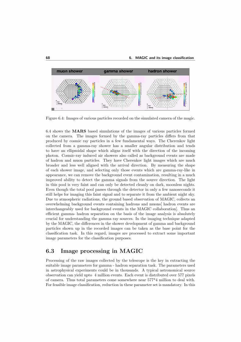
68 6. MAGIC and its image classification
Figure 6.4: Images of various particles recorded on the simulated camera of the magic.
6.4 shows the MARS based simulations of the images of various particles formedon the camera. The images formed by the gamma-ray particles differs from thatproduced by cosmic ray particles in a few fundamental ways. The Cherenkov lightcollected from a gamma-ray shower has a smaller angular distribution and tendsto have an ellipsoidal shape which aligns itself with the direction of the incomingphoton. Cosmic-ray induced air showers also called as background events are madeof hadron and muon particles. They have Cherenkov light images which are muchbroader and less well aligned with the arrival direction. By measuring the shapeof each shower image, and selecting only those events which are gamma-ray-like inappearance, we can remove the background event contamination, resulting in a muchimproved ability to detect the gamma signals from the source direction. The lightin this pool is very faint and can only be detected cleanly on dark, moonless nights.Even though the total pool passes through the detector in only a few nanoseconds itstill helps for imaging this faint signal and to separate it from the ambient night sky.Due to atmospheric radiations, the ground based observation of MAGIC, collects anoverwhelming background events containing hadrons and muons[ hadron events areinterchangeably used for background events in the MAGIC collaboration]. Thus anefficient gamma- hadron separation on the basis of the image analysis is absolutelycrucial for understanding the gamma ray sources. In the imaging technique adaptedby the MAGIC, the differences in the shower development of gamma and backgroundparticles shown up in the recorded images can be taken as the base point for theclassification task. In this regard, images are processed to extract some importantimage parameters for the classification purposes.
6.3 Image processing in MAGIC
Processing of the raw images collected by the telescope is the key in extracting thesuitable image parameters for gamma - hadron separation task. The parameters usedin astrophysical experiments could be in thousands. A typical astronomical sourceobservation can yield upto 4 million events. Each event is distributed over 577 pixelsof camera. Thus total parameters come somewhere near 577*4 million to deal with.For feasible image classification, reduction in these parameter set is mandatory. In this
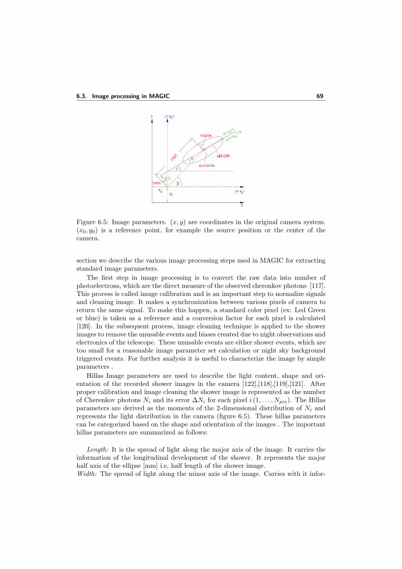
6.3. Image processing in MAGIC 69
Figure 6.5: Image parameters. (x, y) are coordinates in the original camera system.(x0, y0) is a reference point, for example the source position or the center of thecamera.
section we describe the various image processing steps used in MAGIC for extractingstandard image parameters.
The first step in image processing is to convert the raw data into number ofphotoelectrons, which are the direct measure of the observed cheronkov photons [117].This process is called image calibration and is an important step to normalize signalsand cleaning image. It makes a synchronization between various pixels of camera toreturn the same signal. To make this happen, a standard color pixel (ex: Led Greenor blue) is taken as a reference and a conversion factor for each pixel is calculated[120]. In the subsequent process, image cleaning technique is applied to the showerimages to remove the unusable events and biases created due to night observations andelectronics of the telescope. These unusable events are either shower events, which aretoo small for a reasonable image parameter set calculation or night sky backgroundtriggered events. For further analysis it is useful to characterize the image by simpleparameters .
Hillas Image parameters are used to describe the light content, shape and ori-entation of the recorded shower images in the camera [122],[118],[119],[121]. Afterproper calibration and image cleaning the shower image is represented as the numberof Cherenkov photons Ni and its error ∆Ni for each pixel i (1, . . . , Npix). The Hillasparameters are derived as the moments of the 2-dimensional distribution of Ni andrepresents the light distribution in the camera (figure 6.5). These hillas parameterscan be categorized based on the shape and orientation of the images . The importanthillas parameters are summarized as follows:
Length: It is the spread of light along the major axis of the image. It carries theinformation of the longitudinal development of the shower. It represents the majorhalf axis of the ellipse [mm] i.e, half length of the shower image.Width: The spread of light along the minor axis of the image. Carries with it infor-
70 6. MAGIC and its image classification
mation of lateral development of the shower. In the image it represents the minoraxis of the ellipse [mm] i.e half width of the shower image.Size: The total integrated light content of the shower. It represents the total numberof photons in the shower.Conc2: It is the ratio of sum of two highest pixels over size ratio.Conc1: It is the ratio of the brightest pixel over size.Asym: Assymetry of the photon distribution along the shower axis.MDIST: Distance between the center of the shower image and the brightest pixel.LEAKAGE: Fraction of photons contained in the pixels close to the edge of the cam-era.DELTA: angle δ between the shower axis and the x− axis of the cameraDIST: distance of center of shower image from the Reference Point (RP)MISS: distance of the shower axis from the RPALPHA: angle α by which shower axis misses the RP, as seen from the center of theshower imageBETA: angle β between the x − axis of the camera and the line connecting the RPwith the center of the shower imageAZWIDTH: half width of the shower image as seen from the RP.
Traditionally the separation task is carried out by statistical techniques such asdynamical cuts. These cuts operate on one variable at a time but often made depen-dent on other parameters based on logical operators such as AND or OR to partitionthe given n-dimensional space; the problem gets unwidely even for a low n-space offeatures, nevertheless this is the widely used technique for many cheronkov experi-ments for image classification [123]. Now we discuss the usage of the machine learningalgorithms both supervised and unsupervised for the image classification task basedon these image parameters.
6.4 Supervised classification
Previous classification studies performed on MAGIC data sets shown that randomforest, neural networks performed better than other classifiers [124]. Here we experi-ment with ensembles of random forests, neural networks and study their performanceresults. The experiment is conducted on crab astronomical source. The data ana-lyzed here were taken during September and October 2004 and in January 2005. TheCrab nebula is the remnant of a supernova explosion that occurred in 1054. Theγ-emissions from this source was first reported by the Whipple collaboration [136].It exhibits a stable and strong γ-emission and is frequently used as the “standardcandle” in very high energy γ-astronomy [135]. The Crab nebula has been observedextensively in the past over a wide range of wavelengths, covering the radio, opticaland X-ray bands, as well as high-energy regions up to nearly 100TeV [137].
Probing the presence of gamma signals from this sources is a challenge for ex-perimenters. A total of 2.8 million images in 2004 and 4.5 million images from the2005 observations were used . The overall observation time of the sample analyzed

6.4. Supervised classification 71
corresponds to 13 hours on-source and the data collected [around 25 Giga bytes], isused as a test set for separating gammas from the hadrons. The training data setsfor the algorithms have been generated by a monte-carlo program, CORSIKA [125].It is a package used to perform detail simulation of cheronkov light effect observedby the MAGIC for various sky objects. The CRAB source was simulated with thesame parameter set that has been used for the observation. The Monte Carlo rawdata has been subjected to image calibration and image cleaning to extract the imageparameters. Image cleaning eliminates the biased data and outliers. Subsequentlythe analysis is simplified with little or no loss of information, by converting the pixelsof image into image parameters for both gamma and other background particles. Assuggested in [124], the following image parameters have been chosen based on theirimportance in the image properties : length, width, size, conc2, conc1, pdist, m3long,m3trans, alpha, dist. They are used only for relative comparison of algorithms. At im-age processing stage, no care has been taken to optimize the data. Also, no particularcare has been taken to choose independent parameters since a robust discriminationmethod should itself take care of correlations between parameters. The sample inthe training set contains 122800 background events, 720000 gamma events. Now wediscuss the algorithms used for the classification purpose and study the performanceresults. Random forests, back propagation neural nets and their ensembles are devel-oped for the classification tasks. WEKA, a very nice machine learning framework isused for this purpose[126]. It facilitates powerful object oriented programming frame-work for making ensembles. It provides facilities for using various machine learningalgorithms as base classifiers for ensembles.
6.4.1 Random forests and its ensembles
Random forests and its ensembles have been thoroughly described in chapter “MetaRandom Forests”. Here we used these algorithms for studying the performance resultsof the MAGIC experiment. The tree growing begins with all cases being contained inthe root node. The root node is then split by a cut using one of the image parameters,into two successive nodes to achieve a classification by separation of the classes. Whenusing all of 10 image parameters, three of them are chosen randomly and uniformlydistributed. The image parameter yielding the smallest Gini-index among these threeis used for splitting. Subsequently, the same procedure is applied to each branch inturn. The tree growing stops only when all nodes contain pure data, i.e. from oneclass only. These nodes are then called terminal nodes and receive their class labelfrom the training data. No pruning is performed. Using unpruned trees (in generalpoor classifiers) requires a reasonably large number of them to be combined. For ourdata, growing 20 trees turns out to be sufficient: the quality of the classification interms ROC plot remains unchanged after a certain number of trees has been reached.Combining classifications from the trees is simply done by calculating the arithmeticmean from the 20 classifications of all trees (considered as 0 and 1). The resultsare verified with R statistical software [127], Breiman original FORTRAN sources forthe Random Forests technique [128]. Random Forests are themselves proved to bepowerful classifiers, and given good results for MAGIC data sets. The ensembles of
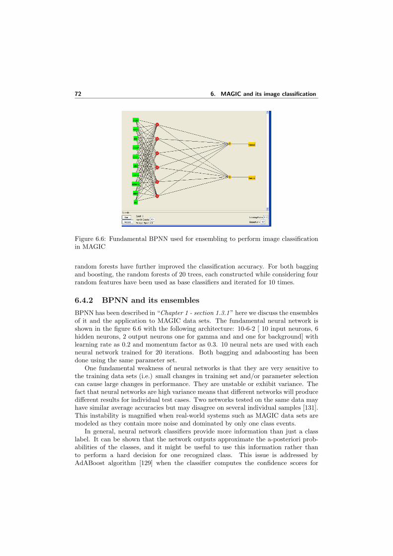
72 6. MAGIC and its image classification
Figure 6.6: Fundamental BPNN used for ensembling to perform image classificationin MAGIC
random forests have further improved the classification accuracy. For both baggingand boosting, the random forests of 20 trees, each constructed while considering fourrandom features have been used as base classifiers and iterated for 10 times.
6.4.2 BPNN and its ensembles
BPNN has been described in “Chapter 1 - section 1.3.1” here we discuss the ensemblesof it and the application to MAGIC data sets. The fundamental neural network isshown in the figure 6.6 with the following architecture: 10-6-2 [ 10 input neurons, 6hidden neurons, 2 output neurons one for gamma and and one for background] withlearning rate as 0.2 and momentum factor as 0.3. 10 neural nets are used with eachneural network trained for 20 iterations. Both bagging and adaboosting has beendone using the same parameter set.
One fundamental weakness of neural networks is that they are very sensitive tothe training data sets (i.e.) small changes in training set and/or parameter selectioncan cause large changes in performance. They are unstable or exhibit variance. Thefact that neural networks are high variance means that different networks will producedifferent results for individual test cases. Two networks tested on the same data mayhave similar average accuracies but may disagree on several individual samples [131].This instability is magnified when real-world systems such as MAGIC data sets aremodeled as they contain more noise and dominated by only one class events.
In general, neural network classifiers provide more information than just a classlabel. It can be shown that the network outputs approximate the a-posteriori prob-abilities of the classes, and it might be useful to use this information rather thanto perform a hard decision for one recognized class. This issue is addressed byAdABoost algorithm [129] when the classifier computes the confidence scores for
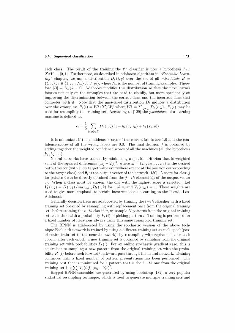
6.4. Supervised classification 73
each class. The result of the training the tth classifier is now a hypothesis ht :XxY → [0, 1]. Furthermore, as described in adaboost algorithm in “Ensemble Learn-ing” chapter, we use a distribution Dt (i, y) over the set of all miss-labels B =(i, y) : i ∈ 1, . . . , Nv , y 6= yi, where Nv is the number of training examples. There-fore |B| = Nv (k − 1). Adaboost modifies this distribution so that the next learnerfocuses not only on the examples that are hard to classify, but more specifically onimproving the discrimination between the correct class and the incorrect class thatcompetes with it. Note that the miss-label distribution Dt induces a distributionover the examples: Pt (i) = W t
i /∑
i W ti where W t
i =∑
y 6=yiDt (i, y). Pi (i) may be
used for resampling the training set. According to [129] the pseudoloss of a learningmachine is defined as:
εt =12
∑(i,y)∈B
Dt (i, y) (1− ht (xi, yi) + ht (xi, y))
It is minimized if the confidence scores of the correct labels are 1.0 and the con-fidence scores of all the wrong labels are 0.0. The final decision f is obtained byadding together the weighted confidence scores of all the machines (all the hypothesish1, h2, . . .).
Neural networks have trained by minimizing a quadric criterion that is weightedsum of the squared differences (zij − zij)
2, where zi = (zi1, zi2, . . . zik) is the desiredoutput vector (with a low target value everywhere except at the position correspondingto the target class) and zi is the output vector of the network [130]. A score for class jfor pattern i can be directly obtained from the j− th element zij of the output vectorzi. When a class must be chosen, the one with the highest score is selected. LetVt (i, j) = D (i, j) /maxk 6=yi
Dt (i, k) for j 6= yi and Vt (i, yi) = 1. These weights areused to give more emphasis to certain incorrect labels according to the Pseudo-LossAdaboost.
Generally decision trees are adaboosted by training the t−th classifier with a fixedtraining set obtained by resampling with replacement once from the original trainingset: before starting the t−th classifier, we sample N patterns from the original trainingset, each time with a probability Pt (i) of picking pattern i. Training is performed fora fixed number of iterations always using this same resampled training set.
The BPNN is adaboosted by using the stochastic version of the above tech-nique.Each t-th network is trained by using a different training set at each epoch(passof entire train set to the neural network), by resampling with replacement for eachepoch: after each epoch, a new training set is obtained by sampling from the originaltraining set with probabilities Pt (i). For an online stochastic gradient case, this isequivalent to sampling a new pattern from the original training set with the proba-bility Pt (i) before each forward/backward pass through the neural network. Trainingcontinues until a fixed number of pattern presentations has been performed. Thetraining cost that is minimized for a pattern that is the i − th one from the originaltraining set is 1
2
∑j Vt (i, j) (zij − zij)
2.Bagged BPNN ensembles are generated by using bootstrap [132], a very popular
statistical resampling technique, which is used to generate multiple training sets and
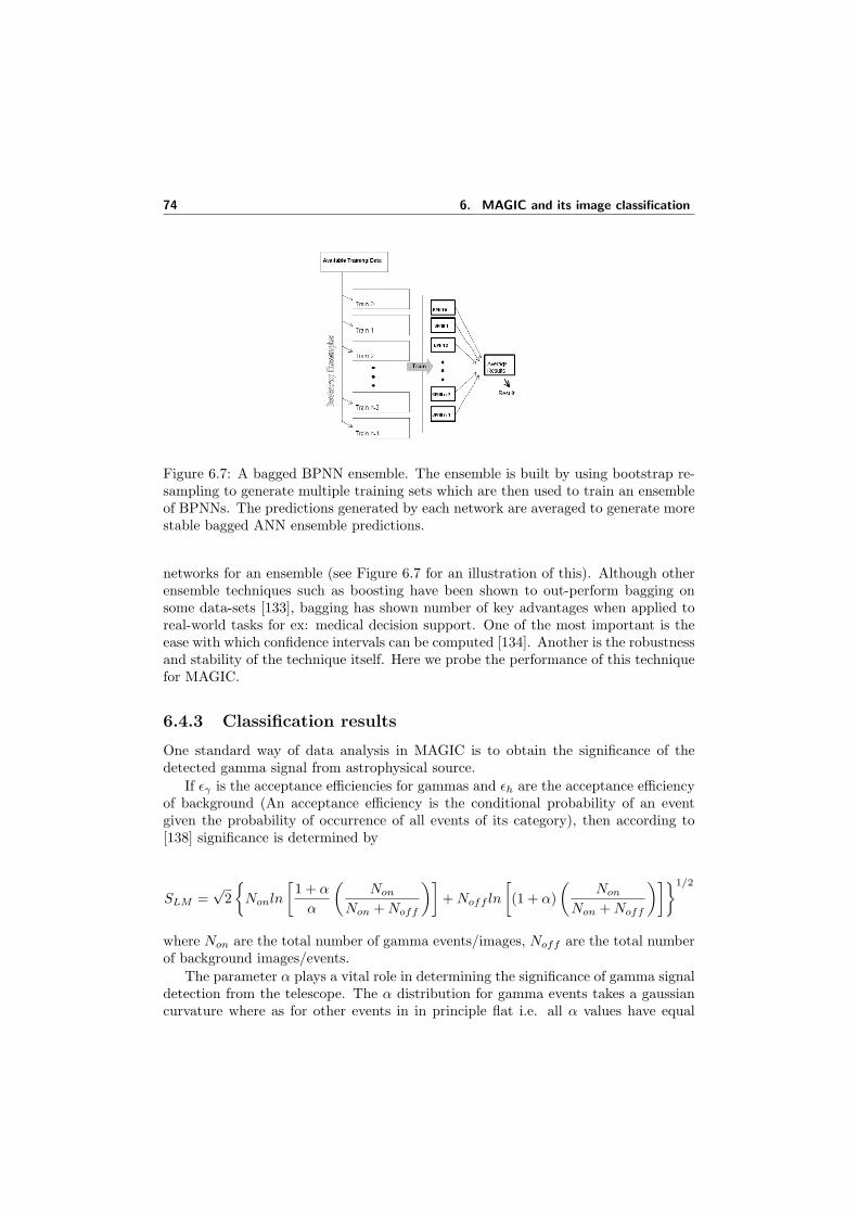
74 6. MAGIC and its image classification
Figure 6.7: A bagged BPNN ensemble. The ensemble is built by using bootstrap re-sampling to generate multiple training sets which are then used to train an ensembleof BPNNs. The predictions generated by each network are averaged to generate morestable bagged ANN ensemble predictions.
networks for an ensemble (see Figure 6.7 for an illustration of this). Although otherensemble techniques such as boosting have been shown to out-perform bagging onsome data-sets [133], bagging has shown number of key advantages when applied toreal-world tasks for ex: medical decision support. One of the most important is theease with which confidence intervals can be computed [134]. Another is the robustnessand stability of the technique itself. Here we probe the performance of this techniquefor MAGIC.
6.4.3 Classification results
One standard way of data analysis in MAGIC is to obtain the significance of thedetected gamma signal from astrophysical source.
If εγ is the acceptance efficiencies for gammas and εh are the acceptance efficiencyof background (An acceptance efficiency is the conditional probability of an eventgiven the probability of occurrence of all events of its category), then according to[138] significance is determined by
SLM =√
2
Nonln
[1 + α
α
(Non
Non + Noff
)]+ Noff ln
[(1 + α)
(Non
Non + Noff
)]1/2
where Non are the total number of gamma events/images, Noff are the total numberof background images/events.
The parameter α plays a vital role in determining the significance of gamma signaldetection from the telescope. The α distribution for gamma events takes a gaussiancurvature where as for other events in in principle flat i.e. all α values have equal
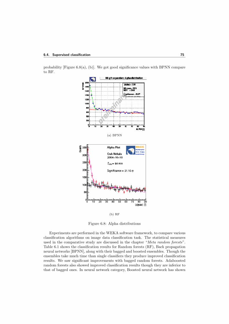
6.4. Supervised classification 75
probability [Figure 6.8(a), (b)]. We got good significance values with BPNN compareto RF.
(a) BPNN
(b) RF
Figure 6.8: Alpha distributions
Experiments are performed in the WEKA software framework, to compare variousclassification algorithms on image data classification task. The statistical measuresused in the comparative study are discussed in the chapter “Meta random forests”.Table 6.1 shows the classification results for Random forests (RF), Back propagationneural networks [BPNN], along with their bagged and boosted ensembles. Though theensembles take much time than single classifiers they produce improved classificationresults. We saw significant improvements with bagged random forests. Adaboostedrandom forests also showed improved classification results though they are inferior tothat of bagged ones. In neural network category, Boosted neural network has shown
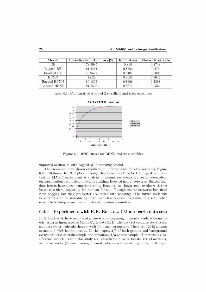
76 6. MAGIC and its image classification
Model Classification Accuracy[%] ROC Area Mean Error rateRF 78.9085 0.818 0.2748
Bagged RF 81.2461 0.8753 0.276Boosted RF 79.9527 0.8481 0.2006
BPNN 78.28 0.8651 0.2644Bagged BPNN 80.1893 0.8666 0.2888Boosted BPNN 81.7508 0.8671 0.2564
Table 6.1: Comparative study of 2 classifiers and their ensembles
Figure 6.9: ROC curves for BPNN and its ensembles
improved accuracies with bagged MLP standing second.The ensembles have shown classification improvements for all algorithms, Figure
6.9, 6.10 shows the ROC plots. Though they take more time for training, it is impor-tant for MAGIC experiment as analysis of gamma ray events are heavily dependenton classification accuracies. In overall rankings Boosted neural networks, Bagged ran-dom forests have shown superior results. Bagging has shown good results with treebased classifiers, especially for random forests. Though neural networks benefitedfrom bagging but they got better accuracies with boosting. The future work willbe concentrated on introducing more base classifiers and experimenting with otherensemble techniques such as multi-boost, random committee.
6.4.4 Experiments with R.K. Bock et.al Monte-carlo data sets
R. K. Bock et.al, have performed a case study comparing different classification meth-ods, using as input a set of Monte Carlo data [124]. The data set contains two classes,gamma rays or hadronic showers with 10 image parameters. There are 12332 gammaevents and 6688 hadron events. In this paper, 2/3 of both gamma and backgroundevents are used as train sample and remaining 1/3 as test sample. The various clas-sification models used in this study are: classification trees, forests, kernel methods,neural networks (Neunet package, neural network with switching units, multi-layer
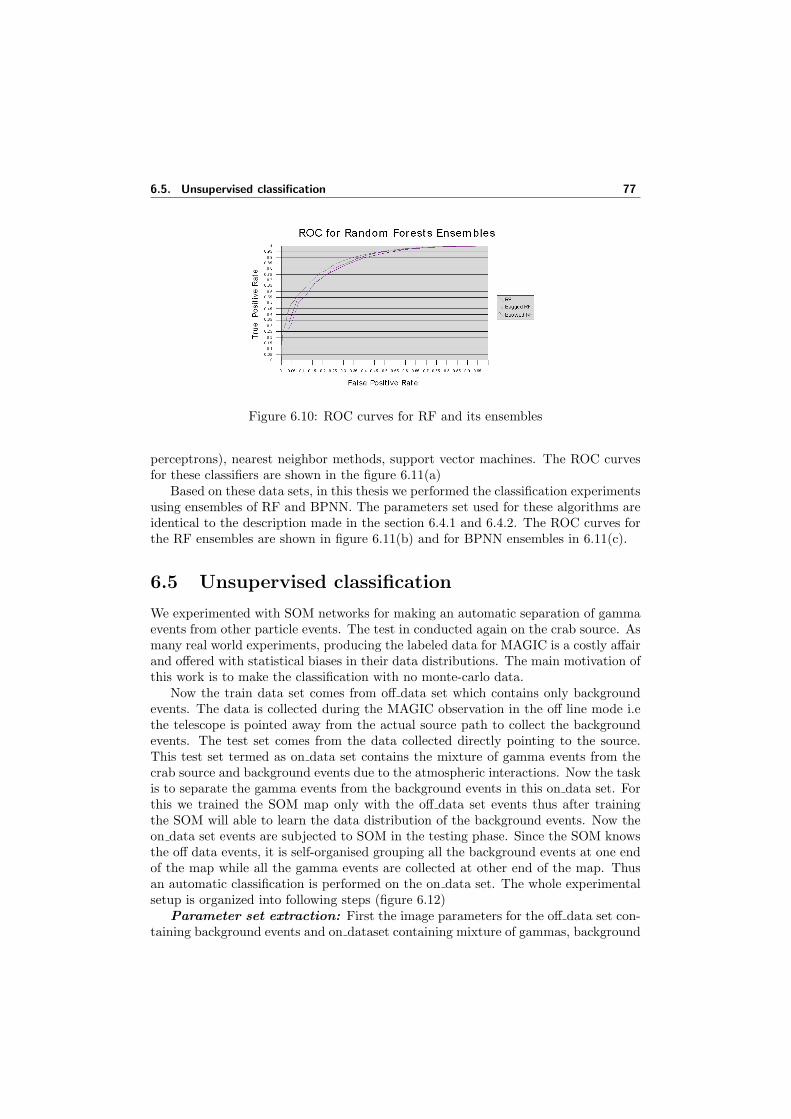
6.5. Unsupervised classification 77
Figure 6.10: ROC curves for RF and its ensembles
perceptrons), nearest neighbor methods, support vector machines. The ROC curvesfor these classifiers are shown in the figure 6.11(a)
Based on these data sets, in this thesis we performed the classification experimentsusing ensembles of RF and BPNN. The parameters set used for these algorithms areidentical to the description made in the section 6.4.1 and 6.4.2. The ROC curves forthe RF ensembles are shown in figure 6.11(b) and for BPNN ensembles in 6.11(c).
6.5 Unsupervised classification
We experimented with SOM networks for making an automatic separation of gammaevents from other particle events. The test in conducted again on the crab source. Asmany real world experiments, producing the labeled data for MAGIC is a costly affairand offered with statistical biases in their data distributions. The main motivation ofthis work is to make the classification with no monte-carlo data.
Now the train data set comes from off data set which contains only backgroundevents. The data is collected during the MAGIC observation in the off line mode i.ethe telescope is pointed away from the actual source path to collect the backgroundevents. The test set comes from the data collected directly pointing to the source.This test set termed as on data set contains the mixture of gamma events from thecrab source and background events due to the atmospheric interactions. Now the taskis to separate the gamma events from the background events in this on data set. Forthis we trained the SOM map only with the off data set events thus after trainingthe SOM will able to learn the data distribution of the background events. Now theon data set events are subjected to SOM in the testing phase. Since the SOM knowsthe off data events, it is self-organised grouping all the background events at one endof the map while all the gamma events are collected at other end of the map. Thusan automatic classification is performed on the on data set. The whole experimentalsetup is organized into following steps (figure 6.12)
Parameter set extraction: First the image parameters for the off data set con-taining background events and on dataset containing mixture of gammas, background
78 6. MAGIC and its image classification
events are extracted following the image processing steps described in this chapterData Normalization: Normalization usually means linear scaling of variables.
More generally, it corresponds to selecting a distance metric in the input space.The distance metric sets the viewpoint from which the whole sample analysis looksinto the data by defining how important different variables are in the subsequentanalysis methods.A well known normalization technique [range method] is used tonormalize the components of the input vector so that the component values lie inthe range [0, 1]. Each attribute xi in the event vector is divided by the factor√
x1 + . . . + xi + . . . + xm, m being the dimension of the event vector. This stepis useful to make a balanced comparison of euclidean distance among the various mapunits. The transformation permits a clear differentiation between gamma events andbackground events.
SOM Training: The normalized train data is then used for SOM training. EachSOM map unit is randomly initialized with an event vector from the off data set.During the training process, SOM model unfold itself according to the data distribu-tion of the background events. The neighborhood functions used for self-organisingin the map are gaussian and cut-gaussian kernels. The training is carried out in 2phases. The first phase of training was carried out for 150 epochs, with a learningrate of 0.5, while the second phase was 300 epochs, with a learning rate of 0.01.These parameters were retained, after we tried more than 50 trainings, with differentarchitectures. After these two phases, the codebook( which is the collection of the ref-erences vectors of all map units) approximates the probability density function p (x)of the background events. The power law relating codebook vectors and p (x) of inputdata set is given by p (x)
dd+r [140], where d is the dimension and r is the distance
norm . Thus SOM follows the density of the input data reducing the computationalcomplexities to the linear functions of the input data samples. Experiments shownthat clustering SOM codebook is better then clustering the entire data set [140]. Nowthe trained map represented by its codebook is ready to be tested and can be usedfor event classification task.
SOM Testing - Cluster Analysis: Group formation or clustering is one ofthe main application of SOM. The groups in the the on data set are detected bycomparing its event vectors with every reference vector in the codebook of the SOMmap. In [139], [140], [45] different ways to cluster data using SOM has discussed. Inthis thesis we employed, a knn based partitional clustering algorithm listing 6.1 forfinding the groups in on data set. The algorithm is is based on a cluster distancefunction S (Qk) and a cut value c in (0, 1) interval for labeling the groups it found.If S (Qk) <= c, it is more likely to be a background event otherwise it is more likelyto be a gamma event. Thus the events are got labeled resulting in an automaticclassification. The following cluster-distance measures [140] have been used in theexperiment .
Let S (Qk) be the cluster distance function for a cluster Qk; here we have onlyone cluster i.e., the codebook of SOM map.
Nk be the number of codebook vectors,
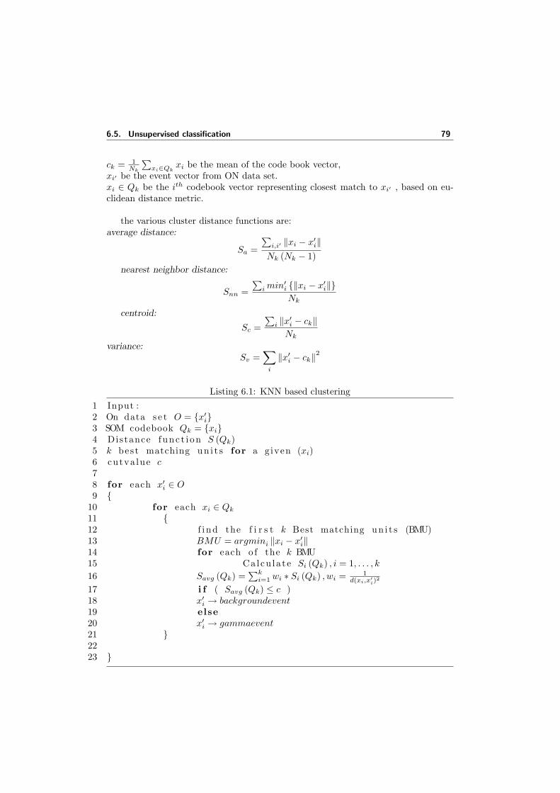
6.5. Unsupervised classification 79
ck = 1Nk
∑xi∈Qk
xi be the mean of the code book vector,xi′ be the event vector from ON data set.xi ∈ Qk be the ith codebook vector representing closest match to xi′ , based on eu-clidean distance metric.
the various cluster distance functions are:average distance:
Sa =
∑i,i′ ‖xi − x′i‖
Nk (Nk − 1)nearest neighbor distance:
Snn =∑
i min′i ‖xi − x′i‖Nk
centroid:
Sc =∑
i ‖x′i − ck‖Nk
variance:Sv =
∑i
‖x′i − ck‖2
Listing 6.1: KNN based clustering1 Input :2 On data s e t O = x′i3 SOM codebook Qk = xi4 Distance func t i on S (Qk)5 k best matching un i t s for a given (xi)6 cutva lue c78 for each x′i ∈ O9
10 for each xi ∈ Qk
11 12 f i nd the f i r s t k Best matching un i t s (BMU)13 BMU = argmini ‖xi − x′i‖14 for each o f the k BMU15 Ca lcu la te Si (Qk) , i = 1, . . . , k
16 Savg (Qk) =∑k
i=1 wi ∗ Si (Qk) , wi = 1d(xi,x′
i)2
17 i f ( Savg (Qk) ≤ c )18 x′i → backgroundevent19 else20 x′i → gammaevent21 2223
80 6. MAGIC and its image classification
The k BMU’s are weighted according to their inverse square distances from the in-put event vector. The data sets are stored in the secondary memory and data itemsare transferred to the main memory one at a time for clustering. Only the clusterrepresentations are stored permanently in the main memory to alleviate space limita-tions. The computational complexity of the nearest-neighbor algorithm both in space(storage of prototypes) and time (search) has received a great deal of analysis. Thereare a number of elegant theorems from computational geometry on the constructionof Voronoi tesselations and nearest-neighbor searches in one- and two-dimensionalspaces. However, because the MAGIC is a multidimensional data classification prob-lem we concentrate on the more general d-dimensional case. For n labelled trainingsamples in d- dimensions, and seek to find the closest to a test point x′ (k = 1). Inthe most naive approach we inspect each stored point in turn, calculate its Euclideandistance to x, retaining the identity only of the current closest one. Each distancecalculation is O (d), and thus this search is O
(dn2). One method for reducing the
complexity of nearest-neighbor search is to eliminate “useless” codebook vectors dur-ing testing, a technique known variously as editing, pruning or condensing. A simplemethod to reduce the O (n) space complexity is to eliminate prototypes that are sur-rounded by training points of the same category label. Now the complexity statisticsreduces to O
(d3nbd/2c lnn
), b.c is the “floor” operation.
Cluster visulisation: The clusters discovered by SOM are visualised using U-matrix, a matlab tool to visualize these clusters [141]. SOM is an excellent tool forvisualisation of high dimensional data. Figure 6.13 displays the data distribution ofindividual image parameters for crab on data. These distribution maps can assistanalyst to observe the possible relationships that exist between the variables andeven roughly distinguish the structure of the input data. The variable distributionplanes are organized in such a way that similar planes lie close to each other; thisorganization is carried out by SOM itself. We experimented with two types of kernelsbased on gaussian curvature. The group visualisation by these two type of kernelbased SOM maps are shown in the figure 6.14, the color coding of the map basedon the HSV color system [142]. The value of component H (hue) was dependent ondirection from the center of the map, S (saturation) was held constant, and V (value)was inversely proportional to the map unit distance from the center of the map. Thusthe groups are formed at the ends of the map with separation boundaries and theclusters concentrated in the center of the map. Figure 6.14 visualizes the classificationgroups found by the SOM system. The 2 groups found here are represented by bluecolor. The experiments are performed by using two kernels gaussian and cutgaussian.For gaussian kernel a map of 25X25 network is used and trained for 300 epochs.Cutgaussian kernel map of 40X30 size is trained with 300 epochs. The cut-gaussiankernel shown better performance than that of of gaussian kernel.
The data set is again taken from the CRAB data source, this time with numberof off data events 2.5 million and on data set contains 7.3 million events [ mixture ofgamma and background] to be classified. An quantisation error represents the normof difference of an input vector from the closest reference vector. We used AverageQuantization Error (QE) of the MAP as the benchmark criteria. The experimentsare carried out with various distance functions and the nearest neighbor measure has
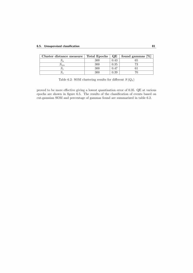
6.5. Unsupervised classification 81
Cluster distance measure Total Epochs QE found gammas [%]Sa 300 0.43 65Snn 300 0.35 73Sc 300 0.47 61Sv 300 0.39 70
Table 6.2: SOM clustering results for different S (Qk)
proved to be more effective giving a lowest quantisation error of 0.35. QE at variousepochs are shown in figure 6.5. The results of the classification of events based oncut-gaussian SOM and percentage of gammas found are summarized in table 6.2.
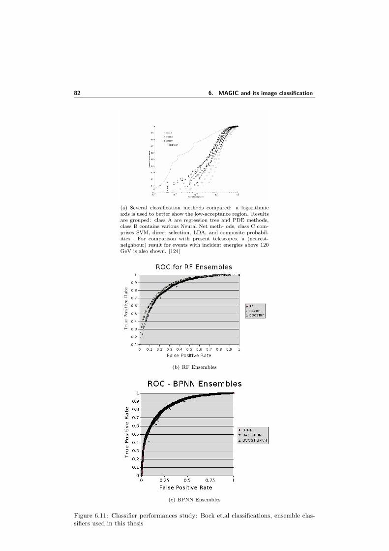
82 6. MAGIC and its image classification
(a) Several classification methods compared: a logarithmicaxis is used to better show the low-acceptance region. Resultsare grouped: class A are regression tree and PDE methods,class B contains various Neural Net meth- ods, class C com-prises SVM, direct selection, LDA, and composite probabil-ities. For comparison with present telescopes, a (nearest-neighbour) result for events with incident energies above 120GeV is also shown. [124]
(b) RF Ensembles
(c) BPNN Ensembles
Figure 6.11: Classifier performances study: Bock et.al classifications, ensemble clas-sifiers used in this thesis

6.5. Unsupervised classification 83
Figure 6.12: The SOM based system for automatic separation of gamma events frombackground events
Figure 6.13: Data distributions for image parameters in crab on data set.
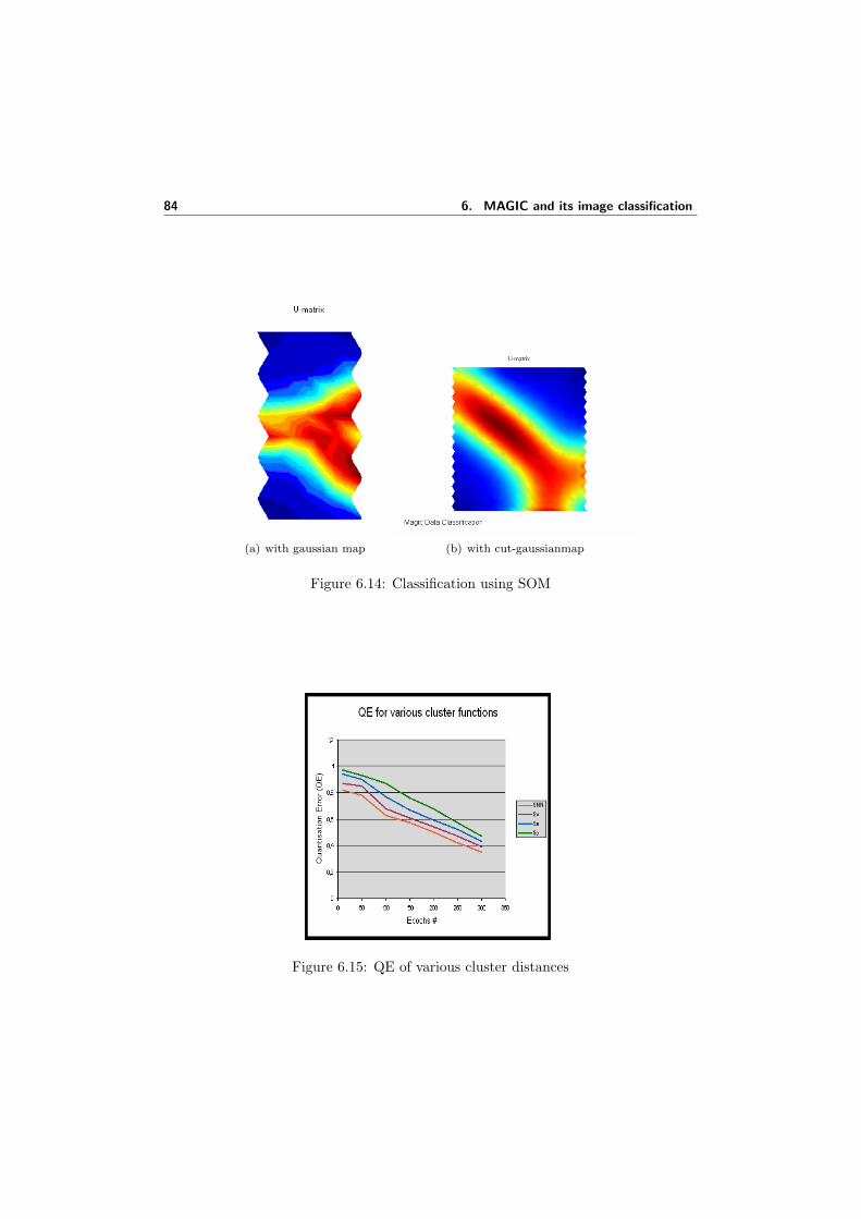
84 6. MAGIC and its image classification
(a) with gaussian map (b) with cut-gaussianmap
Figure 6.14: Classification using SOM
Figure 6.15: QE of various cluster distances
Conclusions
In this thesis experiments on novel machine learning algorithms are performed basedon unsupervised and supervised learning techniques. In unsupervised model, we ex-perimented with Self-Organizing Maps (SOM) with new kernel neighborhood func-tions. The SOM capabilities for data visualization have been explored. Experimentsare performed on an astrophysics data catalog (Gamma ray bursts). We used SOMsystem for data exploration, visualization and cluster discovery in the data sets. Thecluster discovery resulted in 3 groups in the data set, which well agrees with the pre-vious studies of GRB studies. The experiment is conducted with two different datasets on the BATSE 4B Catalog. The first case study demonstrates the existence of 3classes, but the class 3 is not clearly distinguished from class 1 supporting the hypoth-esis of instrument bias in the misclassification of some events of class 1 as class 3. Inthe second case study we used the bagoly et.al., suggested attributes . This time theSOM has clearly distinguished the class 2 events from the class1. The cut gaussiankernel makes the winner map unit to get adapted to the data vectors to maximumextent and the adaptation falls away as the distance of map units increases from thewinner unit. This gaussian form of adaption to the data set distribution forms the ba-sis for the self organisation with in the map thus assisting in the automatic discoveryof the groups that exist in the dataset.
In the ensemble (supervised) learning, we experimented with 2 different machinelearning algorithms. BPNN, a neural network model is used to grow ensembles withbagging and boosting. In tree based model we choose random forests to grow en-sembles. The methodology is novel and experiments on standard UCI data sets haveshown improvements in the classification results compared to the standard randomforest algorithm.
The above developed algorithms are used in the image data classification per-formed with in the MAGIC telescope experiment framework. The research is carriedout to perform the classification both in supervised and unsupervised fashion. Weused BPNN ensembles and random forest ensembles to perform a supervised classifi-cation. The results show that the ensembles have performed superior to the originalalgorithms with BPNN ensemble giving better performances. All the experiments arecarried out using the WEKA software tool for machine learning. One of the impor-tant requirements for the MAGIC is to perform the classification of image data in anautomatic way. We worked on this task by applying SOM based system. The clustersdiscovered by SOM are labeled by using a KNN- model algorithm to perform an au-tomatic classification of images. The self-organisation capability of SOM directed byits kernel function, makes the identical types of events to be accumulated at one endof the map where as the other event types are moved toward the other end. Thus theself-organisation capability of the map forms the basis for the automatic classification

86 Conclusions
of events. We used various cluster distance measures for this task and the results arecompared.
Future work can be concentrated on working with various image data collectionsavailable in the MAGIC experiment. More ensemble learning techniques as describedin section 4.3.3 can be introduced to work with the base classifiers introduced in thethesis. On other hand there is a scope of introducing new base classifiers such as K-Nearest Neighbor (K-NN), Radial basis function networks, Probabilistic neural nets,support vector machines etc to grow the ensembles.
In unsupervised learning category, more work can be concentrated on using dif-ferent map dimensionalities, learning rates. Experiments can be performed by usingthe SOM variants such as Self-organizing tree algorithm (SOTA) [143], Generativetopographic map(GTM) etc. [144].
Bibliography
[1] A. K. Jain, R. P. W. Duin, J. Mao Statistical Pattern Recognition: A Review,EEE Transactions on Pattern Analysis and Machine Intelligence (1999)
[2] D. Judd, P. K. McKinley, and A. K. Jain. Large scale parallel data clustering.IEEE Transactions on Pattern Analysis and Machine Intelligence, 20(8):871876(1998)
[3] T. M. Mitchell, Machine Learning, McGraw Hill (2005)
[4] M. Kantardzic, Data Mining: Concepts, Models, Methods, and Algorithms, JohnWiley &Sons (2003)
[5] L. Kuncheva, C. Whitaker, Measures of diversity in classifier ensembles andtheir relationship with ensemble accuracy, Machine Learning, pp. 181-207 (2003)
[6] P. Melville, R. J. Mooney, Constructing Diverse Classifier Ensembles UsingArtificial Training Examples, In Proceedings of the Eighteenth InternationalJoint Conference on Artificial Intelligence (IJCAI-03), pp. 505-510, Mexico (2003)
[7] A. D. Gordon. Classification, Chapman & Hall/CRC (1999)
[8] H. Frigui, R. Krishnapuram, A robust competitive clustering algorithm withapplications in computer vision, IEEE Transactions on Pattern Analysis andMachine Intelligence, 21(5):450465 (1999)
[9] S. K. Bhatia, J. S. Deogun. Conceptual clustering in information retrieval. IEEETransactions on Systems, Man, and Cybernetics, 28(3):427436 (1998)
[10] C. Carpineto and G. Romano. A lattice conceptual clustering system and itsapplication to browsing retrieval. Machine Learning, 24(2):95122 (1996)
[11] F. Rosenblatt: The Perceptron: a perceiving and recognizing automaton, Tech-nical Report 85-460-1, Cornell Aeronautical Laboratory, Ithaca, N.Y., 1957.
[12] J. L. McClelland, D. E. Rumelhart: Explorations in Parallel Distributed Pro-cessing, Cambridge, MA: MIT Press 1988.
[13] D. E. Rumelhart, G.E. Hinton, R. J. Williams: Learning Representations byBack-propagating Error, Nature, 323:533/536. Reprinted in Anderson& Rosen-feld, pp. 696-699, 1988.
[14] S. Haykin: Neural Networks- A comprehensive Foundation, Macmillan CollegePublishing Company, 1994.
88 Bibliography
[15] L. Fausett: Fundamentals of Neural Networks, Prentice Hall, 1994.
[16] K. Hornik, M. Stinchcombe, and H. White: Multilayer feedforward networksare universal approximators, Neural Networks, 2:359-366, 1989.
[17] J. Platt, Fast training of support vector machines using sequential minimal op-timization, In, B. Scholkopf, C. Burges, A. Smola, (eds.): Advances in KernelMethods - Support Vector Learning, MIT Press (1998)
[18] V. N. Vapnik, The nature of statistical learning theory, Springer Verlag (1995)
[19] G. A. carpenter, S. Grossberg, A massively Parallel Architecture for a Self-organizing Neural Pattern Recognition Machine, Computer vision, Graphics andImage processing, 37:54-115 (1987)
[20] J. Friedman, T. Hastie, R. Tibshirani, The Elements of Statistical Learning:Data Mining, Inference and Prediction, Springer series (2001)
[21] L. Akarun, D. O. zdemir, and O. Yalc, In. Joint quantization and ditheringof color images, In Proc. IEEE Int. Conf. on Image Processing, pages 557-560(1996)
[22] M. Aguilar, D. A. Fay, D. B. Ireland, J. P. Racamoto, W. D. Ross, and A. M.Waxman, Field evaluations of dual-band fusion for color night vision, In J.G.Verly, editor, SPIE Conference on Enhanced and Synthetic Vision 1999, pages168-175, (1999)
[23] J. Hartigan, Clustering Algorithms, Wiley (1975)
[24] A. K. Jain, R. C. Dubes, Algorithms for Clustering Data, Prentice-Hall, Engle-wood Cliffs, NJ (1988)
[25] L. Kaufman, P. J. Rousseeuw, Finding Groups in Data, John Wiley & Sons(1990)
[26] R.O. Duda, P. E. Hart, D. G. Stork, Pattern Classification , John Wiley & Sons,Inc (2001)
[27] R. O. Duda, P. E. Hart, Pattern classification and scene analysis, John Wiley,New York (1973)
[28] U. Fayyad, G. Piatetsky-Shapiro, P. Smyth, and R. Uthurusamy, editors, Ad-vances in Knowledge Discovery and Data Mining AAAI/MIT Press (1996)
[29] D. J. Hand, H. Mannila, and P. Smyth, Principles of Data Mining, MIT Press(2000)
[30] M. Kamber J. Han, Data Mining : Concepts and Techniques, Morgan Kaufmann(2000)
Bibliography 89
[31] B. D. Ripley, Pattern Recognition and Neural Networks, Cambridge UniversityPress, Cambridge (1996)
[32] D. J. Willshaw, C. V. der malsburg, How patterned neural connections can besetup by self-organization, Proc.Roy.Soc. Lond. B, 194, 431-445.
[33] T. Kohonen, Self-Organizing Maps, third edition Springer-Verlag (2002)
[34] Website for GRB’s, http://imagine.gsfc.nasa.gov/docs/science/know_l1/grbs_proof.html
[35] Site for GRB data from BATSE:, http://www.batse.com/
[36] SOM research website: http://www.cis.hut.fi/research/som-research/som.shtml
[37] Mukherjee, S., et al. 1998, ApJ, 508, 314
[38] Hakkila, J., et al. 2000, ApJ, 538, 165
[39] Bagoly, Z., et al. 1998, ApJ, 498, 342
[40] H. J. Rajaneimi, P. Mahonen, Classifying Gamma-Ray Bursts using Self-Organizing maps, The Astrophysical Journal, 566:202-209 (2002)
[41] L. Chittaro, L. Ieronutti, A Visual Tool for Tracing Behaviors of Users inVirtual Environments, Proceedings of AVI 2004: 6th International Conferenceon Advanced Visual Interfaces, pp.40-47 ACM Press (2004)
[42] O. Simula, E. Alhoniemi, J. Hollmn, and J. Vesanto. Monitoring and model-ing of complex processes using hierarchical self-organizing maps, In Proceedingsof the 1996 IEEE International Symposium on Circuits and Systems, volumeSupplement, pages 73-76. IEEE, (1996)
[43] T. Kohonen, S. Kaski, K. Lagus, J. Salojrvi, J. Honkela, V. Paatero, and A.Saarela, Self organization of a massive document collection IEEE Transactionson Neural Networks, (11):574-585 (2000)
[44] J. Vesanto, Importance of Individual Variables in the k-Means Algorithm, InProceedings of the Pacific-Asia Conference Advances in Knowledge Discoveryand Data Mining (PAKDD2001), Springer-Verlag, pp. 513518 (2001)
[45] J. Vesanto, Data exploration process based on the SOM, PhD thesis, HelsinkiUniversity of Technology (2002)
[46] T. Kohonen, Comparison of SOM Point Densities Based on Different Criteria,Neural Computation, 11(8):20812095 (1999)
[47] J. Lampinen and T. Kostiainen, Generative probability density model in theSelf-Organizing Map, In U. Seiffert and L. Jain, editors, Self-organizing neuralnetworks: Recent advances and applications, pages 7594. Physica Verlag (2002)
90 Bibliography
[48] G. Deboeck, T. Kohonen, editors, Visual explorations in Finance using Self-Organizing Maps, Springer-Verlag, London (1998)
[49] J. B. Kruskal, Multidimensional Scaling by Optimizing Goodness of Fit to aNonmetric Hypothesis, Psychometrika, 29(1):127 (1964)
[50] J. Himberg, J. Ahola, E. Alhoniemi, J. Vesanto, and O. Simula, The selforga-nizing map as a tool in knowledge engineering, In N. R. Pal, editor, Patternrecognition in soft computing paradigm, pages 3865. World Scientific (2001)
[51] J. W. Sammon, Jr., A Nonlinear Mapping for Data Structure Analysis, IEEETransactions on Computers, C-18(5):401409 (1969)
[52] P. Demartines, J. Hrault, Curvilinear Component Analysis: A Self- OrganizingNeural Network for Nonlinear Mapping of Data Sets, IEEE Transactions onNeural Networks, 8(1):148154 (1997)
[53] J. Moody, C. J. Darken, Fast Learning in Networks of Locally- Tuned ProcessingUnits, Neural Computation, 1(2):281294 (1989)
[54] T. Kohonen, E. Oja, O. Simula, A. Visa, and J. Kangas, Engineering Applica-tions of the Self-Organizing Map, Proceedings of the IEEE, 84(10):1358-1384,(1996)
[55] O. Simula and J. Kangas, Neural Networks for Chemical Engineers, volume 6of Computer-Aided Chemical Engineering, chapter 14, Process monitoring andvisualization using self-organizing maps. Elsevier, Amsterdam (1995)
[56] S. Kaski, J. Kangas, and T. Kohonen, Bibliography of self-organizing map(SOM) papers: 1981-1997, Neural Computing Surveys, 1:102-350 (1998)
[57] J. Vesanto, Neural network tool for data mining: SOM Toolbox, In Proceedingsof Symposium on Tool Environments and Development Methods for IntelligentSystems (TOOLMET2000), pages 184-196, Oulu, Finland (2000)
[58] R. M. Gray, Vector quantization, IEEE ASSP Magazine, pages 4-29, (1984)
[59] S. Kaski, Data Exploration Using Self-Organizing Maps, PhD thesis, HelsinkiUniversity of Technology, Acta Polytechnica Scandinavica: Mathematics, Com-puting and Management in Engineering, (1997)
[60] T. Samad, S.A. Harp, Self-Organization with Partial Data, Network, 3:205-212,IOP Publishing Ltd, (1992)
[61] H. Ritter, Asymptotic Level Density for a Class of Vector Quantization Pro-cesses, IEEE Transactions on Neural Networks, 2(1):173175 (1991)
[62] T. G. Dietterich, Ensemble Methods in Machine Learning, Proc. of the 1st Inter-national Workshop on Multiple Classifier Systems, Lecture Notes in ComputerScience, 1857, 1-15. Springer-Verlag (2000)
Bibliography 91
[63] T. G. Dietterich, Ensemble learning, In Arbib, M. (Ed.), The Handbook ofBrain Theory and Neural Networks, 2nd Edition. MIT Press (2002)
[64] T. Dietterich, Machine learning research: Four current directions, AI Magazine,18(4), 97-136 (197)
[65] Data Analysis hand book website http://rkb.home.cern.ch/rkb/AN16pp/node237.html#SECTION0002370000000000000000
[66] T. G. Dietterich, Machine Learning, In Nature Encyclopedia of Cognitive Sci-ence, Macmillan, London (2003)
[67] K. Ali, J. Pazzani, Error reduction through learning multiple descriptions, Ma-chine, Learning 24(3), 173-202 (1996)
[68] J. M. Bernardo, A. F. M. Smith, Bayesian Theory, JohnWiley & Sons, NewYork (1993)
[69] A. Krogh, J. Vedelsby, Neural network ensembles, cross validation, and ac-tive learning, In G. Tesauro, D. Touretzky, T. Leen (Eds), Advances in NeuralInformation Processing System, 7, 231-238. MIT Press (1995)
[70] D. Opitz, J. Shavlik, Generating accurate and diverse members of a neural-network ensemble, In D. Touretzky, M. Mozer, M. Hesselmo, (Eds.), Advancesin Neural Information Processing Systems, 8, 535-451. MIT Press (1996)
[71] T. G. Dietterich, An experimental comparison of three methods for constructingensembles of decision trees: Bagging, Boosting and randomization, MachineLearning 40 (2) 139-157 (2000)
[72] Y. H. Hu, J. N. Hwang, Handbook of Neural Network Signal Processing, CRCPress (2002)
[73] L. Breiman, Bagging predictors Machine Learning, 24(2), 123-140 (1996)
[74] Y. Freund, R. Schapire, Experiments with a new boosting algorithm In Saitta, L.(Ed), Proceedings of the 13th International Conference on Machine Learning,148-156. Morgan Kaufmann (1996)
[75] K. Cherkauer, Human expert-level performance on a scientific image analysistask by a system using combined artificial neural networks, In P. Chan, editor,Working Notes of the AAAI Workshop on Integrating Multiple Learned Models,,pages 15-21. (1996)
[76] J. Carney, P. Cunningham, The NeuralBAG algorithm: optimizing generaliza-tion performance in Bagged Neural Networks, In: Verleysen, M. (eds.): Pro-ceedings of the 7th European Symposium on Artificial Neural Networks , pp.3540 (1999)
[77] B. Efron, R. Tibshirani, An Introduction to the Bootstrap, Chapman and Hall(1993)
92 Bibliography
[78] J.H. Friedman, Bias, variance, 0-1 loss and the curse of dimensionality, Tech-nical report, Stanford University (1996)
[79] Y. Grandvalet, Bagging can stabilize without reducing variance, In ICANN’01,Lecture Notes in Computer Science. Springer (2001)
[80] P. Domingos, Why does bagging work? A bayesian account and its implications,In D. Heckerman, H. Mannila, D. Pregibon, and R. Uthurusamy, (eds), Pro-ceedings of the Third International Conference on Knowledge Discovery andData Mining (KDD-97), page 155. AAAI Press (1997)
[81] J. A. Madigan, D. Hoeting, C. T. Raftery, Bayesian model averaging: A tuto-rial. Statistical Science, 44(4):382417 (1999)
[82] R. E. Schapire, The strength of weak learnability, Machine Learning, 5:197-227(1990)
[83] Y. Freund, Boosting a weak learning algorithm by majority, Information andComputation, 121(2):256-285 (1995)
[84] E. B. Kong, T. G. Dietterich, Error-correcting output coding corrects bias andvariance, In Proceedings of the Twelfth International Conference on MachineLearning, pages 313-321 (1995)
[85] H. Drucker, R. Schapire, P. Simard, Boosting performance in neural net-works, International Journal of Pattern Recognition and Artificial Intelligence,7(4):705-719 (1993)
[86] H. Drucker, C. Cortes, L. D. Jackel, Y. LeCun, and V. Vapnik, Boosting andother ensemble methods, Neural Computation, 6(6):1289-1301 (1994)
[87] H. Drucker, C. Cortes, Boosting decision trees, In Advances in Neural Informa-tion Processing Systems 8 (1996)
[88] J. C. Jackson, M. W. Craven, Learning sparse perceptrons, In Advances inNeural Information Processing Systems 8 (1996)
[89] M. Skurichina, R. P. W. Duin, Bagging, Boosting and the Random SubspaceMethod for Linear Classifiers, Vol. 5, no. 2: 121-135, Pattern Analysis andApplications (2002)
[90] P. Bhlmann, B. Yu, Analyzing bagging, Annals of Statistics 30, 927-961 (2002)
[91] L. Breiman, Out-of-bag estimation, Technical Report (1996)
[92] S. Borra, A. Di Ciaccio, Improving nonparametric regression methods by baggingand boosting, Computational Statistics & Data Analysis 38, 407-420 (2002)
[93] A. J. C. Sharkey, Types of multinet system, In Proc. of the Third InternationalWorkshop on Multiple Classifier Systems (2002)

Bibliography 93
[94] L. Xu, A. Krzyzak, C. Y. Suen, Methods for combining multiple classifiers andtheir applications in handwritten character recognition, IEEE Trans. Syst., Man,Cybern., vol. 22, pp. 418-435, 1992.
[95] Y. Freund, R. E. Schapire, A decision-theoretic generalization of online learningand an application to boosting, In Computational Learning Theory: SecondEuropean Conference, EuroCOLT ’95, pages 23-37, Springer-Verlag (1995)
[96] L. Breiman, Random Forests Technical Report, University of California, 2001.
[97] Website for Random Forests: http://www.stat.berkeley.edu/users/breiman
[98] L. Breiman, Looking Inside the Black Box, Wald Lecture II, Department ofStatistics, California University (2002)
[99] M. Sikonja, Improving Random Forests. , In J.-F. Boulicaut et al.(Eds): ECML2004, LNAI 3210: pp. 359-370, Springer, Berlin, (2004)
[100] L. Breiman, J. H. Friedman, R. A. Olshen and C. J. Stone. Classification andregression trees. Wadsworth Inc., Belmont, California (1984)
[101] J. R. Quinlan, C4.5: Programs for Machine Learning, Morgan Kaufmann, SanFrancisco, (1993)
[102] I. Kononenko. Estimating attributes: analysis and extensions of Relief. In LucDe Raedt and Francesco Bergadano, editors, Machine Learning: ECML-94,pages 171-182. Springer Verlag, Berlin (1994)
[103] I. Kononenko. On biases in estimating multi-valued attributes. In Proceedingsof the International Joint Conference on Artificial Intelligence (IJCAI’95), pages1034-1040. Morgan Kaufmann (1995)
[104] T. G. Dietterich, M. Kerns, and Y. Mansour. Applying the weak learning frame-work to understand and improve C4.5. In Lorenza Saitta, editor, MachineLearning: Proceedings of the Thirteenth International Conference (ICML’96),pages 96-103. Morgan Kaufmann, San Francisco (1996)
[105] L. Breiman, J. H. Friedman, R. A. Olshen, and C. J. Stone. Classification andregression trees. Wadsworth Inc., Belmont, California (1984)
[106] UCI data sets repository, http://www.ics.uci.edu/~mlearn/MLRepository.html
[107] J.R. Quinlan, Bagging, Boosting, and C4.5, In Proceedings, Fourteenth Na-tional Conference on Artificial Intelligence (1996)
[108] R. E. Schapire, Y. Freund, P. Bartlett, and W. S. Lee. Boosting the margin:a new explanation for the effectiveness of voting methods. In D. H. Fisher, edi-tor, Machine Learning: Proceedings of the Fourteenth International Conference(ICML’97), pages 322-330. Morgan Kaufmann (1997)
94 Bibliography
[109] Website for MAGIC Telescope: http://wwwmagic.mppmu.mpg.de
[110] A. Moralejo for the MAGIC Collaboration, The MAGIC telescope for gamma-ray astronomy above 30 GeV, Chin. J. Astron. Astrophys. Vol.3 Suppl. 531-538(2003)
[111] D. Paneque, The MAGIC Telescope: development of new technologies and firstobservations, PhD thesis , MPI Munich, August (2004)
[112] Nasa website on cernkov radiation: http://imagine.gsfc.nasa.gov/docs/science/how_l2/Cherenkov.html
[113] P. A. Cherenkov, C.R. Acad. Sci. U.S.S.R., 2, p. 451 (1934)
[114] ROOT website: http://root.cern.ch/
[115] MARS website: http://magic.astro.uni-wuerzburg.de/mars/
[116] D. Kranich, Temporal and spectral characteristics of the active galactic nucleusMkn -501 during a phase of high activity in the TeV range, PhD thesis, Max-Plank Institute of Astro-physics, Munich (2002).
[117] T. C. Weekes, M.F. Cawley, D.J. Fegan et al.,Observation of TeV gamma raysfrom the Crab nebula using the atmospheric Cherenkov imaging technique. As-trophysical Journal, 342: 379-395 (1989)
[118] A.M. Hillas, Proc. 19th ICRC, La Jolla 3 (1985) 445
[119] P.T. Reynolds et al., ApJ 404 (1993) 206
[120] F. Barbarino, Gamma-hadron separation using neural network techniques, Tesidi Laurea, Udine University (2004)
[121] D.J. Fegan, J.Phys.G: Nucl. Part. Phys. 23 (1997) 1013
[122] W. Wittek, Image Parameters , MAGIC-TDAS 02-03, Internal Technical report(2002)
[123] D.J.Fegan,Gamma/hadron separation at TeV energies, Topical Review,J.Phys.G: Nucl. Part. Phys. 23 (1997) 1013.
[124] R. K. Bock et al., Methods for multidimensional event classification: a casestudy using images from a Cherenkov gamma-ray telescope, Nucl. Instr. MethodsA516: 511-528 (2004)
[125] D. Heck, et al., CORSIKA, A Monte Carlo code to simulate extensive air show-ers, Forschungszentrum Karlsruhe, Report FZKA 6019 (1998)
[126] Ian H. Witten, E. Frank, Data Mining: Practical machine learning tools andtechniques, 2nd Edition, Morgan Kaufmann, San Francisco (2005)
[127] R statistical software: www.r-project.org/

Bibliography 95
[128] Fortran Source code for random forestshttp://www.stat.berkeley.edu/users/breiman/RandomForests
[129] Y. Freund, R. E. Schapire, A decision-theoretic generalization of online learningand an application to boosting, In Computational Learning Theory: SecondEuropean Conference, EuroCOLT ’95, pages 23-37, Springer-Verlag (1995)
[130] H. Schwenk, Y.Bengio, Boosting Neural Networks, Neural Computation, Volume12, Number 8, pp. 1869-1887(19), MIT Press (2000)
[131] P. Cunningham, J. Carney, S. Jacob, Stability Problems with Artificial NeuralNetworks and the Ensemble Soloution , Technical report, Department of Com-puter Science, Trinity College Dublin, Ireland (2003)
[132] B. Efron, R. Tibshirani, An Introduction to the Bootstrap, Monographs onStatistics and Applied Probability, No 57, Chapman and Hall (1994)
[133] D. Opitz, J. Shavlik, Generating accurate and diverse members of a neuralnetwork ensemble, in D. Touretzky, M. Mozer and M. Hasselmo, eds.,Advancesin Neural Information Processing Systems 8, 535-541, MIT Press (1996)
[134] J. Carney, P. Cunningham, Confidence and prediction intervals for neural net-work ensembles, in proceedings of IJCNN99, The International Joint Conferenceon Neural Networks, Washington, USA (1999)
[135] R. M. Wagner et al., Observations of the Crab nebula with the MAGIC telescope,29th International Cosmic Ray Conference Pune (2005) 00, 101.106
[136] T. Weekes et al., Astrophys. J. 342 (1998) 379
[137] F. A. Aharonian et al, Astrophys. J. 614 (2004) 897
[138] T. Li, Y. Ma, ApJ, 272, 317 (1983)
[139] E. Alhoniemi, Unsupervised Pattern Recognition Methods for Exploratory Anal-ysis of Industrial Process Data, PhD thesis, Helsinki University of Technology(2002)
[140] J. Vesanto, E. Alhoniemi Clustering of the Self-Organizing Map. In IEEE Trans-actions on Neural Networks, Volume 11, Number 3, pp. 586600 (2000).
[141] J. Vesanto, Neural network tool for data mining: SOM Toolbox, In Proceedingsof Symposium on Tool Environments and Development Methods for IntelligentSystems (TOOLMET2000), pages 184-196, Oulu, Finland (2000)
[142] A. R. Smith. Color gamut transform pairs, Computer graphics, 12(3):1219(1978)
[143] J. Dopazo, J. M. Carazo, Phylogenetic reconstruction using an unsupervisedgrowing neural network that adopts the topology of a phylogenetic tree, Journalof Molecular Evolution 44, 226-233 (1997)

96 Bibliography
[144] C. M. Bishop, M. Svensn, C. K. I. Williams, GTM: The generative topographicmapping. Neural Computation, 10:215234 (1998)