insights from demand estimation in the airline industry
35
-
Upload
khangminh22 -
Category
Documents
-
view
3 -
download
0
Transcript of insights from demand estimation in the airline industry

The invisible costs of competition : insights from
demand estimation in the airline industry
Hoang Dao
Abstract
Ever since the Airline Deregulation Act in 1978, the airline industry drastically
transitioned from the most condensed and regulated industry to one of the most
competitive one. Severe competition makes airline industry's prot margin among
the lowest at 8.2% in 2018, only slightly more than half of U.S. average (15.2%).
The introduction of electronic booking and budget airlines increased the com-
petition in this market to an unparalleled degree. How would such competition
aect airline's behavior, market structure, and ultimately, the future of aviation?
This paper explores the eects of airline industry competition on the rms' costs
and operations behavior. Specically, the eects of competition on airline's safety
expense, product-dierentiation expense, route choices and eets.
This article begins by deriving an estimate for the degree of competition, em-
ploying the discrete choice techniques with dierentiated product to estimate the
demand for air travel in the U.S. domestic markets. A substitution matrix and a
vector of preferences for observable characteristics are obtained for each quarter
from 1993Q1 to 2018Q4. A measure for competition in the industry is formulated
for each airline during the period. This competition index is then used to evaluate
the eect of competition on the multiple costs and characteristics of airlines, us-
ing the instrumented dierence in dierences method. My result shows that, the
expense for safety does not change signicantly, but the expenses for product dif-
ferentiation decreases as the markets become more competitive. Airlines y longer
routes on average, and air eets gravitates towards homogeneously narrow-body,
long-distance airplanes as airlines face more competition.
JEL Classication: R41, H22, L11
Key words: Demand Estimation, Competition, Airline, Safety, Transportation
1

1 Introduction
Before 1978, air travel was one of the most regulated industries in America, with limited
licenses to only a small group of airlines. The government decided the routes, which
airline to operate a route, airport security, and pricing. The Airline Deregulation Act in
1978 drastically transformed this industry from the most regulated to one of the most
competitive ones. From 1990 to 2018, scheduled passenger enplanement almost doubled
from 460 million to 888 million customers per year, while average ination-adjusted
fare plummeted from around $500 to $350. Severe competition makes airline industry's
prot margin among the lowest at 8.2% in 2018, only slightly more than half of that of
U.S. average at 15.2%. This is obviously good from the view point of customers, since
they can enjoy lower prices and more route diversity. It is also empirically better for
interregional economic activities(Brueckner 2003) . However, competition comes with a
cost. This paper explores how competition in the industry would aect airline's cost and
operations behavior. Specically, the airlines' safety expenses, product-dierentiation
expenses, and changes of route, eet, and ying models.
The airline industry: history and literature
Although the industry is still highly condensed, prices are extremely competitive. Mar-
ket power is not manifested through high prices. A series of mergers of major airlines
and the overwhelming 65% market share of the big four airlines suggested that fares
should have climbed in the past three decades. On the contrary, gure 1 from Airlines
for America suggests that ination-adjusted prices have decreased in the past thirty
years.
The declining protability of airlines are well documented throughout the years. After
liberalization, the industry as a whole lost $10 billion in the decade following 1979,
gained back $5 billion in the 1990s and lost $54 in the 2000s (Borenstein 2011). Boren-
stein (2011) listed some notable reasons: demand shocks, entrance of low cost carriers,
and tax and fuel costs1. Among these reasons, taxes and the existence of budget air-
lines are crucial, since they made airline product dierentiation futile and airlines had
to be extremely competitive in prices. The tickets are taxed at 7.5%, on top of $6.2 per
segment own. Multiple airport service and security surcharges, and the decline in fare
1For airline prices estimation, see Snider and Williams(2015) ,Borenstein and Rose(1994),Goolsbeeand Syverson (2008), Borenstein(1989), Borenstein (1989), Brueckner (1994)
2

Figure 1: Average US Domestic air fare 1980-2012
Blue = not ination adjusted. Orange = ination adjusted with base year 2017. Source:Bureau of Transportation Statistics
makes the tax portion keep their uptrend on a ticket. The growth of online booking
and the prevalence of budget airlines also contribute largely to the competitiveness of
air travel.
Competition in the airlines industry has been analyzed extensively throughout the
years. Borenstein discussed the industrial organization aspect of airline competition,
pointing out that a series of mergers following deregulation would condense the market.
Potentially, consumers will be the one at a disadvantage due to loss in welfare along with
competition. In a series of later articles, Borenstein discusses the thin prot margin by
the airlines, and the role of hubs in determining market power and Oum et al.(1995)
pointed out the reasons for airline industry to be so competitive. Berry (1990) provided
a model to estimate airport presence as product dierentiation.
Regarding air travel as a consumer welfare, Olivier (2008) recently investigates the
impacts of airline alliances on consumer well-being. Brueckner (2003) also provided
empirical evidence to the positive impact of increased air travel to the urban economic
development. Graham et al. (1983) provided a discussion about the eects of com-
3

petition on welfare post the 1978 deregulation. These papers all pointed towards the
positive aspects of deregulation: increased airline competition decreases prices, increase
volume traveled, increase technology, increase the degree of connections between cities,
etc.
This paper contributes to the existing discussion of pros and cons following the airline
deregulation by adding the argument that: competition in the industry also drives down
the cost of airlines and creates disutility to consumers. It also adds a projection of how
the aviation industry is going to shape in the near future with increasing competition.
Article agenda
The airline industry is notorious for being price-sensitive (Oum et al 1993, Ruben 2005).
Since airlines cannot freely adjust their pricing, it is intuitive to expect them to cut
its costs to cope with competition, but which costs to get cut? Dierent costs have
dierent eects on the industry. If the costs for gates and ground control gets cut, it
means the airline will shift its transportation model or exit entirely from certain airports,
increasing market shares of existing airlines. If the cost for in-ight amenities (food,
entertainment, reclined seats, etc) gets cut, it means airlines are prepared to engage in
price competition, and the rms then pay much less attention to dierentiating their
products. If the crew training cost or maintenance cost gets cut, it would pose some
safety concerns to the public.
This paper explores the eects of competition in the airline industry in two steps.
In the rst step, I constructed an index for competition for each of the airlines in
the industry2. Following the discrete choice framework proposed by Berry(1994), and
Berry-Lehvinson-Pakes(1995), I estimate the demand elasticity between products in the
markets, then come up with a volume-weighted average of the own price elasticity for
each airline in a given year-quarter in the period of 1993Q1-2018Q4. The model allows
that a consumer can choose to not participate in the market. The rst step produces
the necessary proxies of competition needed for the second step. This step reveals that
competition in the industry has increased throughout the last quarter of a century:
own price elasticity uniformly decreases during the mentioned time period. The result
is consistent throughout dierent carriers and the industry average.
The second step uses the level of competition from the rst step to evaluate the eects
2For more demand estimation styles, see Brueckner 1994, McFadden 1989
4
of competition on costs and operations behavior. The costs discussed in this paper are
maintenance expenses (safety cost) and other operating expenses, which involves in-
ight entertainment, ground service, etc (product dierentiation costs). The paper also
explores if competition shifts the transportation model by airlines: it examines wherther
airlines are more inclined to y longer or shorter routes, and if airlines' eets are more
or less homogeneous. The main identication issue that discourages any inferences from
an ordinary least square (OLS) is that there may exist endogeneity, reverse causality to
be specic, between costs/operations and the level of competition: a decrease in costs
may cause more rms to enter a given market, and more rms entering the market may
also decrease costs. Therefore, OLS might be an overmeasurement of causal eects
between competition and costs/operations by airlines. To address this issue, I employ
the method of instrumented dierences in dierences (DDIV) and performed two stage
least squares. The instrumental variable is the presence of nonstop ights oered by rival
budget airlines, which are proxies of increased competition. The rst stage shows that
airlines with more market shares that face nonstop budget rivals are more competitive.
The second stage result shows that in presence of increased competition, airlines tend
to cut costs related to product dierentiation. The maintenance costs related to safety
does not vary signicantly. Airlines y longer routes on average, and air eets gravitates
towards homogeneously small, long-distance, narrow-body airplanes as airlines face
more competition. This signals the transition away from the traditional hub-to-spoke
model and towards the point-to-point model.
This paper is organized as follows: section 2 discusses the data that were used in my
analysis, section 3 describes the demand estimation procedure and its output, section
4 presents the empirical model that evaluates the eects of competition on costs and
its results, and section 5 gives policy suggestions and concludes.
2 Data
The primary data source this article utilizes is the quarterly Origin-Destination Survey
Data Bank 1B (DB1B) published by the Bureau of Transportation Statistics. The data
contains 10% of all U.S. domestic itineraries within a quarter of a year. DB1B dates
back to the rst quarter of 1993, replacing the old version DB1A, which is no longer
available to the public. The data set contains the essential information on individual
itinerary: after tax prices, yield (price per mile own), the ticketing carrier, the number
5

of stops, plane load factor, coupons, and miles own. Ticket class, one of the important
identication factor for elasticity of demand, is reported in the DB1B Coupon data
table. Customer demographics (age, income, education,etc) are not reported in the
survey data. This data is used to construct the demand estimation (step 1 between the
two steps) discussed in Section 3.
The nancial information are obtained through the Air Carrier Financial Reports form
41, Schedule P-1.2, P-7,B-4.3. Schedule P-1.2 is the quarterly prot-loss nancial state-
ment for carriers with operating revenues at least $20 million. The data contains mul-
tiple operating revenues and costs. Schedule P-7 contains detailed quarterly aircraft
operating expenses for large aircrafts. Schedule B-4.3 lists aircraft inventories (airline
eets) by airlines in a given year.
2.1 Sample selection
As per tradition in the literature, this paper denes a market m=1,2,...M as a uni-
directional origin-destination pair. This means a trip from point A to point B is, by
denition, in a dierent market than a trip from point B to point A. Each market
has dierent routes that dierent carriers operate. Each route can be understood as a
product that belongs to a carrier in the context of a dierentiated product market.
For consistency, I use products to refer to routes henceforth. The index for product
in each market is j=1,2,...J. Time t=1,...T is each quarter in the data. In this paper, I
choose the time period from 1993Q1 to 2018Q4.
The sample is restricted along the following dimensions: price, routes, airport, and car-
rier (rms). For prices, I omit the observations with price less than $40 or greater than
$1500. This is a more conservative restriction of data than the standard Department
of Transportation unreliable range. These fares are rare within the dataset and it
might be a result of data collection error or a redemption of the frequent yer miles.
For routes, I omit the observations that uses more than one carrier and open-jaw in-
tineraries (ones with dierent returning tickets). At the aggregate route level, I omit
routes with less than 1 ight per week, or 13 ights in a quarter, since this might
represent test ights or very small markets that does not provide valuable variation in
competition. For carriers, I omit small airlines that has less than 100 passengers per
week, or 1300 passengers in a year-quarter. In the remaining sample, all the major
6

Table 1: Airlines includedAirline Code
American AAAlaska ASJet Blue B6
Continental CODelta DLFrontier F9ATA TZ
Allegiant G4Spirit NK
NorthWest NWAirTran FLUnited UAUSAir US
SouthWest SWTrans World TWHawaiian HA
Virgin Atlantic VX
airlines are retained, plus some regional airlines.
The data are aggregated to the product level for each of the year-quarter. It contains
the volume traveled in each route by each carrier in a time period. The nal data set
has 13,142,196 observations in 19,675 origin-destination pair markets.
2.2 Descriptive Statistics
Market concentration is reected through the dominance of major airlines. The big
four airlines in 2018 serve more than 60% of all passenger enplanement domestically.
We can project the trend that airlines now condense their routes to protable ones,
which increases the volume that they serve and also the homogeneity of aircraft eet
that they employ. Table2 below describes an example of the market volume in terms
of passenger enplanement by airlines. We can observe that the top airlines occupy a
volume signicantly higher than others.
Average air fares for domestic ights has been stable around $250. This number has
not been adjusted to reect the change in distance preference by airlines.
The number of markets has increased consistently along with the number of products
7
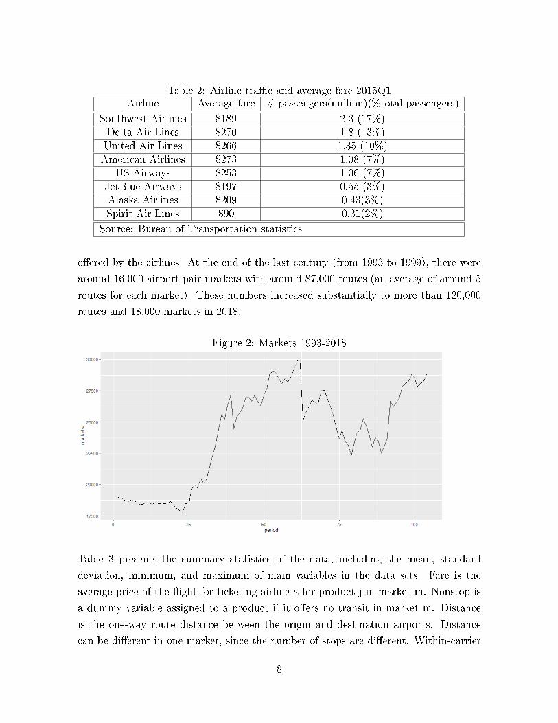
Table 2: Airline trac and average fare 2015Q1Airline Average fare # passengers(million)(%total passengers)
Southwest Airlines $189 2.3 (17%)Delta Air Lines $270 1.8 (13%)United Air Lines $266 1.35 (10%)American Airlines $273 1.08 (7%)
US Airways $253 1.06 (7%)JetBlue Airways $197 0.55 (3%)Alaska Airlines $209 0.43(3%)Spirit Air Lines $90 0.31(2%)
Source: Bureau of Transportation statistics
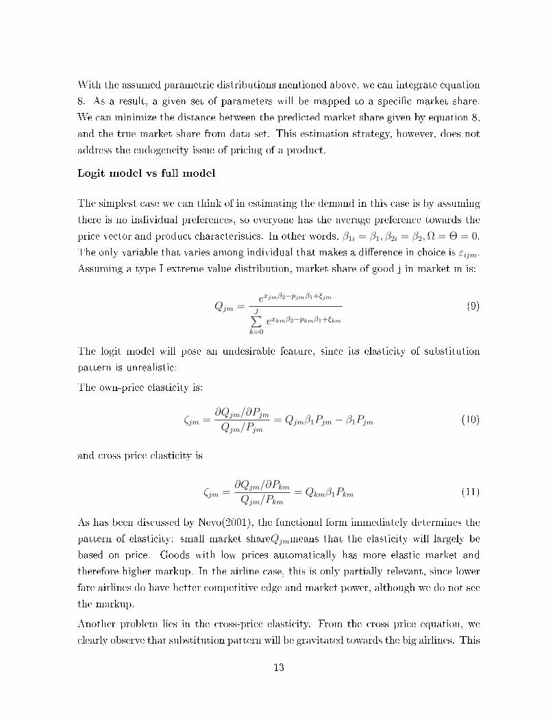
oered by the airlines. At the end of the last century (from 1993 to 1999), there were
around 16,000 airport pair markets with around 87,000 routes (an average of around 5
routes for each market). These numbers increased substantially to more than 120,000
routes and 18,000 markets in 2018.
Figure 2: Markets 1993-2018
Table 3 presents the summary statistics of the data, including the mean, standard
deviation, minimum, and maximum of main variables in the data sets. Fare is the
average price of the ight for ticketing airline a for product j in market m. Nonstop is
a dummy variable assigned to a product if it oers no transit in market m. Distance
is the one-way route distance between the origin and destination airports. Distance
can be dierent in one market, since the number of stops are dierent. Within-carrier
8

origin share measures the percentage of ights originated from an airport as a percent
of all airports that the carrier operates. Nonstop rivals is the number of rivals in a
market that oers nonstop ights, which is a proxy for competition within a market
m. Budget_airlines is the number of budget airlines operating in market m. Budget
airline is one of the following: Allegiant, Frontier, Jet Blue, Southwest, Spirit, Sun
Country. Southwest gets the most attention due to its prevalent presence and rapid
growth. Number of routes per market represents the number of dierentiated products
within a market m. It has slightly increased over the years, suggesting that consumers
now have more choices to y in a market.
Maintenance cost per aircraft is extracted from two dierent sources. Schedule P-7
provides the quarterly maintenance expense, and schedule B-4.3 provides the list of
aircrafts that belongs to dierent carriers. Food and other operating costs are obtained
from schedule P-7.
3 Demand Estimation
This section employs discrete choice methods to estimate the demand for air travel.
I will present some dierent measures of demand, each with a dierent methodology
and slightly dierent assumptions. First, a simple reduced form OLS result will be
introduced, regressing market shares on prices, then multinominal logit, and a full BLP
model is estimated. The main results is from heterogeneous discrete choice (BLP)
model.
In this section, I assume away the supply side of the market, since I am specically inter-
ested in the competitiveness of the industry. In the literature, markups can be estimated
using the models of Ciliberto and Williams(2014), Berry, Carnall and Spiller(2006).
3.1 Empirical strategy & identication
The demand estimation model in this paper is mainly following Berry-Lehvinson-Pakes
(1995) and Nevo (2001). The reason for this model choice is to address the endogeneity
in pricing behavior, as well as to generate a realistic substitution pattern between
carriers within each year-quarter.
9

Model
First, the model includes utility-maximizing consumers. Each choose a route in a given
origin-destination pair market and derive the following random utility:
Uijm = −β1i.Pjm + β2ixjm + εijm (1)
Where εijm = ξjm + εijm, the unobservable individual deviation term consists of two
parts: the average market-product specic characteristic ξjmand the mean zero indi-
vidual deviation εijmfrom that average.
i=1,2,...,I is an index for individual i, j=1,2,...,J is an index for product j. and m=1,2,...,M
is an index for market m. Consumers are exogenously sorted into dierent markets m's.
They derive their utility from budget Yiand pay price Pjmif choose product j, in this
case, the choice of airline. xjmis the vector of market-product characteristics that are
observed by the economist.β1iis the marginal utility of income, specic to each individ-
ual, and β2iis the vector of parameters indicating the marginal utility of each of the
observed characteristics from xjm.
The utility choice indicates that the nature of product dierentiation is vertical, since
the coecient β1of prices is allowed to vary with individuals, while everyone in the same
market m observes the same price Pjm
Market is dened as a pair of origin-destination, in which a ight from A to B is
counted as a dierent market than the ight from B to A. This obviously assumes that
the customers in region A (origin) only choose from airline choices within that region.
This assumption might not hold if the airport lies in between two states, so that a
customer might have a larger choice set than assumed. I assume that such cases do not
exist.
Individual characteristics that shape the choices are categorized into two major types:
observed characteristics Oi and unobserved characteristics θi. In a traditional BLP
model, no individual data is observed, so demographics variables are drawn from the
outside datasets such as the Current Population Survey (CPS). In our case, the dataset
DB1B does provide individual ticket characteristics, but no demographics are recorded.
As a result, we cannot observe basic variables that potentially signicantly aect in-
dividual choices such as income, age, sex, education, etc. Therefore, in each of these
10

two cases, Oiwill consist of dierent information set. On the other hand, θiis in no way
observable, therefore we would have to make a parametric assumptions about it.
(β1i
β2i
)=
(β1
β2
)+ ΩOi + Θθi (2)
Where Oi ∼ FO(O), θi ∼ Fθ(θ)
Where β1and β2are the average preferences of prices and product-market character-
istics, respectively. Ω and Θ are matrices that indicate observable and unobservable
individual deviation from the mean. The distribution of observables, FO(O), can be
taken nonparametrically from other data sources, or can be parametric with param-
eters estimated from a dierent source. In this paper, I employ both multinominal
logit estimation and the BLP estimation with demographics drawn from demographic
parametric distribution provided by the Bureau of Labor Statistics(BLS). The BLS
extracted and aggregated data from CPS for each of the states in a given year-quarter.
The demographic I got from each state in a year-quarter are GDP per capita, average
age, and gender composition.The distribution of unobservables, Fθ(θ) is a parametric
multivariable normal distribution.
Next, we discuss the modelling of the outside good, or choice 0. Consumers will com-
pare utility across every choices, including to step out of a market, to decide on their
consumption. By choosing to stay out of a market, in our context, it means that con-
sumers either choose an international airline that operates on the same route that the
dataset does not contain, choose other transportation modes(car, train, boat, etc) or
just completely does not make the trip. If the origin and destination is within driv-
ing/train distance, ying may not be an optimal choice. The outside choice is needed
since it would create a realistic consumption pattern, because otherwise everyone will
unrealistically consume the same amount of the good when prices are proportionately
increased throughout the market. Normally, we would expect consumers to exit the
market when there is an uniform ination. I will later use an assumption on this to
simplify the computation of demand. The utility for an outside choice is as follows:
ui0m = −β2i.0 + ω0Oi+Θ0θi0 + εi0m (3)
The outside choice is normalized to have a zero utility by setting Θ0, ω0,ξ0mto 0.
11

For estimation purpose, we can rewrite equation (1) into:
Uijm = [xjmβ2 − β1Pjm + ξjm]︸ ︷︷ ︸ + [[−Pjm, xjm](ΩOi + Θθi)]︸ ︷︷ ︸+εijm
µjm δijm(4)
Where µjmis the mean utility faced by everyone, and δijm + εijmis the individual devi-
ation from the mean.
Consumers are assumed to consume only one unit of the good that gives the highest
utility. This is relevant in our context, since it is reasonable to expect a person to travel
about once every quarter. Market share is therefore determined by the proportion of
customers who choose to buy good j in market m. This has to come from the individual
deviation of preferences from the mean. Therefore, market share is inversely mapped
to the set of individual characteristics that makes a person choose a given good j. The
set of individual characteristics that makes a person i choose good j in market m is:
Sjm(xm, Pm, µm; Ω,Θ) = (Oi, θi, εi0m, εi1m, ..., εiJm)|Uijm ≥ Uikm,∀kε0, 1, ..., J (5)
The market share of good j in market m is then simply the weighted sum of people
who buy good j out of the total market m. Since a consumer is dened by the joint
characteristics of (Oi, θi, εijm),we can get market share Qjmfor each good j in market m
by integrating the joint distribution function of (Oi, θi, εijm) over the region of Sjm.
Qjm(xm, Pm, µm; Ω,Θ) =
∫Sjm
dF (Oi, θi, εijm) (6)
Applying Bayes' Rule, we get
Qjm(xm, Pm, µm; Ω,Θ) =
∫Sjm
dF (Oi, θi, εijm) =
∫Sjm
dF (ε|O, θ)dF (O|θ)dF (θ) (7)
From independence of O, θ, ε, we have:
Qjm(xm, Pm, µm; Ω,Θ) =
∫Sjm
dFε(ε)dFO(O)dFθ(θ) (8)
12
With the assumed parametric distributions mentioned above, we can integrate equation
8. As a result, a given set of parameters will be mapped to a specic market share.
We can minimize the distance between the predicted market share given by equation 8,
and the true market share from data set. This estimation strategy, however, does not
address the endogeneity issue of pricing of a product.
Logit model vs full model
The simplest case we can think of in estimating the demand in this case is by assuming
there is no individual preferences, so everyone has the average preference towards the
price vector and product characteristics. In other words, β1i = β1, β2i = β2,Ω = Θ = 0.
The only variable that varies among individual that makes a dierence in choice is εijm.
Assuming a type I extreme value distribution, market share of good j in market m is:
Qjm =exjmβ2−pjmβ1+ξjm
J∑k=0
exkmβ2−pkmβ1+ξkm(9)
The logit model will pose an undesirable feature, since its elasticity of substitution
pattern is unrealistic:
The own-price elasticity is:
ζjm =∂Qjm/∂PjmQjm/Pjm
= Qjmβ1Pjm − β1Pjm (10)
and cross price elasticity is
ζjm =∂Qjm/∂PkmQjm/Pkm
= Qkmβ1Pkm (11)
As has been discussed by Nevo(2001), the functional form immediately determines the
pattern of elasticity: small market shareQjmmeans that the elasticity will largely be
based on price. Goods with low prices automatically has more elastic market and
therefore higher markup. In the airline case, this is only partially relevant, since lower
fare airlines do have better competitive edge and market power, although we do not see
the markup.
Another problem lies in the cross-price elasticity. From the cross price equation, we
clearly observe that substitution pattern will be gravitated towards the big airlines. This
13

is very plausible in the airline case, but will not be true if small airlines dierentiate
their product better and suer smaller markup. One would expect to see older and
richer people to prefer more leg space and smoother ticketing/boarding process and
somewhat indierent about prices, as opposed to the younger/poorer public who would
respond more to prices.
In the full model, however, dierences in choice are also drawn from dierences in
demographics and individual preferences δijm.
In the full model, equation8 becomes:
Qjm =eµjm+δijm
J∑k=0
eµkm+δikm
(12)
The own price elasticity is
ζjm =∂Qjm/∂PjmQjm/Pjm
=−PjmQjm
∫β1iQijm − β1iQ2
ijmdFO(O)dFθ(θ) (13)
And the cross price elasticity is
ζjm =∂Qjm/∂PjmQjm/Pjm
=PjmQjm
∫β1iQijmQikmdFO(O)dFθ(θ) (14)
These elasticity equations does not posess the potential bias of the pure logit model.
If the price of an airline increases, old and rich customers will switch to similar air-
lines which oer better services, rather than to switch to the most major airline who
dominates the route.
3.2 Estimation
In this section, I will discuss the estimation procedures and results for three dierent
specications. First, I simply run a reduced form OLS to make a benchmark of the
estimates on preferences parameters and elasticity of demand for each of the good. In
this section, I also employ instrumental varibale to address the concern that pricing
behavior correlates to unobservable product characteristics. After that, I run a logit
estimation of demand, assuming that there is no unobservable preferences for product
14

characteristics. Finally, I run a full model estimation of parameters. Results are re-
ported for each year-quarter. This is dierent from the literature since traditionally,
every origin-destination pair in each year-quarter can be treated as a dierent mar-
ket. For example, the market from New York JFK to Bualo BUF in 2018Q1 and
2018Q2 can be treated as two dierent markets, and the data can be regarded as a
large cross-sectional dataset. However, since this paper is interested in competition
in the industry in each year-quarter, the same procedure is applied repeatedly for the
104 year-quarters that were used (from 1993Q1 to 2018Q4). Each year quarter then
provides a competition index for each airline and thus the industry in general.
Airlines are mapped into product characteristics pjm,xjm, ξjm. The observable product-
market characteristics are prices, whether the ight is straight, whether the airline is
a budget airlines, and if the airline is major in the airport. Unobservables include
the quality of service, seat space, boarding process, whether the ight takes place at
midnight or early morning, etc.
Demographics are not included at all in the dataset, except for the indicator whether
the ight is business class or not. Demographics and individual characteristics are
parameterized to have a multivariate normal distribution. Each variable's mean and
standard deviation is obtained from the origin state's demographics data. The variables
include income, age, and gender.
The entire market size is dened by the total above-16-years population of the origin
state in a year-quarter. As a result, the market size of choice zero (the percentage of
people who choose not to participate in a market) is the entire market size minus the
people who has chosen to air travel. A weak point of this is it neglects the possibility
that one person travels more than once in a year-quarter. In a setting where airlines
have data about the number of people searching for a trip available, that can be used
as a perfect measure of the total market size.
Instruments
As addressed earlier, prices are likely endogenous and correlates with the product char-
acteristics. The instruments must be orthogonal to the structural errors of the estima-
tion model. In other words, an instrument must be a cost shifter3 in order to identify
3Within the airline literature, cost shifters and other rm characteristics are common instrumentsfor prices and qithin-market shares. For more instruments choice, see [?, ?, ?]Ciliberto Williams 2014,Gayle 2007, Berry 2010
15

the slope of the demand curve. One set of instrument is standard for BLP estimation,
in which prices by airline j in market m are instrumented by the average price or airline
j outside of the market m. This is under the assumption that prices are set indepen-
dently across states, and the average price in other states indicate the overall shift in
costs of the airlines. Besides, I use airline xed eect, which can account for the general
cost of a carrier across markets in a year-quarter, and a lot of un observable product
characteristics that does not get reported in the dataset.
OLS and Multinomial Logit
OLS
To explore the dataset, I rst employed OLS and simple logit for the entire year-quater
dataset. Furthermore, using DB1B Coupon dataframe, I segment markets for airlines
into two major categories: business yers and leisure yers. This segmentation is to
address the concern that dierent types of travelers have dierent preferences and hence
fundamentally dierent in choice behavior. The business yers (classes C,D,F,G) are
about 11% of the remaining data, and leisure (classes X,Y) are 89%. This segmentation
is not done in the full model, since the cost observations cannot be attributed towards
business or leisure class, and hence cannot be used in the next section.
The OLS specication simply measures the cross-sectional elasticity of demand accord-
ing to this empirical model
lnQjm − lnQ0m = β1lnPjm + βjkln[(∏k 6=j
Pkm)1
Km−1 ] + xjmβ2 + εjm (15)
Where β1is the own price elasticity of airline j in market m, βjkis the average cross
price elasticity between airline j and airline k, and β2is the preference towards observ-
able characteristics of airline j in market m. In this case, I treat the average fare of
other products(routes) within the market as a product characteristic (part of xjm).βjkis
constructed this way because the number of airlines that operates in each market (K) is
dierent. This specication implies that there are no individual variation in valuation
of price vector and characteristics.
16

Logit
In the logit specication, no demographics matter in airline choice. Endogeneity in this
specication is adressed again through a set of instrumental variables Z.
Uijm = −β1Pjm + xjmβ2 + ξjm + εijm = µjm + εijm (16)
Instrumentals Z satisfy:
E(Z.ξ) = 0
That is, instruments are independent of the unobservable product characteristics.4
The GMM estimation is therefore:
β∗ = argminβ∗
ξ′ZΦ−1Z ′ξ (17)
Where
• Φis an estimation of E[Z ′ξξ′Z], the weighting matrix of the GMM calculation.
• ξ = µjm − (−β1Pjm + β2xjm)
• And β∗ = (β1, β2,Ω,Θ)
In the logit specication, nding µjmis simply taking the dierence: µjm = lnQjm −lnQ0m = Qjm= observed market share
Given the above functions, we can rewrite ξjmentirely as a function of β∗and perform
the GMM estimation
The result in table 4is quite intuitive: airlines will lose customers or market share to
opponents if their prices are increased. The group of business class travelers does not
have signicant coecients on prices , although the signs are as expected. Business
travelers are much less price sensitive than leisure travelers. Business class has a strong
4There are a lot of unobservable characteristics that the literature has discussed but I did not havethe data on. Such are whether the ight is at late night or early morning, whether it has code shareswith other airlines and so on.
17

and consistently signicant distaste towards transiting throughout dierent models.
This is intuitive, since this group has more opportunity cost of time. Major airlines
are strongly preered by business travelers while leisure travelers are quite indierent
exept in two specications. This is consistent with Borenstein 1989, who indicates that
airlines that has major control of an airport will be able to attract more frequent yers
who are often business travelers and have more income than average.
Main demand estimation results
The main results from the model is summarized in table 5 . The result shows a strong
distaste for price in the utility function. In 2018, there seems to be a signicantly
stronger disutility for high prices, which points towards a more competitive market. A
ight through a hub ( a non-direct ight) and budget airlines also create disutility to
the consumer. The dummy variable budget airline = 1 captures variation in in-ight
service and ticketing service. We can expect budget airlines to have minimal airport
employees, therefore a lack of assistance service from the airline; they also serve minimal
to no in-ight meal, and the seats are often not reclinable. Routes with major airline
operating can imply more access to information and less delay, leading to a higher utility
to consumers. This can simply the major airline's dominance in the airport leads to
their ability to advertise their products.
The heterogeneity captured through income, age and gender. From the results, wealth-
ier passengers care less about prices and more about product characteristics, especially
about whether the ight is nonstop. This is intuitive since we expect higher income
individuals to have higher opportunity costs of time. Higher income and older individ-
uals also care more about comfort (whether the airline is budget). Females have strong
distaste towards both higher prices and discomfort.
Further market segmentation shows more interesting results. Long haul ights( ights
with nonstop distance more than 2200 nmiles) customers experience less disutility from
prices than short haul yers (nonstop distance less than 600 miles). This is intuitive
since short haul yers faces more choices of transportation and can choose choice zero.
Prices relatively matter less and comfort matters more for longhaul market. The op-
posite is true for short-haul ights. We can project that competition is dierent along
18

each of the distance type of markets. Product dierentiation matters more in longhaul
markets, and less in shorthaul ones.
Given the results for marginal utility of income and product characteristics, we can
derive a substitution matrix between dierent products, then aggregate these own and
cross price elasticities for each airlines. We can observe coecients with absolute values
higher than one across the diagonal. Substitution towards the choice zero is quite
inelastic. This means that travel demand will be substituted between airlines and
hardly out of the market. The implication of this points towards a very agressive
pricing behavior between airlines.
The results from table6 with 8 dierent types of products are translated into a substi-
tution matrix between airlines, so as to observe the competition between airlines, which
is relevant to the section that follows. For each market, I compute own price elasticity
by adding up the own price elasticity of all its product types oerred in the market,
weighted by its market share within market, then add back the cross-price elasticity,
also weighted by market share within market. This is to address that consumers can
switch from one product type to the other within a carrier. The resulting estimated
elasticity is reported below:
The matrix in table7 indicates a quite elastic own price elasticity of demand for domestic
airlines in 2018Q4. For each of the year-quarter, we can then obtain the weighted
average own-price elasticity.
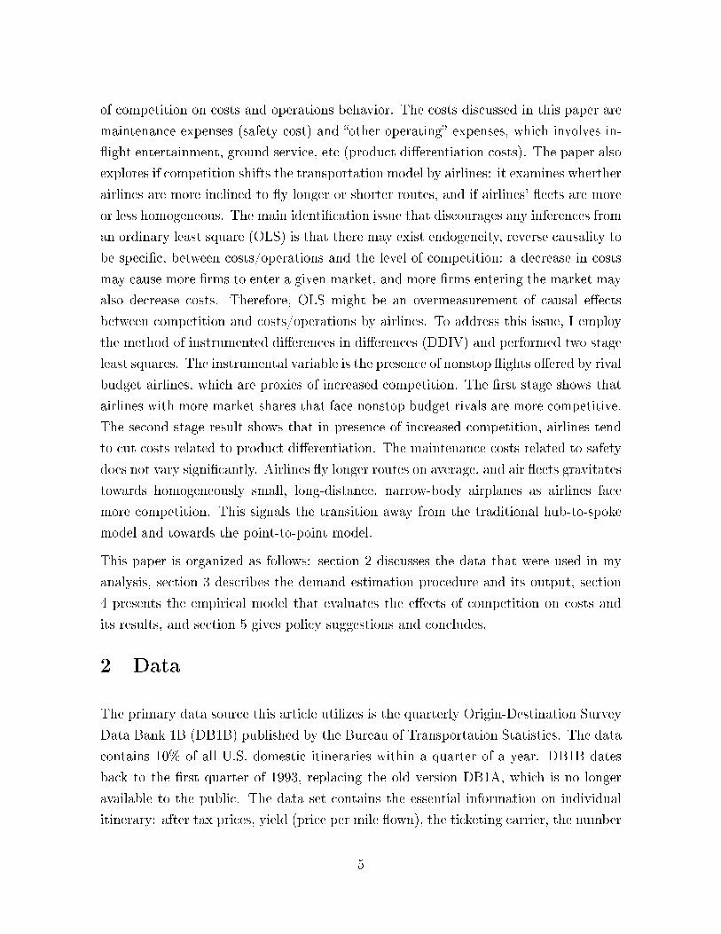
In gures 4 and 3, we can see the trend for the own-price elasticity for industry average
and also select carriers in the US in the period from the rst quarter of 1993 to the
end of 2018. The gures suggest an increasingly elastic market for the industry: the
absolute value of own-price elasticity is signicantly higher than 1993 for every one of
the graphs. The whole market uniformly face with an increasingly competitive market.
This variations in average industry elasticity is used in the next section to examine the
eects of such increased competition on the cost behavior of airlines.
4 The eects of competition on costs and market struc-
ture
As we can see from the previous section, the US airline competition has become more
competitive over the last quarter of the century. In this section, I will explore the eects
19

Figure 3: Average own-price elasticity from 1993Q1 to 2018Q4
of such changes in the market on the cost behavior and the market structre . The result
from section 3 gives us a panel with 24 major airlines over 104 periods (year-quarter).
In a ercely competitive market, it is expected that the markup for each airline is
minimal , and the market is so elastic that raising price is not an option. This would
expectedly push the rm to reduce its marginal cost to maintain a competitive edge
with its industry rivals. But which costs to cut is the question. In this section, I explore
the eects of competition on safety expenses and product-dierentiating expenses.
The measure of market structure that I use in this article is the average nonstop distance
and the homogeneity of airline eets. The nonstop distance and the airplane eets give
us information on the preference of airlines on which type of routes they want to operate.
The eet homogeneity is a measure if the airlines are using the same type of plane across
their eets. It is measured by the sum of squared dierences of plane characteristics
(capacity, manufacturer, model), normalized to a range from 0 to 1. For example, a 0 in
homogeneity index means that every airplanes that the airline owns are dierent, while
1 means the airline has the same planes for operation everywhere . The combination of
information regarding airlines' nonstop distance and eet homogeneity gives us some
insights to the future of aviation: is it transitioning from the traditional hub-to-spoke
model to point-to-point model? The hub-to-spoke model connects local ights to a hub
rst, therefore it often includes a short ight and a eet that consists of small planes
to connect local airports to hubs and big planes to connect between big hubs. We will
20

Figure 4: Ownprice elasticities for specic airlines, 1993Q1-2018Q3
see at the end of this section that the traditional transportation model is changing.
OLS
The costs chosen to make this analysis are the quarterly airline maintenance cost,
the quarterly total food costs, and the other operating expenses. The maintenance
cost relates to our safety interest of the story. The food cost and operating costs are
often related to the degree of dierentiated product, since at the same price and safety
preference, consumers choose an airline that oers better in-ight and airport service. A
naive way to answer the question is to take a simple ordinary least square with respect
to costs as a dependent variable and the degree of competition, the average ζat as the
independent variable:
Cat = γ1 + γ2ζat + la +Xatγ3 + eat (18)
Where a=AA,DL,US,.. is the index for an airline, t=1,2,...104 is the index for the
year-quater. Since the variation in costs is only observed at each airline's year-quarter
level, it is hard to assign these costs to dierent products in dierent markets.lais the
xed eect for airline a, which captures the characteristic of an airline across the time
periods. lt is the period xed eects. Xatis a vector of other controls such as labor cost,
average ight distance of the airlines, percentage of ights from a hub, and percentage
of direct nonstop ights. The independent variable of interest, ζat, is an absolute value
21

of the own-price elasticity of an airline in a year-quarter.
A concern over the ordinary least squares is that, there might exist endogeneity within
the regression in equation 18. Specically, reverse causality may be severe: not only
can an airline cut costs due to more competition, competition also could increase due
to an observation of lower costs. A decreased cost in a period can make airlines ex-
pand their operation, not necessarily by ordering new planes, but could be utilizing
idle ones or underused ones. This makes the market increasingly competitive for more
origin-destination pair, and thus the own price elasticity is going to become more elas-
tic. To address this endogeneity issue, I employ a couple of indentication strategies
that exploit the natural experiment nature of the data: Dierence in dierence and
Instrumental variable.
Instrumented Dierence in Dierences
I address endogeneity in this model by applying the instrumented dierence in dier-
ences method, which gives an estimation of the weighted average causal eects5. The
assumption to be met in this specication is quite standard in the dierence in dierence
as well as the instrumental variable literature: (1) exclusion restriction, the instrument
only aects the outcome through the treatment, and (2) parallel trend, both dierence
of treatment values and outcomes are mean independent of treatment.
The instrument in our case is the volume-weighted percentage of markets of an airline
with a presence of a budget airline's nonstop route. A dummy variable Post=0,1 is
assigned such that an entrance or exit of a budget airline (dened in section 2) switches
it from Post=0 to Post=1 for every existing airlines in each of the markets in a year-
quarter. The number of markets with Post=1 is then aggregated accross markets for
each ariline in a year-quarter.
Cat = la + πTt + γ2ζat +Xatγ3 + εat (19)
ζat = ka + δ1Tt + δ2ZatTt + ηat (20)
Where ζat is the treatment (competition), Zatis the instrument (weighted percentage of
markets that has a nonstop budget rival), and Ttis the period indicator for when the
5Method was widely used but not discussed as much formally. See Duo 2001, Angrist 1995
22
level of instrument jumps.
Exclusion restriction requires that the percentage of presence of nonstop budget com-
petitor in an airline's market has no eect on its cost decision. It is reasonable to expect
that the decision to enter a given market and oer a nonstop route by a budget airline
has little to do with existing carrier's costs. It is rather by the rm's connection, avail-
able type of plane, and risk tolerance, which is independent of the costs of an existing
airline.
The rst stage in the two stage least square is, as usual, to measure equation20 above.
This is measured by a standard dierence in dierence procedure. The second stage
returns the average causal eect of competition on the rms' cost:
γ2 =E[Ca1 − Ca0|Za = z1]− E[Ca1 − Ca0|Za = z0]
E[ζa1 − ζa0|Za = z1]− E[ζa1 − ζa0|Za = z0](21)
where z1 > z0, which represents a discrete jump in percentage of market of an airline
faced with nostop budget competition.
The rst stage result shows that, a 10% jump in the percentage of markets faced by
nonstop rival rises an airline's absolute average own-price elasticity by 1.37 percentage
points.
Table 8 presents the estimation result for the two models with three dierent choices
of dependent variable.
The OLS specication result shows that a 1 percentage point increase in absolute ownprice elasticity would also increase the maintenance cost, but not statistically signi-cant. The OLS estimation of Food cost and Other operating cost is more statisticallysignicant, both pointing out that the airlines are cutting Food and Operating costswhen facing more competition. This is also conrmed by the DDIV estimations for bothFood and Operating expenses. The result suggests that when rms face more compe-tition, their willingness to spend for product dierentiation decreases. This is specicto the airline industry and might not be extrapolated to a dierent technology-orientedconsumer experience industry like smart phone or computer.
The DDIV estimate shows a slightly negative but statistically insinicant coecient for
maintenance cost. This is reassuring regarding the concern over safety. The airlines
may be aware that an accident would be detrimental to its market power and thus
safety costs like maintenance is inelastic even with more severe competition. It is
also because the government rule on maintenance is extremely strict. Airplanes would
23
have to undergo small maintenance after a xed number of ying hours and grand
maintenance after a xed period of time.
Other coecients also provide interesting insights: the Average Nonstop distance uni-
formly increases every types of costs under every models. However, it may be misleading
to think that airlines should shift to shorter markets and be local, since this increase in
total maintenance, food, and operating cost might be subject to economies of scale. By
ying longer haul, the airlines keep their planes ying and making more prot instead
of having to transit a lot. From an engineering standpoint, a plane's age counts not by
the miles own, but by the number of times it takes o and lands, so having a plane to
y longer route would depreciate it less than to y short routes and take o multiple
times.
The results in both OLS and DDIV shows that with more competition, airlines y
longer nonstop routes and employ more homogeneous eets. Since competition makes
airline more aware about cost saving and revenue maximizing, they would want the
airplanes to spend as much time ying and as little time on the ground as possible.
On top of that, fuel eciency for new small, narrow-body planes allows them to travel
longer, point-to-point routes without going through costly and densely populated hubs.
This allows airlines to operate more locally and serve a smaller demand without having
to connect. Therefore, it is intuitive that we see an increasing nonstop distance as a
result of more competition. The gravitation towards a homogeneous eet of planes is
also justed, since airlines would only have to train one type of pilot and hire one type
of engineer to perform maintenance on their eets, exploiting economies of scale. One
more justication for a homogeneous eet goes back to the observation that airlines now
prefer longer, poin-to-point routes. It is very intuitive to see their eet transitioning
towards a homogeneous eet of small ecient planes.
5 Conclusion
In this paper, I estimated the eects of competition on cost behavior and market struc-
ture of the airline industry. The estimation is broken into two steps: step one estimates
the demand elasticities for the airlines, while step two takes the elasticity derived from
step one to evaluate the eect of more competition on costs behavior of the rm and
the market structure.
In step one, this paper used the Berry-Lehvinson-Pakes (1995) method to estimate the
24
demand for a dierentiated product airline market. For each of an year-quarter from
1993Q1 to 2018Q4, an own-price elasticity is derived for each airline. The result shows
that, during the period of the estimation, own-price elasticity has increased signicantly
throughout the United States aviation market. The whole industry uniformly faces more
competition.
In step two, I estimated the eects of increased competition on dierent costs by the
airlines and how airline change their structures. The costs chosen were maintenance
cost, food cost, and other operating costs. Maintenance cost addresses the concern
over safety that might be compromised by airlines. The coecient, however, does not
indicate that airlines changed their safety cost behavior signicantly. Instead, airlines
might be strongly willing to compromise customer comfort and airline's dierentiated
product, as they decrease food cost and other operating expenses when faced with
more competition. This also implies that they are more prepared to engage in price
competition, since the dierentiated product aspect is gradually being removed. Air-
lines are ying longer nonstop routes with a more homogeneous eets as a result of
competition. This signals a transition of the transportation model from the traditional
hub-to-spoke to point-to point model. The new plane orders are mostly small, ecient
narrow-body planes which can y longer distance and serve a lower demand market
without connecting through costly, populated hubs.
In order to address the increasing competitiveness in the industry, in a future research,
it would be interesting to examine the eects of dierent government subsidies in order
to maintain consumer experience in air travel. I would also like to see the eects of
competition on overbooking and delay behavior of airlines, and develop a model to
explore which policy to be derived.
6 References
Richard Olivier Armantler Olivier. Domestic airline alliances and consumer wel-
fare. RAND Journal of Economics, 2008.
Pakes Berry, Lehvinson. Automobile prices in market equilibrium. Econometrica,
1995.
Steven Berry. Estimation of a model of entry in the airlines industry. Econometrica,
1992.
25
Steven Berry and Panle Jia. Tracing the woes: An empirical analysis of the airline
industry. American Economic Journal: Microeconomics, 2010.
Steven T. Berry. Airport presence as product dierentiation. American Economic
Review, 1990.
Severin Borenstein. Airline mergers, airport dominance, and market power. Amer-
ican Economic Review, 1990. 21
Severin Borenstein. Why can't us airline make money? American Economic Review:
Papers and Proceedings, 2011.
Jan Brueckner. Airline trac and urban economic development. Urban Studies, 2003.
Jan Brueckner and Pablo T. Spiller. Economies of trac density in the deregulated
airline industry: Journal of Law and Economics; 1994
Jan K. Brueckner and Pablo T. Spiller. Economics of trac density in the deregu-
lated airline industry. Journal of Law and Economics, 379, 1994.
Nichola J. Dyer Brueckner, Jan and Spiller. Fare determination in airline hub-
and-spoke networks. The RAND Journal of Economics, 1992.
Federico Ciliberto and Jonathan W Williams. Does multimarket contact facil-
itate tacit collusion? inference on conduct parameters in the airline industry. The
RAND Journal of Economics, 2014.
David Sibley David Graham, Daniel Kaplan. Eciency and competition in the
airline industry. The Bell Journal of economics, 1983.
Esther Duo. Schooling and labor market consequences of school construction in
indonesia: Evidence from an unusual policy experiment,â. American Economic Review,
2001.
P. G. Gayle. An empirical analysis of the competitive eects of the delta/ continental/
northwest code share alliance, Journal of Law and Economics; 2008
D. Gilo and F. Simonelli. The price-increasing eects of domestic codes sharing
agreements for non stop airline routes: Journal of Competition Law and Economics
Pinelopi Koujianou Goldberg. Product dierentiation and oligopoly in interna-
tional markets : The case of the us auto mobile industry:Econometrica; 1995
Austan Goolsbee and Chad Syverson. How do incumbents respond to the threat
of entry? evidence from the major airlines. The Quarterly Journal of Economics, 2008.
26

Vijay Singal Han Kim. Mergers and market power: Evidence from airline industry.
American Economic Review, 1993.
Oum, Zhang, and Zhang , Inter-Firm Rivalry and Firm-Specic Price Elasticities
in Deregulated Airline Markets, 1993.
Rubin and Joy . Where are the Airlines Headed? Implications of Airline Industry
Structure and Change for Consumers, 2005.
M. Piccione Hendricks, K. and G. Tan. Entry and exit in hub-spoke networks.
RAND Journal of Economics, 1997.
Alfred E. Kahn. Surprises from deregulation. American Economic Review, 1988. 22
E. H. Kim and V. Singal. Mergers and market power : Evidence from the airline
industry. The American Economic Review, 1993.
Dominic L.Daher. The proposed federal taxation of frequent yer miles received from
employers: Good tax policy but bad politics. Akron Tax Journal, 2001.
Mara Lederman. Do enhancements to loyalty programs aect demand? the impact of
international frequent yer partnerships on domestic airline demand. RAND Journal of
Economics, 2007.
D Luo. The price eects of the delta /northwest airline merger: Review of Industrial
Organization; 2014
Levine M. Airline competition in deregulated market: Theory, rm strategy and public
policy. Yale Journal of Regulation, 4:393494, 1987.
Daniel McFadden. A method of simulated moments for estimation of discrete choice
response models without numerical integration. Econometrica, 57:9951026, September
1989.
Gayle Philip. Airline code-share alliances and their competitive eects: The Journal
of Law and Economics; 2007
Marvin Rothstein. An online overbooking model. Transportation science, 1971.
Borenstein S. Hubs and high fares: Dominance and market power in the u.s. airline
industry. RAND Journal of Economics, 1989.
Doug S and James Stock. Barriers to entry in the airline industry: A multidimen-
sional regression-discontinuity analysis of air-21. Review of Economics and Statistics
2015.
27

Lee S.Garson. Frequent yer bonus program: To tax or not to tax- is this the only
question? Journal of Air Law and Commerce, 1987.
Yimin Zhang Tae Hoon Oum, Anming Zhang. Airline network rivalry. The
Canadian Journal of Economics, 1995.
Z. Yuan. Network competition in the airline industry : A framework for empirical
policy analysis. 2016.
28

Table3:
Summary
mean
sdmin
max
Source
Fare
218.19
146.23
401500
DB1B
Nonstop
0.101
01
DB1B
Distance
(miles)
1,560
7545
7550
DB1B
Within-carrier
origin
share
0.15
0.11
01
DB1B
Nonstop
rivals
1.22
1.43
012
DB1B
Budgetairlines
1.75
05
DB1B
Number
ofroutesper
market
10.47
6.55
181
DB1B
Number
ofcarriers
per
market
4.98
2.33
114
DB1B
Maintenance
costsper
aircraft(x1000)
3,145
1.23
019.23
P-7.B-4.3
Foodcostsper
aircraft(x1000)
64.12
9.93
0172.62
P-7,B-4.3
Operatingcosts(x1000)
517,132
417.76
22,934
P-7
N13,142,196
29

Table 4: OLS estimation of demandDemand estimation-OLS vs Multinomial Logit
OLS Multinomial LogitBusiness Leisure Business Leisure
Price β1 -0.32 -3.87 -0.09 -3.21***(0.42) (2.38) (0.54) (1.39)
Average competitor price βjm 0.06 0.86 0.04 1.37***(1.80) (0.65) (0.12) (0.55)
Nonstop=0 -10.36*** -2.98* -2.25*** 0.08(2.00) (1.72) (0.33) (0.59)
Budget =1 0.004 1.47** -0.076 1.66***(1.13) (0.64) (0.32) (0.42)
Major 6.4*** 0.657 1.11** 0.73***(1.05) (2.88) (0.60) (0.17)
R2 0.09 0.17 0.14 0.20
30

Table5:
Logitestimation
Fullmodelestimation
Allyear-quater
1993Q1
2018Q4
Longhaul
Shorthaul
Mean
Stdv
Mean
Stdv
Mean
Stdv
Mean
Mean
Constant
71.45***
30.12***
72.12***
27.98***
82.92***
29.19***
62.55***
82.92***
(1.26)
(6.37)
(20.29)
(8.43)
(13.75)
(11.12)
(20.19)
(13.75)
Price
-44.05***
2.86
-20.24***
1.72
-79.75***
6.12***
-11.24***
-36.75***
(3.08)
(2.45)
(2.43)
(1.98)
(4.16)
(0.87)
(1.43)
(4.95)
Nonstop=0
-4.17***
1.17
0.04
0.02
-7.88***
3.98***
-1.47***
-3.68*
(0.15)
(2.12)
(0.11)
(1.64)
(0.04)
(1.82)
(0.11)
(2.14)
Majorat
origin
8.14***
3.11***
13.11***
5.44
6.09**
3.12*
11.81***
3.90*
(1.03)
(1.10)
(1.71)
(4.32)
(2.97)
(2.45)
(1.88)
(2.05)
Budget=
1-9.72***
1.45***
-15.44***
3.23***
-18.45
1.04*
-26.74***
-1.64***
(2.11)
(0.42)
(1.20)
(0.67)
(1.99)
(0.66)
(6.56)
(0.59)
Income*Price
31.69***
17.42***
23.42***
(5.76)
(1.28)
(6.72)
Age*P
rice
1.45***
6.28***
5.45***
(0.14)
(1.12)
(1.42)
Fem
ale*Price
-1.45***
-3.14***
-0.95
(0.16)
(0.89)
(0.75)
Income*(N
onstop=0)
-18.12***
-16.42***
-31.78***
(1.94)
(3.65)
(4.42)
Income*Budget
0.45
1.88
-2.16
(1.72)
(1.64)
(3.49)
Fem
ale*Budget
-7.25*
-7.28***
-17.45***
(4.53)
(2.55)
(4.76)
GMM
objective
688.9
1,277.95
877.38
31

Table6:
Average
own-andcross-price
elasticity
Elasticity-calculation
from
GMM
BLPestimation-2018Q
4
Product
type
Characteristics
12
34
56
78
Nonstop
Budget
Majorat
origin
10
00
-3.468
0.421
1.488
0.089
0.124
0.236
2.445
0.143
21
00
0.251
-2.515
0.644
0.378
0.223
0.420
0.975
0.128
30
10
0.124
0.141
-7.257
1.644
0.015
2.057
2.689
0.045
40
01
0.339
0.321
0.348
-5.988
0.029
0.701
1.084
0.012
51
10
0.434
0.039
1.12
0.475
-2.756
0.096
0.992
0.001
61
01
0.211
0.110
1.021
0.493
0.086
-4.779
1.104
0.556
70
11
0.121
0.450
2.667
1.748
0.324
1.799
-8.75
0.425
81
11
0.421
0.199
0.145
0.001
0.103
0.212
0.345
-1.454
0-Outsidegood
--
-0.020
0.015
0.042
0.075
0.142
0.037
0.987
0.137
32
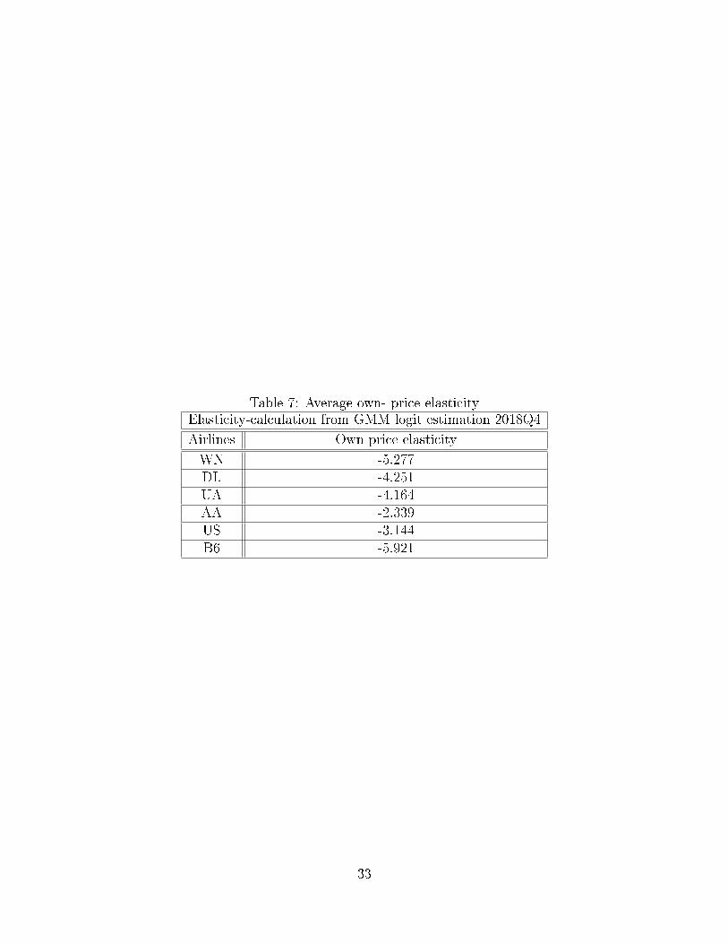
Table 7: Average own- price elasticityElasticity-calculation from GMM logit estimation 2018Q4
Airlines Own price elasticity
WN -5.277DL -4.251UA -4.164AA -2.339US -3.144B6 -5.921
33
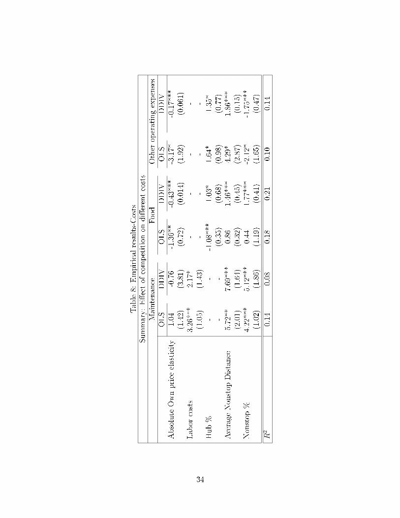
Table8:
Empiricalresults-Costs
Summary:Eectof
competitionon
dierentcosts
Maintenance
Food
Other
operatingexpenses
OLS
DDIV
OLS
DDIV
OLS
DDIV
Absolute
Ownprice
elasticity
1.04
-0.76
-1.36**
-0.43***
-3.17*
-0.17***
(1.42)
(3.81)
(0.72)
(0.014)
(1.92)
(0.061)
Labor
costs
3.26***
2.17*
--
--
(1.05)
(1.43)
--
--
Hub%
--
-1.08***
1.03*
1.64*
1.35*
--
(0.35)
(0.68)
(0.98)
(0.77)
Average
Nonstop
Distance
5.72**
7.69***
0.86
1.46***
4.29*
1.86***
(2.01)
(1.64)
(0.32)
(0.45)
(2.87)
(0.15)
Nonstop
%4.22***
5.12***
0.44
1.77***
-2.12*
-1.75***
(1.02)
(1.86)
(1.19)
(0.41)
(1.65)
(0.47)
R2
0.14
0.08
0.18
0.21
0.10
0.14
34

Table 9: Empirical results- nonstop distance and eet homogeneitySummary: Eect of competition on dierent airlines
Nonstop distance Fleet HomogeneityOLS DDIV OLS DDIV
Absolute Own price elasticity 0.318*** 0.157*** 0.110*** 0.014***(0.092) (0.048) (0.034) (0.002)
Labor costs - - 0.032 0.041***- - (0.025) (0.009)
Hub % -0.151*** -0.271*** - -(0.022) (0.485) - -
Average Nonstop Distance - - - -- - - -
Nonstop % - - - -- - - -
R2
35