Infrastructure Interdependencies Simulation (I2Sim) System ...

Infrastructure InterdependenciesSimulation (I2Sim) System Model and

Toolboxby

HyunJung Lee

B.A.Sc., The University of British Columbia, 2007

A THESIS SUBMITTED IN PARTIAL FULFILLMENT OFTHE REQUIREMENTS FOR THE DEGREE OF

MASTER OF APPLIED SCIENCE

in

The Faculty of Graduate Studies

(Electrical and Computer Engineering)

THE UNIVERSITY OF BRITISH COLUMBIA

(Vancouver)

April 2010

© HyunJung Lee 2010

Abstract

The interdependencies between infrastructures have become more complex with thegrowth of the civilization. As a result, the cascading effects on the system caused bya failure of one infrastructure became larger and unpredictable. As seen from the ma-jor disasters such as the Sichuan earthquake in China, understanding infrastructureinterdependencies and allocating resources efficiently in the system can facilitate therecovery process significantly. As a part of Canadian Government’s effort to developinnovative ways to mitigate large disaster situations and grow resiliences of systems,Joint Infrastructure Interdependencies Research Program (JIIRP) has been formed. TheUBC’s Infrastructure Interdependencies Simulation (I2Sim) group led by Dr. Jose Martiparticipated to study decision making for critical linkages in infrastructure networks.At the end of the program period, its achievement was recognized, and the I2Simgroup was selected to develop a simulator for the Vancouver 2010 Winter Olympics.

As a part of this research, the concept of cells, channels, and tokens along with com-ponents consisting the cells were developed. The core of the cells and the channels areformed by the Human Readable Tables (HRT) which describe the relationship betweenthe inputs and the outputs of the unit. The HRT allows a reasonable prediction of thereal life system even with limited data. As a result, the infrastructure owners do nothave to disclose the confidential operational information of the system. The test casemodels were built based on the UBC Campus first and extended to the Olympics sitesin Vancouver.

To simulate the test cases, a customized Matlab/Simulink toolbox called I2Sim wasdeveloped. The I2Sim toolbox follows a graphical drag-and-drop box format. Since theuser of the toolbox only has to deal with the graphical interface, even the non-expertscan build a case easily. The main improved features included in the new version isthat the effect of time delay in the channels and the human flow. The test case resultshelps producing an optimal resource allocation and the restoration priorities duringdisasters.

ii

Table of Contents

Abstract . . . . . . . . . . . . . . . . . . . . . . . . . . . . . . . . . . . . . . . . . . ii

Table of Contents . . . . . . . . . . . . . . . . . . . . . . . . . . . . . . . . . . . . iii

List of Tables . . . . . . . . . . . . . . . . . . . . . . . . . . . . . . . . . . . . . . . vi

List of Figures . . . . . . . . . . . . . . . . . . . . . . . . . . . . . . . . . . . . . . vii

Acknowledgements . . . . . . . . . . . . . . . . . . . . . . . . . . . . . . . . . . . x

1 Introduction . . . . . . . . . . . . . . . . . . . . . . . . . . . . . . . . . . . . . 11.1 Motivation . . . . . . . . . . . . . . . . . . . . . . . . . . . . . . . . . . . . 11.2 Background . . . . . . . . . . . . . . . . . . . . . . . . . . . . . . . . . . . 3

1.2.1 Infrastructure Interdependencies . . . . . . . . . . . . . . . . . . 31.2.2 Previous Researches . . . . . . . . . . . . . . . . . . . . . . . . . . 4

1.3 Research Objectives . . . . . . . . . . . . . . . . . . . . . . . . . . . . . . 61.4 Organization of the Thesis . . . . . . . . . . . . . . . . . . . . . . . . . . . 6

2 Infrastructure Interdependencies Simulation (I2Sim) . . . . . . . . . . . . . 82.1 I2Sim Ontology . . . . . . . . . . . . . . . . . . . . . . . . . . . . . . . . . 8

2.1.1 Cell and Channel Classification . . . . . . . . . . . . . . . . . . . 92.2 I2Sim Architecture . . . . . . . . . . . . . . . . . . . . . . . . . . . . . . . 102.3 Discrete Event Simulation . . . . . . . . . . . . . . . . . . . . . . . . . . . 11

2.3.1 Uncontrollable Event . . . . . . . . . . . . . . . . . . . . . . . . . 112.3.2 Time-dependent Event . . . . . . . . . . . . . . . . . . . . . . . . 112.3.3 Decision-making Event . . . . . . . . . . . . . . . . . . . . . . . . 12

2.4 UBC Campus and Vancouver 2010 Winter Olympics . . . . . . . . . . . 122.4.1 UBC Campus Test Case . . . . . . . . . . . . . . . . . . . . . . . . 122.4.2 Vancouver 2010 Winter Olympics . . . . . . . . . . . . . . . . . . 13

iii

Table of Contents

3 Human Readable Table (HRT) . . . . . . . . . . . . . . . . . . . . . . . . . . . 153.1 Human Readable Table . . . . . . . . . . . . . . . . . . . . . . . . . . . . 15

3.1.1 Types of Human Readable Tables . . . . . . . . . . . . . . . . . . 163.2 Physical Mode (PM) and Resource Mode (RM) . . . . . . . . . . . . . . . 183.3 Color Scheme . . . . . . . . . . . . . . . . . . . . . . . . . . . . . . . . . . 193.4 Construction of a Model . . . . . . . . . . . . . . . . . . . . . . . . . . . . 21

3.4.1 Information Gathering . . . . . . . . . . . . . . . . . . . . . . . . 213.4.2 Building Human Readable Table . . . . . . . . . . . . . . . . . . . 223.4.3 Designing Cells using I2Sim Toolbox . . . . . . . . . . . . . . . . 23

4 I2Sim Toolbox . . . . . . . . . . . . . . . . . . . . . . . . . . . . . . . . . . . . 244.1 Development of Customized Blocks . . . . . . . . . . . . . . . . . . . . . 254.2 I2Sim Components . . . . . . . . . . . . . . . . . . . . . . . . . . . . . . . 25

4.2.1 Aggregator . . . . . . . . . . . . . . . . . . . . . . . . . . . . . . . 264.2.2 Human Readable Table (HRT) . . . . . . . . . . . . . . . . . . . . 264.2.3 Distributor . . . . . . . . . . . . . . . . . . . . . . . . . . . . . . . 294.2.4 Channel . . . . . . . . . . . . . . . . . . . . . . . . . . . . . . . . . 314.2.5 Storage . . . . . . . . . . . . . . . . . . . . . . . . . . . . . . . . . 344.2.6 Source . . . . . . . . . . . . . . . . . . . . . . . . . . . . . . . . . . 364.2.7 Sink . . . . . . . . . . . . . . . . . . . . . . . . . . . . . . . . . . . 37

5 Simulations and Results . . . . . . . . . . . . . . . . . . . . . . . . . . . . . . 385.1 UBC Campus Case . . . . . . . . . . . . . . . . . . . . . . . . . . . . . . . 38

5.1.1 Scenario 2 of Liu’s Thesis . . . . . . . . . . . . . . . . . . . . . . . 415.1.2 Modified Version of the Scenario 2 of Liu’s Thesis . . . . . . . . . 46

5.1.2.1 Model and Scenario Change . . . . . . . . . . . . . . . . 465.1.2.2 Scenario and Results . . . . . . . . . . . . . . . . . . . . 47

5.2 Vancouver 2010 Winter Olympics Case . . . . . . . . . . . . . . . . . . . 535.2.1 Crowd Behavior . . . . . . . . . . . . . . . . . . . . . . . . . . . . 535.2.2 Initial Conditions and Scenario . . . . . . . . . . . . . . . . . . . . 545.2.3 Results and Analysis . . . . . . . . . . . . . . . . . . . . . . . . . 56

5.3 Simulation Conclusion . . . . . . . . . . . . . . . . . . . . . . . . . . . . . 605.4 Limitation of the MATLAB . . . . . . . . . . . . . . . . . . . . . . . . . . 60

iv

Table of Contents

6 Conclusion . . . . . . . . . . . . . . . . . . . . . . . . . . . . . . . . . . . . . . 626.1 Contribution . . . . . . . . . . . . . . . . . . . . . . . . . . . . . . . . . . 626.2 Future Work . . . . . . . . . . . . . . . . . . . . . . . . . . . . . . . . . . . 63

Bibliography . . . . . . . . . . . . . . . . . . . . . . . . . . . . . . . . . . . . . . . 65

Appendices

A Aggregator MATLAB System Function Code . . . . . . . . . . . . . . . . . . 68

B HRT MATLAB System Function Code . . . . . . . . . . . . . . . . . . . . . . 70

C Distributor MATLAB System Function Code . . . . . . . . . . . . . . . . . . 77

D Channel MATLAB System Function Code . . . . . . . . . . . . . . . . . . . . 80

E Statement of Collaboration . . . . . . . . . . . . . . . . . . . . . . . . . . . . . 83

v

List of Tables

3.1 Production Human Readable Table . . . . . . . . . . . . . . . . . . . . . . 163.2 Channel Human Readable Table . . . . . . . . . . . . . . . . . . . . . . . 173.3 Distributor Human Readable Table . . . . . . . . . . . . . . . . . . . . . . 17

vi

List of Figures

2.1 Cell Classification Example . . . . . . . . . . . . . . . . . . . . . . . . . . 92.2 I2Sim Architecture . . . . . . . . . . . . . . . . . . . . . . . . . . . . . . . 10

3.1 Physical Mode and Resource Mode . . . . . . . . . . . . . . . . . . . . . . 193.2 Color Scheme . . . . . . . . . . . . . . . . . . . . . . . . . . . . . . . . . . 203.3 PM RM Color Representation in a Block . . . . . . . . . . . . . . . . . . . 203.4 Generic Cell Design . . . . . . . . . . . . . . . . . . . . . . . . . . . . . . . 23

4.1 I2Sim Toolbox in Simulink . . . . . . . . . . . . . . . . . . . . . . . . . . . 244.2 Aggregator Block . . . . . . . . . . . . . . . . . . . . . . . . . . . . . . . . 264.3 Human Readable Table Block . . . . . . . . . . . . . . . . . . . . . . . . . 274.4 Distribution Example . . . . . . . . . . . . . . . . . . . . . . . . . . . . . . 294.5 Distributor Block . . . . . . . . . . . . . . . . . . . . . . . . . . . . . . . . 304.6 Channel Block . . . . . . . . . . . . . . . . . . . . . . . . . . . . . . . . . . 324.7 Storage Block . . . . . . . . . . . . . . . . . . . . . . . . . . . . . . . . . . 354.8 Source Block . . . . . . . . . . . . . . . . . . . . . . . . . . . . . . . . . . . 364.9 Sink Block . . . . . . . . . . . . . . . . . . . . . . . . . . . . . . . . . . . . 37

5.1 Design of Reduced UBC Campus Test Case . . . . . . . . . . . . . . . . . 395.2 Simulation of Reduced UBC Campus Test Case . . . . . . . . . . . . . . . 405.3 Substation Comparison . . . . . . . . . . . . . . . . . . . . . . . . . . . . . 425.4 Substation Cell Results . . . . . . . . . . . . . . . . . . . . . . . . . . . . . 435.5 Power House, Steam Station, Water Station Cell Results . . . . . . . . . . 445.6 Hospital Cell Results . . . . . . . . . . . . . . . . . . . . . . . . . . . . . . 455.7 Water Station Back-up Oil Tank Level . . . . . . . . . . . . . . . . . . . . 455.8 Human Flow Model for Purdy Hospital . . . . . . . . . . . . . . . . . . . 475.9 Water Station and Steam Station Cell Outputs . . . . . . . . . . . . . . . . 495.10 Hospital Cell Outputs . . . . . . . . . . . . . . . . . . . . . . . . . . . . . 50

vii

List of Figures

5.11 Vancouver 2010 Winter Olympics Study Area . . . . . . . . . . . . . . . . 515.12 Vancouver 2010 Winter Olympics Simulink Model . . . . . . . . . . . . . 525.13 GM Place with Crowd Model . . . . . . . . . . . . . . . . . . . . . . . . . 535.14 Electricity to BC Place, GM Place, and St Paul’s Hospital . . . . . . . . . 565.15 Water to Hospitals . . . . . . . . . . . . . . . . . . . . . . . . . . . . . . . 575.16 Waiting Area for Olympics Venues . . . . . . . . . . . . . . . . . . . . . . 585.17 Olympics Case Hospital Model Results . . . . . . . . . . . . . . . . . . . 59

viii

List of Algorithms

4.1 Human Readable Table Search Algorithm . . . . . . . . . . . . . . . . . . . 284.2 Distributor Search Algorithm . . . . . . . . . . . . . . . . . . . . . . . . . . 31

ix

Acknowledgements

I am very grateful to my supervisor, Professor Jose R. Marti, for his guidance duringthe last three years. Dr. Marti introduced me to the rich field of power engineering andinfrastructure simulation and demonstrated first-hand the level of dedication and hardwork required to be successful in this field. This thesis would not have been possiblewithout his help and support. I would also like to thank Professor K.D. Srivastava andProfessor Juri Jatskevich for being the members of my thesis committee and providinginsightful feedback throughout my Master’s program. I would like to thank my col-leagues and friends Marcelo Tomim, Hugon Juarez, Brian Burtchett, Jian Xu, ShahrzadRostamirad, Tom De Rybel, and Lucy Liu as well as the students in the Power Lab-oratory for the interesting discussions we had and for the valuable comments theyprovided for the work in this thesis. They made my experience at UBC unforgettableand I am very lucky to have been able to meet them.

I am grateful to my family for their unconditional love and support throughout mylife. I would not be where I am today without the sacrifices that they have made. Iwould never forget the cheer-up shopping with my sister SookSook and the summertrips with my brother ChangChang. I also want to thank my best friends, Nara Shinand Eugenia Chen, for their emotional supports. Above all, I wish to sincerely thankmy husband George Yuan, who was there since the first day as a UBC graduate stu-dent, for his unyielding support and love, bearing with me through the tough times.

Finally I would like to express my thanks to Natural Sciences and EngineeringResearch Council (NSERC) of Canada and Vancouver Olympics Committee (VANOC)that provided the support for this work.

x

To George, my husband

xi

Chapter 1

Introduction

The topic of this thesis is the development of a simulator and models in order to studythe interdependencies between infrastructures and critical buildings during disastersas well as the effective decision making processes. The work in this thesis is a part ofthe research done by Infrastructure Interdependencies Simulation (I2SiM) group ledby Dr. Jose Marti at the University of British Columbia (UBC) for the Joint Infrastruc-ture Interdependencies Research Program (JIIRP) [19] and the Vancouver OrganizingCommittee for the 2010 Olympics and Paralympics Winter Games (VANOC) [12].

1.1 Motivation

The effective allocation of resources and services among the different infrastructures,such as power and water utilities, telecommunications, transportation networks andhospitals, has become significant in the modern society. At the same time, the intercon-nection and interdependencies between these infrastructures have become intenselycomplex which makes the system more vulnerable to failures from cascading effects.Since the dependencies between infrastructures are not easily identified, it is difficultto determine how to operate the system by intuition alone. Especially during largedisasters, prompt and effective responses and resilience are very closely related to theprobability of human survivals. Through major events, such as the New York Cityattacks on September 11, 2001, the Eastern North America power blackout on August14, 2003 [4], and the South Asia tsunami on December 26, 2004 [6], we have learnedthe importance of operating infrastructures effectively to achieve fast restorations andstrong resilience of the system.

To ensure the resilience of the system, it is important to define what it is first. Theresilience of a system can be conceptualized into four categories as follows [8] [21]:

• Robustness - the ability of elements and system to withstand stress without suf-fering degradation

1

1.1. Motivation

• Redundancy - the extent to which elements and system to be substitutable byother elements in the event of disruption

• Resourcefulness - the capacity to identify problems, establish priorities, and mo-bilize resources during the event of disruption or scarceness of resources

• Rapidity - the capacity to meet priorities and goals within the required time inorder to avoid future disruption

Ensuring resilience of the system during the disaster requires more than a fast andproper response during the disaster. It also involves the preparations before the dis-aster and the restorations after the disaster. Hollman et al define the four stages ofmanagement of infrastructures for disasters as follows [16]:

• Mitigation - long before the disaster

• Preparedness - long and shortly before the disaster

• Response - during and shortly after the disaster

• Recovery - shortly and long after the disaster

Mitigation refers to the sustained actions to reduce the long-term impacts from dis-asters long before the disaster while preparedness is the policies and plans on emer-gency management. Response is the actions taken during or immediately after thedisaster; and Recovery is the restoration actions after the disaster. Any actions that aretaken during these stages are dynamically interconnected.

As part of Canadian Governments effort to develop innovative ways to mitigatelarge disaster situation and grow resilience of systems, Joint Infrastructure Interdepen-dencies Research Program (JIIRP) has been formed through the Natural Sciences andEngineering Research Council (NSERC) and Public Safety Canada (PS) [19] [20]. UBCI2Sim group led by Dr. Jose Marti was the largest group out of six university groupsparticipating in this project to study decision making for critical linkages in infrastruc-ture networks. At the end of the project period, its achievement was recognized, andI2Sim group was selected to develop a simulator for Vancouver 2010 Winter Olympicsin 2009.

2

1.2. Background

1.2 Background

This section gives an overview of the fundamental concepts of the infrastructure inter-dependencies and related researches that have been conducted.

1.2.1 Infrastructure Interdependencies

The study of infrastructure interdependency has not been emphasized until recently.As a result, the definition of infrastructures and the classification of interdependenciesbetween them may not be clear to many people. The Critical Infrastructure AssuranceOffice (CIAO) defined infrastructure as [1] [27]:

”the framework of interdependent networks and systems comprising identifiableindustries, institutions (including people and procedures), and distribution capa-bilities that provide a reliable flow of products and services essential to the defenseand economic security of the United States, the smooth functioning of governmentsat all levels, and society as a whole [1].”

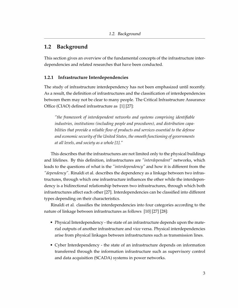
This describes that the infrastructures are not limited only to the physical buildingsand lifelines. By this definition, infrastructures are ”interdependent” networks, whichleads to the questions of what is the ”interdependency” and how it is different from the”dependency”. Rinaldi et al. describes the dependency as a linkage between two infras-tructures, through which one infrastructure influences the other while the interdepen-dency is a bidirectional relationship between two infrastructures, through which bothinfrastructures affect each other [27]. Interdependencies can be classified into differenttypes depending on their characteristics.

Rinaldi et al. classifies the interdependencies into four categories according to thenature of linkage between infrastructures as follows [10] [27] [28]:

• Physical Interdependency - the state of an infrastructure depends upon the mate-rial outputs of another infrastructure and vice versa. Physical interdependenciesarise from physical linkages between infrastructures such as transmission lines.

• Cyber Interdependency - the state of an infrastructure depends on informationtransferred through the information infrastructure such as supervisory controland data acquisition (SCADA) systems in power networks.

3

1.2. Background

• Geographic Interdependency - a local environmental event can create state changesin all infrastructure due to close spatial proximity such as collocated elements indifferent infrastructures in a common right-of-way.

• Logical Interdependency - the state of an infrastructure depends upon the state ofanother infrastructure and vice versa through the means that is not all of above.The logical linkage can be policy, legal or regulatory regimes.

Rinaldi et al’s interdependency classification is a simple but yet comprehensiveway of describing different types of infrastructure linkages.

1.2.2 Previous Researches

As mentioned above, the research of infrastructure interdependency simulation aloneis relatively new; however, the techniques and studies regarding disasters have beenactively developed and evolved since Oklahoma City bombing in 1995 and the reportfrom the Defense Science Board Task Force on Information Warfare in 1996.

According to Marti et al. [17], present simulation tools involve either the macro-scopic view of emergency preparedness organizations or the microscopic view of thefirst responders. The emergency preparedness organizations may see the whole pic-ture of how the infrastructures interact; they, however, may miss the details and com-plexity of each infrastructure and hidden interdependencies between infrastructures,which could result in a sequential catastrophic responses. The first responders may bean expert in their field, but they would not be able to see the operation of other infras-tructures. In this thesis, the simulation itself is proceeded as an integrated simulationwhile each infrastructure can be modeled separately by its own expert. In this way,the simulator can capture the advantages of both approaches taking macroscopic andmicroscopic view of the situation.

According to the survey performed by Pederson et al., most infrastructure simu-lation tools have taken two approaches on modeling the infrastructure system: inte-grated and coupled models [2]. The integrated model is designed to model multipleinfrastructures and their interdependencies within one framework. The coupled ap-proach takes multiple simulations of infrastructures and connect them together. Themajor modeling techniques using these two approaches are Petri Nets, System Dy-namics, Agent-based, Physics based and Input-output Model [2]. In addition to thesetechniques, Cell-channel model has been developed by UBC I2Sim group, which this

4

1.2. Background

thesis has been developed upon. The following is a summary of techniques mentionedabove.

• Petri Net - A Petri net is a graphical and mathematical tool for modeling dis-crete distritbuted systems. It is composed of places, transitions, and directedarc connecting places and transitions. Petri Net uses the flow of tokens to showthe state of the infrastructures and the interdependencies between them. Tokensare stored in the places and transferred to another places through transitions. In[13], Gurseli et al use the Petri net’s place invariants to model the major infras-tructures such as electricity, oil, water, natural gas, and telecommunication andidentify the interdependencies and vulnerabilities by assigning 1 for ”ON” and0 for ”OFF”. Petri net has an advantage of presenting a simple visualization ofinterdependencies. However, it lacks the ability to model quantitative informa-tion.

• System Dynamics - System Dynamics is a continuous time based approach tomodel complex feedback systems. Forrester developed the methodology focus-ing on stocks, flows, and the feedback of the system over time [26]. Min et al.simulated an infrastructure interdependency model using this technique com-bined with IDEFO for decision makings [15]. System Dynamics are more suitablefor high-level view of the system rather than a detailed model of infrastructures.That is, it gives a macroscopic view of the effect from policies or plans on multipleinfrastructures for the emergency preparedness organizations.

• Agent-Based Model - The agent-based modeling paradigm is one of the mostpopular approaches used for the infrastructure interdependency simulations [2].An agent-based model consists of autonomous decision makers called agentswho each assesses the situation and makes decision according to their own rules [7].Each agent is assigned with different responsibilities such as water production,electricity distribution, or back-up system start. When a simple behavior ofeach agent is combined, it creates complex random patterns of a system. Anumber of infrastructure models have been developed using agent-based modelincluding Critical Infrastructure Modeling Software (CIMS) developed by theIdaho National Laboratory [10] [25], Critical Infrastructure Simulation by Inter-dependent Agents (CISIA) presented by Panzieri et al. [2] [23] [24], and Next-generation agent-based economic laboratory (N-ABLE) by Sandia National Lab-

5

1.3. Research Objectives

oratories [2] [11]. In the agent-based model, the detailed models of infrastruc-tures, in general, are done separately and fed into agents as inputs [22].

• Cell-Channel Model - The cell-channel model is a unique modeling techniqueused for UBC I2Sim project by Marti et al. [17]. This thesis is the extension ofthe first version of cell-channel model which was implemented by Liu [18]. Themodel consists of the identities called cells, channels, and tokens. Infrastructuresare defined as cells where transformation of tokens occur. The tokens are theresources or services that flow between cells using channels. The channels arethe representation of lifelines such as transmission lines and water pipe lines.Cells and channels are composed of Human Readable Tables and other addi-tional components. The operating state of cells and channels are expressed asphysical modes and resource modes of the system. The details about cell-channelmodel will be discussed throughout chapter 2 and chapter 3 of this thesis.

All of above methods have their strengths and weaknesses. For the new I2Simmodel, I studied previous work done on the infrastructure interdependency simulationto take advantage of strengths and improve on weaknesses. The main advantages ofthe new I2Sim model are that: (1) it can simulate and produce a reasonable predictionwith both limited and extensive information; and (2) the goal of the simulations (e.g.the human survival, economics, etc) can be easily modified by the users; and (3) thesimulations can be put together by a non-expert of the infrastructures.

1.3 Research Objectives

The objective of my research is to develop a simulation tool, I2Sim Simulator, that canhelp study decision making process and interdependencies in infrastructure networkbefore, during, and after disasters in real time. I2Sim Simulator is designed to helpeven the non-experts of the infrastructures before, during, and after the disaster to in-crease the resilience of the system. The goal of test cases performed during my researchis to demonstrate the effective application and the usage of the I2Sim Simulator.

1.4 Organization of the Thesis

The rest of the thesis is organized as follows:

6

1.4. Organization of the Thesis

• Chapter 2 describes the ontology and the architecture of Infrastructure Interde-pendency Simulation as well as the scale of test cases performed.

• Chapter 3 presents the modeling of different types of Human Readable Table aswell as the concept of physical modes and resource modes. It then introduceshow to construct physical area of interest into a virtual model using I2Sim.

• Chapter 4 proposes the techniques to build I2Sim Toolbox using Matlab/Simulinkand the different components of the toolbox.

• Chapter 5 presents and analyzes simulation test cases and results.

• Chapter 6 concludes this thesis and suggests some of the future works that canbe done.

7

Chapter 2

Infrastructure InterdependenciesSimulation (I2Sim)

The behavior of the infrastructure systems such as power, water, and gas networks ishighly non-linear and complex in nature. Even though many tools have been devel-oped specialized in each of these infrastructures to accurately calculate and estimatethe results, predicting the outcome when these infrastructures are interconnected to-gether in a single system is still difficult. In addition, it is even more difficult to find anexpert who is experienced enough to handle and make a decision upon such system.

The purpose of Infrastructure Interdependency Simulator is to aid in decision mak-ing processes without the user being an expert in the area of all infrastructures. I2Simis a tool that can help a non-expert to build a system of interdependent infrastructuresand accurately predict the direct and indirect outcomes of the decisions made. In ad-dition, it can help discover the hidden interdependencies between infrastructures.

2.1 I2Sim Ontology

In Infrastructure Interdependencies Simulation (I2Sim), physical entities such as build-ings and lifelines in a geographical area are represented by three major virtual entities:a token, a cell, and a channel.

• A token is an entity that flows and is transformed in the system. It includes theresources, services and humans.

• A cell is an entity where one or more types of tokens are consumed to produce aspecific type of tokens. That is, it is a functional unit where a transformation oftokens occur.

• A channel is an entity where a specific type of tokens flow. Unlike a cell, thenature of tokens does not change in the channel, but there may be losses and a

8

2.1. I2Sim Ontology

time delay between the input and the output.

2.1.1 Cell and Channel Classification

In general, cells are used to represent physical buildings such as hospitals, substations,and water stations. For instance, a water station cell takes electricity and low-pressuredwater as input tokens and produces high-pressured water as an output token. How-ever, a cell does not necessarily means one building. A group of buildings with thesame functionality and geographical location can be represented as one cell whereasone building with multiple functionalities can be represented by a number of cells. Forexample, a power house building with two functionalities, a water station and a steamstation, will be represented by two cells as shown in Figure 2.1(a). Also, a group ofhouses in an area can be one cell as shown in Figure 2.1(b).Power House BuildingWater StationCell Steam StationCell

(a) One building with Two Cells

Residence CellHouse1 House2House3(b) One cell with Multiple Buildings

Figure 2.1: Cell Classification Example

Channels are virtual representations of uni-directional connection from one cell toanother. The type of channels can vary from the roads for cars and humans to thelifelines for water, gas, and electricity. A channel model simplifies the complex charac-teristics of a physical connection by capturing only total loss and time delay occurredduring the transportation in the channel. For examples, water from a water stationmay go through different types of water pipes with the breakages at different parts toarrive at a residence, but only factors needed to build a channel are the total leakageadded up throughout the pipes and the total time it takes to arrive at the residence.

9

2.2. I2Sim Architecture- Study area- Critical buildings (infrastructure, hospitals, etc)- lifelinesI2Sim GIS - Virtual cell and channel models- Human Readable TablesI2DB- Disaster scenario- Physical damage assessment to buildings and lifelinesI2Sim Damage Assessment - SimulationI2Sim Toolbox

- Result analysis- Decision makingI2Sim Operating Centre

MappingImplementationAssessmentScenario Development

Results DecisionsFigure 2.2: I2Sim Architecture

2.2 I2Sim Architecture

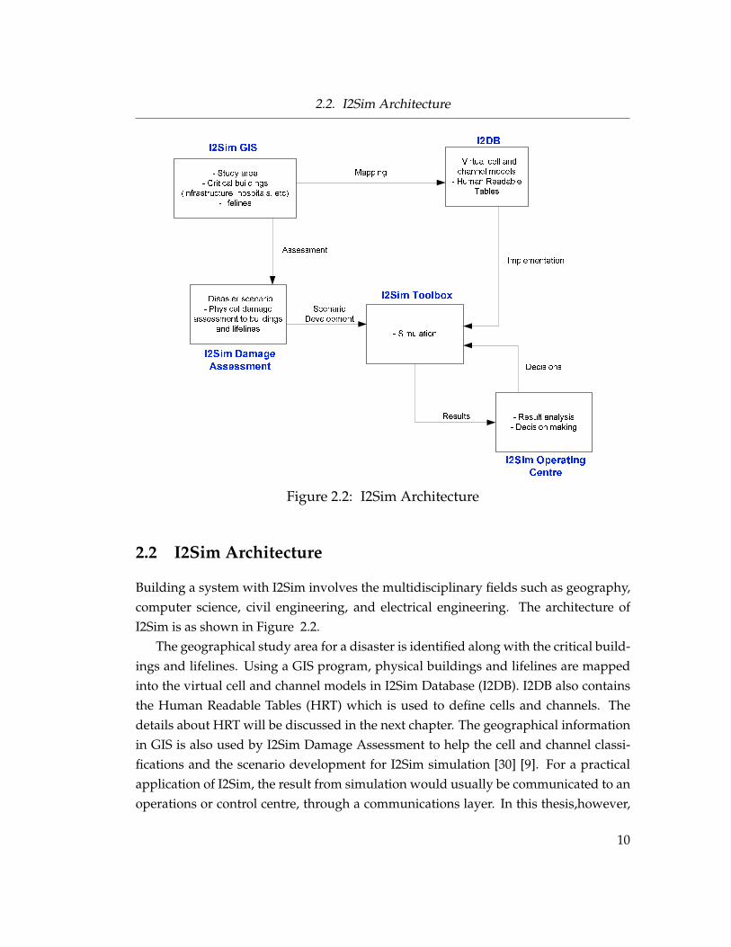
Building a system with I2Sim involves the multidisciplinary fields such as geography,computer science, civil engineering, and electrical engineering. The architecture ofI2Sim is as shown in Figure 2.2.

The geographical study area for a disaster is identified along with the critical build-ings and lifelines. Using a GIS program, physical buildings and lifelines are mappedinto the virtual cell and channel models in I2Sim Database (I2DB). I2DB also containsthe Human Readable Tables (HRT) which is used to define cells and channels. Thedetails about HRT will be discussed in the next chapter. The geographical informationin GIS is also used by I2Sim Damage Assessment to help the cell and channel classi-fications and the scenario development for I2Sim simulation [30] [9]. For a practicalapplication of I2Sim, the result from simulation would usually be communicated to anoperations or control centre, through a communications layer. In this thesis,however,

10

2.3. Discrete Event Simulation

the role of an operations centre is played by the user of the I2Sim toolbox. The ad-justments and decisions by the operations centre or user may be incorporated in otherpossible scenarios for additional simulations.

This thesis focusses on the I2Sim toolbox development and the simulation of studyareas with different scenarios.

2.3 Discrete Event Simulation

The cells and channels in a I2Sim system creats a discrete event-driven system. Thatis, the system condition can be dynamically changed through discrete time or events.As a result, it shows non-deterministic behaviors. In a discrete event-driven system,an event can cause one or more state changes in the components while a combinationof events can also cause one or more state changes in the system. There are three typesof discrete events that affect the I2Sim system in this thesis: the uncontrollable event,the time-dependent event, and the decision-making event.

2.3.1 Uncontrollable Event

The uncontrollable event is an unexpected event that can change the internal variablesof the system such as a cell and channel functionality. In I2Sim, the physical modes forcells and channels can change with an uncontrollable event. The concept of physicalmodes will be discussed in details in the next chapter. The effect of events to the systemwill vary depending on the diaster type itself and the time of the disaster. For example,the power system failure during a winter nighttime would have different effects on thesystem from the one during a summer daytime. The examples of uncontrollable eventscould be an operation failure of the system or a natural disaster such as a tsunami. Inthe thesis, an earthquake and a snow storm have been used as uncontrollable events.

2.3.2 Time-dependent Event

The time-dependent event is a scheduled event that will happen to a cell or a channelafter a period of time when it is in a specific state. Other entities that are connectedto the cell or the channel of the event may be affected but the whole system will notbe affected. However, the effect can be spread out to the later layer of the connectedentity. An example of a time-dependent event trigger can be the run-time of internal

11

2.4. UBC Campus and Vancouver 2010 Winter Olympics

back-up resources such as an oil and water tank. One of the examples from the test casein the thesis is diesel water pump in the water station. When the diesel runs out afterthe run-time of the tank, the water station can no longer supply water to the hospitalswhich may interrupt the treatment of the patients in the hospitals.

2.3.3 Decision-making Event

The decision-making event is triggered by the human decisions after the analysis ofthe current system condition. During disasters, the effective prioritization of the re-pairs, restorations, and the resource allocations can increase the probability of humansurvival significantly, which are examples of decision-making events. In I2Sim, it isdescribed as an operating and physical mode changes in the distributors, the cells, andthe channels, which are the actions taken by the I2Sim operating centre. A decisionmaking action on one cell may affect other cells in the system either positively or neg-atively. For example, both hospitals and roads are damaged due to an earthquake. Ifthe repair crews are sent to the hospitals first, it will increase the number of treatablepatients at the hospital. However, it may delay the transportation of the patients fromthe diaster sites to the hospitals since the bridge is not fixed. As a result, it is verycritical to analyze the situation accurately since decision-making events can affect awide variety of cells and channels in different ways. As mentioned above, I2Sim helpssaving time for decision-making processes to save more human lives.

2.4 UBC Campus and Vancouver 2010 Winter Olympics

I2Sim model is implemented and tested in two area settings: the UBC Campus and theDowntown Vancouver. The brief descriptions of the test cases are written below. Thedetailed test results will be discussed in Chapter 5.

2.4.1 UBC Campus Test Case

The UBC Campus is a well-qualified study space for the first demonstration site be-cause of its unique characteristic as a municipality independent of City of Vancouver.In relatively small area of 2000 acres, it contains all the critical sectors defined by PublicSafety Canada. Also, the UBC Campus displays infrastructure complexity and popula-tion diversity that are difficult to find in other communities. The UBC Campus case has

12


nineteen cell types that classifies the critical infrastructures and buildings on campusas below:

• Hospital

• Fire Hall

• Ambulance Service

• RCMP

• Classroom and Library

• Research Lab and Museum

• Residential

• Parking Lots

• Recreation and Society

• Substation

• Water Station

• Telecom Generator

• Transportation

• Food Services

• Commercial

• Administrator

• Services and Utility

• Power House

• Steam Station.

Out of these nineteen cell types, I have implemented a system using the five criticaltypes of cells with the I2Sim toolbox, which will be introduced in Chapter5.

2.4.2 Vancouver 2010 Winter Olympics

After successfully implementing the reduced UBC Campus test case, I2Sim groupsigned a contract with V2010 Olympics committee to build a case for olympic venues,hospitals and critical infrastructures in Downtown Vancouver. The buildings designedfor the olympic case in this thesis are as below:

• BC Place

• GM Place

• Cathedral Square Substation

• Dal Grauer Substation

• Sperling Substation

13


• Murrin Substation

• Water Station

• Vancouver General Hospital

• St. Paul’s Hospital

Out of the buildings above, I designed BC Place, GM Place, the water station, andtwo hospitals. The buildings above has the same types of cells that has been imple-mented in the UBC Campus case except for BC Place and GM Place. They are classifiedas a Recreation and Society among the 19 cell types of I2Sim, but in Olympics scenario,I defined them to behave as evacuation centres. For this type of cells, the human flowis very critical. The detailed design of BC Place and GM Place cells will be discussedin Chapter 5.

14

Chapter 3

Human Readable Table (HRT)

3.1 Human Readable Table

Human Readable Table (HRT) is a table containing the relationship between inputsand outputs of a system. Unlike the previous HRT by Liu [18], a new concept of econ-omy has been adopted to build the new I2Sim HRTs. For a factory to produce a cer-tain amount of outputs, it requires a combination of different inputs such as materials,labors, and capitals. That is, increasing one of the inputs alone with other inputs fixedwould not increase the output after it reaches a certain limit. In fact, having to manyworkers in the area may even lowers the production rate. In economy, this concept iscalled the law of diminishing marginal returns. I applied this concept in the new HRTsbuilt in this thesis.

This is a significant improvement from the previous HRTs developed by Liu [18].Liu’s tables try to identify all potential combinations of the inputs and the outputs us-ing an interpolation technique. As a result, a size of the table increases exponentiallyas the number of inputs increases, which makes it difficult to build and understandthe tables. However, the new HRT introduced here simplifies the construction processof HRT by identifying only the actual output levels at which a cell can produce. Forexample, a water pumping station with two water pumps would have only three pos-sible output levels depending on the number of functional pumps: 100%, 50%, and0% of the full capacity. The interpolation between these output levels would not benecessary since the station will not be able to operate at those levels. Each row of thenew HRT contains the threshold values of the inputs required to produce those outputlevels. The principal behind the use of threshold values in HRTs is adopted from thelaw of diminishing marginal returns as mentioned above. No matter how much watera water pumping station has, it would not be able to produce above 50% output if evenone of other inputs such as electricity is limited to 50%. As a result, the HRT for waterpumping station above would be simplified into only three rows.

15

3.1. Human Readable Table

Water StationOutput Input

High-pressured Water Electricity Low-pressured Water(m3/hr) (MW) (m3/hr)

103 0.011 10377 0.008 7751 0.005 5126 0.003 260 0 0

Table 3.1: Production Human Readable Table

Another major improvement made in the new Human Readable Table is the phys-ical mode and the resource mode which will be discussed in detail in section 3.2.

3.1.1 Types of Human Readable Tables

Even though the core concept of the Human Readable Tables is the same, the formats ofthe HRTs used for the different components of the I2Sim are quite different. To makeit clear to understand, I categorized them into three major types: production HRTs,channel HRTs, and distribution HRTs.

The production HRT is used for the cell units. It represents the relationship betweenmultiple inputs and a single output of a cell as shown in table: 3.1, which is an exampleof water station production unit. The physical damages to the cell are portrayed by thenumber of physical modes corresponding to different HRTs, which will be explainedin detail in the next section.

The channel HRT represents the lifelines and roads with a traveling time delay, acapacity, and a gain factor (which is less than or equal to one) of the channel as shownin table: 3.2, which is an example of a people channel. The channels in I2Sim have thesame type of an input and a output. Also, unlike cell’s production unit, the output ofa channel does not have discrete threshold levels. Instead, it is calculated using thevariable transport delay function with the amount of the input and the gain specified,which will be discussed in detail in chapter 4. As a result, the input and the output arenot in part of the channel HRT. In the channel HRT, each row of the table is treated asan operating mode since each row is a unique condition caused by different events.

The third type of HRT is the distribution HRT. A distributor in I2Sim takes this HRT

16

3.1. Human Readable Table

People channelGain Delay Capacity

(ratio) (hours) (people)1 0.5 1001 1 1001 2 100

0.9 1.5 800.9 2 80

0.75 1.5 500.5 1.5 50

0.25 2 250 0 0

Table 3.2: Channel Human Readable Table

Water Station DistributorTotal Water Hospital Residence

(m3/hr) (ratio) (ratio)103 0.5 0.577 0.34 0.6651 0.01 0.990 0 0

Table 3.3: Distributor Human Readable Table

to find the ratio of how the output from a cell or a channel is distributed to differentplaces. Opposite to the production HRT, the distribution HRT has a single input withmultiple outputs. While the production HRT contains actual physical units of inputsand outputs, only the input column of the distribution HRT has a physical unit. Theoutput columns of the distribution HRT is in ratios rather than a physical units, andthe sum of output ratios for each row must be equal to one. In this way, there willnot be any calculation loss from distributors. In addition, the distribution HRT has theoperating modes instead of the physical modes since the switches to different HRTs ismade by the distribution policy changes instead of a physical damage. An example ofthe distribution HRT is shown in table: 3.3, which is an example of a water distributionfrom a water station.

17

3.2. Physical Mode (PM) and Resource Mode (RM)

3.2 Physical Mode (PM) and Resource Mode (RM)

In the new I2Sim, the operating state of a cell and a channel is defined by two means: aphysical mode (PM) and a resource mode (RM). The physical mode reflects the physi-cal state of a cell while the resource mode represents the actual operating output leveldetermined by the available inputs to the cell. These two modes combined togetherproduce a final operating state of a cell.

In a regular operating condition, a cell most likely has 100% physical functionality.That is, the buildings is not suffering any structural damages or equipment failures,so they can work in their full capacity as long as the input resources are available.However, when an event like an earthquake occurs, the physical mode of the cell maychange. For example, if the half of the transformers in a substation is broken due toshaking from an earthquake, the physical functionality of the substation will be only50% of its full functionality. In this case, the cell that represents the substation goes intothe physical mode with a different HRT.

The maximum RM level is limited by the current PM of the cell. That is, whenthe physical functionality of a cell is only 50%, the highest output level the cell canproduce, the maximum RM level, will be only 50% no matter how much resourcesare available from the outside. For example, even though a hospital has enough staffsand resources to perform four surgeries, if only two surgical rooms are available, themaximum surgeries that can be done is only two.

Each PM is assigned to a Human Readable Table (HRT), so a cell has multiple HRTseqault to the number of the PMs it has. In the HRT, each row becomes one of the RMsfor that specific PM. The detail of how this is done is shown in figure 3.1.

In figure 3.1, it shows an example of a hospital cell in percentiles for easier un-derstanding of the PM and RM concept. There are four PMs according to physicaloperability of the hospital, and each PM is pointed to a table consists of RMs. Forinstance, PM02 in the figure has the HRT with three RMs, and the maximum patientlevel is 66% since PM02 represents the physical operability of 66%.

Prior to the simulation, a specific PM is predicted by the damage assessment data.The damage assessment gives a data such that after an earthquake with intensity VIII,the hospital will be 66% functional.

18

3.3. Color Scheme�� !!� !!� !!� !!� !!�� !!� �� " �� #��$��%��

��&��&�!!��&��"�&��

#��#��#��Figure 3.1: Physical Mode and Resource Mode

3.3 Color Scheme

The physical mode (PM) and the resource mode (RM) mentioned above are repre-sented inside the I2Sim Cell and Channel blocks through a color scheme for the visual-ization purpose. The color scheme used contains five color levels shown in figure 3.2,which is used by Color-coded Threat Level System of U.S. Department of HomelandSecurity (DHS).

Each color is assigned to a range of the nominal output levels or the unit function-ality as listed below.

• Green: 85-100%

• Blue: 70-84%

• Yellow: 45-69%

• Orange: 26-44%

• Red: 0-25%

19

3.3. Color Scheme

Figure 3.2: Color Scheme

Figure 3.3: PM RM Color Representation in a Block

A unit in a normal condition would be in green and precede down to red as the unitis damaged and becomes no longer functional. In a I2Sim block, I programmed themask of the block with a small rectangle on the top left corner showing the PM withits color level, and the rest of the block with the color representing the output colorlevel of RM as shown in figure 3.3. To maximize the speed of the Simulink/MATLABsimulation, I designed the colors of the blocks to be checked for an update only wherethere is a change in the output level of the block instead of every loop. The figure 3.3is an example of cells in a green physical mode with different colored resource modes.The color representations of PM and RM help the users to capture the system conditionand respond faster during the simulations or the disasters.

20

3.4. Construction of a Model

3.4 Construction of a Model

This section describes the construction process that I took to build the I2Sim virtualmodels from the physical area of interest. The process consists of researching and in-terviewing for information gathering, filling the Human Readable Tables, and buildinga virtual model using the I2Sim toolbox.

3.4.1 Information Gathering

Prior to building a HRT, it is very important to identify the information that is neededto build the HRT. This may be one of the most difficult steps in the construction of themodel since it involves the interviews with the infrastructure stakeholders about theconfidential information on the operation of the system. As a result, I found that itis very essential to determine the minimum data required by every unit of the virtualmodel to build the HRTs. Through the experience I had from the interviews with UBCPower House personnel, VANOC, and Vancouver health care, I observed at least thefollowing data has to be acquired before building any virtual systems:

• The type and the amount of the output produced by the unit

• The types and the amount of the inputs used to produce the output

• The number of the different lifelines and the roads that carry the inputs and theoutputs of the building

• The capacity and the traveling time of the channels

• The basic internal configurations that can help define the different physical modesat which a unit can operate

• The internal reserves or the back-up sources and their capacity

• The resources required to run the internal back-up sources

Depending on the nature of the unit, each unit requires additional information tocreate an accurate model. Information gathering was the most time-consuming anddifficult part of the model construction. Another technique that I learned to receive thebetter cooperations from the infrastructure stakeholders is presenting how I2Sim canbenefit them in return of their help before the actual interview. Once all the required

21


information is collected, HRTs has to be built for the various components of the cellwhich will be discussed in the next section.

3.4.2 Building Human Readable Table

The list of information gathered was used to create the production, distribution andchannel HRTs.

First, the different physical modes of the cell production HRTs were determinedusing the internal configurations of the cell. For example, when a substation has twotransformers, three physical modes can be used: both transformers functional, onetransformer functional, and no transformers functional. For each PM, the HRT is builtusing the types and the amount of the inputs and the output. With the full capacitybeing the first row, the discrete threshold levels which become the rest of the rows ofHRT can be determined according to the internal configurations as well.

The output produced from the cells may be distributed to the other cells throughthe different channels. The distribution HRT lists the ratio at which the output is dis-tributed. The ratio could be either given by the infrastructure stakeholders or calcu-lated by the number of the channels that carry the output and the capacity of the chan-nels. The distribution ratio of the resources in case of emergency must be differentfrom when in the normal condition. For example, in a normal condition, a substationis able to distribute the electricity as needed by all customers such as hospitals andresidences. However, in emergency, when the electricity is scarce, the substation maygo into an operating mode where the hospitals become the first priority, which wouldchange the ratio of distribution.

The third step would be building the HRTs for channels that are connected to thecell. The channel HRT is consisted of the different combinations of the traveling timedelay, the capacity, and the gain of the channel, which is less than or equal to one.The time delay and the gain in the normal condition become the first row of the HRT.The time delay and the gain may vary depending on what flows in the channel. Forexample, a traffic channel with cars may have a large time delay such as one hour withno loss while a electricity channel has no time delay with small loss in the transmissionlines. The capacity of the channel may change due to the damages to the physicalchannel. One of the factors that helped me building more realistic channel HRTs werethe damage assessment from Juarez [14]. Juarez calculated possible immediate andprogressive states at which channels can fall into during the earthquakes with different

22


intensities.

3.4.3 Designing Cells using I2Sim Toolbox

Figure 3.4: Generic Cell Design

After the Human Readable Tables for each component of all the cells in a desiredsystem are built, the connectivity of components has to be designed. Each cell hasthe following generic components: aggregators, internal reserves, a production unit,and distributors. The same type of inputs entering a cell through different channelsor internal reserves should be added up using an aggregator before the productionunit. When the output of the production unit is distributed to more than one places,a distributor should be added to divide the output. One cell should be connected toother cells using the channels. An example of a generic one-cell design is shown infigure 3.4.

After the design is done, the system can be built using the components in the I2SimToolbox. The functionalities and the interfaces of the I2Sim Toolbox components inSimulink will be discussed in detail in the next chapter.

23

Chapter 4

I2Sim Toolbox

Figure 4.1: I2Sim Toolbox in Simulink

24

4.1. Development of Customized Blocks

I2Sim Toolbox in Simulink is a library containing the customized blocks of the com-ponents which are created based on the I2Sim concept introduced earlier in this the-sis. Once the library is installed on a computer, the toolbox will show up from theSimulink library browser along with other toolboxes that originally come with MAT-LAB/Simulink software as shown in figure 4.1. To simplify the installation processof the toolbox, I wrote a MATALB script that can be run and automatically installs orupdates the toolbox.

4.1 Development of Customized Blocks

The component blocks used in I2Sim are created through a subsystem containing acombination of pre-existing Simulink blocks and customized system-function(s-function)blocks. The most challenging part of the development process was programming thes-function blocks in the m-file. To create a s-function block, all characteristics such asquantities, types, and dimensions of inputs, outputs, and parameters, the initial stateof the block, and the outlook of the block have to be all programmed in a single m-filealong with its functional algorithm as shown in Appendix A. As a result, the s-functionblocks allow the higher flexibility compared to the other customized blocks such as anembedded MATLAB function block. Another reason s-function blocks were chosenis due to its compatibility with the toolbox libraries. Other customized blocks cannothave more than one instances in one system once it is added to the toolbox library.Since Matlab/Simulink is not commonly used for the customized blocks, I had a diffi-cult time realizing these limitations of different customized blocks. The details abouthow each customized components are built will be discussed in the next section.

4.2 I2Sim Components

There are seven functional components in I2Sim Toolbox as followings: an aggregator,a HRT, a storage, a distributor, a channel, a source, and a sink. Their functionality andimplementation using MATLAB/Simulink will be discussed in detail in this section.In addition to these components, the toolbox has a I2Sim control panel, a I2Sim visu-alization panel, and a probe for visualization purposes which were developed by mycolleague, Tomim. As a result, they will not be discussed in this thesis.

25

4.2. I2Sim Components

4.2.1 Aggregator

Figure 4.2: Aggregator Block

The functionality of the aggregator block is producing an output which is the sum-mation of all inputs into the block. It is used when a same type of resources reaches acell through multiple routes. For example, when the electricity to a hospital can comefrom an external substation, an internal back-up generator or both, the aggregator addsthe electricity from both sources and inputs it into the HRT block as one input. To beable to change the number of input ports as a parameter of the aggregator, I built theaggregator using a s-function block instead of a pre-existing summation block from theSimulink. The MATLAB code used for the aggregator can be found in Appendix A.The figure 4.2 is the aggregator block on the left and the user interface on the right. Theaggregator block needs the number of inputs specified on the user interface beforehandto change the number of input ports accordingly for the block.

4.2.2 Human Readable Table (HRT)

The Human Readable Table block represents the core production unit for the cell. Ittakes the values from the input ports and searches for the matching entries in the pro-duction HRT; and it produces the corresponding threshold output value found. As aresult, it requires a pre-defined production HRT to operate.

I designed the HRT block with three parameters to be specified in the user inter-face as shown in figure 4.3: the name of a HRT, a physical mode (PM) setting, and aphysical mode. The HRT name is the name of the production HRT variable, which has

26


Figure 4.3: Human Readable Table Block

to be created in MATLAB. I chose the struct as the standard variable format for theHRTs in I2Sim, since it has the flexibility of storing different types of variables underone struct. For example, the HRT structs used for the test cases in this thesis containthe input/output names, units, and maximums along with description for the HRT.This makes the Human Readable Tables more readable. The physical mode setting isused to set whether the PM is determined internally through the interface parameteror externally as an extra input to the block. Only when PM is set internal, the thirdparameter, the physical mode, is used to set which physical mode the cell is under. Inaddition, the HRT being used by the block can be viewed by clicking on the checkboxbeside View-HRT, which was implemented by my colleague, Tomim. By Dr. Marti’srequest, I added the feature of a checkbox for Pause-when-there-is-a-change. It enablesthe simulation to pause whenever there is a change in the state of the production HRTsuch as the output levels and the PMs, so the users can monitor the situation in depth.

The HRT block automatically creates the number of the input ports according to theproduction HRT entered in the user interface. In addition to these ports, the port forthe physical mode is created below the input ports when the PM setting is external. As

27


mentioned in chapter 3, there are two colors shown in the block: a physical mode colorfor the small square and an actual output level color for rest of the block. Also, insidethe small square, the current physical mode number is shown as in figure 4.3. In thisparticular example in figure 4.3, HRT block is in the physical mode yellow, which is 45-69% functional, but the actual output level is red, which is 0-25% of its rated capacity,due to lack of resources. The rated output capacity of the cell at its normal condition isalso shown on the right top corner of the block. One of the features of the HRT blockthat helps users to assess the situation faster is the NEED display on the right bottomcorner. It shows the input resource that is needed to increase the output level. Infigure 4.3, the input resource needed is electricity. All these display and color featuresalong with the input and PM ports are controlled by a single s-function file that alsocontains the functional codes of the HRT block. The reason I chose this method is tokeep the synchronization of all the changes on the block. The detailed codes of theHRT block can be found in Appendix B.

The search algorithm implemented in the s-function code in HRT block is as above.It searches for the maximum possible output level that can be produced with the giveninput amounts. This algorithm works for only the tables with a descending order ofentries in the rows.

Data: input vector xResult: output yr = 1 % start at the first row;for ix = 1,...,nx do

% iterate over each input variable;for i = r,...,nrow do

% iterate over each row;if HRT(r, ix+1) ≤ x(ix) then

break for-loop;% go to next input variable;

elser = r + 1;% go to next row;

endendix = ix + 1;

endy = HRT(r, 1);

Algorithm 4.1: Human Readable Table Search Algorithm

28


4.2.3 Distributor

Substation60MW AvailableHospital60MW needed100L/hour needed

Water Station40MW needed60MW0MW Electricity ChannelWater Channel0L/hour 0% of patients healed

(a) Bad Distribution of Resource

Substation60MW AvailableHospital60MW needed100L/hour needed

Water Station40MW needed40MW

20MW Electricity ChannelWater Channel50L/hour 70% of patients treated(b) Good Distribution of Resource

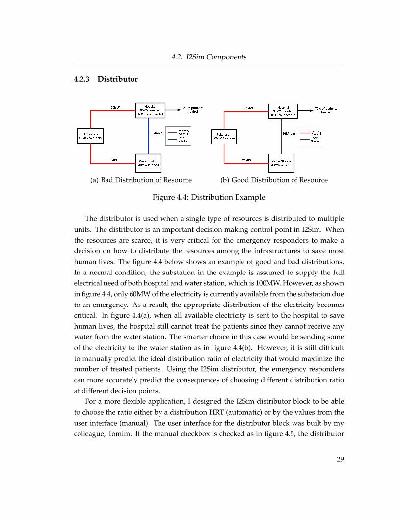
Figure 4.4: Distribution Example

The distributor is used when a single type of resources is distributed to multipleunits. The distributor is an important decision making control point in I2Sim. Whenthe resources are scarce, it is very critical for the emergency responders to make adecision on how to distribute the resources among the infrastructures to save mosthuman lives. The figure 4.4 below shows an example of good and bad distributions.In a normal condition, the substation in the example is assumed to supply the fullelectrical need of both hospital and water station, which is 100MW. However, as shownin figure 4.4, only 60MW of the electricity is currently available from the substation dueto an emergency. As a result, the appropriate distribution of the electricity becomescritical. In figure 4.4(a), when all available electricity is sent to the hospital to savehuman lives, the hospital still cannot treat the patients since they cannot receive anywater from the water station. The smarter choice in this case would be sending someof the electricity to the water station as in figure 4.4(b). However, it is still difficultto manually predict the ideal distribution ratio of electricity that would maximize thenumber of treated patients. Using the I2Sim distributor, the emergency responderscan more accurately predict the consequences of choosing different distribution ratioat different decision points.

For a more flexible application, I designed the I2Sim distributor block to be ableto choose the ratio either by a distribution HRT (automatic) or by the values from theuser interface (manual). The user interface for the distributor block was built by mycolleague, Tomim. If the manual checkbox is checked as in figure 4.5, the distributor

29


Figure 4.5: Distributor Block

divides the input according to the number of outputs and the ratio entered manuallyby the user. The ratio can be entered using the scroll bar or the numbers. The sumof the ratio entered has to add up to 100%. The compute button calculates the ratiofor the selected output by subtracting the rest of the entered ratio from 100%. Whenthe manual checkbox is unchecked, the distributor block uses a pre-defined HumanReadable Table to find the ratio. In this case, the number of output ports of the blockwill automatically change according to the outputs from the HRT.

30


The distributor HRT may have multiple operating modes (OM) as discussed inchapter 3. The OM for the distributor can be determined either internally or externallyas in the PM for the HRT block in the previous section. When the OM is externally set,the distributor block has an extra OM port in addition to an input port and a numberof output ports.

I built the distributor block with a customized s-function code block. The searchalgorithm implemented in the s-function code is as below. It searches for the closestinput level to the given input amount and read the corresponding ratio to be used. Thegiven input amount is multiplied by the ratio found and outputted into each outputport. The detailed codes for the distributor can be found in Appendix C.

Data: input xResult: output vector y% initialization;deltax = | HRT(1,1) - x |;tempr = 1;for r = 2,...,nrow do

% iterate over each row;if | HRT(r,1) - x | < deltax then

% save the location of the closest input;tempr = r; deltax=|HRT(r,1)-x|;

else% do nothing;

endr = r + 1;

endfor c = 2,...,ncol do

% iterate over each output ratio;y(c-1) = HRT(tempr,c) * x;i = i + 1;

end

Algorithm 4.2: Distributor Search Algorithm

4.2.4 Channel

The I2Sim channel is an entity where a token flows from one unit to another. Unlike acell, the channel does not change the nature of the input token; however, there may be

31


(a) External View

(b) Inside the Mask

(c) Interface

Figure 4.6: Channel Block

32


losses or a time delay between the input token and the output token as mentioned inchapter 2.

In the I2Sim channel, the time delay and the losses are found from a pre-built chan-nel HRT, where each row is a pre-defined physical mode. The channel block contains acombination of a s-function block and the pre-existing Simulink blocks. The time delayin the channel is apply to the input token through the variable transport delay Simulinkblock, and the output from the block is multiplied by the loss factor before exiting thechannel as shown in figure 4.6(b). I designed the physical mode to choose the lossfactor and the time delay produced from the s-function block. The detailed s-functioncodes can be found in Appendix D. The channel block is masked as a block coloredaccording to the current loss factor. It also shows the physical mode and the tokentype as in figure 4.6(a). In the figure, it shows a steam pipe that is severely damaged.Similar to the other blocks discussed earlier in the chapter, the channel block takes thename of the channel HRT as a parameter in the user interface, and the physical modecan be either an external input or an internal parameter as shown in figure 4.6(c).

The variable transportation delay uses the following concept to accurately calculatethe total time delay throughout the channel when the time delay on the channel varieswith time [31].

With fixed length of channel, L, the propagation speed of the token at time t wouldbe as below:

v(t) =L

τ(t)(4.1)

When equation 4.1 is applied to a infinitesimal fragment of a length, the equationbecomes as below:

v(t) =∆L

∆t⇒ ∆L = v(t)×∆t (4.2)

When the integral of equation 4.2 is taken from time t to td(t), it becomes:

∫ L

0dl =

∫ t

t−td(t)v(t)dt ⇒ L =

∫ t

t−td(t)

L

τ(t)dt (4.3)

When equation 4.3 is simplified, it becomes as below, which is used in the Simulinkblock to solve for the total time delay throughout the channel by calculating td(t) at

33


every time step.

1 =∫ t

t−td(t)

1τ(t)

dt (4.4)

4.2.5 Storage

In I2Sim, the storage is used to represent a point at which a token is accumulated andflows out at a desired rate. The most straightforward use of storage is as an internalback-up source storage such as an oil and water tank. However, that is not the onlyway to use the storage block. I used the storage block as a waiting area for people out-side of each cell during the disaster in the test cases in chapter 6. When it is combinedwith a channel, it can also be a part of a cell with people as an input and an outputsuch as hospitals and stadiums. People are contained in the storages waiting for thetreatments or watching a show and released after a certain time delay which can bedepicted by a channel with possibly zero loss factor. Also, the rate at which peopleare released can be determined by a HRT block with the physical modes determinedby the number of professional personnel and resources to facilitate the function of thecells. This concept is implemented in the Vancouver 2010 Winter Olympics cases whichwould be discussed in more details in chapter 6.

The I2Sim storage block is consist of pre-existing Simulink blocks without any s-function block. The storage has a single input and a single output. In addition, thecommand for the output is added as an extra input to be able to vary the flow ratesover time as shown in figure 4.7(a). Also, the current level of the storage is producedas an additional output. The maximum and minimum command signals are specifiedas the parameters of the block along with the maximum, minimum and initial levelsof the storage on the user interface as shown in figure 4.7(c). A storage unit can storethe input resource up to the maximum capacity and gives out the output resource ata desired flow rate until the minimum level of the tank is reached. The flow rate mayeither be given by the infrastructure stakeholders or be calculated from the time thatthe storage can supply the cell and the capacity of the storage. The concept behind thestorage was designed by my colleague, Tomim, and it will be discussed below.

As shown in figure 4.7(b), the storage outputs the resource according to the com-mand signal as long as the level of the storage is above the minimum level limit. Also,the command signal is checked for its boundary limit set by the parameters in the in-

34


(a) External View

(b) Inside the Mask

(c) Interface

Figure 4.7: Storage Block 35


terface. When the minimum level limit of storage is reached, the storage outputs zeroamount of resources regardless of the command signal. The current level of storageis determined by the integration between the current input and output along with theinitial level as described in the equation 4.5 [31].

level =

lmax level ≥ lmax

level0 +∫ t0 (xin − xcmd)dt lmin < level < lmax

lmin level ≤ lmin

(4.5)

4.2.6 Source

A source represents the resources coming from the outside into the defined system. Idesigned the source block to have an unlimited capacity of resources, but it can onlyoutput resources at a certain rate defined by the owner of the physical source. Thesize of source can vary from a small local water station to a large water reservoir for adistrict. Every resource that is used by the cells in a system has to either come from asource or be produced within the system.

In I2Sim, the source block is a simple block with no input and one output system asshown in figure 4.8. The output of the source is determined by the parameter, sourcevalue, entered in the user interface.

Figure 4.8: Source Block

36


4.2.7 Sink

Figure 4.9: Sink Block

A sink represents a point at which the resources exit the defined system. The re-sources entering the sink are no longer used by any of the components in the system.They may be passed onto another defined system as a source. In addition, the valueof the resources may be plotted or stored before entering the sink since some of themmay be the total output goal of the system. For example, for the purpose of I2Simproject, the goal of the project is maximizing the human survival, which is the numberof people treated from the hospital. However, people exiting from the hospital is notused by the system anymore, so it is sent to the sink. Since monitoring and improvingthe number of people survived is the goal of the system operation, the signal may beplotted before it enters the sink. Once resources enter the sink, they are terminatedsince it has no preservation value to the system.

In I2Sim, I designed the source block to be a block with only an input port and nooutput or parameters as in figure 4.9.

37

Chapter 5

Simulations and Results

As an implementation of the I2Sim toolbox discussed in chapter 4, I re-created one ofthe scenario cases which were developed on the University of British Columbia (UBC)campus by Liu [18] and compared the results with the previous I2Sim model. Also, atest case has been developed for the Vancouver 2010 Winter Olympics as a part of theV2010 project led by Dr. Marti at UBC.

5.1 UBC Campus Case

In Liu’s thesis, she simulated a reduced test case for the UBC campus with the fiveinfrastructures: the substation, the powerhouse, the water station, the steam station,and the hospitals. To compare the performance of the new I2Sim model and toolboxwith Liu’s model and simulator, I re-built the same test case scenario with one of Liu’sscenarios. In addition to the original case, I also developed another case with the samescenario but with the people’s flows and the distribution decision making points. Thisfeatures allowed the model to produce more realistic results.

The simulated scenario depicts the power outage happened during the snowstormat the UBC on November 27, 2006. During the snowstorm, the heavy snow caused thetree branches to fall down on two of the major transmission lines coming into the UBCcampus [3]. As a result, the power was out for all parts of the UBC campus includingthe student residences for about twelve hours. Liu also added an additional event ofthe water pipe brokage to the real situation to demonstrate a multiple disaster situation[18].

38

5.1.U

BCC

ampus

Case

UBC Water StationElectricity SourceBC Hydro Substation Electricity Channel SubstationCell

Power HouseCellElectricity Channel Water StationCell Steam StationCellWater SourceGVRD WaterChannel

UBC SubstationUBC Power House

Back-up Oil Tank Back-up GeneratorGas SourceTerasen Gas GasChannel UBC Steam Station

Purdy Hospital Cell(Long-term Patients)Koerner Hospital Cell(Short-term Patients)

WaterChannelSteamChannel

Electricity ChannelElectricity Channel Back-up Water Tank Back-up Water TankBack-up Generator

Back-up GeneratorGasChannel

Medicine&PersonnelSourceTreated Short-term PatientsSinkTreated Long-term PatientsSink

UBC HospitalElectricityWaterGasSteam

Returned Steam Source SteamChannelFigure 5.1: Design of Reduced UBC Campus Test Case

39

5.1.U

BCC

ampus

Case

Figure 5.2: Simulation of Reduced UBC Campus Test Case

40

5.1. UBC Campus Case

Liu’s model has been modified according to the new concept introduced in thisthesis as shown in figure 5.1. I divided the hospital cell into two different cells for thelong term and short term patients since the new I2Sim cell is one output only unit. Inaddition, these two cells are separated into two hospital buildings in real. The modelhas been simplified significantly since it no longer requires the internal configurationof the cells, but it still produces accurate results using the physical modes and thethreshold levels. It makes the process of developing the case and collecting the infor-mation from the infrastructure stakeholders much easier. Previously, the user had tobecome an expert on the Simulink program since the test case was hard-coded. As aresult, it is difficult to modify the case to add new cells without fully understandingthe I2Sim model. However, with the new I2Sim toolbox, the user needs only the basicknowledge on the toolbox and can still create an accurate case through the publiclyavailable information on the infrastructures. A comparison between the models andthe HRTs of Liu’s substation and the new substation is shown in figure 5.3. The modelpresented in this thesis has significantly fewer components as compared to the earliermodel proposed by Liu. For example, the new HRT for a substation comprises threetables, with less than six rows per table.

5.1.1 Scenario 2 of Liu’s Thesis

The scenario contains the sequential events listed below:

• Initial State (t < 0): All cells and channels are functional.

• t = 20 min:

– The electrical channel from the outside to the UBC substation goes to 0%functional due to the fallen tree branches caused by snow.

– The back-up generator for the steam station starts to warm up but is notstarted yet.

– The diesel back-up pump in the water station starts right away.

• t = 40 min:

– The water pipe from the water station to the hospitals breaks, so the func-tionality of the water channel goes to 0%.

– The water from the hospitals’ back-up water tank starts being used.

41


(a) Liu’s Substation Model [18] (b) Liu’s Substation HRT [18]

(c) New Substation Model

PM01 PM02 PM03output input output input output inputelectricity electricity electricity electricity electricity electricityMW MW MW MW MW MW22800 22800 11400 11400 0 018240 18240 9120 912013680 13680 6840 68409120 9120 4560 45604560 4560 2280 22800 0 0 0(d) New Substation HRT

Figure 5.3: Substation Comparison

• t = 50 min: The back-up generator in the steam station starts providing power.

• t = 14 hr: The transmission lines are restored, and the functionality of the electri-cal channel from the source to the substation becomes 100%.

• t = 24 hr: The water channel is fully restored.

Twenty minutes after the initial state, the transmission lines to the UBC substationis down. As a result, the electrical channel in the model goes to functionality of 0%.Even though the substation is in the physical mode 01 with no damage to the building,it cannot deliver any power to the other cells as in figure 5.4, since there is no inputto the system. In the previous model, it was difficult to identify whether failure toproduce the output was due to a physical damage to the building or lack of input

42


resources. As mentioned in chapter 3 section chapter 3, the new I2Sim toolbox showsthe levels of the physical mode and the resource mode in colors within the cell duringthe simulation. For example, in the left top corner of figure 5.2, the substation has agreen PM color and a red RM color to present that the output level for the substationis 0% due to lack of resources.

(a) Electricity from Source to Substation

(b) Electricity from Substation to PowerHouse

(c) Electricity from Substation to Hospitals

Figure 5.4: Substation Cell Results

The powerhouse behaves similarly to the substation not being able to provide anypower to the water station and the steam station. However, both water station andsteam station quickly goes back to its normal state as soon as their back-up dieselpump and generator come up. As a result, the water supply to the hospitals is notdisrupted since the diesel water pump was hot on standby. However, the steam supplyto the hospitals is stopped for 30 minutes due to the back-up generator start-up timeas shown in figure 5.5.

43


(a) Electricity from PowerHouse to Water Station and Steam Station

(b) Steam from Steam Station to UBC Campus

(c) Water from Water Station to UBC Campus

Figure 5.5: Power House, Steam Station, Water Station Cell Results

Even though the water station is producing water at the full capacity, no water isreceived by the hospitals starting from t = 40 minute to t = 24 hour. It is because the wa-ter channel from the water station to hospitals is broken. As a result, the amount of thewater sent out from the water station to the hospitals does not affect the functionalityof the hospitals anymore. In the next scenario, a re-distribution of the water from thewater station will be discussed in details. The hospitals start using the internal back-upwater tanks, so there is no interruption of services even without the water. In fact, thehospitals can survive for about three days without an external water or power supply.However, when the steam supply is interrupted for 30 minutes from t = 20minute, thetreatments for the long-term patients are affected significantly since the Purdy hospitalcannot self-supply steam as shown in figure 5.6.

At t = 14 hour as the transmission lines are restored, the oil tank level for the dieselpump in the water station stops decreasing as shown in figure 5.7.

44


Figure 5.6: Hospital Cell Results

Figure 5.7: Water Station Back-up Oil Tank Level

From the simulation, it is found that the redundancy in the resource availabilitysuch as the back-up sources ensures the important infrastructures and hospitals on theUBC campus to function at the full capacity for more than twenty four hours withoutan external source. The results from the simulation closely follow the results fromLiu’s scenario 2 [18]. It shows that the new model can produce the same results as theprevious one with a significantly easier design and process.

In the next scenario, the improvements in functionality of the new I2Sim modeland the toolbox will be captured through the effects of the people’s flow and the dis-tribution control points to the simulation.

45


5.1.2 Modified Version of the Scenario 2 of Liu’s Thesis

This section describes a modified version of previous simulation above.

5.1.2.1 Model and Scenario Change

In this modified version of the scenario above, the back up diesel pump in the waterstation can supply only 50% of its total capacity. As a result, the steam station and thehospitals cannot function fully due to lack of water. I moved the water pipe breakagefrom t = 40 minutes to t = 4 hours to see the effect of the breakage on the system moreclearly. When the water pipe to the hospitals breaks, the water sent to the hospitals islost in the channel. Thirty minutes after the pipe breakage, I decided to send all thewater produced to the steam station instead of the hospitals to see the effect of a newdistribution ratio. The distributor at the water station is switched to the third operatingmode which to sending all the water to the steam station, so steam station producessteam at the full capacity. At this point, the hospitals starts using their back up watertanks. As seen in figure 5.10(a), when the water is directed correctly, it can increasethe number of treated patients at the hospitals compared to the result from the originalscenario. This increase demonstrates the importance of the decision making points.

On top of the scenario modification, I also modified the structure of the hospitalmodel to represent the output as the human flow instead of the total capacity of thehospital. The prediction of the human flow plays an important role in determining theappropriate resource allocation. For example, in power system, a transmission line toan area has a maximum power flow capacity. However, the actual power flow on theline is equivalent to the instantaneous demand not the maximum capacity. It would bewaste to send all the generated power to the area at its maximum capacity when it isnot actually needed. The rest of generated power can be directed to another area thatneeds power. In British Columbia, BC Hydro makes a large profit by redirecting andselling their unconsumed power to USA.

The hospitals are usually the first priority for the resource allocation. However,when there are less than the full capacity of patients in the hospital, it would not makesense to send the amount of the resources that meets its full capacity. By implementingthe patient flow into the hospital model, the instantaneous amount of the resourcesrequired by the hospitals can be determined. In the new model I designed, the out-puts of the hospital Human Readable Tables are modified to the number of treatable

46


Figure 5.8: Human Flow Model for Purdy Hospital

patients per hour from the total capacity of the hospitals. As shown in figure 5.8, theoutput from the HRT unit is fed into a I2Sim storage unit as a command input. Thenumber of patients entering the hospital is put into the storage unit as an input. TheI2Sim storage unit accumulates these two numbers and calculates the actual numberof patients treated per hour according to the following equations:

Total patients = total paitents0 + entering patients− treated patients (5.1)

Treated patients =

treatable patients total patients ≥ treatable patients

total patients total patients < treatable patients

(5.2)

The channel after the storage output as shown in figure 5.8 is added to representthe average time taken to treat the patients.

5.1.2.2 Scenario and Results

The modified version of the original scenario contains the sequential events as below:

47


• Initial State (t < 0): All cells and channels are 100% functional. The hospital bedsare half full with patients. Twenty five short-term patients comes into Koernerhospital every hour while fifteen long-term patients are admitted to Purdy hos-pital every hour.

• t = 20 min:

– The electrical channel to the UBC substation from the outside goes to 0%functional due to the fallen tree branches caused by snow.

– The back-up generator for the steam station starts to warm up but is notstarted yet.

– The diesel back-up pump in the water station starts right away supplyingonly 50% of the full capacity.

• t = 50 min: The back-up generator in the steam station starts providing power.

• t = 4 hr:

– The water pipe from the water station to the hospitals breaks, so the func-tionality of the water channel goes to 0%.

– The water from the hospitals’ back-up water tank starts being consumed.

• t = 4.5 hr: The operating mode of the distributor in the water station is changed.All water is sent to the steam station, and none is sent to the hospitals.

• t = 14 hr: The transmission lines are restored, and the functionality of the electri-cal channel from the source to the substation becomes 100%.

• t = 24 hr: The water channel is restored fully.

As mentioned above, when the water station switches to its diesel back-up pumpfrom the electrical pump at t = 20 minute, the water station can only supply 50% of therequired water on the campus. As a result, the steam from steam station decreases toabout 50% as shown in figure 5.9, and the treated patients from the hospitals dropsdown to less than 50% of its full capacity due to lack of water and steam as shown infigure 5.10(a). At this point, no decision-making action is taken to the system.

As soon as the water pipe breaks, hospitals turn on their back-up water tank whichwould satisfy its full needs of water. However, it still cannot operate at its full capacity

48


(a) Water from Water Station to Hospitals

(b) Water from Water Station to Steam Station

(c) Steam from Steam Station to Hospitals

Figure 5.9: Water Station and Steam Station Cell Outputs

due to lack of steam. Thirty minutes after the water pipe to the hospitals breaks, thewater station operator decided to send all its output to the steam station instead ofdistributing to both the steam station and the hospitals as shown in figure 5.9. Asa result, the steam station can now produce steam at 100%. The hospitals can starttreating patients at their full capacity again since they have 100% water and steam asshown in figure 5.10(a).

The figure 5.10(b) shows the total number patients in the hospitals. Until t = 4.5hour, the total number of the patients increases fast since the hospitals cannot treatthe patients at their full capacity. At t = 4.5 hour, the total number of the patients atKoerner starts to decrease while the one at Purdy still increases. It is because twentyfive patients enter Purdy every hour while the maximum treatable patients per hourat Purdy is only twenty. As a result, all the beds in Purdy fills up after t = 17 hour. Inprevious case, this problem was not shown through the simulation because it looked

49


(a) Hospital Patient per Hour

(b) Hospital Total Number of Patients

Figure 5.10: Hospital Cell Outputs

at only the total number of beds that can be filled at the moment instead of the actualfilled number of the beds. Knowing the hospitals cannot accept any more patientsdue to lack of beds even at the full capacity, the simulation can help the emergencyresponders to prepare for re-direction of the patients in advance.

Through this case, the importance of resource distribution and human flow in thehospitals were explained. In the next section, I will present the case of V2010 WinterOlympics with a new type of cell as well as an implementation of the crowd behaviorduring the evacuation of a enclosed space. In addition, the physical damage to thecells will be implemented whereas in UBC Campus case, no physical damage to thecells was occurred.

50

5.1.U

BCC

ampus

Case

Figure 5.11: Vancouver 2010 Winter Olympics Study Area

51

5.1.U

BCC

ampus

Case

Figure 5.12: Vancouver 2010 Winter Olympics Simulink Model

52

5.2. Vancouver 2010 Winter Olympics Case

5.2 Vancouver 2010 Winter Olympics Case

To demonstrate the feasibility of the new I2Sim model outside of the UBC Campus, acase on Vancouver 2010 Winter Olympics Venues and the critical buildings has beenset up by the I2Sim group. In addition, the physical mode and the resource mode fea-tures are emphasized in the Olympics case. The case includes BC Place, GM Place,Vancouver General Hospital (VGH), St. Paul’s Hospital (SPH), a Water Station supply-ing hospitals, and four substation, Cathedral Square (CSQ), Dal Grauer (DGR), Murrin(MUR), and Sperling (SPG) supplying power to the buildings. A map of study areawith the buildings except SPR substation is shown in figure 5.11. In addition, the vir-tual model developed with the I2Sim toolbox is shown in figure 5.12. The four cellson the left represents the substations which were built by Rostamirad while the two onthe right are the hospitals. Two cells in the centre top represent the BC and GM Place,and the bottom one is the Water Station. Except for the substation cells, the informa-tion on all cells were collected by Mirza and Khouj while the cells and the HRTs werebuilt by me. I also built the channels and put all the components together.

5.2.1 Crowd Behavior

Figure 5.13: GM Place with Crowd Model

As mentioned in the previous section, the new type of cells, the BC Place and theGM Place, are implemented in the V2010 Olympics case. In a normal condition, theywould be classified as a recreation cell. However, during disaster such as an earth-quake in this case, I decoded it would act as a place filled with crowds evacuating.As a result, I designed a new cell model for the crowd behavior evacuating from the

53


enclosed space.Based on Shendarkar et al. [29]’s study, the number of the police on site, the number

of the exits of the buildings, and the population are the factors that will affect the crowdevacuation time. Along with those three factors, I added the electricity for the lightingsas an input for the BC Place and the GM Place in the Olympics case. The output of thecell would be the number of people evacuating per hour.

As in the hospital model from the UBC Campus case, the HRTs for the venuesproduce the possible number of people evacuating per hour, and this number is fedinto the storage unit which represents the total population inside the venues as shownin figure 5.13. Upon exiting the venues, I added a triage to discriminate the crowdsinto dead, injured, and healthy people. Since only the injured people are of interest tothe hospitals for the purpose of this simulation, the dead and healthy people are sentto the sink exiting the system. I used another storage unit to represent the area wherethe injured people are sent to wait for the transportation of the hospitals.

Unlike the UBC Campus case, the patients entering the hospitals changes with timeaccording to the system conditions. The effect of this will be described in the nextsection.

5.2.2 Initial Conditions and Scenario

The scenario for the Vancouver Olympics test case below was developed by the I2Simgroup. The scenario starts at 5:11pm on Thursday, February 25, 2010, which is the 14th

day of the Vancouver 2010 Winter Olympics. GM Place is hosting the Women’s IceHockey Final while BC Place is hosting Women’s Figure Skating Final. Both venueswill be fully filled up with people. Since it is a weekday, the rush hour traffic in Down-town Vancouver and bridges connected to it will be high. Also, there will be a sun-set in 20 minutes, which would affect the demand of the electricity for the lightings.Including the spectators, the media, the residents, etc., the estimated population inDowntown Vancouver will be around 420,000 [14] [12].

The selected earthquake for the case will be of magnitude 7.3 occurred on the Van-couver Island. The intensity in Downtown Vancouver would be VI. The damage to thebuildings will be light, and there will be casualties with light injuries.

The scenario contains the sequential events as below:

• Initial State (t < 0):

54


– MUR substation is down due to shaking, so its physical mode becomes red.

– BC Place, GM Place, VGH, and SPH suffer light damages going into thephysical mode of 50-75%

– The electrical feeders from CSQ to GM Place break.

– The roads from the Olympics Venues experience a traffic jam due to thetraffic light outages. As a result, the people channel from the venues to thehospitals goes into the operating mode of two hour delay.

– The water pipe from the water station to VGH is broken due to shaking onCambie Bridge.

– 120 people from BC Place and 38 people from GM Place are injured whichis 0.2% of the total population in each venue.

• t < 1 min: The emergency lights in BC and GM Place come on, so the venuesbecome 30% functional.

• t = 20 min:

– The back-up generator in the water station comes on.

– The back-up water pump and generator from VGH come on.

– The back-up generator from SPH comes on.

• t = 2 hr:

– The electrical feeder to GM Place is fixed to 100%.

– The delay in the people channel to the hospitals decrease to 1.5 hours by thetraffic police.

• t = 5 hr: The traffic returns to normal with only 1 hour delay from the venues tothe hospitals.

• t = 7 hr: The water station is restored fully.

• t = 7.5 hr: The water pipe to VGH is restored, and the back-up water tank isturned off.

• t = 8 hr: GM Place is fully repaired.

55


• t = 10 hr: St. Paul’s Hospital is fully restored.

• t = 11 hr: Vancouver General Hospital is fully restored.

5.2.3 Results and Analysis

(a) Electricity to BC Place

(b) Electricity to GM Place

(c) Electricity to St. Paul’s Hospital

Figure 5.14: Electricity to BC Place, GM Place, and St Paul’s Hospital

As shown in the figure 5.12, the DGR substation receives all its input electricityfrom the MUR substation. When MUR goes to the physical mode of red after theearthquake, DGR goes to 0% resource mode even though its physical mode is 100%.As a result, DGR cannot supply any power to the BC Place and St. Paul’s hospitalas shown in figure 5.14(a) and 5.14(c). The MUR substation also supplies the waterstation and part of the GM place and VGH electricity. As a result, the water stationcannot produce any water for the hospitals as shown in figure 5.15, and the hospitals

56


cannot treat any patients due to lack of water as shown in figure 5.17. VGH stillreceives some of its electricity from SPG, but its functionality is still 0% due to lack ofwater. Since the electrical channel from CSQ to the GM Place is broken, the GM Placecannot receive any electricity for two hours until the feeder is fixed as shown in figure5.14(b). In addition, since the roads are experiencing two hour delay, no patients arearrived at either hospitals as shown in figure 5.17.

(a) Water to Vancouver General Hospital

(b) Water to St. Paul’s Hospital

Figure 5.15: Water to Hospitals

As soon as the emergency lights in the venues come on, the evacuation of crowdbegins as shown in figure 5.16. However, the injured people cannot arrive at thehospitals until two hours later due to the traffic delay.

When the back-up generator comes on at the water station at t = 20 minute, it canstart supplying water at 50% of the full capacity, which is the maximum it can producewith its current physical mode. However, VGH still cannot receive water from theoutside due to the water channel breakage, so it relies its water supply on the internalwater tank. The water station distributor chooses the operating mode that directs allits output to SPH instead of VGH, so SPH receives 100% of water needed as shownin figure 5.15(b). In addition, VGH and SPH can start treating the patients since theyreceive electricity from their back-up generators.

The main goal of the simulation is predicting the human flow from the Olympics

57


Venues to the hospitals and their survival during the disaster.Right after the earthquake, the injured people waiting outside of the venues to

be transported to the hospitals increase rapidly due to traffic delay as shown in figure5.16. As the traffic clears up at t = 2 hour and t = 5 hour, the number of people waiting infront of the GM Place and the BC Place starts decreasing. As shown in figure 5.16, theI2Sim simulation predicts that the evacuation will be completed at eight hours for theGM Place and twelve hours for the BC Place after the earthquake. These times reflecton the number of the patients in the hospitals’ waiting room. This consequence wasnot predicted during the scenario designing process. The direct output of a cell withgiven input resources can be obvious, but the effect of the output to the system can onlybe predicted through the simulation. It is one of advantages of the I2Sim simulationmodel. Using I2Sim, the user can observe the hidden interdependencies between thevenues and other infrastructures that will help the decision making processes duringthe actual disaster.

(a) Waiting Area of BC Place

(b) Waiting Area of GM Place

Figure 5.16: Waiting Area for Olympics Venues

For the first two hours after the earthquake, there is no output from the hospitalssince the patients from the venues are still on the road. At t = 2 hour, even though both

58


(a) Patients at Vancouver General Hospital

(b) Patients at St. Paul’s Hospital

Figure 5.17: Olympics Case Hospital Model Results

hospitals start treating the patients, they cannot meet the full needs due to the physicaldamages to the buildings. As a result, the number of the patients in the waiting roomcontinues to increase rapidly. At t = 7 hour, even if the water station is repaired, andSPH can receive 100% of water, SPH still cannot treat the patients at the 100% capacitydue to the physical damages to the hospital building itself.

As mentioned above, when the evacuation at the GM Place is completed eighthours after the earthquake, the patients arriving at the hospitals decrease, and the in-crease in the number of the patients in the waiting room slows down. Ten hours afterthe earthquake, SPH is fully restored, and it can treat the patients at the 100% capacity.As a result, it can match the number of the patients coming in and being treated, so

59

5.3. Simulation Conclusion

the level of the waiting room patients stops increasing as shown in the figure 5.17(b).When the evacuation is completed at BC Place at t = 12 hour, the number of the patientsin the SPH and VGH waiting rooms start decreasing.

As shown from the figure 5.17, all patients in VGH and SPH are treated less thantwenty hours after the earthquake. It is one possible case out of many scenarios whichcan be tested. With this result as a base case, the Olympics Committee can try differentdecisions on the resources allocations and the infrastructure restoration priorities tomaximize their needs to reach the goal.

5.3 Simulation Conclusion

In this chapter, the I2Sim system model and the toolbox components has been vali-dated and tested by using the known UBC Campus cases and an unknown Vancouver2010 Winter Olympics case. The advanced I2Sim model and toolbox demonstratedthe improvements on the previous I2Sim version [18] and the accuracy for predict-ing behaviors of the interdependent infrastructure systems using the flow of resourcesinstead of the capacity. The redundancy in the system such as the internal back-upgenerators and the secondary power lines increases the robustness of the system. Theperformance of the cells may be optimized or degraded depending on the distributionof the resources. In addition, the resource alone cannot increase the output of a cellwhen the physical damage is occurred to the building or the equipments. The allo-cation of the resources should be changed according to the flow of humans. Variousdifferent scenarios can be simulated easily by installing and using the I2Sim toolboxdeveloped in MATLAB/Simulink.

5.4 Limitation of the MATLAB

The limitation of the Matlab/Simulink that I discovered from the test case simulationsis that as the number of components in the system increases, the simulation speeddecreases by a fast rate. While the Vancouver Olympics case contains eighty one com-ponents in total, the simulation time for the case is still slightly faster than the realtime. My colleague, Tomim, and I were able to increase the speed by cleaning up theloops and the conditional statements in the MATLAB code. However, for the furtherincrease in speed, the features such as the color and the mask of the blocks may have

60

5.4. Limitation of the MATLAB

to be compromised. I believe the main cause of the speed degradation is the nature ofMATLAB/Simulink being a fourth generation programming language. This character-istics allows a higher abstraction and statement power, which allowed us to developthe toolbox with efficient graphical interfaces incorporated within less time and effort.However, both Tomim and I agreed that the final version of the simulator using a lowerlevel programming language such as C++ or Java would be needed to build detailedand bigger simulation cases. Therefore, I would conclude that this version of the I2Simtoolbox should be used as a prototype for next version of the I2Sim simulator. Also, thelimit of the number of components that will degrade the simulation time to be slowerthan the real time can be tested for future work.

61

Chapter 6

Conclusion

This chapter describes the main contribution of the thesis and the future work that canbe done.

6.1 Contribution

This thesis is presented as a contribution to the development of the Infrastructure In-terdependency Simulation project led by Dr. Jose Marti at the University of BritishColumbia for the JIIRP and the Vancouver 2010 Olympics. In particular, one of themain contributions is developing a methodology for an improved I2Sim model withthe physical modes and the resource modes. The new HRT contains only five to tenrows per physical mode which makes it significantly simpler and easier to build, com-pared to the original version [18]. The simplification was achieved by understandingof the threshold output level for each input resource instead of finding all possiblecombinations of the resources using the interpolation methods. In addition, the re-source mode is limited by the physical mode. That is, even though the resources areavailable, if the buildings or the lifelines are physically damaged, they cannot produceat its full capacity. Previously, only cells had the HRTs associated with them; however,in this research, channels and distributors also adopted the HRTs. The complexity andthe importance of the cells, the channels, and the distributors was fully integrated tothe system using the HRTs. Using this technique, the substation, the water station, thesteam station, the power house, and the hospitals at the UBC Campus were modeledas well as the BC place, the GM Place, four substations, the water station, St. Paul’sHospital, and Vancouver General Hospital for the Vancouver 2010 Winter Olympics asa part of the research.

The second main contribution of this thesis is the development of the I2Sim Toolboxusing Matlab/Simulink. Instead of a hard-coded simulator developed by Liu [18], thetoolbox uses the standardized graphical component boxes to allow the users to build

62

6.2. Future Work

any cases they want even with basic knowledge about the Simulink. The previousversion of the I2Sim simulation test case was a very important starting point for thenew I2Sim toolbox, but it was difficult to modify or create the cells. The new I2Simtoolbox allows an easy modification to the existing cells and channels as well as thecreation of new cells and channels by dragging and connecting components as theyare connected in real. The users do not need to have any professional programmingbackground to develop a new case for themselves. The I2Sim toolbox consists of sevencomponents: an aggregator, a HRT, a storage, a distributor, a channel, a source, and asink. The combinations of these components were used successfully to build the testcases for the UBC Campus and the Vancouver 2010 Winter Olympics in this thesis.

In addition, the future works mentioned by Liu [18] in her thesis have been testedand implemented in this thesis. The time delay has been taken into considerations forthe patient transportation from the olympic venues to the hospitals. Also, the flowof patients and its effect at the hospital was implemented through the waiting areaoutside the disaster site and the waiting room in the hospitals.

6.2 Future Work

An important part of future research in this area will be to improving the speed andperformance of the simulator. As mentioned in chapter 5, the simulation time in-creases significantly as the number of cells increases since it is highly dependent onefficiency of Matlab/Simulink. As a result, the simulator with a lower level program-ming language can be built using the I2Sim toolbox as a prototype. This would requirea longer time to be able to incorporate the graphical features that were given by MAT-LAB/Simulink.

As expected, the development of the I2Sim toolbox has progressed in the JIIRP-UBC group. By changing the integration routine in the Simulink, from continuousto discrete steps, has significantly increased the simulation speed. In addition, theparallel computation methodology of MATE should further speed up simulation [5].

The speed issue leads to another work that can be done which is simulating a largercase such as a provincial-wise system. The toolbox has been used to successfully sim-ulate city-wise systems so far. However, whether it can handle a bigger case is yet tobe proven.

To extend the research carried out beyond Vancouver 2010 Winter Olympics, fu-

63

6.2. Future Work

ture works can be done to build infrastructure systems with different goals such as aneconomical aspect instead of the human survival. Also, it can focus on the single typeof infrastructure network to test if it can successfully produce the similar results com-pared to the results predicted by a specialized infrastructure program. For instance, itis interesting to note that, in most power system control centres, the ’daily operatingorders’ are pre-computed and are essentially similar to HRTs in this thesis. It shouldbe possible to extend I2Sim methodology to future developments in the power systemcontrol centres.

64

Bibliography

[1] Presidential decision directive 63. [Online]. Available: http://www.ciao.

gov/.

[2] Critical Infrastructure Interdependency Modeling: A Survey of US and Interna-tional Research. Technical report, Idaho National Laboratory, 2006.

[3] Winter storm report october 2006 - january 2007. Technical report, BC Hydro,2007.

[4] Massoud Amin. North america’s electricity infrastructure: Are we ready for moreperfect storms? IEEE Security and Privacy, 1(5):19–25, 2003.

[5] Tomim Marcelo Aroca. Parallel computation of large power system networks using themulti-area The’venin equivalents. PhD thesis, University of British Columbia, 2009.

[6] P. Athukorala and B. P. Resosudarmo. The indian ocean tsunami: Economic im-pact diaster management and lessons. Asian Economic Papers, 2005.

[7] Eric Bonabeau. Agent-based modeling: Methods and techniques for simulatinghuman systems. Proceedings of the National Academy of Sciences of the United Statesof America, 99(Suppl 3):7280–7287, 2002.

[8] Michel Bruneau, Stephanie E. Chang, Ronald T. Eguchi, George C. Lee,Thomas D. O’Rourke, Andrei M. Reinhorn, Masanobu Shinozuka, Kathleen Tier-ney, William A. Wallace, and Detlof von Winterfeldt. A framework to quantita-tively assess and enhance the seismic resilience of communities. Earthquake Spec-tra, 19(4):733–752, 2003.

[9] A. Cervantes-Larios. A Geographical Information Systems Approach to Analyz-ing Critical Infrastructure Interdependencies: A Case Study at the UBC Campus.Master’s thesis, University of British Columbia, 2008.

66

http://www.ciao.gov/�

http://www.ciao.gov/�

Chapter 7. Bibliography

[10] Donald D. Dudenhoeffer, May R. Permann, and Milos Manic. Cims: a frameworkfor infrastructure interdependency modeling and analysis. In WSC ’06: Proceed-ings of the 38th conference on Winter simulation, pages 478–485. Winter SimulationConference, 2006.

[11] M.A. Ehlen and A.J. Scholand. Modeling interdependencies between power andeconomic sectors using the n-able agent-based model. In Power Engineering SocietyGeneral Meeting, 2005. IEEE, pages 2842–2846, June 2005.

[12] The Vancouver Organizing Committee for the 2010 Olympics and Para-lympics Winter Games. 2010 vancouver olympics games medals results sched-ule sports : Vancouver 2010 winter olympics. [Online]. Available: www.

vancouver2010.com/, 2009.

[13] O. Gursesli and A.A. Desrochers. Modeling infrastructure interdependencies us-ing petri nets. In Systems, Man and Cybernetics, 2003. IEEE International Conferenceon, volume 2, pages 1506–1512 vol.2, Oct. 2003.

[14] Juarez Garcia H. Multi-Hazard Risk Assessment: an interdependency approach. PhDthesis, University of British Columbia, 2010.

[15] Min H., Beyeler W., Brown T., Son Y., and Jones A.T. Toward modeling andsimulation of critical national infrastructure interdependencies. IIE Transactions,39(1):57–71, 2007.

[16] Hollman J.A., Marti J.R., Jatskevich J., and Srivastava K.D. Dynamic islanding ofcritical infrastructures, a suitable strategy to survive and mitigate critical events.Int. J. Emergency Management.

[17] Marti J.R., Hollman J.A., Ventura C., and Jatskevich J. Design for survival real-time infrastructures coordination. CNIP, 2007.

[18] L. Liu. Prototyping and Cells Modeling of the Infrastructure InterdependenciesSimulator I2Sim. Master’s thesis, University of British Columbia, 2007.

[19] J. R. Marti. I2sim. [Online]. Available: http://www.i2sim.ca/, 2007.

[20] Government of Canada. The government of canada announces $2.98 million tofund research on critical infrastructure interdependencies. Ottawa, April 2005.

67

www.vancouver2010.com/�

www.vancouver2010.com/�

http://www.i2sim.ca/�

Chapter 7. Bibliography

[21] T.D. O’Rourke. Critical infrastructure, interdependencies, and resilience. TheBridge, 2007.

[22] Nathan Ozog. Power systems modeling for multiple infrastructure damage andrepair simulations. Master’s thesis, University of British Columbia.

[23] S. Panzieri, R. Setola, and G. Ulivi. An agent based simulator for critical inter-dependent infrastructures. In In Proceedings of the 2nd International Conference onCritical Infrastructures, October 2004.

[24] S. Panzieri, R. Setola, and G. Ulivi. An approach to model complex interdepen-dent infrastructures. In 16th IFAC World Congress, 2005.

[25] May Robin Permann. Genetic algorithms for agent-based infrastructure interde-pendency modeling and analysis. In SpringSim ’07: Proceedings of the 2007 springsimulation multiconference, pages 169–177, San Diego, CA, USA, 2007. Society forComputer Simulation International.

[26] George P. Richardson and Alexander L. Pugh. Introduction to System DynamicsModeling with Dynamo. MIT Press, Cambridge, MA, USA, 1981.

[27] S.M. Rinaldi, J.P. Peerenboom, and T.K. Kelly. Identifying, understanding, and an-alyzing critical infrastructureinterdependencies. Control Systems Magazine, IEEE,21:11–25, December 2001.

[28] Steven M. Rinaldi. Modeling and simulating critical infrastructures and their in-terdependencies. Hawaii International Conference on System Sciences, 2:20054a, 2004.

[29] A. Shendarkar, K. Vasudevan, Seungho Lee, and Young-Jun Son. Crowd simu-lation for emergency response using bdi agent based on virtual reality. WinterSimulation Conference, 0:545–553, 2006.

[30] K. Thibert. A methodology of assessing the seismic risk of buildings. Master’sthesis, University of British Columbia, 2008.

[31] M. A. Tomim, H. Lee, and J. R. Marti. I2Sim Simulink Toolbox Specification. Univer-sity of British Columbia, 2009.

68

Appendix A

Aggregator MATLAB SystemFunction Code

1 function aggregator_sfun(block)

2 setup(block);

3 function setup(block)

4 %% Register number of input and output ports

5 numInPorts = block.DialogPrm(1).Data;

6 if isa(numInPorts,'double')

7 block.NumInputPorts = numInPorts;

8 for k = 1:numInPorts

9 block.InputPort(k).Complexity = 'Real';

10 block.InputPort(k).DataTypeId = 0;

11 block.InputPort(k).SamplingMode = 'Sample';

12 block.InputPort(k).Dimensions = 1;

13 end

14 end

15 %% Setup functional port properties to dynamically

16 %% inherited.

17 block.SetPreCompInpPortInfoToDynamic;

18 block.SetPreCompOutPortInfoToDynamic;

19 %% Dynamically adjusting the dimension of the output according to

20 %% available distribution factors

21 block.NumOutputPorts = 1;

22 block.OutputPort(1).Complexity = 'Real';

23 block.OutputPort(1).DataTypeId = 0;

24 block.OutputPort(1).SamplingMode = 'Sample';

25 block.OutputPort(1).Dimensions = 1;

26 %% Register parameters

27 block.NumDialogPrms = 1;

28 block.DialogPrmsTunable = {'NonTunable'};

29 %% Set block sample time to inherited

68

Appendix A. Aggregator MATLAB System Function Code

30 block.SampleTimes = [-1 0];

31 %% Run accelerator on TLC

32 block.SetAccelRunOnTLC(false);

33 %% Register methods

34 block.RegBlockMethod('Outputs', @Output);

35

36 function Output(block)

37 % Read parameters

38 numInPorts = block.NumInputPorts;

39 temp = 0;

40 for k=1:numInPorts

41 temp = temp + block.InputPort(k).Data;

42 end

43 block.OutputPort(1).Data = temp;

69

Appendix B

HRT MATLAB System FunctionCode

1 function hrt_sfun(block)

2 setup(block);


4 is_PM_Internal = block.DialogPrm(2).Data-1;

5 HRT_name = block.DialogPrm(1).Data;

6 if evalin('base',['exist(''' HRT_name ''',''var'')'])

7 HRT_struct = evalin('base',HRT_name);

8 [dummy, num_PM]=size(HRT_struct);

9 temp=HRT_struct.HRT;

10 [nr,nc] = size(temp);

11 InputDimension = nc - 1;

12 numInPorts = InputDimension;

13 if (is_PM_Internal == 0)

14 % In this case, add an input port for the PM

15 numInPorts = numInPorts + 1;

16 end

17 numOutPorts = 2;

18 else

19 numInPorts = 0;

20 numOutPorts = 0;

21 end



24 block.NumOutputPorts = numOutPorts;


26 %% inherited.



29 if numOutPorts

70

Appendix B. HRT MATLAB System Function Code



32 for k = 1:InputDimension


34 end

35 end

36 if ( (is_PM_Internal == 0) && (numInPorts 6= 0) )

37 % In this case, add an input port for the PM

38 block.InputPort(k+1).Dimensions = 1;

39 end

40 %% Dynamically adjusting the dimension of the input according to HRT


42 % 1 - Human Readable Table;

43 % 2 - Flag for internal or external PM;

44 % 3 - PM;


46 block.DialogPrmsTunable = {'Tunable','Tunable','Tunable','Tunable'};






52 block.RegBlockMethod('PostPropagationSetup', @PostPropagationSetup);

53 block.RegBlockMethod('Start', @Start);


55 block.RegBlockMethod('SetInputPortSamplingMode',@SetInputPortSamplingMode);

56 function SetInputPortSamplingMode(block, idx, fd)

57 block.InputPort(idx).SamplingMode = fd;


59 block.OutputPort(1).SamplingMode = fd;




63 isPMInternal = block.DialogPrm(2).Data-1;

64 if isPMInternal

65 PM = block.DialogPrm(3).Data;

66 else

67 PM = block.InputPort(block.Dwork(2).Data+1).Data;

68 end

69 HRT_struct = evalin('base',block.DialogPrm(1).Data);



71



73 HRT=HRT_struct(PM).HRT;

74 base=HRT_struct.Output_Base;

75 rated=[num2str(int16(base)) HRT_struct(1).Output_Unit];

76

77 for k = 1:block.Dwork(2).Data

78 block.Dwork(1).Data(k) = block.InputPort(k).Data;

79 end

80 [y, limit]= HRT_Search(HRT,block.Dwork(1).Data,PM,num_PM);

81 if limit>0

82 limiting_input=HRT_struct(PM).Input_Name(limit,:);

83 limiting_input;

84 else

85 limiting_input='none';

86 end

87 %%%%%%%%%%%%%%%%%%%%%%%%%%%%%%%%%%%%%%%%%%%%%%%%%%%%%%%%%%%%%%%%%%%%%%%%%

88 %% Change the Block Background Color - assiciated with RM (resource mode)

89 %%%%%%%%%%%%%%%%%%%%%%%%%%%%%%%%%%%%%%%%%%%%%%%%%%%%%%%%%%%%%%%%%%%%%%%%%

90 %set big rectangle colour according to output

91 rm_old=get_param(gcb, 'BackgroundColor');

92 if y≥0.85*base

93 rm='[0, 1, 0]';

94 elseif y≥0.7*base

95 rm='[0, 1, 1]';


97 rm='[1, 1, 0]';


99 rm='[1, 0.5, 0]';

100 else

101 rm='[1, 0, 0]';

102 end

103 % Compare old color with new one

104 if ( strcmp('white',rm_old) )

105 set_param(gcb, 'BackgroundColor', rm);

106 if block.DialogPrm(4).Data==1

107 set_param(gcs,'SimulationCommand','pause');

108 end

109 else

110 if (strcmp('orange',rm_old))

111 vec_rm_old=[1 0.5 0];

112 else

113 vec_rm_old = eval(rm_old);

72


114 end

115 vec_rm = eval(rm);

116 if( sum(vec_rm 6= vec_rm_old) )

117 set_param(gcb, 'BackgroundColor', rm);



120 end

121 end

122 end

123 %%%%%%%%%%%%%%%%%%%%%%%%%%%%%%%%%%%%%%%%%%%%%%%%%%%%%%%%%%%%%%%%%%%%%%%%%

124 %% Change the PM Background Color - assiciated with PM (physical mode)

125 %%%%%%%%%%%%%%%%%%%%%%%%%%%%%%%%%%%%%%%%%%%%%%%%%%%%%%%%%%%%%%%%%%%%%%%%%

126 % Check if PM changed

127 is_PM_changed = ( block.Dwork(3).Data 6= PM );

128 is_y_changed = (block.Dwork(4).Data 6= y);

129 is_limit_changed =(block.Dwork(5).Data 6= limit);

130 if (is_PM_changed||is_y_changed||is_limit_changed)

131 %set small rectangle colour according to PM

132 txt=['text(0.1,0.95,''PM=0' num2str(PM) ''')'];

133 txt2='text(0.7,0.95,''{\bf\fontsize{12}Rated:}'',''texmode'',''on'')';

134 txt3=['text(0.75,0.85,''{\bf\fontsize{12}' rated '}'',''texmode'',

135 ''on'')'];

136 txt=[txt txt2 txt3];

137 if HRT(1,1)≥0.85*base

138 code_om=['patch([0 0 0.5 0.5],[0.6 1 1 0.6], [0 1 0]),

139 plot([-0.02 0.49 0.49],[0.61 0.61 1.02])',txt];

140 elseif HRT(1,1)≥0.7*base

141 code_om=['patch([0 0 0.5 0.5],[0.6 1 1 0.6], [0 1 1]),

142 plot([-0.02 0.49 0.49],[0.61 0.61 1.02])',txt];


144 code_om=['patch([0 0 0.5 0.5],[0.6 1 1 0.6], [1 1 0]),

145 plot([-0.02 0.49 0.49],[0.61 0.61 1.02])',txt];


147 code_om=['patch([0 0 0.5 0.5],[0.6 1 1 0.6], [1, 0.5, 0]),

148 plot([-0.02 0.49 0.49],[0.61 0.61 1.02])',txt];

149 else

150 code_om=['patch([0 0 0.5 0.5],[0.6 1 1 0.6], [1 0 0]),

151 plot([-0.02 0.49 0.49],[0.61 0.61 1.02])',txt];

152 end

153

154 port_labels = [];

155 for k = 1: block.Dwork(2).Data

73


156 port_labels = [port_labels ',port_label(''input'',' num2str(k) ',

157 ''in' num2str(k) ''')'] ;

158 end

159 port_labels = [port_labels ',port_label(''input'',' num2str(k+1) ',

160 ''PM'')'];

161 port_labels = [port_labels ',port_label(''output'',1,''out''),

162 port_label(''output'',2,''{\bf\fontsize{13}NEED:' limiting_input'}

163 '',''texmode'',''on'')'];

164 set_param(gcb, 'MaskDisplay',[ code_om port_labels ]);



167 end

168 if isPMInternal

169 block.Dwork(3).Data = block.DialogPrm(3).Data;

170 else

171 block.Dwork(3).Data = block.InputPort(block.Dwork(2).Data+1).Data;

172 end

173 block.Dwork(4).Data=y;

174 block.Dwork(5).Data=limit;

175 end

176 %%%%%%%%%%%%%%%%%%%%%%%%%%%%%%%%%%%%%%%%%%%%%%%%%%%%%%%%%%%%%%%%%%%%%%%%%

177 %% Code for the Pause feature, for everytime the HRT output or PM changes

178 %%%%%%%%%%%%%%%%%%%%%%%%%%%%%%%%%%%%%%%%%%%%%%%%%%%%%%%%%%%%%%%%%%%%%%%%%

179 block.OutputPort(1).Data = y;

180 block.OutputPort(2).Data = limit;

181 function [y, limit] = HRT_Search(HRT,x,PM,num_PM)

182 if num_PM ≥ PM && PM > 0

183 table=HRT;

184 %find the size of HRT

185 [r, c]=size(table);

186 k=1;

187 trig=-1; %tag that changes to 1 when limiting factor is found

188 %in the column

189 temp_row=1;%limiting factor position

190 limit_input=1;

191 %starts from the first column of input and goes down the row until

192 %it finds the entry that is lower than the input(limiting factor)

193 for n=2:c

194 while k≤r && trig==-1

195 if table(k,n)≤x(n-1)

196 trig=1;

197 if temp_row6=k

74


198 limit_input=n-1;%limiting input

199 end

200 temp_row=k;%the row limiting factor was found

201 end

202 k=k+1;

203 end

204 trig=-1;%tag resetted to -1 for next column

205 k=k-1;

206 end

207 y=table(temp_row,1);%output at the row limiting factor was found

208 %when all inputs are equal to or above the maximum capacity of

209 %the cell, limiting factor is zero.

210 if temp_row6=1

211 limit=limit_input;%limiting input

212 else

213 limit=0;

214 end

215 %When there is a negative entry in the HRT, output and limit will

216 %set to unreasonable number to indicate it.

217 else

218 feval('error','Unavailable Operating Mode');

219 y=0;

220 limit=0;

221 end

222 function PostPropagationSetup(block)

223 %% Work vector (persistent data)

224 block.NumDworks = 5;






230 block.Dwork(1).Name = 'x';

231 block.Dwork(1).Dimensions = InputDimension;

232 block.Dwork(1).DatatypeID = 0;

233 block.Dwork(1).Complexity = 'Real';

234 block.Dwork(1).UsedAsDiscState = true;

235

236 block.Dwork(2).Name = 'InputDimension';

237 block.Dwork(2).Dimensions = 1;



75



241

242 block.Dwork(4).Name = 'OldY';





247

248 block.Dwork(3).Name = 'OldPM';





253

254 block.Dwork(5).Name = 'Oldlimit';





259

260 function Start(block)






266 block.Dwork(1).Data = zeros(InputDimension,1);

267 block.Dwork(2).Data = InputDimension;

268 block.Dwork(4).Data=-1;

269 isPMInternal = block.DialogPrm(2).Data-1;

270 if isPMInternal

271 block.Dwork(3).Data = -1;

272 else

273 block.Dwork(3).Data = block.InputPort(block.Dwork(2).Data+1).Data;

274 end

76

Appendix C

Distributor MATLAB SystemFunction Code

1 function distributor_sfun(block)

2 setup(block);


4 try

5 is_OM_Internal = block.DialogPrm(2).Data;

6 if (is_OM_Internal == 0)

7 % In this case, add an input port for the OM

8 numInPorts = 2;

9 else

10 % otherwise

11 numInPorts = 1;

12 end

13 catch

14 numInPorts = 1;

15 end



18 for k = 1:numInPorts

19 block.InputPort(k).Complexity = 'Real';

20 block.InputPort(k).DataTypeId = 0;

21 block.InputPort(k).SamplingMode = 'Sample';


23 end


25 %% inherited.



28 %% Dynamically adjusting the dimension of the output according to

29 %% available distribution factors

77

Appendix C. Distributor MATLAB System Function Code

30 isDistManual = block.DialogPrm(1).Data;

31 if isDistManual

32 OutputDimension = length(block.DialogPrm(5).Data);

33 else





38 OutputDimension = nc - 1;

39 end

40 block.NumOutputPorts = OutputDimension;

41 for k = 1:OutputDimension

42 block.OutputPort(k).Complexity = 'Real';

43 block.OutputPort(k).DataTypeId = 0;

44 block.OutputPort(k).SamplingMode = 'Sample';

45 block.OutputPort(k).Dimensions = 1;

46 end


48 % 1 - Flag for manual or automatic operation;

49 % 2 - Flag for internal or external OM;

50 % 3 - Human Readable Table;

51 % 4 - OM;

52 % 5 - distribution factors;


54 block.DialogPrmsTunable = {'Tunable','Tunable','Tunable','Tunable',

55 'Tunable'};






61 block.RegBlockMethod('CheckParameters', @CheckPrms);



64 function CheckPrms(block)

65 flagManual = block.DialogPrm(1).Data;



68 isOMInternal = block.DialogPrm(2).Data;

69 if isOMInternal

70 OM = block.DialogPrm(4).Data;

71 else

78

Appendix C. Distributor MATLAB System Function Code

72 OM = block.InputPort(2).Data;

73 end

74 isDistManual = block.DialogPrm(1).Data;

75 x = block.InputPort(1).Data;

76 if isDistManual

77 factors = block.DialogPrm(5).Data;

78 y = x*factors;

79 else



82 HRT=HRT_struct(OM).HRT;

83 y = HRT_Search(HRT,x);

84 end

85 for k=1:length(y)

86 block.OutputPort(k).Data = y(k);

87 end

88 function y = HRT_Search(HRT,x)

89 if ¬isempty(HRT)90 [r,c] = size(HRT);

91 % Check x dimension

92 if (length(x) 6= 1)

93 feval('error','DISTRIBUTOR ERROR: There must be only one input

94 into a distributor');

95 end

96 % Checking if operating mode inputted is actually available in HRT

97 %struct

98 table = HRT;

99 % Find the row that best approximate the input

100 [xmin,idx] = min(abs(x-table(:,1)));

101 y = x.*table(idx,2:c);

102 else

103 y = 0;

104 end

105 function SetInputPortSamplingMode(block,port,mode)

106 block.InputPort(port).SamplingMode = mode;

107 block.OutputPort(port).SamplingMode = mode;

79

Appendix D

Channel MATLAB System FunctionCode

1 function hrt_sfun(block)

2 setup(block);



5 block.NumOutputPorts = 3;


7 %% inherited.






13 block.InputPort(1).DImensions = 1;


15 % 1 - HRT


17 block.DialogPrmsTunable = {'Tunable','Tunable'};






23 block.RegBlockMethod('Start', @Start);

24 block.RegBlockMethod('PostPropagationSetup', @PostPropagationSetup);



27 function SetInputPortSamplingMode(block, idx, fd)



80

Appendix D. Channel MATLAB System Function Code





34 OM = block.InputPort(1).Data;

35 HRT_struct = block.DialogPrm(1).Data;

36 HRT=HRT_struct.HRT;

37 is_OM_changed = ( block.Dwork(1).Data 6= OM );

38 if (is_OM_changed)

39 capacity=max(HRT(OM,1));

40 if capacity≥0.85

41 code='[0, 1, 0]';

42 elseif capacity≥0.7

43 code='[0, 1, 1]';


45 code='[1, 1, 0]';


47 code='[1, 0.5, 0]';

48 else

49 code='[1, 0, 0]';

50 end

51 set_param(gcs, 'BackgroundColor', code)

52 token=HRT_struct.Token;

53 txt=['text(0.5,0.9,''PM=0' num2str(OM) ''',''texmode'',''on'')'];

54 txt2=[txt 'text(0.5,0.5,''{\bf\fontsize{13}' token '}'',

55 ''texmode'',''on'')'];

56 txt3=[txt2 ',port_label(''input'',2, ''PM'')'];

57 set_param(gcs,'MaskDisplay',txt3);

58 block.Dwork(1).Data = block.InputPort(1).Data;

59 if block.DialogPrm(2).Data==1;

60 set_param(bdroot(gcb),'SimulationCommand','pause');

61 end

62 end

63 [a, tal, y_max]= HRT_Search(HRT,OM);

64 block.OutputPort(1).Data = a;

65 block.OutputPort(2).Data = tal;

66 block.OutputPort(3).Data = y_max;

67 function [a, tal, y_max] = HRT_Search(HRT,OM)

68 a=HRT(OM,1);

69 tal=HRT(OM,2);

70 y_max=HRT(OM,3);

71 function PostPropagationSetup(block)

81

Appendix D. Channel MATLAB System Function Code

72 block.NumDworks = 1;

73 block.Dwork(1).Name = 'OldOM';





78 function Start(block)

79 block.Dwork(1).Data = -1;

82

Appendix E

Statement of Collaboration

The work of building the Vancouver 2010 Winter Olympics test case presented in thisthesis is a part of work done by I2Sim group. The scenario for the case was built duringthe I2Sim group meetings based on the damage assessment from H. Juarez. I designedand implemented the BC Place, the GM Place, the hospitals, and the Water Station. Themodeling and data collection for four substations were done by S. Rostamirad, and thedata collection for the hospitals and the olympic venues were done by K. Mirza inI2Sim group. Finally, I put together the case using the I2Sim toolbox. In I2Sim toolbox,I developed Source, Sink, HRT, Distributor, Channel, and Aggregator, while Dr. Tomimdeveloped Storage, Distributor interface, and I2Sim Control and Visualization Panelswhich was not introduced in this thesis.

83

Infrastructure Interdependencies Simulation (I2Sim) System ...

Documents

Transcript of Infrastructure Interdependencies Simulation (I2Sim) System ...