Infrared Thermography for Buried Landmine Detection: Inverse Problem Setting

IEEE TRANSACTIONS ON GEOSCIENCE AND REMOTE SENSING, VOL. 46, NO. 12, DECEMBER 2008 3987

Infrared Thermography for Buried LandmineDetection: Inverse Problem Setting

Nguyen Trung Thành, Hichem Sahli, and Dinh Nho Hào

Abstract—This paper deals with an inverse problem arising ininfrared (IR) thermography for buried landmine detection. It isaimed at using a thermal model and measured IR images to detectthe presence of buried objects and characterize them in terms ofthermal and geometrical properties. The inverse problem is math-ematically stated as an optimization one using the well-knownleast-square approach. The main difficulty in solving this problemcomes from the fact that it is severely ill posed due to lack ofinformation in measured data. A two-step algorithm is proposedfor solving it. The performance of the algorithm is illustrated usingsome simulated and real experimental data. The sensitivity of theproposed algorithm to various factors is analyzed. A data process-ing chain including anomaly detection and characterization is alsointroduced and discussed.

Index Terms—Adjoint technique, classification, infrared (IR)thermography, inverse problem, landmine detection, optimization.

I. INTRODUCTION

D ETECTION and clearance of abandon landmines havebeen receiving the special attention of many international

communities. Several demining techniques have been inves-tigated and applied, such as manual demining, mechanicallyassisted demining, and electomagnetic induction (using metaldetectors). Recently, some new technologies, e.g., ground-penetrating radar and infrared (IR) thermography, have alsobeen developed. Reviews on currently used landmine detectiontechniques can be found, e.g., in [1] and [2].

So far, electromagnetic induction is the most popular tech-nique in demining. The main advantage of this technique isthat it can detect metallic structures that are usually present inmetallic mines. However, more and more nonmetallic mines(plastic mines and wooden mines) are used nowadays. It isextremely difficult or even impossible to detect these minesusing metal detectors. As a complement to metal detectors,thermal IR techniques seem to be promising for detectingshallowly buried nonmetallic landmines. The main advantagesof IR techniques are as follows. 1) It is safe (as IR cameras are

Manuscript received May 14, 2007; revised April 16, 2008 and May 20,2008. Current version published November 26, 2008.

N. T. Thành is with the Department of Electronics and Informatics, VrijeUniversiteit Brussel, 1050 Brussel, Belgium (e-mail: [email protected]).

H. Sahli is with the Department of Electronics and Informatics, VrijeUniversiteit Brussel, 1050 Brussel, Belgium, and also with InteruniversitairMicro-Elektronica Centrum vzw (IMEC), 3001 Leuven, Belgium (e-mail:[email protected]).

D. N. Hào is with the Institute of Mathematics, Vietnamese Academy of Sci-ence and Technology, Hanoi 10307, Vietnam, and also with the Department ofElectronics and Informatics, Vrije Universiteit Brussel, 1050 Brussel, Belgium(e-mail: [email protected]).

Color versions of one or more of the figures in this paper are available onlineat http://ieeexplore.ieee.org.

Digital Object Identifier 10.1109/TGRS.2008.2000926

usually placed outside the minefield). 2) We can scan a largearea in a short period of time. However, its reliability stronglydepends on weather and soil conditions. Moreover, IR detectionand decision-making tools are still under development.

IR detection relies on the difference of the thermal char-acteristics between the soil and buried objects. Indeed, thepresence of buried objects affects the heat conduction inside thesoil. Consequently, the soil temperature on the ground abovethe objects is often different from that of unperturbed areas.This temperature signature can be measured by an IR imagingsystem placed above the soil area.

From measured thermal images, it is possible to detectthe presence of buried anomalies using anomaly detectiontechniques such as the RX algorithm, named for its authorsReed and Xiao Yu [3], Neuron Network [4], or mathemat-ical morphology [5]. However, to classify these anomalies,one has to estimate their thermal characteristics (thermal dif-fusivity), size, and shape. Such a problem is often solvedin two steps. The first step, referred to as thermal model-ing, aims at simulating the temporal behavior of the soiltemperature with the presence of buried objects. The secondstep, referred to as inverse problem setting for landminedetection, consists of using the forward thermal model and themeasured IR images to detect the presence of anomalies in thesoil area and characterize them based on the estimation of theirthermal and geometrical properties.

So far, most of the works in the IR technique for landminedetection have focused on defining and validating thermalmodels for buried landmines [6]–[19]. To our best knowledge,the inverse problem has initially just been considered in [10]with some limited results. Mathematically, the inverse problemis stated as the estimation of a piecewise constant coefficientof heat equation. There are two main difficulties in dealingwith this inverse problem. 1) It is extremely difficult to havea thermal model that is valid under different soil and weatherconditions. 2) Lack of spatial information in observed datasince the data are only taken at the air–soil interface while thecoefficient needs to be estimated in a 3-D function.

In [18], we proposed and validated a thermal model with theestimation of soil thermal properties from in situ measurements.This approach enables us to apply the thermal model in a widerange of soil and weather conditions, i.e., the first difficulty canbe overcome. This paper is the continuation of our previouswork [18]. Here, we focus on solving the second difficulty ofthe inverse problem. For simplicity, we assume that there isonly one buried object in the soil domain under investigation(otherwise, we can subdivide the soil domain into subdomainscontaining only one object). Keeping in mind the applicationin landmine detection and for reducing the ill-posedness of the

0196-2892/$25.00 © 2008 IEEE

3988 IEEE TRANSACTIONS ON GEOSCIENCE AND REMOTE SENSING, VOL. 46, NO. 12, DECEMBER 2008

inverse problem, we assume that the object is cylindrical inshape. To solve the inverse problem, we make use of a two-step method. In the first step, we assume that the cross sectionof the object is estimated in advance by anomaly detectiontechniques. Then, the problem is reduced to the estimation ofthree parameters, i.e., the depth of burial, the height, and thethermal diffusivity of the object. This step helps reduce theill-posedness of the inverse problem due to the small numberof unknown parameters. In the second step, the estimation isimproved by using the result of the first step as an initial guessfor estimating the depth of burial, the height, and the thermaldiffusivity at a horizontal plane of the soil volume across theburied object.

In this paper, the inverse problem is stated as a least-squareminimization one. The problem is solved by a quasi-Newtontrust region algorithm [20] accompanied with the discrete ad-joint method for calculating the objective functional’s gradient.

We start with the statement of the inverse problem inSection II. Section III introduces the simplification steps of theinverse problem. In Section IV, we discuss the data processingsteps and numerical results of the inverse problem for somesimulated and real experimental data sets. We also analyze theeffect of different factors on the accuracy of the estimationalgorithm. Finally, some conclusions are drawn in Section V.

II. PROBLEM STATEMENT

This section is devoted to the mathematical formulation ofthe inverse problem setting for landmine detection. To formu-late this problem, we first recall the forward thermal model thatwas proposed in our previous work [18].

Throughout this paper, we make use of the followingassumptions.

1) The soil is homogeneous with a flat air–soil interface.2) The soil moisture content variation and the evaporation/

condensation at the soil surface are negligible.3) All considered objects are homogeneous and fully buried

under the ground.Assumptions 1) and 2) are of course not valid under all soil

and weather conditions. However, in humanitarian demining,clearance is often carried out under reasonably good weatherconditions such as dry climates. Under these conditions, as-sumption 2) is usually acceptable. In addition, we only considera small soil volume, for example, about 50 × 50 × 50 (cm3)around each mine. Within such a small area, assumption 1) onthe homogeneity of the soil and flat soil surface is generallyreasonable. Note that it is almost impossible to estimate thesoil-surface roughness in real situations. On the other hand,as analyzed in [8], the effects of the mine’s insert, top airgap, and thin metal outer case on the distribution of the soiltemperature are crucial on the top and bottom surfaces of themine but small on the soil surface. Hence, for simplicity, weonly consider homogeneous objects. More complex setups needfurther developments and analysis.

A. Forward Thermal Model

Consider an open rectangular parallelepiped Ω, which iscomposed of soil volume containing a buried object as shown

Fig. 1. Soil volume with a buried object.

in Fig. 1 (although we assume, in the following, that there isonly one object buried within the domain Ω, the thermal modelwe propose below is still valid for multiple objects providedthat the boundary conditions are satisfied). We associate thesoil volume with an orthonormal Cartesian coordinate system inwhich the coordinate of a point is denoted by x = (x1, x2, x3).Without loss of generality, we assume that Ω = {x : 0 < xi <li, i = 1, 2, 3}. We denote by Γ1

3 the air–soil interface (soilsurface), the only portion of the soil volume accessible to ther-mal IR measurements, and Γ2

3 the bottom of the soil volume.Duration of analysis is denoted by (0, te). Under the assumptionthat the soil and the object are homogeneous, the temperaturedistribution T (x, t), (x, t) ∈ Qte

:= Ω × (0, te), in the consid-ered domain satisfies the following partial differential equations[21], [22]:

∂T (x, t)∂t

=αo

3∑i=1

∂2T (x, t)∂x2

i

, (x, t) ∈ Ω1 × (0, te) (1)

∂T (x, t)∂t

=αs

3∑i=1

∂2T (x, t)∂x2

i

, (x, t) ∈ (Ω \ Ω1) × (0, te) (2)

where αs and αo (in square meters per second) are the thermaldiffusivity of the soil and the object, respectively, and Ω1 isthe subdomain of Ω occupied by the object (see Fig. 1). Onthe interface between the object and the soil, the temperaturesatisfies the following conditions on the continuity of the soiltemperature and the heat flux [21]:

limy∈Ω1,y→x

T (y, t) = limy∈Ω\Ω1,y→x

T (y, t)

κo∂T |Ω1

∂n(x, t) =κs

∂T |Ω\Ω1

∂n(x, t) (3)

for (x, t) ∈ (Ω̄1 ∩ Ω \ Ω1) × (0, te), with n being the outward(or inward) normal vector of one of the domains, and κo and κs

(in watts per meter per kelvin) being the thermal conductivityof the object and the soil, respectively.

The solve (1)–(3), it is necessary to provide the initialand boundary conditions. These conditions are described asfollows.

1) Initial condition: The soil–temperature distribution at thestarting time of analysis is assumed to be known, i.e.,

T (x, 0) = g(x), x ∈ Ω. (4)

THÀNH et al.: INFRARED THERMOGRAPHY FOR BURIED LANDMINE DETECTION: INVERSE PROBLEM SETTING 3989

It should be noted that in practice, the initial soil tem-perature distribution is not given. There are differentmethods for approximating it (see discussions in [18] and[23]). In this paper, the initial condition is approximatedby interpolations of in situ measured soil temperatureat different depths at a given position and time instant,assuming that at that moment the thermal equilibriumbetween the soil and the buried object takes place, i.e.,the temperature is constant in horizontal planes [10], [18].Our experimental analyses indicated that this assumptionis reasonable around sunrise or sunset [23].

2) Soil-surface heat flux: The incoming heat flux at theair–soil interface Γ1

3 is usually approximated by [24]

−κs∂T

∂x3(x, t) = qsun(t) + qsky(t) + qconv(x, t)

− qemis(x, t), (x, t) ∈ Γ13 × (0, te)

where qsun and qsky are, respectively, the solar and skyirradiance absorbed by the soil, qconv is the heat transferby convection between the soil surface and the air, andqemis is the thermal emittance of the soil. Note that thisboundary condition is nonlinear due to the nonlinearityof qemis as the result of Stefan–Boltzmann’s law

qemis(x, t) = εsoilσT 4(x, t), (x, t) ∈ Γ13 × (0, te)

with εsoil being the soil thermal emissivity, σ isStefan–Boltzmann’s constant, and T (x, t) is the soil-surface temperature. To reduce the computational cost insolving this problem, in [18], we linearized this condi-tion and arrived at the following linear air–soil interfacecondition:

−αs∂T

∂x3(x, t)+ pT (x, t) = q(t), (x, t) ∈ Γ1

3 ×(0, te)

(5)

where p and q(t) are functions of the weather conditionsand soil thermal properties given as

p =αs

κs

(4εsoilσT 3

0 + hconv

)

q(t)=αs

κs

[qsun(t)+ qsky(t)+ 3εsoilσT 4

0 + hconvTair(t)]

with Tair is the air temperature, T0 is an approximatevalue of the soil-surface temperature, and hconv is theconvective heat transfer coefficient. For the derivation ofthese formulas, the reader is referred to [18].

3) The sufficient depth condition: The soil temperature ata sufficiently deep depth is assumed to be diurnallyinvariant, i.e.,

T (x, t) = T∞, (x, t) ∈ Γ23 × (0, te). (6)

The sufficiently deep depth can be approximated usingin situ measurements of the soil temperature at a certaindeep depth. In practice, it can be chosen not greater than0.5 m for most common soil and weather conditions[18], [23].

4) Vertical boundary condition: The soil volume is assumedto be so large that the buried object does not affect the heatconduction around its vertical boundaries. The conditionis written as

∂T

∂n(x, t) = 0 (7)

where n is the outward unit normal vector to the boundaryof the domain Ω.

Equations (1)–(3) with the initial and boundary conditions(4)–(7) are considered as a thermal model of the soil containinga shallowly buried object.

We note that when dealing with real data, both the thermalconductivity and the thermal diffusivity, particularly of the ob-ject, are generally unknown. To characterize the buried object,these parameters must be estimated simultaneously. Unfortu-nately, there is not enough information in measured data forconcurrently obtaining reliable estimates of both coefficients.To reduce the ill-posedness of the inverse problem, we onlyconsider the problem of estimating the thermal diffusivity.Hence, in the following, we approximate the soil temperaturedistribution by the following equation instead of (1)–(3):

∂T (x, t)∂t

=3∑

i=1

∂

∂xi

(α(x)

∂T (x, t)∂xi

), (x, t) ∈ Qte

. (8)

Here, α(x) is the thermal diffusivity in the domain Ω, i.e.,

α(x) ={

αo, x ∈ Ω1

αs, x ∈ Ω \ Ω1.

As the coefficient is discontinuous, the solution of (8) with theinitial and boundary conditions (4)–(7) is understood as thesolution of an integral equation that associates with (8). For itsformulation, we refer to [18] and [23].

In practical applications, the soil thermal diffusivity αs andthe boundary parameters p, q(t) are generally not available. Inour previous work [18], we proposed methods for estimatingthem from in situ measurements. In this paper, we, therefore,assume that these parameters are given.

In the following, equation (8) with the initial and boundaryconditions (4)–(7) is considered as the forward thermal model.To solve this problem, we make use of a fast and stable finite-difference splitting scheme. The detailed formulation of thisscheme and its convergence properties were described in [18].

We emphasize that the validity of the proposed thermalmodel, with the estimation of the above input parameters, forburied landmines was analyzed and confirmed in [18] usingoutdoor experimental data.

B. Statement of the Inverse Problem

Given the forward thermal model (4)–(8) and IR imagesmeasured at the air–soil interface, we now state the inverseproblem for landmine detection. After the detection of buriedobjects, the main purpose of the inverse problem is to classifythem based on the estimation of their thermal as well as geomet-rical properties. Mathematically, it is aimed at estimating the


coefficient α(x) of the domain under consideration. It shouldbe noted that the acquired IR images can be considered asmeasured soil temperature at the air–soil interface, i.e., theboundary Γ1

3 of the domain Ω. The estimation problem is aimedat finding the coefficient α(x) such that the simulated soil-surface temperature -the solution of the forward model (4)–(8)-fits the measured data. The most common way to formulate thisproblem is by the least-square approach, which is equivalent tothe following minimization problem:

minα(x)

F(α) :=12

te∫0

∫Γ1

3

[T (x, t;α) − θ(x, t)]2 dx1dx2dt (9)

where θ(x, t) is the measured soil-surface temperature (IRimages). Here, we use the notation T (x, t;α) to emphasize thedependence of the solution of (4)–(8) on the coefficient α(x).Note that the duration of analysis (0, te) is chosen based on thetime period in which the IR images are acquired, keeping inmind the assumption on the heat equilibrium between the soiland the object at the starting time.

We note that, since the thermal diffusivity of materials ispositive and finite, a bound constraint must be taken intoaccount in solving the inverse problem (9). That is

0 < αl ≤ α(x) ≤ αu, x ∈ Ω (10)

where αl and αu indicate the range that the thermal diffusivityof the object is expected to fall into.

III. SIMPLIFICATION OF THE INVERSE PROBLEM

The inverse problem (9) subject to (4)–(8) is severely ill-posed due to the lack of spatial information in the measureddata. Numerical tests have indicated that it is difficult to obtainreliable estimates unless more constraints or simplifications areused. The constraints or simplifications are based on particularapplications. As our objective is to detect landmines and dis-tinguish them from other objects, we assume that the object isan upright cylinder, but for generality, its cross section is notnecessarily circular. More complex geometries of the object,such as tilted cylinders, will be considered in the future.

Under this assumption, an object is characterized by fourfactors: the depth of burial, the height, the cross section, andthe thermal diffusivity. The estimation of the parameters ofthe object is then done in two steps. In the first step, we useanomaly detection procedures to obtain a rough estimate ofthe cross section of the buried object. The goal of this step is,therefore, to estimate only three parameters, i.e., the thermaldiffusivity, the depth of burial, and the height of the object.This procedure helps reduce the ill-posedness of the estimationproblem as it reduces the number of unknown parameters. Inthe second step, we use the result of the first step as an initialguess for estimating the depth of burial, the height, and thethermal diffusivity in a horizontal plane of the soil domainacross the buried object. The cross section of the object isimplicitly estimated in this step. This step should improve theresult of the first one. For later references, we refer to the first

and the second steps as Step 1 and Step 2, respectively. Theyare formulated in the following.

Under the above assumption, the coefficient α(x) can berepresented as follows:

α(x) ={

α12(x1, x2), if�1 ≤ x3 ≤ �2

αs, otherwise(11)

where �1 and �2 are the locations of the top and bottomsurfaces of the object in the soil volume (0 < �1 < �2 < l3),and α12(x1, x2), 0 ≤ xi ≤ li, i = 1, 2, is the thermal diffusivityon a horizontal surface of the soil domain across the object,as shown in Fig. 1. The estimation problem is now aimed atreconstructing the depths �1, �2 and the thermal diffusivityα12(x1, x2).

In solving the estimation problem, some constraints of theunknown parameters must be taken into account. It is obviousthat α12(x1, x2) is bounded by αl and αu as in (10), i.e.,

0 < αl ≤ α12(x1, x2) ≤ αu. (12)

We also remark that, as analyzed in [23], the detection can onlybe possible for shallowly buried objects, for example, at most10 cm deep for common anti-personnel (AP) mines. Hence, thedepth of burial �1 should not be too large. Moreover, since weassume that the soil surface only contains homogeneous soil,the depth of burial must be positive. More precisely, we have

0 < �l1 ≤ �1 ≤ �u

1 < l3 (13)

where �l1 is a small positive value that prevents the depth of

burial from converging to zero, and �u1 is the maximum depth

of burial at which the object is still detectable.Concerning the height of the object, we indicated in [23]

that the effect of the object’s height on the soil-surface thermalcontrast is very small, particularly when the height exceeds acertain value (e.g., about 5 cm for common AP mines). Hence,an estimated value of the height may only be reliable in thisrange. Moreover, for simplicity of formulation, we also assumethat the height of the object is not less than the discretizationgrid size in the x3-direction, i.e.,

h3 ≤ ς ≤ ςu (14)

where h3 is the discretization grid size in the x3-direction, andςu is the maximum height of the object at which the estimationis still reliable. Note that this parameter must be chosen so that�u1 + ςu < l3.

A. Step 1: Cylindrical Object With Given Cross Section

Our first idea is to reduce the ill-posedness of the parameterestimation problem by applying image segmentation techniquesto estimate the cross section of the buried object and hencereduce the number of unknown parameters. The image segmen-tation techniques help detect the presence of an anomaly in theimage sequence and provide a rough estimate of its horizontalsize and shape. We assume that Γ̃1

3 is the estimated crosssection of the buried object. With the estimated cross section


and the assumption that the buried object is homogeneous,we have

α12(x1, x2) ={

αo, for(x1, x2) ∈ Γ̃13

αs, for(x1, x2) ∈ Γ13 \ Γ̃1

3

where αo, �1, and ς are the unknown parameters needed to beestimated. To avoid the dependence of the unknown parameterson their units and absolute values, we introduce the followingdimensionless variable:

v = (�1/l3, ς/l3, αo/αs)′.

The estimation problem is subject to the constraints of the forms(12)–(14). In this case, they are rewritten as

(�l1

l3,h3

l3,αl

αs

)′≤ v ≤

(�u1

l3,ςu

l3,αu

αs

)′.

To make the estimation problem stable, we apply the Tikhonovregularization technique. More precisely, we minimize the fol-lowing objective function:

G1(v) = F(α) +12γ1‖v − v′‖2 (15)

where v∗ is an approximation of the desired solution, whichshould be chosen based on a priory information about theobjects to be detected, and ‖ · ‖ represents the usual Euclideannorm. The regularization parameter γ1 should properly bechosen for each particular problem.

B. Step 2: Cylindrical Object With the Estimation of theCross Section

It is clear that the result of Step 1 depends on the estimationof the object’s cross section. To improve it, in Step 2, weestimate the depth of burial �1, the height ς , and the fullfunction α12(x1, x2) in (11). In numerical reconstruction, thisfunction is replaced by its mean values around the discretizationgrid points. Therefore, the estimation problem is devoted tothe reconstruction of the new vector V consisting of �1/l3,ς/l3, and the matrix v of the dimensionless mean values of thefunction α12. Due to the discontinuity of the thermal diffusivity,in this step, we make use of the total variation regularizationtechnique that has the ability to preserve the discontinuity (see,e.g., [25]). The objective function is written as

G2(V ) = F(α) + γ2TV (α12) (16)

where TV (α12) is the total variation of the thermal diffusivityα12. The problem is also subject to the constraints of the forms(12)–(14).

In numerically solving these inverse problems, we make useof the iterative quasi-Newton trust region algorithm proposedby Coleman and Li [20] accompanied with the discrete adjointmethod for calculating the objective functional’s gradient. Theadjoint technique is the most common and useful methodfor calculating the objective functional’s gradient [26]–[29].This technique helps calculate the gradient of the objectivefunctional just by solving one forward problem and one adjointproblem. It is usually applied in the way that the gradient of the

objective functional is formulated. Then, all the forward andadjoint problems, the objective functional, and its gradient areapproximated by discrete formulas for numerical computations.Although the formulation of this approach is usually straight-forward, many numerical experiences have indicated that it maynot well approximate the gradient of the objective functional,even if it may not converge at all [30], [31]. To avoid this draw-back, we propose another approach to the adjoint technique.That is, we first approximate the forward model (1)–(7) by adiscrete one using a finite-difference splitting scheme intro-duced in our previous work [18]. Then, the objective functionals(15) and (16) are replaced by discrete ones corresponding to thediscrete forward model. The gradient of the discrete objectivefunctionals is calculated via the solution of the discrete forwardmodel and its adjoint problem. The detailed formulation of thistechnique is presented in [23].

The performance of the two steps of the proposed algorithmis illustrated in the next section. The sensitivity of the estima-tion results to various input parameters is also analyzed.

IV. DATA PROCESSING CHAIN AND RESULTS

In this section, we present the performance of the fullprocessing chain including anomaly detection, estimation ofthe cross sections of the detected anomalies, and the two stepsof the inverse problem, i.e., the estimation of the thermal diffu-sivity, the depth of burial, and the height of buried objects. Twodata sets are being used, i.e., a simulated data set and a real dataset acquired in an outdoor minefield. The real data used in thispaper, referred to as TNO-FOI data, were acquired in a dummyminefield in an experiment organized by The NetherlandsOrganization for Applied Scientific Research (TNO) andSwedish Defense Research Agency (FOI) in July 2001 [32].

A. Data Sets and Ground Truth

1) Simulated Data: The simulated data set is obtained bynumerical solutions of the forward thermal model. To test theperformance of the estimation algorithms in practical situationsand to compare with the result of the real data set, we simulateIR measurements under the same conditions as the TNO-FOIdata. The measurement location is 52◦06′ north and 4◦19′ east,and the date is July 25, 2001. The air–soil interface boundaryparameter p and function q(t) are calculated as functions ofsimulated weather conditions and soil parameters. Detailedformulas can be found in [18] and [23]. In this case, we havep = 7.093 × 10−6, and q(t) is depicted in Fig. 2(a).

The time period of analysis is chosen to be from 8:00 to 24:00(te = 16 (h)), because at around 8:00, the thermal equilibriumbetween the soil and the landmines takes place in the TNO-FOI data, as discussed in [18]. The initial soil temperature isassumed to be homogeneous and specified by

g(x) = 293 (K), x ∈ Ω.

The temperature at sufficient depth is set to T∞ = 293 (K) tomake it consistent with the initial condition.

In this data set, two circular cylindrical objects of di-ameters 0.06 and 0.10 (m) and height of 0.05 (m) buried


Fig. 2. Air–soil interface boundary function q(t). (a) Simulated data. (b) TNO-FOI data.

TABLE ITHERMAL PROPERTIES OF SAND AND TNT

at depths of 0.01, 0.03, 0.06, and 0.09 m are used. Thesevalues are similar to those of some mines used in theTNO-FOI experiment. Their thermal properties are set tobe those of Trinitrotoluene (TNT) (see Table I). In thissimulation setup, we use the same soil type as in theTNO-FOI experiment, that is, sandy soil whose thermal prop-erties are given in Table I. In each simulation, a soil volumeof 0.40 × 0.40 × 0.50 (m3) around each object is considered.To make the data independent of the numerical scheme used inthe inverse problem, the simulations are done using an explicitfinite-difference scheme (note that in solving the inverse prob-lem, we make use of the splitting scheme). The discretizationgrid sizes are h = (0.01, 0.01, 0.01) (m) and Δt = 20 (s). Thedata were stored every 2 min, resulting in 481 IR frames.

To analyze the stability of the estimation algorithm withrespect to measurement noise, a random noise of magnitude of0.1 K is added to the simulated data. Note that the temperatureresolution of the IR camera used in the TNO-FOI experiment is0.03 K.

2) Real Experimental Data: The TNO-FOI minefield is abox of sandy soil (sand lane) with dimensions of 10 × 3 ×1.5 m for length, width, and depth, respectively. The thermalcharacteristics of the soil in the minefield are given in Table I.There are 34 mines and nine other objects (Time DomainReflectometers, test objects) buried in the sand lane. Some ofthe mines are fully buried under the soil, whereas some of themare partly buried. The considered objects in the minefield aregiven in Table II, whereas their locations and depths of burial(between brackets) are depicted in Fig. 3.

To measure the soil-surface temperature, a multicamera sys-tem was fixed on a sky lift placed about 7 m above the mine-field. During the experiment, the measured data were sent to aworkstation for processing. The data set consists of a sequenceof 479 IR frames acquired by a Quantum Well IR Photo detector(QWIP), every 5 min, from 16:00, July 24, 2001, to 8:05,July 26, 2001. Moreover, a weather station was used to measuremeteorological data such as solar irradiance, sky irradiance, airtemperature, and wind speed during the same period. A SoilTemperature Profile was placed at a corner of the test minefieldto measure the soil temperature on the surface (0 cm) at 2.5,5, 7.5, 10, 20, 30, and 50 cm deep. We choose the data (IRimages, weather data, and soil temperature) from 0:00 to 24:00,July 25, 2001, to analyze the soil-surface thermal behavior in adiurnal cycle.

Before this data set can be used for the inverse prob-lem, a chain of preprocessing steps (calibration, coregistra-tion, apparent temperature conversion, and inverse perspectiveground projection) is applied to obtain an image sequenceof the soil-surface apparent temperature. For more detailson the preprocessing chain, we refer the reader to [33]. Inthis paper, we consider the measured data as the soil-surfacetemperature.

As mentioned in Section II, the soil-surface boundary con-ditions p and q(t) are estimated using in situ soil–temperaturemeasurements following the approach in [18]. For this data set,the estimated value of the parameter p is p = 6.76 × 10−6, andthe function q(t) is depicted in Fig. 2(b).

B. Anomaly Detection and Reduction

In Sections II and III, we assumed that there was onlyone buried object in each region under investigation. Hence,in dealing with a full IR image sequence containing severalobjects, we first split it into subimage sequences so that eachof them contains only one possible object. To do that, we applyan anomaly detection procedure to get a rough estimate aboutthe locations of possible anomalies. Then, the image sequence


TABLE IIDESCRIPTION OF THE OBJECTS USED IN TNO-FOI DATA

Fig. 3. Ground truth of TNO-FOI data set. The circles represent the locations and sizes of landmines, and the plus signs (+) represent the locations of some testobjects and equipment. The numbers in brackets indicate the depths of the objects in meters (the positive number corresponds to buried objects, and the negativeones correspond to surface-laid objects).

is subdivided in such a way that the detected anomalies fall intothe middle of the subimages.

Among the existing anomaly detection techniques, the math-ematical morphology approach seems to be preferable due toits high rate of detection and low rate of false alarms [5], [33].However, when we applied this technique to the used data sets,we realized that it could not detect some objects buried at about6-cm depth because their thermal contrasts are low comparedto that of others in the image sequence.

We proposed a simple idea for detecting anomalies, whichrelies on the analysis of the effect of the buried objects’ proper-ties on the soil-surface thermal behavior. The idea is describedhereafter.

Denote by {In} the measured full IR image sequence. Wedivide the sequence into overlapped subimage sequences {In

i,j}.For each frame In

i,j , we denote by σ2(Ini,j) its variance. The

anomaly detection criterion is based on the assumption thatthe IR signatures of anomalies should be different from that

of unperturbed soil. Here, the anomaly consists of all pixelssatisfying the following condition:

σ2(Ini,j

)≥ δmσ2(In

i,j) (17)

where mσ2(Ini,j

) is the mean value of the variance of the imageIni,j , and δ is a threshold parameter. By testing this method for

some simulated and real data sets, we found that the thresholdδ = 1.5 seems to be a reasonable choice for different datasets [23]. However, further analyses should be carried out toimprove the method.

The detection result of the full sequence is the combination ofthe results of the subimage sequences. The detected anomaliesof the TNO-FOI data set are depicted in Fig. 4 along with theresult of mathematical morphology. The numbers of detectedburied landmines of the two methods are, respectively, 14 and11 over the total amount of 20. However, the number of falsealarms detected by our method is higher. Fortunately, these false


Fig. 4. Detected anomalies of the TNO-FOI data set. (a) Using mathematical morphology. (b) Using subimage sequences and detection criterion (17).

Fig. 5. (a) Reduced detected anomalies of the TNO-FOI data set. (b) Detected anomalies and ground truth.

alarms may be reduced in the classification step when theirthermal diffusivity is estimated.

More results with simulated data indicated that the proposedmethod may be able to detect deeply buried objects that cannotbe detected by the mathematical morphology approach [23].

Considering that our application is mainly detecting buriedlandmines, one can reduce the number of false alarms basedon the phenomenon that the soil-surface thermal contrast ofa buried mine should be negative at night and positive duringdaytime (as analyzed in [18]). Hence, the anomalies that do notsatisfy this property should be classified as nonmine objects.Applying this criterion, the reduced detected anomalies of theTNO-FOI data set are given in Fig. 5(a). As can be noticed,21 over 46 detected anomalies are reduced, in which nine aresurface-laid mines. Note that surface-laid objects are beyondthe topic of this paper as the thermal model (4)–(8) is notapplicable to them, so it is not surprising that we classify thesurface-laid mines as nonmine targets. However, in practice,these mines can easily be detected using visible cameras. In the26 remaining anomalies, there are 14 buried mines (over thetotal number of 18 buried mines in the minefield), one surface-laid mine, and 15 other objects and false alarms. Among thedetected mines, all the mines buried at 1-cm depth and threeover five mines buried at 6-cm depth are accurately located,whereas the two other mines buried at 6-cm depth are notdetected at the same locations as in the ground truth. The

correspondence of the detected anomalies to the ground truthis depicted in Fig. 5(b).

C. Estimation of the Cross Section of the Object

The size of the detected anomalies generally does not ap-proximate well the cross section of the objects. To derive agood estimate of the cross section, the forward model should beused for analyzing the effect of different properties such as thethermal diffusivity, the depth of burial, and the size of the buriedobject on the soil-surface temperature. In this paper, we proposea criterion that was empirically developed based on the analysisof the simulated data of several objects. It can give reasonableestimates of the cross section of the object. The improvementof this method is being considered.

Let {θn} be the images at different time instants in an areaaround the buried object. In addition, we assume that the objectdoes not affect the soil temperature at the boundaries of thevolume. Thus, the soil-surface temperature near the boundariesis assumed to be constant at each time instant. The soil-surfacethermal contrast is then calculated as the difference betweenthe soil-surface temperature of the full soil area and that at theboundaries. Denote by Δθn the thermal contrast at time instanttn. Our numerical simulations indicated that except at sometime instants when the heat equilibrium between the soil andthe object takes place, the thermal contrast Δθn depends on


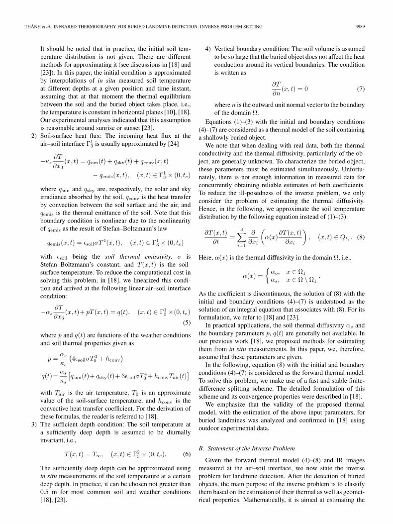
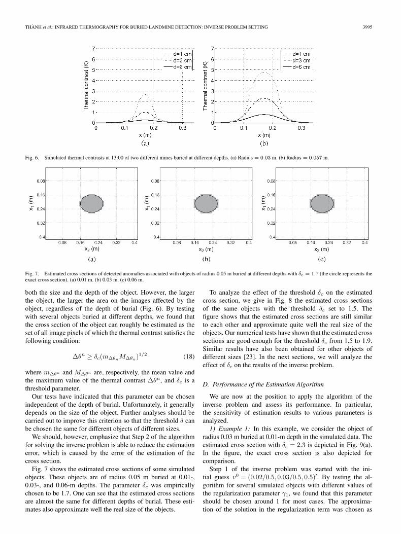
Fig. 6. Simulated thermal contrasts at 13:00 of two different mines buried at different depths. (a) Radius = 0.03 m. (b) Radius = 0.057 m.

Fig. 7. Estimated cross sections of detected anomalies associated with objects of radius 0.05 m buried at different depths with δc = 1.7 (the circle represents theexact cross section). (a) 0.01 m. (b) 0.03 m. (c) 0.06 m.

both the size and the depth of the object. However, the largerthe object, the larger the area on the images affected by theobject, regardless of the depth of burial (Fig. 6). By testingwith several objects buried at different depths, we found thatthe cross section of the object can roughly be estimated as theset of all image pixels of which the thermal contrast satisfies thefollowing condition:

Δθn ≥ δc(mΔθnMΔθn

)1/2 (18)

where mΔθn and MΔθn are, respectively, the mean value andthe maximum value of the thermal contrast Δθn, and δc is athreshold parameter.

Our tests have indicated that this parameter can be chosenindependent of the depth of burial. Unfortunately, it generallydepends on the size of the object. Further analyses should becarried out to improve this criterion so that the threshold δ canbe chosen the same for different objects of different sizes.

We should, however, emphasize that Step 2 of the algorithmfor solving the inverse problem is able to reduce the estimationerror, which is caused by the error of the estimation of thecross section.

Fig. 7 shows the estimated cross sections of some simulatedobjects. These objects are of radius 0.05 m buried at 0.01-,0.03-, and 0.06-m depths. The parameter δc was empiricallychosen to be 1.7. One can see that the estimated cross sectionsare almost the same for different depths of burial. These esti-mates also approximate well the real size of the objects.

To analyze the effect of the threshold δc on the estimatedcross section, we give in Fig. 8 the estimated cross sectionsof the same objects with the threshold δc set to 1.5. Thefigure shows that the estimated cross sections are still similarto each other and approximate quite well the real size of theobjects. Our numerical tests have shown that the estimated crosssections are good enough for the threshold δc from 1.5 to 1.9.Similar results have also been obtained for other objects ofdifferent sizes [23]. In the next sections, we will analyze theeffect of δc on the results of the inverse problem.

D. Performance of the Estimation Algorithm

We are now at the position to apply the algorithm of theinverse problem and assess its performance. In particular,the sensitivity of estimation results to various parameters isanalyzed.

1) Example 1: In this example, we consider the object ofradius 0.03 m buried at 0.01-m depth in the simulated data. Theestimated cross section with δc = 2.3 is depicted in Fig. 9(a).In the figure, the exact cross section is also depicted forcomparison.

Step 1 of the inverse problem was started with the ini-tial guess v0 = (0.02/0.5, 0.03/0.5, 0.5)′. By testing the al-gorithm for several simulated objects with different values ofthe regularization parameter γ1, we found that this parametershould be chosen around 1 for most cases. The approxima-tion of the solution in the regularization term was chosen as


Fig. 8. Estimated cross sections of detected anomalies associated with the objects of radius 0.05 m buried at different depths with δc = 1.5 (the circle representsthe exact cross section). (a) 0.01 m. (b) 0.03 m. (c) 0.06 m.

Fig. 9. Example 1. (a) Estimated cross section. (b) Distribution in depth of the estimated and exact thermal diffusivity. (c) Evolution of the objective function ofStep 1. (d) Evolution of the objective function of Step 2. (e) Estimated mean values of α12. (f) Exact mean values of α12.


TABLE IIIEXAMPLE 1: EXACT, INITIAL GUESS, REGULARIZATION APPROXIMATION, AND ESTIMATED PARAMETERS OF THE BURIED OBJECT

Fig. 10. Example 2. (a) Estimated cross section. (b) Distribution in depth of the estimated and exact thermal diffusivity. (c) Evolution of the objective functionof Step 1. (d) Evolution of the objective function of Step 2. (e) Estimated mean values of α12. (f) Exact mean values of α12.

v∗ = (0.02/0.5, 0.05/0.5, 0.25)′, which is not close to the realsolution.

The lower and upper bounds of the parameters werechosen as

αl = 0.064 × 10−7 αu = 6.402 × 10−7

�l1 = 0.001 �u

1 = 0.15 ςu = 0.06.

The algorithm was stopped after 12 iterations, i.e., when thereduction of the objective function was small enough [seeFig. 9(c)]. The distribution of the estimated thermal diffusivityin depth is plotted in Fig. 9(b). The result of this step isalso given in Table III along with the exact parameters, theinitial guess, and the approximation of the solution in theregularization term.


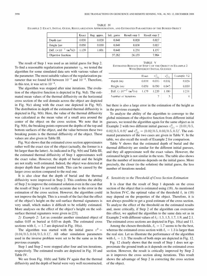
TABLE IVEXAMPLE 2: EXACT, INITIAL GUESS, REGULARIZATION APPROXIMATION, AND ESTIMATED PARAMETERS OF THE BURIED OBJECT

The result of Step 1 was used as an initial guess for Step 2.To find a reasonable regularization parameter γ2, we tested thealgorithm for some simulated data sets with various values ofthe parameter. The most suitable values of the regularization pa-rameter that we found fell between 10−3 and 10−4. Therefore,in this test, it was set to 10−4.

The algorithm was stopped after nine iterations. The evolu-tion of the objective function is depicted in Fig. 9(d). The esti-mated mean values of the thermal diffusivity on the horizontalcross section of the soil domain across the object are depictedin Fig. 9(e) along with the exact one depicted in Fig. 9(f).The distribution in depth of the estimated thermal diffusivity isdepicted in Fig. 9(b). Here, the value of the thermal diffusivitywas calculated as the mean value of a small area around thecenter of the object on the cross section. We note that inFig. 9(b), the breaking points represent the depths of the top andbottom surfaces of the object, and the value between these twobreaking points is the thermal diffusivity of the object. Thesevalues are also given in Table III.

Fig. 9(a) shows that the estimated cross section approximatesrather well the exact size of the object (actually, the former is abit larger than the latter). As indicated in Fig. 9(b) and Table III,the estimated thermal diffusivity of Step 1 approximates wellthe exact value. However, the depth of burial and the heightare not really well estimated. Indeed, the object was detected atdeeper depth than the ground truth. This can be caused by thelarger cross section compared to the real one.

It is also clear that the depth of burial and the thermaldiffusivity were improved in Step 2. This confirms the abilityof Step 2 to improve the estimated solution even in the case thatthe result of Step 1 is not really accurate due to the error in theestimation of the cross section. However, the algorithm couldnot improve the height. This is a result of the fact that the effectof the object’s height on the soil-surface thermal signatures isvery small, which makes it difficult to be reliably estimated.More analyses on the effect of the object’s height on the soil-surface thermal signatures were given in [23].

2) Example 2: Let us consider another simulated object ofradius 0.05 m buried at 0.03-m depth. The estimated crosssections with δc = 1.7 are depicted in Fig. 10(a).

The algorithm was started with the initial guess v0 =(0.04/0.5, 0.04/0.5, 0.1)′. All other simulation parametersused in the inverse problem were set to be the same as in theprevious example.

Step 1 and Step 2 were stopped after four and ten iterations,respectively. The estimated results are depicted in Fig. 10 andTable IV.

We see from Fig. 10(b) and Table IV again that the thermaldiffusivity and the depth of burial were very well reconstructed,

TABLE VESTIMATED RESULTS OF STEP 1 OF THE OBJECT IN EXAMPLE 2

WITH DIFFERENT INITIAL GUESSES

but there is also a large error in the estimation of the height asin the previous example.

To analyze the ability of the algorithm to converge to theglobal minimum of the objective function from different initialguesses, we tested the algorithm again for the same object as inExample 2 with two different initial guesses v0

(1) = (0.01/0.5,

0.02/0.5, 0.9)′ and v0(2) = (0.02/0.5, 0.03/0.5, 0.5)′. The esti-

mated parameters of the two cases are given in Table V. In thetable, we also recall the result of Example 2 for comparison.

Table V shows that the estimated depth of burial and thethermal diffusivity are similar for the different initial guesses,and they all approximate well the exact values. However, theestimated height is not similar in the tests. The table also showsthat the number of iterations depends on the initial guess. Moreprecisely, the closer (to the solution) the initial guess, the lessnumber of iterations needed.

E. Sensitivity to the Threshold of Cross Section Estimation

It is clear that the result of Step 1 depends on the crosssection of the object that is estimated using (18). As mentionedin Section IV-C, the optimal value of the threshold δc in (18)may depend on the properties of the object. Therefore, it isnot always possible to get a good estimate of the cross section.To analyze the effect of the threshold on the estimated resultsand, more critically, if Step 2 of the algorithm can overcomethis effect, we applied the algorithm to the same data set as inExample 2 with different values of δc: 1.3, 1.5, 1.7, 1.9, and 2.1.The estimated cross sections are depicted in Figs. 10(a) and 11.

Among the chosen thresholds, δc = 1.7 seems to be the best,whereas the estimated cross section with δc = 1.3 is larger thanthe real size. Let us illustrate the performance of the algorithmwith δc = 1.3. The results of both steps are depicted in Fig. 12.

Fig. 12 clearly shows that the result of Step 1 does not ap-proximate the ground truth as it depends on the estimated crosssection. However, the result is critically improved by Step 2as it improves the cross section along iterations. This resultshows the advantage of Step 2 in correcting the cross sectionof the object.


Fig. 11. Estimated cross section with different values of the threshold δc. (a) 1.3. (b) 1.5. (c) 1.9. (d) 2.1.

Fig. 12. Result of the inverse problem with δc = 1.3. (a) Evolution of the objective function of Step 1. (b) Evolution of the objective function of Step 2.(c) Distribution in depth of the estimated and exact thermal diffusivity. (d) Estimated mean values of α12.


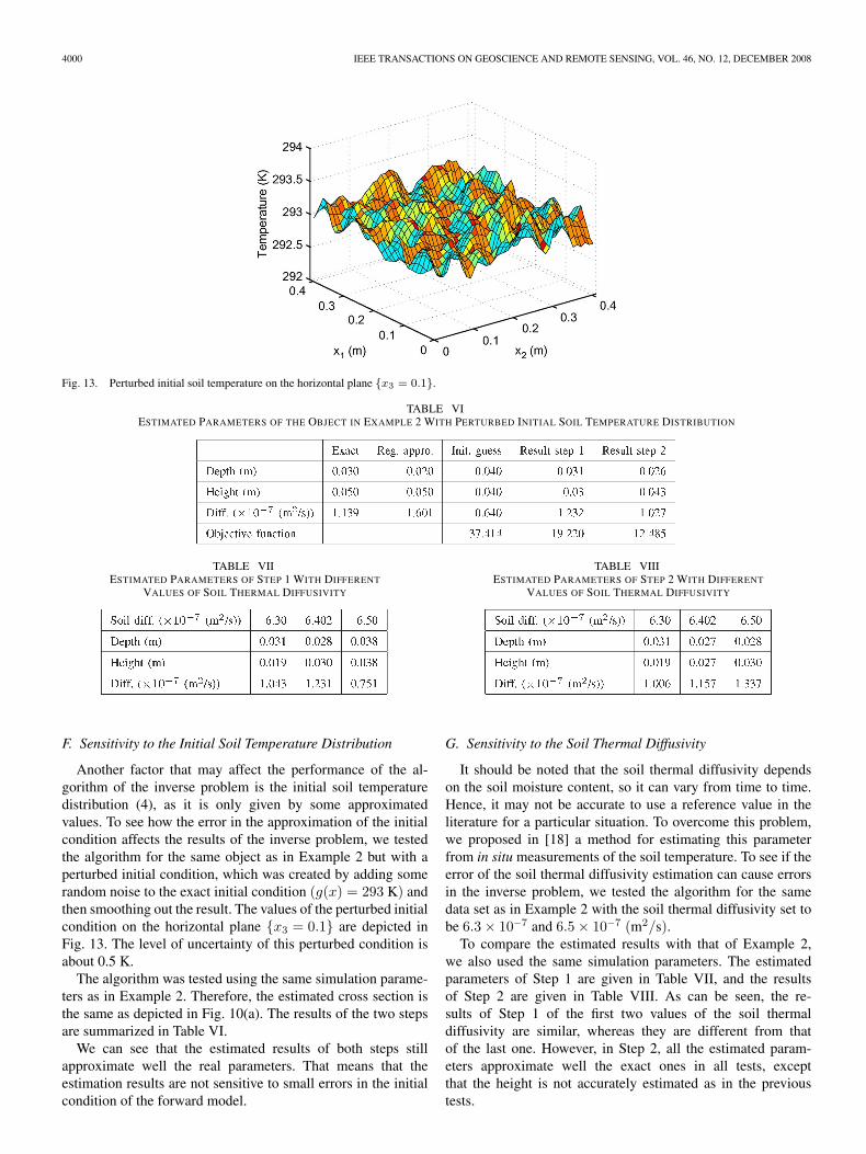
Fig. 13. Perturbed initial soil temperature on the horizontal plane {x3 = 0.1}.

TABLE VIESTIMATED PARAMETERS OF THE OBJECT IN EXAMPLE 2 WITH PERTURBED INITIAL SOIL TEMPERATURE DISTRIBUTION

TABLE VIIESTIMATED PARAMETERS OF STEP 1 WITH DIFFERENT

VALUES OF SOIL THERMAL DIFFUSIVITY

F. Sensitivity to the Initial Soil Temperature Distribution

Another factor that may affect the performance of the al-gorithm of the inverse problem is the initial soil temperaturedistribution (4), as it is only given by some approximatedvalues. To see how the error in the approximation of the initialcondition affects the results of the inverse problem, we testedthe algorithm for the same object as in Example 2 but with aperturbed initial condition, which was created by adding somerandom noise to the exact initial condition (g(x) = 293 K) andthen smoothing out the result. The values of the perturbed initialcondition on the horizontal plane {x3 = 0.1} are depicted inFig. 13. The level of uncertainty of this perturbed condition isabout 0.5 K.

The algorithm was tested using the same simulation parame-ters as in Example 2. Therefore, the estimated cross section isthe same as depicted in Fig. 10(a). The results of the two stepsare summarized in Table VI.

We can see that the estimated results of both steps stillapproximate well the real parameters. That means that theestimation results are not sensitive to small errors in the initialcondition of the forward model.

TABLE VIIIESTIMATED PARAMETERS OF STEP 2 WITH DIFFERENT

VALUES OF SOIL THERMAL DIFFUSIVITY

G. Sensitivity to the Soil Thermal Diffusivity

It should be noted that the soil thermal diffusivity dependson the soil moisture content, so it can vary from time to time.Hence, it may not be accurate to use a reference value in theliterature for a particular situation. To overcome this problem,we proposed in [18] a method for estimating this parameterfrom in situ measurements of the soil temperature. To see if theerror of the soil thermal diffusivity estimation can cause errorsin the inverse problem, we tested the algorithm for the samedata set as in Example 2 with the soil thermal diffusivity set tobe 6.3 × 10−7 and 6.5 × 10−7 (m2/s).

To compare the estimated results with that of Example 2,we also used the same simulation parameters. The estimatedparameters of Step 1 are given in Table VII, and the resultsof Step 2 are given in Table VIII. As can be seen, the re-sults of Step 1 of the first two values of the soil thermaldiffusivity are similar, whereas they are different from thatof the last one. However, in Step 2, all the estimated param-eters approximate well the exact ones in all tests, exceptthat the height is not accurately estimated as in the previoustests.


Fig. 14. Estimated cross section of a buried object tilted at different angles. (a) 15◦. (b) 30◦. (c) 45◦.

TABLE IXESTIMATED PARAMETERS OF STEP 1 OF TILTED OBJECTS

TABLE XESTIMATED PARAMETERS OF STEP 2 OF TILTED OBJECTS

H. On Tilted Cylindrical Objects

When dealing with buried object detection, it is not alwaysthe case that an object is vertically buried. However, the pro-posed algorithm estimates the depth of burial, the height, andthe thermal diffusivity of buried objects. We always assumedthat the object is approximated by an upright cylinder, althoughit is somehow tilted. To evaluate the performance and thelimits of the proposed algorithm in case of tilted objects, wesimulated some data of a circular cylinder of radius 0.05 mwith the same thermal diffusivity as in the previous examples(i.e., αo = 1.139 × 10−7 m2/s). The center of the cylinder wasfixed at (0.02, 0.02, 0.055) in the soil domain, whereas it wastilted at the angles of 15◦, 30◦, and 45◦ in the x1-direction.

For anomaly detection, the cross section was estimated withδc = 1.7. The result is depicted in Fig. 14. The estimatedparameters of Step 1 are given in Table IX, and the results ofStep 2 are given in Table X.

The estimated values indicated that the proposed algorithmstill gives good results for a slanted object up to 15◦. However,the results are not stable for large tilt angles. The possiblereason is due to the parameterization of the tilted objects usingthe parameters as in the case of upright objects. More suitableparameterization techniques are under development to handlethis case.

I. Classification Result of the TNO-FOI Data

The algorithm was applied to the full image sequence ofthe TNO-FOI data set. We note that the ground truth is onlyavailable for some of the detected anomalies due to two reasons:the properties of some test objects are not given, and someanomalies that were detected do not correspond to any objectsgiven in the ground truth. These anomalies are referred to asdetected false alarms.

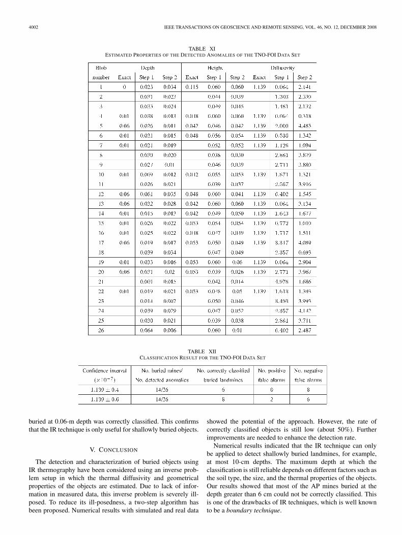
The estimated parameters of the detected anomalies of theTNO-FOI data set are given in Table XI. Although we con-currently estimate the thermal diffusivity, the depth of burial,and the height of the detected anomalies, the classification ofthe detected anomalies is based only on the estimated thermaldiffusivity. The depth of burial and the height are only used asadditional information in the clearance process.

To decide if the detected anomalies are mines or not, weintroduce a confidence interval so that the detected anomalieswhose thermal diffusivity falls within this interval are classifiedas mines. Otherwise, they are classified as nonmine objects.Since in our approach, we assume that mines are specified asTNT, the confidence interval should be chosen around the ther-mal diffusivity of TNT, which is given in Table I. The wronglyclassified anomalies are divided into two types: positive falsealarms and negative false alarms. Positive false alarms consistof all nonmine objects but classified as mines. On the contrary,negative false alarms are the buried mines but classified asnonmine targets.

It is clear that the classification results depend on the choiceof the confidence interval. If the interval is large, the numberof buried mines correctly classified is high, and therefore,the number of negative alarms is low. However, the numberof positive false alarms is high. That means more suspectedanomalies must be checked in the clearance process. On theother hand, if the confidence interval is small, the number ofpositive false alarms is reduced, but the number of negativefalse alarms is also reduced, i.e., some mines may be missedin the classification step and they can cause danger in the clear-ance process. Table XII summarizes the classification results ofthe full data set for two different confidence intervals.

The table shows that about half of the buried mines arecorrectly classified in this data set. Comparing to the groundtruth, we realized that most of the mines buried at 0.01-m depthare detected and correctly classified. However, only one mine


TABLE XIESTIMATED PROPERTIES OF THE DETECTED ANOMALIES OF THE TNO-FOI DATA SET

TABLE XIICLASSIFICATION RESULT FOR THE TNO-FOI DATA SET

buried at 0.06-m depth was correctly classified. This confirmsthat the IR technique is only useful for shallowly buried objects.

V. CONCLUSION

The detection and characterization of buried objects usingIR thermography have been considered using an inverse prob-lem setup in which the thermal diffusivity and geometricalproperties of the objects are estimated. Due to lack of infor-mation in measured data, this inverse problem is severely ill-posed. To reduce its ill-posedness, a two-step algorithm hasbeen proposed. Numerical results with simulated and real data

showed the potential of the approach. However, the rate ofcorrectly classified objects is still low (about 50%). Furtherimprovements are needed to enhance the detection rate.

Numerical results indicated that the IR technique can onlybe applied to detect shallowly buried landmines, for example,at most 10-cm depths. The maximum depth at which theclassification is still reliable depends on different factors such asthe soil type, the size, and the thermal properties of the objects.Our results showed that most of the AP mines buried at thedepth greater than 6 cm could not be correctly classified. Thisis one of the drawbacks of IR techniques, which is well knownto be a boundary technique.


ACKNOWLEDGMENT

The authors would like to thank the editor and the refereesfor their stimulating comments and suggestions that helpedimprove this paper.

REFERENCES

[1] C. Bruschini and B. Gros, “A survey of current sensor technology researchfor the detection of landmines,” in Sustainable Humanitarian Demining:Trends, Techniques and Technologies. Verona, VA: Mid Valley Press,Dec. 1998, pp. 172–187.

[2] C. Gooneratne, S. Mukhopahyay, and G. Sen Gupta, “A review of sens-ing technologies for landmine detection: Unmanned vehicle based ap-proach,” in Proc. 2th Int. Conf. Auton. Robots Agents, Palmerston North,New Zealand, Dec. 2004, pp. 401–407.

[3] Q. A. Holmes, C. R. Schwartz, J. H. Seldin, J. A. Wright, andL. J. Witter, “Adaptive multispectral CFAR detection of land mines,” Proc.SPIE, vol. 2496, pp. 421–432, 1995.

[4] P. López, “Detection of landmines from measured infrared images usingthermal modelling of the soil,” Ph.D. dissertation, Univ. Santiago deCompostela, Santiago de Compostela, Spain, 2003.

[5] S. Batman and J. Goutsias, “Unsupervised iterative detection of landmines in highly cluttered environments,” IEEE Trans. Image Process.,vol. 12, no. 5, pp. 509–523, May 2003.

[6] J. Deans, J. Gerhard, and L. Carter, “Analysis of a thermal imagingmethod for landmine detection, using infrared heating of the sand sur-face,” Infrared Phys. Technol., vol. 48, no. 3, pp. 202–216, Aug. 2006.

[7] K. Khanafer and K. Vafai, “Thermal analysis of buried land mines over adiurnal cycle,” IEEE Trans. Geosci. Remote Sens., vol. 40, no. 2, pp. 461–473, Feb. 2002.

[8] K. Khanafer, K. Vafai, and B. A. Baertlein, “Effects of thin metal outercase and top air gap on thermal IR images of buried antitank and antiper-sonnel land mines,” IEEE Trans. Geosci. Remote Sens., vol. 41, no. 1,pp. 123–135, Jan. 2003.

[9] K. Lamorski, P. Pregowski, W. Swiderski, D. Szabra, R. Walczak, andB. Usowicz, “Thermal signatures of land mines buried in mineral andorganic soils—Modelling and experiments,” Infrared Phys. Technol.,vol. 43, no. 3–5, pp. 303–309, Jun. 2002.

[10] P. López Martínez, L. van Kempen, H. Sahli, and D. C. Ferrer, “Improvedthermal analysis of buried landmines,” IEEE Trans. Geosci. Remote Sens.,vol. 42, no. 9, pp. 1965–1975, Sep. 2004.

[11] F. Moukalled, N. Ghaddar, H. Kabbani, N. Khalid, and Z. Fawaz, “Nu-merical and experimental investigation of thermal signatures of buriedlandmines in dry soil,” Trans. ASME, J. Heat Transf., vol. 128, no. 5,pp. 484–494, May 2006.

[12] A. Muscio and M. A. Corticelli, “Land mine detection by infrared ther-mography: Reduction of size and duration of the experiments,” IEEETrans. Geosci. Remote Sens., vol. 42, no. 9, pp. 1955–1964, Sep. 2004.

[13] I. K. Sendur and B. A. Baertlein, “Numerical simulation of thermal sig-natures of buried mines over a diurnal cycle,” in Proc. SPIE—Detectionand Remediation Technologies for Mines and Minelike Targets V,A. C. Dubey, J. F. Harvey, J. T. Broach, and R. E. Dugan, Eds., Aug. 2000,vol. 4038, pp. 156–167.

[14] S. Sjökvist, R. Garcia-Padron, and D. Loyd, “Heat transfer modelling ofsolar radiated soil, including moisture transfer,” in Proc. 3rd Baltic HeatTransfer Conf., Gdansk, Poland, Sep. 22–24, 1999, pp. 707–714.

[15] S. Sjökvist, A. Linderhed, S. Nyberg, M. Uppsall, and D. Loyd,“Land mine detection by IR temporal analysis: Physical numericalmodeling,” in Proc. SPIE—Detection and Remediation Technologiesfor Mine and Minelike Targets X, R. S. Harmon, J. T. Broach, andJ. H. Holloway, Jr., Eds., 2005, vol. 5794, pp. 30–41.

[16] N. T. Thành, D. N. Hào, P. López, F. Cremer, and H. Sahli, “Thermalinfrared identification of buried landmines,” in Proc. SPIE—Detectionand Remediation Technologies for Mine and Minelike Targets X,R. S. Harmon, J. T. Broach, and J. H. Holloway, Jr., Eds., 2005, vol. 5794,pp. 198–208.

[17] N. T. Thành, D. N. Hào, and H. Sahli, “Thermal model for landminedetection: Efficient numerical methods and soil parameter estimation,”in Proc. SPIE—Detection and Remediation Technologies for Mine andMinelike Targets XI, R. S. Harmon, J. T. Broach, and J. H. Holloway, Jr.,Eds., 2006, vol. 6217, pp. 517–528.

[18] N. T. Thành, H. Sahli, and D. N. Hào, “Finite-difference methods andvalidity of a thermal model for landmine detection with soil propertyestimation,” IEEE Trans. Geosci. Remote Sens., vol. 45, no. 3, pp. 656–674, Mar. 2007.

[19] A. Zare, J. Bolton, P. Gader, and M. Schatten, “Vegetation mapping forlandmine detection using long-wave hyperspectral imagery,” IEEE Trans.Geosci. Remote Sens., vol. 46, no. 1, pp. 172–178, Jan. 2008.

[20] T. F. Coleman and Y. Li, “An interior trust region approach for nonlinearminimization subject to bounds,” SIAM J. Optim., vol. 6, no. 2, pp. 418–445, 1996.

[21] H. S. Carslaw and J. C. Jaeger, Conduction of Heat in Solids, 2nd ed.Oxford, U.K.: Oxford Univ. Press, 1959.

[22] A. A. Samarskii and P. N. Vabishchevich, Computational Heat Transfer.Volume 1: Mathematical Modelling. Chichester, U.K.: Wiley, 1995.

[23] N. T. Thành, “Infrared thermography for the detection and characteri-zation of buried objects,” Ph.D. dissertation, Vrije Universiteit Brussel,Brussels, Belgium, 2007.

[24] K. Watson, “Geologic applications of thermal infrared images,” Proc.IEEE, vol. 63, no. 1, pp. 128–137, Jan. 1975.

[25] D. Strong and T. Chan, “Edge-preserving and scale-dependent proper-ties of total variation regularization,” Inverse Probl.—Special Section onImaging, vol. 19, no. 6, pp. S165–S187, Dec. 2003.

[26] J. L. Lions, Optimal Control of Systems Governed by Partial DifferentialEquations. Berlin, Germany: Springer-Verlag, 1971.

[27] G. I. Marchuk, Adjoint Equations and Analysis of Complex Systems.Dordrecht, The Netherlands: Kluwer, 1995.

[28] S. J. Norton, “Iterative inverse scattering algorithms: Methods of comput-ing Fréchet derivatives,” J. Acoust. Soc. Amer., vol. 106, no. 5, pp. 2653–2660, Nov. 1999.

[29] S. J. Norton, “Iterative algorithms for computing the shape of a hardscattering object: Computing the shape derivative,” J. Acoust. Soc. Amer.,vol. 116, no. 2, pp. 1002–1008, Aug. 2004.

[30] H. Banks, “Computational issues in parameter estimation and feedbackcontrol problems for partial differential equations systems,” Phys. D,vol. 60, no. 1–4, pp. 226–238, Nov. 1992.

[31] C. R. Vogel and J. G. Wade, “Analysis of costate discretizations in param-eter estimation for linear evolution equations,” SIAM J. Control Optim.,vol. 33, no. 1, pp. 227–254, Jan. 1995.

[32] W. de Jong, H. A. Lensen, and Y. H. Janssen, “Sophisticated test facilityto detect land mines,” in Proc. SPIE—Detection and Remediation Tech-nologies for Mine and Minelike Targets IV, A. C. Dubey, J. F. Harvey,J. T. Broach, and R. E. Dugan, Eds., Orlando, FL, Apr. 1999, vol. 3710,pp. 1409–1418.

[33] F. Cremer, N. T. Thành, L. Yang, and H. Sahli, “Stand-off thermal IRminefield survey, system concept and experimental results,” in Proc.SPIE—Detection and Remediation Technologies for Mine and MinelikeTargets X, R. S. Harmon, J. T. Broach, and J. H. Holloway, Jr., Eds., 2005,vol. 5794, pp. 209–220.

Nguyen Trung Thành was born in Hatinh, Vietnam,in 1980. He received the M.S. degree in mathe-matics from Hanoi University of Science, Hanoi,Vietnam, in 2003 and the Ph.D. degree in engi-neering from Vrije Universiteit Brussel, Brussels,Belgium, in 2007.

He is currently a Postdoc Researcher with theDepartment of Electronics and Informatics, VrijeUniversiteit Brussel. His studies have focused onthe theoretical and numerical aspects of partialdifferential equations, optimization methods, inverse

problems, and applications.


Hichem Sahli received the Ph.D. degree in com-puter sciences and the “Habilitation diriger desrecherches” from Ecole Nationale Sup. De PhysiqueStrasbourg, Strasbourg, France, in 1991 and 1996,respectively.

From 1991 to 1996, he was an attach de recherchewith the Department of CAD and Robotics, Ecoledes Mines de Paris, Paris, France. From 1997 to1998, he held visiting professor appointments withVrije Universiteit Brussel (VUB), Brussel, Belgium.Since 1999, he has been a Professor with the Depart-

ment of Electronics and Informatics (ETRO), VUB, and a Group Coordinatorwith the Interuniversitair Micro-Elektronica Centrum vzw (IMEC), Leuven,Belgium. He coordinates the research team in computer vision within ETRO.His principal research fields are inverse problems in computer vision, imageand motion analysis, and subsurface imaging.

Dinh Nho Hào received the M.S. degree in mathe-matics from Baku State University, Baku, Azerbaijan(former Soviet Union), in 1983, the Ph.D. degreein mathematics from the Free University of Berlin,Berlin, Germany, in 1991, and the Habilitation de-gree in mathematics from the University of Siegen,Siegen, Germany, in 1996.

He was a Visiting Professor at several universitiesin Germany, France, and U.K. He is currently an As-sociate Professor with the Institute of Mathematics,Vietnamese Academy of Science and Technology,

Hanoi, Vietnam. He is also with Vrije Universiteit Brussel, Brussel, Belgium.Dr. Hào has been awarded several grants from German Academic Ex-

change Service (DAAD), German Research Association (DFG), Alexander vonHumboldt Stiftung, CNR (Italy), and Royal Society (U.K.).

Infrared Thermography for Buried Landmine Detection: Inverse Problem Setting

Documents

Transcript of Infrared Thermography for Buried Landmine Detection: Inverse Problem Setting