Information-theoretic ideas in Poisson approximation and concentration

Information-Theoretic Ideasin Poisson Approximation and Concentration

Ioannis KontoyiannisAthens Univ Econ & Business

joint work withP. Harremoes, O. Johnson, M. Madiman

LMS/EPSRC Short CourseStability, Coupling Methods and Rare Events

Heriot-Watt University, Edinburgh, September 2006

1

Outline

1. Poisson Approximation in Relative Entropy

Motivation: Entropy and the central limit theoremMotivation: Poisson as a maximum entropy distributionA very simple general bound; Examples

2. Analogous Bounds in Total Variation

Suboptimal Poisson approximationOptimal Compound Poisson approximation

3. Tighter Poisson Bounds for Independent Summands

A (new) discrete Fisher information; subadditivityA log-Sobolev inequality

4. Measure Concentration and Compound Poisson Tails

The compound Poisson distributionsA log-Sobolev inequality and its info-theoretic proofCompound Poisson concentration

2

Motivation: The Central Limit Theorem

Recall

N(0, σ2) has maximum entropy among all distributions with variance ≤ σ2

where the entropy of a RV Z with density f is

h(Z) := h(f ) := −∫

f log f

The Central Limit Theorem

For IID RVs X1, . . . , Xn with zero mean, variance σ2, and a ‘nice’ density,

not only Sn :=1√n

n∑i=1

XiD−→ N(0, σ2) but in fact h(Sn) ↑ h(N(0, σ2))

; Accumulation of many, small, independent random effects

is maximally random (cf. second law of thermodynamics)

; Monotonicity in n indicates that the entropy is a natural measure

for the convergence of the CLT

; This powerful intuition comes with powerful new techniques

[Linnik (1959), Brown (1982), Barron (1985), Ball-Barthe-Naor (2003),...]

3

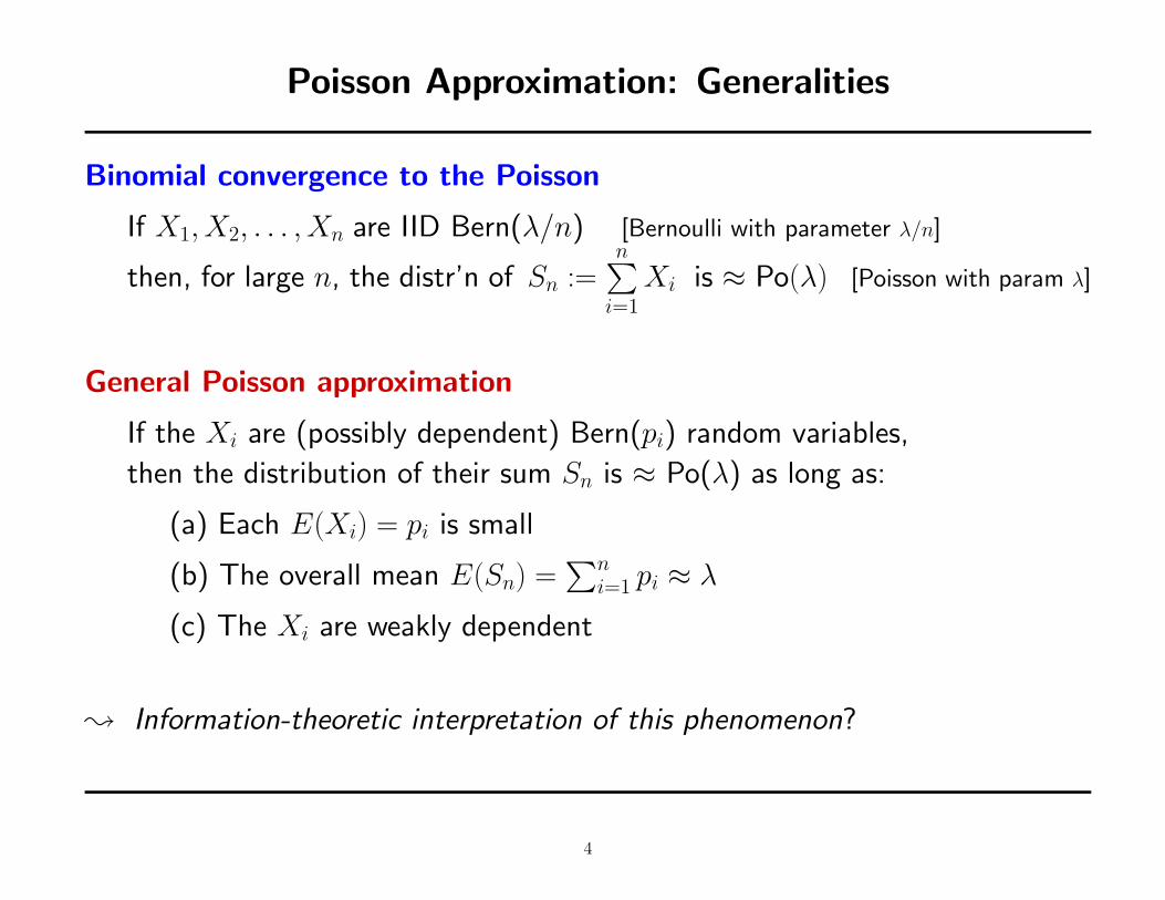
Poisson Approximation: Generalities

Binomial convergence to the Poisson

If X1, X2, . . . , Xn are IID Bern(λ/n) [Bernoulli with parameter λ/n]

then, for large n, the distr’n of Sn :=n∑

i=1

Xi is ≈ Po(λ) [Poisson with param λ]

General Poisson approximation

If the Xi are (possibly dependent) Bern(pi) random variables,

then the distribution of their sum Sn is ≈ Po(λ) as long as:

(a) Each E(Xi) = pi is small

(b) The overall mean E(Sn) =∑n

i=1 pi ≈ λ

(c) The Xi are weakly dependent

; Information-theoretic interpretation of this phenomenon?

4

The Poisson Distribution and Entropy

Recall: the entropy of a discrete random variable X with distribution P is

H(X) = H(P ) = −∑x

P (x) log P (x)

Theorem 0: Maximum Entropy

The Po(λ) distribution has maximum entropy

among all distributions that can be obtained as sums of Bernoulli RVs:

H(Po(λ)) = sup{

H(Sk) : Sk =k∑

i=1

Xi, Xi ∼ indep Bern(pi),k∑

i=1

pi = λ, k ≥ 1

}Proof. Messy but straightforward convexity arguments a la

[Mateev 1978] [Shepp & Olkin 1978] [Harremoes 2001] [Topsøe 2002] 2

5

Measuring Distance Between Probability Distributions

Recall

The total variation distance between two distributions P and Q

on the same discrete set S is

‖P −Q‖TV = 12

∑x∈S

|P (x)−Q(x)|

The entropy of a discrete random variable X with distribution P is

H(X) = H(P ) = −∑x

P (x) log P (x)

The relative entropy (or Kullback-Leibler divergence) is

D(P‖Q) =∑x∈S

P (x) log P (x)Q(x)

Pinsker’s ineq: 12‖P −Q‖2

TV ≤ D(P‖Q)

6

A Simple Poisson Approximation Bound

Theorem 1: Poisson Approximation [KHJ 05]

Suppose the Xi are (possibly dependent) Bern(pi) random variables

such that the mean of Sn =∑n

i=1 Xi is E(Sn) =∑n

i=1 pi = λ. Then:

The distribution PSn of Sn satisfies

D(PSn

∥∥∥Po(λ))≤

n∑i=1

p2i + D(PX1,...,Xn‖PX1 × · · · × PXn)

Note

; D(PX1,...,Xn‖PX1 × · · · ×PXn) ≥ 0 with “=” iff the Xi are independent

; More generally, the bound is “small” iff (a)–(c) are satisfied!

; Alternatively,

D(PX1,...,Xn‖PX1 × · · · × PXn) =n∑

i=1

H(Xi)−H(X1, . . . , Xn)

7

Elementary Properties of D(P‖Q)

Properties

i. Data processing inequality: D(Pg(X)‖Pg(Y )) ≤ D(PX‖PY )

Proof. By Jensen’s inequality:

D(Pg(X)‖Pg(Y )) =∑z

Pg(X)(z) logPg(X)(z)

Pg(Y )(z)

=∑z

[ ∑x:g(x)=z

PX(x)]

log

[ ∑x:g(x)=z PX(x)

][ ∑

x:g(x)=z PY (x)]

≤∑z

∑x:g(x)=z

PX(x) logPX(x)

PY (x)

= D(PX‖PY ) 2

ii. D(Bern(p)‖Po(p)) ≤ p2

Proof. Elementary calculus 2

8

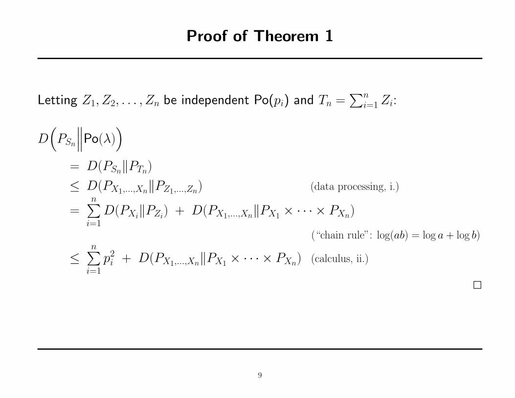
Proof of Theorem 1

Letting Z1, Z2, . . . , Zn be independent Po(pi) and Tn =∑n

i=1 Zi:

D(PSn

∥∥∥Po(λ))

= D(PSn‖PTn)

≤ D(PX1,...,Xn‖PZ1,...,Zn) (data processing, i.)

=n∑

i=1

D(PXi‖PZi

) + D(PX1,...,Xn‖PX1 × · · · × PXn)

(“chain rule”: log(ab) = log a + log b)

≤n∑

i=1

p2i + D(PX1,...,Xn‖PX1 × · · · × PXn) (calculus, ii.)

2

9

Example: Independent Bernoullis

If X1, X2, . . . , Xn are indep Bern(pi), Theorem 1 gives

D(PSn‖Po(λ)) ≤n∑

i=1

p2i

Convergence: In view of Barbour-Hall (1984) this is

necessary and sufficient for convergence

Rate: Pinsker’s ineq gives ‖PSn − Po(λ)‖TV ≤√

2[ ∑n

i=1 p2i

]1/2

but Le Cam (1960) gives the optimal TV rate as O( ∑n

i=1 p2i

)Question: Can we get the optimal TV rate with IT methods??

10

Two Examples

The classical Binomial/Poisson example

If X1, X2, . . . , Xn are IID Bern(λ/n), Theorem 1 gives


i=1

(λ/n)2 = λ2/n

Sufficient for convergence, but the actual rate is O(1/n2)

A Markov chain example

Suppose X1, X2, . . . , Xn is a stationary Markov chain with transition matrix nn+1

1n+1

n−1n+1

2n+1

and each Xi having (the stationary) Bern(1n) distribution

Theorem 1 ⇒ D(PSn‖Po(1)) ≤ 3 log n

n+

1

n

Pinsker ⇒ ‖PSn − Po(1)‖TV ≤ 4[log n

n

]1/2

but optimal rate is O(1/n)

11

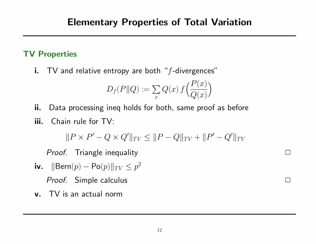
Elementary Properties of Total Variation

TV Properties

i. TV and relative entropy are both “f -divergences”

Df(P‖Q) :=∑x

Q(x) f(P (x)

Q(x)

)ii. Data processing ineq holds for both, same proof as before

iii. Chain rule for TV:

‖P × P ′ −Q×Q′‖TV ≤ ‖P −Q‖TV + ‖P ′ −Q′‖TV

Proof. Triangle inequality 2

iv. ‖Bern(p)− Po(p)‖TV ≤ p2

Proof. Simple calculus 2

v. TV is an actual norm

12

A Simple Poisson Approximation Bound in TV

Theorem 2: Poisson Approximation in TV [K-Madiman 06]

Suppose the Xi are independent Bern(pi) random variables

such that the mean of Sn =∑n

i=1 Xi is E(Sn) =∑n

i=1 pi = λ.

Then the distribution PSn of Sn satisfies

‖PSn − Po(λ)‖TV ≤n∑

i=1

p2i

Proof. Letting Z1, Z2, . . . , Zn be independent Po(pi) and Tn =∑n

i=1 Zi:

‖PSn − Po(λ)‖TV

= ‖PSn − PTn‖TV

≤ ‖PX1,...,Xn − PZ1,...,Zn‖TV (data processing)

≤n∑

i=1

‖PXi− PZi

‖TV (chain rule)

≤n∑

i=1

p2i (calculus) 2

13

Example Revisited: Independent Bernoullis

Recall: If X1, . . . , Xn are indep Bern(pi) with λ =∑n

i=1 pi then Thm 2 says


i=1

p2i

& from Barbour-Hall (1984): C1

∑ni=1 p2

i ≤ ‖PSn − Po(λ)‖TV ≤ C2

∑ni=1 p2

i

so we have the right convergence rate!

For finite n: Stein’s method actually yields

‖PSn − Po(λ)‖TV ≤ min{

1,1

λ

} n∑i=1

p2i ,

which is much better for large λ

E.g. if all pi = 1√n

then λ =√

n and our bound = 1

whereas Stein’s method yields the bound 1/√

n

14

Corollary: Generalization to Dependent RVs

Corollary: General Poisson Approximation in TV [K-Madiman 06]

Suppose the Xi are (possibly dependent) Z+-valued random variables

with pi = Pr{Xi = 1}, and let λ =∑n

i=1 pi. Then the distribution PSn

of Sn =∑n

i=1 Xi satisfies


i=1

p2i +

n∑i=1

E|pi − qi| +n∑

i=1

Pr{Xi ≥ 2}

where qi = Pr{Xi = 1|X1, . . . , Xi−1}

15

Proof of Corollary

To show: ‖PSn − Po(λ)‖TV ≤n∑

i=1

p2i +

n∑i=1

E|pi − qi| +n∑

i=1

Pr{Xi ≥ 2}

As before (data processing+chain rule):

‖PSn − Po(λ)‖TV ≤ ‖PX1,...,Xn − PZ1,...,Zn‖TV

≤n∑

i=1

E[‖PXi|X1,...,Xi−1

− PZi‖TV

]Letting Ii = I{Xi=1}, by the triangle ineq:


i=1

‖PZi− PIi

‖TV

+n∑

i=1

E[‖PIi

− PIi|X1,...,Xi−1‖TV

]+

n∑i=1

E[‖PIi|X1,...,Xi−1

− PXi|Xi,...,Xi−1‖TV

]2

16

Compound Poisson Approximation

Can IT methods actually yield optimal bounds?We turn to a more general problem:

Compound Binomial convergence to the compound Poisson

If X1, X2, . . . , Xn are IID ∼ Q and I1, I2, . . . , In are IID Bern(λ/n)

then, for large n, the distr’n of

Sn :=n∑

i=1

IiXi =Bin(n,λ/n)∑

i=1

Xi ≈Po(λ)∑i=1

Xi

which is the compound Poisson distr CP(λ, Q)

General Compound Poisson approximation

For a general sum Sn =∑n

i=1 Yi of (possibly dependent) Rd-valued RVs Yi

we may hope that the distribution of Sn is ≈ CP(λ, Q) as long as:

(a) Each pi := Pr{Yi 6= 0} is small

(b) The Yi are weakly dependent

(c) The distr Q is chosen appropriately

17

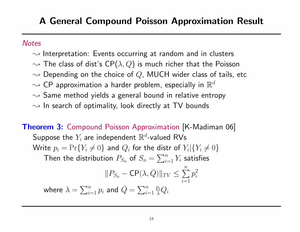
A General Compound Poisson Approximation Result

Notes

; Interpretation: Events occurring at random and in clusters

; The class of dist’s CP(λ, Q) is much richer that the Poisson

; Depending on the choice of Q, MUCH wider class of tails, etc

; CP approximation a harder problem, especially in Rd

; Same method yields a general bound in relative entropy

; In search of optimality, look directly at TV bounds

Theorem 3: Compound Poisson Approximation [K-Madiman 06]

Suppose the Yi are independent Rd-valued RVs

Write pi = Pr{Yi 6= 0} and Qi for the distr of Yi|{Yi 6= 0}Then the distribution PSn of Sn =

∑ni=1 Yi satisfies

‖PSn − CP(λ, Q)‖TV ≤n∑

i=1

p2i

where λ =∑n

i=1 pi and Q =∑n

i=1piλQi

18

Proof of Theorem 3

Let Z1, Z2, . . . , Zn be indep CP(pi, Qi), so that Tn =∑n

i=1 Zi ∼ CP(λ, Q)

19

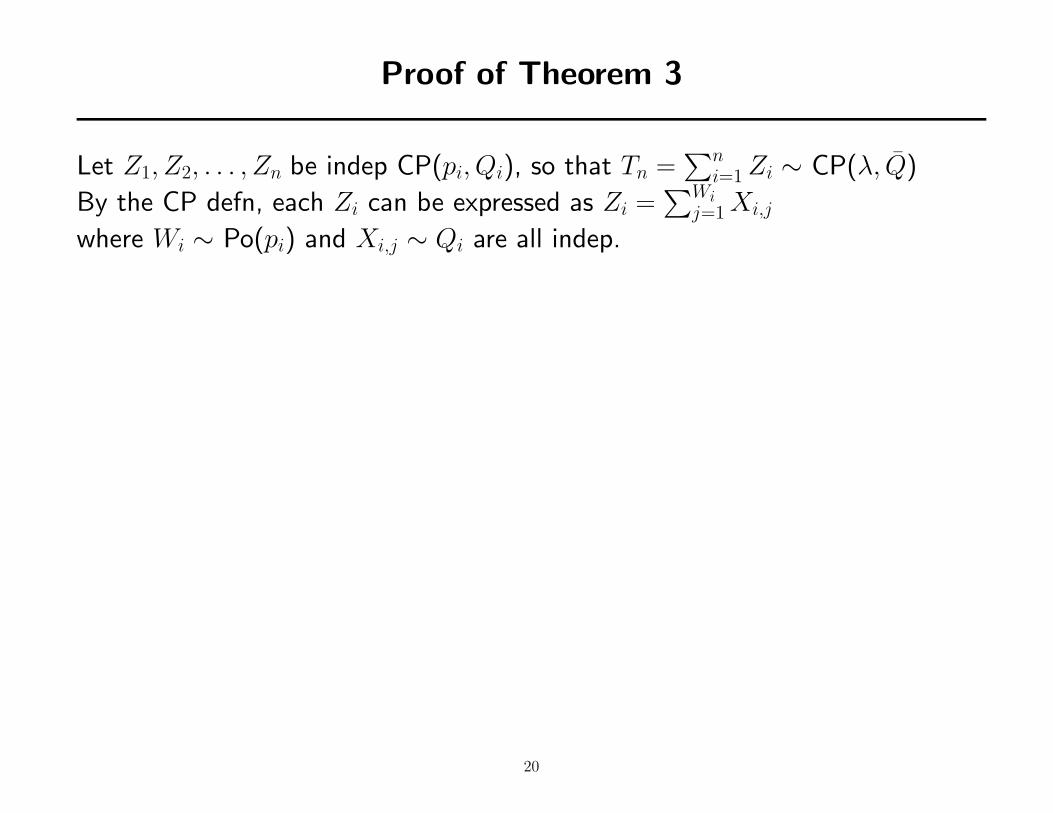
Proof of Theorem 3



By the CP defn, each Zi can be expressed as Zi =∑Wi

j=1 Xi,j

where Wi ∼ Po(pi) and Xi,j ∼ Qi are all indep.

20

Proof of Theorem 3




j=1 Xi,j

where Wi ∼ Po(pi) and Xi,j ∼ Qi are all indep. Hence:

Tn =

n∑i=1

Zi =

n∑i=1

Wi∑j=1

Xi,j

21

Proof of Theorem 3




j=1 Xi,j


Tn =

n∑i=1

Zi =

n∑i=1

Wi∑j=1

Xi,j

Similarly let I1, I2, . . . , In be indep Bern(pi) and write Yi = IiXi,1. Hence:

Sn =

n∑i=1

Yi =

n∑i=1

Ii∑j=1

Xi,j

22

Proof of Theorem 3




j=1 Xi,j


Tn =

n∑i=1

Zi =

n∑i=1

Wi∑j=1

Xi,j

Similarly let I1, I2, . . . , In be indep Bern(pi) and write Yi = IiXi,1. Hence:

Sn =

n∑i=1

Yi =

n∑i=1

Ii∑j=1

Xi,j

Then: ‖PSn − CP(λ, Q)‖TV = ‖PSn − PTn‖TV

≤ ‖P{Ii},{Xi,j} − P{Wi},{Xi,j}‖TV (data processing)

≤n∑

i=1

‖PIi− PWi

‖TV (chain rule)

≤n∑

i=1

p2i (calculus) 2

23

Comments

; In general, the bound of Theorem 3 ‖PSn − CP(λ, Q)‖TV ≤∑n

i=1 p2i

cannot be improved

; Here, the IT method gives the optimal rate and optimal constants

; Can we refine our IT methods to recover the optimal 1/λ factor

in the simple Poisson case?

; Recall the earlier example: If X1, . . . , Xn are i.i.d. Bern( 1√n)

with λ =√

n, Stein’s method gives

‖PSn − Po(λ)‖TV ≤1√n

whereas we got

‖PSn − Po(λ)‖TV ≤ 1

; To obtain tighter bounds, take a hint from corresponding work for the

CLT [Barron, Johnson, Ball-Barthe-Naor, ...] and turn to Fisher information

24

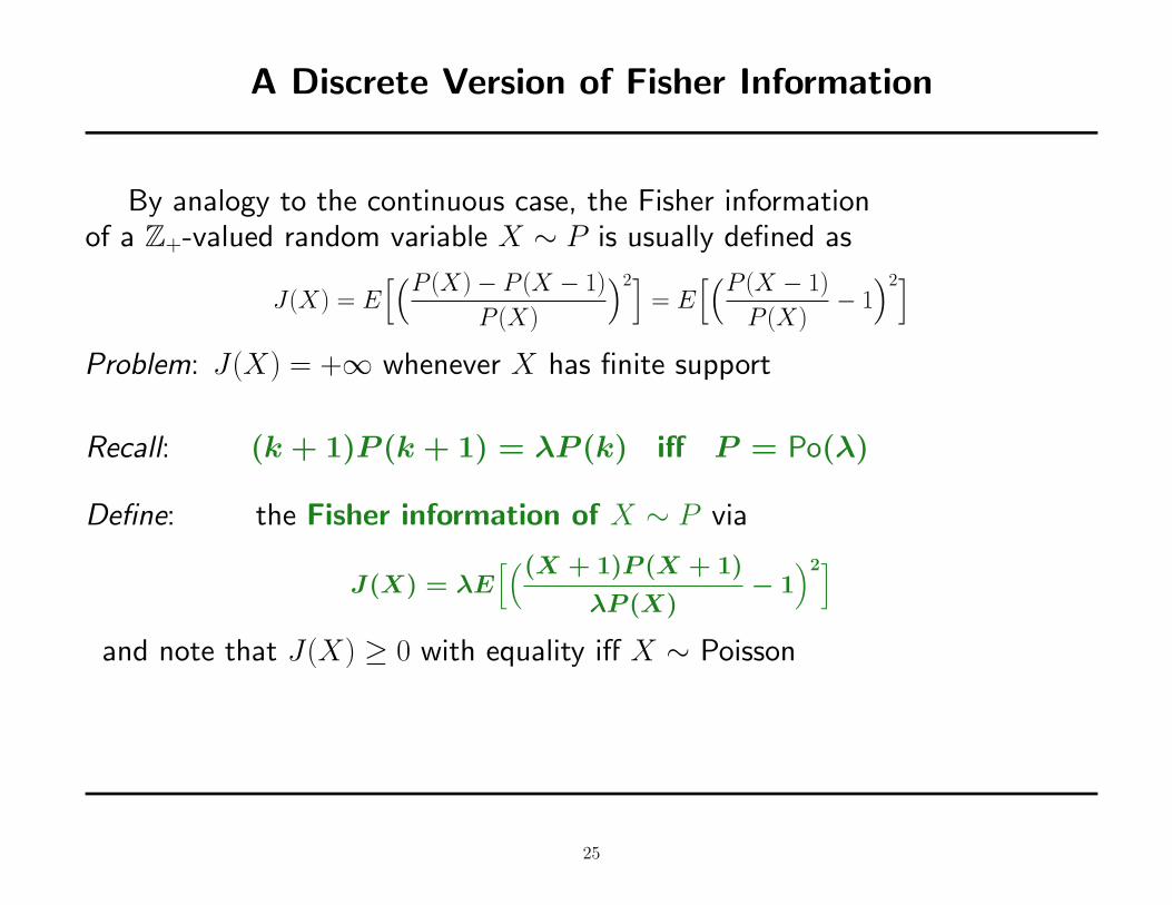
A Discrete Version of Fisher Information

By analogy to the continuous case, the Fisher informationof a Z+-valued random variable X ∼ P is usually defined as

J(X) = E[(P (X)− P (X − 1)

P (X)

)2]= E

[(P (X − 1)

P (X)− 1

)2]Problem: J(X) = +∞ whenever X has finite support

Recall: (k + 1)P (k + 1) = λP (k) iff P = Po(λ)

Define: the Fisher information of X ∼ P via

J(X) = λE[((X + 1)P (X + 1)

λP (X)− 1

)2]and note that J(X) ≥ 0 with equality iff X ∼ Poisson

25

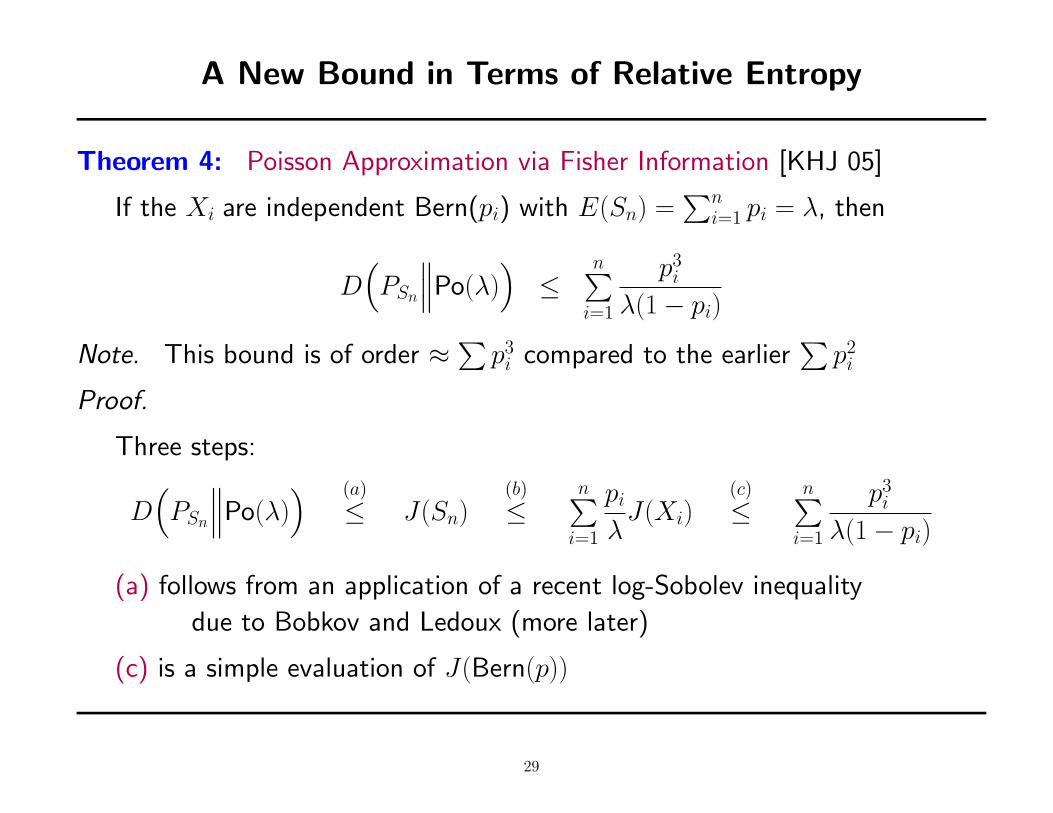
A New Bound in Terms of Relative Entropy

Theorem 4: Poisson Approximation via Fisher Information [KHJ 05]

If the Xi are independent Bern(pi) with E(Sn) =∑n

i=1 pi = λ, then

D(PSn

∥∥∥Po(λ))

≤n∑

i=1

p3i

λ(1− pi)

Note. This bound is of order ≈∑

p3i compared to the earlier

∑p2

i

26




i=1 pi = λ, then

D(PSn

∥∥∥Po(λ))

≤n∑

i=1

p3i

λ(1− pi)



∑p2

i

Proof.

Three steps:

D(PSn

∥∥∥Po(λ)) (a)

≤ J(Sn)

(a) follows from an application of a recent log-Sobolev inequality

due to Bobkov and Ledoux (more later)

27

A New Bound in Terms of Relative Entorpy



i=1 pi = λ, then

D(PSn

∥∥∥Po(λ))

≤n∑

i=1

p3i

λ(1− pi)



∑p2

i

Proof.

Three steps:

D(PSn

∥∥∥Po(λ)) (a)

≤ J(Sn)(b)

≤n∑

i=1

pi

λJ(Xi)



28




i=1 pi = λ, then

D(PSn

∥∥∥Po(λ))

≤n∑

i=1

p3i

λ(1− pi)



∑p2

i

Proof.

Three steps:

D(PSn

∥∥∥Po(λ)) (a)

≤ J(Sn)(b)

≤n∑

i=1

pi

λJ(Xi)

(c)

≤n∑

i=1

p3i

λ(1− pi)



(c) is a simple evaluation of J(Bern(p))

29

Subadditivity of Fisher Information

Proof cont’d.

D(PSn

∥∥∥Po(λ)) (a)

≤ J(Sn)(b)

≤n∑

i=1

pi

λJ(Xi)

(c)

≤n∑

i=1

p3i

λ(1− pi)

(b) is based on the more general subadditivity property

J(Sn) ≤n∑

i=1

E(Xi)

E(Sn)J(Xi) (∗)

RecallJ(X) = λE

[((X + 1)P (X + 1)

λP (X)− 1

)2](∗) is proved by writing

[(z+1)P∗Q(z+1)

P∗Q(z) − 1]

as a conditional expectation

and using ideas about L2 projections of convolutions

Ineq (∗) is the natural discrete analog of Stam’s Fisher information ineq

(in the continuous case), used to prove the entropy power inequality 2

30

Example Revisited: Independent Bernoullis

Recall the earlier example

Suppose X1, . . . , Xn are i.i.d. Bern( 1√n) and let λ =

√n

Our earlier bound was

‖PSn − Po(λ)‖TV ≤ 1

Stein’s method gives

‖PSn − Po(λ)‖TV ≤1√n

Theorem 4 combined with Pinsker’s ineq gives

‖PSn − Po(λ)‖TV ≤√

2[D(PSn‖Po(λ))

]1/2

≤ 1√n

√5

2

Moreover, Theorem 4 gives a strong new bound in terms of relative entropy!

31

Outline

1. Poisson Approximation in Relative Entropy

Motivation: Entropy and the central limit theoremMotivation: Poisson as a maximum entropy distributionA very simple general bound; Examples

2. Analogous Bounds in Total Variation

Suboptimal Poisson approximationOptimal Compound Poisson approximation

3. Tighter Poisson Bounds for Independent Summands

A (new) discrete Fisher information; subadditivityA log-Sobolev inequality

4. Measure Concentration and Compound Poisson Tails

The compound Poisson distributionsA log-Sobolev inequality and its info-theoretic proofCompound Poisson concentration

32

Motivation: The Concentration Phenomenon

An Example [Bobkov & Ledoux (1998)]

If W ∼ Po(λ) and f (i) is 1-Lipschitz, i.e., |f (i + 1)− f (i)| ≤ 1

Pr{

f (W )− E[f (W )] > t}≤ exp

{− t

4log

(1 +

t

2λ

)}for all t > 0

Note

; Sharp bound, valid for all t and all such f

; One example from a very large class of such results

; Many different methods of proof

dominant one probably the “entropy method”

33

Proof by the Entropy Method: First Step

Define

The relative entropy of a function g > 0 w.r.t. a prob distr P

EntP (g) =∑i

P (i)g(i) log g(i)−[ ∑

i

P (i)g(i)]

log[ ∑

i

P (i)g(i)]

e.g., if g(i) = Q(i)/P (i), then EntP (g) = D(Q‖P ) = relative entropy

A Logarithmic Sobolev Inequality

Our earlier log-Sobolev ineq D(P‖Po(λ)) ≤ λE[(

(X+1)P (X+1)λP (X) − 1

)2]is equivalent to: If W ∼ Po(λ), then for any function g > 0:

EntPo(λ)(g) ≤ λE[|Dg(W )|2

g(W )

]where Dg(i) = g(i + 1)− g(i)

Proof: Information-theoretic tools

Use the tensorization property of relative entropy – more later...

34

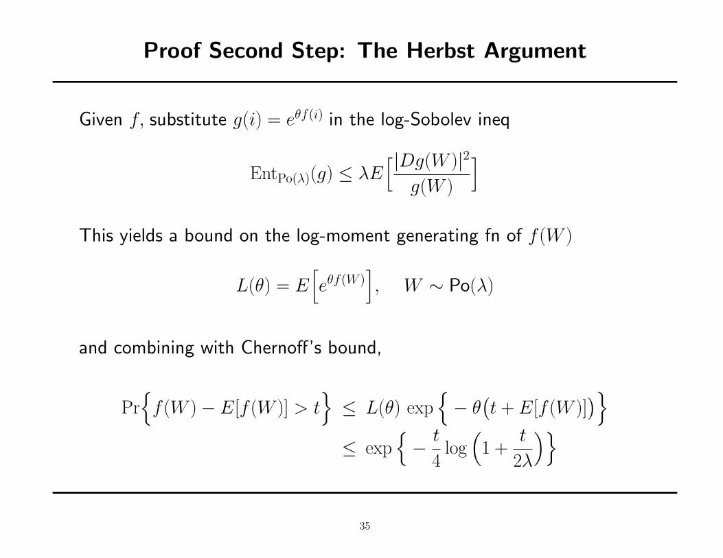
Proof Second Step: The Herbst Argument

Given f, substitute g(i) = eθf(i) in the log-Sobolev ineq

EntPo(λ)(g) ≤ λE[|Dg(W )|2

g(W )

]This yields a bound on the log-moment generating fn of f (W )

L(θ) = E[eθf(W )

], W ∼ Po(λ)

and combining with Chernoff’s bound,

Pr{

f (W )− E[f (W )] > t}≤ L(θ) exp

{− θ

(t + E[f (W )]

)}≤ exp

{− t

4log

(1 +

t

2λ

)}

35

Remarks

Note; General, powerful inequality, proved by info-theoretic techniques

; Proof heavily dependent on existence of log-moment generating fn

; Domain of application restricted to a small family (Poisson distr)

Generalize to Compound Poisson Distrs on Z+

; The asymptotic tails of Z ∼ CP(λ, Q) are determined by those of Q

e.g., if Q(i) ∼ e−αi then CPλ,Q(i) ∼ e−αi

if Q(i) ∼ 1/iβ then CPλ,Q(i) ∼ 1/iβ, etc

Versatility of tail behavior is attractive for modelling

Concentration? If Q has sub-exponential tails the Herbst argument fails

; The CP(λ, Q) distribution can be built up from “small Poissons”

CP(λ, Q)D=

Po(λ)∑i=1

XiD=

∞∑j=1

j · Po(λQ(j))

36

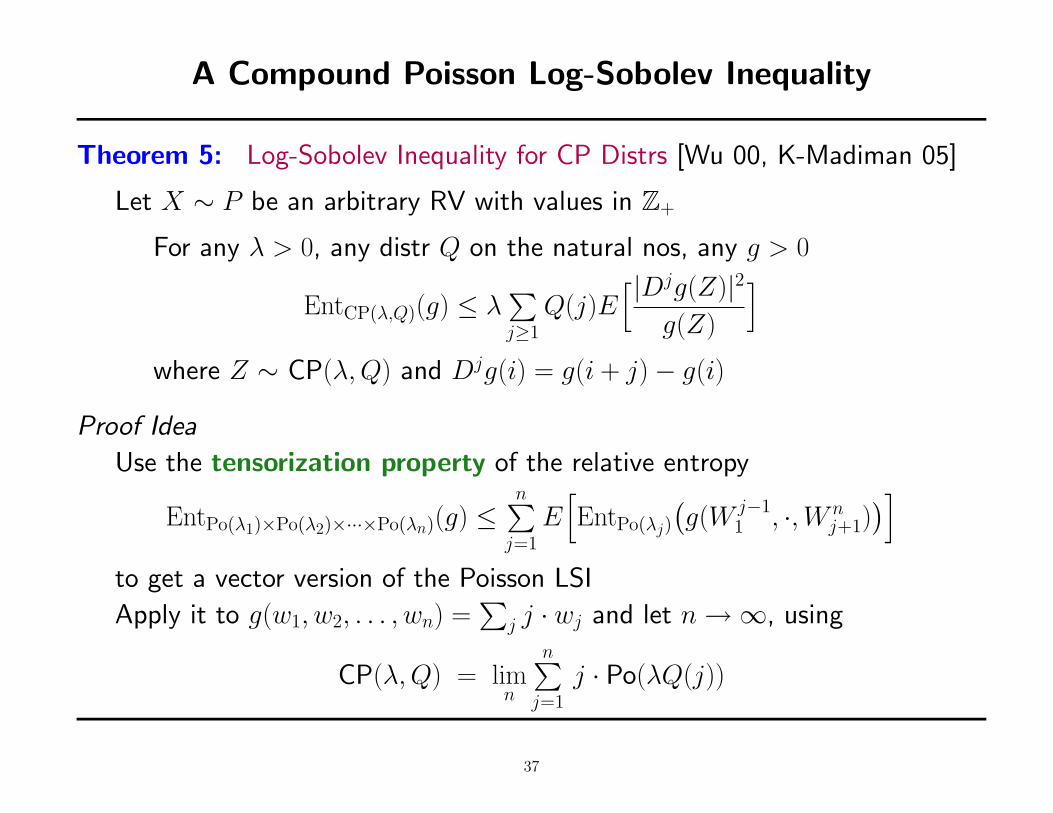
A Compound Poisson Log-Sobolev Inequality

Theorem 5: Log-Sobolev Inequality for CP Distrs [Wu 00, K-Madiman 05]

Let X ∼ P be an arbitrary RV with values in Z+

For any λ > 0, any distr Q on the natural nos, any g > 0

EntCP(λ,Q)(g) ≤ λ∑j≥1

Q(j)E[|Djg(Z)|2

g(Z)

]where Z ∼ CP(λ, Q) and Djg(i) = g(i + j)− g(i)

Proof Idea

Use the tensorization property of the relative entropy

EntPo(λ1)×Po(λ2)×···×Po(λn)(g) ≤n∑

j=1

E[EntPo(λj)

(g(W j−1

1 , ·, W nj+1)

)]to get a vector version of the Poisson LSI

Apply it to g(w1, w2, . . . , wn) =∑

j j · wj and let n →∞, using

CP(λ, Q) = limn

n∑j=1

j · Po(λQ(j))

37

New Measure Concentration Bounds

Theorem 6: Measure Concentration for CP Distributions [K-Madiman 05]

(i) Suppose Z ∼ CP(λ, Q) and Q has finite Kth moment∑j

jKQ(j) < ∞

If f is 1-Lipschitz, i.e., |f (i + 1)− f (i)| ≤ 1 for all i

then for t > 0

Pr{∣∣f (Z)− E[f (Z)]

∣∣ > t} ≤ A(B

t

)K

where the constants A, B are explicit and depend only

on λ, K, |f (0)|, and on the integer moments of Q

(ii) An analogous bound holds for any RV Z whose distr satisfies

the log-Sobolev ineq of Thm 5

38

The Constants in Theorem 2

Let

q(r) =∑j

jr Q(j)

Then

Pr{∣∣f (Z)− E[f (Z)]

∣∣ > t} ≤ A(B

t

)K

where

A = exp{ K∑

r=1

(K

r

)q(r)

}B = 2|f (0)| + 2λq(1) + 1

39

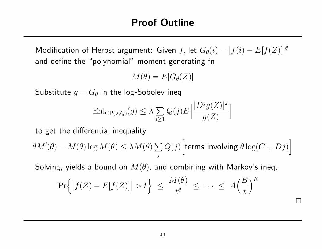
Proof Outline

Modification of Herbst argument: Given f, let Gθ(i) = |f (i)− E[f (Z)]|θand define the “polynomial” moment-generating fn

M(θ) = E[Gθ(Z)]

Substitute g = Gθ in the log-Sobolev ineq

EntCP(λ,Q)(g) ≤ λ∑j≥1

Q(j)E[|Djg(Z)|2

g(Z)

]to get the differential inequality

θM ′(θ)−M(θ) log M(θ) ≤ λM(θ)∑j

Q(j)[terms involving θ log(C + Dj)

]Solving, yields a bound on M(θ), and combining with Markov’s ineq,

Pr{∣∣f (Z)− E[f (Z)]

∣∣ > t}≤ M(θ)

tθ≤ · · · ≤ A

(B

t

)K

2

40

Final Remarks

Information-theoretic approach to (Compound-)Poisson approximation

Two approaches

; A simple, very general one

; A tight one for the independent Poisson case

Non-asymptotic, strong new bounds, intuitively satisfying

Ideas

A new version of Fisher information

L2-theory and log-Sobolev inequalities for discrete random variables

Concentration

A simple, general CP-approximation bound

A log-Sobolev ineq for the CP dist

New non-exponential measure concentration bounds

41

Information-Theoretic Interpretation

D(PSn

∥∥∥N(0, σ2))↓ 0 ⇐⇒ h(Sn) ↑ h(N(0, σ2)) as n →∞

(i) The accumulation of many, small, independent random effects

is maximally random

(ii) The monotonicity in n indicates that the entropy

is a natural measure for the convergence of the CLT

More generally the CLT holds as long as

(a) Each E(Xi) is small

(b) The overall variance Var(Sn) ≈ σ2

(c) The Xi are weakly dependent

; Next look at the other central result on the distribution of the sum

of many small random effects: Poisson approximation

42

Two Examples

The defining compound Poisson example

If X1, X2, . . . , Xn are IID ∼ Q on N and I1, I2, . . . , In are IID Bern(λ/n)

then for Sn =∑n

i=1 IiXi Theorem 3 gives

D(PSn‖CP(λ, Q)) ≤n∑

i=1

(λ/n)2 = λ2/n

Again, sufficient for convergence, but the optimal rate is O(1/n2)

A Markov chain example

Let Sn =∑n

i=1 IiXi where X1, . . . , Xn are IID ∼ Q on N and I1, . . . , In

is a stationary Markov chain with transition matrix nn+1

1n+1

n−1n+1

2n+1

Theorem 3 easily gives D(PSn‖CP(1, Q)) ≤ 3 log n

n+

1

n

43

Another Example

Theorem 2 easily generalizes to non-binary Xi, as long as J(Xi) can be

evaluated or estimated. E.g.:

Sum of Small Geometrics

Suppose X1, X2, . . . , Xn are indep Geom(qi)

let λ = E(Sn) =∑n

i=1[(1− qi)/qi]

Then J(Xi) = (1− qi)2/qi and proceeding as in the proof of Theorem 2


i=1

(1− qi)3

λq2i

In the case when all qi = n/(n + λ) ≈ 1− λ/n this takes the elegant form

D(PSn‖Po(λ)) ≤ λ2

n2

44

Tighter Bounds Compound Poisson Approximation?

Recall the proof of Theorem 2 in the Poisson case:

D(PSn

∥∥∥Po(λ)) (a)

≤ J(Sn)(b)

≤n∑

i=1

pi

λJ(Xi)

(c)

≤n∑

i=1

p3i

λ(1− pi)

; In order to generalize this approach we first need a new version

of the Fisher information, and a corresponding log-Sobolev ineq

for the compound Poisson measure . . .

45

Properties of the Compound Poisson Distribution

; The CP(λ, Q) laws are the only infinitely divisible distr’s on Z+

; The asymptotic tails of Z ∼ CP(λ, Q) are determined by those of Q

e.g., if Q(i) ∼ e−αi then CPλ,Q(i) ∼ e−αi

if Q(i) ∼ 1/iβ then CPλ,Q(i) ∼ 1/iβ, etc

Versatility of tail behavior is attractive for modelling

Concentration? If Q has sub-exponential tails the Herbst argument fails

; The CP(λ, Q) distribution can be built up from “small Poissons”

CP(λ, Q)D=

Po(λ)∑i=1

XiD=

∞∑j=1

j · Po(λQ(j))

46

A New Log-Sobolev Inequality

Let Cλ,Q(k) denote the compound Poisson probabilities Pr{CP(λ, Q) = k}

Theorem 4: Log-Sobolev Inequality for the Compound Poisson Measure

Let X ∼ P be an arbitrary Z+-valued RV

(a) [Bobkov-Ledoux (1998)] For any λ > 0:

D(P

∥∥∥Po(λ))≤ λE

[((X + 1)

λ

P (X + 1)

P (X)− 1

)2]

(b) For any λ > 0 and any measure Q on N:

D(P

∥∥∥CP(λ, Q))≤ λ

∞∑j=1

Q(j)E[( Cλ,Q(X)

Cλ,Q(X + j)

P (X + j)

P (X)− 1

)2]

47

Proof of Theorem 4 (a)

Step 1. Derive a simple log-Sobolev ineq for the Bernoulli measure Bp(k)For any binary RV X ∼ P :

D(P

∥∥∥Bern(p))≤ p(1− p)E

[( Bp(X)

Bp(X + 1)

P (X + 1)

P (X)− 1

)2]Step 2. Recall the “tensorization” property of relative entropy

Whenever X = (X1, . . . , Xn) ∼ Pn:

D(Pn

∥∥∥ n∏i=1

νi

)≤

n∑i=1

EPn

[D

(Pn(·|X1, . . . , Xi−1, Xi+1, . . . , Xn)

∥∥∥νi

)]Use this to extend step 1 to products of Bernoullis:

D(Pn

∥∥∥ n∏i=1

Bern(p))≤ p(1− p)E

[ n∑i=1

( Bnp (X)

Bnp (X + ei)

Pn(X + ei)

Pn(X)− 1

)2]Step 3. Since Po(λ)

D= limn

∑ni=1 Bern(λ/n), applying step 2 to a Pn

that only depends on X1 + · · · + Xn and taking n →∞:

D(P

∥∥∥Po(λ))≤ λE

[((X + 1)

λ

P (X + 1)

P (X)− 1

)2]

48

Proof of Theorem 4 (b)

In (a), the key was the representation of Po(λ) in terms of indep Bernoullis

Po(λ)D= lim

n

n∑i=1

Bern(λ/n)

Here use an alternative representation of CP(λ, Q) in terms of indep Poissons

CP(λ, Q)D=

Po(λ)∑i=1

XiD=

∞∑i=1

j ·Po(λQ(j))D= lim

n

n∑i=1

j ·Po(λQ(j)) (∗)

Step 1. Start with the Poisson log-Sobolev ineq of (a)

Step 2. Tensorize to obtain an ineq for products of PoissonsWhenever X = (X1, . . . , Xn) ∼ Pn:

D(Pn

∥∥∥ n∏i=1

Po(λi))≤

[· · ·

]Step 3. Apply step 2 to a Pn that only depends on

∑nj=1 j ·Xj

and take n →∞ using (∗) 2

49

Measure Concentration Bounds

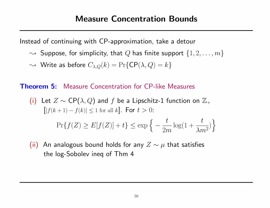
Instead of continuing with CP-approximation, take a detour

; Suppose, for simplicity, that Q has finite support {1, 2, . . . ,m}; Write as before Cλ,Q(k) = Pr{CP(λ, Q) = k}

Theorem 5: Measure Concentration for CP-like Measures

(i) Let Z ∼ CP(λ, Q) and f be a Lipschitz-1 function on Z+

[|f (k + 1)− f (k)| ≤ 1 for all k]. For t > 0:

Pr{f (Z) ≥ E[f (Z)] + t} ≤ exp{− t

2mlog(1 +

t

λm2)}

(ii) An analogous bound holds for any Z ∼ µ that satisfies

the log-Sobolev ineq of Thm 4

50

Remarks

Proof. Follows Herbst’s Gaussian argument: Apply the log-Sobolev ineq

to f = eθg for a Lipschitz g. Expand to get a differential inequality

for the M.G.F. L(θ) = E[eθg(Z)]. Use the bound and apply Chebychev

The finite-support assumption. Can be relaxed at the price of technicalities.

More general bounds, much more general class of tails

Poisson tails. From Theorem 5 we see that Lipschitz-1 functions

of CP-like RVs have Poisson tails. In particular:

Corollary: Poisson Tails for Lipschitz Functions

Let Z ∼ CP(λ, Q) or any other distr satisfying the assumptions of Thm 5

For any Lipschitz-1 function f on Z+ we have:

E[eθ|f(Z)| log+ |f(Z)|

]< ∞ for all θ > 0 small enough

51

Information-theoretic ideas in Poisson approximation and concentration

Documents

Transcript of Information-theoretic ideas in Poisson approximation and concentration