INFLUENCE OF TEMPERATURE - Universidad y Sociedad

382

Volume 14 | Number 3 | May - June, 2022UNIVERSIDAD Y SOCIEDAD | Have Scientific of the University of Cienfuegos | ISSN: 2218-3620

Presentation date: December, 2021 Date of acceptance: March, 2022 Publication date: May, 202238 INFLUENCIA DE LA TEMPERATURA Y LA COMPOSICIÓN EN LA PREDIC-CIÓN DE LAS PROPIEDADES TERMOFÍSICAS DEL ACERO (I).

AND COMPOSITION ON THE PREDICTION OF THE THERMOPHYSI-CAL PROPERTIES OF STEEL (I).

INFLUENCE OF TEMPERATURE

Yanan Camaraza-Medina1

E-mail: [email protected]: https://orcid.org/0000-0003-2287-75191Universidad de Matanzas. Cuba.

ABSTRACT

A proposal for the modeling of two thermo physical properties of steel as a function of the temperature and composition is presented. A residual method based on a progressive adjustment of functions is applied to estimate two thermo physical properties (electrical resistivity and linear thermal expansion) corresponding to 32 steels types with a composition (C, Mn , P, S, Si, Ni, Cr, Mo, V) and that operate in a temperature range from 0oC to 800oC. The validation and adjustment of the proposed models is made by comparing it with available experimental data. The weaker adjustment was achieved in the modeling of the electrical resistivity of AISI-SAE 405 steel with a mean and maximum deviation obtained of 8,2% and -9,9% respectively, while the best indices were obtained in the estimation of the density of AISI-SAE 1030 steel with a mean and maximum deviation obtained from 0,9% and 1,3% respectively. In all cases, the agreement of the proposed model is good enough to be considered satisfactory for practical design. Regarding the elements of study presented, there is no evidence of similar expressions in the available and known literature, which is why they are considered a scientific novelty.

Keywords: thermo physical properties, progressive adjustment method, experimental data generalization, mean absolute error.

RESUMEN

Se presenta una propuesta para el modelado de dos propiedades termofísicas del acero en función de la temperatura y la composición. Se aplica un método residual basado en un ajuste progresivo de funciones para estimar dos propiedades termofísicas (resistividad eléctrica y dilatación térmica lineal) correspondientes a 32 tipos de aceros con una composición (C, Mn, P, S, Si, Ni, Cr, Mo , V) y que operan en un rango de temperatura de 0oC a 800oC. La validación y ajuste de los modelos propuestos se realiza comparándolos con los datos experimentales disponibles. El ajuste más débil se logró en el modelado de la resistividad eléctrica del acero AISI-SAE 405 con una desviación media y máxima obtenida de 8,2% y -9,9% respectivamente, mientras que los mejores índices se obtuvieron en la estimación de la densidad de acero AISI-SAE 1030 con una desviación media y máxima obtenida de 0,9% y 1,3% respectivamente. En todos los casos, la concordancia del modelo propuesto es suficientemente buena para considerarse satisfactoria para el diseño práctico. En cuanto a los elementos de estudio presentados, no existe evidencia de expresiones similares en la literatura disponible y conocida, por lo que se consideran una novedad científica.

Palabras clave: propiedades termofísicas, método de ajuste progresivo, generalización de datos experimentales, error absoluto medio.

Cita sugerida (APA, séptima edición)

Camaraza-Medina, Y., (2022). Influence of temperature and composition on the prediction of the thermophysical properties of steel (I). Revista Universidad y Sociedad, 14(3), 382-394.

383

UNIVERSIDAD Y SOCIEDAD | Revista Científica de la Universidad de Cienfuegos | ISSN: 2218-3620

Volumen 14 | Número 3 | Mayo - Junio, 2022

INTRODUCTION

Currently, the high cost in money and time linked to expe-rimental tests for the evaluation of thermo physical proper-ties of steels, has established the preference for the use of predictive models in order to avoid this complex task (ŞahinoŞlu & Rafighi, 2021).

When a large set of experimental data is available, arti-ficial neural network (ANN) and finite element method (FEM) have been widely used in predictive modeling (Min, et al., 2020). A detailed review of the available and known literature shows that currently reported methods for esti-mating thermo physical properties of steels, although they include dependence on composition and temperatures, only have the ability to predict a unitary property of the a selected steel (Shi, et al., 2018).

Using ANN, a model was created to predict the thermal conductivity of AISI-SAE1045 steel, establishing its de-pendence on temperature and composition. The predic-tion was based on a Bayesian statistical framework (Peet, Hasan & Bhadeshia, 2011).

Other studies were focused on the prediction of three-dimensional heat flow, as well as heat transfer coefficient distributions in space and time. FEM techniques are used to study the phase transformation and its impact on the average heat transfer coefficient in the heat treatment of forged steels (Khodabakhshi & Kazeminezhad, 2011; Bouissa, et al., 2019).

The dependence between the temperature and the mean heat transfer coefficient, as well as the cooling curves, the cooling rate curves and the distortion are predicted from the iterative modification of the concentrated heat capa-city method and the heat transfer method. reverse heat in AISI-304 and AISI-1045 steels. To study the density variation of AISI-316L steel, the laser power, speed and scanning spacing were used during selective laser mel-ting, using variance analysis for this purpose (Miranda, et al., 2016).

Five different numerical algorithms, including Heat Balance Method (HBM), Revised Heat Balance Method (R-HBM), Nonlinear Beck Estimation Method (BEM), Inverse Finite Element Optimization Method (FIOM) and the finite element optimization method (FOM) were used for the prediction of thermal conductivity in carbon steels (Somasundharam & Reddy, 2020).

Another work considers that the simultaneous estimation of the thermal conductivity is dependent on the tempera-ture and the specific heat, assuming that this dependence is a parametric variation of the temperature, estimating the properties from the solution of the inverse problem (Wang

& Adachi, 2019). With this objective, it is established that the prediction models must take the composition as the only input data (Lieth, et al., 2021).

Recently, a combined model was presented that includes the influence of composition and temperature on the va-riation of thermal conductivity in austenitic stainless steels (Narayana, et al., 2020). Other methods, to perform pre-diction correlations, use a multiple linear regression analy-sis in the estimation of the thermal conductivity of carbon steels (Zheng, et al., 2020). A similar study proposes a nonlinear regression equation to predict the cooling limit curve and thermal conductivity in carbon steels (Borisade, et al., 2021). Other researchers, through the use of ANN, take the composition (Si, Cr, Ni, Mo) in alloyed steels as a starting point to estimate the cooling curve required in the heat treatment, also facilitating the evaluation of thermal conductivity (Xie, et al., 2021).

Therefore, despite the existence of multiple investigative works on the subject, none of them presents a methodolo-gy that allows the prediction of an extended group of ther-mo physical properties of a wide range of steels, nor does it establish the dependence of these properties with com-position and temperature, so the existence of a prediction method that resolves these limitations would be extremely useful (Gomez, et al., 2020; Li, et al., 2021).

In this study, a prediction method based on the adjustment and validation of experimental data is presented through the mathematical application of the residual method ba-sed on the progressive adjustment of functions (PAF), which will allow estimating two thermo physical properties (electrical resistivity and linear thermal expansion) corres-ponding to 32 classes of steels with a composition (C, Mn, P, S, Si, Ni, Cr, Mo, V), operating in a temperature range from 0oC to 800oC.

MATERIALS AND METHODS

2.1 Data processing using the progressive adjustment method.

The available experimental data relate the influence of temperature and composition on the variation of the stu-died thermo physical properties. In collaboration with the School of Engineering and Applied Science, Khazar University (Azerbaijan), the experimental data used in the adjustment and validation of the models were obtained. Table 1 summarizes the number of available experimental data for each value of temperature and thermo physical property studied, while Table 2 summarizes the validity range of the proposed method.

384



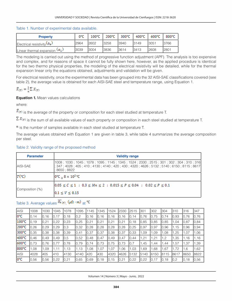
Table 1. Number of experimental data available.

Property

Electrical resistivity 2964 2602 3258 3940 3149 3051 3766

Linear thermal expansion 3039 3004 3836 3614 3413 2608 2801

The modeling is carried out using the method of progressive function adjustment (APF). The analysis is too expensive and complex, and for reasons of space it cannot be fully shown here, however, as the applied procedure is identical for the two thermo physical properties, the modeling of the electrical resistivity will be detailed, while for the thermal expansion linear only the equations obtained, adjustments and validation will be given.

For electrical resistivity, once the experimental data has been grouped into the 32 AISI-SAE classifications covered (see table 2), the average value is obtained for each AISI-SAE steel and temperature range, using Equation 1.

Equation 1. Mean values calculations

where:

is the average of the property or composition for each steel studied at temperature T.

is the sum of all available values of each property or composition in each steel studied at temperature T.

is the number of samples available in each steel studied at temperature T.

The average values obtained with Equation 1 are given in table 3, while table 4 summarizes the average composition per steel.

Table 2. Validity range of the proposed method

Parameter Validity range

AISI-SAE1008 ; 1030 ; 1045 ; 1078 ; 1095 ; 1145 ; 1345 ; 1524 ; 2330 ; 2515 ; 301 ; 302 ; 304 ; 310 ; 316 ; 347 ; 4028 ; 405 ; 410 ; 4130 ; 4140 ; 420 ; 430 ; 4320 ; 4626 ; 5132 ; 5140 ; 6150 ; 8115 ; 8617 ; 8650 ; 8822

a

Composition (%)

Table 3. Average values , at

AISI 1008 1030 1045 1078 1095 1145 1345 1524 2330 2515 301 302 304 310 316 347

0,14 0,16 0,17 0,18 0,2 0,16 0,16 0,16 0,16 0,14 0,76 0,75 0,74 0,93 0,76 0,76

0,19 0,21 0,22 0,23 0,25 0,21 0,21 0,21 0,21 0,18 0,85 0,85 0,85 1,04 0,87 0,84

0,26 0,29 0,29 0,3 0,32 0,28 0,28 0,28 0,28 0,25 0,97 0,97 0,96 1,15 0,96 0,94

0,35 0,38 0,38 0,39 0,41 0,37 0,37 0,38 0,37 0,33 1,09 1,09 1,08 1,25 1,07 1,06

0,46 0,49 0,49 0,5 0,52 0,48 0,47 0,49 0,47 0,44 1,21 1,21 1,2 1,35 1,16 1,16

0,73 0,76 0,77 0,78 0,79 0,74 0,73 0,75 0,73 0,7 1,45 1,44 1,44 1,57 1,37 1,39

1,08 1,09 1,11 1,13 1,13 1,08 1,07 1,07 1,06 1,03 1,69 1,68 1,67 1,72 1,6 1,62

AISI 4028 405 410 4130 4140 420 430 4320 4626 5132 5140 6150 8115 8617 8650 8822

0,56 0,56 0,22 0,21 0,65 0,69 0,18 0,15 0,21 0,22 0,22 0,17 0,18 0,2 0,18 0,56

385



0,65 0,66 0,27 0,26 0,76 0,81 0,23 0,2 0,26 0,28 0,28 0,22 0,23 0,25 0,24 0,65

0,75 0,77 0,34 0,34 0,88 0,93 0,3 0,27 0,33 0,35 0,35 0,29 0,3 0,33 0,31 0,75

0,86 0,88 0,43 0,43 1,01 1,05 0,39 0,35 0,41 0,43 0,45 0,38 0,39 0,42 0,4 0,86

0,97 1 0,53 0,53 1,15 1,2 0,5 0,45 0,52 0,53 0,56 0,49 0,5 0,52 0,5 0,97

1,23 1,26 0,78 0,78 1,44 1,51 0,77 0,72 0,78 0,78 0,83 0,75 0,76 0,79 0,77 1,23

1,52 1,54 1,1 1,09 1,75 1,8 1,1 1,05 1,1 1,1 1,17 1,09 1,1 1,13 1,11 1,52

From the average composition (see table 4), the composition factors y , are determined, given in Equations 2 and 3, (Camaraza-Medina, Hernandez-Guerrero & Luviano-Ortiz, 2021a).

Equation 2. Calculation of the composition factor

Equation 3. Calculation of the composition factor

In Equations 2 and 3, the composition values are given in %.

Table 4. Average composition values per steel studied, (%)

AISI 1008 1030 1045 1078 1095 1145 1345 1524 2330 2515 301 302 304 310 316 347

C 0,08 0,31 0,47 0,78 0,98 0,46 0,41 0,22 0,33 0,15 0,13 0,13 0,07 0,23 0,07 0,08

Mn 0,4 0,7 0,75 0,45 0,39 0,84 1,72 1,49 0,69 0,49 1,89 1,89 1,89 1,89 1,89 0,4

P 0,03 0,03 0,03 0,03 0,03 0,03 0,03 0,03 0,03 0,03 0,03 0,03 0,03 0,03 0,03 0,03

S 0,04 0,04 0,04 0,04 0,04 0,06 0,03 0,04 0,03 0,03 0,02 0,02 0,02 0,02 0,02 0,04

Si - - - - - - 0,26 - 0,28 0,28 0,64 0,64 0,64 1,31 0,64 -

Ni - - - - - - - - 3,47 4,97 7 6,7 9,06 20,31 11,66 -

Cr - - - - - - - - - - 17,2 18,2 19,2 24 17 -

Mo - - - - - - - - - - - - - - 2,58 -

V - - - - - - - - - - - - - - - -

AISI 4028 405 410 4130 4140 420 430 4320 4626 5132 5140 6150 8115 8617 8650 8822

C 0,07 0,28 0,06 0,13 0,31 0,41 0,13 0,1 0,2 0,27 0,33 0,41 0,51 0,16 0,18 0,51

Mn 1,89 0,79 0,84 0,84 0,49 0,87 0,87 0,87 0,54 0,54 0,69 0,78 0,8 0,79 0,79 0,87

P 0,03 0,03 0,03 0,03 0,03 0,03 0,03 0,03 0,03 0,03 0,03 0,03 0,04 0,03 0,03 0,03

S 0,02 0,04 0,03 0,02 0,03 0,03 0,02 0,03 0,03 0,03 0,03 0,03 0,04 0,03 0,03 0,03

Si 0,64 0,28 0,77 0,77 0,28 0,28 0,86 0,86 0,24 0,23 0,28 0,28 0,28 0,23 0,28 0,28

Ni 10,66 - - 0,61 - - - 0,61 1,8 0,83 - - - 0,29 0,53 0,53

Cr 18,2 - 13,3 12,7 0,98 0,98 13,2 17,2 0,52 0,9 0,8 0,98 0,42 0,52 0,52

Mo - 0,26 - - 0,21 0,21 - - 0,26 0,21 - - - 0,12 0,2 0,2

V - - - - - - - - - - - - 0,13 - - -

The PAF method is generated from a base correlation, to which corrections are made through linear or polynomial functions (Camaraza-Medina, 2021). To obtain the base correlation, the method of least squares is applied to the mean

values given in Table 3, obtaining a polynomial in the form per steel, (it can be used a linear function, but the predictive capacity of the model is reduced). Table 5 summarizes the parameters a, b and c for each correla-tion performed, the , as well as the respective composition values estimated with Equation 2, (see table 4 for the composition values used).

386



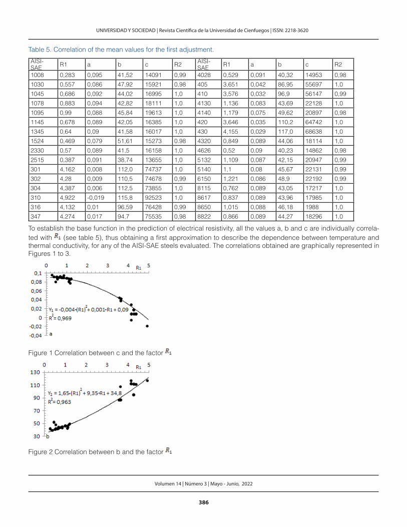
Table 5. Correlation of the mean values for the first adjustment.

AISI-SAE R1 a b c R2 AISI-

SAE R1 a b c R2

1008 0,283 0,095 41,52 14091 0,99 4028 0,529 0,091 40,32 14953 0,98

1030 0,557 0,086 47,92 15921 0,98 405 3,651 0,042 86,95 55697 1,0

1045 0,686 0,092 44,02 16995 1,0 410 3,576 0,032 96,9 56147 0,99

1078 0,883 0,094 42,82 18111 1,0 4130 1,136 0,083 43,69 22128 1,0

1095 0,99 0,088 45,84 19613 1,0 4140 1,179 0,075 49,62 20897 0,98

1145 0,678 0,089 42,05 16385 1,0 420 3,646 0,035 110,2 64742 1,0

1345 0,64 0,09 41,58 16017 1,0 430 4,155 0,029 117,0 68638 1,0

1524 0,469 0,079 51,61 15273 0.98 4320 0,849 0,089 44,06 18114 1,0

2330 0,57 0,089 41,5 16158 1,0 4626 0,52 0,09 40,23 14862 0,98

2515 0,387 0,091 38,74 13655 1,0 5132 1,109 0,087 42,15 20947 0,99

301 4,162 0,008 112,0 74737 1,0 5140 1,1 0,08 45,67 22131 0,99

302 4,28 0,009 110,5 74678 0,99 6150 1,221 0,086 48,9 22192 0,99

304 4,387 0,006 112,5 73855 1,0 8115 0,762 0,089 43,05 17217 1,0

310 4,922 -0,019 115,8 92523 1,0 8617 0,837 0,089 43,96 17985 1,0

316 4,132 0,01 96,59 76428 0,99 8650 1,015 0,088 46,18 1988 1,0

347 4,274 0,017 94,7 75535 0,98 8822 0,866 0,089 44,27 18296 1,0

To establish the base function in the prediction of electrical resistivity, all the values a, b and c are individually correla-ted with (see table 5), thus obtaining a first approximation to describe the dependence between temperature and thermal conductivity, for any of the AISI-SAE steels evaluated. The correlations obtained are graphically represented in Figures 1 to 3.

Figure 1 Correlation between c and the factor

Figure 2 Correlation between b and the factor

387



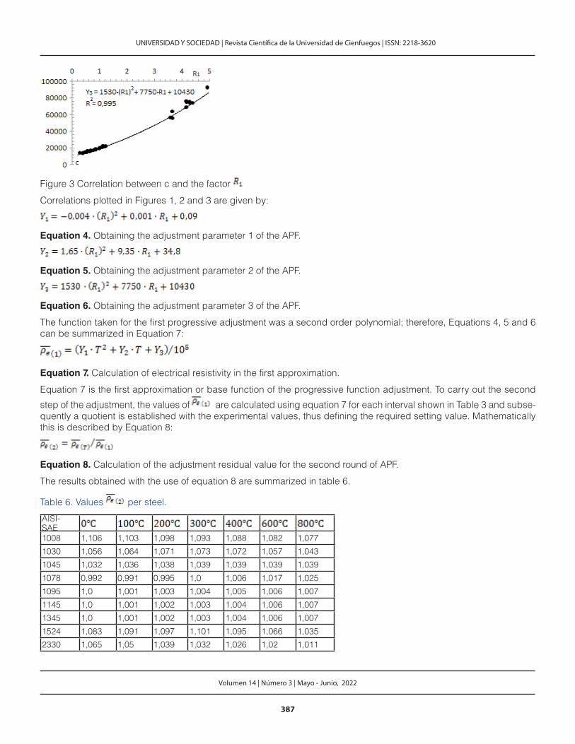
Figure 3 Correlation between c and the factor

Correlations plotted in Figures 1, 2 and 3 are given by:

Equation 4. Obtaining the adjustment parameter 1 of the APF.



The function taken for the first progressive adjustment was a second order polynomial; therefore, Equations 4, 5 and 6 can be summarized in Equation 7:

Equation 7. Calculation of electrical resistivity in the first approximation.

Equation 7 is the first approximation or base function of the progressive function adjustment. To carry out the second

step of the adjustment, the values of are calculated using equation 7 for each interval shown in Table 3 and subse-quently a quotient is established with the experimental values, thus defining the required setting value. Mathematically this is described by Equation 8:

Equation 8. Calculation of the adjustment residual value for the second round of APF.

The results obtained with the use of equation 8 are summarized in table 6.

Table 6. Values per steel.

AISI-SAE1008 1,106 1,103 1,098 1,093 1,088 1,082 1,077

1030 1,056 1,064 1,071 1,073 1,072 1,057 1,043

1045 1,032 1,036 1,038 1,039 1,039 1,039 1,039

1078 0,992 0,991 0,995 1,0 1,006 1,017 1,025

1095 1,0 1,001 1,003 1,004 1,005 1,006 1,007

1145 1,0 1,001 1,002 1,003 1,004 1,006 1,007

1345 1,0 1,001 1,002 1,003 1,004 1,006 1,007

1524 1,083 1,091 1,097 1,101 1,095 1,066 1,035

2330 1,065 1,05 1,039 1,032 1,026 1,02 1,011

388



2515 0,999 1,001 1,002 1,003 1,004 1,006 1,007

301 1,091 1,068 1,071 1,068 1,062 1,04 1,013

302 1,049 1,038 1,034 1,034 1,03 1,015 0,995

304 1,003 1,002 1,003 1,003 1,002 0,993 0,979

310 1,053 1,031 1,017 1,001 0,987 0,98 0,939

316 1,101 1,088 1,061 1,05 1,02 0,984 0,96

347 1,068 1,025 1,011 1,011 0,993 0,98 0,957

4028 1,0 1,001 1,002 1,003 1,004 1,006 1,007

405 0,94 0,947 0,947 0,953 0,95 0,959 0,964

410 0,976 0,984 0,992 0,996 1,0 0,994 0,985

4130 1,043 1,019 1,001 0,988 0,98 0,969 0,964

4140 0,969 0,968 0,97 0,97 0,968 0,954 0,944

420 1,101 1,109 1,117 1,119 1,125 1,124 1,111

430 1,001 1,013 1,031 1,03 1,054 1,083 1,079

4320 1,0 1,001 1,002 1,004 1,005 1,006 1,007

4626 1,0 1,001 1,002 1,003 1,004 1,006 1,007

5132 1,004 0,985 0,974 0,969 0,967 0,967 0,97

5140 1,053 1,038 1,027 1,006 0,992 0,976 0,968

6150 1,001 1,002 1,003 1,004 1,005 1,007 1,007

8115 1,0 1,001 1,002 1,003 1,004 1,006 1,007

8617 1,0 1,001 1,002 1,004 1,005 1,006 1,007

8650 1,001 1,002 1,003 1,004 1,005 1,006 1,007

8822 1,0 1,001 1,002 1,004 1,005 1,006 1,007

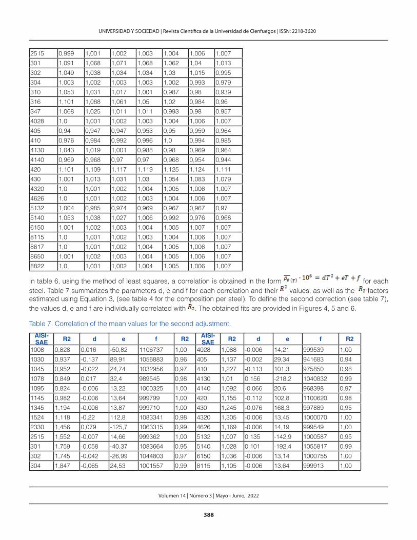
In table 6, using the method of least squares, a correlation is obtained in the form for each steel. Table 7 summarizes the parameters d, e and f for each correlation and their values, as well as the factors estimated using Equation 3, (see table 4 for the composition per steel). To define the second correction (see table 7), the values d, e and f are individually correlated with . The obtained fits are provided in Figures 4, 5 and 6.

Table 7. Correlation of the mean values for the second adjustment.

AISI-SAE R2 d e f R2 AISI-

SAE R2 d e f R2

1008 0,828 0,016 -50,82 1106737 1,00 4028 1,088 -0,006 14,21 999539 1,00

1030 0,937 -0,137 89,91 1056883 0,96 405 1,137 -0,002 29,34 941683 0,94

1045 0,952 -0,022 24,74 1032956 0,97 410 1,227 -0,113 101,3 975850 0,98

1078 0,849 0,017 32,4 989545 0,98 4130 1,01 0,156 -218,2 1040832 0,99

1095 0,824 -0,006 13,22 1000325 1,00 4140 1,092 -0,066 20,6 968398 0,97

1145 0,982 -0,006 13,64 999799 1,00 420 1,155 -0,112 102,8 1100620 0,98

1345 1,194 -0,006 13,87 999710 1,00 430 1,245 -0,076 168,3 997889 0,95

1524 1,118 -0,22 112,8 1083341 0,98 4320 1,305 -0,006 13,45 1000070 1,00

2330 1,456 0,079 -125,7 1063315 0,99 4626 1,169 -0,006 14,19 999549 1,00

2515 1,552 -0,007 14,66 999362 1,00 5132 1,007 0,135 -142,9 1000587 0,95

301 1,759 -0,058 -40,37 1083664 0,95 5140 1,028 0,101 -192,4 1055817 0,99

302 1,745 -0,042 -26,99 1044803 0,97 6150 1,036 -0,006 13,14 1000755 1,00

304 1,847 -0,065 24,53 1001557 0,99 8115 1,105 -0,006 13,64 999913 1,00

389



310 2,203 0,035 -157,9 1048715 0,97 8617 1,168 -0,006 13,26 1000081 1,00

316 2,025 0,045 -221,1 1105170 0,99 8650 1,18 -0,005 12,98 1000428 1,00

347 1,908 0,11 -207,0 1057128 0,94 8822 1,199 -0,005 13,23 1000135 1,00

Figure 4 Correlation between d and the factor

Figure 5 Correlation between e and the factor

Figure 6 Correlation between f and the factor

The correlations plotted in Figures 4 to 6 are given by:




The function taken for the second progressive adjustment was a second order polynomial, therefore, Equations 9, 10 and 11 can be summarized in Equation 7:

390



Equation 12. Calculation of electrical resistivity in the second approximation.

The electrical resistivity can then be estimated from the product of the two progressive adjustments made, (Equations 7 and 12), obtaining that:

Equation 13. Calculation of the estimated electrical resistivity.

The electrical resistivity values computed using Equation 13 are given in the table 8.

Table 8 Values per studied steel, at

1008 1030 1045 1078 1095 1145 1345 1524 2330 2515 301 302 304 310 316 347

0,13 0,16 0,17 0,19 0,2 0,17 0,17 0,15 0,16 0,15 0,75 0,78 0,81 1,01 0,78 0,79

0,18 0,21 0,22 0,24 0,25 0,22 0,22 0,2 0,21 0,2 0,86 0,89 0,93 1,14 0,88 0,9

0,24 0,27 0,29 0,31 0,32 0,29 0,29 0,27 0,28 0,27 0,98 1,01 1,04 1,25 0,99 1,02

0,32 0,36 0,38 0,4 0,41 0,38 0,38 0,35 0,37 0,35 1,09 1,13 1,16 1,37 1,11 1,13

0,42 0,46 0,48 0,5 0,52 0,48 0,48 0,46 0,48 0,46 1,22 1,25 1,28 1,47 1,22 1,25

0,67 0,72 0,74 0,76 0,78 0,74 0,75 0,72 0,75 0,72 1,47 1,49 1,52 1,66 1,46 1,49

0,99 1,05 1,07 1,09 1,11 1,08 1,09 1,06 1,09 1,06 1,73 1,75 1,76 1,83 1,7 1,73

4028 405 410 4130 4140 420 430 4320 4626 5132 5140 6150 8115 8617 8650 8822

0,15 0,61 0,6 0,22 0,22 0,61 0,72 0,19 0,15 0,21 0,21 0,23 0,18 0,19 0,21 0,19

0,2 0,71 0,7 0,27 0,28 0,71 0,83 0,24 0,2 0,27 0,27 0,29 0,23 0,24 0,26 0,24

0,27 0,81 0,8 0,35 0,36 0,81 0,94 0,32 0,27 0,34 0,35 0,36 0,3 0,31 0,34 0,32

0,36 0,93 0,92 0,44 0,45 0,93 1,06 0,41 0,36 0,44 0,44 0,45 0,39 0,4 0,43 0,41

0,47 1,05 1,04 0,55 0,56 1,05 1,18 0,52 0,47 0,54 0,55 0,56 0,5 0,51 0,54 0,52

0,73 1,32 1,31 0,82 0,83 1,32 1,44 0,79 0,73 0,81 0,82 0,83 0,77 0,78 0,81 0,79

1,06 1,61 1,61 1,16 1,17 1,61 1,72 1,13 1,07 1,15 1,15 1,17 1,1 1,12 1,15 1,13

The percentage of deviation (error) computed with the proposed method is obtained through Equation 14 (Camaraza-Medina, Guerrero-Hernandez & Luviano-Ortiz, 2021b):

Equation 14. Calculation of the correlation error of the proposed method (Equation 13).

Table 9 summarizes values obtained by comparing the experimental data tabulated in Table 3 with the results obtai-

ned through Equation 14. Figure 7 correlates the and values with an error band of 10%.

Table 9 Values obtained in the correlation of experimental data.

AISI 1008 1030 1045 1078 1095 1145 1345 1524 2330 2515 301 302 304 310 316 347

8,5 3,7 1,2 -2,8 -1,5 -2,4 -3,8 4,5 0,6 -6,6 0,1 -3,9 -9,7 -9 -2 -3,7

8,3 4,7 1,3 -2,1 -0,8 -1,9 -3,3 5,7 -0,5 -6,5 -1,5 -4,4 -9,1 -9,5 -2,2 -7,2

8,4 5,2 2 -1,6 -0,3 -1,8 -3,6 6 -1,4 -6,4 -0,6 -4,3 -8,2 -9,4 -3,5 -7,7

8,3 5,5 2,3 -0,5 0 -1,3 -3 6,6 -2,2 -5,4 -0,4 -3,7 -7,4 -9,3 -3,4 -6,9

8,1 5,7 2,4 0,4 0,4 -1,1 -3 6,1 -2,3 -5 -0,3 -3,4 -6,7 -8,9 -5,2 -7,8

391



7,9 4,7 2,9 1,8 1,1 -0,7 -2,5 3,9 -2,5 -4,2 -1 -3,5 -5,7 -5,8 -6,2 -7

8 3,8 3,2 3 1,7 -0,2 -2 1,3 -2,5 -3 -2 -3,9 -5,1 -6,2 -5,9 -7,2

AISI 4028 405 410 4130 4140 420 430 4320 4626 5132 5140 6150 8115 8617 8650 8822

-2,7 -9,9 -6,4 1,8 -6,2 6,2 -4,1 -4,4 -3,4 -2,4 2,3 -2,7 -3,5 -3,3 -3,5 -3,8

-3 -8,9 -5,6 -0,4 -6,4 6,8 -2,7 -4,3 -3,5 -3,8 1,5 -2,5 -3,1 -3 -3,1 -3,8

-2,6 -9 -4,6 -2 -5,9 7,5 -0,8 -4,3 -3,4 -4,9 0,3 -2 -2,7 -3,3 -3,4 -3,6

-2,3 -8,2 -4,1 -3,3 -5,9 7,8 -0,9 -4,1 -2,8 -5,3 -1,6 -1,8 -2,4 -2,8 -3,1 -3,3

-2,2 -8,4 -3,5 -4 -5,9 8,4 1,6 -3,6 -2,6 -5,4 -3 -1,4 -2,3 -2,6 -2,9 -3,2

-1,7 -7 -3,8 -4,7 -7,2 8,6 4,5 -3,1 -2,4 -4,9 -4,2 -1,1 -1,7 -2,2 -2,4 -2,6

-1,2 -6,1 -4,4 -4,9 -7,9 7,8 4,6 -2,5 -1,8 -4,3 -4,7 -0,7 -1,3 -1,7 -1,8 -2,1

Figure 7 Correlation of and

Applying a procedure analogous to the electrical resistivity, a methodology is established to estimate linear thermal expansion, which is given by Equations 15 to 22:



Equation 17. Calculation of linear thermal expansion in the first approximation.




Equation 21. Calculation of linear thermal expansion in the second approximation.

392



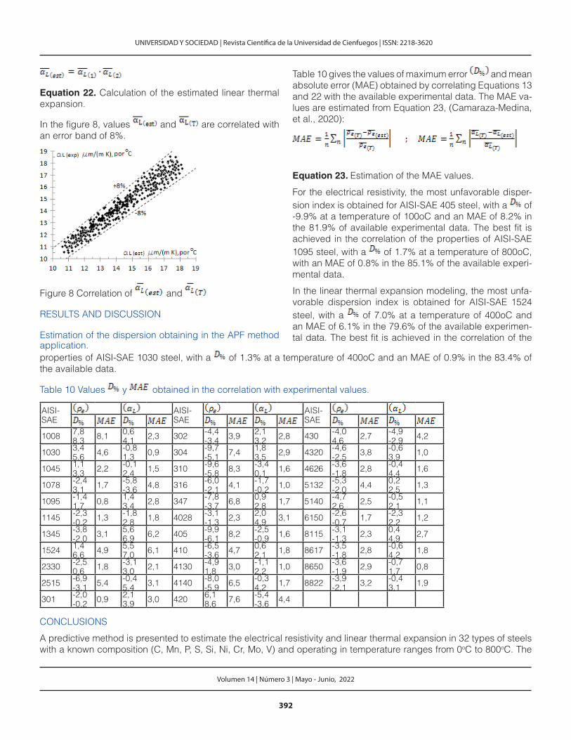
Equation 22. Calculation of the estimated linear thermal expansion.

In the figure 8, values and are correlated with an error band of 8%.

Figure 8 Correlation of and

RESULTS AND DISCUSSION

Estimation of the dispersion obtaining in the APF method application.

Table 10 gives the values of maximum error and mean absolute error (MAE) obtained by correlating Equations 13 and 22 with the available experimental data. The MAE va-lues are estimated from Equation 23, (Camaraza-Medina, et al., 2020):

Equation 23. Estimation of the MAE values.

For the electrical resistivity, the most unfavorable disper-sion index is obtained for AISI-SAE 405 steel, with a of -9.9% at a temperature of 100oC and an MAE of 8.2% in the 81.9% of available experimental data. The best fit is achieved in the correlation of the properties of AISI-SAE 1095 steel, with a of 1.7% at a temperature of 800oC, with an MAE of 0.8% in the 85.1% of the available experi-mental data.

In the linear thermal expansion modeling, the most unfa-vorable dispersion index is obtained for AISI-SAE 1524 steel, with a of 7.0% at a temperature of 400oC and an MAE of 6.1% in the 79.6% of the available experimen-tal data. The best fit is achieved in the correlation of the

properties of AISI-SAE 1030 steel, with a of 1.3% at a temperature of 400oC and an MAE of 0.9% in the 83.4% of the available data.

Table 10 Values y obtained in the correlation with experimental values.

AISI-SAE

AISI-SAE

AISI-SAE

1008 7,88,3 8,1 0,6

4,1 2,3 302 -4,4-3,4 3,9 2,1

3,2 2,8 430 -4,04,6 2,7 -4,9

-2,9 4,2

1030 3,45,6 4,6 -0,8

1,3 0,9 304 -9,7-5,1 7,4 1,8

3,5 2,9 4320 -4,6-2,5 3,8 -0,6

3,9 1,0

1045 1,13,3 2,2 -0,1

2,4 1,5 310 -9,6-5,8 8,3 -3,4

0,1 1,6 4626 -3,6-1,8 2,8 -0,4

4,4 1,6

1078 -2,43,1 1,7 -5,8

-3,6 4,8 316 -6,0-2,1 4,1 -1,7

-0,2 1,0 5132 -5,3-2,0 4,4 0,2

2,5 1,3

1095 -1,41,7 0,8 1,4

3,4 2,8 347 -7,8-3,7 6,8 0,9

2,8 1,7 5140 -4,72,6 2,5 -0,5

2,1 1,1

1145 -2,3-0,2 1,3 -1,8

2,8 1,8 4028 -3,1-1,3 2,3 2,0

4,9 3,1 6150 -2,6-0,7 1,7 -2,3

2,2 1,2

1345 -3,8-2,0 3,1 5,6

6,9 6,2 405 -9,9-6,1 8,2 -2,5

-0,9 1,6 8115 -3,1-1,3 2,3 0,4

4,9 2,7

1524 1,46,6 4,9 5,5

7,0 6,1 410 -6,5-3,6 4,7 0,6

2,1 1,8 8617 -3,5-1,8 2,8 -0,6

4,2 1,8

2330 -2,50,6 1,8 -3,1

3,0 2,1 4130 -4,91,8 3,0 -1,1

2,2 1,0 8650 -3,6-1,9 2,9 -0,7

1,7 0,8

2515 -6,9-3,1 5,4 -0,4

5,4 3,1 4140 -8,0-5,9 6,5 -0,3

4,2 1,7 8822 -3,9-2,1 3,2 -0,4

3,1 1,9

301 -2,0-0,2 0,9 2,1

3,9 3,0 420 6,18,6 7,6 -5,4

-3,6 4,4

CONCLUSIONS

A predictive method is presented to estimate the electrical resistivity and linear thermal expansion in 32 types of steels with a known composition (C, Mn, P, S, Si, Ni, Cr, Mo, V) and operating in temperature ranges from 0oC to 800oC. The

393



proposed models were verified by comparison with avai-lable experimental data.

In the electrical resistivity modeling, the most unfavorable dispersion index is obtained for AISI-SAE 405 steel, with a of -9.9% at a temperature of 100oC and an MAE of 8.2% in the 81.9% of available experimental data. The best fit is achieved in the correlation of the properties of AISI-SAE 1095 steel, with a of 1.7% at a temperature of 800oC, with an MAE of 0.8% in the 85.1% of the available experimental data. In the linear thermal expansion mode-ling, the most unfavorable dispersion index is obtained for AISI-SAE 1524 steel, with a of 7.0% at a temperature of 400oC and an MAE of 6.1% in the 79.6% of the available experimental data. The best fit is achieved in the correla-tion of the properties of AISI-SAE 1030 steel, with a of 1.3% at a temperature of 400oC and an MAE of 0.9% in the 83.4% of the available data.

In all cases, the agreement of the proposed model with the available experimental data is good enough to be con-sidered satisfactory for practical design. Regarding the elements of the study presented, there is no evidence of similar expressions in the available and known literature, for this reason, the proposal presented is considered as a scientific novelty in the field of knowledge addressed.

REFERENCES

Borisade, S.G., Ajibola, O.O., Adebayo, A.O., & Oyetunji, A. (2021). Development of mathematical models for the prediction of mechanical properties of low carbon steel (LCS). Materials Today: Proceedings, 38, 1133-1139.

Bouissa, Y., Shahriari, D., Champliaud, H., &Jahazi, M. (2019). Prediction of heat transfer coefficient during quenching of large size forged blocks using modeling and experimental validation. Case Studies in Thermal Engineering, 13, 100379.

Camaraza-Medina, Y., Sanchez-Escalona, A.A., Retirado-Mediaceja, Y., & García-Morales, O.F. (2020). Use of air cooled condenser in biomass power plants: a case study in Cuba. International Journal of Heat and Technology, 38(2), 425-431.

Camaraza-Medina, Y. (2021) Methods for the determination of the heat transfer coefficient in air cooled condenser used at biomass power plants, International Journal of Heat and Technology, 39(5), 1443-1450.

Camaraza-Medina, Y., Hernandez-Guerrero, A., & Luviano-Ortiz, J.L. (2021a). New method for the cost assessment analysis of shell-and-tube heat exchangers. Latin American Applied Research, 51(4), 315-320.

Camaraza-Medina, Y.,Hernandez-Guerrero, A., & Luviano-Ortiz, J.L. (2021b). New Improved Method for Heat Transfer Calculation Inside Rough Pipes. Journal of Heat Transfer- ASME, 143(7), 074503.

Gomez, C.F., van der Geld, C.W.M., Kuerten, J.G.M., Bsibsi, M., & van Esch, B.P.M. (2020). Quench cooling of fast moving steel plates by water jet impingement. International Journal of Heat and Mass Transfer, 163, 120545.

Khodabakhshi, F., & Kazeminezhad, M. (2011). The effect of constrained groove pressing on grain size, dislocation density and electrical resistivity of low carbon steel. Materials & Design, 32, 3280-3286.

Li, W., Chen, H., Li, C., Huang, W., Chen, J., Zuo, L., & Zhang, S. (2021). Microstructure and tensile properties of AISI 321 stainless steel with aluminizing and annealing treatment. Materials & Design, 205, 109729.

Lieth, H.M., Al-Sabur, R., Jassim, R.J., &Alsahlani, A. (2021) Enhancement of corrosion resistance and mechanical properties of API 5L X60 steel by heat treatments in different environments. Journal of Engineering Research, 9(4B), 428-440.

Min, K.M., Jeong, W., Hong, S.H., Lee, C.A., Cha, P.R., Han, H.N., & Lee, M.G. (2020). Integrated crystal plasticity and phase field model for prediction of recrystallization texture and anisotropic mechanical properties of cold-rolled ultra-low carbon steels. International Journal of Plasticity, 127, 102644.

Miranda, G., Faria, S., Bartolomeu, F., Pinto, E., Madeira, S., Mateus, A., & Carvalho, O. (2016). Predictive models for physical and mechanical properties of 316L stainless steel produced by selective laser melting. Materials Science and Engineering: A, 657, 43-56.

Narayana, P.L., Lee, S.W., Park, C.H., Yeom, J.-T., Hong, J.-K., Maurya, A.K., & Reddy, N.S. (2020). Modeling high-temperature mechanical properties of austenitic stainless steels by neural networks. Computational Materials Science,179,109617.

Peet, M.J., Hasan, H.S., &Bhadeshia, H.K.D.H. (2011). Prediction of thermal conductivity of steel. International Journal of Heat and Mass Transfer, 54(11-12), 2602-2608.

394



ŞahinoŞlu, A., & Rafighi, M. (2021) Investigation of tool wear, surface roughness, sound intensity, and power consumption during hard turning of AISI 4140 steel using multilayer-coated carbide inserts. Journal of Engineering Research, 9(4B), 377-395.

Shi, L., Lin, S.T.K., Lu, Y., Ye, L., & Zhang, Y.X. (2018). Artificial neural network based mechanical and electrical property prediction of engineered cementitious composites. Construction and Building Materials, 174, 667-674.

Somasundharam, S., & Reddy, K.S. (2020). Inverse analysis for simultaneous estimation of temperature dependent thermal properties of isotropic materials. Thermal Science and Engineering Progress, 20, 100728.

Wang, Z. L., & Adachi, Y. (2019). Property prediction and properties-to-microstructure inverse analysis of steels by a machine-learning approach. Materials Science and Engineering: A, 744, 661-670.

Xie, Q., Suvarna, M., Li, J., Zhu, X., Cai, J., & Wang, X. (2021). Online prediction of mechanical properties of hot rolled steel plate using machine learning. Materials & Design, 197, 109201.

Zheng, B., Shu, G., Wang, J., Gu, Y., & Jiang, Q. (2020). Predictions of material properties in cold-rolled austenitic stainless steel tubular sections. Journal of Constructional Steel Research, 164, 105820.

INFLUENCE OF TEMPERATURE - Universidad y Sociedad

Documents

Transcript of INFLUENCE OF TEMPERATURE - Universidad y Sociedad