Influence of Indian Ocean Dipole and Pacific recharge on following year’s El Niño: interdecadal...
20
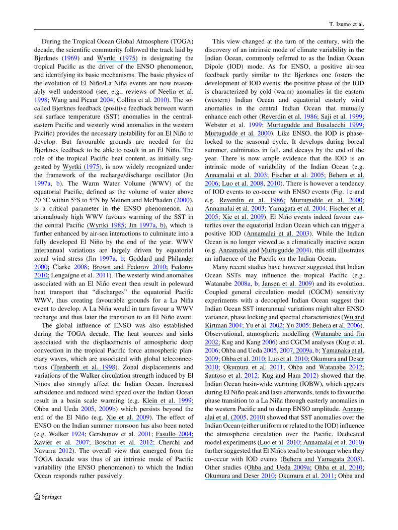
Influence of Indian Ocean Dipole and Pacific recharge on following year’s El Nin ˜ o: interdecadal robustness Takeshi Izumo • Matthieu Lengaigne • Je ´ro ˆme Vialard • Jing-Jia Luo • Toshio Yamagata • Gurvan Madec Received: 14 August 2012 / Accepted: 7 December 2012 Ó Springer-Verlag Berlin Heidelberg 2013 Abstract The Indian Ocean Dipole (IOD) can affect the El Nin ˜o–Southern Oscillation (ENSO) state of the fol- lowing year, in addition to the well-known preconditioning by equatorial Pacific Warm Water Volume (WWV), as suggested by a study based on observations over the recent satellite era (1981–2009). The present paper explores the interdecadal robustness of this result over the 1872–2008 period. To this end, we develop a robust IOD index, which well exploits sparse historical observations in the tropical Indian Ocean, and an efficient proxy of WWV interannual variations based on the temporal integral of Pacific zonal wind stress (of a historical atmospheric reanalysis). A lin- ear regression hindcast model based on these two indices in boreal fall explains 50 % of ENSO peak variance 14 months later, with significant contributions from both the IOD and WWV over most of the historical period and a similar skill for El Nin ˜o and La Nin ˜a events. Our results further reveal that, when combined with WWV, the IOD index provides a larger ENSO hindcast skill improvement than the Indian Ocean basin-wide mode, the Indian Mon- soon or ENSO itself. Based on these results, we propose a revised scheme of Indo-Pacific interactions. In this scheme, the IOD–ENSO interactions favour a biennial timescale and interact with the slower recharge-discharge cycle intrinsic to the Pacific Ocean. Keywords El Nin ˜o–Southern Oscillation (ENSO) Indian Ocean Dipole Warm Water Volume (WWV) recharge-discharge of the equatorial Pacific Ocean Indian and Asian monsoons Tropical Tropospheric Biennial Oscillation (TBO) Interannual and interdecadal climate variability and predictability Walker circulation Air-sea interactions Tropical Indo-Pacific Indian Ocean basin- wide warming/cooling (IOBW) Observational uncertainties 1 Introduction In a seminal paper, Sir Gilbert Walker wrote ‘‘By the Southern Oscillation it is implied the tendency of pressure at stations in the Pacific (…), and of rainfall in India and Java (…) to increase while pressure in the region of the Indian Ocean (…) decreases’’ (Walker 1924). He had come to identify what would be later known as the El Nin ˜o– Southern Oscillation (ENSO) phenomenon, and was clearly describing it as a phenomenon encompassing both the Indian and Pacific Oceans. T. Izumo T. Yamagata University of Tokyo, Tokyo, Japan Present Address: T. Izumo (&) M. Lengaigne J. Vialard G. Madec Laboratoire d’Oce ´anographie: Expe ´rimentation et Approches Nume ´riques (LOCEAN), IRD, CNRS, UPMC, Case 100, 4 Place Jussieu, 75252 Paris Cedex 05, France e-mail: [email protected] J.-J. Luo Research Institute for Global Change, JAMSTEC, Yokohama, Japan Present Address: J.-J. Luo CAWCR, Bureau of Meteorology, Melbourne, Australia Present Address: T. Yamagata Application Laboratory, JAMSTEC, Yokohama, Japan G. Madec National Oceanographic Centre, Southampton, UK 123 Clim Dyn DOI 10.1007/s00382-012-1628-1
-
Upload
independent -
Category
Documents
-
view
0 -
download
0
Transcript of Influence of Indian Ocean Dipole and Pacific recharge on following year’s El Niño: interdecadal...
Influence of Indian Ocean Dipole and Pacific rechargeon following year’s El Nino: interdecadal robustness
Takeshi Izumo • Matthieu Lengaigne •
Jerome Vialard • Jing-Jia Luo • Toshio Yamagata •
Gurvan Madec
Received: 14 August 2012 / Accepted: 7 December 2012! Springer-Verlag Berlin Heidelberg 2013
Abstract The Indian Ocean Dipole (IOD) can affect theEl Nino–Southern Oscillation (ENSO) state of the fol-
lowing year, in addition to the well-known preconditioning
by equatorial Pacific Warm Water Volume (WWV), assuggested by a study based on observations over the recent
satellite era (1981–2009). The present paper explores the
interdecadal robustness of this result over the 1872–2008period. To this end, we develop a robust IOD index, which
well exploits sparse historical observations in the tropical
Indian Ocean, and an efficient proxy of WWV interannualvariations based on the temporal integral of Pacific zonal
wind stress (of a historical atmospheric reanalysis). A lin-
ear regression hindcast model based on these two indices in
boreal fall explains 50 % of ENSO peak variance14 months later, with significant contributions from both
the IOD and WWV over most of the historical period and a
similar skill for El Nino and La Nina events. Our resultsfurther reveal that, when combined with WWV, the IOD
index provides a larger ENSO hindcast skill improvement
than the Indian Ocean basin-wide mode, the Indian Mon-soon or ENSO itself. Based on these results, we propose a
revised scheme of Indo-Pacific interactions. In this scheme,
the IOD–ENSO interactions favour a biennial timescaleand interact with the slower recharge-discharge cycle
intrinsic to the Pacific Ocean.
Keywords El Nino–Southern Oscillation (ENSO) !Indian Ocean Dipole ! Warm Water Volume (WWV)
recharge-discharge of the equatorial Pacific Ocean ! Indianand Asian monsoons ! Tropical Tropospheric Biennial
Oscillation (TBO) ! Interannual and interdecadal climate
variability and predictability ! Walker circulation ! Air-seainteractions ! Tropical Indo-Pacific ! Indian Ocean basin-
wide warming/cooling (IOBW) ! Observationaluncertainties
1 Introduction
In a seminal paper, Sir Gilbert Walker wrote ‘‘By the
Southern Oscillation it is implied the tendency of pressure
at stations in the Pacific (…), and of rainfall in India andJava (…) to increase while pressure in the region of the
Indian Ocean (…) decreases’’ (Walker 1924). He had come
to identify what would be later known as the El Nino–Southern Oscillation (ENSO) phenomenon, and was
clearly describing it as a phenomenon encompassing both
the Indian and Pacific Oceans.
T. Izumo ! T. YamagataUniversity of Tokyo, Tokyo, Japan
Present Address:T. Izumo (&) ! M. Lengaigne ! J. Vialard ! G. MadecLaboratoire d’Oceanographie: Experimentation et ApprochesNumeriques (LOCEAN), IRD, CNRS, UPMC,Case 100, 4 Place Jussieu, 75252 Paris Cedex 05, Francee-mail: [email protected]
J.-J. LuoResearch Institute for Global Change, JAMSTEC,Yokohama, Japan
Present Address:J.-J. LuoCAWCR, Bureau of Meteorology, Melbourne, Australia
Present Address:T. YamagataApplication Laboratory, JAMSTEC, Yokohama, Japan
G. MadecNational Oceanographic Centre, Southampton, UK
123
Clim Dyn
DOI 10.1007/s00382-012-1628-1
During the Tropical Ocean Global Atmosphere (TOGA)
decade, the scientific community followed the track laid byBjerknes (1969) and Wyrtki (1975) in designating the
tropical Pacific as the driver of the ENSO phenomenon,
and identifying its basic mechanisms. The basic physics ofthe evolution of El Nino/La Nina events are now reason-
ably well understood (see, e.g., reviews of Neelin et al.
1998; Wang and Picaut 2004; Collins et al. 2010). The so-called Bjerknes feedback (positive feedback between warm
sea surface temperature (SST) anomalies in the central-eastern Pacific and westerly wind anomalies in the western
Pacific) provides the necessary instability for an El Nino to
develop. But favourable grounds are needed for theBjerknes feedback to be able to result in an El Nino. The
role of the tropical Pacific heat content, as initially sug-
gested by Wyrtki (1975), is now widely recognized underthe framework of the recharge/discharge oscillator (Jin
1997a, b). The Warm Water Volume (WWV) of the
equatorial Pacific, defined as the volume of water above20 "C within 5"S to 5"N by Meinen and McPhaden (2000),
is a critical parameter in the ENSO phenomenon. An
anomalously high WWV favours warming of the SST inthe central Pacific (Wyrtki 1985; Jin 1997a, b), which is
further enhanced by air-sea interactions to culminate into a
fully developed El Nino by the end of the year. WWVinterannual variations are largely driven by equatorial
zonal wind stress (Jin 1997a, b; Goddard and Philander
2000; Clarke 2008; Brown and Fedorov 2010; Fedorov2010; Lengaigne et al. 2011). The westerly wind anomalies
associated with an El Nino event then result in poleward
heat transport that ‘‘discharges’’ the equatorial PacificWWV, thus creating favourable grounds for a La Nina
event to develop. A La Nina would in turn favour a WWV
recharge and thus later the transition to an El Nino event.The global influence of ENSO was also established
during the TOGA decade. The heat sources and sinks
associated with the displacements of atmospheric deepconvection in the tropical Pacific force atmospheric plan-
etary waves, which are associated with global teleconnec-
tions (Trenberth et al. 1998). Zonal displacements andvariations of the Walker circulation strength induced by El
Ninos also strongly affect the Indian Ocean. Increased
subsidence and reduced wind speed over the Indian Oceanresult in a basin scale warming (e.g. Klein et al. 1999;
Ohba and Ueda 2005, 2009b) which persists beyond the
end of the El Nino (e.g. Xie et al. 2009). The effect ofENSO on the Indian summer monsoon has also been noted
(e.g. Walker 1924; Gershunov et al. 2001; Fasullo 2004;
Xavier et al. 2007; Boschat et al. 2012; Cherchi andNavarra 2012). The overall view that emerged from the
TOGA decade was thus of an intrinsic mode of Pacific
variability (the ENSO phenomenon) to which the IndianOcean responds rather passively.
This view changed at the turn of the century, with the
discovery of an intrinsic mode of climate variability in theIndian Ocean, commonly referred to as the Indian Ocean
Dipole (IOD) mode. As for ENSO, a positive air-sea
feedback partly similar to the Bjerknes one fosters thedevelopment of IOD events: the positive phase of the IOD
is characterized by cold (warm) anomalies in the eastern
(western) Indian Ocean and equatorial easterly windanomalies in the central Indian Ocean that mutually
enhance each other (Reverdin et al. 1986; Saji et al. 1999;Webster et al. 1999; Murtugudde and Busalacchi 1999;
Murtugudde et al. 2000). Like ENSO, the IOD is phase-
locked to the seasonal cycle. It develops during borealsummer, culminates in fall, and decays by the end of the
year. There is now ample evidence that the IOD is an
intrinsic mode of variability of the Indian Ocean (e.g.Annamalai et al. 2003; Fischer et al. 2005; Behera et al.
2006; Luo et al. 2008, 2010). There is however a tendency
of IOD events to co-occur with ENSO events (Fig. 1c ande.g. Reverdin et al. 1986; Murtugudde et al. 2000;
Annamalai et al. 2003; Yamagata et al. 2004; Fischer et al.
2005; Xie et al. 2009). El Nino events indeed favour eas-terlies over the equatorial Indian Ocean which can trigger a
positive IOD (Annamalai et al. 2003). While the Indian
Ocean is no longer viewed as a climatically inactive ocean(e.g. Annamalai and Murtugudde 2004), this still illustrates
an influence of the Pacific on the Indian Ocean.
Many recent studies have however suggested that IndianOcean SSTs may influence the tropical Pacific (e.g.
Watanabe 2008a, b; Jansen et al. 2009) and its evolution.
Coupled general circulation model (CGCM) sensitivityexperiments with a decoupled Indian Ocean suggest that
Indian Ocean SST interannual variations might alter ENSO
variance, phase locking and spectral characteristics (Wu andKirtman 2004; Yu et al. 2002; Yu 2005; Behera et al. 2006).
Observational, atmospheric modelling (Watanabe and Jin
2002; Kug and Kang 2006) and CGCM analyses (Kug et al.2006; Ohba and Ueda 2005, 2007, 2009a, b; Yamanaka et al.
2009; Ohba et al. 2010; Luo et al. 2010; Okumura and Deser
2010; Okumura et al. 2011; Ohba and Watanabe 2012;Santoso et al. 2012; Kug and Ham 2012) showed that the
Indian Ocean basin-wide warming (IOBW), which appears
during El Nino peak and lasts afterwards, tends to favour thephase transition to a La Nina through easterly anomalies in
the western Pacific and to damp ENSO amplitude. Annam-
alai et al. (2005, 2010) showed that SST anomalies over theIndian Ocean (either uniform or related to the IOD) influence
the atmospheric circulation over the Pacific. Dedicated
model experiments (Luo et al. 2010; Annamalai et al. 2010)further suggested that El Ninos tend to be stronger when they
co-occur with IOD events (Behera and Yamagata 2003).
Other studies (Ohba and Ueda 2009a; Ohba et al. 2010;Okumura and Deser 2010; Okumura et al. 2011; Ohba and
T. Izumo et al.
123
Watanabe 2012) have discussed the possible role of the
Indian Ocean basin-wide warming/cooling onto El Nino/LaNina asymmetries.
While most of the above studies focus on the synchro-
nous influence of the Indian Ocean on the Pacific, a few
studies have explored potential precursors of ENSO in the
Indian Ocean. Several early studies have indeed noticedthat interannual anomalies that lead to an El Nino event
appeared to be originating from the Indian Ocean (Barnett
1983; Yasunari 1985; Krishnamurti et al. 1986; Watanabe
(a)
(b)
(c)
(d)
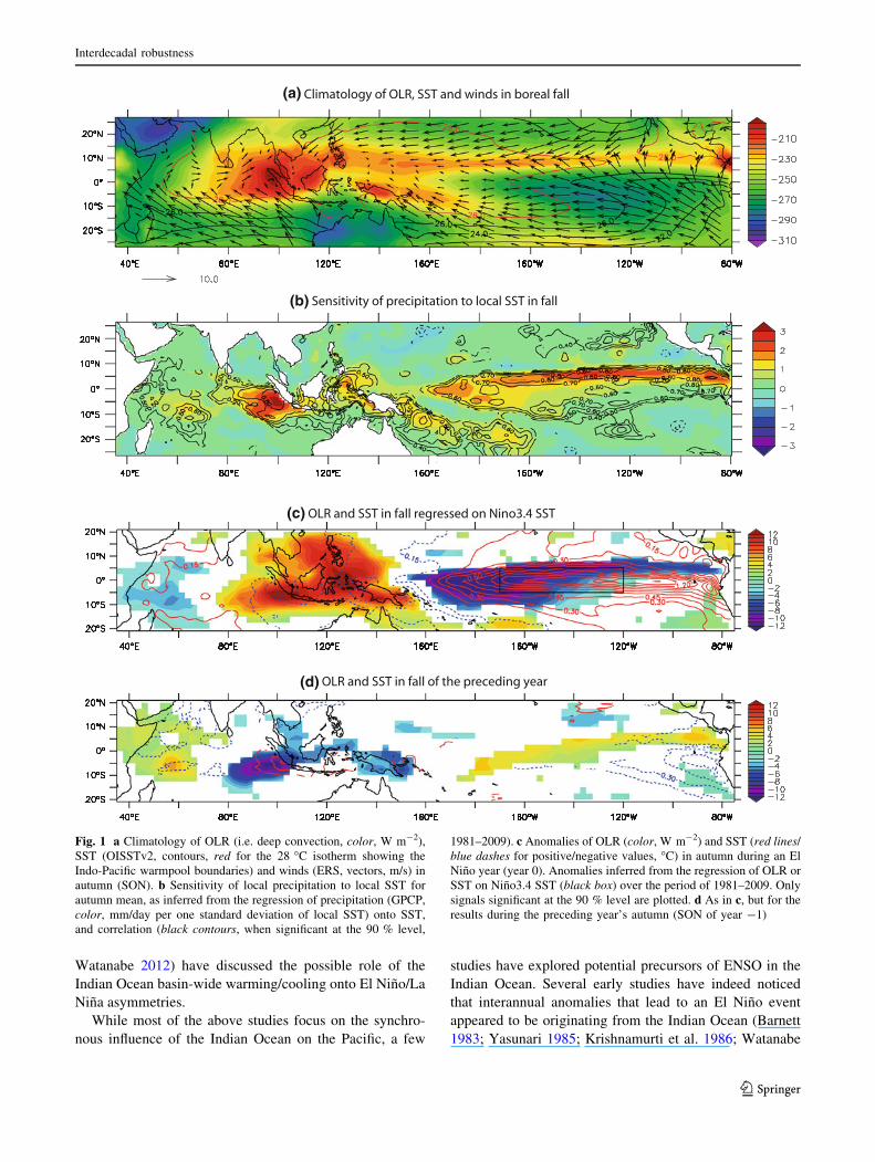
Fig. 1 a Climatology of OLR (i.e. deep convection, color, W m-2),SST (OISSTv2, contours, red for the 28 "C isotherm showing theIndo-Pacific warmpool boundaries) and winds (ERS, vectors, m/s) inautumn (SON). b Sensitivity of local precipitation to local SST forautumn mean, as inferred from the regression of precipitation (GPCP,color, mm/day per one standard deviation of local SST) onto SST,and correlation (black contours, when significant at the 90 % level,
1981–2009). c Anomalies of OLR (color, W m-2) and SST (red lines/blue dashes for positive/negative values, "C) in autumn during an ElNino year (year 0). Anomalies inferred from the regression of OLR orSST on Nino3.4 SST (black box) over the period of 1981–2009. Onlysignals significant at the 90 % level are plotted. d As in c, but for theresults during the preceding year’s autumn (SON of year -1)
Interdecadal robustness
123
2008b) and maritime continent (Nicholls 1984). This fea-
ture was exploited in a statistical forecasting scheme byClarke and van Gorder (2003): in their scheme, zonal wind
anomalies in the Indian Ocean are used as a predictor to the
ENSO peak occurring 1 year later. Terray and Dominiak(2005) also noted that cold SST anomalies in the south-
eastern Tropical Indian Ocean in February–March serve as
an efficient predictor of the El Nino peak 10 months later.The influence of the Indian Ocean on the Pacific the fol-
lowing seasons was also suggested to be through themonsoon, and was built into the Tropical Tropospheric
Biennial Oscillation (TBO; e.g. Meehl 1987; Meehl et al.
2003), a framework to explain the biennial tendency in thesystem formed by the Indian and Australian monsoons,
Indian Ocean SST, and ENSO. However, the mechanism
for the observed eastward propagation of zonal wind fromthe Indian Ocean to the Pacific remained unclear as pointed
out by Clarke 2008.
Izumo et al. (2010a; hereafter I10) recently suggestedthat a negative (positive) IOD in the Indian Ocean tends to
favour an El Nino (La Nina) about 14 months later
(Fig. 1d). They have further demonstrated that using anIOD index in addition to the WWV predictor in fall results
in a significant improvement of the prediction skill score of
the ENSO peak in winter about 14 months later. Theysuggested the following mechanism to explain the influ-
ence of the Indian Ocean on the Pacific. In boreal fall (the
peak season for the IOD), the strongest atmospheric con-vection in the tropics is found in the eastern equatorial
Indian Ocean (Fig. 1a), where the highest sensitivity of
precipitation to local SST is found (Fig. 1b) and whereIOD SST and related convection anomalies are strongest
(Fig. 1c). A developing IOD in this region can thus have a
significant influence on the ascending branch of the Walkercirculation, and hence on its strength. A negative IOD (i.e.
with positive SST anomalies in the eastern Indian Ocean)
hence externally forces equatorial Pacific easterly anoma-lies in fall, which suddenly relax in winter in association
with the IOD demise. Wave reflections in essence similar
to the delayed (Schopf and Suarez 1988; Battisti and Hirst1989) and advective-reflective oscillators (Picaut et al.
1997) act to reinforce the Pacific Ocean response to the
IOD-related winds and their relaxation, and drive eastwardcurrent anomalies and positive SST anomalies in the cen-
tral Pacific through zonal advection of the warm pool
eastern edge (the main process that controls SST variationsin the central Pacific, e.g. Vialard et al. 2001). These SST
anomalies may be amplified by the Bjerknes feedback and
culminate into an El Nino event at the end of the year. Onemust note that the scenario presented above describes the
influence of external forcing of the tropical Indian Ocean
on the Pacific Ocean. This effect will combine to theexisting internal dynamics of the tropical Pacific during the
onset phase, i.e. the preconditioning by the Pacific WWV
as described by the recharge oscillator theory (as do wes-terly wind bursts, e.g. Fedorov 2002). At the end, the two
effects (external forcing from the Indian Ocean and local
preconditioning in the Pacific) will combine (or opposeeach other) to influence the ENSO evolution during the
following year.
I10 obtained their results using recent high-qualitysatellite and in situ observations only available since 1981.
Many papers have however documented decadal changesin ENSO (e.g. An and Wang 2000; Wang and Picaut 2004;
Leloup et al. 2007) or IOD (e.g. Abram et al. 2008;
Ummenhofer et al. 2009) characteristics; or changes inlinks between the two modes (e.g. Terray et al. 2005;
Annamalai et al. 2005). As stated by Webster and Hoyos
(2010), it is important to test whether these interactions area feature of the Indian and Pacific climate that is not
restricted to the recent period. The first objective of this
paper is hence to investigate the interdecadal robustness ofI10’s scenario over a much longer period. In order to do
that, we define, after presenting datasets and methods in
Sect. 2, an improved IOD index that efficiently exploitssparse historical observations in the Indian Ocean (Sect.
3.1). Similarly, observed WWV is not available prior to the
1980’s due to insufficient subsurface observations. Sec-tion 3.2 shows that WWV can be efficiently reconstructed
by integrating zonal wind stress of the equatorial Pacific.
We hence reconstruct WWV from wind stress since the1870s (wind of the historical 20th Century atmospheric
reanalysis). In Sect. 4 we investigate the robustness and the
decadal stability of the IOD/WWV/ENSO relationshipsusing these historical indices, as well as possible asym-
metries in the skills of El Nino/La Nina predictions. We
also investigate a long coupled model simulation, and findsimilar results to the observations. Section 5.1 shows that
the IOD is a better predictor of following year’s ENSO
state than other climate indices (including the Indianmonsoon) over the historical 1870’s–2000’s period. Sec-
tion 5.2 discusses our results about the Indian Ocean–
Indian monsoon–ENSO relations in the context of theTBO. Section 6 provides a summary and a discussion of
our results and their potential applications.
2 Datasets and methods
2.1 Datasets
Depending on the period considered and to assess therobustness of the results, several SST observational data-
sets have been analysed. For the recent period, we use the
recent optimal interpolation (OI) SSTv2 from NationalOceanic and Atmospheric Administration (NOAA) that
T. Izumo et al.
123
blends in situ and satellite data sources (Reynolds et al.
2002) and is available from November 1981 onward. Overthe historical period, we use the HadiSSTv1.1 product
(Rayner et al. 2003) that is based on sparse ship datasets
before 1981 and is available from 1870 onwards. Reduced-space optimal interpolation allows filling gaps in data-
sparse oceanic regions. Because of the limitations inherent
to this approach, we recomputed our analyses with twoother products: ERSSTv3b (Smith et al. 2008) that uses an
interpolation strategy similar to HadiSSTv1.1, and Had-SST2 (Rayner et al. 2006) that does not use any interpo-
lation. Results derived from these datasets are consistent
with each other, except during the Second World Warwhen data were extremely sparse (cf. Sects. 3, 4). We also
analyse the density of in situ SST observations from
ICOADS (International Comprehensive Atmosphere–Ocean Data Set, http://icoads.noaa.gov) database, on which
the three SST products are based. The quality and sampling
issues before the satellite era are discussed in Sect. 3, byexploiting the accurate estimates of uncertainties available
in the HadSST2 product.
The subsurface oceanic conditions in the equatorialPacific are described using the Warm Water Volume index
(the volume of water above the 20 "C isotherm in the
[120"E–80"W, 5"N–5"S] region; hereafter WWV), madeavailable since 1980 at http://www.pmel.noaa.gov/tao/
elnino/wwv/ (Meinen and McPhaden 2000). This index is
derived from the Australian Bureau of Meteorology Rea-search Center tropical Pacific subsurface temperature
dataset (Smith 1995) that includes XBT measurements and
data from the Tropical Atmosphere Ocean (TAO) array. Ahistorical proxy for the WWV will be constructed from
1871 to present using zonal wind stress from the twentieth
century atmospheric reanalysis version 2 (20CR; Compoet al. 2011) that is forced by HadiSSTv1.1 SST dataset and
assimilates sea level pressure measurements. This proxy
will be validated over the recent period against theobserved WWV estimate described above. Interpolated
outgoing longwave radiation (OLR) from NOAA (Lieb-
mann and Smith 1996) is used as a proxy for deep atmo-spheric convection in the tropics, and is available since
1974 (with a gap in 1978). The GPCP precipitation dataset
(Huffman et al. 1997) and ERS1-2 scatterometer winds(1992–2001, Bentamy et al. 1996) are also used in Fig. 1.
The strength of the Indian summer monsoon is charac-
terized using the All Indian Rainfall (AIR) dataset, and therainfall over the Indian homogeneous regions defined by
the IITM, available from 1871 to 2008 (Parthasarathy et al.
1994). For the analysis of historical rainfall variabilityglobally in relation with previous year’s IOD and WWV,
we use GPCC land precipitation dataset based on in situ
gauges (Rudolf et al. 2010) and the precipitation from20CR reanalysis. Similarly, for historical sea level pressure
(SLP) variability, we use ICOADS SLP in situ observations
at sea, as well as SLP from 20CR reanalysis.Finally, we also analyse a 220 years-long climate sim-
ulation performed with the SINTEX-F coupled general
circulation model (GCM). This model is based on theOPA8.2 (Madec et al. 1998; former NEMO) ocean GCM
(ORCA2 grid; resolution of 2" zonally and 0.5" meridio-
nally near the equator) coupled to the ECHAM4 atmo-sphere GCM (Roeckner et al. 1996) at a T106 resolution
(1.125"). A detailed description of this model can be foundin Luo et al. (2005) and Masson et al. (2005). We use here
years 7–221 of the control experiment (CTL) used in Luo
et al. (2005).
2.2 Methods and indices
For datasets covering the recent period (1981–2010),
interannual variations have simply been computed by
subtracting the mean seasonal cycle from the original timeseries. Further linearly detrending the time series yields
very similar results. For datasets covering the historical
period (1871–2008) and coupled GCM outputs, trends anddecadal-to-multidecadal fluctuations have been removed
using a Hanning filter (almost all energy is preserved at
periods lower than 7 years, and half-power cut at 13 years).Due to filter edge effects, the first and last 6 years of the
time series are not considered in the analysis. Other types
of filtering methods (e.g. cutting at 5 or 9 years instead of7) give similar results.
Statistical relationships between two variables are
described using linear regression and simple correlations. Toextract a signal related to one index independently from
another one, we also use partial correlations (see, e.g. Ya-
magata et al. 2004) as well as multiple linear regressions (asin I10). Regression coefficients are computed from normal-
ized climate indices (i.e., divided by their standard deviation)
so that regression coefficients discussed in the paper hencecorrespond to the typical amplitude of the signals associated
with a given climate mode. Significance tests were computed
from Student’s two-tailed t test (assuming one degree offreedom per year throughout the paper, as the autocorrelation
at lag 1 year for the indices used here was either non-sig-
nificant or negative). ‘‘first-order’’ asymmetries betweenpositive and negative phases of IOD, ENSO or WWV are
identified using ‘‘one-way means’’, i.e. usual composites for
positive or negative events. More subtle ‘‘second-order’’asymmetries are identified using one-way correlations, i.e.
the correlation for the positive or negative phase (Hoerling
et al. 2001; Ohba et al. 2010).We use several classical definitions to describe the
variability associated with the IOD (Dipole Mode Index or
DMI), ENSO (Nino3.4), Indian Ocean basin-wide warm-ing/cooling (IOBW) associated with El Nino/La Nina
Interdecadal robustness
123
events, and All India Rainfall (AIR). The DMI is defined as
the September–November SST anomaly differencebetween [50"E–70"E, 10"S–10"N] and [90"E–110"E,
10"S–0"] following Saji et al. (1999). Observed ENSO
variability is characterized using the November–JanuarySST anomalies in the Nino3.4 region [170"W–120"W,
5"S–5"N]. IOBW variability is characterized as the Janu-
ary–March SST anomaly averaged over the entire tropicalIndian Ocean [40"E–110"E, 20"S–20"N]. AIR is defined as
the average June–September (JJAS) interannual rainfallanomaly over India. All indices are normalised by their
interannual standard deviations. Due to sparse in situ data
coverage before the satellite era, some of the above indicesare not properly sampled. More robust and homogeneous
indices over the historical period will be proposed in the
following section.
3 Construction of historical IOD and WWV indices
3.1 An improved historical IOD index
3.1.1 SST observational coverage
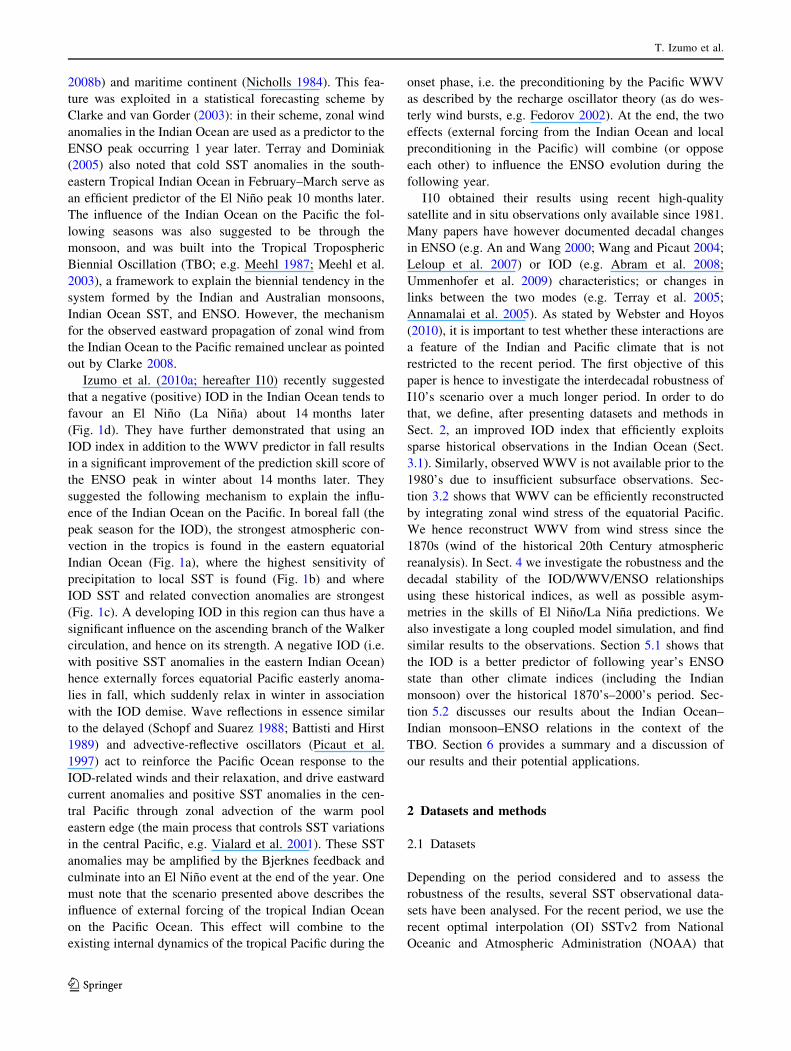
Figure 2a displays the density of observations for the pre-satellite era (1870–1979) in ICOADS (i.e. the database
used to construct most of available SST products). Regions
commonly used to define ENSO and DMI indices arepoorly spatially sampled (e.g. strong lack of observations
in the central equatorial Pacific). The time evolution of the
number of observations for the various boxes used to cal-culate these climate indices (Fig. 2b) reveals that obser-
vations are very sparse before the 1870’s. It then remains
relatively stable until the early 1980’s, except for twomajor drops observed during both world wars. As mea-
surement and sampling random errors available in Had-
SST2 dataset are assumed to be uncorrelated in space andtime, we thus estimate the error from the sum of their
squares at each grid point and for each of the 3 months
used for the spatio-temporal average (Fig. 2c). With anestimated sampling error of 30–50 % of interannual vari-
ability amplitude, the eastern DMI box is the most heavily
affected by sampling issues. The western DMI and theequatorial Pacific are better sampled (with sampling errors
respectively of *30 and *20 %), owing to their larger
covered areas and larger spatial (Figs. 1c, 3) and temporaldecorrelation scales than those of the smaller and shorter-
living IOD eastern pole, with moreover a historically well-
sampled ship route in the north Indian Ocean (Fig. 2a, cf.also Chowdary et al. 2012) capturing IOD western pole
variability (Fig. 3). The sampling errors increase dramati-
cally during both world wars, especially affecting easternpole sampling.
3.1.2 A regression-based IODhist index
The above analyses suggest that conventional ENSO andIOD indices should be interpreted cautiously before 1981,
because of the sparse data sampling. Obviously, these data
are much more reliable from 1981 onwards, as in situ dataare complemented by satellite data. A possible way to
reduce sampling-related uncertainties during the historical
period is to define indices with a spatially and/or tempo-rally extended average, as recently proposed for ENSO
index by Bunge and Clarke (2009). They used an EOF
technique to interpolate spatio-temporally the sparse SSTobservations available before the 1980’s, exploiting a much
larger area of SST measurements than Nino3.4. Compared
to the conventional Nino3.4 SST index, their Nino3.4hist
index is thus an improved ENSO index (available from
1872 to 2008), which better matches with a similarly
reconstructed ESOIhist index based on historical sea levelpressure data. We hence use this Nino3.4hist index for
historical analyses throughout the present study (using their
ESOIhist gives similar results).To build a robust IOD index over the historical period,
we follow a relatively similar strategy based on a spatial
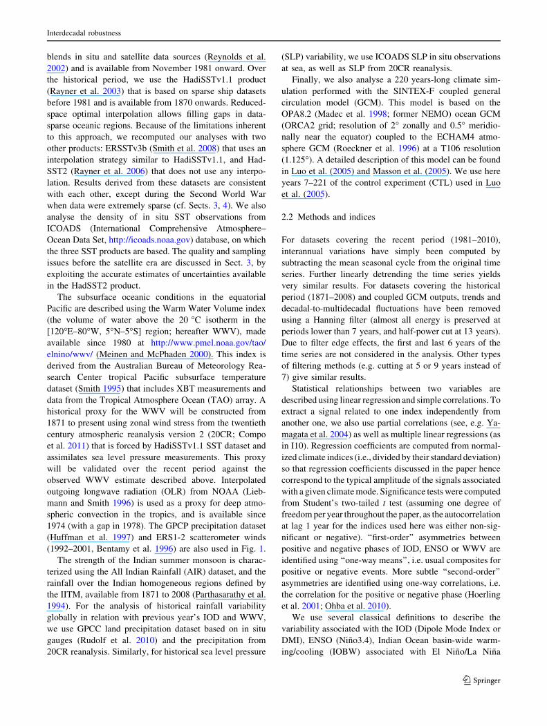
linear regression (an EOF-based method led to similarresults). Figure 3 shows the regression coefficients in the
Indian Ocean of the DMI index onto September–November
SST over the recent period (1981–2009). We build a newindex, referred to as IODhist, by projecting the September–
November SST anomalies on that spatial pattern wherever
the regression coefficient is significant above the 90 %level over the tropical Indian Ocean. The correlation
between IODhist and the DMI exceeds 0.9 for both the
recent and historical period, and for the three SST datasets.In the present study, both the conventional DMI and the
IODhist index are used; they give qualitatively similar
results. However, using DMI results in weaker correlationsand statistical significances, especially around World War
II, a period heavily affected by data sampling issues. We
also tested the sensitivity of the results to the SST productused (HadiSST, HadSST2 or ERSSTv3b). All products led
to similar results when using IODhist, but to quantitatively
different interdecadal variations when using DMI (cf. Sect.4.1).
3.2 An historical WWV proxy
Physically, interannual variations of the WWV (or equiv-
alently equatorial Pacific averaged thermocline depth ‘‘h’’)are mainly caused by Sverdup transport across the basin,
which is proportional to the zonal windstress sx along theequatorial Pacific (e.g. Jin 1997a). This is translated into
mathematical terms by the WWV recharge-discharge
equation (Jin 1997a, b):
T. Izumo et al.
123
(a)
(b)
(c)
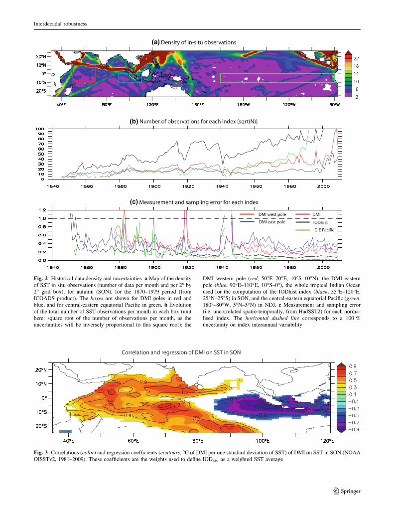
Fig. 2 Historical data density and uncertainties. a Map of the densityof SST in situ observations (number of data per month and per 2" by2" grid box), for autumn (SON), for the 1870–1979 period (fromICOADS product). The boxes are shown for DMI poles in red andblue, and for central-eastern equatorial Pacific in green. b Evolutionof the total number of SST observations per month in each box (unithere: square root of the number of observations per month, as theuncertainties will be inversely proportional to this square root): the
DMI western pole (red, 50"E–70"E, 10"S–10"N), the DMI easternpole (blue, 90"E–110"E, 10"S–0"), the whole tropical Indian Oceanused for the computation of the IODhist index (black, 35"E–120"E,25"N–25"S) in SON, and the central-eastern equatorial Pacific (green,180"–80"W, 5"N–5"N) in NDJ. c Measurement and sampling error(i.e. uncorrelated spatio-temporally, from HadSST2) for each norma-lised index. The horizontal dashed line corresponds to a 100 %uncertainty on index interannual variability
Fig. 3 Correlations (color) and regression coefficients (contours, "C of DMI per one standard deviation of SST) of DMI on SST in SON (NOAAOISSTv2, 1981–2009). These coefficients are the weights used to define IODhist as a weighted SST average
Interdecadal robustness
123
dWWV=dt " #rWWV# asx $1%
Burgers et al. (2005) showed from a fit to observations that
the damping term r was not significantly different from zero.
This implies that WWV could be derived from temporalintegration of equatorial Pacific zonal windstress variations.
A fit between observed dWWV/dt and 20CR zonal wind
stress within the equatorial Pacific wave guide (130"E–80"W, 2"S–2"N) provides a value for a = 6.1 9
108 m5 N-1 s-1 (using a low-pass filter removing periods
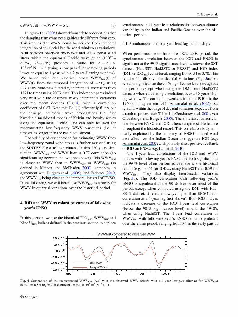
lower or equal to 1 year, with a 2 years Hanning window).We hence build our historical proxy WWVhist(t) of
WWV(t) from the temporal integration of -asx, using
2–7 years band-pass filtered sx interannual anomalies from1871 to time t using 20CR data. This index compares indeed
very well with the observed WWV interannual variations
over the recent decades (Fig. 4), with a correlationcoefficient of 0.87. Note that Eq. (1) effectively filters out
the principal equatorial wave propagations (i.e. first
baroclinic meridional modes of Kelvin and Rossby wavesalong the equatorial Pacific), and can only be used for
reconstructing low-frequency WWV variations (i.e. at
timescales longer than the basin adjustment).The validity of our approach for estimating WWV from
low-frequency zonal wind stress is further assessed using
the SINTEX-F control experiment. In this 220 years sim-ulation, WWVhist and WWV have a 0.77 correlation (no
significant lag between the two; not shown). This WWVhist
is closer to WWV than to WWVwest or WWVeast (as
defined in Meinen and McPhaden 2000), somehow in
agreement with Burgers et al. (2005), and Fedorov (2010,the WWVhist being close to the temporal integral of ENSO.
In the following, we will hence use WWVhist as a proxy for
WWV interannual variations over the historical period.
4 IOD and WWV as robust precursors of followingyear’s ENSO
In this section, we use the historical IODhist, WWVhist andNino34hist indices defined in the previous section to explore
synchronous and 1-year lead relationships between climate
variability in the Indian and Pacific Oceans over the his-torical period.
4.1 Simultaneous and one year lead-lag relationships
When performed over the entire 1872–2008 period, the
synchronous correlation between the IOD and ENSO issignificant at the 99 % significance level, whatever the SST
dataset (HadiSST, HadSST2 or ERSST) and IOD index(DMI or IODhist) considered, ranging from 0.54 to 0.70. This
relationship displays interdecadal variations (Fig. 5a), but
remains significant at the 90 % significance level throughoutthe period (except when using the DMI from HadSST2
dataset) when calculating correlations over a 30 years slid-
ing window. The correlation weakens from the 1940’s to the1960’s, in agreement with Annamalai et al. (2005) but
remains within the range of decadal variations expected from
a random process (see Table 1 in Gershunov et al. 2001; vanOldenborgh and Burgers 2005). The simultaneous correla-
tion between ENSO and IOD is hence a quite stable feature
throughout the historical record. This correlation is dynam-ically explained by the tendency of ENSO-induced wind
anomalies over the Indian Ocean to trigger an IOD (e.g.
Annamalai et al. 2003; with possibly also a positive feedbackof IOD on ENSO, e.g. Luo et al. 2010).
The 1-year lead correlations of the IOD and WWV
indices with following year’s ENSO are both significant atthe 99 % level when performed over the whole historical
record (e.g. -0.44 for IODhist using HadiSST and 0.59 for
WWVhist). They also display interdecadal variations(Fig. 5b). The IOD correlation with following year’s
ENSO is significant at the 90 % level over most of the
period, except when computed using the DMI with Had-SST2 dataset. It remains always higher than ENSO auto-
correlation at a 1-year lag (not shown). Both IOD indices
indicate a decrease of the IOD 1-year lead correlation(below the 90 % significance level) around the 1940’s
when using HadiSST. The 1-year lead correlation of
WWVhist with following year’s ENSO remain significantover the entire period, ranging from 0.4 in the early part of
Fig. 4 Comparison of the reconstructed WWVhist (red) with the observed WWV (black, with a 1-year low-pass filter as for WWVhist;correl. = 0.87; regression coefficient = 6.1 9 108 m5 N-1 s-1)
T. Izumo et al.
123
the record to 0.7 in the 1940’s. In general, the tendency of
the IOD to precede ENSO by 1 year is relatively stable,although not as much as the recharge mechanism or as the
simultaneous correlation between ENSO and IOD.
4.2 ENSO one year-lead hindcast using IOD
and WWV indices
I10 showed the benefit of including IOD information in a
multiple linear regression model based on the WWV andIOD indices in SON to predict the ENSO state 14 months
later, with a skill score of *0.8 over the 1981–2009 period.
Their results suggested an equivalent importance of theIOD external forcing and Pacific heat content at 1-year
lead. A similar analysis is conducted over the entire
1872–2008 period using the WWVhist and IODhist indices.Figure 6 shows the time series of the Nino3.4hist index and
the 14-month lead hindcast using WWVhist and IODhist
over the entire period. This hindcast has a skill score of0.72 (significant at the 99 % level), only slightly weaker
compared to I10 study for the recent period. The relative
contributions of -IOD and WWV, inferred from norma-lised coefficients, are respectively of 0.40 ± 0.10 and
0.57 ± 0.10, the difference between the two coefficients
being non-significant at the 90 % level. A similar skill of0.71 is found when using an equal weight for the IOD and
the WWV. This underlines that, over the entire historical
period, the contributions of WWV and IOD to the fol-lowing year’s ENSO were almost equivalent (as in I10).
Computing this multiple linear regression using point-
wise HadiSST SST instead of the IODhist index shows adistinct IOD-like dipolar pattern in the Indian Ocean SST
precursors to El Nino 14 months later (not shown). A
higher skill score is however obtained when using thewestern (0.72) rather than the eastern pole (0.62) of the
(a)
(b)
(c)
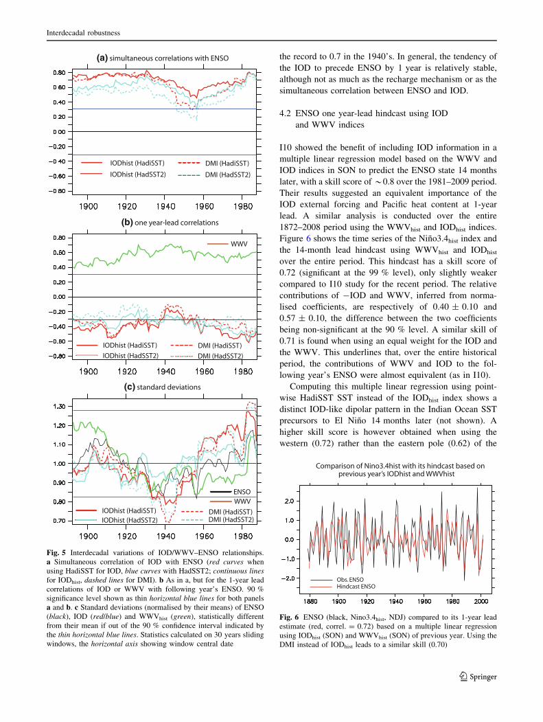
Fig. 5 Interdecadal variations of IOD/WWV–ENSO relationships.a Simultaneous correlation of IOD with ENSO (red curves whenusing HadiSST for IOD, blue curves with HadSST2; continuous linesfor IODhist, dashed lines for DMI). b As in a, but for the 1-year leadcorrelations of IOD or WWV with following year’s ENSO. 90 %significance level shown as thin horizontal blue lines for both panelsa and b. c Standard deviations (normalised by their means) of ENSO(black), IOD (red/blue) and WWVhist (green), statistically differentfrom their mean if out of the 90 % confidence interval indicated bythe thin horizontal blue lines. Statistics calculated on 30 years slidingwindows, the horizontal axis showing window central date
Fig. 6 ENSO (black, Nino3.4hist, NDJ) compared to its 1-year leadestimate (red, correl. = 0.72) based on a multiple linear regressionusing IODhist (SON) and WWVhist (SON) of previous year. Using theDMI instead of IODhist leads to a similar skill (0.70)
Interdecadal robustness
123
IOD over the historical period. This difference in skill
score may be related to observational issues: as shown inSect. 3.1, there is a poor observational coverage of the IOD
eastern pole over most of the historical (pre-satellite) per-
iod, while the western pole interannual SST variations arebetter sampled. Over the recent 1981–2010 satellite period
indeed there are insignificant skill score differences
between the two poles, while using an OLR-based indicatorof deep atmospheric convection (cf. I10) results in a higher
score for the eastern pole of the IOD (not shown). While itis difficult to conclude which pole of the IOD is the most
efficient predictor from historical data, it remains clear that
both poles bring added predictability during boreal fall, theperiod of the year with strongest IOD signals.
Figure 7a shows the interdecadal fluctuations of the
14 months-lead ENSO hindcast skill (black line) and thesimple correlation of ENSO with IOD (red) and WWV
(green) 14 months before. The skill is stable throughout the
period with a skill score ranging from *0.65 to *0.8.Both IOD and WWV’s independent contributions always
remain significantly above zero at the 90 % level (Fig. 7b).
The IOD almost always brings a significant contribution inaddition to the WWV. The IOD contribution to the ENSO
hindcast reaches a minimum around 1940–1960 (Fig. 7b),i.e. a period with statistically weaker IOD influence and
relatively stronger WWV influence (the difference is sig-
nificant at the 90 % level), whereas the IOD and WWVcontribute equally during the early and late parts of the
record. Interestingly the *1940–1960 minimum period
corresponds to a period when ENSO amplitude (Fig. 5c)and frequency were lower with weaker biennality (as
inferred from wavelet and autocorrelation analyses; not
shown).These results show that the I10 results are valid over the
much longer 1872–2008 period, although there appears to
be significant decadal fluctuations in the contribution of theIOD to next year’s ENSO predictability. Other IOD and
ENSO indices give very consistent results.
4.3 Comparing skills of El Nino/La Nina hindcasts
In this subsection, we investigate potential asymmetries inthe 1-year lead/lag relation between IOD and ENSO to
infer if the mechanism proposed by I10 operates for both
positive and negative phases of ENSO. To qualitativelyand quantitatively assess possible asymmetries, we thus
display scatterplots between IOD, WWV, hindcasted
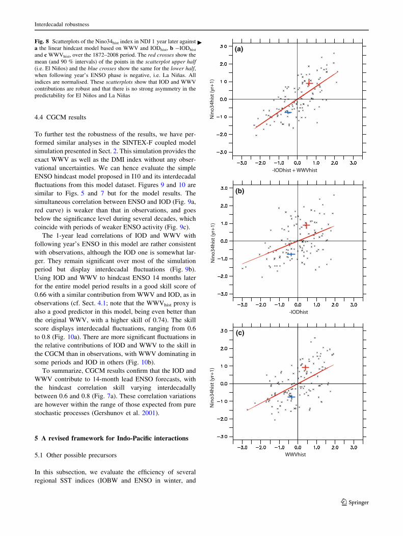
ENSO amplitudes and observed ENSO amplitudes(Fig. 8). Figure 8a shows that the 14-month lead El Nino
hindcast performs as well for El Nino and for La Nina.
This comes partly from the equivalent efficiency of WWVto predict positive and negative phases of ENSO
(Fig. 8c). But this also comes partly from the fact that El
Ninos (La Ninas) are on average preceded by negative(positive) IODs. There might be a slight asymmetry in the
slope of the IOD versus Nino3.4 regression due to
Nino3.4 and IOD skewnesses (not shown). But quantita-tively, there is no significant first-order asymmetry
between the 14-month lead IODhist value before an El
Nino (-0.44 ± 0.19, cf. crosses in Fig. 8b) and a La Nina(0.36 ± 0.20, Fig. 8b). We also computed one-way cor-
relations, but could not identify any consistent and sig-
nificant second-order asymmetries when comparing thevarious indices (not shown). The lead-lag IOD–ENSO
relationship hence operates for both positive and negative
phases of ENSO (and for both positive and negativephases of IOD).
(a)
(b)
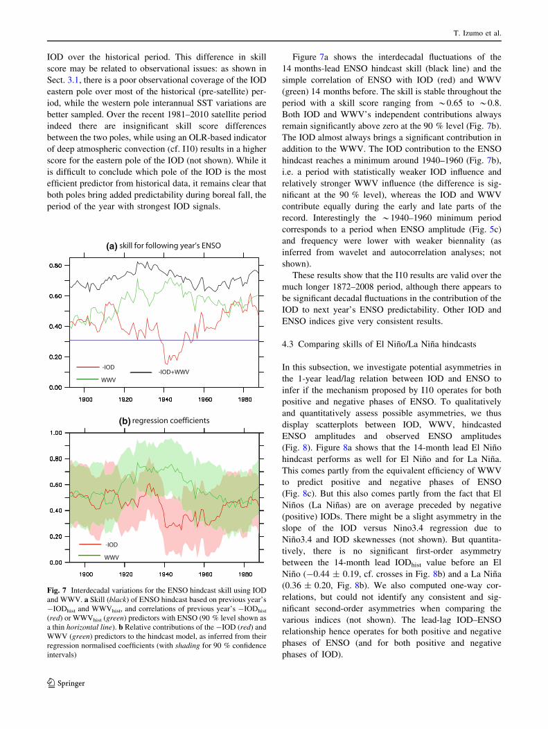
Fig. 7 Interdecadal variations for the ENSO hindcast skill using IODand WWV. a Skill (black) of ENSO hindcast based on previous year’s-IODhist and WWVhist, and correlations of previous year’s -IODhist
(red) or WWVhist (green) predictors with ENSO (90 % level shown asa thin horizontal line). b Relative contributions of the -IOD (red) andWWV (green) predictors to the hindcast model, as inferred from theirregression normalised coefficients (with shading for 90 % confidenceintervals)
T. Izumo et al.
123
4.4 CGCM results
To further test the robustness of the results, we have per-formed similar analyses in the SINTEX-F coupled model
simulation presented in Sect. 2. This simulation provides the
exact WWV as well as the DMI index without any obser-vational uncertainties. We can hence evaluate the simple
ENSO hindcast model proposed in I10 and its interdecadal
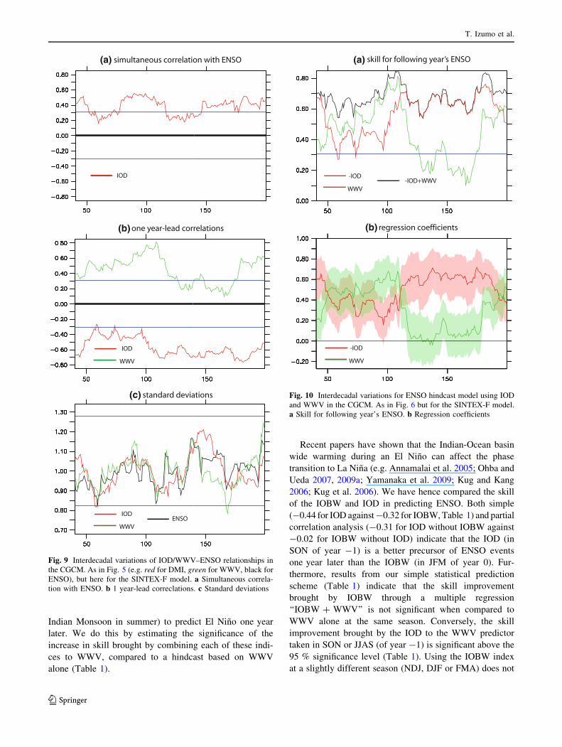
fluctuations from this model dataset. Figures 9 and 10 aresimilar to Figs. 5 and 7 but for the model results. The
simultaneous correlation between ENSO and IOD (Fig. 9a,
red curve) is weaker than that in observations, and goesbelow the significance level during several decades, which
coincide with periods of weaker ENSO activity (Fig. 9c).
The 1-year lead correlations of IOD and WWV withfollowing year’s ENSO in this model are rather consistent
with observations, although the IOD one is somewhat lar-
ger. They remain significant over most of the simulationperiod but display interdecadal fluctuations (Fig. 9b).
Using IOD and WWV to hindcast ENSO 14 months later
for the entire model period results in a good skill score of0.66 with a similar contribution from WWV and IOD, as in
observations (cf. Sect. 4.1; note that the WWVhist proxy is
also a good predictor in this model, being even better thanthe original WWV, with a higher skill of 0.74). The skill
score displays interdecadal fluctuations, ranging from 0.6
to 0.8 (Fig. 10a). There are more significant fluctuations inthe relative contributions of IOD and WWV to the skill in
the CGCM than in observations, with WWV dominating in
some periods and IOD in others (Fig. 10b).To summarize, CGCM results confirm that the IOD and
WWV contribute to 14-month lead ENSO forecasts, with
the hindcast correlation skill varying interdecadallybetween 0.6 and 0.8 (Fig. 7a). These correlation variations
are however within the range of those expected from pure
stochastic processes (Gershunov et al. 2001).
5 A revised framework for Indo-Pacific interactions
5.1 Other possible precursors
In this subsection, we evaluate the efficiency of several
regional SST indices (IOBW and ENSO in winter, and
Fig. 8 Scatterplots of the Nino34hist index in NDJ 1 year later againsta the linear hindcast model based on WWV and IODhist, b -IODhist
and c WWVhist, over the 1872–2008 period. The red crosses show themean (and 90 % intervals) of the points in the scatterplot upper half(i.e. El Ninos) and the blue crosses show the same for the lower half,when following year’s ENSO phase is negative, i.e. La Ninas. Allindices are normalised. These scatterplots show that IOD and WWVcontributions are robust and that there is no strong asymmetry in thepredictability for El Ninos and La Ninas
c
Interdecadal robustness
123
Indian Monsoon in summer) to predict El Nino one yearlater. We do this by estimating the significance of the
increase in skill brought by combining each of these indi-
ces to WWV, compared to a hindcast based on WWValone (Table 1).
Recent papers have shown that the Indian-Ocean basinwide warming during an El Nino can affect the phase
transition to La Nina (e.g. Annamalai et al. 2005; Ohba and
Ueda 2007, 2009a; Yamanaka et al. 2009; Kug and Kang2006; Kug et al. 2006). We have hence compared the skill
of the IOBW and IOD in predicting ENSO. Both simple
(-0.44 for IOD against -0.32 for IOBW, Table 1) and partialcorrelation analysis (-0.31 for IOD without IOBW against
-0.02 for IOBW without IOD) indicate that the IOD (in
SON of year -1) is a better precursor of ENSO eventsone year later than the IOBW (in JFM of year 0). Fur-
thermore, results from our simple statistical prediction
scheme (Table 1) indicate that the skill improvementbrought by IOBW through a multiple regression
‘‘IOBW ? WWV’’ is not significant when compared to
WWV alone at the same season. Conversely, the skillimprovement brought by the IOD to the WWV predictor
taken in SON or JJAS (of year -1) is significant above the
95 % significance level (Table 1). Using the IOBW indexat a slightly different season (NDJ, DJF or FMA) does not
(a)
(b)
(c)
Fig. 9 Interdecadal variations of IOD/WWV–ENSO relationships inthe CGCM. As in Fig. 5 (e.g. red for DMI, green for WWV, black forENSO), but here for the SINTEX-F model. a Simultaneous correla-tion with ENSO. b 1 year-lead correclations. c Standard deviations
(a)
(b)
Fig. 10 Interdecadal variations for ENSO hindcast model using IODand WWV in the CGCM. As in Fig. 6 but for the SINTEX-F model.a Skill for following year’s ENSO. b Regression coefficients
T. Izumo et al.
123
change the above conclusions. This result may seem at odd
with the extensive literature that shows that the IOBW actsas a negative feedback on ENSO, concurring to the demise
of ENSO events and promoting a rapid phase transition,
possibly asymmetric (Kug and Kang 2006; Ohba and Ueda2007, 2009a; Yamanaka et al. 2009; Ohba et al. 2010; Luo
et al. 2010; Okumura and Deser 2010; Okumura et al.
2011; Ohba and Watanabe 2012). Our interpretation fol-lows: as the IOBW is intimately tied to the ENSO cycle
(ENSO/IOBW squared correlation, i.e. explained variance,of 66 %), its influence on ENSO is rather systematic. Each
El Nino/La Nina event promotes an Indian Ocean basin-
wide warming/cooling that systematically acts to promotethe transition to ENSO opposite phase one year later. This
tight ENSO/IOBW relationship is probably the reason why
including an IOBW index does not significantly improveENSO prediction. In contrast, the IOD is more independent
from the ENSO cycle (IOD/ENSO squared correlation of
49 %) and hence brings an external forcing (on Pacificwind, cf. I10) more independent of the ENSO cycle. The
fact that the IOD is a more robust ENSO predictor than the
IOBW does not preclude a systematic influence of theIOBW on ENSO. As for the IOBW, ENSO itself is not a
significant predictor of following year’s ENSO throughout
the whole historical record (Table 1). These results arestable interdecadally, being also valid for 30 years-long
periods (not shown).
In the conceptual scheme proposed by Webster andHoyos (2010) and in the TBO framework (e.g. Webster
et al. 2002; Loschnigg et al. 2003), the Indian summer
monsoon (or in a broader context the Asian monsoon) canindirectly influence the following year’s ENSO. Indicators
of the Indian monsoon may hence provide some predictive
skill for following year’s El Nino. However, neither thesummer monsoon historical index (AIR) nor historical
rainfall regional data (over the Indian regions defined by
IITM; not shown) brings any significant increase in thehindcast skill of El Nino 16 months later, whereas IOD
does (Table 1). As another independent confirmation, we
also used the satellite-based NOAA OLR data (from 1974)as a proxy of deep atmospheric convection, and winds
(from 1979, NCEP2 reanalysis, Kanamitsu et al. 2002) as
an indicator of monsoon circulation. These tests also sug-gest that the Indian/Asian summer monsoon does not seem
to significantly influence the following year’s ENSO
(*18 months later).
5.2 Biennial interactions between ENSO and Indian
Ocean variability
The influence of the IOD on following year’s ENSO cannaturally produce a biennial tendency of the IOD–ENSO
system, as suggested by I10. In this section, we will review
and discuss biennial relations between ENSO and thevariability in Indian Ocean (IOD, IOBW and the Indian/
Asian monsoon), in the light of the results presented in this
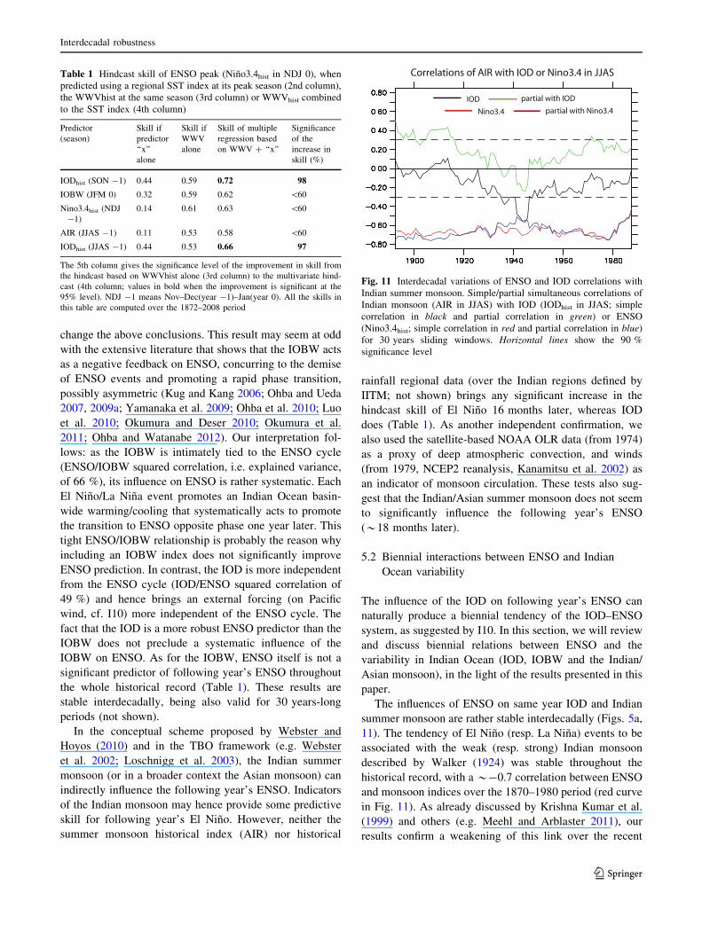
paper.The influences of ENSO on same year IOD and Indian
summer monsoon are rather stable interdecadally (Figs. 5a,
11). The tendency of El Nino (resp. La Nina) events to beassociated with the weak (resp. strong) Indian monsoon
described by Walker (1924) was stable throughout the
historical record, with a *-0.7 correlation between ENSOand monsoon indices over the 1870–1980 period (red curve
in Fig. 11). As already discussed by Krishna Kumar et al.
(1999) and others (e.g. Meehl and Arblaster 2011), ourresults confirm a weakening of this link over the recent
Table 1 Hindcast skill of ENSO peak (Nino3.4hist in NDJ 0), whenpredicted using a regional SST index at its peak season (2nd column),the WWVhist at the same season (3rd column) or WWVhist combinedto the SST index (4th column)
Predictor(season)
Skill ifpredictor‘‘x’’alone
Skill ifWWValone
Skill of multipleregression basedon WWV ? ‘‘x’’
Significanceof theincrease inskill (%)
IODhist (SON -1) 0.44 0.59 0.72 98
IOBW (JFM 0) 0.32 0.59 0.62 \60
Nino3.4hist (NDJ-1)
0.14 0.61 0.63 \60
AIR (JJAS -1) 0.11 0.53 0.58 \60
IODhist (JJAS -1) 0.44 0.53 0.66 97
The 5th column gives the significance level of the improvement in skill fromthe hindcast based on WWVhist alone (3rd column) to the multivariate hind-cast (4th column; values in bold when the improvement is significant at the95% level). NDJ -1 means Nov–Dec(year -1)–Jan(year 0). All the skills inthis table are computed over the 1872–2008 period
Fig. 11 Interdecadal variations of ENSO and IOD correlations withIndian summer monsoon. Simple/partial simultaneous correlations ofIndian monsoon (AIR in JJAS) with IOD (IODhist in JJAS; simplecorrelation in black and partial correlation in green) or ENSO(Nino3.4hist; simple correlation in red and partial correlation in blue)for 30 years sliding windows. Horizontal lines show the 90 %significance level
Interdecadal robustness
123
satellite period that is however within the range of sto-
chastic fluctuations (Gershunov et al. 2001; van Olden-borgh and Burgers 2005).
Some authors have proposed that the Indian summer
monsoon may influence the IOD but do not agree on thesign of this influence. Webster et al. (2002), Loschnigg
et al. (2003), Meehl et al. (2003) and Webster and Hoyos
(2010) propose that a strong Indian monsoon circulationinduce westerlies along the equatorial Indian Ocean, in turn
favouring a negative IOD. Annamalai et al. (2003) andKrishnan and Swapna (2009) showed that a strong Indian
monsoon could favour a positive IOD through southeas-terlies along Sumatra coast [another CGCM experiment(Izumo et al. 2008, their Fig. 2d) also suggests such
influence]. Other authors have also proposed that the IOD
influences the monsoon, usually positively (Behera et al.1999; Ashok et al. 2001, 2004; Annamalai et al. 2003,
2010; Gadgil et al. 2004; Ashok and Saji 2007; Um-
menhofer et al. 2011; Boschat et al. 2012). Here, we notethat, compared to the synchronous ENSO–IOD and ENSO-
monsoon relations and to the IOD’s impact on ENSO at
1 year lead, the synchronous IOD-monsoon relationappears to be weak and not very stable interdecadally
(Fig. 11). The simple and partial correlations between JJAS
AIR and the IOD are indeed not significant during longperiods of the historical record (Fig. 11). They are also
rather weak when taken over the complete record (simple
correlation of -0.09 and partial correlation of ?0.23).
These results suggest that the interactions between themonsoon and the IOD are much weaker than those between
the IOD and ENSO.
In the light of the discussion above, AIR–IOD–IOBW–ENSO relationships appear to only fit partially within the
frame of the TBO. We thus suggest a slightly revised
conceptual scheme of Indo-Pacific relations outlined in theTBO framework (e.g. Loschnigg et al. 2003) or in Webster
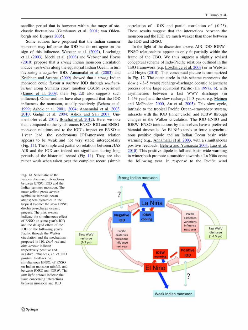
and Hoyos (2010). This conceptual picture is summarizedin Fig. 12. The outer circle in this scheme represents the
slow (*3–5 years) recharge-discharge oceanic adjustment
process of the large equatorial Pacific (Jin 1997a, b), withasymmetries between a fast WWV discharge (in
1–1! year) and the slow recharge (1–3 years; e.g. Meinen
and McPhaden 2000, An et al. 2005). This slow cycle,intrinsic to the tropical Pacific Ocean–atmosphere system,
interacts with the IOD (inner circle) and IOBW through
changes in the Walker circulation. The IOD–ENSO andIOBW–ENSO interactions by themselves have a preferred
biennial timescale. An El Nino tends to force a synchro-
nous positive dipole and an Indian Ocean basin widewarming (e.g., Annamalai et al. 2003, with a simultaneous
positive feedback; Behera and Yamagata 2003; Luo et al.
2010). This positive dipole in fall and basin-wide warmingin winter both promote a transition towards a La Nina event
the following year, in response to the Pacific wind
Fig. 12 Schematic of thevarious discussed interactionsbetween ENSO, IOD and theIndian summer monsoon. Theouter yellow-green arrowssymbolise intrinsic ocean–atmosphere dynamics in thetropical Pacific: the slow ENSOdischarge-recharge oceanicprocess. The pink arrowsindicate the simultaneous effectof ENSO on same year’s IODand the delayed effect of theIOD on the following year’sPacific through the Walkercirculation and the mechanismproposed in I10. Dark red andblue arrows indicaterespectively positive andnegative influences, i.e. of IODpositive feedback onsimultaneous ENSO, of ENSOon Indian monsoon rainfall, andbetween ENSO and IOBW. Thethin light arrows indicate theissue concerning interactionsbetween monsoon and IOD
T. Izumo et al.
123
variations promoted by both IOD events (I10) and IOBW
(e.g. Annamalai et al. 2005; Kug and Kang 2006; Ohba andUeda 2007). The Indo-Pacific relations then tend to induce
an ENSO–IOD–IOBW state with opposite polarities, and
thus a tendency toward a biennial timescale. The IOD ishowever more independent of ENSO than the IOBW, and
hence brings more in terms of predictability (i.e. the role of
the IOBW in the phase transition of ENSO is much moresystematic than the role of the IOD).
We found no significant improvement of ENSO hind-casts when accounting for previous year’s Indian monsoon.
In view of this result, and because of the apparent lack of
consensus of previous studies on that account, we suggest amore passive role of the Indian Monsoon in our scheme
than in TBO studies such as Loschnigg et al. (2003) or
Webster and Hoyos (2010). We suggest that ENSO hasmore influence on the Indian monsoon than the other way
around. We also suggest that, while simultaneous interac-
tions between the monsoon and IOD may exist, they are nothighlighted by as significant and stable correlations as
IOD–ENSO relations.
6 Summary and discussion
6.1 Summary
I10 demonstrated that, over the 1981–2009 period, the IODbrings preconditioning information in addition to the
Pacific WWV when predicting ENSO 14 months later. In
the present study, we have examined the robustness andinterdecadal stability of this scenario over the 1872–2008
period. To this end, we have constructed a historical IOD
index and a WWV proxy over this period. The historicalIOD index is based on a spatial regression over the whole
Indian Ocean, exploiting much more SST observations
than the classical DMI. The historical WWV proxy takesadvantage of the linear link between the recharge process
and average zonal wind stresses at low frequency, and is
correlated at 0.87 with observed WWV over the recentperiod.
We have then used these historical indices to test I10
results over a much longer period. The tendency for theIOD events and WWV to precede ENSO events by
*14 months was strong not only during the recent period,
but remained significant before the satellite era. In contrast,ENSO itself, the Indian Ocean basin-wide warming/cool-
ing (IOBW), or the Indian Monsoon, do not provide
additional predictability to following year’s ENSOthroughout the historical record. A decrease of the syn-
chronous and lagged relationships between the IOD and
ENSO and a stronger influence of WWV however appeararound the sparsely sampled period of World War II.
Overall, the IOD and WWV collectively explain about
50–60 % of following year’s ENSO interannual varianceover the 1870’s–2000’s period. Both IOD and WWV
independent contributions always remain significant, with a
similar contribution of IOD and WWV to the ENSO skillfor the early and late part of the record but a larger WWV
contribution from the 1920’s to the 1960’s. The influences
of the IOD and WWV on following year’s ENSO areroughly symmetric, being significant for both phases, with
negative (resp. positive) IODs and positive (negative)WWV tending to induce an El Nino (resp. La Nina) the
following year. Results from a 200 years CGCM simula-
tion display similar influences of the IOD and WWV onENSO 14 months later, with notable decadal fluctuations.
Based on these results and analyses of biennial relations
between ENSO, IOD and the Indian Monsoon, we proposea slightly revised scenario of Indo-Pacific interactions
(Fig. 12), more consistent with observations (see also
Tamura et al. 2011), compared to the Tropical Tropo-spheric Biennial Oscillation (TBO) or Webster and Hoyos
(2010) frameworks. In the framework presented here, the
IOD–ENSO interactions favour a biennial timescale, andinteract with the slower recharge-discharge cycle intrinsic
to the Pacific Ocean; but the Indian monsoon responds
rather passively to the IOD–ENSO coupled system.
6.2 Discussion and perspectives
The present study provides additional evidence of the IOD
influence on ENSO one year later. The simple statistical
analyses performed in Sect. 5.1 further suggest that theIOD brings a larger improvement to the predictive skill of
following year’s ENSO state than the IOBW or ENSO
itself. These results complement the existing views on theIndian Ocean influence on ENSO, either through the IOD
or through the IOBW (e.g. Nicholls 1984; Annamalai et al.
2005; Kug and Kang 2006; Ohba and Ueda 2007, 2009a, b;Yamanaka et al. 2009; Annamalai et al. 2010, Santoso et al.
2012). These views could well be complementary. Con-
cerning predictability, the slowly growing IOBW is prob-ably too much related to ENSO to bring a Pacific wind
forcing independent of the ENSO cycle. The partial inde-
pendency of IOD with regard to the ENSO cycle bringsmore predictability to ENSO hindcast 1 year later than the
IOBW or ENSO itself. I.e. while warming in the Indian
Ocean systematically tends to damp ENSO events (e.g.Santoso et al. 2012) and promotes a rapid phase transition
towards the opposite ENSO phase (e.g. Annamalai et al.
2005; Kug and Kang 2006; Ohba and Ueda 2007), the IODdoes not always co-occur with ENSO, and needs to be
accounted for to improve the ENSO hindcasts.
Other possible influences on ENSO have been proposed.Intraseasonal Westerly Wind Bursts (WWBs) and Madden-
Interdecadal robustness
123
Julian Oscillation can strongly influence El Nino onset and
development (e.g. Lengaigne et al. 2004 for a review).They could even play a role in the IOD influence on El
Nino onset (Izumo et al. 2010a, b). Mid-latitude forcing
(Vimont et al. 2003; Chang et al. 2007; Terray 2011) ispotentially another powerful ENSO precursor in boreal
spring. The tropical Atlantic (e.g. Rodriguez-Fonseca et al.
2009; Jansen et al. 2009; Ding et al. 2011) might also havean influence on El Nino mature phase. It seems important
to better understand if these influences are independent, orpart of a larger picture.
Concerning the hindcast model constructed with IODhist
and WWVhist, we should also remark that, in a real forecastexercise, the 7 years high-pass and 2–7 years band-pass
filters (cf. Sects. 2.2, 3.2) can not be used, as they use the
months/years after November 30th (the date for SONaverages, from which real statistical forecasts could start).
One way to overcome this issue is for example to use
indices that are ‘‘backward high-pass filtered’’, by remov-ing their 3 last years mean, and for the WWVhist to also use
a ‘‘backward low-pass filter’’ by averaging WWVhist over
JJASON. When using such filter, the correlation skill over
the 1872–2008 period remains high, 0.66, close to the 0.72
skill found in sect. 4An interesting perspective is the potential improvement
of global seasonal forecasts at a *0.5 to *1.5 year lead.
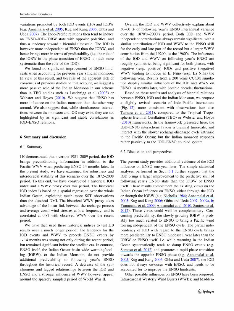
Figure 13 gives a simple illustration of this potential.Figure 13a shows the well-known global impacts of ENSO
through teleconnections on land precipitation and sea level
pressure (SLP; from ship observations or 20CR reanalysis),here shown in boreal winter from historical data from 1901.
The ENSO estimate based on previous year’s IODhist andWWVhist has indeed a significant skill to forecast following
year’s rainfall, SLP (Fig. 13b) and SST (not shown) in
large areas of the tropics, as well as at higher latitudes, inregions influenced by the tropical Indo-Pacific through
teleconnections, including north, central and south Amer-
ica, Australia, Indonesia, India, south-east Asia and China,eastern and southern Africa (e.g. Philander 1990; Trenberth
et al. 1998).
The scenario for the IOD influence on the followingyear’s ENSO proposed in this study relies on observational
analysis, some modelling experiments and statistical anal-
yses that leave some issues. The mechanisms for the
(a)
(b)
Fig. 13 Example of application (? observationally-independenthistorical validation) of IOD and WWV influences on followingyear’s ENSO, to hindcast at 1-year lead global land rainfall and SLPin boreal winter. a Correlation of land precipitation (color on land,with sign reversed, i.e. dry in red, wet in blue; GPCC, 1901–2008)and SLP (color on oceans, from I-COADS; black contours from 20CRreanalysis) in NDJFM with simultaneous Nino3.4hist. b The same butwith Nino3.4 hindcast estimate based on previous year’s -IODhist andWWVhist (SON). Only signals significant at the 90 % level are shown.ENSO has significant impacts on rainfall and SLP globally (a).Hence, IOD and WWV, by influencing following year’s ENSO, have
significant delayed global impacts on rainfall and SLP (i.e. atmo-spheric circulation), and so have a significant skill to predict theseimpacts with a 1-year lead (b). We found such significant skillglobally also for other seasons until the following spring, i.e. with a1.5 year lead, for SST or 20CR precipitation over 1872–2008. Asexamples, the correlation skill to hindcast following year’s precip-itation is 0.46/0.45 over central-northwest America (15"N–35"N, westof 95"W), 0.30/0.41 over southern Africa (south of 20"S) usingGPCC/20CR dataset in NDJFM, and 0.39 for All Indian Rainfall inJJAS, all significant at the 99 % level
T. Izumo et al.
123
apparently robust IOD influence need to be better under-
stood by other sensitivity experiments with a variety ofcoupled models capturing the complexity of the ocean–
atmosphere interactions at stake following the IOD demise.
Acknowledgments We thank Dr. Sebastien Masson and Dr.Swadhin Behera for constructive comments on this paper. We wouldlike to thank Dr. Lucia Bunge for sending us the ENSO historicalindices of Bunge and Clarke (2009), as well as Dr. Tomoki Tozuka,Dr. Pascal Oettli, Dr. Sophie Cravatte, Dr. Caroline Ummenhofer, Dr.Pascal Terray, Hugo Dayan and Chloe Prodhomme for their help andfruitful discussions. We would like to thank the three anonymousreviewers, as well as Dr Julie Arblaster, for their constructive com-ments. The first author would like to thank Pr. Toshio Yamagata andhis colleagues at the University of Tokyo, especially Miss JunkoMoriyama, for their hospitality and help during his stay there. Thefirst author was funded by the University of Tokyo (partly through theSATREPS JICA/JST program) and now by the Institut de Recherchepour le Developpement (IRD). Matthieu Lengaigne and JeromeVialard are funded by IRD. Matthieu Lengaigne gratefullyacknowledges the National Institute of Oceanography (NIO, Goa,India) for hosting him during this work. Support for the 20CR projectis provided by the US DOE INCITE program, and BER, and by theNOAA Climate Program Office. Also, the NOAA and IRI datalibraries were used for this study. The IODhist and WWVhist historicalindices constructed here are available at http://www.locean-ipsl.upmc.fr/*Takeshi-Izumo/data.html.
References
Abram NJ, Gagan MK, Cole JE, Hantoro WS, Mudelsee M (2008)Recent intensification of tropical climate variability in the IndianOcean. Nat Geosci 1:849–853
An S-I, Wang B (2000) Interdecadal change of the structure of theENSO mode and its impact on the ENSO frequency. J Clim13:2044–2055
An S-I, Hsieh WW, Jin F-F (2005) A nonlinear analysis of the ENSOcycle and its interdecadal changes. J Clim 18:3229–3239
Annamalai H, Murtugudde R (2004) Role of the Indian Ocean inregional climate variability. In: Wang C, Xie S-P, Carton JA(eds) Earth climate: the ocean-atmosphere interaction. AGUGeophysical Monograph 147:213–246
Annamalai H, Murtugudde R, Potemra J, Xie SP, Liu P, Wang B(2003) Coupled dynamics in the Indian Ocean: spring initiationof the zonal mode. Deep-Sea Res 50B:2305–2330
Annamalai H, Xie S-P, McCreary J-P, Murtugudde R (2005) Impactof Indian Ocean sea surface temperature on developing El Nino.J Clim 18:302–319
Annamalai H, Kida S, Hafner J (2010) Potential impact of the tropicalIndian Ocean-Indonesian Seas on El Nino characteristics. J Clim23:3933–3952
Ashok K, Saji NH (2007) On impacts of ENSO and Indian Ocean Dipoleevents on the sub-regional Indian summer monsoon rainfall. NatHazards 42(2):273–285. doi:10.1007/s11069-006-9091-0
Ashok K, Guan Z, Yamagata T (2001) Impact of the Indian OceanDipole on the relationship between the Indian Monsoon rainfalland ENSO. Geophys Res Lett 28:4499–4502
Ashok K, Guan Z, Saji NH, Yamagata T (2004) Individual andcombined influences of the ENSO and Indian Ocean Dipole onthe Indian summer monsoon. J Clim 17:3141–3155
Barnett TP (1983) Interaction of the Monsoon and Pacific trade windsystem at interannual time scales. Part I: the equatorial zone.Mon Wea Rev 111:756–773
Battisti DS, Hirst AC (1989) Interannual variability in the tropicalatmosphere-ocean model: influence of the basic state, oceangeometry and nonlineary. J Atmos Sci 45:1687–1712
Behera SK, Yamagata T (2003) Influence of the Indian Ocean Dipoleon the Southern Oscillation. J Meteorol Soc Jpn 81(1):169–177
Behera SK, Krishnan R, Yamagata T (1999) Unusual ocean-atmosphere conditions in the tropical Indian Ocean during1994. Geophys Res Lett 26:3001–3004
Behera SK, Luo J-J, Masson S, Rao SA, Sakuma H, Yamagata T(2006) A CGCM study on the interaction between IOD andENSO. J Clim 19:1688–1705
Bentamy A, Quilfen Y, Gohin F, Grima N, Lenaour M, Servain J(1996) Determination and validation of average field from ERS-1 scatterometer measurements. Global Atmos Ocean Syst 4:1–29
Bjerknes J (1969) Atmospheric teleconnections from the equatorialPacific. Mon Weather Rev 97:163–172
Boschat G, Terray P, Masson S (2012) Robustness of SST telecon-nections and precursory patterns associated with the Indiansummer monsoon. Clim Dyn 38(11–12):2143–2165. ISSN0930-7575
Brown JN, Fedorov AV (2010) Estimating the diapycnal transportcontribution to warm water volume variations in the tropicalPacific Ocean. J Clim 23:221–237
Bunge L, Clarke AJ (2009) A verified estimation of the El Nino indexNINO3.4 since 1877. J Clim 22(14):3979–3992
Burgers G, Jin F-F, van Oldenborgh GJ (2005) The simplest ENSOrecharge oscillator. Geophys Res Lett 32:L13706. doi:10.1029/2005GL022951
Chang P, Zhang L, Saravanan R, Vimont DJ, Chiang JCH, Ji L, SeidelH, Tippett MK (2007) Pacific meridional mode and El Nino–Southern Oscillation. Geophys Res Lett 34:L16608. doi:10.1029/2007GL030302
Cherchi A, Navarra A (2012) Influence of ENSO and of the IndianOcean Dipole on the Indian summer monsoon variability. ClimDyn. doi: 10.1007/s00382-012-1602-y
Chowdary JS, Xie S-P, Tokinaga H, Okumura YM, Kubota H,Johnson NC, Zheng X-T (2012) Interdecadal variations in ENSOteleconnection to the Indo-western Pacific for 1870–2007. J Clim25:1722
Clarke AJ (2008) An introduction to the dynamics of El Nino & theSouthern Oscillation. Elsevier (Academic Press). ISBN: 978-0-12-088548-0
Clarke AJ, Van Gorder S (2003) Improving El Nino prediction usinga space-time integration of Indo-Pacific winds and equatorialPacific upper ocean heat content. Geophys Res Lett 30(7):1399.doi:10.1029/2002GL016673
Collins M, An S-I, Cai W, Ganachaud A, Guilyardi E, Jin F-F,Jochum M, Lengaigne M, Power S, Timmermann A, Vecchi G,Wittenberg A (2010) The impact of global warming on thetropical Pacific Ocean and El Nino. Nat Geosci 3:391–397
Compo GP et al (2011) The twentieth century reanalysis project. Q JR Meteorol Soc 137:1–28. doi:10.1002/qj.776
Ding H, Keenlyside NS, Latif M (2011) Impact of the equatorialAtlantic on the El Nino Southern Oscillation. Clim Dyn. doi:10.1007/s00382-011-1097-y
Fasullo J (2004) Biennial characteristics of All India rainfall. J Clim17:2972–2982
Fedorov AV (2002) The response of the coupled tropical ocean–atmosphere to westerly wind bursts. Q J R Meteorol Soc128:1–23
Fedorov AV (2010) Ocean response to wind variations, warm watervolume, and simple models of ENSO in the low-frequencyapproximation. J Clim 23:3855–3873
Fischer A, Terray P, Guilyardi E, Gualdi S, Delecluse P (2005) Twoindependent triggers for the Indian Ocean Dipole/Zonal Mode ina coupled GCM. J Clim 18:3428–3449
Interdecadal robustness
123
Gadgil S, Vinayachandran PN, Francis PA, Gadgil S (2004) Extremesof the Indian summer monsoon rainfall, ENSO, and equatorialIndian Ocean oscillation. Geophys Res Lett 31:1821. doi:10.1029/2004GL019733
Gershunov A, Schneider N, Barnett T (2001) Low frequencymodulation of the ENSO-Indian monsoon rainfall relationship:signal or noise. J Clim 14:2486–2492
Goddard L, Philander SGH (2000) The energetics of El Nino and LaNina. J Clim 13:1496–1516
Hoerling MP, Kumar A, Xu T-Y (2001) Robustness of the nonlinearatmospheric response to opposite phases of ENSO. J Clim14:1277–1293
Huffman GJ, Adler RF, Arkin PA, Chang A, Ferraro R, Gruber A,Janowiak J, Joyce RJ, McNab A, Rudolf B, Schneider U, Xie P(1997) The global precipitation climatology project (GPCP)combined precipitation data set. Bull Am Meteorol Soc 78:5–20
Izumo T, de Boyer Montegut C, Luo J-J, Behera SK, Masson S,Yamagata T (2008) The role of the western Arabian Seaupwelling in Indian monsoon rainfall variability. J Clim21:5603–5623
Izumo T, Vialard J, Lengaigne M, de Boyer Montegut C, Behera SK,Luo J-J, Cravatte S, Masson S, Yamagata T (2010a) Influence ofthe Indian Ocean Dipole on following year’s El Nino. NatGeosci 3:168–172
Izumo T, Masson S, Vialard J, de Boyer Montegut C, Behera SK,Madec G, Takahashi K, Yamagata T (2010b) Low and highfrequency Madden-Julian Oscillations in Austral Summer—interannual variations. Clim Dyn 35:669–683
Jansen MF, Dommenget D, Keenlyside N (2009) Tropical atmo-sphere-ocean interactions in a conceptual framework. J Clim22:550–567
Jin FF (1997a) An equatorial ocean recharge paradigm for ENSO.Part I: conceptual model. J Atmos Sci 54:811–829
Jin FF (1997b) An equatorial ocean recharge paradigm for ENSO.Part II: a stripped-down coupled model. J Atmos Sci 54:830–847
Kanamitsu M, Ebisuzaki W, Woollen J, Yang S-K, Hnilo JJ, FiorinoM, Potter GL (2002) NCEP-DOE AMIP-II reanalysis. Bull AmMeteorol Soc 83:1631–1643
Klein SA, Soden BJ, Lau NC (1999) Remote sea surface temperaturevariations during ENSO: evidence for a tropical atmosphericbridge. J Clim 12:917–932
Krishna Kumar KK, Rajagopalan KB, Cane MA (1999) On theweakening relationship between the Indian monsoon and ENSO.Science 284:2156–2159
Krishnamurti TN, Chu SH, Iglesias W (1986) On the sea-levelpressure of the Southern Oscillation. Arch Meteorol GeophysBioclimatol Ser A Meteorol Geophys 34:384–425
Krishnan R, Swapna P (2009) Significance influence of the borealsummer monsoon flow on the Indian Ocean response duringdipole events. J Clim 22:5611–563410
Kug J-S, Ham Y-G (2012) Indian Ocean feedback to the ENSOtransition in a multi-model ensemble. J Clim 25:6942–6957. doi:10.1175/JCLI-D-12-00078.1
Kug J-S, Kang I-S (2006) Interactive feedback between the IndianOcean and ENSO. J Clim 19:1784–1801
Kug J-S, Li T, An S-I, Kang I-S, Luo J-J, Masson S, Yamagata T(2006) Role of the ENSO–Indian Ocean coupling on ENSOvariability in a coupled GCM. Geophys Res Lett 33:L09710. doi:10.1029/2005GL024916
Leloup JA, Lachkar Z, Boulanger JP, Thiria S (2007) Detectingdecadal changes in ENSO using neural networks. Clim Dyn. doi:10.1007/s00382-006-0173-1
Lengaigne M, Boulanger J-P, Menkes C, Delecluse P, Slingo J (2004)Westerly wind events in the tropical Pacific and their influenceon the coupled ocean-atmosphere system: a review. In: Earth
climate: the ocean-atmosphere interaction, Geophys. Monogr.Ser., 147. AGU, Washington, DC, pp 49–69
Lengaigne M, Hausmann U, Madec G, Menkes C, Vialard J, MolinesJM (2012) Mechanisms controlling warm water volume inter-annual variations in the equatorial Pacific: diabatic versusadiabatic processes. Clim Dyn 38:1031–1046. doi:10.1007/s00382-011-1051-z
Liebmann B, Smith CA (1996) Description of a complete (interpo-lated) outgoing longwave radiation dataset. Bull Am MeteorolSoc 77:1275–1277
Loschnigg J, Meehl GA, Webster PJ, Arblaster JM, Compo GP(2003) The Asian monsoon, the tropospheric biennial oscillatio-nand the Indian Ocean Dipole in the NCAR CSM. J Clim16:2138–2158
Luo J-J, Masson S, Roeckner E, Madec G, Yamagata T (2005)Reducing climatology bias in an ocean-atmosphere CGCM withimproved coupling physics. J Clim 18:2344–2360
Luo J-J, Behera S, Masumoto Y, Sakuma H, Yamagata T (2008)Successful prediction of the consecutive IOD in 2006 and 2007.Geophys Res Lett 35:L14S02. doi:10.1029/2007GL032793
Luo J-J, Zhang R, Behera S, Masumoto Y, Jin F-F, Lukas R,Yamagata T (2010) Interaction between El Nino and extremeIndian Ocean Dipole. J Clim 23:726–742
Madec G, Delecluse P, Imbard M, Levy C (1998) OPA 8.1 Oceangeneral circulation model reference manual. Notes du pole demodelisation de l’IPSL 11, 91 pp, available at http://www.lodyc.jussieu.fr/opa
Masson S et al (2005) Impact of barrier layer on winter-springvariability of the southeastern Arabian Sea. Geophys Res Lett32:L07703. doi:10.1029/2004GL021980
Meehl GA (1987) The annual cycle and interannual variability in thetropical Pacific and Indian Ocean region. Mon Wea Rev115:27–50
Meehl GA, Arblaster JM (2011) Decadal variability of Asian-Australian monsoon-ENSO-TBO relationships. J Clim24:4925–4940
Meehl GA, Arblaster JM, Loschnigg J (2003) Coupled ocean-atmosphere dynamical processes in the tropical Indian andPacific Ocean regions and the TBO. J Clim 16:2138–2158
Meinen CS, McPhaden MJ (2000) Observations of warm watervolume changes in the equatorial Pacific and their relationship toEl Nino and La Nina. J Clim 13:3551–3559
Murtugudde R, Busalacchi AJ (1999) Interannual variability of thedynamics and thermodynamics of the tropical Indian Ocean.J Clim 12:2300–2326
Murtugudde R, McCreary JP, Busalacchi AJ (2000) Oceanicprocesses associated with anomalous events in the Indian Oceanwith relevance to 1997–1998. J Geophys Res 105:3295–3306
Neelin JD, Battisti DS, Hirst AC, Jin F-F, Wakata Y, Yamagata T,Zebiak SE (1998) ENSO theory. J Geophys Res 103:14261–14290
Nicholls N (1984) The Southern Oscillation and Indonesian seasurface temperature. Mon Wea Rev 112:424–432
Ohba M, Ueda H (2005) Basin-wide warming in the equatorial IndianOcean associated with El Nino. Scientific Online Lett Atmos1:089–092. doi:10.2151/sola
Ohba M, Ueda H (2007) An impact of SST anomalies in the IndianOcean in acceleration of the El Nino to La Nina transition.J Meteorol Soc Jpn 85:335–348
Ohba M, Ueda H (2009a) Role of nonlinear atmospheric response toSST on the asymmetric transition process of ENSO. J Clim22:177–192
Ohba M, Ueda H (2009b) Seasonally different response of the IndianOcean to the remote forcing of El Nino: linking the dynamicsand thermodynamics. SOLA 5:176–179. doi:10.2151/sola.2009-045
T. Izumo et al.
123
Ohba M, Watanabe M (2012) Role of the Indo-Pacific interbasincoupling in predicting asymmetric ENSO transition and dura-tion. J Clim 25(9):3321–3335
Ohba M, Nohara D, Ueda H (2010) Simulation of asymmetric ENSOtransition in WCRP CMIP3 multi-model experiments. J Clim.doi:10.1175/2010JCLI3608.1
Okumura YM, Deser C (2010) Asymmetry in the duration of El Ninoand La Nina. J Clim 23:5826–5843
Okumura YM, Ohba M, Deser C, Ueda H (2011) A proposedmechanism for the asymmetric duration of El Nino and La Nina.J Clim 24:3822–3829
Parthasarathy B, Munot AA, Kothawale DR (1994) All India monthlyand seasonal rainfall series—1871–1993. Theor Appl Climatol49:217–224
Philander SG (1990) El Nino, La Nina, and the Southern Oscillation.ix ? 293 pp. San Diego, New York, Berkeley, Boston, London,Sydney, Tokyo. In: International Geophysics Series Vol. 46.Academic Press (Harcourt Brace Jovanovich), Toronto. ISBN 012 553235 0
Picaut J, Masia F, du Penhoat Y (1997) An advective-reflectiveconceptual model for the oscillatory nature of the ENSO.Science 277:663–666
Rayner NA, Parker DE, Horton EB, Folland CK, Alexander LV,Rowell DP, Kent EC, Kaplan A (2003) Global analyses of seasurface temperature, sea ice, and night marine air temperaturesince the late nineteenth century. J Geophys Res 108(D14):4407.doi:10.1029/2002JD002670
Rayner NA, Brohan P, Parker DE, Folland CK, Kennedy JJ, VanicekM, Ansell T, Tett SFB (2006) Improved analyses of changes anduncertainties in sea surface temperature measured in situ sincethe mid-nineteenth century: the HadSST2 data set. J Clim19(3):446–469
Reverdin G, Cadet D, Gutzler D (1986) Interannual displacements ofconvection and surface circulation over the equatorial IndianOcean. Q J R Meteorol Soc 112:43–46
Reynolds RW, Rayner NA, Smith TM, Stokes DC, Wang W (2002)An improved in situ and satellite SST analysis for climate.J Clim 15:1609–1625
Rodriguez-Fonseca B, Polo I, Garcia-Serrano J, Losada T, Mohino E,Mechoso CR, Kucharski F (2009) Are the Atlantic Ninosenhancing Pacific ENSO events in recent decades? Geophys ResLett 36:L20705. doi:10.1029/2009GL040048
Roeckner E et al (1996) The atmospheric general circulation modelECHAM-4: Model description and simulation of present-dayclimate. Max-Planck-Institut fur Meteorologie Rep., 218, 90 pp
Rudolf B et al (2010) GPCC Status Report December 2010 (On themost recent gridded global data set issued in fall 2010 by theGlobal Precipitation Climatology Centre (GPCC))
Saji NH, Goswami BN, Vinayachandran PN, Yamagata T (1999) Adipole mode in the tropical Indian Ocean. Nature 401:360–363
Santoso A, England MH, Cai W (2012) Impact of Indo-Pacificfeedback interactions on ENSO dynamics diagnosed usingensemble climate simulations. J Clim 25:7743–7763. http://dx.doi.org/10.1175/JCLI-D-11-00287.1
Schopf PS, Suarez MJ (1988) Vacillations in a coupled ocean-atmosphere model. J Atmos Sci 45:549–566
Smith NR (1995) An improved system for tropical ocean sub-surfacetemperature analyses. J Atmos Ocean Technol 12:850–870
Smith TM, Reynolds RW, Peterson TC, Lawrimore J (2008)Improvements to NOAA’s historical merged land–ocean surfacetemperature analysis (1880–2006). J Clim 21:2283–2296. doi:10.1175/2007JCLI2100.1
Tamura T, Koike T, Yamamoto A, Yasukawa M, Kitsuregawa M(2011) Contrasting impacts of the Indian Ocean Dipole andENSO on the tropospheric biennial oscillation. SOLA 7:13–16
Terray P, Dominiak S (2005) Indian Ocean sea surface temperatureand El Nino-Southern Oscillation: a new perspective. J Clim18:1351–1368
Terray P, Dominiak S, Delecluse P (2005) Role of the southern IndianOcean in the transitions of the monsoon-ENSO system duringrecent decades. Clim Dyn 24:169–195. doi:10.1007/s00382-004-0480-3
Terray P (2011) Southern hemisphere extra-tropical forcing: a newparadigm for El Nino-Southern Oscillation. Clim Dyn36:2171–2199
Trenberth KE, Branstator GW, Karoly D, Kumar A, Lau N-C,Ropelewski C (1998) Progress during TOGA in understandingand modeling global teleconnections associated with tropical seasurface temperatures. J Geophys Res 103:14291–14324
Ummenhofer CC, England MH, McIntosh PC, Meyers GA, Pook MJ,Risbey JS, Sen Gupta A, Taschetto AS (2009) What causesSoutheast Australia’s worst droughts? Geophys Res Lett36:L04706. doi:10.1029/2008GL036801
Ummenhofer CC, Sen Gupta A, Li Y, Taschetto AS, England MH(2011) Multi-decadal modulation of the El Nino-Indian monsoonrelationship by Indian Ocean variability. Environ Res Lett6:034006. doi:10.1088/1748-9326/6/3/034006
van Oldenborgh GJ, Burgers G (2005) Searching for decadalvariations in ENSO precipitation teleconnections. Geophys ResLett 32(15):L15701
Vialard J, Menkes C, Boulanger J-P, Delecluse P, Guilyardi E,McPhaden MJ, Madec G (2001) A model study of oceanicmechanisms affecting equatorial Pacific sea surface temperatureduring the 1997–98 El Nino. J Phys Oceanogr 31:1649–1675
Vimont DJ, Wallace JM, Battisti DS (2003) The seasonal footprintingmechanism in the Pacific: implications for ENSO. J Clim16:2668–2675
Walker GT (1924) World weather IX. Mem Indian Meteorol Dept24:275–332
Wang C, Picaut J (2004) Understanding ENSO physics—a review. In:Wang C, Xie S-P, Carton JA (eds) Earth’s climate: the ocean-atmosphere interaction. AGU Geophysical Monograph Series147:21–48
Watanabe M (2008a) Two regimes of the equatorial warm pool. PartI: a simple tropical climate model. J Clim 21:3533–3544
Watanabe M (2008b) Two regimes of the equatorial warm pool. PartII: hybrid coupled GCM experiments. J Clim 21:3545–3560
Watanabe M, Jin F-F (2002) Role of Indian Ocean warming in thedevelopment of Philippine Sea anticyclone during ENSO.Geophys Res Lett 29(10):1478. doi:10.1029/2001GL014318
Webster PJ, Hoyos CD (2010) Beyond the spring barrier? Nat Geosci3:152–153. doi:10.1038/ngeo800
Webster PJ, Moore A, Loschnigg J, Leban M (1999) Coupleddynamics in the Indian Ocean during 1997–1998. Nature401:356–360
Webster PJ, Clark C, Chrikova G, Fasullo J, Han W, Loschnigg J,Sahami K (2002) The monsoon as a self-regulating coupledocean-atmosphere system. In: Pierce R (ed) Meteorology at theMillennium. Academic press, London, pp 198–219
Wu R, Kirtman BP (2004) Understanding the impacts of the IndianOcean on ENSO variability in a coupled GCM. J Clim17:4019–4031
Wyrtki K (1975) El Nino—the dynamic response of the equatorialPacific Ocean to atmospheric forcing. J Phys Oceanogr5(4):572–584
Wyrtki K (1985) Water displacements in the Pacific and the genesisof El Nino cycles. J Geophys Res 90:7129–7132
Xavier PK, Marzin C, Goswami BN (2007) An objective definition ofthe Indian summer monsoon season and a new perspective onENSO-monsoon relationship. Q J R Meteorol Soc 133:749–764
Interdecadal robustness
123
Xie S-P, Hu K, Hafner J, Tokinaga H, Du Y, Huang G, Sampe T(2009) Indian Ocean capacitor effect on Indo-western Pacificclimate during the summer following El Nino. J Clim22:730–747
Yamagata T, Behera SK, Luo J-J, Masson S, Jury MR, Rao SA (2004)The coupled ocean-atmosphere variability in the tropical IndianOcean. Earth’s climate: the ocean-atmosphere interaction. Geo-phys Monogr 147:189–211
Yamanaka G, Yasuda T, Fujii Y, Matsumoto S (2009) Rapidtermination of the 2006 El Nino and its relation to the IndianOcean. Geophys Res Lett 36:L07702. doi:10.1029/2009GL037298
Yasunari T (1985) Zonally propagating modes of the global East-West circulation associated with the Southern Oscillation.J Meteorol Soc Jpn 63:1013–1029
Yu J-Y (2005) Enhancement of ENSO’s persistence barrier bybiennial variability in a coupled atmosphere-ocean generalcirculation model. Geophys Res Lett 32:L13707. doi:10.1029/2005GL023406
Yu J-Y, Mechoso CR, McWilliams JC, Arakawa A (2002) Impact ofthe Indian Ocean on the ENSO cycle. Geophys Res Lett 29:1204.doi:10.1029/2001GL014098
T. Izumo et al.
123