Inferring Phylogenetic Networks by the Maximum Parsimony Criterion: A Case Study

and Evolution. All rights reserved. For permissions, please e-mail: [email protected] The Author 2006. Published by Oxford University Press on behalf of the Society for Molecular Biology

Inferring Phylogenetic Networks by the Maximum

Parsimony Criterion: A Case Study

(Research Article)

Guohua Jin Luay Nakhleh Sagi Snir Tamir Tuller

Dept. of Computer Science Dept. of Mathematics School of Computer Science

Rice University University of California Tel Aviv University

Contact author:

Luay Nakhleh

Department of Computer Science

Rice University

6100 Main Street, MS 132

Houston, Texas 77005

Tel: (713) 348 3959

Fax: (713) 348 5930

Email: [email protected]

Keywords:

Reticulate evolution; phylogenetic networks; horizontal gene transfer; maximum parsimony.

1

MBE Advance Access published October 26, 2006 by guest on February 21, 2016

http://mbe.oxfordjournals.org/

Dow

nloaded from


Abstract

Horizontal gene transfer (HGT) may result in genes whose evolutionary histories

disagree with each other, as well as with the species tree. In this case, reconciling the

species and gene trees results in a network of relationships, known as the phylogenetic

network of the set of species. A phylogenetic network that incorporates HGT consists

of an underlying species tree that captures vertical inheritance, and a set of edges which

model the “horizontal” transfer of genetic material. In a series of papers, Nakhleh and

colleagues have recently formulated a maximum parsimony criterion for phylogenetic

networks, provided an array of computationally efficient algorithms and heuristics for

computing it, and demonstrated its plausibility on simulated data.

In this article, we study the performance and robustness of this criterion on bio-

logical data. Our findings indicate that MP is very promising when its application is

extended to the domain of phylogenetic network reconstruction and HGT detection.

In all cases we investigated, the MP criterion detected the correct number of HGT

events required to map the evolutionary history of a gene data set onto the species

phylogeny. Further, our results indicate that the criterion is robust with respect to

both incomplete taxon sampling and the use of different site substitution matrices.

Finally, our results show that the MP criterion is very promising in detecting HGT in

chimaeric genes whose evolutionary histories are a mix of vertical and horizontal evo-

lution. Beside the performance analysis of MP, our findings offer new insights into the

evolution of four biological data sets, and new possible explanations of HGT scenarios

in their evolutionary history.

2

by guest on February 21, 2016http://m

be.oxfordjournals.org/D

ownloaded from


Introduction

Whereas eukaryotes evolve mainly though lineal descent and mutations, bacteria obtain a

large proportion of their genetic diversity through the acquisition of sequences from dis-

tantly related organisms via horizontal gene transfer (HGT) (Doolittle et al., 2003; Eisen,

2000a; Lake et al., 1999; Kurland, 2000; Ochman et al., 2000; Brown, 2003; Jain et al.,

2002; Jain et al., 2003). Views as to the extent of HGT in bacteria vary between the two

extremes (Doolittle, 1999b; Doolittle, 1999a; Kurland et al., 2003; Welch et al., 2002; Hao

& Golding, 2004; McClilland et al., 2004; Nakamura et al., 2004). There is a big “ideolog-

ical and rhetorical” gap between the researchers believing that HGT is so rampant that a

prokaryotic phylogenetic tree is useless and those who believe HGT is merely “background

noise” that does not affect the reconstructibility of a phylogenetic tree for bacterial genomes.

Supporting arguments for these two views have been published. For example, the hetero-

geneity of genome composition between closely related strains (only 40% of the genes in

common with three E. coli strains (Welch et al., 2002)) supports the former view, whereas

the well-supported phylogeny reconstructed by Lerat et al. from about 100 “core” genes in

γ-Proteobacteria (Lerat et al., 2003) gives evidence in favor of the latter view.

Nonetheless, regardless of the views and the accuracy of the various analyses, there is a

consensus as to the occurrence of HGT and the evolutionary role it plays in bacterial genome

diversification. Further, recent evidence shows that HGT also plays a major evolutionary

role in plants (Mower et al., 2004; Bergthorsson et al., 2003; Bergthorsson et al., 2004).

Horizontal gene transfer is considered a primary explanation of incongruence among gene

phylogenies and a significant obstacle to reconstructing the Tree of Life (Daubin et al., 2003).

A gene tree is a model of how a gene evolves. As a gene at a locus in the genome replicates

and its copies are passed on to more than one offspring, branching points are generated in the

gene tree. Because the gene has a single ancestral copy, barring recombination, the resulting

3



ownloaded from


history is a branching tree (Maddison, 1997). Thus, within a species, many tangled gene

trees can be found, one for each nonrecombined locus in the genome. Exploring incongruence

among gene trees is the basis for phylogeny-based HGT detection and reconstruction.

The goal of many biological studies has been to identify genes that were acquired by the

organism through horizontal transfers rather than inherited from their ancestors. In one of

the first papers on the topic, Medigue (Medigue et al., 1991) proposed the use of multivariate

analysis of codon usage to identify such genes; since then various authors have proposed other

intrinsic methods, such as using GC content, particularly in the third position of codons

(e.g., (Lawrence & Ochman, 1997)). On the basis of such approaches, a database of putative

horizontally transfered genes in prokaryotes has been established (Garcia-Vallve et al., 2003).

An advantage of intrinsic approaches is their ability to identify and eliminate genes that do

not obey a tree-like process of evolution—genes that prevent classical phylogenetic methods

from reconstructing an accurate tree. With the advent of whole-genome sequencing, more

powerful intrinsic methods become possible, such as those using the location of suspect genes

with each genome: such locations tend to be preserved through lineages, but a transfer

event can place the new gene in a more or less random location. However, even advanced

approaches are sensitive to differential selection pressures, uneven evolutionary rates, and

biased sampling, all of which can give rise to false identification of HGT events (Eisen,

2000b).

Non-intrinsic approaches use phylogenetic reconstructions to identify incongruence that

can indicate transfer events (Daubin et al., 2003). Incongruence identification has been ad-

dressed with phylogenetic reconstruction as follows: given DNA sequences for several genes,

should the sequence datasets be combined and then analyzed, or should they be analyzed

separately and the analyses results reconciled? (e.g. (Bull et al., 1993; Chippindale &

Wiens, 1994; Cunningham, 1997; de Queiroz et al., 1995; Huelsenbeck et al., 1996; Olm-

stead & Sweere, 1994; Wiens, 1998)). The standard conclusion that many genes inherited

4



ownloaded from


through lineal descent would override the confusing signal generated by a few genes acquired

through horizontal transfer appears wrong (Brown et al., 2001; Teichmann & Mitchison,

1999). Lawrence and Ochman surveyed some of these methods (Lawrence & Ochman, 2002).

With whole-genome sequencing, extra information for resolving gene tree incongruence

become available. Huynen and Bork (Huynen & Bork, 1998) advocate the use of two types

of data: the fraction of shared orthologs and gene synteny. Synteny (the conservation of

genes on the same chromosome) is not widely applicable to prokaryotes, but its logical ex-

tension, conservation of gene order, definitely is. Huynen and Bork proposed to measure

the fraction of conserved adjacencies, a notion that had been introduced earlier by Sankoff

in a series of papers defining breakpoints (adjacencies that are not conserved) and their

uses (Blanchette et al., 1997; Sankoff & Blanchette, 1998). Proposing a different approach,

Daubin (Daubin et al., 2002) combined orthology search techniques and information from

the DNA sequences themselves to improve the detection of horizontal transfers. Orthologs

are a phylogenetic notion: two homologous genes are orthologs if they are the product of

speciation from a common ancestor; in contrast, two homologous genes are paralogs if they

are the product of duplication. However, determining orthologs can be difficult and has

added to the complexity of the problem. Other methods, such as quartet mapping, have

been proposed recently, but they have been found to significantly overestimate the extent of

HGT (Daubin & Ochman, 2004). Finally, from a computational point of view, the problem

can be formulated as a graph-theoretic problem of reconciling species and gene trees into

phylogenetic networks (Moret et al., 2004). Computational approaches have been proposed

by Hallett and Lagergren (Addario-Berry et al., 2003; Hallett & Lagergren, 2001), Boc and

Makarenkov (Boc & Makarenkov, 2003), and Nakhleh et al. (Nakhleh et al., 2005b). A

slightly different approach to the problem was taken by Kunin et al., in which they recon-

structed the tree for “vertical inheritance” and used an ancestral state inference algorithm

to map the HGT events to the tree, thus obtaining a network (Kunin et al., 2005).

5



ownloaded from


Maximum parsimony (MP) is one of the most popular methods used for phylogenetic

tree reconstruction. Roughly this method is based on the assumption that “evolution is

parsimonious”, i.e., the best evolutionary trees are the ones that minimize the number of

changes along the edges of the tree. The tree sought is one that minimizes the total number

of mutations along its branches. The MP criterion has been successfully used to study the

evolution of various data sets for almost thirty years, and despite a heated debate concerning

its performance, it is one of the most commonly used criteria for phylogeny reconstruction.

In the early 1990’s, Jotun Hein introduced an extension of the maximum parsimony (MP)

criterion to model the evolutionary history of a set of sequences in the presence of recombina-

tion (Hein, 1990; Hein, 1993). In 2005 and 2006, Nakhleh and colleagues gave a mathematical

formulation of the MP criterion for phylogenetic networks and devised computationally effi-

cient solutions aimed at reconstructing and evaluating the quality of phylogenetic networks

under the MP criterion (Nakhleh et al., 2005a; Jin et al., 2006b). Further, they investigated

the performance of the criterion on small synthetic data sets.

In this article, we investigate the performance and robustness of the MP criterion for

phylogenetic networks on real biological data sets. In particular, we study the performance

of the MP criterion with respect to detecting the actual number and location of HGT events,

the robustness of the criterion with respect to incomplete taxon sampling and different site

substitution matrices, and the applicability of the criterion to detecting HGT in chimaeric

genes.

Our findings indicate that MP is very promising when extended to the domain of phy-

logenetic network reconstruction and HGT detection. In all cases we investigated, the MP

criterion detected the correct number of HGT events required to map the evolutionary his-

tory of a gene data set onto the species phylogeny. Further, our results indicate the criterion

is robust with respect to both incomplete taxon sampling and the use of different site sub-

stitution matrices. Finally, our results show that the MP criterion is very promising in

6



ownloaded from


detecting HGT in chimaeric genes whose evolutionary histories are a mix of vertical and

horizontal evolution.

Beside the performance analysis of MP, our findings offer new insights into the evolution

of four biological data sets, and new possible explanations of HGT scenarios in their evo-

lutionary history. For the rbcL gene data set of (Delwiche & Palmer, 1996), we identified

seven HGT edges, resolving some questions left open by the authors regarding the exact

location of some of these edges. For the rpl12e gene data set, we identified three HGT edges

whose addition to the species tree explain its incongruence with the gene tree, as reported

in (Matte-Tailliez et al., 2002). In the case of the rps11 gene data set of (Bergthorsson et al.,

2003), we identified three HGT edges, including one partial HGT involving the 3’ half of

the gene in the Sanguinaria species. Finally, for the cox2 gene data set of (Bergthorsson

et al., 2004), we identified two HGT edges, one which includes the only well-supported HGT

postulated by the authors, and another that is a reflection of the lack of resolution in the

gene tree.

The rest of the paper is organized as follows. In the Materials and Methods section, we

briefly review the MP criterion for phylogenetic networks, describe the data sets we used,

and explain the phylogenetic analyses we conducted and the questions we attempted to

answer. In the Results and Discussion section, we report on our findings and discuss the

performance of the MP criterion with respect to four different questions. Finally, we review

our recent introduction of the maximum likelihood criterion to phylogenetic networks (Jin

et al., 2006a), and compare it to the parsimony criterion.

7



ownloaded from


Materials and Methods

Maximum Parsimony of Phylogenetic Networks

Phylogenetic networks model evolutionary histories in the presence of non-treelike events

such as HGT and hybrid speciation. In the case of HGT, a phylogenetic network N is

a rooted, directed, acyclic graph, whose leaves are labeled uniquely by a set of taxa, and

which consists of an underlying species tree augmented with a set of additional HGT edges.

Additionally, the graph must satisfy certain temporal constraints; a formal description of

the model and these constraints is given in (Moret et al., 2004).

We say that a tree is contained in a phylogenetic network if it can be obtained from the

network by the following two steps: (1) for every node in the network, remove all but one of

the edges incident into it (i.e., the edges whose head is the node under consideration); (2) for

every node u with a single parent p and a single child c, remove u and the two edges incident

to it, and add a new edge from p to c (repeat this step as long as such nodes as u exist).

Given a phylogenetic network N , we denote by T (N) the set of all trees contained inside N .

While a phylogenetic network models the evolutionary history of species, the evolution of

each individual gene is modeled by some tree (except for cases we will handle later) contained

in the network. Figure 1(a) shows a phylogenetic network on four taxa, with a single HGT

edge that models horizontal transfer from species B to species C. The evolutionary history

of the genes that evolve vertically is shown in Figure 1(b), while that of the horizontally

transferred genes is shown in Figure 1(c).

This relationship between a phylogenetic network and its constituent trees is the basis for

the MP extension to phylogenetic networks described. We now briefly review the definitions

of (Nakhleh et al., 2005a).

Definition 1 The Hamming distance between two equal-length sequences x and y, denoted

by H(x, y), is the number of positions j such that xj 6= yj.

8



ownloaded from


CBA D CBA D CBA D

N T1 T2

Figure 1: A phylogenetic network N on four taxa, A, B, C, and D, and the two trees itcontains; T (N) = {T1, T2}.

Given a fully-labeled tree T , i.e., a tree in which each node v is labeled by a sequence sv over

some alphabet Σ, we define the Hamming distance of an edge e ∈ E(T ), denoted by H(e),

to be H(su, sv), where u and v are the two endpoints of e. We now define the parsimony

score of a tree T .

Definition 2 The parsimony score of a fully-labeled tree T , is∑

e∈E(T ) H(e). Given a set S

of sequences, a maximum parsimony tree for S is a tree leaf-labeled by S and assigned labels

for the internal nodes, of minimum parsimony score.

The parsimony definitions can be extended in a straightforward manner to incorporate

different site substitution matrices, where different substitutions do not necessarily con-

tribute equally to the parsimony score, by simply modifying the formula H(x, y) to reflect

the weights. Let Σ be the set of states that the two sequences x and y can take (e.g.,

Σ = {A, C, T,G} for DNA sequences), and W the site substitution matrix such that W [σ1, σ2]

is the weight of replacing σ1 by σ2, for every σ1, σ2 ∈ Σ. In particular, the identity site sub-

stitution matrix satisfies W [σ1, σ2] = 0 when σ1 = σ2, and W [σ1, σ2] = 1 otherwise. The

weighted Hamming distance between two sequence is H(x, y) =∑

1≤i≤k W (xi, yi), where k

is the length of the sequences x and y. The rest of the definitions are identical to the simple

Hamming distance case.

Given a set S of sequences, the MP problem is to find a maximum parsimony phylogenetic

9



ownloaded from


tree T for the set S. Unfortunately, this problem is NP-hard, even when the sequences are

binary (Day, 1983; Foulds & Graham, 1982). One approach that is used in practice is to

look at as many leaf-labeled trees as possible, and choose one with a minimum parsimony

score. The problem of computing the parsimony score of a fixed leaf-labeled tree is solvable

in polynomial time (Fitch, 1971; Hartigan, 1973).

As described above, the evolutionary history of a single (non-recombining) gene is mod-

eled by one of the trees contained inside the phylogenetic network of the species containing

that gene. Therefore the evolutionary history of a site s is also modeled by a tree contained

inside the phylogenetic network. A natural way to extend the tree-based parsimony score to

fit a dataset that evolved on a network is to define the parsimony score for each site as the

minimum parsimony score of that site over all trees contained inside the network.

Definition 3 ((Hein, 1990; Hein, 1993; Nakhleh et al., 2005a)) The parsimony score of a

network N leaf-labeled by a set S of taxa, is

NCost(N, S) :=∑

si∈S(minT∈T (N) TCost(T, si))

where TCost(T, si) is the parsimony score of site si on tree T .

This definition is illustrated in Figures 2 and 3. Notice that as usually large segments of

DNA, rather than single sites, evolve together, Definition 3 can be extended easily to reflect

this fact, by partitioning the sequences S into non-overlapping blocks bi of sites, rather than

sites si, and replacing si by bi in Definition 3. This extension may be very significant if, for

example, the evolutionary history of a gene includes some recombination events, and hence

that evolutionary history is not a single tree. In this case, the recombination breakpoint can

be detected by experimenting with different block sizes.

Based on this criterion, we would want to reconstruct a phylogenetic network whose

parsimony score is minimized. In the case of horizontal gene transfer, a species tree that

10



ownloaded from


GCACAA GA GCACAA GA

AA

AA

GA

GCACAA GA

AC

AA

AA

N T1 T2

Figure 2: A phylogenetic network N on four taxa, each labeled by a sequence of length 2so that there are two sites s1 and s2. A maximum parsimony labeling of the internal nodesof the two trees T1 and T2 that are contained inside N are shown. TCost(T1, s1) = 1,TCost(T1, s2) = 2, TCost(T2, s1) = 2, and TCost(T2, s2) = 1. Based on Definition 3,NCost(N,S) = min{TCost(T1, s1), TCost(T2, s1)}+ min{TCost(T1, s2), TCost(T2, s2)} = 1 + 1 =2. In this case, tree T1 is the optimal tree for site s1 and tree T2 is the optimal tree for site s2. Inother words, under the maximum parsimony criterion, site s1 evolved vertically under tree T1, andsite s2 was horizontally transferred according to tree T2. The phylogenetic network in Figure 3 isoptimal based on Definition 3.

models vertical inheritance is usually known; e.g., see (Lerat et al., 2003). Hence, the problem

of reconstructing phylogenetic networks in this case becomes one of finding a set of edges

whose addition to the species tree “best explains” the horizontal gene transfer events. This

is defined as the fixed-tree MP on phylogenetic networks problem in (Nakhleh et al., 2005a).

Definition 4 Fixed-Tree MP on Phylogenetic Networks (FTMPPN):

Input: A species tree T leaf-labeled by a set S of sequences, and a non-negative integer

k.

Output: A phylogenetic network N , consisting of T and a set X of additional HGT

edges with |X| = k, which minimizes NCost(N, S).

A major challenge for solving the FTMPPN problem, as formulated in Definition 4, is

that the value of k (the number of HGT edges to be added) is usually unknown and one of

the outcomes sought by a biologist. This challenge is further complicated by the following

observation.

11



ownloaded from


G CA CA A G A

Figure 3: An MP phylogenetic network, with NCost(N,S) = 2 for the leaf-labeled phylogeneticnetwork in Figure 2. The MP tree of the first site is described by the dash-dot lines, whereas theMP tree of the second site is described by the dashed lines. Each tree has a single mutation, andthey are both reconciled inside the phylogenetic network with a single HGT edge, described by thesolid lines.

Observation 1 Let N1 and N2 be two phylogenetic networks which are obtained by adding

two sets X1 and X2 of HGT edges, respectively, to a species tree T , such that X1 ⊆ X2.

Then,

1. T (N1) ⊆ T (N2).

2. NCost(N1, S) ≥ NCost(N2, S).

The implication of Observation 1 is that the more edges are added to species tree T in

solving the FTMPPN problem, the parsimony score either improves or remains unchanged,

but never gets worse. Therefore, we reformulate the FTMPPN problem so as to add more

HGT edges as long as the improvement in the parsimony score is beyond a certain threshold.

Definition 5 Threshold-based FTMPPN (θ-FTMPPN):

Input: A species tree T leaf-labeled by a set S of sequences and a positive threshold

value θ.

Output: A phylogenetic network N , consisting of T and a set X of HGT edges

h1, h2, . . . , hm such that:

12



ownloaded from


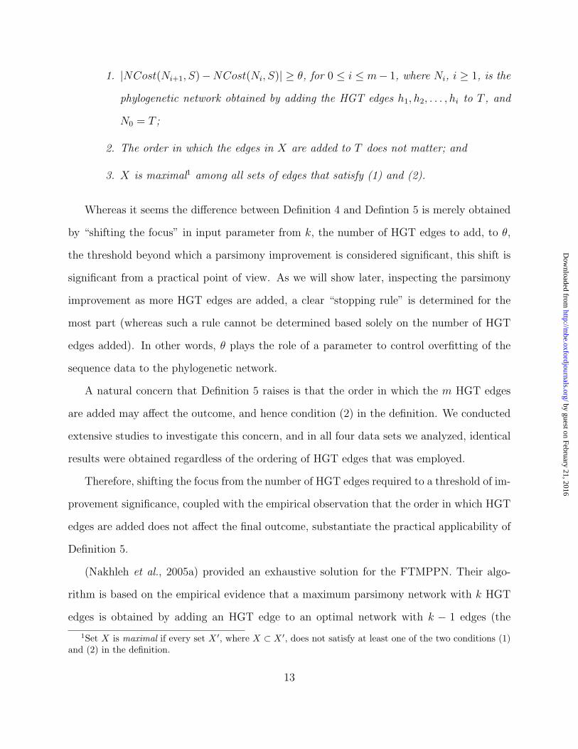
1. |NCost(Ni+1, S)−NCost(Ni, S)| ≥ θ, for 0 ≤ i ≤ m− 1, where Ni, i ≥ 1, is the

phylogenetic network obtained by adding the HGT edges h1, h2, . . . , hi to T , and

N0 = T ;

2. The order in which the edges in X are added to T does not matter; and

3. X is maximal1 among all sets of edges that satisfy (1) and (2).

Whereas it seems the difference between Definition 4 and Defintion 5 is merely obtained

by “shifting the focus” in input parameter from k, the number of HGT edges to add, to θ,

the threshold beyond which a parsimony improvement is considered significant, this shift is

significant from a practical point of view. As we will show later, inspecting the parsimony

improvement as more HGT edges are added, a clear “stopping rule” is determined for the

most part (whereas such a rule cannot be determined based solely on the number of HGT

edges added). In other words, θ plays the role of a parameter to control overfitting of the

sequence data to the phylogenetic network.

A natural concern that Definition 5 raises is that the order in which the m HGT edges

are added may affect the outcome, and hence condition (2) in the definition. We conducted

extensive studies to investigate this concern, and in all four data sets we analyzed, identical

results were obtained regardless of the ordering of HGT edges that was employed.

Therefore, shifting the focus from the number of HGT edges required to a threshold of im-

provement significance, coupled with the empirical observation that the order in which HGT

edges are added does not affect the final outcome, substantiate the practical applicability of

Definition 5.

(Nakhleh et al., 2005a) provided an exhaustive solution for the FTMPPN. Their algo-

rithm is based on the empirical evidence that a maximum parsimony network with k HGT

edges is obtained by adding an HGT edge to an optimal network with k − 1 edges (the

1Set X is maximal if every set X ′, where X ⊂ X ′, does not satisfy at least one of the two conditions (1)and (2) in the definition.

13



ownloaded from


experiments were conducted several times, while taking the HGT edges in different orders,

and in all these cases, the same resulting networks were obtained). The algorithm seeks to

add an edge in all possible ways to all optimal networks with k− 1 network edges. This ap-

proach requires computing the parsimony score, based on Definition 3, of every phylogenetic

network obtained during the search; we refer to this computation as the PSPN problem.

Definition 6 Parsimony Score of Phylogenetic Networks (PSPN):

Input: A set S of aligned sequences, and a phylogenetic network N leaf-labeled by S.

Output: NCost(N, S).

Nakhleh et al. provided a straightforward algorithm for solving the PSPN problem which

enumerates all trees contained inside the network and therefore runs in O(m`n) time, where

m = |T (N)|, ` is the sequence length, and n is the number of taxa (leaves) in the phylogenetic

network. Since the number of HGT edges is O(n2) in the worst case, the number of trees

inside a network may be exponential in the number of leaves, and hence the running time

of the algorithm is exponential in the number of HGT edges (in the number of taxa in the

worst case). We proved the PSPN problem is NP-hard, and developed more computationally

efficient algorithms and heuristics for the PSPN and FTMPPN problems in (Jin et al.,

2006b).

Data Sets

We analyzed four biological data sets with the aim of identifying the number of HGT events,

as well as their respective donors and recipients:

1. The rubisco gene rbcL of a group of 46 plastids, cyanobacteria, and proteobacteria,

which was analyzed by Delwiche and Palmer (Delwiche & Palmer, 1996). This data

set consists of 46 aligned amino acid sequences (each of length 532), 40 of which are

14



ownloaded from


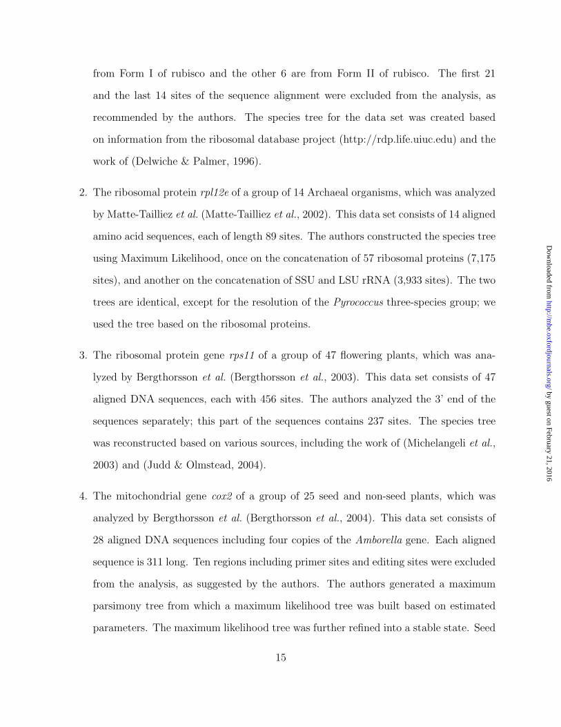
from Form I of rubisco and the other 6 are from Form II of rubisco. The first 21

and the last 14 sites of the sequence alignment were excluded from the analysis, as

recommended by the authors. The species tree for the data set was created based

on information from the ribosomal database project (http://rdp.life.uiuc.edu) and the

work of (Delwiche & Palmer, 1996).

2. The ribosomal protein rpl12e of a group of 14 Archaeal organisms, which was analyzed

by Matte-Tailliez et al. (Matte-Tailliez et al., 2002). This data set consists of 14 aligned

amino acid sequences, each of length 89 sites. The authors constructed the species tree

using Maximum Likelihood, once on the concatenation of 57 ribosomal proteins (7,175

sites), and another on the concatenation of SSU and LSU rRNA (3,933 sites). The two

trees are identical, except for the resolution of the Pyrococcus three-species group; we

used the tree based on the ribosomal proteins.

3. The ribosomal protein gene rps11 of a group of 47 flowering plants, which was ana-

lyzed by Bergthorsson et al. (Bergthorsson et al., 2003). This data set consists of 47

aligned DNA sequences, each with 456 sites. The authors analyzed the 3’ end of the

sequences separately; this part of the sequences contains 237 sites. The species tree

was reconstructed based on various sources, including the work of (Michelangeli et al.,

2003) and (Judd & Olmstead, 2004).

4. The mitochondrial gene cox2 of a group of 25 seed and non-seed plants, which was

analyzed by Bergthorsson et al. (Bergthorsson et al., 2004). This data set consists of

28 aligned DNA sequences including four copies of the Amborella gene. Each aligned

sequence is 311 long. Ten regions including primer sites and editing sites were excluded

from the analysis, as suggested by the authors. The authors generated a maximum

parsimony tree from which a maximum likelihood tree was built based on estimated

parameters. The maximum likelihood tree was further refined into a stable state. Seed

15



ownloaded from


and non-seed plants were analyzed separately. We used a species tree for the data

set based on information at NCBI (http://www.ncbi.nih.gov) and analyzed the entire

data set with both seed and nonseed plants together.

Phylogenetic Analyses

To understand the performance of maximum parsimony as a criterion for reconstructing

phylogenetic networks in general, and detecting HGT in particular, we investigated the four

data sets with respect to four different questions.

1. Does the MP criterion correctly identify the number and location (i.e., donors and recip-

ients) of HGT events needed to explain the evolutionary history of a gene with respect

to a species phylogeny? To answer this question, we analyzed the rbcL, rpl12e, and

cox2 data sets by running the methods of (Jin et al., 2006b) for solving the FTMPPN

problem. More specifically, for each of the data sets, we sought a set of edges whose

addition to the species tree yielded an optimal phylogenetic network under the par-

simony criterion. As discussed before, adding more edges to a phylogenetic network

either improves the parsimony score of the phylogenetic network or leaves it unchanged.

We analyzed the rate of improvement as a way to determine when to stop adding extra

edges. The quality of the MP criterion with respect to this question (as well as the

next three questions) was determined by comparing our findings to the hypotheses

postulated by the authors of the data sets we considered.

2. How does incomplete taxon sampling affect the performance of the criterion with re-

spect to question (1)? To answer this question, we sampled 15 taxa from the rbcL data

set in such a way to ensure that the donors and recipients of the HGTs detected in

the analysis of question (1) were present among these 15 taxa. We used this 15-taxon

data set to study the performance of the MP criterion with respect to detecting the

16



ownloaded from


number of HGTs as well as the donor/recipient of these HGTs.

3. Does the site substitution matrix affect the performance of the criterion? To answer

this question, we re-analyzed the 15-taxon rbcL data set under various amino acid

substitution matrices. Once again, we analyzed the data set with respect to the number

as well as location of the HGTs.

4. Can the MP criterion help identify partial (chimaeric) HGT? Bergthorsson et al. an-

alyzed the rps11 gene in a group of flowering plants and postulated that not only did

this gene involve HGT, but also that it was chimaeric: its 5’ half was vertically inher-

ited, whereas its 3’ half was horizontally transferred (Bergthorsson et al., 2003). We

analyzed both the complete rps11 gene as well as its 3’ half.

Results and Discussion

Identifying The Numbers and Locations of HGT Events

In this section, we report on our findings when analyzing the rbcL, rpl12e, and cox2 data

sets using our methods for solving the FTMPPN. For each data set we show the optimal

improvement in parsimony scores as new edges are added to the species trees, as well as

the location of the edges that correspond to these optimal improvement. All results in this

section are based on the identity substitution matrix (which assigns value 0 to two identical

sites, and value 1 to two different sites).

The rbcL Gene Data Set

We analyzed the rbcL gene data set twice in this context: once with the complete data set

of 46 organisms, and another with only 40 organisms; the latter was obtained by removing

17



ownloaded from


0 2 4 6 8 10

2000

2500

3000

3500

4000

Number of HGT edgesP

arsi

mon

y sc

ore

40 taxa46 taxa

Figure 4: Optimal improvement in the parsimony score as extra edges are added to thespecies tree to obtain a phylogenetic network on the rbcL data set. The most significantimprovements are obtained by adding the first seven HGT edges in the case of the 46-taxondata set, and the first four HGT edges in the case of the 40-taxon data set.

the Form II rubisco.2 The optimal improvements in the parsimony score as ten edges are

added to both species trees of this data set are shown in Figure 4.

We observe that the optimal improvement in parsimony score is always higher than 80

points for every edge added of the first seven in the case of the 46-taxon data set, and the

first four in the case of the 40-taxon data set. The actual HGT edges that correspond to the

first seven and first four of these optimal improvements for the 46- and 40-taxon data sets

are shown in Figures 5(a) and 5(b), respectively.

The HGT edges H1, H3, and H4 in Figure 5(a) group all the Form II species together;

since these species are excluded from the 40-taxon data set, these edges have no equivalent

ones in Figure 5(b). The remaining four HGT edges, H2, H5, H6, and H7 in Figure 5(a)

achieve the same effect of the four HGT edges H1, H2, H3, and H4 in Figure 5(b). Edges H2

and H5 in Figures 5(b) and 5(a), respectively, group the three Alcaligenes species together

with the Rhodobacter Sphaeroides I and Xanthobacter species, indicating an HGT from the

most recent common ancestor of the latter two species to the most recent common ancestor of

2The original data set had 48 species, but the two species Endosymbiont of Alvinoconcha and PseudomonasHydrogenothermophila were unclassified in (Delwiche & Palmer, 1996); hence, we excluded them.

18



ownloaded from


RhodospirillumRhodobacter capsulatusRhodobacter sphaeroides II

NitrobacterMn oxidizing bacterium SI85-9a1

Rhodobacter sphaeroides IXanthobacter

Thiobacillus denitrificans IAlcaligenes 17707 chromosomal

Alcaligenes H16 chromosomalAlcaligenes H16 plasmid

Hydrogenovibrio L2Hydrogenovibrio L1Chromatium AChromatium L

Thiobacillus ferrooxidans fe1Thiobacillus ferrooxidans 19859

SynechococcusAnabaena

ProchlorothrixAnacystis

SynechocystisProchloron

Gonyaulax Cyanophora

CyanidiumAhnfeltiaAntithamnion

PorphyridiumCryptomonas

EctocarpusOlistodiscusCylindrotheca

EuglenaPyramimonas

ChlamydomonasChlorellaBryopsis

ColeochaeteMarchantia

PseudotsugaNicotianaOryza

H2

H3

H4

H5

H7

H1

H0: 4094+ H1: 3859 (-235)+ H2: 3635 (-224)+ H3: 3421 (-214)+ H4: 3266 (-155)+ H5: 3129 (-137)+ H6: 3009 (-120)+ H7: 2927 ( -82)

Thiobacillus denitrificans II

α Proteobacteria

β Proteobacteria

γ Proteobacteria

Cyanobacteria

Dinoflagellate PlastidGlaucophyte Plastid

Red and Brown Plastids

Green Plastids

ProchlorococcusH6

Hydrogenovibrio II

NitrobacterMn oxidizing bacterium SI85-9a1

Rhodobacter sphaeroides IXanthobacter

Thiobacillus denitrificans IAlcaligenes 17707 chromosomal

Alcaligenes H16 chromosomalAlcaligenes H16 plasmid

Hydrogenovibrio L2Hydrogenovibrio L1

Chromatium AChromatium L

Thiobacillus ferrooxidans fe1Thiobacillus ferrooxidans 19859

ProchlorococcusSynechococcusAnabaena

ProchlorothrixAnacystis

SynechocystisProchloron

CyanophoraCyanidium

AhnfeltiaAntithamnion

PorphyridiumCryptomonas

EctocarpusOlistodiscusCylindrotheca

EuglenaPyramimonas

ChlamydomonasChlorellaBryopsis

ColeochaeteMarchantiaPseudotsuga

NicotianaOryza

H2

H3

H0: 2573+ H1: 2351 (-222)+ H2: 2208 (-143)+ H3: 2087 (-121)+ H4: 2006 ( -81)

H1

H4

Green Plastids

Red and Brown Plastids

Glaucophyte Plastid

Cyanobacteria

γ Proteobacteria

β Proteobacteria

α Proteobacteria

(a) 46 taxa (b) 40 taxa

Figure 5: The MP phylogenetic networks of the rbcL data set obtained by adding sevenedges for the 46 taxa case (a) and four edges for the 40 taxa case (b) to the underlyingspecies tree. Parsimony score improvement after incrementally adding the horizontal genetransfers are shown at the bottom. Form II rubisco are shown in bold. The improvement inthe parsimony score per each HGT edge is shown next to each phylogenetic network. ‘H0:X’ indicates that X is the parsimony score of the species tree. ‘+Hi: X (Y)’ indicates thatthe parsimony score of the phylogenetic network after adding the ith HGT edge is X, andthe decrease in the parsimony score achieved by HGT edge Hi alone is Y.

the Alcaligenes species. Edges H3 and H6 in Figures 5(b) and 5(a), respectively, group three

α-Proteobacteria with the group of red and brown plastids. Edges H1 and H4 in Figure 5(b)

and edges H2 and H7 in Figure 5(a) indicate different HGT’s in the two data sets, yet

achieve exactly the same grouping: they group the two cyanobacteria Prochlorococcus and

Prochloron together, and then group these two together with the green plastid Pyramimonas.

How do these findings compare to the hypotheses of (Delwiche & Palmer, 1996)? The

authors postulated that at least four independent HGTs were required to explain the division

19



ownloaded from


of plastids and proteobacteria into the green-like and red-like groups:

1. A transfer of red-like rubisco operon from a proteobacterium to a common ancestor of

red and brown plastids. Our analysis computed such a transfer, but we found that it

is from a common ancestor of red and brown plastids to a proteobacterium (edge H6

in Figure 5(a)).

2. A transfer of a cyanobacterial green-like rbcL to an ancestor of γ-proteobacteria early

in their evolution (but after the emergence of the β-proteobacteria from within the

γ-proteobacteria).

3. A transfer from this same γ-proteobacterial lineage to ancestor of the α-proteobacterium

Nitrobacter vulgaris.

4. A transfer from this same γ-proteobacterial lineage to ancestor of the β-proteobacterium

Thiobacillus denitrificans.

In the case of the last three transfers, the authors were not certain about them (even pos-

tulating that the incongruence may be due to inaccurate identification of some of the taxa).

Our analysis, instead, indicates two transfers from the β-proteobacterium Thiobacillus den-

itrificans II to the α and γ groups of the form II rubisco. Further, they postulated three

more HGTs to account for incongruities in the rbcL phylogeny:

1. A transfer of the Gonyaulax rubisco (in the gene tree, it is grouped within the α-

proteobacteria of the Form II rubisco). Our analysis indicates an HGT from the

common ancestor of Rhodobacter capsulatus/Rhodobacter sphaeroides II to Gonyaulax

(edge H4 in Figure 5(a)), which results in a grouping identical to that based on the

rbcL gene tree in (Delwiche & Palmer, 1996).

2. A transfer from the green-like proteobacterial group to Prochlorococcus. In this case,

the authors could not determine with certainty where the transfer occurred. Our

20



ownloaded from


analysis shows that the transfer occurred from the cyanobacterium Prochloron to the

cyanobacterium Prochlorococcus (edge H2 in Figure 5(a)).

3. A transfer involving one of the three groups Rhodobacter/Xanthobacter, Alcaligenes,

and Mn-oxidizing bacterium. In this case as well, the authors could not determine with

certainty which of the three groups involved the transfer. Our analysis shows that the

transfer occurred from the Rhodobacter/Xanthobacter group to the Alcaligenes group

(edge H5 in Figure 5(a)).

Finally, our analysis gave rise to edge H7 in Figure 5(a), which gives indication of a transfer

that was not postulated by the authors, but among all seven edges found in our analysis,

this edge led to the smallest improvement in the parsimony score.

Edges H1, H3, and H4 in Figure 5(a) all correspond to Form II rubisco; since these

taxa are not present in the 40-taxon species tree, only the four remaining HGT edges were

identified, and they are shown in Figure 5(b)—the correspondence is described above.

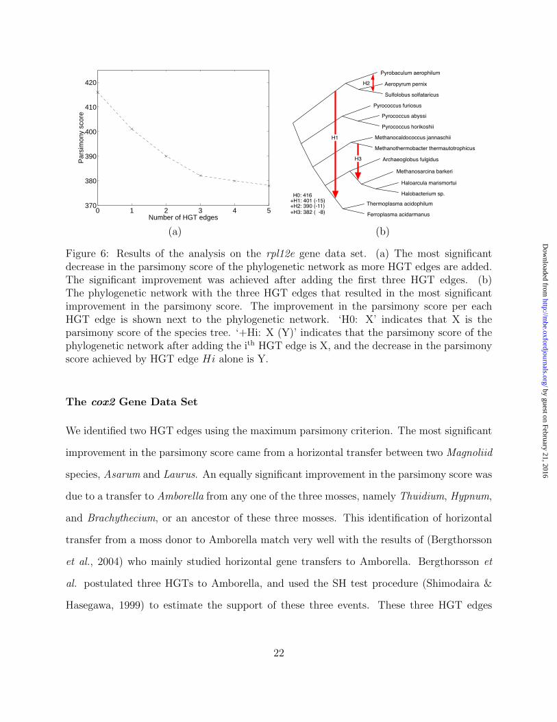
The rpl12e Gene Data Set

Our analysis of the data set of (Matte-Tailliez et al., 2002) inferred three significant HGT

edges, shown in Figure 6. Edge H1 resulted in the most significant improvement in the par-

simony score, and indicated the transfer which was postulated by the authors. Edge H2 ac-

counts for the incongruence between the species tree and the tree based on the rpl12e protein,

where the two trees differ in the phylogenetic pattern of the Aeropyrum pernix/Pyrobaculum

aerophilum/Sulfolobus solfataricus group. Edge H3 indicates a transfer between Methanobac-

terium thermoautotrophicum and the group of Methanosarcina barkeri, Haloarcula marismor-

tui, and Halobacterium sp.

21



ownloaded from


0 1 2 3 4 5370

380

390

400

410

420

Number of HGT edges

Par

sim

ony

scor

e

Halobacterium sp.

Haloarcula marismortui

Ferroplasma acidarmanus

Thermoplasma acidophilum

Pyrobaculum aerophilum

Pyrococcus furiosus

Sulfolobus solfataricus

Pyrococcus abyssi

Pyrococcus horikoshii

Methanocaldococcus jannaschii

Archaeoglobus fulgidus

Methanosarcina barkeri

Methanothermobacter thermautotrophicus

Aeropyrum pernix

H1

H3

H2

H0: 416+H1: 401 (-15)+H2: 390 (-11)+H3: 382 ( -8)

(a) (b)

Figure 6: Results of the analysis on the rpl12e gene data set. (a) The most significantdecrease in the parsimony score of the phylogenetic network as more HGT edges are added.The significant improvement was achieved after adding the first three HGT edges. (b)The phylogenetic network with the three HGT edges that resulted in the most significantimprovement in the parsimony score. The improvement in the parsimony score per eachHGT edge is shown next to the phylogenetic network. ‘H0: X’ indicates that X is theparsimony score of the species tree. ‘+Hi: X (Y)’ indicates that the parsimony score of thephylogenetic network after adding the ith HGT edge is X, and the decrease in the parsimonyscore achieved by HGT edge Hi alone is Y.

The cox2 Gene Data Set

We identified two HGT edges using the maximum parsimony criterion. The most significant

improvement in the parsimony score came from a horizontal transfer between two Magnoliid

species, Asarum and Laurus. An equally significant improvement in the parsimony score was

due to a transfer to Amborella from any one of the three mosses, namely Thuidium, Hypnum,

and Brachythecium, or an ancestor of these three mosses. This identification of horizontal

transfer from a moss donor to Amborella match very well with the results of (Bergthorsson

et al., 2004) who mainly studied horizontal gene transfers to Amborella. Bergthorsson et

al. postulated three HGTs to Amborella, and used the SH test procedure (Shimodaira &

Hasegawa, 1999) to estimate the support of these three events. These three HGT edges

22



ownloaded from


0 0.5 1 1.5 2 2.5 3200

210

220

230

240

250

260

270

280

Number of HGT edges

Par

sim

ony

scor

eArabidopsisBrassica

OenotheraBeta

DaucusPetunia

Agave

ZeaPhilodendron

Oryza

AmborellalesEichhornia

Liriodendron

Asarum

ZamiaLaurusPiper

BrachytheciumThuidium

HypnumPinus

Marchantia

PorellaPallavicinia

Trichocolea

H2H1

Bryo

phyt

a

Mag

nolio

phyt

aEudi

coty

ledo

ns

Mon

ocot

yledo

ns

Mog

noliid

s

Hypn

ales

H0: 270+ H1: 242 (-28)+ H2: 217 (-25)

(a) (b)

Figure 7: Results of the analysis on the cox2 gene data set. (1) The most significant de-crease in the parsimony score of the phylogenetic network as more HGT edges are added.The significant improvement was achieved after adding the first two HGT edges. (b) Thephylogenetic network with the two HGT edges that resulted in the most significant improve-ment in the parsimony score. The circle at the source of the second HGT edge denote thatany of the tree edges within the circle could be the donor of the HGT, and with the sameeffect on the parsimony score. The improvement in the parsimony score per HGT edge isshown next to the phylogentic network. ‘H0: X’ indicates that X is the parsimony score ofthe species tree. ‘+Hi: X(Y)’ indicates that the parsimony score of the phylogenetic networkafter adding the ith HGT edge is X, and the decrease in the parsimony score achieved byHGT edge Hi alone is Y.

consisted of one from a moss donor, with the strongest evidence and support from the SH

test (< 0.001) and bootstrap value (> 90%), two from other angiosperms, which the authors

deemed insignificant based on the SH test (> 0.05) and weak bootstrap supports due to

largely poorly resolved trees within angiosperms. As noted, the HGT edge H1, which was

found to be most significant under the parsimony criterion, corresponds to the only well

supported HGT event that Bergthorsson et al. found. The second HGT edge, H2, that was

found by the parsimony analysis is probably a reflection of the “weak” phylogenetic signal

in this gene sequence data (which is reflected by the weak support of most branches in the

gene tree of cox2 in (Bergthorsson et al., 2004)).

23



ownloaded from


0 2 4 6 8

1600

1800

2000

2200

2400

2600

Number of HGT edges

Par

sim

ony

scor

eRhodobacter capsulatus

Nitrobacter

Rhodobacter sphaeroides I


Thiobacillus denitrificans I

Alcaligenes H16 plasmid

Hydrogenovibrio II

Chromatium L

Thiobacillus ferrooxidans 19859

Prochlorococcus

Synechococcus

Gonyaulax

Cyanophora

Cyanidium

Euglena

H2

H1

H4

H3

H5

H0: 2572+ H1: 2361 (-211)

+ H5: 1762 (-105)

+ H2: 2151 (-210)+ H3: 1991 (-160)+ H4: 1867 (-124)

(a) (b)

Figure 8: Results of the analysis on the 15-taxon rbcL gene data set. (a) The most significantdecrease in the parsimony score of the phylogenetic network as more HGT edges are added.The significant improvement in the parsimony score was achieved after adding the first fiveHGT edges. (b) The phylogenetic network with the three HGT edges that resulted in themost significant improvement in the parsimony score. The improvement in the parsimonyscore per each HGT edge is shown next to the phylogenetic network. ‘H0: X’ indicates thatX is the parsimony score of the species tree. ‘+Hi: X (Y)’ indicates that the parsimonyscore of the phylogenetic network after adding the ith HGT edge is X, and the decrease inthe parsimony score achieved by HGT edge Hi alone is Y.

Effects of Incomplete Taxon Sampling

To investigate the effects of incomplete taxon sampling on the performance of the MP cri-

terion for detecting HGT, we selected 15 taxa from the rbcL data set so as to cover all the

groups in the data set. These 15 taxa are shown at the tips of the tree in Figure 8(b). The

improvement in parsimony score as extra edges are added to the species tree, as well as the

edges that correspond to the optimal improvements, are shown in Figures 8(a) and 8(b),

respectively. The figure shows clearly that the first five added edges lead to significant

improvement in the parsimony score of the resulting phylogenetic network, whereas the im-

provement afterwards is relatively much less significant.

24



ownloaded from


Our results indicate that in this case we observe a similar trend to that of the full data set

in terms of the improvement in parsimony score, yet slightly different results in terms of the

locations of the HGT edges themselves. Since Prochloron—the donor in the HGT event H2

in Figure 5(a)—was not sampled, the analysis did not detect the HGT event that involved

it. Edges H1, H3, and H4 in Figure 5(a) all involved form II species. Their counterparts

in the analysis of the 15-taxon data set are edges H1, H2, and H3, respectively, as shown

in Figure 8(b). Notice that these edges in both figures achieve the same result, namely the

grouping of the form II species, yet they differ in explaining the donor of the rbcL gene in

the Hydrogenovibrio II species (edges H3 and H2 in Figures 5(a) and 8(b), respectively).

Edges H4 and H5 in Figure 8(b) achieve the same grouping as edges H5 and H6 in

Figure 5(a), yet they place the groups in different places in their respective trees. Notice

that since neither the donor nor the recipient of HGT edge H7 in Figure 5(a) are present in

the 15-taxon data set, no counterpart to this edge was found when analyzing the 15-taxon

data set.

To conclude about the findings in this analysis, incomplete taxon sampling does not

seem to affect the trend in parsimony score improvement, whereas it may have impact

on the directions of the HGT edges detected, as illustrated in the differences between the

phylogenetic networks of Figures 5(a) and 8(b). A very significant implication of the results

of this analysis is that the MP criterion is robust with respect to incomplete taxon sampling

in terms of identifying the number of HGT events, as well the identity of the donors and

recipients, yet it may get the directions of the HGT edges in reversed order.

Effects of Site Substitution Matrix

To investigate the robustness of the MP criterion for HGT detection with respect to the site

substitution matrix used in the analysis, we re-analyzed the 15-taxon rbcL data set using four

different matrices, in addition to the identity matrix used in the previous section: BLOSUM

25



ownloaded from


0 2 4 6 8

0.6

0.8

1

1.2

1.4

1.6

x 104

Number of HGT edges

Par

sim

ony

scor

e

PAM120PAM250BLOSUM45BLOSUM62

Figure 9: The most significant decrease in the parsimony score of the phylogenetic network asmore HGT edges are added in the analysis of the 15-taxon rbcL data set under four differentsite substitution matrices. In all four cases, the significant improvement in the parsimonyscore was achieved after adding the first six HGT edges.

45, BLOSUM 62, PAM 250, and PAM 120. The improvements in parsimony scores as extra

HGT edges are added are shown in Figure 9, and the phylogenetic networks with the HGT

edges resulting in the optimal improvements are shown in Figure 10.

In terms of the improvement in parsimony scores as extra HGT edges are added, Figure 9

shows trends similar to that when using the identity matrix, as shown in Figure 8(a). The

only difference is that in the case of these four matrices, the trends indicate six extra HGT

edges, rather than five edges as in the case of the identity matrix.

As for the detected HGT edges themselves, the results are very similar to those under

the identity matrix in terms of the species grouping they achieve. The HGT edges detected

under both BLOSUM matrices were identical, whereas these were different from the edges

detected under the two PAM matrices, which also differed between them, as shown in the

three phylogenetic networks in Figure 10. The three edges H1, H2, and H3 in all three

phylogenetic networks have exactly the same effect, namely the grouping of all form II

species. Nonetheless, the phylogenetic networks differ in the placement of the groups. Edges

H4 and H5 achieve the exact same result as that achieved by H4 and H5 under the identity

26



ownloaded from


Rhodobacter capsulatus

Nitrobacter





Hydrogenovibrio II

Chromatium L


Prochlorococcus

Synechococcus

Gonyaulax

Cyanophora

Cyanidium

Euglena

H0: 16538

+ H4: 9593 ( -834)

+ H1: 14368 (-2170)+ H2: 12248 (-2120)+ H3: 10427 (-1821)

+ H5: 8960 ( -633)+ H6: 8518 ( -442)

BLOSUM45

H1

H2

H3

H6

H5

H4

H0: 14446

+ H4: 8177 ( -695)

+ H1: 12526 (-1920)+ H2: 10547 (-1979)+ H3: 8872 (-1675)

+ H5: 7644 ( -533)+ H6: 7261 ( -383)

BLOSUM62


Nitrobacter





Hydrogenovibrio II

Chromatium L


Gonyaulax

Cyanophora

Cyanidium

Euglena

H0: 12874+ H1: 10943 (-2439)+ H2: 9117 (-1826)+ H3: 7562 (-1555)

H1H2

H3

H4H4

H5

H6

Prochlorococcus

Synechococcus

+ H4: 6976 ( -586)+ H5: 6479 ( -497)+ H6: 6169 ( -310)


Nitrobacter





Hydrogenovibrio II

Chromatium L


Gonyaulax

Cyanophora

Cyanidium

Euglena

H2

H1

H4

H3 H5

H0: 15455+ H1: 13382 (-2073)+ H2: 11292 (-2090)+ H3: 9516 (-1776)

H6

Prochlorococcus

Synechococcus

+ H5: 8193 ( -569)+ H4: 8762 ( -754)

+ H6: 7777 ( -416)

BLOSUM 45 and 62 PAM250 PAM120

Figure 10: The MP phylogenetic networks of the 15-taxon rbcL data set obtained with thePAM and BLOSUM matrices. The improvement in the parsimony score per each HGTedge is shown next to each phylogenetic network. ‘H0: X’ indicates that X is the parsimonyscore of the species tree. ‘+Hi: X (Y)’ indicates that the parsimony score of the phylogeneticnetwork after adding the ith HGT edge is X, and the decrease in the parsimony score achievedby HGT edge Hi alone is Y. Having more than one HGT edge Hi in a phylogenetic networkindicates that this edge can be added in any of these locations, yet leading to exactly thesame improvement in the parsimony score.

matrix. In conclusion, the first five HGT edges detected under the various site substitution

matrices achieve the same results. The sixth edge detected under the four matrices, but

not the identity matrix, all involve Prochlorococcus. This edge had the least significant

contribution to improving the parsimony score among all six edges.

Detection of Partial HGT

In their analysis of a group of flowering plants, Bergthorsson et al. reported on transfers that

created chimaeric, half-monocot, half-dicot genes (Bergthorsson et al., 2003). In particular,

they showed that Sanguinaria rps11 is chimaeric: its 5’ half is of expected eudicot, vertical

origin, whereas its 3’ half is “indisputably of monocot, horizontal origin.”

To investigate the performance of the MP criterion for detection HGT events in the case

of chimaeric genes, we analyzed the complete rps11 gene sequences as well as their 3’ half

27



ownloaded from


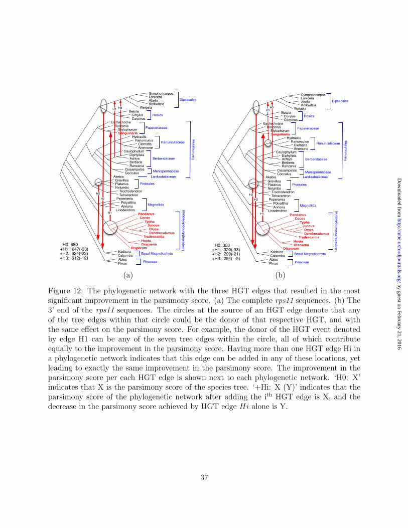
separately. The improvements in the parsimony scores as HGT edges are added are shown in

Figure 11, and the phylogenetic networks themselves are shown in Figure 12. The parsimony

score improvement has almost identical trends in both cases of the complete and partial gene

data sets, where in both cases it indicates that at most three HGT edges need to be added.

A significant observation is that in both cases, the first two HGT edges detected in the

analysis are identical. Further, the first edge, H1, leads to exactly the same improvement

in the parsimony score (the parsimony score drops by 33 points in both cases). This clearly

indicates that all the improvement in the parsimony score results in a transfer that involves

only the 3’ half of the rps11 gene. Similarly, edge H2 leads to almost the same drop in the

parsimony score in both cases: 23 points in the case of the complete gene and 21 points in

the case of its 3’ half, once again indicating the transfer of the 3’ half only.

0 1 2 3 4 5 6590

600

610

620

630

640

650

660

670

680

690

Number of HGT edges

Par

sim

ony

scor

e

0 1 2 3 4 5 6280

290

300

310

320

330

340

350

360

Number of HGT edges

Par

sim

ony

scor

e

(a) (b)

Figure 11: The most significant decrease in the parsimony score of the phylogenetic networkas more HGT edges are added for the rps11 data set. (a) The complete rps11 sequences.(b) The 3’ end of the rps11 sequences. In both cases, the significant improvement in theparsimony score was achieved after adding the first three HGT edges.

In this analysis, we used the knowledge that the 3’ half was involved in the transfer and

hence we were able to conduct the analysis on the complete gene as well as on its 3’ half. An

interesting question is whether the MP criterion could detect that the 3’ half was involved in

28



ownloaded from


the transfer without having the knowledge a priori. To answer this question, we considered a

phylogenetic sub-network obtained from the phylogenetic network in Figure 12(a), by taking

only the species tree and the HGT edge H1, which is the one that corresponds to HGT

in Sanguinaria. Since there are seven possible donors for the HGT denoted by H1, this

phylogenetic network in fact represents seven networks, each of which contains the species

tree and the gene tree obtained by moving the Sanguinaria close to the Monocotyledons.

For each such phylogenetic network, we passed a window of a fixed size across the sequence

alignment, and computed the parsimony score of the block within the window on the species

as well as the seven gene trees inside the network. Figure 13 shows the results for blocks of

sizes 200, 100, 50, 25, and 5 positions.

The position from which the parsimony score on the gene trees becomes lower than that

on the species tree is position 221. Interestingly, the 3’ half of the rps11 gene starts at

position 220, indicating that, indeed, this part of the gene had evolved down a tree other

than the species tree.

The Maximum Likelihood Criterion for Phylogenetic Networks

In the context of optimization criteria for phylogeny reconstruction, we have recently intro-

duced a maximum likelihood (ML) framework for evaluating and reconstructing phylogenetic

networks (Jin et al., 2006a). Like the ML criterion for phylogenetic trees, this framework

views a phylogenetic network from a probabilistic perspective as a generative model, and the

phylogenetic network that maximizes the likelihood of the sequences at its leaves is sought.

Further, in a similar manner to that of defining the parsimony of networks, the ML crite-

rion for phylogenetic networks is defined in terms of the trees contained inside the networks

(maximizing or summing over all trees). Our preliminary results indicate that the ML frame-

work is a promising approach as well. Yet, the parsimony criterion currently outperforms

it, in terms of computational requirements as well as accuracy of the inferred HGT events.

29



ownloaded from


However, it is important to note that the accuracy issue is just an artifact of our initial (and

naive) way of estimating the parameters associated with the branches of the networks and

trees. Once more appropriate stochastic models of evolution down phylogenetic networks

are defined and used, we expect the relative performance of the two criteria to be similar to

that in the context of phylogenetic trees.

Acknowledgments

This work was supported in part by the Rice Terascale Cluster funded by NSF under grant

EIA-0216467, Intel, and HP. Luay Nakhleh was supported in part by the Department of

Energy grant DE-FG02-06ER25734, the National Science Foundation grant CCF-0622037,

the George R. Brown School of Engineering Roy E. Campbell Faculty Development Award,

and the Department of Computer Science at Rice University. We are grateful to Associate

Editor Dan Graur, and the two anonymous reviewers for helpful comments and suggestions.

References

Addario-Berry, L., Hallett, M.T., & Lagergren, J. 2003. Towards identifying lateral gene

transfer events. Pages 279–290 of: Proc. 8th Pacific Symp. on Biocomputing (PSB03).

Bergthorsson, U., Adams, K.L., Thomason, B., & Palmer, J.D. 2003. Widespread horizontal

transfer of mitochondrial genes in flowering plants. Nature,424, 197–201.

Bergthorsson, U., Richardson, A., Young, G.J., Goertzen, L., & Palmer, J.D. 2004. Mas-

sive horizontal transfer of mitochondrial genes from diverse land plant donors to basal

angiosperm Amborella. Proc. Nat’l Acad. Sci., USA,101, 17747–17752.

30



ownloaded from


Blanchette, M., Bourque, G., & Sankoff, D. 1997. Breakpoint phylogenies. Pages 25–34 of:

Miyano, S., & Takagi, T. (eds), Genome Informatics. Tokyo: Univ. Academy Press.

Boc, A., & Makarenkov, V. 2003. New Efficient Algorithm for Detection of Horizontal

Gene Transfer Events. Pages 190–201 of: Proc. 3rd Int’l Workshop Algorithms in

Bioinformatics (WABI03), vol. 2812. Springer-Verlag.

Brown, J.R. 2003. Ancient horizontal gene transfer. Nat. Rev. Genet.,4, 121–132.

Brown, J.R., Douady, C.J., Italia, M.J., Marshall, W.E, & Stanhope, M.J. 2001. Universal

trees based on large combined protein sequence data sets. Nat. Genet.,28, 281–285.

Bull, J.J., Huelsenbeck, J.P., Cunningham, C.W., Swofford, D., & Waddell, P. 1993. Parti-

tioning and combining data in phylogenetic analysis. Syst. Biol.,42(3), 384–397.

Chippindale, P.T., & Wiens, J.J. 1994. Weighting, partitioning, and combining characters

in phylogenetic analysis. Syst. Biol.,43(2).

Cunningham, C.W. 1997. Can three incongruence tests predict when data should be com-

bined? Mol. Biol. Evol.,14, 733–740.

Daubin, V., & Ochman, H. 2004. Quartet mapping and the extent of lateral transfer in

bacterial genomes. Mol. Biol. Evol.,21(1), 86–89.

Daubin, V., Gouy, M., & Perriere, G. 2002. A phylogenomic approach to bacterial phylogeny:

evidence of a core of genes sharing a common history. Genome Res.,12, 1080–1090.

Daubin, V., Moran, N.A., & Ochman, H. 2003. Phylogenetics and the cohesion of bacterial

genomes. Science,301, 829–832.

Day, W.H.E. 1983. Computationally difficult parsimony problems in phylogenetic systemat-

ics. Journal of Theoretical Biology,103, 429–438.

31



ownloaded from


de Queiroz, A., Donoghue, M.J., & Kim, J. 1995. Separate versus combined analysis of

phylogenetic evidence. Annu. Rev. Ecol. Syst.,25, 657–681.

Delwiche, C. F., & Palmer, J. D. 1996. Rampant Horizontal Transfer and Duplicaion of

Rubisco Genes in Eubacteria and Plastids. Mol. Biol. Evol,13(6).

Doolittle, W.F. 1999a. Lateral genomics. Trends in Biochemical Sciences,24(12), M5–M8.

Doolittle, W.F. 1999b. Phylogenetic classification and the universal tree. Science,284, 2124–

2129.

Doolittle, W.F., Boucher, Y., Nesbo, C.L., Douady, C.J., Andersson, J.O., & Roger, A.J.

2003. How big is the iceberg of which organellar genes in nuclear genomes are but the

tip? Phil. Trans. R. Soc. Lond. B. Biol. Sci.,358, 39–57.

Eisen, J.A. 2000a. Assessing evolutionary relationships among microbes from whole-genome

analysis. Curr. Opin. Microbiol.,3, 475–480.

Eisen, J.A. 2000b. Horizontal gene transfer among microbial genomes: New insights from

complete genome analysis. Curr Opin Genet Dev.,10(6), 606–611.

Fitch, W.M. 1971. Toward defining the course of evolution: minimum change for a specified

tree topology. Syst. Zool.,20, 406–416.

Foulds, L.R., & Graham, R.L. 1982. The Steiner Problem in Phylogeny is NP-Complete.

Adv. Appl. Math.,3, 43–49.

Garcia-Vallve, S., Guzman, E., Montero, M.A., & Romee, A. 2003. HGT-DB: a database of

putative horizontally transferred genes in prokaryotic complete genomes. Nucleic Acids

Research,31, 187–189. http://www.fut.es/∼debb/HGT/.

32



ownloaded from


Hallett, M.T., & Lagergren, J. 2001. Efficient algorithms for lateral gene transfer problems.

Pages 149–156 of: Proc. 5th Ann. Int’l Conf. Comput. Mol. Biol. (RECOMB01). New

York: ACM Press.

Hao, W., & Golding, G.B. 2004. Patterns of Bacterial Gene Movement. Mol. Biol.

Evol.,21(7), 1294–1307.

Hartigan, J.A. 1973. Minimum mutation fits to a given tree. Biometrics,29, 53–65.

Hein, J. 1990. Reconstructing evolution of sequences subject to recombination using parsi-

mony. Mathematical Biosciences,98, 185–200.

Hein, J. 1993. A heuristic method to reconstruct the history of sequences subject to recom-

bination. Journal of Molecular Evolution,36, 396–405.

Huelsenbeck, J.P., Bull, J.J., & Cunningham, C.W. 1996. Combining data in phylogenetic

analysis. Trends in Ecol. and Evol.,11(4), 151–157.

Huynen, M.A., & Bork, P. 1998. Measuring genome evolution. Proc. Nat’l Acad. Sci.,

USA,95, 5849–5856.

Jain, R., Rivera, M.C., Moore, J.E., & Lake, J.A. 2002. Horizontal gene transfer in microbial

genome evolution. Theoretical Population Biology,61(4), 489–495.

Jain, R., Rivera, M.C., Moore, J.E., & Lake, J.A. 2003. Horizontal Gene Transfer Accelerates

Genome Innovation and Evolution. Molecular Biology and Evolution,20(10), 1598–1602.

Jin, G., Nakhleh, L., Snir, S., & Tuller, T. 2006a. Maximum Likelihood of Phylogenetic

Networks. Bioinformatics. In press.

Jin, G., Nakhleh, L., Snir, S., & Tuller, T. 2006b. Parsimony of phylogenetic networks:

hardness results and efficient algorithms and heuristics. In: Proceedings of the European

Conference on Computational Biology (ECCB). In press.

33



ownloaded from


Judd, W.S., & Olmstead, R.G. 2004. A survey of tricolpate (eudicot) phylogenetic relation-

ships. American Journal of Botany,91, 1627–1644.

Kunin, V., Goldovsky, L., Darzentas, N., & Ouzounis, C.A. 2005. The net of life: recon-

structing the microbial phylogenetic network. Genome Research,15, 954–959.

Kurland, C.G. 2000. Something for everyone—horizontal gene transfer in evolution. Embo

Reports,1(2), 92–95.

Kurland, C.G., Canback, B., & Berg, O.G. 2003. Horizontal gene transfer: A critical view.

Proc. Nat’l Acad. Sci., USA,100(17), 9658–9662.

Lake, J.A., Jain, R., & Rivera, M.C. 1999. Mix and match in the tree of life. Science,283,

2027–2028.

Lawrence, J.G., & Ochman, H. 1997. Amelioration of bacterial genomes: rates of change

and exchange. J. Mol. Evol.,44, 383–397.

Lawrence, J.G., & Ochman, H. 2002. Reconciling the many faces of lateral gene transfer.

Trends in Microbiology,10(1), 1–4.

Lerat, E., Daubin, V., & Moran, N.A. 2003. From Gene Trees to Organismal Phylogeny in

Prokaryotes: The case of the γ-Proteobacteria. PLoS Biology,1(1), 1–9.

Maddison, W. 1997. Gene trees in species trees. Syst. Biol.,46(3), 523–536.

Matte-Tailliez, O., Brochier, C., Forterre, P., & Philippe, H. 2002. Archaeal Phylogeny

Based on Ribosomal Proteins. Molecular Biology and Evolution,19(5), 631–639.

McClilland, M., Sanderson, K.E., Clifton, S.W., Latreille, P., Porwollik, S., Sabo, A., Meyer,

R., Bieri, T., Ozersky, P., McLellan, M., Harkins, C.R., Wang, C., Nguyen, C., Berghoff,

A., Elliott, G., Kohlberg, S., Strong, C., Du, F., Carter, J., Kremizki, C., Layman,

34



ownloaded from


D., Leonard, S., Sun, H., Fulton, L., Nash, W., Miner, T., Minx, P., Delehaunty, K.,

Fronick, C., Magrini, V., Nhan, M., Warren, W., Florea, L., Spieth, J., & Wilson, R.K.

2004. Comparison of genome degradation in Paratyphi A and Typhi, human-restricted

serovars of Salmonella enterica that cause typhoid. Nature Genetics,36(12), 1268–1274.

Medigue, C., Rouxel, T., Vigier, P., Henaut, A., & Danchin, A. 1991. Evidence for horizontal

gene transfer in E. coli speciation. J. Mol. Biol.,222, 851–856.

Michelangeli, F.A., Davis, J.I., & Stevenson, D.Wm. 2003. Phylogenetic relationships among

Poaceae and related families as inferred from morphology, inversions in the plastid

genome, and sequence data from mitochondrial and plastid genomes. American Journal

of Botany,90, 93–106.

Moret, B.M.E., Nakhleh, L., Warnow, T., Linder, C.R., Tholse, A., Padolina, A., Sun, J.,

& Timme, R. 2004. Phylogenetic networks: modeling, reconstructibility, and accuracy.

IEEE/ACM Transactions on Computational Biology and Bioinformatics,1(1), 13–23.

Mower, J.P., Stefanovic, S., Young, G.J., & Palmer, J.D. 2004. Gene transfer from parasitic

to host plants. Nature,432, 165–166.

Nakamura, Y., Itoh, T., Matsuda, H., & Gojobori, T. 2004. Biased biological functions of

horizontally transferred genes in prokaryotic genomes. Nature Genetics,36(7), 760–766.

Nakhleh, L., Jin, G., Zhao, F., & Mellor-Crummey, J. 2005a. Reconstructing Phylogenetic

Networks Using Maximum Parsimony. Proceedings of the 2005 IEEE Computational

Systems Bioinformatics Conference (CSB2005),August, 93–102.

Nakhleh, L., Ruths, D., & Wang, L.S. 2005b. RIATA-HGT: A Fast and accurate heuristic for

reconstrucing horizontal gene transfer. Pages 84–93 of: Wang, L. (ed), Proceedings of

the Eleventh International Computing and Combinatorics Conference (COCOON 05).

LNCS #3595.

35



ownloaded from


Ochman, H., Lawrence, J.G., & Groisman, E.A. 2000. Lateral gene transfer and the nature

of bacterial innovation. Nature,405(6784), 299–304.

Olmstead, R.G., & Sweere, J.A. 1994. Combining data in phylogenetic systematics: an

empirical approach using three molecular data sets in the Solanaceae. Syst. Biol.,43(4),

467–481.

Sankoff, D., & Blanchette, M. 1998. Multiple genome rearrangement and breakpoint phy-

logeny. J. Comput. Biol.,5, 555–570.

Shimodaira, H., & Hasegawa, M. 1999. Multiple comparisons of log-likelihoods with appli-

cations to phylogenetic inference. Mol. Biol. Evol.,16, 1114–1116.

Teichmann, S.A., & Mitchison, G. 1999. Is there a phylogenetic signal in prokaryote proteins?

J. Mol. Evol.,49, 98–107.

Welch, R.A., Burland, V., Plunkett, G., Redford, P., Roesch, P., Rasko, D., Buckles, E.L.,

Liou, S.R., Boutin, A., Hackett, J., Stroud, D., Mayhew, G.F., Rose, D.J., Zhou, S.,

Schwarz, D.C., Perna, N.T., Mobley, H.L., Donnenberg, M.S., & Blattner, F.R. 2002.

Extensive mosaic structure revealed by the complete genome sequence of uropathogenic

Escherichia coli. Proc. Natl. Acad. Sci. U.S.A.,99, 17020–17024.

Wiens, J.J. 1998. Combining data sets with different phylogenetic histories. Syst. Biol.,47,

568–581.

36



ownloaded from


H3

Papaveraceae

SymphoricarposLoniceraAbeliaKolkwitzia

WeigelaBetula

CorylusCarpinus

Stylophorum

EschscholziaBocconia

SanguinariaHydrastis

RanunculusClematisAnemone

CaulophyllumDiphylleiaAchlysBerberisRanzania

CissampelosCocculus

AkebiaGrevilleaPlatanusNelumbo

TrochodendronTetracentron

PandanusCocos

TyphaJuncusOryzaDendrocalamus

TradescantiaHostaDracaena

Disporum

PeperomiaPolyalthiaAnnona

Liriodendron

KadsuraCabombaAbiesPinus

Lilio

psid

a(M

onoc

otyle

dons

)

Pinaceae

Ranu

ncul

ales Ranunculaceae

Berberidaceae

Menispermaceae

Proteales

Magnoliids

Dipsacales

Rosids

Basal Magnoliophyta

Lardizabalaceae

H1

H2H2

H0: 680+H1: 647(-33)+H2: 624(-23)+H3: 612(-12)

H3 H3H3

Papaveraceae

SymphoricarposLoniceraAbeliaKolkwitzia

WeigelaBetula

CorylusCarpinus

Stylophorum

EschscholziaBocconia

SanguinariaHydrastis

RanunculusClematisAnemone

CaulophyllumDiphylleiaAchlysBerberisRanzania

CissampelosCocculus

AkebiaGrevilleaPlatanusNelumbo

TrochodendronTetracentron

PandanusCocos

TyphaJuncusOryzaDendrocalamus

TradescantiaHostaDracaena

Disporum

PeperomiaPolyalthiaAnnona

Liriodendron

KadsuraCabombaAbiesPinus

Lilio

psid

a(M

onoc

otyle

dons

)

Pinaceae

Ranu

ncul

ales Ranunculaceae

Berberidaceae

Menispermaceae

Proteales

Magnoliids

Dipsacales

Rosids

Basal Magnoliophyta

Lardizabalaceae

H1

H2H2

H0: 353+H1: 320(-33)+H2: 299(-21)+H3: 294( -5)

(a) (b)

Figure 12: The phylogenetic network with the three HGT edges that resulted in the mostsignificant improvement in the parsimony score. (a) The complete rps11 sequences. (b) The3’ end of the rps11 sequences. The circles at the source of an HGT edge denote that anyof the tree edges within that circle could be the donor of that respective HGT, and withthe same effect on the parsimony score. For example, the donor of the HGT event denotedby edge H1 can be any of the seven tree edges within the circle, all of which contributeequally to the improvement in the parsimony score. Having more than one HGT edge Hi ina phylogenetic network indicates that this edge can be added in any of these locations, yetleading to exactly the same improvement in the parsimony score. The improvement in theparsimony score per each HGT edge is shown next to each phylogenetic network. ‘H0: X’indicates that X is the parsimony score of the species tree. ‘+Hi: X (Y)’ indicates that theparsimony score of the phylogenetic network after adding the ith HGT edge is X, and thedecrease in the parsimony score achieved by HGT edge Hi alone is Y.

37



ownloaded from


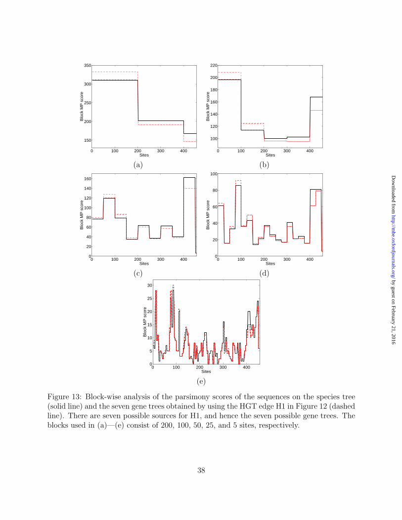
0 100 200 300 400

150

200

250

300

350

Sites

Blo

ck M

P s

core

0 100 200 300 400

100

120

140

160

180

200

220

Sites

Blo

ck M

P s

core

(a) (b)

0 100 200 300 4000

20

40

60

80

100

120

140

160

Sites

Blo

ck M

P s

core

0 100 200 300 4000

20

40

60

80

100

Sites

Blo

ck M

P s

core

(c) (d)

0 100 200 300 4000

5

10

15

20

25

30

Sites

Blo

ck M

P s

core

(e)

Figure 13: Block-wise analysis of the parsimony scores of the sequences on the species tree(solid line) and the seven gene trees obtained by using the HGT edge H1 in Figure 12 (dashedline). There are seven possible sources for H1, and hence the seven possible gene trees. Theblocks used in (a)—(e) consist of 200, 100, 50, 25, and 5 sites, respectively.

38



ownloaded from


Inferring Phylogenetic Networks by the Maximum Parsimony Criterion: A Case Study

Documents

Transcript of Inferring Phylogenetic Networks by the Maximum Parsimony Criterion: A Case Study