Inference for Treatment Regime Models in PersonalizedMedicine

Adam Kapelner∗†1, Justin Bleich†‡1, Zachary D. Cohen§2,Robert J. DeRubeis¶2, and Richard Berk‖1

1Department of Statistics, The Wharton School of the University ofPennsylvania

2Department of Psychology, University of Pennsylvania

May 8, 2014

Abstract

In medical practice, when more than one treatment option is viable, there is lit-tle systematic use of individual patient characteristics to estimate which treatmentoption is most likely to result in a better outcome for the patient. We introduce anew framework for using statistical models for personalized medicine. Our frameworkexploits (1) data from a randomized comparative trial, and (2) a regression modelfor the outcome constructed from domain knowledge and no requirement of correctmodel specification. We introduce a new “improvement” measure summarizing theextent to which the model’s treatment allocations improve future subject outcomes onaverage compared to a business-as-usual treatment allocation approach. Proceduresare provided for estimating this measure as well as asymptotically valid confidenceintervals. One may also test a null scenario in which the hypothesized model’s treat-ment allocations are not more useful than the business-as-usual treatment allocationapproach. We demonstrate our method’s promise on simulated data as well as on datafrom a randomized experiment testing treatments for depression. An open-source soft-ware implementation of our procedures is available within the R package “PersonalizedTreatment Evaluator” currently available on CRAN as PTE.

∗Electronic address: kapelner@wharton.upenn.edu; Prinicipal Corresponding author†Both authors contributed equally to this work.‡Electronic address: jbleich@wharton.upenn.edu; Corresponding author§Electronic address: zcohen@sas.upenn.edu; Corresponding author¶Electronic address: derubeis@psych.upenn.edu; Corresponding author‖Electronic address: berkr@wharton.upenn.edu; Corresponding author

1

1 Introduction

Medical patients often respond differently to treatments and can experience varying side ef-fects. Personalized medicine is a medical paradigm emphasizing the use of individual patientinformation to address such heterogeneity (Chakraborty and Moodie, 2013). Much recentstatistical research on personalized medicine has focused on how to best estimate dynamictreatment regimes, which are essentially strategies that vary treatments administered overtime as more is learned about how particular patients respond to one or more interventions.

Elaborate models are often proposed that purport to estimate optimal dynamic treatmentregimes from multi-stage experiments (Murphy, 2005) and observational data. However,there is little research addressing several fundamental questions.

• How well do these fitted treatment regimes perform on new subjects?

• How much better are they expected to do compared to “naive” strategies for allocatingtreatments currently used by medical practitioners?

• How confident can one be about estimates of “how much better?”

• Is there enough evidence to reject a null hypothesis that personalized treatment regimesperform no better than naive, default treatment allocation procedures?

Chakraborty and Moodie (2013, page 168) believe that “more targeted research is war-ranted,” and this is the goal of the paper. We focus on providing a rigorous inferentialprocedure for a two-arm single-stage treatment regime from a randomized controlled trial(RCT) testing the impact of two interventions on one continuous endpoint measure.

The paper proceeds as follows. In Section 2, we locate our procedure within the existingpersonalized treatment regime literature. Section 3 describes our methods in depth, bydescribing the conceptual framework, specifying the data and model inputs, defining animprovement metric, and illustrating a strategy for providing practitioners with estimatesand inference. Section 4 applies our methods to (1) a simple simulated dataset in whichthe response model is known, (2) a more complicated dataset characterized by an unknownresponse model, and (3) a real data set from a published clinical trial investigating twotreatments for a major depressive disorder. We also demonstrate basic software features inthis section. Section 5 concludes and offers future directions.

2 Background

Consider an individual seeking medical treatment for a set of symptoms. After a diagnosis,suppose a medical practitioner has two treatment options (denoted T1 and T2), neither ofwhich is known to be superior for all patients. How does the practitioner choose whichtreatment to administer?

Sometimes practitioners will select a treatment based informally on personal experience.Other times, practitioners may choose the treatment that their clinic or peers recommend. Ifthe practitioner happens to be current on the research literature and there happens to be a

2

published RCT with what are taken to be clear clinical implications, the study’s “superior”treatment may be chosen.

Each of these approaches can sometimes lead to improved outcomes, but each also can bebadly flawed. For example, in a variety of clinical settings, “craft lore” has been demonstratedto perform poorly, especially when compared to even very simple statistical models (Dawes,1979). It follows that each of these “business-as-usual” treatment allocation procedures can inprinciple be improved if there are patient characteristics related to how well an interventionperforms. Patient characteristics and circumstances, also known as “features,” “states,”“histories,” “prognostic / prescriptive factors,” “pretreatment variables,” and other terms ofart, we will consider here to be “covariates” in a regression modeling context.

Should available patient covariates be related to the outcome of interest, one can imaginea statistical model f providing a better guess as to which treatment (T1 or T2) to admin-ister compared to a business-as-usual approach. One can also imagine that estimates of“how much better” could be computed. The preferred treatment could then be individuallyselected for each patient.

The need for personalized medicine is by no means a novel idea. As noted as early as 1865,“the response of the average patient to therapy is not necessarily the response of the patientbeing treated” (see the Bernard, 1957 translation). There is now a substantial literatureaddressing numerous aspects of personalized medicine. Byar (1985) provides an early reviewof work involving treatment-covariate interactions. Byar and Corle (1977) investigate testsfor treatment-covariate interactions in survival models and discuss methods for treatmentrecommendations based on covariate patterns. Shuster and van Eys (1983) considers twotreatments and proposes a linear model composed of a treatment effect, a prognostic factor,and their interaction. Using this model, the authors create confidence intervals to determinefor which values of the prognostic factor one of two treatments is superior.

Many researchers also became interested in discovering “qualitative interactions”, whichare interactions that create a subset of patients for which one treatment is superior andanother subset for which the alternative treatment is superior. Gail and Simon (1985)develop a likelihood ratio test for qualitative interactions, but they require that the subsetsbe specified in advance. Pan and Wolfe (1997) and Silvapulle (2001) extend the testingframework for qualitative interactions.

Much of the early work in detecting these interactions required a prior specification ofsubgroups. This can present significant difficulties in the presence of high dimensionality orcomplicated associations. More recent approaches such as Su et al. (2009) and Dusseldorpand Van Mechelen (2014) favor recursive partitioning trees that discover important non-linearities and interactions. These methods have promise, but as a form of model selectionintroduce difficult inferential complications that are beyond the scope of this paper (see Berket al., 2013b).

Another important area of statistical research for personalized medicine is the estimationof dynamic treatment regimes (DTRs). DTRs constitute a set of optimal decision rules,estimated from many experimental and longitudinal intervals. Each regime is intended toproduce the highest mean response over that time interval. Murphy (2003) and James (2004)develop two influential approaches. Moodie et al. (2007) compares the two. More recently,McKeague and Qian (2014) estimate treatment regimes from functional predictors in RCTsto incorporate biosignatures such as brain scans or mass spectrometry. Laber et al. (2014)

3

demonstrate the application of set-valued DTRs that allow balancing of multiple possibleoutcomes, such as relieving symptoms or minimizing patient side effects. Their approachproduces a subset of recommended treatments rather than a single treatment.

Many of the procedures developed for estimating DTRs have roots in reinforcementlearning. Two widely-used methods are Q-learning and A-learning (see Schulte and Tsiatis,2012 for an overview of these concepts). One well-noted difficulty with Q-learning and A-learning are their susceptibility to model misspecification. Consequently, researchers havebegun to focus on “robust” methods.

Zhang et al. (2012) consider the context of treatment regime estimation in the presence ofmodel misspecification when there is a single-point treatment decision. By applying a doubly-robust augmented inverse probability weighted estimator that under the right circumstancescan adjust for confounding and by considering a restricted set of policies, their approach canhelp protect against misspecification of either the propensity score model or the regressionmodel for patient outcome.

Other approaches to estimating regimes have been proposed. Brinkley et al. (2010) de-velop a regression-based framework for personalized treatment regimes within the rubric of“attributable risk”. They propose developing optimal treatment regimes that minimize theprobability of a poor outcome, and then consider the positive consequences, or “attributablebenefit”, of their regime. Gunter et al. (2011) develop a stepwise approach to variable selec-tion. Rather than using a traditional sum-of-squares metric, the authors’ method comparesthe estimated mean response, or “value,” of the optimal policy for the models considered, aconcept we make use of in Section 3.

More generally, we also draw on recent papers addressing model selection for hetero-geneous treatment effects models. Methods designed for accurate estimation of an overallconditional mean of the response may not perform well when the goal is to estimate thedifferent heterogeneous treatment effects (Rolling and Yang, 2014). For example, Qian andMurphy (2011), propose a two-step approach to estimating “individualized treatment rules”based on single-stage randomized trials using `1-penalized regression. But here too, thereare difficult inferential complications because of model selection.

Most directly, the methods developed in this paper are motivated by the work of DeRubeiset al. (2014), who consider heterogeneous responses to interventions for clinical depression.That research, in turn, has roots in the earlier efforts of Byar and Corle (1977) and Yakovlevet al. (1994) who studied interventions that improve cancer survival. Yakovlev et al. (1994)take a split sample approach to covariate selection and arrive at a model that sorts patientsinto subsets while DeRubeis et al. (2014) use leave-one-out cross validation. These authorsappreciate that their approaches do not produce valid statistical inference, and that theconceptual framework for such inference needs clarification.

One major drawback of many of the above approaches is significant difficulty evaluat-ing estimator performance. Given the complexity of the estimation procedures, statisticalinference is very challenging. Additionally, many of the approaches require that the pro-posed model be correct. There are numerous applications in the biomedical sciences forwhich this assumption is neither credible on its face nor testable in practice. For example,Evans and Relling (2004) consider pharmacogenomics, and argue that as our understandingof the genetic influences on individual variation in drug response and side-effects improves,there will be increased opportunity to incorporate genetic moderators to enhance personal-

4

ized treatment. Other biomarkers (e.g. neuroimaging) of treatment response have begun toemerge, and the integration of these diverse moderators will require flexible approaches thatare robust to model misspecification (McGrath et al., 2013). How will the models of todayincorporate important relationships that can be anticipated but have yet to be identified?At the very least, therefore, there should be alternative inferential frameworks for evaluatingtreatment regimes that do not require correct model specification. And that is precisely towhat we turn now.

3 Methodology

3.1 Conceptual Framework

We imagine a set of random variables having a joint probability distribution characterizedby a full rank covariance matrix and four moments. Neither requirement will likely matter inpractice. The joint probability distribution can be properly seen as a population from whichdata could be randomly and independently realized. The population can also be imaginedas all potential observations that could be realized from the joint probability distribution.Either conception is consistent with the material to follow.

A researcher chooses one of the random variables to be the response Y ∈ R (assumed tobe continuous). We assume without loss of generality that a larger outcome is better for allindividuals. Then, one or more of the other random variables are covariates X ∈ X . At themoment, we do not distinguish between observed and unobserved covariates. There is then aconditional distribution P (Y | X) whose conditional expectation E [Y | X] constitutes theoverall population response surface. No functional forms are imposed and for generality weallow the functional form to be nonlinear with interactions among the covariates.

All potential observations are hypothetical study subjects. Each can be exposed to atreatment denoted A ∈ A. In our formulation, we assume one experimental condition T1 andanother experimental condition T2 (which may be considered the “control” or “comparison”condition) coded as 0 and 1 respectively. Thus, A = {0, 1}. Under either condition, thereis a putative outcome and values for the covariates for each subject. Outcomes under eithercondition can vary over subjects (Rosenbaum, 2002, Section 2.5.1). We make the standardassumption of no interference between study subjects, which means that the outcome for anygiven subject is unaffected by the interventions to which other subjects are randomly assigned(Cox, 1958). In short, we have adopted many features of the conventional Neyman-Rubinapproach but in contrast, treat all the data as randomly realized (Berk et al., 2014).

The joint density can be factored as

fY,X,A(y,x, a) = fX(x)fA|X(a,x)fY |X,A(y,x, a). (1)

A standard estimation target in RCTs is the average treatment effect (ATE), defined hereas the difference between the population expectations E [Y | A = 1] − E [Y | A = 0]. Thatis, the ATE is defined as the difference in mean outcome were all subjects exposed to T2 oralternatively were all exposed to T1.

5

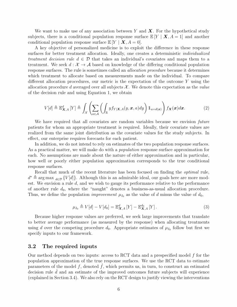
We want to make use of any association between Y and X. For the hypothetical studysubjects, there is a conditional population response surface E [Y | X, A = 1] and anotherconditional population response surface E [Y | X, A = 0].

A key objective of personalized medicine is to exploit the difference in these responsesurfaces for better treatment allocation. Ideally, one creates a deterministic individualizedtreatment decision rule d ∈ D that takes an individual’s covariates and maps them to atreatment. We seek d : X → A based on knowledge of the differing conditional populationresponse surfaces. The rule is sometimes called an allocation procedure because it determineswhich treatment to allocate based on measurements made on the individual. To comparedifferent allocation procedures, our metric is the expectation of the outcome Y using theallocation procedure d averaged over all subjects X . We denote this expectation as the valueof the decision rule and using Equation 1, we obtain

V [d] , EdX,A [Y ] ,∫X

(∑a∈A

(∫RyfY |X,A(y,x, a)dy

)1a=d(x)

)fX(x)dx. (2)

We have required that all covariates are random variables because we envision futurepatients for whom an appropriate treatment is required. Ideally, their covariate values arerealized from the same joint distribution as the covariate values for the study subjects. Ineffect, our enterprise requires forecasts for each patient.

In addition, we do not intend to rely on estimates of the two population response surfaces.As a practical matter, we will make do with a population response surface approximation foreach. No assumptions are made about the nature of either approximation and in particular,how well or poorly either population approximation corresponds to the true conditionalresponse surfaces.

Recall that much of the recent literature has been focused on finding the optimal rule,d∗ , arg max d∈D {V [d]}. Although this is an admirable ideal, our goals here are more mod-est. We envision a rule d, and we wish to gauge its performance relative to the performanceof another rule d0, where the “naught” denotes a business-as-usual allocation procedure.Thus, we define the population improvement µI0 as the value of d minus the value of d0,

µI0 , V [d]− V [d0] = EdX,A [Y ]− Ed0X,A [Y ] . (3)

Because higher response values are preferred, we seek large improvements that translateto better average performance (as measured by the response) when allocating treatmentsusing d over the competing procedure d0. Appropriate estimates of µI0 follow but first wespecify inputs to our framework.

3.2 The required inputs

Our method depends on two inputs: access to RCT data and a prespecified model f for thepopulation approximation of the true response surfaces. We use the RCT data to estimateparameters of the model f , denoted f , which permits us, in turn, to construct an estimateddecision rule d and an estimate of the improved outcomes future subjects will experience(explained in Section 3.4). We also rely on the RCT design to justify viewing the interventions

6

as manipulable in practice. Were the interventions not manipulable, there would be no pointin providing the practitioner with information about which interventions should be offered towhich patients. We assume that the model f is specified before looking at the data. To allow“data snooping” fosters overfitting, can introduce serious estimation bias, and can invalidateconfidence intervals and statistical tests we develop further on (Berk et al., 2013b).

3.2.1 The RCT data

The RCT data come from an experiment undertaken to estimate the ATE for treatments T1and T2 for a diagnosis of a disease of interest. T1 and T2 are the same treatments one wouldoffer to future subjects with the same diagnosis. There are n subjects each with p covariateswhich are denoted for the ith subject as xi , [xi1, xi2, . . . , xip] that can be continuous orbinary. Because the covariates will be used to construct a decision rule applied with futurepatients in clinical settings, the xi’s in the RCT data must be the same covariates measured inthe same way for new subjects in the future. Thus, all “purely experimental covariates” suchas site of treatment (in a multi-center trial) or the identification of the medical practitionerwho treated each subject are not included. We assume the continuous outcome measure ofinterest yi is assessed once per subject. Aggregating all covariate vectors, binary allocationsand responses row-wise, we denote the full RCT data as the column-bound matrix [X,A,y].We will be drawing inference to a patient population beyond those who participated in theexperiment. Formally, new subjects in the future must be sampled from that same populationas were the subjects in the RCT. In the absence of explicit probability sampling, the casewould need to be made from subject-matter expertise and the manner in which the studysubjects were recruited.

3.2.2 The Model f

Our method assumes the practitioner has decided upon an approximate response model f apriori, which is a function of x and A. Our decision rule d is a function of x through f —allocations are assigned by comparing an individual’s f(x) for both T1 and T2 and assigningthe higher response estimate. Thus, we define d, our decision rule of interest as

d[f(x)] , 1f(x,1)−f(x,0). (4)

Informed by the population approximation framework of Berk et al. (2013a), we assumethe model f provided by the practitioner to be an approximation using the available covari-ates of the response’s true data generating process,

Yi = f(X i, Ai) + ξi(X i,U i, Ai)︸ ︷︷ ︸E[Yi | Xi,U i,Ai]

+Ei. (5)

In Equation 5, X denotes the random covariates available in the RCT data and U repre-sents unobserved random covariates. The first two terms together compose the conditionalexpectation of the population response. The last term Ei is the irreducible noise around thetrue conditional expectations and is taken to be independent and identically distributed.

7

It is mean-centered and uncorrelated with the covariates by definition. We emphasize thatthe proposed model f is not necessarily the true conditional expectation function. Evenin the absence of Ei, f will always differ from the true conditional expectation function byξi(X i,U i, Ai), which represents model misspecification.

We wish to determine whether f is useful for improving treatment allocation for futurepatients and do not expect to recover the optimal allocation rule d∗. There are no necessarysubstantive interpretations associated with any of the p covariates. In trade, our methodis robust to model misspecification. One implication is that a wide variety of models andestimation procedures could in principle prove useful.

We employ here a conventional linear regression model with first order interactions be-cause much of the literature we reviewed in Section 2 favored this class of models. Morespecifically, we specify a linear model containing a subset of the covariates used as first or-der interactions with the treatment indicator, {x1′ , . . . , xp′} ⊂ {x1, . . . , xp}, selected usingdomain knowledge:

f(xi1, Ai) = β0 + β1x1 + . . .+ βpxp + Ai (γ0 + γ1′x1′ + . . .+ γp′xp′) . (6)

These interactions induce heterogeneous effects between T1 and T2 for a subject x andthus d[f(x)] = 1 when γ0 + γ1′x1′ + . . . + γp′xp′ > 0 and 0 otherwise. The γ’s are a criticalcomponent of the model if there are systematic patient-specific responses to the interventions.Thereby, d varies over different points in X space. Note that rules derived from this type ofconventional model also have the added bonus as being interpretable to the practitioner atleast as a best linear approximation.

3.3 Other allocation procedures

Although d0 can be any allocation rule, for the purposes of the paper, we examine only“naive” or “business-as-usual” allocation procedures of which we present two in Table 1.

Name Procedure Descriptionrandom random allocation to T1 or T2 with

probability 12

best unconditional allocation to the“best” treatment on average asmeasured by whichever sample groupaverage is numerically larger, yT1 or yT2

Table 1: Two baseline business-as-usual allocation procedures denoted as d0.

A practitioner may not actually employ d0 precisely as specified by the descriptions ofrandom or best, but we view this as a good start for providing a baseline for comparison.The table could be expanded to include other allocation procedures such as heuristics, simplemodels and others. We consider other d0 choices in Section 5.

8

3.4 Estimating the improvement scores

How well do future subjects with treatments allocated by d do on average compared to thesame future subjects with treatments allocated by d0? We start by computing the estimatedimprovement score, a sample statistic given by

I0 , V [d]− V [d0], (7)

where d is an estimate of the rule d derived from the population response surface approxi-mation, V is an estimate of its corresponding value V and I0 is an estimate of the resultingpopulation improvement µI0 (Equation 3). The d0 notation indicates that sometimes thecompetitor d0 may have to be estimated from the data as well. For example, the allocationprocedure best (Table 1) must be calculated by using the sample average of the responsesfor both T1 and T2 in the data. We leave discussion of inference for µI0 to Section 3.5 andhere only discuss construction of the sample statistic.

In order to properly gauge how well d performs allocating the better of the treatmentsfor each subject, we begin by splitting the RCT data into two disjoint subsets: training datawith ntrain of the original n observations [Xtrain,ytrain] and testing data with the remainingntest = n− ntrain observations [Xtest,ytest]. Then ftrain can be fitted using the training datato construct d via Equation 4. Performance of d, explained in the subsequent paragraph,is then evaluated on the test data. Hastie et al. (2013) explain that this procedure yieldsan estimate of the “performance” of the procedure on future individuals conditional on[Xtrain,ytrain] (we address the conditioning on the training data later). By splitting theRCT data into training and test subsets, Equation 7 can provide an honest assessmentof improvement for future individuals who are allocated using our proposed methodologycompared to a baseline business-as-usual allocation strategy (Faraway, 2013).

Given the estimate d (and d0, estimated analogously), the question remains of how tocompute V for subjects we have not yet seen in order to estimate I0. That is, we are tryingto estimate the expectation of an allocation procedure over covariate space X .

Recall that in the test data, our allocation prediction d(xi) is the binary recommendationof T1 or T2 for each xtest,i. If we recommended the treatment that the subject actually was

allocated in the RCT, i.e. d(xi) = Ai, we consider that subject to be “lucky.” We definelucky in the sense that by the flip of the coin, the subject was randomly allocated to thetreatment that our model-based allocation procedure estimates to be the better of the twotreatments. This definition of a “lucky subject” was also employed by Yakovlev et al. (1994)and DeRubeis et al. (2014).

The average of the lucky subjects’ responses should estimate the average of the responseof new subjects who are allocated to their treatments based on our procedure d. Thisaverage is exactly the estimate of V (d) we are seeking. Because the x’s in the test data areassumed to be sampled randomly from population covariates, this sample average estimatesthe expectation over X , i.e. EdX,A [Y ] conditional on the training set.

In order to make this concept more clear, it is convenient to consider a 2 × 2 matrixwhich houses the sorted entries of the out-of-sample ytest based on the predictions d(xi)’s(Table 2). This matrix illustrates the cross tabulated entries of the out-of-sample ytest andthe predictions d(xi)’s. The diagonal entries of sets P and S contain the “lucky subjects.”

9

The off-diagonal entries of sets R and Q contain other subjects. The notation y· indicatesthe sample average among the elements of ytest specified in the subscript located in the cellsof the table.

d(xi) = 0 d(xi) = 1

Ai = 0 P , {ytest,0,01 , . . . , ytest,0,0ntest0,0} Q , {ytest,0,11 , . . . , ytest,0,1ntest0,1

}Ai = 1 R , {ytest,1,01 , . . . , ytest,1,0ntest1,0

} S , {ytest,1,11 , . . . , ytest,1,1ntest1,1}

Table 2: The elements of ytest cross-tabulated by their administered treatment Ai and ourmodel’s estimate of the better treatment d(xi).

To compute I0, the last quantity to compute is V [d0]. V [d0] for the business at usualprocedure rand is simply the average of the ytest responses. V [d0] for the business as usualprocedure best is simply the average of the ytest responses for the treatment group that hasa larger sample average. Thus, the sample statistic of Equation 7 can be written specificallyfor the two d0’s as

Irandom , yP∪S − ytest, (8)

Ibest , yP∪S −

{yP∪Q when yP∪Q ≥ yR∪S

yR∪S when yR∪S > yP∪Q.(9)

Remember that our value estimates V [·] are conditional on the training set and thus donot estimate the unconditional EdX,A [Y ]. To address this, Hastie et al. (2013, Chapter 7) rec-ommend that the same procedure be performed across many different splits, thereby buildingmany models, a strategy called “K-fold cross-validation” (CV). This strategy integrates outthe effect of a single training set.

In practice, how large should the training and test splits be? Depending on the size ofthe test set relative to the training set, CV can trade bias for variance when estimating anout-of-sample metric. Small training sets and large test sets give more biased estimates sincethe training set is built with less data than the n observations given. However, large testsets have lower variance estimates since they are composed of many examples. There is noconsensus in the literature about the optimal training-test split size (Hastie et al., 2013, page242). 10-fold CV is a common choice employed in many statistical applications and providesfor a relatively fast algorithm. In our implementation, we default to 10-fold cross validation.This estimation procedure outlined above is graphically illustrated in the top of Figure 1.

Recall that if we were not careful to calculate I0 from hold out test sets, our improvementestimates would be estimates for the in-sample value difference. Thus, the estimate ofimprovement would not be applicable for “new subjects” who enter and wish to receive atreatment allocation.

3.5 Inference for the population improvement parameter

The I0 estimates are elaborate estimates from a sample of data. We can employ the non-parametric bootstrap to obtain an asymptotic estimate of its sampling variability, which can

10

be used to construct asymptotically valid confidence intervals and testing procedures (Efronand Tibshirani, 1994).

In the context of our proposed methodology, the bootstrap procedure works as followsfor the target of inference µIrandom . We take a sample with replacement from the RCT dataof size n denoted with tildes [X, y]. Using the 10-fold CV procedure described at the end ofSection 3.4, we create an estimate Irandom. We repeat the resampling of the RCT data andthe recomputation of Irandom B times where B is selected for resolution of the confidenceinterval and significance level of the test. In practice we found B = 3000 to be sufficient, sowe leave this as the default in our software implementation. Because the n’s of usual RCT’sare small, and the software is parallelized, this is not an undue computational burden.

In this application, the bootstrap approximates the sampling of many RCT datasets.Each I that is computed corresponds to one out-of-sample improvement estimate for a par-ticular RCT dataset drawn from the population of RCT datasets. The frequentist confidenceintervals and tests that we develop for the improvement measure do not constitute inferencefor a new individual’s improvement, it is inference for the average improvement for manynew future subjects.

The bootstrap samples {IRandom,1, . . . , IRandom,B} provide an asymptotically valid sam-pling distribution of improvement measures. To create an 1 − α level confidence interval,first sort the I’s by value, and then report the values corresponding to the empirical α/2 and1− α/2 percentiles. This is called the “percentile method.” There are other ways to gener-ate asymptotically valid confidence intervals using bootstrap samples but some debate aboutwhich has the best finite sample properties. For instance, DiCiccio and Efron (1996) claimthat the bias-corrected “BCa method” (Efron, 1987) can perform an order of magnitudebetter in accuracy. In this paper we illustrate only the percentile method. Implementingother confidence interval methods for the bootstrap may be instructive future work.

If a higher response is better for the subject, we set H0 : µI0 ≤ 0 and Ha : µI0 > 0.Thus, we wish to reject the null that our allocation procedure is only as useful as a naivebusiness-as-usual procedure. To obtain an asymptotically valid p value, we count the numberof bootstrap sample I estimates below 0 and divide by B. This bootstrap procedure isgraphically illustrated in the bottom half of Figure 1 and the bootstrap confidence intervaland p value computation is illustrated in the center.

3.6 Future Subjects

The implementation of this procedure for future individuals is straightforward. Using theRCT data, estimate f to arrive at f . When a new individual, whose covariates denoted x∗,enters a clinic, our estimated decision rule is calculated by predicting the response underboth treatments, then allocating the treatment which corresponds to the better outcome,d(x∗). This final step is graphically illustrated in the top left of Figure 1.

11

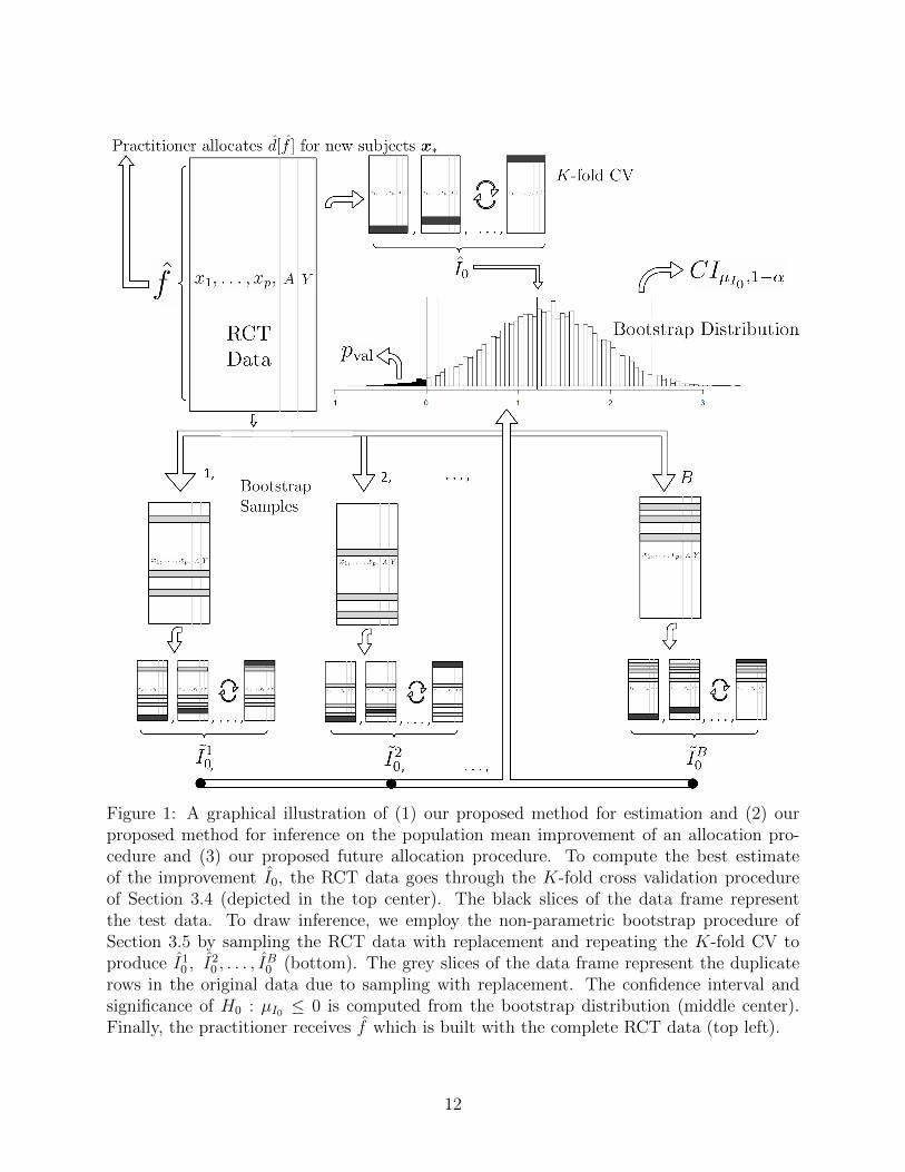
Figure 1: A graphical illustration of (1) our proposed method for estimation and (2) ourproposed method for inference on the population mean improvement of an allocation pro-cedure and (3) our proposed future allocation procedure. To compute the best estimateof the improvement I0, the RCT data goes through the K-fold cross validation procedureof Section 3.4 (depicted in the top center). The black slices of the data frame representthe test data. To draw inference, we employ the non-parametric bootstrap procedure ofSection 3.5 by sampling the RCT data with replacement and repeating the K-fold CV toproduce I10 , I

20 , . . . , I

B0 (bottom). The grey slices of the data frame represent the duplicate

rows in the original data due to sampling with replacement. The confidence interval andsignificance of H0 : µI0 ≤ 0 is computed from the bootstrap distribution (middle center).Finally, the practitioner receives f which is built with the complete RCT data (top left).

12

4 Data Examples

4.1 Simulation with correct regression model

Consider RCT data with one covariate x where the true response function is known:

Y = β0 + β1X + A(γ0 + γ1X) + E , (10)

where E is mean-centered. We employ f(x,A) as the true response function, E [Y | X,A].Thus, d is the “optimal” rule in the sense that a practitioner can make correct allocationdecisions modulo noise using d(x) = 1γ0+γ1x>0. Consider d0 to be the random allocationprocedure (see Table 1). Note that within the improvement score definition (Equation 3),the notation EdX [Y ] is an expectation over the noise E and the joint distribution of X, A.After taking the expectation over noise, the improvement under the model of Equation 10becomes

µI0 = EX [β0 + β1X + 1γ0+γ1X>0(γ0 + γ1X)]− EX [β0 + β1X + 0.5(γ0 + γ1X)]

= EX [(1γ0+γ1x>0 − 0.5) (γ0 + γ1X)]

= γ0 (P (γ0 + γ1X > 0)− 0.5) + γ1 (EX [X1γ0+γ1x>0]− 0.5EX [X]) .

We further assume X ∼ N (µX , σ2X) and we arrive at

µI0 = (γ0 + γ1µX)

(.5− Φ

(−γ0γ1

))+ γ1

σX√2π

exp

(− 1

2σ2X

(−γ0γ1− µ

)2).

We simulate under a simple scenario to clearly highlight features of our methodology. IfµX = 0, σ2

X = 1 and γ0 = 0, neither treatment T1 or T2 is on average better. However, ifx > 0, then treatment T2 is better in expectation by γ1 × x and analogously if x < 0, T1is better by −γ1 × x. We then set γ1 =

√2π to arrive at the round number µI0 = 1. We

set β0 = 1 and β1 = −1 and let Eiiid∼ N (0, 1). We let the treatment allocation vector A

be a random block permutation of size n, balanced between T1 and T2. Since there is noATE, the random and best d0 procedures (Table 1) are the same in value. We then varyn ∈ {100, 200, 500, 1000} to assess convergence for both d0 procedures and display the resultsin Figure 2.

Convergence to µI0 = 1 is observed clearly for both procedures but convergence for d0best is slower than d0 rand. This is due to the V being computed with fewer samples: ytest,which uses all of the available data, versus yP∪Q or yR∪S, which uses only half the availabledata (see Equations 8 and 9).

In this section we assumed knowledge of f and thereby had access to an optimal rule. Inthe next section we explore convergence when we do not know f but pick an approximatemodel yielding a non-optimal rule.

13

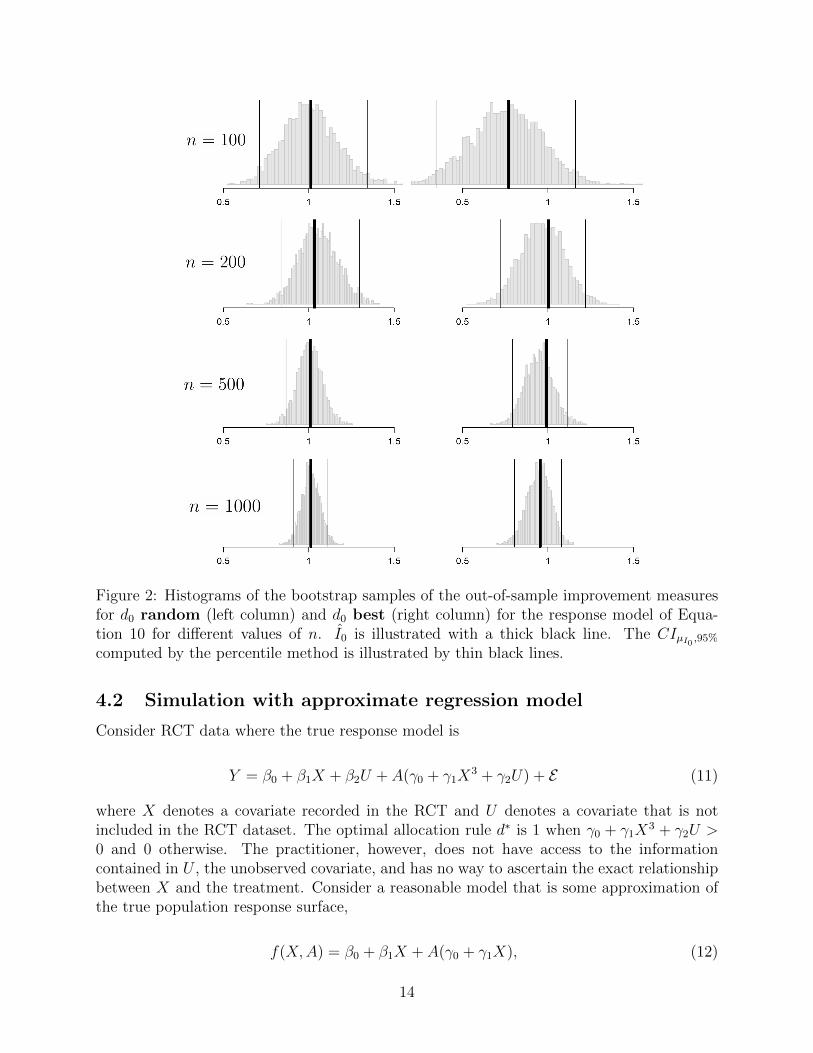
Figure 2: Histograms of the bootstrap samples of the out-of-sample improvement measuresfor d0 random (left column) and d0 best (right column) for the response model of Equa-tion 10 for different values of n. I0 is illustrated with a thick black line. The CIµI0 ,95%computed by the percentile method is illustrated by thin black lines.

4.2 Simulation with approximate regression model

Consider RCT data where the true response model is

Y = β0 + β1X + β2U + A(γ0 + γ1X3 + γ2U) + E (11)

where X denotes a covariate recorded in the RCT and U denotes a covariate that is notincluded in the RCT dataset. The optimal allocation rule d∗ is 1 when γ0 + γ1X

3 + γ2U >0 and 0 otherwise. The practitioner, however, does not have access to the informationcontained in U , the unobserved covariate, and has no way to ascertain the exact relationshipbetween X and the treatment. Consider a reasonable model that is some approximation ofthe true population response surface,

f(X,A) = β0 + β1X + A(γ0 + γ1X), (12)

14

which is different from the true response model due to misspecification (Equation 5). Thisis a more realistic scenario; even with infinite data, the best treatment allocation procedurecannot be found.

To simulate, we set the X’s, U ’s and E ’s to be standard normal variables and thenset β0 = 1, β1 = −1, β2 = 0.5, γ0 = 0, γ1 = 1 and γ2 = −3. The Xi’s and the Ui’sare deliberately made independent of one another so that the observed covariates cannotcompensate for the unobserved covariates. The independence makes any comparison betweenthe improvement under d∗ and d more stark. To find the improvement when the true modeld∗ is used to allocate (Equation 11), we simulate to find µ∗I0 ≈ 1.65 and analogously, theimprovement if the approximation model d is used to allocate (Equation 12) is found to beµI0 ≈ 0.79. Further simulation shows that not observing U is responsible for 85% of thistheoretical drop and employing the linear X in place of the non-linear X3 is responsible forthe remaining 15%. Since γ0 = 0, there is no ATE and thus these simulated improvementsapply to both the cases where d0 is random and d0 is best (Table 1).

Figure 3 demonstrates results for n = {100, 200, 500, 1000} analogous to Figure 2. Weobserve that the bootstrap confidence intervals contain µI0 but not µ∗I0 . This is expected;we are not allocating using an estimate of d∗, only an estimate of d.

Convergence towards µI0 ≈ 0.79 is observed clearly for both procedures and once againthe convergence is slower for the best procedure for the same reasons outlined in Section 4.1.Note that the coverage illustrated here is far from µ∗I0 , the improvement using the optimalallocation rule.

The point of this section is to illustrate the realistic scenario that if the response modelis unknown and/or covariates are unobserved, the improvement of an allocation proceduremay fall short of optimal. However, the effort can still yield an improvement that can beclinically significant and useful in practice.

In the next section, we explore using our procedure for RCT data from a real clinical trialwith a latent response model. Thus, µ∗I0 is inaccessible, so the strategy is similar as foundhere: we approximate the response function using a reasonable model f , this time built fromdomain knowledge.

4.3 Clinical trial demonstration

Now consider the RCT data used in DeRubeis et al. (2005). There are two depression treat-ments: cognitive behavioral therapy (T1) and an antidepressant medication paroxetine (T2)on 154 subjects. The primary outcome measure y is the Hamilton Rating Scale for Depres-sion (HRSD), a continuous composite score of depression symptoms where lower means lessdepressed, assessed by a clinician after 16 weeks of treatment. A simple t test revealed thatthere was no statistically significant difference between the cognitive behavioral therapy andparoxetine. Despite the lack of an ATE, we anticipate using a principled response model todrive a significant negative µI0 . The lack of an ATE also suggests that the random d0 is anappropriate baseline comparison.

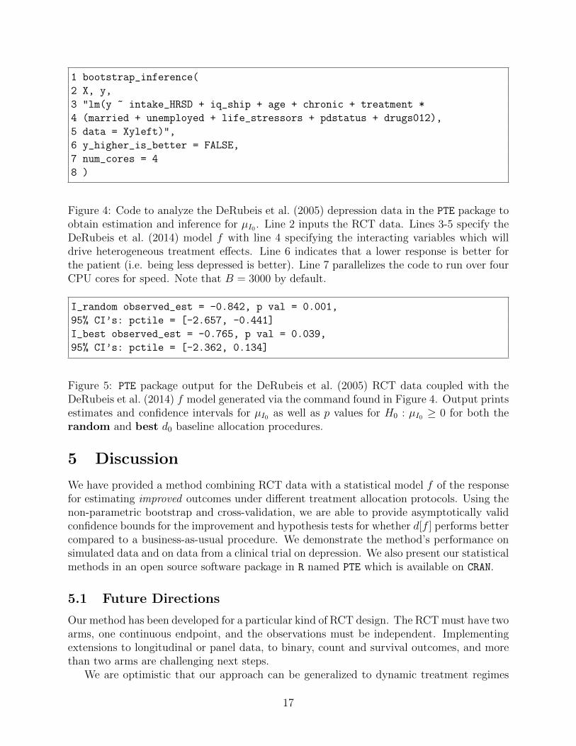
Figure 4 illustrates the software function for running the procedure described in Section 3,which employs the identical linear model with first order treatment interactions found inDeRubeis et al. (2014, Table 3) for the model f .

15

Figure 3: Histograms of the bootstrap samples of the out-of-sample improvement measuresfor d0 random (left column) and d0 best (right column) for the response model of Equa-tion 11 for different values of n. I0 is illustrated with a thick black line. The CIµI0 ,95%computed via the percentile method is illustrated by thin black lines. The true populationimprovement µ∗I0 given the optimal rule d∗ is illustrated with a dotted black line

The output from 3,000 bootstrap samples is printed in Figure 5, and the histograms ofthe bootstrap samples and confidence intervals are shown in Figure 6. From these results,we anticipate that a new subject allocated using the model f will be less depressed onaverage by 0.84 HRSD units compared to that same subject being allocated randomly tocognitive behavioral therapy or paroxetine. We can easily reject the null hypothesis that ffor allocation over random allocation is no better for the new subject (p value = 0.004). Fora new subject allocated using the model f versus using the “best” treatment as determinedby yT1 and yT1 , the estimated improvement is 0.77 with a marginally significant p value 0.04(note that this p value is one-sided and that the two-sided confidence interval contains 0).

In short, the results are statistically significant, but the estimated improvement may notbe of great clinical importance. According to the criterion set out by the National Institutefor Health and Care Excellence, three points on the HRSD is considered clinically important.However, the statistical significance suggests that nevertheless the model f generated fromthis data set could be implemented in practice with new subjects if there are no importantcost or organizational constraints.

16

1 bootstrap_inference(

2 X, y,

3 "lm(y ~ intake_HRSD + iq_ship + age + chronic + treatment *

4 (married + unemployed + life_stressors + pdstatus + drugs012),

5 data = Xyleft)",

6 y_higher_is_better = FALSE,

7 num_cores = 4

8 )

Figure 4: Code to analyze the DeRubeis et al. (2005) depression data in the PTE package toobtain estimation and inference for µI0 . Line 2 inputs the RCT data. Lines 3-5 specify theDeRubeis et al. (2014) model f with line 4 specifying the interacting variables which willdrive heterogeneous treatment effects. Line 6 indicates that a lower response is better forthe patient (i.e. being less depressed is better). Line 7 parallelizes the code to run over fourCPU cores for speed. Note that B = 3000 by default.

I_random observed_est = -0.842, p val = 0.001,

95% CI’s: pctile = [-2.657, -0.441]

I_best observed_est = -0.765, p val = 0.039,

95% CI’s: pctile = [-2.362, 0.134]

Figure 5: PTE package output for the DeRubeis et al. (2005) RCT data coupled with theDeRubeis et al. (2014) f model generated via the command found in Figure 4. Output printsestimates and confidence intervals for µI0 as well as p values for H0 : µI0 ≥ 0 for both therandom and best d0 baseline allocation procedures.

5 Discussion

We have provided a method combining RCT data with a statistical model f of the responsefor estimating improved outcomes under different treatment allocation protocols. Using thenon-parametric bootstrap and cross-validation, we are able to provide asymptotically validconfidence bounds for the improvement and hypothesis tests for whether d[f ] performs bettercompared to a business-as-usual procedure. We demonstrate the method’s performance onsimulated data and on data from a clinical trial on depression. We also present our statisticalmethods in an open source software package in R named PTE which is available on CRAN.

5.1 Future Directions

Our method has been developed for a particular kind of RCT design. The RCT must have twoarms, one continuous endpoint, and the observations must be independent. Implementingextensions to longitudinal or panel data, to binary, count and survival outcomes, and morethan two arms are challenging next steps.

We are optimistic that our approach can be generalized to dynamic treatment regimes

17

−4 −3 −2 −1 0 1

(a) IRand bootstrap samples

−4 −3 −2 −1 0 1

(b) IBest bootstrap samples

Figure 6: Histograms of the bootstrap samples of improvement measures for both randomand best d0 business-as-usual allocation procedures. The thick black line is the best estimateof I0, the thin black lines are the confidence interval computed via the percentile method.

if we are provided with RCT data from sequential multiple assignment randomized trials(SMARTs, Murphy, 2005) and an a priori response model f . We believe the estimate ofV (d) (Equation 7) can be updated for a SMART with k stages. Table 2 summarizes asingle stage. In a SMART with k stages, the matrix becomes a hypercube of dimension k .Thus, the average of diagonal entries in the multi-dimensional matrix is the generalizationof the estimate of V (d) found in Equations 8 and 9. Many of the models for dynamictreatment regimes found in Chakraborty and Moodie (2013) can then be incorporated intoour methodology as d, and we may be able to provide many of these models with validstatistical inference. Other statistics computed from this multi-dimensional matrix may begeneralized as well.

Requiring a model f a priori is a constraint in practice: what if the practitioner cannotconstruct a suitable f using domain knowledge and past research? There are three scenariosthat pose different technical problems. Under one scenario, a researcher is able to specifya suite of possible models before looking at the data. The full suite can be viewed ascomprising single procedure for which nonparametric bootstrap procedures may in principleprovide simultaneous confidence intervals (Buja and Rolke, 2014). Under the other twoscenarios, models are developed inductively from the data. If it is possible to specify exactlyhow the model search us undertaken (e.g., using the lasso), some forms of statistical inferencemay be feasible. This is currently an active research area (Lockhart et al., 2013). If it isnot possible to specify exactly how the search is undertaken, for instance by allowing f toassume the form of a popular machine learning algorithm such as Random Forests (Breiman,2001), we do not currently see how to make inference feasible.

It might also be useful to consider building from an observational design rather than arandomized controlled trial. The literature reviewed in Section 2 generally does not requireRCT data but “only” a model that accurately captures selection into treatments. This seemsto us a very demanding requirement. In this paper, we do not even require valid estimates of

18

the true population response surface. In an observational study one would need that modelto be correct and/or a correct model of the way in which subjects and treatments were paired(see Freedman and Berk, 2008).

Finally, our choices of d0 explored here were limited to the random or the best rules(see Table 1). There may be other business-as-usual allocation procedures to use here thatmake for more realistic baseline comparisons. For instance, one can modify best to only usethe better treatment if a two-sample t-test rejects at prespecified Type I error level. Onecan further set d0 to be a regression model and use our framework to pit two models againsteach other.

Replication

Our procedure is available as the R package PTE on CRAN. The results and simulations foundin this paper can be duplicated by installing the package and running the R scripts foundat github.com/kapelner/PTE/tree/master/paper_duplication. Note that we cannot re-lease the depression data of Section 4.3 due to privacy concerns.

Acknowledgements

We would like to thank Larry Brown, Andreas Buja, Ed George, Abba Krieger, Dan Mc-Carthy and Linda Zhao for helpful discussions and comments. Adam Kapelner acknowledgesthe National Science Foundation for his Graduate Research Fellowship which helped to sup-port this research.

References

Berk, R., Brown, L., Buja, A., George, E., Pitkin, E., Zhang, K., and Zhao, L. (2013a). MisspecifiedMean Function Regression: Making Good Use of Regression Models that are Wrong. Universityof Pennsylvania working paper.

Berk, R., Pitkin, E., Brown, L., Buja, A., George, E. I., and Zhao, L. (2014). Covariance Adjust-ments for the Analysis of Randomized Field Experiments. Evaluation Review (in press).

Berk, R. A., Brown, L., Buja, A., Zhang, K., and Zhao, L. (2013b). Valid post-selection inference.The Annals of Statistics, 41(2):802–837.

Bernard, C. (1957). An introduction to the study of experimental medicine. Dover Publications,New York.

Breiman, L. (2001). Random Forests. Machine learning, pages 5–32.

Brinkley, J., Tsiatis, A., and Anstrom, K. J. (2010). A generalized estimator of the attributablebenefit of an optimal treatment regime. Biometrics, 66(2):512–22.

Buja, A. and Rolke, W. (2014). Calibration for simultaneity: (Re) sampling methods for simul-taneous inference with applications to function estimation and functional data. University ofPennsylvania working paper.

19

Byar, D. P. (1985). Assessing apparent treatmentCovariate interactions in randomized clinicaltrials. Statistics in Medicine, 4:255–263.

Byar, D. P. and Corle, D. K. (1977). Selecting optimal treatment in clinical trials using covariateinformation. Journal of chronic diseases, 30(7):445–59.

Chakraborty, B. and Moodie, E. E. M. (2013). Statistical Methods for Dynamic Treatment Regimes.Springer, New York.

Cox, D. R. (1958). Planning of experiments. Wiley, New York.

Dawes, R. M. (1979). The robust beauty of improper linear models in decision making. Americanpsychologist, 34(7):571–582.

DeRubeis, R. J., Cohen, Z. D., Forand, N. R., Fournier, J. C., Gelfand, L., and Lorenzo-Luaces,L. (2014). The personalized advantage index: Translating research on prediction into individualtreatment recommendations. A demonstration. PloS one, 9(1):e83875.

DeRubeis, R. J., Hollon, S. D., Amsterdam, J. D., Shelton, R. C., Young, P. R., Salomon, R. M.,O’Reardon, J. P., Lovett, M. L., Gladis, M. M., Brown, L. L., and Gallop, R. (2005). Cognitivetherapy vs medications in the treatment of moderate to severe depression. Archives of generalpsychiatry, 62(4):409–16.

DiCiccio, T. J. and Efron, B. (1996). Bootstrap confidence intervals. Statistical Science, 11(3):189–212.

Dusseldorp, E. and Van Mechelen, I. (2014). Qualitative interaction trees: a tool to identifyqualitative treatment-subgroup interactions. Statistics in medicine, 33(2):219–37.

Efron, B. (1987). Better bootstrap confidence intervals. Journal of the American statistical Asso-ciation, 82(397):171–185.

Efron, B. and Tibshirani, R. (1994). An introduction to the bootstrap, volume 57. CRC press.

Evans, W. E. and Relling, M. V. (2004). Moving towards individualized medicine with pharma-cogenomics. Nature, 429(6990):464–8.

Faraway, J. J. (2013). Does Data Splitting Improve Prediction? arXiv, (2009):1–17.

Freedman, D. A. and Berk, R. A. (2008). Weighting regressions by propensity scores. Evaluationreview, 32(4):392–409.

Gail, M. and Simon, R. (1985). Testing for qualitative interactions between treatment effects andpatient subsets. Biometrics, 41(2):361–72.

Gunter, L., Zhu, J., and Murphy, S. (2011). Variable selection for qualitative interactions inpersonalized medicine while controlling the family-wise error rate. Journal of BiopharmaceuticalStatistics, 21(6):1063–1078.

Hastie, T., Tibshirani, R., and Friedman, J. H. (2013). The Elements of Statistical Learning.Springer Science, tenth printed edition.

20

James, M. R. (2004). Optimal structural nested models for optimal sequential decisions. In InProceedings of the Second Seattle Symposium on Biostatistics. Springer.

Laber, E. B., Lizotte, D. J., and Ferguson, B. (2014). Set-valued dynamic treatment regimes forcompeting outcomes. Biometrics, 70(1):53–61.

Lockhart, R., Taylor, J., Tibshirani, R. J., and Tibshirani, R. (2013). A significance test for thelasso. Arxiv.

McGrath, C. L., Kelley, M. E., Holtzheimer, P. E., Dunlop, B. W., Craighead, W. E., Franco,A. R., Craddock, R. C., and Mayberg, H. S. (2013). Toward a neuroimaging treatment selectionbiomarker for major depressive disorder. JAMA psychiatry, 70(8):821–9.

McKeague, I. W. and Qian, M. (2014). Estimation of treatment policies based on functionalpredictors. Statistica Sinica.

Moodie, E. E. M., Richardson, T. S., and Stephens, D. A. (2007). Demystifying optimal dynamictreatment regimes. Biometrics, 63(2):447–55.

Murphy, S. A. (2003). Optimal dynamic treatment regimes. Journal of the Royal Statistical Society:Series B (Statistical Methodology), 65(2):331–366.

Murphy, S. A. (2005). An experimental design for the development of adaptive treatment strategies.Statistics in medicine, 24(10):1455–1481.

Pan, G. and Wolfe, D. A. (1997). Test for qualitative interaction of clinical significance. Statisticsin medicine, 16(February 1996):1645–1652.

Qian, M. and Murphy, S. A. (2011). Performance Guarantees for Individualized Treatment Rules.Annals of statistics, 39(2):1180–1210.

Rolling, C. A. and Yang, Y. (2014). Model selection for estimating treatment effects. Journal ofthe Royal Statistical Society: Series B (Statistical Methodology), in press.

Rosenbaum, P. R. (2002). Observational studies. Springer, New York.

Schulte, P. J. and Tsiatis, A. A. (2012). Q-and A-learning methods for estimating optimal dynamictreatment regimes. arXiv preprint.

Shuster, J. and van Eys, J. (1983). Interaction between prognostic factors and treatment. Controlledclinical trials, 4(3):209–14.

Silvapulle, M. J. (2001). Tests against qualitative interaction: Exact critical values and robusttests. Biometrics, 57(4):1157–65.

Su, X., Tsai, C. L., and Wang, H. (2009). Subgroup analysis via recursive partitioning. Journal ofMachine Learning Research, 10:141–158.

Yakovlev, A. Y., Goot, R. E., and Osipova, T. T. (1994). The choice of cancer treatment based oncovariate information. Statistics in medicine, 13:1575–1581.

Zhang, B., Tsiatis, A. A., Davidian, M., Zhang, M., and Laber, E. (2012). Estimating optimaltreatment regimes from a classification perspective. Stat, pages 103–114.

21