
Indranil Das Saha Institute of Nuclear Physics - CERN ...
236
CERN-THESIS-2010-261 //2011 Development, Implementation and Performance Report of Dimuon High Level Trigger of ALICE by Indranil Das Saha Institute of Nuclear Physics Kolkata A thesis submitted to the Board of Studies in Physical Science Discipline In partial fulfillment of requirements For the Degree of DOCTOR OF PHILOSOPHY of HOMI BHABHA NATIONAL INSTITUTE 2011
-
Upload
khangminh22 -
Category
Documents
-
view
2 -
download
0
Transcript of Indranil Das Saha Institute of Nuclear Physics - CERN ...

CER
N-T
HES
IS-2
010-
261
//20
11
Development, Implementation andPerformance Report of DimuonHigh Level Trigger of ALICE
by
Indranil DasSaha Institute of Nuclear Physics
Kolkata
A thesis submitted to theBoard of Studies in Physical Science Discipline
In partial fulfillment of requirementsFor the Degree of
DOCTOR OF PHILOSOPHYof
HOMI BHABHA NATIONAL INSTITUTE
2011


Homi Bhabha National Institute
Recommendations of the Viva Voce Board
As members of the Viva Voce Board, we certify that we have read the dissertationprepared by Indranil Das entitled ”Development, Implementation and PerformanceReport of Dimuon High Level Trigger of ALICE” and recommended that it maybe accepted as fulfilling the dissertation requirement for the Degree of Doctor ofPhilosophy.
Date :
Chairman : Prof. J. B. Singh, Punjub University
Date :
Convener : Prof. P. Mitra, SINP
Date :
Guide : Prof S. Chattopadhyay, SINP
Date :
Member : Prof. K. Kar, SINP
Date :
Member : Prof. A. K. Dutt-Mazumdar, SINP
Date :
Member : Prof. S. Saha, SINP
Final approval and acceptance of this dissertation is contingent upon the candidatessubmission of the final copies of the dissertation to HBNI.
I hereby certify that I have read this dissertation prepared under my directionand recommended that it may be accepted as fulfilling the dissertation requirement.
Date :Place :


STATEMENT BY AUTHOR
This dissertation has been submitted in partial fulfillment of requirements for
an advanced degree at Homi Bhabha National Institute (HBNI) and is deposited in
the Library to be made available to borrowers under rules of the HBNI.
Brief quotations from this dissertation are allowable without special permission,
provided that accurate acknowledgment of source is made. Requests for permission
for extended quotation from or reproduction of this manuscript in whole or in part
may be granted by the Competent Authority of HBNI when in his or her judgment the
proposed use of the material is in the interests of scholarship. In all other instances,
however, permission must be obtained from the author.
INDRANIL DAS


DECLARATION
I, hereby declare that the investigation presented in the thesis has been carried
out by myself. The work is original and has not been submitted earlier as a whole or
in part for a degree / diploma at this or any other Institution / University.
INDRANIL DAS


A«zkaoerr Us Hooet Usaoirt AaoelaoesI oeta oetamar Aaoela .
skl Øo«Øo - oiboeraz - maoeC jagRt oeJ vaoelaoesI oeta oetamar vaoela .
rbÞnaQ Fakur
Yours is the light
that breaks forth from the dark,
and the good that sprouts.
from the cleft heart of strife.
– Rabindranth Tagore


ACKNOWLEDGMENTS
It is the time of sunset at the seashore and when I look back, I discover a longbusy day with colourful activities and golden moments. This small part of beachhas been transformed into a lonely island which has the roaring sound of the wavesand the long shadows of the trees. Undoubtedly, the longest shadow of the personthrough out this thesis work belongs to my supervisor Sukalyan Chattopadhyay. Aftersix years of uninterrupted sharing of all serious and informal ideas, I find it hard todescribe his role in single paragraph. In Hindu philosophy there is a concept offive fathers, j«mdata, oiSXadata, dXadata, knYadata, Aßdata which are, father by birth,man who teaches us (guru), man who shows us path of spiritual life like the fatherof church, father in law, and the man who provides us food (boss), respectively. Ihave respected Sukalyan-da as guru-ji and without his constant courage, support andapproval nothing was possible to accomplish.
The lonely moments force us nothing but to think. The soothing breeze withtiny water droplets is taking away my tiredness. It pulls me back to the night, whenVolker Lindenstruth drove us (me and Jochen) to the ALI-CR2 where I found thefirst glimpse dismantled HLT machines. I am in debt to Volker Lindenstruth andDieter Rohrich for their important suggestions at every stage and for the supportduring my stay at CERN. Probably the most interesting part of the HLT projectis that it is fully operated by young students. I feel lucky to be the part of it andto have Jochen, Artur, Oystein, Timm, Matthias, Timo, Pierre, Arshad, Torsten,Stefan, Sergey, Kennith, Kalliopi, Svein, Federico, Olav as friends and collaborators.At one stage of the thesis work I was very confused with different tracking methods,when Ivan Kisel helped me to get rid of this confusions. I am thankful to him andVolker for the support. In addition, I am very much thankful to the dHLT teamspecially Corrado Cicalo, Zebulon Vilakazi and Bruce.
It is now the winter season in India, the most pleasant time for picnic andouting. In my childhood (and college life), I used to visit the big lakes of theforest close to our university, in order to watch the migratory birds from Siberia.They were the first foreign delegates. Since I started my research carrier, the winterseason became the season for symposiums, conferences and workshops, the time whena large number of our foreign collaborators love to visit India. In the winter of2005, I met with our foreign collaborators of “Forward” Muon Spectrometer, GinesMartinez, Christian Finck, Herve Borel, Florent Staley, Zebulon Vilakazi. This wasa turning point, since then I became interested with AliRoot, offline activities ofMuon Spectrometer and dimuon High Level Trigger (dHLT) and the wheel startedto roll. After that meeting, I slowly acquainted with other collaborators like PhilippeCrochet, Ivana Hrivnacova, Laurent Aphecetche, Ermanno Vercellin, ChristopheSuire, Alberto Baldisseri, Philippe Pillot, Pascal Dupieux. They helped to understandthe different components of the Spectrometer. The first version of dHLT code for hit-

reconstruction was implemented in AliRoot with the help from core offline people,Federico Carminati, Peter Hristov and Cvetan Cheshkov. At different stages of thisthesis I have learned several important facts from Andreas Morsch, Matevz Tadel andLatchezar Betev and I owe to them for their patience and help.
However, the winter in CERN is not a very enjoyable time, which I have realizedin the first visit. But, it is the warmth of the friends and colleagues like Badri, Jacob,Miranda, Sabyasachi (Gudda), Dilip, that helps to survive at this odd environment.In fact, in bigger sense I have to thank the point II crew and all ALICE members forthe friendly atmosphere.
The memory pages of our brain does not follow the chronological order,therefore, the colleagues and friends who were associated with me even before thestarting of this course appear at the bottom of the page. It is my greatest pleasure tohave Sanjoy-da, Purnendu-da, Pradip-da, Dabasish-da, Santosh, Bhola, Satya, Safi,Bhabesh, Lipy-di, Dipankar-da, Sampa, Pappu-da and Sanjib-da around all the time,whenever I needed them. I would like to convey my sincere thanks to Suvendu Boseand Tinku Sinha for their suggestions and effort to maintain the homely atmosphereduring the stay at CERN. I would also like to thank Abhee K. Dutt-Mazumdar andspecially to Pradip Roy for the theoretical lessons of heavy ion collisions before thestart of this thesis work. In similar way, I am also thankful to Dinesh Srivastavafor the important discussions and suggestions regarding the HIJING Monte Carlo.People who know Bikash Sinha, would agree that the Indian effort to the QGP studyat large scale has been started by him. But even within his busy schedule he alwayshad time for the students and always tried to motivate us towards the fundamentallaws of nature. I would like to thank him for his constant support at every stagewhenever it was needed.
Now only the half of the sun is visible in the horizon and the birds are comingback to their nests. I remember the appreciation and courage of both of my families(by birth and in-law’s) that always recharges me at the moment, when I am tired andshattered. I owe my life to my, father, mother, father-in-law, mother-in-law and twogrown up children my sister and brother-in-law. In this occasion, I also like to thankour well wisher Kaushik Mazumder for sharing the wonderful moments with us.
This sunset at the seashore is the moment when the night slowly embraces theday light at a place where the earth kisses the sea. The ambiance reminds me thebetter half of mine, and I like to thank her for everything. A large part of this workis based on the sacrifice of the sweetest moments of our life. I am fortunate to haveGargi as wife and without her appreciation, adjustment, sacrifice nothing was possibleto complete.
I am thankful to all of the above persons from the bottom of my heart to helpme to complete this thesis work. When we remember people at our leisure time wedo not mark them with their titles (Prof. or Dr.), but rather by their role in ourlife. Therefore, I apologize for my daring thanksgiving which I have cherished in theserene beach at Goa.
Lastly, I beg apology to all the people whom I have missed to mention in thispage.
.

Contents
1 Physics Motivation 11.1 Standard Model and Quark Gluon Plasma Phase transition . . . . . 21.2 Heavy Ion Collision and Experimental observables . . . . . . . . . . 5
1.2.1 Particle multiplicities . . . . . . . . . . . . . . . . . . . . . . . 91.2.2 Particle spectra . . . . . . . . . . . . . . . . . . . . . . . . . . 101.2.3 Particle correlations . . . . . . . . . . . . . . . . . . . . . . . 111.2.4 Fluctuations . . . . . . . . . . . . . . . . . . . . . . . . . . . . 121.2.5 Jets . . . . . . . . . . . . . . . . . . . . . . . . . . . . . . . . 121.2.6 Direct photons . . . . . . . . . . . . . . . . . . . . . . . . . . 131.2.7 Dileptons . . . . . . . . . . . . . . . . . . . . . . . . . . . . . 141.2.8 Heavy-quark and quarkonium production . . . . . . . . . . . . 14
1.3 Simulation of heavy ion collisions at LHC energies . . . . . . . . . . . 191.3.1 HIJING Generation Method . . . . . . . . . . . . . . . . . . . 191.3.2 HIJING Simulation . . . . . . . . . . . . . . . . . . . . . . . . 19
2 ALICE Detector and Dimuon Spectrometer 272.1 Overview . . . . . . . . . . . . . . . . . . . . . . . . . . . . . . . . . . 272.2 Central Barrel Detectors . . . . . . . . . . . . . . . . . . . . . . . . . 28
2.2.1 Inner Tracking System (ITS) . . . . . . . . . . . . . . . . . . 292.2.2 Time Projection Chamber (TPC) . . . . . . . . . . . . . . . . 312.2.3 Transition-Radiation Detector (TRD) . . . . . . . . . . . . . 322.2.4 Time Of Flight (TOF) detector . . . . . . . . . . . . . . . . . 332.2.5 Electromagnetic Calorimeter (EMCal) . . . . . . . . . . . . . 342.2.6 Photon Spectrometer (PHOS) Detector . . . . . . . . . . . . 362.2.7 High-Momentum Particle Identification Detector
(HMPID) . . . . . . . . . . . . . . . . . . . . . . . . . . . . . 392.3 Forward and other Detectors . . . . . . . . . . . . . . . . . . . . . . . 40
2.3.1 Multiplicity Detectors . . . . . . . . . . . . . . . . . . . . . . 402.3.2 Zero-Degree Calorimeters (ZDC) . . . . . . . . . . . . . . . . 442.3.3 ALICE Cosmic Ray Detector (ACORDE) . . . . . . . . . . . 46
2.4 Muon Spectrometer . . . . . . . . . . . . . . . . . . . . . . . . . . . . 472.4.1 Detector Layout . . . . . . . . . . . . . . . . . . . . . . . . . . 472.4.2 Detector Readout . . . . . . . . . . . . . . . . . . . . . . . . . 532.4.3 RawData Format . . . . . . . . . . . . . . . . . . . . . . . . . 55
xiii

3 High Level Trigger 673.1 Overview of ALICE Online Systems . . . . . . . . . . . . . . . . . . . 67
3.1.1 Detector Control System (DCS) . . . . . . . . . . . . . . . . . 673.1.2 Experiment Control System (ECS) . . . . . . . . . . . . . . . 683.1.3 Central Trigger Processor (CTP) . . . . . . . . . . . . . . . . 693.1.4 Data Acquisition’s (DAQ) . . . . . . . . . . . . . . . . . . . . 703.1.5 High-Level Trigger (HLT) . . . . . . . . . . . . . . . . . . . . 71
3.2 Dataflow Scheme . . . . . . . . . . . . . . . . . . . . . . . . . . . . . 733.3 HLT Online Framework . . . . . . . . . . . . . . . . . . . . . . . . . 74
3.3.1 HLT Data Processing and Transport . . . . . . . . . . . . . . 763.3.2 HLT Output . . . . . . . . . . . . . . . . . . . . . . . . . . . . 783.3.3 HLT Online Configuration . . . . . . . . . . . . . . . . . . . . 79
3.4 HLT Analysis . . . . . . . . . . . . . . . . . . . . . . . . . . . . . . . 833.4.1 Base Classes and functionalities . . . . . . . . . . . . . . . . . 833.4.2 Online Interface . . . . . . . . . . . . . . . . . . . . . . . . . . 873.4.3 Offline Interface . . . . . . . . . . . . . . . . . . . . . . . . . . 88
3.5 HLT of Muon Spectrometer . . . . . . . . . . . . . . . . . . . . . . . 903.5.1 Motivation . . . . . . . . . . . . . . . . . . . . . . . . . . . . . 903.5.2 MUON HLT Module Architecture . . . . . . . . . . . . . . . . 903.5.3 Dimuon Components . . . . . . . . . . . . . . . . . . . . . . . 91
4 Algorithms 1054.1 Hit Reconstruction . . . . . . . . . . . . . . . . . . . . . . . . . . . . 106
4.1.1 Algorithm . . . . . . . . . . . . . . . . . . . . . . . . . . . . . 1064.1.2 HLT Interface . . . . . . . . . . . . . . . . . . . . . . . . . . . 109
4.2 Track Formation . . . . . . . . . . . . . . . . . . . . . . . . . . . . . 1154.2.1 Offline Tracker . . . . . . . . . . . . . . . . . . . . . . . . . . 1154.2.2 Manso Tracker . . . . . . . . . . . . . . . . . . . . . . . . . . 1164.2.3 Full Tracker algorithm . . . . . . . . . . . . . . . . . . . . . . 1174.2.4 Implementation in HLT . . . . . . . . . . . . . . . . . . . . . 121
5 Simulation Studies and Validation of Algorithms 1275.1 AliRoot Simulation Scheme for Muon Spectrometer . . . . . . . . . . 1275.2 Results of Hit Reconstruction . . . . . . . . . . . . . . . . . . . . . . 128
5.2.1 Reference Data Sets for Hit Reconstruction . . . . . . . . . . 1285.2.2 Resolution and Efficiency . . . . . . . . . . . . . . . . . . . . 1305.2.3 Other important histograms from Hit Reconstruction . . . . . 132
5.3 dHLT Full Tracking Offline Validation . . . . . . . . . . . . . . . . . 1355.3.1 Reference Data Sets for Tracker comparison . . . . . . . . . . 1355.3.2 Resolution and Convoluted Efficiency . . . . . . . . . . . . . . 1365.3.3 Dimuon mass distribution . . . . . . . . . . . . . . . . . . . . 138
5.4 Online Commissioning of Full Tracker . . . . . . . . . . . . . . . . . . 1425.4.1 Configuration . . . . . . . . . . . . . . . . . . . . . . . . . . . 1425.4.2 Benchmark Results of Online Trackers . . . . . . . . . . . . . 148

6 Experimental Results and Performance Study 1536.1 Cosmic Runs of Muon Spectrometer . . . . . . . . . . . . . . . . . . . 153
6.1.1 First Cosmic Run . . . . . . . . . . . . . . . . . . . . . . . . . 1546.1.2 Second Cosmic Run . . . . . . . . . . . . . . . . . . . . . . . . 159
6.2 pp Colliding beam at Center of Mass Energy√s=7 TeV . . . . . . . 164
6.2.1 Online Event Display . . . . . . . . . . . . . . . . . . . . . . . 1656.2.2 Muon QA plots from HLT . . . . . . . . . . . . . . . . . . . . 1686.2.3 GRID Analysis and Comparison of the trackers . . . . . . . . 169
6.3 Pb-Pb Colliding beam at√s=2.76 TeV/nucleon . . . . . . . . . . . . 174
7 Summary 177
A Concepts of Cellular Automata 181A.1 Tracklet generation . . . . . . . . . . . . . . . . . . . . . . . . . . . . 183A.2 Tracklet connection . . . . . . . . . . . . . . . . . . . . . . . . . . . . 184A.3 Track evolution . . . . . . . . . . . . . . . . . . . . . . . . . . . . . . 185A.4 Track collection . . . . . . . . . . . . . . . . . . . . . . . . . . . . . . 186
B Kalman Filter for Track Fitting 191
C Effect of Muon Absorber on Track Parameter 199C.1 Geometry of Muon Absorber . . . . . . . . . . . . . . . . . . . . . . . 199C.2 Absorber effect on mass spectrum . . . . . . . . . . . . . . . . . . . . 200


List of Figures
1.1 The three generation of quarks, leptons and the force carryingmediators. . . . . . . . . . . . . . . . . . . . . . . . . . . . . . . . . 2
1.2 The phase diagram of strongly interacting matter, where the normalnuclear matter is shown as the black dot close to horizontal axis. . . 3
1.3 The geometry of high energy nucleus nucleus collision, where the nucleiare squeezed to straight line due to Lorentz contraction along thedirection of motion (i.e. longitudinal direction). The figures on theleft and right side show nuclei before and after the collision, respectively. 6
1.4 The space time evolution of heavy ion collisions are shown for twoscenarios with (right side) or without (left side) the formation QGP,where the vertical axis shows the proper time in the centre of massfame of the colliding nuclei. The lines of constant temperature indicatethe hadronization (Tc), chemical freeze-out (Tch) and kinetic freeze-outtemperature(Tfo). . . . . . . . . . . . . . . . . . . . . . . . . . . . . 7
1.5 The pseudorapidity distribution of ALICE for inelastic (INEL) andnon-single diffractive (NSD) collisions for p-p collision at
√s =
2.36TeV [11]. . . . . . . . . . . . . . . . . . . . . . . . . . . . . . . . 9
1.6 The Charged-particle pseudorapidity density in thecentral pseudorapidity region |η| < 0.5 for inelastic and non-single-diffractive collisions, and in |η| < 1 for inelastic collisions with at leastone charged particle in that region (INEL>0 |η| <1), as a function ofthe centre of mass energy [12]. . . . . . . . . . . . . . . . . . . . . . 10
1.7 The left figure shows the nuclear modification factor RAA and the rightfigure shows the azimuthal distribution of back to back jets for pp andnucleus-nucleus collisions at RHIC energies [7]. . . . . . . . . . . . . 13
1.8 The sequential suppression of different heavy quark resonances . . . . 15
xvii

1.9 The ratio of measured J/Ψ production to the conventional expectationas a function of the energy density produced in the collision is measuredby the NA50 experiment at SPS . . . . . . . . . . . . . . . . . . . . 16
1.10 (I) The RAA of J/Ψ vs. pT for different centrality bins, (II a) RAA ofJ/Ψ vs. Npart and (II b) ratio of forward/mid rapidity RAA vs. Npart,in Au+ Au collisions at
√s = 200 GeV/nucleon at RHIC. . . . . . . 17
1.11 The event averaged charged particle η-distribution for Pb-Pb at√s =
5.5 TeV/A. . . . . . . . . . . . . . . . . . . . . . . . . . . . . . . . . 18
1.12 The event averaged charged particle pt-distribution for Pb-Pb at√s =
5.5 TeV/A. . . . . . . . . . . . . . . . . . . . . . . . . . . . . . . . . 20
1.13 The event averaged net baryon η-distribution for Pb-Pb at√s = 5.5
TeV/A. . . . . . . . . . . . . . . . . . . . . . . . . . . . . . . . . . . 21
1.14 The strangeness enhancement signature in K/π ratio and comparisonwith HIJING-1.3 prediction . . . . . . . . . . . . . . . . . . . . . . . 22
2.1 ALICE detector arrangement and co-ordinate system. The positiveand negative z-directions are also known as A-side C-side,respectively,following the LHC convention of beam rotation along anti clockwiseand clockwise direction. . . . . . . . . . . . . . . . . . . . . . . . . . 28
2.2 The front view of central barrel showing the layout of different detectors. 29
2.3 Layout of the Inner Tracking System (ITS). . . . . . . . . . . . . . . 30
2.4 A schematic of the Time Projection Chamber (TPC), of ALICE. . . . 32
2.5 Transition Radiation Detector (TRD) working principle and modulearrangement . . . . . . . . . . . . . . . . . . . . . . . . . . . . . . . . 33
2.6 Time Of Flight (TOF) detector arrangement and working principle ofMRPC . . . . . . . . . . . . . . . . . . . . . . . . . . . . . . . . . . . 35
2.7 Electromagnetic Calorimeter (EMCAL) module and detectorarrangement. . . . . . . . . . . . . . . . . . . . . . . . . . . . . . . . 36
2.8 Photon Spectrometer (PHOS) crystal and assembly of modules. . . . 37
2.9 Schematic of the working principles of HMPID and detector setup . . 39
2.10 The left most FMD module is placed towards the C-side and themodule at the right end towards the A-side. . . . . . . . . . . . . . . 40

2.11 V0 detector setup. The detector in the left side and the right side ofthe figure are, V0C and V0A, respectively. . . . . . . . . . . . . . . . 41
2.12 The layout for T0 detector. The left half of T0, i.e. T0L detector(left side module of this figure) is placed towards the A-side and T0Rtowards the C-side. . . . . . . . . . . . . . . . . . . . . . . . . . . . 43
2.13 The working principle and a supermodule layout for the PhotonMultiplicity Detector (PMD) . . . . . . . . . . . . . . . . . . . . . . . 44
2.14 The figure shows the front view(left) and side view(right) of a Zero-Degree Calorimeters(ZDC) module . . . . . . . . . . . . . . . . . . . 45
2.15 The arrangement of ALICE Cosmic Ray Detector (ACORDE) on theL3 magnet. . . . . . . . . . . . . . . . . . . . . . . . . . . . . . . . . 47
2.16 The Layout of Muon Spectrometer. . . . . . . . . . . . . . . . . . . . 48
2.17 The Front Absorber of Muon Spectrometer. . . . . . . . . . . . . . . 49
2.18 The Dipole Magnet after the first assembly. . . . . . . . . . . . . . . 49
2.19 Working principle of cathode pad chamber. . . . . . . . . . . . . . . . 50
2.20 A photograph of the Dipole Magnet and Muon Filter. . . . . . . . . . 52
2.21 A schematic view of a Resistive Plate Chamber. . . . . . . . . . . . . 53
2.22 A schematic diagram for the Tracking chamber readout. . . . . . . . 54
2.23 Schematic of the DDL raw event for Tracking chambers . . . . . . . . 55
2.24 Schematic of the DDL raw event of Trigger Chambers. . . . . . . . . 58
3.1 A schematic for TRIGGER–DAQ–HLT overall architecture. . . . . . 69
3.2 A schematic view of DAQ–HLT interface. . . . . . . . . . . . . . . . . 70
3.3 A schematic for DAQ–HLT Data Flow overview. . . . . . . . . . . . . 71
3.4 A schematic representation of data flow in the LDC of DAQ withoutthe HLT components. . . . . . . . . . . . . . . . . . . . . . . . . . . . 72
3.5 A schematic representation of data flow mechanism in the LDC of DAQwhen the HLT has been turned on. . . . . . . . . . . . . . . . . . . . 73
3.6 The general HLT multi-stage processing scheme. . . . . . . . . . . . 75

3.7 The HLT Components schematic . . . . . . . . . . . . . . . . . . . . 76
3.8 The working principle of the HLT data transport framework. . . . . 77
3.9 The state diagram of the HLT system shows the different states HLT.When the HLT receives command from ECS, the HLT moves betweenthese states depending on the success or the failure of the command.[11]. . . . . . . . . . . . . . . . . . . . . . . . . . . . . . . . . . . . . 82
3.10 The HLT analysis chains in the online and offline modes. . . . . . . 83
3.11 The Modular organization of the HLT analysis framework. . . . . . . 84
3.12 The HLT component with overloaded methods. . . . . . . . . . . . . 85
3.13 The figure shows the utilization of the C wrapper interface by theonline HLT. . . . . . . . . . . . . . . . . . . . . . . . . . . . . . . . . 87
3.14 The overall AliRoot processing sequence. The event reconstruction isperformed on either real raw data or simulated data which producesEvent Summary Data (ESD) as final output for subsequent physicsanalysis. . . . . . . . . . . . . . . . . . . . . . . . . . . . . . . . . . 88
3.15 The HLT reconstruction in the simulation chain of AliRoot. . . . . . 89
4.1 A simulation study of hit multiplicity for central Pb-Pb collision inMuon Spectrometer Tracking Chambers. The mean position of thehistograms signifies average number of particle trajectories in for agiven chamber. . . . . . . . . . . . . . . . . . . . . . . . . . . . . . . 107
4.2 The inefficiency of central hit reconstruction (left) and the timingperformance on a 2.93 GHz Nihalam processor (right) of the HitReconstruction algorithm as a function of the DC cut. . . . . . . . . . 107
4.3 A sinusoidal curve of tailing effect. It is observed from the y-axis of thesubfigures that, in case of the uncorrected reconstructed hit position(left figure) the Gaussian distribution of (recY-geantY) will have alarge tail than the corrected subfigure (right). Therefore, this curvesignifies the “tailing effect”. . . . . . . . . . . . . . . . . . . . . . . . 108
4.4 The flow chart of hit reconstruction algorithm. . . . . . . . . . . . . . 109
4.5 A schematic for processing steps of AliHLTMUONHitReconstructor class. 110

4.6 The concept of Manso Tracker shows that the tracking upto fourthtracking station improves momentum estimation. This is mainly dueto the fact that the tracking chambers have better position resolutionthan trigger chamber and the track is not deflected by the Muon Filter. 116
4.7 The concept of Full Tracker shows various methods of tracking fordifferent segments of Muon Spectrometer. A track following method isused for the fourth and fifth station, whereas for the first and secondstation the Cellular Automaton is used. The segmented tracks from therear and the front side of the Spectrometer are matched using Kalmanχ2 technique. Finally, the tracks are extrapolated to the origin throughthe front absorber, using parametrised corrections originating from themultiple Coulomb scattering and energy loss of the track in the absorber.118
4.8 The schematic diagram of the functions of Full TrackerAliHLTMUONFullTracker class. . . . . . . . . . . . . . . . . . . . . . . 122
5.1 The pt spectrum of the generated particles of the reference data setshows the inclusive pt measurement. . . . . . . . . . . . . . . . . . . 129
5.2 The subfigures 5.2(a) and 5.2(b) show the resolution of HitReconstruction algorithm for chamber 3 and 8, respectively. The samefor Offline Clusterfinder are shown in subfigures 5.2(c) and 5.2(d),respectively. . . . . . . . . . . . . . . . . . . . . . . . . . . . . . . . 133
5.3 The subfigures show different Quality Assurance (QA) histograms.thedistribution of the charged particle hits. . . . . . . . . . . . . . . . . 134
5.4 The comparison of different tracking approaches for the generatedspectrum at (a). The (b), (c) and (d) shows the reconstructedpt spectrum for Offline, Manso and Full Tracker methods, respectively. 137
5.5 The plot shows the pt-cut efficiency as found for L0 trigger, MansoTracker, Offline Tracker and Full Tracker. . . . . . . . . . . . . . . . . 138
5.6 The invariant mass of J/Ψ in case of no hadronic background bydifferent tracking approaches. . . . . . . . . . . . . . . . . . . . . . . 139
5.7 The dimuon invariant mass spectrum shows J/Ψ signal merged withHIJING background for various tracking algorithms. In subfigures (a),(b) and (c) the mass spectrum has been plotted without any pt-cut.Whereas the effect of pt-cuts on the invariant dimuon mass spectrumby different trackers are shown in subfigures (d), (e) and (f). . . . . . 141
5.8 The CPU Memory and Network Load has been monitored for HIJING8000 using dmon (distributed monitoring) commands of HLT cluster.It is to be noted that fepspare0 was connected with the DDL linkscoming from the third muon tracking station as fepdimutrk3 was underrepair during the test. . . . . . . . . . . . . . . . . . . . . . . . . . . 151
6.1 An online event display of cosmic run . . . . . . . . . . . . . . . . . . 154
6.2 The first cosmic track observed in Muon Spectrometer from Run 23549has been shown in (a) and (b). The following two sub-figure (c) and(d) show the charge distribution and pedestal distribution of the runcontaining the first track, respectively. . . . . . . . . . . . . . . . . . 155
6.3 The first cosmic full track together in the Muon Trigger and Trackingstations (Run 28841) and a snapshot of very frequent cosmic showerevents. . . . . . . . . . . . . . . . . . . . . . . . . . . . . . . . . . . . 156
6.4 The dHLT serves as an online monitor for detector problems. . . . . . 157
6.5 The superposition of all available cosmic tracks of the first cosmic run. 159
6.6 The distribution of charge per cluster (left) and number of pads percluster (right) summed over all chambers displayed at ACR during thecosmic run. . . . . . . . . . . . . . . . . . . . . . . . . . . . . . . . . 160
6.7 The results of offline analysis using online algorithms. . . . . . . . . . 162
6.8 The superimposed tracks of the five runs in second cosmic run. . . . . 163
6.9 The interaction trigger rate as seen by ALICE during April-May,2010. 164
6.10 First online full track as observed in run 119842. . . . . . . . . . . . . 165
6.11 The HLT online Quality Assurance (QA) plots at ACR during the p-pcollision at
√s=7 TeV. . . . . . . . . . . . . . . . . . . . . . . . . . 166
6.12 Summary of distribution of charge/cluster, pads/cluster and ratio ofbending to non-bending charges in twenty individual DDLs. The typeof trigger issued by trigger station is shown in the lower right corner.The HLT online plots in the p-p collision at
√s=7 TeV. . . . . . . . . 167
6.13 The HLT online track summary plots at ACR during the p-p collisionat√s=7 TeV. The sub-figures, clock-wise from the top left, are
inclusive pt spectrum, number of clusters in track, dimuon invariantmass distribution and vertex distribution. . . . . . . . . . . . . . . . . 168

6.14 An proposed QA for Muon Spectrometer in future ALICE data takinghas been prepared from the data of p-p collision of Run 120003 at 7 TeVenergies. The plots along the clock-wise direction from top-left are,mean value of the Landau distribution of charge per cluster for bendingplane, same for non-bending plane, number of the reconstructed hitpoints associated with track, the ratio of bending to non-bending percharge DDLs. . . . . . . . . . . . . . . . . . . . . . . . . . . . . . . . 170
6.15 The pt spectrum for all tracks validated by the L0 trigger (Eventaveraged) . . . . . . . . . . . . . . . . . . . . . . . . . . . . . . . . . 171
6.16 The η spectrum for all tracks validated by the L0 trigger (Event averaged)171
6.17 The effect of 0.5 GeV/c pt-cut by dHLT and Offline reconstructionalgorithms on reference experimental data set. . . . . . . . . . . . . . 172
6.18 The ongoing analysis results show effect of 1.0 GeV/c pt-cut by dHLTand Offline reconstruction algorithms on reference experimental dataset. . . . . . . . . . . . . . . . . . . . . . . . . . . . . . . . . . . . . . 173
6.19 Online display of oppositely sign dimuon tracks during the Pb-Pbcollisions at
√s=2.76 TeV/A in Run 137441 . . . . . . . . . . . . . . 174
A.1 A glider example for Cellular Automata . . . . . . . . . . . . . . . . 182
A.2 An array of two dimensional detectors with particles hits. . . . . . . . 183
A.3 The tracklet generation by connecting the hits of adjacent chambers. 183
A.4 The tracklet connection . . . . . . . . . . . . . . . . . . . . . . . . . . 184
A.5 The creation of virtual hits . . . . . . . . . . . . . . . . . . . . . . . . 185
A.6 The ranking of the tracklets. . . . . . . . . . . . . . . . . . . . . . . 186
A.7 The collection of tracks shows the final set of tracks. . . . . . . . . . . 187
B.1 Kalman recurrence logic for updated evaluation of the state vector . . 193
C.1 A cross-sectional view of front absorber in y-z plane. . . . . . . . . . 200
C.2 Invariant mass spectrum of Υ without the absorber and in a idealsituation without any pion or kaon background. . . . . . . . . . . . . 201

C.3 Effect of absorber on mass spectrum of parametrised Υ : a) Effect ofabsorber on mass spectrum (top-left), b) Effect of absorber on massspectrum when only the correction due multiple Coulomb scattering isapplied, (top-right) c) Effect of absorber on mass spectrum when onlythe correction due to energy loss is applied (bottom-left), d) Effectof absorber on mass spectrum when both the corrections are applied(bottom-right). . . . . . . . . . . . . . . . . . . . . . . . . . . . . . . 202

List of Tables
2.1 Parameters of the various ITS detectors detector [1] . . . . . . . . . . 31
2.2 General parameters of the ALICE TPC. . . . . . . . . . . . . . . . . 31
2.3 Synopsis of TRD parameters. . . . . . . . . . . . . . . . . . . . . . . 34
2.4 Overview of TOF parameters. . . . . . . . . . . . . . . . . . . . . . . 35
2.5 Synopsis of EMCAL parameters. . . . . . . . . . . . . . . . . . . . . 37
2.6 Synopsis of PHOS parameters. . . . . . . . . . . . . . . . . . . . . . . 38
2.7 Synopsis of HMPID parameters. . . . . . . . . . . . . . . . . . . . . . 40
2.8 The distance z, from the detector to the interaction point, the innerand outer radii, and the resulting pseudo-rapidity coverage of each ring. 41
2.9 V0A and V0C arrays. Pseudo-rapidity coverage and angularacceptance (in degrees) of the rings. . . . . . . . . . . . . . . . . . . . 42
2.10 Overview of the T0 detector parameters. . . . . . . . . . . . . . . . . 43
2.11 Summary of design and operating parameters of the PMD. . . . . . . 45
2.12 Dimensions and main characteristics of absorber and quartz fibres forneutron and proton calorimeters. . . . . . . . . . . . . . . . . . . . . 46
2.13 Summary of main characteristics of the Muon Spectrometer . . . . . 64
3.1 The different HLT modes in ALICE data-taking . . . . . . . . . . . . 73
5.1 A comparison of resolution and efficiency of Hit Reconstructionalgorithm with Offline clustering method, based on the simulation results131
5.2 pt Efficiency of different tracking approach . . . . . . . . . . . . . . . 138
xxv

5.3 pt Resolution of different tracking approach . . . . . . . . . . . . . . 138
5.4 Resolution of Invariant Mass distribution with and without pt-cut . . 140
5.5 Processor and memory configuration of front-end-processing nodes . 143
5.6 Processor and memory configuration of computing nodes . . . . . . . 144
5.7 Software version of HLT cluster used for online performance test . . 145
5.8 The results of online performance test with HIJING 1000,2000,4000particle generators of ALICE. (Bytes/s) . . . . . . . . . . . . . . . . . 149
5.9 The results of online performance test with HIJING 6000 and 8000particle generators of ALICE. (Bytes/s) . . . . . . . . . . . . . . . . . 150
6.1 Run statistics table for cosmic data analysis . . . . . . . . . . . . . . 158
6.2 Table contains the list of runs analysed for pp collision at√s= 7 TeV 170
Listings
3.1 AliHLTMUONRecHitStruct, the output block structure of classAliHLTMUONHitReconstructorComponent. . . . . . . . . . . . . . . . . 92
3.2 AliHLTMUONTriggerRecordStruct, the output block structure of classAliHLTMUONTriggerReconstructorComponent. . . . . . . . . . . . . . . 92
3.3 AliHLTMUONMansoTrackStruct, the output block structure of classAliHLTMUONMansoTrackerFSMComponent. . . . . . . . . . . . . . . . 94
3.4 AliHLTMUONTrackStruct, the output block structure of classAliHLTMUONFullTrackerComponent. . . . . . . . . . . . . . . . . . . . 94
3.5 AliHLTMUONTrackDecisionStruct, the output block structure of classAliHLTMUONDecisionComponent. . . . . . . . . . . . . . . . . . . . . 96
3.6 AliHLTMUONPairDecisionStruct, the output block structure of classAliHLTMUONDecisionComponent. . . . . . . . . . . . . . . . . . . . . 96
4.1 Data Type containing the mapping and calibration values . . . . . . 110
4.2 Data Type specifing the mapping of unique pad identity . . . . . . . 111
4.3 Data Type specifing the buspatch occupancy list . . . . . . . . . . . 111
4.4 The AliHLTMUONClusterStruct data type . . . . . . . . . . . . . . . 113
4.5 The AliHLTMUONChannelStruct data type . . . . . . . . . . . . . . . 113
5.1 Particle generator for a given ptwindow . . . . . . . . . . . . . . . . 128
5.2 Simulation macro for muon offline analysis. . . . . . . . . . . . . . . 129
5.3 Reconstruction macro for muon offline analysis . . . . . . . . . . . . 130
5.4 Parametrised particle generator for J/Ψ . . . . . . . . . . . . . . . . 135
xxvii

5.5 Parametrised HIJING generator for dNchdη
= 8000 in |η| ≤ 1 . . . . . . 136
5.6 XML Configuration file for PbPb test . . . . . . . . . . . . . . . . . 146
xxviii

Chapter 1
Physics Motivation
A new journey of High Energy Physics has begun with the start of Large HadronCollider (LHC). In the ultra-relativistic proton-proton collisions, the experiments ofLHC namely, ALICE, ATLAS, CMS and LHCb are retesting and re-validating the fewdecades old Standard Model, which governs the basic laws of interaction of elementaryparticles. The search for the Higgs Boson is the central attention of the LHC program.But this is not the only interest of LHC operation. It extends to the search ofCP violation for matter anti-matter asymmetry or the experimental verification of aentirely new theory named SUSY (Supersymmetry). There is possibility of a lot ofexciting phenomena at LHC, such as the creation of miniature black holes which willdecay immediately into the elementary particles by Hawking radiation.
But the understanding of such high energy phenomena is never complete unlessthe proper estimation of collective behaviour of collision is realized. Thus, ALICE(A Large Ion Collider Experiment) plans to study the heavy ion collision, in order tounderstand the bulk properties of matter. It is a dedicated experiment for the heavyion physics of LHC. The main motivation of ALICE is to investigate the astoundingfeature of phase transition of quantum fields under characteristic energy densities.This striking phenomena of phase transition is predicted by the collective feature ofStandard Model. It is supposed that in this new phase, the quarks and gluons willexist as free particles unlike the bound states inside hadrons. Therefore, the newphase is known as Quark Gluon Plasma (QGP). The following sections describe thekey concepts of Standard Model and a short review of the possible signatures of QGP.
1

Chapter. Physics Motivation
1.1 Standard Model and Quark Gluon Plasma
Phase transition
The Standard Model of particle physics provides the theoretical backboneconcerning the electromagnetic, weak and strong nuclear interactions which mediatethe dynamics of the known subatomic particles. The matter is built from quarksand leptons, also known as the “elementary particles” [see Fig. 1.1]. In the presentStandard Model, there are six “flavors” of quarks. They can successfully accountfor all known mesons and baryons. The quarks are always observed to occur onlyin combinations of two quarks (mesons) and three quarks (baryons). The reason forthe lack of direct observation is that, the color force does not drop off with distancelike the other observed forces. It is postulated that it may actually increase withdistance at the rate of about 1 GeV per fermi. A free quark is not observed becauseby the time the separation is on an observable scale, the energy is far above the pairproduction energy for quark-antiquark pairs. This idea of binding of quark bonds isknown as quark confinement.
Figure 1.1: The three generation of quarks, leptons and the force carrying mediators.
Another interesting feature of Standard Model is the asymptotic nature of strongforces. It is a property of gauge theories which predict that the interactions betweenthe quarks (and gluons) become arbitrarily weak at shorter distances, i.e. length scalesthat asymptotically converge to zero (or, equivalently, energy scales that becomearbitrarily large). This implies that in high-energy scattering, for large momentumtransfer, when the quarks come very close together, they behave as free particles.
The concept of asymptotic freedom can be further extended to coalesce the
2

1.1. Standard Model and Quark Gluon Plasma Phase transition
neutrons and protons, by compression, so that the quarks and gluons can freely movewithin the domain of nucleus. The nucleus then is no more a nucleonic matter but a“quark matter”. It was first suggested in 1970 by Naoki Itoh [1] during the descriptionof stars with density more than hyperon stars, when the asymptotic freedom hasnot been proposed. He pointed out the possibility of unbound states of fundamentalparticles in the interior of the superdense stars. At a later stage, the formal derivationof the existence of quark matter from asymptotic freedom has been carried out byCollins and Perry 1975 [2].
It has been also realised that quark matter can be formed not just when thedensity of baryons is large but also when the temperature becomes large. In 1978,Edward Shuryak [3] did the first high temperature computation, followed closelyby Joseph Kapusta [4]. The rename of quark matter at finite temperature asQuark Gluon Plasma (QGP) was coined by Shuryak. The QCD predicts a phasetransition, above a critical temperature Tc, from ordinary hadronic matter to a phaseof deconfined quarks and gluons called the quark gluon plasma. The system of freequarks and gluons at high temperatures is also expected to have the QCD symmetryof color, i.e. chiral symmetry is restored. With the restoration of chiral symmetry,the (light) quarks are expected to regain their small current quark masses and appearas nearly massless particles compared to their larger constituent quark masses whenconfined inside hadrons.
Figure 1.2: The phase diagram of strongly interacting matter, where the normalnuclear matter is shown as the black dot close to horizontal axis.
The phase diagram of the transition of strongly interacting matter from confinedstate to deconfined state is shown in Fig. 1.2. In the 1990s, the first signs of a newphase have been found in the form of anomalous suppression of J/Ψ at the CERN
3

Chapter. Physics Motivation
Super Proton Synchrotron (SPS). But the extent of suppression as predicted by SPSwas not cross confirmed by the similar experiment at Brookhaven National Laboratory(BNL). Therefore, the existence of a Quark Gluon Plasma was still in question in thebeginning of this decade. However, the recent experimental data of Flow [5] andFluctuation studies [6], back to back jet suppression in heavy ion collision [7] andseveral other indications of RHIC (Relativistic Heavy Ion Collider at BNL) showstrong evidence for the existence of the QGP. Thus, the investigation of its propertiesand in-medium effects have moved into focus. Formerly considered to be a state likea gas where particles are loosely bound, QGP turned out to have more the characterof a fluid.
The energy density and the strong coupling makes perturbative approaches ofQCD inappropriate for theoretical calculations. The most used method for theoreticalcalculations and predictions is “Lattice Gauge Theory” where space-time has beendiscretized onto a lattice [8]. It predicts that at a critical temperature of ' 170 MeV,corresponding to an energy density of εc ' 1 GeV/fm3, nuclear matter undergoes aphase transition to a deconfined state of quarks and gluons.
However, it is to be noted that the exact order of the phase transition isnot known. The most recent calculations indicate that at zero chemical potential(µB = 0), it is likely to be a smooth cross-over between the confined and deconfinedstate.
The concept of deconfinement is described as an effect of color screening. Theconfining potential between the quark and anti-quark separated by a distance r canbe written in the form:
V (r) ∼ kr − αeffr, (1.1)
where αeff is the effective coupling constant and k ' 0.8 GeV/fm is the string tension.This expression shows that to break a hadron into its colored constituents an infiniteamount of energy is required.
On the other hand, atomic physics suggest that in a dense medium, the presenceof many charges induce a charge screening, which reduce the range of the forcesbetween the charges and can be responsible for the dissociation of bound states. TheDebye-Huckle theory for plasma of electric charges predict a change in the 1/r termin the coulomb potential in the following way:
V (r) ∼ 1
r→ 1
re−µr → 1
re− rλD (1.2)
where λD(µ ≡ 1λD
) is the Debye radius that represents the range of the effectiveforces. It depends on the medium density and it decreases with increase of density.According to Mott’s theory, if the Debye radius is smaller than the Bohr radius wehave a metal, otherwise we have an insulator. The same argument can be extendedto Eqn. 1.1 as the quarks carry the colour charge and then the expression for screened
4

1.2. Heavy Ion Collision and Experimental observables
inter-quark potential is,
V (r) ∼ kr → kr
[1− eµr
µr
]− αeff
re−µr. (1.3)
As for the electric charge case, we can expect that if µ−1 is bigger than the typicalhadron size, we have a color insulator hadronic matter made of colorless bound state,while in the other case, we have a color conductor plasma state made of deconfinedcolored quarks and gluons.
The possible existence of this deconfined state of matter is explored in the heavyion collisions.
1.2 Heavy Ion Collision and Experimental
observables
The ultra-relativistic nucleus-nucleus collisions are described by Bjorken’shydrodynamical model [9]. In the centre of mass frame of the colliding nuclei atrelativistic energies, the shape of the nuclei are viewed as two thin disks due toLorentz contraction along the longitudinal direction [see Fig. 1.3]. The particles withwide range of momentum distribution are produced after the collision as shown inright side of the figure. It has been pointed out [Ref. [10]], that the hadrons with lowenergy are produced after the high energy hadrons. This feature of nucleus-nucleuscollision is the known as the inside-outside cascade.
The space time evolution of nucleus-nucleus collisions are shown in Fig. 1.4. Inthe left side of the figure, the evolution has been shown for no QGP. Whereas, thescenario of expected formation of thermalised quark-gluon plasma is shown in theright side of the figure.
The variables and notation for the understanding of nucleus-nucleus collisionare described below,
Kinematic variables
The properties of the high energy collisions are studied using the followingkinematic variables,
5

Chapter. Physics Motivation
Figure 1.3: The geometry of high energy nucleus nucleus collision, where the nucleiare squeezed to straight line due to Lorentz contraction along the direction of motion(i.e. longitudinal direction). The figures on the left and right side show nuclei beforeand after the collision, respectively.
• Transverse momentum : The transverse momentum of a particle withmomentum (px, py, pz) is defined as
pt =√p2x + p2
y
• Transverse mass : In the similar way, the transverse mass of a particle withrest mass m is defined as,
mt =√p2t +m2
• Rapidity : Often in high energy physics theory, the evolution of the collisionis characterized by a dimensionless quantity, which is known as rapidity. It isrelated with the energy E and longitudinal momentum component pz as,
y =1
2ln
(E + pzE − pz
). (1.4)
The rapidity is not an Lorentz invariant quantity, but changes by an additiveconstant. If yA and yB represents the rapidity of a particle in two referenceframes A and B, respectively, under Lorentz boost along the z-direction, theyare related as,
yA = yB + yβ
6

1.2. Heavy Ion Collision and Experimental observables
Figure 1.4: The space time evolution of heavy ion collisions are shown for twoscenarios with (right side) or without (left side) the formation QGP, where the verticalaxis shows the proper time in the centre of mass fame of the colliding nuclei. Thelines of constant temperature indicate the hadronization (Tc), chemical freeze-out(Tch) and kinetic freeze-out temperature(Tfo).
Where,
yβ =1
2ln
(1 + β
1− β
)with β = v/c.
• Pseudorapidity : In experiments, sometimes the kinematic properties of theparticles are expressed in terms of pseudorapidity variables instead of rapidity,which is defined as,
η = − ln
[tan
(θ
2
)]=
1
2ln
(|~p|+ pz|~p| − pz
). (1.5)
where, θ and |~p| are the angle of particle trajectory with respect to beam axisand magnitude of momentum, respectively. It is more useful in case of detectorswhere the energy of the particles are not directly estimated using calorimeters.
Using Eqn. 1.4 and 1.5 the rapidity y can be expressed in terms ofpseudorapidity η as,
7

Chapter. Physics Motivation
y =1
2ln
√p2T cosh2 η +m2 + pT sinh η√p2T cosh2 η +m2 − pT sinh η
.and vice-verse as,
η =1
2ln
√p2T cosh2 y +m2 + pT sinh y√p2T cosh2 y +m2 − pT sinh y
.If the particle have a distribution dN/dydpT in terms of the rapidity variable y,then the distribution in terms of the pseudorapidity variable η is
dN
dηdpT=
√1− m2
m2T cosh2 y
dN
dydpT. (1.6)
Experimental observables
A experiment can not directly probe the evolution of the nucleus-nucleuscollisions, but several indirect model dependent methods are applied on theexperimental data to back-trace the nature of collisions. Therefore, it is essentialto study the properties of the collisions using all possible observables in order to testthe expected formation of the QGP. The ALICE is studying the following observablesto understand the collision dynamics.
1. Particle Multiplicity
2. Particle Spectra
3. Particle Correlation
4. Fluctuations
5. Jets
6. Direct Photons
7. Dileptons
8. Heavy quarkonia study
8

1.2. Heavy Ion Collision and Experimental observables
1.2.1 Particle multiplicities
Since the energy density of the initial fireball after collision is the key parameterin the analysis of heavy ion physics, one of the important observable of the heavy ionexperiments is the charged particle multiplicity distribution (or in short multiplicitydistribution). The charged particle multiplicity per rapidity (rapidity density) isrelated with the energy density ε0 averaged over the transverse overlapping area A ofcolliding nuclei as,
ε0 ∝1
Aτ0
dN
dy
∣∣∣∣y=0
(1.7)
where τ0 is the proper time in the centre of mass frame of the nuclei. In the
Figure 1.5: The pseudorapidity distribution of ALICE for inelastic (INEL) and non-single diffractive (NSD) collisions for p-p collision at
√s = 2.36TeV [11].
experimental measurements the pseudorapidity density is more favourable observablecompared to rapidity density due to its simple dependence on single track parameter(i.e. track angle with beam axis). The pseudorapidity distribution of ALICE in thep-p run at
√s = 2.36 TeV is shown in Fig. 1.5, for inelastic and non-single diffractive
collisions. It is observed from the figure that in both cases the PYTHIA fail toexplain the enhanced multiplicity spectra. The dependency of rapidity distributionwith
√s is shown in Fig. 1.6. An increase of 57.6%±0.4%(stat.)+3.6
−1.8(syst.) has beenfound for dNch/dη measurement at
√s = 7 TeV when compared with 900 GeV pp
collisions. In case of heavy ion collision, the energy density can be calculated fromthe pseudorapidity density using Eqn. 1.7 and pt integrated relation of Eqn. 1.6.
9

Chapter. Physics Motivation
Figure 1.6: The Charged-particle pseudorapidity density in the central pseudorapidityregion |η| < 0.5 for inelastic and non-single-diffractive collisions, and in |η| < 1 forinelastic collisions with at least one charged particle in that region (INEL>0 |η| <1),as a function of the centre of mass energy [12].
1.2.2 Particle spectra
In nucleus-nucleus collision a large number of particles are produced in thelow transverse kinetic energy (<2 GeV) from the late hadronic freeze-out [(Tc) ofFig. 1.4] stage of the evolution. Since these particles are emitted from the later stageof evolution, these are useful for the study of the Chemical and Kinetic freeze-outand particle Flow [8, 13, 14, 15, 16, 17, 18].
Chemical and Kinetic freeze-out
After the first impact, the matter produced expands and cools down to attaina state called pre-equilibrium state. This state then evolves to a state of interactivehadron gas, either from the QGP phase or not [see Fig. 1.4]. The temperature ofconversion of QGP state to interactive hadronic state is called Chemical freeze-outtemperature. But since the fireball has not yet expanded, the hadrons interact amongthemselves, to create other species of hadrons by method of rescattering. Thesehadronic reactions stop when the system expands and hadrons move far apart so thatthey no longer interact and the corresponding temperature is called Kinetic freeze-out temperature. This freeze-out temperature of a specific hadron group is estimatedfrom the pt spectrum of that group.
Flow
10

1.2. Heavy Ion Collision and Experimental observables
The collective spacial expansion of the fireball created in nucleus-nucleuscollision is termed as Flow. In a perfect head-on collision of heavy ion nuclei,the expansion is isotropic, whereas for non-central collision it follows anisotropicexpansion pattern. The shape of the expansion in the transverse plane of the collisionis found out by the Fourier expansion of the density distribution into the azimuthalangles (ϕ) as
dN(b)
dy mtdmtdϕ=
1
2π
dN(b)
dy mtdmt
(1 + 2v1(pt, y; b) cos(ϕ) + 2v2(pt, y; b) cos(2ϕ) + . . .
).
where mt and b are the transverse mass and impact parameter, respectively. Thecoefficient of direct flow (v1) at mid-rapidity (y = 0), vanishes due to symmetry andthe first nonzero coefficient (also called elliptic flow coefficient) v2(pt; b) is the largestamong all other non-zero coefficients [5]. It is expected that due to high initialenergy density in heavy ion collision at LHC, the elliptic flow is generated before thehadronization. Thus, a systematic comparison of v2 from the azimuthally averagedspectra, for different types of hadrons at given freeze-out will correspond to the ratioof pressure to energy density of the initial QGP state [19]. The recent results ofelliptic flow signal, v2, in Pb-Pb collisions at
√sNN=2.76 TeV has been measured as
0.087 ± 0.002(stat) ± 0.004(sys.) using 4-particle correlation method averaged overpt and η for 40-50% centrality [Ref. [20]]. This is about 30% increase in the ellipticflow as compared to RHIC Au-Au collision at
√sNN=200 GeV.
1.2.3 Particle correlations
The particle correlation technique provide a useful method to study the sizeof the fireball, its expansion, and its phase-space density. It is also possible tocalculate the timing of hadronization or the sequence of emission of individual species(Refs. [21, 22, 23]). At high particle multiplicity, the two types of methods are followedto study the properties of evolution of collision are,
• Hanbury-Brown-Twiss Effect
• Final State Interaction
Hanbury-Brown-Twiss (HBT) Effect
A correlation method of two photons have been used to measure the angulardiameter of distant star by Hanbury-Brown and Twiss [24]. Similar method hasbeen applied to study the size and evolution of the fireball by photon [25] and pioninterferometry [26]. The order of phase transition during the first impact of collisionusing this method. If P (k) and P (k1, k2) represents the single particle and twoparticles momentum distributions, respectively, the correlation function is defined
11

Chapter. Physics Motivation
as,
C(k1, k2) =P (k1, k2)
P (k1)P (k2)
The ratio of the inverse width of this two particle correlation function along theoutward and sideward direction is used to calculate the lifetime of the emittedsource [27]. These HBT radius of ALICE experiment shows an increasing behaviourwith the increase of event multiplicity [Ref. [28]].
Final State Interaction (FSI)
The HBT effect arises due to the momentum correlation of the identicalparticles, whereas the final state interaction method uses the correlation of the non-identical particles to study the emission time of the different species of hadrons. Thisis achieved by taking the ratio of two correlation functions with opposite orientationof their relative momentum vector k1−k2. The correlation asymmetry in the outwarddirection is determined by the difference of emission times of the hadronic species used[29] and by the intensity of the transverse collective flow [30]. Thus, FSI is an usefulmethod to probe the hot matter produced in nucleus-nucleus collisions.
1.2.4 Fluctuations
The physical quantities which measure the properties of the collisions exhibitfluctuations. The fluctuations arise from different sources, for instance, thefluctuations of an observable of system reflect the bulk properties of the system orthe fluctuation in the charge particle multiplicity in the central rapidity reflects thesusceptibility of the system under external electrostatic field. But most interestingly,the study of the fluctuations of multiplicity is helpful to identify the order of phasetransition. In case of first order phase transition or smooth cross over a largefluctuation in multiplicity in a given rapidity interval is expected as compared toa second order phase transition [6]. Therefore, the fluctuation study is useful tounderstand the evolution of the system. It is interesting to note that heavy ioncollisions at LHC energies will produce substantially larger particle multiplicities [31],which will allow event-by-event fluctuation studies for the first time.
1.2.5 Jets
In hard nucleus-nucleus collisions, the scattered partons are sometimes emittedwith a large cascade of secondary partons. This bunch of partons when transformedinto the hadrons at the final stage produce a large hadronic flux along the direction offirst pair of scattered partons, which is known as Jets. If a hot equilibrated mediumis formed after the collision and a scattered parton propagates through this medium,the momentum of the parton will be modified due to collisional and radiative energy
12

1.2. Heavy Ion Collision and Experimental observables
losses. These effects are studied for back to back jets to experimentally measure the
Figure 1.7: The left figure shows the nuclear modification factor RAA and the rightfigure shows the azimuthal distribution of back to back jets for pp and nucleus-nucleuscollisions at RHIC energies [7].
formation of hot hadronic or quark matter. The figure 1.7 shows effect of momentumbroadening due to partonic energy loss inside hot fireball by STAR collaboration [7].The left figure shows the large suppression in hadron production at large pt for d-Auand central Au-Au collisions. It is also observed from this figure that central Au-Auis more suppressed than the d-Au collisions. The right figure shows that back toback jets are more suppressed in the central Au-Au collisions than that in the d-Aucollisions. This is indicative of more dense matter which is formed in central Au-Au collisions compared to d-Au and the jets passing through this dense medium aresuppressed. This observation opens up the possibility of the creation of a superdensematter in nucleus-nucleus collisions at LHC.
1.2.6 Direct photons
The photon as probe to study the properties of matter, is the oldest of allknown observables. The main reason is that it carries unscattered informationabout the state of their formation. In nucleus-nucleus collision, the photon beingan electro-magnetically interacting particle, carries the signature of initial state ofthe collision. Since the hard photons are produced from partonic scattering, themomentum distribution of these photons corresponds to the partonic momentumdistribution. But the photons are emitted from all stages nucleus-nucleus collisions,such as,
• photons from the pre-equilibrium state of the collision
• photons produced in QGP (if any)
13

Chapter. Physics Motivation
• photon emission from during the phase transition
• photons from the hadronic phase after chemical freeze-out
• photons from the hadronic decays after kinetic freeze-out (also known as decayphotons)
The photon of the first four stages are called direct photons, which are groupedin two categories according to nature of their origin,
• Prompt photons are produced from the hard process at the very first momentafter collision.
• Thermal photons are the rest of photons that are emitted after the equilibriumhas been achieved for QGP or the hadronic phase
Therefore, the study of the photon spectrum is an important marker of evolutionof the fireball in p-p and A-A collisions [32].
1.2.7 Dileptons
In a similar way of photon radiation from all stages, the lepton pairs are alsoemitted throughout the evolution of the system. The dilepton sources in nucleus-nucleus collisions are, prompt production from hard collisions, thermal generationfrom the QGP and hot hadronic phases, and as final-state meson decays after freeze-out. The momentum distribution of the prompt and thermal dileptons closely followmomentum distribution of quark-antiquark pair. The prompt contribution in thedilepton mass range above pair mass M ∼ 2 GeV is dominated by semileptonicdecays of heavy-flavour mesons and by the Drell-Yan process [33]. It is found fromtheoretical calculations that the dilepton mass above ∼1.5 GeV thermal radiation issensitive to temperature variations and thus believed to be originated from the earlyhot phases. Therefore, the physics objective [34, 35] is to discriminate of thermalQGP radiation from the large prompt background [33]. However, at low masses, lessthan 1.5 GeV, thermal dilepton spectra are dominated by radiation from the hothadronic phase [36].
1.2.8 Heavy-quark and quarkonium production
The study of heavy quarks (charm and bottom) and quarkonium spectra providean important tool to probe the expected formation of QGP. Since the heavy quarksare produced at a very earlier stage (1/mQ) of collision and have long lifetime, theyare expected to live through the thermalisation phase of the plasma (if present). If
14

1.2. Heavy Ion Collision and Experimental observables
the heavy quark pair create a quarkonium bound state (J/Ψ for cc and Υ for bb)before the expected formation of QGP, it will pass through the deconfined state ofQGP. It has been proposed that the heavy quarkonium will then melt due to colorscreening in the deconfined medium [37].
As the binding energies are different for different resonances, the resonancewith lowest binding energy is expected to melt first inside QGP. Therefore, a study ofsequential suppression of different resonance species produce more convincing resultsof the formation hot deconfined matter (see Fig. 1.8). The suppression of J/Ψ and
Figure 1.8: The sequential suppression of different heavy quark resonances
Ψ′ production relative to Drell-Yan continuum has been reported at SPS energies(√sNN = 17.3 AGeV) for central nucleus-nucleus collisions [38]. It has been found
that the Ψ′ is more suppressed than J/Ψ. But interestingly the ratio of J/Ψ to Ψ′
has been found to be constant for proton-proton and proton-nucleus collisions.
The ratio of measured J/Ψ to the conventionally expected production has beenplotted as a function of the energy density in Fig. 1.9. It indicates a clear suppressionof J/Ψ production for the central Pb-Pb collisions at SPS.
However, the PHENIX experiment [39] of the Relativistic Heavy Ion Collider(RHIC) at energy
√sNN = 200 GeV, has reported that the suppression observed in
this experiment does not scale with SPS as a function of energy density. The modelswhich explain the lower energy J/Ψ data at the Super Proton Synchrotron (SPS)invoking only J/Ψ melting based on the local medium density, predict a significantlylarger suppression at RHIC. In addition, it has been suggested from SPS extrapolationthat more suppression at mid rapidity is expected than at forward rapidity for RHICenergies. But a opposite scenario has been observed in PHENIX.
In RHIC the modification have been measured in terms of nuclear modificationfactor RAA as,
RAA =d2NAA
J/Ψ/dpTdy
Ncolld2NppJ/Ψ/dpTdy
(1.8)
where d2NAAJ/Ψ/dpTdy being the J/Ψ yield in Au-Au collisions, Ncoll the corresponding
mean number of binary collisions and d2NppJ/Ψ/dpTdy the J/Ψ yield in p-p inelastic
collisions. The Fig. 1.10(I) shows the RAA of J/Ψ vs. pT for different centrality
15

Chapter. Physics Motivation
Figure 1.9: The ratio of measured J/Ψ production to the conventional expectation asa function of the energy density produced in the collision is measured by the NA50experiment at SPS
bins and Fig. 1.10(II a) shows the pT integrated RAA vs. Npart at mid and forwardrapidity. It is observed that for each rapidity, RAA decreases with increasing Npart.The Fig. 1.10(II b) shows ratio of forward/mid rapidity RAA vs. Npart. The ratio firstdecreases then reaches a plateau of about 0.6 for Npart > 100. This appearance ofplateau region has not been expected from SPS data, which suggests that probablythere is effect of recombination in RHIC energy.
Thus, ALICE will play a crucial role to study properties of the fireball formedin nucleus-nucleus collision through the suppression/enhancement pattern of heavyquark resonances. ALICE Muon Spectrometer will measure both J/Ψ and Υ yields atLHC energies. This feature will help to investigate the recombinatorial effects, since∼115 cc pairs are expected to be produced in central Pb-Pb collision, while only ∼5bb pairs [see Table 6.53 of Ref. [40]] are expected and this will indicate that Υ yieldis not expected to have any contribution due to recombination.
In the next section the results of a simulation study has been discussed usingthe HIJING (Heavy Ion Jet Interaction Generator, version 1.3) Monte Carlo program.The motivation for this study is to understand the underlying physics processes inheavy-ion collision.
16

1.2. Heavy Ion Collision and Experimental observables
Figure 1.10: (I) The RAA of J/Ψ vs. pT for different centrality bins, (II a) RAA ofJ/Ψ vs. Npart and (II b) ratio of forward/mid rapidity RAA vs. Npart, in Au + Aucollisions at
√s = 200 GeV/nucleon at RHIC.
17

Chapter. Physics Motivation
(a) The charged particle η-distribution for a combination of with orwithout jet quenching and nuclear shadowing effects in case of mostcentral (10%) Pb-Pb collision at 5.5 TeV/nucleon
(b) The charged particle η-distribution at different centrality binsfor Pb-Pb collision at at
√s = 5.5 TeV/A with jet quenching and
shadowing effect
Figure 1.11: The event averaged charged particle η-distribution for Pb-Pb at√s = 5.5
TeV/A.
18

1.3. Simulation of heavy ion collisions at LHC energies
1.3 Simulation of heavy ion collisions at LHC
energies
1.3.1 HIJING Generation Method
HIJING is a Monte Carlo program, for particle production in hadron-hadron(h-h) collisions. It is based on the generation of the multiple minijets in the h-hcollisions, which then transformed to the final products of hadrons and leptons. TheQCD interactions of the partons are calculated by the perturbative methods usingPYTHIA (Monte Carlo program for proton-proton collision), which are incorporatedinto the multiple minijets production via the pQCD models. In order to scale for thenucleus-nucleus (A-A) collision, the Glauber model is used to calculate the multipleproton-proton interactions. In addition, it uses a parametrised parton distributionfunction to incorporate the parton shadowing. It also includes the Jet Quenchingmechanism of the partons through the dense medium produced in the collision andLund jet-fragmentation model for hadronization of the jets. The detail explanationof HIJING can be found in Ref. [41].
1.3.2 HIJING Simulation
It has been pointed out in Eqn. 1.7 that the first observable to measure inthe relativistic collision is the pseudorapidity (η) distribution of produced chargeparticles, since it can be used to estimate the energy density of the fireball produced.In Fig. 1.11, the event averaged pseudorapidity distribution has been plotted forPb-Pb collision at
√s = 5.5 TeV/A. Since jet quenching and nuclear shadowing
play important roles to determine the temperature of the fireball and hence the phasetransitions, a combination of the jet quenching and shadowing effect has been studiedin Fig. 1.11(a) for most central (10%) collisions. It is found from the figure that alarger number of particles with low pt are produced in the presence of jet quenchingphenomena. This can be understood as when a partonic jet is quenched in the densemedium it fragments into a large numbers partons which results into the increaseof number of particles produced with low pt. The effect can also be seen in thefigure 1.12(a), where a large number of low pt particles are produced in case of jetquenching compared to the scenario of no jet quenching. The effect of shadowing ofthe parton distribution function inside the nucleus is also manifested in Fig. 1.11(a).Since in the presence of shadowing the cross section of the minijets are reduced,therefore, less number of particles are produced in the transverse direction due to theinfluence of shadowing. This effect is less visible in the pt spectrum of figure 1.12(a)due to the stronger effect of jet quenching. However, the influence of quenching ornuclear shadowing effect is not visible in the net baryon pseudorapidity spectrum inFig. 1.13(a).
19

Chapter. Physics Motivation
(a) The charged particle pt-distribution for a combination of withor without jet quenching and nuclear shadowing effects in case ofmost central (10%) Pb-Pb collision at 5.5 TeV/nucleon
(b) The charged particle pt-distribution at different centrality binsfor Pb-Pb collision at at
√s = 5.5 TeV/A with jet quenching and
shadowing effect
Figure 1.12: The event averaged charged particle pt-distribution for Pb-Pb at√s = 5.5 TeV/A.
The figure 1.13(a) clearly shows that a net baryon free region is produced inthe mid-rapidity region in the Pb-Pb collision at
√s = 5.5 TeV/A. However, it is
interesting to note that the net baryon density does not vanish for Au-Au collisionsat√s = 200 GeV/A in RHIC [see Fig. 1.13(b)]. Therefore, for the first time at LHC
an net baryon free region is produced, which will be ideal place to test the LatticeQCD calculations [Ref. [42]]. The recent measurements of pp ratio in the mid rapidityregion of ALICE experiment has been found to be unity [Ref. [43]], which is a clearindication to the possibility of net baryon free region in Pb-Pb collisions at
√s = 5.5
20

1.3. Simulation of heavy ion collisions at LHC energies
TeV/A.
(a) The net baryon η-distribution for a combination of with orwithout jet quenching and nuclear shadowing effects in case of mostcentral (10%) Pb-Pb collision at 5.5 TeV/nucleon
(b) The net baryon η-distribution atdifferent centrality bins for Au-Aucollision at at
√s = 200 GeV/A with jet
quenching and shadowing effect
(c) The net baryon η-distribution atdifferent centrality bins for Pb-Pbcollision at at
√s = 5.5 TeV/A with jet
quenching and shadowing effect
Figure 1.13: The event averaged net baryon η-distribution for Pb-Pb at√s = 5.5
TeV/A.
The expected variation of the particle production with centrality is shown infigures 1.11(b), 1.12(b) and 1.13(c). It is found form the figures that the particleabundance is governed by the centrality of the collision. The pt-spectrum showsthe information about soft and hard scattering processes [44]. The calculationspredict almost a factor of two increase in particle production for most central (0-10%)compared to the peripheral (60%-100%) collisions for Pb-Pb collisions at
√s = 5.5
TeV/A.
Strangeness enhancement has been identified as a possible signature for theformation of QGP. This has been reported in terms of K/π ratio in the Au-Aucollisions at RHIC in Ref. [45]. This data shows a large production of strange quarks
21

Chapter. Physics Motivation
(K+ = us) in the heavy ion collisions, which gets slowly saturated when the energy isincreased beyond 20 GeV/A. The figure 1.14 shows that the enhancement of K+/π+
and K−/π− ratios at low energies is not accounted by the present simulation withHIJING-1.3. The increase of K+/π+ compared to K−/π− close to 5 GeV center ofmass energy is attributed due to increased K+ production compared to K−, whereas,the π+/π− ratio is close to unity at this energy [46, 47].
Figure 1.14: The strangeness enhancement signature in K/π ratio and comparisonwith HIJING-1.3 prediction
These predictions of Pb-Pb collisions at√s = 5.5 TeV/A are being tested by
the ALICE detector at CERN, which is the only dedicated detector for heavy ioncollisions. This detector system has been described in the following chapter.
22

Bibliography
[1] Naoki Itoh. Prog. Theor. Phys. 44 (1970) 291-292.
[2] J. C. Collins and M. J. Perry. Phys. Rev. Lett. 34 (1975) 1353.
[3] Edward V. Shuryak. Phys. Lett. B 78 (1978) 150.
[4] Joseph I. Kapusta Nucl. Phys. B 148 (1979) 461-498.
[5] STAR Collaboration. Phys. Rev. Lett. 86 (2001) 402.
[6] STAR Collaboration. Nucl. Phys. A 757 (2005) 102-183
[7] STAR Collaboration. Phys. Rev. Lett. 91 (2003) 072304.
[8] H. Satz, Rep. Prog. Phys. 63 (2000) 1511.
[9] J.D. Bjorken, Phys. Rev. D 27 (1983) 140
[10] A. Bialas and M. Gyulassy, Nucl. Phys. B 291 (1987) 793
[11] ALICE Collaboration. Eur. Phys. J. C 68 (2010) 89-108.
[12] ALICE Collaboration. Eur. Phys. J. C 68 (2010) 345-354.
[13] J.W. Harris and B. Muller, Annu. Rev. Nucl. Part. Sci. 46 (1996) 71;S.A. Bass, M. Gyulassy, H. Stocker and W. Greiner, J. Phys. G25 (1999) R1.
[14] U. Heinz, Nucl. Phys. A638 (1998) 357c; J. Phys. G25 (1999) 263; Nucl. Phys.A661 (1999) 140c.
[15] R. Stock, Phys. Lett. B456 (1999) 277; Prog. Part. Nucl. Phys. 42 (1999) 295.
23

BIBLIOGRAPHY
[16] J. Stachel, Nucl. Phys. A654 (1999) 119c.
[17] U. Heinz, Nucl. Phys. A685 (2001) 414c.
[18] P. Braun-Munzinger and J. Stachel, Nucl. Phys. A606 (1996) 320.
[19] ALICE Collaboration. J. Phys. G: Nucl. Part. Phys. 30 (2004) 1517-1763.
[20] ALICE Collaboration, arXiv:1011.3914v1 [nucl-ex].
[21] U.A. Wiedemann and U. Heinz, Phys. Rep. 319 (1999) 145.
[22] R.M. Weiner, Phys. Rep. 327 (2000) 249.
[23] T. Csorgo, Heavy Ion Phys. 15 (2002) 1.
[24] R. Hanbury Brown and R. Q. Twiss. Nature 178 (1956) 1046.
[25] D. Das et al., arXiv:0511055v1 [nucl-ex].
[26] ALICE Collaboration. arXiv:1012.4035 [nucl-ex].
[27] M Herrmann and G.F.Bertsch Phys. Rev C 51 (1995) 328.
[28] ALICE Collaboration. Phys. Rev. D 82 (2010) 052001.
[29] R. Lednicky, V.L. Lyuboshits, B. Erazmus and D. Nouais, Phys. Lett. B373(1996) 30.
[30] R. Lednicky, arXiv:nucl-th/0112011.
[31] ALICE Collaboration. arXiv:1011.3916 [nucl-ex].
[32] K. Reygers. Eur. Phys. J. C 43 (2005) 393-398
[33] S. Gavin, P. L. McGaughey, P. V. Ruuskanen and R. Vogt, Phys. Rev. C 54(1996) 2606.
[34] E. V. Shuryak, Phys. Rept. 61, 71 (1980).
[35] R. Rapp and E. V. Shuryak, Phys. Lett. B 473, 13 (2000).
24

BIBLIOGRAPHY
[36] R. Rapp, Phys. Rev. C 63, 054907 (2001).
[37] T. Matsui, H. Satz. Phys. Lett. B 178 (1986) 416-422.
[38] NA50 Collaboration. Phys. Lett. B 521 (2001) 195-203.
[39] PHENIX Collaboration. Phys. Rev. Lett. 98 (2007) 232301.
[40] ALICE Collaboration. J. Phys. G: Nucl. Part. Phys. 32 (2006) 1295-2040.
[41] X.N. Wang and M. Gyulassy, Phys. Rev D. 44 (1991) 3501.
[42] R. V. Gavai, arXiv:hep-ph/0010048v1.
[43] ALICE Collaboration. Phys Rev Lett Vol.105, No.7, (2010)
[44] ALICE Collaboration. Physics Letters B 693 (2010) 5368
[45] STAR Collaboration, Phys. Lett. B 595 (2004) 143150.
[46] STAR Collaboration, Phys. Rev. C 81 (2010) 024911.
[47] D. Das, arXiv:0906.0630v1 [nucl-ex].
25

BIBLIOGRAPHY
26

Chapter 2
ALICE Detector and DimuonSpectrometer
2.1 Overview
ALICE [Fig. 2.1] is designed to study the properties of matter at extreme hightemperatures and densities in ultra relativistic proton-proton and heavy ion collisions[1]-[2]. It has seventeen different type of detectors which can be broadly dividedinto two groups, central and forward detectors, in terms of centrality coverage of thedetectors. These detectors record the path marks of bended charged particle tracksunder the influence of magnetic field. ALICE uses two magnets for this purpose.
The central detectors of the ALICE is housed inside the L3 magnet, whichis a solenoidal magnet with an internal length of 12 m and radius of 5 m and hasthe nominal field of 0.5 T. On the other hand the Dimuon Spectrometer, a forwarddetector, uses a warm dipole magnet with resistive coil which has conical field integralof 3 Tm.
The ALICE detector has been discussed in short in the following sections.
27

Chapter. ALICE Detector and Dimuon Spectrometer
Figure 2.1: ALICE detector arrangement and co-ordinate system. The positive andnegative z-directions are also known as A-side C-side,respectively, following the LHCconvention of beam rotation along anti clockwise and clockwise direction.
2.2 Central Barrel Detectors
The set of central barrel detectors are placed inside the L3 magnet and arededicated detectors to study the matters produced in the central region after collision.As seen from the Fig. 2.1 and Fig. 2.2, it is composed of the following group ofdetectors which detects the particles over full azimuth angle and pseudo-rapidityrange −0.9 ≤ η ≤ 0.9,
• ITS : Inner Tracking System
• TPC : Time Projection Chamber
• TRD : Transition Radiation Detector
• TOF : Time of Flight
and the rest of the central barrel detectors cover partial azimuth angle, such as,
• EMCAL : Electromagnetic Calorimeter (|η| ≤ 0.7 , 60 ≤ ϕ ≤ 180)
• PHOS : Photon Spectrometer (|η| ≤ 0.12 , ∆ϕ = 100)
28

2.2. Central Barrel Detectors
• HMPID : High-Momentum Particle Identification Detector (|η| ≤ 0.6, ∆ϕ =57.61)
Figure 2.2: The front view of central barrel showing the layout of different detectors.
2.2.1 Inner Tracking System (ITS)
The Inner Tracking System (ITS) [Fig. 2.3 [3]] is the closest detector to theinteraction point and it has inner diameter of 8 cm and outer diameter of 86 cm.It consists of six cylindrical layers of silicon detectors, located at radii, r = 3.9, 7.6,15.0, 23.9, 38.0 and 43.0 cm. The six layers of ITS are grouped in three pairs, whichform three different detectors systems. The innermost two layers are silicon pixeldetectors and therefore it is called Silicon Pixel Detector (SPD). It can handle up to80 particles per cm2. The following two layers are known as Silicon Drift Detector(SDD), which deals with particle density of about 7 cm−2. On the outer side of SDD,there is Silicon Strip Detector (SSD), where the track densities are below one particleper sq. cm. The salient features of these detectors are listed in the table 2.1.
The main physics motivation of ITS is to reconstruct the vertex with an accuracybetter than 100 µm, so that the momentum estimation of the track gets improved.It also plays an important role to find out the secondary vertices from the decays
29

Chapter. ALICE Detector and Dimuon Spectrometer
of hyperons (Σ, Λ, Ξ, Ω), open-charm (D) and open-beauty (B) decays. The othermain capabilities of ITS are listed below :
• Improvement of the momentum resolution, in order to observe the predictedchiral symmetry. This is due to the fact that the precision in the massresolution of the resonance mesons (ρ, ω and φ) has to be comparable to,or better than, the natural width of the resonances to establish the expectedchiral symmetry restoration and the mass resolution of any track depends onmomentum resolution.
• Identification of particles with momentum below 100 MeV/c.
• Improvement of the momentum and angular resolution for the high-pt trackswhich also traverse the TPC.
• Reconstruction of the particles which passes through the dead regions of theTPC.
• Improvement of mass measurements for heavy-flavour states with bettermomentum resolution, so that the signal-to-background ratio of heavy-quarkonia suppression, such as J/ψ and Υ, can be better estimated.
• Enhancement of momentum resolution increases the performance in theobservation of jet production and jet quenching, i.e. the energy loss of partonsin strongly interacting dense matter.
Figure 2.3: Layout of the Inner Tracking System (ITS).
30

2.2. Central Barrel Detectors
Table 2.1: Parameters of the various ITS detectors detector [1]
Parameter Silicon Pixel Silicon Drift Silicon StripSpatial precision rϕ (µm) 12 38 20Spatial precision z (µm) 100 28 830Two track resolution rϕ (µm) 100 200 300Two track resolution z (µm) 850 600 2400Total number of readout channels (k) 9 835 133 2608Total number of cells (M) 9.84 23 2.6Average occupancy (inner layer) (%) 2.1 2.5 4Average occupancy (outer layer) (%) 0.6 1.0 3.3
2.2.2 Time Projection Chamber (TPC)
The Time Projection Chamber (TPC) of ALICE is the central tracking devicefor the charged particles. It is a hollow cylinder [Fig. 2.4] placed surrounding the ITSwith an inner radius of 85 cm and outer radius of about 250 cm and has a span of 500cm along the beam direction. The cylindrical axis of TPC is parallel to magnetic fieldof L3 solenoid. A conducting electrode at the middle of the cylinder is charged to100 kV. This electrode along with the two outer surfaces of the cylinder generates theaxial electric field of 400 V/cm. The hollow cylinder is filled with the gas mixture ofNe+CO2+N2 at a ratio of 85:10:5 at atmospheric pressure. When a charged particlepasses through the detector, it ionizes the gas. The ionization electrons move towardsthe end plates of the detector due to electric field. Their arrival times in the end platesare measured precisely with respect to an external reference clock, which helps to findout the charged particle trajectory inside the detector at different instances. The mainfeatures of the TPC are listed in table 2.2.
Table 2.2: General parameters of the ALICE TPC.
Pseudo-rapidity coverage −0.9 < η < 0.9 for full radial track length−1.5 < η < 1.5 for 1/3 radial track length
Azimuthal coverage 360
Radial position (active volume) 848 < r < 2466 mmRadial size of vessel (outer dimensions) 610 < r < 2780 mmRadial size of vessel (gas volume) 788 < r < 2580 mmLength (active volume) 2× 2497 mmFront-End Cards (FECs) 121 per sector × 36 = 4356Readout partitions 6 per sector, 18 to 25 FECs eachTotal readout control units 216Total pads — readout channels 557 568Pad occupancy (for dN/dy = 8 000) 40 to 15% inner / outer radiusPad occupancy (for pp) 5 to 2× 10⁻⁴ inner / outer radius
31

Chapter. ALICE Detector and Dimuon Spectrometer
Figure 2.4: A schematic of the Time Projection Chamber (TPC), of ALICE.
2.2.3 Transition-Radiation Detector (TRD)
The schematic design layout and operational principle of Transition RadiationDetector (TRD) is shown in Fig. 2.5. The main motivation of TRD is to separate theelectron and pion tracks found by TPC. It is composed of 18 supermodules and eachof the supermodules has 5 stacks with 6 layers each. These are placed around TPCover the full azimuthal angle starting at a distance of 260 cm, upto 370 cm. Someimportant design aspects of TRD are listed in table 2.3. The principle of TRD detectoris based on the phenomena of emission of transition radiation (TR) for the passageof a relativistic charged particle through the boundary of two media with differentdielectric constants. The radiator of the TRD serves as inhomogeneous material. Thetotal energy loss by TR depends on the Lorentz factor γ of a charged particle. Sincethe TR photons are in keV range they are detected by gaseous detector. Since the TRis emitted at a very small angle with respect to charged particles, TRD detects thesum of ionisation loss of charged particle and TR X-rays. To optimise the absorptionof X-rays, xenon rich gas mixture (Xe/CO2 = 85%/15%) is used. Since the pion isheavier, their ionisation loss is smaller than electron. The pions does not emit TRbelow ∼100 GeV/c. This is the key principle of TRD to identify pions and electrons,separately.
32

2.2. Central Barrel Detectors
(a) Working principle of TransitionRadiation Detectors
(b) Showing half of the TRD of ALICE
(c) A supermodule of TRD (d) A stack of TRD with six layers,radiator is displayed in red. Theyellow coloured layer represents theamplification and drift volume, and theregion in blue color contains the readoutcards.
Figure 2.5: Transition Radiation Detector (TRD) working principle and modulearrangement
2.2.4 Time Of Flight (TOF) detector
The Time Of Flight (TOF) detector of ALICE is cylindrical in shape [Fig. 2.6].It is placed around the TRD starting from radius 370 cm upto 400 cm covering polarangles between 45 degrees and 135 degrees over the full azimuth. It has a modularstructure with 18 sectors in ϕ and each of these sectors is divided into 5 modules
33

Chapter. ALICE Detector and Dimuon Spectrometer
Table 2.3: Synopsis of TRD parameters.
Pseudo-rapidity coverage −0.9 < η < 0.9Azimuthal coverage 2πRadial position 2.9 < r < 3.7 mLength up to 7.0 mAzimuthal segmentation 18-foldRadial segmentation 6 layersLongitudinal segmentation 5-foldTypical pad size 0.7× 8.8 = 6.2 cm2
Number of pads 1.16× 10⁶
Detector gas Xe/CO2 (85%/15%)Pad occupancy for dNch/dη = 8000 34%Pad occupancy in pp 2× 10⁻⁴
along the beam direction. The modules contain a total of 1638 detector elements(MRPC strips), covering an area of 160 m2 with 157248 readout channels (pads).It’s main task is to identify the charged particles in the intermediate momentumrange (from 0.2 to 2.5 GeV/c). The time measurement with the TOF, along with themomentum and track length measured by the tracking detectors, is used to calculatethe particle mass. A time resolution of 100 ps provides 3σ π/K separation up to 2.2GeV/c and K/p separation up to 4 GeV/c. This is performed using the Multi-gapResistive Plate Chamber (MRPC), which is a stack of resistive glass plates placedinside the cathode plates with an anode plate in between. A high voltage is applied tothe external surfaces of the stack. The charged particles ionize the gas and the highelectric field amplifies this ionization by an electron avalanche, which are stopped dueto the resistive plates in each gap. Therefore, the total signal is the sum of the signalsfrom all gaps, whereas the time jitter of the signal depends on the individual gapwidth. It is to be noted that the reason for many gaps is to achieve high efficiencyand the reason for narrow gaps is to achieve good time resolution. A summary of themain features of the detector is listed in table 2.4.
2.2.5 Electromagnetic Calorimeter (EMCal)
The main physics motivation of Electromagnetic Calorimeter (EMCal) ofALICE is to measure the jet quenching. It also provides fast unbias (L0/L1) trigger forhigh energy jets and neutral part of jet energy. This unbias trigger has advantage ofbetter selection of high energy jets since jet measurements are solely based on chargedparticle reconstruction, suffers from measurement bias. The EMCAL increases the jetenergy resolution and offers enhanced capability to measure high pt photons, neutralhadrons and electrons. It is placed inside the L3 magnet and the outer side of the TOFabout ≈450 cm from interaction point and covers the pseudorapidity −0.7 ≤ η ≤ 0.7.
34

2.2. Central Barrel Detectors
(a) The TOF of ALICE (b) Working principle of MRPC
Figure 2.6: Time Of Flight (TOF) detector arrangement and working principle ofMRPC
Table 2.4: Overview of TOF parameters.
Pseudo-rapidity coverage −0.9< η <0.9Azimuthal coverage 2πRadial position 3.70< r <3.99 mLength 7.45 mSegmentation in ϕ 18-foldSegmentation in z 5-foldTotal number of modules 90Detector active area 141 m2
Detector gas C2H2F4(90%),i-C4F10(5%),SF6(5%)
Number of readout channels 157 248Occupancy for dNch/dη = 8000 13% (B = 0.4 T)Occupancy for pp 6× 10⁻⁴
The main physical characteristics are summarised in table 2.5. The EMCAL detectoris a layered Pb-scintillator sampling calorimeter [Fig. 2.7] with a longitudinal pitchof 1.44 mm Pb and 1.76 mm scintillator with longitudinal wavelength shifting fiber.A module is a single self contained detector unit. Each module comprises of fourindependent detector channels/towers giving a total of 1152 per full sized supermodule. The schematic diagram for detector segmentation of EMCAL modules andthe super modules are shown in Fig. 2.7.
35

Chapter. ALICE Detector and Dimuon Spectrometer
(a) The full EMCAL (b) An EMCALsupermodule of 24 taperstrips
(c) An EMCAL taper strip (d) An EMCAL module is a collection offour towers (channels)
Figure 2.7: Electromagnetic Calorimeter (EMCAL) module and detectorarrangement.
2.2.6 Photon Spectrometer (PHOS) Detector
The Photon Spectrometer (PHOS) of ALICE is a single-arm electromagneticspectrometer including a highly segmented ElectroMagnetic CAlorimeter (EMCA)and a Charged-particle Veto (CPV) detector. The design parameters of PHOS aregiven in Tab. 2.6. PHOS is subdivided into five independent EMCA+CPV units,named PHOS modules [Fig. 2.8(b)], positioned on the bottom of the ALICE setupat a distance of 460 cm from the interaction point. It covers approximately a quarterof a unit in pseudo-rapidity, −0.12 ≤ η ≤ 0.12, and 100 in azimuthal angle. It hastotal area of ∼8 m2.
It detects electromagnetic particles in a limited acceptance domain at centralrapidity and provide photon identification as well as neutral mesons identificationthrough the 2-photon decay channel.
The principal requirements on PHOS include the ability to identifyphotons, discriminate direct photons from decay photons and perform momentummeasurements over a wide dynamic range with high energy and spatial resolutions.
36

2.2. Central Barrel Detectors
Table 2.5: Synopsis of EMCAL parameters.
Coverage in pseudo-rapidity −0.7 ≤ η ≤ 0.7Coverage in azimuthal angle ∆ϕ = 107
Distance to interaction point 450 cmNumber of super modules 10 full modules and 2 one third moduleNumber of modules 3072Number of towers 12 288Sampling ratio 1.44 mm Pb / 1.76 mm scintillatorNumber of layers 77Effective radiation length 12.3 mmEffective density 5.68 gm/cm2
Tower Size 6.0×6.0×24.6 cmWeight of super module ≈7.7 metric tons
(a) PHOS Crystal (b) PHOS modules
Figure 2.8: Photon Spectrometer (PHOS) crystal and assembly of modules.
ElectroMagnetic CAlorimeter (EMCA)
Each EMCA module is segmented into 3584 detection channels arranged in56 rows of 64 channels. A detection channel consists of a 22×22×180 mm3 lead-tungstate crystal, PbWO4 (PWO) [see Fig. 2.8(a)], coupled to a 5×5 mm2 AvalanchePhoto-Diode (APD) whose signal is processed by a low-noise preamplifier. The totalnumber of crystals in PHOS is 17 920 representing a total volume of ∼1.5 m3. Themain mechanical assembly units in a module is the crystal strip unit consisting ofeight crystal detector units forming 1/8 of a row. The APD and the preamplifier areintegrated in a common body glued onto the end face of the crystal with opticallytransparent glue of a high refractive index. The EMCA modules are operated at atemperature of −25 C to significantly (by about a factor of 3) increase the light yieldof the PWO crystals (temperature coefficient ∼ −2% per C).
37

Chapter. ALICE Detector and Dimuon Spectrometer
Charged-particle Veto (CPV) detector
The CPV detector equipping each PHOS module is a Multi-Wire ProportionalChamber (MWPC) with cathode-pad readout. Its charged-particle detectionefficiency is better than 99%. The spatial precision of the reconstructed impact pointis about 1.6 mm in both directions.
The CPV consists of five separate modules placed on top of the EMCA modulesat a distance of about 5 mm. The material budget is less than 5% of the radiationlength. The active area of 14 mm separating the anode from the cathode is filled witha gas mixture is 80%Ar + 20%CO2 at a pressure slightly (1 mbar) above atmosphericpressure. A total of 256 anode wires, 30 µm in diameter, are stretched 7 mm abovethe cathode with a pitch of 5.65 mm. They are oriented along the direction of the L3magnetic field. The cathode plane is segmented into 7168 of 22×10.5 mm2 pads withan inter-pad distance of 0.6 mm. The larger dimension is aligned along the wires.The total sensitive area of the CPV module is equal to about 1.8 m2.
Table 2.6: Synopsis of PHOS parameters.
Coverage in pseudo-rapidity −0.12 ≤ η ≤ 0.12Coverage in azimuthal angle ∆ϕ = 100
Distance to interaction point 4600 mmModularity: 5 modules of 3584 crystals
EMCAMaterial Lead tungstate crystals (PWO)Crystal dimensions 22×22×180× mm3
Depth in radiation length: 20Number of crystals 17 920Segmentation 3584 crystals/moduleOperating temperature −25 C
CPVGas 80%Ar/20%CO2
Thickness 0.5X0
Active area 1.8 m2×14 mm/moduleWire diameter: 30 µmNumber of wires/module 256Wire pitch 5.65 mmPad size 22x10.5 mm2
Pad inter-distance 0.6 mmNumber of pads/module 7168
38

2.2. Central Barrel Detectors
2.2.7 High-Momentum Particle Identification Detector(HMPID)
The High-Momentum Particle Identification Detector (HMPID) has beendesigned to extend the range for the identification of proton and kaon up to 3 GeV/cand of proton up to 5 GeV/c, on a track-by-track basis. It measures inclusive particleratios and transverse-momentum spectra in the region relevant for the study ofphenomena connected with the pre-equilibrium stage of the nucleus-nucleus collisions.The low rate of high momentum particles in Pb-Pb collisions at the LHC energyregime justifies the single-arm geometry of the HMPID covering about 5% of thecentral barrel phase space.
(a) HMPID working principle (b) HMPID position in ALICE
Figure 2.9: Schematic of the working principles of HMPID and detector setup
The ALICE HMPID is based on proximity focusing Ring Imaging Cherenkov(RICH) counters and consists of seven modules mounted in an independent supportcradle, which has been be fixed to the space frame, at two o’clock position [Fig. 2.9(b)].Cherenkov photons, emitted when a fast charged particle traverses the 15 mm thicklayer of liquid C6F14 (perfluorohexane), are detected by a photon counter, which usesthe technology of a thin layer of CsI deposited onto the pad cathode of a multiwireproportional chamber (MWPC). The HMPID, with its surface of about 12 m2,represents the largest scale application of such a technique. The Cherenkov photonsrefract out of the liquid radiator and reach the CsI-coated pad cathode, located ata suitable distance (the proximity gap) that reduces the geometrical aberration tothe Cherenkov angle. The electrons released by ionizing particles in the proximitygap, filled with CH4, are prevented from entering the MWPC sensitive volume bya positive voltage of the collection electrode close to the radiator. The importantfeatures of HMPID are listed in table 2.7.
39

Chapter. ALICE Detector and Dimuon Spectrometer
Table 2.7: Synopsis of HMPID parameters.
Pseudo-rapidity coverage −0.6 < η < 0.6Azimuthal coverage (rad) 57.61 degRadial position 5 mSegmentation in ϕ 3-foldSegmentation in z 3-foldTotal number of modules 7Occupancy (dNch/dη = 8000) 12%
2.3 Forward and other Detectors
2.3.1 Multiplicity Detectors
The forward detectors of ALICE primarily measures the multiplicity of theparticles in order to judge the global characteristics of events.
Forward Multiplicity Detectors (FMD)
The silicon strip Forward Multiplicity Detector (FMD) of ALICE is designedto measure the charged particles that are produced in the collisions and which areemitted at small angles relative to the beam line direction [Fig. 2.10]. The FMDis the primary detector to measure the multiplicity distribution of charged particlesover a wide kinematical range (rapidity coverage in the interval 1.7 ≤ |η| ≤ 5.1)corresponding to an angular interval of about 0.75 degrees to 21 degrees with respectto the beam direction.
Figure 2.10: The left most FMD module is placed towards the C-side and the moduleat the right end towards the A-side.
40

2.3. Forward and other Detectors
In addition, the FMD determines the total particle production in p+p andPb+Pb collisions at the LHC, to study elliptic flow and multiplicity fluctuations.These quantities are essential for understanding the properties of the Quark GluonPlasma, and the phase transition from normal matter to quark matter. Furthermore,the properties of particle emission at forward angles are sensitive to the properties ofthe Color Glass Condensate. The pseudo-rapidity coverage of different parts of FMDare listed in table 2.8.
Table 2.8: The distance z, from the detector to the interaction point, the inner andouter radii, and the resulting pseudo-rapidity coverage of each ring.
Ring z (cm) Rin (cm) Rout (cm) η coverageSi1 outer −75.2 15.4 28.4 −2.29 < η < −1.70Si1 inner −62.8 4.2 17.2 −3.40 < η < −2.01Si2 outer 75.2 15.4 28.4 1.70 < η < 2.29Si2 inner 83.4 4.2 17.2 2.28 < η < 3.68Si3 340.0 4.2 17.2 3.68 < η < 5.09
V0 Detector
The V0 detector is made of two arrays (V0A and V0C) located asymmetricallyon each side of the interaction point. It provides the L0 (zeroth level) trigger forALICE. The V0A is located 340 cm from the vertex, on the side opposite to themuon spectrometer. The V0C is fixed at the front face of the front absorber, 90 cmfrom the vertex.
Figure 2.11: V0 detector setup. The detector in the left side and the right side ofthe figure are, V0C and V0A, respectively.
The V0A/V0C are segmented (Table 2.9, Fig. 2.11) into 32 elementary countersdistributed in 4 rings. Each ring covers 0.4–0.6 unit of pseudo-rapidity. The rings are
41

Chapter. ALICE Detector and Dimuon Spectrometer
divided into 8 sectors of 45. The elementary counter consists of scintillator materialwith embedded Wave-Length Shifting (WLS) fibres. The light from the WLS iscollected by clear fibre and transported to PhotoMultiplier (PM) installed at 3–5 mfrom the detectors, inside the L3 magnet. The time resolution of each individualcounter is better than 1 ns.
Table 2.9: V0A and V0C arrays. Pseudo-rapidity coverage and angular acceptance(in degrees) of the rings.
Ring V0A V0Cηmax/ηmin θmin/θmax ηmax/ηmin (π − θ)min/(π − θ)max
1 5.1/4.5 0.7/1.3 −3.7/− 3.2 2.8/4.72 4.5/3.9 1.3/2.3 −3.2/− 2.7 4.7/7.73 3.9/3.4 2.3/3.8 −2.7/− 2.2 7.7/12.54 3.4/2.8 3.8/6.9 −2.2/− 1.7 12.5/20.1
The V0 detector has multiple roles. It provides:
• a minimum bias trigger for the central barrel detectors
• two centrality triggers in Pb-Pb collisions
• a centrality indicator
• a control of the luminosity
• a validation signal for the muon trigger to filter background in pp mode
T0 Detector
The T0 detector also provides the L0 trigger for ALICE. It consists of two arraysof Cherenkov counters, 12 counters per array. Each Cherenkov counter is based ona fine-mesh photomultiplier tube, 30 mm in diameter, 45 mm long optically coupledto a quartz radiator 30 mm in diameter and 30 mm thick. One of the arrays T0R
is placed 70 cm from the nominal vertex. Such a small distance has been chosenbecause of the space constraints imposed by the front cone of the muon absorber andother forward detectors. The pseudo-rapidity range of T0R is 2.9 ≤ η ≤ 3.3. On theopposite side the distance of the left array T0L is about 350 cm from the congestedcentral region. T0L is grouped together with the other forward detectors (FMD, V0,and PMD) and covers the pseudo-rapidity range of −5 ≤ η ≤ −4.5. In the radial(transverse) direction both T0 arrays are placed as close to the beam pipe as possibleto maximize triggering efficiency.
42

2.3. Forward and other Detectors
The triggering efficiency of the detector for minimum bias pp collisions,estimated by Monte Carlo simulations, is about 48% for all inelastic processes. Theefficiencies of T0R and T0L for pp inelastic processes are 60% and 67%, respectively.The triggering efficiency in heavy ion collisions is, due to the high multiplicities,practically 100%. The basic parameters of the T0 detector are summarized inTab. 2.10.
Figure 2.12: The layout for T0 detector. The left half of T0, i.e. T0L detector (leftside module of this figure) is placed towards the A-side and T0R towards the C-side.
Table 2.10: Overview of the T0 detector parameters.
Parameters Left array Right arrayz-position (cm) −350 +70Number of Cherenkov counters 12 12Pseudorapidity coverage −5 ≤ η ≤ −4.5 2.9 ≤ η ≤3.3Detector active area (cm2) 84.78 84.78Efficiency with beam pipe (%) 67 60
Photon Multiplicity Detector (PMD)
The objective of ALICE Photon Multiplicity Detector (PMD) is to measure themultiplicity and spacial distribution of photons in the forward direction on an event-by-event basis. The PMD is installed at 360 cm from the interaction point, on theopposite side of the forward muon spectrometer, covering the region 2.3 ≤ η ≤ 3.5.A lead converter is placed between the veto detector and the preshower plane. Theworking principle of PMD [Fig. 2.13(a)] relies on the fact that a charged particleproduce hits of same dimension on both of the detector. But a photon track doesnot produce hits on veto detector, whereas a large number of hits are observed inpreshower plane. This is due to the conversion of the photon to the pion in thePb-converter. The important parameters of the PMD are listed in table 2.11.
43

Chapter. ALICE Detector and Dimuon Spectrometer
(a) PMD working principle (b) PMD Super module
Figure 2.13: The working principle and a supermodule layout for the PhotonMultiplicity Detector (PMD)
The PMD consists of four supermodules, two of each kind A and B, as shown inFig. 2.13(b). Two A type supermodules are placed diagonally as shown in this figure,and the B type supermodules are placed in the remaining two diagonally oppositezones. A supermodule is a gas-tight enclosure. There are six identical unit modulesin each supermodule. The unit modules are separated among themselves by a thin100 µm kapton strip supported on a 0.3 mm thick FR4 sheet for rigidity. This provideshigh voltage isolation among the unit modules.
Each unit module contains a collection of detection elements in the form ofhoneycomb array [Fig. 2.13(a)]. A honeycomb cell is an proportional counter with ananode wire at the middle. The honeycomb, made of copper sheet, has 48×96 cellscovered on both sides by printed circuit boards (PCBs). The inner parts of the PCBprovide extensions to the honeycomb cathode. The upper part of the top PCB hastracks that are connected to the cell centres (connecting anode wires).
2.3.2 Zero-Degree Calorimeters (ZDC)
In the ALICE experiment, the ZDCs are placed at 116 m from the InteractionPoint (IP), where the distance between beam pipes (∼8 cm) allows insertion of adetector.
At this distance, spectator protons are spatially separated from neutrons by the
44

2.3. Forward and other Detectors
Table 2.11: Summary of design and operating parameters of the PMD.
Pseudorapidity coverage 2.3< η <3.5Azimuthal coverage 2πDistance from vertex 361.5 cmDetector active area 2m2
Detector weight 1200 kgNumber of planes two (Veto and Preshower)Converter 3X0 leadHexagonal cell cross section 0.22 cm2
Hexagonal cell depth (gas thickness) 0.5 cmDetector gas Ar/CO2 (70% / 30%)Cell occupancy for dNch/dη = 8000 for veto plane 13%Cell occupancy for dNch/dη = 8000 for preshower plane 28%
(a) The ZDC front-view shows the lightsthrough the quartz fibres
(b) A ZDC module in the laboratory
Figure 2.14: The figure shows the front view(left) and side view(right) of a Zero-Degree Calorimeters(ZDC) module
magnetic elements of the LHC beam line. Therefore, two distinct detectors have beenused: one for spectator neutrons, placed at zero degrees relative to the LHC axis, andone for spectator protons, placed externally to the outgoing beam pipe on the sidewhere positive particles are deflected, see Fig. 2.14.
The quartz fibres calorimetry technique has been adopted for the ALICEZDC. The shower generated by incident particles in a dense absorber (the so-called‘passive’ material) produces Cherenkov radiation in quartz fibres (‘active’ material)interspersed in the absorber. This technique fulfills two fundamental requirements.Firstly, due to the small amount of space available (particularly for the neutroncalorimeter), the detectors need to be compact and therefore a very dense passivematerial must be used for the absorber to contain the shower. Secondly, the ZDC
45

Chapter. ALICE Detector and Dimuon Spectrometer
operates in a very high radiation environment (about 104 Gy/day is the estimateddose for the neutron calorimeter at a luminosity of 1027 cm−2 s−1 for Pb-Pb collision,where one Gy [gray] unit represents the absorption of one joule of energy, in the formof ionizing radiation, by one kilogram of matter). Radiation hardness is guaranteedby radiation resistance of quartz fibres. Furthermore, Cherenkov effect has two moreadvantages: it provides a very fast signal due to the intrinsic speed of the emissionprocess and a very low sensitivity to induced radioactivation due to its thresholdbehaviour. The main design features of ZDC are listed in table 2.12 .
Table 2.12: Dimensions and main characteristics of absorber and quartz fibres forneutron and proton calorimeters.
ZN ZPDimensions (cm3) 7.04× 7.04× 100 12× 22.4× 150Absorber tungsten alloy brassρabsorber (g cm−3) 17.61 8.48Fibre core diameter (µm) 365 550Fibre spacing (mm) 1.6 4Filling ratio 1/22 1/65
2.3.3 ALICE Cosmic Ray Detector (ACORDE)
The ALICE Cosmic Ray Detector (ACORDE) is array of plastic scintillatordetectors to provide the cosmic ray trigger for ALICE. At present there are 60 plasticscintillator modules placed on the top of the L3 magnet [Fig. 2.15]. A module consistsof two plastic scintillator paddles with 188×20 cm2 effective area. Each doubletconsists of two superimposed scintillator counters. A coincidence signal, in a timewindow of 40 ns, from the two scintillator paddles generate the cosmic trigger. A PCIBUS electronics card has been developed in order to measure plateau and efficiencyof the module counters. The cosmic ray trigger system (CRT) provides a fast level-zero trigger (L0) signal to the central trigger processor, when atmospheric particlesimpinge upon the ACORDE.
46

2.4. Muon Spectrometer
Figure 2.15: The arrangement of ALICE Cosmic Ray Detector (ACORDE) on theL3 magnet.
2.4 Muon Spectrometer
The central interest of Muon Spectrometer of ALICE is to study the propertiesof heavy quarkonia states (J/Ψ,Ψ′ and Υ,Υ′,Υ′′) through their dimuon decay channelin the beam direction [see sec. §1.2.8]. In order to separately identify the resonancestates, the spectrometer needs a mass resolution of 70 MeV/c2 in the J/Ψ mass regionand 100 MeV/c2 in the Υ mass region. It consists of an arrangement of ten trackingchambers and four trigger chambers, covering an pseudo-rapidity region from -2.5 to-4.0. The important features of the spectrometer can be found at table 2.13
2.4.1 Detector Layout
The Muon Spectrometer is a unique apparatus at the LHC to measurecharmonia production down to pt∼ 0. The low pt quarkonia is expected to besensitive to medium effects like heavy-quark potential screening. The spectrometer issituated from ∼90 cm to ∼1720 cm along the negative z-direction, according to theALICE co-ordinate system [see Fig. 2.1] and it has polar and azimuthal coverage of171 ≤ θ ≤ 178 and 2π, respectively.
The layout of the muon spectrometer is presented in Fig. 2.16. The spectrometeris composed of the following components:
• Front absorber
• Small Angle Absorber
• Dipole Magnet
47

Chapter. ALICE Detector and Dimuon Spectrometer
Figure 2.16: The Layout of Muon Spectrometer.
• Tracking Stations
• Muon Absorber
• Trigger Stations
Front Absorber
Since the spectrometer is placed along the beam direction, it suffers heavilyfrom high particles flux of low mass hadrons (e.g. proton, π, K). Therefore, thefront absorber [Fig. 2.17] has the double task of reducing the forward flux of primaryhadrons from nucleus-nucleus collisions by a factor 100 and of decreasing the decaymuon background by limiting the free path for primary π,K → µ decay. It iscomprised with a 4.13 m long central cone located inside the L3 magnet at 90 cmaway from IP. The main ingredients of the absorber are graphite, concrete, Lead,polyCH2, tungsten and steel of radiation lengths (in cm) 13.87, 11.27, 0.05, 46.47,0.37 and 1.76, respectively.
Small Angle Absorber
The small angle absorber shields the beam pipe along the spectrometerextension. It protects the tracking detectors from particles produced at very smallangles and secondaries generated in the beam pipe. It has an open geometry witha 4 cm thick stainless steel outer shield. The section nearest to the IP is made oftungsten, while the far end is made of lead. The structure of the small angle absorber
48

2.4. Muon Spectrometer
Figure 2.17: The Front Absorber of Muon Spectrometer.
end with an iron plug of 1.1 m in diameter and 1 m thick, which protect the triggerdetectors against the background particles coming from the LHC Ring.
Dipole Magnet
Figure 2.18: The Dipole Magnet after the first assembly.
The Dipole magnet [Fig. 2.18] placed about 7 m away from the IP, providesthe bending power to measure the muon momenta by muon tracking detectors. It is
49

Chapter. ALICE Detector and Dimuon Spectrometer
a warm dipole of 850 tons (5 m long,6.6 m wide and 8.6 m high) and is the largestwarm dipole in the world with a nominal field of 0.7 T and a field integral of 3 Tmalong beam axis. The magnetic field is directed in the horizontal plane perpendicularto the beam direction (x axis) defining a bending plane (zy plane) and a non bendingplane (xz plane).
Tracking System
The tracking detector system of Muon Spectrometer is ∼1000 cm long startingfrom ∼500 cm of the interaction point (IP). It is composed of ten tracking chambers,and each pair of detection chamber is considered as one station. The layout is shownin Fig. 2.16. On each side of the dipole magnet there are two stations with oneremaining station situated at the middle of the magnet. In central Pb-Pb collisions,a few hundred particles are expected to hit the muon chambers, with a maximum hitdensity of about 5×10⁻² cm−2. Moreover, the tracking system has to cover a totalarea of about 100 m2. The basic design criteria of dimuon tracking chamber is to copewith such high particle flux in the forward direction and to achieve a spatial resolutionof about 100 µm to distinguish the members of the resonance family. Both of theconditions are found to be satisfied by Cathode Pad Chambers (CPC). Therefore, thetracking detectors are comprised of segmented Cathode with anode wires in betweenand are operated following the principle of Multiwire Proportional Counters (MWPC)with gas mixture of Ar/CO2 (80 %/20 %).
Figure 2.19: Working principle of cathode pad chamber.
The basic geometry of CPC is shown Fig. 2.19 , in which both the cathode planesare divided into sensitive pads, which are used to determined the position of particletraversing the detector. When a charged particle passes through the active gas volume
50

2.4. Muon Spectrometer
of the detector, it produces ionization (electron ion pair) along its trajectories. Theseprimary electrons drift towards the nearest anode wire, where avalanche take place.The pads of specific geometric shape are used to sample the charge induced on thecathode planes. The relative values of the induced charges and the absolute positionsof the pads in a charge cluster are used to determine the position of the chargedparticle passing through the detector.
In order to keep the number of overlapping clusters to be less than 1%, the padoccupancy should be kept below 5%. Thus a large segmentation of the readout padsis needed. For instance, pads as small as 4.2×6 mm2 are needed for the region of thefirst station close to the beam pipe, where the highest charged particle multiplicityis expected. Since the hit density decreases with the distance from the beam, largerpads are used at larger radii. This enables keeping the total number of channels toabout 1 million.
Multiple scattering of the muons in the chambers is minimised by keeping thematerial budget less than 3% of the radiation length. Because of the different sizeof the stations, (ranging from few square metres for station 1 to more than 30 m2
for station 5) two different designs have been adopted. The first two stations havea quadrant structure, with the readout electronics distributed on their surface. Forthe other stations, a slat architecture has been chosen. The maximum size of a slatis 40 × 280 cm2 and the electronics is implemented on the top and bottom sides ofthe slats. Thus, the slats have been overlapped to avoid dead zones on the detector.
The position of the tracking chambers is continuously monitored by asophisticated system of optical lines inspired to the RASNIK concept. The maincomponents of each optical line are a IR LED, a lens and a CCD or CMOS camera.The relative positions of the different chambers are monitored with an accuracy betterthan 20 µm by means of about 100 optical lines, while 160 lines are used to monitorthe planarity of the chambers.
Muon Filter
The muon filter [Fig 2.20] is a 5.6× 5.6× 1.2 m3 iron wall placed at 15 m fromthe interaction point, between the last tracking station and the first trigger station.It reduces the back ground on the trigger stations by absorbing the punch-throughpions and low momentum muons. The combined effect of the front absorber andmuon filter prevents muons with momentum less than 4 GeV/c from reaching thetrigger station and enhance the trigger chamber performance.
51

Chapter. ALICE Detector and Dimuon Spectrometer
Figure 2.20: A photograph of the Dipole Magnet and Muon Filter.
Trigger system
The motivation of the muon trigger system is to select unlike sign muon pairsfrom the decay of quarkonia resonances, single muons from heavy flavors and like signmuon pairs for combinatorial background studies. It is found from the simulationof central Pb-Pb events that about eight low-pt muons from π and K decays areexpected to be detected per event in the spectrometer. To reduce the probabilityof triggering on events where these low-pt muons are not accompanied by the high-pt ones (emitted in the decay of heavy quarkonia or in the semi-leptonic decay ofopen charm end beauty), a pt cut has been applied at the trigger level on eachindividual muon. A dimuon trigger signal is issued when at least two tracks above apredefined pt threshold are detected in an event. According to simulation results, alow-pt cut (1 GeV/c) is used for J/Ψ and a ‘high’ one (2 GeV/c) for Υ selection. Toperform the pt selection, a position-sensitive trigger detector with space resolutionbetter than 1 cm has been designed which can issue trigger within a very short timeinterval (∼600 ns). This is achieved by Resistive Plate Chambers (RPCs) operatedin streamer mode. The trigger system consists of four RPC planes arranged in twostations (MT1 and MT2), one metre apart from each other, placed behind the muonfilter about 1600 cm and 1700 cm, respectively, from the IP. Each trigger station ismade of two parallel detection planes of 18 single-gap RPCs separated by 15 cm, sothat the total number of RPCs is 72. The active area covered by the first station andthe second are 6.12× 5.44 m2 and 6.50× 5.78 m2, respectively.
A RPC is a planner geometry gaseous detector [Fig. 2.21], where the activegas material is flushed through the resistive electrode plates. A High voltage isapplied to the plate by means of a conducted layer coated on their outer surfaces.It is kept at a constant distance by plastic spacers placed inside the gas gap. The
52

2.4. Muon Spectrometer
Figure 2.21: A schematic view of a Resistive Plate Chamber.
detector is filled with gas at atmospheric pressure, and kept in flow mode. The voltagerequired for operation is 4-5 kV/mm. When an ionising particle crosses the gas gap,the liberated electrons gives rise to a discharge on the anode, which are absorbedby organic gas and electronegative gases (Ar+C2H2F4+isobuthane+SF6 at a ratio49:40:7:1). Since duration of discharge (∼10 ns) is much shorter than the relaxationtime of the electrodes, they behave as an insulator through out the whole discharge.The signal can be picked up by induction method using insulated conductive stripsplaced on the electrodes.
The readout of these detectors is discussed in the following subsection.
2.4.2 Detector Readout
The front-end electronics of the tracking stations are based on a 16-channel chip(MANAS), which includes the following functionalities: charge amplifier, filter, shaperand track & hold. It also includes a 16 to 1 analog multiplexer. The channels of foursuch chips are fed into a 12-bit ADCs, read out by the MARC chip which includeszero suppression. This chain is mounted on front-end boards (MANUs). A totalof 16,816 MANU cards are necessary to read the 1,076,224 channels of the trackingsystem. Up to 26 MANUs are connected (via PATCH bus) to the translator boardwhich allows the data transfer to the Concentrator ReadOut Cluster Unit System(CROCUS). Each chamber is read out by two CROCUS, leading to a total numberof 20 CROCUS. The main tasks of the CROCUS are to concentrate data from thechambers, to transport them to the DAQ and to perform control of the front-endelectronics, including calibration and dispatching of the trigger signals. The data link
53

Chapter. ALICE Detector and Dimuon Spectrometer
that connects the top most readout element of the detector (i.e. CROCUS for dimuontracking chambers) to the DAQ is called Detector Data Link (DDL). This scheme isshown in Fig. 2.22.
Figure 2.22: A schematic diagram for the Tracking chamber readout.
The RPCs are equipped with dual-threshold front-end discriminators (ADULT),adapted to the timing properties of the detector and reach the time resolution (1–2 ns)necessary for the identification of the bunch crossing. From the discriminators, thesignals are sent to the trigger electronics (local trigger cards, based on programmablecircuits working in pipeline mode) where the coordinates measured in the first andsecond stations are compared to determine the muon pt. Due to the short decisiontime (600–700 ns) of the electronics, the dimuon trigger participates in the ALICEL0 trigger.
Finally, it is to be noted that, according to simulations, the total dimuon triggerrate (with low and high-pt cut) is not expected to exceed 1 kHz, for Pb-Pb collisions.This rate is compatible with the ALICE DAQ bandwidth.
54

2.4. Muon Spectrometer
Figure 2.23: Schematic of the DDL raw event for Tracking chambers
2.4.3 RawData Format
Tracking chamber DDL event
A DDL event has a tree like structure (looped like a Russian doll). It contains,the standard ALICE header of 17 words (32 bits), followed by two data blocks (A
55

Chapter. ALICE Detector and Dimuon Spectrometer
and B for two DSPs labeled odd and even, respectively). A block contains the datafrom five (at most) FRT CROCUS. Each FRT structure consists of ten (at most)bus patches data. Some redundant information exits in the structures for debuggingpurposes. The 20 DDLs for the tracking chambers ranges from 0xA00 to 0xA13 .Schematic overview of the DDL raw event were shown in Fig. 2.23.
The structure of the different data blocks have been discussed below.
Concentrator CROCUS Block Structure
The block header contains 8 words followed by the Front End CROCUSStructure:
• Data key (0xFC0000FC).
• Total length of block.
• Raw data length : length of the block minus the header (8 words).
• DSP identification.
• L1 trigger word.
• Bunch Crossing Id (for mini-event Id).
• Event Id in bunch crossing.
• Event Id in orbit number Id.
Front End CROCUS Structure
The Front End CROCUS header contains 8 words followed by the bus patchStructure:
• Data key (0xF000000F).
• Total length of DSP structure.
• Raw data length : length of the DSP structure minus the header (i.e. 10 words).
• Front end DSP identification.
• L1 accept in Block Structure (CRT).
• Mini Event Id in bunch crossing.
• Number of L1 accept in DSP Structure (FRT).
• Number of L1 reject in DSP Structure (FRT).
56

2.4. Muon Spectrometer
• Padding flag: this number is set to one if the number of rawdata word is oddand set to zero otherwise.
• Error word.
If the padding flag is set to one, an additional word (0xBEEFFACE) is put atthe end of the structure to keep the number of words even.
Buspatch Structure
The buspatch header contains 4 words followed by the data:
• Data key (0xB000000B).
• Total length of buspatch structure.
• Raw data length: length of the buspatch structure minus the header (4 words).
• Buspatch identification: this allows to identify the buspatch as well as thecorresponding detection element.
Data Structure
The data are packed in 32 bit words; the structure of each word is the following:
• [31]: parity bit : The ADC (MARC) chip set to one the most significant bit(bit 31) of each 32 bit data word if the number of bit equal to 1 in the 31 leastsignificant bits is odd.
• [29− 30]: must be zero (MBZ).
• [18 − 28]: MANU identification number (11 bits). This number is unique foreach detection element.
• [12− 17]: channel identification number in the MANU card (6 bits).
• [0− 11]: pad charge digitalized with the ADC (12 bits).
The DDL payload ends with two 32 bit words (0xD000000D) to separate eachConcentrator CROCUS structure.
57

Chapter. ALICE Detector and Dimuon Spectrometer
Figure 2.24: Schematic of the DDL raw event of Trigger Chambers.
Trigger chamber DDL event
The data flow of the about 21,000 strips has been concentrated in two DARCreadout cards. The structure of a trigger DDL event is depicted in Fig. 2.24. The DDLevent header contains 8 additional words, followed by 8 regional controller structures,including the 16 local controller structures. There are two types of data structuredepending on the type of trigger. For a physics trigger, only data from the detectors
58

2.4. Muon Spectrometer
are read out, while for software triggers additional information (from scalers) are readout as well.
Header
• Header word:
– trigger occurrence (2 bits) : 01 = trigger physics 10 = trigger software StartOf Run 11 = trigger software End Of Run 00 = other trigger software
– application type: dimuon, ZDC,... (3 bits),
– DARC type: Vadorh, Def,... (3 bits),
– serial number (4 bits),
– version (8 bits),
– VME trigger used (internal) (1 bit),
– global card data occurrence (1 bit),
– central trigger (or LTU) interfaced (1 bit),
– DAQ interfaced (1 bit),
– regional cards occurrence (8 bits).
• 8 scaler words (if soft event type)
• separator 0xDEADFACE
• 4 words of global input : 8-bit words coming from each of the 16 regionalcontrollers.
• global card information:
– configuration (16 bits),
– output (6 bits) : unlike sign pair (high and low pt ), like sign pair (highand low pt ) and single muon (high and low pt ).
• 10 scaler words (if soft event type).
• separator 0xDEADBEEF. The global card information are only present in oneDDL (global card data occurrence bit set to one), in the other the words areset to zero. If there is a software trigger, scaler information from DARC andGlobal cards are added (see section Scalers events for details).
Regional card structure
The header of this structure consists of four words:
• DARC status word:
59

Chapter. ALICE Detector and Dimuon Spectrometer
– MBZ (2 bits)
– error status (8 bits),
∗ 1 = physic, 0 = software error
∗ regional occurrence
∗ full error
∗ empty error
∗ Darc L2 reject error
∗ Darc L2 error
∗ Darc L1 error
∗ Darc L0 error
– FPGA number in card (3 bits),
– MBZ (3 bits),
– physics trigger occurrence (1 bit),
– regional card occurrence (1 bit),
– flag for not fully filled RAM (1 bit),
– flag for not empty RAM (1 bit),
– flag for L2 rejected (1 bit),
– flag for L2 accepted (1 bit),
– flag for L1 (1 bit),
– flag for L0 (1 bit),
– number of events in RAM (4 bits),
– busy word (4 bits).
Whenever the regional board is masked or could not be readout the value ofthe DARC status word is set to 0xCAFEDEAD.
• Regional word:
– physics trigger occurrence (1 bit),
– number of reset (6 bits),
– regional controller serial number (5 bits),
– regional crate identification (4 bits),
– FPGA software version (8 bits),
– regional output (8 bits) :
∗ two bits for single high pt muon (00: none, 01: at least one withpositive charge, 10: at least one with negative charge, 11 at least onepositive and one negative charge) ;
60

2.4. Muon Spectrometer
∗ one bit for unlike sign pair of high pt muon (bit on if + or 0+ or 0 or00) ;
∗ one bit for like sign pair of high pt muon (bit on if ++ or or 0+ or0 or 00) ;
∗ two bits for single low pt muon (00: none, 01: at least one withpositive charge, 10: at least one with negative charge, 11 at least onepositive and one negative charge) ;
∗ one bit for unlike sign pair of low pt muon (bit on if + or 0+ or 0 or00) ;
∗ one bit for like sign pair of low pt muon (bit on if ++ or or 0+ or 0or 00).
• 2 words of regional input corresponding to the 16 local controllers data:
– low pt word (00: none, 01: at least one with positive charge, 10: at leastone negative charge, 11 at least one positive and one negative charge), 2bits for each local board.
– high pt word (00: none, 01: at least one with positive charge, 10: at leastone negative charge, 11 at least one positive and one negative charge), 2bits for each local board.
• L0 counter (16 bits) and enable pattern for local board (16 bits).
• 10 scaler words (if soft event type).
• separator 0xBEEFFACE Followed by the local card structure. If there is asoftware trigger, scaler information from regional cards are added (see sectionScaler events for details).
Local card structure
The local structure format contains 5 words defined as follows:
• 16 bits corresponding to position along X axis in plane 2, first station (x2) and16 bits corresponding to X in the first plane (x1).
• 16 bits corresponding to position along X axis in plane 4, second station (x4)and 16 bits corresponding to X in the third plane (x3).
• 16 bits corresponding to y2 and 16 bits to y1.
• 16 bits corresponding to y4 and 16 bits to y3.
• 32 bits word (more details can be found in chapter 3.3 in ref. [4]) :
– 9 bits are set to zero.
61

Chapter. ALICE Detector and Dimuon Spectrometer
– 4 bits are used to encode the local card identification number in the crate(0-15).
– 4 bits are used to encode the trigger information from the local carddecision: 2 bits for high pt and 2 bits for low pt trigger (least bits). Notrigger: 00, trigger for negative particles: 01, trigger for positive particles:10, trigger with no deviation: 11.
– 1 bit is used for y trigger: trigger occurrence of the local card along the Xstrips.
– 4 bits are used for y position (if there is a trigger, the parameter y triggeris set to 0, if not, the parameter is set to 1 and the y position is equal to15).
– 5 bits are used to encode the x trigger and x deviation information 1 bitis used for the sign of the deviation and 4 bits are used for the deviation:(negative particle: sign = 0 and xdev = 1-15; positive particle: sign = 1and xdev = 1-15; undefined deviation: sign = 0 and xdev = 0; no x trigger:sign = 1 and xdev = 0)
– 5 bits are used for x position.
– 45 scaler words (if soft event type).
– separator 0xCAFEFADE.
For empty or non-notified local card slots, the 5 words are set to the value:0x10CDEAD. If there is a software trigger, the data structure is replaced by 45 wordsof scaler information (see next section for details).
Scalers events
Whenever a software trigger (also called checking trigger) occurs a set ofadditional or replacing data is sent to the DAQ system. There are extra wordsfor the DARC card scalers, global card scalers, regional card scalers and local cardscalers. The latter are replacing the physics trigger words.
1. DARC scaler words
The 8 scaler words are the following:
• number of L0 triggers received (16 bits), number of trigger L0 used (16bits),
• number of L1 physics triggers, received (16 bits) and used (16 bits),
• number of L1 software triggers received (16 bits) and used (16 bits),
• number of L2 accept triggers, received (16 bits) and used (16 bits),
• number of L2 reject triggers, received (16 bits) and used (16 bits),
62

2.4. Muon Spectrometer
• number of clock cycles,
• number of clock cycles during Hold (dead time),
• spare (16 bits), number of prepulses, received (16 bits).
2. Global card scaler words
The 10 scaler words are the following:
• number of L0 triggers,
• number of clock cycles,
• 6 words for global card output scalers (low and high transverse momentumfor unlike, like sign muon pairs and single muons),
• number of Hold (dead time),
• spare word.
3. Regional card scaler words
The 10 scaler words are the following:
• number of clock cycles,
• 8 words for regional card scalers output,
• number of clock cycles during Hold (dead time).
4. Local card scaler words The 45 scaler words are the following:
• number of trigger L0,
• number of Hold (dead time),
• number of clock cycles,
• 8 words for local trigger card scalers (low and high transverse momentumfor no trigger, positive charge, negative charge and undefined chargescalers),
• 4 16 words of single counting strips X1 to X4 (or Y1 to Y4) coded on 16bits each stored two by two in a 32 bits word,
• switches configuration (10 bits) and the ComptXY (1 bit) (set to 0 for Xstrip configuration and to 1 for Y strip configuration).
• spare.
For empty or non-notified local card slots, the 45 words are set to the value:0x10CDEAD.
When the data is read from the detectors, it is the responsibility of ALICE DataAcquisition System (DAQ) to process and store them to the data storage. Therefore,the ALICE online systems are discussed in the following chapter.
63

Chapter. ALICE Detector and Dimuon Spectrometer
Table 2.13: Summary of main characteristics of the Muon Spectrometer
Muon detectionPolar, azimuthal angle coverage 171 ≤ θ ≤ 178 , 2πMinimum muon momentum 4 GeV/cResonance detection J/Ψ ΥPseudo-rapidity coverage −2.5 ≤ η ≤ −4.0 −2.5 ≤ η ≤ −4.0Transverse momentum range 0 ≤ pt 0 ≤ pt
Mass resolution 70 MeV 100 MeVFront absorberLongitudinal position (from IP) −5030 mm ≤ z ≤ −900 mmTotal thickness (materials) ∼ 10λ (carbon–concrete–steel)Dipole magnetNominal magnetic field, field integral 0.7 T, 3 T mFree gap between poles 2.972–3.956 mOverall magnet length 4.97 mLongitudinal position (from IP) −z = 9.87 m (centre of the dipole yoke)Tracking chambersNo. of stations, no. of planes per station 5, 2Longitudinal position of stations −z = 5 357, 6 860, 9 830, 12 920, 14 221 mmAnode–cathode gap (equal to wire pitch) 2.1 mm for st. 1; 2.5 mm for st. 2–5Gas mixture 80 %Ar/20 %CO2
Pad size st. 1 (bending plane) 4× 6, 4× 12, 4× 24 mm2
Pad size st. 2 (bending plane) 5× 7.5, 5× 15, 5× 30 mm2
Pad size st. 3, 4 and 5 (bending plane) 5× 25, 5× 50, 5× 100 mm2
Max. hit dens. st. 1–5 5.0, 2.1, 0.7, 0.5, 0.6 · 10−2 hits/cm2
(central Pb–Pb × 2)Spatial resolution (bending plane) ' 70µmTracking electronicsTotal no. of FEE channels 1.09× 10⁶
Shaping amplifier peaking time 1.2µsTrigger chambersNo. of stations, no. of planes per station 2, 2Longitudinal position of stations −z = 16 120, 17 120 mmTotal no. of RPCs, total active surface 72, ∼ 150 m2
Gas gap single, 2 mmElectrode material and resistivity BakeliteTM, ρ = 2 – 4× 10⁹ Ω cmGas mixture Ar/C2H2F4/i-buthane/SF6 ratio 49/40/7/1Pitch of readout strips (bending plane) 10.6, 21.2, 42.5 mm (for trigger st. 1)Max. strip occupancy of 3 %(10 %) in central Pb–Pbbending (non-bending) planeMaximum hit rate on RPCs 3 (40) Hz/cm2 in Pb–Pb (Ar–Ar)Trigger electronicsTotal no. of FEE channels 2.1× 10⁴
No. of local trigger cards 234 + 2
64

Bibliography
[1] ALICE Collaboration. J. Phys. G: Nucl. Part. Phys. 30 (2004) 1517-1763.
[2] ALICE Collaboration. J. Phys. G: Nucl. Part. Phys. 32 (2006) 1295-2040.
[3] ALICE Collaboration. JINST 5 P03003 (2010)
65

BIBLIOGRAPHY
66

Chapter 3
High Level Trigger
The High Level Trigger (HLT) is one of the four major online data processingsystem of ALICE. It is motivated by the goal of delivering the best possible triggercut based on event selection by online reconstruction. Since a typical data rate of25 GBytes/s is expected for the central Pb-Pb collisions, it becomes inevitable toreduce the background events before it is written to disk. A short description of themain online systems are summarised at the beginning, in order to explain the generaldata flow scheme of the experiment. This is followed by the detail description of theonline and analysis scheme. The last part of this chapter contains the overview of thepresent HLT functionalities of the MUON detector.
3.1 Overview of ALICE Online Systems
The four main online systems of ALICE are Detector Control System (DCS),Central Trigger Processor (CTP), Data Acquisition System (DAQ) and HLT. Thesesystems are steered by another system known as Experimental Control System (ECS).The functionality and inter-communication of the five system are explained below.
3.1.1 Detector Control System (DCS)
The primary task of the DCS is to ensure safe and correct operation of theALICE experiment. It provides the detector configuration, remote control, andmonitoring of all experimental equipments.
A tree like software architecture has been used to connect the detector modulesto their sub-detectors and devices. The basic building blocks for implementationof the controls hierarchy are Control Units (that model the behaviour and
67

Chapter. High Level Trigger
communication between components) and Device Units (that drive the equipmentto which they correspond). The DCS uses an implementation based on Finite-StateMachines (FSMs), which provides an intuitive and convenient mechanism to modelthe functionality and behaviour of components.
In addition, to the controlling of all sub-detector equipments, the DCS alsointerfaces to the various external services needed for the operation of the experimentsuch as gas, cooling, electricity, safety. Another important task of DCS is to performthe handshaking with LHC control during the beam injection and beam dumping toinsure the safety of the subdetectors.
3.1.2 Experiment Control System (ECS)
The architecture of Experiment Control System (ECS) can be realised in termsof a intercommunication of several lower level components.
It has been described in the final section of the last chapter that the data ofdetectors are collected by the DDLs. The DDLs are read by the Run Control (RC)manager of DAQ. This has also been used to validate the detector performance usingthe pedestal, calibration and standalone runs during the detector integration stageat ALICE pit. In the next level the Run Control is integrated with the DetectorControl Agent (DCA) and the setup gets connected with the DCS, CTP and HLT.This forms a complete standalone detector configuration connected with all necessaryonline systems. In the final stage of detector integration, several different typesof detectors (or individual DCAs) are connected via a framework called PartitionControl Agent (PCA). Thus, the ECS is the central control point of the experimentand provides a overall view of the experiment using the PCAs.
The available resources (DCS, CTP, HLT, DAQ) are described at the centraldatabase of ECS. The Experiment Control Agent (ECA) is a utility that manages thedatabase on the basis of the resources that are allocated by the PCA. The commandsfrom PCA flows to the detectors following the simple schematic path of
ECS =⇒ PCA =⇒ DCA =⇒ RC,
in the hierarchical manner as it has been described above.
The communication technology and the priority logic between the control agentsis implemented via Finite-State Machines (FSMs). This provides a natural way ofcommunication, based on the control of objects located in a remote Activity Domain.For instance, a sub-detector can be controlled either by the DCA or from PCAdepending on the owner of the control of the detector.
68

3.1. Overview of ALICE Online Systems
3.1.3 Central Trigger Processor (CTP)
Figure 3.1: A schematic for TRIGGER–DAQ–HLT overall architecture.
The first trigger levels in ALICE (L0, L1, L2) are provided by the followingdetector systems, V0, T0, PHOS, TRD, Muon Trigger detectors and ACORDE.Each of them generate a number of logic trigger signals which characterize a specificmeasurement in a particular detector (e.g. multiplicity, high-pt, muon pair). Theselogical signals (up to a total of 49 inputs) are sent to the Central Trigger Processor(CTP), which is located in the experimental hall. These signals are combined bylogical operations inside a FPGA to form the different physics triggers (e.g. minimum-bias or central collisions, high-pt jets etc.). The output trigger signal is sent to anumber of Local Trigger Units (LTUs), typically one for each sub-detector, where theyare further processed according to the different detector requirements and finally sentback to the detector Front-End Electronics (FEE). In addition, the CTP takes careof downscaling, pile-up protection, check on the ready status of different detectorsand read-out memories, trigger priority, and finally synchronization with the machineclock.
Another feature of the ALICE trigger is the possibility to dynamically configuregroups of detectors that participate in the readout of any given event. The TPC isconstrained to low trigger rates, both because of drift time and data volume, comparedto the other detectors (e.g. the muon arm), which can record events at a much higherrate. Therefore, in order to improve statistics for specific physics channels, groups ofdetectors, called trigger clusters, are read out separately.
As pointed before, the ALICE trigger is organized into three different levels, L0,
69
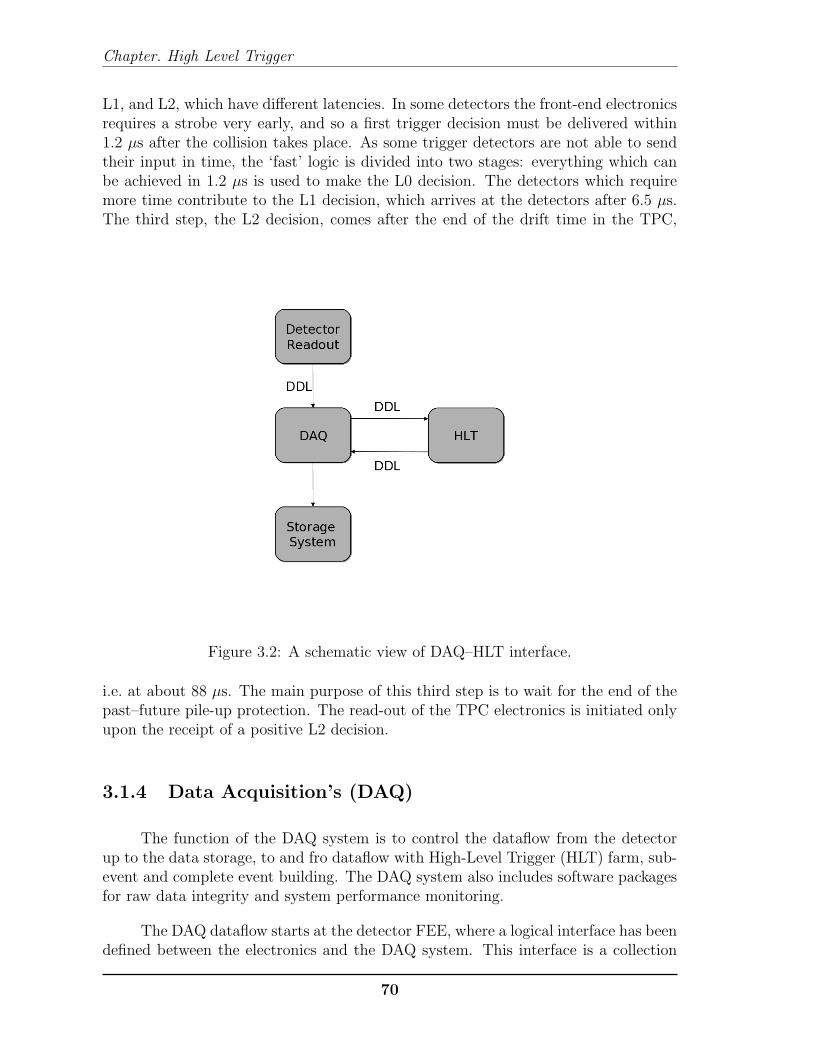
Chapter. High Level Trigger
L1, and L2, which have different latencies. In some detectors the front-end electronicsrequires a strobe very early, and so a first trigger decision must be delivered within1.2 µs after the collision takes place. As some trigger detectors are not able to sendtheir input in time, the ‘fast’ logic is divided into two stages: everything which canbe achieved in 1.2 µs is used to make the L0 decision. The detectors which requiremore time contribute to the L1 decision, which arrives at the detectors after 6.5 µs.The third step, the L2 decision, comes after the end of the drift time in the TPC,
Figure 3.2: A schematic view of DAQ–HLT interface.
i.e. at about 88 µs. The main purpose of this third step is to wait for the end of thepast–future pile-up protection. The read-out of the TPC electronics is initiated onlyupon the receipt of a positive L2 decision.
3.1.4 Data Acquisition’s (DAQ)
The function of the DAQ system is to control the dataflow from the detectorup to the data storage, to and fro dataflow with High-Level Trigger (HLT) farm, sub-event and complete event building. The DAQ system also includes software packagesfor raw data integrity and system performance monitoring.
The DAQ dataflow starts at the detector FEE, where a logical interface has beendefined between the electronics and the DAQ system. This interface is a collection
70

3.1. Overview of ALICE Online Systems
Figure 3.3: A schematic for DAQ–HLT Data Flow overview.
of the hardwares and softwares used for the readout of the different detectors. Thehardware consists of a bi-directional optical cable, known as Detector Data Link(DDL) [see sec. §2.4.2]. This is used both for the transfer of physics data from thedetector to the DAQ and for the transfer of control commands and configurationparameters in the opposite direction.
Once the data are collected from detector, they are transferred directly to thememory of standard Personal Computers (PCs) via a DDL adapter connected to D-RORC mounted on the PCI bus. Those computers which collect the data from thedetectors are called Local Data Concentrators (LDCs). The D-RORC can have abandwidth of 250 MBytes/s. In addition, it sends a second copy of the raw data viaa DDL link to the HLT system.
The event building is performed by a switching network with a total internalbandwidth of 2.5 GBytes/s. The data are archived in two steps, Transient DataStorage (TDS) based on disks close to the experiment and Permanent Data Storage(PDS) based on magnetic tapes in the CERN computing centre [Fig. 3.1].
3.1.5 High-Level Trigger (HLT)
The High Level Trigger combines and processes the full information from allmajor detectors of ALICE. It selects the most relevant data from the large inputstream. This includes the reduction of the data volume by an order of magnitude tofit the available storage bandwidth and is achieved by a combination of techniques:
71

Chapter. High Level Trigger
Figure 3.4: A schematic representation of data flow in the LDC of DAQ without theHLT components.
• reducing the event rate by selecting interesting events (software trigger);
• reducing the event size by selecting sub-events (Region of Interest, RoI);
• reducing the event size by advanced data compression.
All three tasks require online event reconstruction, which involves clusteringand track finding. These items are discussed in detail in the later sections.
The HLT farm is designed to be completely fault-tolerant, avoiding all singlepoints of failures, except for the unique DDL links. A generic data transportframework has been developed based on the Publisher Subscriber (Pub-Sub) principle,which allows the construction of any hierarchy of communication processing elements.
The HLT output [trigger decisions, Event Summary Data (ESD), and modifiedraw data as appropriate] is forwarded to the DAQ again via DDL connections.
The ECS running modes of HLT during global data taking of ALICE is describedin table 3.1. It is to be pointed out that, in modes B and C, HLT is treated like anyother detector and generated data are stored as part of the event building.
72

3.2. Dataflow Scheme
Figure 3.5: A schematic representation of data flow mechanism in the LDC of DAQwhen the HLT has been turned on.
Table 3.1: The different HLT modes in ALICE data-taking
(A) : DAQ is running without HLT.(B/Test1) : HLT is included with no HLT output to DAQ and HLT-busy
is not respected.(B/Test2) : HLT is included with no HLT output to DAQ and HLT-busy
is respected.(B) : HLT is fully included into the system, which means HLT output
is sent to DAQ and HLT-busy is respected. But the HLT triggerdecision is not considered.
(C) : DAQ performs event and sub-event selection based on the triggerinformation from HLT.
3.2 Dataflow Scheme
The full description of the ALICE data flow scheme can be found at Ref.[1]. Ashort description is presented here which is related with the data processing in HLT.
The architecture and interlinks of the Trigger, DAQ and HLT systems are
73

Chapter. High Level Trigger
illustrated in Fig. 3.1.
The detectors start to record the data as soon it receives the CTP trigger. Thedata is then collected from the detectors by the DAQ. A copy of the data is sent toHLT, which are processed and the HLT output and/or decision is sent back to DAQ.As soon as the analysed data are received from HLT output DDLs, the data streammoves to the event building process and are stored first into the TDS. The data arefinally migrated from TDS to PDS. A schematic view of the DAQ–HLT interfaceis illustrated in Fig. 3.2. The interface is based on the DDL and the associatedDestination Interface unit (DIU) and Source Interface Unit (SIU) cards. The samecomponents are also used to transfer data from the detector FEE electronics to theDAQ system.
Every D-RORC can host two DIUs, which can be used in two ways:
• both can be connected to the front-end electronics and serve as two readoutlinks,
• one DIU can be connected to the front-end electronics while the other is ableto transfer a copy of all the raw data to the HLT RORC (H-RORC) mountedon the HLT computers, through the standard DDL [Fig. 3.3].
The H-RORC receives all the raw data as they have been received by the front-endelectronics. All the LDCs dedicated to the detectors which make use of the HLTsystem are equipped with D-RORCs working in the second mode.
The processed data from HLT are received back by the DAQ via the HLTLDCs. These LDCs also receive messages specifying whether to discard or accepta given event. Furthermore, for accepted events, the HLT decision can specify apattern of sources for a given event, resulting in a partial readout of the raw data.A decision broker process, running in the HLT LDCs, transfers the HLT informationand decision to a decision agent process, running in the detector LDCs, as shown inFig. 3.5. The figure 3.4 shows the data flow in DAQ in the absence of HLT (i.e. HLTmode “A” as explained in Tab. 3.1).
3.3 HLT Online Framework
It is important to present a basic view of data flow scheme of HLT before theexplanation of HLT processing mechanism. Inside the HLT PC farm, the Front EndProcessors (FEPs) are responsible for zeroth level of data processing, as these areconnected to the FEE by the H-RORC. When the H-RORC receives rawdata it istransferred to the memory using DMA (Direct Memory Access) method. In the nextstep the processing components of the FEPs analyse the data and the output are
74

3.3. HLT Online Framework
passed to the next level of computing nodes for subsequent analysis. In this way therawdata blocks are parallely and independently analysed for every DDLs. The mergeddata blocks from all or part of FEPs for a given detector are collected and analysedfor track formation. Once the tracks and ESDs for every detectors participating inHLT analysis are produced, they are merged and sent to DAQ for event building. Onthe basis of the event analysis, HLT can issue a trigger about the goodness/badnessof the current event depending on the pre-defined trigger criteria. The online analysis
Figure 3.6: The general HLT multi-stage processing scheme.
scheme of HLT is explained in three subsections :
i) Data Processing and Transport
ii) HLT Output to DAQ
iii) Online Configuration
75

Chapter. High Level Trigger
3.3.1 HLT Data Processing and Transport
Components for Data Processing
The data processing within the HLT hierarchy is carried out by individualprocesses. These applications are derived from the same base class of the datatransport framework which provides the interface. The processes are known as HLTcomponents, following identical working principles. This term is also motivatedby the modular concept. The components carry out different tasks in the HLTprocessing hierarchy, treating input data and producing new data for subsequentcomponents. Each component is an individual process which is initiated at start-upof the processing chain. The state of a component can be changed by commandsvia network ports. In general, the components of data transport framework can bearranged in three categories :
• Data Source : The components that load data from the input device or file intoshared memory and create the corresponding data descriptors.
• Data Processing (Processors) : The components which subscribe to data of itsparents, process the data and publish the result to the next level.
• Data Sink : The components that implement the last stage in the chain, doingthe appropriate action on the output of the chain [Fig. 3.7].
Figure 3.7: The HLT Components schematic.
Although the HLT is an online framework, the analysis algorithms runningon it has to be tested and validated in offline mode well before their properonline implementation. Thus, a special group of processing components has beencreated by HLT analysis components. They allow the analysis processes to run
76

3.3. HLT Online Framework
in either the offline environment or in the online HLT environment without anychange in the code or the need of recompilation. A special component of the HLTdata transport framework, the AliRootWrapperSubscriber is the link between offlineanalysis components and the online environment.
Publisher-Subscriber Transport Framework
The high overall processing rate demands an efficient framework for fast datatransport. A dedicated data transport framework has been developed for this purposewhich is known as Publisher-Subscriber framework. It carries out all data transportand communication in HLT [2]. In addition to parallel processing of events, theALICE HLT’s data transport framework allows to split and distribute single eventsover a set of cluster nodes. The splitting of an event reduces the amount of data tobe copied. For instance, in the first step of the analysis, clusters and/or space pointsare reconstructed from the raw data. Thus, the resulting data volume has alreadybeen significantly reduced compared to the raw data.
The entire communication mechanism is designed for a low processing overhead.The figure 3.8 shows the working principle of the online framework. On one node,the data are exchanged via shared memory, a publisher can write the data directlyto memory and makes it available for subscribers without any intermediate copying.All processes communicate via named pipes (Named pipes implement a method ofinter-process communication on Unix/Unix-like systems) and exchange small datadescription information. The data transport framework takes care of data transportamong the nodes transparently. More details about the online framework can befound in [3] and [4].
Figure 3.8: The working principle of the HLT data transport framework.
For load balancing, the data stream can be split into several data streams eachcarrying a smaller data volume,
Furthermore, the distribution of the analysis leads to a short processing timeper event and node. This has additional advantage that if one node fails, the data lossis much smaller than in a conventional event building and filtering approach where
77

Chapter. High Level Trigger
a complete event or at least the processing time is lost. An intelligent scheduler canrestart processes on another node and resume event processing in case of a severefailure of a computing nodes.
It is to be noted that in parallel computing, process synchronization plays animportant role, for example a subscriber must not access data until the publisherhas announced readiness. The data transport framework carries out all processsynchronization.
3.3.2 HLT Output
The primary goal of HLT is to produce separate trigger information of varioustypes. This implies the identification of the events triggered by particle multiplicities,particle energies or transverse momenta, certain decay processes, or distinct particledensities in limited regions of the detector setup.
The event triggering is mostly a yes/no decision, the event is either consideredvaluable or not. But the result of the online reconstruction needs to be stored togetherwith the trigger information in order to determine the efficiency and selectivity of thetrigger in later offline stages of the analysis. In addition, data volume is reduced byselective readout and storing only the relevant part of data. This technique is calledRegion Of Interest readout. The ROI criteria can be applied in the first place on thelevel of DDL inputs and HLT simply provides a list of DDLs to be included into finalevent building. The format is defined in Ref. [5].
All readout lists from the running trigger components are treated by theprocesses on the HLTOUT nodes and formatted together with the HLTOUT payloadinto a defined DDL format ([5], [6]).
HLT Output Payload
Beside trigger information, HLTOUT format includes also payload data whichDAQ just forwards to storage. As a matter of fact, any output of HLT componentscan be directed to the HLTOUT and is included in the payload.
Since HLT is an online system, the payload contains information about fullyreconstructed events as part of the normal raw data stream. Beside this informationwhich is essential for the evaluation of the trigger, data blocks of varying nature arestored depending on the configuration of the analysis chain.
78

3.3. HLT Online Framework
Compressed Raw Data
A special feature of HLT is the reduction of the data volume by applyingappropriate compression techniques. The original data are encoded according toa compression algorithm and stored as a part of the HLTOUT payload. Datacompression has been extensively studied for the Time Projection Chamber whichis the biggest contributor to the data volume in ALICE [7]
In general there are two data compression paradigms. A Loss-less compressiontechniques allow to restore the original data from the compressed data set. Highercompression ratios can be achieved by applying specific models suited for the natureof data and omitting irrelevant information. However, the original data cannot berestored from the compressed data.
In both cases the offline reconstruction will treat the compressed instead ofthe original data and data flow schemes need to be designed. Thus, it is importantto completely separate the reconstruction algorithm and the data input in order tohandle different types of compressed data.
3.3.3 HLT Online Configuration
The mode of online HLT analysis is defined by the HLT configuration. Forinstance, in case of online testing of the analysis components, a online configurationis composed of file publishing, clustering, tracking and display components. Whereas,in experiment the configuration can be imagined as, DDL publishing, clustering,tracking and ESD building. Thus, in the two cases two different component sets areused in the form of two different configurations. Therefore, a configuration selects thecomponents to be used and the rules of communication between them. A configurationdescribes basic properties of the HLT processing layers,
• Type of the componentThe configuration specifies the application to run.
• Command line arguments of the componentIn order to adapt to different needs, components understand certaincommand line parameters. The exact format of parameters depends on theimplementation of the specific component.
• Interconnections of componentsThe configuration specifies all parent processes the component needs tosubscribe to in order to receive data.
• Reserved output buffer size and number of available buffersOutput data buffers have to be allocated before the processing loop of the
79

Chapter. High Level Trigger
component is invoked. The component has a fixed size of memory available inorder to write its output. The number of available buffers has an importantimpact to pipelined processing.
• Process multiplicityFor load distribution, multiple instances of the same component can run inparallel. The process multiplicity is part of the configuration.
• Fan-in/Fan-outThe configuration defines the topology of the chain which includes merging ofmultiple publishers to one consumer (Fan-in) and distribution of one publisherto multiple consumers (Fan-out)
In HLT, a configuration is described in XML notation, which stands forExtensible Markup Language. In general, a Markup Language is an artificial languageadding information on how to deal with a certain type of text and content. Markuplanguages are suited to categorize properties in an hierarchical way and are easy toparse in order to build the structure defined in this markup language.
The HLT configuration defines the execution sequence of the TaskManagerapplications, which run on each node of the computing cluster and supervise allprocesses on a given node [8]. Since the HLT chain can easily describe severalhundreds of components on hundreds of nodes, abstractions of configurations havebeen introduced with an automated generation of the final configuration [9].
Integration into the ALICE experiment
It is to be noted that, the HLT is integrated into the ALICE experiment bya couple of interfaces. For normal operation, HLT requires not only data exchangewith the DAQ but also the availability of calibration data and permanently monitoredvalues from the detector survey. Thus it has to communicate with all other ALICEsystems, such as the ECS, DCS, and the offline system. All interfaces are described indetail at [10]. HLT implements a finite state machine as outlined in [11] and Fig. 3.9.
Each state and transition correspond to certain actions and run conditions ofthe different parts of HLT.
(i) The transition from state INITIALIZED to CONFIGUREDentails the PubSub framework compiling all configuration files. At thisstage, no components are yet running, only TaskManagers are loaded onthe different nodes.
(ii) The transition from state CONFIGURED to READY by
80

3.3. HLT Online Framework
the ENGAGE command implies start and setup of all components. Aftergoing to state READY, HLT can be started by a START command andprocesses events when in state RUNNING.
The next section describes the HLT online and offline analysis framework.This will help to understand the implementation of data analysis algorithms in HLTframework.
81

Chapter. High Level Trigger
Figure 3.9: The state diagram of the HLT system shows the different states HLT.When the HLT receives command from ECS, the HLT moves between these statesdepending on the success or the failure of the command. [11].
82

3.4. HLT Analysis
3.4 HLT Analysis
The validation of HLT trigger selectivity and performance study of thealgorithms requires comparison of its components to the offline reconstruction andanalysis. Thus, it is important to run online analysis components without any changein the source code. To achieve this the HLT analysis chains have to be present inAliRoot as in the online framework.
Figure 3.10: The HLT analysis chains in the online and offline modes.
A schematic view of of the online and offline analysis procedures have beenshown in Fig. 3.10.
3.4.1 Base Classes and functionalities
Modularization
In the large scale software project, sometimes it is found that a compiled libraryA depends on a program declared in B, whereas B depends on a program specified inA. This dependency problem is known as circular library dependency problem. TheHLT analysis framework follows a clear dependency tree in order to avoid the circularlibrary dependency problems. The organization is outlined in Fig. 3.11. The librariesfall in 3 categories, (i) Framework Layer, (ii) Service Layer, and (iii) Module Layer.
• Framework Layer : In the Framework Layer, a base library, libHLTbase,provides all functionality needed for HLT analysis. It only depends on ROOTlibraries, apart from system libraries. The second library of the FrameworkLayer, libHLTinterface, implements an abstract interface intended to allowutilization of HLT components in external applications (i.e. the online Pub-Sub).
• Service Layer : The Service Layer contains libraries with AliRootbinding functionality, libHLTsim and libHLTrec for the offline simulation and
83

Chapter. High Level Trigger
Figure 3.11: The Modular organization of the HLT analysis framework.
reconstruction, respectively. A utility toolbox, libAliHLTUtil, implements bothsupporting classes and utility components.
• Module Layer : The HLT analysis components of individual detectors areaccessed via their corresponding libraries. All these libraries of this categoryfall under Module Layer. These libraries of this layer depend on the FrameworkLayers and offline analysis libraries of the given detector. As the libraries ofthe module layer implement HLT analysis components, they are also referredas component libraries.
HLT Analysis Component Interface
The main objective of the interface is a unified utilization from the online andoffline systems.
The component interface makes use of function overloading supported by C++classes. A couple of member functions of the base class are defined virtual,indicating the compiler that those functions can be overloaded by child classes. Theanalysis framework always uses references to objects of type AliHLTComponent foreach instantiated object of component implementations. If an overloaded function ispresent in the child class, it is invoked instead of the base class method. The ability totreat derived class members just like their parent class members is referred in softwareengineering to be Polymorphism.
84

3.4. HLT Analysis
Figure 3.12: The HLT component with overloaded methods.
The HLT work-flow with these overloaded methods are shown in Fig. 3.12. Thechild classes of the analysis component of an individual detector implement thesemethods, namely, Constructor, DoInit, DoEvent, Reconfigure, ReadPreprocessor,
85

Chapter. High Level Trigger
DoDeinit and Destructor. In the online analysis environment these functions arecalled during the different states of HLT as shown in Fig. 3.9. In the offline analysis,these same methods are called but from the AliSimulation class instead of ECScommand. In this way, HLT executes the same analysis components for a givendetector, irrespective of the origin of the data - online or offline. Each of theseoverloaded components is uniquely identified by the ComponentId, a character stringof arbitrary length and content. It is used by the ComponentHandler to register thecomponent and to create instances on demand. For practical reasons, a descriptivename is used, like e.g. MUONHitReconstructor. The data processing carried outby the component is characterized by component data types and the amount ofdata going to be produced with respect to the input data size. A component isfurthermore classified by the amount of memory it uses for data processing and theoverall processing time.
Module Agents
When a new functionality needs to be announced to the system, it is declaredusing the Module Agent. The agent defines the properties of the library, in suchway that when the offline simulation or reconstruction queries for the HLT analysis,the module agents instantiates the corresponding HLT analysis chain for each of theindividual detector. Therefore it is the responsibility of analysis developer to definethe functionalities of components via the module agents.
Component Registration
The components are the worker plug-ins for HLT analysis and are createddynamically according to the configuration. As a prerequisite, components mustbe known to the system. The analysis framework implements a registration schemewhich is the backbone for the realization of modularity. The agent needs to implementthe function, which is invoked by the system after the library has been loaded.
HLT Offline Configurations
In the online system, configurations are fully separated from the actualimplementation of both data transport and analysis.
The offline environment also requires mechanisms to describe an HLT chainand run components in an analysis hierarchy, both in simulation and reconstruction.The AliRoot binding functionality of the HLT analysis framework provides simplenotations to specify hierarchies of component for processing. The module agent
86

3.4. HLT Analysis
specifies HLT configurations which are supposed to run as default configurations inthe different steps of AliRoot by means of the functions.
3.4.2 Online Interface
The interface between the online data transport framework and the HLTanalysis components is provided by a C-interface.
In dynamic libraries, functions in the source code correspond to entry pointersin a compiled library. During program execution, all parameters are stored on thestack ( in computing architectures, a stack is a special kind of data storage basedon the Last-In-First-Out paradigm ) and the program jumps to the address in thelibrary. A C-interface uses this execution sequence by providing the entry pointersto the external application. The figure 3.13 sketches the entry points of the interfaceused by the online HLT system.
Figure 3.13: The figure shows the utilization of the C wrapper interface by the onlineHLT.
During initialization of the interface, the internal ComponentHandler and theexecution environment is set up. Subsequently, component libraries can be loaded,components be created and events processed.
A special care has to be taken with all memory allocations and data processingas the two (online and offline) frameworks run in different domains. So a memorybuffer allocated inside the HLT analysis cannot be freed in the PubSub systemwithout introducing a potential source for memory corruption. Depending on thecompilation and running environment, memory management might be different inthe two domains.
The interface consists of a set of functions and data structure definitionsprovided by the HLT analysis framework and is known to the external application.The definitions have three parts,
87
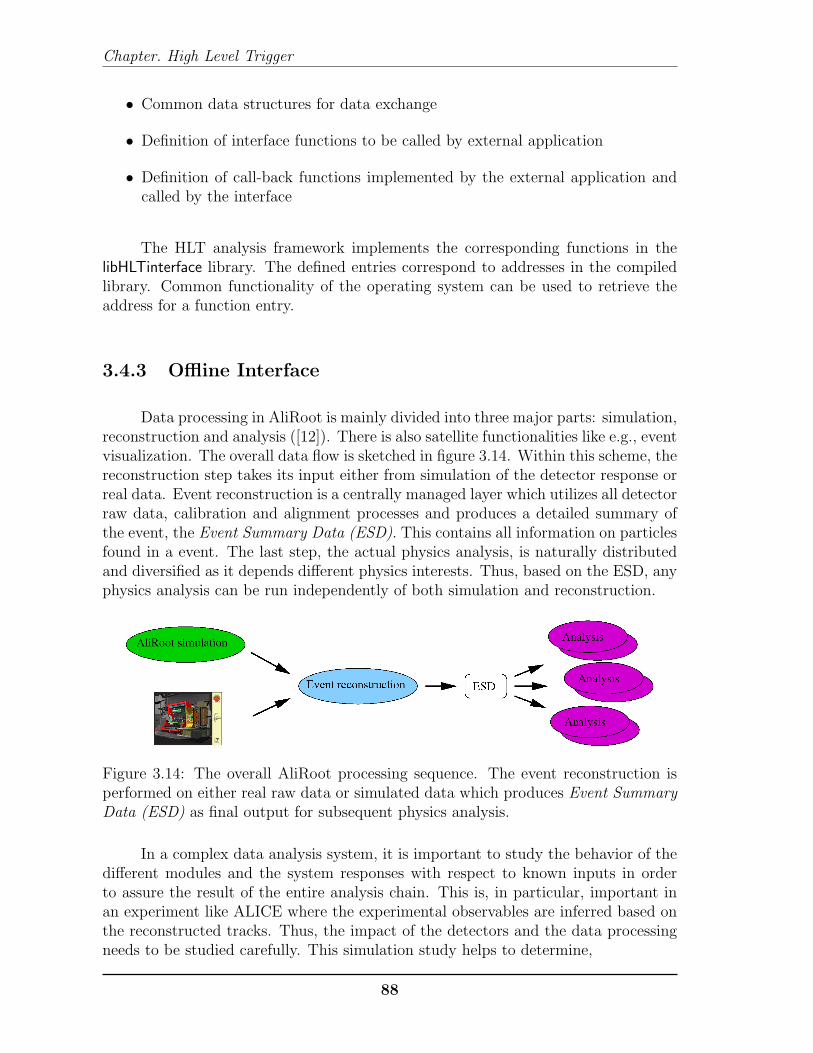
Chapter. High Level Trigger
• Common data structures for data exchange
• Definition of interface functions to be called by external application
• Definition of call-back functions implemented by the external application andcalled by the interface
The HLT analysis framework implements the corresponding functions in thelibHLTinterface library. The defined entries correspond to addresses in the compiledlibrary. Common functionality of the operating system can be used to retrieve theaddress for a function entry.
3.4.3 Offline Interface
Data processing in AliRoot is mainly divided into three major parts: simulation,reconstruction and analysis ([12]). There is also satellite functionalities like e.g., eventvisualization. The overall data flow is sketched in figure 3.14. Within this scheme, thereconstruction step takes its input either from simulation of the detector response orreal data. Event reconstruction is a centrally managed layer which utilizes all detectorraw data, calibration and alignment processes and produces a detailed summary ofthe event, the Event Summary Data (ESD). This contains all information on particlesfound in a event. The last step, the actual physics analysis, is naturally distributedand diversified as it depends different physics interests. Thus, based on the ESD, anyphysics analysis can be run independently of both simulation and reconstruction.
Figure 3.14: The overall AliRoot processing sequence. The event reconstruction isperformed on either real raw data or simulated data which produces Event SummaryData (ESD) as final output for subsequent physics analysis.
In a complex data analysis system, it is important to study the behavior of thedifferent modules and the system responses with respect to known inputs in orderto assure the result of the entire analysis chain. This is, in particular, important inan experiment like ALICE where the experimental observables are inferred based onthe reconstructed tracks. Thus, the impact of the detectors and the data processingneeds to be studied carefully. This simulation study helps to determine,
88

3.4. HLT Analysis
1. the desired detector performance required for a given physics interest,
2. the data analysis algorithms required to extract the experimental observablesfor that particular physics interest.
The optimization is done by comparing the values of the reconstructed observableswith the input values used for simulation. This approach is similar to signal responsestudies used in electronics engineering.
HLT has a special position within the described AliRoot processing chain. Asa matter of fact, HLT executes event reconstruction independently by utilizing thesimulated data from sub-detectors. Thus, it is often referred to be as HLT simulation.Figure 3.15 sketches the data flow for HLT simulation.
Figure 3.15: The HLT reconstruction in the simulation chain of AliRoot.
The lower block denoted by HLT system in Fig. 3.15 implements an encapsulatedHLT analysis with well defined input and output. It is important to notice thatthe placement of HLT analysis is flexible and depends only on the availability ofcustomized input data sources and output data sinks.
Since HLT reconstruction is executed either as part of simulation or online dataprocessing, the result only needs to be extracted during AliRoot reconstruction andstored appropriately.
In order to run the HLT analysis components in a chain-like fashion, thebehavior of the online data transport framework has been modeled by the HLTAliRoot integration. The AliHLTSystem class together with a few satellite classessteers HLT analysis chains in AliRoot.
The processing is determined by a configuration describing different componentsconnected to each other. Even though AliHLTSystem uses the same process as thealiroot executable, accessibility to data is strictly limited. As outlined in Fig. 3.10,
89

Chapter. High Level Trigger
apart from data input and output, the data processing is exactly identical in bothonline and offline environment.
AliHLTSystem is able to parse a configuration, build a task list from the entriesin the configuration and connect them forming an HLT analysis chain. It also carriesout memory allocation and organizes data transport between the components of thechain. The entity of AliHLTSystem can be plugged into the AliRoot processing streamat different places like AliSimulation or AliReconstruction.
3.5 HLT of Muon Spectrometer
3.5.1 Motivation
The main goal of High Level Trigger of Muon Spectrometer is to provide abetter transverse momentum (i.e. pT ) cut over that provided by the Muon Triggerstations. In case of central Pb-Pb collision a typical data rate of 500 MB/s is expectedfor Muon Spectrometer at 1 kHz L0 trigger rate. Therefore, a better estimation oftrack momentum will help to reject the background events before the data is writtento disk. The main challenge of the ALICE HLT project for dimuon spectrometeris to perform a fast analysis at highest possible rate (1 kHz trigger rate) with largeparticle multiplicity (∼300 particles hits in a given chamber for Pb-Pb collision at√s = 5.5 TeV), with best possible results in terms of resolution and efficiency. As
discussed in the last chapter that Muon Spectrometer measures the production cross-section of heavy-quark resonances, such as the J/Ψ, the Υ and their families, via theirdecay to muon pairs. The task of identifying muon candidates coming from theseresonances becomes complicated because of the presence of muons from pion/kaondecay. However, these muons can be rejected by an appropriate pt-cut since theirpt’s are predominantly low. These pt-cuts has been found to be 1 (low pt-cut) and 2GeV/c (high pt-cut) for J/Ψ and Υ , respectively, through simulation studies. TheL0 trigger provides an crude estimate of this pt-cut due to the poor pt resolution ofthe trigger chambers. Thus, HLT does a fast online data processing of the trackingchambers, in order to improve the transverse momentum estimate of the tracks.
3.5.2 MUON HLT Module Architecture
The MUON module for HLT analysis has been well integrated inside the AliRootsoftware package. All of the analysis codes are written in C++ language following thescheme accepted by AliRoot and HLT project. The MUON HLT module is designedto analyse the online experimental data with proper muon L0 trigger. But beforeapplying the analysis methods in the real time complex experiment, it is mandatoryto validate analysis algorithms on simulated data, which demands offline execution
90

3.5. HLT of Muon Spectrometer
of the online codes. Therefore analysis programs are arranged accordingly in theOnlineAnalysis and OfflineAnalysis directories inside the path AliRoot/HLT/MUON ofoffline software. However, the base classes which are important for both ways ofanalysis execution (i.e. offline/online) reside in AliRoot/HLT/MUON. The utilitypackages that are useful for dHLT processing, i.e. histogramming, rootification ofthe MUON HLT data blocks and dumping the MUON HLT data blocks from binaryfile, are situated inside utils directory of AliRoot/HLT/MUON. Some useful macrosand FSM (Finite State Machine) schematic diagrams can be found in macros anddocs, respectively, under the same base directory. A major part of this package hasbeen developed as a part of this thesis work.
3.5.3 Dimuon Components
The dimuon HLT (dHLT) analysis methods can be realised in terms of theprocessing components that have been explained before [sec.§ 3.4.1]. At the input,the dimuon component of the class receives data stream from 20 tracking DDLs and2 triggers DDLs which are then analysed and final output is merged into global HLTtrigger component and global HLT ESD component. A part of analysed data is sentto the TCP port, which are used for the event visualization of Muon Spectrometer ina machine at the user-end.
The main dimuon HLT analysis components are,
• Hit Reconstruction
• Trigger Reconstruction
• Tracking
• Decision
• ESDMaker
• HLTMuonTrigger
The first and the third items are discussed in short since those are subject todetail explanation in the next chapter.
Hit Reconstruction
The “Hit-Reconstructor” component is steered byAliHLTMUONHitReconstructorComponent class of HLT analysis frameworkimplemented in AliRoot. It receives the raw data streams as inputs, either from DDL
91

Chapter. High Level Trigger
links or from simulated files. The outputs of this component are the data blocks ofreconstructed particle hits ( in short rechits) of type AliHLTMUONRecHitStruct asspecified in the listing 3.1.
Listing 3.1: AliHLTMUONRecHitStruct, the output block structure of classAliHLTMUONHitReconstructorComponent.
1 struct AliHLTMUONRecHitStruct2 3 // The f l a g s word conta ins the f o l l ow i n g b i t f i e l d s ( b i t 31 i s4 // most s i g n i f i c a n t ) :5 //6 // b i t s : [ 31 −− 16 ] [ 15 −− 12 ] [ 11 −−− 0 ]7 // f i e l d : r e s e rved chamber detElemId8 //9 // Where we have ,
10 // re se rved b i t s must be s e t to zero .11 // chamber − s p e c i f i e s the chamber number in the range12 // [ 0 . . 1 3 ] , 0xF fo r i n v a l i d .13 // detElemId − s p e c i f i e s the d e t e c t o r e lement ID number .14 AliHLTUInt32 t fF l a g s ;15
16 AliHLTFloat32 t fX ; // X coord ina te .17 AliHLTFloat32 t fY ; // Y coord ina te .18 AliHLTFloat32 t fZ ; // Z coord ina te .19 ;
Where the AliHLTUInt32 t and AliHLTFloat32 t are unsigned 32-bit integer and 32-bit floating point data types, respectively. The steering class uses the core classAliHLTMUONHitReconstructor, which finds out the reconstructed space points of themuon tracking stations. The output of the Hit-Reconstructor component is sent as theinput of the tracker. The machinery of the core class AliHLTMUONHitReconstructorwill be discussed in detail in the following chapter.
Trigger Reconstruction
A similar task for muon trigger chamber hit finding is performed by “Trigger-Reconstructor” component AliHLTMUONTriggerReconstructorComponent. Since theareas of strips of Muon Trigger chambers are larger compared to Muon Trackingchambers, there is no need for clusterization. Therefore, Trigger Reconstructionperform faster operation than the Hit Reconstruction. The Trigger-Reconstructoralso receives raw data stream as input and the output (see listing 3.2) is directlyfed as input to the tracking component. In addition to the trigger chamber hitpoints, the data block also contains the momentum vectors. which point towardsthe origin. It helps to select the search region for track extrapolation through thetracking chambers.
92

3.5. HLT of Muon Spectrometer
Listing 3.2: AliHLTMUONTriggerRecordStruct, the output block structure of classAliHLTMUONTriggerReconstructorComponent.
1 struct AliHLTMUONTriggerRecordStruct2 3 AliHLTInt32 t f I d ; // Each t r i g g e r record shou ld have an ID4 // number unique f o r a g iven event .5 // −1 == i n v a l i d .6
7 // The f l a g s word conta ins the f o l l ow i n g b i t f i e l d s8 // ( b i t 31 i s most s i g n i f i c a n t ) :9 // b i t s : [ 3 1 ] [ 3 0 ] [ 2 9 −−− 4 ] [ 3 ] [ 2 ] [ 1 ] [ 0 ]
10 // f i e l d : − + reserved h s t [ 3 ] h s t [ 2 ] h s t [ 1 ] h s t [ 0 ]11 // Where f i e l d s h s t [ i ] i n d i c a t e s i f fH i t [ i ] has been f i l l e d / s e t .12 // Reserved b i t s shou ld be s e t to zero .13 // Pa r t i c l e s i gn : i f ’− ’ i s s e t then p a r t i c l e has minus s i gn .14 // i f ’+ ’ i s s e t then p a r t i c l e has nega t i v e s i gn .15 // Ei ther ’+ ’ or ’− ’ shou ld be s e t and i f n e i t h e r then the16 // p a r t i c l e s i gn i s unknown .17
18 AliHLTUInt32 t fF l a g s ;19
20 AliHLTFloat32 t fPx ; // Pa r t i c l e momentum X component in GeV/c .21 AliHLTFloat32 t fPy ; // Pa r t i c l e momentum Y component in GeV/c .22 AliHLTFloat32 t fPz ; // Pa r t i c l e momentum Z component in GeV/c .23
24 // Pa r t i c l e h i t coord ina t e s on t r i g g e r chambers 11 to 14.25 AliHLTMUONRecHitStruct fH i t [ 4 ] ;26 ;
In case of trigger reconstruction, the core class AliHLTMUONTriggerReconstructoris called by Trigger-Reconstructor component. The core functionality executes theactual finding of trigger chamber hit points.
Tracking
In dHLT, there exists two types of tracking algorithms for Muon SpectrometerHLT analysis. A partial straight line tracking method proposed by F. Manso [seeRef. [13]] and recently introduced full tracker using Kalman Filtering and CellularAutomata approach, which is the part of present thesis work. In case of Manso trackerthe inputs are Trigger-Reconstructor and rechits from chamber 7 to 10. Whereas forthe Full-Tracker the Hit-Reconstructor inputs and Trigger-Reconstructor inputs fromall chambers (except chamber 5 and 6) are utilised.
Manso Tracker : In case of tracking using Manso’s algorithm the componentAliHLTMUONMansoTrackerFSMComponent controls the main processing, usingAliHLTMUONMansoTrackerFSM core analysis class. The output of the Manso trackeris of type AliHLTMUONMansoTrackStruct as shown in the list 3.3.
93

Chapter. High Level Trigger
Listing 3.3: AliHLTMUONMansoTrackStruct, the output block structure of classAliHLTMUONMansoTrackerFSMComponent.
1 struct AliHLTMUONMansoTrackStruct2 3 AliHLTInt32 t f I d ; // Each Manso t rack shou ld have an ID number4 // unique f o r a g iven event . −1 == i n v a l i d .5
6 AliHLTInt32 t fTrigRec ; // The a s s o c i a t e d t r i g g e r record ID used7 // as the seed f o r the Manso a l gor i thm .8
9 // The f l a g s word conta ins the f o l l ow i n g b i t f i e l d s10 // ( b i t 31 i s most s i g n i f i c a n t ) :11 // b i t s : [ 3 1 ] [ 3 0 ] [ 2 9 −−− 4 ] [ 3 ] [ 2 ] [ 1 ] [ 0 ]12 // f i e l d : − + reserved h s t [ 3 ] h s t [ 2 ] h s t [ 1 ] h s t [ 0 ]13 // Where f i e l d s h s t [ i ] i n d i c a t e s i f fH i t [ i ] has been f i l l e d / s e t .14 // Reserved b i t s shou ld be s e t to zero .15 // Pa r t i c l e s i gn : i f ’− ’ i s s e t then p a r t i c l e has minus s i gn .16 // i f ’+ ’ i s s e t then p a r t i c l e has nega t i v e s i gn .17 // Ei ther ’+ ’ or ’− ’ shou ld be s e t and i f n e i t h e r then the18 // p a r t i c l e s i gn i s unknown .19 AliHLTUInt32 t fF l a g s ;20
21 AliHLTFloat32 t fPx ; // Pa r t i c l e ’ s momentum X component in GeV/c .22 AliHLTFloat32 t fPy ; // Pa r t i c l e ’ s momentum Y component in GeV/c .23 AliHLTFloat32 t fPz ; // Pa r t i c l e ’ s momentum Z component in GeV/c .24 AliHLTFloat32 t fChi2 ; // The ch i squared o f the f i t o f fH i t25 // po in t s to the t rack model . I f −1 then26 // no f i t done and momentum vec to r i s27 // i n v a l i d .28
29 // Pa r t i c l e h i t coord ina t e s on t r a c k i n g chambers 7 to 10.30 // fH i t [ 0 ] i s f o r chamber 7 fH i t [ 1 ] f o r chamber 8 e t c . . .31 AliHLTMUONRecHitStruct fH i t [ 4 ] ;32 ;
Full Tracker : The online tracking with inputs from all the chambers isperformed by the interface class AliHLTMUONFullTrackerComponent, whereas theAliHLTMUONFullTracker class implements the tracking algorithms and carries outthe calculation of track parameter. It produces the output block arrays ofAliHLTMUONTrackStruct (see list 3.4).
Listing 3.4: AliHLTMUONTrackStruct, the output block structure of classAliHLTMUONFullTrackerComponent.
1 struct AliHLTMUONTrackStruct2 3 AliHLTInt32 t f I d ; /// Each t rack shou ld have an ID number4 ///unique f o r a g iven event . −1 == i n v a l i d .5
6 AliHLTInt32 t fTrigRec ; /// The a s s o c i a t e d t r i g g e r record ID7 /// t ha t was matched to the t rack .
94

3.5. HLT of Muon Spectrometer
8
9 // The f l a g s word conta ins the f o l l ow i n g b i t f i e l d s10 // ( b i t 31 i s most s i g n i f i c a n t ) :11 // b i t s : [ 3 1 ] [ 3 0 ] [ 2 9 − 16 ] [ 15 ] [ 14 ] . . . [ 1 ] [ 0 ]12 // f i e l d : − + reserved h s t [ 1 5 ] h s t [ 1 4 ] h s t [ 1 ] h s t [ 0 ]13 // Where f i e l d s h s t [ i ] i n d i c a t e s i f fH i t [ i ] has been f i l l e d / s e t .14 // Reserved b i t s shou ld be s e t to zero .15 // Pa r t i c l e s i gn : i f ’− ’ i s s e t then p a r t i c l e has minus s i gn .16 // i f ’+ ’ i s s e t then p a r t i c l e has nega t i v e s i gn .17 // Ei ther ’+ ’ or ’− ’ shou ld be s e t and i f n e i t h e r then18 // the p a r t i c l e s i gn i s unknown .19 AliHLTUInt32 t fF l a g s ; // Bit f i e l d s f o r the t rack s t r u c t u r e .20
21 AliHLTFloat32 t fPx ; // Pa r t i c l e ’ s momentum X component in GeV/c .22 AliHLTFloat32 t fPy ; // Pa r t i c l e ’ s momentum Y component in GeV/c .23 AliHLTFloat32 t fPz ; // Pa r t i c l e ’ s momentum Z component in GeV/c .24
25 AliHLTFloat32 t fInverseBendingMomentum ; // One over the26 // momentum of the27 // f i t t e d t rack [GeV/c ] .28
29 AliHLTFloat32 t fThetaX ; /// The s l o p e o f the f i t t e d t rack in30 /// the non−bending p lane .31
32 AliHLTFloat32 t fThetaY ; /// The s l o p e o f the f i t t e d t rack in33 /// the bending p lane .34
35 AliHLTFloat32 t fX ; /// Non−bending p lane coord ina te f o r the36 /// d i s t ance o f c l o s e s t approach (DCA) [cm ] .37
38 AliHLTFloat32 t fY ; // Bending p lane coord ina te f o r the DCA [cm ] .39 AliHLTFloat32 t fZ ; // Z coord ina te f o r the DCA [cm ] .40
41 // Chi squared o f the t rack f i t .42 // I f s e t to −1 then no f i t was done and the momentum vec to r43 ///and DCA coord ina te i s i n v a l i d .44 AliHLTFloat32 t fChi2 ; /// The ch i squared o f the f i t o f fH i t45 /// po in t s to the t rack model .46
47 AliHLTMUONRecHitStruct fH i t [ 1 6 ] ; /// Pa r t i c l e h i t coord ina t e s48 /// found by the h i t49 /// r e con s t ru c t i on s t a g e .50 ;
The following chapter includes a detail description of the tracking algorithms.
Decision
The “Decision” component filters the track results according to the predefineddHLT trigger condition. It is implemented by the AliHLTMUONDecisionComponent
95

Chapter. High Level Trigger
class on the input blocks of AliHLTMUONMansoTrackStruct orAliHLTMUONTrackStruct. It has already been pointed out that the muonsfrom π and K decays can be efficiently suppressed by applying a cut on the pt ofthese muons. This idea has been adopted in the component to generate the dimuontrigger decision by first applying two pT cuts to the single tracks: a low cut for theJ/Ψ family and a high cut for the Υ family. Finally, the tracks that pass the cutsare counted and a statistics is build up for the tracks that passes the low or high pTcut. For instance, the decision component looks at pairs of tracks and counts thenumber of like-sign or unlike-sign pairs where both tracks passed the low or highpT cut or pairs that did not pass any cuts. There is a provision to calculate theinvariant mass of the oppositely charged track pairs that passes the mass cut. Theresults are encoded into two data blocks, one for trigger decisions for single tracks oftype AliHLTMUONTrackDecisionStruct (listing 3.5) and another for the track pairsof type AliHLTMUONPairDecisionStruct (see listing 3.6).
Listing 3.5: AliHLTMUONTrackDecisionStruct, the output block structure of classAliHLTMUONDecisionComponent.
1 struct AliHLTMUONTrackDecisionStruct2 3 AliHLTInt32 t fTrackId ; // The ID number o f the t rack we are4 // r e f e r r i n g to . This cou ld a l s o be5 // a t r i g g e r record ID .6
7 // The t r i g g e r b i t s have the f o l l ow i n g meaning :8 // b i t : [31 −−− 2 ] [ 1 ] [ 0 ]9 // f i e l d : r e s e rved h i p t l o p t
10 // Reserved b i t s shou ld be s e t to zero .11 // h i p t == passed h igh pt cut . l o p t == passed low pt cut .12 AliHLTUInt32 t f T r i g g e r B i t s ;13
14 AliHLTFloat32 t fPt ; // The c a l c u l a t e d t r an s v e r s e momentum of15 // the t rack in (GeV/c ) .16 ;
Listing 3.6: AliHLTMUONPairDecisionStruct, the output block structure of classAliHLTMUONDecisionComponent.
1 struct AliHLTMUONPairDecisionStruct2 3 // The ID numbers o f the t r a c k s we are r e f e r r i n g to .4 // These cou ld a l s o be t r i g g e r record ID numbers .5 AliHLTInt32 t fTrackAId ;6 AliHLTInt32 t fTrackBId ;7
8 // The t r i g g e r b i t s have the f o l l ow i n g meaning :9 // b i t : [31 −−− 7 ] [ 6 ] [ 5 ] [ 4 ][3−−2][1−−0]
10 // f i e l d : r e s e rved hiM loM un l i k e h i p t l o p t11 // Reserved b i t s shou ld be s e t to zero .12 // hiM == Pair passed the h igh i n va r i an t mass cut .13 // loM == Pair passed the low inva r i an t mass cut .14 // un l i k e == i s the pa i r an un l i k e s i gn pa i r .
96

3.5. HLT of Muon Spectrometer
15 // h i p t : 0 i f n e i t h e r t rack has pt > high pt cut , 1 i f e i t h e r has16 // and 2 i f both have . A va lue o f 3 i s i n v a l i d .17 // l o p t : 0 i f n e i t h e r t rack has pt > l o p t cut , 1 i f e i t h e r has18 // and 2 i f both have . A va lue o f 3 i s i n v a l i d .19 AliHLTUInt32 t f T r i g g e r B i t s ;20
21 AliHLTFloat32 t fInvMass ; // Invar i an t mass o f the t rack pa i r22 // assuming they are both muons23 // in (GeV/c ˆ2)24 ;
The input arguments of the Decision component are listed below,
• -lowptcut valueIt sets the low pt-cut value. The value should be a floating point number andhas units GeV/c. If this parameter is specified then it will not be loaded fromCDB.
• -highptcut valueIt sets the high pt-cut value and has the same properties as -lowptcut.
• -lowmasscut valueIt sets the low invariant mass cut value to use when applying the decision. Thevalue should be a floating point number and has units GeV/c2. If this parameteris specified then it will not be loaded from CDB.
• -highmasscut valueIt sets the high invariant mass cut value to use when applying the decision andhas the same properties as -lowmasscut.
• -no singles detailIf specified the detailed decision information for tracks is not added to theoutput. Only the scalar values are then stored in the output data block fordecisions on single tracks.
• -no pairs detailIf specified the detailed decision information for track pairs is not added to theoutput. Only the scalar values are then stored in the output data block fordecisions for track pairs.
• -warn on unexpected blockThis will cause the component to generate warnings when it receives non-standard data block types. This option increases the robustness of thecomponent.
• -cdbpath pathThis allows one to override the path to use for the CDB location. The pathmust be a valid CDB URI. By default the HLT system framework sets the CDBpath.
97

Chapter. High Level Trigger
• -run numberThis resets the run number for CDB objects.
• -delaysetupIf indicated then part of the initialisation of the component is forcefully delayedto the first event received, i.e. the Start-of-Run event.
• -dumponerrorThis flag allows to dump the data blocks if an error occurs during the processingof the event.
• -dumppath pathAllows one to specify the path in which to dump the received data blocks if anerror occurs.
The output of decision component is useful to build the online statistics of thedHLT tracking components and therefore can be sent to the TCP port for display orcan be sent to the HLTMuonTrigger component to issue the suitable trigger.
ESDMaker
The “ESDMaker” component (AliHLTMUONESDMaker class) is usedto convert the dHLT reconstructed data (AliHLTMUONMansoTrackStruct orAliHLTMUONTrackStruct and AliHLTMUONTriggerRecordStruct as inputs) toAliESDEvent objects. This is stored in ROOT files during offline reconstruction. ThedHLT chain produces TClonesArray of AliESDMuonTrack objects. These are thenmerged together with ESD tracks from all the other parts of HLT (eg. TPC, TRD,ITS, PHOS, EMCAL) using global ESD converter to build AliESDEvent. Finally,it is pushed into the HLTOUT DDL to DAQ for event building. The following listcontains the optional arguments of ESDMaker component.
• -make minimal esdIt indicates that AliESDEvent objects should be created with only theTClonesArray for the muon tracks created. (default is to generate all standardESD objects)
• -add rootified objectsIf specified then the any rootified dHLT event data that is found is added tothe ESD list of objects as a custom data object.
• -makeclonesarrayThis option will cause the component to generate a TClonesArray of MUONESD tracks and send it as a kAliHLTDataTypeTObject data block type.
98

3.5. HLT of Muon Spectrometer
• -makeonlyclonesarraySame as the -makeclonesarray option, however the data blocks with theAliESDEvent object are not generated.
• -warn on unexpected blockIf set, then warning messages are generated for any data block types that werenot expected. (default is to generate only debug messages)
• -dumponerrorThis flag will cause the component to dump the data blocks it received if anerror occurs during the processing of an event.
• -dumppath pathAllows one to specify the path in which to dump the received data blocks if anerror occurs.
HLTMuonTrigger
The “HLTMuonTrigger” component uses the decision generated by theAliHLTMUONDecisionComponent as input and creates HLT trigger data blockssuitable for the HLT global trigger framework. In addition, several other data blocks(e.g tracks, rechits, trighits ) can also be provided as input to generate the muontrigger. It is important to note that in case of DDL stream as inputs with properargument “-triggerddls”, the component will trigger every single event trigger byMuon Trigger cluster of CTP. The possible list of arguments of this components are,
• -makestatsIf specified, the summary statistics scalars object is generated as output. Thedefault is not to generate the statistics object.
• -triggerddlsIndicates that the component should trigger if any DDLs are found in the muonspectrometer.
• -triggerhitsIndicates that the component should trigger if any hits are found in themuon spectrometer tracking chambers. This option requires that this triggercomponent receives the reconstructed hits data blocks.
• -triggertrigrecsIndicates that the component should trigger if any muon trigger records arefound. This option requires that this trigger component receives the triggerrecord data blocks.
• -triggertracksIndicates that the component should trigger if any track is found.
99

Chapter. High Level Trigger
• -triggerdimuonsIndicates that the component should trigger if any dimuon pair is found.
• -triggeranyThis option indicates that it should trigger, if any of the above mentioned triggercondition is satisfied.
It is to be noted that if none of the “triggerddls” ,“triggerhits”, “-triggertrigrecs”, “-triggertracks” or “-triggerdimuons” options are specified then thedefault triggering mode is to trigger on tracks and dimuon pairs.
Apart from the above mentioned components there are few less frequently usedcomponents, which are explained in brief,
ClusterFinderComponent This cluster finder component(AliHLTMUONClusterFinderComponent class) executes offline algorithms, in theonline HLT. It processes the raw data of tracking stations and returns the clusterinformation in the form of offline cluster (i.e. array of AliMUONVCluster objects). Itcan also produce dHLT internal hit coordinates (i.e AliHLTMUONRecHitStruct), if“-makehits” option is explicitly specified in component argument.
DigitPublisherComponent The component (classAliHLTMUONDigitPublisherComponent) is used to convert simulated or reconstructeddigits into DDL raw data streams on the fly and publish them. It is useful forrunning dHLT simulations on digit data where the raw data files are not available.The component is also used for the dHLT simulation under AliSimulation whenthere is no direct access to a raw data reader.
ClusterHistoComponent This AliHLTMUONClusterHistoComponent class getsthe cluster data blocks from Hit-Reconstructor component and produces histogramsin the form of ROOT object TH1. These are then transported to the network portfor online display.
RawDataHistoComponent This component (classAliHLTMUONRawDataHistoComponent) is useful for performing basic monitoringtasks on the raw data from the muon spectrometer. It will try and decode the dataand histogram the following information:
• The distribution of signals per DDL.
• The number of ADC values found per MANU for each DDL.
100

3.5. HLT of Muon Spectrometer
• The error codes found by the decoders while trying to decode the data for eachDDL.
EmptyEventFilterComponent This component classAliHLTMUONEmptyEventFilterComponent is a utility component for debugging.It is used to filter empty dHLT events. (In particular, it was built for the Dec 2007Cosmic tests, where the muon spectrometer was not expecting hits for most of theevents triggered by ACORDE.)
DataCheckerComponent This class AliHLTMUONDataCheckerComponent is usedto check and validate the integrity of dHLT internal raw data blocks. If there is anyproblem then an appropriate error message is logged. This component should be usedfor debugging and testing only, since the validation procedure can be slow.
RootifierComponent This component class AliHLTMUONRootifierComponent isused to convert all internal raw dHLT data blocks into ROOT object that can bestored in ’.root’ files in a platform independent manner. This also makes some of theanalysis easier because the dHLT internal data are available in the form of TObjects.
The main features of dimuon HLT components are discussed in this section toillustrate the dHLT scheme for fast Hit-Reconstruction and track finding algorithms,which are discussed in the next chapter.
101

Chapter. High Level Trigger
102

Bibliography
[1] ALICE Collaboration, Technical Design Report: Trigger, DAQ, HLT, DCS,CERN-LHCC-2003-062, 2004.
[2] T. M. Steinbeck, “A modular and fault-tolerant data transportframework”, Ruprecht-Karls-University Heidelberg, Germany, 2004,[http://arxiv.org/abs/cs/0404014].
[3] T. M. Steinbeck et al., IEEE Trans. Nucl. Sci., vol. 49, pp. 455-459, 2002
[4] T. M. Steinbeck et al., “New experiences with the ALICE High Level TriggerData Transport Framework”, in Proc. Computing in High Energy Physics Conf.2004 (CHEP04), 2004 [http://chep2004.web.cern.ch/chep2004/]
[5] R. Divia and T.M. Steinbeck., Data format and specificationsfor the HLT-to-DAQ interface, ALICE-INT-2007-015, ver. 3 2008,[https://edms.cern.ch/document/871995].
[6] R. Divia, P. Jovanovic, P. Vande Vyvre, Data Format over the ALICE DDL,ALICE-INT-2002-010, ver. 11 2007, [https://edms.cern.ch/document/340186].
[7] J. Wagner, V. Lindenstruth, M. Richter, T.M. Steinbeck, J. Thader., LosslessData Compression for ALICE HLT, ALICE-INT-2008-020, ver. 1 2008,[https://edms.cern.ch/document/948159].
[8] T. M. Steinbeck et al., “A Control Software for the ALICE High Level Trigger”,in Proc. Computing in High Energy Physics Conf. 2004 (CHEP04), 2004[http://chep2004.web.cern.ch/chep2004/]
[9] T. M. Steinbeck, “SimpleChainConfig”, HLT project internal information,University of Heidelberg, Germany, 2007.
[10] S. Bablok et al., High level trigger online calibration framework in ALICE, J.Phys.: Conf. Ser. 119 022007 (2008)
103

BIBLIOGRAPHY
[11] S.R. Bablok et al., ALICE HLT interfaces and data organisation , in Proc.Computing in High Energy Physics Conf. 2006 (CHEP06), Mumbai, India (2006)
[12] The ALICE Collaboration, JINST 3 S08002 (2008) 175.
[13] F. Manso and the Clermont-Fd ALICE group. A first algorithm for a dimuonhigh level trigger. ALICE Internal Note, 2002. ALICE-INT-2002-004.
104

Chapter 4
Algorithms
This chapter discusses the key ideas of the main dHLT analysis components. Ithas been explained before (see last chapter) that the motivation of the dHLT is toimprove the pt-cut for muons by online reconstruction. This is achieved in two steps.
• Hit Reconstruction : Reconstruction of the pad clusters on each individualchamber leading to reconstructed hit points.
• Track Formation : Reconstruction of the trajectory of the charged particlesusing the reconstructed hit points.
The official analysis software, MUON Offline of AliRoot [discussed later insec. §5.1], solves this problem mainly by Mathieson fitting for cluster reconstructionand Kalman filtering for track formation. It is to be noted that there are alternateclustering and tracking methods for offline analysis. But none of these methods canbe applied for online reconstruction. This is due to the fact of time constrain. Forinstance, the time to reconstruct a simulated central Pb-Pb event using offline analysistakes ∼1 second on standard computer of 2.93 GHz clock speed. However in onlineanalysis this has to be achieved within 1 ms, as the estimated L0 trigger rate forcentral Pb-Pb collision is 1 kHz. Thus, two separate algorithms for hit reconstructionand track formation have been proposed for online analysis in the present thesis work.In addition, to the problem of full reconstruction, there are challenges of the onlineanalysis. These are,
• An online processing has to be robust, so that it can run 24x7 without anysystem crash. The presence of any small memory leak, or bug in any part ofthe code will lead to immediate instability.
• The online components should not crash due to any data corruption in the inputbuffer.
105

Chapter. Algorithms
• The event processing has to be done upto a rate of 1 kHz even for the highestmultiplicity Pb-Pb collision. This will ensure that the dHLT component willnot generate a back pressure to the whole experimental system.
The online algorithm not only has to satisfy these online analysis criteria butalso produce results of appreciable quality. In order to check the quality of onlinereconstruction a detail study on the comparison of online and offline algorithms havebeen presented in the following chapter. The discussion of a new tracking algorithmis never complete unless it is compared with the existing algorithm. Therefore, ashort overview of the Manso’s algorithm is included.
The core ideas of online Hit-Reconstruction has been discussed in the followingsection.
4.1 Hit Reconstruction
4.1.1 Algorithm
It is clear from the above discussion that the motivation of the dHLT HitReconstruction analysis is to perform fast identification of a charged particle’strajectory in the spectrometer. Since the algorithm aims to reconstruct the highmultiplicity central Pb-Pb events, a study has been performed to estimate the averagenumber of charged particle hits for a given detection plane using HIJING eventgenerator. The result of this simulation study is shown in Fig. 4.1. Each entry of thehistogram corresponds a single central Pb-Pb event and the number of hits for thatevent for a given plane is filled as the value of that entry. Therefore, the mean valuesof the histogram shows the average number of hit multiplicity for a given detectionplane in case of central Pb-Pb collision. It is evident from this study that on average300 particle hits have to be reconstructed in case of highest multiplicity events.
The first step of cluster reconstruction is the identification of the pad cluster.In offline analysis a cluster is found by a detail scan on the pads with a commonboundary following the concept of nearest neighbour. This method of clustering isaccurate but slow and thus is not suitable for online analysis. Therefore, the firstchallenge was to search for an alternate method for fast identification of the chargeclusters. This is solved applying the concept of central pad. The central pad of agiven cluster is the pad with the maximum charge. At the start of the rawdataprocessing the data array is split into two sets of arrays for pads of bending andnon-bending planes. These arrays are called as total hit registers, where the pads areidentified by a unique combination of buspatch number with MANU card number andchannel number [ref. Chapter 2]. The hit register for bending (non-bending) planeis then scanned along the y-direction (x-direction) to collect the central pads, which
106

4.1. Hit Reconstruction
Figure 4.1: A simulation study of hit multiplicity for central Pb-Pb collision in MuonSpectrometer Tracking Chambers. The mean position of the histograms signifiesaverage number of particle trajectories in for a given chamber.
Figure 4.2: The inefficiency of central hit reconstruction (left) and the timingperformance on a 2.93 GHz Nihalam processor (right) of the Hit Reconstructionalgorithm as a function of the DC cut.
are stored in a different array. In addition to ∼300 hits for Pb-Pb collision theremay be pad clusters arising due to noisy electronics. Thus, an intelligent selection ofthe central hit is required to avoid these noise clusters. It has been found from the
107

Chapter. Algorithms
simulation study that a threshold cut on ADC value, while scanning for central pads,helps to remove these noises. This ADC threshold is henceforth referred as DC-cut.It is apparent that if the DC-cut is set to higher value there is a chance to looseclusters originating from charged particle tracks. The effect of DC-cut on efficiencyand timing performance of the analysis algorithm are shown in Fig. 4.2. It is realisedthat a DC-cut of 50 ADC channel is acceptable, which provides the best compromisebetween the central pad finding efficiency and timing performance of the online code.
Once the central hit for a given cluster is identified, the centre of gravity (COG)of the pad charges of the central pad and its two immediate neighbours are calculated.This gives the reconstructed hit position along the bending (non-bending) direction,when COG method is applied along the y-direction (x-direction) of central pad,respectively.
(a) Residual oscillation in reconstructedhit position
(b) Correction of residual oscillation ofreconstructed hits by sine curve withnegative amplitude
Figure 4.3: A sinusoidal curve of tailing effect. It is observed from the y-axis ofthe subfigures that, in case of the uncorrected reconstructed hit position (left figure)the Gaussian distribution of (recY-geantY) will have a large tail than the correctedsubfigure (right). Therefore, this curve signifies the “tailing effect”.
The position resolution calculated with COG method suffers due to to finite padsize (5mm in y-direction and 7.5 mm in the x direction). This effect in the bendingdirection can be seen in Fig. 4.3(a), where the residue (reconstructed position - true hitposition as obtained from GEANT3 [v1-11] ) is plotted as a function of (reconstructedposition - pad center). It is interesting to note that the wavelength of the oscillationis exactly equal to the pad size. Thus, a correction term for the reconstructed hitcan be found as a function of the hit position with respect to the pad center. TheFig. 4.3(b) shows the residue plot after this correction. Finally, the reconstructed hitsfrom the bending and non-bending planes are merged to form the reconstructed (x,y)position of the cluster. A flow chart of the algorithm is given in Fig. 4.4.
In the next subsection the implementation scheme of Hit Reconstructionalgorithm to the HLT framework is discussed.
108

4.1. Hit Reconstruction
Figure 4.4: The flow chart of hit reconstruction algorithm.
4.1.2 HLT Interface
It has already been described in brief in the previous chapter that the mainclasses AliHLTMUONHitReconstructor and AliHLTMUONHitReconstructorComponentare responsible for hit reconstruction in dHLT. The core processing is carried outby AliHLTMUONHitReconstructor, which represents the hit reconstruction algorithmin the form of a C++ code. Each of the method of this class is explained in detailbelow and the overall processing scheme is shown in Fig. 4.5.
The class AliHLTMUONHitReconstructor mainly consists of a initialisation part(SetLookUpTable and InitDetElemInDDLArray methods) and an execution part whichis controlled by the Run function.
SetLookUpTable :
Three pointers are set in the arguments of this method, which are essentialduring the following analysis. The purpose of these pointers are explained below.
109

Chapter. Algorithms
Figure 4.5: A schematic for processing steps of AliHLTMUONHitReconstructor class.
1. The memory location of the geometrical mapping, pedestal and gain for thecathode pads. It has the following data type.
Listing 4.1: Data Type containing the mapping and calibration values
1 struct AliHLTMUONHitRecoLutRow2 3 AliHLTInt32 t fDetElemId ; // The de t e c t o r e lement ID of the pad .4 AliHLTInt32 t fIX , fIY ; // The X,Y number o f the pad .5 AliHLTFloat32 t fRealX , fRealY , fRealZ ;
// The r e a l coord ina te6 // o f the pad .7 AliHLTFloat32 t fHa l fPadSize ; // h a l f pad s i z e in X fo r bending8 //and Y fo r nonbending9 AliHLTFloat32 t fPadSizeXY ; // pads i z e in Y fo r bending p lane
10 //and X fo r nonbending11 AliHLTInt32 t fPlane ; // The p lane and PCB zone ID numbers .12 AliHLTFloat32 t fPed , fSigma , fA0 , fA1 ; // Ca l i b r a t i on va l u e s13 AliHLTInt32 t fThres , fSa t ; // Ca l i b r a t i on va l u e s14 ;
This pointer address carries the most important reference data set for hitreconstruction algorithm.
2. The one to one mapping of the unique identity of a pad (combiningbuspatch number, MANU number, channel number) to the array position ofAliHLTMUONHitRecoLutRow is defined as data type IdManuChannelToEntry
110

4.1. Hit Reconstruction
Listing 4.2: Data Type specifing the mapping of unique pad identity
1 typedef std : : map<AliHLTInt32 t , AliHLTInt32 t>2 IdManuChannelToEntry ;
It helps in fast identification of a pad instead of searching over the entirehierarchical loop of buspatch, MANU and channel.
3. The last pointer address points towards a list, which contains the maximumnumber of allowed rawdata for a given buspatch. This is implemented to protectthe analysis code from slowing down due to the presence of noisy buspatches.As it is presently set, if the occupancy of a buspatch is found to be higher that5%, then it is skipped from analysis. This pointer is of same type as of theprevious item.
Listing 4.3: Data Type specifing the buspatch occupancy list
1 typedef IdManuChannelToEntry MaxEntryPerBusPatch ;
It is to be noted that the initialization of the mapping and calibration and otherentries into the memory is performed by AliHLTMUONHitReconstructorComponentclass.
InitDetElemInDDLArray :
It may be recapitulated from the detector description that for a given DDL thereare several detection elements. In this method new memory location is allocated tomaintain a structured list of number of pads fired per detection element and itssummary over the DDL. These memory locations are then filled and utilized in theAliMUONTrackerDDLDecoder::OnData() method during rawdata decoding.
Run :
As it has been shown in the schematic diagram 4.5, the central Run method isexecuted for every event of Muon Spectrometer. In the input argument, it receivesthe address of the rawdata stream, the size of the rawdata block, the pointer for theoutput blocks and size of it. The analysis is done in two steps, in the first stage therawdata address and it size is handled by DecodeDDL method, which in turn usesAliMUONTrackerDDLDecoder::Decode to decode the rawdata DDL stream. Once itis decoded the data stream is then arranged in proper form, for next stage of hitreconstruction. The central control of analysis is carried out by FindRecHits method,where the decoded rawdata is separately analysed for each detection element. Insidethe loop of detection elements, five functions are called to find out hit points as shownschematically in Fig. 4.5.
111

Chapter. Algorithms
FindCentralHits :
In this method the central pads are identified separately for each bending ornon-bending plane. Since the bending (non-bending) plane gives better resolution inthe y-direction (x-direction), the pads are scanned along y-axis (x-axis). If the centralpad is found to satisfy the DC cut, the cluster is forwarded to the next processingstep, otherwise rejected as noise cluster.
RecXRecY :
This function calculates the reconstructed hit position by the Centre of Gravity(COG) method separately for bending and non-bending planes. For instance, if threeconsecutive pads with ADC values C1, C2, and C3 are found at y-positions, y1, y2,and y3, respectively, then the hit centre is calculated as,
yrec =y1C1 + y2C2 + y3C3
C1 + C2 + C3
This calculation is carried out for each central pad. But the accuracy of thereconstructed position suffers from the oscillation as indicated in Fig. 4.3(a). Thus,a correction of the form
Asin(2π
dx)
is applied, where x = (reconstructed position - pad center), A = normalizationconstant and d = pad dimension along the high resolution direction. The effectof this correction for residual oscillation is shown in Fig. 4.3(b).
MergeSlatRecHits :
The final merging of bending and non-bending hits is done by two methods. Asthe name suggests this function merges the reconstructed hits for the slat chambers.In case of merging of slat chamber hits, first the adjacent reconstructed hits yrec (xrec)of bending (non-bending) plane are merged which are with same x (y) co-ordinate.In the final step the bending and non-bending hits are merged which are within half-pad size as explained in the algorithm part. Finally, the output data block of typeAliHLTMUONRecHitStruct (see list 3.1) is filled to the output buffer. It is to be notedthat for online detector diagnostics two additional types of data blocks can also beprepared AliHLTMUONClusterStruct and AliHLTMUONChannelStruct (see list 4.4 and4.5), which are used for real time histograms.
Listing 4.4: The AliHLTMUONClusterStruct data type
1 struct AliHLTMUONClusterStruct2
112
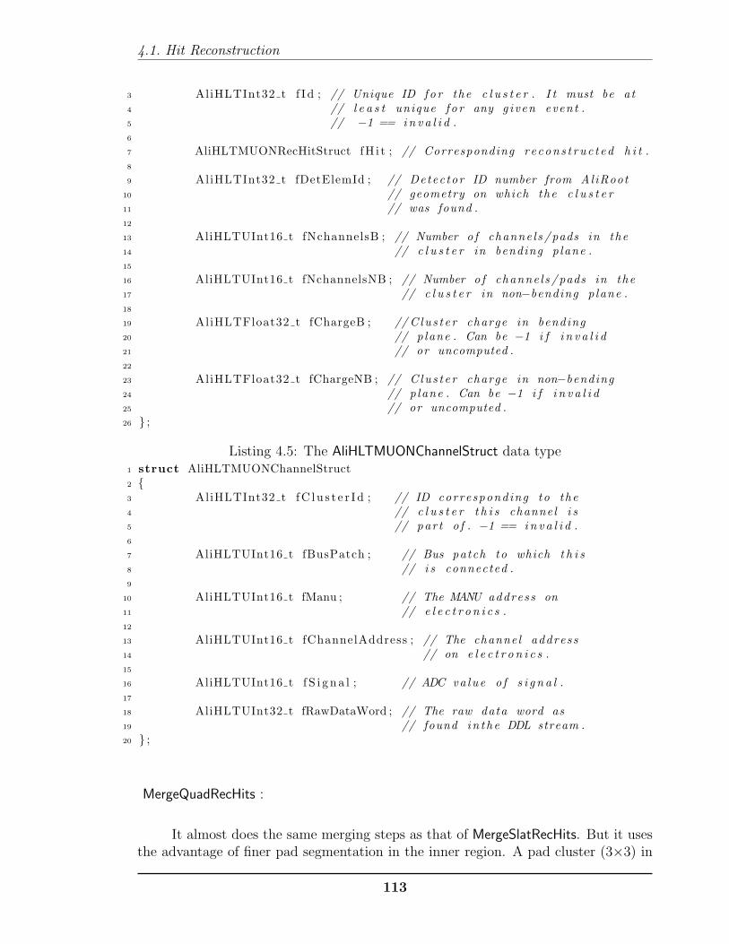
4.1. Hit Reconstruction
3 AliHLTInt32 t f I d ; // Unique ID fo r the c l u s t e r . I t must be at4 // l e a s t unique f o r any g iven event .5 // −1 == i n v a l i d .6
7 AliHLTMUONRecHitStruct fH i t ; // Corresponding r econs t ruc t ed h i t .8
9 AliHLTInt32 t fDetElemId ; // Detec tor ID number from AliRoot10 // geometry on which the c l u s t e r11 // was found .12
13 AliHLTUInt16 t fNchannelsB ; // Number o f channe l s /pads in the14 // c l u s t e r in bending p lane .15
16 AliHLTUInt16 t fNchannelsNB ; // Number o f channe l s /pads in the17 // c l u s t e r in non−bending p lane .18
19 AliHLTFloat32 t fChargeB ; // C lus t e r charge in bending20 // p lane . Can be −1 i f i n v a l i d21 // or uncomputed .22
23 AliHLTFloat32 t fChargeNB ; // C lus t e r charge in non−bending24 // p lane . Can be −1 i f i n v a l i d25 // or uncomputed .26 ;
Listing 4.5: The AliHLTMUONChannelStruct data type1 struct AliHLTMUONChannelStruct2 3 AliHLTInt32 t f C l u s t e r I d ; // ID corresponding to the4 // c l u s t e r t h i s channel i s5 // par t o f . −1 == i n v a l i d .6
7 AliHLTUInt16 t fBusPatch ; // Bus patch to which t h i s8 // i s connected .9
10 AliHLTUInt16 t fManu ; // The MANU address on11 // e l e c t r o n i c s .12
13 AliHLTUInt16 t fChannelAddress ; // The channel address14 // on e l e c t r o n i c s .15
16 AliHLTUInt16 t f S i g n a l ; // ADC va lue o f s i g n a l .17
18 AliHLTUInt32 t fRawDataWord ; // The raw data word as19 // found in the DDL stream .20 ;
MergeQuadRecHits :
It almost does the same merging steps as that of MergeSlatRecHits. But it usesthe advantage of finer pad segmentation in the inner region. A pad cluster (3×3) in
113

Chapter. Algorithms
the inner most zone, is capable to provide adequate resolution in both bending andnon-bending directions. Therefore, during the final merging step and if no hits arefound on the other plane still that hit on the single plane is considered as a validreconstructed hit.
Clear :
As it appears from the name, it clears all the pointers and arrays that are usedfor a given detection element.
The next part explains the methods of the classAliHLTMUONHitReconstructorComponent, which controls the classAliHLTMUONHitReconstructor to analyse the events. But before that it is importantto highlight the following three features of dHLT analysis scheme.
DoInit :
During the initialization process, the DoInit method reads the geometricalmapping of the spectrometer from the Conditional Data Base (CDB)ReadLutFromCDB, or from the text file ReadLookUpTable of predefined format.In either case it loads data format of type AliHLTMUONHitRecoLutRow into thememory. Along with mapping, the retrieval of the last pedestal and calibration runparameters that are stored in the same CDB is also performed inside this method.The calculation of the maximum allowable buspatch occupancy level for eachbuspatch is also carried out and filled into memory array. The memory addresses arethen passed to the initialisation function of AliHLTMUONHitReconstructor.
DoEvent :
This function receives rawdata block addresses from the rawdata publishercomponent RORCPublishers using common HLT data abstraction method. SinceHLT is an online system, it is important to pickup the correct data block for a givendetector analysis, where the data block identification plays an important role. Oncethe proper rawdata blocks are found, it calls the AliHLTMUONHitReconstructor::Run()method for hit-reconstruction analysis. The final result is packed into the outputblocks using the template class AliHLTMUONDataBlockWriter. It is important tonote that during the preparation of the output data stream, it again has to apply thedata abstraction, data identification and data specification schemes to publish it tothe next processing component.
114

4.2. Track Formation
DoDeInit :
This method clears the memory allocation done by the core analysis componentand also calls the destructor of that class. If needed some cleaning of the memoryblocks owned by the component class itself can also be performed.
At the end of the hit reconstruction, the tracks are formed using thereconstructed hits. Thus, the following sections discuss the various tracking schemesof Muon Spectrometer, with an emphasis on online FullTracker.
4.2 Track Formation
Once the hit points of the tracking chambers are found, these are connected toform the tracks of the particles through the Spectrometer. As it has been pointed outbefore, there exits two online tracking methods in dHLT analysis Manso Tracker andFull Tracker. The concepts of online algorithms of tracking has been discussed in thefollowing subsections. Since the quality of the online tracking will be compared withoffline analysis, a short description of the offline tracker has been given.
4.2.1 Offline Tracker
The offline tracker uses either the fit of the track parameters (x, y, α, β,q/p) [where x(y) and α(β) are the bending (non-bending) co-ordinates, and thecorresponding angles, respectively, and q/p represents the charge over momentum]using the MINUIT package of Root or the reconstruction using the Kalman Filter.In the first step the primary track candidates are build using the clusters of station4 and 5 using all combinations of clusters between the two chambers of station 5(4). Then the pairs are selected for which the estimated bending momentum and thenon-bending impact parameter at vertex are within given error limits. In the nextstep, the primary tracks are formed with station 4 and 5 and the identical tracksare eliminated. It is then propagated to stations 3, 2 and 1; in each step the trackparameters are updated. In the last part, the tracks are extrapolated to the collisionvertex which is measured by SPD of Inner Tracking System. The final results ofthe reconstruction are stored in objects of the class AliESDMuonTrack and saved inAliESD.root file. Three kinds of tracks are saved, tracker tracks matched with triggertracks, only tracker tracks and only trigger tracks.
115

Chapter. Algorithms
4.2.2 Manso Tracker
The primary motivation of dHLT is to reduce the background events byimproving the pt-cut resolution provided by the L0 trigger, which depends on theposition resolution of the trigger chambers. Manso proposed that since the positionresolution of the tracking chambers are better than that of trigger chambers, theextrapolation of the tracks to the fifth and fourth tracking stations will improvept estimation of the tracks [Ref. [1]]. Therefore, a parametrized Region of Interest(RoI) is defined for the fast track extrapolation,
Figure 4.6: The concept of Manso Tracker shows that the tracking upto fourthtracking station improves momentum estimation. This is mainly due to the fact thatthe tracking chambers have better position resolution than trigger chamber and thetrack is not deflected by the Muon Filter.
Rs = a.Rp + b
where Rs is radius of the RoI and Rp is the position of the RoI with respect tothe centre of the detector as shown in Fig. 4.6. The parameters a and b are found as,
Station5 : a = 0.020; b = 3.0
Station4 : a = 0.016; b = 2.0
When the hit points in the fourth and fifth station is found, the track momentumcan be calculated using the following formula [2],
p = 0.3qBL
θd(4.1)
where q is the charge of the particle, B is the magnetic field, L is the length
116

4.2. Track Formation
of the dipole. If the hit positions of stations 4 and 5 are at (x1, y1, z1 ) and (x2,y2, z2 ) respectively, the deviation of the track due to the magnetic field (θd) can becalculated as,
θd =1
zf
(y1z2 − y2z1
z1z2
)
where zf represents the z-position at the middle of the dipole. The momentumcomponents are calculated as,
px = pxfzf, py = p
yfzf, pz =
√p2 −
(p2x + p2
y
)where (xf ,yf ) represents the extrapolated track position in the middle of the thirdstation. Thus, the Manso algorithm uses the property of better position resolution ofthe fourth and fifth tracking station for better estimation of momentum.
4.2.3 Full Tracker algorithm
Basic Concepts
The Manso tracker provides a partial improvement in pt estimation but it is notadequate (discussed in sec. §5.3.2). Therefore, a Full Tracker was proposed [3] whichallows track reconstruction upto the front absorber of the Muon Spectrometer.
The Full Tracking formalism can be viewed as a composition of four stagesof track reconstruction. The full tracking also starts from trigger chambers and astraight line track is drawn upto the seventh chamber, since it is the first chamberafter the dipole magnet. In the second step of tracking, the tracklets are calculatedin station 1 and 2 using Cellular Automata method since this method does not needany a priori knowledge of the seed of the tracking. When the tracklets are found inthe front and rear side of the spectrometer, they are matched using χ2 test of Kalmanfiltering. If a track passes the Kalman testing, the track parameters are improved bythe track extrapolation through parametrised front absorber.
The various stages of the Full Tracker are described below.
Trigger Chamber Tracking
The Muon Trigger stations are operated in streamer mode and provides the levelzero (L0) trigger for the Muon Spectrometer. The global trigger processors provides
117

Chapter. Algorithms
Figure 4.7: The concept of Full Tracker shows various methods of tracking fordifferent segments of Muon Spectrometer. A track following method is used forthe fourth and fifth station, whereas for the first and second station the CellularAutomaton is used. The segmented tracks from the rear and the front side ofthe Spectrometer are matched using Kalman χ2 technique. Finally, the tracks areextrapolated to the origin through the front absorber, using parametrised correctionsoriginating from the multiple Coulomb scattering and energy loss of the track in theabsorber.
the track parameters (px, py, pz) for the tracks formed in the Trigger stations.
Tracking in Station 4,5
The tracking of the Full Tracker starts from this step, as the trigger track isalready calculated during the issuance of the hardware trigger. The track segment ofthe trigger station is then extrapolated to the fifth tracking station using straight lineextrapolation. Since the Muon Filter is situated in between the trigger and trackingchambers of Muon Spectrometer, care has been taken during this extrapolation fordeflection of the track in this iron wall. Since the effect of magnetic field is almostzero on fourth and fifth station, the track is extended further through straight lineextrapolation. It is to be noted, in the real experimental condition, all the detectorsmay not function properly. Thus, a track is validated, if three out of four trackingchambers have hits associated with that track.
118

4.2. Track Formation
Tracking in Station 1,2
Since the extrapolation of the track to the third station involves the addedcomplexity of the magnetic field, it has been skipped. This also saves vital time.As an alternative scheme, tracking in Station 1 and 2 has been proposed by formingtracklets in these stations. So the important criterion is that, one has to do thetracking without any seed or any priori information of the track direction. Therefore,the method of Cellular Automation [4, 5] is used for track finding which is a fastmethod and needs no a priori information of the direction of the tracks. The mainfeatures of the Cellular Automation are :
• The cell state is discrete [either living (1) or dead (0)]
• The number of neighboring cells is fixed, in most of the cases they are thenearest cells.
• The rules describing the dynamics of the evolution of the cellular automatondepend on the type problem.
• The cell states change simultaneously i.e. they are clocked.
A detail description of the Cellular Automata can be found in the Appendix A.
In present case, we have virtually segmented the detector in cells and any cellcontaining a hit point is living, otherwise is dead. In the next step the living cellsof the consecutive chambers are connected for a given station, with the conditionthat the living cells from other chambers have to be its closest neighbour. The ruleof evolution or the rule of survival is based on the selection that there has to be aneighbour in the adjacent station and if extrapolated to third station should matchthe track extrapolated in the backward direction from fourth and fifth station. Thetracklets found in this method are validated using the same criteria as applied in caseof tracking in stations 4 and 5, i.e. the tracklet is valid if there are three hit pointsout of the four detector planes. If needed, this condition can also be loosen to onehit per station.
Connect and Validate Track in Station 3
It has been discussed above that, a tracklet in the front section of thespectrometer may get connected to more than one tracklets in rear section or atracklet of the rear chambers can get connected with more than one tracklets ofthe front chambers. These are ghost tracks and can be removed by two differenttechniques, namely,
• Chi-square text of Kalman filtering method [6, 7, 8].
119

Chapter. Algorithms
• The extrapolation of tracklets through magnetic field, using track propagationmethod. (e.g. G3HELIX or G3HELX3 of Geant3)
In case of p-p events χ2-test of Kalman Filtering is applied to evaluate the χ2 ofthe tracks and removal of ghost tracks based on best chi-square selection. However, incase of Pb-Pb events the ghost tracks are removed through the track extrapolation inmagnetic field by Geant methods. But in this case also the χ2 of the set of tracks afterghost removal is calculated by Kalman Filter. The χ2-test of Kalman Filter whichhas been used in connecting and validating tracks through station 3 is described inbrief below.
The Kalman Filter is a recursive tool for the prediction of the state of thesystem at a future point, and constantly updating the quality of prediction of thenext future point by incorporating the immediate future point into the parameter forfuture prediction. This is done in three steps,
• Prediction is the estimation of the state vector at a future time.
• Filtering is the process to update the predicted state vector at point (k) basedon the observations at points up to (k − 1) by adding the observation at point(k).
• In smoothing step the filtered state at site (k′ < k) is updated by using all theobservations made at points upto (k).
In the present algorithm, the first two steps have been applied and the χ2 isdefines as (see Appendix on Kalman Filter and [8]),
χ2k = χ2
k−1 + (mk −Hkak)Tk Gk (mk −Hkak) +
(ak − ak−1
k
)T (Ck−1k
)−1 (ak − ak−1
k
)where,
χ2k−1 = chi-square upto point k − 1ak = new estimate of state vector at point kak−1k = prediction of state vector at k with the information unto k − 1Ck−1k = covariance matrix for the state vectormk = measurement vector at point kHkak = measurement vector at point k if measurement noise is zeroG = inverse of the covariance matrix for measurement noise.
The second term of the above expression represents the error matrix associatedwith the process noise at site k, and the third term represents the measurement noise
120

4.2. Track Formation
for the same site. A summary of the Kalman filtering formulas are found at AppendixB.
Track Extrapolation through Muon Absorber
Since the track suffers substantial energy loss and scattering during its passagethrough the Front Absorber, it is very important to include these effects in estimatingthe momentum of the tracks. The energy loss is calculated using the Bethe-Blochformula for ionisation energy loss. In case of multiple Coulomb scattering thecomposite effect of the different absorber materials is estimated using the Bransoncorrection. If θ is the polar angle of a track at vertex with respect to the z-axiswhich passes through the front absorber. The Branson method gives the convenientway of the estimation of θ using the particle direction at the rear end of the frontabsorber [9].
A detail study of these effect can be found in the Appendix C.
4.2.4 Implementation in HLT
The Full Tracker analysis is carried out by two main classes.AliHLTMUONFullTracker is the core analysis class which performs all the trackproperty calculations while AliHLTMUONFullTrackerComponent is the componentclass which controls the core class to execute the tracking analysis on behalf ofHLT chain. The schematic diagram of the Fig. 4.8 explains the track parameterscalculation methods of AliHLTMUONFullTracker class.
Init :
During initialisation of the Full Tracker class, the geometrical segmentations ofthe Muon Spectrometer is loaded from CDB. The other important parameter loadedfrom CDB is the value of the L3 and dipole magnetic fields. If the magnetic fieldvalues are set by other components, that values are used instead. Otherwise thedefault instance is created with (+/+) magnetic field direction. The other importanttask of Init method is to book a memory map for detection elements.
SetInput :
This method copies the pointer address of the input data sets into an array ofpointers and a counter keeps the record of number of triggers and hit reconstruction
121

Chapter. Algorithms
Figure 4.8: The schematic diagram of the functions of Full TrackerAliHLTMUONFullTracker class.
blocks. A test is performed in this method to assure that the number of data pointsdo not overflow the size specified for the array of pointers. In addition, the detectionelement list is used to identify the proper data blocks which have valid detectionelement number. The SetInput function and the Run methods are called for eachMuon trigger event.
Run :
The central control of the analysis is carried out by the Run method. It uses themethod CheckInput to start the processing and stops at the Clear function as shown inFig. 4.8. As the argument it receives the event number and the pointer to the outputdata block (of type AliHLTMUONTrackStruct) and the size of the output data.
CheckInput :
This method serves the most vital part of the analysis, protecting the codefrom incomplete data blocks. During the data taking, there are “soft” triggers fromMuon Trigger, for the calibration purpose. Thus, these events has no tracking data.This type of events are skipped from this method. Furthermore, in case of detectorproblem is it possible that some of the DDLs are switched off, which are also properly
122

4.2. Track Formation
accounted in this method.
SlatTrackSeg :
The tracking process starts only when there is one reconstructed hit in each ofthe last two tracking stations. In the next step for each trigger record the associatedtracks is searched within a predefined window. At present, the search windows arewide open (twice the simulated results), tuned to the cosmics result analysis. Thiswill be optimised later, after the analysis of experimental data of sufficient statistics.If a track segment is found in station four and five, it is extrapolated to the thirdstation to create a virtual hit point on that chamber. This hit point is utilised in theQuadTrackSeg method.
PrelimMomCalc :
It is possible that there are no track segments found in the first two stationseither due to detector or tracking inefficiency. In both cases the full tracking is notpossible for these tracks. But the track momentum is calculated using the sameformula that has been used for the Manso Tracker in Eqn. 4.1.
It is obvious that the momentum calculated from the half tracks suffers from badreconstruction resolution compared to the full tracks, since the half track calculationdepends on approximate evaluation of θd. But this partial tracking method helps toimprove the efficiency of online dHLT tracking performance.
QuadTrackSeg :
The QuadTrackSeg starts with checking for single hits in first and secondstations. If there is no track in the rear end, the tracking in the first and secondstations are skipped. In the first step, a set of tracklets are formed among thechambers of a given station. Then these tracklets are joined within certain boundarycuts on mutual angle and orientation to form a track segment. Finally the tracksegments are extrapolated to the middle of the third station and its position iscompared with one obtained from SlatTrackSeg. If matching is found within a suitablelimit then the next step of track matching is performed for those track segments.
KalmanChi2Test :
In the Kalman χ2 test method, all the tracks, that are found by the SlatTrackSegmethod are checked with the track segments found in QuadTrackSeg. If the track
123

Chapter. Algorithms
segments from the rear and front end of the spectrometer are matched using the χ2
minimization test, they are saved into the array for full tracks. The track parametersare recomputed for the tracks in the arrays of full tracks.
SelectFront :
The SelectFront uses a simpler test to match the tracks from SlatTrackSeg withthe tracks from QuadTrackSeg. A rough estimate of the track momentum is calculatedfor the track in the last two tracking stations. This is used to predict the hit positionin the third and subsequently second tracking station. The track segment on the firsttwo tracking stations if found to be closer to that extrapolated line from rear end aredeclared as matched track segment pair.
ExtrapolateToOrigin :
In the ExtrapolateToOrigin method, the correction for Multiple Coulombscattering (MCS) and energy loss are applied to correct the track momentum.
Clear :
As the name suggests this method cleans any dynamic memory allocation andreset the counters for next event.
This chapter has illuminated the key ideas of tracking and clustering in theMuon Spectrometer, which are compared and validated with detail simulation resultsin the following chapter.
124

Bibliography
[1] F. Manso and the Clermont-Fd ALICE group. A first algorithm for a dimuonhigh level trigger. ALICE Internal Note, 2002. ALICE-INT-2002-004.
[2] ALICE Collaboration, Technical Design Report of the Dimuon ForwardSpectrometer, CERN/LHCC 9922, 13 August 1999.
[3] Indranil Das, Sukalyan Chattopadhyay A new formalism of full tracking indimuon high level trigger. DAE-BRNS Symposium on Nuclear Physics, 2009.
[4] A. Glazov, I. Kisel, E. Konotopskaya and G. Ososkov. Nucl. Instr. and Meth. A329 (1993) 262-268.
[5] I. Kisel. Nucl. Instr. and Meth. A 566 (2006) 85-88.
[6] R.E. Kalman. Trans. ASME-Journal of Basic Engineering 82 (Series D) (1960)35-45.
[7] P. Billoir, R. Fruehwirth and M. Regler. Nucl. Instr. and Meth. A 241 (1985)116-131.
[8] R. Fruehwirth. Nucl. Instr. and Meth. A 262 (1987) 444-450.
[9] J.P.Cussonneau, P.Lautridou, L.Luquin, V.Metivier, A.Rahmani, V.Ramillien,T.Reposeur and A.Morsch. Tracking Peformances of Several Front-AbsorberDesigns. Report. ALICE Internal Note, 1998, INT-98-27
125

BIBLIOGRAPHY
126

Chapter 5
Simulation Studies and Validationof Algorithms
This chapter describes the performance of Full Tracker in a simulatedenvironment which closely matches the experimental condition. The tracking andclustering codes depend on different selection windows, either due to detectorboundary conditions (i.e maximum angle of the tracks or tracks pointing towardsthe origin) or the region of physics interest (pt-cut of 1 GeV/c and 2 GeV/c). Theranges of these selection windows are obtained from simulation studies. This offlineanalysis environment is described in the first section, which is followed by the resultsof simulation studies of Hit Reconstruction and Full Tracker algorithms, respectively.In the last section, the commissioning of the Full Tracker in the online environmentof HLT computing cluster is discussed.
5.1 AliRoot Simulation Scheme for Muon
Spectrometer
The AliRoot simulation framework provides and maintains the exact detectorsimulation, reconstruction and analysis for ALICE detector. In the first step ofparticles generation, all primary and daughter particles are produced using the MonteCarlo generators (e.g. HIJING, PYTHIA, DPMJET, HERWIG). In addition, it isalso possible to create particles of fixed and predefined spectrum from parametrized(i.e. where pt, rapidity, azimuthal and polar angles are input parameter) generators.Once the particles are produced they are transported through the detectors and thedetector responses are simulated via GEANT3 or GEANT4 or FLUKA. In the nextstage of digitization, the analog detector signal is converted to ADC output to producedigits, which mimics the actual detector behaviour during the electronic readout. Thedigits are then converted into the structured raw data format, which is identical to
127

Chapter. Simulation Studies and Validation of Algorithms
that collected in real experimental environment. The offline analysis of HLT usesthese as input and the results are saved in the ESD format (HLTESD), which aresimultaneously stored along with the simulated rawdata data set. This analysis partin AliRoot has already been discussed before in sec. §3.4.3. At the end of the HLTanalysis process a Quality Assurance (QA) analysis of the data is carried out, whichmarks the end of offline simulation by AliRoot.
The reconstruction of rawdata is performed in three basic steps. In the firststep, the rawdata is decoded and the corresponding calibration is applied to recreatethe digits. In case of Muon Trackers the set of digits which form a charge clusteris found out by scanning the neighbouring digits. The charge distribution of thecluster is then reconstructed using Mathieson function. Once the reconstructed hitpositions are obtained, the tracking using Kalman filter starts from the rear end of thespectrometer. It goes on attaching clusters with minimum χ2 of track parameters, tillit reaches to the first Muon chamber. In the final step of the offline reconstruction thetracks are filled into the ESD tree and the offline ESD tree is stored into a rootifiedfile along with the tree that contains ESD objects of HLT.
5.2 Results of Hit Reconstruction
5.2.1 Reference Data Sets for Hit Reconstruction
The quality of the track parameters like momentum and rapidity, relies mostlyon position resolution of the space points that forms the tracks. Thus, it is veryimportant to study the position resolution and the efficiency of the hit reconstructionalgorithm in order to test the quality of the fast algorithm. Therefore, the AliGenBoxgenerator of AliRoot has been used to simulate the tracks within given a momentumrange. The setup of the generator is listed in 5.1.
Listing 5.1: Particle generator for a given ptwindow
96 i f ( ! strcmp ( option , "box" ) ) 97 AliGenBox ∗ gener = new AliGenBox ( 1 ) ;98 gener−>SetPtRange ( 0 . 5 , 2 0 . 0 0 0 1 ) ;99 gener−>SetPhiRange ( 0 . , 3 6 0 . ) ;
100 gener−>SetThetaRange ( 1 7 1 . 0 0 0 , 1 7 8 . 0 0 1 ) ;101 gener−>SetPart (kMuonMinus ) ; // Muons102 gener−>SetOr ig in ( 0 . , 0 . , 0 . ) ; // v e r t e x p o s i t i o n103 //Sigma in (X,Y,Z) (cm) on IP po s i t i o n104 gener−>SetSigma ( 0 . 0 , 0 . 0 , 0 . 0 ) ;105
The complete configuration file can be found in the AliRoot at$ALICE ROOT/MUON/Config.C. A set of 10000 events have been generatedand reconstructed. The list 5.2 and 5.3 presents the muon offline simulation and
128
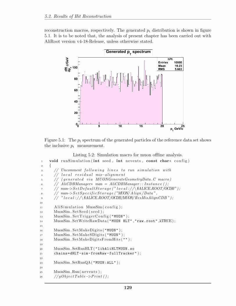
5.2. Results of Hit Reconstruction
reconstruction macros, respectively. The generated pt distribution is shown in figure5.1. It is to be noted that, the analysis of present chapter has been carried out withAliRoot version v4-18-Release, unless otherwise stated.
Figure 5.1: The pt spectrum of the generated particles of the reference data set showsthe inclusive pt measurement.
Listing 5.2: Simulation macro for muon offline analysis.1 void runSimulat ion ( int seed , int nevents , const char∗ c o n f i g )2 3 // Uncomment f o l l ow i n g l i n e s to run s imu la t i on wi th4 // l o c a l r e s i d u a l mis−al ignment5 // ( generated v ia MUONGenerateGeometryData .C macro )6 // AliCDBManager∗ man = AliCDBManager : : Ins tance ( ) ;7 // man−>Se tDe fau l tS to rage (” l o c a l ://\$ALICE ROOT/OCDB”) ;8 // man−>Se t Sp e c i f i c S t o r a g e (”MUON/Align /Data ” ,9 // ” l o c a l ://\$ALICE ROOT/OCDB/MUON/ResMisAlignCDB ”) ;
10
11 Al iS imulat ion MuonSim( c o n f i g ) ;12 MuonSim . SetSeed ( seed ) ;13 MuonSim . SetTr iggerConf ig ("MUON" ) ;14 MuonSim . SetWriteRawData ("MUON HLT" ,"raw.root" ,kTRUE) ;15
16 MuonSim . SetMakeDigits ("MUON" ) ;17 MuonSim . SetMakeSDigits ("MUON" ) ;18 MuonSim . SetMakeDigitsFromHits ("" ) ;19
20 MuonSim . SetRunHLT("libAliHLTMUON.so21 chains=dHLT-sim-fromRaw-fullTracker" ) ;22
23 MuonSim . SetRunQA("MUON:ALL" ) ;24
25 MuonSim . Run( nevents ) ;26 // gObjectTable−>Print ( ) ;
129

Chapter. Simulation Studies and Validation of Algorithms
27
28
Listing 5.3: Reconstruction macro for muon offline analysis
1 void runReconstruct ion ( int seed , const char∗ input , const char∗ r e c o p t i o n s )2 3 AliCDBManager∗ man = AliCDBManager : : In s tance ( ) ;4 man−>SetDe fau l tStorage ("local://\$ALICE_ROOT/OCDB" ) ;5
6 gRandom−>SetSeed ( seed ) ;7
8 Al iRecons t ruc t i on ∗ MuonRec = new Al iRecons t ruc t i on ("galice.root" ) ;9 MuonRec−>SetInput ( input ) ;
10 MuonRec−>SetRunVertexFinder (kFALSE ) ;11 MuonRec−>SetRunLocalReconstruct ion ("MUON" ) ;12 MuonRec−>SetRunTracking ("MUON" ) ;13 MuonRec−>SetFil lESD ("HLT" ) ;14 MuonRec−>SetOption ("HLT" , "libAliHLTMUON.so" ) ;15 MuonRec−>SetLoadAlignData ("MUON" ) ;16 MuonRec−>SetNumberOfEventsPerFile ( 1 0 0 0 ) ;17 MuonRec−>SetOption ("MUON" , r e c o p t i o n s ) ;18 MuonRec−>SetRunQA("MUON:ALL" ) ;19 MuonRec−>SetQAWriteExpert ( AliQAv1 : :kMUON) ;20
21 // uncomment the f o l l ow i n g l i n e s22 // i f you want to s e t custom RecoParam23 //24 // in s t ead o f g e t t i n g them from the OCDB25 // AliMUONRecoParam ∗muonRecoParam26 // = AliMUONRecoParam : : GetLowFluxParam ( ) ;27 // muonRecoParam−>SaveFul lClusterInESD (kTRUE, 1 0 0 . ) ;28 // MuonRec−>SetRecoParam(”MUON” ,muonRecoParam ) ;29
30 MuonRec−>Run ( ) ;31
32 delete MuonRec ;33
34 // gObjectTable−>Print ( ) ;35
5.2.2 Resolution and Efficiency
The residuals between the reconstructed hits and the original Geant hits forthe Hit Reconstruction algorithm and Offline Clusterfinder method are comparedin Fig. 5.2 and Tab. 5.1. It is evident from the figure and the table that the hitreconstruction of the bending plane is more accurate than the non bending plane.This is due to the fact that the resolution in the bending direction is determined alongthe anode wires and the pad dimension is 5 mm, while the non-bending resolutionis determined perpendicular to the anode wires. Thus, this resolution is purely
130

5.2. Results of Hit Reconstruction
determined by anode wire spacing (2.5 mm) and expected to be 2.5/√
12 mm. Itis also found from the figures that for bending plane the Hit Reconstruction has anaverage resolution of 33 ± 9 µm, which is close to the offline resolution of 21 ± 5µm. However, for non-bending plane the offline (876 ± 55 µm) and HLT (896 ± 31µm) shows almost same resolution, which is close to the expected value. The overallefficiency is almost the same between online and offline Hit Reconstruction algorithmsand is 98%.
Table 5.1: A comparison of resolution and efficiency of Hit Reconstruction algorithmwith Offline clustering method, based on the simulation results
Offline Clustering dHLT Hit ReconstructionChamber Plane Resolution(µm) Efficiency Resolution(µm) Efficiency
Chamber 1 bending 12.0±0.0 99.67% 14.6±0.0 98.65%non-bending 760.5±0.5 99.67% 838.8±0.6 98.65%
. . . . . . . . . . . . . . . . . . . . . . . . . . . . . . . . . . . . . . . . . . . . . . . . . . . . . . . . . . . . . . . . . . . . . . . . . . . . . . . . . . .Chamber 2 bending 11.9±0.0 99.82% 16.0±0.0 99.8%
non-bending 771.5±0.5 99.82% 836.0±1.0 99.8%. . . . . . . . . . . . . . . . . . . . . . . . . . . . . . . . . . . . . . . . . . . . . . . . . . . . . . . . . . . . . . . . . . . . . . . . . . . . . . . . . . .
Chamber 3 bending 21.7±0.0 99.91% 43.3±0.0 99.91%non-bending 913±1.0 99.91% 938.4±0.7 99.91%
. . . . . . . . . . . . . . . . . . . . . . . . . . . . . . . . . . . . . . . . . . . . . . . . . . . . . . . . . . . . . . . . . . . . . . . . . . . . . . . . . . .Chamber 4 bending 22.1±0.0 99.81% 43.3±0.0 99.76%
non-bending 897.2±0.6 99.81% 913.1±0.7 99.76%. . . . . . . . . . . . . . . . . . . . . . . . . . . . . . . . . . . . . . . . . . . . . . . . . . . . . . . . . . . . . . . . . . . . . . . . . . . . . . . . . . .
Chamber 5 bending 24.3±0.0 98.64% 34.9±0.0 98.6%non-bending 898.5±0.6 98.64% 903.9±0.6 98.6%
. . . . . . . . . . . . . . . . . . . . . . . . . . . . . . . . . . . . . . . . . . . . . . . . . . . . . . . . . . . . . . . . . . . . . . . . . . . . . . . . . . .Chamber 6 bending 24.6±0.0 98.57% 36.0±0.0 98.55%
non-bending 910.6±0.6 98.57% 908.5±0.6 98.55%. . . . . . . . . . . . . . . . . . . . . . . . . . . . . . . . . . . . . . . . . . . . . . . . . . . . . . . . . . . . . . . . . . . . . . . . . . . . . . . . . . .
Chamber 7 bending 25.5±0.0 98.47% 35.2±0.0 98.44%non-bending 898.0±1.0 98.47% 906.5±0.6 98.44%
. . . . . . . . . . . . . . . . . . . . . . . . . . . . . . . . . . . . . . . . . . . . . . . . . . . . . . . . . . . . . . . . . . . . . . . . . . . . . . . . . . .Chamber 8 bending 25.4±0.0 98.38% 34.7±0.0 98.38%
non-bending 900.1±0.6 98.38% 904.2±0.6 98.38%. . . . . . . . . . . . . . . . . . . . . . . . . . . . . . . . . . . . . . . . . . . . . . . . . . . . . . . . . . . . . . . . . . . . . . . . . . . . . . . . . . .
Chamber 9 bending 25.6±0.0 98.53% 35.2±0.0 98.51%non-bending 906.1±0.6 98.53% 910.0±0.6 98.51%
. . . . . . . . . . . . . . . . . . . . . . . . . . . . . . . . . . . . . . . . . . . . . . . . . . . . . . . . . . . . . . . . . . . . . . . . . . . . . . . . . . .Chamber 10 bending 24.9±0.0 98.37% 34.7±0.0 98.35%
non-bending 901±1.0 98.37% 902.6±0.6 98.35%
131

Chapter. Simulation Studies and Validation of Algorithms
A comparison of the figures clearly shows that the online resolution is worse bya factor of 1.5 compared to the offline resolution. However, it is to be noted thatthe online algorithm does not perform clustering and reconstructs the hit positionby centre of gravity method (as described in the last chapter) instead of detailedMathieson fit. Thus, the fast online algorithm makes a small compromise on theresolution but ensures a large gain in timing without loosing efficiency which is theessential criterion.
5.2.3 Other important histograms from Hit Reconstruction
Since HLT algorithm provides real-time reconstruction of the charge clusters,it can be used as a tool for online investigation of the working conditions of thedetectors. This online evaluation of the quality of the experimental run can save alot of analysis time. Three QA histograms have been described below.
• Charge per cluster : This histogram represents the MIP signal for the MuonChambers [see Fig. 5.3(a)]. The mean of this histogram is directly proportionalto the gain of the chamber. Thus, monitoring this mean as a functions ofdifferent DDLs, ensures an uniformity of overall gain of Muon Tracking system.In case of inadequate high voltage, the MIP signal will be incomplete.
• Number of pads per cluster : As the name suggests it presents the size of theclusters. Any abrupt change in this size also represent an abnormal behaviourof the detector. A typical distribution is shown in figure 5.3(a).
• Ratio of bending to non-bending charge : Since the two cathode planes are placedsymmetrically about the anode wire plane, the ratio of the bending to thenon-bending charges should be the close to 1 (one) in ideal scenario. Thus, asignificant deviation will indicate a problem in the readout of either the bendingor non-bending plane. The Fig. 5.3(b) shows the distribution for the firstchamber.
132

5.2. Results of Hit Reconstruction
(a) HLT Hit Reconstruction resolution for chamber 3
(b) HLT Hit Reconstruction resolution for chamber 8
(c) Offline Clusterfinder resolution for chamber 3
(d) Offline Clusterfinder resolution for chamber 8
Figure 5.2: The subfigures 5.2(a) and 5.2(b) show the resolution of Hit Reconstructionalgorithm for chamber 3 and 8, respectively. The same for Offline Clusterfinder areshown in subfigures 5.2(c) and 5.2(d), respectively.
133

Chapter. Simulation Studies and Validation of Algorithms
(a) The charge per cluster(left) and Number of pads per cluster (right) plottedfrom the reference data set
(b) The ratio of Bending to non-bending ADC charges
Figure 5.3: The subfigures show different Quality Assurance (QA) histograms.thedistribution of the charged particle hits.
134
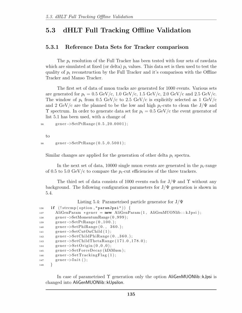
5.3. dHLT Full Tracking Offline Validation
5.3 dHLT Full Tracking Offline Validation
5.3.1 Reference Data Sets for Tracker comparison
The pt resolution of the Full Tracker has been tested with four sets of rawdatawhich are simulated at fixed (or delta) pt values. This data set is then used to test thequality of pt reconstruction by the Full Tracker and it’s comparison with the OfflineTracker and Manso Tracker.
The first set of data of muon tracks are generated for 1000 events. Various setsare generated for pt = 0.5 GeV/c, 1.0 GeV/c, 1.5 GeV/c, 2.0 GeV/c and 2.5 GeV/c.The window of pt from 0.5 GeV/c to 2.5 GeV/c is explicitly selected as 1 GeV/cand 2 GeV/c are the planned to be the low and high pt-cuts to clean the J/Ψ andΥ spectrum. In order to generate data set for pt = 0.5 GeV/c the event generator oflist 5.1 has been used, with a change of
98 gener−>SetPtRange ( 0 . 5 , 2 0 . 0 0 0 1 ) ;
to
98 gener−>SetPtRange ( 0 . 5 , 0 . 5 0 0 1 ) ;
Similar changes are applied for the generation of other delta pt spectra.
In the next set of data, 10000 single muon events are generated in the pt-rangeof 0.5 to 5.0 GeV/c to compare the pt-cut efficiencies of the three trackers.
The third set of data consists of 1000 events each for J/Ψ and Υ without anybackground. The following configuration parameters for J/Ψ generation is shown in5.4.
Listing 5.4: Parametrised particle generator for J/Ψ136 i f ( ! strcmp ( option , "paramJpsi" ) ) 137 AliGenParam ∗ gener = new AliGenParam (1 , AliGenMUONlib : : kJps i ) ;138 gener−>SetMomentumRange ( 0 , 9 9 9 ) ;139 gener−>SetPtRange ( 0 , 1 0 0 . ) ;140 gener−>SetPhiRange ( 0 . , 3 6 0 . ) ;141 gener−>SetCutOnChild ( 1 ) ;142 gener−>SetChildPhiRange ( 0 . , 3 6 0 . ) ;143 gener−>SetChildThetaRange ( 1 7 1 . 0 , 1 7 8 . 0 ) ;144 gener−>SetOr ig in ( 0 , 0 , 0 ) ;145 gener−>SetForceDecay (kDiMuon ) ;146 gener−>SetTrackingFlag ( 1 ) ;147 gener−>I n i t ( ) ;148
In case of parametrised Υ generation only the option AliGenMUONlib::kJpsi ischanged into AliGenMUONlib::kUpsilon.
135

Chapter. Simulation Studies and Validation of Algorithms
In the fourth set of data the J/Ψ and Υ signals are merged with the hadronicbackgrounds generated from HIJING generator using,
Listing 5.5: Parametrised HIJING generator for dNchdη
= 8000 in |η| ≤ 1
484 case kParam 8000 :485 486 comment = comment . Append(":HIJINGparam N=8000" ) ;487 AliGenHIJINGpara ∗ gener = new AliGenHIJINGpara (86 030 ) ;488 gener−>SetMomentumRange (0 , 9 9 9 9 9 9 . ) ;489 gener−>SetPhiRange ( 0 . , 3 6 0 . ) ;490 // Set p s eudorap i d i t y range from −8 to 8 .491 F l o a t t thmin = EtaToTheta ( 8 ) ; // t h e t a min . <−−−> e ta max492 F l o a t t thmax = EtaToTheta (−8); // t h e t a max . <−−−> e ta min493 gener−>SetThetaRange ( thmin , thmax ) ;494 gGener=gener ;495 496 break ;
The full configuration for HIJING generation can be found at$ALICE ROOT/macros/ConfigPPR.C A study of the signal events with andwithout the presence of the background helps to estimate the convoluted efficiencyand resolution of the three trackers.
5.3.2 Resolution and Convoluted Efficiency
The test has been carried for the first data set, with a given pt at 2.0 GeV/c [Fig.5.4(a)]. This pt has been reconstructed using the Offline Tracker (Fig. 5.4(b)), MansoTracker (Fig. 5.4(c)) and Full Tracker (Fig. 5.4(d)). It is evident from the figures5.4(c) and 5.4(d) that the resolution of the Full Tracker (∼ 74 MeV/c) is muchbetter than the Manso’s Tracker (∼ 180 MeV/c). In addition, the peak position (2.0GeV/c) is improved in case of Full Tracker. A detail analysis of track matching of thegenerated particles to the reconstructed one, shows that Manso Tracker and the FullTracker are affected by the problem of ghost tracks. But the incorporation of the ghosttracks does not affect the efficiency of the online Full Tracker, which can be foundin Table 5.2. The efficiency of the different tracking approaches are compared fordifferent pt values. For a given tracking algorithm, the efficiency has been determinedby comparing the space points of the reconstructed tracks with the space points ofthe generated tracks. If 70% of the reconstructed track points are found to matchwith the simulated track points, it is considered as a valid reconstructed track. It isclear from the table that Offline Tracker is the most efficient tracker, where as the FullTracker shows the close agreement with the Offline Tracker. Although the efficiencyof the Manso Tracker increases for higher pt, the efficiency is far worse than the othertwo trackers in case of low momentum particles.
In the table 5.3, the resolution of the different trackers are compared. Theresolution represents the standard deviation (σ) value for the given pt. It can be
136

5.3. dHLT Full Tracking Offline Validation
(a) The pt spectrum plotted from MonteCarlo generation
(b) The reconstructed pt spectrum usingALICE Offline reconstruction
(c) The reconstructed pt spectrum usingManso’s approach
(d) The reconstructed pt spectrum usingthe Full Tracker method.
Figure 5.4: The comparison of different tracking approaches for the generatedspectrum at (a). The (b), (c) and (d) shows the reconstructed pt spectrum for Offline,Manso and Full Tracker methods, respectively.
inferred from this the table that the resolution for Offline Tracker is nearly constantover the pT range but for Manso and Full Tracker the resolution deteriorates for higherpT . However, the Full Tracker resolution is found to be much better than the MansoTracker.
In figure 5.5, the efficiencies of the pt-cut for the three cases have beeninvestigated. The second data set have been used for this evaluation. It is evidentthat the pt-cut efficiency of Manso Tracker is very low. The desired efficiency isreached only 0.5 GeV/c above the pt-cut. However, it is capable of improving thept-cut from L0. The Full Tracker on the other hand provides a sharp pt-cut whichis comparable to that from offline analysis. Thus, this figure clearly summarizes theimprovement achieved by the Full Tracker over the Manso Tracker and is expectedto ensure the same efficiency as the offline reconstruction.
137

Chapter. Simulation Studies and Validation of Algorithms
Table 5.2: pt Efficiency of different tracking approach
Offline (%) Full Tracker (%) Manso Tracker (%)0.5 GeV/c 96.49± 0.91 95.61± 0.91 71.56± 0.741.0 GeV/c 99.57± 0.53 97.57± 0.52 86.86± 0.481.5 GeV/c 98.86± 0.47 97.95± 0.47 88.84± 0.442.0 GeV/c 98.61± 0.46 98.50± 0.46 88.72± 0.422.5 GeV/c 98.83± 0.46 97.98± 0.45 88.92± 0.42
Table 5.3: pt Resolution of different tracking approach
Offline (MeV/c) Full Tracker (MeV/c) Manso Tracker (MeV/c)0.5 GeV/c 33.8± 0.7 44.7± 1.0 84.5± 3.71.0 GeV/c 34.9± 0.2 47.0± 0.3 127.0± 1.31.5 GeV/c 39.8± 0.2 61.6± 0.4 146.9± 1.72.0 GeV/c 43.9± 0.2 74.9± 0.4 180.7± 1.92.5 GeV/c 40.5± 0.1 78.8± 0.5 175.3± 2.7
Figure 5.5: The plot shows the pt-cut efficiency as found for L0 trigger, Manso Tracker,Offline Tracker and Full Tracker.
5.3.3 Dimuon mass distribution
The third set of simulated data is used to study the resonance spectrum in theabsence of background. In the figure 5.6, the J/Ψ resonance has been reconstructedusing Offline Tracker, Manso Tracker and Full Tracker from the decay muons. Itis seen from the figure that in terms of resolution the Full Tracker is much better
138

5.3. dHLT Full Tracking Offline Validation
compare to the Manso Tracker and reconstructs more tracks as found by the OfflineTracker, which confirms the reasonable efficiency of the Full Tracker.
(a) Invariant dimuon mass distributionwithout any without any background byOffline
(b) Invariant dimuon mass distributionby Manso Tracker
(c) The Full Tracker result of invariantdimuon mass distribution
Figure 5.6: The invariant mass of J/Ψ in case of no hadronic background by differenttracking approaches.
Finally, the effects of transverse momentum cuts on the dimuon invariant massspectrum have been demonstrated in Fig. 5.7 using the fourth data set. In the firstthree histograms Fig. 5.7(a), Fig. 5.7(b) and Fig. 5.7(c) the inclusive invariant massspectrums of two oppositely charged muons in presence of HIJING background hasbeen shown for Offline, Manso and Full Tracker, respectively. The combinatorialbackground in the low mass region is due to the muons coming from the decay ofpions and kaons. The next set of figures Fig. 5.7(d), Fig. 5.7(e) and Fig. 5.7(f) showthe effect of 1 GeV/c pt-cut on the invariant mass spectrum the for Offline, Manso andFull Tracker, respectively. This exercise has been repeated for Υ with and withoutpt-cut at 2.0 GeV/c. The mass resolution of the three tracking methods for the twotypes of resonances are summarised in table 5.4. It is again established from thesecomparisons that the Full Tracker produces better results than the Manso Tracker.In fact the quality of reconstruction by Full Tracking method is in close agreementwith the Offline results. Thus, the comparison tests show that the Full Tracker hasreasonable pT efficiency and resolution when compared with Offline Tracker but most
139

Chapter. Simulation Studies and Validation of Algorithms
importantly, it is three orders of magnitude faster than Offline Tracker. This is theessential requirement of a real time analysis tool.
Table 5.4: Resolution of Invariant Mass distribution with and without pt-cut
J/Ψ (MeV/c) Υ (MeV/c)no pt-cut at pt =1.0 GeV/c no pt-cut at pt =2.0 GeV/c
Offline 66.4±4.2 58.1±3.4 106.6±5.9 106.4±5.9Full Tracker 104.1±9.8 106.0±11.7 237.1±17.8 236.6±17.7Manso Tracker 318.6±12.4 255.7±11.8 482.5±27.5 472.1±27.1
140

5.3. dHLT Full Tracking Offline Validation
(a) Invariant dimuon mass distributionwithout any pt-cut as reconstructed byOffline algorithm
(b) Invariant dimuon mass distributionby Manso Tracker without any pt-cut
(c) The Full Tracker result of invariantdimuon mass distribution without any pt-cut
(d) Invariant dimuon mass distributionwith pt-cut at 1.0 GeV/c as reconstructedby Offline algorithm
(e) Invariant dimuon mass distributionby Manso Tracker with a pt-cut at 1.0GeV/c
(f) The Full Tracker result of invariantdimuon mass distribution with a pt-cutat 1.0 GeV/c
Figure 5.7: The dimuon invariant mass spectrum shows J/Ψ signal merged withHIJING background for various tracking algorithms. In subfigures (a), (b) and (c)the mass spectrum has been plotted without any pt-cut. Whereas the effect of pt-cutson the invariant dimuon mass spectrum by different trackers are shown in subfigures(d), (e) and (f).
141

Chapter. Simulation Studies and Validation of Algorithms
5.4 Online Commissioning of Full Tracker
The online performance of the full tracker has been tested in ALICE HLTcomputer farm, with the simulated Pb-Pb data generated by HIJING Monte Carlocodes. The main motivation of this test are explained below,
• Timing Estimation : The first important test for the online tracking is the rateof data processing. It has to satisfy the timing constrain of 1 kHz processingrate as expected in case of central Pb-Pb collision.
• Long Time Stability : The online Full Tracker has to be absolute free from anymemory leak, fault tolerant against any corrupted data blocks and several otherreal time computation challenges. Thus, rigorous tests with simulated Pb-Pbevents have been checked for the stability of the chain over long time.
• Requirement for Extra Resource : A series of tests have been carried out withdifferent particle multiplicities. This is important to scale the requirements ofresources during the optimised beam condition of Pb-Pb collision. Therefore,the benchmark results of this test provide the scalability factors for the futureheavy ion runs.
5.4.1 Configuration
In order to carry out the above tests, different sets of HIJING Monte Carlo
data have been simulated for(dNdη
)|η|≤1
= 1000, 2000, 4000, 6000 and 8000 with
the similar configuration as described in list 5.5. It is equally important to explainthe HLT cluster specification in order to understand the test bench of performancestudy of the FullTracker. The HLT consists of several computer nodes dedicated foreach detector group of ALICE. The Dimuon part of the HLT consists of five nodes(FEPs) with direct connection to DDLs. There are two other computing nodes (CN)dedicated for dHLT online data processing. The specifications of the nodes are givenin table 5.5-5.6,
142

5.4. Online Commissioning of Full Tracker
Table 5.5: Processor and memory configuration of front-end-processing nodes
processor : 0vendor id : AuthenticAMDcpu family : 16model : 4model name : Quad-Core AMD Opteron(tm) Processor 2378stepping : 2cpu MHz : 2400.000cache size : 512 KBphysical id : 0siblings : 4core id : 0cpu cores : 4apicid : 0initial apicid : 0fpu : yesfpu exception : yescpuid level : 5wp : yesflags : fpu vme de pse tsc msr pae mce cx8 apic sep
mtrr pge mca cmov pat pse36 clflush mmx fxsr sse sse2ht syscall nx mmxext fxsr opt pdpe1gb rdtscp lm3dnowext 3dnow constant tsc rep good nonstop tscextd apicid pni monitor cx16 popcnt lahf lmcmp legacy svm extapic cr8 legacy abm sse4amisalignsse 3dnowprefetch osvw ibs skinit wdt
bogomips : 4787.14TLB size : 1024 4K pagesclflush size : 64cache alignment : 64address sizes : 48 bits physical, 48 bits virtualpower management: ts ttp tm stc 100mhzsteps hwpstateMemTotal: 12343632 kBMemFree: 7891860 kBBuffers: 271292 kBCached: 1537608 kBSwapCached: 0 kB
143

Chapter. Simulation Studies and Validation of Algorithms
Table 5.6: Processor and memory configuration of computing nodes
processor : 7vendor id : GenuineIntelcpu family : 6model : 23model name : Intel(R) Xeon(R) CPU E5420 @ 2.50GHzstepping : 6cpu MHz : 2493.900cache size : 6144 KBphysical id : 1siblings : 4core id : 3cpu cores : 4apicid : 7initial apicid : 7fpu : yesfpu exception : yescpuid level : 10wp : yesflags : fpu vme de pse tsc msr pae mce cx8 apic sep mtrr pge mca
cmov pat pse36 clflush dts acpi mmx fxsr sse sse2ss ht tm pbe syscall nx lm constant tsc arch perfmonpebs bts rep good aperfmperf pni dtes64 monitor ds cpl vmxest tm2 ssse3 cx16 xtpr pdcm dca sse4 1 lahf lmtpr shadow vnmi flexpriority
bogomips : 4987.66clflush size : 64cache alignment : 64address sizes : 38 bits physical, 48 bits virtualMemTotal: 16469864 kBMemFree: 9558952 kBBuffers: 198248 kBCached: 3737556 kBSwapCached: 0 kB
These FEP and CN machines are dedicated to run certain Dimuon HLTcomponents. For instance, the FEP nodes are connected to DDLs of the detectorstherefore, the Hit Reconstruction algorithm is executed in these nodes. Thereconstructed hits are forwarded to the Full Tracker components which run in theCN-machines. The software versions used during this study are tabulated at 5.7.
While the BASE, DEFINITION are the basic modules for HLT clustersoftware operations and the interface between HLT and other online systems are
144

5.4. Online Commissioning of Full Tracker
Table 5.7: Software version of HLT cluster used for online performance test
1) BASE/base 9) DATATRANSPORT/20091127.0743002) DEFINITION/base 10) ECSPROXY/v1.5.4-20091127.0743003) ALIEN/v2-17 11) PENDOLINO/v1.3-v4-18-Rev-054) FASTJET/2.4.1 12) HCDBMANAGER/v1.5-v4-18-Rev-055) ROOT/v5-26-00b 13) CONTROL/HEAD 2010-03-036) GEANT3/v1-11 14) HLT/HEAD 2010-03-03-prod7) TAXI/v2.2-v4-18-Rev-05 15) HLTdevel/HEAD 2010-03-12-custom-prod8) ALIROOT/v4-18-Rev-05
maintained by the TAXI, PENDOLINO, ECSPROXY, HCDBMANAGER. TheDATATRANSPORT and CONTROL modules constitute of the online data transportframework. The rest of the modules comprise the HLT analysis part.
In online analysis the data exchange between the different components anddifferent computer nodes are defined in a configuration file of XML file format. Atypical data transport configuration used for online testing is listed in 5.6.
145

Chapter. Simulation Studies and Validation of Algorithms
Listing 5.6: XML Configuration file for PbPb test1 <?xml v e r s i o n="1.0" encoding="ISO-8859-1"?>2 <SimpleChainConfig2 ID="DIMUON" v e r b o s i t y="0x30">3 <i n f ob l ock>4 <author>indra</author>5 <date>Friday 12 February 2010</date>6 <d e s c r i p t i o n>Ful l Tracker chain for Dimuon</d e s c r i p t i o n>7 </in fob lock>8 <ALICE>9
10 <!−− <Sources type="ddl"> −−>11 <Sources type="file">12
13 <!−− TEMPLATE BEGIN −−>14 <DDL>DIMU</DDL>15 <Directory>/tmp/HIJING−4000/raw∗</Directory>16
17
18 </Sources>19
20 <Fi l ePub l i sherOpt ions>−eventt ime 333</ Fi l ePub l i sherOpt ions> <!−−21 333 corresponds to 3 kHz−−>22 <RORCShm b l o c k s i z e="50k" blockcount="100"/>23
24 <DIMU>25 <TRG>26 <Part i t i on>27 <Component ID="TrigRec">28 <ComponentID>MUONTriggerReconstructor</ComponentID>29 <Options>−dd l id \$DDL −b f i e l d i n t e g r a l 3 −cdbpath30 l o c a l : //\$ALIHLT\ HCDBDIR −s u p p r e s s p a r t i a l t r i g g e r s31 −t r y r e c o v e r −dontpr intwrongeventer ror </Options>32 <Parent>DDL</Parent>33 <Shm b l o c k s i z e="2k" blockcount="1000"/>34 <M u l t i p l i c i t y >2</M u l t i p l i c i t y>35 <Library>libAliHLTMUON . so</Library>36 </Component>37 </Par t i t i on>38 </TRG>39
40
41 <TRK>42 <Part i t i on>43 <Component ID="HitRec">44 <ComponentID>MUONHitReconstructor</ComponentID>45 <Options>−dd l id \$DDL −cdbpath46 l o c a l : //\$ALIHLT\ HCDBDIR −t r y r e co v e r47 −d o n t p r i n t p a r i t y e r r o r s </Options>48 <Parent>DDL</Parent>49 <Shm b l o c k s i z e="5k" blockcount="1000"/>50 <M u l t i p l i c i t y >2</M u l t i p l i c i t y>51 <Library>libAliHLTMUON . so</Library>52 <ForceFEP/>53 </Component>
146

5.4. Online Commissioning of Full Tracker
54 </Par t i t i on>55 </TRK>56
57 <Process ID="Merger" type="prc">58 <Command>Relay</Command>59 <Parent>TrigRec</Parent>60 <Parent>HitRec</Parent>61 <M u l t i p l i c i t y >1</M u l t i p l i c i t y>62 <Shm b l o c k s i z e="6k" blockcount="5000"/>63 </Process>64
65 <Component ID="Tracker">66 <ComponentID>MUONFullTracker</ComponentID>67 <Options>−cdbpath l o c a l : //\$ALIHLT\ HCDBDIR</Options>68 <Parent>Merger</Parent>69 <Shm b l o c k s i z e="2k" blockcount="5000"/>70 <M u l t i p l i c i t y >27</M u l t i p l i c i t y>71 <Library>libAliHLTMUON . so</Library>72 </Component>73
74 <Component ID="Decision">75 <ComponentID>MUONDecisionComponent</ComponentID>76 <Options>−lowptcut 1 −highptcut 2 −lowmasscut 2 .5 −highmasscut77 7 </Options>78 <Parent>Tracker</Parent>79 <Shm b l o c k s i z e="2k" blockcount="5000"/>80 <M u l t i p l i c i t y >1</M u l t i p l i c i t y>81 <Library>libAliHLTMUON . so</Library>82 </Component>83
84
85 <Component ID="MuonTrig">86 <ComponentID>MuonSpectroTrigger</ComponentID>87 <Options>−t r i g g e r h i t s </Options>88 <Parent>Merger</Parent>89 <Shm b l o c k s i z e="2k" blockcount="5000"/>90 <M u l t i p l i c i t y >1</M u l t i p l i c i t y>91 <AddLibrary>libAliHLTMUON . so</AddLibrary>92 <Library>l ibAl iHLTTrigger . so </Library>93 </Component>94
95 <Component ID="MuonESD">96 <ComponentID>MUONESDMaker</ComponentID>97 <Options>−makeonlyc lonesarray</Options>98 <Parent>Tracker</Parent>99 <Parent>Merger</Parent>
100 <Shm b l o c k s i z e="2k" blockcount="5000"/>101 <M u l t i p l i c i t y >1</M u l t i p l i c i t y>102 <Library>libAliHLTMUON . so</Library>103 </Component>104
105 </DIMU>106
107 <Component ID="GlobalTrigger">
147

Chapter. Simulation Studies and Validation of Algorithms
108 <ComponentID>HLTGlobalTrigger</ComponentID>109 <Options></Options>110 <Parent>DIMU/MuonTrig</Parent>111 <Shm b l o c k s i z e="2k" blockcount="5000"/>112 <M u l t i p l i c i t y >3</M u l t i p l i c i t y>113 <AddLibrary>libAliHLTMUON . so</AddLibrary>114 <Library>l ibAl iHLTTrigger . so</Library>115 </Component>116
117 <Component ID="GlobalESD">118 <ComponentID>GlobalEsdConverter</ComponentID>119 <Options></Options>120 <Parent>DIMU/MuonESD</Parent>121 <Shm b l o c k s i z e="2k" blockcount="5000"/>122 <M u l t i p l i c i t y >9</M u l t i p l i c i t y>123 <Library>l ibAliHLTGlobal . so</Library>124 </Component>125
126 <Dump>127 <Type>tcp</Type>128 <Parent>GlobalESD</Parent>129 <Parent>GlobalTrigger</Parent>130 <Parent>DIMU/Merger</Parent>131 <Parent>DIMU/Tracker</Parent>132 <Parent>DIMU/ Decis ion</Parent>133 <AllEvents/>134 <Node>cndimutrg19</Node>135 <!−− needed to s p e c i f y the port e x p l i c i t l y for di sp lay−−>136 <Port>49152</Port>137 </Dump>138
139 </ALICE>140
141 </SimpleChainConfig2>
5.4.2 Benchmark Results of Online Trackers
The main motivation was to test the speed of the Full Tracker and it’scomparison with the existing Manso Tracker. For this purpose, the configuration(see list 5.6) has been tested to reach at the speed of ∼1 kHz as this is the designgoal of dimuon HLT for Pb-Pb run. It is to be noted that the data processing rateis limited by the slowest component of the chain. Therefore, in case of Full Trackerand Manso Tracker chain the performance was slowed down due to the Full Trackerand MUONHitReconstructor component, respectively. The data processing rate ofthe trackers are reported in tables 5.8 and 5.9.
The stability of the dHLT chain has been individually checked for both the oftrackers with HIJING 4000 and real p-p data set (Run : 104867) for ∼23 hours andno connection error problem or memory leaks has been found.
148

5.4. Online Commissioning of Full Tracker
Table 5.8: The results of online performance test with HIJING 1000,2000,4000 particlegenerators of ALICE. (Bytes/s)
HIJING-1000Components Nof. Proc. Input Output I/O Speed (Hz)
HitRec 2 2356752 289488 8.14TrigRec 2 3920384 29080 134.8
MansoTracker 1 10770140 68004 158.37 1518.7FullTracker 3 6053463 202092 29.95 1015.8
FullTracker (-usefast) 1 8482980 235232 36.06 1578.25Decision 1 197716 75732 2.61
MuonESD 1 276068 266625 1.04MuonTrig 1 6177120 360584 17.13
HIJING-2000Components Nof. Proc. Input Output I/O Speed (Hz)
HitRec 2 2163968 431504 5.01TrigRec 2 4366336 98528 44.32
MansoTracker 1 20743172 171132 121.21 1537.08FullTracker 7 13794396 531188 25.82 1072.96
FullTracker (-usefast) 1 17706308 502260 35.25 1528.56Decision 1 587396 118004 4.98
MuonESD 1 691684 359597 1.35MuonTrig 1 13214472 359597 36.75
HIJING-4000Components Nof. Proc. Input Output I/O Speed (Hz)
HitRec 2 2808000 900800 3.12TrigRec 2 3015168 159792 18.86
MansoTracker 1 37964572 315784 120.22 1430.26FullTracker Processor Multiplicity 27 is required to run at the rate of 1kHz,
which not available in dimuon node group.This has been tested with extra support of cnemcal nodes
FullTracker (-usefast) 3 25222260 729396 34.58 1051.19Decision 1 775952 131448 5.9
MuonESD 1 1108532 756535 1.47MuonTrig 1 25241508 343147 73.56
The monitoring of the processor, memory and network load during the dataprocessing is important to understand the behavior of the components. An interestingphenomena is observed from above results. A falling trend is found for input to outputdata size (I/O) ratio of the dHLT components from HIJING 1000 to HIJING 8000.
149

Chapter. Simulation Studies and Validation of Algorithms
Table 5.9: The results of online performance test with HIJING 6000 and 8000 particlegenerators of ALICE. (Bytes/s)
HIJING-6000Components Nof. Proc. Input Output I/O Speed (Hz)
HitRec 2 4292816 1817472 2.36TrigRec 2 3387904 179000 18.92
MansoTracker 1 53250336 363528 146.48 1287.35FullTracker Not possible to test
FullTracker (-usefast) 6 42754776 794640 53.8 1100.1Decision 1 855356 154072 5.55
MuonESD 1 1136676 710296 1.6MuonTrig 1 39724188 348411 114.01
HIJING-8000Components Nof. Proc. Input Output I/O Speed (Hz)
HitRec 2 4408512 2350448 1.88TrigRec 2 8659456 851408 10.17
MansoTracker 1 49116536 500456 98.14 1056.61FullTracker Not possible to test
FullTracker (-usefast) Processor Multiplicity 15 is required to run at the rate of 1kHz.But in that case none of the following components,
(Decision, MuonESD, MuonTrig) can not be includeddue to present cndimuon nodes limitation to 16 processors.
Decision 1 490936 350116 1.4MuonESD 1 1237992 834009 1.48MuonTrig 1 50566808 318472 158.77
This is expected since the number of tracks increases with particle multiplicity. Butsurprisingly, the I/O ratio for “MuonTrig” component, increases with multiplicityinstead of falling down. To explain this, it is important to note that according to theconfiguration in list 5.6, the “MuonTrig” has been running with
option,
87 <Options>−t r i g g e r h i t s </Options>
It means that MuonTrig component issues a positive flag if any hit or track isfound. In case of Pb-Pb collisions, there is large particle multiplicity in the detector,therefore, the MuonTrig issues positive signal more frequently.
The values of the processing rates of these tables ( 5.8 and 5.9) have beencalculated using the “StatusDump” command of data transport framework. In
150

5.4. Online Commissioning of Full Tracker
Figure 5.8: The CPU Memory and Network Load has been monitored for HIJING8000 using dmon (distributed monitoring) commands of HLT cluster. It is to benoted that fepspare0 was connected with the DDL links coming from the third muontracking station as fepdimutrk3 was under repair during the test.
addition, there are commands to monitor CPU load, memory and network usageof cluster group, which are known as “dmon” (distributed monitoring). Themonitoring results [see Fig. 5.8] with dmon commands during the execution of Pb-Pbchain test shows good agreement with the results from “StatusDump” command.The average transmitted datasize from the five tracking front end processor is,7328.81+12910.69+7535.57+11342.11+8524.34
5= 47641.52
5= 9528.304 kBytes/s. Whereas the
StatusDump results show that, there are about 2350.448 kBytes/sec output fromeach of the HitRec component. Four such components are running on each dimuonFEP nodes (excluding the hits from third station since it does not contribute to theTrackers), which result to 4×2350.448 = 9401.792 kBytes/s. For TrigRec componentsalso they are of same order.
To summarize it can be concluded, that,
151

Chapter. Simulation Studies and Validation of Algorithms
• The full tracker can run at 1kHz rate and scales with the processor multiplicity.
• The stability of the chain (with both trackers) has been tested for long timewith clear startup and clean shutdown.
• If the Full Tracker is planned to reconstruct the high multiplicity Pb-Pbcollisions, eight more computing machines (i.e. 32 processors) are requiredto be added to the present Dimuon node group.
The analysis of the experimental data demonstrates the final validation of theonline algorithms, which are presented in the next chapter.
152

Chapter 6
Experimental Results andPerformance Study
This chapter describes the online performance of the dHLT algorithms duringthe comic runs and proton-proton collisions at 7 TeV energy of LHC. In addition, itcontains the analysis techniques of the experimental data with the online algorithmsin the offline mode. Since the development of online analysis framework and theintegration to ALICE detector have evolved in parallel, each data set was analysedwith different versions of dHLT components. For instance, the cosmic runs have beenanalysed with primary version of the Full Tracker whereas the 7 TeV data have beenreconstructed with most updated versions of the Full Tracker.
The real-time performance of dHLT analysis components with the cosmic setupis discussed in the first section, whereas the p-p data analysis is reported in the secondhalf.
6.1 Cosmic Runs of Muon Spectrometer
There were several cosmic data taking periods in ALICE before the first p-pcollision, where each cosmic run period continued for about one to three months ofdata collection. The main goal of these cosmic setup was to test the stability of thedetectors and online systems (HLT, DCS, DAQ and CTP) of ALICE. There was nophysics proposal of ALICE with the set of cosmic runs, however, a group of centralbarrel detectors (ITS, TPC etc.) have used these cosmic tracks for the alignment ofthe detection elements. Thus, the two magnets (L3 and dipole) were off during theserun period, except for the last one where dHLT did not join due to technical problem.In present section the Dimuon HLT analysis results are shown for two sets cosmicruns corresponding to partial and complete Spectrometer setup. In both cases, dHLT
153

Chapter. Experimental Results and Performance Study
participated to the global data taking in a mode where HLT busy was respected byDAQ but no HLT output was sent to DAQ (i.e mode B/Test2 in ALICE experimentalterm [sec. §3.1.5]).
6.1.1 First Cosmic Run
The first online performance of the dHLT analysis chain with experimental datahas been successfully tested in the cosmic run period during February-March of 2008.It is to be noted that the Muon Spectrometer was not fully operational in that cosmicrun and only the first two Tracking stations were ready along with only the right halfof the Trigger stations. Although the trigger was issued by the full trigger station butthe hit information from the left side was not available. Since the Full Tracker wasnot integrated to the framework and the Manso Tracker could not be applied due tothe absence of 4th and 5th Tracking station, the dHLT online analysis was configuredwith,
DDLPublisher =⇒ Hit Reconstruction =⇒ TCP Dump =⇒ EventDisplay.
Apart from the first real-time performance of dHLT analysis, the main achievementof first cosmic run was the development of the online event display with AliEve. Asnapshot of one typical cosmic event is shown in Fig. 6.1. The cosmic runs were mainly
(a) Online display of clusters (b) Online display of track during the first cosmic run
Figure 6.1: An online event display of cosmic run
triggered by the ACORDE (placed on the top of L3) trigger and very few runs havebeen recorded with the Muon Trigger. As the Muon Spectrometer is placed alongthe horizontal direction, it receives very few cosmic tracks due to substantial earthpayload. In addition, the tracks triggered by ACORDE were mostly limited withinthe L3 region, very few slant tracks were recorded in the first two tracking stationsof Muon Spectrometer. Thus, a typical trigger rate of ∼0.1 Hz was observed withMuon Trigger, whereas for ACORDE it was ∼100 Hz. A total of ∼8800 events passedthrough the dHLT chain when summed over all runs.
154
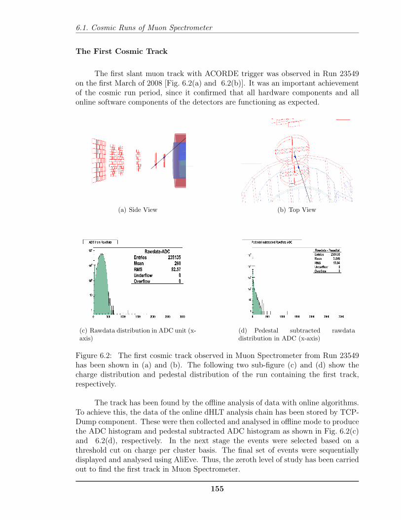
6.1. Cosmic Runs of Muon Spectrometer
The First Cosmic Track
The first slant muon track with ACORDE trigger was observed in Run 23549on the first March of 2008 [Fig. 6.2(a) and 6.2(b)]. It was an important achievementof the cosmic run period, since it confirmed that all hardware components and allonline software components of the detectors are functioning as expected.
(a) Side View (b) Top View
(c) Rawdata distribution in ADC unit (x-axis)
(d) Pedestal subtracted rawdatadistribution in ADC (x-axis)
Figure 6.2: The first cosmic track observed in Muon Spectrometer from Run 23549has been shown in (a) and (b). The following two sub-figure (c) and (d) show thecharge distribution and pedestal distribution of the run containing the first track,respectively.
The track has been found by the offline analysis of data with online algorithms.To achieve this, the data of the online dHLT analysis chain has been stored by TCP-Dump component. These were then collected and analysed in offline mode to producethe ADC histogram and pedestal subtracted ADC histogram as shown in Fig. 6.2(c)and 6.2(d), respectively. In the next stage the events were selected based on athreshold cut on charge per cluster basis. The final set of events were sequentiallydisplayed and analysed using AliEve. Thus, the zeroth level of study has been carriedout to find the first track in Muon Spectrometer.
155

Chapter. Experimental Results and Performance Study
The first horizontal track through the Muon Tracking and Trigger station [seeFig. 6.3(a)] was found in run 24841 on third day of March, 2008, two days after thefirst track.
(a) The first track through the Muon Trackingand Trigger detectors
(b) A Cosmic shower event
Figure 6.3: The first cosmic full track together in the Muon Trigger and Trackingstations (Run 28841) and a snapshot of very frequent cosmic shower events.
Online Detector Diagnostics
In the cosmic run the dHLT was running with simplest analysis configuration.But even that short configuration was very helpful for the online diagnostics ofdetectors. Some of the interesting observations are listed below :
• Cosmic shower : It was found ( HLT event-display) during the experimentthat the upper part of Muon Trigger detector often had large number of hits.These were due to the large cosmic shower events. An online screen-shot of suchevent is shown in Fig. 6.3(b).
• Sudden malfunctioning due to pedestal shift : It was observed few times,that after long period of normal operation, the zero suppression for a certainbus patch would fail leading to large data size. Such a scenario is shown inFig. 6.4(a) and 6.4(b). However, it went back to normal operation again in thenext run. In the later analysis it was found that, the problem occurred due topedestal shift.
• Hot spot : A hot spot on a detection element are some specific channelswhich becomes noisy over different runs. It was found that a hot spot did notnecessarily stays noisy in every the subsequent runs but reappeared over andover again throughout the entire cosmic data taking period. One such behaviourfor MANU 1122 of buspatch 728 is shown for run 25910 and 25915 in Fig. 6.4(c)and 6.4(d), respectively. This was traced to a faulty MANU card in the readoutchain.
156

6.1. Cosmic Runs of Muon Spectrometer
(a) Sudden malfunctioning of part ofdetector with normal noise cut on data
(b) Sudden malfunctioning goes awaywith extra 10 ADC channel noise cut ontop of conventional noise cut
(c) Hot spot on a part of detector ( Run25910 )
(d) Hot spot on a part of detector ( Run25915 )
Figure 6.4: The dHLT serves as an online monitor for detector problems.
In this way, the first online performance of dHLT analysis established itself anexcellent detector monitoring tool for quick and fast detector diagnostics.
Data Analysis of Cosmic Runs
At the end of the cosmic run period a selected set of “good runs” (as definedby Muon Run Coordinator) have been analysed with the online algorithms in offlinemode. In the first step the raw-data has been decoded and processed to producethe hit points in station 1 and 2 using the dHLT Hit Reconstruction algorithm. Thehit points were then joined to form the track using to Cellular Automaton (CA)method. It has been explained in the appendix that the CA first creates the tracklets(connected hit points in consecutive chambers of a station), which are later joinedto form a complete track. Thus, the tracks have been grouped in two categories, thetracks with two tracklets out of possible three (trigger tracklet, tracklets in first andsecond stations) are called general tracks, whereas the tracks with all three trackletsare called golden tracks.
The summary of the results are tabulated in 6.1. The third column gives thenumber of events for which hit reconstruction could be achieved (i.e. 6489) in station
157

Chapter. Experimental Results and Performance Study
Table 6.1: Run statistics table for cosmic data analysis
Run Events Hit Rec. able Events Shower Events Tracks Golden Tracks26024 508 392 184 24 1125985 2209 1628 795 72 625960 846 661 316 39 1725954 65 42 15 6 325944 129 100 51 5 225915 805 591 270 31 1025911 209 166 83 12 625910 15 11 3 1 025898 792 584 290 24 425862 331 252 123 1 025836 1326 1003 471 10 525821 1014 733 339 4 225793 263 190 104 9 024943 72 0 0 0 024925 166 120 64 6 224841 16 16 0 3 2total 8766 6489 3108 247 70
1 and 2, out of 8766 trigger from the Muon Trigger station. It is also evident fromthe table that ∼48% of the reconstructable events is contaminated with the cosmicsshower, where a cosmic shower event have been defined as the event with more than8 hits in the Muon Trigger stations. The third and fourth column reveal that for eachrun the number of shower events are almost half of the number of reconstructableevents. This is due to the fact that half of the hit position readout of Trigger stationswas not functional. Thus if the Trigger station was fully operational during the cosmicrun in terms of hit position and trigger readouts then, the results of third and fourthcolumn would have been the same. The number of horizontal tracks were very rarewhich is reflected in the fifth column of the table that shows that only 3.8% of thereconstructable events form general tracks. The number of golden tracks are evenfewer, about 1% of the reconstructable events are found to contain a golden tracks.
A super imposed picture of all these tracks is shown in Fig. 6.5. It is interestingto note from the figure that the number of tracks in the upper half of the MuonSpectrometer is much less than the lower part. Since the earth payload is much moreat the bottom compared to the upper part of ALICE, it is reasonable to assume thatall the recorded tracks were originated from top surface of ALICE cavern. For thisreason fewer tracks have been observed in the upper half of the spectrometer. Thus,the tracks originating from top-right (Fig. 6.5(b)) entered the spectrometer from thefront while these originating from top-left entered from the back side. But there isa predetermined hardware delay between the first and second trigger stations whichtakes into account the flight time of the muons to traverse the distance of 1 m. Due
158

6.1. Cosmic Runs of Muon Spectrometer
(a) Track superposition side view (b) Track superposition front view
(c) Track superposition angle view
Figure 6.5: The superposition of all available cosmic tracks of the first cosmic run.
to this delay, there is a inherent bias of trigger matching for tracks coming from thefront side.
6.1.2 Second Cosmic Run
The next cosmic run period took place during the March-April of 2009, when thedHLT components and most of the Muon Spectrometer (except the problems with fewbuspatches of chamber 9 and 10 of the Tracking stations) was fully operational. Thedipole magnet was off during the data taking therefore the physics analysis was notpossible. However, on the HLT side, the full analysis chain have been switched on withDDLPublisher =⇒ Hit Reconstruction =⇒ Manso Tracker =⇒ MuonDecision =⇒TCP Dump =⇒ EventDisplay. This was important to test the online performancesof the code with real data from all the tracking stations and real-time problems.
159

Chapter. Experimental Results and Performance Study
The dimuon HLT operation was stable during this global data collection. Inthese runs dHLT included the online histograms of charge per cluster and number offired pads per cluster to the online display. It has been explained before (sec. §5.2.3)that these plots are important to investigate the cluster size and the cluster charge,which reflects the high voltage characteristics of the detector. Therefore, the plotswere helpful for online data quality monitoring of the detector. A sample histogramset for run 67303 is shown in figure 6.6.
Figure 6.6: The distribution of charge per cluster (left) and number of pads percluster (right) summed over all chambers displayed at ACR during the cosmic run.
Cosmic Run Analysis
The cosmic data have been replayed again for offline analysis with the onlinealgorithms, which included both approaches of Manso Tracker and straight linetracking with Cellular Automata. A total of 73 selected cosmics runs have beenanalysed following the same procedure as described in the previous subsection. Inorder to analyse the data with CA, it was updated to include tracklets in the fourthand fifth station during formation of a track. Therefore, the definition of general andgolden track has been modified compared to the first cosmic run period.
General Track : 1 tracklet in station 1 or 2 + 1 tracklet station 4 or 5 + 1 trackletin Muon Trigger stations
Golden Tracks : 3 tracklets in Muon Tracking stations + 1 tracklet in MuonTrigger stations
One general and one golden track is shown in Fig. 6.7(a) and 6.7(b),respectively. In total 71557 events have been analysed from 73 runs, which contains1986 general tracks and 1009 golden tracks. The charge distribution and size of theassociated clusters with the general tracks is shown in Fig. 6.7(c). The shape of
160

6.1. Cosmic Runs of Muon Spectrometer
the charge per cluster histograms closely follow the Landau distribution which is theproperty of minimum ionising particles. A super position of general tracks from 5runs are shown in Fig. 6.8.
It is important to note that there were no Cosmic Run analysis results withoffline software when the first analysis with dHLT algorithm was reported in theALICE Offline Week [April, 2008]. However, in the second Cosmics Run both groups(dHLT and Muon Offline) had presented their results separately in Annual MuonSpectrometer Workshop [June, 2009]. But since the two collaborations have followeddifferent approaches for tracking and data analysis techniques, the offline and dHLTresults could not be compared. In addition, there were no physics observables due toabsence of dipole magnet.
161

Chapter. Experimental Results and Performance Study
(a) A general track (b) A golden track
(c) The charge per cluster and pad per cluster distribution associated withgeneral tracks
Figure 6.7: The results of offline analysis using online algorithms.
162

6.1. Cosmic Runs of Muon Spectrometer
Figure 6.8: The superimposed tracks of the five runs in second cosmic run.
163
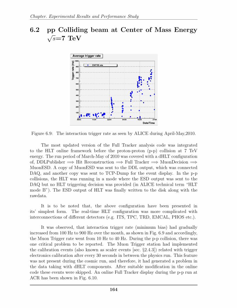
Chapter. Experimental Results and Performance Study
6.2 pp Colliding beam at Center of Mass Energy√s=7 TeV
Figure 6.9: The interaction trigger rate as seen by ALICE during April-May,2010.
The most updated version of the Full Tracker analysis code was integratedto the HLT online framework before the proton-proton (p-p) collision at 7 TeVenergy. The run period of March-May of 2010 was covered with a dHLT configurationof, DDLPublisher =⇒ Hit Reconstruction =⇒ Full Tracker =⇒ MuonDecision =⇒MuonESD. A copy of MuonESD was sent to the DDL output, which was connectedDAQ, and another copy was sent to TCP-Dump for the event display. In the p-pcollisions, the HLT was running in a mode where the ESD output was sent to theDAQ but no HLT triggering decision was provided (in ALICE technical term “HLTmode B”). The ESD output of HLT was finally written to the disk along with therawdata.
It is to be noted that, the above configuration have been presented inits’ simplest form. The real-time HLT configuration was more complicated withinterconnections of different detectors (e.g. ITS, TPC, TRD, EMCAL, PHOS etc.).
It was observed, that interaction trigger rate (minimum bias) had graduallyincreased from 100 Hz to 900 Hz over the month, as shown in Fig. 6.9 and accordingly,the Muon Trigger rate went from 10 Hz to 40 Hz. During the p-p collision, there wasone critical problem to be reported. The Muon Trigger station had implementedthe calibration events (also known as scaler events [sec. §2.4.3]) related with triggerelectronics calibration after every 30 seconds in between the physics run. This featurewas not present during the cosmic run, and therefore, it had generated a problem inthe data taking with dHLT components. After suitable modification in the onlinecode these events were skipped. An online Full Tracker display during the p-p run atACR has been shown in Fig. 6.10.
164

6.2. pp Colliding beam at Center of Mass Energy√s=7 TeV
Figure 6.10: First online full track as observed in run 119842.
The other online histograms and the future quality assurance (QA) plots havebeen discussed in the following section. The final validation based on dHLT andoffline analysis using the experimental data stored in GRID, has been described inthe subsequent subsection.
6.2.1 Online Event Display
The online event display for p-p run was improved to include the histogramsto check the quality of the run and preliminary physics results. A description of theonline histograms are summarised in the following items.
• Charge per cluster : The charge per cluster distribution has been portedto the display for each plane of a given DDL. It is to be noted that in thelast cosmic there was an inclusive spectrum summed over all DDLs. The roleof these plots have already been discussed before (sec. §5.2.3). An impropersetting of the detector high voltage (possible fault in DCS) or the presence ofcopious noisy clusters can be identified from these plots [see Fig. 6.11(a)].
• Pad per cluster : This plots have also been displayed for every single plane ofa given DDL and the role of these plots has been discussed before (sec. §5.2.3)as well [see Fig. 6.11(b)].
• Ratio of the bending to non-bending charge : The ratio of charge percluster of bending to non-bending plane should be close to unity, since the two
165

Chapter. Experimental Results and Performance Study
(a) The charge per cluster distribution (b) The distribution of number pads percluster
(c) The charge correlation of bending andnon-bending plane
(d) Distance of Closest Approach (DCA)
Figure 6.11: The HLT online Quality Assurance (QA) plots at ACR during the p-pcollision at
√s=7 TeV.
cathodes are equidistant from the anode plane. This was found to be truefor all detection elements for most of the clusters. But if in a DDL, there isa significant departure, it will indicate a readout error (may be due to tripin low voltage supply) for either bending or non-bending plane. The chargecorrelation plot have been discussed before and presented with the simulationresults (sec. §5.2.3). The experimental correlation plot of individual DDL andsummary of all DDLs are shown in Fig. 6.11(c) and bottom-left figure of 6.12,respectively.
• Total charge per data link : In experiment it is cumbersome to look intoevery single DDLs, thus several summary plots have been produced. One suchsummary plot shows the total charge distribution for all DDL connections intop-left of Fig. 6.12.
• Trigger type : This histogram shows the trigger types of the event as selectedby the Trigger station. The possible values are, single low pt, single high pt,unlike sign low pt, unlike sign high pt, like sign low pt, like sign high pt [seebottom-right of Fig. 6.12]. If the a track is identified by trigger chamber theassociated trigger type will be displayed in this histogram.
166

6.2. pp Colliding beam at Center of Mass Energy√s=7 TeV
Figure 6.12: Summary of distribution of charge/cluster, pads/cluster and ratio ofbending to non-bending charges in twenty individual DDLs. The type of trigger issuedby trigger station is shown in the lower right corner. The HLT online plots in the p-pcollision at
√s=7 TeV.
• pt spectrum : The inclusive transverse momentum of the tracks detected bydHLT Tracker are shown in this spectrum. The top-left histogram of Fig. 6.13shows the online pt-spectrum as calculated by Full Tracker.
• Clusters of the track : The number of clusters associated with thereconstructed tracks are shown in this histogram [see top-right histogram ofFig. 6.13]. In case of Manso Tracker and Full Tracker this is limited to four andeight, respectively.
• Vertexing : Since in dimuon HLT a parametrised calculation is performedto include the Muon Absorber effect in case of Full Tracker method, a zerothlevel of vertex histograms have been produced. It shows the distance of closestapproach of tracks to the vertex at the z=0 plane [see Fig. 6.11(d) and bottom-left figure of snapshot 6.13]. Similar online display of vertex distribution forp-p collision at
√s = 900 GeV has been reported in Ref. [1].
167

Chapter. Experimental Results and Performance Study
Figure 6.13: The HLT online track summary plots at ACR during the p-pcollision at
√s=7 TeV. The sub-figures, clock-wise from the top left, are inclusive
pt spectrum, number of clusters in track, dimuon invariant mass distribution andvertex distribution.
• Invariant mass plot : As the final result of the dHLT online analysis theinvariant mass plot have been produced. This is again a preliminary plot,which does not include any efficiency or acceptance correction [see bottom-rightof Fig. 6.13].
6.2.2 Muon QA plots from HLT
The appreciation of these HLT QA plots in the Muon Spectrometer communityhas opened a possibility to publish them as Muon QA plot in future data taking.Therefore, a set of histograms for run 120003 at 7 TeV energy, are shown in Fig. 6.14,which are proposed to validate the quality of the experimental data for MuonSpectrometer using the results of dHLT online analysis. The two figures at the toprepresents the mean value of charge per cluster histogram for 20 tracking chamberDDLs for bending and non-bending cathodes. These plots reflect the gain of the
168

6.2. pp Colliding beam at Center of Mass Energy√s=7 TeV
individual half detector planes of the Spectrometer. It is evident from the figurethat the chambers of second station (DDL number 5,6,7,8) had appreciably lowergain during this run. Thus, this QA plots can be used to fine tune the high voltagesettings for individual quadrants so that there is a gain uniformity among differenttracking planes of the spectrometer. However, since there are number of detectionelements per DDL ( 2 for station 1 and 2 and 13 for station 3,4,5), it is not possible toidentify if one of the high voltage setting has tripped or has stayed in BEAM-TUNEsetting. This is because this element will not produce any charge cluster and themean value of the charge cluster histogram will be filled with entries from detectionelements which have the proper high voltage setting. Thus, in order to get a betterQA, a third histogram has been proposed which shows the number of pad clusters foreach DDL. It is interesting to note that although the gain of the chambers of secondstation was low, the number of identified pad clusters were large. This is possible asthe average electronic noise for second station is quite low (∼1.2 ADC channel). Onthe other hand it is interesting to note that the second DDL has less pad clustersalthough the gain of the chamber was substantially large. The fourth histogram isthe overall QA for the individual tracking planes. It shows the number of pad clustersper DDL which has been associated with reconstructed tracks. This online histogramshows the power of online tracking for the Full Tracker. It is quite obvious from thehistogram that all the planes participates uniformly in reconstruction of the tracks.Thus, this run, on the whole, was a physics validated run. It should be noted thatin the present scenario, the Full Tracker does not includes the pad clusters of station3. It is foreseen to include this station in near future, when the upgradation of thedHLT resources will be completed.
6.2.3 GRID Analysis and Comparison of the trackers
The analysis of the p-p data at√s= 7 TeV was motivated to test the quality of
the dHLT triggering algorithm on experimental data set. Therefore, the analysis havebeen performed using the AliEn software on the data set stored in GRID. The AliRootversion “VO ALICE@AliRoot::v4-20-04-AN” has been used for this purpose. In caseof the offline results, the plots were produced by the PASS1 (first reconstruction ofthe real data) reconstruction of the corresponding data set.
This analysis have been carried out in two steps. At the beginning a set of 54runs have been selected which have been tagged as “good” runs by Run Coordinator[see Tab. 6.2]. These runs were then reconstructed using the dHLT analysis tool,which have produced about 85,000 files corresponding to each rootified rawdata filesof 54 runs, which contains the ESD objects of dHLT muon tracks. In the next stepthe muon tracks from the offline ESD objects and dHLT ESD objects have beencompared for every single events. All calculations have been performed over GRID.The tracks statistics have been summarised in the following histograms.
169

Chapter. Experimental Results and Performance Study
Figure 6.14: An proposed QA for Muon Spectrometer in future ALICE data takinghas been prepared from the data of p-p collision of Run 120003 at 7 TeV energies.The plots along the clock-wise direction from top-left are, mean value of the Landaudistribution of charge per cluster for bending plane, same for non-bending plane,number of the reconstructed hit points associated with track, the ratio of bending tonon-bending per charge DDLs.
Table 6.2: Table contains the list of runs analysed for pp collision at√s= 7 TeV
126097 126088 126087 126081 126078 126073 126008 126007126004 125855 125848 125847 125844 125843 125842 125632125630 125628 125296 125292 125186 125156 125139 125134125131 125101 125100 125097 125085 125083 124608 124607124606 124605 124604 124603 124600 124388 124380 124378124374 124371 124367 124364 124362 124360 124359 124358124355 124187 124186 124183 122375 122374
• pt spectrum : In the p-p data collection of 7 TeV, there were no hardwareL0 trigger, in order to perform inclusive measurements. The event averagedpt spectrum of the tracks that are validated by the Muon Trigger stations isshown in Fig. 6.15. This plot reflects the unique feature of Muon Spectrometerto measure the momentum of the particles upto very low pt value.
170

6.2. pp Colliding beam at Center of Mass Energy√s=7 TeV
Figure 6.15: The pt spectrum for all tracks validated by the L0 trigger (Eventaveraged)
• η spectrum : The angular distribution of the tracks are best described in termsof the pseudorapidity (η) distribution. Thus the event averaged η spectrum isplotted in Fig. 6.16.
Figure 6.16: The η spectrum for all tracks validated by the L0 trigger (Eventaveraged)
• Effect of pt cut on Invariant mass plot : It has been pointed out severaltimes that the motivation of dHLT is to provide a better transverse momentumcut on the muon tracks to clean the backgrounds mainly coming from pions andkaons. Therefore, in the analysis it has been checked that if one or more muonpairs of opposite signs have found for a given event. If the pt of the both ofthe tracks have been found to be more than certain cuts (0.5 GeV/c and 1.0GeV/c) as calculated separately by dHLT and Muon Offline logic, the eventwas said to validated by dHLT and Muon Offline, respectively. The two pt-cutshave been chosen to clean the invariant mass spectrum. It has been shown inthe previous chapter that simulation supports a pt-cut of 1 GeV/c to clean thebackground for central Pb-Pb collisions. But in the p-p collisions one does not
171

Chapter. Experimental Results and Performance Study
know a priori the correct value of pt-cut, thus another lower pt-cut of 0.5 GeV/chave been chosen. Once the event have been validated, in the next step theinvariant mass spectrum was calculated and filled for the oppositely chargedtracks to the corresponding histograms of dHLT and muon offline.
(a) Effect of dHLT trigger decision on mass spectrum for pt-cut of0.5 GeV/c
(b) Effect of Offline decision on mass spectrum for pt-cut of 0.5GeV/c
Figure 6.17: The effect of 0.5 GeV/c pt-cut by dHLT and Offline reconstructionalgorithms on reference experimental data set.
This can be explained better with an example. Suppose, for a given event, dHLTread the pt of oppositely charged tracks pair as 0.7 GeV/c and 0.9 GeV/c thenthe event is said to be validated by the dHLT decision for 0.5 GeV/c pt-cut butnot validated for the 1.0 GeV/c pt-cut. It may happen that the pt of that samepair of tracks have been found as 0.3 GeV/c and 0.4 GeV/c by offline analysis.In that case the event has not been validated by offline for both pt-cut of 0.5
172

6.2. pp Colliding beam at Center of Mass Energy√s=7 TeV
GeV/c and 1.0 GeV/c. Therefore only the invariant mass histogram of dHLTdecision, corresponding to pt-cut 0.5 GeV/c will be filled. Therefore, the triggerefficiency of online tracks can be compared with that obtained from detailedOffline reconstruction. The two invariant mass spectra, obtained from dHLTtrigger and Offline reconstruction has been plotted for the pt-cut of 0.5 and 1GeV in Fig. 6.17(a),6.18(a) and Fig. 6.17(b), 6.18(b), respectively.
(a) Effect of dHLT trigger decision on mass spectrum for pt-cut of1.0 GeV/c
(b) Effect of Offline decision on mass spectrum for pt-cut of 1.0GeV/c
Figure 6.18: The ongoing analysis results show effect of 1.0 GeV/c pt-cut by dHLTand Offline reconstruction algorithms on reference experimental data set.
The Fig. 6.17(a) and 6.17(b) show clearly the J/Ψ peak but with substantialbackground from low momentum particles. The spectrums are clean when a1.0 GeV/c pt-cut is applied. The results of offline triggering and the dHLTtrigger shows a reasonable agreement. It is found from Fig. 6.17(a) Fig, 6.17(b),Fig. 6.18(a) and Fig. 6.18(b), that there is a scope to improve the dHLT triggerto reach the J/Ψ resolution of offline.
173

Chapter. Experimental Results and Performance Study
6.3 Pb-Pb Colliding beam at√s=2.76
TeV/nucleon
The first Pb-Pb collision in LHC at√sNN=2.76 TeV took place in the beginning
of November of 2010. The dHLT chain was found to break when events with verylarge data blocks were transmitted. These events occured largely due to pedestalshifts in station 4 and 5 and led to the overflow of memory buffer. During 2011shutdown, effort are being made to correct for this problem at hardware level. Onthe other hand the dHLT resources are being augmented which will allow more stableoperation during the heavy ion run. Thus, the problem is expected to be solved infuture runs involving Full Tracker. In the meantime, during the rest of Pb-Pb run of2010, dHLT was operated with the partial tracker. It is to be noted that the successfulexecution of online HLT components in the highest possible primary charged particle
multiplicity dNchdη
∣∣∣η≤0.5
= 1584 ± 4(stat.) ± 76(sys.) [Ref. [2]] within 5% centrality
marked new era of online computing. Since the dHLT validation for Pb-Pb collisionsis still ongoing, only a snapshot of Pb-Pb collisions has been shown in Fig. 6.19
Figure 6.19: Online display of oppositely sign dimuon tracks during the Pb-Pbcollisions at
√s=2.76 TeV/A in Run 137441
174

Bibliography
[1] ALICE Collaboration, Eur. Phys. J. C (2010)65:111-125.
[2] ALICE Collaboration, arXiv:1011.3916v2 [nucl-ex].
175

BIBLIOGRAPHY
176

Chapter 7
Summary
This chapter summarizes the motivation, development, implementation andfinal results of the present thesis work. The first chapter gives a description of thenucleus-nucleus collisions, which mimics early state of the universe few micro secondsafter the Big Bang. The most exciting feature of heavy ion collision is to probe theexpected formation of quark gluon plasma. The concept of phase transition of nuclearmatter to quark matter has been discussed in the framework of standard model. Thisphase transition will be investigated in ALICE. Thus, the main physics observablesof ALICE has been reviewed which includes the possible signals of hot quark matter.
An accurate identification of the QGP signals need detail data analysis andhence require proper understanding of detector components. Therefore, the followingchapter focuses on the description of the ALICE detector with a special emphasis onMuon Spectrometer. In particular, the readout electronics and rawdata format havebeen explained in detail.
The need of online data analysis for ALICE has been highlighted in the thirdchapter and the High Level Trigger system has been described in detail. It hasbeen pointed out that the framework provides the possibility for processing thealgorithms both in online and offline environments, without any change in the analysiscomponents. Thus, the operational details of HLT in online and offline mode havebeen described. In the final part of this chapter some of the important Dimuon HighLevel Trigger processing components have been explained.
The core processing algorithms have been discussed in the fourth chapter,which are Hit Reconstruction and Full Tracking algorithms. The Hit Reconstructionalgorithm has been explained in detail with its key features responsible for fasttracking. In case of Full Tracker algorithms, the different parts of the highperformance tracking have been separately discussed in detail. The associated tuningparameters of the algorithms, as implemented in HLT framework have been describedsubsequently.
177

Chapter. Summary
The testing and validation of the dHLT analysis algorithms with the simulateddata set is the subject of the fifth chapter. The performance and quality of the HitReconstruction has been illustrated in the first part of this chapter. It shows that thedetail offline clustering algorithm has bending resolution of ∼20 µm and the dHLTalgorithm gives ∼33 µm. But most importantly, the Hit Reconstruction is more than1000 times faster than the offline clustering process, which makes this fast algorithmbetter suited for online processing. The Full-Tracker also performs ∼100 times fasterthan the detail offline Kalman tracking method. This comes at a cost of 1.3 and 1.7times worse pt resolution at 1.0 GeV/c and 2.0 GeV/c, respectively. It is to be notedthat the Manso Tracker can analyse data at a 104 times faster rate than offline, butresolution is worse by a factor of 3.7 and 4.1 at the given pt values of 1.0 GeV/cand 2.0 GeV/c, respectively. The effect of these resolutions has been summarized inpt-cut efficiency plot of Fig. 5.5, which shows that for both the pt-cuts, the results ofOffline Tracker and Full Tracker matches closely and provide better pt-cuts comparedto Manso Tracking. The online validation of Full Tracker with the simulated data hasbeen demonstrated in the last section of this chapter. These results are based on theexhaustive performance test of the complete dHLT analysis chain in the HLT clusterframework at CERN. It has been shown that the Hit Reconstruction and Full Trackersatisfies all the necessary conditions for high performance online analysis component.
In the sixth chapter, the online performance of the dHLT analysis chain hasbeen discussed with experimental data. This is divided into two parts. In the firstpart the online execution of the dHLT components has been explained with the cosmicmuon data set. In these cosmics runs dHLT played an important role for the onlineevent display at ALICE control room. For instance, the first identification of thecosmic track in Muon Spectrometer has been announced by dHLT. The discrepancybetween the tracks with positive and negative angles has been pointed out from thedHLT analysis, which was later understood as due to the predefined delay setup inthe timing logic circuit of Muon Trigger station. In the second part of the chapterthe LHC data of proton-proton collisions at 7 TeV energies has been analysed withthe dHLT components and Offline method. Only the Full Tracker has been used forthe p-p data analysis since the Manso Tracker already fails to achieve the sufficienttracking resolution with the simulated data. The dimuon invariant mass distributionswith pt-cut of 1 GeV/c show that the efficiency of offline and dHLT triggering closelymatches. However, the dHLT triggering needs to be improved by 2.5% to reach theoffline pt-cut efficiency.
The HLT is still in developing stage and detail validation tests for eachsubdetector is foreseen by comparing the online histograms with the detail Offlinereconstruction. Once this is achieved, HLT framework will be ready for the generationof rare physics triggers. It is to be noted that the CTP trigger logic is hard coded forindividual trigger detectors of ALICE and is designed to collect as inclusive dataas possible. But since a large fraction of ALICE detectors participates in HLTframework, the various observables obtained from online reconstruction can be usedto generate rare physics stamps for particular events.
178

In this regard, the pt estimation for the muon tracks can be further improved byaccessing the vertex information from the HLT-ITS component. The rare J/Ψ or Υtriggers in Muon Spectrometer can be identified in dHLT as two muons both with largept and these events can be tagged along with other signals from different subdetectorslike PHOS (direct photon), FMD (charged particle multiplicity in forward direction),ITS (centrality), TPC (jet trigger) etc.
As a concluding note, this thesis work includes the development,implementation, execution and validation of new formalisms of online data analysisfor Muon Spectrometer. The associated algorithms have emerged as an powerfulonline tool for real time data analysis for LHC collisions. In this way, the workcarried out for the degree of “Doctor of Philosophy” becomes a important gear wheelof the gigantic experiment, named ALICE.
179

Chapter. Summary
180

Appendix A
Concepts of Cellular Automata
The concepts of cellular automata became popular by Conway’s model of Gameof Life. The exciting part of this model is that it has some feature that closelycorresponds to the living cells. The state of cell is governed by some rule imposed bythe ’game of life’ model,
• The cell state is discrete [either living (1) or dead (0)]
• The number of neighboring cells is fixed, in most of the cases they are thenearest cells.
• The rules describing the evolution of the cells depend on the type problem.
• The cell states change simultaneously i.e. they are clocked.
The model can be explained using the figure of A.1, if the rule of birth, deathare presumed as,
• Birth : If a dead cell has three living neighbours, that cell will become alive.
• Death : If a cell has less than two neighbours, it dies of loneliness. If there aremore than three neighbours, the area is overpopulated and the cell dies “of”“starvation”.
The dead cells are shown as colorless boxes in the figure A.1 whereas the darkcolored cells represent the living cells. At t = 0 of the figure, the colorless cells thatare marked as B has exactly three neighbours. Therefore in the next time instant att = 1, these give birth of new cells. In addition, the figure at t = 0 has some darkcells which are marked as D. These boxes represent the cells that dies in the nexttime instant at t = 1 due to loneliness. An example of death of cell due to starvation
181

Chapter. Concepts of Cellular Automata
Figure A.1: A glider example for Cellular Automata
can be found for the cell in the third row and fourth column of t = 1. This cell hasfour neighbouring cells therefore it dies at t = 2. It is interesting to note form theset of figures, that the pattern at t = 0 repeats itself at t = 4. As if the patternmoves through the cell grid from top left to the right bottom. This type of cellularautomaton is known as glider motion through the grid.
The successful implementation of cellular automata for track formation inhigh energy physics experiments has been presented by Ivan Kisel [1]-[4]. A twodimensional description of the cellular automata has been discussed in this appendix,which provides the basic understanding of this pattern recognition algorithm. InFig. A.2 a set of detector layers are shown with the particle hits from charged particletrack. The point of collision can be imagined to the left side of Fig. A.2. Thus, thedetectors are numbered in increasing order from the left to the right direction.
The track formation for this problem following the cellular automata can beachieved in four steps,
1. Tracklet generation
2. Tracklet connection by neighbour finding
182

A.1. Tracklet generation
Figure A.2: An array of two dimensional detectors with particles hits.
3. Automaton evolution
4. Final selection of track candidates
A.1 Tracklet generation
Figure A.3: The tracklet generation by connecting the hits of adjacent chambers.
183

Chapter. Concepts of Cellular Automata
In the step of tracklet generation, the hits of the adjacent chambers areconnected by straight lines as shown in Fig. A.3. This reduces the combinatorics asearly as possible in the algorithm. The measurements, which are within the allowedlimit of geometrical constraints, are used to form tracklets. For instance, the slopeof the line between the two measurements. Another possible cut is the requirementthat the tracklets point towards the primary vertex. It helps to skip the noises whichare not in the immediate vicinity of the tracks. One such sample noise hit can befound at the top side of the second chamber, which is not connected to any tracklet.This property of the tracker is a key factor for its’ fast processing rate even at thepresence of considerable noise.
A.2 Tracklet connection
Figure A.4: The tracklet connection
The aim of this stage is to form a relationship between a combination of twotracklets which look like they might have been originated from a particle travelingthrough the detector. This is performed by implementing another cut on the angleof track. Since in high energy physics experiments, there are large number of tracks,this step allows to filter the candidates of the longest tracks. The rest of the trackscan be identified and recovered after the evolution step of the track formation. Theneighbouring tracklets can be selected as,
• A χ2-test of the local track fit parameters for each of the two tracklets.
• By searching windows around the projected position of the tracklet into thenext layer.
184

A.3. Track evolution
• Using an additional cuts on any other parameter (e.g. momentum or angle),but this is only applicable in case of large number noise in the vicinity of thetrack.
The connected tracks are shown as the continuous lines, whereas the fakeclusters are connected by broken lines in Fig. A.4.
A.3 Track evolution
Figure A.5: The creation of virtual hits
When the neighbourhood of a tracklet is defined, the track formation entersinto the evolution step of the cellular automaton. The goal is to collect the chains oftracklets, with each tracklet chain being a candidate for a track. The long chains arefavoured over short ones because the track parameters or the momentum for trackgoing through the whole detector can be measured more precisely than the incompletetracks. Therefore, it is the task of the evolution of the cellular automaton to dig outthe long chains before the shorter ones.
This task is divided into two segments. In the first step the death and the birthof virtual hits are looped following the basic rule of game of life (as stated above).This continues until a stable configuration is confirmed by cyclic redundancy check(CRC). The generated virtual hits are shown in the Fig. A.5 as the circle in the secondand sixth detection plane.
In the second step, the tracklets are ranked in such way that a hierarchicalconnection is established between them. Initially each of tracklet is assigned to rank
185

Chapter. Concepts of Cellular Automata
Figure A.6: The ranking of the tracklets.
0, including those which are discarded in track connection, as shown in Fig. A.5.Then the rank counter of each tracklet is incremented if one of its neighbours has acounter which is at least as high as its own present counter. For example, a tracklethas a counter 3 and neighbours with counters 0, 1, 2 and 3. Then, the new counterof the tracklet will be 4 for the next step. The evolution stops when all counters havestabilised. The final step of evolution is shown in Fig. A.6.
The reason to rank the tracklets which failed in tracklet connection stage isto improve statistics so that no good track candidates are lost. The exact value ofχ2 limit for neighbour selection is either fixed via simulation result or on a set ofexperimental data. This makes the limit of χ2 is a soft parameter.
A.4 Track collection
After the evolution phase, the tracklets with the highest counter are those whichform the longest tracklet chains. The tracklet with highest counter in the chain servesas the starting seed, the track is followed by selecting the tracklets for which the rankdecreases by -1. It may also happen that there are chains with smaller counter valuefor initial seeding, for instance the track at the bottom has highest counter 3 [seeFig. A.6], which is much less than the longer chains with highest counter as 6. Thecollection of those tracks (with highest counter 3) depends on the motivation of theexperiment. The general assumption is to collect the track of the longest chains firstand then the shorter ones. It continues till all the tracks of minimum predefinedlength are collected.
186

A.4. Track collection
Figure A.7: The collection of tracks shows the final set of tracks.
At the final state of the track collection a track fitting can be employed tomeasure the momentum the tracks depending on the intention of the developer.
The final set of the tracks for the given problem are shown in Fig. A.7.
187

Chapter. Concepts of Cellular Automata
188

Bibliography
[1] A. Glazov, I. Kisel, E. Konotopskaya and G. Ososkov. Nucl. Instr. and Meth. A329 (1993) 262-268.
[2] I. Kisel, V. Kovalenko, F. Laplanche, and others (NEMO Collaboration). Cellularautomaton and elastic net for event reconstruction in the nemo-2 experiment. .Technical report (1997)
[3] I. Abt, D. Emeliyanov, I. Kisel, and S. Masciocchi. Nucl. Instr. and Meth. A 489(2002) 389-405.
[4] I. Abt, D. Emeliyanov, I. Gorbounov, and I. Kisel. Cellular automa-ton andkalman filter based track search in the hera-b pattern tracker. Technical report(2002).
189

BIBLIOGRAPHY
190
Appendix B
Kalman Filter for Track Fitting
Kalman filter [1] is one of the most promising tool for optimal solution to manytracking and data prediction task. It was originally invented for ballistic missileguidance.
Suppose ak−1 represents the state vector at any site k − 1,
ak−1 =
(xp
)k−1
with process noise wk−1. Then using the radar detected position and velocityat site k − 1 and with measurement noise εk−1, the state vector can be predicted fornext site k. The estimation of state vector ak improves in the next step, when themeasurement of the current site k is taken into account. In this way the Kalman filtercan be used for better prediction of next site in a recursive manner.
In general a system is subject to random disturbances (process noise) during itsevolution following an equation of motion. The goal is to derive the best estimate ofthis system’s state at a given point from information collected at multiple observationpoints. In order to achieve this, it is assumed that a system is specified by a p-dimensional column vector ak at site k, where the bar over ak signifies the true valueand without bar it represents an estimated value at site k. The system equation thatdescribes the evolution of the state vector from site k − 1 to k can be written in thefollowing form,
ak = Fk−1ak−1 +wk−1 (B.1)
where wk−1 represent the process noise as before and Fk−1 is a (p× p)-matrix,known as state propagator. It is also assumed that process noise has no bias, i.e,
191

Chapter. Kalman Filter for Track Fitting
< wk−1 >= 0 and the covariance is given by,
Qk−1 =⟨wk−1w
Tk−1
⟩(B.2)
In practice a state vector cannot be directly measured, but the observables of thestate vector at the measurement site is calculated. A set of observed values of theseobservables at site k, forms a n-dimensional column vector called as measurementvector mk. The relation between the measurement vector and state vector forms ameasurement equation,
mk = Hkak + εk (B.3)
where Hk and εk represents the (n × n) dimensional measurement matrix andmeasurement noise, respectively. The measurement noise is presumably unbiased, i.e.< εk−1 >= 0 and has a covariance given by,
Vk = (Gk)−1 =⟨εkε
Tk
⟩(B.4)
It is further assumed that all εk and all wk are independent and have mean valuezero.
The evolution of the state vector is indicated by the index k, where k may bediscrete time instant as in case of tracking of space craft or hit points in the detectoras in case of high energy experiment. In both type of cases there are three typeof operations to be performed to establish the Kalman machinery or the recurrenceformulae,
• Filtering is the estimation of the state vector at present site, based upon allprevious measurements.
• Prediction is the estimation of the state vector at next site.
• Smoothing is the re-estimation of the state vector at the past site based on allmeasurement taken upto the present site.
It can be described in terms of schematic figure B.1. After the initialisationstep the Kalman gain matrix (see below) is updated in prediction step. The nextstep is to include the measurement in the account and accordingly the estimation isimproved. Then the covariance matrix is updated for the next site and the guess forthe next site k + 1 is calculated subsequently.
Thus, using the following notations based on Eqn. B.1-B.4, the fomulae forprediction, filtering and smoothing are given below [see Ref. [2]]. It is to be noted that
192

Figure B.1: Kalman recurrence logic for updated evaluation of the state vector
for filtering step two approaches are described. The Kalman gain matrix formulationis the most widely used scheme, but there exists also the weighed mean approachwhich has been followed in this thesis for the particle tracking in Muon Spectrometer.
aik : Estimate of ak using measurement upto site i (i.e. akk = ak for simplicity)
Cik : Covariance matrix (or error matrix) for aik (i.e. Cik =⟨
(aik − ak) (aik − ak)T⟩
)
rik : Residual of measurements as rik = mk −Hkaik
Rik : Covariance matrix for rik (i.e. Ri
k =⟨rikr
iTk
⟩=⟨
(mk −Hkaik) (mk −Hka
ik)T⟩
)
• Prediction :Extrapolation of the state vector,
ak−1k = Fk−1ak−1
Extrapolation of the covariance matrix,
193

Chapter. Kalman Filter for Track Fitting
Ck−1k = Fk−1Ck−1FTk−1 +Qk−1
Residuals of predictions,
rk−1k = mk −Hka
k−1k
Covariance matrix of predicted residuals,
Rk−1k = Vk +HkCk−1
k HTk
• Filtering : (Using the gain matrix formalism)
Update of the state vector,
ak = ak−1k +Kk
(mk −Hka
k−1k
)Kalman gain matrix,
Kk = Ck−1k HT
k
(Vk +HkCk−1
k HTk
)−1= CkHT
k Gk
Update of the covariance matrix,
Ck = (I −KkHk) Ck−1k
Filtered residuals,
rk = mk −Hkak = (I −HkKk) rk−1k
Covariance matrix of filtered residuals,
Rk = (I −HkKk)Vk = Vk −HkCkHTk
χ2 increment,χ2
+ = rTkR−1k rk
χ2 update,χ2k = χ2
k−1 + χ2+
• Filtering : (Using the weighted mean formalism)
Update of the state vector,
ak = Ck[(Ck−1k
)−1ak−1k +HT
k Gkmk
]194

Covariance matrix update,
Ck =[(Ck−1k
)−1+HT
k GkHk
]−1
χ2 increment,
χ2+ = rTk Gkrk +
(ak − ak−1
k
)T (Ck−1k
)−1 (ak − ak−1
k
)(B.5)
χ2 update,χ2k = χ2
k−1 + χ2+ (B.6)
• Smoothing :
Smoothed state vector,
ank = ak +Ak(ank+1 − akk+1
)Smoother gain matrix,
Ak = CkFTk(Ckk+1
)−1
Covariance matrix of the smoothed state vector,
Cnk = Ck +Ak(Cnk+1 − Ckk+1
)ATk
Smoothed residuals,
rnk = rk −Hk (ank − ak) = mk −Hkank
Covariance matrix of smoothed residuals,
Rnk = Rk −HkAk
(Cnk+1 − Ckk+1
)ATkHT
k = Vk −HkCnkHTk
It is to be mentioned that Eqn. B.5 together with Eqn. B.6, has been used inthe thesis work to improve the particle track parameters.
195

Chapter. Kalman Filter for Track Fitting
196

Bibliography
[1] R.E. Kalman. Trans. ASME-Journal of Basic Engineering 82 (Series D) (1960)35-45.
[2] R. Fruehwirth. Nucl. Instr. and Meth. A 262 (1987) 444-450.
197

BIBLIOGRAPHY
198

Appendix C
Effect of Muon Absorber on TrackParameter
Since the Muon Spectrometer is placed in the forward direction of ALICE, itsuffers from high flux of hadrons along the beam direction. Therefore, two absorbershave been used : the beam shielding, which covers the beam pipe and the frontabsorber that reduces the hadrons by two orders of magnitude within the acceptanceregion of 2o < θ < 9o. The front absorber has an additional responsibility to decreasethe decay muon background, by limiting the free path of the muonic decay of π’s andK’s toward the Muon Spectrometer. This is achieved, as the absorber is placed closedto the vertex at 90 cm from the interaction point.
C.1 Geometry of Muon Absorber
ALICE is composed of a large variety of detector systems and so special care hasbeen taken to select the materials for front absorber. Otherwise the back scatteringfrom the absorber may create undesirable backgrounds to the other detectors insidethe L3 magnet. Another impact of this absorber has been observed in the dimuoninvariant mass distribution of the Muon Spectrometer. It is important of to find thevertex as accurately as possible in order to measure the momentum of the particles.Therefore low-Z materials are used for the front part and high-Z materials are placedin the rear part of the absorber.
The present geometry of the absorber, shown in Fig. C.1, is investigated usingthe geometry package of ROOT. A navigation pointer is propagated through theabsorber from front part to rear region of the absorber in small steps. It keepson recording the type of material in two dimensional histograms. Finally the twodimensional histograms are plotted on canvas, which produces the cross-sectional
199

Chapter. Effect of Muon Absorber on Track Parameter
view of the upper half of y-z plane of the absorber presented in Fig. C.1.
Figure C.1: A cross-sectional view of front absorber in y-z plane.
C.2 Absorber effect on mass spectrum
The effect of absorber on the dimuon invariant mass spectrum has been observedin for multiple Coulomb scattering and energy loss. These effects are demonstratedusing the figure C.2 and C.3. Two data-sets of parametrised Υ have been generatedwith and without the absorber. In Fig. C.2, the invariant mass spectrum of theoppositely charged muon pairs are shown in the case where there is no absorber.Ideally this should be close to the delta function but it has a width ( ∼60 MeV )limited by the finite detector resolution and performance of the tracker.
The histograms of Fig. C.3 shows the effect of the absorber on mass spectrum.As it can be observed, the absorber increases the width of the mass spectrum to∼300 MeV and it is shifted by ∼400 MeV from peak position at 9.4 GeV. If thecorrection due to multiple Coulomb scattering is considered then this reduces to 166MeV, but the peak is still shifted to 8.9 GeV instead of 9.4 GeV. The mean positionof the spectrum can be corrected if the ionisation energy loss is taken into account.When both of the corrections are applied together, one gets back the Υ spectrum withproper correction for multiple Coulomb scattering and energy loss. The quantitativeformulation of these effect are presented below.
The energy loss is mainly due to the ionization energy loss process, since the
200

C.2. Absorber effect on mass spectrum
Figure C.2: Invariant mass spectrum of Υ without the absorber and in a idealsituation without any pion or kaon background.
radiative energy loss plays the major role only after few hundred GeV [1]. Thus, theionisation energy loss is calculated with the Bethe-Bloch formula [2],
−dE
dx= κz2 · Z
A
1
β2
[ln
2γ2β2mec2
I− β2
],
with,κ = 4πNr2
emec2 .
where N is the Avogadro number, z is the charge of the external particle in theabsorber, re is the classical electron radius, me is the electron mass, Z is the atomicnumber of the absorber material, A is the atomic mass of the absorber material,I is the mean excitation energy of the material, and β and γ are the conventionalrelativistic parameters.
The other important effect is the scattering of the particles inside the FrontAbsorber. It is measured in terms of the angle (θ) between the track and thebeam axis. However, if the invariant mass is calculated by assuming this scatteringangle then the mass resolution gets worse. Therefore, a correction in the angularmeasurement (∆θ2
B) is performed following the Branson correction [3].
∆θ2B = α2(F0 −
F 21
F2
)
201

Chapter. Effect of Muon Absorber on Track Parameter
Figure C.3: Effect of absorber on mass spectrum of parametrised Υ : a) Effect ofabsorber on mass spectrum (top-left), b) Effect of absorber on mass spectrum whenonly the correction due multiple Coulomb scattering is applied, (top-right) c) Effectof absorber on mass spectrum when only the correction due to energy loss is applied(bottom-left), d) Effect of absorber on mass spectrum when both the corrections areapplied (bottom-right).
Where the F0, F1, and F2 are, respectively, the 0th, 1st and 2nd moment of (z)calculated with the inverse radiation-length X0(z) distribution,
F0 =∫ L
0dz
X0(z)
F1 =∫ L
0z dzX0(z)
F2 =∫ L
0z2 dz
X0(z)
and α (=0.0136/p, with p in GeV/c) is inversely proportional to total momentum.
A detailed derivation can be found in the reference [1]. When both theseeffects are incorporated, the reconstructed transverse momentum matches closely tothe Monte Carlo value.
202

Bibliography
[1] Homepage of Andreas Morsch[http://morsch.web.cern.ch/morsch/MUONdoc/Contents.html]
[2] H.A. Bethe and J. Ashkin. Passage of radiation through matter, in”Experimental Nuclear Physics” (E. Segre, ed). Report. vol. 1 Part 2, (JohnWiley and Sons, New York), 1959, pp. 166-357
[3] J.P.Cussonneau, P.Lautridou, L.Luquin, V.Metivier, A.Rahmani, V.Ramillien,T.Reposeur and A.Morsch. Tracking Peformances of Several Front-AbsorberDesigns. Report. ALICE Internal Note, 1998, INT-98-27
203

BIBLIOGRAPHY
204

List of Publications
Journal Publications :
1. “ALICE: Physics performance report, volume II”,The ALICE Collaboration et. al.,J. Phys. G 32 (2006) 1295-2040[http://iopscience.iop.org/0954-3899/32/10/001/pdf/0954-3899 32 10 001.pdf]
2. “The ALICE experiment at the CERN LHC”,The ALICE Collaboration et. al.,JINST 3:S08002 (2008)[http://iopscience.iop.org/1748-0221/3/08/S08002/pdf/1748-0221 3 08 S08002.pdf]
3. “Heavy flavour physics in ALICE”,The ALICE Collaboration et. al.,J. Phys. G 35 (2008) 104144[http://iopscience.iop.org/0954-3899/35/10/104144/pdf/0954-3899 35 10 104144.pdf]
4. “The ALICE muon spectrometer and related physics”,The ALICE Collaboration et. al.,J. Phys. G 35 (2008) 104145[http://iopscience.iop.org/0954-3899/35/10/104145/pdf/0954-3899 35 10 104145.pdf]
5. “Alignment of the ALICE Inner Tracking System with cosmic-raytracks”,The ALICE Collaboration et. al.,JINST 5:P03003 (2010)[http://iopscience.iop.org/1748-0221/5/03/P03003/pdf/1748-0221 5 03 P03003.pdf]
6. “First proton-proton collisions at the LHC as observed withthe ALICE detector: Measurement of the charged particlepseudorapidity density at sqrts = 900 GeV”,
205

BIBLIOGRAPHY
The ALICE Collaboration et. al.,Eur. Phys. J. C 65 1-2 (2010) 111-125[http://epjc.edpsciences.org/articles/epjc/pdf/2010/01/10052 2009 Article 1227.pdf]
7. “Charged-particle multiplicity measurement inproton-proton collisions at
√s = 0.9 and 2.36 TeV with ALICE at
LHC”,The ALICE Collaboration et. al.,Eur. Phys. J. C 68 (2010) 89-108[http://epjc.edpsciences.org/articles/epjc/pdf/2010/07/10052 2010 Article 1339.pdf]
8. “Charged-particle multiplicity measurement in proton-protoncollisions at
√s = 7 TeV with ALICE at LHC”,
The ALICE Collaboration et. al.,Eur. Phys. J. C 68 (2010) 345-354[http://epjc.edpsciences.org/articles/epjc/pdf/2010/08/10052 2010 Article 1350.pdf]
9. “Midrapidity antiproton-to-proton ratio in pp collisions at√s = 0.9
and 7 TeV measured by the ALICE experiment”,The ALICE Collaboration et. al.,Phys. Rev. Lett. 105 (2010) 072002[http://prl.aps.org/pdf/PRL/v105/i7/e072002]
10. “Two-pion Bose-Einstein correlations in pp collisions at√s =
900 GeV”,The ALICE Collaboration et. al.,Phys. Rev. D. 82 (2010) 052001[http://prd.aps.org/pdf/PRD/v82/i5/e052001]
11. “Transverse momentum spectra of charged particles in protonprotoncollisions at
√s = 900 GeV with ALICE at the LHC”,
The ALICE Collaboration et. al.,Phys. Lett. B. 693 (2010) 53-68[http://dx.doi.org/10.1016/j.physletb.2010.08.026]
12. “Charged-particle multiplicity density at mid-rapidity in central Pb-Pb collisions at
√sNN = 2.76 TeV”,
The ALICE Collaboration et. al.,[arXiv:1011.3916v2 [nucl-ex]]
13. “Elliptic flow of charged particles in Pb-Pb collisions at 2.76 TeV”,The ALICE Collaboration et. al.,[arXiv:1011.3914v1 [nucl-ex]]
14. “Suppression of Charged Particle Production at Large TransverseMomentum in Central Pb-Pb Collisions at
√sNN = 2.76 TeV”,
The ALICE Collaboration et. al.,[arXiv:1012.1004v1 [nucl-ex]]
206

BIBLIOGRAPHY
Other Refereed Publications :
ALICE Internal Note :
1. “RawData format for the MUON spectrometer”,Ch. Finck, L. Aphecetche, A. Baldisseri, V.Barret-Ramillien, J.-L.Berney,V.Chambert, I.Das, I.Hrivnacova, B.Y.Ky, Y.Le Bornec, F. Lefevre, S.Pal,Ch.Renard, S.Rousseau, A.Szostak and N.Willis,ALICE Internal Note, ALICE-INT-2005-012,[https://edms.cern.ch/document/591904/3]
2. “ALICE Dimuon High Level Trigger : Project Review”,Bruce Becker, Roger Fearick, Artur Szostak, Gareth de Vaux, Zeblon Vilakazi,Corrado Cicalo, Davide Marras, Gianluca Usai, Sukalyan Chattopadhyay,Indranil Das, Sabyasachi Siddhanta, Volker Lindenstruth, Timm Steinbeckand Florent Staley,ALICE Internal Note, ALICE-INT-2007-022,[https://edms.cern.ch/document/878756/1]
Publications in Conferences/Symposiums :
1. “Heavy quark resonance suppression in relativistic heavy ioncollision”,I.Das, S.Chattopadhyay, A.K.Dutta-Majumdar, P.Roy, P.Bhattacharya,B.Sinha,XVI DAE-BRNS High Energy Physics Symposium (Nov 29 - Dec 3, 2004).
2. “J/Ψ Suppression as a signure of QGP”I.Das, S.Chattopadhyay, A.K.Dutta-Majumdar, P.Roy, P.Bhattacharya,B.Sinha,DAE-BRNS Symposium on Nuclear Physics (Dec 6-10, 2004), Vol 45B, p. 484,2004.
3. “Hit reconstruction algorithm for high level trigger of dimuonspectrometer of ALICE”,S.Chatterjee, I.Das, S.Pal, S.Chattopadhyay,DAE-BRNS Symposium on Nuclear Physics (Dec 12-16, 2005), Vol 50, p. 402.
4. “Single muon pt-distribution from open and hidden charm (bottom)at s1/2 = 5.5 ATeV”,Indranil Das, Sanjoy Pal,DAE-BRNS Symposium on Nuclear Physics (Dec 12-16, 2005), Vol 50, p.403.DAE Sym.
207
BIBLIOGRAPHY
5. “Production of Cathode Pad Chambers for 2nd Muon TrackingStation of ALICE”,M.Danish Azmi, S.Bose, S.Chattopadhyay, D.Das, I.Das, P.Datta, A.K.Dutt-Majumdar, M.Irfan, S.Jana, I.A.Khan, S.Pal, L.Paul, P.Roy, T.Sinha,B.C.Sinha,DAE-BRNS Symposium on Nuclear Physics (Dec 12-16, 2005), Vol 50, DAESym.
6. “Study of Characteristics of Production Batch MANAS chips”,M.Danish Azmi, S.Chattopadhyay, I.Das, S.Pal, P. Roy, S.Sarkar, S.Sen,T.Sinha. B.C.Sinha,DAE-BRNS Symposium on Nuclear Physics (Dec 12-16, 2005), Vol 50, p. 449.
7. “High Voltage characteristic of large area Cathode Pad Chambers forMuon Spectrometer of ALICE”,M.Danish Azmi, S.Bose, S.Chattopadhyay, D.Das, I.Das, M.Irfans, S.Das,S.Pal, L.Das, T.Sinha and B.C.Sinha,Quark Matter (2008).
8. “Commissioning tests of the 2nd Muon Tracking Station of ALICE”,M.Danish Azmi, S.Bose, S.Chattopadhyay, D.Das, I.Das, L.Das, S.Das,M.Irfans, S.Pal, T.Sinha and B.C.Sinha,DAE-BRNS Symposium on Nuclear Physics (2008).
9. “The first Muon Track in ALICE Dimuon Spectrometer”,Indranil Das, Sukalyan Chattopadhyay,DAE-BRNS Symposium on Nuclear Physics (2008).
10. “A new formalism of full tracking in dimuon high level trigger”,Indranil Das, Sukalyan Chattopadhyay,DAE-BRNS Symposium on Nuclear Physics (2009).
11. “The ALICE Dimuon Spectrometer High Level Trigger”,Bruce Becker, Sukalyan Chattopadhyay, Corrado Cicalo, Indranil Das,Gareth de Vaux, Roger Fearick, Volker Lindenstruth, Davide Marras, AbhijitSanyal, Sabyasachi Siddhanta, Florent Staley, Timm Steinbeck, Artur Szostak,Gianluca Usai, Zeblon Vilakazi,IEEE NSS conference Oct 2008 Dresden, Germany.
208