A University of Sussex PhD thesis 

Available online via Sussex Research Online: 

http://sro.sussex.ac.uk/   

This thesis is protected by copyright which belongs to the author.   

This thesis cannot be reproduced or quoted extensively from without first obtaining permission in writing from the Author   

The content must not be changed in any way or sold commercially in any format or medium without the formal permission of the Author   

When referring to this work, full bibliographic details including the author, title, awarding institution and date of the thesis must be given 

Please visit Sussex Research Online for more information and further details   

Essays in Indian Trade Policy

Amrita Saha

Submitted for the degree of Doctor of Philosophy

Department of Economics

University of Sussex

June 2016

Declaration

I hereby declare that this thesis has not been and will not be submitted in whole or in part

to another University for the award of any other degree.

Signature:

Amrita Saha

iii

UNIVERSITY OF SUSSEX

Amrita Saha

Essays in Indian Trade Policy

Summary

My thesis explores the political economy of trade protection in India. The first essayoutlines the political economy of trade protection in India. My second essay asks: HasProtection really been for Sale in India? To answer this question, I use a unique datasetto explain the political economy of trade protection since liberalisation. The traditionalGrossman and Helpman (1992) (GH henceforth) model of Protection for Sale (PFS hence-forth) is used with a new measure of political organization. I undertake cross-sectionalanalysis for several years from 1990-2007 and use the pooled dataset. The third essayoutlines the modified PFS framework that introduces a new measure of lobbying effect-iveness to analyse how heterogeneity in lobbying affects trade protection. The underlyingframework is based on the idea that government preferences or the market structure of theindustry can influence lobbying effectiveness. The empirical evidence provides estimateson effectiveness and examines its determinants. The fourth essay explores: Is Protectionstill for Sale with Lobbying Effectiveness? I undertake an estimation of the modified PFSmodel against the conventional results presented in my second essay. I examine if differ-ences in lobbying effectiveness can explain the variation in tariff protection levels acrossIndian manufacturing sectors and construct a direct measure of lobbying effectiveness forIndian manufacturing. Finally, I include additional political factors of importance to Indiantrade policy. The fifth essay asks: Join Hands or Walk Alone? I examine the factors thataffect the choice of lobbying strategy of Indian manufacturing firms for trade policy andconsider the exclusive use of a single strategy, to lobby collectively (Join hands) and lobbyindividually (Walk Alone), along with the possibility of a dual strategy i.e. a combinationof collective and individual lobbying using information from a primary survey across 146firms. The results are new for India and reveal the overall preference of a dual lobbyingstrategy.

iv

Acknowledgements

The journey of my thesis has been one of ups and downs; a concoction of awe and ques-

tioning of self-beliefs has characterized its life span of four years. Nonetheless, in hindsight

it is a sojourn that I will cherish forever. I am grateful to several individuals as without

their support I would not have reached this stage.

My greatest debts are to my supervisors Prof. L. Alan Winters and Ingo Borchert for

their sheer dedication as mentors. Alan has been a constant support; without his encour-

agement and methodological rigour this thesis would have remained a set of ideas. Ingo

has constantly challenged me to think more critically and deeply; I have learnt from him

not only discipline but commitment. I hope to continue and aspire towards the standards

that have been set for me by my supervisors.

I gratefully acknowledge financial support for my PhD from the Commonwealth Schol-

arship Commission in the United Kingdom. I am thankful to the Government of India for

having deemed worthy my candidature for this award. At the University of Sussex, I am

grateful to Andy McKay and Mike Barrow who provided me teaching opportunities. I also

thank Peter Holmes and Michael Gasiorek for opportunities working with Tradesift and

advice on my PhD proposal.

The Confederation of Indian Industry in New Delhi has been instrumental in its sup-

port for my survey and I am forever indebted to them. I am thankful to United Nations

Asia-Pacific Research and Training Network on Trade, in particular Mia Mikic for provid-

ing a platform to build and showcase my research, she has been a great role-model. I must

also thank Cosimo Beverelli for invaluable supervision at the WTO; I have learnt much

from him to aspire for. I also owe thanks to Rashmi Banga for providing opportunities

that supported the final stage of this PhD.

v

I was fortunate to have the advice of great practitioners in my field who were not

only kind but encouraging. I cannot thank enough Prof. Kishore Gawande for patiently

responding to several queries over the years. I am grateful to Prof. Gene Grossman for

giving me initial feedback on my research idea. This list would be incomplete without

thanking my examiners Prof. Marcelo Olarreaga and Dr Dimitra Petropoulou who kindly

agreed to examine my thesis.

I would also like to thank everyone that provided me with support to persevere on this

path. My first mentor Prof. Pradip Biswas at Delhi University for believing in me at a

very early stage and providing my first break into research in New Delhi. Prabir De who

has not only been an inspiration but a very generous colleague and co-author who has

supported every data concern and query that I have put to him in the past four years.

Deputy Secretary Indira Murthy at the Ministry of Commerce and Industry who gave me

the opportunity to learn trade policy in practice. This list would be incomplete without

thanking Abhijit Das and Rajan Sudesh Ratna for their encouragement.

I must mention my dear friends at Sussex who have supported this endeavour and also

provided much needed diversion from depths of the thesis. Ani for his insightful comments;

Mattia-fellow Trade PhD, Matteo, Eva, Egidio, Hector, Pedro, Tsegay, Yashodhan, Cecilia

and Nihar for being great friends and colleagues. I also thank Javier Lopez whose work

inspired me even before arriving to Sussex; Edgar Cooke for being a great mentor. I deeply

thank all my close friends back in India who have supported me at all times.

I cannot thank enough Marco Carreras who has supported me through the final stages

of the PhD; Bottarga made the journey a very pleasant one.

Finally, I dedicate this thesis to my family; my father who has provided me with the

means to reach where I am today and continues to be my primary problem-solver, my

mother who has enabled me to believe in myself with her unconditional love, and my sister

who is my moral support and now on the path of her own PhD.

vi

Contents

List of Tables xi

List of Figures xii

1 Introduction 1

2 Political Economy of Indian Trade Policy 9

3 Has Protection really been for Sale in India? 16

3.1 Introduction . . . . . . . . . . . . . . . . . . . . . . . . . . . . . . . . . . . . 16

3.2 Protection for Sale . . . . . . . . . . . . . . . . . . . . . . . . . . . . . . . . 20

3.3 Literature on Protection for Sale . . . . . . . . . . . . . . . . . . . . . . . . 22

3.3.1 Selected estimations of PFS . . . . . . . . . . . . . . . . . . . . . . 23

3.3.2 Indian Protection for Sale . . . . . . . . . . . . . . . . . . . . . . . . 26

3.4 Empirical Issues . . . . . . . . . . . . . . . . . . . . . . . . . . . . . . . . . 28

3.4.1 Functional Form . . . . . . . . . . . . . . . . . . . . . . . . . . . . . 28

3.4.2 Measurement Error . . . . . . . . . . . . . . . . . . . . . . . . . . . . 30

3.4.3 Endogeneity . . . . . . . . . . . . . . . . . . . . . . . . . . . . . . . . 30

3.4.4 Organization . . . . . . . . . . . . . . . . . . . . . . . . . . . . . . . 31

3.5 Political Organization . . . . . . . . . . . . . . . . . . . . . . . . . . . . . . 31

3.6 Data and Mapping . . . . . . . . . . . . . . . . . . . . . . . . . . . . . . . . 35

3.6.1 Industry Data . . . . . . . . . . . . . . . . . . . . . . . . . . . . . . . 35

3.6.2 Trade and Tariffs Data . . . . . . . . . . . . . . . . . . . . . . . . . . 36

3.6.3 Elasticities . . . . . . . . . . . . . . . . . . . . . . . . . . . . . . . . 37

3.6.4 Political Organization . . . . . . . . . . . . . . . . . . . . . . . . . . 37

3.7 Methodology . . . . . . . . . . . . . . . . . . . . . . . . . . . . . . . . . . . 38

3.7.1 PFS with Complete Political Organization . . . . . . . . . . . . . . . 41

3.7.2 Has Protection really been for Sale in India? . . . . . . . . . . . . . . 48

vii

3.7.3 Robustness . . . . . . . . . . . . . . . . . . . . . . . . . . . . . . . . 53

3.8 Conclusion . . . . . . . . . . . . . . . . . . . . . . . . . . . . . . . . . . . . . 54

4 Trade Protection and Lobbying Effectiveness 56

4.1 Introduction . . . . . . . . . . . . . . . . . . . . . . . . . . . . . . . . . . . . 56

4.2 Literature . . . . . . . . . . . . . . . . . . . . . . . . . . . . . . . . . . . . . 59

4.2.1 Literature on PFS . . . . . . . . . . . . . . . . . . . . . . . . . . . . 60

4.2.2 Heterogeneity in Lobbying . . . . . . . . . . . . . . . . . . . . . . . . 62

4.2.3 Government Welfare . . . . . . . . . . . . . . . . . . . . . . . . . . . 63

4.3 The Model . . . . . . . . . . . . . . . . . . . . . . . . . . . . . . . . . . . . . 64

4.3.1 Government Preferences . . . . . . . . . . . . . . . . . . . . . . . . . 66

4.3.2 Lobbying Costs . . . . . . . . . . . . . . . . . . . . . . . . . . . . . . 70

4.4 Methodology . . . . . . . . . . . . . . . . . . . . . . . . . . . . . . . . . . . 72

4.4.1 Data . . . . . . . . . . . . . . . . . . . . . . . . . . . . . . . . . . . . 72

4.4.2 Estimating Lobbying Effectiveness . . . . . . . . . . . . . . . . . . . 72

4.4.3 Lobbying Effectiveness in India . . . . . . . . . . . . . . . . . . . . . 91

4.4.4 What determines Lobbying Effectiveness? . . . . . . . . . . . . . . . 92

4.5 Conclusions . . . . . . . . . . . . . . . . . . . . . . . . . . . . . . . . . . . . 98

5 Is Protection still for Sale with Lobbying Effectiveness? 99

5.1 Introduction . . . . . . . . . . . . . . . . . . . . . . . . . . . . . . . . . . . . 99

5.2 Literature . . . . . . . . . . . . . . . . . . . . . . . . . . . . . . . . . . . . . 102

5.3 Theoretical Framework . . . . . . . . . . . . . . . . . . . . . . . . . . . . . . 104

5.3.1 PFS and Lobbying Effectiveness . . . . . . . . . . . . . . . . . . . . 104

5.3.2 Additional Political Factors . . . . . . . . . . . . . . . . . . . . . . . 107

5.4 Data . . . . . . . . . . . . . . . . . . . . . . . . . . . . . . . . . . . . . . . . 111

5.4.1 Lobbying Effectiveness γai . . . . . . . . . . . . . . . . . . . . . . . . 111

5.4.2 Predicted Lobbying Effectiveness γ̂bi . . . . . . . . . . . . . . . . . . 112

5.4.3 Additional Political Factors Ei . . . . . . . . . . . . . . . . . . . . . 113

5.5 Methodology . . . . . . . . . . . . . . . . . . . . . . . . . . . . . . . . . . . 116

5.5.1 PFS with Lobbying Effectiveness . . . . . . . . . . . . . . . . . . . . 116

5.5.2 PFS with Lobbying Effectiveness & Additional Political Factors . . . 128

5.6 Overall Findings . . . . . . . . . . . . . . . . . . . . . . . . . . . . . . . . . 132

5.7 Conclusion . . . . . . . . . . . . . . . . . . . . . . . . . . . . . . . . . . . . . 135

viii

6 Join Hands or Walk Alone? Evidence on Lobbying for Trade Policy in

India 136

6.1 Introduction . . . . . . . . . . . . . . . . . . . . . . . . . . . . . . . . . . . . 136

6.2 Survey . . . . . . . . . . . . . . . . . . . . . . . . . . . . . . . . . . . . . . . 139

6.2.1 Survey Design and Sampling Reference . . . . . . . . . . . . . . . . . 141

6.2.2 Stratified Sampling . . . . . . . . . . . . . . . . . . . . . . . . . . . . 141

6.2.3 Randomization . . . . . . . . . . . . . . . . . . . . . . . . . . . . . . 143

6.2.4 Potential and Target Respondents . . . . . . . . . . . . . . . . . . . 144

6.2.5 Final Sample and Limitations . . . . . . . . . . . . . . . . . . . . . . 144

6.3 Stylized Findings on Lobbying for Trade Policy in India . . . . . . . . . . . 147

6.4 The Model . . . . . . . . . . . . . . . . . . . . . . . . . . . . . . . . . . . . . 153

6.5 Empirical Analysis . . . . . . . . . . . . . . . . . . . . . . . . . . . . . . . . 156

6.5.1 Lobbying Decision . . . . . . . . . . . . . . . . . . . . . . . . . . . . 157

6.5.2 Lobbying Strategy . . . . . . . . . . . . . . . . . . . . . . . . . . . . 161

6.5.3 Robustness . . . . . . . . . . . . . . . . . . . . . . . . . . . . . . . . 168

6.6 Conclusions and future Research . . . . . . . . . . . . . . . . . . . . . . . . 173

7 Conclusion 175

7.1 Summary of Findings . . . . . . . . . . . . . . . . . . . . . . . . . . . . . . . 175

7.1.1 Protection has been for Sale in India from 1999 . . . . . . . . . . . . 175

7.1.2 Modified PFS with Lobbying Effectiveness . . . . . . . . . . . . . . . 176

7.1.3 Geographically concentrated firms are more effective in lobbying where

effectiveness declines with increase in product similarity . . . . . . . 176

7.1.4 Protection is for sale (only) for very effective sectors . . . . . . . . . 176

7.1.5 Competition effects clearly dominate any free-riding for Indian man-

ufacturing . . . . . . . . . . . . . . . . . . . . . . . . . . . . . . . . . 177

7.1.6 Indian manufacturing firms join hands while walking alone to lobby

the government . . . . . . . . . . . . . . . . . . . . . . . . . . . . . . 177

7.2 Limitations and Future Research . . . . . . . . . . . . . . . . . . . . . . . . 177

7.3 Concluding Remarks and Policy Implications . . . . . . . . . . . . . . . . . 178

Bibliography 178

A Appendix 186

A.1 Mappings . . . . . . . . . . . . . . . . . . . . . . . . . . . . . . . . . . . . . 186

A.1.1 Industry Data . . . . . . . . . . . . . . . . . . . . . . . . . . . . . . . 186

ix

A.1.2 WBES and NIC Data . . . . . . . . . . . . . . . . . . . . . . . . . . 190

A.2 Chapter 3 . . . . . . . . . . . . . . . . . . . . . . . . . . . . . . . . . . . . . 196

A.2.1 PFS Theoretical Setup . . . . . . . . . . . . . . . . . . . . . . . . . . 196

A.2.2 Summary Statistics . . . . . . . . . . . . . . . . . . . . . . . . . . . . 202

A.2.3 First Stage Estimates . . . . . . . . . . . . . . . . . . . . . . . . . . 203

A.2.4 Robustness . . . . . . . . . . . . . . . . . . . . . . . . . . . . . . . . 206

A.2.5 Political Organization . . . . . . . . . . . . . . . . . . . . . . . . . . 208

A.2.6 Comparison . . . . . . . . . . . . . . . . . . . . . . . . . . . . . . . . 213

A.3 Chapter 4 . . . . . . . . . . . . . . . . . . . . . . . . . . . . . . . . . . . . . 218

A.3.1 OLS Estimates . . . . . . . . . . . . . . . . . . . . . . . . . . . . . . 218

A.3.2 First Stage Estimates . . . . . . . . . . . . . . . . . . . . . . . . . . 225

A.3.3 Comparison . . . . . . . . . . . . . . . . . . . . . . . . . . . . . . . . 232

A.4 Chapter 5 . . . . . . . . . . . . . . . . . . . . . . . . . . . . . . . . . . . . . 236

A.4.1 Summary Statistics . . . . . . . . . . . . . . . . . . . . . . . . . . . . 236

A.4.2 First Stage Estimates . . . . . . . . . . . . . . . . . . . . . . . . . . 238

A.4.3 Robustness . . . . . . . . . . . . . . . . . . . . . . . . . . . . . . . . 240

A.4.4 Comparison . . . . . . . . . . . . . . . . . . . . . . . . . . . . . . . . 241

A.5 Chapter 6 . . . . . . . . . . . . . . . . . . . . . . . . . . . . . . . . . . . . . 245

A.5.1 Survey . . . . . . . . . . . . . . . . . . . . . . . . . . . . . . . . . . . 245

A.5.2 Additional Regressions . . . . . . . . . . . . . . . . . . . . . . . . . . 253

x

List of Tables

3.1 Percentage of organized firms and 4-dgt sectors . . . . . . . . . . . . . . . . 38

3.2 Protection for Sale across the Years: OLS vs Exact Identification . . . . . . 43

3.3 Cross-Sectional Structural Estimates . . . . . . . . . . . . . . . . . . . . . . 46

3.4 Pooled Cross-Sections: OLS and IV . . . . . . . . . . . . . . . . . . . . . . . 47

3.5 Pooled Cross-Section with Political Organization IiWBES . . . . . . . . . . . 51

3.6 Implied a, αL and Sum of Coefficients . . . . . . . . . . . . . . . . . . . . . 53

4.1 Summary of Estimates: Models 1-4 . . . . . . . . . . . . . . . . . . . . . . . 77

4.2 Modified PFS: IV Estimates . . . . . . . . . . . . . . . . . . . . . . . . . . . 78

4.3 Lobbying Effectiveness . . . . . . . . . . . . . . . . . . . . . . . . . . . . . . 87

4.4 Most Effective Sectors . . . . . . . . . . . . . . . . . . . . . . . . . . . . . . 91

4.5 Least Effective Sectors . . . . . . . . . . . . . . . . . . . . . . . . . . . . . . 92

4.6 Determinants of Lobbying Effectiveness . . . . . . . . . . . . . . . . . . . . 97

5.1 Lobbying Effectiveness and Additional Political Factors . . . . . . . . . . . . 114

5.2 Determinants of Effectiveness in Lobbying using Membership . . . . . . . . 122

5.3 Lobbying Effectiveness and Predicted Effectiveness . . . . . . . . . . . . . . 124

5.4 Protection for Sale with Lobbying Effectiveness . . . . . . . . . . . . . . . . 126

5.5 PFS with Additional Political Factors . . . . . . . . . . . . . . . . . . . . . 131

5.6 Overall Findings . . . . . . . . . . . . . . . . . . . . . . . . . . . . . . . . . 133

5.7 Structural Estimates from the PFS models . . . . . . . . . . . . . . . . . . . 134

6.1 Survey Summary . . . . . . . . . . . . . . . . . . . . . . . . . . . . . . . . . 140

6.2 Lobbying by Average Firm Size . . . . . . . . . . . . . . . . . . . . . . . . . 150

6.3 MFN by Lobbying Strategy . . . . . . . . . . . . . . . . . . . . . . . . . . . 151

6.4 SC by Lobbying Strategy . . . . . . . . . . . . . . . . . . . . . . . . . . . . 152

6.5 Lobbying Effectiveness by Lobbying Strategy . . . . . . . . . . . . . . . . . 153

6.6 Lobbying Decision . . . . . . . . . . . . . . . . . . . . . . . . . . . . . . . . 160

xi

6.7 Lobbying Strategy: Baseline Regressions . . . . . . . . . . . . . . . . . . . . 163

6.8 Lobbying Strategy given trade policy outcomes, Model 1 . . . . . . . . . . . 166

6.9 Lobbying Strategy given trade policy outcomes, Model 2 . . . . . . . . . . . 167

6.10 Selection Equation . . . . . . . . . . . . . . . . . . . . . . . . . . . . . . . . 169

6.11 Lobbying Strategy given Trade Policy outcomes, Model 1 with Selection . . 171

6.12 Lobbying Strategy given Trade Policy outcomes, Model 2 with Selection . . 172

A.1 Concordance of WBES to NIC/ISIC . . . . . . . . . . . . . . . . . . . . . . 190

A.2 Summary Statistics by Years . . . . . . . . . . . . . . . . . . . . . . . . . . 202

A.3 First Stage Estimates: IV . . . . . . . . . . . . . . . . . . . . . . . . . . . . 203

A.4 Pooled First Stage Estimates: IV1-IV4 . . . . . . . . . . . . . . . . . . . . . 204

A.5 Pooled Cross-Section with Political Organization IiWBES : First Stage . . . 205

A.6 Protection for Sale across the Years: OLS vs 2 IVs . . . . . . . . . . . . . . 206

A.7 Pooled Cross-Sections with Time Dummies: IV . . . . . . . . . . . . . . . . 207

A.8 Pooled Cross-Sections with Time Dummies: First Stage . . . . . . . . . . . 208

A.9 Thresholds to define Organization . . . . . . . . . . . . . . . . . . . . . . . . 209

A.10 Summary of Political Organization Measures . . . . . . . . . . . . . . . . . 209

A.11 Summary Statistics by Organized and Unorganized Sectors: IiCadot . . . . . 209

A.12 PFS with various Thresholds . . . . . . . . . . . . . . . . . . . . . . . . . . 211

A.13 Pooled Cross-Section with Political Organization: IiCadot . . . . . . . . . . . 212

A.14 Comparison of Political Organization Measures . . . . . . . . . . . . . . . . 213

A.15 Modified PFS, OLS Estimates . . . . . . . . . . . . . . . . . . . . . . . . . . 218

A.16 First Stage Estimates Summary . . . . . . . . . . . . . . . . . . . . . . . . . 225

A.17 Comparison with previous estimates on India . . . . . . . . . . . . . . . . . 232

A.18 WBES Sample . . . . . . . . . . . . . . . . . . . . . . . . . . . . . . . . . . 237

A.19 Protection for Sale with Lobbying Effectiveness: First Stage . . . . . . . . . 238

A.20 PFS with Additional Political Factors: First Stage . . . . . . . . . . . . . . 239

A.21 Model 1 and Model 2, Additional Regressions . . . . . . . . . . . . . . . . . 240

A.22 Comparison of Effectiveness: Chapter 4 and 3 . . . . . . . . . . . . . . . . . 241

A.23 Sampling Procedure . . . . . . . . . . . . . . . . . . . . . . . . . . . . . . . 251

A.24 ASI Data 2010 . . . . . . . . . . . . . . . . . . . . . . . . . . . . . . . . . . 251

A.25 Target vs Actual Distribution across Sectors . . . . . . . . . . . . . . . . . . 252

A.26 Lobbying Strategy: Preliminary Regressions . . . . . . . . . . . . . . . . . . 253

xii

List of Figures

2.1 MFN Applied Tariffs in India . . . . . . . . . . . . . . . . . . . . . . . . . . 10

2.2 Pre-reform MFN tariff changes 1990-1996 . . . . . . . . . . . . . . . . . . . 12

2.3 MFN tariffs and tariff changes 1999-2001 . . . . . . . . . . . . . . . . . . . . 12

2.4 MFN tariffs and tariff changes 2001-2007 . . . . . . . . . . . . . . . . . . . . 12

3.1 Output and Imports in Indian Manufacturing . . . . . . . . . . . . . . . . . 37

3.2 Tariffs, Output and Imports in Indian Manufacturing . . . . . . . . . . . . . 39

3.3 Relative weight on Welfare in India across the years . . . . . . . . . . . . . 45

4.1 Kernel Density estimates for coefficients from OLS1 and IV1 . . . . . . . . . 86

4.2 Kernel Density estimates for coefficients from OLS3 and IV3 . . . . . . . . . 86

4.3 Lobbying Effectiveness . . . . . . . . . . . . . . . . . . . . . . . . . . . . . . 90

5.1 Lobbying Effectiveness and Additional Political Factors . . . . . . . . . . . . 116

5.2 Traditional PFS versus PFS with γai . . . . . . . . . . . . . . . . . . . . . . 121

5.3 Lobbying Effectiveness and Predicted Effectiveness . . . . . . . . . . . . . . 123

5.4 Sum of Coefficients versus Lobbying Effectiveness . . . . . . . . . . . . . . . 128

6.1 Geographical Distribution of Sample . . . . . . . . . . . . . . . . . . . . . . 145

6.2 Lobbying Decisions . . . . . . . . . . . . . . . . . . . . . . . . . . . . . . . . 148

6.3 Lobbying Strategy . . . . . . . . . . . . . . . . . . . . . . . . . . . . . . . . 149

A.1 Questionnaire . . . . . . . . . . . . . . . . . . . . . . . . . . . . . . . . . . . 245

A.2 Count distribution of World Bank Enterprise Survey . . . . . . . . . . . . . 250

1

Chapter 1

Introduction

Trade policy is important especially in its role of securing balanced outcomes across dis-

parate needs in the economy. Discerning trends in trade policy across countries has been a

topic of interest both in economics and politics. It is widely acknowledged that trade policy

is governed by complex set of interactions, one crucial aspect being government-industry

correspondence having a profound impact on the development and design of trade policy re-

form. To a large extent, such interactions ascertain if the underlying determinants of trade

policy are economically appropriate and feasible in addition to being politically acceptable.

The political economy literature in the context of trade policy has served the spe-

cific aim of explaining the factors that have shaped different outcomes. Examples include

Grossman and Helpman (1994), Bhagwati and Srinivasan (1982), and Gawande et al.

(2015) among others. This literature has recognized differences in examining trade policy

for developed countries versus developing ones. However, I find only limited empirical

research to explain the forces that shape trade policy in developing countries. This thesis

seeks to contribute towards this gap in the literature by examining the case of India.

Trade theory prescribed free trade, yet in practice we observe protection. Political

circumstances and development realities often govern this trade policy choice. This links

back to the complex interplay of interactions shaping such outcomes. Political economy

of trade policy has endeavoured to offer insights on these choices. The analysis of trade

policy with a political economy dimension finds one established and popular framework

in the model of Protection for Sale (PFS henceforth) by Grossman and Helpman (1994)

(American Economic Review 84: 833–850, GH henceforth). PFS describes trade policy

outcomes as the result of interactions between the government and special-interest groups.

2

The model has been traditionally estimated for the United States using a binary measure

of political organization that is identified using information from contributions data.

Estimating the PFS model for developing countries has limitations that include at

least the following. First, the absence of data on contributions (as available for the United

States) for developing countries makes it hard to appropriately identify the binary measure

of political organization. Second, the political economy of trade policy can differ signific-

antly in developing countries. This finds acknowledgement also in Gawande et al. (2015)

among others who argue that there exist factors specific to explaining the political economy

of trade policy in developing countries that are not incorporated in PFS.

The arguments presented raise an important question, how do economic and political

factors determine trade policy formulation in India? My thesis is devoted to seeking mean-

ingful answers. Government-industry interaction in developing countries can bring crucial

information to domestic trade policy formulation. I exploit variation in trade, tariffs and

political organization for the manufacturing sector to examine the link between trade pro-

tection and political economy factors. The thesis begins with Chapter 2 that discusses the

political economy of trade policy in India and its evolution since independence. Chapters

3-6 seek answers to the question posed above by examining a set of hypotheses and testing

them against the widely developed empirical evidence for the United States.

One key ingredient in my story is that the interaction between the government and

industry, termed as "Lobbying" in the political economy literature, is a complex process

in the absence of any quantifiable political contributions, and is compared to the political

economy of trade policy in the United States. I adopt a structural approach in my thesis

that follows the PFS environment. The empirical analysis undertaken is based on a simple

intuitive modification of this framework that is arguably suited to examining the model

for India taking into explicit account the cross-sectional variation in protection across the

years since liberalization.

In applying the PFS model to India, an issue of importance is to incorporate spe-

cific features from Indian policy making. This motivates one of the primary aims of the

Chapter 3 which is to examine the question "Has Protection really been for Sale

in India?". I estimate the standard model of PFS using a new and unique dataset that

3

combines trade and industry data. To enable comparison with two existing studies on

India, I first estimate PFS using cross-sectional data. Using data for each of the nine years

1990, 1992, 1996, 1999, 2000, 2001, 2004, 2006, and 2007, I find that protection has been

for sale only for 1999, 2000, 2001 and 2004. This goes in contradiction to Bown and Tovar

(2011), who find support for the model in 1990. There are at least two explanations for

this finding. First, the cross sector endogeneity in tariff changes prior to 1991 is very weak

(shown earlier) explained in part by the large public ownership of industries before the

reforms. Second, I examine the model using 4-digit industrial data, while I believe there

were changes at the product-level of 6-digit classifications used in Bown and Tovar (2011),

but are much less attributable to being politically organized and more to commitments to

protect its infant industries at an early stage of development.

The estimation of the PFS model depends on the crucial identification of a binary

political organization measure. The absence of political contributions data for several

other countries has prompted the use of various methods to identify political organization

to estimate the PFS with data. However, the literature remains divergent on the correct

method to construct this measure. In the PFS model, the organized groups put forth

political contributions that are valued by the government to finance election campaigns.

On the other hand, political organization in developing countries is often a means of com-

munication and information exchange between policy-makers and industry. It can also be

argued that political organization does not necessarily imply actual lobbying.

Political organization can arise for different purposes in different countries. For ex-

ample, Mitra et al. (2002) uses information on individual members of one Turkish associ-

ation to respective sectors and uses a cut-off to construct organization, while McCalman

(2004) identifies political organization using information on the operation of an independ-

ent advisory body known as the Tariff Board in Australia. Also, it is often assumed that

all sectors are politically organized as in Gawande et al. (2009). However, making the as-

sumption that all industries are organized eliminates the binary identification of differences

in achieving trade protection. At the same time, it is arguably a reasonable one as most

industries are organized where organization implies membership to associations. This is

evidenced in positive contributions across all industries in the United States and informa-

tion on membership for other countries. Finally, with a binary measure there is no way to

account for further differences in lobbying that can achieve more or less favourable influence

4

for policy-making. Thereby, it can be contested that moving forward with the assumption

of full organization, the further step is to incorporate differences in lobbying and exam-

ine how this disperse lobbying component affects the influence on protection across sectors.

Next, Chapter 3 uses the pooled data across all years with a new measure of political

organization arguably more reflective for the case of trade policy in India as defined in

the framework of GH. This estimation is undertaken to study the period as a whole and

derive structural estimates as averages to explain the political economy of protection from

1990-2007. In India, membership to associations are often seen as a more legitimate means

of lobbying where associations have close ties to the government and are seen a means of

crucial information for policy. These associations include especially the apex bodies of CII

and FICCI that sponsor and participate in general policy debates as outlined in Kochanek

(1996). In this light, I construct a new binary indicator for political organization based

on data from the World Bank Enterprise Survey (WBES) that identifies firms that are

members of associations and has not been used in estimating the PFS model before. I

begin by using this information to construct the binary indicator in the traditional model.

The WBES data was collected from 2000-2004 and can be argued as a more appropri-

ate measure for the decade of 2000. I restrict my pooled dataset for 2000 onwards and

find strong support for the argument that MFN applied trade protection was in fact for sale.

Empirical evidence on the PFS with pooled data suggests that applied MFN protection

has been for sale only from 1999-2004. However, as argued above, organization as in the

PFS model is only a discrete story which has limitations in capturing how differences in

actual lobbying affect the influence on trade policy. Also, political organization does not

necessarily imply actual lobbying. Thereby, the empirical evidence on the traditional PFS

motivates the need of a measure to incorporate differences in lobbying across sectors. I

believe that such a modification can add value to the GH hypothesis, reflecting actual

lobbying abilities across sectors that leads to the next chapter of the thesis.

What is new in Chapter 4 of my thesis is allowance for the fact that different kinds

of lobbying which are hitherto unexplained in the PFS model can vary in their effective-

ness of achieving favourable influence for policy-making. But why one should explore this

question requires further depth. A primary explanation follows from the basic premise

of PFS that is the fact that an interest group can influence the outcome of trade policy,

5

however in practice it is observed that the level of trade protection obtained by groups

can vary immensely. These are not simply restricted to being politically organized versus

unorganized as in the traditional framework. This motivates the need to understand why

different interest groups have different impact on policy outcomes and therefore achieve

different effectiveness in their lobbying efforts when interacting with the government.

An understanding of the sources of such differences can allow me to offer insights into

the political economy conditions that generate higher effectiveness in Indian manufactur-

ing. Quantifying lobbying effectiveness in obtaining policy outcomes has been a challenging

task as discussed by de Figueiredo and Richter (2014) in a very useful review on the lit-

erature on lobbying. In this light, the PFS model provides a potentially clean structural

framework to examine lobbying effectiveness. Chapter 4 begins with the primary aim to

provide original estimates on lobbying effectiveness for the manufacturing sector in India.

I use a simple modification of the structural framework of the PFS to derive theoretically

consistent empirical measures of lobbying effectiveness. Asserting potential heterogeneity

in terms of differences in lobbying for a trade policy outcome across sectors, the natural

questions to ask are the following. First, how to introduce this into the theoretical frame-

work of the traditional PFS model? Second, what can generate these differences?

The differences in lobbying for trade policy influence are introduced using a measure

of lobbying effectiveness that varies across sectors where heterogeneity derives from the

idea that lobbies have different influence on the equilibrium policy. It has been implicitly

assumed in much of the literature on PFS that lobbies only differ in terms of organization

that misses on several dimensions of potential heterogeneity in actual lobbying. To analyse

the impact of lobbying effectiveness on trade protection, I build a framework that follows

the environment in GH and makes the assumption that there may be two alternate factors

that can influence effectiveness in lobbying. This includes the predisposition of the gov-

ernment to supply protection (owing arguably to a perception bias to certain lobby groups

that present their policy stance better) or the ability of a lobby to organize and make a

case for protection (Baldwin (1989); Pincus (1975)). This simple modification gives us the

framework of Modified PFS with Lobbying Effectiveness.

The chapter concludes by examining the question: "What determines Lobbying Ef-

fectiveness in the Indian manufacturing sector?". I use the estimates derived from the

6

modified framework and examine these in terms of the sector ability to lobby given by the

geographical location, similar or differentiated goods produced in the sector, opportunity

to interact with the government among others. The evidence suggests that sectors with

geographically concentrated firms are more effective in lobbying and the effectiveness de-

clines with an increase in similarity of goods produced in the sector. Further, for sectors

where firms produce differentiated goods, lobbying effectiveness increases with an increase

in geographical spread. This suggests an overall competition effect that seems to dominate

any free-riding effects that will be examined further in Chapter 5 of the thesis.

Accounting for differences of lobbying effectiveness in the PFS model can explain the

variation of trade protection across sectors. The primary question of interest is now to

examine how the differences in political economy factors explain the variation in trade

protection data across Indian manufacturing sectors. I attempt to construct a direct meas-

ure of lobbying effectiveness for the modified PFS framework developed in Chapter 3. As

stated earlier, the industry dealings with the Indian government for trade policy are of-

ten facilitated by associations in turn accompanied by rising government responsiveness in

industry association meetings. This information was used to construct a binary indicator

in Chapter 2 to estimate the traditional PFS model. The modified PFS model allows to

construct measures based on the information on firms that are members of industry asso-

ciations in each sector as proxy measure of lobbying effectiveness.

Using this in Chapter 5, I ask "Is Protection still for Sale with Lobbying Ef-

fectiveness?". The aim of this chapter is to examine if the traditional PFS model holds

with heterogeneity in lobbying effectiveness. The motivation for this chapter derives from

examining the estimates of the modified PFS framework with that of the traditional model.

I find that for the PFS model with lobbying effectiveness, protection is for sale but only

for those sectors that are very effective in lobbying the government.

In the traditional PFS, the government maximizes industry contributions and utilit-

arian social welfare and there is no scope for additional factors. However, there exist other

political factors that can influence government maximization that include employment in

marginal constituencies and other forms of representation. I control for additional factors

to account for any other political economy factors particular to Indian trade policy that

may be transferred to the government. This evidence further re-instates that for lower

7

measures of additional political economy factors (in addition to lower values of effective-

ness), the PFS relationship between trade protection and inverse import penetration is

found reversed. Therefore, protection is not for sale for sectors with lower lobbying effect-

iveness and lower additional factors that influence protection.

Finally, the reason for writing Chapter 6 titled "Join Hands or Walk Alone?" is

to complement the structural analysis in this thesis with original information on the ac-

tual trade policy process in India. I examine the choice of lobbying strategy that includes

collective lobbying (Join Hands) by a group of firms or individual lobbying (Walk Alone)

by a single firm. Milner and Mukherjee (2011) suggest that trade policies in India before

1991 were often held hostage to the interests of few big business houses. The IMF support

to India in 1991 came conditional on an adjustment program of structural reforms that

included a reduction in the level and dispersion of tariffs. This was followed by the elim-

ination of licensing and introduction of competition that potentially reduced the pay-offs

to individual lobbying. I therefore argue that it is likely that individual lobbying prior to

the reforms were more effective as sectors were dealing with specific concerns. Post 1997,

there started evolving a duality in industry dealings with the government that consisted

of organized industry associations in addition to individual lobbying.

However, there exists an informal mechanism of government-industry interaction for

trade policy such that the earlier literature has argued that the exact role of these inter-

actions is not well defined. In this light, an understanding of various lobbying strategies

can motivate a clear mechanism for both industry associations and firms to interact with

the government. Overall, I find that Indian manufacturing firms join hands while walking

alone to lobby the government such that this constitutes a dual strategy. I find that the

likelihood of lobbying collectively is higher in sectors characterized by low concentration

(in relation to chapter 3 these are expected to be less effective) that suggests competition

effects clearly dominate any free-riding for Indian manufacturing firms and re-instate the

findings on lobbying effectiveness earlier in Chapter 3. The unique finding is the preference

of a dual strategy over the use of each exclusive single strategy by Indian firms.

The thesis concludes by outlining the results of examining the political economy of

Indian trade policy. I highlight the unique contributions that this thesis set out to make.

This includes explaining Indian trade protection in a new framework, estimating unique

8

measures of lobbying effectiveness that derive from the preceding relationship and finally

studying lobbying strategies that is a first for India. Policy implications are brought to the

spotlight with the aspiration of reaching out to stakeholders. Finally, I identify avenues

for further research that emerge from the analysis.

9

Chapter 2

Political Economy of Indian Trade

Policy

The political economy of Indian trade policy is interesting on account of a unique insti-

tutional framework. My own experience of working at the Ministry of Commerce and

Industry (MOCI) in India led me to explore the mechanisms of this structure that seemed

dynamic yet not very well-defined in the past (Yadav (2008); Saha (2013)). Trade policies

in India have been the subject of strong political economy arguments. The interaction

between the manufacturing industry and the government has been a topic of wide debate

with a seemingly likely impact on India’s stance in multilateral forums.

Until economic liberalization in the 1990s, domestic interaction for trade policy was

only at the margin. By 2000, the policy scenario was transformed such that domestic pro-

ducer interests could effectively determine negotiating positions by communicating with the

apex organization of MOCI overseeing Indian trade policy as outlined in Narlikar (2006).

The increased engagement of India in international negotiations stimulated overlaps across

its fragmented ministries and sectors that further demanded greater domestic interactions

and meetings for mediation of differences across sectors.

Bodies such as the Confederation of Indian Industry (CII) and the Federation of Indian

Chambers of Commerce and Industries (FICCI) became very active during the decade of

2000s. That associations sought to combine the interests of domestic business with the

imperatives of economic liberalization faced by India is asserted in Baru (2009). Govern-

ment response to domestic business concerns grew as industry was also actively involved

in multilateral negotiations at the WTO; in turn government participated in business as-

10

sociation meetings at home to inform its multilateral agenda.

Another reason why it is interesting to examine political economy of Indian trade policy

owes to historically one of the highest trade barriers in the world. Figure 2.1 shows the

average Most Favoured Nation (MFN) tariffs (at the 4-digit of National Industrial Clas-

sification)1 for the manufacturing sector stood at a high of 85 per cent in 1990. Post the

IMF mandate in 1991, these tariffs reduced to 44 per cent by 1996. I find that the stand-

ard deviation of tariffs dropped by half during the same period but remained quite high

between 32-36 per cent. The nature of these changes in applied MFN protection across

1990-2007 (observed below) present the case of these tariffs as a potentially interesting

question to examine the extent to which political economy factors can be used to under-

stand the determinants of this specific trade policy in India. This enables an investigation

of whether these tariffs align closely with the well-known predictions of existing political

economy models.

Figure 2.1: MFN Applied Tariffs in India

Figure 2.1 shows the Mean and Standard Deviation (S.D.) for the MFN Applied Tariffs in India from

1990-2007.

India has always aligned to the importance of international trading systems while hav-

ing a degree of independence in its trade policy formulation. This stance is often linked to

the domestic set-up that has constantly expressed the specific needs of developing countries.

How this domestic political economy of trade policy evolved since liberalization deserves

attention. Figure 2.2 outlines the linear relationship between the pre-reform MFN applied1The following figures 2.1, 2.2, 2.3, and 2.4 are based on my own calculations using data at 4-digit of

NIC, following a similar analysis in Topalova (2007).

11

tariff levels and the tariff changes in the period immediately after liberalization from 1991-

1996 for the manufacturing sectors. This uniformity is evidence that the tariff changes in

this period were in fact exogenous. After 1997, the sectors were characterized by uneven

levels of liberalization, explained in part by domestic interests fearful of market-oriented

reforms as found in Topalova (2007). This suggests trade protection may have been used

selectively after 1997 to meet certain objectives such as protection of less efficient indus-

tries or to meet other political economy objectives. In fact, I find a non-linear relationship

between the immediate post-reform tariff levels in 1999 and tariff changes across from 1999

to 2001 in Figure 2.3 and a similar picture for the tariff changes for 2001-2007 in Figure

2.4. This is evidence of the endogeneity in tariff protection assigned across manufacturing

sectors in India that warrants an understanding of the political economy changes over the

entire period of 1990-2007.

12

Figure 2.2: Pre-reform MFN tariff changes 1990-1996

Figure 2.2 shows a linear relationship between Pre-Reform MFN tariff and tariff changes from 1990-1996.

Figure 2.3: MFN tariffs and tariff changes 1999-2001

Figure 2.3 shows a non-linear relationship between 1999 MFN tariffs and tariff changes from 1999-2001.

Figure 2.4: MFN tariffs and tariff changes 2001-2007

Figure 2.4 shows further non-linear relationship for 2001 MFN and tariff changes from 2001-2007.

Kochanek (1996) outlines the post-independence economy of India subject to heavy

government regulation weighted towards the dominance of the public sector. Indian policy-

13

makers followed import-substitution industrialization as the chosen model of development

with extensive regulatory controls as asserted in Sinha (2007). High levels of trade protec-

tion were in place to protect infant industries considered vital to the country’s economic

growth. Milner and Mukherjee (2011) suggest that trade policies in India before 1991 were

often held hostage to the interests of few big business houses that were able to influence

the content of trade policies. This was the era of central planning when the state retained

autonomy of agenda. I therefore argue that it is likely that individual lobbying during that

time was more effective than any kind of collective effort as these businesses were lobbying

for their specific concerns. Industries only occasionally reacted to policy decisions and re-

sorted to lobbying the government directly for specific benefits. This is also evidenced by

findings in the literature and in interviews with the policy-makers that all point to a nar-

row group of large business houses that constituted the most influential groups sharing a

close relationship with the state. Yadav (2008) terms it as an opaque and unrepresentative

system where access only in few hands with money or strong political connections. It can

be said that the policy regime in place during this period was not conducive to collective

action and there were no associations lobbying for policy influence. Policy seemed skewed

to favour those who contributed to the political party in power as stated in Piramal (1996).

The IMF support to India in the face of an external payment crisis of 1991 came con-

ditional on an adjustment program of structural reforms. Chopra (1995) outlines that

for trade policy this included a reduction in the level and dispersion of tariffs, removal

of quantitative restrictions on imported inputs and capital goods for export production.

As a result import and export restrictions were eased and tariffs were drastically reduced

such that the data on average Most Favoured Nation (MFN) tariffs suggests a decline from

approximately 85 percent in 1990 to 44 percent by 1996 across the National Industrial

Classification (NIC) 4-digit manufacturing industries. This was in accordance with the

guidelines outlined in the report of the Tax Reform Commission constituted in 1991. Also,

as alluded to in the introduction, the standard deviation of tariffs dropped by half during

the same period but remained quite high between 32-36 per cent. A linear relationship

was observed in Figure 2.2 between the pre-reform tariff levels and the tariff changes in the

period immediately after liberalization from 1991-1996 which is known to be an exogenous

shock.

Milner and Mukherjee (2011) outline the interaction between the government and in-

14

dustry immediately after the 1991 reforms. Confronted with the need to raise funds to

finance the ruling party’s campaign for the 1994 state elections, the incumbent govern-

ment turned to large industrial houses for financial support as argued in Kochanek (1996).

The business groups in turn formed an organization called the Bombay Club consisting of

a group of prominent Indian industries to voice their concerns against trade reforms that

sought their reversal and demanded more protection for their industries from the surge in

import competition as outlined in Kochanek (1996) and Kochanek and Hardgrave (2006).

This seems to have marked the beginning of a transformation in collective influence of

business from individual business to associations.

The elimination of licensing and introduction of competition accompanied by an emer-

ging pattern of coalition governments could have potentially reduced the pay-offs to indi-

vidual lobbying. At this stage there started evolving a duality in business and industry

dealings with the government that consisted of organised industry associations in addition

to direct individual lobbying. Also, Indian business began to look at market opportunit-

ies abroad including overseas investment as highlighted by Baru (2009). India continued

on the path of further trade liberalization in the post reforms era. However, after 1997

tariff movements were not as uniform. Topalova (2007) shows that Indian sectors were

characterized by uneven levels of liberalization owing partly to domestic interests fearful

of market-oriented reforms. This suggests trade protection measures may have been used

selectively such as to protect less efficient industries during 1999-2001. This is evidence

of the endogeneity in tariff protection assigned across manufacturing sectors in India that

warrants an understanding of the political economy changes over the entire period. In fact,

I found a non-linear relationship between the immediate post-reform tariff levels in 1997

and the tariff changes across the manufacturing sector from 1999 to 2001 in Figure 2.3. A

similar picture was also observed for the tariff changes in 2001-2007 in Figure 2.4.

Further, there is an emphasis to understand the extent to which these changes in tariffs

reflected the lobbying power of the industry. Sinha (2007) outlines the policy scenario dur-

ing this time when the power and status of the nodal Ministry of Commerce and Industry

(MOCI) was enhanced and new institutions of trade policy compliance were created with

radically reformed policy processes and policy–expert networks. This strengthened the cre-

ation of new policy practices such that the number of officials devoted exclusively to trade

policy in the MOCI increased significantly. Following this, Baru (2009) outlines that the

15

Council on Trade and Industry was also created for partnership between the government

and business in this period.

My own experience of working at the MOCI suggests the importance that the WTO

and its trade policy review seems to have played in the transformation that fostered

policy–expert networks.The trade policy review created increased opportunities of trade

and industry consultations within the domestic trade policy set-up. In light of this, do-

mestic trade policy witnessed several changes to adhere to rules in Geneva which received

participation from industry at home and their representation abroad.

The increased engagement of India in international negotiations stimulated overlaps

across its fragmented ministries and sectors that further demanded greater interactions

and meetings for mediation of differences. This was the time when bodies such as the CII

and the Federation of Indian Chambers of Commerce and Industries (FICCI) became very

active. Baru (2009) outlines that these bodies started representing industry views on com-

promise formulas between sectors that would combine the interests of domestic business

with the imperatives of economic liberalization. Government response to business concerns

grew as industry was actively involved in WTO negotiations. In turn government parti-

cipated in business association meetings. CII and FICCI organized such regular meetings

with government officials to discuss policy and other matters. Individual lobbying became

more of informal personal access as it seems likely that it had lost steam with trade and

industry associations gaining influence in interaction with the government. These bodies

emerged as industry-led and industry-managed organizations consisting of several members

drawn from both public and private firms in India. The CII became actively involved in

projecting Indian interests abroad and in pursuing diplomacy both at home and abroad as

asserted in Baru (2009). Other sector-level associations also rose during this period such

as the Confederation of Indian Textile Industry(CITI), Council for Leather Exports among

others2.

2A further step would be to delineate association lobbying in terms of national associations and thesector-level ones. This is not dealt with in this Chapter as there is no available information and the scaleof the survey did not allow me to cover this. I therefore consider the overall decision of association vsindividual lobbying.

16

Chapter 3

Has Protection really been for Sale

in India?

3.1 Introduction

The Protection for Sale (PFS) model by Grossman and Helpman (1994) (GH henceforth)

has been traditionally estimated for the United States. However, the political economy of

trade policy can differ significantly in developing countries. Lobbying for trade policy in

India for instance rose in importance in the last two decades with a unique institutional

framework. The objective of this chapter is to put forth new empirical evidence on the

standard GH hypothesis as the first step to motivate potential modifications of the model

reflecting actual trade policy set-up for the Indian case in the following chapters.

The PFS model is a popular approach to endogenous trade policy. The model provides

micro foundations to the behaviour of organized lobby groups and the government to derive

the level of endogenous protection. It explains the differences in protection across sectors

with the inverse import-penetration ratio, the import elasticities and whether or not the

industry is politically organized1. The distribution of firms within the sector does not

matter for the determination of trade policy in the traditional PFS setting. Protection is

derived as positively related to inverse import penetration for politically organized sectors

and negatively related for the unorganized ones. Equilibrium tariffs are based on the joint

maximization of welfare for the government and special interest groups.

1The level of ‘industry’ and ‘sector’ is used alternatively in the PFS to imply the same unit of analysisthat is the sector such that the decision to lobby and how much to contribute is made at this level.

17

The model assumes binary sectoral political organization where groups are either un-

organized or fully organized to lobby for protection. Import-competing producers have

an incentive to organize politically to lobby the government for tariffs on imports. The

owners of specific factors in each sector thereby organize to form interest groups to lobby

the government. In the model, such lobby groups put forth political contributions that are

valued by the government to finance election campaigns etc. The government in turn cares

both about social welfare and the contributions and seeks to maximize their weighted sum.

The lobby groups seek to maximize private returns in terms of their producer rents, and

their labour incomes, surplus and redistributed revenues as consumers.

The GH hypothesis has been examined by a number of studies that include Goldberg

and Maggi (1997) (GM henceforth) and Gawande and Bandyopadhyay (2000) (GB hence-

forth) for the United States. Estimates for other countries include Mitra et al. (2002) for

Turkey; McCalman (2004) for Australia; Belloc (2007) for the EU; and Bown and Tovar

(2011) and Cadot et al. (2007) for India. This empirical literature has focussed on checking

the predictions of the model and estimating its structural parameters, as a strict test of the

PFS model would require a well-specified alternative hypothesis to explain trade protection

as argued in GM. Further, the absence of data on political contributions or lobbying for

developing countries such as India makes it hard to appropriately identify political organ-

ization when estimating the model for such countries.

In this chapter, I discuss the traditional model of PFS and use it to provide an inter-

pretation of the political economy forces that have driven the Indian experience of trade

liberalization. The analysis attempts to deal with various empirical issues outlined in the

existing literature on PFS and provides new evidence for India using data from 1990 to

2007. The estimation does not significantly detach from the original theoretical model. In

applying the model to India, I attempt to incorporate specific features from Indian policy

making. A unique dataset that combines trade, industry and lobbying information is com-

piled for analysis. A new empirical measure of political organization is constructed which is

based on the lobbying behaviour of firms in each sector within the set-up of the traditional

model. The empirical strategy attempts to overcome the weaknesses of previous empirical

tests using better political organization indicators. The estimation is undertaken particu-

larly for the manufacturing sector as the changes in political economy of trade protection

have undergone interesting transformation in previous years.

18

The predictions of the model also depend on the nature of protective instrument ana-

lysed2 as argued in Maggi and Rodriguez-Clare (2000). An important question dealt with

in this chapter is to what extent the PFS model can be used to understand the determin-

ants of the specific trade policy of MFN applied tariffs. This enables an investigation of

the specific question of whether the particular trade policy aligns the tariffs closely with

the assumptions of PFS. Also, as observed in Figure 2.1, the MFN applied tariffs have

undergone several changes in the period under study until the late 2000s.

The structural estimates of the model include weight on welfare in the government’s

objective function relative to the weight on political contributions and the fraction of pop-

ulation that owns specific factors. There are issues in interpreting the weight on welfare as

several previous studies such as GB find large values for this parameter. The large values

of the weight on welfare documented in literature seem associated to large estimates of the

other parameter that is the fraction of population who are owners of specific factors. This

seems to be a contradiction, as if a large fraction of the voting population is organized when

the weight on welfare is much larger than one, there is doubt whether the government that

places such a huge weight on welfare is then exposed to the political pressures from lobby

groups (Mitra et al. (2002)). The structural estimates obtained from the estimation of the

PFS model in this Chapter are argued as being reasonable with the trade policy setting

in India. This provides evidence to the fact that the government cares both about social

welfare and producer interests reflected in lobbying interests in India.

Previous estimates on the PFS for India are found in Bown and Tovar (2011) and in

Cadot et al. (2014) and Cadot et al. (2007) that undertake estimations for India for se-

lect years that are 1990, 1997 and 2000. In this chapter, I examine the PFS for various

years from 1990-2007 as a means of comparison with the two existing studies. Further, I

attempt to use the pooled dataset that spans the entire period. One potential advantage

of the pooled data for the PFS set-up is the use of time fixed effects that can capture the

effect of political economy factors controlling for unobserved effects across the years. This

could be on lines of changes in political parties that can potentially alter the government

preferences for social welfare versus producer interests. I estimate the PFS model with

time fixed effects to control for any such effects.

2Tariffs and quantitative restrictions can produce different predictions

19

In the PFS set-up, trade flows and import penetration are determined as in the specific-

factors model. Import penetration can however be correlated with the error term because

of endogeneity with respect to the tariff (GM, GB). This is solved using instrumental vari-

ables correlated with import penetration but not correlated with the error. I use variables

similar to the import equation in Trefler (1993), where the import-penetration ratio is a

function of factor shares in each sector that include the measures of capital and labour. I

attempt to analyse the estimation of PFS with a new set of instruments examining their

excludability. I present estimates using the method of Limited Information Maximum Like-

lihood (LIML)3.

The first aim of this chapter is to discuss the interpretation and derivation of the tra-

ditional model and examine the empirical issues in estimation by putting forth relevant

data concerns. The selected literature on the PFS and its extensions are also laid out for

the scope of the theses. Second, I examine the model using a new dataset for India, where

consistency is determined by examining if the signs of the coefficients are in line with the

predictions of the model. If the consistency check is satisfied, the structural parameters

can be calculated using the coefficients. Third, the attempt is to deal with the absence of

data on political contributions and lobbying for India. I construct a new indicator for polit-

ical organization in India based on data from the World Bank Enterprise Survey (WBES)

which has not been used in estimating the PFS model before. The indicator is based on

lobbying behaviour of firms in each sector within the framework of the traditional model.

Finally, I undertake a structural interpretation of the political economy factors of trade

liberalization in India along the lines of changes in government preferences across time

based on the findings of the model. The parameter values can then be used to explain the

tariff liberalization process that was undertaken in India.

What are the unique contributions of this Chapter? To the best of my knowledge,

this is the first attempt estimating the PFS model using a dataset that combines trade,

industrial data across a time period of 1990-2007 with lobbying information for the Indian

manufacturing sector. The two papers that have estimated the PFS model for India, have

restricted their analysis for only select years. Second, I construct a new indicator of polit-

3These were compared with the Two-Stage Least Squares (TSLS) method. However LIML is know togive better estimates with potentially weak instruments. This will be argued in the following sections andI will discuss the results using this method.

20

ical organization in India based on firm lobbying in each sector within the letup of the

traditional model. Finally, I offer a structural interpretation of political economy of Indian

trade liberalization for several years.

The main findings of this chapter are the following. First, using the cross-sectional

data for each year, PFS hypothesis finds strong support for MFN tariff protection in India

for the select years 1999, 2000, 2001 and 2004. Second, I find support for the GH find-

ings using the entire pooled dataset that includes trade protection across nine years since

liberalization. Third, I no longer find the GH findings in terms of the traditional set-up

when I control for time or sector fixed effects. Finally, I present a more realistic structural

interpretation of the political economy of Indian trade policy that gives evidence on the

political economy of trade protection such that the Indian government seems to attach

importance both to social welfare and producer concerns.

The remainder of the chapter is organized as follows. Section 2 discusses the PFS

model briefly focusing on specific interpretations. Section 3 includes a discussion of selec-

ted literature on estimating PFS with empirical data and select theoretical extensions of

PFS that are relevant to the scope of my thesis. Section 4 presents details on two papers

that have undertaken estimations of PFS for India. The empirical issues in estimation of

the PFS are discussed in Section 5, while Section 6 focuses on identification of political

organization in the model in detail. Section 7 outlines the data followed by the empirical

evidence in Section 8 using the cross-section and pooled data for India. Finally, Section 9

concludes the chapter setting the ground for following chapters.

3.2 Protection for Sale

The PFS is a specific factors model in a multi-sector framework. Individuals have identical

preferences and differ in their specific factor endowments. The interaction between the

government and lobbying groups takes the form of a menu auction. It is a two stage

non-cooperative game. In the first stage, each lobby can present the government with a

contribution schedule. In the second stage, the government sets trade policy. The details

of the PFS model are attached in Appendix A.2.1

In PFS, the government weighs each dollar of contributions equally such the govern-

21

ment objective is a weighted sum of the contributions Ci from the set of organized sectors

i ∈ L and the aggregate welfare W as shown below.

G =∑i∈L

Ci + aW (3.1)

The political equilibrium is a two-stage non-cooperative game. In the first stage, each lob-

bying group presents the government with a contribution schedule and in the second stage

the government chooses the policy to maximize its objective function. The equilibrium set

of contribution schedules is a policy vector that maximizes the objective function of the

government. In this game, the contribution schedule is set so that the marginal change in

the gross welfare of the lobby for a small change in policy equals the effect of the policy

change in contribution i.e. each lobby makes locally truthful contributions that reflects

true preferences of the lobby.

In the original PFS model, GH assume the interaction between the government and

lobby groups takes the form of a menu auction as outlined in Bernheim and Whinston

(1986). A sub game-perfect Nash equilibrium of the trade-policy game is outlined. The

interaction between lobby groups and the government has the structure of a menu-auction

problem following which the equilibrium is characterized as a joint maximization of welfare

net of lobbying cost. GH use Bernheim and Whinston (1986) to define a truthful contri-

bution function 4 Bernheim and Whinston (1986) state that the equilibria supported by

truthful strategies are the only stable and coalition-proof strategy. Coalition-proof means

non-binding communication among players that implies an equilibrium such that players

bear no cost from playing truthful strategies5.

Re-writing the traditional GH equation (A.15 in Appendix A.2.1) gives the following

estimable form, where the ratio of output to imports Xi/Mi equals zi6:

4GH argue that this contribution schedule reflects the true preferences of the lobby. However, I arguethat this approach from Bernheim and Whinston (1986) describes individual behaviour in menu auctions.The GH is however an application of the cumulative group behaviour of individuals. Therefore, the notionof truthfulness in this game may be questionable.

5Goldberg and Maggi (1997) proposed a Nash bargaining game as the simplified mechanism that theyargue gives the same trade policy outcome such that at the Nash bargaining solution, trade policies areselected to maximize the joint surplus of both groups. Therefore, the first-order condition for the GHapproach and that of GM are shown to be the same. However, to the best of my knowledge, the proofshowing the equivalence of the two approaches is not available.

6I replace j with i which is only a notation for the empirical estimation.

22

ti1 + ti

=

(Ii − αLa+ αL

)ziei

(3.2)

Here ti is the ad-valorem tariff in equilibrium, Ii is an indicator variable that equals 1

if sector i is organized, the parameter αL > 0 is the fraction of the population organized

into any lobby and the parameter a is the weight that the government places on aggregate

welfare relative to political contributions. Finally zi is the inverse import penetration ratio

that equals the ratio of output to imports, and ei is the import demand elasticity.

From equation (3.2), I observe that for organized sectors the term 1−αLa+αL

is positive

where Ii = 1. Sectors that are politically organized are thereby granted positive rates of

protection. The level of protection is positively related to the ratio of domestic outputs

to imports for such organized sectors. −αLa+αLis negative for unorganized sectors such that

those sectors that are not organized face negative rates of protection. This implies that

protection is negatively related to the ratio of domestic outputs to imports for the unor-

ganized sectors.

GM outlined the free trade equilibrium in this set-up. The PFS model will predict free

trade as the equilibrium outcome if all industries are organized such that Ii is one for all

sectors and the entire population owns specific factors implies αL is also one. This gives

the ad-valorem tariff as zero implies the free trade outcome. As discussed earlier values

of a above one show that the government favours welfare of the population very highly

compared to the contributions, while values below one show evidence of favour to lobby

groups. The model also predicts that protection for organized industries increases with the

relative weight the government attaches to political contributions relative to welfare and

falls with the fraction of voters that belong to an organized lobby group.

3.3 Literature on Protection for Sale

The GH hypothesis has been tested considering different countries and using various econo-

metric techniques. This section discusses selected literature on the PFS model in detail to

outline the theoretical and empirical issues that are dealt with in this thesis. In particular,

23

I take up the first empirical investigations of the PFS by GM and GB. The two papers

that estimate the PFS with India are also discussed in detail.

3.3.1 Selected estimations of PFS

The earliest study to test the predictions of the GH hypothesis was GM. Their paper

considers the following form of the government objective function shown below where β

captures the weight on welfare. In this case, a the relative weight on welfare in the PFS

model is now replaced by β1−β .

G = βW + (1− β)n∑i∈L

Ci (3.3)

GM deviates from the GH menu auction and assume a Nash bargaining solution such that

trade policies maximize the joint surplus of the government and the lobby groups. Their

maximization yields the equation shown below.

ti1 + ti

=Ii − αLβ

1−β + αL

ziei

+ ui (3.4)

The econometric estimation takes the elasticity to the left hand side and an error term is

added7:

ti1 + ti

ei = γXi

Mi+ δIi

Xi

Mi+ vi (3.5)

Where,

γ =−αLβ

(1−β) + αL

δ =1

β(1−β) + αL

Using maximum likelihood on data aggregated up to the 3-digit SIC level, GM use cov-

erage ratios of non-tariff barriers to find the pattern of protection as broadly consistent

with the predictions of the GH hypothesis. The import demand elasticities are from Shiells

(1991). Political contributions are at the 3-digit of the Standard Industrial Classification

7Conceptualised as a composite of variables potentially affecting protection and the error in the meas-urement of the dependent variable.

24

(SIC) and a threshold level of 100, 000, 000 USD is used to assign the political-organization

dummy. This threshold was chosen on account of a natural break in the data around that

point. To investigate the model predictions, GM used two set of criteria. First, if the signs

of coefficients in the equation above were as predicted by theory. Second, the structural

parameters were derived to check the admissible range between 0 and 1. GM also did

additional robustness checks by adding more variables in the estimation to test for better

fit.

The results show the signs and t-statistics of the coefficients are consistent with the

predictions of PFS. The structural estimates include the weight on welfare β found to be

0.986, 0.984 and 0.981 that are many times larger than that of the contributions while

fraction of the population represented by a lobby αL is found to be 0.883, 0.858 and 0.840

respectively. These are significantly different from zero and also fall in the admissible

range even without any restrictions on the empirical specification by GM. Thereby, GM

concludes that United States was relatively open to trade even when non-tariff barriers

were accounted for. The observed low protection levels can be explained by the large es-

timated weight on welfare and the lesser importance of political contributions.

Gawande and Bandyopadhyay (2000)(GB henceforth) also tested the predictions of

GH for the United States. A modified PFS model is set-up including new variables on

intermediate goods: an average tariff on intermediate goods in an industry and the av-

erage Non-Tariff barrier (NTB) coverage of intermediate goods. The dead weight loss

(DWL) from protection is also analysed where the greater the DWL, the greater is polit-

ical spending. GB considers the case in which members of lobbies are a small fraction

of the population where actions of any lobby do not affect other lobbies. This simplifies

the menu auction into a set of independent principal-agent relationships where each lobby

compensates according to the DWL times the weight on welfare for the corresponding

amount of protection. Lobbying competition is measured by the bargaining strength of

downstream users and upstream producers.

The intermediate input is assumed to be produced under constant returns to scale and

used by some or all industries. Now there are two parameters αL and αX , the fraction of

population organized into final good (L) and intermediate goods (X) lobbies respectively.

The government attaches a weight a to welfare relative to both contributions. Protection

25

in an industry is an increasing function of the tariff on intermediate input tx. A system

of equations is estimated by GB that include the protection equation, the first stage for

import penetration and the effects of the DWL on lobbying spending. The two-stage least-

squares estimator proposed by ? is employed.

The empirical evidence strongly confirms the main prediction that in politically or-

ganized industries protection varies directly with z and inversely with e. The measure of

weight on welfare in the government’s objective is however quite large and similar to GM

that suggests welfare considerations figure prominently than political contributions. The

fraction of population represented by a lobby group is reported as one. The overall predic-

tion is the rate of protection on intermediates positively influences the rate of protection

for the final good. On the whole, GB concludes that the U.S. pattern of protection is

influenced by lobbying such that protection is for sale.

Mitra et al. (2002) investigate the predictions of the PFS model for Turkey using various

protection instruments: nominal protection rates, effective rates of protection and NTB

coverage ratios. The period under investigation is four different years from 1983 to 1990.

Lobbying is mapped to one of the most important Turkish industrialist organizations (the

Turkish Industrialists and Businessmen Association or the TUSIAD). The identification is

then validated using statistical discriminant and probit estimation techniques. The findings

augment support to the fundamental predictions of PFS, they find that politically organ-

ized industries receive higher protection than unorganized ones. Tariff rates are decreasing

in the import-penetration ratio and the absolute value of the import-demand elasticity for

organized industries, while they are increasing for unorganized sectors.

McCalman (2004) estimated the PFS model for Australia using ad-valorem tariff on

final goods, domestic output and imports for the two periods 1968/69 and 1991/92. Follow-

ing GM, he also moved the elasticities to the left of the equation to control for measurement

error. He endogenizes political organization and uses 2-stage least squares (2-sls) to deal

with endogeneity in political organization and import penetration ratio. The results find

signs of statistically significant coefficients confirming the GH hypothesis. The proportion

of population represented by lobbies is 0.88 in 1968/69 increases to 0.96 in 1991/92 and is

similar to the finding in GM.

26

Imai et al. (2009) estimate a modified version of the PFS model where it does not

require industries to be classified as organized or unorganized. They use instrumental vari-

ables quantile regression presenting results that question the findings of the PFS model.

They argue that using a binary identification of organization can lead to misclassification

of industries that lead to inconsistent estimates of the PFS model. Their findings challenge

the traditional GH hypothesis and suggests the need to address the empirical inconsisten-

cies in estimating the PFS.

Mitra (1999) extended the PFS model by adding a new stage where interest groups

decide whether or not to incur the costs of getting organized. An industry being organized

is a consequence of several aspects in an industry. The level of protection in turn depends

on industry characteristics and other political and economic factors. He begins with the

second stage in PFS and solves the model by backward induction. In the second stage, the

government sets trade policy to maximize a weighted sum of political contributions and

overall social welfare. The first stage includes the decision of creating a lobby. Here he

concludes that the equilibrium ad-valorem tariff for an organized sector is no longer always

positively related to the government’s weight on political contributions. Also, larger groups

benefit less than the smaller groups from organizing.

3.3.2 Indian Protection for Sale

To the best of my knowledge there are two papers that have estimated the PFS model

with Indian data for specific years: Cadot et al. (2014) and Cadot et al. (2007) for 1997

and Bown and Tovar (2011) for 1990 and 2000-2002 averages.

Cadot et al. (2007) were the first that applied the PFS to estimate determinants of

Indian import protection. They present results for the GH hypothesis at the 4-digit In-

ternational Standard Industrial Classification (ISIC) Revision 2 for 81 sectors using tariffs

for 1997. Their results are qualitatively consistent with the PFS predictions. The empir-

ical estimation presents a method to identify jointly the driving forces behind the observed

patterns of trade protection and which sectors find it profitable to organize for trade policy

influence.

They identify the politically organized industries using trade and production data in

27

a multi-stage iterative procedure based on a grid-search procedure to generate a variable

that can define the cut-off between the organized and unorganized sectors. The first stage

consists of a standard GH equation without distinguishing between organized and unor-

ganized sectors to obtain the endogenous tariffs as functions of import penetration rates.

The first stage residuals are used to rank industries where sectors with high residuals are

assumed to be organized. A cut-off value is set based on this ranking and the magnitude

of the residuals is taken to indicate how successful each lobby was in obtaining protection.

This cut-off value is used to determine political organization Ii. The cut-off value that

yields the absolute minimum of the residual sum of squares is chosen to give a binary sec-

toral political organization vector. The political organization measures are then introduced

into a stochastic unconstrained version of the estimating equation and the coefficients are

re-estimated. The procedure is iterated until the system minimizes the residual sum of

squares.

The structural estimates are then used to derive estimates of lobbying contributions.

The weight put by the Indian government on contributions is a third (a = 3.09) of social

welfare is much lower than that estimated later by Bown and Tovar (2011) and the iden-

tified organized sectors are also very low at αL = 0.12.

Bown and Tovar (2011) later used the PFS model to estimate structural determinants

on India’s import protection. Pre-reform tariff data from 1990 is found broadly consistent

with the GH hypothesis. Immediately post liberalization, the cross-product variation in

import tariffs no longer supports the findings of the model. This is explained by India’s

1991–1992 IMF arrangement which is known to be an exogenous shock to its tariff policy.

The estimates using the post-reform average cross-product variation in import protection

from 2000–2002 restores the significant determinants of the PFS model.

The unit of observation is an imported product at the 6-digit Harmonized System (HS)

level in 1990 or averaged for 2000–2002. Indian applied ad-valorem tariff data is used.

The sum of the applied tariff and an anti-dumping ad-valorem equivalent is also employed

as an alternative. Their combined results indicate that tariffs moved away from the GH

equilibrium with the 1991 reform. However, after 1997 it seems that the overall level of

protection was back to a new post-reform political–economy equilibrium consistent with

the PFS model.

28

Several papers use coverage ratios for non-tariff barriers to measure protection in the

PFS model. However, the PFS model strictly interpreted should be estimated with tariffs

data. Bown and Tovar (2011) estimate the following equation, where the dependent vari-

able τ is defined as the applied tariff only or the tariff plus an anti-dumping measure:

τi,t = β0 + β1Iiziεi

+ β2ziεi

(3.6)

The paper finds the estimates from 1990 to be consistent with the GH hypothesis such

that organized sectors receive more tariff protection than unorganized ones. The estim-

ated weight of welfare a = 833 was found very high and the fraction of organized lobby

at αL = 0.28. Their estimates on immediate post-1990s were found inconsistent with the

model predictions8. For 2000 − 2002, the significance of the estimates using post-reform

tariffs and additional Anti Dumping (AD) ad-valorem equivalent were restored. However,

the estimates of a = 537 and 397 were again very high (though lower than 1990), while

αL = 0.98 was much higher than 1990.

3.4 Empirical Issues

This section presents a discussion of various empirical issues on estimating PFS in the

existing literature.

3.4.1 Functional Form

A number of empirical studies (Baldwin (1989), Trefler (1993)) found a positive relation-

ship between import-penetration ratios and the level of protection. The logic being that

industries with high import-penetration reflect higher comparative disadvantage such that

these industries tend to lobby harder than others for trade protection. The GH model pre-

dicts a different relationship between equilibrium protection and the import penetration

ratio (in GH, it is the ratio of the domestic output to imports which is the inverse import

penetration) for organized sectors vs. unorganized ones. For the former, the relationship

is positive (hence negative between protection and import penetration, as noted above),

and for the latter, it is the reverse.

8On lines of India’s 1991-92 IMF arrangement interpreted as an exogenous shock to its tariff policy.

29

GM argues that protection levels being inversely related to import penetration is con-

trary to the traditional view of trade protection. The estimating equations employed in

earlier literature introduced import-penetration and political-organization variables ad-

ditively on the right-hand side. Estimating the protection equation without interacting

import penetration with political organization would be expected to document a positive

relation between import penetration and trade protection.

Another puzzle when taking the PFS model to data is that most industries classified

as unorganized receive positive levels of trade protection from the government9. The lack

of negative levels of protection cannot be taken as a refutation of the PFS model. It may

simply be evidence for extraneous factors that can potentially influence the equilibrium

level of trade protection. Empirically, this is typically dealt by introducing a constant term

as in GB, while an additive error term is introduced in GM who describe the error as a

composite of variables potentially affecting protection left out of the theoretical model.

But the main estimations in GM do not include a constant term which confirms to the

strict structural set-up of PFS. The trade protection equation is however derived by the

maximization of the joint welfare function of the lobbies, the government and additional

terms that imply deviations from welfare-maximizing behaviour. In this light, GM suggest

that political factors can be introduced into the model only by adding them into the welfare

functions. This argument holds importance in Chapter 4 where I introduce heterogeneity

in lobbying by introducing changes into the welfare function of the government.

The predictions of PFS also depend on the nature of protective instrument analysed

such that tariffs and quantitative restrictions can produce different predictions (Maggi and

Rodriguez-Clare (2000)). The nature of changes in applied MFN protection in India across

1990-2007 present the case of these tariffs as a potentially interesting question to examine

the extent to which the PFS model can be used to understand the determinants of this

specific trade policy in India. This enables an investigation of whether these tariffs align

closely with the assumptions of the PFS model. Further, Cadot et al. (2014) argue that

estimating the PFS for India is not subject to the same critique of the model as using

United States data, shown by estimates in Kee et al. (2008) where non-tariff barriers ar-

9Often discussed in the empirical literature such as in GM and GB, one of the basic predictions isthat unorganized industries should receive import subsidies and export taxes. However, in reality, suchinstruments are rarely observed.

30

guably explain as high as 75 per cent of trade restrictiveness in the United States, but less

than 20 per cent in India.

3.4.2 Measurement Error

The trade price elasticity ei that enters the PFS model is an estimate and could thereby

suffer potential measurement errors. One strategy to deal with this has been to move

the elasticity on the left-hand side as in GM and McCalman (2004) . GB and Mitra et al.

(2002) use instrumental variables estimation for the elasticities keeping it on the right-hand

side. To deal with the possible measurement error in this thesis, I follow the strategy in

GM and move the ei estimates to the left-hand side. However, it must be noted that the

dependent variable is an estimated variable where the estimated elasticities are multiplied

by the ad-valorem MFN tariffs. This presents a potential problem of heteroskedasticity as

also pointed out by GM such that I perform tests for heteroskedasticity in my estimations.

3.4.3 Endogeneity

The logic of endogeneity here points to a high level of imports as a cause of protection

when protection is in turn directed to reduce imports. As argued by Trefler (1993), this can

disguise the relationship between protection and imports. The import penetration ratio

is thereby endogenously determined in the PFS model as tariff levels can in turn have an

effect on import penetration ratios. The method of estimation used in various empirical

papers on PFS have attempted to deal with this endogeneity.

GM used a reduced form equation for the inverse penetration ratio using maximum

likelihood in their estimation of the PFS. GB, McCalman (2004), Gawande and Hoekman

(2006) used instrumental variables (2-SLS). These methods helped deal with the endo-

geneity in import penetration ratio. I instrument for import penetration using variables

motivated in the PFS literature presented in the following sections.

Gawande and Li (2009) discuss the problem of weak instruments in the 2-SLS estim-

ation of the PFS. They show that if the correlation of the instrumental variables with

the endogenous variable is weak then the parameter remains invalid. Thereby instrument

diagnosis needs to be included with F-tests to validate the results. The method of LIML

31

is presented as the more reliable method than the 2-SLS with weak instruments for PFS.

3.4.4 Organization

The estimation of the PFS model depends on the identification of the binary political or-

ganization measure Ii. This is an exogenous identification in the PFS model. There are

several methods that have been used to determine this measure for various countries. For

the United States, the construction of this measure has relied mainly on what are called

political action committee (PAC) contributions. Such data on contributions for lobbying

is well documented. However, the absence of such contributions data for several other

countries has prompted the use of various methods to identify organization. In the case

of India for instance, Cadot et al. (2007) used an iterative procedure to identify 17 out

of their 81 ISIC Revision 2 sectors as organized10. I attempt to use new data to identify

politically organized manufacturing sectors in India.

3.5 Political Organization

The PFS model classifies every sector as either fully organized or completely unorganized.

The politically organized sectors are inferred by looking at the level of political contribu-

tions for the United States such that if the contribution is positive, the sector should be

organized. Empirical papers on PFS have used various methodologies to determine this

indicator.

A widely used method is information on political action committee (PAC) contributions

to proxy for the existence of a lobby. However, GM and GB that use PAC contributions

differ in their classification of sectors for the United States. In GM an absolute cut-off

for the contributions data made by firms is selected such that those above the cut-off are

considered organized. It can be seen that the sectoral contribution levels are all positive

for the 3-digit SIC sectors. However, it has been argued that not all contributions are

made to influence trade policy. This is put forth as a basis for the chosen threshold level at

100, 000, 000 USD. GB on the other hand regress the contributions on bilateral import pen-

etration interacted with 20 two-digit dummies that cover the total sample of 242 four-digit

SIC industries, where the organized industries are identified based on positive coefficients.10This method is discussed in detail in the following section.

32

All four-digit SIC codes within the two-digit code get the same level of binary sectoral

political organization.

Mitra et al. (2002) map individual members of a Turkish association to respective sec-

tors and use a cut-off to classify 12 of the 37 sectors as organized. The paper considers a

democratic versus an autocratic political regime. The political organization variable was

constructed in two steps. First, the membership data for the Turkish association was used

to determine the organized sectors. Second, discriminant analysis methods and probit re-

gressions were used to statistically validate the choice in the first step.

McCalman (2004) identified political organization using information on Australian

trade policy institutions namely the operation of an independent advisory body known

as the Tariff Board. After 1960, tariffs emerged as the major protective instrument such

that industries were able to initiate inquiries to have tariffs revised. The analysis is under-

taken for seven industry classes (groups) for Australia. If an industry was able to initiate a

request for tariff revision to the Australian Tariff Board and a report was prepared between

1960 and 1969, it was defined as politically organized. The number of politically organized

classes was aggregated and divided by the number of total classes within each group.

Bohara et al. (2004) estimated the PFS for Mercosur using various methods to construct

political organization. It is assumed that industries with total imports above the sample

mean are politically organized. Four other methods were also analysed to statistically

validate the binary partitioning of organized and unorganized sectors. First, all industries

were assumed organized. Second, industries with total imports from the world exceed-

ing the 85th percentile were considered politically organized. Third, the industries with

total imports exceeding the 90th percentile were considered politically organized. Finally, a

combination of a mean cut-off on imports and a 25th percentile cut-off on output was used.

Another method used is to assume that all sectors are politically organized to the same

degree is also used in the literature. Looking at equation (3.2) and assigning the value 1

for political organization gives the following equation.

ti1 + ti

=1− αLa+ αL

ziei

(3.7)

33

This equilibrium tariff is also referred to as the cooperative lobbying outcome in Gawande

et al. (2012), and it is argued as evidence of perfect cooperation between sector-specific

capital owners in their lobbying behaviour. It is important to note here that assuming

all industries are organized is different from any assumption on the fraction of population

represented by organized lobby groups (αL). Given political organization of sectors there

can still be a substantial proportion of the population that are not sector owners and hence

are politically unorganized and are absent from αL. Mitra et al. (2002) argue that using

an empirical specification tied more tightly to the theoretical model and classifying all sec-

tors as politically organized can produce more sensible estimated parameter combinations.

According to the PFS model, all organized sectors obtain positive protection while the

unorganized ones are given negative protection. However, all sectors in United States and

the Turkish datasets have positive or at least non-negative protection. Further, given the

positive amounts of political contributions for the United States observed for all sectors

there seems a strong possibility that all are politically organized.

Gawande et al. (2009) also assumes all sectors are politically organized at the aggrega-

tion level of 3-digit ISIC industries. They argue that this is true of manufacturing sectors

in most advanced countries where political action committees and industry associations

lobby their governments and also for similar industry coalitions prevalent in developing

countries. Further, as the analysis is at the aggregated level of twenty-eight ISIC at three-

digit level industries, the assumption is stated as being empirically reasonable. Using this

assumption, PFS is estimated to compare the welfare-mindedness of the government across

fifty-four countries.

Belloc (2007) tests the PFS for the European Union as one entity. She identifies the sec-

tors that are organized as lobbies with regard to trade policy. The Civil Society Dialogue-

External Trade (European Commission DG-Trade) is used as a means of constructing the

political organization indicator. This body holds regular meetings on external trade mat-

ters between the European Commissioner for Trade, senior Commission officials and trade

negotiators. She incorporates a feature of the EU institutional arena where lobbying is

mainly at the early stages of the policy formation by information provision to and ne-

gotiations with the European Commission. Using this information the organizations are

coded according to the ISIC Rev. 2 system at the 3-digit level. If, in a given sector, there

are at least five European-wide organizations registered in the Civil Society Dialogue Ex-

34

ternal Trade, political organization is set equal to 1, and zero otherwise. A concordance

is used from ISIC Rev. 2 corresponding to 6-digit HS as the estimation uses data at this

level. Political organization is thereby more aggregated than the trade variables. This is

justified on grounds of advantages from lobbying by organizing at the industry level and

more variation in protection across industries rather than within them. The identification

is validated using a discriminant function analysis, cluster analysis and probit estimation

techniques.

Bown and Tovar (2011) and Cadot et al. (2007) construct indicators on political organ-

ization for India. Bown and Tovar (2011) used data about organizations from World Guide

to trade associations for 199511, where an industry is organized if it lists membership to

at least five organizations. Cadot et al. (2007) identify the politically organized industries

using trade and production data in a multi-stage iterative procedure. The identified or-

ganized sectors are only 17 out of 81. They estimate the mean equilibrium contributions

using the PFS equations at 33 million USD per sector. When I examined the identified

17 sectors, it seems to have missed out on several very important sectors that are active

in lobbying. This may partly owe to the fact that the data refers to 1997 which was still

early in the era of organization and lobbying in India.

Political organization can be determined by other factors besides political contributions.

Imai et al. (2009) state that a particular threshold of campaign contribution to distinguish

between politically organized and unorganized industries as in GM is inconsistent and res-

ults in misclassification of political organization of an industry. PAC contributions can

understate or overstate trade-related influence activities and this can affect the cut off

between organized and unorganized ones. They argue that on reclassifying the politically

organized industries, one would obtain parameter estimates which no longer support the

PFS hypothesis. To show this, artificial data is generated from a simple equilibrium model

of trade where the political organization is purely random and government imposes a quota

on politically organized industries uniformly such that there was no protection for sale ef-

fect. Estimating the simulated model, the coefficients were found consistent with the PFS

model. It is assumed that there are 100 industries and each industry has 64 sub-industries.

Each sub-industry is politically organized with a probability allowing for some variation in

11There are limitations to this information that may not reflect accurately the actual membership orlobbying behaviour of the domestic trade policy in India. I was unable to obtain the mentioned data andcheck the validity of this information.

35

the political organization probability across industries. They replicate GB and GM using

simulated data from the model above. It is shown that the PFS results can come from a

model where quotas can be obtained and these could be either binding or non-binding but

the imposition depends on organization: politically organized sectors get them, others do

not. Furthermore, import penetration and equilibrium campaign contributions are shown

negatively correlated in GM, which is exactly the opposite of the relationship assumed by

GB that classify industries as politically organized when the import penetration and the

PAC contributions per value added are positively correlated.

In this chapter I use new data to identify political organization in the PFS model.

This data is on membership to trade associations from the WBES of 2005. As a means

of comparison, I also take the political organization indicators from Cadot et al. (2007),

obtained from the authors.

3.6 Data and Mapping

To estimate the PFS model I needed data on imports and output to calculate the import

penetration ratio, data on MFN tariffs, industry characteristics and information on polit-

ical organization. The dataset in this chapter spans from 1990–2007 with gaps. The time

frame is a total of nine years: 1990, 1992, 1996, 1999, 2000, 2001, 2004, 2006, 2007. The

main data is summarized in Appendix A.2.2.

3.6.1 Industry Data

The industry data for India is taken from the All India Survey of Industries (ASI) com-

piled by the Central Statistical Organisation (CSO) at the National Industrial Classifica-

tion (NIC). The NIC underwent several revisions from 1990 − 2007. For the scope of the

selected time period for my thesis, I deal with four revisions of the NIC namely: NIC-1987,

NIC-1998, NIC-2001 and NIC-2004. In 1998, 4-digit of ISIC Revision 3 was folded into

NIC-1998 and these 4-digits were extended up to 5-digits based on national needs for NIC.

After release of the ISIC Rev. 3.1 in 2002, NIC-1998 was updated keeping consistent with

ISIC Rev 3.1 and the updated version, namely NIC-2004 was adopted. I map all revisions

to NIC-1998. An important point to note here is that there exists a perfect one-to-one

correspondence between NIC-1998 and the ISIC Revision 3 of All Economic Activities of

36

the United Nations at the 4-digit level. This helped achieve correspondence between the

tariffs and industry data.

The ASI data covers only the registered sectors. It consists of compiled time series data

on industry characteristics from 1998-99 to 2007-08 generated from the detailed results of

ASI for the corresponding year. The tables are by 2-digit, 3-digit and 4-digit industry

division for each State/UT. All data for the years 1999-2000 and 2001-2007 consisted of

127 manufacturing sectors each at the four-digit classification of the NIC. For 1990-1996

there are 98 manufacturing sectors. The differences in the number of observations across

the changes in classifications owe to the revisions across the years. The data had to be

mapped across these to NIC-1998 for comparability across the years. Finally, the 98 sec-

tors were selected for all the estimations to compare the results (Details on Mappings in

Appendix A.1.1).

3.6.2 Trade and Tariffs Data

The tariffs and imports data are from WITS TRAINS and WTO IDB. These contain tariff

data from 1990-2011 with gaps in the years. This database contains comprehensive inform-

ation on Most Favoured Nation (MFN) applied and bound tariffs at the standard codes of

the Harmonized System (HS) and ISIC for all WTO Members. This information on tariffs

and trade is compiled at the 4-digit level of NIC. Both output and imports are measured

at domestic prices shown in Figure 3.1 below. Since 1990s, the increase in average output

across the 4-digit sectors is clearly higher than that of the average imports in the same

period.

37

Figure 3.1: Output and Imports in Indian Manufacturing

Figure 3.1 shows the average output and average imports for the Indian Manufacturing sector based on

the 98 sectors of the 4-digit of NIC/ISIC Rev. 3

3.6.3 Elasticities

Elasticities are from Kee et al. (2008). They provide a systematic estimation of import de-

mand elasticities at a much disaggregated level for various countries. It uses a semi-flexible

translog GDP function approach to formally derive import demands and their elasticities

which are estimated with data on prices and endowments.

3.6.4 Political Organization

Identification of political organization has for long been an issue in the empirical literature

on PFS. This study constructs a new measure of political organization for India using data

from WBES. Additionally, I take the organization indicators from Cadot et al. (2007) who

identify the politically organized industries using trade and production data in a multi-

stage iterative procedure12

Using information from the WBES, I construct a new measure of Political Organization

(IWBES) for Indian manufacturing sectors. This is based on the share of firms that are

members of associations in each 4-digit sector. The number of sectors varying in terms of

this share (from <0.20 upto 1) is shown in Table 3.1 below. Based on the shares of firms

as members of associations, I created four quantiles for the shares taking the percentiles of

0.74, 0.82, 0.85 and 0.89 (LM I- LM IV) as different thresholds to construct the political

12They identify 17 out of 81 industries as organized at ISIC Revision 2. This is mapped to the 4-digitlevel of NIC in my study that corresponds to 4-digit of ISIC Revision 3. I identify 47 out of the 98manufacturing industries as politically organized when I use their classification.

38

organization indicator. I found the threshold of 0.75 gives the most variation to identify

differences by organized and unorganized sectors. I find that with the other thresholds

higher than the share of 0.75 do not fit the model. I use this threshold as the cut-off meas-

ure for the political organization indicator in my estimations13. Finally, the WBES data is

based on information collected over the period of 2000-2004, such that this is potentially

good reflection of organization for the decade of 2000s.

Table 3.1: Percentage of organized firms and 4-dgt sectors

% of Firms No. of Sectors

Members at 4-dgt

<0.20 1

0.20-0.30 0

0.30-0.40 0

0.40-0.50 8

0.50-0.60 0

0.60-0.70 10

0.70-0.80 16

0.80-0.90 44

0.90-1 19

Total 98

Note: Table 3.1 shows the various brackets of shares of firms that are members of associations in each

sector (<0.20-1) with the corresponding number of sectors in each bracket. Note that the highest number

of 44 sectors fall in the bracket of 80-90 per cent firms as members of associations.

3.7 Methodology

Tying the empirical work in this chapter closely to the theory, I estimate equation (3.2),

by adding an error term such that the equation can be re-written as:

ti1 + ti

= (Ii − αLa+ αL

)ziei

+ ui (3.8)

13This will be discussed in detail in section 3.7.3 on robustness. The PFS model was estimated with eachthreshold. 0.75 was then selected as the cut-off owing to greater variation in the organization indicatorsuch that the data fits the PFS model.

39

Where i represent 4-digit NIC/ISIC Rev. 3 industries. In my sample, I have 98 manu-

facturing industries at this level. The dependent variable is the applied ad-valorem Most

Favoured Nation (MFN) tariff protection. The average MFN tariffs across the sectors are

shown in Figure 3.2 showing a noticeable decline. Also, the maximum MFN tariff has

declined from a peak of more than 300 per cent to around 150 per cent.

To deal with the measurement error in the estimates of import demand elasticities,

following once again the empirical approach of GM, I take the elasticities to the left hand

side14 :

ti1 + ti

ei = (Ii − αLa+ αL

)zi + εi (3.9)

Figure 3.2: Tariffs, Output and Imports in Indian Manufacturing

Figure 3.2 shows the Average Tariffs, Maximum Tariffs and the Ratio of Average Output to Average

Imports for the Indian Manufacturing sector based on 98 sectors at the 4-digit of the NIC/ISIC Rev. 3.

The maximum tariffs are observed for the sector 1551 defined as the Distilling, rectifying and blending of

spirits. This sector is dropped for robustness checks for the baseline regressions.

As discussed earlier, Trefler (1993) showed that tariff levels have an effect on import

penetration ratios. This suggests that the inverse of import penetration must be treated as

endogenous as it enters the PFS equation. The determination of import penetration in this

thesis is on lines of the specific factors model as also in GM. Thereby, z is an endogenous

regressor which means that z and the error term are correlated and a random shock to

14Taking the elasticities to the left hand side gives the errors as say ε that is uiei. The measurement

errors for the elasticities are now arguably in the error term.

40

the dependent variable also affects the regressor. To solve this issue, I specify a first stage

model for the endogenous regressor as shown below.

zi = δY + εi (3.10)

The exogeneity assumption is that the set of instrumental variables Y is uncorrelated with

the error term. For the instrumental variables estimator to be consistent, the instruments

must satisfy the following two conditions15. First, the instruments must be exogenous

such that the variable should impact the dependant variable (tariff protection) only in its

effect on the endogenous explanatory variable (inverse import penetration). The J-test

for over identifying restrictions can however be undertaken to check if all instruments are

exogenous. Second, excludability implies that the instruments influence the inverse import

penetration rates and do not have any direct effect on the MFN tariffs or any effect through

omitted variables. It is also important to rule out any reverse effect of the MFN tariffs on

the instrumental variables. Finally, the instruments must be correlated with the inverse

import penetration that implies it must be relevant. The relevance condition can be tested

by computing the t-statistics in the first stage regression and testing for joint significance

of instrumental variables.

Exogenous variables motivated in the literature are used to instrument for the inverse

import penetration in this chapter. This follows the import equation of Trefler (1993) where

the import-penetration is a function of factor shares in each sector namely the measures

of the amounts of capital and labour. Here, I discuss the instrumental variables that are

used in the following estimation. First, I use inventories as a measure of physical cap-

ital. Second, labour-intensive sectors that are exposed to higher imports can potentially

receive relatively higher trade protection. It is thereby expected that there is a comparat-

ive advantage for India in terms of unskilled workers measured by the number of workers

in production. I use the number of production workers as a measure of labour intensity

across sectors to instrument for inverse import penetration. Historically, India exports

both labour-intensive and capital-intensive goods but imports less labour-intensive ones.

Based on the presumption that India is labour abundant with capital being relatively

scarce in India, one would expect the Ordinary Least Squares (OLS) coefficients to be

15Wooldridge (2010) for details.

41

biased upwards compared to Instrumental Variables (IV) estimates. However, the de-

pendent variable in my model may suffer from measurement error owing to the estimated

elasticties16. This could create an attenuation bias that leads to an opposite downward

bias of the OLS coefficients. In this case, the IV estimator can potentially correct for both

problems. Given that the excluded instruments are uncorrelated with the measurement

error, the IV procedure corrects for both endogeneity and attenuation bias. Depending on

the extent of each bias, it is quite conceivable for IV estimates to increase/decrease once

the attenuation bias is removed.

Gawande and Li (2009) highlight the weak instruments (WIs) problem in the empirical

testing of PFS. On the whole, for estimators to possess a low bias, the instruments must

be strongly correlated with the endogenous regressor. The strength of the instruments can

be diagnosed using the F-Statistics on excluded instruments compared with the Stock and

Yogo (2005) critical values to check for the extent of bias. The Limited Information Max-

imum Likelihood (LIML) estimator is suggested as better suited to exact inference with

WIs. LIML has better small sample properties than 2SLS with weak instruments. To in-

vestigate the quality of instruments, I check the F-statistic from the first-stage regressions

on the IVs and present the LIML estimations17. The Pagan and Hall test for heterogeneity

is undertaken for the instrumental variables and the fitted values of the dependent variable.

I find that the null of homoskedasticity is rejected such that I use robust standard errors

in my estimations.

3.7.1 PFS with Complete Political Organization

First, I begin by estimating the PFS model with the assumption that Ii = 1∀i, i.e. all

industries are organized18

ti1 + ti

ei = (1− αLa+ αL

)zi + εi (3.11)

Note that I do not include a constant term in my estimations. I drop the constant16We take the elasticities to the left-hand side to deal with errors in these estimates. But the left hand

variable is now an estimate that suggests potential measurement errors in coefficients.17I did the 2SLS estimates and compared the results with the LIML estimations. The chapter will focus

on LIML estimations as the preferred method for small samples and potentially weak instruments.18This follows Gawande et al. (2015) at the 4-digit.

42

following GM such that I seek to explain trade protection strictly within the PFS frame-

work19. For consistency with the GH hypothesis, the expected sign on ( 1−αLa+αL) > 0. The

underlying implication is that if domestic output is larger, specific-factor owners have more

to gain from an increase in the domestic price, while (for a given import-demand elasti-

city) the economy has less to lose from protection if the volume of imports is lower. If the

coefficient is also significant, it is seen as evidence on support of the GH hypothesis.

Re-writing equation (3.11) above, I get the following specification termed as Model 1.

I estimate this using the cross-section data across the years, where ρ is defined in terms

of the underlying parameters a and αL. I check the expected sign and significance for the

coefficient ρ > 0:

ti1 + ti

ei = ρzi + ui (3.12)

ρ =1− αLa+ αL

I begin by testing the PFS model using MFN applied tariffs in 1990, the year prior to

India’s trade policy reform and follow by testing the findings for each of the years following

immediately after the reform20.

Table 3.2 presents the results from estimating Model 1 in equation (3.12) using Ordinary

Least Squares (OLS) and those for exact identification with IV using Limited Information

Maximum Likelihood (LIML)21. The first stage estimates are attached in Table A.3 of Ap-

pendix A.2.3. The F-statistic on the excluded instruments are quite small in all cases such

that I present the LIML results22. The IV results from exact identification are used to

interpret the findings of the model23. The F-statistics are more than 10 for the years of

19The inclusion of constant term can be understood as explaining the following. First, as in Ederingtonand Minier (2008) explains this as deviations from welfare-maximizing behaviour. Second, as in Gawandeet al. (2012) it reflects the fact that industries may have non-zero trade barriers in practice even when theright-hand side variables are zero.

20I check the OLS with the IV specification using a Durbin Wu Hausman (DWH) which is an augmentedregression test suggested by Davidson and MacKinnon (1993) to confirm the endogeneity in inverse importpenetrationn. This is undertaken by including the residuals of the endogenous variable as a function of allthe exogenous variables in a regression of the original model. I get a small p-value that indicates that OLSis not consistent and supports the use of the instrumental variables.

21Table A.6 in Appendix A.2.4 presents the results for Model 1 using OLS and those for over-identificationwith IV using LIML.

22I estimated the model using 2SLS, and chose LIML as giving better results with weak instruments.23I also examine with other sets of instruments such as the combination of workers and inventories,

43

2000 and 2001 where the model finds strong support.

Table 3.2: Protection for Sale across the Years: OLS vs Exact Identification

(I) (II) (III)

1990 1992 1996

Model OLS IV1 OLS IV1 OLS IV1

X/M 0.004*** 0.021 0.002 0.009 0.003 0.025

(0.001) (0.011) (0.001) (0.005) (0.001) (0.011)

N 94 94 96 96 98 98

(IV) (V) (VI)

1999 2000 2001

Model OLS IV1 OLS IV1 OLS IV1

X/M 0.010** 0.049** 0.007** 0.022** 0.018** 0.032**

(0.003) (0.017) (0.002) (0.008) (0.004) (0.011)

N 98 98 98 98 98 98

(VII) (VIII) (IX)

2004 2006 2007

Model OLS IV1 OLS IV1 OLS IV1

X/M 0.016** 0.070** 0.004* 0.010 0.004** 0.010

(0.004) (0.027) (0.001) (0.007) (0.001) (0.006)

N 98 98 98 98 98 98

* p < 0.1; ** p < 0.05; *** p < 0.01

Note: Table 3.2 shows the results for PFS assuming all industries are organized. Limited Information

Maximum Likelihood is used that is shown to provide better estimates with weak instruments. I find

strong support in 1999, 2000, 2001 and 2004. Robust standard errors in parentheses.

I find only weak support for the GH hypothesis with the Indian MFN tariffs in 1990.

This is shown in column (I) of Table 3.2. The coefficient has the correct sign in all cases.

however I discuss the ones with exact identification as they provide a better fit. The results for over-identification are attached in Table A.6 of Appendix A.2.4. The criteria for preference was the first stageF-statistic. It can be argued that with a small cross-section, the exact identification case with LIMLprovides better estimates.

44

However, I find strong significance only for the years 1999-2004, while it is insignificant

for the years 1990, 1992, 1996, 2006 and 2007. This is opposed to findings in Bown and

Tovar (2011) discussed above that find strong evidence for the GH findings using tariffs

for 1990 at the 6-digit of the HS. The empirical evidence that I consider in this thesis also

includes the years 1992 and 1996 in addition to 1990. Tariff reductions under the reforms

in India were mostly undertaken between 1991 and 1996. It is observed that for 1992 and

1996 again the coefficient has the expected sign but is insignificant in columns (II) and

(III) in Table 3.2. Thereby, the GH findings find support for the Indian manufacturing

MFN tariffs for only a few years.

The lack of support PFS in 1990 can be explained in terms of cross-sectional differences

in MFN trade protection changes. This is argued based on the fact that policy-makers were

not very selective in setting tariffs such that the cross-sectional variations in changes of

protection were not really based on economic and political factors. Prior to liberalization

in India, most manufacturing industries were publicly owned such that it can be asser-

ted that political economy factors may not have played an eminent role in setting trade

protection. Further, there is a linear relationship between the pre-reform tariff levels in

1990 and the decline in tariffs across the manufacturing sector from 1990 to 1996 such that

the movements in tariffs were strikingly uniform until 1997 (Figure 2.2 in the introduction).

The results for 1999 however confirm to the findings for PFS observed in column (IV). I

also check the model for the selected years from 2000 onwards in columns (V)-(IX). Bown

and Tovar (2011) shows that the GH hypothesis holds for tariffs plus an anti-dumping

(AD) equivalent for averages in 2000-2002. However, here I observe that the GH findings

hold even with the ad-valorem MFN tariff protection in each of the years 2000, 2001 and

also 2004. The coefficients are significant in columns (V) - (VII). Again in 2006 and 2007,

it is observed in columns (VIII) and (IX) that the coefficients are not significant. This is

explained on lines of a similar argument as above of cross-sectional differences being less

pronounced for MFN tariffs after 2004.

On the whole, the results are evidence of the political economy influences on India’s

import tariff protection over the selected years. The PFS model finds support for the years

1999, 2000, 2001 and 2004 in my period of investigation since liberalisation. This can be

explained by the fact that cross-sectional variations in changes of protection were based

45

on economic and political factors before 1991. This was followed by the exogenous reform

in 1991 such that MFN tariffs reductions were undertaken until 1997. The GH hypothesis

no longer holds for the MFN tariffs for the years after 2004 as most cross-sectoral changes

were already undertaken. Indian trade policy was now looking more to the increased use

of other barriers in combination with MFN tariffs that still reflected political economy

objectives but to a lesser extent.

To provide a structural interpretation of Indian MFN trade protection for the years

where the GH hypothesis holds, I use the results from exact identification (IV1) in Table

3.2 (assuming all industries are organized) to estimate the structural parameter a across

the years where the coefficients are of correct sign and are significance. Additionally, as-

sume 24 αL = 0 as a means of empirical ease, such that the estimated coefficients are 25

1a . I find the estimate for government weight on welfare for each year shown in Figure 3.3

below. The estimates suggest that government weight on welfare was 20 times the weight

on contributions for 199926. This weight rose to 45 times in 2000 before declining again

to less than 15 times by 2004. These estimates on a are significant and much lower than

those observed in Bown and Tovar (2011).

Figure 3.3: Relative weight on Welfare in India across the years

Figure 3.3 shows the weight attached to welfare relative to contributions of Indian manufacturing sector.

24This assumption implies that the share of the population that are organized specific factor owners isnegligible.

25This follows Gawande et al. (2015) among others.26These are comparable to estimates for India for the cross-country model for 1988–2000 in Gawande

et al. (2015).

46

Table 3.3: Cross-Sectional Structural Estimates

Years 1999 2000 2001 2004

1/a 0.049** 0.022** 0.032** 0.065**

Implied a 20.410** 44.584** 31.654** 14.212**

S.E. 7.156 15.8 11.453 5.424

Note: Table 3.3 shows the structural estimates 1a

and Implied a based on coefficients from Table 3.2

assuming all industries are organized, across the years where the coefficients are of correct sign and are

significant. Additionally, assume αL = 0 as a means of empirical ease, such that the estimated coefficients

are a 1a. I find strong support in 1999, 2000, 2001 and 2004.

aThis follows Gawande et al. (2015) among others.

Now, re-writing equation (3.12) above including the time dimension, I get the following

equation that can be estimated using the pooled dataset for all years.

tit1 + tit

ei = ρzit + εit (3.13)

The results are presented in Table 3.4 by pooling the data across 1990−2007 where column

(I) presents the results with OLS, column (II) outlines the results when the model is over-

identified and columns (III)-(VI) presents results with alternate IV strategies outlined in

the corresponding first stage estimates in A.4. I use various combinations of the lagged

value of workers, lagged values of inventories and the square of workers to further alle-

viate endogeneity concerns in the pooled dataset, where IV3 using the lagged values of

inventories and workers squared gives the best fit in terms of the F-statistic (12.46). The

coefficients are statistically significant and of expected sign27. I check the t-statistics on

the instrumental variables to examine if they are significantly different from zero with signs

supporting the identification story. The Cragg-Donald Wald F-statistic on the excluded

instruments is more than 10 for IV strategies in columns (III) and (IV) (10 is desirable as

in Stock and Yogo (2005))28.

27The 2-SLS results are slightly lower than LIML estimates.28There may be a potential weak instrument problem when IV is biased towards OLS and the bias

is worse when there are many over-identifying restrictions (many instruments compared to endogenousregressors as in my case). I attempt to deal with this problem of weak instruments in my estimationsusing the LIML. I also attempted to use other instrumental variables such as the theoretically consistentGross Fixed Capital and semi-skilled workers and additionally profits and the lag of import penetrationas an exogenous source of identification in my specification. However, these emerged weak instruments forinverse import penetration and were also found insignificant.

47

Table 3.4: Pooled Cross-Sections: OLS and IV

(I) (II) (III) (IV) (V) )

Model OLS IV1 IV2 IV3 IV4

X/M 0.003*** 0.020*** 0.021*** 0.018*** 0.018***

(0.000) (0.004) (0.005) (0.004) (0.004)

N 876 876 876 876 876

* p < 0.1; ** p < 0.05; *** p < 0.01

Note: Table 3.4 shows the results from Limited Information Maximum Likelihood for the pooled dataset.

The results are presented for IV strategies I-V presented in Table A.4 of Appendix A.3.2.

The estimates from the pooled data can be biased and inconsistent due to correlation

of regressors with the error terms in other periods. This is based on the logic that there

are unobserved characteristics that are common to all sectors of Indian manufacturing but

vary across time, one example being changes in governments since 1990 to 2007. I use time

fixed effects and include dummies for all years that allows the intercept to have a different

value in each period. Both the dependent variable and X/M varies across time and across

sectors29:

tit1 + tit

ei = (1− αLa+ αL

)zit + λt (3.14)

The results are presented in Table A.7 of Appendix A.2.4. On comparing with results

from the specification without any fixed effects, it is observed that the coefficient sizes

are much lower. Controlling for differences in lobbying for the sectors that vary across

time also changes the structural interpretation of the model estimates, as I capture the

political economy factors controlling for unobserved effects over the years. This may in-

clude changes in governments and are correlated with the explanatory variables. However,

including such time fixed effects changes the interpretation of standard PFS and requires

a different approach that will be taken up in the empirical section of Chapter 4. Next, I

estimate the PFS model where I include the political organization indicators to examine

the political economy of Indian trade protection.29Note if there was any variable that varies only across time will be collinear with the dummy variables

and its effect cannot be estimated

48

3.7.2 Has Protection really been for Sale in India?

Now, re-writing equation (3.9), I get the estimable equation:

ti1 + ti

ei = ρzi + β(Iizi) + ui (3.15)

ρ =−αLa+ αL

β =1

a+ αL

When the time dimension t is included in this model, the specification can be written as

shown below for Model 2:

tit1 + tit

ei = ρzit + βIizit (3.16)

I employ a new approach to identify political organization across the manufacturing

sectors in India. Interest groups often organize themselves into producer or trade asso-

ciations that lobby the government for industry-level tariffs. Trade associations such as

the CII and FICCI in India provide a common lobbying organization that can handle the

concerns of industry in a more effective manner than if the firms/industries lobbied them-

selves. This is arguably on lines of cooperative lobbying as in Gawande et al. (2012), if

these industries achieve full organization. Political organization in the PFS model across

sectors can be identified using such information on membership to these associations. Data

on such membership is available at the firm-level from the WBES. At the industry-level,

this survey identifies 24 sectors30.

Lobby membership is thereby identified at the firm level, using the response from the

following question of the WBES: "Is your firm a member of a producer or trade associ-

ation?". A positive answer is coded 1, while the value of 0 is assigned to a negative answer.

30Of these we drop two sectors with respect to the scope of the manufacturing sector sample such thatit now consists of a total of 22 sectors. These sectors can be matched with the selected sample of 98industries in this thesis at the 4-digit NIC using product descriptions. Each NIC sector is matched to onesector from the Enterprise survey (Attached in Appendix A.1.2).

49

To reach identification of political organization at the level of 4-digit ISIC, I first aggregate

the membership of the firms in each sector. This is defined as the share of member firms

for each of the 22 sectors as shown in Table 3.1. The percentage of organized firms that

are members of these associations is observed to be quite high in each sector. I use this

data to construct the political organization indicator. Four different thresholds were set

in terms of the quantiles for the percentage organized firms across sectors. This is to set

a threshold to identify political organization across the ISIC 4-digit sectors. Using this

threshold, each industry is identified as organized or unorganized. I constructed four in-

dicators named Lobby Membership (LM) defined as LM I, LM II, LM III and LM IV based

on the thresholds of 0.75, 0.82, 0.84 and 0.89 from quantile values respectively shown in

Table A.9 of Appenidx A.2.5. I estimate the PFS model based on these measures of LM

across industries, shown in Table A.12 in Appendix A.2.5. The results for thresholds above

0.75 differ in terms of signs on coefficients and in terms of significance. On the whole, this

confirms to the argument in Imai et al. (2009) that on reclassifying politically organized

industries, the estimates may no longer support the GH hypothesis. I select the threshold

of 0.75 to construct the political organization indicator for the following analysis31.

Now, I estimate the PFS with political organization. Both the dependent variable and

X/M varies across time and sectors, but political organization varies only across sectors.

The following quantitative implications are now testable. First, ρ, the coefficient on X/M

for unorganized sectors is negative ( −αLa+αL< 0). Second, β, the coefficient on X/M for

organized sectors is positive ( 1a+αL

> 0). Second, the sum of the coefficients is positiveIi−αLa+αL

> 0. If these quantitative findings are confirmed, the GH hypothesis finds support.

If the GH hypothesis is found to hold, then the structural estimates can be derived. This

includes the weight on government welfare a and also the fraction of population organized

as lobbies αL. I check if these are within the expected values of 0 and 1 and are statistically

significantly different from 0.

The results are outlined in Table 3.5 where I estimate the baseline in column (I) using

the pooled dataset from 1990-2007. I use the IV strategy from Table 3.4 (IV3 was argued

31To statistically validate this identification I use probit estimation. The political organization dummyis the dependent variable and the right-side variables include the import penetration ratio and the importdemand elasticity. This validation follows Mitra et al. (2002) where all the variables on the RHS include theimport-related variables only. The variables are jointly significant and have the expected signs (negativefor both the import demand elasticity and import penetration. I now predict the probability of beingpolitically organized using the mean values of the predictors at 0.76. This is used to construct an ex postclassification by categorizing a sector as organized if the predicted probability of being organized using theestimated probit regression) is 0.76 or higher. The average percentage error is around 11 per cent.

50

as the preferred strategy). Simple robustness checks are in columns (II)-(IV), where (II)

shows the results dropping the maximum tariff, (III) shows the results for the data with a

restricted sample for the years 2000 onwards. I also check this specification including time

dummies32 such that (IV) shows the results with time dummies.

The GH hypothesis finds strong support such that the basic quantitative findings are

confirmed where ρ is negative and significant at −0.131 and β is positive and significant at

0.158, and the sum of the coefficients is also found positive and statistically significantly

different from zero. The first stage estimates for each estimation is outlined in Table

A.5 of Appendix A.3.2 where the F-statistics are greater than 10 for the models IV1-IV3,

introducing time dummies seems to take away from the explanatory power of the model.

32It can be argued that when I include political organization in the PFS and estimate with the pooleddata, controlling for unobserved characteristics that vary across time will also wipe out any sector specificcharacteristics that need to be captured to explain the cross-sectional endogeneity in trade protectionacross periods.

51

Table 3.5: Pooled Cross-Section with Political Organization IiWBES

(I) (II) (III) (IV)

Pooled Drop Restricted Pooled with

Outlier Sample Time Dummies

Baseline Robustness Robustness Robustness

X/M -0.131** -0.091** -0.210** 0.006**

(0.053) (0.042) (0.099) (0.003)

X/M ∗ IiWBES 0.158*** 0.114*** 0.252*** 0.005*

(0.053) (0.041) (0.097) (0.003)

yr1 3.119*

(1.738)

yr2 1.141

(1.698)

yr3 2.697***

(1.045)

yr4 3.291***

(0.679)

yr5 3.102***

(0.722)

yr6 3.463***

(0.624)

yr7 3.389***

(0.592)

yr8 1.860***

(0.648)

yr9 1.778**

(0.691)

N 876 867 490 876

* p < 0.1; ** p < 0.05; *** p < 0.01

Note: (I) shows the results for the pooled data, (II) shows the results dropping the maximum tariff, (III)

shows the results for the data for years 2000 onwards, finally (IV) shows the results with time dummies.

52

The robustness checks in (II)-(IV) suggest that the GH hypothesis is robust to the

outlier observation. Further, I restrict the sample for 2000 onwards, I find the coefficients

are higher when I restrict the time-period of my estimation and the corresponding Shea

R-squares are the highest for the corresponding fit of the first stage estimates. It is import-

ant to note that the political organization indicator uses the information from the WBES

that collected information from 2000 onwards such that these are arguably more reflective

of the political economy set-up in that period.

Finding support for the PFS model using the pooled dataset with the new political or-

ganization indicator warrants a comparison with previous political organization indicators

available for India. I under take this comparison with the political organization indicator

from Cadot et al. (2007) that was available33. A simple comparison (attached in Table

A.14 in Appendix A.2.6) reveals that 63 out of 98 industries are politically organized for

my set of industries using this indicator, lets call it ICadot34. This is significantly higher

than the 47 industries identified in the paper by Cadot et al. (2007).

In addition, I estimate the PFS on my dataset using the measures ICadot, the results

are attached in Table A.2.5 in Appendix A.13. I find that the GH hypothesis does not find

support when I use the ICadot indicator with my pooled dataset. There are two potential

explanations for this. First, their estimations are based on data from 1997 and it can be

argued that the organization measure reflects the period for 1995-1997 when industries

were not very organized. Second, when I map their measures from ISIC Revision 2 to

NIC/ISIC Revision 3 at the 4-digit, I find that there is not enough variation in the organ-

ization measure.

I estimate the structural parameters a and αL using the results in Table 3.5 for the

pooled cross-section. Finding strong support for the restricted sample, I use data for 2000

onwards such that the results can be interpreted as averages for the decade of 2000. The

estimated coefficients ρ and β can be used to calculate the parameters such that αL = ρβ

and a = 1+ρ1+ρ+β . Table 3.6 shows that the relative weight on welfare with respect to in-

dustry interactions (political contributions in terms of the PFS model) for the government

33This data was kindly provided by Marcelo Olarreaga and Jean-Marie Grether.34The results are attached in Table A.13 in Appendix as a means of comparison only. I believe that

the Cadot et al. (2007) measures are reflective of the year 1997 only, also the year of estimation in theirsample. This measure misses out on crucial information that shows actual organization of manufacturingindustries in India for the years 1999 onwards as more industries started interacting with the government.

53

in India was 0.758 for the period of 2000 onwards35. This means that the government

weighs industry interactions along with welfare when formulating trade policy. The es-

timate of αL is approximately 0.832 that implies a very high proportion of specific factor

owners are organized as members of associations in India.

The structural estimates suggest that there is a high proportion of sector specific owners

that are organized. The next step is in the direction of examining potential heterogeneity

in terms of actual lobbying behaviour across sectors. In fact, if it is the case that at the

industry-level most of the population engaged in the manufacturing sectors are politically

organized, the variation would thereby be expected in terms of the lobby behaviour. These

estimates therefore imply that even though the government cares about social welfare, it

is still open to industry opinion and corresponding producer welfare also owing to the fact

that a large fraction of the population are specific factor owners who can organize to lobby

the government.

Table 3.6: Implied a, αL and Sum of Coefficients

Structural Parameters Estimates

(Data 2000 onwards)

a 0.758*** (0.094)

αL 0.832*** (0.078)

Sum of Coefficients 0.042*** (0.009)

Note: Table 3.6 shows the structural parameters. The estimated coefficients ρ and β are used to calculate

the parameters such that αL = − ρβand a = 1+ρ

1+ρ+β, where ρ=-0.210 and β=0.252.

3.7.3 Robustness

In this section, I examine the robustness of my findings. This was achieved using the

following methods that are discussed briefly.

Taking into account the nature of the estimated dependent variable used in my model

(trade protection interacted with the estimated import demand elasticities), I undertake

two robustness checks. First, I use weighted least squares using the inverse standard errors35Note the interpretation of this estimate is now different from that discussed in Table 3.3 as I also

consider political organization

54

of the elasticity estimates from Kee et al. (2008). I use the inverse standard errors of

the import demand elasticities to weight my estimates. Second, I bootstrap the standard

errors for the dependent variable in my instrumental variable estimations. In both cases,

the qualitative findings of the model were found unchanged.

To examine robustness of the main findings in this chapter, I also considered altern-

ate definitions of my political organization dummy constructed using the WBES data. I

created four quantiles for the shares of firms that are members of associations, taking the

percentiles of 0.74, 0.82, 0.85 and 0.89 (LM I-LM IV) as different thresholds to construct the

political organization indicator. The threshold of 0.75 gives the most variation to identify

differences by organized and unorganized sectors. The results are attached in Table A.12

in Appendix A.2.5. I find that the signs of coefficients fail to support the primary findings

above with higher thresholds to identify organization, while I also lose in terms of signi-

ficance of the coefficients. This owes to the fact that organization measures constructed

with the higher alternate thresholds did not give enough variation to identify the effect of

being organized. Therefore, I select the organization measure with the preferred threshold

of 0.75 for the share of firms as organized in every sector in the sections above.

3.8 Conclusion

The chapter provides evidence on the traditional PFS model using a unique dataset for

India. It is observed, that across the selected time period of study, the GH hypothesis

holds for only few years. In this light, Has Protection really been for Sale in India?. The

answer to this question is that protection has been for sale in India since 1999 with increase

in political organization in the decade of 2000s.

First, assuming full organization in Indian manufacturing, I find that for applied MFN

tariff protection, the GH hypothesis holds only for 1999, 2000 and 2001. The findings for

1990 are in contradiction to Bown and Tovar (2011) which can be explained in terms of the

cross-sectional differences in protection were less explained by political economy factors as

most sectors had high public ownership before the reforms. The results also differ for 2000-

2002 averages such that it can be argued that the GH hypothesis holds even in explaining

MFN protection without Anti-dumping equivalents for 2000 and 2001. I find only weak

support for the PFS model in early 1990s and post 2004.

55

Second, political organization is identified using the WBES data for India. The PFS

model with the new measure of political organization for the Indian manufacturing indus-

tries explains the observed pattern of MFN tariff protection. I find very strong evidence

for the model using the data from 2000 onwards. However, organization as in the PFS

model is a discrete story which has limitations in capturing actual lobbying or variations

in lobbying strategies. Organization alone does not imply that a firm or industry will

necessarily lobby the government.

On the whole, the empirical evidence on the original PFS presented here motivates a

continuous measure to reflect heterogeneity in lobbying across sectors. Political organiz-

ation is thereby useful as a discrete story but lobbying in terms of a continuous measure

can add value to the GH hypothesis reflecting actual lobbying abilities across sectors. This

argument is motivation for the next chapter of the thesis where I explore a simple modi-

fication of PFS to include differences in lobbying across sectors.

56

Chapter 4

Trade Protection and Lobbying

Effectiveness

4.1 Introduction

This chapter examines the impact of differences in effectiveness to lobby across industries

for trade policy. I introduce a new measure of lobbying termed henceforth as Lobbying

Effectiveness into the Grossman and Helpman (1994) (American Economic Review 84:

833–850, GH henceforth) model of Protection for Sale (PFS henceforth) to analyse how

heterogeneity in lobbying effectiveness affects the trade protection outcome. The under-

lying theoretical framework is based on the idea that government preferences and/or the

market structure of the industry leads to differences in the effectiveness in lobbying. Ad-

ditionally, I examine the political economy determinants of lobbying effectiveness in the

context of Indian trade policy.

In the PFS model, the ability to lobby is specified in terms of political organization

across industries and is given exogenously. The distinction is dichotomous such that the

classification is into those industries that are fully organized and those that are unor-

ganized. The effect of lobbying on the equilibrium policy thereby derives from only an

identification of being politically organized or not. This effect is homogeneous such that

all fully organized industries exhibit the same relationship between import penetration and

trade protection, while the unorganized industries show the opposite relationship. There

exist no differences in this effect across the set of organized or unorganized industries. Any

differences in intra-industry free rider problems are also assumed away such that those

industries that overcome the free rider problem are organized while others are not.

57

The exogenous and dichotomous distinction of political organization is known to suffer

from limitations when taken to empirical data often discussed in the literature on PFS1.

First, political contributions have been used to assign the exogenous political-organization

dummies. These contributions are actually endogenous and there exist differences across

sectors in the contribution offers forwarded to the government. Second, there exist unob-

served factors that can discriminate in lobbying ability across industries. The assumption

of all industries being politically organized or not however does not account for any such

differences in lobbying. I find that there is only limited direct evidence on this issue within

the PFS literature.

In this chapter, I introduce a new measure of Lobbying Effectiveness to replace the

exogenous political organization variable in the traditional PFS model to capture differ-

ences in lobbying across sectors. The ability of interest groups to organize politically and

cooperate for lobbying can have an obvious effect on the trade policy outcome. Asserting

potential heterogeneity in lobbying for a trade policy outcome across sectors, I explore the

question of what can generate these differences and how to introduce this into the theor-

etical framework of the traditional PFS model. The measures of lobbying effectiveness are

then derived from the data such that heterogeneity is based on the idea that not all sectors

have the same influence on the equilibrium policy.

In the literature, most industries are found to make some amount of political contri-

butions. In this light, it has often been assumed that all industries are fully organized as

in Gawande and Magee (2012). This assumption seems to make the binary measure of the

PFS model somewhat redundant. However, I argue that while it is plausible that all indus-

tries make some amount of contributions, there are varying degrees of lobbying that affects

the amount of contributions or information that can be supplied to the government across

sectors. Gawande and Magee (2012) allow for another class of partially-organized indus-

tries. This additional classification creates three categories of political organization but it

does not fully account for differences in lobbying across all sectors. Endogenizing the bin-

ary measure of political organization, Mitra (1999) showed that industry groups organize

according to some dominant kind of heterogeneity that addresses the demand side com-

ponent of protection but again identifies the binary measure of organization across sectors.

1In Goldberg and Maggi (1997) and Imai et al. (2009) among others.

58

However, not much has been said about the effectiveness of lobbying within the PFS model.

Understanding and quantifying the effectiveness of lobbying in obtaining policy out-

comes has been a challenging task. de Figueiredo and Richter (2014) in a very useful

review of the literature on lobbying discuss the econometric identification issues that make

it problematic to ascertain causal mechanisms for lobbying effectiveness on trade policy2.

In this light, the PFS model provides a potentially clean structural framework to examine

lobbying effectiveness. However, the implicit assumption that lobbies only differ in terms

of being organized or unorganized misses on several dimensions of potential heterogeneity

in actual lobbying.

To provide theoretical motivation for pursuing this line of reasoning, I explore two dif-

ferent approaches within the traditional PFS setting. On the supply side of protection,

there can be potential bias from the government to a particular lobby3. This is based on

government preferences such that the weight the government puts on different sectors is

not the same (not all dollar contributions are equal when coming from different sectors).

On the demand side of sectors lobbying for protection, the iceberg cost component4 is

introduced on lines of differences in market structure that can lead to lobbying advantages

or disadvantages. These may include inherent resource advantages across sectors say in

terms of geographical location that can enable easier and more effective lobbying by certain

groups than others. It may also be determined by factors such as the sum of exporter and

importer lobbying interests in each sector or foreign ownership versus domestic lobbying

in a given industry.

Following the theoretical motivation, this chapter provides empirical estimates on lob-

bying effectiveness using a panel dataset for India from 1999-2007. I estimate varying

degrees of lobbying effectiveness across sectors5. To further explore the demand side of

2This includes a significant omitted variable problem as not all political instruments for influence canbe observed such as ability to lobby. The omitted variables correlated with the included terms can resultin biased parameter estimates and incorrect causal inference.

3I find such biases have found various explanations in the existing literature. For example, Baldwin andRobert-Nicoud (2007) relate this to the ability of expanding and contracting industries to appropriate thebenefits of lobbying such that government policy is likely to pick losers. Fernandez and Rodrik (1991) usethe notion of identity bias to account for a potential reluctance of governments to adopt changes in policies.Often the government can be committed to protect its infant industries in earlier stages of development.

4It is based on paying the cost of lobbying with a portion of the lobbying resources.5The main aim of this chapter is to use the variation in the dataset to estimate the theoretical measure

of lobbying effectiveness based on the political economy framework of modified PFS. Note that I examinethe predictions of the modified PFS framework in terms of the expected signs of the coefficients in Chapter5.

59

protection, I ask the question of what determines lobbying effectiveness in terms of po-

tential resource advantages across sectors. I use the same dataset as in Chapter 3 of my

thesis. The main aim of the empirical exercise here is to obtain estimates on lobbying

effectiveness for India and to examine the determinants of these measures to explain the

differences across sectors.

The remainder of this chapter is as follows. Section 2 outlines the relevant literature

to motivate this study followed by Section 3 where I outline the theoretical framework.

Section 4 will present the empirical evidence. Finally, Section 6 will conclude the chapter.

4.2 Literature

The effectiveness of interest groups in lobbying the government to obtain policy outcomes

has been of much interest in the area of international trade. This literature has recognized

that policy outcomes are influenced by lobbying activities of groups in pursuit of their own

interests to secure trade protection. Issues with empirical data availability and economet-

ric identification make the causal mechanisms for lobbying effectiveness on trade policy

hard to discern. This section presents the literature that has dealt with political organiz-

ation and lobbying in GH and discusses possible sources of heterogeneity in lobbying that

emerges from the existing literature.

Political organization in the PFS model gives the exogenous structure of lobby groups

where some industries are organized while others are not. It gives the exogenous parti-

tion of interest groups where the producers in organized sectors can influence the policy

outcome. However, this indicator does not account for potential heterogeneity in actual

lobbying across industries. Political organization of the interest groups to form a lobby

is assumed to have an impact on the policy outcome. Government preferences are given

such that a dollar of the underlying political contributions by an organized lobby has the

same effect irrespective of identity. However, in practice political organization differs from

actual lobbying wherein organized groups may engage in lobbying or may choose to not

lobby at all. The identification of sectors as being organized and unorganized in the model

does not reflect this actual variation in lobbying that suggests an endogenous selection of

interest groups.

60

4.2.1 Literature on PFS

Determining the status of being politically organized is complex and there exist several

approaches un the literature. Gawande and Magee (2012) assert that identification of

political organization in PFS using a binary measure is problematic. This owes to the fact

that every industry has positive campaign contributions in the datasets for United States

that are commonly used. Using a modified version of the PFS model, their paper allows

for what are termed as partially-organized industries. The binary organization variable is

dropped and every industry is assumed to be partially organized defined as the ability of

an industry to overcome the free-rider problem. This tackles the empirical issue of classi-

fying industries as either fully organized or completely unorganized to an extent. However,

one equilibrium tariff is the cooperative lobbying outcome based on perfect cooperation

between sector-specific capital owners by assuming the political organization indicator as

equal to 1. The other equilibrium outcome is classified as the non-cooperative outcome

where there is greater free-riding. This identification is quite useful but may not fully

capture differences in the ability to lobby across industries.

A threshold level of contributions is often used below which industries are assumed

to be unorganized as in Goldberg and Maggi (1997) (GM henceforth). Further, they ar-

gue that the menu auction set-up in PFS yields the same equilibrium output as the joint

maximization in a Nash bargaining game. Using this reasoning, the equilibrium in the

GM paper is obtained through the maximization of the joint welfare of the lobbies and

the government with respect to the tariff. A connected question concerns if the truthful

Nash equilibrium in GH and the joint maximization of GM lead to the same estimable

specification to study the effect of organization on the protection outcome. In the PFS

model, the equilibrium policy for the government and lobby groups is pinned down using

the common agency framework of Bernheim and Whinston (1986). It is demonstrated

that playing truthful strategies is the best-response for lobby groups and this set always

contains a truthful strategy. Also, this equilibrium is coalition proof, such that this being

the only one that is stable against non-binding communication among the players.

Preliminary regressions have also been used to divide industries into organized and

unorganized, as in Gawande and Bandyopadhyay (2000)6. The reduced-form equation in-

cluded a set of traditional political-economy regressors that include concentration indices,

6The methodology is discussed at length in Chapter 3

61

minimum efficient scale, unionisation, and geographical concentration termed as natural in-

struments for contributions and organization dummies, estimated using OLS regressions to

examine correlations. The organization variable is assigned the value 1 for those industries

where the relationship between campaign spending and trade flows is positive. The finding

is that all else held constant, on average tariffs are higher in industries represented by

organized lobbies. Going further, I find that there is also literature that proves otherwise,

such as Imai et al. (2009) who have argued that using such an identification of organiz-

ation can lead to misclassification of industries as politically organized and unorganized

that will give inconsistent estimates of the PFS model. They do a quantile regression of

the protection measure on the inverse import penetration ratio divided by the import de-

mand elasticities and show that the results do not provide any evidence to favour the model.

Mitra (1999) uses industry characteristics to determine whether a sector is organized

or not in the PFS, such that industry groups organize according to the dominant kind of

heterogeneity across sectors. He endogenized the binary indicator for political organiza-

tion in the PFS model specifying a reduced form equation using industry characteristics

to determine whether an industry is organized or not such that political organization is

according to a dominant kind of heterogeneity across sectors. This includes high capital

stock levels, low levels of geographical dispersion, and fewer members, while the groups

with the opposite characteristics will remain unorganized in equilibrium. The question

that is answered in the above analysis is how the organized lobbies come into existence.

Owners of specific factors decide whether to incur the fixed cost of forming a lobby. Organ-

ization depends on the condition that the benefit to form a lobby is greater than the cost

of organizing. In this approach, it can be argued that the sectors are black boxes where

actual lobbying by firms does not play any role. In fact it is an implicit assumption that

firms are all identical and coordinate to reach the organization outcome.

There is even limited evidence to account for varying lobbying ability in the PFS model

for India. As outlined in Chapter 3, in Cadot et al. (2014) and Cadot et al. (2007), sectors

are endogenously partitioned into organized versus unorganized using an iterative proced-

ure where the first stage estimates a standard GH equation with all sectors as unorganized.

This is used to determine the endogenous tariffs as a function of import penetration rates.

The first stage residuals are then used to rank the industries, those with higher residuals

being more likely to be organized than others and a cut-off value is used. In Bown and

62

Tovar (2011), the binary organization measure is determined using data on organizations

listed in the World Guide to Trade Associations in 19957.

Therefore, the existing literature asserts various ways to deal with identifying political

organization, a dominant method being industries as fully organized. Moving beyond the

binary identification, I aim to analyse the steps following organization where firms in an

industry actually lobby the government for trade policy influence and there are differences

in their effectiveness to lobby across sectors.

4.2.2 Heterogeneity in Lobbying

Heterogeneity in lobbying effectiveness has been suggested in the previous literature. Hill-

man et al. (2001) has explored the possibility of an ex-ante decision to invest in lobbying

activity. He shows that the industry equilibrium is influenced by lobbying technology,

establishing that an index of concentration is related to effectiveness of collective action

of the industry. Further, Hillman (1989) has argued that heterogeneity among firms in

terms of a fixed stock of resources and distribution of market shares plays a major role in

political allocations of firms to influence endogenous economic policies.

Long and Soubeyran (1996) provides theoretical support for the idea that degree of het-

erogeneity within a pressure group is an important determinant of the group’s influence.

In their paper, heterogeneity is defined in terms of differences in unit costs of production.

In the cooperative lobbying case, an increase in heterogeneity will lead to an increase in

total lobbying expenditures if in equilibrium the elasticity of demand curve is negative.

In the non-cooperative lobbying case, an increased tariff tends to benefit large firms relat-

ive to small firms, and the bias is more pronounced if the variance of the unit costs is higher.

Bombardini (2008) builds a model with heterogeneous firms in the presence of a fixed

cost of channelling political contributions. A continuous measure of organization is de-

veloped where the equilibrium share of total output is the continuous measure that char-

acterizes firms. However, it builds on the PFS assumption that some industries perfectly

overcome the free rider problem and therefore organize, other industries are unorganized.

The focus of her paper is to examine how differences in firm size affects the propensity

7This is an international directory of trade associations.

63

to lobby. However, the empirical evidence still includes the binary sectoral political or-

ganization variable. The government is assumed to place equal weights on welfare and

contributions where the estimates for the weight on welfare are found extremely high.

Interpreting the measure a has in fact met with several problems in the literature with

often implausibly large estimates. In Mitra et al. (2002), they argue that plausible (i.e.

low) estimates of the policy maker weight on social welfare a are obtained if the fraction of

population represented by an industry lobby is close to 90 percent. If the lobby groups and

the population in a given country have comparable influence on policy-makers, then this

measure should be approximately 1. Providing further support in this direction, Chapter

3 of my thesis provides estimates for India that are close to 1. Following this, the empirical

analysis in this Chapter will assume a = 1 to estimate the variable of interest in this case

being measures on lobbying.

4.2.3 Government Welfare

Assuming differences across sectors in terms of government preference would imply differ-

ent weights on different components. Additional weights for political strength have also

been included in government preferences in the literature following different reasoning than

in this thesis. In Maggi and Rodriguez-Clare (2000), the government objective is taken as

the sum of the consumer surplus, the producer surplus weighted by a different factor (in-

terpreted as the valuation of rent to specific factor owners relative to consumer surplus),

the rents from importers weighted by another factor (interpreted as capturing political

strength of importers) and the tariff revenue also assigned a different weight. The weight

attached to producer rents is of interest to my work, however there is no empirical evidence

on this measure as the model is not estimated with data.

Swinnen and Vandemoortele (2011) postulate a political economy model of public

standards where the government objective function is a sum of the contributions of produ-

cers with a factor attached (interpreted as lobbying strength of producers), contributions

of the consumers (also assumed to be organized into interest groups) with another factor

(interpreted as lobbying strength of consumers) and welfare. In their paper, the govern-

ment preferences are altered to reflect differences between groups of producers, consumers

or importers assigning additional weights for lobbying strengths. However, again there is

no empirical evidence and the exposition does not address heterogeneity across different

64

producer lobby groups.

On lines of the above, different weights are also adopted more recently in Gawande

et al. (2015) to examine cross-country heterogeneity in government preferences. Their pa-

per develops a broad theoretical framework that derives predictions on three determinants:

consumer welfare, producer interests, and tariff revenue. They obtain quantitative estim-

ates of underlying parameters describing the relative weights that government places on

the three factors. A high degree of cross-country heterogeneity is observed in the estimates

of the absolute weights placed by governments. Their results suggest that developing coun-

tries with weak tax systems have higher valuation for tariff revenue, while more developed

countries value producer interests the most. Finally, they find that very few countries hold

consumer welfare dear. An understanding of these weights hold importance for the under-

lying determinants of trade policy reform especially for developing countries to formulate

policy prescriptions. In this light, this chapter attempts to provide evidence on government

valuation of lobbying that can differ by industries providing empirical evidence for India.

4.3 The Model

To analyse the impact of effectiveness in lobbying on trade protection, I consider a modi-

fication of the standard PFS model. The framework follows the environment in PFS by

making the assumption that there can be two factors that influence effectiveness in lobby-

ing. This includes the predisposition of the government to supply protection8 or the ability

of sectors to organise and make a case for protection (Baldwin (1989); Pincus (1975)). In

my model, I will demonstrate that lobbying effectiveness can be explained by either of

these two factors. First, it can be explained by being observationally equivalent to differ-

ent weights associated by the government to political contributions coming from different

lobby groups. The government weighs different sectors differently (not all dollar contribu-

tions are equal when coming from different sectors) explained by the idea that there may

be some perception bias from the government to certain lobby groups that present their

policy stance better. Second, it can arise from differences in the ability of groups to lobby

in a given sector that in turn depend on a sum of various factors that include geographical

location, similar or differentiated goods produced in the sector, the opportunity to interact

8In GH, this is explained in terms of the relative weight of contributions and aggregate welfare

65

with the government9 among others.

In the PFS model, the government sets trade policy that is independent of any differ-

ences across the lobbies. The lobby groups are the principals and the government is the

agent. The menu auction induces lobbies to design a contribution schedule that reflects

truthfully the effect of the trade policy on their welfare driven by import competition. The

equilibrium trade policy is pinned down using the truthful equilibrium of Bernheim and

Whinston (1986). The truthful contribution schedules induce the government to behave

as if it were maximizing a social-welfare function that weights different members of society

differently, with those sectors represented by a lobby group receiving a weight of (1 + a)

and those not so represented receiving the smaller weight of a. However, I argue that

the approach in Bernheim and Whinston (1986) essentially describes individual behaviour

in menu auctions, while the GH is an application of the cumulative group behaviour of

individuals that constitute the lobby groups. While, individuals play truthful strategic

games, the cumulative behaviour of such individuals will not always translate to satisfy

truthful revelations in terms of contributions made by a group of such individuals. So far

to the best of MY knowledge, none of the existing empirical tests of the GH suggest any

alternatives to the truthful Nash equilibria concept.

Heterogeneity in this chapter is based on the idea that not all lobbies have the same

influence on the equilibrium policy. I make the assumption that industries engage in Co-

operative Lobbying10 that is conducted by interest groups to maximize the welfare of the

entire group. There exists no private incentive to lobby the government in this scenario as

the underlying fixed costs of lobbying are greater than any gain from lobbying privately. I

consider that all industries are organized11 and engage in some form of cooperative lobby-

ing alone. Following political organization, these industries decide to lobby when they are

able to overcome the free rider-problem to different degrees which can make them more or

less effective in lobbying.

In terms of government preferences, given the offers of lobby groups, the government

can maximize its welfare by choosing a set of trade policy. The contribution schedule will

allow the government to know the contribution level associated to a particular policy such

9Other underlying factors can include exporter versus importer interests, foreign ownership vis-a-visdomestic lobby groups etc.

10This term is used by Gawande and Magee (2012).11This can be related to the case of all industries being fully organized in traditional PFS.

66

that the government has varying preferences across sectors. Therefore, there can exist a

bias wherein the government may value lobbying by one sector more than another. An-

other motivation to explain differences in lobbying is the ability to lobby such that the

heterogeneity is in the method to put forth the dollars of contribution to the government.

This derives from potential differences in market structure of industries that can imply in-

herent resource advantages for the ability to lobby. Both cases are examined in detail below.

4.3.1 Government Preferences

An important element of success in securing protection depends on the predisposition of

the government to supply protection as in Baldwin (1989). This section considers the ef-

fectiveness of lobbying in terms of government preferences across sectors. One assumption

of the PFS model consists that the government weighs lobby groups equally in terms of

the dollars of contributions made by them. This means that government is not concerned

about the identities of the lobby groups as any dollar of contribution is of the same value.

However, it is expected that government preferences for contributions will differ across

sectors when interest groups can send a signal regarding some information they possess

and the policy makers observe the signal before setting the trade policies. Following this,

I can assume the weight the government puts on lobbying by different sectors is not the

same12 (not all dollar contributions are equal when coming from different sectors). The

weight the government puts on contributions from different sectors is used to define the

measure of lobbying effectiveness in this section.

To develop the empirical specification, I treat lobbying effectiveness to depend on the

predisposition of the government to supply protection. The government objective function

is characterized as a sum of the contributions of producer lobby groups weighted by γi that

represents their lobbying effectiveness and the aggregate voter welfare weighted by a that

represents the weight attached by the government to welfare:

Governments maximize their objective G in terms of industry contributions Ci and

(anonymous) utilitarian social welfare W :

12In terms of truthful revelation where a change in contributions equals change in welfare, this wouldimply that the government prefers benefits for some sectors more than others.

67

G = aW +n∑i=1

γiCi (4.1)

I assume a = 1 for estimating γi later. In this set-up, each sector i receive a different weight

given by (a + γi). This approach differs from previous literature as I define lobbying ef-

fectiveness in terms of government valuation of lobby contributions, accounting for various

degrees of lobbying. γi is the lobbying effectiveness that translates into a high valuation

of the political contribution in government’s preferences.

Substituting for W defined in terms wages at 1, the returns to specific factor πi, tariff

revenue from a specific import tariff ti with imports given asMi = di−yi and the consumer

surplus si, and Ci in the government objective, where Ci =Wi −Bi as in GH, gives:

G = a

[1 +

n∑i=1

πi +n∑i=1

(tiMi + si)

]+

n∑i=1

γi

πi + αi

1 +n∑j=1

(tjMj + sj)

−Bi(4.2)

Expanding gives:

G = a+ an∑i=1

πi + an∑i=1

(tiMi + si) +n∑i=1

γi

πi + αi + αi

n∑j=1

(tjMj + sj)−Bi

= a+

n∑i=1

aπi + an∑i=1

(tiMi + si) +n∑i=1

γiπi +n∑i=1

γiαi +n∑i=1

γiαi

n∑j=1

(tjMj + sj)−n∑i=1

γiBi

I can bring∑n

j=1 (tjMj + sj) to the front of∑n

i=1 γiαi, hence:

G = a+

n∑i=1

aπi+a

n∑i=1

(tiMi + si)+

n∑i=1

γiπi+

n∑i=1

γiαi+

n∑j=1

(tjMj + sj)

n∑i=1

γiαi−n∑i=1

γiBi

Replacing j with i in(∑n

j=1 (tjMj + sj))has no impact since it is just a label and is

isolated by a bracket, so:

G = a+n∑i=1

aπi+a

n∑i=1

(tiMi + si)+

n∑i=1

γiπi+

n∑i=1

γiαi+

(n∑i=1

(tiMi + si)

)n∑i=1

γiαi−n∑i=1

γiBi

Clustering terms gives:

68

G = a+∑i

(a+ γi)πi +

(a+

n∑i=1

γiαi

)(n∑i=1

(tiMi + si)

)+

n∑i=1

γi (αi −Bi)

Replacing i with j in (a+∑n

i=1 γiαi) again has no impact since it is just a label and

is isolated by a bracket, so:

G = a+

n∑i=1

(a+ γi)πi +

a+ n∑j=1

γjαj

( n∑i=1

(tiMi + si)

)+

n∑i=1

γi (αi −Bi) (4.3)

Differentiating (4.3) with respect to ti (equivalent to differentiating w.r.t. pi), gives13

∂G

∂ti= (a+ γi)Xi +

a+ n∑j=1

γjαj

(tiM ′i +Mi − di)= 0 (4.4)

Substituting and solving for ti gives:

ti = −

(γi −

∑nj=1 γjαj

a+∑n

j=1 γjαj

)Xi

M ′i(4.5)

Hence, following Chapter 3, I can re-write this in terms of the import demand elasticity

ei and assuming the import penetration ratio XiMi

equals zi:

ti1 + ti

=γi −

∑nj=1 γjαj

a+∑n

j=1 γjαj

ziei

(4.6)

Now, interpreting (4.6), the term∑n

j=1 γjαj is the sum of lobbying effectiveness times

the fraction of sector-specific capital owners across all j sectors. Let γjαj = γ understood

as the mean lobbying effectiveness for all sectors. Therefore,γi−

∑nj=1 γjαj

a+∑nj=1 γjαj

is the weighted

deviation of the lobbying effectiveness measure for each sector γi from the mean effect-

iveness for all sectors γ. I can now test the hypothesis that the effect of inverse import

penetration on the trade protection outcome can be explained significantly by deviations

from mean lobbying effectiveness across sectors.

13Note that the derivative of total consumer surplus si with respect to trade protection is minus the levelof consumption di, that for producer surplus πi is the level of domestic production Xi, and the derivativeof revenue tiMi equals the level of importsMi plus the level of the tariff times the change in imports tiM

′i .

69

In the GH, opposite relationships were hypothesized for organized versus unorganized

sectors. Note that my model differs from the straightforward interpretation in traditional

GH. There is now a disperse component in the overall relationship between inverse import

penetration and trade protection explained by lobbying effectiveness. I test the following

hypothesis for very effective versus ineffective sectors:

Hypothesis: For the most effective sectors i.e. higher the deviation in lobbying effect-

iveness of a given sector from the mean effectiveness γi − γ>0, a higher inverse of import

penetration will translate to higher trade protection such thatγi−

∑nj=1 γjαj

a+∑nj=1 γjαj

> 0. For the

least effective/ineffective sectors i.e. lower the deviation in lobbying effectiveness from

mean effectivenessγi − γ<0, a higher import penetration will translate to lower trade pro-

tection, such thatγi−

∑nj=1 γjαj

a+∑nj=1 γjαj

< 0.

Further, for (4.6):

• If γi = 1 for all i, then the equation collapses to traditional GH:

ti1 + ti

=1−

∑nj=1 αj

a+∑n

j=1 αj

ziεi

=1− αLa+ αL

ziεi

(4.7)

If it were the case that additionally αL = 1, I get the standard free trade outcome.

• If γi = γ for all i, then:

ti1 + ti

=γ − γ

∑nj=1 αj

a+ γ∑n

j=1 αj

ziεi

=γ − γαLa+ γαL

ziεi

=1− αLaγ + αL

ziεi

(4.8)

If γ < 1, then:1− αLaγ + αL

ziεi<

1− αLa+ αL

ziεi

(4.9)

If γ > 1, then:1− αLaγ + αL

ziεi<

1− αLa+ αL

ziεi

(4.10)

So tariff is lower than in GH if contributions have a lower weight (γ < 1) and tariff is

higher if contributions have a higher weight (γ > 1). This is equivalent to changing

the weightings on W and∑n

i=1Ci in the GH Government objective function.

70

4.3.2 Lobbying Costs

I examine an alternate approach to the government preferences in this section. In the

locally truthful framework of PFS, around the equilibrium a change in welfare W equals

the change in contribution, C with respect to the policy. This is the PFS game in which

lobbies determine the policy level that maximizes their welfare. Now, to include hetero-

geneity in terms of the lobbying costs, I can assume that each firm maximizes its profit

with respect to the contribution schedule itself and not to the policy. This is again based

on the reasoning that not all lobbies have the same influence on the equilibrium policy but

I explain this in terms of costs to lobby.

In PFS, the lobbies commit to a contribution contingent on which the government se-

lects policy. This section appeals to the money-buys-access idea as in Ansolabehere et al.

(2003) such that I assume the lobby groups commit to organizing campaigns for the gov-

ernment that involves a certain lobbying expense. This expense is no longer contingent on

the future policy chosen by the government. It is now the means to obtain access to the

government. Based on this idea, the dollars of contributions raised by the interest groups

involves a dissipation of resources on the way by means of paying for campaigns etc. such

that only a part of those dollars actually reach the government and achieves influence for

the policy.

In this context, I can define the actual cost to lobby the government that is incurred at

two points. The lobby cost to raise the offerings is a fixed cost across the sectors. However,

access costs can be defined in terms of lobbying effectiveness such that the access cost is

γi times the actual lobby cost. This implies that lobbying effectiveness determines what

part of offerings actually reach the government. A less effective lobby pays a higher access

cost to lobby while a more effective lobby group pays a lower cost to access. I can now

define the total lobby cost faced by an interest group in terms of the actual cost to lobby

comprising the cost to raise the offerings and an access cost to forward the offerings.

In PFS, each organized interest group offers a contribution schedule to the government

allowing it to know the contribution level associated to a particular policy. The contribu-

tion schedule is also assumed to be locally differentiable. The PFS assumption of truthful

strategy by lobby groups implies that competition between the lobbies is choice of a scalar

amount that remains with the lobbies. If I assume that lobbies have to bear an access cost

71

in the second stage, now in addition to the scalar amount, the lobbies vary in their effect-

iveness to put forth the dollars of contribution to the government. An additional stage

can be included into the PFS framework. In the first stage, the interest groups decide to

organize. This decision is based on a fixed cost component. All sectors that meet this cost

organize into lobbies and raise dollars of contributions to organize campaign support. In

the second stage, the lobbies meet the access costs and make the final offers in the form of

contribution schedules. Finally, the government sets trade policy.

The access cost say ζi is assumed to be a dissipation of resources on lines of Topalova and

Khandelwal (2011) for each sector. The government does not consider this cost incurred

by lobby groups and weighs each dollar of contributions equally. However, once the access

costs are incurred, let the contributions that actually reach the government are 1−ζi raised

by lobby groups where lobbying effectiveness is γi = 1 − ζi. I can define the government

objective as a weighted sum of the contributions and aggregate welfare below:

G = aW +n∑i=1

(1− γi)Ci (4.11)

This means that the dollars of contributions raised by lobby groups is Ci. However, the

access costs incurred by each lobby finally determines the amount that effectively reaches

the government. Defined in terms of costs, an effective lobby group would incur only a

small access cost and would have a higher γi. A not so effective lobby would have to incur

a very high access cost and have lower γi. This is lobby effectiveness as it determines the

effective dollars of contributions to reach the government. The government is concerned

about the total amount of contributions it receives from each sector.

If I substitute for W and Ci in the government objective and follow the same maxim-

ization as above, I arrive at a similar specification as in equation 4.6. This owes to the

fact that both the changes in terms of government preferences and market structure of

lobbying are introduced into the government objective function14.

Altering the contributions technology itself is in violation of the truthful criteria. An

14Therefore, note that the two representations of the model lead to the same estimable equation and areexpressed as being isomorphic. This is true for the case where say for every dollar raised the state acts asif it received the γ cents, so while the contributions are in fact one dollar, the trade policy decisions areas if less were contributed. However, there may be an alternative interpretation where lobbies fail to raiseenough or where there are costs (more or less) for trade advocacy, then there will be a real resource costsomewhere in the economy (or higher profits for free-riding firms.

72

important underlying question is therefore if the truthful relationship between contribu-

tions by lobby groups and the level of protection continues to hold. This can potentially

account for why some lobbies achieve a more influential relationship with policy-makers

than others15

4.4 Methodology

This section will outline the data used and the empirical analysis in this chapter.

4.4.1 Data

The estimation of Equation 4.6 requires data on imports, elasticity of import demand and

tariff preferences by the 4-digit NIC/ISIC Revision 3 Industry for India. The dataset is the

same used in Chapter 3 of the thesis from All India Survey of Industries (ASI) and covers

the years from 1990 to 2007 with gaps. The issues related to the data will be discussed at

length in the following sections.

4.4.2 Estimating Lobbying Effectiveness

This section presents the empirical framework to examine heterogeneity in lobbying effect-

iveness across industries and its impact on trade policy outcomes. The empirical approach

consists of two steps, first to estimate lobbying effectiveness measures, second to examine

the determinants of these measures.

First, I obtain the estimates on effectiveness of lobbying that will vary across the sec-

tors. Using the theoretical model motivated above, introducing heterogeneity within the15The truthful contributions criteria implies that the contribution schedule is set so that the marginal

change in the lobby’s gross welfare for a small change in policy equals the effect of the policy changein contribution i.e. each lobby makes locally truthful contributions that reflects true preferences of thelobby. I have explored altering the contributions technology to introduce costs of lobbying that violatesthis assumption, I argue that the original Bernheim and Whinston (1986) essentially describes individualbehaviour in menu auctions, while the GH is an application of the cumulative group behaviour of individu-als constituting the lobby groups. Individuals play coalition-proof (non-binding communication amongplayers) truthful strategic games, but the cumulative behaviour of such individuals may not always trans-late to satisfy truthful revelations in terms of contributions made by a group of such individuals. Anotherline of reasoning is on lines of miscalculations on parts of lobbies when stating their contributions whichagain links to truthful contributions. Goldberg and Maggi (1997) argues that their joint maximizationis equivalent to the truthful Nash equilibrium concept, however I found no mathematical proof for this.Further, the existing theoretical advances do not suggest any alternatives to the truthful revelations.

73

traditional PFS model enables an empirical estimation of the effectiveness measures con-

sistent with the underlying model of PFS. To obtain the estimates on effectiveness from

equation (4.6), the first econometric issue is the measurement error in the estimates of

import demand elasticities. To deal with this, I take the elasticities to the left hand side

(as in Chapter 3). Time-variation is introduced such that the stochastic version of the

equation can now be written as:

tit1 + tit

ei = (γi −

∑nj=1 γjαj

a+∑n

j=1 γjαj)zit + uit (4.12)

I assumed that a = 1 (earlier in this Chapter), the mean lobbying effectiveness is given

by∑n

j=1 γjαj = γ. So, the termγi−

∑nj=1 γjαj

a+∑nj=1 γjαj

can be written as γi−γ1+γ . The estimates of β

measure deviation from the mean effectiveness. β will be normalized 16 into a unit interval

(0, 1). Now, if the fraction of specific factor owners is negligible such that∑

j=1 αj = 0,

then the estimated β collapse to direct measures of lobbying effectiveness.

Therefore, in this approach I am interested to obtain the estimates on lobbying ef-

fectiveness γi. To estimate this equation, I need a panel dataset as β varies by sector i.

The estimates of β by sector can be obtained by the interaction of a sector dummy with

the inverse of the import penetration for each sector. This generates interaction terms for

every sector that gives the variation to obtain the estimates of lobbying effectiveness that

vary across sectors. I estimate four different specifications to enable comparison across the

models and ascertain the best fit of the data:

Model 1 is estimated as:

tit1 + tit

ei = β1izit + uit (4.13)

Here, the parameter β1i can be estimated across the sectors using variation of the interac-

tion of zit with the sector dummies for each sector where β1i is defined as:

β1i =γi −

∑nj=1 γjαj

a+∑n

j=1 γjαj(4.14)

16coef − r(min))/(r(max)− r(min))

74

It estimates the effect of inverse import penetration on trade protection across the sectors.

This relationship given by the coefficient β1 which varies by the sectors i.

The type of sector can significantly affect the ability to lobby such that different sec-

tors may show different propensities to lobby for protection. In this context some sec-

tors maybe more effective than others for lobbying the policy-makers. If certain factors

associated to lobbying propensity are time invariant, say owing to some comparative ad-

vantage/disadvantage, sector fixed effects provide a means for controlling for such omitted

variable bias with time-invariant values. The fixed effects capture political economy factors

that do not vary substantially across years. This could involve the ability to lobby the

government for trade protection where some industries may easily organize and lobby for

protection. To the extent that few industries may systematically receive more protection is

also captured by these fixed effects. However, note that the sector fixed effects also remove

the cross-sectional variation used in the estimation of traditional PFS. Model 2 includes

the sector fixed effects and is written as:

tit1 + tit

ei = β0i + β1izit + uit (4.15)

Here, β0i are sector dummies that is included in addition to β1i, both vary by sector i.

Model 2 allows the effect of inverse import penetration on trade protection to be identified

off the variation across years. This relationship is given by the coefficient β1 controlling for

any unobserved effects across the sectors that are correlated with the explanatory variable.

The estimates from the pooled data can also be biased and inconsistent due to correla-

tion of regressors with the error terms in other periods. Unobserved effects over the years

can include changes in governments for instance that are correlated with the explanatory

variables. To address this, year fixed effects can be employed to capture any pattern that

the sectors exhibit as a group over the years. To control for this, I now introduce time fixed

effects into the earlier specification and estimateModel 3 that includes time dummies and

is written as:

tit1 + tit

ei = β0t + β1i(zitDi) + uit (4.16)

75

Here, β0t are the time fixed effects. The parameters β0t is included in addition to β1i .

The effect of inverse import penetration on trade protection differs across sectors. This

relationship is now given by the coefficient β1 which is identified off the variation across

the sectors controlling for any unobserved effects across the years that maybe correlated

with the explanatory variable.

Finally, Model 4 includes sector and time dummies and is written as:

tit1 + tit

ei = β0i + β1i(zitDi) + β0t + uit (4.17)

Here, β0t are the time fixed effects. The parameters β0i and β0t are included in addition

to β1 . The relationship between inverse import penetration and trade protection is now

given by the coefficient β1 which is identified off the variation across the sectors controlling

for any unobserved heterogeneity across the sectors and years that maybe correlated with

the explanatory variable. However, note that this estimation places huge demands on the

dataset.

The identifying assumption for the political economy parameter (lobbying effectiveness)

in my model is time-invariance. This may be a problem for developing countries as often

there are several changes in the political economy across years. But following Gawande

et al. (2015), who adopt a similar logic focussing on lobbying effectiveness estimates as an

average across their period of study, I present the effectiveness estimates for 1990-2007.

This is a good starting point for India as it underwent major economic and trade reforms

during the period under study. The aim of the empirical analysis is thereby to obtain lob-

bying effectiveness estimates as the average parameters during the entire period controlling

for any unobserved effects over the years of study (examples include change in governments

and so on) that can be correlated with the explanatory variables. This in turn allows us

to use the variation in trade protection and inverse import penetration over the period to

identify lobbying effectiveness across the sectors. Fitting with my objective, Model 3 is

thereby the baseline that is compared with the other models that are estimated without

any fixed effects, with sector fixed effects and including both sector and time fixed effects.

Another econometric issue in the estimation is that import penetration is determined

76

endogenously with trade protection. The endogenous variable here enters as an interac-

tion with the sector fixed effects. I will use an instrumental variables approach on lines

of Chapter 3 using Limited Information Maximum Likelihood (LIML). The instrumental

variables include the lag of inventories and workers and the interaction of the instrument

lag of workers with the sector dummies. The IV strategy is different for each model on

account of the sector or time dummies that gives exact identification in IV2 and IV4. Table

4.1 presents a summary of the estimated coefficients for all the Models using IV and the

over-identification tests in the relevant case. The Anderson-Rubin Statistics tests the joint

significance of the endogenous regressor in the main equation such that over-identifying

restrictions can be argued as valid in IV1 and IV3; in both Models the null cannot be re-

jected. The corresponding IV results are outlined in Table 4.2, the corresponding product

descriptions can be read from Table A.14 of Appendix A.2.6 in Chapter 3. The estimated

coefficients reflect the individual correlation of the dependent variable with the inverse

import penetration across sectors. All else equal, this examines the relationship between

trade protection and the penetration of imports in Indian manufacturing. A negative and

significant coefficient suggests a higher inverse import penetration is associated with lower

MFN trade protection while a positive sign is evidence for the opposite relationship to

hold. Each model is examined in terms of the first stage results of the IV and compared

in terms of the IV and corresponding OLS estimates to examine the extent to which the

IV corrects for the bias in the OLS. The OLS results are outlined for Models 1-4 in Table

A.15 in Appendix A.3.1.

In examining the estimated coefficients across columns (I)-(IV), my interest was to ob-

tain estimates on lobbying effectiveness that in the model are given as γi. In the baseline

results in column (3), the coefficient estimates explains one sector receiving higher pro-

tection vis-a-vis another controlling for changes across time. The first stage estimates for

the models are attached in Table A.16 of Appendix A.3.2 which presents the First stage

F-Statistics and the Shea Partial R-Squares for all the interactions across the 98 sectors.

The F-test shows better fit for Models IV1 and IV3 where it is more than 10 for most sec-

tors, while the F-statistic is lower than 10 for several sectors in IV2 and IV4 that include

the sector fixed effects. LIML is used as the better estimation method with any problem

of weak instruments in small samples (as in Chapter 3), however I use the criteria of the

F-test to select the preferred model.

77

Table 4.1: Summary of Estimates: Models 1-4

Variable IV1 IV2 IV3 IV4

Summary

Obs 98 98 98 98

Mean 0.311 -0.382 -0.371 0.127

Std. Dev. 0.448 6.539 0.784 1.878

Min -0.011 -56.971 -4.899 -5.897

Max 2.301 21.981 0.618 15.207

Instrumental Variables

IV lag workers, lag workers, lag workers, lag workers,

lag inventories lag inventories lag inventories lag inventories

Interactions lag workers*Di lag workers*Di lag workers*Di lag workers*Di

Sector Dummies No Yes No Yes

Time Dummies No No Yes Yes

Overidentification

Sargan Statistic 5.74 Exact 1.856 Exact

p-value 0.219 Identification 0.603 Identification

Descriptives

Significant Coefficients 34 0 31 0

Positive Coefficients 96 69 28 60

Note: Table 4.1 shows the first stage results for each Model IV1-IV4 for the endogenous variable.

78

Table 4.2: Modified PFS: IV Estimates

(I) (II) (III) (IV)

Variables Model 1 (IV1) Model 2 (IV2) Model 3 (IV3) Model 4 (IV4)

Baseline

NIC 1511 1.28100* -0.06205 0.03465 0.22075

(0.711) (1.710) (0.604) (1.735)

NIC 1512 0.01793* 0.00070 -0.00339 -0.00021

(0.011) (0.005) (0.009) (0.005)

NIC 1513 0.01446** 0.00183 0.00367 0.00123

(0.007) (0.004) (0.005) (0.005)

NIC 1514 0.40268*** 0.03911 0.11210 0.04748

(0.136) (0.334) (0.129) (0.268)

NIC 1520 0.03413*** 0.03975 0.01526* 0.01893

(0.009) (0.108) (0.008) (0.117)

NIC 1531 0.01870*** -0.00003 0.00986** 0.00152

(0.004) (0.010) (0.004) (0.011)

NIC 1532 0.06347*** 0.01476 0.01607 0.01556

(0.024) (0.073) (0.021) (0.070)

NIC 1533 0.00813 0.00119 -0.06804** -0.01243

(0.040) (0.064) (0.035) (0.066)

NIC 1541 0.00043 0.00013 -0.00781** -0.00129

(0.004) (0.007) (0.004) (0.008)

NIC 1542 0.00230*** -0.00029 0.00103* -0.00043

(0.001) (0.001) (0.001) (0.002)

NIC 1543 0.04211 0.00611 -0.01410 0.00252

(0.032) (0.045) (0.027) (0.037)

NIC 1544 0.04096 -0.02341 -0.01072 -0.00762

(0.025) (0.094) (0.023) (0.100)

NIC 1551 0.49764*** 0.13711 0.45106*** 0.11882

(0.022) (0.139) (0.021) (0.120)

NIC 1552 0.22015*** -0.05672 0.17072*** -0.05442

(0.024) (0.124) (0.022) (0.100)

NIC 1553 0.00431** 0.00016 0.00047 -0.00045

79

Modified PFS: IV Estimates (cont.)

(I) (II) (III) (IV)

Variables Model 1 (IV1) Model 2 (IV2) Model 3 (IV3) Model 4 (IV4)

Baseline

(0.002) (0.004) (0.002) (0.003)

NIC 1554 0.00334 0.00029 -0.00155 0.00021

(0.003) (0.003) (0.002) (0.002)

NIC 1600 0.02016*** -0.00083 0.01703*** -0.00100

(0.001) (0.008) (0.001) (0.006)

NIC 1711 0.14148*** 0.13535 0.03260 0.11727

(0.052) (0.202) (0.049) (0.219)

NIC 1721 0.10731 0.06867 -0.00253 0.05373

(0.079) (0.093) (0.059) (0.090)

NIC 1722 0.13149** 0.01874 0.03264 0.01539

(0.059) (0.029) (0.044) (0.026)

NIC 1723 0.09719 0.24966 -0.01148 0.18317

(0.059) (0.489) (0.051) (0.441)

NIC 1729 1.82261 21.98081 -0.22942 15.20661

(1.152) (36.617) (0.974) (35.582)

NIC 1730 0.12692*** 1.10218 0.04495 0.87030

(0.045) (1.290) (0.041) (1.174)

NIC 1810 0.01090** 0.00393 0.00749** 0.00273

(0.004) (0.006) (0.004) (0.006)

NIC 1820 0.20153 -0.25010 -0.04156 -0.20049

(0.173) (0.369) (0.138) (0.299)

NIC 1911 0.13582 -0.02572 -0.55774* 0.17670

(0.325) (3.173) (0.311) (2.327)

NIC 1912 0.07037 0.03222 -0.06786 0.01097

(0.072) (0.109) (0.062) (0.118)

NIC 1920 0.05937 0.06478 -0.04127 0.03230

(0.050) (0.185) (0.045) (0.170)

NIC 2010 0.84837*** -7.08433 0.33233 -5.89724

(0.234) (7.597) (0.235) (8.736)

80

Modified PFS: IV Estimates (cont.)

(I) (II) (III) (IV)

Variables Model 1 (IV1) Model 2 (IV2) Model 3 (IV3) Model 4 (IV4)

Baseline

NIC 2021 0.19127** -0.39366 0.00752 -0.15172

(0.087) (1.467) (0.082) (1.013)

NIC 2022 0.02861*** 0.00691 0.01468** 0.00489

(0.007) (0.010) (0.006) (0.009)

NIC 2023 0.10933*** 0.12267 0.05485** 0.11018

(0.026) (0.188) (0.024) (0.136)

NIC 2029 0.49974*** 0.07934 0.10633 -0.01251

(0.184) (0.655) (0.175) (0.460)

NIC 2101 0.43978 12.59152 -0.48515 5.00262

(0.438) (81.197) (0.415) (61.784)

NIC 2102 0.04010 -0.09653 -0.01382 -0.06217

(0.028) (0.190) (0.025) (0.203)

NIC 2109 0.21149 0.46846 -0.44885 0.02130

(0.354) (2.220) (0.307) (2.267)

NIC 2212 -0.00003 0.00000 -0.01409** 0.00335

(0.007) (0.019) (0.006) (0.017)

NIC 2219 0.57991 0.48306 -2.37177* -0.50440

(1.401) (13.213) (1.341) (9.060)

NIC 2221 0.00377 0.00562 -0.00960 -0.00520

(0.006) (0.045) (0.006) (0.039)

NIC 2222 0.09899 0.06097 -0.36030* -0.03566

(0.228) (0.776) (0.208) (0.589)

NIC 2310 0.07179 -0.02097 -0.42340* -0.35507

(0.298) (2.782) (0.254) (2.583)

NIC 2320 -0.01147 -0.01836 -0.20857** 0.01994

(0.130) (0.242) (0.103) (0.227)

NIC 2411 0.53260 1.80816 -2.16366* -2.74697

(1.279) (30.876) (1.200) (30.782)

NIC 2412 0.12324 -0.92435 -0.48868* 1.24826

81

Modified PFS: IV Estimates (cont.)

(I) (II) (III) (IV)

Variables Model 1 (IV1) Model 2 (IV2) Model 3 (IV3) Model 4 (IV4)

Baseline

(0.288) (18.961) (0.273) (13.871)

NIC 2413 0.10296 -0.22685 -0.72402* 0.30281

(0.401) (3.640) (0.371) (3.760)

NIC 2422 0.03446 0.01251 -0.10422* 0.01653

(0.065) (0.208) (0.062) (0.165)

NIC 2423 0.06604 1.04867 -0.26789* -1.23460

(0.165) (11.722) (0.151) (12.046)

NIC 2424 0.04458 0.05724 -0.11580 0.00328

(0.078) (0.365) (0.072) (0.338)

NIC 2429 0.24728 -0.70967 -0.84300* 1.29132

(0.513) (18.231) (0.487) (17.765)

NIC 2430 0.43249* -2.64842 -0.06195 -0.51529

(0.234) (46.389) (0.221) (17.937)

NIC 2511 0.00539 0.00522 -0.03222* -0.01084

(0.018) (0.101) (0.017) (0.104)

NIC 2519 0.08421 0.16293 -0.49775* -0.23138

(0.283) (2.027) (0.261) (2.112)

NIC 2520 0.08703 0.10324 -0.15774 0.00277

(0.123) (0.515) (0.111) (0.552)

NIC 2610 0.77928** 0.49720 0.11215 0.99869

(0.324) (4.044) (0.304) (3.618)

NIC 2691 0.15571 0.27024 -0.06358 0.19327

(0.103) (1.344) (0.097) (0.924)

NIC 2692 0.36850** 0.36478 0.06705 0.32570

(0.160) (0.665) (0.144) (0.530)

NIC 2694 0.00740*** 0.00343 0.00575*** 0.00297

(0.001) (0.003) (0.001) (0.003)

NIC 2695 0.02360** 0.00724 -0.00088 0.00509

(0.010) (0.015) (0.009) (0.015)

82

Modified PFS: IV Estimates (cont.)

(I) (II) (III) (IV)

Variables Model 1 (IV1) Model 2 (IV2) Model 3 (IV3) Model 4 (IV4)

Baseline

NIC 2696 0.00847 0.00300 -0.00177 0.00185

(0.005) (0.006) (0.005) (0.005)

NIC 2699 0.20486* 0.15284 -0.05918 0.10815

(0.122) (0.437) (0.121) (0.472)

NIC 2710 0.25000* 0.19709 -0.07982 0.11071

(0.145) (1.351) (0.145) (0.965)

NIC 2720 2.30107 1.26729 -1.08151 0.66861

(1.548) (3.006) (1.475) (3.109)

NIC 2811 0.12931*** 0.50815 0.04698 0.40107

(0.041) (0.754) (0.038) (0.521)

NIC 2812 0.05729** 0.02115 0.00521 0.02209

(0.024) (0.078) (0.023) (0.068)

NIC 2813 0.15790 -0.15858 -0.27987 0.07340

(0.216) (1.543) (0.201) (1.094)

NIC 2893 0.09893 -0.00824 -0.40725* 0.11026

(0.237) (1.204) (0.227) (0.930)

NIC 2899 0.55133 -1.41123 -0.25073 -0.88918

(0.511) (3.196) (0.415) (3.175)

NIC 2912 1.32276 6.16343 -0.48968 3.33211

(0.886) (16.217) (0.816) (15.948)

NIC 2919 0.14191 0.05483 -0.13320 0.03859

(0.133) (0.281) (0.130) (0.276)

NIC 2921 0.02499 0.01464 -0.01796 0.00387

(0.020) (0.074) (0.019) (0.055)

NIC 2922 1.73735 1.61463 -2.06251 1.20606

(1.770) (6.353) (1.744) (6.448)

NIC 2924 0.67472 -3.42895 -1.00013 1.01518

(0.792) (51.059) (0.753) (38.268)

NIC 2925 0.65600 0.66451 -1.54121 0.31128

83

Modified PFS: IV Estimates (cont.)

(I) (II) (III) (IV)

Variables Model 1 (IV1) Model 2 (IV2) Model 3 (IV3) Model 4 (IV4)

Baseline

(1.021) (19.087) (0.979) (14.135)

NIC 2930 0.12611** 0.04809 -0.00456 0.05409

(0.061) (0.211) (0.058) (0.166)

NIC 3000 0.48626 0.08102 -1.78995* -0.08159

(1.111) (2.661) (1.066) (2.394)

NIC 3110 0.20389 0.10782 -0.45735 -0.18345

(0.315) (1.635) (0.292) (1.485)

NIC 3130 0.07197 0.03702 -0.15255 -0.06870

(0.127) (0.812) (0.120) (0.788)

NIC 3140 0.11929 0.03736 -0.25762 -0.00661

(0.186) (0.275) (0.166) (0.285)

NIC 3150 0.26195 0.13409 -0.10145 0.03725

(0.183) (0.535) (0.162) (0.504)

NIC 3190 1.01819 -2.01219 -0.84484 -1.21429

(1.076) (5.135) (0.904) (5.316)

NIC 3210 0.35429 -1.09934 -1.98821* -0.23674

(1.294) (5.429) (1.114) (5.569)

NIC 3220 0.06935 0.01071 -0.19233 0.04756

(0.134) (0.373) (0.122) (0.285)

NIC 3230 0.21134 0.10587 -0.42968 -0.56871

(0.315) (6.231) (0.286) (5.817)

NIC 3311 1.51585 -11.63940 -2.71078 -0.83967

(2.141) (58.431) (1.933) (55.052)

NIC 3320 0.87293 -56.97120 -2.19333 -3.86902

(1.570) (306.879) (1.394) (237.271)

NIC 3330 0.32375 0.22553 -0.25087 0.16215

(0.268) (1.069) (0.260) (0.962)

NIC 3410 0.83882*** -2.00261 0.61762*** -1.77377

(0.115) (1.326) (0.103) (1.235)

84

Modified PFS: IV Estimates (cont.)

(I) (II) (III) (IV)

Variables Model 1 (IV1) Model 2 (IV2) Model 3 (IV3) Model 4 (IV4)

Baseline

NIC 3511 1.12389 -0.33013 -2.02978 0.53256

(1.522) (6.986) (1.429) (5.487)

NIC 3520 0.14069 0.12718 -0.26663 -0.00943

(0.215) (1.247) (0.207) (1.335)

NIC 3530 1.37176 0.57359 -4.89945* 0.35758

(2.993) (10.415) (2.903) (9.064)

NIC 3591 0.01331*** 0.01438 0.00439 0.06038

(0.005) (0.215) (0.004) (0.177)

NIC 3592 0.12566*** 0.09745 0.04142 0.10299

(0.039) (0.190) (0.038) (0.159)

NIC 3599 0.00259 -0.00054 -0.00102 -0.00127

(0.002) (0.007) (0.002) (0.006)

NIC 3610 0.05932 0.01952 -0.02498 0.01296

(0.042) (0.040) (0.037) (0.040)

NIC 3691 0.27740 0.13832 -0.41410 0.05516

(0.344) (0.481) (0.323) (0.472)

NIC 3692 0.25853 0.08971 -0.54856 -0.02426

(0.379) (0.627) (0.378) (0.752)

NIC 3693 0.18826 1.59730 -0.54021 -0.10808

(0.409) (8.844) (0.345) (9.121)

NIC 3694 0.34491 -2.02034 -0.28777 -1.13888

(0.334) (5.293) (0.292) (5.874)

Sector FE Yes Yes

Year FE Yes Yes

Observations 876 876 876 876

Standard errors in parentheses

*** p<0.01, ** p<0.05, * p<0.1

Note: Table shows the coefficients from the estimation with the models.

85

Column (I) of Table 4.2 shows the coefficient estimates obtained from Model 1 with

the pooled dataset. This identifies the coefficient β1i that serves as the benchmark for the

competing models. Comparison of the OLS results (OLS1) and the IV (IV1) is presented

in Figure 4.1. There are arguably endogeneity issues and an attenuation bias working in

opposite directions in the OLS estimations. First, an upward bias on account of endo-

geneity in estimating the relationship between trade protection and the ratio of output to

imports. Second, there may also be a downward bias on account of measurement error in

the dependent variable that includes the estimated import demand elasticities. This was

discussed in Chapter 3, such that if the excluded instruments are uncorrelated with any

measurement error, the IV procedure corrects for both bias. On account of the bias being

in opposite directions however, I expect the IV estimates may be higher or lower than the

OLS estimates depending on the correction across sectors.

Column (II) outlines the results for Model 2 that includes the sector fixed effects in the

estimation. Including the sector fixed effects wipes out the cross-sector variation tradition-

ally used in the PFS. This reveals the expected change in trade protection associated with

a one unit of within-sector change in import penetration, all else equal. Next, the results

for the baseline Model 3 are outlined in column (III). Comparison of the OLS (OLS3) and

(IV3) reveals that in this Model, the IV estimates are a clear correction over the OLS bias.

The distribution of the coefficient estimates (with time fixed effects) that are identified off

the cross-sector variation are shown in Figure 4.2. Note that there is a clear left shift in

the distribution for IV3 as compared to IV1 that owes to the fact that the coefficient es-

timates in IV3 explains one sector receiving higher protection vis-a-vis another controlling

for changes across time. Finally, Model 4 includes both time and sector fixed effects. The

significance of most of the coefficients are wiped out such that this model controls for both

changes across sectors and time.

86

Figure 4.1: Kernel Density estimates for coefficients from OLS1 and IV1

Figure 4.1 shows the coefficient estimates from Model OLS1 and IV1 for the modified PFS.

Figure 4.2: Kernel Density estimates for coefficients from OLS3 and IV3

Figure 4.2 shows the coefficient estimates from Model OLS3 and IV3 for the modified PFS.

It is important to note that there are both positive and negative signs on the coefficients

for interactions of the inverse import penetration. This can be understood on lines of the

GH hypothesis such that opposed relationships are found for organized versus unorgan-

ized sectors. The interaction term gives the disperse component in the overall relationship

between the inverse import penetration and trade protection explained by what I termed

as lobbying effectiveness γi.

Table 4.3 presents the coefficients of interaction terms from Model 3 that are used to

derive lobbying effectiveness and the corresponding estimates of lobby effectiveness. Using

87

this method, the effectiveness estimates are derived as relative to each other and as a de-

viation from the mean effectiveness in manufacturing shown in Figure 4.3.

Table 4.3: Lobbying Effectiveness

NIC/ISIC Estimated Coefficients Effectiveness

1511 0.035 0.894

1512 -0.003 0.887

1513 0.004 0.889

1514 0.112 0.908

1520 0.015 0.891

1531 0.010 0.890

1532 0.016 0.891

1533 -0.068 0.876

1541 -0.008 0.887

1542 0.001 0.888

1543 -0.014 0.885

1544 -0.011 0.886

1551 0.451 0.970

1552 0.171 0.919

1553 0.000 0.888

1554 -0.002 0.888

1600 0.017 0.891

1711 0.033 0.894

1721 -0.003 0.888

1722 0.033 0.894

1723 -0.011 0.886

1729 -0.229 0.846

1730 0.045 0.896

1810 0.007 0.889

1820 -0.042 0.881

1911 -0.558 0.787

1912 -0.068 0.876

1920 -0.041 0.881

88

Lobbying Effectiveness (cont.)

NIC/ISIC Estimated Coefficients Effectiveness

2010 0.332 0.948

2021 0.008 0.889

2022 0.015 0.891

2023 0.055 0.898

2029 0.106 0.907

2101 -0.485 0.800

2102 -0.014 0.886

2109 -0.449 0.807

2212 -0.014 0.885

2219 -2.372 0.458

2221 -0.010 0.886

2222 -0.360 0.823

2310 -0.423 0.811

2320 -0.209 0.850

2411 -2.164 0.496

2412 -0.489 0.799

2413 -0.724 0.757

2422 -0.104 0.869

2423 -0.268 0.839

2424 -0.116 0.867

2429 -0.843 0.735

2430 -0.062 0.877

2511 -0.032 0.882

2519 -0.498 0.798

2520 -0.158 0.859

2610 0.112 0.908

2691 -0.064 0.877

2692 0.067 0.900

2694 0.006 0.889

2695 -0.001 0.888

2696 -0.002 0.888

89

Lobbying Effectiveness (cont.)

NIC/ISIC Estimated Coefficients Effectiveness

2699 -0.059 0.877

2710 -0.080 0.874

2720 -1.082 0.692

2811 0.047 0.897

2812 0.005 0.889

2813 -0.280 0.837

2893 -0.407 0.814

2899 -0.251 0.843

2912 -0.490 0.799

2919 -0.133 0.864

2921 -0.018 0.885

2922 -2.063 0.514

2924 -1.000 0.707

2925 -1.541 0.609

2930 -0.005 0.887

3000 -1.790 0.564

3110 -0.457 0.805

3130 -0.153 0.860

3140 -0.258 0.841

3150 -0.101 0.870

3190 -0.845 0.735

3210 -1.988 0.528

3220 -0.192 0.853

3230 -0.430 0.810

3311 -2.711 0.397

3320 -2.193 0.491

3330 -0.251 0.843

3410 0.618 1

3511 -2.030 0.520

3520 -0.267 0.840

3530 -4.899 0

90

Lobbying Effectiveness (cont.)

NIC/ISIC Estimated Coefficients Effectiveness

3591 0.004 0.889

3592 0.041 0.896

3599 -0.001 0.888

3610 -0.025 0.884

3691 -0.414 0.813

3692 -0.549 0.789

3693 -0.540 0.790

3694 -0.288 0.836

Note: Table shows the coefficients and corresponding effectiveness measures. I assume that a = 1, the

mean lobbying effectiveness is given by∑nj=1 γjαj = γ. So, the term

γi−∑n

j=1 γjαj

a+∑n

j=1 γjαjcan be written as γi−γ

1+γ.

The estimates of β measure deviation from the mean effectiveness. β will be normalized 17 into a unit

interval (0, 1). Now, if the fraction of specific factor owners is negligible such that∑j=1 αj = 0, then the

estimated β collapse to direct measures of lobbying effectiveness.

Figure 4.3: Lobbying Effectiveness

Figure 4.3 shows the lobbying effectiveness estimates at the 4-digit of the NIC/ISIC Rev. 3. Among the

most effective sectors, I also observe the one with the highest tariffs being the ISIC sector 1551 defined as

the Distilling, rectifying and blending of spirits.

17coef − r(min))/(r(max)− r(min))

91

4.4.3 Lobbying Effectiveness in India

In this section, I discuss the most effective and least effective sectors based on the estim-

ated relative lobbying effectiveness measures above.

I find the NIC industries of Manufacture of motor vehicles and Distilling, rectifying

and blending of spiritsas the most effective lobby groups and that of Manuf. of aircraft

and spacecraft and Medical, surgical and orthopaedic equipment the least effective in terms

of lobbying effectiveness over the period 1990-2007. It is important to note that these

effectiveness measures reflect the relative effectiveness of each sector in comparison to the

mean for the period of 1990-2007. The underlying theoretical framework implies this as

the government weight on these sectors relative to aggregate welfare. The list of ten most

effective and least effective sectors are listed in Tables 4.4 and 4.5.

The ten most effective sectors compared to the mean show an effectiveness measure

between 0.90 to 1, while the ten least effective ones range from 0.61 to 0. Across all the

4-digit NIC/ISIC sectors, the average effectiveness is found quite high at 0.82 interpreted

as the average lobbying effectiveness of the Indian manufacturing sector between 1990-2007.

Table 4.4: Most Effective Sectors

NIC/ISIC Description Effectiveness

3410 Manufacture of motor vehicles 1

1551 Distilling, rectifying and blending of spirits 0.9698111

2010 Saw milling and planing of wood 0.9482902

1552 Manuf. of wines 0.9189974

1514 Manuf. of glass and glass products 0.9083804

2029 Manuf. of Vegetable and animal oils and fats 0.9083728

2023 Manuf. of other products of wood 0.9073268

2811 Manuf. of refractory ceramic products 0.9002057

2610 Manuf. of wooden containers 0.8979955

Note: Table 4.4 shows the most effective sectors.

92

Table 4.5: Least Effective Sectors

NIC/ISIC Description Effectiveness

3530 Manuf. of aircraft and spacecraft 0

3311 Manuf. of medical and surgical equipment 0.3967087

2219 Other publishing 0.4581567

2922 Manuf. of optical instruments and photographic equip. 0.4905004

3320 Manuf. of basic chemicals 0.4958775

2411 Manuf. of machine-tools 0.514211

3511 Building and repairing of ships 0.520144

3210 Manuf. of electronic valves and tubes 0.5276788

3000 Manuf. of office, accounting machinery 0.5636151

2925 Manuf. of machinery for food, beverage processing 0.6087002

Note: Table 4.5 shows the least effective sectors.

I also compare my estimates on lobbying effectiveness from the PFS model with the

political organization measures constructed for India earlier in Chapter 3 and in the liter-

ature18. I find that the most effective sector of Manufacture of motor vehicles is labelled as

organized using my measure of organization but identified as unorganized in Cadot et al.

(2007) while the least effective sector of Manuf. of aircraft and spacecraft is identified as

being politically organized in both measures. This suggests support for the earlier argu-

ment that political organization alone does not imply actual lobbying, while some sectors

can be organized they may be very ineffective at lobbying. Thereby, the natural question

is to examine what determines this effectiveness in the next section.

4.4.4 What determines Lobbying Effectiveness?

Why are some industries more effective in lobbying for trade protection than others?

Whether or not firms are successful in securing protection depends on their ability to

organise and make a case for protection. A fundamental issue is what characteristics de-

termine the ability of influence interests groups to lobby for protection. There is only

scarce evidence on this question with few empirical papers that have looked at the effect-

18Outlined in table A.14 of Appendix A.2.6, political organization from Cadot et al. (2007) is presentedcorresponding to the effectiveness estimates. The estimates in Cadot et al. (2007) for ISIC Revision 2 weremapped to the 4-digit sectors of NIC/ISIC Revision 3 in my study for comparison.

93

iveness of lobbying in shaping policy outcomes19 with no empirical evidence whatsoever in

the context of lobbying effectiveness for trade policy in India. I am therefore interested to

examine the determinants of the measures on lobbying effectiveness for trade policy using

a set of traditional political-economy regressors.

It is widely accepted that industry characteristics determine lobbying for trade policy

influence20 where individual firms play an important role the structure of protection across

sectors21. These factors have been shown to predict the ability of an industry to organize

and lobby the government for trade policy. In this section, I explain effectiveness of lob-

bying using the demand side of trade policy in terms of the underlying costs and benefits

of lobbying22. The success of these sectors in securing protection will in turn depend on

several political economy factors.

Trefler (1993) provides certain criteria relevant to predict whether an industry will

achieve sectoral political organization and obtain favourable legislation. The country-

specific empirical literature for Australia, Turkey and the United States discussed in

Chapter 3 uses trade specific characteristics such as imports and exports to identify polit-

ical organization. Gawande and Bandyopadhyay (2000) use some of these trade oriented

variables, along with additional ones such as political contributions, value added, compos-

ition of employees and firm concentration that are not strictly trade oriented to explain

political organization. These determinants that have been used in the PFS framework to

explain political organization may also affect lobbying effectiveness.

The evidence on how geographic location determines effectiveness in lobbying for policy

is at best mixed23. If firms in a given industry are spread across all the country, then their

influence on the government decision-making process can potentially be stronger as they

would exert their influence through different channels. This implies broad political repres-

entation with a potentially greater voice in trade politics. At the same time, it has been19One study in this area is by De Figueiredo and Silverman (2006) who statistically estimate the returns

to lobbying by universities for educational earmarks. They find that for a university with representationin the House or Senate appropriations committees, a 10 per cent increase in lobbying yields a 3 to 4 percent increase in earmark grants obtained by the university.

20In the traditional PFS setting, examples include Mitra (1999).21The role of firms in shaping protection for a sector has been explored in Bombardini (2008).22In my theoretical framework, effectiveness is linked to the preferences of the government on the supply

side of protection as one alternative. The estimated effectiveness measures are now explained with empiricaldata on demand specific determinants of effectiveness.

23I find two opposing views that are discussed at length in Busch and Reinhardt (1999). The relationshipbetween geographic concentration and protection has been explained using the idea of a closed group withno incentive to free-ride on one hand and the logic of broad political representation on the other.

94

suggested in the literature that it could be harder/expensive for firms that are spread out

to organize and lobby. This is based on the idea of a closed group that implies the costs

of organization and monitoring effective lobbying is lower such that there is less incentive

to free-ride. The geographical concentration of firms in a given industry is therefore an

important determinant of the effectiveness in lobbying. However, I argue that this rela-

tionship may be dependent on the nature of goods produced in a given sector in terms of

being similar or differentiated varieties. Firms in a given sector that produce similar goods

cooperate to lobby effectively when they are concentrated, these firms may also lobby

effectively when they are geographically dispersed that can translate to better political

representation.

It is often suggested that as size of the group increases, it can lead to greater lobbying

by the group. Bombardini (2008) shows that the characteristics of size distribution of firms

are important in explaining the pattern of protection across industries in the PFS model

such that larger firms in a given sector are more likely to lobby. She shows that the share

of total output in a sector produced by firms that lobby is increasing with the average firm

size and firm size dispersion within the sector. A more unequal distribution of firm size,

implies a larger industry-level of lobbying for a given output that can get a higher level

of protection. Thereby to study lobbying effectiveness, one must account for unequal size

distribution of firms in a given sector. Following this line of analysis, I control for the idea

that unequal size distribution of firms may result in lower effectiveness. Given that the

average size of firms in a given sector is an important factor that can determine lobbying

effectiveness, I control for the average size of firms and output concentration in a given

sector in the specification below.

The dependent variable is the lobbying effectiveness measure γi estimated above that

lies between 0 and 1. Using pooled OLS, I test the hypothesis that a sector with geographic-

ally concentrated firms is more effective in lobbying by achieving cooperation to effectively

influence the government decision-making process. Additionally, I will test if the relation-

ship between geographical concentration and lobbying effectiveness varies in terms of the

elasticity of substitution in a given sector. Taking into account the bounded nature of

the response variable, I will use a fractional logit model with lobbying effectiveness in the

(0,1) interval as a dependent variable (Papke and Wooldridge (1996)) as a robustness check.

95

I include the following set of political economy determinants to examine the impact on

lobbying effectiveness:

γi = α0 + α1G+ α2Elasticity + α3G ∗ Elasticity + βB + ui (4.18)

Where Geography (G) is the geographical concentration in a particular sector (that is

time-invariant) taken from Lall et al. (2003). Elasticity is the elasticity of substitution

in a given sector from Broda and Weinstein (2004). The effect of geography of lobbying

effectiveness is potentially heterogeneous such that I argue this differs by the similarity or

differences in the types of products produced in a sector.

A higher elasticity of substitution (which also implies smaller economies of scale in

equilibrium) works against regional divergence as asserted in Krugman (1990). There-

fore, the interaction of geographical concentration with the elasticity of substitution i.e.

G*Elasticity is included24. The control variables B include output concentration measured

as the share of output produced by the four largest firms in a given sector and the average

size of a sector (in terms of number of firms that proxy for lobby strength in numbers.)

from the WBES. Additionally, the effectiveness in lobbying can also be affected by the

opportunity for direct interactions with the government that will affect the ability to lobby

effectively. I construct a measure using data on the following question on average time

spent by firms on direct interactions with the government (scaled by the output of the

given sector) from the WBES to control for this effect:

“In a typical week over the last year, what percentage of total senior management’s

time was spent in dealing with requirements imposed by government regulations including

dealings with officials, completing forms, etc.?”

The fractional logit model can be represented as the following equation:

E[y|x] = exp(Xβ)

1 + exp(Xβ)(4.19)

Where y is the dependent variable lobbying effectiveness and X is the vector of explanatory

24Note that elasticity of substitution among the products in a given sector differs from the elasticity ofimport demand faced by the firm that was included in the PFS estimations earlier.

96

regressors. Both results from the pooled OLS and fractional logit are presented in Table

4.6. I find the results are qualitatively similar for both the estimations. In all columns

(I)-(V), the results suggest evidence for the hypothesis that geographical concentration is

a positive and significant determinant of lobbying effectiveness in Indian manufacturing.

The more concentrated the firms in a given industry, more effective is the industry in

lobbying for trade policy. This effect also depends on the elasticity of substitution i.e.

the similarity or differentiated varieties produced in the sector evidenced in the positive

and significant coefficient for elasticity. Being geographically concentrated and producing

similar varieties of goods is found to translate to lower costs of lobbying that determines

lobbying effectiveness significantly such that I find a negative and significant coefficient

for the interaction term25. Overall, I find a significant interaction for Geography and the

Elasticity that indicates that the effect of geographical spread on lobbying effectiveness

differs by the elasticity of the industry that also confirms Krugman (1990). This implies

that for Indian manufacturing sectors producing differentiated goods will be more effective

in lobbying the government when firms are geographically concentrated26.

25This will also be taken up in Chapter 6 where I examine how elasticity of substitution determinescollective versus individual lobbying.

26In Chapter 6, I will show evidence that suggests if firm dispersion is higher, firms will be likely tolobby using a Dual Strategy that is arguably more effective.

97

Table 4.6: Determinants of Lobbying Effectiveness

Ordinary Least Squares on Pooled data Robustness: Fractional Logit Regression

Variables (I) (II) (III) (IV) (V) (I) (II) (III) (IV) (V)

Geography 0.4550*** 0.5401*** 0.6731*** 0.6794*** 3.2358*** 3.7970*** 4.7277*** 4.7786***

(0.0742) (0.0760) (0.1271) (0.1270) (0.5286) (0.5233) (0.9093) (0.9066)

Elasticity 0.0012*** 0.0013*** 0.0020*** 0.0020*** 0.0109*** 0.0120*** 0.0165*** 0.0169***

(0.0001) (0.0001) (0.0003) (0.0003) (0.0009) (0.0010) (0.0028) (0.0028)

G*Elasticity -0.0202* -0.0211** -0.1458* -0.1538*

(0.0104) (0.0104) (0.0799) (0.0802)

Opportunity 0.0001*** 0.0006***

(0.0000) (0.0001)

Controls

Concentration 0.0005** 0.0007*** 0.0002 0.0002 0.0002 0.0041** 0.0053*** 0.0013 0.0019 0.0018

(0.0002) (0.0002) (0.0002) (0.0002) (0.0002) (0.0017) (0.0015) (0.0016) (0.0018) (0.0018)

Avg. Size 0.0003*** 0.0002*** 0.0003*** 0.0003*** 0.0003*** 0.0019*** 0.0016*** 0.0019*** 0.0019*** 0.0019***

(0.0000) (0.0000) (0.0000) (0.0000) (0.0000) (0.0003) (0.0003) (0.0003) (0.0003) (0.0003)

Constant 0.7678*** 0.7776*** 0.7543*** 0.7499*** 0.7494*** 1.1648*** 1.2101*** 1.0568*** 1.0258*** 1.0218***

(0.0109) (0.0092) (0.0112) (0.0124) (0.0124) (0.0667) (0.0582) (0.0683) (0.0770) (0.0770)

N 882 882 882 882 877 882 882 882 882 877* p < 0.1; ** p < 0.05; *** p < 0.01

Note: Table 4.6 examines the determinants of lobbying effectiveness. Columns (I)-(V) for each OLS and Fractional Logit regressions control for output concentration of the

sector and average size of the sector in terms of number of firms. All columns also include a constant term in the regression.

98

4.5 Conclusions

This paper suggests the origin of heterogeneity in lobbying in PFS using the idea of lob-

bying effectiveness. It provides new empirical evidence on India in terms of estimates on

lobbying effectiveness for trade policy that have been non-existent for India.

I used the estimates to examine determinants of lobbying effectiveness in terms of mar-

ket structure. The findings suggests that sectors with geographically concentrated firms

are likely to be more effective in lobbying, the effectiveness will decline with an increase

in similarity of goods produced in the sector which implies they are likely to be competitors.

In the next chapter, I examine that if introducing such a measure changes the well-

known implications and results of the PFS model.

99

Chapter 5

Is Protection still for Sale with

Lobbying Effectiveness?

5.1 Introduction

The modified framework of Protection for Sale (PFS) introduced the idea of lobbying ef-

fectiveness into the traditional model. This leads me to examine if the introduction of such

a measure changes the well-known implications and results of the traditional model. In

this light, the motivation for this Chapter is to examine the following: "Is Protection

still for sale with Lobbying Effectiveness?". The primary objective is to examine

how the differences in political economy factors in terms of lobbying effectiveness explain

the variation in trade protection across Indian manufacturing sectors.

The modified framework allows to account for differences in lobbying effectiveness across

sectors to explain the variation in trade protection. To estimate this model with data, I

need a proxy for the new measure of lobbying effectiveness γi defined in Chapter 4. The

trade policy set-up in India consists of the apex government body i.e. Ministry of Com-

merce and Industry (MOCI) that oversees trade policy formulation. This leads to the

premise that the interactions of the manufacturing industry with the MOCI has important

implications for the hypothesis discussed by means of the modified PFS framework. I have

information on firm membership to associations that have close ties to the government and

are perceived as a legitimate means of lobbying1. In Chapter 3, I used this information

taken from the World Bank Enterprise Survey (WBES) to identify a binary measure of

1The associations developed close ties to the government and are perceived as a legitimate means oflobbying with detailed information and corresponding awareness of international trade negotiations asdiscussed in Narlikar (2006).

100

political organization in traditional PFS. Now, I use the same data on firms that are mem-

bers of industry associations in each sector to construct the proxy measure of lobbying

effectiveness

I recognize two qualifications that are worth mentioning. First, membership alone may

not fully capture the extent of actual lobbying. Firms can lobby more or less effectively by

means of their membership. This implies a sector with a lower share of firms as members

can be more effective in lobbying than another sector with a higher share of members.

If this argument is true, it will lead to a downward bias when examining the impact of

lobbying effectiveness on trade protection2. Second, there may be additional political eco-

nomy factors at work besides interactions by means of membership to associations that can

help explain the variation in trade protection in the model. Such factors can be potential

substitutes or complements to lobbying by means of membership. I believe the nature of

this relationship will depend on the trade policy instrument under study3.

The arguments made above inform the empirical analysis of this Chapter where I at-

tempt to meet the primary objective of using a direct measure of lobbying effectiveness

and then try to deal with each of the arguments above. I construct the proxy measure of

lobbying effectiveness and estimate PFS with lobbying effectiveness as the baseline model.

The underlying motivation is to measure effectiveness based on the actual set-up of Indian

trade policy. The industry dealings with the government are often facilitated by industry

associations that include especially the national bodies of Confederation of Indian Indus-

tries (CII) and Federation of Indian Chambers of Commerce and Industry (FICCI). The

associations sponsor and participate in general policy debates as emphasized in Kochanek

(1996) and have played a significant role in Indian trade policy as outlined in Sagar and

Madan (2009). This has in turn been accompanied by rising government responsiveness

in industry association meetings. Thereby, I use the data on firms that are members of

industry associations as the proxy measure of lobbying effectiveness.

2I recognize that one may further argue that membership to associations may not always imply lobbyingonly for trade policy influence. Associations can also represent interests for industrial policy. If one believesthat the associations lobby more for industrial policy than trade policy, the measure of effectiveness basedon membership will suffer from a potential measurement error. This argument is found in the existingliterature on PFS for the United States in the context of political organization where political contributionsare not always for trade policy influence Gawande and Bandyopadhyay (2000). I have undertaken anadditional estimation using an IV for lobbying effectiveness for India. The qualitative results are similarsuch that I believe that this argument does not affect the findings of this Chapter. This owes primarilyto the fact that the national associations in India engage majorly in trade lobbying while lobbying forindustries is only at the margin.

3This is a motivation for examining different lobbying strategies in Chapter 6 of my thesis.

101

It is a fair argument that membership to associations does not imply actual lobbying

that can bias the impact of effectiveness on trade protection downwards. This leads to the

first robustness check for the baseline estimation. I take the measures of lobbying effect-

iveness constructed above and use a binary equation to estimate the likelihood of a firm to

lobby effectively for trade policy influence using its membership to an association. A set of

firm and industry characteristics are used to explain this likelihood with the aim to reduce

the bias. This gives a predicted measure of lobbying effectiveness such that the PFS model

is estimated using the predicted measure as a robustness check for the qualitative findings

of the baseline.

The second qualification to my framework finds discussion in Goldberg and Maggi

(1997) who have extended the empirical specification of PFS to include variables that may

affect protection but were left out of the model. They include employment size, sectoral un-

employment rate, measures of unionisation, changes in import penetration, and buyer and

seller concentration. The conclusion was that some variables have additional explanatory

power that can significantly improve the fit of the model. Following this line of thought,

one can contest that there maybe additional political economy factors that can influence

the equilibrium level of trade protection specific to developing countries and more so for

India that may still be left out of the theoretical model. This leads to the next robustness

check for my baseline model where I add another factor that can help explain the variation

in trade protection in the model. To achieve this however, I choose to drive the empirics

using a theoretically consistent specification derived by another simple alteration to the

functional form of the modified PFS framework.

The remainder of the chapter is organized as follows. In Section 2, I present a dis-

cussion of relevant literature, followed by Section 3 where I will outline the theoretical

framework and build the hypothesis for analysing the data outlined in section 4. Section 5

then outlines the Methodology. Section 6 summarizes the overall findings. Finally, Section

7 outlines concluding remarks.

102

5.2 Literature

The literature on PFS has recognized the limitations for undertaking this estimation for

developing countries. Issues with the availability of data has made it hard to discern the

extent to which political economy factors determine trade policy for these countries. This

section presents the literature that has attempted to deal with such issues and identifies

possible ways forward.

Weymouth (2012) uses the WBES data for 2002-2005 for over 42 developing and trans-

ition countries to examine the determinants of lobbying and perceived policy influence.

He argues that firm-level heterogeneity explains political behaviour while political institu-

tions shape the incentives of policy-makers to respond to business interests. On the whole,

the estimates give support to the hypotheses that lobbying and influence increases with

the firm size and market power in these countries. However, India is not included in this

study because WBES data for India is not comparable with the global dataset. This war-

rants a case specific study of India using the WBES data that is undertaken in this chapter.

Chen (2013) shows firm-level heterogeneity determines the nature of firm engagement

with government officials in China. A Chinese firm-director panel dataset is used to exam-

ine the matching of heterogeneous firms and politicians using 36, 308 detailed observations.

The results show that the more productive firms are the ones paired with more powerful

politicians. The preference for political capital relative to human capital increases with firm

dependence on external financing and the inefficiency of local governments. This provides

further evidence on the importance of industry-government interactions and lobbying in

developing countries.

Olarreaga et al. (1999) conclude that industrial lobbies had an important influence on

the determination of Mexican trade policy. They conduct a survey with Mexican business

executives and conclude that only three percent of the executives think that it is useless to

attempt and influence government policy. This shows the importance attached to lobbying

as a means of influence on trade policy for Mexico. It is shown that foreign firms may in

fact have a higher influence than domestic firms in Mexico as the industries with a higher

concentration of foreign firms are likely to achieve greater trade protection. The influence

of foreign firms versus domestic firms in lobbying for trade policy of a country has emerged

as an important element of policy processes for developing countries.

103

The determinants of association membership have received significant attention in the

lobbying literature. One important factor is firm size that is expected to be positively

correlated with the likelihood of lobbying as shown in Kerr et al. (2014). One reason

cited is that larger firms offer greater potential pay-off to support policy-makers such that

firms with more employees provide politicians with a greater pool of potential support.

For example, if policy-makers aim to reduce unemployment with a policy outcome, firm

expectations of lobbying success will potentially increase with size. While, smaller firms

often lack sufficient scale to cover the fixed costs of becoming a member of a lobby associ-

ation. This proposition is examined in the context of the firm decision to be a member of

a lobbying association in India.

Campos and Giovannoni (2007) provide evidence on lobbying and influence for 25 trans-

ition countries. Their results suggest that firm size and ownership are amongst the most

important determinants of lobby membership even for less developed countries. Further,

if a firm is foreign-owned it is more likely to be a member of a lobby group and in turn

to attract foreign investment, governments could also be particularly attentive to requests

from foreign investors. Foreign firms in India are subject to greater trade regulations than

domestic firms such that foreign ownership could imply that they must lobby harder to

achieve the same influence. It can also be hypothesized that firms with foreign ownership

are also likely to have an advantage in negotiating with foreign partners in international

negotiations such that they would leverage this by taking membership in domestic lobbying

associations for a better stance at lobbying the policy-makers.

If firms in a given industry are spread across the country, then their influence on the

government’s decision-making process can potentially be stronger as they would exert their

influence through different channels Facchini et al. (2006). This can in addition be linked

to greater political representation across different locations in the country. At the same

time, it has been suggested in earlier literature that it could be harder/expensive for firms

that are spread out to organize and lobby. As argued in Chapter 4, this is based on the idea

of a closed group that implies lower costs of organization and correspondingly lower incent-

ive to free-ride. The concentration of firms in geographical locations can have important

implications for cooperation in lobbying. To explain effectiveness in terms of membership

to associations, this reasoning would imply that firms in sectors with lower geographical

104

concentration would be more likely to achieve effectiveness in lobbying by means of its

membership.

To examine the political economy of trade protection in India, the next section presents

the structural model to guide the analysis of PFS accounting for differences in lobbying

effectiveness and the underlying set up to examine membership of firms to associations.

5.3 Theoretical Framework

This section outlines the theoretical framework in two steps. First, I present the model

motivated earlier in Chapter 4 and use a direct measure to proxy for lobbying effectiveness

to estimate the baseline model. To check robustness of the findings to the concern that

membership may not always imply actual lobbying effectiveness, I predict the likelihood

of a firm being lobbying by means of its membership of an association and construct the

second proxy measure for effectiveness. Second, I introduce additional political factor into

the PFS framework with lobbying effectiveness.

5.3.1 PFS and Lobbying Effectiveness

Chapter 3 outlines the fact that the original PFS model explains the trade policy outcome

when the industry is organized and when it is not organized. A heterogeneous measure of

lobbying effectiveness γi was introduced in Chapter 4 to replace the binary identification

that gave Equation 4.12. Assume that the∑n

j=1 αjγj is given by a constant A that shows

the product of the proportion of a country’s population that is politically organized and the

lobbying effectiveness measure as aggregated across the j sectors4. The stochastic version

of the equation with time-variation is shown below5.

tit1 + tit

ei = (γi

a+A− A

a+A)zit + uit (5.1)

Separating the two terms, the equation can be re-written as:

4A is summed over the product of αj which represents the proportion of of specific factor owners thatare organized and the lobbying effectiveness measure for the other j sectors

5To deal with the measurement error in the estimates of import demand elasticities, I have taken theelasticities to the left hand side as in Chapter 3.

105

tit1 + tit

ei = (1

a+A)γizit − (

A

a+A)zit + uit (5.2)

With reference to Cooperative Lobbying in Chapter 4, a requisite for such lobbying is

membership to trade associations. This form of cooperative lobbying seems to have also

been more effective in India as discussed above on lines of Narlikar (2006). The literature

on collective action has often repeated that trade associations provide a common lobbying

organization that can handle the concerns of industries in a more effective manner than if

the firms lobbied themselves as argued in Olson (1971). The national associations in India

also seem to have a significant say in policy formulation of the government. I construct

direct measures of lobbying effectiveness γi using information about the membership of

firms to associations across industries6 I also argued that following political organization,

the industries were able to overcome the free rider-problem to different degrees to lobby

such that they are more or less effective in lobbying. To test this proposition, I construct

γai that is the proportion of firms that are members of associations in every industry. This

measure can potentially account for the extent of cooperation versus free riding in every

sector. The specification will constitute the baseline for PFS with heterogeneity in lobby-

ing effectiveness.

Then, I check the robustness of the baseline findings to the concerns that member-

ship may not always imply actual lobbying effectiveness. I construct another measure by

introducing a preliminary stage where I examine the determinants of membership to asso-

ciations to lobby effectively for trade policy influence. Consider the decision of a firm j in

sector i to become a member of an association as Membershipji. The trade association

lobbies the government on behalf of its members. The members consist of firms within each

industry that seek membership to the association. As noted before, lobbying by means of

such membership is seen as more legitimate and can provide advantages by way of greater

information about the costs and benefits associated to a particular policy. In addition to

lobbying for trade policy influence, it is a source of political support for vote-maximizing

politicians. Membership with an association may thereby increase the political activity

and influence of the firm as emphasized in Weymouth (2012). There is a cost fji for

6It is important to note that there is no existing data on actual lobbying by association members forIndia. I collect original information on lobbying in Chapter 6.

106

membership to the lobby association. In turn, a member of an association then derives

a benefit bji. Both the lobbying costs and benefits depend on firm and industry-level

characteristics as evidenced in the existing literature. This can be defined as a function

of the membership cost and the benefit to be derived from the membership as shown below:

Membershipji = f(fji, bji) (5.3)

The decision to lobby by means of membership to an association now depends on the be-

nefit outweighing the cost. Let the decision be based as a latent variable formulation such

that the unobserved (latent) continuous variable y∗ represents the excess utility derived by

lobbying as a member compared to not lobbying via membership in the association. The

observed decision takes a value of 1 (becomes a member) if the excess utility from lobbying

via membership to associations compared to not doing sp (value 0) is positive.

Membershipji =

1 if y∗ > 0

0 otherwise

(5.4)

This decision to lobby by means of membership of an association is taken by the firm, such

that in every sector there are a number of firms that lobby as members of associations and

some firms that are members but do not actually use their membership to lobby. Mem-

bership brings benefits when firms cooperate in a given sector and lobby the government

through the association. If all firms in a given sector lobby the government as members

of associations, they have solved the free-rider problem and all firms cooperate to lobby

effectively. While, as stated earlier not all membership is to lobby and may in fact be

just to serve the purpose of political support. Therefore, if some firms join the association

but do not actually lobby as members, this would mean that such firms free-ride and that

would make a sector less effective than a sector where all firms are lobbying as members of

associations. Thereby, I predict the likelihood of firms to lobby effectively as members of

trade associations to achieve influence on trade policy. The predicted probabilities for firms

will be collapsed by sectors of the WBES by taking an average across all firms that map

to each sector. Therefore, such a predicted measure can be understood as the likelihood of

firm lobbying as members of associations in terms of cooperation in lobbying versus free

riding which then gives the lobbying effectiveness of the sector.

107

5.3.2 Additional Political Factors

There are specific arguments relevant for Indian trade policy that may be left out in the

empirical specification for protection in the PFS and the modified framework. As men-

tioned earlier, there is no usable data on lobbying in India such that information on direct

industry and government interactions are not available. Direct interactions between the

government and industry can take various forms which in the traditional PFS set-up can

be attributed to the additional error term in the empirical estimation. I seek to include

such interactions by introducing an additional factor in the government objective.

Goldberg and Maggi (1997) introduced such variables into the PFS7. This argument

was taken forward by Ederington and Minier (2008) who included additional terms into

the trade policy equation, arguing that this can actually reverse some of the fundamental

predictions of the model8. It can be argued that in the traditional PFS, the government

maximizes industry contributions and (anonymous) utilitarian social welfare and there are

no scope for additional factors. However, there can be other political factors that can influ-

ence government maximization. Examples include employment in marginal constituencies

and other forms of representation.

In terms of the strict structural interpretation of the model, import-penetration, trade

elasticities and a measure for lobbying can explain protection and no other additional vari-

ables should be included. Following the explanation in Goldberg and Maggi (1997) and

Ederington and Minier (2008), I estimate Model 3 with the additional political economy

factor that can potentially affect trade protection in India. The empirical extension de-

rives from a well-specified alternative hypotheses, suggesting the additional regressor and

its functional form that enables a further check on the robustness of the findings in the

baseline.

To include additional political economy factors, the government objective can be char-

acterized as a sum of the contribution schedules of lobby groups weighted by lobbying

effectiveness γi, the aggregate voter welfare W (anonymous) weighted by a, and an addi-

tional factor. This new factor is introduced as an additional term Li that could potentially

7These included employment size, sectoral unemployment rate, measures of unionisation, changes inimport penetration, buyer and seller concentration among others.

8To the best of my knowledge, while the PFS including additional explanatory variables has beenestimated with empirical data, the estimation of a modified framework of PFS with additional factors hasnot been attempted

108

affect the trade policy outcome for the manufacturing industry in India9. In my framework,

the government attaches a relative weight of b to this additional factor, which implies the

government weighs every individual by the weights attached to the overall welfare, their

effectiveness in lobbying as producers and any other political factor (a + γi + b):

G = aW +∑i=1

γiCi + b∑i=1

Li (5.5)

In terms of the traditional PFS, the government maximization implied that a change in

the contribution schedule equals the change in welfare weighted by a:

∂Ci∂ti

= −a∂Wi

∂pi(5.6)

Now, with an additional political economy factor, the government maximization is now

given as follows:∂Ci∂ti

= −a∂Wi

∂pi− ∂Li∂pi

(5.7)

Substituting for W and Ci in the government objective, where Ci = Wi − Bi as in PFS,

gives:

G = a

[1 +

n∑i=1

πi +n∑i=1

(tiMi + si)

]+

n∑i=1

γi

πi + αi

1 +n∑j=1

(tjMj + sj)

−Bi+b∑

i=1

Li

(5.8)

Maximizing this government welfare function with respect to trade protection ti (that is

equivalent to differentiating with pi gives the following:

∂G

∂ti= (a+ γi)Xi +

a+ n∑j=1

γjαj

(tiM ′i +Mi − di)+ b

∂Lj∂ti

= 0 (5.9)

I make the simplifying assumption that there are no cross-price effects across the sectors

for the additional political factors (∂Li∂tj= 0 ∀j 6=i)10.

9 Ederington and Minier (2008) discuss two means of integrating such factors into the PFS model.First, by defining the government objective in terms of contributions and non-anonymous social welfare ineach industry. Second, they discuss the theoretical model in terms of appending an additional term intothe government’s welfare function when the industries are either organized or unorganized. However, thereis no formal test with empirical data in the paper.

10This can also be thought on lines of additional political factors that come into play primarily from the

109

Now, substituting Mi − di = −Xi and separating the terms, I get:

∂G

∂ti= (a+ γi)Xi +

a+ n∑j=1

γjαj

tiM′i −

a+ n∑j=1

γjαj

Xi + b∂Li∂ti

= 0 (5.10)

Simplifying and re-arranging, I get the following specifications:

−

a+ n∑j=1

γjαj

tiM′i = γiXi −

n∑j=1

γjαj

Xi + b∂Li∂ti

(5.11)

ti =γiXi −

(∑nj=1 γjαj

)Xi + b∂Li∂ti(

a+∑n

j=1 γjαj

) −1M ′i

(5.12)

Assume li is the additional political economy factor defined above that is transferred to

the government. The marginal effect of the additional political economy factor now enters

the structural determination of trade protection.

ti =γi −

(∑nj=1 γjαj

)+ b(li/Xi)(

a+∑n

j=1 γjαj

) −Xi

M ′i(5.13)

Multiplying on both sides of the equation:

Mi

piti =

γi −(∑n

j=1 γjαj

)+ b(li/Xi)(

a+∑n

j=1 γjαj

) Xi

−M ′ipiMi

(5.14)

producer end and do not include any consumption externalities (for producers) in relation to price changesin other sectors. This effect is so small that it can be well approximated to zero. The original approach inGrossman and Helpman (1992) article calls such an approximation as Example 3 which is employed here.

110

Let elasticity of import demand ei equals −M ′ipiMi

and pi = p∗i + ti where international

prices p∗i are assumed equal to one. Substitution gives:

ti1 + ti

=γi −

∑nj=1 γjαj + b(li/Xi)

(a+∑n

j=1 γjαj)

ziei

(5.15)

A question of importance in terms of the PFS framework is how the interest groups

would choose between cooperative lobbying and other factors. For the total offerings for-

warded to the government in the PFS model, firms in an industry could choose to divert

resources from cooperative lobbying to additional political factors11.

For this specification, note that if γi = 1∀i, and li is zero, then Equation 5.15 will

collapse to standard PFS that implies the following:

ti1 + ti

=1−

∑nj=1 αj

a+∑n

j=1 αj

ziεi

=1− αLa+ αL

ziei

(5.16)

If γi equals 1 such that all sectors are equally effective in lobbying by means of associations

and the only differences in lobbying arise from the additional lobbying factor (li is not

zero), then:

ti1 + ti

=1− αL + b(li/Xi)

a+ αL

ziei

(5.17)

11There are two ways to think about this. First, government may receive this additional political resourcesuch that these are employment in marginal constituencies and there are no associated cost for the firmsin every sector. Second, the additional political economy factors in PFS could imply that the lobbies maypotentially follow non-truthful strategies. The competition between the firms would no longer be limitedto the choice of a scalar amount. The additional factor would in turn depend on the producer returns. Ithas been shown in Grossman and Helpman (1992) working paper that every lobby can always substitutea truthful strategy for a non-truthful strategy and achieve the same net pay-off after the substitution asin the non-truthful equilibrium. Truthful contributions as outlined in the PFS is discussed in Chapter 3of the theses.

111

5.4 Data

This section explains the data employed in the empirical section. One contribution of

this study is to assemble a dataset that combines industry, trade and lobbying data for

the Indian manufacturing sector. I use industry data from All India Survey of Indus-

tries (ASI). The Indian Industrial Classification is the National Industrial Classification

(NIC) developed following the ISIC Revision 3 of classifying data according to the kind of

economic activity. The industry sample consists of 98 sectors (i) at the 4-digit of manu-

facturing industries. The firm-level characteristics are from the WBES in 2005 for 2, 286

firms (j ), but these are categorized into 22 sectors (k). The distribution of firms across the

WBES sectors is attached in Table A.18 of Appendix A.4.1. However, there is no standard

identifier for firms in the WBES to match to sector identifiers of NIC. To overcome this,

the 22 sectors in the WBES are manually matched to the 98 sectors in the ASI by careful

examination of product descriptions attached in Table A.1.2 of Appendix A.1.1.

Using the firm-level data from WBES, measures are constructed across the 22 sectors

and then matched with the 98 NIC sectors using product descriptions12. To the best of my

knowledge, this is the first study that attempts to measure the effects of lobbying using

the WBES data13 combined with trade and industry data for India. Following a probit

estimation for firm membership using the WBES data in the following sections, the predic-

tions will collapsed at the level of 22 sectors to construct measures of lobbying reflecting

variation within each sector.

5.4.1 Lobbying Effectiveness γai

The first proxy measure for lobbying effectiveness is γai measured as the proportion of firms

that are members of associations in each sector. This is a potential measure to account

for heterogeneity in lobbying effectiveness across various sectors. It is constructed using

information identified from the WBES, the following question is asked for each firm:

12The selection of sectors in the WBES represented the largest manufacturing sectors in India in termsof employment and output shares. The count distribution of firms is presented as a reliable estimate forthe proportion of firms by sectors for the scope of the conducted interviews. Note that some sectors arepopulated by fewer firms. However, constructing average measure of lobbying effectiveness should not beaffected by this as I attempt to construct the measures using proportion of firms and average time spentby firms in a particular sector. This gives an idea of within sector lobbying dynamics based on the sampleof WBES.

13Details on WBES are included in Chapter 3.

112

“Is your firm a member of a producer or trade association?”

A positive answer is coded as 1, while the value of 0 was assigned to a negative answer

that gives a binary variable termed as Membership at the firm-level. Using this identific-

ation, I get the number of firms that are members of associations in every sector across

the 22 sectors of the WBES. I construct a measure based on the proportion of firms that

are members in each sector. The 22 sectors are mapped to the corresponding 98 4-digit

sectors of NIC using the concordance developed above. Each 4-digit sector is then alloc-

ated the measure of the corresponding sector of the WBES. Therefore, the measures γai are

constructed as the proportion of firms that are members of associations across the 4-digit

sectors, shown in Table 5.1 at the end of this section.

Approximately 77 per cent of the firms in the WBES sample (2, 286 firms) said they

were members of an association. The sectors of Textiles and Electrical Appliances are

found to have the highest percentage of firms as members of associations. It is import-

ant to note that in this Chapter, I consider the first measure of effectiveness in terms of

collective lobbying where firms seek membership to associations for lobbying the govern-

ment.This definition of lobbying effectiveness identifies sectors in terms of differences in

their capability to lobby as an organized group.

5.4.2 Predicted Lobbying Effectiveness γ̂bi

The second measure for lobbying effectiveness is denoted by γ̂bi that consists of the pre-

dicted probability values (of the likelihood of firm membership to lobby effectively for trade

policy) from a probit regression for the binary measure of Membership defined above. It

is explained by the following firm-level and the sector-level determinants discussed in the

literature above.

Firm Size is measured as the log of average number of workers for each firm from the

WBES survey. The information is identified using the following question on the number

of permanent workers: "Average number of workers during fiscal year 2002. Permanent

workers are defined as all paid workers that are employed for a term of one or more years

and/or have a guaranteed renewal of their employment contract."

113

A dummy for foreign ownership Foreign Ownership is constructed across firms using

percentage foreign ownership calculated across sectors using the following question: “What

percentage of your firm is private foreign ownership?"

Competitors is the number of competitors faced by a firm from the WBES using the

question: "Thinking of your firm’s major product line in the domestic market, how many

competitors do you face?"

Finally, the sector level determinants that enter the probit estimation include geo-

graphic concentration Geog. Concentration from Lall et al. (2003) that provide estimates

on concentration across the states of India in a given sector. Output concentration is

denoted as Output Concentration measured as the share of output produced by the four

largest firms in a given sector i using data from the ASI and mapped to the 22 sectors of

the WBES.

5.4.3 Additional Political Factors Ei

Next, I define a potential measure of additional political economy factors for Indian trade

policy. While γi reflects the collective lobbying effectiveness of sectors, there can be firm-

specific individual lobbying that may be a substitute for collective lobbying. If additional

political factors can be understood as the firm-specific strength of a sector, the measure

for such factors can be seen as the opportunity for firms to interact with the government

directly. I argue that such interactions do not occur by means of cooperative lobbying that

is undertaken via the association and are firm-specific. I measure this using information

from the WBES on the following question:

“In a typical week over the last year, what percentage of total senior management’s

time was spent in dealing with requirements imposed by government regulations including

dealings with officials, completing forms, etc.?”

This is taken as the mean for each sector across the 22 sectors of the WBES to con-

struct the proxy measure for additional political economy factors Ei that may impact trade

protection. Taking the average value per sector allows to interpret the additional factors as

an average measure of time spent by the firms in each sector. The measures for the WBES

114

sectors are mapped to the 4-digit sectors where similar to the method to construct γai , each

4-digit sector is allocated the measure of the corresponding sector of WBES. This measure

can be seen as the opportunity to interact with the government directly, shown in Table 5.1.

Table 5.1: Lobbying Effectiveness and Additional Political Factors

S. No. Industry Firms γai Ei

1 Textiles 222 1.000 0.159

2 Electrical Appliances inc. white goods 155 0.944 0.129

3 Paper & paper products 24 0.903 0.329

4 Rubber & rubber products 38 0.891 0.320

5 Electronics inc. Cons. Durables 100 0.867 0.178

6 Food Processing 155 0.855 0.178

7 Leather & leather products 74 0.842 0.270

8 Other chemicals 112 0.840 0.192

9 Machine tools, Mach. & parts 195 0.833 0.146

10 Drugs & Pharma 165 0.821 0.149

11 Mineral processing 32 0.817 0.128

12 Mining 3 0.816 0.145

13 Marine food processing 14 0.792 0.180

14 Structural metals and metal products 303 0.786 0.087

15 Agro processing 26 0.766 0.130

16 Garments 275 0.745 0.361

17 Paints and varnishes 20 0.680 0.203

18 Plastics & plastics products 122 0.667 0.175

19 Auto Components 218 0.614 0.143

20 Wood and furniture 16 0.466 0.733

21 Sugar 4 0.462 0.147

22 Cosmetics and toiletries 13 0.188 0.157

Total 2,286

Pearson Correlation -0.213

Note: Table shows the sectors and corresponding measures of Lobbying Effectiveness γai and the measure

for Additional Political Factors Ei, the average time firms in a sector spend on direct interactions with the

government.

115

Ei is an average measure of how much time firms in a sector spend on direct interac-

tions with the government. The sector of Garments and Wood and Furniture seem to be

spending the most time on average in such interactions. By way of construction of this

empirical measure, I believe these are substitutes to the previous lobbying effectiveness

measures which are in the nature of lobbying by means of membership to associations.The

additional factor is firm-specific such that it represents individual lobbying by firms in a

given sector. The correlation between the two measures appear in Table 5.1 which shows

evidence of these being substitutes. However, a natural question here is that if such in-

dividual lobbying could complement association lobbying. I argue that the nature of this

relationship would be determined by the specific policy instrument and will be examined

at the firm-level in Chapter 6.

Figure 5.1 outlines the correlation between the lobbying effectiveness measure γai and

the additional political factors Ei. Textiles is the sector that is most effective in terms of

γai , while the use of additional factors is quite low for that suggests this sector is very ef-

fective in lobbying by means of membership to associations and does not resort very much

to additional political factors for influence on trade protection. Therefore, these seem to

be substitutes. On the other hand, I draw attention to the sector Wood for which I find the

highest use of additional political factors and correspondingly low lobbying effectiveness in

terms of γai . At the same time, I also find sectors such as Paper and Leather that are not

only very effective in lobbying but also using substantial additional factors. This suggests a

weak negative correlation such that this choice needs careful examination at the firm-level

both in terms of specific policy instruments and its determinants 14.

14The evidence in this paper can therefore be read as motivation for Chapter 6 where I collect primaryinformation on these choices.

116

Figure 5.1: Lobbying Effectiveness and Additional Political Factors

Figure 5.1 shows lobbying effectiveness and additional political factors across the WBES sectors.

5.5 Methodology

I discuss the methodology and corresponding empirical results in this section. A specific

focus is to examine the findings of the modified PFS in terms of interpretation and the

IV strategy that builds on the approach from Chapter 3 of the thesis. I estimate the

model derived from the PFS framework in Chapter 4 termed as Model 1 using the measure

γai which outlines the baseline result. Additionally, Model 2 tests the robustness of the

baseline by using predicted values of lobbying effectiveness. The results from estimating

both Models 1 and 2 are outlined in Table 5.4 to enable comparison across the estimates.

5.5.1 PFS with Lobbying Effectiveness

In Chapter 3, I used the data from the WBES to identify a binary measure of political

organization to estimate the traditional PFS model. Now, I use the same data to construct

a proxy for the measure of lobbying effectiveness motivated in the PFS framework outlined

in Chapter 4.

Model 1 includes γai the lobbying effectiveness measure defined as the proportion of

firms that are members of associations for each 4-digit level of the NIC15. Lobbying ef-

15Note that the WBES data is on the number of firms that are members of associations in each of the22 sectors. This was mapped to the 98 sectors at the 4-digit of NIC.

117

fectiveness is interacted with import penetration where the parameter β will test if the

relationship between inverse import penetration and trade protection is homogeneous or

depends on the lobbying effectiveness of the sector below. Re-writing equation 5.2 above,

I get the following estimable equation16:

tit1 + tit

ei = ρzit + β(γai .zit) + uit (5.18)

Here ρ and β are comparable to Chapter 3 and defined in terms of the underlying para-

meters a and A:

ρ =−Aa+A

β =1

a+A

The partial derivative of trade protection with respect to inverse import penetration is the

sum ρ + βγai . Therefore, the interpretation of the coefficient ρ is the partial derivative of

trade protection with respect to inverse import penetration if γai = 0. The coefficients ρ

and β can be estimated using the variation in zit and its interaction with γai .

Empirical estimation of equation 5.18 yields the coefficients ρ and β. The structural para-

meters a and A can then be derived as point estimates using the non-linear combinations of

the parameter estimates. Calculation of point estimates for (possibly) non-linear combin-

ations of parameter estimates after any Stata estimation command are based on the delta

method that is an approximation. However, with the modified model the interpretation

of the structural findings cannot be compared with the traditional PFS and is not the

primary purpose in this chapter. I discuss these briefly in section 5.7.

As outlined in the earlier chapters, the tariff levels have an effect on import penetration

ratios that must be treated as endogenous. I adopt a similar IV strategy to Chapter 3.

The instruments used for import penetration include the lagged values of inventories for

each sector (as a measure for physical capital) and the square of the number of production

workers for every sector (as a measure of the labour intensity across sectors). I use a similar

strategy to enable comparison with previous results. As observed in Chapter 3, following

Gawande and Li (2009), the Limited Information Maximum Likelihood (LIML) estimator

16Note that I do not include lobbying effectiveness as an additional explanatory variable in this specific-ation as it derives from the structural model. To check the robustness of the results, I will examine thefindings if lobbying effectiveness enters as an exogenous variable in addition to its interaction term.

118

is used to enable inference with weak instruments owing to better small sample properties

than Two Stage Least Squares (2SLS).

In Model 1, there are two endogenous variables, the inverse import penetration ratio

and its interaction term. First, the inverse of the import penetration (X/M) is endogenous

with respect to tariff protection that can in turn affect penetration. Second, the interac-

tion of the inverse import penetration with the proportion of members of trade associations

(X/M ∗ γai ) is potentially endogenous as it is an interaction of the endogenous variable

with the proxy measure γai that is assumed exogenous. To instrument for an endogenous

variable and its interaction with another exogenous variable, a standard approach sugges-

ted is to include the interaction of the instrumental variable with the exogenous variable

as another instrument17.

I instrument for the two endogenous variables using a set of instrumental variables Fi18

that includes Lag Inventories and Workers Squared and another instrumental variable

Lag Workers∗γai 19. Therefore, I adopt an approach where the interaction of γai with the

lagged measure of Workers is used as an IV. Lobbying effectiveness in terms of the pro-

portion of firms that are members of associations in every sector is assumed exogenous to

trade protection where effectiveness depends on the underlying costs and benefits to seek

membership for lobbying. Membership to associations enters the structural framework

only in its interaction with the endogenous variable.

Therefore, the final set of empirical equations for Model 1 are as shown below:

tit1 + tit

ei = ρzit + β(γai zit) + uit (5.19)

zit = ζ ′1Fi + e1it (5.20)

17To deal with this endogeneity issue, I find two approaches discussed in the literature. First, given avector of valid instrumental variables, the interaction term is treated as exogenous and included as part ofthe instrument set. This can however lead to under identification as shown in Maurice and Teresa (2014).Second, the interaction term is treated as a second endogenous regressor, such that the instrument setshould include interactions of the instrumental variables with the exogenous variables in order to satisfythe necessary rank condition for IV estimation. The literature does not agree on one accepted way todeal with this. However, the second approach is suggested as the most natural approach. Some headwayin this direction is in Hatice and Bent (2013) that provides empirical observation on the validity of theinstruments in this case.

18I use lag values of the instruments to further alleviate endogeneity concerns.19When estimating the empirical model, the complete set of three instruments have to be specified for

both the endogenous variables such that the set of instruments are identical for both endogenous variables.

119

γai zit = ζ ′2Fi + e2it (5.21)

In the earlier specification, I assumed lobbying effectiveness in the PFS model is given exo-

genously. This was constructed using intra-sector variation of firms. A further step is to

account for the issue that membership to associations may not imply actual lobbying that

can bias the impact of effectiveness in the resulting model. The results will be compared

with the baseline Model 1. I estimate Model 2, where I use a binary equation to estimate

the likelihood of firm lobbying via its membership of associations. This is undertaken using

the set of firm and industry characteristics (discussed above) to construct a proxy measure

for lobbying effectiveness γ̂bi .

The firm decision to lobby as a member of an association is directly linked to produ-

cer returns and the costs of lobby membership. The dependent variable Membershipji is

binary that indicates whether or not a firm j in a given sector i is a member of a lobby

association. An appropriate econometric methodology to study the likelihood of lobbying

via this membership is the probit estimation. The unit of observation here is the firm j

from the WBES (distributed across the 22 sectors of the WBES matched to the 4-digit

sector i. Membershipji is explained by both firm-level and industry characteristics based

on the underlying assumption of homogeneity across firms. This can be specified as shown

below.

P (Membershipji) = φ(θDji + πCji) (5.22)

Here, Dji represents the main variables of interest that includes FirmSize of each firm

j, the measure for geographic concentration Geographic for firms in every sector i, and

foreign ownership is Foreign for every firm j. Cji is the vector of controls on competition

that includes the Concentration in a given sector i and Competition which is the number

of competitors faced by each firm j. φ is the cumulative standard normal distribution

function. The predicted values based on the marginal effects is used to construct the lobby

effectiveness measure aggregated by each sector i from the following equation:

γbji = φ(θD′ji + πC ′ji) (5.23)

120

The predicted values are then used to proxy for lobbying effectiveness as γ̂bi , that enters the

structural framework of PFS as an interaction with the endogenous variable X/M . The

IV strategy is similar to Model 1, such that I instrument for the two endogenous variables

using the set of instrumental variables Fi that includes Lag Inventories and Workers

Squared and the interaction variable Lag Workers*γ̂ib as another IV.

The final set of equations for Model 2 include the following:

tit1 + tit

ei = ρzit + β(γ̂bi zit) + uit (5.24)

zit = ζ ′1Fi + e1it (5.25)

γ̂bi zit = ζ ′2Fi + e2it (5.26)

Predicted probabilities from equation 5.23 are used in the specifications 5.24-5.26.

Table 5.4 presents the results from estimating Model 1 and Model 2. It is important

to note that introducing the heterogeneous measures of lobbying effectiveness changes the

interpretation of the coefficients of the traditional PFS model while the overall predictions

are preserved20. The first stage statistics are attached in Table A.19 of Appendix A.4.2

where the F-statistics are heteroskedasticity-robust. The Weak Identification Test exam-

ines the null hypothesis that the equation is weakly identified where the Kleibergen-Paap

rk Wald F statistic is more than 10 in both Models for each endogenous variable. The

Anderson-Rubin Statistics tests the joint significance of endogenous regressors in the main

equation such that over-identifying restrictions are valid and in both Models.

In the original model, the partial derivative of trade protection with respect to inverse

import penetration would be ρ for sectors that were politically unorganized (binary meas-

ure of political organization being 0) and ρ+β for sectors that were fully organized (binary

measure being 1). Thereby, if ρ+β is positive and significant for γi = 1, the estimates seem

to be in line with the findings of the PFS model. Further, in my model the partial derivat-

ive of trade protection with respect to the inverse import penetration is the sum ρ+ βγi,

that means this relationship is no longer homogeneous and differs by the value of lobbying

effectiveness. This relationship is depicted in Figure 5.2 for different sectors. It shows an

20The modified PFS framework is a simple alteration of traditional PFS to incorporate differences inlobbying.

121

upward sloping relationship for the most effective sector of Textiles (Effectiveness=1) that

can be said to correspond to full organization as defined in traditional PFS. For the least

effective sector of Cosmetics, the downward sloping relationship is comparable to being

unorganized in traditional PFS.

Figure 5.2: Traditional PFS versus PFS with γai

Figure 5.2 shows the sum ρ+βγi, the relationship between trade protection and inverse import penetration

is no longer homogeneous and differs by the value of lobbying effectiveness for different sectors. It shows

an upward sloping relationship for the most effective sector of Textiles (Effectiveness=1) that can be said

to correspond to full organization as defined in traditional PFS. For the least effective sector of Cosmetics,

the downward sloping relationship is comparable to being unorganized in traditional PFS.

Model 1 presents the results of the baseline for PFS with lobbying effectiveness meas-

ures γai . The coefficient for lobbying effectiveness γai interacted with import penetration

shows a positive relationship between tariff protection and inverse import penetration that

is found increasing in lobbying effectiveness γai . To check the robustness of the baseline, I

estimate Model 2. To examine the likelihood of Membership, I rely on findings of previous

studies discussed above to inform the specification outlining the main variables of interest.

Table 5.2 presents the results for the probit estimation on the determinants of membership

to associations. Columns (1) to (4) include controls on competition and output concentra-

tion and standard errors are robust and clustered by 22 sectors of WBES. I find evidence

that supports the fact that lobbying via association membership is increasing with firm

size and foreign ownership, while firms in more concentrated sectors are less likely to seek

membership to lobby via associations. These results are not surprising in terms of firm

size and are in line with the existing literature. Lobbying by foreign owned firms seem

122

in confirmation with Olarreaga et al. (1999) for Mexico. Further, this lends support to

the hypothesis that if firms are geographically concentrated, the costs of organizing by

themselves is lower and they are less likely to join an association for lobbying. The finding

implies that in these sectors, firms may be lobbying using other channels. I attempt to

incorporate these as additional political factors that can be used to lobby the government

in the following section. The predicted probabilities are used to construct γ̂bi .

Table 5.2: Determinants of Effectiveness in Lobbying using Membership

Variables (1) (2) (3) (4)

Firm Size 0.253*** 0.237***

(0.070) (0.065)

Foreign Ownership 1.164*** 0.787**

(0.376) (0.382)

Geog. Concentration -0.269*** -0.224***

(0.079) (0.077)

Controls

Output Concentration -0.207 -0.013 -0.046 -0.247

(0.14198) (0.057) (0.062) (0.160)

Competitors -0.0001 -0.000 -0.000 -0.000

(0.00010) (0.000) (0.000) (0.000)

Constant 0.107 0.788*** 1.350*** 0.583**

(0.262) (0.096) (0.174) (0.262)

N 892 1,052 1,052 892

Psuedo R-Square 0.039 0.017 0.021 0.057

Log Likelihood -432.450 -534.582 -528.998 -424.256

* p < 0.05; ** p < 0.01

Note: Table 5.2 examines the determinants of membership to associations for manufacturing firms in

India using data from the WBES for 2005. Columns (1)-(4) include control variables on Competition and

Output Concentration. Probit coefficients are reported and the marginal effects are used to construct lobby

effectiveness. This is undertaken with the underlying intuition that lobbying by means of associations is

potentially more effective than any other means in India. Individual correlations are observed in column

(1) to (3). Robust standard errors clustered by 22 sectors of WBES in parentheses.

Figure 5.3 outlines the correlation between lobbying effectiveness measure γai and the

123

predicted measures γ̂bi that exhibits the differences in membership and actual lobbying

across sectors. The lobbying effectiveness measures γai and the predicted estimates γ̂bi are

compared in Table 5.3 below. I find only weak correlation between these measures. This

aligns with the first qualification made in the introduction regarding membership not being

the same as lobbying by means of this membership. Therefore, I check the baseline model

to check for robustness to these differences. The predicted measures suggests that the

coefficients for the effect on trade protection in the modified PFS framework are expected

to change. However, it is important to examine if this changes the overall findings of the

model.

Figure 5.3: Lobbying Effectiveness and Predicted Effectiveness

Figure 5.3 shows lobbying effectiveness and predicted effectiveness across the WBES sectors.

124

Table 5.3: Lobbying Effectiveness and Predicted Effectiveness

S. No. Industry Firms γai γ̂bi γ∗i

10 Textiles 222 1.000 0.843 0.891

13 Electrical Appliances inc. white goods 155 0.944 0.799 0.584

20 Paper & paper products 24 0.903 0.823 0.792

2 Rubber & rubber products 38 0.891 0.852 0.840

12 Electronics inc. Consumer Durables 100 0.867 0.813 0.781

18 Food Processing 155 0.855 0.793 0.897

16 Leather & leather products 74 0.842 0.423 0.858

3 Other chemicals 112 0.840 0.832 0.727

14 Machine tools inc. Machinery & parts 195 0.833 0.810 0.730

11 Drugs & Pharma 165 0.821 0.865 0.839

5 Mineral processing 32 0.817 0.797 0.890

4 Mining 3 0.816 0.603 0.831

6 Marine food processing 14 0.792 0.853 0.891

22 Structural metals and metal products 303 0.786 0.656 0.835

7 Agro processing 26 0.766 0.811 0.899

1 Garments 275 0.745 0.825 0.871

23 Paints and varnishes 20 0.680 0.799 0.869

19 Plastics & plastics products 122 0.667 0.793 0.808

15 Auto Components 218 0.614 0.806 0.850

9 Wood and furniture 16 0.466 0.743 0.902

17 Sugar 4 0.462 0.863 0.888

24 Cosmetics and toiletries 13 0.188 0.776 0.867

Total 2,286

Pearson Correlation -0.017 -0.356

Note: Table shows the sectors with corresponding measure of lobbying effectiveness and predicted lobbying

effectiveness measures, and compares them with lobbying effectiveness estimates from Chapter 4.

125

In Table 5.4, I observe a negative and significant coefficient of −0.103 for ρ in column

(1), that suggests the corresponding inverse relationship for inverse import penetration

and tariff protection when the measure of lobbying effectiveness is zero. This relationship

turns positive at the value of lobbying effectiveness of 0.745 for the sector Garments. For

the most effective sector (γi = 1), the sum of the coefficients ρ and β is positive and sig-

nificant at 0.04 that suggests an overall positive relationship with the inverse of import

penetration. The higher the ratio of output to imports, higher is the lobbying effectiveness

for positive influence on tariff protection. In Model 1, Textiles which is the most effective

sector in terms of γai exhibits a positive relationship with the ratio of output to imports.

This is similar to the observed finding for fully organized sectors in traditional PFS. If I

pick another sector of Food Processing which is effective but has a lower effectiveness than

Textiles with γai = 0.85, I observe a positive relationship but with a lower marginal effect

of 0.02 than the most effective sector as also highlighted in Figure 5.2 above. Therefore,

for the very effective industries, a higher output to import ratio maps to higher trade pro-

tection. The relationship between import penetration and trade protection is thereby not

homogeneous and depends on the lobbying effectiveness of the sector.

126

Table 5.4: Protection for Sale with Lobbying Effectiveness

Model 1 Model 2

Baseline Robustness

Variables (I) (II)

X/M -0.103** -0.840*

(0.037) (0.347)

X/M*γai 0.143**

(0.047)

X/M*γ̂bi 1.051*

(0.432)

Instrumental Variables Lag Inventories, Lag Inventories,

Workers Squared, Workers Squared,

γai .Lag Workers γ̂bi .Lag Workers

Weak identification test

Kleibergen-Paap rk X/M 10.80 11.86

Wald F statistic X/M*γi 10.20 11.77

Overidentification

Anderson Rubin Statistics 0.243 0.774

Chi-square P-values 0.62 0.37

N 876 876

* p < 0.05; ** p < 0.01

Note: Table 5.4 shows the results from the estimation of the PFS using LIML as it gives better inference

with potentially weak instruments. Robust standard errors in parentheses. First-stage F-statistics are

heteroskedasticity-robust. The Weak Identification Test has Ho: equation is weakly identified, gives the

Kleibergen-Paap rk Wald F statistic as more than 10 in both Models for each endogenous variable. The

Anderson-Rubin Statistics tests the joint significance of endogenous regressors in main equation such

that over-identifying restrictions are valid. In both Models, the null cannot be rejected.

127

Model 2 presents the results for robustness of PFS using the predicted lobbying effect-

iveness measure γ̂bi . The signs of the coefficients ρ and β are robust such that I observe

that the relationship between trade protection and inverse import penetration is increasing

in the predicted probability of lobbying by means of being a member of an association.

This reaffirms the finding that the higher the import penetration, the more intense is the

association lobbying for positive influence on tariff protection. The marginal effect for

X/M (when γbi = 0) is however lower at −0.084 compared to Model 1, while the overall

relationship is more positive (for γai = 1). This suggests that even if the qualitative find-

ings of the model are robust, the donward bias in the interaction term is reduced by the

predicted measure of effectiveness. Examining the first stage estimates in Table A.19 of

Appendix A.4.2, I find that the partial R-square is slightly higher for the interaction term.

However, in terms of the traditional PFS, the findings are preserved in both Models

1 and 2. This suggests that the overall results of the baseline model holds even when I

use alternate measures of effectiveness. The overall picture provides evidence that intro-

ducing heterogeneity in the PFS model in terms of differences in lobbying effectiveness

helps understand the non-homogeneity in the nature of relationship between import pen-

etration and trade protection. In our modification of the PFS model, this relationship is

found to depend on the lobbying effectiveness of the sector. Introducing different measures

of effectiveness further re-iterates this evidence. The findings also confirm to the overall

positive correlations observed between protection and import penetration in Trefler (1993)

and Baldwin (1989) across industries. Finally, using the estimated coefficients ρ and β

from Model 1, I examine the resulting relationship between trade protection and lobbying

effectiveness in terms of the sum of coefficients ρ + βγai across various values of lobbying

effectiveness in Figure 5.4.

This leads to the next question of how the lobbying effectiveness measures in Chapter

4 compare to the lobbying effectiveness measures in this Chapter. Table A.4.4 in Ap-

pendix A.4.4 compares the estimated effectiveness measures from Chapter 4 with lobbying

effectiveness γai . While, lobbying effectiveness in Chapter 4 reflects an overall measure of

effectiveness derived from actual protection and inverse import penetration across sectors,

this Chapter attempts to construct direct measures of effectiveness based on information

on lobbying via membership associations. A noteworthy observation includes the finding

that the most effective sectors in terms of lobbying by means of associations membership

128

Figure 5.4: Sum of Coefficients versus Lobbying Effectiveness

Figure 5.4 shows the resulting relationship between trade protection and lobbying effectiveness in terms of

the sum of coefficients ρ+ βγai across various values of lobbying effectiveness.

(under Textiles) are different from the ones that are the most effective in terms of overall

effectiveness in Chapter 4 (such as Distilling of spirits andManufacture of Motor Vehicles).

This further re-instates additional political economy factors for the modified PFS frame-

work in the next section21

5.5.2 PFS with Lobbying Effectiveness & Additional Political Factors

Now for equation 5.15, I adopt the earlier assumption of∑n

j=1 αjγj equals the constant

A from Chapter 4. Taking elasticities to the left and separating the three terms gives the

following equation:

ti1 + ti

ei = (1

a+A)γizi − (

A

a+A)zi +

b(li/Xi)

a+Azi (5.27)

Assume that the additional political factor is the opportunity to interact with the gov-

ernment in the structural model given by Ei = li/Xi that varies across sectors. Ei can

be interpreted as an additional political economy factor of importance to the trade policy

process in India. This enters as an interaction with the inverse import penetration in the

final specification that follows from the model. I test the hypothesis that industries with21I also observe that the least effective sector in terms of overall effectiveness is still quite effective in

terms of association membership. This is explained by my first qualification to the effectiveness measurethat they reflect firm membership and may not necessarily imply actual lobbying. I checked for robustnessto this issue that changed the size of the coefficients but the qualitative findings are preserved.

129

higher import penetration achieving higher protection can be further explained by addi-

tional political economy factors that vary by the sector. Re-specifying the equation and

introducing time variation, I get the following stochastic version of the estimable equation:

tit1 + tit

ei = ρzit + β(γizit) + δ(Eizit) + uit (5.28)

ρ, β and γ are defined in terms of the underlying terms a, A and b:

ρ =−Aa+A

β =1

a+A

δ =b

a+A

The partial derivative of trade protection with respect to inverse import penetration is

now the sum ρ+βγai +δEi. I have three coefficients ρ, β and δ that are estimated off the

variation in zit and its interaction with γi and Ei respectively. Note, δ is estimated using

the interaction of Ei with zit. Empirical estimation of equation 5.28 yields the coefficients

ρ, β and δ. The structural parameters a, A and b can then be derived as point estimates

using the non-linear combinations of the parameter estimates. However, as mentioned

above these structural parameters cannot be compared to those from the traditional PFS.

I present these later as a means of possible understanding of relative weights in the gov-

ernment objective.

Now, I have three endogenous variables, the inverse import penetration and two interac-

tion terms for import penetration. Again X/M is endogenous with respect to tariff protec-

tion and the interaction termsX/M∗γai andX/M∗Ei are also endogenous as they are inter-

actions of the endogenous variables with proxy measures γai and Ei that are exogenous by

assumption. The instrumental variables include the measure Lag Inventories, Workers

Squared and additionally the interactions γai * Lag Workers and Ei* Lag Inventories as

two IVs. The opportunity for direct interactions with the government enters the structural

set-up of PFS only in its interaction with the endogenous variable.

Therefore, the final set of equations for Model 3 include the following:

130

tit1 + tit

ei = ρzit + β(γai zit) + δ(Eizit) + uit (5.29)

zit = ζ ′1Fi + e1it (5.30)

γai zit = ζ ′2Fi + e2it (5.31)

Eizit = ζ ′3Fi + e3it (5.32)

The results are outlined in Table 5.5 when Ei is interacted with import penetration. The

relationship of trade protection is now defined in terms of the inverse import penetration

and two interaction terms. This relationship between tariff protection and the ratio of

output to imports now depends on lobbying effectiveness and additional political factors.

The first stage results attached in Table A.20 in Appendix A.4.2 show the F-statistics that

are lower than the baseline model.

The overall positive relationship between tariff protection and inverse import penet-

ration still holds when there are no additional factors such that Ei = 0. However, this

relationship is reversed when the additional political economy factors are high. This sug-

gests that lobbying effectiveness in terms of association membership and the opportunity

for direct interactions with the government may in fact be substitutes as lobbying strategies.

131

Table 5.5: PFS with Additional Political Factors

Model 3

Lobbying

Effectiveness

Variables (I)

X/M -0.074**

(0.037)

X/M*γai 0.142***

(0.044)

X/M*Ei -0.132*

(0.077)

Instrumental Variables Lag Inventories,

Workers Squared,

γai .Lag Workers Ei.Lag Inventories

Weak identification test

Kleibergen-Paap rk X/M 8.87

Wald F statistic X/M*γi 8.52

X/M*Ei 7.67

Overidentification

Anderson Rubin Statistics 0.001

Chi-square P-values 0.978

N 876

* p < 0.05; ** p < 0.01

Note: Table 5.5 shows the results from the estimation of the Protection for Sale (PFS) using Limited

Information Maximum Likelihood (LIML) as it gives better inference with potentially weak instruments.

Model 3 uses the additional political economy factors in every sector to proxy for lobbying effectiveness

in the modified PFS model. The specification derives from the structural model of PFS. Robust standard

errors in parentheses. First-stage F-statistics are heteroskedasticity-robust. The Weak Identification Test

has Ho: equation is weakly identified, gives the Kleibergen-Paap rk Wald F statistic as more than 10 for

each endogenous variable. The Anderson-Rubin Statistics tests the joint significance of endogenous

regressors in main equation such that over-identifying restrictions are valid. The null cannot be rejected.

132

5.6 Overall Findings

Table 5.6 summarizes the marginal effects for the baseline Model 1 and in addition Model

3 from the empirical analysis above. This is interesting as a means of comparison of dif-

ferent kinds of lobbying. Given the estimated overall positive relationship between trade

protection and inverse import penetration, the evidence suggests that higher lobbying ef-

fectiveness is associated with higher trade protection. However, in Model 1 this depends

on lobbying effectiveness while in Model 3 in addition to effectiveness, it depends on other

political factors. So, is "Protection still for Sale with Lobbying Effectiveness?". In light of

the findings above, I conclude that protection is still for sale with Lobbying Effectiveness,

but the traditional findings of the GH model will differ by the values of the heterogeneous

measure of effectiveness.

I find that the traditional PFS hypothesis in terms of the sum of the coefficients ρ+ β

for Model 1 and ρ+β+ δ for Model 3 is positive for higher values of lobbying effectiveness

and in addition the political factor respectively. These estimates seem to confirm to the

traditional findings of the PFS model. However, it is interesting to note that for lower

values of effectiveness and higher measures of additional political economy factors, the

sum of coefficients is no longer positive. For lower values of these heterogeneous measures,

the relationship between trade protection and inverse import penetration is found reversed.

Therefore, for the PFS model with lobbying effectiveness, protection is for sale but

only for those sectors that are very effective in lobbying the government. In terms of the

empirical measure, this implies that the sectors with a greater number of firms that lobby

by means of their membership to associations are very effective in lobbying and are suc-

cessful in achieving positive trade protection. Controlling for additional political economy

factors in this model, further re-instates this finding but factors in a substitute in terms of

lobbying strategy. This observation leads to the objective of examining different lobbying

strategies in the next Chapter.

133

Table 5.6: Overall Findings

Model 1 Model 3

Industry γai ρ+ βγai Ei ρ+ βγai + δEi

agro processing 0.766 0.006546 0.130 0.017609

auto components 0.614 -0.01522 0.143 -0.00565

cosmetics and toiletries 0.188 -0.07619 0.157 -0.06807

drugs & pharm 0.821 0.01443 0.149 0.022947

electrical appliances inc. white goods 0.944 0.032056 0.129 0.043125

electronics inc. consumer durables 0.867 0.020933 0.178 0.025546

food processing 0.855 0.0192 0.178 0.023789

garments 0.745 0.0036 0.361 -0.01578

leather & leather products 0.842 0.017421 0.270 0.009939

machine tools inc. machinery & parts 0.833 0.016167 0.146 0.02506

marine food processing 0.792 0.010208 0.180 0.014609

mineral processing 0.817 0.01383 0.128 0.025057

mining 0.816 0.013735 0.145 0.022773

other chemicals 0.840 0.01719 0.192 0.019966

paints and varnishes 0.680 -0.00576 0.203 -0.00424

paper & paper products 0.903 0.026161 0.329 0.010881

plastics & plastic products 0.667 -0.00767 0.175 -0.00245

rubber & rubber products 0.891 0.0244 0.320 0.010269

structural metals and metal products 0.786 0.009357 0.087 0.026131

sugar 0.462 -0.037 0.147 -0.0279

textiles 1.000 0.04 0.159 0.047051

wood and furniture 0.466 -0.0364 0.733 -0.10466

Note: Table compares the coefficients across the models.

134

I have stated above that the structural parameters in my specifications do not have any

direct meaning as in the theoretical framework of traditional PFS. However, I attempt to

interpret these in the context of the proxy measures of lobby effectiveness in the baseline

Model 1 and additional political economy factors for Indian trade policy in Model 3. The

non-linear transformations of the estimated parameter vector from the fitted models can

be calculated to obtain the structural parameters a, A and b as shown in Table 5.7 with

their standard errors. The weight on welfare is found lower at 0.862 and 0.867 in Models

1 and 3 as compared to Chapter 3.

Table 5.7: Structural Estimates from the PFS models

(I) (II)

Structural Estimates Model 1 Model 3

Weight on Welfare (a) 0.862*** 0.867***

(0.040) (0.040)

A 0.716*** 0.522***

(0.130) (0.130)

Additional Political Factor (b) 0.560

(0.478)

Note: Table 5.7 presents the structural estimates from the PFS estimations for Models 1 and 3. In

each case the interpretation of the structural estimate is different and derived from the underlying set-

up. In Model 1, the empirical estimation yields the coefficients ρ and β defined in terms of the underlying

parameters a and A: ρ= −Aa+A

and a= 1a+A

. The structural parameters a and A can then be derived as point

estimates using the non-linear combinations of the parameter estimates. Calculation of point estimates

for (possibly) non-linear combinations of parameter estimates after any Stata estimation command are

based on the delta method that is an approximation. In each case, the estimated coefficients are used to

calculate the parameters such that A = − ρβ

and a = 1+ρ1+ρ+β

. Similarly, ρ, β and γ are defined in terms

of the underlying terms a, A and b: ρ= −Aa+A

, β= 1a+A

, and δ= ba+A

. Now, the parameters are calculated

such that A = − ρβ, b = ρ

δand a = 1+ρ

1+ρ+β+δ.

In each model, the interpretation of the structural estimate is different and derived

135

from the underlying set-up. The interpretation of the government weight on welfare is rel-

ative to the weight on contribution in Model 1 and relative to contributions and additional

political economy in Model 3. In both models, a is significant and approximately close

to 1 that suggests the government weight on welfare is comparable to that for political

contributions. The aggregate lobbying effectiveness times the specific factor owner share

of the population is approximately 0.762 when I estimate Model 1. Using the predicted

probabilities in Model 3, the measure of A is found quite low at 0.522. The role of A is

less clear and needs further examination.

5.7 Conclusion

This chapter provides evidence on political economy of protection in India. Lobbying ef-

fectiveness is proxied using measures on membership to associations that seem the more

effective mechanism to lobby the government in India. Additional political factors may

enter the government objective in explaining trade protection in India. The findings of the

model confirm to traditional findings of PFS but differ in terms of interpretation on lines

of heterogeneity in lobbying effectiveness.

136

Chapter 6

Join Hands or Walk Alone? Evidence

on Lobbying for Trade Policy in India

6.1 Introduction

The choice of lobbying strategy includes collective lobbying (Join Hands) by a group of

firms or individual lobbying (Walk Alone) by a single firm1. The existing literature on

lobbying has identified the two strategies as a means of influence for the policy choice of

the government2. However, the analytical evidence on this specific choice is only limited,

with one useful framework outlined in Bombardini and Trebbi (2012) (BT henceforth)

that provides evidence for the United States, while there are limitations in examining such

specific questions on lobbying for developing countries mainly due to the lack of data. The

main objective of this chapter is to provide primary evidence on the choice of lobbying

strategy for India.

While public discussion on lobbying for trade policy in India seems widespread3, aca-

demic research has been limited owing to little or no data. The model of Protection for

Sale(PFS) by Grossman and Helpman (1994) estimated by Bown and Tovar (2011) and

Cadot et al. (2014) provides some political economy evidence for India4, but it remains an

open question as to what extent the existing studies reflect actual lobbying in India.1Lobbying is defined in terms of attempts to communicate information to political actors following

de Figueiredo and Richter (2014)2Examples include the work of Stigler (1971) and Olson (1994)3Saha (2013) draws attention to lobbying in India.4As observed in previous chapters of my thesis, no actual lobbying data is available for India. Bown and

Tovar (2011) used data on organizations from World Guide to trade associations in 1995 and identify anindustry in India is organized if it lists at least five organizations, while Cadot et al. (2014) and Cadot et al.(2007) identify politically organized industries using trade and production data in a multi-stage iterativeprocedure.

137

The objective of this paper is to address the obvious gap in the context of lobbying

in developing countries by investigating the choice of lobbying strategy for trade policy in

India. The paper seeks to answer the following questions:

• What lobbying strategies do firms use for trade policy influence?

• How do lobbying strategies link to specific trade policy outcomes?

An understanding of the factors that affect the choice of lobbying strategy for trade

policy has important implications for democratic policy-making by offering evidence to

recognize the types of lobbying strategies and their influence across different instruments

of trade policy. Further, the link between lobbying strategies and trade policy outcomes is

important to assess the resources used and potential benefits for each strategy5. Collective

lobbying can provide the advantage of lower costs to each firm6 and greater legitimacy

especially in developing countries as also observed for India by Narlikar (2006). An indi-

vidual lobbying strategy on the other hand is expected to be more viable when fixed costs

are low and the output includes product-specific policy across firms. Following the line of

argument on collective lobbying above, government support for collective lobbying would

be more forthcoming, while firm-specific outcomes maybe supported only in particular cir-

cumstances.

My analysis proceeds in two steps. I begin by outlining the details of a primary survey

that was undertaken specifically for this study. There are two prior surveys that attempt

to capture general industrial lobbying in India. First, Yadav (2008) provides a useful

examination of the various stages of the lobbying process. However, a limitation to her

study is that she interviews only members of business associations. Second, the World

Bank Enterprise Survey (WBES) in 2005 asked one question on membership to industry

associations which does not however directly imply actual lobbying. In the absence of data

on lobbying specifically for trade policy in India, I designed and implemented a primary

survey to collect original information across 146 manufacturing firms interviewed from the

period of July 2013 to November 2014. Following the outline of the survey, I use the

primary data to examine the choice of lobbying strategy for manufacturing firms.

5Olson (1994) provides a discussion on the use of political strategies by firms and expected outcomes.6The fixed cost of collective lobbying is the membership fees of an association. Once the fixed cost is

paid, there is a variable cost shared by the members that cooperate to lobby as a group.

138

The survey identified that Indian manufacturing firms prefer the use of a dual strategy

i.e. a combination of collective and individual lobbying. In light of this stylized finding, I

set up a broad framework to motivate the empirical evidence. The main objective was to

explore the possibility of adopting a dual strategy to lobby for trade policy. BT provide

empirical evidence for the United States using individual lobbying expenditures, output

concentration and product substitutability, where an increase in concentration has two

effects, the Competition Effect that would imply that for sectors with higher concentration

firms lobby more individually (sectors with a lower output concentration, firms choose to

lobby together), and the Free-Riding Effect such that a higher concentration creates higher

incentive to lobby via associations when the larger firm can internalize a higher fraction of

the total return from an increase in the sector-wide outcome. Their estimates show that

lower concentration in the product market can deliver more cooperation in lobbying for

protection7 that is the competition effect. I confirm findings for the competition effect also

for India such that the competition effects are clearly dominating any free-riding effects

for Indian manufacturing firms.

Second, I examine an underlying assumption (also made in BT) that firms are more

likely to adopt a collective lobbying strategy for sector-wide trade policy in the nature of

public goods while they are likely to lobby individually for product-specific outcomes for

India. Examining lobbying strategies with regard to specific trade policy derives from the

argument that each policy outcome requires a group to convey to policy-makers different

types of information8. This suggests there are differences between the use of each lobby-

ing strategy. I argue that certain firms with higher stakes in the specific policy are likely

to adopt a dual strategy and lobby individually in addition to collective lobbying9. The

premise of such differences between the use of each single strategy and a dual strategy

lends itself to examine the use of lobbying strategies across trade policy choices. Finally,

the unique finding is the overall preference of the dual strategy over each exclusive single

strategy by Indian firms.

The remainder of this paper is organized as follows. Section 2 outlines the motivation

7However, the empirical literature on lobbying has shown ambiguity in results that connect firm con-centration to political influence.

8Hojnacki and Kimball (1998) argue that while collective lobbying helps communicate preferences ofa group (in my case the industry), direct interactions on the other hand allow interest groups to providespecialized and discrete information to policy-makers.

9Hojnacki and Kimball (1998) also provide empirical evidence to show that when lobbying for changein a policy, groups are likely to lobby using both kinds of lobbying, while a single strategy is sufficient todefend an existing policy.

139

and specific details on the survey. Section 3 outlines stylized facts on the choice of man-

ufacturing firms to lobby the government for trade policy. In Section 4, I motivate the

hypothesis for analysing the survey data. This is followed by Section 5 that presents the

empirical analysis. Finally, Section 6 concludes the paper by providing a discussion on

policy implications and further research.

6.2 Survey

This section summarizes the multi-stage stratified random sampling that I implemented

to collect the data. The Confederation of Indian Industries (CII) was the starting point

for my survey. A list of target firms was provided from the member directories of the CII.

A questionnaire was designed carefully incorporating views from preliminary interviews

with industry associations and a pilot survey. I initiated the survey with a pilot for 20

firms10. Preliminary findings were recorded and changes made to the sample questionnaire

incorporating certain additional elements. Sensitive questions can discourage respondents

from answering openly such that any questions on informal payments were also dropped.

Finally, the survey asked the firms their responses on lobbying in a typical year across

2010-2014 in particular, and how lobbying evolved for them since liberalisation in 1991. A

copy of this questionnaire is attached in Figure A.1 in Appendix A.5.1, outlining the list

of questions and corresponding choices for the firms.

The survey scheme comprised five stages in total. Table 6.1 presents a summary of each

stage along with the criteria followed. It begins with a sampling reference and then under-

takes stratified sampling. The attempt was to make the sample representative to include

both association members and non-members. The sampling procedure is randomized and

the final target sample consists of 250 firms that eventually gave 146 eligible responses11.

10No specific criteria was used for the pilot and these interviews were not included in the final interviews.The 20 firms were taken from the lists provided by CII.

11This is arguably a reasonable representation of the population of firms I am studying, the sample beingroughly ten per cent of the population.

140

Table 6.1: Survey Summary

Detail/Stage Numbers Sources/Task Criteria Target Preci-

sion (Reduce

Possible Bias)

Sampling Reference 508+913

=1421

Lists from Asso-

ciations & Phone

Directories

Sectoral weights from

World Bank Enter-

prise Survey

By Economic Sec-

tors

Stratification 1032 Comparison of

Lists

Drop overlapping

firms (389)

By Association

Members & Non-

Members

Randomization 508+524

=1032

Lists Re-arranged

in descending order

Distribution of firms

by size.

By Firm Size

(Number of Work-

ers)

350 Random Selection Draw one firm at

fixed intervals of size

+ Budget (Optimum

Allocation)

By Strata

E-Mails 320 Potential Respond-

ents

Sectoral weights

from World Bank

Enterprise Survey

(30 Firms dropped)

By Economic Sec-

tors

Final Appoint-

ments

250 Target Coverage Follow-ups + Contri-

bution to economic

activity + Budget

By Economic Sec-

tors

Actual Interviews 146 Actual Coverage Complete and

eligible responses

By Economic Sec-

tors

Note: Table shows the summary of sampling scheme for the survey.

141

6.2.1 Survey Design and Sampling Reference

Lists from associations have been traditionally used for lobbying surveys as in Yadav (2008).

However, there is a potential drawback in interviewing only association members. I aimed

to target a more representative sample of firms that would include both members and

non-members of trade associations. This is important as the objective of my study was

to examine different strategies of lobbying, these being collective and individual lobbying.

While, association members can lobby individually in addition to their collective member-

ship, it is important to include non-members who might decide to lobby the government

only individually. In this light, while the members directories of CII is a good starting

point, I aimed to capture other firm lobbying behaviour usually left out in existing studies.

Following this, a systematic sampling procedure was chosen with two strata, the list from

CII and list of non-members from phone directories in major cities in India.

With the assistance of carefully monitored and trained local survey teams based in New

Delhi, details regarding the survey were sent out via personalised emails to potential re-

spondents. The target respondents were trade specialist officers at the firms such that they

were fully aware of lobbying strategies of their organization. Not all firms in my sample

had specialist officers dealing with trade activities. In those cases, the high-level managers

were targeted. Appointments were then sought for face-to-face interviews. Interviews in

Delhi and NCR were conducted in person, for the remaining geographical locations, we used

telephone conversations and voice over internet protocol (IP) to avoid transportation costs.

The first contact emails were sent in late May 2014 followed by telephone conversa-

tions to brief the respondents about the nature of the survey. Reminders were sent two

weeks later for those who had not yet responded to the requests. There were follow-ups

when appointments were made and interviews carried out. Guarantees of anonymity were

provided to the firms and thorough advance information supplied in all cases.

6.2.2 Stratified Sampling

The first step was to create a reliable reference for the sampling. The closest and most

relevant reference in my case was the WBES conducted in India in 2005. The distribu-

tion of firms across the 20 sub-sectors was taken as the reference for the sampling. The

selection of these sectors in the WBES is claimed as representative of the largest manu-

142

facturing sectors in India in terms of employment and output shares by 2005. The aim

was to sample the same proportions such that the count distribution of firms in each sec-

tor was taken as the reference estimate for the proportion of firms to be drawn across the

sectors. This count distribution is attached in the Figure A.2 in Appendix A.1 for reference.

Following this reference, I constructed a base list of firms distributed across the 20 man-

ufacturing sub-sectors of the WBES classification. For this I used stratified sampling using

two strata, first the list from CII and second the list based on various phone directories.

I began with a list of 508 firms that was provided by CII, compiled as a random sample

based on the WBES count distribution of firms in each sector. I believe this sample is a

reasonable representation of the population of firms who are members of associations, the

sample drawn being roughly ten per cent of the population of firms. Second, the phone

directories in the major cities of India were used to build another list. The second list

was constructed by an initial draw of a list of firms from the phone directories, of which

913 were kept based on the criteria of working contact details12. This was followed by

dropping any overlapping firms as there was the possibility that the ones from the phone

directories could be members of associations. Overlapping firms were dropped from the

second list (389 firms were dropped) that finally consisted of 524 member fims that were

not on the CII lists. Therefore, each stratum was made mutually exclusive. The purpose

of using these two lists was to attempt to draw a representative sample of firms such that

the broad target population comprised both the association members and non-members.

Using this stratified sampling frame as the base, the next objective was to enable random

selection of a sample of firms to be included in the survey.

The two lists together consisted a total of 1, 032 firms. Note two important points

about the final list of firms. First, the manufacturing sector is complicated by firms that

are active in more than one sector for more than one product. For this analysis, all the

designated sectors of activity and products were used when compiling the final list of firms.

Therefore, multi-sector firms can appear more than once in a few cases13. Second, I ad-

opted a disproportionate random sampling technique as there was no a priori14 for the

distribution of firms across the two strata in my survey. This means that the sampling

12This included a working phone number. In several cases, where the phone number was not working,an internet search for an e-mail address and/or a website was done.

13Roughly 10 per cent of the firms appear more than once.14To the best of my knowledge there is no existing survey that interviews members and non-members of

associations on lobbying in India.

143

fraction for each stratum will be different such that the criteria are discussed in the next

section.

6.2.3 Randomization

Following this broad sampling procedure, in the third stage the complete list of firms

were arranged in descending order of firm size expressed in terms of number of workers.

The sampling was then randomized such that firms were selected at random from the

re-arranged lists. One firm was drawn at fixed intervals (ranking size) from the entire dis-

tribution to create a target list for the survey interviews. This enabled random selection

and covered the entire range of firms in terms of size (in my list) than mostly from any one

end of the distribution. This was done to deal with the potential problem of large firms

being over-represented in the sample.

I use a disproportionate sampling procedure outlined in Table A.23 in Appendix A.1.

This consists of using a different sampling fraction to each stratum.Following this approach,

I set the final sample size (distributed across the two different strata) taking into account

two important aspects of costs and precision. The precision is targeted at the level of eco-

nomic sub-sectors and contribution to economic activity. Using optimum allocation, the

number of elements selected from each stratum were made directly related to the standard

deviation of the firm size in the stratum. The greater the variability in the stratum, higher

sample size of the stratum should be. Moreover, taking into account data collection costs,

the higher the data collection costs of a stratum, the lower the targeted sample size. Note

that data collection costs were lower for firms in member directories than in the phone

directories15. Costs (c) for the two lists were 20 USD and 5 USD per firm respectively.

The distribution of the sample sizes for the two strata takes into account these varying data

collection costs. Standard deviations of size (s) were 6.4 and 5.2 for member directories

and phone directories each. The resulting list consisted of 350 firms drawn randomly from

the distribution of firms.

15Interviews with member directories were facilitated by CII and did not incur a very high cost.

144

6.2.4 Potential and Target Respondents

Of the randomly selected firms, local survey teams were instructed to target a total of 320

potential respondents. 30 firms were dropped based on the WBES count of firms across all

the sectors discussed above. This enabled coherence with the reference for the sampling

frame in stage one of the sample selection procedure. Following this, the local survey

teams sent out personalized e-mails with the survey details to the potential respondents.

Appointments were sought and follow-ups were done with all potential respondents. Fi-

nally, of the 320 potential respondents, 250 were finalised for the interviews. This target

was based on the following criteria, first being the responses from the follow-ups and second

based on contribution to economic activity from All India Survey of Industries for 201016.

The process so far was therefore based on the following set of criteria. First, being the

budget and response to the e-mails and follow-ups. Not all firms responded to the e-mails

and telephone calls. Reasons being unavailability of the high-level officers for interview.

The response rate remained fairly even across all the follow-ups such that for every five

firms that responded there was on average one non-responsive firm17. Second, the distri-

bution of the initial 350 firms between the two stratum were based on optimum allocation

for disproportionate sampling discussed above. Third, the distribution of the final 320 po-

tential respondents is based on the WBES count across sectors. Finally, the target sample

size was set at 250 firms across the manufacturing sectors based on the contribution to

economic activity and response to follow-ups.

6.2.5 Final Sample and Limitations

At this stage, there were incomplete and no responses to questions in a few cases such

that some interviews did not give usable information. In total, the survey rendered 146

useful responses, representing a final response rate of 58 per cent (146/250)18. I find some

firms were unwilling to divulge part or full information on lobbying strategies and refused

16The data on contribution to economic activity across the ASI sectors is attached in Table A.24 inAppendix A.1 that were adjusted for the scope of the sectors in the survey (this was done using corres-pondence between the 20 sectors in the World Bank with the National Industrial Classification sectorsfor India). The primary reason for this is that the sampling reference is based on the WBES that wasconducted in 2005 while my interviews were done in 2013-2014. Therefore, in an attempt to update thedistribution in light of changes across the years I use this criterion.

17I find no significant differences between responsive and non-responsive firms by firm size and economicsector

18Table A.25 of Appendix A.1 contains a comparison of the target and actual coverage to examine theresponse rates across the sectors.

145

to participate in the survey. The reasons given for this were lack of willingness to reveal

information to a foreign university student, refusal to comment on few questions and lack

of knowledge. I believe these reasons were unrelated with the lobbying behaviour of the

firms and thus should not bias the results19. The sectors recording lowest responses were

Electrical Appliances, Auto Components and Sugar. Owing to these reasons, some re-

sponses were not obtained and others were incomplete and could not be used. While, 23

responses were not obtained, 81 were dropped.

Figure 6.1: Geographical Distribution of Sample

Figure 6.1 shows the distribution of the sample across the cities of India.

Geographical distribution of the final sample was in four main cities of India and its

periphery, Delhi and National Capital Region (NCR), Mumbai (Maharashtra), Kolkata

(West Bengal) and Chennai (Tamil Nadu). The surveyed firms were broadly located in

the large cities and the periphery of small towns across the states. 58 per cent of the

interviewed firms had a presence in New Delhi. It is likely that firms have corporate offices

in the capital city of Delhi owing to commercial significance of location20. The distribution

of the sample across the cities is shown in Figure 6.1.

Every possible attempt was made to ensure that the sample of firms surveyed were rep-

resentative of the population of firms under study, although I recognize it is not possible

to do so fully and there may be potential issues with the final sample that could bias the19Based on the response rates, I test the null hypothesis that there is no statistically significant difference

in the response rates across economic sectors (responses and economic sectors are independent). Using thePearson chi-square test, I find a p-value of 0.880 for the range of expected and actual response rates thatsuggests that the non-response rates are independent of the sector identity.

20This is also the case in the WBES and in Yadav (2008).

146

results. The attempt was to deal with the potential bias at each stage as explained below.

First, the sample could be biased in terms of economic sector or size due to non-response.

The distribution of responses deviates from the initial sample design due to low response

rates in some sectors. In terms of the economic sector, I do not find any significant differ-

ence in non-response such that non-response rates are independent of the sector identity.

Also, the list of respondents and non-respondents were compared by the number of work-

ers such that the non-response rates were independent of firm size with no statistically

significant differences between respondents and non-respondents. I find respondents had

an average of 74 number of workers compared to 82 for non-respondents. Second, concern

regarding the reliability of information revealed by the firms. In terms of industry and

government interaction, I find evidence of high lobbying intensity (discussed in the next

section) such that the sample of firms engage regularly in the policy-making process. This

is important to assess if firms responses are based on actual lobbying interactions. Since,

I find high evidence of lobbying, I can assert that the lobbying data could be based on

actual experience of the firms.

Finally, I consider any possible bias in terms of the distribution of the realized sample

across the two initial strata. This is important as one aim of the study was to obtain a

representative sample and interview both members and non-members of associations which

is a potential contribution to the lobbying literature. I have used a disproportionate strati-

fied sampling method as outlined earlier. It provides the advantage to study the responses

of both sub-groups of members and phone directories accounting for the fact that firms

drawn from phone directories were harder to reach for appointments. A proportionate

sample in this case would give a smaller sample than the 250 firms on the whole. Also, it is

important to re-iterate that members of associations can also lobby individually, I refer to

phone directories to include representation for firms that lobby only individually without

membership to an association. In this case, the views of the total firms interviewed will be

representative of the lobbying strategies and a disproportionate sampling will provide more

accurate responses. I believe this sample is a reasonable representation of the population of

firms I am studying, the sample size being roughly ten per cent of the population of firms.

On the whole, in spite of the potential limitations of the data, information from the survey

helps reveal important lobbying phenomena for trade policy across Indian manufacturing

firms that has been non-existent so far.

147

6.3 Stylized Findings on Lobbying for Trade Policy in India

At present, there exists an effective but quite informal mechanism on government-industry

consultations for trade policy-making in India. I find that the sample of firms surveyed

stressed the rise in their lobbying efforts from the 1990s as the government became more

responsive to industry. Also, I find while MFN tariffs, import licenses and Non-tariff meas-

ures were primary issues of approaching the government in late 90s, instruments such as

special consignments at the border21 and preferential tariffs became quite important by

the end of 2000s.

Before exploring the mechanism of this interaction, I attempt to assess how often firms

interact with the government for lobbying for trade policy in India. In my survey, firms

were asked a general question about their overall decision to lobby the government. Lob-

bying Decision was measured as: Does your firm undertake activities for lobbying the

government for trade policy? Responses are binary coded as 0 = no and 1 = yes based

on firm lobbying in a typical year during the period 2010-2014. 137 of the 146 firms in my

sample reported to be lobbying, such that I find 94 per cent of the manufacturing firms in

my sample decided to actively lobby the government in a typical year in that period. This

means that most Indian firms interact with the government on trade issues.

However, it seems that the exact form of government consultations with industry for

the trade policy-making process is not defined. There exist industry associations that of-

ten facilitate these interactions. At the same time, Indian firms can choose to approach

the government by themselves. The argument that associations are allowed to operate

officially and openly as legal entities but lack a confirmed status to be heard is found in

Sen (2004). Further, Saha (2013) has also repeated that while there are no regulations

governing lobbying in India, it is not deemed an illegal activity either. Also, there seems to

be an absence of a set criteria or standards for access or acceptance of industry suggestion

in these consultations as in most developing countries. There are no formal laws like in

the United States and Europe where it is mandatory to disclose the amounts invested in

lobbying and neither is there a disclosure body that allows sharing of such information.

21A question on special consignments was added to the survey following the pilot interviews that revealedconsignments at the border being an important lobbying objective for the firms. In this case, I found thatfirms might face specific issues related to incoming imports at the border which relate to custom delaysand procedures.

148

In this light, an understanding of lobbying decisions on various choices followed by

Indian firms can motivate a clear mechanism for both associations and firms to interact

with the government. Overall decision on lobbying differs from pursuing different choices

to lobby, such that I also ask questions to measure the firm decision on the different choices

again based on a typical year during the period 2010-2014. Being a member of an associ-

ation does not necessarily mean actual lobbying (as argued in Chapter 5) and it arguably

covers only the fixed membership cost of lobbying. Therefore, I will also examine what

can potentially account for the marginal cost component such that I ask firms about their

actual lobbying activities using their decision to lobby via the membership. Following a

question on general lobbying decision, primarily two kinds of choices were quoted by the

sample of 146 firms: Collective lobbying via trade associations and individual lobbying

using direct contact with officials.

Lobbying Decision was therefore examined as a binary variable for each kind of lobby-

ing: Collective lobbying is denoted as Collective when the firm is coded as 1 if it lobbies

collectively and 0 otherwise, individual Lobbying is Individual that assigns the firm a

value of 1 if it engages in individual lobbying and 0 otherwise. For dual lobbying I define

Dual where the firm is coded as 1 if it undertakes lobbying using both collective and indi-

vidual lobbying, and 0 otherwise. Finally, I identify the firms that are not lobbying as No

Lobbying. The number of firms that adopt each choice are outlined in Figure 6.2 below.

Figure 6.2: Lobbying Decisions

Figure 6.2 shows the number of firms by the Lobbying Decision choices.

Next, using the binary measures above, I defined Lobbying Strategy (L) such that

I identified firms that adopt the exclusive use of each lobbying choice and the dual use of

149

both to include: No Lobbying (=1), Lobbying only collectively (=2), Lobbying only indi-

vidually (=3) and Lobbying both collectively and individually (=4) as outlined in Figure

6.3 below as exclusive choices.

Figure 6.3: Lobbying Strategy

Figure 6.3 shows the number of firms by Lobbying Strategy, the categories are mutually exclusive.

The firms in my sample were asked specific questions on lobbying. I find on average

83 per cent of Indian manufacturing firms lobby using membership to associations as a

possible strategy to lobby the government particularly for trade policy. In terms of indi-

vidual Lobbying, an average of approximately 71 per cent firms lobby individually. Based

on this information, I identified the number of firms undertaking each strategy exclusively.

I construct a measure Lobbying Strategy (L) such that I identify firms that choose

the exclusive use of each strategy and a combination of the two single strategies which is

termed as a dual strategy. Using this method, Figure 6.3 shows that only 34 firms use

the single strategy of lobbying only collectively (L=2), while only 16 firms use the other

single strategy being lobbying only individually (L=3). 87 firms use a dual strategy that

is a combination of lobbying both collectively and individually (L=4). This suggests the

preferred choice of Indian firms is therefore a dual strategy to lobby for trade policy.

Further, examining the lobbying strategy across the 20 sectors of WBES, the number

of firms opting for the lobbying strategies is shown by average firm size in Table 6.2 below.

On the whole, there is evidence that sectors with larger average firm size seem to opt for

dual lobbying using both collective and individual lobbying.

150

Table 6.2: Lobbying by Average Firm Size

Industry Firms Avg. No Collective Individual Dual

Firm Size Lobbying Lobby Only Lobby Only Lobbying

Str. Metals, Prod. 16 6.551 1 1 1 13

Paper, Prod. 6 6.53 1 0 0 5

Auto Compo. 6 6.421 0 2 2 2

Rubber, Prod. 5 6.373 1 1 0 3

Other Chem 6 6.362 1 1 0 4

Wood, Furniture 5 6.261 1 0 1 3

Electr. Appl. 3 6.24 0 0 0 3

Garments 8 6.224 0 2 0 6

Sugar 4 6.103 0 0 0 4

Plastics, Prod. 5 6.095 0 1 0 4

Mach. Tools, Parts 7 5.958 0 2 0 5

Mineral Pro. 5 5.897 0 0 3 2

Food Pro. 8 5.892 3 0 2 3

Textiles 29 5.759 1 13 1 14

Electr., durables 4 5.728 0 1 0 3

Agro Pro. 5 5.684 0 0 1 4

Paints, Varnish 6 5.68 0 2 2 2

Drugs, Pharma. 6 5.63 0 3 2 1

Cosmetics 5 5.491 0 2 1 2

Leather, prod. 7 5.06 0 3 0 4

Total 146 5.991 9 34 16 87

Note: Table 6.2 shows the sectors in decreasing order of firm size (average of log firm size) and reports

the number of firms by sector opting for various lobbying strategies.

To examine the differences in lobbying strategy by outcomes, I ask the firm questions

on their intensity of lobbying for specific trade policy outcomes. Termed as Lobbying

Activity, firms were asked about various trade policy outcomes22, but in the thesis I will

compare the case of MFN and Special Consignments (SC).

22This includes preferential tariffs, import licenses and non-tariff barriers

151

The intensity of lobbying in the survey is captured as a self-assessed measure of lob-

bying activity for each outcome of MFN and Special Consignments (SC, henceforth): "On

a scale of 1 − 4, where 1 shows not active and 4 shows very active, how active would you

say your firm was in lobbying with regard to the following: MFN Tariff Protection, Special

Consignments?" (1 = Not active, 2 = Moderately active, 3 = Fairly Active, 4 = Very

Active). MFN is defined as the average of lobbying activity for MFN using both collective

and individual lobbying. SC takes the average of lobbying activity for using both collective

and individual lobbying for Special Consignment lobbying.

This question asked separately for collective and individual lobbying reveal firm pref-

erences such that I find 58 (39.7%) firms use a dual strategy when lobbying for the public

good MFN while 47 (32.2%) firms use the single strategy of individual lobbying when tar-

geting special consignments shown below. These numbers for the choice of each strategy

(by outcome) motivates an empirical analysis of lobbying strategies by different trade policy

outcomes.

Table 6.3: MFN by Lobbying Strategy

CollectiveIndividual

Total1 2 3 4

1 0.014 0.007 0.027 0.055 0.103

2 0.000 0.068 0.096 0.000 0.164

3 0.000 0.089 0.397 0.000 0.486

4 0.007 0.000 0.164 0.075 0.247

Total 0.021 0.164 0.685 0.130 1.000

Note: Table 6.3 shows the relative frequencies of firms based on responses to the question "On a scale

of 1 − 4, where 1 shows not active and 4 shows very active, how active would you say your firm was in

lobbying with regard to the following: MFN Tariff Protection?" (1 = Not active, 2 = Moderately active, 3

= Fairly Active, 4 = Very Active) for Collective and Individual Lobbying

152

Table 6.4: SC by Lobbying Strategy

CollectiveIndividual

Total1 2 3 4

1 0.034 0.000 0.322 0.048 0.404

2 0.007 0.000 0.075 0.041 0.123

3 0.014 0.000 0.068 0.068 0.151

4 0.007 0.000 0.137 0.178 0.322

Total 0.062 0.000 0.603 0.336 1

Note: Table 6.4 shows the relative frequencies of firms based on responses to the question "On a scale

of 1 − 4, where 1 shows not active and 4 shows very active, how active would you say your firm was in

lobbying with regard to the following: Special Consignments?" (1 = Not active, 2 = Moderately active, 3

= Fairly Active, 4 = Very Active) for Collective and Individual Lobbying

Finally, effectiveness in lobbying has been an unexplored question for firms in India.

Following the exercises on lobbying effectiveness in previous Chapters, I also ask firms

about their perceived Lobbying Effectiveness as a sector. It is measured using the per-

ception of firms on their ability to influence trade policy based on firm-level responses to

the following question: "On a scale of 1 to 4, how successful would you rate a typical firm

in your sector in lobbying the government for trade policy influence?" (1 = Not effective,

2 = Moderately Effective, 3 = Moderately Effective, 4 = Very Effective).

This question asked separately for collective and individual lobbying reveal perceptions

on effectiveness by lobbying strategy. Of the total of 146 firms surveyed, 25 firms did not

choose to lobby through any associations (refer Figure 6.2). However, I find that only 20

(13.7%) firms perceive themselves being ineffective in collective lobbying. 71 (48.6%) firms

perceive that they have only moderately effective lobbying through associations while 55

(37.7%) firms think they have very effective collective lobbying. 43 of the total of 146 firms

do not lobby individually (refer Figure 6.2). However, I find that only 32 (21.9%) of the

firms actually perceive their individual lobbying as ineffective. 82 (56.2%)firms report only

moderate effectiveness of their individual lobbying and only 32 (21.9%) firms have very

effective individual lobbying.

153

Table 6.5: Lobbying Effectiveness by Lobbying Strategy

CollectiveIndividual

Total1 2 3 4

1 2 3 4

1 0.048 0.041 0.007 0.041 0.137

2 0.082 0.055 0.048 0.027 0.212

3 0.062 0.082 0.116 0.014 0.274

4 0.027 0.055 0.158 0.137 0.377

Total 0.219 0.233 0.329 0.219 1.000

Note: Table 6.5 shows the relative frequencies of firms based on responses to the question "On a scale of 1

to 4, how successful would you rate a typical firm in your sector in lobbying the government for trade policy

influence?" (1 = Not effective, 2 = Moderately Effective, 3 = Moderately Effective, 4 = Very Effective).)

for Collective and Individual Lobbying

On the whole, firm perception on lobbying effectiveness is higher for collective lobbying

through associations in comparison to individual lobbying. It can thereby be inferred that

firms are confident in using association lobbying when channelling their lobbying efforts.

Firms seem to perceive themselves more effective in lobbying via associations than indi-

vidual lobbying. In light of the observed findings in my data, I set-up a framework to

conduct an empirical analysis of the data in the following section.

6.4 The Model

This section presents the theoretical framework to guide the empirical analysis on lobby-

ing strategies. The underlying motivation derives from the specific features observed in

the context of India. Firms seek trade policy influence by lobbying the government using

available resources. There is an associated cost for each lobbying strategy i.e. to lobby

collectively via trade associations for a collective outcome T or individual firms lobbying

themselves for an individual outcome ti. Here, I consider the possibility that firms can

lobby for both trade policy outcomes at the same time using a dual strategy i.e. a com-

bination of collective and individual lobbying.

154

A rise in concentration creates a Free-Riding Effect and a Competition Effect. Free-

riding implies that higher concentration creates greater incentive to lobby via associations

as the larger firm gets more of the total return from an increase the sector-wide outcome.

Therefore, if the size dispersion of firms is larger (higher concentration), there is more in-

centive for the large firm to lobby for the public good. The competition effect on the other

hand creates a stronger incentive to lobby for a product-specific outcome than for the pub-

lic good when the size dispersion is larger (higher concentration). A stronger competition

effect would thereby imply that for sectors with low output concentration, firms choose to

lobby together, and for sectors with higher concentration firms lobby more individually.

Assume that the government welfare G is such that different weights are attached to

the two kinds of lobbying strategies relative to the aggregate welfare V (as in BT). I ar-

gue that particularly for India, government preferences vary for the two kinds of lobbying

strategies (evidenced in Chapter 5). G is specified in terms of V as a function of the

trade policy outcomes for two firms t1, t2 and the collective outcome T . The association

lobbying expenses are L and the total individual firm lobbying expenses are l. Each is

valued differently by the government, weights given by τ and θ respectively in the welfare

function shown below on lines of Bombardini and Trebbi (2009):

G = V (t1, t2, T ) +1

τL+

1

θl (6.1)

However, it is important to note here that the BT model does not make any assumptions

on whether trade associations might be more effective at lobbying than individual firms or

why individual lobbying may be more effective than lobbying via associations. In the con-

text of India, the choice of collective lobbying is the preferred medium for the government

to consider industry influence in formulating trade policy in India (argued in Chapters 3

and 5). Also, I assume there is an imperfect trade-off between lobbying collectively and

individual lobbying that in turn depends on the trade policy.

In BT, the extent of free-riding determines the trade-off between collective and indi-

vidual lobbying where firms may choose to contribute less for the lobbying expenditures of

the trade association as they expect the return from a collective outcome to be spread over

all firms in the sector. While in some sectors firms may prefer the collective outcome be

raised for all firms simultaneously. Note that if firms decide to lobby collectively, there is

155

no individual lobbying in BT. I introduce the following in this existing framework. First,

the possibility that firms can decide to adopt both lobbying strategies. Second, the notion

of an imperfect trade-off between the sector-wide outcome from collective lobbying and the

product-specific one from individual lobbying. Finally, the idea that lobbying collectively

is more effective than individual lobbying.

The combination of individual and collective lobbying would depend on the specific

trade policy instrument and the degree of substitutability of these strategies for that in-

strument. The firms in a given sector will take the decision on collective lobbying. Once

the firms know their contribution to the association, they decide on individual lobbying

that is undertaken by each firm in its own capacity. Therefore, some firms can adopt a

dual strategy where they maximize their returns by considering a combination of the two

lobbying strategies.

For asymmetric firms, with firm 1 being larger, the incentive to lobby individually will

increase in concentration and the incentive to lobby via associations will decrease with rise

in concentration (as in BT). Therefore, as concentration increases, firm 1 has a higher in-

centive to lobby for the collective trade policy outcome (as it internalizes a higher fraction

of the total return) and also to deviate and lobby individually for the individual outcome.

This is the scenario when the larger firm is likely to adopt a dual strategy.

This framework motivates the following directly testable hypothesis:

Proposition 1. A lower elasticity of substitution among goods is associated with

higher individual lobbying, while sectors with firms producing similar goods are likely to

lobby collectively (as in BT). For similar goods, firms are likely to lobby only collectively.

Proposition 2. A lower output concentration is associated with higher collective and

dual lobbying, while sectors with higher output concentration lobby more individually.

Competition effect is stronger than free-riding effects such that in sectors with larger num-

ber of firms producing the output, firms choose to lobby together.

Proposition 3. Firms lobby for a sector-wide outcome using collective lobbying,

individual lobbying is used to target product-specific outcomes. This is an underlying

156

assumption in BT that I seek to examine. In addition, I examine the likelihood of dual

lobbying, a dual strategy is preferred to the use of each single strategy. Introducing the

possibility of a dual strategy in the BT set-up, I attempt to provide evidence to this un-

derlying assumption of the model. Complemented with the stylized findings for India, I

test the preference of a dual strategy to the use of each single strategy in lobbying.

6.5 Empirical Analysis

This section will outline the data and present the empirical analysis. Sector and firm char-

acteristics include the primary determinants of interest from the model and in addition

control variables.

The first variable of interest include the elasticities of substitution from Broda and

Weinstein (2004)23 taken as the logarithmic transformation to deal with outliers and is

defined as Elasticity for each sector. Second, Concentration is the output concentration

calculated as the share of output of the four largest firms in a sector using data from All

India Survey of Industries (ASI). The third variable is Firm Size where firms were asked

about the number of workers, as: "What is the size (number of workers) of your firm?”.

In the empirical analysis, it is measured using the log of number of workers.

The control variables include the following. First, Foreign defined using: "What is

the ownership structure of your firm in terms of Private Foreign Ownership?" (1 = None,

2 = Less than 10 per cent, 3 = Between 10 percent-40 per cent, 4 = More than 40 per

cent). This information is used to construct the binary variable that takes the value 1 for

foreign ownership and 0 for none. Second, Competition measured by asking how many

competitors the firm faces. “In the last year, how many competitors did your firm face for

its top 3 products?” (1 = No competitors, 2 =1-3 Competitors, 3 = 4-10 Competitors, 4

= More than 10 Competitors). This is constructed as a variable that can take the values

from 1 to 4, where 1 shows no competitors, 4 shows more than ten competitors for the top

products produced by the firm. Note that I will have two measures for competition, the

firm-level control is the number of competitors while the sector-level variable (discussed23They use the 6-digit HS import data (1992 classification system) from the COMTRADE database from

1994- 2003 to estimate the elasticities between varieties of imported goods that are reported at the 3-digitHS. I obtain concordances between 3-digit HS codes and 4-digit NIC/ISIC codes to group the estimates ofelasticities of substitution by NIC/ISIC. Finally, I take the mean elasticity of substitution for each of the20 sectors in this study.

157

below) is the output concentration.

6.5.1 Lobbying Decision

Lobbying Decision was defined as a binary variable for each kind of lobbying strategy:

Collective, Individual and Dual.

I begin by examining the three propositions derived from the framework above. The

determinants of the lobbying decision are examined in terms elasticities and concentra-

tion. The implicit assumption in BT that firms lobby collectively to target sector-wide

tariffs and lobby individually for product-specific tariffs is also examined. In what follows,

I examine the decision to lobby as a binary variable for each single strategy and the dual

strategy to examine the determinants of each lobbying strategy as a binary decision vari-

able. Let Lobby Decisioni be a binary variable that takes the value one when the firm

reports to have undertaken lobbying in a typical year using a specific strategy during the

period 2010-2014. This depends on the benefit from lobbying outweighing the cost to lobby.

Let this decision be based as a latent variable formulation such that y∗ is the unobserved

continuous latent variable representing the excess utility derived by lobbying compared to

not lobbying. The observed decision to lobby takes a value of one if the excess utility from

lobbying (1) compared to not lobbying (0) is positive.

LobbyDecisioni =

1 if y∗ > 0

0 otherwise

(6.2)

I estimate a probit model as specified below assuming that the error terms are inde-

pendent and normally distributed on the entire sample of 146 firms:

LobbyingDecisioni = β0 + βR+ ηC + φi (6.3)

The main variables of interest are the sector-specific variables in R that include the elasti-

city of substitution among goods in a given sector and output concentration of the sector.

B includes the control variables at the firm-level: firm-size in each sector (Firm Size) is ex-

amined as a control variable for lobbying decision; foreign ownership of the firm (Foreign);

158

and the number of competitors faced by the firm for its top products (Competitors). It

is important to note here that a firm reporting to have done one single strategy does not

exclude the use of the other single lobbying strategy. An empirical complication here is

that the observations within each sector may not be independently distributed. Therefore

I report robust standard errors and accounting for small sample size, I cluster the boot-

strapped standard errors.

The empirical evidence in BT examines the determinants for the fraction of individual

lobbying by firms. I provide empirical evidence on the determinants of lobbying decisions

for each strategy of collective lobbying, individual lobbying and dual lobbying. Table 6.6

presents the results for the binary lobbying decision variables.

Proposition 1 and 2 are examined using the data from the survey using the baseline

estimation Model 1. Model 1 examines the determinants of lobbying decision for each

strategy in columns (1)-(3). Sectors with firms producing similar goods are found more

likely to lobby in all models except for collective strategy in Model 1 and Model 3; however

this effect is insignificant. In terms of proposition 2, I find the likelihood of collective and

dual lobbying is increasing significantly with fall in sector concentration. This provides

support for proposition 2 such that the competition effect is clearly dominating any free-

riding effects as sectors with higher concentration (small number of firms producing most

of the output) will be more likely to lobby for trade policy influence using collective lob-

bying, and a combination of collective and individual lobbying.

Next, I include the variables MFN and SC to test Proposition 3, I estimate Model 2

and Model 3 respectively. Columns (4)-(6) in Model 2 includes the objective of lobbying

activity MFN and columns (7)-(9) includes the activity SC. Introducing the additional lob-

bying covariates on activity, I find support for MFN activity being positively related to the

likelihood of collective lobbying and dual lobbying, while special consignments are found

to show a positive and significant relationship to individual and also dual lobbying. The

evidence thereby gives support to the overall firm preference of a dual strategy, with the

single strategy of collective lobbying being likely for a public good and individual strategy

for product-specific outcomes.

Finally, I find only weak evidence for firm-size at the sector-level for the decision on

159

each lobbying strategy. There is a negative but insignificant effect of size for collective

lobbying in columns (1), (4) and (7). For individual lobbying, I find a positive yet in-

significant effect; where including the objective of lobbying for SC in this framework, in

Models 2 and 3, it turns negative. I find a positive effect for dual lobbying across all models.

Overall, these findings lend evidence in the direction that justifies the argument of

differences in lobbying strategies controlling for specific trade policy outcomes. However,

it is important to examine these differences by defining the strategies as exclusive choices

in the next section.

160

Table 6.6: Lobbying Decision

Model 1 Model 2 Model 3

Variables Collective Individual Dual Collective Individual Dual Collective Individual Dual

Elasticity -0.017 0.179 0.123 0.0329 0.192 0.153 -0.022 0.127 0.079

(0.248) (0.235) (0.181) (0.158) (0.247) (0.194) (0.281) (0.196) (0.140)

Concentration -0.018* -0.013 -0.029*** -0.018* -0.011 -0.028*** -0.017** -0.011 -0.029***

(0.007) (0.007) (0.007) (0.007) (0.007) (0.006) (0.006) (0.007) (0.008)

MFN 0.480** 0.203 0.389***

(0.161) (0.108) (0.112)

SC 0.050 0.283** 0.265*

(0.126) (0.109) (0.108)

Controls

Firm Size -0.074 0.011 0.044 -0.121 -0.005 0.013 -0.08 -0.025 0.012

(0.081) (0.164) (0.200) (0.064) (0.164) (0.203) (0.108) (0.191) (0.234)

Foreign -0.268 -0.408 -0.708 -0.143 -0.399 -0.701 -0.255 -0.392 -0.711

(0.535) (0.277) (0.448) (0.613) (0.280) (0.467) (0.585) (0.367) (0.589)

Competitors 0.099 0.277** 0.330* 0.0662 0.272** 0.327** 0.091 0.255** 0.317**

(0.289) (0.107) (0.147) (0.300) (0.096) (0.119) (0.304) (0.097) (0.119)

N 146 146 146 146 146 146 146 146 146

Note: Table 6.6 shows probit coefficients; constant term is included in all estimations; Standard errors are bootstrapped using ten replications and clustered by sector.

161

6.5.2 Lobbying Strategy

Lobbying Strategy (L) was defined such that I identified firms that adopt the exclus-

ive use of each strategy and the dual use of both: No Lobbying (=1), Lobbying only

collectively (=2), Lobbying only individually (=3) and Lobbying both collectively and in-

dividually (=4). I argue that there exist significant differences between the use of each

exclusive lobbying strategy on its own and the dual lobbying strategy as motivated above.

What lends further support to this argument is that these differences are more evident if

one considers the objective of lobbying activity for specific trade policy outcomes. This is

in turn strengthened by the assumption that I made above in terms of imperfect substitu-

tion between each lobbying strategy and the dual strategy. Also, I find support from the

existing literature that suggests the domestic institutional environment creates differences

for the firm decision to do dual lobbying for a public good vs. only collective lobbying or

only individual lobbying as in Beyers (2004).

The differences between each strategy to lobby collectively via the association and

lobby individually by going directly to the government or between one of these and using

a combination of both, lends direction to examine the differences across these choices. If

the assumption of the random disturbance term associated with each strategy for firm i

satisfies the independence of irrelevant alternatives (IIA) assumption24, I can examine the

likelihood of lobbying using the exclusive strategies as independent choices in a Multinomial

Logit (MNL) model25, given the objective of lobbying activity. An empirical complication

here is that the observations within each sector may not be independently distributed,

therefore I report robust standard errors that have been corrected for clustering by sector.

24To check the IIA, I examined the coefficient estimates by dropping each of the choices. However, Ifind that the statistical inference is unchanged even when I eliminate one option at a time. Now, if theerrors for each lobbying strategy are highly correlated, dropping a choice should change the results a lot asoutlined in Hausman and McFadden (1984). However, note that the results are interpreted as conditionalon satisfying the assumption of the IIA.

25Multinomial Logit was preferred over the Multinomial Probit (MNP) even though MNP relaxes theIIA by allowing error terms across different choices to be correlated. This is because MNP requiresalternative-specific variables in order to converge, However in my framework THE variables vary acrossthe agents that are firms and not across alternatives. Therefore, the identification of the matrix of variance-covariance parameters here requires the correlation across errors to be independent and standard errors tobe homoskedastic. Therefore, I undertake the MNL as the preferable empirical strategy over the MNP forpurpose of this study.

162

If one believes the data from the survey justifies the assumption of IIA, then lobby-

ists are indifferent between any two or more of the choices. The firm facing N lobbying

strategies chooses a particular strategy if the utility of that choice is greater than the util-

ity it derives from the remaining strategies. This utility is dependent on a set of firm and

sector characteristics motivated in the framework above. Accounting for small sample size,

I also cluster the bootstrapped standard errors. The multinomial logit helps examine the

exclusive lobbying choices compared to the base category. Fitting the log-odds of lobbying

strategy in each category pij vs. base pik as a linear function of the covariates with each ex-

planatory variable having j−1 coefficients, one for each category of the dependent variable:

logpijpiK

= αi + βiR+ ηiC (6.4)

The lobbying strategy is examined in terms of the main covariates of interest from the

model R that include elasticity, concentration and firm size and the additional control

variables C including foreign ownership and competition. The log odds of the lobbying

outcomes are modelled as a linear combination of the predictor variables. The likelihood of

each single strategy compared to the dual strategy are presented in Table 6.7. The depend-

ent variable is the response variable consisting of three categories of lobbying strategies:

Only Collective Lobbying=2, Only Individual Lobbying=3, Both Collective and Individual

Lobbying=4 as unordered choices. I report the relative log odds from the multinomial logit

regression for each lobbying strategy compared to the base outcome for each explanatory

variable. All columns report the logit coefficients controlling for foreign ownership and

competition. I present the results using alternate base categories in Model 1 and Model

2 as a means of comparison. The direct propositions suggest Model 2 to be of primary

interest such that I examine the likelihood of dual lobbying compared to collective lobby-

ing. However, examining the two models together shows the differenced in one strategy

compared to the other.

Now, to provide evidence on the theoretical model, the primary cases of interest include

the following. First, to examine individual lobbying vs. cooperation in lobbying in terms

of competition effects for proposition 1 and 2 of my framework. Second, the dual strategy

(Dual) compared to the base category of each single strategy is of interest for the third

proposition of my framework26.

26I began by examining the likelihood of pursuing each lobbying strategy compared to the base category

163

Table 6.7: Lobbying Strategy: Baseline Regressions

Dependent variable: Lobbying Strategy = Collective, Individual, Dual

MNL Model 1. Base-Individual Lobbying

Individual Correlations Baseline 1 Bootstrap

Variables Categories (1) (2) (3) (4) (5)

Elasticity Collective -0.449 -0.344 -0.344

(0.398) (0.445) (0.619)

Dual -0.312 -0.036 -0.036

(0.200) (0.229) (0.425)

Concentration Collective -0.022 -0.015 -0.015

(0.014) (0.012) (0.017)

Dual -0.062** -0.061** -0.061**

(0.012) (0.012) (0.016)

Firm Size Collective -0.051 -0.010 -0.010

(0.235) (0.332) (0.384)

Dual 0.186 0.160 0.160

(0.253) (0.291) (0.347)

Controls

Foreign Collective -0.542 -0.554 -0.475 -0.555 -0.563

(0.840) (0.918) (0.845) (0.816) (7.660)

Dual -1.873* -1.914* -1.917* -1.946 -1.945

(0.835) (0.931) (0.945) (1.002) (8.100)

Competition Collective -0.246 -0.151 -0.288 -0.133 -0.129

(0.345) (0.344) (0.321) (0.343) (0.495)

Dual 0.374 0.580 0.323 0.563 0.547

(0.370) (0.382) (0.348) (0.365) (0.522)

N 137 137 137 137 137

of no lobbying. These preliminary regressions on lobbying strategies are attached in Table A.26 in AppendixA.5.2. I consider the base category as no lobbying. Columns (1)-(3) report the individual correlations.Compared to the base category of no lobbying, the findings are similar in sign for each strategy in terms ofelasticity of substitution, concentration and firm size, the coefficients are however insignificant in all casesbut one where I find support for proposition 2 such that a higher concentration implies greater likelihoodof individual lobbying. To discern the likelihood of a single strategy compared to the dual strategy, I dropthe 9 firms that are not lobbying.

164

MNL Model 2. Base-Collective Lobbying

Individual Correlations Baseline 2 Bootstrap

Variables Categories (1) (2) (3) (4) (5)

Elasticity Individual 0.449 0.344 0.344

(0.398) (0.445) (0.619)

Dual 0.137 0.308 0.308

(0.366) (0.442) (0.502)

Concentration Individual 0.022 0.015 0.015

(0.014) (0.012) (0.017)

Dual -0.041** -0.046** -0.046*

(0.015) (0.015) (0.019)

Firm Size Individual 0.051 0.010 0.010

(0.235) (0.332) (0.384)

Dual 0.237 0.170 0.170

(0.313) (0.391) (0.500)

Controls

Foreign Individual 0.542 0.554 0.475 0.555 0.563

(0.840) (0.918) (0.845) (0.816) (7.660)

Dual -1.331** -1.359** -1.442** -1.392** -1.382*

(0.316) (0.330) (0.346) (0.430) (0.602)

Competition Individual 0.129 0.246 0.151 0.288 0.133

(0.345) (0.344) (0.321) (0.343) (0.495)

Dual 0.621** 0.731** 0.611** 0.696** 0.677**

(0.215) (0.230) (0.186) (0.225) (0.224)

N 137 137 137 137 137

* p < 0.05; ** p < 0.01

Note: Table 6.7 shows the coefficients (log odds) from the Multinomial Logit (MNL) regressions. Constant

term included in all estimations. Top panel shows the results for model 1 with base category of lobby-

ing individually. Bottom panel reports results for model 2 WITH base category collective lobbying. In

column (4), I test the baseline specification. Robust (clustered by industry) standard errors in parentheses.

Bootstrapped standard errors (30 replications) in column (5) to check robustness.

In the top panel, model 1 presents the relative log odds from the multinomial logit

regression for the lobbying strategy compared to the base outcome of individual lobbying.

The bottom panel presents results for model 2 where the base category is collective lobby-

ing. Column (4) presents the baseline estimation for each model. In terms of Proposition

1, the signs are found reversed in columns (1)-(5) such that I find negative coefficients for

collective lobbying and positive for individual lobbying, both are however found insignific-

ant. In column (2), I find support for Proposition 2 of the model such that I observe a

165

negative coefficient for concentration in model 1 and a positive coefficient in model 2, in

both cases the coefficients are however insignificant. The dual strategy compared to each

single strategy shows a negative and significant coefficient for concentration. This implies

strong competition effects where if the firm dispersion is higher (lower concentration), con-

sequently firms will cooperate and lobby more using a collective lobbying strategy or a

dual strategy. The strong competition effects in lobbying add support to the BT findings.

In column (5), to check the robustness of the results, I bootstrap the standard errors.

Table 6.8 introduces additional lobbying covariates on activity, these being lobbying

activity MFN and Special consignments (SC) to test Proposition 3 for Model 1. I find

that the baseline results hold when I control for each trade policy outcome. In addition,

there is support for this proposition such that MFN activity is positively related to the like-

lihood of collective lobbying and dual lobbying in column (1) and (3), with the coefficient

for dual lobbying being significant in (3) when I control for both outcomes. SC is found

to show a negative relationship for the likelihood of collective lobbying in column (2) and

(3), this being significant in (3). Further, the coefficient for dual lobbying is positive in (2)

that suggests the preference of a dual strategy compared to collective lobbying for a SC.

However, controlling for both MFN and SC, gives a negative coefficient (insignificant) for

dual lobbying that indicates the possibility of a stronger preference for individual lobbying

to target SC. These findings for Model 1 imply that firms are most likely to adopt a dual

strategy to lobby for MFN.

Table 6.9 outlines the results for model 2. Now, SC shows a positive relationship for

individual and dual lobbying in comparison to lobbying collectively in column (2) and (3),

that is significant when we control for both MFN and SC in (3). MFN is found to be

negatively related to the likelihood of individual lobbying. Controlling for MFN and SC

together, reverses the sign for dual lobbying in the case of MFN as seen for SC in Table

6.8. This suggests that it is less likely for firms to use a collective strategy to target SC as

firms prefer to lobby individually or adopt a dual strategy.

166

Table 6.8: Lobbying Strategy given trade policy outcomes, Model 1

Dependent variable: Lobbying Strategy = Collective, Individual, Dual

MNL Model 1. Base-Individual Lobbying

Variables Categories (1) (2) (3)

Elasticity Collective -0.305 -0.250 -0.135

(0.428) (0.338) (0.313)

Dual 0.017 -0.067 0.058

(0.166) (0.207) (0.186)

Concentration Collective -0.012 -0.016 -0.011

(0.013) (0.010) (0.012)

Dual -0.059** -0.062** -0.059**

(0.012) (0.013) (0.013)

Firm Size Collective -0.057 0.020 -0.023

(0.313) (0.340) (0.354)

Dual 0.056 0.127 0.067

(0.305) (0.316) (0.329)

MFN Collective 0.575 1.058

(0.428) (0.592)

Dual 0.962* 0.960*

(0.401) (0.509)

SC Collective -0.343 -0.716*

(0.267) (0.314)

Dual 0.243 -0.102

(0.219) (0.252)

Controls

Foreign Collective -0.492 -0.492 0.006

(0.836) (0.836) (0.678)

Dual -1.898 -1.898 -1.446

(1.027) (1.027) (0.809)

Competition Collective -0.191 -0.191 0.166

(0.335) (0.335) (0.541)

Dual 0.498 0.498 0.795

(0.361) (0.361) (0.553)

N 137 137 137

* p < 0.05; ** p < 0.01

Note: Table 6.8 shows the coefficients (log odds) from the Multinomial Logit (MNL) regressions given the

objective of lobbying activity for MFN and Special Consignments (SC). Constant term in all estimations.

Robust (clustered by industry) standard errors in parentheses.

167

Table 6.9: Lobbying Strategy given trade policy outcomes, Model 2

Dependent variable: Lobbying Strategy = Collective, Individual, Dual

MNL Model 2. Base-Collective Lobbying

Variables Categories (1) (2) (3)

Elasticity Individual 0.305 0.250 0.135

(0.428) (0.338) (0.313)

Dual 0.321 0.183 0.194

(0.423) (0.311) (0.303)

Concentration Individual 0.012 0.016 0.011

(0.013) (0.010) (0.012)

Dual -0.047** -0.047** -0.047**

(0.014) (0.015) (0.015)

Firm Size Individual 0.057 -0.020 0.023

(0.313) (0.340) (0.354)

Dual 0.113 0.107 0.090

(0.374) (0.409) (0.416)

MFN Individual -0.575 -1.058

(0.428) (0.592)

Dual 0.387 -0.099

(0.281) (0.356)

SC Individual 0.343 0.716*

(0.267) (0.314)

Dual 0.585** 0.614*

(0.219) (0.244)

Controls

Foreign Individual 0.492 0.492 -0.006

(0.836) (0.836) (0.678)

Dual -1.406** -1.406** -1.452**

(0.448) (0.448) (0.539)

Competition Individual 0.191 0.191 -0.166

(0.335) (0.335) (0.541)

Dual 0.689** 0.689** 0.629**

(0.229) (0.229) (0.212)

N 137 137 137* p < 0.05; ** p < 0.01

Note: Table 6.9 shows the coefficients (log odds) from the Multinomial Logit (MNL) regressions given

the lobbying activity for MFN and Special Consignments (SC). Constant term in all estimations. Robust

(clustered by industry) standard errors in parentheses.

168

The evidence in Table 6.8 and 6.9 thereby points to the overall firm preference of a

dual strategy, with the single strategy of collective lobbying being likely for MFN and the

individual strategy for product-specific outcomes. What is surprising is that firms seem to

prefer the dual strategy compared to the exclusive use of the other single strategy (which

is individual lobbying for MFN and collective lobbying for SC). This lends evidence to the

underlying assumption in BT, where firms lobby collectively for a public good which in

my case is the MFN and lobby individually for policy specific to products. Additionally,

it points to the preference of dual strategies which is explained by groups lobbying for a

change in policy, while each single strategy is potentially to only defend the existing policy.

Lobbying for a product-specific outcome therefore seems to fit into the criteria where firms

react quickly and defend an existing policy (say that relating to a customs regulation).

6.5.3 Robustness

A potential problem in regressing lobbying strategy on determinants for firms that are

lobbying, is that the equation for the entire population of the firms is not observed. Those

firms that decide to lobby will be more likely to select a strategy that being a single or the

dual strategy than those that are not lobbying. Hence, there maybe an issue of sample se-

lection bias. Since the results so far reveal that the determinants on firm lobbying strategy

are not random, sample selection bias may plague the primary findings.

The Heckman (1979) selection model is a type of simultaneous equations model that

can help address this potential bias caused by the lobbying decision27. The first equation

is the selection equation that includes all 146 firms in the sample since it is designed to get

at the decision to lobby or not. The sample in the second equation is restricted to include

only firms that do lobby as we observe the lobbying strategy only for them.

The first step is to estimate the selection equation using a a probit model as spe-

cified in equation 6.3 above assuming that the error terms are independent and normally

distributed on the entire sample of 146 firms. The variables of interest here are the sector-

specific variables in R, that include the elasticity of substitution, output concentration of

the sector and firm size. The control variables in B include foreign ownership of the firm

27Greene (2006) discusses this case of a multinomial outcome after selection. I use a conventional non-linear multinomial choice regression specification while accounting for the potential selection from thebinary decision variable.

169

(Foreign) and the number of competitors faced by the firm for its top products (Com-

petitors). Additionally, I include lobbying activity for MFN and Special Consignments

(SC). The exclusion restriction is Lobbying Effectiveness that is the firm perception on

effectiveness of lobbying of the sector28.

The estimates (coefficients shown in Table 6.10) 29 are then used to calculate an inverse

Mills ratio (IMR). It is important to note here that these are firm perceptions on effect-

iveness of their lobbying as a sector and this is different from actual effectiveness of the firm.

Table 6.10: Selection Equation

Variables (1)

Elasticity -0.036

(0.233)

Concentration 0.022

(0.014)

Firm Size -0.160

(0.180)

MFN 0.598**

(0.163)

Special -0.217

(0.121)

Effectiveness 0.586**

(0.222)

N 146

Note: Table 6.10 shows probit coefficients; Robust standard errors; Constant and control variables in-

cluded.

The second step then is to add the IMR to the second equation as an additional

independent variable. The equation for lobbying strategy is modified such that it is now

given by:28The overall effectiveness in lobbying is not expected to affect the choice of lobbying strategy and only

affects the decision to lobby. Further, the effectiveness is measured as the perception of the firm about theeffectiveness in lobbying as a sector. By definition, lobbying effectiveness is not expected to be correlatedwith the regressors in the second stage.

29I report the coefficients on the primary variables, coefficients on foreign ownership and competitiondiscussed earlier are not shown.

170

logpijpiK

= αi + βiR+ ηiC + γIMR (6.5)

The correction for selection enters the multinomial logit model. The standard errors are

bootstrapped and clustered by sector. I do the Heckman selection as a robustness check for

the primary findings above. Table 6.11 and 6.12 present the results for lobbying strategy

with selection for Model 1 and 2 respectively, given MFN lobbying and SC lobbying30.

The IMR is found negative and significant for the dual strategy in columns (1) to (4) in

both tables, that suggests a selection problem and a downward bias31. Correcting for

selection, I find higher coefficients for concentration, the main variable of interest. The

findings in terms of the lobbying strategy for MFN and SC outcomes are upheld though

we lose on significance. Therefore, the selection problem seems to affect the likelihood

of dual lobbying even if the overall qualitative results are unchanged and robust to selection.

30I have not included the coefficients on the control variables foreign ownership and competitors discussedearlier in the interest of space.

31To examine the exclusion restriction, I check for the correlation of effectiveness with the regressors instep 2, the results are in column (5) for each model. I find effectiveness is insignificant in Model 1, howeverin Model 2 the effectiveness is found significant. Recognizing the issue of identification in Model 2, I focuson the findings from Model 1.

171

Table 6.11: Lobbying Strategy given Trade Policy outcomes, Model 1 with Selection

Dependent variable: Lobbying Strategy = Collective, Individual, Dual

MNL Model 1. Base-Individual Lobbying

Variables Categories (1) (2) (3) (4) (5)

Elasticity Collective -0.271 -0.265 -0.140 0.000 0.118

(0.389) (0.364) (0.308) (0.248) (0.238)

Dual -0.013 -0.033 0.029 0.051 -0.060

(0.243) (0.248) (0.230) (0.251) (0.232)

Concentration Collective -0.024 -0.012 -0.025 -0.008 -0.017

(0.015) (0.017) (0.014) (0.019) (0.012)

Dual -0.081** -0.076** -0.081** -0.078** -0.056**

(0.017) (0.016) (0.017) (0.017) (0.014)

Firm Size Collective -0.099 -0.218 -0.067 -0.267 -0.243

(0.295) (0.296) (0.322) (0.314) (0.323)

Dual 0.200 0.190 0.129 0.150 -0.060

(0.310) (0.333) (0.327) (0.341) (0.302)

MFN Collective 0.759 0.206 0.928

(0.555) (0.597) (0.501)

Dual 0.275 1.574 1.084

(0.499) (0.936) (0.604)

SC Collective -0.392 -0.011 -0.210

(0.219) (0.227) (0.244)

Dual 0.081 -0.850* -0.500

(0.186) (0.362) (0.311)

IMR Collective -1.383 1.654 -1.946 3.602

(2.593) (3.335) (2.682) (4.686)

Dual -9.594** -8.826** -9.030** -9.174*

(2.499) (3.359) (2.606) (3.852)

Effectiveness Collective -1.002

(0.711)

Dual 0.634

(0.461)

N 137 137 137 137 137

* p < 0.05; ** p < 0.01

Note: Table 6.11 shows the results from Heckman selection as a robustness check for the primary findings.

The IMR is based on the first stage probit reported in Table 6.10. Constant term and controls in all

estimations. Robust (clustered by industry) standard errors in parentheses.

172

Table 6.12: Lobbying Strategy given Trade Policy outcomes, Model 2 with Selection

Dependent variable: Lobbying Strategy = Collective, Individual, Dual

MNL Model 2. Base-Collective Lobbying

Variables Categories (1) (2) (3) (4) (5)

Elasticity Individual 0.271 0.265 0.140 -0.000 -0.118

(0.389) (0.364) (0.308) (0.248) (0.238)

Dual 0.257 0.233 0.169 0.051 -0.178

(0.363) (0.351) (0.278) (0.210) (0.207)

Concentration Individual 0.024 0.012 0.025 0.008 0.017

(0.015) (0.017) (0.014) (0.019) (0.012)

Dual -0.058** -0.064** -0.056** -0.070** -0.039**

(0.015) (0.015) (0.015) (0.019) (0.017)

Firm Size Individual 0.099 0.218 0.067 0.267 0.243

(0.295) (0.296) (0.322) (0.314) (0.323)

Dual 0.299 0.407 0.196 0.418 0.182

(0.266) (0.238) (0.280) (0.221) (0.192)

MFN Individual -0.759 -1.574 -1.084

(0.555) (0.684) (0.604)

Dual -0.484 -1.367* -0.156

(0.403) (0.936) (0.360)

SC Individual 0.392 0.850* 0.289

(0.219) (0.304) (0.362)

Dual 0.473* 0.839** 0.289

(0.222) (0.304) (0.304)

IMR Individual 1.383 -1.654 1.946 -3.602

(2.593) (3.335) (2.682) (4.686)

Dual -8.211** -10.480** -7.084* -12.775**

(3.095) (3.841) (3.134) (4.844)

Effectiveness Individual 1.002

(0.711)

Dual 1.637*

(0.633)

N 137 137 137 137 137* p < 0.05; ** p < 0.01

Note: Table 6.12 shows the results from Heckman selection as a robustness check for the primary findings

above. The IMR is based on the first stage probit reported in Table 6.10. Constant term and controls in

all estimations. Robust (clustered by industry) standard errors in parentheses.

173

6.6 Conclusions and future Research

This paper provides a new element for understanding lobbying behaviour for trade

policy in India. It has important implications for democratic policy-making and offers

evidence to recognize that specific types of groups are utilizing dual lobbying strategies

and potentially achieving more influence. The results outline broad patterns of lobbying

strategies that suggest the most likely combinations of factors that predict use of various

lobbying strategies.

In the context of individual lobbying compared to lobbying via collective action, I

found that Indian manufacturing firms seem reactionary such that they respond quickly

in order to capitalize on a change in the political status of a policy. For this, the specific

policy issue and resource constraints can potentially limit their choices. The use of dual

lobbying strategies have significant implications to identify the process of policy-making

in trade but the underlying mechanisms have remained unexplored in the Indian context.

On the whole, Indian manufacturing firms prefer a dual lobbying strategy i.e. Firms

Join Hands while Walking Alone. The probability of lobbying via associations and

lobbying using a dual strategy is higher in sectors with lower concentration such that

the competition effect is clearly dominating any free-riding effects in lobbying for Indian

trade policy. Third, firms are likely to adopt a collective lobbying strategy when targeting

sector-wide public goods such as MFN tariffs while they are likely to lobby individually

when targeting more product-specific trade policy outcomes; the dual strategy is preferred

over each single strategy that suggests firms often lobby for changes in ongoing policy

than defend existing ones.

One main finding for policy that emerged both from interviews with policy-makers

and the manufacturing firms is the need for a structured consultative framework that

would encompass associations and trade groups. A strengthened structure of domestic

lobbying can in turn feed into responsible multilateral representation. Also, interest

group representation can further democratic participation and better policy while the

potential threat of corruption can be curbed. In this light, the study provides primary

information on lobbying as a means of approaching policy-makers to support transparency

and accountability to the trade policy process.

174

Finally, there are directions for further research that emerge from this study. First, I

believe that an improvement of the primary investigation will consist of following up on

the survey with a larger sample and constructing a panel. This will allow an examination

of specific trade policy changes that include preferential tariffs which have implications

for ongoing trade negotiations. Second, reducing the non-response bias and a detailed

questionnaire can enable a better investigation into the findings. Third, I seek to address

potential issues of endogeneity that may affect the choice of lobbying strategy. Finally, the

survey collected lobbying information on preferential tariffs, import licenses and non-tariff

measures in addition to that discussed in the text, this will be used for further research

on differences in lobbying strategies across different outcomes.

175

Chapter 7

Conclusion

This thesis set out to examine the political economy of trade protection in India. It adopted

an intuitive modification of a structural model to examine Indian trade protection. New

and original estimates of effectiveness in lobbying were presented and examined in terms

of their determinants. This was complemented with an analysis of original information on

the actual trade policy process collected by means of a survey.

7.1 Summary of Findings

The primary findings of this thesis appear below in the order with which they were taken

up for analysis in the Chapters.

7.1.1 Protection has been for Sale in India from 1999

The first essay of this thesis aimed at resolving various empirical issues of the PFS model.

The analysis used a novel dataset that combined trade and industry data with informa-

tion on membership to associations. It provided a new measure of political organization

arguably more reflective of the actual trade policy set-up in India. The results presented

evidence for the cross-section across various years to enable comparison with two exist-

ing studies that estimate PFS for India but have differed on several accounts. The pre-

liberalization results are opposed to that of existing findings. The pooled dataset was also

used to examine the findings for all the years together, the results presented structural es-

timates as an average for the decade of 2000s. Overall, the findings suggest that protection

has been for sale after 1999.

176

7.1.2 Modified PFS with Lobbying Effectiveness

The literature correctly argued that quantifying effectiveness in lobbying to obtain policy

outcomes is a challenging task. I used the structural framework of PFS model with

an intuitive modification to provide original estimates on lobbying effectiveness using a

panel dataset. Two alternate factors were suggested to explain the differences in lobbying

effectiveness across sectors, this included the predisposition of the government to supply

protection or the ability to lobby based on market structure. The theoretical framework

was pursued using the former logic.

7.1.3 Geographically concentrated firms are more effective in lobbying

where effectiveness declines with increase in product similarity

I used the estimates derived from the modified framework to examine its determinants

in terms of market structure. The evidence suggests that sectors with geographically

concentrated firms are more effective in lobbying and the effectiveness declines with an

increase in similarity of goods produced in the sector. This provides support for an overall

competition effect such that if concentrated firms in a given sector produce similar goods

they are likely to be competitors and will lobby against each other. Being geographically

close together, these firms have less opportunity to free ride and in fact compete for

protection.

7.1.4 Protection is for sale (only) for very effective sectors

Chapter 4 began with the premise that accounting for differences in effectiveness to lobby

across sectors in the PFS model explains the variation of trade protection across sectors.

The modified PFS framework taken to the pooled data suggests that protection is still

for sale with lobbying effectiveness but only for those sectors that are very effective in

lobbying the government. Effectiveness in this Chapter was proxied using a measures on

firm membership to associations that is seen as the more effective mechanism to lobby the

government in India.

177

7.1.5 Competition effects clearly dominate any free-riding for Indian

manufacturing

Based on the primary survey conducted in Chapter 6, I found the likelihood of lobbying

collectively was higher in sectors characterized by low concentration in India. This

further re-instated the earlier finding that competition effects are clearly dominating any

free-riding for Indian manufacturing firms. Thereby, if the firm dispersion is higher (lower

concentration), firms will cooperate and lobby more using a collective lobbying strategy or

a dual strategy. This can be further explained by the finding in Chapter 4, where sectors

with geographically spread firms are less effective such that they have to increase their

chances of trade policy influence and therefore employ collective and dual strategies than

just lobbying individually.

7.1.6 Indian manufacturing firms join hands while walking alone to

lobby the government

Chapter 6 provided evidence that firms lobby collectively for a public good and lobby

individually for policy specific to products. The unique finding was that firms preferred

the dual strategy compared to the exclusive use of the other single strategy. The preference

of dual strategies is explained by groups lobbying for changes in current policies, while each

single strategy is potentially to only defend the existing policy. Lobbying for a product-

specific outcome therefore fits with the criteria where firms react quickly and defend an

existing policy.

7.2 Limitations and Future Research

This thesis was constrained by several factors, some caveats are worth noting. During the

study, topic for future research have also emerged. These are discussed below to highlight

both limitations and direction of future research.

Key issues calling for further investigation include examination of the basic analytical

approach developed in Chapter 4 of this thesis to include further improvements. Sug-

gestions consist incorporating information on the proportion of sector-specific capital

owners αi, that would then give direct measures of lobbying effectiveness γi. Variables

on intermediate goods tariffs in an industry and exporter vs importer lobbying can also

178

be introduced. The current work can serve as the benchmark for such further analysis to

refine the estimates on lobbing effectiveness that are new for India.

It would be desirable to examine equivalence of the joint maximization approach

used by following work on PFS and that of the truthful criteria in traditional PFS.

While we have attempted to examine both frameworks, it remains a direction of future

research. Also, we believe that truthful revelations applies primarily to individuals and

has limitations in explaining group behaviour as in PFS. It would be worth exploring

other alternate approaches to explain the joint maximization in PFS.

The survey conducted in this study faced several limitations, primarily owing to time

and budget constraints. The survey collected lobbying information on preferential tariffs,

import licenses and non-tariff measures in addition to the ones discussed in the text. This

data will be used for further research on differences in lobbying strategies across different

outcomes. Additionally, I believe that an improvement of the primary investigation will

consist of following up on the survey and constructing a panel. This has the potential to

enable an examination of specific trade policy changes for example of preferential tariffs

which have implications for ongoing trade negotiations..

7.3 Concluding Remarks and Policy Implications

The aim of this thesis was to contribute towards the limited literature on political economy

of India. In the process, it has identified a simple intuitive modification to the PFS model

that can potentially capture the actual trade policy set-up.

This thesis has been able to identify manufacturing sectors based on lobbying effect-

iveness that can facilitate informed trade policy reform. It has shed light on factors that

determine such effectiveness. The importance of competition over free-riding suggests the

role of market structure in Indian manufacturing and how that can influence policy changes.

Primary evidence on lobbying strategies presents original information. An understand-

ing of such strategies in the manufacturing sector can be a means of informed decision-

making. The results can inform policy-makers and industry to facilitate support towards

transparency and accountability to the trade policy process.

179

Bibliography

Ansolabehere, S., de Figueiredo, J. M., and Snyder, J. M. (2003). Why is there so little

money in politics? Working Paper 9409, National Bureau of Economic Research. 70

Baldwin, R. E. (1989). The political economy of trade policy. The Journal of Economic

Perspectives, pages 119–135. 5, 28, 64, 66, 127

Baldwin, R. E. and Robert-Nicoud, F. (2007). Protection for sale made easy. Discussion

Paper No. 800. 58, 198

Baru, S. (2009). The influence of business and media on indian foreign policy. India Review,

8(3):266–285. 9, 14, 15

Belloc, M. (2007). Protection for sale in the eu. Working Paper - Department of Public

Economics, 100(July):1–30. 17, 33

Bernheim, B. D. and Whinston, M. D. (1986). Common agency. Econometrica, 54(4):923–

942. 21, 60, 65, 72, 199

Beyers, J. (2004). Voice and access political practices of european interest associations.

European Union Politics, 5(2):211–240. 161

Bhagwati, J. N. and Srinivasan, T. N. (1982). The welfare consequences of directly-

unproductive profit-seeking (dup) lobbying activities: Price versus quantity distortions.

Journal of International Economics, 13(1–2):33–44. 1

Bohara, A. K., Gawande, K., and Sanguinetti, P. (2004). Trade diversion and declining

tariffs: evidence from mercosur. Journal of International Economics, 64(1):65–88. 32

Bombardini, M. (2008). Firm heterogeneity and lobby participation. Journal of Interna-

tional Economics, 75(2):329–348. 62, 93, 94

Bombardini, M. and Trebbi, F. (2009). Competition and political organization: Together

180

or alone in lobbying for trade policy? Technical report, National Bureau of Economic

Research. 154

Bombardini, M. and Trebbi, F. (2012). Competition and political organization: Together

or alone in lobbying for trade policy? Journal of International Economics, 87(1):18–26.

136

Bown, C. P. and Tovar, P. (2011). Trade liberalization, antidumping, and safeguards:

evidence from india’s tariff reform. Journal of Development Economics, 96(1):115–125.

3, 17, 18, 26, 27, 28, 34, 44, 45, 54, 61, 136

Broda, C. and Weinstein, D. E. (2004). Globalization and the gains from variety. Technical

report, National Bureau of Economic Research. 95, 156

Busch, M. L. and Reinhardt, E. (1999). Industrial location and protection: The political

and economic geography of u.s. nontariff barriers. American Journal of Political Science,

43(4):1028–1050. 93

Cadot, O., Dutoit, L., Grether, J.-M., and Olarreaga, M. (2007). Endogenous tariffs in

a common-agency model: a new empirical approach applied to india. University of

Geneva. 17, 18, 26, 31, 34, 35, 37, 52, 61, 92, 136

Cadot, O., Laure, D., Grether, J.-M., and Olarreaga, M. (2014). Endogenous tariffs in

a common-agency model: A new empirical approach applied to india. La Revista de

Economía y Estadística, Volume LI:pp.25–52. 18, 26, 29, 61, 136

Campos, N. and Giovannoni, F. (2007). Lobbying, corruption and political influence.

Public Choice, 131(1-2):1–21. 103

Chen, M. X. (2013). The matching of heterogeneous firms and politicians. Economic

Inquiry, 51(2):1502–1522. 102

Chopra, A. (1995). India: economic reform and growth, volume 134. International monet-

ary fund. 13

Davidson, R. and MacKinnon, J. G. (1993). Estimation and inference in econometrics.

OUP Catalogue. 42

de Figueiredo, J. M. and Richter, B. K. (2014). Advancing the empirical research on

lobbying. Annual Review of Political Science, 17(1):163–185. 5, 58, 136

181

De Figueiredo, J. M. and Silverman, B. (2006). Academic earmarks and the returns to

lobbying. The Journal of Law and Economics, 49(2):597–625. 93

Ederington, J. and Minier, J. (2008). Reconsidering the empirical evidence on the

grossman-helpman model of endogenous protection. The Canadian Journal of Econom-

ics / Revue canadienne d’Economique, 41:501–516. 42, 107, 108

Facchini, G., Van Biesebroeck, J., and Willmann, G. (2006). Protection for sale with imper-

fect rent capturing. Canadian Journal of Economics/Revue canadienne d’économique,

39(3):845–873. 103

Fernandez, R. and Rodrik, D. (1991). Resistance to reform: Status quo bias in the presence

of individual- specific uncertainty. The American Economic Review, 81(5):1146–1155.

58

Gawande, B. K., Krishna, P., and Olarreaga, M. (2012). Lobbying competition over trade

policy*. International Economic Review, 53(1):115–132. 33, 42, 48

Gawande, K. and Bandyopadhyay, U. (2000). Is protection for sale? evidence on the

grossman-helpman theory of endogenous protection. Review of Economics and statistics,

82(1):139–152. 17, 24, 60, 93, 100

Gawande, K. and Hoekman, B. (2006). Lobbying and agricultural trade policy in the

united states. International Organization, 60(03):527–561. 30

Gawande, K., Krishna, P., and Olarreaga, M. (2009). What governments maximize and

why: The view from trade. International Organization, 63(3):491–531. 3, 33

Gawande, K., Krishna, P., and Olarreaga, M. (2015). A political-economic account of

global tariffs. Economics and Politics, 27(2):204–233. 1, 2, 41, 45, 46, 64, 75

Gawande, K. and Li, H. (2009). Dealing with weak instruments: An application to the

protection for sale model. Political Analysis, 17(3):236–260. 30, 41, 117

Gawande, K. and Magee, C. (2012). Free riding and protection for sale1. International

Studies Quarterly, 56(4):735–747. 57, 60, 65

Goldberg, P. K. and Maggi, G. (1997). Protection for sale: An empirical investigation.

American Economic Review, 89:1135–1155. 17, 21, 57, 60, 72, 101, 107

Greene, W. (2006). A general approach to incorporating selectivity in a model. 168

182

Grossman, G. and Helpman, E. (1994). Protection for sale. American Economic Review,

84(4):833–50. 1, 16, 56, 136

Grossman, G. M. and Helpman, E. (1992). Protection for sale. Technical report, National

Bureau of Economic Research. iii, 109, 110

Hatice, B. and Bent, S. (2013). Interaction effects in econometrics. Empirical Economics,

45. 118

Hausman, J. and McFadden, D. (1984). Specification tests for the multinomial logit model.

Econometrica, 52(5):1219–1240. 161

Heckman, J. J. (1979). Sample selection bias as a specification error. Econometrica:

Journal of the econometric society, pages 153–161. 168

Hillman, A. L. (1989). The political economy of protection. Harwood Academic Publisher,

Chur, London and New York. 62

Hillman, A. L., Van Long, N., and Soubeyran, A. (2001). Protection, lobbying, and market

structure. Journal of International Economics, 54(2):383–409. 62

Hojnacki, M. and Kimball, D. C. (1998). Organized interests and the decision of whom to

lobby in congress. The American Political Science Review, 92(4):775–790. 138

Imai, S., Katayama, H., and Krishna, K. (2009). Protection for sale or surge protection?

European Economic Review, 53(6):675–688. 25, 34, 49, 57, 61

Kee, H. L., Nicita, A., and Olarreaga, M. (2008). Import demand elasticities and trade

distortions. The Review of Economics and Statistics, 90(4):666–682. 29, 37, 54

Kerr, W. R., Lincoln, W. F., and Mishra, P. (2014). The dynamics of firm lobbying.

American Economic Journal: Economic Policy, 6(4):343–79. 103

Kochanek, S. and Hardgrave, R. (2006). India: Government and Politics in a Developing

Nation, volume 7th Rev Ed edition. Wadsworth. 14

Kochanek, S. A. (1996). Liberalisation and business lobbying in india. Journal of Com-

monwealth and Comparative Politics, 34(3):155–173. 4, 12, 14, 100

Krugman, P. (1990). Increasing returns and economic geography. Working Paper 3275,

National Bureau of Economic Research. 95, 96

183

Lall, S. V., Jun, K., and Chakravorty, S. (2003). Diversity matters - the economic geography

of industry location in india. Technical report, The World Bank. Policy Research

Working Paper Series. 95, 113

Long, N. V. and Soubeyran, A. (1996). Lobbying for protection by heterogeneous firms.

European Journal of Political Economy, 12(1):19–32. 62

Maggi, G. and Rodriguez-Clare, A. (2000). Import penetration and the politics of trade

protection. Journal of International Economics, 51(2), 287-304. 18, 29, 63

Maurice, J. G. B. and Teresa, D. H. (2014). Ols and iv estimation of regression models

including endogenous interaction terms. University of Amsterdam Discussion Paper, 2.

118

McCalman, P. (2004). Protection for sale and trade liberalization: an empirical investiga-

tion. Review of International Economics, 12(1):81–94. 3, 17, 25, 30, 32

Milner, H. V. and Mukherjee, B. (2011). Democracy and Trade Policy in Developing

Countries: Particularism and Domestic Politics with a Case Study of India. 7, 13

Mitra, D. (1999). Endogenous lobby formation and endogenous protection: a long-run

model of trade policy determination. American Economic Review, pages 1116–1134. 26,

57, 61, 93

Mitra, D., Thomakos, D. D., and Ulubaşoğlu, M. A. (2002). “protection for sale” in a

developing country: Democracy vs. dictatorship. Review of Economics and statistics,

84(3):497–508. 3, 17, 18, 25, 30, 32, 33, 49, 63

Narlikar, A. (2006). Peculiar chauvinism or strategic calculation? explaining the negotiat-

ing strategy of a rising india. International Affairs, 82(1):59–76. 9, 99, 105, 137

Olarreaga, M., Grether, J.-M., and Melo, J. d. (1999). Who Determines Mexican Trade

Policy? Policy Research Working Papers. The World Bank. doi:10.1596/1813-9450-2187.

102, 122

Olson, M. (1971). The logic of collective action: Public goods and the theory of groups,

revised edition. Cambridge: Harvard University Press.[1965. 105

Olson, M. K. (1994). Political influence and regulatory policy: the 1984 drug legislation.

Economic Inquiry, 32(3):363–382. 136, 137

184

Papke, L. E. and Wooldridge, J. M. (1996). Econometric methods for fractional response

variables with an application to 401(k) plan participation rates. Journal of Applied

Econometrics, 11(6):619–632. 94

Pincus, J. J. (1975). Pressure groups and the pattern of tariffs. Journal of Political

Economy, 83(4):757–778. 5, 64

Piramal, G. (1996). Business maharajas (viking penguin india, new delhi). 13

Sagar, P. and Madan, P. (2009). Public policy consulting in an emerging indian framework.

Zeitschrift für Politikberatung, 2(4):663–677. 100

Saha, A. (2013). Make lobbying legal. Economic and Political Weekly, 48(30). 9, 136, 147

Sen, J. (2004). Trade-policy making in india–the reality below the waterline. CUTS Paper,

(0415). 147

Shiells, C. R. (1991). Errors in import-demand estimates based upon unit-value indexes.

The Review of Economics and Statistics, 73(2):378–382. 23

Singh, N. and Vives, X. (1984). Price and quantity competition in a differentiated duopoly.

The RAND Journal of Economics, 15(4):546–554.

Sinha, A. (2007). Global linkages and domestic politics trade reform and institution build-

ing in india in comparative perspective. Comparative Political Studies, 40(10):1183–1210.

13, 14

Stigler, G. J. (1971). The theory of economic regulation. The Bell journal of economics

and management science, pages 3–21. 136

Stock, J. H. and Yogo, M. (2005). Testing for weak instruments in linear iv regression. Iden-

tification and inference for econometric models: Essays in honor of Thomas Rothenberg.

41, 46

Swinnen, J. F. M. and Vandemoortele, T. (2011). Trade and the political economy of food

standards. Journal of Agricultural Economics, 62(2):259–280. 63

Topalova, P. (2007). Trade liberalization, poverty and inequality: Evidence from Indian

districts, pages 291–336. University of Chicago Press. 10, 11, 14

Topalova, P. and Khandelwal, A. (2011). Trade liberalization and firm productivity: The

case of india. Review of Economics and statistics, 93(3):995–1009. 71

185

Trefler, D. (1993). Trade liberalization and the theory of endogenous protection: an eco-

nometric study of us import policy. Journal of Political Economy, pages 138–160. 19,

28, 30, 39, 40, 93, 127

Weymouth, S. (2012). Firm lobbying and influence in developing countries: a multilevel

approach. Business and Politics, 14(4):1–26. 102, 105

Wooldridge, J. M. (2010). Econometric analysis of cross section and panel data, volume 1.

MIT press. 40

Yadav, V. (2008). Business lobbies and policymaking in developing countries: The con-

trasting cases of India and China. Journal of Public Affairs, 8(12), 67-82. 9, 13, 137,

141, 145

186

Appendix A

Appendix

A.1 Mappings

A.1.1 Industry Data

The Indian Industrial Classification is called the National Industrial Classification (NIC).

It has been developed following the International Standard Industrial Classification (ISIC)

of classifying data according to the kind of economic activity. The Annual Survey of

Industries (ASI) in India collects data using the NIC classification. To build a dataset for

Indian industry from 1990-2009, I have data at various revisions of the NIC: NIC-1987,

NIC-1998, NIC-2004 and NIC-2008. I will discuss each of these in detail and develop a

mapping for all data to be at a common classification for all years.

The NIC-87 groups together economic activities which are similar in terms of process

type, raw material used and finished goods produced. It is a hierarchical system of

categories arranged on a decimal coding system with four levels similar to that of ISIC

Rev. 2. This comprises 10 sections at one-digit level and 72 codes at 2-digit. Further, the

scale of operation/technology has been used as criteria for classifying certain activities in

the manufacturing sector such that the four digit classifications increased to 687 codes.

NIC-1987 later gave way to NIC-1998 that identifies 99 categories at the 2-digit level

of the classification. Similar to ISIC Rev.3, it makes use of the concept of ‘tabulation

categories’ which makes it possible to identify more than 9 broad categories of the

economy. The new NIC has 17 such tabulation categories; ‘A’ through ‘Q’ called Sections,

easily convertible into one digit major divisions of NIC 1987. Each section consists of one

or more Divisions which are 60 in total. In turn, each Division is divided into groups: there

187

are a total of 159 Groups in the revised NIC. These Groups are further sub-divided into

292 Classes at 4-digit. The ultimate category at the 5-digit level is termed as Sub-class

which meets the national requirements and accommodates appropriate 4-digit categories

of NIC 1987. The number of such sub-classes is 1021.

The major changes comparing across the two classifications for the manufacturing

sector in particular is listed below: 1. NIC-1998 consists of 23 2-digit divisions compared

to only 18 in NIC-1987. 2. 191 3-digit groups in NIC-1987 were compressed to only 61 in

NIC-1998. 3. At the 4-digit level, 687 classes were re-defined to only 127 4-digit classes in

NIC-1998. 4. The 5-digit level of classification was now introduced as 611 sub-classes. 5.

A new division Recycling (37) was added to include the transformation of unusable waste

and scrap into usable waste and scrap by means of an industrial process.

From NIC-1987 to NIC-1998 in Section D Manufacturing

NIC-1987 NIC-1998

2-digit (DIVISIONS) 18 23

3-digit (GROUPS) 191 61

4-digit (CLASSES) 687 127

5-digit (SUB-CLASSES) - 611

The NIC-1998 is a classification of economic activities undertaken by economic units.

It has followed the principles of ISIC Rev. 3 and identical with its structure up to the

4-digit level. The NIC in 1998 was extended to the 5-digit level to adjust for appropriate

four-digit categories of NIC-1987 and national requirements. For the scope of my study,

I take up only Section D, which is the manufacturing sector comprising 23 divisions. All

the divisions taken together consist of 61 Groups that are further disaggregated to 127

Classes and 611 Sub-Classes.

The ISIC Rev.3 was updated to ISIC Rev 3.1 and to meet the national requirements

on account of changes in the structure of economy, the NIC-1998 was also updated to

NIC-2004. The updated NIC-2004 is also comparable with ISIC Rev 3.1 till four digits.

NIC-2004 has 17 sections, 62 divisions, 161 groups, 310 classes and 1191 subclasses. It

should be noted that there are no changes at the 2-digit and 3-digit. The major changes

188

comparing across the two classifications for the manufacturing sector in particular is

listed. Total 4-digit sectors have increased from 127 to 139. 4-digit classes 1713 and

1714 under Group 171 (Spinning, weaving and finishing of textiles), classes 1724 and

1725 under Group 172 (Manufacture of other textiles) and classes 2711 to 2719 under

the Group 271(Manufacture of Basic Iron and Steel) have been created. Sub-classes on

activities of ‘repair and maintenance’ have been introduced under their related 4-digit

classes. There are many changes at 5-digit (sub-class) level to meet national requirements

that increased from1021 to 1191 5-digit sub-classes.

From NIC-1998 to NIC-2004 in Section D Manufacturing

NIC-1998 NIC-2004

2-digit (DIVISIONS) 23 23

3-digit (GROUPS) 61 61

4-digit (CLASSES) 127 139

5-digit (SUB-CLASSES) 611 708

Now, in order to build a complete dataset of India’s industrial data for the scope

of my thesis, I select the NIC-1998 4-digit that has a perfect one-to-one correspondence

with ISIC Revision 3 at 4-digit. Data from 2004-2007 is reported at NIC-2004. The task

at hand was then to map all data for the available years to the NIC-1998 classification.

For this, I develop concordance tables based on mappings by Ministry of Statistics and

Programme Implementation (MOSPI) India. I begin by discussing the mappings from

NIC-2004 to NIC-1998.

As we observed, at the 4-digit there are additions and changes to sectors. There are

12 new additions to NIC 4-digit from 1998 to 2004. There are also changes in terms of

classifications. These additions and changes are shown in Table 4 below. For the new

additions, I convert industrial data to NIC-1998 by summing or averaging depending on

the industrial characteristic we are dealing with. For example, for output data we sum

across the new classifications, while for average wage per worker we would take average

across them.

Observing the changes in the classifications, we reach both one-to-many and many-to

189

one mapping. Now, I refer to explanatory notes on these classifications by MOSPI to

observe the mappings. This however leaves some ambiguity which could be dealt with by

aggregating from 5-digit of NIC. Another way to deal with this is to use these mappings

to combine these 4-digit sectors.

190

A.1.2 WBES and NIC Data

Table A.1: Concordance of WBES to NIC/ISIC

WBES Description NIC498/ISIC Sector NIC/ISIC Description

Garments 1729 other textiles n.e.c.

1730 knitted and crocheted fabrics and articles

Rubber & rubber products 2511 rubber tyres and tubes; retreading and rebuilding of rubber tyres

2519 other rubber products

Other chemicals 2411 basic chemicals except fertilizers and nitrogen compounds

2412 fertilizers and nitrogen compounds

2429 other chemical product n.e.c.

2430 man-made fibers

Mining 2310 coke oven products

2320 refined petroleum products

Mineral processing 2610 glass and glass products

2691 non-structural non-refractory ceramic ware

2692 refractory ceramic products

2694 cement, lime and plaster

2695 articles of concrete, cement and plaster

2696 Cutting, shaping and finishing of stone

191

Concordance of WBES to NIC/ISIC (cont.)

WBES Description NIC498/ISIC Sector NIC/ISIC Description

2699 other non-metallic mineral products n.e.c.

Marine food processing 1512 Processing and preserving of fish and fish products

1532 starches and starch products

Agro processing 1533 prepared animal feeds

1541 bakery products

1543 cocoa, chocolate and sugar confectionery

1544 macaroni, noodles, couscous and similar farinaceous products

Wood and furniture 2010 Saw milling and planing of wood

2021 veneer sheets; plywood, laminboard, particle, other panels and boards

2022 builders’ carpentry and joinery

2023 Manufacturing of wooden containers

3610 furniture

2029 other products of wood, articles of cork, straw and plaiting materials

Textiles 1711 Preparation, spinning of textile fiber incl. weaving of textiles

1721 made-up textile articles, except apparel

1722 carpet and rugs other than by hand

1723 cordage, rope, twine and netting

Drugs & pharm 2423 pharmaceuticals, medicinal chemicals and botanical products

192

Concordance of WBES to NIC/ISIC (cont.)

WBES Description NIC498/ISIC Sector NIC/ISIC Description

1600 tobacco products

Electronics inc. consumer durables 2930 domestic appliances, n.e.c.

3000 office, accounting and computing machinery

3110 electric motors, generators and transformers

3130 insulated wire and cable

3140 accumulators, primary cells and primary batteries

3150 electric lamps and lighting equipment

3190 other electrical equipment n.e.c.

3210 electronic valves, tubes and other electronic components

3220 television, radio transmitters, apparatus for line telephony, telegraphy

3230 television, radio receivers, sound/video recording

3694 games and toys

Electrical appliances inc. white goods 3311 medical equipment, orthopaedic appliances

3320 optical instruments and photographic equipment

3330 watches and clocks

3692 musical instruments

3693 sports goods

Machine tools inc. machinery & parts 2912 pumps, compressors, taps and valves

193

Concordance of WBES to NIC/ISIC (cont.)

WBES Description NIC498/ISIC Sector NIC/ISIC Description

2919 other general purpose machinery

2921 agricultural and forestry machinery

2922 machine-tools

3511 Building and repairing of ships

2924 machinery for mining, quarrying and construction

2925 machinery for food, beverage and tobacco processing

Auto components 3410 motor vehicles

3520 railway and tramway locomotives and rolling stock

3530 aircraft and spacecraft

3591 motorcycles

3592 bicycles and invalid carriages

3599 other transport equipment n.e.c.

Leather & leather products 1810 wearing apparel, except fur apparel

1820 Dressing and dyeing of fur; articles of fur

1911 Tanning and dressing of leather

1912 luggage, handbags, and the like, saddlery and harness

1920 footwear.

Sugar 1553 malt liquors and malt

194

Concordance of WBES to NIC/ISIC (cont.)

WBES Description NIC498/ISIC Sector NIC/ISIC Description

1554 soft drinks; production of mineral waters

1542 sugar

Food processing 1511 Production, processing and preserving of meat products.

1513 Processing and preserving of fruit, vegetables and edible nuts

1514 Vegetable and animal oils and fats

1520 dairy product

1531 grain mill products

1551 Distilling, rectifying and blending of spirits

1552 wines

Plastics & plastic products 2413 plastics in primary forms and of synthetic rubber.

2520 plastic products

Paper & paper products 2101 pulp, paper and paper board

2102 corrugated paper and paper board, containers

2109 other articles of paper and paperboard

2212 Publishing of newspapers, journals and periodicals

2219 Other publishing

2221 Printing

2222 Service activities related to printing

195

Concordance of WBES to NIC/ISIC (cont.)

WBES Description NIC498/ISIC Sector NIC/ISIC Description

Structural metals and metal products 2710 Manufacture of basic iron and steel

2720 basic precious and non-ferrous metals

2811 structural metal products

2812 tanks, reservoirs and containers of metal

2813 steam generators, except central heating hot water boilers

2893 cutlery, hand tools and general hardware

2899 other fabricated metal products n.e.c.

3691 jewellery and related articles

Paints and varnishes 2422 paints, varnishes, printing ink and mastics

Cosmetics and toiletries 2424 soap, detergents, cleaning, polishing, perfumes, toilet prep

196

A.2 Chapter 3

A.2.1 PFS Theoretical Setup

The model assumes a small economy with n+ 1 goods. Let the goods be produced across

i sectors where i = 0, . . . , n. Let 0 is the numeraire and n be the number of non-numeraire

sectors.

The population size in the economy is normalized to 1. Let the model comprise m

individuals with identical quasi-linear preferences. This assumption eliminates general

equilibrium considerations stemming from income effects. Individuals differ in specific

factor endowments.

Each individual maximizes his/her direct utility function u shown in the equation

below. The preferences are separable by sector that eliminates any cross-price effects on

demand.

u = x0 +n∑i=1

ui(xi) (A.1)

Where, x0 is consumption of the numeraire and xi is consumption of good in sector i. ui is

the sub-utility that is an increasing concave function. As the utility function is separable

by sector, the demand in each sector depends only on the price of the good in that sector.

Let the demand function di for sector i be defined as: di(pi) and consumption be defined

as xi = di(pi).

Now, the indirect utility v of an individual with income E and the sector-specific

consumer surplus si(pi), takes the following form:

v = E +

n∑i=1

si(pi) (A.2)

Where s(p) = u(d(p)) − pd(p) and s′i(pi) = −di. Maximizing u subject to

x0 +∑n

i=1 pixi ≤ E, can be formulated as the maximization problem below:

L = x0 +n∑i=1

ui(xi)− λ(x0 +n∑i=1

pixi − E)

197

This gives the folowing:dL

dx0= 1− λ = 0

dL

dxi= u

′i(xi)− λpi = 0

The above equations imply u′i(xi) = p, such that xi = di(pi) = [u′i(xi)]

−1. Therefore, the

demand function di is the inverse of u′i(xi). The demand for numeraire can be written as

x0 = E −∑

i pidi(pi)

In GH, an almost partial equilibrium demand structure implies that the consumer

surplus perfectly captures the welfare impact of price changes. The numeraire is manu-

factured from labour alone with constant returns to scale and an input-output coefficient

of 1. Wages are fixed at 1 in a competitive equilibrium. Production of the non-numeraire

good requires labour and a sector-specific input for each sector1. The technology for these

also exhibits constant returns to scale with inelastic supply of the specific inputs. With

wage at 1, the aggregate reward to the specific factor depends only on domestic price. Let

the returns to specific factor used in sector i be denoted by πi and by Hotelling’s lemma,

yi(pi) = π′i(pi) where yi(pi) is the supply function of good in sector i. World prices are

exogenous at p∗i such that domestic price is pi = p∗i + ti , where ti represents a specific

import tariff if the good is imported2. Government redistributes revenue from trade policy

in lump-sums equally to all citizens. Net imports are given as Mi = di − yi.

An individual derives income from wages, government transfers, and from ownership

of sector specific input. Summing indirect utilities over all k individuals across i sectors,

aggregate welfare in the economy equals:

W = 1 +

n∑i=1

πi +

n∑i=1

tiMi +

n∑i=1

si (A.3)

Those who own a specific input will have a direct interest in the tax applicable to trade

1On the supply side, a Ricardo-Viner set-up is assumed, that eliminates general equilibrium supply sideeffects because labour’s price now depends on productivity in the numeraire sector and each sector-specificfactor is paid the Ricardian rent. This means that expenditure for a typical consumer equals labour income,share of tariff revenue and payment to the sector-specific factors owned.

2It can represent an export subsidy if the good is exported and exports are also considered.

198

in the good3. The owners of specific factors can choose to organize their interests into

lobby groups for political activity4, where lobby existence is exogenous. It is assumed in

the model that only i ∈ L sectors, the owners of specific factors are able to form lobbies.

αi is the fraction of population that owns the factors. Gross-of-contributions joint welfare

of members of a lobby group in sector i, can be defined as:

Wi = πi + αi(1 +n∑j=1

(tjMj) +n∑j=1

(sj)) (A.4)

The contribution schedule of a lobby group in sector i can be defined as shown below (as

in Baldwin and Robert-Nicoud (2007)):

Ci = [πi + αi(1 +

n∑j=1

(tjMj) +

n∑j=1

(sj))]−Bi (A.5)

This shows the contributions of a lobby group in sector i should be directly related to its

rents πi , the first term in the equation above. Contributions are reduced by a constant

term Bi, as it does not require lobbies to contribute all their rents to the government and

allows the lobby to retain some fruits of their lobbying as outlined in Baldwin and Robert-

Nicoud (2007). The second term assumes that lobbies maximise the utility of the owners

of industry-specific factors who are also consumers. This is included in the contribution

schedule as it includes elements of the owner’s indirect utility function that involve prices

in other j sectors–the per-capita distribution of tariff revenue∑n

j=1(tjMj), the per capita

consumer surplus∑n

j=1 sj , and the per capita labour endowment. This term is mul-

tiplied by αi, to represent the share of lobby i of the social gains/losses due to these factors.

The government objective is a weighted sum of the contributions Ci from the set of

organized sectors i ∈ L and the aggregate welfare W as shown below.

G =∑i∈L

Ci + aW (A.6)

The political equilibrium is the two-stage non-cooperative game, where first each lobbying

group presents the government with a contribution schedule and in the second stage the

government chooses the policy to maximize its objective function. The equilibrium set3This goes beyond the general consumer interest in trade policies that affect domestic prices.4This collective action has to overcome free-rider problems.

199

of contribution schedules is a policy vector that maximizes the objective function of the

government. In this game, the contribution schedule is set so that the marginal change in

the gross welfare of the lobby for a small change in policy equals the effect of the policy

change in contribution i.e. each lobby makes locally truthful contributions that reflects

true preferences of the lobby.

GH assume the interaction between the government and lobby groups takes the

form of a menu auction as in Bernheim and Whinston (1986). (C0i )i∈L, p0 is outlined

as a sub game-perfect Nash equilibrium of the trade-policy game where C0i is the

equilibrium contribution that is feasible for all i ∈ L. In this setting, p0 maximizes

the joint welfare of lobbies and the government. The interaction between lobby groups

and the government has the structure of a menu-auction problem following which

the equilibrium is characterized as a joint maximization of welfare net of lobbying cost.

The maximization of government welfare in GH outlines the following first-order condition:

∑i∈L5C0

i (p) + a5W (p0) = 0 (A.7)

GH use Bernheim and Whinston (1986) to define a truthful contribution function as

shown below. The government is paid for any policy p that is the excess of the gross

welfare of lobby j at this price relative to a base level of welfare for some scalar amount Bj :

CTj (p,Bj) = max[0,Wj(p)−Bj ] (A.8)

Bernheim and Whinston (1986) state that the equilibria supported by truthful strategies

are the only stable and coalition-proof strategy. Further, the truthful Nash equilibria is

focal among the set of Nash equilibria. This assumption implies that the government

maximizes a social-welfare function where the individuals represented by a lobby group

are weighted by (1 + a) and those not represented receiving the smaller weight of a.

GH assume that lobbies set contribution functions that are differentiable around an

equilibrium price say po. Finally, the characterization of equilibrium trade policies is in

terms of this differentiable contribution function shown below:

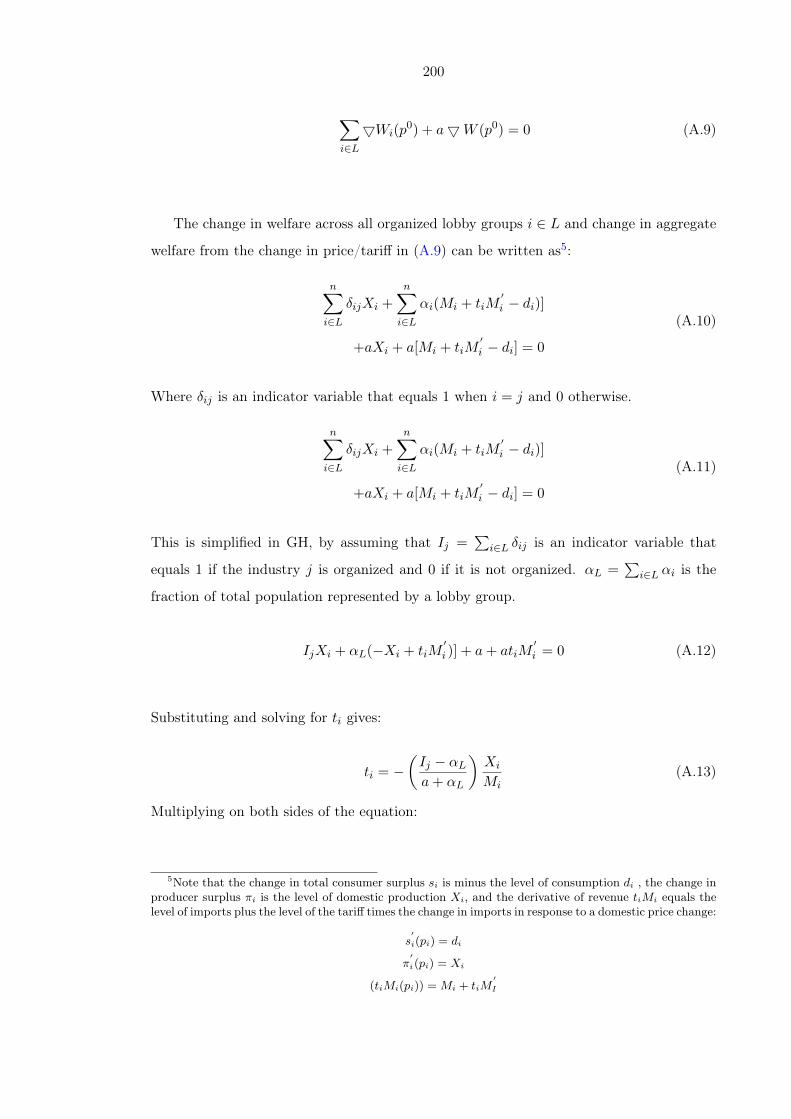
200

∑i∈L5Wi(p

0) + a5W (p0) = 0 (A.9)

The change in welfare across all organized lobby groups i ∈ L and change in aggregate

welfare from the change in price/tariff in (A.9) can be written as5:

n∑i∈L

δijXi +

n∑i∈L

αi(Mi + tiM′i − di)]

+aXi + a[Mi + tiM′i − di] = 0

(A.10)

Where δij is an indicator variable that equals 1 when i = j and 0 otherwise.

n∑i∈L

δijXi +

n∑i∈L

αi(Mi + tiM′i − di)]

+aXi + a[Mi + tiM′i − di] = 0

(A.11)

This is simplified in GH, by assuming that Ij =∑

i∈L δij is an indicator variable that

equals 1 if the industry j is organized and 0 if it is not organized. αL =∑

i∈L αi is the

fraction of total population represented by a lobby group.

IjXi + αL(−Xi + tiM′i )] + a+ atiM

′i = 0 (A.12)

Substituting and solving for ti gives:

ti = −(Ij − αLa+ αL

)Xi

Mi(A.13)

Multiplying on both sides of the equation:

5Note that the change in total consumer surplus si is minus the level of consumption di , the change inproducer surplus πi is the level of domestic production Xi, and the derivative of revenue tiMi equals thelevel of imports plus the level of the tariff times the change in imports in response to a domestic price change:

s′i(pi) = di

π′i(pi) = Xi

(tiMi(pi)) =Mi + tiM′I

201

Mi

piti =

(Ij − αLa+ αL

)Xi

−M ′ipiMi

(A.14)

Let the positive values of the elasticity of import demand ei equals −M ′ipiMi

and pi = p∗i +ti

where international prices p∗i are assumed equal to6 1. Substitution gives:

ti1 + ti

=

(Ij − αLa+ αL

)Xi

Mi

1

ei(A.15)

6As p∗ equals 1, the ad-valorem tariffs and specific tariffs are easily equated.

202

A.2.2 Summary Statistics

Table A.2: Summary Statistics by Years

Variable1990 1992 1996

Mean SD Mean SD Mean SD

Tariff 84.61 36.09 59.42 32.29 43.51 31.39

t/1+t 0.441 0.096 0.357 0.088 0.286 0.090

Import Demand Elasticity 15.46 16.33 15.46 16.33 15.46 16.33

Output (X in Rs Lakhs) 265740.00 490250.60 323287.60 546612.10 643002.20 1021357.00

Imports (M in Rs Lakhs) 25479.34 60135.34 35271.05 87494.62 91821.57 230574.70

X/M (Rs Lakhs) 385.35 1251.97 466.16 1744.09 232.91 792.02

Workers 53751.54 113891.00 56509.16 115956.80 61753.63 116945.70

Inventories 36881.09 75337.71 56166.04 97248.94 94672.22 155715.70

Variable 1999 2000 2001

Tariff 36.16 20.01 36.04 19.00 34.85 19.73

t/1+t 0.257 0.067 0.256 0.068 0.249 0.071

Import Demand Elasticity 15.46 16.33 15.46 16.33 15.46 16.33

Output (X in Rs Lakhs) 862037.30 1301237.00 896164.50 1404715.00 933621.30 1531384.00

Imports (M in Rs Lakhs) 132369.20 326822.10 123997.40 301809.10 137303.30 320044.30

X/M (Rs Lakhs) 115.03 338.26 137.37 469.84 86.41 196.11

Workers 59336.74 107800.60 58185.84 105608.40 56802.05 101885.20

Inventories 162381.40 271251.40 170176.10 314749.40 167874.30 323319.60

Variable 2004 2006 2007

Mean SD Mean SD Mean SD

Tariff 31.51 18.21 18.40 18.59 19.28 21.36

t/1+t 0.230 0.071 0.142 0.091 0.145 0.097

Import Demand Elasticity 15.46 16.33 15.46 16.33 15.46 16.33

Output (X in Rs Lakhs) 1618978.00 3382978.00 2300029.00 4873125.00 2657099.00 5715065.00

Imports (M in Rs Lakhs) 302604.70 688638.50 506018.70 1071660.00 397520.40 898767.50

X/M (Rs Lakhs) 63.06 159.95 86.96 380.63 103.24 410.77

Workers 62480.14 102477.20 74172.18 116810.40 77405.94 119382.30

Inventories 242219.80 422042.70 346800.20 613800.70 423931.90 752664.60

203

A.2.3 First Stage Estimates

Table A.3: First Stage Estimates: IV

(I) (II) (III)

1990 1992 1996

Model IV IV IV

Inventories 0.00163 0.00276 0.00050

(0.001) (0.002) (0.000)

Observations 94 96 98

Shea R-squared 0.011 0.030 0.012

F-Statistic 1.458 1.818 2.578

(IV) (V) (VI)

1999 2000 2001

Model IV IV IV

Inventories 0.00016* 0.00029*** 0.00019***

(0.000) (0.000) (0.000)

Observations 98 98 98

Shea R-squared 0.019 0.046 0.100

F-Statistic 3.712 10.29 11.79

(VII) (VIII) (IX)

2004 2006 2007

Model IV IV IV

Inventories 0.00006* 0.00020 0.00019

(0.000) (0.000) (0.000)

Observations 98 98 98

Shea R-squared 0.033 0.137 0.145

F 3.864 1.463 1.643

Robust standard errors in parentheses

*** p<0.01, ** p<0.05, * p<0.1

204

Table A.4: Pooled First Stage Estimates: IV1-IV4

(I) (II) (III) (IV)

Model IV1 IV2 IV3 IV4

Lag Inventories 0.00152*** 0.00226* 0.003444*** 0.00639***

(0.000) (0.001) (0.001) (0.002)

Lag Workers -0.00065 -0.00223**

(0.001) (0.001)

Workers Squared -0.00336*** -0.00406***

(0.001) (0.001)

Observations 876 876 876 876

R-squared 0.045 0.046 0.073 0.082

F 14.88 12.25 12.46 10.87

Note: Table A.4 shows the first stage results for the pooled dataset assuming all industries are organized.

Limited Information Maximum Likelihood is used that is shown to provide better estimates with weak

instruments. Robust standard errors in parentheses.

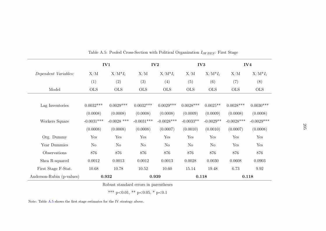
205

Table A.5: Pooled Cross-Section with Political Organization IiWBES : First Stage

IV1 IV2 IV3 IV4

Dependent Variables: X/M X/M*Ii X/M X/M*Ii X/M X/M*Ii X/M X/M*Ii

(1) (2) (3) (4) (5) (6) (7) (8)

Model OLS OLS OLS OLS OLS OLS OLS OLS

Lag Inventories 0.0032*** 0.0029*** 0.0032*** 0.0029*** 0.0028*** 0.0025** 0.0028*** 0.0030***

(0.0008) (0.0008) (0.0008) (0.0008) (0.0009) (0.0009) (0.0008) (0.0008)

Workers Square -0.0031*** -0.0028 *** -0.0031*** -0.0028*** -0.0033** -0.0029** -0.0028*** -0.0029***

(0.0008) (0.0008) (0.0008) (0.0007) (0.0010) (0.0010) (0.0007) (0.0008)

Org. Dummy Yes Yes Yes Yes Yes Yes Yes Yes

Year Dummies No No No No No No Yes Yes

Observations 876 876 876 876 876 876 876 876

Shea R-squared 0.0012 0.0013 0.0012 0.0013 0.0028 0.0030 0.0608 0.0903

First Stage F-Stat. 10.68 10.78 10.52 10.60 15.14 19.48 6.73 9.92

Anderson-Rubin (p-values) 0.932 0.939 0.118 0.118

Robust standard errors in parentheses

*** p<0.01, ** p<0.05, * p<0.1

Note: Table A.5 shows the first stage estimates for the IV strategy above.

206

A.2.4 Robustness

Table A.6: Protection for Sale across the Years: OLS vs 2 IVs

(I) (II) (III)

1990 1992 1996

Model OLS IV2 OLS IV2 OLS IV2

X/M 0.004*** 0.024** 0.002 0.008 0.003* 0.022

(0.001) (0.008) (0.001) (0.004) (0.001) (0.013)

R2 0.21 -5.25 0.15 -0.96 0.08 -3.32

N 94 94 96 96 98 98

(IV) (V) (VI)

1999 2000 2001

Model OLS IV2 OLS IV2 OLS IV2

X/M 0.010** 0.031* 0.007** 0.017* 0.018** 0.037**

(0.003) (0.012) (0.002) (0.008) (0.004) (0.009)

N 98 98 98 98 98 98

(VII) (VIII) (IX)

2004 2006 2007

Model OLS IV2 OLS IV2 OLS IV2

X/M 0.016** 0.065** 0.004* 0.018 0.004** 0.013

(0.004) (0.022) (0.001) (0.029) (0.001) (0.013)

R2 0.15 -1.33 0.06 -0.83 0.08 -0.29

N 98 98 98 98 98 98

* p < 0.1; ** p < 0.05; *** p < 0.01

Note: Table A.6 shows the results for PFS assuming all industries are organized. Robust standard errors

in parentheses.

207

Table A.7: Pooled Cross-Sections with Time Dummies: IV

(I) (II) (III) (IV)

IV1 IV2 IV3 IV4

X/M 0.015*** 0.012*** 0.011*** 0.012***

(0.005) (0.004) (0.004) (0.004)

yr1 1.374 2.447 2.977 2.441

(2.548) (2.136) (1.902) (2.049)

yr2 -0.902 0.396 1.038 0.389

(2.231) (1.868) (1.701) (1.875)

yr3 1.431 2.080 2.401* 2.076

(1.620) (1.359) (1.259) (1.370)

yr4 2.668*** 2.988*** 3.147*** 2.986***

(0.870) (0.785) (0.754) (0.785)

yr5 2.371** 2.754*** 2.943*** 2.752***

(0.969) (0.865) (0.828) (0.868)

yr6 3.012*** 3.253*** 3.372*** 3.252***

(0.705) (0.666) (0.652) (0.663)

yr7 3.051*** 3.227*** 3.314*** 3.226***

(0.639) (0.611) (0.603) (0.614)

yr8 1.487* 1.729** 1.848*** 1.727**

(0.769) (0.685) (0.643) (0.678)

yr9 1.335 1.623** 1.765** 1.621**

(0.830) (0.736) (0.690) (0.728)

N 876 876 876 876* p < 0.1; ** p < 0.05; *** p < 0.01

Note: Table A.7 shows the results from Limited Information Maximum Likelihood for the pooled dataset

with time dummies. The results are presented for IV strategies 1-4.

208

Table A.8: Pooled Cross-Sections with Time Dummies: First Stage

(1) (2) (3) (4)

Model OLS OLS OLS OLS

Lag Inventories 0.00097** 0.00276** 0.00276*** 0.00595***

(0.000) (0.001) (0.001) (0.002)

Lag Workers -0.00164** -0.00254***

(0.001) (0.001)

Workers Squared -0.00270*** -0.00334***

(0.001) (0.001)

Observations 876 876 876 876

R-squared 0.090 0.095 0.104 0.115

First Stage F-Stat. 9.062 8.314 7.931 7.259

Anderson-Rubin statistic . . . .

(Over-identification test)

Robust standard errors in parentheses

*** p<0.01, ** p<0.05, * p<0.1

Note: Table A.8 shows the first stage estimates for the IV strategy in Table A.7.

A.2.5 Political Organization

209

Table A.9: Thresholds to define Organization

Thresholds to define Organization

Percentiles Percent Cum. Organized Unorganized

Sectors Sectors

0.75 25 25 79 19

0.82 25 50 63 35

0.84 25 75 47 51

0.89 25 100 21 77

Table A.10: Summary of Political Organization Measures

Organization Years Organized Unorganized

I (WBES) All 79 19

I (Cadot) All 47 51

Table A.11: Summary Statistics by Organized and Unorganized Sectors: IiCadot

Tariffs by Organized and Unorganized Sectors

YearOrganized I=1 Unorganized I=0

Avg. Max Avg. Max

Average Max Average Max

1990 84.49 180.38 84.72 318.13

1992 57.85 172.86 60.86 318.13

1996 42.98 241.29 44.01 247.56

1999 33.85 100.00 38.29 206.11

2000 33.43 110.00 38.44 188.50

2001 31.41 100.00 38.03 190.56

2004 28.22 100.00 34.54 165.11

2006 14.30 100.00 22.17 134.44

2007 14.28 100.00 23.88 165.11

Total 37.87 241.29 42.77 318.13

210

Dependent Variable (t/1+t)*e by Organized and Unorganized Sectors

YearOrganized I=1 Unorganized I=0

Avg. Max Avg. Max

1990 4.27 23.74 9.64 55.38

1992 3.46 23.74 8.21 55.38

1996 2.91 26.49 6.66 51.84

1999 2.48 18.73 6.09 49.01

2000 2.47 19.63 6.17 47.56

2001 2.36 18.73 6.05 47.73

2004 2.20 18.73 5.62 45.33

2006 1.41 18.73 4.02 41.74

2007 1.38 18.73 4.22 45.33

Total 2.55 26.49 6.30 55.38

X/M by Organized and Unorganized Sectors

YearOrganized I=1 Unorganized I=0

Avg. Max Avg. Max

1990 95.13 2495.71 651.87 10086.30

1992 34.88 606.32 846.69 13948.44

1996 155.50 5716.44 304.25 4051.37

1999 91.11 2058.35 137.07 1720.80

2000 87.40 2848.68 183.42 3431.56

2001 41.59 584.87 127.72 1071.44

2004 22.09 329.87 100.83 961.17

2006 16.48 208.60 151.92 3608.05

2007 22.76 249.09 177.40 3795.65

Total 62.97 5716.44 296.36 13948.44

211

Table A.12: PFS with various Thresholds

(I) (II) (III) (IV)

X/M -0.131* 0.003 0.002 0.011***

(0.053) (0.005) (0.004) (0.003)

X/M*LM I 0.158**

(0.053)

X/M*LM II 0.025**

(0.082)

X/M*LM III 0.035***

(0.007)

X/M*LM IV 0.024**

(0.007)

N 876 876 876 876

F 21.01 20.31 19.54 13.12

Note: Table A.12 shows the results for PFS with different political organization measures constructed

with the thresholds of 0.75 (LM I), 0.82 (LM II), 0.84 (LM III) and 0.89 (LM IV). Limited Information

Maximum Likelihood is used that is shown to provide better estimates with weak instruments. Robust

standard errors in parentheses.

212

Table A.13: Pooled Cross-Section with Political Organization: IiCadot(I) (II) (III) (IV) (V) (VI)

Pooled Restricted Restricted Sample Drop Drop Outlier Drop Outlier

Sample Time Dummies Outlier Restr. Sample Restr. Sample

Time Dummies

IV1 IV2 IV3 IV4 IV5 IV6

X/M 0.0154*** 0.0120*** 0.0108*** 0.0146*** 0.0115** 0.0110**

(0.0039) (0.0046) (0.0040) (0.0038) (0.0046) (0.0047)

X/M*IiCadot 0.0256* 0.0225 -0.0034 0.0272** 0.0236 0.0086

(0.0132) (0.0158) (0.0118) (0.0137) (0.0164) (0.0157)

yr1 3.0526 1.8715

(2.2734) (2.4659)

yr2 0.9989 0.1520

(1.5766) (1.8819)

yr3 2.6037 1.1639

(1.7652) (2.3552)

yr4 3.2698*** 2.2611*

(1.0885) (1.2738)

N 876 386 386 867 382 382

* p < 0.1; ** p < 0.05; *** p < 0.01

Note: (I) shows the results for the pooled data, (II) restricts the sample till 1999, (III) restricts the sample with time dummies, (IV) drops maximum tariff, (V) data till

1999 and dropping the outlier, finally (VI) results for years till 1999 and dropping the outlier with time dummies.

213

A.2.6 Comparison

Table A.14: Comparison of Political Organization Measures

NIC498 Description Political Org. Cadot et al

(WBES) Measure

1511 Production, processing and preserving of meat and meat products. 1 1

1512 Processing and preserving of fish and fish products 1 0

1513 Processing and preserving of fruit, vegetables and edible nuts 1 0

1514 Manuf. of Vegetable and animal oils and fats 1 0

1520 Manuf. of dairy product [production of raw milk is classified in class 0121] 1 0

1531 Manuf. of grain mill products 1 0

1532 Manuf. of starches and starch products 1 0

1533 Manuf. of prepared animal feeds 1 0

1541 Manuf. of bakery products 1 0

1542 Manuf. of sugar 1 0

1543 Manuf. of cocoa, chocolate and sugar confectionery 1 0

1544 Manuf. of macaroni, noodles, couscous and similar farinaceous products 1 0

1551 Distilling, rectifying and blending of spirits 1 0

1552 Manuf. of wines 1 1

1553 Manuf. of malt liquors and malt 0 0

1554 Manuf. of soft drinks; production of mineral waters 0 1

1600 Manuf. of tobacco products 1 0

1711 Preparation and spinning of textile fiber including weaving of textiles 1 0

1721 Manuf. of made-up textile articles, except apparel 1 0

1722 Manuf. of carpet and rugs other than by hand 1 0

214

Comparison of Political Organization Measures

NIC498 Description Political Org. Cadot et al

(WBES) Measure

1723 Manuf. of cordage, rope, twine and netting 1 0

1729 Manuf. of other textiles n.e.c. 1 1

1730 Manuf. of knitted and crocheted fabrics and articles 1 0

1810 Manuf. of wearing apparel, except fur apparel 1 1

1820 Dressing and dyeing of fur; Manuf. of articles of fur 1 0

1911 Tanning and dressing of leather 1 0

1912 Manuf. of luggage, handbags, and the like, saddlery and harness 1 1

1920 Manuf. of footwear. 0 0

2010 Saw milling and planing of wood 0 0

2021 Manufacture of veneer sheets; plywood, laminboard, particle board 0 0

2022 Manufacture of builders’ carpentry and joinery 0 0

2023 Manufacturing of wooden containers 0 0

2029 Manufacture of other products of wood, manufacture of articles of cork 0 0

2101 Manufacture of pulp, paper and paper board 1 1

2102 Manufacture of corrugated paper and paperboard 1 0

2109 Manufacture of other articles of paper and paperboard 1 1

2212 Publishing of newspapers, journals and periodicals 1 0

2219 Other publishing 1 1

2221 Printing 1 1

2222 Service activities related to printing 1 0

2310 Manufacture of coke oven products 1 0

215

Comparison of Political Organization Measures

NIC498 Description Political Org. Cadot et al

(WBES) Measure

2320 Manufacture of refined petroleum products 1 1

2411 Manufacture of basic chemicals except fertilizers and nitrogen compounds 1 1

2412 Manufacture of fertilizers and nitrogen compounds 1 1

2413 Manufacture of plastics in primary forms and of synthetic rubber. 0 1

2422 Manufacture of paints, varnishes and similar coatings,printing ink and mastics 0 1

2423 Manufacture of pharmaceuticals, medicinal chemicals and botanical products 1 1

2424 Manufacture of soap and detergents, cleaning and polishing preparations 0 0

2429 Manufacture of other chemical product n.e.c. 1 1

2430 Manufacture of man-made fibers 1 1

2511 Manufacture of rubber tyres and tubes; retreading and rebuilding of rubber tyres 1 0

2519 Manufacture of other rubber products 1 1

2520 Manufacture of plastic products 0 1

2610 Manufacture of glass and glass products 1 0

2691 Manufacture of non-structural non-refractory ceramic ware 1 0

2692 Manufacture of refractory ceramic products 1 0

2694 Manufacture of cement, lime and plaster 1 0

2695 Manufacture of articles of concrete, cement and plaster 1 0

2696 Cutting, shaping and finishing of stone 1 0

2699 Manufacture of other non-metallic mineral products n.e.c. 1 0

2710 Manufacture of basic iron and steel 1 0

2720 Manufacture of basic precious and non-ferrous metals 1 1

216

Comparison of Political Organization Measures

NIC498 Description Political Org. Cadot et al

(WBES) Measure

2811 Manufacture of structural metal products 1 0

2812 Manufacture of tanks, reservoirs and containers of metal 1 0

2813 Manufacture of steam generators, except central heating hot water boilers 1 1

2893 Manufacture of cutlery, hand tools and general hardware 1 1

2899 Manufacture of other fabricated metal products n.e.c. 1 1

2912 Manufacture of pumps, compressors, taps and valves 1 1

2919 Manufacture of other general purpose machinery 1 1

2921 Manufacture of agricultural and forestry machinery 1 0

2922 Manufacture of machine-tools 1 1

2924 Manufacture of machinery for mining, quarrying and construction 1 1

2925 Manufacture of machinery for food, beverage and tobacco processing 1 1

2930 Manufacture of domestic appliances, n.e.c. 1 1

3000 Manufacture of office, accounting and computing machinery 1 1

3110 Manufacture of electric motors, generators and transformers 1 1

3130 Manufacture of insulated wire and cable 1 0

3140 Manufacture of accumulators, primary cells and primary batteries 1 0

3150 Manufacture of electric lamps and lighting equipment 1 1

3190 Manufacture of other electrical equipment n.e.c. 1 1

3210 Manufacture of electronic valves and tubes and other electronic components 1 1

3220 Manufacture of television and radio transmitters and apparatus for line telephony 1 1

3230 Manufacture of television and radio receivers, sound or video recording 1 1

217

Comparison of Political Organization Measures

NIC498 Description Political Org. Cadot et al

(WBES) Measure

3311 Manufacture of medical and surgical equipment and orthopedic appliances 1 1

3320 Manufacture of optical instruments and photographic equipment 1 1

3330 Manufacture of watches and clocks 1 1

3410 Manufacture of motor vehicles 1 0

3511 Building and repairing of ships 1 1

3520 Manufacture of railway and tramway locomotives and rolling stock 1 1

3530 Manufacture of aircraft and spacecraft 1 1

3591 Manufacture of motorcycles 0 0

3592 Manufacture of bicycles and invalid carriages 0 1

3599 Manufacture of other transport equipment n.e.c. 0 1

3610 Manufacture of furniture 0 0

3691 Manufacture of jewellery and related articles 0 1

3692 Manufacture of musical instruments 0 0

3693 Manufacture of sports goods 0 0

3694 Manufacture of games and toys 1 1

218

A.3 Chapter 4

A.3.1 OLS Estimates

Table A.15: Modified PFS, OLS Estimates

(I) (II) (III) (IV)

Variables Model 1 (OLS1) Model 2 (OLS2) Model 3 (OLS3) Model 4 (OLS4)

Baseline

NIC 1511 1.05828** -0.08579 0.02069 0.46371*

(0.474) (0.298) (0.384) (0.237)

NIC 1512 0.00266 0.00106 -0.00062 -0.00015

(0.002) (0.001) (0.001) (0.001)

NIC 1513 0.00385*** 0.00160*** 0.00102 0.00051

(0.001) (0.001) (0.001) (0.000)

NIC 1514 0.19667*** 0.03309 0.03595 -0.01364

(0.065) (0.032) (0.053) (0.025)

NIC 1520 0.02790*** -0.00256 0.01090** -0.00512

(0.006) (0.005) (0.005) (0.004)

NIC 1531 0.01320*** -0.00005 0.00754*** 0.00329**

(0.003) (0.002) (0.002) (0.001)

NIC 1532 0.03310*** 0.00564 0.00467 -0.00427

(0.010) (0.006) (0.008) (0.004)

NIC 1533 0.00285 0.00069 -0.03828*** -0.01359**

(0.015) (0.008) (0.012) (0.006)

NIC 1541 0.00027 0.00011 -0.00520*** -0.00207**

(0.002) (0.001) (0.002) (0.001)

NIC 1542 0.00097*** 0.00003 0.00038 -0.00004

(0.000) (0.000) (0.000) (0.000)

NIC 1543 0.01089 0.00310 -0.00362 -0.00081

(0.008) (0.004) (0.007) (0.003)

NIC 1544 0.03280** -0.00729 -0.00787 0.01358

(0.016) (0.013) (0.013) (0.010)

NIC 1551 0.37747*** 0.05306*** 0.33920*** 0.04053***

(0.013) (0.010) (0.010) (0.008)

219

Modified PFS, OLS Estimates (cont.)

Variables Model 1 (OLS1) Model 2 (OLS2) Model 3 (OLS3) Model 4 (OLS4)

Baseline

NIC 1552 0.19431*** -0.00185 0.14677*** -0.01785*

(0.016) (0.013) (0.013) (0.010)

NIC 1553 0.00152** 0.00006 -0.00033 -0.00062**

(0.001) (0.000) (0.001) (0.000)

NIC 1554 0.00083 0.00020 -0.00034 -0.00005

(0.001) (0.000) (0.001) (0.000)

NIC 1600 0.01233*** 0.00331*** 0.01039*** 0.00276***

(0.001) (0.000) (0.001) (0.000)

NIC 1711 0.14817*** 0.11820*** 0.03482 0.05078*

(0.035) (0.035) (0.029) (0.028)

NIC 1721 0.07142*** 0.03715*** 0.01330 0.01478*

(0.020) (0.011) (0.016) (0.009)

NIC 1722 0.02289*** 0.00854** 0.00863 0.00445

(0.008) (0.004) (0.007) (0.003)

NIC 1723 0.09861*** 0.07092*** 0.00015 0.02780

(0.031) (0.025) (0.026) (0.020)

NIC 1729 2.03005*** 1.27452 -0.12902 0.45204

(0.682) (0.920) (0.557) (0.732)

NIC 1730 0.08463*** 0.01028 0.03087* 0.00798

(0.022) (0.012) (0.018) (0.010)

NIC 1810 0.00500*** 0.00220*** 0.00090 0.00072

(0.002) (0.001) (0.001) (0.001)

NIC 1820 0.18298 -0.18006*** -0.03195 -0.06899

(0.114) (0.062) (0.092) (0.050)

NIC 1911 0.13128 0.08272 -0.56200*** -0.33564*

(0.213) (0.215) (0.174) (0.171)

NIC 1912 0.04189 0.02477 -0.03850* -0.00912

(0.027) (0.016) (0.022) (0.013)

NIC 1920 0.05333* 0.04456* -0.03600 -0.00567

(0.028) (0.025) (0.023) (0.020)

220

Modified PFS, OLS Estimates (cont.)

Variables Model 1 (OLS1) Model 2 (OLS2) Model 3 (OLS3) Model 4 (OLS4)

Baseline

NIC 2010 0.67566*** -0.16343 0.22295* -0.10431

(0.148) (0.194) (0.121) (0.155)

NIC 2021 0.15914*** 0.08437*** 0.01042 0.02227

(0.049) (0.031) (0.040) (0.025)

NIC 2023 0.00797*** 0.00337*** 0.00450*** 0.00215***

(0.002) (0.001) (0.001) (0.001)

NIC 2029 0.03990*** 0.00111 0.01964** -0.00030

(0.010) (0.005) (0.008) (0.004)

NIC 2101 0.40684*** 0.14794* 0.09490 0.08989

(0.111) (0.076) (0.091) (0.060)

NIC 2102 0.46018 0.82274 -0.50322** -0.14136

(0.295) (0.548) (0.241) (0.437)

NIC 2109 0.04249** -0.04100 -0.01480 -0.00561

(0.019) (0.027) (0.016) (0.021)

NIC 2212 0.23081 0.31573 -0.45386*** -0.29884

(0.208) (0.312) (0.171) (0.249)

NIC 2219 0.00000 0.00000 -0.01022*** 0.00342

(0.004) (0.003) (0.003) (0.002)

NIC 2221 0.43515 -0.11441 -1.96917*** 0.78953

(0.850) (0.876) (0.693) (0.698)

NIC 2222 0.00325 0.00210 -0.00805*** -0.00284

(0.004) (0.003) (0.003) (0.002)

NIC 2310 0.06334 0.02341 -0.24676*** -0.10290**

(0.105) (0.060) (0.086) (0.048)

NIC 2320 0.02637 0.00706 -0.19440*** -0.07651**

(0.084) (0.041) (0.069) (0.032)

NIC 2411 0.01518 -0.01117 -0.13304** 0.04467

(0.082) (0.041) (0.066) (0.033)

NIC 2412 0.52111 0.67011 -2.28651*** -1.94796*

(0.857) (1.376) (0.701) (1.098)

221

Modified PFS, OLS Estimates (cont.)

Variables Model 1 (OLS1) Model 2 (OLS2) Model 3 (OLS3) Model 4 (OLS4)

Baseline

NIC 2413 0.11781 0.05603 -0.47947*** -0.08212

(0.193) (0.254) (0.157) (0.202)

NIC 2422 0.08364 -0.02510 -0.59736*** 0.15700

(0.253) (0.214) (0.206) (0.170)

NIC 2423 0.03200 0.02245 -0.09043*** -0.03262

(0.040) (0.026) (0.033) (0.021)

NIC 2424 0.05325 0.01236 -0.28677*** 0.04376

(0.108) (0.229) (0.089) (0.182)

NIC 2429 0.04061 0.02815 -0.10704*** -0.04415

(0.046) (0.042) (0.038) (0.034)

NIC 2430 0.25235 0.29255 -0.88684*** -0.66564

(0.348) (0.547) (0.284) (0.436)

NIC 2511 0.38520*** 0.23362** -0.03675 0.10167

(0.140) (0.106) (0.114) (0.085)

NIC 2519 0.00504 0.00417 -0.02882*** -0.01412**

(0.011) (0.008) (0.009) (0.007)

NIC 2520 0.08262 0.07347 -0.49133*** -0.27876*

(0.176) (0.187) (0.144) (0.150)

NIC 2610 0.07352 0.07577 -0.15885*** -0.08874

(0.071) (0.087) (0.058) (0.070)

NIC 2691 0.76613*** 1.16593*** 0.10869 0.53318*

(0.201) (0.349) (0.164) (0.279)

NIC 2692 0.13550** 0.08127* -0.04917 0.00559

(0.060) (0.043) (0.049) (0.034)

NIC 2694 0.33928*** 0.30136*** 0.06309 0.14364**

(0.086) (0.087) (0.070) (0.069)

NIC 2695 0.00435*** 0.00213*** 0.00344*** 0.00177***

(0.000) (0.000) (0.000) (0.000)

NIC 2696 0.00979*** 0.00648*** -0.00137 0.00127

(0.004) (0.002) (0.003) (0.002)

222

Modified PFS, OLS Estimates (cont.)

Variables Model 1 (OLS1) Model 2 (OLS2) Model 3 (OLS3) Model 4 (OLS4)

Baseline

NIC 2699 0.00248* 0.00092 -0.00027 0.00019

(0.001) (0.001) (0.001) (0.000)

NIC 2710 0.20279** 0.16015** -0.06589 0.00351

(0.083) (0.072) (0.068) (0.058)

NIC 2720 0.22293** 0.22167 -0.08227 0.10096

(0.096) (0.179) (0.079) (0.142)

NIC 2811 1.60168** 0.90309* -0.71467 -0.02238

(0.772) (0.478) (0.631) (0.382)

NIC 2812 0.09874*** 0.05161*** 0.04158*** 0.02924***

(0.019) (0.011) (0.016) (0.009)

NIC 2813 0.04831*** 0.02744*** 0.00556 0.00942

(0.014) (0.008) (0.012) (0.007)

NIC 2893 0.16343 0.01510 -0.30187** -0.05108

(0.148) (0.214) (0.121) (0.170)

NIC 2899 0.09592 0.06044 -0.38164*** -0.18263*

(0.150) (0.118) (0.122) (0.094)

NIC 2912 0.63510** -0.36153 -0.25737 0.05170

(0.316) (0.337) (0.258) (0.268)

NIC 2919 1.37919** 2.74750 -0.55168 -0.15473

(0.595) (1.877) (0.486) (1.496)

NIC 2921 0.05594 0.02378 -0.05228 -0.01535

(0.053) (0.022) (0.043) (0.018)

NIC 2922 0.01558 0.00492 -0.01296 -0.00555

(0.010) (0.006) (0.008) (0.004)

NIC 2924 1.73304 1.65815* -1.87803** -0.04553

(1.152) (0.863) (0.942) (0.689)

NIC 2925 0.66137 0.40822 -1.04862** -0.73453

(0.526) (0.680) (0.431) (0.542)

NIC 2930 0.63247 0.47786 -1.52690*** -0.92859

(0.666) (0.761) (0.545) (0.607)

223

Modified PFS, OLS Estimates (cont.)

Variables Model 1 (OLS1) Model 2 (OLS2) Model 3 (OLS3) Model 4 (OLS4)

Baseline

NIC 3000 0.09615*** 0.04998*** -0.00046 0.01173

(0.033) (0.019) (0.027) (0.015)

NIC 3110 0.46893 0.31918 -1.41750*** -0.32697

(0.670) (0.377) (0.548) (0.301)

NIC 3130 0.11799 0.07010 -0.44403*** -0.26641*

(0.173) (0.176) (0.142) (0.141)

NIC 3140 0.03861 0.02873 -0.16012*** -0.06276

(0.063) (0.048) (0.052) (0.038)

NIC 3150 0.07615 0.03855 -0.16080** -0.04404

(0.081) (0.051) (0.066) (0.041)

NIC 3190 0.19106** 0.11179** -0.05500 0.01267

(0.082) (0.051) (0.067) (0.041)

NIC 3210 1.14338 -1.38821* -0.91665 0.05598

(0.730) (0.833) (0.594) (0.664)

NIC 3220 0.37643 -0.75085 -2.07985*** 0.70684

(0.887) (0.909) (0.722) (0.724)

NIC 3230 0.02936 -0.00060 -0.09442* -0.00259

(0.063) (0.029) (0.051) (0.023)

NIC 3311 0.19927 0.18050 -0.39447*** -0.15094

(0.185) (0.190) (0.151) (0.151)

NIC 3320 1.54948 -1.47940 -2.87681** 1.19461

(1.437) (2.835) (1.173) (2.256)

NIC 3330 0.74632 0.16680 -1.70262** 0.02708

(0.890) (0.621) (0.725) (0.494)

NIC 3410 0.31650* 0.24015 -0.24655* -0.02933

(0.179) (0.158) (0.146) (0.126)

NIC 3511 0.86302*** -0.43749*** 0.63026*** -0.32178***

(0.077) (0.119) (0.063) (0.095)

NIC 3520 0.78608 0.19610 -1.44416** -0.30318

(0.840) (0.485) (0.685) (0.387)

224

Modified PFS, OLS Estimates (cont.)

Variables Model 1 (OLS1) Model 2 (OLS2) Model 3 (OLS3) Model 4 (OLS4)

Baseline

NIC 3530 0.13020 0.03565 -0.23455** -0.07990

(0.120) (0.099) (0.098) (0.079)

NIC 3591 0.66968 0.22966 -2.16524** -0.23781

(1.337) (0.625) (1.086) (0.497)

NIC 3592 0.00838*** -0.00003 0.00258 0.00133

(0.002) (0.002) (0.002) (0.001)

NIC 3599 0.11942*** 0.08345*** 0.03891* 0.04787***

(0.026) (0.022) (0.021) (0.018)

NIC 3594 0.00167 0.00039 -0.00046 0.00014

(0.001) (0.001) (0.001) (0.001)

NIC 3610 0.02180* 0.01035** -0.00555 0.00046

(0.011) (0.005) (0.009) (0.004)

NIC 3691 0.13773 0.05579 -0.12735 -0.03790

(0.099) (0.050) (0.081) (0.040)

NIC 3692 0.04884 -0.00401 -0.16719 -0.05326

(0.145) (0.059) (0.117) (0.047)

NIC 3693 0.14515 -0.02183 -0.42846** -0.02071

(0.213) (0.152) (0.174) (0.121)

NIC 3694 0.32823 -0.14961 -0.26656 0.00289

(0.210) (0.204) (0.171) (0.162)

Sector FE Yes Yes

Year FE Yes Yes

Observations 876 876 876 876

R-squared 0.729 0.966 0.828 0.979

* p < 0.1; ** p < 0.05; *** p < 0.01

225

A.3.2 First Stage Estimates

Table A.16: First Stage Estimates Summary

VariableIV1 IV2 IV3 IV4

Shea F Shea F Shea F Shea F

Partial R2 Partial R2 Partial R2 Partial R2

X/M*1511 0.9089 75.73 0.8111 28.62 0.6513 75.16 0.3482 28.33

X/M*1512 0.0534 0.44 0.5417 7.88 0.0374 0.45 0.1889 7.8

X/M*1513 0.0759 0.71 0.3936 4.33 0.0635 0.75 0.1685 4.29

X/M*1514 0.4679 6.68 0.2411 2.12 0.2761 6.63 0.1657 2.14

X/M*1520 0.7798 26.89 0.0625 0.44 0.4896 26.58 0.0236 0.45

X/M*1531 0.7407 21.85 0.7936 25.63 0.45 21.61 0.2928 25.39

X/M*1532 0.3649 4.37 0.1561 1.23 0.2482 4.36 0.0768 1.26

X/M*1533 0.2864 3.05 0.4211 4.85 0.1958 3.06 0.1714 4.8

X/M*1541 0.4475 6.15 0.5503 8.16 0.2843 6.09 0.2264 8.08

X/M*1542 0.4201 5.55 0.235 2.05 0.2599 5.5 0.0888 2.03

X/M*1543 0.1422 1.26 0.175 1.41 0.105 1.26 0.1158 1.41

X/M*1544 0.8289 37.09 0.4811 6.18 0.5027 36.77 0.1874 6.14

X/M*1551 0.7001 17.72 0.1282 0.98 0.4293 17.55 0.0755 1

X/M*1552 0.8576 45.7 0.298 2.83 0.5507 45.26 0.2029 2.86

226

First Stage Estimates Summary (cont.)

VariableIV1 IV2 IV3 IV4

Shea F Shea F Shea F Shea F

Partial R2 Partial R2 Partial R2 Partial R2

X/M*1553 0.2403 2.4 0.2134 1.81 0.1666 2.41 0.1196 1.81

X/M*1554 0.1299 1.14 0.4593 5.66 0.1033 1.15 0.3384 5.62

X/M*1600 0.5423 9.01 0.0707 8.51 0.3203 8.93 0.0597 6.87

X/M*1711 0.9292 113.84 0.7912 213.57 0.5567 117.65 0.2969 174

X/M*1721 0.1398 1.31 0.3852 4.18 0.1231 1.44 0.1818 4.14

X/M*1722 0.0447 0.36 0.3984 4.41 0.0391 0.42 0.2253 4.38

X/M*1723 0.5741 10.24 0.0702 0.5 0.4047 10.23 0.0383 0.51

X/M*1729 0.7197 19.61 0.0169 0.11 0.5257 19.64 0.0079 0.12

X/M*1730 0.4803 7.58 0.0025 0.02 0.315 7.48 0.0013 0.03

X/M*1810 0.3107 4.91 0.4027 9.58 0.2392 5.1 0.1673 8.46

X/M*1820 0.8896 61.15 0.7668 21.92 0.7046 60.46 0.5144 21.7

X/M*1911 0.8771 54.17 0.1223 0.93 0.5185 53.66 0.1007 0.99

X/M*1912 0.2864 3.06 0.584 9.36 0.2041 3.12 0.2176 9.26

X/M*1920 0.6285 12.94 0.4935 6.5 0.4084 12.76 0.2586 6.43

X/M*2010 0.8217 34.97 0.0175 0.12 0.4448 35.01 0.0058 0.12

X/M*2021 0.6548 14.39 0.0122 0.08 0.3914 14.26 0.0114 0.14

227

First Stage Estimates Summary (cont.)

VariableIV1 IV2 IV3 IV4

Shea F Shea F Shea F Shea F

Partial R2 Partial R2 Partial R2 Partial R2

X/M*2022 0.1293 1.13 0.1337 1.03 0.0825 1.13 0.0799 1.06

X/M*2023 0.3073 3.37 0.0172 0.12 0.1884 3.34 0.0144 0.13

X/M*2029 0.7554 23.44 0.3588 3.73 0.4444 23.26 0.3197 3.74

X/M*2101 0.9292 99.74 0.0012 0.01 0.5575 98.59 0.0009 0.06

X/M*2102 0.9557 163.86 0.5367 7.72 0.6498 162.06 0.2087 7.64

X/M*2109 0.7106 18.64 0.5273 7.44 0.4975 18.65 0.2237 7.35

X/M*2212 0.7714 25.61 0.6059 10.25 0.4659 25.33 0.3099 10.15

X/M*2219 0.7554 23.45 0.1175 0.89 0.4422 23.22 0.1102 0.91

X/M*2221 0.6664 15.16 0.0885 0.65 0.4087 15 0.0508 0.67

X/M*2222 0.4402 5.97 0.1614 1.28 0.2828 5.93 0.1242 1.3

X/M*2310 0.1698 1.57 0.0057 0.04 0.1207 1.63 0.0029 0.09

X/M*2320 0.8109 38.81 0.7857 49.93 0.6556 38.66 0.3935 44.35

X/M*2411 0.9194 86.65 0.0532 0.37 0.5621 85.71 0.0236 0.41

X/M*2412 0.9149 81.57 0.0048 0.03 0.547 80.68 0.0039 0.05

X/M*2413 0.8187 34.26 0.0921 0.68 0.5064 33.87 0.038 0.68

X/M*2422 0.7747 26.1 0.416 4.75 0.451 25.97 0.2936 4.77

228

First Stage Estimates Summary (cont.)

VariableIV1 IV2 IV3 IV4

Shea F Shea F Shea F Shea F

Partial R2 Partial R2 Partial R2 Partial R2

X/M*2423 0.8882 61.14 0.0102 0.07 0.5607 60.17 0.0042 0.08

X/M*2424 0.7256 20.08 0.3616 3.78 0.4555 19.86 0.1868 3.76

X/M*2429 0.9423 123.83 0.024 0.16 0.5643 122.56 0.0112 0.22

X/M*2430 0.7351 21.06 0.0001 0 0.4416 20.83 0.0004 0.04

X/M*2511 0.7313 20.66 0.1887 1.55 0.4456 20.46 0.0793 1.6

X/M*2519 0.7971 29.82 0.2284 1.97 0.5017 29.5 0.0932 1.98

X/M*2520 0.6834 16.77 0.7645 21.65 0.4478 16.47 0.2944 21.44

X/M*2610 0.7889 28.49 0.1995 1.66 0.4825 28.34 0.1103 1.72

X/M*2691 0.6979 17.53 0.0272 0.19 0.4183 17.36 0.0254 0.23

X/M*2692 0.5917 11.91 0.4561 5.59 0.3874 11.64 0.3169 5.57

X/M*2694 0.4065 5.2 0.0663 0.47 0.2421 5.15 0.0406 0.52

X/M*2695 0.278 3.32 0.65 12.38 0.1638 3.38 0.2919 12.27

X/M*2696 0.1356 1.2 0.2759 2.54 0.0901 1.19 0.1354 2.53

X/M*2699 0.9473 136.54 0.7301 18.04 0.5222 135.39 0.2772 17.89

X/M*2710 0.9053 74.75 0.4674 5.85 0.4918 74.89 0.4018 5.79

X/M*2720 0.5126 8.01 0.6777 14.02 0.3035 7.91 0.281 13.87

229

First Stage Estimates Summary (cont.)

VariableIV1 IV2 IV3 IV4

Shea F Shea F Shea F Shea F

Partial R2 Partial R2 Partial R2 Partial R2

X/M*2811 0.4655 6.71 0.006 0.04 0.2931 6.64 0.0056 0.08

X/M*2812 0.7104 18.61 0.3177 3.1 0.4097 18.47 0.185 3.11

X/M*2813 0.9614 189.29 0.5146 7.07 0.5961 187.13 0.45 7.05

X/M*2893 0.8198 34.53 0.2579 2.32 0.4827 34.26 0.1918 2.38

X/M*2899 0.7859 28.23 0.2972 2.82 0.6119 27.79 0.1329 2.8

X/M*2912 0.9221 89.96 0.3583 3.72 0.5826 88.77 0.1636 3.69

X/M*2919 0.3226 3.61 0.166 1.33 0.182 3.59 0.076 1.32

X/M*2921 0.505 7.74 0.1528 1.2 0.3034 7.66 0.1223 1.21

X/M*2922 0.8681 49.92 0.4932 6.49 0.4864 49.55 0.2123 6.48

X/M*2924 0.9034 70.97 0.0047 0.03 0.5397 70.25 0.0037 0.09

X/M*2925 0.8711 51.28 0.0425 0.3 0.5125 50.76 0.0343 0.34

X/M*2930 0.6234 12.56 0.2063 1.73 0.3683 12.47 0.1482 1.78

X/M*3000 0.7473 22.44 0.537 7.73 0.4374 22.41 0.294 7.8

X/M*3110 0.6194 12.53 0.3117 3.02 0.3866 12.31 0.1676 3.02

X/M*3130 0.5128 8.11 0.0939 0.69 0.308 8.38 0.0441 0.73

X/M*3140 0.3892 4.84 0.9348 95.58 0.2578 4.86 0.3858 94.55

230

First Stage Estimates Summary (cont.)

VariableIV1 IV2 IV3 IV4

Shea F Shea F Shea F Shea F

Partial R2 Partial R2 Partial R2 Partial R2

X/M*3150 0.4148 5.38 0.243 2.14 0.28 5.38 0.1211 2.17

X/M*3190 0.9412 121.68 0.7039 15.85 0.693 121.17 0.2903 15.67

X/M*3210 0.9621 192.76 0.7493 19.92 0.6783 190.73 0.3141 19.71

X/M*3220 0.4514 6.24 0.1637 1.31 0.2848 6.18 0.123 1.3

X/M*3230 0.7094 18.59 0.0248 0.17 0.4578 18.46 0.0126 0.23

X/M*3311 0.9226 90.53 0.063 0.45 0.6013 89.58 0.0312 0.45

X/M*3320 0.6595 14.7 0.0001 0 0.44 14.55 0.0001 0.01

X/M*3330 0.9108 77.44 0.583 9.32 0.5225 76.92 0.3188 9.28

X/M*3410 0.9201 92.16 0.2156 1.83 0.6036 91.08 0.1095 1.82

X/M*3511 0.6262 12.71 0.1291 0.99 0.3795 12.61 0.0923 1.03

X/M*3520 0.6413 13.71 0.1684 1.35 0.3728 14.21 0.0647 1.34

X/M*3530 0.4125 5.33 0.0964 0.71 0.234 5.27 0.056 0.71

X/M*3591 0.6036 11.67 0.0014 0.01 0.3899 11.5 0.0009 0.02

X/M*3592 0.8783 54.74 0.366 3.85 0.5155 54.23 0.2306 3.85

X/M*3599 0.5709 10.1 0.2383 2.09 0.4609 10 0.1533 8

X/M*3610 0.1536 1.38 0.4472 5.39 0.1029 1.38 0.1955 5.35

231

First Stage Estimates Summary (cont.)

VariableIV1 IV2 IV3 IV4

Shea F Shea F Shea F Shea F

Partial R2 Partial R2 Partial R2 Partial R2

X/M*3691 0.1753 1.85 0.2872 2.69 0.105 1.82 0.1318 2.66

X/M*3692 0.3036 3.31 0.237 2.07 0.1634 3.31 0.0724 2.06

X/M*3693 0.5595 9.65 0.0079 0.05 0.4082 9.63 0.0033 0.06

X/M*3694 0.8076 31.89 0.0397 0.28 0.554 31.57 0.0142 0.28

232

A.3.3 Comparison

Table A.17: Comparison with previous estimates on India

NIC498 I1 Cadot et al Effectiveness

1511 1 1 0.894334

1512 1 0 0.887439

1513 1 0 0.888718

1514 1 0 0.908373

1520 1 0 0.89082

1531 1 0 0.88984

1532 1 0 0.890966

1533 1 0 0.875721

1541 1 0 0.886638

1542 1 0 0.888239

1543 1 0 0.885498

1544 1 0 0.88611

1551 1 0 0.969811

1552 1 1 0.918997

1553 0 0 0.888138

1554 0 1 0.887772

1600 1 0 0.891139

1711 1 0 0.893962

1721 1 0 0.887595

1722 1 0 0.893969

1723 1 0 0.885972

1729 1 1 0.84647

1730 1 0 0.896201

1810 1 1 0.889411

1820 1 0 0.880521

1911 1 0 0.786959

1912 1 1 0.875753

1920 0 0 0.880574

2010 0 0 0.94829

2021 0 0 0.889417

233

Comparison with previous estimates on India (cont.)

NIC498 I1 Cadot et al Effectiveness

2022 0 0 0.890714

2023 0 0 0.897996

2029 0 0 0.907327

2101 1 1 0.800116

2102 1 0 0.885549

2109 1 1 0.806697

2212 1 0 0.8855

2219 1 1 0.458157

2221 1 1 0.886313

2222 1 0 0.822747

2310 1 0 0.81131

2320 1 1 0.850249

2411 1 1 0.495878

2412 1 1 0.799478

2413 0 1 0.756821

2422 0 1 0.869163

2423 1 1 0.839497

2424 0 0 0.867064

2429 1 1 0.735254

2430 1 1 0.876824

2511 1 0 0.882213

2519 1 1 0.797833

2520 0 1 0.859462

2610 1 0 0.90838

2691 1 0 0.876529

2692 1 0 0.900206

2694 1 0 0.889096

2695 1 0 0.887893

2696 1 0 0.887733

2699 1 0 0.877327

2710 1 0 0.873585

234

Comparison with previous estimates on India (cont.)

NIC498 I1 Cadot et al Effectiveness

2720 1 1 0.692024

2811 1 0 0.896569

2812 1 0 0.888997

2813 1 1 0.837325

2893 1 1 0.814237

2899 1 1 0.842606

2912 1 1 0.799295

2919 1 1 0.863911

2921 1 0 0.884799

2922 1 1 0.514211

2924 1 1 0.706773

2925 1 1 0.6087

2930 1 1 0.887226

3000 1 1 0.563615

3110 1 1 0.805156

3130 1 0 0.860403

3140 1 0 0.841359

3150 1 1 0.869665

3190 1 1 0.73492

3210 1 1 0.527679

3220 1 1 0.853193

3230 1 1 0.810172

3311 1 1 0.396709

3320 1 1 0.4905

3330 1 1 0.842582

3410 1 0 1

3511 1 1 0.520144

3520 1 1 0.839726

3530 1 1 0

3591 0 0 0.888849

3592 0 1 0.895561

235

Comparison with previous estimates on India (cont.)

NIC498 I1 Cadot et al Effectiveness

3599 0 1 0.887869

3610 0 0 0.883526

3691 0 1 0.812996

3692 0 0 0.788624

3693 0 0 0.790138

3694 1 1 0.835894

Note: Table compares the political organization measures based on Cadot et al (2007) with the lobbying

effectiveness measures estimated across the industries at the 4-digit of ISIC.

236

A.4 Chapter 5

A.4.1 Summary Statistics

Table A.18: WBES Sample

WBES Sector Firms % Firms Members* Additional**

Garments 275 12.03 205 255

Textiles 222 9.71 196 207

Drugs & Pharma 165 7.22 137 154

Electronics inc. Consumer Durables 100 4.37 80 92

Electrical Appliances inc. white goods 155 6.78 125 142

Machine tools inc. Machinery & parts 195 8.53 152 183

Auto Components 218 9.54 167 208

Leather & leather products 74 3.24 34 62

Sugar 4 0.17 4 4

Food Processing 155 6.78 124 140

Plastics & plastics products 122 5.34 104 115

Rubber & rubber products 38 1.66 34 35

Paper & paper products 24 1.05 20 20

Structural metals and metal products 303 13.25 186 272

Paints and varnishes 20 0.87 16 19

Cosmetics and toiletries 13 0.57 6 11

Other chemicals 112 4.9 94 109

Mining 3 0.13 2 3

Mineral processing 32 1.4 28 28

Marine food processing 14 0.61 11 12

Agro processing 26 1.14 17 24

Wood and furniture 16 0.7 3 13

Total 2,286 100 1745 2108

Note: Table A.18 presents the sampling distribution of the WBES survey. There are 22 sectors in total,

with 2,286 firms distributed across the sectors. % Firms shows the percentage of firms in each sector.

*Members shows the number of firms that are members of associations in every sector. **Additional

shows the number of firms that report having direct interactions (additional political factors) with the

government.

237

A.4.2 First Stage Estimates

Table A.19: Protection for Sale with Lobbying Effectiveness: First Stage

Model 1 Model 2

Dependent Variables: X/M X/M*γai X/M X/M*γbi

(I) (II) (III) (IV)

Instrumental Variables

Lag Inventories 0.009** 0.006** 0.009** 0.008**

(0.0041) (0.0032) (0.0038) (0.0031)

Workers Squared -0.003*** -0.003*** -0.004*** -0.003***

(0.0007) (0.0006) (0.0010) (0.0008)

Lag Workers*γai -0.006* -0.004*

(0.0039) (0.0030)

Lag Workers*γbi -0.006* -0.005*

(0.0035) (0.0028)

Centered R-Square 0.0386 0.0520 0.0384 0.0438

Shea Partial R-Square 0.0196 0.0223 0.0026 0.0028

N 876 876 876 876

* p < 0.10; ** p < 0.05; *** p < 0.01

Note: Table A.19 shows the first stage results for the endogenous variable X/M and its interaction term

for Models 1 and 2. Model 1 in column (1) uses the percentage members to associations in every sector

to proxy for lobbying effectiveness in the modified PFS model. Model 2 uses predicted values of lobbying

membership for each sector as another proxy measure of lobby effectiveness. Robust standard errors and

first-stage F-statistics are heteroskedasticity-robust.

238

Table A.20: PFS with Additional Political Factors: First Stage

Model 3

Dependent Variables: X/M X/M*γai X/M*Ei

(I) (II) (III)

Instrumental Variables

Lag Inventories 0.0002 0.0002 0.00003

(0.0002) (0.0032) (0.0038)

Workers Squared -0.0037*** -0.0031*** -0.0008***

(0.0001) (0.0007) (0.0002)

Lag Workers*γai -0.0003 0.0001 -0.0001

(0.0012) (0.0009) (0.0002)

Lag Inventories*Ei 0.0136** 0.0109** 0.0036***

(0.0047) (0.0039) (0.0010)

Shea Partial R-Square 0.0811 0.0302 0.0258

N 876 876 876

* p < 0.10; ** p < 0.05; *** p < 0.01

Note: Table A.20 shows the first stage results for the endogenous variable X/M and its interaction terms

in Model 3. Robust standard errors and first-stage F-statistics are heteroskedasticity-robust.

239

A.4.3 Robustness

Table A.21: Model 1 and Model 2, Additional Regressions

Variables (1) (2) (3) (4) (5) (6)

X/M -0.058 -0.103*** -0.063*** -0.200 -0.840** -0.222***

(0.049) (0.037) (0.014) (0.139) (0.347) (0.055)

X/M*a 0.090 0.143*** 0.079***

(0.061) (0.047) (0.018)

X/M*y 0.267 1.051** 0.274***

(0.172) (0.432) (0.068)

yr1 7.548*** 9.300***

(1.745) (2.150)

yr2 6.765*** 8.996***

(1.709) (2.711)

yr3 6.743*** 6.504***

(1.719) (1.195)

yr4 4.691*** 5.545***

(0.761) (1.108)

yr5 4.432*** 5.765***

(0.831) (1.441)

yr6 4.498*** 5.269***

(0.650) (0.866)

yr7 4.222*** 4.720***

(0.631) (0.769)

yr8 2.876*** 3.104***

(0.559) (0.571)

yr9 2.959*** 3.249***

(0.603) (0.605)

R2 -1.54 -3.20 -0.69 -2.78 -32.39 -1.99

N 876 876 876 876 876 876* p < 0.1; ** p < 0.05; *** p < 0.01

240

A.4.4 Comparison

Table A.22: Comparison of Effectiveness: Chapter 4 and 3

NIC498 Effectiveness Effectiveness

(γai ) (γi)

Chapter 4 Chapter 3

1511 0.854546 0.894334

1512 0.854546 0.887439

1513 0.854546 0.888718

1514 0.854546 0.908373

1520 0.854546 0.89082

1531 0.854546 0.88984

1532 0.791667 0.890966

1533 0.766055 0.875721

1541 0.766055 0.886638

1542 0.766055 0.888239

1543 0.766055 0.885498

1544 0.766055 0.88611

1551 0.766055 0.969811

1552 0.854546 0.918997

1553 0.461539 0.888138

1554 0.461539 0.887772

1600 1 0.891139

1711 1 0.893962

1721 1 0.887595

1722 1 0.893969

1723 1 0.885972

1729 0.745455 0.84647

1730 0.745455 0.896201

1810 0.842105 0.889411

1820 0.842105 0.880521

1911 0.842105 0.786959

1912 0.842105 0.875753

241

Comparison of Effectiveness: Chapter 4 and 3

NIC498 Effectiveness Effectiveness

(γai ) (γi)

Chapter 4 Chapter 3

1920 0.465753 0.880574

2010 0.465753 0.94829

2021 0.465753 0.889417

2022 0.465753 0.890714

2023 0.465753 0.897996

2029 0.465753 0.907327

2101 0.903226 0.800116

2102 0.903226 0.885549

2109 0.903226 0.806697

2212 0.903226 0.8855

2219 0.903226 0.458157

2221 0.903226 0.886313

2222 0.903226 0.822747

2310 0.816327 0.81131

2320 0.816327 0.850249

2411 0.840491 0.495878

2412 0.840491 0.799478

2413 0.666667 0.756821

2422 0.68 0.869163

2423 0.821192 0.839497

2424 0.1875 0.867064

2429 0.840491 0.735254

2430 0.840491 0.876824

2511 0.890909 0.882213

2519 0.890909 0.797833

2520 0.666667 0.859462

2610 0.816994 0.90838

2691 0.816994 0.876529

2692 0.816994 0.900206

242

Comparison of Effectiveness: Chapter 4 and 3

NIC498 Effectiveness Effectiveness

(γai ) (γi)

Chapter 4 Chapter 3

2694 0.816994 0.889096

2695 0.816994 0.887893

2696 0.816994 0.887733

2699 0.816994 0.877327

2710 0.785714 0.873585

2720 0.785714 0.692024

2811 0.785714 0.896569

2812 0.785714 0.888997

2813 0.785714 0.837325

2893 0.785714 0.814237

2899 0.785714 0.842606

2912 0.833333 0.799295

2919 0.833333 0.863911

2921 0.833333 0.884799

2922 0.833333 0.514211

2924 0.833333 0.706773

2925 0.833333 0.6087

2930 0.866667 0.887226

3000 0.866667 0.563615

3110 0.866667 0.805156

3130 0.866667 0.860403

3140 0.866667 0.841359

3150 0.866667 0.869665

3190 0.866667 0.73492

3210 0.866667 0.527679

3220 0.866667 0.853193

3230 0.866667 0.810172

3311 0.944444 0.396709

3320 0.944444 0.4905

243

Comparison of Effectiveness: Chapter 4 and 3

NIC498 Effectiveness Effectiveness

(γai ) (γi)

Chapter 4 Chapter 3

3330 0.944444 0.842582

3410 0.944444 1

3511 0.944444 0.520144

3520 0.944444 0.839726

3530 0.944444 0

3591 0.613861 0.888849

3592 0.613861 0.895561

3599 0.613861 0.887869

3610 0.613861 0.883526

3691 0.613861 0.812996

3692 0.613861 0.788624

3693 0.613861 0.790138

3694 0.866667 0.835894

244

A.5 Chapter 6

A.5.1 Survey

Figure A.1: Questionnaire

245

246

247

248

249

Figure A.2: Count distribution of World Bank Enterprise Survey

This shows the coverage of the World Bank Enterprise Survey of 2005. I drop the sector of Mining and

Marine food processing that gives me 20 sectors. These sectors are the base sampling reference of my

survey.

250

Table A.23: Sampling Procedure

Stratum

Population Criteria Sample

Firms % Cost (c) Variability (s) s√c

Firms %

Member Directories 508 49.20% $20 6.4 1.431 211 60.30%

Phone directories 524 50.80% $32 5.2 0.919 139 39.70%

Total 1032 100% 350 100%

Table A.24: ASI Data 2010

SECTORASI data (2010)

Economic Activity

GARMENTS AND TEXTILES 7.69

PHARMACEUTICAL 5.28

ELECTRICAL EQUIPMENTS 4.49

MACHINERY AND EQUIPMENT N.E.C. 6.09

MOTOR VEHICLES, TRAILERS AND SEMI-TRAILERS 5.91

LEATHER AND RELATED PRODUCTS 0.64

FOOD PRODUCTS 6.73

RUBBER AND PLASTIC PRODUCTS 4.07

PAPER AND PAPER PRODUCTS 1.37

BASIC METALS 12.32

CHEMICALS AND CHEMICAL PRODUCTS 8.74

MINERAL PRODUCTS 5.14

AGRO 0.52

FURNITURE 0.18

OTHERS 30.83

251

Table A.25: Target vs Actual Distribution across Sectors

IndustryTarget Coverage

Actual Response

Coverage Rate

Firms Percent Firms Percent Percent

Garments 18 7.2 8 5.48 44.40%

Textiles 32 12.8 29 19.86 90.60%

Drugs & Pharma. 12 4.8 6 4.11 50.00%

Electronics inc. consumer durables 9 3.6 4 2.74 44.40%

Electrical Appliances 15 6 3 2.05 20.00%

Machine Tools incl. Machinery & Parts 9 3.6 7 4.79 77.80%

Auto Components 18 7.2 6 4.11 33.30%

Leather & leather products 10 4 7 4.79 70.00%

Sugar 12 4.8 4 2.74 33.30%

Food Processing 9 3.6 8 5.48 88.90%

Plastics & Plastic Products 11 4.4 5 3.42 45.50%

Rubber & Rubber Products 10 4 5 3.42 50.00%

Paper & Paper Products 10 4 6 4.11 60.00%

Structural Metals & Metal Products 22 8.8 16 10.96 72.70%

Paints & Varnishes 11 4.4 6 4.11 54.50%

Cosmetics & Toiletries 8 3.2 5 3.42 62.50%

Other Chemicals 9 3.6 6 4.11 66.70%

Mineral Processing 7 2.8 5 3.42 71.40%

Agro Processing 10 4 5 3.42 50.00%

Wood & Furniture 8 3.2 5 3.42 62.50%

Total 250 100 146 100 58.40%

252

A.5.2 Additional Regressions

Table A.26: Lobbying Strategy: Preliminary Regressions

Dependent variable: Lobbying Strategy = No Lobbying, Collective, Individual, Dual

Preliminary MNL. Base-No Lobbying

Individual Correlations Primary

Variables Categories (1) (2) (3) (4)

Elasticity Collective 0.003 -0.159

(0.586) (0.626)

Individual 0.503 0.223

(0.337) (0.381)

Dual 0.195 0.217

(0.287) (0.275)

Concentration Collective 0.058 0.060

(0.037) (0.032)

Individual 0.083* 0.076**

(0.034) (0.028)

Dual 0.021 0.015

(0.033) (0.030)

Firm Size Collective -0.492 -0.443

(0.458) (0.457)

Individual -0.350 -0.369

(0.433) (0.439)

Dual -0.342 -0.347

(0.442) (0.411)

N 146 146 146 146

* p < 0.05; ** p < 0.01

Note: Table A.26 shows the coefficients (log odds) from the preliminary regressions where the likelihood

of collective, individual and dual lobbying is compared to the base category of no lobbying. Note that all

categories are mutually exclusive. Columns (1) - (4) contains control variables on Foreign Ownership and

Competition. Individual correlations controlling for foreign ownership and competition are observed in

columns (1) - (3). In column (4), I test the primary specification with the controls. Robust (clustered by

industry) standard errors in parentheses in columns (1) - (4).