In search for a long-run relationship between aid and growth: Pitfalls and findings
43
Ibero-Amerika Institut für Wirtschaftsforschung Instituto Ibero-Americano de Investigaciones Económicas Ibero-America Institute for Economic Research (IAI) Georg-August-Universität Göttingen (founded in 1737) Nr. 196 In Search for a Long-run Relationship between Aid and Growth: Pitfalls and Findings Felicitas Nowak-Lehmann D., Inmaculada Martínez- Zarzoso, Dierk Herzer, Stephan Klasen, Axel Dreher July 2009 Diskussionsbeiträge · Documentos de Trabajo · Discussion Papers Platz der Göttinger Sieben 3 ⋅ 37073 Goettingen ⋅ Germany ⋅ Phone: +49-(0)551-398172 ⋅ Fax: +49-(0)551-398173 e-mail: [email protected] ⋅ http://www.iai.wiwi.uni-goettingen.de
Transcript of In search for a long-run relationship between aid and growth: Pitfalls and findings

Ibero-Amerika Institut für Wirtschaftsforschung Instituto Ibero-Americano de Investigaciones Económicas
Ibero-America Institute for Economic Research (IAI)
Georg-August-Universität Göttingen
(founded in 1737)
Nr. 196
In Search for a Long-run Relationship between Aid and Growth: Pitfalls and Findings
Felicitas Nowak-Lehmann D., Inmaculada Martínez-Zarzoso, Dierk Herzer, Stephan Klasen, Axel Dreher
July 2009
Diskussionsbeiträge · Documentos de Trabajo · Discussion Papers
Platz der Göttinger Sieben 3 ⋅ 37073 Goettingen ⋅ Germany ⋅ Phone: +49-(0)551-398172 ⋅ Fax: +49-(0)551-398173
e-mail: [email protected] ⋅ http://www.iai.wiwi.uni-goettingen.de


1
In Search for a Long-run Relationship between Aid and Growth: Pitfalls and Findings
Felicitas Nowak-Lehmann D.*, Inmaculada Martínez-Zarzoso, Dierk Herzer,
Stephan Klasen and Axel Dreher
Abstract
In this paper we investigate the relationship between per capita income and foreign aid for a panel
of 131 (alternatively 52) recipient countries over the period 1960 to 2006 by employing annual data
and 5-year averages. Reliance on standard panel estimation techniques, such as 2-ways FE
estimation, panel GMM and SUR estimation, points to some pitfalls (impossibility of possible
cointegration between aid and growth, autocorrelation of the error terms, endogeneity of the
variables) that must be dealt with panel time series techniques (such as panel unit root test, panel
cointegration tests and panel dynamic feasible generalized least squares estimation (DFGLS)).
Estimations with DFGLS show that aid has an insignificant or a minute negative significant impact
on per capita income. This result holds for countries with above- and below-average aid-to-GDP
ratios, for countries with different levels of human development, with different income levels and
from different regions of the world. It can be shown that by not controlling for autocorrelation, one
erroneously attributes to aid a larger, significant negative impact on per capita income. We also find
that aid has a significant positive (even though) small impact on investment, but a negative and
significant impact on domestic savings (crowding out) and the real exchange rate (appreciation).
JEL-Classification: F35; O11; C23; C51
Keywords: Foreign aid; real per capita income; panel time series techniques; dynamic feasible
generalized linear least squares (DFGLS)
* Corresponding author: Ibero-Amerika Institut and cege (University of Goettingen); Platz der
Goettinger Sieben 3, 37073 Goettingen, Germany; e-mail: [email protected];
Ph.: +49 551 397487; fax: +49 551 398173;

2
1. Introduction
For a new paper investigating the impact of aid on economic growth, it may be good practice to
begin with an apology for adding to such an immense literature. However, there is still heated
debate on whether or not foreign aid is effective in promoting economic development in aid-
recipient countries. According to Sen (2006) and Tarp (2006), Easterly’s (2006) claim that aid has
done “so much ill and so little good” obscures that aid can work if done right. Even recent surveys
of the literature on the aid-growth nexus come to sharply opposing conclusions. While
Doucouliagos and Paldam (2008a and 2008b) conclude that the aid effectiveness literature has
failed to establish that aid works, McGillivray et al. (2005) stress that practically all research
published since the late 1990s finds exactly that.
Rather than looking at the unconditional average effect of aid, the recent literature has tried to
establish that aid works under certain conditions only. Starting with Burnside and Dollar (2000),
various scholars have argued that aid is indeed effective in “good” policy environments. Daalgard et
al. (2004) focus on the recipient country’s geography, rather than its policies. Hansen and Tarp
(2004) argue that aid is effective up to a certain amount of aid, after which the marginal effect
becomes negative. Still others claim that aid has to be decomposed rather then investigated in total.
Dreher et al. (2008a) look at sectoral aid rather than looking at aggregates and investigate how aid
given for education affects educational outcomes. It has also been argued that some donors might be
more effective in promoting growth than others, e.g., because their aid is not given for strategic or
commercial reasons.1 Results might even depend on the specifics of how aid flows are measured.2
1 For the United States and Japan, geopolitical and commercial interests seem to be the most important determinants of aid, respectively (Alesina and Dollar 2000). Berthélemy (2006) finds that “all donors are not the same” with respect to various indicators of recipient need as well as donor interests. Multilateral institutions seem to generally pay greater attention to recipient needs than bilateral donors do (Burnside and Dollar 2000; Alesina and Dollar 2000). Canavire et al. (2006) find no indication that donor countries were able to push through their individual trade and political interests at the multilateral level. However, various other studies suggest that multilateral institutions are also not invulnerable to donor pressure (Weck-Hannemann and Schneider 1981; Frey and Schneider 1986; Fleck and Kilby 2006; Kilby 2006; Dreher, Sturm and Vreeland, 2009, 2010; Dreher and Jensen 2007). 2 See, e.g., the discussion in Clemens et al. (2004) concerning effective development assistance vs. official development assistance.

3
Rajan and Subramanian (2008) investigate all those suggestions in one common framework
revisiting the cross-section and the panel evidence. According to their results, it is difficult to
discern any systematic effect of aid on growth. This finding holds across time horizons, time
periods, cross-section and panel contexts, types of aid distinguished by what it is used for, who
gives it, who it is given to and how long it takes to have a potential effect (contemporaneous versus
lagged aid).
While these studies are clearly important and innovative, they all rely on a similar econometric
framework. As we will argue below, this framework has some limitations to analyze the question at
hand. As one major drawback, the existing empirical literature keeps on looking at growth
relationships that cannot be cointegrated (cannot reflect a long-run equilibrium) by any means. The
existence of a long-run relation between economic growth, which is generally stationary, and
population growth, technology growth, savings, investment and aid, which are generally non-
stationary, must be ruled out from a statistical and econometric point of view.
A second drawback, linked to the problem of non-stationarity, is the problem of autocorrelation of
the disturbances that can be dealt with by some type of feasible Generalized Least Squares (FGLS)
estimation. A third problem inter-linked with autocorrelation is the problem of omitted-variable bias
that can be tackled in various ways, e.g., by auxiliary variables or so-called concomitants (Swamy
and Chang, 2002) to obtain consistent estimators. Amazingly, both problems have not adequately
been treated in the existing aid-growth literature so far (Rajan and Subramanian, 2008).3 Averaging
data over time and the application of time dummies are often thought to be suitable to eradicate the
autocorrelation of the error terms and cross-section dummies are utilized to capture time-invariant
cross-section characteristics (sample heterogeneity).
A fourth and major flaw of the existing empirical literature is the way it treats the likely
endogeneity of the explanatory variables. At times all right hand side variables are treated as
exogenous, at other times endogeneity is taken care of by (internal or external) instruments. 3 Rajan and Subramanian (2005b) raise the issue of autocorrelation and Roodman (2007a) points to autocorrelation in several studies.

4
However, utilization of lagged variables as instruments (as it is standard in the Generalized Method
of Moments (GMM) procedure) becomes doubtful if series and error terms show signs of
persistence (autocorrelation) as endogeneity will not disappear by mere replacement of the
endogenous variable by its lagged value. At other instances the instruments are very weak, e.g., if
they are insufficiently correlated with the endogenous variables or still strongly correlated with the
error term (Roodman, 2007a).
It is to these four methodological issues that our paper contributes. While arguably being less fancy
than other models (we employ a parsimonious growth model without the invention of a new
interaction term or a new category of aid on which to focus), we will concentrate on some of the
neglected issues, such as existence of a long-run relationship between aid and income, control for
autocorrelation and omitted variables, elimination of endogeneity and the estimation of a short-to-
medium run model. With panel time series data at hand that stretch over a long period of time,
dynamic ordinary least squares (DOLS) or dynamic feasible generalized least squares (DFGLS)
could be the methods of choice for treating endogeneity (Stock and Watson, 1993). The application
of the GMM procedure could be another option to “exogenize” variables but this technique requires
averaging the data over time (utilizing 5-year averages) to avoid an explosion of instruments in our
case. Surprisingly, these techniques have only been applied to the problem at hand without due
control of autocorrelation. Moreover, if a long-run aid-income relationship cannot be established
with some certainty, we will then estimate the indirect effects of aid in a long-run model and set-up
a short-to-medium term autoregressive (ARMAX-model) to quantify the short- and medium term
impact of aid. In all applications, we will utilize an improved measure of Net ODA, which is called
Net Aid Transfers (NAT) and which has been computed by David Roodman (Roodman, 2008).
As to the results regarding the long-run relationship between aid and per capita income, we find that
aid has mostly an insignificant impact on the level of real GDP per capita in our long-run Solow-
type growth model. However, the search for a long-run relationship in the aid-income context has
not been easy and the results have not been clear-cut. We have obtained mixed and contradicting

5
signals applying various cointegration tests. These inconclusive results seem to be perfectly in line
with the insignificant long-run aid coefficient that we obtained by applying DFGLS. In addition, it
has to be pointed out that the other explanatory variables of the Solow-type model (internal and
external savings, population growth and technological change) have all passed the cointegration
tests with clear, unanimous results implying a long-run equilibrium with real per capita income. We
therefore conclude that aid has not been part of the cointegrating (long-run) relationship.
Investigating possible long-run transmission channels (indirect links) between aid and per capita
income, we can observe that the impact of aid on investment is positive, but very small. Its impact
on the domestic savings-GDP ratio is quite small but negative, which indicates some crowding out
of domestic savings. Furthermore, we find that capital inflows (aid being one component of it) lead
to a slight appreciation of the real exchange rate in the long run. This finding together with the very
small positive impact on investment and a small crowding out effect with respect to domestic
savings might result in an insignificant impact on the level of real per capita GDP in the long run.
As to reverse causality between aid and per capita income, we find that on the one hand aid Granger
causes the level of real per capita GDP in the short run (the impact is positive but very small!)
together with population growth, internal and external saving, which have a long-run impact on aid.
On the other hand, per capita income does not Granger cause aid at conventional error levels in the
short term and the relationship is therefore uni-directional going from aid to income. This finding
leads us to look for a short-to-medium run relationship between aid and real per capita income.
Contrary to what is argued in much of the recent literature, we also find that the impact of aid on
real per capita income is linear. The non-linear model has been rejected.
The outline of the study is as follows. After reporting the related literature in Section 2 the
empirical growth model will be motivated and derived in Section 3. Section 4 presents the empirical
findings. In Section 5 the results will be evaluated from an economic policy and an econometric
point of view.

6
2. Review of related literature and points of concern
In recent decades a multitude of studies has evolved that examine the effectiveness of aid in terms
of increases in real per capita GDP or growth and studies that analyze the effectiveness of aid in
terms of reaching the Millennium Development goals (MDGs). While we think that reducing
poverty and hunger, child mortality, overcoming HIV and malaria, improving gender equality,
literacy and so forth are extremely important objectives of giving aid, the “older” question of
whether we can increase per capita income and enable a self-sustaining growth process in recipient
countries is equally important from a development economics point of view. Morrissey (2001),
Hansen and Tarp (2001), Easterly (2003), Easterly, Levine and Roodman (2004), and Pattillo et al.
(2007) concentrate on studying the effectiveness of aid in terms of promoting real GDP growth in
recipient countries and get mixed results. Morrissey (2001), Reddy and Minoiu (2006) and Minoiu
and Reddy (2007) point to a positive growth effect of developmental aid even independent of the
quality of economic policies in recipient countries. The famous results by Burnside and Dollar
(2000) suggested that aid promoted growth only in an environment of ‘good policies’. Following
Burnside and Dollar, most of the research has focused on the importance (or lack) of certain
conditions in the recipient country. The “good policy” model, in which aid is effective only when
the recipient country government already pursues growth-promoting policies, has been very
influential in shaping aid allocation procedures of major multilateral development agencies and
bilateral donors. Related research considers the effectiveness of aid to be dependent on certain
features of recipient countries such as the share of a country’s area that lies in the tropics (Daalgard
et al., 2004), the level of democratization (Svensson, 1999), institutional quality (Burnside and
Dollar, 2004), political stability (Chauvet and Guillaumont, 2004), vulnerability to external shocks
(Guillaumont and Chauvet, 2001) and absorptive capacity (Chauvet and Guillaumont, 2004).
However, Easterly et al. (2004) and Rajan and Subramanian (2008) showed that the results were
very fragile, being sensitive to small changes in the data set or in the model specification.

7
Other empirical studies have even pointed to a questionable or negative growth effect of aid in the
long run (Svensson, 1999; Ovaska, 2003). Doucouliagos and Paldam (2008a and 2008b) conclude
that the aid effectiveness literature has failed to establish that aid works. The insignificant long-run
effect is said to be due to weak institutions, increased corruption and a dwindling willingness to
raise taxes (Knack, 2004; Rajan and Subramanian, 2007) and/or to real exchange-rate appreciation
(Rajan and Subramanian, 2005b) in the recipient economies. It is argued that real exchange rate
overvaluation, which eventually harms exports and the import-substitution sectors, is brought about
by the aid inflow which affects the capital account under both flexible and fixed exchange rate
systems. Next to the effect on the exchange rate, the impact of aid on investment has to be clarified.
It is relatively unclear whether aid increases investment (overall investment; i.e., public and private
investment), whether it crowds out domestic investment or whether it is primarily consumed.
An intermediate perspective is taken in the so-called “medicine” model (Jensen and Paldam 2006)
that sees some levels of aid as growth-promoting regardless of recipient government policies.
However, at higher levels of aid, the marginal effect on growth becomes negative so that aid is less
effective, or even harmful.
Even though donors surely would want aid to be effective in furthering exports, growth and human
development in recipient countries, ineffectiveness of aid is apparently not a sufficient condition for
donors to refuse aid. Studies on aid allocation have shown that historical ties, political and strategic
interests of donor countries, as well as incentive structures within the donor community and its
agencies are also very important factors in determining aid flows and can easily ensure aid flows
even in the absence of effectiveness (Alesina and Dollar, 2000; Mosley, Harrington, and Toye,
1990; Kuziemko and Werker, 2006; Bourguignon and Sundberg, 2007).
It is often argued that the motivation with which aid is given (Dreher, 2006; Dreher et al., 2008b,
2009, 2010) and the type of aid given (Clemens et al., 2004; Reddy and Minoiu, 2006) have an
impact on the effectiveness of aid.

8
Likewise, it has been argued that aid given for different sectors of an economy4 might have a
different impact on per capita income (Clemens et al., 2004). On top of that, there might exist a
“macro-micro paradox” of aid. Many aid-funded projects report positive micro-level returns that are
undetectable at the macro-level (Boone, 1994).
Also while it is clear that the short-run impact of aid on growth may differ from its long-run impact
(Clemens et al., 2004), that aid may impact positively or negatively in the short run depending on
the project or its macroeconomic side effects (Roodman, 2007a), from an economic policy point of
view the analysis of the long-term aid-growth relationship should be given priority. This involves
observation of the aid-growth nexus over a long time horizon (1960-2006). In our analysis we will
work with aggregate data as we are interested in studying the aid-per capita income relationship
over the long-run in a complex environment of institutions, motivations, and organizational
abilities. Given that data on the latter will not be available for the whole sample period and all the
recipient countries under study, we are confronted with an “omitted variables” problem.
We will address the problem of “omitted variables,”5 which is more pressing in our type of
approach than in a cross-section analysis, in two ways: first, we will insert country fixed effects and
second, we will correct for autocorrelation with due caution. Under the condition that omitted
variables cannot be quantified and must therefore be relegated to the error term (!), the correction of
autocorrelation via Feasible Generalized Least Squares (FGLS) or a similar method also helps to
moderate the omitted variable problem. Whereas the country fixed effects capture omitted country
characteristics that are time-invariant, taking out the “swings of the error terms” will also absorb
unobservable or unquantifiable country characteristics that might vary over time (changing attitudes
towards corruption, rent-seeking, inequality, poverty, and law enforcement; improvement of
administrative efficiency; progress in efficiency in handling projects, changing organizational and
managerial capabilities).
4 Michaelowa and Weber (2006) and Dreher et al. (2008a) look at whether aid for education raises primary enrollment rates. Mishra and Newhouse (2007) study the relationship between health aid and infant mortality. 5 The omitted variable problem is more pressing in our type of approach as it will be very difficult to get coherent series on institutional quality, rent-seeking, corruption or organizational aspect of aid over the period 1960-2006.

9
3. Empirical growth model: Linking aid and per capita income, but not aid and growth
Following Cellini (1997) we apply a parsimonious Solow-type model based on non-stationary
( )1(I )-variables with a stochastic steady state. We relegate time-varying unobservable or
unquantifiable country characteristics (of the above-mentioned type) into the error term ( tiue , ). In
contrast to Cellini’s model, our model reflects an open economy that allows for external financing.
It is assumed that external savings are used to finance at least partly domestic investment. The
capital stock in the recipient country’s economy (the domestic capital stock) can be either
domestically financed (by domestic savings (private+public), externally financed (without a grant
element; by net external savings=external savings minus foreign aid or externally financed by Net
Official Development Aid (ODA)) or Net Aid Transfers (NAT). NAT is our preferred measure of
ODA for the reasons given above. The domestic capital stock then consists of domestically financed
physical capital (K1), externally financed physical capital following market conditions (K2) and
externally financed physical capital involving a grant element (K3)
K= K1+K2+K3 (1)
The output equation that assumes constant returns to scale then reads as follows
tiutitititititi eLAKKKY ,321321 1
,,,3,2,1, )( ⋅⋅⋅⋅⋅= −−− αααααα (2)
where 3,2,1 ααα are technology parameters; subscripts i and t indicate country and time,
respectively; tiue , is the error term; L is labor, 21 , KK and 3K are physical capital financed by
three different sources, while A indicates the technology level, which is the same across countries
at date t .
21, KK and 3K grow according to the following equations
1,,,1 1 KYsdomy
dtdK
tiKti
ti δ−= (3)

10
2,,,2 2 KYsextny
dtdK
tiKti
ti δ−= (4)
3,,,3 3 KYsnaty
dtdK
tiKti
ti δ−= (5)
Where sdomsy is the domestic savings-to-GDP ratio, sextny is equal to snatysexty −= , which is
the external savings-to-GDP ratio minus external savings in the form of aid (NAT )(snaty ; δ is the
depreciation rate, which is assumed to be the same for all three types of capital and to be constant
across countries and over time. The rate of technological progress g , is also constant and such that:
gtiti eAA 0,, = (6)
And the growth of labor force is denoted by tin , , so that
tiniti eLL ,
0,, = (7)
A constant steady state level can be derived for
( ) ( ) )1/(11*1
*1
3213232 )/(/ααααααα δ
−−−−− ++== gnsnatysextnysdomykALK (8)
( ) ( ) )1/(11*2
*2
3213311 )/(/ααααααα δ−−−−− ++== gnsnatysextnysdomykALK (9)
( ) ( ) )1/(11*3
*3
3212121 )/(/ααααααα δ−−−−− ++== gnsnatysextnysdomykALK (10)
( )
⎟⎟⎟
⎠
⎞
⎜⎜⎜
⎝
⎛
++
==
−−−++
−−− −−−−−−
321321
3211/33211/23211
1/
1/
*
)(
/
*/
αααααα
αααα
δ
αααααααα
gn
snatysextnysdomy
yALY
(11)
where the variables k and y are in efficiency units, and stars indicate steady state variables.
The steady state per capita income *y varies according to the following stochastic equation:

11
tititi
tititi
ugnsnaty
sextnysdomygtAy
,,321
321,
321
3
,321
2,
321
10
*,
)ln(1
ln1
ln1
ln1
)(lnln
+++−−−
++−
−−−
+−−−
+−−−
++=
δααα
αααααα
αααα
αααα
α
(12)
In the neighborhood of the steady state path, per capita income growth evolves according to the
following equation
titititi
titititi
uygnsnaty
sextnysdomygtAegyy ti
,,,321
321,
321
3
,321
2,
321
10,1,
ln)ln(1
ln1
ln1
ln1
)).((ln1(lnln ,
+−++−−−
++−
−−−+
−−−+
−−−++−+=− −
+
δααα
αααααα
αααα
αααα
αλ
…………………………………………………………………………… (13)
where −⋅++= 1()( ,, δλ gn titi 321 ααα −− ), which is the speed of convergence. It is not constant
due to the variability of the employment rate (population growth rate). In theory, g and δ could
also vary over time.
Note that Eq. (12) explains the level of real per capita income in the long-run, whereas Eq. (13)
describes the determinants of per capita income growth. A long-run equilibrium or a long-run
relationship between growth and the level of real per capita income and its determinants requires all
variables to be non-stationary (e.g. I(1)). Looking at Appendix A1 it becomes clear that in eq. (13)
growth is I(0) and can therefore not be determined by variables that are I(1), which are
characterized by larger upward and downward movements. In visualized form the relationship
between growth and aid does not show a clear upward or downward-sloping regression line for the
period 1960-2006 in our sample of recipient countries (see Appendix A2). The correlation
coefficient between aid and growth is about -7.8 % and the correlation coefficient between aid and
growth controlling for domestic savings and other factors is around +0.6%, pointing to insufficient
correlation which would express itself by a very low R2 (around 13%) when estimating a
regression. Therefore we must conclude that eq. (13), i.e. the aid –growth relationship, is not
amenable to econometric treatment.

12
For statistical reasons, only eq. (12), the aid-per capita income relationship, can be estimated with
econometric techniques, all regression variables being I(1)). Non-stationarity of the series implies
that real per capita income could potentially be in a long-run relationship with domestic and
external savings and aid. This, however, will be more closely investigated by panel cointegration
tests in section 4.3.
Eq. (12) is estimated in a simplified form (see Eq. (14)).
tititititiiti uLPOPGPLUSbLSNATYbLSEXTNYbLSDOMYbbLRYPOP ,,4,3,2,10, +++++= (14)
where all variables are in natural logs;
subscripts i and t indicate country and time, respectively
tiLRYPOP , = real per capita income
tiLSDOMY , = domestic savings-to-GDP ratio
tiLSEXTNY , = external savings minus aid-to-GDP ratio
tiLPOPGPLUS , = population growth + 5% (includes technological progress and capital
depreciation6)
tiu , = all unobservable and unquantifiable variables that impact on per capita income and that vary
over countries and over time.
The data of LRYPOP, LSDOMY, LSEXTNY and LPOPGPLUS are taken and compiled from the
World Development Indicators 2008 CD-ROM. tiLSNATY , = net aid transfers-to-GDP ratio (in
6 Sum of the growth rate of technology and the rate of capital depreciation are assumed to be equal to 5 percent (following Mankiw, Romer and Weil, 1992, p. 413).

13
logs). NAT is available from the Center for Global Development.7 It has been computed by
Roodman (2008) and embodies two modifications of Net ODA (from the DAC committee of the
OECD). First, it substracts interest payments received from developing countries on outstanding aid
loans, which are now treated as capital outflows just as principal payments. Second, NAT takes out
debt relief. The cancellation of old non-aid loans (in the form of export credits or loans with too
high interest rates) boosted Net ODA and is therefore removed in NAT. 8
4. The aid-per capita income link: Empirical findings
4.1. Applying regular panel data estimation techniques
This section follows the panel data approach where emphasis is often put on the “within”
estimation, i.e. an exploitation of the variation of the variables over time. Studies of this type are
frequently performed to present an overview of what happened in the 1960-2006 period on average
in the developing world when it received aid.
We use a panel of 131 countries, utilize annual and averaged data (5-year averages; to smooth the
data over time) and then estimate Eq. (14) in various ways: with fixed effects, time-effects,
controlling for autocorrelation, panel Generalized Method of Moments (GMM) and Seemingly
Unrelated Regression (SUR). In addition, we will discuss the inclusion of time effects to control for
events that vary over time but are the same in all cross-sections, leading to a 2-ways fixed effects
estimation and the problem of finding adequate instruments.
7 See http://www.cgdev.org/content/publications/detail/5492 (February 20, 2009). 8 See examples given by David Roodman in: http://blogs.cgdev.org/globaldevelopment/2007/01/new_aid_data_paint_more_realis_1.php

14
Table 1. The income-aid relationship: Dependent variable: real per capita income (LRYPOP);
sample size: 131 countries
2-ways-FE
estimation
(annual
data)
2-ways-FE
estimation
(5-year
averages)
FE+FGLS
estimation
(5-year
averages)
GMM
(5-year
averages)
GMM
estimation
(5-year
averages)
SUR
estimation
(5-year
averages)
Indepen.
Vars↓
Dependent variable: Real per capita income
(LRYPOP)
LPOPG-
PLUS
-0.12**
(-2.43)
-0.08
(-0.46)
0.17
(1.28)
0.37
(1.33)
0.28
(1.57)
0.30
(0.36)
LSDOMY 0.09***
(12.99)
0.10***
(5.17)
0.02*
(1.56)
0.04*
(1.92)
0.01*
(1.99)
-0.18
(-1.11)
LSEXTNY 0.01
(1.32)
0.01
(0.70)
0.01**
(2.07)
0.01
(0.53)
0.01
(1.61)
0.12
(1.10)
LSNATY -0.06***
(-13.05)
-0.05***
(-4.03)
-0.02**
(-2.01)
-0.02*
(-1.69)
-0.02
(-1.37)
-0.13
(-1.40)
Fixed
effects
yes yes yes yes yes yes
Time
effects
yes yes no yes yes no
Instruments
(IV)
no no no yes yes no
Auto-
correlation
control
AR-term
no no yes
0.94***
(7.52)
no yes yes via
SUR
R2 adj. 0.99 0.99 0.86 ___ ___ ___
DW-stat. 0.21 0.77 2.48 ___ ___ ___ Note: t-values in parentheses. The 2-ways-FE-estimation relies on cross-section fixed effects and time effects. The FE+FGLS estimation utilizes cross-section fixed (country fixed effects) and corrects for autocorrelation of the error terms. Panel GMM (Generalized Method of Moments) is applied to the sample with 5-year averages to limit the number

15
of moment conditions. Due to autocorrelation of the disturbances the instruments (lagged values of the variables) become invalid. As we can see from Table 1, the two-ways fixed effects estimation (columns 2 and 3) remains
subject to autocorrelation, the Durbin-Watson statistic being 0.21 and 0.77. In columns 4 and 5 the
equation has been estimated via Feasible Generalized Least Squares (FGLS) to purge the error term
from autocorrelation. By doing so, the impact of domestic and external savings and of aid on per
capita income has been reduced compared to the 2-ways-FE estimation. The FGLS-results point to
a minute negative impact of aid on per capita income. The Durbin-Watson statistic improves and
moves closer towards two (the DW-statistic being 1.64 and 2.48). The application of the panel
GMM estimation technique (column 6) is only possible when we work with 5-year averages9 or 10-
year averages. If we utilized annual data, we would create 4324 (47*46*4/2) moment conditions. A
potential “plus” of GMM is that it works in dynamic models and can handle endogenous variables,
if autocorrelation of the error terms is absent.10 The results are presented in column 5. We control
for autocorrelation in a first step and then apply GMM (results are presented in column 6). Running
this GMM, we obtain an insignificant impact of aid on per capita income. As to the SUR estimation
(column 7), this estimation method will not be feasible if we work with yearly data.11 Therefore, we
follow Alesina et al. (2003) and work with 5-year averages, to set up a system of equations and to
switch cross-section and periods when the number of cross-sections is large and the number of time
periods is small. In our case, this implies that separate equations are utilized for the 60-64, 65-69,
70-74, 75-79, 80-84, 85-89, 90-94, 95-99, 00-06. Following this estimation procedure, we basically
estimate nine cross-section equations (with 131 countries in each equation) in the system. By
switching cross-sections and time-periods the estimation becomes a “between” estimation and
autocorrelation over time is controlled for by the Seemingly Unrelated Regression (SUR)-
technique. Also in the SUR estimation the impact of aid on per capita income is insignificant.
9 Working with 5-year averages we have already created 144 moment conditions. 10 Due to lack of control for autocorrelation in the xtabond2 procedure in STATA, we do not use this procedure. 11 A system of 48 equations cannot be estimated with the computer programs at hand.

16
However, a further finding – given our data – is that averaging over time does not (and cannot)
eradicate autocorrelation, as it has often been suggested in the literature since autocorrelation
between time-intervals persists. On top of that, we give up a lot of information on the behavior of
the variables over time by strongly averaging the data over time and/or working with time effects.
We would therefore vote against averaging data over time and against employing time fixed effects.
4.2 Dealing with possible endogeneity of the explanatory variables
So far we have dealt with endogeneity only in the GMM procedure. However, GMM can only be
utilized if the number of observations over time is small or kept small by averaging data over
time.12 In the GMM procedure all explanatory variables of the model are replaced by instruments
(either the lagged values of the variables in levels or the lagged values of the variables in
differences); autocorrelation of the error terms must be ruled out in the xtabond2 procedure of
STATA which led us to run an autocorrelation-corrected version of it. Another option is the
instrumental variable technique utilizing Two Stage Least Squares (TSLS) to get rid of
endogeneity; either lagged values of the endogenous variables in question (not applicable in the
presence of autocorrelation) or external instruments can be utilized (this is extremely difficult and
not always advisable; see Rajan and Subramanian, 2005a, 2008). A third option are the dynamic
ordinary least squares (DOLS) and the dynamic feasible generalized least squares technique
(DFGLS if autocorrelation must be taken care of) which can be utilized if the time series are long
enough; endogeneity is controlled for by using numerous leads and lags of the variables in
differences that absorb the effect of the correlation with the error term (Stock and Watson, 1993).
However, when utilizing DOLS and DFGLS the variables must be linked to each other in the long
run (they must be cointegrated, i.e. in a long-run equilibrium).13 DFGLS has an advantage over
DOLS since it controls for spuriousness in the regression due to autocorrelation. We therefore have
12 In our case this requires averaging the data over time. 13 To avoid spurious regression results, we estimated the relationship between aid and real per capita income (and not growth) in the previous section.
17
to test for these properties before we can estimate the aid-per capita income relationship via
DOLS/DFGLS. Note that unit-root and cointegration tests require long coherent time spans so that
the sample size must be reduced to 52 countries.
4.3. Existence of a long-run equilibrium between aid and per capita income (52 country
sample): mixed evidence
In Appendix Table A1 we find that per capita income growth is stationary (I(0)) and that real per
capita income, population growth + technological progress + capital depreciation ( LPOPGPLUS ),
the domestic savings-to-GDP ratio (LSDOMY), the net external savings-to-GDP ratio (LSEXTNY)
and the net aid transfer-to-GDP measure (LSNATY) (all in logs) are (I(1). In visual terms we
observe that growth rates of real per capita income show, in general, very little persistence over
time (they are stationary series, I(0))), whereas the aid-to-GDP ratio and the level of real per
capita income and the other covariates exhibit large and persistent movements with strong positive
trends for most developing countries since 1960 (they are non-stationary series, I(1)). The
empirical implication of this fact is that there can be a long-run relationship between the level of per
capita output and the level of the aid-to-GDP ratio over time, but there cannot be a long-run
relationship between the growth rate of per capita output and the level of the aid-to-GDP ratio over
time (Herzer, 2008). Cointegration between a dependent I(0)-variable and independent (I(1))-
variables must be ruled out for statistical reasons since a long-run statistical correlation between I(0)
and I(1)-variables is impossible. Consequently, panels with stationary and non-stationary variables
can, even in cross-country growth analyses, lead to misleading results (see, e.g., Ericsson et al.,
2001).
We investigate the long-run relationship between aid and per capita income by first testing for
cointegration between aid, its covariates and per capita income, which are all I(1)-variables. Various
cointegration tests are applied (Johansen, 1988; Kao, 1999; Pedroni, 1999, 2004). However,
cointegrations tests can be problematic themselves. Gregory et al. (2004) emphasize the instability

18
of cointegration tests, i.e. a relatively high test statistic for one test and a relatively low test statistic
for another, for time series cointegration tests. This effect is particularly strong when comparing
residual and system-based tests. This finding is confirmed by Hanck (2006) who compares
cointegration test results by means of p-values in panel data settings. In panel data cointegration
tests this problem is exacerbated by cross-sections which might cover different spans of time. In our
case Pedroni’s, Kao’s and Johansen’s cointegration tests deliver contradicting results. Kao’s and
Johansen’s cointegration test signal the existence of cointegration (even though Johansen signals
several cointegrating vectors) whereas Pedroni’s cointegration test rejects the existence of a long-
run relationship between LYRPOP and LPOPGPLUS, LSDOMY, LSEXTNY and LSNATY.14
To recall, cointegration would imply that the augmented Solow model (Eq. (14)) holds in the long
run and that aid helps to determine real per capita income in the long run. However, the finding of
‘no cointegration’ does neither preclude the existence of a long-run relationship in which aid does
not play a role nor the existence of a short-to-medium run relationship between the level of per
capita income and the explanatory variables (including aid).
In case of a long-run relationship we can formulate a long-run model. If the estimates show an
insignificant impact of aid on per capita income in the long run, this can be taken as evidence of no
cointegration between aid and per capita income. Therefore, we consider the estimation of the long-
run relationship as a further test of cointegration.
4.4. Estimation of the long-run aid-per capita income relationship via DOLS/DFGLS
According to Stock and Watson (1993), both the DOLS and the DFGLS procedure generate
unbiased estimates for variables that cointegrate, even with endogenous regressors. They do so by
employing leads and lags of the variables in differences that absorb changes in the variables caused
by changes in the disturbances if both are correlated.
14 Hjalmarsson and Österholm (2007) propose a more robust residual-based cointegration test for near unit root variables which are usually detected in macroeconomic data settings. This test possesses very good finite sample properties.

19
itp
pmmitim
p
pmmitim
p
pm
p
pmmitimmitim
ititititiit
uLSNATYLSEXTNY
LSDOMYLPOPGPLUS
LSNATYLSEXTNYLSDOMYLPOPGPLUSLRYPOPX
+∆+∆+
∆+∆+
++++=
∑∑
∑ ∑
−=−
−=−
−= −=−−
εφ
εδ
χχχχα 4321
(15)
can be estimated by a dynamic ordinary least squares technique (DOLS) if autocorrelation of the
disturbances is absent (which is not the case in our study). To correct for autocorrelation of the
disturbances we utilize Dynamic Feasible Generalized Least Squares (DFGLS). The same way as
one would apply FGLS when OLS is inefficient due to autocorrelation by pre-estimating the extent
of autocorrelation of the residuals ρ̂ , one can apply DFGLS when DOLS is inefficient due to
autocorrelation (see Stock and Watson, 1993).
DFGLS requires a transformation of the original variables as outlined in the Technical Appendix
below.
Table 2: The impact of aid on per capita income: DFGLS versus DOLS estimation
(1)
The aid-per capita income relationship (DOLS estimation)
(2)
The aid-per capita income relationship (DFGLS estimation)
(3) Independent variables Dependent variable:
Real per capita income (in logs) LRYPOP
Dependent variable: Real per capita income (in logs) LRYPOP
LPOPGPLUS -1.20*** (-9.23) -0.003 (-0.02) LSDOMY 0.21*** (13.13) 0.07***(5.56)

20
LSEXTNY 0.11*** (7.29) 0.05***(4.79) LSNATY -0.13*** (-10.25) -0.02 (-1.47) Fixed effects yes yes 2 leads and 2 lags yes yes Cross-sections included 52 50 R-squared adj. 0.99 0.99 Durbin-Watson stat. 0.15 2.02 t-values in parentheses.
As can be seen from column (2), the regression results of the DOLS estimation are subject to
autocorrelation. They will not be discussed. The DFGLS results show an insignificant impact of the
aid-to-GDP ratio on real per capita income. This result seems to be in line with the “mixed” results
of the cointegration tests which pointed to cointegration (twice) and no cointegration (once)
depending on the cointegration test applied. Interpreting the significant coefficients of the DFGLS
estimation (column (3)), we can conclude that a doubling of the domestic savings-to-GDP ratio
would increase per capita income by 7% and a doubling of the net capital inflows (minus aid)-to-
GDP ratio would increase per capita income by 5% (α being 1%). In column 3 autocorrelation is
controlled for, the DW-statistic being 2.02.
4.5 The impact of aid on income in different sub-samples
Considering countries with different aid-to-GDP ratios (Table 3) and only interpreting the DFGLS
results which have validity, we observe that a higher aid-to-GDP ratio has a slightly negative
impact (-0.03) in the recipient countries with a high aid-to-GDP ratio and an insignificant impact in
those developing countries that have a low aid-to-GDP ratio. Of course, one could argue that aid-to-
GDP ratios in the countries with above-average aid-to-GDP ratios might not yet have been
sufficient to generate positive income effects. This, however, is beyond the conclusions one can
draw with the data at hand. Again, correction for autocorrelation strongly reduces aid’s negative
impact on per capita income.

21
Table 3: Different impact depending on the aid-to-GDP ratio? DOLS versus DFGLS
estimation
Above-average aid-to-GDP ratio
countries
Below-average aid-to-GDP ratio
countries
DOLS DFGLS DOLS DFGLS
Independent
variables↓
Dependent
variable:
LRYPOP
Dependent
variable:
LRYPOP
Dependent
variable:
LRYPOP
Dependent
variable:
LRYPOP
LPOPGPLUS 0.98***(5.02) 0.04 (0.23) -2.06***(-12.49) 0.37 (1.31)
LSDOMY 0.12***(8.67) 0.05***(3.87) 0.39***(11.77) 0.16***(5.37)
LSEXTNY 0.08***(4.28) 0.04**(2.29) 0.16*** (8.26) 0.06***(4.32)
LSNATY -0.16***(-8.95) -0.03* (-1.70) -0.10*** (-5.63) -0.01 (-0.78)
Fixed effects yes yes yes yes
2 leads and 2
lags
yes yes yes yes
Cross-sections
included
23 23 29 29
R-squared adj. 0.99 0.99 0.99 0.99
Durbin-Watson
stat.
0.19 2.27 0.20 1.99
t-values in parentheses.
To see whether the aid-per capita income link depends on other influencing factors that are linked to
a country’s human development, economic development or regional affiliation, we estimated the
long-run relationship for different sub-categories of the above-mentioned characteristics.
Again when controlling for autocorrelation, the impact of aid on per capita income becomes
insignificant (see Tables 4, 5 and 6; DOLS-results are available upon request). These findings
support the result of no cointegration (no long-run link between aid and per capita income).
The aid and per capita income relationship in different subsamples of developing countries

22
Table 4: Different impact depending on the level of human development? DFGLS estimation Dependent variable: LRYPOP (log of real per capita income);
estimation via DFGLS for different levels of human development
Independent variables↓
Low human development countries (HDI below 0.500)
Medium human development countries (HDI 0.500-0.799)
High human development countries (HDI 0.800 and above)
LPOPGPLUS -0.53 (-1.47) 0.43* (1.69) 0.68 (0.06) LSDOMY 0.06*** (3.53) 0.09*** (3.46) 1.91 (0.43) LSEXTNY 0.02 (0.69) 0.05*** (4.08) -1.01 (-0.30) LSNATY -0.03 (-1.11) -0.01 (-0.45) -0.17 (-0.21)
Fixed effects yes yes yes 2 leads and 2 lags yes yes yes Cross-sections included
20 25 4
R-squared adj. 0.99 0.99 0.99 Durbin-Watson stat.
1.89 2.14 1.55
Note: t-values in parentheses. Table 5: Different impact depending on the level of income? DFGLS estimation Dependent variable: LRYPOP (log of real per capita income);
estimation via DFGLS for different levels of income
Independent variables↓
Least developed countries (LLDC)
Low income countries (GNI per capita of $735 or less in 2002)
Middle income countries (GNI per capita of $736-9,075 in 2002)
LPOPGPLUS -0.23 (-0.71) -0.30 (-1.09) 0.23 (0.70) LSDOMY 0.05*** (3.37) 0.06*** (4.08) 0.18*** (4.62) LSEXTNY 0.08*** (3.25) 0.05*** (3.37) 0.06*** (3.99) LSNATY -0.01 (-0.53) -0.02 (-1.12) -0.01 (-0.93)
Fixed effects yes yes yes 2 leads and 2 lags yes yes yes Cross-sections included
18 24 24
R-squared adj. 0.99 0.99 0.99 Durbin-Watson stat.
2.14 1.73 2.41
Note: t-values in parentheses. High income countries (GNI per capita of $9,076 or more in 2002) were not among our 58 developing countries. LLDC are defined by the United Nations. It is a socioeconomic classification considering per capita income, economic vulnerability and human development.

23
Table 6: Different impact when countries are sorted by region? DFGLS estimation Dependent variable: LRYPOP (log of real per capita income); estimation
via DFGLS for different regions Independent variables↓
Caribbean countries
Latin American countries
Latin American and Caribbean countries
African countries
Asian countries
LPOPG- PLUS
2.87*** (2.84)
0.58 (1.17)
1.22*** (3.07)
-0.10 (-0.41)
-0.51 (-1.18)
LSDOMY 0.17*** (2.89)
0.12** (2.44)
0.12*** (3.67)
0.06*** (4.00)
0.02 (0.61)
LSEXTNY 0.06 (0.94)
0.06*** (2.78)
0.07*** (3.32)
0.04+** (2.45)
0.02 (1.12)
LSNATY -0.04 (-1.17)
-0.03 (-0.67)
-0.05** (-2.30)
-0.01 (-0.44)
-0.03 (-1.30)
Fixed effects yes yes yes yes yes 2 leads and 2 lags
yes yes yes yes yes
Cross-sections included
5 11 16 25 6
R-squared adj.
0.99 0.99 0.99 0.99 0.99
Durbin-Watson stat.
2.18 2.16 1.92 1.93 2.16
Note: t-values in parentheses.
In general we observe that aid has an insignificant impact on per capita income irrespective of the
level of human development, irrespective of the level of income and irrespective of the region.
The mixed results with respect to cointegration (together with the finding of an insignificant impact
of aid on real per capita income in the DFGLS estimations) lead us to conclude that there is no
long-run relationship between aid and income.15
4.6 Transmission channels from aid to per capita income (the long-run view)
15 This conclusion is further reinforced by a long-run Granger causality test that points to a bi-directional link between aid and per capita income which makes the quantification of the aid impact on income impossible (results are available from the authors upon request).

24
Even though we found a statistically insignificant impact of aid on per capita income in the overall
and sub-samples in the long run, aid could still affect per capita income in an indirect way. In the
literature on the transmission channels of aid to per capita income, one is exactly concerned about
aid’s impact on investment, on domestic savings (public and private) and on the real exchange rate
in the long run (Rajan and Subramanian, 2005a, 2005b).
As to the transmission channels of aid to per capita income, we clearly find cointegration (all
cointegration tests find a long-run equilibrium between aid and investment, aid and domestic
savings and aid and the real exchange rate). Table 7 presents the strength of the above-mentioned
transmission channels. The relationships are estimated by applying DFGLS and thus controlling for
autocorrelation and endogeneity.
Table 7. Possible transmission channels that link aid and per capita income
Possible transmission channels (DFGLS estimation)
Independent variables↓
Dependent variable: Investment-to-GDP ratio (in logs) LINVY
Dependent variable: Domestic Savings-to-GDP ratio (in logs) LDOMSY
Dependent variable: Real exchange rate (in logs) LRER
LPOPGPLUS --- --- --- LSDOMY 0.42***(19.76) --- --- LSEXTNY 0.29***(15.30) --- -0.14 (-0.66) LSNATY 0.04**(2.17) -0.12***(-3.45) -0.51**(-2.27)
Fixed effects yes yes yes 2 leads and 2 lags yes yes yes Cross-sections included
50 56 20
R-squared adj. 0.91 0.66 0.66 Durbin-Watson stat. 1.92 1.83 2.13 Note: t-values in parentheses.
The domestic savings-to-GDP ratio, the net external savings-to-GDP and the net aid transfers-to-
GDP ratio all have a positive and significant impact on recipient country’s investment.

25
The domestic savings-to-GDP ratio declines with the aid-to-GDP ratio so that there is some
crowding out and the real effective exchange rate appreciates with an increase in the aid-to GDP
ratio.
To sum up the results, we find that aid does not directly affect per capita income in the long run,
while we do observe that aid has a long-run impact on per capita income via investment, domestic
savings and the real exchange rate. Thus, aid is not directly, but indirectly linked to per capita
income in the long-run.
4.7 In search of a short- to medium-term relationship between aid and per capita income
However, per capita income could still be determined by aid in the short-to-medium run. The short-
run Granger causality test (results are available upon request) shows that aid determines per capita
income in the short run but not the other way around. Therefore, aid can be considered a weakly
exogenous variable and instrumentation for aid is not necessary. Instrumentation for the other
variables in the model might be a good idea. Concentrating on the short-to-medium run relationship
between aid and its covariates and per capita income, we estimate an ARMAX-model
(Autoregressive-moving average model) that explains variations in the dependent variable not only
by its lagged values but also by additional variables, (X). Given that our observations over time are
large (T=47) we cannot utilize GMM16 to instrument for potentially endogenous variables.
Searching for the specific form of the ARMAX (p,q)-model we find that the error term is a first
order moving average process (MA1 with q=1), i.e. we observe first order autocorrelation and start
by estimating the autoregressive process by p lags. As lags higher than p=1 are not significant at
conventional levels, we end up estimating an ARMAX (p=1, q=1) model17 of the following form
16 GMM was developed for panel data that consist of many cross-sections (large N) and few observations over time (small T). 17 The lags of the ARMAX (p,1) models turned out to be not significant at conventional levels.

26
1,,1
0,
1
0,
1
0,
1
0,1,,
−=
−=
−
=−
=−−
−++
+++++=
∑∑
∑∑
titip
ptipp
ptip
pptip
pptiptititi
LSNATYLSEXTNY
LSDOMYLPOPGPLUSLRYPOPLRYPOP
ρεεδγ
βαχηµ
(16)
In estimating the ARMAX-model we have three options: The first option is to estimate the model
by two ways- fixed effects (cross-section fixed effects and time year dummies) instrumenting for
the lagged dependent variable. Since the other explanatory variables (including aid)18 turned out to
be weakly exogenous, we don’t have to instrument for them. The second option is to estimate the
model in a stepwise regression (suggesting appropriate instruments that are added at a later step) via
FGLS, removing the moving average process of the disturbances.19 The third option is to take 5-
year averages and to estimate the model by means of an autocorrelation-corrected GMM.
18 See also the Granger causality test. 19 This is accomplished by transforming the error term and all the variables; time year dummies cannot be utilized then.
2, −tiTLRYPOP and 3, −tiTLRYPOP are utilized as search regressors of which 3, −tiTLRYPOP is added to the regression.

27
Table 8: Impact of aid on per capita income in the short and medium term (ARMAX-model)
Estimation methods→
The aid-per capita income relationship (2 ways-fixed effects estimation)
The aid-per capita income relationship (Stepwise FGLS estimation)
The aid-per capita income relationship (5-year averages; auto-correlation corrected GMM)
Independent variables ↓
Dependent variable: Real per capita income (in logs) LRYPOP
Dependent variable: Real per capita income (in logs and transformed)
Dependent variable: Real per capita income (in logs and transformed)
1, −tiLRYPOP 0.97*** (146.15) 0.99*** (50.07) 0.87***(11.23)
tiLPOPGPLUS , -0.02 (-0.52) -0.01 (-0.08) -0.01 (-0.14)
1, −tiLPOPGPLUS -0.02 (-0.77) -0.00 (-0.04) -0.15 (-1.10)
tiLSDOMY , 0.01*** (4.05) 0.01*** (4.53) 0.03** (2.38)
1, −tiLSDOMY 0.00 (-0.19) 0.00 (-0.09) 0.02 (1.25)
tiLSEXTNY , 0.01*** (2.15) 0.01*** (2.37) ---
1, −tiLSEXTNY 0.00 (-0.16) 0.00 (-1.23) ---
tiLSNATY , -0.01*** (-2.74) -0.01*** (-2.77) -0.03* (-1.87)
1, −tiLSNATY 0.01*** (3.51) 0.01*** (2.86) 0.06*** (4.40) Added regressors no 3, −tiTLRYPOP no Fixed effects yes no yes Time year dummies yes no yes Number of observations
1366 1182 461
R-squared adj. 0.97 0.99 ___ Durbin-Watson statistic
1.98 ___
Note: t-values in parentheses
We observe very similar results across the different techniques of estimation chosen. As expected,
today’s per capita income depends on lagged per capita income and domestic and external savings
(net of aid) increase per capita income. This year’s aid decreases per capita income and we consider
real exchange rate appreciation responsible for this empirical finding as capital flows react faster
than the real economy. Furthermore, last year’s aid impacts positively on per capita income as it has
been either used for investment or consumption, both adding to GDP.

28
5. Conclusions
In this paper, we have shown that the direct impact of aid impact on per capita income is
statistically insignificant or negative, but very small. This finding holds for the long-run and for the
recipient countries in general, but also for sub-groups of recipient countries which have been
formed according to an above-average/below-average aid-to-GDP ratio, the level of human
development, the level of income and the region of the world. In the short and medium run the
impact of current aid (slightly negative) and of lagged aid (slightly positive) cancel themselves out.
From an economic policy view the negative short run impact through (presumably) real exchange
rate appreciation could be ameliorated by building up foreign exchange reserves or other types of
macroeconomic management.
Furthermore, we find for the long run that aid increases investment, whereas it causes a small
crowding out of domestic savings and leads to some appreciation of the real exchange rate. In
contrast to external savings (net capital inflows minus aid), which obey to market conditions
(interest rate differentials and exchange rate expectations), net aid transfers (which are grants or
loans with a grant element) do not increase real per capita income. The rate of return of aid-financed
projects seems to be below the interest to be paid on those loans, whereas the rate of return of
externally-financed investment projects seems to be higher than the interest to be paid on those
loans.
Interestingly, we also observe that the impact of aid on per capita income gets smaller when we
control for autocorrelation by means of FGLS. As swings of error terms around the regression line
can be due to both pure autocorrelation (this is very likely if time series are non-stationary) and
omitted variables (this is equally very likely if we have unobservable or unquantifiable country
characteristics that vary over time) we eliminate both problems at the same time. Intuitively, by
controlling for unobservable or unquantifiable country characteristics, which very likely are related
to the reasons why aid has been granted in the first place (donors motivations and donors
perceptions) or how aid transfers have been managed and spent in the second place (efficiency of

29
bureaucracy, absence of corruption and rent-seeking, organizational, managerial and workers’
capabilities) the negative impact of aid on per capita income gets noticeably reduced.
However, to see our main finding (no statistically significant long-run relationship between aid and
real per capita income) in perspective, It has to be kept in mind that per capita income is influenced
by a multitude of factors20 (unfortunately they cannot be all possibly captured), aid playing only
one part in it. In addition, given that the average amount of aid provided is quite small (on average
5% of recipient countries’ GDP), it is reasonable to assume that at best aid will only marginally
contribute to per capita income. This is not to say that aid cannot have important indirect effects
(e.g. on investment). Development projects should therefore concentrate on delivering those effects
and emphasize on infrastructure projects with many backward and forward linkages. Crowding out
of domestic saving (the dwindling willingness of recipient countries’ governments to tax) should be
hampered by helping developing countries set up a functioning tax system and an efficient
administration. Some donor countries have started to send experts and provide training in exactly
that area.The real appreciation effect linked to the inflow of aid is probably something recipient
countries have to live with to a certain extent, but there are promising country experiences in which
real exchange rate appreciation could be attenuated by a successful macroeconomic management of
aid flows.21 In addition, a positive aspect of a real exchange rate appreciation can be found in a
strengthening of the service sectors (resources are allocated away from tradables to non-tradables),
such as the provision of water, electricity, oil and gas, health services, education and public
transport.
20 Not controlling for these factors leads to inconsistent parameter estimates (over- or under-estimation of parameter values). Even though cross-section analyses suffer less from finding a certain piece of information on a certain country characteristic for a certain period of time, they are unable to solve the problem of unobserved heterogeneity in general. Much better mechanisms of intervention (tackling the omitted variables problem, dealing with endogeneity) exist when performing panel analyses which stretch over long time periods. 21 See Aiyar et al. (2008).

30
References
Aiyar, S., Berg, A. and M. Hussain (2008) The macroeconomic management of increased aid.
Research Paper No. 2008/79. United Nations University. UNU-WIDER. Helsinki. Finland.
Alesina, A. and Dollar, D. (2000) Who gives aid to whom and why? Journal of Economic Growth
5(1): 33-63.
Alesina, A., Devleeschauwer, A., Easterly, W., Kurlat, S. and Wacziarg, R. (2003)
Fractionalization. Journal of Economic Growth 8(2): 155-194.
Berthélemy, J.-C. (2006) Bilateral donors’ interest vs. recipients’ development motives in aid
allocation: Do all donors behave the same? Review of Development Economics 10(2): 179-194.
Boone, P. (1994) The impact of aid on savings and growth. Centre for Economic Performance
Working Paper No. 677. London School of Economics.
Bourguignon, F. and Sundberg, M. (2007) Aid effectiveness—opening a black box. American
Economic Review: Papers and Proceedings 97(2): 316-321.
Burnside, C. and Dollar, D. (2000) Aid, policies, and growth. American Economic Review 90(4):
847-868.
Burnside, C. and Dollar, D. (2004) Aid, policies, and growth: revisiting the evidence. Policy
Research Working Paper Series 3251. The World Bank.
Canavire, G., Nunnenkamp, P., Thiele, R. and Triveño, L. (2006). Assessing the Allocation of Aid:
Developmental Concerns and the Self-Interest of Donors. The Indian Economic Journal 54(1): 26–
43.
Cellini, R. (1997) Implications of Solow’s growth model in the presence of a stochastic steady state.
Journal of Macroeconomics 19(1): 135-153.
Chauvet, L. and Guillaumont, P. (2004) Aid and growth revisited: Policy, economic vulnerability,
and political instability. In: Tungodden, B., Stern, N., Kolstad, I. (Eds.), Toward pro-poor policies.

31
Aid, institutions, and globalization. Washington and New York: World Bank and Oxford University
Press, pp. 95–109.
Clemens, M. A., Radelet, S, Bhavnani; R. (2004) Counting chickens when they hatch: The short-
term effect of aid on growth. Center for Global Development Working Paper # 44.
Daalgard, C.-H., Hansen, H. and Tarp, F. (2004) On the empirics of foreign aid and growth.
Economic Journal 114(496): 191–216.
Doucouliagos, H. and Paldam, M. (2008a) Aid effectiveness on growth: a meta study. European
Journal of Political Economy 24(1): 1-24.
Doucouliagos, H. and Paldam, M. (2008b). “The aid effectiveness literature: The sad results of 40
years of research.” Forthcoming in The Journal of Economic Surveys.
Dreher, Axel, 2006, IMF and Economic Growth: The Effects of Programs, Loans, and Compliance
with Conditionality, World Development 34(5): 769-788.
Dreher, A. and Jensen, N. (2007) Independent actor or agent? An empirical analysis of the impact
of US interests on IMF conditions. Journal of Law and Economics 50(1): 105-124.
Dreher, A. Thiele, R. and Nunnenkamp, P. (2008a) Does Aid for Education Educate Children?
Evidence from Panel Data, World Bank Economic Review 22 (2): 291-314.
Dreher, A. Thiele, R. and Nunnenkamp, P. (2008b) Does US Aid Buy UN General Assembly
Votes? A Disaggregated Analysis, Public Choice 136(1): 139-164.
Dreher, A. Sturm, J.-E. and Vreeland, J. (2009) Development Aid and International Politics: Does
membership on the UN Security Council influence World Bank decisions? Journal of Development
Economics 88: 1-18.
Dreher, A. Sturm, J.-E. and Vreeland, J. (2010) Global Horse Trading: IMF loans for votes in the
United Nations Security Council, European Economic Review, forthcoming.

32
Easterly, W. (2003) Can foreign aid buy growth? Journal of Economic Perspectives 17(3): 23-48.
Easterly, W. (2006). The White Man’s burden: Why the West’s efforts to aid the rest have done so
much ill and so little good. Oxford University Press, UK.
Easterly, W., Levine, R. and Roodman, D. (2004) Aid, policies, and growth: comment. American
Economic Review 94(3): 774-780.
Ericsson, N.R., Irons, J.S. and Tryon, R.W. (2001) Output and inflation in the long run. Journal of
Applied Econometrics 16: 241-253.
Fleck, R. and Kilby, C. (2006). How do political changes influence U.S. bilateral aid allocations?
Evidence from panel data. Review of Development Economics 10(2): 210-223.
Frey, B.S., and Schneider; F. (1986). Competing Models of International Lending Activities.
Journal of Development Economics 20: 225–245.
Gregory, A., Haug, A. and Lomuto, N. (2004) Mixed signals among tests for cointegration. Journal
of Applied Econometrics 19(1): 89-98.
Guillaumont, P. and Chauvet, L. (2001) Aid and performance: a reassessment. Journal of Deve-
lopment Studies 37(6): 66–92.
Hank, C. (2006) Mixed signals among panel cointegration tests.
Working Paper. TU Dortmund. Germany. http://www.statistik.tu-
dortmund.de/fileadmin/user_upload/Lehrstuehle/MSind/SFB_475/2006/tr45-06.pdf
Hansen, H. and Tarp, F. (2001) Aid and growth regressions. Journal of Development Economics,
64(2): 547-570.
Hjalmarsson, E. and Österholm, P. (2007) A residual-based cointegration test for near unit root
variables. International Finance Discussion Papers No. 907. Board of Governors of the Federal
Reserve System.

33
Jensen, P. S. and Paldam, M. (2006) Can the new aid-growth models be replicated? Public Choice
127: 147-175.
Johansen, S. (1988) Statistical analysis of cointegration vectors. Journal of Economic Dynamics
and Control 12: 231-254.
Kao, C. (1999) Spurious regression and residual based tests for cointegration in panel data. Journal
of Econometrics 90: 1-44.
Kilby, C. (2006). Donor influence in multilateral development banks: the case of the Asian
Development Bank. Review of International Organizations 1(2): 173-195.
Knack, S. (2004). Does foreign aid promote democracy? International Studies Quarterly 48(1):
251-266.
Kuziemko; I. and Werker, E. (2006) How much is a seat on the Security Council worth? Foreign
aid and bribery at the United Nations. Journal of Political Economy 114: 905-930.
Mankiw, N.G., Romer, D. and Weil, D.N. (1992) A contribution to the empirics of economic
growth. Quarterly Journal of Economics 107: 407-437.
McGillivray, M. (2003). Aid Effectiveness and Selectivity: Integrating Multiple Objectives into Aid
Allocations. DAC Journal 4(3): 27–40.
McGillivray, M., Feeny, S., Hermes, N. and Lensink, R. (2005) It works; it doesn’t; it can, but that
depends…: 50 years of controversy over the macroeconomic impact of development aid. Research
Papers No. 54. United Nations University WIDER, Helsinki.
Michaelowa, K. and Weber, A. (2006) Aid effectiveness reconsidered: Panel data evidence for the
education sector. Discussion Paper 264. Hamburg Institute of International Economics.
Minoiu, C. and Reddy, S.G. (2007) Aid does matter, after all: revisiting the relationship between aid
and growth. Challenge 50(2): 39-58.

34
Mishra, P. and Newhouse, D. (2007) Health aid and infant mortality. Working Paper 07/100.
International Monetary Fund, Washington, DC, April.
Morrissey, O. (2001) Does aid increase growth? Progress in Development Studies, 1(1): 37-50.
Mosley, P., Harrington, J. and Toye, J. (1990) Aid and power: the World Bank and policy-based
lending. (London, New York: Routledge).
Ovaska, T. (2003) The failure of development aid. Cato Journal, 23(2): 175–188.
Pattillo, C., Polak, J. and Roy, J. (2007) Measuring the effect of foreign aid on growth and poverty
reduction or the pitfalls of the interaction variables. IMF Working Paper WP/07/145. Washington
DC: IMF.
Pedroni, P. (1999) Critical values for cointegration tests in heterogeneous panels with multiple
regressors. Oxford Bulletin of Economics and Statistics 61: 653-670.
Pedroni, P. (2004) Panel cointegration: asymptotic and finite sample properties of pooled time
series tests with an application to the PPP hypothesis. Economic Theory 20: 597-625.
Rajan, R. and Subramanian, A. (2005a) Aid and growth: What does the cross-country evidence
really show? IMF Working Paper, WP/05/127.
Rajan, R. and Subramanian, A. (2005b) What undermines aid’s impact on growth? IMF Working
Paper, September 2005.
Rajan, R. and Subramanian, A. (2007) Does aid affect governance? American Economic Review:
Papers and Proceedings 97(2): 322-327.
Rajan, R. and Subramanian, A. (2008) Aid and growth: What does the cross-country evidence
really show? Review of Economics and Statistics XC(4): 643-665.

35
Reddy, S.G. and Minoiu, C. (2006) “Development Aid and Economic Growth: A Positive Long-
Run Relation.” DESA Working Paper No.29. United Nations. Department of Economic and Social
Affairs.
Roodman, D. (2007a) Macro aid effectiveness research: a guide for the perplexed. Center for
Global Development. Washington, D.C.Working Paper Number 134, December 2007.
Roodman, D. (2007b) The anarchy of numbers: Aid, development, and cross-country empirics.
World Bank Economic Review 21(2): 255-277.
Roodman, D. (2008) Net Aid Transfers data set (1960-2006). Center for Global Development.
Washington, D.C. http://www.cgdev.org/content/publications/detail/5492.
Stock, J.H. and Watson, M.W. (1993) A simple estimator of cointegrating vectors in higher order
integrated systems. Econometrica 61(4): 783-820.
Swamy, P. and Chang, I.-L. (2002) A method of correcting for omitted variables and measurement-
error bias in panel data. Computing in Economics and Finance 69:
Svensson, J. (1999) Aid, growth and democracy. Economics and Politics 11(3): 275–297.
Tarp, F. (2006). Aid and development. Swedish Economic Policy Review 13: 9-61.
Weck-Hannemann, H., and F. Schneider (1981). Determinants of Foreign Aid Under Alternative
Institutional Arrangements. In: R. Vaubel and D. Willett (eds.), The Political Economy of
International Organizations: A Public Choice Approach. Boulder, Westview: 245–266.
World Bank (1998) Assessing aid: what works, what doesn’t, and why. Washington, D.C.: World
Bank.

36
Appendix
Table A1. Results of the ADF-Fisher panel unit root test
Variable tested Fisher statistic Probability Variable is
integrated
LRYPOP∆
(growth of per capita income)
226.91 0.00 I(0)
LRYPOP
(per capita income (in levels))
82.73 0.99 )1(I
LPOPGPLUS
(population growth, technological
change and capital depreciation
rate)
104.20 0.78 )1(I
LSDOMY (domestic savings) 89.35 0.94 )1(I
LSEXTNY (external savings \
aid)
100.84 0.20 )1(I
LSNATY (aid) 95.64 0.89 )1(I
LINVY (investment) 110.70 0.62 )1(I
LRER (real exchange rate) 60.00 0.33 )1(I
Note: the first differences of the series are stationary (results not reported). The Fisher statistic is distributed as 2χ with 2 N× degrees of freedom, where N is the number of countries in the panel.

37
Table A2. Scatterplot of the aid-growth relationship (1960-2006) in a sample of 58 recipient
countries
-.8
-.6
-.4
-.2
.0
.2
.4
-8 -6 -4 -2 0 2 4 6
LNATY
DLR
YPO
P

38
Table A3. The growth rate of real per capita income in a sample of 58 recipient countries
(1960-2006)
-.4
-.2
.0
.2
.4
60 70 80 90 00
1
-.2
-.1
.0
.1
.2
60 70 80 90 00
2
-.10
-.05
.00
.05
.10
60 70 80 90 00
3
-.1
.0
.1
.2
.3
60 70 80 90 00
4
-.08
-.04
.00
.04
.08
.12
60 70 80 90 00
5
-.2
-.1
.0
.1
.2
60 70 80 90 00
6
-.2
-.1
.0
.1
.2
60 70 80 90 00
7
-.12
-.08
-.04
.00
.04
.08
60 70 80 90 00
8
-.4
-.2
.0
.2
.4
60 70 80 90 00
9
-.08
-.04
.00
.04
.08
60 70 80 90 00
10
-.2
-.1
.0
.1
.2
60 70 80 90 00
11
-.2
-.1
.0
.1
.2
60 70 80 90 00
12
-.12
-.08
-.04
.00
.04
.08
60 70 80 90 00
13
-.2
-.1
.0
.1
.2
60 70 80 90 00
14
-.2
-.1
.0
.1
.2
60 70 80 90 00
15
-.1
.0
.1
.2
60 70 80 90 00
16
-.04
.00
.04
.08
.12
60 70 80 90 00
17
-.10
-.05
.00
.05
.10
.15
60 70 80 90 00
18
-.10
-.05
.00
.05
.10
60 70 80 90 00
19
-.2
-.1
.0
.1
60 70 80 90 00
20
-.08
-.04
.00
.04
.08
60 70 80 90 00
21
-.2
-.1
.0
.1
60 70 80 90 00
22
-.2
-.1
.0
.1
60 70 80 90 00
23
-.08
-.04
.00
.04
.08
60 70 80 90 00
24
-.08
-.04
.00
.04
.08
60 70 80 90 00
25
-.2
-.1
.0
.1
60 70 80 90 00
26
-.1
.0
.1
.2
60 70 80 90 00
27
-.2
-.1
.0
.1
.2
60 70 80 90 00
28
-.2
.0
.2
.4
60 70 80 90 00
29
-.2
-.1
.0
.1
60 70 80 90 00
30
-.2
-.1
.0
.1
.2
60 70 80 90 00
31
-.15
-.10
-.05
.00
.05
.10
60 70 80 90 00
32
-.1
.0
.1
.2
.3
60 70 80 90 00
33
-.10
-.05
.00
.05
.10
60 70 80 90 00
34
-.10
-.05
.00
.05
.10
.15
60 70 80 90 00
35
-.2
-.1
.0
.1
.2
60 70 80 90 00
36
-.08
-.04
.00
.04
.08
60 70 80 90 00
37
-.4
-.2
.0
.2
60 70 80 90 00
38
-.3
-.2
-.1
.0
.1
60 70 80 90 00
39
-.2
.0
.2
.4
60 70 80 90 00
40
-.04
.00
.04
.08
60 70 80 90 00
41
-.08
-.04
.00
.04
.08
.12
60 70 80 90 00
42
-.2
-.1
.0
.1
.2
60 70 80 90 00
43
-.12
-.08
-.04
.00
.04
.08
60 70 80 90 00
44
-.8
-.4
.0
.4
60 70 80 90 00
45
-.10
-.05
.00
.05
.10
60 70 80 90 00
46
-.10
-.05
.00
.05
.10
.15
60 70 80 90 00
47
-.1
.0
.1
.2
60 70 80 90 00
48
-.2
-.1
.0
.1
.2
60 70 80 90 00
49
-.08
-.04
.00
.04
.08
.12
60 70 80 90 00
50
-.2
-.1
.0
.1
.2
60 70 80 90 00
51
-.2
-.1
.0
.1
.2
60 70 80 90 00
52
-.2
-.1
.0
.1
.2
60 70 80 90 00
53
-.05
.00
.05
.10
.15
60 70 80 90 00
54
-.08
-.04
.00
.04
.08
60 70 80 90 00
55
-.2
-.1
.0
.1
.2
60 70 80 90 00
56
-.2
-.1
.0
.1
.2
60 70 80 90 00
57
-.2
-.1
.0
.1
.2
60 70 80 90 00
58
DLRYPOP

39
Table A4. The aid-to-GDP ratio in a sample of 58 recipient countries (1960-2006)
-2
0
2
4
60 70 80 90 00
1
-5
-4
-3
-2
-1
60 70 80 90 00
2
-6
-4
-2
0
2
4
60 70 80 90 00
3
-2
0
2
4
60 70 80 90 00
4
-8
-6
-4
-2
0
2
60 70 80 90 00
5
0
1
2
3
4
60 70 80 90 00
6
-6
-4
-2
0
2
4
60 70 80 90 00
7
-6
-4
-2
0
2
4
60 70 80 90 00
8
-6
-4
-2
0
2
4
60 70 80 90 00
9
-4
-2
0
2
60 70 80 90 00
10
0
1
2
3
60 70 80 90 00
11
-6
-4
-2
0
2
4
60 70 80 90 00
12
-4
-2
0
2
60 70 80 90 00
13
-6
-4
-2
0
2
4
60 70 80 90 00
14
-4
-2
0
2
4
60 70 80 90 00
15
-1.5
-1.0
-0.5
0.0
0.5
1.0
60 70 80 90 00
16
-2
0
2
4
60 70 80 90 00
17
-1
0
1
2
3
60 70 80 90 00
18
0
2
4
6
60 70 80 90 00
19
-2
0
2
4
60 70 80 90 00
20
-0.5
0.0
0.5
1.0
1.5
60 70 80 90 00
21
0
1
2
3
4
60 70 80 90 00
22
-2
0
2
4
60 70 80 90 00
23
0
1
2
3
60 70 80 90 00
24
-4
-2
0
2
60 70 80 90 00
25
-4
-2
0
2
60 70 80 90 00
26
-4
-2
0
2
4
60 70 80 90 00
27
-1
0
1
2
3
60 70 80 90 00
28
1
2
3
4
60 70 80 90 00
29
-2
0
2
4
60 70 80 90 00
30
0
1
2
3
4
60 70 80 90 00
31
-6
-4
-2
0
60 70 80 90 00
32
-6
-4
-2
0
2
4
60 70 80 90 00
33
-6
-4
-2
0
60 70 80 90 00
34
-1
0
1
2
60 70 80 90 00
35
0
1
2
3
60 70 80 90 00
37
0
1
2
3
4
60 70 80 90 00
38
-8
-4
0
4
60 70 80 90 00
39
-4
-2
0
2
60 70 80 90 00
40
-2
0
2
4
60 70 80 90 00
41
-.8
-.4
.0
.4
.8
60 70 80 90 00
42
-2
-1
0
1
60 70 80 90 00
43
-2
-1
0
1
2
60 70 80 90 00
44
1
2
3
4
5
60 70 80 90 00
45
-8
-4
0
4
60 70 80 90 00
46
-1
0
1
2
3
60 70 80 90 00
47
-2
0
2
4
60 70 80 90 00
48
-2
0
2
4
60 70 80 90 00
49
-2
0
2
4
60 70 80 90 00
50
-4
-2
0
2
4
60 70 80 90 00
51
-3
-2
-1
0
1
60 70 80 90 00
52
-4
-2
0
2
4
60 70 80 90 00
53
-4
-2
0
2
4
60 70 80 90 00
54
-2
0
2
4
60 70 80 90 00
55
-6
-4
-2
0
2
60 70 80 90 00
56
-4
-2
0
2
4
6
60 70 80 90 00
57
-8
-4
0
4
60 70 80 90 00
58
LNATY
Table A5. Results of Kao’s panel cointegration test
Kao residual cointegration
test
t-statistic p-value
DF*-statistics -2.97*** 0.00
Note: H0: The variables of interest are not cointegrated ; H1: The variables of interest are cointegrated (Kao, 1999). Kao’s cointegration test is based on a fixed effects models (our model of choice) which Pedroni does not discuss. *** indicate a rejection of the null of no cointegration at the 1% level. All test statistics are asymptotically normally distributed. The number of lags was automatically determined by the Schwartz criterion.
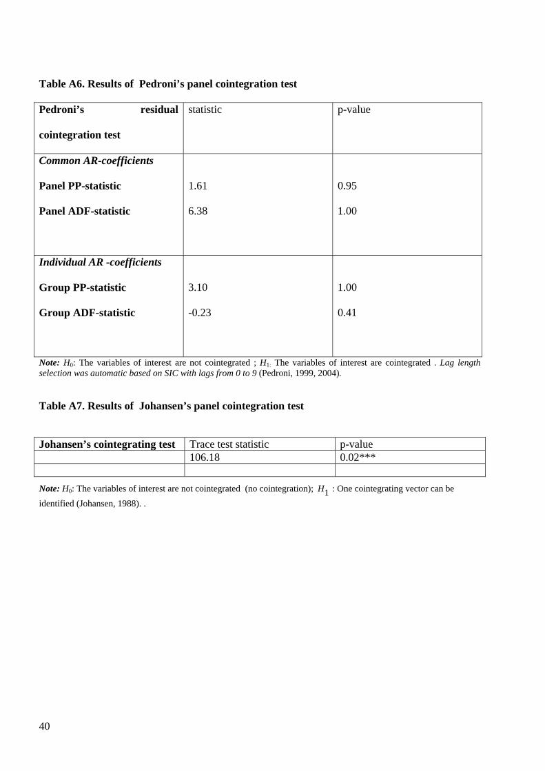
40
Table A6. Results of Pedroni’s panel cointegration test
Pedroni’s residual
cointegration test
statistic p-value
Common AR-coefficients
Panel PP-statistic
Panel ADF-statistic
1.61
6.38
0.95
1.00
Individual AR -coefficients
Group PP-statistic
Group ADF-statistic
3.10
-0.23
1.00
0.41
Note: H0: The variables of interest are not cointegrated ; H1: The variables of interest are cointegrated . Lag length selection was automatic based on SIC with lags from 0 to 9 (Pedroni, 1999, 2004). Table A7. Results of Johansen’s panel cointegration test
Johansen’s cointegrating test Trace test statistic p-value 106.18 0.02*** Note: H0: The variables of interest are not cointegrated (no cointegration); 1H : One cointegrating vector can be identified (Johansen, 1988). .

41
Technical Appendix
Estimated error terms are obtained by estimating Eq. (14) via DOLS in a first step. The extent of
autocorrelation of the disturbances ρ is then estimated via DOLS in a second step:
ititit uu ερ +⋅= −1 leading to ρ̂ . The third step involves the transformation of the variables (see
below). Note, that the transformation of the variables is driven by ρ̂ , the estimated coefficient of
autocorrelation of the disturbances. This transformation leads to new variables in soft first
differences (characterized by *) and a new error term *u that is uncorrelated to the error term of the
previous period.22
1ˆ* −⋅−= ititit uuu ρ
1* ˆ −⋅−= ititit LRYPOPLRYPOPLRYPOP ρ ;
1* ˆ −⋅−= ititit LPOPGPLUSLPOPGPLUSLPOPGPLUS ρ ;
1* ˆ −⋅−= ititit LSDOMYLSDOMYLSDOMY ρ ;
1* ˆ −⋅−= ititit LSEXTNYLSEXTNYLSEXTNY ρ ;
1* ˆ −⋅−= ititit LSNATYLSNATYLSNATY ρ ;
and then in a fourth step Equation (15*) is estimated by DOLS
***
**
*4
*3
*2
*1
*
itp
pmmitim
p
pmmitim
p
pm
p
pmmitimmii
ititititjit
uLSNATYLSEXTNY
LSDOMYLPOPGPLUS
LSNATYLSEXTNYLSDOMYLPOPGPLUSLRYPOPX
+∆+∆+
∆+∆+
++++=
∑∑
∑ ∑
−=−
−=−
−= −=−−
εφ
εδ
χχχχα
(15*)
22 In our case only first order autocorrelation was detected. However, also higher orders of autocorrelation reaching back two or more periods could be modeled.