Possible pitfalls in pressure transient analysis: Effect of ...

Vol.:(0123456789)1 3

Journal of Petroleum Exploration and Production Technology https://doi.org/10.1007/s13202-019-0701-2

ORIGINAL PAPER - PRODUCTION ENGINEERING

Possible pitfalls in pressure transient analysis: Effect of adjacent wells

Ali Mirzaalian Dastjerdi1 · Asgar Eyvazi Farab3 · Mohammad Sharifi2

Received: 10 January 2019 / Accepted: 28 May 2019 © The Author(s) 2019

AbstractWell testing is one of the important methods to provide information about the reservoir heterogeneity and boundary limits by analyzing reservoir dynamic responses. Despite the significance of well testing data, misinterpreted data can lead us to a wrong reservoir performance prediction. In this study, we focus on cases ignoring the adjacent well’s production history, which may lead to misinterpretation. The analysis was conducted on both homogeneous and naturally fractured reservoirs in infinite-acting and finite-acting conditions. The model includes two wells: one is “tested well” and the other is “adjacent one.” By studying different scenarios and focusing on derivative plots, it was perceived that both reservoir and boundary models might be misinterpreted. Additionally, in all cases, a sensitivity analysis was performed on parameters affecting interpretation process. Studying the literatures, few articles have focused on drawbacks during diagnostic plot interpretation and also the effect of adjacent wells. Hence, these issues were addressed. Overall, considering several cases it was proved that neglecting the production effect of adjacent wells causes wrong interpretation, and this should be avoided in all inter-pretation cases. Regarding the importance of reservoir characteristics and its flow regime, any wrong interpretation may create huge uncertainties in the reservoir development. As a result, this paper aimed to address the well testing, especially in brown fields where the production of other wells may affect the pressure response of the tested well; therefore, it will be pivotal to consider the effect of adjacent wells’ production history.

* Ali Mirzaalian Dastjerdi [email protected]

1 Sharif University of Technology, Tehran, Iran2 Amirkabir University of Technology, Tehran, Iran3 Tehran, Iran

http://crossmark.crossref.org/dialog/?doi=10.1007/s13202-019-0701-2&domain=pdf

Journal of Petroleum Exploration and Production Technology

1 3

Graphic abstract

Keywords Well testing · Production history · Adjacent wells · Pressure derivative · Misinterpretation

List of symbolsBo Formation volume factor, bbl/STBCt Total compressibility, 1/ψh Thickness, ftk Permeability, mdpi Initial reservoir pressure, ψpwf Wellbore flow pressure, ψQo Oil rate, STB/dayr Distance, ftt Time, hts Shut down time, h

Greek symbolsλ Dimensionless interporosity parameterμo Oil viscosity, cpω Dimensionless storativity ratioφ Porosity

Introduction

Well testing is divided into two types, constant rate (Dejam et al. 2018; Mashayekhizadeh et al. 2011) and constant pressure test (Dejam et al. 2017a, b). It is more common to design tests as constant rate, which in that case, the pressure transient is recorded. The numerical model is one of the technical advances for simulating pressure transient analysis (PTA). In recent years, numerical models have been utilized in order to analyze the well testing procedure not only for models with analytical and semi-analytical simulation, but also it can be applied for more elaborated cases. Numerical models can address the limitations of analytical approaches in modeling of complicated geometries and nonlinear dif-fusion terms in which the superposition of time and space does not work (Houze et al. 2008).

Conventional analysis just is usable with pressure versus time data, but sometimes it does not identify the correct flow regime. In well testing, the pressure variation is more significant than the pressure value itself (Bourdet 2002). So, Tiab and Kumar (1980a, b), and Bourdet (2002) addressed the issue of identifying the correct flow regime and choosing


1 3

the proper interpretation model. Bourdet and his co-authors proposed that it is much easier to recognize the flow regimes with analyzing pressure derivative versus time in log–log plots in comparison with conventional semilog pressure curves (Ahmed and McKinney 2011). The modern analy-sis defines the derivative term and interprets pressure and derivative data together.

Derivative plots are usually known as diagnostic plots. It is due to the fact that they identify different flow regimes and distinguish the reservoir model much easier. For example, interpretation of well testing results of a naturally fractured reservoir is carried out remarkably easier with the aid of pressure derivative (Cinco-Ley 1996). Interpreting of the transition period of naturally fractured reservoirs is an obsta-cle which many analyzers tackle with (Aguilera 1987; Feng et al. 2016; Seyedi et al. 2014). Many authors applied this period for different models of naturally fractured reservoirs and their corresponding pressure transient analyses pub-lished in the literature (Dejam et al. 2018; Aguilera 1987; Najurieta 1980; Warren and Root 1963; Odeh 1965; Kazemi 1969; Kazemi et al. 1969; de Swaan 1976; Aguilera and Song 1988; Kuchuk and Biryukov 2014; Al-Rbeawi 2017).Wang et al. examined the characteristics of the flow period in a multiple-fracture model by considering the features wellbore pressure and also analyzing the pressure-deriva-tive data (Xiaodong et al. 2014). Cinco and Ley reported that considering a naturally fractured reservoir and utiliz-ing the interference test results, it is impossible to carry out the characterization by regarding the transient pressure data solely (Cinco et al. 1976). Examining the pressure-derivative approach for highly permeable reservoirs demonstrated that this approach is suitable-adapted to this type of reservoirs (Clark and Golf-Racht 1985). Also, many papers investigate the behavior of pressure transient in fractured wells (Kou and Dejam 2018; Zhang et al. 2018). Iraj and Woodbury (1985) studied examples of possible pitfalls in the well test-ing analysis using pressure versus time data. In 2001, Al-Ghamdi et al. pointed out uncertainties in model selection by modern well testing interpretation. They expressed that in

pressure transient analysis, uncertainty associated with the non-uniqueness of model response can generally be summa-rized by the inability to identify the appropriate model and/or distinguish between similar patterns of pressure behavior (Al-Ghamdi and Issaka 2001). Also, some authors examine both the interpretation of diagnostic plots and their limita-tion for various reservoir models (Beauheim et al. 2004; Veneruso and Spath 2006; Renard et al. 2009; Engler and Tiab 1996).

Nearly all the published papers emphasize on the inter-pretation of models which only include one well, and this interpretation is done by using either wellbore pressure or pressure-derivative data. In this paper, we have scrutinized the models which include two wells. In other words, the effect of the other well’s production history on the interpre-tation of pressure responses was investigated.

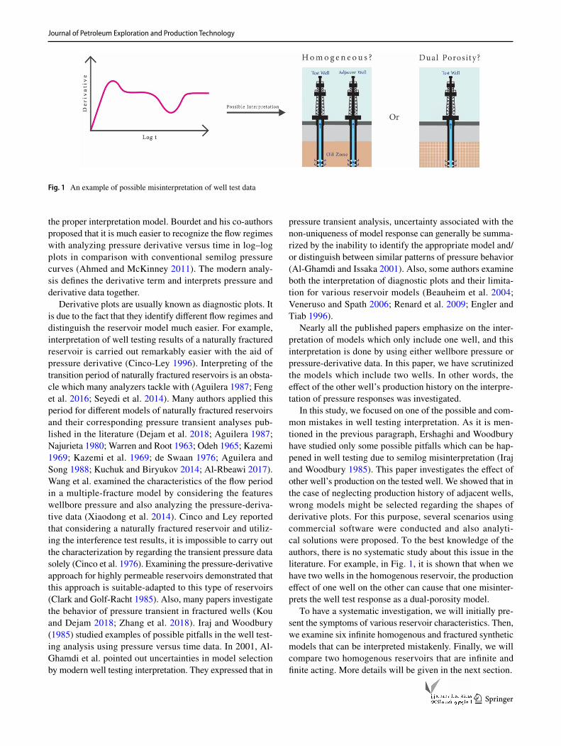
In this study, we focused on one of the possible and com-mon mistakes in well testing interpretation. As it is men-tioned in the previous paragraph, Ershaghi and Woodbury have studied only some possible pitfalls which can be hap-pened in well testing due to semilog misinterpretation (Iraj and Woodbury 1985). This paper investigates the effect of other well’s production on the tested well. We showed that in the case of neglecting production history of adjacent wells, wrong models might be selected regarding the shapes of derivative plots. For this purpose, several scenarios using commercial software were conducted and also analyti-cal solutions were proposed. To the best knowledge of the authors, there is no systematic study about this issue in the literature. For example, in Fig. 1, it is shown that when we have two wells in the homogenous reservoir, the production effect of one well on the other can cause that one misinter-prets the well test response as a dual-porosity model.

To have a systematic investigation, we will initially pre-sent the symptoms of various reservoir characteristics. Then, we examine six infinite homogenous and fractured synthetic models that can be interpreted mistakenly. Finally, we will compare two homogenous reservoirs that are infinite and finite acting. More details will be given in the next section.

Fig. 1 An example of possible misinterpretation of well test data


1 3

Various reservoirs characteristic symptoms

For drawdown tests, at every recorded drawdown pressure point, i.e., flowing time Δt and a corresponding bottom-hole flowing pressure (pwf), the pressure difference is calculated as follows:

The derivative is defined as:

The curve that is obtained from the pressure-derivative versus time data was originally utilized for diagnostic pur-pose and recognition of reservoir models. Each type of flow exhibits a specific trend on the derivative which represents an excellent diagnostic tool (Bourdet 2002).

As long as the wellbore storage effect is dominant, the pressure-derivative curve has the unit slope which is depicted as a straight line for all types of reservoirs (Bour-det 2002). For middle and late periods, reservoirs might be categorized as follows:

1. Homogenous reservoirs: The signature of these types of reservoirs in derivative curve is depicted as a horizontal straight line in transient flow regimes (Bourdet 2002; Cinco-Ley and Samaniego 1982). After the transient time, during the pseudo-steady-state flow since pres-sure varies linearly versus time, it is characterized on the pressure derivative by a straight line with the unit slope on log–log plot (Bourdet 2002). If buildup test is run, the derivative will go down. In the case that reservoir boundary is a constant pressure, the pressure derivative indicates a sharp plunge in the log–log representation corresponding to the pressure stabilization (Bourdet 2002). These mentioned signatures are only valid for a

(1)Δp = pi − pwf.

(2)(

dp

d ln t

)

= t

(

Δp

Δt

)

.

test which is run in a reservoir where there is no effect of nearby wells. If some other wells exist close to the test well, the production history of them can effect on the well test results. This occurrence may show itself as a similar signature to cases, which is explained above. In this paper, some of these tests are discussed.

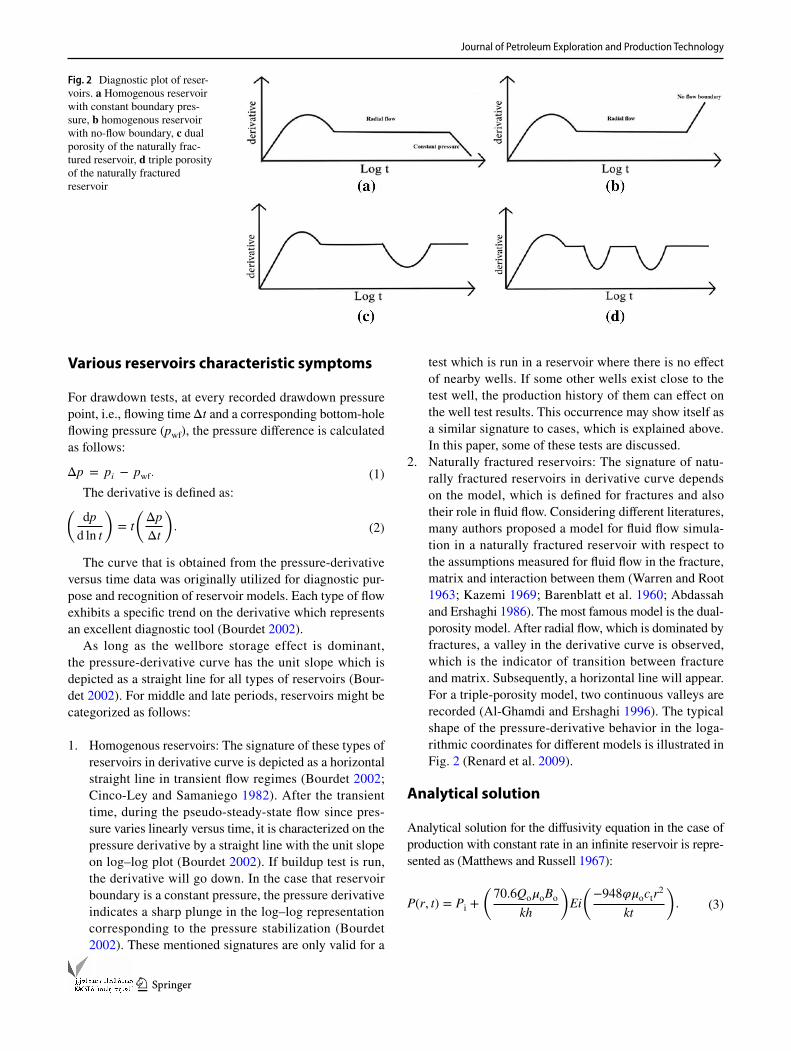
2. Naturally fractured reservoirs: The signature of natu-rally fractured reservoirs in derivative curve depends on the model, which is defined for fractures and also their role in fluid flow. Considering different literatures, many authors proposed a model for fluid flow simula-tion in a naturally fractured reservoir with respect to the assumptions measured for fluid flow in the fracture, matrix and interaction between them (Warren and Root 1963; Kazemi 1969; Barenblatt et al. 1960; Abdassah and Ershaghi 1986). The most famous model is the dual-porosity model. After radial flow, which is dominated by fractures, a valley in the derivative curve is observed, which is the indicator of transition between fracture and matrix. Subsequently, a horizontal line will appear. For a triple-porosity model, two continuous valleys are recorded (Al-Ghamdi and Ershaghi 1996). The typical shape of the pressure-derivative behavior in the loga-rithmic coordinates for different models is illustrated in Fig. 2 (Renard et al. 2009).

Analytical solution

Analytical solution for the diffusivity equation in the case of production with constant rate in an infinite reservoir is repre-sented as (Matthews and Russell 1967):

(3)P(r, t) = Pi +

(

70.6Qo�oBo

kh

)

Ei

(

−948��octr2

kt

)

.

Fig. 2 Diagnostic plot of reser-voirs. a Homogenous reservoir with constant boundary pres-sure, b homogenous reservoir with no-flow boundary, c dual porosity of the naturally frac-tured reservoir, d triple porosity of the naturally fractured reservoir


1 3

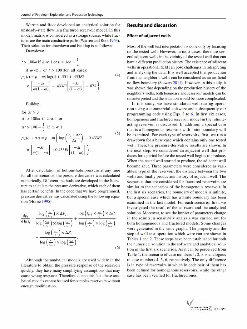
Warren and Root developed an analytical solution for unsteady-state flow in a fractured reservoir model. In this model, matrix is considered as a storage source, while frac-tures are the main conductive paths (Warren and Root 1963). Their solution for drawdown and buildup is as follows:

Drawdown:

Buildup:

After calculation of bottom-hole pressure at any time for all the scenarios, the pressure derivative was calculated numerically. Different methods are developed in the litera-ture to calculate the pressure derivative, which each of them has certain benefits. In the code that we have programmed, pressure derivative was calculated using the following equa-tion (Horne 1995):

Although the analytical models are used widely in the literature to obtain the pressure response of the reservoir quickly, they have many simplifying assumptions that may cause wrong response. Therefore, due to this fact, these ana-lytical models cannot be used for complex reservoirs without enough modification.

(4)

t > 100𝜔 if 𝜆 ≪ 1 or t > 1oo −1

𝜆

if 𝜔 ≪ 1 or t > 100 (for all cases)

pw(t) ≅ p − m{log(t) + .351 + .433Ei

×

[

−𝜆t

𝜔(1 − 𝜔)

]

− .433Ei

[

−𝜆t

(1 − 𝜔)

]

− .87S

}

.

(5)

for 𝜆t > 3

Δt > 100𝜔 if 𝜆 ≪ 1 or

Δt > 100 −1

𝜆if 𝜔 ≪ 1

pw(ts + Δt) ≅ p − m

{

log

(

ts + Δt

Δt

)

− 0.433Ei

×

[

−𝜆t

𝜔(1 − 𝜔)

]

+ 0.433Ei

[

−𝜆t

(1 − 𝜔)

]}

.

(6)

dpi

d ln ti=

log(

ti

ti−1

)

× ΔPi+1

log(

ti+1

ti

)

× log(

ti+1

ti−1

) +

log(

ti+1 ×ti−1

t2i

)

× ΔPi

log(

ti+1

ti

)

× log(

ti

ti−1

)

−

log(

ti+1

ti

)

× ΔPi

log(

ti

ti−1

)

× log(

ti+1

ti−1

) .

Results and discussion

Effect of adjacent wells

Most of the well test interpretation is done only by focusing on the tested well. However, in most cases, there are sev-eral adjacent wells in the vicinity of the tested well that can have a different production history. The existence of adjacent wells in operational field can pose challenges in interpreting and analyzing the data. It is well accepted that production from the neighbor’s wells can be considered as an artificial no-flow boundary (Stewart 2011). However, in this study, it was shown that depending on the production history of the neighbor’s wells, both boundary and reservoir models can be misinterpreted and the situation would be more complicated.

In this study, we have simulated well testing opera-tion using a commercial software and subsequently our programming code using Eqs. 3 to 6. In first six cases, homogenous and fractured reservoir model in the infinite-acting reservoir is discussed. In addition, a special case that is a homogenous reservoir with finite boundary will be examined. For each type of reservoirs, first, we run a drawdown for a base case which contains only one tested well. Then, the pressure-derivative results are shown. In the next step, we considered an adjacent well that pro-duces for a period before the tested well begins to produce. When the tested well started to produce, the adjacent well became shut. Three parameters were considered as vari-ables: type of the reservoir, the distance between the two wells and finally production history of adjacent well. The scenarios that are considered for fractured reservoirs are similar to the scenarios of the homogenous reservoir. In the first six scenarios, the boundary of models is infinite, but a special case which has a finite boundary has been examined in the last model. For each scenario, first, we investigated the result of the software and the analytical solution. Moreover, to see the impact of parameters change in the results, a sensitivity analysis was carried out for both homogeneous and fractured models. Some changes were generated in the same graphs. The property and the step of well test operation which were run are shown in Tables 1 and 2. These steps have been established for both the numerical solution in the software and analytical solu-tion in the first six scenarios. As it can be perceived from Table 1, the scenario of case numbers 1, 2, 3 is analogous to case numbers 4, 5, 6, respectively. The only difference is in type of reservoirs in which in each pair of them has been defined for homogenous reservoirs, while the other case has been verified for fractured ones.


1 3

Homogenous reservoir’s base case

This case is a homogeneous reservoir that has one tested well. This well begins to produce at the rate of 300 bbl/day

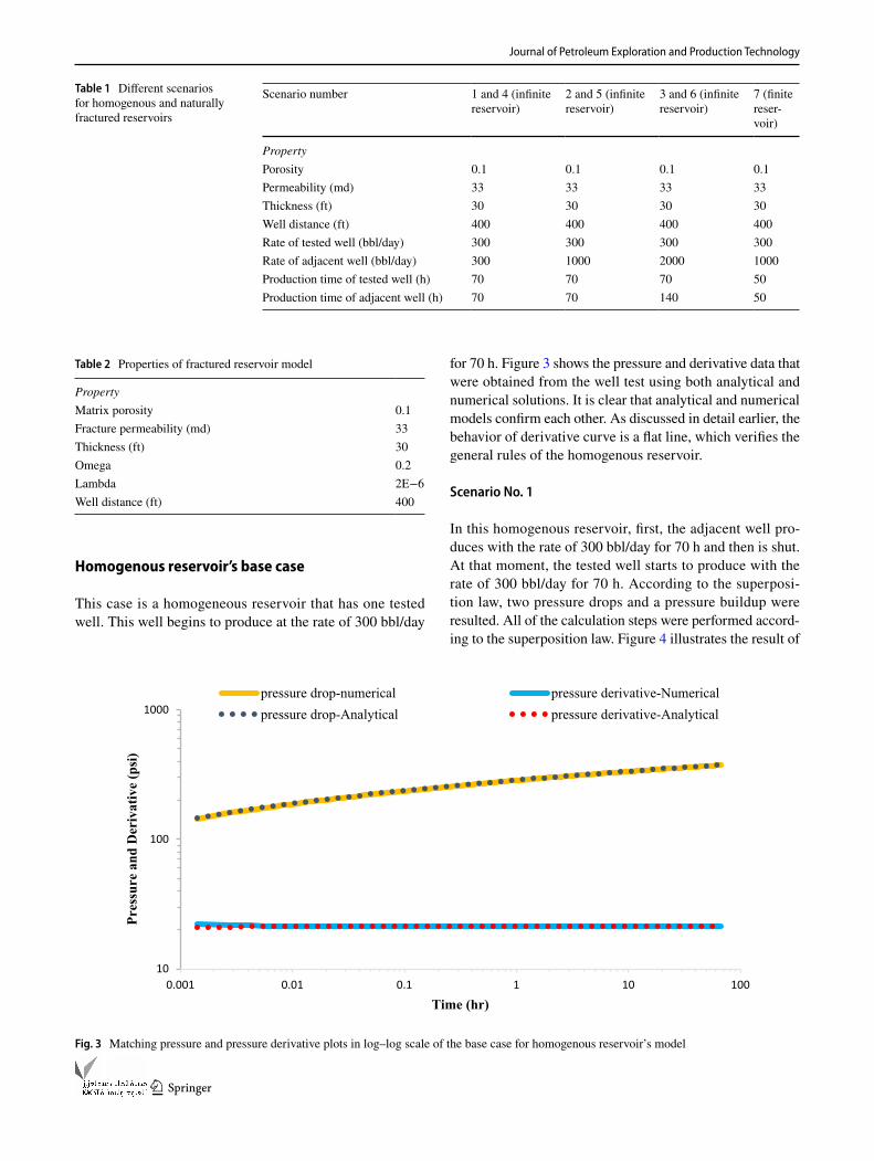
for 70 h. Figure 3 shows the pressure and derivative data that were obtained from the well test using both analytical and numerical solutions. It is clear that analytical and numerical models confirm each other. As discussed in detail earlier, the behavior of derivative curve is a flat line, which verifies the general rules of the homogenous reservoir.

Scenario No. 1

In this homogenous reservoir, first, the adjacent well pro-duces with the rate of 300 bbl/day for 70 h and then is shut. At that moment, the tested well starts to produce with the rate of 300 bbl/day for 70 h. According to the superposi-tion law, two pressure drops and a pressure buildup were resulted. All of the calculation steps were performed accord-ing to the superposition law. Figure 4 illustrates the result of

Table 1 Different scenarios for homogenous and naturally fractured reservoirs

Scenario number 1 and 4 (infinite reservoir)

2 and 5 (infinite reservoir)

3 and 6 (infinite reservoir)

7 (finite reser-voir)

PropertyPorosity 0.1 0.1 0.1 0.1Permeability (md) 33 33 33 33Thickness (ft) 30 30 30 30Well distance (ft) 400 400 400 400Rate of tested well (bbl/day) 300 300 300 300Rate of adjacent well (bbl/day) 300 1000 2000 1000Production time of tested well (h) 70 70 70 50Production time of adjacent well (h) 70 70 140 50

Table 2 Properties of fractured reservoir model

PropertyMatrix porosity 0.1Fracture permeability (md) 33Thickness (ft) 30Omega 0.2Lambda 2E−6Well distance (ft) 400

10

100

1000

0.001 0.01 0.1 1 10 100

Pres

sure

and

Der

ivat

ive

(psi)

Time (hr)

pressure drop-numerical pressure derivative-Numericalpressure drop-Analytical pressure derivative-Analytical

Fig. 3 Matching pressure and pressure derivative plots in log–log scale of the base case for homogenous reservoir’s model


1 3

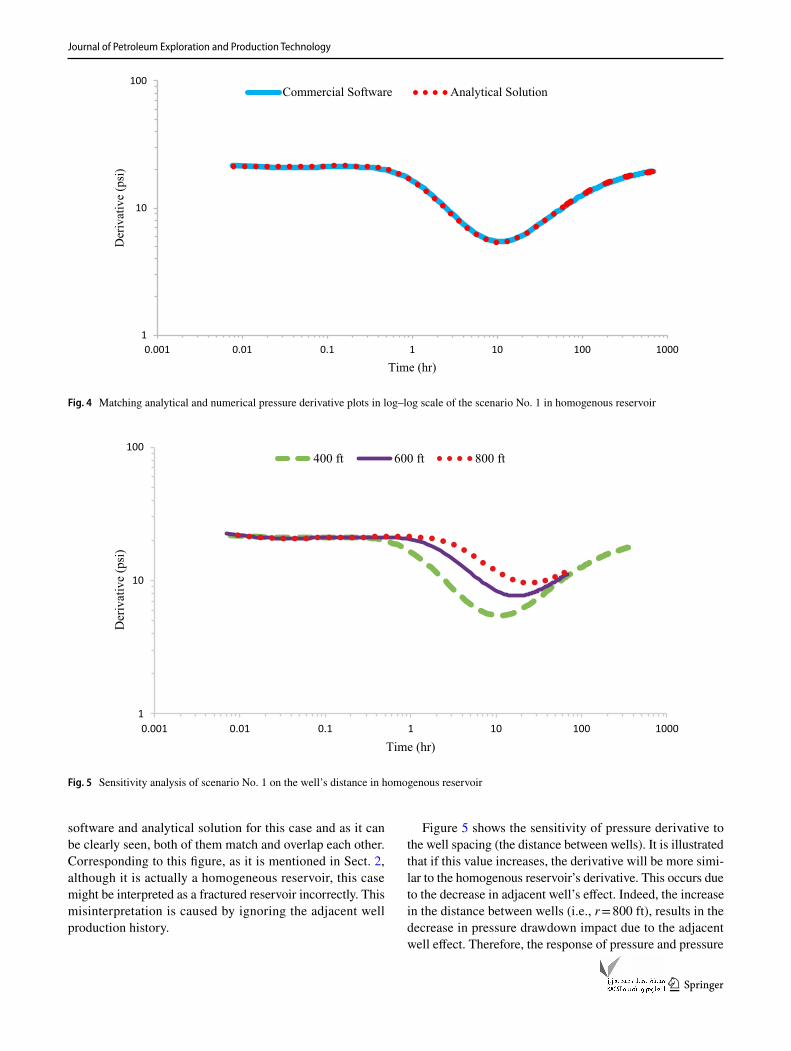
software and analytical solution for this case and as it can be clearly seen, both of them match and overlap each other. Corresponding to this figure, as it is mentioned in Sect. 2, although it is actually a homogeneous reservoir, this case might be interpreted as a fractured reservoir incorrectly. This misinterpretation is caused by ignoring the adjacent well production history.

Figure 5 shows the sensitivity of pressure derivative to the well spacing (the distance between wells). It is illustrated that if this value increases, the derivative will be more simi-lar to the homogenous reservoir’s derivative. This occurs due to the decrease in adjacent well’s effect. Indeed, the increase in the distance between wells (i.e., r = 800 ft), results in the decrease in pressure drawdown impact due to the adjacent well effect. Therefore, the response of pressure and pressure

1

10

100

0.001 0.01 0.1 1 10 100 1000

Der

ivat

ive

(psi

)

Time (hr)

Commercial Software Analytical Solution

Fig. 4 Matching analytical and numerical pressure derivative plots in log–log scale of the scenario No. 1 in homogenous reservoir

1

10

100

0.001 0.01 0.1 1 10 100 1000

Der

ivat

ive

(psi

)

Time (hr)

400 ft 600 ft 800 ft

Fig. 5 Sensitivity analysis of scenario No. 1 on the well’s distance in homogenous reservoir


1 3

derivative become more similar to a homogenous case. (The derivative shape is more flat.)

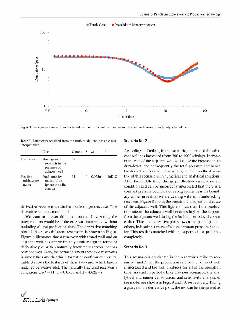
We want to answer this question that how wrong the interpretation would be if the case was interpreted without including all the production data. The derivative matching plot of these two different reservoirs is shown in Fig. 6. Figure 6 illustrates that a reservoir with tested well and an adjacent well has approximately similar sign in terms of derivative plot with a naturally fractured reservoir that has only one well. Also, the permeability of these two reservoirs is almost the same that this information confirms our results. Table 3 shows the features of these two cases which have a matched derivative plot. The naturally fractured reservoir’s conditions are k = 31, ω = 0.0556 and λ = 4.62E−8.

Scenario No. 2

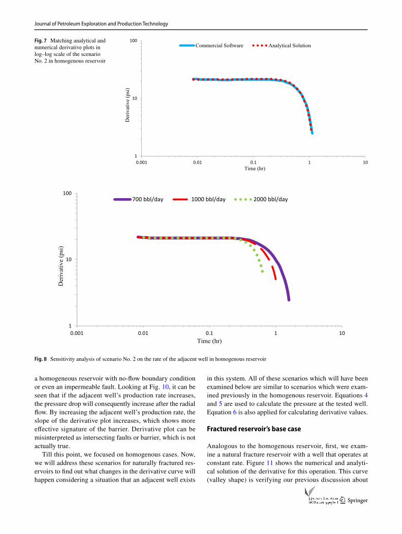
According to Table 1, in this scenario, the rate of the adja-cent well has increased (from 300 to 1000 stb/day). Increase in the rate of the adjacent well will cause the increase in its drawdown, and consequently the total pressure and hence the derivative form will change. Figure 7 shows the deriva-tive of this scenario with numerical and analytical solutions. After the middle time, this graph illustrates a steady-state condition and can be incorrectly interpreted that there is a constant pressure boundary or strong aquifer near the bound-ary while, in reality, we are dealing with an infinite-acting reservoir. Figure 8 shows the sensitivity analysis on the rate of the adjacent well. This figure shows that if the produc-tion rate of the adjacent well becomes higher, the support from the adjacent well during the buildup period will appear earlier. Thus, the derivative plot shows a sharper slope than others, indicating a more effective constant pressure behav-ior. This result is matched with the superposition principle completely.

Scenario No. 3

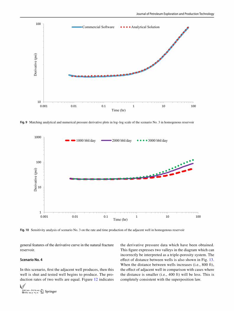
This scenario is conducted in the reservoir similar to sce-nario 1 and 2, but the production rate of the adjacent well is increased and the well produces for all of the operation time (no shut-in period). Like previous scenarios, the ana-lytical and numerical solutions and sensitivity analysis of the model are shown in Figs. 9 and 10, respectively. Taking a glance to the derivative plots, the test can be interpreted as

1

10

100

0.01 0.1 1 10 100

Der

ivat

ive

(psi

)

Time (hr)

Truth Case Possible misinterpretation

Fig. 6 Homogenous reservoir with a tested well and adjacent well and naturally fractured reservoir with only a tested well

Table 3 Parameters obtained from the truth model and possible mis-interpretation

Case K (md) S ω λ

Truth case Homogenous reservoir in the presence of adjacent well

33 0 – –

Possible misinterpre-tation

Dual-porosity model (if we ignore the adja-cent well)

31 0 0.0556 4.26E−8


1 3

a homogeneous reservoir with no-flow boundary condition or even an impermeable fault. Looking at Fig. 10, it can be seen that if the adjacent well’s production rate increases, the pressure drop will consequently increase after the radial flow. By increasing the adjacent well’s production rate, the slope of the derivative plot increases, which shows more effective signature of the barrier. Derivative plot can be misinterpreted as intersecting faults or barrier, which is not actually true.

Till this point, we focused on homogenous cases. Now, we will address these scenarios for naturally fractured res-ervoirs to find out what changes in the derivative curve will happen considering a situation that an adjacent well exists

in this system. All of these scenarios which will have been examined below are similar to scenarios which were exam-ined previously in the homogenous reservoir. Equations 4 and 5 are used to calculate the pressure at the tested well. Equation 6 is also applied for calculating derivative values.

Fractured reservoir’s base case

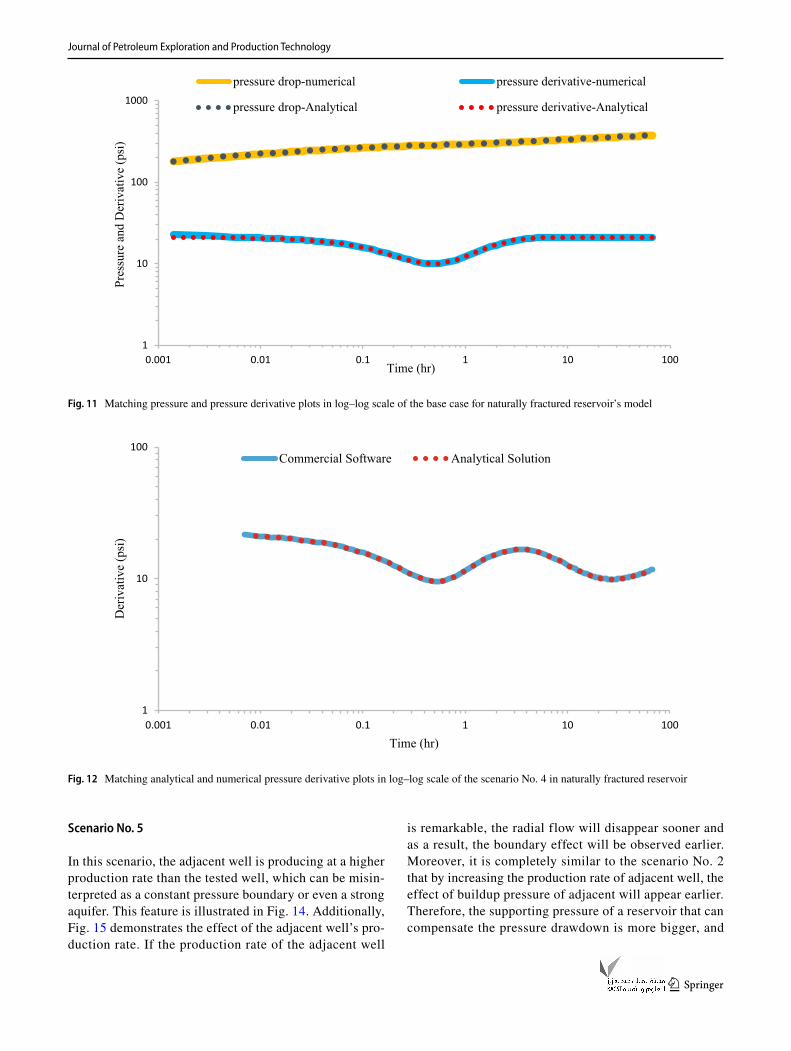
Analogous to the homogenous reservoir, first, we exam-ine a natural fracture reservoir with a well that operates at constant rate. Figure 11 shows the numerical and analyti-cal solution of the derivative for this operation. This curve (valley shape) is verifying our previous discussion about

Fig. 7 Matching analytical and numerical derivative plots in log–log scale of the scenario No. 2 in homogenous reservoir

1

10

100

0.001 0.01 0.1 1 10

Der

ivat

ive

(psi

)

Time (hr)


1

10

100

0.001 0.01 0.1 1 10

Der

ivat

ive

(psi

)

Time (hr)

700 bbl/day 1000 bbl/day 2000 bbl/day

Fig. 8 Sensitivity analysis of scenario No. 2 on the rate of the adjacent well in homogenous reservoir


1 3

general features of the derivative curve in the natural fracture reservoir.

Scenario No. 4

In this scenario, first the adjacent well produces, then this well is shut and tested well begins to produce. The pro-duction rates of two wells are equal. Figure 12 indicates

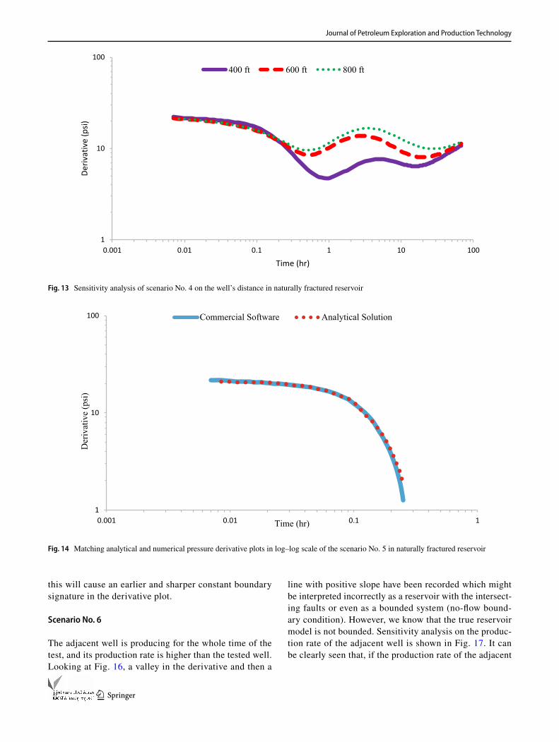
the derivative pressure data which have been obtained. This figure expresses two valleys in the diagram which can incorrectly be interpreted as a triple-porosity system. The effect of distance between wells is also shown in Fig. 13. When the distance between wells increases (i.e., 800 ft), the effect of adjacent well in comparison with cases where the distance is smaller (i.e., 400 ft) will be less. This is completely consistent with the superposition law.

10

100

0.001 0.01 0.1 1 10 100

Der

ivat

ive

(psi

)

Time (hr)


Fig. 9 Matching analytical and numerical pressure derivative plots in log–log scale of the scenario No. 3 in homogenous reservoir

1

10

100

1000

0.001 0.01 0.1 1 10 100

Der

ivat

ive

(psi

)

Time (hr)


Fig. 10 Sensitivity analysis of scenario No. 3 on the rate and time production of the adjacent well in homogenous reservoir


1 3

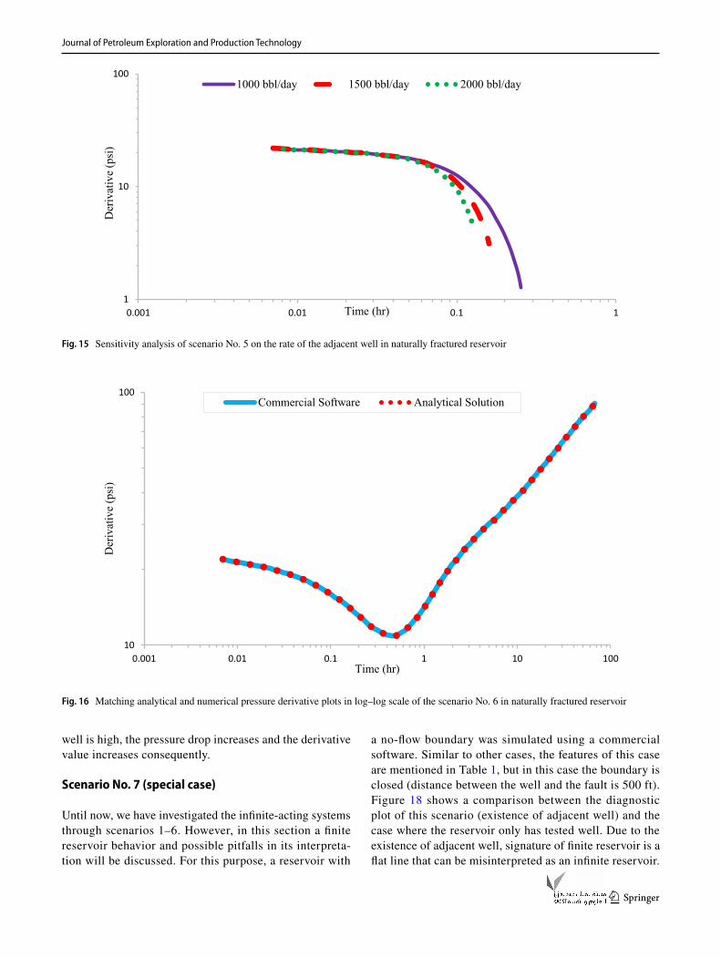
Scenario No. 5

In this scenario, the adjacent well is producing at a higher production rate than the tested well, which can be misin-terpreted as a constant pressure boundary or even a strong aquifer. This feature is illustrated in Fig. 14. Additionally, Fig. 15 demonstrates the effect of the adjacent well’s pro-duction rate. If the production rate of the adjacent well

is remarkable, the radial flow will disappear sooner and as a result, the boundary effect will be observed earlier. Moreover, it is completely similar to the scenario No. 2 that by increasing the production rate of adjacent well, the effect of buildup pressure of adjacent will appear earlier. Therefore, the supporting pressure of a reservoir that can compensate the pressure drawdown is more bigger, and

1

10

100

1000

0.001 0.01 0.1 1 10 100

Pres

sure

and

Der

ivat

ive

(psi

)

Time (hr)

pressure drop-numerical pressure derivative-numerical

pressure drop-Analytical pressure derivative-Analytical

Fig. 11 Matching pressure and pressure derivative plots in log–log scale of the base case for naturally fractured reservoir’s model

1

10

100

0.001 0.01 0.1 1 10 100

Der

ivat

ive

(psi

)

Time (hr)


Fig. 12 Matching analytical and numerical pressure derivative plots in log–log scale of the scenario No. 4 in naturally fractured reservoir


1 3

this will cause an earlier and sharper constant boundary signature in the derivative plot.

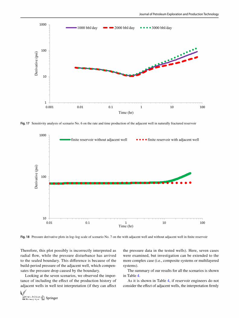
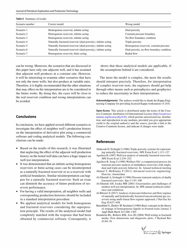
Scenario No. 6

The adjacent well is producing for the whole time of the test, and its production rate is higher than the tested well. Looking at Fig. 16, a valley in the derivative and then a

line with positive slope have been recorded which might be interpreted incorrectly as a reservoir with the intersect-ing faults or even as a bounded system (no-flow bound-ary condition). However, we know that the true reservoir model is not bounded. Sensitivity analysis on the produc-tion rate of the adjacent well is shown in Fig. 17. It can be clearly seen that, if the production rate of the adjacent

1

10

100

0.001 0.01 0.1 1 10 100

Der

ivat

ive

(psi

)

Time (hr)

400 ft 600 ft 800 ft

Fig. 13 Sensitivity analysis of scenario No. 4 on the well’s distance in naturally fractured reservoir

1

10

100

0.001 0.01 0.1 1

Der

ivat

ive

(psi

)

Time (hr)




1 3

well is high, the pressure drop increases and the derivative value increases consequently.

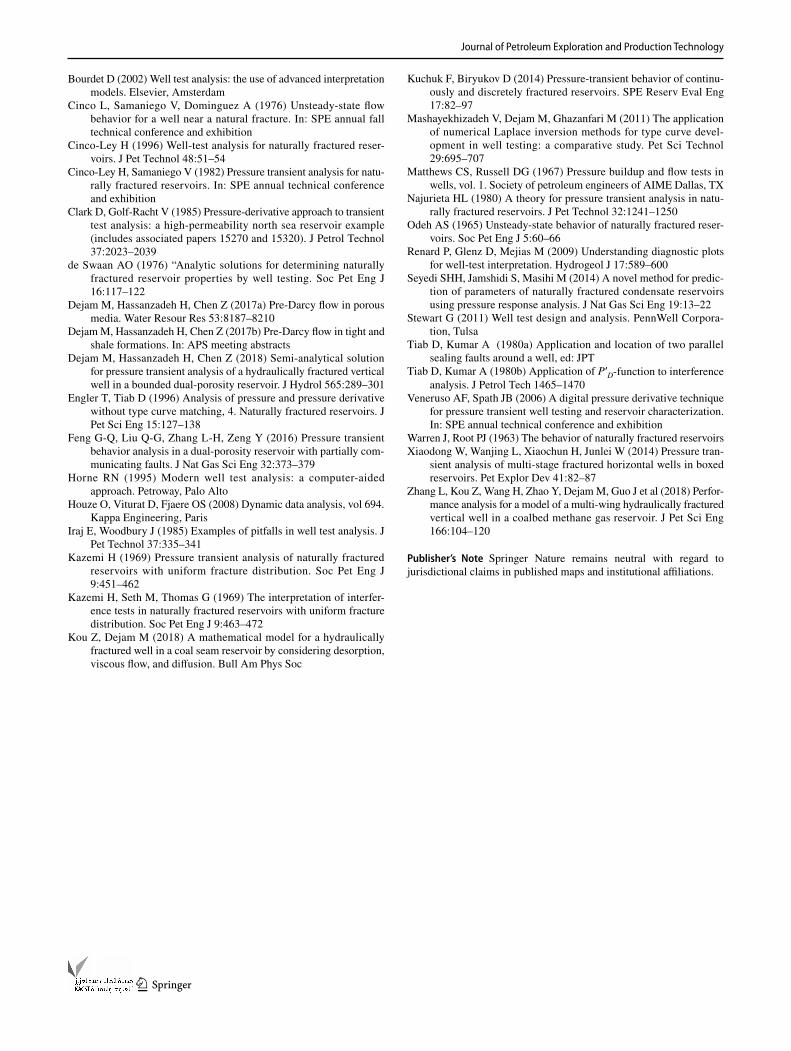
Scenario No. 7 (special case)

Until now, we have investigated the infinite-acting systems through scenarios 1–6. However, in this section a finite reservoir behavior and possible pitfalls in its interpreta-tion will be discussed. For this purpose, a reservoir with

a no-flow boundary was simulated using a commercial software. Similar to other cases, the features of this case are mentioned in Table 1, but in this case the boundary is closed (distance between the well and the fault is 500 ft). Figure 18 shows a comparison between the diagnostic plot of this scenario (existence of adjacent well) and the case where the reservoir only has tested well. Due to the existence of adjacent well, signature of finite reservoir is a flat line that can be misinterpreted as an infinite reservoir.

1

10

100

0.001 0.01 0.1 1

Der

ivat

ive

(psi

)

Time (hr)


Fig. 15 Sensitivity analysis of scenario No. 5 on the rate of the adjacent well in naturally fractured reservoir

10

100

0.001 0.01 0.1 1 10 100

Der

ivat

ive

(psi

)

Time (hr)




1 3

Therefore, this plot possibly is incorrectly interpreted as radial flow, while the pressure disturbance has arrived to the sealed boundary. This difference is because of the build-period pressure of the adjacent well, which compen-sates the pressure drop caused by the boundary.

Looking at the seven scenarios, we observed the impor-tance of including the effect of the production history of adjacent wells in well test interpretation (if they can affect

the pressure data in the tested wells). Here, seven cases were examined, but investigation can be extended to the more complex case (i.e., composite systems or multilayered systems).

The summary of our results for all the scenarios is shown in Table 4.

As it is shown in Table 4, if reservoir engineers do not consider the effect of adjacent wells, the interpretation firmly

1

10

100

1000

0.001 0.01 0.1 1 10 100

Der

ivat

ive

(psi

)

Time (hr)


Fig. 17 Sensitivity analysis of scenario No. 6 on the rate and time production of the adjacent well in naturally fractured reservoir

10

100

1000

0.01 0.1 1 10 100

Der

ivat

ive

(psi

)

Time (hr)

finite reservoir without adjacent well finite reservoir with adjacent well

Fig. 18 Pressure derivative plots in log–log scale of scenario No. 7 on the with adjacent well and without adjacent well in finite reservoir


1 3

can be wrong. Moreover, the scenarios that are discussed in this paper have only one adjacent well, and it has assumed that adjacent well produces at a constant rate. However, it will be interesting to examine other scenarios that have not only the more wells, but also produce at variable rates. Therefore, it is highly recommended that the other situations that may effect on the interpretation are to be considered in the future works. By doing this, the cases will be close to the real reservoir condition and wrong interpretations can be avoided.

Conclusions

In conclusion, we have applied several different scenarios to investigate the effect of neighbor well’s production history on the interpretation of derivative plot using a commercial software and coding analytical models. The following con-clusions can be made:

• Based on the results of this research, it was illustrated that neglecting the effect of the adjacent well production history on the tested well data can have a huge impact on well test interpretation.

• It was demonstrated that an infinite-acting homogenous reservoirs or finite-acting cases can be misinterpreted as a naturally fractured reservoir or as a reservoir with artificial boundaries. Similar misinterpretation can hap-pen for a naturally fractured reservoir. Such an issue can diminish the accuracy of future prediction of res-ervoir performance.

• For having a valid interpretation, all neighbor wells and corresponding production histories should be included in a standard interpretation procedure.

• We applied analytical models for both homogenous and fractured reservoirs considering the superposi-tion principle. The results of the analytical model had completely matched with the response that had been obtained by commercial software. Consequently, it

shows that these analytical models are applicable, if the assumptions behind it are considered.

The more the model is complex, the more the results should interpret precisely. Therefore, for interpretation of complex reservoir tests, the engineers should get help through other means such as petrophysics and geophysics to reduce the uncertainty in their interpretations.

Acknowledgements The authors would like to thank the Kappa Engi-neering Company for providing licensed Kappa workstation v5.10.0.

Open Access This article is distributed under the terms of the Crea-tive Commons Attribution 4.0 International License (http://creat iveco mmons .org/licen ses/by/4.0/), which permits unrestricted use, distribu-tion, and reproduction in any medium, provided you give appropriate credit to the original author(s) and the source, provide a link to the Creative Commons license, and indicate if changes were made.

References

Abdassah D, Ershaghi I (1986) Triple-porosity systems for represent-ing naturally fractured reservoirs. SPE Form Eval 1:113–127

Aguilera R (1987) Well test analysis of naturally fractured reservoirs. SPE Form Eval 2:239–252

Aguilera R, Song S (1988) Welltest-Nfr: a computerized process for transient pressure analysis of multiphase reservoirs with single, dual and triple porosity behavior. In: Annual technical meeting

Ahmed T, McKinney P (2011) Advanced reservoir engineering. Elsevier, Amsterdam

Al-Ghamdi A, Ershaghi I (1996) Pressure transient analysis of dually fractured reservoirs. Spe J 1:93–100

Al-Ghamdi AH, Issaka MB (2001) Uncertainties and challenges of modern well test interpretation. In: SPE annual technical confer-ence and exhibition

Al-Rbeawi S (2017) Analysis of pressure behaviors and flow regimes of naturally and hydraulically fractured unconventional gas res-ervoirs using multi-linear flow regimes approach. J Nat Gas Sci Eng 45:637–658

Barenblatt G, Zheltov IP, Kochina I (1960) Basic concepts in the theory of seepage of homogeneous liquids in fissured rocks [strata]. J Appl Math Mech 24:1286–1303

Beauheim RL, Roberts RM, Avis JD (2004) Well testing in fractured media: flow dimensions and diagnostic plots. J Hydraul Res 42:69–76

Table 4 Summary of results

Scenario number Correct model Wrong model

Scenario 1 Homogenous reservoir, infinite acting Dual porosityScenario 2 Homogenous reservoir, infinite acting Constant pressure boundaryScenario 3 Homogenous reservoir, infinite acting No-flow boundary conditionScenario 4 Naturally fractured reservoir (dual porosity), infinite acting Triple porosityScenario 5 Naturally fractured reservoir (dual porosity), infinite acting Homogenous reservoir, constant pressureScenario 6 Naturally fractured reservoir (dual porosity), infinite acting Dual porosity, no-flow boundary conditionScenario 7 Homogenous reservoir, finite acting Radial flow

http://creativecommons.org/licenses/by/4.0/

http://creativecommons.org/licenses/by/4.0/


1 3

Bourdet D (2002) Well test analysis: the use of advanced interpretation models. Elsevier, Amsterdam

Cinco L, Samaniego V, Dominguez A (1976) Unsteady-state flow behavior for a well near a natural fracture. In: SPE annual fall technical conference and exhibition

Cinco-Ley H (1996) Well-test analysis for naturally fractured reser-voirs. J Pet Technol 48:51–54

Cinco-Ley H, Samaniego V (1982) Pressure transient analysis for natu-rally fractured reservoirs. In: SPE annual technical conference and exhibition

Clark D, Golf-Racht V (1985) Pressure-derivative approach to transient test analysis: a high-permeability north sea reservoir example (includes associated papers 15270 and 15320). J Petrol Technol 37:2023–2039

de Swaan AO (1976) “Analytic solutions for determining naturally fractured reservoir properties by well testing. Soc Pet Eng J 16:117–122

Dejam M, Hassanzadeh H, Chen Z (2017a) Pre-Darcy flow in porous media. Water Resour Res 53:8187–8210

Dejam M, Hassanzadeh H, Chen Z (2017b) Pre-Darcy flow in tight and shale formations. In: APS meeting abstracts

Dejam M, Hassanzadeh H, Chen Z (2018) Semi-analytical solution for pressure transient analysis of a hydraulically fractured vertical well in a bounded dual-porosity reservoir. J Hydrol 565:289–301

Engler T, Tiab D (1996) Analysis of pressure and pressure derivative without type curve matching, 4. Naturally fractured reservoirs. J Pet Sci Eng 15:127–138

Feng G-Q, Liu Q-G, Zhang L-H, Zeng Y (2016) Pressure transient behavior analysis in a dual-porosity reservoir with partially com-municating faults. J Nat Gas Sci Eng 32:373–379

Horne RN (1995) Modern well test analysis: a computer-aided approach. Petroway, Palo Alto

Houze O, Viturat D, Fjaere OS (2008) Dynamic data analysis, vol 694. Kappa Engineering, Paris

Iraj E, Woodbury J (1985) Examples of pitfalls in well test analysis. J Pet Technol 37:335–341

Kazemi H (1969) Pressure transient analysis of naturally fractured reservoirs with uniform fracture distribution. Soc Pet Eng J 9:451–462

Kazemi H, Seth M, Thomas G (1969) The interpretation of interfer-ence tests in naturally fractured reservoirs with uniform fracture distribution. Soc Pet Eng J 9:463–472

Kou Z, Dejam M (2018) A mathematical model for a hydraulically fractured well in a coal seam reservoir by considering desorption, viscous flow, and diffusion. Bull Am Phys Soc

Kuchuk F, Biryukov D (2014) Pressure-transient behavior of continu-ously and discretely fractured reservoirs. SPE Reserv Eval Eng 17:82–97

Mashayekhizadeh V, Dejam M, Ghazanfari M (2011) The application of numerical Laplace inversion methods for type curve devel-opment in well testing: a comparative study. Pet Sci Technol 29:695–707

Matthews CS, Russell DG (1967) Pressure buildup and flow tests in wells, vol. 1. Society of petroleum engineers of AIME Dallas, TX

Najurieta HL (1980) A theory for pressure transient analysis in natu-rally fractured reservoirs. J Pet Technol 32:1241–1250

Odeh AS (1965) Unsteady-state behavior of naturally fractured reser-voirs. Soc Pet Eng J 5:60–66

Renard P, Glenz D, Mejias M (2009) Understanding diagnostic plots for well-test interpretation. Hydrogeol J 17:589–600

Seyedi SHH, Jamshidi S, Masihi M (2014) A novel method for predic-tion of parameters of naturally fractured condensate reservoirs using pressure response analysis. J Nat Gas Sci Eng 19:13–22

Stewart G (2011) Well test design and analysis. PennWell Corpora-tion, Tulsa

Tiab D, Kumar A (1980a) Application and location of two parallel sealing faults around a well, ed: JPT

Tiab D, Kumar A (1980b) Application of P′D-function to interference analysis. J Petrol Tech 1465–1470

Veneruso AF, Spath JB (2006) A digital pressure derivative technique for pressure transient well testing and reservoir characterization. In: SPE annual technical conference and exhibition

Warren J, Root PJ (1963) The behavior of naturally fractured reservoirsXiaodong W, Wanjing L, Xiaochun H, Junlei W (2014) Pressure tran-

sient analysis of multi-stage fractured horizontal wells in boxed reservoirs. Pet Explor Dev 41:82–87

Zhang L, Kou Z, Wang H, Zhao Y, Dejam M, Guo J et al (2018) Perfor-mance analysis for a model of a multi-wing hydraulically fractured vertical well in a coalbed methane gas reservoir. J Pet Sci Eng 166:104–120

Publisher’s Note Springer Nature remains neutral with regard to jurisdictional claims in published maps and institutional affiliations.

Possible pitfalls in pressure transient analysis: Effect of ...

Documents

Transcript of Possible pitfalls in pressure transient analysis: Effect of ...