materials

Article

In-Process Measurement for the Process Control of theReal-Time Manufacturing of Tapered Roller Bearings

Francisco Javier Brosed 1,*, A. Victor Zaera 2, Emilio Padilla 2, Fernando Cebrián 2 andJuan José Aguilar 1 ID

1 Design and Manufacturing Engineering Department, Universidad de Zaragoza, 3 María de Luna Street,Torres Quevedo Bld, 50018 Zaragoza, Spain; jaguilar@unizar.es

2 FERSA, 18 Bari Street-PLAZA, 50197 Zaragoza, Spain; victor.zaera@fersa.com (A.V.Z.);emilio.padilla@fersa.com (E.P.); fernando.cebrian@fersa.com (F.C.)

* Correspondence: fjbrosed@unizar.es; Tel.: +34-876-555-456

Received: 19 June 2018; Accepted: 2 August 2018; Published: 7 August 2018�����������������

Abstract: Tapered roller bearings can accommodate high radial loads as well as high axial loads.The manufacturing process consists of machining processes for ring and component assembly.In this contribution, the parameters of influence on the measurement procedure were studied.These parameters of influence were classified as environmental, process, and machine parameters.The main objective of this work was to optimize the process using real-time measurements, whichrequired the study of the influence of several parameters on the measurement uncertainty and howto correct their effects.

Keywords: in-process measurement; geometric accuracy; grinding process; tapered roller bearings

1. Introduction

Bearing manufacturing is a high-precision technology where the material composition, hardness,and micrometric dimensions need to be ensured to meet the product requirements [1,2].

The quality of the product is an important strategic factor for the competitiveness of the Europeanmanufacturing industry in the global market [3]. In this context, process control, automation, andoptimization are key to having the best quality at a competitive cost [4,5]. Process control ensuresquality and reduces scrap and rework, but requires dimensional measurements (the effect on thetemperature of the grinding process needs to be considered). Automation is the key to achievingcompetitive cost by using machines with enough accuracy and cycle time, and automatic adjustmentof the manufacturing process in real time. Current data collection and inspection technologies allowdata to be collected online along the process chain and can significantly increase quality controland improvements in current dynamic and modifiable environments [6,7]. The real challenge facingcompanies is the problem of synthesizing highly heterogeneous data to gain in-depth understandingof the correlations between the variables throughout the stages of a multi-stage system. This is aimedat achieving the generation of zero defects at the single process level, and the propagation of zerodefects at the system level through the proactive control of the process [8].

Tapered roller bearings can accommodate high radial loads as well as high axial loads. They havefour main components: inner ring, outer ring, rollers, and cage. In general and in the caseunder investigation, these components are metallic, although the cage can be plastic dependingon the application. The manufacturing process consists of the machining processes of rings andcomponent assembly. The expected quality standard needs to measure each individual part using anappropriate measurement instruments. These instruments have an uncertainty in their measurements.Ambient temperature, the temperature of the system, and the temperature of the part under inspection

Materials 2018, 11, 1371; doi:10.3390/ma11081371 www.mdpi.com/journal/materials

Materials 2018, 11, 1371 2 of 17

also influences the precision of the components and of the mounted bearing [9]. Different methodscan be used to measure the size of the parts: touch probes [10,11], air pressure [12,13], and lasersystems [14,15]. Most of the developments that can be found in the literature regarding bearinginspection are methods for fault diagnosis and service life estimation. Many experiments and studieshave been performed to explore the nature of bearing defects with the help of several monitoringtechniques such as vibration, acoustic emissions, oil-debris, ultrasound, electrostatic, shock-pulsemeasurements, etc. [1,16,17], although some of them estimate the size of the manufacturing defects oftapered roller bearings with vibration measurement [18].

As stated before, process optimization and online monitoring and control are key factors forimproving efficiency and quality in machining [19]. With the development of intelligent machining,the optimization of cutting process configuration during actual production has become more accessible,and optimizing the volume of removed metal by adjusting the grinding time for each part can decreasethe process time and improve tool life [20,21]. Finally, the grinding machine control system can receivethe measurement results of the machined part as feedback information for process verification.

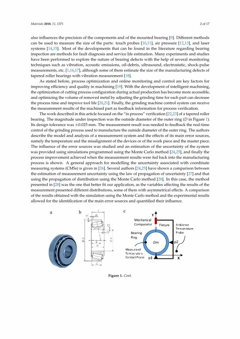
The work described in this article focused on the “in process” verification [22,23] of a tapered rollerbearing. The magnitude under inspection was the outside diameter of the outer ring (D in Figure 1).Its design tolerance was ±0.025 mm. The measurement result was needed to feedback the real-timecontrol of the grinding process used to manufacture the outside diameter of the outer ring. The authorsdescribe the model and analysis of a measurement system and the effects of its main error sources,namely the temperature and the misalignment of the devices or of the work piece and the master piece.The influence of the error sources was studied and an estimation of the uncertainty of the systemwas provided using simulations programmed using the Monte Carlo method [24,25], and finally theprocess improvement achieved when the measurement results were fed back into the manufacturingprocess is shown. A general approach for modelling the uncertainty associated with coordinatemeasuring systems (CMSs) is given in [26]. Several authors [24,25] have shown a comparison betweenthe estimation of measurement uncertainty using the law of propagation of uncertainty [27] and thatusing the propagation of distribution using the Monte Carlo method [28]. In this case, the methodpresented in [28] was the one that better fit our application, as the variables affecting the results of themeasurement presented different distributions, some of them with asymmetrical effects. A comparisonof the results obtained with the simulation using the Monte Carlo method and the experimental resultsallowed for the identification of the main error sources and quantified their influence.

Materials 2018, 11, x FOR PEER REVIEW 2 of 17

temperature, the temperature of the system, and the temperature of the part under inspection also influences the precision of the components and of the mounted bearing [9]. Different methods can be used to measure the size of the parts: touch probes [10,11], air pressure [12,13], and laser systems [14,15]. Most of the developments that can be found in the literature regarding bearing inspection are methods for fault diagnosis and service life estimation. Many experiments and studies have been performed to explore the nature of bearing defects with the help of several monitoring techniques such as vibration, acoustic emissions, oil-debris, ultrasound, electrostatic, shock-pulse measurements, etc. [1,16,17], although some of them estimate the size of the manufacturing defects of tapered roller bearings with vibration measurement [18].

As stated before, process optimization and online monitoring and control are key factors for improving efficiency and quality in machining [19]. With the development of intelligent machining, the optimization of cutting process configuration during actual production has become more accessible, and optimizing the volume of removed metal by adjusting the grinding time for each part can decrease the process time and improve tool life [20,21]. Finally, the grinding machine control system can receive the measurement results of the machined part as feedback information for process verification.

The work described in this article focused on the “in process” verification [22,23] of a tapered roller bearing. The magnitude under inspection was the outside diameter of the outer ring (D in Figure 1). Its design tolerance was ± 0.025 mm. The measurement result was needed to feedback the real-time control of the grinding process used to manufacture the outside diameter of the outer ring. The authors describe the model and analysis of a measurement system and the effects of its main error sources, namely the temperature and the misalignment of the devices or of the work piece and the master piece. The influence of the error sources was studied and an estimation of the uncertainty of the system was provided using simulations programmed using the Monte Carlo method [24,25], and finally the process improvement achieved when the measurement results were fed back into the manufacturing process is shown. A general approach for modelling the uncertainty associated with coordinate measuring systems (CMSs) is given in [26]. Several authors [24,25] have shown a comparison between the estimation of measurement uncertainty using the law of propagation of uncertainty [27] and that using the propagation of distribution using the Monte Carlo method [28]. In this case, the method presented in [28] was the one that better fit our application, as the variables affecting the results of the measurement presented different distributions, some of them with asymmetrical effects. A comparison of the results obtained with the simulation using the Monte Carlo method and the experimental results allowed for the identification of the main error sources and quantified their influence.

a b c

Figure 1. Cont.

Materials 2018, 11, 1371 3 of 17

Materials 2018, 11, x FOR PEER REVIEW 3 of 17

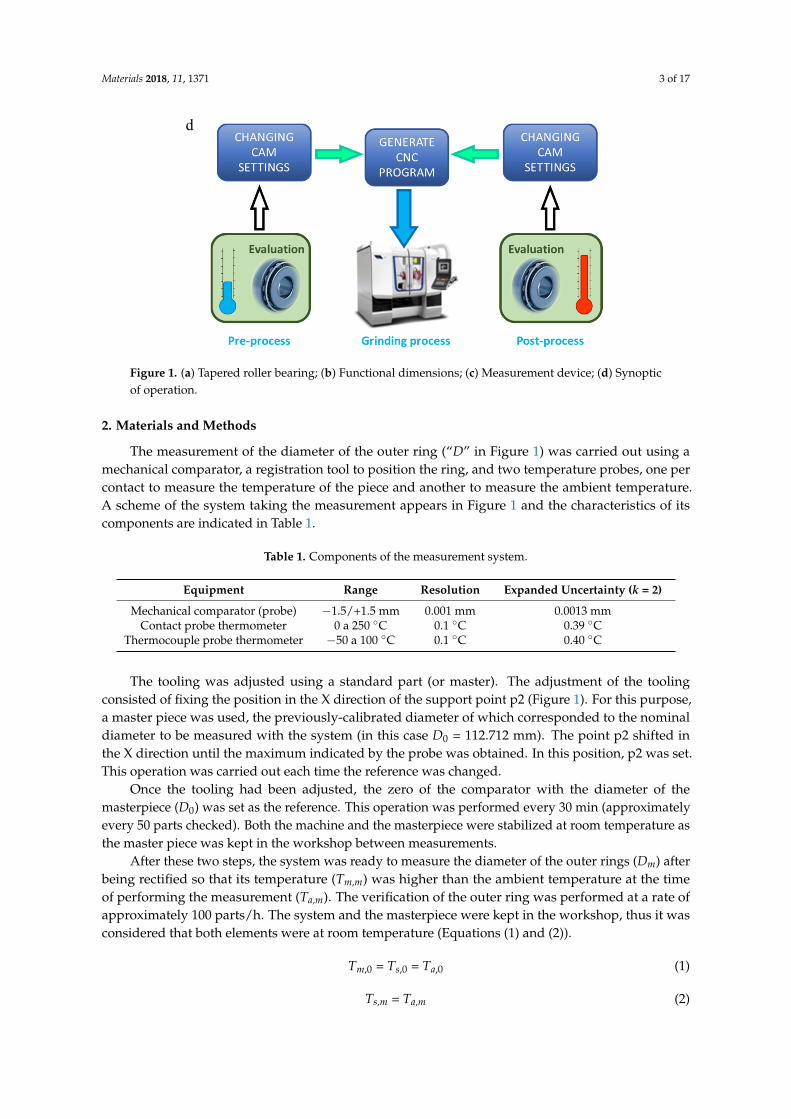
Figure 1. (a) Tapered roller bearing; (b) Functional dimensions; (c) Measurement device; (d) Synoptic of operation.

2. Materials and Methods

The measurement of the diameter of the outer ring (“D” in Figure 1) was carried out using a mechanical comparator, a registration tool to position the ring, and two temperature probes, one per contact to measure the temperature of the piece and another to measure the ambient temperature. A scheme of the system taking the measurement appears in Figure 1 and the characteristics of its components are indicated in Table 1.

Table 1. Components of the measurement system.

Equipment Range Resolution Expanded Uncertainty (k = 2) Mechanical comparator (probe) −1.5/+1.5 mm 0.001 mm 0.0013 mm

Contact probe thermometer 0 a 250 °C 0.1 °C 0.39 °C Thermocouple probe thermometer −50 a 100 °C 0.1 °C 0.40 °C

The tooling was adjusted using a standard part (or master). The adjustment of the tooling consisted of fixing the position in the X direction of the support point p2 (Figure 1). For this purpose, a master piece was used, the previously-calibrated diameter of which corresponded to the nominal diameter to be measured with the system (in this case D0 = 112.712 mm). The point p2 shifted in the X direction until the maximum indicated by the probe was obtained. In this position, p2 was set. This operation was carried out each time the reference was changed.

Once the tooling had been adjusted, the zero of the comparator with the diameter of the masterpiece (D0) was set as the reference. This operation was performed every 30 min (approximately every 50 parts checked). Both the machine and the masterpiece were stabilized at room temperature as the master piece was kept in the workshop between measurements.

After these two steps, the system was ready to measure the diameter of the outer rings (Dm) after being rectified so that its temperature (Tm,m) was higher than the ambient temperature at the time of performing the measurement (Ta,m). The verification of the outer ring was performed at a rate of approximately 100 parts/h. The system and the masterpiece were kept in the workshop, thus it was considered that both elements were at room temperature (Equations (1) and (2)).

Tm,0 = Ts,0 = Ta,0 (1)

Ts,m = Ta,m (2)

where Tx,t is the temperature of the ambience if x = a, of the system if x = s, and of the measured part if x = m. The temperature changes over time, thus Tx,t indicates the temperature at the moment of measuring the m-th part if t = m and at the time of measuring the master piece if t = 0.

d

Figure 1. (a) Tapered roller bearing; (b) Functional dimensions; (c) Measurement device; (d) Synopticof operation.

2. Materials and Methods

The measurement of the diameter of the outer ring (“D” in Figure 1) was carried out using amechanical comparator, a registration tool to position the ring, and two temperature probes, one percontact to measure the temperature of the piece and another to measure the ambient temperature.A scheme of the system taking the measurement appears in Figure 1 and the characteristics of itscomponents are indicated in Table 1.

Table 1. Components of the measurement system.

Equipment Range Resolution Expanded Uncertainty (k = 2)

Mechanical comparator (probe) −1.5/+1.5 mm 0.001 mm 0.0013 mmContact probe thermometer 0 a 250 ◦C 0.1 ◦C 0.39 ◦C

Thermocouple probe thermometer −50 a 100 ◦C 0.1 ◦C 0.40 ◦C

The tooling was adjusted using a standard part (or master). The adjustment of the toolingconsisted of fixing the position in the X direction of the support point p2 (Figure 1). For this purpose,a master piece was used, the previously-calibrated diameter of which corresponded to the nominaldiameter to be measured with the system (in this case D0 = 112.712 mm). The point p2 shifted inthe X direction until the maximum indicated by the probe was obtained. In this position, p2 was set.This operation was carried out each time the reference was changed.

Once the tooling had been adjusted, the zero of the comparator with the diameter of themasterpiece (D0) was set as the reference. This operation was performed every 30 min (approximatelyevery 50 parts checked). Both the machine and the masterpiece were stabilized at room temperature asthe master piece was kept in the workshop between measurements.

After these two steps, the system was ready to measure the diameter of the outer rings (Dm) afterbeing rectified so that its temperature (Tm,m) was higher than the ambient temperature at the timeof performing the measurement (Ta,m). The verification of the outer ring was performed at a rate ofapproximately 100 parts/h. The system and the masterpiece were kept in the workshop, thus it wasconsidered that both elements were at room temperature (Equations (1) and (2)).

Tm,0 = Ts,0 = Ta,0 (1)

Ts,m = Ta,m (2)

Materials 2018, 11, 1371 4 of 17

where Tx,t is the temperature of the ambience if x = a, of the system if x = s, and of the measured partif x = m. The temperature changes over time, thus Tx,t indicates the temperature at the moment ofmeasuring the m-th part if t = m and at the time of measuring the master piece if t = 0.

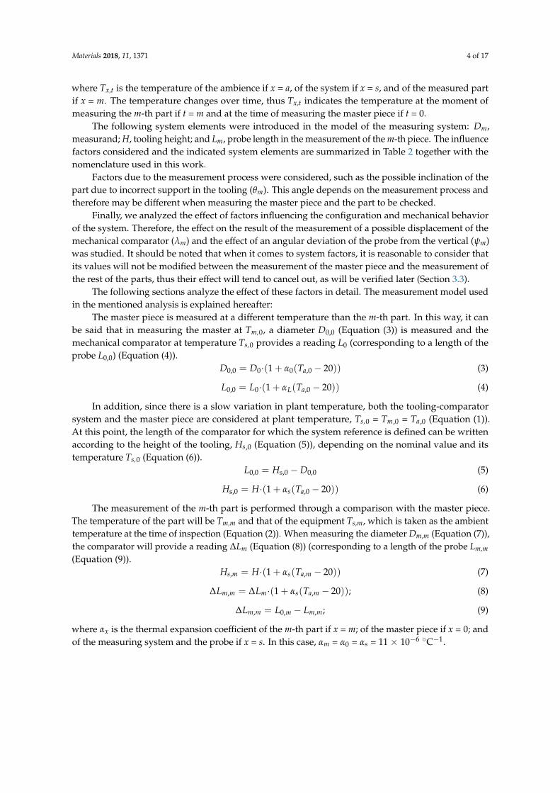
The following system elements were introduced in the model of the measuring system: Dm,measurand; H, tooling height; and Lm, probe length in the measurement of the m-th piece. The influencefactors considered and the indicated system elements are summarized in Table 2 together with thenomenclature used in this work.

Factors due to the measurement process were considered, such as the possible inclination of thepart due to incorrect support in the tooling (θm). This angle depends on the measurement process andtherefore may be different when measuring the master piece and the part to be checked.

Finally, we analyzed the effect of factors influencing the configuration and mechanical behaviorof the system. Therefore, the effect on the result of the measurement of a possible displacement of themechanical comparator (λm) and the effect of an angular deviation of the probe from the vertical (ψm)was studied. It should be noted that when it comes to system factors, it is reasonable to consider thatits values will not be modified between the measurement of the master piece and the measurement ofthe rest of the parts, thus their effect will tend to cancel out, as will be verified later (Section 3.3).

The following sections analyze the effect of these factors in detail. The measurement model usedin the mentioned analysis is explained hereafter:

The master piece is measured at a different temperature than the m-th part. In this way, it canbe said that in measuring the master at Tm,0, a diameter D0,0 (Equation (3)) is measured and themechanical comparator at temperature Ts,0 provides a reading L0 (corresponding to a length of theprobe L0,0) (Equation (4)).

D0,0 = D0·(1 + α0(Ta,0 − 20)) (3)

L0,0 = L0·(1 + αL(Ta,0 − 20)) (4)

In addition, since there is a slow variation in plant temperature, both the tooling-comparatorsystem and the master piece are considered at plant temperature, Ts,0 = Tm,0 = Ta,0 (Equation (1)).At this point, the length of the comparator for which the system reference is defined can be writtenaccording to the height of the tooling, Hs,0 (Equation (5)), depending on the nominal value and itstemperature Ts,0 (Equation (6)).

L0,0 = Hs,0 − D0,0 (5)

Hs,0 = H·(1 + αs(Ta,0 − 20)) (6)

The measurement of the m-th part is performed through a comparison with the master piece.The temperature of the part will be Tm,m and that of the equipment Ts,m, which is taken as the ambienttemperature at the time of inspection (Equation (2)). When measuring the diameter Dm,m (Equation (7)),the comparator will provide a reading ∆Lm (Equation (8)) (corresponding to a length of the probe Lm,m

(Equation (9)).Hs,m = H·(1 + αs(Ta,m − 20)) (7)

∆Lm,m = ∆Lm·(1 + αs(Ta,m − 20)); (8)

∆Lm,m = L0,m − Lm,m; (9)

where αx is the thermal expansion coefficient of the m-th part if x = m; of the master piece if x = 0; andof the measuring system and the probe if x = s. In this case, αm = α0 = αs = 11 × 10−6 ◦C−1.

Materials 2018, 11, 1371 5 of 17

Table 2. Factors influencing the measurement result and system elements. Nomenclature.

Influencing Factors Measurement System Elements (H, L, D)

T, temperature (◦C)

Tx,t t = m t = 0

H, tooling height (mm)

Hs,t

t = m t = 0

L, probe length (mm)

Lx,t t = m t = 0

D, measurand (mm)

Dx,t t = m t = 0

x = a Ta,m Ta,0 Hs,m Hs,0x = m Lm,m N.a. (1) x = m Dm,m N.a. (1)

x = s Ts,m Ts,0 x = 0 L0,m L0,0 x = 0 D0,m D0,0

x = m Tm,m Tm,0 H, tooling height at 20 ◦C Lt, probe length at 20 ◦C Dt, measurand at 20 ◦Cθt (◦) θm θ0

ψt (◦) ψm ψ0 - H - Lm L0 - Dm D0

λt (mm) λm λ0

x, parameter corresponding to the measurand, x = m; to the system, x = s; to the ambience, x = a; and to the master piece, particular case of measurand, x = 0. t, value of the parameterduring the measurement of the m-th part, t = m; and of the master piece, particularly in the case of measuring, t = 0. (1) N.a.: Not applicable.

Materials 2018, 11, 1371 6 of 17

Substituting Equation (9) into Equation (7) provides the dimension of the diameter (Equations (10)and (11)).

Dm,m = Hs,m − L0,m − ∆Lm,m (10)

Dm,m = Dm·(1 + αm(Tm,m − 20)); (11)

L0,m can be calculated by taking the reference each time the temperature changes (Equation (12)).Substituting Equation (12) into Equation (10), the part diameter from the master piece data and theprobe reading is calculated (Equation (13)).

L0,m = Hs,m − D0,m; with D0,m = D0·(1 + α0(Ta,m − 20)) (12)

Dm,m = Hs,m − Hs,m − D0,m − ∆Lm,m ⇒⇒ Dm,m = D0·(1 + α0(Ta,m − 20))− ∆Lm·(1 + αs(Ta,m − 20))

(13)

In the case of not measuring the reference when the temperature changes, it is possible to estimateL0,m (Equation (14)) and D0,m (Equation (15)), however, the result of Equations (13) and (15) will onlycoincide if the thermal expansion coefficients of the probe and the measurand coincide. In Figure 2,the error of Equation (15) calculated as Equations (15)–(13) is plotted when αs differs from αm.

L0,m = L0·(1 + αL(Ta,m − 20)) (14)

Dm,m = Hs,m − L0·(1 + α0(Ta,m − 20)) + ∆Lm·(1 + αs(Ta,m − 20)) (15)

Materials 2018, 11, x FOR PEER REVIEW 6 of 17

Substituting Equation (9) into Equation (7) provides the dimension of the diameter (Equations (10) and (11)).

, = , − , − , (10)

, = · 1 + ( , − 20) ; (11)

L0,m can be calculated by taking the reference each time the temperature changes (Equation (12)). Substituting Equation (12) into Equation (10), the part diameter from the master piece data and the probe reading is calculated (Equation (13)).

, = , − , ; with , = · 1 + ( , − 20) ; (12)

, = , − , − , − , ⇒⇒ , = · 1 + , − 20 − · 1 + ( , − 20) ; (13)

In the case of not measuring the reference when the temperature changes, it is possible to estimate L0,m (Equation (14)) and D0,m (Equation (15)), however, the result of Equations (13) and (15) will only coincide if the thermal expansion coefficients of the probe and the measurand coincide. In Figure 2, the error of Equation (15) calculated as Equations (15)–(13) is plotted when αs differs from αm.

, = · 1 + ( , − 20) (14)

, = , − · 1 + , − 20 + · 1 + ( , − 20) (15)

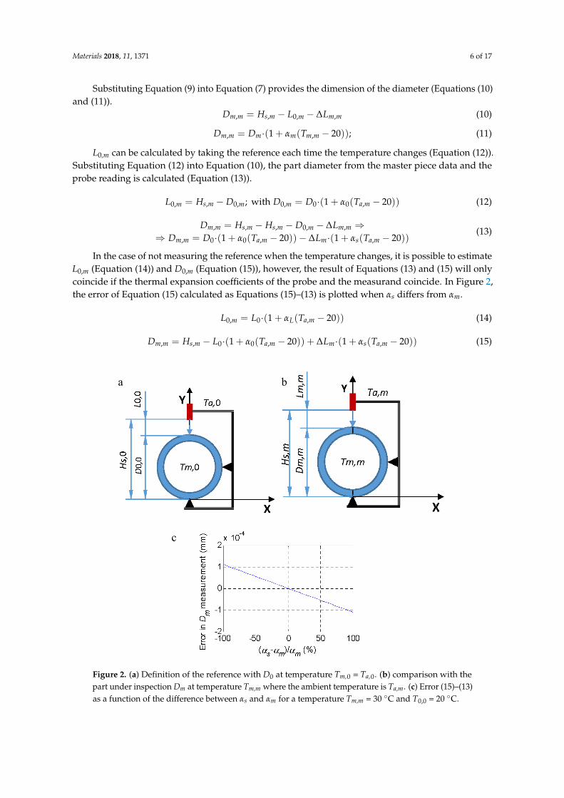
Figure 2. (a) Definition of the reference with D0 at temperature Tm,0 = Ta,0. (b) comparison with the part under inspection Dm at temperature Tm,m where the ambient temperature is Ta,m. (c) Error (15)–(13) as a function of the difference between αs and αm for a temperature Tm,m = 30 °C and T0,0 = 20 °C.

a b

c

Figure 2. (a) Definition of the reference with D0 at temperature Tm,0 = Ta,0. (b) comparison with thepart under inspection Dm at temperature Tm,m where the ambient temperature is Ta,m. (c) Error (15)–(13)as a function of the difference between αs and αm for a temperature Tm,m = 30 ◦C and T0,0 = 20 ◦C.

Materials 2018, 11, 1371 7 of 17

To obtain Dm, the mechanical comparator reading for the m-th part was compared with thereading taken when measuring D0, thus the result of the measurement (Dm at 20 ◦C) was obtainedfrom Equation (16).

Dm =H·(1 + αs(Ta,m − 20))− L0·(1 + αL(Ta,m − 20)) + ∆Lm·(1 + αL(Ta,m − 20))

1 + αm(Tm,m − 20)(16)

3. Results

3.1. Effect of Temperature on Measurement

The effect of the temperature in the process can be corrected using Equation (16), as thetemperature was known. However, if one of the process temperatures (the ambient temperatureor the temperature of the m-th part) was not known, the following situations could occur, as describedin Table 3.

Table 3. Cases if one or both of the temperature probes are not available. “1” means that the temperaturedata are available, “0” means that the temperature data are not available.

Diameter (eq.) Ta Tc ∆T for 0.025 mm Error (◦C)

Dm with ambient and contact thermometer (16) 1 1 Not applicableDm w/o contact thermometer 1 0 20.8Dm w/o ambient thermometer 0 1 19.6

Dm w/o any thermometer 0 0 19.6

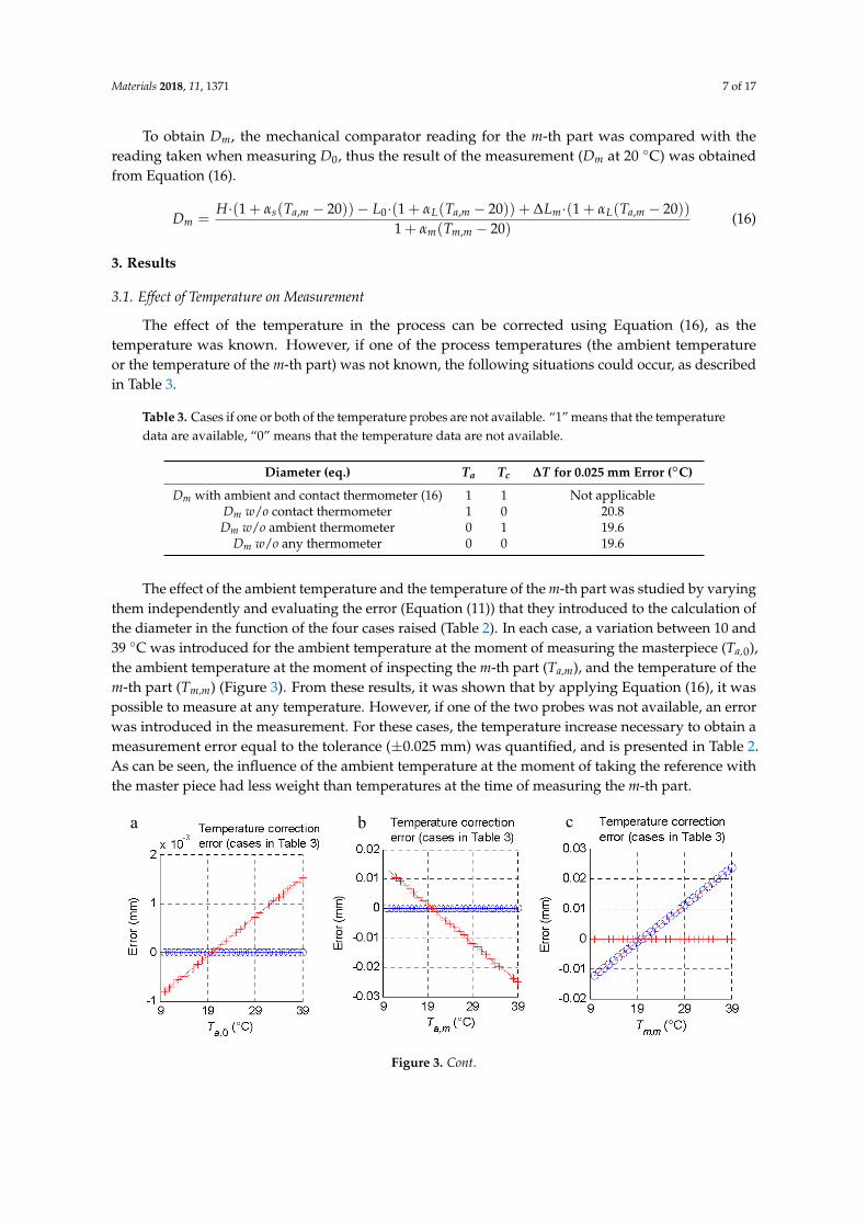
The effect of the ambient temperature and the temperature of the m-th part was studied by varyingthem independently and evaluating the error (Equation (11)) that they introduced to the calculation ofthe diameter in the function of the four cases raised (Table 2). In each case, a variation between 10 and39 ◦C was introduced for the ambient temperature at the moment of measuring the masterpiece (Ta,0),the ambient temperature at the moment of inspecting the m-th part (Ta,m), and the temperature of them-th part (Tm,m) (Figure 3). From these results, it was shown that by applying Equation (16), it waspossible to measure at any temperature. However, if one of the two probes was not available, an errorwas introduced in the measurement. For these cases, the temperature increase necessary to obtain ameasurement error equal to the tolerance (±0.025 mm) was quantified, and is presented in Table 2.As can be seen, the influence of the ambient temperature at the moment of taking the reference withthe master piece had less weight than temperatures at the time of measuring the m-th part.

Materials 2018, 11, x FOR PEER REVIEW 7 of 17

To obtain Dm, the mechanical comparator reading for the m-th part was compared with the reading taken when measuring D0, thus the result of the measurement (Dm at 20 °C) was obtained from Equation (16).

= · 1 + ( , − 20) − · 1 + , − 20 + · 1 + ( , − 20)1 + ( , − 20) (16)

3. Results

3.1. Effect of Temperature on Measurement

The effect of the temperature in the process can be corrected using Equation (16), as the temperature was known. However, if one of the process temperatures (the ambient temperature or the temperature of the m-th part) was not known, the following situations could occur, as described in Table 3.

Table 3. Cases if one or both of the temperature probes are not available. “1” means that the temperature data are available, “0” means that the temperature data are not available.

Diameter (eq.) Ta Tc ΔT for 0.025 mm Error (°C) Dm with ambient and contact thermometer (16) 1 1 Not applicable

Dm w/o contact thermometer 1 0 20.8 Dm w/o ambient thermometer 0 1 19.6

Dm w/o any thermometer 0 0 19.6

The effect of the ambient temperature and the temperature of the m-th part was studied by varying them independently and evaluating the error (Equation (11)) that they introduced to the calculation of the diameter in the function of the four cases raised (Table 2). In each case, a variation between 10 and 39 °C was introduced for the ambient temperature at the moment of measuring the masterpiece (Ta,0), the ambient temperature at the moment of inspecting the m-th part (Ta,m), and the temperature of the m-th part (Tm,m) (Figure 3). From these results, it was shown that by applying Equation (16), it was possible to measure at any temperature. However, if one of the two probes was not available, an error was introduced in the measurement. For these cases, the temperature increase necessary to obtain a measurement error equal to the tolerance (±0.025 mm) was quantified, and is presented in Table 2. As can be seen, the influence of the ambient temperature at the moment of taking the reference with the master piece had less weight than temperatures at the time of measuring the m-th part.

a b c

Figure 3. Cont.

Materials 2018, 11, 1371 8 of 17

Materials 2018, 11, x FOR PEER REVIEW 8 of 17

Figure 3. Temperature compensation depending on the measurement process: correction error of the cases described in Table 3 (the first case of Table 3 is the reference); (a) Effect of the ambient temperature variation at the moment of measuring the masterpiece (Ta,0). (b) Effect of the ambient temperature variation at the moment of inspecting the m-th part (Ta,m). (c) Effect of the temperature of the m-th part (Tm,m) variation. (d) Legend of the results from using each case of Table 3.

3.2. Effect of Process and Machine Factors on the Measurement

In this section, we analyzed the effect of the incorrect positioning of the part on the tooling (θm, process factor) and the effect of a possible deformation of the tooling-comparator system (λm displacement and rotation ψm, machine factors) (Figures 4 and 5).

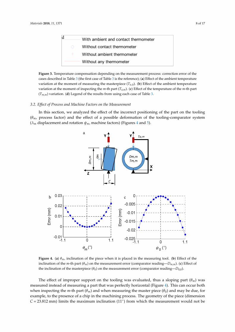
Figure 4. (a) θm, inclination of the piece when it is placed in the measuring tool. (b) Effect of the inclination of the m-th part (θm) on the measurement error (comparator reading—Dm,m). (c) Effect of the inclination of the masterpiece (θ0) on the measurement error (comparator reading—D0,0).

The effect of improper support on the tooling was evaluated, thus a sloping part (θm) was measured instead of measuring a part that was perfectly horizontal (Figure 4). This can occur both when inspecting the m-th part (θm) and when measuring the master piece (θ0) and may be due, for example, to the presence of a chip in the machining process. The geometry of the piece (dimension C = 23.812 mm) limits the maximum inclination (11°) from which the measurement would not be

With ambient and contact thermometer

Without contact thermometer

Without ambient thermometer

Without any thermometer

d

a

b c

Figure 3. Temperature compensation depending on the measurement process: correction error of thecases described in Table 3 (the first case of Table 3 is the reference); (a) Effect of the ambient temperaturevariation at the moment of measuring the masterpiece (Ta,0). (b) Effect of the ambient temperaturevariation at the moment of inspecting the m-th part (Ta,m). (c) Effect of the temperature of the m-th part(Tm,m) variation. (d) Legend of the results from using each case of Table 3.

3.2. Effect of Process and Machine Factors on the Measurement

In this section, we analyzed the effect of the incorrect positioning of the part on the tooling(θm, process factor) and the effect of a possible deformation of the tooling-comparator system(λm displacement and rotation ψm, machine factors) (Figures 4 and 5).

Materials 2018, 11, x FOR PEER REVIEW 8 of 17

Figure 3. Temperature compensation depending on the measurement process: correction error of the cases described in Table 3 (the first case of Table 3 is the reference); (a) Effect of the ambient temperature variation at the moment of measuring the masterpiece (Ta,0). (b) Effect of the ambient temperature variation at the moment of inspecting the m-th part (Ta,m). (c) Effect of the temperature of the m-th part (Tm,m) variation. (d) Legend of the results from using each case of Table 3.

3.2. Effect of Process and Machine Factors on the Measurement

In this section, we analyzed the effect of the incorrect positioning of the part on the tooling (θm, process factor) and the effect of a possible deformation of the tooling-comparator system (λm displacement and rotation ψm, machine factors) (Figures 4 and 5).

Figure 4. (a) θm, inclination of the piece when it is placed in the measuring tool. (b) Effect of the inclination of the m-th part (θm) on the measurement error (comparator reading—Dm,m). (c) Effect of the inclination of the masterpiece (θ0) on the measurement error (comparator reading—D0,0).

The effect of improper support on the tooling was evaluated, thus a sloping part (θm) was measured instead of measuring a part that was perfectly horizontal (Figure 4). This can occur both when inspecting the m-th part (θm) and when measuring the master piece (θ0) and may be due, for example, to the presence of a chip in the machining process. The geometry of the piece (dimension C = 23.812 mm) limits the maximum inclination (11°) from which the measurement would not be

With ambient and contact thermometer

Without contact thermometer

Without ambient thermometer

Without any thermometer

d

a

b c

Figure 4. (a) θm, inclination of the piece when it is placed in the measuring tool. (b) Effect of theinclination of the m-th part (θm) on the measurement error (comparator reading—Dm,m). (c) Effect ofthe inclination of the masterpiece (θ0) on the measurement error (comparator reading—D0,0).

The effect of improper support on the tooling was evaluated, thus a sloping part (θm) wasmeasured instead of measuring a part that was perfectly horizontal (Figure 4). This can occur bothwhen inspecting the m-th part (θm) and when measuring the master piece (θ0) and may be due, forexample, to the presence of a chip in the machining process. The geometry of the piece (dimensionC = 23.812 mm) limits the maximum inclination (11◦) from which the measurement would not be

Materials 2018, 11, 1371 9 of 17

possible. In the measurement process, a slope close to the indicated maximum would be visuallydetected, so the slope range studied was lower (± 1.1◦, Figure 4b,c).

Materials 2018, 11, x FOR PEER REVIEW 9 of 17

possible. In the measurement process, a slope close to the indicated maximum would be visually detected, so the slope range studied was lower (± 1.1°, Figure 4b,c).

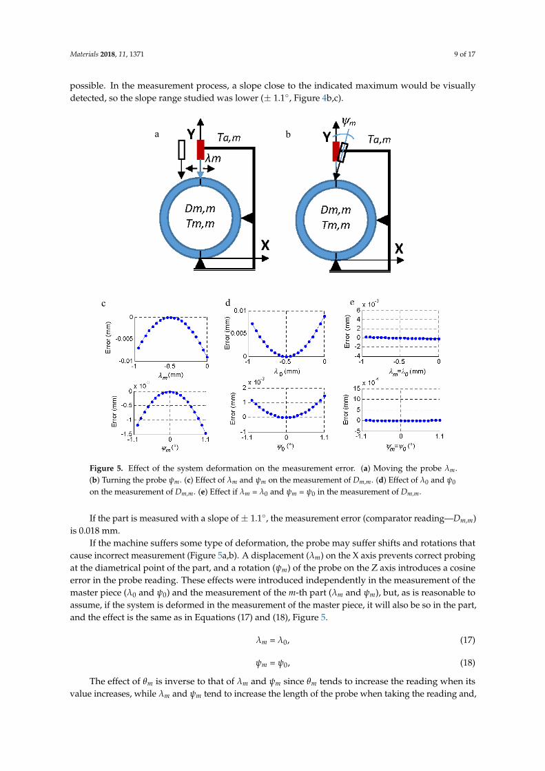
Figure 5. Effect of the system deformation on the measurement error. (a) Moving the probe λm. (b) Turning the probe ψm. (c) Effect of λm and ψm on the measurement of Dm,m. (d) Effect of λ0 and ψ0 on the measurement of Dm,m. (e) Effect if λm = λ0 and ψm = ψ0 in the measurement of Dm,m.

If the part is measured with a slope of ± 1.1°, the measurement error (comparator reading—Dm,m) is 0.018 mm.

If the machine suffers some type of deformation, the probe may suffer shifts and rotations that cause incorrect measurement (Figure 5a,b). A displacement (λm) on the X axis prevents correct probing at the diametrical point of the part, and a rotation (ψm) of the probe on the Z axis introduces a cosine error in the probe reading. These effects were introduced independently in the measurement of the master piece (λ0 and ψ0) and the measurement of the m-th part (λm and ψm), but, as is reasonable to assume, if the system is deformed in the measurement of the master piece, it will also be so in the part, and the effect is the same as in Equations (17) and (18), Figure 5.

λm = λ0, (17)

ψm = ψ0, (18)

The effect of θm is inverse to that of λm and ψm since θm tends to increase the reading when its value increases, while λm and ψm tend to increase the length of the probe when taking the reading and, therefore, reduce the diameter of the ring when they increase their value, as seen in Figure 5.

a b

c d e

Figure 5. Effect of the system deformation on the measurement error. (a) Moving the probe λm.(b) Turning the probe ψm. (c) Effect of λm and ψm on the measurement of Dm,m. (d) Effect of λ0 and ψ0

on the measurement of Dm,m. (e) Effect if λm = λ0 and ψm = ψ0 in the measurement of Dm,m.

If the part is measured with a slope of ± 1.1◦, the measurement error (comparator reading—Dm,m)is 0.018 mm.

If the machine suffers some type of deformation, the probe may suffer shifts and rotations thatcause incorrect measurement (Figure 5a,b). A displacement (λm) on the X axis prevents correct probingat the diametrical point of the part, and a rotation (ψm) of the probe on the Z axis introduces a cosineerror in the probe reading. These effects were introduced independently in the measurement of themaster piece (λ0 and ψ0) and the measurement of the m-th part (λm and ψm), but, as is reasonable toassume, if the system is deformed in the measurement of the master piece, it will also be so in the part,and the effect is the same as in Equations (17) and (18), Figure 5.

λm = λ0, (17)

ψm = ψ0, (18)

The effect of θm is inverse to that of λm and ψm since θm tends to increase the reading when itsvalue increases, while λm and ψm tend to increase the length of the probe when taking the reading and,

Materials 2018, 11, 1371 10 of 17

therefore, reduce the diameter of the ring when they increase their value, as seen in Figure 5. The effectof λm and ψm tends to be canceled when their values are the same at the time of measurement of themaster piece and at the time of measurement of the rest of the parts (Equations (17) and (18), Figure 5e).

3.3. Estimation of the Uncertainty and Contribution of Each Parameter

Simulations were programmed using the Monte Carlo method [24,25] to determine thecontribution of each parameter to the final uncertainty. The probability density distributions (PDD) ofeach factor were defined based on its calibration data or the characteristics of the process. The PDDsassociated with the measurement equipment, such as temperature probes or the mechanical comparator,were defined based on their measurement uncertainty. The PDDs associated with the process or toolingfactors were defined from a uniform distribution where the limit values were defined from the analysisperformed in Section 3 and according to the process and characteristics of the tooling (Table 4).

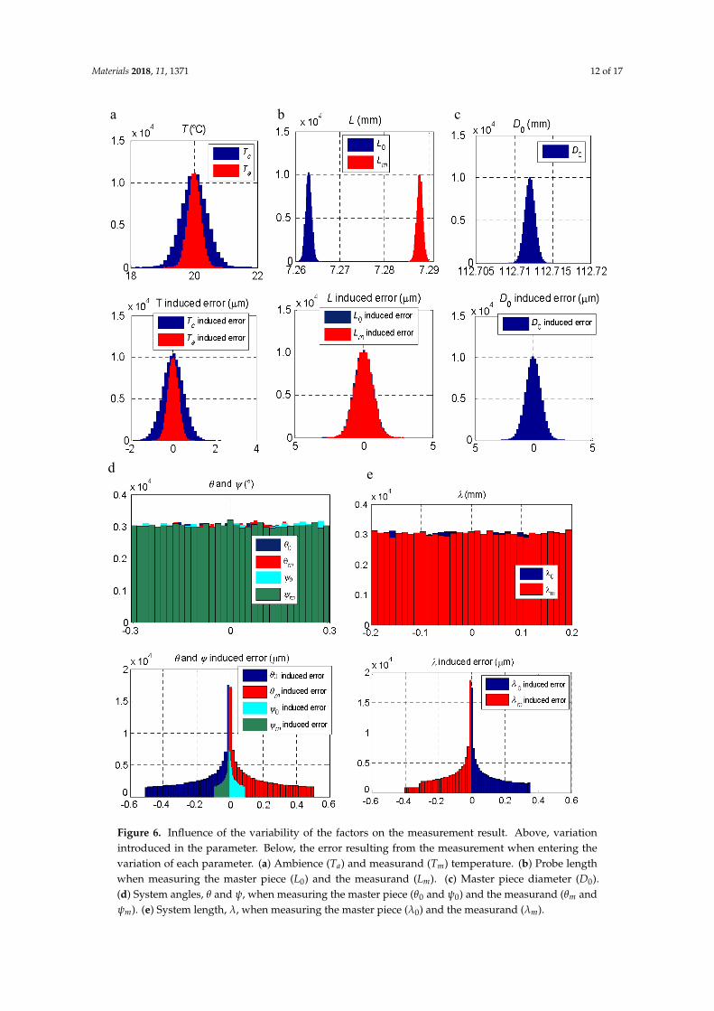
A simulation of the effect of each parameter was carried out by introducing the PDDs indicatedin Table 4. The results of the simulation of the effect of each parameter are shown in Figure 6, wherethe distribution of the error in the measurement resulting from the variation of the parameter below itare presented.

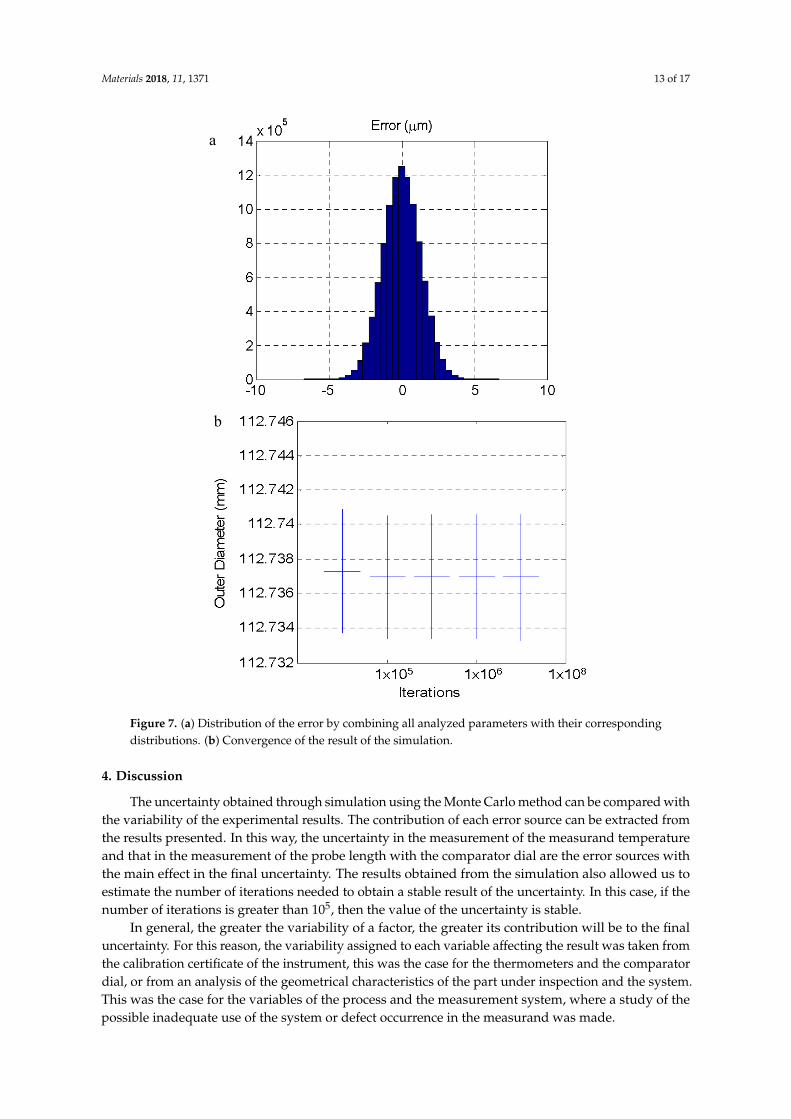
Simulation using the Monte Carlo method allows for the estimation of the value of themeasurement uncertainty according to the “Guide to the expression of uncertainty in measurement”(GUM) and its supplement 1 [28] from the PDD of the influence factors. From the simulation shownin Figure 7, the uncertainty values shown in Table 4 were obtained as a function of the parameterthat introduced the variation. At the end of Table 4, the uncertainty obtained when combining thevariation of all the factors appeared. The distribution of the error by combining all the factors is shownin Figure 8 together with the evolution of the results of the uncertainty estimated as a function of thenumber of iterations used. The result stabilized from 105 iterations. Other authors [24,29,30] haveobserved a similar number of iterations to obtain a stabilized result with simulation using the MonteCarlo method.

Materials 2018, 11, 1371 11 of 17

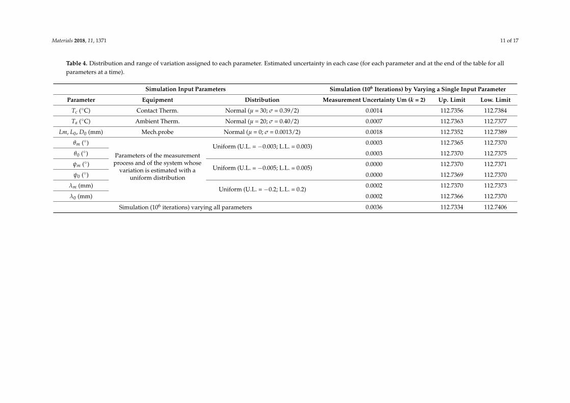
Table 4. Distribution and range of variation assigned to each parameter. Estimated uncertainty in each case (for each parameter and at the end of the table for allparameters at a time).

Simulation Input Parameters Simulation (106 Iterations) by Varying a Single Input Parameter

Parameter Equipment Distribution Measurement Uncertainty Um (k = 2) Up. Limit Low. Limit

Tc (◦C) Contact Therm. Normal (µ = 30; σ = 0.39/2) 0.0014 112.7356 112.7384

Ta (◦C) Ambient Therm. Normal (µ = 20; σ = 0.40/2) 0.0007 112.7363 112.7377

Lm, L0, D0 (mm) Mech.probe Normal (µ = 0; σ = 0.0013/2) 0.0018 112.7352 112.7389

θm (◦)

Parameters of the measurementprocess and of the system whose

variation is estimated with auniform distribution

Uniform (U.L. = −0.003; L.L. = 0.003)0.0003 112.7365 112.7370

θ0 (◦) 0.0003 112.7370 112.7375

ψm (◦)Uniform (U.L. = −0.005; L.L. = 0.005)

0.0000 112.7370 112.7371

ψ0 (◦) 0.0000 112.7369 112.7370

λm (mm)Uniform (U.L. = −0.2; L.L. = 0.2)

0.0002 112.7370 112.7373

λ0 (mm) 0.0002 112.7366 112.7370

Simulation (106 iterations) varying all parameters 0.0036 112.7334 112.7406

Materials 2018, 11, 1371 12 of 17Materials 2018, 11, x FOR PEER REVIEW 12 of 17

Figure 6. Influence of the variability of the factors on the measurement result. Above, variation introduced in the parameter. Below, the error resulting from the measurement when entering the variation of each parameter. (a) Ambience (Ta) and measurand (Tm) temperature. (b) Probe length when measuring the master piece (L0) and the measurand (Lm). (c) Master piece diameter (D0). (d) System angles, θ and ψ, when measuring the master piece (θ0 and ψ0) and the measurand (θm and ψm). (e) System length, λ, when measuring the master piece (λ0) and the measurand (λm).

a b c

d e

Figure 6. Influence of the variability of the factors on the measurement result. Above, variationintroduced in the parameter. Below, the error resulting from the measurement when entering thevariation of each parameter. (a) Ambience (Ta) and measurand (Tm) temperature. (b) Probe lengthwhen measuring the master piece (L0) and the measurand (Lm). (c) Master piece diameter (D0).(d) System angles, θ and ψ, when measuring the master piece (θ0 and ψ0) and the measurand (θm andψm). (e) System length, λ, when measuring the master piece (λ0) and the measurand (λm).

Materials 2018, 11, 1371 13 of 17Materials 2018, 11, x FOR PEER REVIEW 13 of 17

.

Figure 7. (a) Distribution of the error by combining all analyzed parameters with their corresponding distributions. (b) Convergence of the result of the simulation.

4. Discussion

The uncertainty obtained through simulation using the Monte Carlo method can be compared with the variability of the experimental results. The contribution of each error source can be extracted from the results presented. In this way, the uncertainty in the measurement of the measurand temperature and that in the measurement of the probe length with the comparator dial are the error sources with the main effect in the final uncertainty. The results obtained from the simulation also allowed us to estimate the number of iterations needed to obtain a stable result of the uncertainty. In this case, if the number of iterations is greater than 105, then the value of the uncertainty is stable.

In general, the greater the variability of a factor, the greater its contribution will be to the final uncertainty. For this reason, the variability assigned to each variable affecting the result was taken from the calibration certificate of the instrument, this was the case for the thermometers and the comparator dial, or from an analysis of the geometrical characteristics of the part under inspection and the system. This was the case for the variables of the process and the measurement system, where a study of the possible inadequate use of the system or defect occurrence in the measurand was made.

a

b

Figure 7. (a) Distribution of the error by combining all analyzed parameters with their correspondingdistributions. (b) Convergence of the result of the simulation.

4. Discussion

The uncertainty obtained through simulation using the Monte Carlo method can be compared withthe variability of the experimental results. The contribution of each error source can be extracted fromthe results presented. In this way, the uncertainty in the measurement of the measurand temperatureand that in the measurement of the probe length with the comparator dial are the error sources withthe main effect in the final uncertainty. The results obtained from the simulation also allowed us toestimate the number of iterations needed to obtain a stable result of the uncertainty. In this case, if thenumber of iterations is greater than 105, then the value of the uncertainty is stable.

In general, the greater the variability of a factor, the greater its contribution will be to the finaluncertainty. For this reason, the variability assigned to each variable affecting the result was taken fromthe calibration certificate of the instrument, this was the case for the thermometers and the comparatordial, or from an analysis of the geometrical characteristics of the part under inspection and the system.This was the case for the variables of the process and the measurement system, where a study of thepossible inadequate use of the system or defect occurrence in the measurand was made.

Materials 2018, 11, 1371 14 of 17

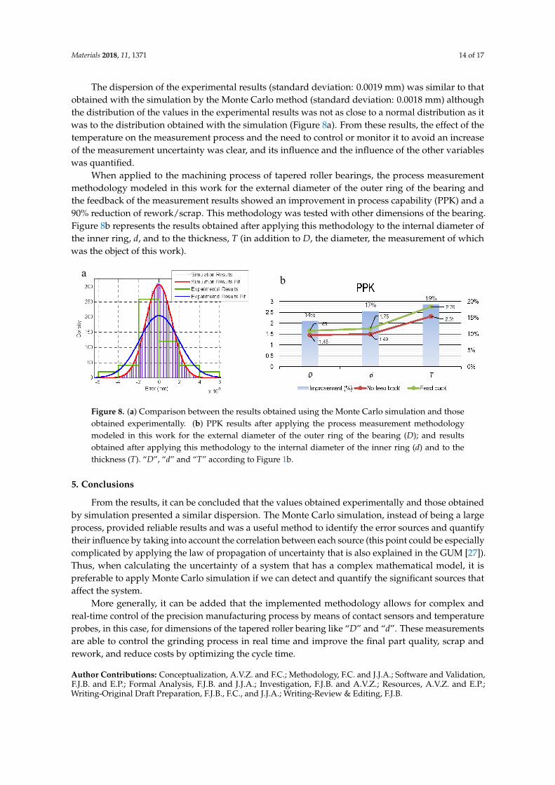
The dispersion of the experimental results (standard deviation: 0.0019 mm) was similar to thatobtained with the simulation by the Monte Carlo method (standard deviation: 0.0018 mm) althoughthe distribution of the values in the experimental results was not as close to a normal distribution as itwas to the distribution obtained with the simulation (Figure 8a). From these results, the effect of thetemperature on the measurement process and the need to control or monitor it to avoid an increaseof the measurement uncertainty was clear, and its influence and the influence of the other variableswas quantified.

When applied to the machining process of tapered roller bearings, the process measurementmethodology modeled in this work for the external diameter of the outer ring of the bearing andthe feedback of the measurement results showed an improvement in process capability (PPK) and a90% reduction of rework/scrap. This methodology was tested with other dimensions of the bearing.Figure 8b represents the results obtained after applying this methodology to the internal diameter ofthe inner ring, d, and to the thickness, T (in addition to D, the diameter, the measurement of whichwas the object of this work).

Materials 2018, 11, x FOR PEER REVIEW 14 of 17

The dispersion of the experimental results (standard deviation: 0.0019 mm) was similar to that obtained with the simulation by the Monte Carlo method (standard deviation: 0.0018 mm) although the distribution of the values in the experimental results was not as close to a normal distribution as it was to the distribution obtained with the simulation (Figure 8a). From these results, the effect of the temperature on the measurement process and the need to control or monitor it to avoid an increase of the measurement uncertainty was clear, and its influence and the influence of the other variables was quantified.

When applied to the machining process of tapered roller bearings, the process measurement methodology modeled in this work for the external diameter of the outer ring of the bearing and the feedback of the measurement results showed an improvement in process capability (PPK) and a 90% reduction of rework/scrap. This methodology was tested with other dimensions of the bearing. Figure 8b represents the results obtained after applying this methodology to the internal diameter of the inner ring, d, and to the thickness, T (in addition to D, the diameter, the measurement of which was the object of this work).

Figure 8. (a) Comparison between the results obtained using the Monte Carlo simulation and those obtained experimentally. (b) PPK results after applying the process measurement methodology modeled in this work for the external diameter of the outer ring of the bearing (D); and results obtained after applying this methodology to the internal diameter of the inner ring (d) and to the thickness (T). “D”, “d” and “T” according to Figure 1b.

5. Conclusions

From the results, it can be concluded that the values obtained experimentally and those obtained by simulation presented a similar dispersion. The Monte Carlo simulation, instead of being a large process, provided reliable results and was a useful method to identify the error sources and quantify their influence by taking into account the correlation between each source (this point could be especially complicated by applying the law of propagation of uncertainty that is also explained in the GUM [27]). Thus, when calculating the uncertainty of a system that has a complex mathematical model, it is preferable to apply Monte Carlo simulation if we can detect and quantify the significant sources that affect the system.

More generally, it can be added that the implemented methodology allows for complex and real-time control of the precision manufacturing process by means of contact sensors and temperature probes, in this case, for dimensions of the tapered roller bearing like “D” and “d”. These measurements are able to control the grinding process in real time and improve the final part quality, scrap and rework, and reduce costs by optimizing the cycle time.

Author Contributions: Conceptualization, A.V.Z. and F.C.; Methodology, F.C. and J.J.A.; Software and Validation, F.J.B. and E.P.; Formal Analysis, F.J.B. and J.J.A.; Investigation, F.J.B. and A.V.Z.; Resources, A.V.Z. and E.P.; Writing-Original Draft Preparation, F.J.B., F.C., and J.J.A.; Writing-Review & Editing, F.J.B.

Funding: This research was funded by the Universidad de Zaragoza and Fundación Ibercaja grant number JIUZ-2016-TEC-05.

a b

Figure 8. (a) Comparison between the results obtained using the Monte Carlo simulation and thoseobtained experimentally. (b) PPK results after applying the process measurement methodologymodeled in this work for the external diameter of the outer ring of the bearing (D); and resultsobtained after applying this methodology to the internal diameter of the inner ring (d) and to thethickness (T). “D”, “d” and “T” according to Figure 1b.

5. Conclusions

From the results, it can be concluded that the values obtained experimentally and those obtainedby simulation presented a similar dispersion. The Monte Carlo simulation, instead of being a largeprocess, provided reliable results and was a useful method to identify the error sources and quantifytheir influence by taking into account the correlation between each source (this point could be especiallycomplicated by applying the law of propagation of uncertainty that is also explained in the GUM [27]).Thus, when calculating the uncertainty of a system that has a complex mathematical model, it ispreferable to apply Monte Carlo simulation if we can detect and quantify the significant sources thataffect the system.

More generally, it can be added that the implemented methodology allows for complex andreal-time control of the precision manufacturing process by means of contact sensors and temperatureprobes, in this case, for dimensions of the tapered roller bearing like “D” and “d”. These measurementsare able to control the grinding process in real time and improve the final part quality, scrap andrework, and reduce costs by optimizing the cycle time.

Author Contributions: Conceptualization, A.V.Z. and F.C.; Methodology, F.C. and J.J.A.; Software and Validation,F.J.B. and E.P.; Formal Analysis, F.J.B. and J.J.A.; Investigation, F.J.B. and A.V.Z.; Resources, A.V.Z. and E.P.;Writing-Original Draft Preparation, F.J.B., F.C., and J.J.A.; Writing-Review & Editing, F.J.B.

Materials 2018, 11, 1371 15 of 17

Funding: This research was funded by the Universidad de Zaragoza and Fundación Ibercaja grantnumber JIUZ-2016-TEC-05.

Conflicts of Interest: The authors declare no conflict of interest. The funders had no role in the design of thestudy; in the collection, analyses, or interpretation of data; in the writing of the manuscript, and in the decision topublish the results.

Nomenclature

Ta,m (◦C) Ambient temperature when measuring the m-th piece.Ta,0 (◦C) Ambient temperature when measuring the master piece.Ts,m (◦C) System temperature when measuring the m-th piece.Ts,0 (◦C) System temperature when measuring the master piece.Tm,m (◦C) Measurand temperature when measuring the m-th piece.Tm,0 (◦C) Measurand temperature when measuring the master piece.Tc (◦C) Temperature from the contact thermometer (used in the Monte Carlo simulation).Ta (◦C) Temperature from the ambient thermometer (used in the Monte Carlo simulation).Hs,m (mm) Tooling height of the system (see Figure 2) when measuring the m-th piece.Hs,0 (mm) Tooling height of the system (see Figure 2) when measuring the master piece.H (mm) Tooling height of the system at 20 ◦C.Lm,m (mm) Probe length when measuring the m-th piece.L0,m (mm) Probe length from the measurement of the master piece but when measuring the m-th piece.L0,0 (mm) Probe length when measuring the master piece.Lm (mm) Probe length when measuring the m-th piece (dimension at 20 ◦C).L0 (mm) Probe length when measuring the master piece (dimension at 20 ◦C).Dm,m (mm) Measurand (diameter) of the m-th piece at the moment of measure it.D0,m (mm) Measurand (diameter) of the master piece at the moment of measure the m-th piece.D0,0 (mm) Measurand (diameter) of the master piece at the moment of measure it.Dm (mm) Measurand (diameter) of the m-th piece (dimension at 20 ◦C).D0 (mm) Measurand (diameter) of the master piece (dimension at 20 ◦C).∆Lm (mm) Figure, at 20 ◦C, of the difference between L0,m and Lm,m, see Equations (8) and (9).θm (◦) Angle between a vertical line and the front face of the ring (see Figure 4) when measuring the

m-th piece.θ0 (◦) Angle between a vertical line and the front face of the ring (see Figure 4) when measuring the

master piece.ψm (◦) Angle between a vertical line and the axis of the contact prober of the comparator dial when

measuring the m-th piece (see Figure 5).ψ0 (◦) Angle between a vertical line and the axis of the contact prober of the comparator dial when

measuring the master piece (see Figure 5).λm (◦) Linear translation on X-axis direction (see Figure 5) when measuring the m-th piece.λ0 (◦) Linear translation on X-axis direction (see Figure 5) when measuring the master piece.αm (◦C−1) Thermal expansion coefficient of the m-th piece.α0 (◦C−1) Thermal expansion coefficient of the master piece.αs (◦C−1) Thermal expansion coefficient of the system.

References

1. El-Thalji, I.; Jantunen, E. A summary of fault modelling and predictive health monitoring of rolling elementbearings. Mech. Syst. Signal Process. 2015, 60–61, 252–272. [CrossRef]

2. Liu, J.; Shao, Y.; Qin, X. Dynamic simulation for a tapered roller bearing considering a localized surface faulton the rib of the inner race. Proc. Inst. Mech. Eng. Part K 2017, 231, 670–683. [CrossRef]

3. Wee, D.; Kelly, R.; Cattel, J.; Breunig, M. Industry 4.0: How to Navigate Digitization of the ManufacturingSector. Available online: https://www.mckinsey.com/~/media/McKinsey/Business%20Functions/Operations/Our%20Insights/Industry%2040%20How%20to%20navigate%20digitization%20of%20the%20manufacturing%20sector/Industry-40-How-to-navigate-digitization-of-the-manufacturing-sector.ashx(accessed on 20 July 2018).

Materials 2018, 11, 1371 16 of 17

4. D’Addona, D.M.; Bracco, F.; Bettoni, A.; Nishino, N.; Carpanzano, N.; Bruzzone, A.A. Adaptive automationand human factors in manufacturing: An experimental assessment for a cognitive approach. CIRP Ann.2018, 67, 455–458. [CrossRef]

5. Finlay, B.; Rackwitz, N.; Conerney, B.; Warren, E.; Erdmann, D.; Stoddard, K.; Weber, A.; Scanlon, T.Requirements for First-Time-Right Response in Advanced Manufacturing. In Proceedings of the 29th AnnualSEMI Advanced Semiconductor Manufacturing Conference (ASMC), Saratoga Springs, NY, USA, 30 April–3May 2018; pp. 186–188.

6. Fraunhofer IPA. Statista—Das Statistik-Portal, Worin sehen Sie konkrete Bedarfe an IntelligentenLösungen im Produktionsalltag; Fraunhofer IPA: Hamburg, Germany, 2016. Available online:https://de.statista.com/statistik/daten/studie/605169/umfrage/bedarf-an-intelligenten-loesungen-im-produktionsalltag-im-deutschen-mittelstand/ (accessed on 20 July 2018).

7. Horváth & Partners. Statista—Das Statistik-Portal, Welche Industrie 4.0-Technologien Sind Heute Bzw. WerdenZukünftig in Unternehmen von Bedeutung Sein; Horváth & Partners: Hamburg, Germany, 2015. Availableonline: https://de.statista.com/statistik/daten/studie/606952/umfrage/bedeutung-von-technologien-der-industrie-40-heute-und-zukuenftig-in-der-dach-region/ (accessed on 20 July 2018).

8. Colledani, M.; Fischer, A.; Iung, B.; Lanza, G.; Schmitt, R.; Tolio, T.; Vancza, J. Design and management ofmanufacturing systems for production quality. CIRP Ann. Manuf. Technol. 2014, 63, 773–796. [CrossRef]

9. Jurko, J.; Panda, A.; Valícek, J.; Harnicárová, M.; Pandová, I. Study on cone roller bearing surface roughnessimprovement and the effect of surface roughness on tapered roller bearing service life. Int. J. Adv.Manuf. Technol. 2016, 82, 1099–1106. [CrossRef]

10. Weckenmann, A.; Estler, T.; Peggs, G.; McMurtry, D. Probing systems in dimensional metrology. CIRP Ann.Manuf. Technol. 2004, 53, 657–684. [CrossRef]

11. Neugebauer, M.; Lüdicke, F.; Bastam, D.; Bosse, H.; Reimann, H.; Töpperwien, C. A new comparatorfor measurement of diameter and form of cylinders, spheres and cubes under clean-room conditions.Meas. Sci. Technol. 1997, 8, 849. [CrossRef]

12. Olczyk, A.; Magiera, R.; Kabalyk, K. A 2-port, space-saving, maintenance-friendly pneumatic probe forvelocity measurements. Metrol. Meas. Syst. 2018, 1, 171–185.

13. Crnojevic, C.; Roy, G.; Bettahar, A.; Florent, P. The Influence of the Regulator Diameter and Injection NozzleGeometry on the Flow Structure in Pneumatic Dimensional Control Systems. J. Fluids Eng. 1997, 119, 609–615.[CrossRef]

14. Hoffrogge, C.; Mann, R. Measuring Laser Inferometer Device for Inside and Outside Dimensions. Messtechnik1973, 81, 1–6.

15. Kim, J.A.; Kim, J.W.; Kang, C.S.; Eom, T.B. An interferometric Abbe-type comparator for the calibration ofinternal and external diameter standards. Meas. Sci. Technol. 2010, 21, 75–109. [CrossRef]

16. Chen, Y.; He, Z.; Yang, S. Research on On-Line Automatic Diagnostic Technology for Scratch Defect ofRolling Element Bearings. Int. J. Precis. Eng. Manuf. 2012, 13, 357–362. [CrossRef]

17. Kumar, R.; Singh, M. Outer race defect width measurement in taper roller bearing using discrete wavelettransform of vibration signal. Measurement 2012, 46, 537–545. [CrossRef]

18. Deák, K.; Mankovits, T.; Kocsis, I. Optimal Wavelet Selection for the Size Estimation of Manufacturing Defectsof Tapered Roller Bearings with Vibration Measurement using Shannon Entropy Criteria. Stroj. Vestnik J.Mech. Eng. 2017, 63, 3–14. [CrossRef]

19. Chen, M.; Wang, C.; An, Q.; Ming, W. Tool path strategy and cutting process monitoring in intelligentmachining. Front. Mech. Eng. 2018, 13, 232–242. [CrossRef]

20. Zhou, M.; Zheng, G.; Chen, S. Identification and looping tool path generation for removing residual areasleft by pocket roughing. Int. J. Adv. Manuf. Technol. 2016, 87, 765–778. [CrossRef]

21. Gao, X.; Mou, W.; Peng, Y. An intelligent process planning method based on feature-based history machiningdata for aircraft structural parts. Procedia CIRP 2016, 56, 585–589. [CrossRef]

22. Tönshoff, H.K.; Friemuth, T.; Becker, J.C. Process Monitoring in Grinding. CIRP Ann. Manuf. Technol. 2002,51, 551–571. [CrossRef]

23. Shiraishi, M. Scope of in-process measurement, monitoring and control techniques in machiningprocesses—Part 3: In-process techniques for cutting processes and machine tools. Precis. Eng. 1989,11, 39–47. [CrossRef]

Materials 2018, 11, 1371 17 of 17

24. Brosed, F.J.; Aguilar, J.J.; Santolaria, J.; Lázaro, R. Geometrical verification based on a laser triangulationsystem in industrial environment. Effect of the image noise in the measurement results. Procedia Eng. 2015,132, 764–771. [CrossRef]

25. Jalid, A.; Hariri, S.; El Gharad, A.; Senelaer, J.P. Comparison of the GUM and Monte Carlo methods on theflatness uncertainty estimation in coordinate measuring machine. Int. J. Metrol. Qual. Eng. 2016, 7, 302.[CrossRef]

26. Forbes, A.B.; Mengot, A.; Jonas, K. Uncertainty associated with coordinate measurement in comparatormode. In Proceedings of the Laser Metrology and Machine Performance XI, Huddersfield, UK, 17–18 March2015; pp. 150–159.

27. BIPM; IEC; IFCC; ILAC; ISO; IUPAC; IUPAP; OIML. Evaluation of Measurement Data—Guide to the Expressionof Uncertainty in Measurement; JCGM 100: Bureau International des Poids et Mesures (BIPM): Sèvres,France, 2008.

28. BIPM; IEC; IFCC; ILAC; ISO; IUPAC; IUPAP; OIML. Evaluation of Measurement Data—Supplement 1 to the“Guide to the Expression of Uncertainty in Measurement”—Propagation of Distributions Using a Monte CarloMethod; JCGM 101: Bureau International des Poids et Mesures (BIPM): Sèvres, France, 2008.

29. Eichstädt, S.; Link, A.; Harris, P.M.; Elster, C. Efficient implementation of a Monte Carlo method foruncertainty evaluation in dynamic measurements. Metrologia 2012, 49, 401–410. [CrossRef]

30. Los, A.; Mayer, J.R.R. Application of the adaptive Monte Carlo method in a five-axis machine tool calibrationuncertainty estimation including the thermal behavior. Precis. Eng. 2018, 53, 17–25. [CrossRef]

© 2018 by the authors. Licensee MDPI, Basel, Switzerland. This article is an open accessarticle distributed under the terms and conditions of the Creative Commons Attribution(CC BY) license (http://creativecommons.org/licenses/by/4.0/).