Remote Sens. 2014, 6, 12187-12216; doi:10.3390/rs61212187

remote sensing ISSN 2072-4292

www.mdpi.com/journal/remotesensing

Article

Improved Wetland Classification Using Eight-Band High Resolution Satellite Imagery and a Hybrid Approach

Charles R. Lane 1,*, Hongxing Liu 2,3, Bradley C. Autrey 1, Oleg A. Anenkhonov 4, Victor V. Chepinoga 5,6 and Qiusheng Wu 2,3

1 United States Environmental Protection Agency, Office of Research and Development,

Cincinnati, OH 45268, USA; E-Mail: Autrey.Brad@epa.gov 2 Dynamac Corporation c/o, United States Environmental Protection Agency,

Cincinnati, OH 45268, USA; E-Mails: Liu.Hongxing@epa.gov (H.L.);

Wu.Qiusheng@epa.gov (Q.W.) 3 Department of Geography, University of Cincinnati, Cincinnati, OH 45221, USA 4 Institute of General and Experimental Biology, Russian Academy of Sciences, Siberian Branch,

Ulan-Ude 670047, Russia; E-Mail: Anen@yandex.ru 5 Department of Botany and Genetics, Irkutsk State University, Irkutsk 664003, Russia;

E-Mail: victor.chepinoga@gmail.com 6 Institute of Geography, Russian Academy of Sciences, Siberian Branch, Irkutsk 664003, Russia

* Author to whom correspondence should be addressed; E-Mail: Lane.Charles@epa.gov;

Tel.: +1-513-569-7854; Fax: +1-513-569-7438.

External Editors: Alisa L. Gallant and Prasad S. Thenkabail

Received: 13 June 2014; in revised form: 18 November 2014 / Accepted: 27 November 2014 /

Published: 8 December 2014

Abstract: Although remote sensing technology has long been used in wetland inventory and

monitoring, the accuracy and detail level of wetland maps derived with moderate resolution

imagery and traditional techniques have been limited and often unsatisfactory. We explored

and evaluated the utility of a newly launched high-resolution, eight-band satellite system

(Worldview-2; WV2) for identifying and classifying freshwater deltaic wetland vegetation

and aquatic habitats in the Selenga River Delta of Lake Baikal, Russia, using a hybrid

approach and a novel application of Indicator Species Analysis (ISA). We achieved an

overall classification accuracy of 86.5% (Kappa coefficient: 0.85) for 22 classes of aquatic

and wetland habitats and found that additional metrics, such as the Normalized Difference

Vegetation Index and image texture, were valuable for improving the overall classification

OPEN ACCESS

Remote Sens. 2014, 6 12188

accuracy and particularly for discriminating among certain habitat classes. Our analysis

demonstrated that including WV2’s four spectral bands from parts of the spectrum less

commonly used in remote sensing analyses, along with the more traditional bandwidths,

contributed to the increase in the overall classification accuracy by ~4% overall, but with

considerable increases in our ability to discriminate certain communities. The coastal band

improved differentiating open water and aquatic (i.e., vegetated) habitats, and the yellow,

red-edge, and near-infrared 2 bands improved discrimination among different vegetated

aquatic and terrestrial habitats. The use of ISA provided statistical rigor in developing

associations between spectral classes and field-based data. Our analyses demonstrated the

utility of a hybrid approach and the benefit of additional bands and metrics in providing the

first spatially explicit mapping of a large and heterogeneous wetland system.

Keywords: Selenga River delta; Lake Baikal; coastal band; NIR2 band; NDVI; grey-level

co-occurrence matrix; image texture; Worldview-2

1. Introduction

Wetlands perform vital functions by providing habitat, improving water quality, recharging

groundwater aquifers, reducing erosion, and mitigating flood severity [1,2]. Despite their importance for

increasing biodiversity and provisioning ecosystem services and goods, extensive loss of wetlands has

occurred throughout the world [3–6]. Recently, there has been considerable concern regarding the

impact of global and regional climate change on wetlands, especially in light of increasing temperatures

and changing trends in precipitation [7,8]. Due to their limited adaptation capability, wetlands in high-

latitude, arid, and semi-arid regions are especially vulnerable to changes in temperature and

precipitation. Scientific knowledge of the current status and future trends of wetlands in these regions is

fundamentally important for formulating planning measures and effective management policies.

Wetland mapping and inventory represent the first steps toward acquiring scientific knowledge about

wetland habitats [9,10].

Wetlands are among the most difficult ecosystems to classify using remote sensing data due to their

high spatial heterogeneity and temporal variability [10–14]. Sizes and shapes of wetlands vary greatly,

as do the diversity of plant species and vegetation structures and types (e.g., open water, submerged

plants, floating-leaved plants, emergent herbaceous vegetation, woody shrubs, and forest). Water levels

fluctuate daily and seasonally, which can confound spectral classification, and many wetland plant

species are spectrally similar to one another, which makes separation of unique signatures difficult,

particularly when only a few broad spectral bands are available for classification. The presence of water

interspersed with the vegetation dampens the overall spectral reflectance of the vegetation and further

diminishes separability of individual species [15,16]. Periphyton and algae can form large floating

masses around wetland vegetation and may further complicate wetland vegetation classification.

Despite these limitations, the remotely sensed multispectral imagery from Landsat, SPOT, and other

major data sources [10,15], as well as synthetic aperture radar images [17–20], have a long history of

use in wetland mapping applications. The launch of the IKONOS satellite in 1999 signaled the advent

Remote Sens. 2014, 6 12189

of the new era of high-resolution satellite remote sensing, with panchromatic imagery at 1-m spatial

resolution and four-band multispectral imagery at 4-m resolution. Since then, additional high-resolution

satellite systems have been placed in orbit, including QuickBird, WorldView-1, GeoEye-1,

WorldView-2 (WV2), and WorldView-3, and the launches of additional sub-meter sensors are pending.

The multispectral imagery of the WV2 satellite (DigitalGlobe, Longmont, Colorado, USA) is of

particular interest for wetland mapping because, in addition to the typical spectral bands (i.e., visible

blue, green, red, and near-infrared), WV2 also provides four new spectral bands (coastal (400–450 nm),

yellow (585–625 nm), red-edge (705–745 nm), and near-infrared 2 (NIR2; 860–1040 nm)) from parts

of the energy spectrum not typically covered by satellite sensors. These bands are expected to better

discriminate vegetation properties and penetrate water features [21]. For example, the coastal band is

characterized by its relatively shorter wavelength and higher energy, which penetrate deeper into water

bodies. It has been reported that water depths down to 30 m can be effectively observed with coastal

bands [22], which would add to the understanding of subsurface features at the interface of aquatic and

terrestrial landscapes. The yellow band can further assist in discriminating vegetation properties or

penetrating water bodies. Lee et al. [23] demonstrated that the yellow band was more effective for

determining depth between 2.5 and 20 m. The red-edge band facilitates the identification of vegetative

condition, and has been shown to reveal difference between healthy trees and those impacted by disease

or pollution [24]. This feature could be useful in identifying wetland features affected by hydrologic

stress (e.g., excessive inundation or drought conditions [25]). The NIR2 band that partially overlaps the

NIR1 band is less affected by atmospheric influence, enabling broader vegetation analysis and biomass

studies. The majority of studies to date have taken advantage of WV2 characteristics to conduct

bathymetric studies in coastal waters [22,23,26,27]. To our knowledge, only Lantz and Wang [28] have

used WV2 to study freshwater wetlands and aquatic habitats in their research of the distribution of the

species Phragmites australis.

We developed and applied a hybrid approach to analyze and classify the heterogeneous wetland

habitat of the Selenga River Delta in Siberian Russia, taking advantage of the eight-band satellite WV2

sensor data for the first spatially explicit system-level mapping and inventory of this Ramsar wetland of

international importance [29]. Our two major objectives were to: (1) present a practical and effective

classification approach to using multispectral image bands for multi-scale wetland mapping and

inventory; and (2) evaluate the utility of four additional spectral bands typically not available in satellite

sensors for enhancing overall and habitat-specific wetland discrimination and increasing classification

accuracy. We also quantified the potential improvement to our resultant wetland classification

through the inclusion of the Normalized Difference Vegetation Index (NDVI, [30]) and image texture

measures [31], that we hypothesized would increase our classification accuracy.

2. Methods

2.1. Study Area

The Selenga River Delta (SRD) in southeastern Siberia, Russia, is the terminus of the Selenga

River, the largest among over 350 rivers and streams flowing into Lake Baikal (Figure 1). The Selenga

River drains an area of 447,060 km2 across Mongolia and Russia and accounts for 83.4% of

Remote Sens. 2014, 6 12190

the Baikal drainage basin. The area of the SRD is approximately 540 to 600 km2 [32], with a continental

semi-arid climate [33] and mean air temperatures ranging from +14 °C in July to −19.4 °C in January.

The growing season in the SRD lasts 140–150 days, and the mean annual precipitation is ~315 mm.

The hydrologic regime of the delta has a seasonal pulse of high water from April to October caused by

water level increases in Lake Baikal from the Selenga River and other tributaries during floods and

freshets [34]. Water levels fluctuate daily depending on the direction and force of the wind, as well as

the volume of water from the Selenga River, though the effect outside the channels and immediately

adjacent wetlands or near-Baikal areas is tempered by wetland vegetation (e.g., [35]). The study area

includes the Kabansky District of the Baikalsky Nature Reserve (see Figure 1). The Kabansky District,

established in 1974, has an area of approximately 120 km2 and is bounded by the Sredneustie Channel

to the west, the Lobanovskaya Channel to the southeast, the Kolpinnaya Channel to the east, and Lake

Baikal to the north.

Figure 1. Location of Selenga River Delta study area in the Kabansky District of the Baikalsky

Nature Preserve, shown with bands 7, 4, and 3 from the WorldView-2 (WV2) imagery

as background.

2.2. Satellite Data Acquisition and Processing

We acquired two overlapping, cloud-free WV2 images from 25 June and 3 July 2011. During this

part of the year, many of the marsh species that grow in the delta have emerged from winter dormancy

after the spring floods have receded, making the wetland vegetation more easily distinguishable from

the adjacent upland vegetation. The two images together cover an area of 215 km2 that includes the entire

Remote Sens. 2014, 6 12191

Kabansky District (Figure 2). Both images have a panchromatic band resampled to 0.5-m pixels and

eight multispectral bands resampled to 2-m pixels. The two images have a 5-km wide overlap area.

Although the two images were acquired at similar times of day (approximately 4:20 UTC) and have

similar solar illumination conditions (sun elevation angle of 60°, sun azimuth angle of 164°), there is a

noticeable radiometric difference between them. This difference is a result of both the additional eight

days of vegetation growth and the wind conditions captured by the 3 July image. The images were

successfully mosaicked using the ENVI georeferenced mosaicking tool (Exelis Visual Information

Solutions, Boulder, CO, USA, version 4.8) after converting to top-of-atmosphere spectral reflectance

values (see below) to account for the radiometric contrast.

Figure 2. Adjacent WorldView-2 multi-spectral images (near-infrared false-color composite

of bands 7, 5, and 3) with ground control points and ground-truth sites.

The 25 June image was acquired with a mean off-nadir view angle of 16 degrees, and the 3 July image

with a mean off-nadir view angle of 28.5 degrees. Because the Earth-Sun distance, solar elevation angle,

and atmospheric conditions influence the actual solar spectral irradiance for a given image, the two images

Remote Sens. 2014, 6 12192

acquired on different days have different radiances. To make the two WV2 images radiometrically

comparable, the digital number values were calibrated and converted to top-of-atmosphere (TOA) spectral

radiance values based on the absolute radiometric calibration factor and effective bandwidth values for

each band. The TOA spectral radiance was converted to surface reflectance based on parameters of solar

elevation angle, solar spectral irradiance, and acquisition time.

To georeference and orthorectify images, 21 ground control points (GCPs; i.e., features that can be

easily identified on the WV2 images and visited in the field) were acquired using field GPS. We selected

the best available sites for GCPs, including building corners (small hunting shacks, isolated houses),

single isolated trees, tree stands, and identifiable points near river channels (i.e., where two tributaries

meet). The Ortho-Ready Standard (OR2A) image products were projected to an average height of

414.03 m above the WGS-84 ellipsoid. OR2A products are not corrected for topographic relief so we

applied a custom orthorectification. The OR2A image product geolocation root mean square error

(RMSE) is estimated to be about 3–7 m in comparison with field-based GPS measurements of GCPs.

To improve geolocation accuracy and image geometric integrity, we orthorectified the imagery using

the GCPs and ASTER GDEM with a 30-m spatial resolution using the “rational function” method in

ENVI software (Exelis Visual Information Solutions, Boulder, CO, USA, version 4.8) to perform

orthorectification in Universal Transverse Mercator system zone 48N referenced to the WGS84 ellipsoid,

and evaluated the resulting planimetric positional accuracy to be better than 2 m RMSE.

2.3. Vegetation Abundance and Habitat Structure Characterization

The NDVI and an image texture measure were derived and included in the wetland habitat

characterization and classification. Both NDVI and the texture measure were linearly scaled to the

numerical range similar to the surface reflectance of multispectral bands and used in the supervised

wetland classification as described further below.

The NDVI is a well-established indicator for the presence and condition (i.e., abundance, vigor, and

health) of vegetation [30] and is widely used for mapping the extent and abundance of vegetation,

estimating biomass or the leaf area index, and distinguishing areas of unhealthy or stressed vegetation

from healthy green vegetation. It is also utilized to enhance discrimination between different wetland

habitats and upland features [36–38]. The NDVI is constructed based on the inverse relationship between

chlorophyll absorption of red radiant energy and increased reflectance of near-infrared energy for

vegetative canopies. Values of the NDVI range from −1.0 (i.e., no green biomass detected) to 1.0

(i.e., vigorous, dense green biomass). Healthy and abundant vegetation reflects strongly in the

near-infrared portion of the spectrum while absorbing strongly in the visible red light, thereby yielding

high positive NDVI values. Sparse, stressed, and flooded vegetation have nearly equal reflectances in

both the near-infrared and red portions of the spectrum, resulting in small positive or zero NDVI values.

Open water bodies yield negative values due to red reflectance larger than near-IR reflectance. The

NDVI values for bare soil ground are near zero due to their similar reflectance in both bands. Thus, the

NDVI image would be expected to enhance the discrimination between different wetland habitats.

However, short-term changes in site hydrology (e.g., flooding) can result in spurious NDVI values due

to water temporarily flooding or covering areas of substantial vegetative growth. We calculated the

Remote Sens. 2014, 6 12193

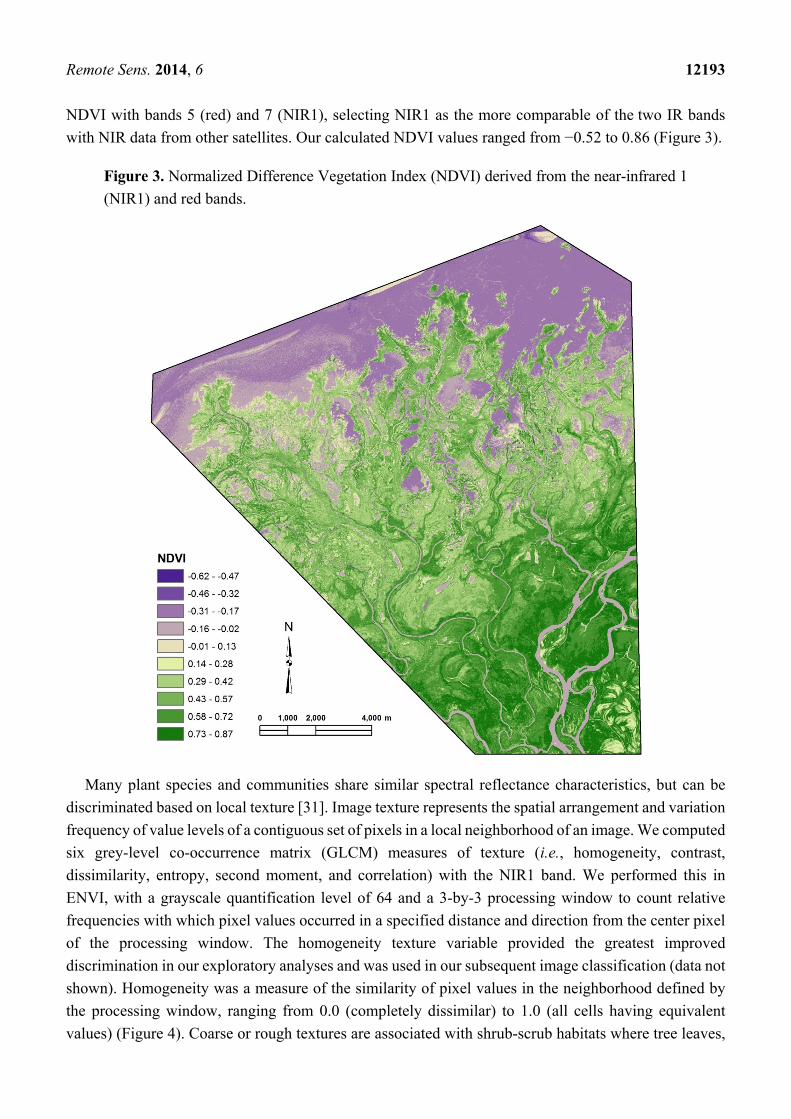
NDVI with bands 5 (red) and 7 (NIR1), selecting NIR1 as the more comparable of the two IR bands

with NIR data from other satellites. Our calculated NDVI values ranged from −0.52 to 0.86 (Figure 3).

Figure 3. Normalized Difference Vegetation Index (NDVI) derived from the near-infrared 1

(NIR1) and red bands.

Many plant species and communities share similar spectral reflectance characteristics, but can be

discriminated based on local texture [31]. Image texture represents the spatial arrangement and variation

frequency of value levels of a contiguous set of pixels in a local neighborhood of an image. We computed

six grey-level co-occurrence matrix (GLCM) measures of texture (i.e., homogeneity, contrast,

dissimilarity, entropy, second moment, and correlation) with the NIR1 band. We performed this in

ENVI, with a grayscale quantification level of 64 and a 3-by-3 processing window to count relative

frequencies with which pixel values occurred in a specified distance and direction from the center pixel

of the processing window. The homogeneity texture variable provided the greatest improved

discrimination in our exploratory analyses and was used in our subsequent image classification (data not

shown). Homogeneity was a measure of the similarity of pixel values in the neighborhood defined by

the processing window, ranging from 0.0 (completely dissimilar) to 1.0 (all cells having equivalent

values) (Figure 4). Coarse or rough textures are associated with shrub-scrub habitats where tree leaves,

Remote Sens. 2014, 6 12194

leaf shadows, and interspersed grasses create relatively high variation of the reflectance intensity within

local neighborhoods. Coarse texture is indicated by very low values of the homogeneity measure. In

contrast, calm water bodies and aquatic beds with submerged vascular vegetation have smooth, or fine,

image textures indicated by very large homogeneity values. Aquatic beds with floating vascular

vegetation have coarse, rough and jagged textures (i.e., low homogeneity values), produced by an

aggregation of floating vascular leaves and interspersed water surfaces. Most herbaceous habitats have

quite smooth textures because their plant species and heights are similar within local neighborhoods and

result in high homogeneity values.

Figure 4. Homogeneity texture measure based on the grey-level co-occurrence

matrices (GLCM).

2.4. Hybrid Classification

We adopted a hybrid classification approach [10,39] that synergistically combines conventional

unsupervised and supervised classification approaches with field survey and indicator species analysis

(ISA) [40] (Figure 5). Our hybrid approach exploited the respective strengths of both unsupervised and

supervised classification methods [10,39]. We first performed an unsupervised classification on the

Remote Sens. 2014, 6 12195

eight-band imagery to create clusters prior to the field survey. The spectrally homogenous regions

derived from each cluster were used for guiding field sampling and training data collection. The survey

sites were 100 m2 quadrats (described below), which were selected to be located within large spectrally

homogeneous regions and to cover the various types of spectral clusters identified. Training sites with

very similar spectral characteristics were then grouped for the field survey. Next, we applied ISA to each

class of training sites to identify the habitat type or taxa with sufficient fidelity and specificity to that

particular class. The identified indicator habitat types or taxa were then coupled with visual

interpretations of the field photographs and the hydrogeomorphic positions of the training sites, so that

each class of training sites could be characterized and labeled as a thematic aquatic or wetland class. In

the final stage, we classified the orthorectified WV2 images using the interpreted and labeled training

sites and a maximum likelihood supervised classification method, resulting in a fine-scale aquatic and

wetland classification at the genus/community level. To facilitate a regional comparison with other

wetland classification schemes, the aquatic and wetland classes at the genus/community level were

progressively recoded and aggregated into broader wetland classes, culminating in a total of five

hierarchical levels.

Figure 5. The data processing and information flow of the hybrid classification approach.

2.4.1. Unsupervised Classification

We classified the radiometrically calibrated eight spectral bands into an initial 24 clusters using

the Iterative Self-Organizing Data Analysis Technique (ISODATA) unsupervised classification

method [41–44]. We originally tried using a larger number of clusters, but the resulting spectral

Remote Sens. 2014, 6 12196

separability between some clusters was low, as indicated by small Jeffries-Matusita separability values

(ENVI, Exelis Visual Information Solutions, Boulder, CO, USA, version 4.8). We made no attempt to

interpret and label the 24 clusters; instead, we treated spatially connected pixels of the same cluster as

spectrally homogeneous regions. These raster regions were subsequently converted into a set of polygons

that we used for field sampling design and for collection of reference training data, as described below.

2.4.2. Field Sampling

We conducted the field sampling within two weeks of image acquisition, a period at the height of the

growing season and, ideally, a period of little phenological change in species’ characteristics.

The spectrally homogeneous polygons of 24 clusters derived from the unsupervised classification were

loaded into a GPS receiver as a vector data layer along with pan-sharpened WV2 imagery. Polygons

of <0.1 ha were removed prior to inclusion to limit errors associated with the non-georectified

ISODATA unsupervised classification. We targeted three sites for each unsupervised class, sampling a

separate polygon for each of the three locations. The total number (72) of sites surveyed was constrained

by the size of the survey crew (three scientists) and eight days of survey time. We accessed sampling

locations by foot and/or boat, and penetrated each polygon at least 30 m, when possible, to limit errors

associated with the non-georeferenced unsupervised classification. At each site, the percent cover for each

species contributing ≥ 10% of the total cover was estimated within a typically square 100-m2 plot, though

in some cases the plot shape was modified to accommodate the polygon of interest. We observed and

recorded dominant vegetation height, dominant species characteristics (e.g., perennial, annual, deciduous)

and water depth, and recorded the geographic location of the plot center with 2- to 5-m real-time accuracy

by taking the average of 20 location readings from a GPS receiver (Trimble Nomad, Sunnyvale, CA,

USA). We took photographs in the cardinal directions from the plot center to record local vegetation

structure and substrate composition, and investigated areas immediately around the sampling plot to ensure

that the quadrat was representative of the community. We subsequently collapsed species-level data to the

genus level to facilitate the initial stages of this exploratory study, which resulted in the identification of

30 genera and four aquatic habitat classes (i.e., open water, bare ground, thatch, and algae) that were used

in the analyses.

2.4.3. Development of Training and Validation Datasets

After field sampling, we delineated regions of interests (ROIs) on the computer screen as small

polygons across the 72 ground-truth sites, using the GPS coordinates of the field locations to center

the ROIs. These ROIs were split into a training dataset for calibrating the supervised classifier

and a validation dataset for assessing classification accuracy. The training ROIs contained

28,953 pixels. Based on the spectral characteristics, we grouped the training data into 22 classes using

clustering analysis in ArcGIS (ESRI, Redlands, CA, USA, version 10.1). We examined the spectral

separability among the 22 classes of training sites using the Jeffries-Matusita separability measure in

ENVI [45] and determined that the Jeffries-Matusita value for all cluster groups was greater than 1.9,

indicating good separability.

Remote Sens. 2014, 6 12197

2.4.4. Indicator Species Analysis

Indicator Species Analysis (ISA) [40,46] detects and evaluates the value of different taxa for

characterizing a pre-determined class. We conducted ISA using PC-ORD (MJM Software, Gleneden

Beach, Oregon, USA, version 6.0) to detect taxa or community components with specificity and fidelity

to our derived classes, using genus-level percent cover and habitat descriptors (noted in Section 2.4.2,

above) as potential indicators for each site. We calculated the indicator value (IV) for each species or

habitat in PC-ORD by combining the percent cover at each sampling site with its relative frequency of

occurrence in each class of training sites. Maximum IV for a species is achieved when all individuals of

a taxon are found only in a single class of habitats and the taxon occurs in all habitats of that class.

According to McCune and Grace [46] (2002, p. 198, italics in original), “[a] perfect indicator of a

particular group should be faithful to that group (always present) [and] should also be exclusive to that

group, never occurring in other groups.” To assess the statistical significance of class membership, each

indicator taxon and/or habitat was evaluated for group membership using a randomization procedure

with 9999 Monte Carlo runs and an acceptance alpha of 0.10. Not all classes would be expected to have

significant indicator taxa/habitats. In those instances, we assigned a descriptive thematic label to the

class based on the topographical location and hydrogeomorphic position [47] of each field site, as guided

by field photographs, field records of soils, and species dominance within that class. These training sites

with interpreted class labels were subsequently used in the supervised image classification.

2.4.5. Supervised Classification and Multi-Scale Aggregation

At the final stage of the hybrid classification, we used the maximum likelihood (ML) supervised

method [44,48] in ENVI to classify the 10-layer image stack (the eight multispectral bands plus the

NDVI and homogeneity texture measures) using the labeled training sites. Multivariate normality was

confirmed by checking the histograms of training pixels for different bands of each class. An accuracy

assessment, reported as producer’s and user’s accuracies, of the most refined classification level was

quantitatively evaluated based on a random sample of 16,544 validation pixels from ground-truth

polygons. Random points were generated using “Create Random Points” in ArcGIS, with the number of

random points within each polygon being proportional to the area of the polygon.

To meet various requirements for wetland management and to facilitate comparisons between

wetland classification systems, a five-tiered hierarchical classification of the SRD was conducted. We

progressively aggregated the most refined output of the ML supervised method (Level 5, with 22 classes,

see below) into broad substrate and vegetation classes at more generalized levels, as guided by ecological

and taxonomical relations of various wetland habitats in the Cowardin wetland classification system [49]

and the Ramsar Classification System (RCS) [50]. The Cowardin system was designed for the National

Wetlands Inventory program of the U.S. Fish and Wildlife Service and is comprised of several levels

(i.e., system, subsystem, class, subclass, and modifiers). The RCS was developed after the signing of the

1971 Ramsar, Iran, International Convention on Wetlands that provides a treaty framework for the

conservation of the worldʼs wetlands. The RCS identifies three general categories of wetlands: marine-

coastal, inland, and human-made. The RCS further divides inland wetlands, such as those relevant to this

Remote Sens. 2014, 6 12198

study, into 21 types, including permanent inland deltas. Wetland classes in the RCS are much coarser and

broader than classes in the Cowardin classification system.

2.4.6. Testing the Efficacy of Additional Spectral Bands, NDVI, and Texture

Once the final classification was completed, we retrospectively analyzed the effectiveness of the

four new WV2 spectral bands for habitat discrimination by adding bands (coastal; coastal plus yellow,

red-edge, and NIR2) and data layers (NDVI; NDVI plus texture) to the base layer of the four traditional

bands. We assessed change in overall classification accuracy as well as accuracy improvements within

certain groups with the addition of our data layers.

3. Results

3.1. Vegetation and Site Data

We sampled a range of wetland habitats in the SRD and identified 34 taxa or habitat descriptors across

the 72 sites sampled, including habitats dominated by open water and floating leaved plants

(e.g., Nymphoides, Nuphar, Nymphaea), floating plants (Lemna, Spirodela, Utricularia), rooted water

plants (e.g., Potamogeton, Myriophyllum, Ceratophyllum), emergent plants (e.g., Polygonum, Hippuris),

and several ruderal plants from grazed areas (e.g., Trifolium, Galeopsis, and Agrostis). The most

commonly identified genera and/or wetland habitats included open water, Nymphoides, thatch (i.e., the

previous seasonʼs often unidentifiable senescent or dead vegetation), Calamagrostis, Carex, and

Equisetum. These occurred at >10% cover (i.e., the lower limit at which a vegetation class or habitat

was recorded for this study) at >5% of the plots.

3.2. Multi-Scale Hierarchical Habitat Classification

Although we aggregated classes from the finest level to the most general, the results are more

logically described from the coarsest to the finest resolution. We anticipate that end-users would select

the hierarchical level at which their needs would be met. At the coarsest scale, or Level 1, we described

the entirety of the inland freshwater deltaic wetland (data not shown). This top-level class corresponds

to the “System” level in the Cowardin wetland classification scheme and the sub-type “permanent inland

deltas (L)” of the general wetland type “inland wetlands” in the RCS [49,50]. The second level consisted

of two classes (Figure A1): (1) open water and aquatic bed and (2) emergent herbaceous and woody

wetland. The Level 3 classification resulted in five basic aquatic and wetland types: (1) stream, river and lake

bed; (2) unconsolidated bottom; (3) aquatic bed; (4) emergent herbaceous wetland; and (5) scrub-shrub

wetland (Figure 6). Level 3 generally corresponds with the “Class” level in the Cowardin classification

scheme. Level 4, with 13 classes, approximates the “Subclass” level in the Cowardin scheme [49,51]

(Figure 7). In Level 5, which is the finest scale and which served as the initial classification from which

all other groupings were aggregated, we identified 22 classes of aquatic substrates and wetland

vegetation cover at genus and community levels (Figure 8).

Remote Sens. 2014, 6 12199

Figure 6. Level 3 classification at the Class level of the Cowardin scheme.

3.3. Accuracy Assessment

We conducted an accuracy assessment of the habitat classification at the finest scale (Level 5), as

subsequent and coarser classifications originated from the collapsing of Level 5 classes to more general

groups (Table 1). Our accuracy assessment was quantitatively evaluated based on a stratified random

sample of 16,544 validation pixels from ground-truth site polygons independent of training pixels. As

we were limited to the number of sampling points we could visit across the study area, our use of site

polygons may over-estimate the accuracy of our study. However, we found overall classification

accuracy, computed by taking the total number of correctly classified pixels (i.e., diagonal cells of

confusion matrix) and dividing by the total number of samples, to be 86.5%. We calculated the Kappa

coefficient, which is a measure of the likelihood that the observed classification is due to chance

Remote Sens. 2014, 6 12200

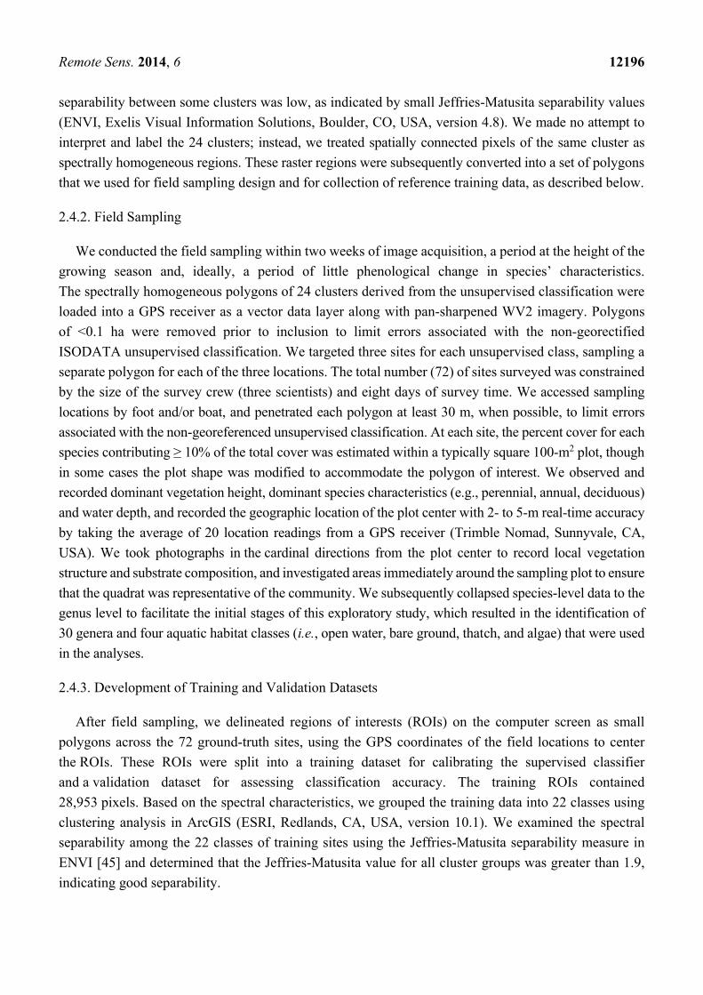
(Kappa = 0) or true agreement (Kappa = 1.0) [52], to be 0.85. Individual class accuracies were evaluated

by producer’s accuracy (PA) and user’s accuracy (UA) measures (see Table 1). The PA for 22 classes

ranged from 60.7% to 98.3%, and four classes (Classes 2, 7, 9, and 19) had PA values <70%

(i.e., omission error larger than 30%). The UA for 22 classes ranged from 52.3% to 99.5%, and two

classes (Classes 9 and 18) had UA values of <70% (i.e., commission error larger than 30%).

Figure 7. Level 4 classification at the Subclass level of the Cowardin scheme.

Remote Sens. 2014, 6 12201

Figure 8. Genus and community aquatic and wetland habitat classification at Level 5.

Remote Sens. 2014, 6 12202

Table 1. Percent classification error for 22 classes of aquatic and wetland habitats at Level 5. Class numbers correspond with those in the legend

of Figure 8.

Class 1 2 3 4 5 6 7 8 9 10 11 12 13 14 15 16 17 18 19 20 21 22 PA UA

1 92.5 - 0.1 - - - 26.3 - - - - - - - - - - - - - - - 92.5 92.7

2 - 60.7 - - - - 0.5 - - - - - - - - - - - - - - - 60.7 99.2

3 7.4 36.8 91.6 4.7 - 0.2 - - - - - - - - - - - - - - - - 91.6 79.7

4 - - 8.3 94.6 2.3 - - - - - - - - - - - - - - - - - 94.6 82.3

5 - - - 0.4 97.6 - - - - - - - - - - - - - - - - - 97.6 99.5

6 - - - - - 93.5 5.3 2.1 - - - - - - - - - - - - - - 93.5 96.6

7 0.1 2.5 - - - 4.0 67.8 - - - - - - - - - - - - - - - 67.8 86.8

8 - - 0.1 - - 0.7 - 70.6 16.9 - - - - - - - - - - - - - 70.6 82.4

9 - - - - - 1.2 - 9.6 69.9 8.5 2.0 0.6 - - - - - - - - - 0.2 69.9 52.3

10 - 0.2 - - - 0.4 - 17.8 1.2 86.5 4.5 0.2 - - - - - - - - - - 86.5 71.4

11 - - - - - - - - 2.4 5.0 86.8 4.9 - - - - - - - - - - 86.8 88.0

12 - - - - - - - - - - 6.8 91.2 1.5 - - - - - - - - - 91.2 95.2

13 - - - - - - - - - - - 2.7 98.3 - - - - - - - - - 98.3 96.2

14 - - - 0.4 0.2 - - - 8.4 - - - - 97.2 3.7 - - - 0.7 - - 0.1 97.2 90.2

15 - - - - - - - - - - - - - 0.8 79.3 4.8 - - - - - 0.1 79.3 84.3

16 - - - - - - - - - - - - - 1.2 16.6 94.2 - 0.4 2.2 - - 0.8 94.2 88.2

17 - - - - - - - - 1.2 - - - 0.2 0.4 0.5 - 83.9 19.8 7.9 - - 0.1 83.9 78.9

18 - - - - - - - - - - - - - - - 0.7 12.2 74.4 27.7 1.3 - 1.0 74.4 53.4

19 - - - - - - - - - - - - - - - - 2.5 3.0 60.9 - - - 60.9 93.0

20 - - - - - - - - - - - 0.2 - - - - 1.0 2.2 0.1 94.4 8.1 14.2 94.6 74.5

21 - - - - - - - - - - - - - - - - - - - - 89.1 2.1 89.1 94.7

22 - - - - - - - - - - - 0.3 - 0.4 - 0.3 0.4 0.2 0.4 4.3 2.8 81.4 81.4 95.0

Remote Sens. 2014, 6 12203

3.4. ISA/Vegetation Analyses

We identified 11 indicator taxa/habitats using ISA for the 22 wetland classes at Level 5 (Table 2 and

Figure 8), and in no cases were multiple plants/habitats identified with sufficient fidelity and specificity

to be indicators of the same wetland class. This suggests that at 22 classes, our analyses identified plants

and habitats that tended to dominate plots (Nymphoides, Potamogeton, Phragmites, Equisetum, thatch

(often composed of last season’s Equisetum), bare ground, etc.) in the multiple sites in which they were

found. These taxa and habitats tended to be common throughout the delta. We found >100 measureable

occurrences of these 11 indicators.

Table 2. Indicator and dominant species of Level 5 of the classification. Higher mean

indicator values suggest greater fidelity and specificity to habitat classes, and the p-value is

based on the Monte Carlo class randomization with 9999 runs.

Class # Class Name (Indicator and/or

Hab. Descriptor) Indicator

Taxa/Habitat Indicator

Value Mean Indicator p-Value

Dominant Species/Substrate

1 Deep Water with Sand Bottom Not detected Open water

2 Shallow Water with Sediment Not detected Open water

3 Shallow Water with Mud Bottom Not detected Open water

4 Very Shallow Water with Sand Bottom Not detected Open water

5 Shallow Water with Sand Bottom Not detected Open water

6 Submerged Aquatic Vascular

(Potamogeton) Potamogeton 21.1 0.0464 Potamogeton

7 Submerged Aquatic Vascular

(Sparganium) Sparganium 20.9 0.0158 Sparganium

8 Submerged Aquatic Vascular

(Utricularia) Utricularia 31.1 0.0661 Utricularia

9 Submerged and Floating Vascular

(Agrostis/Eleocharis) Not detected Agrostis and Eleocharis

10 Very Sparse Floating Vascular

(Nymphoides) Not detected Nymphoides

11 Sparse Floating Vascular (Nymphoides) Not detected Nymphoides

12 Dense Floating Vascular (Nymphoides) Not detected Nymphoides

13 Very Dense Floating Vascular

(Nymphoides) Nymphoides 14.3 0.0001 Nymphoides

14 Persistent Emergent (Phragmites) Phragmites 25.6 0.0044 Phragmites

15 Persistent Emergent (Bare Ground and

Carex) Bare Ground 22.3 0.0276

Bare Ground and

Carex

16 Persistent Emergent (Equisetum) Equisetum 16.3 0.0262 Equisetum

17 Persistent Emergent (Thatch) Thatch 15.7 0.0006 Thatch

18 Persistent Emergent (Carex) Carex 17.0 0.0028 Carex

19 Persistent Emergent (Calamagrostis) Calamagrostis 16.6 0.0365 Calamagrostis

20 Persistent Emergent (Scolochloa) Scolochloa 22.3 0.0097 Scolochloa

21 Persistent Emergent

(Amoria/Galeopsis/Trifolium) Not detected

Amoria, Galeopsis,

and Trifolium

22 Scrub-shrub (Salix with Calamagrostis) Not detected Salix and

Calamagrostis

Remote Sens. 2014, 6 12204

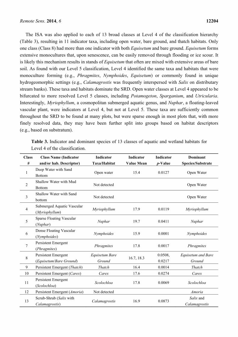
The ISA was also applied to each of 13 broad classes at Level 4 of the classification hierarchy

(Table 3), resulting in 11 indicator taxa, including open water, bare ground, and thatch habitats. Only

one class (Class 8) had more than one indicator with both Equisetum and bare ground. Equisetum forms

extensive monocultures that, upon senescence, can be easily removed through flooding or ice scour. It

is likely this mechanism results in stands of Equisetum that often are mixed with extensive areas of bare

soil. As found with our Level 5 classification, Level 4 identified the same taxa and habitats that were

monoculture forming (e.g., Phragmites, Nymphoides, Equisetum) or commonly found in unique

hydrogeomorphic settings (e.g., Calamagrostis was frequently interspersed with Salix on distributary

stream banks). These taxa and habitats dominate the SRD. Open water classes at Level 4 appeared to be

bifurcated to more resolved Level 5 classes, including Potamogeton, Sparganium, and Utricularia.

Interestingly, Myriophyllum, a cosmopolitan submerged aquatic genus, and Nuphar, a floating-leaved

vascular plant, were indicators at Level 4, but not at Level 5. These taxa are sufficiently common

throughout the SRD to be found at many plots, but were sparse enough in most plots that, with more

finely resolved data, they may have been further split into groups based on habitat descriptors

(e.g., based on substratum).

Table 3. Indicator and dominant species of 13 classes of aquatic and wetland habitats for

Level 4 of the classification.

Class #

Class Name (Indicator and/or hab. Descriptor)

Indicator Taxa/Habitat

Indicator Value Mean

Indicator p-Value

Dominant Species/Substrate

1 Deep Water with Sand

Bottom Open water 15.4 0.0127 Open Water

2 Shallow Water with Mud

Bottom Not detected Open Water

3 Shallow Water with Sand

bottom Not detected Open Water

4 Submerged Aquatic Vascular

(Myriophyllum) Myriophyllum 17.9 0.0119 Myriophyllum

5 Sparse Floating Vascular

(Nuphar) Nuphar 19.7 0.0411 Nuphar

6 Dense Floating Vascular

(Nymphoides) Nymphoides 15.9 0.0001 Nymphoides

7 Persistent Emergent

(Phragmites) Phragmites 17.8 0.0017 Phragmites

8 Persistent Emergent

(Equisetum/Bare Ground)

Equisetum Bare

Ground 16.7, 18.3

0.0508,

0.0217

Equisetum and Bare

Ground

9 Persistent Emergent (Thatch) Thatch 16.4 0.0014 Thatch

10 Persistent Emergent (Carex) Carex 17.6 0.0274 Carex

11 Persistent Emergent

(Scolochloa) Scolochloa 17.8 0.0069 Scolochloa

12 Persistent Emergent (Amoria) Not detected Amoria

13 Scrub-Shrub (Salix with

Calamagrostis) Calamagrostis 16.9 0.0873

Salix and

Calamagrostis

Remote Sens. 2014, 6 12205

We did not apply ISA to the classes at Level 3 or above, since the wetland and aquatic habitat classes

at these levels are too broad and ecologically heterogeneous to identify indicator or dominant species.

Instead, the broad classes at Levels 3 and 2 are to be interpreted and labeled in terms of their

topographical positions, substrate composition, and taxonomical relations with the fine-scale wetland

habitat classes at Level 4.

3.5. Improved Classification with Additional Spectral Bands and Metrics

In this study, we evaluated the utility of four new spectral bands, NDVI, and a textural measure to

differentiate among wetland habitats. The contribution of new bands to wetland habitat discrimination

was evaluated by observing the changes in overall classification accuracy, PA and UA for each class,

when one or more new bands was included in the classification in addition to four traditional bands

(Table 4). Using the finest resolved hierarchical classification of 22 classes, the overall accuracy with

the four traditional spectral bands was only 79.0% and the Kappa coefficient was 0.77. When the coastal

band was included in the classification along with the four traditional bands, the UA for Class 1 (Deep

Water with Sand Bottom) increased from 86.2% to 97.8% and the PA for Class 7 (Submerged Aquatic

Vascular—Sparganium) increased from 86.1% to 96.4%, despite only a small increase in the overall

accuracy from 79.0% to 80.4%. The new yellow, red-edge, and NIR2 bands were useful for

discriminating many different types of vegetated habitats, including scrub-shrub, emergent herbaceous,

and submerged aquatic vascular. When the yellow, red-edge, and NIR2 bands were used along with the

four traditional bands, the overall classification accuracy increased from 79.0% to 82.0%. In particular,

the PA for Class 22 (Scrub-shrub) increased from 59.6% to 73.0% and the UA increased from 82.0% to

92.2%. Both the UA and PA for Class 21 (Persistent Emergent—Amoria/Galeopsis/Trifolium) and Class

20 (Persistent Emergent—Scolochloa) also significantly increased. The UA for Class 16 (Persistent

Emergent—Equisetum) and the PA for Class 7 (Submerged Aquatic Vascular—Sparganium) improved

considerably as well (see Table A1).

Table 4. Variation of classification accuracy with different combinations of WV2 spectral

bands, NDVI, and texture for 22 classes of wetland and aquatic habitats.

Input Overall Accuracy 4 traditional bands only (red, blue, green, NIR) 79.0% 4 traditional bands plus coastal band 80.4% 4 traditional bands plus yellow, red-edge, NIR2 bands 82.0% 8 bands (4 traditional bands plus 4 new bands) 82.9% 8 bands plus NDVI 83.9% 8 bands plus Texture 84.8% 8 bands plus NDVI and Texture 86.5%

While some particular classes improved substantially, the combined benefit of the four new bands

increased the overall classification accuracy by only about 4%. Understanding the ecology and relative

abundance of different habitats within a study system may, then, dictate the utility of the additional

bands and processing steps. The classification scale may also help to determine whether the time and

resources to acquire and process the additional bands are necessary. When dealing with large systems in

Remote Sens. 2014, 6 12206

remote areas with substantial vegetative heterogeneity, it is prudent to err on the side of caution when

conducting vegetative assessments and system classification by acquiring the additional bands to

calculate the NDVI and textural measures.

Table 5. Mean and standard deviation (Stdv) of NDVI and textural homogeneity using the

Level 5 classification. NDVI values < 0.0 represent little to no detectable photosynthetic

activity, while higher values suggest increased green biomass and synthetic activity. Lower

homogeneity values (i.e., 0.0–1.0) represent areas of greater textural heterogeneity.

Class # Class Name NDVI Homogeneity

Mean Stdv Mean Stdv 1 Deep Water with Sand Bottom −0.33 0.04 0.72 0.09

2 Shallow Water with Sediment −0.19 0.05 0.86 0.16

3 Shallow Water with Mud Bottom −0.27 0.11 0.87 0.16

4 Very Shallow Water with Sand Bottom −0.18 0.09 0.87 0.13

5 Shallow Water with Sand Bottom 0.00 0.04 0.66 0.16

6 Submerged Aquatic Vascular (Potamogeton) −0.05 0.08 0.90 0.16

7 Submerged Aquatic Vascular (Sparganium) −0.23 0.04 0.97 0.05

8 Submerged Aquatic Vascular (Utricularia) 0.19 0.06 0.80 0.15

9 Submerged and Floating Vascular

(Agrostis/Eleocharis) 0.36 0.08 0.45 0.19

10 Very Sparse Floating Vascular (Nymphoides) 0.25 0.08 0.61 0.15

11 Sparse Floating Vascular (Nymphoides) 0.32 0.06 0.64 0.14

12 Dense Floating Vascular (Nymphoides) 0.41 0.05 0.60 0.14

13 Very Dense Floating Vascular (Nymphoides) 0.57 0.04 0.52 0.16

14 Persistent Emergent (Phragmites) 0.32 0.07 0.64 0.12

15 Persistent Emergent (Bare Ground and Carex) 0.41 0.06 0.72 0.12

16 Persistent Emergent (Equisetum) 0.54 0.04 0.71 0.14

17 Persistent Emergent (Thatch) 0.37 0.06 0.67 0.16

18 Persistent Emergent (Carex) 0.51 0.04 0.59 0.11

19 Persistent Emergent (Calamagrostis) 0.39 0.04 0.75 0.11

20 Persistent Emergent (Scolochloa) 0.67 0.05 0.50 0.17

21 Persistent Emergent (Amoria/Galeopsis/Trifolium) 0.78 0.03 0.63 0.15

22 Scrub-shrub (Salix with Calamagrostis) 0.66 0.06 0.24 0.11

The capabilities of the NDVI and image texture in differentiating wetland habitats were evaluated

similarly (Table 5). In general, water bodies (Classes 1 to 5) and aquatic bed with submerged vascular

vegetation (Classes 6 to 8) demonstrated a negative or approximately zero NDVI value. Aquatic beds

with floating vascular vegetation (Classes 9 to 11) and some emergent wetlands (Classes 14, 17, and 19)

had NDVI values <0.4. Aquatic beds with dense floating vascular vegetation (Classes 12 and 13) and

other emergent wetlands (Classes 15, 16, and 18) had NDVI values ranging between 0.4 and 0.6, while

persistent emergent and scrub-shrub wetlands (Classes 20 to 22) had NDVI values >0.65. The NDVI

layer contributed to the improvement of the classification mainly through better distinguishing of aquatic

habitats with floating vegetation (i.e., those with moderate NDVI values) in contrast to aquatic beds with

submerged vegetation or open water bodies (i.e., those with low NDVI values; see Figure 3). When the

Remote Sens. 2014, 6 12207

NDVI layer was included along with the eight spectral bands in the classification, the overall

classification accuracy increased from 82.9% to 83.9% (see Table 4). In addition, inclusion of the NDVI

improved both the UA and PA for Class 10 (13.8% and 5.1%, respectively) and Class 11 (8.7% and

10.2%, respectively). The UA for Class 2 improved by 9.6% and PA for Class 19 improved by 10.9%.

Water surfaces of lakes, streams (Classes 1 to 4), and aquatic beds with submerged vegetation

(i.e., Classes 6 to 8) had smooth textures, with homogeneity values >0.7 (see Table 5). Some types of

emergent herbaceous stands (Classes 14 to 17, 19, and 21) also had quite fine and smooth textures, and

their homogeneity values were >0.6. Scrub-shrub covered areas (Class 22) had coarse and rough textures

with the lowest homogeneity value (0.24), strongly contrasting with the surrounding emergent

herbaceous wetlands (see Figure 4). Class 9 (Submerged and Floating Vascular—Agrostis/Eleocharis)

and Class 20 (Persistent Emergent—Scolochloa) also had relatively coarse and rough textures resulting

in low homogeneity values. The inclusion of image texture with the eight spectral bands increased the

overall classification accuracy by 2% (see Table 4), but most greatly affected the PA for Class 22

(Scrub-Shrub), which improved by 12% (from 75.7% to 87.7%). Both the PA and UA for Class 21

(Persistent Emergent—Amoria/Galeopsis/Trifolium) and Class 19 (Persistent Emergent—Calamagrostis)

were also considerably improved, suggesting that image texture plays a critical role in discriminating

scrub-shrub habitats from emergent herbaceous vegetation and open waters.

4. Discussion

The advent of high-resolution multispectral satellite remote sensing systems presents new and

exciting capabilities in mapping wetland resources with very high accuracy and spatial detail.

The inclusion of multiple bands and derived measures (e.g., NDVI, textural metrics) improved our

overall mapping accuracy, as well as the discrimination of particular wetland elements. We developed a

hybrid classification approach by synergistically combining conventional unsupervised and supervised

classification methods with Dufrêne and Legendre’s [40] ISA statistical analysis, and found that

including the additional bands slightly increased overall accuracy but had a more substantial contribution

in decreasing errors associated with specific classes.

4.1. Classification of the Selenga River Delta

4.1.1. Classification Overview

As satellite sensors have improved over time, increased efforts in the past decades have been devoted

to the development of image classification methods for wetland applications. However, wetlands remain

one of the most difficult ecosystems to be classified with remote sensing data [10–13] due to their high

spatial heterogeneity and temporal variability. Though our ~87% accuracy was satisfying, improved

accuracy and detail would likely be useful to scientists and managers assessing the resource, and may

be obtained through newer classification methods proposed for wetland classification and inventory.

For instance, fuzzy classifications [53], linear spectral unmixing [54–56], and direct subpixel

techniques [10,57] are potential methods to improve wetland classification.

Some wetland studies [58–62] have adopted decision tree and other rule-based classification methods

in which ancillary environmental data, intuitive rules and scientific knowledge can be explicitly

Remote Sens. 2014, 6 12208

incorporated to improve the flexibility, robustness and reliability of wetland classification. Recently,

object-based image classification methods have been applied to wetland classifications [28,63–66].

Different from per-pixel-based classification methods, the object-oriented method first segments an

image into a set of homogenous objects called regions, then groups the image objects into different

thematic classes based on spectral, textural, geometric, and/or topological properties of image objects.

As we found useful differentiation between classes using spectral and textural approaches and a more

traditional analytical method, adding additional properties with an object-oriented approach could

substantially improve wetland classification.

Using satellite sensors with higher resolution and additional bands will necessitate improved

analytical techniques that better incorporate ancillary data. However, for a system with the size of

the SRD, data requirements should be identified at the scale of the management need. This can be

accomplished while concurrently delving further into wetland classification and synecological

relationships using highly resolved data and advanced analytical techniques by creating a hierarchical

classification. This ensures that outcomes provide useful information for a multitude of end users.

4.1.2. Classification Error Assessment

Classification errors associated with this study likely reflect ecological gradients and vegetation

growth patterns not following rigid and well-defined geographical separations. For instance, we often

encountered Carex co-occurring with Calamagrostis as they both occupy similar ecological niches.

There was sufficient fidelity of plants to Class 18 and Class 19 for ISA to identify Carex and

Calamagrostis as unique indicator taxa, yet their ecological niches were apparently not distinct enough

for the hybrid classification to accurately discriminate between them. It is also worth noting that there

are tens of species of Carex that occur in the wetland habitats that we surveyed, confounding their use

as indicators. We addressed field-scale botanical heterogeneity by only characterizing percent cover for

plants and habitats at ≥10%, using a large (100 m2) quadrat for sampling and only focusing on taxa at

the genus level. Further accuracy improvement would likely come from additional imagery acquisition

over time that could capture phenological changes associated with, and specific to, the most commonly

occurring taxa in the hybrid classification classes, as well as focusing on species-level analyses.

Both the omission and commission error rates associated with certain Level 5 classes (e.g., Classes 1,

5, 6, 12–14) were excellent, with errors <10%. Phragmites, an indicator of Class 14, is known to form

extensive monocultures, thus providing limited spectral variance within a given stand [28,60]. In our

study, two areas with extensive Phragmites were noted to have >75% and >90% Phragmites dominance.

Similarly, Nymphoides (Classes 12 and 13) are mat-forming plants with floating leaves that can

completely dominate areas of moderate depth (<2 m) and low-flow velocities. The depth prevents many

plants from successfully rooting and the relative density can vary markedly (e.g., sparse, dense, very

dense) depending upon multiple factors, including wind direction, water depth, and wave exposure. We

found measureable stands of Nymphoides at 19 sampling locations, ranging from 10% to 97% coverage.

The SRD includes large areas of deeper waters, with no readily apparent vegetation, identified as both

Deep Water with Sand Bottom (Class 1) and Shallow Water with Sand Bottom (Class 5). Moderately

deep water with limited wind exposure would often be dominated by stands of Potamogeton (Class 6).

Remote Sens. 2014, 6 12209

We encountered sufficient Potamogeton on five sites, four with ≥30% and one with ≥90% coverage.

Few other plants were found intermixed with Potamogeton, limiting its spectral variance.

4.2. Indicator Species Analysis

Indicator Species Analysis is a powerful tool to explore the associations between particular taxa

or described habitats and satellite-based classifications and we suggest increased application of this tool

to remote sensing analyses because the ISA can be useful to “[d]escribe species relationships

to environmental categories or experimental groups” [46]. In our study we were able to identify

11 taxa/habitats with sufficient specificity and fidelity to our supervised groups at the Level 5

classification and another 11 at Level 4. That is useful for end users who, upon identifying the abundant

taxa/habitat within their plot, can use that knowledge to determine the plot’s habitat class and the

corresponding frequency, abundance, and function of that class. Furthermore, knowing the relationships

between taxa fidelity and classes can improve our knowledge of botanical synecological relationships

in subsequent studies.

Though not conducted in this study, ISA can also be used in remote sensing studies to discern output

from cluster analyses. For instance, as shown by McCune et al. [46] for dendrogram pruning, output

from a supervised classification demonstrated a certain number of unique classes can be explored

through calculating and plotting the average ISA p-value and number of significant ISA taxa for each

class. The final number of unique classes, or clusters, can be iteratively tested in this manner based on

the field data and the selection of the final number of classes of the remotely sensed data based on the

lowest average p-value and/or the highest number of significant ISA taxa.

4.3. Additional Bands, NDVI, and Texture Metrics

This research quantitatively evaluated the benefits of four new spectral bands in addition to more

typical bandwidths from a high-resolution satellite system for discriminating freshwater wetland habitats

and plant communities. Like several other studies [28,67,68], our analysis indicated that the addition of

the four new spectral bands contributed little to the overall increase in the classification accuracy (<4%

improvement), but was beneficial for distinguishing specific wetland classes. In our study, the coastal

band made the greatest contribution in the separation between different open water and aquatic habitats.

This is similar to the results from Souza and Kux [69], who found high discrimination of tidal channels

from other satellite systems with the coastal band. The yellow, red-edge and NIR2 bands were more

useful for discriminating among different vegetated terrestrial and aquatic habitats, especially on less

frequently inundated areas (e.g., Classes 20 and 21), and areas with an interplay of Equisetum, thatch,

and bare ground (Class 16). We did not further separate the bands to determine the relative importance

of each band, outside of the coastal band, to improving our accuracy. In an area such as the SRD, with

so much vegetation diversity, further studies of the influence of these additional bands are warranted.

Our analysis also showed that the NDVI remains valuable for improving overall classification

accuracy, and image texture can be particularly useful for separating scrub-shrub wetlands from

emergent herbaceous wetlands. In comparison with the four traditional spectral bands, the introduction

of four new spectral bands, NDVI, and image texture increased the overall wetland classification

accuracy by 7.5%.

Remote Sens. 2014, 6 12210

5. Summary

Increasingly available at finer resolutions and temporal coverages, remotely sensed imagery provides

an excellent data source for providing inventories of wetland systems. Because of their fluctuating water

levels, large and heterogeneous wetland systems are likely among the most difficult systems to

inventory. Remotely sensed data and increasingly effective analyses (e.g., [60]) are providing

informative baselines for scientists and resource managers to study the effects of climate change, altered

hydrology, and other perturbations and adaptive management techniques on wetland systems. In this

study, we developed a hierarchical inventory of wetlands of Russia’s SRD, a Ramsar Wetland of

International Importance and a UN World Heritage site, and tested the ability of additional WV2 bands

to classify the wetland landscape. As others have found, overall accuracy increased little with the

addition of the four extra WV2 bands, though the accuracy associated with certain classes did increase

markedly. Incorporating NDVI and texture measures resulted in a substantial improvement in the

accuracy, suggesting that these metrics will continue to improve our understanding of wetland landscape

environments. In addition to better classifying the SRD, we anticipate that the five levels of our hierarchy

will be useful to effectively managing this important resource in light of changes to inputs to Lake Baikal

from climate modification as well as anthropogenic disturbances in the Selenga River watershed.

Improved mapping and inventories of the SRD will come from increased field-based data sets with

improved spatial distribution within the delta, species-level analyses, additional imagery from “shoulder

seasons” within the SRD, and modifications to the classification algorithms.

Acknowledgments

The U.S. Environmental Protection Agency Office of Research and Development partially funded

and collaborated in the research described here under contract number EP-D-06-096 to Dynamac

Corporation. The research conducted herein was also partially funded by the U.S. Department of State,

Biochemical Redirect Program with support from the International Science and Technology Center,

Moscow, Russia. We appreciate the technical review and feedback provided by John Lin, U.S. EPA,

and the programmatic support of Doug Steele, U.S. EPA. This paper has been reviewed in accordance

with the U.S. Environmental Protection Agency’s peer and administrative review policies and approved

for publication. Mention of trade names or commercial products does not constitute endorsement or

recommendation for use. Statements in this publication reflect the authors’ professional views and

opinions and should not be construed to represent any determination or policy of the U.S. Environmental

Protection Agency.

Author Contributions

All authors have made significant contributions to the manuscript. Charles Lane, Bradley Autrey,

and Oleg Anenkhonov developed the original idea, supervised the study, analyzed the data,

and contributed in manuscript development and revision. Charles Lane and Hongxing Liu are the main

authors who developed and revised the manuscript. Hongxing Liu processed the spatial data, developed

the methodology, analyzed the results and co-wrote the manuscript. Victor Chepinoga contributed to field

Remote Sens. 2014, 6 12211

study development and collection and data analyses. Qiusheng Wu contributed literature reviews, spatial

data analyses, ideas and discussions. All authors shared equally the editing of the manuscript.

Conflicts of Interest

The authors declare no conflicts of interest.

References

1. Daily, G.C.; Alexander, S.; Ehrlich, P.R.; Goulder, L.; Lubchenco, J.; Matson, P.A.; Mooney, H.A.;

Postel, S.; Schneider, S.H.; Tilman, D. Ecosystem Services: Benefits Supplied to Human Societies by

Natural Ecosystems; Ecological Society of America: Washington, DC, USA, 1997.

2. Millennium Ecosystem Assessment. Millennium Ecosystem Assessment Synthesis Report;

Millennium Ecosystem Assessment: Washington, DC, USA, 2005.

3. Dahl, T.E. Status and Trends of Wetlands in the Conterminous United States 1986 to 1997; US Fish

and Wildlife Service: Washington, DC, USA, 2000.

4. Dahl, T.E.; Watmough, M.D. Current approaches to wetland status and trends monitoring in prairie

Canada and the continental United States of America. Can. J. Remote Sens. 2007, 33, S17–S27.

5. Finlayson, C.; Davidson, N.; Spiers, A.; Stevenson, N. Global wetland inventory—Current status

and future priorities. Mar. Freshw. Res. 1999, 50, 717–727.

6. Mitsch, W.J. Wetlands; Van Nostrand Rheinhold: New York, NY, USA, 1993; p. 722.

7. Robarts, R.D.; Zhulidov, A.V.; Pavlov, D.F. The state of knowledge about wetlands and their future

under aspects of global climate change: The situation in Russia. Aquat. Sci. 2013, 75, 27–38.

8. Titus, J.; Hudgens, D.; Trescott, D.; Craghan, M.; Nuckols, W.; Hershner, C.; Kassakian, J.;

Linn, C.; Merritt, P.; McCue, T. State and local governments plan for development of most land

vulnerable to rising sea level along the US Atlantic coast. Environ. Res. Lett. 2009, 4, 044008.

9. McKinney, R.A.; Charpentier, M.A. Extent, properties, and landscape setting of geographically

isolated wetlands in urban southern New England watersheds. Wetl. Ecol. Manag. 2009, 17,

331–344.

10. Ozesmi, S.L.; Bauer, M.E. Satellite remote sensing of wetlands. Wetl. Ecol. Manag. 2002, 10,

381–402.

11. Bourgeau-Chavez, L.L.; Riordan, K.; Powell, R.B.; Miller, N.; Nowels, M. Improving wetland

characterization with multi-sensor, multi-temporal SAR and optical/infrared data fusion. In

Advances in Geoscience and Remote Sensing; INTECH: Rijeka, Croatia, 2009.

12. Wickham, J.; Stehman, S.; Smith, J.; Yang, L. Thematic accuracy of the 1992 National

Land-Cover Data for the western United States. Remote Sens. Environ. 2004, 91, 452–468.

13. Wright, C.; Gallant, A. Improved wetland remote sensing in Yellowstone national park using

classification trees to combine TM imagery and ancillary environmental data. Remote Sens. Environ.

2007, 107, 582–605.

14. Klemas, V. Remote sensing of wetlands: Case studies comparing practical techniques.

J. Coast. Res. 2011, 27, 418–427.

15. Adam, E.; Mutanga, O.; Rugege, D. Multispectral and hyperspectral remote sensing for identification

and mapping of wetland vegetation: A review. Wetl. Ecol. Manag. 2010, 18, 281–296.

Remote Sens. 2014, 6 12212

16. Silva, T.S.; Costa, M.P.; Melack, J.M.; Novo, E.M. Remote sensing of aquatic vegetation: Theory

and applications. Environ. Monitor. Assess. 2008, 140, 131–145.

17. Hess, L.L.; Melack, J.M.; Filoso, S.; Wang, Y. Delineation of inundated area and vegetation along

the Amazon floodplain with the SIR-C synthetic aperture radar. IEEE Trans. Geosci. Remote Sens.

1995, 33, 896–904.

18. Kasischke, E.S.; Bourgeau-Chavez, L.L. Monitoring South Florida wetlands using ERS-1 SAR

imagery. Photogram. Eng. Remote Sens. 1997, 63, 281–291.

19. Kushwaha, S.; Dwivedi, R.; Rao, B. Evaluation of various digital image processing techniques for

detection of coastal wetlands using ERS-1 SAR data. Int. J. Remote Sens. 2000, 21, 565–579.

20. Townsend, P.A.; Walsh, S.J. Modeling floodplain inundation using an integrated GIS with radar

and optical remote sensing. Geomorphology 1998, 21, 295–312.

21. DigitalGlobe. Whitepaper: The Benefits of the 8 Spectral Bands of Worldview-2. DigitalGlobe,

2010. Available online: https://www.digitalglobe.com/sites/default/files/DG-8SPECTRAL-WP_0.pdf

(accessed on 22 June 2014).

22. Yuzugullu, O.; Aksoy, A. Generation of the bathymetry of a eutrophic shallow lake using

Worldview-2 imagery. J. Hydroinform. 2014, 16, 50–59.

23. Lee, K.R.; Kim, A.M.; Olsen, R.; Kruse, F.A. Using Worldview-2 to determine bottom-type and

bathymetry. Proc. SPIE 2011, doi:10.1117/12.883578.

24. Asmaryan, S.; Warner, T.A.; Muradyan, V.; Nersisyan, G. Mapping tree stress associated with

urban pollution using the Worldview-2 red edge band. Remote Sens. Lett. 2013, 4, 200–209.

25. Cronk, J.K.; Fennessy, M.S. Wetland Plants: Biology and Ecology; CRC Press: New York, NY,

USA, 2001.

26. Collin, A.; Hench, J.L. Towards deeper measurements of tropical reefscape structure using the

Worldview-2 spaceborne sensor. Remote Sens 2012, 4, 1425–1447.

27. Reshitnyk, L.; Costa, M.; Robinson, C.; Dearden, P. Evaluation of Worldview-2 and acoustic

remote sensing for mapping benthic habitats in temperate coastal Pacific waters. Remote Sens.

Environ. 2014, 153, 7–23.

28. Lantz, N.J.; Wang, J. Object-based classification of Worldview-2 imagery for mapping invasive

common reed, Phragmites australis. Can. J. Remote Sens. 2013, 39, 328–340.

29. Ramsar Convention on Wetlands Factsheet. Information Sheet on Ramsar Wetlands. Available

online: http://sites.wetlands.org/reports/ris/2RU018en.pdf (accessed on 13 November 2012).

30. Tucker, C.J. Red and photographic infrared linear combinations for monitoring vegetation.

Remote Sens. Environ. 1979, 8, 127–150.

31. Haralick, R.M.; Shanmugam, K.; Dinstein, I.H. Textural features for image classification. IEEE

Trans. Syst. Man. Cybern. 1973, 3, 610–621.

32. Gyninova, A.; Korsunov, V. The soil cover of the Selenga Delta area in the Baikal region.

Eurasian Soil Sci. 2006, 39, 243–250.

33. Konovalova, T. Mapping geosystems in the Selenga River delta. Mapp. Sci. Remote Sens. 2002,

39, 295–302.

34. Ilyicheva, E. Dynamics of the Selenga River network and delta structure. Geogr. Nat. Resour. 2008,

29, 343–347.

Remote Sens. 2014, 6 12213

35. Pavelsky, T.M.; Smith, L.C. Remote sensing of hydrologic recharge in the Peace–Athabasca Delta,

Canada. Geophys. Res. Lett. 2008, 35, L08403.

36. Hui, Y.; Rongqun, Z.; Xianwen, L. Classification of wetland from tm imageries based on decision

tree. WSEAS Trans. Infor. Sci. Appl. 2009, 6, 1790–0832.

37. Melesse, A.M.; Jordan, J.D.; Graham, W.D. Enhancing land cover mapping using Landsat derived

surface temperature and NDVI. Bridges 2001, 10, 439.

38. Narumalani, S.; Jensen, J.R.; Burkhalter, S.; Althausen, J.D.; Mackey, H.E., Jr. Aquatic macrophyte

modeling using GIS and logistic multiple regression. Photogram. Eng. Remote Sens. 1997, 63,

41–49.

39. Hodgson, M.; Jensen, J.; Mackey H., Jr.; Coulter, M. Remote sensing of wetland habitat: A wood

stork example. Photogram. Eng. Remote Sens. 1987, 53, 1075–1080.

40. Dufrêne, M.; Legendre, P. Species assemblages and indicator species: The need for a flexible

asymmetrical approach. Ecol. Monogr. 1997, 67, 345–366.

41. Ball, G.H.; Hall, D.J. Isodata, A Novel Method of Data Analysis and Pattern Classification;

DTIC Document; Stanford Research Institute: Menlo Park, CA, USA, 1965.

42. Tou, J.T.; Gonzalez, R.C. Pattern Recognition Principles; Addison-Wesley: London, UK, 1974.

43. Jain, A.K.; Dubes, R.C. Algorithms for Clustering Data; Prentice-Hall, Inc.: Englewood Cliffs, NJ,

USA, 1988.

44. Jensen, J.R. Remote Sensing of the Environment: An Earth Resource Perspective; Prentice-Hall,

Inc.: Upper Saddle River, NJ, USA, 2007.

45. Richards, J.; Jia, X. Remote Sensing Digital Image Analysis—An Introduction, 3rd ed.;

Springer-Verlag New York, Inc.: New York, NY, USA, 2006.

46. McCune, B.; Grace, J.B.; Urban, D.L. Analysis of Ecological Communities; MjM Software Design:

Gleneden Beach, OR, USA, 2002.

47. Brinson, M.M. A Hydrogeomorphic Classification for Wetlands; Technical Report WRP-DE-4;

US Army Corps of Engineers, Waterways Experiment Station: Washington, DC, USA, 1993.

48. Foody, G.M.; Campbell, N.; Trodd, N.; Wood, T. Derivation and applications of probabilistic

measures of class membership from the maximum-likelihood classification. Photogram. Eng.

Remote Sens. 1992, 58, 1335–1341.

49. Cowardin, L.M.; Carter, V.; Golet, F.C.; LaRoe, E.T. Classification of Wetlands and Deepwater

Habitats of the United States; Fish and Wildlife Service, US Department of the Interior: Washington,

DC, USA, 1979.

50. Ramsar Convention of Wetlands. The Ramsar Convention Definition of “Wetland” and

Classification System for Wetland Type. Available online: http://www.ramsar.org/cda/en/

ramsar-activities-cepa-classification-system/main/ramsar/1-63-69%5E21235_4000_0 (accessed

on 2 Ocotober 2012).

51. Cowardin, L.M.; Golet, F.C. US Fish and Wildlife Service 1979 wetland classification: A review.

Vegetatio 1995, 118, 139–152.

52. Lillesand, T.M.; Kiefer, R.W.; Chipman, J.W. Remote Sensing and Image Interpretation;

John Wiley & Sons Ltd.: Hoboken, NJ, USA, 2004.

Remote Sens. 2014, 6 12214

53. Stankiewicz, K.; Dabrowska-Zielinska, K.; Gruszczynska, M.; Hoscilo, A. Mapping vegetation of

a wetland ecosystem by fuzzy classification of optical and microwave satellite images supported

by various ancillary data. In Proceedinsg of International Symposium on Remote Sensing, Crete,

Greece, 23 September 2002; International Society for Optics and Photonics: Bellingham, WA, USA,

2003; pp. 352–361.

54. Oki, K.; Oguma, H.; Sugita, M. Subpixel classification of alder trees using multitemporal Landsat

Thematic Mapper imagery. Photogram. Eng. Remote Sens. 2002, 68, 77–82.

55. Shanmugam, P.; Ahn, Y.-H.; Sanjeevi, S. A comparison of the classification of wetland

characteristics by linear spectral mixture modelling and traditional hard classifiers on multispectral

remotely sensed imagery in southern India. Ecol. Model. 2006, 194, 379–394.

56. Wang, J.; Lang, P.A. Detection of cypress canopies in the Florida Panhandle using subpixel analysis

and GIS. Remote Sens. 2009, 1, 1028–1042.

57. Huguenin, R.L.; Karaska, M.A.; van Blaricom, D.; Jensen, J.R. Subpixel classification of bald

cypress and tupelo gum trees in Thematic Mapper imagery. Photogram. Eng. Remote Sens. 1997,

63, 717–724.

58. Baker, C.; Lawrence, R.; Montagne, C.; Patten, D. Mapping wetlands and riparian areas using

Landsat ETM+ imagery and decision-tree-based models. Wetlands 2006, 26, 465–474.

59. Bolstad, P.V.; Lillesand, T. Improved classification of forest vegetation in northern Wisconsin

through a rule-based combination of soils, terrain, and Landsat Thematic Mapper data. For. Sci.

1992, 38, 5–20.

60. Frick, A.; Steffenhagen, P.; Zerbe, S.; Timmermann, T.; Schulz, K. Monitoring of the vegetation

composition in rewetted peatland with iterative decision tree classification of satellite imagery.

Photogram. Fernerkund. Geoinfor. 2011, 2011, 109–122.

61. Lunetta, R.S.; Balogh, M.E. Application of multi-temporal Landsat 5 TM imagery for wetland

identification. Photogram. Eng. Remote Sens. 1999, 65, 1303–1310.

62. Na, X.; Zhang, S.; Zhang, H.; Li, X.; Yu, H.; Liu, C. Integrating TM and ancillary geographical

data with classification trees for land cover classification of marsh area. Chin. Geogr. Sci. 2009, 19,

177–185.

63. Fournier, R.A.; Grenier, M.; Lavoie, A.; Hélie, R. Towards a strategy to implement the Canadian

wetland inventory using satellite remote sensing. Can. J. Remote Sens. 2007, 33, S1–S16.

64. Frohn, R.; Autrey, B.; Lane, C.; Reif, M. Segmentation and object-oriented classification

of wetlands in a Karst Florida landscape using multi-season Landsat-7 ETM+ imagery. Int. J.

Remote Sens. 2011, 32, 1471–1489.

65. Grenier, M.; Labrecque, S.; Garneau, M.; Tremblay, A. Object-based classification of a SPOT-4

image for mapping wetlands in the context of greenhouse gases emissions: The case of the Eastmain

region, Québec, Canada. Can. J. Remote Sens. 2008, 34, S398–S413.

66. Powers, R.P.; Hay, G.J.; Chen, G. How wetland type and area differ through scale: A GEOBIA

case study in Albertaʼs boreal plains. Remote Sens. Environ. 2012, 117, 135–145.

67. Chen, Q. Comparison of Worldview-2 and IKONOS-2 Imagery for Identifying Tree Species in the

Habitat of An Endangered Bird Species in Hawaii 8-Band Research Challenge; DigitalGlobe:

Longmont, CO, USA, 2011.

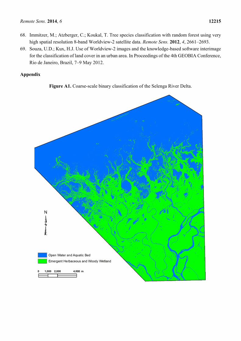
Remote Sens. 2014, 6 12215

68. Immitzer, M.; Atzberger, C.; Koukal, T. Tree species classification with random forest using very

high spatial resolution 8-band Worldview-2 satellite data. Remote Sens. 2012, 4, 2661–2693.

69. Souza, U.D.; Kux, H.J. Use of Worldview-2 images and the knowledge-based software interimage

for the classification of land cover in an urban area. In Proceedings of the 4th GEOBIA Conference,

Rio de Janeiro, Brazil, 7–9 May 2012.

Appendix

Figure A1. Coarse-scale binary classification of the Selenga River Delta.

Remote Sens. 2014, 6 12216

Table A1. Variation of classification accuracy with different combinations of WV2 spectral bands, NDVI, and texture for 22 classes of wetland

and aquatic habitats.

Wetland

Class

4 Traditional Bands only

(Red, Blue, Green, NIR)

4 Traditional Bands

plus Coastal Band

4 Traditional Bands plus Yellow,

Red-Edge, NIR2 Bands

8 Bands (4 Traditional Bands

plus 4 New Bands)

8 Bands

plus NDVI

8 Bands

plus Texture

8 Bands plus NDVI

and Texture

PA (%) UA (%) PA (%) UA (%) PA (%) UA (%) PA (%) UA (%) PA (%) UA (%) PA (%) UA (%) PA (%) UA (%)

1 84.91 86.20 87.50 97.77 85.98 99.31 87.82 99.59 91.98 92.75 89.69 97.87 92.47 92.74

2 64.66 87.36 67.30 87.64 60.86 88.37 61.51 88.59 61.79 98.19 61.42 90.39 60.65 99.24

3 66.98 72.20 68.38 72.05 73.72 72.63 74.89 74.40 88.54 79.40 80.44 76.23 91.56 79.66

4 95.47 55.54 93.29 55.66 95.65 61.98 94.80 62.90 95.69 77.42 93.48 68.45 94.59 82.26

5 96.32 99.73 95.90 99.56 98.32 99.68 98.79 99.68 97.06 99.62 98.79 98.17 97.55 99.46

6 95.49 97.69 95.25 97.36 91.43 99.12 91.58 98.99 86.65 97.96 93.62 98.02 93.49 96.58

7 76.84 86.13 94.62 96.36 95.52 90.22 95.94 90.58 70.70 76.37 83.78 93.62 67.79 86.79

8 72.63 76.57 72.43 75.54 68.93 78.27 69.34 78.01 70.58 79.40 66.67 79.61 70.55 82.40

9 68.23 54.78 66.43 52.72 70.04 53.30 68.95 51.07 69.68 54.21 70.04 50.26 69.88 52.25

10 79.96 56.22 78.68 60.99 82.30 55.70 79.74 58.07 84.84 71.87 81.24 54.04 86.52 71.35

11 77.94 81.67 80.81 81.99 75.66 81.07 78.02 80.82 88.22 90.37 78.36 80.19 86.76 88.00

12 88.31 94.58 88.89 94.43 88.27 94.44 88.45 94.23 91.89 96.20 87.33 93.21 91.19 95.17

13 97.29 92.92 97.36 93.62 97.36 90.26 97.42 90.65 99.03 95.17 96.91 90.60 98.28 96.22

14 94.26 88.53 96.95 88.81 95.60 91.37 97.92 92.82 97.07 91.17 97.56 92.48 97.15 90.19

15 81.99 73.72 84.76 76.88 86.57 76.31 87.67 78.83 82.83 83.64 87.40 78.78 79.26 84.31

16 91.60 75.33 90.83 78.84 90.22 86.63 90.17 88.05 94.27 85.59 89.45 93.52 94.20 88.18

17 82.30 81.49 83.26 78.74 80.47 74.56 81.76 74.01 82.30 81.66 86.17 70.47 83.93 78.91

18 78.56 48.30 76.65 48.06 81.24 48.80 79.93 48.73 77.55 49.51 75.88 52.26 74.40 53.42

19 59.93 88.59 59.14 90.08 47.12 92.01 47.04 92.45 57.94 92.72 49.50 93.17 68.92 92.99

20 84.34 62.93 85.29 65.34 92.77 67.37 93.09 68.72 95.86 63.79 88.93 76.77 94.43 74.54

21 80.22 89.17 80.89 91.53 82.95 94.44 83.99 95.85 86.55 93.04 86.42 97.79 89.10 94.74

22 59.64 82.04 64.76 84.17 72.95 92.16 75.70 93.44 65.86 94.37 87.68 93.55 81.43 95.02

© 2014 by the authors; licensee MDPI, Basel, Switzerland. This article is an open access article distributed under the terms and conditions of the Creative

Commons Attribution license (http://creativecommons.org/licenses/by/4.0/).