Implementation of a multigrid solver on a GPU for Stokes equations with strongly variable viscosity...
12
http://hpc.sagepub.com/ Computing Applications International Journal of High Performance http://hpc.sagepub.com/content/28/1/50 The online version of this article can be found at: DOI: 10.1177/1094342013478640 2014 28: 50 originally published online 5 March 2013 International Journal of High Performance Computing Applications Liang Zheng, Huai Zhang, Taras Gerya, Matthew Knepley, David A Yuen and Yaolin Shi based on Matlab and CUDA Implementation of a multigrid solver on a GPU for Stokes equations with strongly variable viscosity Published by: http://www.sagepublications.com can be found at: International Journal of High Performance Computing Applications Additional services and information for http://hpc.sagepub.com/cgi/alerts Email Alerts: http://hpc.sagepub.com/subscriptions Subscriptions: http://www.sagepub.com/journalsReprints.nav Reprints: http://www.sagepub.com/journalsPermissions.nav Permissions: http://hpc.sagepub.com/content/28/1/50.refs.html Citations: What is This? - Mar 5, 2013 OnlineFirst Version of Record - Jan 20, 2014 Version of Record >> at University of Missouri-Columbia on February 7, 2014 hpc.sagepub.com Downloaded from at University of Missouri-Columbia on February 7, 2014 hpc.sagepub.com Downloaded from
Transcript of Implementation of a multigrid solver on a GPU for Stokes equations with strongly variable viscosity...

http://hpc.sagepub.com/Computing Applications
International Journal of High Performance
http://hpc.sagepub.com/content/28/1/50The online version of this article can be found at:
DOI: 10.1177/1094342013478640
2014 28: 50 originally published online 5 March 2013International Journal of High Performance Computing ApplicationsLiang Zheng, Huai Zhang, Taras Gerya, Matthew Knepley, David A Yuen and Yaolin Shi
based on Matlab and CUDAImplementation of a multigrid solver on a GPU for Stokes equations with strongly variable viscosity
Published by:
http://www.sagepublications.com
can be found at:International Journal of High Performance Computing ApplicationsAdditional services and information for
http://hpc.sagepub.com/cgi/alertsEmail Alerts:
http://hpc.sagepub.com/subscriptionsSubscriptions:
http://www.sagepub.com/journalsReprints.navReprints:
http://www.sagepub.com/journalsPermissions.navPermissions:
http://hpc.sagepub.com/content/28/1/50.refs.htmlCitations:
What is This?
- Mar 5, 2013OnlineFirst Version of Record
- Jan 20, 2014Version of Record >>
at University of Missouri-Columbia on February 7, 2014hpc.sagepub.comDownloaded from at University of Missouri-Columbia on February 7, 2014hpc.sagepub.comDownloaded from

Article
Implementation of a multigrid solveron a GPU for Stokes equations withstrongly variable viscosity based onMatlab and CUDA
Liang Zheng1,2,3, Huai Zhang1,2, Taras Gerya4,Matthew Knepley5, David A Yuen3,6 and Yaolin Shi1,2
AbstractThe Stokes equations are frequently used to simulate geodynamic processes, including mantle convection, lithosphericdynamics, lava flow, and among others. In this study, the multigrid (MG) method is adopted to solve Stokes and continuityequations with strongly temperature-dependent viscosity. By taking advantage of the enhanced computing power ofgraphics processing units (GPUs) and the new version of Matlab 2010b, MG codes are optimized through ComputeUnified Device Architecture (CUDA). Herein, we illustrate the approach that implements a GPU-based MG solver withRed–Black Gauss–Seidel (RBGS) smoother for the three-dimensional Stokes and continuity equations, in a hope that ithelps solve the synthetic incompressible sinking problem in a cubic domain with strongly variable viscosity, and finally ana-lyze our solver’s efficiency on a GPU.
KeywordsGPU, Matlab, multigrid, Stokes flow, strongly variable viscosity
1 Introduction
Graphics processing units (GPUs) are increasingly being
used to solve numerical problems, since NVIDIA first
released the Compute Unified Device Architecture
(CUDA) in 2007. Modern GPUs enjoy a laudable perfor-
mance in parallel computing thanks to the unique architec-
ture of single instruction multiple thread (SIMT) it applies.
With a different design philosophy to the central processing
unit (CPU), the GPU is oriented by throughput design with
many cores, but without powerful or adequate cache,
branch prediction or data forwarding functionalities. GPUs
consume much less energy, compared with PC clusters of
the same computing capacity. For example, Tesla 2050 has
a peak performance of 1.03 Tflops for single precision
floating point operation and 515 Gflops for double preci-
sion floating point operation on a single GPU card with the
max power consumption at 238 W, while a single i7-960
CPU with the limited performance of 3.2 Gflops needs a
power consumption at 130 W. This is one critical issue
because the enhanced power efficiency economizes the
device for a noticeably reduced electricity bill.
CUDA is a parallel programming model designed to
manage thousands of threads running on the streaming mul-
tiprocessors (SMs) and the streaming processors (SPs) at
the hardware level of GPU. CUDA threads are organized
in blocks and grids at the software level, where one grid
contains numerous blocks, and one block contains numer-
ous threads. This architecture hierarchy allows the threads
in the same block to communicate with each other through
the shared memory using SMs and barrier synchronization.
The number of threads in each block and the number of
blocks in each grid have to be defined explicitly in CPU
codes (host codes) which are usually written in C or other
conventional languages such as Python and Fortran.
CUDA, as a high-level language, allows a programmer to
use CUDA C to define GPU kernel’s functionalities. As a
1 Key Laboratory of Computational Geodynamics, University of Chinese
Academy of Sciences, China2 College of Earth Science, University of Chinese Academy of Sciences,
China3 Minnesota Supercomputing Institute, University of Minnesota, MN, USA4 Institute of Geophysics, ETH-Zurich, Switzerland5 Computational Institute, University of Chicago, Chicago, IL, USA6 School of Environmental Sciences, China University of Geosciences,
Wuhan, China
Corresponding author:
Huai Zhang, Yaolin Shi, Key Laboratory of Computational Geodynamics,
University of Chinese Academy of Sciences, 19A Yuquan Road,
Shijingshan, Beijing 100049, China.
Email: [email protected]; [email protected]
The International Journal of HighPerformance Computing Applications2014, Vol. 28(1) 50–60ª The Author(s) 2013Reprints and permissions:sagepub.co.uk/journalsPermissions.navDOI: 10.1177/1094342013478640hpc.sagepub.com
at University of Missouri-Columbia on February 7, 2014hpc.sagepub.comDownloaded from

result, CUDA C kernel functions (device codes), which are
called by host codes in principal, could be able to be exe-
cuted in parallel through CUDA threads (NVIDIA, 2011).
Developing CUDA applications is still challenging, espe-
cially when most codes are written in other languages rather
than C. On the one hand, script codes, such as Matlab and
Python, are often used to implement and optimize the algo-
rithms. Furthermore, using script language as an interface
to call C and Fortran codes is commonplace in scientific com-
putation, as it reduces the workload of programming without
compromising the core performance. Fortunately, some
script programming tools, such as Jacket Matlab toolbox1 and
PyCUDA (Klockner et al., 2009), have already supported
porting CUDA kernels. The latest version of Matlab (Matlab
2010b or newer versions) released a parallel computing tool-
box available to support GPU computing. Compared with the
Jacket Matlab toolbox, Matlab 2010b can call parallel thread
execution (PTX) directly. PTX provides a low-level instruc-
tion set for CUDA programming, similar to the assemble lan-
guage applied in the x86 architecture. The handwriting
CUDA kernels can be transformed into PTX codes with –ptx
flag at command line while compiling the codes , which can
be called as Matlab functions as well. In this paper, we discuss
how to solve the three-dimensional Stokes flow problem in
detail using PTX kernels called by the Matlab 2010b.
2 Background of Stokes flow problem
The Stokes flow can be applied to study geodynamical phe-
nomena, as the Earth behaves like an incompressible creep-
ing flow that would last for hundreds of millions of years in
its history. For example, Earth’s mantle can be deemed as a
flow with very high viscosity that has sustained for millions
of years. Stokes flow, also named as creeping flow, has a
relatively low Reynolds number when the advective trans-
port term in the Navier–Stokes equations is negligible. In
general, we utilize the conservation of mass and momen-
tum to describe the stable status of Stokes flow problem
as follows:
qui
qxi
¼ 0 ð1Þ
qs0ij
qxj
� qP
qxi
þ rgi ¼ 0 ð2Þ
where ui is velocity, s0ij is the deviatoric stress, P is pres-
sure, r is density and gi represents acceleration of body
force such as the gravity in most cases. Equation (1) is the
continuity equation, and Equation (2) is indeed the Stokes
equation. Einstein’s summation convention is used here. In
fact, the coupled equations of (1) and (2) lead the system to
saddle point problem, which needs to meet the LBB criteria
(also known as the Ladyzhenskaya–Babuska–Breezi condi-
tion) when a numerical scheme is implemented. LBB cri-
teria is a compatibility condition between the velocity
and pressure spaces, which is necessary to yield stable pres-
sure approximations. The constitutive relationship bridging
the velocity ui and the deviatoric stress s0ij in Equations (1)
and (2) is defined as
s0
ij ¼ 2Z_Eij ¼ Zqui
qxj
þ quj
qxi
� �ð3Þ
in which, _Eij is the strain rate and the viscosity Z describes
the rheology of the fluid.
In most cases, the numerical algorithms built on high-
performance computing philosophy are proved more realis-
tic, although analytic solutions can be used to address the
flow problem given simple geometries and boundary condi-
tions (Payne and Pell, 1960; Schubert et al., 2001; Turcotte
and Schubert, 2002). To date, many numerical methods have
been developed and applied to solve the Stokes equations,
including the finite difference method, the finite volume
method, and the finite element method (Patankar, 1980;
Elman et al., 2005; Lynch, 2005). However, in the context
of geodynamical modeling, the Stokes equations will pro-
duce difficulties numerically due to strongly variable coeffi-
cients, and hence need more wisdom to be handled (Moresi
et al., 1996; Deubelbeiss and Kaus, 2008). This effects from
temperature-dependent viscosity can be summarized as
Zeff / expEa þ VaP
RT
� �ð4Þ
where, Zeff represents the effective viscosity, Ea represents
activation energy, and Va activation volume, R is the gas
constant, with P for the pressure and T the temperature.
Apparently, the effective viscosity may vary by orders of
magnitudes even with a small change of environmental
properties such as temperature or pressure. Some previous
studies reported using MG methods to accelerate the itera-
tive convergence in the Stokes flow problem with strongly
variable viscosity (Auth and Harder, 1999; Kameyama
et al., 2005; Tackley, 2009; Oosterlee and Lorenz, 2006;
Gerya, 2010), which solves the N unknown problems
approximately with OðNÞ time complexity. The MG
method was recast for the first time by Bachvalov and
Fedorenko in 1964, based on the standard five-point finite
difference scheme applied in the Poisson equation. The
method has been applied in a wide range of previous stud-
ies (Fedorenko, 1964; Bachvalov, 1966; Hackbusch, 1977,
1978; Wesseling, 1991). An MG method allows people to
run iterations between coarse and refined grids. As a result,
iterative information propagates faster, and the residuals
with a longer wavelength decay faster, compared with the
one running on the finest grids. MG methods are capable
to solve the problems across several grids with different
resolutions, mainly through three operations: restriction,
smoothing, and prolongation. Restriction projects the coef-
ficients from finer grids to the coarser one, while prolonga-
tion interpolates the coefficients simply in an opposite
manner. Smoothing (smoother) runs limited iterations at
each point of different grids. There are two MG methods
that are frequently used: geometric multigrid (GMG) and
algebraic multigrid (AMG). AMG is more applicable,
Zheng et al. 51
at University of Missouri-Columbia on February 7, 2014hpc.sagepub.comDownloaded from
compared with GMG, especially for the finite element
method that needs an explicitly built-up linear matrix sys-
tem, but less efficient in performance compared with the lat-
ter. A GPU-based GMG solver has already been released,
but fully rewritten in Cþþ that we cannot reuse the existing
codes (Cohen and Molemaker, 2009). We also implemented
a two-dimensional GMG solver fully rewritten in CUDA,
and a fairly primitive three-dimensional version with
MATLAB and CUDA (Zheng et al., 2013).
In this study, we introduce an optimized three-
dimensional GMG implementation in detail by solving the
Stokes flow problem using a cubic sinking model (SIN-
KER) under the Cartesian coordinate system, which is sup-
posed that a high-viscosity and high-density block sinks in
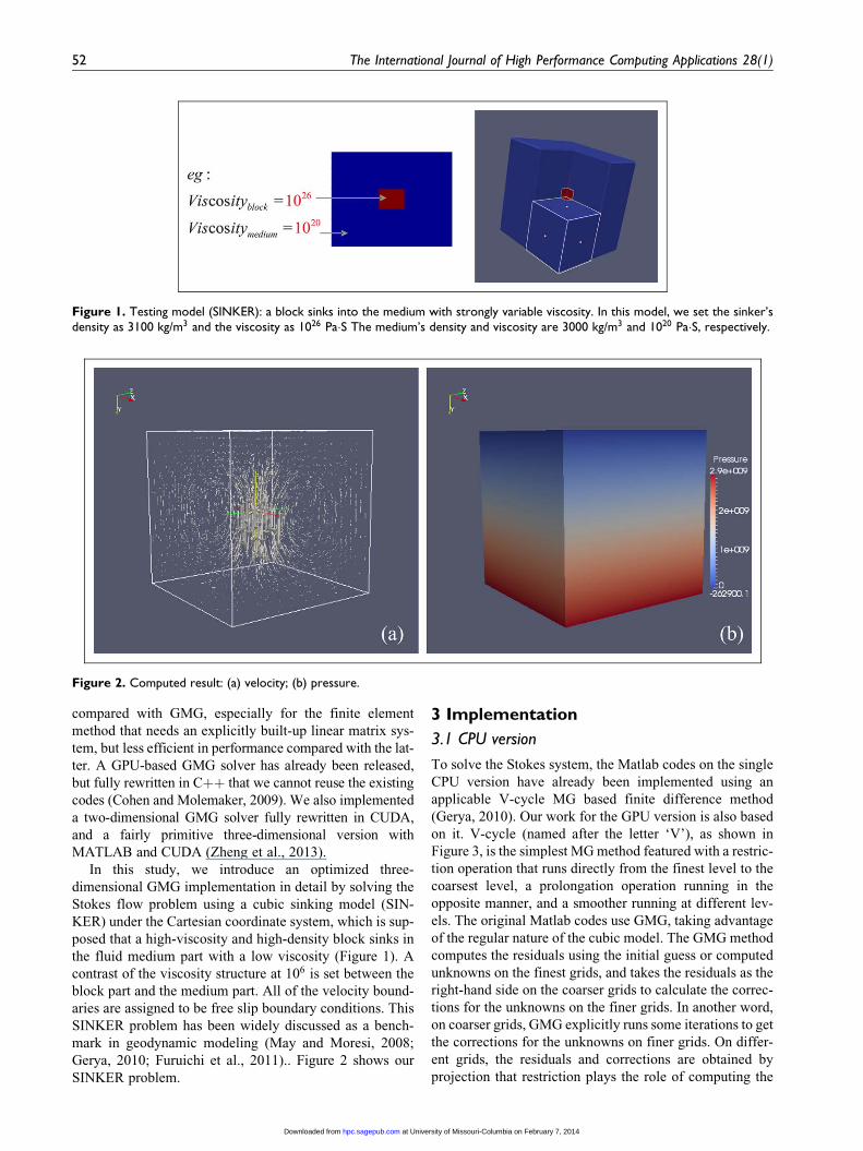
the fluid medium part with a low viscosity (Figure 1). A
contrast of the viscosity structure at 106 is set between the
block part and the medium part. All of the velocity bound-
aries are assigned to be free slip boundary conditions. This
SINKER problem has been widely discussed as a bench-
mark in geodynamic modeling (May and Moresi, 2008;
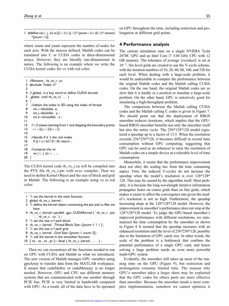
Gerya, 2010; Furuichi et al., 2011).. Figure 2 shows our
SINKER problem.
3 Implementation
3.1 CPU version
To solve the Stokes system, the Matlab codes on the single
CPU version have already been implemented using an
applicable V-cycle MG based finite difference method
(Gerya, 2010). Our work for the GPU version is also based
on it. V-cycle (named after the letter ‘V’), as shown in
Figure 3, is the simplest MG method featured with a restric-
tion operation that runs directly from the finest level to the
coarsest level, a prolongation operation running in the
opposite manner, and a smoother running at different lev-
els. The original Matlab codes use GMG, taking advantage
of the regular nature of the cubic model. The GMG method
computes the residuals using the initial guess or computed
unknowns on the finest grids, and takes the residuals as the
right-hand side on the coarser grids to calculate the correc-
tions for the unknowns on the finer grids. In another word,
on coarser grids, GMG explicitly runs some iterations to get
the corrections for the unknowns on finer grids. On differ-
ent grids, the residuals and corrections are obtained by
projection that restriction plays the role of computing the
Figure 1. Testing model (SINKER): a block sinks into the medium with strongly variable viscosity. In this model, we set the sinker’sdensity as 3100 kg/m3 and the viscosity as 1026 Pa�S The medium’s density and viscosity are 3000 kg/m3 and 1020 Pa�S, respectively.
Figure 2. Computed result: (a) velocity; (b) pressure.
52 The International Journal of High Performance Computing Applications 28(1)
at University of Missouri-Columbia on February 7, 2014hpc.sagepub.comDownloaded from

residuals, and prolongation calculates the corrections. A
brief description of V-cycle GMG is shown in Figure 3.
For the Stokes system, the smoother must be applicative
to deal with pressure which does not show up in the conti-
nuity equations. To explicitly compute the pressure, a com-
putational compressibility approach is used by updating the
pressure using the computed residuals of the continuity
equation at each iteration:
Pnew ¼ Pþ ZRescontinuityycontinuity ð5Þ
where Pnew is the pressure to be solved, P is the pressure
obtained from the previous iteration, Z is the local viscosity,
Rescontinuity is the residual of continuity equation, and
ycontinuity is the relaxation coefficient of continuity equation.
For the strongly variable viscosity problem, the big con-
trast of coefficients hinder the convergence rate, especially
for the initial iterations. We applied the approach to gain
the initial guess of the unknowns with a gradually increased
computational viscosity contrast to overcome it, which is
named as a continuation method. In the beginning of the
V-cycle, the viscosity is rescaled to a low-viscosity con-
trast. After some iterations the computational viscosity
contrast gradually increases until the original viscosity val-
ues of the problem are restored. The rescaling operations
are shown as follows:
Zi;j ¼ Zcomputationalmin exp
ln Zcomputationalmax =Zcomputational
min
� �ln Zoriginal
max =Zoriginalmin
� � lnZi;j
Zoriginalmin
!24
35ð6Þ
where Zcomputational and Zoriginal represent current and origi-
nal viscosity, respectively, with Zmin and Zmax for the min-
imal and maximal viscosity of the model. Zi;j depicts the
viscosity on each grid. One alternative is to use a small
modification of multigrid (MG) that right-hand side on the
finest grids is also assigned with the residual obtained in the
previous cycle. Together with the gradual increasing in a
computational viscosity contrast, the convergence perfor-
mance for large viscosity contrasts can be achieved
efficiently. This method is also named as ‘multi-multigrid’
(Gerya, 2010).
In addition, we applied the staggered schemes to avoid
decoupling of odd–even problem, which meets the require-
ment of LBB condition at the same time, as we have men-
tioned. The conservative finite difference scheme is applied
for variable viscosity case, which satisfies the conservation
of stress between the nodal points on the three-dimensional
staggered grids. Equations (7) and (8) are given below as an
example of discretizing the continuum equation and dis-
crete Stokes equation in the x-direction. In case of utilizing
the staggered grids, that different variables have individual
index systems, respectively (see Figure 4), where viscosity
is defined as Zn, Zxy, Zyz and Zxz corresponding to the com-
ponents of normal stress and shear stress:
uxðiþ1;jþ1;lþ1Þ � uxðiþ1;j;lþ1ÞDxjþ1=2
þuyðiþ1;jþ1;lþ1Þ � uyði;jþ1;lþ1Þ
Dyiþ1=2
þuzðiþ1;jþ1;lþ1Þ � uzðiþ1;jþ1;lÞ
Dzlþ1=2
¼ 0ð7Þ
4Znði�1;j;l�1Þ
uxði;jþ1;lÞ � uxði;j;lÞ
Dxjþ1=2 Dxj�1=2 þ Dxjþ1=2
� ��4Znði�1;j�1;l�1Þ
uxði;j;lÞ � uxði;j�1;lÞ
Dxj�1=2 Dxj�1=2 þ Dxjþ1=2
� �!
þ2Zxyði;j;l�1Þ
uxðiþ1;j;lÞ�uxði;j;lÞ
Dyi�1=2 Dyi�1=2þDyiþ1=2ð Þ þuyði;jþ1;lÞ�uyði;j;lÞ
Dyi�1=2 Dxj�1=2þDxjþ1=2ð Þ
� �
�2Zxyði�1;j;l�1Þuxði;j;lÞ�uxði�1;j;lÞ
Dyi�1=2 Dyi�3=2þDyi�1=2ð Þ þuyði�1;jþ1;lÞ�uyði�1;j;lÞ
Dyi�1=2 Dxj�1=2þDxjþ1=2ð Þ
� �0BBBB@
1CCCCA
þ2Zxzði�1;j;lÞ
uxði;j;lþ1Þ�uxði;j;lÞ
Dzl�1=2 Dzl�1=2þDzlþ1=2ð Þ þuzði;jþ1;lÞ�uzði;j;lÞ
Dzl�1=2 Dxj�1=2þDxjþ1=2ð Þ
� �
�2Zxzði�1;j;l�1Þuxði;j;lÞ�uxði;j;l�1Þ
Dzl�1=2 Dzl�3=2þDzl�1=2ð Þ þuzði;jþ1;l�1Þ�uzði;j;l�1Þ
Dzl�1=2 Dxj�1=2þDxjþ1=2ð Þ
� �0BBBB@
1CCCCA
�2Pi�1;j;l�1 � Pi�1;j�1;l�1
Dxj�1=2 þ Dxjþ1=2
þ 1
4ri�1;j;l�1 þ ri;j;l�1 þ ri�1;j;l þ ri;j;l
� �gx ¼ 0
ð8Þ
1. Smooth Ax=R with initial guess to get iterative values x;2. Calculate residuals: Res_0=R-Ax;
3. Restriction: obtain the residuals on coarser grids
4. Smooth Ax=Res_0 with initial guess to get corrections dx_0;5. Calculate residuals: Res_1=Res_0-Adx_0;
7. Prolongation: obtain the corrections dx_n onfinergrids
6. Smooth Ax=Res_n with initial guess to get corrections dx_n;
9. Smooth Ax=Res_(n-1) with initial values setting as dx_(n-1);8. Correct the unknowns: dx_(n-1)=dx_(n-1)+dx_n;
10. Correct the unknows: x=x+dx_0.
Figure 3. V-cycle GMG: A represents the coefficients of the discrete equations, R represents the right-hand side, x represents theunknowns, Res_0,1, . . . , n represents the residuals at each level, and dx_0,1, . . . , n represents the corrections on finer grids respec-tively. (For example, dx_1 is the correction of dx_0.) The black dots are smoothing operations. The dotted lines on the left-hand sideand right-hand side are restrictions and prolongations, respectively.
Zheng et al. 53
at University of Missouri-Columbia on February 7, 2014hpc.sagepub.comDownloaded from

3.2 GPU version
In the next step, we will put forward the GPU implementa-
tion. An analysis of the time consumed at each individual
part of the original Matlab codes (Figure 5) shows that the
three components, namely smoother, restriction, and pro-
longation, take the lion’s share.
To figure out what may happen with a real compiled
language, most of the reused functions were translated
in the first place into C codes to be called by Matlab with
mexfuntion. Table 1 shows the comparison of running
time consumption between Matlab codes and its calling
C codes using an Intel i7 CPU (3.07 GHz).
One can see from Table 1 that simply rewriting the
majority of reused functions in the C language, including
smoother, restriction and prolongation components, can
accelerate the performance of original Matlab codes,
though it’s not sufficiently fast enough at current stage.
In both of the cases of original Matlab codes and its calling
C codes, the smoother takes up most part of the time con-
sumed, which apparently needs optimization.
On GPU, the sequential inner cycle can be modified into
parallel threads across all grid points under the SIMT
model. A common style of the SIMT model can be written
using CUDA as:
1 –global– void function ( double x, double y, . . . )2 f3 // calculate the index using the thread id and block id4 int i¼blockIdx . x;5 int j¼threadIdx . x;6 . . . . . .7 g
where the instruction in the C_like function we defined
is indeed the single instruction to manage many threads
running simultaneously to fulfill one function. As what
we introduced in the previous section, CUDA organizes
the threads in block and grid style at the software level.
The thread index can be calculated using the CUDA
defined structural variables blockIdx and threadIdx
(NVIDIA, 2011). In our implementation, the setting of
boundary conditions, restriction and prolongation can
apply this SIMT model conveniently. For the smoother,
the original CPU based Matlab codes utilize the Gauss–
Seidel iterations, in which computing depends on the new-
est updated neighborhood nodes. It is difficult to imple-
ment this strongly inter-dependent algorithms on a GPU
by multi-threading stylish, as all of the threads are running
simultaneously in a disordered manner. To overcome this
hurdle during GPU implementation, the RBGS algorithm
is adopted in our application. The RBGS splits the
Gauss–Seidel iteration into two parts by red and black col-
ors, allowing the computing point to keep using the newest
information associated with it (Figure 6).
Next, we will talk about the workflow of our imple-
mentation. As we mentioned before, the pressure is
updated with the residuals of continuity equation which
requires an initial smoothing loop to compute the resi-
duals on the finest level. During the iteration of the
smoother (inner iteration), there are three major procedures:
setting boundaries, running the kernels of red and black col-
ors. All of them run on a GPU. One thing that should be
noted in advance is that the values on the boundary points
have to be imposed ahead of CUDA kernels, for the sake
of reducing the logic operations (there is only one logic unit
on the SM, which means logic operations may run 16 times
or half warp without doing anything). After the initial
smoothing loop, we run the main V-cycle loop (outer itera-
tion) containing smoother together with the restriction and
prolongation procedures until the tolerance criteria is meet.
The workflow can be described as in Algorithm 1.
Matlab index starts from 1 by column-major, while the
C language starts from 0 through row-major. Due to the
index difference between Matlab and C, macros can be
defined to convert the indices. We take vx for example:
Algorithm 1 V-cycle multigrid with RBGS.1: initialize the density, viscosity and unknowns;2: smoother(iternum¼1)f3: for k ¼ 1 to iternum do4: set velocity boundaries5: run kernels of red color6: run kernels of black color7: end for8: compute the residuals9: g10: while (residual > tolerance) do11: for n ¼ 1 to levelnum do12: smoother(iternum¼iternum(n))13: run restriction14: end for15: for n ¼ levelnum to 1 do16: smoother(iternum¼iternum(n))17: run prolongation18: end for19: end while
Figure 4. Indexing of different variables for a three-dimensionalstaggered grid. (Reproduced with permission from Gerya (2010).)
54 The International Journal of High Performance Computing Applications 28(1)
at University of Missouri-Columbia on February 7, 2014hpc.sagepub.comDownloaded from
1 #define vx( i , j , k) vx [( i –1)þ(j –1)* (ynumþ1)þ(k–1)* (xnum)*(ynumþ1)]
where xnum and ynum represent the number of nodes for
each axis. With the macros defined, Matlab codes can be
translated into C or CUDA codes in three-dimensional
arrays. However, they are literally one-dimensional in
nature. The following is an example where we write the
CUDA kernel codes for vx with red color:
1 //filename : rb_vx_r .cu2 #include ’’Index .h’’34 //–global– is a key word to define CUDA kernels5 –global– void rb_vx_r( . . . )6 f7 //obtain the index in 3D using the index of thread8 int i¼blockIdx .x;9 int j¼blockIdx . y ;
10 int k¼threadIdx . x ;1112 //þ2 means starting from 1 and skipping the boundary points13 iþ¼2;jþ¼2;kþ¼2;1415 //decide if it ’s the red nodes16 if (( iþjþk)%2!¼0) return ;1718 //compute the vx19 vx ( i , j ,k) ¼ . . . ;20 g
The CUDA kernel code rb_vx_r.cu will be compiled into
the PTX file rb_vx_r.ptx with nvcc compiler. Then we
need to define Kernel Object and the size of block and grid
in Matlab. The following is an example using vx in red
color:
1 % set the kernel in the main function2 global rb_vx_r_kernel ;3 % define the kernel object connecting the ptx and cu files we
have4 rb_vx_r_kernel¼parallel . gpu .CUDAKernel ( ’ rb_vx_r . ptx
’ , ’ rb_vx_r . cu ’ ) ;5 % set the size o f each block6 rb_vx_r_kernel . Thread Block Size¼[znum–1 1 1 ] ;7 % set the size o f each grid8 rb_vx_r_kernel . Grid Size¼[ynum–1 xnum–2] ;9 % call the kernel in the smoother function
10 [ vx , vy , vz , pr ]¼ feval ( rb_vx_r_kernel , . . . ) ;
Then we can reconstruct all the functions needed to run
on GPU with CUDA and Matlab as what we introduced.
The new version of Matlab manages GPU variables using
gpuArray to transfer data from the MATLAB workspace.
It means that cudaMalloc or cudaMemcpy is no longer
needed. However, GPU and CPU use different memory
systems that are communicated with one another through
PCIE bus. PCIE is very limited in bandwidth compared
with GPU. As a result, all of the data have to be operated
on GPU throughout the time, including restriction and pro-
longation at different grid points.
4 Performance analysis
The current simulation runs on a single NVIDIA Tesla
2070C GPU and an Intel Core i7 3.04 GHz CPU with 12
GB memory. The tolerance of average residualk k is set at
10�5. Six-level grids are created to use the V-cycle scheme,
with the iteration numbers of 10, 20, 40, 80, 160, and 320 for
each level. When dealing with a large-scale problem, it
would be undesirable to compare the performance between
the original Matlab codes and the Matlab calling CUDA
codes. On the one hand, the original Matlab codes are so
slow that it is hardly in a position to simulate a large-scale
problem. On the other hand, GPU is selectively good for
simulating a high-throughput problem.
The comparison between the Matlab calling CUDA
codes and the Matlab calling C codes is given in Figure 7.
We should point out that the deployment of RBGS
smoother reduces iterations, which implies that the GPU-
based RBGS smoother benefits not only the smoother itself
but also the entire cycle. The 256*128*128 model regis-
tered a speedup up to a factor of 13.5. When the resolution
exceeds 256*256*128, it becomes difficult to record time
consumption without GPU computing, suggesting that
GPU can be used as an enhancer to raise the resolution of
Matlab codes on a simple device at a tolerable level of time
consumption
Meanwhile, it seems that the performance improvement
does not obey the scaling law from the time consuming
aspect. First, the reduced V-cycles do not increase the
speedup when the model’s resolution is over 128*128*
128. This may be caused by the algorithm itself. Most prob-
ably, it is because the long-wavelength iterative information
propagates faster on coarse grids than on fine grids, which
makes it easier to affect the convergence rate given the mod-
el’s resolution is not so high. Furthermore, the speedup
increasing stops at the 128*128*128 model. However, the
improvement in smoother’s performance does not stop at the
128*128*128 model. To judge the GPU-based smoother’s
improved performance with different resolutions, we sum-
marized the time consumption by the smoother as shown
in Figure 8 It seemed that the speedup increases with an
enhanced resolution until the level of 256*256*128, possibly
due to the limitation of GPU catch size. In other words, the
scale of the problem is a bottleneck that confines the
potential performance of a single GPU card, and hence
solving a large problem needs an even more powerful
multi-GPU system
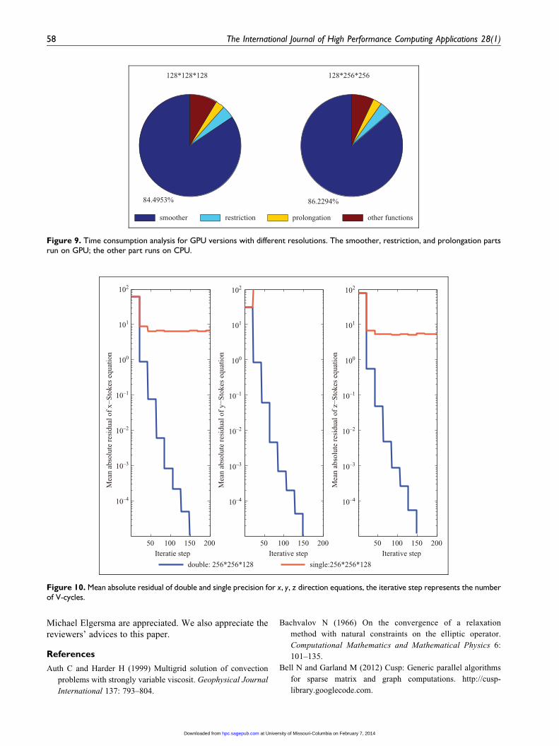
Evidently, the smoother still takes up most of the run-
ning time on the GPU (Figure 9), but restriction and
prolongation consume limited time. The reasons why
GPU’s smoother takes a larger share may be explained
that the GPU codes for others parts are more effective
than smoother. Because the smoother needs a more com-
plex implementation, somehow we cannot optimize it
Zheng et al. 55
at University of Missouri-Columbia on February 7, 2014hpc.sagepub.comDownloaded from

efficiently in the current version. In other words, the
speedup of prolongation, restriction, and other parts such
as boundary condition setting is better than the smoother
itself, also suggesting that even a limited improvement
of the smoother’s performance would result in a notice-
able improvement to the entire codes.
The time consumed by other functionalities that are not
run on the GPU saw no change, compared with the modi-
fied Matlab codes with C. The important reason may be
explained that the improvement of GPU parts makes the
weight of other part increase, while the reduced V-cycles
makes the weight of other part decrease more than the GPU
parts. These two functions may lead to a balance that we
cannot see the change of ‘other’ component’s share clearly.
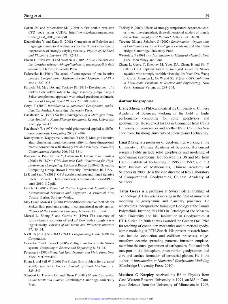
However, the current GPU’s (even on Fermi) double pre-
cision computing capacity remains unideal, compared with
single precision case. In this study, double precision is
needed, as the residuals cannot be guaranteed to conver-
gence when using single precision. In Figure 10 where single
precision is used, the y-Stokes equation shows a divergence
that is possibly caused by the limited word length of single
precision. Apparently, a mixed-precision scheme (Furuichi
et al., 2011) may solve the problem, as it gives a balanced
consideration to both efficiency and precision. In this paper,
only the codes with double precision are used.
5 Conclusions
In this paper, a GPU-based MG solver has been pro-
posed to simulate the Stokes flow problem. Time
efficiency can be enhanced on a GPU with the parallel
RBGS smoother. Matlab’s parallel computing toolbox
allows user to quickly implement hybrid programming
using both script language and CUDA C. In addition
to MG method, the Krylov subspace method is often
applied to solve the Stokes flow problem. One can
accelerate the Krylov subspace-based iterative solver
or the preconditioned iterative linear solver using GPU
(Bell and Garland, 2012; Li and Saad, 2011). Mean-
while, the GPU-based GMG solver is applicable as a
preconditioner of Krylov subspace method for the cubic
model (Furuichi et al., 2011; Kameyama et al., 2005). In
summary, the hybrid GPU–CPU architecture, such as the
combination of MPI and CUDA, is able to enhance the
resolution, and can be considered as a useful alternative
architecture.
75.9887%
Original Matlab codes
78.6104%
Matlab with C codes
smoother restriction prolongation other functions
Figure 5. Time consumption analysis for CPU version. For the original Matlab codes, all of the parts are written in Matlab; for theMatlab with C codes, the smoother, restriction, and prolongation parts are rewritten in C.
Table 1. Time consumption of original Matlab and Matlab callingC codes.
Resolution Original Matlab Matlab calling C
25*25*25 160 s 15 s49*49*49 1108 s 125 s
Figure 6. Red–black method: red and black cycles denote redand black nodes, blue cycles denote boundary nodes.
56 The International Journal of High Performance Computing Applications 28(1)
at University of Missouri-Columbia on February 7, 2014hpc.sagepub.comDownloaded from

Funding
This work was supported by the National High Technology
Research and Development Program of China (863 Pro-
gram), ‘Rapid visualization and diagnosis techniques of
earth system model output data’ (grant number
2010AA012402), the NSF CMG Program and the Project
SinoProbe-07 of China.
Note
1. See http://www.accelereyes.com
Acknowledgements
We would like to thank Masanori C. Kameyama for dis-
cussing the comparison between the single and double pre-
cision problems. The discussions with Dmitri Karpeev and
64*64*64 128*128*128 256*128*128 256*256*1280
5000
10000
15000
Tot
al ti
me
Uni
t: se
c
Models with different resolutons
0
20
40
60
Tim
e pe
r V
−cy
cle
Uni
t: se
c
0
100
200
300
V−
cycl
es
GPU CPU
64*64*64 128*128*128 256*128*1280
10
20
Spee
dup
Models with different resolutons
0
5
10
Spee
dup
80
100
120
140
Red
uced
V−
cycl
es
Figure 7. Iterations and time for different models: blue bars denote the Matlab with CUDA codes running on GPU, redbars denote the Matlab with C codes running on CPU. For the model 256*256*128, CPU-based Matlab with C codes aredifficult to time.
0
20
40
60
Tot
al ti
me
Uni
t: se
c
Models with different resolutons
64*64*64
128*64*64
128*128*64
128*128*128
256*128*128
256*256*128
GPU CPU
0
2
4
6
Spee
dup
Figure 8. Time and speedup for different smoothers: blue bars denote the Matlab with CUDA codes running on GPU, red bars denotethe Matlab with C codes running on CPU. Total time means 10 iterations for each timing.
Zheng et al. 57
at University of Missouri-Columbia on February 7, 2014hpc.sagepub.comDownloaded from
Michael Elgersma are appreciated. We also appreciate the
reviewers’ advices to this paper.
References
Auth C and Harder H (1999) Multigrid solution of convection
problems with strongly variable viscosit. Geophysical Journal
International 137: 793–804.
Bachvalov N (1966) On the convergence of a relaxation
method with natural constraints on the elliptic operator.
Computational Mathematics and Mathematical Physics 6:
101–135.
Bell N and Garland M (2012) Cusp: Generic parallel algorithms
for sparse matrix and graph computations. http://cusp-
library.googlecode.com.
84.4953%
128*128*128
86.2294%
128*256*256
smoother restriction prolongation other functions
Figure 9. Time consumption analysis for GPU versions with different resolutions. The smoother, restriction, and prolongation partsrun on GPU; the other part runs on CPU.
50 100 150 200
10–4
10–3
10–2
10–1
100
101
102
10–4
10–3
10–2
10–1
100
101
102
10–4
10–3
10–2
10–1
100
101
102
Iteratie step50 100 150 200
Mea
n ab
solu
te r
esid
ual o
f y−
Stok
es e
quat
ion
Iterative step50 100 150 200
Mea
n ab
solu
te r
esid
ual o
f z−
Stok
es e
quat
ion
Iterative step
double: 256*256*128 single:256*256*128
Mea
n ab
solu
te r
esid
ual o
f x−
Stok
es e
quat
ion
Figure 10. Mean absolute residual of double and single precision for x, y, z direction equations, the iterative step represents the numberof V-cycles.
58 The International Journal of High Performance Computing Applications 28(1)
at University of Missouri-Columbia on February 7, 2014hpc.sagepub.comDownloaded from
Cohen JM and Molemaker MJ (2009) A fast double precision
CFD code using CUDA. http://www.jcohen.name/papers/
Cohen_Fast_2009_final.pdf.
Deubelbeiss Y and Kaus B (2008) Comparison of Eulerian and
Lagrangian numerical techniques for the Stokes equations in
the presence of strongly varying viscosity. Physics of the Earth
and Planetary Interiors 171: 92–111.
Elman H, Silvester D and Wathen A (2005) Finite elements and
fast iteratice solvers with applications to incompressible fluid
dynamics. Oxford University Press.
Fedorenko R (1964) The speed of convergence of one iterative
process. Computational Mathematics and Mathematical Phy-
sics 4: 227–235.
Furuichi M, May DA and Tackley PJ (2011) Development of a
Stokes flow solver robust to large viscosity jumps using a
Schur complement approach with mixed precision arithmetir.
Journal of Computational Physics 230: 8835–8851.
Gerya T (2010) Introduction to numerical Geodynamic model-
ling. Cambridge: Cambridge University Press.
Hackbusch W (1977) On the Convergence of a Multi-grid Itera-
tion Applied to Finite Element Equations. Report, Universitat
Koln, pp. 76–12.
Hackbusch W (1978) On the multi-grid method applied to differ-
ence equations. Computing 20: 291–306.
Kameyama M, Kageyama A and Sato T (2005) Multigrid iterative
algorighm using pseudo-compressibility for three-dimensional
mantle convection with strongly variable viscosity. Journal of
Computational Physics 206: 162–181.
Klockner A, Pinto N, Lee Y, Catanzaro B, Ivanov P and Fasih A
(2009) PyCUDA: GPU Run-time Code Generation for High-
performance Computing. Technical Report 2009-40, Scientific
Computing Group, Brown University, Providence, RI, USA.
Li R and Saad Y (2011) GPU-accelerated preconditioned iterative
linear solvers. http://www-users.cs.umn.edu/*saad/PDF/
umsi-2010-112.pdf.
Lynch D (2005) Numerical Partial Differential Equations for
Environmental Scientists and Engineers: A Practical First
Course. Berlin: Springer-Verlag.
May D and Moresi L (2008) Preconditioned iterative methods for
Stokes flow problems arising in computational geodynamics.
Physics of the Earth and Planetary Interiors 171: 33–47.
Moresi L, Zhong S and Gurnis M (1996) The accuracy of
finite element solutions of Stokes’ flow with strongly vary-
ing viscosity. Physics of the Earth and Planetary Interiors
97: 83–94.
NVIDIA (2011) NVIDIA CUDA C Programming Guide. NVIDIA
Corporation.
Oosterlee C and Lorenz F (2006) Multigrid methods for the Stokes
system. Computing in Science and Enginering 8: 34–43.
Patankar S (1980) Numerical Heat Transfer and Fluid Flow. New
York: McGraw-Hill.
Payne L and Pell W (1960) The Stokes flow problem for a class of
axially symmetric bodies. Journal of Fluid Mechanics 7:
529–549.
Schubert G, Turcotte DL and Olson P (2001) Mantle Convection
in the Earth and Planets. Cambridge: Cambridge University
Press.
Tackley P (2009) Effects of strongly temperature-dependent visc-
osity on time-dependent, three-dimensional models of mantle
convection. Geophysical Research Letters 124: 18–28.
Turcotte DL and Schubert G (2002) Geodynamics: Applications
of Continuum Physics to Geological Problems, 2nd edn. Cam-
bridge: Cambridge University Press.
Wesseling P (1991) An Introduction to Multigrid Methods. New
York: John Wiley and Sons.
Zheng L, Gerya T, Knepley M, Yuen DA, Zhang H and Shi Y
(2013) GPU implementation of multigrid solver for Stokes
equation with strongly variable viscosity. In: Yuen DA, Wang
L, Chi X, Johnsson L, Ge W and Shi Y (eds.), GPU Solutions
to Multi-scale Problems in Science and Engineering. New
York: Springer-Verlag, pp. 293–304.
Author biographies
Liang Zheng is a PhD candidate at the University of Chinese
Academy of Sciences, working in the field of high-
performance computing for solid geophysics and
geodynamics. He received his BS in Geomatics from China
University of Geosciences and another BS in Computer Sci-
ence from Huazhong University of Sciences and Technology.
Huai Zhang is a professor of geodynamics working at the
University of Chinese Academy of Sciences. His current
research fields include solid geophysics and modeling of
geodynamics problems. He received his BS and MS from
Harbin Institute of Technology in 1995 and 1997, and PhD
from Institute of Mathematics, Chinese Academy of
Sciences in 2000. He is the vice director of Key Laboratory
of Computational Geodynamics, Chinese Academy of
Sciences.
Taras Gerya is a professor at Swiss Federal Institute of
Technology (ETH-Zurich) working in the field of numerical
modeling of geodynamic and planetary processes. He
received his undergraduate training in Geology at the Tomsk
Polytechnic Institute, his PhD in Petrology at the Moscow
State University and his Habilitation in Geodynamics at
ETH-Zurich. In 2008 he was awarded the Golden Owl Prize
for teaching of continuum mechanics and numerical geody-
namic modeling at ETH-Zurich. His present research inter-
ests include subduction and collision processes, ridge-
transform oceanic spreading patterns, intrusion emplace-
ment into the crust, generation of earthquakes, fluid and melt
transport in the lithosphere, precambrian geodynamics and
core and surface formation of terrestrial planets. He is the
author of Introduction to Numerical Geodynamic Modeling
(Cambridge University Press, 2010).
Matthew G Knepley received his BS in Physics from
Case Western Reserve University in 1994, an MS in Com-
puter Science from the University of Minnesota in 1996,
Zheng et al. 59
at University of Missouri-Columbia on February 7, 2014hpc.sagepub.comDownloaded from

and a PhD in Computer Science from Purdue University in
2000. He was a Research Scientist at Akamai Technologies
in 2000 and 2001. Afterwards, he joined the Mathematics
and Computer Science department at Argonne National
Laboratory (ANL), where he was an Assistant Computa-
tional Mathematician, and a Fellow in the Computation
Institute at University of Chicago. In 2009, he joined the
Computation Institute as a Senior Research Associate. His
research focuses on scientific computation, including fast
methods, parallel computing, software development,
numerical analysis, and multicore architectures. He is an
author of the widely used PETSc library for scientific com-
puting from ANL, and is a principal designer of the PyLith
library for the solution of dynamic and quasi-static tectonic
deformation problems. He was a J. T. Oden Faculty
Research Fellow at the Institute for Computation Engineer-
ing and Sciences, UT Austin, in 2008, and won the R&D
100 Award in 2009 as part of the PETSc team.
David A Yuen is a professor of geophysics and scientific
computation at the University of Minnesota. He graduated
from Caltech with a bachelor’s degree in physical chem-
istry in 1969, masters in geophysics from Scripps in
1973 and PhD in geophysics and Space Physics from
UCLA in 1978. He received a postdoc at the Department
of Physics, University of Toronto to 1979. He was an
Assistant Professor and Associate Professor at Arizona
State University in 1985. From September 1985 he has
worked at the University of Minnesota. He became an
AGU Fellow in 2005.
Yaolin Shi is a professor of geophysics at the University of
Chinese Academy of Sciences. He received a PhD from UC
Berkeley in 1986. He was vice president of the Chinese
Geophysical Society (2008–2012) and vice president of the
Chinese Seismological Society (2007–2011). He has been a
member of the Chinese Academy of Sciences since 2001.
60 The International Journal of High Performance Computing Applications 28(1)
at University of Missouri-Columbia on February 7, 2014hpc.sagepub.comDownloaded from