Contents lists available at ScienceDirect

Water Resources and Economics

Water Resources and Economics 4 (2013) 52–68

2212-42http://d

n CorrE-m1 N

journal homepage: www.elsevier.com/locate/wre

Impacts of climate variability on the irrigationsector in the southern Murray-Darling Basin,Australia

Muhammad Ejaz Qureshi a,c,n,1, Stuart M. Whitten a,Brad Franklin b

a Ecosystem Sciences, Black Mountain, Canberra, ACT 2601, Australiab Department of Economics, University of California, Riverside, CA, USAc Fenner School of Environment & Society, ANU, Australia

a r t i c l e i n f o

Article history:Received 28 June 2013Received in revised form6 December 2013Accepted 6 December 2013

Keywords:Irrigation waterEconomic impactDroughtAdaptationPMP modelWater policy

84/$ - see front matter Crown Copyright &x.doi.org/10.1016/j.wre.2013.12.001

esponding author at: CSIRO Ecosystem Scieail address: Ejaz.Qureshi@aciar.gov.au (M.E.ow at ACIAR, Canberra, ACT 2601, Australia

a b s t r a c t

Climate variability impacts on options available to irrigation land-holders now, as will climate change into the future. In this paper, wedemonstrate that factors that reduce effective rainfall and increaseevapotranspiration and irrigation water salinity during drier periodsact to reinforce climate variability impacts on irrigation wateravailability, indicating substantially larger costs of climate variability,and potentially climate change, than previously thought. Counteractingthese impacts is the potential for on-farm and institutional adaptationoptions to moderate impacts. The impacts of climate variability andincremental adaptation options (including water markets) are mod-elled for the southern Murray Darling Basin, Australia. The estimatedreductions in economic returns due to climate variability are muchhigher when combined effects are included but are markedly reducedwhen farm adaptation options are considered. There is also evidenceof a threshold effect beyond which adaptation options become lesseffective, indicating the challenge in adapting to the larger changesanticipated under climate change.Crown Copyright & 2013 Published by Elsevier B.V. All rights reserved.

1. Introduction

Availability of water for irrigation varies with time in response to climatic variations. In recentyears major droughts have seen significant reductions in irrigated water availability in Australia [1],

2013 Published by Elsevier B.V. All rights reserved.

nces, Canberra, ACT 2601, Australia.Qureshi).. Tel.: þ61 2 6217 0591.

M.E. Qureshi et al. / Water Resources and Economics 4 (2013) 52–68 53

the western US [2] and China [3] amongst other examples. In the Australian case, inflows into theMurray River in the last decade (except year 2010–2011) were about half the historic average [4] whilethose in 2006–2007 were considerably lower (i.e. less than 10%) than the previous historic minimum[5]. The resultant volume of water available for diversion and final annual allocations of irrigationwater were close to 20% of high security and 0% of low or general security entitlements in someregulated river valleys of the Murray-Darling Basin (MDB) [6], with initial allocations much lower.

Factors such as population and income growth and the consequent increases in the demand forirrigationwater to meet food production requirements [6], reduced water availability due to enhancedenvironmental flows, and competition from urban and industrial uses may increase future demandand variability of water available. Compounding changes to water demands are climate changemodels which suggest reduced long-term water availability and enhanced short-term variability ofwater resources in many regions [7,8]. For example, in the Murray-Darling Basin (MDB) Australia,climate change is expected to cause reductions in rainfall with consequent effects on surface wateravailability of up to 40% depending on the degree of change [9].

Understanding the economic impact of climate variability is an important step in identifyingwhether existing policies are effective in reducing the impact of climate variability on individuallandholders and the irrigated agriculture sector as a whole. Economic analyses can also provide someguidance as to whether additional policies are required to accommodate the additional climatevariability challenges that are posed by future climate change. In this paper, we focus on recentAustralian experience where a series of major water reforms over the last 20 or more years haveprogressively created an interconnected market for water across the southern Murray-Darling Basin(sMDB) (Fig. 1) at the same time that a major drought was impacting the basin (the ‘millenniumdrought’). Our objectives in this paper are two-fold: first, to assess the economic implications ofclimate variability when negative feedbacks from lower effective rainfall, and increased salinity andevapotranspiration are taken into account in economic models; and second, to identify the potential

Fig. 1. Interconnected catchments of the southern Murray-Darling Basin.

M.E. Qureshi et al. / Water Resources and Economics 4 (2013) 52–6854

for farm adaptation options (crop and water management, technology investment and water markets)to reduce the impact of water variability on economic returns from irrigated agriculture.

Several studies have attempted to address the impact of drought or proposed reductions in wateravailability (via increased environmental allocations) in the Australian setting and have applieddifferent water availability scenarios to estimate impacts on irrigated gross value and/or profit in theMDB [10–13]. ABARE-BRS [12] estimated that a 29% reduction in water availability will reduce grossvalue by 16.5% and profit by 8.2%. Mallawaarachchi [14] estimated that a 29% reduction in wateravailability will reduce gross value by 20%. Jiang and Grafton [13] estimated that a 13% and 81%reduction in water availability will result in 5% and 44% reduction in profit, respectively. In contrast,Kirby [15] suggested that the millennium drought caused a 70% reduction in irrigation water use from2000 to 2001, while the gross value of irrigated agricultural produce fell only by 14%.

There are a number of potential weaknesses across these studies. The first three studies onlyaccommodated a subset of the impacts of climate variability and did not identify the effects ofdifferent elements of adaptation response available to landowners and government. For example,most of these studies only considered the reduction in water allocations and not the impacts of crop-specific regional effective rainfall and net irrigation requirement shifts due to salinity andevapotranspiration changes linked to climate variation. These may be significant as illustratedbiophysically by Austin et al. [16], Chiew and MacMahon [17] and Tubiello et al. [18] and economicallyby Connor et al. [19]. These MDB studies also did not account for commonly practised farm leveladaptation, such as deficit irrigation or on-farm efficiency improvements. The last estimate by Kirby[15] was intended to be illustrative and identified the influence of differential effects of increasedcommodity prices and adjustment factors such as costs and substitution effects (for example the dairysector buying feed from other regions and water purchases to support perennial activities).Consequently these studies may have under or overestimated the economic losses associated withclimate variability as well as the effectiveness of on and off-farm adaptation and policy in managingclimate variability impacts.

The paper is structured as follows. In Section 2, we provide a brief overview of recentmethodological developments in examination of climate variability impacts on agriculture. Thissection links different aspects of climate variability impacts and adaptation options, and describes arange of deficiencies in these studies and the innovation in the current study. The case study, climatevariability and data are described in Section 3. An irrigation sector positive mathematicalprogramming model and its calibration are described in Section 4. Results and key policy implicationsare the focus in Section 5 before we conclude the paper with a brief summary of the main points andopportunities for further work.

2. Literature review

Biophysical impacts of climate variability are exhibited via reduced rainfall and increased waterconsumed by irrigated crops. Reduced rainfall has two effects, it reduces inflows to storages andconsequent water allocations, and it also directly reduces rainfall on some crops. Reduced rainfallreduces drainage and increases salt concentration in the crop root zone. Crop water requirements areincreased by higher evapotranspiration and irrigation water salinity concentration. Irrigation withsaline water can accumulate salts in the soil, thereby hindering crop-yields. In response to thisaccumulation, water is applied in excess of plant requirements, for leaching purposes [20]. Althoughwe consider our results to inform the direction and type of adaptation likely under climate change, wedo not incorporate higher concentrations of carbon dioxide (CO2) that may lead to enhanced plantgrowth through a range of effects [21] and could affect crop yield.

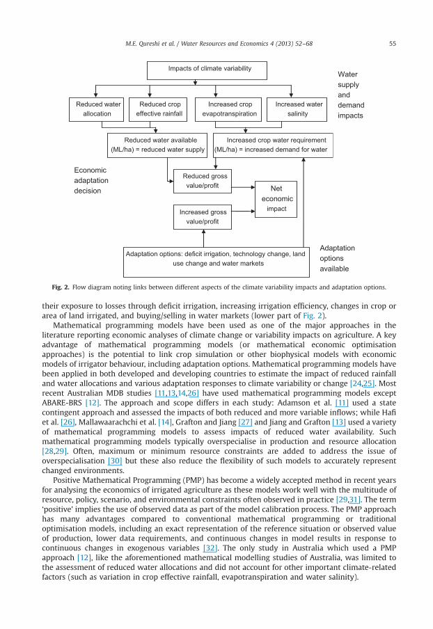
Loch et al. [22] distinguish between incremental and transformational options in landholderadaptation to climate change and a similar set of strategies is available for adapting to climatevariability. Transformational options effectively render irrigation options that resemble the currentsystem untenable. Incremental adaptation is the focus in this paper and the options set out in Fig. 2encompass the majority of those available to landholders [22,23]. Irrigators can adapt and minimise

Impacts of climate variability

Reduced water allocation

Reduced crop effective rainfall

Increased water salinity

Increased crop water requirement (ML/ha) = increased demand for water

Increased crop evapotranspiration

Reduced water available (ML/ha) = reduced water supply

Reduced gross value/profit

Adaptation options: deficit irrigation, technology change, land use change and water markets

Increased gross value/profit

Net economic

impact

Water supply and demand impacts

Adaptation options available

Economic adaptation decision

Fig. 2. Flow diagram noting links between different aspects of the climate variability impacts and adaptation options.

M.E. Qureshi et al. / Water Resources and Economics 4 (2013) 52–68 55

their exposure to losses through deficit irrigation, increasing irrigation efficiency, changes in crop orarea of land irrigated, and buying/selling in water markets (lower part of Fig. 2).

Mathematical programming models have been used as one of the major approaches in theliterature reporting economic analyses of climate change or variability impacts on agriculture. A keyadvantage of mathematical programming models (or mathematical economic optimisationapproaches) is the potential to link crop simulation or other biophysical models with economicmodels of irrigator behaviour, including adaptation options. Mathematical programming models havebeen applied in both developed and developing countries to estimate the impact of reduced rainfalland water allocations and various adaptation responses to climate variability or change [24,25]. Mostrecent Australian MDB studies [11,13,14,26] have used mathematical programming models exceptABARE-BRS [12]. The approach and scope differs in each study: Adamson et al. [11] used a statecontingent approach and assessed the impacts of both reduced and more variable inflows; while Hafiet al. [26], Mallawaarachchi et al. [14], Grafton and Jiang [27] and Jiang and Grafton [13] used a varietyof mathematical programming models to assess impacts of reduced water availability. Suchmathematical programming models typically overspecialise in production and resource allocation[28,29]. Often, maximum or minimum resource constraints are added to address the issue ofoverspecialisation [30] but these also reduce the flexibility of such models to accurately representchanged environments.

Positive Mathematical Programming (PMP) has become a widely accepted method in recent yearsfor analysing the economics of irrigated agriculture as these models work well with the multitude ofresource, policy, scenario, and environmental constraints often observed in practice [29,31]. The term‘positive’ implies the use of observed data as part of the model calibration process. The PMP approachhas many advantages compared to conventional mathematical programming or traditionaloptimisation models, including an exact representation of the reference situation or observed valueof production, lower data requirements, and continuous changes in model results in response tocontinuous changes in exogenous variables [32]. The only study in Australia which used a PMPapproach [12], like the aforementioned mathematical modelling studies of Australia, was limited tothe assessment of reduced water allocations and did not account for other important climate-relatedfactors (such as variation in crop effective rainfall, evapotranspiration and water salinity).

Table 1Factors affecting water availability and adaptation options in previous MDB studies.

Adamson et al.[11]

Hafi et al.[26]

Mallawaarachchiet al. [14]

ABARE-BRS[12]

Jiang and Grafton[13]

Variation in water allocations Yes Yes Yes Yes YesEvapotranspiration and effectiverainfall

No No No No No

Salinity of water Yes No No No NoCrop mix or land use change Yes Yes Yes Yes YesDeficit irrigation No Yes No Yes NoChange to irrigation technology Yes Not clear No No NoInter-regional water trading Yes No Yes Yes Yes

Table 2Predicted available water for diversion, associated probabilities and change from the long term base case scenario expectedmean (Base case expected mean ¼ 6146 GL).

sMDB water available for diversion in four states of nature

Climate variability state of nature (probability) Very low(p¼12%)

Low(p¼38%)

High(p¼38%)

Very high(p¼12%)

Water diversion (change from the base caseexpected mean)

4495 (�27%) 5727 (�7%) 6708 (9%) 7339 (19%)

M.E. Qureshi et al. / Water Resources and Economics 4 (2013) 52–6856

The present study extends the previous mathematical programming modelling approaches byexplicitly considering several climate-induced water resource impacts and adaptation options in thesMDB that have not been considered in a single analysis as shown in Table 1. We anticipate that thecombined impact of climate variability on irrigated agriculture may be greater than assessed in theprevious studies. This is because water supply reductions are reinforced by the direct impacts ofreduced rainfall, greater evapotranspiration and increased salinity. However, adaptation options andinstitutional policies (including crop/land use decisions, deficit irrigation and technology adoption,and opportunities to trade water) may ameliorate the impacts of reduced water availability. Thus,incorporating a wider range of adaptation and institutional responses, as undertaken in this study,yields a more thorough understanding of the differential impacts and will inform a more sound policyresponse.

3. Case study and data – southern Murray-Darling Basin

This study is focussed on the sMDB, which is Australia's most significant river system and accountsfor about 40% of Australia's gross value of agricultural production and around 70% of all water used foragriculture in Australia [33]. Significant water scarcity and quality issues have been experienced inrecent years due to over-allocation compounded by drought. The millennium drought (2001–2010approximately) had a disproportionately severe impact on the basin, causing record low inflows withsimilar implications for the volume of water held in major storages and allocations of irrigation water[34]. In addition, there are concerns about the ecological health of the sMDB, as the annual averageflow to the sea in the 2000–2010 period was close to zero [9].

The Australian climate has always exhibited a high degree of rainfall variability. In order to assessthe economic impacts of climate variability, we focus our evaluation on variability within a time seriesdata set compiled as a historical base case climate scenario (details of this scenario, including data,methods, and the models used can be found in the CSIRO Sustainable Yield reports [9]). To representthe variability in water diversion (supply) within the CSIRO base case scenario, the data were brokeninto four distinct categories or, states of nature as shown in Table 2. A very low state of naturerepresents the 12% of driest years, a low state of nature represents the next 38% of dry years, a high

M.E. Qureshi et al. / Water Resources and Economics 4 (2013) 52–68 57

state of nature represents the next 38% of relatively wet years, and a very high state of naturerepresents the 12% of the wettest years in the 111 years simulation. The non-uniform segmentationwas selected to identify the influence of rare (approximately 1 in 10 years) but still regular andinfluential events which lie toward the tail of the climate distribution.

Climate change has the potential to induce similar reductions to rainfall and consequent waterallocations to those experienced in the recent drought [9]. According to CSIRO estimates, diversions in driestyears will fall by more than 10% in most NSW regions, around 20% in the Murrumbidgee and Murrayregions, and from around 35% to over 50% in Victorian regions. Hence, recent drought experience can act asan analogue of some, but not all, of the changes likely under climate change and therefore as an indication ofthe scale and direction of both the impacts and effectiveness of the adaptation options available.2

Land use data for 2005–2006 (an average rainfall and allocation year) were obtained from theAustralian Bureau of Statistics (ABS) agricultural Statistics at Statistical Local Area (or SLA) level [9]and aligned across the catchment boundaries in order to estimate the agricultural activity occurringwithin equivalent catchment areas.3 Evapotranspiration, effective rainfall and net irrigationrequirements of different crops grown in the sMDB were estimated using a soil water balancesimulation model. The model is similar to that of CROPWAT model developed by the FAO [35]. Eightmajor agricultural activities which occupy most of the irrigated area within the catchments areincluded in our model: cereals represented by wheat, rice, pasture related activities represented bydairy, vegetables represented by potatoes, citrus fruits, deciduous fruits, stone fruits and grapes.Maximum crop water requirements for these activities are estimated (shown in Table A2). We usedMDB MSM-BIGMOD models to provide information regarding the salinity across catchments [36,37].The key economic data are commodity and input prices (also shown in Table A2). Average pricesacross 2002–2003 to 2007–2008 of individual commodities observed and reported by ABARE [38],ABS [39] and several agricultural departments and state agencies and industry reports were used inthe analysis to deal with temporal variation in commodity prices of the individual commodities[39,40]. Crop yield data which are critical for modelling agriculture production were either notavailable for all the activities in the regions or there was great variation in crop yields across regions.One of the reasons might be a small sample size and under or over representation of the population asthe data standard deviation in some crops was 4 times greater than the data mean values [41]. Wesourced average yields, variable and establishment costs from agricultural departments and agenciesof NSW and Vic and SA and industry reports and cross checked and adjusted after discussing withlocal farmers (Ikram, farmer Leeton, pers. comm.), agronomists and irrigation scientists (DanArmstrong, DPI Vic, pers. comm.). Average yields are used in developing crop–water productionfunctions discussed later. Variation in water charges by different irrigation water providers acrosscatchments can be significant [42], but is generally small as a proportion of total costs and forsimplicity a constant water charge is used across catchments.

4. Irrigation sector mathematical model

4.1. Structure of the model

At the core of the PMP approach is an integrated biophysical and economic model of the irrigationresponse that would be expected under the alternative climate variability states (i.e. water demandand supply). The objective function of the model is to maximise profits ‘π’ under each state of naturefor the whole basin after accounting for amortised annual establishment costs and operating orvariable costs subject to available land and water.

2 Under climate change or variability, there are likely to be a wider range of both impacts (e.g. different pests, diseases,weeds etc.) and adaptation options (e.g. technologies such as crops and crop varietals). However, the focus of this study is onthe impacts related to water supply and demand only for simplicity.

3 The remaining mismatch between the ABS estimated/observed irrigated land use data and CSIRO simulated waterdiversion was adjusted using catchment land use, crop evapotranspiration, effective rainfall, irrigation efficiency and netirrigation requirements.

M.E. Qureshi et al. / Water Resources and Economics 4 (2013) 52–6858

The objective function of maximising long-run regional profit is expressed algebraically in Eq. (1).All of the variables and parameters used in model (in Eq. (1) and subsequent equations) are defined inTable A1 in Appendix A. These include indices by crop, irrigation system, region and state of naturewith a probability. The variables are presented in capital letters. The first expression in Eq. (1)characterises the longer-run on-farm irrigation and agricultural activity infrastructure capitalinvestment choices that can vary across, but typically not within, a growing season. The secondtwo expressions characterise the short-run decisions that can be varied within a season (such asvariable or operating input levels, and water application rates) after stochastically determined factorsaffecting production are revealed (in this case levels of water allocations and salinity).

∑rπ ¼∑

sprobs∑

j∑h

Areasrjhð�ðie cos trjhþce cos trjÞþcpricerjYieldsrjh�ðv cos trjþwchargesr iwR

srjhÞÞ

" #8r ð1Þ

The water availability constraint is given in Eq. (2) and a land availability constraint in Eq. (3).Eq. (2) allows intra-regional water trading where irrigators with surplus or buffer water sell to thosewho are water deficient within the sMDB.

∑j∑hIWC

srjh Areasrjhrð1�clossrÞtwatsr 8s; r ð2Þ

∑j∑hAreasrjhrtarear 8r; s ð3Þ

The crop–water production function is shown as

Yieldsrjh ¼ f ðETRsrjhÞ ¼ arjþbrj ET

RsrjhþcrjðETR

srjhÞ2 ð4ÞThe parameters a, b, and c in Eq. (4) are estimated using crop–water production functions

developed from estimated maximum crop evapotranspiration and average yield data and Food andAgriculture Organization (FAO) crop–yield relationships [43]. These relationships have been used toestimate parameter values of each crop–water (quadratic) production function, given in Table A3.A minimum threshold is imposed on crop–water requirements in those production (yield) functionswhere the intercept (arj) is not zero to deal with negative yield occurrence at zero crop water usage.

Deficit irrigation is also included via Eq. (4), which allows less water to be applied andconsequently delivering a lower yield. By reducing the water use per hectare, a greater area can beirrigated. However, the potential for deficit irrigation depends on the type of crop. In general, cerealsand grapes are tolerant to some water stress but rice is sensitive [43].

The irrigation water required per hectare depends on crop evapotranspiration, crop regionaleffective rainfall and the on-farm irrigation system efficiency as shown in Eq. (5a). Similarly, Eq. (5b)incorporates the additional water that may be required to maintain crop production where irrigationwater salinity is high.4 Total irrigation water is obtained following [44,19,20] as shown in Eq. (5c).These crop–water–salinity functions are in line with the literature on yield–water–salinity relation-ships [19,45] and research on the economics of salinity management [20]:

IWRsrjh ¼ ðETR

srjh�erainsrjÞ=ief f rjh ð5aÞ

IWCsrjh ¼ ðetCsrjh�erainsrjÞ=ief f rjh ð5bÞ

where

ETCsrjh ¼

ðx1þγ1 tecsr=th1ÞetRsrjh if tecsrr th1

ðx2þγ2ðtecsr�th1Þ=thðth2�th1ÞÞETRsrjh if th1rtecsrr th2

ðx3þγ3ðtecsr�th2Þ=ðth2�th1ÞÞETRsrjh if tecsrZ th2

8>>><>>>:

ð5cÞ

4 Irrigation water salinity is accounted for in the form of two components, i.e. concentration scr and electrical conductivityecsr . The values of these two components result in total electrical conductivity tecsr(i.e.tecsr ¼ scrþecsr) of available water foreach scenario and in each catchment/region.

M.E. Qureshi et al. / Water Resources and Economics 4 (2013) 52–68 59

The portion of the total available area not irrigated is considered dryland and represented byEq. (6). The dryland constraint is used to release irrigated land towards dryland activities (such aswheat, beef or sheep) if it is not economic to irrigate given water allocations and market conditions.Land released to dryland activities is assumed to generate zero net return because significant areas ofland are only released under relatively dry conditions when the alternative uses are unlikely togenerate significant net returns:

DArear ¼ tarear�∑j∑hAreasrjh 8r; s ð6Þ

Later in the analysis, the model is runwith a water trade component so as to evaluate the economicimpacts of water trading, especially as water availability changes. For the water trading component,the water constraint presented in Eq. (2) is modified to allow trade of water among regions across thebasin, as shown below:

∑r∑j∑hIWC

srjh Areasrjhr∑rð1�clossrÞtwatsr 8s ð7Þ

This component is broadly consistent with observed responses during the recent (Millennium)drought in Australia where up to 35% of the total announced water allocations were traded ontemporary water markets in some parts of the sMDB [1]. Those regions which have no physicallinkage with other catchments are excluded from the interregional water trading market. Watertrading equates the value of marginal product to shadow price of the water and results in optimalallocation across the trading regions. At the basin scale analysis, no water price is included as thevalue of water trades represents a transfer payment within the basin therefore does not impact onaggregate results. For convenience, we assume that there is no restriction on interregional watertrading and zero transaction costs of trade. The zero transaction cost is consistent with previousestimates of relatively low per unit transaction cost [46].

The model has been coded in the General Algebraic Modelling System (GAMS) using non-linearprogramming solver CONOPT [47] and is available on request.

4.2. Model calibration

Positive mathematical programming (PMP) approaches incorporate an assumption of profit-maximising equilibrium in the reference period to address the overspecialisation problem [48]. Themost common version of the PMP approach involves adding a cost function to the model specificationabove that is quadratic in functional form and increasing in land area in production. In the first step,variable cost function parameters are solved for that result in the PMP calibrated model solutionreplicating the observed areas by crop for conditions in a chosen baseline year. In this sense, the PMPapproach can be thought of as capturing information on all farming conditions influencing thedistribution of returns that are not modelled in an explicit way with normal linear programming.

A key decision in construction of PMP models is the choice of an appropriate reference period for modelcalibration. The use of a specific calibration reference period has been critiqued in the literature [49] andvariations have been proposed including a generalised maximum entropy or GME [50,51]. However, theGME procedure has seen little application in applied research and one of the reasons of its limitedapplication is the limited availability and/or reliability of the required information [52]. A variant of PMP [32]that accounts for the greater elasticity of substitution amongst crop variants than amongst completelydifferent crops is applied. Crop variants include the same crop grownwith different water application rates(i.e. individual crop deficit irrigation). The PMP approach is used to recover additional information (based onan assumption of unobserved information) from observed activity levels in order to specify a non-linearobjective function such that the resulting model exactly produces the observed behaviour of farmers [53].

The model is calibrated to the irrigated land use observed in 2005/2006 and the water available fordiversion for each catchment in the Base Case climate scenario for the high allocation state of nature inTable 2. The 2005/2006 year was considered a suitable base year for calibration because irrigationallocations were close to historical averages, sufficient data is available, and it is relatively recent avoiding

Table 3Impacts considered and adaptation response scenarios.

Impacts considered Model scenarios

Analysis with no inter-regional trade Analysis with inter-regional trade

NT1 NT2 NT3 T1 T2 T3

Water allocations Yes Yes Yes Yes Yes YesCrop evapotranspiration No Yes Yes No Yes YesCrop effective rainfall No Yes Yes No Yes YesSalinity No Yes Yes No Yes YesAdaptation optionsCrop mix Yes Yes Yes Yes Yes YesDeficit irrigation No No Yes No No YesEfficiency improvement No No Yes No No YesWater market No No No Yes Yes Yes

M.E. Qureshi et al. / Water Resources and Economics 4 (2013) 52–6860

significant changes in technology, tastes or other unobserved factors. We used the long term average ofeffective rainfall and average prices across 5 years of the individual commodities for the purpose ofcalibration. Examining sectoral impacts required adjustment in rice and pasture for dairy yield. Forconsistency, we reduced yield of both these crops and associated variable costs for dairy as well as priceof rice.

4.3. Model simulation scenarios

Six model scenarios are evaluated for four states of nature of the CSIRO climate base case scenario(Table 2) as follows (summarised in Table 3):

(1)

Base case with no trade – varying water allocations but constant crop effective rainfall,evapotranspiration and irrigation water salinity and no adaptation and no water trading (NT1).

(2)

Base case with trade – varying water allocations but constant crop effective rainfall, evapotranspirationand irrigation water salinity and water trading without on-farm (deficit irrigation and efficiencyimprovement technology) adaptation (T1).

(3)

Variation with trade but no on-farm adaptation – variation in water allocations, crop effec-tive rainfall, evapotranspiration and irrigation water salinity but trading without on-farmadaptation (T2);

(4)

Variation with trade and on-farm adaptation – variation in water allocations, crop effectiverainfall, evapotranspiration and irrigation water salinity but trading and on-farm adaptation (T3).

(5)

`Variation without trade and no on farm adaptation – variation in water allocations, crop effectiverainfall, evapotranspiration and irrigation water salinity but no trading and no on-farm adaptation(NT2).

(6)

Variation without trade and on-farm adaptation – variation in water allocations, crop effectiverainfall, evapotranspiration and irrigation water salinity and on-farm adaptation but notrading (NT3).

5. Model results and discussion

5.1. PMP model results

The PMP model was applied across 11 sub-catchments of the sMDB as described in [37], howeverwe only report aggregated results in this paper. In the analysis and comparisons that follow, wecompare the results for each of the four climate variability states of nature and policies (called hereafter model scenarios) as shown in Fig. 3 and Tables 4 and 5. Across all model scenarios, adaptation

Fig. 3. sMDB gross values in alternative climate variability – states of nature.

Table 4Gross values of alternative model scenarios in four states of nature ($m).

Scenario State of nature Weighted average

Very Low Low High Very High

$m %a $m %a $m %a $m %a $m %a

NT1 2942 −23 3427 −10 3810 0 3810 0 3561 −7T1 3114 −18 3541 −7 3881 2 3881 2 3660 −4T2 2605 −32 3163 −17 3822 0 3822 0 3425 −10T3 2804 −26 3419 −10 4038 6 4058 6 3657 −4NT2 2275 −40 2982 −22 3700 −3 3700 −3 3256 −15NT3 2444 −36 3209 −16 4014 5 4014 5 3520 −8

a Calibration base is base case high, scenario 1 (shown in bold red font) – the percentages represent the difference from thisbase case allocation.

M.E. Qureshi et al. / Water Resources and Economics 4 (2013) 52–68 61

compounds from changes to crop mix (which can be considered unusual as some form of adaptationwill take place whether there is any scenario implementation or not) to additionally incorporate farmadaptation options via deficit irrigation, or alternatively the adaptation response facilitated by inter-regional water markets.5,6 In our discussion below we focus on percentage changes rather than dollarestimates as these are likely to be a more reliable estimate of the quantum of change.

Consider first the overall impact of climate variability irrespective of the scenario applied (i.e. thevariability along each row). There is negligible difference in either gross value or profit between thehigh and very high state of nature. This is as expected as there is a relatively small increase inextraction of water from the sMDB (it is capped by regulation) and an area constraint in the modelwhich results in no increase under a very high state of nature. This constraint also reflects the fact thatmany irrigators retain a surplus or buffer water allocation and allocation reductions are unlikely tobecome a production for most landholders until they fall below the ‘high’ state of nature. In contrastthere is a large difference between the low and very low states of nature exhibiting a likely thresholdeffect whereby the impact more than doubles for most model scenarios. As anticipated the impacts onprofits are lower than on-farm gross values, and the impacts under the trading scenarios are lowerthan without trading (more on this later).

5 In this paper, all dollars refer to Australian dollars, 1 Australian dollar¼1.03 US dollar as on 19 April 2013.6 While we report monetary data in Tables 5 and 6, we suggest percentage change results are the more appropriate for

interpreting and comparing conclusions from our model (as is generally the case). In particular we note our use of average cropyield data obtained from relevant government departments and agencies and adjusted after discussing with agronomists andirrigation scientists and farmers will substantially alter the gross values in our results when compared to the implied ABS yielddata used in some other models but are unlikely to substantively alter or distort percentage changes.

Table 5Profit under alternative model scenarios in four states of nature ($m).

Scenario State of nature Weighted average

Very Low Low High Very High

$m %a $m %a $m %a $m %a $m %a

NT1 1000 −19 1128 −8 1228 0 1228 0 1163 −5T1 1059 −14 1161 −6 1242 1 1242 1 1189 −3T2 891 −27 1034 −16 1217 −1 1262 −1 1114 −9T3 962 −22 1132 −8 1320 7 1373 7 1212 −1NT2 765 −38 973 −21 1186 −3 1230 −3 1060 −14NT3 824 −33 1050 −15 1294 5 1344 5 1151 −6

a Calibration base is base case high, scenario 1 (shown in bold red font) – the percentages represent the difference from thisbase case allocation.

Fig. 4. Impact of biophysical drivers on gross value of production.

M.E. Qureshi et al. / Water Resources and Economics 4 (2013) 52–6862

Next consider the general impact of climate variability on economic returns irrespective ofadaptation response by landholders or government represented by the difference between modelScenarios 1 and 2 under both a trade and non-trade setting. A shift from high to low to very lowrepresents a reduction in the available water (relative to mean) of 7% and 27% respectively (althoughthe net reduction in profit from the high state of nature is 8% and 19% in total respectively). The effectsof climate variability on the actual cropping system act to reinforce the reduction in water availabilitywith both gross values and profit falling by approximately double the water reduction (close to 40%reductions in gross values before on-farm adaptation). Interestingly the impacts of climate variabilityappear to be largest on the low state of nature (approximately three times than when they areignored) and proportionately decline under the very low state of nature (50% higher than when theyare ignored).

The relative impacts of the three drivers (raised salinity concentrations in irrigation water, higherevapotranspiration and reduced crop effective rainfall in dryer conditions) are illustrated in Fig. 4. The NT1scenario which demonstrates the physical impact in the absence of adaptation except change to crop mixand the combined impact under the NT2 scenario are also shown in Fig. 4. In the very low and low statesof nature reduced crop effective rainfall has the highest impact followed by evapotranspiration. Salinityconcentration has a similar effect under all states of nature. The combined effect nearly doubles theimpact of climate variability on gross value of production. These results clearly demonstrate that ignoringthe compounding impacts of climate variability, particularly of effective rainfall, will underestimate thefull impact of climate variability on agricultural production.

Fig. 5. Example impact of biophysical drivers and adaptation responses on gross value of production (NT3p¼partial adaptationonly; NT3f¼ full adaptation through deficit irrigation and improved technology).

M.E. Qureshi et al. / Water Resources and Economics 4 (2013) 52–68 63

Finally, we turn to the direct comparison of the model scenarios. First consider the impact of on-farm adaptation keeping in mind that adaptation via a change to crop mix (effectively a reduction inthe land use allocated to the least profitable crop by water use) is allowed under all model scenarios.Adoption of improved technology improves economic returns under all states of nature (by around4–6% for gross values and a similar impact for profits). It has a similar positive impact with andwithout trade. Interestingly the impact is greatest under the very low state of nature (10%) and falls toaround 6% under the low state of nature. The effectiveness of on-farm adaptation is dominated byadoption of more efficient irrigation technology as illustrated in Fig. 5, which shows that technology ismost effective under the low state of nature. The intuitive explanation is obvious, improvedtechnology allows similar cropping mixes to be maintained under the low state of nature but isincreasingly ineffective under the very low state of nature as water-use becomes concentrated in highvalue crops. Deficit irrigation becomes less effective as it becomes drier.

Throughout the analysis we have chosen to analyse model scenarios with and withoutinterregional water trade in parallel because there is already significant interregional trade in thesMDB [1]. Water trade is generally argued by economists to have an unambiguously positive impacton gross values and profits because it facilitates the redistribution of water from low to high valueuses, and that benefit is likely to be higher under increasing scarcity. Our results are consistent withthis observation but perhaps weaker than may be generally anticipated (see subsequent discussion).Trade improves gross value of production by up to an additional 10% and profits by slightly higher 11%under a low state of nature on top of on-farm adaptation. Similar to on-farm adaptation the additionalbenefits under the very low state of nature are small relative to those delivered under the low state ofnature. Further it is likely that trade and on-farm adaptation are partial substitutes and therefore thebenefits cannot be considered fully additive and separable.

Given the recent shifts in the prices of major agricultural commodities we tested the impact ofthese factors on our results. A price increase of 100% for cereals and 50% for rice is shown in Table 6but only for the trade scenarios. The impact of price increases is higher (8%) with high waterallocations and lower (6%) with low water allocations. The former is due to the opportunisticexpansion in use of annual crops (such as cereals) when water allocations are high.

5.2. Implications for climate change

Climate change is anticipated to cause a reduction to the amount and an increase in the variabilityof water available for diversion in the sMDB. As an indication of the scale of change the CSIROsustainable yields study estimated the climate variability under three possible climate change futureslabelled dry, medium and wet. Our results provide an indication of the direction of change that mightbe anticipated under more moderate climate change (say to a medium future) along with the limits toeffectiveness. Our results should not be interpreted as presenting an indication of the costs of climatechange however since additional climatic (e.g. effects of increasing CO2 concentrations) andadaptation factors are likely to become available (e.g. new crops and irrigation technologies).

Table 6Sensitivity of gross value to price.

State of nature Weighted average

very low Low High Very high

$m % $m % $m % $m % $m %

T1 3152 1 3677 4 4091 5 4093 5 3821 4T2 2447 �6 3194 1 3966 4 3966 4 3490 2T3 2985 6 3623 6 4351 8 4382 8 3914 7

M.E. Qureshi et al. / Water Resources and Economics 4 (2013) 52–6864

The analysis presented above indicates that a combination of on-farm adaptation via technologyadoption and participation in water markets are reasonably effective in managing relatively smallreductions in available water (in the order of 10% reductions from current means or close to 40%reductions from current maximum available water) limiting losses to 22% of profits.7 Under the ‘dryclimate’ diversions would be below the base case very low state of nature approximately half of thetime, with approximately half as much water available under the very low state of nature compared tothe base case presented. Our results clearly suggest there would be major economic impacts of climatechange of this scale, indicating there is likely to be a threshold shift in adaptation and policyeffectiveness, and correspondingly in costs, once the water available for diversion is reduced by morethan 10–15% below baseline estimates.

5.3. Comparison with previous studies and relevance to government policy

The model used in the current study does not specifically calculate the effects of reductions towater diversions under the new sMDB target for sustainable diversions of 7405 GL/year to be achievedby 2019 [54], or the quantities identified by previous studies [12–14]. However, the range of climatevariability scenarios for which estimates are provided does span the options proposed by previousstudies. Furthermore, while the modelling and approach to optimisation are broadly similar, themodelling structures and input data differ. A relatively easy comparison can be made with theestimates of Grafton and Jiang [27]: like our model, their model was calibrated to the 2005–2006 year.It differs from our model in methodology and in only accounting for the variable costs while ignoringcapital costs which are accounted for in the current analysis. They estimated a reduction ofagricultural profits of 14% for the southern connected basin under a reduction in water allocations of34% (3000 GL basin wide) and 24% under a 45% reduction (4000 GL basin wide). Assuming very lowstate of nature (27%), T3 (full water trading and on-farm adaptation) our model suggests a 22%reduction and a total reduction of 40% with climate reinforcement (salinity, effective rainfall, andevapotranspiration) but reducing to 33% when on-farm adaptation is included.

Similar comparisons against basin wide estimates, such as ABARE-BRS [12], Mallawaarachchi et al.[14] and Hafi et al. [26] are more difficult as these studies did not include all of the impacts of climatevariability and have been undertaken for a different comparison year (2000–2001). However forillustrative purposes we note that a 30% reduction in water availability [14] suggests a reduction ingross value of production 20%, and by about 15% [12] with profit reduced by about 8%. Our modelsuggests comparable reductions in gross values under similar assumptions, much larger reductionsonce additional climate reinforcing factors are taken into account (potentially 41% reductions in grossvalues with profit 38%), but with some reductions likely due to on-farm adaptation (34% and 25%respectively). Our estimates are consistent with Kirby's [15] when recalibrated to the period2005–2006 to 2008–2009, which represents more closely the period for which our model iscalibrated. Kirby's estimates for this period indicate a reduction in water use of around 53% across the

7 We assume that the available diversions under the very high state of nature represent the approximate maximum ofentitlements currently available.

M.E. Qureshi et al. / Water Resources and Economics 4 (2013) 52–68 65

entire MDB for this period with a reduction in gross values of around 21%. Our sensitivity testsindicate a 33% reduction in allocations delivers a 26% decline in gross values when higher prices forcereals and dairy are incorporated. Alternatively, an across the board increase of around 13% in pricesreceived by farmers, broadly consistent with ABARES [55], estimates of grains, fruit, vegetable anddairy prices received by farmers of 15%, 12%, 15% and 19% respectively over our model inputs suggest asimilar result from our model.

There are a number of areas where additional analysis may prove productive. The impact of climatevariability impacts combined with the effectiveness of on-farm and institutional adaptation optionsraise the prospect of substantive differences in regional effects – an area we assess in a complimentarypaper [56]. Similarly, understanding further opportunities such as a more detailed analysis of theinteraction between water recovery, management of irrigation storages, and the impact of climatevariability on allocations may change the influence of climate on production. Other potentially fruitfulresearch opportunities could target the impacts of increased water variability on enterprise structureand irrigation decisions and the potential for shifts in irrigated cropping opportunities, especiallywhen taking into account the further impacts and opportunities afforded by climate change.

6. Conclusions

The recent drought across southeastern Australia has focused attention on the likely economicimpacts of climate variability and future climate change on irrigated agriculture, especially in the foodbowl of the sMDB. Managing these impacts requires an understanding of the likely impacts andoptions available to governments, communities and landholders in responding to climate variability.In this paper we contribute to this debate by considering the effects of climate variability on the grossvalues and profits generated from irrigated agriculture. The specific contribution of this paper is toextend economic analysis of irrigated agriculture to include the combined effects of reduced cropeffective rainfall, and increase irrigation water salinity and crop evapotranspiration along with thestandard variation in water allocations. We further assess the impact of on-farm adaptation beyondthe obvious option of changing crop mix or area.

Using a PMP approach, we calculate that the inclusion of climate reinforcing factors may doublethe impacts of dryer than mean conditions (low state of nature) on gross values and profits fromirrigated agriculture, but that under more extreme dry conditions the impacts are reduced to anadditional 60% over the reduction to water allocations alone. The combined effects of these factors issufficient to negate the standard economic assumption that the proportionate reduction in waterallocations will be less than the impact on gross values and profits – rather it is likely to be similar orlarger than the reduction in water availability.

Adoption of on-farm technology adaptation options via investment in improved irrigationefficiency technology does reduce the impact of climate variability, but deficit irrigation offersrelatively little scope for adaptation.

Institutional adaptation options offered by inter-regional water markets are also effective inreducing impacts on both gross values and profits of production. The net impacts of water efficienttechnology and institutional adaptation options are broadly similar (on the order of 5–10% dependingon state of nature), suggesting that, at least in some circumstances, policies supporting the adoption ofimproved on-farm technology may be more effective than previously thought in reducing the impactof climate variability on irrigated agriculture.

Our results are robust when compared to a number of studies with differing objectives but whichalso considered the implication of a reduction in water availability in the sMDB. Our results alsoindicate that the mean reduction in these studies (but not the impact of variability) is likely to bewithin the range of experience of landholders within the recent drought. We also confirmed that ourresults hold when the prices of cereals and rice are increased, though greater increases are seen whenwater allocations are high. Further, our results suggest that there is likely to be a threshold reductionin the effectiveness of both on-farm adaptation and institutional adaptation (water markets) beyondapproximately a 10% reduction in meanwater diversions (or about a 40% reduction in available water).

M.E. Qureshi et al. / Water Resources and Economics 4 (2013) 52–6866

This conclusion has important implications for the limits of adaptation under more extreme climatevariability and in identifying the challenges of adaptation to climate change.

Acknowledgements

The authors wish to thank Mohammad Mainuddin, Amgad Elmahdi and Steve Marvanek for thedata they provided and contribution made by Jeff Connor and Kurt Schwabe for very useful discussionon mathematical modelling in general and on PMP in particular. The authors also thank RussellGorddard for useful suggestions and comments. Two reviewers provided many useful comments andsuggestions. Addressing them improved the manuscript quality and we thank them for theircontribution.

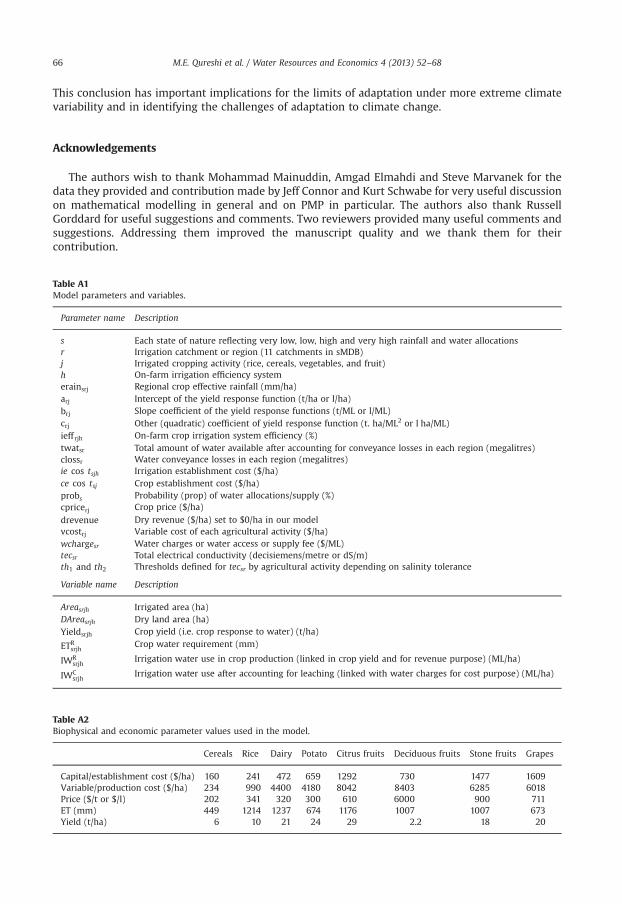
Table A1Model parameters and variables.

Parameter name Description

s Each state of nature reflecting very low, low, high and very high rainfall and water allocationsr Irrigation catchment or region (11 catchments in sMDB)j Irrigated cropping activity (rice, cereals, vegetables, and fruit)h On-farm irrigation efficiency systemerainsrj Regional crop effective rainfall (mm/ha)arj Intercept of the yield response function (t/ha or l/ha)brj Slope coefficient of the yield response functions (t/ML or l/ML)crj Other (quadratic) coefficient of yield response function (t. ha/ML2 or l ha/ML)ieff rjh On-farm crop irrigation system efficiency (%)twatsr Total amount of water available after accounting for conveyance losses in each region (megalitres)clossr Water conveyance losses in each region (megalitres)ie cos tsjh Irrigation establishment cost ($/ha)ce cos tsj Crop establishment cost ($/ha)probs Probability (prop) of water allocations/supply (%)cpricerj Crop price ($/ha)

drevenue Dry revenue ($/ha) set to $0/ha in our modelvcostrj Variable cost of each agricultural activity ($/ha)wchargesr Water charges or water access or supply fee ($/ML)tecsr Total electrical conductivity (decisiemens/metre or dS/m)th1 and th2 Thresholds defined for tecsr by agricultural activity depending on salinity tolerance

Variable name Description

Areasrjh Irrigated area (ha)DAreasrjh Dry land area (ha)Yieldsrjh Crop yield (i.e. crop response to water) (t/ha)

ETRsrjh Crop water requirement (mm)

IWRsrjh

Irrigation water use in crop production (linked in crop yield and for revenue purpose) (ML/ha)

IWCsrjh

Irrigation water use after accounting for leaching (linked with water charges for cost purpose) (ML/ha)

Table A2Biophysical and economic parameter values used in the model.

Cereals Rice Dairy Potato Citrus fruits Deciduous fruits Stone fruits Grapes

Capital/establishment cost ($/ha) 160 241 472 659 1292 730 1477 1609Variable/production cost ($/ha) 234 990 4400 4180 8042 8403 6285 6018Price ($/t or $/l) 202 341 320 300 610 6000 900 711ET (mm) 449 1214 1237 674 1176 1007 1007 673Yield (t/ha) 6 10 21 24 29 2.2 18 20

Table A3Production function parameters values of selected major agricultural activities.

Cereals Rice Dairy Potato Citrus fruits Deciduousfruits

Stone fruits Grapes

Intercept(a)

�4.6168 �15.062 �13.065 �22.004 �20.178 �1.5307 �12.524 �10.969

Quadratic(b)

�6.00E�05 �2.00E�05 �2.00E�05 �1.00E�04 �4.00E�05 �3.00E�05 �3.00E�05 �7.00E�05

Slope (c) 4.99E�02 4.51E�02 5.19E�02 1.39E�01 8.88E�02 0.0592 6.16E�02 9.51E�02

M.E. Qureshi et al. / Water Resources and Economics 4 (2013) 52–68 67

Appendix A. Model parameter description and biophysical and economic values used

See Tables A1–A3.

References

[1] National Water Commission, Australian Water Markets: Trends and Drivers 2007–08 to 2010–11, National WaterCommission, Canberra, 2011.

[2] G.B. Frisvold, K. Konyar, Less water: how will agriculture in Southern Mountain states adapt? Water. Resour. Res. 48 (2012).[3] D. Barriopedro, C.M. Gouveia, R. Trigo, L. Wang, The 2009/10 drought in China: possible causes and impacts on vegetation, J.

Hydrometeorol. 13 (4) (2012) 1251–1267.[4] MDBA, River Murray Drought Update, Murray-Darling Basin Authority, Canberra, 2009.[5] M. Kirby, R. Bark, J. Connor, M.E. Qureshi, S. Keyworth, Sustainable irrigation: how did irrigated agriculture in Australia’s

Murray–Darling Basin adapt in the millennium drought? Agricultural Water Management, Special Issue, The complexnature of sustainable irrigation, in press.

[6] M.W. Rosegrant, S.A. Cline, Global food security: challenges and policies, Science 302 (5652) (2003) 1917–1919.[7] S. Solomon, D. Qin, M. Manning, Z. Chen, M. Marquis, K.B. Averyt, M.Tignor, H.L. Miller (Eds.), IPCC, Climate Change 2007:

The Physical Science Basis. Contribution of Working Group I to the Fourth Assessment Report of the IntergovernmentalPanel on Climate Change, Intergovernmental Panel on Climate Change, Cambridge, 2007.

[8] R. Ragab, C. Prudhomme, Climate change and water resources management in arid and semi-arid regions: perspective andchallenges for the 21st century, Biosyst. Eng. 81 (1) (2002) 3–34.

[9] CSIRO, Water Availability in the Murray. A Report to the Australian Government from the CSIRO Murray-Darling BasinSustainable Yields Project, CSIRO, Canberra, 2008.

[10] J. Quiggin, D. Adamson, P. Schrobback, S. Chambers, Report to Garnaut Review: The Implications of Climate Change forIrrigation in the Murray Darling Basin, Risk and Sustainable Management Group (RSMG), School of Economics, Universityof Queensland, Brisbane, 2008.

[11] D. Adamson, T. Mallawaarachchi, J. Quiggin, Declining inflows and more frequent droughts in the Murray-Darling Basin:climate change, impacts and adaptation, Austr. J. Agric. Resour. Econ. 53 (3) (2009) 345–366.

[12] ABARE–BRS, Environmentally Sustainable Diversion Limits in the Murray-Darling Basin: Socioeconomic Analysis,Australian Bureau of Agricultural and Resource Economics, Canberra, 2010.

[13] Q. Jiang, G.R. Quentin, Economic effects of climate change in the Murray-Darling Basin, Australia, Agric. Syst. 110 (2012)10–16.

[14] T. Mallawaarachchi, D. Adamson, S. Chambers, P. Schrobback, Economic Analysis of Diversion Options for the Murray-Darling Basin Plan: Returns to Irrigation Under Reduced Water Availability, Risk and Sustainable Management Group,University of Queensland, Brisbane, 2010.

[15] M. Kirby, Irrigation, in: I. Prosser (Ed.), Water: Science and Solutions for Australia, CSIRO Publishing, Collingwood, Victoria,2011.

[16] J. Austin, L. Zhang, R.N. Jones, P. Durak, D. Dawes, P. Hairsine, Climate change impact on water and salt balances: anassessment of the impact of climate change on catchment salt and water balances in the Murray-Darling Basin, Australia,Clim. Change. 100 (3–4) (2010) 607–631.

[17] F.H.S. Chiew, T.A. McMahon, Modelling the impacts of climate change on Australian streamflow, Hydrol. Process 16 (6)(2002) 1235–1245.

[18] F.N. Tubiello, J.-F. Soussana, S.M. Howden, Crop and pasture response to climate change, Proc. Natl. Acad. Sci. 104 (50)(2007) 19686–19690.

[19] J.D. Connor, K. Schwabe, D. King, K. Knapp, Irrigated agriculture and climate change: the influence of water supplyvariability and salinity on adaptation, Ecol. Econ. 77 (2012) 149–157.

[20] K.A. Schwabe, I. Kan, K.C. Knapp, Drainwater management for salinity mitigation in irrigated agriculture, Am. J. Agric. Econ.88 (1) (2006) 135–149.

[21] B.G. Drake, M.A. Gonzalez–Meler, S.P. Long, More efficient plants: a consequence of rising atmospheric CO2? Annu. Rev.Plant. Physiol. Plant. Mol. Biol. 48 (1997) 609–639.

M.E. Qureshi et al. / Water Resources and Economics 4 (2013) 52–6868

[22] A. Loch, S. Wheeler, H. Bjornlund, S. Beecham, J. Edwards, A. Zuo, M. Shanahan, The Role of Water Markets in ClimateChange Adaptation, National Climate Change Adaptation Research Facility, Gold Coast125.

[23] S.M. Howden, et al., Adapting agriculture to climate change, Proc. Natl. Acad. Sci. 104 (50) (2007) 19691–19696.[24] M.E. Qureshi, et al., Economic assessment of environmental flows in the Murray Basin, Austr. J. Agric. Resour. Econ. 51 (3)

(2007) 283–303.[25] T.W. Hertel, S.D. Rosch, Cliamte change, agriculture and poverty, Appl. Econ. Perspect. Pol. 32 (3) (2010) 1–31.[26] A. Hafi, S. Thorpe, A. Foster, The impact of climate change on the irrigated agriculture industries in the Murray-Darling

Basin, in: Proceedings of the Australian Agricultural and Resource Economics Society Conference, ABARE Conference Paper,Cairns, 2009.

[27] R.Q. Grafton, Q. Jiang, Economic effects of water recovery on irrigated agriculture in the Murray-Darling Basin, Austr. J.Agric. Resour. Econ. 55 (4) (2011) 487–499.

[28] R.E. Howitt, Positive Mathematical-Programming, Am. J. Agric. Econ. 77 (1995) 329–342.[29] R. Howitt, et al., Economic Modelling of Agriculture and Water in the California Using the Statewide Agricultural

Production Model, a Report for the California Department of Water Resources, CA Water Plan Update 2009, University ofCalifornia, Davis, 2010.

[30] M.E. Qureshi, J. Connor, M. Kirby, M. Mainuddin, Economic assessment of acquiring water for environmental flows in theMurray Basin, Austr. J. Agric. Resour. Econ. 51 (3) (2007) 283–303.

[31] R.C. Griffin, Water Resource Economics: The Analysis of Scarcity, Policies, and Projects, MIT Press, Cambridge, MA, 2006.[32] O. Röhm, S. Dabbert, Integrating agri-environmental programs into regional production models: an extension of positive

mathematical programming, Am. J. Agric. Econ. 85 (1) (2003) 254–265.[33] ABS, Australian Bureau of Statistics Agricultural Census 1996–97, Australian Bureau of Statistics, Canberra, 1997.[34] MDBA, Water Audit Monitoring Report: Report of the Murray-Darling Basin Authority on the Cap on Diversions, Murray

Darling Basin Authority, Canberra, 2009.[35] R.G. Allen, et al., Crop Evapotranspiration: Guidelines for Computing Crop Water Requirements. FAO Irrigation and

Drainage Paper, 1998, p. 56.[36] A. Elmahdi, J. Connor, R. Doble, M. Stenson, M. Kirby, G. Walker, Forecasting lower murray river salinity under climatic

uncertainty and reduced dilution flow, in: International Salinity Forum, Adelaide, 2008.[37] M.E. Qureshi, M. Mainuddin, S. Marvanek, A. Elmahdi, J. Connor, S. Whitten, Irrigation Futures for the Murray Basin –

Technical Documentation, CSIRO, Canberra33.[38] ABARE, Australian Crop Report, Australian Bureau of Agricultural and Resource Economics, Canberra, 2008.[39] ABS, Value of Agricultural Commodities Produced, Australian Bureau of Statistics, Canberra, 2006.[40] ABARE, Australian Commodities, Australian Bureau of Agricultural and Resource Economics, Canberra, 2007.[41] M.E. Qureshi, M. Ahmad, S. Whitten, M. Kirby, A multi-period positive mathematical programming model for assessing

economic impact of drought in the Murray-Darling Basin, Australia, Econ. Model. (2013). (in preparation).[42] Australian Competition and Consumer Commission, ACCC Water Monitoring Report 2011–12, Australian Competition and

Consumer Commission, Canberra, 2013.[43] J. Doorenbos, A.H. Kassam, Yield Response to Water, in FAO Irrigation and Drainage Paper, Rome, 1979.[44] I. Kan, K.A. Schwabe, K.C. Knapp, Microeconomics of irrigation with saline water, J. Agric. Resour. Econ. 27 (1) (2002)

16–39.[45] J. Letey, A. Dinar, K.C. Knapp, Crop–water production function model for saline irrigation waters, Soil Sci. Soc. Am. J. 49 (4)

(1985) 1005–1009.[46] M.E. Qureshi, T. Shi, S.E. Qureshi, W. Proctor, Removing the Barriers to Facilitate Efficient Water Markets in the Murray

Darling Basin of Australia. Agricultural Water Management, 2009.[47] A. Brooke, et al., GAMS: A User's Guide, GAMS Development Corporation, Washington, DC, 2004.[48] R.E. Howitt, Agricultural and Environmental Policy Models: Calibration, Estimation and Optimization, University of

California Davis, UC Davis, 2005.[49] T. Heckelei, H. Wolff, Estimation of constrained optimisation models for agricultural supply analysis based on generalised

maximum entropy, Eur. Rev. Agric. Econ. 30 (1) (2003) 27–50.[50] T. Heckelei, W. Britz. Models based on positive mathematical programming: state of the art and further extensions, in:

Proceedings of the 89th European Seminar of the European Association of Agricultural Economists, Modelling AgriculturalPolicies: State of the Art and the New Challenges, Minte Universita, Parma Editore 2005.

[51] Q. Paris, R.E. Howitt, An analysis of ill-posed production problems using maximum entropy, Am. J. Agric. Econ. 80 (1)(1998) 124–138.

[52] P. Merel, S. Bucaram, Exact calibration of programming models of agricultural supply against exogenous supply elasticities,Eur. Rev. Agric. Econ. 37 (3) (2010) 395–418.

[53] R. Cortignani, S. Severini, Modeling farm-level adoption of deficit irrigation using Positive Mathematical Programming,Agric. Water Manage. 96 (12) (2009) 1785–1791.

[54] Murray-Darling Basin Authority, Water Act 2007, Basin Plan, Commonwealth of Australia, Minister for Sustainability,Environment, Water, Population and Communities, 2012.

[55] ABARES, Agricultural Commodity Statistics 2012, Australian Bureau of Agricultural and Resource Economics and Sciences,Canberra, 2012.

[56] M.E. Qureshi, S.M. Whitten, Regional impact of climate variability in the southern Murray-Darling Basin, Australia, WaterResources and Economics. http://dx.doi.org/10.1016/j.wre.2013.12.002, this issue.