ORIGINAL ARTICLE

Wildflower areas within revitalized agricultural matrices boostsmall mammal populations but not breeding Barn Owls

Raphael Arlettaz • Markus Krahenbuhl •

Bettina Almasi • Alexandre Roulin •

Michael Schaub

Received: 6 August 2009 / Revised: 10 December 2009 / Accepted: 11 December 2009 / Published online: 8 January 2010

� Dt. Ornithologen-Gesellschaft e.V. 2010

Abstract Agro-ecosystems have recently experienced

dramatic losses of biodiversity due to more intensive pro-

duction methods. In order to increase species diversity,

agri-environment schemes provide subsidies to farmers

who devote a fraction of their land to ecological compen-

sation areas (ECAs). Several studies have shown that

invertebrate biodiversity is actually higher in ECAs than in

nearby intensively cultivated farmland. It remains poorly

understood, however, to what extent ECAs also favour

vertebrates, such as small mammals and their predators,

which would contribute to restoring functional food chains

within revitalised agricultural matrices. We studied small

mammal populations among eight habitat types—including

wildflower areas, a specific ECA in Switzerland—and

habitat selection (radiotracking) by the Barn Owl Tyto

alba, one of their principal predators. Our prediction was

that habitats with higher abundances of small mammals

would be more visited by foraging Barn Owls during the

period of chicks’ provisioning. Small mammal abundance

tended to be higher in wildflower areas than in any other

habitat type. Barn Owls, however, preferred to forage in

cereal fields and grassland. They avoided all types of crops

other than cereals, as well as wildflower areas, which

suggests that they do not select their hunting habitat pri-

marily with respect to prey density. Instead of prey abun-

dance, prey accessibility may play a more crucial role:

wildflower areas have a dense vegetation cover, which may

impede access to prey for foraging owls. The exploitation

of wildflower areas by the owls might be enhanced by

creating open foraging corridors within or around wild-

flower areas. Wildflower areas managed in that way might

contribute to restore functional links in food webs within

agro-ecosystems.

Keywords Ecological compensation areas �Agro-ecosystems � Small mammals � Species conservation

Introduction

During the past decades, flora and fauna within agricultural

ecosystems have been radically impoverished due to more

intensive production methods (Donald et al. 2001; Benton

et al. 2003; Britschgi et al. 2006). Simplification of crop

rotations, larger fields, loss of ecological relevant structures

caused by land consolidation and widespread use of agro-

chemicals have led to a dramatic decline in plant and

animal species richness (Schmid 2002). In order to improve

the state of biodiversity in farmland, several countries have

adopted agri-environment schemes. Their efficacy has been

Communicated by F. Bairlein.

R. Arlettaz (&) � M. Krahenbuhl � M. Schaub

Division of Conservation Biology, Institute of Ecology

and Evolution, University of Bern, Baltzerstrasse 6,

3012 Bern, Switzerland

e-mail: raphael.arlettaz@iee.unibe.ch

R. Arlettaz

Swiss Ornithological Institute, Valais Field Station,

Nature Centre, 3970 Salgesch, Switzerland

R. Arlettaz

The Ecology Centre, University of Queensland,

St Lucia, QLD 4072, Australia

B. Almasi � M. Schaub

Swiss Ornithological Institute, 6204 Sempach, Switzerland

A. Roulin

Department of Ecology and Evolution, University of Lausanne,

1012 Lausanne, Switzerland

123

J Ornithol (2010) 151:553–564

DOI 10.1007/s10336-009-0485-0

vigorously debated and is still controversial, especially

with respect to some groups of vertebrates, although ben-

efits for some invertebrates seem indisputable (Nentwig

2000; Kleijn et al. 2001, 2006; Kleijn and Sutherland 2003;

Knop et al. 2006; Aschwanden et al. 2007).

Interestingly, agri-environment schemes are primarily

considered as biodiversity promoters (e.g. Kleijn and

Sutherland 2003; Knop et al. 2006; Whitthingham 2007).

Until very recently, their role in enhancing biomass along

food chains has not been a major focus of research (Shore

et al. 2005; Aschwanden et al. 2007; Askew et al. 2007;

MacDonald et al. 2007; Reid et al. 2007). This is surprising

because ecosystem functionalities largely depend upon

major fluxes of biomass and energy from the lower to the

upper trophic levels; a few dominant producer and consumer

species usually constitute the basic architecture of an

ecological community. As such, the presence of abundant

populations of these dominant taxa often remains the best

predictor of predator occurrence and breeding success (e.g.

Hansson and Henttonen 1988; Korpimaki and Norrdahl

1991; Veit et al. 1993; Reid and Croxall 2001; Gilg et al.

2003, 2006; Palma et al. 2006). As a result, favouring the

abundance of common species at lower trophic levels may

eventually be crucial for promoting biodiversity as a whole,

since the existence of good prey reservoirs will contribute to

attract their predators, i.e. a symbolic ‘‘flagship’’ fraction of

species diversity. Agri-environment schemes must restore

agricultural landscape matrices in such a way that predators,

which were first to vanish after the dramatic land use inten-

sification, progressively reappear in farmland. In doing so,

agri-environment schemes would contribute to the recovery

of functional links in food webs within agro-ecosystems.

Ecological compensation areas (ECAs) have become

major elements of agri-environment schemes in several

countries of the European Union, totalling €24 billion of

subsidies for the period 1994–2003 (Kleijn and Sutherland

2003; Askew et al. 2007). In Switzerland, for instance,

farmers can only receive federal agricultural subsidies if

7% of their land is designated as an ECA. Swiss ECAs

contain, among other habitats, extensive meadows and

wildflower areas (Schweizer Eidgenossenschaft 1998).

Such ECAs may enhance the diversity and richness of

plants and some insects, but the evidence for benefits

remains controversial for several groups of arthropods such

as spiders and for most vertebrates (Kleijn et al. 2006;

Birrer et al. 2007). Wildflower areas are a kind of ‘‘man-

aged’’ set-aside in the sense that seeds of wild flowers are

sown by farmers whereas some invasive weeds are con-

trolled through targeted, plant-by-plant herbicide applica-

tion. To our knowledge, they have no equivalent in other

European agri-environment schemes, although they look

similar to set-aside and fallowland from a vegetation

structural viewpoint. In Switzerland, wildflower areas

represent only 2% of the ECAs (3,700 ha in total in 2004),

but have become obvious features of modern farmland due

to their high flower species richness that renders them

especially attractive for the public. These ECAs have been

shown to enhance ‘‘beneficial’’ organisms (e.g. Revaz et al.

2008) and also the abundance of agricultural pests such as

voles (Microtus spp.; Tattersall et al. 1997, 2000; Briner

et al. 2005; Aschwanden et al. 2007). Small mammals

exploit wildflower areas preferentially because they offer a

high food supply and a dense vegetation cover that protects

them from predators (Wakeley 1978; Baker and Brooks

1981; Bechard 1982; Dickman et al. 1991; Jacob and

Hempel 2003; Aschwanden et al. 2007). In the present

study, we attempted to quantify small mammal population

densities in different habitats, including wildflower areas,

and to study patterns of habitat selection in one of their

major nocturnal predators, the Barn Owl Tyto alba. We

tested whether wildflower areas may favour small mam-

mals and their vertebrate predators, thereby contributing to

restore functional links along the food chain in agricultural

ecosystems.

The Barn Owl has a wide distribution range (Mebs and

Scherzinger 2000). In temperate biomes, it has followed

the spread of agriculture as it hunts small mammals such as

microtid rodents and shrews mostly in open and semi-open

habitats (Snow and Perrins 1998). There has been a

widespread decline of the Barn Owl in the twentieth cen-

tury due to intensification of farming practices and habitat

loss, including shortage of suitable breeding sites (Snow

and Perrins 1998; Mebs and Scherzinger 2000; Mebs and

Roulin 2002; Altwegg et al. 2006; Askew et al. 2007). The

species is near endangered in Switzerland (Burkhardt and

Schmid 2001) with an estimated 1,000–1,500 breeding

pairs (Schmid et al. 1998). Local density may reach up to

42 pairs per 100 km2 in suitable farmland and with a good

availability of nest-boxes (Roulin 1999). Swiss populations

fluctuate in synchrony with vole populations (Roulin 2002)

as is the case for many avian predators (Korpimaki 1994).

The present study addresses two main questions: (1) is

the abundance of small mammals higher in wildflower

areas than in other agricultural and nearby habitats? and (2)

if so, do Barn Owls spend a disproportionate fraction of

time hunting in wildflower areas compared to other habi-

tats, and is this reflected in subsequent productivity of

breeding pairs? We use the information to assess the extent

to which Barn Owls benefit from wildflower areas designed

to revitalise the agricultural matrix.

Materials and methods

The fieldwork was conducted in the region around Payerne

in Western Switzerland, a 190-km2-wide plain bordered by

554 J Ornithol (2010) 151:553–564

123

a hilly landscape (46�43–560N, 6�490–7�020E, 434–650 m

elevation). Intensive agriculture is the dominant land use in

the area. The most important crops on the plain are cereals

(mostly winter wheat Triticum aestivum), maize Zea mays,

sugar beet Beta vulgaris, and tobacco Nicotiana tabacum.

On the lower hill slopes, there is some viniculture, whereas

the hills themselves are mainly used for dairy farming.

Wildflower areas are scattered across the study area. The

region supports a relatively high population density of Barn

Owls (e.g. Altwegg et al. 2003, 2007).

Density of small mammals

For estimating small mammal abundance, we selected four

study sites which all included the eight following habitat

types in close proximity: (1) wildflower areas that

were [2 years old (because in [2 years old wildflower

strips vole abundance is no longer related to age; Tattersall

et al. 2000) and had a size of [1 ha to minimise edge

effects which may influence local densities of small

mammals; (2) banks of canals and ditches; (3) edges of

forests or hedgerows; (4) fields of winter wheat; (5) maize;

(6) tobacco; (7) extensive meadows that had not been

ploughed for at least 5 years (permanent meadow); and (8)

intensively fertilised grassland that is part of the crop

rotation (intensive meadow).

We used three trap types (Longworth, Penlon, Abing-

don, UK; Sherman, H.B. Sherman Traps, Tallahassee,

USA; Trip Trap, Alana Ecology, Bishops Castle, UK) and

always placed three traps, one of each type, at capture

locations. As bait, pieces of carrots and cheese as well as

grains (Hamster food from Coop, CH) were used (Briner

et al. 2005). Additionally, a handful of hay was put into the

traps to enhance survival of the animals captured (Briner

et al. 2005).

Capture design followed that of Aschwanden et al.

(2005, 2007) who also investigated small mammals in

agro-ecosystems. We applied a capture–mark–recapture

protocol to estimate population sizes in May, July and

September 2005. In each habitat, traps were placed in a

reticulated pattern with distances of 5 m between trap sets

along two parallel 45-m-long transects. This design defines

20 trap points, totalling 60 traps per sampled habitat.

Assuming a capture radius of ca. 5 m around traps, the

overall catching area of each study plot was about 825 m2.

Traps were set over a period of three nights and days and

were visited every 8 h. We installed them at 1400 hours on

day 1 and removed them at 0600 hours on day 4. The

number of traps available (n = 240 in total) and the han-

dling time allowed us to set traps in four habitat types per

site simultaneously (4 9 60 = 240 traps). After trapping in

these first four habitat types (randomised habitat sequence),

the same procedure was immediately repeated in the four

other habitat types at the same study site. Thus, one com-

plete capture series at one study site (each site comprising

the eight different habitat types mentioned above, i.e. eight

study plots) lasted 7 days in a row. At each visit, small

mammals were identified, sexed, aged, weighed and

marked. Marking consisted of local cutting of the fur on the

back and the head at seven different places to make the

darker underfur visible. Varied cutting codes enabled

individual recognition. Subsequent trap checks enabled a

capture history to be constructed for each animal. We

found no movement of individuals between the habitat

types sampled at each study site.

Because the populations were likely to be demographi-

cally and geographically closed during the short sampling

period (72 h), we used closed population models imple-

mented in the program ‘‘Capture’’ to estimate population

sizes (Otis et al. 1978). Because of the closure, the only

parameters to be estimated are capture rates and the pop-

ulation size. We fitted eight models to each dataset that

used different structures for the capture rates. Capture rates

were allowed to be constant, to be variable across time, to

change in response to whether or not an individual has been

captured previously, to be individually different, and

combinations thereof (Otis et al. 1978). For each month,

habitat type and site, the best fitting model was chosen

(Appendix). When no individual was recaptured, popula-

tion size could not be estimated with the closed population

models. In these cases, we used the number of captured

individuals as the minimal population size. We calculated

the mammal density (n/ha, with the catching area of

825 m2 as the reference area) for each study plot and tested

whether habitat type and study site explained the variance

between plots using repeated measures ANOVA (JMP

4.0.4; SAS Institute, Cary, NC, USA) on the ranks of

densities. As densities were sampled in equal time intervals

throughout the season, the three consecutive capture series

(May, July, September) were considered as repeated

measures, providing information about temporal trends.

P values are two-tailed with rejection levels set at 5%.

Differences in densities were finally tested with posthoc

pairwise comparisons with respect to habitat type and

season (Tukey–Kramer HSD test).

Habitat selection

Seven breeding male owls were radio-tagged for the study

of habitat selection; we selected birds nesting in the

vicinity of the small mammal capture sites, but owl nests

were well scattered throughout the study area. The owls

were caught and tagged with radio transmitters (ATS type

A1240, 8 g, mortality sensor: 6 h fast; ATS, Isanti, USA,

fixed with a Rappole leg-harness with a rubber band that

falls off after 1 year). Owls were radio-located using a

J Ornithol (2010) 151:553–564 555

123

portable receiver (Telonics TR-5; Telonics;, Mesa AZ,

USA), and a hand-held 3-element Yagy antenna.

Radiotracking lasted from June to September 2005 with

interruptions during the small mammal capture sessions

(see above). We tracked only males, since this sex is the

main food provider to Barn Owl broods (Roulin et al.

2001). The tagged owls were radiotracked from a car and

located by the ‘‘homing-in’’ on the animal method descri-

bed by White and Garrot (1990). Visual localisations were

attempted in open areas, using an observation spyglass

(Aspectem 80/500 with vario ocular; Docter, Eisfeld,

Germany), a powerful torch (Maglite; Mag Instrument,

Ontario, USA), and a GPS device (eTrex Gecko; Garmin

International, Olathe, USA).

Positions of hunting or resting owls were obtained from

GPS readings. Commuting activity (rapid flight between

areas) was not part of the dataset used for analysis, which

focused only on actual foraging activity (i.e. activity con-

centrated on a given area). The time, behaviour (sitting/

flying), hunting activity (‘‘dives’’ to the ground) and habitat

type of all observations were also recorded. Bearings were

used to draw home ranges as minimum convex polygons

(MCP; Mohr 1947). These MCPs were mapped in the field

for estimating agricultural land-use (habitat types and lin-

ear features, see below). MCPs were divided into 1-ha

squares according to the official reference grid of the Swiss

Federal Topographic Service (Arlettaz 1999). For each 1-

ha grid cell, we noted the dominant habitat type in the cell

(cereals, maize, tobacco, other crops, grassland, forest,

wildflower area, riparian and settlement). Wildflower areas

were often present in the form of strips, i.e. too small to be

the dominant habitat type in a square of 1 ha. We therefore

also recorded all 1-ha cells containing wildflower strips.

The length of different linear structures (forest edges, riv-

ers, ditches, wildflower strips, hedgerows and total linear

structures) was also estimated for each 1-ha cell (0: no

linear structure; 1: 0–25; 2: 25–50; 3: 50–75; 4: 75–100;

5: [100 m).

Radiotracking data allowed distinguishing between

visited and non-visited 1-ha grid cells within individual

home ranges (MCPs). We assumed that visited cells mir-

rored habitat preferences, whilst non-visited cells were

avoided because they represented non-suitable habitat. This

assumption is realistic since every cell in the MCP was

potentially overflown by the owl. This approach has been

used with success in other studies (e.g. Arlettaz 1999).

For habitat selection analysis at the population level, we

conducted a Compositional Analysis (Aebischer et al.

1993) to test for differences between used and available

habitat (the latter obtained from all 1-ha cells across indi-

vidual MCPs; Aschwanden et al. 2005). This non-para-

metric technique takes into account that the proportional

use of one habitat type is dependent on that of other habitat

types (Aebischer et al. 1993). Compositional Analysis

enables the examination of only n-1 factors, with n being

the number of individuals considered. Our basic habitat

matrix had thus to be reduced to six parameters: maize,

tobacco and other crops were grouped together as cropland,

whereas settlements were excluded. According to Aebi-

scher et al. (1993), zero values in the ‘‘used’’ worksheet

were replaced by a small number (0.001).

Because Compositional Analysis was only appropriate

to study habitat selection at the population level (although

through the individuals), we used alternative statistical

methods to test for individual preferences. Frequency dis-

tributions of visited versus non-visited cells were computed

through randomised contingency table procedures with the

program Actus2 (G. F. Estabrook, University of Michigan,

Ann Arbor, MI 48109-1048, USA; Estabrook and Esta-

brook 1989; Arlettaz 1999). This program provides levels

of probability for any positive or negative deviation

between observed and expected frequencies, showing

habitat selection patterns for each individual owl and the

nine habitat types. Comparing selection trends among the

seven individuals also enabled us to draw information on

general habitat selection pattern. For that purpose, we

developed an ad hoc selection index by subtracting for each

habitat type the percentage of owls that avoided that habitat

from the percentage of owls that showed positive selection.

To further assess a possible effect of wildflower areas

and strips, we used randomised contingency table proce-

dures (as above), testing for differences for each owl sep-

arately, between the frequency distribution of visited and

non-visited cells in presence or absence of that habitat.

For a comparison of linear features (structural length)

between visited and non-visited cells, we relied on non-

parametric statistics because the variables were not normally

distributed and could not be transformed appropriately

(two-tailed, Wilcoxon-Kruskal-Wallis Test; program JMP

4.0.4; SAS Institute).

Reproductive output versus home range size

and habitat characteristics

The relationship (Spearman rank correlation) between

reproductive parameters and habitat structure in radio-

tracked owls was considered in two ways. First, we

examined whether there was a relationship between home

range size and availability of suitable foraging habitats

within an individual home range, predicting smaller home

range sizes where the proportion of suitable habitat was

high. Second, we tested whether breeding performance

(clutch size and number of fledglings) correlated with

home range size and/or proportion of suitable foraging

habitat within the home range, predicting higher produc-

tivity where habitat conditions were more favourable (i.e.

556 J Ornithol (2010) 151:553–564

123

small home range and high foraging habitat quality). Given

the unilateral direction of these predictions, correlation

tests were one-tailed.

Results

Density of small mammals

During three sampling sessions in May, July and Septem-

ber, we captured 1,286 small mammals, including 224

recaptures (17.4%; Fig. 1). In total, we thus examined

1,062 individuals, of which 1,035 could be identified to one

of the following eight species: Apodemus sylvaticus

(n = 329), Microtus arvalis (n = 316) and A. flavicollis

(n = 261) largely dominated the sample, followed by

Clethrionomys glareolus (n = 74), Crocidura russula

(n = 33), Sorex araneus/S. coronatus (n = 19), Mus

musculus (n = 2) and Arvicola terrestris (n = 1). Species

abundance varied with respect to habitat type (Fig. 2), but

the three most common species dominated in all habitats.

Species richness was highest in wildflower areas with six

species (A. flavicollis, A. sylvaticus, C. russula, M. arvalis,

M. musculus and S. araneus/S. coronatus), followed by

canal bank and wood edge, each with five species

(A. flavicollis, A. sylvaticus, C. glareolus, M. arvalis and

S. araneus/S. coronatus at canal bank, and C. russula at

wood edge; Figs. 1 and 2). The poorest species habitat type

was tobacco with only two species (A. flavicollis and

A. sylvaticus). The efficacy of traps differed slightly among

types, with 457 captures in Trip-Traps, 441 in Longworth

traps and 388 in Sherman traps (v2 = 6.211, df = 2,

P = 0.045).

Densities of small mammals varied significantly

between habitat types (F1,8 = 195.69, P \ 0.0001),

throughout the season (F1,2 = 7.47, P \ 0.0001), and

Fig. 1 Mean (?SE, showing the variation between study sites)

number of rodents (Muridae, Arvicolidae) and shrews (Soricidae)

caught with pitfalls in May, July and September at four sites within

each habitat type

Fig. 2 Mean (?SE, showing the variation between study sites)

number of dominant species of rodents and shrews caught in May,

July and September at four study sites within eight different habitat

types

J Ornithol (2010) 151:553–564 557

123

between study sites (F1,4 = 1.66, P = 0.0001; Fig. 3). The

highest average densities in all 3 months were within

wildflower areas (mean ± SE: 458 ± 189, 1,030 ± 133

and 1,285 ± 440 individuals per hectare in May, June and

September, respectively). The highest density recorded was

in a wildflower area with an estimated 1,976 (±75) indi-

viduals per hectare in September. In May, small mammal

densities were significantly higher in wildflower areas,

canal banks and winter wheat (P \ 0.05; Tukey–Kramer

HSD) than in maize, tobacco, permanent (for wildflower

areas only) and intensive meadows. Densities were also

higher in woodland edges than in maize and tobacco. In

July, densities were significantly higher in wildflower areas

and winter wheat than in tobacco or permanent and

intensive meadows, while in September they were only

significantly higher in wildflower areas than in winter

wheat (Fig. 3).

To sum up, species richness and densities of small

mammals varied significantly between habitat types, but in

general wildflower areas were supporting consistently

higher numbers of species and individuals throughout the

trapping season.

Habitat selection

A total of 158 precise localisations of the seven foraging

male Barn Owls were obtained (mean ± SD: 22.6 ± 5.8,

range 17–34). There was a large variance in individual

home range size (mean 335.6 ± 234.2 ha, median 297 ha;

range 93–804 ha; Table 1). Compositional Analysis at the

population level suggested that habitat types were not

chosen at random (k = 0.07, v2 = 18.58, P = 0.0023). In

particular, cereals (winter wheat) were significantly pre-

ferred over crops (other than cereals and maize), this rel-

ative to availability (Table 2).

The randomised contingency table analyses run on the

individuals separately are presented in Table 3. Our ad hoc

index of habitat selection suggests the following decreasing

order in habitat preferences: cereals [ grassland [ forest,

settlement [ riparian [ tobacco [ maize, other crops [wildflower areas (Table 3).

That wildflower areas ranked low in foraging habitat

preferences (the two above analyses; Tables 2 and 3) was

further supported by the fact that two owls showed a sig-

nificant difference in the frequency distribution of this

habitat between visited and non-visited cells: both avoided

this habitat (randomised contingency tables, P \ 0.05;

Table 4).

The comparison of structural length of linear habitat

features showed that there were few consistent patterns of

selection: only two owls showed preference for 1-ha cells

with longer streams and hedgerows (Table 5). A third

individual showed a marginal preference for longer forest

edge (P = 0.08; Table 5).

A total of 24 hunting events (n = 4 birds) were

observed visually: 22 (92%) of these were of owls

searching for prey on the wing, patrolling in flight above

foraging grounds, and only 2 cases (8 %) were of owls

perch-hunting.

Reproductive output versus home range size

and habitat characteristics

There was a negative relationship between home range size

and proportion of preferred foraging habitat (grassland and

cereals) within individual home ranges (Spearman rank

correlation, rs = –0.714, n = 7, P = 0.044), suggesting

that male Barn Owls tended to compensate for low habitat

suitability by increasing territory size. Increasing home

range size, or lack of suitable foraging habitat, seems to

bear costs: both clutch size (range 5–9, rs = –0.674, n = 7,

P = 0.049) and number of fledglings (range 4–6)

Fig. 3 Mean densities of small mammals (n/ha ? SE, showing the

variation among the four study sites) in eight habitat types in May,

July and September. Asterisks indicate significant differences

(P \ 0.05, Tukey–Kramer post hoc pairwise comparison)

558 J Ornithol (2010) 151:553–564

123

correlated negatively with home range size (rs = –0.850,

n = 7, P = 0.015).

Discussion

This study suggests that the abundance of small mammals,

which varied markedly between habitat types, is not the

principal factor dictating habitat selection patterns in the

Barn Owl: the habitats offering the highest densities of

prey, especially wildflower areas, were avoided during

foraging. This discrepancy is most probably due to the fact

that it is prey detectability and/or accessibility and not prey

density which ultimately defines its availability for the

owls. This pattern has been found in several species of

birds inhabiting farmland (reviewed in Atkinson et al.

Table 1 Synopsis of radiotracking sessions carried out with seven male Barn Owls Tyto alba in summer 2005

Individual # Radiotracking

period

Number of nights

with effective

tracking

Number of

bearings

Number of

visited 1-ha

squares

Visually

observed hunting

events

Foraging home

range (ha) (MCP)

Clutch

size

Number of

fledglings

1 07.06–26.06.05 11 39 26 4 211 7 6

2 07.06–15.08.05 8 19 17 3 93 6 6

3 27.06–27.07.05 14 28 22 4 804 5 4

4 04.08–10.08.05 7 24 21 0 380 5 4

5 10.08–06.09.05 14 22 20 0 214 6 5

6 12.08–06.09.05 14 19 18 0 419 5 5

7 15.08–26.08.05 7 35 34 13 228 9 5

Total 75 186 158 24

MCP Minimum convex polygon

Table 2 Results of compositional analysis pinpointing differences in habitat selection of seven male Barn Owls

Cereals Crops Grassland Wildflower area Forest Riparian Rank

Cereals ??? ? ? - ? 4

Crops --- - ? - ? 2

Grassland - ? ? - ? 3

Wildflower area - - - - - 0

Forest ? ? ? ? ? 5

Riparian - - - ? - 1

Signs indicate directions in pairwise habitat preferences (?) and avoidances (-) when reading the table line after line (e.g. cereals preferred over

crops, grassland, etc.). Three symbols express a significant difference (P \ 0.05); one symbol indicates a trend. The rank shows the order of

preferred (high values) versus avoided (low values) habitats

Table 3 Habitat selection index (see text for details about calculation) estimated from randomised contingency tables obtained from seven male

Barn Owls

Owl Cereals Grassland Forest Settlement Riparian Tobacco Maize Other crop Wildflower area

1 ? - NS - ? ? NS - -

2 ? NS - NS 0 - NS NS NS

3 ? NS NS NS NS - NS - ?

4 - ? NS ? - - - NS -

5 NS NS ? ? ? 0 - ? NS

6 NS NS 0 NS - ? NS NS NS

7 NS ? 0 - - 0 NS - -

Index ?29% ?14% 0% 0% -17% -20% -29% -29% -33%

For every owl, the probability of a deviation between visited and non-visited 1-ha squares for a given habitat type is indicated: ? shows a

significant positive selection; - a significant negative selection; NS no significant selection pattern; 0 not available

J Ornithol (2010) 151:553–564 559

123

2005). The ultimate conservation question thus remains

how to render these exceptional food reservoirs better

exploitable by the owls?

Wildflower areas, canal banks and wood edges were the

most species-rich habitat types for small mammals (micro-

rodents and shrews). This may be a result of their diverse

vegetation structure, offering a wide range of niches and

refuges, compared to monocultures such as arable crops.

The two habitat types that were ploughed in spring (maize

and tobacco) were dominated by the two more mobile

Apodemus species. Intensive meadows, which are ploughed

after a few years, attracted wood mice (A. sylvaticus).

Wood edges were dominated by the yellow-necked mice

(A. flavicollis). In wildflower areas, canal banks, winter

wheat and permanent meadows, voles (Microtus) were

the dominant species. Hence, voles mainly build up

Table 4 Comparison of the frequency distribution of wildflower areas and strips between visited and non-visited 1-ha cells within the individual

home ranges of seven male Barn Owls (randomised contingency table procedures)

Owl Visited Non-visited Randomisation

Wildflower No wildflower Wildflower No wildflower

1 2 21 21 164 NS

2 0 17 0 76 Not applicable

3 1 21 42 740 NS

4 1 20 27 332 NS

5 3 17 23 171 NS

6 0 18 3 398 *

7 0 34 7 187 *

NS non-significant selection

* Significant avoidance (P \ 0.01)

Table 5 Differences between average (X ± SD) estimated structure lengths (0: no such linear structure; 1: 1–25; 2: 25–50; 3: 50–75; 4: 75–100;

5: [100 m) in visited versus non-visited 1-ha cells in the home ranges of seven male Barn Owls

Owl Forest edge length Stream length Wildflower strip length

Used Unused P Used Unused P Used Unused P

X SD n X SD n X SD n X SD n X SD n X SD n

1 1.4 2.1 26 1.2 2 185 0.56 0.5 1.4 26 0.5 1.4 185 0.73 0.1 0.4 26 0.3 1 185 0.54

2 0.4 1.2 17 0.2 0.8 76 0.21 0.6 1.2 17 0.6 1.4 76 0.70 0 0 0 0 0 0 0

3 1 1.8 22 0.6 1.6 782 0.20 1 2 22 0.6 1.5 782 0.14 0.2 1.1 22 0.2 0.8 782 0.89

4 0.9 1.8 20 0.3 1.1 194 0.08 0.7 1.7 20 0.6 1.5 194 0.92 0.6 1.4 20 0.4 1.2 194 0.67

5 0.5 1.4 21 0.2 1 359 0.10 1.1 2 21 0.2 0.9 359 <0.01 0.1 0.4 21 0.3 1.1 359 0.60

6 0 0 0 0 0 0 0 2.9 2.3 18 0.8 1.7 401 <0.01 0 0 18 0 0.3 401 0.71

7 0.1 0.9 34 0.1 0.5 194 0.56 0 0 0 0 0 0 0 0 0 34 0.1 0.7 194 0.26

Owl Hedgerow length Total structure length

Used Unused P Used Unused P

X SD n X SD n X SD n X SD n

1 0.5 1.4 26 0.3 1.1 185 0.19 2.6 3.8 26 2.3 3.6 185 0.64

2 0.9 1.7 17 0.4 1.2 76 0.10 1.9 2.1 17 1.1 1.8 76 0.09

3 0 0 22 0.2 0.8 782 0.32 2.2 2.8 22 1.5 2.3 893 0.18

4 0.3 1.1 20 0.2 0.9 194 0.31 2.4 3 20 1.5 2.4 194 0.18

5 0.5 1.4 21 0.1 0.7 359 0.01 2.2 3 21 0.8 2 359 <0.01

6 0.9 1.9 18 0.2 0.8 401 <0.01 3.9 2.7 18 1 1.8 401 <0.01

7 0 0 0 0 0 0 0 0.1 0.9 34 0.2 0.9 194 0.60

n Number of 1-ha cells, P probability (Wilcoxon–Kruskal Wallis Test); significant difference in bold, trend in bold italics

560 J Ornithol (2010) 151:553–564

123

populations in habitats that are not regularly ploughed. In

addition, population densities of small mammals appeared

to be related to vegetation cover. Mammal densities in

habitats with high vegetation cover like wildflower areas,

canal bank and wood edges were in all seasons higher than

in habitats with low vegetation cover. During July, when

the vegetation cover in maize and winter wheat was also

well developed, mammal density increased significantly. In

September, after harvesting, small mammals had left

winter wheat.

The habitat selection analyses showed that foraging

activity of breeding Barn Owls was more intense in

grassland (very low densities of small mammals) and cer-

eal fields, in agreement with former studies (Mebs and

Scherzinger 2000; Roulin 2002). In contrast, wildflower

areas were avoided although they represented the best food

reservoirs across seasons, followed by canal banks and

wood edges. Finally, the availability of cereals and grass-

land seems to influence both home range size and repro-

ductive performance, i.e. to determine habitat quality.

These results suggest that prey detectability or accessi-

bility may play a crucial role in habitat selection for

foraging Barn Owls, as for other raptors (Wakeley 1978;

Baker and Brooks 1981; Bechard 1982; Dickman et al.

1991; Jacob and Hempel 2003; Aschwanden et al. 2005,

2007). Open habitats such as cereal fields and grassland are

likely to provide an optimal compromise between prey

abundance and detectability and/or accessibility. Wild-

flower areas, with their dense vegetation, are probably not

easy to exploit, particularly given that Barn Owls from our

study searched for prey almost exclusively on the wing,

contrary to findings reported by Taylor (1994). High and

dense stalks, or barbed and inflexible plants like teasel

Dipsacus fullonum, may hinder raptors from hunting within

set-aside and wildflower areas, despite the potentially

abundant prey. Similar conclusions have been reached for

insectivorous, grassland birds foraging on ground-dwelling

prey (Atkinson et al. 2005).

It could be argued that wildflower areas smaller than

0.5 ha would be too small to appear as the dominant habitat

type within a 1-ha grid cell, which may lead to erroneous

results. This is precisely why we additionally used an

alternative approach, for that habitat type only, which

consisted in testing the frequency distribution of presence–

absence of wildflower areas and strips between visited and

non-visited cells (Table 4). Although we found a difference

in only two out of seven owls, both avoided wildflower

areas and strips, which further supports the view that this

habitat was relatively unattractive for the owls. Of course,

wildflower areas may act as source habitats and enhance

small mammal numbers in their direct surroundings, but

then a positive effect should have been observed in at least

one of our analyses. In the end, small mammals may prefer

to stay in the dense sward of wildflower areas, possibly to

avoid exposure to predators in the surrounding open

habitats.

Our results support the findings of Aschwanden et al.

(2005) that set-aside and wildflower areas cannot be

exploited directly by raptors. However, Aschwanden et al.

(2005) observed a preference for grassland adjacent to set-

aside for Common Kestrels Falco tinnunculus and Long-

eared Owls Asio otus. We found no such a preference,

possibly because wildflower areas in our study area were

rarely adjacent to grassland. Grassland is also compara-

tively rarer in our study area, which harbours more cereal

fields, tobacco and vegetable crops.

The apparent avoidance of riparian habitats (where

small mammals were abundant) in the compositional

analysis may be an artefact; rivers, canals and ditches have

a narrow linear structure, and hence rarely appeared as the

dominant habitat type within 1-ha cells. The fact that the

1-ha cells visited by 2–3 owls tended to have longer linear

structures (streams, hedges, forest edges, etc.) than non-

visited cells suggests that our approach may not have been

adequate to estimate the importance of these linear

habitats.

In conclusion, although abundance of small mammals

was highest in wildflower areas, Barn Owls avoided such

habitats while hunting, probably because of low prey

accessibility and/or detectability. The exploitation by Barn

Owls of these valuable food reservoirs may be facilitated if

wildflower areas (and probably also set-aside) were placed

along linear landscape features, where the habitat is usually

more open and where hunting perches are more numerous

(hedges, forest edge, pylons, etc.). Artificial perches could

also be placed along wildflower area borders to facilitate

hunting by avian predators (Buner 1998). However, given

that Swiss Barn Owls seem to hunt mostly on the wing

(which may not necessarily result from an absence of

perches in the agricultural matrix), a better option for

enhancing prey accessibility would be to systematically

create open vegetation corridors, of a few metres breadth,

within or around wildflower areas. This could, for instance,

be achieved by mowing. As shown by Aschwanden et al.

(2005), areas where prey is readily accessible (short

swards) are preferentially exploited by Kestrels and Long-

eared Owls. Such open corridors may also temporarily

increase local prey accessibility and/or detectability for

Barn Owls, especially with regard to common voles which

do not usually leave recently mown meadows (Tew and

Macdonald 1993; Jacob and Hempel 2003). Experiments

with radiotagged owls could be conducted to test if these

measures were appropriate, i.e. if they could increase for-

aging habitat suitability and owls’ hunting efficiency. If so,

agricultural policies could promote new management

practices of wildflower areas (and by extension set-aside

J Ornithol (2010) 151:553–564 561

123

and fallowland) for the attribution of subsidies to farmers.

With their outstanding density of small mammals, wild-

flower areas have a huge potential for reinstating integral

food chains within agro-ecosystems; there is, however,

some further effort to consent for enhancing the accessi-

bility of these fantastic food reservoirs so as to benefit in

turn their principal avian predators.

Zusammenfassung

Buntbrachen in revitalisiertem Agrarland fordern Popula-

tionen von Kleinsaugern, aber nicht von Schleiereulen

Wegen der intensiven Nutzung hat die Biodiversitat in

Agrarokosystemen in den letzten Jahren dramatisch

abgenommen. Um die Biodiversitat wieder zu erhohen,

werden Landwirte nun finanziell unterstutzt, wenn sie

okologische Ausgleichsflachen anlegen. Mehrere Studien

haben gezeigt, dass die Arthropodenvielfalt in solchen

Ausgleichsflachen hoher ist, als im angrenzenden,

konventionell genutzten Agrarland. Bisher war aber wenig

untersucht, wie weit sich Ausgleichflachen auch auf

Wirbeltierpopulationen, und somit auf Tiere einer hoheren

trophischen Ebene, positiv auswirken. Wir untersuchten die

Populationsdichten von Kleinsaugern in 8 verschiedenen

Habitattypen (darunter Buntbrachen), und die Nutzung

dieser Habitattypen durch Schleiereulen Tyto alba. Wir

erwarteten, dass Schleiereulen Habitate mit einer großen

Kleinsaugerdichte haufiger zur Nahrungssuche aufsuchen

wurden, als Habitate mit geringen Kleinsaugerdichten.

Buntbrachen wiesen die deutlich hochsten Kleinsauger-

dichten auf. Schleiereulen jagten jedoch bevorzugt uber

Getreidefeldern und Grunland. Sie vermieden alle

Ackerflachen (außer Getreide) wie auch Buntbrachen, was

zeigt, dass sie ihr Nahrungssuchverhalten nicht primar

nach der Nahrungsdichte ausrichteten. Anstatt der

Nahrungsdichte, durfte die Nahrungszuganglichkeit viel

entscheidender sein: Buntbrachen weisen eine dichte

Vegetationsstruktur auf, was die Zuganglichkeit zu Klein-

saugern erschwert. Buntbrachen konnten fur Schleiereulen

dennoch attraktive Habitate werden, wenn offene, vegeta-

tionsarme Flachen innerhalb oder um die Buntbrachen

geschaffen wurden. Auf diese Weise konnten Buntbrachen

dazu beitragen, dass Nahrungsketten in Agrarokosystemen

bis zu hoheren trophischen Stufen wieder funktionieren.

Acknowledgments We are grateful to Adrian Aebischer, Jean-

Pierre Airoldi, Janine Aschwanden, Iris Baumgartner, Julien Beguin,

Otto Holzgang, Alan Juilland, Olivier Roth and Christine Wisler for

their assistance. Special thanks also to the farmers who authorised

captures on their land and to Juliet Vickery for corrections of the

English of an earlier version of the manuscript and for constructive

criticism.

Appendix

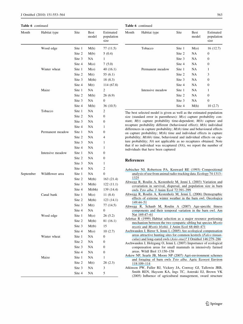
See Table 6.

Table 6 Population sizes of small mammals estimated with program

CAPTURE (Otis et al. 1978) recorded in May, July and September, in

eight habitat types and at four capture sites each

Month Habitat type Site Best

model

Estimated

population

size

May Wildflower area Site 1 M(o) 16 (3.7)

Site 2 M(o) 26 (5.2)

Site 3 M(o) 25 (6.5)

Site 4 M(o) 84 (22.7)

Canal bank Site 1 M(o) 18 (9.0)

Site 2 M(h) 23 (5.1)

Site 3 M(tb) 27 (0.0)

Site 4 NA 3

Wood edge Site 1 NA 1

Site 2 M(o) 36 (10.5)

Site 3 M(t) 23 (1.7)

Site 4 NA 0

Winter wheat Site 1 NA 1

Site 2 M(th) 14 (4.0)

Site 3 No model 3

Site 4 M(h) 14 (4.1)

Maize Site 1 NA 0

Site 2 NA 0

Site 3 NA 0

Site 4 NA 0

Tobacco Site 1 NA 0

Site 2 NA 0

Site 3 NA 0

Site 4 NA 0

Permanent meadow Site 1 NA 1

Site 2 NA 1

Site 3 NA 1

Site 4 NA 2

Intensive meadow Site 1 NA 1

Site 2 NA 0

Site 3 NA 0

Site 4 NA 0

July Wildflower area Site 1 M(o) 64 (10.4)

Site 2 M(t) 81 (5.8)

Site 3 M(th) 79 (7.7)

Site 4 M(t) 116 (86.0)

Canal bank Site 1 NA 1

Site 2 M(t) 74 (3.8)

Site 3 M(o) 28 (2.5)

Site 4 NA 2

562 J Ornithol (2010) 151:553–564

123

References

Aebischer NJ, Robertson PA, Kenward RE (1993) Compositional

analysis of use from animal radio-tracking data. Ecology 74:1313–

1325

Altwegg R, Roulin A, Kestenholz M, Jenni L (2003) Variation and

covariation in survival, dispersal, and population size in barn

owls Tyto alba. J Anim Ecol 72:391–399

Altwegg R, Roulin A, Kestenholz M, Jenni L (2006) Demographic

effects of extreme winter weather in the barn owl. Oecologica

149:44–51

Altwegg R, Schaub M, Roulin A (2007) Age-specific fitness

components and their temporal variation in the barn owl. Am

Nat 169:47–61

Arlettaz R (1999) Habitat selection as a major resource portioning

mechanism between the two sympatric sibling bat species Myotismyotis and Myotis blythii. J Anim Ecol 68:460–471

Aschwanden J, Birrer S, Jenni L (2005) Are ecological compensation

areas attractive hunting sites for common kestrels (Falco tinnun-culus) and long-eared owls (Asio otus)? J Ornithol 146:279–286

Aschwanden J, Holzgang O, Jenni L (2007) Importance of ecological

compensation areas for small mammals in intensively farmed

areas. Wildl Biol 13:150–158

Askew NP, Searle JB, Moore NP (2007) Agri-environment schemes

and foraging of barn owls Tyto alba. Agric Ecosyst Environ

118:109–114

Atkinson PW, Fuller RJ, Vickery JA, Conway GJ, Tallowin JRB,

Smith REN, Haysom KA, Ings TC, Asteraki EJ, Brown VK

(2005) Influence of agricultural management, sward structure

Table 6 continued

Month Habitat type Site Best

model

Estimated

population

size

Wood edge Site 1 M(h) 77 (11.5)

Site 2 M(b) 5 (0.4)

Site 3 NA 1

Site 4 M(o) 7 (5.0)

Winter wheat Site 1 M(o) 40 (16.1)

Site 2 M(t) 55 (6.1)

Site 3 M(th) 18 (8.3)

Site 4 M(t) 114 (67.8)

Maize Site 1 NA 2

Site 2 M(h) 26 (6.9)

Site 3 NA 0

Site 4 M(h) 36 (10.5)

Tobacco Site 1 NA 2

Site 2 NA 0

Site 3 NA 0

Site 4 NA 1

Permanent meadow Site 1 NA 0

Site 2 NA 4

Site 3 NA 1

Site 4 NA 1

Intensive meadow Site 1 NA 0

Site 2 NA 0

Site 3 NA 1

Site 4 NA 2

September Wildflower area Site 1 NA 0

Site 2 M(th) 163 (21.4)

Site 3 M(th) 122 (11.1)

Site 4 M(tbh) 139 (14.4)

Canal bank Site 1 M(o) 11 (8.4)

Site 2 M(th) 123 (14.1)

Site 3 M(t) 77 (14.5)

Site 4 NA 0

Wood edge Site 1 M(o) 26 (5.2)

Site 2 M(th) 81 (16.1)

Site 3 M(tb) 15

Site 4 M(o) 10 (2.7)

Winter wheat Site 1 NA 0

Site 2 NA 0

Site 3 NA 0

Site 4 NA 0

Maize Site 1 NA 1

Site 2 M(t) 28 (2.3)

Site 3 NA 3

Site 4 NA 5

Table 6 continued

Month Habitat type Site Best

model

Estimated

population

size

Tobacco Site 1 M(o) 16 (12.7)

Site 2 NA 0

Site 3 NA 0

Site 4 NA 0

Permanent meadow Site 1 NA 1

Site 2 NA 3

Site 3 NA 0

Site 4 NA 0

Intensive meadow Site 1 NA 1

Site 2 NA 0

Site 3 NA 0

Site 4 M(h) 10 (2.7)

The best selected model is given as well as the estimated population

size (standard error in parentheses): M(o) capture probability con-

stant; M(t) capture probability time-dependent; M(b) capture and

recapture probability different (behavioural effect); M(h) individual

differences in capture probability; M(tb) time and behavioural effects

on capture probability; M(th) time and individual effects in capture

probability; M(thb) time, behavioural and individual effects on cap-

ture probability; NA not applicable as no recaptures obtained. Note

that if no individual was recaptured (NA), we report the number of

individuals that have been captured

J Ornithol (2010) 151:553–564 563

123

and food resources on grassland field use by birds in lowland

England. J Appl Ecol 42:932–942

Baker JA, Brooks RJ (1981) Distribution patterns of raptors in

relation to density of meadow voles. Condor 83:42–47

Bechard MJ (1982) Effect of vegetative cover on foraging site by

Swainson’s hawk. Condor 84:153–159

Benton TG, Vickery JA, Wilson JD (2003) Farmland biodiversity: is

habitat heterogeneity the key? Trends Ecol Evol 18:182–188

Birrer S, Spiess M, Herzog F, Jenny M, Kohli L, Lugrin B (2007) The

Swiss agri-environment scheme promotes farmland birds: but

only moderately. J Ornithol 148:S295–S303

Briner T, Nentwig W, Airoldi J-P (2005) Habitat quality of

wildflower strips for common voles (Microtus arvalis) and

its relevance for agriculture. Agric Ecosyst Environ 105:173–

179

Britschgi A, Spaar R, Arlettaz R (2006) Impact of grassland farming

intensification on the breeding ecology of an indicator insectiv-

orous passerine, the Whinchat Saxicola rubetra: lessons for

overall Alpine meadowland management. Biol Conserv 130:193–

205

Buner F (1998) Habitat use of wintering Kestrels (Falco tinnunculus)

in relation to perch availability, vole abundance and spatial

distribution. Diploma Thesis, University of Basel, Swiss Orni-

thological Institute Sempach

Burkhardt M, Schmid H (2001) Vogel der Schweiz. Schweizerische

Vogelwarte, Sempach

Dickman CR, Predavec M, Lynam AJ (1991) Differential predation of

size and sex classes of mice by the barn owl, Tyto alba. Oikos

62:67–76

Donald PF, Green RE, Heath MF (2001) Agricultural intensification

and the collapse of Europe’s farmland bird populations. Proc

R Soc Lond B 268:25–29

Estabrook CB, Estabrook GF (1989) Actus: a solution to the problem

of small samples in the analysis of two-way contingency tables.

Hist Methods 82:5–8

Gilg O, Hanski I, Sittler B (2003) Cyclic dynamics in a simple

vertebrate predator-prey community. Science 302:866–868

Gilg O, Sittler B, Sabard B, Hurstel A, Sane R, Delattre P, Hanski I

(2006) Functional and numerical responses of four lemming

predators in higharctic Greenland. Oikos 113:193–216

Hansson L, Henttonen H (1988) Rodent dynamics as community

processes. Trends Ecol Evol 3:195–200

Jacob J, Hempel N (2003) Effects of farming practices on spatial

behaviour of common voles. J Ethol 21:45–50

Kleijn D, Sutherland WJ (2003) How effective are European agri-

environmental schemes in conserving and promoting biodiver-

sity? J Appl Ecol 40:947–969

Kleijn D, Berendse F, Smit R, Gillissen N (2001) Agri-environment

schemes do not effectively protect biodiversity in Dutch

agricultural landscapes. Nature 413:723–725

Kleijn D, Baquero RA, Clough Y, Diaz M, De Esteban J, Fernandez

F, Gabriel D, Herzog F, Holzschuh A, Johl R, Knowp E, Kruess

A, Marshall EJP, Steffan-Dewenter I, Tscharntke T, Verhulst J,

West TM, Yela JL (2006) Mixed biodiversity benefits of agri-

environment schemes in five European countries. Ecol Lett

9:243–254

Knop E, Kleijn D, Herzog F, Schmid B (2006) Effectiveness of the

Swiss agri-environment scheme in promoting biodiversity.

J Appl Ecol 43:120–127

Korpimaki E (1994) Rapid or delayed tracking of multi-annual vole

cycles by avian predators? J Anim Ecol 63:619–628

Korpimaki E, Norrdahl K (1991) Numerical and functional responses

of kestrels, short-eared owls, and long-eared owls to vole

densities. Ecology 72:814–826

MacDonald DW, Tattersall FH, Service KM, Firbank LG, Feber RE

(2007) Mammals, agri-environment schemes and set-aside—

what are the putative benefits? Mammal Rev 37:259–277

Mebs T, Scherzinger W (2000) Die Eulen Europas. Kosmos, Stuttgart

Mohr CO (1947) Table of equivalent populations of North American

small mammals. Am Midl Nat 37:223–249

Nentwig W (2000) Streifenformige okologische Ausgleichsflachen in

der Kulturlandschaft: Ackerkrautstreifen, Buntbrache, Feldran-

der. Agrarokologie, Bern, p 293

Otis DL, Burnham KP, White GC, Anderson DR (1978) Statistical

inference from capture data on closed animal populations. Wildl

Monogr 62:1–135

Palma L, Beja P, Pais M, Cancela da Fonseca L (2006) Why do

raptors take domestic prey? the case of Bonelli’s eagles and

pigeons. J Appl Ecol 43:1075–1086

Reid K, Croxall JP (2001) Environmental response of upper trophic-

level predators reveals a system change in an Antarctic marine

ecosystem. Proc R Soc Lond B 268:377–384

Reid N, McDonald RA, Montgomery WI (2007) Mammals and agri-

environment schemes: hare haven or pest paradise? J Appl Ecol

44:1200–1208

Revaz E, Schaub M, Arlettaz R (2008) Foraging ecology and

reproductive biology of the Stonechat Saxicola torquata: com-

parison between a revitalized, intensively cultivated and a

historical, traditionally cultivated agro-ecosystem. J Ornithol

149:301–312

Roulin A (1999) Natural and experimental nest-switching in Barn

Owl Tyto alba fledglings. Ardea 87:237–246

Roulin A (2002) Tyto alba Barn Owl. BWP Update 4(2):115–138

Roulin A, Riols C, Dijkstra C, Ducrest A-L (2001) Female- and male-

specific signals of quality in the barn owl. J Evol Biol 14:255–267

Schmid B (2002) The species richness-productivity controversy.

Trends Ecol Evol 17:113–114

Schmid H, Luder R, Naef-Daenzer B, Graf R, Zbinden N (1998)

Schweizer Brutvogelatlas. Verbreitung der Vogel in der Schweiz

und im Furstentum Liechtenstein 1993–1996. Schweizerische

Vogelwarte, Seampach

Schweizer Eidgenossenschaft (1998) Verordnungen uber die Direkt-

zahlungen an die Landwirtschaft 910.13, 3. Titel, 1. Kapitel, 16–24

Shore RF, Meek WR, Sparks TH, Pywell RF, Nowakowski M (2005)

Will Environmental Stewarship enhance small mammal abundance

on intensively managed farmland? Mammal Rev 35:277–284

Snow DW, Perrins CM (1998) The birds of the western palearctic,

concise edition, vol I. Oxford University Press, Oxford, pp 886–

888

Tattersall FH, Macdonald DW, Manley WJ, Gates S, Feber R, Hart BJ

(1997) Small mammals on one-year set-aside. Acta Theriol

42:329–334

Tattersall FH, Avundo AE, Manley WJ, Hart BJ, Macdonald DW

(2000) Managing set-aside for field voles (Microtus agrestis).

Biol Conserv 96:123–128

Taylor IR (1994) Barn owls: predator-prey relationships. Cambridge

University Press, Cambridge

Tew TE, Macdonald DW (1993) The effects of harvest on arable

wood mice Apodemus sylvaticus. Biol Conserv 65:279–283

Veit RR, Silverman ED, Everson I (1993) Aggregation patterns of

pelagic predators and their principal prey, antarctic krill, near

South Georgia. J Anim Ecol 62:551–564

Wakeley JS (1978) Factors affecting the use of hunting sites by

Ferruginous hawks. Condor 80:316–326

White GC, Garrot RA (1990) Analysis of wildlife radiotracking data.

Academic, San Diego, p 383

Whitthingham MJ (2007) Will agri-environment schemes deliver

substantial biodiversity gain, and if not why? J Appl Ecol 44:1–5

564 J Ornithol (2010) 151:553–564

123