
Impact of the cycle-to-cycle variation of an internal combustion ...
167
ARISTOTLE UNIVERSITY OF THESSALONIKI FACULTY OF ENGINEERING MECHANICAL ENGINEERING DEPARTMENT LABORATORY OF APPLIED THERMODYNAMICS Impact of the cycle-to-cycle variation of an internal combustion engine to gaseous pollutants emissions Apostolos Karvountzis-Kontakiotis Dipl. Mechanical Engineer Thessaloniki, August 2015
-
Upload
khangminh22 -
Category
Documents
-
view
0 -
download
0
Transcript of Impact of the cycle-to-cycle variation of an internal combustion ...

ARISTOTLE UNIVERSITY OF THESSALONIKI
FACULTY OF ENGINEERING
MECHANICAL ENGINEERING DEPARTMENT
LABORATORY OF APPLIED THERMODYNAMICS
Impact of the cycle-to-cycle variation of an
internal combustion engine to gaseous
pollutants emissions
Apostolos Karvountzis-KontakiotisDipl. Mechanical Engineer
Thessaloniki, August 2015


Apostolis Karvountzis-Kontakiotis
Impact of the cycle-to-cycle variation of an
internal combustion engine to gaseous
pollutants emissions
2015
Supervisor: Assistant Professor L. Ntziachristos
Members of Examination Committee:
Full Professor Z. Samaras
Associate Professor G. Koltsakis
Assistant Professor L. Ntziachristos
This thesis is submitted in partial fullfillment of the requirements for the degree of
Doctor of Engineering
c©Aristotle University, 2015. All rights reserved. No part of this publication my be
reproduced without written permission of the copyright holder.


This work is dedicated to
all the members of my family,
and to my only one Paschalena.


Acknowledgements
First of all, I would like to thank my supervisor Prof. Leonidas Ntziachristos
for his time, ideas and contribution on this PhD thesis. Our long discussions
instigated many of the themes presented here.
I would like to express my gratitude to the director of the laboratory (LAT)
Prof. Zissis Samaras for his trust and his support, particularly on the experi-
mental part of this project. I also wish to thank Prof. Grigoris Koltsakis for
teaching me internal combustion engines and aftertreatment modeling and for
his confidence in me during our cooperation with automotive industry. I also
wish to extend my gratitude to all the teachers that inspired and shaped me
as an engineer and person throughout my studies.
Special thanks to the 7th European Framework ”LESSCCV” for the financial
support. The discussions and ideas of the partners of this project were source
of inspiration to me. I am especially thankful to Prof. Ananias Tomboulides
for his advice and support during the LESSCCV project. I also want to
thank Prof. Anestis Kalfas who inspires me to work in the research area and
motivates me to publish my research work.
Special thanks to all the staff of the Laboratory of Applied Thermodynamics
(LAT) for their valuable services and support. Thanks are due to my colleague
and friend Dr. Athanasios Dimaratos for our interesting discussions on the
topics of internal combustion engines and their measurement techniques as
well as for his great contribution on the experimental part of this thesis. I owe
a lot to Dr. Mark Peckham, Director at Cambustion Ltd, for his technical
support and his grant of the NDIR500 CO/CO2 analyzer. Special thanks to
Dr. Costas Michos for the stimulating discussions and his advice on emission
modeling. Thanks are due to Dr. Elias Vouitsis for his fruitful and interesting
discussions on engine design and emissions trends. The assistance of the Aris-
totle Racing Team on the engine measurements is gratefully acknowledged.
Many thanks to my colleagues Dimitrios, Thomas, Elias, Christos and my
tolerant officemate Dora, for sharing our thoughts and worries, and for making
this personal research journey a bit less lonely. I also want to thank my younger
colleagues and wish them good luck to their new start. Thanks are also due
to all staff of Exothermia S.A for their support and assistance during my
collaboration with Exothermia S.A.

I had the chance to work with many MSc students and gain through them
much experience and knowledge. Many thanks to George Giannakopoulos,
Orestis Mpouras, Thomas Souliotis, Lazaros Kefalidis, Nikos Zigkopis and
Pavlos Evagelidis.
I am deeply grateful to my old friends and classmates Teo, Panos, Christos,
Vasilis, Thanos and Orestis for giving me so many nice memories all these
years.
Last but not least, I would like to thank my parents, my sister, my uncle
and his family and my patient Paschalena, for all their help, support and
encouragement all these years.

Abstract
This work focuses on the computational and experimental investigation of cyclic emis-
sion variability, particularly on NOx emissions. In this context, this thesis contributes
towards clarifying the following gray aspects of future engine development:
• the development and validation of a detailed chemistry emission model for the ki-
netically prediction of the gaseous pollutants emissions
• the experimental investigation of cyclic emission variability, using fast response an-
alyzers and the correlation with combustion characteristics
• the utilization of the detailed chemistry model for the improved prediction of emis-
sion variability under engine homogeneous conditions
The first and third objectives requires the development of an advance emission model
that presents improved accuracy compared to conventional emission approaches. This is
performed with the utilization of a detailed chemical reaction scheme, assuming that each
burned zone is a well-stirred reactor. Compared to existing emission models, the model
is characterized by the absence of both the use of chemical equilibrium and any tuning
parameter or calibration factor. The model presents computational time in the same order
of magnitude of conventional emission models. As this model presents improved accuracy
of NO emissions and reduced computational time, it can contribute to the design of more
efficient engines.
Regarding the second objective, in this study is experimentally explained how com-
bustion variability affects emissions variability. Although the impact of cyclic combustion
variability has been extensively investigated in the past, only very little concern has been
paid on cyclic emission variability. This experimental study presents the impact of various
engine parameters, such as engine load, equivalence ratio, and ignition timing on cyclic
emission variability.
i

ii

Contents
Abstract i
Table of Contents ii
List of Figures vi
List of Tables x
Nomenclature xi
1 Introduction 1
1.1 Research scope . . . . . . . . . . . . . . . . . . . . . . . . . . . . . . . . . 1
1.2 Fundamentals of spark ignition engines . . . . . . . . . . . . . . . . . . . . 2
1.2.1 Engine operation . . . . . . . . . . . . . . . . . . . . . . . . . . . . 3
1.2.2 Mixture formation . . . . . . . . . . . . . . . . . . . . . . . . . . . 3
1.2.3 The ignition process . . . . . . . . . . . . . . . . . . . . . . . . . . 3
1.2.4 The combustion process . . . . . . . . . . . . . . . . . . . . . . . . 4
1.2.5 Pollutant formation . . . . . . . . . . . . . . . . . . . . . . . . . . . 5
1.3 Thesis aim and objectives . . . . . . . . . . . . . . . . . . . . . . . . . . . 6
1.4 Thesis structure . . . . . . . . . . . . . . . . . . . . . . . . . . . . . . . . . 7
2 Literature Review 9
2.1 Introduction . . . . . . . . . . . . . . . . . . . . . . . . . . . . . . . . . . . 9
2.2 Pollutants Formation Modeling . . . . . . . . . . . . . . . . . . . . . . . . 10
2.2.1 NOx Emissions . . . . . . . . . . . . . . . . . . . . . . . . . . . . . 11
2.2.2 CO Emissions . . . . . . . . . . . . . . . . . . . . . . . . . . . . . . 14
2.2.3 HC Emissions . . . . . . . . . . . . . . . . . . . . . . . . . . . . . . 15
2.2.4 Pollutants Formation Models . . . . . . . . . . . . . . . . . . . . . 15
2.2.4.1 Simplified Kinetic Models . . . . . . . . . . . . . . . . . . 16
2.2.4.2 Detailed Kinetic Models . . . . . . . . . . . . . . . . . . . 17
2.3 Cycle-to-Cycle Variability . . . . . . . . . . . . . . . . . . . . . . . . . . . 18
iii
2.3.1 The Nature of Cyclic Variation . . . . . . . . . . . . . . . . . . . . 19
2.3.2 Origins of Cyclic Variation . . . . . . . . . . . . . . . . . . . . . . . 20
2.3.3 Measures of Cyclic Variation . . . . . . . . . . . . . . . . . . . . . . 21
2.3.4 Effects of Engine Variables on Cyclic Variability . . . . . . . . . . . 24
2.3.4.1 Equivalence Ratio . . . . . . . . . . . . . . . . . . . . . . 24
2.3.4.2 Fuel Type . . . . . . . . . . . . . . . . . . . . . . . . . . . 25
2.3.4.3 Combustion Chamber Geometry . . . . . . . . . . . . . . 26
2.3.4.4 Compression Ratio . . . . . . . . . . . . . . . . . . . . . . 27
2.4 Cyclic Emissions Variability . . . . . . . . . . . . . . . . . . . . . . . . . . 28
2.5 Summary and Conclusions . . . . . . . . . . . . . . . . . . . . . . . . . . . 29
3 Proposed Emissions Model 31
3.1 Introduction . . . . . . . . . . . . . . . . . . . . . . . . . . . . . . . . . . . 31
3.2 Emission Model . . . . . . . . . . . . . . . . . . . . . . . . . . . . . . . . . 32
3.2.1 Mass Balance . . . . . . . . . . . . . . . . . . . . . . . . . . . . . . 33
3.2.1.1 New Burned Mass . . . . . . . . . . . . . . . . . . . . . . 33
3.2.1.2 Inlet/Outlet Concentrations . . . . . . . . . . . . . . . . . 35
3.2.2 Energy Balance . . . . . . . . . . . . . . . . . . . . . . . . . . . . . 36
3.3 Validation Data . . . . . . . . . . . . . . . . . . . . . . . . . . . . . . . . . 36
3.4 Modeling Approach . . . . . . . . . . . . . . . . . . . . . . . . . . . . . . . 37
3.4.1 Engine Model . . . . . . . . . . . . . . . . . . . . . . . . . . . . . . 38
3.4.2 Modeling Assumptions . . . . . . . . . . . . . . . . . . . . . . . . . 38
3.4.3 Coupling Simulation . . . . . . . . . . . . . . . . . . . . . . . . . . 39
3.5 Emission Model Validation . . . . . . . . . . . . . . . . . . . . . . . . . . . 39
3.5.1 Mean Cycle Validation . . . . . . . . . . . . . . . . . . . . . . . . . 39
3.5.2 Cycle-to-Cycle NO Variation . . . . . . . . . . . . . . . . . . . . . . 42
3.5.2.1 Contribution of Prompt Mechanism on the CCV of NO
Emissions . . . . . . . . . . . . . . . . . . . . . . . . . . . 45
3.5.3 Deviation Between Mean Cycle Values and Mean CCV Values . . . 47
3.6 Conclusions . . . . . . . . . . . . . . . . . . . . . . . . . . . . . . . . . . . 49
4 Experimental Investigation of Cyclic Emissions Variability 51
4.1 Introduction . . . . . . . . . . . . . . . . . . . . . . . . . . . . . . . . . . . 51
4.2 Experimental Set up . . . . . . . . . . . . . . . . . . . . . . . . . . . . . . 52
4.2.1 Engine Test Bed . . . . . . . . . . . . . . . . . . . . . . . . . . . . 52
4.2.2 Experimental Configuration . . . . . . . . . . . . . . . . . . . . . . 53
4.2.3 Measurement Protocol . . . . . . . . . . . . . . . . . . . . . . . . . 54
4.3 Measurements . . . . . . . . . . . . . . . . . . . . . . . . . . . . . . . . . . 54
4.3.1 In cylinder pressure . . . . . . . . . . . . . . . . . . . . . . . . . . . 54
4.3.2 Engine and Cylinder Emissions . . . . . . . . . . . . . . . . . . . . 56
iv

4.3.3 Exhaust Temperature . . . . . . . . . . . . . . . . . . . . . . . . . . 59
4.3.4 Data Acquisition Card . . . . . . . . . . . . . . . . . . . . . . . . . 60
4.3.5 Engine Control Unit . . . . . . . . . . . . . . . . . . . . . . . . . . 60
4.4 Data Processing . . . . . . . . . . . . . . . . . . . . . . . . . . . . . . . . . 61
4.4.1 Combustion Analysis . . . . . . . . . . . . . . . . . . . . . . . . . . 61
4.4.2 Performance Analysis . . . . . . . . . . . . . . . . . . . . . . . . . . 63
4.4.3 Emissions Analysis . . . . . . . . . . . . . . . . . . . . . . . . . . . 63
4.4.4 Cyclic Variability . . . . . . . . . . . . . . . . . . . . . . . . . . . . 64
4.5 Results . . . . . . . . . . . . . . . . . . . . . . . . . . . . . . . . . . . . . . 65
4.5.1 Impact of Engine Load on Variability . . . . . . . . . . . . . . . . . 67
4.5.2 Impact of Stoichiometry on Variability . . . . . . . . . . . . . . . . 72
4.5.3 Impact of Ignition Timing on Variability . . . . . . . . . . . . . . . 79
4.6 Conclusions . . . . . . . . . . . . . . . . . . . . . . . . . . . . . . . . . . . 87
5 Emission Model Validation and Application for CCV Prediction 89
5.1 Introduction . . . . . . . . . . . . . . . . . . . . . . . . . . . . . . . . . . . 89
5.2 Modeling Approach . . . . . . . . . . . . . . . . . . . . . . . . . . . . . . . 90
5.2.1 Two Zone Combustion Analysis . . . . . . . . . . . . . . . . . . . . 90
5.2.1.1 Cylinder Model . . . . . . . . . . . . . . . . . . . . . . . . 90
5.2.1.2 Integration Flow . . . . . . . . . . . . . . . . . . . . . . . 91
5.2.1.3 Error Formula . . . . . . . . . . . . . . . . . . . . . . . . 93
5.2.2 Emissions Modeling . . . . . . . . . . . . . . . . . . . . . . . . . . . 94
5.2.2.1 Proposed Modeling . . . . . . . . . . . . . . . . . . . . . . 94
5.2.2.2 Simplified Modeling . . . . . . . . . . . . . . . . . . . . . 94
5.3 Cycle Simulation . . . . . . . . . . . . . . . . . . . . . . . . . . . . . . . . 94
5.4 Mean Cycle Emissions Prediction . . . . . . . . . . . . . . . . . . . . . . . 96
5.4.1 Engine Load . . . . . . . . . . . . . . . . . . . . . . . . . . . . . . . 96
5.4.2 Mixture Stoichiometry . . . . . . . . . . . . . . . . . . . . . . . . . 98
5.4.3 Ignition Timing . . . . . . . . . . . . . . . . . . . . . . . . . . . . . 101
5.5 Sensitivity Analysis of the Emission Model . . . . . . . . . . . . . . . . . . 102
5.6 Application of the model to predict CCV . . . . . . . . . . . . . . . . . . . 104
5.7 Cycle to Cycle Emission Prediction . . . . . . . . . . . . . . . . . . . . . . 106
5.7.1 Engine Load . . . . . . . . . . . . . . . . . . . . . . . . . . . . . . . 107
5.7.2 Mixture Stoichiometry . . . . . . . . . . . . . . . . . . . . . . . . . 110
5.7.3 Ignition Timing . . . . . . . . . . . . . . . . . . . . . . . . . . . . . 113
5.8 Summary and Conclusions . . . . . . . . . . . . . . . . . . . . . . . . . . . 116
v

6 Conclusions & Future Work 119
6.1 Experimental Work . . . . . . . . . . . . . . . . . . . . . . . . . . . . . . . 119
6.2 Emissions Modeling . . . . . . . . . . . . . . . . . . . . . . . . . . . . . . . 120
6.3 Novelty . . . . . . . . . . . . . . . . . . . . . . . . . . . . . . . . . . . . . 123
6.4 Future Work . . . . . . . . . . . . . . . . . . . . . . . . . . . . . . . . . . . 125
A A FORTRAN Program for Predicting Homogeneous Gas Phase Chem-
ical Kinetics 127
A.1 Introduction . . . . . . . . . . . . . . . . . . . . . . . . . . . . . . . . . . . 127
A.2 Governing Equations . . . . . . . . . . . . . . . . . . . . . . . . . . . . . . 128
References 132
vi

List of Figures
2.1 Spark ignition engine emissions for different air/fuel ratios [16]. . . . . . . . 10
2.2 Cross-sections of combustion chambers investigated in Young [55] with var-
ious spark locations. . . . . . . . . . . . . . . . . . . . . . . . . . . . . . . 27
3.1 Schematic of the two zone detailed chemistry emission model. . . . . . . . 32
3.2 Schematic of the Rover K4 model developed in BOOST. . . . . . . . . . . 38
3.3 Comparison of measured and simulated NO molar fractions for stoichio-
metric combustion (λ=1.0). Results without prompt mechanism are also
presented. . . . . . . . . . . . . . . . . . . . . . . . . . . . . . . . . . . . . 41
3.4 Comparison of measured and simulated NO molar fractions for lean (λ=1.5)
operating engine conditions. . . . . . . . . . . . . . . . . . . . . . . . . . . 42
3.5 Impact of slight stoichiometry variation on NO formation. . . . . . . . . . 43
3.6 CCV of in-cylinder pressure and temperature evolution, which results on
the distribution of imep and NO emissions (P1015 point). . . . . . . . . . . 44
3.7 CCV of in-cylinder pressure and temperature evolution, which results on
the distribution of imep and NO emissions (W1030 point). . . . . . . . . . 46
3.8 CCV NO distribution w/o the prompt mechanism. . . . . . . . . . . . . . 48
4.1 Schematic of the experimental configuration . . . . . . . . . . . . . . . . . 53
4.2 Sample of processing pressure raw data at 4000 rpm, 50% throttle position
and rich operating conditions (λ=0.93). . . . . . . . . . . . . . . . . . . . . 56
4.3 Photo from the experimental configuration regarding the positioning of the
probes for the cylinder and engine exhaust emissions sampling. . . . . . . . 57
4.4 The Cambustion fast response analyzers . . . . . . . . . . . . . . . . . . . 59
4.5 The LabVIEW interface and the data acquisition card. . . . . . . . . . . . 61
4.6 Typical NO recording in the exhaust with reference to the cylinder pressure. 64
4.7 IMEP and emissions distributions at 4000 rpm, 80% open throttle position,
stoichiometric mixture and MBT ignition timing. . . . . . . . . . . . . . . 65
vii

4.8 Pressure variability at 4000 rpm, 80% open throttle position, stoichiometric
mixture and MBT ignition timing. Mean pressure curve, maximum and
minimum gross heat release rates for the 150 consecutive cycles are also
illustrated. . . . . . . . . . . . . . . . . . . . . . . . . . . . . . . . . . . . 66
4.9 Mean pressure and gross heat release traces for stoichiometric conditions,
4000 rpm, identical spark timing and various throttle positions. . . . . . . 67
4.10 Relationship between IMEP and ϑ5% at 4000 rpm, stoichiometric mixture,
identical ignition timing and various throttle positions (TP: 20% and TP:
80%). . . . . . . . . . . . . . . . . . . . . . . . . . . . . . . . . . . . . . . . 69
4.11 Relationship between IMEP and NO at 4000 rpm, stoichiometric mixture,
identical ignition timing and various throttle positions. . . . . . . . . . . . 70
4.12 Relationship between Pmax and NO concentration at 4000 rpm, stoichio-
metric mixture, identical ignition timing and various throttle positions. . . 71
4.13 Mean pressure and gross heat release traces for rich, stoichiometric and
lean mixture, 6000 rpm, 80% TP, and identical spark timing. . . . . . . . . 72
4.14 Relationship between ϑ5% and mixture stoichiometry at 6000 rpm, 80% TP
and identical ignition timing. . . . . . . . . . . . . . . . . . . . . . . . . . . 73
4.15 Relationship between IMEP and mixture stoichiometry at 4000 rpm, 80
per cent throttle position and constant ignition timing. . . . . . . . . . . . 75
4.16 Relationship between λ and NO concentration at 6000 rpm, 80% throttle
position and identical spark ignition timing. . . . . . . . . . . . . . . . . . 76
4.17 Relationship between NO and early flame kernel development (ϑ5%) at
4000 rpm, 80% TP and identical ignition timing. . . . . . . . . . . . . . . . 77
4.18 Relationships between λ and carbon monoxide and carbon dioxide concen-
trations at 6000 rpm, 80% TP and identical spark ignition timing. . . . . . 78
4.19 Mean pressure and gross heat release traces for rich conditions (λ=0.93),
4000 rpm, 80% throttle position and various spark timings. . . . . . . . . . 80
4.20 Relationship between IMEP and maximum cylinder pressure at 4000 rpm,
80% TP and λ=0.94, for different ignition timings. . . . . . . . . . . . . . 81
4.21 Relationship between ignition delay and maximum cylinder pressure at
4000 rpm, at 4000 rpm, 80% TP and λ=0.94, for different ignition timings. 82
4.22 Relationship between maximum cylinder pressure and crank angle at which
maximum cylinder pressure occurs for different ignition timings at 4000
rpm, 80% TP and λ=0.94. . . . . . . . . . . . . . . . . . . . . . . . . . . . 83
4.23 Relationship between NO formed and crank angle at which maximum cylin-
der pressure occurs for different ignition timings at 4000 rpm, 80% TP and
λ=0.94. . . . . . . . . . . . . . . . . . . . . . . . . . . . . . . . . . . . . . 84
viii

4.24 Relationship between NO formed and crank angle at which maximum cylin-
der pressure occurs for different ignition timings at 4000 rpm, 80% TP and
λ=0.94. . . . . . . . . . . . . . . . . . . . . . . . . . . . . . . . . . . . . . 85
5.1 Flowchart of the two zone heat release model. . . . . . . . . . . . . . . . . 92
5.2 Evolution of cylinder pressure, zone temperatures, NO and CO concentra-
tions at 4000 rpm, 80% throttle position, stoichiometric mixture and MBT.
(a) measured cylinder pressure of the closed thermodynamic cycle, (b) the
calculated gas temperature (Tg), the burned zone temperature (Tb) and
the unburned temperature (Tun), (c) calculated NO concentrations under
conditions of equilibrium/kinetics control, (d) CO concentrations under
conditions of equilibrium/kinetics control. . . . . . . . . . . . . . . . . . . 95
5.3 Effect of engine load on NO and CO formation for stoichiometric mixture
and various engine speed conditions: (left column) NO simulation, (right
column) CO simulation. . . . . . . . . . . . . . . . . . . . . . . . . . . . . 97
5.4 Effect of mixture lambda on NO and CO formation for 80% throttle po-
sition and various engine speed conditions: (left column) NO simulation,
(right column) CO simulation. . . . . . . . . . . . . . . . . . . . . . . . . . 99
5.5 Effect of ignition timing on NO and CO formation at 4000 rpm, 80% throt-
tle position and stoichiometric conditions: (left column) NO simulation,
(right column) CO simulation. . . . . . . . . . . . . . . . . . . . . . . . . . 101
5.6 Effect of ignition timing on NO and CO formation at 6000 rpm, 20% throt-
tle position and stoichiometric conditions: (left column) NO simulation,
(right column) CO simulation. . . . . . . . . . . . . . . . . . . . . . . . . . 102
5.7 Impact of wall temperature on pollutants formation using the detailed
chemistry model. . . . . . . . . . . . . . . . . . . . . . . . . . . . . . . . . 103
5.8 Impact of residual gas fraction on pollutants formation using the proposed
detailed chemistry model. . . . . . . . . . . . . . . . . . . . . . . . . . . . 104
5.9 Evolution of maximum and minimum IMEP cycle in relationship to crank
angle: (a) measured cylinder pressure, (b) calculated heat release and
burned zone temperature, (c) NO formation and (d) CO formation. . . . . 105
5.10 Prediction of cyclic NO variability for 20% (left column) and 80% (right
column) throttle position. (a) Relationship between NO and measured
cylinder pressure, (b) NO return map, (c) Relationship between measured
and calculated NO. . . . . . . . . . . . . . . . . . . . . . . . . . . . . . . . 108
5.11 Prediction of cyclic CO variability for 20% (left column) and 80% (right
column) throttle position. (a) CO return map, (b) Relationship between
measured and calculated CO. . . . . . . . . . . . . . . . . . . . . . . . . . 109
ix

5.12 Prediction of cyclic NO variability for rich (left column) and lean (right
column) mixture composition. (a) Relationship between NO and measured
cylinder pressure, (b) NO return map, (c) Relationship between measured
and calculated NO. . . . . . . . . . . . . . . . . . . . . . . . . . . . . . . . 111
5.13 Prediction of cyclic CO variability for rich (left column) and lean (right col-
umn) mixture composition. (a) CO return map, (b) Relationship between
measured and calculated CO. . . . . . . . . . . . . . . . . . . . . . . . . . 112
5.14 Prediction of cyclic NO variability at 4000 rpm, stoichiometric mixture,
80% TP, 52o[CA] BTDC ignition timing (first row), 48o[CA] BTDC ignition
timing (second row) and 42o[CA] BTDC ignition timing (third row). Left
column: NO return map, Right column: Relationship between measured
and calculated NO. . . . . . . . . . . . . . . . . . . . . . . . . . . . . . . . 114
5.15 Prediction of cyclic CO variability at 4000 rpm, stoichiometric mixture,
80% TP, 52o[CA] BTDC ignition timing (first row), 48o[CA] BTDC ignition
timing (second row) and 42o[CA] BTDC ignition timing (third row). Left
column: CO return map, Right column: Relationship between measured
and calculated CO. . . . . . . . . . . . . . . . . . . . . . . . . . . . . . . . 115
x

List of Tables
2.1 Speed coefficients for the forward reaction of the Zeldovich mechanism [16] 12
3.1 New burned mass composition based on λ . . . . . . . . . . . . . . . . . . 34
3.2 Rover K4 engine characteristics . . . . . . . . . . . . . . . . . . . . . . . . 37
3.3 Validation of the thermodynamic model using BOOST. . . . . . . . . . . . 40
3.4 Comparison of COV values for imep and NO with and without the prompt
mechanism. . . . . . . . . . . . . . . . . . . . . . . . . . . . . . . . . . . . 47
3.5 Comparison of mean cycle values (MC) and mean CCV values for imep
and NO with and without the prompt mechanism. . . . . . . . . . . . . . . 47
4.1 Honda CBR600 engine characteristics . . . . . . . . . . . . . . . . . . . . . 52
4.2 Experimental engine test conditions. . . . . . . . . . . . . . . . . . . . . . 54
4.3 Specifications of the cylinder pressure experimental equipment . . . . . . . 55
4.4 Specifications of the emission gas analyzers and sensors. . . . . . . . . . . . 57
4.5 Mean and COV experimental data for two different throttle positions at
4000 rpm, identical ignition timing (48o [CA] BTDC) and stoichiometric
operating conditions (λ=0.99). . . . . . . . . . . . . . . . . . . . . . . . . . 68
4.6 Mean and COV experimental data for two different throttle positions at
6000 rpm, identical ignition timing (41o [CA] BTDC) and stoichiometric
operating conditions (λ=1.0). . . . . . . . . . . . . . . . . . . . . . . . . . 68
4.7 Mean and COV experimental data for various mixture lambda operating
conditions at 4000 rpm, 80 % throttle position and identical ignition timing
(48o [CA] BTDC). . . . . . . . . . . . . . . . . . . . . . . . . . . . . . . . 74
4.8 Mean and COV experimental data for various mixture lambda operating
conditions at 6000 rpm, 80 % throttle position and identical ignition timing
(41o [CA] BTDC). . . . . . . . . . . . . . . . . . . . . . . . . . . . . . . . 74
4.9 Mean and COV experimental data for various spark ignition timings at
4000 rpm, 80% throttle position and rich operating conditions (λ=0.94). . 80
4.10 Mean and COV experimental data for various spark ignition timings at
6000 rpm, 20% throttle position and rich operating conditions (λ=0.93). . 86
xi

xii

Nomenclature
Roman Symbols
Acyl cylinder wet area [m2]
aht heat transfer coefficient [-]
bht heat transfer coefficient [-]
εht radiation coefficient [-]
xb burn rate [-]
xi species mole fraction [-]
ycyl cylinder position [m]
yi species mass fraction [-]
Greek Symbols
α the carbon moles of the fuel molecular formula
β the hydrogen moles of the fuel molecular formula
δ the nitrogen moles of the fuel molecular formula
ε the stoichiometric fuel/air molar ratio
γ the oxygen moles of the fuel molecular formula
λ mixture lambda
φ equivalence ratio
σ Stefan-Boltzmann constant [W/m2K]
ϑ crank angle [degrees]
xiii

Subscripts
b burned
bb blowby
cyl cylinder
f flame
ht heat transfer
j number of elements
k number of species
L Loss
mix mixture
u unburned
w wall
Acronyms
A wet area [m2]
CCV Cyclic Combustion Variability
CD Combustion Duration
CEV Cyclic Emissions Variability
CO Carbon Monoxide
CO2 Carbon Dioxide
COV Coefficient Of Variation
D Piston Bore [m]
EOC End of Combustion
EVO Exhaust Valve Open
H2O Steam
xiv

HC Unburned hydrocarbons
ICEs Internal Combustion Engines
IMEP Indicated Mean Effective Pressure
IVC Intake Valve Close
LDVs Light Duty Vehicles
MBT Maximum Breaking Torque
MFB Mass Fraction Burned
MW Molecular mass
N2 Nitrogen
NO Nitric Oxide
NO2 Nitrogen Dioxide
NOx Nitrogen Oxides
O2 Oxygen
PFI Port Fuel Injection
PM Particulate Matter
PMEP Pumping Mean Effective Pressure
P Pressure [Pa]
RON Research Octane Number
SI Spark Ignition
SOI Start Of Ignition
SUVs Sport Utility Vehicles
TDC Top Dead Center
T Temperature [K]
TWC Three Way Catalyst
WGS Water Gas Shift reaction
WOT Wide Open Throttle
xv

Chapter 1
Introduction
1.1 Research scope
Transportation is responsible for approximately one third of global CO2 emissions due
to human activity [1]. Road transportation accounts for the great majority of energy
consumption (∼ 85%) [2] and therefore the great majority of greenhouse emissions. At
the same time, light duty vehicles (LDVs) - vehicles that people use in their daily lives
such as cars, pickup trucks and sport utility vehicles (SUVs) - represent more than 20%
of transportation, as the world population grows and economic activity is developed.
During the twentieth century, the internal combustion engines (ICEs) became the
predominant source of power for light duty vehicles. This is expected to be continued
during the twenty first century, as the forecast of electric and plug-in vehicles (LDVs) for
2040 is that they reach about 70 million cars, or less than 5% of the total fleet [3]. The
rest 95% of engine propulsion vehicles use at about 90% the well-known spark ignition
(SI) engine in their powertrain [3], mostly utilizing gasoline.
Gasoline engine technology is currently entering a new phase of intense development
and technology deployment due to three basic determinants: legislation limits on exhaust
gas emissions, relatively low manufacturing costs and advanced engine performance char-
acteristics. European legislation exerts an ever increasing pressure on automotive industry
for low exhaust gas pollutants [4] and greenhouse emissions [5]. The latter is described
by European CO2 regulation to reach 95 g/km by 2020; this can be achieved by adopting
new technologies on SI engines [6]. Lowering CO2 emissions has also a benefit on fuel
consumption. On the other side, fuel economy and low exhaust gas emissions should be
combined with drivability refinement and torque characteristics in a new technology SI
engine. It is meanwhile widely accepted [7] that engine downsizing in combination with
pressure charging, such as turbocharging, is the most appropriate technology bundle to
combine fuel economy and engine performance. It also has been discussed in depth that
1

1. Introduction
direct injection is a technology with high synergy potential to further enhance the merits
of turbocharging [8].
The complete stoichiometric homogeneous combustion of the fuel hydrocarbon (CxHy)
results to exhaust gas with components such as nitrogen (N2), carbon dioxide (CO2) and
steam (H2O). In a real combustion chamber of an internal combustion engine, incomplete
combustion occurs. Nitrogen oxides (NOx), carbon monoxide (CO), unburned hydrocar-
bons (HC) and particulates are components of incomplete combustion that are emitted
together with the complete combustion components. These substances are detrimental
to human health and should be limited by the engine operation during the combustion
process or by using the engine aftertreatment system. Conventional SI engines operate
in the narrow stoichiometric window and therefore are characterized by generally low
exhaust gas emissions. The Three-Way Catalyst (TWC) which is located downstream
the SI engine is a simple and low cost device which ensures the complete combustion of
gaseous phase exhaust gas emissions.
Cycle combustion variability is an undesirable characteristic of SI engines due to fluc-
tuations in both early flame kernel development and turbulent flame propagation. Com-
bustion in engines evolves differently in each operation cycle at nominally steady state
operating conditions. Experimentally, cycle-to-cycle variability is best observed by the
scatter of the measured cylinder pressure around the mean pressure curve. Such fluctua-
tions of the cylinder pressure have an impact on engine performance [9], fuel consumption
[10] and pollutant emission [11–14], while in some extreme cases such as highly diluted
lean mixtures could result in misfiring or knocking [10].
The scope of this thesis is to contribute towards understanding the impact of cyclic
combustion variability on emissions in homogeneous combustion; from a literature point
of view, this belongs to a gray research area. For this purpose, an experimental and
computational investigation of cycle to cycle emissions variability on SI engine was the
objective of this thesis.
1.2 Fundamentals of spark ignition engines
As this thesis is focused on homogeneous combustion and SI engines, it would be essential
to preliminary present a literature review on the fundamentals of SI engines. Although
further details of the literature review on cycle combustion variability and pollutant for-
mation will be given within each chapter, this section aims to briefly introduce the tech-
nology of SI engines, regarding the injection, ignition and combustion procedures, as it is
presented in a large number of textbooks [15–17].
2
1.2. Fundamentals of spark ignition engines
1.2.1 Engine operation
In SI engines, the fuel vapor and air are mixed together either in the intake system or by
direct fuel injection in the cylinder. In the first case, so-called as single or multi point
injection [16], the homogeneous mixture is mixed with the residual gas in the cylinder
during the cylinder charging phase; then it is compressed. Under normal operating con-
ditions, combustion is initiated towards the end of the compression stroke at the spark
plug by an electric discharge. During the combustion process, the initial flame kernel is
transformed to a turbulent flame which propagates through the homogeneous mixture.
The end of the combustion comes when the flame quenches on the cylinder or piston walls.
Although the combustion process is qualitatively repeated from cycle to cycle, quanti-
tatively it is observed that cylinder pressure evolves differently in each operation cycle at
nominally steady state operating conditions. The root of this observation is combustion
variability; the flame development and flame propagation vary from cycle to cycle giving
a different mass fraction burned and heat release at each working cycle. This is because
flame growth depends on local mixture motion and composition. These quantities vary
not only from cycle to cycle but also from cylinder to cylinder. Cycle to cycle and cylinder
to cylinder fluctuations are of highly importance as the extreme cycles limit the operating
regime of the engine.
1.2.2 Mixture formation
The main target of engine fuel systems is to prepare an air-fuel mixture that fulfills the
requirements of the engine over various operating conditions. Although the carburetor
has been the most common device for the control of the fuel flow into the intake manifold,
today electronic fuel injection is the most common fuel flow control system used in SI
engines. The latter is further divided into multi point port injection when external mixture
formation is used and direct injection when internal mixture formation is applied.
In conventional SI engines with external mixture formation, the multi point port
injection is applied in common. It is recognized that the fuel injection system is a source
of cyclic combustion variability, the origins of which are in detail presented in chapter 2.
Furthermore, the fuel and air distribution between engine cylinders is not uniform and
also varies from cycle to cycle. Finally, these fluctuations of the equivalence ratio have an
impact on fuel consumption and at extreme cases could lead to misfiring and drivability
issues.
1.2.3 The ignition process
In external mixture formation SI engine, ignition of the air-fuel mixture takes place at
the minimum cylinder volume; that occurs slightly before the top dead center via spark
3

1. Introduction
discharge between the spark plug electrodes. The ignition procedure through which energy
is transmitted to the mixture through spark discharge is well known as thermal explosion
and differs significantly from the chemical or chain explosion which is met in diesel engines.
The ignition process is summarized into the three phases, as it is presented by Stone [17].
1. Pre-breakdown. Before the discharge occurs, the mixture in the cylinder is a per-
fect insulator. As the spark pulse occurs, the potential difference across the plug
gap increases rapidly (typically 10-100kV/ms). This causes electrons in the gap to
accelerate towards the anode. With a sufficiently high electric field, the acceler-
ated electrons may ionise the molecules they collide with, which leads to the second
phase.
2. Breakdown. Once enough electrons are produced by the pre-breakdown phase, an
overexponential increase in the discharge current occurs. This can produce currents
of the order of 100 A within a few nanoseconds. This is concurrent with a rapid
decrease in the potential difference and electric field across the plug gap (typically to
100 V and 1kV/cm respectively. The breakdown causes a very rapid temperature
and pressure increase. Temperatures of 60000K give rise to pressures of several
hundred bars locally. These high pressures cause an intense shock wave as the
spark channel expands at supersonic speed. Expansion of the spark channel allows
the conversion of potential energy to thermal energy, and facilitates cooling of the
plasma. Prolonged high currents lead to thermionic emission from hot spots on the
electrodes and the breakdown phase ends as the arc phase begins.
3. Arc discharge. The characteristics of the arc discharge phase arc controlled by
the external impedances of the ignition circuit. Typically, the burning voltage is
about 100 V and the current is greater than 100 mA, and is dependent on external
impedances. The arc discharge is sustained by electrons emitted from the cathode
hot spots. Depending on the conditions, the efficiency of the energy-transfer process
from the arc discharge to the thermal energy of the mixture is typically between 10
and 50 per cent.
1.2.4 The combustion process
In SI engines that operate homogeneously, the combustion process is initiated by the
thermal explosion and it is ended by wall flame quenching. For the characterization of
the combustion process completeness, it is well spread in literature to use the mass fraction
burned profiles as a function of crank angle. In some other cases, the gross heat release,
which represents the total chemical energy of the burned fuel, is also used. Both profiles
of mass fraction burned and gross heat release present the characteristic S-shape; that is
divided into three main areas:
4

1.2. Fundamentals of spark ignition engines
• Early flame kernel development is defined as the time period between spark dis-
charge start and combustion start. Generally start of combustion corresponds to
a significant small percent of mass fraction burned. In this thesis, it was adopted
that the 0-5% of mass fraction burn (MFB) duration corresponds to the early flame
kernel development. The index of 5% is adopted by the experimental observation
of the measured data: it is hard or even impossible to measure lower values of MFB
from the indicator diagram because of uncertainties in the measured in-cylinder
pressure [18, 19].
• Turbulence flame propagation represents the main combustion process, which is
defined as the 5-95% of the mass fraction burn duration. During this phase the
transition of initial laminar combustion to fully turbulence combustion occurs. This
second stage of combustion ends after the peak pressure during the operating cycle;
however this is ill-defined in most of the cycles.
• Wall flame quenching is the final stage of combustion. At this stage, the flame front
area is contacting more of the combustion chamber wall, therefore the flame front
area is reduced and the remaining unburned mixture is being burnt more slowly.
The final stage of combustion is too slow and may not be completed by the time
of exhaust valve open. The result of the incomplete combustion is the unburned
hydrocarbons fraction measured downstream of the engine exhaust valve. A typical
value of 1000 to 3000 ppm C1 unburned hydrocarbons corresponds to 1 to 2.5% of
unbunred fuel [15].
Those steps correspond to normal combustion conditions; however at few cycles ab-
normal combustion occurs. Abnormal combustion takes place due to pre-ignition or self-
ignition. In the case of pre-ignition, fuel is ignited by a hot spot; these could be located
at the exhaust valves or could even be hot carbon combustion deposits. On the other
hand, self-ignition is when pressure and temperature of a particular air/fuel composition
mixture are such that the unburned gas upstream of the flame front ignites spontaneously.
Both cases could lead to knocking.
During operation of a SI engine, not all cycles can be ideal, leading to cyclic combustion
variability. Cyclic dispersion occurs because the turbulence within the cylinder varies from
cycle to cycle and mixture composition and uniformity randomly fluctuate. The impacts
of combustion variability are on the variability of engine-out emissions, an increase on
fuel consumption and on limitation of engine performance.
1.2.5 Pollutant formation
In homogeneous SI engines, the fuel vapor, air and any residual exhaust gas from the
previous combustion cycle are essentially uniformly mixed. In such a case, the pollu-
5

1. Introduction
tants formation is a function of cylinder overall equivalence ratio, combustion rate and
temperature as well as residence time of the gas in the post-flame burned zone.
Nitric Oxide (NO) formation comes from both flame front and post-flame gases [15].
In the case of turbulence premixed flames, the flame reaction zone is extremely thin (∼0.1 mm) and residence time of the gas is too short. What is more, cylinder pressure
and temperature rise during most of the combustion process; this explains the higher
temperature at the post-flame zone. Therefore post-flame gases contribute to the majority
of the final nitric oxide concentration.
Carbon monoxide (CO) is also formed by the combustion process. Its formation is
mainly affected by stoichiometry. On the one hand, in rich fuel-air mixtures, fuel carbon
cannot be completely converted to CO2 due to lack of oxygen. On the other hand, in stoi-
chiometric and slightly lean fuel-air mixtures, CO2 dissociation also results to substantial
CO level. Due to lambda control of the engine operation close to stoichiometric, engine
carbon monoxide emissions are not constant but follow the engine lambda target.
Hydrocarbons (HC) emissions in the exhaust of a SI engine are usually related with the
engine combustion efficiency. Rich mixtures increase HC emissions, as oxygen availability
is decreased. Flame quenching at the combustion chamber walls and the filling of crevice
volumes with air/fuel mixture which escapes the primary combustion process are the
main reasons of incomplete combustion, even at lean conditions. Additionally, at very
lean mixtures (λ > 1.2) combustion temperature drops and HC emissions increase.
In real operation of a SI engine operating homogeneously, engine-out emissions are
not constant from cycle to cycle. Mixture composition is affected by fuel and residual gas
fluctuations [20] that results to a significant perturbation of stoichiometry from cycle to
cycle. In addition perturbations of the combustion rate, maximum burned zone temper-
ature and residence time are also observed at each operating cycle. All the above reasons
result to engine emissions variability. The experimental observation and computational
prediction of homogeneous SI engines emissions variability are the main scope of this
thesis.
1.3 Thesis aim and objectives
The aim of this thesis is demonstrate the development and validation of a novel detailed
engine-out emissions model, in order to explore the cyclic emission variability of SI engines.
The work is split into the following individual objectives:
1. The development of a novel engine-out emissions model, which compared to existing
emissions models utilizes a detailed reaction scheme that includes all the potentially
possible chemical pathways for pollutant formation, particularly for NO. The model
6
1.4. Thesis structure
assumes that the burned zone of the cylinder is a homogeneous reactor and concen-
trations are kinetically controlled in the post flame region.
2. The validation of the proposed emissions model in mean IMEP cycle simulations
under various engine conditions and engine types. The model is validated against
experimental NO data found in literature from a methane fueled engine and against
experimental NO and CO data from a high speed SI engine. The model is vali-
dated under various engine operating conditions, such as engine load, speed, ignition
timing and mixture lambda.
3. The comparison of the proposed emissions model with widely used simplified emis-
sions models, which highlights the advantages of the new modeling methodology.
The comparison of the different modeling methodologies is focused on the accuracy
and computational cost of the algorithms for both NO and CO prediction.
4. The experimental investigation of the cyclic emission variability of a high speed SI
engine. The impact of various engine parameters, such as engine load, equivalence
ratio, and ignition timing on cyclic emission variability is studied. The overall objec-
tive is primarily to explain emissions variability based on observations of combustion
variability.
5. The predictability of cyclic emission variability, using the proposed emissions model
and comparison of this prediction with simplified models. As cyclic variability is
the result of fluctuations in both mixture and combustion characteristics, detailed
reaction schemes seem to be more sensitive on these perturbations and more accurate
at final prediction.
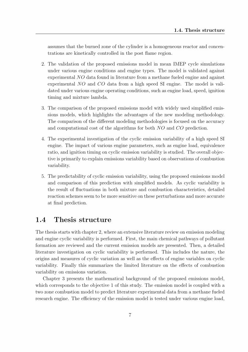
1.4 Thesis structure
The thesis starts with chapter 2, where an extensive literature review on emission modeling
and engine cyclic variability is performed. First, the main chemical pathways of pollutant
formation are reviewed and the current emission models are presented. Then, a detailed
literature investigation on cyclic variability is performed. This includes the nature, the
origins and measures of cyclic variation as well as the effects of engine variables on cyclic
variability. Finally this summarizes the limited literature on the effects of combustion
variability on emissions variation.
Chapter 3 presents the mathematical background of the proposed emissions model,
which corresponds to the objective 1 of this study. The emission model is coupled with a
two zone combustion model to predict literature experimental data from a methane fueled
research engine. The efficiency of the emission model is tested under various engine load,
7

1. Introduction
ignition timing, and equivalence ratio conditions. The validated model is utilized on a
cycle to cycle emissions analysis which is focused on determining the impact of prompt
NO formation mechanism on cyclic emissions variability.
Chapter 4 deals with the experimental investigation of cyclic dispersion in objective
4. This includes the investigation of combustion, performance, and emissions variability
under various engine operating conditions. The investigation is performed on a high speed,
port fueled injected, spark ignition engine. In this chapter it is attempted to correlate the
combustion variability with the observed emissions fluctuations.
Chapter 5 presents the validation of the proposed emissions model against simplified
emissions models in order to accomplish objectives 2, 3 and 5. First mean IMEP cycle
simulations are utilized to validate the mean NO and CO emissions. Then, the validated
model is used in a cycle to cycle simulation basis, to predict cyclic NO and CO variability.
Widely used simplified emissions models are compared to the new proposed emissions
model to highlight the benefits. The computational cost of each modeling approach is
also estimated.
Final chapter 6 summarizes the most important findings of the experimental and
modeling work, identifies the novelty and the contribution to knowledge of this thesis and
ends with some potential future work directions.
8

Chapter 2
Literature Review
2.1 Introduction
In order to better understand the process of cyclic emission variability, some of the funda-
mental theories of pollutants formation for conventional SI engines and the causes of cycle
to cycle variability are reviewed in this chapter. The current literature review gives good
insights into the chemical pathways of emissions formation as well as the mechanisms
that affect the combustion process and its variability. The main purpose of this chapter
is to review the current status regarding emissions modeling and the feasibility to predict
cyclic emissions variability, as this is described in published literature.
The chapter starts by laying the pollutants formation theory, regarding NOx, CO and
HC emissions at homogeneous charge conditions. Different types of emissions models are
reviewed to answer the question whether the accurate estimation of engine-out emissions
is primarily a thermodynamic or a kinetic issue. The sensitivity of these emission models
to residual gas fraction or burning rate is also reviewed. The second part of this chapter
includes a detailed literature investigation on cyclic variability. Firstly, the nature of cyclic
variability is defined, which is a combination of stochastic and deterministic aspects. Then
the origins and measures of cyclic variability are presented. Finally, the effects of each
parameter on cyclic variability are reviewed, such as mixture composition, small and
large scale turbulence, fuel type, engine geometry etc. The final section of this chapter
reviews the effect of combustion variability on emissions variability, an area which is of
high interest, particularly to this work. This part is the most essential of this chapter, as
cyclic emissions variability is a rather grey research area with only a handful number of
studies available in published literature.
9

2. Literature Review
2.2 Pollutants Formation Modeling
In the complete combustion of the fuel hydrocarbons, the exhaust gas consists of oxygen
(O2), nitrogen (N2), carbon dioxide (CO2) and steam (H2O), which are not detrimental
to human health. In fact, CO2 is responsible for the greenhouse effect but it doesn’t
pose a direct health hazard. However, in incomplete combustion that is observed in
actual operation of the internal combustion engines, carbon monoxide (CO), unburned
hydrocarbons (HC), nitrogen oxides (NOx) and particulate matter (PM) also appear as
exhaust gas components. These components are controlled by the emissions legislation,
as the exposure of humans to high concentrations of these species pose a direct health
hazard.
In conventional PFI SI engines, the emissions of interest are NOx, CO and HC. These
emissions vary between different engines and are dependent on such variables as ignition
timing, engine load, engine rotational speed and, in particular, air/fuel ratio. Figure 2.1
shows typical variations of the emissions with air/fuel ratio for a spark ignition engine
[16].
Figure 2.1: Spark ignition engine emissions for different air/fuel ratios [16].
The mechanisms that describe the NOx, CO and HC pollutants formation is the field
of interest of this section.
10
2.2. Pollutants Formation Modeling
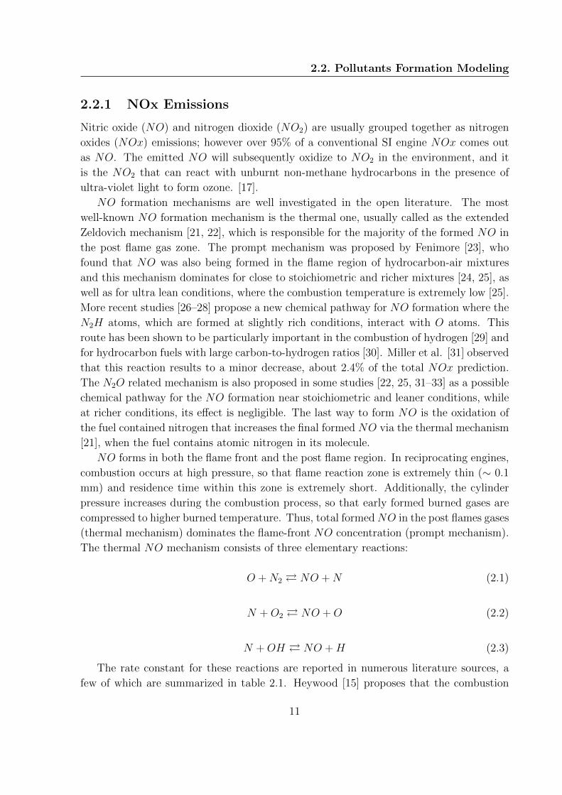
2.2.1 NOx Emissions
Nitric oxide (NO) and nitrogen dioxide (NO2) are usually grouped together as nitrogen
oxides (NOx) emissions; however over 95% of a conventional SI engine NOx comes out
as NO. The emitted NO will subsequently oxidize to NO2 in the environment, and it
is the NO2 that can react with unburnt non-methane hydrocarbons in the presence of
ultra-violet light to form ozone. [17].
NO formation mechanisms are well investigated in the open literature. The most
well-known NO formation mechanism is the thermal one, usually called as the extended
Zeldovich mechanism [21, 22], which is responsible for the majority of the formed NO in
the post flame gas zone. The prompt mechanism was proposed by Fenimore [23], who
found that NO was also being formed in the flame region of hydrocarbon-air mixtures
and this mechanism dominates for close to stoichiometric and richer mixtures [24, 25], as
well as for ultra lean conditions, where the combustion temperature is extremely low [25].
More recent studies [26–28] propose a new chemical pathway for NO formation where the
N2H atoms, which are formed at slightly rich conditions, interact with O atoms. This
route has been shown to be particularly important in the combustion of hydrogen [29] and
for hydrocarbon fuels with large carbon-to-hydrogen ratios [30]. Miller et al. [31] observed
that this reaction results to a minor decrease, about 2.4% of the total NOx prediction.
The N2O related mechanism is also proposed in some studies [22, 25, 31–33] as a possible
chemical pathway for the NO formation near stoichiometric and leaner conditions, while
at richer conditions, its effect is negligible. The last way to form NO is the oxidation of
the fuel contained nitrogen that increases the final formed NO via the thermal mechanism
[21], when the fuel contains atomic nitrogen in its molecule.
NO forms in both the flame front and the post flame region. In reciprocating engines,
combustion occurs at high pressure, so that flame reaction zone is extremely thin (∼ 0.1
mm) and residence time within this zone is extremely short. Additionally, the cylinder
pressure increases during the combustion process, so that early formed burned gases are
compressed to higher burned temperature. Thus, total formedNO in the post flames gases
(thermal mechanism) dominates the flame-front NO concentration (prompt mechanism).
The thermal NO mechanism consists of three elementary reactions:
O +N2 � NO +N (2.1)
N +O2 � NO +O (2.2)
N +OH � NO +H (2.3)
The rate constant for these reactions are reported in numerous literature sources, a
few of which are summarized in table 2.1. Heywood [15] proposes that the combustion
11

2. Literature Review
Table 2.1: Speed coefficients for the forward reaction of the Zeldovich mechanism [16]
Reaction i ki,r[cm3/mol · s] Author
1
1.8 · 104 · exp[− 38, 400
T
]Baulch at al. [34]
0.544 · 1014 · T 0.1 · exp[− 38, 020
T
]GRI-MECH 3.0 [35]
0.76 · 1014 · exp[− 38, 000
T
]Heywood [15]
2
6.4 · 109 · T · exp[− 3, 150
T
]Baulch at al. [34]
9.0 · 109 · T · exp[− 3, 280
T
]GRI-MECH 3.0 [35]
1.48 · 108 · T 1.5 · exp[− 2, 860
T
]Pattas [33]
3
3.0 · 1013 Baulch at al. [34]
3.36 · 1013 · exp[− 195
T
]GRI-MECH 3.0 [35]
4.1 · 1013 Heywood [15]
and thermal NO formation are decoupled and that equation (2.4) describes the kinetically
controlled NO rate, based on the equilibrium NO value. Typical values of R1, R2 and
R3 are given by Heywood [15] and are strongly depended on mixture equivalence ratio.
d[NO
]dt
=
2R1
[1−
([NO
]/[NO
]e
)2]1 +
[NO
]/[NO
]eR1
R2 +R3
(2.4)
The formation of the prompt NO in the flame front itself is much more complicated
that thermal NO formation, because this process is closely related to the formation of
the CH radical, which can react in many ways. The general scheme of the Fenimore
mechanism is that hydrocarbon radicals react with molecular nitrogen to form amines or
cyano compounds. The amines and cyano compounds are then converted to intermediate
compounds that ultimately form NO.
12

2.2. Pollutants Formation Modeling
CH +N2 � HCN +N (2.5)
C +N2 � CN +N (2.6)
Ignoring the processes that form CH radicals to initiate the mechanism, the prompt
mechanism is described by equation 2.7. For equivalence ratios higher that 1.2, other
routes open up and the chemistry becomes more complex [16, 24].
d[NO
]dt
= k10,r[HCN ][O] + k11,r[CN ][O2] (2.7)
k10,r = 2.3 · 104 · T 1.71exp
(− 3, 521
T
)m3
kmol · s(2.8)
k11,r = 8.7 · 109 · T 1.71exp
(216
T
)m3
kmol · s(2.9)
The N2O intermediate mechanism is important in fuel lean mixtures and low temper-
ature conditions. The three steps of this mechanism are:
O +N2 +M � N2O +M (2.10)
H +N2O � NO +NH (2.11)
O +N2O � NO +NO (2.12)
The N2H mechanism is a two key step mechanism, particularly important in the
combustion of fuel rich hydrogen mixtures [36]:
N2 +H → NNH (2.13)
NNH +O → NO +NH (2.14)
Finally, in the combustion of fuels with bound nitrogen, the nitrogen in the parent
fuel is rapidly converted to hydrogen cyanide (HCN) or ammonia (NH3), following the
above described reaction pathways.
13

2. Literature Review
2.2.2 CO Emissions
Carbon monoxide (CO) is abundant in rich-combustion products [15]. In SI engines, rich
mixtures are employed during engine startup to prevent stalling, as well as at wide open
throttle (WOT) to provide maximum power. At stoichiometric and slightly lean mixtures,
CO is produced at typical combustion temperatures as a result of the dissociation of
CO2. Turns [37] describes the relationship between CO and mixture temperature, where
carbon monoxide concentration rapidly falls as equilibrium temperature is decreased.
In SI engines, temperature falls rapidly during the expansion and exhaust process and
equilibrium is likely not to prevail. Conversely, CO exhaust concentration is “frozen”
between the procedures of combustion process and expansion/exhaust blowdown processes
[38, 39].
The observation that, in the combustion of premixed hydrocarbon-air mixtures, CO
concentration differs from the equilibrium value, implies that CO level is kinetically con-
trolled [15, 40]. The most important reaction that controls the CO exhaust concentration
is the Water Gas Shift (WGS) reaction (2.15), and appears to be significant in the post-
flame:
CO +OH � CO2 +H (2.15)
Calculations indicate that the WGS reaction is equilibrated during the expansion
and exhaust blowdown processes; however the three-body recombination processes (e.g
H + OH + M � H2O + M) are not fast enough to maintain equilibrium among all the
radicals [37]. This causes the partial-equilibrium CO concentrations to be well above
those of full equilibrium [39, 41].
A widely used model for CO emissions is given by D’Errico et al. [40, 42]. This model
uses the WGS reaction, given at Eq. (2.15), and expresses the resulting CO reaction rate
as follows:
d[CO]
dt=(R1 +R2
)(1−
[CO][
CO]e
)(2.16)
where [CO]e is the predicted equilibrium concentration of CO, and values for the rates
R1 and R2 are given by Heywood [15] and D’Errico et al. [40, 42]. This model appears
more accurate compared to the equilibrium assumption [43], however its kinetics needs
calibration for different type of engines.
Other CO production mechanisms include quenching by cold surface, where CO is
formed though the WGS reaction as well as partial oxidation of unburned fuel, in crevices.
Both these two mechanisms produce mainly hydrocarbons and are described in detail in
the next section.
14

2.2. Pollutants Formation Modeling
2.2.3 HC Emissions
Hydrocarbons (HC) are the consequence of incomplete combustion of the hydrocarbon
fuel. In the exhaust of the vehicles, unburned hydrocarbons are measured as total hydro-
carbon concentration in C1 base, usually in parts per million (ppm). Unburned hydrocar-
bon levels in the exhaust of a SI engine under normal operating conditions are typically in
the range of 1000 to 3000 ppm C1, which correspond to between about 1 and 2.5% of the
fuel flow into the engine [15]. The hydrocarbon profile in the exhaust of engines consists
of a combination of paraffins, olefins, acetylene and aromatics compounds, as a result of
unburned or partially burned fuel hydrocarbons and engine oil. Polyaromatic species are
also present in less abundance.
Heywood’s textbook [15] provides four possible HC emissions formation mechanisms
for conventional SI engines: a) flame quenching at the cold surfaces of the combustion
chamber; b) the contribution of crevice volume with unburned mixture that due to flame
quenching can not follow the main combustion rate; c) absorption of fuel vapor into oil
layers during compression stroke; a fraction of which is desorbed during the expansion
and the exhaust blowflow; and finally d) incomplete flame propagation in the bulk of the
charge.
2.2.4 Pollutants Formation Models
The previous section presented the most important formation mechanisms for main pollu-
tants emitted by conventional SI engines, such as NOx, CO, HC. These mechanisms can
be classified into mainly physical or chemical processes. Reaction mechanisms are suitable
to describe in detail the overall chemical reaction pathway; that is the formation of NOx
and CO emissions, as HC emissions are more a complex physical issue, as it was described
above. Such reaction mechanisms can consist of a single or limited steps of elementary
reactions or a detailed reaction scheme. In this study, it is adopted that the first case
belongs to the category of simplified kinetic models and the second to the detailed kinetic
models. Both models can be coupled with combustion models, as their input requires the
temperature and pressure cylinder profile and some other cylinder mixture characteris-
tics, such as A/F ratio and residual gas fraction. Simplified kinetic models exhibit short
execution time and reduced requirements for input information, but they suffer from low
sensitivity to various engine conditions and they require calibration. Conversely, detailed
kinetic models are computationally more expensive and require more input data; however
they can give a better picture of the step by step sequence of the elementary reactions,
they can more accurately estimate the exhaust concentration of many chemical species
and they do not need any calibration. In several studies simplified or detailed kinetic
models are utilized, the results of which are reviewed in this section.
15
2. Literature Review
2.2.4.1 Simplified Kinetic Models
Many researchers in the past have tried to answer the question whether the engine out
pollutants formation is primarily a thermodynamic or a chemistry problem. Adopting
temperature stratification during combustion can improve the predicted in-cylinder NO
concentration [32, 44]. In these studies, it was observed that the extended Zeldovich
mechanism is able to predict NO emissions within an error of 15-60%. This result implies
that the NO simulation is not just a temperature issue, but also a significant chemistry
problem. The first NO kinetic control mechanisms [21, 22, 33] were utilized at older
studies, instead of the inaccurate assumption of equilibrium [43].
In 1979, Heywood et al. [45] proposed a thermodynamic engine cycle simulation
and a chemical model to predict NOx emissions from a conventional SI engine. The
required inputs were engine geometry, engine speed, overall equivalence ratio, residual
gas fraction and intake manifold pressure and temperature. For the heat release, Vibe
model was applied [46]. NOx emissions are calculated by using the extended Zeldovich
kinetic scheme, with the steady state assumption for the N concentration and equilibrium
values used for H, O, O2 and OH concentrations in the adiabatic core. A three zone
combustion model was used to describe the combustion process: an adiabatic burned
zone, an unburned zone and a burned gas boundary layer where combustion occurs.
The simulation was compared against experimental data from a research single cylinder
SI engine. It was found that NOx emissions are very sensitive to equivalence ratio,
residual gas fraction and combustion duration. Although further comparison between
experimental and simulation NOx data is not given, this study is important as it is
the first cycle simulation investigation in published literature, including performance and
NOx emissions calculations.
In a more recent study, D’Errico et al. [40] presented a pollutant emissions model
for SI engines, which included an eddy burning model for the accurate prediction of heat
release, the extended Zeldovich mechanism for the prediction of NOx emissions, a two
step reactions CO model and a single Arrhenius equation for HC post oxidation, given
by Lavoie and Blumberg [47]. The temperature distribution is achieved by dividing the
mixture into an adiabatic core and a thermal boundary layer, where this core was further
divided into an equal mass of adiabatic zones. The emission model was calibrated, based
on one engine operating point. The simulation values were validated against experimental
data from a 2.0L Fiat-Alfa Romeo four cylinder engine. On the results of this study, it
was found that the model was able to predict engine-out emissions qualitatively and
quantitatively at full load conditions over the entire engine speed range. However, the
study does not present the validation of the model on partial load conditions.
The multizoning technique is performed for the more accurate prediction of the tem-
perature distribution, which significantly affects the chemical kinetics and finally the es-
timated exhaust emissions. Michos et al. [44] utilized a multizone turbulent combustion
16

2.2. Pollutants Formation Modeling
model in coupling with the extended Zeldovich mechanism to predict NOx emissions.
In this model, the number of zones are user defined and each zone exchanges heat with
the chamber wall but zone mass remains constant. They found that by increasing the
number of zones, NO error estimation initially decreases and then slightly increases and
converges to a constant value after the fifth zone assumption. At partial engine load, NO
error is higher while this deviation decreases as engine load increases. The five burned
zone emission model was able to qualitatively predict the measured NOx concentrations
at various engine load conditions but not quantitatively.
Finally, Richard et al. [48] used a physical 0D combustion model for simulating heat
release and simple kinetics to predict NO and CO emissions. The experimental data
were from a turbocharged SI engine. They noticed that the reduced physical combustion
model was able to accurately predict pressure rise and heat release, although engine
emissions were not well predicted. Under the entire engine speed range, NOx emissions
were underestimated at partial load and slightly overestimated at full load conditions,
while CO emissions were consistently underestimated and the error was increased at
higher engine speed conditions. This last study is informative, as the same experimental
data and the same combustion model were used in coupling with a detailed kinetic model
and much more accurate emissions prediction [49]. These results are discussed in the next
section.
2.2.4.2 Detailed Kinetic Models
Detailed chemistry models contain more reaction pathways compared to simplified kinetics
models; therefore they are able to predict and explain NO formation in a more analytical
way. A lot of experimental and theoretical studies present the significant impact of residual
gas fraction on charge dilution, which finally steeply decreases NO formation [50–52].
However, it was found that simplified kinetic models overestimate NO from 12 to 25%
when engine load increases and residual fraction drops [31, 32, 53]. Burn rate is another
critical engine variable where NO prediction is very sensitive on [32]. Cyclic combustion
variability studies can be used to examine fast and slow burning rates on NO formation
[54]; however it is known that by only changing the burning rate is not possible to predict
the scatter of NO variability with a simplified NO kinetic model [13]. Besides, the
most important feature of detailed chemistry models for realistic NO predictions is the
capability to predict NO and CO emissions with a good accuracy under various engine
operating conditions and without any calibration methodology.
Miller et al. [31] proposed a super extended Zeldovich mechanism (SEZM) for the pre-
diction of NOx, which consists of 67 reactions and 13 chemical species, while it assumes
equilibrium concentrations for all other species. Steady-state engine cycle modeling was
performed by GESIM, a quasi-dimensional cycle simulation which takes into consideration
turbulent entrainment and eddy burnup, swirl, tumble, chamber geometry on flame de-
17
2. Literature Review
velopment, burn rate, and fuel consumption. In conjunction with the combustion model,
a quasi one-dimensional dynamics model (MANDY) for the wave dynamics in the pipes
was also applied in this study. The target of this study was to improve the NOx predic-
tion, as the extended Zeldovich mechanism over predicted NOx by more than 25%. It
was found that both termolecular/unimolecular reactions and N2H chemistry give a 2.4%
reduction on observed NOx; however, predicted NOx levels are in excess of the experi-
mental data by more than 20%. This observation could be explained by pressure effects
on the radical pool, which was assumed to be in equilibrium in this study. In addition,
the proposed modified pressure dependent reaction one rate of the Zeldovich mechanism
shows improved accuracy on NOx prediction as a function of load. Last but not least,
the proposed super extended Zeldovich model presented good accuracy within 10% for
lean, rich and EGR diluted mixtures.
Rublewski and Heywood [32] tried to answer to the question if accurately prediction
of engine out NO concentration is primarily a thermodynamic problem, or a chemistry
problem. Therefore, temperature stratification during combustion in combination with
a crevice/combustion inefficiency routine was applied in their modeling. This multizone
approach with an adiabatic core improves the NO simulation; however the NO formation
was found to be mainly affected by the residual gas fraction and the burn rate. In addition,
it was shown that model accuracy would be modestly improved if the equilibrium burned
gas radical pool assumption was removed and a kinetically controlled radical pool was
adopted. Last but not least, in this study it was found that theN2O mechanism little affect
the NO formation, although other researchers [22, 31] suggested that this mechanism can
be significant under highly dilute conditions.
Last but not least, Bougrine et al. [49] introduced a tabulated chemistry approach in
coupling with a detailed chemistry model (SENKIN) to predict NO and CO emissions.
The initial values are given by equilibrium, while detailed chemistry calculates the differ-
ence of the equilibrated value from the kinetic value. Compared with the results of their
previous investigation [48], the new emission approach shows smaller errors, especially
for the estimation of CO emissions. However, NOx emissions demonstrate that errors in
calculations may occur due to temperature stratification and the equilibrium assumption
in the early stage.
2.3 Cycle-to-Cycle Variability
Cyclic combustion variability is experimentally identified by the variation of cylinder
pressure evolution from one cycle to another. Since the pressure development is closely
related to the combustion process, substantial variations in the combustion process on
a cycle to cycle basis are occurring. CCV has a negative effect on engine performance,
fuel consumption as well as engine-out emissions [10, 12, 55, 56]. The nature, the origins
18

2.3. Cycle-to-Cycle Variability
and the indicators of cyclic combustion variability are discussed in this section. Finally,
a literature review is performed on the engine parameters that affect cyclic variation.
2.3.1 The Nature of Cyclic Variation
Cyclic combustion variability is experimentally identified by the variation of cylinder
pressure evolution from one cycle to the next [57], as a result of both stochastic and
deterministic combustion related effects [58, 59]. Although much of the research on cyclic
variability has focused on stochastic aspects, such as two well known review studies on
cyclic variability [10, 55], it is widely accepted that observed cyclic variations can present
a high degree of low-dimensional deterministic structure [58]. This deterministic aspect
implies some degree of predictability and potential for real-time control [60].
In order to better understand the nature of cyclic variability, it is of interest to de-
fine the terms ”stochastic” and ”deterministic”. A stochastic size takes a random value
between the minimum and the maximum limits, which can be predicted in a probability
sense by using a probability density function. In the case of combustion variability, small-
scale and large-scale turbulence of the gas mixture is known for its stochastic nature. On
the other hand, the term ”deterministic” is used for a system that follows explicit laws
of cause and effect, such that if we know precisely what the initial conditions are, we can
predict the state of the system at any time in the future [60]. Regarding CCV, residual
gas fraction is a deterministic parameter, as the residual gas of the previous cycle affects
the combustion and emissions of the next, which implies a strong ”memory” effect from
cycle to cycle.
The stochastic and deterministic dimensions of cyclic variability have been adopted
by many researchers in the past, in order to model the cyclic variations in spark ignition
engines, although not by using exactly the same terminology. Dai et al. [61] classified the
causes of cyclic variations into two major groups: (a) prior-cycle effects and (b) same-
cycle effects. The prior-cycle effects stands for residual gas variation in the combustion
chamber, whereas the same-cycle effects refer to variations in air/fuel mixtures in the
cylinder.
The main difference between the stochastic and deterministic aspects of cyclic variabil-
ity is that the deterministic structure can be potentially limited through engine control.
Therefore, exploring the deterministic nature of cyclic variability gives the potential op-
portunity to engine manufactures of further improving the engines emissions and fuel
economy by the limitation of the deterministic nature of CCV. In fact, the deterministic
nature of cyclic variability can be highlighted close to the unstable combustion limits
[61–63]; that is at lean, non-homogeneous charged and high diluted engine conditions. At
this combustion area, limitation of the deterministic combustion variations can extend the
engine limits to leaner and more diluted mixtures, while this can benefit the engine ther-
19

2. Literature Review
mal efficiency. As cyclic variability is a nonlinear complex phenomenon with very large
degrees of freedom, the control of such systems can be performed by the chaos theory
[64, 65].
2.3.2 Origins of Cyclic Variation
Cycle-to-cycle variability (CCV) is an undesirable characteristic of internal combustion
engines. This is caused by the non identical in-cylinder conditions from one combustion
cycle to the other, at nominally identical operating conditions. As air pollutant and green-
house gas emissions standards are getting more stringent around the world, mitigation of
CCV can improve fuel efficiency and minimize engine emissions. In addition, limitation
of CCV allows better engine calibration and enables performance close to the optimum
conditions [10].
The origins of CCV in a spark-ignition (SI) engine can be summarized as follows
[10, 15, 17, 63]:
i the variations in the gas motion and the mixture strength near the spark plug location
at time of ignition [66],
ii the variation in air-fuel ratio supplied to each cycle [20, 67–69]
iii non-uniform mixture composition in the cylinder due to incomplete mixing between
air, fuel, and residual gas [68, 70]
iv ability of different ignition systems to ignite the local mixture [68, 71–74]
Early flame kernel development corresponds to the combustion process from SI initi-
ation to the transition to a fully turbulent combustion. This early burn period, which is
often approximated by the 5% mass fraction burned (MFB) limit, is recognized as the
most crucial stage of the combustion evolution [75, 76]. Early flame kernel development
greatly affects the development of combustion and build-up of cylinder pressure [77, 78].
Slow early burning rate cycles continue to burn slowly during flame propagation and sub-
sequently lead to lower peak pressures [79]. Actually, the initial laminar flame initiated
by the spark has been found to be very repeatable. Curry [79] found that the burning
rate was very repeatable within some 5 millimeters from the spark plug, and significant
deviations occurred only thereafter. Variations in the early flame kernel development
should not so much depend on spark intensity, as long as the mixture can be ignited [20],
but on follow up in-cylinder conditions. However, in case that the mixture is not easily
ignited, such as very lean and highly diluted mixtures, the spark ignition energy has a
remarkable impact on the combustion process [80].
20
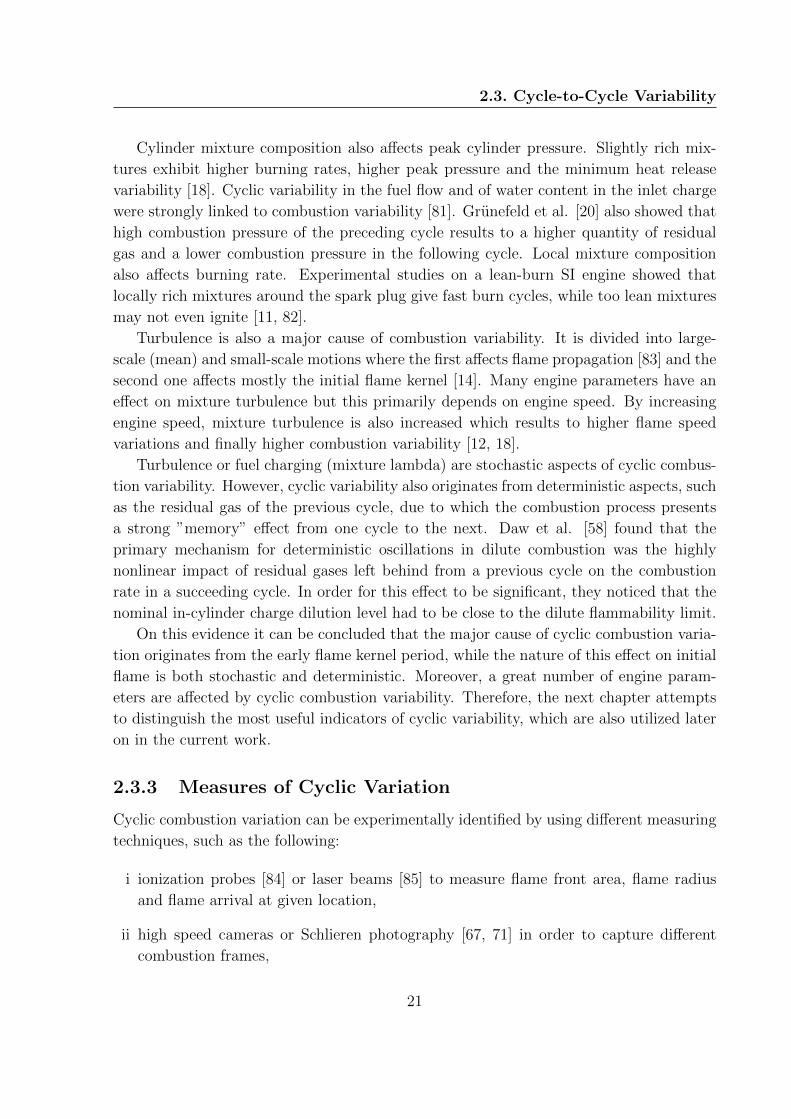
2.3. Cycle-to-Cycle Variability
Cylinder mixture composition also affects peak cylinder pressure. Slightly rich mix-
tures exhibit higher burning rates, higher peak pressure and the minimum heat release
variability [18]. Cyclic variability in the fuel flow and of water content in the inlet charge
were strongly linked to combustion variability [81]. Grunefeld et al. [20] also showed that
high combustion pressure of the preceding cycle results to a higher quantity of residual
gas and a lower combustion pressure in the following cycle. Local mixture composition
also affects burning rate. Experimental studies on a lean-burn SI engine showed that
locally rich mixtures around the spark plug give fast burn cycles, while too lean mixtures
may not even ignite [11, 82].
Turbulence is also a major cause of combustion variability. It is divided into large-
scale (mean) and small-scale motions where the first affects flame propagation [83] and the
second one affects mostly the initial flame kernel [14]. Many engine parameters have an
effect on mixture turbulence but this primarily depends on engine speed. By increasing
engine speed, mixture turbulence is also increased which results to higher flame speed
variations and finally higher combustion variability [12, 18].
Turbulence or fuel charging (mixture lambda) are stochastic aspects of cyclic combus-
tion variability. However, cyclic variability also originates from deterministic aspects, such
as the residual gas of the previous cycle, due to which the combustion process presents
a strong ”memory” effect from one cycle to the next. Daw et al. [58] found that the
primary mechanism for deterministic oscillations in dilute combustion was the highly
nonlinear impact of residual gases left behind from a previous cycle on the combustion
rate in a succeeding cycle. In order for this effect to be significant, they noticed that the
nominal in-cylinder charge dilution level had to be close to the dilute flammability limit.
On this evidence it can be concluded that the major cause of cyclic combustion varia-
tion originates from the early flame kernel period, while the nature of this effect on initial
flame is both stochastic and deterministic. Moreover, a great number of engine param-
eters are affected by cyclic combustion variability. Therefore, the next chapter attempts
to distinguish the most useful indicators of cyclic variability, which are also utilized later
on in the current work.
2.3.3 Measures of Cyclic Variation
Cyclic combustion variation can be experimentally identified by using different measuring
techniques, such as the following:
i ionization probes [84] or laser beams [85] to measure flame front area, flame radius
and flame arrival at given location,
ii high speed cameras or Schlieren photography [67, 71] in order to capture different
combustion frames,
21

2. Literature Review
iii piezoelectric crystal for the measurement of the cylinder pressure over crankangle.
In most studies two techniques are applied simultaneously, in order to identify cyclic
cylinder pressure and flame variation. Based on Matekunas [71] and Heywood [15], the
cyclic variations can be grouped into four main categories, depending on the variation of
different type of parameters. The following quantities have been used [10]:
1. Pressure-related parameters. The maximum cylinder pressure Pmax; the crank
angle at which this maximum pressure occurs ϑPmax; the maximum rate of pressure
rise (dP
dϑ)max; the crank angle at which the maximum rate of pressure rise occurs
ϑ(dP
dϑ)max
; the IMEP of the individual cycles.
2. Combustion-related parameters. The maximum rate of heat release (net or gross);
the maximum rate of mass burning or maximum rateof change of burnt mass frac-
tion in the cylinder (dxbdϑ
)max; the early flame kernel development angle ϑ5%; the
combustion duration ϑ5−90%.
3. Flame front-related parameters. Flame radius, flame front area enflamed or burned
volume at given times; flame arrival time at given locations.
4. Exhaust gas-related parameters. Concentration of different components in the ex-
haust gases.
One important measure of cyclic variability, derived from pressure data, is coefficient
of variation of indicated mean effective pressure. It is defined as the standard deviation
in imep divided by the mean imep, and is usually expressed in percent:
COVimep =σimepimep
× 100 (2.17)
It defines the cyclic variability in indicated work per cycle and it has been found that
vehicle drivability problems usually result when COVimep exceeds about 10 percent. The
same definition of COV is also used for the other parameters defined above.
Brown et al. [86] conducted tests on a research Ricardo E6 engine at various engine
loads, ignition timings and equivalence ratio conditions. They have noticed that the cycle
to cycle variations in combustion should be characterized by the COV of the imep. Often
the COV of the maximum cylinder pressure (Pmax) is used since it is easier to quantify.
However, it has been proved in this study that this can lead to misleading results when
the ignition timing is varied in the region of the MBT ignition timing. It has also been
demonstrated that when the ignition timing is varied there is no correlation between the
COV of the imep and COV of the maximum cylinder pressure. The experimental data
22

2.3. Cycle-to-Cycle Variability
also show that the COV of the imep is at minimum in the region of the MBT ignition
timing, and this also corresponds to a minimum in the 0-10 % burn time.
The most characteristic relationships between maximum cylinder pressure (Pmax),
crank angle that maximum cylinder pressure occurs (ϑPmax) and imep are described by
Matekunas [71]. In that study, a single cylinder flame photography engine was employed
under various ignition timing and equivalence ratio conditions at constant inlet manifold
pressure (55 kPa). It was found that as the spark timing approaches the MBT conditions,
the relative variations in imep are very small as compared with the variations in ϑPmax,
and become more significant with advanced ignition timing.
Early flame kernel development also presents a strong relationship with imep. Aleiferis
et al. [80] experimentally investigated the flame behavior in a lean-burn optical stratified-
charge single cylinder SI engine. A strong relationship between imep and ϑ5% was ob-
served, especially at lean operating conditions. However, ϑ5% is not a very informative
parameter, as it does not provide any information about the reasons for early combustion
from cycle to cycle. Analysis of the projected flame-front shape and its wrinkling (small
scale) showed that the fastest lean flames were associated with a large standard devia-
tion (σd) of the local displacement between the instantaneous and filtered flame contours
and with a small number of crossing points (M) between the instantaneous and filtered
contours. Additionally, the fastest lean flames possessed values of d and M similar to
those measured from the images of stoichiometric flames. This suggested that the fastest
flames on a cycle-by-cycle basis might have been burning with a richer than average A/F
ratio around the spark plug. The measured shape factors (large scale) did not show any
strong correlation between the crank angle of 5% mass fraction burned and the ratio of
the length of the instantaneous flame contour to the length of the filtered flame contour,
or to the perimeter of a circle with the same radius to the equivalent radius of the flame.
As it follows from the relevant discussion, a limited number of parameters are preferred
as CCV indicators. The most widely used quantities are the pressure related parameters
( Pmax, ϑPmax and imep), while flame radius and displacement of the flame kernel center
from the spark plug center can also be found in a number of studies. The first three are
the easiest to acquire, as the experimental equipment which is needed is only the pressure
transducer. When ignition timing is set to MBT, using Pmax as the CCV indicator will be
the most prominent among others. However, if the interest is limited to CCV in the stage
of the early flame kernel development, then the most suitable parameter would be ϑPmax.
The imep is most useful for indicating the engine response to CCV in the combustion
process. The two flame front-related parameters seem to provide valuable information for
a better understanding of the in-cylinder combustion and the fundamental reasons for the
cyclic variations.
23

2. Literature Review
2.3.4 Effects of Engine Variables on Cyclic Variability
Many studies investigate the impact of various engine variables on combustion variation.
Young [87] categorized engine operating and design variables into two main groups, i.e.
chemical and physical factors.
Chemical factors are those variables that determine the composition of the trapped
cylinder charge. Such factors are equivalence ratio, the residual gas that dilutes the
charged mixture and the fuel type. These factors were thought to influence cycle-to-cycle
variations by affecting laminar flame speeds and expansion velocity. In fact, equivalence
ratio and residual gas fraction are factors that mainly relate with the deterministic na-
ture of cyclic variability; therefore their control is of primary importance as it gives the
potential opportunity to improve fuel economy and engine-out emissions.
On the other hand, physical factors are related with the physical conditions under
which combustion proceeds, and can also affect the cycle-to-cycle combustion variations.
These factors are combustion chamber geometry, ignition system, compression ratio, en-
gine speed, mixture preparation and motion.
The factors that influence cyclic variability are reviewed in this section.
2.3.4.1 Equivalence Ratio
Equivalence ratio is highlighted as the mixture parameter that has a strong influence on
cyclic combustion variability. A number of CCV studies have investigated the impact of
equivalence ratio on combustion variability. Slightly rich mixtures exhibit higher burning
rates, higher peak pressure and the minimum heat release variability [80]. Generally,
the minimum cyclic variations occur at slightly rich equivalence ratios corresponding
approximately to the mixture strength for best power [87].
Using ionization gaps located 16.5 mm (probe 1) and 65 mm (probe 2) from the spark
plug, Harrow and Orraan [22] observed minimum variations in flame arrival times at
1.15 to 1.25 equivalence ratio (13 to 12 air-fuel ratio (A/F)), as shown in Fig. 3a. The
variations in arrival times were characterized by the time interval between the arrival of
10% and 90% of the cycles monitored. Minimum variations in arrival times were 0.49
and 0.35 at probes 1 and 2, respectively. For a normally distributed random variable,
this spread would correspond to 2.45 times the standard deviation. Flame speeds, calcu-
lated from arrival times at the two probes, were showed highest values at approximately
1.25 equivalence ratio (12 A/F) for engine speeds from 750 to 2500 r/min. Warren and
Hinkamp [23] noted similar variations of flame arrival times at a distance of 73 mm from
the spark gap as a function of air-fuel ratio. Test results showed that minimum variations
in flame arrival times occurred at about the mixture strength for maximum power, 13:1
A/F (1.15 equivalence ratio). As a fraction of the mean arrival time, the minimum spread
was approximately 0.38. A non-normal distribution in arrival times was observed. In
24

2.3. Cycle-to-Cycle Variability
both studies, minimum variation in arrival times occurred where the mean arrival times
were at minimum, i.e., flame speeds were highest.
Matthew et al. [88] investigated the impact of equivalence ratio on cyclic variability
using both an SI engine model and experimental data. The SI engine model was a quasi-
dimensional code that utilized the concepts of fractal geometry to simulate the effects of
turbulence on the flame propagation process. A single cylinder research engine, fueled
with propane, operated at 600 rpm and at constant intake manifold conditions (170kPa,
65degC) was utilized for the model validation. It was found that the equivalence ratio
affects flame stretch and the distribution of the flame wrinkling scales. In fact, variations
in equivalence ratio also result in variations of the residual gas fraction and therefore
independent effects of variations in the equivalence ratio and in the residual fraction have
not been examined. Variations in the equivalence ratio have a dominant effect on cyclic
variability in the peak cylinder pressure, but have little effect on the crank angle that
peak pressure occurs and an insignificant effect on the early flame kernel development.
Although the early flame kernel is controlled by laminar flame chemistry, it was found that
if the engine conditions are sufficiently turbulent, flame wrinkling can begin to dominate
very early in the combustion process.
2.3.4.2 Fuel Type
Different types of fuel can be injected in SI engines, either in liquid or in gaseous phase.
Gasoline, iso-octane, methane, propane, hydrogen, liquid petroleum gas (LPG) and com-
pressed natural gas (CNG) are the most widely used fuels in the open literature. Each
of these fuels present different chemical and physical properties, while the fuel type also
affects the combustion process, its variability as well as the pollutants formation. How-
ever, it is recognized that fuels which are rich in hydrogen present faster burning rates
and lower combustion variability due to the high flame velocity of H2.
The first study that presents the impact of fuel type on cyclic variability was performed
by Soltau [89]. In these test, a variety of liquid fuels (gasoline, benzene, and methanol)
and gaseous fuels (town gas, i.e., coal gas, butane, and methane) were experimentally
investigated. The single cylinder research engine had a compression ratio of 9:1, while
engine speed was varied from 500 to 3500 rpm with throttle setting. On the results, it was
found that town gas which was hydrogen-rich presented the lower combustion variability.
With the exception of town gas, no significant difference in combustion variation was
observed among the other fuels.
Sen et al. [90] investigated the effect of hydrogen addition on cyclic variability in a
natural gas SI engine. The engine was a three cylinder one, operating at 3000 rpm and
an excess air ratio of 1.4. Three cases were examined: natural gas with no hydrogen
added, and natural gas with the addition of 23% and 40% hydrogen by volume, while
192 consecutive cycles were analyzed, using the wavelet multiresolution analysis. It was
25

2. Literature Review
found that by increasing the hydrogen volume in the fuel, this had a pronounced effect on
reducing the cyclic variability of the imep. Finally, it was observed that the 23% hydrogen
by volume mixture contributed more to the limitation of CCV, while the limitation of
CCV from the 23% to the 40% hydrogen by volume mixture was lower.
Wang et al. [91] examined the cyclic variation in a hydrogen-enriched gasoline SI
engine under various hydrogen volume fractions. The test was carried out on a modified
four-cylinder gasoline engine equipped with an electronically controlled hydrogen injection
system. The engine was operated at 1400 rpm, on different hydrogen volume fractions in
the total intake, excess air ratios, spark timings and manifold absolute pressures. The test
results demonstrated that the coefficient of variation in indicated mean effective pressure
was distinctly decreased with the increase of hydrogen blending ratio. At manifold abso-
lute pressure of 61.5 kPa, the relevant excess air ratio for the engine lean burn limit was
extended from 1.45 to 2.55 when the hydrogen volume fraction in the intake was raised
from 0% to 4.5%. By performing the same investigation at 790 rpm, it was found that
hydrogen addition was more effective on reducing engine cyclic variation at low loads.
2.3.4.3 Combustion Chamber Geometry
The combustion chamber geometry is mainly refers to the chamber shape in conjunction
with the spark plug location and affects primarily the length of the main combustion
period and secondarily its variation from cycle to cycle [87]. The most effective combustion
chamber geometry that improves engine stability is the design that reduces the combustion
process duration (on a crankangle basis) through mainly chamber openness and turbulence
- generating features.
Young [55] used four variables to describe the combustion chamber geometry: (a)
intake valve area, (b) squish area, (c) maximum flame travel distance and (d) a chamber
openness parameter. Only squish area and a chamber openness parameter, were found to
be important. Squish represents the normalized maximum flame-travel distance at TDC
and was computed for each chamber from measurements of piston - crown and cylinder-
head contours. The openness parameter is related to the accessibility of the combustion
chamber volume to a spherical flame propagating from the spark plug location, and is
influenced by both the shape of the combustion chamber and the location of the spark plug.
Figure 2.2 illustrates the cross-sections of the three combustion chambers investigated in
this study. The more desirable location of the spark plug is given for the case of the
opened chamber, which presented a faster burning rate, due to the more spherical flame
propagating from the spark plug.
The impact of combustion chamber geometry on cyclic variability and engine stability
was also validated by Lucas and Brunt [92]. In this experimental study, the effects of
various combustion chamber designs on combustion rate in an SI engine were explored,
by measuring the flame propagation rate and cylinder pressure. It was noticed that
26
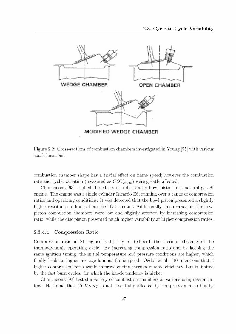
2.3. Cycle-to-Cycle Variability
Figure 2.2: Cross-sections of combustion chambers investigated in Young [55] with various
spark locations.
combustion chamber shape has a trivial effect on flame speed; however the combustion
rate and cyclic variation (measured as COVPmax) were greatly affected.
Chanchaona [93] studied the effects of a disc and a bowl piston in a natural gas SI
engine. The engine was a single cylinder Ricardo E6, running over a range of compression
ratios and operating conditions. It was detected that the bowl piston presented a slightly
higher resistance to knock than the ”flat” piston. Additionally, imep variations for bowl
piston combustion chambers were low and slightly affected by increasing compression
ratio, while the disc piston presented much higher variability at higher compression ratios.
2.3.4.4 Compression Ratio
Compression ratio in SI engines is directly related with the thermal efficiency of the
thermodynamic operating cycle. By increasing compression ratio and by keeping the
same ignition timing, the initial temperature and pressure conditions are higher, which
finally leads to higher average laminar flame speed. Ozdor et al. [10] mentions that a
higher compression ratio would improve engine thermodynamic efficiency, but is limited
by the fast burn cycles. for which the knock tendency is higher.
Chanchaona [93] tested a variety of combustion chambers at various compression ra-
tios. He found that COV imep is not essentially affected by compression ratio but by
27
2. Literature Review
combustion chamber shape, since increasing compression ratio for various combustion
chambers gave inconsistent results for imep variation. Altering compression ratio results
in distorting the combustion chamber geometry and flame propagation patterns.
2.4 Cyclic Emissions Variability
Cyclic dispersion of mixture composition and turbulence, even at nominally steady state
operating conditions, are linked to fluctuations on burning rate and finally on cycle to cycle
variation of engine-out emissions. As mixture characteristics and combustion evolution
seems to affect each other, a deeper understanding of the crucial parameters that affect
pollutants formation can be given by engine simulation [12, 31, 32, 44, 45, 53].
Despite combustion CCV has been studied rather extensively, its effect on engine
emissions is not well understood. Milkins et al. [94] found that the mean combustion
cycle corresponds to relatively low CO and HC emissions while faster and slower burning
cycles always lead to higher emissions. It is known from mean cycle studies that at partial
load engine conditions, CO emissions are correlated with heat release characteristics of
premixed burn and at higher load conditions, CO emissions are mainly controlled by
mixing [95]. However the impact of these parameters on the scatter of CO variability
has not been investigated in literature. On the other hand, NO formation is linked to
oxygen availability, burning rate and maximum cylinder pressure [54, 96, 97]. Cyclic
variations of combustion and pressure development [98], cyclic fluctuations of mixture
stoichiometry [99], and heterogeneities of cylinder charge [70] are the main sources of NO
variation. One study [12] showed that NO formation presents a non-linear correlation
with indicated mean effective pressure (IMEP). However, a detailed experimental study
that investigates the impact of various engine parameters such as stoichiometry, load or
ignition timing on NO cycle-to-cycle variation has yet to be conducted.
Ball et al. [13] presented a methodology for the estimation of NO formation on
a cycle to cycle basis. The experimental data consisted of cyclic resolved NO values
obtained with a fast CLD, while the modeled data were calculated using the extended
Zeldovich mechanism. Wiebe model was used for the prediction of the heat release on the
thermodynamic model, while combustion duration and completeness of combustion were
obtained by the measured cylinder pressure, on a cycle to cycle basis. The results of the
NO modeling showed good agreement with experimental data, in terms of the mean NO
level. However, the modeled data showed less scatter in the plots than the experimental
data, as residual gas fraction, temperature at IVC and mixture lambda were not cyclic
varied.
28

2.5. Summary and Conclusions
2.5 Summary and Conclusions
Cyclic combustion variation in SI engines occurs in all operating conditions and becomes
worse when engines operate under lean and highly diluted conditions. The main impact of
cyclic variability is on early flame kernel development, that affects the combustion process.
The control of the deterministic aspect of cyclic variability, which is mainly defined as the
elimination of the residual gas fraction and its variability, could lead to improvements on
fuel consumption and to lower engine-out emissions.
Pollutants formation can be described by chemical or physical submodels. Reaction
mechanisms are suitable to describe in detail the overall chemical reaction pathway. Con-
versely to simplified kinetic models, detailed kinetic models describe better the step by
step sequence of the elementary reactions, they calculate accurately the exhaust concen-
tration of the total chemical species and they do not need a separate calibration. Such
models present all the necessary physical and chemical properties for accurate estimation
of cyclic emission variability.
Although the engine parameters that affect the pollutants formation are widely known,
cyclic emission variability is a gray aspect of internal combustion engine modeling. Emis-
sions prediction is not always accurate due to modeling assumptions and the nature of
cyclic variability. The limited literature on emissions variability proves that this topic has
to be better investigated, as automotive industry is under stricter emission legislation.
29

2. Literature Review
30

Chapter 3
Proposed Emissions Model
3.1 Introduction
In this chapter, an engine-out emissions model for the prediction of NO formation in
homogeneous engine conditions is presented. The model can be coupled with any multi-
zone thermodynamic model, where the burned zones are assumed as perfectly-stirred
reactors. In this study, a two zone approach is adopted, which consists of an unburned
and a burned region. The computational time of the proposed detailed chemistry model
is slightly increased but at the same order of magnitude to the Zeldovich mechanism. The
basic benefits of this detailed chemistry model are its simplicity and the absence of any
calibration parameter that makes it a generalized application, possible to be applied in
any type of homogeneous combustion engine.
This chapter aims to investigate the impact of a detailed chemical mechanism on NO
prediction. The presented detailed chemistry model is coupled with an existing two zone
combustion model. The Vibe model [46] is used for the prediction of heat release; then the
calculated thermodynamic data are fed into the detailed chemistry model to predict NO
evolution at each degree of crank angle. Different chemical reaction schemes are examined
to qualitatively evaluate the impact of prompt mechanism in a detailed chemical kinetic
model. Experimental data obtained from literature were used to validate the mean NO
levels calculated. Then the validated model is utilized to predict the impact of cyclic
variability on mean NO and the amplitude of its variation. The cyclic variability was
simulated by introducing random perturbations, which followed a normal distribution,
to the Vibe function parameters. The results of this approach show that the proposed
emission model better predicts effectively mean NO formation. Also, it shows that due
to the non linear formation rate of NO with temperature, cycle-to-cycle variation leads
to higher mean NO emission levels than what one would predict without taking cyclic
variation into account.
31

3. Proposed Emissions Model
3.2 Emission Model
The proposed emission model uses the fundamentals of the widely known two zone pol-
lutant formation models [33, 45]; however in this model the burned zone is assumed as a
well-stirred reactor. A well-stirred, or perfectly-stirred, reactor is an ideal reactor in which
perfect mixing is achieved inside the control volume. The equations describing the reactor
are a set of coupled nonlinear algebraic equations, which are solved by using SENKIN,
a FORTRAN based code developed in Sandia Laboratories [100]. SENKIN solves the
chemical kinetics differential equations and predicts the formation rate of products. The
calculations of kinetics are based on the GRI 3.0 mechanism, a reaction scheme which was
initially proposed for methane-air combustion and consists of 53 species and 325 reactions
[35]. The reaction scheme involved of a number of carbon-nitrogen species and radicals
which are relevant in the NO formation chemistry, including HCN , H2CN , CN , HCNO
and HOCN . Further information about SENKIN solver can be found in Appendix A.
Figure 3.1: Schematic of the two zone detailed chemistry emission model.
Figure 3.1 illustrates the detailed chemistry model developed in the current study. The
solver requires the thermodynamic data of the burned zone such as the calculated burned
32

3.2. Emission Model
temperature and cylinder pressure at each crank angle. The calculated mass fraction
burned (MFB) defines the newly burned moles which enter from the flame front to the
burned zone. The newly burned moles are calculated from the oxidation rate of the fuel,
according to the stoichiometry of the combustion.
The newly burned moles and the composition from the previous step are assumed
to be homogeneously mixed and are imported as the initial input composition of the
burned zone in homogeneous reactor (SENKIN). The homogeneous reactor calculates as
an output the new composition of the burned zone which will be again imported in the
next crank angle. At the end of the combustion process, no new moles are assumed in the
SENKIN input speciation. The loop ends at the EVO and kinetics are thereafter tend to
be frozen, regarding the burned zone temperature.
In the magority of the existing two zone emissions models [14, 40, 45, 48, 101], only
the thermal mechanism is considered. Additionally, the necessary species for the ther-
mal mechanism (H2, H, O2, O, OH, H2O) are calculated assuming equilibrium. The
proposed emission model uses a detailed chemical mechanism which includes all the pos-
sible chemical pathways of NO formation, while the other necessary species are calculated
not from equilibrium but from detailed kinetics. This improves the precision in NOx
prediction, with a cost though in computational time [32]. However, a reduced detailed
chemical mechanism but with explicit kinetics for intermediate species could serve as a
compromise between accuracy and computational time. Last but not least, the proposed
emission model calculates not only NO emissions, but also CO emissions as it will be
presented on model validation (Chapter 5).
3.2.1 Mass Balance
The mass balance equation is utilized for the calculation of the new burned mass at each
crank angle as well as for the calculation of the inlet concentrations to the homogeneous
reactor. The first step considers the fuel oxidation, which products are imported to the
burned zone. The second step considers a mixing process between the six (6) new burned
species and the fifty three (53) species calculated from the previous time step by the
well-stirred reactor.
3.2.1.1 New Burned Mass
By representing the chemical formula of a fuel as CαHβOγNδ, the overall combustion
reaction as a function of mixture lambda can be written as:
φεCαHβOγHδ + (O2 + 3.76N2)→ ν1CO2 + ν2H2O + ν3N2 + ν4O2 + ν5CO + ν6H2 (3.1)
where ε is the stoichiometric fuel/air molar ratio and it is given by equation 3.2.
33
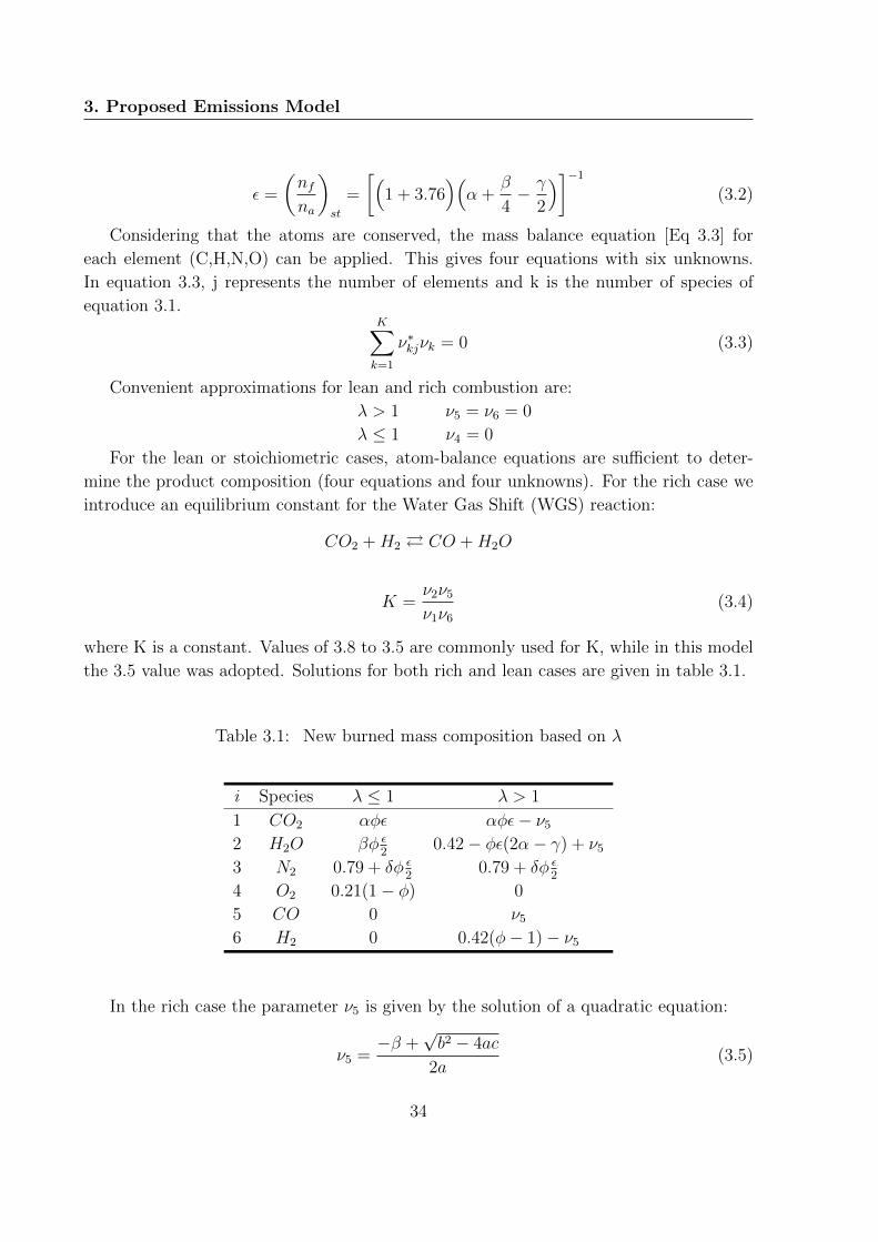
3. Proposed Emissions Model
ε =
(nfna
)st
=
[(1 + 3.76
)(α +
β
4− γ
2
)]−1(3.2)
Considering that the atoms are conserved, the mass balance equation [Eq 3.3] for
each element (C,H,N,O) can be applied. This gives four equations with six unknowns.
In equation 3.3, j represents the number of elements and k is the number of species of
equation 3.1.K∑k=1
ν∗kjνk = 0 (3.3)
Convenient approximations for lean and rich combustion are:
λ > 1 ν5 = ν6 = 0
λ ≤ 1 ν4 = 0
For the lean or stoichiometric cases, atom-balance equations are sufficient to deter-
mine the product composition (four equations and four unknowns). For the rich case we
introduce an equilibrium constant for the Water Gas Shift (WGS) reaction:
CO2 +H2 � CO +H2O
K =ν2ν5ν1ν6
(3.4)
where K is a constant. Values of 3.8 to 3.5 are commonly used for K, while in this model
the 3.5 value was adopted. Solutions for both rich and lean cases are given in table 3.1.
Table 3.1: New burned mass composition based on λ
i Species λ ≤ 1 λ > 1
1 CO2 αφε αφε− ν52 H2O βφ ε
20.42− φε(2α− γ) + ν5
3 N2 0.79 + δφ ε2
0.79 + δφ ε2
4 O2 0.21(1− φ) 0
5 CO 0 ν56 H2 0 0.42(φ− 1)− ν5
In the rich case the parameter ν5 is given by the solution of a quadratic equation:
ν5 =−β +
√b2 − 4ac
2a(3.5)
34

3.2. Emission Model
where
a = 1−Kb = 0.42− φε
(2α− γ
)+K
[0.42big(φ− 1
)+ αφε
]c = −0.42αφε
(φ− 1
)K
In reciprocating engines, residual gas is well mixed with the fresh fuel/air mixture. At
each crank angle step, the new burned mass consists of the combustion products and the
residual gas products. Ferguson [102] has presented a subroutine for the calculation of
the composition of fuel-air residual gas mixtures. By rewriting the combustion equation
3.1 it gives us:
φεCαHβOγHδ + ν ′4O2 + ν ′3N2 → ν ′′1CO2 + ν ′′2H2O + ν ′′3N2 + ν ′′4O2 + ν ′′5CO + ν ′′6H2 (3.6)
where
ν ′: reactant coefficient
ν ′′: product coefficient
Adopting similar notation for other symbols, it should be clear that for a mixture of
residual gas and premixed fuel-air, the mass fraction which finally enters the burned zone
is given by equation 3.7.
yi = (1− f)y′i + fy′′i (3.7)
Similarly, the species molar fractions are given by equation 3.8:
xi = (1− xr)x′i + xrx′′i (3.8)
where the residual mole fraction is:
xr =
[1 +
M ′′
M ′
(1
f− 1
)](3.9)
3.2.1.2 Inlet/Outlet Concentrations
By the time the combustion starts, it is assumed that air, fuel and residual gas are perfectly
mixed. During the combustion process, the cylinder mass is divided into the burned and
unburned zones, while the mass balance is described by equation 3.10. Although during
the combustion process the cylinder pressure increases remarkably, which benefits the
blow-by of the cylinder mass through crevices, in this model it is assumed that blowby
does not occur. Thus, at each crank angle step, the new burned mass that enters the
burned zone is equal to the unburned mass that ”leaves” the fresh zone (eq. 3.11).
dmcyl
dϑ=dmb
dϑ+dmu
dϑ+dmbb
dϑ(3.10)
35

3. Proposed Emissions Model
dmb
dϑ= −dmu
dϑ(3.11)
In the previous section it was presented that the new burned mass that enters the
burned zone consists of six (6) species (CO2,CO,H2O,H2,O2,N2) which originate from the
fuel-air reaction and the residual gas of the fresh zone. These new species are assumed
to be perfectly mixed with the fifty three (53) species that burned zone consists of, so as
the sum of all the constituent mass fractions must be unity (eq 3.12).∑i
Yi = 1 (3.12)
The homogeneous reactor solver requires the mole fractions of the 53 species. The
mass fraction is converted to mole fraction by using the molecular mass of the species of
interest and of the mixture:
χi =YiMWmix
MWi
(3.13)
where the mixture molecular mass is given by equation 3.14:
MWmix =1∑
i
(Yi/MWi
) (3.14)
3.2.2 Energy Balance
There are many possibilities for the chemical kinetics problems that one may need to
solve for various applications (Appendix A). In this case, where SENKIN is used for the
prediction of pollutant formation, it is considered that the pressure and temperature of
the system are constant. In fact, heat release, pressure and burned zone temperature are
calculated by the two zone combustion model. In such cases, where the pressure is held
constant, the energy equation is replaced by the condition that the temperature is known.
Therefore, the calculated burned zone temperature is considered.
3.3 Validation Data
Experimental data are necessary for the validation of the model presented in this chapter.
Ball et al. [12] used experimental data from a Rover K4 optical engine in order to perform
combustion analysis in a SI engine and to correlate the combustion process with the NO
emissions. The fuel used in those experiments was methane. That engine from the Ball
et al. work is simulated in the present study, as many engine specifications necessary for
the modeling are contained in that publication and are summarized in table 3.2. The
36
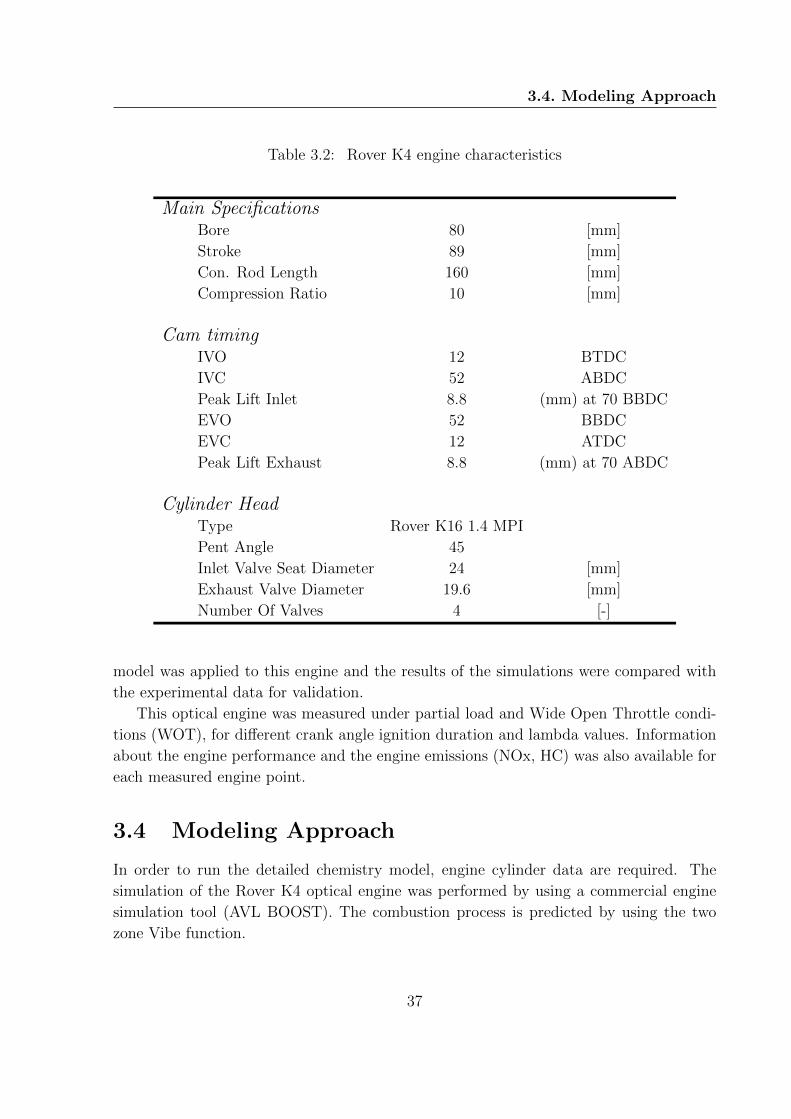
3.4. Modeling Approach
Table 3.2: Rover K4 engine characteristics
Main SpecificationsBore 80 [mm]
Stroke 89 [mm]
Con. Rod Length 160 [mm]
Compression Ratio 10 [mm]
Cam timingIVO 12 BTDC
IVC 52 ABDC
Peak Lift Inlet 8.8 (mm) at 70 BBDC
EVO 52 BBDC
EVC 12 ATDC
Peak Lift Exhaust 8.8 (mm) at 70 ABDC
Cylinder HeadType Rover K16 1.4 MPI
Pent Angle 45
Inlet Valve Seat Diameter 24 [mm]
Exhaust Valve Diameter 19.6 [mm]
Number Of Valves 4 [-]
model was applied to this engine and the results of the simulations were compared with
the experimental data for validation.
This optical engine was measured under partial load and Wide Open Throttle condi-
tions (WOT), for different crank angle ignition duration and lambda values. Information
about the engine performance and the engine emissions (NOx, HC) was also available for
each measured engine point.
3.4 Modeling Approach
In order to run the detailed chemistry model, engine cylinder data are required. The
simulation of the Rover K4 optical engine was performed by using a commercial engine
simulation tool (AVL BOOST). The combustion process is predicted by using the two
zone Vibe function.
37

3. Proposed Emissions Model
3.4.1 Engine Model
As already mentioned, the commercial engine simulation package AVL BOOST is applied
for the simulation of the single cylinder SI engine. The model configuration is illustrated
on figure 3.2.
Figure 3.2: Schematic of the Rover K4 model developed in BOOST.
The simulation calculates the heat release rate and the in-cylinder thermodynamic
properties. The combustion submodel used for the prediction of heat release was a two-
zone Vibe model. The Vibe function describes the MFB at a given crank angle [46]:
Qf
(ϑ)
Qf,total
= 1− e−a
(ϑ−ϑSOI∆ϑCD
)m+1
(3.15)
In equation 3.15, ϑSOI is the degree of crank angle where ignition starts, ϑCD is the
duration of combustion in crank angle degrees, m is the shape parameter for Vibe function,
and a is the Vibe combustion efficiency parameter.
The two-zone approach consists of a burned zone with a calculated burned temperature
for the combustion products and an unburned zone with a unburned temperature for
the fresh compressed mixture and any residuals from the previous combustion cycle. A
uniform pressure for both zones is assumed. As Vibe function is an empirical model
and not a ”physical” model, it was used in this study for the estimation of the pressure
and temperature history at each operating point and not for further detailed combustion
investigation.
3.4.2 Modeling Assumptions
The following assumptions are considered in this modeling approach:
38

3.5. Emission Model Validation
1. uniform pressure in the cylinder (burned and unburned zone at the same pressure);
2. a complete combustion of hydrocarbon fuel with air;
3. uniform composition in the burned zone;
4. NOx emissions solely consisting of NO.
The validity and impact of these assumptions in the final results is investigated in the
results section.
3.4.3 Coupling Simulation
The coupling between the BOOST model and the detailed chemistry model is performed
offline. Firstly the thermodynamic characteristics of the cylinder are calculated by the
engine simulation tool, then the crank angle series data of the cylinder pressure, the
burned zone temperature and the MFB during the combustion phase are imported in the
emission model as a post processing procedure. The final NO emissions are calculated at
the end of the closed thermodynamic cycle, when the exhaust valves open.
3.5 Emission Model Validation
3.5.1 Mean Cycle Validation
The Rover K4 was simulated with the AVL BOOST model for mean cycle Vibe parameters
and the results were compared with the experimental cycle-averaged engine data found in
Ball et al. [12]. The comparison between experimental and simulated data refers to the
IMEP, the maximum pressure during the combustion phase, the crank-angle degree where
maximum pressure occurs, and the crank angle degree where 10% of MFB is observed. All
these data are presented in table 3.3. The designation of each point in table 3.3 is done
with the P and W initials corresponding to partial load or wide open throttle operation,
respectively, followed by two digits corresponding to the lambda value (10 corresponding
to λ = 1 and 15 corresponding to λ = 1.5), followed by two digits of crank angle degree
where ignition starts before top dead center.
The predicted thermodynamic data of the ten simulated operating points were used
as an input for the NO prediction. The simulated NO emissions are compared with the
experimental NO emissions in figure 3.3 for stoichiometric combustion and in figure 3.4
for lean combustion. In stoichiometric combustion, NO predictions are shown with and
without the effect of the prompt mechanism. The prompt mechanism has been switched
off by zeroing the HCN radicals in the chemical mechanism.
39
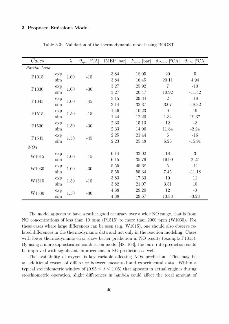
3. Proposed Emissions Model
Table 3.3: Validation of the thermodynamic model using BOOST.
Cases λ ϑign [oCA] IMEP [bar] Pmax [bar] ϑPmax [oCA] ϑ10% [oCA]
Partial Load
P1015exp
1.00 -153.84 18.05 20 5
sim 3.84 16.45 20.11 4.94
P1030exp
1.00 -303.27 25.92 7 -10
sim 3.27 20.47 10.92 -11.42
P1045exp
1.00 -453.15 29.34 2 -18
sim 3.14 32.37 3.07 -18.32
P1515exp
1.50 -151.46 10.23 0 19
sim 1.44 12.20 1.34 19.37
P1530exp
1.50 -302.33 15.13 12 -2
sim 2.33 14.96 11.84 -2.24
P1545exp
1.50 -452.25 21.44 6 -16
sim 2.23 25.48 6.26 -15.91
WOT
W1015exp
1.00 -156.14 33.02 18 3
sim 6.15 35.76 19.99 2.27
W1030exp
1.00 -305.55 45.68 5 -11
sim 5.55 55.34 7.45 -11.18
W1515exp
1.50 -153.83 17.33 10 11
sim 3.82 21.07 3.51 10
W1530exp
1.50 -304.38 29.20 12 -3
sim 4.38 29.67 13.83 -3.23
The model appears to have a rather good accuracy over a wide NO range, that is from
NO concentrations of less than 10 ppm (P1515) to more than 2000 ppm (W1030). For
these cases where large differences can be seen (e.g. W1015), one should also observe re-
lated differences in the thermodynamic data and not only in the reaction modeling. Cases
with lower thermodynamic error show better prediction in NO results (example P1015).
By using a more sophisticated combustion model [48, 103], the burn rate prediction could
be improved with significant improvement in NO prediction as well.
The availability of oxygen is key variable affecting NOx prediction. This may be
an additional reason of difference between measured and experimental data. Within a
typical stoichiometric window of (0.95 ≤ λ ≤ 1.05) that appears in actual engines during
stoichiometric operation, slight differences in lambda could affect the total amount of
40

3.5. Emission Model Validation
Figure 3.3: Comparison of measured and simulated NO molar fractions for stoichiometric
combustion (λ=1.0). Results without prompt mechanism are also presented.
NOx formed during combustion. The stoichiometric cases of the experimental data were
also simulated with a slightly rich (λ = 0.95) and slightly lean (λ = 1.05) mixture. The
results are presented in figure 3.5. It is observed that the measured NOx concentration
is almost always between these slightly lean and rich simulated values. Hence, slight
departures from the set lambda in the experimental data may be a significant reason for
the difference between experiment and simulation.
Figure 3.3 also shows that the prompt mechanism increases the total amount of NOx
concentrations by 10%-15% in case of stoichiometric combustion. Including the prompt
formation one can increase the accuracy of the chemical mechanism. Bachmaier et al. [24]
used an experimental configuration to define the equivalence ratio in which the prompt
mechanism becomes significant in terms of total NOx formation for various hydrocarbon
mixtures. They found that the prompt NO formation starts to become significant as the
mixture moves towards stoichiometry from λ = 1.33, in the case of methane. The prompt
mechanism was negligible for leaner (λ ≥ 1.5) conditions. Our results confirm the signif-
icance of the prompt mechanism in addition to the thermal one, even for stoichiometric
combustion.
The thermodynamic input scenario is also important in lean conditions; however the
oxygen availability does not affect the final results as much as in the stoichiometric case.
41
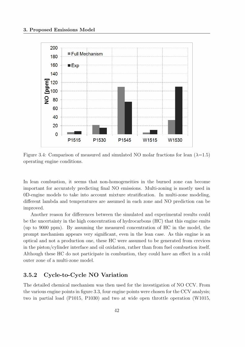
3. Proposed Emissions Model
Figure 3.4: Comparison of measured and simulated NO molar fractions for lean (λ=1.5)
operating engine conditions.
In lean combustion, it seems that non-homogeneities in the burned zone can become
important for accurately predicting final NO emissions. Multi-zoning is mostly used in
0D-engine models to take into account mixture stratification. In multi-zone modeling,
different lambda and temperatures are assumed in each zone and NO prediction can be
improved.
Another reason for differences between the simulated and experimental results could
be the uncertainty in the high concentration of hydrocarbons (HC) that this engine emits
(up to 9000 ppm). By assuming the measured concentration of HC in the model, the
prompt mechanism appears very significant, even in the lean case. As this engine is an
optical and not a production one, these HC were assumed to be generated from crevices
in the piston/cylinder interface and oil oxidation, rather than from fuel combustion itself.
Although these HC do not participate in combustion, they could have an effect in a cold
outer zone of a multi-zone model.
3.5.2 Cycle-to-Cycle NO Variation
The detailed chemical mechanism was then used for the investigation of NO CCV. From
the various engine points in figure 3.3, four engine points were chosen for the CCV analysis;
two in partial load (P1015, P1030) and two at wide open throttle operation (W1015,
42

3.5. Emission Model Validation
Figure 3.5: Impact of slight stoichiometry variation on NO formation.
W1030). All engine points were selected in stoichiometric conditions, to also include the
effect of the prompt mechanism in NO formation.
NO variability was investigated using a statistical analysis. Vibe combustion param-
eters such as the ignition timing (SOI), the CD and the Vibe shape coefficient (m) were
randomly varied within limits, assuming that these parameters follow a normal distribu-
tion. The mean values for these distributions were equal to the values used in the case
of mean cycle modeling. The range of the variation considered was taken from a relevant
analysis in the framework of the FP6 LESSCCV research project [104] and differed for
partial load and WOT operation. Full load points correspond to higher CCV than low
load engine points [10]. One hundred engine cycles were simulated in each engine point
and the results of imep and NOx concentrations are presented in distributions. Differences
between mean cycle indices and CCV values are discussed.
Cycle-to-cycle variation of pressure and temperature are illustrated in figures 3.6a and
3.6b, respectively, for the engine point of partial load and ignition timing of 15o BTDC
(P1015). The mean value of maximum pressure is 16.6 bar and the standard deviation is
0.98 bar, while the peak temperature has a mean value of 2172 K and a standard deviation
of 20 K.
Figures 3.6c and 3.6d illustrate the distributions of imep and NO concentration, re-
spectively, for the same engine point (P1015), due to the variation of the combustion
43
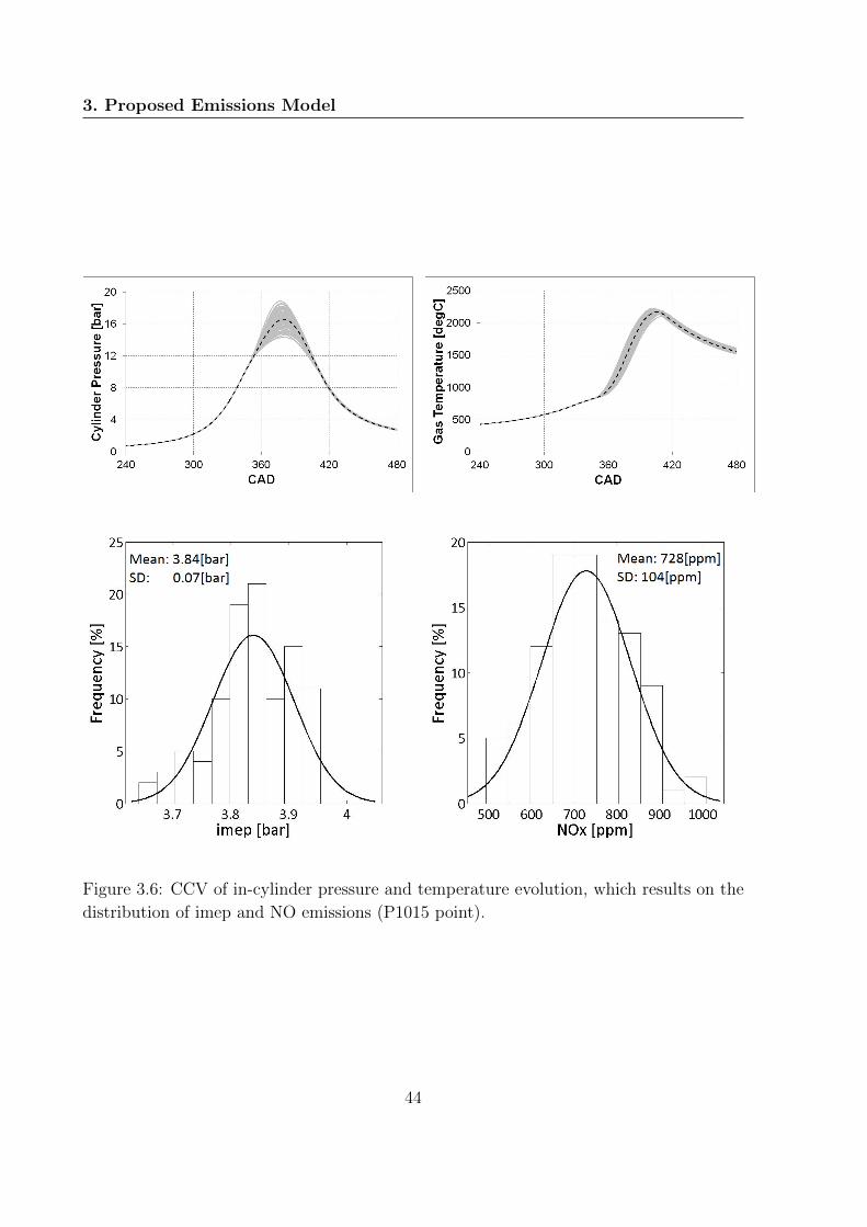
3. Proposed Emissions Model
Figure 3.6: CCV of in-cylinder pressure and temperature evolution, which results on the
distribution of imep and NO emissions (P1015 point).
44

3.5. Emission Model Validation
parameters. Both figures include the statistical characteristics of the distributions such
as the mean value and the Standard Deviation (SD). Mean Cycle imep (MC imep) and
the mean imep value of the CCV analysis coincide perfectly, while MC NOx value and
CCV mean NOx value seems to have a slight deviation.
The same approach was also followed for the operation point at partial load (P1030)
with ignition timing 30o BTDC. The peak pressure distribution has a mean value of 20.6
bar and the standard deviation is 1.05 bar. The peak temperature has a mean of 2173 K
and 30 K respectively. Distributions of this engine point for imep present no difference
for the MC imep and the CCV imep value. In the case of NO, a small difference between
MC NOx and CCV NOx values is again shown.
In the case of WOT, the same approach with a higher range of Vibe parameters
was used for the CCV analysis. Pressure and temperature plots of the engine point
of 30o BTDC (W1030) are presented in figures 3.7a and 3.7b, respectively. Pressure and
temperature peak values have a higher range as a result of higher range in the combustion
parameters. In the case of W1015, the mean value of the maximum pressure is 35.7 bar
and SD is equal with 3.1 bar, while the peak temperature varies from 2121 K to 2310 K
with a mean value and standard deviation equal with 2200 K and 39 K, respectively. Same
order of magnitude differences are noticed for the case of W1030, where peak pressure
varies from 45.5 bar to 61.7 bar (mean 55.5 bar, standard deviation 2.9 bar) and peak
temperature varies from 2281 K to 2503 K (mean 2410 K, standard deviation 42 K).
The distributions of imep and NO are illustrated in figures 3.7c and 3.7d. Due to
higher CCV, MC imep and CCV imep are slightly different in both cases. Thus, MC
NOx value and CCV NOx values present a higher deviation compared with the partial
load. This also indicates that deviation between MC and CCV NO values is affected by
the range of change of the combustion parameters.
3.5.2.1 Contribution of Prompt Mechanism on the CCV of NO Emissions
The impact of the prompt mechanism on NOx CCV has been also investigated. In the
case of mean cycle modeling, it was observed that the prompt mechanism accounts for an
additional 10% to 15% in the final NOx concentration. Therefore, it is expected that the
prompt mechanism should have a corresponding effect on NO CCV.
Figure 3.8 demonstrate the distributions of NO for a partial load and a full load
engine point of CCV analysis, considering only the thermal mechanism. Mean values of
NO distribution show a decrease compared to the mean CCV NO values using the full
mechanism. In addition, for the case of using the detailed chemical mechanism without
the prompt one, a slight difference between MC NO values and CCV NO values is also
observed. However, the prompt mechanism has an additional impact in the statistic
characteristics of the NO distribution, which is described in the next section.
45

3. Proposed Emissions Model
Figure 3.7: CCV of in-cylinder pressure and temperature evolution, which results on the
distribution of imep and NO emissions (W1030 point).
46

3.5. Emission Model Validation
Table 3.4: Comparison of COV values for imep and NO with and without the prompt
mechanism.
Cases COVimep [%]COVNO [%] COVNO [%]
(Full model) (w/o prompt)
P1015 1.81 14.30 14.35
P1030 0.84 14.50 13.77
W1015 0.81 26.03 26.89
W1030 3.81 11.71 16.94
3.5.3 Deviation Between Mean Cycle Values and Mean CCV
Values
CCV does not only result in a range of values for NOx emissions but, due to the non-
linearity of NOx formation with combustion parameters and primarily with temperature,
it may also have an impact on the average NOx emitted. Hence, comparison between
cycle- averaged values and the mean CCV value is important.
Table 3.5: Comparison of mean cycle values (MC) and mean CCV values for imep and
NO with and without the prompt mechanism.
Points CasesIMEP
Diff [%]NO [ppm]
Diff [%]NO [ppm]
Diff [%][bar] (Full model) (w/o prompt)
P1015MC 3.84
0.00735
0.99623
1.71CCV 3.84 728 613
P1030MC 3.27
0.001320
0.651230
4.14CCV 3.27 1311 1181
W1015MC 6.15
0.49646
2.02516
1.78CCV 6.12 633 507
W1030MC 5.55
0.901990
8.051720
0.97CCV 5.5 1842 1703
Partial load and full load are two cases that exhibit different variability for the com-
bustion parameters. In partial load, the mean value of imep CCV distribution is almost
the same to the mean cycle imep value. On the other hand, the CCV imep values are
always lower than the mean cycle imep values in full load operation (Table 3.5). This
47

3. Proposed Emissions Model
(a) P1015 point. (b) W1030 point.
Figure 3.8: CCV NO distribution w/o the prompt mechanism.
means that the impact of CCV on average is a degradation of the engine performance.
NO formation is also affected by the variability in the combustion parameters. Both
in full and partial load CCV NOx values are always less than MC NOx values, which
reflects the CCV impact in NO formation (Table 3.5). In WOT operation, this impact is
higher than in partial load. This result is related with the nonlinearity of NO formation
and for this reason it can not quantitatively correlated with imep variation. As shown in
Table 4, the higher the difference between CCV imep and MC imep is, the higher is this
difference between CCV NOx and MC NOx, too.
The coefficient of variation is used as a metric of the intention of the NO CCV in table
3.4. The impact of the prompt mechanism is also separated in this table. NO in general
presents higher variability due to CCV than imep does. Also, the results show that it
is not possible to establish a direct link between imep CCV and NO CCV. The latter
is dependant on both the operation point and the CCV of imep. Finally, the impact of
the prompt mechanism on CCV is also specific to the engine point considered. In one
of the WOT conditions examined, the prompt mechanism led to a significant increase in
NO CCV, that is not obvious in the other cases. This means that the combination of
heat release rate with reaction kinetics is unique for each engine point that results to a
behaviour which cannot be generalized at this stage. Simulations with other engines and
further refinements in the model may lead to a more consistent behaviour of CCV NO
with CCV in other combustion parameters.
48

3.6. Conclusions
3.6 Conclusions
This chapter presents the mathematical backround of the proposed detailed chemistry
emission model. The model simulates the burned zone as a well-stirred reactor and
utilizes a chemical mechanism for the prediction of homogeneous engine-out emissions.
The emission model can predict NO, CO and other engine-out emissions, however in this
chapter the NOx prediction was preliminary presented.
Literature experimental data were used for the validation of the detailed chemistry
model, assuming steady state conditions. The model satisfactorily predicts NO emissions,
ranging from a few ppm to a couple of thousand of ppm of NO molar fraction, in both sto-
ichiometric and lean conditions and under various ignition timing conditions. Cases with
over 10% error were considered to be either inaccurately thermodynamically simulated or
highly affected by minor mixture lambda fluctuations.
Then, the validated model was used for the simulation of NO variation due to com-
bustion CCV. It was found that CCV NO distributions exhibit a higher COV compared
to the IMEP distributions. In addition, mean CCV NO values are always lower than
the average cycle NO values up to 8%. This clearly declares that elimination of engine
combustion variability could reduce NOx emissions.
Finally, the impact of prompt mechanism in NO cyclic emission variability was also
investigated. The detailed chemistry model was employed without considering the prompt
chemical pathway, which gave a up to 15% deviation on mean cycle NOx prediction
from the ”full model” at stoichiometric conditions. In the case of CCV investigation,
it was found that the prompt mechanism has an impact in the COV and mean value
of NO distributions, although the impact was dependant on the engine operation point
considered.
49

3. Proposed Emissions Model
50
Chapter 4
Experimental Investigation of Cyclic
Emissions Variability
4.1 Introduction
Cycle-to-cycle combustion variation (CCV) is an undesirable characteristic of internal
combustion engines, the origin of which is in detailed presented on chapter 2.3. In this
chapter the impact of various engine operating parameters is explored on performance,
combustion process, early flame kernel development, and especially on pollutants for-
mation of a SI engine on a cycle-to-cycle basis. Although in most of the experimental
studies the CCV trends of various engine calibrations on performance and early flame
kernel are well-known, only a handful number of experimental studies can be found in
published-literature regarding cyclic emissions variability (CEV).
The present work aims at experimentally exploring the impact of various engine operat-
ing parameters on performance, early flame kernel development, and pollutants formation
of a SI engine on a cycle-to-cycle basis. A piezoelectric sensor, integrated in the spark-
plug, and fast response analyzers are employed for the cycle-resolved measurements. The
investigation includes a wide range of engine operating conditions with varying engine
load, equivalence ratio, and ignition timing. The analysis of the results aims at correlat-
ing various interactions among combustion parameters (such as IMEP, maximum pressure
and crank angle of 5% mass fraction burned), and pollutant emissions (NO, CO, CO2).
The overall objective of this study is primarily to explain how combustion variability
affects emissions variability, under various engine operating conditions.
51

4. Experimental Investigation of Cyclic Emissions Variability
4.2 Experimental Set up
4.2.1 Engine Test Bed
The experiments were conducted on an in-line four cylinder PFI SI engine, modified from
an original Honda CBR 600RR motorcycle. Table 4.1 shows the basic features of the
engine. The engine was controlled by an open-access engine control unit (ECU), which
enabled alteration and recording of the entire set of engine parameters (e.g., spark timing,
equivalence ratio, fuel injection timing and duration, etc.) and was connected to a Schenk
steady-state hydraulic brake. The fuel used was a market gasoline with a nominal octane
number of 98 RON.
Table 4.1: Honda CBR600 engine characteristics
Main SpecificationsBore 67 [mm]
Stroke 42.5 [mm]
Con. Rod Length 91.8 [mm]
Compression Ratio 12.2 [mm]
Cam timingIVO 67 BTDC
IVC 42.5 ABDC
EVO 91.8 BBDC
EVC 12.2 ATDC
Valvetrain Chain driven, DOHC
Cylinder HeadType Honda CBR 600RR
Inlet Valve Diameter 26 [mm]
Exhaust Valve Diameter 22.5 [mm]
Number Of Valves 4
Fuel SystemFuel Delivery Port Fuel Injection
52

4.2. Experimental Set up
4.2.2 Experimental Configuration
The experimental configuration is schematically illustrated in figure 4.1. The measure-
ments involved recording of two sets of parameters, one at high and the other at low
sampling frequency. High frequency sampling was conducted for cylinder pressure, ex-
haust gas temperature, crankshaft and camshaft position and cycle resolved emissions
such as CO, CO2, NO and NOx. Pollutants measurement was conducted in the exhaust
manifold directly downstream of the exhaust valve. A National Instruments data acquisi-
tion card was used for high frequency sampling, capable of sampling rates up to 500kHz.
In this experimental study, a set of 150 consecutive cycles was sampled at each engine
operating point, while the sampling rate was adjusted to correspond to 23
degree of crank
angle.
Figure 4.1: Schematic of the experimental configuration
The low sampling frequency set of parameters comprised ECU derived signals, includ-
ing lambda value, ignition timing, throttle position, inlet air pressure and temperature
and coolant temperature, all recorded at a frequency of 10Hz. Average CO, CO2, and
HC emissions were also recorded at low frequency in the exhaust tailpipe, upstream of
the muffler.
53

4. Experimental Investigation of Cyclic Emissions Variability
A spark plug with an integrated piezoelectric transducer was used to measure cylinder
pressure. This is manufactured to fit the particular engine cylinder head and can be used
as a direct replacement of the original spark plug. The signal from the transducer was
fed to the charge amplifier. The exhaust gas temperature was measured by a K-type
thermocouple connected to the relevant transducer.
4.2.3 Measurement Protocol
The test protocol consisted of a three dimensional matrix of measurements at different
throttle positions, equivalence ratios, and ignition timings. The selected engine speed
values were 4000, 5000 and 6000 rpm. Throttle positions were varied from 20% and 50%
to 80% of wide open throttle. Three different lambda settings from the whole range of
fuel/air ratios were tested. The target settings were at λ = 0.93 (rich mixture), λ = 1
(stoichiometric mixture) and λ = 1.07 (lean mixture). Finally, different ignition timings
were examined, including the default setting corresponding to maximum breaking torque
(MBT), a 5o [CA] advanced from MBT ignition case and three retarded ignition from
MBT such as 5o, 10o and 15o [CA]. Table 4.2 presents in detail the test conditions at each
engine speed and throttle position operating point.
Table 4.2: Experimental engine test conditions.
CasesEngine Speed [rpm]
4000 5000 6000
TP: 20[%]L/S/R L/S/R L/S/R
+5/MBT/-5/-10/-15 MBT +5/MBT/-5/-10/-15
TP: 50[%]L/S/R L/S/R L/S/R
MBT MBT MBT
TP: 80[%]L/S/R L/S/R L/S/R
+5/MBT/-5/-10/-15 MBT MBT
4.3 Measurements
4.3.1 In cylinder pressure
In-cylinder pressure was measured by a Kistler 6113B spark plug piezoelectric pressure
transducer that was flush mounted on cylinder number 2. The transducer signal was
amplified using a Kistler 5011B charge amplifier and acquired using a data acquisition
54

4.3. Measurements
card, National Instruments 6341 USB module [NI manual], before finally recorded on a
personal computer for processing. Table 4.3 presents the specifications of the cylinder
pressure experimental equipment. As a crankshaft encoder was not available at the time
period the measurements performed, the engine crankshaft and camshaft signals were
used to synchronize the cylinder pressure signal with the crank angle.
Table 4.3: Specifications of the cylinder pressure experimental equipment
Pressure SensorKistler 6113B Pressure Range: 0-200 [bar]
Natural frequency: ∼ 65% [kHz]
Linearity: ≤ ±0.5% FSO
Sensitivity drift: ≤ ±1%
Signal AmplifierKistler 5011B Linearity: ≤ ±0.05% FSO
Error: ≤ ±0.5% FSO
Aquisition CardNI 6341 USB Channels Number: 8 differential
16 single ended
ADC resolution: 16 bit
Sample rate: 500kS/s
Three sets of 150 consecutive in-cylinder pressure cycles were recorded at each operat-
ing point. As the engine dyno was hydraulic, the set with the minimum speed variability
was selected for further processing. From the selected raw data set, in-cylinder measured
pressure is firstly synchronized with the crank angle signal (Fig. 4.2a) and then pres-
sure cycles are rearranged to the same four stroke crank angle reference area (Fig. 4.2b).
Figure 4.2a illustrates a sample pressure cycles for the case of 4000 rpm, 50% throttle
position and rich conditions (λ=0.93). The pressure cycles are then corrected for the drift
in the vertical direction observed at Fig. 4.2a by pegging the total pressure signal to the
MAP index given by ECU. The result of this process is shown in figure 4.2b, where all 150
cycles are superimposed. Finally, the magnitude of the cycle-to-cycle variation at these
operating engine conditions can be clearly seen.
55

4. Experimental Investigation of Cyclic Emissions Variability
(a) Raw data from one set of 150 consecutive
pressure cycles.
(b) Pegging the pressure signal to the MAP
index at IVC.
Figure 4.2: Sample of processing pressure raw data at 4000 rpm, 50% throttle position
and rich operating conditions (λ=0.93).
4.3.2 Engine and Cylinder Emissions
Owing to the rapid fluctuations of emissions, fast response analyzers are required for
the measurement of the cycle resolved emission levels. Fast response analyzers present
short response time step, at the order of few milliseconds, which makes them suitable
for transient emissions studies [105, 106], as well as for the investigation of cycle-to-cycle
pollutants formation [14, 98, 107]. For the cylinder NO/NOx emissions measurements,
a Cambustion CLD400 analyzer was employed, while CO and CO2 measurements were
conducted using the Cambustion NDIR500 analyzer. Figure 4.3a illustrates the position-
ing of the three probes, regarding NO/NOx and CO/CO2 emissions respectively. At
the engine tailpipe, a Signal 3000HM HC analyzer was employed to detect the engine
average HC exhaust concentration level. The second channel of the CO/CO2 detector
also measured engine averaged concentrations just upstream of the exhaust muffler. The
positioning of the HC heated line as well as the CO/CO2 probe and the lambda sensor are
illustrated on Fig. 4.3b. The main technical characteristics of the total exhaust emission
instrumentation are provided by table 4.4.
A fast response NO detector combines the standard CLD measurement technique with
a rapid sampling method, which slightly varies on different instrumentation [99, 108]. This
Cambustion fNOx400 analyzer utilizes the same sampling system of the fast FID, which
is well-proven and details have appeared in many publications [109, 110]. The sampling
system deliver the sample to the chemiluminescence chamber where it is mixed with a
flow of ozone. The resulting chemiluminescent reaction produces photons in the 700-1500
56

4.3. Measurements
Table 4.4: Specifications of the emission gas analyzers and sensors.
NO/NOX analyzerCambustion fNOX400 Response time: NO:4ms / NOX :8ms
Linearity: ≤ ±1% FSO
CO/CO2 analyzerCambustion NDIR-500 Response time: ≤ 8ms
Linearity: ≤ ±2% FSO
HC analyzerSignal-3000HM Response time: l.5 ms
Linearity: ≤ ±0.5% FSO
Lambda SensorBosch LSU 4.2 Lambda Range: 0.65 to ∞
Exhaust Gas Pressure: ≤ 2.5 [bar]
Exhaust Gas Temperature Range: 930oC
(a) Cylinder exhaust emissions sampling. (b) Engine exhaust emissions sampling.
Figure 4.3: Photo from the experimental configuration regarding the positioning of the
probes for the cylinder and engine exhaust emissions sampling.
57

4. Experimental Investigation of Cyclic Emissions Variability
nm wavelength range which are detected with a photomultiplier tube. The linearity of
this device from 0 to 4000 ppm is within 1% (Table 4.4). Additionally, the fNOx400s
gas reaction chamber is housed in a remote sampling head so that sampling from close to
the exhaust system is facilitated. The light is transferred from the reaction chamber to a
photomultiplier in a main control unit via a fibre-optic bundle. The main control unit also
contains the power supply, electronics, ozone generator, and vacuum regulators to operate
the sampling head. This procedure is performed only to measure NO concentration. The
NO2 can be also be measured by using a pre-reaction to convert NO2 in the sample to
NO, where thereafter both NO species can be detected with the same technique, as NOx
emissions. This process, though easily achieved, would cause unacceptable deterioration
in the time response. However, NO typically accounts for more than 95% of the total
NOx emissions produced from SI engines. In this study, one channel for NO measurement
and one for NOx emissions were used. Figure 4.3a illustrates the locations of the two
NOx and NO probes. NO measurement presented response time in the order of 4ms,
while the measurement of the total NOx presented response time in the order of 8ms,
due to the upstream converter. Finally, after the data processing, it was found that the
NOx analyzer response time was not enough to measure cycle to cycle NOx emissions
and therefore it was not used in the results of this experimental study.
CO and CO2 measurements were conducted using the Cambustion NDIR500 analyzer.
This analyzer also comprised two channels, each able of detecting both CO and CO2
signals. CO and CO2 concentrations are determined using the non-dispersive infrared
(NDIR) technique. The sample is drawn through a narrow heated sample probe capillary
in to the low pressure sample optical chamber. Radiation is produced by an Infra-Red
emitter, then directed through the heated gas sample. Optical filters for monitoring the
absorption of IR at suitable wavelengths for CO and CO2 but avoiding interference from
other exhaust gas constituents (e.g. H2O, H2) are mounted in a chopping wheel which
rotates at 15000rpm and is located beneath the optical chamber. A sensitive IR detector
is located beneath the chopping wheel and is therefore exposed to IR radiation referencing
CO, CO2, a reference filter (for feedback control of emitter intensity, monitoring a wave-
length not affected by sample gas constituents) and a blank sector (for feedback control
of detector temperature). The detectors rapidly changing output from the 4 sectors is
digitally transmitted to the main control unit where it is linearised and output as a 0-10V
analogue DC signal. The system has two sample heads, each measuring CO and CO2
simultaneously and therefore four analogue outputs are available. The response time of
the system is less than 8ms (10-90%), while it is achieved by miniaturizing the sampling
system [98, 111, 112]. The first channel measured cyclic resolved cylinder exhaust port
concentrations while the second one measured averaged concentrations just upstream of
the exhaust muffler.
Furthermore, a conventional analyzer was used for the detection of HC average emis-
58

4.3. Measurements
(a) Cambustion fNOx400. (b) Cambustion NDIR500.
Figure 4.4: The Cambustion fast response analyzers
sions at the engine exhaust tailpipe. The Signal 3000HM HC analyzer presents a response
time at the order of 1-2sec. The analyser uses the well established principle of flame ion-
ization to detect volatile organic compounds in a gas stream. The analyzer uses either H2
or H2/He mixture for calibration and detects methane equivalence (C1 base). A double
insulated heated sampling line at a constant temperature of 220o was also used, in order
to avoid condensation of water vapor. Last but not least, at the exhaust pipe, the engine
lambda sensor was also located (Figure 4.3b). The lambda sensor was a wide-band Bosch
LSU 4.2, where its main characteristics are given in table 4.4.
4.3.3 Exhaust Temperature
Cyclic combustion variability results on exhaust gas temperature variability. For the
measurement of this temperature variation, a thin 0.5mm K-type thermocouple was used
together with the relevant transducer Phoenix Contact for exhaust gas temperature mea-
surement. The position of the thermocouple is presented on figure 4.3a, exactly after the
NOx probe. The thermocouple enters the exhaust pipe manifold through a small hole
59
4. Experimental Investigation of Cyclic Emissions Variability
which was locally blocked using cement, in order to avoid exhaust flow blow-by. Finally,
it was found by the recordings that the measured temperature profile was not that much
fast, possibly affected by the exhaust pipe thermal inertia or the thermocouple mass.
Therefore, the measured temperature variability is used as a reference point to validate
the observations of the combustion analysis and no further analysis was performed.
4.3.4 Data Acquisition Card
A National Instruments X-Series 6341 data acquisition (DAQ) card was used for the ac-
quisition of the high frequency engine data. The DAQ device employs eight (8) differential
channels for the recording of the cylinder pressure, the crank angle signal, the camshaft
signal, the temperature as well as the cylinder exhaust emissions such as the NO, NOx,
CO and CO2. As the maximum device sampling rate was 500kS/s, each channel maxi-
mum sampling rate was 62.5kS/s. Regarding the engine speed, the sampling frequency
equation 4.1 determines the maximum crank angle recording step. Maximum crank angle
recording step is increased as rotational engine speed is increased for constant frequency.
The maximum engine speed, based on the test protocol, was 6000 rpm; therefore the
crank angle step that was constantly adopted at all operating conditions was two third of
the crank angle (23
[oCA]).
fs =360 ·N60 ·∆ϑ
=6 ·N∆ϑ
(4.1)
National Instruments LabVIEW is a software development environment for creating
custom applications that interact with real-world data or signals. In this experimental
study, a LabVIEW interface was developed, in order to import, record and plot the eight
differential signals into a computer. Figure 4.5 illustrates the LabVIEW interface which
utilizes the NI DAQ card. Each recording was saved as a separate file, while at each
operating conditions at least two recordings were performed.
4.3.5 Engine Control Unit
The tested Honda engine was controlled by an open access ECU. The MOTEC M800
allowed the control and the recording of the total engine parameters, such as ignition tim-
ing, lambda, throttle position, MAP index, water and oil temperature etc. Additionally,
MOTEC was utilized as a low frequency data acquisition card, as the CO, CO2 and HC
exhaust emissions were recorded by the ECU.
60

4.4. Data Processing
Figure 4.5: The LabVIEW interface and the data acquisition card.
4.4 Data Processing
The collected data were post-processed by using an in-house MATLAB R© code. The
code, initially transforms the recorded signals to physical magnitudes and then matches
in-cylinder pressure with pollutants (NO, NOx, CO, CO2) traces for each individual
engine cycle (chapter 4.4.3). The code performed at each individual cycle combustion
analysis, such as the calculation of the heat release and the ϑ5%, performance analysis,
such as the calculation of the IMEP and emission analysis, such as the calculation of the
cycle-resolved emissions.
4.4.1 Combustion Analysis
The measured in-cylinder pressure and the geometrical characteristics of the combustion
chamber are used for the combustion analysis at each individual cycle. The cylinder
volume and the differential of the cylinder volume can be calculated as follows:
V (ϑ) = Vc +D2π
4s(ϑ) (4.2)
61

4. Experimental Investigation of Cyclic Emissions Variability
dV
dϑ= D2π
4
ds
dϑ(4.3)
where s(ϑ) is the piston position.
Then, the single zone heat release analysis is performed according to Heywood [15]:
dQnet
dϑ=
γ
γ − 1PdV
dϑ+
1
γ − 1VdP
dϑ(4.4)
where P is the measured cylinder pressure, γ is the specific heat ratio and V is the
instantaneous cylinder volume.
Both cylinder temperature and mixture equivalence ratio influence the specific heat
ratio [113, 114], with the effect of the cylinder temperature being more prominent. In this
study, the specific heat ratio was calculated using the empirical formula of Engel [115], as
described by equation 4.5:
γ = γo − k1 exp(−k2T
) (4.5)
where γo is a reference value (γo=1.38), k1 and k2 are constants (0.2 and 900 respec-
tively) and T is the cylinder gas temperature calculated assuming an ideal gas.
The empirical formula of Han et al. [116] was adopted for the calculation of the heat
transfer coefficient. This formula is described in equations 4.6 and 4.7, while the heat
losses to the cylinder wall are calculated by equation 4.8.
hg(ϑ) = 687P (ϑ)0.75U(ϑ)0.75D−0.25T (ϑ)−0.465 (4.6)
U(ϑ) = 0.494Up + 0.73 · 10−6(
1.35PdV
dϑ+V dP
dϑ
)(4.7)
dQwall
dϑ=∑
hg,i · Ai · (Tw,i − Tg) (4.8)
where P is the cylinder pressure, U is the instantaneous mean gas velocity in the
combustion chamber, given from Eq. 4.7, D is the cylinder bore, T is the cylinder gas
temperature, Up is the mean piston speed, A is the combustion chamber surface in contact
with the gas and Tw is the mean cylinder wall temperature, assumed uniform in the whole
combustion chamber.
The gross heat release rate (Eq. 4.9) is calculated as the sum of net heat release rate
(Eq. 4.4) and heat losses (Eq. 4.8). Integrating the gross heat release rate (at each crank
angle step) and dividing by the fuels lower heating value (LHV) provides the fuel mass
burned at each crank angle step (Eq. 4.10).
dQgross
dϑ=dQnet
dϑ+dQwall
dϑ(4.9)
62

4.4. Data Processing
mf =
∑Qgross
LHV(4.10)
By using equation 4.10, the crank angle at which 5% of the fuel mass has been burned
determines the ϑ5%, which characterizes the crank angle that early flame kernel occurs.
4.4.2 Performance Analysis
The measured in-cylinder pressure over the operating cycle of the engine can be used
to calculate the work transfer from the gas to the piston. For the work calculation the
measured cylinder pressure and the calculated cylinder volume (Eq. 4.2) should be used.
The indicated work per cycle Wc,i (per cylinder) is obtained by integrating the term PV
over the entire four-stroke cycle (Eq. 4.11).
Wc,i =
∮PdV (4.11)
imep =
∮PdV
Vd(4.12)
The gross IMEP is defined as the indicated work per unit displacement volume done
by the gas during the compression and expansion stroke (Eq. 4.12). The work per unit
displacement volume required to pump the working fluid into and out of the engine during
the intake and exhaust strokes is termed the pumping mean effective pressure (PMEP).
Finally, the work per unit displacement volume of the whole cycle corresponds to the
net indicated mean effective pressure, and is described by equation 4.13. In this study,
the term of used IMEP corresponds from the IVC to the EVO, which approximately
corresponds the two stroke (compression-expansion) definition.
IMEPnet = IMEP − PMEP (4.13)
4.4.3 Emissions Analysis
The cycle-resolved emissions are synchronized with the measured cylinder pressure from
the same combustion cycle. Figure 4.6 demonstrates an example of processing the traces
of cylinder pressure and NO emissions from the same cylinder. While the exhaust valve
remains closed, the analyzer measures NO levels in the gas remaining in the exhaust
manifold from the preceding cycle. When the exhaust valve opens (EVO), a portion of
in-cylinder gas exits rapidly (blow-down) and washes the old gas out. A delay between
EVO and analyzer response (point A in figure 4.6) is observed, attributed to the finite
time it takes to the exhaust gas to travel between the valve outlet and the sampling
point, and to the instrument response time [14]. During the exhaust stroke and while the
63

4. Experimental Investigation of Cyclic Emissions Variability
exhaust valve closes (EVC), the analyzer signal shows a slight instability (section B-C in
figure 4.6), indicating a variation of NO concentration in the cylinder gas or interference
from flow phenomena in the exhaust port. The shape of this section may vary in each
cycle due to the bulk gas motion and turbulence [108]. After the exhaust valve closes
again for the next cycle, the analyzer signal remains rather constant (part C-D in Figure
4.6). The mean of this rather stable level is taken as the NO emissions of the latest cycle.
Figure 4.6: Typical NO recording in the exhaust with reference to the cylinder pressure.
Similar procedure is followed for the CO and CO2 recorded signals. Regarding the
NOx signal, the corresponding C-D line was found to be either very short or unsteady at
same operating points, due to the higher response time step of the converter and possibly
due to its conflict with the exhaust pressure, as this device was located very close to the
exhaust valve. Therefore, in this study it is assumed that NOx and NO emissions are
equal.
4.4.4 Cyclic Variability
The intensity of the variability is derived from pressure data and it is expressed by the
coefficient of variation (COV) of indicated mean effective pressure in percent, as it is
64

4.5. Results
described by equation 2.17. In this work, COV index is utilized not only for the variability
of performance (IMEP), but also for maximum cylinder pressure (Pmax) and the cycle
resolved NO, CO, and CO2 emissions. The mathematical definitions of mean value (x),
standard deviation (σ) and coefficient of variation (COV) are also presented in 2.
4.5 Results
Variability in combustion evolution manifests itself as a scatter of the measured pressure
traces around the mean pressure curve. In turn, the variation in pressure build-up leads
to variations of engine performance and emissions from cycle to cycle.
Figure 4.7: IMEP and emissions distributions at 4000 rpm, 80% open throttle position,
stoichiometric mixture and MBT ignition timing.
A typical example of combustion, performance, and emission variability is illustrated
on figure 4.7. This refers to an engine speed of 4000 rpm, 80% throttle position, stoi-
chiometric mixture, and MBT ignition timing. The variation of combustion parameters
is significant under these conditions. The mean IMEP value of 8.8 bar varies with a stan-
dard deviation (SD) of 0.3 bar (COVIMEP=3%). NO emissions show an average content
of 1600 ppm and a standard deviation of 300 ppm (COVNO ∼ 19%), CO levels are at an
65

4. Experimental Investigation of Cyclic Emissions Variability
average of 0.87% and a SD equal to 0.20% (COVCO=22.5%), while CO2 is hardly variable
with an average of 12.9% and a SD equal to 0.17% (COVCO2=1.35%). This example
shows that the CCV severity is different for the various parameters of concern.
Figure 4.8: Pressure variability at 4000 rpm, 80% open throttle position, stoichiometric
mixture and MBT ignition timing. Mean pressure curve, maximum and minimum gross
heat release rates for the 150 consecutive cycles are also illustrated.
Figure 4.8 illustrates the variation of cylinder pressure from cycle to cycle for the
previous example, in order to better understand CCV. The maximum cylinder pressure
ranges between 30 and 58 bar with an average at 43 bar. Based on the heat release
analysis model developed, figure 4.8 also shows the burn rates for the highest and lowest
pressure traces in this diagram. High maximum cylinder pressure cycles are related with
fast burn rates. This is because earlier initial flame kernel development leads to timely
combustion evolution before TDC, which results to higher cylinder pressure. On the
other hand, lower maximum cylinder pressure occurs due to slower combustion process;
late early flame kernel development shifts main flame propagation phase significantly after
TDC where cylinder volume increases and suppresses pressure build up. The origins of
these variations are examined in the next sections.
66

4.5. Results
4.5.1 Impact of Engine Load on Variability
In this presented conventional spark ignition (SI) engine, load is controlled by the throttle
valve. At various throttle angles, air and fuel flow are throttled together, so as mixture
composition is essentially unchanged. In fact, throttle valve controls the volumetric ef-
ficiency of the engine, while it also has an impact on residual gas fraction and an effect
on the pressure waves in the intake manifold. The sensitivity of residual gas to intake
pressure has been shown to affect combustion and emission variability [13, 40, 41]. In
this section, the impact of engine load on combustion, performance and emissions cyclic
variability is in detail experimentally investigated.
Figure 4.9: Mean pressure and gross heat release traces for stoichiometric conditions, 4000
rpm, identical spark timing and various throttle positions.
Volumetric efficiency is maximized at wide open throttle (WOT). Figure 4.9 illustrates
the mean imep cycles for 20% and 80% open throttle, 4000 rpm, stoichiometric mixture
and identical ignition timing. It is observed that pressure traces vary even during the
compression stroke, as the trapped mass at 80% TP is higher. However, during the
combustion phase, the difference between the two pressure traces is further increased, not
only due to the higher fuel mass at 80% TP which is burned, but also due to the faster
combustion process at higher engine load. Heat release rate shows that combustion at
67
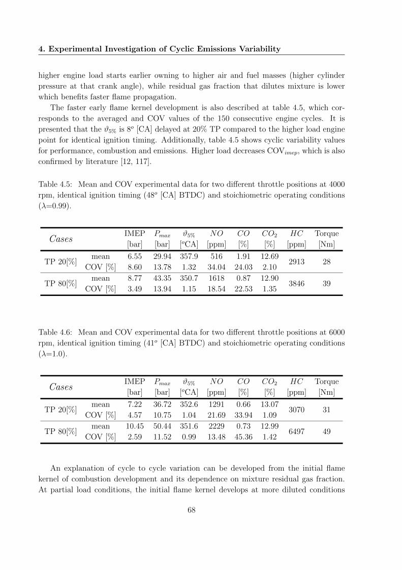
4. Experimental Investigation of Cyclic Emissions Variability
higher engine load starts earlier owning to higher air and fuel masses (higher cylinder
pressure at that crank angle), while residual gas fraction that dilutes mixture is lower
which benefits faster flame propagation.
The faster early flame kernel development is also described at table 4.5, which cor-
responds to the averaged and COV values of the 150 consecutive engine cycles. It is
presented that the ϑ5% is 8o [CA] delayed at 20% TP compared to the higher load engine
point for identical ignition timing. Additionally, table 4.5 shows cyclic variability values
for performance, combustion and emissions. Higher load decreases COVimep, which is also
confirmed by literature [12, 117].
Table 4.5: Mean and COV experimental data for two different throttle positions at 4000
rpm, identical ignition timing (48o [CA] BTDC) and stoichiometric operating conditions
(λ=0.99).
CasesIMEP Pmax ϑ5% NO CO CO2 HC Torque
[bar] [bar] [oCA] [ppm] [%] [%] [ppm] [Nm]
TP 20[%]mean 6.55 29.94 357.9 516 1.91 12.69
2913 28COV [%] 8.60 13.78 1.32 34.04 24.03 2.10
TP 80[%]mean 8.77 43.35 350.7 1618 0.87 12.90
3846 39COV [%] 3.49 13.94 1.15 18.54 22.53 1.35
Table 4.6: Mean and COV experimental data for two different throttle positions at 6000
rpm, identical ignition timing (41o [CA] BTDC) and stoichiometric operating conditions
(λ=1.0).
CasesIMEP Pmax ϑ5% NO CO CO2 HC Torque
[bar] [bar] [oCA] [ppm] [%] [%] [ppm] [Nm]
TP 20[%]mean 7.22 36.72 352.6 1291 0.66 13.07
3070 31COV [%] 4.57 10.75 1.04 21.69 33.94 1.09
TP 80[%]mean 10.45 50.44 351.6 2229 0.73 12.99
6497 49COV [%] 2.59 11.52 0.99 13.48 45.36 1.42
An explanation of cycle to cycle variation can be developed from the initial flame
kernel of combustion development and its dependence on mixture residual gas fraction.
At partial load conditions, the initial flame kernel develops at more diluted conditions
68

4.5. Results
due to the relatively high fraction of residual gas. Figure 4.10 illustrates the relationship
between IMEP for low (TP=20%) and high (TP=80%) engine loads. At 20% throttle
position, ϑ5% is delayed compared to the 80% setting, despite identical ignition timing.
Additionally, at 20% throttle position, ϑ5% presents a higher range of crank angle that it
occurs, compared with the 80% of throttle position. This higher scatter of ϑ5% at low load
conditions is accompanied by a steep decrease of IMEP at very late early flame kernel
cycles.
Figure 4.10: Relationship between IMEP and ϑ5% at 4000 rpm, stoichiometric mixture,
identical ignition timing and various throttle positions (TP: 20% and TP: 80%).
At partial load operating conditions, not only IMEP presents a higher variability
but also emissions present the same trend (Table 4.5). The most significant impact of
engine load on emissions variability is on NO, while CO and CO2 COV slightly vary.
However, it was found a clear index that higher engine load leads to a more stable engine
operation and to lower combustion, performance and emissions CCV (Table 4.5). Figure
4.11 illustrates the relationship between IMEP and NO exhaust content at three different
engine load conditions. The minimum increase of NO at high IMEPs, shows that IMEP
is not a good predictor of NO levels; NO may vary from 1500 to almost 2500 ppm at
an almost constant IMEP close to 9 bar. This plateau could be related with the non
69

4. Experimental Investigation of Cyclic Emissions Variability
Figure 4.11: Relationship between IMEP and NO at 4000 rpm, stoichiometric mixture,
identical ignition timing and various throttle positions.
linear relationship between combustion temperature and NO formation. At high load
conditions, small deviations of the mixture temperature lead to higher scatter of NO
emissions but finally to lower emission variability (Table 4.5).
Nitric oxide is mainly formed at high temperatures, through the well-known Zeldovich
thermal mechanism. Therefore, peak combustion temperature has a remarkable impact
on nitrogen oxidation. Increasing throttle position leads to higher engine load and max-
imum cylinder pressure and also to higher peak combustion temperature. As cylinder
temperature increases, NO emission level also increases for a constant cyclic mixture
composition (figure 4.12). The relationship between maximum cylinder pressure and NO
emissions presents a close to linear trend. In fact, deviations from the linear correlation
occur due to fuel and residual gas variations from cycle to cycle.
Carbon monoxide and carbon dioxide are also affected by engine load. Table 4.5
shows that the average CO emissions are decreased when engine load is increased, which
is accompanied by a minor increase on CO2 concentrations. The latter declares that
completeness of combustion is improved at higher loads, mainly due to the lower residual
gas fraction and the higher combustion temperature. In the same table it is observed that
70

4.5. Results
Figure 4.12: Relationship between Pmax and NO concentration at 4000 rpm, stoichiomet-
ric mixture, identical ignition timing and various throttle positions.
CO variability (COVCO) was found to be slightly decreased at 80% throttle position, while
a clear similar trend is also observed for CO2 variability. Therefore, it is clearly resulted
that residual gas fraction increases combustion, performance and emissions variability and
at higher loads lower COV values can be achieved.
Both table 4.5 and 4.6 present that unburned hydrocarbons are increased at higher
engine load conditions. Higher engine load leads to higher combustion temperature which
benefits the oxidation rate of the fuel hydrocarbons. Therefore, it is clearly believed
that the mechanism which increases the unburned hydrocarbons concentration at higher
engine load condition is through the mixture trapped mass in the crevices. As engine load
is increased, cylinder pressure is also increased which leads more of the air-fuel mixture
into crevices (most significantly the space between the piston crown and cylinder walls),
where the flame is quenched and mixture is left unburned.
Although the trends of the impact of engine load on combustion, performance and
emissions variability are more than clear, it is highly interesting to validate the same
trends at higher engine speed conditions. Table 4.6 presents the impact of engine load on
average and CCV values at 6000 rpm engine operating conditions. Similar to the 4000
71

4. Experimental Investigation of Cyclic Emissions Variability
rpm, variability of IMEP, ϑ5% and NO emissions is decreased at wider open throttle po-
sition. However, it is observed that the variability of CO and CO2 emissions is increased,
conversely to the 4000 rpm observation. This result could be an impact of turbulence in-
tensity on mixing fuel and air, as it is known from other researchers [118] that turbulence
intensity is slightly decreased at higher BMEP (or IMEP), which could affect mixture
homogeneity, completeness of combustion and finally CO and CO2 formation.
4.5.2 Impact of Stoichiometry on Variability
Mixture stoichiometry has a major effect on combustion efficiency and pollutants forma-
tion. On one hand, lean-burn engine operation favors fuel efficiency but diluted mixtures
generally lead to combustion variations, which limit the engine operation range [18]. On
the other hand, rich mixtures ignite easier and lead to more repeatable combustion, with
a cost on fuel consumption.
Figure 4.13: Mean pressure and gross heat release traces for rich, stoichiometric and lean
mixture, 6000 rpm, 80% TP, and identical spark timing.
Mixture composition also has an impact on combustion evolution and appears as an
important source of CCV [119]. Figure 4.13 shows the mean cycle pressure and gross heat
72

4.5. Results
release rate traces for three different mixtures: slightly rich, slightly lean and (almost)
stoichiometric. In all cases, the engine operates at 6000 rpm, 80% throttle position and
constant spark timing. It should be noted here that, owing to the constant throttle
position and the different lambda values, engine load slightly varies. Therefore the results
presented here may also be affected by the slightly differentiated load. The results show
that a slightly rich mixture leads to the maximum cylinder pressure and that leaner
mixtures lead to lower combustion pressure. In fact, both cases of λ=0.92 and λ=0.99
exhibit identical initial early flame kernel development; however in the rich mixture,
flame propagates faster (after the initial flame kernel development) over a smaller cylinder
volume (as the piston is closer to TDC), which leads to higher maximum pressure. On
the other hand, lean mixture not only ignites later but leads to a flame that propagates
at a slower pace.
Figure 4.14: Relationship between ϑ5% and mixture stoichiometry at 6000 rpm, 80% TP
and identical ignition timing.
The observation of the mean cycle heat release rates that mixture lambda has an
impact on combustion process is also validated by the CCV investigation. Initiation of
combustion (ϑ5%) delays when the mixture becomes leaner and this drives the complete
combustion to evolve later (after the TDC). This results to a reduced work by the piston
73

4. Experimental Investigation of Cyclic Emissions Variability
during compression and so is the work done by the piston during the expansion stroke,
which finally leads to a lower IMEP. On the other side, rich mixtures present a more
repeatable (lower scatter of ϑ5%) and initial flame kernel development, which leads to
faster burning rate and finally to high maximum cylinder pressure and a lower scatter of
IMEP. Table 4.7 shows that early flame kernel development presents similar variability
at lean, rich and stoichiometric mixtures, which declares that the observed variability on
combustion, performance and emissions is mainly determined by the mean early flame
kernel value and the impact of mixture lambda on flame propagation.
Table 4.7: Mean and COV experimental data for various mixture lambda operating
conditions at 4000 rpm, 80 % throttle position and identical ignition timing (48o [CA]
BTDC).
CasesIMEP Pmax ϑ5% NO CO CO2 HC Torque
[bar] [bar] [oCA] [ppm] [%] [%] [ppm] [Nm]
λ=0.94mean 8.90 46.95 348.1 1021 2.94 11.90
3913 41COV [%] 2.24 12.64 1.13 17.49 10.45 1.80
λ=1.00mean 8.77 43.35 350.7 1618 0.87 12.90
3846 39COV [%] 3.49 13.94 1.15 18.54 22.53 1.35
λ=1.11mean 8.42 39.90 353.0 1716 0.22 12.63
2911 37COV [%] 5.08 13.11 1.17 26.45 42.57 1.16
Table 4.8: Mean and COV experimental data for various mixture lambda operating
conditions at 6000 rpm, 80 % throttle position and identical ignition timing (41o [CA]
BTDC).
CasesIMEP Pmax ϑ5% NO CO CO2 HC Torque
[bar] [bar] [oCA] [ppm] [%] [%] [ppm] [Nm]
λ=0.92mean 10.70 58.15 348.8 1387 2.91 11.89
6798 49COV [%] 1.71 9.44 0.91 22.44 25.09 3.86
λ=0.99mean 10.50 51.13 351.3 2069 1.06 12.84
6497 49COV [%] 2.62 10.98 0.92 20.10 65.88 2.80
λ=1.06mean 9.87 43.23 354.8 1961 0.26 12.92
5608 46COV [%] 5.22 13.08 1.09 21.91 56.57 1.44
74
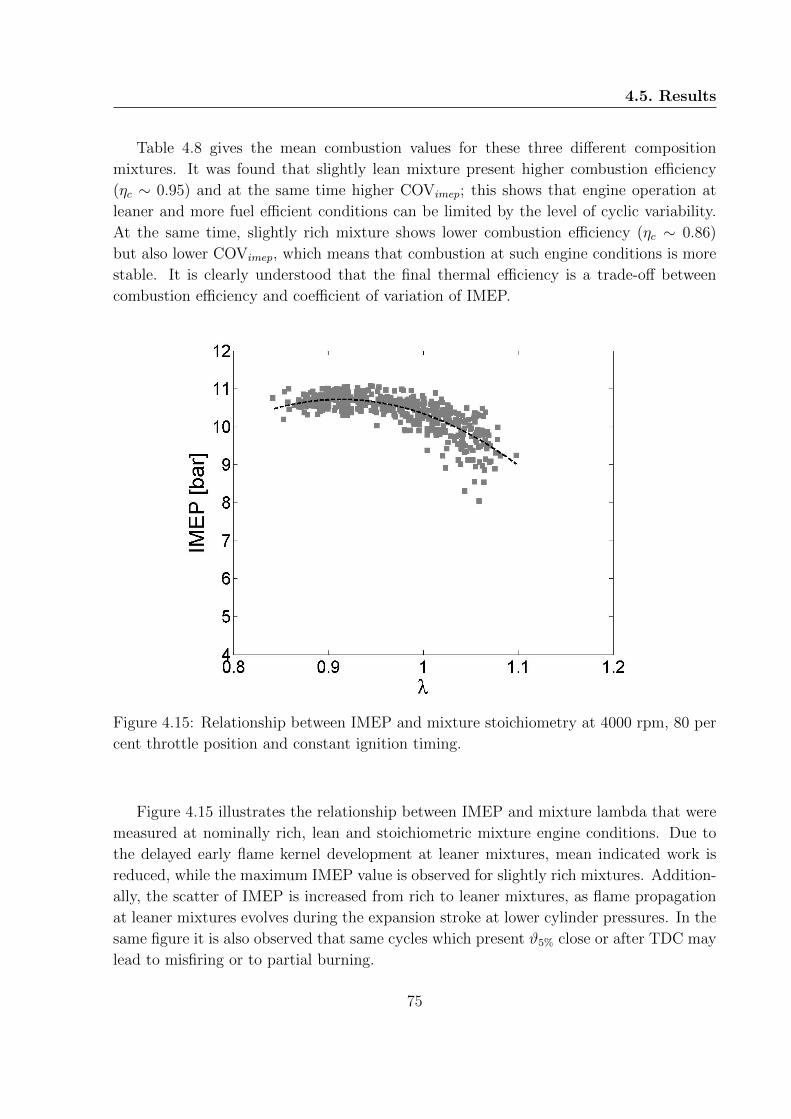
4.5. Results
Table 4.8 gives the mean combustion values for these three different composition
mixtures. It was found that slightly lean mixture present higher combustion efficiency
(ηc ∼ 0.95) and at the same time higher COVimep; this shows that engine operation at
leaner and more fuel efficient conditions can be limited by the level of cyclic variability.
At the same time, slightly rich mixture shows lower combustion efficiency (ηc ∼ 0.86)
but also lower COVimep, which means that combustion at such engine conditions is more
stable. It is clearly understood that the final thermal efficiency is a trade-off between
combustion efficiency and coefficient of variation of IMEP.
Figure 4.15: Relationship between IMEP and mixture stoichiometry at 4000 rpm, 80 per
cent throttle position and constant ignition timing.
Figure 4.15 illustrates the relationship between IMEP and mixture lambda that were
measured at nominally rich, lean and stoichiometric mixture engine conditions. Due to
the delayed early flame kernel development at leaner mixtures, mean indicated work is
reduced, while the maximum IMEP value is observed for slightly rich mixtures. Addition-
ally, the scatter of IMEP is increased from rich to leaner mixtures, as flame propagation
at leaner mixtures evolves during the expansion stroke at lower cylinder pressures. In the
same figure it is also observed that same cycles which present ϑ5% close or after TDC may
lead to misfiring or to partial burning.
75
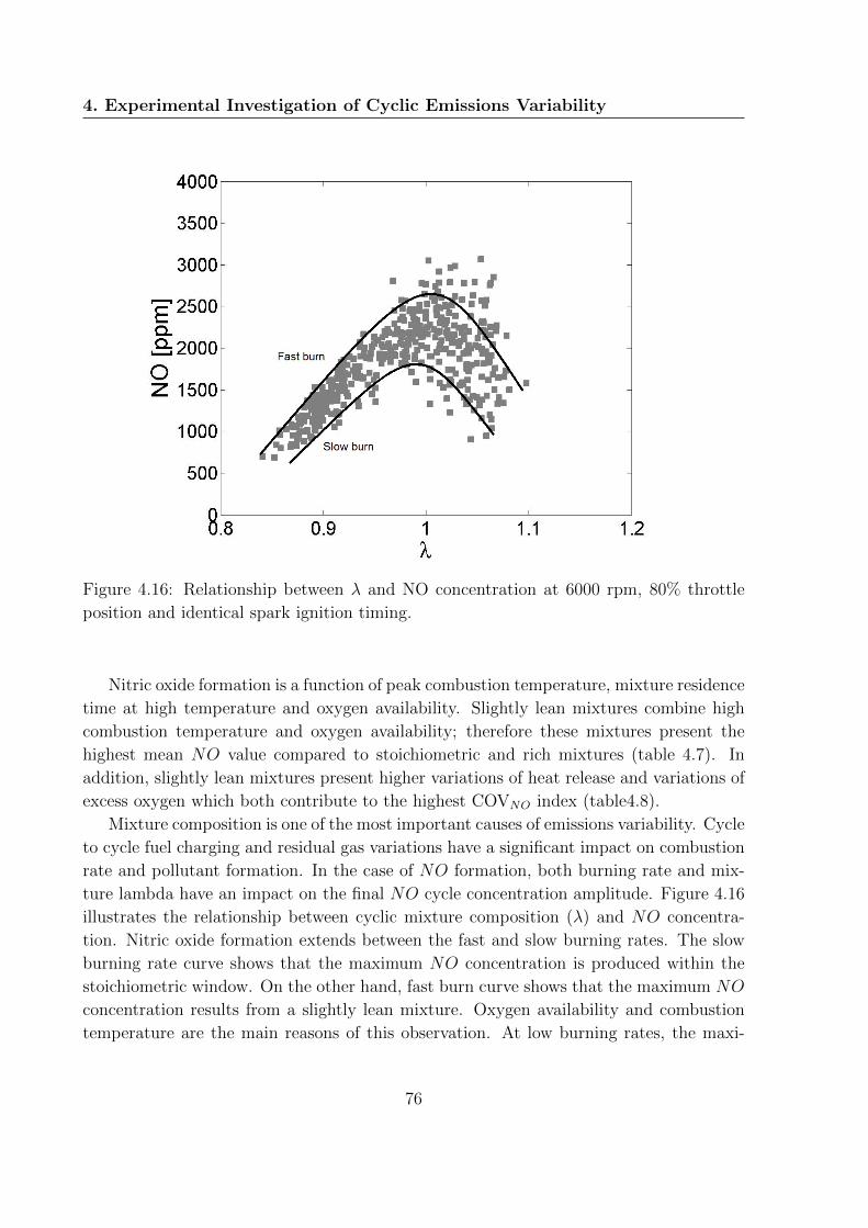
4. Experimental Investigation of Cyclic Emissions Variability
Figure 4.16: Relationship between λ and NO concentration at 6000 rpm, 80% throttle
position and identical spark ignition timing.
Nitric oxide formation is a function of peak combustion temperature, mixture residence
time at high temperature and oxygen availability. Slightly lean mixtures combine high
combustion temperature and oxygen availability; therefore these mixtures present the
highest mean NO value compared to stoichiometric and rich mixtures (table 4.7). In
addition, slightly lean mixtures present higher variations of heat release and variations of
excess oxygen which both contribute to the highest COVNO index (table4.8).
Mixture composition is one of the most important causes of emissions variability. Cycle
to cycle fuel charging and residual gas variations have a significant impact on combustion
rate and pollutant formation. In the case of NO formation, both burning rate and mix-
ture lambda have an impact on the final NO cycle concentration amplitude. Figure 4.16
illustrates the relationship between cyclic mixture composition (λ) and NO concentra-
tion. Nitric oxide formation extends between the fast and slow burning rates. The slow
burning rate curve shows that the maximum NO concentration is produced within the
stoichiometric window. On the other hand, fast burn curve shows that the maximum NO
concentration results from a slightly lean mixture. Oxygen availability and combustion
temperature are the main reasons of this observation. At low burning rates, the maxi-
76

4.5. Results
Figure 4.17: Relationship between NO and early flame kernel development (ϑ5%) at 4000
rpm, 80% TP and identical ignition timing.
mum NO formation is controlled by combustion temperature, while at fast combustion
conditions, this is controlled by oxygen availability. Additionally, as all cycles shown
have the same ignition timing, it has to be concluded that combustion in rich cycles is
more advanced than lean cycles, as equivalence ratio has an impact on laminar flame
speed during early flame kernel development [87]. This behavior is more prominent at the
slow burn limit, also due to the fact that rich cycles present lower combustion variability.
More advanced cycles (which are the rich ones) exhibit higher combustion temperature,
an observation that justifies that NO formation is mainly controlled by combustion tem-
perature at that limit. Nitric oxide variability is also governed by oxygen availability and
combustion temperature. At rich mixture conditions, NO formation presents lower vari-
ation as the faster and slower burning rates do not present significant difference (figure
4.16). On the other hand, stoichiometric and lean mixtures present higher NO emission
variability. As it was revealed in table 4.8 above, stoichiometric and lean mixtures lead
to higher COVimep, translated into more intense combustion variability, which leads to
higher NO emission variability. Finally, figure 4.16 shows that the maximum NO con-
centration is produced by slightly lean mixtures, which is also the area where the higher
77

4. Experimental Investigation of Cyclic Emissions Variability
NO emission variation is observed.
However the question still remains: burn rate or oxygen availability is the most impor-
tant parameter on NO formation. Figure 4.17 illustrates the relationship between nitric
oxide formation and early flame kernel development for rich and lean mixture composi-
tion. In lean mixtures, early flame kernel has a more intensive impact on NO formation
compared to rich operating conditions, mainly due to the excess of oxygen. Cycles that
initial flame kernel occurs early in combination with excess of oxygen benefits the NO
emissions level. Delayed early flame kernel seems to be independent from the overall
mixture equivalence ratio value as the same low NO level is presented at rich and lean
mixtures. In conclusion, oxygen availability significant benefits NO formation at cycles
which present early initial flame kernel and declares fast burning rate. Conversely, excess
of oxygen has no impact on NO formation at cycles which present delayed initial flame
kernel and slow burning rate.
Figure 4.18: Relationships between λ and carbon monoxide and carbon dioxide concen-
trations at 6000 rpm, 80% TP and identical spark ignition timing.
Carbon monoxide is a product of incomplete combustion, due to oxygen depletion in
the bulk flow (rich combustion) or flame quenching (lean combustion), or CO2 dissociation
at high post combustion temperatures. Highest CO levels appear in rich operating condi-
78

4.5. Results
tions where COVCO is minimized (Table 4.8). This is because stoichiometry is basically
the sole parameter affecting CO at rich conditions, while variation of other parameters
may be responsible at stoichiometric and lean conditions. Figure 4.18 illustrates the re-
lationship between measured CO and CO2 at various mixture compositions. CCV of CO
is very low for a given lambda value while it increases exponentially as lambda drops
below unity. Fluctuations of the burn rate and the initial phases of combustion little
affect CO formation, which is known from other studies as well [98, 107]. Similar to CO,
unburned hydrocarbons were maximized at rich conditions due to mixture stoichiometry
(Table 4.8). Therefore, averaged CO2 concentration at that conditions is minimized.
The observed trends for the impact of mixture lambda on combustion and performance
variability are also validated at 4000 rpm and 80% throttle position (Table 4.7). The
minimum COVimep is presented at slightly rich conditions, which is accompanied by the
highest averaged IMEP value. Nitric oxide and carbon monoxide emissions also present
the lowest CCV value at rich conditions, while mixture at rich conditions ignites earlier
(ϑ5%).
4.5.3 Impact of Ignition Timing on Variability
Engine ignition timing setting is usually at the Maximum Braking Torque (MBT) point.
Earlier or later ignition timings lead to lower piston net work. Slightly retarded or ad-
vanced ignition may occur in actual application as a result of random perturbations in
the in-cylinder conditions, such as fuel availability in the spark plug area. Dependence of
combustion and, in particular, emission variability on the ignition timing setting is little
studied in published literature [15, 71].
Table 4.9 shows performance values and emission levels at five different ignition points.
Slightly rich operating conditions were selected in order to limit the effect of lambda fluc-
tuations on the investigation of ignition timing on combustion variability. The maximum
mean IMEP is accompanied by the minimum COVimep at the MBT case. MBT operating
point also presents the minimum COV value for the nitric oxide and carbon monoxide
exhaust gas concentrations. From ”late” to ”early” ignition timings, averaged NO and
CO concentrations are increased, and so does the mean unburned hydrocarbons emissions
measured at the exhaust pipe.
Variations in spark timing lead to heat release rate fluctuations, such as different early
flame kernel phasing and burning rate, which result in different pressure evolutions. Figure
4.19 illustrates the mean pressure trace and gross heat release rate for the same operating
conditions of table 4.9. The MBT ignition timing is the case that presents the higher
average value and the lower COV of IMEP. Advanced ignition timing (MBT +5) presents
the higher maximum cylinder pressure; this occurs because the maximum heat release
rate is achieved before the TDC. In this case, gross heat release traces present that flame
79
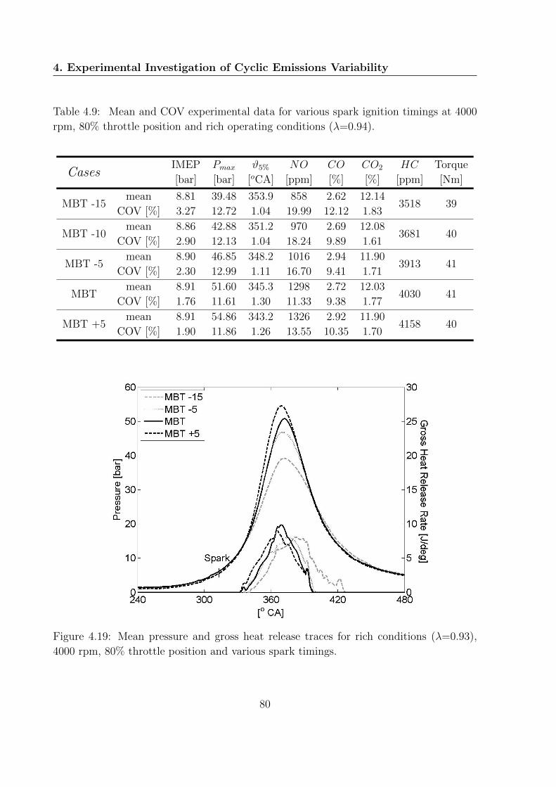
4. Experimental Investigation of Cyclic Emissions Variability
Table 4.9: Mean and COV experimental data for various spark ignition timings at 4000
rpm, 80% throttle position and rich operating conditions (λ=0.94).
CasesIMEP Pmax ϑ5% NO CO CO2 HC Torque
[bar] [bar] [oCA] [ppm] [%] [%] [ppm] [Nm]
MBT -15mean 8.81 39.48 353.9 858 2.62 12.14
3518 39COV [%] 3.27 12.72 1.04 19.99 12.12 1.83
MBT -10mean 8.86 42.88 351.2 970 2.69 12.08
3681 40COV [%] 2.90 12.13 1.04 18.24 9.89 1.61
MBT -5mean 8.90 46.85 348.2 1016 2.94 11.90
3913 41COV [%] 2.30 12.99 1.11 16.70 9.41 1.71
MBTmean 8.91 51.60 345.3 1298 2.72 12.03
4030 41COV [%] 1.76 11.61 1.30 11.33 9.38 1.77
MBT +5mean 8.91 54.86 343.2 1326 2.92 11.90
4158 40COV [%] 1.90 11.86 1.26 13.55 10.35 1.70
Figure 4.19: Mean pressure and gross heat release traces for rich conditions (λ=0.93),
4000 rpm, 80% throttle position and various spark timings.
80

4.5. Results
development and propagation do not have any significant difference with the MBT case,
except from the ignition timing which leads to lower net work during the combustion
cycle. On the other hand, as ignition timing becomes retarded (MBT -5, MBT -15),
maximum cylinder pressure is reduced and occurs later in the cycle. At ”late” ignition,
gross heat release traces present that early flame kernel development takes place close to
TDC, where mixture pressure and temperature are high and this lead to a faster ”ignition”
phase. This could explain the reason why ”MBT -15” case presents a small difference at
the start of heat release rate compared to the other ignition timings. However, the phase
of flame propagation occurs during the expansion of the piston, where pressure increase
during combustion is limited by the volume expansion. This results in a slower burning
rate and a lower peak pressure. In such retarded ignition timing (”MBT -15”), it was also
observed that a few cycles result in incomplete fuel combustion.
Figure 4.20: Relationship between IMEP and maximum cylinder pressure at 4000 rpm,
80% TP and λ=0.94, for different ignition timings.
In most engine operating conditions, ignition timing is usually set at MBT. Figure
4.20 illustrates the relationship between the IMEP and the maximum cylinder pressure
for five different ignition timings. Maximum IMEP is given at the MBT ignition tim-
ing, while advanced ignition timings can lead to higher maximum cylinder pressure but
81

4. Experimental Investigation of Cyclic Emissions Variability
to lower IMEP. In fact, advanced ignition timing over-increases compression work and
although expansion work is also increased, the net work is lower than the MBT case.
Also, with early ignition the peak pressure and temperature may be sufficient to cause
knock, therefore tested ignition cases over ”MBT +5” were avoided in this investigation.
Conversely, retarded ignition leads to lower pressure rise, as combustion evolution occurs
during piston expansion where combustion volume is increased and final maximum cylin-
der pressure and expansion work are also decreased. Finally, it is observed on figure 4.20
that few cycles presented sufficient incomplete combustion that leads to less engine power
and increases IMEP variability.
Figure 4.21: Relationship between ignition delay and maximum cylinder pressure at 4000
rpm, at 4000 rpm, 80% TP and λ=0.94, for different ignition timings.
The effect of ignition timing on burning rate has to be investigated. Figure 4.21
presents the relationship between the required time for the development of the early flame
kernel (ϑ5% - ϑign) and the maximum cylinder pressure (Pmax). Retarded ignition timings
lead to faster development of the ”initial” flame kernel, although they result to a lower
maximum pressure. The spark discharge in relation to piston position can explain this.
Retarded ignition occurs closer to the TDC, where cylinder pressure and temperature are
relatively higher when spark is discharged. The mixture ignites faster but this does not
82
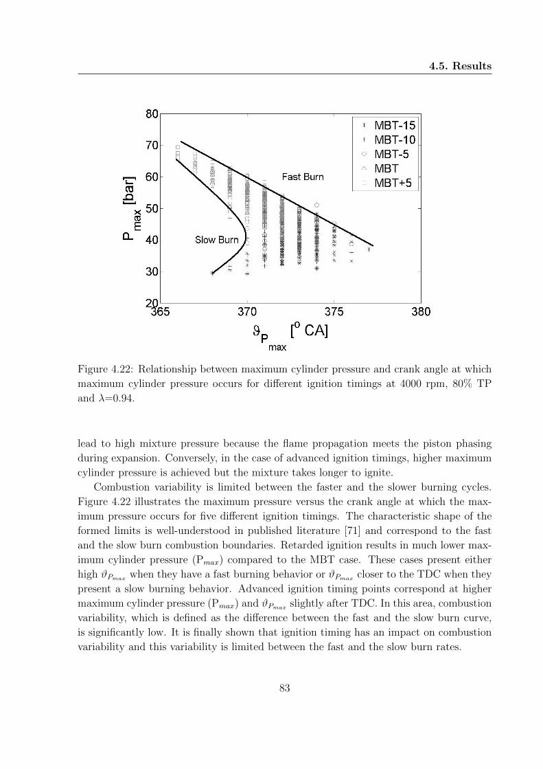
4.5. Results
Figure 4.22: Relationship between maximum cylinder pressure and crank angle at which
maximum cylinder pressure occurs for different ignition timings at 4000 rpm, 80% TP
and λ=0.94.
lead to high mixture pressure because the flame propagation meets the piston phasing
during expansion. Conversely, in the case of advanced ignition timings, higher maximum
cylinder pressure is achieved but the mixture takes longer to ignite.
Combustion variability is limited between the faster and the slower burning cycles.
Figure 4.22 illustrates the maximum pressure versus the crank angle at which the max-
imum pressure occurs for five different ignition timings. The characteristic shape of the
formed limits is well-understood in published literature [71] and correspond to the fast
and the slow burn combustion boundaries. Retarded ignition results in much lower max-
imum cylinder pressure (Pmax) compared to the MBT case. These cases present either
high ϑPmax when they have a fast burning behavior or ϑPmax closer to the TDC when they
present a slow burning behavior. Advanced ignition timing points correspond at higher
maximum cylinder pressure (Pmax) and ϑPmax slightly after TDC. In this area, combustion
variability, which is defined as the difference between the fast and the slow burn curve,
is significantly low. It is finally shown that ignition timing has an impact on combustion
variability and this variability is limited between the fast and the slow burn rates.
83

4. Experimental Investigation of Cyclic Emissions Variability
With regard to ignition timing impact on NO variability, table 4.9 presents that MBT
ignition timing leads to the lowest COVNO, similarly to COVimep. Figure 4.23 illustrates
the relationship between NO and crank angle at which the maximum pressure occurs. The
fast burning rate curve corresponds to higher NO levels, compared to the slow burning
rate. In advanced ignition timings, flame propagation evolves close to or even before TDC,
which results to higher maximum pressure, higher peak combustion temperature and
finally higher level of NO formation. On the other hand, the slow burn limit represents
the incompleteness of combustion; this concludes to lower fuel mass burned per cycle,
lower heat release and finally lower level of nitric oxide formation. As combustion rate
is switched from slow to fast burning rate curve during real operation CCV, nitric oxide
concentration is increased, which declares the relationship between NO formation and
combustion rate.
Figure 4.23: Relationship between NO formed and crank angle at which maximum cylin-
der pressure occurs for different ignition timings at 4000 rpm, 80% TP and λ=0.94.
Ignition timing determines the combustion efficiency and therefore it has an impact
on unburned hydrocarbons and exhaust gas temperature. Table 4.9 shows that retarded
ignition timing leads to lower unburned hydrocarbons concentration, while it was also
found that the mean exhaust temperature was increased by 20K. The same trends are also
84
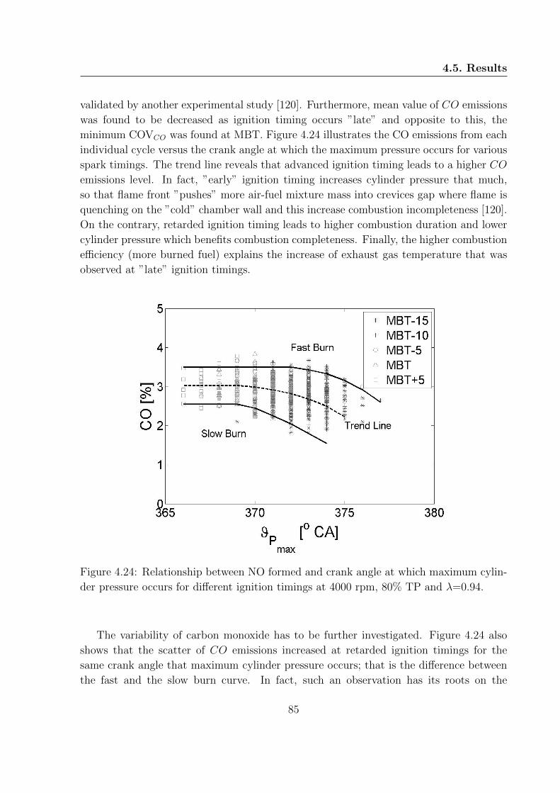
4.5. Results
validated by another experimental study [120]. Furthermore, mean value of CO emissions
was found to be decreased as ignition timing occurs ”late” and opposite to this, the
minimum COVCO was found at MBT. Figure 4.24 illustrates the CO emissions from each
individual cycle versus the crank angle at which the maximum pressure occurs for various
spark timings. The trend line reveals that advanced ignition timing leads to a higher CO
emissions level. In fact, ”early” ignition timing increases cylinder pressure that much,
so that flame front ”pushes” more air-fuel mixture mass into crevices gap where flame is
quenching on the ”cold” chamber wall and this increase combustion incompleteness [120].
On the contrary, retarded ignition timing leads to higher combustion duration and lower
cylinder pressure which benefits combustion completeness. Finally, the higher combustion
efficiency (more burned fuel) explains the increase of exhaust gas temperature that was
observed at ”late” ignition timings.
Figure 4.24: Relationship between NO formed and crank angle at which maximum cylin-
der pressure occurs for different ignition timings at 4000 rpm, 80% TP and λ=0.94.
The variability of carbon monoxide has to be further investigated. Figure 4.24 also
shows that the scatter of CO emissions increased at retarded ignition timings for the
same crank angle that maximum cylinder pressure occurs; that is the difference between
the fast and the slow burn curve. In fact, such an observation has its roots on the
85

4. Experimental Investigation of Cyclic Emissions Variability
Table 4.10: Mean and COV experimental data for various spark ignition timings at 6000
rpm, 20% throttle position and rich operating conditions (λ=0.93).
CasesIMEP Pmax ϑ5% NO CO CO2 HC Torque
[bar] [bar] [oCA] [ppm] [%] [%] [ppm] [Nm]
MBT -15mean 7.45 35.05 356.5 772 1.96 12.61
2973 31COV [%] 3.04 10.51 0.87 22.81 14.15 1.30
MBT -10mean 7.50 39.09 353.3 907 2.77 12.08
3141 32COV [%] 2.96 10.29 0.94 32.08 17.99 2.80
MBT -5mean 7.51 43.14 346.9 1017 2.66 12.11
3261 33COV [%] 2.75 11.35 1.11 23.75 24.74 3.45
MBTmean 7.54 48.38 345.5 1206 2.84 12.00
3497 33COV [%] 2.41 9.05 1.04 22.85 21.47 2.96
MBT +5mean 7.49 52.66 342.9 1410 2.84 12.00
3500 33COV [%] 2.50 9.48 1.02 21.54 22.37 3.03
combustion process, as the achieved cylinder pressure controls the trapped mass into
crevices. Cylinder pressure varies from cycle to cycle and finally the trapped mass and
the completeness of combustion also cyclic varies. Cycles that present higher cylinder
pressure lead to more air-fuel mixture into the piston wall gap that increases CO and HC
emissions while cycles that present lower cylinder pressure have an opposite effect. It is
finally understood that the nature of retarded ignition, which is higher cylinder pressure
variability (COVPmax at table 4.9), is the parameter that leads to higher CO variability
(COVCO).
The impact of ignition timing at combustion and emissions variability has been also in-
vestigated at 6000 rpm and 20% throttle position and rich operating conditions (λ=0.93).
The results of this investigation are briefly presented on table 4.10 and the observed trends
are in agreement with table 4.9. It was found that the MBT case concludes the minimum
COV regarding imep, ϑ5% and emissions. In fact, the lower COVNO is observed at ”MBT
+5” case, however it has to be considered that the observed torque difference between
the two cases is negligible. Unburned hydrocarbons are decreased as ignition timing is re-
tarded, while exhaust temperature was also found to raise. Compared to the table 4.9, the
most important difference is that the COV of carbon monoxide concentrations is higher at
6000 rpm and 20% TP. Although at higher engine speed conditions turbulence intensity
is increased which improves homogeneity and CO consumption, the higher residual gas
fraction at partial load conditions leads to higher COVCO.
86
4.6. Conclusions
4.6 Conclusions
The operation of spark-ignition engines is limited by combustion variations from cycle to
cycle, which results a higher variation on pollutant emissions. In this study, the cycle-
to-cycle variability of NO and CO, as well as of CO2 and HC to a limited extend,
was investigated and the combustion factors which are related with the performance and
emission variability were presented. To that aim, a four cylinder PFI spark ignition engine
was employed, operating in a wide range of load, lambda and ignition timing.
Engine load has a significant impact on the variability of engine performance and
emissions. At low load operating conditions, engine performance variability (COVimep) is
higher. A throttled engine is characterized by higher residual gas fraction which dilutes
mixture and increases combustion and emissions variability. Lower NO mean value was
found at these conditions, due to lower cylinder pressure and mixture temperature, how-
ever the COVNO was higher due to the higher per cent of residual gas and therefore to
the more diluted mixture.
The impact of combustion stoichiometry on the variability of engine performance and
emissions was also investigated. Slightly rich mixtures showed the higher IMEP and
the lower COVimep. Higher variation of combustion in lean mixtures has its roots on
early flame kernel development, as slightly lean mixtures ignite slower and later than
rich ones. This leads to slower flame propagation and lower cylinder pressure. In lean
mixtures, higher variation of the crank angle that early flame kernel development occurs
was detected as the main reason of NO variability, as NO formation depends on burning
rate and mixture temperature.
Last but not least, the impact of ignition timing on the variability of engine per-
formance and emissions has been investigated. MBT ignition timing was found to be
accompanied by the highest IMEP value and the lowest COVIMEP . Advanced ignition
timings are characterized by faster combustion and higher cylinder pressure. On the other
hand,retarded ignition results to a shorter delay in the development of early flame kernel,
as this occurs closer to TDC. At retarded cycles, flame propagation is shifted to the pis-
ton expansion phase, where cylinder volume is increased and finally maximum cylinder
pressure is decreased. Because of the expansion, both cylinder pressure and crank an-
gle at which maximum cylinder pressure occur vary more in each cycle. The significant
variation of cylinder pressure at retarded ignition conditions was found to be the main
source of NO and CO variation in this investigation. On the one hand, NO formation is
strongly linked with the temperature vs time profile, and the higher perturbation of the
latter at retarded cycles is the main root of the high NO variability. On the other hand,
CO variability is linked with the variation of cylinder pressure which affects the trapped
mixture mass into crevices at each cycle and finally the combustion efficiency.
87

4. Experimental Investigation of Cyclic Emissions Variability
88

Chapter 5
Emission Model Validation and
Application for CCV Prediction
5.1 Introduction
This chapter aims to investigate the cyclic emission variability by using the novel emissions
model developed in this study. The new emissions model, which was explicitly presented
on chapter 3 is validated against the experimental data of chapter 4. The results of the
proposed model are compared against the extended Zeldovich mechanism for NO and a
simplified two step reaction kinetic mechanism for CO, which both consist a simplified
modeling approach. The improved predictability of the new model against the simplified
emission model is explored under various engine conditions.
The chapter begins with the detailed presentation of a two zone heat release model.
The model uses the measured cylinder pressure to calculate the net and gross heat release
and the thermodynamic characteristics of the two zones. The two zone thermodynamic
data are utilized not only by the proposed detailed emission model but also by the simpli-
fied model approach. In a first step, the two zone emission model is validated under mean
cycle simulations, and is compared with the simplified emission model. Then, the detailed
emission model is applied on a cyclic emission variability simulation study. Under various
engine operating conditions, the new model is validated against cycle-resolved measured
emission data and is compared with the cyclic prediction of the simplified model. The
comparison between the simplified emissions model and the proposed emissions model
allows to understand whether pollutants formation is primarily a thermodynamic or a
chemistry problem.
89

5. Emission Model Validation and Application for CCV Prediction
5.2 Modeling Approach
The proposed detailed chemistry emission model requires the thermo-physical properties
of the in-cylinder mixture as an input. The cylinder thermodynamic properties are cal-
culated by applying a two zone heat release analysis model on the measured cylinder
pressure. This model requires the measured crank-angle resolved cylinder pressure and
other macroscopic combustion parameters (lambda, residual gas fraction, combustion ef-
ficiency), in order to calculate the heat release, the burn rate, the temperature profiles
and the thermodynamic properties of the two zone mixture. The calculation of NO and
CO concentrations is then performed for each step of the calculation on the burned zone.
Using the calculated thermodynamic properties, the examined detailed chemistry model
[54] is compared against simplified kinetic models for NO and CO prediction [15, 40, 45].
5.2.1 Two Zone Combustion Analysis
5.2.1.1 Cylinder Model
The two-zone heat release analysis is a widely known methodology that offers the possi-
bility of avoiding combustion modeling (when cylinder pressure is measured), to rapidly
calculate the thermodynamic properties of the burned and unburned mixture, while the
number of iterations required for convergence is significantly low [121–123]. In the pro-
posed model the well-known subroutines of Ferguson [102] are used. Ferguson uses a
ten (10) species scheme for the combustion products, which consists of CO2, H2O, N2,
O2, CO, H2, H, O, OH, and NO. The thermodynamic properties of these species are
given by the well-known polynomial fitted curves of JANAF data, as these described by
Buttsworth [124]. Regarding fuel thermodynamic properties, a similar approach with
polynomial curves is given by Heywood [15].
Ferguson [102] calculates mixture temperature separately for burned and unburned
zone. In the unburned zone, which corresponds to mixture temperature lower than 1000K,
thermodynamic properties are calculated by the mixing of fuel, air and residual gas.
Unburned zone temperature is calculated as follows:
dTudϑ
= −
dQL,u
dϑm(1− xb
)cp,u
+υucp,u
∂ ln υu∂ lnTu
dP
dϑ(5.1)
At elevated temperatures, typical of the combustion process (burned zone), speciation
is calculated by the equilibrium state of Olikara and Borman [43] for the combustion
products H, O, N , H2, OH, CO, NO, O2, H2O, CO2 and N2.
At the combustion start crank angle, the initial temperature value of the burned zone
is calculated by assuming adiabatic combustion. Then, at each time interval, the burned
90
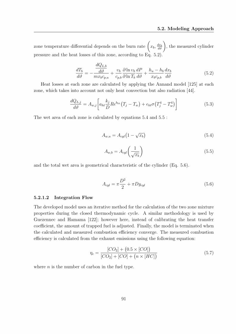
5.2. Modeling Approach
zone temperature differential depends on the burn rate
(xb,
dxbdϑ
), the measured cylinder
pressure and the heat losses of this zone, according to Eq. 5.2).
dTbdϑ
= −
dQL,b
dϑmxbcp,u
+υbcp,b
∂ ln υb∂ lnTb
dP
dϑ+hu − hbxbcp,b
dxbdϑ
(5.2)
Heat losses at each zone are calculated by applying the Annand model [125] at each
zone, which takes into account not only heat convection but also radiation [44].
dQL,j
dϑ= Aw,j
[aht
kjDRebht
(Tj − Tw
)+ εhtσ
(T 4j − T 4
w
)](5.3)
The wet area of each zone is calculated by equations 5.4 and 5.5 :
Aw,u = Acyl(1−√xb)
(5.4)
Aw,b = Acyl
(1√xb
)(5.5)
and the total wet area is geometrical characteristic of the cylinder (Eq. 5.6).
Acyl = πD2
2+ πDycyl (5.6)
5.2.1.2 Integration Flow
The developed model uses an iterative method for the calculation of the two zone mixture
properties during the closed thermodynamic cycle. A similar methodology is used by
Guezennec and Hamama [122]; however here, instead of calibrating the heat transfer
coefficient, the amount of trapped fuel is adjusted. Finally, the model is terminated when
the calculated and measured combustion efficiency converge. The measured combustion
efficiency is calculated from the exhaust emissions using the following equation:
ηc =[CO2] +
(0.5× [CO]
)[CO2] + [CO] +
(n× [HC]
) (5.7)
where n is the number of carbon in the fuel type.
91

5. Emission Model Validation and Application for CCV Prediction
Figure 5.1: Flowchart of the two zone heat release model.
92

5.2. Modeling Approach
The iterative process of the model is schematically outlined in figure 5.1. Firstly, the
model reads all the required engine data, such as the cylinder geometrical characteristics,
the species thermodynamic coefficients, the fuel type data and the user defined data (λ,
f , ηcomb). Before the two zone heat release analysis, the initial condition of the cylinder
model is given by a single zone heat release analysis (Eq. 4.4).
Through the single zone heat release analysis it is possible to estimate the initial values
for the start of combustion (SOC) and the end of combustion (EOC). Furthermore, the
initial value for air mass flow is estimated by assuming a volumetric efficiency, regarding
the throttle position, while the fuel mass flow is calculated using the lambda index. The
cylinder overall lambda was indirectly estimated by the cycle-resolved emissions using the
Brettschneider formula [126].
The main program can be divided into three sub-models; the compression, the com-
bustion and the expansion routines. Compression duration is from intake valve close
(IVC) up to start of combustion (SOC). During this phase, it is calculated the unburned
zone temperature and mixture properties (h,s,u,γ). Combustion phase, which runs from
SOC to EOC, calculates the temperature and thermodynamic properties of the two zones
as well as the net and gross heat release (instantaneous and cumulative), the burned fuel
and the mass fraction burned (xb). The last expansion phase that follows combustion up
to the EVO calculates the temperature and thermodynamic properties of the two zones
and the averaged mixture indexes.
After the main program, the convergence criteria are checked. This includes that the
SOC and the EOC are identical for two iterations (the heat release change due to the
new specific heat ratio at each iteration), while the combustion efficiency is also compared
with Eq. 5.7.
5.2.1.3 Error Formula
The evaluation of modeling is performed by using the percentage error formula. In order
to calculate the percentage error between the measured value and the calculated value,
the following formula is used:
Error[%] =|Simulation− Experiment|
|Experiment|(5.8)
It has to be noted that the error of a group of measured points and a group of simulated
points is performed by utilizing the mean values of each group.
93

5. Emission Model Validation and Application for CCV Prediction
5.2.2 Emissions Modeling
5.2.2.1 Proposed Modeling
The mathematical background of the detailed chemistry model is in detailed presented
in chapter 3. This model provides improved prediction of NOx emissions, while in this
chapter the CO emissions predictability of the model is also presented. The model can be
coupled with any multi-zone thermodynamic model, where the burned zones are assumed
as well-stirred reactors. In this application, a single burned region is adopted. The
computational time of the proposed detailed chemistry model is slightly increased but at
the same order of magnitude to existing simplified emission models. The basic benefits
of this detailed chemistry model are its simplicity and the absence of any calibration
parameter that makes it a generalized application, possible to be applied in any type of
homogeneous combustion engine.
5.2.2.2 Simplified Modeling
The simplified emission model consists of a simplified NO and CO scheme. Regarding
NO emissions, the widely known extended Zeldovich mechanism is utilized. The chemical
pathways of this mechanism are described in Eq. 2.1-2.3. The final NO production rate
is given by Heywood [15], and is described in Eq. 2.4.
As for CO model, a kinetic model for the WGS reaction (Eq. 2.15) is utilized [15, 40].
The model assumes that CO concentration increases rapidly in the flame front zone to
be successively oxidized to CO2 via a kinetically controlled mechanism. Simplified CO
formation rate is expressed through equation 2.16.
5.3 Cycle Simulation
The two-zone heat release analysis estimates the thermodynamic properties of the closed
thermodynamic cycle, from IVC to EVO, by using the measured cylinder pressure. These
thermodynamic properties are utilized from different pollutant formation approaches, such
as equilibrium [43] , the simplified emission model and the detailed chemistry model. As
simplified model uncertainty factor is in the order of 20% to 80% [15], the kinetics of both
NO and CO submodels were adjusted to measured emissions data at 4000 rpm and the
lowest IMEP (20% TP).
An example of the measured pressure trace which corresponds to 4000 rpm, 80%
of wide open throttle and stoichiometric mixture is illustrated in figure 5.2a. The IVC
corresponds to 23o [CA] ABDC, EVO at 40o [CA] BBDC, while the charge is ignited at 48o
[CA] BTDC. Figure 5.2b illustrates the temperature profiles of the two zones, which are
94

5.3. Cycle Simulation
(a) Cylinder pressure. (b) Zones temperature.
(c) NO emissions. (d) CO emissions.
Figure 5.2: Evolution of cylinder pressure, zone temperatures, NO and CO concentra-
tions at 4000 rpm, 80% throttle position, stoichiometric mixture and MBT. (a) measured
cylinder pressure of the closed thermodynamic cycle, (b) the calculated gas tempera-
ture (Tg), the burned zone temperature (Tb) and the unburned temperature (Tun), (c)
calculated NO concentrations under conditions of equilibrium/kinetics control, (d) CO
concentrations under conditions of equilibrium/kinetics control.
95

5. Emission Model Validation and Application for CCV Prediction
calculated by the cylinder model. The mean gas temperature never reaches the maximum
calculated burned zone temperature because of the non-perfect combustion efficiency.
Figure 5.2c illustrates the evolution of NO concentrations assuming different pollutant
formation assumptions, while the calculated values are compared against the measured
NO value experimentally determined at the EVO for this specific combustion cycle. In
the equilibrium model, the NO profile follows the shape of the burned zone temperature,
which seems to be incorrect as the NO formation rate is independent from the burn
rate. The equilibrium model error is about 95%. The simplified model presents faster
NO formation compared to the detailed chemistry model, although both models estimate
finally the same NO level with a minor error of 3%.
CO concentration is also controlled by kinetics. However the air-fuel ratio is more im-
portant for CO formation than temperature [16]. Figure 5.2d depicts that the equilibrium
model corresponds to faster CO formation and destruction, where the final CO predicted
value presents an error of 98%. The simplified model predicts faster CO formation and
almost kinetics equilibrium during the piston expansion, with an error in the order of
74%. On the other hand, the detailed chemistry model predicts slower CO formation and
CO destruction even at EVO. In fact, CO destruction may also occur at the blow down
exhaust process, which can justify the observed 12% error.
5.4 Mean Cycle Emissions Prediction
After this initial validation, the models are tested at various engine conditions to explore
their prediction capabilities. The error magnitude on NO and CO prediction of both the
detailed chemistry model and the simplified model is examined under various engine load,
mixture stoichiometry, ignition timing and engine speed conditions. The effect of each
separate engine variable on emissions modeling error is the field of concern of this section.
5.4.1 Engine Load
In a conventional SI engine, fuel and air are mixed together in the intake system and
further mixed with the residual gas inside the cylinder during intake process. The throttle
valve position controls engine load as it controls the inlet mixture and residual gas fraction.
Lower residual gas fraction improves flame speed and increases combustion temperature
[127]. In this modeling approach, a typical profile of residual gas fraction was adopted
based on previous studies [32, 53], where the residual gas fraction is a function of inlet
pressure and is reduced as IMEP is increased.
The left column of figure 5.3 represents the NO predicted values for both the simplified
and detailed kinetic models which are compared to the cycle resolved experimental values
for various engine speed and IMEP conditions. As IMEP increases, the burned zone
96

5.4. Mean Cycle Emissions Prediction
Figure 5.3: Effect of engine load on NO and CO formation for stoichiometric mixture
and various engine speed conditions: (left column) NO simulation, (right column) CO
simulation.
97

5. Emission Model Validation and Application for CCV Prediction
temperature increases accordingly while the residual gas fraction decreases. The latter
benefits the NO formation.
The simplified NO model was initially calibrated at 4000 rpm and low IMEP con-
ditions, similar to other studies [31]. This low load operating point was selected, as the
thermal NO mechanism underestimates the NO emissions at low temperature conditions.
Without considering this calibrated operating point, the simplified model presents error
within 2% and 81.5% over the eight (8) presented points. Additionally, it is observed that
the error increases, as engine speed also increases.
On the other hand, the detailed chemistry model shows an improved prediction of
formed NO. Its maximum error is 2.6% over the nine (9) presented points, which is found
at 5000 rpm and 80% TP. However the detailed chemistry model presents a typical error
of less than 1.3%. The improved prediction can be explained on the kinetic calculation of
the other important species (CO, O2, H2) and on the detailed chemical pathways, which
are included for the NO formation and destruction.
CO predicted values for the two emission models compared to the experimental values
are also shown in fig 5.3. Similarly to the NO investigation, the simplified CO model is
calibrated to the measured CO value at 4000 rpm and low IMEP (20% TP), as residual gas
fraction and CO2 are increased at this engine point. Considering the remaining operating
points investigated the simplified model presents a mean error of 45.6%. It is also depicted
overall the engine speed conditions that error increases as engine load increases.
The detailed chemistry model can better estimate the CO values at various load
conditions. Its maximum error is 65%, observed at 6000 rpm and high load conditions,
which is an expected behavior of this model. In fact, as IMEP (and speed) are increased,
maximum cylinder pressure is also increased, which ”pushes” more mixture in the crevices
volume, a phenomenon which is non considered by the model, as only one burned region
is adopted. However that, the detailed chemistry model presents an average error of less
than 30%, which is 35% lower than the average observed error of the simplified CO model.
5.4.2 Mixture Stoichiometry
The precision of predicting engine out emissions over different lambda values around
stoichiometry is very important for contemporary gasoline engines, due to its application
on the optimization of the emission control systems. The predictability of the simplified
emission model and the detailed chemistry model for CO and NO engine out emissions
is given in Fig. 5.4.
Regarding NO emissions, the detailed chemistry model presents better accuracy com-
pared to the simplified emission model. In the entire investigated range of engine speeds
and equivalence ratios, the average observed error of the detailed chemistry model is 3.8%
over the nine investigated operating points, while for the simplified model this is 74%.
98

5.4. Mean Cycle Emissions Prediction
Figure 5.4: Effect of mixture lambda on NO and CO formation for 80% throttle position
and various engine speed conditions: (left column) NO simulation, (right column) CO
simulation.
99

5. Emission Model Validation and Application for CCV Prediction
This 74% average observed error mainly originates from stoichiometric and slightly rich
conditions. At these conditions, engine torque and mixture temperature are maximized
but oxygen is expected to be faster consumed by CO and H2 and not by the thermal
NO mechanism. The latter can occur by considering other chemical pathways, which
the detailed chemistry model does. Finally, at both stoichiometric and lean conditions,
detailed chemistry model presents a 2.7% average error while the error of the simplified
model is about 47%, which is comparable to other literature studies [31, 32, 44].
CO formation, at homogeneous combustion conditions, is primarily controlled by
fuel/air equivalence ratio. However, CO is also kinetically controlled, especially at rich
conditions through the WGS reaction [15, 16]. The detailed chemistry model was applied
for the prediction of CO emissions under various lambda conditions. Under lean condi-
tions and especially at 4000 rpm and 6000 rpm, the detailed model underestimates the CO
emissions by 92% and 67% respectively. In fact, under lean conditions, CO is primarily
controlled by other mechanisms such as crevices and mixture non-homogeneneities, which
are not considered in this model. By comparing the two CO models at overall lambda
and engine speed conditions, the detailed chemistry model presents average error of 40%
for the nine investigated operating points, which is better than the 63% average observed
error of the simplified model. Although CO prediction of the detailed chemistry model
was found less efficient at this investigation, it has to be noted that this mixture lambda
investigation occurred at 80% throttle position, where the formed CO in crevices (due
to the high cylinder pressure) is not considered by the single burned zone (see Chapter
5.4.1).
In this investigation, where the effect of lambda mixture is explored, it is worth noting
the benefits of using more complicated chemistry at a cost of computational time. The
most simplified approach is the utilization of the equilibrium, as it was presented by
Olikara and Borman [43]. The model was able to run the total combustion cycle, from
the SOC to the EVO in less than 15 seconds at each operating point and its average error
was 78% for NO emissions and 67% for CO emissions for the nine investigated points.
The simplified kinetic model, which utilizes the Zeldovich mechanism for NO and the
WGS reaction for CO, requires less than two minutes to be executed and its average error
was found to be about 74% for NO and 63% for CO for the same nin points. Additionally,
the kinetics of this simplified model usually require calibration, which time cost is not
considered here [31, 32]. The execution time of the detailed chemistry model is highly
depending on the number of combustion steps and is shorter for rich combustion which
presents lower combustion duration compared to lean conditions. However, its average
execution time is at the order of five to ten minutes and its accuracy was found to be in
the order of 3.8% for NO and 40% for CO emissions. Compared to multi-dimensional
combustion codes, the proposed detailed chemistry model is proposed as a satisfactory
trade-off between computational cost and accuracy. Finally, by increasing the number
100

5.4. Mean Cycle Emissions Prediction
of burned zones, the accuracy of CO can be improved, while the computational cost is
expected to slightly increase, due to the tools of parallel processing.
5.4.3 Ignition Timing
Spark timing controls the initiation of the combustion process and through that the en-
gine IMEP and engine-out emissions. The optimum timing gives the MBT, the maximum
IMEP and the lower cyclic variability of IMEP [17]. On the other hand, retarded ignition
timing is selected at engine warm-up conditions, in order to increase exhaust gas temper-
ature and rapidly warm up the catalyst, with a negative impact on fuel consumption.
Figure 5.5: Effect of ignition timing on NO and CO formation at 4000 rpm, 80% throttle
position and stoichiometric conditions: (left column) NO simulation, (right column) CO
simulation.
Figure 5.5 shows the impact of ignition timing on formed NO and CO for stoichiomet-
ric mixtures, at 4000 rpm and 80% TP. The detailed chemistry model predicts accurately
the decrease of formed NO concentration at retarded ignition timings. At 4000 rpm and
80% TP, the error of the detailed model is between 0.6% and 3.7%, while the error of
the simplified model is between 2.4% and 59%. In the case of CO emissions, it is ex-
perimentally observed that retarded ignition increases CO up to a rapid drop at very
”late” ignition timings. This CO trend is successfully predicted by the detailed chemistry
model, within an average error of 26%, while the simplified model presents a ”flat” area
and an average error of 89%. In fact, simplified model at both NO and CO cases predicts
small differences at various ignition timings and fails not only quantitatively but also
qualitatively.
A similar investigation of ignition timing at NO and CO emissions is presented at 6000
101

5. Emission Model Validation and Application for CCV Prediction
Figure 5.6: Effect of ignition timing on NO and CO formation at 6000 rpm, 20% throttle
position and stoichiometric conditions: (left column) NO simulation, (right column) CO
simulation.
rpm and partial load conditions (20% of WOT). Regarding NO emissions, the detailed
chemistry model accurately predicts the formed NO both qualitatively and quantitatively,
while the simplified model seems to follow only qualitatively. The average error of the
detailed chemistry model is about 1.7%, while the simplified model presents an average
error of 44.5%. In the case of CO emissions, the simplified model can not follow the
experimental CO trend. The mean error of the simplified CO model is about 157%, while
the average observed error for the detailed chemistry model is 36%. However, it has to
be reminded that the simplified model was calibrated at 4000 rpm and 20% and it is
expected to present higher errors at 6000 rpm.
In conclusion, it was found that the detailed chemistry model is able to qualitatively
and quantitatively predict theNO and CO emissions at various ignition timing conditions,
without any calibration and with a limited cost on computational time. On the other
hand, the simplified model was found inefficient for the investigation of the impact of
ignition timing on NO and CO emissions. The usefulness of the proposed model can be
found on engine design and optimization from the automotive industry, considering the
engine ignition timing optimization during warm-up.
5.5 Sensitivity Analysis of the Emission Model
Combustion process is influenced by several flow and chemical properties, such as large
and small scale turbulence, mixture stoichiometry, residual gas, crevices and heat transfer.
All these parameters also affect pollutants formation. In fact, several in-cylinder mixture
102
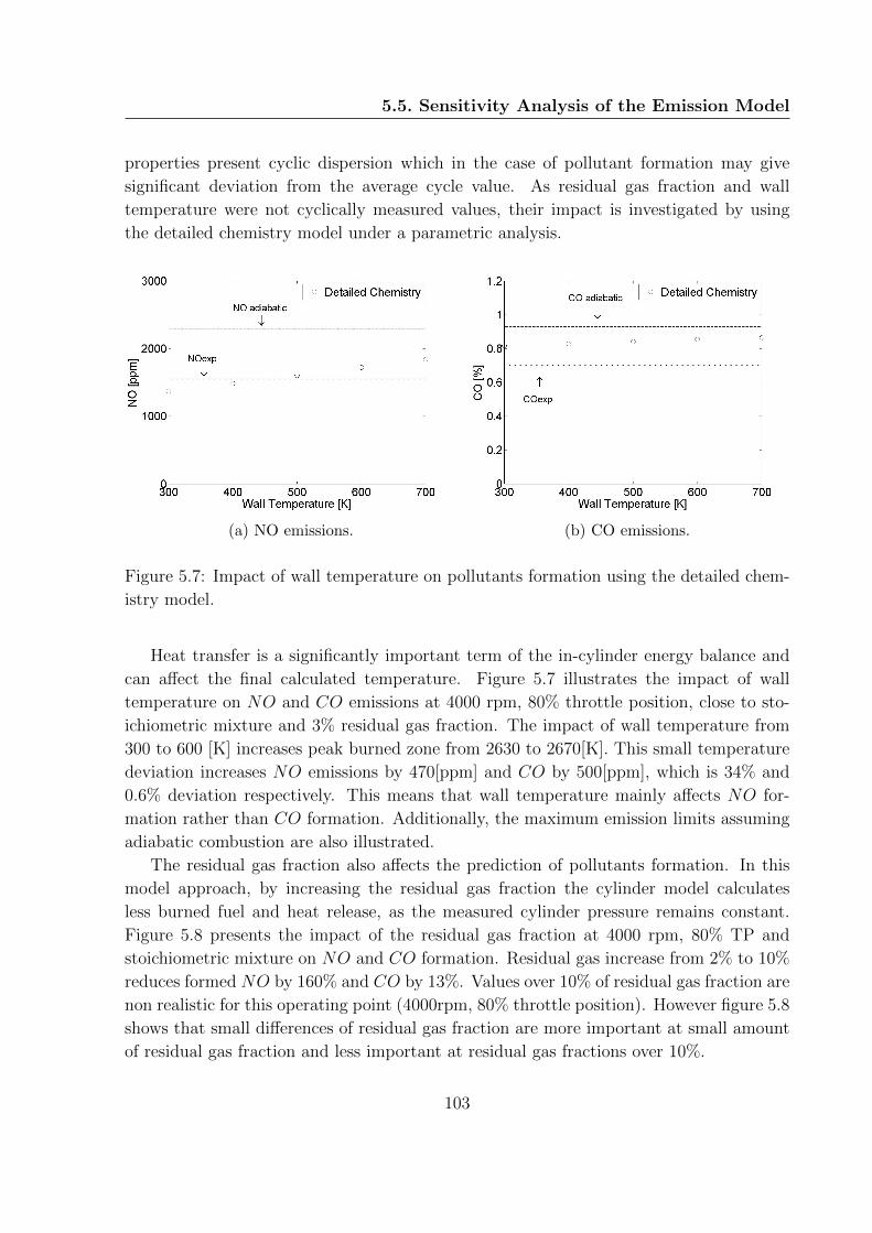
5.5. Sensitivity Analysis of the Emission Model
properties present cyclic dispersion which in the case of pollutant formation may give
significant deviation from the average cycle value. As residual gas fraction and wall
temperature were not cyclically measured values, their impact is investigated by using
the detailed chemistry model under a parametric analysis.
(a) NO emissions. (b) CO emissions.
Figure 5.7: Impact of wall temperature on pollutants formation using the detailed chem-
istry model.
Heat transfer is a significantly important term of the in-cylinder energy balance and
can affect the final calculated temperature. Figure 5.7 illustrates the impact of wall
temperature on NO and CO emissions at 4000 rpm, 80% throttle position, close to sto-
ichiometric mixture and 3% residual gas fraction. The impact of wall temperature from
300 to 600 [K] increases peak burned zone from 2630 to 2670[K]. This small temperature
deviation increases NO emissions by 470[ppm] and CO by 500[ppm], which is 34% and
0.6% deviation respectively. This means that wall temperature mainly affects NO for-
mation rather than CO formation. Additionally, the maximum emission limits assuming
adiabatic combustion are also illustrated.
The residual gas fraction also affects the prediction of pollutants formation. In this
model approach, by increasing the residual gas fraction the cylinder model calculates
less burned fuel and heat release, as the measured cylinder pressure remains constant.
Figure 5.8 presents the impact of the residual gas fraction at 4000 rpm, 80% TP and
stoichiometric mixture on NO and CO formation. Residual gas increase from 2% to 10%
reduces formed NO by 160% and CO by 13%. Values over 10% of residual gas fraction are
non realistic for this operating point (4000rpm, 80% throttle position). However figure 5.8
shows that small differences of residual gas fraction are more important at small amount
of residual gas fraction and less important at residual gas fractions over 10%.
103
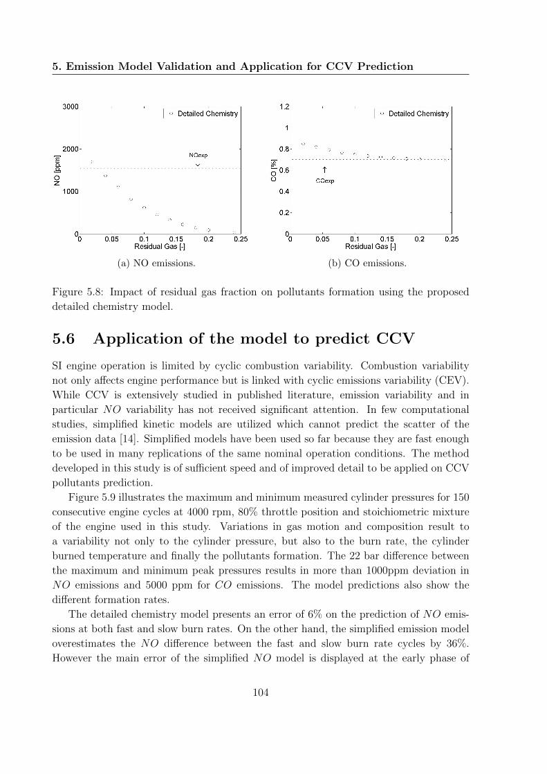
5. Emission Model Validation and Application for CCV Prediction
(a) NO emissions. (b) CO emissions.
Figure 5.8: Impact of residual gas fraction on pollutants formation using the proposed
detailed chemistry model.
5.6 Application of the model to predict CCV
SI engine operation is limited by cyclic combustion variability. Combustion variability
not only affects engine performance but is linked with cyclic emissions variability (CEV).
While CCV is extensively studied in published literature, emission variability and in
particular NO variability has not received significant attention. In few computational
studies, simplified kinetic models are utilized which cannot predict the scatter of the
emission data [14]. Simplified models have been used so far because they are fast enough
to be used in many replications of the same nominal operation conditions. The method
developed in this study is of sufficient speed and of improved detail to be applied on CCV
pollutants prediction.
Figure 5.9 illustrates the maximum and minimum measured cylinder pressures for 150
consecutive engine cycles at 4000 rpm, 80% throttle position and stoichiometric mixture
of the engine used in this study. Variations in gas motion and composition result to
a variability not only to the cylinder pressure, but also to the burn rate, the cylinder
burned temperature and finally the pollutants formation. The 22 bar difference between
the maximum and minimum peak pressures results in more than 1000ppm deviation in
NO emissions and 5000 ppm for CO emissions. The model predictions also show the
different formation rates.
The detailed chemistry model presents an error of 6% on the prediction of NO emis-
sions at both fast and slow burn rates. On the other hand, the simplified emission model
overestimates the NO difference between the fast and slow burn rate cycles by 36%.
However the main error of the simplified NO model is displayed at the early phase of
104

5.6. Application of the model to predict CCV
Figure 5.9: Evolution of maximum and minimum IMEP cycle in relationship to crank
angle: (a) measured cylinder pressure, (b) calculated heat release and burned zone tem-
perature, (c) NO formation and (d) CO formation.
NO formation, where the fast and slow NO rates slightly differ. This declares that Zel-
dovich mechanism is more sensitive to the zone temperature profile and less to the burn
rate. Therefore, the predicted NO difference with the Zeldovich mechanism is more a
temperature effect than a kinetic issue.
CO variability is well described by the detailed chemistry model, while the error of
3.6% can be justified by mixture inhomogeneities, which are not considered here. On
the other hand, the simplified CO kinetic model systematically overestimates the CO
emissions and underestimates the CO deviation between fast and slow burn rate cycles by
67%. This model shows at the early stage of CO formation no significant variation between
the fast and slow burn rates, although the heat release rates differ greatly. Additionally,
the late stage of CO formation appears frozen (constant) with simplified modeling and
105

5. Emission Model Validation and Application for CCV Prediction
not constant with detailed kinetics. The reason that CO is overestimated at the slow
burn cycle from the simplified kinetic model is the mixture temperature, which is higher
during expansion, and the simplification of the WGS reaction. Finally the CO simplified
kinetic model appears to be a temperature dependent model, while detailed chemistry
appears to be more suitable for the estimation of CO variability.
In conclusion, the proposed detailed chemistry model was applied on the maximum
and minimum IMEP cycle at nominally steady state engine operating conditions. It was
found that this model predicts different production rates at various engine IMEP cycles
and finally different emission altitudes. On the other side, the simplified emission model
is less sensitive to the burn rate and may underestimate the cyclic emission variability.
The predictability of cyclic emission variability is investigated in the next section.
5.7 Cycle to Cycle Emission Prediction
In this section, the emission models are applied on a cycle to cycle emission simulation,
in order to explore the error magnitude under various engine operating conditions. In
order to characterize the efficiency of the different emission methodologies, three different
types of plots are utilized, such as the relationship between NO emissions and cylinder
pressure, the return map of each emission variable and the relationship of each variable
between measured and calculated value.
The relationship between NO emissions and maximum cylinder pressure is widely used
on a number of cycle to cycle emission variability studies [13, 14]. Such a figure depicts
the impact of combustion variability (pressure trace) on NO variability and highlights,
whether this relationship is linear or not, the impact of other mixture parameters on NO
formation. The maximum cylinder pressure represents the maximum cylinder temperature
that occurs in the cylinder, which is related with the thermal NO mechanism.
Another widely used method for characterizing cycle-resolved engine variables is the
return map, where a set of data (at nominally constant engine operating point) separated
by a fixed number of cycles (delay pairs) are plotted against each other [60, 128–130].
The resulting aggregate plot of all time-series delay pairs forms the return map, which
can reveal any low-dimensional relationship between two engine variables. In most cases,
the preferred delay interval is one engine cycle, so that next-cycle correlation is most
apparent.
Last but not least, the efficiency of the different modeling approaches is performed by
plotting the measured values versus the calculated values. Values close to the diagonal
represent successful modeling prediction, while the modeling error is higher for values far
from the diagonal. This is a standard methodology for the valuation of modeling approach
and it is adopted in this study.
106
5.7. Cycle to Cycle Emission Prediction
All types of plots have the same target; to depict the impact of detailed chemistry and
the absence of equilibrium on modeling of cyclic emission variability.
5.7.1 Engine Load
It was experimentally observed on chapter 4.5.1 that cyclic emission variability is in-
creased as low engine load conditions. The validation of emission dispersion modeling is
performed at two different engine load conditions (20% and 80%), 6000 rpm, stoichio-
metric mixture and identical ignition timing (41o [CA] BTDC). The predictability of the
simplified emission model and the detailed chemistry model for NO and CO emissions
variability is illustrated in figure 5.10 and in figure 5.11 respectively.
The prediction of cyclic NO variability for 20% throttle position is illustrated on
the left column of figure 5.12. The detailed chemistry model presents a higher scatter
as well as a better accuracy of the experimental data. The detailed chemistry model
underestimates the average NO measured data by 1%, while the simplified model by 43%.
In the third row of plots it is observed that the detailed chemistry model underestimates
the NO concentrations under 1500 ppm and overestimates the higher NO concentrations,
therefore the mean error is balanced to 1% error. A possible root of this observation may
be the mixture composition. In this investigation, HC were not cyclic measured and
mixture lambda may be richer at low IMEP cycles and leaner at high IMEP cycles.
The results of cyclic NO variability at 80% throttle position are illustrated on the
right column of figure 5.12. By comparing the average values of the measured and cal-
culated NO data, detailed chemistry model presents 26.5% error while simplified model
returns a 35.6% error. Compared to the 20% TP, the detailed chemistry model presents
higher error as the minor inaccuracies of the mixture lambda estimation contribute more
at higher cylinder temperature and pressure conditions. At the same time, simplified
model estimation is improved as thermal mechanism is more important at high load con-
ditions. Although that, detailed chemistry model appears more proper to predict NO
cyclic dispersion.
The modeling of cyclic emission variability was performed with a constant residual
gas fraction, and without adopting a residual gas estimation model [51, 131, 132]. Such
kind of models are able to estimate residual gas fraction based on cylinder pressure during
blowdown process. By introducing a residual gas model, NO scatter variability increases
and the standard deviation of the NO data is improved. In the case of 80% TP, the
calculated standard deviation error is about 50% for the detailed chemistry model and
more than 75% for the simplified NO model.
The efficiency of the detailed chemistry model and the simplified model on the pre-
diction of CO variability is illustrated on figure 5.13. Regarding the 20% TP, the error of
the averages value between the detailed chemistry model and the measured CO concen-
107

5. Emission Model Validation and Application for CCV Prediction
Figure 5.10: Prediction of cyclic NO variability for 20% (left column) and 80% (right
column) throttle position. (a) Relationship between NO and measured cylinder pressure,
(b) NO return map, (c) Relationship between measured and calculated NO.
108

5.7. Cycle to Cycle Emission Prediction
Figure 5.11: Prediction of cyclic CO variability for 20% (left column) and 80% (right
column) throttle position. (a) CO return map, (b) Relationship between measured and
calculated CO.
109

5. Emission Model Validation and Application for CCV Prediction
tration is 5.7% while the average error between the simplified model and the measured
values is 69%. As for the case of 80% throttle position, the two models present almost
equal predictability. The detailed chemistry model presents an average observed error of
82%, while the same error of the simplified model is 91%. The observation of both NO
and CO error show that lambda index slightly shifts to richer values. Shifting lambda to
leaner conditions could benefit both the NO and CO prediction. The lambda estimation
utilizes the mean HC value [126], which concludes the oil consumption and not only the
unburned hydrocarbons. Therefore, the qualitative prediction of CO variability from the
detailed chemistry model is satisfactory.
Finally, an important observation from the CO investigation is the scatter of the
predicted data. Detailed chemistry model presents a higher data scatter, which proves
to be primarily a chemistry issue and not just a ”initial” mixture composition problem.
Detailed chemistry model is more sensitive on the burn rate, while the burn rate is related
with the CO and H2 kinetic rates and finally with the CO engine-out emissions. Simplified
model, which assumes that only WGS reaction is kinetically controlled, underestimates
the scatter of CO emissions, conversely to the detailed chemistry model that calculates
all species kinetically.
5.7.2 Mixture Stoichiometry
The impact of mixture lambda on cyclic emission variability, which was experimentally
observed on chapter 4.5.2 is now approached by emission modeling. The rich and lean
operating conditions at 6000 rpm, 80% throttle position and identical ignition timing (41o
[CA] BTDC), which have been primarily presented in table 4.8, were selected to validate
the modeling efficiency. The final results are depicted in figures 5.12 and 5.13 for NO and
CO emissions.
In the case of rich operating conditions (λ ∼ 0.92), the detailed chemistry and the
simplified models seem to predict NO emissions equally. The simplified emission model
overestimates NO emissions over a few high pressure cycles, therefore its average error is
about 15%, while the detailed chemistry model presents on average error of about 41%.
However the detailed chemistry model has lower error on the standard deviation, which
is 1.3% compared to the 124% of the simplified model and finally the COVNO value is
overestimated by 74% compared to the 164% of the simplified model. Additionally, the
constant offset between the detailed chemistry model and the diagonal may be the result
of a constant lambda offset error.
On the right part of figure 5.12 and at slightly lean conditions (λ ∼ 1.06), the detailed
chemistry model is shown to predict cyclic NO variability more accurately. The error of
the detailed chemistry model is less than 10% compared to slightly more than 37% for the
simplified model. The COVNO value of the experimental data is also better estimated by
110

5.7. Cycle to Cycle Emission Prediction
Figure 5.12: Prediction of cyclic NO variability for rich (left column) and lean (right
column) mixture composition. (a) Relationship between NO and measured cylinder pres-
sure, (b) NO return map, (c) Relationship between measured and calculated NO.
111

5. Emission Model Validation and Application for CCV Prediction
Figure 5.13: Prediction of cyclic CO variability for rich (left column) and lean (right
column) mixture composition. (a) CO return map, (b) Relationship between measured
and calculated CO.
112

5.7. Cycle to Cycle Emission Prediction
the detailed chemistry model. As the residual gas fraction was adopted constant, and the
lean and diluted conditions present high residual gas fluctuations, the error in the COV
value was more than 50% for the detailed chemistry model and more than 100% for the
simplified one.
The constant lambda shift error at rich conditions is also confirmed in the CO investi-
gation. Despite that, the detailed chemistry model qualitatively predicts the experimental
trends and the data scatter. On the other side, the simplified CO model seems to be less
sensitive to various burn rates, and presents a ”flat” behavior close to 4% CO concen-
tration. Regarding lean conditions, the detailed chemistry model shows better accuracy
compared to the simplified approach. Their average errors on the mean value are 13%
and 280% for the detailed chemistry and the simplified models respectively. This large
difference was expected, as at lean conditions the WGS reaction is less important as it
is the CO oxidation and the kinetic control of oxygen (O2). Finally at more lean and
diluted conditions, the mixture becomes less homogeneous and the detailed chemistry
error is expected to increase.
5.7.3 Ignition Timing
The potential of the detailed chemistry model to predict cyclic emission variability at
various ignition timing conditions is examined in this sub-section. The test cases include
engine operation at 4000 rpm, 80% TP, stoichiometric mixture and five different ignition
timings (42o, 45o, 48o, 50o, 52o [CA] BTDC), where the 48o [CA] corresponds to the MBT
case. The results of cyclic NO and CO variability, regarding the retarded (42o [CA]
BTDC), advanced (52o [CA] BTDC) and MBT ignition timings are illustrated in figures
5.14 and 5.15.
The cyclic NO variability is investigated on figure 5.14 which includes the return map
and the error plot of NO. Detailed chemistry model has average error of 18%, 42% and
23% for advanced, MBT and retarded ignition timing while the simplified model presents
24%, 70% and 11% average error respectively. Considering all the ignition cases, the
detailed chemistry is better by 20%. At retarded ignition timing, burn rate is slower and
sometimes incomplete. At this limit, the return map of detailed chemistry model shows
a more deterministic rather than stochastic nature of NO cyclic variability, which is not
clearly observed by the measured NO emissions.
The right column of Fig. 5.14 describes the relationship between measured and cal-
culated NO values. It is observed that under all ignition timing conditions (advanced,
MBT and retarded), the detailed chemistry model can not predict the diagonal line, which
corresponds to zero error. Instead, it appears that at low IMEP cycles the model under-
estimates the NO emissions while at high IMEP cycles overestimates formed NO with
greater intensity at MBT and retarded ignition timings. This appears as at 4000 rpm
113

5. Emission Model Validation and Application for CCV Prediction
Figure 5.14: Prediction of cyclic NO variability at 4000 rpm, stoichiometric mixture, 80%
TP, 52o[CA] BTDC ignition timing (first row), 48o[CA] BTDC ignition timing (second
row) and 42o[CA] BTDC ignition timing (third row). Left column: NO return map, Right
column: Relationship between measured and calculated NO.
114

5.7. Cycle to Cycle Emission Prediction
Figure 5.15: Prediction of cyclic CO variability at 4000 rpm, stoichiometric mixture, 80%
TP, 52o[CA] BTDC ignition timing (first row), 48o[CA] BTDC ignition timing (second
row) and 42o[CA] BTDC ignition timing (third row). Left column: CO return map, Right
column: Relationship between measured and calculated CO.
115

5. Emission Model Validation and Application for CCV Prediction
engine lambda fluctuates more compared to the 6000 rpm. High IMEP cycles present a
faster burning rate due to richer mixture conditions and conversely a slower burning rate
leads to lower IMEP cycles. Therefore, it is considered that this wrong trend is the result
of inaccurate lambda estimation.
Figure 5.14 shows the prediction of CO variability for both the detailed and the sim-
plified models. Regarding the model errors, in the five tested ignition timing cases, the
detailed chemistry model presents an average error from 3.5% to 16% while the simplified
CO model has an average error from 79% up to 116%, which implies that the detailed
chemistry model is significantly better on predicting CO. More specifically, the detailed
chemistry model presents 8% error at 52o [CA] BTDC ignition timing, 16% at 48o [CA]
BTDC ignition timing and 11% at 42o [CA] BTDC ignition timing. On the other hand, in
the three presented (left) plots, the simplified CO model predicts average CO concentra-
tion close to 1.8% and seems to be less sensitive on burn rate variability. Its error is 89%,
113% and 86% at advanced, optimum MBT and retarded ignition timings respectively.
The right column of the figure illustrates that the detailed chemistry model predicts qual-
itatively and quantitatively the diagonal of the three plots. Last but not least, the return
maps of CO emissions show that under all examined ignition timing engine conditions,
CO variability nature is more a stochastic rather than a deterministic.
5.8 Summary and Conclusions
In this chapter, the proposed detailed chemistry model was validated against the experi-
mental data of chapter 4, which included various engine operating conditions with different
engine speed, load, stoichiometry and ignition timing. Under these engine conditions, it
was tested whether the detailed chemistry model can better predict NO and CO emis-
sions at mean IMEP cycle simulations and cycle to cycle simulations. Simplified kinetic
mechanisms were compared to the detailed emission model to depict the advantages of
the detailed chemical kinetics.
The engine load investigation on mean cycle NO formation showed that the error of the
simplified emission model is between 2% and 81.5%, while the detailed chemistry model
exhibits a mean prediction error of less than 1.3% over the nine investigated operating
points. Additionally, the mean cycle CO for the detailed chemistry model is less than
30% and for the simplified model about 45.6%. The improved prediction is explained by
the detailed chemical kinetics calculations of the other important species (O2, H2, H, OH
etc.) and on the detailed chemical pathways, which are considered for the NO formation
and destruction in the detailed chemistry model.
The effect of mean cycle mixture lambda on NO and CO formation was also explored.
NO predictions using the detailed chemistry and the simplified models show average errors
of 3.8% and 74% respectively. Furthermore, it was found that the simplified model returns
116
5.8. Summary and Conclusions
mainly fails at rich conditions for NO and at lean conditions for CO. Under all lambda
cases, the detailed chemistry model predicts CO emission better by 36% over the nine
investigated operation points on average, compared to the simplified model.
The prediction of mean cycle formed NO was also investigated under various ignition
timing conditions at two different engine speed and load conditions (4000rpm and 80%TP,
6000rpm and 20%TP). The detailed chemistry model presents better sensitivity on burn
rate, as the total species in the burned zone are kinetically controlled. The average NO
error for the two investigated operating points is 1.8% and 37.5% for the detailed chemistry
and the simplified models, respectively. Regarding the mean cycle CO prediction, the
detailed chemistry model can qualitatively and quantitatively predict the CO trend. As
for the average CO error for the two investigated operating points, this is 31% and 123%
for the detailed chemistry and the simplified models, respectively.
Then, the impact of wall temperature and residual gas fraction on detailed chemistry
model prediction was investigated. The two parameters are difficult to be determined
experimentally, therefore a sensitivity analysis on NO and CO pollutants was presented.
The latter showed that NO formation is mainly affected by these parameters, while CO
formation seems to be less sensitive to these parameters and more on mixture homogeneity
and mixture lambda.
In the next section of this chapter, the detailed chemistry model was applied to sim-
ulate the maximum and minimum engine cycles on a cyclic variability study. It was
observed that the emission variation is highly related to the variation on burn rate for
each combustion cycle. The simplified emission model significantly overestimates the early
pollutant formation at both NO and CO emissions by 36% and 67% respectively, which
declares that these mechanisms are more sensitive on the zone temperature profile and
less on the burn rate. The detailed emission model is more suitable to predict emission
variability and its errors on NO and CO predictions are 6% and 3.6% respectively. The
detailed emission model also illustrates that at slow burn rate cycles, CO emissions may
not achieve the frozen kinetic area until the EVO.
The validated detailed chemistry model was then utilized on the prediction of cyclic
emission variability. The CCV engine load investigation was performed at 6000 rpm,
stoichiometric conditions and two different engine load conditions (20% TP and 80% TP).
At 20% TP, the average NO emission error was 1% for the detailed chemistry model and
43% for the simplified model, while the average CO error was 5.7% and 69% respectively.
At 80% throttle position, the prediction of the average NO error for the two models is
converged, as the thermal mechanism becomes more significant. The average NO error
is for the detailed chemistry model 26.5% and for the simplified model 35.6%.
The detailed chemistry model was able to predict the average concentration in the
CCV mixture lambda investigation. At rich conditions, detailed chemistry model and
simplified model predict average NO emissions similarly with an average error of about
117

5. Emission Model Validation and Application for CCV Prediction
15%, while the average CO error is 13% and 280% respectively for the two models. At
lean conditions, detailed chemistry models predicts 10% average NO error which is lower
than the 37% average NO error of the simplified model.
The prediction of cyclic NO variability at various ignition timing conditions is per-
formed with the detailed chemistry model within an 20% better accuracy compared to
the simplified model. In addition, the average CO error is from 3.5% to 16% for the
detailed chemistry model, while the simplified CO model has an average error from 79%
up to 116%. The return maps of NO and CO emissions showed that NO is becoming
more deterministic as ignition timing is retarded, while CO nature is stochastic under all
ignition timing conditions.
The above results conclude to the fact that the proposed detailed chemistry model
can accurately predict NO and CO emissions without requiring any calibration of kinetic
parameters, is not based on arbitrary equilibrium assumptions, and can be executed in
a comparable computational time with simplified methods. This means that the method
proposed can be used to predict pollutants formation with high accuracy even including
the number of iterations required when studying cyclic combustion variability. Since the
method can be coupled to practically any 0D or 1D combustion model, it can be used for
more precise engine optimization, with expected benefits in both pollutants emission and
engine efficiency.
118

Chapter 6
Conclusions & Future Work
6.1 Experimental Work
Chapter 2 presented an extensive literature survey on the experimental investigation of
cycle to cycle variability. Although the impact of CCV on engine combustion and per-
formance has been investigated in a great number of studies, little effort has been spent
on cyclic emission variability. In fact, the literature review showed that only a handful of
studies have experimentally explored the cyclic emissions variability.
In this thesis, an experimental investigation of NO and CO variation under premixed
combustion was presented. The experiments were conducted on an in-line four cylinder
port fuel injection spark-ignition engine, modified from an original Honda CBR600RR
motorcycle. A Kistler measuring spark plug with an integrated piezoelectric transducer
was used to measure cylinder pressure. The exhaust gas temperature was measured by
a K-type thermocouple connected to the relevant transducer. High frequency pollutants
measurement of cycle-resolved emissions was conducted using fast response analyzers,
which were located close to the exhaust valve. The investigation was performed over a wide
range of engine operating conditions, including different engine load, equivalence ratio,
and ignition timing. The analysis of the results aims at correlating various interactions
among combustion parameters (such as IMEP, maximum pressure and crank angle of 5%
mass fraction burned), and pollutants emissions (NO, CO). The overall objective of this
study was primarily to explain how combustion variability affects emissions variability.
Engine load has a significant impact on the variability of engine performance and
emissions. At low load operating conditions, engine operates with higher residual gas
fraction which dilutes mixture and increases combustion and emissions variability. At
higher engine load conditions and 4000 rpm, it was found that COVimep is decreased by
60%, COVNO drops by 45% and COVCO by 6%, while at 6000 rpm COVimep is decreased
by 43% and COVNO by 38%, compared to low load conditions. At low load conditions,
119

6. Conclusions & Future Work
the early flame kernel development (ϑ5%) exhibits more variance which is accompanied
by a steep decrease at very late early flame kernel cycles.
The impact of combustion stoichiometry on the variability of engine performance and
emissions was also investigated. Slightly rich mixtures showed the higher IMEP and
the lower COVimep. Higher variation of combustion in lean mixtures has its roots on
early flame kernel development, as slightly lean mixtures ignite slower and later than
rich ones. This leads to slower flame propagation and lower cylinder pressure. In lean
mixtures, higher variation of the crank angle that early flame kernel development occurs
was detected as the main reason of NO variability, as NO formation depends on burn
rate and mixture temperature.
Furthermore, the impact of ignition timing on the variability of engine performance and
emissions has been investigated. MBT ignition timing was found to be accompanied by the
highest IMEP value and the lowest COVimep. Advanced ignition timings are characterized
by faster combustion and higher cylinder pressure. On the other hand, retarded ignition
results to a shorter delay in the development of early flame kernel, as this occurs closer
to TDC. At retarded cycles, flame propagation is shifted to the piston expansion phase,
where cylinder volume is increased and finally maximum cylinder pressure is decreased.
Because of the expansion, both cylinder pressure and crank angle at which maximum
cylinder pressure occur vary more in each cycle. The significant variation of cylinder
pressure at retarded ignition conditions was found to be the main source of NO and CO
variation in this investigation. On the one hand, NO formation is strongly linked with
the temperature vs time profile, and the higher perturbation of the latter at retarded
cycles is the main root of the high NO variability. On the other hand, CO variability is
linked with the variation of cylinder pressure which affects the trapped mixture mass into
crevices at each cycle and finally the combustion efficiency.
In conclusion, NO variability was found to be primarily affected by cylinder mixture
characteristics such as mixture equivalence ratio and residual gas fraction. At engine con-
ditions that the residual gas fraction decreases, COVNO and COVCO are simultaneously
decreased. Lean mixture conditions increase COVNO due to the unstable combustion
rate and the oxygen availability. At these conditions, COVNO depends on burn rate and
maximum cylinder pressure and temperature. The impact of burning rate on COVNO
has been also investigated by altering the ignition timing. Faster burning rates are more
repeatable, average NO value is increased and COVNO is decreased, while slower burning
rates present higher variability, average NO value is decreased and COVNO is increased.
6.2 Emissions Modeling
The main contribution of this thesis is the implementation and validation of a novel
emissions model, that predicts NO and CO emissions within an error of less than 10%
120

6.2. Emissions Modeling
and without significant increase of the computational time. The basic benefits of this
proposed emissions model are its simplicity and the absence of any calibration parameter
that makes it a generalized application, possible to be applied in any type of homogeneous
combustion engine. Although this model utilizes detailed kinetics to predict engine-out
emissions, it does not require a sophisticated or advanced combustion model, and can be
combined with any 0D or 1D combustion engine model.
Chapter 3 presents the mathematical background of the proposed detailed chemistry
model. The detailed chemistry model is based on SENKIN, a FORTRAN based code
developed by Sandia Laboratories. The calculations of kinetics are based on the GRI 3.0
mechanism, a reaction scheme which was initially proposed for methane-air combustion
and consists of 53 species and 325 reactions.
The novel emissions model assumes that each burn zone is a homogeneous reactor and
can be applied in coupling with any multi-zone combustion model. In this thesis, a two
zone approach is adopted, which consists of an unburned and a burned region. In the
burned region, at each crank angle step the inlet mass is calculated based on the principle
of mass balance. The inlet species are calculated from the combustion of the air, fuel
and residual gas. The emission composition takes place in the post flame area, where the
homogeneous reactor calculates the combustion speciation with good accuracy.
First, the model was demonstrated in coupling to a engine simulation tool to predict
the NO emissions of a single cylinder research engine. The two zone Vibe model was used
to calculate the burned zone temperature, pressure and the burn rate which were then
imported to the detailed chemistry emission model. The model satisfactorily predicted NO
emissions, ranging from a few ppm to a couple of thousand of ppm of NO molar fraction,
in both stoichiometric and lean conditions and under various ignition timing conditions.
Cases with over 10% error were considered to be either inaccurately thermodynamically
simulated or highly affected by minor mixture lambda fluctuations.
However the literature experimental data were insufficient for a detailed model valida-
tion. The validation of the detailed model is presented in chapter 5, using the experimental
data of chapter 4. The model was first validated in mean IMEP cycle simulations and
then it was used in a cycle to cycle simulation basis. Simplified kinetic mechanisms were
compared to the detailed emission model to depict the advantages of the detailed chem-
ical kinetics intensively. The validation was conducted under various engine operating
conditions such as engine speed, load, stoichiometry and ignition timing.
The engine load investigation on mean cycle NO formation showed that error of the
detailed chemistry model is less than 1.3%, compared to the 42% of the simplified model.
The improved prediction is explained by the detailed chemical kinetics calculations of
the other important species (CO, O2, H2) and on the detailed chemical pathways, which
are considered for the NO formation and destruction in the detailed chemistry model.
The effect of mixture lambda on mean cycle NO and CO formation was explored. NO
121

6. Conclusions & Future Work
predictions using the detailed chemistry and the simplified models show average errors of
3.8% and 74% respectively. It was also found that the simplified model returns mainly
fails at rich conditions for NO and at lean conditions for CO. Under all lambda cases, the
detailed chemistry model predicts CO emission better by 36%, compared to the simplified
model. Under various ignition timing conditions, at two different engine speed and load
conditions, detailed chemistry has better mean cycle prediction. The detailed chemistry
model presents better sensitivity on burn rate, as the total species in the burned zone are
kinetically controlled. The average error for the two investigated operating points is 1.8%
and 37.5% for the detailed chemistry and the simplified models, respectively.
Then, the detailed chemistry model was applied on a cyclic variability study. It was
observed that the emission variation is highly related to the variation on burn rate for each
combustion cycle. The simplified emission models significantly overestimates the early
pollutant formation rate at both NO and CO emissions by 36% and 67% respectively,
which declares that these mechanisms are more sensitive on the zone temperature profile
and less on the burn rate. The detailed emission model is more suitable to predict emission
variability and its errors on NO and CO predictions are 6% and 3.6% respectively. The
model also illustrates that at slow burn rate cycles, CO emissions may not achieve the
frozen kinetic area until the EVO.
The validated detailed chemistry model was then utilized on the prediction of cyclic
emission variability. The CCV engine load investigation performed at 6000 rpm, stoi-
chiometric conditions and 20% TP presented average NO emission error of about 1% for
the detailed chemistry model and 43% for the simplified model, while the average CO
error was 5.7% and 69% respectively. At 80% throttle position, the average NO error
for the detailed chemistry model is better by 34% compared to the simplified model. At
rich conditions, detailed chemistry model and simplified model predict similar average
NO emission error, while the average CO error is 13% and 280% respectively for the
two models. At lean conditions, detailed chemistry models predicts 10% average NO
error which is 270% better to the simplified model. The cyclic NO variability at various
ignition timing conditions is predicted with the detailed chemistry model within an 20%
better accuracy compared to the simplified model. Similar trends were observed for the
average CO error. This is from 3.5% up to 16% for the detailed chemistry model, while
the simplified CO model has an average error from 79% up to 116%.
These results point to the fact that the proposed detailed chemistry model can ac-
curately predict NO and CO emissions without requiring any calibration of kinetic pa-
rameters, is not based on arbitrary equilibrium assumptions, and can be executed in a
comparable computational time with simplified methods. This means that the method
proposed can be used to predict pollutants formation with high accuracy even including
the number of iterations required when studying cyclic combustion variability. Since the
method can be coupled to practically any 0D or 1D combustion model, it can be used for
122
6.3. Novelty
more precise engine optimization, with expected benefits in both pollutants emission and
engine efficiency.
The results of the simulation study indicate that the proposed detailed chemistry
model can be used to predict pollutants formation with high accuracy even including
the number of iterations required when studying cyclic combustion variability. Since the
method can be coupled to practically any 0D or 1D combustion model, it can be used for
more precise engine optimization, with expected benefits in both pollutants emission and
engine efficiency.
6.3 Novelty
In the extensive literature review of this thesis (see Chapter 2), the effect of combus-
tion variability on emissions variability, particularly on NO variability, and the potential
possibility of emission modeling to predict cyclic emission variability have been studied.
Taking into account these studies, this work contributes in the following novelties:
1. A novel emissions model for the improved prediction of NO and CO emissions
has been proposed on chapter 3. The model assumes that each burned zone is a
well-stirred reactor and calculates kinetically the concentrations of all combustion
species, using a detailed reaction scheme. Compared to existing emission models,
the model is characterized by the absence of both the need of chemical equilibrium
assumption and the absence of any tuning parameter or other calibration factor.
The model presents computational time in the same order of magnitude of widely
used simplified emission models. The mean cycle simulation results showed that
the proposed model predicts NO and CO emissions within a reasonable average
error of less than 10%, over a variety of engine operation points. As this model
presents improved accuracy of NO emissions and reduced computational time, it
can contribute to the design of more efficient engines.
2. The impact of CCV on engine combustion and performance had been investigated
in a great number of studies, but only very little concern has been paid on cyclic
emission variability. In fact, the literature review showed that only a handful of
studies experimentally explore the cyclic emission variability. The research gap be-
tween cyclic variability and pollutant formation is bridged into chapter 4 of this
thesis with extensive tests on a high-speed engine. The experimental investigation
studied the impact of various engine parameters, including the engine load, equiv-
alence ratio, and ignition timing on cyclic emission variability. The analysis of the
results aimed at correlating various interactions among combustion parameters and
pollutants emissions (NO, CO). The overall objective of this study was primarily
to explain how combustion variability affects emissions variability.
123

6. Conclusions & Future Work
3. This thesis also contributed on importing the predictability of cyclic emission vari-
ability. A small number of studies earlier presented in literature that used simplified
NO models to calculate cyclic NO variability failed to predict the NO scatter. Also
errors on qualitative NO trends prediction have been often observed, while model-
ing CO variability has not been performed in the earlier published literature. The
new emissions model was developed to predict NO and CO variation, due to CCV,
under various engine conditions. The results were satisfactory and proved that de-
tailed chemistry is more sensitive on burn rate and mixture composition impacts,
compared with simplified emission models.
The results of this work have been published (or submitted) in the following peer-
reviewed journals:
1. Karvountzis-Kontakiotis A., Ntziachristos L., (2015) “Investigation of cycle-
to-cycle variability of NO in homogeneous combustion”, Oil and Gas Science and
Technology, vol: 70 (1), pg: 111-123, doi: 10.2516/ogst/2013199.
2. Karvountzis-Kontakiotis A., Ntziachristos L., (2015) “Improvement of NO and
CO predictions for a homogeneous combustion SI engine using a detailed chemistry
model” (Submitted at Journal of Applied Energy, under review)
3. Karvountzis-Kontakiotis A., Dimaratos A., Ntziachristos L., Samaras Z., (2015)“Ex-
ploring the stochastic and deterministic aspects of cyclic emission variability in a
high speed SI engine” (Submitted at Journal of Energy, under review)
The results of this work have been also presented in the following international con-
ferences:
1. Karvountzis-Kontakiotis A., Ntziachristos L., “A detailed chemical mechanism
to predict NO cycle-to-cycle variation in homogeneous engine combustion”, IFAC
Workshop on Engine and Powertrain Control: Simulation and Modeling, IFP En-
ergies nouvelles, France, 23-25 Oct 2012.
2. Karvountzis-Kontakiotis A., Ntziachristos L., Samaras Z., Dimaratos A., Peck-
ham M., “Experimental investigation of cyclic variability on combustion and emis-
sions of a high-speed SI engine”, 2015, SAE Technical Paper 2015-01-0742.
This work has been initially funded by FP7 (7th Framework Programme). A part of
the results of this work have been also presented in three meetings in Milano, Thessaloniki
and Paris during the LESSCCV project of the 7th European framework.
124

6.4. Future Work
6.4 Future Work
The following aspects could be further pursued in the future in order to improve and
continue the work presented in this thesis:
1. Cylinder temperature is recognized as a very important variable on emissions predic-
tion. Increasing the number of burned zones leads to a more detailed temperature
stratification in the cylinder chamber that could improve the pollutant formation
predictability. Increasing the number of zones close to the chamber wall and in the
crevices volume could improve CO prediction, as CO is formed in this area due to
flame quenching.
2. Although this study was performed assuming homogeneous engine conditions, a
variable degree of stratification occurs in reality, in particular for diesel and direct
injection SI engines. The proposed detailed chemistry model could also be applied
on non-homogeneous mixture conditions by increasing the number of zones, where
each zone is characterized by different oxygen availability and is assumed as a ho-
mogeneous reactor. Mass diffusion between the zones could further improve the
prediction of pollutant formation, however this would complicate the analysis.
3. The novel emissions model proposed reaction schemes are based on the GRI 3.0
mechanism, a reaction scheme which was initially proposed for methane-air com-
bustion and consists of 53 species and 325 reactions. A reduced reaction scheme
with less reactions and species will reduce the computational time without a sig-
nificant impact on the model accuracy. A sensitivity analysis is required in such a
directions.
4. The modeling of cyclic emission variability was performed assuming constant resid-
ual gas fraction, and without adopting a residual gas estimation model [51, 131, 132].
Such kind of models are. By introducing a residual gas model, which would be able
to estimate residual gas fraction based on cylinder pressure during blowdown pro-
cess, NO scatter variability would be improved as well as the estimation of the
standard deviation of the NO data.
5. The cyclic combustion variability is analyzed in chapter 2 to be of both stochastic
and deterministic nature. In most of the CCV literature surveys, no significant
deterministic effects are noted. The lack of an observable determinism is, in part,
due to the nature of the experimental conditions investigated, which tended to
be dominated by operating conditions far from unstable combustion limits, such as
at stoichiometric, homogeneous-charge, low-dilution conditions. More specifically in
this experimental study, no significant deterministic effects on the cyclic combustion
125

6. Conclusions & Future Work
variability were noted, as this study was also performed at engine conditions far from
unstable combustion limits. The definition of the deterministic aspects of cyclic
emission variability would be a great contribution to the published literature.
126
Appendix A
A FORTRAN Program for
Predicting Homogeneous Gas Phase
Chemical Kinetics
A.1 Introduction
SENKIN is a FORTRAN computer program that predicts the time-dependent chemical
kinetics behavior of a homogeneous gas mixture in a closed system. In addition to predict-
ing the species and temperature histories, the program can also compute the first-order
sensitivity coefficients with respect to the elementary reaction rate parameters.
There are many possibilities for the chemical kinetics problems that one may need to
solve for various applications. In this program, six different problem types can be solved.
The distinction between the problems comes from the externally imposed thermodynamic
conditions. The six problems are: A. an adiabatic system with constant pressure, B.
an adiabatic system with constant volume, C. an adiabatic system with the volume a
specified function of time, D. a system where the pressure and temperature are constant,
E. a system where the volume and temperature are constant, and F. a system where the
pressure and temperature is specified functions of time.
For our combustion applications, conditions A through C generally apply to sponta-
neous ignition problems. These options may find use for modeling combustion bombs,
rapid compression machines, and perhaps reflected-wave shock tubes. The assumptions
of constant pressure (case A) and constant volume (case B) are limiting conditions for
a fixed mass of mixture that is reacting in an adiabatic system. For a closed, adiabatic
system at constant pressure, the mixture is free to expand and the enthalpy of the system
is constant. For a closed, adiabatic system with constant volume, no expansion work can
be done on the surroundings and the internal energy of the mixture is constant. Case C
127

A. A FORTRAN Program for Predicting Homogeneous Gas Phase ChemicalKinetics
considers a time-varying volume, and is intended for use in modeling configurations such
as rapid compression machines.
Another general type of homogeneous kinetics problem is considered by problem types
D and E. In these problems, heat release is not important, because either the reaction
mechanism is not strongly exothermic, or the mixture contains such a large fraction of
a diluent that the heat released per mass of mixture is relatively small. In these cases,
the pressure or volume are held constant and the the energy equation is replaced by
the condition that the temperature is known. Case F allows computation of mixture
composition histories for specified temperature and pressure histories. This capability is
useful for modeling situations such as a plug flow reactor, where the temperature history
can be measured accurately.
The computational solution is accomplished by a code called DASAC, which was
written by Caracotsios and Stewart [133]. The software is a modification and exten-
sion of Petzold’s differential/algebraic equation solver called DASSL. DASAC handles the
solution of the governing differential equations together with an efficient simultaneous
computation of the first-order sensitivity coefficients. The numerical method is based on
the backwards differentiation formulas and is especially well suited for solving the stiff
equations that are common in chemical kinetics applications.
The following sections describe the governing equations for each of the cases handled
by the program and provide instructions on how to operate the code. In the last section,
an example problem illustrates the capabilities of the program.
A.2 Governing Equations
In this section, the equations for mass and energy conservation are described for the six
problem types considered by the program. The reacting mixture is treated as a closed
system with no mass crossing the boundary, so the total mass of the mixture m =K∑k=1
mk
is constant, and dm/dt = 0. Here mk is the mass of the kth species and K is the total
number of species in the mixture. The individual species are produced or destroyed
according to
dmk
dt= V ωkWk (A.1)
where t is time, ωk is the molar production rate of the kth species by elementary reaction,
Wk is the molecular weight of the kth species, and V is the volume of the system, which
may vary in time. Since the total mass is constant, this can be written in terms of the
mass fractions as
128

A.2. Governing Equations
dYkdt
= υωkWk (A.2)
where Yk = mk/m is the mass fraction of the kth species and υ = V/m is the specific
volume. The species equations (A.2) are the same in all cases, A through F. For cases
D through F, the temperature is known, so the energy equation is unnecessary and the
problem is completely defined by equations (A.2). For cases A through C, the energy
equation must be derived in light of the specific constraints used in each case.
The first law of thermodynamics for a pure substance in an adiabatic, closed system
states that
de+ pdυ = 0 (A.3)
where e is the internal energy per mass and p is the pressure. This relation holds for an
ideal mixture of gases, with the internal energy of the mixture given by
e =K∑k=1
ekYk (A.4)
where ek is the internal energy of the kth species. Differentiating the internal energy of
the mixture leads to the expression
de =K∑k=1
Ykdek +K∑k=1
ekdYk (A.5)
Assuming calorically perfect gases, we write dek = cv,kdT , where T is the temperature of
the mixture, and cv,k is the specific heat of the kth species evaluated at constant volume.
Defining the mean specific heat of the mixture, cv =K∑k=1
Ykcv,k and differentiating with
respect to time, the energy equation becomes
cvdT
dt+
K∑k=1
ekdYkdt
+ pdυ
dt= 0 (A.6)
Substitution of equation (A.1) for the species production rate gives
cvdT
dt+ p
dυ
dt+ υ
K∑k=1
ekωkWk = 0 (A.7)
where cv =K∑k=1
Ykcv,k. The ideal gas equation of state is used to compute the pressure,
p =%RT
W(A.8)
129

A. A FORTRAN Program for Predicting Homogeneous Gas Phase ChemicalKinetics
where R is the universal gas constant, W is the mean molecular weight of the mixture,
and % is the mass density. In case C, we presume that the volume is provided as a function
of time, so the specific volume and its rate of change are
υ(t)
=V(t)
m(A.9)
and
dυ
dt=
1
m
dV
dt(A.10)
The system of equations for case C consists of equation (A.7) for the energy, and the K
equations (A.2) for the species mass fractions. In case B, the volume is held constant, so
equation (A.7) reduces to
cvdT
dt+ υ
K∑k=1
ekωkWk = 0 (A.11)
In case A, the first law of thermodynamics reduces to the condition that the enthalpy
of the mixture is constant. The definition of enthalpy is, h = e+ pυ, which differentiated
becomes
dh = de+ υdp+ pdυ (A.12)
The pressure is constant, so the term involving dp drops out and the first law (equation
A.3) simplifies to the condition
dh = 0 (A.13)
The mixture enthalpy is
h =K∑k=1
Ykhk (A.14)
where hk is the specific enthalpy of the kth species. Proceeding as before, the energy
equation for the constant pressure case becomes
cpdT
dt+ υ
K∑k=1
hkωkWk = 0 (A.15)
where the mean specific heat of the mixture is cp =K∑k=1
Ykcp,k. The system of equations
for case A consists of equation (A.15) for the energy, and the K equations (A.2) for the
species mass fractions.
130
A.2. Governing Equations
The net chemical production rate ωk of each species results from a competition between
all the chemical reactions involving that species. Each reaction proceeds according to the
law of mass action and the forward rate coefficients are in the modified Arrhenius form
kf = AT βexp
(−ERT
)(A.16)
where the activation energy E, the temperature exponent β, and the pre-exponential
constants A are parameters in the model formulation. The details of the chemical reaction
equations and the thermochemical properties are found in [35].
The initial value problem for each of the different cases formulated above requires
initial conditions for the temperature, pressure, and composition of the mixture. The
initial density is computed from the equation of state. These are intensive variables, so
the problem is independent of the absolute quantity of mixture in question. However,
case C requires input of the system volume V (t), which is an extensive variable. This
forces the computation of another extensive variable, namely the mass of mixture, which
is a constant during the solution. So in case C, the mass is computed from the initial
density and volume, m = %(0)V (0).
The system of ordinary differential equations described in the previous section is gen-
erally stiff, and thus is most efficiently solved by implicit techniques. A software package
called DASAC [133] (Differential Algebraic Sensitivity Analysis Code) performs the time
integration and first-order sensitivity analysis. The DASAC package is based on the dif-
ferential/algebraic system solver DASSL, which performs the time integration using a
backward differentiation formula (BDF). These BDF methods are in regular use for solv-
ing a wide range of stiff problems, including chemical kinetics problems. The notions of
stiffness and implicit numerical methods are described elsewhere (see Kee et al. [134]).
The details of the numerical methods in DASSL are described by Petzold [135], and the
DASAC enhancements by Caracotsios and Stewart [133]. Therefore, it is only briefly
outline some of the central features of the sensitivity methods.
131

A. A FORTRAN Program for Predicting Homogeneous Gas Phase ChemicalKinetics
132

References
[1] Environmental Protection Agency (EPA). U.s. greenhouse gas inventory report:
1990-2013. 2013.
[2] Z. Samaras and I. Vouitsis. 3.13 - Transportation and Energy, pages 183–205.
Academic Press, Oxford, 2013.
[3] ExxonMobil. The outlook for energy: A view to 2040, 2014.
[4] EC (2007a). Regulation (ec) no. 715/2007 of the european parliament and of the
council of 20 june 2007on type approval of motor vehicles with respect to emissions
from light passenger and commercial vehicles (euro 5 and euro 6) and on access to
vehicle repair and maintenance information. Technical report, Official Journal of
the European Union L 171, pg 1-16.
[5] S. Larsson. Commercial vehicles, fuel efficiency and co2: Challenges and possible
solutions. IEA Freight Truck Fuel Economy Workshop. Challenge Bibendum, 20-21
May 2011.
[6] T. V. Johnson. Vehicular emissions in review. SAE Technical Paper, 2012-01-0368,
2012.
[7] M. Wirth and H. Schulte. Downsizing and stratified operation an attractive com-
bination based on a spray-guided combustion system, 2006.
[8] C. Reulein, E. Schnemann, C. Schwarz, and M. Wetzel. Thermodynamics of the
bmw three-cylinder engine. MTZ, 74(5):4–9, 2013.
[9] D.D Brehob and C.E Newman. Monte carlo simulation of cycle by cycle variability.
SAE Technical Paper, 922165, 1992.
[10] N. Ozdor, M. Dulger, and E. Sher. Cyclic variability in spark ignition engines a
literature survey. SAE Technical Paper, 940987, 1994.
[11] E. Milkins, H. Watson, L. Goldsworthy, and R. Hallworth. Cycle by cycle variability
in emissions of a spark ignition engine. SAE Technical Paper, 741034, 1974.
133

REFERENCES
[12] J.K. Ball, R.R. Raine, and C.R. Stone. Combustion analysis and cycle-by-cycle vari-
ations in spark ignition engine combustion part 2: a new parameter for completeness
of combustion and its use in modelling cycle-by-cycle variations in combustion. Pro-
ceedings of the Institution of Mechanical Engineers, Part D: Journal of Automobile
Engineering, 212:507–523, 1998.
[13] J. Ball, C. Stone, and N. Collings. Cycle-by-cycle modelling of no formation and
comparison with experimental data. Proceedings of the Institution of Mechanical
Engineers, Part D: Journal of Automobile Engineering, 213(2):175–189, 1999.
[14] J.K. Ball, J.B. Martin, C.R. Stone, and N. Collings. Validation of a cyclic no
formation model with fast no measurements. SAE Technical Paper, 2001-01-1010,
2001.
[15] J.B. Heywood. Internal Combustion Engines Fundamentals. McGraw-Hill, New
York, 1988.
[16] G.P. Merker, C. Schwarz, G. Stiesch, and F. Otto. Simulation of combustion and
pollutant formation for engine-development. Springer, 2004.
[17] R. Stone. Introduction to Internal Combustion Engines. Macmillan, 1992.
[18] P.G. Aleiferis, Y. Hardalupas, A.M.K.P. Taylor, K. Ishii, and Y. Urata. Flame
chemiluminescence studies of cyclic combustion variations and air-to-fuel ratio of the
reacting mixture in a lean-burn stratified-charge spark-ignition engine. Combustion
and Flame, 136:72–90, 2004.
[19] M.F. Brunt and A.L. Emtage. Evaluation of burn rate routines and analysis errors.
SAE Technical Paper, 970037, 1997.
[20] G. Grnefeld, V. Beushausen, P. Andresen, and W. Hentschel. A major origin of
cyclic energy conversion variations in si engines: Cycle-by-cycle variations of the
equivalence ratio and residual gas of the initial charge. SAE Technical Paper, 941880,
1994.
[21] C.T. Bowman. Kinetics of pollutant formation and destruction in combustion.
Progress in Energy and Combustion Science, 1(1):33–45, 1975.
[22] G. Lavoie, J. Heywood, and J. Keck. Experimental and theoretical study of nitric
oxide formation in internal combustion engines. Combustion Science and Technol-
ogy, 1(4):313–326, 1970.
[23] C.P. Fenimore. Formation of nitric oxide in premixed hydrocarbon flames. Sympo-
sium (International) on Combustion, 13(1):373–380, 1971.
134

REFERENCES
[24] F. Bachmaier, K. H. Eberius, and TH. Just. The formation of nitric oxide and the
detection of hcn in premixed hydrocarbon-air flames at 1 atmosphere. Combustion
Science and Technology, 7(2):77–84, 1973.
[25] J.A. Miller and C.T. Bowman. Mechanism and modeling of nitrogen chemistry in
combustion. Progress in Energy and Combustion Science, 15(4):287–338, 1989.
[26] J.W. Bozzelli and A.M. Dean. O+nnh–a possible new route for nox formation in
flames. International Journal of Chemical Kinetic, 27(11):1097–1109, 1995.
[27] A.M. Dean and J.W. Bozzelli. Combustion Chemistry of Nitrogen, chapter 2, pages
125–341. Springer New York, 2000.
[28] A. N. Hayhurst and E. M. Hutchinson. Evidence for a new way of producing
no via nnh in fuel-rich flames at atmospheric pressure. Combustion and Flame,
114(12):274–279, 1998.
[29] A. A. Konnov, G. Colson, and J. De Ruyck. The new route forming no via nnh.
Combustion and Flame, 121(3):548–550, 2000.
[30] T Rutar, J. C Y. Lee, P Dagaut, P. C. Malte, and A. A. Byrne. Nox formation path-
ways in lean-premixed-prevapourized combustion of fuels with carbon-to-hydrogen
ratio between 0.25 and 0.88. Proceedings of the Institution of Mechanical Engineers,
Part A: Journal of Power and Energy, 221(3):387–398, 2007.
[31] R. Miller, G. Davis, G. Lavoie, C. Newman, and T. Gardner. A super-extended
zel’dovich mechanism for nox modeling and engine calibration. SAE Technical Pa-
per, 980781, 1998.
[32] M. Rublewski and J. Heywood. Modeling no formation in spark ignition engines
with a layered adiabatic core and combustion inefficiency routine. SAE Technical
Paper, 2001-01-1011, 2001.
[33] K. Pattas and G. Hafner. Stickoxydbildung bei der ottomotorischen verbrennung.
MTZ, 12:397–404, 1973.
[34] D. L. Baulch, C. J. Cobos, R. A. Cox, C. Esser, P. Frank, Th. Just, J. A. Kerr,
M. J. Pilling, J. Troe, R. W. Walker, and J. Warnatz. Evaluated Kinetic Data for
Combustion Modelling, volume 21. 1992.
[35] G.P. Smith, D.M. Golden, M. Frenklach, N.W. Moriarty, B. Eiteneer, M. Golden-
berg, C.T. Bowman, R.K. Hanson, S. Song, W.C. Gardiner Jr., V.V. Lissianski,
and Z. Qin. http : //www.me.berkeley.edu/gri−mech/.
135

REFERENCES
[36] D.D Thomsen, F.F Kuligowski, and N.M Laurendeau. Modeling of no formation in
premixed, high-pressure methane flames. Combustion and Flame, 119(3):307–318,
1999.
[37] S.R. Turns. An Introduction to Combustion: Concepts and Applications. McGraw-
Hill, New York, 2012.
[38] H.K. Newhall. Kinetics of engine-generated nitrogen oxides and carbon monoxide.
Symposium (International) on Combustion, 12(1):603–613, 1969.
[39] J.B Heywood. Pollutant formation and control in spark-ignition engines. Progress
in Energy and Combustion Science, 1(4):135–164, 1976.
[40] G. DErrico, G. Ferrari, A. Onorati, and T. Cerri. Modeling the pollutant emissions
from a s.i. engine. SAE Technical Paper, 2002-01-0006, 2002.
[41] J.C. Keck and D. Gillespie. Rate-controlled partial-equilibrium method for treating
reacting gas mixtures. Combustion and Flame, 17(2):237–241, 1971.
[42] A. Onorati and G. Ferrari. Modeling of 1-d unsteady flows in i.c. engine pipe
systems: Numerical methods and transport of chemical species. SAE Technical
Paper, 980782, 1998.
[43] C. Olikara and G. Borman. A computer program for calculating properties of equi-
librium combustion products with some applications to i.c. engines. SAE Technical
Paper, 750468, 1975.
[44] C.D. Rakopoulos and C.N. Michos. Development and validation of a multi-zone
combustion model for performance and nitric oxide formation in syngas fueled spark
ignition engine. Energy Conversion and Management, 49(10):2924–2938, 2008.
[45] J. Heywood, J. Higgins, P. Watts, and R. Tabaczynski. Development and use of a
cycle simulation to predict si engine efficiency and nox emissions. SAE Technical
Paper, 790291, 1979.
[46] A. Jante. The wiebe combustion law (das wiebe-brenngesetz; ein fortschritt in der
thermodynamik der kreisprozesse von verbrennungsmotoren). Kraftfahrzeugtechnik,
9:340–346, 1960.
[47] G. A. Lavoie, A. A. Adamczyk, E. W. Kaiser, J. W. Cooper, and W. G. Roth-
schild. Engine hc emissions modeling: Partial burn effects. Combustion Science
and Technology, 49(1-2):99–105, 1986.
136

REFERENCES
[48] S. Richard, S. Bougrine, G. Font, F.-A. Lafossas, and F. Le Berr. On the reduction
of a 3d cfd combustion model to build a physical 0d model for simulating heat
release, knock and pollutants in si engines. Oil Gas Sci. Technol. Rev. IFP Energies
nouvelles, 64(3):223–242, 2009.
[49] S. Bougrine, S. Richard, J. B. Michel, and D. Veynante. Simulation of co and no
emissions in a si engine using a 0d coherent flame model coupled with a tabulated
chemistry approach. Applied Energy, 113(0):1199–1215, 2014.
[50] W. Li, Z. Liu, Z. Wang, and Y. Xu. Experimental investigation of the thermal and
diluent effects of egr components on combustion and nox emissions of a turbocharged
natural gas si engine. Energy Conversion and Management, 88:1041–1050, 2014.
[51] P. Giansetti, C. Perrier, P. Higelin, Y. Chamaillard, A. Charlet, and S. Couet. A
model for residual gas fraction prediction in spark ignition engines. SAE Technical
Paper, 2002-01-1735, 2002.
[52] Y. Kaneko, H. Kobayashi, and R. Komagome. The effects of exhaust gas recircula-
tion and residual gas on engine emissions and fuel economy. SAE Technical Paper,
750414, 1975.
[53] R. Miller, S. Russ, C. Weaver, E. Kaiser, C. Newman, G. Davis, and G. Lavoie.
Comparison of analytically and experimentally obtained residual fractions and nox
emissions in spark-ignited engines. SAE Technical Paper, 982562, 1998.
[54] A. Karvountzis-Kontakiotis and L. Ntziachristos. Investigation of cycle-to-cycle
variability of no in homogeneous combustion. Oil Gas Sci. Technol. Rev. IFP
Energies nouvelles, 70(1):111–123, 2015.
[55] M. Young. Cyclic dispersion some quantitative cause-and-effect relationships. SAE
Technical Paper, 800459, 1980.
[56] N. Ozdor, M. Dulger, and E. Sher. An experimental study of the cyclic variability
in spark ignition engines. SAE Technical Paper, 960611, 1996.
[57] D. Patterson. Cylinder pressure variations, a fundamental combustion problem.
SAE Technical Paper, 660129, 1966.
[58] C.S. Daw, C.E.A. Finney, J.B. Green, M.B. Kennel, J. F. Thomas, and F. T.
Connolly. A simple model for cyclic variations in a spark-ignition engine. SAE
Technical Paper, 962086, 1996.
[59] J. Roberts, J. Peyton Jones, and K. Landsborough. Cylinder pressure variations as
a stochastic process. SAE Technical Paper, 970059, 1997.
137

REFERENCES
[60] C.E.A. Finney, B.C. Kaul, C.S. Daw, R.M. Wagner, D.K. Edwards, and J.B. Green.
A review of deterministic effects in cyclic variability of internal combustion engines.
International Journal of Engine Research, 2015. 10.1177/1468087415572033.
[61] W. Dai, N. Trigui, and Y. Lu. Modeling of cyclic variations in spark-ignition engines.
SAE Technical Paper, 2000-01-2036, 2000.
[62] M. Belmont, M. Hancock, and D. Buckingham. Statistical aspects of cyclic vari-
ability. SAE Technical Paper, 860324, 1986.
[63] A. Medina, P.L. Curto-Risso, A.C. Hernndez, L. Guzmn-Vargas, F. Angulo-Brown,
and A.K. Sen. Quasi-Dimensional Simulation of Spark Ignition Engines. Springer-
Verlag London, 1 edition, 2014.
[64] E. Schll and H.G. Schuster. Handbook of Chaos Control, volume 2. Wiley, New
York, 2008.
[65] L. Chew, R. Hoekstra, J. Nayfeh, and J. Navedo. Chaos analysis on in-cylinder
pressure measurements. SAE Technical Paper, 942486, 1994.
[66] K. Hamai, H. Kawajiri, T. Ishizuka, and M. Nakai. Combustion fluctuation mecha-
nism involving cycle-to-cycle spark ignition variation due to gas flow motion in s.i.
engines. Symposium (International) on Combustion, 21(1):505–512, 1988.
[67] M. Namazian, S. Hansen, E. Lyford-Pike, J. Sanchez-Barsse, J. Heywood, and
J. Rife. Schlieren visualization of the flow and density fields in the cylinder of
a spark-ignition engine. SAE Technical Paper, 800044, 1980.
[68] C. F. Li, Q. C. Duan, F. Maroteaux, and M. Murat. Time-resolved measurement
of fuel transient behaviour and cycle to cycle variation of local fuel/air equivalence
ratio in gasoline engines. SAE Technical Paper, 940989, 1994.
[69] J. Bedford, G. Brereton, H. Schock, and R. Herrin. Measurements of cycle to cycle
variability of the inlet flow of fuel injectors using lda. SAE Technical Paper, 2006-
01-3314, 2006.
[70] B. Pundi, V. Zvonow, and C. Gupta. Effect of charge non-homogeneity on cycle-by-
cycle variations in combustion in si engines. SAE Technical Paper, 810774, 1981.
[71] F.A. Matekunas. Modes and measures of cyclic combustion variability. SAE Tech-
nical Paper, 830337, 1983.
[72] M. Nakai, Y. Nakagawa, K. Hamai, and M. Sone. Stabilized combustion in a spark
ignited engine through a long spark duration. SAE Technical Paper, 850075, 1985.
138
REFERENCES
[73] T. Alger, J. Gingrich, B. Mangold, and C. Roberts. A continuous discharge ignition
system for egr limit extension in si engines. SAE Int. J. Engines, 4:677–692, 2011.
[74] W. Chen, D. Madison, P. Dice, and J. Naber. Impact of ignition energy phasing
and spark gap on combustion in a homogenous direct injection gasoline si engine
near the egr limit. SAE Technical Paper, 2013-01-1630, 2013.
[75] P.G Hill. Cyclic variations and turbulence structure in spark-ignition engines. Com-
bustion and Flame, 72(1):73–89, 1988.
[76] M.J. Rauckis and W.J. McLean. The effect of hydrogen addition on ignition delays
and flame propagation in spark ignition engines. Combustion Science and Technol-
ogy, 19(5-6):207–216, 1979.
[77] V. Arrigoni, F. Calvi, G. Cornetti, and U. Pozzi. Turbulent flame structure as
determined by pressure development and ionization intensity. SAE Technical Paper,
730088, 1973.
[78] B. Peters and G. Borman. Cyclic variations and average burning rates in a s. i.
engine. SAE Technical Paper, 700064, 1970.
[79] S. Curry. A three-dimensional study of flame propagation in a spark ignition engine.
SAE Technical Paper, 630487, 1963.
[80] P.G. Aleiferis, A.M.K.P. Taylor, K. Ishii, and Y. Urata. The nature of early flame
development in a lean-burn stratified-charge spark-ignition engine. Combustion and
Flame, 136(3):283–302, 2004.
[81] A.A. Burluka, A.M.T.A. El-Dein Hussin, Z.Y Ling, and C.G.W. Sheppard. Effects
of large-scale turbulence on cyclic variability in spark-ignition engine. Experimental
Thermal and Fluid Science, 43(0):13–22, 2012.
[82] S.H. Joo, K.K. Srinivasan, K.C. Lee, and S.R. Bell. The behaviourt of small- and
large-scale variations of in-cylinder flow during intake and compression strokes in a
motored four-valve spark ignition engine. International Journal of Engine Research,
5(4):317–328, 2004.
[83] D. Hana, A.M. Ickes, S.V. Bohac, Z. Huanga, and D.N. Assanis. HC and CO
emissions of premixed low-temperature combustion fueled by blends of diesel and
gasoline. Fuel, 99:13–19, 2012.
[84] S. Petrovic. Cycle by Cycle Variations of Flame Propagation in a Spark Ignition
Engine. SAE Technical Paper, 820091, 1982.
139

REFERENCES
[85] M. Swords, G. Kalghatgi, and A. Watts. An Experimental Study of ignition and
Flame Development in a Spark Ignited Engine. SAE Technical Paper, 821220, 1982.
[86] A. Brown, C. Stone, and P. Beckwith. Cycle-by-cycle variations in spark ignition
engine combustion - part i: Flame speed and combustion measurements and a
simplified turbulent combustion model. SAE Technical Paper, 960612, 1996.
[87] M. Young. Cyclic dispersion in the homogeneous-charge spark-ignition engine - a
literature survey. SAE Technical Paper, 810020, 1981.
[88] R. Matthews, M. Sarwar, M. Hal, D. Filipe, D. Miller, and N. Cernansky. Predic-
tions of cyclic variability in an si engine and comparisons with experimental data.
SAE Technical Paper, 912345, 1991.
[89] J. P. Soltau. Cylinder pressure variations in petrol engines. Proceedings of the
Institution of Mechanical Engineers: Automobile Division, 14(1):99–117, 1960.
[90] A.K. Sen, J. Wang, and Z. Huang. Investigating the effect of hydrogen addition
on cyclic variability in a natural gas spark ignition engine: Wavelet multiresolution
analysis. Applied Energy, 88(12):4860–4866, 2011.
[91] S. Wang and C. Ji. Cyclic variation in a hydrogen-enriched spark-ignition gaso-
line engine under various operating conditions. International Journal of Hydrogen
Energy, 37(1):1112–1119, 2012.
[92] G. Lucas and M. Brunt. The effect of combustion chamber shape on the rate of
combustion in a spark ignition engine. SAE Technical Paper, 820165, 1982.
[93] S. Chanchaona. Cyclic Variability in a Natural Gas Fuelled Spark Ignition Engine.
PhD thesis, 1990.
[94] E. Milkins, H. Watson, L. Goldsworthy, and R. Hallworth. Cycle by cycle variability
in emissions of a spark ignition engine. SAE Technical Paper, 741034, 1974.
[95] Jonathan Etheridge, Sebastian Mosbach, Markus Kraft, Hao Wu, and Nick Collings.
Modelling cycle to cycle variations in an si engine with detailed chemical kinetics.
Combustion and Flame, 158(1):179–188, 2011.
[96] L. Ben, N. Raud-Ducros, R. Truquet, and G. Charnay. Influence of air/fuel ratio
on cyclic variation and exhaust emission in natural gas si engine. SAE Technical
Paper, 1999-01-2901, 1999.
140

REFERENCES
[97] B. P. Pundir, V. A. Zvonow, and C. P. Gupta. Nitric oxide formation in spark-
ignition engines with in-cylinder charge non-homogeneity of a random nature. Pro-
ceedings of the Institution of Mechanical Engineers, Part D: Journal of Automobile
Engineering, 199(3):227–236, 1985.
[98] P. Davis and M. Peckham. Measurement of cycle-by-cycle afr using a fast response
ndir analyzer for cold start fuelling calibration applications. SAE Technical Paper,
2006-01-1515, 2006.
[99] S. Baltisberger and K. Ruhm. Fast no measuring device for internal combustion
engines. SAE Technical Paper, 940962, 1994.
[100] A.E Lutz, R.J Kee, and J.A. Miller. Senkin: A fortran program for predicting
homogeneous gas phase chemical kinetics with sensitivity analysis. SAND87-8248
Revised, 1988.
[101] U. Kesgin. Study on prediction of the effects of design and operating parameters
on nox emissions from a leanburn natural gas engine. Energy Conversion and Man-
agement, 44(6):907–921, 2003.
[102] C. R. Ferguson. Internal Combustion Engines, Applied Thermosciences. John Wiley
and Sons, New York, 1986.
[103] J. P. Duclos, M. Zolver, and T. Baritaud. 3d modeling of combustion for di-si
engines. Oil and Gas Science and Technology - Rev. IFP, 54(2):259–264, 1999.
[104] A. Shuemie, R. Fairbrother, Ch Ptsch, and R. Tatschl. Lessccv project meeting,
milano, wp4. 2011.
[105] M. Peckham, A. Finch, and B. Campbell. Analysis of transient hc, co, nox and co2
emissions from a gdi engine using fast response gas analyzers. SAE Int. J. Engines,
4(1):1513–1522, 2011.
[106] C. Rakopoulos, A. Dimaratos, E. Giakoumis, and M. Peckham. Experimental as-
sessment of turbocharged diesel engine transient emissions during acceleration, load
change and starting. SAE Technical Paper, 2010-01-1287, 2010.
[107] P. Davis and M. Peckham. Cycle-by-cycle gasoline engine cold start measurement
of residual gas and afr using a fast response co/co2 analyzer. SAE Technical Paper,
2008-01-1649, 2008.
[108] K. St. J. Reavell, N. Collings, M. Peckham, and T. Hands. Simultaneous fast
response no and hc measurements from a spark ignition engine. SAE Technical
Paper, 971610, 1997.
141
REFERENCES
[109] I. Finlay, D. Boam, J. Bingham, and T. Clark. Fast response fid measurement
of unburned hydrocarbons in the exhaust port of a firing gasoline engine. SAE
Technical Paper, 902165, 1990.
[110] C. Cheng, W. Cheng, J. Heywood, D. Maroteaux, and N. Collings. Intake port
phenomena in a spark-ignition engine at part load. SAE Technical Paper, 912401,
1991.
[111] T. Hands, M. Peckham, B. Campbell, and C. Sutela. Transient si engine emissions
measurements on the ftp75 drive cycle with a fast response co instrument. SAE
Technical Paper, 2001-01-3540, 2001.
[112] C. Sutela, N. Collings, and T. Hands. Fast response co2 sensor for automotive
exhaust gas analysis. SAE Technical Paper, 1999-01-3477, 1999.
[113] M. Brunt, H. Rai, and A. Emtage. The calculation of heat release energy from
engine cylinder pressure data. SAE Technical Paper, 981052, 1998.
[114] M. A. Ceviz and . Kaymaz. Temperature and airfuel ratio dependent specific heat
ratio functions for lean burned and unburned mixture. Energy Conversion and
Management, 46(1516):2387–2404, 2005.
[115] R. Egnell. Combustion diagnostics by means of multizone heat release analysis and
no calculation. SAE Technical Paper, 981424, 1998.
[116] S. Han, Y. Chung, Y. Kwon, and S. Lee. Empirical formula for instantaneous heat
transfer coefficient in spark ignition engine. SAE Technical Paper, 972995, 1997.
[117] C. Lacour and C. Pera. An experimental database dedicated to the study and
modelling of cyclic variability in spark-ignition engines with les. SAE Technical
Paper, 2011-01-1282, 2011.
[118] R. Prucka, T. Lee, Z. Filipi, and D. Assanis. Turbulence intensity calculation from
cylinder pressure data in a high degree of freedom spark-ignition engine. SAE
Technical Paper, 2010-01-0175, 2010.
[119] G.T. Kalghatgi. Early flame development in a spark-ignition engine. Combustion
and Flame, 60(3):299–308, 1985.
[120] J. Zareei and A.H. Kakaee. Study and the effects of ignition timing on gasoline
engine performance and emissions. European Transport Research Review, 5(2):109–
116, 2013.
142

REFERENCES
[121] K.M. Chun and J.B. Heywood. Estimating heat-release and mass-of-mixture burned
from spark-ignition engine pressure data. Combustion Science and Technology, 54(1-
6):133–143, 2007.
[122] Y. Guezennec and W. Hamama. Two-zone heat release analysis of combustion data
and calibration of heat transfer correlation in an i. c. engine. SAE Technical Paper,
1999-01-0218, 1999.
[123] E. Ortiz-Soto, G. Lavoie, J. Martz, M. Wooldridge, and D. Assanis. Enhanced heat
release analysis for advanced multi-mode combustion engine experiments. Applied
Energy, 136(0):465–479, 2014.
[124] D. Buttsworth. Spark ignition internal combustion engine modelling using matlab.
Technical report, University of Southern Queensland, 2002.
[125] W.J.D. Annand. Heat transfer in the cylinders of reciprocating internal combustion
engines. Proceedings of the Institution of Mechanical Engineers, 177(1):973–996,
1963.
[126] J. Brettschneider. Extension of the equation for calculation of the air-fuel equiva-
lence ratio. SAE Technical Paper, 972989, 1997.
[127] C. Pera, S. Chevillard, and J. Reveillon. Effects of residual burnt gas heterogene-
ity on early flame propagation and on cyclic variability in spark-ignited engines.
Combustion and Flame, 160(6):1020–1032, 2013.
[128] B. Kaul, R. Wagner, and J. Green. Analysis of cyclic variability of heat release for
high-egr gdi engine operation with observations on implications for effective control.
SAE Int. J. Engines, 6(1):132–141, 2013.
[129] D. Scholl and S. Russ. Air-fuel ratio dependence of random and deterministic cyclic
variability in a spark-ignited engine. SAE Technical Paper, 1999-01-3513, 1999.
[130] Guo-xiu Li and Bao-feng Yao. Nonlinear dynamics of cycle-to-cycle combustion vari-
ations in a lean-burn natural gas engine. Applied Thermal Engineering, 28(56):611–
620, 2008.
[131] J. Larimore, E. Hellstrm, S. Jade, A. G. Stefanopoulou, and Li Jiang. Real-time in-
ternal residual mass estimation for combustion with high cyclic variability. Interna-
tional Journal of Engine Research, 16(3):474–484, 2015. 10.1177/1468087414552616.
[132] M. Mladek and C. Onder. A model for the estimation of inducted air mass and the
residual gas fraction using cylinder pressure measurements. SAE Technical Paper,
2000-01-0958, 2000.
143

REFERENCES
[133] M. Caracotsios and W. E. Stewart. Sensitivity analysis of initial-boundary-value
problems with mixed pdes and algebraic equations: Applications to chemical and
biochemical systems. Computers and Chemical Engineering, 19(9):1019–1030, 1995.
[134] R.J. Kee, J.A. Miller, and T.H Jefferson. Chemkin: A general-purpose, problem-
independent, transportable, fortran chemical kinetics code package. Technical re-
port, Sandia National Laboratories, 1980.
[135] L.R Petzold. A description of dassl: a differential/algebraic system solver. Technical
report, Sandia National Laboratories, 1982.
144