Impact of BT Cotton Adoption of Farmers' Wellbeing in Pakistan

IMPACT OF BT COTTON ADOPTION ON FARMERS’ WELLBEING IN

PAKISTAN

A Thesis

Presented to

The Faculty of Graduate Studies

of

The University of Guelph

by

HINA NAZLI

In partial fulfillment of requirements

for the degree of

Doctor of Philosophy

December, 2010

© Hina Nazli, 2010

ABSTRACT

IMPACT OF BT COTTON ADOPTION ON FARMERS’ WELLBEING IN

PAKISTAN

Hina Nazli Co-advisors: University of Guelph, 2010 Professor Rakhal Sarker Professor Karl Meilke Among four largest cotton producing countries, Pakistan is the only one that had not

commercially adopted Bt cotton by 2010. However, the cultivation of Bt cotton, although

unapproved and unregulated, increased rapidly after 2005. This dissertation focused on

two research questions: what is the economic impact of existing unapproved Bt varieties

on farmers’ wellbeing; and what might be the potential impact of the adoption of

commercialized Bt cotton varieties.

The analysis was based on the data collected through structured questionnaires in

January-February 2009 of 208 growers in 16 villages of two cotton-growing districts:

Bahawalpur and Mirpur Khas. The treatment effect model was used to examine the

economic impact of Bt cotton on farmers’ wellbeing. The welfare implications of Bt

cotton adoption were evaluated by employing stochastic simulation model under the

current and four hypothetical adoption scenarios. The component of risk was

incorporated by replacing single-point values with probability distributions for selected

parameters.

The results of treatment effect models indicate a positive impact of Bt cotton on

the wellbeing of cotton farmers in Pakistan, even after controlling for selection bias.

However, the extent of impact varies by agro-climatic conditions and size of farm. Bt

cotton appeared most effective in the hot and humid areas where pest pressure from

bollworms is high. The per-acre yield gains for large farmers were higher than for small

farmers. In the simulation models, the potential benefits of acquiring and

commercializing the latest Bt technology werefound to be much higher than the expected

cost. Contrary to popular belief, the share of benefits to seed companies and technology

innovators was found to be small. These results support the commercial release of the

latest Bt cotton varieties in a regularized seed market. In light of the long-term impacts of

Bt cotton, this study proposes persistent monitoring of pest pressure and seed

performance in different agro-climatic zones by conducting regular surveys over time. To

make Bt technology beneficial for small farmers, this study recommends a well

functioning institutional setup that can cater to the needs of small farmers in terms of

information flow, provision of credit and timely availability of inputs.

DEDICATION

To my mother Iqbal Jehan and the loving memory of my late father Abrar Hussain

i

ACKNOWLEDMENTS

Several individuals extended their generous and valuable help in the preparation and

completion of this dissertation. Without their consistent support this dissertation would

not have been possible. First and foremost, I would like to express my deepest gratitude

to my co-advisors, Professor Rakhal Sarker and Professor Karl Meilke who provided me

the opportunity to conduct this research and gave me invaluable support and advice to

complete this dissertation. I am grateful to other advisory committee members, Professor

Alfons Weersink, Professor Michael Hoy, and Professor David Orden for their valuable

and thoughtful comments that helped me immensely in the shaping of this thesis. I am

indebted to Professors Glenn Fox, John Cranfield, and Jose Falck-Zepeda who served as

members of the examination committee.

I have benefited remarkably from the detailed advice and exceptional generosity

of Professor David Orden. I am especially thankful to him for giving me the opportunity

to spend a semester at the University of Virginia Tech, USA. During this stay, my

research work also benefitted from very useful discussions with Dr Caesar B. Cororaton

and feedback from seminar participants at the International Food Policy Research

Institute, Washington DC.

I gratefully acknowledge the financial and logistic support for the field work in

Pakistan provided by the Institute for Society, Culture and Environment, University of

Virginia Tech, Alexandria, Virginia, USA, Innovative Development Strategies,

Islamabad, Pakistan, and Pakistan Agricultural Research Council, Islamabad, Pakistan.

I would now like to thank several people who helped me during my fieldwork in

Pakistan. I highly appreciate the continuous interest in this research by Dr Zafar Altaf,

ii

Chairman, Pakistan Agricultural Research Council. I am grateful to Dr Abdul Salam,

Former Chairman of Agricultural Prices Commission for his valuable suggestion to

finalize the questionnaire. I am thankful to Dr Rashid Amjad, Vice Chancellor, Pakistan

Institute of Development Economics for providing the sampling frame of Pakistan Rural

Household Survey. My research work has greatly benefited from the discussions with

various people involved in the cotton-textile chain. Dr Zahoor Ahmad of the Ali Akbar

Group and Dr Yusuf Zafar of National Agricultural Research Council went out of their

way to arrange a series of meetings with these people. I extend my heartfelt gratitude for

the valuable information and material that these people provided to me regarding the

status of Bt cotton in Pakistan (see Appendix 3.1 for their names). Thanks are due to

several people, too numerous to name here, who provided logistic support during the

field work (see Appendix 3.2 for their names). I gratefully acknowledge the hard work of

the field enumerators and supervisor who worked diligently in extremely difficult

circumstances (see Appendix 3.3 for their names). I would like to thank the 208 farmers

who participated in this survey and provided their valuable time and useful information.

I am blessed with some wonderful and caring friends. I am deeply thankful to

Kumuduni Kulasekera, Ekaterina Niman, Shashini Ratnasena, Edward Olale, Henry

Anim-Somuah, and Julio Mendoza for their support throughout my research. My thanks

also go to the other faculty, staff, and students of the department of Food, Agricultural

and Resource Economics for their support.

I am highly indebted to Dr Sohail Jehangir Malik, Chairman, Innovative

Development Strategies for his continuous encouragement and intellectual, moral and

emotional support during my stay at the University of Guelph. He remained a source of

iii

inspiration and incredible support throughout my professional career. I am short of words

to express my gratitude to him.

Finally, I am grateful to my mother, Iqbal Jehan, whose prayers are a main source

of comfort in my life. I owe special thanks to all my sisters and brothers and their

families for their prayers and loving care during my Ph.D, especially to Kashif Abrar, his

wife Zunaira Mufti and their daughters, Abeer, Shanze, and Ayesha.

This work is dedicated to the loving memory of my late father, Professor Abrar

Hussain, whose dream for all his children, especially for his daughters was to pursue

academic endeavours against all odds.

iv

TABLE OF CONTENTS

ACKNOWLEDMENTS ...................................................................................................... i TABLE OF CONTENTS ................................................................................................... iv

LIST OF TABLES ............................................................................................................ vii LIST OF FIGURES ......................................................................................................... viii LIST OF APPENDIX TABLES ...................................................................................... viii CHAPTER 1: INTRODUCTION ....................................................................................... 1

1.1 Background Information ........................................................................................... 1

1.2. Economic Problem ................................................................................................... 6

1.3. Economic Research Problem ................................................................................... 9

1.4. Purpose and Objectives .......................................................................................... 10

1.4.1 Purpose ............................................................................................................. 10

1.4.2 Objectives ........................................................................................................ 10

1.4.3 Procedures ........................................................................................................ 11

1.5 Organization of Thesis ............................................................................................ 12

CHAPTER 2: ECONOMIC IMPACTS OF BT COTTON IN DEVELOPING COUNTRIES: REVIEW OF LITERATURE ................................................................... 14

2.1 Impact of Bt cotton in Developing Countries: An Overview of Literature ............ 15

2.1.1 Impact of Bt cotton on Cost of Production, Yield, and Gross Margin ............ 21

2.1.2 Other impacts ................................................................................................... 29

2.2. Distribution of Benefits of GM Cotton among Stakeholders ................................ 34

2.3 Critical Evaluation of Literature ............................................................................. 36

2.3.1 Data Issues ....................................................................................................... 36

2.3.2 Methodological issues ...................................................................................... 38

2.4 Conclusions and implications for future research ................................................... 40

CHAPTER 3: AGRICULTURAL BIOTECHNOLOGY IN PAKISTAN ....................... 44

3.1 Cotton Sector of Pakistan........................................................................................ 45

3.2. Genetically Modified (GM) Cotton ....................................................................... 47

3.3 GM Cotton Adoption in Pakistan ........................................................................... 48

3.4 Regulatory Framework of Agricultural Biotechnology in Pakistan ....................... 49

3.5 Commercial Release of GM cotton: Regulatory Constraints in Pakistan ............... 53

3.5.1 Current situation (as of end 2009) ................................................................... 55

3.6 Key Issues in the Commercial Release of Bt Cotton in Pakistan ........................... 56

3.6.1 Technical issues ............................................................................................... 57

v

3.6.2 Market issues ................................................................................................... 58

3.6.3 Social issues ..................................................................................................... 59

3.6.4 Institutional issues ............................................................................................ 61

3.7 Conclusions and Policy Implications ...................................................................... 62

CHAPTER 4: ECONOMIC PERFORMANCE OF UNAPPROVED BT COTTON VARIETIES IN PAKISTAN: A DESCRIPTIVE ANALYSIS........................................ 65

4.1. Background Information ........................................................................................ 65

4.2. Data Collection Method ......................................................................................... 67

4.2.1. Sample selection procedure ............................................................................ 67

4.2.2. Questionnaires and field survey ...................................................................... 71

4.3. Profile of Selected Villages: Analysis of Community Questionnaire ................... 74

4.4. Households’ Profile: Analysis of Household Questionnaire ................................. 76

4.5. Performance of Bt Cotton in Pakistan ................................................................... 79

4.5.1. Impact on pesticide, seed and other expenditures ........................................... 80

4.5.2. Impact on total expenditure, yield, revenue and gross margin ....................... 85

4.5.3 Impact on poverty ............................................................................................ 87

4.5.4. Performance of Bt versus non-Bt cotton ......................................................... 89

4.6. Conclusions and Policy Implications ..................................................................... 91

CHAPTER 5: IMPACT OF BT COTTON ADOPTION ON THE WELLBEING OF COTTON FARMERS IN PAKISTAN ............................................................................. 94

5.1 Economic Impact of Bt Cotton Adoption: Analytical Framework ......................... 96

5.1.1 Decision of technology adoption ..................................................................... 96

5.1.2 Impact evaluation ............................................................................................. 97

5.2 Results and Discussion ......................................................................................... 111

5.2.1 Descriptive statistics ...................................................................................... 115

5.2.2 Estimation of propensity score ....................................................................... 119

5.2.3 Estimation of Average Treatment Effect on the Treated (ATT) .................... 122

5.3 Conclusions and policy implications .................................................................... 140

CHAPTER 6: POTENTIAL BENEFITS AND ECONOMIC COSTS OF ADOPTING BT COTTON IN PAKISTAN ........................................................................................ 143

6.1 Conceptual Framework ......................................................................................... 144

6.1.1. Economic Surplus Model .............................................................................. 145

6.1.2 Estimation of technology innovator’s surplus ............................................... 149

6.2. Model Specification for Pakistan’s Cotton Sector ............................................... 150

6.2.1 Basic model .................................................................................................... 150

vi

6.2.2 Measuring the supply shift (K-shift) .............................................................. 154

6.3 Parameters and Scenarios ..................................................................................... 155

6.3.1 Parameters ...................................................................................................... 157

6.3.2 Scenarios and data .......................................................................................... 164

6.4. Results and Discussion ........................................................................................ 173

6.4.1 Distribution of benefits .................................................................................. 173

6.4.2 Cost of technology fee and economic benefits .............................................. 180

6.5 Conclusions and Policy Implications .................................................................... 184

CHAPTER 7: CONCLUSIONS AND POLICY IMPLICATIONS ............................... 187

7.1 Summary of Findings ............................................................................................ 189

7.1.1 Factors hampering the commercial release of Bt cotton in Pakistan ............. 189

7.1.2. Economic Impact of Bt cotton adoption ....................................................... 189

7.1.3 Welfare implications of Bt cotton adoption in Pakistan ................................ 192

7.2. Policy Implications .............................................................................................. 193

7.3 Contributions to Knowledge ................................................................................. 194

7.4 Limitations of the Study........................................................................................ 195

7.5 Directions for Future Research ............................................................................. 196

REFERENCES ............................................................................................................... 197

APPENDIX 1: COTTON SECTOR OF PAKISTAN .................................................... 210

APPENDIX 2: AGRICULTURAL BIOTECHNOLOGY REGULATIONS IN THE INTERNATIONAL CONTEXT .................................................................................... 236

APPENDIX 3. LIST OF PERSONS CONSULTED FOR INFORMAL MEETINGS AND INTERVIEWS AND CONTACTED FOR THE BT COTTON SURVEY 2009. 238

Appendix 3.1: List of persons consulted for informal meetings and interviews ........ 238

Appendix 3.2: List of Persons Contacted for the Bt Cotton Survey. .......................... 239

Appendix 3.3: List of field enumerators and supervisor............................................. 240

APPENDIX 4. QUESTIONNAIRES ............................................................................. 241

Appendix 4.1. Household Questionnaire .................................................................... 241

Appendix 4.2: Community Questionnaire .................................................................. 266

APPENDIX 5: FISHER’S EXACT TEST ..................................................................... 275

APPENDIX 6: IMPACT OF RESEARCH ON ECONOMIC BENEFITS: CLOSED ECONOMY CASE ......................................................................................................... 277

APPENDIX 7: APPENDIX TABLES ............................................................................ 283

vii

LIST OF TABLES

Table 2.1: Studies on the impact of Bt cotton by country ................................................ 17 Table 2.2: Comparison of cost and yield between Bt and non-Bt varieties in developing countries ............................................................................................................................ 25 Table 2.3: Comparison of cost and yield between Bt and non-Bt varieties in India ........ 26 Table 4.1: Number of pesticide sprays and pesticide expenditure on Bt and non-Bt varieties ............................................................................................................................. 82 Table 4.2: Quantity, price and expenditure of Bt and non-Bt seed ................................... 83 Table 4.3: Expenditures on fertilizer, irrigation, picking and other items of Bt and non-Bt cotton................................................................................................................................. 85 Table 4.4: Total expenditure, yield, revenue and gross margin of Bt and non-Bt cotton . 86 Table 4.5: Poverty among adopters and non-adopters of Bt cotton in Bahawalpur and Mirpur Khas. ..................................................................................................................... 89 Table 4.6: Comparison of costs, yield, revenue and gross margin between Bt and non-Bt varieties in Pakistan .......................................................................................................... 90 Table 4.7: Comparison of Pakistan’s unapproved Bt varieties with China and India’s approved Bt Varieties ....................................................................................................... 91 Table 5.1: Characteristics of adopters and non-adopters ................................................ 117 Table 5.2: Propensity scores for Bt cotton adoption (probit estimates) .......................... 121 Table 5.3: Average treatment effect for the treated across different matching methods 126 Table 5.4: Comparison of ATT across different estimation techniques ......................... 132 Table 5.5: A comparison of propensity score matching (PSM) method with covariate matching method (CM) ................................................................................................... 136 Table 5.6: Impact of Bt cotton adoption on household wellbeing across operating land categories using PSM and CM methods ......................................................................... 139 Table 6.1: Parameter, their definitions, probability distributions, and information sources......................................................................................................................................... 163 Table 6.2: Assumptions on parameters and probability distribution used in scenarios .. 171 Table 6.3: Present value of change in economic surplus under different scenarios and distribution of benefits in Pakistan ................................................................................. 175 Table 6.4: Impact of technology fee on economic surplus (million US$) ...................... 182

viii

LIST OF FIGURES

Figure 4.1: Selected sample for the Bt cotton survey 2009. ............................................. 69 Figure 4.2: Agro-climatic zones of Pakistan and selected sample for Bt Cotton Survey 2009................................................................................................................................... 70 Figure 6.1: Effect of technology adoption and changes in economic welfare ................ 146 Figure 6.2: Impact of Bt technology on Pakistan’s cotton sector ................................... 152 Figure 6.3: Adoption profile ........................................................................................... 159 Figure 6.4: Adoption profile-Scenarios 1 to 5. ............................................................... 172 Figure 6.5: PV of producer and total net surplus in Pakistan-Scenarios 1 to 5. ............. 179 Figure 6.6: Impact of technology fee on producer and net surplus (Scenario 4) ............ 182

LIST OF APPENDIX TABLES

Appendix Table 1: Yield per hectare of seed-cotton in major cotton growing countries (kg/hectare) ..................................................................................................................... 283 Appendix Table 2: Cotton statistics of Pakistan ............................................................. 285 Appendix Table 3: Distribution of households in four cotton producing districts (PRHS 2004) ............................................................................................................................... 287

1

CHAPTER 1

INTRODUCTION

1.1 Background Information

Cotton is produced in more than seventy countries. However, only four countries (China,

the US, India and Pakistan) produce about two-thirds of the world’s cotton. China is the

largest cotton producer with a share of 25 percent, followed by the US (19%), India

(14%) and Pakistan (9%). Nearly two-thirds of the world’s cotton is consumed in three

countries: China, India and Pakistan with shares of 35 percent, 15 percent and 10 percent,

respectively. About one-third of global cotton production is traded internationally. The

US is the largest exporter of cotton with a share of 41 percent in world exports, and China

is the largest importer with a share of 19 percent in world imports (Cotton and Wool Year

Book, 2008).

Cotton production is important to Pakistan’s agriculture and the overall economy.

Nearly 26 percent of all farmers grow cotton, and over 15 percent of Pakistan’s total

cultivated area is devoted to this crop, with production primarily in two provinces: Punjab

(80%), which has dry conditions, and Sindh (20%), which has a more humid climate

(Government of Pakistan, 2000). Cotton and its products (yarn, textiles and apparel)

contribute significantly to the gross domestic product (8%), total employment (17%),

and, particularly, foreign exchange earnings (54%) of the country (Government of

Pakistan, 2009a; 2009b). In addition, the cotton seed is crushed to make edible oil and

livestock feed. Cotton picking is a labour-intensive activity and provides supplementary

employment and income opportunities to rural farm and non-farm households. Because

of their extensive forward and backward linkages, the cotton-textile sectors have

2

important implications for national economic performance and poverty reduction

(Cororaton and Orden, 2008).

However, the cotton sector in Pakistan is subject to large variations in yield per

hecatre. The cotton crop is highly susceptible to several pests, insects and mites during

the entire growing season. The historical data for Pakistan indicate that pest infestations

have caused large fluctuations in cotton yield, resulting in significant economic losses to

the country (Salam, 2008)1. In order to control cotton pests/insects/mites, a wide range of

pesticides have been introduced in Pakistan over the last 15 years. Cotton alone accounts

for about 70 percent of the total consumption of pesticides. This has resulted in a

phenomenal rise in cotton production in the country (Mazari, 2005). However, inadequate

knowledge about proper pesticide application, techniques, and safety measures has also

led to overuse. Not only has this caused an increase in the cost of cotton production, but it

has also imposed negative externalities on the people and society of Pakistan in the form

of reductions in biodiversity, increased air pollution, harmful residues in food items2, and

direct exposure of farm workers and cotton pickers to severe health hazards3

1 The estimated average losses in cotton are 10-15 percent in a normal year. This proportion increases to 30-40 percent or even more in a bad crop year.

. In this

context, the adoption of environmentally-friendly and pest-resistant varieties of cotton is

important for reducing the cost of cotton production and increasing the yield per hectare.

This would contribute to the growth and development of agriculture, poverty alleviation

and sustainable growth of the overall economy. In addition, a reduction in highly toxic

2 Cotton seed is used in edible oil and animal feed. 3 Since pests developed resistance to these chemicals, that led to a further increase in pesticide use and/or the use of pesticides that have more toxic ingrediants. One estimate shows that the environmental and social costs of pesticide use amounted to Rs 11,941 million (US$ 199 million) per year (Khan et al., 2003).

3

pesticide and the number of pesticide sprays would bring health and environmental

benefits by reducing exposure to pesticide poisoning and protecting biodiversity.

Genetically modified (GM) varieties of cotton provide a significant means for

addressing the issue of crop loss by controlling some of the pest infestations. The GM

cotton varieties are obtained by incorporating the gene of a naturally occurring, soil-

borne bacterium called Bacillus thuringiensis (Bt) into the tissue of a cotton variety. The

Bt gene produces various proteins. Among them, the crystalline proteins, those prefixed

with ‘Cry’, such as Cry1Ab, Cry1Ac, Cry9c, are harmful to the larvae of moths and

butterflies, beetles and flies and thus act as a natural pesticide. Most of these proteins

target specific insect groups. For example, Cry1Ac and Cry2Ab control cotton

bollworms, Cry1Ab controls corn borer, and Cry3Bb controls corn rootworm (Rao,

2005). The transformation event MON531 incorporates Cry1Ac protein into the cotton

variety known as Bollgard4. This variety is patented by the leading agricultural

biotechnology company Monsanto, which has played a central role in the introduction of

genetically modified cotton worldwide, starting in the US in 19965

4 The process of incorporating a unique gene construct into the tissue of a specific crop variety is called an event. This is important from a biosafety regulatory process, as most biosafety systems out there regulate based on whether an application is for an event.

. The commercial

production of GM varieties is conditional on a fee paid to the owners of the gene. This

“technology fee” is charged at a specified rate per hectare. Countries can obtain GM

technology either by developing a system to transform genotypes, or by purchasing the

technology through partnership with public or private with companies that own the genes.

Most of the developing countries do not have the resources to develop a research system

5 Monsanto holds a 90 percent market share for various GM seeds.

4

for isolating their own genes, so they purchase the technology from the gene owner6. By

2008, ten countries had commercialized the GM varieties (e.g., insect resistant (IR),

herbicide tolerant (HT) cotton, or double stack) of cotton7. Currently, about 12.1 million

farmers (46 percent of the global cotton area) are growing GM cotton. Most of them are

in India (5 million) and China (7.1 million)8

Many studies have analysed the impact of Bt cotton in developing countries (Pray

et al., 2001; Huang et al., 2002a; Huang et al., 2002b; Huang et al., 2003 for China;

Ismael et al., 2002c; Thirtle et al., 2003; Gouse et al., 2003; Bennet et al., 2006b; Fok et

al., 2007 for South Africa; Qaim and de Janvry, 2003 for Argentina; Traxler et al., 2003

for Mexico; and Qaim, 2003; Qaim and Zilberman, 2003; Orphal, 2005; Qaim et al.,

2006; Bennett et al., 2006a; Gandhi and Namboodiri, 2006; Morse et al., 2007b; Dev and

Rao, 2007 for India). These studies provide useful information about the performance of

Bt and non-Bt cotton in terms of differences in expenditure, yield, and profit in different

countries. These studies are based on farm surveys conducted after the commercialization

of Bt cotton. Broadly, the results indicate a positive impact on cotton yields and a

reduction in the use of pesticides, resulting in higher profits for Bt-cotton as compared to

conventional varieties. These results, however, vary by region, weather conditions, trait,

pest pressures, type of household, and so on (Smale et al., 2009).

(James, 2008).

6 The cost of the technology fee compared to savings on pesticide sprays against target pests and increased revenue due to higher yields are the critical factors in deciding to adopt Bt cotton. If the target pests are not a serious problem, or if the existing pest-control system costs less than the technology fee, it may not be economically advisable to grow Bt cotton. 7 The ten countries are the US, Australia, Argentina, Brazil, Mexico, Colombia, China, India, South Africa, and Burkina Faso. 8 This figure indicates the number of farmers who adopted the commercialized varieties of Bt cotton.

5

One technical limitation of many of these studies is that the samples used in the

surveys are drawn from non-experimental methods9. The key advantage of experimental

methods (over non-experimental methods) is the ability to generate a control group that

has the same distribution of characteristics as the treatment group10

Despite the encouraging performance reported in the studies cited above, Bt

cotton remains highly controversial in many developing countries. An example relevant

to Pakistan is India. A large number of cotton farmers committed suicide in India during

2002-2006. Several news items and some studies conducted by NGOs suggested that the

use of Bt cotton was the main reason for farmer suicides as a result of debts incurred to

buy Bt cotton seed, which then resulted in crop failure. Some groups blamed Bt cotton

for causing the death of sheep flocks after grazing on Bt cotton fields

. In this case, the

impact of a new policy or program termed “the treatment effect” can be calculated as the

difference of mean outcomes. Conversely, in non-experimental methods, the selection of

subjects is not random; rather they select themselves into a group. Treated and control

groups differ not only with respect to their participation status but also with respect to

many other characteristics that cause self-selection. Calculating the treatment effect as the

difference of mean outcomes between the two groups can yield biased results (selection

bias) in this situation (Thirtle et al., 2003; Crost et al., 2007; and Morse et al., 2007a; Ali

and Abdulai, 2010).

11

9 In experimental methods, the assignment of subjects is random, whereas in non-experimental methods subjects select themselves into a group. Most of the farm survey data are drawn from uncontrolled experiments.

. Other activist

groups challenged the effectiveness of Bt cotton in terms of its higher cost of production

10 The term treatment is used in the biological and experimental sciences to refer to an administered regimen involving participants in some trial. In econometrics, it commonly refers to participation in some activity that may impact an outcome of interest (Cameron and Trivedi, 2005). 11 “Mortality in Sheep Flocks after Grazing on Bt Cotton Fields – Warangal District, Andhra Pradesh”. Report of the Preliminary Assessment April 2006, http://www.gmwatch.org/archive2.asp?arcid=6494

http://www.gmwatch.org/archive2.asp?arcid=6494�

6

and lower yield than the non-Bt varieties (Qayum and Sakkhari, 2005). Analysing the

findings presented to support these claims and comparing the results with empirical

studies, Herring (2009) points out that the reports portraying the negative picture of Bt

cotton are inconsistent with both farmers’ behaviour and scientific studies. An in-depth

analysis based on the published data and empirical studies by Gruère et al. (2008) did not

find any connection between farmer suicides and Bt cotton. Nevertheless, the Indian case

created controversies and apprehensions about Bt cotton adoption in Pakistan12

. Civil

society organizations and NGOs have held demonstrations against the commercial

adoption of Bt cotton by citing the Indian examples. Because of the high price of Bt seed,

these organizations are apprehensive about the indebtedness of poor farmers in case of a

crop failure. In their opinion, Bt cotton cannot address the problems of cotton farmers;

instead, the innovator of the technology will enjoy monopoly profits.

1.2. Economic Problem

The performance of Bt cotton depends on agro-climatic conditions, the genotype of the

variety and cropping practices. A well-performing Bt variety in one area may not produce

desired results if grown under different agro-climatic conditions. Therefore, only

approved Bt varieties that are tested for the local agro-climatic conditions are

recommended for use. A country has to follow biosafety guidelines to assess and approve

a Bt variety for commercial use. In Pakistan, the work on the development of Bt cotton

varieties was started in 1997. The Biosafety Rules and Biosafety Guidelines were

approved in 2005 and Pakistan conducted successful field trials of domestically

12 For example, in the Financial Post, May 12, 2008, Najma Sadeque wrote critically that “After a disastrous track record in 40 countries, Bt cotton is ‘welcomed’ in Pakistan”.

7

developed Bt varieties (Rao, 2006). Despite these administrative and research efforts,

Pakistan had not commercially adopted Bt cotton by late 2010. In March 2009, the

government of Pakistan approved field trials for six Bt cotton varieties developed

domestically using the Cry1Ac gene, and also allowed imports of hybrid seed from India

and China for field trials. In addition, the government of Pakistan has been negotiating

with Monsanto since May 2008 to allow the commercial production and distribution of

the latest Bt cotton seed in a regulated market in Pakistan. These negotiations have not

yet borne fruit due to disagreements over the technology fee demanded by Monsanto,

which the government of Pakistan argues is too high.

The delay in the approval for commercialization has resulted in the unregulated

adoption of Bt cotton varieties. These varieties are distributed without a formal regulatory

framework, which raises several concerns about seed quality, awareness among farmers,

and the possible impacts on human and animal health, and biodiversity (this situation is

herein referred to as “unapproved” adoption of Bt cotton). Most of these unapproved

varieties contain the Cry1Ac gene developed from Monsanto’s transformation event

MON531 but they lack the more advanced traits that have subsequently been

commercialized in other countries13. A recent survey conducted by the Pakistan

Agricultural Research Council (PARC)14

Based on semi-structured questionnaires and informal interviews, a few studies

have attempted to make preliminary comparisons of the performance of existing Bt type

indicates that these unapproved varieties

occupied nearly 60 percent of the cotton growing area in 2007.

13 Bolgard II is a second-generation cotton variety that contains two Bt genes, Cry1Ac and Cry2Ab, and a hybrid cotton seed (third-generation Bt cotton variety) contains the weed resistant gene, Roundup Ready® Flex (RR flex), in addition to Cry1Ac and Cry2Ab. 14 The main purpose of the PARC study was to undertake a scientific analysis of the level of presence or absence of the Bt gene in the unapproved varieties in use in Pakistan.

8

varieties with the recommended non-Bt varieties in Pakistan (Hayee, 2004; Sheikh et al.,

2008; Arshad et al., 2009). These studies indicate that because of a higher cost of

production and no significant difference in the yield of Bt cotton and conventional

varieties, the performance of existing Bt varieties is no better than the conventional

varieties. These preliminary results raise several questions: If there has been lower

profitability, why has the adoption of the Bt varieties increased to 60 percent of the cotton

growing area? What is the impact of Bt cotton adoption on farmers’ wellbeing? Why is

there a delay in the commercial adoption of Bt varieties? What is the level of awareness

among farmers about the use of Bt technology? Only most recently has one study

emerged that provides a systematic positive assessment of the effects of the current Bt

cotton adoption in Pakistan (Ali and Abdulai, 2010). The lack of in-depth research and

the Indian reports about farmers’ suicides, death of sheep flocks and lower profitability

have increased apprehension about the commercial adoption of Bt cotton in Pakistan and

added to the controversy. In addition, some groups, including the government of

Pakistan, have a strong perception that signing a contract with Monsanto for acquiring the

latest Bt technology will not benefit farmers; instead the company will extract the entire

benefit of this technology through its technology fee15

15 The technology fee varies from country to country and depends on how much can be saved on pesticide expenditure (ICAC, 2007). Monsanto’s asking technology fee in Pakistan is US$ 17/acre

. However, the empirical evidence

from other developing countries indicates that farmers receive a major share of the

benefits of GM cotton adoption (Pray et al., 2001 for China; Qaim, 2003 for India; Gouse

et al., 2004 for South Africa; Falck-Zepeda et al., 2007 for West African countries; Vitale

et al., 2007 for Mali). These studies have quantified the size and distribution of benefits,

and provided important information to guide policy decisions about the commercial

9

adoption of Bt cotton in these countries. In Pakistan, however, there is a dearth of

empirical studies that can provide credible estimates of the potential benefits and

expected costs of adopting Bt cotton16

under either unapproved or commercial

conditions; thus the apprehension and controversy mentioned above have not been

addressed.

1.3. Economic Research Problem

In the context of the adoption of Bt cotton in Pakistan, the potential economic problem

points towards two research questions: first, what is the economic impact of existing

unapproved Bt varieties in relation to cost of production, yield and profit?; and second,

what might be the potential impact of the adoption of commercialized Bt cotton varieties

in terms of the size and distribution of benefits among farmers, seed companies,

technology innovators, and cotton consumers?

The lack of a well-researched answer to the first question may be contributing to

apprehensions about the adoption of Bt cotton in Pakistan. The lack of empirical evidence

to answer the second question may be one of the causes of delay in the regulatory

decision to proceed with commercialization of Bt cotton. As mentioned earlier, Pakistan

has recently approved six domestically-produced Bt cotton varieties and some imported

varieties for field trials. It was hoped that these varieties might be commercialized for the

crop year 2010-11, but this did not occur. Approval may occur in the following year;

however, it is also possible that circumstances—including the difficulty of the

16 To examine the regulatory, commercial and intellectual property issues of Bt cotton, the government of Punjab (GoPunjab) formed a task force comprising two sub-committees. These subcommittees estimated the cost that the Government of Pakistan (GoP) will have to pay if a contract with Monsanto will be signed. This report, however, does not provide estimates of economic benefits and therefore no comparison between the expected costs and potential benefits to the innovation provider has been made.

10

government making and implementing such decisions in the context of a tense security

situation—will continue to leave Bt cotton adoption under the whim of the informal

markets, as has been the case since 2002. In either case, this is an opportune time to

analyze the research questions posed earlier by comparing the economic performance of

unapproved Bt varieties with non-Bt varieties by addressing the issue of selectivity bias,

and examining the welfare consequences of the adoption of Bt cotton varieties in

Pakistan. Such an analysis will inform major stakeholders in the cotton sector. In

particular, it will inform policy makers about the economic effects of commercialization

of Bt cotton in Pakistan.

1.4. Purpose and Objectives

1.4.1 Purpose

The overall objective of this study is to examine the economic impacts of Bt cotton

adoption on farmers wellbeing in Pakistan.

1.4.2 Objectives

The specific objectives of the study are as follows:

1. Identify the institutional constraints that are hindering the commercial adoption of

Bt cotton in Pakistan.

2. Estimate the impact of adoption of unapproved Bt cotton on farmers’ wellbeing

(e.g., cotton yield, profit from the sale of cotton crop, household per capita

income and poverty headcount) in two selected districts of Pakistan by addressing

the issue of self-selection bias.

11

3. Measure the potential welfare implications at the national level of commercial

adoption of Bt cotton on four different groups of stakeholders: farmers, seed

companies, technology innovators and cotton consumers.

1.4.3 Procedures

The commercial release of a GM crop requires the adoption and implementation of

various internationally agreed on and related domestic regulations. By conducting

interviews with the stakeholders involved in the cotton-textile chain in Pakistan

(including research scientists, government regulators, social scientists, farmers, traders,

middlemen, and ginners), this study identifies the institutional constraints and issues that

are hampering the commercial release of Bt cotton in the country. This analysis is also

used to help characterize the potential consequences of Bt cotton adoption in Pakistan for

several hypothetical scenarios.

A farm household survey was conducted by the author from January to February

2009 in two cotton-growing districts of Pakistan in order to examine the economic impact

of unapproved Bt varieties. In view of different pest pressures under different weather

conditions, these districts were selected from different agro-climatic conditions. A

structured questionnaire was administered at the household and village levels, covering

208 households in 16 villages in two districts. The data from the survey were used to

compare the economic performance of unapproved Bt cotton varieties versus the

conventional non-Bt varieties, and to examine the impact of these varieties on farmers’

wellbeing.

12

The potential impact of commercial adoption of Bt cotton is examined under

different hypothetical scenarios based on the current situation of Bt cotton adoption in

Pakistan. These scenarios illustrate the size and distribution of benefits by using the

published estimates of yield and cost of Bt and non-Bt cotton in other developing

countries and the expert opinion collected during the interviews with the stakeholders

involved in the cotton-textile chain in Pakistan. In addition to traditional producer and

consumer surplus, this study estimates the seed company’s/innovator’s surplus for every

year over the adoption profile, assuming a trapezoidal adoption profile suggested by

Alston et al. (1995). The seed company’s/innovator’s benefits are assumed to equal the

area under Bt cotton multiplied by the difference between Bt and non-Bt cotton seed

prices (Moschini et al., 2000; Falck-Zepeda et al., 2000). Based on the stream of yearly

estimates, the present value of producer, consumer, seed company’s/innovator’s benefits

are estimated.

1.5 Organization of Thesis

This thesis is divided into seven chapters. Chapter 2 examines the available evidence on

the economic impact of Bt cotton in developing countries. The analysis in the chapter

compares and contrasts studies from an extensive literature review, evaluating their

results and identifying various research issues related to the data and methods used in

these studies. Chapter 3 provides a brief background on Pakistan’s cotton sector and

presents a synthesis of the stakeholders’ interviews to identify the issues, constraints and

apprehensions raised in the public debate about the commercial release of Bt cotton. The

results of the farmers’ survey conducted during January-February 2009 are reported in

13

Chapter 4. A comparison of the economic performance of unapproved varieties of Bt

cotton and conventional varieties of cotton in the selected districts of Pakistan is also

presented there. The impact of Bt cotton adoption on the wellbeing of farmers taking into

account the issue of self-selection bias is examined in Chapter 5. Chapter 6 lays out the

conceptual model for the ex-ante welfare analysis and presents the results of the potential

economic impacts of introducing commercialized Bt cotton in Pakistan by evaluating the

size and distribution of benefits among different stakeholders for this outcome versus the

situation that currently prevails in the country (the widespread adoption of unapproved Bt

varieties). Conclusions and policy implications are provided in Chapter 7.

14

CHAPTER 2

ECONOMIC IMPACTS OF BT COTTON IN DEVELOPING COUNTRIES: REVIEW OF LITERATURE

Since their introduction in 1996, the adoption of genetically modified (GM) crops has

been progressing at a fast pace relative to previous innovations in plant varieties (James,

2008). Since then, twenty-five countries have commercialized GM crops. A large number

of studies have been conducted to assess the impact of GM crops. The analyses in these

studies range from simple descriptive analyses to advanced econometric techniques.

These studies vary by crop, country, types of stakeholders included (consumers,

producers, technology developers, and producers and consumers in the rest of the world),

and analytical frameworks used (Price et al., 2003). Smale et al. (2009) compiled a

survey of 137 peer-reviewed studies conducted during 1996-2007 that examined the

impact of biotech crops on farmers, consumers, industry, and international trade in

developing countries. This literature is dominated by studies on Bt cotton, indicating the

importance of this crop in GM economic research. Of the studies, 63 analysed the impact

of insect resistant cotton. The aim of this chapter is to review the available studies about

the impact of Bt cotton on the cost of production of cotton, its yield and gross margin and

also the impact on health, environment and livelihood in developing countries.

The chapter is organized into five sections. Section 2.1 presents an overview of

studies on the impact of Bt cotton in five developing countries. This literature is sorted by

type of study (ex-ante/ex-post), type of data (experimental plot/farm level), data

collection year, and method of analysis. Section 2.2 provides a detailed comparison of the

performance of Bt and non-Bt cotton in terms of cost of production, yield, and gross

15

margin based on a review of ex-post studies. Other impacts such as those on health,

environment, labour hours and livelihood are also presented in this section. Issues

concerning data and methodologies in the studies reviewed are identified in Section 2.3.

Section 2.4 describes the evidence in past studies on the distribution of benefits from Bt

cotton adoption among different stakeholders. The conclusions and directions for future

research based on this review are presented in section 2.5.

2.1 Impact of Bt cotton in Developing Countries: An Overview of Literature

Among developing countries, Mexico was the first to adopt Bt cotton in 1996. China

commercialized this technology in the following year, Argentina and South Africa in

1998, and India in 2002. Among West African countries, Burkina Faso commercialized

Bt cotton in 2008.

As mentioned earlier the literature surveyed by Smale et al. (2009) covers 137

studies published from 1996 to 2007. Of these, 63 analysed the impact of GM cotton and

of them, 50 studies used the information from farm-level surveys. The majority of the

latter (42 studies) were conducted in three countries: India (16), China (11) and South

Africa (15). Three studies were carried out in Argentina and two in Mexico, while three

others examined the ex-ante impact of Bt cotton adoption in West Africa. Table 2.1

provides an overview of the data and methods used in the different studies that examined

the impact of Bt cotton, organized by the country of the study. This table covers the

period 1996-2010 and includes the peer-reviewed studies collected by Smale et al. (2009)

and nineteen additional peer-reviewed studies and unpublished reports.

16

The studies that examined the impact of Bt cotton can be divided in two groups:

ex-ante and ex-post. The ex-ante studies analyze the expected benefits and costs of GM

cotton by using farm accounting, partial budgeting, partial equilibrium, or general

equilibrium modeling techniques. These studies quantify the benefits and costs associated

with the adoption of a biotech crop and the distribution of benefits among producers,

consumers and seed providers. The ex-post studies measure the actual advantages in yield

and cost of production by applying different statistical and econometric approaches such

as performance of Bt versus non-Bt (difference of means analysis), shifts in the

production frontier (production function analysis), input use per hectare (cost savings by

damage control function), and output per unit of input (efficiency analysis by production

frontier models) (Smale et al., 2009; Pemsl 2006). In addition, treatment effect models

are also applied to examine the impact of Bt cotton adoption (Ali and Abdulai, 2010).

To analyze the ex-ante impact of Bt cotton, some studies used the estimates from

ex-post studies. For example, to examine the potential benefits of Bt cotton in Mali,

Cabanilla et al. (2005) used the estimated percentage difference in the yield and cost of

production of Bt and non-Bt cotton in other countries. Huang et al. (2003) provide an ex-

ante assessment of the impact of Bt cotton in China using field trial data supplemented by

a general equilibrium model. Elbehri and MacDonald (2004) applied a general

equilibrium framework to examine the impact of Bt cotton in West Africa. To assess the

potential impact of Bt cotton adoption in Mali and Burkina Faso, Vitale et al. (2007) and

Vitale et al. (2008) used the field trial data collected in Burkina Faso. Despite being

based on projected estimates, these studies provide useful information with considerable

policy relevance.

17

Table 2.1: Studies on the impact of Bt cotton by country

Country /Study Survey year Sample

size Type of study Method

Argentina 1. Qaim, M., and A. de Janvry (2003)

1999/2000- 2000/01

299 farmers

Ex-post Farmer survey analysis. Contingent valuation (CV) method used to estimate the willingness to pay (WTP) and construct a demand curve for Bt cotton

2. Qaim, M., E. J. Cap, and A. de Janvry (2003)

1999/2000- 2000/01

299 farmers

Ex-post Farm survey analysis, (insecticide use and insecticide reduction functions), damage control production function (IV insecticide use model), simulation of physiological model of resistance,

3. Qaim, M., and A. de Janvry (2005)

1999/2000- 2000/01

299 farmers

Ex-post Damage control framework, simulation of physiological model of resistance, benefits by farm size

China 1. Pray, C., D. Ma, J. Huang, and F. Qiao (2001)

1999 282 farmers

Ex-post Farm survey analysis, economic surplus

2. Fan, C., J. Li, R. Hu, and C. Zhang (2002)

1999-2001 1055 farmers

Ex-post Farm survey analysis

3. Huang, J., R. Hu, C. Fan, C. Pray, and S. Rozelle (2002c)

1999-2001 282; 407; 366 farmers

Ex-post Descriptive analysis, two-stage least squares estimation of pesticide use and cotton yield based on Cobb-Douglas and damage abatement control production functions.

4. Huang, J., R. Hu, Q. Wang, J. Keeley, and J. Falck- Zepeda (2002b)

2000 282 farmers

Ex-post Laboratory survey, farm survey analysis

5. Huang, J., R. Hu, S. Rozelle, F. Qiao, and C. Pray (2002a)

1999 282 farmers

Ex-post Farm survey analysis, pesticide use model, IV estimation, damage control production function

6. Huang, J., R. Hu, C. Pray, F. Qiao, and S. Rozelle (2003)

1999 282 farmers

Ex-post Descriptive analysis, multivariate analysis using OLS

7. Huang, Hu, Meijl, and Tongeren (2004)

12 regions and 17 sectors

Ex-ante GTAP 5.0 model

8. Huang, J., R. Hu, C. Pray, and S. Rozelle (2005)

1999-2001 (bt/non-bt plots) 337/45; 494/122; 542/179; 123/224

Ex-post Farm survey analysis, yield pesticide use model, IV estimation, 2SLS, Cobb-Douglas function, damage control function

9. Yang, P. Y., M. Iles, S. Yan, and F. Jolliffe (2005)

2002 92 farmers Ex-post Farm survey analysis

10. Kuosmanen, T., D. Pemsl, and J. Wesseler (2006)

2002 150 farmers

Ex-post Damage control production function plot monitoring, leaf tissue analysis

18



11. Pemsl, D., H. Waibell, and A. P. Gutierrez (2006)

2002 150 farmers

Ex-post Damage control production function, plot monitoring, leaf tissue analysis

12. Pemsl, D (2006)* 2002 150 farmers

Ex-post Damage control function, efficiency analysis, partial budgeting, bio-economic model,

13. Wang, Z, Just, and P. Pinstrup-Andersen (2006)*

1999, 2000, 2001 and 2004

283, 407, 306 and 481 farmers

Ex-ante/ Ex-post

First degree stochastic dominance tests

14. Wang, Z, Just, and P. Pinstrup-Andersen (2008a)*

1999, 2000, 2001 and 2004

283, 407, 306 and 481 farmers

Ex-ante/ Ex-post

15. Wang, Z., G, Y. Wu, W. Gao, M. Fok, W. Liang (2008b)*

2002-2003 169 Ex-post Canonical correlation analysis and descriptive statistics

16. Z., Wang, L Hai, H. Ji-kun, H. Rui-fa, S. Rozelle and C. Pray (2009)*

1999-2006 522 farmers, 2762 plots

Expost Insecticide use model, IV and 2SLS estimates

India 1. Sahai, S., and S. Rehman (2003)

2002-2003 100 farmers


2. Qaim, M. (2003) 2001 157 farmers

Ex-ante Field trial data analysis

3. Qaim, M., and D. Zilberman (2003)

2001 157 farmers

Ex-post Trial data analysis, yield-density function, logistic damage control function

4. Sahai, S., and S. Rehman (2004)

2002-2003 100 farmers

Ex-post Farm survey analysis, key informant

5. Pemsl, D., H. Waibel, and J. Orphal (2004)

2002 100 farmers

Ex-ante/ Ex-post

Stochastic partial budget

6. Bennett, R., Y. Ismael, U. Kambhampati, and S. Morse (2004a)

2002-2003 7751 (2709); 1580 (787) plots (farmers)


7. Barwale, R.B., V.R. Gadwal, Usha Zehr, and Brent Zehr (2004)*

2001 157 farmers

Ex-ante Field trial data analysis

8. Bennett, R., Y. Ismael, S. Morse, and B. Shankar (2005)

2003 622 farmers

Ex-post Farm survey analysis, multiple regression analysis

9. Morse, S., R. Bennett, and Y. Ismael (2005a)

2003 622 farmers


10. Morse, S., R. Bennett, and Y. Ismael (2005b)

2002-2003 7751; 1580 plots


11. Naik, G., M. Qaim, A. Subramanian, and D. Zilberman (2005)

2003 341 farmers

Ex-post Farm survey analysis, production function

19



12. Orphal, J. (2005)* 2002-2003 100 farmers


13. Bennett, R., U. Kambhampati, S. Morse, and Y. Ismael (2006a)

2002-2003 7751; 1580 plots


14. Narayanamoorthy, A., and S. S. Kalamkar (2006)

2003 150, (50 non-bt) farmers


15. Qaim, M., A. Subramanian, G. Naik, and D. Zilberman (2006)

2003 341 farmers


16. Gandhi, V. P. and N.V. Namboodiri (2006)*

2004 694 farmers


17. Qayum, A and K. Sakkhari (2006)

2002-03, 2003-04, 2004-05

225, 164, 220 farmers

Farm survey analysis

18. Crost , B, B. Shankar, R. Bennett and S. Morse (2007)

2002 and 2003

338 farmers , 718 plots

Ex-post Farm survey analysis, fixed effects, panel data, selectivity bias, Cobb-Douglas production function

19. Morse, S., R. Bennett and Y Ismael (2007a)*

2002 and 2003

63 non-adopters and 94 adopters

Ex-post Comparison between adopters and non-adopters via one-way analysis of variance.

20. Morse, S., R. Bennett and Y Ismael (2007b)

2002 and 2003

63 non-adopters and 94 adopters

Ex-post Comparison between adopters and non-adopters on Bt and non-Bt plots using one-way ANOVA; inequality of gross margin using Gini coefficient

21. Dev, S. M., and N. C. Rao. (2007)*

2004-05 437 Bt and 186 non-Bt farmers

Ex-post Descriptive analysis, comparison of Bt and non-Bt cotton using simple statistics

22. Gruère, P., P. Mehta-Bhatt, and D. Sengupta (2008)*

Meta analysis

Meta analysis of available literature; conceptual framework to examine the farmer suicides and Bt cotton in Central India

23. Crost, B. B. Shankar. (2008)*

2002 and 2003

Ex-post Fixed-effects estimates; Just and Pope model of risk aversion

24. Subramanian, A., M. Qaim (2009)*

2004 305 farmers

Ex-ante/ Ex-post

Developed a village SAM on the basis of complete census of one village (all households and institutions are covered). Two simulations: (i) 10% increase in Bt area (ii) 10% increase in conventional variety of cotton

25. Sadashivappa, Prakash and Matin Qaim (2009)*

Panel data 2002-03, 2004-05, 2006-07

341, 318 and 289 farmers

Ex-post Descriptive analysis and willingness to pay

20



Mexico 1. Traxler, G., S. Godoy-Avila, J. Falck-Zepeda, and J. J. Espinoza- Arellano (2003)

1997-1998 152; 242 farmers

Ex-post Farm survey analysis, economic surplus,

2. Traxler, G., and S. Godoy-Avila (2004)

1997-1998 152; 242 farmers

Ex-post Farm survey analysis, economic surplus, small open economy,

Pakistan 1. Ali and Abdulai (2010)*

2007 325 Ex-post Treatment effect model

South Africa 1. Ismael, Y., L. Beyers, C. Thirtle, and J. Piesse (2002a)

1998/99- 1999/2000

100 farmers

Ex-post Farm survey analysis, adoption model, stochastic production frontier, deterministic frontier programming model, Gini coefficient

2. Ismael, Y., R. Bennett, and S. Morse (2002b)

1998/99- 1999/2000

100 farmers

Ex-post Farm survey analysis, economic surplus model

3. Ismael, Y., R. Bennett, and S. Morse (2002c)

1998/99- 1999/2000

100 farmers


4. Bennett, R., T. Buthelezi, Y. Ismael, and S. Morse (2003)

1997/98- 2000/01

32 farmers Ex-post Case study interview

5. Gouse, M., J. Kirsten, and L. Jenkins (2003)

1999-2001 Unclear Ex-post Descriptive analysis, data envelopment analysis (DEA) model

6. Thirtle, C., L. Beyers, Y. Ismael, and J. Piesse (2003)

1998/99- 1999/2000

100 farmers

Ex-post Farm survey analysis, adoption model, stochastic efficiency frontier

7. Bennett, R., Y. Ismael, S. Morse, and B. Shankar (2004b)

1998/99- 2000/01

Yearly farm records 1283; 441; 499

Ex-post Farm record analysis, production function, Gini coefficient, biocide index

8. Gouse, M., C. Pray, and D. Schimmelpfennig (2004)

1999/2000 143 (100 small 43 large farmers)

Ex-ante Farm survey analysis, economic surplus model

9. Shankar, B., and C. Thirtle (2005)

1999/2000 100 farmers

Ex-post Farm survey analysis, damage control production function, tests for endogeneity of pesticide use and Bt choice, model tests, value of marginal product analysis

10. Morse, S., R. Bennett, and Y. Ismael (2005)

1998/99- 2000/01


Ex-post Farm record analysis

11. Gouse, M., J. Kirsten, B. Shankar, and C. Thirtle (2005)

1998/99 - 2000-2004

100 farmers

Ex-post Farm survey analysis, stochastic production frontier, damage control production function, value of marginal product analysis.

21



12. Hofs, J.-L., M. Fok, and M. Vaissayre (2006)

2002-2004 20 farmers Ex-post Farm survey analysis, plot monitoring

13. Morse, S., R. Bennett, and Y. Ismael (2006)

1998/1999, 1999/2000 2000/2001,

2200 Ex-post Farm survey analysis, biocide index, environmental impact quotient

14. Bennett, R., S. Morse, and Y. Ismael (2006b)

1998/99- 2000/01

1283; 441; 499 farm records

Ex-post Farm record analysis, farm survey analysis, Gini coefficient

15. Shankar, B., R. Bennett and S. Morse (2007)*

1998/99- 2000/01


Ex-post Stochastic dominance model and stochastic production function

16. Morse, S., and R. Bennett (2008)*

2003-04 2004-05

100 Ex-post Farm survey analysis, descriptive statistics

17. Fok, M., M Gouse, J-L Hofs, and J Kristen (2008)*

2002-03 193 Ex-post Farm survey analysis. Comparison with available literature

West Africa 1. Elbehri, A. and S. Macdonalds (2004)*

Ex-ante Multi-region general equilibrium model (GTAP 5.2)

2. Cabanilla, L. S., T. Abdoulaye, and J. H. Sanders (2005)

published reports, expert opinion, and farmer interviews

Ex-ante Linear programming model

3. Falck-Zepeda, J., D. Horna and M. Smale (2007)

Based on estimates in earlier studies

Ex-ante Economic surplus model augmented with sensitivity analysis of model parameters.

4. Vitale, J., T. Boyer, R. Uaiene, and J. H. Sanders (2007)

2006 Based on estimates in earlier studies

Ex-ante Economic surplus method

5. Vitael, J., H. Glick, J. Greenplate, M. Abdennadher, and O. Traoré (2008) *

2003-05 Field trials in Burkina Faso

Ex-ante ANOVA model

Source: Smale et al. (2009) and own compilation. Note: * indicates study is not included in Smale et al. (2009).

2.1.1 Impact of Bt cotton on Cost of Production, Yield, and Gross Margin

The economic impact of Bt cotton at the farm level can be examined by comparing the

income earned from these varieties with conventional varieties. Despite using different

data sets and different methodologies, most of the studies found a positive impact on

22

cotton yield, reduction in pesticide costs and hence an increase in gross margins for Bt

cotton as compared to conventional varieties. This section provides a review of the

country studies that analyze these impacts by focusing on three areas: the cost of

production, yield, and gross margin. Other impacts, such as those on labour hours, health,

environment, and livelihood are also presented.

Table 2.2 provides a comparison of production cost, yield, and gross margin

between Bt and non-Bt varieties in four developing countries: Argentina, China, Mexico

and South Africa17

The studies on Argentina and Mexico are based on surveys carried out soon after

the commercial release of Bt cotton in these countries. Table 2.2 reports the results of

Qaim and de Janvry (2003) for Argentina and Traxler et al. (2003) for Mexico

. During the initial years of adoption, most of the studies focussed on

examining the relative profitability of GM crops. As the time of adoption increased, the

focus shifted to examining the effects of adoption on poverty, inequality, health, and the

environment (Smale et al., 2009).

18

In China, the Center for Chinese Agricultural Policy (CCAP) conducted a series

of surveys to examine the impact of Bt cotton. The surveys covered six provinces over a

period of five years (1999, 2000, 2001, 2004 and 2006). In the early years of Bt cotton

adoption, this database was used to assess the advantages of Bt cotton relative to

conventional cotton varieties in various studies (Pray et al., 2001; Fan et al., 2002; Huang

et al., 2002a; Huang et al., 2002b; Huang et al., 2003). Later studies examined the

changing pattern of insecticide use over time (Wang et al., 2006; Wang et al., 2008a; Zi-

jun et al., 2009). Table 2.2 presents the results of Huang et al. (2002c).

.

17 As mentioned earlier most of the studies that examined the impact of Bt cotton were conducted in three countries: China, India and South Africa. 18 These studies compare the economic performance of Bt and non-Bt varieties in these countries.

23

Most of the studies on South Africa examined the impact of Bt cotton in the

Makhathini Flats where Bt cotton was commercially released in 1998. In this area, the

adoption rate increased to 92 percent by 2002 (Bennet et al., 2006b). Most of the studies

for South Africa listed in Table 2.1 used two different data sets for the analysis: a survey

of 100 farmers conducted in 2000 for two seasons (1998-99 and 1999-2000), and farm

records kept by the Vunisa Cotton19

The case of India is particularly interesting and relevant to Pakistan. This country

has the largest proportion of world cotton area (28%) and the lowest levels of yield per

hectare

. This data set comprises 2,223 farm records over

three seasons, 1998-1999, 1999-2000 and 2000-2001. In addition, the results of Fok et al.

(2007) are based on a survey conducted in 2002-03 that includes 193 farmers. Table 2.2

presents the results of three studies: the results based on a sample of 100 farmers taken

from Ismael et al. (2002c); the results of Bennet et al. (2006b) based on farm records are

also reported; and the results of 193 farmers reported in Fok et al. (2007).

20

19 Vunisa Cotton is a private commercial company in Makhatini Flats, South Africa that extends credit in cash as well as in the form of inputs to the farmers, and buys cotton produce from them. There was no other cotton supply or cotton marketing company in the area during the study period (1998-2001).

. However, after the adoption of Bt cotton in 2002, India’s cotton production

grew at the rate of 10 percent per annum during 2000-2007, and the yield per hectare rose

to 539 kg/hectare in 2007 (Cotton and Wool Year Book, 2008). In India, cotton is

produced in nine states. Only 30 percent of the total cotton area is irrigated and the bulk

of the production takes place under rain-fed conditions. Commercial cultivation of Bt

cotton was initiated in 2002 in six states; Andhra Pradesh, Madhya Pradesh, Gujrat,

Karnataka, Maharashtra, and Tamil Nadu (Barwale et al., 2004). These states differ in

agro-ecological conditions and exhibit varying patterns of cotton production. Various

20 On average, the yield per hectare in India was 385 against the world average of 501 kg/hectare during 1970-2000.

24

surveys were conducted in different states after the commercial adoption of Bt cotton. In

four states, Maharashtra, Karnataka, Andhra Pradesh and Tamil Nadu, a farm panel

survey was carried out in the years 2002-03, 2004-05 and 2006-07. In addition, various

independent studies conducted their own surveys in different states. The available

literature indicates that the impact of Bt technology is not uniform across these states.

Therefore, the case of India is elaborated on in Table 2.3 and the discussion associated

with it highlights the variations across states.

Bt cotton protects against bollworms and other insects thus reduces the

expenditure on pesticides. However, to obtain the Bt technology, farmers have to pay a

technology fee that is reflected in a higher price for Bt seed relative to conventional seed.

The technology fee varies from country to country and depends on how much can be

saved on insecticide/pesticide expenditure and the financial condition of farmers in the

country (ICAC, 2007)21

. Therefore, the cost of pesticides and the cost of seed determine

the extent of the savings in the cost of production per hectare. The last two columns of

Tables 2.2 and 2.3 show the gross margin obtained from Bt and non-Bt varieties in the

studies reported in these tables. Gross margin is defined as the difference between total

revenue and total cost. However, the definition of total cost is not uniform across studies.

Some studies included only pesticide and seed costs; some considered the cost of

bollworm sprays and seed cost only, and some studies included the total cost of

production. Therefore, the results among these studies are not always comparable.

21 The technology fee is the lowest in India (12.5 US$/hectare) and highest in Australia (269.3 US$/hectare).

25

Table 2.2: Comparison of cost and yield between Bt and non-Bt varieties in developing countries

Difference in number of pesticide sprays

Percentage difference in Bt and non-Bt varieties Gross margin*

Pesticide

cost Seed cost

Total cost Yield Bt Non Bt

Argentina (Qaim and de Janvry, 2003) 1999-00 -2.4 -47.4 616.5 36.3 32.4 174 135 2000-01 -2.2 -46.1 462.6 33.6 34.3 19 13 China (Huang et al., 2002c) 1999 -11.7 -82.5 -1.6 -20.5 5.8 351 -6 2001 -- -58.1 333.3 -27.5 10.9 277 -225 Mexico (Traxler et al., 2003) 1997 -2.3 -73.3 154.0 -28.1 -2.2 311 265 1998 -3.1 -81.1 177.3 -26.7 14.5 359 261 South Africa (Ismael et al., 2002c) 1998-99 -- -12.5 102.0 41.5 17.7 811 732 1999-00 -- -37.9 116.5 30.0 59.8 638 361 South Africa (Bennett et al., 2006b)** 1998-99 -- -52.9 101.4 7.8 63.3 859 292 1999-00 -- -53.2 117.4 17.4 85.2 376 -11 2000-01 -- -63.0 47.7 -12.4 56.3 992 277 South Africa (Fok et al., 2007) 2002-03 -0.6 -27.2 90.7 12.5 23.4 631 436

Notes: minus sign indicates the lower value for Bt cotton than non-Bt cotton for respective indicators. * gross margins for Argentina and China are in US$/hectare; for South Africa, Ismael et al. (2002c) and Bennett et al. (2006b) in SAR/hectare; and Fok et al. (2007)converted from US$/hectare to SAR/hectare, using the exchange rate of July 2003, 1US$=7.50930 SAR. ** The cost of weeding is not included in 1999-00. -- indicates not available.

26

Table 2.3: Comparison of cost and yield between Bt and non-Bt varieties in India Difference

in number of

pesticide sprays

Percentage difference Gross margin

Pesticide

cost Seed cost

Total cost Yield Bt Non-Bt

Orphal (2005)a . Karnataka (Irrigated) -1.0 -54.7 304.5 9.4 13.1 444 359

Karnataka (Non-Irrigated) -- -16.3 308.4 26.8 -2.2 256 339

Gandhi and Namboodiri (2006)c Gujrat -- -- 136.8 13.7 35.4 32,065 18,244 Maharashtra -1.9 -21.3 192.4 36.5 46.3 22,634 14,317 Andhra Pradesh -3.8 -25.8 173.1 5.6 44.6 18,831 5,426 Tamil Nadu -2.0 -54.5 237.0 13.7 28.5 15,242 5,772 Qaim et al. (2006)b Maharashtra -1.8 -40.9 -- 16.8 34.2 4,998 3,203 Karnataka -2.8 -43.8 -- 15.4 31.9 8,306 3,051 Tamil Nadu -4.5 -48.9 -- 18.5 72.9 6,890 2,096 Andhra Pradesh -1.8 -72.9 -- 5.4 43.0 2,008 3,353 Average of 4 States -2.6 -40.9 221.0 16.8 34.2 5,294 3,133 Bennett et al. (2006a)b Maharashtra (2002) -0.9 -47.6 232.0 14.7 45.0 15,700 10,524 Maharashtra (2003) -1.1 -57.1 216.6 2.1 62.8 20,600 11,849 Morse et al. (2007b)b, d Maharashtra (2002) -- -5.8 241.2 30.8 84.8 12,523 4,954 Maharashtra (2003) -- -30.2 226.7 33.4 81.7 14,048 5,956 Dev and Rao (2007)b

Andhra Pradesh (2004-05) -- -18.2 134.4 11.5 31.6 -363 -2169

Sadashivappa and Qaim (2009)b 2002-03 -2.6 -40.9 221.0 16.8 34.2 5,294 3,133 2004-05 -2.6 -34.8 208.2 12.6 34.8 4,922 2,152 2006-07 -0.5 3.0 67.6 23.5 42.7 7,121 4,181

Notes: minus sign indicates the indicator for Bt is less than non-Bt variety. a gross margin is in US$/hectare. b gross margin is in Rupees/acre. c gross margin is in Rupees/hectare. d the cost of pesticides includes cost of bollworm sprays only. -- indicates not available.

27

Table 2.2 shows that the adopting countries experienced a decline in the number

of pesticide sprays and pesticide cost after the adoption of Bt cotton; however, the extent

of this reduction varies across countries. For example, the decline in the number of sprays

used in countries ranges between 0.6 to 11.7, resulting in a decline in the pesticide cost

for Bt versus non-Bt cotton in all countries listed in these two tables. This decline was

highest in China where the number of pesticide sprays declined by 11.7 and the cost of

pesticide was reduced to 82.5 percent. The cost of Bt seed was higher than non-Bt seed in

all countries. This difference ranged from 90.7 percent to 616.5 percent. Because of

having the highest technology fee, this difference was highest for Argentina. China and

Mexico experienced a lower cost of production for Bt cotton, whereas this cost was

higher in Argentina and South Africa. The yield of Bt cotton appeared higher than non-Bt

varieties in all countries with the exception of Mexico in 1997. As a result, Bt cotton

appeared to be more profitable than non-Bt varieties even in Mexico where the yield of

Bt cotton was less than non-Bt cotton.

Tables 2.2 and 2.3 show that the effect of Bt cotton varies not only across regions

but also over time. For example, in South Africa, 1999-00 was the wet season when

pressure of bollworms was high; non-Bt cotton suffered from huge losses and the yield

difference between the Bt and non-Bt varieties reached 85.2 percent (Bennett et al.,

2006b). For a small sample of 100 farmers, in the same region and same year, Ismael et

al. (2002c) also observed a higher difference in the yield of Bt and non-Bt cotton.

However, Bennett et al. (2006b) found a larger difference in gross margin than that

estimated by Ismael et al. (2002c). This may partly be explained by the difference in the

calculation method of gross margin used in these studies. Bennett et al. (2006b)

28

considered the total cost of production while calculating the gross margin. Ismael et al.

(2002c) deducted only the cost of pesticides and the cost of seed from the total revenue.

Looking at the performance of Bt cotton over time, these studies show a declining trend

in yield. Unfavourable weather conditions and the lack of timely availability of credit and

other inputs are cited as the major reasons for low cotton yield (Fok et al., 2007).

As indicated earlier, India experienced a substantial increase in yield after the

commercial adoption of Bt cotton. The substantial yield increase resulted in higher gross

margins from Bt cotton. However, significant regional differences can be seen in Table

2.3. For example, the difference in the number of sprays ranges from -0.9 to -3.8 and the

decline in pesticide cost ranges from 2 percent to 57 percent. Maharashtra experienced a

substantially higher yield of Bt as compared to non-Bt varieties in all studies that

included this state in the analysis. In general, these studies show a varying performance

for Bt cotton not only in irrigated and non-irrigated areas of one state (Orphal, 2005) but

also in different regions of the same state (Bennett et al., 2006a; Morse et al., 2007b).

Similar differences have been observed by Gandhi and Namboodiri (2006) in four states

(Gujarat, Maharashtra, Andhra Pradesh and Tamil Nadu). Using the farm household

survey data in four states, Qaim et al. (2006) indicate that, in aggregate, Bt cotton

appeared to be more profitable than non-Bt cotton. However, Bt adopters in Maharashtra,

Karnataka, and Tamil Nadu obtained significant net benefits, while Andhra Pradesh

suffered a loss. An analysis of panel data in four states (Maharashtra, Karnataka, Andhra

Pradesh, and Tamil Nadu) during 2002-03, 2004-05 and 2006-07 shows a varied

performance for Bt cotton not only across regions but also over time in the same region

(Sadashivappa and Qaim, 2009).

29

Most of the studies conducted in India used data collected during 2002-03, 2003-

04 and 2004-05. Using the results of these studies, Gruère et al. (2008) carried out a

meta-analysis to examine the impact of Bt cotton in India. The results (not shown in

Table 2.3) indicate substantial regional differences in the performance of Bt cotton. For

example, the gross margin of the Bt variety relative to the non-Bt was found to be highest

in Tamil Nadu (196%), followed by Gujrat (89%) and Karnataka (59%).

The experience of developing countries presented in this section indicates that Bt

cotton has an advantage over conventional varieties. This advantage can be seen in the

significant cost reduction in countries such as China and the substantial yield increase in

others such as India, South Africa, Argentina and Mexico. The Bt technology itself does

not have a high yielding trait. The increase in yield occurs because of control over crop

loss by the Bt-toxin. The countries that were able to control the crop loss with pesticide

use experienced a high reduction in cost but little increase in yield after adopting Bt

cotton, such as China; however, in countries where crop damage was not controlled by

the use of pesticides for non-Bt cotton, the Bt technology resulted in higher yields.

2.1.2 Other impacts

In addition to the effect on yields, and cost and gross margin, Bt cotton has other impacts

that need to be discussed. These include the impact on labour hours, health, environment,

and livelihood. This section presents a brief review of the literature on these impacts.

Impact on labour hours

A reduction in the number of pesticide sprays may reduce the use of labour (family or

casual labour). However, an increase in cotton production may increase the use of labour

30

at harvest time (Gouse et al., 2005). The reduction in the number of sprays resulted in

lower labour hours in Makhatini Flats, South Africa, where Bt cotton reduced work by

two days for every hectare of Bt cotton grown. In this region, an equal number of males

and females work on the cotton farms. A reduction in work hours allows the women

farmers to devote more time to child care or to generate additional income by

participating in non-farming activities (Bennet et al., 2003). Using the data of 100

farmers in the same area, Thirtle et al. (2003) found similar results. However, in India,

Dev and Rao (2007) observed that Bt cotton is more labour intensive and increases the

demand for casual labour on Bt farms.

Impact on health

The reduction in the number of pesticide sprays can bring health benefits by reducing the

exposure to pesticide poisoning. China experienced a considerable decline in the number

of chemical sprays on Bt cotton that resulted in health benefits to farmers due to their

lower exposure to accidental insecticide poisoning. Huang et al. (2002c) found that the

proportion of non-Bt cotton farmers exposed to insecticide poisoning was 22 percentage

points higher than the Bt cotton farmers who were exposed to such poisoning. This

reduction also has significant implications for the quality of drinking water for local

farmers in the cotton-producing regions of China where farmers depend on ground water

for both domestic and irrigation uses. Bennett et al. (2003) found similar results for

Makhatini Flats, South Africa. Hofs et al. (2006) monitored the insecticide practice of 10

Bt and 10 non-Bt cotton farmers over two consecutive growing seasons (2002-2003 and

2003-2004) in the same area. In contrast to the findings of earlier studies, Hofs et al.

(2006) did not observe a significant reduction in the number of sprays on Bt cotton in

31

South Africa and concluded that the reduction in the number of chemical sprays was too

small to bring about any significant health benefits.

Impact on environment

In addition to health benefits, the reduction in the number of bollworm sprays can bring

about environmental benefits. However, an increase in the non-bollworm pesticides can

nullify the health and environmental benefits of Bt cotton (Bennett et al., 2004b; Morse et

al., 2006). Some studies observed a considerably higher use of chemical insecticides by

the Bt cotton growers in recent years (Pemsl, 2006; Wang et al., 2006). One possible

explanation for the reported increased pesticide applications may be pest resistance

against the Bt-toxin. To address this issue, a refugia strategy is recommended in the US

and other countries using GM crops. Farmers are encouraged to plant a certain fraction of

their cotton area with conventional varieties. In these non-Bt refuges, Bt-susceptible

insects remain unharmed, so they can mate with the resistant insects that survive on the

nearby Bt plot and produce non-resistant insects. In this way, a rapid increase in the

frequency of resistance may be avoided (Qaim and de Janvry, 2005). The refuge area is

especially important in regions where most of the cultivated area is covered by one crop.

For example, in India, to plant one acre the Bt seed is sold in 450-gram packets along

with 120 grams of non-Bt seed. In other developing countries that may need a refugia

strategy a lack of understanding and poor refuge practices may affect the long-term

sustainability of Bt cotton. In South Africa, for example, only 10 percent of farmers

understand the concept, and most of them believe that the refuge area is not essential

(Bennett et al., 2003). In Argentina and China, it has been shown that the presence of a

refuge area can control the rapid resistance buildup and associated pest outbreaks (Qaim

32

and de Janvry, 2005; Wang et al., 2006). This practice may result in maintaining the

technological advantages for a longer time period.

Impact on small versus large farmers

The comparison of yield for large and small farmers shows mixed results. For example,

predicting the benefits of Bt cotton, Qaim et al. (2003) demonstrate that small farmers

gain more than large farmers from Bt technology in Argentina. The net yield gains for

small farmers are predicted to be 41 percent and for large farmers 19 percent. In India,

the pesticide expenditure on Bt cotton was 24 percent lower for small farmers and 14

percent higher for larger farmers. The large farmers experienced a substantially higher

yield for Bt cotton (83%) than the small farmers (10%) (Dev and Rao, 2007). Pray et al.

(2001) indicate that the gain in the incomes of small farmers is twice as much as that of

the large farmers in China. This may be because small farmers have a lower base yield,

and even a small increase from the base level may result in a higher percentage change.

In contrast, Gouse et al. (2003) found that in the dry-land areas of South Africa, large-

scale farmers had yields 64 percent higher on average than the small-scale farmers. Fok

et al. (2007) point out that the lack of access of small farmers to information, credit and

important inputs makes them especially vulnerable. They are unable to cope with

devastating situations such as bad weather and high pest infestation.

Impact on livelihoods

Analyzing the impacts of Bt cotton on household livelihoods in South Africa, Morse et

al. (2008) found that the higher income from Bt cotton plays a significant role in

improving the wellbeing of the household, the members of which utilize the increased

income on children’s education, investment in cotton crops, repayment of loans, and

33

improvements in cultivated land. Wang et al. (2008b) found similar results in China and

showed that the increased income from cotton plays a significant role in farmers’

investment in education, leisure and health care. Dev and Rao (2007) observed an

increase in labour hours after the adoption of Bt technology in India, resulting in

increased employment opportunities in rural areas that can play a significant role in

uplifting the rural economy by increasing the income of casual labourers.

Impact on poverty

Several studies have examined the extent of the impact of Bt cotton on yield and

pesticide use in developing countries. Although results differ across countries and

seasons, these studies are in agreement that Bt cotton helped farmers in controlling yield

losses, reducing pesticide expenditures, and hence increasing their incomes. These

studies did not explicitly examine the impact on poverty but assumed that an increase in

income translates into a reduction in poverty. The results of the studies based on partial

equilibrium displacement models and general equilibrium models also indicate that GM

cotton is a welfare enhancing technology. However, very little is known about the impact

of GM technology on the economic wellbeing of farmers. Only a few studies have

empirically tested the impact of Bt cotton adoption on the welfare of farmers

Subramanian and Qaim (2009; 2010) and Ali and Abdulai (2010). Subramanian and

Qaim (2009; 2010) developed a village Social Accounting Matrix (SAM) for India.

Based on simulation analysis, these studies indicate that Bt technology produces income

gains for all types of households, including those below the poverty line. Bt cotton

appeared to be a poverty reducing technology. Ali and Abdulai (2010) employed the

propensity score-matching approach to examine the impact of Bt cotton adoption on

34

poverty in Pakistan. Both studies indicate a significant role for Bt cotton in reducing rural

poverty through increased cotton yield and farm income.

2.2. Distribution of Benefits of GM Cotton among Stakeholders

The adoption of technology in agriculture can create benefits for farmers and the

consumers of the crop. Several studies quantify the benefits of Bt cotton for consumers,

producers and technology providers using the economic surplus model (Alston et al.,

1995; 1998). This model shows how the adoption of a technological innovation changes

the distribution of benefits between consumers and producers of a commodity. The

economic surplus model can also be used to show how economic policy interventions

change the welfare gains that might otherwise flow from research. This model is usually

based on the assumption of perfectly competitive agricultural markets. Changes in

welfare are measured by changes in consumer and producer surplus. However, the

development and distribution of GM crops is dominated by the private sector. The

technology developers are protected by intellectual property rights (IPRs) that give them

monopoly power over the distribution and use of their innovations. Moschini and Lapan

(1997) extended the basic economic surplus model to account for the intellectual property

rights of technology innovators and calculated the change in monopoly profit as a

component of total welfare change. Several subsequent studies have included monopolist

profits in these models (Falck-Zepeda et al., 2000; Pray et al., 2001; Gouse et al., 2004;

Falck-Zepeda et al., 2007).

Most of the studies found that farmers obtain the highest share of benefits. The

share of benefits by the technology developers is observed to be less than what the

35

farmers received. In the first year of GM cotton adoption in Mexico (1997), the share of

total benefits received by the seed supplier was higher (61%) than the share that went to

farmers (39%). However, in the second year (1998), the share for the seed suppliers

declined to 10 percent and farmers received 90 percent of the total benefits. On average,

Mexican farmers received 86 percent of total benefits generated in two years and the

share for seed suppliers was only 14 percent (Traxler and Godoy-Avila, 2004). In China,

farmers received 82-87 percent of total benefits, while the share of seed provider’s

benefits was only 6 percent during 1999-2001 (Pray et al., 2001). For South Africa,

Gouse et al. (2004) found that although technology suppliers and seed companies

received a larger share of the benefits (21%-54%), the share of benefits received by

farmers was even larger (45%-79%).

For West African (WA) countries, Falck-Zepeda et al. (2007) estimated the

potential impact of the adoption of insect resistant cotton by applying stochastic

simulation using the economic surplus model for different scenarios in five West African

countries (Benin, Burkina Faso, Mali, Senegal, and Togo). This study found that, despite

low net benefits, the West African countries would become worse off if they did not

adopt the Bt technology when other countries in the world were doing so. The

distribution of benefits in West Africa indicates that a higher share of benefits goes to the

technology innovators as compared to producers and consumers.

The negative effect of a high technology fee is identified in other studies as well.

For example, Cabanilla et al. (2004) indicate a reduction in the cotton area at a fee of

US$ 50 per hectare in West African countries. At a technology fee of US $80 per hectare,

non-Bt-cotton may replace Bt-cotton. For Burkina Faso, Vitale et al. (2008) observe that

36

Bt cotton is a more profitable crop than the conventional variety even at a high

technology fee. The benefits from Bt cotton at US$79/hectare are higher than the non-Bt

cotton at a technology fee of US$75/hectare.

Using the data from field trials in Burkina Faso, Vitale et al. (2007) calculated the

distribution of benefits among producers and seed companies in Mali. This study found

that the total benefits remain constant at US$ 45.7 million when the technology fee

ranges between US$0 and US$60/hectare and start declining when the technology fee

exceeds US$60/hectare. In addition, over the range of technology fees, the share of

producers’ benefits remained higher than the seed company. At a $60/hectare technology

premium, the seed company captures 26 percent, while the farmers receive 74 percent of

the total economic benefits from Bt cotton. In addition to the technology fee, the pattern

of adoption and the length of the adoption period affect the share of benefits among

different stakeholders. A fluctuating pattern of adoption may shift the benefits from

producers to innovators (Falck-Zepeda et al., 2007).

2.3 Critical Evaluation of Literature

The review presented in the previous sections identified some issues related to data and

methods. This section elaborates on some of these issues.

2.3.1 Data Issues

Two consistent issues related to data can be identified: 1) small sample size, and 2) recall

survey versus monitoring survey. The sample size of the studies reported in Table 2.1

ranges between 20 and 2,709 farmers. The study that is based on the smallest sample of

37

20 farmers examines the use of insecticides on Bt and non-Bt cotton in a smallholder

farming area in South Africa. These farms were monitored daily over two seasons. The

study found that the adoption of Bt cotton resulted in a decline in the use of ‘pyrethroid’

(chemical use to control bollworms), but relatively high quantities of organophosphates

were still required to control sucking pests (aphids, jassids, thrips and true bugs). It also

found high variability in the insecticide cost, yield, income and gross margins from Bt

and non-Bt varieties in both seasons under study and concluded that the impact of Bt

cotton depends on climatic conditions, pest pressure, input costs and output price (Hofs et

al., 2006).

Conducting a season-long monitoring of inputs and outputs of Bt cotton

production in 2002, Pemsl (2006) found similar results for China. This study observed

that despite a high adoption rate for Bt cotton, farmers in the study area were using high

levels of chemical pesticides; they sprayed on average 11 times, indicating that Bt cotton

did not entirely solve the cotton bollworm problem in China. The performance of the Bt-

toxin and the use of insecticides depend on the level of pest infestation in an area. These

results are different from other studies that are based on a reasonable sample size but

conducted at one point in time in a season. These results highlight the importance of data

collection procedures. The recall surveys, as conducted by most of the studies listed in

Table 2.1, may not always provide accurate information about the use of inputs. The non-

interview studies, however, are limited by small sample size.

38

2.3.2 Methodological issues

The review presented in Section 2.2 identifies three issues related to methods: 1)

measurement problem, i.e., the definition of cost and resultant gross margin; 2) the

problem of selectivity bias due to the use of averages for performance comparisons

assessing Bt and non-Bt varieties; ; and 3) inadequate analysis of counterfactual situation.

Measurement problems

In the studies reviewed, gross margin is defined as the difference between revenue and

cost. However, the definition of cost is not uniform across studies. Some studies included

only pesticide and seed costs; some considered cost of bollworm sprays and seed cost

only; and some studies included the total cost of production. Therefore, the results among

these studies are not always comparable for total cost or gross margin.

Use of averages for performance comparison and sample selection bias

Most of the studies provide a comparison of Bt and non-Bt cotton in terms of average

yield, costs of inputs and net revenue. However, the farmer survey data are drawn from

uncontrolled experiments. Therefore, the estimates of means of yield, cost, and profit

may be influenced by various personal, household, farm, and market-specific factors.

Thus, a comparison of means may create the problem of selection bias that can give

misleading results. Some studies attempted to control for these factors. For example,

Thirtle et al. (2003) applied the adoption model on South African data and found that the

early adopters tend to be the more experienced farmers with larger farms. This study

points out that in any productivity comparisons, if all the differences are attributed to the

new technology, the results will be biased. Crost et al. (2007) and Morse et al. (2007a)

found similar results for India. Morse et al. (2007a) demonstrate that half of the observed

39

increase in yield in India is due to a ‘farmer effect’ and half to the Bt trait. This study

found significant differences in the characteristics of adopters and non-adopters. For

example, adopters derive 80 percent of total income from cotton, whereas the proportion

is 50 percent for non-adopters. This suggests that the categories of adopter and non-

adopter reflect two quite different types of farmers. Therefore, dividing them into two

groups, (adopters and non-adopters) and comparing means may lead to biased estimates

and the model may suffer from the problem of self-selection bias.

Analysis of counterfactual situation is inadequate

The studies that examined the impact of Bt cotton did not compare the observed outcome

of adoption with the outcome that would have resulted had the adopter not adopted Bt

cotton. The impact of new agricultural technology cannot be assessed properly unless the

counterfactual situation is examined. The literature that examined the impact of Bt cotton

adoption on farmers’ well-being is lacking in examining the counterfactual situation22

In addition to above mentioned issues, the review of the literature shows that after

the adoption of Bt technology, China, India and South Africa generated a panel database

to examine the impact of Bt cotton adoption. Most of the studies conducted in these

.

Ali and Abdulai (2010) is the only study used the treatment effect model to examine the

direct effects of adoption of Bt cotton on yields, pesticide demand, household income and

poverty in Pakistan.

22 Few studies that examined the impact of agricultural technologies on farmers wellbeing are: Mendola (2007) for high yielding varieties of rice in Bangladesh; Adekambi et al. (2009) for new rice varieties in Benin; González (2009) for agricultural extension services in Dominican Republic; Wu et al. (2010) for improved rice varieties in rural China; Kassie, et al. (2010) for improved groundnut varieties in Uganda; Otsuki (2010) for agroforestry and soil conservation technologies in Kenya; Becerril and Abdulai (2010) for improved maize varieties in Mexico; Ali and Abdulai (2010) for Bt cotton adoption in Pakistan.

40

countries use these data. Crost et al. (2007) is the only study that used the fixed effect

model to address the issue of panel data estimation.

2.4 Conclusions and implications for future research

Several conclusions can be drawn from this review of the literature that are important for

the countries that are at the initial stages of Bt cotton adoption such as Pakistan. These

conclusions raise several important policy issues that are discussed below.

Impact may vary across different agro-climatic conditions: Since pest pressure varies

according to agro-climatic conditions, the impact of Bt cotton may not be the same across

different areas within a country. The Indian experience indicates significant differences in

yield and cost effects across irrigated and non-irrigated areas. It is important to pay

attention to the locally developed cultivars of cotton that are suitable for different agro-

climatic conditions of the country and can be genetically engineered with Bt-toxin. This

conclusion highlights the importance of a disaggregated analysis by agro-climatic zones

and is important from a policy point of view, suggesting the need to strengthen the

national research system and develop partnerships between national cotton research

institutes and multi-national seed companies.

Small farmers may gain more than the large farmers: The studies that examined the

impact of Bt cotton on large and small farmers separately conclude that small farmers

gain more than the large farmers. Small farmers generally use lower levels of pesticides

and suffer from larger crop losses, especially in case of high pest infestation. Bt

technology may protect them against these losses and can help in increasing the gross

margin. However, the experience of South Africa indicates that the lack of access of

41

small farmers to inputs and credit can result in their having lower profitability when

compared to the large farmers. This conclusion underscores the role of institutional

support in helping small farmers obtain inputs at the right time to make the technology

pro-poor.

High seed price can erode the benefits of Bt technology: Both ex-ante and ex-post

studies found that the high price of seed may erode the benefits of Bt technology. This

may result in reducing the share of benefits accruing to farmers in favour of technology

innovators. This conclusion has important policy implications regarding the seed price

mechanism. It also highlights the need to include the technology fee and seed price when

analyzing the expected benefits and costs of Bt technology in a country that is preparing

for its adoption. The scarcity of seed or lack of purchasing power or both can result in

using either low quality seeds or low adoption rates. Both can have adverse impacts in

general and on small farmers relative to large farmers. Therefore, seed availability and

credit availability are important factors that can make this technology successful. A high

price for seed may leave the small farmers behind.

“Refuge” area is important for the long-term sustainability of Bt cotton: Some studies

point to the importance of refuge areas to control the pressure of secondary pests.

Therefore, a careful analysis of pesticide use and pressure of secondary pests is also

important when analyzing the impact of Bt cotton. The studies indicate that farmers are

not aware of the importance of ‘refuge’ areas to control secondary pests. This conclusion

has policy implications for creating awareness among farmers about the use of Bt

technology through farmers’ education and training and also highlights the importance of

an effective role for extension services.

42

Impact assessment requires carefully collected data: The sample size of the studies

reported in Table 2.1 ranges between 20 and 2,709 farmers. The data collection methods

are based on either recall or continuous monitoring of farming practices over a whole

season. The results of both types of data differ for the same region and the same time

period. The impact of Bt technology depends on pest pressure and climatic conditions

during the growing season. Therefore, results based on data collected in just one

year/season may not reflect the true effect of the technology. There is a need to capture

the effect of agro-climatic conditions and pest pressure in the study area when collecting

data. Whenever possible, the recall surveys should be supplemented by monitoring

surveys. Observing the same farm households over several seasons may provide a rich

and in-depth set of data to assess the impact of Bt technology.

Need to address the methodological issues in policy research studies: The available

literature suffers from some methodological issues, such as the definition of cost and

selectivity bias. Addressing these problems using appropriate techniques is crucial in

deriving proper estimates. In addition, there is a need to fill the empirical gap that arises

because of the lack of research on the risk component of Bt technology.

Overall, the past studies provide useful information and indicate that the impact of

Bt technology depends on pest pressure, farming practices, information flow to farmers,

seed costs, including the technology fee, and agro-climatic conditions. Therefore, the

results of one country/region cannot be generalized to other countries/regions. However,

the lesson learned from the available ex-ante and ex-post studies do underscore the

importance of a strong institutional set up (effective extension services, credit

availability, and a strong monitoring mechanism), a well-developed national research

43

system, a partnership between local cotton research institutes and multinational seed

companies, and farmers’ education and training. In addition, the need for an improvement

in data collection and methods of economic analysis is obvious for determining what the

useful policy implications are.

As indicated in Chapter 1, the main focus of this thesis is to examine the

economic impact of unapproved Bt varieties in Pakistan and to evaluate the welfare

implications of Bt cotton adoption by assessing the potential benefits and costs after the

commercial adoption. The economic impact of Bt varieties will be examined by

addressing the issue of selection bias and considering the counterfactual situation. In

addition, a stochastic simulation model is used to evaluate the welfare implications of Bt

cotton adoption in Pakistan. Before proceeding, it is important to look at the situation of

agricultural biotechnology in Pakistan. The next chapter provides a brief description of

Pakistan’s cotton sector and agricultural biotechnology adoption in Pakistan.

44

CHAPTER 3

AGRICULTURAL BIOTECHNOLOGY IN PAKISTAN

Pakistan initiated research in agricultural biotechnology in 1995. Despite the efforts of

fourteen years, none of the GM crops have been released for commercial use. The

perception of key stakeholders involved in public policy debate about the risks and

benefits of the adoption of GM crops plays a significant role in shaping the agricultural

biotechnology policy in developing countries (Aerni, 2005). To identify the factors

hindering the market release of GM cotton in Pakistan, informal meetings and interviews

with the stakeholders involved in the cotton-textile chain (e.g., farmers, middleman,

owners of cotton ginneries and textile mills, cotton traders, scientists, and policy makers)

were conducted during December 2008 to February 2009 in Pakistan. These discussions

identify the regulatory constraints hampering the market release of GM cotton in the

country. This chapter addresses the first objective of this thesis which is to identify the

institutional constraints that are hindering the commercial adoption of Bt cotton in

Pakistan by presenting a synthesis of these meetings. This synthesis identifies the key

issues related to the regulatory process for the use of agricultural biotechnology in

Pakistan and determines what the important policy implications are.

This chapter is divided into seven sections. A brief background of Pakistan’s

cotton sector is presented in Section 3.1. Section 3.2 provides a brief overview of

genetically modified (GM) cotton. Section 3.3 discusses the situation of agricultural

biotechnology in Pakistan. Section 3.4 explains Pakistan’s regulatory framework for

agricultural biotechnology. Section 3.5 outlines the factors causing a delay in the

commercial adoption of GM cotton. The key issues regarding the commercial release of

45

GM cotton are summarized in Section 3.6. Section 3.7 presents conclusions and policy

implications.

3.1 Cotton Sector of Pakistan23

Cotton is grown primarily in two provinces of Pakistan: Punjab and Sind. About 79

percent of total cotton production takes place in Punjab, 20 percent in Sindh and the

remaining 1 percent in the other two provinces. The average maximum temperature in

cotton growing areas ranges from 33 to 36 degrees centigrade, a temperature range that is

favourable for cotton crop. Most of the cotton growing area in Pakistan is irrigated. Major

sources of irrigation are canals and tube-wells. The cotton sowing season starts in May-

June when the summer temperature hits its peak and picking starts in September and

continues at intervals until December. Picking is usually done manually and most of the

cotton pickers are women.

From sowing to harvest, various pests attack the roots, leaves, stems and fruit of

the cotton. Pest infestation is the major cause of yield losses in the cotton crop. Estimates

indicate that the yield losses due to insect infections amount to almost 15 percent of

world annual production (UNCTAD, 2006). More than 1300 different species of insect

pests attack the crop. These pests can be divided into two categories: “sucking pests”

(e.g., aphids, jassids, thrips, mites, white fly, and mealy bug), and “chewing pests” (e.g.,

cotton bollworms, spotted bollworms, pink bollworms, etc.). In addition, the cotton crop

can be affected by weeds and some diseases such as nematodes, boll rot, bacterial wilt,

verticillium wilt, cotton mosaic virus, and cotton leave curl virus. In Pakistan both types

of pests are common. However, their pressure varies according to the agro-climatic and 23 A detailed background of Pakistan’s cotton sector is provided in Appendix 1.

46

weather conditions. Since the early 1990s, cotton production in Pakistan has been facing

the challenge of large-scale pest infestation that has been contributing to unexpected

fluctuations in cotton yield and significant economic losses. A wide range of pesticides

has been introduced to control various cotton pests during the last 15 years, which has

increased yields but also notably increased the cost of cotton production. Moreover, as

the pests have developed resistance to these chemicals, their effectiveness has declined

over time.

Given the economic importance of this crop, cotton research has always received

a high priority in Pakistan. The primary objective of cotton research has been to develop

new cotton varieties that are resistant to pests, heat, and drought, and have high yield

potentials with desirable fiber characteristics. Despite achieving varietal improvement,

Pakistan still has not been able to achieve its full potential for cotton production. The

yield per hectare is lower than many other cotton growing countries (e.g., China, USA,

Syria, Brazil, Turkey; see Appendix Table 1). Due to a highly fluctuating yield per

hectare and increased domestic use, Pakistan has become a net importer of cotton lint.

High pest infestation and cotton diseases are the main causes of these fluctuations.

The disease cotton leave curl virus (CLCV) has been a continuous threat to the cotton

crop since 1992. In addition, the mealy bug has become a major pest in the recent past,

causing substantial losses in yield. The populations of other sucking insects, namely,

aphids and jassids have also increased in the past few years. These problems have not

only adversely affected the yield per hectare and the quality of cotton, but also increased

the cost of plant protection measures. Pakistan has been suffering from huge economic

losses due to persistent pest attacks on the cotton crop. Estimated losses vary from 10-15

47

percent in a typical year to 30-40 percent in a bad crop year (Salam, 2008). The

vulnerable farm households can be pushed into poverty in a bad crop year by high crop

losses24

. By controlling the crop losses, Pakistan can increase the yield per hectare.

3.2. Genetically Modified (GM) Cotton

As discussed earlier, the cotton crop is highly susceptible to pests and diseases; therefore

cotton has received considerable attention in the field of agricultural biotechnology. The

GM cotton varieties are obtained by incorporating the gene of a naturally occurring, soil

borne bacterium called Bacillus thuringiensis (Bt) into the tissue of a cotton variety; the

bacterium produces a protein that is harmful to the most devastating of cotton pests,

Helicoverpa armigera (cotton bollworms). GM cotton was first introduced in 1996. The

experience of developing countries, presented in Chapter 2, indicates that the use of Bt

cotton reduces the number of pesticide applications and increases yield and profit.

Three generations of GM cotton have been introduced since 1996. The first

generation contains a single gene Cry1Ac. The second generation of GM cotton was

introduced in 2003 and it contains a double gene Cry2Ab, in addition to Cry1Ac in the

same seed. In 2006, a hybrid cotton seed, the third generation, was introduced that

contains the weed resistant gene Roundup Ready® Flex (RR flex), in addition to genes

Cry1Ac and Cry2Ab. The transformation event MON531 incorporates Cry1Ac protein

into the cotton variety known as Bollgard. This variety is patented by the leading

agricultural biotechnology company Monsanto, which has played a central role in the

24 The operated land of most of the farmers is less than 5 hectares. They have limited access to information, technology, and credit. There exists a wide difference in the yield obtained on medium/large versus small farms. For example, the average yield per hectare of seed-cotton on small farms is 1,700 kg, whereas medium/large farms on average can produce 3,500 kg per hectare (Arshad, 2009).

48

introduction of genetically modified cotton worldwide. By 2008, ten countries had

commercialized the GM varieties of cotton25. Currently, about 12.1 million farmers, over

46 percent of the global cotton area, are growing GM cotton. Most of them are in India (5

million) and China (7.1 million)26

(James, 2008).

3.3 GM Cotton Adoption in Pakistan

Pakistan initiated research in biotechnology in 1981. At present, 29 institutes and more

than 300 scientists are involved in biotechnological research. Two public sector institutes,

the Centre of Excellence in Molecular Biology (CEMB) (established in 1984) and the

National Institute of Biotechnology and Genetic Engineering (NIBGE) (established in

1994) are conducting research in agricultural biotechnology. The research on developing

genetically modified varieties of various crops, such as cotton, rice, chickpeas, chilies,

tobacco, sugarcane, tomatoes, canola and potatoes, is underway (Zafar, 2007; USDA,

2009).

Cotton is given a high priority in agricultural biotechnology research in Pakistan.

The work on genetically modified cotton was started in 1995. Both public and private

sector institutes are involved in GM cotton research. These institutes are working on both

the biotic (virus, insect, weeds) and abiotic (salt, drought, high temperature) resistant

varieties of cotton. Despite several research efforts, including successful field trials in

2005, Pakistan did not commercially adopt Bt cotton through 2010. The delay in the

approval of commercialization has resulted in the adoption of unapproved Bt cotton

25 The ten countries are the US, Australia, Argentina, Brazil, Mexico, Colombia, China, India, South Africa, and Burkina Faso. 26 This figure indicates the number of farmers who adopted the commercialized varieties of Bt cotton.

49

varieties. These varieties occupied nearly 60 percent of the cotton growing area in 2007:

50 percent in Punjab and 80 percent in Sindh (PARC, 2008).

Why is Pakistan late in adopting any GM crop? What are the issues raised in

public debate about the adoption of GM crops in general and Bt cotton in particular? To

answer these questions, informal meetings and interviews with the stakeholders involved

in the cotton-textile chain27

in Pakistan were conducted from December 2008 to February

2009. In addition to these meetings, several published and unpublished government

documents including Regulations, Bills, Acts, proceedings/presentations/reports were

also consulted. Both the discussions and written material identify regulatory constraints

and several technical, marketing, social, and institutional issues that are hindering the

market release of GM cotton in Pakistan. A synthesis of these meetings, interviews and

documents is presented in the remainder of this chapter.

3.4 Regulatory Framework of Agricultural Biotechnology in Pakistan

Pakistan signed the Convention on Biological Diversity (CBD) in June 1992 and ratified

it in July 199428

27 These include farmers, middlemen, owners of cotton ginneries and textile mills, cotton traders, scientists, biotechnologists, plant breeders, social scientists, NGOs, and policy makers. Appendix 3.1 provides a list of these stakeholders.

. The Cartagena Protocol on Biosafety was signed in June 2001 and

ratified in March 2009. In order to strengthen research and development in

biotechnology, the government of Pakistan has taken several steps: the establishment of

the National Commission on Biosafety; the formation of the Intellectual Property

Organization, Pakistan (IPOP); amendments to the Seed Act 1976; and approval of the

Plant Breeders Rights Act. These are briefly discussed below.

28 A brief description of agricultural biotechnology regulations in the international context is provided in Appendix 2.

50

National Commission on Biosafety (NCB)

To develop a national policy and action plan that was required to promote the uses and

applications of biotechnology, the National Commission on Biotechnology (NCB) was

established in 2001. This Commission acts as an advisory body to the Ministry of Science

and Technology in the field of biotechnology in providing recommendations for the

biosafety regulations and strengthens the research collaboration between the public and

private sector. The NCB coordinates and serves as a focal point for the exchange of

information with other ministries, agencies, and all international initiatives related to

agricultural biotechnology. The enforcement of intellectual property rights, plant

breeders’ rights and bio-safety laws are the responsibilities of the NCB.

Biosafety Rules and Biosafety Guidelines

To address other issues of the Cartagena Protocol, the Ministry of the Environment

prepared the Pakistan Biosafety Rules in April 2005. These rules are applicable not only

to the manufacture, import, storage, export, sale and purchase of Living Modified

Organism (LMOs), but also to the different stages of research in biotechnology. Based on

Pakistan Biosafety Rules, the National Biosafety Guidelines were developed in 2005.

These guidelines establish the proper procedures for carrying out research in the field of

biotechnology and for the commercial release of GM crops. The Pakistan Biosafety Rules

2005 provide legal cover for the National Biosafety Guidelines and their implementation

within the country.

The mechanism for the monitoring and implementation of the National Biosafety

Guidelines is built on a three-tier system as specified in the Biosafety Rules 2005: (i) the

National Biosafety Committee (NBC); (ii) the Technical Advisory Committee (TAC);

51

and (iii) the Institutional Biosafety Committee (IBC). The Secretary of the Ministry of

Environment heads the NBC, and is responsible for overseeing all laboratory work and

field trials, and authorizing the commercial release of GM products. The TAC is headed

by the Director General of Pakistan’s Environmental Protection Agency (PEPA) and is

responsible for examining and evaluating the submitted applications and preparing

recommendations for the NBC about the submitted cases. The IBC is supervised by the

head of the institution that undertakes research in biotechnology. The IBC serves as a

gateway for the flow of information, ideas, and opinions between the NBC and the

research team. At the institutional level, monitoring and inspection is the responsibility of

the IBC. This committee provides assistance to researchers in undertaking risk

assessment, organizing training programmes, and harmonizing the experimental

conditions with biosafety guidelines. The Ministry of Food and Agriculture is involved in

developing the Standard Operating Procedures (SOP) for the handling of imports,

approvals and environmental release of GM events.

Intellectual Property Organization, Pakistan

Being a member of the World Trade Organization (WTO), Pakistan has the obligation to

develop a strong intellectual property regime within the parameters set by the Trade

Related Aspects of Intellectual Property Rights (TRIPS) agreement. The enforcement of

intellectual property rights (IPRs) was weak in Pakistan. To address this issue, the

government of Pakistan formed an autonomous body, the Intellectual Property

Organization, Pakistan (IPOP) in 2005. This organization is responsible for patents,

trademarks, registry, and copyrights. In the past, three ministries were involved in

52

protecting intellectual property rights: the Ministry of Commerce (trade marks), the

Ministry of Education (copyrights), and the Ministry of Industries (patents).

Interaction between NBC, TAC, IBC and IPOP

The IBC presents its evaluation on the cases submitted to the TAC for further assessment.

The TAC reviews and evaluates all the technical aspects of the submitted cases to ensure

that these cases have gone through the proper risk assessment and submits proposals to

the NBC along with its recommendations. The NBC refers the case to the IPOP to get

information about the patents. The decision for acceptance or rejection is made by the

NBC in the light of the results from the IPOP and the recommendation from the IBC and

TAC.

Amendments in Seed Act 1976

The seed industry of Pakistan is dominated by the public sector. However, in recent years

the participation of private companies and multinationals has increased considerably.

Currently the private sector is playing an important role in seed production and

marketing. The seed industry is regulated by the Seed Act, 1976. This Act, however, does

not cater to the needs of the private sector. To accommodate the private sector, several

amendments to the Seed Act, 1976 have been proposed to the Ministry of Food,

Agriculture and Livestock (MINFAL, recently reorganized as the Ministry of Food and

Agriculture, with a separate Ministry of Livestock). The proposed amendments would

allow the R&D national centers to transfer genetic material to private companies. These

amendments are, however, yet to be approved by the Parliament.

53

Plant Breeders’ Rights Act

The TRIPS agreement of the WTO includes the right of exemption to its members in

granting patents for plants and animals (other than micro-organisms). However, if

members wish to deny patents for plants, they should be protected through some effective

sui generis system. The TRIPS Agreement relied on the existing framework of the

International Convention for the Protection of New Varieties of Plants (UPOV

Convention) 29

, a framework that many countries were already using. Being a signatory to

the WTO and TRIPS agreements, Pakistan is obliged to provide minimum levels of

protection, either by patents or an effective sui generis system, or by any combination.

Under the sui generis system, Pakistan opted for the Plant Breeders’ Rights that is

regulated by the Federal Seed Certification and Registration Department (FSC&RD). The

FSC&RD initiated the draft of the Plant Breeders Rights (PBR) Act, in accordance with

the 1978 and 1991 UPOV conventions. The legislation will encourage the private sector,

especially the multinationals, to initiate large-scale research and seed production in the

country. The federal cabinet approved the draft bill of the Plant Breeders Rights in

February 2007. However, the draft legislation has been awaiting approval from the

parliament.

3.5 Commercial Release of GM cotton: Regulatory Constraints in Pakistan

Pakistan maintains a large infrastructure of 29 state-owned biotech research centers. To

monitor and evaluate the applications for genetically modified products, biosafety

mechanisms are in place, even though Pakistan has not commercialized any GM crop.

29 UPOV was established by the International Convention for the Protection of New Varieties of Plants. The Convention was adopted in Paris in 1961 and it was revised in 1972, 1978 and 1991. The objective of the Convention is the protection of new varieties of plants by an intellectual property right.

54

This section briefly explains the constraints that have caused the delay in the commercial

release of GM crops.

Lack of political will

A careful analysis of the current situation indicates an extremely slow process for

drafting biotechnology legislation in Pakistan. For example, the draft of the Pakistan

Biosafety Guidelines was submitted to the Ministry of Environment in January 2000.

However, enactment of these guidelines only came into force after the approval of the

Pakistan Biosafety Rules in 2005 (Zafar, 2007). The Plant Breeders’ Rights Bill 2008 and

the Seed (Amendment) Bill 2008 have yet to be approved by the parliament. To promote

collaborative research in advanced transgenic technology, the Government of Pakistan

(GoP), through MINFAL, signed a Letter of Intent (LOI) with Monsanto on May 13,

2008. After several meetings and negotiations, the GoP signed an agreement with

Monsanto in March 2009 to import hybrid seed from India. However, due to a

disagreement over the high technology fee, the contract regarding the preparation and

distribution of the latest GM seed using the germplasm of Pakistan’s cotton varieties is

still pending. The lack of political will and the slow legislative process are the major

reasons for delay in the commercial adoption of biotech crops in Pakistan.

Lack of awareness about the biotechnology laws

The cotton farmers in Pakistan have been cultivating unapproved Bt cotton since 2002.

These Bt varieties were developed by various public and private sector plant breeders

through crossing Bt material with local germplasm so that the Bt trait was transferred to

locally developed cotton varieties. Most of these Bt varieties contain the Cry1Ac gene

developed from Monsanto’s transformation event MON531. Because of the fear of a

55

lawsuit and trade sanctions if patent infringement is established none of the varieties was

submitted to the NBC for approval until 2007 (GoPunjab, 2008). The NIBGE developed

a Bt variety in 2004 using the event MON531. The variety was submitted to the NBC for

approval. However, considering the issue of infringement of Monsanto’s patent, the

NIBGE withdrew its case from the NBC. To examine the regulatory, commercial and

intellectual property issues of Bt cotton, the government of Punjab formed a task force

comprising two sub-committees30

. These subcommittees have examined the issue of

infringement of Monsanto’s patent rights on MON531 in Pakistan in detail. They found

that Monsanto does not have patent protection on MON531 in Pakistan. In this situation,

plant breeders and molecular biologists can use this transformation event in Pakistan.

However, because of the lack of awareness about these facts, Pakistani plant breeders are

reluctant to formally approach the regulatory authorities for biosafety assessment. These

sub-committees have recommended that since the use of MON531 is not a violation of

the IPR, plant breeders should apply to the regulatory authorities for a varietal assessment

so that these cases can be examined for distinctiveness, uniformity, stability and desirable

agronomic properties. In 2008, local public and private breeders submitted their cases to

the NBC. The lack of awareness about biotechnology laws is another important reason

for the delay in adoption of biotech crops.

3.5.1 Current situation (as of end 2009)

The government of Pakistan has been negotiating with Monsanto since May 2008 to

allow the commercial production and distribution of the latest Bt cotton seed in a

30 These sub-committees and Mr. Muhammad Ahsan Rana, a member of the Task Force and a PhD candidate at the University of Melbourne, prepared a report on the issues and recommendations for the commercialization of Bt cotton in Pakistan. This section is drawn from that report.

56

regulated market in Pakistan. These negotiations did not bear any fruit due to the

disagreement over the technology fee demanded by Monsanto, which the government of

Pakistan argued is too high. Monsanto agreed to grant the license to the government of

Pakistan for the use of technology in Pakistani varieties; the government would then sub-

license it to the public and private seed companies if the agreement materialized. The

asking technology fee by Monsanto was approximately US$ 21 per acre for Bollgard II.

The government of Pakistan argued that this would cost US$ 104.16 million per year31

In March 2009, the NBC allowed Monsanto and two other private companies to

import the Bt hybrid seed from India until the development of local hybrid seed occurs.

Separate approval was given to import Bt cotton from China for evaluation. In addition,

the NBC approved six domestically developed Bt varieties for field testing. Among these

varieties, two varieties submitted by the CEMB used the gene isolated by the scientists of

the CEMB

and proposed a reduction in the per acre technology fee to US$ 11 per acre. After several

rounds of negotiations, Monsanto offered US$ 17 per acre. The two parties did not reach an

agreement.

32

. All other varieties used the transformation event MON531.

3.6 Key Issues in the Commercial Release of Bt Cotton in Pakistan

The meetings and interviews with stakeholders identified a number of issues that can be

divided into four groups: technical issues, market issues, social issues, and institutional

issues. These issues are discussed briefly in this section. Some of the issues discussed,

reflect concerns about Bt cotton itself; others are concerns that can be addressed by

31 This calculation is based on the maximum adoption rate of 62 percent on an area of 8 million acres. 32 The variety CEMB-1 contains a single gene and CEMB-2 contains double genes. Both genes were developed indigenously at CEMB.

57

establishing a more regulated market compared to the unapproved varieties currently in

use.

3.6.1 Technical issues

Lack of research on economic benefits and costs of Bt cotton

In Pakistan, some groups, including the government of Pakistan, have a strong perception

that signing a contract with Monsanto for acquiring the latest Bt technology will transfer

most or the entire benefit of this technology to the innovator and not to the cotton

growers. In addition, the Indian reports of asserted adverse effects of Bt cotton varieties

as compared to the conventional varieties have increased apprehensions about the

commercial adoption of Bt cotton in Pakistan. There is a lack of empirical analysis that

can provide reliable estimates on the size and distribution of potential benefits and

expected costs of adopting GM cotton in Pakistan.

Suitability for Pakistan

The Bt gene protects the cotton plant against bollworms. Other characteristics, such as

natural resistance to heat, salt, and other insects, come from the conventional

improvement through plant breeding of the germplasm in which the Bt gene is

incorporated. Since these varieties are unapproved, the source of germplasm is not

known. Cotton leave curl virus (CLCV), caused by the white fly, has remained the most

devastating disease since 1990. Recently the mealy bug has created havoc in many

cotton-growing areas. The available Bt varieties are not effective in controlling sucking

pests. The Bt variety will not be effective in Pakistan until and unless the Bt gene is

incorporated into a CLCV resistant variety.

58

Lack of awareness about the use of biotechnology

The farming community in Pakistan is mostly illiterate. Farmers do not have any

knowledge about the use of GM seeds. Because of the absence of any regulatory

framework for the marketing of unapproved varieties, no extension services are available

to the farmers. As will be discussed in subsequent chapters, the Bt Cotton Survey 2009

indicates that despite cultivating Bt cotton for many years, a majority of farmers do not

know what Bt is and how it functions. They do not have any idea about the “refuge area

or refugia”.

3.6.2 Market issues

Uncertain seed quality

In an unregulated seed market, the possibility of seed mixing and spurious seed cannot be

ignored. According to one news item33

33 Business Recorder, 18 March 2009.

, about 400 companies are involved in the sale of

Bt seeds. The PARC conducted a scientific analysis of the samples taken from a Bt field

about the level of presence or absence of the Bt gene in the unapproved varieties in use in

Pakistan. This survey indicates that 10 percent of the samples in Punjab and 19 percent in

Sindh were not positive for the Cry protein. The samples that contained the Cry protein

showed variation in the intensity of protein expression from high to low concentration. In

addition, a non-uniform plant population in the Bt fields indicates the use of multiple

varieties that may have arisen as a result of seed mixing by the seed provider or by the

farmers themselves. Because of the unregulated seed market, the price of Bt seed is not

only higher than conventional seed but also varies widely across areas. The price of Bt

seed is double or more than double the price of conventional seed. Farmers adopting Bt

59

cotton have proven willing to pay this higher price, presumably when they are assured by

seed sellers that they do not need as many pesticide sprays to control their cotton pests.

With unapproved varieties and an unregulated market, there is no way for farmers to

verify the validity of the seed sellers’ claims, a concern that could be addressed with

commercialization.

Impact on textile sector

In Pakistan’s cotton marketing system, the payment to farmers is based on the weight and

variety of the seed-cotton. The Karachi Cotton Association issues the spot rates for cotton

on the basis of the cotton variety. Since none of the Bt variety has been approved, their

price is set by the ginning factories and is, most of the time, the same as the announced

price of the non-Bt variety by the Karachi Cotton Association. The Bt varieties in

Pakistan have not gone through the process of seed certification and quality control, and

so their technical measures such as staple length, micronaire value and strength are not

known. However, ginners indicate that despite having a higher lint content, many of the

unapproved varieties have an inferior quality of fiber, i.e., shorter in length and weaker in

strength. An increase in the cultivation of unapproved varieties is a concern for the textile

sector; again commercialization could help alleviate this concern.

3.6.3 Social issues

The distribution of benefits can be observed between different stakeholders, for example,

farmers and seed providers; large farmers and small farmers; owner operators and

sharecroppers; and so on. It is believed that the seed providers, the large farmers and the

Uneven distribution of benefits

60

owner operators will receive higher benefits from the Bt technology. However, the

experience in developed and developing countries indicates that farmers get a larger share

of the benefits than the seed providers. Among farmers, the rate of per-acre benefits for

small farmers is higher than for the large farmers. For Pakistan, Ali and Abdulai (2010)

observed larger benefits for small farmers. However, there is a need to examine the

distribution of benefits between farmers and seed companies.

Issue of food security

In some of the cotton-growing areas of Punjab, Bt cotton has become a whole year crop.

The early sowing protects the crop from the attack of CLCV. This practice could change

the cropping pattern in the cotton-wheat zone of Punjab. The conventional cotton

varieties are sown in May-June and harvested in November-December. In some areas, Bt

varieties are sown in February-March and harvested in November-December. Because of

the long duration of cotton crop, a wheat crop that has a cropping period from January to

April is negatively affected and farmers obtain only one crop. This raises a concern about

food security, especially for the subsistence farmers. Forrester (2008) investigated this

issue in detail by examining the physiology of cotton crop. This research indicates that

early sowing results in fruiting in the months of highest temperature i.e., May/June when

the day temperature is 45oC and the night temperature is 35oC34

34 At the time of fruiting, the optimum temperatures for cotton are 35oC during the day and 26oC at night.

. A high temperature can

cause the fruit to shed and the plant can turn red/bronze. In addition, the long duration

can result in a higher use of inputs that can raise the cost of production. In addition, the

effectiveness of the seed begins to decline after 100 days. Therefore, the efficacy of long

duration varieties, in terms of yield potential, would be questionable for the latter half of

the crop. Forrester (2008) indicates that early sowing can be a short-term, risk-spreading

61

strategy until a longer term CLCV solution is found. However, this should not be

promoted as the solution to the CLCV problem.

3.6.4 Institutional issues

Weak infrastructure of agricultural research

Pakistan’s national agricultural research system is governed by the federal government,

the provincial governments, and the Higher Education Commission (HEC). The Pakistan

Agricultural Research Council (PARC) is the country’s principal federal agency involved

in agricultural R&D all over the country. In addition, each province has an agricultural

university and a well-established research institute attached to the Department of

Agriculture. Each research institute has several satellite research stations, research farms

and other research facilities in various commodity-specific and agro-ecological zones

within a province. Despite having a large national agricultural research system, Pakistan

spends an extremely low proportion of GDP on agriculture; only 0.004 percent (NARC,

2003). This is far below 1.5 percent of GDP, the proportion recommended by the

National Commission on Agriculture 1988. In addition, the national agricultural research

system is ill-equipped, weakly linked with international and national stakeholders, thinly

staffed with mostly low capacity and unmotivated scientific manpower, lacks autonomy,

and is generally mismanaged (Iqbal and Ahmad, 2006). The lack of incentives, limited

promotions and low salaries have resulted in a brain drain of researchers from the

government sector to universities, non-research agencies, or to opportunities outside

Pakistan (Beintema et al., 2007). Given this situation, the capability of Pakistan’s

62

national agricultural research system to conduct and handle research in biotechnology is

extremely limited.

Weak institutional support structure

In Pakistan, agricultural biotechnology is governed by the Ministry of Environment and

the Ministry of Food and Agriculture; the issue of patents is handled by an independent

body, the IPOP. According to the Constitution of Pakistan, agriculture is a provincial

subject. Therefore, provinces have their own mechanisms available through the

provincial agricultural departments. The Federal Seed Certification and Registration

Department (FSC&RD) is responsible for varietal certification and registration. Punjab

and Sindh Seed Councils are responsible for the evaluation of candidate varieties for their

agronomic properties and approval. Despite having all these systems in place, the

availability of widespread unapproved Bt varieties is a clear indication of a weak

institutional support system. The status of the NCB has not shifted from being a project to

being a regular institute. As a result, the major issues of biotechnology policy such as

intellectual property rights, plant breeders’ rights and biosafety laws are still not resolved.

The delay in implementing seed and plant breeder legislation is a major impediment to

attracting investment in Pakistan by multinational seed companies (USDA, 2009). The

widespread cultivation of unapproved Bt cotton indicates the ineffectiveness of the NBC.

3.7 Conclusions and Policy Implications

Of the four large cotton-producing countries, Pakistan is the only country that has not yet

approved commercial adoption of genetically modified (GM) cotton. Based on interviews

and meetings with different stakeholders involved in the cotton-textile chain in Pakistan,

63

the factors that are hampering the commercial release of Bt cotton have been identified in

this chapter. These meetings and interviews reveal several technical, marketing, social,

and institutional issues. These issues suggest several policy recommendations.

The slow legislative process has resulted in the widespread adoption of unapproved Bt

cotton. Despite considerable progress in preparing the regulatory framework for

agriculture biotechnology, the capacity of the regulatory bodies has remained weak

because of slow legislative process. As a result, none of the GM crops have been released

for commercial adoption. The Plant Breeders’ Rights Bill and the Seed Amendment Bill

are still awaiting approval from the parliament. There is an urgent need to expedite the

legislative process. The approval of these Bills will increase the ability of the private

sector and multinational companies to invest in the seed sector for varietal improvement.

This will help in regulating the presently unregulated Bt cotton market.

Pakistan has a low capacity for implementing biosafety regulations. Pakistan ratified

the Cartagena Protocol in 2009. Despite having all the systems in place, the lack of

skilled human resources and a weak research infrastructure has meant the implementing

capacity of the Protocol is limited. The widespread cultivation of unapproved Bt cotton is

an example. The regulatory process for development, approval, testing and

commercialization of biotech products is cumbersome. Pakistan should make an effort to

build the capacity of scientists not only in biotechnological research, but also in the

legislative, regulatory, and policy areas related to agricultural biotechnology. To increase

the pace of biotech legislation, the capacity building of policy makers, members of

parliament and politicians is also important. The lack of awareness about the appropriate

use of biotech products creates controversies and opposition. To create awareness among

64

farmers about the use of biotech crops, the overhauling of extension departments is

crucial. A strong connection between education, research and extension would strengthen

the institutional support structure.

There is a need to conduct benefit-cost analysis. The negotiations between the

government of Pakistan and Monsanto regarding the commercial production and

distribution of the latest GM cotton seed in a regulated market have remained

inconclusive due to disagreement over the technology fee. The government of Pakistan

argues that the technology fee demanded by Monsanto is too high and that it will transfer

the entire benefit of this technology to the innovator and not to the cotton growers. The

lack of reliable estimates on the size and distribution of potential benefits and expected

costs of adopting GM cotton may be one of the causes of inconclusive negotiations and

the delay in the regulatory decision to proceed with commercialization of GM cotton.

In addition, the lack of in-depth research about the economic performance of

these Bt varieties relative to conventional varieties, and the negative perceptions some

commentators have drawn from the Indian experience raise apprehensions about the

commercial adoption of Bt cotton in Pakistan. Given these circumstances, it is important

to examine the performance of unapproved Bt cotton varieties, some of which have

already been approved for field trials in 2010. In the next chapter, an economic analysis

of the performance of unapproved Bt varieties relative to conventional ones is provided.

This analysis is based on the data collected during January-February 2009 in two cotton

growing districts of Pakistan.

65

CHAPTER 4

ECONOMIC PERFORMANCE OF UNAPPROVED BT COTTON VARIETIES IN PAKISTAN: A DESCRIPTIVE ANALYSIS

The analysis presented in this chapter sets the stage to address the second objective of

this thesis by presenting an overview of the field survey conducted among cotton farmers

in two districts and a comparison of the economic performance of unapproved varieties

of Bt cotton and conventional varieties of cotton based on the survey results for these

selected districts of Pakistan. This chapter is divided into seven sections. After presenting

brief background information in Section 4.1, Section 4.2 describes the data collection

method. The profile of the selected districts and villages is presented in Section 4.3.

Section 4.4 describes the household profile. The adoption of Bt cotton, varieties grown,

their characteristics and sources of seed are discussed in Section 4.5. The analysis of the

economic performance of Bt cotton in Pakistan is presented in Section 4.6 and in Section

4.7 the results are summarized. Further analysis of the effects of adoption of Bt cotton on

farmers’ wellbeing is presented in Chapter 5 in which the issue of selection bias is

addressed.

4.1. Background Information

As mentioned previously, because of the delay in the regulatory process for commercial

adoption, several unapproved varieties of Bt cotton are available in the market in

Pakistan. The seed of Bt cotton was smuggled into the country by a few private growers,

and it was multiplied and distributed to farmers through private channels without the

approval of the government of Pakistan (Hayee, 2004; GoPunjab, 2008). A recent survey

66

by the Pakistan Agricultural Research Center (PARC) (2008) indicates that about 39

varieties of Bt cotton were available in the market in 2007 and nearly 80 percent of the

cotton area in Sindh and 50 percent in Punjab were planted under these Bt varieties. A

few studies have attempted to examine the impact of existing Bt type varieties compared

with the recommended non-Bt varieties (Hayee, 2004; PARC, 2008; Sheikh et al., 2008;

Arshad et al., 2009; Ali and Abdulai, 2010). These studies observe a reduction in the

incidence of bollworm attacks on the existing Bt varieties; however, these varieties are

highly susceptible to CLCV, jassid and mealy bug. The fiber quality of Bt cotton was

found to be inferior to that of non-Bt cotton. A majority of farmers do not know about the

actual resistance mechanism of Bt cotton against pests.

Based on a survey conducted in 2002, Hayee (2004) found higher costs of

production, higher pest infestations, lower yields, and negative gross margins for the Bt

crop as compared to the non-Bt crop. With the help of unstructured interviews and

informal discussions with farmers in Punjab, Sheikh et al. (2008) observed that Bt

varieties require a higher amount of fertilizer and water and fewer pesticide sprays than

the conventional varieties. However, the reduction in pesticide cost is not enough to

compensate for the increased expenditure on other inputs. Sheikh et al. (2008) did not

find any significant difference in the yield of Bt cotton compared with conventional

varieties. As a result, Bt cotton did not appear to be a profitable crop.

The results of these studies raise several questions. Despite lower profitability,

higher susceptibility to sucking pests, and lower fiber quality, why has the area planted to

these varieties continued to increase? Why are farmers adopting these varieties? What is

the awareness level of farmers about these varieties? What are the sources of seed? Based

67

on a stratified random sampling technique, Ali and Abdulai (2010) conducted a study on

a sample of 325 farmers in seven cotton producing districts of province Punjab. This

study finds a positive and significant effect of Bt cotton adoption on yield per acre,

household income, and poverty reduction. The results of this study raise a question: if the

impact of Bt cotton is positive on yield, why at national level yield per acre shows a

declining trend since 2005? It is possible that Bt cotton has positive impact in some areas

and non-positive in the other areas.

To answer these questions, a farm household survey was conducted during

January-February 2009 in two cotton-growing districts of Pakistan: Bahawalpur in the

province of Punjab and Mirpur Khas in the province of Sindh. This survey covered 208

households in 16 villages of two districts. The data were collected by administering

structured questionnaires at the household and village levels. A team of four enumerators

and a field supervisor carried out the survey35

.

4.2. Data Collection Method

This section describes the data collection method by presenting the sample selection

procedure and an overview of the questionnaires and the field survey.

4.2.1. Sample selection procedure

The selected sample is drawn from the existing sampling frame of a panel survey, the

Pakistan Rural Household Survey (PRHS) conducted jointly by the World Bank and the

35 This survey was conducted in difficult circumstances. At the north-western border, Pakistan was fighting with the Taliban as a result the whole country being in a state of acute insecurity. In addition, after the Mumbai attack, the political tension between India and Pakistan created a war-like situation between these countries. Both of the selected provinces are located near the border of Pakistan and India.

68

Pakistan Institute of Development Economics (PIDE)36

Sample selection for the present survey

. The PRHS sample was selected

on the basis of a multi-stage stratified sampling procedure. In the first stage, agro-

climatic zones were selected; in the second stage, districts were selected on the basis of

district rankings prepared by the SPDC (2001). In each agro-climatic zone, one of the

lowest ranked (poorest) districts was selected. In each district, one of the poorest tehsils

(next administrative unit after district) was selected. Two villages from the east, west,

north and south of the selected tehsils were chosen. In the selected villages, a household

census was conducted. Eighteen households were selected randomly from the list of

households obtained during this census.

The PRHS covers four cotton growing districts: Bhawalpur and Vehari in the province of

Punjab and Nawabshah and Mirpur Khas in the province of Sindh. In 2004, the PRHS

covered 249 cotton-growing households in these four cotton-growing districts. The

distribution of households is given in Appendix Table 3. In the district of Bahawalpur

53.4 percent of the households were cotton growers. This proportion was 42.2 percent in

Vehari, 42.1 percent in Mirpur Khas and 19.6 percent in Nawabshah. Based on the share

of cotton growers in total households, the district of Bhawalpur in Punjab and the district

of Mirpur Khas in Sindh37

36 So far, two rounds of the PRHS panel survey have been completed; the first round, conducted in 2001-02, covered 2,738 households; and the second round, completed in 2004, covered 1,081 households

were selected. The PRHS covered a total of 145 cotton-

growing households in these two districts (see Appendix Table 3). Because of the

security situation in the country, one village in district Bahawalpur that has twelve cotton

growers was dropped. This gave a sample of 133 households in both districts. The

37 The national statistics indicate that Bahawalpur produces 11 percent of Punjab’s cotton and Mirpur Khas accounts for 11 percent of the cotton produced in Sindh (Government of Pakistan, 2006).

69

Province

District

Tehsil

Villages

number of cotton growers in each village was uneven in the PRHS. In some villages, 13

out of 18 were cotton growers and in some villages, only 4 households were cotton

growers. Therefore, it was decided to survey a total of 13 households in each village by

selecting new households. To select the new households, a household identification

exercise was carried out. With the help of key informants38

, who identified the cotton-

growing households in the selected villages, a list of cotton growers was prepared. The

required number of households was selected randomly from that list. Finally, 8 villages

and 104 cotton growers in each district were selected. This gave a total sample of 208

cotton growers in 16 villages (see Figure 4.1).

Figure 4.1: Selected sample for the Bt cotton survey 2009.

38 The key informants are the persons who know the community well. They have knowledge about the people, services, and important events that have taken place in a community. A school teacher, police officer, mosque leader, or large landowners are considered key informants in Pakistan’s rural setting.

Punjab

Bahawalpur

Ahmadpur East

1. Ghunia 2. Chak # 157/Np 3. Haji Jhabail 4. Mukhawara 5. Pipli Rajan 6. Qadir Pur 7. Ladan Wali 8. Chak Dawancha

Sindh

Mirpur Khas

Kot Ghulam Mohammad

1. DEH 277 2. DEH 320 3. DEH 348 4. DEH 339-A 5. DEH 306 6. DEH 302 7. DEH 285 8. DEH 257

Thirteen cotton growers were randomly selected in each village

70

Figure 4.2 shows the location of the selected districts. The districts have different agro-

climatic conditions in terms of rainfall, minimum and maximum temperature, and

humidity. Because of these differences, the pest pressure on the cotton crop is also

different. Low temperature and high relative humidity can cause an increase in the

bollworm population and a decline in the population of sucking pests. Bahawalpur has a

hot and dry climate and Mirpur Khas has hot and humid climatic conditions. The average

rainfall is low in both districts. Approximately two-thirds of the Bahawalpur district is

covered by desert. The quality of soil is mostly sandy in Bahawalpur and clay and sandy

loam in Mirpur Khas. Canals are the main sources of irrigation in both districts.

Figure 4.2: Agro-climatic zones of Pakistan and selected sample for Bt Cotton Survey 2009

China

Afghanistan

India

Indian ocean

Iran Bahawalpur

Mirpur Khas

71

The cotton-growing areas can be further divided into six zones on the basis of

rainfall and temperature. Because of weather differences, the pressure of pests is also

different in these zones (Soomro and Khaliq, 1996). The selected districts may or may

not represent all cotton-growing areas of Pakistan39

. Therefore, the results cannot be

generalized for the whole of Pakistan and the analysis in subsequent sections is presented

separately for both districts.

4.2.2. Questionnaires and field survey40

This section briefly explains the contents of the questionnaires and the field survey

process. The survey is herein referred to as the “Bt Cotton Survey 2009”.

Questionnaires

The Bt cotton survey 2009 was conducted in January-February 2009, just after the 2008

Kharif cotton season. At this time, harvesting of the cotton crop was completed and

ginning factories were processing the seed cotton. In Pakistan, like other developing

countries, most farmers do not keep any written records of expenditures made during

farm operations. Therefore, the survey data, in general, are collected on the basis of a

farmer’s recall. In such a situation, intensive training of the survey team, several cross-

checks in the questionnaire design, and monitoring of the survey team are crucial factors

in the collection of accurate information. The Bt cotton survey 2009 collected data on the

basis of farmers’ recall for the period 2007-2008 i.e., two cropping seasons: Rabi 2007

39 In terms of weather conditions, Bahawalpur represents 35 percent of Punjab’s cotton area and Mirpur Khas represents 22 percent of Sindh’s cotton area. Punjab produces 80 percent and Sindh 20 percent of Pakistan’s cotton production. Therefore, it can be said that Bahawalpur and Mirpur Khas represent nearly 28-30 percent of cotton producing areas of Pakistan. 40 Several people helped in conducting the field survey. A list of people who were involved in different stages of this survey is given in Appendix 3.2.

72

(October 2007 to April 2008) and Kharif 2008 (April to December 2008)41

The household questionnaire aims to collect information on the background of the

cotton growers and their farming practices. The contents of the household questionnaire

can be divided into three groups: 1) individual level information (age, education,

technical training, marital status, and main occupation); 2) household information

(household size, number of dependents, housing condition, access to services and

facilities such as phone, electricity, credit, etc.); and 3) detailed information on cotton

farming (cost of production, number of pesticide sprays, yield, perception, and awareness

about Bt cotton). This questionnaire was administered to the main income earner of the

household.

. To obtain

accurate information, intensive training was provided to the field enumerators. Two types

of questionnaires were administered: a household questionnaire and a community

questionnaire. Several cross-checks were included in these questionnaires. The survey

team was monitored by an experienced field supervisor hired for this purpose.

The community questionnaire was completed by interviewing the key informant

of the village such as the village head, local government officials, the principal of a

school etc. The main purpose of this questionnaire is to understand the level of

development of the village by collecting information on the availability and accessibility

of the households to basic services and facilities. This questionnaire collects the village

level information that is common across households, for instance, the location of the

41 There are two cropping seasons in Pakistan: “Kharif”, with sowing beginning in April and harvesting between October and December; and “Rabi” beginning in October-December and ending in April-May. Rice, sugarcane, cotton, maize and millet are Kharif crops, while wheat, gram, tobacco, rapeseed, barley and mustard are Rabi crops.

73

village, its distance to the main market, agricultural input shop, ginning factory, and

different facilities such as schools, hospitals, credit services, post offices, etc.

These questionnaires (see Appendix 4) were finalized after pretesting them in

village “Chak 33” in the Faisalabad district, and in several rounds of discussion with

agricultural scientists and economists42. The questionnaires were initially prepared in

English and then translated into the national language of Pakistan, Urdu. To make sure

that the Urdu translation expresses the correct meanings and message, the English version

was kept in the same questionnaire. To explain the definitions, concepts and codes used

in the questionnaires, instruction manuals were prepared43

Field survey

. Since the selected sample is

based on an existing sample, household listings from the last round of PRHS were

prepared for each village.

In rural Pakistan, people have their own terminology about cropping patterns, crops,

seasons, sowing and harvesting methods, and agricultural tools and implements. This

terminology varies from area to area. In view of this important issue, a team of four

enumerators was selected from local universities in both districts so that they could speak

the local language and understand the local terminology. To monitor the fieldwork, a

team supervisor was hired who was responsible not only to facilitate the survey team but

also to conduct the community questionnaire44

42 Dr Abdul Salam, former Chairman of the Pakistan Agricultural Prices Commission (APCOM), provided the major input in designing the household questionnaire.

. The entire survey process was conducted

and monitored by the author. The enumerators were trained for two days. The

questionnaires were discussed on the first day of training and the pretest exercise was

43 These manuals are available on request. 44 Appendix 3.3 gives the names of all the team members.

74

conducted on the second day. Each enumerator filled out two questionnaires in the nearby

village. These questionnaires were checked and discussed with each enumerator

separately.

Data collection in Mirpur Khas was started on January 12, 2009 and completed on

January 22, 2009. The survey in Bahawalpur started on January 24, 2009 and was

completed on February 4, 2009. The survey teams were constantly monitored. After data

collection, final editing of the questionnaires was performed. The data entry software was

prepared in SPSS. A team of three members entered the collected data.

4.3. Profile of Selected Villages: Analysis of Community Questionnaire

The village profiles were prepared on the basis of information collected in the community

questionnaires. In the Bt cotton survey 2009, each village is considered to be a

community. This section presents the analysis of 16 questionnaires. As already

mentioned, the community questionnaire collected the village level information from the

key informant of the village. Since only one key informant was selected in each village,

the analysis presented in this section represents the perceptions of the key informant that

may or may not be accurate but portrays a broader image of the village.

Most of the villages are located within 20 km of the tehsil headquarters and within

53 km of the district headquarters. The mean distance to the main road outside Mirpur

Khas is 7 km and 3 km in Bahawalpur. The common surface of the village streets in both

districts is mud. A Suzuki van is the common mode of transport to go outside the village

and within the village people either walk or use a bicycle. The main agricultural inputs

such as seed, fertilizers and pesticides are available at one shop. Such shops are located at

75

an average distance of 15 km in Bahawalpur and 12 km in Mirpur Khas. The mean

distance to the grain market from the villages of Bahawalpur is 18 km. In Mirpur Khas

this distance is 15 km. The ginning factory is located closer to the selected villages in

Bahawalpur than in Mirpur Khas. There is no post office, branch of a commercial or

agricultural bank located in any of the surveyed villages. In terms of health facilities,

most of the villages have a basic health unit and dispensary. However, the nearest

hospital is located at an average distance of 12 km. Most of the villages have primary

schools for girls and boys but only one village has a girls’ secondary school and two have

a boys’ secondary school.

Most of the households in these villages have an electricity connection. None of

the villages have gas connections. A landline telephone connection was found in only one

village; however, most of the households in these villages have cellular phones. Only

three villages have a proper sewer channel for the disposal of wastewater and two

villages have a garbage collection system. Ten villages report the presence of an NGO in

the village that extends credit for agricultural purposes. Only six villages report the

presence of an agricultural extension service in the village and in only two villages do all

farmers have access to this service. Most of the villages received less rainfall and higher

summer temperatures than the average during the last year. The lack of access to credit,

high prices of petroleum and electricity outages were the major problems that farmers

faced in 2008.

76

4.4. Households’ Profile: Analysis of Household Questionnaire

The Bt cotton survey 2009 covers 208 households: 104 in each district. These households

consist of 1,634 members, of which 55 percent are males and 45 percent are females.

About 43 percent of the members are currently married. Nearly 30 percent of the

household members are less than 10 years old. Another 11 percent are in the age group

11 to 15 years. This means that 41 percent of 1,634 members are less than 15 years of

age. The average household size is 7.86: 8.35 in Bahawalpur and 7.37 in Mirpur Khas.

The household head is the main earner in 88 percent of the households. In the other cases,

a son or brother of the head is the main earner. Nearly 56 percent of the main earners

never attended school. Of those who attended school, the mean years of schooling is 7.

The main occupation of 99 percent of the main earners is farming.

The data indicate that the majority of farms are small. Nearly 81.6 percent of the

surveyed farmers operate less than 12.5 acres of land. Most of them are concentrated in

the category of less than 5 acres in both districts. These districts differ in the type of land

tenure. A majority of owner farmers are concentrated in Bahawalpur (77.9%) and most of

the sharecroppers are in Mirpur Khas (73.1%). The land distribution in Pakistan,

particularly in Sindh, is highly skewed. As a result, a large number of landless

households and small owners are tied into sharecropping arrangements (World Bank,

2002). Such arrangements are based on a prior understanding between the owner and the

tenant about inputs and output. A majority of the sharecroppers in the survey indicate that

the landlord provides 50 percent of the inputs, except labour, and the sharecropper is

responsible for 50 percent of the inputs and their timely use. Output is divided on a 50-50

basis. However, if the landlord provides a larger share of inputs, he also gets a larger

77

share of output. Most of the surveyed farm families have been growing cotton for

generations.

The adoption of Bt cotton increased rapidly during 2006-2008 in both districts. In

2006, the adoption rate in Bahawalpur was higher (36%) than Mirpur Khas (32%).

However, in 2008, about 90 percent of the farmers in Mirpur Khas cultivated Bt cotton

whereas this proportion was 72 percent in Bahawalpur.

The Bt Cotton Survey 2009 asked some qualitative questions about the

performance of Bt cotton. A large number of sampled farmers indicate that because of the

higher price of seed and the higher use of fertilizer and water, the cost of production is

higher for Bt varieties relative to non-Bt varieties. However, a decline in the intensity of

bollworms increased the yield and they are able to earn larger profits.

This survey asked the month in which cotton sowing took place. Out of 169 Bt

cotton growers, 85 percent sow cotton in April and May. Only 3 percent responded that

the sowing month is March. About 11 percent sow in June and July. Similar patterns have

been found for non-Bt cotton. Farmers indicate no difference in the price of Bt and non-

Bt varieties.

Farmers were asked to report the intensity in yield variation over last three-year

period. About 48.1 percent of farmers in Bahawalpur and 52.9 percent of farmers in

Mirpur Khas indicate high variability. This proportion was 22.1 percent and 12.5 percent

for low variability in Bahawalpur and Mirpur Khas, respectively. The response of 29.8

percent farmers in Bahawalpur and 34.6 farmers in Mirpur Khas was no or extremely low

variability.

78

Farmers obtain seed from different sources. In Bahawalpur, most of the farmers

(86.8%) purchase seed from private seed dealers, whereas in Mirpur Khas, 58.2 percent

of Bt farmers obtain seed from the landlord. A smaller proportion of farmers obtain seeds

from fellow farmers in both districts. A majority of farmers in Mirpur Khas (56.73%) are

not aware of the exact place where their cotton is sold because this is the responsibility of

their landlord. In Bahawalpur, most of the farmers (69.2%) sell their cotton to input

dealers. These input dealers extend in-kind loans in the form of farm inputs. In return,

cotton farmers sell their output to these dealers. The ginning factory is another important

source where 25 percent of Bahawalpur farmers sell their cotton output.

Most of the farmers in both districts do not know the name of the seed company.

They have very limited knowledge about the name of the seed. In Sindh, for example,

farmers know that there are two types of seed, one is Bt seed and the other is ordinary

seed. On further questioning of the farmers and discussion with key informants of the

village, the survey team reports that the private seed dealers are the agents of private Bt

seed companies or private Bt seed developers. They contact farmers directly and inform

them about the quality of this seed that can protect their crop from any type of pest and

give a higher yield, up to 40 maunds45

The level of awareness about Bt technology and its use is extremely low in both

districts. Most of the farmers in both districts do not know the name of the seed variety or

per acre against the existing average of 15 maunds

per acre. In some cases spurious seeds in the name of Bt seed are sold and farmers suffer

the losses.

45 1 maund = 40 kgs.

79

the seed company. Most of the farmers do not have any knowledge about the importance

of seed quality and the refuge area46

.

4.5. Performance of Bt Cotton in Pakistan

To examine the performance of Bt and non-Bt cotton, this section compares the

differences in cost of production, yield and gross margin for both varieties. To evaluate

the significance of the differences in the mean values of these variables, two-group mean-

comparison tests are performed.

Two-group mean-comparison test

The two-group mean-comparison test compares the means between two groups where

there are different subjects in each group. This test assesses whether the mean of a

variable is significantly different between two groups. In other words, this test determines

whether two samples were drawn from the same population. The difference in their

means is not likely to be statistically significant if they were drawn from the same

population. Therefore for the two groups ‘1’ and ‘2’, the null hypothesis 𝐻0: 𝜇1 − 𝜇2 = 0

was tested against the alternative hypothesis 𝐻1: 𝜇1 − 𝜇2 ≠ 0.

𝑡𝑐𝑎𝑙 =(�̂�1 − �̂�2) − (𝜇1 − 𝜇2)

�𝑠12

𝑛1+ 𝑠22𝑛2

where 𝜇1 and 𝜇2 are the population means of the variable for groups ‘1’ and ‘2’,

respectively; �̂�1 and �̂�2 are the sample means of the variable for the two groups, 𝑠1 and

46 Farmers are encouraged to plant a certain fraction of their cotton area with conventional varieties or with some other crop. This area is called the refuge area. In these non-Bt refuges, Bt-susceptible insects remain unharmed, so they can mate with the resistant insects that survive on the nearby Bt plot and produce non-resistant insects. The refuge area is especially important in the regions where most of the cultivated area is covered by one crop.

http://www.businessdictionary.com/definition/sample.html�

http://www.businessdictionary.com/definition/population.html�

http://www.businessdictionary.com/definition/mean.html�

http://www.businessdictionary.com/definition/statistically-significant.html�

80

𝑠2 are the standard deviations of the variable for the two groups, and 𝑛1 and 𝑛2 are the

samples sizes of the two groups. The test is based on the comparison of calculated t-

values with critical t-values at the 10 percent significance level or better. The rejection of

𝐻0 (𝑡𝑐𝑎𝑙 > 𝑡𝑐𝑟𝑖𝑡) indicates that the mean of the variable is significantly different between

the two groups.

4.5.1. Impact on pesticide, seed and other expenditures

Pesticide expenditure

Farmers adopt Bt cotton because of its resistance to pests. About 92.9 percent of the

respondents who are not using Bt cotton reported an infestation of bollworms. Of them,

58.9 percent indicate the high intensity of this infestation. Nearly 35.9 percent of Bt

adopters also reported an infestation of bollworms. However, the infestation intensity was

moderate to low. A majority of farmers reported the attack of CLCV and mealy bug

irrespective of the variety they used. As mentioned earlier, laboratory tests of the samples

of Bt cotton grown in Pakistan indicate the presence of Cry 1Ab/Ac in most of the

samples. However, the intensity varies from low to high, indicating the possibility of seed

mixing (PARC, 2008). In the Bt Cotton Survey 2009, the possibility of spurious seed, as

identified by the key informants, cannot be ruled out as one of the reasons why in 35.9

percent of the cases, the Bt variety is not effective for bollworms.

Table 4.1 reports the means and standard deviations of the number of pesticide

sprays and pesticide expenditure per acre by pest groups on Bt and non-Bt cotton in

Bahawalpur and Mirpur Khas. The pests are divided into two groups: bollworms,

including spotted, pink, American and armyworm; and non-bollworms, including all

81

other pests, such as, white fly, mealy bug, aphids, jassids and others. Different types of

pesticides are used to control these pests. The Bt gene produces a protein that is toxic to

Lepidopteran pests (bollworm complex). However, it is not effective to control the

sucking pests. Therefore, in the areas where the incidence of bollworms is low and

sucking pests is high, Bt technology will be less effective (detail on cotton pests and

diseases is given in Section A-1.6 in Appendix 1). Therefore it would be useful to

disaggregate total pesticide expenditure into bollworm and non-bollworm expenditure.

This table47

shows a significant difference in the number of sprays used on bollworms in

both districts. In Bahawalpur, farmers spray 1.5 times on Bt varieties against 2.6 times on

non-Bt varieties. This number is 1.22 and 2.56 for Bt and non-Bt varieties, respectively in

Mirpur Khas. As a result, the bollworm pesticide expenditure for Bt varieties is

significantly lower for Bt varieties (1,824 Rs/acre in Bahawalpur and 1,402 Rs/acre in

Mirpur Khas) as compared to non-Bt varieties (3,234 Rs/acre in Bahawalpur and 2,272

Rs/acre in Mirpur Khas). No significant difference in the number of sprays or non-

bollworm pesticide expenditure was found in either district. Because of the much lower

expenditure on bollworms, the number of total pesticide sprays and total pesticide

expenditure appeared to be significantly lower for Bt varieties (4,305 Rs/acre in

Bahawalpur and 3,382 Rs/acre in Mirpur Khas) than for non-Bt varieties (5,986 Rs/acre

in Bahawalpur and 4,581 Rs/acre in Mirpur Khas).

47 The number of responses was relatively low for the number of pesticide sprays and pesticide expenditure compared to other survey questions. For example, in Mirpur Khas, out of 93 Bt cotton growers, only 48 gave information on bollworm sprays and 71 on non-bollworm sprays. In each table, the values given are the averages for the households giving responses.

82

Table 4.1: Number of pesticide sprays and pesticide expenditure on Bt and non-Bt varieties Bahawalpur Mirpur Khas Bt Non-Bt t-values Bt Non-Bt t-values Bollworm sprays 1.54 2.63 -6.57*** 1.25 2.56 -4.98***

(0.91) (0.11)

(0.09) (0.24)

Bollworm pesticide expenditure (Rs/acre) 1,824 3,234 -6.18*** 1,402 2,272 -4.74***

(1,213) (858)

(878) (458)

Non-bollworm sprays 4.04 3.70 1.41 3.52 3.30 0.89

(0.15) (0.18)

(1.23) (0.67)

Non-bollworm pesticide expenditure (Rs/acre) 2,950 2,752 0.59 2,577 2,536 0.11

(1,902) (1,369)

(2,437) (731)

Total sprays 5.16 6.33 -3.89*** 3.82 5.60 -3.78***

(0.15) (0.21)

(0.12) (0.34)

Total pesticide expenditure (Rs/acre) 4,305 5,986 -3.67*** 3,382 4,581 -2.41** (2,280) (2,008)

(2,755) (1,285)

Note: Bollworm pesticide refers to pesticides that are used to control bollworm, while non-bollworm pesticides are used for other pests, such as, white fly, mealy bug, aphids, jassids, etc. Results are means. Figures in parentheses are standard deviations. ***, **, * denote statistical significance at the one percent, five percent and 10 percent levels, respectively.

Seed usage and expenditure

The conventional varieties of cotton require 8 to 10 kg of cotton seed per acre. This

requirement is lower for Bt seed48

48 For example, the seed requirement for a recently approved (not commercialized) variety, AS-803 is 5-7 kg/acre.

. However, the survey data shows that the quantity of

seed used is not significantly different between the two varieties. This may be due to the

fact that most of the farmers are receiving seed without proper usage instructions. The

survey results reported in Table 4.2 show that in Mirpur Khas, farmers, in general, use a

lower amount of seed (5.9 kg/acre of Bt and 6.2 kg/acre of non-Bt), whereas in

Bahawalpur this amount is close to the recommended amount for conventional varieties

(7.3 kg/acre for Bt and 7.2 kg/acre for non-Bt). Low values of standard deviation indicate

little variation in the use of seed in both districts. The survey finds that Bt seed is more

83

expensive than the non-Bt seed. In Bahawalpur, the reported average price of Bt seed was

Rs 177.8 per kg, which is significantly higher than the price of non-Bt seed (103.5

Rs/kg). This price difference is higher in Mirpur Khas (Rs 193.9s per kg for Bt and Rs

112 per kg for non-Bt). Both types of seeds are more expensive in Mirpur Khas as

compared to Bahawalpur (see Table 4.2).

The difference in price is reflected in the expenditure on seed. Because of the

lower use of seed in Mirpur Khas, the seed expenditure in this district is less than the

expenditure in Bahawalpur. However, the expenditure on Bt seed in both districts is

significantly higher than that on the conventional varieties. For example, in Bahawalpur,

expenditure on Bt seed was higher than non-Bt seed by 553 Rs/acre and this difference

was 419 Rs/acre in Mirpur Khas. As stated earlier, the results of the Bt Cotton Survey

2009 may not be comparable across districts, but within districts they show a consistent

pattern.

Table 4.2: Quantity, price and expenditure of Bt and non-Bt seed

Bahawalpur Mirpur Khas

Bt Non-Bt t-values Bt Non-Bt t-values

Quantity (kg/acre) 7.3 7.2 0.36 5.8 6.3 -0.53

(1.4) (1.3)

(2.3) (2.1)

Price (Rs/kg) 177.8 103.5 6.13*** 193.9 112.0 10.71***

(75.49) (45.1)

(48.90) (56.9)

Expenditure (Rs/acre) 1,298 745 6.42*** 1,125 706 4.36***

(529) (308)

(594) (318)

Note: Results are means. Figures in parentheses are standard deviations. ***, **, * denote statistical significance at the one percent, five percent and 10 percent levels, respectively.

Other expenditures

Table 4.3 provides the comparative information on the expenditure on fertilizer, cotton

picking and other items, such as, land preparation, sowing, irrigation and other labour

84

charges of Bt and Non-Bt cotton across both districts. This table indicates that the

expenditure on fertilizer and cotton picking is higher for Bt varieties in both districts.

This difference is significant for fertilizer in both districts and for cotton picking in

Mirpur Khas.

The flowering of the cotton plant generally starts one and half months after its

planting. Blooming continues regularly for several weeks. It takes about two months

between the blooming of the flower and the first opening of the bolls. Cotton picking

starts with the opening of the bolls. The planting period for cotton in Pakistan is from

April to June. Picking starts in August and continues until December. In Pakistan, cotton

is picked manually, mostly by women and children. Cotton pickers are hired and

payments are generally made in kind. Pickers are usually paid a 1/16th share of the

harvest, i.e., 2.5 kgs per 40 kg of the harvest. Some of the farmers make cash payments

that are equivalent to the share of harvest mentioned above.

In the Bt cotton survey 2009, a majority of the farmers in Mirpur Khas planted

cotton in April and picking started in early August. In Bahawalpur cotton was sown in

May and picking started by September. The number of pickings differs between the

districts. Cotton was picked two to three times in Bahawalpur and three to five times in

Mirpur Khas. In the survey districts, picking payment is made in-kind, based on a 1/16th

share of the harvest. This survey collected information on the price of cotton received

after the sale of each picking. To compute the picking expenditure, the average price of

all pickings is used to calculate the value of a 1/16th share of total harvest. The survey

farmers indicated more bolls per plant for Bt varieties than non-Bt varieties. This is

reflected in the higher expenditure on the picking of Bt cotton than non-Bt cotton. The

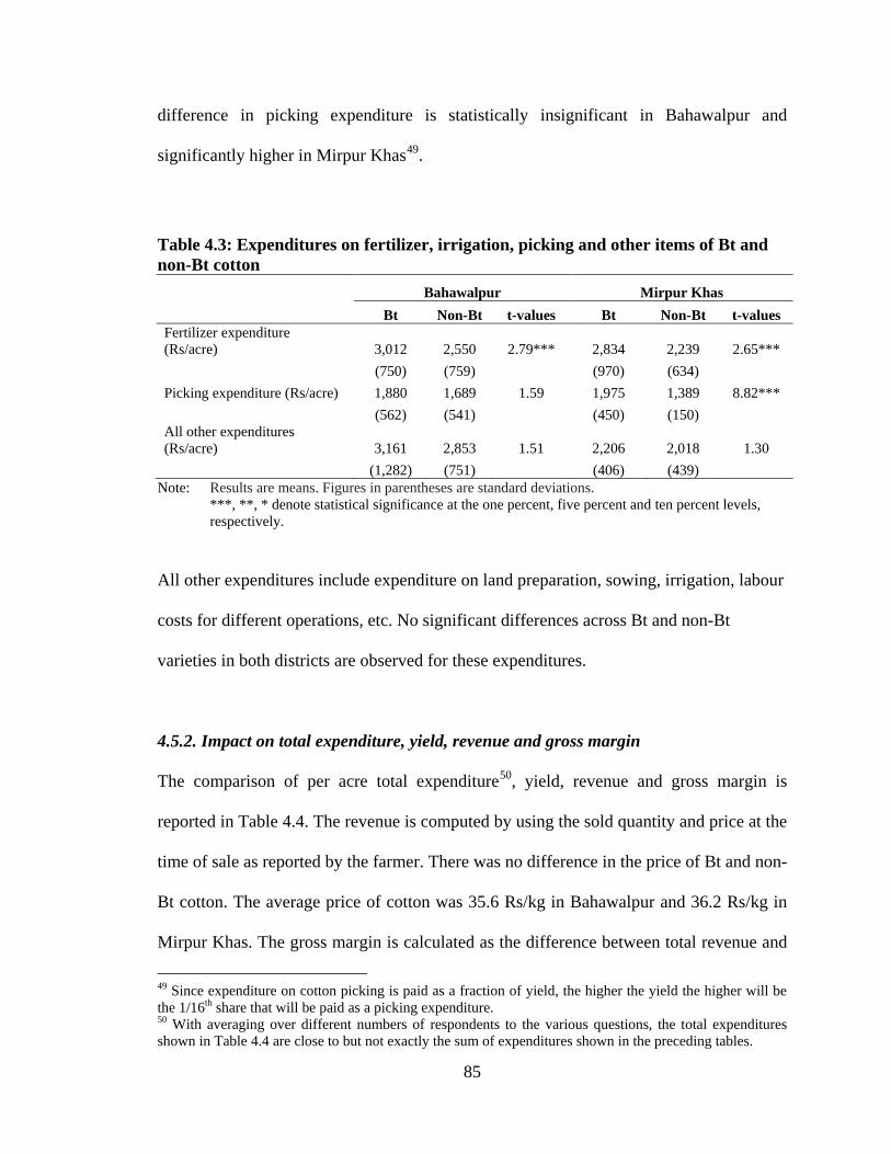
85

difference in picking expenditure is statistically insignificant in Bahawalpur and

significantly higher in Mirpur Khas49

.

Table 4.3: Expenditures on fertilizer, irrigation, picking and other items of Bt and non-Bt cotton


Bt Non-Bt t-values Bt Non-Bt t-values

Fertilizer expenditure (Rs/acre) 3,012 2,550 2.79*** 2,834 2,239 2.65***

(750) (759)

(970) (634)

Picking expenditure (Rs/acre) 1,880 1,689 1.59 1,975 1,389 8.82***

(562) (541)

(450) (150)

All other expenditures (Rs/acre) 3,161 2,853 1.51 2,206 2,018 1.30 (1,282) (751)

(406) (439)

Note: Results are means. Figures in parentheses are standard deviations. ***, **, * denote statistical significance at the one percent, five percent and ten percent levels, respectively.

All other expenditures include expenditure on land preparation, sowing, irrigation, labour

costs for different operations, etc. No significant differences across Bt and non-Bt

varieties in both districts are observed for these expenditures.

4.5.2. Impact on total expenditure, yield, revenue and gross margin

The comparison of per acre total expenditure50

49 Since expenditure on cotton picking is paid as a fraction of yield, the higher the yield the higher will be the 1/16th share that will be paid as a picking expenditure.

, yield, revenue and gross margin is

reported in Table 4.4. The revenue is computed by using the sold quantity and price at the

time of sale as reported by the farmer. There was no difference in the price of Bt and non-

Bt cotton. The average price of cotton was 35.6 Rs/kg in Bahawalpur and 36.2 Rs/kg in

Mirpur Khas. The gross margin is calculated as the difference between total revenue and

50 With averaging over different numbers of respondents to the various questions, the total expenditures shown in Table 4.4 are close to but not exactly the sum of expenditures shown in the preceding tables.

86

total expenditure. Table 4.4 shows that the total expenditure on Bt and non-Bt cotton is

not statistically significant in either district. Higher yield of Bt cotton gave higher

revenue in both districts. Resultantly, Bt varieties appeared more profitable. This table

shows that yield per acre, revenue and gross margins are significantly higher for Bt

varieties in Mirpur Khas whereas in Bahawalpur despite insignificant yield and revenue

per acre, the gross margin appeared significant.

Table 4.4: Total expenditure, yield, revenue and gross margin of Bt and non-Bt cotton


Bt Non-Bt t-values Bt Non-Bt t-values Total expenditure (Rs/acre) 13,662 13,814 -0.22 10,829 10,908 -0.12

(4,003) (2,714)

(3,374) (1,868)

Yield (kg/acre) 845 759 1.59 873 613 8.82***

(253) (244)

(199) (68)

Revenue (Rs/acre) 30,094 27,028 1.59 31,606 22,224 8.82***

(9,003) (8,670)

(7,202) (2,394)

Gross margin (Rs/acre) 16,432 13,213 1.89** 20,776 11,316 8.61***

(8,528) (7,434)

(7,715) (2382) Average price of cotton

(Rs/kg) 35.6 35.6

36.2 36.2 Adjusted Gross margin for

sharecroppers (Rs/acre) 16,206 13,091 1.80* 12,870 6,247 6.94***

(8,627) (7,819)

(6,044) (2,278)

Note: Results are means. Figures in parentheses are standard deviations. Expenditures, revenue and gross margin are in Rs/acre and yield is in kg/acre. ***, **, * denote statistical significance at the one percent, five percent and 10 percent levels, respectively.

As discussed earlier, the sample includes a large number of sharecroppers who

share the harvest and input expenditure with the landlord on a 50-50 basis. A majority of

the sharecroppers in the survey indicate that the landlord provides 50 percent of the

inputs, except labour, and the sharecropper is responsible for 50 percent of the inputs.

87

Adjusted gross margin is calculated as the difference between adjusted revenue (amount

received by sharecropper) and adjusted total expenditure (amount paid by sharecropper).

Last row of Table 4.4 reports the gross margin adjusted for the sharecroppers. The results

indicate significantly higher gross margin for the sharecroppers who grow Bt cotton. An

increase in yield is likely to have a positive impact on the revenue received by the

sharecroppers.

4.5.3 Impact on poverty

At this point it would be interesting to look at the impact of Bt cotton adoption on

poverty. Poverty is defined in absolute terms by Foster-Greer-Thorbecke (FGT) measures

(poverty headcount, poverty severity and poverty gap) using Pakistan’s national poverty

line. These measures can be computed as

𝑃𝛼 =1𝑁��

𝜇 − 𝑦𝑖𝜇

�𝛼

𝑞

𝑖=1

where Pα is the FGT poverty measure, N is the number of households, q is the number of

poor households, μ is the poverty line, and yi is the income of the poor household i.

Different values of α (α = 0, 1, and 2) yield different measures of poverty, giving

different weights to the degree of poverty and inequality among the poor. When α = 0,

the poverty measure P0 is the incidence of poverty, i.e., the proportion of households

whose income is below the poverty line. When α = 1, the poverty measure P1 is the

poverty-gap measure. The poverty gap is equal to the incidence of poverty multiplied by

the average gap between the poverty line and the income of a poor household, expressed

as a percentage of the poverty line. Thus, it takes into account the depth of poverty. If α =

88

2, then the poverty measure P2 takes into account the degree of inequality among poor

households, as well as the depth of poverty and number of poor households. This

‘poverty-gap squared’ is referred to as a measure of the severity of poverty.

The poverty headcount is calculated using the national poverty line51

. This

poverty line is adjusted for 2008-09 at Rs 1,057.81 per capita per month. Because of the

unavailability of data on household consumption expenditure, income is used as a welfare

indicator. The poverty headcount, defined as a dummy variable, takes the value ‘1’ if a

household is poor, i.e., if per capita per month income is below Rs 1,057.81. Table 4.5

reports household income per capita per month and the results of these poverty measures

by adopters and non-adopters in both districts. This table shows that nearly half of the

population in both districts is poor. Despite a significant difference in per capita monthly

income, no significant difference in poverty headcount has been observed. In

Bahawalpur, poverty levels are found to be lower for adopters and the reverse situation is

observed for Mirpur Khas. However, the difference between adopters and non-adopter

does not appear to be significant. This may be due to the fact that the sample selection

process selected the poorest district from an agro-climatic zone. Therefore, the selected

sample may comprise of larger number of poor households.

51 If per capita per month household consumption expenditure was below Rs 944.47, a household was considered to be poor in 2005-06.

89

Table 4.5: Poverty among adopters and non-adopters of Bt cotton in Bahawalpur and Mirpur Khas.


Adopters Non-

adopters t-value Adopters Non-

adopters t-value Household income (per capita per month) (Rs) 2,216 1,215 2.16** 2,087 1,167 2.20**

Poverty headcount (P0) 0.50 0.55 -0.34 0.54 0.50 0.22

Poverty gap (P1) 0.24 0.34 0.55 0.22 0.21 0.01

Severity of poverty (P2) 0.16 0.22 -0.48 0.11 0.12 -0.04 Note: ** denote statistical significance at the five percent level.

4.5.4. Performance of Bt versus non-Bt cotton

Table 4.6 summarizes the results of Sections 4.5.1 and 4.5.2. These results show a

relatively better performance for the existing unapproved varieties of Bt cotton that

contain the first generation of the Bt gene. The number of bollworm sprays declined by

1.09 in Bahawalpur and 1.31 in Mirpur Khas. However, the number of sprays for non-

bollworms showed an increase in both districts. Total pesticide expenditure declined by

28.1 percent in Bahawalpur, and 26.2 percent in Mirpur Khas. This decline is mainly

driven by a substantial decline in the expenditure on bollworm sprays. This indicates the

effectiveness of existing Bt varieties in controlling the bollworms. This result is

comparable with that of Bennet et al. (2006a) who found a similar decline in

Maharashtra, India. The results show that Mirpur Khas experienced a much higher

increase in yield per acre from Bt varieties as compared to non-Bt varieties (42.4%) than

Bahawalpur (11.3%). Table 4.4 indicates that the yield increase in Bahawalpur is not

statistically significant. Sheikh et al. (2008) also found no significant difference in the

yield of Bt and non-Bt varieties in Punjab. Despite higher expenditure on seed, fertilizer

and cotton picking, the total expenditure on Bt varieties was lower than non-Bt varieties

in both districts. A higher yield and the same price for both varieties resulted in a higher

90

gross margin that is Rs 3,219 per acre higher in Bahawalpur and Rs 9,460 per acre higher

in Mirpur Khas.

Table 4.6: Comparison of costs, yield, revenue and gross margin between Bt and non-Bt varieties in Pakistan


Bollworm pesticide sprays -1.09 -1.31 Non-bollworm pesticide sprays 0.34 0.22 Total pesticide sprays -1.17 -1.78 Bollworm pesticide expenditure (Rs/acre) -43.6 -38.3 Non-bollworm pesticide expenditure (Rs/acre) 7.2 1.6 Total pesticide expenditure (Rs/acre) -28.1 -26.2 Seed expenditure (Rs/acre) 74.2 59.3 Total expenditure (Rs/acre) -1.1 -0.7 Yield (kg/acre) 11.3 42.4 Gross margin (Rs/acre) 3,219 9,460 Adjusted Gross margin for sharecroppers (Rs/acre) 3,115 6,623

Note: Figures are percentage differences. Number of sprays and gross margin are in simple difference.

It would be useful to compare the results of Pakistan with other countries. Table 4.7

provides a comparison of the performance of unapproved Bt varieties in Pakistan with the

performance of approved Bt varieties in India and China. This table shows that the

difference in pesticide expenditure, yield and gross margins in Pakistan is comparable

with both these countries. Similar to Pakistan, India also exhibits regional differences in

the performance of Bt cotton. However, the difference in the price of Bt and non-Bt seed

varieties is much lower in Pakistan than in India and China. This may be due to the

difference in approved and unapproved varieties.

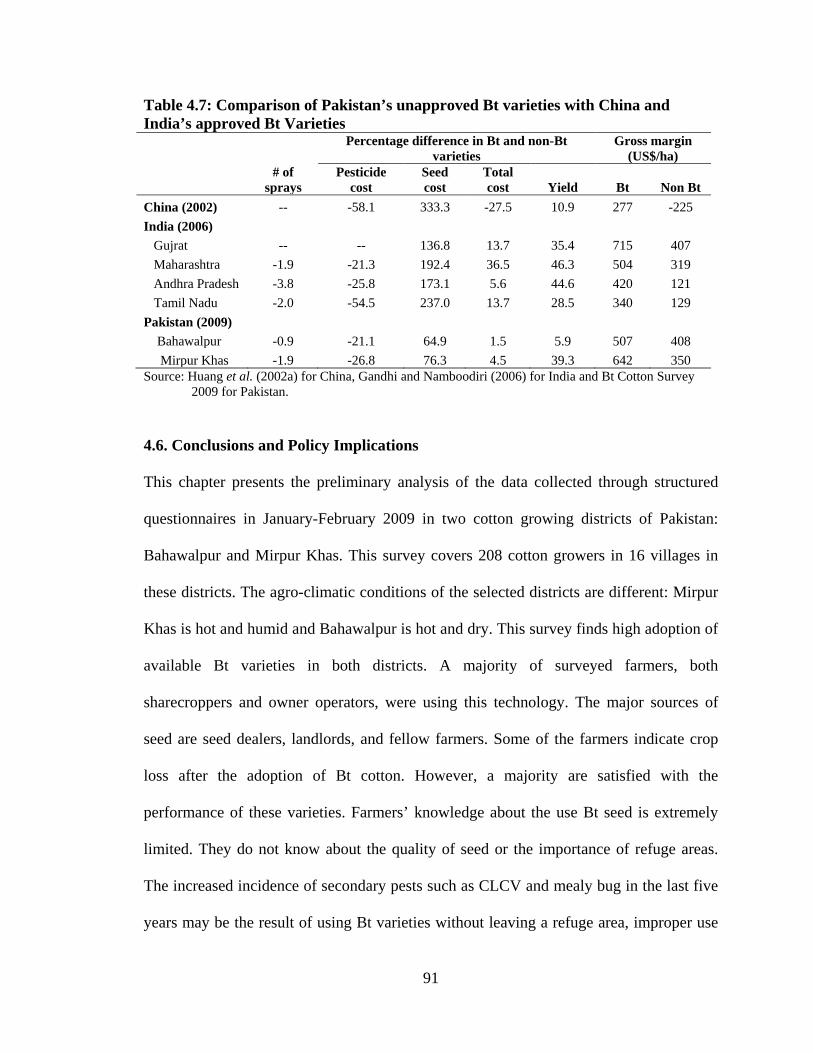
91

Table 4.7: Comparison of Pakistan’s unapproved Bt varieties with China and India’s approved Bt Varieties

Percentage difference in Bt and non-Bt

varieties Gross margin

(US$/ha)

# of

sprays Pesticide

cost Seed cost

Total cost Yield Bt Non Bt

China (2002) -- -58.1 333.3 -27.5 10.9 277 -225 India (2006)

Gujrat -- -- 136.8 13.7 35.4 715 407 Maharashtra -1.9 -21.3 192.4 36.5 46.3 504 319 Andhra Pradesh -3.8 -25.8 173.1 5.6 44.6 420 121 Tamil Nadu -2.0 -54.5 237.0 13.7 28.5 340 129 Pakistan (2009) Bahawalpur -0.9 -21.1 64.9 1.5 5.9 507 408 Mirpur Khas -1.9 -26.8 76.3 4.5 39.3 642 350 Source: Huang et al. (2002a) for China, Gandhi and Namboodiri (2006) for India and Bt Cotton Survey

2009 for Pakistan.

4.6. Conclusions and Policy Implications

This chapter presents the preliminary analysis of the data collected through structured

questionnaires in January-February 2009 in two cotton growing districts of Pakistan:

Bahawalpur and Mirpur Khas. This survey covers 208 cotton growers in 16 villages in

these districts. The agro-climatic conditions of the selected districts are different: Mirpur

Khas is hot and humid and Bahawalpur is hot and dry. This survey finds high adoption of

available Bt varieties in both districts. A majority of surveyed farmers, both

sharecroppers and owner operators, were using this technology. The major sources of

seed are seed dealers, landlords, and fellow farmers. Some of the farmers indicate crop

loss after the adoption of Bt cotton. However, a majority are satisfied with the

performance of these varieties. Farmers’ knowledge about the use Bt seed is extremely

limited. They do not know about the quality of seed or the importance of refuge areas.

The increased incidence of secondary pests such as CLCV and mealy bug in the last five

years may be the result of using Bt varieties without leaving a refuge area, improper use

92

of inputs by farmers, the use of non-CLCV resistant varieties to transfer the Bt gene, etc.

These findings are consistent with the results from other developing countries. The main

findings of this survey are summarized below.

Relatively better performance of Bt varieties: Contrary to the findings of earlier studies

(Hayee, 2004; Sheikh et al., 2008; Arshad et al., 2009), but similar to the study of Ali and

Abdulai (2010), the results of this study show a relatively better performance of the

existing unapproved varieties of Bt cotton that contain the first generation of the Bt gene

compared to conventional (non Bt) varieties. A decline in the number of bollworm

sprays, and hence in the expenditure of pesticides, was observed. Both districts

experienced a decline in pesticide expenditure and an increase in expenditure on seed,

fertilizer, and picking. An increase in yield was observed in both districts that resulted in

a higher gross margin for Bt varieties.

The impact of Bt varieties is not the same across districts: The extent of the impact of Bt

cotton on cost of production and yield is different across districts. For example, the

number of non-bollworm sprays increased by 7.2 percent in Bahawalpur, whereas this

increase was 1.6 percent in Mirpur Khas. Bahawalpur experienced a yield increase by

11.3 percent and Mirpur Khas by 42.4 percent. This resulted in differences in the effect of

Bt cotton on total revenue and gross margins.

No significant difference in the poverty measures for adopters and non-adopters: The

incidence of poverty is found high in both districts. No significant difference in poverty

measures has been observed between adopters and non-adopters.

The results are similar to other studies of Bt cotton in India. There are gains from

the adoption of unapproved Bt-cotton and this suggests further gains for Pakistan are

93

possible by progressing to a regulated national market for Bt cotton technologies. Despite

a small sample, this analysis captures the agro-climatic diversity in the selected districts

and highlights different effects of Bt cotton for different intensities of pest pressure. Due

to the high diversity of the cotton-growing areas, more location-specific information and

a larger sample size are required to capture the impact of Bt technology in the cotton-

growing areas of Pakistan on a full national scale.

94

CHAPTER 5

IMPACT OF BT COTTON ADOPTION ON THE WELLBEING OF COTTON FARMERS IN PAKISTAN

This chapter addresses the second objective of this thesis which is to examine the impact

of the adoption of Bt cotton on the wellbeing of farmers in Pakistan by addressing the

issue of selection bias in evaluating the survey results presented in Chapter 4. This

chapter is divided into three sections. Section 5.1 presents the analytical framework that

outlines the model for technology choice and impact assessment. Section 5.2 discusses

the results. Conclusions and policy implications are discussed in Section 5.3.

The preliminary results of the Bt Cotton Survey 2009 reported in Chapter 4

indicate a better performance for Bt cotton than for the conventional cotton in Pakistan.

These results are based on a comparison of means of outcome variables, which are,

pesticide expenditure, seed expenditure, total expenditure on cotton production, yield,

and gross margin, for Bt and non-Bt cotton. As discussed in Chapter 2, in non-

experimental studies of this sort, where the selection of subjects is not random, the

problem of self-selection arises. In the presence of self-selection, it is difficult to isolate

the effect of technology from other factors that can affect the decision of adoption. For

example, it is possible that the adopters are better informed and more resourceful than the

non-adopters. In such a situation, it is difficult to determine whether adoption promotes

farmers’ wellbeing or whether better-off farmers have a higher probability of adopting

technology. Therefore, the comparison of means may provide misleading results (Thirtle

et al., 2003; Crost et al., 2007; Morse et al., 2007a; Ali and Abdulai, 2010).

95

To address the problem of selection bias, “treatment effect models” are commonly

applied. These are two-stage models: in the first stage, the decision model (treated or

untreated) is estimated; and in the second stage, the results of the first stage are used to

estimate the impact of treatment on the outcome variables. Four commonly used methods

are: instrumental variables (IV) and two stage least squares (2SLS); Heckman’s two-step

method; difference-in-differences estimation; and propensity score matching (PSM)

method. These models evaluate the causal effect52 of an intervention by estimating the

average treatment effect (ATE) or average treatment effect on the treated (ATT). Several

studies used the treatment effect models to examine the economic impact of agricultural

technologies in developing countries: Mendola (2007) for high yielding varieties of rice

in Bangladesh; Adekambi et al. (2009) for new rice varieties in Benin; González (2009)

for agricultural extension services in Dominican Republic; Wu et al. (2010) for improved

rice varieties in rural China; Kassie, et al. (2010) for improved groundnut varieties in

Uganda; Otsuki (2010) for agro-forestry and soil conservation technologies in Kenya;

Becerril and Abdulai (2010) for improved maize varieties in Mexico; Ali and Abdulai

(2010) for Bt cotton adoption in Pakistan. However, the application of these models in

analyzing the impact of GM crops on household wellbeing is limited. Based on the

propensity score matching method, this chapter examines the impact of Bt cotton

adoption on the wellbeing of cotton farmers in Pakistan by addressing the issue of

selection bias in a counterfactual framework53

. The data from the Bt Cotton Survey 2009

collected in Bahawalpur and Mirpur Khas are used for this empirical analysis.

52 Causal effect compares the average difference in the outcome variable(s) of treated and untreated groups. 53 The counterfactual situation analyzes “how much did the treated individuals benefit from the treatment compared to the situation if they would not have been treated”.

96

5.1 Economic Impact of Bt Cotton Adoption: Analytical Framework

5.1.1 Decision of technology adoption

The economic rationale driving the the analytical framework underlying the the choice

between two technologies is the maximization of perceived utility. The adoption of a new

technology is usually modeled as a choice between two alternatives: the conventional

technology and the new one. Farmers are assumed to make their decisions by choosing

the alternative that maximizes their perceived utility. A farmer’s decision to adopt a new

technology can be described as a binary choice where the farmer can choose to adopt (I =

1) or not (I = 0). The adoption of new technology incurs a fixed cost (C) that will be

positive if technology is adopted and zero if not adopted. Therefore, C > 0 if I = 1 and C

= 0 if I = 0. A risk-averse farmer i decides to adopt a new technology if the expected

utility of profit of adoption 𝐸𝑈(𝜋𝑖1) minus its cost is larger than the expected utility of

not adopting 𝐸𝑈(𝜋𝑖0), i.e., 𝐸𝑈(𝜋𝑖1 − 𝐶) − 𝐸𝑈(𝜋𝑖0) > 0 (Marra et al., 2001; Payne et al.,

2003; Alexander and Mellor, 2005; Koundouri et al., 2006; Kolady and Lesser, 2006).

Let 𝐼∗ = 𝐸𝑈(𝜋𝑖1 − 𝐶) − 𝐸𝑈(𝜋𝑖0). Since I* is not observable, it can be expressed

as a function of observable elements in the following latent variable model:

𝐼𝑖∗ = 𝑍𝑖𝛾 + 𝜀𝑖 (5.1)

and

𝐼𝑖 = �1 𝑖𝑓 𝐼𝑖∗ > 00 𝑜𝑡ℎ𝑒𝑟𝑤𝑖𝑠𝑒

� (5.2)

where Ii is a binary variable defined earlier (Ii=1 if farm household i adopts Bt

technology, and 0 otherwise); 𝛾 is a vector of parameters to be estimated, Zi is a vector of

individual, household and farm-level characteristics, and 𝜀𝑖 is the error term assumed to

be normally distributed. The probability of adoption of Bt technology can be expressed as

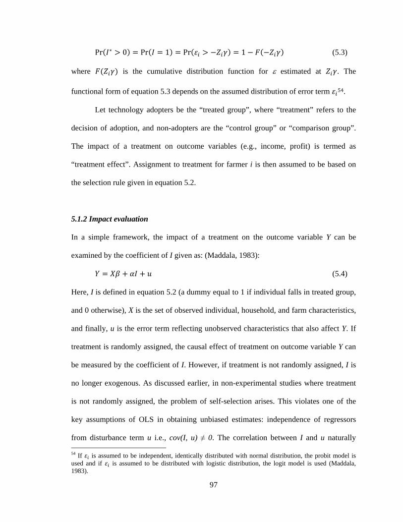
97

Pr(𝐼∗ > 0) = Pr(𝐼 = 1) = Pr(𝜀𝑖 > −𝑍𝑖𝛾) = 1 − 𝐹(−𝑍𝑖𝛾) (5.3)

where 𝐹(𝑍𝑖𝛾) is the cumulative distribution function for ε estimated at 𝑍𝑖𝛾. The

functional form of equation 5.3 depends on the assumed distribution of error term 𝜀𝑖54.

Let technology adopters be the “treated group”, where “treatment” refers to the

decision of adoption, and non-adopters are the “control group” or “comparison group”.

The impact of a treatment on outcome variables (e.g., income, profit) is termed as

“treatment effect”. Assignment to treatment for farmer i is then assumed to be based on

the selection rule given in equation 5.2.

5.1.2 Impact evaluation

In a simple framework, the impact of a treatment on the outcome variable Y can be

examined by the coefficient of I given as: (Maddala, 1983):

𝑌 = 𝑋𝛽 + 𝛼𝐼 + 𝑢 (5.4)

Here, I is defined in equation 5.2 (a dummy equal to 1 if individual falls in treated group,

and 0 otherwise), X is the set of observed individual, household, and farm characteristics,

and finally, u is the error term reflecting unobserved characteristics that also affect Y. If

treatment is randomly assigned, the causal effect of treatment on outcome variable Y can

be measured by the coefficient of I. However, if treatment is not randomly assigned, I is

no longer exogenous. As discussed earlier, in non-experimental studies where treatment

is not randomly assigned, the problem of self-selection arises. This violates one of the

key assumptions of OLS in obtaining unbiased estimates: independence of regressors

from disturbance term u i.e., cov(I, u) ≠ 0. The correlation between I and u naturally 54 If 𝜀𝑖 is assumed to be independent, identically distributed with normal distribution, the probit model is used and if 𝜀𝑖 is assumed to be distributed with logistic distribution, the logit model is used (Maddala, 1983).

98

biases the other estimates in the equation (Maddala, 1983; Greene, 2008; Khandker et al.,

2010).

The literature indicates four approaches to evaluate the impact of a treatment I on

the outcome variable Y by controlling the self-selection bias: 1) instrumental variables

(IV) and two stage least squares (2SLS); 2) Heckman’s two-step method; 3) difference-

in-differences estimation; and 4) propensity score matching (PSM) method55

55 Bryson et al. (2002) discussed these methods in detail.

. The

IV/2SLS method addresses the issue of self-selection bias with the help of an instrument

that is highly correlated with I and uncorrelated with u. In other words, the instrument

can have an effect on selection into the treatment but is not correlated with factors

affecting the outcomes. The IV/2SLS method requires the identification of a suitable

instrument. However, it is often difficult to find a suitable instrument (Wooldridge, 2002;

Vandenberghe and Robin, 2004). The IV/2SLS estimation method is applicable if the

treatment variable is continuous and endogenous. When the treatment variable is binary

and endogenous, Heckman’s two-step method provides the solution. It relies on the

assumption that a specific distribution of the unobservable characteristics jointly

influences the participation and the outcome. Heckman’s estimation method requires an

exclusion restriction to generate credible estimates. This restriction indicates that there

must be at least one variable that appears with a non-zero coefficient in the selection

equation but does not appear in the equation of interest. If no such variable is available, it

may be difficult to correct for selectivity bias (Goldberger, 1983; Puhani, 2000). The

difference-in-differences estimation examines the effect before and after the treatment

and between treated and untreated groups and, therefore, requires longitudinal data

(Buckley and Shang, 2003).

99

The matching method is another technique that controls the selection bias in a

nonparametric fashion. This method creates a situation similar to what would have been

observed in a random experiment. This method does not assume a functional form on the

outcome equation; and hence does not require the identification restriction. Thus the

difficulty of finding valid (good) instrumental variables can be avoided; and cross-

sectional data collected at one point in time can be used (Dehejia and Wahba, 1999;

2002; Smith and Todd, 2005). These methods give more consistent and realistic estimates

than the IV and Heckman’s methods (Wooldridge, 2005). The underlying principle is to

match the units in the treated group with the units in the control group that are similar in

terms of their observable characteristics. Matching is performed either on the basis of

similar propensity scores (Rosenbaum and Rubin, 1983; 1985) or on similar covariates

(Abadie and Imbens, 2002; Zhao, 2004; 2006).

Based on these attributes, propensity score matching is chosen for the analysis

presented in this chapter. The rest of this sub-section gives a detailed description on how

propensity score matching is used in evaluating the impact of technology adoption on

farmers’ wellbeing. Wellbeing is defined in terms of cotton yield, gross margin,

household income, and poverty headcount. The results are compared with other methods,

such as, Heckman’s two-step method, and difference of means method, and the covariate

matching method developed by Abadie and Imbens (2002). The remainder of this sub-

section gives a detailed description of how propensity score matching is used in

evaluating the impact of treatment on outcome variables.

100

Propensity Score Matching (PSM): Basic Model

Let y1ik be the level of outcome variable k for an individual i who receives treatment

(treated group) and y0ik represents the potential level of outcome variable k if this

individual does not receive treatment (control group). The gain from treatment called

“treatment effect” or “causal effect” is defined as:

𝜏𝑖𝑘 = 𝑦1𝑖𝑘 − 𝑦0𝑖𝑘 (5.5)

In equation 5.5 for individual i, only one value of outcome variable k, either y0i or y1i, can

be observed. The unobserved outcome is called the counterfactual outcome. Therefore,

the individual treatment effect 𝜏𝑖𝑘 defined in equation 5.5 cannot be estimated for the

same individual. In this situation, the parameter of interest is the ‘average treatment

effect’ (ATE), which is defined as

𝜏𝐴𝑇𝐸,𝑘 = 𝐸(𝑦1𝑖𝑘 − 𝑦0𝑖𝑘) (5.6a)

𝜏𝐴𝑇𝐸,𝑘 = 𝐸(𝑦1𝑖𝑘|𝐼𝑖 = 1) − 𝐸(𝑦0𝑖𝑘|𝐼𝑖 = 0) (5.6b)

The ATE is the average of the individual treatment effects across the whole population of

interest (Wooldridge, 2002). However, ATE does not address the issue of a counterfactual

situation, the situation a treated individual would have experienced had he/she not been

treated. In experimental studies where assignment to treatment is random, equation 5.5

can be used to estimate the average treatment effect. However, in non-experimental

studies, the treated and non-treated groups may not be the same before receiving

treatment. Therefore, the expected difference between these groups may not be due

entirely to the treatment. Adding and subtracting the expected outcome for non-treated

had they been treated and dropping the subscript k, 𝐸(𝑦0𝑖|𝐼𝑖 = 1)� in equation 5.6b gives:

𝜏𝐴𝑇𝐸 = 𝐸(𝑦1𝑖|𝐼𝑖 = 1)� − 𝐸(𝑦0𝑖|𝐼𝑖 = 1)� + 𝐸(𝑦0𝑖|𝐼𝑖 = 1)� − 𝐸(𝑦0𝑖|𝐼𝑖 = 0)� (5.7)

101

The first term in equation 5.7 𝐸(𝑦1𝑖|𝐼𝑖 = 1)� is the average outcome (e.g., income) of the

treated. This component is observed in the surveys. The second term 𝐸(𝑦0𝑖|𝐼𝑖 = 1)� is the

average outcome of the treated had they not been treated. The difference 𝐸(𝑦1𝑖|𝐼𝑖 = 1)� −

𝐸(𝑦0𝑖|𝐼𝑖 = 1)� is called Average Treatment Effect on the Treated (ATT) and indicates

‘How much did the treated individuals benefit from the treatment compared to the

situation if they would not have been treated?’ To estimate ATT, information on

𝐸(𝑦0𝑖|𝐼𝑖 = 1)� is required. If both outcomes are observed, the ATT or the causal effect

can be estimated by 1𝑁1∑ 𝐼𝑖𝑖 [𝑦1𝑖 − 𝑦0𝑖], where 𝑁1 = ∑ 𝐼𝑖𝑖 is the number of treated units in

the sample. In experimental studies, the mean outcome of untreated individuals

𝐸(𝑦0𝑖|𝐼𝑖 = 0)� can be used as a proxy for 𝐸(𝑦0𝑖|𝐼𝑖 = 1)�. However, in non-experimental

surveys, treated and non-treated groups may not be the same before receiving treatment.

Therefore, 𝐸(𝑦0𝑖|𝐼𝑖 = 0)� cannot be used as a proxy for 𝐸(𝑦0𝑖|𝐼𝑖 = 1)�. Equation 5.7 can

be written as 𝜏𝐴𝑇𝐸 = 𝜏𝐴𝑇𝑇 + 𝐵, where 𝐵 = 𝐸(𝑦0𝑖|𝐼𝑖 = 1)� − 𝐸(𝑦0𝑖|𝐼𝑖 = 0)� indicates the

extent of selection bias that arises when ATE is considered to examine the impact of a

treatment in non-experimental studies. The basic objective of the impact analysis is either

to make selection bias zero (B = 0) or to find ways to account for it, i.e., to make 𝜏𝐴𝑇𝑇 =

𝜏𝐴𝑇𝐸 by making 𝐸(𝑦0𝑖|𝐼𝑖 = 1)� = 𝐸(𝑦0𝑖|𝐼𝑖 = 0)�, so that:

𝜏𝐴𝑇𝑇 = 𝜏𝐴𝑇𝐸 = 𝐸(𝑦1𝑖|𝐼𝑖 = 1)� − 𝐸(𝑦0𝑖|𝐼𝑖 = 0)� (5.8)

The validity of matching methods depends on two conditions: (i) unconfoundedness or

conditional independence assumption (CIA); and (ii) common support (for each value of

X there should be both treated and untreated cases).

Unconfoundedness or conditional independence assumption: This assumption was

introduced by Rosenbaum and Rubin (1983). Lechner (1999, 2002) refers to it as the

102

“conditional independence assumption”. Barnow et al. (1980) and Fitzgerald et al. (1998)

call this selection on observables, and Imbens (2004) terms it exogeneity. This

assumption states that conditional on a set of observables, X, the respective treatment

outcomes y1i, y0i are independent of the actual treatment status I:

(𝑦0𝑖 ,𝑦1𝑖) ⊥ 𝐼𝑖|𝑋 (5.9)

where ⊥ is the symbol of independence. This means that given X, one can use the income

of non-treated units to approximate the income of treated units to describe the

counterfactual situation.

Common support or overlap: This assumption rules out the phenomenon of perfect

predictability of I given X and ensures that for each value of X there are both treated and

untreated cases:

0 < Pr(𝐼𝑖 = 1|𝑋) < 1 (5.10)

This indicates that there is an overlap between the treated and untreated sub-samples. For

each treated individual there is another matched untreated individual with a similar X.

The observations from the non-treated group that fall outside the common support region

should be dropped. Rosenbaum and Rubin (1983) termed assumptions 1 and 2 as “strong

ignorability”. When these assumptions are satisfied, the experimental and non-

experimental analyses identify the same parameters.

When the assumptions of unconfoundedness and common overlap are satisfied,

the treated group is matched with the non-treated group for each value of X using an

appropriate matching algorithm56

56 Commonly used algorithms are: nearest neighbour matching, radius matching, kernel matching, and stratification. These algorithms are explained in detail under the discussion on matching methods.

. The higher number of covariates (X’s) can cause the

103

problem of dimensionality, i.e., it is difficult to hold the condition 𝑦𝑖0 ⊥ 𝐼|𝑋.57

𝑝(𝑋) = 𝑝(𝐼𝑖 = 1|𝑋) (5.11)

An

important advancement was made by Rosenbaum and Rubin (1983) with the introduction

of the propensity score, defined as the conditional probability of receiving a treatment

given pre-treatment characteristics. Propensity scores summarize all of the covariates into

one scalar: the probability of being treated, p(X):

There are two key properties of propensity scores. The first is that propensity

scores are balancing scores. This property states that if p(X) is the propensity score, then

conditioning covariates should be independent of the decision of treatment, i.e., 𝑋 ⊥

𝐼𝑖|𝑝(𝑋). In other words, at each value of the propensity score, the distribution of the

covariates X defining the propensity score should be the same in the treated and control

groups: �̂�(𝑋|𝐼𝑖 = 1) = �̂�(𝑋|𝐼𝑖 = 0). Thus, grouping individuals with similar propensity

scores creates the situation of a randomized experiment with respect to the observed

covariates. The second property of propensity score is that if treatment assignment is

ignorable given the covariates, i.e., (𝑦0𝑖 ,𝑦1𝑖) ⊥ 𝐼𝑖|𝑋, then treatment assignment is also

ignorable given the propensity score, i.e., (𝑦1𝑖, 𝑦0𝑖) ⊥ 𝐼𝑖|𝑝(𝑋). This reduces the problem

of high dimensionality to a single index variable, the propensity score, i.e., the probability

of being treated p(X), and matching can be performed on p(X) alone rather than on the

full set of covariates. Thus, when treatment assignment is ignorable, the difference in

means in the outcome between treated and control individuals with similar propensity

scores gives an estimate of the treatment effect by describing the counterfactual situation.

Summarizing the above discussion, the estimation of a causal effect of a treatment in a

57 “If X contains s covariates which are all dichotomous, the number of possible matches will be 2s” (see Caliendo and Kopeinig, 2005, page 4).

104

counterfactual situation can be described as a two-step procedure. In the first step,

propensity score is estimated given the observed covariates that fulfil the assumptions of

unconfoundedness and overlapping and satisfy the balancing property. In the second step,

for outcome k, the ATT is estimated by matching the treated group with the control group

based on the estimated propensity scores as:

𝜏𝐴𝑇𝑇 = 𝐸�𝑦1𝑖 − 𝑦0𝑖�𝑝(𝑋)� = 𝐸(𝑦1𝑖|𝑝(𝑋), 𝐼𝑖 = 1) − 𝐸(𝑦0𝑖|𝑝(𝑋), 𝐼𝑖 = 0) (5.12)

Step 1: Estimation of propensity score:

This step requires choosing the covariates and selection of the model.

Choice of covariates: The implementation of matching requires choosing a set of

variables X that credibly satisfy the condition of unconfoundedness, i.e., the outcome

variable(s) must be independent of treatment. In selecting the covariates, it is important to

consider those variables that influence the participation decision and the outcome

simultaneously. Therefore, the variables that are unaffected by participation should be

included in the model. To ensure this, variables should either be fixed over time or

measured before participation, variables such as age, education, gender, farm size,

location, etc. (Caliendo and Kopeinig, 2005).

Model selection: The propensity score is the conditional probability of treatment given a

vector of pre-treatment covariates. The propensity score p(X) is defined in Equation 5.11.

The question is what would be the appropriate functional form of p(X) to estimate the

propensity score. In principle, any discrete choice model, such as a logit or probit model,

can be used to estimate the propensity to participate that gives the measure of the

propensity score (Becker and Ichino, 2002).

105

In the propensity score matching method, the primary concern is not to test the

statistical properties of the parameter estimates of the model, but rather with the resulting

balance of the covariates (Rosenbaum and Rubin, 1985; Augurzky and Schmidt, 2001;

Dehejia and Wahba, 2002). After estimating the propensity scores, a balancing test is

performed. Three methods are commonly used to test the balancing property. First,

calculate the standardized bias before and after matching and check for the significant

difference in the covariates for both groups using a t-test. The balancing property will be

satisfied if the t-value is low (Rosenbaum and Rubin, 1985). Second, re-estimate the

propensity score on the matched sample for treated and non-treated groups and compare

the pseudo R2 before and after matching. The low value of pseudo R2 indicates balancing

property is satisfied (Sianesi, 2004). Third, perform a stratification test by dividing the

sample into blocks. In each block, the similarity of average propensity score for treated

and non-treated units should be tested using a t-test. The balancing property would be

satisfied if the difference between treated and non-treated groups appeared insignificant

(Dehejia and Wahba, 1999; 2002). When the balancing property is satisfied, the region of

common support needs to be defined. In this region, the distributions of the propensity

score for the treatment and comparison groups should be overlapped. A standard

approach for checking common support is to compare variable minima and maxima.

Observations whose propensity scores are smaller than the minimum and/or larger than

the maximum are dropped from the sample (Caliendo and Kopeinig, 2005). The greater

the overlap in all characteristics, the more comparable the groups are, and the smaller the

bias (Heckman et al., 1997; Heckman et al., 1998).

106

Once the above mentioned properties are satisfied, the next step is to perform

matching using the estimated propensity score. The literature suggests various methods

for matching the propensity scores. However, four methods are widely used: nearest

neighbour matching, radius matching, kernel matching, and stratification matching

(Becker and Ichino, 2002). In all matching algorithms, each treated individual i is paired

with some group of ‘comparable’ non-treated individuals j and then the outcome of the

treated individual i, yi, is linked with the weighted outcomes of his ‘neighbours’ j in the

comparison (control) group.

Nearest neighbour (NN): In the nearest neighbour (NN) matching method, each treated

unit is matched with the comparison unit with the closest propensity score. Matching can

be performed ‘with replacement’ or ‘without replacement’. In matching with

replacement, each treatment unit is matched to the nearest comparison unit, thus

minimizing the propensity score distance (or reducing the bias) between the treated and

comparison units. Thus a comparison unit can be matched more than once with a treated

unit. In contrast, in matching without replacement, any observation in the comparison

group is matched only once with the treated observation, which is the closest match. In

this case, matches may not be very close in terms of p(X), which will increase the bias of

the estimator (Smith and Todd, 2005). Let 𝐴𝑖(𝑋) be the set of comparison units matched

to the treated unit i such that 𝐴𝑖(𝑋) = �𝑗| min𝑗�𝑋𝑖 − 𝑋𝑗��, where ‖ ‖ is the Euclidean

distance between vectors. In terms of propensity scores, 𝐴𝑖(𝑋) for the nearest neighbour

matching can be defined as 𝐴𝑖𝑁𝑁�𝑝(𝑋)� = �𝑝𝑗|�𝑝𝑖 − 𝑝𝑗��.

Radius matching (RM): As mentioned earlier, if the comparison group is small, the

closest neighbour may fall far away. In this situation, the NN matching faces the risk of

107

bad matches. A partial solution is to use a predefined neighbourhood in terms of a radius

around the p(X) of the treated observation and to exclude matches that lie outside this

neighbourhood. This is called “caliper or radius matching” (Dehejia and Wahba, 2002).

In this method, each treated unit is matched with those comparison units whose

propensity score falls into a predefined neighbourhood of the propensity score of the

treated unit. This method not only uses the nearest neighbour within each caliper, but also

uses all the comparison units within the caliper. For caliper/radius matching, the

comparison set is defined as 𝐴𝑖𝑅𝑀�𝑝(𝑋)� = �𝑝𝑗|�𝑝𝑖 − 𝑝𝑗� < 𝑟�. This implies that all

cases in the comparison group with estimated propensity scores falling within radius r are

matched to the ith treated case. In this technique, it is, however, difficult to know a priori

what choice for the tolerance level is reasonable (Smith and Todd, 2005).

Kernel matching: Kernel matching (KM) uses the weighted averages of all individuals in

the control group to construct the counterfactual outcome (Heckman et al., 1998; Smith

and Todd, 2005). The weights are inversely proportional to the distance between the

propensity scores of the treated and comparison units. With kernel matching, all treated

units are matched with a weighted average of all comparison units.

Stratification matching: This method divides the sample into five equal intervals

(quintiles) based on the propensity score; then, within each interval, the difference

between the average outcomes of the treated and comparison units is obtained. Finally,

weights are applied across intervals to calculate the average treatment effect. One of the

drawbacks of the stratification method is that it discards observations in blocks where

either treated or control units are absent.

108

After matching, the average treatment effect on treated is calculated to compare

the outcome variables. The difference is the estimate of the gain due to the program for

that observation. In view of the issue of small control groups, the nearest neighbour

matching method with replacement is chosen for this study.

Step 2: Estimation of average treatment effect on the treated (ATT)

As discussed above, the nearest neighbour (NN) matching method matches each treated

unit with similar values of propensity score for the untreated units. Then, the average

effect of the treatment on the treated units is estimated by averaging within-match

differences in the outcome variable between the treated and the untreated units. The

general formula for estimating the ATT for nearest neighbour, radius, and kernel

matching, with cross-section data and within the common support, can be written as

follows (Cameron and Trivedi, 2005):

𝐴𝑇𝑇𝑀 = 1𝑁𝑇∑ �𝑦1𝑖 − ∑ 𝑤(𝑖, 𝑗)𝑦0𝑗𝑗 �𝑖∈{𝐼=1} (5.13)

where {I = 1} is the set of treated individuals, and j is an element of the set of matched

comparison units; NT is the number of individuals in the treated groups (Ii=1); 𝑦1𝑖 is the

value of the outcome variable for the ith individual in treated group; 𝑦0𝑗 is the value of the

outcome variable for the jth individual in the comparison group; w(i, j) denotes the weight

given to the jth case in making a comparison with the ith treated case, 0 < w(i, j) ≤ 1.

Becker and Ichino (2002) define weights as: 𝑤(𝑖, 𝑗) = 1𝑁𝐶,𝑖

𝑖𝑓 𝑗 ∈ 𝐶(𝑖), 𝑎𝑛𝑑 𝑤(𝑖, 𝑗) =

0 𝑜𝑡ℎ𝑒𝑟𝑤𝑖𝑠𝑒. where 𝑁𝐶,𝑖 is the number in the comparison group corresponding to the ith

observation, the ATT for nearest neighbour matching can be written as

109

𝐴𝑇𝑇𝑀(𝑁𝑁) = 1𝑁𝑇∑ �𝑦𝑖 −

1𝑁𝐶,𝑖

∑ 𝑦𝑗𝑗∈(𝐼=0) �𝑖 (5.14)

Testing the statistical significance of treatment effects and computing their

standard errors is not straightforward. The estimated variance of the treatment effect in

PSM should include the variance attributable to the derivation of the propensity score, the

determination of the common support and (if matching is done without replacement) the

order in which treated individuals are matched (Caliendo and Kopeinig 2008). These

estimation steps add variation beyond the normal sampling variation (Heckman,

Ichimura, and Todd, 1998). One solution suggested by Lechner (2002) is to use

bootstrapping, where repeated samples are drawn from the original sample, and

properties of the estimates (such as standard error and bias) are re-estimated with each

sample. Each bootstrap sample estimate includes the first steps of the estimation that

derive the propensity score, common support, and so on. In this study, the bootstrapping

method is used to obtain the standard errors of the ATT.

Abadie and Imbens (2002) show that if the number of continuous covariates

available for matching exceeds one, the matching estimator of nearest neighbour can be

biased. To address this problem, they developed a bias-corrected covariate matching

(CM) method where the difference within the matches is regression-adjusted for the

difference in covariate values. Abadie and Imbens (2002) show that the bias corrected

matching estimator is consistent and has a sampling distribution that is asymptotically

normal. In addition, they provide expressions for computing the variance of the bias-

corrected estimator, making it possible to test the significance of the treatment effect

without relying on bootstrapping.

110

The adjustment is based on the estimation of two regression functions: �̂�𝐼(𝑥) =

𝐸[𝑦(𝐼)|𝑋 = 𝑥] 𝑓𝑜𝑟 𝐼𝑖 = 0 𝑜𝑟 = 1. The regression functions are approximated by linear

functions and estimated using least squares on the matched observations. If the estimator

of interest is average treatment effect on the treated, the estimation of the regression

function for the controls, 𝜇0(𝑥) is required. For estimating the average treatment effect

on the control, the estimation of the regression function for the treated 𝜇1(𝑥) is needed.

The bias-corrected covariate matching estimator suggested by Abadie and Imbens (2002)

can be written as:

𝐴𝑇𝑇𝐴𝐼 = 1𝑁𝑇∑ (𝑦𝑖 − 𝑦�0𝑖)𝑖:𝐼𝑖=1 (5.15)

where AI stands for Abadie-Imbens matching, 𝑦𝑖 = �𝑦0𝑖 𝑖𝑓 𝐼𝑖 = 0𝑦1𝑖 𝑖𝑓 𝐼𝑖 = 1

�, NT is the number of

individuals in the treated group, and 𝑦�𝑖0 is the missing potential outcome. Let individual i

of the treated group is matched with all observations l of the non-treated group, each time

weighted by the total number of matches for observations l; let 𝑗𝑀(𝑖) is the set of indices

for the matches for unit i that are at least as close as the Mth match. The missing potential

outcome 𝑦�𝑖0 is estimated as

𝑦�0𝑖 = �𝑦𝑖 𝑖𝑓 𝐼𝑖 = 0

1

#𝐽𝑀(𝑖)∑ �𝑦𝑗 + �̂�0(𝑥𝑖) − �̂�0(𝑥𝑙)� 𝑖𝑓 𝐼𝑖 = 1𝑙∈𝐽𝑀(𝑖)

� (5.16)

where #JM(i) is the number of elements of JM(i), and �̂�0(𝑋) denotes the estimated

regression function for the controls with covariates values X=x. The bias-adjusted

matching estimator combines some of the bias reductions from the matching by

comparing units with similar values for the covariates, and the bias reduction from the

regression.

111

This study compares the ATT estimated by PSM with CM method suggested by

Abadie and Imbens (2002).

5.2 Results and Discussion

The impact of Bt cotton adoption on the wellbeing of cotton farmers is measured using

the average treatment effect on the treated (ATT) approach, where treatment refers to the

decision of Bt cotton adoption. Wellbeing is measured in terms of outcome variables

(pesticide and seed expenditures, total cost of cotton production, cotton yield, gross

margin, per capita household income, and poverty status). As described in the empirical

framework, the ATT measures the causal effect, i.e., average change in the outcome

variables of adopters as a result of Bt cotton adoption. The calculation of the ATT

involves three steps: estimating the propensity scores; matching the propensity scores

(generating treated and comparison groups); and undertaking impact analysis using the

matched groups/samples. As discussed in the previous section, the estimation of

propensity scores requires two steps: (i) selection of covariates, and (ii) selection of

model.

Selection of covariates

Rosenbaum and Rubin (1983) indicate that if treated units and control units have the

same value of propensity score, they have the same distribution of Xi, irrespective of the

dimension of Xi. Thus, if there are differences in outcomes between the treated and

control units, these differences cannot be due to observed covariates. In other words, if

treatment and control groups have the same distribution of propensity scores, they have

112

the same distribution of all observed covariates, just as in a randomized experiment.

Therefore, the choice of explanatory variables (i.e., conditioning variables) in predicting

propensity scores is crucial in propensity score matching analysis. The selection of

covariates should fulfill the assumption of unconfoundedness. Therefore, there is a need

to select variables that influence both treatment and outcome variables, but are not

affected by the treatment (Caliendo and Kopeinig, 2008). The variables employed in this

study are based on research that examined the impact of technology adoption on farmers’

wellbeing in developing countries (Mendola, 2007; Adekambi et al., 2009; González,

2009; Wu et al., 2010; Ali and Abdulai, 2010; Kassie, et al., 2010; Otsuki, 2010; Becerril

and Abdulai, 2010). These factors can be divided into five groups: human capital factors

(age and education of a farmer); household level factors (household composition, wealth

factors); accessibility factors (access to information and credit); farm-related factors (type

of tenure, operated land); and yield variation.

Human capital factors: Human capital factors (education and experience of a farmer) can

influence the probability of adoption (Feder et al., 1985; Huffman, 2001). However, the

probability of adoption does not affect them. Education can enable a farmer to better

process the information that he obtains from different sources (Jamison and Lau, 1982).

Through experience a farmer can accumulate the farming knowledge and can better judge

the advantages and disadvantages of new technology. To capture the effect of education,

a dummy variable is defined that takes the value of 1 if farmers obtained some formal

education, and 0 if no formal education. In this study, age is used as a proxy for

experience in cotton growing. This is a continuous variable measured in years. The

113

literature indicates a positive impact of age and education on the decision of technology

adoption.

Household characteristics: To assess household characteristics, several indicators are

used. These indicators are divided into two groups: (i) household composition, and (ii)

wealth factors.

Household composition is measured by household size that can be defined as “all

household members,” “adult household members,” or “adult equivalents” (Doss, 2006).

This measure is used as a proxy for family labour. In this study, “household male

members, sixteen years or older58

Wealth is another factor that can affect the probability of adoption. The wealthier farmers

have greater access to resources and may be better able to adopt a new technology.

Several measures, such as the value of agricultural land, livestock, property, or non-

agricultural assets, can be used to measure wealth (Doss, 2006). In addition, participation

in non-farm income generating activities can also play an important role in accumulating

wealth and increasing household income, and hence improving access to resources.

Considering the monetary value of household assets and/or other incomes as explanatory

variables can violate the assumption of unconfoundedness. Therefore, the ownership of a

motor vehicle and TV, and access to non-farm employment are used as indicators of

household wealth status. These factors are defined by dummy variables that take the

value ‘1’ if a household owns these assets or has access to non-farm income sources, and

‘0’ otherwise. A positive sign is expected for the coefficients of these dummy variables.

” are used to explain the household composition. The

sign of the coefficient of household size would be positive if Bt technology is labour-

using and negative if technology is labour-saving.

58 Household size consists of all the members who live and eat together.

114

Factors related to access to services: Information about new technologies, timely

availability of agricultural inputs, and the availability of appropriate funds to make

investments in new technology are important factors in determining the technology

adoption decisions of farmers (Doss, 2006). Access to extension services is used as a

measure of access to information. This is measured as a binary variable that takes the

value of 1 if the farmer has been in contact with any extension services, 0 otherwise. A

positive relationship can be hypothesized between extension services and the probability

of technology adoption. In addition, distance to input shop can act as a proxy for access

to credit and marketing services59

Farm characteristics: The literature offered mixed results about the impact of type of

land tenure on the probability of technology adoption (Feder et al., 1985). It is expected

that owners are more likely to adopt a new technology as compared to tenants and

sharecroppers. A binary variable is used to define the type of land tenure. This variable

takes the value of 1 for owners and fixed-rent tenants, and 0 for sharecroppers. In

Pakistan, land is concentrated in a few hands and a majority of farmers operate the land

on a sharecropping basis. Owner-operators and fixed-rent tenants make their own

decisions about the use of inputs and adopting a new technology. However, for

. This is measured as a binary variable: 1 if distance is

more than 10 kilometers, and 0 if distance is less than 10 kilometers. It is hypothesized

that the greater the distance to the input shop, the less likely the farmers will adopt Bt

cotton. Therefore, the variable ‘distance to input shop’ is expected to have a negative

sign.

59 In Pakistan, input dealers extend cash as well as in-kind loans in the form of agricultural inputs; in return, farmers sell their crops to them. Therefore, input dealers act as a source of credit and output marketing services.

115

sharecroppers, these decisions are made by landlords. Therefore, the variable defining

type of land tenure can take a positive or negative sign.

The literature indicates that the adoption of an agricultural innovation takes place

earlier on larger farms than on smaller farms (Fernandez-Cornejo et al., 1994). In

Pakistan, the land distribution is highly skewed. The use of average operated land can

mask the differences between large and small farmers. Therefore, on the basis of land

under operation, three categories of farm size are defined: large farms (more than 12.5

acres); medium farms (more than 5 acres and up to 12.5 acres); and small farms (up to 5

acres). Small farmers are expected to have a lower probability of adopting Bt cotton

relative to medium and large farmers.

Yield variability: As mentioned previously, Bt cotton controls some of the pests and,

therefore, can control yield variations. The survey asked whether farmers had

experienced high, low or no variability in cotton yield over the last three years. Based on

this information, three dummy variables are defined. It is expected that variability (high

or low) is a motivation for a farmer to adopt Bt cotton.

5.2.1 Descriptive statistics

Table 5.1 provides the mean and standard deviation for the variables used in the decision

model for both adopters and non-adopters. Adopters are those farmers who cultivated Bt

cotton in 2008. This includes all households who grew both Bt and non-Bt varieties in

2008. To examine the difference in the characteristics of adopters and non-adopters, two

statistical tests are applied: (i) a two-group mean-comparison to test the continuous

variables such as experience, household size, etc.; and (ii) a Fisher’s Exact test to

116

compare the dummy variables such as access to credit, farm size, etc. The two-group

mean-comparison test is described in Section 4.6 of Chapter 4. The Fisher’s Exact test is

explained in Appendix 5. The mean, standard deviations, value of t-test (for the two-

group mean-comparison test) and p-values for Fisher's Exact test are reported in Table

5.1.

No significant difference is observed between adopters and non-adopters for the

variables related to human capital, household composition and wealth factors in either

district. Among accessibility factors, non-adopters have a significantly higher access to

extension services in Mirpur Khas, whereas in Bahawalpur this difference is not

significant. This result confirms that agriculture extension workers are still propagating

non-Bt cotton varieties in Pakistan. The variable indicating access to input dealers did not

show any significant difference for adopters and non-adopters in either district.

The disaggregation of operated land by farm size shows that most of the non-

adopters are small farmers (operate less than 5 acres) in both districts, and a majority of

adopters are medium (operate more than 5 but up to 12.5 acres) or large (operate more

than 12.5 acres) farmers. In Mirpur Khas, none of the non-adopters are large farmers. The

difference between adopters and non-adopters with respect to size of operational land is,

however, not statistically significant. The type of tenure is either owner or sharecropper.

Type of tenure for adopters and non-adopters is not statistically different in either district.

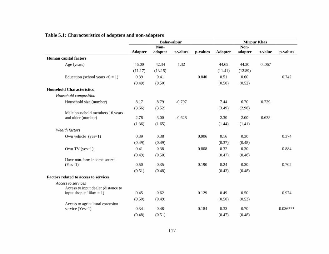
117

Table 5.1: Characteristics of adopters and non-adopters Bahawalpur Mirpur Khas

Adopter Non-

adopter

t-values p-values Adopter Non-

adopter t-value p-values Human capital factors Age (years) 46.00 42.34 1.32 44.65 44.20 0..067 (11.17) (13.15) (11.41) (12.89) Education (school years >0 = 1) 0.39 0.41 0.840 0.51 0.60 0.742 (0.49) (0.50) (0.50) (0.52) Household Characteristics Household composition Household size (number) 8.17 8.79 -0.797 7.44 6.70 0.729 (3.66) (3.52) (3.49) (2.98)

Male household members 16 years and older (number) 2.78 3.00 -0.628 2.30 2.00 0.638

(1.36) (1.65) (1.44) (1.41) Wealth factors Own vehicle (yes=1) 0.39 0.38 0.906 0.16 0.30 0.374 (0.49) (0.49) (0.37) (0.48) Own TV (yes=1) 0.41 0.38 0.808 0.32 0.30 0.884 (0.49) (0.50) (0.47) (0.48)

Have non-farm income source (Yes=1) 0.50 0.35 0.190 0.24 0.30 0.702

(0.51) (0.48) (0.43) (0.48) Factors related to access to services Access to services

Access to input dealer (distance to input shop > 10km = 1) 0.45 0.62 0.129 0.49 0.50 0.974

(0.50) (0.49) (0.50) (0.53)

Access to agricultural extension service (Yes=1) 0.34 0.48 0.184 0.33 0.70 0.036***

(0.48) (0.51) (0.47) (0.48)

118


Adopter Non-

adopter

t-values p-values Adopter Non-

adopter t-value p-values Farm Characteristics Small farmer (< 5 acres=1) 0.41 0.55 0.272 0.43 0.60 0.331 (0.49) (0.51) (0.50) (0.52)

Medium farmers (between 5 and 12.5 acres = 1) 0.40 0.38 0.846 0.34 0.40 0.735

(0.49) (0.49) (0.47) (0.52) Large farmers (>= 12.5 acres=1) 0.11 0.04 0.439 0.19 0.00 0.204 (0.31) (0.18) (0.39) Owner (Yes=1) 0.92 0.90 0.840 0.28 0.10 0.448 (0.28) (0.31) (0.45) (0.32) Yield variability

High yield variability in last 3 years (yes=1) 0.58 0.25 0.002*** 0.54 0.30 0.193

(0..49) (0.44) (0.50) (0.51)

Low yield variability in last 3 years (yes=1) 0.22 0.20 0.917 0.09 0.10 0.882

(0.42) (0.41) (0.28) (0.32)

No yield variability in last 3 years (yes=1) 0.20 0.55 0.001*** 0.37 0.60 0.191

(0.40) (0.51) (0.49) (0.52) Note: Results are means. Figures in parentheses are standard deviations. t-values are computed for the two-group mean comparison test and p-values

are for the Fisher’s Exact test. ***, **, * denote statistical significance at the one percent, five percent and ten percent levels, respectively.

119

The breakdown of the yield variability variable into adopters and non-adopters shows that

in Bahawalpur 58 percent of adopters and 25 percent of non-adopters face high

variability; 20 percent of adopters and 55 percent of non-adopters do not face any

variability. These differences are statistically significant. However, the difference in low

yield variability is not significant. In Mirpur Khas, 54 percent of adopters and 30 percent

of non-adopters indicate high variability, and 37 percent of adopters and 60 percent of

non-adopters indicate no variability; 10 percent of non-adopters face low variability

against 9 percent of adopters. These differences, however, are not significant.

These results indicate that adopters and non-adopters are not different in terms of

human capital and household characteristics. However, there are significant differences in

terms of accessibility factors (access to extension services), and yield variability.

5.2.2 Estimation of propensity score

Model selection

A Probit model is applied to estimate the propensity scores. The covariates included in

the probit model are used to predict the propensity score. Rubin and Thomas (1996)

suggest using all the covariates included in the model, even if they are not statistically

significant. The propensity score represents the estimated propensity of being treated. Its

magnitude ranges between 0 and 1; the larger the score, the more likely the individual

would receive treatment. The mean propensity scores for Bahawalpur, Mirpur Khas, and

full sample are 76 percent, 91 percent, and 81 percent, respectively. The results are

presented in Table 5.2. The dependent variable takes the value of 1 if the household is

adopter, and 0 otherwise. Three models are estimated: Model 1 and Model 2 are

120

estimated for Bahawalpur and Mirpur Khas, respectively, and Model 3 utilizes the data of

the full sample. In Model 3 the effect of district is captured by introducing a dummy

variable; the dummy variable is 1 if the observation is from Bahawalpur, and 0 otherwise.

As noted in Table 5.1, there are no large farmers among the non-adopters in Mirpur

Khas; therefore, two categories of farm size are used in the probit model: ‘medium and

large’ if farm size is more than 5 acres, and ‘small’ if farm size is up to 5 acres.

The log likelihood of the fitted model, which is used in the likelihood ratio chi-

square to test the null hypothesis that all regressors in the model are zero, is rejected at

the one-percent level in all three models. The McFadden pseudo R2 is 0.21, 0.26, and

0.21 for Models 1, 2 and 3, respectively. These diagnostic statistics suggest that the

estimated model provides an adequate fit for the data.

A comparison of Model 1 and Model 2 shows that the probability of Bt cotton

adoption is determined by different factors in Bahawalpur and Mirpur Khas. For

example, distance to input shop, access to services, and high yield variability appear to be

important in Bahawalpur. In Mirpur Khas, education, ownership of assets, access to

agricultural extension services, farm size, and high yield variability are found to be

significant determinants of Bt cotton adoption. In the full sample (Model 3), access to

services, yield variability and location appear to be important. A negative and significant

district dummy indicates that the probability of adoption is lower if the district is

Bahawalpur. A positive and significant impact of yield variability factors on the adoption

decision indicates that an increase in yield variability increases the probability of

adopting Bt cotton.

121

Table 5.2: Propensity scores for Bt cotton adoption (probit estimates)

Model 1:

Bahawalpur Model 2:

Mirpur Khas Model 3:

Full sample

Coeffi-cient z-value



Age 0.078 (0.87) 0.171 (1.31) 0.080 (1.14)

Age square -0.001 (-0.55) -0.002 (-1.5) -0.001 (-0.97) Education (=1 if school years>0) -0.544 (-1.54) -0.714* (-1.78) -0.485* (-1.83) Adult household members(=1 if >15 years) -0.167 (-1.38) 0.009 (0.05) -0.064 (-0.67)

Owns a vehicle (yes=1) 0.110 (0.29) -1.102*** (-2.12) -0.214 (-0.71)

Owns TV (yes=1) 0.295 (0.86) 0.314 (0.64) 0.323 (1.22)

Non-farm work (yes=1) 0.246 (0.79) 0.054 (0.13) 0.094 (0.38) Distance to input shop (=1 if distance >10 km) -0.604** (-2.08) 0.213 (0.43) -0.383 (-1.59) Small farmer (< 5 acres=1) -0.145 (-0.38) -0.757* (-1.76) -0.340 (-1.26)

Owner (owner farmer=1) -0.757 (-0.77) 0.924 (1.35) 0.362 (0.96) Agriculture extension contact (yes=1) -0.604* (-1.64) -1.200*** (-3.27)

-0.593*** (-2.35)

High yield variability in last 3 years (yes=1) 1.06*** (3.12) 0.814** (2.04) 0.842*** (3.4) Low yield variability in last 3 years (yes=1) 0.608 (1.56) 0.178 (0.20) 0.401 (1.18)

District (Bahawalpur =1) -

1.151*** (-3.08)

Constant -0.483 (-0.21) -0.881 (-0.31) -0.105 (-0.07)

Model Statistics

Number of observations 103 103 206

Log likelihood -48.47 -24.22 -78.91

Wald chi-square (df=13) 28.4*** 22.05** 42.44***

Pseudo R2 0.21 0.26 0.21

Predicted probability 0.76 0.91 0.81 Note: The dependent variable is the decision to adopt Bt cotton equals one, zero otherwise.

***, **, * denote statistical significance at the one percent, five percent and ten percent levels, respectively; z-values (in parentheses) are calculated from robust standard errors; df is degrees of freedom (df=13 for Models 1 and 2, and =14 for Model 3).

122

Checking balancing property and defining the region of common support

After estimating the propensity score, a balancing test is performed using the

stratification test suggested by Dehejia and Wahba (1999; 2002). The sample is divided

into five blocks based on the predicted propensity score. In each block, the predicted

propensity score is tested for the similarity between adopters and non-adopters using the

t-test. The propensity score does not appear statistically different for adopters and non-

adopters in these blocks. Once all the blocks are balanced, the individual mean t-test

between adopters and non-adopters for each variable used to predict the propensity score

is performed in each block. The low values of t-test show that the distribution of

conditioning covariates does not differ across adopters and non-adopters in the matched

sample60

To make the samples of treated and control groups comparable, matching was

undertaken within a region of common support (region of overlap between the propensity

scores of treated and non-treated units). The region of common support for Bahawalpur is

[.18504992, .96829685] and for Mirpur Khas is [.32751401, .99729959] and for the full

sample is [.18504992, .99729959]. The values that do not fall in these ranges are

discarded.

. The balancing property is satisfied for both districts.

5.2.3 Estimation of Average Treatment Effect on the Treated (ATT)

This section presents a discussion of the results from the analysis of the impact of Bt

cotton adoption on the wellbeing of cotton farmers. In view of different weather

conditions, the results of both districts are presented. Based on the findings of the studies

60 These results are not reported here.

123

on the economic impact of Bt cotton in other developing countries, discussed in Chapter

2, the following hypotheses are tested:

1. Pesticide expenditure is lower on Bt cotton than non-Bt cotton.

2. Bt cotton incurs higher expenditure on seed.

3. The total cost of cotton cultivation is lower for Bt cotton.

4. Bt cotton gives a higher yield per acre as compared to non-Bt cotton.

5. Bt cotton gives higher profits as compared to non-Bt cotton.

6. Household income is higher for Bt cotton adopters.

7. Bt cotton reduces rural poverty.

These hypotheses are tested by estimating the ATT using the nearest neighbour matching

method. However, in order to verify the results, sensitivity analysis is conducted using

other propensity score matching methods (radius matching, kernel matching, and

stratification matching) and other estimation techniques (Heckman’s method, difference

of means method, and covariate matching (CM) method).

ATT across different matching methods

Table 5.3 presents the results of four matching methods: nearest neighbour matching,

radius matching, kernel matching and stratification matching. The statistical significance

of the ATT was tested using t-values calculated from bootstrapped standard errors61

61 Following Becker and Ichino (2002), the bootstrapped standard errors are calculated by 1000 replications. The estimated standard errors are then used to calculate t-values.

. The

ATT is estimated in the region of common support. The observations that do not fall in

the range of common support region are dropped. The last two rows of Table 5.3 show

that in Bahawalpur, none of the adopter is dropped when the region of common support is

imposed and in Mirpur Khas and in the full sample all households fall in the region of

124

common support62

The results of full sample show a positive impact of Bt cotton adoption on

farmers’ wellbeing. As compared to non-adopters, the adopters experience a significant

decline in pesticide expenditure, significant increase in yield, gross margin and per capita

household income. However, the district-level results show that the extent of the impact

of Bt cotton adoption is different in each district. For example, in Mirpur Khas, the

adopters have a significantly higher yield and gross margin and lower pesticide

expenditure than their counterparts, the non-adopters. The Bt adopters in Bahawalpur

also experienced an increase in gross margin; however, this increase is not statistically

significant. In view of the differential impact of Bt cotton across districts, the analysis

presented below is based on district-level results.

. However, the number of matched differ across different matching

methods. For example, in Bahawalpur, 74 adopters were matched with 19 non-adopters

when nearest neighbour matching method is used. These numbers are 74 and 28 in radius

matching and kernel matching and 73 and 29 in stratification matching methods. In

Mirpur Khas, 93 adopters are matched with 9 non-adopters in nearest neighbour

matching and in other matching methods these numbers are 93 and 10 for adopters and

non-adopters, respectively.

Impact on pesticide expenditure: The decline in pesticide expenditure in both districts is

driven by a significant decline in bollworm expenditure. The adopters have a

significantly lower per acre expenditure on bollworm sprays than the non-adopters. The

causal effect of Bt cotton adoption on bollworm sprays, across four matching methods,

62 The sample of Bahawalpur consists of 74 adopters and 29 non-adopters and there were 93 adopters and 10 non-adopters in the sample of Mirpur Khas.

125

ranges from -1,638 Rs/acre to -1,671 Rs/acre in Bahawalpur; and from -1,150 Rs/acre to -

1,449 Rs/acre in Mirpur Khas.

Impact on seed expenditure: Per acre seed expenditure is significantly higher in both

districts. Across four matching methods, the adopters pay Rs 477 to Rs 611 per acre more

than the non-adopters on seed in Bahawalpur; this range is Rs 358 to Rs 489 per acre in

Mirpur Khas. The sum of pest and seed expenditure indicates that the decline in pesticide

expenditure is higher than the increase in seed expenditure.

Impact on cost of cotton production: The causal effects for total cost of cotton cultivation

appeared positive but insignificant in both districts. The range of these effects across four

matching methods is -362 Rs/acre to 447 Rs/acre in Bahawalpur and 73 Rs/acre to 233

Rs/acre in Mirpur Khas.

Impact on yield: Table 5.3 shows that adopters have a higher yield than the non-adopters

in both districts with the exception of nearest neighbour method in Bahawalpur, but the

difference in yield appears to be significant only in Mirpur Khas that ranges between 232

kg/acre to 262 kg/acre.

126

Table 5.3: Average treatment effect for the treated across different matching methods Bahawalpur Mirpur Khas

Nearest

neighbour Radius Kernel Stratificat

ion Nearest

neighbour Radius Kernel Stratificat

ion Pesticide expenditure (Rs/acre) -1,359** -1,085** -1,157** -1,138* -1,535** -1,540** -1,539** -1,584**

(-2.02) (-2.11) (-2.01) (-1.81) (-2.10) (-2.43) (-2.40) (-2.46)

Expenditure on bollworm sprays -1,668*** -1,647*** -1,638*** -1,671*** -1,449** -1,177** -1,150** -1,263***

(-5.92) (-6.33) (-6.01) (-5.96) (-2.53) (-2.56) (-2.48) (-2.69)

Expenditure on non-bollworm sprays 308 562 480 533 -85 -363 -390 -321

(0.64) (1.54) (1.18) (1.28) (-0.23) (-1.03) (-1.09) (-0.91)

Seed expenditure (Rs/acre) 477*** 563*** 577*** 611*** 489*** 412*** 415*** 358***

(3.42) (4.83) (4.82) (6.39) (3.31) (3.69) (3.53) (2.62)

Expenditure on seed and pesticides -883 -522 -581 -527 -1,046 -1,128* -1,124* -1,227**

(-1.15) (-0.90) (-0.93) (-0.78) (-1.53) (-1.85) (-1.81) (-2.03)

Total expenditure (Rs/acre) -362 370 314 447 213 210 233 73

(-0.29) (0.43) (0.31) (0.47) (0.20) (0.21) (0.23) (0.07)

Yield (Kg/acre) -8 35 33 40 232*** 262*** 261*** 255***

(-0.08) (0.50) (0.41) (0.50) (5.54) (7.97) (7.94) (7.80)

Gross margin (Rs/acre) 89 883 869 982 8,189*** 9,268*** 9,222*** 9,172***

(0.04) (0.42) (0.40) (0.42) (6.71) (7.79) (7.88) (7.51)

Per capita income (Rs/month) 964 587 419 576 1,523*** 1,140** 1,147*** 1,157***

(0.14) (1.04) (0.69) (0.90) (3.20) (2.47) (2.92) (2.66)

Poverty headcount 0.19 0.10 0.13 0.08 -0.27 0.08 0.08 0.11

(1.31) (0.75) (0.89) (0.53) (-0.85) (0.36) (0.34) (0.50)

Common support region imposed Yes Yes Yes Yes Yes Yes Yes Yes Balancing property satisfied Yes Yes Yes Yes Yes Yes Yes Yes Number of treated units 74 74 74 73 93 92 93 92 Number of comparison units 19 28 28 29 9 10 10 10

(Cont…)

127

Table 5.3: Average treatment effect for the treated across different matching methods Full sample

Nearest

neighbour Radius Kernel Stratification Pesticide expenditure (Rs/acre) -1,082** -1,587*** -1,582*** -1,541***

(-1.98) (-3.56) (-3.06) (-3.29)

Expenditure on bollworm sprays -1,331*** -1,527*** -1,487*** -1,560***

(-3.36) (-6.06) (-5.15) (-5.92)

Expenditure on non-bollworm sprays 248 -60 -95 18

(0.81) (-0.20) (-0.29) (0.06)

Seed expenditure (Rs/acre) 610*** 494*** 500*** 504***

(5.84) (6.06) (6.06) (6.32)

Expenditure on seed and pesticides (Rs/acre) -473 -1,093** -1,082** -1,037**

(-0.80) (-2.23) (-1.98) (-2.16)

Total expenditure (Rs/acre) 948 -101 -29 -121

(0.98) (-0.13) (-0.03) (-0.16)

Yield (Kg/acre) 186*** 129** 136** 128**

(2.94) (2.29) (2.20) (2.21)

Gross margin (Rs/acre) 5,733** 4,813*** 4,988*** 4,833***

(2.37) (3.22) (3.12) (3.07)

Per capita income (Rs/month) 1,666** 1,101* 1,115 726

(2.43) (1.76) (1.61) (1.05)

Poverty headcount -0.13 0.12 0.12 0.10

(-0.63) (1.08) (0.96) (0.83)

Common support region imposed Yes Yes Yes Yes Balancing property satisfied Yes Yes Yes Yes Number of treated units 167 167 167 166 Number of comparison units 29 38 38 39

Note: The analysis is conducted using pscore module in STATA. ***, **, *denote statistical significance at the one percent, five percent, and ten percent levels, respectively; t-values (in parentheses) are calculated from bootstrapped standard errors.

128

Impact on gross margin: The higher yield of Bt cotton results in a higher gross margin.

The adopters in Mirpur Khas experience a significantly higher gross margin as compared

to non-adopters, ranging from 8,189 Rs/acre to 9,268 Rs/acre. The adopters of

Bahawalpur also obtain a higher gross margin (ranging from 89 Rs/acre to 982 Rs/acre).

However, no significant advantage to Bt variety is observed for this district. For example,

considering only ‘nearest-neighbour’, the results indicate that the average difference

between the gross margin of similar pairs of adopters and non-adopters is 89 Rs/acre in

Bahawalpur (only 0.5% higher than the non-adopters) and 8,189 Rs/acre in Mirpur Khas

(65% percent higher than the non-adopters).

Impact on household income: The matching results for per capita monthly income

indicate an insignificant causal effect in Bahawalpur whereas this effect appeared

positive and significant in Mirpur Khas.

Impact on poverty headcount: To examine the effect of Bt cotton adoption on poverty,

the matching procedure is applied to poverty headcount. No significant difference in the

poverty levels of adopters and non-adopters has been observed in either district.

Table 5.3 shows that different matching methods produced different quantitative

results however, the level of significance remains the same. Overall, the matching

estimates indicate that the adoption of Bt cotton increases the wellbeing of cotton farmers

by increasing the total per capita income. However, this increase is not enough to reduce

poverty significantly. The results show an uneven impact of Bt technology across

districts, i.e., this technology appears more effective in Mirpur Khas as compared to

Bahawalpur. This result is in line with the findings of studies reviewed in Chapter 2. This

result indicates that the relative magnitudes of the benefits of Bt cotton depend on the

129

weather conditions and pest pressure, both of which may differ not only across

districts/regions but also among years even in the same district/region.

Of the seven hypotheses listed above, only two hypotheses (decline in pesticide

expenditure, and increase in seed expenditure) could be confirmed for Bahawalpur,

whereas five hypotheses (decline in pesticide expenditure, increase in seed expenditure,

increase in yield, increase in gross margin, and increase in per capita income) are

validated for Mirpur Khas.

ATT across different estimation techniques

Table 5.4 provides a comparison of average treatment effect across four different

techniques: (i) the PSM using nearest neighbour method; (ii) Heckman’s two-stage

method63; and (iii) simple difference of means method64

63 The matching estimators and Heckman’s two-step method differ in their assumptions and estimation approach, but they both share the underlying two-stage model. The first stage requires estimating the decision of adoption using a discrete choice model. The second stage uses the information from the first stage to estimate the average treatment effect.

. These three methods are

different in terms of estimation techniques. For example, the difference of means does

not control for the self-selection bias; the Heckman’s two-step procedure controls for the

self-selection, but does not estimate the counterfactual situation, i.e., the estimated effect

is the average treatment effect (ATE) not the average treatment effect on the treated

(ATT). The PSM method controls for self-selection bias as well as estimates the ATT. A

comparison of difference of means method with the other two methods indicates the

actual difference in the values of outcome variables after controlling for the factors that

can raise the problem of self-selection bias. A comparison of PSM method with

Heckman’s two-stage method describes the difference between average treatment effect

for the treated (ATT) and average treatment effect (ATE).

64 The results reported in Section 4.5 of Chapter 4 are reproduced here.

130

Comparison of difference of means method with PSM and Heckman’s method: As

mentioned earlier the difference of means does not control for the self-selection bias.

Comparing the results of difference of means method with other two methods, Table 5.4

indicates that the difference between adopters and non-adopters for the difference of

means method is over-estimated for most of the variables with the exception of yield and

per capita income. In terms of level of significance, the results are robust with the

exception of total expenditure. The difference in total expenditure was significantly lower

for adopters in difference of means method. However, when situation of counterfactual is

taken into account, this causal effect became positive and became insignificant. Similar

results were found for Bahawalpur. For example, the pesticide expenditure is

significantly lower for adopters in difference of means method (-1,681 Rs/acre).

However, after controlling for selection bias, this difference is reduced (-809 Rs/acre in

Heckman’s method, and -1,359 Rs/acre in PSM method). The causal effect of Bt cotton

adoption on total expenditure is statistically insignificant in the difference of means

method. This result is confirmed by the PSM method. However, Heckman’s method

indicates a significantly higher expenditure for the adopters. The difference of means

method shows significantly higher yield for the adopters (86 Kg/acre). However, the size

of increase declined to 33 Kg/acre when Heckman’s method is used and became

insignificant when the PSM method is applied. A striking difference is observed for gross

margin across the three methods. The difference of means method shows a significantly

higher gross margin for adopters than the non-adopters (3,219 Rs/acre). However, after

controlling for self-selection bias, this difference was not significantly different from

zero. Similarly, a lower value of per capita income is observed after addressing the issue

131

of selection bias that appeared significant in Heckman’s method and insignificant in PSM

method.

In Mirpur Khas, when the issue of selection bias is addressed, the size of the

causal effect for yield and gross margin reduced and this effect is mostly significant for

pesticide, seed and total expenditure, and per capita income. However, in terms of

significance level, the results remain robust. The causal effect on total expenditure shows

different results across the three methods. For example, this effect was negative and

insignificant in the difference of means method. The Heckman’s method showed a

significantly lower expenditure for adopters. However, the propensity matching method

indicates a higher but insignificant expenditure for adopters.

Comparison of ATT and ATE: A comparison of PSM method with Heckman’s two-stage

method indicates a large difference in the magnitude of ATT and ATE in both districts as

well as in full sample. The level of significance for the causal effect on some of the

outcome variables is also different across these two methods. For example, in

Bahawalpur, the ATE of pesticide expenditure, total expenditure, yield, and per capita

income is significant whereas, the ATT for these variables appeared insignificant. In

Mirpur Khas, non-bollworm expenditure and total expenditure appeared significant in

Heckman’s method but insignificant PSM method and per capita income was significant

in PSM method not in Heckman’s method

132

Table 5.4: Comparison of ATT across different estimation techniques Bahawalpur Mirpur Khas

PSM-Nearest

neighbour

Heckman’s two-step method

Difference of mean

PSM-Nearest neighbour

Heckman’s two-step method

Difference of mean

Pesticide expenditure (Rs/acre) -1,359** -809*** -1,681*** -1,535** -2,397*** -1,199**

(-2.02) (-4.49) (3.67) (-2.10) (-12.17) (-2.41)

Expenditure on bollworm sprays -1,668*** -1,739*** -1,410*** -1,449** -1,123*** -870***

(-5.92) (-28.01) (6.18) (-2.53) (-21.19) (-4.74)

Expenditure on non-bollworm sprays 308 946*** 198 -85 -1,274*** 41

(0.64) (6.53) (0.59) (-0.23) (-7.54) (0.11)

Seed expenditure (Rs/acre) 477*** 720*** 553*** 489*** 422*** 419***

(3.42) (18.67) (6.42) (3.31) (19.41) (4.66)

Expenditure on seed and pesticides (Rs/acre) -883 -73 -1,114** -1,046 -1,975*** -1,449***

(-1.15) (-0.34) (2.31) (-1.53) (-9.76) (-2.91)

Total expenditure (Rs/acre) -362 1,228*** -152 213 -1,175*** -79

(-0.29) (3.65) (-0.22) (0.20) (-4.25) (-0.12)

Yield (Kg/acre) -8 33* 86 232*** 150*** 260***

(-0.08) (1.78) (1.60) (5.54) (9.12) (8.82)

Gross margin (Rs/acre) 89 -57 3,219* 8,189*** 6,600*** 9,460***

(0.04) (-0.08) (1.89) (6.71) (12.12) (8.61)

Per capita income (Rs/acre) 96 774*** 1,002** 1,523*** 104 919**

(0.14) (3.04) (2.15) (3.20) (0.33) (2.20)

Poverty headcount 0.19 - -0.038 -0.27 - 0.038

(1.31) - (-0.34) (-0.85) - (0.2156)

(Cont…)

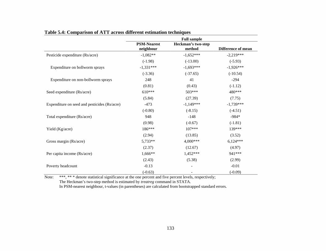
133

Table 5.4: Comparison of ATT across different estimation techniques Full sample

PSM-Nearest

neighbour Heckman’s two-step

method Difference of mean Pesticide expenditure (Rs/acre) -1,082** -1,652*** -2,219***

(-1.98) (-13.00) (-5.93)

Expenditure on bollworm sprays -1,331*** -1,693*** -1,926***

(-3.36) (-37.65) (-10.54)

Expenditure on non-bollworm sprays 248 41 -294

(0.81) (0.43) (-1.12)

Seed expenditure (Rs/acre) 610*** 503*** 480***

(5.84) (27.39) (7.75)

Expenditure on seed and pesticides (Rs/acre) -473 -1,149*** -1,739***

(-0.80) (-8.15) (-4.51)

Total expenditure (Rs/acre) 948 -148 -984*

(0.98) (-0.67) (-1.81)

Yield (Kg/acre) 186*** 107*** 139***

(2.94) (13.85) (3.52)

Gross margin (Rs/acre) 5,733** 4,000*** 6,124***

(2.37) (12.67) (4.97)

Per capita income (Rs/acre) 1,666** 1,452*** 941***

(2.43) (5.38) (2.99)

Poverty headcount -0.13 - -0.01

(-0.63) - (-0.09)

Note: ***, ** * denote statistical significance at the one percent and five percent levels, respectively; The Heckman’s two-step method is estimated by treatreg command in STATA.

In PSM-nearest neighbour, t-values (in parentheses) are calculated from bootstrapped standard errors.

134

The results of these three methods indicate that the causal effect of Bt technology

on yield and gross margin is overestimated when simple mean values are compared. After

addressing the issue of selection bias, the size of the causal effect is reduced. Despite this

reduction, the impact of Bt cotton is still substantial in Mirpur Khas, while in

Bahawalpur, Bt cotton does not appear to be a beneficial option.

Comparison of PSM method with CM method

As discussed earlier, the possibility of bad matches cannot be ruled out in the nearest

neighbour matching based on the propensity score (Becker and Ichno, 2002). In addition,

Abadie and Imbens (2002) point out the inconsistency in the estimated causal effect if

more than one continuous variable is used for matching. They suggested covariate

matching method based on nearest neighbour. This section compares the estimated ATT

based on propensity score matching (PSM) method with the ATT estimated by covariate

matching (CM) suggested by Abadie and Imbens (2002). The analysis is based on one-to-

one matching in which each control observation is matched with the closest observation

in the treatment group. The results are presented in Table 5.5.

A comparison of PSM and CM methods indicates a lower standard error in CM

method as compared to PSM method. The results are robust in terms of level of

significance with the exception of per capita income that became insignificant in CM

method. This may be due to substantial reduction in the size of causal effect when biased

corrected covariate matching method is used. Looking across district-level results, Table

5.5 indicates that the causal effect of Bt cotton adoption on pesticide expenditure became

insignificant in Bahawalpur when the CM method is used. This may be due to the fact

that the CM method found a significantly high expenditure on non-bollworm sprays.

135

Similar effect is observed for yield. In Mirpur Khas, most of the causal effects of Bt

cotton adoption remain in the same direction with the same level of significance in the

PSM and CM methods. However, in CM method, the causal effect for non-bollworm

expenditure became positive and for total expenditure negative. These effects, however,

do not appear significant.

The estimates of ATT derived from the CM method confirm the results of PSM

method that Bt cotton is more effective in Mirpur Khas than in Bahawalpur. The results

indicate that despite a significant decline in bollworm expenditure, the adopters in

Bahawalpur spend a significant amount on non-bollworm sprays. In addition, the increase

in yield is marginal (33 Kg/acre). As a result, the gross margin of adopters is not

significantly different from that of the non-adopters in Bahawalpur. In terms of

hypothesis testing, the results are in line with the previous sub-section, i.e., only two

hypotheses could be validated for Bahawalpur whereas only two hypotheses could not be

confirmed for Mirpur Khas.

136

Table 5.5: A comparison of propensity score matching (PSM) method with covariate matching method (CM) Bahawalpur Mirpur Khas Full sample

PSM CM PSM CM PSM CM Pesticide expenditure (Rs/acre) -1,359** -1,013 -1,535** -1,563*** -1,082** -1,786***

(-2.02) (-1.58) (-2.10) (-2.99) (-1.98) (-4.37)

Expenditure on bollworm sprays -1,668*** -1,642*** -1,449** -1,740*** -1,331*** -1,456***

(-5.92) (-4.53) (-2.53) (-5.95) (-3.36) (-6.87)

Expenditure on non-bollworm sprays 308 629* -85 177 248 -330

(0.64) (1.84) (-0.23) (0.46) (0.81) (-1.25)

Seed expenditure (Rs/acre) 477*** 766*** 489*** 542*** 610*** 488***

(3.42) (8.05) (3.31) (9.64) (5.83) (8.57)

Expenditure on seed and pesticides (Rs/acre) -883 -247 -1,046 -1,021** -473 -1,298***

(-1.15) (-0.37) (-1.53) (-1.91) (-0.80) (-3.05)

Total expenditure (Rs/acre) -362 1,087 213 -102 948 -440

(-0.29) (1.18) (0.20) (-0.14) (0.98) (-0.77)

Yield (Kg/acre) -8 33 232*** 162*** 186*** 123***

(-0.08) (0.41) (5.54) (6.10) (2.94) (3.00)

Gross margin (Rs/acre) 89 95 8,189*** 5,965*** 5,733** 4,897***

(0.04) (0.04) (6.71) (5.70) (2.37) (3.93)

Per capita income (Rs/acre) 96 509 1,523*** 1,016*** 1,666** 693

(0.14) (1.22) (3.20) (3.53) (2.43) (1.28)

Poverty headcount 0.19 0.002 -0.27 -0.120 -0.13 0.15

(1.30) (0.03) (-0.85) (-0.56) (-0.63) (1.43)

Note: ***, ** * denote statistical significance at the one percent and five percent levels, respectively; t-values (in parentheses) are calculated from bootstrapped standard errors.

CM is covariate matching suggested by Abadie and Imbens (2002). The analysis is implemented by using the “nnmatch” module in STATA.

137

ATT by size of operated land

The results presented in Tables 5.3 to 5.5 indicate that the adoption of Bt cotton

contributes to improving the yield, the gross margin from the cotton crop, and total

household income. However, this increase is not enough to take farmers out of poverty.

This issue can further be examined by dividing the farmers into two groups according to

their operated land (large farmers who operate more than 5 acres and small farmers who

operate up to 5 acres). Because of small control group in Mirpur Khas across size of

operated land, this analysis is conducted on the full sample of 206 households. The

estimated ATT using the PSM method and CM method by farm size are reported in Table

5.6. In both categories of farm size, the adopters experience a significant decline in

pesticide expenditure and a significant increase in gross margin. A comparison of PSM

method and CM method indicate differences in the size of the effect. However, the level

of significance is not different across these two methods with the exception of total

expenditure and yield for small farmers. The PSM method found negative and

insignificant causal effect for total expenditure and positive and significant for yield for

small farmers. These results were reversed in terms of level of significance in the CM

method.

Considering the results of PSM method, Table 5.6 shows that the impact of Bt

cotton adoption on yield is lower (125 Kg/acre) for small farmers than that of large

farmers (246 Kg/acre). This result is not in line with the findings of Ali and Abdulai

(2010) who found a larger gain in yield per acre for small farmers as compared to

medium and large farmers. The results show that the small adopting farmers spend a

lower amount on pesticide sprays and experience a lower yield as compared to large

138

farmers. This may be attributed to the differences in farming practices and/or differences

in financial and human capital of large and small farmers. Because of limited time and

resources, the data of Bt cotton Survey 2009 do not have enough information to probe

deeply into these reasons. However, it is intuitive that small farmers have limited access

to information, technology, and credit, and possess lower levels of human capital. For

these reasons, their farming practices are different than those of large farmers. Because of

financial constraints, they are less likely to adopt proper pest control practices. As a

result, they may experience higher crop losses and lower yield as compared to large

farmers. However, there is a need to examine this issue with larger data set.

Table 5.6 shows a significantly lower causal effect of Bt cotton on non-bollworm

expenditure for small farmers, whereas, for large farmers, this effect is positive though

insignificant. It is also possible that due to lower levels of education and lack of proper

information, they do not have accurate awareness about the resistance mechanism of Bt

cotton against pest65

. This point, however, needs to be further investigated with a larger

sample size. Contrary to the findings of Ali and Abdulai (2010), the causal effect of Bt

cotton adoption on per capita income appeaed insignificant for small farmers whereas

large adopting farmers experienced a significant gain. This may be due to the fact that

large farmers are more resourceful and have better access to other sources of income that

small farmers, in general, are lacking, such as, livestock and non-farm income generating

activities. This is an unexpected result. There is a need to examine this issue in a broader

context.

65 Most of the small farmers think that Bt cotton has resistance against all kind of pests (PARC, 2008; Bt cotton Survey, 2009).

139

Table 5.6: Impact of Bt cotton adoption on household wellbeing across operating land categories using PSM and CM methods

PSM CM

Small farmers

(≤ 5 acres)

Large farmers

(> 5 acres)

Small farmers

(≤ 5 acres)

Large farmers

(> 5 acres) Pesticide expenditure (Rs/acre) -1,849*** -1,015 -2,296*** -1,651***

(-3.62) (-0.94) (-4.19) (-2.89)

Expenditure on bollworm sprays -1,529*** -1,551*** -1,720*** -1,785***

(-4.25) (-3.75) (-5.21) (5.97)

Expenditure on non-bollworm sprays -320 536 -576* 134

(-1.11) (0.68) (-1.91) (0.36)

Seed expenditure (Rs/acre) 374*** 562*** 298*** 551***

(3.30) (3.39) (4.62) (4.86)

Expenditure on seed and pesticides (Rs/acre) -1,475*** -454 -1,998*** -1,100*

(-2.94) (-0.38) (-3.61) (-1.74)

Total expenditure (Rs/acre) -732 731 -1,905** -176

(-0.91) (0.39) (-2.37) (-0.20)

Yield (Kg/acre) 125* 246** 74 142*

(1.88) (2.02) (1.52) (1.75)

Gross margin (Rs/acre) 5,230*** 8,094* 4,697*** 5,441**

(2.68) (1.77) (3.10) (2.41)

Per capita income (Rs/acre) -182 2,698* -289 1,243***

(-0.68) (1.76) (-1.60) (2.82)

Poverty headcount 0.27 -0.32 0.30 -0.04

(1.41) (-1.12) (1.17) (-0.38)

Number of treated units 70 97 92 114 Number of comparison units 16 14 70 97 Total matched units 86 111 22 17

Note: ***, ** * denote statistical significance at the one percent and five percent levels, respectively. t-values (in parentheses) are calculated from bootstrapped standard errors.

The results presented in Tables 5.3 to 5.6 are generally in line with the findings of

studies conducted in India and China, reviewed in Chapter 2. The results are consistent

with Crost et al. (2007) who observed a significant positive yield effect from the adoption

of Bt cotton in India after controlling for self-selection bias. Similar to Pakistan, India

also exhibits regional differences in the performance of Bt cotton (e.g., see Gandhi and

Namboodiri, 2006; Qaim et al., 2006; Pemsl, 2006). Overall, these results confirm the

140

findings of Ali and Abdulai (2010) in terms of improvement in yield and household

income as a result of reduction in pesticide use in Pakistan. However, the present study

has not found any significant difference in poverty headcount of adopters and non-

adopters as was observed by Ali and Abdulai (2010).

5.3 Conclusions and policy implications

This chapter examines the impact of Bt cotton adoption on the wellbeing of cotton

farmers in Pakistan by addressing the issue of self-selection bias. Wellbeing is measured

in terms of outcome variables such as pesticide and seed expenditures, total cost of cotton

production, cotton yield, gross margin, and per capita household income. This study

employed a propensity score-matching approach to examine the counterfactual situation,

i.e., how much did the adopters benefit from the Bt cotton adoption compared to the

situation if they would not have been adopted. The data of the Bt Cotton Survey 2009

collected in Bahawalpur and Mirpur Khas is used for the empirical analysis. Several key

conclusions are:

Causal effect of Bt cotton adoption is overestimated if the issue of self-selection bias is

not addressed: Addressing the issue of selection bias reduces the size of outcome

variables obtained in the difference of means method. This indicates that the estimates of

the effect of the outcome variables that do not control for self-selection effects are likely

exaggerated.

Bt technology has positive impact on farmer’s wellbeing: The empirical results indicate

that adoption of Bt cotton has a negative impact on pesticide expenditure and positive

effects on cotton yield, gross margin, and household income. However, this increase is

141

not enough to reduce poverty significantly. These results hold even after controlling for

selection bias.

Impact of Bt cotton varies across agro-climatic conditions: Despite a small sample, the

Bt Cotton Survey captures the agro-climatic diversity that Ali and Abdulai (2010) failed

to incorporate in their study even with a larger sample. The results indicate a varying

effect of Bt technology in different agro-climatic conditions. The impact is found

significant in the areas where pest pressure of bollworms is high and no significant

impact is observed where pest pressure of sucking pests is high. This result indicates that

the benefits of Bt cotton relative to non Bt cotton vary across cotton-growing regions in

Pakistan, depending on the factors determining different pest infestations in different

years. The Bt gene alone cannot solve the diverse pest problems of Pakistan unless it is

incorporated in the varieties that have resistance against sucking pests such as white fly

and mealy bug.

Bt cotton is effective for large as well as small farmers: The results are encouraging for

both large as well small farmers. Both categories of farmers experience a decline in

pesticide expenditure and an increase in gross margin. These results indicate that Bt

cotton has a positive impact on the well-being of cotton farmers. However, the gains for

large farmers are higher than the gains of small farmers.

Overall the results show a relatively better performance for Bt cotton as compared

to non-Bt cotton that helped in improving the wellbeing of cotton farmers. The results,

however, indicate that the same technology may not be beneficial for all areas. Therefore,

there is a need to develop Bt varieties according to the needs of different cotton-growing

areas.

142

Being a lagged adopter, Pakistan should take advantage of the experience of other

countries and adopt those strategies that can maintain the technological advantage for a

longer time period. For example, many studies point out the importance of refuge area,

especially in the regions where most of the cultivated area is covered by one crop

(Bennett et al., 2003; Qaim and de Janvry, 2005; Wang et al., 2006). In addition, the

literature indicates that the institutional support structure is crucial in improving the

productivity of small farmers66

Pakistan is in the process of considering the commercializing Bt cotton. The

results from the analysis of the survey data in this chapter are positive for the existing

unapproved varieties. Additional gains from commercialization may be possible. In the

next chapter, the potential benefits and expected costs associated with Bt cotton adoption

under different hypothetical scenarios are examined at a national level, building in part on

the in-depth analysis of the effects of the unapproved varieties assessed for the two

survey districts, as well as bringing in other considerations.

. Therefore, to make Bt technology successful and pro-

poor, several steps are needed: such as, an increase in small farmers’ access to credit and

information; improvement in the outreach of extension services; development of physical

infrastructure; and continuous monitoring and evaluation of the technological effects of

Bt cotton in different regions by collecting within each region a series of data over time.

66 In South Africa, for instance, Gouse et al. (2005) observed that the lack of credit has resulted in a drastic reduction in cotton crops. After seven years of Bt cotton adoption, the authors described the impact of Bt technology as a “technological triumph but institutional failure”.

143

CHAPTER 6

POTENTIAL BENEFITS AND ECONOMIC COSTS OF ADOPTING BT COTTON IN PAKISTAN

Pakistan had not commercially adopted Bt cotton by late 2010 despite administrative and

research efforts over a number of years. The government of Pakistan has been negotiating

with Monsanto since May 2008 to allow the commercial production and distribution of

the latest Bt cotton seed in the regulated market; however, these negotiations have

remained inconclusive because of disagreement over the technology fee demanded by

Monsanto, a fee which the government argues is too high. The argument is that because

of the high technology fee, most of the benefits would transfer to the technology

innovator. The lack of empirical evidence providing credible estimates of the potential

benefits and expected costs of adopting Bt cotton in Pakistan may be the cause of this

delay in the regulatory decision to proceed with commercialization of Bt cotton.

This chapter addresses the third objective of this thesis which is to measure the

potential welfare implications of commercial adoption of Bt cotton on four different

groups of stakeholders: farmers, seed companies, technology innovators, and cotton

consumers. This is accomplished by examining the potential economic impact of

introducing commercialized Bt cotton into Pakistan through simulation modeling, ex-ante

evaluation of the size and distribution of economic benefits of commercialized Bt cotton,

and comparing the results to an assessment in the simulation model of the costs and

benefits from the current situation of adoption of unapproved varieties. The modified

economic surplus model that accounts for the market power of the technology innovator

is used to measure the economic benefits and their distribution.

144

This chapter is divided into five sections. Section 6.1 describes the general

characteristics of the economic surplus model. The model for Pakistan’s cotton sector is

specified in Section 6.2. Section 6.3 describes the parameters used in specifying the

model. This section explains five scenarios that are developed to present different

situations of Bt cotton adoption in Pakistan. Section 6.4 presents the results under these

different scenarios. Conclusions and policy implications are presented in Section 6.5.

6.1 Conceptual Framework

The economic surplus model developed by Alston et al., (1995) is widely used to

examine the research-induced economic surpluses generated in an output market67

. Total

economic surplus is distributed between producers and consumers. This model is based

on the assumption of competitive input markets. However, the assumption of a

competitive input market does not hold when the IPR-protected input (GM seed) is

introduced. The technology innovator has monopoly power over the distribution and use

of IPR-protected input. In this situation, total surplus is distributed between consumers,

producers and the technology innovator (Moschini and Lapan, 1997). To incorporate the

monopoly rent received by the gene developer, a modified economic surplus model

suggested by Falck-Zepeda et al. (2000) is used.

67 The economic surplus model measures the aggregated social benefits of a research project by calculating the changes in consumer and producer surplus through a technological change originated by research. The economic surplus can be used to calculate the net present value, the internal rate of return, or the benefit-cost-ratio (Alston et al., 1995). The main advantage of using the economic surplus method is that this method needs less information than the other models, such as, partial budgeting, and programming methods. Additionally, it can produce useful and effective outputs in showing the benefits generated by agricultural research.

145

6.1.1. Economic Surplus Model

Several studies quantify the benefits of Bt cotton among consumers, producers and

technology providers using the economic surplus model. This model shows how the

adoption of a technological innovation changes the distribution of benefits between

consumers and producers of a commodity (Alston et al., 1995).

A simple supply-demand framework is used to show that consumers benefit from

a decline in price and producers gain from selling greater quantities. A simple static

model with the assumptions of linear demand D and supply S 68 is presented in Figure

6.1. Assuming a closed economy and parallel research-induced supply shift69

68 Alston et al (1995) provide an in-depth analysis of research-induced supply shifts on the size and distribution of research benefits in various scenarios, such as different directions and modes, open and closed economy, partial and general equilibrium, various measurement methods, and so on.

, the

adoption of new technology reduces the cost of production and shifts the supply curve

from S to S′. Output increases from Q0 to Q1 and price declines from P0 to P1. Consumer

surplus changes by the area PoabP1, and the change in producer surplus is given by the

area (P1bI1- PoaIo). The aggregate welfare gain is represented by the areas between S and

S' below the demand curve, i.e., IoabI1. The case of a small open economy (importing

country) is also presented in Figure 6.1. At world price Pw, home consumption is Qd,

home production is Qso, and Qd – Qso is the quantity imported. A shift in supply as a

result of new technology causes an increase in home production from Qso to Qs1, which

results in a decline in the imports to Qd - Qs1. Because of no change in prices, consumer

surplus will remain unchanged. The change in total surplus is driven by the change in

producer surplus that is equal to the area IodcI1.

69 Alston, et al (1995) reviewed various forms of supply-shift and concluded that in the absence of the information required to choose a particular type of supply shift, the most practical solution is to assume a parallel research-induced supply shift and a local linear approximation of the supply and demand curves.

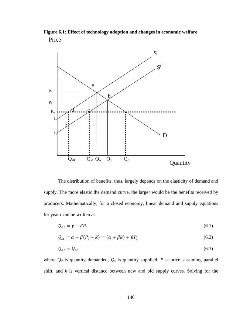
146

Figure 6.1: Effect of technology adoption and changes in economic welfare

The distribution of benefits, thus, largely depends on the elasticity of demand and

supply. The more elastic the demand curve, the larger would be the benefits received by

producers. Mathematically, for a closed economy, linear demand and supply equations

for year t can be written as

𝑄𝑑𝑡 = 𝛾 − 𝛿𝑃𝑡 (6.1)

𝑄𝑠𝑡 = 𝛼 + 𝛽(𝑃𝑡 + 𝑘) = (𝛼 + 𝛽𝑘) + 𝛽𝑃𝑡 (6.2)

𝑄𝑑𝑡 = 𝑄𝑠𝑡 (6.3)

where Qd is quantity demanded, Qs is quantity supplied, P is price, assuming parallel

shift, and k is vertical distance between new and old supply curves. Solving for the

Io

I1

Pw

S

S′

Po

a

b

d

Price

Quantity

D

c P1

Qs0 Qs1 Qo Q1 Qd

e

147

equilibrium condition and writing in terms of elasticities, change in consumer surplus

(∆CS), producer surplus (∆PS), and total surplus (∆TS) can be written as

∆𝐶𝑆𝑡 = 𝑃0𝑄0𝑍(1 + 0.5𝜀𝑑𝑍) (6.4)

∆𝑃𝑆𝑡 = (𝐾 − 𝑍)𝑃0𝑄0(1 + 0.5𝜀𝑑𝑍) (6.5)

∆𝑇𝑆𝑡 = 𝐾𝑃0𝑄0(1 + 0.5𝜀𝑑𝑍) (6.6)

where P0 and Q0 are the initial price and quantity when supply curve is S, and decrease in

price relative to the “without research” price, due to the shift in supply is represented by

𝑍𝑡 = −(𝑃𝑡−𝑃𝑡−1)𝑃𝑡−1

= 𝜀𝑠𝐾𝑡𝜀𝑑+𝜀𝑠

, where εd and εs are the elasticities of demand and supply

respectively. In the case of a small open economy, using the linear demand and supply

curves and parallel supply shift defined in equations 6.1 and 6.2, evaluated at world price

Pw, the change in consumer surplus is zero and change in total surplus equals change in

producer surplus (∆CSt=0) and (∆TSt=∆PSt). This can be written as:

∆𝑃𝑆𝑡 = 𝐾𝑡𝑃𝑤𝑄0(1 + 0.5𝜀𝑠𝐾𝑡) = ∆𝑇𝑆𝑡 (6.7)

In equation (6.7) K is the measure of the research-induced supply shift. The expected K-

shift at time t can be measured by following formula:

𝐾𝑡 = �𝐸(𝑌)𝜀𝑠

− 𝐸(𝐶)1+𝐸(𝑌)

� 𝑝𝐴𝑡(1 − 𝛿𝑡) (6.8)

where E(Y) is expected proportionate yield change per hectare as a result of new

technology (horizontal shift in supply curve), εs is the elasticity of supply, E(C) is the

proportionate change in the variable input cost per hectare, and p is the probability that

research will achieve the yield change. A is the rate of technology adoption and δ is the

annual depreciation rate. The term 𝐸(𝑌)𝜀𝑠

converts the proportionate yield change to a

proportionate gross reduction in marginal cost per ton of output. The term 𝐸(𝐶)1+𝐸(𝑌)

converts

148

proportionate input cost change per hectare to proportionate input cost change per ton of

output. The difference between these two terms �𝐸(𝑌)𝜀𝑠

− 𝐸(𝐶)1+𝐸(𝑌)

� nets out the effect of

variable input cost changes associated with the yield change to give the maximum

potential net change in marginal cost per ton of output (see Alston et al., 1995, p. 380-

383). The measurement of K requires information on the following: probability of

success of research; adoption rate, research and extension cost; per unit cost reduction;

increase in yield; lags in research; and depreciation rate. To measure the expected

benefits from the adoption of a technology, information on expected reduction in cost,

expected increase in yield adoption rate and depreciation rate over time is needed. This

information can be gathered from the expert opinions of scientists, farm management

experts, extension workers, and farmers.

Limitations of the Economic Surplus Model

Alston et al. (1995) and Falck-Zepeda et al. (2007) point out some limitations of the

economic surplus model:

• The economic surplus is calculated on the basis of Marshallian demand that takes

into account the effects of change in prices but ignores the effect of changes in

income.

• The model assumes there are no transaction costs, and the markets clear and

function well.

• This approach ignores general equilibrium effects by assuming that prices and

quantities of other commodities produced by farmers are fixed.

• The model does not take into account the effects on input markets.

• This model assumes farmers are risk-neutral and price-takers who either

maximize profits or minimize costs.

149

Despite these limitations the economic surplus model is widely used to examine the

distribution of benefits of new agricultural technology.

6.1.2 Estimation of technology innovator’s surplus

As discussed earlier, one of the limitations of the economic surplus model is that it

considers the effects of new agricultural technology in the output market where technical

change takes place and ignores the effects that can occur in input markets. Therefore, the

change in welfare is measured by the changes in consumer and producer surpluses.

However, as discussed in Chapter 2, the developers of GM crops are protected by

intellectual property rights (IPRs) that give them a market power over the distribution and

use of their innovations. Because of IPRs, the conventional assumption of competitive

input markets does not hold. Moschini and Lapan (1997) developed a theoretical

framework to measure the social welfare impacts of introducing an IPR- protected

technology in agriculture. The econometric estimation of this model requires data that are

often not available, such as recent innovations. Later, Moschini et al. (2000) estimated

the monopolist profit as 𝐴𝑏𝑡(𝑃𝑏𝑡 − 𝑐) where 𝐴𝑏𝑡 is the area under the Bt crop, and 𝑃𝑏𝑡 is

the price charged for Bt seed per acre, and c is the marginal cost of producing Bt cotton

seed. The assumption is that, as the conventional seed market is competitive, 𝑃𝑛𝑏𝑡

represents the marginal cost of seed production, which is equal for conventional and Bt

seed. Therefore, monopolist profit can be computed as 𝐴𝑏𝑡(𝑃𝑏𝑡 − 𝑃𝑛𝑏𝑡), where 𝑃𝑛𝑏𝑡 is the

price of conventional seed.

Chapter 2 provides a review of studies that examined the distribution of benefits

of Bt cotton adoption in developing countries, including several that accounts for

150

monopolist profit in empirical model (Pray et al., 2001; Qaim, 2003; Gouse et al., 2004;

Falck-Zepeda et al., 2007; Vitale et al., 2007). These studies indicate that farmers receive

the major share of the benefits. In contrast, Falck-Zepeda et al. (1999; 2000; 2000b) and

Price et al. (2003) examined the potential benefits of Bt cotton in the United States. They

found that US producers obtained the highest share of benefits (34% to 59%) followed by

the technology innovators (26% to 47%). The share received by US consumers is in the

range of 6 percent to 16 percent. The Rest of the World received 4 to 20 percent of the

total benefits. A comparison of these results with those discussed in Chapter 2 for

developing countries indicates that the extent of benefits to farmers is much higher if a

country has weak IPR protection. For example, in China where IPRs are weak, producers

receive 83-87 percent of total benefits, while the share for the technology innovator is

only 17 percent (Pray et al., 2001).

6.2. Model Specification for Pakistan’s Cotton Sector

6.2.1 Basic model

The value chain of cotton has five major stages: (i) production of seed-cotton at the farm

level; (ii) production of lint at the ginning level; (iii) production of yarn; (iv) weaving and

production of gray cloth; and (v) finished textile such as apparel, towels, bed wear, etc. A

change at any of these stages can have welfare effects on the other stages of the cotton-

textile chain through vertical linkages. A multi-market model can be used to describe the

interaction between market linkages. The theory of multi-market welfare analysis is well

established (Just et al., 1982; Alston and James, 2002). In a multi-market setting, the

construction of total welfare measures is not affected by the choice of where to measure

151

the benefits in the marketing chain. In other words, measured total surplus (the sum of

consumer and producer surplus) is the same regardless of which market is used to make

the measurement (Just et al., 1979). However, the interpretations of consumer and

producer surplus differ among the markets. The consumer surplus in one market not only

measures the benefits to buyers in that market alone, but also measures the sum of

benefits to producers selling in all higher markets, plus the final consumer surplus.

Similarly, producer surplus measures not only the benefits to producers in the market

where it is measured, but also for all producers selling in more basic markets (Just et al.,

1979; Alston and James, 2002).

As an example, consider farm, processing and retail as three vertically related

markets, denoted by f, p, and r. The producer surplus at the retail level (PSr) is the sum of

producer surpluses at processing (PSp) and farm levels (PSf), and the consumer surplus

(CSr) is the surplus obtained by the final consumers. The producer surplus at farm level

(PSf) is the rent received by the factors of production, and the consumer surplus (CSf) is

the sum of producer surplus at processing level (PSp) and consumer surplus at the retail

level (CSr). In the processing market, the producer surplus (PSp) is the rent received by

the processors and the consumer surplus (CSp) is the sum of producer surplus at farm

level and consumer surplus at retail level. Total surplus at each level is the sum of

producer surpluses at farm and processing levels and consumer surplus at final (retail)

level (see Figure 6.2).

152

Figure 6.2: Impact of Bt technology on Pakistan’s cotton sector

Source: Adapted from Alston and James (2002). Note: f, p, and r indicate farm, processing and retail markets, respectively.

CSr

PSf+PSp

PSf+CSr

PSp

PSp+CSr

PSf

Df

Retail sector

Processing sector

Farm sector

Pr0

Pr

Qr

Dr

Sr

Qr0

Pf0

Pf

Qf

Sf

Qf0

Pp0

Pp

Qp

Dp

Sp

Qp0

Producer surplus = PSf+PSp Consumer surplus = CSr Total surplus = PSf + PSp + CSr

Producer surplus = PSp Consumer surplus = PSf+CSr Total surplus = PSf + PSp + CSr

Producer surplus = PSf Consumer surplus = PSp+CSr Total surplus = PSf + PSp + CSr

153

In the cotton-textile chain, the producer surplus at the farm level is the benefit

obtained by farmers, whereas the consumer surplus is the sum of producer surpluses at all

stages above the farm level, plus the consumer surplus at the final stage. The estimation

of disaggregated benefits at each stage of a multi-market model requires an extensive

amount of data that may not be available. However, the total welfare effects of a policy

change can be examined in any single market. In terms of total welfare effects, the single-

market approach and the multi-market approach are equivalent. However, care is needed

in interpreting the results. This thesis focuses on the farm sector where, as a result of a

research-induced shift in supply curve, equilibrium moves from a to b in Figure 6.1. The

change in consumer, producer and total surplus can be estimated by using equations 6.4,

6.5 and 6.6. The derivation of these equations is presented in Appendix 6.

As discussed earlier, the price of Bt seed is higher than the price of non-Bt seed.

As a result, Bt seed companies/technology innovators can earn profit. This study makes a

distinction between the benefits of technology earned by domestic seed companies (SB)

(who develop and sell seeds locally) and the benefits to technology innovator (IB)

(foreign company who is the technology developer, e.g., Monsanto). If technology is

developed within the country, the benefits earned by a domestic firm are used as ‘benefits

to seed company’. Seed premium is used to calculate the seed companies’ benefit.

However, if a foreign company is the owner of technology and the government pays a fee

to obtain this technology, the benefits earned by the foreign company will be ‘innovators’

benefits’. The technology fee is used to calculate the innovators’ surplus. Therefore, seed

companies’ benefits and the innovator’s benefits are calculated as defined by Moschini et

al. (2000) and Falck-Zepeda et al. (2000):

154

𝑆𝐵 = 𝐴𝑏𝑡(𝑃𝑏𝑡 − 𝑃𝑛𝑏𝑡) (6.9a)

𝐼𝐵 = 𝐴𝑏𝑡 ∗ 𝑇𝐹 (6.9b)

where Abt is area under Bt cotton (Abt = Ac * Adoption rate), and where Ac is the total area

under cotton in the country. Pbt and Pnbt are the prices of Bt and non-Bt seed respectively,

and TF is the technology fee. Therefore, change in gross surplus is the sum of changes in

producer, consumer, seed companies’ benefits, and innovators’ benefits.

∆𝑇𝑆𝑡 = ∆𝑃𝑆𝑡 + ∆𝐶𝑆𝑡 + 𝑆𝐵𝑡 + 𝐼𝐵𝑡 (6.10)

The Present Value (PVi) of change in ith economic surpluses ∆ESi (where i=∆PS, ∆CS,

SS, IS, and ∆TS) at time t can be calculated by applying the discount rate (r):

𝑃𝑉𝑖 = ∑ ∆𝐸𝑆𝑖𝑡𝑇𝑡=0 (1 + 𝑟)𝑡⁄ (6.11)

Total net surplus is obtained by subtracting the cost of R&D from gross total surplus70.

The innovator’s benefits will not be a part of total surplus earned by the country71

𝑁𝑃𝑉∆𝑇𝑆 = ∑ ∆𝑇𝑆𝑡𝑇𝑡=0 (1 + 𝑟)𝑡⁄ − ∑ 𝑇𝐶𝑖𝑡𝑇

𝑡=0 (1 + 𝑟)𝑡⁄ (6.12)

, and

will also be subtracted from total gross surplus. Therefore, net present value of change in

gross total surplus would be:

where TC is total cost involved in commercializing a Bt variety.

6.2.2 Measuring the supply shift (K-shift)

The K-shift takes into account the net effect of yield and cost increase or decrease. The

K-shift is calculated by considering the effect of yield change that reflects not only the

70 The R&D cost differs by scenariois and discussed in detail in Section 6.3.2. 71 It is also possible the foreign company makes a partnership with a domestic seed company. In this situation, some part of surplus will transfer to the domestic seed company and will be added in gross total surplus. This situation, however, is not examined in this study.

155

control over crop loss, but also the genotype into which the Bt gene is introduced.

Following steps are involved in the computation of K-shift given in equation 6.8:

• Compute proportionate change in yield (E(Y)).

• Translate yield change into gross cost change (E(Y)/εs).

• Compute proportionate change in the pesticide cost per acre (E(Cpest)).

• Convert ‘per acre’ cost change in ‘per kg’ cost change by dividing the change in

pesticide cost (E(Cpest)) by (1+E(Y)). 𝐸(𝐶𝑝𝑒𝑠𝑡)1+𝐸(𝑌)

.

• Compute the shares of seed premium (𝑆𝑠) or technology fee (tf) in total cost of

cotton production in year t as: 𝑆𝑠 = 𝐶𝑠𝑒𝑒𝑑/𝑇𝐶 or (tf=TF/TCc), where Cseed is seed

premium, TF is technology fee, and TCc is total cost of production of cotton.

• Compute net cost change ∆𝐶𝑛𝑒𝑡 = 𝐸(𝑌)𝜀𝑠

− �𝐸(𝐶𝑝𝑒𝑠𝑡)1+𝐸(𝑌)

+ 𝑆𝑠1+𝐸(𝑌)

�. The expression

within brackets is equal to the term 𝐸(𝐶)1+𝐸(𝑌)

in equation 6.8.

• Compute (𝐾𝑡 = ∆𝐶𝑛𝑒𝑡 ∗ 𝐴𝑡 ∗ 𝑝 ), where A is the adoption rate and p is the

probability of success.

6.3 Parameters and Scenarios

The economic surplus model assumes that the values of key parameters are known with

certainty. However, most of the parameters used to calculate the impact of research are

uncertain (Alston et al., 1995)72

72 For example, market parameters (such as prices, income, yield, costs, and elasticities of demand and supply), time profile of research, and the adoption rate of new technology are uncertain.

. Therefore, the economic benefits that are based on

uncertain parameters will also be uncertain. To address the uncertainties in key variables,

information on the probability distribution of relevant variables is required. In ex-ante

156

analysis, the information on a few points, such as minimum, maximum, and most likely

can be obtained from experts and published estimates. This information can be used to

parameterize the potential distribution of an experimental outcome for a given scenario

(Alston et al., 1995). The annual flows of benefits to consumers and producers can be

aggregated over the technology diffusion path. The stochastic simulation technique can

be used to compute the corresponding draws of economic surplus measures. (Alston et

al., 1995; Davis and Espinoza 1998; Zhao et al., 2000; Falck-Zepeda et al., 2000;

Hardaker et al., 2004; Falck-Zepeda et al., 2007). To generate the specified input

distribution, repetitive Monte Carlo sampling or Latin Hypercubic sampling methods are

used. At each random draw (or iteration) a set of samples is obtained representing a

possible combination of values of specified stochastic elements that could occur. The

resulting values for the variables of interest are computed and stored. With enough

iterations, the distributions around the mean of each variable converge to a stable

distribution and these distributions can be examined to determine how likely it is to get a

negative value for producer surplus, total surplus, etc. This approach has recently been

used in some studies to examine the economic impact of GM technology (see for

example, Pemsl et al., 2004 for Bt cotton in India; Pemsl, 2006 for Bt cotton in China;

Hareau et al., 2006 for GM rice in Uruguay; Falck-Zepeda et al., 2007 for Bt cotton in

West African countries).

This section outlines the methodological steps to examine the welfare impacts of

Bt cotton adoption in Pakistan. Section 6.3.1 defines the parameters used in estimating

the economic surplus and describes the distributions assigned to them. Section 6.3.2

explains each scenario and provides the values assigned to each parameter. Some

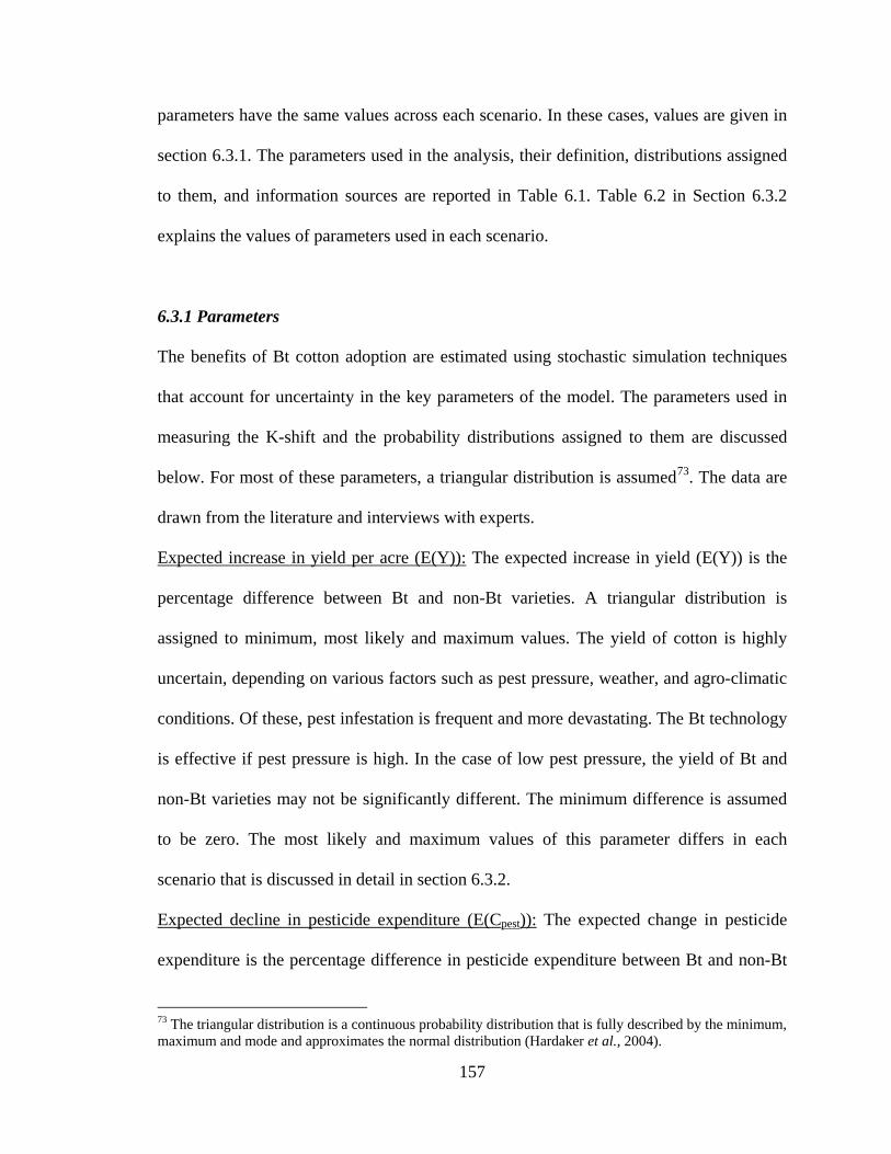
157

parameters have the same values across each scenario. In these cases, values are given in

section 6.3.1. The parameters used in the analysis, their definition, distributions assigned

to them, and information sources are reported in Table 6.1. Table 6.2 in Section 6.3.2

explains the values of parameters used in each scenario.

6.3.1 Parameters

The benefits of Bt cotton adoption are estimated using stochastic simulation techniques

that account for uncertainty in the key parameters of the model. The parameters used in

measuring the K-shift and the probability distributions assigned to them are discussed

below. For most of these parameters, a triangular distribution is assumed73

Expected increase in yield per acre (E(Y)): The expected increase in yield (E(Y)) is the

percentage difference between Bt and non-Bt varieties. A triangular distribution is

assigned to minimum, most likely and maximum values. The yield of cotton is highly

uncertain, depending on various factors such as pest pressure, weather, and agro-climatic

conditions. Of these, pest infestation is frequent and more devastating. The Bt technology

is effective if pest pressure is high. In the case of low pest pressure, the yield of Bt and

non-Bt varieties may not be significantly different. The minimum difference is assumed

to be zero. The most likely and maximum values of this parameter differs in each

scenario that is discussed in detail in section 6.3.2.

. The data are

drawn from the literature and interviews with experts.

Expected decline in pesticide expenditure (E(Cpest)): The expected change in pesticide

expenditure is the percentage difference in pesticide expenditure between Bt and non-Bt

73 The triangular distribution is a continuous probability distribution that is fully described by the minimum, maximum and mode and approximates the normal distribution (Hardaker et al., 2004).

158

varieties. A triangular distribution is assigned to minimum, most likely and maximum

values. The pesticide expenditure will be low in the case of low pest pressure, and the

difference in the pesticide expenditure between Bt and conventional varieties may not be

significantly different. The minimum difference is assumed to be zero. The most likely

and maximum values of this parameter differs in each scenario that is discussed in detail

in section 6.3.2.

Seed premium (Cseed): Seed premium is the price that seed companies charge above the

competitive price of the seed in order to recover their research investments. A triangular

distribution is assigned to the minimum, most likely, and maximum values of seed

premium.

Technology fee (TF): Technology fee is the amount that a country pays to the owner of

Bt technology if it is owned by a foreign company, such as, Monsanto. It is assumed the

fee is only paid once adoption takes place, and there is no initial fee involved. A

triangular distribution is assigned to this parameter. Both, seed premium and technology

fee, are used in the calculation of K-shift.

Adoption profile and technology diffusion path (A): Rogers (1983) defines diffusion as

“the process by which an innovation is communicated through certain channels over time

among the members of a social system”. The technology diffusion path can be defined

either by logistic adoption profile or by trapezoidal adoption profile. The logistic

adoption profile is typically illustrated as an S-shaped curve. This curve indicates that the

first group of people who use a new product are called “innovators”, followed by “early

adopters”, “early and late majority”, and “laggards”. The adoption curve plots adoption

rate against time. It can be described in a general way with the following formula:

159

𝐴𝑡 =𝐴𝑚𝑎𝑥

1 + 𝑒−(𝛼+𝛽𝑡)

where At is the actual adoption rate t years after the release of technology, Amax is the

maximum adoption rate, α and β are parameters that define the path of the adoption rate

that asymptotically approaches the maximum. It is difficult to obtain information on α

and β, especially in ex-ante analysis. Alston et al. (1995) suggest a trapezoidal adoption

profile. According to this profile, the technology diffusion path depends on time lag74 in

the initial adoption (λR), time period to reach at the maximum (λA), years to stay at the

maximum (λM), and a time period in reaching at the complete dis-adoption (λD)75

. The

adoption profile is depicted in Figure 6.3.

Figure 6.3: Adoption profile

Source: Alston et al. (1995)

74 Time lag occurs due to the research and development efforts. 75 After that time, the technology may become obsolete or may simply be substituted for by other innovations (Dinar and Yaron, 1992).

100%

Adoption rate

years λR λA λM λD

Amax

160

The adoption profile over technology diffusion path is calculated as

𝐴𝑡 = 0 𝑖𝑓 0 ≤ 𝑡 ≤ 𝜆𝑅

𝐴𝑡 =𝐴𝑚𝑎𝑥(𝑡 − 𝜆𝑅)

𝜆𝐴 𝑖𝑓 𝜆𝑅 < 𝑡 ≤ 𝜆𝑅 + 𝜆𝐴

𝐴𝑡 = 𝐴𝑚𝑎𝑥 𝑖𝑓 𝜆𝑅 + 𝜆𝐴 < 𝑡 ≤ 𝜆𝑅 + 𝜆𝐴 + 𝜆𝑀

𝐴𝑡 = 𝐴𝑚𝑎𝑥 𝜆𝑅 + 𝜆𝐴 + 𝜆𝑀 + 𝜆𝐷 − 𝑡𝜆𝐷

𝑖𝑓 𝜆𝑅 + 𝜆𝐴 + 𝜆𝑀 < 𝑡 ≤ 𝜆𝑅 + 𝜆𝐴 + 𝜆𝑀 + 𝜆𝐷

𝐴𝑡 = 0 𝑖𝑓 𝑡 > 𝜆𝑅 + 𝜆𝐴 + 𝜆𝑀 + 𝜆𝐷

A triangular distribution is applied to the maximum adoption rate. Other parameters

related to technology diffusion path vary according to scenario. These are discussed in

Section 6.3.2. The adoption profile under different scenarios is presented in Figure 6.4.

Supply elasticity (εs): The supply elasticity plays an important role in measuring the shift

in the supply curve. It is used in converting the yield increase (horizontal shift in supply

curve) in equivalent cost change (vertical shift in supply curve) by dividing the

percentage change in yield with supply elasticity. Therefore, the value of supply elasticity

is crucial in computing the K-shift. The information on supply elasticity is drawn from

published reports. The range of supply elasticity reported in Shepherd (2006) is 0.3 to

1.2. This study assumes unitary elasticity as the most likely value. The minimum value

(0.3) is taken from Shepherd (2006) based on Falck-Zepeda et al. (2007); the maximum

value is assumed to be 1.5. These values are assumed the same across all scenarios.

Demand elasticity (εd): The value of demand elasticity affects the distribution of benefits

between producers and consumers. Consumers (producers) will get a larger share of

benefits if demand is inelastic (elastic). A higher share of benefits goes to producers if the

absolute value of demand elasticity is higher than the value of supply elasticity. The

161

literature indicates low elasticity of demand for cotton (Coleman and Thigpen, 1991).

The argument for low elasticity is the low share of raw cotton in the final demand for

cotton clothing. However, the demand for cotton is driven by the ginning sector where

raw cotton is the major raw material. Therefore, any change in price may affect the

consumption decision of the ginnery and the demand elasticity may not be as low as

suggested by the studies cited above. Recent studies in the literature have used the higher

absolute value for demand elasticity. For example, for all cotton-producing countries,

Goreux (2003) used values in the range of -0.05 to -0.6; Sumner (2003) reports a range of

between -0.14 to -0.47, and Poonyth et al. (2004) indicate a range of demand elasticities

between -0.60 to -1.3 for cotton-producing countries. For Pakistan, these values were -

0.24 (Sumner, 2003) and -1.0 (Poonyth et al., 2004). Falck-Zepeda et al. (2007) used the

value of -0.5 for all West African countries. The triangular distribution is assumed: -0.24,

-0.5, and -1.0 as the minimum, most likely and maximum values of demand elasticity.

These values are assumed the same across all scenarios. Demand elasticity is used in the

closed economy cases. For open economy cases, perfectly elastic demand curve is

assumed.

Area (Ac): This information is drawn from published national statistics. The area under

cotton grew by only 0.26 percent during 2001-2008, therefore, an average value of area

for this period is used in the analysis. Area is assumed to be fixed (3,032 million hectare);

no distribution is assigned. This parameter is assumed the same across all scenarios.

Yield (Yc): The information on yield of cotton for the years 2001-2008 is obtained from

published national statistics. A normal distribution with a mean of 1,962 and a standard

deviation of 204 is assigned to the yield data. Same values are assumed for all scenarios.

162

Quantity of output (Qc): The quantity of output is the sum of quantities obtained from Bt

as well as non-Bt varieties. This can be computed by multiplying the area by the yield.

The information on yield and area is obtained from published national statistics. In ex-

ante analysis, the information on Bt yield is not available. Therefore the existing yield

and the expected increase in yield as a result of Bt adoption are used to compute the

output of cotton.

𝑄𝑐 = 𝐴𝑛𝑏𝑡𝑌𝑐 + 𝐴𝑏𝑡(𝑌𝑐(1 + 𝐸(𝑌))

where Yc is the yield of cotton, Abt is computed by the cotton areas multiplied by adoption

rate, and Anbt is the total cotton area minus Abt. 𝐸(𝑌) is the yield difference between Bt

and non-Bt varieties. This parameter depends on two parameters: the adoption rate and

the expected change in yield.

Price of output (Pc): The data on output price is taken from published national statistics

for the period 2001-2008. A normal distribution is applied with a mean of 1,034 and a

standard deviation of 226.

Cost of production (TCc): This parameter includes all costs involved in producing cotton.

The information is derived from published data. The values of latest available year (2004-

05) are inflated to year 2008. A deterministic value is used for the cost of production data

(no distribution is assigned).

163

Table 6.1 give the name of parameters, their definition, distributions assigned to them and

sources of information.

Table 6.1: Parameter, their definitions, probability distributions, and information sources Parameter

name Parameter definition Probability distribution Information source

E(Y) Expected increase in yield per acre (%) Triangular

Bt Cotton Survey 2009; Gandhi and Namboodiri (2006); and Experts’ opinions.

E(Cpest) Expected decline in pesticide expenditure per acre (%) Triangular -do-

Cseed Seed premium (US$/hectare) Triangular -do-

TF Technology fee (US$/hectare) Triangular Monsanto-Pakistan

εs Supply elasticity Triangular Shepherd (2006); and Falck-Zepeda et al. (2007)

εd Demand elasticity Triangular

Sumner, (2003); Poonyth et al., (2004); and Falck-Zepeda et al. (2007)

A Maximum adoption rate (%) Triangular Bt Cotton Survey 2009; and Experts’ opinions.

λR R&D lag (years) - -do-

λA Adoption lag (years) - -do-

λM Years at maximum adoption - -do-

λD Years to dis-adoption - -do-

Diffusion path (years) =λR +λA+λM+λD - -

Ac Area (million hectares) - Economic Survey 2008-09

Yc Yield of raw cotton (Kg/hectare) Normal Economic Survey 2008-09

Pc Price of raw cotton (Rs/40kg) Normal Salam (2009)

Qc Cotton output (calculated with Ac and Yc) - -

TCc Cost of production (US$/hectare) - APCOM

R&D expenditures (US$) - Pray et al. (2006)

TC Total cost (US$) = R&D exp+IB benefits - - Notes: - indicates not applicable.

Experts’ opinions were collected through informal interviews and meetings with agricultural scientists, breeders and seed developers during the Bt Cotton Survey 2009.

164

R&D expenditures: In Pakistan, the information on research and development (R&D)

expenditures76

The K-shift is estimated using equation 6.8 as specified in section 6.2.2. The

change in consumer surplus, producer surplus, seed companies’ surplus, and total surplus

is calculated by using equations 6.4, 6.5, 6.9 and 6.10, respectively. To obtain the present

value, the sum of benefits is discounted by using the real discount rate of 5.6 percent

involved in developing the Bt cotton varieties is not available. Therefore,

the available information for India and China from Pray et al. (2006) is used. This is

further explained under different scenarios.

77

.

The @Risk software (an add-in to Excel) is used to estimate the distributions that best fit the

data and information used in the analysis. The mean present values (PV) of producer,

consumer, seed companies’, innovator, gross total, and net total surpluses are obtained

after 10,000 iterations.

6.3.2 Scenarios and data

In view of the current steps towards the commercial adoption of Bt cotton in Pakistan,

this section develops five different scenarios. These scenarios are: (1) baseline scenario

presents the current situation of Pakistan, i.e., adoption of unapproved Bt varieties; (2)

commercial adoption of varieties developed domestically in Pakistan; (3) commercial

adoption of hybrid seed imported from India by Monsanto; (4) commercial adoption of

latest Bt technology (Bollgard II); and (5) irregular adoption of latest Bt technology. The

76 The cost of developing Bt technology includes preparation and enforcement of regulations, developing the Bt gene, breeding, field trials, approval, and commercialization. 77 The nominal discount rate was 15 percent in 2008 (GOP, 2009). The real discount rate is calculated using the Fisher’s equation: 𝑟 = 𝑖−𝑚

1+𝑚 where 𝑟 is real discount rate, i is nominal discount rate, m is average

inflation rate over the period ten years.

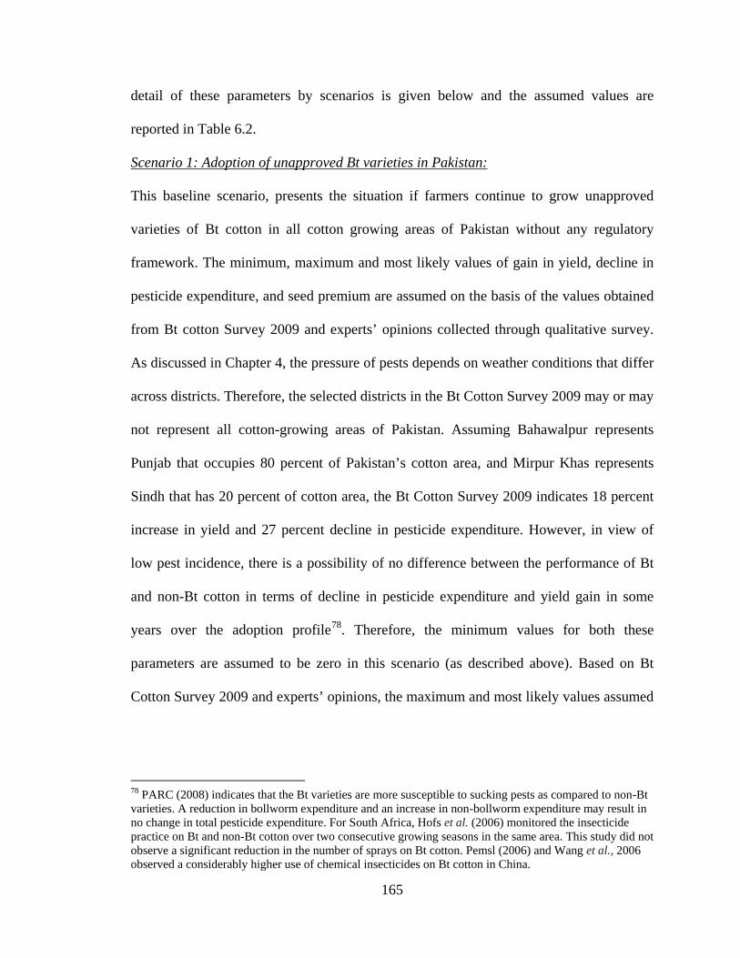
165

detail of these parameters by scenarios is given below and the assumed values are

reported in Table 6.2.

Scenario 1: Adoption of unapproved Bt varieties in Pakistan:

This baseline scenario, presents the situation if farmers continue to grow unapproved

varieties of Bt cotton in all cotton growing areas of Pakistan without any regulatory

framework. The minimum, maximum and most likely values of gain in yield, decline in

pesticide expenditure, and seed premium are assumed on the basis of the values obtained

from Bt cotton Survey 2009 and experts’ opinions collected through qualitative survey.

As discussed in Chapter 4, the pressure of pests depends on weather conditions that differ

across districts. Therefore, the selected districts in the Bt Cotton Survey 2009 may or may

not represent all cotton-growing areas of Pakistan. Assuming Bahawalpur represents

Punjab that occupies 80 percent of Pakistan’s cotton area, and Mirpur Khas represents

Sindh that has 20 percent of cotton area, the Bt Cotton Survey 2009 indicates 18 percent

increase in yield and 27 percent decline in pesticide expenditure. However, in view of

low pest incidence, there is a possibility of no difference between the performance of Bt

and non-Bt cotton in terms of decline in pesticide expenditure and yield gain in some

years over the adoption profile78

78 PARC (2008) indicates that the Bt varieties are more susceptible to sucking pests as compared to non-Bt varieties. A reduction in bollworm expenditure and an increase in non-bollworm expenditure may result in no change in total pesticide expenditure. For South Africa, Hofs et al. (2006) monitored the insecticide practice on Bt and non-Bt cotton over two consecutive growing seasons in the same area. This study did not observe a significant reduction in the number of sprays on Bt cotton. Pemsl (2006) and Wang et al., 2006 observed a considerably higher use of chemical insecticides on Bt cotton in China.

. Therefore, the minimum values for both these

parameters are assumed to be zero in this scenario (as described above). Based on Bt

Cotton Survey 2009 and experts’ opinions, the maximum and most likely values assumed

166

for yield gain are 20 percent and 10 percent respectively. For decline in pesticide

expenditure these values are assumed to be 15 percent and 7 percent, respectively.

The seed premium found in the Bt Cotton Survey 2009 averages is US$ 16 per

hectare across two districts. Because of unregulated market, the price of Bt seed varies

largely across different areas. Therefore, the seed premium for this scenario is assumed to

be in the range of 20 US$/hectare to 5 US$/hectare with 10 US$/hectare as the more

likely value. The Bt Cotton Survey 2009 observed an average adoption rate of 77 percent.

However, in 2007, the adoption rate in Sindh was 80 percent and in Punjab was 50

percent (PARC, 2008). Therefore, this scenario assumes a most likely value of 60

percent. The minimum adoption rate is assumed to be 50 percent and the maximum 70

percent.

This scenario is assumed to start in 2002 when Bt cotton was cultivated on a small

scale. The R&D lag of two years and an adoption lag of five years is assumed after 2002.

Therefore, the maximum adoption rate is achieved in 2009. It is assumed that this rate

will sustain for next five years and then it will start declining. To calculate net total

surplus, information on cost of R&D79 and the cost of the technology fee are required.

This scenario assumes domestically developed varieties using the existing transformation

event80. Therefore, there is no cost for developing own transformation event. These

varieties have not gone through any regulatory and approval process. Therefore, there is

no technology fee involved for these varieties. This scenario assumes a cost of US$

50,000 for three years as a cost of developing and distribution81

79 This includes the cost of developing Bt cotton and field trials by both public and private companies.

.

80 As described in Chapter 3, the unapproved varieties are using Monsanto’s transformation event MON531. 81 This figure is drawn from Pray et al. (2006).

167

Scenario 2: Commercial adoption of varieties developed domestically in Pakistan

As indicated earlier, six Bt cotton varieties developed by the public and private sectors of

Pakistan are approved for field trials. Success of these trials would result in the

commercialization of these varieties, which is assumed to occur, for the crop year 2010-

11. Most of the approved varieties that are developed by the private sector are already

available to farmers. Therefore, it can be assumed that there will be some difference in

yield and pesticide expenditure between Bt and non-Bt varieties as assumed in the

baseline scenario. However, in view of the possibility of low pest pressure, this scenario

takes into account the possibility of no difference in yield and pesticide expenditure of Bt

and non-Bt varieties. Therefore, the minimum values for both these parameters are

assumed to be zero. The expected yield difference will have a triangular distribution

around (0, 0.15, 0.25) and the triangular distribution for the pesticide expenditure will be

(0, 0.10, 0.15). Commercialization can improve the confidence of farmers about Bt

technology that may result in a higher adoption rate. This scenario assumes 50 percent,

65 percent, and 80 percent as minimum, most likely, and maximum values of adoption

rate, respectively. This scenario assumes a regulated seed market that can lower the seed

premium82. Therefore, comparing with Scenario 1, lower values of seed premium are

assumed in this scenario. The seed premium for this scenario is assumed to be in the

range of 6 US$/hectare to 11 US$/hectare with 8 US$/hectare as the more likely value83

82 Currently, the Bt seed market is not regulated and there exists wide differences in price across area, farmers, and seed provider. It is expected that the regulated market will reduce the existing large seed premium by increasing competition among seed providers and the market price of Bt seed will become more transparent.

.

This scenario assumes an R&D lag of four years and an adoption lag of five years.

83 These values are calculated as 25 percent of technology fee that is under negotiation between Monsanto and the government of Pakistan because of the cost of publically developed domestic varieties would be less than charged by Monsanto for private development.

168

As discussed in Chapter 3, out of eight approved varieties, six varieties use the

event MON531 and two varieties use the Bt gene developed by the public sector. This

case is very similar to China as reported in Pray et al. (2006). Therefore, the expenditure

on developing and approval of Bt cotton is taken from Pray et al. (2006).

Scenario 3: Commercial adoption of hybrid seed imported from India

As indicated earlier, the government of Pakistan allowed Monsanto to import hybrid Bt

seed from India. These varieties will be commercialized in 2011-2012 if the field trials

are successful. The discussion in Chapter 2 indicates a better economic performance for

Bt hybrid varieties as compared to conventional varieties in India. However, scientists

and the farm community have expressed their concerns over the suitability of this seed

for the agro-climatic conditions of Pakistan’s cotton-growing areas. Therefore, this

scenario assumes that the difference in yield and pesticide expenditure of Bt and non-Bt

varieties will be higher than that assumed in scenario 1 but less than that in India. It is

also assumed that the maximum yield gain will be 35 percent and most likely would be

22 percent. However, in view of the possibility of low pest pressure, this scenario

assumes there will be no difference in yield and pesticide expenditure of Bt and non-Bt

varieties. Therefore, the minimum values for both these parameters are assumed to be

zero. Based on experts’ opinion, the more likely difference in pesticide expenditure is

assumed to be 13 percent and a maximum of 30 percent. In India, the range of the price

difference for Bt hybrid and conventional seed is 68 percent to 308 percent84

84 See Table 2.3 in Chapter 2.

. Therefore a

high seed premium for this scenario is assumed. This value is calculated by increasing the

technology fee that is under negotiation between Monsanto and the government of

Pakistan by 25 percent. A triangular distribution is assumed for 33 US$/hectare, 40

169

US$/hectare, and 53 US$/hectare as minimum, more likely, and maximum values.

However, being a foreign company, seed premium would go to Monsanto. In Table 6.2, it

is given under the heading ‘technology fee’. The adoption rate is assigned a triangular

distribution with 50, 70 and 90 percent as mean, more likely, and maximum values. This

scenario assumes an R&D lag of four years and adoption lag of five years. The total

technology diffusion time path would be 21 years. Total cost consists of field trials,

approval, and commercialization. There is no breeding cost for the imported varieties.

The data on cost are drawn from Pray et al. (2006).

Scenario 4: Commercial adoption of latest Bt technology (Bollgard II).

This scenario represents the situation if the government of Pakistan signs an agreement

with Monsanto. Under this scenario, the latest Bt gene will be incorporated into the

cotton varieties that are suitable for different agro-climatic conditions of Pakistan.

Therefore, this technology is expected to be more effective than the ones that are

described in previous scenarios. Based on the discussions with experts during the Bt

Cotton Survey 2009, this scenario assumes 0 percent, 30 percent, and 40 percent as

minimum, most likely and maximum increases in yield. Similarly, the decline in pesticide

expenditure is expected to be higher than that assumed in scenarios 1 and 2. The assumed

values are 0 percent, 20 percent and 35 percent as minimum, most likely, and maximum

values for the difference in pesticide expenditure. As discussed earlier, the technology fee

that Monsanto will charge if the government of Pakistan signs an agreement with

Monsanto is 17 US$/acre, whereas the government of Pakistan offered 11 US$/acre. It is

expected that most likely value will be in between 11 US$/acre and 17 US$/acre.

Therefore a value of 13 US$/acre is assumed as most likely value. Converting these into

170

hectares, a triangular distribution with 27, 32 and 42 US$/hectare as minimum, most

likely and maximum values are assumed to calculate the technology fee.

The adoption rate is assumed to have a triangular distribution with 50, 70 and 90

percent as minimum, most likely and maximum values in this scenario. The R&D lag

would be five years and adoption will take five years. Therefore, the total years of the

simulation would be 22 years. In this scenario, the initial adoption year is 2013. For the

R&D cost, the information for India reported in Pray et al. (2006) is used85

Scenario 5: Irregular adoption of Bt technology

.

Technology adoption can be influenced by various factors over its diffusion path:

examples include low success rate, effect of a change in a policy, concerns about

technology, price fluctuations in seed and raw cotton, and weather and climatic

conditions. The influence of these factors may result in a non-smooth adoption curve with

a cycle of adoption-decline and adoption-re-adoption over the diffusion path of the

technology that can influence the size and distribution of the benefits that are generated

(Zhao et al., 2002; Gouse et al., 2005; Falck-Zepeda et al., 2007). To capture these

effects, the fluctuating adoption rates on the values that are assumed for Scenario 4 are

used. In this scenario the adoption rate is allowed to fluctuate; a decline in the rate by 20

percent, followed by an increase of 25 percent, and then a decline of 40 percent and again

an increase of 60 percent over the span of maximum adoption86

85 In India, the development of Bt technology is in the hands of private and foreign firms.

(see adoption profile of

Scenario 5 in Figure 6.4).

86 These values are chosen to show the effect of random variation in adoption rate. Any change in these values may affect the economic benefits. The purpose of this scenario is to show the change in economic benefits as a result of fluctuations in adoption rate.

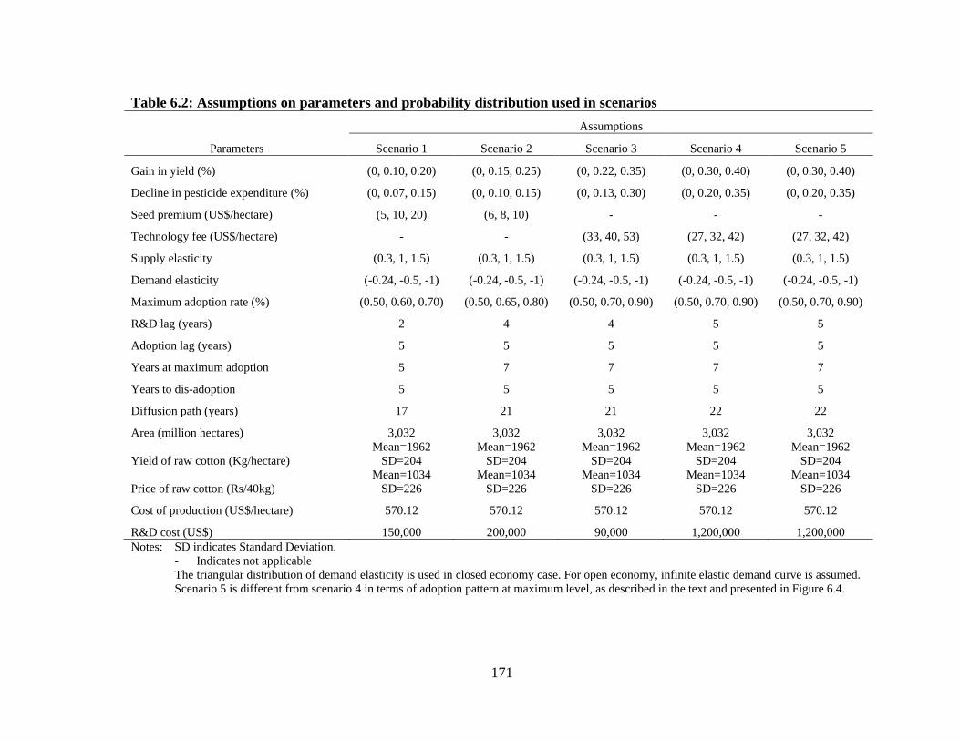
171

Table 6.2: Assumptions on parameters and probability distribution used in scenarios Assumptions

Parameters Scenario 1 Scenario 2 Scenario 3 Scenario 4 Scenario 5

Gain in yield (%) (0, 0.10, 0.20) (0, 0.15, 0.25) (0, 0.22, 0.35) (0, 0.30, 0.40) (0, 0.30, 0.40)

Decline in pesticide expenditure (%) (0, 0.07, 0.15) (0, 0.10, 0.15) (0, 0.13, 0.30) (0, 0.20, 0.35) (0, 0.20, 0.35)

Seed premium (US$/hectare) (5, 10, 20) (6, 8, 10) - - -

Technology fee (US$/hectare) - - (33, 40, 53) (27, 32, 42) (27, 32, 42)

Supply elasticity (0.3, 1, 1.5) (0.3, 1, 1.5) (0.3, 1, 1.5) (0.3, 1, 1.5) (0.3, 1, 1.5)

Demand elasticity (-0.24, -0.5, -1) (-0.24, -0.5, -1) (-0.24, -0.5, -1) (-0.24, -0.5, -1) (-0.24, -0.5, -1)

Maximum adoption rate (%) (0.50, 0.60, 0.70) (0.50, 0.65, 0.80) (0.50, 0.70, 0.90) (0.50, 0.70, 0.90) (0.50, 0.70, 0.90)

R&D lag (years) 2 4 4 5 5

Adoption lag (years) 5 5 5 5 5

Years at maximum adoption 5 7 7 7 7

Years to dis-adoption 5 5 5 5 5

Diffusion path (years) 17 21 21 22 22

Area (million hectares) 3,032 3,032 3,032 3,032 3,032

Yield of raw cotton (Kg/hectare) Mean=1962

SD=204 Mean=1962

SD=204 Mean=1962

SD=204 Mean=1962

SD=204 Mean=1962

SD=204

Price of raw cotton (Rs/40kg) Mean=1034

SD=226 Mean=1034

SD=226 Mean=1034

SD=226 Mean=1034

SD=226 Mean=1034

SD=226

Cost of production (US$/hectare) 570.12 570.12 570.12 570.12 570.12 R&D cost (US$) 150,000 200,000 90,000 1,200,000 1,200,000 Notes: SD indicates Standard Deviation.

- Indicates not applicable The triangular distribution of demand elasticity is used in closed economy case. For open economy, infinite elastic demand curve is assumed. Scenario 5 is different from scenario 4 in terms of adoption pattern at maximum level, as described in the text and presented in Figure 6.4.

172

Figure 6.4: Adoption profile-Scenarios 1 to 5.

01020304050607080

2008

2010

2012

2014

2016

2018

2020

2022

2024

2026

2028

Adop

tion

rate

(%)

Scenario 5

01020304050607080

2008

2010

2012

2014

2016

2018

2020

2022

2024

2026

Adop

tion

rate

(%)

Scenario 3

010203040506070

2002

2003

2004

2005

2006

2007

2008

2009

2010

2011

2012

2013

2014

2015

2016

2017

2018

Adop

tion

rate

(%)

Scenario 1

010203040506070

2006

2008

2010

2012

2014

2016

2018

2020

2022

2024

2026

Adop

tion

rate

(%)

Scenario 2

01020304050607080

2008

2010

2012

2014

2016

2018

2020

2022

2024

2026

2028

Adop

tion

rate

(%)

Scenario 4

173

6.4. Results and Discussion

6.4.1 Distribution of benefits

The cotton sector at farm level is a closed economy. Therefore, it is reasonable to assume

that prices are determined by domestic market forces, in the sense that raw seed cotton as

sold by farmers is not traded internationally. The shift in supply curve as a result of cost

reducing technology may push the farm-level price downward. However, a close link

between domestic market prices of seed cotton and export parity prices87

Table 6.3 reports the results of economic surplus model for both, closed as well as

open economy cases. This table shows that the adoption of Bt cotton generates

significantly larger benefits for the cotton producers than the cost of Bt cotton adoption in

has been

observed since 1990 (Salam, 2008; Cororaton and Orden, 2008). In recent years, the

international price of cotton appears as an important reference for the domestic price of

seed cotton. In this situation, a decline in price deviating from the world price cannot be

sustained over a long period of time. Most recently, Pakistan has become a net importer

of cotton, with a less close match between import parity prices and farm-level prices.

Hence, it is relevant to consider both international and domestic factors affecting farm-

level cotton prices in Pakistan. In the long-run, international factors may prove dominant

in which case it is most appropriate to consider the case of an open economy. Since

Pakistan has become a net cotton importer, the case of a small importing economy is

considered in the simulations.

87 The export parity price of raw seed cotton is the price derived by working down to the farm level from observed international prices of traded cotton lint, taking processing marketing and transportation costs and the by-product (cotton seed) value into account.

174

regulated market, under both, closed as well as open economy cases88

Since the objective of scenario analysis is to examine the stream of benefits over

the technology diffusion paths defined in Table 6.2, the discussion in rest of this section

is based on the long-run situation, i.e., open economy case.

. The present value

of average gross total economic surplus falls in the range of US$ 1,139 million to US$

3,526 million if closed economy is considered and a shift in supply curve reduces the

price of seed cotton. The economic surplus is highest for Scenario 4 (adoption of latest Bt

technology after signing contract with Monsanto) and lowest for Scenario 1 (if Bt cotton

adoption remains in the unregulated market). Because of the decline in prices, consumers

obtain the larger share of benefits in all scenarios (48.8% to 58.1%), followed by

producers (30.6% to 36.4%). The share of benefits to seed companies is 5.6 percent and

11.4 percent for Scenario 2 and Scenario 1, respectively. The share of technology

innovators fall between 13.3 to 20.5 percent. The gross total surplus is higher in case of

open economy as compared to closed economy, ranging between US$ 1,160 for Scenario

1 to US$ 3,526 for Scenario 4. Producers get the larger share of total benefits in each

scenario (i.e., in the range of 80.2% in Scenario 3 to 94.6% in Scenario 2).

Scenario 1 presents the situation that currently prevails in the country, i.e., the adoption

of unapproved Bt cotton varieties. The gross total surplus under this scenario is US$

1,160 million. Farmers obtain 88.9 percent of total benefits and 11.2 percent goes to the

seed companies. This result is in line with the findings of Chapter 5.

88 Martin and Alston (1997) point out the possibility of truncation of supply curves at the axes in case of inelastic supply curve. In such a situation, producer surplus measures may be overestimated. The analysis presented in this study uses linear supply curves and supply elasticity ranges from 0.3 to 1.5. Therefore, ignoring the possibility of truncation of supply curves at the axes may cause overestimation of producer surplus. This point, however, needs to be further investigated.

175

Table 6.3: Present value of change in economic surplus under different scenarios and distribution of benefits in Pakistan

Scenario 1 Scenario 2 Scenario 3 Scenario 4 Scenario 5

Closed economy

Open economy

Closed economy

Open economy

Closed economy

Open economy

Closed economy

Open economy

Closed economy

Open economy

Present value (million US$)

1. Producer surplus 389 1,031 675 1,812 939 2,556 1,164 3,211 965 2,648

2. Consumer surplus 621 - 1,077 - 1,499 - 1,858 - 1,541 - 3. Seed company’s benefits 129 129 104 104 - - - - - -

4. Innovator’s benefits - - - - 631 631 504 504 504 504 5. Gross total surplus (1+2+3+4) 1,139 1,160 1,855 1,916 3,069 3,187 3,526 3,715 3,010 3,152

6. R&D costs 0.13 0.13 0.17 0.17 0.08 0.08 1.02 1.02 1.02 1.02 7. Net total benefits to the country (5-6-4) 1,139 1,160 1,855 1,916 2,438 2,556 3,021 3,210 2,505 2,647

Distribution of gross total surplus (%)

Share of producers 34.14 88.85 36.36 94.59 30.60 80.21 33.01 86.42 32.06 83.99

Share of consumers 54.50 - 58.05 - 48.85 - 52.69 - 51.18 -

Share of seed company 11.37 11.15 5.59 5.41 - - - - - -

Share of innovator - - - - 20.54 19.79 14.31 13.58 16.76 16.01 Note: Figures of present value are the mean values of 10,000 iterations.

176

Scenario 2 examines the situation if Pakistan commercially adopts the domestically

developed varieties. Under this scenario, the average present value of gross economic

surplus is US$ 1,916 million. Comparing with Scenario 1, producer surplus is US$ 781

million, and gross total surplus is US$ 756 million higher than that is observed in

Scenario 1. Because of lower seed premium as compared to baseline scenario, the share

of surplus obtained by seed companies reduces from 11.2 percent in Scenario 1 to 5.4

percent in Scenario 2, and producers obtain 94.6 percent share of total gross benefits.

Scenario 3 (import of Bt hybrid seed from India) gives a gross total surplus of US$ 3,187

million. Because of imported Bt hybrid variety, the technology innovator earns US$ 631

million as seed premium. As a result, net total surplus is US$ 2,556. The distribution of

total benefits shows that the share of producer declined to 80.2 percent as compared to

94.6 percent in Scenario 1 (a decline of 14.4 percentage points). However, in absolute

terms, producer benefit is US$ 1,525 million higher than that is observed in the baseline

scenario (Scenario 1). Because of the high seed premium, innovators can extract 19.8

percent of total benefits, the highest in all the scenarios.

Scenario 4: The estimated average present value of total gross benefits is US$ 3,715

million i.e., US$ 2,551 million higher than that is found in Scenario 1 and US$ 528

million higher than that is observed for Scenario 3. In this scenario, benefits to innovator

(i.e., Monsanto) are US$ 504 million. As a result, net total surplus to the country is US$

3,210 million. Despite higher costs, net benefits are higher than the other scenarios. The

result of this scenario indicates substantial economic benefits even in the presence of a

high technology fee. Farmers obtain 86.4 percent of total benefits and the share of

technology innovators is 13.6 percent. These results are consistent with the findings of

177

other studies conducted in Mexico and China and lower than those in South Africa and

India89

Scenario 5 examines the influence of fluctuating adoption rate on economic benefits

under the assumption of Scenario 4

.

90

The basic decision rule for accepting or rejecting a project depends on whether its

NPV is positive or negative. Thus it is important to observe the probability of negative

economic benefits. Figure 6.5 shows the probability distributions of present value for

producer surplus and net total surplus. The x-axis shows the values for economic surplus

. The results of this scenario show that fluctuations

in adoption cause a decline in the producer as well as total surplus. Farmers pay a higher

price for seed and the government bears a higher cost for the technology fee. A

comparison with Scenario 4 shows that because of disruption in adoption, producer

surplus is lower by US$ 563 million. This result is consistent with Falck-Zepeda et al.

(2007) for West African countries. This scenario highlights the importance of addressing

the issues that can cause fluctuations in the adoption of Bt cotton before introducing the

technology. For example, easy and timely availability of inputs is crucial to avoid crop

failure. Therefore, easy access to credit is an important institutional factor that should be

addressed before the introduction of technology. Similarly, a higher price for seed, or sale

of spurious seed, and the lack of awareness about the use of Bt technology are some

important issues that can cause fluctuations in the adoption rate. If these issues are not

addressed properly, the actual benefits may be lower than the potential benefits.

89 The share of innovator surplus in Mexico was found to be 14 percent (Traxler and Godoy-Avila, 2004); in China it was 17 percent (Pray et al., 2001); in India 33 percent (Qaim, 2003); and in South Africa it ranged from 21 to 54 percent (Gouse et al., 2004). 90 Fluctuations in adoption rate can arise because of various factors, such as fluctuations in the price of seed and raw cotton, bad weather, unavailability of adequate and timely credit to purchase inputs, and so on.

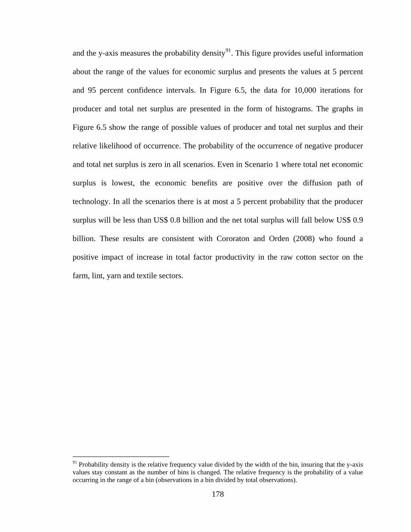
178

and the y-axis measures the probability density91

. This figure provides useful information

about the range of the values for economic surplus and presents the values at 5 percent

and 95 percent confidence intervals. In Figure 6.5, the data for 10,000 iterations for

producer and total net surplus are presented in the form of histograms. The graphs in

Figure 6.5 show the range of possible values of producer and total net surplus and their

relative likelihood of occurrence. The probability of the occurrence of negative producer

and total net surplus is zero in all scenarios. Even in Scenario 1 where total net economic

surplus is lowest, the economic benefits are positive over the diffusion path of

technology. In all the scenarios there is at most a 5 percent probability that the producer

surplus will be less than US$ 0.8 billion and the net total surplus will fall below US$ 0.9

billion. These results are consistent with Cororaton and Orden (2008) who found a

positive impact of increase in total factor productivity in the raw cotton sector on the

farm, lint, yarn and textile sectors.

91 Probability density is the relative frequency value divided by the width of the bin, insuring that the y-axis values stay constant as the number of bins is changed. The relative frequency is the probability of a value occurring in the range of a bin (observations in a bin divided by total observations).

179

Figure 6.5: PV of producer and total net surplus in Pakistan-Scenarios 1 to 5.

(Cont…)

180

6.4.2 Cost of technology fee and economic benefits

As discussed earlier, the negotiations between the government of Pakistan and Monsanto

have not borne any fruit due to disagreement over the technology fee demanded by the

Monsanto, that the government of Pakistan argued is too high. In view of this situation,

this section examines the impact of technology fee on economic surplus by comparing

the benefits and costs of adopting latest Bt technology after signing the contract with

Monsanto (i.e., using the assumptions of Scenario 4) considering two cases. In both cases

a deterministic value of technology fee is assumed. In the first case, technology fee is

181

assumed to be equal to the value that Monsanto is offering when negotiating with the

government of Pakistan (US$ 17 per acre). In the other case, the assumed value of

technology fee is equal to the amount that government of Pakistan is offering to

Monsanto (US$ 11/acre).

The results presented in Table 6.4 compare the economic surplus in these two

situations. The results suggest that under the assumption of Scenario 4, the government

accepts Monsanto’s proposed technology fee (US$ 17/acre), the present value of

innovators benefits is US$ 628 million and farmers will be able to receive a stream of

benefits worth US$ 3,097 million over a period of 22 years. If technology fee reduces to

11 US$/acre, producer surplus92

The probability distribution of present value for producer surplus and net total

surplus for two different technology fees (17 US$/acre and 11 US$/acre) is presented in

Figure 6.6. This figure shows that the probability of the occurrence of negative producer

and net total surplus is negligible even if technology fee is 17 US$/acre. In all scenarios,

there is only a 5 percent probability that the producer surplus and net total surplus will be

less than US$ 2.3 billion.

increases to US$ 3,303 million and benefits to innovator

decline to US$ 406 million. This results in lowering the gross total benefits (US$ 3,709).

However, after subtracting the innovator’s benefits and R&D cost in each case, net

benefits are higher when technology fee is 11 US$/acre. The concern of the government

of Pakistan is about the high cost involved in the adoption of latest Bt technology.

However, the analysis presented in this section indicates that, at high technology fee,

despite an increase in cost the net benefits are considerable (US$ 3,302 million).

92 Based on the assumption of small open economy and zero profits of domestic seed companies, gross total surplus equals producer surplus.

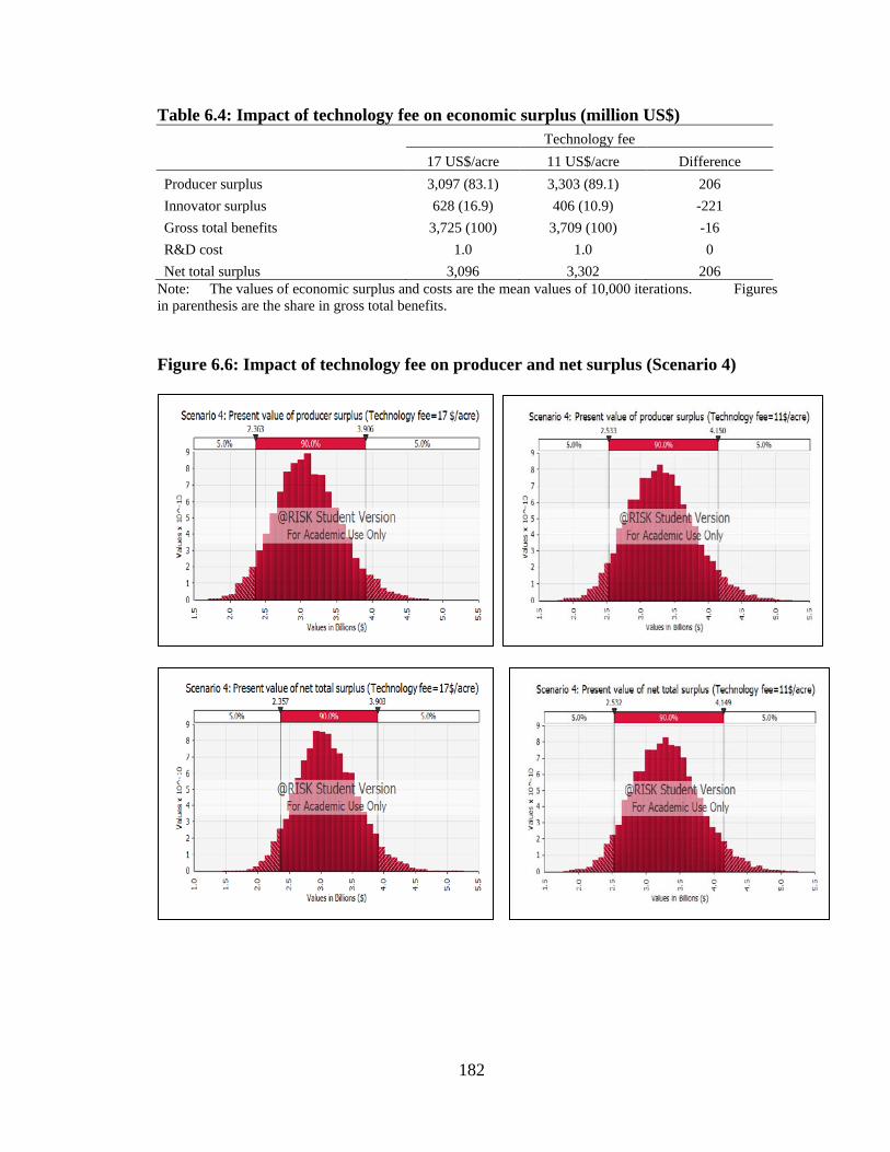
182

Table 6.4: Impact of technology fee on economic surplus (million US$) Technology fee 17 US$/acre 11 US$/acre Difference

Producer surplus 3,097 (83.1) 3,303 (89.1) 206 Innovator surplus 628 (16.9) 406 (10.9) -221 Gross total benefits 3,725 (100) 3,709 (100) -16 R&D cost 1.0 1.0 0 Net total surplus 3,096 3,302 206

Note: The values of economic surplus and costs are the mean values of 10,000 iterations. Figures in parenthesis are the share in gross total benefits. Figure 6.6: Impact of technology fee on producer and net surplus (Scenario 4)

183

Scenarios 4 assumes that the latest Bt technology will be incorporated in the

cotton varieties that are high yielding, have resistance against secondary pests such as

white fly and mealy bug, and thus are suitable for different agro-climatic conditions.

Therefore, a higher decline in pesticide expenditure and a higher increase in yield are

assumed as compared to other scenarios. However, if the technology is not able to control

the pesticide expenditure and crop losses, the yield gains will be lower. The effect of high

technology fee (17 US$/acre) on economic benefits is examined by assuming maximum

difference in yield and pesticide expenditure to 20 percent and 10 percent respectively.

The minimum difference is assumed zero. Because of two values (minimum and

maximum), a uniform distribution is assigned to these two parameters. For other

parameters, assumptions of Scenario 4 are used. This gives the mean present value of

total gross surplus US$ 693 million, whereas, the mean present value of the cost of

technology fee is US$ 628 million. Producers obtain 52 percent share of total benefits

and the share of technology innovator is 47 percent. However, if technology fee is 11

US$/acre, total gross surplus becomes US$ 882 million. This amount is, however, less

than the value of gross surplus that country can obtain under Scenario 1. Therefore,

acquiring Bt technology by signing a contract with Monsanto at any technology fee (17

US$/acre or 11US$/acre) will not be beneficial if the effectiveness of this technology in

the form of decline in pesticide expenditure is less than 10 percent and increase in yield is

not more than 20 percent. If the negotiations between the government of Pakistan and

Monsanto fail, the only way to obtain the latest Bt technology is a contract with

Monsanto with the private sector. In this case, the technology fee will be closer to world

price of the technology, i.e., 32 US$/acre. Under the assumptions of Scenario 4 described

184

in Table 6.2, the producer surplus is higher (US$ 2,589 million) than the benefits to

technology innovators (US$ 1,886 million). These benefits are still the highest among

four scenarios described in Table 6.2. This indicates if Bt cotton can control pests

effectively and is able to increase yield, the latest Bt technology, even at high technology

fee, will be beneficial for Pakistan. However, if the effective of Bt technology is low, i.e.,

maximum difference in yield and pesticide expenditure to 20 percent and 10 percent

respectively, the technology innovator obtains a larger share of total benefits (84%).

There is 7 percent probability that the producer surplus will be less than zero. In this

situation, obtaining Bt technology by paying technology fee may not be a wise decision.

6.5 Conclusions and Policy Implications

This chapter has examined the potential impact of the adoption of Bt cotton in Pakistan

by presenting the ex-ante assessment of the adoption of the size and distribution of the

economic benefits from commercial adoption of Bt cotton in Pakistan under different

scenarios. The economic surplus model is used to measure the total benefits and their

distribution between producers, seed companies, technology innovators and consumers.

To account for uncertainty in key parameters, stochastic simulation technique is applied.

Key conclusions are:

Unapproved Bt varieties have positive impact on the welfare of farmers at the national

level: The baseline scenario (Scenario 1) presents the currently prevailing situation, i.e.,

adoption of unapproved Bt varieties without any regulatory framework. The results

indicate that the adoption of unapproved varieties of Bt cotton can bring substantial

economic benefits to the farmers under an open-economy assumption, and to both

185

farmers and consumers under a closed-economy assumption. Because of low seed

premium, the share of benefits going to innovators is very small. These results build on

and generalize the more in-depth, survey-based analysis of the impacts of Bt cotton on

farmers’ wellbeing in two districts presented in preceding chapters.

The commercial adoption of Bt cotton can bring substantial benefits: The results of

other scenarios present the situation after potential commercial adoption of Bt cotton. The

results indicate that, based on the assumptions used in the analysis, Bt cotton adoption

can bring substantial benefits. Contrary to popular belief, the share of benefits to

technology innovators is small as compared to the share that farmers receive. These

results are consistent with other studies conducted in Mexico, China, India and South

Africa. The probability of finding the national benefits to Pakistan are negative over the

technology diffusion path is zero.

Total gross benefits are much higher than the cost that the government of Pakistan

might incur: Even with the high possible technology fee 17 US$/acre, the total gross

benefits are much higher than the cost to the government of Pakistan. A large share of

total benefits goes to producers under the long-run, open-economy assumption.

Fluctuating adoption rate can reduce the economic benefits: The results show that the

institutional and market constraints can cause irregular adoption that may reduce the

economic benefits of Bt technology. Farmers pay a higher price for seed and the

government bears a higher cost for the technology fee. High costs can erode the benefits

of the technology. If the government of Pakistan decides to acquire the latest Bt

technology from Monsanto, there is a need to address the issues that can disrupt the

process of adoption.

186

Latest Bt technology is not a viable option if its effectiveness is low: Acquiring the latest

Bt technology by paying a technology fee does not generate economic gains for Pakistan

if the maximum decline in pesticide expenditure is less than 10 percent and maximum

increase in yield is not more than 20 percent. The benefits under these circumstances are

lower than the benefits obtained from the unapproved Bt variety.

Overall, the analysis indicates that, in the case of Pakistan, the adoption of a high

yielding and cost reducing technology can compensate for the high cost of acquiring such

a technology. In a country like Pakistan where most of the crop losses occur due to pest

infestation, and most of the small farmers cannot afford expensive plant protection

measures, a technology that can control crop damage can produce enormous benefits. In

order to make such a technology successful, there is a need to address several technical

and institutional issues by taking appropriate policy measures. In addition, to make Bt

varieties more effective, there is a need to develop cotton varieties that can control

secondary pests.

187

CHAPTER 7

CONCLUSIONS AND POLICY IMPLICATIONS

Among the four large cotton producing countries, Pakistan is the only one that had not

commercially adopted Bt cotton by 2010. However, the cultivation of Bt cotton, although

formally unapproved and unregulated, increased rapidly after 2005. This thesis, is

therefore, motivated by two research questions: first, what is the economic impact of the

existing unapproved Bt varieties on farmers’ wellbeing; and second, what might be the

potential impact of the adoption of commercialized Bt cotton varieties in terms of the size

and distribution of benefits among farmers, seed companies, technology innovators, and

cotton consumers.

The analysis is based on the data collected through a farm household survey using

structured questionnaires in January-February 2009 in two cotton-growing districts of

Pakistan: Bahawalpur and Mirpur Khas. This survey covered 208 cotton growers in 16

villages in these districts. To capture the effects of weather conditions and levels of pest

infestation, these districts were selected from areas with two very different agro-climatic

conditions: Mirpur Khas is hot and humid; and Bahawalpur is hot and dry. In addition to

the farm household survey, in identifying the factors hampering the commercial release

of Bt cotton, a qualitative survey was also conducted. Information was collected through

interviews and meetings with different stakeholders involved in the cotton-textile chain in

Pakistan.

The economic impact of Bt varieties was examined by addressing the issue of

self-selection bias that arises when assignment (i.e., technology adoption in the present

case) is not random. The analysis considers the causal relationship between adoption of

188

the Bt technology and household wellbeing by taking into account the counterfactual

situation: “how much did the adopters benefit from Bt cotton compared to the situation if

they would not have adopted”. The following hypotheses were tested:

1. Pesticide expenditure is lower for Bt cotton than non-Bt cotton.

2. Bt cotton incurs higher expenditure on seed.

3. The total cost of cotton cultivation is lower for Bt cotton.

4. Bt cotton gives a higher yield per acre as compared to non-Bt cotton.

5. Bt cotton gives higher farm profits as compared to non-Bt cotton.

6. Household income is higher for Bt cotton adopters.

7. Bt cotton reduces rural poverty.

These hypotheses were tested by estimating the Average Treatment Effect on the Treated

(ATT) using the propensity score matching method based on nearest neighbour matching.

However, to verify the results, sensitivity analysis was undertaken using other matching

methods (e.g., radius matching, kernel matching, and stratification matching). In addition,

the estimates of the ATT based on propensity score matching method were compared

with the causal effect obtained by the Heckman’s two-stage method and the simple

difference of means method. Further, the results of the propensity score matching method

were compared with a covariate matching method suggested by Abadie and Imbens

(2002).

To evaluate the national welfare implications of Bt cotton adoption in Pakistan, a

stochastic simulation model was used, building in part on the survey data and analysis.

The component of risk and uncertainty was incorporated by replacing single-point values

189

with probability distributions for selected parameters. Based on the current situation of Bt

cotton adoption in Pakistan, five scenarios were developed and simulated:

1. Adoption of unapproved Bt varieties (the current situation);

2. Commercial adoption of varieties developed domestically in Pakistan;

3. Commercial adoption of hybrid seed imported from India;

4. Commercial adoption of latest Bt technology; and

5. Irregular adoption of the latest Bt technology.

7.1 Summary of Findings

7.1.1 Factors hampering the commercial release of Bt cotton in Pakistan

The results of the qualitative survey identified the slow legislative process; cumbersome

procedures for the development, approval, testing and commercialization of biotech

products; lack of skilled human resources; and, weak research infrastructure as the major

factors hindering the commercial release of Bt cotton.

7.1.2. Economic Impact of Bt cotton adoption

The results of the farm household survey indicate that the majority of farmers are small.

Most of them are concentrated in the category of less than 5 acres in both districts. The

selected districts differ in the type of land tenure. A majority of owner farmers are

concentrated in Bahawalpur and most of the sharecroppers are in Mirpur Khas. The

adoption of Bt cotton increased rapidly during 2006-2008 in both districts. In 2008, about

90 percent of the farmers in Mirpur Khas cultivated Bt cotton, whereas this proportion

was 72 percent in Bahawalpur. Seed dealers, landlords, and fellow farmers were the

190

major sources of seed. A majority of farmers, irrespective of farm size, do not know

about the quality of seed or the importance of refuge areas. This is significant since an

increased incidence of secondary pests such as white fly and mealy bugs in the last five

years may be the result of using Bt varieties without providing a refuge area, improper

use of inputs by farmers, or transferring the Bt gene into such varieties that are not

resistant against secondary pests.

The major findings on the economic impact of the adoption of Bt Cotton from the

analysis are summarized below.

Impact on pesticide expenditure, yield and gross margin

Overall, this study found a relatively better performance for unapproved varieties of Bt

cotton compared to conventional (non-Bt) varieties. Despite the increase in seed

expenditures, the adopters experienced a decline in pesticide expenditure, improvement

in yield, higher gross margins, and higher household income. These results confirm the

findings of Ali and Abdulai (2010). However, the present study did not find any

significant difference in poverty headcount of adopters and non-adopters as was observed

by Ali and Abdulai (2010). The results indicate that the estimates of the outcome

variables which do not control for self-selection effects are biased upwards. However, the

impact of Bt cotton remained positive and significant even after controlling for selection

bias. The results are consistent with Crost et al. (2007) and Ali and Abdulai (2010) who

observed a significant positive impact of Bt cotton adoption after controlling for self-

selection bias.

191

Impact across different agro-climatic conditions

Despite a small sample, this study captured the influence of agro-climatic diversity,

which is a unique dimension. The results indicate a varying effect of Bt technology in

different agro-climatic conditions. The impact was found to be significant in the areas

where the pest pressure of bollworms was high and non significant where the pest

pressure of sucking pests was high. For example, in Bahawalpur, where the pressure of

sucking pests was high, the adopters spent a significant amount on non-bollworm sprays.

The decline in total pesticide expenditure was not enough to compensate for the higher

price of Bt seed. As a result, the gross margin of adopters was not significantly different

from the non-adopters. Conversely, in Mirpur Khas, where the pressure of bollworms

was high, Bt cotton appeared to be more effective and profitable.

Impact for small versus large farmers

The results are encouraging for both large as well as small farmers. Both categories of

farmers experienced a decline in pesticide expenditure and an increase in gross margin

per acre. These results indicate that Bt cotton has a positive impact on the well-being of

cotton farmers. However, the per-acre gains for large farmers are higher than the gains of

small farmers. This result is not in line with the findings of Ali and Abdulai (2010) who

found small adopting farmers obtained higher yields per acre than the medium and large

farmers. The present study observed significantly lower pesticide expenditure by small

adopting farmers in Bahawalpur. At the same time, these farmers experienced a lower

yield of Bt cotton as compared to non-Bt cotton. This difference may be attributed to the

differences in the financial and human capital between small and large farmers. Small

farmers have limited access to information, technology, and credit, and possess lower

192

levels of human capital that can cause them to invest less in adopting proper pest control

practices. As a result, they experience higher crop losses. It is also possible that due to

lower levels of education and lack of proper information, they do not have accurate

awareness about the resistance mechanism of Bt cotton against pest. This point, however,

needs to be further investigated with a larger sample size. The analysis needs to be

extended to the other agro-climatic zones before a definitive conclusion can be arrived at.

7.1.3 Welfare implications of Bt cotton adoption in Pakistan

The results of the stochastic simulation analysis indicate that Bt cotton adoption can bring

substantial benefits to the farmers in Pakistan. Contrary to popular belief, the share of

benefits to seed companies and technology innovators was found to be small. In

particular, despite a high technology fee (17 US$/acre), total gross benefits will be higher

than the cost to the government of Pakistan if an agreement is reached with Monsanto to

license the latest Bt technology. Other scenarios for commercialization of Bt cotton also

yield national economic gains. However, the estimates of benefits are sensitive to

expected increase in yield, expected decline in pesticide expenditure, and maximum

adoption rate. The results issue a caveat that in case of low effectiveness and high

technology fee, total benefits may be lower than the benefits that can be obtained from

the unapproved Bt variety. In addition, a disruption in the adoption rates that may be

caused by several technical and institutional issues can also reduce the economic benefits.

The analysis indicates that the adoption of a high yielding and cost reducing

technology can compensate for the high cost of acquiring such a technology. In a country

like Pakistan, where most of the crop losses occur due to pest infestation, and most of the

193

small farmers cannot afford expensive plant protection measures, a technology that can

control crop damage can produce enormous benefits.

7.2. Policy Implications

The analysis undertaken for this study indicates several important policy implications for

Pakistan’s cotton sector. First, the better performance of unapproved Bt cotton, and its

positive impact on the wellbeing of cotton farmers, are established. There appear to be

benefits relative to the cost of acquiring other technologies. This suggests that the latest

Bt technology should be acquired and the domestically produced Bt cotton varieties

should be released in a regularized seed market. However, the government should move

with caution because under the worst case scenario (i.e., low effectiveness of Bt cotton)

where Pakistan buys Bt cotton seed from the technology innovator, economic surplus

may be less than those with the status quo. However, under normal conditions buying Bt

cotton from the technology innovator provides the largest economic gains even with a

high tecnology fee. In this regard, it is important to consider the expected gains of Bt

technology before making a decision of paying a technology fee. Second, the varying

impact of Bt cotton across districts may indicate that the impact can also vary over time

in the same area. Therefore, there is a need to conduct regular surveys over time to

monitor pest pressure and performance of Bt cotton. The findings concerning the

effectiveness of Bt cotton for the larger farmers, lack of knowledge about the proper use

of Bt technology, and decline in the potential benefits due to any disruption in the

adoption rate suggest the important need for a well-functioning institutional setup that

can cater for the needs of small farmers in terms of information flow, provision of credit

194

and availability of inputs. Third, the results of the qualitative interviews conducted in this

study suggest the need to expedite the legislative process and encourage the Parliament to

approve the Plant Breeders Rights Bill and the Seed Amendment Bill. The approval of

these Bills will increase the ability of the private sector and multinational companies to

invest in the seed sector for varietal improvement. This will help in regulating the

presently unregulated Bt cotton market. And finally, since the regulatory process for

development, approval, testing and commercialization of biotech products is

cumbersome, Pakistan should make efforts to build the capacity of its scientists not only

in biotechnological research but also in the legislative, regulatory, and policy areas

related to agricultural biotechnology. To increase the pace of biotech legislation, the

capacity building of policy makers, members of parliament and politicians is also

important.

7.3 Contributions to Knowledge

In the context of the debate over the economic impact of Bt cotton on farmers wellbeing,

this thesis makes three broad contributions to the existing literature on the impact of Bt

cotton adoption in developing countries. First, based on the findings of the qualitative

information, this study is the first attempt to highlight the issues underlying the delay in

the commercial adoption of Bt cotton in Pakistan. It highlights the need for the

government of Pakistan to expedite the legislative process for the adoption of genetically

modified crops. Second, this is the first study that examines the impact of Bt cotton

adoption under different agro-climatic conditions in Pakistan by addressing the issue of

self-selection bias. The literature on the impact of Bt cotton adoption is generally lacking

195

in addressing the self-selection bias. In addition, few studies that are conducted in

Pakistan have ignored the agro-climatic diversity. Third, this is the first study in Pakistan

that has informed about the potential benefits and expected costs of the adoption of latest

Bt technology for the cotton crop. This information can be used in policy decision

making about the commercialization of Bt cotton under different situations. Perhaps the

most important finding from this analysis is that the adoption of latest Bt cotton

technology can provide substantial economic benefits even with a high tecnology fee.

The analysis conducted in this study can be applied to examine the impact of any

agricultural innovation (such as, new varieties of inputs, improved technologies for

irrigation and harvesting, etc.) in Pakistan as well as in other developing countries.

7.4 Limitations of the Study

Despite making a number of contributions, this study has a few limitations. First, the

analysis is based on a small sample survey that did not allow the disaggregation of

households by income group, educational level, more than two categories of farm size,

and type of tenure for the selected districts. Due to the high diversity of the cotton-

growing areas, more location-specific information and a larger sample size are required

to capture the full overall impact of Bt technology on the cotton growing areas of

Pakistan. Second, this survey collected data on quantities of inputs used and their

expenditures. However, due to the complex nature of pesticides applied on cotton crops,

farmers were not able to report the exact or approximate quantities of pesticides.

Therefore, this thesis could not examine the decline in the quantity demanded of chemical

pesticides. Third, because of reduction in the number of pesticide sprays, Bt cotton can be

196

considered to be a labour-saving technology. However, an increase in production or

increase in number of pickings can result in an increased demand for picking labour. In

the absence of detailed disaggregated information on labour use (family and hired – both

casual and permanent) the impact of Bt cotton adoption on labour demand has not been

examined. These limitations need to be addressed in future studies.

7.5 Directions for Future Research

The experience of other adopting countries shows that in the early years of Bt cotton

adoption, the collected data were used to assess the performance of Bt cotton relative to

conventional cotton varieties. Later studies examined the changing pattern of pesticide

use over time, impact on health, environment, and livelihood. Therefore, this study

suggests conducting a series of surveys after the commercial adoption of Bt cotton in

Pakistan to monitor and evaluate the impact of Bt technology over time, in the light of the

changing pattern of pesticide use over time. Data on pesticide quantities and family and

hired labour should be collected as part of these surveys. These data could be analysed

using appropriate methods. For example, the productivity assessment of pest control

agents (e.g., chemical pesticides and Bt varieties) could be undertaken using a damage

control function and the performance of Bt adopters could be evaluated by measuring the

efficiency of resource use through production frontier models.

197

REFERENCES

Abadie, Alberto and Guido W. Imbens. 2002. Simple and Bias-Corrected Matching Estimators for Average Treatment Effects. Technical Working Paper 283, National Bureau of Economic Research. http://www.nber.org/papers/T0283

Abadie, Alberto, David Drukker, Jane Leber Herr, and Guido W. Imbens. 2004. Implementing matching estimators for average treatment effects in Stata. The Stata Journal. Volume 4, Number 3, pp. 290–311.

Abro, G.H., T.S. Syed, G.M. Tnuio and M.A. Khuro, 2004. Performance of transgenic Bt cotton against insect pest infestation. Biotechnol., 3: 75–81

Adekambi, Souléïmane Adéyèmi, Aliou Diagne, Franklin Peter Simtowe, and Gauthier Biaou. 2009. The Impact of Agricultural Technology Adoption on Poverty: The case of NERICA rice varieties in Benin. Paper presented at the International Association of Agricultural Economists’ 2009 Conference, Beijing, China, August 16-22, 2009.

Aerni, Philipp. 2005. Stakeholder attitudes towards the risks and benefits of genetically modified crops in South Africa. Environmental Science & Policy 8 (2005) 464–476

Ahmad, Zahoor and Mahbub Ali, (1994). Study of Cotton Production Prospects for the Next Decade. Pakistan Case Study Report World Bank.

Ahmad, Zahoor., M. R. Attique, and Abdul Rashid. 1985. An estimate of the loss in cotton yield in Pakistan attributable to the jassid Amrasca devastans. Crop Protection (1985) 5 (2), 105-108

Alexander, Corinne E. and Thuy Van Mellor. 2006. Determinants of Corn Rootworm Resistant Corn Adoption in Indiana. AgBioForum, 8(4): 197-204.

Ali, Akhter and Awudu Abdulai. 2010. The Adoption of Genetically Modified Cotton and Poverty Reduction in Pakistan. Journal of Agricultural Economics Vol. 61, No. 1, 175–192

Alston, J.M., G.W. Norton, and P.G. Pardey. 1995. Science under scarcity: Principles and Practice for Agricultural Research Evaluation and Priority Setting. Ithaca NY: Cornell University Press, 1995.

Alston, Julian M. and Jennifer S. James, , 2002. The incidence of agricultural policy, in: B. L. Gardner and G. C. Rausser (ed.), Handbook of Agricultural Economics, edition 1, volume 2, chapter 33, pages 1689-1749 Elsevier.

APTMA. 2009. All Pakistan Textile Mills Association. http://www.aptma.org.pk/Pak_Textile_Statistics. Last accessed January 8, 2010.

Arshad, Mohammad. 2009. Country Report: Pakistan. Central Cotton Research Institute, Multan.

Arshad, Muhammad, Suhail, Anjum, Gogi, M. Dildar, Yaseen, M., Asghar, M., Tayyib, M., Karar, Haider, Hafeez, Faisal and Ullah, Unsar Naeem. 2009. Farmers’ perceptions of insect pests and pest management practices in Bt cotton in the Punjab, Pakistan. International Journal of Pest Management, 55:1, 1 – 10.

Augurzky, B., and C. Schmidt. 2001. The propensity score: A means to an end. IZA discussion paper 271. Institute for the Study of Labor (IZA), Bonn

http://www.nber.org/papers/T0283�

http://www.aptma.org.pk/Pak_Textile_Statistics�

198

Barnow, B. S., G. G. Cain, and A. S. Goldberger. 1980. Issues in the Analysis of Selectivity Bias,” in E. Stromsdorfer and G. Farkas (Eds.), Evaluation Studies vol. 5.San Francisco: Sage.

Barwale, R. B., V. R. Gadwal, U. Zehr, and B. Zehr. 2004. Prospects for Bt cotton technology in India. AgBioForum 7 (1–2): 23–26.

Becerril, Javier and Awudu Abdulai. 2010.The Impact of Improved Maize Varieties on Poverty in Mexico: A Propensity Score-Matching Approach. World Development Volume 38, Issue 7, July 2010, Pages 1024-1035

Becker, S.O. and A. Ichino. 2002. Estimation of average treatment effects based on propensity scores. The Stata Journal, 2 (4): 358–377.

Beintema, Nienke M., Waqar Malik, Muhammad Sharif, Gert-Jan Stads, and Usman Mustafa. 2007. Agricultural Research and Development in Pakistan: Policy, Investments, and Institutional Profile. ASTI Country Report. International Food Policy Research Institute and Pakistan Agricultural Research Council.

Bennett, Richard, Stephen Morse, and Yousouf Ismael. 2006b. The Economic Impact of Genetically Modified Cotton on South African Smallholders: Yield, Profit and Health Effects. Journal of Development Studies, Vol. 42, No. 4, 662–677.

Bennett, Richard., T. Joseph Buthelezi, Yousouf. Ismael, and Stephen. Morse. 2003. Bt cotton, pesticides, labour and health: A case study of small holder farmers in the Makhathini Flats, Republic of South Africa. Outlook on Agriculture, 32, 123-128.

Bennett, Richard., Uma. Kambhampati, Stephen. Morse, and Yousouf. Ismael. 2006a. Farm-level economic performance of genetically modified cotton in Maharashtra, India. Review of Agricultural Economics. 28, 59-71.

Bennett, Richard., Yousouf. Ismael, Uma Kambhampati, and Stephen. Morse. 2004a. Economic impact of genetically-modified cotton in India. AgBioForum, 7(3), 1-5.

Bennett, Richard., Yousouf. Ismael, Stephen. Morse, and Bhavani Shankar. 2004b. Reductions in insecticide use from adoption of Bt cotton in South Africa: Impacts on economic performance and toxic load to the environment. Journal of Agricultural Science 142 (6): 665–674.

Block, Steven. 1991. The Cotton Economy of Pakistan. Technical Report 121. Agricultural Policy Analysis Project, Phase II, Pakistan.

Bryson, A., R. Dorsett and S. Purdon. 2002. The use of propensity score matching in the evaluation of active labour market policies. Working paper, volume 4. Policy Studies Institute, London.

Buckley, J. and Y. Shang. 2003. Estimating policy and program effects with observational data: the “differences-in-differences” estimator. Practical Assessment, Research and Evaluation, 8(24).

Cabanilla, Liborio S., Tahirou Abdoulaye, and John H. Sanders. 2004. Economic cost of non-adoption of Bt-cotton in West Africa: With special reference to Mali. International Journal of Biotechnology 7 (1/2/3): 46-61.

Caliendo, Marco and Sabine Kopeinig. 2005. Some Practical Guidance for the Implementation of Propensity Score Matching. Discussion Paper No. 1588. Institute for the Study of Labor, Bonn.

Caliendo, Marco and Sabine Kopeinig. 2008. Some practical guidance for the implementation of propensity score matching, Journal of Economic Surveys, Vol. 22, (2008) pp. 31–72.

199

Cameron, Adrian Colin, and Pravin K. Trivedi. 2005. Microeconometrics: Methods and Applications. Cambridge University Press: Cambridge ; New York, NY.

Coleman, Jonathan and M. Elton Thigpen. 1991. An Econometric Model of the World Cotton and Non-Cellulosic Fibres Markets, World Bank Staff Commodity Working Paper No. 24,

Cororaton, Caesar B. and David Orden, 2008. Pakistan's cotton and textile economy: Intersectoral linkages and effects on rural and urban poverty, Research reports 158, International Food Policy Research Institute (IFPRI).

COTLOOK http://www.cotlook.com/index.php?action=more_indices. Last accessed January 12, 2010.

Cotton and Wool Situation and Outlook Yearbook. (2008) Market and Trade Economics Division, Economic Research Service, U.S. Department of Agriculture, November 2008, CWS-2008

Crost, Benjamin, Bhavani Shankar, Richard Bennett and Stephen Morse. 2007. Bias from Farmer Self-Selection in Genetically Modified Crop Productivity Estimates: Evidence from Indian Data. Journal of Agricultural Economics, Vol. 58, No. 1, 2007, 24–36.

Crost, Benjamin, Bhavani Shankar. 2008. Bt-cotton and Production Risk: Panel Data Estimates. International Journal of Biotechnology, Vol. 10, No. 2/3, 2008.

Davis, G. C. and M. C. Espinoza. 1998. A unified approach to sensitivity analysis in equilibrium displacement models, American Journal of Agricultural Economics 80: 868 - 879.

Dehejia, R., and S. Wahba. 1999. Causal Effects in Nonexperimental Studies: Reevaluating the Evaluation of Training Programs, Journal of the American Statistical Association, 94, 1053-1062.

Dehejia, R.H. and S. Wahba. 2002. Propensity score-matching methods for nonexperimental causal studies. The Review of Economics and Statistics, 84 (1): 151–161.

Dev, S. Mahendra,, and N. Chandrasekhara Rao. 2007. Socio-economic impact of BT cotton. Centre for Economic and Social Studies (CESS) Monograph No. 3. Hyderabad, India: CESS.

Doss Cheryl R. 2006. Analyzing technology adoption using microstudies: limitations, challenges, and opportunities for improvement. Agricultural Economics. Vol. 34 (2006) 207–219

Elbehri Aziz and Steve Macdonald 2004. Estimating the Impact of Transgenic Bt Cotton on West and Central Africa: A General Equilibrium Approach. World Development Vol. 32, No. 12, pp. 2049–2064.

Ender, Gary. 1990. Government Interventions in Pakistan’s Cotton Sector. USDA/ERS, Agriculture and Trade Analysis Division, Washington, D. C.

Falck-Zepeda, J, Traxler, G. And Nelson, R G, 2000b. Rent creation and distribution from biotechnology innovations: The case of Bt Cotton and herbicide-tolerant soybeans in 1997. Agribusiness 16 (1), 1-23.

Falck-Zepeda, J., G. Traxler, and R. Nelson 2000. Surplus distribution from the introduction of a biotechnology innovation. American Journal of Agricultural Economics, 82(5), 360-369.

http://www.cotlook.com/index.php?action=more_indices�

200

Falck-Zepeda, Jose. Daniela Horna and Melinda Smale 2007. The Economic Impact and the Distribution of Benefits and Risk from the Adoption of Insect Resistant (Bt) Cotton in West Africa. IFPRI Discussion Paper 00718. International Food Policy Research Institute, Washington, D.C.

Fan, C., J. Li, R. Hu, and C. Zhang. 2002. Effects of planting of transgenic Bt (Bacillus thuringiensis) insect-resistant cotton on herbicide application. China Rural Survey, 2-10.

FAO: FAOSTAT http://faostat.fao.org/. Last accessed October 30, 2010. Feder, G., R. J. Just, and D. Zilbennan. 1985. “Adoption of Agricultural Innovations in

Developing Countries: A Survey.” Economic Development and Cultural Change, (1985):255-98.

Fernandez-Cornejo Jorge, E. Douglas Beach, and Wen-Yuan Huang. 1994. The Adoption of 1PM Techniques By Vegetable Growers in Florida, Michigan and Texas. Journal of Agricultural and Applied Economics 26 (1), July, 1994:158-172.

Fernandez-Cornejo, J. and W.D. McBride. 2002. The Adoption of Bioengineered Crops. Agricultural Economic Report No. 810. U.S. Department of Agriculture, Economic Research Service.

Fernandez-Cornejo, Jorge, Cassandra Koltz-Ingram and Sharon Jans. 2002b. Farm-Level Effects of Adopting Herbicide-Tolerant Soybeans in the USA. Journal of Agricultural and Applied Economics. 34(1): 149-163.

Fernandez-Cornejo, Jorge, Chad Hendricks, and Ashok Mishra. 2005. Technology Adoption and Off-Farm Household Income: The Case of Herbicide-Tolerant Soybeans. Journal of Agricultural and Applied Economics. 37(3): 549-563.

Fitzgerald, J., P. Gottschalk, and R. Moffitt. 1998. An Analysis of Sample Attrition in Panel Data: The Michigan Panel Study of Income Dynamics, Journal of Human Resources 33, 251–299.

Fok Michel., Jean-Luc Hofs, Marnus Gouse, Johann F. Kirsten. 2007. Contextual appraisal of GM cotton diffusion in South Africa. Life Science International Journal, 1 (4): 468-482.

Forrester, Neil. 2008. Changing the Cotton Landscape in Pakistan. Ali Tareen Farms, Pakistan.

Gandhi, Vasant, and N. Namboodiri 2006. The Adoption and Economics of Bt Cotton in India: Preliminary Results from a Study, Working Paper No. 20006-09-04. Indian Institute of Management, Ahmedabad.

Gillham, Fred E. M., Thomas M. Bell, Tijen Arin, Graham A. Matthews, Claude Le Rumeur, and A. Brian Hearn. 1995.Cotton Production Prospects for the Next Decade. Technical Papers 287, World Bank, Washington, D.C.

Goldberger, A. 1983. Abnormal selection bias. In: S. Karlin, T. Amemiya and L. Goodman (Eds.), Studies in Econometrics, Time Series and Multivariate Statistics. Academic Press, New York, 67-84.

González, Verónica, Pablo Ibarrarán, Alessandro Maffioli, and Sandra Rozo. 2009. The Impact of Technology Adoption on Agricultural Productivity: The Case of the Dominican Republic, OVE Working Papers 0509, Inter-American Development Bank, Office of Evaluation and Oversight (OVE), Washington, D.C..

Goreaux, Louis. 2003. Prejudice Caused by Industrialized Countries Subsidies to Cotton Sector in Western and Central Africa. Background document to the submission

http://faostat.fao.org/�

201

made by Benin, Burkina Faso, Chad, and Mali to the World Trade Organization (WTO).

Gouse, M., J. Kirsten, B. Shankar, and C. Thirtle. 2005. Bt cotton in KwaZulu Natal: Technological triumph but institutional failure. AgBiotechNet 7 (134): 1-7.

Gouse, M., Kirsten, J., and Jenkins, L. 2003. Bt cotton in South Africa: Adoption and the impact on farm incomes amongst small-scale and large-scale farmers. Agrekon, 42, 15-28.

Gouse, Marnus., Carl Pray, and David Schimmelpfennig 2004. The distribution of benefits from Bt cotton adoption in South Africa. AgBioForum, 7(4), 187-194.

Government of Pakistan (GoP). 2003. Census of Agriculture 2000. Lahore: Agriculture Census Organization.

Government of Pakistan (GoP). various issues. Support Price Policy for Seed Cotton. Annual Reports. Agricultural Prices Commission (APCOM): Islamabad

Government of Pakistan (GoP). 2009. Statistical Supplement of Economic Survey 2007-2008. Economic Advisor’s Wing, Ministry of Finance, Islamabad. http://www.finance.gov.pk/finance_economic_survey.aspx

Government of Pakistan (GoP). 1988. Report of the National Commission on Agriculture, Ministry of Food, Agriculture and Livestock, Islamabad.

Government of Pakistan (GoP). 2006. Agricultural Statistics of Pakistan 2005-06. Ministry of Food Agriculture and Livestock.

Government of Pakistan (GoP). 2009a. Pakistan Economic Survey 2008-2009. Federal Bureau of Statistics, Government of Pakistan.

Government of Pakistan (GoP). 2009b. Census of Manufacturing Industries 2005-2006. Federal Bureau of Statistics, Government of Pakistan.

Government of Punjab (GoPunjab). 2009. Directorate of Pest Warning & Quality Control of Pesticides Punjab, Multan.

Government of Punjab (GoPunjab). 2008. Findings and Recommendations. Prepared by the Task force on promotion of Bt cotton in Punjab.

Greene, W.H. (2008). Econometric analysis (6th edition). Prentice Hall. Gruère, Guillaume P., Purvi Mehta-Bhatt, and Debdatta Sengupta. 2008. Bt Cotton and

Farmer Suicides in India. IFPRI Discussion Paper 00808. Environment and Production Technology Division, International Food Policy Research Institute, Washington, D.C.

Hameed, S., S. Khalid, Ehsan-ul-Haq and A. A. Hashrni. 1994. Cotton Leaf Curl Disease in Pakistan Caused by a Whitefly-Transmitted Geminivirus. Journal of plant disease. 78(5):529.

Hardaker, J. Brian, Ruud B. M. Huirne, Jock R. Anderson, and Gudbrand Lien. (Eds), 2004. Coping with Risk in Agriculture. CABI Publishing, Wallingford.

Hareau, Guy G., Bradford F. Mills, George W. Norton, and Darrell Bosch. 2006. The potential benefits of herbicide-resistant transgenic rice in Uruguay: Lessons for small developing countries. Food Policy 31 (2).

Hayee, Abdul. 2004. Cultivation of Bt Cotton - Pakistan's Experience. Action Aid, Pakistan.

Heckman, J., H. Ichimura and P. Todd. 1997. Matching as an econometric evaluation estimator: Evidence from evaluating a job training program. Review of Economic Studies 64: 605–654.

http://www.finance.gov.pk/finance_economic_survey.aspx�

202

Heckman, J., H. Ichimura, and P. Todd. 1998. Matching as an Econometric Evaluation Estimator, Review of Economic Studies 65, 261–294.

Herring, Ron 2009. Persistent Narratives: Why is the “Failure of Bt Cotton in India” Story Still with Us? AgBioForum, 12(1): 14-22.

Hofs, J.-L., M. Fok, and M. Vaissayre. 2006. Impact of Bt cotton adoption on pesticide use by smallholders: A 2-year survey in Makhatini Flats (South Africa). Crop Protection, 25, 944-988.

Huang, J., R. Hu, C. E. Pray, F. Qiao, and S. Rozelle. 2003. Biotechnology as an alternative to chemical pesticides: A case study of Bt cotton in China. Agricultural Economics 29 (1): 55–67.

Huang, J., R. Hu, C. Fan, C. Pray, and S. Rozelle. 2002a. Bt cotton benefits, costs, and impacts in China. AgBioForum, 5, 153-166.

Huang, J., R. Hu, Q. Wang, J. Keeley, and J. Falck-Zepeda. 2002c. Agricultural biotechnology development, policy and impact in China. Economic and Political Weekly 37 (27): 2756–2761.

Huang, J., R. Hu, S. Rozelle, and C. E. Pray. 2005. Insect-resistant GM rice in farmers’ fields: Assessing productivity and health effects in China. Science 308 (5722): 688–690.

Huang, J., R. Hu, S. Rozelle, F. Qiao and C. E. Pray, 2002b. Transgenic varieties and productivity of smallholder cotton farmers in China. The Australian Journal of Agricultural and Resource Economics 46(3): 367-387.

Huang, J., R. Hu, H. van Meijl, and F. van Tongeren. 2004. Biotechnology boosts to crop productivity in China: Trade and welfare implications. Journal of Development Economics 75 (1): 27–54.

Huang, Jikun, Hai Lin, Ruifa Hu, Scott Rozelle, and Carl Pray. 2006 Eight Years of Bt Cotton in Farmer Fields in China: Is the Reduction of Insecticide Use Sustainable? Center for Chinese Agricultural Policy Chinese Academy of Sciences.

Huffman, Wallace E., 2001."Human capital: Education and agriculture," in: B. L. Gardner & G. C. Rausser (ed.), Handbook of Agricultural Economics, edition 1, volume 1, chapter 7, pages 333-381. Elsevier.

Hussain, Akhlaq and Abdul Rauf Bhutta. 2002. Focus on Seed Programs: The Pakistan Seed Industry. Federal Seed Certification and Registration Department, Islamabad. http://www.icarda.org/Seed_Unit/Pdf/Focus/FOCUS-Pakistan.pdf

ICAC. 2007. Biotechnology Applications in Cotton: Concerns and Challenges. ICAC Recorder. March 2007.

Imbens, Guido W and Wooldridge, Jeffrey M 2009. Recent Developments in the Econometrics of Program Evaluation. By. Journal of Economic Literature, Mar2009, Vol. 47 Issue 1, p5-86, 82p,

Imbens, Guido W., 2004. Nonparametric Estimation of Average Treatment Effects Under Exogeneity: A Review, The Review of Economics and Statistics, MIT Press, vol. 86(1), pages 4-29, 06.

Iqbal, Muhammad and Munir Ahmad. 2006. Science & Technology Based Agriculture Vision of Pakistan and Prospects of Growth. Pakistan Institute of Development Economics, Islamabad

http://www.icarda.org/Seed_Unit/Pdf/Focus/FOCUS-Pakistan.pdf�

203

Ismael, Yousouf. L. Beyers, C. Thirtle, and J. Piesse. 2002a. Efficiency effects of Bt cotton adoption by smallholders in Makhathini Flats, KwaZulu-Natal, South Africa. In R.E. Evenson, V. Santaniello, and D. Zilberman (Eds.), Economic and social issues in agricultural biotechnology (pp. 325-349). Wallingford: CABI Publishing.

Ismael, Yousouf., Richard. Bennett, and Stephen. Morse. 2002c. Farm-level economic impact of biotechnology: Smallholder Bt cotton farmers in South Africa. Outlook on Agriculture, 31, 107-111.

Ismael, Yousouf., Richard. Bennett, and Stephen. Morse. 2002b. Benefits from Bt cotton use by smallholder farmers in South Africa. AgBioForum, 5, 1-6.

James, Clive. 2008. Global Status of Commercialized Biotech/GM Crops: 2008. ISAAA Brief No. 39. ISAAA: Ithaca, NY.

Jamison, D. T. and L. J. Lau. 1982. Farmer Education and Farm Efficiency. Baltimore: Johns Hopkins University Press.

Just, Richard E and Hueth, Darrell L, 1979. Welfare Measures in a Multimarket Framework, American Economic Review, American Economic Association, vol. 69(5), pages 947-54, December.

Just, Richard E, Hueth, Darrell L, and A. Schmitz. 1982. Applied Welfare Economics and Public Policy. Prentice-Hall Inc., Englewood Cliffs, New Jersey.

Kassie, Menale, Bekele Shiferaw, and Geoffrey Muricho. 2010. Adoption and Impact of Improved Groundnut Varieties on Rural Poverty: Evidence from Rural Uganda. Discussion Paper Series, EfD-DP 10-11. Environment for Development

Khan, M. Azeem, M. Iqbal, M. H. Soomro, and Iftikhar Ahmad. 2003. Economic Evaluation of Pesticide Use Externalities in the Cotton Zone of Punjab, Pakistan. The Pakistan Development Review 41:4, 683–698.

Khandker, Shahidur R., Gayatri B. Koolwal, Hussain A. Samad. 2010. Handbook on Impact Evaluation: Quantitative Methods and Practices. The World Bank, Washington, D.C.

Kirsten, J., and M. Gouse 2003. The adoption and impact of agricultural biotechnology in South Africa. In N.Kalaitzandonakes (Ed.), The economic and environmental impacts of agbiotech: A global perspective (pp. 243-242). New York: Kluwer Academic/Plenum Publishers.

Kolady, Deepthi Elizabeth and William Lesser. 2006. Who Adopts What Kind of Technologies? The Case of Bt Eggplant in India. AgBioForum, 9(2): 94-103.

Koundouri, Phoebe, Céline Nauges, and Vangelis Tzouvelekas. 2006. Technology Adoption under Production Uncertainty: Theory and Application to Irrigation Technology. American Journal of Agricultural Economics. 88(3): 657-670

Krishna, Vijesh V and Matin Qaim. 2007. Estimating the adoption of Bt eggplant in India: Who Benefits from public–private partnership? Food Policy 32 (2007) 523–543.

Kuosmanen, T., D. Pemsl, and J. Wesseler 2006. Specification and estimation of production functions involving damage control inputs: A two-stage, semiparametric approach. American Journal of Agricultural Economics, 88, 499-511.

204

Lechner, M. 1999. Earnings and Employment Effects of Continuous Off-the-job Training in East Germany After Unification, Journal of Business and Economic Statistics, 17(1), 74-90

Lechner, M., 2002. Program Heterogeneity and Propensity Score Matching: An Application to the Evaluation of Active Labor Market Policies, Review Economics and Statistics, 84(2): 205-220, May.

Lohano, Hari Ram, Laurence E.D. Smith, and Mike Stockbridge. 1998. Comparing the Seed Cotton and Wheat Marketing Chains in Sindh. The Pakistan Development Review. 37 : 1 (Spring 1998) pp. 53-75

Maddala, G.S. (1983). Limited-dependent and qualitative variables in econometrics. Cambridge, UK: Cambridge University Press.

Malik, Sohail. Jehangir. 2005. Agricultural Growth and Rural Poverty in Pakistan. Pakistan Resident Mission Working Paper No. 2. Islamabad: Asian Development Bank. www.adb.org/documents/PRM/Working_Papers/wp-02.pdf

Marra, Michele C., Bryan J. Hubbell, and Gerald A. Carlson. 2001. Information Quality, Technology Depreciation, and Bt Cotton Adoption in the Southeast. Journal of Agricultural and Resource Economics 26(1): 158-175.

Martin, Will and Julian M. Alston. 1997. "Producer Surplus without Apology? Evaluating Investments in R&D" The Economic Record, The Economic Society of Australia, vol. 73(221), pages 146-58, June.

Mazari, Raashid Bashir. 2005. International Code of Conduct on the Distribution and Use of Pesticides. Country Report. Department of Plant Protection, Ministry of Food, Agriculture & Livestock, Government of Pakistan. www.fao.org/world/regional/rap/.../2005/.../Pakistan%20Report.doc

McKay, Michael D. 1992. Latin Hypercube Sampling as a Tool in Uncertainty Analysis of Computer Models. In J. J. Swain, D. Goldsman, R. C. Crain, and J. R. Wilson (ed.) Proceedings of the 1992 Winter Simulation Conference.

Mendola, Mariapia. 2007. Agricultural technology adoption and poverty reduction: A propensity-score matching analysis for rural Bangladesh. Food Policy. Volume 32, Issue 3, 372-393 .

Morse, Stephen and Richard Bennett. 2008. Impact of Bt cotton on farmer livelihoods in South Africa. International Journal of Biotechnology. Vol. 10, No. 2/3, 2008.

Morse, Stephen, Richard Bennett, and Yousouf Ismael. 2005a. Comparing the Performance of Official and Unofficial Genetically Modified Cotton in India. AgBioForum, 8(1): 1-6.

Morse, Stephen, Richard Bennett, and Yousouf Ismael. 2007a. Isolating the ‘farmer’ effect as a component of the advantage of growing genetically modified varieties in developing countries: a Bt cotton case study from Jalgaon, India. Journal of Agricultural Science (2007), 145, 491–500.

Morse, Stephen, Richard Bennett, and Yousouf Ismael. 2007b. Inequality and GM Crops: A Case-Study of Bt Cotton in India. AgBioForum, 10(1): 44-50.

Morse, Stephen., Richard. Bennett, and Yousouf. Ismael. 2005b. Genetically modified insect resistance in cotton: Some farm level economic impacts in India. Crop Protection, 24, 433-440.

Moschini and Lapan 1997 Intellectual property rights and the welfare effects of agricultural R&D, American Journal of Agricultural Economics, 79, 1229–1242.

http://www.adb.org/documents/PRM/Working_Papers/wp-02.pdf�

http://www.fao.org/world/regional/rap/.../2005/.../Pakistan%20Report.doc�

205

Moschini, Giancarlo, Harvey Lapan, and Andrei Sobolevsky, 2000. “Roundup ready® soybeans and welfare effects in the soybean complex,” Agribusiness, Ltd., vol. 16(1), pages 33-55.

Naik, G., Qaim, M., Subramanian, A., and Zilberman, D. 2005. Bt cotton controversy-Some paradoxes explained. Economic and Political Weekly, 40, 1514-1517.

NARC. 2003. Strategic Environment for Research: Environment Analyses and Strategy of the National Agricultural Research Center, Pakistan. National Agricultural Research Center: Islamabad.

Orden, David, Abdul Salam, Reno Dewina, Hina Nazli and Nicholas Minot. 2006. The Impact of Global Cotton Markets on Rural Poverty in Pakistan. Paper presented at the Annual Meeting of the American Agricultural Economics Association, Long Beach, California, July 23-26, 2006.

Orphal, Jana., 2005. Comparative analysis of the economics of Bt and non-Bt cotton production. Pesticide Policy Project Publication Series Special Issue No. 8. Hannover, University of Hannover.53 pp.

Otsuki, Tsunehiro.2010. Estimating Agroforestry’s Effect on Productivity in Kenya: An Application of a Treatment Effects Model. OSIPP Discussion Paper : DP-2010-E-001

PARC. 2008. Status of Cotton Harboring Bt Gene in Pakistan. Institute of Agr-Biotechnology & Genetic Resources, National Agricultural Research Centre, Pakistan Agricultural Research Council, Islamabad.

Pemsl, D. 2006: Economics of Agricultural biotechnology in Crop Protection in Developing Countries - The Case of Bt Cotton in Shandong Province, China, Publication Series, Special Issue No. 11, Hannover, Pesticide Policy Project.

Pemsl, D., H. Waibel and J. Orphal, 2004. A methodology to assess the profitability of Bt cotton: case study results from the state of Karnataka, India. Crop Protection 23(12): 1249-1257.

Pemsl, D., H. Waibel, and A. P. Gutierrez 2005: Why do some Bt cotton farmers in China continue to use high levels of pesticides? International Journal of Agricultural Sustainability, 3(1), 44–56.

Poonyth, Daneswar, Alexander Sarris, Ramesh Sharma and Shangnan Shui. 2004. The Impact of Domestic and Trade Policies on the World Cotton Market, FAO Commodity and Trade Policy Research Working Paper No. 8,

Pray, C.E., D. Ma, J. Huang, and F. Qiao 2001: “Impact of Bt Cotton in China,” World Development, 29(5), 813-825.

Pray, C.E., J. Huang, R. Hu, and S. Rozelle 2002: Five Years of Bt Cotton in China – the Benefits Continue. The Plant Journal, 31(4), 423-430.

Pray, Carl E. 1981. Agricultural Research in British and Pakistani Punjab: An Induced Innovation Interpretation. Staff Paper P81-21. Department of Agriculture and Applied Economics, University of Minnesota.

Pray, Carl E., Bharat Ramaswami, Jikun Huang and Ruifa Hu, Prajakta Bengali, and Huazhu Zhang. 2006. Costs and enforcement of biosafety regulations in India and China. International Journal of Technology and Globalisation, Vol. 2, Nos. 1/2, 2006.

Price, Gregory K. William Lin, José B. Falck-Zepeda, and Jorge Fernandez-Cornejo. 2003. Size and Distribution of Market Benefits From Adopting Biotech Crops.

206

United States Department of Agriculture. Technical Bulletin Number 1906. www.ers.usda.gov.

Puhani, P. 2000. The Heckman correction for sample selection and its critique – a short survey. Journal of Economic Surveys, 14 (1): 53-68.

Qaim, M. 2003. Bt cotton in India: Field trial results and economic projections. World Development, 31, 2115-2127.

Qaim, M., and A. de Janvry. 2003. Genetically Modified Crops, Corporate Pricing Strategies, and Farmers’ Adoption: The Case of Bt Cotton in Argentina. American Journal of Agricultural Economics 85(4): 814-828.

Qaim, M., and A. de Janvry. 2005. Bt cotton and pesticide use in Argentina: Economic and environmental effects. Environmental and Development Economics, 10, 179-200.

Qaim, M., E. J. Cap, and A. de Janvry. 2003. Agronomics and sustainability of transgenic cotton in Argentina. AgBioForum, 6, 41-47.

Qaim, Matin, and David Zilberman. 2003. “Yield Effects of Genetically Modified Crops in Developing Countries,” Science, Vol. 299, pp. 900–902.

Qaim, Matin., Arjunan Subramanian, Gopal Naik, and David Zilberman. 2006. Adoption of Bt cotton and impact variability: insights from India. Review of Agricultural Economics. 28, 48-58.

Qayum, Abdul., and Kiran Sakkhari. 2005. Bt cotton in Andhra Pradesh -3 year assessment. The first sustained independent scientific study of Bt cotton in India. Andhra Pradesh, India: Deccan Development Society.

Rao, C Kameswara 2005. Transgenic Bt Technology. Foundation for Biotechnology Awareness and Education, Bangalore, India. www.fbae.org

Rao, Ijaz Ahmad 2006. First Bt Cotton Grown in Pakistan. Pak Kissan, 17 March 2006. http://www.pakissan.com/english/advisory/biotechnology/first.bt.cotton.grown.in.pakistan.shtml.

Rogers, E. M. 1983. Diffusion of Innovations, third edition. New York: Free Press. Rosenbaum, P.R. and D.B. Rubin. 1983. The central role of the propensity score in

observational studies for casual effects. Biometrika, 70 (1): 41-55. Rosenbaum, P.R. and D.B. Rubin. 1985. Constructing a control group using multivariate

matched sampling methods that incorporate the propensity score. The American Statistician, 39(1): 33-38.

Rubin, D.B. and N. Thomas. 1996. Matching using estimated propensity scores: relating theory to practice. Biometrics 52(1): 249–264.

Sadashivappa, Prakash and Matin Qaim. 2009. Bt cotton in India: Development of benefits and the role of government seed price interventions. AgBioForum, 12(2), 172-183.

Sadeque, Najma. (2008, May 12). After a disastrous track record in 40 countries, Bt cotton is ‘welcomed’ in Pakistan. Financial Post. Available on the World Wide Web: http://www.dailyfpost.com/btcotton.htm.

Sahai, S., and S. Rehman. 2003. Performance of Bt cotton: Data from first commercial crop. Economic and Political Weekly 38 (30): 3139–3141.

Sahai, S., and S. Rehman. 2004. Bt-Cotton 2003-2004, fields swamped with illegal variants. Economic and Political Weekly, 39(24), 2673-2674.

http://www.ers.usda.gov/�

http://www.fbae.org/�

http://www.pakissan.com/english/advisory/biotechnology/first.bt.cotton.grown.in.pakistan.shtml�

http://www.pakissan.com/english/advisory/biotechnology/first.bt.cotton.grown.in.pakistan.shtml�

http://www.dailyfpost.com/btcotton.htm�

207

Salam, Abdul. 2008. Production, Prices and Emerging Challenges in the Pakistan Cotton Sector. In Cororaton, Caesar B. et al (ed.) Cotton-Textile-Apparel Sectors of Pakistan: Situation and Challenges Faced. IFPRI Discussion Paper 00800. Washington, D.C. IFPRI.

Salam, Abdul. 2009. Distortions in Incentives to Production of Major Crops in Pakistan: 1991-2008. Journal of International Agricultural Trade and Development. Volume 5 Issue 2

SBP. 2005. The State of Pakistan’s Economy. First Quarterly Report 2004-2005. State Bank of Pakistan. Karachi

Shankar, B., and C. Thirtle. 2005. Pesticide productivity and transgenic cotton technology: The South African smallholder case. Journal of Agricultural Economics 56 (1): 97–116.

Shankar, Bhavani, Richard Bennett, and Steve Morse. 2007. Output Risk Aspects of Genetically Modified Crop Technology in South Africa. Economics of Innovation and New Technology. Vol. 16(4), June, pp. 277–291

Sheikh, A. D., M. Ather Mahmood, Abid Hussain, Arshed Bashir and Rashid Saeed. 2008. Bt-Cotton Situation in Punjab. Technology Transfer Institute. Faisalabad.

Shepherd, Ben. 2006. Estimating price elasticities of supply for cotton: a structural time-series approach. FAO Commodity and Trade Policy Research Working Paper No. 21. August 2006

Sianesi, B. 2004. An Evaluation of the Active Labour Market Programmes in Sweden. The Review of Economics and Statistics, 86(1), 133-155.

Siddiqui, Ibad Badar. 2004. Pakistan Cotton Market - An Overview. Paper presented at the ICAC Research Associates Program. April 19-28,

Smale, Melinda, Patricia Zambrano, Guillaume Gruère, José Falck-Zepeda, Ira Matuschke, Daniela Horna, Latha Nagarajan, Indira Yerramareddy, and Hannah Jones. 2009. Measuring the Economic Impacts of Transgenic Crops in Developing Agriculture during the First Decade: Approaches, Findings, and Future Directions. Food Policy Review 10. International Food Policy Research Institute, Washington, D.C.

Smith, J. A. and P. E. Todd, 2005, Does Matching Address LaLonde’s Critique of Nonexperimental Estimators, Journal of Econometrics, 125(1-2), 305-353.

Social Policy Development Center. 2001. Social Development in Pakistan, Towards Poverty Reduction: Annual Review 2000. Oxford University Press.

Subramanian, Arjunan and Qaim, Matin. 2009. Village-Wide Effects of Agricultural Biotechnology: The Case of Bt Cotton in India. Department of Agricultural Economics and Rural Development, Georg-August-University of Goettingen, Germany.

Sumner, D. A. 2003. The Impact of U.S. Cotton Subsidies on Cotton Prices and Quantities: Simulation Analysis for WTO Disputes. Background paper prepared for the Brazil WTO Case.

Tariq, M. I., Afzal, S. and Hussain, I. 2004. Pesticides in Shallow Watertable Areas of Bhawalnagar, Muzafargarh, D G Khan, and Rajanpur Distiricts of Punjab, Pakistan. Environment International 30 (471-479)

208

Thirtle, C., L. Beyers, Y. Ismael, and J. Piesse. 2003. Can GM-technologies help the poor? The impact of Bt cotton in Makhathini Flats, KwaZulu-Natal. World Development 31 (4): 717–732.

Thirtle, Colin, Lin and Jenifer Piesse. 2004. The Impact of Research Led Agricultural Productivity Growth on Poverty Reduction in Africa, Asia and Latin America. Proceedings of the 25th International Conference of Agricultural Economists (IAAE), Durban, South Africa. 22 August 2003. ISBN Number: 0-958-46098-1.

Traxler, G., and S. Godoy-Avila. 2004. Transgenic cotton in Mexico. AgBioForum 7 (1–2): 57–62.

Traxler, G., and J. Falck-Zepeda. 1999. The distribution of benefits from the introduction of transgenic cotton varieties. AgBioForum, 2(2), 94-98.

Traxler, G., S. Godoy-Avila, J. Falck-Zepeda, and J. J. Espinoza-Arellano. 2003. Transgenic cotton in Mexico: Economic and environmental impacts of the first generation biotechnologies. In The economic and environmental impacts of agbiotech: A global perspective, ed. N. Kalaitzandonakes, 183–202. New York: Kluwer Academic/Plenum.

UNCTAD. 2006. Information on Cotton. UNCTAD and ICAC. http://unctad.org/infocomm/anglais/cotton/crop.htm

USDA 2007. Pakistan Biotechnology Agricultural Biotechnology Report 2007. Agricultural Information Network, USDA-FSA. GAIN Report Number: PK7029. www.fas.usda.gov/gainfiles/200803/146293898.doc

USDA. 2009. Agricultural Biotechnology Annual: Pakistan Report 2009. Global Agricultural Information Network, USDA-FSA. Gain Report Number PK9012. 9/8/2009. http://gain.fas.usda.gov/Recent%20GAIN%20Publications/AGRICULTURAL%20BIOTECHNOLOGY%20ANNUAL_Islamabad_Pakistan_9-15-2009.pdf

Vandenberghe, V. and S. Robin. 2004. Evaluating the effectiveness of private education across countries: a comparison of methods. Labour Economics, 11 (4): 487-506.

Vitale, Jeffrey, Harvey Glick, John Greenplate, Mourad Abdennadher, and Oula Traore. 2008. Second-Generation Bt Cotton Field Trials in Burkina Faso: Analyzing the Potential Benefits to West African Farmers. Crop Science, Vol. 48:1958–1966

Vitale, Jeffrey, Tracey Boyer, Rafael Uaiene, and John H. Sanders. 2007. The Economic Impacts of Introducing Bt Technology in Smallholder Cotton Production Systems of West Africa: A Case Study from Mali. AgBioForum, 10(2): 71-84.

Wang, Guiyan Yuhong Wu Wangsheng Gao Michel Fok Weili Liang. 2008b. Impact of Bt Cotton on the Farmer’s Livelihood System in China. Paper presented at the ISSCRI International Conference "Rationales and evolutions of cotton policies", Montpellier, May 13-17, 2008.

Wang, Shenghui, David R. Just, and Per Pinstrup-Andersen. 2006. Damage from Secondary Pests and the Need for Refuge in China. In Regulating Agricultural Biotechnology Economics and Policy. ed. R. E. Just, J.M. Alston, and D. Zilberman, 625-637. New York: Springer-Verlag.

Wang, Shenghui, David R. Just, Per Pinstrup-Andersen. 2008a. Bt-cotton and secondary pests International Journal of Biotechnology 2008 - Vol. 10, No.2/3 pp.113 – 121.

http://unctad.org/infocomm/anglais/cotton/crop.htm�

http://www.fas.usda.gov/gainfiles/200803/146293898.doc�

http://gain.fas.usda.gov/Recent%20GAIN%20Publications/AGRICULTURAL%20BIOTECHNOLOGY%20ANNUAL_Islamabad_Pakistan_9-15-2009.pdf�

http://gain.fas.usda.gov/Recent%20GAIN%20Publications/AGRICULTURAL%20BIOTECHNOLOGY%20ANNUAL_Islamabad_Pakistan_9-15-2009.pdf�

209

Wooldridge, J.M. 2002. Econometric Analysis of Cross Section and panel Data. MIT Press, Cambridge, MA.

Wooldridge, J.M., 2005. Instrumental variables estimation of the average treatment effect in the correlated random coefficient model. Michigan: Department of Economics. Michigan State University.

Wu, Haitao, Shijun Ding, Sushil Pandey and Dayun Tao. 2010. Assessing the Impact of Agricultural Technology Adoption on Farmers’ Well-being Using Propensity-Score Matching Analysis in Rural China. Asian Economic Journal 2010, Vol. 24 No. 2, 141–160

Yang, P. Y., M. Iles, S. Yan, and F. Jolliffe. 2005. Farmers’ knowledge, perceptions and practices in transgenic Bt cotton in small producer systems in Northern China. Crop Protection 24 (3): 229–239.

Zafar, Yusuf. 2007. Development of Agricultural Biotechnology in Pakistan. Journal of AOAC International. Vol 90, No 5; 1500-1507.

Zhao, X., W. E. Griffiths, R. Griffith, and J. D. Mullen. 2000. Probability distributions for economic surplus changes: the case of technical change in the Australian wool industry, The Australian Journal of Agricultural and Resource Economics 44: 83.

Zhao, Zhong. 2004. Using Matching to Estimate Treatment Effects: Data Requirements, Matching Metrics, and Monte Carlo Evidence, Review of Economics and Statistics 86 (February 2004), 91–107.

Zhao, Zhong. 2006. Matching Estimators and the Data from the National Supported Work Demonstration Again. IZA Discussion Paper No. 2375. Institute for the Study of Labor, Bonn.

Zi-jun, Wang, Lin Hai, Huang Ji-kun, Hu Rui-fa, Scott Rozelle, and Carl Pray. 2009. Bt Cotton in China: Are Secondary Insect Infestations Offsetting the Benefits in Farmer Fields? Agricultural Sciences in China. 2009, 8(1): 83-90

Documets consulted for Chapter 3 and Appendix 2 but not cited: Cartagena Protocol on Biosafety http://www.cbd.int/biosafety Convention on Biodiversity http://www.cbd.int Government of Pakistan. 2005. BioSafety and Genetically Modified Organisms. National

Biosafety Center, Pakistan Environmental Protection Agency, Ministry of Environment.

Government of Pakistan. 2005. Pakistan Biosafety Guidelines, 2005. Pakistan Environmental Protection Agency, Ministry of Environment. www.environment.gov.pk/act-rules/BiosafetyGlines2005.pdf

Government of Pakistan. 2005. Pakistan Biosafety Rules, 2005: Notification. Pakistan Environmental Protection Agency, Ministry of Environment. www.environment.gov.pk/act-rules/Biosafetyrules.pdf

http://www.cbd.int/biosafety/�

http://www.cbd.int/�

http://www.environment.gov.pk/act-rules/BiosafetyGlines2005.pdf�

http://www.environment.gov.pk/act-rules/Biosafetyrules.pdf�

210

APPENDIX 1: COTTON SECTOR OF PAKISTAN

This Appendix presents an overview of Pakistan’s cotton sector in terms of production,

trade, cost of production, pest infestation and history of cotton research.

Trends in Cotton Production in Major Cotton Producing Countries

Nearly half of the world cotton is produced in three Asian countries, China (24%), India

(16%) and Pakistan (9%). Despite a very little change in the harvested area, these

countries experienced remarkable increase in yield per hectare of seed-cotton over time93.

World area has increased by 0.2 percent per year since 1970 and yield per hectare

increased by 1.9 percent per year during this period. India experienced largest increase in

yield per hectare (4% per annum) and Pakistan in area (1.7% per annum)94

93 Most of the studies report yield of cotton lint. This study uses the yield of cotton-seed.

. The yield per

hectare of China and Pakistan was very close in early 1970 (see Figure A1.1). China

however, made a remarkable progress after 1980s. China was able to maintain a growth

rate of more two percent after 1980. Because of agro-climatic conditions, the yield per

hectare is the lowest in India. However, India made a notable progress in yield over last

four decades. This country shows the highest annual growth rate in yield per hectare

since 1970. Highest increased (10%) was occurred after 2000. Pakistan’s yield per

hectare shows fluctuations around world yield (Figure A1.1). During late 1980s, it was

above the world yield. After 1990, it remained below with the exception of few years.

Pakistan experienced highest growth in 1980s. Since 1990s, yield growth rate remained

94 Growth rate of yield per hectare of major cotton growing countries are reported in Appendix Table 1

211

less than one percent. Figure A1.1 shows a sharp increase in yield per hectare in India

after 200295

. Pakistan, however, shows a declining trend during this period.

Figure A1.1: Yield (kg/ha) of seed-cotton in three major cotton producing countries

Source: FAOSTAT. http://faostat.fao.org/ (Last access: October 30, 2010)

Trends in Production and Trade of Cotton in Pakistan

In Pakistan, total area under cotton has increased from 1.9 million hectares to 3.2 million

hectares during 1972-2005. Increase in yield per hectare of seed-cotton is recorded 1,084

kg/hectare to 2,280 kg/hectares during this period. A decline in area and yield has been

observed after 2005 (see Appendix Table 2). Historical data shows that cotton yield

remained constant during 1950s at around 600 kg/hectares. The chemical fertilizers were

introduced in 1960 that resulted in an increase in yield per hectare during the 1960s that

averaged 845 kg/hectare. Country faced the first cotton crisis in 1970s due to severe and

persistent pest attacks (bollworm), resulted in large fluctuations in yield during the 1970s

95 India adopted Bt cotton in 2002. The studies reviewed in Chapter 2 indicate a considerable increase in yield per hectare of cotton in India after the adoption of Bt cotton.

0

500

1,000

1,500

2,000

2,500

3,000

3,500

4,000

4,50019

6119

6319

6519

6719

6919

7119

7319

7519

7719

7919

8119

8319

8519

8719

8919

9119

9319

9519

9719

9920

0120

0320

0520

0720

09

Kg/h

ecta

re

ChinaIndiaPakistanWorld


212

that ranged between 699 to 1084 kg/hectare. Cotton crop experienced another decline in

yield per hectare in 1983. In this year, excessive rains, persistent cloudy weather and

increase in atmospheric humidity cause both direct and indirect damage to the cotton

crop. In 1983-84 Pakistan imported 39,234 tonnes of cotton worth of US$ 64 million.

To control pest infestation, a series of pesticides was introduced in 1980s. This

period witnessed a sharp increase in yield that continued until 1991 when yield reached at

maximum (2,307 kg/ha). In 1992-93, cotton crop faced another severe crisis in the form

of cotton leaf curl virus (CLCV) and yield declined to 1,463 kg/hectare (37 percent

decline) during 1991-1994. Due to persistent pest attacks, high fluctuations in cotton

yield were recorded during the 1990s. During 1991-2000, cotton yield declined by an

annual rate of 2.3 percent and use of cotton increased by 3 percent. In 2004-05 cotton

yield increased to 2,280 kg/hectare and then again show a decline until 2007 and again an

increase in 2008.

Textile industry in Pakistan grew at faster rate since independence. The number of

textile units increased from 70 in 1958-59 to 461 in 2006-07. The number of installed

capacity in the form of number of spindles, rotors and looms increased considerably

during this period. In 2007, the installed capacity of textile industry was 10,514 thousand

spindles, 150 thousand rotors and 8 thousand looms (APTMA, 2009). This expansion

increased the domestic consumption of cotton that resulted in decline in the exports of

cotton lint and increase in the exports of cotton yarn and cotton cloth (see Figure A1.2).

During 1970-79, Pakistan’s cotton lint exports grew at an annual rate of 9.5 percent while

imports declined annually by 4 percent. This trend reversed after 1980. In 1991-92, when

production declined from 10 million bales to 7 million bales, exports declined from 2

213

million bales to 1 million bales in 1992-93. Exports declined further in subsequent years

and cotton imports jumped from 20 thousand bales in 1991-92 to 696 thousand bales in

194-95. Imports grew by 72.6 percent per annum during 1990s and the country became

net importer of cotton. At the same time the exports of cotton yarn and cotton cloth

increased. Pakistan is the third largest producer and second largest exporter of cotton

yarn, and third largest producers and exporter of cotton cloth. However, in terms of value,

the share of cotton yarn in total exports is 6.2 percent and cotton cloth contributes 11

percent (GoP, 2009)96

. The lower value of yarn exports is attributed by the lower prices

of Pakistani yarn in the international market as compared to other competing countries.

The main reason is the quality of yarn that depends on the quality of cotton lint supplied

to the spinners. The use of multiple varieties on one farm, presence of impurities during

picking and obsolete machinery used for ginning negatively affects the quality of yarn.

Figure A 1.2: Trends in the value of exports of cotton lint, cotton yarn and cotton cloth from Pakistan.

Source: Appendix Table 2

96 Other textile products (bed wear, knitwear, towel, readymade garments, etc.) account for 35.7 percent in total exports value.

-

500

1,000

1,500

2,000

2,500

1971

-72

1973

-74

1975

-76

1977

-78

1979

-80

1981

-82

1983

-84

1985

-86

1987

-88

1989

-90

1991

-92

1993

-94

1995

-96

1997

-98

1999

-00

2001

-02

2003

-04

2005

-06

2007

-08

mill

ion

US$

Cotton lintCotton YarnCotton cloth

214

The data on cotton and textile indicates that the textile sector expanded at higher

rate than the cotton sector. As a result Pakistan spends nearly US$ 0.5 billion per year on

the imports of cotton lint. The current yield of seed-cotton produces 11.6 million cotton

bales of 170 kg. The domestic consumption by the textile sector is 15.5 million bales.

Therefore, to meet the current domestic demand, there is a need to increase the

production of cotton lint at least by 3.9 million bales (i.e., an increase by 34%). Pakistan

can become an exportable country again if yield increases by 40 percent. The government

of Pakistan’s Cotton Vision 2015 sets the target of achieving 20.7 million bales by 2015

(i.e., an increase in yield by 72 percent). Is this target achievable? The experience of

India gives a good answer to this question. India had lowest yield per hectare in world

and was the cotton importer prior to 2002. During five years, India has increased the

yield of lint from 301 kg/hectare in 2002 to 579 kg/hectare in 2008; an increase by 92

percent. The exports of cotton increased from 56 thousand bales in 2002 to 5.9 million

bales in 200897

At present Pakistan is facing various problems in cotton production, such as, pest

infestations that cause a loss of 10-40 percent; low quality of inputs; water shortage; and

lack of proper farming practices. The operated land of most of the farmers is less than 5

hectare. They have limited access to information, technology, and credit. There exists

wide difference in the yield obtained on medium/large versus and small farms. For

example, the average yield per hectare of seed-cotton on small farms is 1,700 kg,

whereas, medium/large farms on average can produce 3,500 kg per hectare (Arshad,

. In view of Indian example, the target of 20.7 million bales by 2015 is not

unrealistic. The question is how Pakistan can increase yield.

97 See Cotton and Wool Year Book (2008).

215

2009)98

. Assuming 36 percent of Ginning-Out-Turn (GOT), the lint yield of

large/medium farms is 1,260 kg/hectare, (i.e., 7.4 bales/hectare of 170 kg/bale). Keeping

the average area of cotton crop constant at the level of 3.1 million hectares, the total

production of 23 million bales is possible. An increase in the productivity of small

farmers can add 11 million bales in the current production levels of 12 million bales. This

indicates that Pakistan has a large potential to increase the yield per hectare by

controlling the pest infestation and increasing the productivity of small farmers. In view

of this potential, the target of 20.7 million bales of lint by 2015 is achievable.

Distribution of cotton farms and farming area

In Pakistan land distribution is highly skewed, especially in the cotton growing areas of

Pakistan (Malik, 2005). More than half (57.6%) of the total farms are smaller than two

hectares in size (see Table A1.1). Excessive land fragmentation and the sub-division of

landholdings from generation to generation are causing a persistent decline in the size of

farm that resulted in declining agricultural productivity. Out of total 6.62 million farms,

25 percent are the cotton farms. The average farm size under cotton crop in Pakistan is

1.97 hectares (GoP, 2003). About 49 percent of total cotton farms are less than 2

hectares. These farms occupy 18.29 percent of total cotton area. Only 6.27 percent farms

are above 10 hectares and 28.39 percent of total cotton area is under these farms (Table

A1.1).

98 Small farmers are less productive due to various constraints, such as, low quality inputs, credit constraints, lack of knowledge about proper use of pesticides.

216

Table A1.1: Number of farms and cultivated area under cotton by farm size.

Farm size (hectares) Total farms

Farms reporting

cotton Area under

cotton

Distribution of cotton

farms

Distribution of cotton

area Under 2.0 3,814,798 797,505 585,590 49.02 18.29 2.0 to under 5.0 1,857,166 533,364 1,022,427 32.79 31.94 5.0 to under 10.0 580,200 193,952 684,438 11.92 21.38 10.0 and above 367,895 101,944 908,751 6.27 28.39 Total (%) - - 100 100 Total (hectares) 6,620,059 1,626,765 3,201,206 1,626,742 3,201,214

Source: GoP (2003) Pakistan Agriculture Census 2000.

Because of various constraints, the farm management practices of small farmers are

different than the large/medium farmers. A majority of small farmers is uneducated with

weak farm management practices. They have limited access to credit and therefore,

unable to purchase quality inputs. The data on seed availability and distribution indicates

that the national seed requirement of cotton is 62 thousand tonnes while its availability

from local seed sector is about 34 thousand tonnes (55 percent of the total seed

requirement). The remaining 46 percent seed is produced and distributed through

informal sector i.e., grower-to-grower exchange (Hussain and Bhutta, 2002). Due to

credit constraints, small farmers are not able to buy quality seeds.

Cotton Farm-gate Prices

Cotton pricing and marketing practices in Pakistan have gone through several changes

since the independence of the country. The marketing and the price determination of

seed-cotton that farmers receive from the ginners, were handled by the Karachi Cotton

Exchange. Both ‘spot’ and ‘future’ markets were operated at the Karachi Cotton

Exchange up to 1975 (Siddiqui, 2004). To handle the trade of cotton, government of

Pakistan established a Cotton Export Corporation (CEC) in 1973. After the initiation of

217

the Structural Adjustment Program of the IMF and The World Bank in 1979-80, the CEC

was merged into Trading Corporation of Pakistan (TCP)99 that procures cotton from

different locations. To control the wide and unwarranted price fluctuations, the future

market was closed in 1975. In 1975-76, the government began announcing the minimum

support prices (MSP) for cotton lint and seed-cotton. Agricultural Prices Commission

(APCOM)100

However, a close link between domestic market prices of seed cotton and export

parity prices

was responsible to compute the MSP by considering the average production

cost per acre. The aim of MSP was to cover the average production cost per unit of area

and to compensate for the increase in the prices of inputs, particularly the labour,

fertilizers and pesticides. The government of Pakistan announces the MSP for cotton at

the start of each marketing season. The Trading Corporation of Pakistan (TCP) acts as a

third buyer in order to avoid price crashes, especially during the peak of harvest. The

TCP intervenes in the market if prices fall below the MSP. However, historical data

shows that market price has remained much above the MSP. For example, in 2001-02

when market price declined from Rs 900/40 kg in 2000-01 to 761/40 kg, the government

instructed the TCP to procure cotton from farmers at the support price. This intervention,

however, failed to guarantee the support price to the growers (Salam, 2008).

101

99 TCP acts as a public sector trade house that deals in the export of agriculture and consumer goods and import of essential commodities under specific directives of the Government of Pakistan.

has been observed since 1990 (Salam, 2008; Cororaton and Orden, 2008).

In recent years, the international price of cotton appears as an important reference for the

domestic price of seed cotton. The low price of Pakistani cotton lint in the international

100 The name of this institute changed recently to Agricultural Policy Institute (API). 101 The export parity price of raw seed cotton is the price derived by working down to the farm level from observed international prices of traded cotton lint, taking processing marketing and transportation costs and the by-product (cotton seed) value into account.

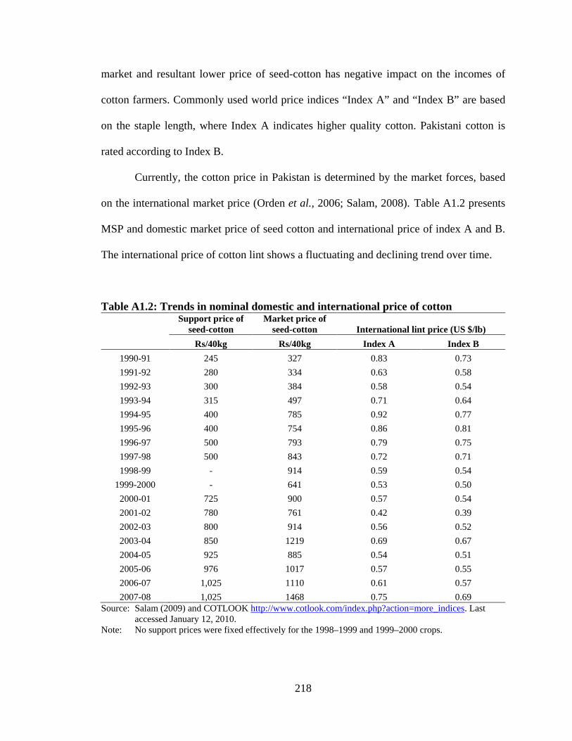
218

market and resultant lower price of seed-cotton has negative impact on the incomes of

cotton farmers. Commonly used world price indices “Index A” and “Index B” are based

on the staple length, where Index A indicates higher quality cotton. Pakistani cotton is

rated according to Index B.

Currently, the cotton price in Pakistan is determined by the market forces, based

on the international market price (Orden et al., 2006; Salam, 2008). Table A1.2 presents

MSP and domestic market price of seed cotton and international price of index A and B.

The international price of cotton lint shows a fluctuating and declining trend over time.

Table A1.2: Trends in nominal domestic and international price of cotton

Support price of seed-cotton

Market price of seed-cotton International lint price (US $/lb)

Rs/40kg Rs/40kg Index A Index B

1990-91 245 327 0.83 0.73 1991-92 280 334 0.63 0.58 1992-93 300 384 0.58 0.54 1993-94 315 497 0.71 0.64 1994-95 400 785 0.92 0.77 1995-96 400 754 0.86 0.81 1996-97 500 793 0.79 0.75 1997-98 500 843 0.72 0.71 1998-99 - 914 0.59 0.54

1999-2000 - 641 0.53 0.50 2000-01 725 900 0.57 0.54 2001-02 780 761 0.42 0.39 2002-03 800 914 0.56 0.52 2003-04 850 1219 0.69 0.67 2004-05 925 885 0.54 0.51 2005-06 976 1017 0.57 0.55 2006-07 1,025 1110 0.61 0.57 2007-08 1,025 1468 0.75 0.69

Source: Salam (2009) and COTLOOK http://www.cotlook.com/index.php?action=more_indices. Last accessed January 12, 2010.

Note: No support prices were fixed effectively for the 1998–1999 and 1999–2000 crops.

http://www.cotlook.com/index.php?action=more_indices�

219

The decade of 1990s experienced a steady drop that reached to historic lows in 2002.

After an increase in 2002 and 2003, prices dropped again in 2004. However, an

improvement has been observed after 2004. Similar trend is observed in the domestic

market price of seed-cotton; price rose up to 1998-99 in Pakistan and then shows a

declining trend until 2003-04. An improvement has been observed in subsequent years

(see Table A1.2).

In Pakistan, the pricing system of seed-cotton was based on cotton varieties.

However, in the traditional marketing system, price of seed-cotton is determined by

weight102. To increase the weight of cotton output, some farmers adopt unsuitable

methods in cotton picking, such as, adulteration with water and trash. These impurities

reduce the beneficial effect of the improvement in cultivars and impair the quality of lint,

yarn and fabric. The contamination of cotton results in an annual loss of US$ 1.4 billion

(SBP, 2005). The majority of farmers market their crop through intermediaries, so-called

arthis. However, large farmers sell directly to the ginneries. The ginneries offer a price

after subtracting their factory margin. Farmers receive the prices that ginners offered103

102 Weight is determined on the basis of formula that two-third of seed-cotton consists of cotton seed and one-third cotton lint.

.

However, the involvement of intermediaries in transactions reduces the price that farmers

receive by the amount of middleman’s profit margin and the cost of services that he

performs. For example, the middleman bears the expenses of weighing, transportation,

loading/unloading, factory charges and local taxes. Factory gate price is the market price.

Farm-gate price depends on the expenses borne by the middleman and his profit margin

(Lohano et al., 1998). To control the quality of cotton both at farm and ginning level,

Pakistan Cotton Standards Institute (PCSI) project was established in 1987. The PCSI

103 Farmers sell their output to the ginners either directly or through the middleman.

220

introduced the cotton grading system for seed-cotton and lint. These grades were

formally approved by the government in 1990 and were declared as the official standards.

The purchase of raw cotton was suggested to be based on the grade of the cotton. The

Karachi Cotton Association announces its daily spot rates on the basis of PCSI standard

grades, but local cotton dealers continues to sell according to traditional pattern. The lack

of implementation of PCSI grading system for seed-cotton and lint causes wide quality

variation within a cotton bale.

Cost of Cotton Production

Cost of production plays an important role in determining the relative profitability of a

crop. To compute the cost of production, the Agricultural Prices Commission of Pakistan

(APCOM) collects data on various field operations through field surveys. This data is

reported in Table A1.3. This table shows that the cost of cotton production in nominal

terms grew by 11 percent during 1990-2005. However, adjusting for inflation this

increase is 3 percent.

Highest growth rate occurred in seed and sowing expenditures (13.4%) followed

by expenditure on fertilizers (12.8%), plant protection measures (10.9%), land rent

(10.7%), and irrigation expenditure (10.4%). Table A1.3 indicates that much of the

increase in the cost of production took place during 1990-2001. For example, the

expenditure on plant protection measures increase from 649 Rs/acre to 2,023 Rs/acre

1990-2001 and further increased to 2,769 Rs/acre in 2004-05. This slow increase during

2001-2005 may be due to the availability of Bt type seed varieties of cotton that reduces

the expenditure of chemical sprays. The increase in the irrigation expenditure is mainly

221

attributed to the rising cost of tubewell irrigation. The prices of electricity and diesel went

up many folds since 1990. This may be one of the causes of higher cost of tubewell

irrigation.

It is important to note that the cost of production grew at an annual average rate of

11 percent during 1990-91 to 2004-05. However, the average annual increase in the

market price of seed-cotton has been only 7.5 percent. A higher increase in cost of

production relative to the price of output has negative impact on the net income of cotton

farmers. It can also be noted from this table that a large component of cost of production

comes from plant protection measures that account for about 19 percent in total cost of

production. The historical data indicates that the use of pesticides increased from 15

thousand tonnes in 1980s to 90 thousand tonnes in 2007 in Pakistan (GoP, 2009). As

indicated earlier, about 70 percent of total pesticides are used on cotton crop. The

pesticides applied on cotton are mostly insecticides against various pests such as,

bollworms, white fly, jassid, aphid, etc. The next section provides a brief description of

major pests and diseases of cotton crop in Pakistan.

222

Table A1.3: Trends in the cost of cotton production in Pakistan.

Nominal cost of production (Rs/acre) Real cost of production (Rs/acre)

Growth rate (%) (1991-2005)

1990-91 2000-01 2004-05 1990-91 2000-01 2004-05 Nominal Real

Land preparation 272 838 1,018 629 838 835 9.9 2.0 Seed and sowing operations 108 564 628 251 564 515 13.4 5.3 Irrigation 374 1,104 1,491 866 1,104 1,222 10.4 2.5 Inter-culture 288 597 856 666 597 702 8.1 0.4 Plant Protection 649 2,023 2,769 1,503 2,023 2,270 10.9 3.0 Farm yard manure 59 158 142 137 158 116 6.4 -1.2 Fertilizers 357 1,187 1,920 826 1,187 1,574 12.8 4.7 Picking 961 1,174 1,392 504 1,174 1,141 2.7 -4.7 Land rent 800 2,667 3,333 1,852 2,667 2,733 10.7 2.8 Other costs 314 1,014 1,240 727 1,014 1,017 10.3 2.4 Total cost of cultivation 3,440 11,325 14,791 7,962 11,325 12,125 11.0 3.0

Source: GoP-APCOM (various issues).

223

Major pests of cotton crop in Pakistan

From sowing to harvest, various pests attack the roots, leaves, stems and fruit of cotton.

Pest infestation is the major reason of yield losses in cotton crop. Estimates indicate that

the yield losses due to insect infections would amount to almost 15 percent of world

annual production (UNCTAD, 2006). About more than 1300 different species of insect

pests attack the crop. These pests can be divided into two categorized: “sucking pests”,

(e.g., aphids, jassids, thrips, mites, white fly, and mealy bug); and “chewing pests”, (e.g.,

cotton bollworms, spotted bollworms, pink bollworms, etc.). In addition, cotton crop is

affected by weeds and some diseases, such as, nematodes, boll rot, bacterial wilt,

verticillium wilt, cotton mosaic virus, and cotton leave curl virus. The economic

threshold levels have been established for many cotton pests104. The pest infestation

varies with the variation in weather. In Pakistan both types of pests are common.

However, their pressure varies according to the agro-climatic and weather conditions.

Bollworms are serious pests of cotton in Pakistan. The major bollworm pests are spotted

bollworms (Earias insulana, Earias vittella), pink bollworm (Pectinophora gossypiella),

American bollworm (Helicoverpa armigera) and armyworms (Spodoptera litura &

Spodoptera exigua). All these pests were widely spread throughout the country. High

rains and high humidity encourages the population of bollworms. These pests withdraw

nutrients from the inside of the cottonseed and may cause serious yield losses. Bollworms

cause heavy damage, which may vary in extent from year to year but generally cause 30-

40 percent yield reduction (Abro et al., 2004). The peak period of the spotted bollworm is

Major chewing pests in Pakistan

104 A threshold infestation is the point at which control measures are needed to prevent the target pest from reaching its economic injury level.

224

from last week of July to second week of October. High infestation of pink and American

bollworm occurs during last week of August to last week of October. The armyworms

appear in the last week of August and remain in the field until harvest of the crop.

However, the intensity of infestation depends on the levels of humidity in an area.

The major sucking pests are whitefly (Bemisia tabaci), jassid (Amrasca devastans), thrips

(Thrips tabaci), and spotted mites (Tetranychus urticae). Cotton mealy bug (Phenacoccus

solani) was also detected a major pest in 2005. These sucking pests suck the cell sap of

the plant, reduce its vitality and adversely affect the fruiting capacity of the cotton plant.

An excessive use of pyrethroids pesticides and dry weather encourages sucking pests.

Major sucking pests in Pakistan

White fly develops sooty-mold on the leaves of cotton plant which affects the

photosynthesis process and results in shedding of leaves and premature opening of bolls.

This pest remains active from June to October. The early attack of white fly badly affects

the cotton plant and yield may reduce. The late attack may not affect the production but it

can affect quality of lint if contaminated with honeydew. So far Pakistan does not have

honeydew contamination problem.

Jassid is an injurious pest of cotton in Pakistan. This pest appears in the first week

of June, peaks during first week of July and remains active until last week of August.

Heavy infestations during vegetative growth cause leaf shedding and, later, loss of flower

buds and bolls. The quality of fibre is also reduced when attack is severe during boll

formation. High humidity is favourable for cotton jassid (Ahmad et al., 1985).

Thrips attack during first week of June to second week of October. The peak

period is from third week of July to last week of August. These pests damage the leaves

225

of cotton plant such that the photosynthesis capacity of plant reduced that affects the

overall growth of plant.

Aphids not only damage the plant by infesting seedlings. They suck sap from

leaves and produce a sugary substance (honeydew) on the underside of leaves that

develops black mold. As the honeydew falls onto the lint, this moldy growth can stain the

lint, reducing its quality and value. Honeydew secretions may burn the leaves and

interfere with photosynthesis.

Mealy bug is a new emerging pest. This was first detected in Pakistan in 2005.

This pest is a potential threat to Pakistan’s agriculture. From 2007 onwards it is

considered as one of the major causes in decline of cotton production. It has now spread

almost throughout the country.

Major disease of cotton crop in Pakistan

Cotton diseases can cause huge crop losses. Some of the major diseases of this crop in

Pakistan are: leaf curl, stunting, boll rot, bacterial blight, and root rot, while minor

diseases are: seedling rot, anthracnose, leaf spot, wet rot, and the diseases caused by

nematodes (Arshad, 2009). Among all these, the cotton leaf curl virus (CLCV) is one of

the most damaging cotton diseases. This disease is transmitted by whitefly Bemisia

tabaci. The symptoms of this disease include leaf curling, darkened veins, and vein

swelling. This disease was first observed in 1967 in Multan area. In 1987, this disease

reoccurred on a smaller area in Punjab. In 1992, this virus destroyed cotton crop in on

large scale that resulted in an estimated yield reduction of 30-35 percent (Hameed et al.,

226

1994). After 1992, several CLCV tolerant cotton varieties were developed. However, in

2001, a new strain of CLCV ‘Burewala strain’ was observed in Punjab province.

Measures to control pest infestation

The persistent pest attacks on cotton crop are resulting in huge economic losses in

Pakistan. In a normal year, on average estimated losses are 10-15 percent, and 30-40

percent or even more in a bad crop year (Salam, 2008). In order to control pest

infestation, a wide range of pesticides was introduced over last 15 years. In Pakistan,

about 70 percent of total pesticides are used on cotton crop (Mazari, 2005). The major

pesticides belong to organophosphate and pyrethroids groups. In multi pest situations, the

mixtures of pesticides have commonly been used for controlling the cotton pest complex.

The maximum number of sprays in Punjab was 5 per acre in 1990 against more than 10

sprays per acre in 2008. A majority of farmers spray cotton crop 5 to 8 times per acre (see

Table A1.4). Because of the lack of knowledge about their proper use, pesticides are

overused by the farmers. This has resulted in several problems, such as, outbreak of

secondary pests, residue of pesticides in soil, surface and groundwater, and health

problems (Tariq et al., 2004; Salam, 2008). In addition to pest infestation, the problem of

weeds, especially in rainy season, is also causes economic losses. However, only one

percent of the farmers, particularly large scale growers, use herbicides regularly. Because

of high prices of herbicides and poor extension services, small farmers suffer from crop

losses due to weeds (Gillham et al., 1995).

227

Table A1.4. Frequency of pesticides application per acre by cotton growers (figures are percent farmers) Year Number of Sprays

1 2 3 4 5 6 7 8 9 10 >10

1990 2.6 8.9 23.2 38.8 19.7 - - - - - - 1991 2.1 4.7 42.0 39.4 12.4 - - - - - - 1992 0.5 7.1 26.4 38.9 25.0 - - - - - - 1993 0.0 1.4 12.7 29.4 45.2 11.3 - - - - - 1994 0.9 3.4 11.9 31.5 32.6 18.1 1.6 - - - - 1995 0.8 3.9 21.2 28.2 3.6 14.2 1.1 - - - - 1996 0.4 2.0 3.4 19.8 36.3 27.6 6.0 1.8 0.2 0.8 - 1997 1.6 3.4 8.9 21.5 30.7 15.5 8.8 5.4 2.7 1.5 0.1 1998 0.9 2.6 7.2 12.1 20.9 24.8 14.4 8.2 5.2 2.6 1.1 1999 1.5 3.3 15.6 32.5 27.4 11.6 6.4 1.4 0.1 0.1 - 2000 0.2 1.5 10.6 27.5 34.7 16.8 6.2 1.7 0.4 0.0 - 2001 0.6 1.3 4.9 17.2 25.8 20.3 17.5 6.6 3.2 2.5 0.2 2002 1.0 3.5 13.7 25.2 23.0 16.6 6.7 4.7 3.0 2.5 0.2 2003 0.3 1.0 3.5 8.5 12.5 16.5 17.6 17.3 9.8 7.1 3.2 2004 1.1 2.4 6.4 17.4 24.6 21.9 15.5 10.1 4.6 2.2 1.5 2005 0.5 2.4 7.3 19.9 25.6 21.0 13.4 6.1 2.3 1.0 0.5 2006 1.1 3.5 7.8 12.9 18.5 22.5 17.0 10.0 4.1 2.1 0.6 2007 0.8 2.3 5.6 10.3 14.4 19.1 18.9 11.8 9.4 5.5 1.8

2008 0.6 1.8 5.0 19.8 19.4 14.2 13.3 9.1 8.4 4.5 3.8

Source: Directorate of Pest Warning & Quality Control of Pesticides Punjab, Multan (2009). Note: - indicates no data or proportion less than 1 percent.

Cotton Research in Pakistan

The origin of cotton fabric is traced out back to approximately 3200 BC, as revealed by

the fragments of cloth found at the Mohenjo-Daro archaeological site on the banks of the

River Indus in Pakistan. Cotton is primarily grown in dry tropical and subtropical

climates at temperatures between 11°C and 25°C. It is a warm climate crop threatened by

228

heat or freezing temperatures (below 5°C or above 25°C), although its resistance varies

from species to species. In addition, excessive exposure to dryness or moisture at certain

stages of the plant development is detrimental to cotton quality and yields. Cotton is a

five to seven month crop depending on the climatic conditions. Flowering starts within

two months of planting and blooming continues for several months. Harvesting depends

on the maturity of “cotton-boll”, the inner part of the bloom that develops into a fruit.

Each boll contains about 30 seeds, and up to 500,000 fibers of cotton. Cotton varieties

differ in yield per hectare, disease resistance, heat and salt tolerance, ginning percentage

and technical measures of fiber quality. Technical measures include: staple length,

micronaire value and pressley strength. Staple length refers to the length of cotton fiber;

micronaire is a composite measure of fineness and maturity of the fibers; and pressley

strength measures the maximum tensile strength of lint at the time of rupture. The quality

of cotton depends on these technical measures, colour and cleanliness of cotton fiber. The

world price indices “Index A” and “Index B” are based on the staple length, where Index

A indicates higher quality cotton.

The early type of cotton grown in sub-continent India, Thailand and China, was

known as short staple ‘desi’ arboreum cotton. The long staple cottons of Egypt and West

Indies (sea island cotton) known as upland hirsutum (American) cotton that was first

introduced in the sub-continent India in 1913 and replaced the desi cotton quickly. In the

early 1920s, nearly 40 percent of total cotton area and 90 percent of irrigated cotton area

of the sub-continent was under this type of cotton (Pray, 1981). At present, 97 percent of

cotton area in Pakistan is under American cotton.

229

Agricultural research has a long history in the sub-continent India. The

department of Land Records and Agriculture was established in 1880 that collects the

agricultural statistics. The first agricultural experiment farm was set up in 1901 in

Lyallpur (now Faisalabad) where trials of wheat and cotton varieties were started.

However, the research was not started on regular basis until the Department of

Agriculture was set up in 1905. Research work on breeding of new cotton varieties was

intensified in 1906 after the establishment of Punjab Agricultural College and Research

Institute, Lyallpure105. The first variety of American cotton ‘4F’ was released in 1910.

The release of another variety ‘289F’ in 1926 introduced American cotton in Sindh

province. The process of evaluation of cotton varieties continued for other zones. During

1910-1945, eight varieties of American cotton and four varieties of desi cotton were

developed. After independence of Pakistan in 1947, the work on cotton research

continued and several varieties have been developed. As a result of research efforts in

cotton varieties, the quality of Pakistan’s cotton has improved considerably over time.

Table A1.5 presents the characteristics of cotton varieties produced after independence.

This table shows improvement in all the measures of cotton quality106

105 Now University of Agriculture, Faisalabad.

. The staple length

of most of the varieties is either medium-long or long. The improved varieties contributed

significantly to increase in production and quality of cotton over time. For example, the

original variety, 4F, introduced in 1910, was a short staple, late maturing variety with a

Ginning-Out-Turn (GOT) of about 32.0 percent. The quality of cotton has made steady

progress. The staple length has increased from 22.2 to 23.8mm for the early varieties to

27.0 to 32.2 mm for the more recent varieties.

106 Five different staple lengths are defined as: short (less than 21 mm), medium (21-25 mm), medium long (26-27 mm), long (28-34 mm), and extra long (more than 35 mm).

230

Table A1.5: Characteristics of Cotton Varieties in Pakistan

Variety name

Year of release

GOT (%)

Staple Length (mm)

Micronaire value

(µg/inch) Strength (TPPSI)* Staple Group

M-100 a 1963 34 26.2 3.5-4.0 85 Medium long H-59-1 a 1974 34 28.6 3.5-3.7 90 Long S-59-1 a 1975 34 28.6 3.5-3.7 92.7 Long B-557 1975 34.5 26.2 4.5 92.9 Medium long K-68/9 a 1977 30 30.2 4.3 96.1 Long MNH-93 1980 36.5 27 4.7 94 Medium long NIAB-78 1983 36.6 26.2 4.6 92.5 Medium long MS-84 1983 34 31.8 3.9 91.3 Long SLH-41 1984 34 26.2 4.4 95.8 Medium long TH-1101 a 1985 35 27 4.0-4.4 89.0-90.0 Medium long CIM-70 1986 31.2 29.4 4.2 92.5 Long MNH-1986 1986 38.5 27 4.4 95.4 Medium long CIM-109 1990 35.1 27.2 4.4 92.0 Medium long CIM-240 1992 36.5 27.5 4.7 93.7 Medium long CIM-1100 1996 38 29 3.9 94.0 Long CIM-448 1996 38 28.5 4.5 93.8 Long Karishma 1996 37.4 28.6 4.9 93.3 Long CIM-443 1998 36.7 27.6 4.9 96.0 Medium long CIM-446 1998 36.2 27 4.7 97.4 Medium long CIM-482 2000 39.2 28.5 4.5 98.0 Long FH-901 2000 38.2 26.8 5.1 92.0 Medium long FH-900 2000 37.5 28.5 4.5 94.0 Long CIM-473 2002 39.7 29.6 4.3 95.2 Long CIM-499 2003 40.2 29.6 4.4 97.3 Long NIAB-999 2003 36.5 28.7 4.6 95.0 Long FH-1000 2003 38.8 29.5 4.6 96.9 Long Alseemi 2003 38.0 32.5 4.6 100.3 Long NIAB-111 2004 37.5 30.5 4.4 90.5 Long BH-160 2004 35.5 29 4.2 95.1 Long CIM-707 2004 38.1 32.2 4.2 97.5 Long CIM-506 2004 38.5 28.7 4.5 98.9 Long CIM-496 2005 41.1 29.7 4.6 93.5 Long

Source: Ender (1990), Block (1991), Arshad (2009) Notes: * TPPSI = Thousand pounds per square inches

In most recent varieties GOT increased to 38.0−41.0 percent. As a result of varietal

improvement, the production of short-staple cotton declined from 319 thousand bales in

231

1954-55 to 53 thousand bales in 2001-02 and the production of medium-long varieties,

increased from 2 thousand bales in 1958-59 to 7,201 thousand bales in 2001-02.

The abiotic stress (e.g., heat, drought, strong winds, etc.) differs from variety to

variety. Therefore, one variety is not suitable for all areas. The Cotton Control Act 1949

regulates the cultivation of recommended varieties according to the agro-climatic

conditions of the region. However, in practice, farmers grow multiple varieties on one

farm. This gives non-uniform plant population and differences in fiber quality (Ahmad

and Ali, 1994). In addition to the development of new varieties, various steps had been

taken for better crop management. For example, through extension services, farmers were

trained for better sowing techniques, proper seed rate, use of high quality seed,

appropriate use of chemical fertilizers, on-farm water management, judicious use of

pesticides through Integrated Pest Management (IPM) program. To provide credit

facility, the Agricultural Development Bank of Pakistan was established. In addition, to

give incentives to the farmers, the government announces the minimum assured price

before the start of sowing.

Given the economic importance of this crop, cotton research has always received

high priority in Pakistan. The primary objective of cotton research has been to develop

new cotton varieties that are resistant to pests, heat, and drought, and have high yield

potentials with desirable fiber characteristics. In Pakistan, cotton research is carried out at

federal and provincial levels through research institutes, research stations, laboratories

and universities. At federal level, cotton research is managed by the Pakistan Central

cotton Committee (PCCC) and at provincial level by the Provincial Department of

Agriculture. The PCCC, established in 1948, has two multi-disciplinary institutes, one at

232

Multan in the Punjab and the other at Sakrand in Sindh107. In addition, the Pakistan

Agricultural Research Council (PARC) also provides research advisory services, at

national and international level. At provincial level, the Department of Agriculture

Punjab has research centers are at Faisalabad, Sahiwal, Multan, Bahawalpur and

Rahimyar Khan with major breeding research centers at Faisalabad and Multan. In Sindh,

the main Department of Agriculture cotton research center is located at Tandojam. In

addition to PCCC, the Nuclear Institutes for Agriculture and Biology (NIAB) and the

Universities of Agriculture at Faisalabad and at Tandojam conduct research on cotton in

all disciplines. The research efforts are strengthen by the extension services. These

services are provided by the Extension Wing of the Agriculture Department of each

province. The personnel of extension services are distributed across all administrative

units (district, tehsil and union council)108

. At present, nearly ten cotton research

institutes are working in the public sector of Pakistan.

Quality of seed

The varietal improvement cannot be effective until the quality seeds are available to the

growers. The poor quality seeds can increases the susceptibility to diseases and pest

attacks. In Pakistan, nearly half of the cotton crop is planted from farmer’s own seed. The

continuous production of cotton from the same original source of seed reduces the vigour

of the variety and can lead to a decline in both yield and quality. In Pakistan, under the

Seeds Act of 1976, approved varieties of a crop need to be registered and their sale,

107 These institutes conduct research on Plant Breeding, Cytogenetics, Agronomy, Physiology, Entomology, Pathology and Fiber Technology. 108 The component of extension services are Adaptive Research, On-the-Job Training, Agricultural Extension and Monitoring and Evaluation.

233

exchange and barter is subject to regulation. The multiplication and supply of crop seeds

is catered at provincial level through Punjab and Sindh Seed Corporations. The system of

seed multiplication and supply is regulated by the National Seed Council at the federal

level. The Federal Seed Certification Department (FSCD) supervises the quality seed

production at all stages and to verify the purity and the viability of seed. Under the

Cotton Control Act 1949, it is obligatory for the Government to supply 100 percent of the

seed requirements of each registered variety. At present, 55 percent of the seed

requirement is fulfilled by the public sector. Rest of the requirement is fulfilled either by

the private sector or by farmer-to-farmer exchange. The Seed Corporations distribute

their seed through their own sale points and private dealers. The Punjab Seed Corporation

provides seed for sale to cooperative societies and through branches of cooperative

banks. Private companies have their own dealers, while the ginning factories supply seed,

usually on credit, to the growers who bring their seed-cotton to them for ginning.

Conclusions

Despite achieving varietal improvement, Pakistan could not achieve the actual potential

of cotton production. The yield per hectare is lower than many other cotton growing

countries (e.g., China, USA, Syria, Brazil, Turkey). Due to highly fluctuating yield per

hectare and increased domestic use, Pakistan became the net importer of cotton lint.

Cotton farmers of Pakistan are facing several challenges from sowing to the

marketing of the crop. These challenges can be divided into three groups: input related

problems (availability and prices of inputs); production related problems (pest

infestation); and marketing related problems (contamination in picking). Major input

234

related problems are the lack of availability of quality seed, shortage of irrigation water,

and rising prices of fertilizer and pesticides. Because of the lack of professional

cottonseed industry, the cotton seed supplied in the market has poor germination. Cotton

is high water consumptive crop. The decline in water supply for irrigation has adverse

effect on the crop yield. Because of persistent electricity outages, the use of diesel

tubewell increased. Increased pest infestation led to higher use of pesticides. The rising

prices of pesticides, fertilizer and irrigation resulted in increasing the real cost of cotton

production by more than 50 percent since 1990. Among production related problems,

pest infestation and cotton diseases are most important. CLCV is the continuous threat to

the cotton crop since 1992. In addition, the mealy bug became a major pest in recent past

that caused substantial loss in yield. The population of other sucking insects, namely,

whitefly and jassid has also increased in past few years. These problems not only

adversely affected yield per hectare and quality of cotton but also increased the cost of

plant protection measures. The marketing level issues start with picking. The production

of clean lint depends upon clean picking, free from contaminants/ trash and low moisture

content at the field level. However, the improper handling at the picking level and high

levels of contamination reduce the quality as well value of the crop. The resultant low

quality of lint and yarn cannot fetch high price in the international market. In addition,

high fluctuations in cotton prices have negative impact on the incomes of cotton farmers

(Salam, 2008).

The average yield of Pakistan can increase with controlling pest infestation and

better crop management practices. The relative profitability of a crop for the grower can

be determined by yield, price and cost of production. The discussion in this chapter

235

indicates that cotton growers in Pakistan are facing low/fluctuating yield, fluctuating

prices, and high cost of production. The vulnerable farm households can be pushed into

poverty in a bad crop year with high crop loss. If Pakistan controls pest infestations, yield

can increase by 30-40 percent without increasing the cultivated area. The yield can be

increased further if quality inputs are used and better crop management practices are

adopted. The staple length and uniformity ratio could be improved if the supply of

certified seed could reach the 100 percent level. By increasing the yield per hectare of

cotton, Pakistan can save foreign exchange and can also reduce the cost of production of

textile production that is crucial to make the textiles exports competitive, especially after

the abolition of multi-fiber agreement.

236

APPENDIX 2: AGRICULTURAL BIOTECHNOLOGY REGULATIONS IN THE INTERNATIONAL CONTEXT

The pace of varietal improvement has been accelerated through the advancements in

molecular biology and genetics, especially after the discovery of the structure of DNA.

The molecular techniques “recombinant DNA technology” isolates genes from plants,

insects, animals, and microorganisms and inserts into the genetic material of other

organisms. This technique produces genetically modified (GM) products. Since the GM

crops deal with living organisms, the possibility of potential risks associated with the use

of these crops persists. This entails new regulatory procedures at national and

international levels; from laboratory to farmer.

The Convention on Biological Diversity (CBD) is the first treaty that provides a

legal framework for biodiversity conservation109

The Cartagena Protocol outlines the framework for the use and the commercial

release of GM crops. A country must take into account the measures outlined in the

. The Convention established three main

goals: the conservation of biological diversity; the sustainable use of its components; and

the fair and equitable sharing of the benefits arising from the use of genetic resources.

The agreement covers all ecosystems, species, and genetic resources. On 29 January

2000, the Conference of the Parties to the Convention on Biological Diversity adopted a

supplementary agreement, the Cartagena Protocol on Biosafety, came into force in

September 2003. This Protocol promotes biosafety by establishing rules and procedures

for the safe transfer, handling, and use of LMOs, with specific focus on transboundary

movements of LMOs.

109 This convention was adopted in May 1992 and entered into force in December 1993 at the UN Conference on Environment and Development.

237

Protocol, such as, biosafety risk assessment procedures, socio-economic consideration,

legal liability and redress, coexistence policies and labeling, and intellectual property

rights. The biosafety risk assessment procedures examine the potential adverse impacts of

transgenic crops on humans, animals and the environment. The socioeconomic

considerations as a part of the Cartagena Protocol focus on the costs and benefits accrue

to society as a result of the cultivation of a transgenic crop. The Article 27 of the

Cartagena Protocol covers the legal liability and redress. This Article is about the

compensation of a possible damage resulting from transboundary movements of living

modified organisms. The coexistence policy allows the simultaneous cultivation of GM,

organic, and conventional crops. European Union proposed the establishment of

traceability and labeling to maintain the coexistence between transgenic, non transgenic

and organic products. To facilitate the exchange of information and strengthening human

resources and institutional capacities in biosafety, the Cartagena Protocol calls for

establishing Biosafety Clearing House and Capacity Building. Each country is required to

prepare country specific biosaftey guidelines and rules.

238

APPENDIX 3. LIST OF PERSONS CONSULTED FOR INFORMAL MEETINGS AND INTERVIEWS AND CONTACTED FOR THE BT

COTTON SURVEY 2009.

Appendix 3.1: List of persons consulted for informal meetings and interviews

1. Dr Abdul Salam, Former Chairman APCOM and Professor, Urdu University, Islamabad.

2. Dr Ali Muhammad Khushk, Director, Technology Transfer Institute, Tandojam 3. Mr Mohammad Arshad, Director CCRI, Multan 4. Dr Ghazanfar Ali Khan, TAC Bt cotton, Lahore 5. Dr Professor Hafeez Rana, Agriculture University, Faisalabad 6. Dr Iftekhar, Dean Faculty of Agriculture, University of Agriculture, Faisalabad 7. Dr Ijaz Pervaiz, Pest control department Lahore 8. Mr Iqbal Mahmood, owner of Mehmood Textile mills, Multan 9. Dr Khalid Hamid, Ali Akbar Group, Lahore 10. Dr M. E. Tusneem, Member Planning Commission, GOP, Islamabad 11. Mr Maqbool Sadiq, Zahid Bashir, Karachi Cotton Exchange, Karachi 12. Mr Mohammad Asim, Monsanto Pakistan, Lahore 13. Dr Mohammad Aslam, Deputy Chief Scientist/Group leader Cotton, NIAB,

Faisalabad 14. Dr. Muhammad Hanif, Chief Scientific Officer, Ali Akbar Group, Multan 15. Dr Mohammad Jameel, Planning Commission, Islamabad 16. Mr Masood Majeed, Owner off Bismillah Ginnery, Bahawalpur 17. Mr Mazhar Abbas, Director, Technology Transfer Institute, PARC, Faisalabad 18. Dr Noor ul Islam, Director, Ayub Agricultural Research Institute, Faisalabad 19. Mr S A Javed, Secretary General, Karachi Cotton Association 20. Dr Sagheer, Director Cotton Research Station, Multan 21. Dr Shahid Mansoor, Principal Scientist, NIBGE, Faisalabad 22. Mr Shoaib Aziz, Policy Officer Food Rights, Action Aid, Islamabad 23. Dr Siddique, Bt cotton Seed Dealer, Faisalabad 24. Dr Tayyab Husnain, Professor, CEMB, Lahore 25. Dr Yusuf Zafar, Project Director, NIGAB, NARC, Islamabad 26. Dr Zahoor Ahmad, Ali Akbar Group, Multan.

239

Appendix 3.2: List of Persons Contacted for the Bt Cotton Survey.

Overall Logistics of Bt Cotton Survey:

1. Dr Zafar Altaf, Chaiman, PARC, Islamabad 2. Dr Sohail Malik, Chairman IDS, Islamabad 3. Dr Zakir Rana, Dean, University of Sargodha, Sargodha 4. Dr Khalid Mehmood, PARC, Islamabad 5. Mr Imran Malik, Director Operations, IDS, Islamabad

Logistics -- Bahawalpur

1. Dr Rukhsana, PARC, Bahawalpur 2. Mr Jamshed, NGO, Bahawalpur 3. Social Welfare Department, Ahmadpur East 4. Mr Sheikh Aziz, Ahmadpur East

Logistics -- Mirpur Khas

1. Mr Imtiaz Pirzada, Assistant Professor, Sindh University, Jamshoro 2. Mr Masood Khalid, PPAF, Islamabad 3. Mr Mustafa Ujjan, Mirpur Khas 4. Dr Mubarik Ahmad, Director, PARC Karachi 5. Mr Aslam Mahar, Irrigation Department, Government of Sindh, Mirpur Khas. 6. Dr Yamin Memon

Sample Frame

1. Dr Rashid Amajd, VC PIDE, Islamabad 2. Dr G. M. Arif, Dean Faculty of Development Studies, PIDE, Islamabad 3. Mr Masood Ishfaq, Head, Computer Division, PIDE, Islamabad 4. Mr Syed Abdul Majid, Team Supervisor, PRHS, Islamabad

Questionnaire Formatting and Urdu typing

1. Mr Afsar Khan, PIDE, Islamabad 2. Mr Siddiq, PIDE Islamabad

Pretesting

• Dr Professor Hafeez Rana, Chak 33, Faisalabad Data Entry Software

• Mr Arshad Khurshid, IDS, Islamabad

240

Appendix 3.3: List of field enumerators and supervisor

Enumerators in Bahawalpur 1. Mr. Farhan Altaf 2. Mr. Nasir Saleem 3. Mr. Waqar Ul Haq 4. Mr. Waqas Ul Haq

Enumerators in Mirpur Khas

1. Mr. Abdul Khalique 2. Mr. Abdul Sami Bhurgari 3. Mr. Aijaz Ali Kalroo 4. Mr. Ibrar Hussain Bhurgri

Household identfication team in Mirpur Khas

1. Mr Abdul Aziz 2. Mr. Wazir Hussain Soomro

Team supervisor in both districts

• Mr. Mubashir Ijaz Data Entry

1. Mr. Mubashir Ijaz 2. Mr Yamin Khalid 3. Mr. M. Afsar Khan

241

APPENDIX 4. QUESTIONNAIRES Appendix 4.1. Household Questionnaire

For office use only

IMPACT OF BT COTTON ON POVERTY REDUCTION IN RURAL PAKISTAN

HOUSEHOLD QUESTIONNAIRE--2009

HOUSEHOLD IDENTIFIER CODE Province: Punjab 1 Sindh 2 District: Mirpur Khas 1 Bahwalpur 2 Village Name: _________________________________________ Village Code: __________________________________________ Tehsil/Taluka Name: _____________________________________ Tehsil/Taluka code:______________________________________ Settlement (Basti) 1 2 3 4 5 6 7 8

Respondent Name: Zaat: Native Language Punjabi 1 Sarikey 2 Urdu 3 Sindhi 4 Relation with Head Head 1 Spouse 2 Son/Daughter 3 Grand child 4 Father/Mother 5 Brother/Sister 6 Nephew/Niece 7 Son/Daughter-in-law 8 Brother/Sister-in-law 9 Father/Mother-in-law 10

Gender: Male 1 Female 2 Name of Interviewer Same of Supervisor Start time: __________ Finish time: _________ Date of interview --------/--------/2009 Day/Month/Year Result of the visit Complete 1 Partially complete 2 Refuse 3 No Respondent was available 4

242

SECTION 1: HOUEHOLD INFORMATION

ID

C O D E

Q1. Name of

household members who

“usually live and eat here”.

Do not list guests, visitors etc.

Q2.

Gender

Male .......... 1 Female ........ 2

Q3. Relation

to head

Head ....................... 1 Spouse .................... 2 Son/Daughter ......... 3 Grand child ............ 4 Father/Mother ........ 5 Brother/ Sister ...................... 6 Nephew/ Niece ...................... 7 Son/Daughter-in-law .......................... 8 Brother/Sister-in-law .......................... 9 Father/Mother-in-law ........................ 10 Servants ................ 11 Other .................... 77

Q4. Age

(in

completed years)

Q5. Marital Status

Never Married ................. Currently Married ................. Widow / widower ................

Divorced .............

Q6. ID code of

spouse.

( If not in the roster write code "99")

Q7 Have …. ever

attended school

Never attended school/ institution .............. 1 Attended school/institution in the past .................. 2 Currently attending school/

institution ............ 3

Q8 What was the

highest class, …., complete

d

See below for codes.

Q9. Any technical

training?

Yes .................... 1 No .................... 2 If No then go to Q 11

Q10. Type of

technical training

Diploma .......... Certificate ....... Self-taught ...... Apprenticeship ........................ Friends/ relatives ........... Other ...............

Q11 Main

occupation

Farming ............ Livestock ......... Agri. labourer ... School teacher .............. Govt. employee .......... Private sector employee .......... Non-agri labourer ............ Army................. Own business ... Other .................

Q12. Who is the

main earner in

this household

(write appropriate code in front of

that person)

main earner ........... second earner ........... third earner .

01

02

03

04

05

06

07

08

09

10

11

12

13

14

243

Codes of education Q9 Less than class 1= 00 Class 1 = 01 Class 2 = 02 Class 3 = 03

Class 4 = 04 Class 5 = 05 Class 6 = 06 Class 7 = 07

Class 8 = 08 Class 9 = 09 Class 10 = 10 Class 11 = 11

Class 12 = 12 Class 13 = 13 BA / B Sc/B.Ed= 14 Class 15 = 15

Post graduate ( MA, M Sc/M.Ed.) =16 Polytechnic Diploma = 17

Degree in Engineering = 18 Degree in Medicine = 19 Degree in Agriculture = 20 Degree in Law = 21

M. Phil, Ph. D = 22 Other = 23

SECTION 2: INFORMATION ON LAND OPERATIONS AND CROPS GROWN (during last year Rabi and Kharif 2007-08) Part 1: Land operations

Land operated last year Q1

Total operated land

Q2 Number of plots of operated land

Q3 How much

operated land was owned? (write 0 if no

land was owned)

Q4 How much operated land was rented-in?

(write 0 if no land was rented-in)

If answer is 0 then go to Q6

Q5 How much rent

was paid last year

Q6 How much

operated land was under

sharecropping? (write 0 if no

land was sharecropped)

If answer is 0 then go to Q8

Q7 % Share under sharecropping arrangement

Q8 How much

operated land was fallow

(write 0 if no land was fallow)

(acres) (number) (acres) (acres) (Rs) (acres) (%) (acres)

244

Q9 How much land

was rented out last year

(write 0 if no land was rented out

if answer is 0 then go to Q11

Q10 How much money

received as rent (include both cash

and kind)

Q11 How much land did you own last

year

(this includes owned, rented out, and uncultivated

land that a household owns)

Q12 Main source of

irrigation

Canal ........................ Electric Tube-well ... Diesel tubewell ........ River ........................ 1 & 2 ........................ 1 & 3 ........................ 2 & 3 ........................ Other ........................

Q13 Main source of power for ploughing Tractor ..................... Animal ..................... Tractor + animal ......

Q14 Brackishness in subsoil water

low ........................... medium .................... high ..........................

Conversion factors For produce 1 maund=37.32702 kg For land area 1 acre=8 Kanal 1 Jareb=4 Kanal 1 Murabba=25 acre 1 acre=0.40468 hectares

(acre) (Rs) (acre) (code) (code) (code)

245

Part 2: Crops grown last year (2007-08) Instruction for enumerator: Expenditures include all operational inputs from pre-sowing to harvesting and marketing (do not include land rent)

Q1

Crop Name (Rabi)

Q2 Area

(acres)

Q3 Yield/acre

(40 kg/acre)

Q4 Expenditure/acre

(Rs)

Q1 Crops Name (Kharif)

Q2 Area

(acres)

Q3 Yield/acre

(40 kg/acre)

Q4 Expenditure/acre

(Rs)

01=Wheat 31=Rice

02=Barley 32=Maize

03=Gram/Chana Daal 33=Jawar (Sorghum)

04=Masoor Daal 34=Bajra (Millet)

05=Other Pulses(Rabi) 35=Cotton

06=Rapeseed/Mustard 36=Sugarcane

07=Sunflower 37=Sugar-beets

08=Other Oilseeds 38=Moong Daal

09=Potato 39=Mash Daal

10=Onion 40=Other pulses (Kharif)

11=Tomato 41=Groundnuts/Peanuts

12=Peas 42=Sesamum

13=Other Vegetables (Rabi)

43=Soybean

14=Spices 44=Castorseed

15=Tobacco 45=Gwaraseed

16=Barseem/Lucern 46=Other oil seed (Kharif)

17=Oats 47=Chilies

18=Other Rabi fodder 48=other vegetables Kharif

246

19=Orchard 49=Maize fodder

50=Sorghum fodder

51=Bajra fodder

52=Other Kharif fodder

SECTION 3: INFORMATION ABOUT COTTON PRODUCTION AND BT COTTON ADOPTION Q1. Do your household grow cotton (1=Yes, 2=No) _________________ Q2. How long have you been growing cotton _________________ years Part 1: Varieties of cotton grown during last three years (Instruction: A farmer may grow more than one variety in one year. Write the name of all varieties grown during last three years. Please provide information on the varieties of cotton you grew during last five years

Q1 Year

Q2 Variety name

Q3 Is this variety Bt type

Yes .............................1 No ...............................2

Q4 Area under this

variety

Q5 Quantity of seed

used per acre

Q6 Price of seed per

Kg

Q8 Total produce of

seed cotton (including that paid as wages)

Q9 Where did you sell your cotton

crop

Input dealer ............................ 1 Ginning Factory ..................... 2 Commission agent/ middleman ............................. 3 Other farmer ........................... 4 my landlord sells .................... 5 shopkeeper ............................. 6 Other ...................................... 7

(name) (code) (acres) (Kg/acre) (Rs/kg) (40kg)

2008

247

Characteristics of varieties grown during last three years (1=Yes, 2=No, 3=Don’t know) Instruction: Please copy the name of varieties from previous page in place of V1, V2, V3 and V4

Characteristics V1 Variety name

V2 Variety name

V3 Variety name

V4 Variety name

Characteristics V1 Variety name

V2 Variety name

V3 Variety name

V4 Variety name

General Characteristics

Input requirement

Q1. Higher yielding

Q14. Lesser seed required

Q2. Higher Profit

Q15. More water demanded,

Q3. Higher cost of production

Q16. More fertilizer demanded

Q4. Resistant to pests

Q17. More labour intensive

Q5. Resistant to insects

Q18. Requires better land preparation

Q6. Resistant to bollworms

Q19. High expenditure on seed

Q7 Resistant to heat

Q20. Higher pesticide expenditure

Q8. Short duration Cotton quality Q9. Early maturing

Q21. Long staple length

Q10. Late maturing

Q22. Medium staple length

Q11. Short stature (easy picking)

Q23. Short staple length

Q12. More flowering, so less number of pickings

Q24. High GOT

Q13. Wheat sowing remains timely

Q25. Higher market price

248

Instruction: If farmer did not grow any non-Bt variety in 2008, go to part 2B on page 10 Part 2A: Cost of production of Cotton using Non-Bt variety in 2008

Write the name of this variety ___________ When did you sow this variety __________ (write month)

Operations/units

Q1 Power used

tractor ............ bullock .......... manual ..........

Q2 Area

covered

Q3 Average No. of

Operations

/units/acre

Q4 Cost per

unit

Q5 cost per

acre

Q6 Number of family

labour worked

on

Q7 Average

number of days/seas

on/ person

Q8 Number of hired labour worked

on

Q9 Average

number of days/seas

on/ person

Land preparation:

01 Deep ploughing

02 Rotavator

03 Ploughing

04 Planking

05 Levelling

Seed and sowing operations:

06 Seed (kgs) (including treatment)

Sowing

07 Ploughing+planking

08 Ridging

09 Drilling

10

Manual labour for sowing, bund making etc

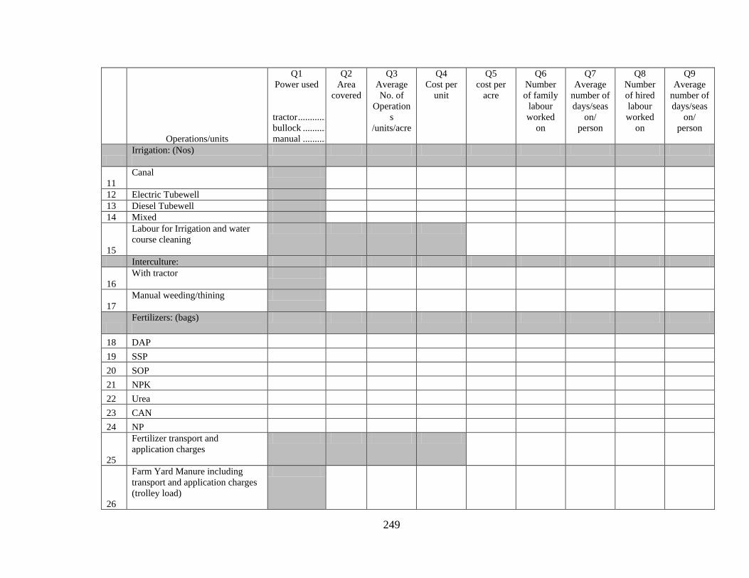
249

Operations/units

Q1 Power used


Q2 Area

covered

Q3 Average No. of

Operations

/units/acre

Q4 Cost per

unit

Q5 cost per

acre

Q6 Number of family

labour worked

on

Q7 Average

number of days/seas

on/ person


on

Q9 Average

number of days/seas

on/ person

Irrigation: (Nos)

11 Canal

12 Electric Tubewell 13 Diesel Tubewell 14 Mixed

15

Labour for Irrigation and water course cleaning

Interculture:

16 With tractor

17 Manual weeding/thining

Fertilizers: (bags)

18 DAP

19 SSP

20 SOP

21 NPK

22 Urea

23 CAN

24 NP

25

Fertilizer transport and application charges

26

Farm Yard Manure including transport and application charges (trolley load)

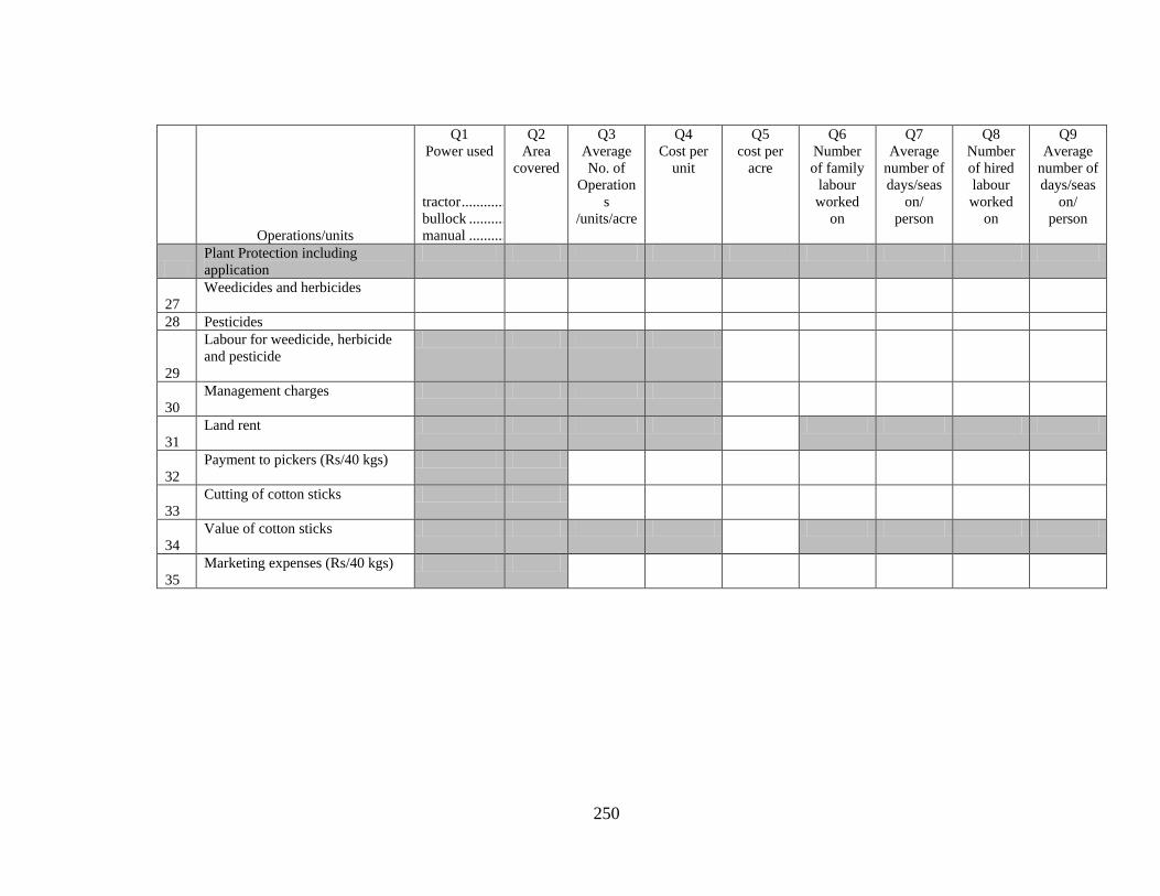
250

Operations/units

Q1 Power used


Q2 Area

covered

Q3 Average No. of

Operations

/units/acre

Q4 Cost per

unit

Q5 cost per

acre

Q6 Number of family

labour worked

on

Q7 Average

number of days/seas

on/ person


on

Q9 Average

number of days/seas

on/ person

Plant Protection including application

27 Weedicides and herbicides

28 Pesticides

29

Labour for weedicide, herbicide and pesticide

30 Management charges

31 Land rent

32 Payment to pickers (Rs/40 kgs)

33 Cutting of cotton sticks

34 Value of cotton sticks

35 Marketing expenses (Rs/40 kgs)

251

Part 2B: Cost of production of Cotton using Bt variety in 2008 Write the name of this variety ___________ When did you sow this variety __________ (write month)

Operations/units

Q1 Power used

tractor ........... bullock ......... manual .........

Q2 Area

covered

Q3 Average No. of

Operations

/units/acre

Q4 Cost per

unit

Q5 cost per

acre

Q6 Number of family

labour worked

on

Q7 Average

number of days/seas

on/ person

Q8 Number of hire labour worked

on

Q9 Average

number of days/seas

on/ person

Land preparation:

01 Deep ploughing

02 Rotavator

03 Ploughing

04 Planking

05 Levelling

Seed and sowing operations:

06 Seed (kgs) (including treatment)

Sowing

07 Ploughing+planking

08 Ridging

09 Drilling

10 Manual labour for sowing, bund making etc

252

Operations/units

Q1 Power used


Q2 Area

covered

Q3 Average No. of

Operations

/units/acre

Q4 Cost per

unit

Q5 cost per

acre

Q6 Number of family

labour worked

on

Q7 Average

number of days/seas

on/ person

Q8 Number of family

labour worked

on

Q9 Average

number of days/seas

on/ person

Irrigation: (Nos)

11 Canal

12 Electric Tubewell 13 Diesel Tubewell 14 Mixed

15

Labour for Irrigation and water course cleaning

Interculture:

16 With tractor

17 Manual weeding/thining

Fertilizers: (bags)

18 DAP 19 SSP 20 SOP 21 NPK 22 Urea 23 CAN 24 NP

25

Fertilizer transport and application charges

26

Farm Yard Manure including transport and application charges (trolley load)

253

Operations/units

Q1 Power used


Q2 Area

covered

Q3 Average No. of

Operations

/units/acre

Q4 Cost per

unit

Q5 cost per

acre

Q6 Number of family

labour worked

on

Q7 Average

number of days/seas

on/ person

Q8 Number of family

labour worked

on

Q9 Average

number of days/seas

on/ person

Plant Protection including application

27 Weedicides and herbicides

28 Pesticides

29 Labour for weedicide, herbicide and pesticide

30 Management charges

31 Land rent

32 Payment to pickers (Rs/40 kgs)

33 Cutting of cotton sticks

34 Value of cotton sticks

35 Marketing expenses (Rs/40 kgs)

254

Part 3: Information on Harvested quantity in 2008

First picking Second picking

Q1 Month of 1st

picking

Q2 Quantity harvested in 1st picking

Q3 Quantity sold after 1st picking

Q4 Price received after 1st picking

Q5 Month of 2nd

picking

Q6 Quantity harvested in 2nd picking

Q7 Quantity sold after 2nd picking

Q8 Price received after 2nd picking

(month) (40 kg) (40kg) (Rs/40 kg) (month) (40 kg) (40kg) (Rs/40 kg)

1. Bt cotton

2. Non – Bt cotton

Third picking All other pickings

Q9 Month of 3rd

picking

Q10 Quantity

harvested in 3rd picking

Q11 Quantity sold

after 3rd picking

Q12 Price received

after 3rd picking

Q13 Month of last

picking

Q14 Quantity

harvested in remaining pickings

Q15 Quantity sold in

remaining pickings

Q16 Average price

received in remaining pickings

(month) (40 kg) (40kg) (Rs/40 kg) (month) (40 kg) (40kg) (Rs/40 kg) 1. Bt cotton

2. Non – Bt cotton

255

Part 4A: Information on Pest Attacks in 2008 Q1

White Fly Attacked

Yes ............... 1 No................. 2

Q2 Mealy Bug Attacked

Yes ............... 1 No ................ 2

Q3 CLV attacked

Yes ............... 1 No ................. 2

Q4 Bollworm attacked

Yes ............... 1 No ................ 2

Q5 Intensity of

this attack on your farm

high ................... moderate (not too high and not too small) .... small .................

Q6 What remedial measures have you adopted to

avoid crop loss

Extensive use of pesticides ..... none .................. other (specify) ..

Q7 Whose advice

have you followed for pesticide use

Extension service person ... Landlord ........... Input dealer/ginning factory ............... Fellow farmer ... No one .............. Other .................

Q8 How much variations have you

experienced in yield per acre

during last three years

High variability ......... Low variability ......... No variability ...

Q9 Compare this

year expenditure

with last three years

more than doubled ............. doubled ............. less than doubled ............. unchanged ......... declined .............

(code) (code) (code) (code) (code) (code) (code) (code) (code)

1. Bt cotton

2. Non

– Bt cotton

256

Part 4B: Information on Plant protection measures and expenditures for Bt and non-Bt cotton Non-Bt variety Bt Variety

Month

Pest/Insect, etc

Spray cost/acre

Method Tractor ................. Manual .................

Month

Pest/Insect, etc

Spray cost/acre

Method Tractor ................. Manual .................

01. 1st spray

02. 2nd spray

03. 3rd spray

04. 4th spray

05. 5th spray

06. 6th spray

07. 7th spray

08. 8th spray

09. 9th spray

10. 10th spray

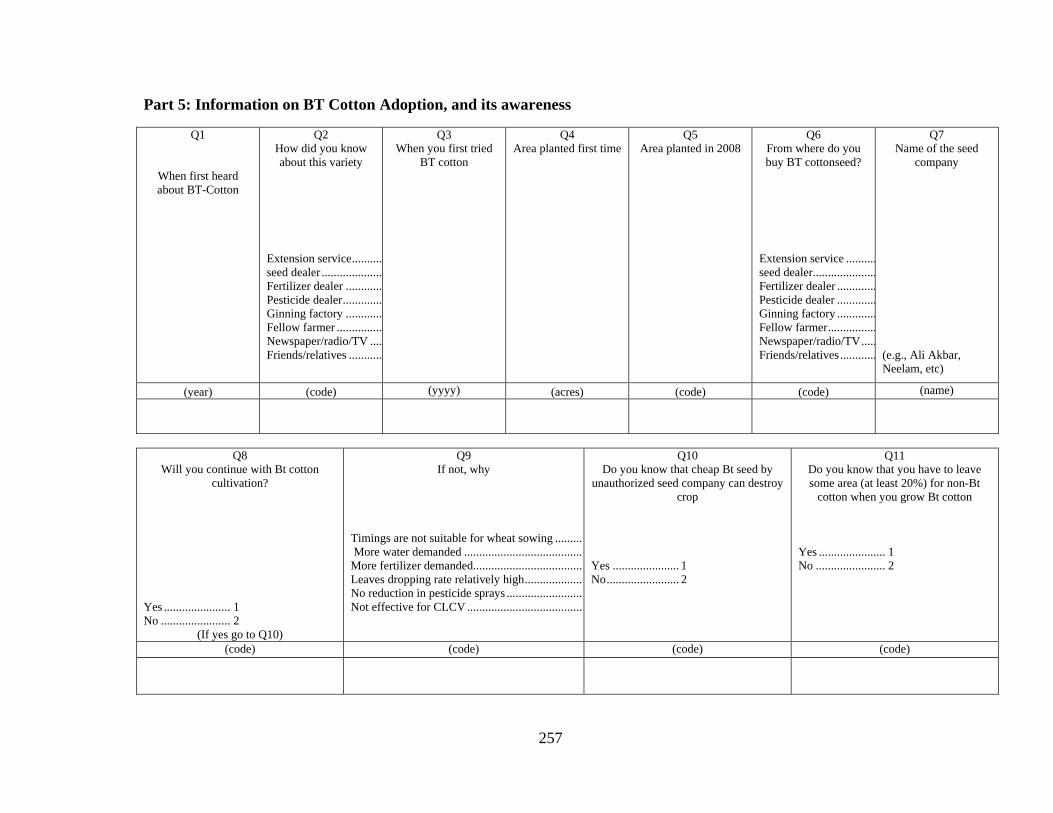
257

Part 5: Information on BT Cotton Adoption, and its awareness

Q1

When first heard about BT-Cotton

Q2 How did you know about this variety

Extension service .......... seed dealer .................... Fertilizer dealer ............ Pesticide dealer ............. Ginning factory ............ Fellow farmer ............... Newspaper/radio/TV .... Friends/relatives ...........

Q3 When you first tried

BT cotton

Q4 Area planted first time

Q5 Area planted in 2008

Q6 From where do you buy BT cottonseed?

Extension service .......... seed dealer ..................... Fertilizer dealer ............. Pesticide dealer ............. Ginning factory ............. Fellow farmer ................ Newspaper/radio/TV ..... Friends/relatives ............

Q7 Name of the seed

company

(e.g., Ali Akbar, Neelam, etc)

(year) (code) (yyyy) (acres) (code) (code) (name)

Q8

Will you continue with Bt cotton cultivation?

Yes ...................... 1 No ....................... 2

(If yes go to Q10)

Q9 If not, why

Timings are not suitable for wheat sowing .......... More water demanded ........................................ More fertilizer demanded ..................................... Leaves dropping rate relatively high .................... No reduction in pesticide sprays .......................... Not effective for CLCV .......................................

Q10 Do you know that cheap Bt seed by

unauthorized seed company can destroy crop

Yes ...................... 1 No ........................ 2

Q11 Do you know that you have to leave some area (at least 20%) for non-Bt

cotton when you grow Bt cotton

Yes ...................... 1 No ....................... 2

(code) (code) (code) (code)

258

Part 6: Why Farmers are not Using BT variety (ask with farmers who are not using Bt variety) Q1. Why you are not using BT cotton. Check (√) against reason which is valid.

1. I have never heard about this variety

Go to Q11

2. I heard about this variety but don’t know from where I can buy

Go to Q11

3. I heard about this variety but I also heard that this is not good and farmers should avoid cultivating this variety

Go to Q11

4. It is expensive, I cannot afford

Go to Q11

5. I cultivated this variety and had a severe crop loss, so I stopped using

Go to Q2

Q2

When had you cultivated this

variety

Q3 Who advised

you to use this variety

Extension service ................. Landlord .............. input dealer .......... Ginning factory ... Fellow farmer ...... newspaper/radio /TV ......................

Q4 From where did

you buy BT seed?

Landlord .............. Village input dealer ................... Authorized input dealer .......... Ginning factory .... Other ....................

Q5 Name of the

seed company

Q6 Why crop destroyed

Mealy bug attack ........ CLCV ......................... I have no idea but crop started dying ....... Seed seems faulty ....... No instructions about its usage of seed ............................ Excessive rains and storms ......................... Floods ......................... Drought .......................

Q7 What

proportion of total

produce was destroyed

Q8 Estimated value

of loss

Q9 Did you observe

lesser cost of production as compared to other variety

Yes ....................... Yes, but loss was high ............... No ........................

Q10 Would you use this variety now if you hear it is

not faulty

yes ----------------- yes if I observe good results in my or nearby villages--- No ------------------

(year) (code) (code) (Name) (code) (%) (Rs) (code) (code)

259

Q11

If you find out that this variety is useful and results in increased yield and better quality, will you adopt

yes immediately ............................................................ yes if I observe good results in my or nearby villages .. No, I will adopt ..........................................................

Q12 If you know about its availability, would you adopt it?

yes immediately ........................................................................... yes but I will experiment it at some proportion of my farm ......... No, I will not adopt ......................................................................

Q13 If it become cheaper would you cultivate this variety?

yes immediately ......................................................................... yes but I would like to make sure that it is of good quality ........ No, I will not adopt ....................................................................

SECTION 4: SOURCES OF INCOME Part 1: Earned Income

Sources of income Q1 Hours/day

Q2 months/year

Q3 Income/revenue

Q4 Expenditure

1 Cropping operations at own farm

2 Cropping operations for others farm (work for wages)

3 Livestock operations for own household

4 Livestock operation for others (work for wages)

5 Off-farm wage work (as employee)

6 Off-farm business work (as own account worker or employer)

260

Part 2: Unearned Income

Pension Rental income Amount of pension that any member of household received last year

Rent received from renting out non-agricultural land or building

Rent paid for renting in non-agricultural land or building

Rent received from renting out agricultural or non-agricultural machinery/tools

Rent paid for renting in agricultural or non-agricultural machinery/tools

(Rs) (Rs) (Rs) (Rs) (Rs)

Domestic remittances Foreign remittances Income from assistance Other income Amount received from domestic remittances

Amount sent as domestic remittances

Amount received from foreign remittances

Amount sent as foreign remittances

Amount received as assistance (for

example, zakat, Baitul Mal, charity)

Amount paid as charity (for example, zakat, Sadqa, Khairat,

fitrana)

Any other income (if any)

(Rs) (Rs) (Rs) (Rs) (Rs) (Rs) (Rs)

261

SECTION 5 HOUSEHOLD SAVINGS AND ASSETS Household Assets: (Instruction: Read all the listed items and write appropriate code (yes=1, no=2) in the next column. If yes, ask other questions if not leave blank

Do you own now?

Yes ................. 1 No .................. 2

How many do you own now

Q1 How did you get

Purchased ................... As gift ......................... Inherited ..................... Through Gov. ............. Leased in .................... Encroached ................. Others .........................

Q2 Time of

acquisition

Last year ................. 1-5 yrs ago .............. 5 10 yrs ago ............ 10-15 yrs ago .......... 10-15 yrs ago .......... >15 yrs ago .............

Q3 Value if sale

now

(Rs)

Q4 Value If you want

to rent out

(Rs)

Land and Building

01 Agricultural land owned

02

Other land or building

(commercial or residential in urban or rural

area)

Livestock, fish, poultry

03 Livestock

04 Fish pond

05 Poultry farm

Farm implements/machinery

06 Tractor

07 Plough

08 Trolley

09 Thresher

10 Rotavator

Do you own now?

Yes 1


Q1 How did you get

Q2 Time of

acquisition

Q3 Value if sale

now


to rent out

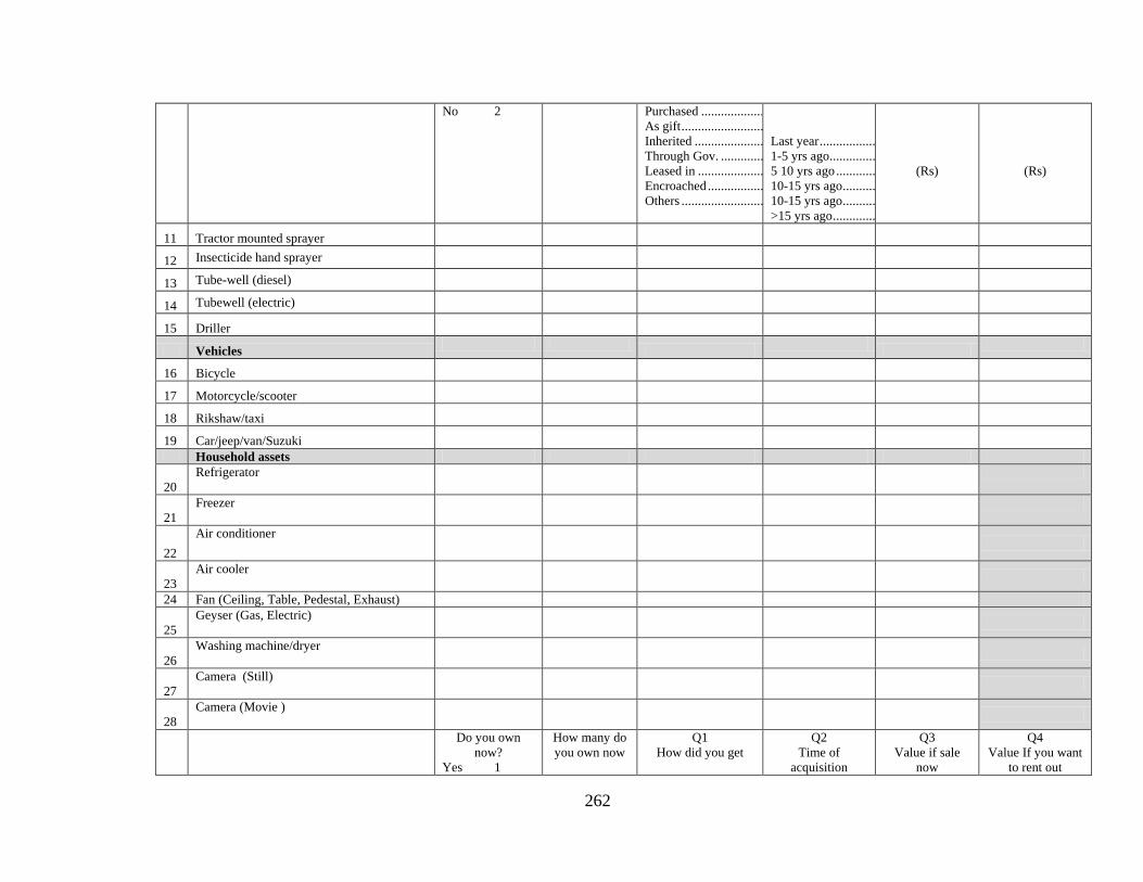
262

No 2 Purchased ................... As gift ......................... Inherited ..................... Through Gov. ............. Leased in .................... Encroached ................. Others .........................


(Rs)

(Rs)

11 Tractor mounted sprayer

12 Insecticide hand sprayer

13 Tube-well (diesel)

14 Tubewell (electric)

15 Driller

Vehicles

16 Bicycle

17 Motorcycle/scooter

18 Rikshaw/taxi

19 Car/jeep/van/Suzuki

Household assets

20 Refrigerator

21 Freezer

22 Air conditioner

23 Air cooler

24 Fan (Ceiling, Table, Pedestal, Exhaust)

25 Geyser (Gas, Electric)

26 Washing machine/dryer

27 Camera (Still)

28 Camera (Movie )

Do you own now?

Yes 1


Q1 How did you get

Q2 Time of

acquisition

Q3 Value if sale

now


to rent out

263

No 2 Purchased ................... As gift ......................... Inherited ..................... Through Gov. ............. Leased in .................... Encroached ................. Others .........................


(Rs)

(Rs)

29 Cooking stove

30 Cooking Range, Microwave oven

31 Heater

32 TV

33 VCR, VCP, Receiver, De-coder

34 Radio / cassette player

35 CD/DVD player

36 Vacuum cleaner

37 Sewing/Knitting Machine

38 Personal Computer

39 Furniture, fixture

Jewelry and liquid savings 40 Gold/silver jewelry, precious stones

41 Estimated amount in bank accounts

42 Estimated amount at home (in hand)

264

SECTION 6: HOUSING AND LIVING CONDITION

Q1 Q2 Q3 Q4 Q5 Q7 Q8 Q9 Q10 Q11 Q12 Q13 What is the

dwelling type?

Non-permanent material (Kacha) ............. permanent material (pacca) .............. mix ...................

How long have you been living here

What is your present

occupancy status?

Owner occupied (not self hired) ................. Owner occupied (self hired) ......... On rent .............. Rent free ............. Other ..................

How many rooms does

your household occupy, include

bed rooms and living

rooms? (Do not count storage rooms, bath rooms, toilets, kitchen or rooms for business)

Does your household

have electricity connection

Yes ............ 1 No .............. 2

Does your household have gas

connection

Yes ............ 1 No .............. 2

Does your household

have telephone connection

Yes ............ 1 No .............. 2

Does your household

have mobile phone

Yes 1 No 2

What is the main source of drinking

water for the household?

Tap in house................ Tap outside house ....... Hand pump ................. Motorized pumping .... Open well ................... Pond ........................... Canal / River / Stream ......................... Other ...........................

Type of toilet used by the household

Ventilated pit latrine .... Flush connected to septic tank .................... Dry raised latrine ......... No toilet/fields ............. Other (specify)______________ .............................

How would you compare your living condition

with that was three years

ago

improved ......... deteriorated ..... unchanged .......

What you predict

about your housing

condition after three years (i.e.,

2011)

improved ...... deteriorated .. unchanged ....

(Code) (years) (Code) (No) (Code) (Code) (Code)

(Code) (Code) (Code) (Code)

265

SECTION 7: INFORMATION ON BORROWING AND LENDING Q1 Q2 Q3 Q4 Q5 Q6 Q7 Q8 Q9

Have you borrowed in cash or kind during last five years

Yes ................. 1 No .................. 2 If answer is No then go to Q 7

Amount borrowed

What was the purpose of borrowing

input for crop ................................... land improvement ............................ start up a non-farm business ............ livestock/poultry .............................. Purchase of Agriculture mach/Land ....................................... migration ......................................... education .......................................... house construction ........................... health ............................................... others (indicate) ...............................

What was the source of borrowing

ZTBL ............................. Commercial bank .......... Cooperatives .................. NGO .............................. SME/Khushali bank ...... informal money lender .. Input dealer .................... Shopkeeper .................... Friends and relatives ...... Others ............................

What was used as collateral?

No collateral ............... Land ........................... House/building ........... Other valuable ........... Personal guarantee ..... No collateral ...............

What proportion

of this loan have you repaid

Have you lent any money

during last five years

Yes ..................... 1 No ...................... 2 If answer is No then go to Next section

Amount lent

What proportion of this loan have you received

(code) (Rs) (code) (code) (code) (%) (code) (Rs) (%)

266

Appendix 4.2: Community Questionnaire

For office use only

IMPACT OF BT COTTON ON POVERTY REDUCTION IN RURAL PAKISTAN

COMMUNITY QUESTIONNAIRE--2009 COMMUNITY IDENTIFIER CODE

Province: Punjab 1 Sindh 2 District: Mirpur Khas 1 Bahwalpur 2 Village Name: Village Code: Tehsil/Taluka Name: Tehsil/Taluka code: Settlement (Basti) i 1 2 3 4 5 6 7 8

Name of Interviewer Same of Supervisor Start time: __________ Finish time: _________ Date of interview --------/--------/2009 Day/Month/Year Result of the visit Complete 1 Partially complete 2 Refuse 3 No Respondent was available 4

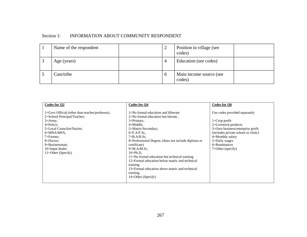
267

Section 1: INFORMATION ABOUT COMMUNITY RESPONDENT 1 Name of the respondent

2 Position in village (see

codes)

3 Age (years)

4 Education (see codes)

5 Cast/tribe

6 Main income source (see codes)

Codes for Q2 1=Govt Official (other than teacher/professor), 2=School Principal/Teacher; 3=Army; 4=Police; 5=Local Councilor/Nazim; 6=MNA/MPA, 7=Farmer, 8=Doctor; 9=Businessman; 10=Input dealer 11=Other (Specify)

Codes for Q4 1=No formal education and illiterate 2=No formal education but literate , 3=Primary, 4=Middle, 5=Matric/Secondary, 6=F.A/F.Sc, 7=B.A/B.Sc, 8=Professional Degree, (does not include diploma or certificate) 9=M.A/M.Sc, 10=Ph.D, 11=No formal education but technical training 12=Formal education below matric and technical training 13=Formal education above matric and technical training 14=Other (Specify)

Codes for Q6 Use codes provided separately 1=Crop profit 2=Livestock products 3=Own business/enterprise profit (includes private school or clinic) 4=Monthly salary 5=Daily wages 6=Remittances 7=Other (specify)

268

Section 2: Village Profile 01 Land area of the village (squares km) acre 02 Agricultural area of the village (sq. km)

03 Tractors in the village (#) 04 Tractor mounted sprayers (#)

05 Tractor trolleys (#) 06 Wheat threshers

07 Tubewells (electric) 08 Tubewells (diesel)

09 Total No. of Pacca houses 10 Average rent of irrigated land (Rs/acre)

11 Average price of irrigated land? (Rs/acre) 12 Average price of non-irrigated land? (Rs/acre)

13 Total number of households 14 Total number of farming households

15 Proportion of owner farmers in total farm households (%)

16 Proportion of owner-cum-tenant farmers in total farm households (%)

17 Proportion of tenant farmers (sharecroppers) in total farm households (%)

18 Proportion of non-farm households (who do not cultivate land) in total households (%)

19 Proportion of livestock holders (who do not cultivate land and do not have non-farm activity) (%)

20 Share of households with no operated land, depend on farm wage work (%)

269

Section 3: Location Related Information: Distances (Km) 01 Distance to Tehsil headquarters (km) 02 Distance to District headquarters (km)

03 Distance to transport pickup point outside village (km) 04 Distance to external main road from this village (km)

05 Most common road surface of internal road (see road surface code) 1=Mud, 2=Asphalt, 3=Concrete, 4=Gravel,

06 Most common road surface of external road (see road surface code) 1=Mud, 2=Asphalt, 3=Concrete, 4=Gravel

07 Main means of transportation for nearest city/market 1=Bullock cart, 2=Tractor trolley, 3=Three Wheeler, 4= suzuki van/Hilux, 5=Bus, 6=Train, 7=Private Vehicle

08 Main means of transportation within village 1=Walk, 2=Bullock cart, 3=Bicycle, 4=Three Wheeler, 5= suzuki van/Hilux, 6=Bus, 8=Motor Cycle, 9=Private Vehicle

09 Distance to cotton and wheat seed shop 10 Distance to fertilizer shop

11 Distance to pesticide shop 12 Distance to grain market

13 Distance to cotton ginning factory (write zero if within village)

14 Distance to post office (write zero if within village)

15 Distance to Zari Taraqiati Bank Limited (write zero if within village)

16 Distance to Commercial bank (write zero if within village)

17 Distance to BHU (write zero if within village) 18 Distance to RHC (write zero if within village)

19 Distance to Clinic/dispensary (write zero if within village) 20 Distance to Hospital (write zero if within village)

21 Distance to Primary girls school (write zero if within village)

22 Distance to Primary boys school (write zero if within village)

23 Distance to Secondary girls school (write zero if within village)

24 Distance to Secondary boys school (write zero if within village)

25 Distance to Primary co-education school (write zero if within village)

26 Secondary co-education school (write zero if within village)

270

Section 4: Information on Public Utilities and Facilities within village

Information about the Availability of Public Utilities 2008 2005 2002

01. Share of households that use electricity? %

02. Share of households that use cylinder gas? %

03. Share of households have access to sui-gas? 1=Yes, 2=No

04. Share of households with access to protected water (piped water, protected well, etc.) as drinking water? %

05. Share of households with fixed-line telephone? %

06. Share of households with cellular phone? %

07. Is there a system of sewage channels for the disposal of waste water? 1=Yes; 2=No

08. Is there a garbage collection or disposal service in your community? 1=Yes; 2=No

09. Is there an NGO in this village that extends credit for farm and non-farm purposes

1=Yes; 2= Yes, credit for farm purposes only; 3= Yes, but for non-farm purposes only; 4= Yes, but does not extend credit, 5=No

10. Does this village have any representative in national assembly/senate 1=Yes; 2=No

11. Does this village have any representative in provincial assembly/senate 1=Yes; 2=No

12. Are you satisfied with the functions of your union council 1=Yes; 2=No

13. Is there an agricultural extension service in your village.? 1=Yes; 2=No

14. Is this service accessible by all types of farmers? 1=Yes, 2=small farmers face problems, 3=women face problems, 4=we heard there is service but we have never seen any person, 5=there is an office but we never found any technical person there

15. How would you compare last year rainfall with normal? 1 = much higher; 2 = somewhat higher; 3 = about normal; 4 = somewhat lower; 5 = much lower

16. . How would you compare last year temperature with normal? 1 = much higher; 2 = somewhat higher; 3 = about normal; 4 = somewhat lower; 5 = much lower

271

Section 5: Major constraints in crop production and livestock raising Instruction: Please read out these constraints and write ‘1’ for which respondent said this is the most important one

Constraints Rank now (month of survey)

Rank last year Rank five years ago

01. Lack of access to formal credit

02. Water shortage

03. Lack of storage facilities

04. Persistent electricity outages

05. High price of electricity

06. High price of petroleum

07. Lack of proper marketing facilities

08. Lack of veterinary services

09. CLCV attack

10. Bollworm attack

11. Mealy bug attack

12. Excessive rains

272

Section 6: Prices of raw material, wages and consumer goods

Commodities Q1 Average during the

Survey Month

(Rs)

Q2 Average during the

last year

(Rs)

Q3 Average two years

ago

(Rs)

Q4 Average five years

ago

(Rs) 01. Fertilizer (Urea) (50kg bag)

02. Fertilizer (DAP) (50kg bag)

03. Cement (50kg bag)

04. Bricks (per thousands)

05. Cost of transporting goods/commodities to/from nearest market (Rs)

06. Average wage of casual agricultural male labour (Rs/day)

07. Average wage of casual agricultural female labour (Rs/day)

08. Average wage of casual agricultural child labour (Rs/day)

09. Average wage of permanent agricultural labour (Rs/day)

10. Average wage of construction unskilled labour (Rs/day)

11. Average wage of construction skilled labour (Rs/day)

12. Rental rate of tractor (Rs/hours)

13. Rental rate of tube-well (Rs/hours)

273


Survey Month (Rs)


last year

(Rs)


ago (Rs)


ago

(Rs) 14. Rental rate of thresher (Rs/hour)

15. Abiana (water rate) (Rs/acre)

Information on the Prices of Consumer Goods

16. Wheat flour (Atta) (Rs/kg)

17. Maize flour (Rs/kg)

18. Basmati rice (Rs /kg)

19. IRRI Rice (Rs/kg)

20. Masoor dal (Rs/kg)

21. Mong dal (Rs /kg)

22. Mash dal (Rs/kg)

23. Cooking oil (Rs/liter)

24. Ghee (Rs /kg)

25. Fresh milk (Rs/liter)

26. Sugar (Rs/kg)

274


Survey Month (Rs)


last year

(Rs)


ago (Rs)


ago

(Rs) 27. Gur (Rs /kg)

28. Mutton (Rs /kg)

29. Beef (Rs/kg)

30. Chicken (Rs/kg)

31. Eggs (Rs /doz)

32. Onion (Rs /kg)

33. Potatoes (Rs /kg)

34. Chilies (Rs /kg)

35. Tea (Rs/kg)

36. Kerosene oil (Rs/liter)

37. Fire wood (Rs/40kg)

275

APPENDIX 5: FISHER’S EXACT TEST

Fisher's exact test is a statistical test that is used to determine if there are nonrandom

associations between two categorical variables. The null hypothesis is that that there is no

association between two categories. For example, to test the difference between adopters

and non-adopters by land ownership, the null hypothesis would be that the proportion of

landowners is the same across adopters and non-adopters. This test assumes that each

observation is classified into exactly one cell, and the row and column totals are fixed.

The hypergeometric probability distribution is used to compute the probability (p-value)

of the observed results. The p-value for a 2x2 table is calculated by summing the

probabilities of the tables that are less than or equal to that for the observed table, given

the fixed marginal totals (Bailey, 1977). The probability of any particular outcome (table)

is given by a general form:

𝑝 =number of possibilities favourable to the occurrence of the outcome

total number of pertinent possibilities

For a formulaic structure, assume a 2x2 contingency table, where cell frequencies are: a,

b, c, and d, and the row totals are: a+b and c+d; column totals are: a+c, b+d; and n is the

sum of the frequencies in four cells. Given this notation, the exact probability of any

particular outcome can then be calculated by the hypergeometric distribution:

𝑝 = �𝑎 + 𝑏𝑎 � �𝑐 + 𝑑

𝑐 � � 𝑛𝑎 + 𝑐� =

(𝑎 + 𝑏)! (𝑐 + 𝑑)! (𝑎 + 𝑐)! (𝑏 + 𝑑)!𝑛!𝑎! 𝑏! 𝑐!𝑑!

�

Where �𝑛𝑘� is the binomial coefficient and the symbol “!” indicates the factorial operator.

One sided p-values are used when there is prior information on the alternative to

276

independence between two categories (i.e., negative or positive association) and two-

sided values are used when there is no prior alternative. This study uses the two-sided p-

values of the Fisher’s exact test.

277

APPENDIX 6: IMPACT OF RESEARCH ON ECONOMIC BENEFITS: CLOSED ECONOMY CASE

The closed economy case in Figure A 2.1 shows the research-induced supply shift and

change in consumer, producer and total surplus. The change in total surplus is measured

by the cost saving on the original quantity (𝐼𝑜𝑎𝑐𝐼1), and the economic gains (abc) due to

increment to consumption (𝑄𝑜𝑎𝑏𝑄1) minus the total cost of the increment to production

(𝑄𝑜𝑐𝑏𝑄1). Therefore, the change in total surplus is ∆𝑇𝑆 = 𝐼𝑜𝑎𝑏𝐼1. The change in

consumer surplus is ∆𝐶𝑆 = 𝑃𝑜𝑎𝑏𝑃1, and the change in producer surplus is ∆𝑃𝑆 =

𝑃1𝑏𝐼1 − 𝑃0𝑎𝐼𝑜.

Figure A 2.1: Effect of technology adoption and changes in welfare: Closed economy case

b a

I1

I0

d P1 P0

S

S′

D

Price

Quantity Q0 Q1

278

Where, K is the vertical shift in supply curve (P0-d), can be expressed in proportion of the

initial price as k=K/Po=(P0-d)/Po.

Computing change in producer surplus

Figure 6.2 indicates that ∆𝑃𝑆 = 𝑃1𝑏𝐼1 − 𝑃0𝑎𝐼𝑜. This is equivalent to ∆𝑃𝑆 = 𝑃1𝑏𝑐𝑑 +

𝑑𝑐𝐼1 − 𝑃0𝑎𝐼𝑜. Under the assumption of linear supply curve and parallel shift, the areas,

𝑑𝑐𝐼1 = 𝑃𝑜𝑎𝐼𝑜 therefore, the change in producer surplus is ∆𝑃𝑆 = 𝑃1𝑏𝑐𝑑 = 𝑃1𝑒𝑐𝑑 + 𝑒𝑏𝑐,

where 𝑃1𝑒𝑐𝑑 = (𝑃1 − 𝑑)𝑄𝑜,𝑎𝑛𝑑 𝑒𝑏𝑐 = 12

(𝑃1 − 𝑑)(𝑄1 − 𝑄𝑜).

𝑃1 − 𝑑 = (𝑃𝑜 − 𝑑) − (𝑃𝑜 − 𝑃1)

Let Z is the reduction in price relative to its initial value that can be expressed in terms of

demand and supply elasticties 𝑍 = −�𝑃1−𝑃𝑜𝑃𝑜

� = 𝑒𝑠𝑘𝑒𝑠+𝑒𝑑

. We can write

𝑃1 − 𝑑 = 𝑘 − 𝑃𝑜𝑍

𝑃1 − 𝑑 = 𝐾𝑃𝑜 − 𝑃𝑜𝑍 = 𝑃𝑜(𝐾 − 𝑍)

∆𝑃𝑆 = 𝑃𝑜(𝐾 − 𝑍)𝑄𝑜 + 0.5𝑃𝑜(𝐾 − 𝑍)(𝑄1 − 𝑄𝑜)

∆𝑃𝑆 = 𝑃𝑜(𝐾 − 𝑍)𝑄𝑜(1 + 0.5(𝑄1 − 𝑄𝑜𝑄𝑜

))

∆𝑃𝑆 = 𝑃𝑜𝑄𝑜(𝐾 − 𝑍)(1 + 0.5𝑒𝑑𝑍) Where 𝑄1−𝑄𝑜

𝑄𝑜= 𝑒𝑑𝑍.

Computing change in consumer surplus

In Figure 6.1, ∆𝐶𝑆 = 𝑃𝑜𝑎𝑏𝑃1 = 𝑃𝑜𝑎𝑒𝑃1 + 0.5𝑎𝑏𝑒

∆𝐶𝑆 = (𝑃𝑜 − 𝑃1)𝑄𝑜 + 0.5(𝑃𝑜 − 𝑃1)(𝑄1 − 𝑄𝑜)

∆𝐶𝑆 = (𝑃𝑜 − 𝑃1)[𝑄𝑜 + 0.5(𝑄1 − 𝑄𝑜)]

∆𝐶𝑆 = (𝑃𝑜 − 𝑃1)𝑄𝑜 �1 + 0.5(𝑄1 − 𝑄𝑜)

𝑄𝑜�

∆𝐶𝑆 = 𝑃𝑜𝑍𝑄𝑜[1 + 0.5𝑒𝑑𝑍]

279

Computing change in total surplus

∆𝑇𝑆 = ∆𝑃𝑆 + ∆𝐶𝑆

∆𝑇𝑆 = 𝑃𝑜(𝐾 − 𝑍)𝑄𝑜 + (1 + 0.5𝑒𝑑𝑍) + 𝑃𝑜𝑍𝑄𝑜[1 + 0.5𝑒𝑑𝑍]

∆𝑇𝑆 = 𝐾𝑃𝑜𝑄𝑜[1 + 0.5𝑒𝑑𝑍]

Proof −𝑷𝟏−𝑷𝒐𝑷𝒐

= 𝒆𝒔𝒌𝒆𝒔+𝒆𝒅

= 𝒁

The closed economy model is presented by equations 6.4, 6.5 and 6.6. Solving 6.6 gives

equilibrium prices (Po and P1) and quantities (Qo and Q1) before and after supply shift. Po

without supply shift:

𝑃𝑜 =𝛾 − 𝛼𝛽 + 𝛿

and P1 after supply shift

𝑃1 =𝛾 − 𝛼 − 𝛽𝑘𝛽 + 𝛿

Solving Po and P1 in terms of elasticities, we need to calculated α, β, δ, and γ.

Calculating for β using supply equation before shift:

𝑄𝑜 = 𝛼 + 𝛽𝑃𝑜

𝜕𝑄𝑜𝜕𝑃𝑜

= 𝛽


𝑃𝑜𝑄𝑜

= 𝛽𝑃𝑜𝑄𝑜

𝑒𝑠 = 𝛽𝑃𝑜𝑄𝑜

𝛽 = 𝑒𝑠𝑄𝑜𝑃𝑜

280

Calculating 𝛼

Substituting the value of β in supply equation

𝑄𝑜 = 𝛼 + 𝑒𝑠𝑄𝑜𝑃𝑜𝑃𝑜

𝑄𝑜 = 𝛼 + 𝑒𝑠𝑄𝑜

𝛼 = 𝑄𝑜 − 𝑒𝑠𝑄𝑜

Calculating for δ, using demand curve:

𝑄𝑑 = 𝛾 − 𝛿𝑃


= −𝛿


𝑃𝑜𝑄𝑜

= −𝛿𝑃𝑜𝑄𝑜

𝑒𝑑 = −𝛿𝑃𝑜𝑄𝑜

𝛿 = 𝑒𝑑𝑄𝑜𝑃𝑜

Calculating for γ

Substituting the value of δ in demand equation:

𝑄𝑜 = 𝛾 − 𝑒𝑑𝑄𝑜𝑃𝑜𝑃𝑜

𝑄𝑜 = 𝛾 − 𝑒𝑑𝑄𝑜

𝛾 = 𝑄𝑜 − 𝑒𝑑𝑄𝑜

Substituting these values in Po gives:

𝑃𝑜 =𝑄𝑜 + 𝑒𝑑𝑄𝑜 − 𝑄𝑜 + 𝑒𝑠𝑄𝑜

𝑒𝑠𝑄𝑜𝑃𝑜

+ 𝑒𝑑𝑄𝑜𝑃𝑜

And

281

𝑃1 =𝑄𝑜 + 𝑒𝑑𝑄𝑜 − (𝑄𝑜 − 𝑒𝑠𝑄𝑜) − 𝑒𝑠

𝑄𝑜𝑃𝑜𝑘𝑃𝑜



𝑃1 =𝑒𝑑𝑄𝑜 + 𝑒𝑠𝑄𝑜 − 𝑒𝑠𝑄𝑜𝑘



Solving for Qo and Q1

𝑄𝑜 =𝑄𝑜𝑒𝑠 + 𝑄𝑜𝑒𝑑𝑒𝑠 + 𝑒𝑑

𝑄1 =𝑄𝑜𝑒𝑠 + 𝑄𝑜𝑒𝑑 + 𝑒𝑠𝑒𝑑𝑄𝑜𝑘

𝑒𝑠 + 𝑒𝑑

Proportionate change in price can be measured by (𝑃1 − 𝑃0)/𝑃0

𝑃1 − 𝑃𝑜 =𝑒𝑑𝑄𝑜 + 𝑒𝑠𝑄𝑜 − 𝑒𝑠𝑄𝑜𝑘 − 𝑒𝑠𝑄𝑜 − 𝑒𝑑𝑄𝑜



𝑃1 − 𝑃𝑜 =−𝑒𝑠𝑄𝑜𝑘

𝑄𝑜𝑃𝑜

(𝑒𝑠 + 𝑒𝑑)

𝑃1 − 𝑃𝑜𝑃𝑜

=−𝑒𝑠𝑘𝑒𝑠 + 𝑒𝑑

−𝑃1 − 𝑃𝑜𝑃𝑜

=𝑒𝑠𝑘

𝑒𝑠 + 𝑒𝑑= 𝑍

Where Z is the reduction in price relative to its initial value, depends on the elasticities of

demand and supply.

Proof: 𝑸𝟏−𝑸𝒐𝑸𝒐

= 𝒆𝒅𝒁

The increase in quantity relative to initial quantity can be calculated as 𝑄1−𝑄𝑜𝑄𝑜

282

𝑄1 − 𝑄𝑜 =𝑄𝑜𝑒𝑠 + 𝑄𝑜𝑒𝑑 + 𝑒𝑠𝑒𝑑𝑄𝑜𝑘 − 𝑄𝑜𝑒𝑠 − 𝑄𝑜𝑒𝑑

𝑒𝑠 + 𝑒𝑑

𝑄1 − 𝑄𝑜𝑄𝑜

=𝑒𝑠𝑒𝑑𝑘𝑒𝑠 + 𝑒𝑑


= 𝑒𝑑𝑒𝑠𝑘

𝑒𝑠 + 𝑒𝑑


= 𝑒𝑑𝑍

283

APPENDIX 7: APPENDIX TABLES

Appendix Table 1: Yield per hectare of seed-cotton in major cotton growing countries (kg/hectare)

Years Brazil China India Pakistan Syria Turkey USA World 1961 631 621 343 697 1,304 881 1,349 8,582 1962 735 644 410 800 1,336 991 1,396 9,093 1963 661 817 419 854 1,405 1,075 1,556 9,789 1964 654 1,012 387 772 1,641 1,257 1,574 9,992 1965 583 1,259 377 801 1,655 1,244 1,593 10,585 1966 735 1,425 382 869 1,472 1,395 1,468 10,662 1967 455 1,387 420 901 1,375 1,435 1,401 10,061 1968 512 1,418 417 903 1,411 1,588 1,602 10,772 1969 503 1,293 409 921 1,279 1,629 1,312 10,091 1970 455 1,368 376 932 1,539 1,971 1,309 10,377 1971 483 1,284 484 1,084 1,629 1,971 1,320 10,613 1972 457 1,201 455 1,047 1,780 1,859 1,499 10,916 1973 526 1,557 475 1,071 2,020 1,969 1,523 11,590 1974 539 1,474 512 937 1,881 1,857 1,301 11,814 1975 451 1,443 467 833 1,991 1,863 1,328 11,075 1976 370 1,252 468 699 2,249 2,124 1,368 11,001 1977 464 1,270 470 935 2,117 1,924 1,516 11,530 1978 397 1,337 500 751 2,246 1,891 1,243 10,928 1979 449 1,469 486 1,050 2,223 2,023 1,623 12,210 1980 453 1,652 496 1,017 2,307 1,935 1,211 11,997 1981 493 1,719 503 1,014 2,481 1,941 1,644 13,139 1982 532 1,854 488 1,092 2,659 2,137 1,754 13,321 1983 546 2,291 422 668 2,997 2,243 1,508 13,552 1984 694 2,715 588 1,350 2,524 1,984 1,785 15,794 1985 796 2,420 591 1,544 2,860 2,041 1,863 15,155 1986 732 2,466 507 1,580 2,902 2,302 1,624 14,382 1987 848 2,629 504 1,715 2,727 2,382 2,081 16,085 1988 991 2,251 612 1,633 2,763 2,284 1,831 15,615 1989 873 2,184 763 1,681 2,728 2,213 1,787 15,460 1990 1,009 2,420 675 1,845 2,821 2,654 1,851 16,310 1991 1,129 2,604 647 2,307 3,257 2,523 1,929 17,206 1992 1,004 1,979 771 1,629 3,250 2,409 2,036 15,431 1993 1,071 2,250 749 1,463 3,252 2,749 1,791 15,661 1994 1,157 2,356 770 1,673 2,827 2,817 2,073 16,410 1995 1,218 2,638 726 1,804 2,937 2,999 1,561 15,913 1996 1,253 2,670 796 1,519 3,462 2,800 2,069 15,991

(cont…)

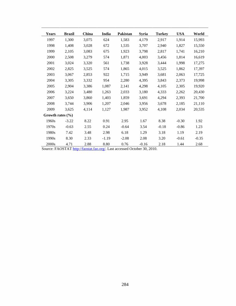
284

Years Brazil China India Pakistan Syria Turkey USA World 1997 1,300 3,075 624 1,583 4,179 2,917 1,914 15,993 1998 1,408 3,028 672 1,535 3,707 2,940 1,827 15,550 1999 2,105 3,083 675 1,923 3,798 2,817 1,741 16,210 2000 2,508 3,279 574 1,871 4,003 3,456 1,814 16,619 2001 3,024 3,320 561 1,738 3,928 3,444 1,998 17,275 2002 2,825 3,525 574 1,865 4,015 3,525 1,862 17,397 2003 3,067 2,853 922 1,715 3,949 3,681 2,063 17,725 2004 3,305 3,332 954 2,280 4,395 3,843 2,373 19,998 2005 2,904 3,386 1,087 2,141 4,298 4,105 2,305 19,920 2006 3,224 3,480 1,263 2,033 3,180 4,333 2,262 20,430 2007 3,650 3,860 1,403 1,859 3,691 4,294 2,393 21,700 2008 3,744 3,906 1,207 2,046 3,956 3,678 2,185 21,110 2009 3,625 4,114 1,127 1,987 3,952 4,108 2,034 20,535

Growth rates (%) 1960s -3.22 8.22 0.91 2.95 1.67 8.38 -0.30 1.92

1970s -0.63 2.55 0.24 -0.64 3.54 -0.18 -0.86 1.23 1980s 7.42 3.48 2.98 6.18 1.29 3.18 1.19 2.19 1990s 8.30 2.33 -1.19 -2.08 2.08 3.20 -0.61 -0.35 2000s 4.71 2.88 8.80 0.76 -0.16 2.18 1.44 2.68

Source: FAOSTAT http://faostat.fao.org/. Last accessed October 30, 2010.


285

Appendix Table 2: Cotton statistics of Pakistan

Years

Area Harvested

(Ha)

Production (seed

cotton) (tonnes)

Yield (seed

cotton) (kg/Ha)

Yield (cotton lint)

(kg/Ha)

Domestic consumption (cotton lint)

(tonnes)

Imports (cotton

lint) (000 US$)

Exports (cotton

lint) (000 US$)

Exports (cotton

yarn) (000 US$)

Exports (cotton cloth)

(000 US$) 1972 1,958,700 2,122,452 1,084 361 455,940 1,794 200,493 127,501 81,539 1973 2,011,300 2,105,538 1,047 349 561,340 508 106,089 200,535 126,770 1974 1,845,000 1,975,450 1,071 357 560,320 877 34,192 189,479 143,911 1975 2,031,100 1,902,597 937 312 450,500 609 157,934 92,314 132,580 1976 1,851,100 1,541,608 833 277 484,160 375 96,602 144,986 137,320 1977 1,864,700 1,304,100 699 233 429,420 - 29,304 118,352 161,950 1978 1,843,200 1,723,700 935 312 412,420 2,121 112,351 107,024 175,881 1979 1,891,200 1,419,600 751 250 430,270 1,930 66,593 197,586 215,675 1980 2,081,000 2,184,600 1,050 350 402,730 2,088 337,538 205,860 244,096 1981 2,108,500 2,143,500 1,017 339 468,180 2,220 525,599 207,043 241,375 1982 2,214,100 2,244,000 1,014 338 509,660 2,800 278,501 196,672 279,538 1983 2,262,900 2,471,700 1,092 364 532,100 1,571 306,339 247,317 281,367 1984 2,220,700 1,483,767 668 223 506,770 64,129 132,355 217,627 360,220 1985 2,241,600 3,025,713 1,350 450 549,780 28,488 279,229 260,421 305,918 1986 2,364,100 3,650,000 1,544 515 541,280 2,724 513,271 279,176 314,841 1987 2,505,200 3,958,800 1,580 527 709,240 1,424 446,493 506,089 345,263 1988 2,567,800 4,404,541 1,715 572 787,100 1,998 609,967 541,024 485,402 1989 2,619,400 4,278,112 1,633 544 874,310 2,875 929,563 600,847 464,754 1990 2,598,500 4,367,245 1,681 560 1,115,710 5,496 442,995 833,711 558,957 1991 2,662,200 4,912,740 1,845 615 1,356,600 1,016 411,812 1,183,040 675,853 1992 2,835,500 6,542,790 2,307 769 1,439,220 5,375 518,302 1,172,526 819,440 1993 2,835,900 4,619,880 1,629 543 1,516,570 11,555 270,813 1,121,510 863,101 1994 2,804,600 4,103,130 1,463 488 1,576,920 79,770 79,461 1,259,285 820,583 1995 2,652,800 4,437,869 1,673 557 1,509,770 312,648 62,082 1,528,149 1,081,444 1996 2,997,300 5,406,260 1,804 601 1,549,210 66,577 506,765 1,540,259 1,275,855

(cont...)

286

Years

Area Harvested

(Ha)

Production (seed

cotton) (tonnes)

Yield (seed

cotton) (kg/Ha)

Yield (cotton lint)

(kg/Ha)

Domestic consumption (cotton lint)

(tonnes)

Imports (cotton

lint) (000 US$)

Exports (cotton

lint) (000 US$)

Exports (cotton

yarn) (000 US$)

Exports (cotton cloth)

(000 US$) 1997 3,148,600 4,783,373 1,519 506 1,560,940 121,241 30,749 1,411,519 1,262,389 1998 2,959,700 4,686,218 1,583 528 1,597,660 116,070 126,139 1,159,542 1,250,280 1999 2,922,800 4,485,375 1,535 512 1,586,440 253,065 2,327 945,169 1,115,181 2000 2,983,100 5,735,435 1,923 641 1,690,310 81,300 72,560 1,071,616 1,096,232 2001 2,927,500 5,476,167 1,871 624 1,520,310 166,659 138,138 1,076,603 1,035,043 2002 3,115,800 5,415,600 1,738 579 1,930,860 227,208 24,581 942,359 1,132,730 2003 2,793,600 5,210,400 1,865 622 2,031,840 235,767 49,016 928,358 1,345,650 2004 2,989,300 5,127,200 1,715 572 2,023,850 523,049 48 1,126,878 1,711,492 2005 3,192,600 7,279,400 2,280 760 2,207,620 519,977 109,957 1,056,535 1,862,886 2006 3,103,000 6,644,000 2,141 714 2,532,320 371,209 68,151 1,382,874 2,108,183 2007 3,074,900 6,252,000 2,033 711 2,633,130 645,786 50,226 1,428,041 2,026,388 2008 3,054,300 5,677,397 1,859 649 2,640,100 70,122 1,300,968 2,010,611

Source FAO FAO FAO GoP APTMA FAO APTMA APTMA APTMA Sources: FAO: FAOSTAT http://faostat.fao.org/. Last accessed January 8, 2010.

APTMA: All Pakistan Textile Mills Association, http://www.aptma.org.pk/Pak_Textile_Statistics. Last accessed January 8, 2010. GoP (2009). Statistical Supplement of Economic Survey 2007-2008. http://www.finance.gov.pk/finance_economic_survey.aspx


http://www.aptma.org.pk/Pak_Textile_Statistics�

http://www.finance.gov.pk/finance_economic_survey.aspx�

287

Appendix Table 3: Distribution of households in four cotton producing districts (PRHS 2004)

District Number of Households Cotton growers

Proportion of cotton growers in total households

Bhawalpur (Punjab) 161 86 53.4 Vehari (Punjab) 180 76 42.2 Mirpur Khas (Sindh) 140 59 42.1 Nawabshah (Sindh) 143 28 19.6 Total 624 249 39.9

Impact of BT Cotton Adoption of Farmers' Wellbeing in Pakistan

Documents

Transcript of Impact of BT Cotton Adoption of Farmers' Wellbeing in Pakistan