European Journal of Agronomy 129 (2021) 126329

Available online 6 June 20211161-0301/© 2021 Elsevier B.V. All rights reserved.

Impact assessment of soybean yield and water productivity in Brazil due to climate change

Evandro Henrique Figueiredo Moura da Silva a,*, Luis Alberto Silva Antolin a, Alencar Junior Zanon b, Aderson Soares Andrade Junior c, Henrique Antunes de Souza c, Kassio dos Santos Carvalho d, Nilson Aparecido Vieira Junior a, Fabio Ricardo Marin a

a Luiz de Queiroz College of Agriculture (ESALQ), University of Sao Paulo, Piracicaba, SP 13418-900, Brazil b Federal University of Santa Maria (UFSM), Santa Maria, RS 97105-900, Brazil c Brazilian Agricultural Research Corporation (Embrapa), Mid-North, Teresina, PI 64008-780, Brazil d Federal Institute of Mato Grosso (IFMT), Sorriso, MT 78890-000, Brazil

A R T I C L E I N F O

Keywords: Crop modeling Food security Water use Climate change projections DSSAT

A B S T R A C T

In the next decades, the population is expected to rise by more than two billion people, and the projections of climate change have been considered as one of the greatest future challenges for world food security. Soybean represents more than 60 % of all plant protein produced in the world, and Brazil is the largest world exporter and the second-largest producer. In this paper, we simulated soybean yields for 16 strategically selected agroclimatic zones (CZs) to represent Brazilian production. Experiments conducted throughout the country were used to calibrate the CROPGRO-Soybean model for Brazilian conditions, for the main maturity groups used in Brazil, to simulate current and 40 future climate scenarios, provided by Coupled Model Intercomparison Project 5 (CMIP5) for 2050 in the both 4.5 and 8.5 representative concentration pathways (RCP). We found soybean yield varying by +1 to +32 % across 16 CZs in the average scenario of future climate when compared to the current yields. Yet, we found an increase of about 5% in the yield production risk for RCP 8.5. The main reason for such results was associated with the positive effect of increasing CO2 on crop water productivity, which overcomes the negative effects of temperature and water stress increases on rainfed Brazilian soybeans.

1. Introduction

The global population has grown dramatically in the last decades. Between 2017 and 2050, the world’s population is projected to rise from 7.7 billion to 9.8 billion (United Nations, 2017). Similarly, there is a projection of income increase across the developing world, which would imply an increase in demand for meat and dairy products by rates ranging from 50 to 100 % in the next decades (Thornton, 2010; Foley et al., 2011; Tilman et al., 2011; Clark and Tilman, 2017; Searchinger et al., 2019). This may result in grain price increases (Marchand et al., 2016), which might worsen food insecurity in the world’s poorest countries (Sternberg, 2012; D’Amour et al., 2016).

Soybean (Glycine max L.) is currently the world’s most important food protein source, and so it is crucial for food security. Soybean is main source of high-quality vegetable protein for the production of food of animal origin (Speedy, 2002; Thomson, 2019). In the past twenty years,

Brazil had one of the most significant expansions of agricultural land use (Zalles et al., 2019), and has established itself as the world’s largest soybean producer, with over 38 million hectares of soybean production (CONAB, 2017), being the main economic product of Brazil (Ministerio da Economia, 2020).

Climate change is expected to affect agriculture worldwide in the next decade (Zabel et al., 2019; Baldos et al., 2020). General circulation models (GCMs) are central to climate change research (Field, 2014) and can be coupled to the cropping system model (CSM) to investigate the scientific hypotheses about the impacts of climate change on agriculture (Rosenzweig et al., 2013; He et al., 2017). The CSM-CROPGRO-Soybean (Boote et al., 1998) is one of the more robust and widely model used to simulate crop production systems. The model has a modular structure (Jones et al., 2001), which consider process of carbon and nitrogen balance (Godwin and Allan, 1991; Godwin and Singh, 1998), soil water balance (Ritchie, 1998; Silva et al., 2021); and it is able to simulate

* Corresponding author. E-mail address: ehfmsilva@usp.br (E.H. Figueiredo Moura da Silva).

Contents lists available at ScienceDirect

European Journal of Agronomy

journal homepage: www.elsevier.com/locate/eja

https://doi.org/10.1016/j.eja.2021.126329 Received 2 September 2020; Received in revised form 27 May 2021; Accepted 27 May 2021

European Journal of Agronomy 129 (2021) 126329

2

evapotranspiration (Boote et al., 2008; Cuadra et al., 2021), crop water productivity (Dias et al., 2020; Edreira et al., 2018; Er-Raki et al., 2020; Timsina et al., 2008), soybean growth and development (Boote et al., 1998; Bhatia et al., 2008), and crop production under climate change conditions (Adhikari et al., 2016; Antolin et al., 2021; Bao et al., 2015; Fava et al., 2020; Quansah et al., 2020; Souza et al., 2019).

Climate change effects on soybean have been globally studied in recent papers (Schauberger et al., 2017; Lee and Mccann, 2019; Mourtzinis et al., 2019). In Brazil, Rio et al. (2016) found a decrease in the yield of up to 35 % for the southern Brazilian region, while Justino et al. (2013) found an increase of up to 60 % for the Midwest and northern Brazilian regions. These researches, however, lack consistency in modeling frameworks, did not cover the whole country using a consistent protocol, and did not consider the regional variability in terms of genetics and farming systems.

In this paper, we used a large experimental dataset collected in the several key-producing regions of Brazil for calibrating a process-based crop model and then simulated 40 future climate scenarios to prospect the soybean yield and water productivity in Brazil, for 2050. For those simulations, we have considered the future atmospheric dioxide carbon concentration ([CO2]), maturity group, sowing date window, and soil water content across environments to represent the climate change impact around Brazil. Our main goal was to evaluate the effects of future

climate scenarios on rainfed soybean yield and water productivity and propose strategies to cope with possible future climate limitations.

2. Materials and methods

2.1. Determination of representative areas and agroclimatic zones

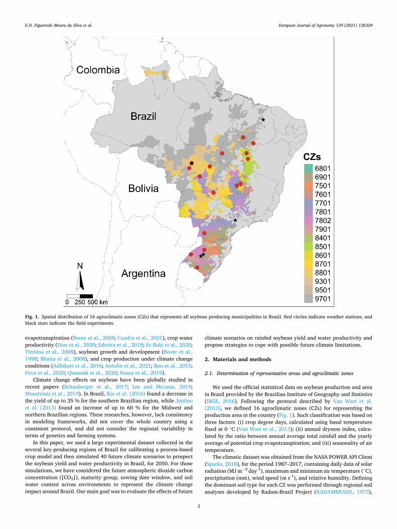
We used the official statistical data on soybean production and area in Brazil provided by the Brazilian Institute of Geography and Statistics (IBGE, 2016). Following the protocol described by Van Wart et al. (2013), we defined 16 agroclimatic zones (CZs) for representing the production area in the country (Fig. 1). Such classification was based on three factors: (i) crop degree days, calculated using basal temperature fixed at 0 ◦C (Van Wart et al., 2013); (ii) annual dryness index, calcu-lated by the ratio between annual average total rainfall and the yearly average of potential crop evapotranspiration; and (iii) seasonality of air temperature.

The climatic dataset was obtained from the NASA POWER API Client (Sparks, 2018), for the period 1987–2017, containing daily data of solar radiation (MJ m− 2 day-1), maximum and minimum air temperature (◦C), precipitation (mm), wind speed (m s-1), and relative humidity. Defining the dominant soil type for each CZ was performed through regional soil analyses developed by Radam-Brazil Project (RADAMBRASIL, 1973),

Fig. 1. Spatial distribution of 16 agroclimatic zones (CZs) that represents all soybean producing municipalities in Brazil. Red circles indicate weather stations, and black stars indicate the field experiments.

E.H. Figueiredo Moura da Silva et al.

European Journal of Agronomy 129 (2021) 126329

3

and based on the dominant soil type for each CZ, we selected the correspondent soil profile from the WISE (World Inventory of Soil Emission Potentials) database available at International Soil Reference and Information Centre (ISRIC. http://www.isric.org).

2.2. The climate change scenarios

We considered the climate forcing levels from twenty Global Climate Models (GCMs) of the Coupled Model Intercomparison Project 5 (CMIP5) (Taylor et al., 2012) as provided by Agricultural Model Inter-comparison and Improvement Project (AgMIP, www.agmip.org). We used the algorithm provided by Hudson and Ruane (2013) in R to generate future climate based on trajectories of greenhouse gas emis-sions, and the representative concentration pathways (RCPs) for each CZ. The RCP 4.5 (radiative forcing level of 4.5 W m− 2) is based in the MiniCAM model (Brenkert et al., 2003), developed by the Global Change Research Institute and the Pacific Northwest National Laboratory, and

considers the possibility of stabilization of [CO2] through the employee of technologies and strategies which will allow reducing the greenhouse gas emissions until 2100 (Thomson et al., 2011). The RCP 8.5 (radiative forcing level of 8.5 W m− 2) is based on the MESSAGE model, developed by the International Institute for Applied Systems Analysis and is char-acterized for the increase in the greenhouses gas emissions that will result in the elevation of the [CO2] to 1370 ppm until 2100 (Riahi et al., 2011). In this study, we adopted [CO2] levels of 526 and 658 ppm for RCP 4.5 and RCP 8.5, respectively, for a representative of 2050 (Riahi and Nakicenovic, 2007). For each RCP, we used 20 climate scenarios represented by the GCMs (Supplementary Materials – Table S1) avail-able for 30-year future periods named as 2050 (2040− 2069).

2.3. Field experimental data

The field data that were used in this study were obtained from well- conducted experiments across regions from Brazil (Table 1): (i) Piraci-caba (PI), Sao Paulo, during one crop season (2016/2017) with a climate classification of Cwa (high-altitude tropical) (Koeppen, 1948) on a Eutric Rhodic Ferralic Nitisol (S-PI), (ii) Sorriso (SO), Mato Grosso during two crop seasons (2018/2019 and 2019/2020) with climate classification of Aw (tropical moist, dry winter, savanna-like) on Dystrophic Red Yellow Ferrosol (S-SO), (iii) Tupancireta (TU), Rio Grande do Sul during two crop seasons (2018/2019), with a climate classification of Cfa (subtropical with no dry season and hot summer) on Dystrophic Red Acrisol (S-TU), and irrigated (50 % of water require-ment) (iv) Teresina (TE), Piaui, during one crop season (2019) with a climate classification of Aw (tropical savanna climate) on Dystrophic Red Yellow Acrisol (S-TE). Each experimental plot consisted of 12 rows, 9.0 m long, with a spacing of 0.5 m between rows and 0.04 m for planting depth, and was replicated four times.

In each experimental field, data were recorded 7–8 times during the cycle for the following variables: (i) leaf area index (LAI), was measured using the plant canopy analyzer LI− COR Model LAI-2200C and following the recommendations proposed by Gonçalves et al. (2020); (ii) canopy weight (CW, kg DM ha− 1), and (iii) grain weight (GW, kg DM ha− 1). Measurements included the phenological development for anthesis (R1), beginning of pod formation (R3), beginning of seed for-mation (R5), and physiological maturity (R7). For each sample, we collected 1 m of a row from each of four replications and computed the average. The final grain measurement was conducted by harvesting 9.0

Table 2 Soil parameters for Eutric Rhodic Ferralic Nitisol (S-PI), Dystrophic Red Yellow Ferrosol (S-SO), and Dystrophic Red Yellow Acrisol (S-TU), including soil root growth factor (SRGF) for experiments conducted in Piracicaba/SP (PI-1), Sorriso/MT (SO-1), Tupancireta(TU-1), and Teresina/PI (TE-1).

Soil Soil depth Bulk density SRGF Lower limit Upper limit drained Upper limit saturated (m) (gcm− 1) (cm3 cm− 3)

S-PI 0.1 1.34 1 0.243 0.369 0.419 0.2 1.32 1 0.218 0.375 0.426 0.4 1.34 0.549 0.294 0.407 0.427 0.6 1.30 0.368 0.342 0.441 0.458 1.4 1.29 0.247 0.333 0.438 0.445 1.5 1.28 0.165 0.336 0.441 0.448

S-SO 0.1 1.50 1 0.144 0.309 0.39 0.2 1.30 1 0.144 0.309 0.32 0.3 1.50 0.638 0.069 0.219 0.399 0.7 1.48 0.368 0.154 0.289 0.418 1.0 1.47 0.168 0.154 0.289 0.422

S-CA 0.1 1.59 1 0.106 0.312 0.402 0.3 1.60 0.931 0.117 0.323 0.408 0.5 1.60 0.650 0.118 0.324 0.409 0.8 1.57 0.456 0.142 0.329 0.420 1.0 1.59 0.078 0.169 0.358 0.441

S-TE 0.2 1.51 1 0.062 0.162 0.405 0.3 1.51 0.607 0.062 0.162 0.405 0.4 1.49 0.497 0.122 0.139 0.413 0.6 1.49 0.368 0.122 0.239 0.413 0.7 1.49 0.273 0.122 0.239 0.413 1.8 1.50 0.082 0.118 0.232 0.413

Table 1 Description of field experiments conducted in Piracicaba/SP, Sorriso/MT, Tupancireta/RS, and Teresina/PI, Brazil.

Experiment Crop season

Lat., long. and altitude

Cultivar and maturity group (MG)

Sowing data

Plant density (plant m− 2)

Piracicaba (PI-1)

2016/ 2017

22◦42′N 47◦30′W 546 a.m.s.l

TMG6410 (MG 6.0)

Nov 14 35

Piracicaba (PI-2)

2016/ 2017

22◦42′N 47◦30′W 546 a.m.s.l

NS6700 (MG 7.0)

Nov 14 28

Sorriso (SO-1)

2018/ 2019

12◦42′S 55◦48′W 375 a.m.s.l

TMG7063 (MG 7.0)

Nov 20 30

Sorriso (SO-2)

2019/ 2020

12◦42′S 55◦48′W 375 a.m.s.l

NS7901 (MG 8.0)

Nov 01 30

Tupancireta (TU-1)

2019/ 2020

28◦48′S 53◦36′W 476 a.m.s.l

BMX Compacta (MG 6.0)

Dec 03 35

Teresina (TE-1)

2019 05◦02′S 42◦47′W 78 a.m.s.l

BMX Bonus (MG 8.0)

Jul 23 25

E.H. Figueiredo Moura da Silva et al.

European Journal of Agronomy 129 (2021) 126329

4

m2 (three center rows) of each soybean plot.

2.4. Crop model

The CROPGRO-SOYBEAN-Soybean model v.4.7 (Jones et al., 2003; Hoogenboom et al., 2019a, b) was calibrated and evaluated specifically for each maturity group (MG). For calibration, we randomly selected the experiments PI-1 for MG 6.0, PI-2 for MG 7.0, and TE-1 for MG 8.0. After calibration, we evaluated the model considering the performance to reproduce the observed variables: phenological development, LAI, CW, GW using the following experimental datasets: TU-1 for MG 6.0, and SO-1 for MG 7.0, and SO-2 for MG 8.0.

In each experiment, the weather daily data were measured by an on- site automatic weather station. The soil profile data was created using the percent sand, silt, and clay of soil for each depth of soil (Table 2). The soil root growth factor (SRGF), soil water-holding characteristics for each soil layer, and saturated hydraulic conductivity were computed via the DSSAT-SBUILD tool (Jones et al., 1998).

The cultivar coefficients for the MG 6.0, GM 7.0, and MG 8.0 were estimated following the steps suggested by Boote et al. (1998), as summarized in three phases: (i) in the first phase, the goal was to evaluate the efficiency of simulations with a default of each MG cali-bration by using observed weather, soil, and management; (ii) in the second phase, only the coefficients associated to crop phenology were calibrated, including the following crop stages (R1, R3, R5, and R7); (iii) and the third phase considered also the calibration of crop growth co-efficients and the final values of the calibration (Table 3).

The quality of calibration was evaluated by using the root mean square error (RMSE) (Loague and Green, 1991) and index of agreement (D-index) (Willmott, 1982) as measures of goodness-of-fit.

2.5. Simulation of the future scenarios of soybean yield

After calibrating and evaluating the CROPGRO-SOYBEAN, we used the specific calibration coefficients for each CZ, based on the criteria suggested by Alliprandini et al. (2009), which is considered on distri-bution of MG as function of latitude in Brazil. The model was used to estimate phenology, yield, water balance, and water productivity (WP), the mass of grain per unit of evapotranspiration.

To represent the Brazilian soybean cropping systems, we initially simulated sowing every day of the sowing window officially recom-mended by the Ministry of Agriculture in Brazil (Ministerio da Agri-cultura, Pecuaria e Abastecimento, 2019), for each CZ (Table 4). We then noted that by adopting this criterion, we could establish scenarios

Table 3 Final values of the calibrated cultivar GM 6.0, GM 7.0 and GM 8.0 with exper-iments conducted in Piracicaba/SP (PI-1 and PI-2) and Teresina/PI (TE-1) respectively.

Traits Definition Unit GM 6.0

GM 7.0

GM 8.0

CSDL Critical Short Day Length below which reproductive development

hour 12.58 12.33 14.07

PPSEN Slope of the relative response of development to photoperiod with time

1/hour 0.311 0.320 0.001

EM-FL Time between VE and R1

photothermal days

25.3 20.6 22.2

FL-SH Time between R1 and R3

photothermal days

8.2 8.2 10.0

FL-SD Time between R1 and R5

photothermal days

13.7 15.0 11.7

SD-PM Time between R5 and R7

photothermal days

37.0 37.0 24.1

FL-LF Time between R1 and end of leaf expansion

photothermal days

18.8 18.0 18.0

LFMAX Maximum leaf photosynthesis rate at 30 ◦C, 350 vpm CO2, and high light

mg CO2/m2/s 1.03 1.10 1.50

SLAVR Specific leaf area of cultivar under standard growth conditions

cm2/g 335 335 495

SIZLF Maximum size of full leaf (three leaflets)

cm2 180 180 200

XFRT Maximum fraction of daily growth that is partitioned to seed +shell

g 1 1 1

WTPSD Maximum weight per seed

photothermal days

0.19 0.19 0.19

SFDUR Seed filling duration for pod cohort at standard growth conditions

#/pod 23 23 21

SDPDV Average seed per pod under standard growing conditions

photothermal days

2.4 2.7 2.3

PODUR Time required for cultivar to reach final pod load under optimal conditions

#/pod 10 10 10

THRSH Threshing percentage seed/(seed +shell)

78 78 78

SDPRO Fraction protein in seeds g(protein)/g (seed)

0.4 0.4 0.4

SDLIP Fraction oil in seeds g(oil)/g(seed) 0.2 0.2 0.2

Table 4 Name of the weather station used from each agroclimatic zones (CZ), official sowing window, soil, long-term annual average temperature and total annual rainfall, and maturity group (MG) used for CROPGRO-Soybeansimulations.

CZ Weather Station

Sowing date window

Representative soil classification

Average temperature and annual rainfall

MG

Start End

6801 Cascavel - PR

Sep 1

Dec 31

Ultisols 18.2 ◦C 1822 mm

6

6901 Dom Pedrito - RS

Sep 1

Dec 31

Entisols 18.5 ◦C 1313 mm

6

7501 Unaí- MG Sep 1

Dec 31

Oxisols 23.5 ◦C 1275 mm

7

7601 Cristalina - GO

Sep 1

Dec 31

Oxisols 20.1 ◦C 1422 mm

7

7701 Jataí- GO Sep 1

Dec 31

Oxisols 23.3 ◦C 1541 mm

7

7801 Primavera do Leste - MT

Sep 1

Dec 31

Ultisols 22.0 ◦C 1784 mm

7

7802 Sao Borja - RS

Sep 1

Dec 31

Oxisols 20.5 ◦C 1567 mm

6

7901 Palmeira das Missoes - RS

Sep 1

Dec 31

Oxisols 18.7 ◦C 1838 mm

6

8401 Formosa do Rio Preto - BA

Oct 1

Jan 31

Oxisols 24.3 ◦C 902 mm

8

8501 Barreiras - BA

Oct 1

Jan 31

Entisols 24.9 ◦C 1045 mm

8

8601 Canarana- MT

Sep 1

Dec 31

Oxisols 24.8 ◦C 1541 mm

7

8701 Sorriso - MT Sep 1

Dec 31

Oxisols 25.0 ◦C 1883 mm

7

8801 Nova Mutum - MT

Sep 1

Dec 31

Entisols 24.6 ◦C 1934 mm

7

9301 Bom Jesus - PI

Nov 1

Jan 31

Entisols 26.7 ◦C 1002 mm

8

9501 Balsas - MA Nov 1

Jan 31

Entisols 26.4 ◦C 1190 mm

8

9701 Lagoa da Confusao - TO

Nov 1

Jan 31

Inceptisols 27.2 ◦C 1882 mm

8

E.H. Figueiredo Moura da Silva et al.

European Journal of Agronomy 129 (2021) 126329

5

with distorted reality, as we had not considered the farmers do not sow the crop during drought periods. Thus, we implemented an algorithm to trigger the model for sowing the crop only after at least 20 mm of rainfall over three successive days within the official soybean sowing window (Ministerio da Agricultura, Pecuaria e Abastecimento, 2019). With this feature, each simulated season had a different sowing date, but all were inside the official sowing window, which made our simulations closer to the practice adopted by farmers.

Altogether, we generated 1.21 × 108 simulations for soybean yield for the baseline and the future climate scenarios and both RCP 4.5 and 8.5 for each CZ. Based on this database we calculated the (i) yield average, (ii) yield upper limit (average added one standard deviation), and (iii) yield lower limit (average less one standard deviation). We also calculated the yield risk was assumed to be represented by the ratio between the frequency of years in which the yield was below average and the total number of years simulated. In this way, the occurrence of extreme events as high temperatures, drought stress or flooding would explain the drop in productivity and the increase in yield risk in relation to the baseline.

2.6. Statistics for model evaluation

The accuracy of simulations was evaluated by comparing simulated with the observed data from all field experiments, as described in the previous section. We used the root mean square error (RMSE) (Loague and Green, 1991) and index of agreement (D-index) (Willmott, 1982) as measures of goodness-of-fit. The values were calculated using the following equations:

RMSE =

∑ni=1(si − oi)

n

√

(1)

D = 1 −

[ ∑ni=1 (si − oi)

2

∑ni=1|(si − o| + |oi − o|)2

]

, 0 ≤ D ≤ 1 (2)

where n is number of observations; si is simulated value corresponding

to measurement i on each date; oi is observed value for measurement i; and o is the average of observed values.

The D-index and RMSE were used to assess the error associated with simulation in relation to observed data described in the previous session. The D-index is the degree to which the observed values are approached by the model simulated values; it ranges from 0 to 1, with 0 indicating no agreement between the observed and predicted values and 1 indicating perfect agreement. Thus, a high value for the D-index and a low value for RMSE would imply better performance.

3. Results

3.1. Simulated soybean phenology, growth, and development

We observed good accuracy in simulations for the MG 6.0, MG 7.0, and MG 8.0 across the phenological stages; the maximum difference was five days between the simulated and the observed values (Table 5).

In our calibration procedure for PI-1, PI-2, and TE-1, we minimized RMSE, maximized D-index, and visually evaluated whether the trait adjustments better described the observed growing season mainly for leaf area index, canopy dry matter, and grain weight. Based on these indicators, we obtained the best possible adjustment, and the calibrated model was able to correctly simulate variables over time (Table 5). We evaluated the CROPGRO-Soybean simulations using TU-1, SO-1, and SO-2 experiments; all evaluation variables were very well simulated, as D-index > 0.7 (Table 6).

3.2. Simulated of the future scenarios of soybean yield

Future air temperature scenarios showed a consistently increasing trend across CZs, ranging from 1.55 to 3.02 ◦C, with an overall average increase of 2.2 ◦C and a highest absolute increase of 3.02 ◦C, in CZ 8801 (Table 7). The scenarios also indicated rainfall changes ranging from -4.5–7.9% in rainfall volume across CZs with a remarkably high coeffi-cient of variation around 500 % across GCMs and RCPs. The WP increased in all CZs, ranging from 7 to 47 %. Higher variations were observed for RCP 8.5 in CZ 7501. The CZs 9501, 6901, and 9701 showed the lowest variation in comparison with the baseline (Table 7).

Crop phenology was affected by the reduction of the crop cycle, mainly in the phase R1 (first flower) and R5 (first seed) (Fehr and Caviness, 1977). On average, there would be a reduction of three days for RCP 4.5 and five days for RCP 8.5 in the crop cycles in the future.

Table 5 Soybean crop phenology observed and simulated for the experiments conducted in Piracicaba/SP (PI-1 and PI-2), Teresina/PI (TE-1), Tupancireta (TU-1), and Sorriso/MT (SO-1, SO-2), with the CROPGRO-Soybean. RMSE values in brackets.

Maturity group/experiment Phenology Observed Simulated day after sowing (DAS)

Model calibration MG 6.0 (PI-1) Beginning flowering 46 46 (0)

Beginning pod 61 61 (0) Beginning seed 71 71 (0) Physiological maturity 113 113 (0)

MG 7.0 (PI-2) Beginning flowering 47 47 (0) Beginning pod 64 64 (0) Beginning seed 78 78 (0) Physiological maturity 117 117 (0)

MG 8.0 (TE-1) Beginning flowering 30 30 (0) Beginning pod 41 41 (0) Beginning seed 48 48 (0) Physiological maturity 83 83 (0)

Model evaluation MG 6.0 (TU-1) Beginning flowering 57 57 (0)

Beginning pod 75 74 (1) Beginning seed 90 84 (6) Physiological maturity 130 130 (0)

MG 7.0 (SO-1) Beginning flowering 32 33 (-1) Beginning pod 48 42 (-6) Beginning seed 56 54 (-2) Physiological maturity 103 100 (-3)

MG 8.0 (S0-2) Beginning flowering 35 32 (-3) Beginning pod 51 55 (4) Beginning seed 62 65 (3) Physiological maturity 105 109 (4)

Table 6 Statistical analysis for leaf area index (LAI), above dry matter (CW), and grain weight (GW) over time for PI-1, PI-2, TU-1, SO-1, SO-2, TE-1 with the CROP-GRO-Soybean.

Treatment Variable Unit RMSE D-index

Model calibration MG 6.0 (PI-1) LAI — 0.411 0.982

CW kg/ha 659 0.992 GW kg/ha 655 0.957

MG 7.0 (PI-2) LAI — 0.778 0.813 CW kg/ha 120 0.894 GW kg/ha 578 0.753

MG 8.0 (TE-1) LAI — 0.92 0.944 CW kg/ha 147 0.934 GW kg/ha 271 0.974

Model evaluation MG 6.0 (CA-1) LAI — 0.971 0.960

CW kg/ha 560 0.987 GW kg/ha 1043 0.942

MG 7.0 (SO-1) LAI — 0.873 0.868 CW kg/ha 1060 0.811 GW kg/ha 943 0.840

MG 8.0 (SO-2) LAI — 0.962 0.860 CW kg/ha 865 0.817 GW kg/ha 453 0.742

E.H. Figueiredo Moura da Silva et al.

European Journal of Agronomy 129 (2021) 126329

6

That was mainly caused by the air temperature increase, which influ-enced the response of the CROPGRO-Soybean to the traits of the pho-tothermal duration of crop phases. In the model, the main traits affected were: EM-FL (time between plant emergence and flower appearance); FL-SH (time between first flower and first pod); FL-SD (time between first flower and first seed); SD-PM (time between first R5 seed and physiological maturity). The variation of rainfall amount did not show a clear trend across CZs, and this makes it difficult to directly analyze its influence on crop phenology, but matters to highlight that the crop model does take into account the effect of water stress on the photo-synthesis rates and crop cycle.

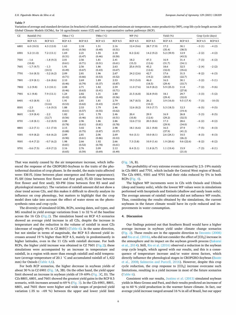
The diversity of simulated GCMs, RCPs, sowing dates, soil types, and MG resulted in yield average variations from 1 to 32 % of the baseline across the 16 CZs (Fig.2). The simulation based on RCP 4.5 scenarios showed an average yield increase in all CZs, despite the increase in temperature and the reduction in the volume of rainfall in most CZs (decrease of roughly 4% in CZ 8601) (Table 6). In the same direction, but not similar in terms of magnitude, the RCP 8.5 showed yield in-creases around 19 % higher than RCP 4.5, mainly in predominantly in higher latitudes, even in the 11 CZs with rainfall decrease. For both RCPs, the higher yield increase was obtained in CZ 7601 (Fig.2); these simulations were accompanied by an increase in temperature and rainfall, in a region with more than enough rainfall and mild tempera-ture (average temperature of 20.1 ◦C and accumulated rainfall of 1,422 mm) for Oxisols (Table 4,6).

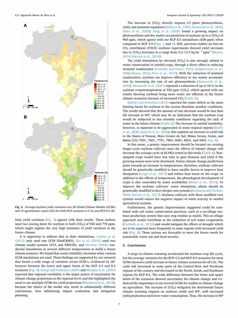
For both RCP scenarios, the higher decrease in soybean yields of about 30 % in CZ 6901 (Fig. 3A, 3B). On the other hand, the yield upper limit showed an increase in soybean yields of 19–69% (Fig. 3C, D). The CZs 8801, 6801, and 7601 showed the greatest yield gains in the RCP 8.5 scenario, with increases around to 69 % (Fig. 3). In the CZs 6901, 8801, 6801, and 7601 there were higher and wide ranges of projected yield variation (-35 to +69 %) between the upper and lower yield limit

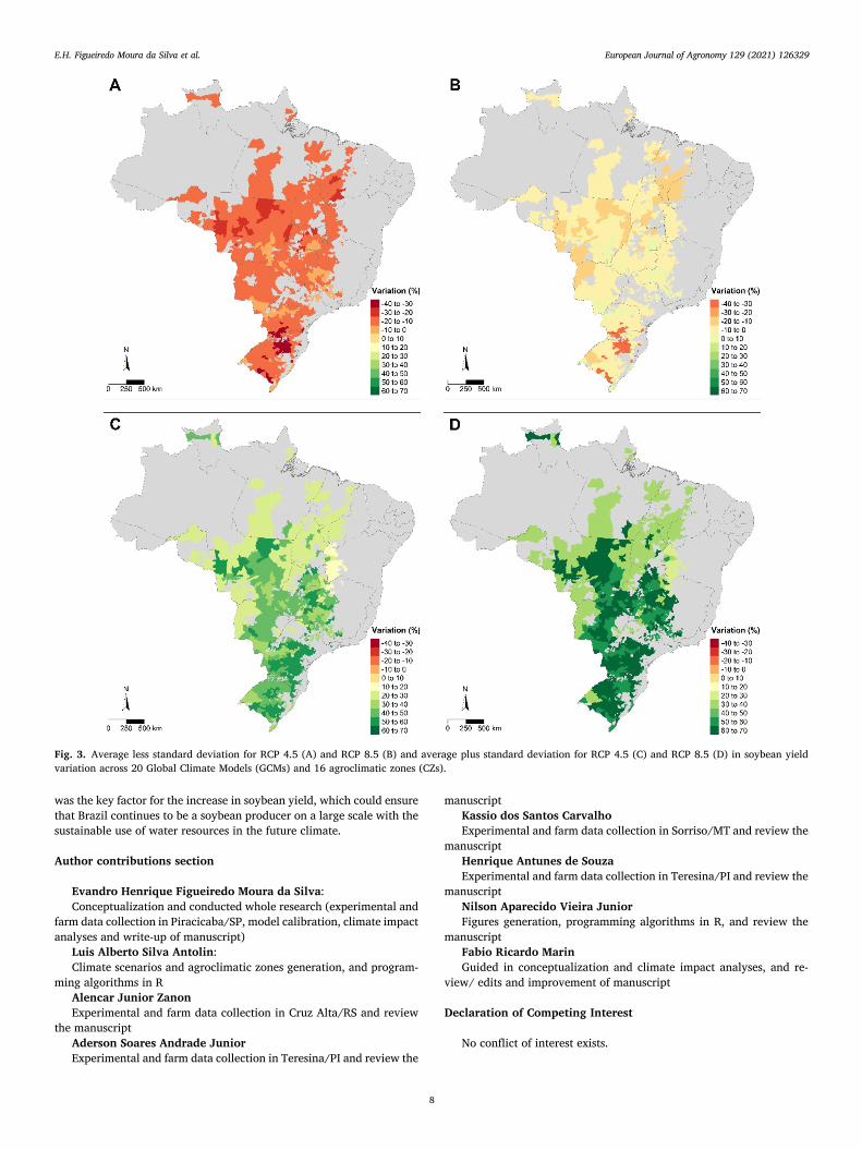
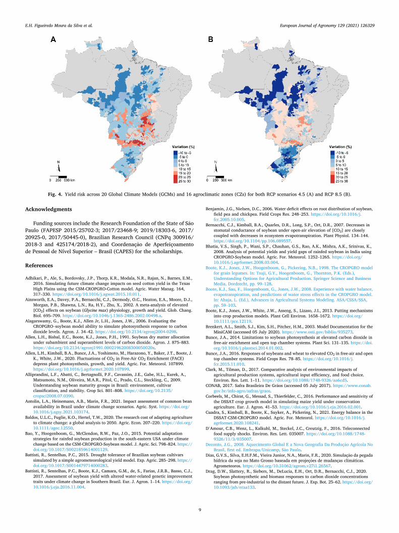
(Fig. 3A, B). The probability of very extreme events increased by 2.5–19% mainly

in CZs 8801 and 7701, which include the Central West region of Brazil. The CZs 6901, 9301 and 9701 had their risks reduced by 5% in both RCPs (Fig. 4).

The highest WP increments were in CZs with Oxisols and Ultisols (deep and loamy soils), while the lowest WP values were in simulations performed with Inceptisols and Entisols (shallow and sandy loam soils). The average amount of rainfall variation did not influence WP results. Thus, considering the results obtained by the simulations, the current soybeans in the future climate would have its cycle reduced and im-provements in water consumption.

4. Discussion

Our findings pointed out that Southern Brazil would have a higher average increase in soybean yield under climate change scenarios (Fig. 2). These results are in the opposite direction to Deconto (2008) and Rio et al. (2016), who did not consider the effect of [CO2] increase in the atmosphere and its impact on the soybean growth process (Sakurai et al., 2014). Still, Rio et al. (2016) observed a reduction in the soybean crop cycle length, which agreed with our results, and this is a conse-quence of temperature increase and/or water stress factors, which directly influence the phenological stages in CROPGRO-Soybean (Boote et al., 2008; Salmeron and Purcell, 2016). However, despite this crop cycle reduction, the crop response to [CO2] increase overcame such limitations, resulting in a yield increase in most of the future scenarios (Table 6).

Consistent with our results, Justino et al. (2013) simulated soybean yields in Mato Grosso and Para, and their results predicted an increase of up to 60 % yield production in the warmer future climate. In fact, our average yield increase ranged around 16 % in all of Brazil, but our upper

Table 7 Variation of average and standard deviation (in brackets) of rainfall, maximum and minimum air temperature, water productivity (WP), crop life cycle length across 20 Global Climate Models (GCMs), for 16 agroclimatic zones (CZ) and two representative carbon pathways (RCP).

CZ Rainfall (%) TMax (◦C) TMin (◦C) WP (%) Yield (%) Crop Cycle (days)

RCP 4.5 RCP 8.5 RCP 4.5 RCP 8.5 RCP 4.5 RCP 8.5 RCP 4.5 RCP 8.5 RCP 4.5 RCP 8.5 RCP 4.5 RCP 8.5

6801 6.0 (10.5) 4.3 (12.0) 1.63 (0.41)

2.18 (0.56)

1.51 (0.40)

2.16 (0.51)

12.4 (9.6) 28.7 (7.9) 17.2 (35.4)

30.1 (38.5)

− 3 (1) − 4 (2)

6901 5.2 (11.0) 7.2 (13.1) 1.69 (0.31)

2.21 (0.47)

1.55 (0.46)

2.18 (0.50)

8.2 (2.6) 14.2 (9.2) 5.2 (39.9) 12.9 (43.5)

− 2 (2) − 4 (2)

7501 − 1.6 (10.8)

− 1.8 (9.3) 2.01 (0.61)

2.56 (0.71)

1.81 (0.51)

2.41 (0.61)

18.2 (15.3)

47.3 (12.6)

16.9 (31.7)

31.4 (34.1)

− 7 (3) − 6 (2)

7601 − 1.7 (9.7) − 1.3 (10.5)

1.91 (0.49)

2.56 (0.67)

1.86 (0.43)

2.63 (0.67)

25.6 (9.5) 45.2 (12.6)

18.6 (32.0)

32.5 (35.6)

− 2 (4) − 2 (2)

7701 − 3.6 (8.3) − 3.2 (6.2) 2.09 (0.71)

2.81 (0.66)

1.96 (0.53)

2.67 (0.52)

24.2 (2.6) 42.7 (19.2)

17.6 (20.0)

31.5 (22.7)

− 8 (2) − 6 (3)

7801 − 2.9 (8.1) − 2.6 (8.6) 2.10 (0.46)

2.69 (0.79)

1.89 (0.37)

2.53 (0.87)

19.3 (5.0) 46.0 (18.5)

16.5 (29.4)

30.1 (33.7)

− 3 (2) − 5 (1)

7802 1.2 (9.8) 1.3 (10.1) 2.08 (0.46)

2.71 (0.63)

1.82 (0.41)

2.59 (0.71)

11.0 (7.6) 16.9 (8.2) 5.9 (25.3) 11.8 (27.8)

− 7 (2) − 9 (6)

7901 6.1 (9.8) 7.9 (13.1) 1.24 (0.42)

2.82 (0.45)

1.31 (0.40)

2.80 (0.56)

21.5 (6.8) 32.8 (9.0) 18.1 (29.4)

29.7 (32.0)

− 3 (3) − 5 (2)

8401 − 4.5 (8.9) − 3.1 (12.6)

1.91 (0.53)

2.81 (0.62)

1.81 (0.43)

2.79 (0.67)

18.7 (8.5) 26.2 (10.2)

3.9 (16.0) 9.5 (17.4) − 7 (3) − 10 (5)

8501 − 2.3 (12.0)

− 1.6 (9.3) 1.88 (0.61)

2.53 (0.57)

1.79 (0.55)

2.46 (0.62)

12.6 (8.2) 19.5 (7.7) 5.3 (18.3) 12.3 (19.4)

− 6 (5) − 9 (5)

8601 − 3.9 (8.4) − 2.2 (12.7)

1.82 (0.56)

2.41 (0.46)

1.78 (0.51)

2.46 (0.51)

20.4 (10.8)

29.9 (12.6)

16.9 (29.2)

26.8 (32.5)

− 5 (3) − 8 (5)

8701 − 1.8 (8.1) − 3.2 (8.9) 2.08 (0.78)

2.96 (0.61)

1.86 (0.81)

2.86 (0.78)

12.6 (7.5) 20.5 (8.6) 17.3 (29.9)

28.6 (34.0)

− 6 (2) − 8 (2)

8801 − 2.2 (7.1) − 3.1 (7.0) 2.15 (0.88)

3.02 (0.75)

1.96 (0.87)

2.98 (0.57)

18.1 (6.6) 22.1 (9.8) 16.5 (37.9)

27.9 (41.2)

− 7 (5) − 8 (3)

9301 − 0.9 (8.2) − 0.6 (6.2) 2.09 (0.90)

2.81 (0.61)

2.06 (0.86)

2.69 (0.53)

9.6 (3.1) 10.0 (8.1) 2.6 (24.1) 10.5 (26.2)

− 8 (3) − 8 (3)

9501 − 0.4 (7.2) − 0.7 (6.2) 1.98 (0.81)

2.66 (0.52)

1.92 (0.78)

2.66 (0.61)

7.3 (3.8) 10.9 (1.6) 1.9 (20.6) 9.6 (22.6) − 8 (2) − 8 (2)

9701 − 0.6 (7.5) − 0.9 (7.2) 2.16 (0.65)

2.76 (0.59)

2.09 (0.69)

2.12 (0.49)

8.4 (5.1) 11.8 (6.7) 1.1 (19.4) 15.9 (21.0)

− 7 (3) − 8 (1)

E.H. Figueiredo Moura da Silva et al.

European Journal of Agronomy 129 (2021) 126329

7

limit yield variation (Fig. 3) agreed with their results. These authors used two sowing dates for soybean in both [CO2] of 550 and 770 ppm, which might explain the very high estimates of yield variation in the future climate.

It is important to address that in their simulations, Justino et al. (2013) only used one GCM (HadCRM3), Rio et al. (2016) used two climate model systems (ETA and PRECIS), and Deconto (2008) con-ducted simulations at several different temperatures to build a future climate scenario. We found that result reliability increases when various GCM simulations are used. These findings are supported by our research that found a wide range of variation across GCM’s, evidenced by dif-ferences between the lower and upper limits of the RCP 4.5 and 8.5 scenarios (Fig. 3). Giorgi and Francisco (2000) and Murphy et al. (2004) reported that regional variability is the major source of uncertainty for climate change projections at the regional level, and this highlighted the need to use multiple GCMs for yield projections (Shepherd et al., 2018), because the choice of the model may result in substantially different conclusions, thus influencing impact evaluation and mitigation planning.

The increase in [CO2] directly impacts C3 plant photosynthesis, yield, and stomatal regulation (Allen et al., 1991; Ainsworth et al., 2002; Allen et al., 2020). Drag et al. (2020) found a growing impact on photosynthesis and dry matter accumulation of soybean up to a [CO2] of 900 ppm, which agrees with our RCP 8.5 simulations (658 ppm) when compared to RCP 4.5 (Figs. 2 and 3). Still, previous studies on free-air CO2 enrichment (FACE) soybean experiments showed yield increases due to [CO2] increases in a range from 2.2–13.3 kg ha− 1 ppm-1 (Bunce, 2014; Sakurai et al., 2014).

The yield stimulation by elevated [CO2] is also strongly related to water conservation in rainfed crops, through a direct effect in reducing stomatal conductance (Tubiello and Ewert, 2002; Alagarswamy et al., 2006; Bunce, 2016; Silva et al., 2019). With the reduction of stomatal conductance, soybean can improve efficiency in dry matter accumula-tion by increasing the rate of net photosynthesis (Ainsworth et al., 2002). Bernacchi et al. (2007) reported a reduction of up to 16 % in the soybean evapotranspiration at 550 ppm [CO2], which agreed with our results showing soybean being more water use efficient in the future climate scenarios because of increased CO2 (Table 6).

Battisti and Sentelhas (2015) reported the water deficit as the main limiting factor for soybean in the current Brazilian weather conditions. The results showed that the amount of rain decrease would be less than the increase in WP, which may be an indication that the soybean crop would be subjected to less stressful conditions regarding the lack of water in the future climate (Table 6). The increase in rainfall instability, however, is expected to be aggravated in some tropical regions (Duffy et al., 2020; Saint-lu et al., 2020); this explains an increase in yield risk in the States of Parana, Mato Grosso do Sul, Minas Gerais, Goias, and Bahia (CZs 7501, 7601, 7701, 7801, 8401, 8501, and 9301; Fig. 4).

In this sense, a genetic improvement should be focused on creating longer-cycle soybean cultivars since the effects of climate change will decrease the average cycle of all MGs tested in this study (Table 6). Non- adapted crops would have less time to gain biomass and yield if the growing season were to be shortened. Future climate change predictions point towards an increase in temperatures; therefore, soybean cultivars should be genetically modified to have smaller leaves to improve heat dissipation (Leigh et al., 2017) and reduce heat stress on the crops. In addition to the effects of temperature, the phenological development of crops is also controlled by water availability (Boote et al., 2013). To improve the soybean cultivars’ water absorption, plants should be genetically modified to have deeper root systems (Benjamin and Nielsen, 2006; Battisti et al., 2017). Soybean cultivars with these modified root systems would reduce the negative impact of water scarcity in rainfed agricultural systems.

Furthermore, the genetic improvements suggested could be com-bined with soil water conservation practices, such as a no-tillage soy-bean production system that uses crop residue as mulch. This no-tillage approach would contribute to the reduction of soil water evaporation (Corbeels et al., 2016) and would mitigate the effects of drought which are to be expected more frequently in some regions with increased yield risk (Fig. 4). These actions are favorable to meet the future needs for sustainable water use and food security.

5. Conclusions

A surge in climate warming accelerated the soybean crop life cycle, but the average variation for the RCP 4.5 and RCP 8.5 scenarios for most GCMs showed a yield increase in future climate scenarios for all CZs. The yield risk increased in some parts of the Central-West and Northeast regions of the country and decreased in the North, South, and Southeast regions for RCP 8.5. The wide difference between the lower and upper limits of the scenarios showed uncertainty for climate change and evi-denced the importance to use several GCMs for studies in climate change on agriculture. The increase of [CO2] mitigated the detrimental future climate warming impacts on soybean yields and WP, with increased yield production and lower water consumption. Thus, the increase in WP

Fig. 2. Average soybean yield variation over 20 Global Climate Models (GCMs) and 16 agroclimatic zones (CZs) for both RCP scenarios 4.5 (A) and RCP 8.5 (B).

E.H. Figueiredo Moura da Silva et al.

European Journal of Agronomy 129 (2021) 126329

8

was the key factor for the increase in soybean yield, which could ensure that Brazil continues to be a soybean producer on a large scale with the sustainable use of water resources in the future climate.

Author contributions section

Evandro Henrique Figueiredo Moura da Silva: Conceptualization and conducted whole research (experimental and

farm data collection in Piracicaba/SP, model calibration, climate impact analyses and write-up of manuscript)

Luis Alberto Silva Antolin: Climate scenarios and agroclimatic zones generation, and program-

ming algorithms in R Alencar Junior Zanon Experimental and farm data collection in Cruz Alta/RS and review

the manuscript Aderson Soares Andrade Junior Experimental and farm data collection in Teresina/PI and review the

manuscript Kassio dos Santos Carvalho Experimental and farm data collection in Sorriso/MT and review the

manuscript Henrique Antunes de Souza Experimental and farm data collection in Teresina/PI and review the

manuscript Nilson Aparecido Vieira Junior Figures generation, programming algorithms in R, and review the

manuscript Fabio Ricardo Marin Guided in conceptualization and climate impact analyses, and re-

view/ edits and improvement of manuscript

Declaration of Competing Interest

No conflict of interest exists.

Fig. 3. Average less standard deviation for RCP 4.5 (A) and RCP 8.5 (B) and average plus standard deviation for RCP 4.5 (C) and RCP 8.5 (D) in soybean yield variation across 20 Global Climate Models (GCMs) and 16 agroclimatic zones (CZs).

E.H. Figueiredo Moura da Silva et al.

European Journal of Agronomy 129 (2021) 126329

9

Acknowledgments

Funding sources include the Research Foundation of the State of Sao Paulo (FAPESP 2015/25702-3; 2017/23468-9; 2019/18303-6, 2017/ 20925-0, 2017/50445-0), Brazilian Research Council (CNPq 300916/ 2018-3 and 425174/2018-2), and Coordenaçao de Aperfeiçoamento de Pessoal de Nível Superior – Brasil (CAPES) for the scholarships.

References

Adhikari, P., Ale, S., Bordovsky, J.P., Thorp, K.R., Modala, N.R., Rajan, N., Barnes, E.M., 2016. Simulating future climate change impacts on seed cotton yield in the Texas High Plains using the CSM-CROPGRO-Cotton model. Agric. Water Manag. 164, 317–330. https://doi.org/10.1016/j.agwat.2015.10.011.

Ainsworth, E.A., Davey, P.A., Bernacchi, C.J., Dermody, O.C., Heaton, E.A., Moore, D.J., Morgan, P.B., Shawna, L.N., Ra, H.Y., Zhu, X., 2002. A meta-analysis of elevated [CO2] effects on soybean (Glycine max) physiology, growth and yield. Glob. Chang. Biol. 695–709. https://doi.org/10.1046/j.1365-2486.2002.00498.x.

Alagarswamy, G., Boote, K.J., Allen Jr, L.H., Jones, J.W., 2006. Evaluating the CROPGRO–soybean model ability to simulate photosynthesis response to carbon dioxide levels. Agron. J. 34–42. https://doi.org/10.2134/agronj2004-0298.

Allen, L.H., Bisbal, E.C., Boote, K.J., Jones, P.H., 1991. Soybean dry matter allocation under subambient and superambient levels of carbon dioxide. Agron. J. 875–883. https://doi.org/10.2134/agronj1991.00021962008300050020x.

Allen, L.H., Kimball, B.A., Bunce, J.A., Yoshimoto, M., Harazono, Y., Baker, J.T., Boote, J. K., White, J.W., 2020. Fluctuations of CO2 in Free-Air CO2 Enrichment (FACE) depress plant photosynthesis, growth, and yield. Agric. For. Meteorol. 107899. https://doi.org/10.1016/j.agrformet.2020.107899.

Alliprandini, L.F., Abatti, C., Bertagnolli, P.F., Cavassim, J.E., Gabe, H.L., Kurek, A., Matsumoto, N.M., Oliveira, M.A.R., Pitol, C., Prado, C.L., Steckling, C., 2009. Understanding soybean maturity groups in Brazil: environment, cultivar classification, and stability. Crop Sci. 801–808. https://doi.org/10.2135/ cropsci2008.07.0390.

Antolin, L.A., Heinemann, A.B., Marin, F.R., 2021. Impact assessment of common bean availability in Brazil under climate change scenarios. Agric. Syst. https://doi.org/ 10.1016/j.agsy.2021.103174.

Baldos, U.L.C., Fuglie, K.O., Hertel, T.W., 2020. The research cost of adapting agriculture to climate change: a global analysis to 2050. Agric. Econ. 207–220. https://doi.org/ 10.1111/agec.12550.

Bao, Y., Hoogenboom, G., McClendon, R.W., Paz, J.O., 2015. Potential adaptation strategies for rainfed soybean production in the south-eastern USA under climate change based on the CSM-CROPGRO-Soybean model. J. Agric. Sci. 798–824. https:// doi.org/10.1017/S0021859614001129.

Battisti, R., Sentelhas, P.C., 2015. Drought tolerance of Brazilian soybean cultivars simulated by a simple agrometeorological yield model. Exp. Agric. 285–298. https:// doi.org/10.1017/S0014479714000283.

Battisti, R., Sentelhas, P.C., Boote, K.J., Camara, G.M., de, S., Farias, J.R.B., Basso, C.J., 2017. Assessment of soybean yield with altered water-related genetic improvement traits under climate change in Southern Brazil. Eur. J. Agron. 1–14. https://doi.org/ 10.1016/j.eja.2016.11.004.

Benjamin, J.G., Nielsen, D.C., 2006. Water deficit effects on root distribution of soybean, field pea and chickpea. Field Crops Res. 248–253. https://doi.org/10.1016/j. fcr.2005.10.005.

Bernacchi, C.J., Kimball, B.A., Quarles, D.R., Long, S.P., Ort, D.R., 2007. Decreases in stomatal conductance of soybean under open-air elevation of [CO2] are closely coupled with decreases in ecosystem evapotranspiration. Plant Physiol. 134–144. https://doi.org/10.1104/pp.106.089557.

Bhatia, V.S., Singh, P., Wani, S.P., Chauhan, G.S., Rao, A.K., Mishra, A.K., Srinivas, K., 2008. Analysis of potential yields and yield gaps of rainfed soybean in India using CROPGRO-Soybean model. Agric. For. Meteorol. 1252–1265. https://doi.org/ 10.1016/j.agrformet.2008.03.004.

Boote, K.J., Jones, J.W., Hoogenboom, G., Pickering, N.B., 1998. The CROPGRO model for grain legumes. In: Tsuji, G.Y., Hoogenboom, G., Thornton, P.K. (Eds.), Understanding Options for Agricultural Production. Springer Science and Business Media, Dordrecht, pp. 99–128.

Boote, K.J., Sau, F., Hoogenboom, G., Jones, J.W., 2008. Experience with water balance, evapotranspiration, and predictions of water stress effects in the CROPGRO model. In: Ahuja, L. (Ed.), Advances in Agricultural Systems Modeling. ASA/CSSA/SSA, pp. 59–103.

Boote, K.J., Jones, J.W., White, J.W., Asseng, S., Lizaso, J.I., 2013. Putting mechanisms into crop production models. Plant Cell Environ. 1658–1672. https://doi.org/ 10.1111/pce.12119.

Brenkert, A.L., Smith, S.J., Kim, S.H., Pitcher, H.M., 2003. Model Documentation for the MiniCAM (accessed 05 July 2020). https://www.osti.gov/biblio/935273.

Bunce, J.A., 2014. Limitations to soybean photosynthesis at elevated carbon dioxide in free-air enrichment and open top chamber systems. Plant Sci. 131–135. https://doi. org/10.1016/j.plantsci.2014.01.002.

Bunce, J.A., 2016. Responses of soybeans and wheat to elevated CO2 in free-air and open top chamber systems. Field Crops Res. 78–85. https://doi.org/10.1016/j. fcr.2015.11.010.

Clark, M., Tilman, D., 2017. Comparative analysis of environmental impacts of agricultural production systems, agricultural input efficiency, and food choice. Environ. Res. Lett. 1–11. https://doi.org/10.1088/1748-9326/aa6cd5.

CONAB, 2017. Safra Brasileira De Graos (accessed 05 July 2017). https://www.conab. gov.br/info-agro/safras/graos.

Corbeels, M., Chirat, G., Messad, S., Thierfelder, C., 2016. Performance and sensitivity of the DSSAT crop growth model in simulating maize yield under conservation agriculture. Eur. J. Agron. 41–53. https://doi.org/10.1016/j.eja.2016.02.001.

Cuadra, S., Kimball, B., Boote, K., Suyker, A., Pickering, N., 2021. Energy balance in the DSSAT-CSM-CROPGRO model. Agric. For. Meteorol. https://doi.org/10.1016/j. agrformet.2020.108241.

D’Amour, C.B., Wenz, L., Kalkuhl, M., Steckel, J.C., Creutzig, F., 2016. Teleconnected food supply shocks. Environ. Res. Lett. 035007. https://doi.org/10.1088/1748- 9326/11/3/035007.

Deconto, J.G., 2008. Aquecimento Global E a Nova Geografia Da Produçao Agrícola No Brasil, first ed. Embrapa/Unicamp, Sao Paulo.

Dias, G.V.S., Silva, E.H.F.M., Vieira Junior, N.A., Marin, F.R., 2020. Simulaçao da pegada hídrica da soja no Mato Grosso baseada em projeçoes de mudanças climaticas. Agrometeoros. https://doi.org/10.31062/agrom.v27i1.26567.

Drag, D.W., Slattery, R., Siebers, M., DeLucia, E.H., Ort, D.R., Bernacchi, C.J., 2020. Soybean photosynthetic and biomass responses to carbon dioxide concentrations ranging from pre-industrial to the distant future. J. Exp. Bot. 25–62. https://doi.org/ 10.1093/jxb/eraa133.

Fig. 4. Yield risk across 20 Global Climate Models (GCMs) and 16 agroclimatic zones (CZs) for both RCP scenarios 4.5 (A) and RCP 8.5 (B).

E.H. Figueiredo Moura da Silva et al.

European Journal of Agronomy 129 (2021) 126329

10

Duffy, M.L., O’Gorman, P.A., Back, L.E., 2020. Importance of Laplacian of low-level warming for the response of precipitation to climate change over tropical oceans. J. Clim. 88–101. https://doi.org/10.1175/JCLI-D-19-0365.1.

Edreira, J.I.R., Guilpart, N., Sadras, V., Cassman, K.G., van Ittersum, M.K., Schils, R.L., Grassini, P., 2018. Water productivity of rainfed maize and wheat: a local to global perspective. Agric. For. Meteorol. 259, 364–373. https://doi.org/10.1016/j. agrformet.2018.05.019.

Er-Raki, S., Bouras, E., Rodriguez, J.C., Watts, C.J., Lizarraga-Celaya, C., Chehbouni, A., 2020. Parameterization of the AquaCrop model for simulating table grapes growth and water productivity in an arid region of Mexico. Agric. Water Manag. 106585, 106585. https://doi.org/10.1016/j.agwat.2020.

Fava, S.A.Q., Silva, E.H.F.M., Antolin, L.A.S., Marin, F.R., 2020. Simulaçao de cenarios agrícolas futuros para algodoeiro com base em projeçoes de mudanças climaticas. Agrometeoros. https://doi.org/10.31062/agrom.v27i1.26556.

Fehr, W.R., Caviness, C.E., 1977. Stages of Soybean Development (accessed 08 August 2020). https://lib.dr.iastate.edu/specialreports/87/.

Field, C.B., 2014. Climate Change 2014–Impacts, Adaptation and Vulnerability: Regional Aspects, first ed. Cambridge University Press, New York.

Foley, J.A., Ramankutty, N., Brauman, K.A., Cassidy, E.S., Gerber, J.S., Johnston, M., Mueller, C.O., Ray, D.K., West, P.C., Balzer, C., Bennett, E.M., Carpenter, S.R., Hill, J., Monfreda, C., Polasky, S., Rockstrom, J., Sheehan, J., Siebert, S., Tilman, D., Zaks, P.M., 2011. Solutions for a cultivated planet. Nature 337–342. https://doi.org/ 10.1038/nature10452.

Giorgi, F., Francisco, R., 2000. Evaluating uncertainties in the prediction of regional climate change. Geophys. Res. Lett. 1295–1298. https://doi.org/10.1029/ 1999GL011016.

Godwin, D.C., Allan, C.J., 1991. Nitrogen dynamics in soil-plant systems. Modeling Plant and Soil Systems 287–321. https://doi.org/10.2134/agronmonogr31.c13.

Godwin, D.C., Singh, U., 1998. Nitrogen balance and crop response to nitrogen in upland and lowland cropping systems. In: Tsuji, G.Y., Hoogenboom, G., Thornton, P.K. (Eds.), Understanding Options for Agricultural Production. Springer Science and Business Media, Dordrecht, pp. 55–77.

Gonçalves, A.O., Silva, E.H.F.M., Gasparotto, L.G., Mantelatto, J.R., Carmo, S., Fattori Júnior, I.M., Marin, F.R., 2020. Improving indirect measurements of the leaf area index using canopy height. Pesquisa Agropecuaria Brasileira 55, 1–9. https://doi. org/10.1590/S1678-3921.pab2020.v55.01894.

He, D., Wang, E., Wang, J., Robertson, M.J., 2017. Data requirement for effective calibration of process-based crop models. Agric. For. Meteorol. 136–148. https://doi. org/10.1016/j.agrformet.2016.12.015.

Hoogenboom, G., Porter, C.H., Boote, K.J., Shelia, V., Wilkens, P.W., Singh, U., White, J. W., Asseng, S., Lizaso, J.I., Moreno, L.P., Pavan, W., Ogoshi, R., Hunt, L.A., Tsuji, G. Y., Jones, J.W., 2019a. In: Boote, K.J. (Ed.), Advances in Crop Modeling for a Sustainable Agriculture.. Burleigh Dodds Science Publishing, Cambridge, pp. 173–216.

Hoogenboom, G., Porter, C.H., Shelia, V., Boote, K.J., Singh, U., White, J.W., Hunt, L.A., Ogoshi, R., Lizaso, J.I., Koo, J., Asseng, S., Singels, A., Moreno, L.P., Jones, J.W., 2019b. Decision Support System for Agrotechnology Transfer (DSSAT) Version 4.7 (accessed 08 August 2020). www.DSSAT.net.

Hudson, N., Ruane, A., 2013. Guide for Running AgMIP Climate Scenario Generation Tools With R. AgMIP (accessed 12 February 2019). http://www.agmip.org/wpcont ent/uploads/2013/10/Guide-for-Running-AgMIPClimate-Scenario-Generation-with.

IBGE, 2016. Produçao agrícola municipal (accessed 12 Jan 2018). https://sidra.ibge.gov. br/tabela/1612.

Jones, J.W., Keating, B.A., Porter, C.H., 2001. Approaches to modular model development. Agric. Syst. 421–443. https://doi.org/10.1016/S0308-521X(01) 00054-3.

Jones, J.W., Hoogenboom, G., Porter, C.H., Boote, K.J., Batchelor, W.D., Hunt, L.A., Wilkens, P.W., Singh, U., Gijsman, A.J., Ritchie, J.T., 2003. The DSSAT cropping system model. Eur. J. Agron. 235–265. https://doi.org/10.1016/S1161-0301(02) 00107-7.

Justino, F., Oliveira, E.C., de Avila Rodrigues, R., Gonçalves, P.H.L., Souza, P.J.O.P., Stordal, F., Marengo, J., Silva, T.G., Delgado, R.C., Silva, D., Lindemann, L.C.C., 2013. Mean and interannual variability of maize and soybean in Brazil under global warming conditions. Am. J. Clim. Change 237–253. https://doi.org/10.4236/ ajcc.2013.24024.

Koeppen, W., 1948. Climatologia: Con Un Estudio De Los Climas De La Tierra, first ed. Fondo de Cultura Economica, Mexico City.

Lee, S., McCann, L., 2019. Adoption of cover crops by US soybean producers. J. Agric. Appl. Econ. 527–544. https://doi.org/10.1017/aae.2019.20.

Leigh, A., Sevanto, S., Close, J.D., Nicotra, A.B., 2017. The influence of leaf size and shape on leaf thermal dynamics: does theory hold up under natural conditions? Plant Cell Environ. 237–248. https://doi.org/10.1111/pce.12857.

Loague, K., Green, R.E., 1991. Statistical and graphical methods for evaluating solute transport models: overview and application. J. Contam. Hydrol. 51–73. https://doi. org/10.1016/0169-7722(91)90038-3.

Marchand, P., Carr, J.A., Dell’Angelo, J., Fader, M., Gephart, J.A., Kummu, M., Ratajczak, Z., 2016. Reserves and trade jointly determine exposure to food supply shocks. Environ. Res. Lett. 095009. https://doi.org/10.1088/1748-9326/11/9/ 095009.

Ministerio da Agricultura, Pecuaria e Abastecimento, 2019. Zoneamento Agrícola (accessed 12 April 2019). https://www.gov.br/agricultura/pt-br/assuntos/politica -agricola/outras-publicacoes/zoneamento-agricola.pdf/view.

Ministerio da Economia, 2020. Balança comercial brasileira: Acumulado do ano (accessed 1 April 2019). http://www.mdic.gov.br/index.php/comercio-exterior/e statisticas-de-comercio-exterior/balanca-comercial-brasileira-acumulado-do-ano.

Mourtzinis, S., Specht, J.E., Conley, S.P., 2019. Defining optimal soybean sowing dates across the US. Sci. Rep. 1–7. https://doi.org/10.1038/s41598-019-38971-3.

Murphy, J.M., Sexton, D.M.H., Barnett, D.N., Jones, G.S., Webb, M.J., Collins, M., Stainforth, D.A., 2004. Quantification of modelling uncertainties in a large ensemble of climate change simulations. Nature 768–772. https://doi.org/10.1038/ nature02771.

Quansah, J.E., Welikhe, P., El Afandi, G., Fall, S., Mortley, D., Ankumah, R., 2020. CROPGRO-soybean model calibration and assessment of soybean yield responses to climate change. Am. J. Clim. Change 297–316. https://doi.org/10.4236/ ajcc.2020.93019.

Radambrasil, P., 1973. Levantamento De Recursos Naturais, First Ed. Rio De Janeiro. Riahi, K., Nakicenovic, N., 2007. 4 Emissions Pathways Infographic: Sources. World

Resources Institute (accessed 10 April 2019). http://www.wri.org/4-emissions- pathways-infographic-sources.

Riahi, K., Rao, S., Krey, V., Cho, C., Chirkov, V., Fischer, G., Kindermann, G., Nakicenovic, N., Rafaj, P., 2011. RCP 8.5—a scenario of comparatively high greenhouse gas emissions. Clim. Change 109–133. https://doi.org/10.1007/s10584- 011-0149-y.

Rio, A., Sentelhas, P.C., Farias, J.R.B., Sibaldelli, R.N.R., Ferreira, R.C., 2016. Alternative sowing dates as a mitigation measure to reduce climate change impacts on soybean yields in southern Brazil. Int. J. Climatol. 3664–3672. https://doi.org/10.1002/ joc.4583.

Ritchie, J.T., 1998. Soil water balance and plant water stress. In: Tsuji, G.Y., Hoogenboom, G., Thornton, P.K. (Eds.), Understanding Options for Agricultural Production. Kluwer Academic Publishers, London, pp. 41–54.

Rosenzweig, C., Jones, J.W., Hatfield, J.L., Ruane, A.C., Boote, K.J., Thorburn, P., Janssen, S., 2013. The agricultural model intercomparison and improvement project (AgMIP): protocols and pilot studies. Agric. For. Meteorol. 166–182. https://doi.org/ 10.1016/j.agrformet.2012.09.011.

Saint-Lu, M., Chadwick, R., Lambert, F.H., Collins, M., Boutle, I., Whitall, M., Daleu, C., 2020. Influences of local and remote conditions on tropical precipitation and its response to climate change. J. Clim. 4045–4063. https://doi.org/10.1175/JCLI-D- 19-0450.1.

Sakurai, G., Iizumi, T., Nishimori, M., Yokozawa, M., 2014. How much has the increase in atmospheric CO2 directly affected past soybean production? Sci. Rep. 1–5. https:// doi.org/10.1038/srep04978.

Salmeron, M., Purcell, L.C., 2016. Simplifying the prediction of phenology with the DSSAT-CROPGRO-soybean model based on relative maturity group and determinacy. Agric. Syst. 178–187. https://doi.org/10.1016/j.agsy.2016.07.016.

Schauberger, B., Archontoulis, S., Arneth, A., Balkovic, J., Ciais, P., Deryng, D., Elliott, J., Folberth, C., Khabarov, N., Müller, C., Pugh, T.A.M., Rolinski, S., Schaphoff, S., Schmid, E., Wang, X., Schlenker, W., Frieler, K., 2017. Consistent negative response of US crops to high temperatures in observations and crop models. Nat. Commun. 1–9. https://doi.org/10.1038/ncomms13931.

Searchinger, T., Waite, R., Hanson, C., Ranganathan, J., Dumas, P., Matthews, E., Klirs, C., 2019. Creating a Sustainable Food Future: a Menu of Solutions to Feed Nearly 10 Billion People by 2050 (accessed 16 April 2020). https://agritrop.cirad. fr/593176/1/WRR_Food_Full_Report_0.pdf.

Shepherd, T.G., Boyd, E., Calel, R.A., et al., 2018. Storylines: an alternative approach to representing uncertainty in physical aspects of climate change. Clim. Change 555–571. https://doi.org/10.1007/s10584-018-2317-9.

Silva, E.H.F.M., Gonçalves, A.O., Pereira, R.A., Júnior, I.M.F., Sobenko, L.R., Marin, F.R., 2019. Soybean irrigation requirements and canopy-atmosphere coupling in Southern Brazil. Agric. Water Manag. 218, 1–7. https://doi.org/10.1016/j. agwat.2019.03.003.

Silva, E.H.F.M., Boote, K.J., Hoogenboom, G., Gonçalves, A.O., Junior, A.S.A., Marin, F. R., 2021. Performance of the CSM-CROPGRO-soybean in simulating soybean growth and development and the soil water balance for a tropical environment. Agric. Water Manag. 252, 106929 https://doi.org/10.1016/j.agwat.2021.106929.

Souza, T.T., Antolin, L.A.S., Bianchini, V.J.M., Pereira, R.A.A., Silva, E.H.F.M., Marin, F. R., 2019. Longer crop cycle lengths could offset the negative effects of climate change on Brazilian maize. Bragantia. https://doi.org/10.1590/1678- 4499.20190085.

Sparks, A.H., 2018. NasaPower: a NASA POWER global meteorology, surface solar energy and climatology data client for R. J. Open Source Softw. 1-3 https://doi.org/ 10.21105/joss.01035.

Speedy, A.W., 2002. Overview of World Feed Protein Needs and Supply, first ed. FAO, Bangkok.

Sternberg, T., 2012. Chinese drought, bread and the Arab Spring. Appl. Geogr. 519–524. https://doi.org/10.1016/j.apgeog.2012.02.004.

Taylor, K.E., Stouffer, R.J., Meehl, G.A., 2012. An overview of CMIP5 and the experiment design. Bull. Am. Meteorol. Soc. 485–498.

Thomson, H., 2019. Food and Power: Regime Type, Agricultural Policy, and Political Stability, first ed. Cambridge University Press, New York.

Thomson, A.M., Calvin, K.V., Smith, S.J., Kyle, G.P., Volke, A., Patel, P., et al., 2011. RCP4. 5: a pathway for stabilization of radiative forcing by 2100. Clim. Change 77–94. https://doi.org/10.1175/BAMS-D-11-00094.1.

Thornton, P.K., 2010. Livestock production: recent trends, future prospects. Philos. Trans. Biol. Sci. 2853–2867. https://doi.org/10.1098/rstb.2010.0134.

Tilman, D., Balzer, C., Hill, J., Befort, B.L., 2011. Global food demand and the sustainable intensification of agriculture. Proc. Natl. Acad. Sci. 20260–20264. https://doi.org/ 10.1073/pnas.1116437108.

Timsina, J., Godwin, D., Humphreys, E., Kukal, S.S., Smith, D., 2008. Evaluation of options for increasing yield and water productivity of wheat in Punjab, India using the DSSAT-CERES-Wheat model. Agric. Water Manag. 1099–1110. https://doi.org/ 10.1016/j.agwat.2008.04.009.

E.H. Figueiredo Moura da Silva et al.

European Journal of Agronomy 129 (2021) 126329

11

Tubiello, F.N., Ewert, F., 2002. Simulating the effects of elevated CO2 on crops: approaches and applications for climate change. Eur. J. Agron. 57–74. https://doi. org/10.1016/S1161-0301(02)00097-7.

United Nations, 2017. World Population Projected to Reach 9.8 Billion in 2050 (accessed 28 January 2020). htps://www.un.org/development/desa/en/news/population/ world-population-prospectS-SO017.html.

Van Wart, J., van Bussel, L.G.J., Wolf, J., Licker, R., Grassini, P., Nelson, A., Boogaard, H., Gerber, J., Mueller, N.D., Claessens, L., 2013. Use of agro-climatic zones to upscale simulated crop yield potential. Field Crop Research 44–55. https:// doi.org/10.1016/j.fcr.2012.11.023.

Willmott, C.J., 1982. Some comments on the evaluation of model performance. Bull. Am. Meteorol. Soc. 1309–1313. https://doi.org/10.1175/1520-0477.

Zabel, F., Delzeit, R., Schneider, J.M., Seppelt, R., Mauser, W., Vaclavík, T., 2019. Global impacts of future cropland expansion and intensification on agricultural markets and biodiversity. Nat. Commun. 1–10. https://doi.org/10.1038/s41467-019-10775-z.

Zalles, V., Hansen, M.C., Potapov, P.V., Stehman, S.V., Tyukavina, A., Pickens, A., Song, X., Adusei, B., Okpa, C., Aguilar, R., John, N., Chavez, S., 2019. Near doubling of Brazil’s intensive row crop area since 2000. Proc. Natl. Acad. Sci. 428–435. https://doi.org/10.1073/pnas.1810301115.

E.H. Figueiredo Moura da Silva et al.