E X T E N D I N G R E S O L U T I O N I N A L L D I R E C T I O N S :

I M A G E S C A N N I N G M I C R O S C O P Y A N D

M E TA L - I N D U C E D E N E R G Y T R A N S F E R

sebastian isbaner

E X T E N D I N G R E S O L U T I O N I N A L L D I R E C T I O N S :

I M A G E S C A N N I N G M I C R O S C O P Y A N D

M E TA L - I N D U C E D E N E R G Y T R A N S F E R

Dissertation

zur Erlangung des mathematisch-naturwissenschaftlichenDoktorgrades

“Doctor rerum naturalium”der Georg-August-Universität Göttingen

im Promotionsprogramm

Physics of Biological and Complex Systemsder Göttingen Graduate School of Neurosciences, Biophysics,

and Molecular Biosciences (GGNB)der Georg-August University School of Science (GAUSS)

vorgelegt von

sebastian isbaner

aus Bremerhaven.Göttingen, Dezember 2018

betreuungsausschuss

Prof. Dr. Jörg Enderlein (Referent)Drittes Physikalisches Institut - BiophysikGeorg-August-Universität Göttingen

Prof. Dr. Helmut GrubmüllerTheoretical and Computational BiophysicsMax-Planck-Institut für Biophysikalische Chemie, Göttingen

Prof. Dr. Andreas JanshoffInstitut für Physikalische ChemieGeorg-August-Universität Göttingen

prüfungskomission

referent : Prof. Dr. Jörg EnderleinDrittes Physikalisches Institut - BiophysikGeorg-August-Universität Göttingen

korreferent : Prof. Dr. Helmut GrubmüllerTheoretical and Computational BiophysicsMax-Planck-Institut für Biophysikalische Chemie, Göttingen

weitere mitglieder der prüfungskomission

Prof. Dr. Andreas JanshoffInstitut für Physikalische ChemieGeorg-August-Universität Göttingen

Prof. Dr. Fred S. WoutersInstitut für NeuropathologieUniversitätsklinikum Göttingen

Dr. Alexander EgnerLaser-Laboratorium Göttingen

Dr. Sarah AdioInstitut für Microbiologie und GenetikGeorg-August-Universität Göttingen

tag der mündlichen prüfung : 13 .02 .2019

E X T E N D I N G R E S O L U T I O N I N A L L D I R E C T I O N S :

I M A G E S C A N N I N G M I C R O S C O P Y A N D

M E TA L - I N D U C E D E N E R G Y T R A N S F E R

Dissertation

to acquire the doctoral degree in mathematics and natural science“Doctor rerum naturalium”

at the Georg-August-Universität Göttingen

within the doctoral degree program

Physics of Biological and Complex Systemsof the Göttingen Graduate School of Neurosciences, Biophysics,

and Molecular Biosciences (GGNB)of the Georg-August University School of Science (GAUSS)

submitted by

sebastian isbaner

from Bremerhaven, GermanyGöttingen, December 2018

thesis committee

Prof. Dr. Jörg EnderleinThird Institute of Physics - BiophysicsGeorg-August-University Göttingen

Prof. Dr. Helmut GrubmüllerTheoretical and Computational BiophysicsMax Planck Institute for Biophysical Chemistry, Göttingen

Prof. Dr. Andreas JanshoffInstitute for Physical ChemistryGeorg-August-University Göttingen

examination board

first referee : Prof. Dr. Jörg EnderleinThird Institute of Physics - BiophysicsGeorg-August-University Göttingen

second referee : Prof. Dr. Helmut GrubmüllerTheoretical and Computational BiophysicsMax Planck Institute for Biophysical Chemistry, Göttingen

other members of the examination board :

Prof. Dr. Andreas JanshoffInstitute for Physical ChemistryGeorg-August-University Göttingen

Prof. Dr. Fred S. WoutersInstitute for NeuropathologyUniversity Medical Center Göttingen

Dr. Alexander EgnerLaser Laboratory Göttingen

Dr. Sarah AdioInstitute for Microbiology and GeneticsGeorg-August-University Göttingen

date of oral examination : 13 .02 .2019

A B S T R A C T

Fluorescence microscopy is a powerful tool in the life sciences and isused to study structure and function on length scales from cells downto single molecules. In recent years, fluorescence microscopy has seenenormous improvements on the sensitivity to detect single moleculesand on the resolution to look at ever smaller details. However, theresolution of an optical microscope is fundamentally limited by thediffraction limit of light. This limit can be bypassed using superreso-lution methods, but they often come with a trade-off against the com-plexity of the method which limits its wide application. In this thesis,we present three techniques that each improve the resolution of fluo-rescence microscopy: First, we increased the lateral resolution and thecontrast of a confocal spinning disk microscope with image scanningmicroscopy. We developed a software package that controls the im-age acquisition and performs the image reconstruction. This allowsto upgrade confocal spinning disk systems with a superresolutionoption without changing the optical path of the microscope. Second,we used metal-induced energy transfer to increase the axial resolu-tion. We localized single emitters on DNA origami nanostructureswith a precision of 5 nm along the optical axis and demonstrated co-localization of up to three emitters. This method allows exceptionalaxial resolution within a range of 100 nm for microscopes which areable to measure fluorescence lifetimes. Third, we developed an algo-rithm to correct dead-time artifacts in fluorescence lifetime imaging.This enabled us to accurately measure fluorescence lifetimes at highcount rates which allows to increase the frame rate and thereby thetime resolution of fluorescence lifetime imaging. All our methods ex-tend the resolution in a different direction and thereby expand thecapabilities of fluorescence microscopy.

Z U S A M M E N FA S S U N G

Die Fluoreszenzmikroskopie ist eine bedeutende Methode in den Le-benswissenschaften zur Erforschung von Struktur und Funktion aufLängenskalen von Zellen bis hin zu einzelnen Molekülen. In den letz-ten Jahren hat die Fluoreszenzmikroskopie enorme Verbesserungenhinsichtlich der Empfindlichkeit der Detektion einzelner Moleküleund der Auflösung immer kleinerer Strukturen erfahren. Die Auf-lösung eines optischen Systems ist jedoch grundsätzlich durch dasBeugungslimit des verwendeten Lichts begrenzt. Dieses kann zwarmit hochauflösenden Methoden umgangen werden, die gesteigerteAuflösung geht allerdings oft auf Kosten erhöhter methodischer Kom-plexität, was ihre breite Anwendung beschränkt. In dieser Arbeit stel-len wir drei Methoden vor, die eine Verbesserung der Auflösung ei-nes Fluoreszenzmikroskops bieten: Im ersten Teil haben wir die la-terale Auflösung und den Kontrast eines konfokalen Spinning-Disk-Mikroskops mithilfe des Image-Scanning-Microscopy-Verfahrens er-höht. Wir haben ein Softwarepaket entwickelt, das die Bilderfassungsteuert und die Bildrekonstruktion durchführt. Dadurch können Spin-ning-Disk-Mikroskope zu hochauflösenden Mikroskopen aufgerüs-tet werden, ohne dass der Strahlengang des Mikroskops verändertwerden muss. Im zweiten Teil haben uns wir das Phänomen desmetallinduzierten Energietransfers zunutze gemacht, um die axialeAuflösung zu erhöhen. Wir haben damit einzelne Emitter auf DNA-Origami-Nanostrukturen mit einer Genauigkeit von 5 nm auf der op-tischen Achse lokalisiert und die Kolokalisation von bis zu drei Emit-tern gezeigt. Dieses Verfahren ermöglicht Fluoreszenzlebensdauer-Mikroskopen eine herausragende axiale Auflösung innerhalb einesBereichs von etwa 100 nm. Im dritten Teil haben wir einen Algorith-mus entwickelt, um Totzeit-Artefakte in der Fluoreszenzlebensdauer-Mikroskopie zu korrigieren. Wir haben damit genaue Messungen derFluoreszenzlebensdauer bei hohen Zählraten durchführen können,was es erlaubt, die Bildfrequenz und damit die Zeitauflösung derFluoreszenzlebensdauer-Mikroskopie zu erhöhen. Alle unsere Metho-den erhöhen die Auflösung in eine andere Richtung und erweiterndadurch das Anwendungsspektrum der Fluoreszenzmikroskopie.

A F F I D AV I T

Hereby, I declare that the presented thesis has been written indepen-dently and with no other sources and aids than quoted.

Parts of this thesis and some figures have been published in the arti-cles listed below.

list of related publications

Sebastian Isbaner1, Narain Karedla1, Daja Ruhlandt, Simon ChristophStein, Anna Chizhik, Ingo Gregor, and Jörg Enderlein. “Dead-timecorrection of fluorescence lifetime measurements and fluorescencelifetime imaging.” In: Optics Express 24.9 (May 2, 2016), pp. 9429–9445.doi: 10.1364/OE.24.009429

Thilo Baronsky, Daja Ruhlandt, Bastian Rouven Brückner, Jonas Schä-fer, Narain Karedla, Sebastian Isbaner, Dirk Hähnel, Ingo Gregor, JörgEnderlein, Andreas Janshoff, and Alexey I. Chizhik. “Cell–SubstrateDynamics of the Epithelial-to-Mesenchymal Transition.” In: Nano Let-ters 17.5 (May 10, 2017), pp. 3320–3326. doi: 10.1021/acs.nanolett.7b01558

Arindam Ghosh, Sebastian Isbaner, Manoel Veiga-Gutiérrez, Ingo Gre-gor, Jörg Enderlein, and Narain Karedla. “Quantifying MicrosecondTransition Times Using Fluorescence Lifetime Correlation Spectros-copy.” In: The Journal of Physical Chemistry Letters 8.24 (Dec. 21, 2017),pp. 6022–6028. doi: 10.1021/acs.jpclett.7b02707

Sebastian Isbaner, Narain Karedla, Izabela Kaminska, Daja Ruhlandt,Mario Raab, Johann Bohlen, Alexey Chizhik, Ingo Gregor, Philip Tin-nefeld, Jörg Enderlein, and Roman Tsukanov. “Axial Colocalizationof Single Molecules with Nanometer Accuracy Using Metal-InducedEnergy Transfer.” In: Nano Letters 18.4 (Apr. 11, 2018), pp. 2616–2622.doi: 10.1021/acs.nanolett.8b00425

Shama Sograte-Idrissi, Nazar Oleksiievets, Sebastian Isbaner, MarianaEggert-Martinez, Jörg Enderlein, Roman Tsukanov, and Felipe Opazo.“Nanobody Detection of Standard Fluorescent Proteins Enables Multi-Target DNA-PAINT with High Resolution and Minimal DisplacementErrors.” In: Cells 8.1 (Jan. 10, 2019), p. 48. doi: 10.3390/cells8010048

Göttingen, December 2018

1 These authors contributed equally to this work.

C O N T E N T S

1 introduction 1

2 fundamentals 3

2.1 Motivation 3

2.2 Fluorescence 4

2.3 Time Correlated Single Photon Counting 8

2.3.1 TCSPC Hardware 9

2.3.2 TCSPC Schemes 11

2.4 Theory of Metal-induced Energy Transfer 13

2.4.1 Oscillating Dipole 13

2.4.2 Electric Field of a Dipole Near a Metal Surface 16

2.4.3 Metal-induced Energy Transfer 20

2.4.4 Angular Distribution of Radiation Near a MetalSurface 23

3 confocal spinning disk image scanning microscopy 25

3.1 Introduction 25

3.2 Theory 29

3.2.1 ISM Theory 29

3.2.2 Image Reconstruction 29

3.3 Methods 33

3.3.1 Setup 33

3.3.2 Software 33

3.4 Results 35

3.4.1 Spinning Disk Trigger Signal 35

3.4.2 Reference Measurements 36

3.4.3 Image Artifacts 38

3.4.4 Example 1: Fluorescent Beads 40

3.4.5 Example 2: Argo-SIM Fluorescent Slide 42

3.4.6 Example 3: 3D Multi-Color Imaging of Cells 43

3.5 Discussion 46

4 axial co-localization using miet 49

4.1 Introduction 49

4.2 Methods 55

4.2.1 Sample Preparation 55

4.2.2 Setup 56

4.2.3 Measurement Procedure 58

4.2.4 Data Analysis 59

4.3 Results 63

4.3.1 Axial Localization of Single Emitters 63

4.3.2 Co-localization of Two Emitters 70

4.3.3 Multi-Emitter Co-localization of Three Emitters 80

contents

4.4 Discussion 84

4.5 Outlook – MIET with DNA-PAINT 87

4.5.1 Proof-of-Principle Experiments 87

5 dead-time correction for tcspc systems 91

5.1 Introduction 91

5.2 Theory 93

5.2.1 Distortion Effects in TCSPC Measurements 93

5.2.2 Dead-time Effects on TCSPC Histograms 96

5.2.3 Determination of the Photon Hit Rate 99

5.2.4 Determination of Detector and Electronics Dead-times 101

5.3 Methods 105

5.3.1 Monte Carlo Simulations 105

5.3.2 Software 105

5.3.3 Setup for Cell Measurements 105

5.3.4 Setup for Solution Measurements 106

5.3.5 Cell Culture and Staining 106

5.4 Results 108

5.4.1 Numerical Simulation of Dead-time Correction 108

5.4.2 Fluorescence Decay Measurements on Dye So-lution 109

5.4.3 Fluorescence Lifetime Imaging 110

5.5 Discussion 116

6 conclusion 119

a other contributions 121

a.1 Cell–Substrate Dynamics of the Epithelial-to-MesenchymalTransition 122

a.2 Quantifying Microsecond Transition Times Using Fluo-rescence Lifetime Correlation Spectroscopy 124

a.3 Multi-Target Exchange-PAINT with Nanobodies 126

bibliography 129

xii

L I S T O F F I G U R E S

Figure 2.1 Jablonski diagram 5

Figure 2.2 Spectrum of Atto 647N in PBS 6

Figure 2.3 TCSPC principle 8

Figure 2.4 TCSPC setup 9

Figure 2.5 TCSPC scheme 11

Figure 2.6 Angular distribution of radiation of a dipole 15

Figure 2.7 Geometry of a plane wave refracted at a planarinterface 17

Figure 2.8 Emission power 19

Figure 2.9 Local quantum yield and collection efficiency 21

Figure 2.10 MIET brightness and emission channels 22

Figure 2.11 Angular distribution of radiation 23

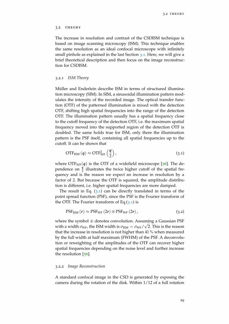
Figure 3.1 Principle of CSDISM 26

Figure 3.2 Principle of ISM 30

Figure 3.3 ISM image reconstruction algorithm 31

Figure 3.4 CSDISM setup 34

Figure 3.5 Trigger signal timing 36

Figure 3.6 Reference measurement 37

Figure 3.7 Reconstruction artifacts 38

Figure 3.8 CSDISM Example 1: Fluorescent beads 41

Figure 3.9 Resolution enhancement factor 41

Figure 3.10 Example 2: Argo-SIM slide 42

Figure 3.11 Multi-color CSDISM image of a fixed cell 44

Figure 3.12 Example 3: 3D multi-color CSDISM 45

Figure 4.1 Orientation factor in FRET 53

Figure 4.2 DNA origami pillar 56

Figure 4.3 FLIM Setup 57

Figure 4.4 Scan image of the sample 58

Figure 4.5 Data analysis 59

Figure 4.6 MIET curve for the pillar experiments 61

Figure 4.7 Results: single labeled pillar 64

Figure 4.8 3D-DNA-PAINT experiment 66

Figure 4.9 MIET curve error 68

Figure 4.10 On-times of the filtered T2 data 71

Figure 4.11 Lifetime Histograms of T2 72

Figure 4.12 Height histograms of T2 72

Figure 4.13 Distance histograms of T2 74

Figure 4.14 Simulation of the T2 pillar lifetime fitting 75

Figure 4.15 Protection from photobleaching by MIET 76

Figure 4.16 Height histogram of B2 and layer thickness es-timation 78

Figure 4.17 T3 measurement 80

Figure 4.18 Localization of three emitters 82

Figure 4.19 Summary of the smMIET experiments on theDNA origami pillar 84

Figure 4.20 smMIET combined with DNA-PAINT 88

Figure 5.1 Dead-time effects in different TCSPC schemes 94

Figure 5.2 Schematic of possible effects of detector andelectronics dead-time 96

Figure 5.3 Schematic of two successive photon recordingevents 97

Figure 5.4 Monte Carlo Simulation with dead-time 99

Figure 5.5 Inter-photon time distribution 100

Figure 5.6 Autocorrelation function 103

Figure 5.7 Setup for FLIM and solution measurements 107

Figure 5.8 Dead-time correction of simulated data 109

Figure 5.9 Measured TCSPC histograms and correction110

Figure 5.10 Dead-time correction: solution 111

Figure 5.11 FLIM of a cell with high laser power 112

Figure 5.12 FLIM of a cell with low laser power 114

Figure 5.13 FLIM of a cell – line plots 115

Figure A.1 Cell–Substrate Dynamics of EMT 122

Figure A.2 Quantifying Microsecond Transition Times us-ing FLCS 124

Figure A.3 Multi-Target Exchange-PAINT with Nanobodies 126

L I S T O F TA B L E S

Table 4.1 Microscope Resolution 51

Table 4.2 Layers for MIET curve calculation 61

Table 4.3 Heights of single labeled pillars 65

Table 4.4 Heights of dual labeled pillars 73

Table 4.5 Height difference T2 74

Table 4.6 Heights T3 81

Table 4.7 Height difference T3 83

A C R O N Y M S

NA Numerical Aperture

QY Quantum Yield

TCSPC Time-Correlated Single Photon Counting

CSD Confocal Spinning Disk

ISM Image Scanning Microscopy

CSDISM Confocal Spinning Disk Image Scanning Microscopy

PSF Point Spread Function

OTF Optical Transfer Function

SIM Structured Illumination Microscopy

AOTF Acousto-Optical Tunable Filter

FPGA Field-Programmable Gate Array

DMD Digital Micromirror Device

MIET Metal-Induced Energy Transfer

smMIET single-molecule Metal-Induced Energy Transfer

FRET Förster Resonance Energy Transfer

DNA-PAINT DNA Points Accumulation for Imaging in NanoscaleTopography

STED Stimulated Emission Depletion

RESOLFT Reversible Saturable Optical Fluorescence Transitions

STORM Stochastic Optical Reconstruction Microscopy

PALM Photoactivation Localization Microscopy

TIR Total Internal Reflection

TIRF Total Internal Reflection Fluorescence

vaTIRF variable angle TIRF

SAF Supercritical Angle Fluorescence

SEM Standard Error of the Mean

FWHM Full Width at Half Maximum

acronyms

FLIM Fluorescence Lifetime Imaging

SPAD Single-Photon Avalanche Diode

APD Avalanche Photodiode

PMT Photomultiplier Tube

CFD Constant Fraction Discriminator

TDC Time-to-Digital Converter

TAC Time-to-Analog Converter

ADC Analog-to-Digital Converter

TTTR Time-Tagged Time-Resolved

(E)GFP (Enhanced) Green Fluorescent Protein

FLCS Fluorescence Lifetime Correlation Spectroscopy

EMT Epithelial-to-Mesenchymal Transition

xvi

1I N T R O D U C T I O N

Fluorescence microscopy has become a powerful tool in modern biol-ogy and medicine [6, 7]. The high sensitivity of fluorescence detectiontogether with the high specificity of labeling allows studying livingand fixed cells in terms of structure and dynamics. However, fluores-cence microscopy is limited by the diffraction of light, rendering alldetail smaller than about 200 nm invisible. Many cellular structuresare smaller and many cellular processes are carried out by moleculesonly a few nanometers in size. Huge efforts have been made to over-come this limitation. In the last thirty years, the field has seen tremen-dous advances by the detection of single fluorescent molecule [8, 9]and the development of superresolution techniques [10–13]. Singlemolecule techniques have allowed for example to track labeled pro-teins within cells with nanometer precision [14] and superresolutionmicroscopy techniques have looked at cellular structures with un-precedented detail [15–17]. Spectroscopic techniques such as Försterresonance energy transfer (FRET) have allowed to study biomoleculesof a few nanometers in size and advanced our understanding ofthe structure and function of the cellular machinery at the singlemolecule level [18, 19].

Improving the spatial resolution of fluorescence microscopy is of-ten a trade-off against the speed or the complexity of the method.The complexity of a method is connected to the alignment and main-tenance required to operate the system and to the availability andcost of the equipment needed. The speed of a method is importantfor high-throughput screening applications which aim at optimizingthe data collection efficiency [20, 21]. Furthermore, it is connected tothe time resolution (e.g. the frame rate) which is crucial for followingfast processes within living cells.

The challenge of fluorescence microscopy today is to resolve finestructures within the cell at the detail of cellular machinery. The de-mand to optical microscopy and spectroscopy is thus to develop tech-niques that enable measurements with high resolution in space andtime, and are low in complexity to be widely applied. In this work,we present three techniques that each improve the resolution in adifferent direction:

• Image Scanning Microscopy (ISM) improves the lateral resolu-tion of a confocal microscope. We present an ISM upgrade fora confocal spinning disk system which is easy to implement,improves resolution and contrast, and offers fast image acquisi-tion.

introduction

• Metal-induced energy transfer (MIET) is used to resolve singleemitters along the optical axis. With this method, emitters canbe localized with nanometer precision on the optical axis withina range of more than 100 nm and it has the potential to measureintra-molecular distances of large biomolecular complexes.

• A dead-time correction algorithm enables the accurate determi-nation of fluorescence lifetimes even at high count rates. Be-cause the dead-times induce distortions of the measured fluo-rescence decay, this limited the acquisition speed of fluorescencelifetime imaging (FLIM). The correction allows FLIM imaging athigher frame rates, i.e. recording data at higher time resolution.

With these three techniques, we expand the toolbox of fluorescencemicroscopy and spectroscopy and tackle the challenge for higher re-solution.

2

2F U N D A M E N TA L S

In this chapter, we lay the theoretical foundations for the thesis. Westart with a general motivation on fluorescence and then explain thephysical background and some key parameters such as the fluores-cence lifetime and quantum yield. Following this, we introduce timecorrelated single photon counting (TCSPC) which we examine indepth with respect to its accuracy at high count rates in Chapter 5.TCSPC is a technique that allows measuring the fluorescence lifetimewhich is a prerequisite for axial localization using metal-induced en-ergy transfer (MIET) as in Chapter 4. To provide the theoretical back-ground, we give an introduction to the theory of MIET at the end ofthis chapter.

2.1 motivation

Fluorescence is an every-day phenomenon and can be observed innature in living as well as in non-living systems. A fluorescent objecthas the ability to emit light in a different color than it is illuminatedwith. Three examples are listed below:

• Minerals such as calcites (CaCO3) fluoresce in UV to visiblelight. The source of the fluorescence are impurities in the crys-tal. These ions are called activators and determine the emissionspectrum. Manganese (Mn2+) is the most common source forthe red to orange fluorescence of calcite under UV light. Otherimpurities such as iron or copper may also act as quencherand prevent fluorescence. The fluorescent properties can helpto identify origin or composition of a mineral [22].

• The jellyfish species Aequorea victoria is famous for its biolumi-nescence. The protein aequorin can emit flashes of blue lightwhen stimulated by calcium ions. The so-called green fluores-cent protein (GFP) converts it into green light that can be seen asa glowing ring around the margin of the jellyfish. Although thebiological function of the bioluminescence is not well known,GFP has become famous for many biochemical applications.It is widely used for example in cell biology to study proteinexpression and in biophysics to label cell structures of inter-est [23].

• Quinine is probably best known for its use as a malaria drugand as an ingredient of tonic water. The substance can be iso-lated from the bark of cinchona trees and its fluorescence has

fundamentals

been described already in 1845 by Sir John Herschel which makesit the first known fluorophore [24]. It absorbs UV light (around350 nm) and fluoresces in bright blue (around 460 nm). Likemost organic dyes, quinine has an aromatic ring structure thatis responsible for the fluorescence. Electrons in aromatic ringsare delocalized in molecular π orbitals, making it an ideal struc-ture for a Hertzian dipole which is the most simple theoreticalmodel of an emitter (see also Section 2.4.1).

The fluorescence can be used to label structures of interest in cellsor in biomolecular complexes. The already mentioned GFP can begenetically encoded into proteins, and organic fluorophores can bechemically bound to structures of interest or to antibodies, which inturn bind to structures of interest. The fluorescence signal then isspecific to the structures of interest and can be measured with highsensitivity. With appropriate filters in the illumination and detectionside of a microscope, the fluorescence from different components canbe distinguished and viewed separately. This is important to visual-ize the interplay of cellular processes and structures. New develop-ments such as superresolution methods have allowed to view cellularmachinery and structure in fixed and living cells at unprecedenteddetail and enabled researchers to ask entirely new questions in bio-logical research [16, 17, 25–27]. In summary, fluorescence microscopyhas become an indispensable tool for biological research. In the fol-lowing section, we will look at fluorescence in more detail.

2.2 fluorescence

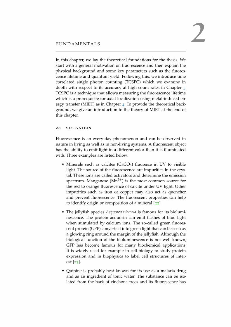
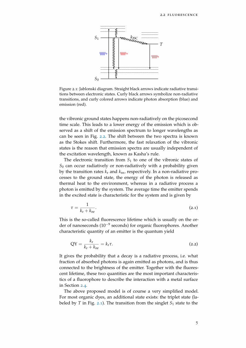
Fluorescence is the process of light absorption and re-emission. Lightas a form of energy can be transmitted only in quantized energy por-tions, the photons. In the quantum mechanical picture, a fluorescentemitter can be seen as an energetic two state system. The system isexcited into the higher energetic state by the absorption of a photon.When the system returns back into its ground state, the energy can bereleased in form of a fluorescent photon (radiative transition). Alter-natively, the energy is dissipated into heat or transfered into anotherexcited state and no photon is emitted (non-radiative transition). Thismodel is visualized in a Jablonski diagram, see Fig. 2.1. A state isdisplayed as a vertical line and transitions between the states by ar-rows. Because electrons in the fluorescent material interact with thelight, the main states are called electronic states. The transition of thesinglet ground state S0 to the first excited state S1 requires the ab-sorption of a photon with an energy equal to the energy difference ofthe two states. However, the electronic states have additional vibronicsubstates which allow many more transitions with slightly differentenergies. Additionally, thermal fluctuations can slightly shift the ener-getic states which is the reason that the absorption spectra are broadas for example in Fig. 2.2. Relaxation of the excited vibronic states into

4

2.2 fluorescence

S0

S1

T

kISC

Figure 2.1: Jablonski diagram. Straight black arrows indicate radiative transi-tions between electronic states. Curly black arrows symbolize non-radiativetransitions, and curly colored arrows indicate photon absorption (blue) andemission (red).

the vibronic ground states happens non-radiatively on the picosecondtime scale. This leads to a lower energy of the emission which is ob-served as a shift of the emission spectrum to longer wavelengths ascan be seen in Fig. 2.2. The shift between the two spectra is knownas the Stokes shift. Furthermore, the fast relaxation of the vibronicstates is the reason that emission spectra are usually independent ofthe excitation wavelength, known as Kasha’s rule.

The electronic transition from S1 to one of the vibronic states ofS0 can occur radiatively or non-radiatively with a probability givenby the transition rates kr and knr, respectively. In a non-radiative pro-cesses to the ground state, the energy of the photon is released asthermal heat to the environment, whereas in a radiative process aphoton is emitted by the system. The average time the emitter spendsin the excited state is characteristic for the system and is given by

τ =1

kr + knr. (2.1)

This is the so-called fluorescence lifetime which is usually on the or-der of nanoseconds (10−9 seconds) for organic fluorophores. Anothercharacteristic quantity of an emitter is the quantum yield

QY =kr

kr + knr= krτ. (2.2)

It gives the probability that a decay is a radiative process, i.e. whatfraction of absorbed photons is again emitted as photons, and is thusconnected to the brightness of the emitter. Together with the fluores-cent lifetime, these two quantities are the most important characteris-tics of a fluorophore to describe the interaction with a metal surfacein Section 2.4.

The above proposed model is of course a very simplified model.For most organic dyes, an additional state exists: the triplet state (la-beled by T in Fig. 2.1). The transition from the singlet S1 state to the

5

fundamentals

Figure 2.2: Spectrum of Atto 647N in PBS. The blue curve shows the ab-sorption spectrum of the dye and the red curve the emission spectrum. Thepeak of the emission is shifted to longer wavelengths which is known as theStokes shift. Data provided by the manufacturer (ATTO-TEC).

triplet state is called inter-system crossing (ICS) and occurs with arate kICS. Because the transition requires a spin change it belongs tothe so-called forbidden transitions. In practice, there is still a smallprobability of the transition to occur, resulting in transition rates be-tween the singlet and the triplet states that are several orders of mag-nitude smaller than the rates between the singlet states. The averageresidence time in the triplet states is on the order of microseconds tomilliseconds during which the emitter is dark. This is often referredto as blinking.

Because the rate for inter-system crossing is orders of magnitudesmaller than the fluorescent rate, we can approximate fluorescence asa two state system. Then, the probability that the system is still in thefirst excited state S1 after some time t is given by

p(t) =1τ

e−tτ , (2.3)

where τ is the average time in the excited state as given in Eq. (2.1).The fluorescent lifetime can be measured by exciting the molecule

with a short laser pulse and measuring the time t until a photon isemitted. The arrival time t follows the probability distribution of afluorescence decay according to Eq. (2.3). The average arrival time isthen an estimator of the fluorescence lifetime:

〈t〉 =∫ ∞

0dt tp(t) = τ. (2.4)

The uncertainty of this measurement is στ =√〈t2〉 − 〈t〉2 = τ. Re-

peating the measurement N times reduces the uncertainty of the life-time to

∆τ =τ√N

. (2.5)

This is a simplification because in an experiment one has to accountfor different factors such as a background or the finite response time

6

2.2 fluorescence

of the photon detector. Therefore, the lifetime is usually determinedin a different way: A histogram of arrival times is fitted with I(t) =A · p(t) + b as fit function, where A is the amplitude of the fluores-cence decay and b the background. However, Eq. (2.5) is still a goodapproximation of the error as it provides a lower bound for the er-ror of a fluorescence lifetime measurement. Experimentally, the mea-surement can be realized by time correlated single photon counting(TCSPC) and will be explained in detail in the next section.

7

fundamentals

2.3 time correlated single photon counting

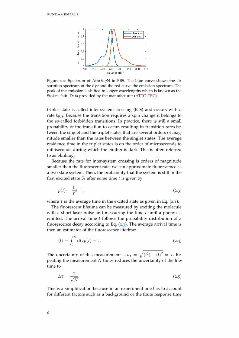
With the advent of pulsed lasers and single-photon sensitive detec-tors, time-resolved spectroscopy has become an important tool in thelife sciences, fundamental physics, and chemistry. The sample is il-luminated with a short laser pulse and the time-dependent intensitydecay of the sample is recorded. The direct recording of this decay isvery challenging: Fast processes on the order of nanoseconds requirea high time resolution on the order of picoseconds which cannot beachieved with traditional photodiodes and amplifiers. Furthermore, ahigh number of photons is required to observe the whole decay afterone excitation cycle which, for example, is impossible to obtain froma single emitter. Time Correlated Single Photon Counting (TCSPC)solves these problems by exciting the sample with a periodic trainof laser pulses. This extends the observation over multiple excitationand emission cycles and the decay can be reconstructed from all sin-gle photon events collected over many cycles. The photon flux on thedetector can be orders of magnitude less than the repetition rate ofthe laser. Each detector signal indicates the arrival of a single pho-ton which is recorded as a time stamp with respect to the laser pulse.Only by recording a large number of these events and histogrammingthe arrival times, the periodic signal is recovered. See Fig. 2.3 for anillustration of this principle for the measurement of a fluorescencelifetime decay.

102

104

lase

rpr

obab

ility

phot

ons

0 1 2 3 4 5 6 7 8 9 100123

time0 1

Figure 2.3: TCSPC principle. Top row: A pulsed laser excites fluorescence.The probability of a fluorescence decay is shown in the row below (in loga-rithmic scale). Less than one photon is detected in one excitation period onaverage. The detected photons (red dots) are histogrammed (bottom row).Each excitation period shows the full histogram with new photons in red.Right: After many excitation periods, the histogram resembles the decayprobability.

8

2.3 time correlated single photon counting

Figure 2.4: A minimal TCSPC setup: A pulsed laser (left) excites fluorescencein the sample which is detected by a fast single-photon counter. Both thelaser and the detector are connected to the TCSPC electronics which recordsthe time difference between the laser pulse and the detected photon.

Single-photon arrival times can be recorded at much higher timeresolution than analog intensity recording with a precision up to pi-coseconds. TCSPC can then be used to measure the fluorescence life-time by using a repetition rate smaller than the inverse of the fluo-rescence lifetime. Apart from spectroscopy, an important applicationof TCSPC is ranging with light (lidar) [28]: The reflected light from atarget is measured and the return time is proportional to the distance.Combined with a laser scanning setup, this can be used to make a 3Drepresentation of the target and is employed, for example, to makehigh-resolution maps in geodesy [29] or for control and navigationfor autonomous cars [30].

2.3.1 TCSPC Hardware

A TCSPC setup consists of a pulsed excitation source and a detectorwhich both are linked to the TCSPC electronics, see Fig. 2.4. The exci-tation source provides a reference signal given by the repetition rateof the light pulses, the so-called sync. The detector provides an elec-trical pulse for each photon that it detects. In the TCSPC electronics,both signals are processed and photon events are eventually storedin a computer.

detectors Detectors generate an electrical signal proportional tothe incoming light flux. For single-photon counting applications, thedetectors generate an electrical pulse upon the incidence of a sin-gle photon. Thus, detectors for photon counting applications needto have a high gain in order to produce a useful signal for the TCSPCelectronics from a single photon. The signal is usually a short pulsewhere the width limits the minimum distance between two arrivingphotons, thus limiting the count rate. The minimum time between

9

fundamentals

two successive signals is also called the dead-time of the detector.However, for the timing precision of the TCSPC measurement, thetiming jitter or the transit time spread (TTS) of the pulse is moreimportant than the pulse shape. Because the TTS is typically muchsmaller than the response signal of the detector, TCSPC has a muchbetter timing resolution in contrast to analog techniques that recordthe photo-response of the detector directly [31].

Typical detector types are the photomultiplier tube (PMT) and thesingle-photon avalanche photodiode (SPAD), and all detector typeshave their individual strengths and shortcomings. For example, thecounting efficiency of PMTs is typically in the range of 10 % to 40 %,limited by the frequency a photo-electron is generated by an incidentphoton (the so-called quantum efficiency). For SPADs, the quantumefficiency can be > 70 %, but a smaller active area makes focusing thelight on the SPAD more challenging [32]. Typical values for the dead-time are in the tens of nanoseconds range, limiting the count rate toa few tens of MHz. The timing jitter in SPADs is mainly due to thedifferent depth in which photons are absorbed, resulting in differenttimes for the avalanche built-up [33], and is on the order of 100 ps. Acomprehensive review on PMTs, SPADs, and more detector types canbe found in Ref. [32].

tcspc electronics The TCSPC electronics converts the outputpulses of the detector and an external sync into a timing information.The most important building block in modern TCSPC hardware isthe time-to-digital converter (TDC), an electronic timer. It is typicallybased on a crystal oscillator and converts a time into a digital output.Because the output pulses of the detector may have different ampli-tudes, a constant fraction discriminator (CFD) ensures triggering ata constant fraction of the pulse amplitude and produces a normedsignal for the TDC [34]. Instead of an TDC, older TCSPC hardwaretypically use a time-to-amplitude converter (TAC) together with ananalog to digital converter (ADC). When the TAC is activated, theTAC charges a capacitor until stopped. The charge in the capacitoris proportional to the time between start and stop of the TAC andis read out and converted into a digital signal by the ADC. Duringthe time of the capacitor discharge and the read-out, the TCSPC elec-tronics is unable to process further events. We refer to this as theelectronic dead-time. If the dead-time is much shorter than the aver-age time between two photons, TCSPC reaches a near ideal countingefficiency. In particular, the efficiency is much higher than for gatedtechniques which shift a time-gate over the periodic signal (see forexample Ref. [24, Chapter 4]).

10

2.3 time correlated single photon counting

tsync tphoton

Figure 2.5: TCSPC scheme. Laser pulses (black bars) excite the sample andstart a timer. The arrival of a photon (red circle) stops the timer. The mea-sured time t = tsync − tphoton is used for the TCSPC histogram.

2.3.2 TCSPC Schemes

TCSPC records the the arrival time of a photon tphoton with respectto a sync signal tsync. In Fig. 2.5, the vertical bars mark the beginningof a new period from the sync signal. A photon is symbolized bya circle and the arrival time of a photon relative to the laser pulset = tsync − tphoton is recorded. In a classical TCSPC system, this isrealized by starting a timer at each sync event and stopping it at thearrival of a photon and called “forward start-stop TCSPC”. With theadvent of pulsed laser with repetition rates in the MHz regime, thisapproach became unfeasible: Because in most excitation periods nophoton is detected, the TDC needs to be reset at each sync signal.Photons detected during the dead-time of the electronics would bediscarded, thus limiting the count rate and making the system lessefficient. To avoid this, TCSPC electronics can be operated in reversemode. Here, the arrival of a photon starts the timer and the nextsync stops it. This avoids unnecessary resets of the TDC, and theconversion rate of the timer is equal to the count rate which is usuallymuch smaller than the repetition rate. Care has to be taken if therepetition rate of the laser is unstable. Then, the reference pulses fromthe light source need to be shifted, so that they arrive after the pulsesfrom the detector. Furthermore, the time axis of the histogram needsto be internally reversed to obtain the decay [35].

Recent TCSPC electronics works in forward start-stop mode, butwith an independent timing of the photons and the sync signal [36].This works even with lasers with high repetition rates because a di-vider in front of the sync input reduces the input rate so that theperiod is at least as long as the dead-time of the TDC. Internal logicdetermines the sync period and re-calculates the sync signals thatwere divided out. Because the photon TDC is independent of the syncTDC, no photon events are discarded as in classical forward TCSPC.If a photon is detected, the times tphoton and tsync of the two TDCs areused to calculate the time difference t = tsync− tphoton internally. Thisallows – in principle – to detect several photons per excitation periodan furthermore to record the absolute times with respect to the startof the experiment, as described below.

11

fundamentals

tttr scheme The time t is also called the micro time and is dis-tinguished from the global arrival time with respect to the start ofthe experiment, the macro time. Modern TCSPC hardware allows thesimultaneous recording of both times, so that not only the TCSPC his-togram can be constructed, but also the time trace of the count ratewith high time resolution [37]. The macro time is usually recorded onthe coarser timescale of the sync, tsync. In this so-called time-taggedtime-resolved (TTTR) data format, a stream of events is stored consec-utively where each record consists of the arrival times (micro time tand macro time tsync) together with information such as the detectionchannel. Additional records can be added to synchronize the datastream to the experiment. These so-called markers are for exampleused in a scanning confocal microscope to indicate a line change orthe end of a frame. Later, each photon can be assigned to a line anda pixel number and an intensity image can be constructed. TCSPChistograms in a single pixels can be used to estimate the fluorescencelifetime, enabling Fluorescence Lifetime Imaging (FLIM). The TTTRrecording scheme is thus a valuable extension to the above discussedTCSPC schemes and allows to follow processes from picoseconds toseconds in a single measurement.

TTTR is useful for a multitude of techniques in the life sciencessuch as Fluorescence Correlation Spectroscopy (FCS) [38], Fluores-cence Lifetime Correlation Spectroscopy (FLCS) [39, 40], photon-arrival-time interval distribution (PAID) [41, 42], and others. Furthermore,photon counting and antibunching experiments are extensively usedin quantum optics experiments and quantum sensing [43].

12

2.4 theory of metal-induced energy transfer

2.4 theory of metal-induced energy transfer

Metal-induced Energy Transfer (MIET) describes the phenomenonthat a fluorescent emitter is quenched by a metal surface. Experimen-tal studies by Drexhage, Kuhn, and Schäfer in 1968 showed how thefluorescent lifetime of phosphorescent europium chelate complexeschanges in proximity to a metal mirror [44]. Their model included theinterference of the reflected wave with the electric field of the emitterwhich was in agreement to the oscillations of the radiative rate theyobserved. It failed however at distances shorter than the wavelength,where the emitters are quenched due to non-radiative energy transferfrom the excited molecule to the metal.

The interaction of a dipole in close proximity to a metal surface hasbeen described theoretically by Kuhn where the dipole is consideredas a damped oscillator and involves the calculation of the reflectedfield at the dipole’s position [45]. A few years later, Chance, Prock andSilbey developed a comprehensive description of the energy trans-fer from a dipole emitter to a metal surface which they termed theenergy-flux method [46]. This theory allows to separate the energyflux into the bottom and top half-spaces and gives the exact amountof radiation that propagates through a thin semi-transparent metalfilm. In contrast to the experiments by Drexhage and coworkers whoused a thick metal mirror, the use of a thin metal film allows somepart of the radiation to propagate into the dielectric medium be-low. This enables the optical detection of fluorescence through themetal film which was experimentally demonstrated by Amos andBarnes [47]. A few years later, the detection of single molecules througha metal film was reported [48]. The quenching of the fluorescence dueto the interaction with the metal film has then been used to measurenanometer axial distances [49]. Recently, the localization of singlefluorescent emitters along the optical axis with a precision of about3 nm has been demonstrated [50].

An excellent introduction on the physics and the mathematical de-scription of an oscillating dipole in the context of MIET is given inRef. [51]. In the following, we briefly state the main points and dis-cuss how the properties of an emitter such as fluorescent lifetime orbrightness are changed close to a metal surface.

2.4.1 Oscillating Dipole

An oscillating dipole is a fundamental source of electromagnetic ra-diation: a charge oscillating along a line. The charge generates anelectric field in space and the oscillations lead to changing electricand magnetic fields, an electromagnetic wave. The emission of manyfluorescent molecules can be well described by such a dipole emitter.

We begin by recalling the electric field of a static dipole. The dipoleconsists of two opposite charges q with a distance d apart and is

13

fundamentals

characterized by its electric dipole moment p = qd. The embeddingmedium is described by its permittivity ε which can be thought of asthe microscopic polarizability of the medium. The electric field of thestatic dipole is given by

E(r) =3(r · p)r− p

εr3 , (2.6)

where r is the position, r = |r|, and r = rr . When the charges oscillate

with a frequency ω, the electric field becomes a function of time. Ifwe switch to polar coordinates and assume that the dipole is orientedalong the polar axis, we can write the electric field as

E(r) = k20k[(−1− 3i

kr+

3(kr)2

)(r · p)r +

(1 +

ikr− 1

(kr)2

)p]

eikr

kr(2.7)

where k = k0n, k0 = ωc = 2π

λ with the velocity of light c is thewave vector in vacuum, and n =

√ε is the refractive index. The time

evolution of the field of the oscillating dipole is given by multiply-ing E(r) with the phase factor e−iωt. Although all of the terms ex-tend to infinity, only a part of it actually transports energy. The totalenergy flux is given by the time-averaged Poynting vector S(r) =

c8π< E× B∗, where < denotes the real part and ∗ denotes com-plex conjugation. The magnetic field corresponding to Eq. (2.7) canbe computed by means of Maxwell’s equation in free space fromiωB(r, t) = ∇× E(r, t) [52].

Although the emitted energy is constant at any distance from thedipole, it is spread over an area that increases with distance. Thesurface area of a sphere with radius r around the dipole will increasewith r2, thus all terms that fall off faster than r2 will not contributeto the energy flux far away from the emitter. One can show that thecontributing terms in Eq. (2.7) are proportional to r−1. These termsare called the far-field and correspond to the part of the field thatcontribute to the energy transport. In contrast to the far-field, one canalso define a near-field. Close to the dipole, the term r−3 dominatesthe electric field and is thus called the near-field of the dipole. In thestatic limit k → 0 the whole field reduces to the near field term andis equal to the field of the static dipole in Eq. (2.6).

For the radiation that can be detected optically, we usually considerthe far-field. We can neglect components in E and B that fall off fasterthan r−1 and compute the Poynting vector as

S =cnk4

08πr2 r

(|p|2 − (rp)2) = cnk4

08πr2 p2 sin2(θ)r, (2.8)

where the last equal sign holds true when the dipole axis is orientedalong the polar axis. The power radiated in a solid angle elementdΩ = dφ sin(θ)dθ is

d2SdΩ

= r2S =cnk4

08π

p2 sin2(θ), (2.9)

14

2.4 theory of metal-induced energy transfer

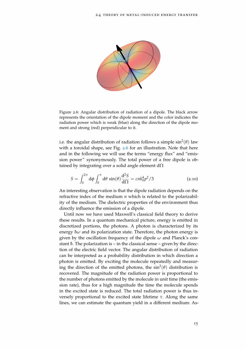
Figure 2.6: Angular distribution of radiation of a dipole. The black arrowrepresents the orientation of the dipole moment and the color indicates theradiation power which is weak (blue) along the direction of the dipole mo-ment and strong (red) perpendicular to it.

i.e. the angular distribution of radiation follows a simple sin2(θ) lawwith a toroidal shape, see Fig. 2.6 for an illustration. Note that hereand in the following we will use the terms “energy flux” and “emis-sion power” synonymously. The total power of a free dipole is ob-tained by integrating over a solid angle element dΩ

S =∫ 2π

0dφ∫ π

0dθ sin(θ)

d2SdΩ

= cnk40 p2/3 (2.10)

An interesting observation is that the dipole radiation depends on therefractive index of the medium n which is related to the polarizabil-ity of the medium. The dielectric properties of the environment thusdirectly influence the emission of a dipole.

Until now we have used Maxwell’s classical field theory to derivethese results. In a quantum mechanical picture, energy is emitted indiscretized portions, the photons. A photon is characterized by itsenergy hω and its polarization state. Therefore, the photon energy isgiven by the oscillation frequency of the dipole ω and Planck’s con-stant h. The polarization is – in the classical sense – given by the direc-tion of the electric field vector. The angular distribution of radiationcan be interpreted as a probability distribution in which direction aphoton is emitted. By exciting the molecule repeatedly and measur-ing the direction of the emitted photons, the sin2(θ) distribution isrecovered. The magnitude of the radiation power is proportional tothe number of photons emitted by the molecule in unit time (the emis-sion rate), thus for a high magnitude the time the molecule spendsin the excited state is reduced. The total radiation power is thus in-versely proportional to the excited state lifetime τ. Along the samelines, we can estimate the quantum yield in a different medium: As-

15

fundamentals

suming that the radiative rate changes proportionally to the emissionpower of a dipole, we find

QY = QY0nn0

τ

τ0, (2.11)

where the subscript 0 denotes the known quantum yield and fluores-cent lifetime in a medium with refractive index n0.

2.4.2 Electric Field of a Dipole Near a Metal Surface

We have already seen that the environment (i.e. the refractive indexof the medium) can have an influence on the dipole’s emission prop-erties. When a dipole emitter is placed in the vicinity of a dielectric ormetallic surface, its local environment is not altered, but at each inter-face the electro-magnetic (EM) waves can be reflected or transmitted.Reflected waves will interfere with the waves emitted by the dipole,changing the electric field. Furthermore, the near-field of the emittercan couple to the metal and transfer energy which again changes theemission properties, as we will see. Also the propagation of the EMwaves is affected: Inside a metal, the energy of an EM wave is attenu-ated by absorption. This is reflected in the non-zero imaginary part ofthe refractive index of a metal. As above, we will start the descriptionwith the electric field and use it to calculate the energy flux.

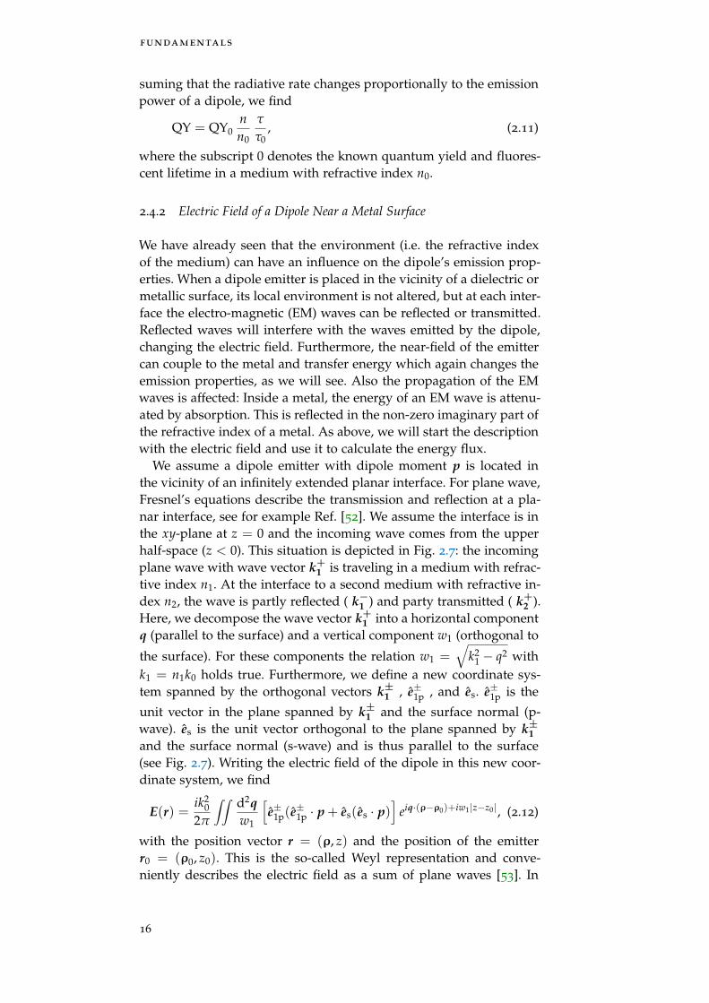
We assume a dipole emitter with dipole moment p is located inthe vicinity of an infinitely extended planar interface. For plane wave,Fresnel’s equations describe the transmission and reflection at a pla-nar interface, see for example Ref. [52]. We assume the interface is inthe xy-plane at z = 0 and the incoming wave comes from the upperhalf-space (z < 0). This situation is depicted in Fig. 2.7: the incomingplane wave with wave vector k+

1 is traveling in a medium with refrac-tive index n1. At the interface to a second medium with refractive in-dex n2, the wave is partly reflected ( k−

1 ) and party transmitted ( k+2 ).

Here, we decompose the wave vector k+1 into a horizontal component

q (parallel to the surface) and a vertical component w1 (orthogonal to

the surface). For these components the relation w1 =√

k21 − q2 with

k1 = n1k0 holds true. Furthermore, we define a new coordinate sys-tem spanned by the orthogonal vectors k±

1 , e±1p , and es. e±1p is the

unit vector in the plane spanned by k±1 and the surface normal (p-

wave). es is the unit vector orthogonal to the plane spanned by k±1

and the surface normal (s-wave) and is thus parallel to the surface(see Fig. 2.7). Writing the electric field of the dipole in this new coor-dinate system, we find

E(r) =ik2

02π

∫∫ d2qw1

[e±1p(e

±1p · p + es(es · p)

]eiq·(ρ−ρ0)+iw1|z−z0|, (2.12)

with the position vector r = (ρ, z) and the position of the emitterr0 = (ρ0, z0). This is the so-called Weyl representation and conve-niently describes the electric field as a sum of plane waves [53]. In

16

2.4 theory of metal-induced energy transfer

n1

n2

ezey

ex

k−1

k+1

e+1p

e−1pes

es

q

w1

k+2

ese+2p

Figure 2.7: Geometry of a plane wave refracted at a planar interface. Anincoming wave with wave vector k+

1 is traveling in a medium with refractiveindex n1. At the interface to a second medium with refractive index n2, thewave is partly reflected ( k−

1 ) and party transmitted ( k+2 ). The coordinate

system is chosen so that the interface is in the xy-plane and ez parallel tothe surface normal.

this representation we can apply Fresnel’s theory to obtain the ampli-tude of the electric field of the reflected and transmitted waves. Forthe transmitted wave, the Fresnel coefficients are

Tp =2n2n1w1

w2n21 + w1n2

2and Ts =

2w1

w1 + w2(2.13)

for p-waves and s-waves respectively. Thus, the electric field of thetransmitted wave is given by

ET(r) =ik2

02π

∫∫ d2qw1

[Tpe±1p(e

±1p · p + Tses(es · p)

]eiq·(ρ−ρ0)+iw1|z−z0|.

(2.14)

Similarly, the result for the reflected wave can be obtained. With thisresult, we are able to calculate the electric field on both sides of theinterface: Below the interface it consists simply of the transmittedelectric field (Eq. (2.14)), but above the interface, one has to take intoaccount that the electric field is the superposition of the reflected fieldand the field of the free dipole, Eq. (2.7). With this result, we are ableto calculate the Poynting vector S as in the previous section. Since weare interested in the total energy flux only, we project the Poynting

17

fundamentals

vector on z and integrating over an area A, which encloses the dipoleand is parallel to the interface. The energy flux through A is then

SA =c

8π<∫∫

dA z · (E× B∗)

, (2.15)

where B can be obtained from iωB = ∇ × E as before. Using thetransmitted electric field according to Eq. (2.14) at the interface (z = 0)and extending the area A to infinity, we obtain the energy flux intothe lower medium which we will denote as S↓. Note that becauseof energy conservation, the result is identical if one uses the electricfield in the lower half-space (between the interface and the emitterposition) at the interface.

The total emission power S is obtained from the electric field at theposition of the dipole z = z0. One can either use the electric field inthe upper or in the lower half-space, yielding the same result.

We will now simply quote the emission powers into the lowermedium, S↓, and the total emission power S for the limiting casesof a vertical dipole (denoted by ⊥) and a dipole parallel to the sur-face (denoted by ‖). It can be shown that these allow us to calculatethe emission power of a dipole with any (fixed) orientation α withrespect to the surface normal as

S(α, z0) = S⊥(z0) cos2(α) + S‖(z0) sin2(α). (2.16)

The energy flux for a vertical dipole (p = pz) into the lower mediumis

S⊥↓ =ck4

0 p2

4<∫

dqq3n∗1w1

k1|k1w1|2(1− Rp)(1 + R∗p)e

2=w1z0

, (2.17)

with Fresnel’s reflection coefficient Rp for p-waves and = denotingthe imaginary part. The total energy flux of a vertical dipole is givenby

S⊥ =ck4

0 p2

4<∫

dqq3n∗1w1

k1|k1w1|2(

1− Rpe−2iw1z0)

. (2.18)

For a dipole parallel to the surface, one obtains

S‖↓ =ck4

0 p2

8<∫

dqqn∗1

k1|w1|2

[|w1|2

k21

w1(1− Rp)(1 + R∗p)+

w∗1(1− Rs)(1 + R∗s )e2=w1z0

],

(2.19)

and the total energy flux

S‖ =ck4

0 p2

8<∫

dqqn∗1w1

k1|w1|2

[|w1|2

k21

(1 + Rpe−2iw1z0

)+

(1 + Rse−2iw1z0

)].

(2.20)

18

2.4 theory of metal-induced energy transfer

nmetal

θmax

nmedium

nglass

S↑

L↓

S↓

(a) (b)

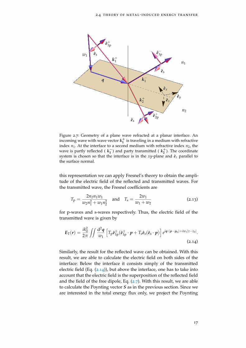
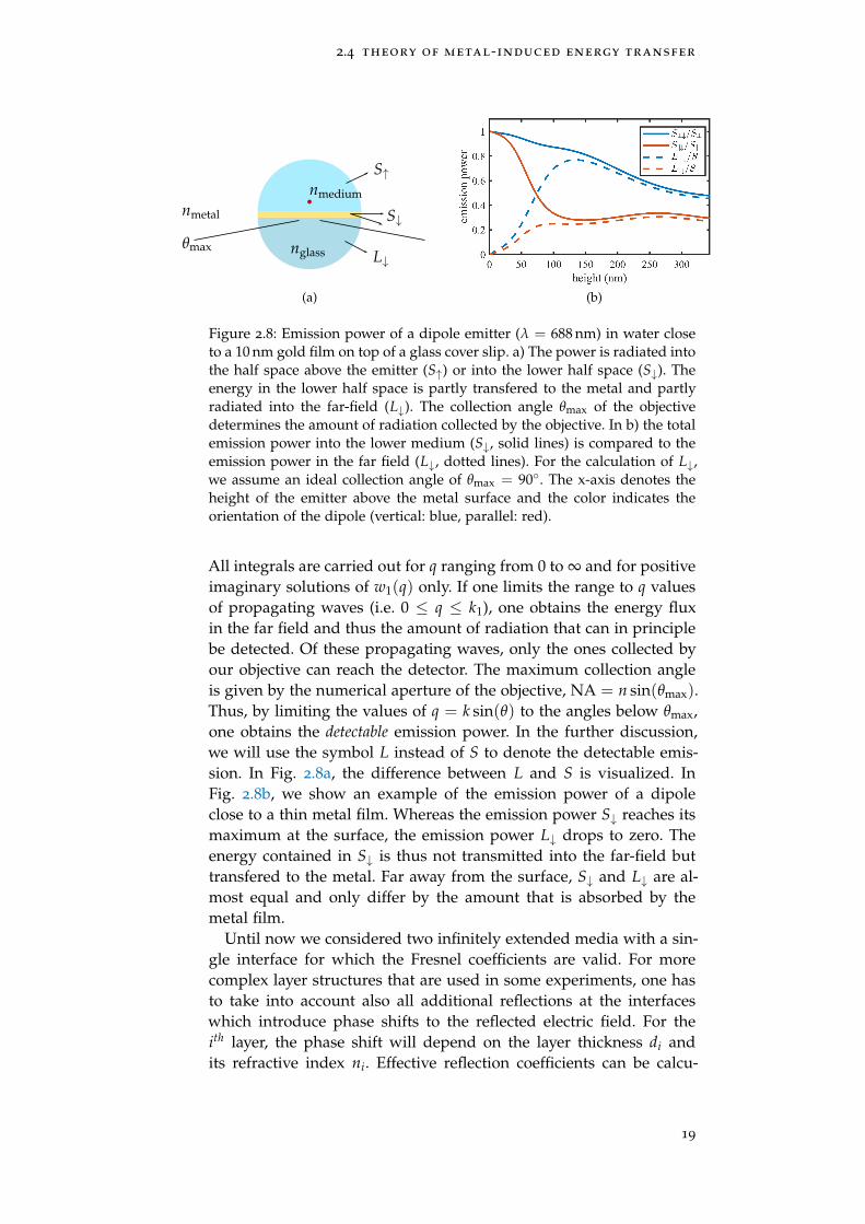
Figure 2.8: Emission power of a dipole emitter (λ = 688 nm) in water closeto a 10 nm gold film on top of a glass cover slip. a) The power is radiated intothe half space above the emitter (S↑) or into the lower half space (S↓). Theenergy in the lower half space is partly transfered to the metal and partlyradiated into the far-field (L↓). The collection angle θmax of the objectivedetermines the amount of radiation collected by the objective. In b) the totalemission power into the lower medium (S↓, solid lines) is compared to theemission power in the far field (L↓, dotted lines). For the calculation of L↓,we assume an ideal collection angle of θmax = 90. The x-axis denotes theheight of the emitter above the metal surface and the color indicates theorientation of the dipole (vertical: blue, parallel: red).

All integrals are carried out for q ranging from 0 to ∞ and for positiveimaginary solutions of w1(q) only. If one limits the range to q valuesof propagating waves (i.e. 0 ≤ q ≤ k1), one obtains the energy fluxin the far field and thus the amount of radiation that can in principlebe detected. Of these propagating waves, only the ones collected byour objective can reach the detector. The maximum collection angleis given by the numerical aperture of the objective, NA = n sin(θmax).Thus, by limiting the values of q = k sin(θ) to the angles below θmax,one obtains the detectable emission power. In the further discussion,we will use the symbol L instead of S to denote the detectable emis-sion. In Fig. 2.8a, the difference between L and S is visualized. InFig. 2.8b, we show an example of the emission power of a dipoleclose to a thin metal film. Whereas the emission power S↓ reaches itsmaximum at the surface, the emission power L↓ drops to zero. Theenergy contained in S↓ is thus not transmitted into the far-field buttransfered to the metal. Far away from the surface, S↓ and L↓ are al-most equal and only differ by the amount that is absorbed by themetal film.

Until now we considered two infinitely extended media with a sin-gle interface for which the Fresnel coefficients are valid. For morecomplex layer structures that are used in some experiments, one hasto take into account also all additional reflections at the interfaceswhich introduce phase shifts to the reflected electric field. For theith layer, the phase shift will depend on the layer thickness di andits refractive index ni. Effective reflection coefficients can be calcu-

19

fundamentals

lated that consist of the Fresnel coefficients and the phase shift. Thesecan be calculated for any number of layers using the transfer-matrixmethod [54]. These effective coefficients replace then the Fresnel co-efficients in Eqs. (2.17) to (2.20) and allow the calculation of S for adipole emitter on top (or even in between) any structure of layeredmedia. More information on the formalism can be found in Refs. [51,53, 54].

2.4.3 Metal-induced Energy Transfer

We have already seen earlier that the emission power of a dipole emit-ter depends on its environment and thereby influences the emissionproperties such as the fluorescent lifetime. We have extended this tothe effect of thin metal films in the proximity of the emitter with theabove derivation. We assume that the emitter’s internal non-radiativerate knr stays constant and only the radiative rate kr (not to be con-fused with the absolute value of the wave vector k in the previoussection) changes according to the emission power S,

kr

kfreer

=S

Sfree. (2.21)

Here, kfreer and Sfree are the radiative rate and the power of a free

dipole in the same medium, i.e. far away from any interface (“freespace”). Sfree = nS0 = cnk4

0 p2/3 was already calculated in Eq. (2.10).Assuming the molecule has a quantum yield QY0 in free space, the

fluorescent rate kr + knr = 1/τ is obtained as

kr(α, z0) + knr

k0r + knr

= 1−QY0 + QY0S(α, z0)

nS0=

τ0

τ(α, z0). (2.22)

Under the same assumption, we can define a local quantum yield

QY(α, z0) =kr(α, z0)

kr(α, z0) + knr

=

(1−

(1

QY0− 1)−1 S(α, z0)

nS0

)−1

= 1− τ(α, z0)

τ0(1−QY0).

(2.23)

In an experimental setting, a fluorescent emitter is often attachedto the object of interest by a flexible linker. In solution, the emitter dif-fuses and randomly rotates. If this rotation diffusion is fast comparedto its fluorescence lifetime, the emitter can be considered isotropic.Its radiating power is obtained by averaging over all possible orienta-tions,

Sr(z0) =12

∫ π

0dθ sin(θ)

[S⊥(z0) cos2(θ) + S‖(z0) sin2(θ)

]=

13

S⊥(z0) +23

S‖(z0).(2.24)

20

2.4 theory of metal-induced energy transfer

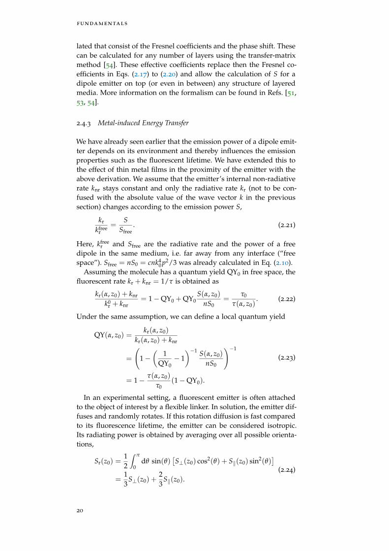
(a) (b)

Figure 2.9: a) Local quantum yield according to Eq. (2.23) of a dipole emitter(λ = 688 nm, QY0 = 0.5) in water close to a 10 nm gold film on top of a glasscover slip. b) Collection efficiency according to Eq. (2.26) of the emissionof a dipole as in a) with a 1.49 NA objective. The collection efficiency isnormalized to the collection efficiency far away from the surface (z = 10λ).The color indicates the orientation of the dipole with blue for vertical, redfor parallel, and yellow for a randomly oriented emitter.

The emitter “samples” all possible orientations and thus decay prob-abilities before the emission of a photon, therefore a rate averaging isappropriate here. This result can be used to calculate the lifetime of aquickly rotating emitter, e.g. a dye with a linker, by plugging the re-sult into Eq. (2.22). Further information on the influence of the dye’srotational diffusion can be found in Ref. [55].

The case is slightly different when we look at an ensemble of ran-domly oriented, but fixed emitters: Then, we measure the superpo-sition of all the emitters’ lifetimes weighted by their brightness. Themeasured average lifetime is

τfixed(z0) =12

∫ π

0dθ sin(θ)τ(θ, z0)b(α, z0). (2.25)

In addition to the rates, we can also estimate the relative bright-ness of an emitter. Assuming a constant excitation rate, the brightnessshould be proportional to the amount of energy the dipole emits. Aswe have seen in Section 2.4.2, The amount of radiated energy we candetect is given by the far-field energy L. This allows us to define thecollection efficiency η, i.e. the probability to collect a photon in thefar field with the objective:

η(α, z0) =L↓(α, z0)

S(α, z0). (2.26)

An example for the collection efficiency is shown in Fig. 2.9b. Notethat the curves are similar to the curves of L↓/S in Fig. 2.8b. Thedifference is that here we take into account the collection angle ofa 1.49 NA objective. Note that the curves are normalized to the col-lection efficiency far away from the surface. The figure shows that

21

fundamentals

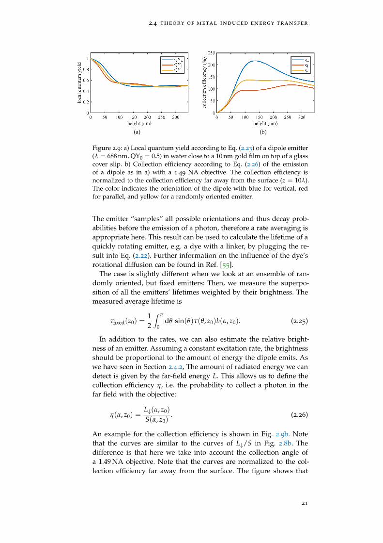
(a) (b)

Figure 2.10: a) Brightness of a dipole emitter (λ = 688 nm, QY0 = 0.5) inwater close to a 10 nm gold film on top of a glass cover slip. b) Emissionchannels of a dipole emitter with the same parameters.

close to the surface the energy transfer to the metal dominates andthe collection efficiency is low. But for vertical dipoles, the collectionefficiency at around λ/4 can be a factor 2 higher than in solution.

The collection efficiency is equal to the brightness if every absorbedphoton is emitted again. However, if the emitter has additional non-radiative decay channels, we need to consider the local quantumyield. The brightness b is then given as the product of the collectionefficiency (Eq. (2.26)) and the local quantum yield (Eq. (2.23))

b(α, z0) ∝ η(α, z0)QY(α, z0). (2.27)

In Fig. 2.10a the brightness is shown for an emitter on top of a thingold film. Because the local quantum yield is increased close to thesurface, the brightness there is larger as one would expect by lookingat the collection efficiency only. Furthermore, the oscillations at far-ther distances due to interference effects, which can be seen in boththe local quantum yield and the collection efficiency, cancel out andlead to an almost constant brightness.

The different emission channels are summarized in Fig. 2.10b. In-ternal non-radiative decay channels of the emitter convert the energyinto heat (purple). This mechanism is strongly suppressed close thesurface (cf. also Fig. 2.9a). There, most of the energy is transfered intothe metal (blue). Only a small part is emitted into the far-field andcan be detected optically (red and orange). The light emitted into theupper half-space or above the collection angle of the objective is lost(orange), but the remaining part can be detected (red). Although thelosses seem very high, the collection efficiency is actually comparableand can even be larger than far away from the surface as we haveseen in Fig. 2.9b.

22

2.4 theory of metal-induced energy transfer

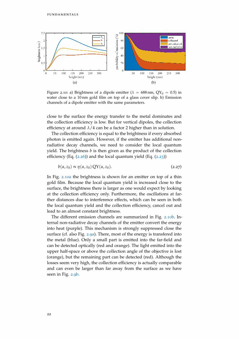
(a) (b)

Figure 2.11: Angular distribution of radiation d2S↓dΩ (r, z) of a dipole emitter

at z0 = λ/20 in water. a) shows the distribution on a 10 nm gold film andb) on pure glass for different orientations of the dipole (which is located inthe top left corner). Additionally, the dashed gray line indicates the angle oftotal internal reflection (TIR) for water and the solid gray line the maximumcollection angle of an NA 1.49 objective. Note that only the radiation intothe lower half-space is shown here because of its relevance for the collectionefficiency.

2.4.4 Angular Distribution of Radiation Near a Metal Surface

In the last two sections we have studied the total radiated power of adipole emitter close to an interface, independent of the angle underwhich the power is emitted. For the angular distribution of a freedipole emitter, we have seen that it follows a sin2(θ) law in the far-field (see Eq. (2.10) and Fig. 2.6). If the dipole comes close to a thinmetal film, the near-field coupling increases the radiation towards themetal film. In Fig. 2.8b, we saw that the dipole can emit up to 100 %of its radiated energy into the metal. The angular distribution thusbecomes highly asymmetric towards the metal. Most of the energywill be transfered to the metal at q = k1, i.e. via an EM wave travelingalong the surface [55]. This wave excites oscillations of the electronsin the metal. The energy quanta of these waves are called surfaceplasmons, thus one can say that the energy of the photons of thedipole emitter is transfered to the surface plasmons of the metal.

Experimentally, the distribution of the far-field is more interestingbecause it relates to the amount of collected radiation. In Fig. 2.11, the

distribution of d2S↓dΩ is shown for a dipole emitter close to a thin metal

film (Fig. 2.11a) in comparison to pure glass (Fig. 2.11b). The emissionof a vertical or randomly oriented dipole on gold is mostly above theangle of total internal reflection (TIR) which underlines the need forhigh NA objectives especially for single molecule studies with MIET.

With this, we conclude the theoretical description of MIET. We haveseen how MIET influences the emission power of a dipole emitter,which in turn changes the fluorescence lifetime and the brightnessdetected through the metal film. Furthermore, we studied the differ-

23

fundamentals

ent emission channels and the influence of the dipole orientation independence of the emitter height above the surface. Further informa-tion on the MIET effect can be found in Refs. [51, 53, 54].

24

3C O N F O C A L S P I N N I N G D I S K I M A G E S C A N N I N GM I C R O S C O P Y

The aim of this project was to supply a combined hard- and softwaresolution for upgrading a Confocal Spinning Disk (CSD) microscopewith a superresolution option. Image Scanning Microscopy (ISM) hasbeen shown to increase resolution and contrast in a CSD setup byour colleagues Schulz et al. [56]. To achieve this, the key point is thesynchronization between the CSD and a stroboscopic illumination ofthe sample. Here, we present a software that works with a commer-cially available FPGA card and controls the complete image acquisi-tion process. The software is written as a plugin in the open-sourcemicroscopy software µManager [57, 58]. Furthermore, we developeda stand-alone software for image reconstruction in Java. A manuscriptis in preparation.

This work was carried out as a joint project with my colleagueShun Qin. My focus was on building the setup, testing the hard- andsoftware, and running measurements. Therefore, I will not focus onthe software itself, but on the general operating principle, a charac-terization of the setup, and give some examples of its function. Thesoftware will be covered in detail in Shun Qin’s doctoral dissertation.

3.1 introduction

The confocal spinning disk (CSD) microscope was developed to over-come the speed limitation of confocal microscopes. In the latter, theexcitation light is focused into a diffraction-limited spot and fluores-cence is detected by a point detector. A pinhole in the image planesuppresses out-of-focus light which gives the confocal microscope itsunique sectioning capability. By shifting the laser focus relative to thesample by a known distance, a scanned image can be obtained. Evenwith a fast scanner the process is limited by the photon throughput ofthe single point detection, i.e. in an image with 100× 100 pixels, eachpixel is illuminated only 1/10.000 of the time. A CSD parallelizes theimage acquisition by scanning hundreds of beams through the samenumber of pinholes directly on a camera, achieving frame rates of upto 1.000 Hz [59]. The idea to use a patterned disk is not new, Paul Nip-kow patented this idea already in 1884. It was used in the beginningof the twentieth century in mechanical television for both recordingand playback. Today, CSD systems can be found in many labs all overthe world and play an important role for fast 3D imaging of fluores-cent samples. A good introduction to CSD systems and their applica-tions can be found in Ref. [60, Chapter 10]. Besides its speed, one of

confocal spinning disk image scanning microscopy

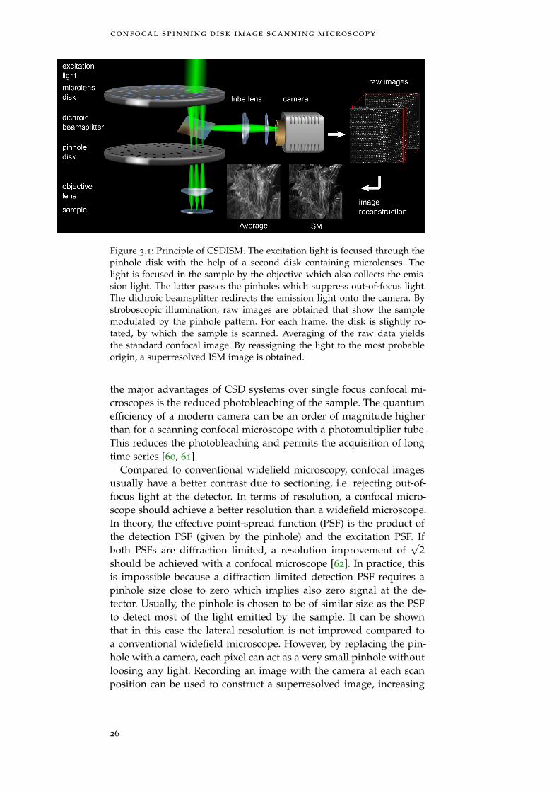
Figure 3.1: Principle of CSDISM. The excitation light is focused through thepinhole disk with the help of a second disk containing microlenses. Thelight is focused in the sample by the objective which also collects the emis-sion light. The latter passes the pinholes which suppress out-of-focus light.The dichroic beamsplitter redirects the emission light onto the camera. Bystroboscopic illumination, raw images are obtained that show the samplemodulated by the pinhole pattern. For each frame, the disk is slightly ro-tated, by which the sample is scanned. Averaging of the raw data yieldsthe standard confocal image. By reassigning the light to the most probableorigin, a superresolved ISM image is obtained.

the major advantages of CSD systems over single focus confocal mi-croscopes is the reduced photobleaching of the sample. The quantumefficiency of a modern camera can be an order of magnitude higherthan for a scanning confocal microscope with a photomultiplier tube.This reduces the photobleaching and permits the acquisition of longtime series [60, 61].

Compared to conventional widefield microscopy, confocal imagesusually have a better contrast due to sectioning, i.e. rejecting out-of-focus light at the detector. In terms of resolution, a confocal micro-scope should achieve a better resolution than a widefield microscope.In theory, the effective point-spread function (PSF) is the product ofthe detection PSF (given by the pinhole) and the excitation PSF. Ifboth PSFs are diffraction limited, a resolution improvement of

√2

should be achieved with a confocal microscope [62]. In practice, thisis impossible because a diffraction limited detection PSF requires apinhole size close to zero which implies also zero signal at the de-tector. Usually, the pinhole is chosen to be of similar size as the PSFto detect most of the light emitted by the sample. It can be shownthat in this case the lateral resolution is not improved compared toa conventional widefield microscope. However, by replacing the pin-hole with a camera, each pixel can act as a very small pinhole withoutloosing any light. Recording an image with the camera at each scanposition can be used to construct a superresolved image, increasing

26

3.1 introduction

signal level and contrast. This idea has been theoretically described bySheppard [62, 63] in 1988 and first implemented by Müller and Ender-lein in 2010 under the name of Image Scanning Microscopy (ISM) [64].In this implementation, the point detector of a confocal microscopeis replaced by a camera. At each scan position, one camera frame isread out which limits the acquisition speed. A straightforward wayto speed up the acquisition is to parallelize it using several scanningbeams.

As the CSD can be seen as a parallelized confocal microscope, theCSDISM can be seen as a parallel image scanning microscope. Thescanning is achieved by using stroboscopic illumination where theduration of illumination is so short that the rotating disk can be con-sidered stationary. The image recorded by the camera is then theproduct of the sample modulated with the pinhole pattern of thedisk. By successively recording images at slightly different disk posi-tions until the disk is in its initial position again, the whole sampleis scanned. Figure 3.1 shows an overview of the technique. An imple-mentation of the CSDISM was first realized by our colleagues Schulzet al. in 2013 [56].

Apart from the CSDISM, a few other implementations of a paral-lelized ISM have been realized. York et al. developed a multi-pointscanning system termed “Multifocal SIM” [65] due to its close rela-tion to structured illumination microscopy (SIM) [66]. The multifocalSIM system is based on a widefield microscope with scanning beamsgenerated by a digital micromirror device (DMD). Because it paral-lelizes the acquisition of scan positions, it offers an improved tem-poral resolution but loses the sectioning ability of confocal systems.Software pinholing can be introduced to suppress out-of-focus light,but will not work in thick samples. York et al. also developed “in-stant SIM” [67] which is even faster: A microlens array produces themulti focus excitation, a pinhole array rejects out-of-focus light, anda second microlens array images the pinholes onto the camera witha demagnification factor of 2. The whole image is scanned by meansof a galvo mirror. The 2× demagnification obviates the need for post-processing, and the ISM image can be directly read from the camera.This allows for very high speeds up to 100 Hz but comes at the costof high complexity in construction and maintenance. The idea to opti-cally process the ISM image was also published around the same timefor a confocal microscope by Roth et al., termed optical photon reas-signment (OPRA) [68]. Here, a scan unit scans the excitation beamthrough the sample. The fluorescence light is separated from the ex-citation by a dichroic mirror and passed through a pinhole after des-canning. Then, the beam is magnified 2× via a telescope lens systemand again scanned by the same scan unit and imaged on a camera.Around the same time, another optical processing method called re-scan confocal microscopy was proposed by De Luca et al. [69]. There-scan microscope uses a second, synchronized scan unit to transfer

27

confocal spinning disk image scanning microscopy

the beam onto a camera with twice the scan angle which results ina 2× demagnification. Both methods produce an ISM image directlyon the camera without further processing. By using a 2-photon laser,Gregor et al. demonstrated that the pinhole can be omitted, obviatingthe need to scan the beam twice [70].

Optical processing was also realized in a spinning disk by addinga second microlens array to the pinhole disk [71]. This allows veryfast acquisition speed in a low maintenance system. Instead of pin-holes, also lines have been used similar to the sinusoidal illuminationin classical SIM [72]. A review of implementations can be found inRef. [73].

Here, the aim was to construct and operate a CSDISM setup thatcan be used as an upgrade kit to add a superresolution option toexisting CSD systems. To this end, we developed a plugin for the mi-croscope control software µManager, enabling CSDISM imaging inone click, and a program for reconstruction of the ISM image. Weinvestigated the performance of the setup and the ISM image recon-struction.

28

3.2 theory

3.2 theory

The increase in resolution and contrast of the CSDISM technique isbased on image scanning microscopy (ISM). This technique enablesthe same resolution as an ideal confocal microscope with infinitelysmall pinhole as explained in the last Section 3.1. Here, we will give abrief theoretical description and then focus on the image reconstruc-tion for CSDISM.

3.2.1 ISM Theory

Müller and Enderlein describe ISM in terms of structured illumina-tion microscopy (SIM). In SIM, a sinusoidal illumination pattern mod-ulates the intensity of the recorded image. The optical transfer func-tion (OTF) of the patterned illumination is mixed with the detectionOTF, shifting high spatial frequencies into the range of the detectionOTF. The illumination pattern usually has a spatial frequency closeto the cutoff frequency of the detection OTF, i.e. the maximum spatialfrequency moved into the supported region of the detection OTF isdoubled. The same holds true for ISM, only there the illuminationpattern is the PSF itself, containing all spatial frequencies up to thecutoff. It can be shown that

OTFISM (q) ≈ OTF2WF

(q2

), (3.1)

where OTFWF(q) is the OTF of a widefield microscope [56]. The de-pendence on q

2 illustrates the twice higher cutoff of the spatial fre-quency and is the reason we expect an increase in resolution by afactor of 2. But because the OTF is squared, the amplitude distribu-tion is different, i.e. higher spatial frequencies are more damped.

The result in Eq. (3.1) can be directly translated in terms of thepoint spread function (PSF), since the PSF is the Fourier transform ofthe OTF. The Fourier transform of Eq.(3.1) is

PSFISM (r) ≈ PSFWF (2r)~ PSFWF (2r) , (3.2)

where the symbol ~ denotes convolution. Assuming a Gaussian PSFwith a width σWF, the ISM width is σISM = σWF/

√2. This is the reason

that the increase in resolution is not higher than 41 % when measuredby the full width at half maximum (FWHM) of the PSF. A deconvolu-tion or reweighting of the amplitudes of the OTF can recover higherspatial frequencies depending on the noise level and further increasethe resolution [56].

3.2.2 Image Reconstruction

A standard confocal image in the CSD is generated by exposing thecamera during the rotation of the disk. Within 1/12 of a full rotation

29

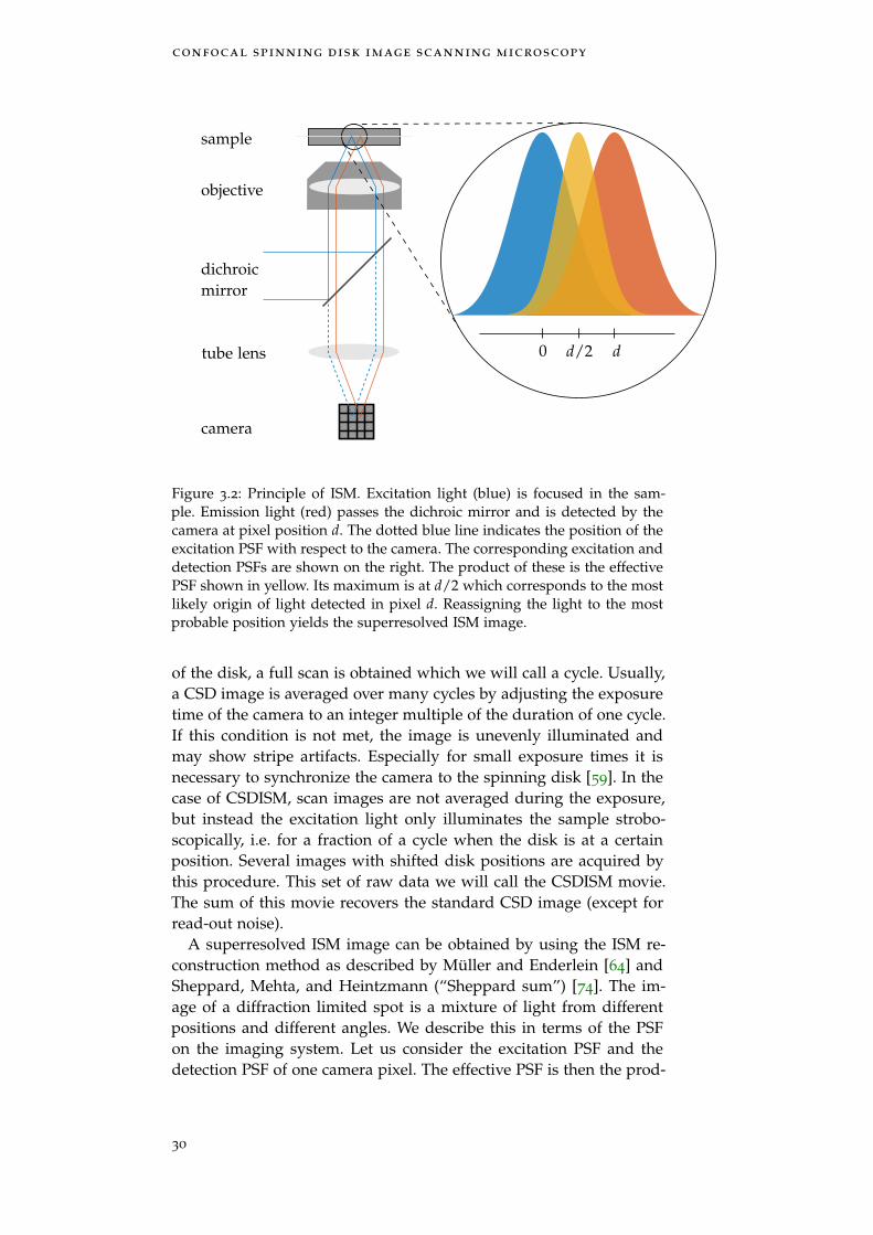
confocal spinning disk image scanning microscopy

d/20 d

camera

dichroicmirror

objective

sample

tube lens

Figure 3.2: Principle of ISM. Excitation light (blue) is focused in the sam-ple. Emission light (red) passes the dichroic mirror and is detected by thecamera at pixel position d. The dotted blue line indicates the position of theexcitation PSF with respect to the camera. The corresponding excitation anddetection PSFs are shown on the right. The product of these is the effectivePSF shown in yellow. Its maximum is at d/2 which corresponds to the mostlikely origin of light detected in pixel d. Reassigning the light to the mostprobable position yields the superresolved ISM image.

of the disk, a full scan is obtained which we will call a cycle. Usually,a CSD image is averaged over many cycles by adjusting the exposuretime of the camera to an integer multiple of the duration of one cycle.If this condition is not met, the image is unevenly illuminated andmay show stripe artifacts. Especially for small exposure times it isnecessary to synchronize the camera to the spinning disk [59]. In thecase of CSDISM, scan images are not averaged during the exposure,but instead the excitation light only illuminates the sample strobo-scopically, i.e. for a fraction of a cycle when the disk is at a certainposition. Several images with shifted disk positions are acquired bythis procedure. This set of raw data we will call the CSDISM movie.The sum of this movie recovers the standard CSD image (except forread-out noise).

A superresolved ISM image can be obtained by using the ISM re-construction method as described by Müller and Enderlein [64] andSheppard, Mehta, and Heintzmann (“Sheppard sum”) [74]. The im-age of a diffraction limited spot is a mixture of light from differentpositions and different angles. We describe this in terms of the PSFon the imaging system. Let us consider the excitation PSF and thedetection PSF of one camera pixel. The effective PSF is then the prod-

30

3.2 theory

d 2d

raw image ISM image ISM image

(physical size)

Figure 3.3: ISM image reconstruction algorithm. The bright spots (red) inthe raw image are cropped at the reference positions (marked by x). Thecropping window (blue rectangles) are centered around the reference posi-tions and copied to the ISM image (middle) with twice the (pixel) distancebetween the reference position. The physical dimensions of the image areunchanged, resulting in a shrinking of the spot by a factor of 2.

uct of the two. The PSF of a confocal excitation spot is a diffractionlimited spot which can be approximated by a Gaussian function. Viceversa, because a camera pixel is imaged as a diffraction limited objectinto the sample plane, the detection PSF has approximately the sameshape. Assuming the excitation PSF at position zero and a detectionPSF that is shifted by some distance d, the effective PSF is locatedat d/2. Thus, detecting a photon at position d most probably wasemitted at position d/2, see also Fig. 3.2. By reassigning the light de-tected at d to d/2, the ISM image is constructed. Mathematically, thiscorresponds to a shrinkage of the light spots by a factor of two. The re-construction of a CSDISM movie can be implemented on a computerin an efficient way by the following algorithm:

1. Initialize an empty image with twice the size as the raw image.

2. Crop a spot in the raw data at reference position r (measured inpixels).

3. Place the spot at position 2r in the new image.

4. Repeat for all spots.

5. Repeat for all raw image in the CSDISM movie.

6. Sum up all new frames.

Thereby, the distance between spots is doubled which is equivalentto shrinking the spots by a factor of 2, see Fig. 3.3 for a graphicalexplanation. Here, the reference position corresponds to the positionof the excitation PSF on the camera and has to be determined beforereconstruction as described in Section 3.4.2.

31

confocal spinning disk image scanning microscopy

In the above algorithm the pixel values can only be placed withthe accuracy of one pixel. Since the PSF size is on the order of a fewpixels only, the positioning accuracy is limited. Thus, the raw imagesare usually upsampled by a scaling factor M before applying the al-gorithm. This allows an M-times higher position accuracy which iscrucial for a reconstruction without artifacts as we will see in Sec-tion 3.4.3.

32

3.3 methods

3.3 methods

3.3.1 Setup

The setup is based on a Yokogawa CSU-X1 (M1N-E) connected tothe side port of an Olympus IX71 microscope. The microscope isequipped with a PIFOC objective scanner (P-725.2CD, Physik Instru-mente) and controller (E-709.CRG, Physik Instrumente). The dichroicmirror in the spinning-disk unit was replaced by a custom made quadline beam splitter (zt405/473/556/640tpc, AHF) to match the laserlines. Four lasers (638L-11A Matchbox 2, Integrated Optics; MGL-N-556/500, MBL-FN-473,and MDL-III-405, all CNI Laser, China) werecombined by dichroic mirrors (LaserMUX 375-405R, LaserMUX 561-594R, and LaserMUX 473-491R, all AHF) and guided into the AOTF(AOTFnC-400.650-TN with driver AA.MDS4C-B65-22-74.158, AA Op-toelectronic). The first diffraction maximum was coupled into a singlemode fiber (SMC-E-400Si-2.6-NA012-3-APC.EC, Schäfter and Kirch-hoff) with a fiber coupler (60SMS-1-4-RGBV11-47, Schäfter and Kirch-hoff) and connected to the CSU. The camera used for the measure-ments was either an Andor iXon 888 Ultra (Andor) or an ORCA-Flash 4.0 sCMOS (Hamamatsu). For some measurements, a quad-band emission filter (BrightLine HC 446/523/600/677, Semrock) wasused. The microscope was controlled by a PC (Windows 10 x64, IntelCore i5-4590, 16 GB RAM) with an FPGA board (NI PCIe-7842R, Na-tional Instruments) using µManager (version 1.4). The triggering sig-nals from the connector block (SCB-68A with SHC68-68-RMIO cable)were connected to the camera, the AOTF driver, and to the controlunit of the CSU (CSUX1CU, Yokogawa). The setup with its connec-tions is shown in Fig. 3.4.

The CSU provides an additional 1.2× magnification, so the pixelsizes of the cameras were 108 nm for the EMCCD and 54 nm for thesCMOS with a 100× objective which ensured Nyquist sampling.

The trigger signal for the camera was a TTL signal with HIGHindicating to start the exposure until the signal was LOW again. Thetime until the next HIGH was used for read-out (about 4 cycles forthe ORCA Flash and up to 40 cycles for the Andor EMCCD camera,configured via the µManager control plugin). In order for the camerato comply with these specifications, the trigger mode of the cameraswas set as following: for the Andor camera, the trigger setting was setto external exposure, and for the ORCA Flash, the trigger source was setto external, the trigger active property to level, and the trigger polarityto positive.

3.3.2 Software

The CSDISM setup was controlled with the µManager [57] software.A custom written plugin by Shun Qin allowed the recording of CS-

33

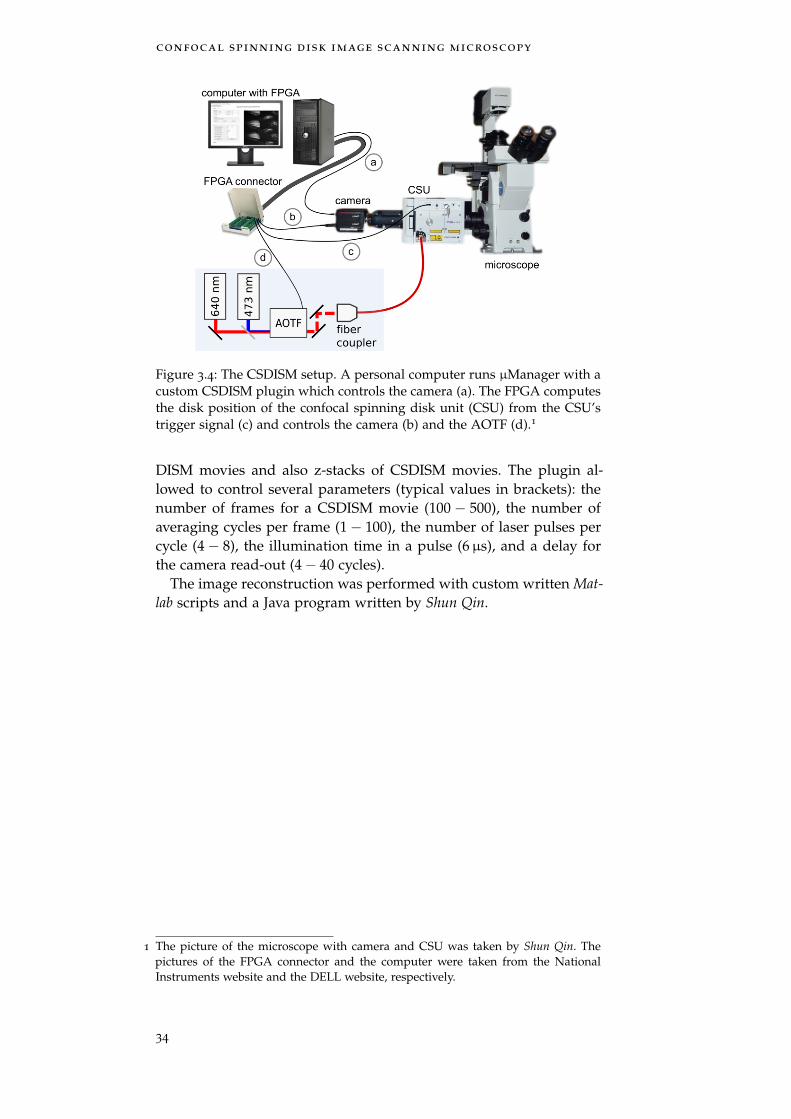
confocal spinning disk image scanning microscopy

Figure 3.4: The CSDISM setup. A personal computer runs µManager with acustom CSDISM plugin which controls the camera (a). The FPGA computesthe disk position of the confocal spinning disk unit (CSU) from the CSU’strigger signal (c) and controls the camera (b) and the AOTF (d).1

DISM movies and also z-stacks of CSDISM movies. The plugin al-lowed to control several parameters (typical values in brackets): thenumber of frames for a CSDISM movie (100− 500), the number ofaveraging cycles per frame (1− 100), the number of laser pulses percycle (4− 8), the illumination time in a pulse (6µs), and a delay forthe camera read-out (4− 40 cycles).

The image reconstruction was performed with custom written Mat-lab scripts and a Java program written by Shun Qin.

1 The picture of the microscope with camera and CSU was taken by Shun Qin. Thepictures of the FPGA connector and the computer were taken from the NationalInstruments website and the DELL website, respectively.

34

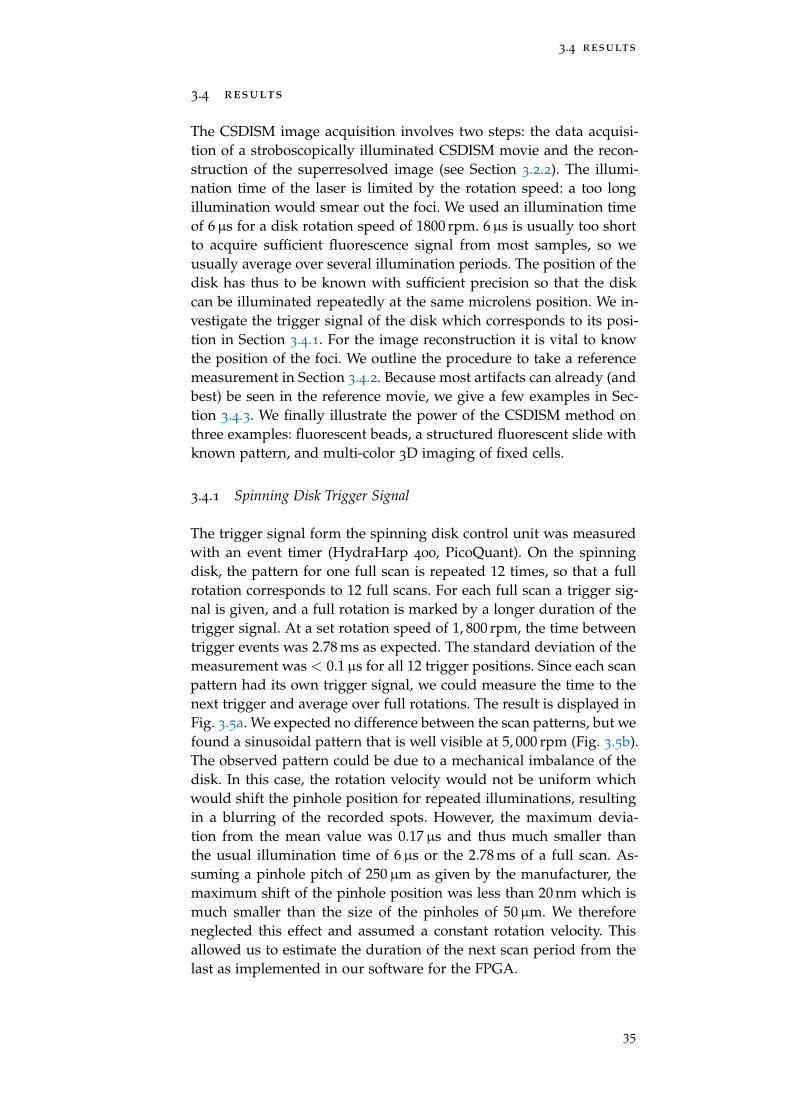
3.4 results

3.4 results

The CSDISM image acquisition involves two steps: the data acquisi-tion of a stroboscopically illuminated CSDISM movie and the recon-struction of the superresolved image (see Section 3.2.2). The illumi-nation time of the laser is limited by the rotation speed: a too longillumination would smear out the foci. We used an illumination timeof 6µs for a disk rotation speed of 1800 rpm. 6µs is usually too shortto acquire sufficient fluorescence signal from most samples, so weusually average over several illumination periods. The position of thedisk has thus to be known with sufficient precision so that the diskcan be illuminated repeatedly at the same microlens position. We in-vestigate the trigger signal of the disk which corresponds to its posi-tion in Section 3.4.1. For the image reconstruction it is vital to knowthe position of the foci. We outline the procedure to take a referencemeasurement in Section 3.4.2. Because most artifacts can already (andbest) be seen in the reference movie, we give a few examples in Sec-tion 3.4.3. We finally illustrate the power of the CSDISM method onthree examples: fluorescent beads, a structured fluorescent slide withknown pattern, and multi-color 3D imaging of fixed cells.

3.4.1 Spinning Disk Trigger Signal

The trigger signal form the spinning disk control unit was measuredwith an event timer (HydraHarp 400, PicoQuant). On the spinningdisk, the pattern for one full scan is repeated 12 times, so that a fullrotation corresponds to 12 full scans. For each full scan a trigger sig-nal is given, and a full rotation is marked by a longer duration of thetrigger signal. At a set rotation speed of 1, 800 rpm, the time betweentrigger events was 2.78 ms as expected. The standard deviation of themeasurement was < 0.1µs for all 12 trigger positions. Since each scanpattern had its own trigger signal, we could measure the time to thenext trigger and average over full rotations. The result is displayed inFig. 3.5a. We expected no difference between the scan patterns, but wefound a sinusoidal pattern that is well visible at 5, 000 rpm (Fig. 3.5b).The observed pattern could be due to a mechanical imbalance of thedisk. In this case, the rotation velocity would not be uniform whichwould shift the pinhole position for repeated illuminations, resultingin a blurring of the recorded spots. However, the maximum devia-tion from the mean value was 0.17µs and thus much smaller thanthe usual illumination time of 6µs or the 2.78 ms of a full scan. As-suming a pinhole pitch of 250µm as given by the manufacturer, themaximum shift of the pinhole position was less than 20 nm which ismuch smaller than the size of the pinholes of 50µm. We thereforeneglected this effect and assumed a constant rotation velocity. Thisallowed us to estimate the duration of the next scan period from thelast as implemented in our software for the FPGA.

35

confocal spinning disk image scanning microscopy

(a) (b)

Figure 3.5: Trigger signal timing. The time between successive trigger signalswas measured for each of the twelve scan patterns at a) 1, 800 rpm and b)5, 000 rpm. The shape of the curve is probably due to a slight mechanicalimbalance of the disk, well visible at high speed. The overall timing error isabout 0.17µs.

3.4.2 Reference Measurements

As described in Section 3.2.2, the positions of the excitation PSFs areneeded to reconstruct the ISM image. These reference positions wereobtained by recording a CSDISM movie of a homogeneous fluores-cent sample. Each spot in the raw data then corresponded to theposition of a pinhole. Localization of the center of the spots gave asub-pixel precise position of the pinhole. Because the excitation lightis focused through the pinholes, we did not distinguish between thepinhole position and the position of the excitation PSF and use thesesynonymously, or refer to it simply as the reference position.

A drop of homogeneous dye solution (e.g. 1µM Atto 655 in water)on a cover slip sufficed for a measurement of the reference positions.An example is shown in Fig. 3.6. Alternatively, autofluorescent plasticslides (92001, Chroma) can be used.

In SIM, the illumination pattern is often estimated from the rawdata. If the SNR of the raw data is low, the estimation can be erro-neous and introduce artifacts in the reconstruction. Here, we chosea calibration approach to circumvent this problem. This introducesan additional step to the measurement, but it only needs to be re-peated in case of changes in the optical path, e.g. exchanging thecamera, which are not expected to occur often in a CSD. Unlike SIM,where the pattern crucially depends on the excitation wavelength, thedistances between the pinholes do not change. However, we have ob-served that chromatic aberrations of the setup influence the pattern.In first order approximation, this introduces a global shift of the pat-tern on the order of a few tens of nanometers. As long as the windowsize in the reconstruction software is chosen large enough, this willresult in a global shift of the reconstructed image only. Thus, a refer-ence measurement in a single color is usually enough to reconstruct

36

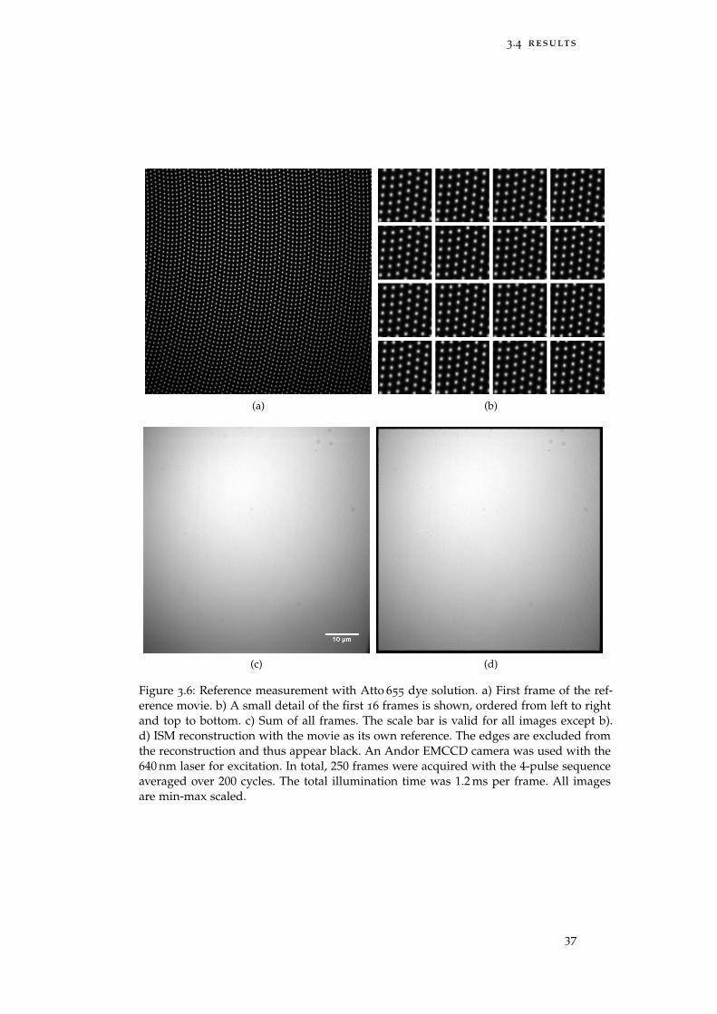
3.4 results

(a) (b)

(c) (d)

Figure 3.6: Reference measurement with Atto 655 dye solution. a) First frame of the ref-erence movie. b) A small detail of the first 16 frames is shown, ordered from left to rightand top to bottom. c) Sum of all frames. The scale bar is valid for all images except b).d) ISM reconstruction with the movie as its own reference. The edges are excluded fromthe reconstruction and thus appear black. An Andor EMCCD camera was used with the640 nm laser for excitation. In total, 250 frames were acquired with the 4-pulse sequenceaveraged over 200 cycles. The total illumination time was 1.2 ms per frame. All imagesare min-max scaled.

37

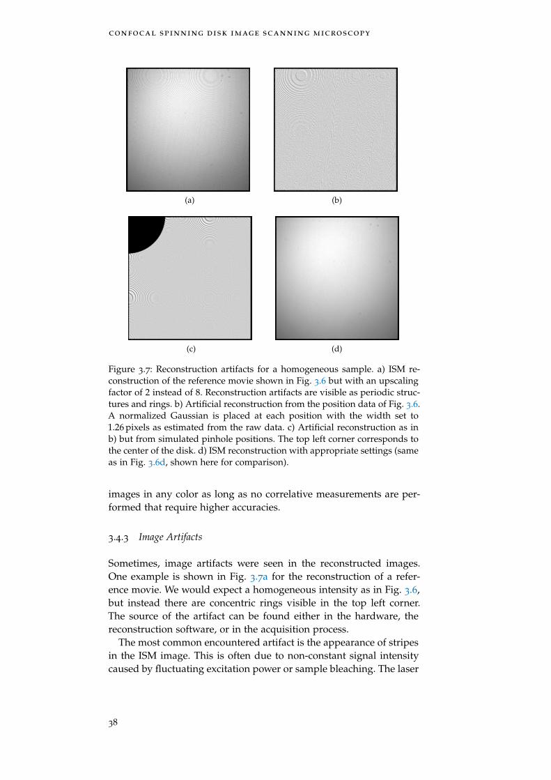
confocal spinning disk image scanning microscopy

(a) (b)

(c) (d)

Figure 3.7: Reconstruction artifacts for a homogeneous sample. a) ISM re-construction of the reference movie shown in Fig. 3.6 but with an upscalingfactor of 2 instead of 8. Reconstruction artifacts are visible as periodic struc-tures and rings. b) Artificial reconstruction from the position data of Fig. 3.6.A normalized Gaussian is placed at each position with the width set to1.26 pixels as estimated from the raw data. c) Artificial reconstruction as inb) but from simulated pinhole positions. The top left corner corresponds tothe center of the disk. d) ISM reconstruction with appropriate settings (sameas in Fig. 3.6d, shown here for comparison).

images in any color as long as no correlative measurements are per-formed that require higher accuracies.

3.4.3 Image Artifacts

Sometimes, image artifacts were seen in the reconstructed images.One example is shown in Fig. 3.7a for the reconstruction of a refer-ence movie. We would expect a homogeneous intensity as in Fig. 3.6,but instead there are concentric rings visible in the top left corner.The source of the artifact can be found either in the hardware, thereconstruction software, or in the acquisition process.

The most common encountered artifact is the appearance of stripesin the ISM image. This is often due to non-constant signal intensitycaused by fluctuating excitation power or sample bleaching. The laser

38

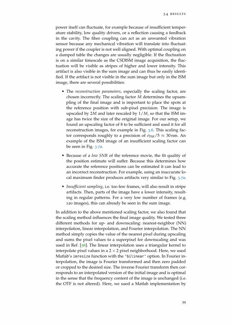
3.4 results

power itself can fluctuate, for example because of insufficient temper-ature stability, low quality drivers, or a reflection causing a feedbackin the cavity. The fiber coupling can act as an unwanted vibrationsensor because any mechanical vibration will translate into fluctuat-ing power if the coupler is not well aligned. With optimal coupling ona damped table the changes are usually negligible. If the fluctuationis on a similar timescale as the CSDISM image acquisition, the fluc-tuation will be visible as stripes of higher and lower intensity. Thisartifact is also visible in the sum image and can thus be easily identi-fied. If the artifact is not visible in the sum image but only in the ISMimage, there are several possibilities:

• The reconstruction parameters, especially the scaling factor, arechosen incorrectly. The scaling factor M determines the upsam-pling of the final image and is important to place the spots atthe reference position with sub-pixel precision. The image isupscaled by 2M and later rescaled by 1/M, so that the ISM im-age has twice the size of the original image. For our setup, wefound an upscaling factor of 8 to be sufficient and used it for allreconstruction images, for example in Fig. 3.6. This scaling fac-tor corresponds roughly to a precision of σPSF/5 ≈ 30 nm. Anexample of the ISM image of an insufficient scaling factor canbe seen in Fig. 3.7a.

• Because of a low SNR of the reference movie, the fit quality ofthe position estimate will suffer. Because this determines howaccurate the reference positions can be estimated it can lead toan incorrect reconstruction. For example, using an inaccurate lo-cal maximum finder produces artifacts very similar to Fig. 3.7a.

• Insufficient sampling, i.e. too few frames, will also result in stripeartifacts. Then, parts of the image have a lower intensity, result-ing in regular patterns. For a very low number of frames (e.g.120 images), this can already be seen in the sum image.

In addition to the above mentioned scaling factor, we also found thatthe scaling method influences the final image quality. We tested threedifferent methods for up- and downscaling: nearest-neighbor (NN)interpolation, linear interpolation, and Fourier interpolation. The NNmethod simply copies the value of the nearest pixel during upscalingand sums the pixel values to a superpixel for downscaling and wasused in Ref. [56]. The linear interpolation uses a triangular kernel tointerpolate pixel values in a 2× 2 pixel neighborhood. Here, we usedMatlab’s imresize function with the ’bilinear’ option. In Fourier in-terpolation, the image is Fourier transformed and then zero paddedor cropped to the desired size. The inverse Fourier transform then cor-responds to an interpolated version of the initial image and is optimalin the sense that the frequency content of the image is unchanged (i.e.the OTF is not altered). Here, we used a Matlab implementation by

39

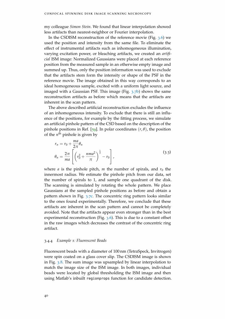
confocal spinning disk image scanning microscopy

my colleague Simon Stein. We found that linear interpolation showedless artifacts than nearest-neighbor or Fourier interpolation.

In the CSDISM reconstruction of the reference movie (Fig. 3.6) weused the position and intensity from the same file. To eliminate theeffect of instrumental artifacts such as inhomogeneous illumination,varying excitation power, or bleaching artifacts, we created an artifi-cial ISM image: Normalized Gaussians were placed at each referenceposition from the measured sample in an otherwise empty image andsummed up. Thus, only the position information was used to excludethat the artifacts stem form the intensity or shape of the PSF in thereference movie. The image obtained in this way corresponds to anideal homogeneous sample, excited with a uniform light source, andimaged with a Gaussian PSF. This image (Fig. 3.7b) shows the samereconstruction artifacts as before which means that the artifacts areinherent in the scan pattern.

The above described artificial reconstruction excludes the influenceof an inhomogeneous intensity. To exclude that there is still an influ-ence of the positions, for example by the fitting process, we simulatean artificial pinhole pattern of the CSD based on the description of thepinhole positions in Ref. [59]. In polar coordinates (r, θ), the positionof the nth pinhole is given by

rn = r0 +ma2π

θn

θn =2π

ma

(r20 +

nma2

π

) 12

− r0

,(3.3)

where a is the pinhole pitch, m the number of spirals, and r0 theinnermost radius. We estimate the pinhole pitch from our data, setthe number of spirals to 1, and sample one quadrant of the disk.The scanning is simulated by rotating the whole pattern. We placeGaussians at the sampled pinhole positions as before and obtain apattern shown in Fig. 3.7c. The concentric ring pattern looks similarto the ones found experimentally. Therefore, we conclude that theseartifacts are inherent in the scan pattern and cannot be completelyavoided. Note that the artifacts appear even stronger than in the bestexperimental reconstruction (Fig. 3.6). This is due to a constant offsetin the raw images which decreases the contrast of the concentric ringartifact.

3.4.4 Example 1: Fluorescent Beads

Fluorescent beads with a diameter of 100 nm (TetraSpeck, Invitrogen)were spin coated on a glass cover slip. The CSDISM image is shownin Fig. 3.8. The sum image was upsampled by linear interpolation tomatch the image size of the ISM image. In both images, individualbeads were located by global thresholding the ISM image and thenusing Matlab’s inbuilt regionprops function for candidate detection.

40

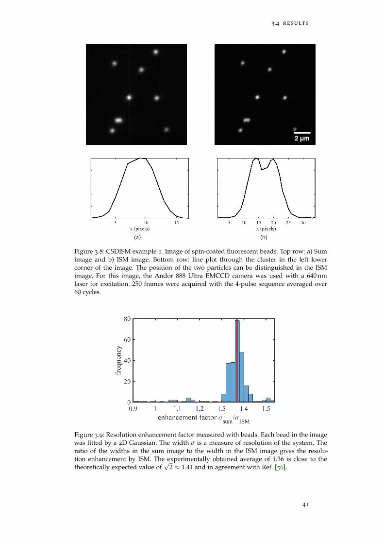
3.4 results

(a) (b)

Figure 3.8: CSDISM example 1. Image of spin-coated fluorescent beads. Top row: a) Sumimage and b) ISM image. Bottom row: line plot through the cluster in the left lowercorner of the image. The position of the two particles can be distinguished in the ISMimage. For this image, the Andor 888 Ultra EMCCD camera was used with a 640 nmlaser for excitation. 250 frames were acquired with the 4-pulse sequence averaged over60 cycles.

Figure 3.9: Resolution enhancement factor measured with beads. Each bead in the imagewas fitted by a 2D Gaussian. The width σ is a measure of resolution of the system. Theratio of the widths in the sum image to the width in the ISM image gives the resolu-tion enhancement by ISM. The experimentally obtained average of 1.36 is close to thetheoretically expected value of

√2 ≈ 1.41 and in agreement with Ref. [56].

41

confocal spinning disk image scanning microscopy

(a) (b) (c)

Figure 3.10: CSDISM example 2. Fluorescent star structure on the Argo-SIMslide. Top row: a) CSD image with 100 ms exposure time. b) Sum image ofthe CSDISM raw data. c) CSDISM image. Bottom row: line sections throughthe northern arm of the star. This image was acquired using the Orca Flashcamera with 2× 2 binning and the 4-pulse sequence for 250 images averagedover 50 cycles.

A 2D Gaussian with constant offset was then fitted to a small areaaround each detected spot. The width of the Gaussian σ is directlyrelated to the FWHM and shown in Fig. 3.9. The resolution improve-ment factor (as measured by the FWHM) is thus σsum

σISM. We find an

average resolution improvement of 36 %, close to the theoretically ex-pected 41 % (cf. Section 3.2.1).

3.4.5 Example 2: Argo-SIM Fluorescent Slide

The Argo-SIM slide (Argolight) is a solid state fluorescent samplethat is designed for calibration and performance monitoring of SIMmicroscopes. It comes with a variety of different patterns of whichwe show one example in Fig. 3.10. There is no difference between thestandard CSD and the sum image, especially for the line sections. Inthe ISM image however, the lines are better separated, demonstratingthe improved resolution.

42

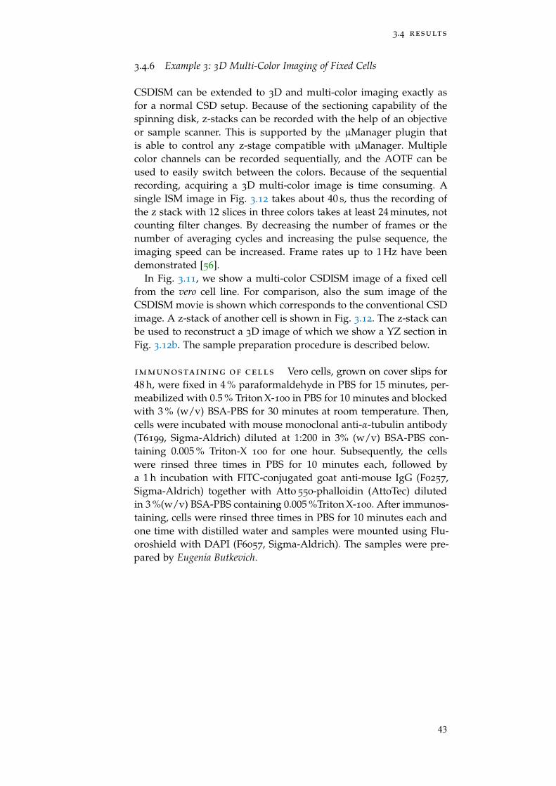
3.4 results

3.4.6 Example 3: 3D Multi-Color Imaging of Fixed Cells

CSDISM can be extended to 3D and multi-color imaging exactly asfor a normal CSD setup. Because of the sectioning capability of thespinning disk, z-stacks can be recorded with the help of an objectiveor sample scanner. This is supported by the µManager plugin thatis able to control any z-stage compatible with µManager. Multiplecolor channels can be recorded sequentially, and the AOTF can beused to easily switch between the colors. Because of the sequentialrecording, acquiring a 3D multi-color image is time consuming. Asingle ISM image in Fig. 3.12 takes about 40 s, thus the recording ofthe z stack with 12 slices in three colors takes at least 24 minutes, notcounting filter changes. By decreasing the number of frames or thenumber of averaging cycles and increasing the pulse sequence, theimaging speed can be increased. Frame rates up to 1 Hz have beendemonstrated [56].

In Fig. 3.11, we show a multi-color CSDISM image of a fixed cellfrom the vero cell line. For comparison, also the sum image of theCSDISM movie is shown which corresponds to the conventional CSDimage. A z-stack of another cell is shown in Fig. 3.12. The z-stack canbe used to reconstruct a 3D image of which we show a YZ section inFig. 3.12b. The sample preparation procedure is described below.

immunostaining of cells Vero cells, grown on cover slips for48 h, were fixed in 4 % paraformaldehyde in PBS for 15 minutes, per-meabilized with 0.5 % Triton X-100 in PBS for 10 minutes and blockedwith 3 % (w/v) BSA-PBS for 30 minutes at room temperature. Then,cells were incubated with mouse monoclonal anti-α-tubulin antibody(T6199, Sigma-Aldrich) diluted at 1:200 in 3% (w/v) BSA-PBS con-taining 0.005 % Triton-X 100 for one hour. Subsequently, the cellswere rinsed three times in PBS for 10 minutes each, followed bya 1 h incubation with FITC-conjugated goat anti-mouse IgG (F0257,Sigma-Aldrich) together with Atto 550-phalloidin (AttoTec) dilutedin 3 %(w/v) BSA-PBS containing 0.005 %Triton X-100. After immunos-taining, cells were rinsed three times in PBS for 10 minutes each andone time with distilled water and samples were mounted using Flu-oroshield with DAPI (F6057, Sigma-Aldrich). The samples were pre-pared by Eugenia Butkevich.

43

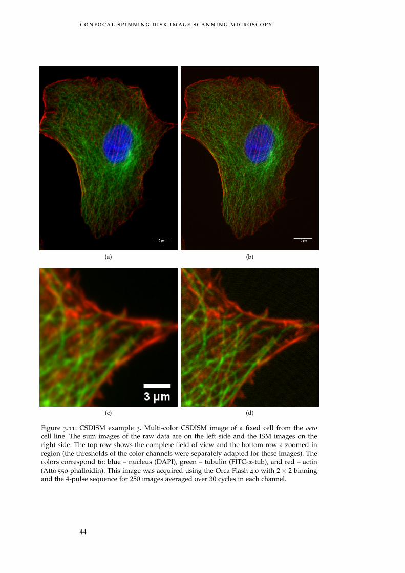
confocal spinning disk image scanning microscopy

(a) (b)

(c) (d)

Figure 3.11: CSDISM example 3. Multi-color CSDISM image of a fixed cell from the verocell line. The sum images of the raw data are on the left side and the ISM images on theright side. The top row shows the complete field of view and the bottom row a zoomed-inregion (the thresholds of the color channels were separately adapted for these images). Thecolors correspond to: blue – nucleus (DAPI), green – tubulin (FITC-α-tub), and red – actin(Atto 550-phalloidin). This image was acquired using the Orca Flash 4.0 with 2× 2 binningand the 4-pulse sequence for 250 images averaged over 30 cycles in each channel.

44

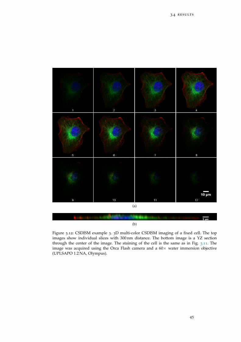
3.4 results

(a)

(b)

Figure 3.12: CSDISM example 3. 3D multi-color CSDISM imaging of a fixed cell. The topimages show individual slices with 300 nm distance. The bottom image is a YZ sectionthrough the center of the image. The staining of the cell is the same as in Fig. 3.11. Theimage was acquired using the Orca Flash camera and a 60× water immersion objective(UPLSAPO 1.2 NA, Olympus).

45

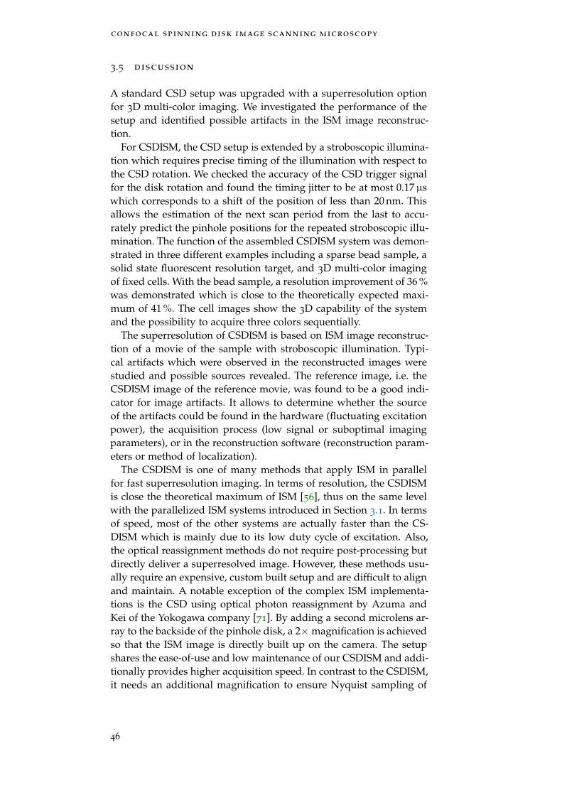
confocal spinning disk image scanning microscopy

3.5 discussion

A standard CSD setup was upgraded with a superresolution optionfor 3D multi-color imaging. We investigated the performance of thesetup and identified possible artifacts in the ISM image reconstruc-tion.

For CSDISM, the CSD setup is extended by a stroboscopic illumina-tion which requires precise timing of the illumination with respect tothe CSD rotation. We checked the accuracy of the CSD trigger signalfor the disk rotation and found the timing jitter to be at most 0.17µswhich corresponds to a shift of the position of less than 20 nm. Thisallows the estimation of the next scan period from the last to accu-rately predict the pinhole positions for the repeated stroboscopic illu-mination. The function of the assembled CSDISM system was demon-strated in three different examples including a sparse bead sample, asolid state fluorescent resolution target, and 3D multi-color imagingof fixed cells. With the bead sample, a resolution improvement of 36 %was demonstrated which is close to the theoretically expected maxi-mum of 41 %. The cell images show the 3D capability of the systemand the possibility to acquire three colors sequentially.

The superresolution of CSDISM is based on ISM image reconstruc-tion of a movie of the sample with stroboscopic illumination. Typi-cal artifacts which were observed in the reconstructed images werestudied and possible sources revealed. The reference image, i.e. theCSDISM image of the reference movie, was found to be a good indi-cator for image artifacts. It allows to determine whether the sourceof the artifacts could be found in the hardware (fluctuating excitationpower), the acquisition process (low signal or suboptimal imagingparameters), or in the reconstruction software (reconstruction param-eters or method of localization).

The CSDISM is one of many methods that apply ISM in parallelfor fast superresolution imaging. In terms of resolution, the CSDISMis close the theoretical maximum of ISM [56], thus on the same levelwith the parallelized ISM systems introduced in Section 3.1. In termsof speed, most of the other systems are actually faster than the CS-DISM which is mainly due to its low duty cycle of excitation. Also,the optical reassignment methods do not require post-processing butdirectly deliver a superresolved image. However, these methods usu-ally require an expensive, custom built setup and are difficult to alignand maintain. A notable exception of the complex ISM implementa-tions is the CSD using optical photon reassignment by Azuma andKei of the Yokogawa company [71]. By adding a second microlens ar-ray to the backside of the pinhole disk, a 2×magnification is achievedso that the ISM image is directly built up on the camera. The setupshares the ease-of-use and low maintenance of our CSDISM and addi-tionally provides higher acquisition speed. In contrast to the CSDISM,it needs an additional magnification to ensure Nyquist sampling of

46

3.5 discussion

the superresolved image which crops the field of view. In CSDISM,only the raw image needs to be Nyquist sampled and additional up-sampling is only needed during post-processing.

The main advantage of the CSDISM is that any CSD system canbe easily upgraded with a superresolution option. The upgrade doesnot require any changes in the optical path of the microscope since alloptical components in the CSD are pre-aligned by the manufacturer.Furthermore, many existing CSD systems already use an AOTF toselect the wavelength for excitation. Some lasers allow a fast modu-lation of the laser intensity, then no AOTF is needed at all. The syn-chronization of the AOTF or the laser with the CSD can be achievedwith our µManager plugin and a commercially available FPGA card.Then, the acquisition of an ISM image is a one-click process. Stan-dard CSD systems are widely spread in labs all over the world andwe hope that our software will be used to upgrade them with a su-perresolution option, allowing researchers to look at their samples innew detail.

47

4A X I A L C O - L O C A L I Z AT I O N O F S I N G L EM O L E C U L E S U S I N G M E TA L - I N D U C E D E N E R G YT R A N S F E R

In this chapter, we present a new method to measure distances alongthe optical axis on the nanometer scale. We use single-molecule metal-induced energy transfer (smMIET) with step-wise bleaching to mea-sure intra-molecular axial distances in DNA origami structures. Thisopens up new possibilities to study the structure of large biomoleculesor complexes.

Parts of this chapter have been published in:Sebastian Isbaner, Narain Karedla, Izabela Kaminska, Daja Ruhlandt,Mario Raab, Johann Bohlen, Alexey Chizhik, Ingo Gregor, Philip Tin-nefeld, Jörg Enderlein, and Roman Tsukanov. “Axial Colocalizationof Single Molecules with Nanometer Accuracy Using Metal-InducedEnergy Transfer.” In: Nano Letters 18.4 (Apr. 11, 2018), pp. 2616–2622.doi: 10.1021/acs.nanolett.8b00425.

4.1 introduction

Distinguishing fluorescent emitters from each other is a prerequisiteto resolve structural details in a fluorescent sample. The resolution ofan optical microscope is limited by the diffraction of light. The reso-lution limit defines the closest distance of point emitters in focus sothey can be distinguished on a screen or a camera. A first theoreticaldescription was given by Abbe [75] in 1873 as

dxy =λ

2NA(4.1)

with λ being the emission wavelength and NA the numerical apertureof the objective. For a typical optical microscope, the resolution limitis on the order of 200 nm. A similar argument holds true for the axialresolution

dz =λ

n(1− cos(θmax))≈ 2nλ

NA2 , (4.2)

where θmax is half the opening angle of the objective given by NA =

n sin(θmax), and is usually several times larger than dxy, on the orderof 500− 800 nm.

Superresolution techniques developed in the past twenty years havepushed the limits of the lateral resolution down to the nanometerregime. Structured illumination microscopy (SIM) uses a diffractionlimited excitation pattern which reveals new spatial frequencies in

axial co-localization using miet

the sample. Several recorded images are used to reconstruct an imagewith doubled resolution [66]. Stimulated emission depletion (STED)microscopy and other members of the reversible saturable opticalfluorescence transitions (RESOLFT) family use point-spread function(PSF) engineering through optically saturable transitions of the fluo-rescent labels. The size of the excitation PSF is effectively reducedby an overlapping laser beam with a donut shaped PSF which de-pletes the fluorescence of molecules [26]. Another class of superreso-lution techniques is based on the precise localization of spatially well-separated fluorescent molecules. The diffraction limit is bypassed be-cause the center position of a single fluorescent emitter can be local-ized much more precise than the width of the PSF [25, 76, 77]. To beable to image densely labeled samples, spatial separation is achievedby multiplexing the emission of several emitters in time: In a singlecamera frame, only a sparse subset of all emitters is fluorescent andcan be localized. In subsequent frames, different subsets are fluores-cent and the aggregated localizations can then be combined into asuperresolved image. The main difference between methods of thisclass is the mechanism to switch molecules on or off. Stochastic opti-cal reconstruction microscopy (STORM) and its variant direct STORM(dSTORM) use the intrinsic blinking behavior of organic dyes [13,78]. Photoactivation localization microscopy (PALM) uses photoacti-vatable molecules that can be switched on by irradiation with UVlight [11]. In DNA points accumulation for imaging in nanoscale to-pography (DNA-PAINT), fluorescently labeled oligonucleotides tran-siently bind to the structure of interest [79]. All of the superresolutionmethods above improve the lateral resolution beyond the diffractionlimit but do not change the resolution along the optical axis. Thislimits these methods to very flat objects or poses the difficulty to in-terpret the images as projections of 3D objects.

Several of the lateral superresolution techniques have been extendedto 3D and improved also on the axial resolution. For example, 3D-SIM extends the planar structured illumination pattern to a 3D inter-ference pattern. In 3D-STED, the size of the excitation PSF is reducedalong the optical axis by an additional depletion beam. In the localiza-tion methods, a common approach is to introduce a cylindrical lensinto the emission path which introduces an artificial astigmatism inthe PSF, encoding the z-position of the emitter. In biplane imaging,the emission light is split into two focal planes on the camera whichhold information on the emitter position [80]. An overview over thelateral and axial resolution of the above mentioned methods can befound in Table 4.1. Although these methods greatly improve on theaxial resolution, their axial resolution usually still remains a factor of2 to 5 worse than their lateral resolution. An exception is the interfer-ometric PALM (iPALM) method that combines localization of photo-switchable proteins with interferometric imaging and achieves a sub-20 nm isotropic resolution [81]. However, this comes at the cost of

50

4.1 introduction

method lateral axial Ref.

resolution resolution

3D-SIM 120 nm 360 nm Fiolka et al. [82]

3D STED 50 nm 125 nm Harke et al. [83]

astigmatic imaging 20 nm 50 nm Huang et al. [84]

biplane imaging 30 nm 75 nm Juette et al. [80]

iPALM < 20 nm < 10 nm Shtengel et al. [81]

SAF (+ dSTORM) 20 nm 20 nm Bourg et al. [85]

vaTIRF ∼ 200 nm > 10 nm Olveczky et al. [86]

Table 4.1: Examples of the lateral and axial resolution of optical microscopymethods. Comprehensive overviews can be found in Refs. [87] and [25].

increased complexity of the system: iPALM detects single moleculeswith two objectives, interferes their emission in a custom-made 3-waybeamsplitter, and images them onto three cameras to reconstruct theheight information.

In contrast to the imaging methods discussed above, methods thatuse a near-field coupling of the emitter have been used for distancemeasurements as well. When the incidence angle of the excitationlight is higher than the critical angle, an evanescent wave along theoptical axis is produced which decays exponentially within a few hun-dreds of nanometers above the coverslip, depending on the angle ofincidence. This can be used to selectively excite fluorescence close tothe coverslip and is known as total internal reflection fluorescence(TIRF) [88]. Illuminating the sample with light at different incidenceangles changes the distance over which the evanescent wave decaysand thus the fluorescence intensity. The ratio of the observed fluores-cence intensities allows to estimate the distance of an emitter from thesurface and is known as variable angle TIRF (vaTIRF) and achievesan axial localization precision on the nanometer scale [86, 89, 90]. Arecent implementation showed an axial resolution of 20 nm by usingthe intensity ratio of two excitation wavelengths in TIRF [91]. Apartfrom the excitation, also the emission intensity can be used to infer theheight of an emitter above the coverslip. In supercritical angle fluores-cence (SAF) microscopy, the emission light is split into two channelscorresponding to the light emitted above and below the critical an-gle [92]. Because the angular distribution of radiation of an emitterclose to a glass-water interface changes with height, the intensity ra-tio of the two channels can be used to estimate the emitter height. Thismethod can be used for confocal as well as widefield microscopes toachieve nanometer axial resolution [93, 94]. A recent implementationcombined SAF with STORM and achieved an isotropic resolution of20 nm within a range of 150 nm from the surface [85]. The high axial

51

axial co-localization using miet

localization precision of both the SAF and the vaTIRF families de-pend on the precise measurement of the fluorescence intensity whichsuffers from cross-talk and background and thus requires careful cal-ibration.

Another prominent example of the spectroscopic methods for dis-tance measurements is Förster Resonance Energy Transfer (FRET): Afluorescent molecule (the donor) transfers its excited state energy toanother fluorescent molecule (the acceptor). Since this process is me-diated via dipole-dipole interaction, the rate of the energy transferdepends on the sixth power of the distance r:

kfret ∝(

R0

r

)6

(4.3)

Here, R0 is the so-called Förster radius,

R0 =9 ln(10)

128π5NA

κ2QYD

n4

∫dλ FD(λ)εA(λ), (4.4)

where NA is the Avogadro constant, and depends on the mutual ori-entation of the two dipole emitters κ2, the donor’s quantum yieldQYD, the refractive index of the medium n, and the overlap integralof the donor’s emission spectrum FD(λ) with the acceptor’s absorp-tion spectrum εA(λ) [95]. The value of the Förster radius is typicallyon the order of 5 nm, limiting the useful range of FRET to distancesbetween 1 to 10 nm. In that range, FRET has been proven very success-ful to measure intramolecular distances or to study conformationaldynamics in biomolecular complexes [19, 96–98].

One particularity of FRET is that it requires double labeling of themolecule of interest which can be tedious to achieve if the yield ofone of the dyes’ coupling reaction is low. Especially in bulk measure-ments, incomplete labeling leads to a skewed value of the FRET effi-ciency because donor-only labeled molecules will show a low FRETefficiency and acceptor-only labeled molecules show a high FRET effi-ciency due to direct excitation of the acceptor dye. Several techniqueshave been developed to overcome this limitation, notably alternat-ing laser excitation FRET (ALEX-FRET) [99] and pulsed interleavedexcitation (PIE-FRET) [100] which both aim at distinguishing singlelabeled from double labeled molecules.

To use FRET as a quantitative and accurate ruler, precise knowl-edge of the Förster radius is essential. All contributing factors inEq. (4.4) can be measured with standard spectroscopic methods ex-cept for the orientation factor κ2. This factor depends on the mutualorientation of the labels

κ2 = (cos(θDA)− 3 cos(θD) cos(θA))2 , (4.5)

where the angles between the dipole moments of the two emitters aredefined in Figure 4.1. κ2 is often assumed to be equal to 2

3 for freelyrotating dipoles, but can vary between 0 and 4 for orthogonal and

52

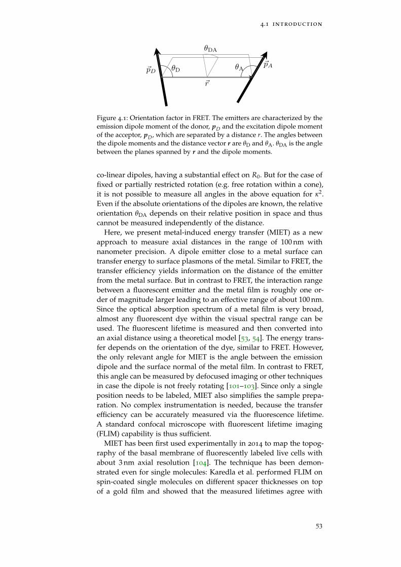
4.1 introduction

~r

~pD θD~pAθA

θDA

Figure 4.1: Orientation factor in FRET. The emitters are characterized by theemission dipole moment of the donor, pD and the excitation dipole momentof the acceptor, pD, which are separated by a distance r. The angles betweenthe dipole moments and the distance vector r are θD and θA. θDA is the anglebetween the planes spanned by r and the dipole moments.

co-linear dipoles, having a substantial effect on R0. But for the case offixed or partially restricted rotation (e.g. free rotation within a cone),it is not possible to measure all angles in the above equation for κ2.Even if the absolute orientations of the dipoles are known, the relativeorientation θDA depends on their relative position in space and thuscannot be measured independently of the distance.

Here, we present metal-induced energy transfer (MIET) as a newapproach to measure axial distances in the range of 100 nm withnanometer precision. A dipole emitter close to a metal surface cantransfer energy to surface plasmons of the metal. Similar to FRET, thetransfer efficiency yields information on the distance of the emitterfrom the metal surface. But in contrast to FRET, the interaction rangebetween a fluorescent emitter and the metal film is roughly one or-der of magnitude larger leading to an effective range of about 100 nm.Since the optical absorption spectrum of a metal film is very broad,almost any fluorescent dye within the visual spectral range can beused. The fluorescent lifetime is measured and then converted intoan axial distance using a theoretical model [53, 54]. The energy trans-fer depends on the orientation of the dye, similar to FRET. However,the only relevant angle for MIET is the angle between the emissiondipole and the surface normal of the metal film. In contrast to FRET,this angle can be measured by defocused imaging or other techniquesin case the dipole is not freely rotating [101–103]. Since only a singleposition needs to be labeled, MIET also simplifies the sample prepa-ration. No complex instrumentation is needed, because the transferefficiency can be accurately measured via the fluorescence lifetime.A standard confocal microscope with fluorescent lifetime imaging(FLIM) capability is thus sufficient.

MIET has been first used experimentally in 2014 to map the topog-raphy of the basal membrane of fluorescently labeled live cells withabout 3 nm axial resolution [104]. The technique has been demon-strated even for single molecules: Karedla et al. performed FLIM onspin-coated single molecules on different spacer thicknesses on topof a gold film and showed that the measured lifetimes agree with

53

axial co-localization using miet

the theoretical model. Furthermore, these single molecule MIET (sm-MIET) experiments reached about the same axial localization accu-racy of 3 nm as in bulk [50]. In these two publications, the absolutedistances from the metal film were determined. To measure relativedistances, dual-color MIET was introduced by Chizhik et al. and usedto measure the distance between the two lipid membranes of the in-ner and outer nuclear envelope in fixed cells. There, the distancesof the two differently labeled membranes from the surface were mea-sured sequentially and afterwards the distance between them was cal-culated [105]. Thus, MIET has been applied successfully to measureaxial distances on the single molecule level and relative distances inbulk, but not relative distances in single molecules yet.

Here, we are interested in studying large (bio)molecular complexeson the single molecule level and obtain intramolecular distances. Mea-suring relative distances with dual color MIET has the disadvantagethat FRET between the labels influences the measurement. This can beavoided by using only a single color for co-localization. Gordon andcolleagues combined the superresolution approach of single moleculelocalization with step-wise photobleaching to co-localize fluorescentemitters laterally. The technique was named single-molecule high-resolution imaging with photobleaching (SHRImP) and allowed tomeasure the lateral distance between two emitters with a precisionof 5 nm [106, 107]. Based on the same idea of step-wise bleaching, wedeveloped a new technique for axial co-localization.

The aim of this work is to measure intramolecular distances by us-ing only one kind of label and to axially co-localize several individualemitters on the same structure. The sample was subject to two majorchallenges: First, in prospect of future applications, the environmentshould be close to the native environment of biomolecules, i.e. aque-ous solution. Second, the sample should be robust and the distancesof the labels should be known to verify our method. We chose DNAorigami as a reference sample because of its 3D structure, rigidity, andeasy addressability with fluorescent labels. DNA origami structuresare commonly employed as reference samples for superresolution mi-croscopy and even have been recently used as a traceable distancemeasurement standard for fluorescence microscopy [108].

In the following, we perform axial localization of single fluores-cent emitters based on single molecule MIET. We use step-wise pho-tobleaching to achieve axial co-localization of up to three emitters.The accuracy of the method is verified by using three-dimensionalDNA origami structures with well-known geometry as reference.

54

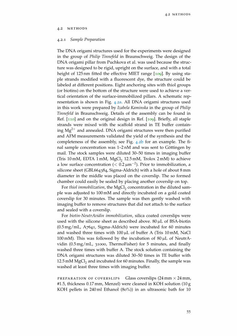
4.2 methods

4.2 methods

4.2.1 Sample Preparation

The DNA origami structures used for the experiments were designedin the group of Philip Tinnefeld in Braunschweig. The design of theDNA origami pillar from Puchkova et al. was used because the struc-ture was designed to be rigid, upright on the surface, and with a totalheight of 125 nm fitted the effective MIET range [109]. By using sta-ple strands modified with a fluorescent dye, the structure could belabeled at different positions. Eight anchoring sites with thiol groups(or biotins) on the bottom of the structure were used to achieve a ver-tical orientation of the surface-immobilized pillars. A schematic rep-resentation is shown in Fig. 4.2a. All DNA origami structures usedin this work were prepared by Izabela Kaminska in the group of PhilipTinnefeld in Braunschweig. Details of the assembly can be found inRef. [110] and on the original design in Ref. [109]. Briefly, all staplestrands were mixed with the scaffold strand in TE buffer contain-ing Mg2+ and annealed. DNA origami structures were then purifiedand AFM measurements validated the yield of the synthesis and thecompleteness of the assembly, see Fig. 4.2b for an example. The fi-nal sample concentration was 1–2 nM and was sent to Göttingen bymail. The stock samples were diluted 30–50 times in imaging buffer(Tris 10 mM, EDTA 1 mM, MgCl2 12.5 mM, Trolox 2 mM) to achievea low surface concentration (< 0.2µm−2). Prior to immobilization, asilicone sheet (GBL664384, Sigma-Aldrich) with a hole of about 8 mmdiameter in the middle was placed on the coverslip. The so formedchamber could easily be sealed by placing another coverslip on top.

For thiol immobilization, the MgCl2 concentration in the diluted sam-ple was adjusted to 100 mM and directly incubated on a gold coatedcoverslip for 30 minutes. The sample was then gently washed withimaging buffer to remove structures that did not attach to the surfaceand sealed with a coverslip.

For biotin-NeutrAvidin immobilization, silica coated coverslips wereused with the silicone sheet as described above. 80µL of BSA-biotin(0.5 mg/mL, A7641, Sigma-Aldrich) were incubated for 60 minutesand washed three times with 100µL of buffer A (Tris 10 mM, NaCl100 mM). This was followed by the incubation of 80µL of NeutrA-vidin (0.5 mg/mL, 31000, ThermoFisher) for 5 minutes, and finallywashed three times with buffer A. The stock solution containing theDNA origami structures was diluted 30–50 times in TE buffer with12.5 mM MgCl2 and incubated for 60 minutes. Finally, the sample waswashed at least three times with imaging buffer.

preparation of coverslips Glass coverslips (24 mm× 24 mm,#1.5, thickness 0.17 mm, Menzel) were cleaned in KOH solution (10 gKOH pellets in 240 ml Ethanol (80%)) in an ultrasonic bath for 10

55

axial co-localization using miet

26nm

58nm

32nm

(a) (b)

Figure 4.2: a) A DNA origami pillar was designed with dyes at differentdistances from the surface. Here, eight thiol groups on the bottom of thestructure can bind to the gold directly to ensure the vertical orientation ofthe pillar. This figure was adapted from Roman Tsukanov. b) AFM image ofthe DNA origami pillars. This figure was reproduced from [110].

minutes, followed by three ultrasonic baths in deionized water for 2minutes each. The clean coverslips were coated with a 10 nm thin filmof gold or silver on top of 2 nm titanium which improves the adhe-sion to glass. The thin films were generated by chemical vapor de-position using an electron beam source (Univex 350, Leybold) underhigh-vacuum conditions (10−6 mbar). The lowest deposition speed of1 Ås−1 was chosen and the film thickness monitored using an oscillat-ing quartz unit. For coverslips with a silica spacer, additional layersof 1 nm titanium and 10 nm SiO2 were deposited in the same way.

The surface roughness of the coverslips were measured by AFMand showed a RMS roughness of 0.5 nm (cleaned glass coverslip),1.5 nm (BSA-biotin coated on mica), and 1 nm (BSA-biotin coated oncleaned glass).

The coverslips were prepared by Alexey Chizhik and the AFM mea-surements for surface characterization were performed by Amna Khalid.

4.2.2 Setup

The experiments were carried out on the commercial Microtime 200

setup (PicoQuant, Germany). The light of a 640 nm pulsed diode laser(LDH-D-C-640, PicoQuant), equipped with a cleanup filter (Z640/10,Chroma Technology), was coupled into a polarization-maintainingsingle mode optical fiber (Schäfter + Kirchhoff). An achromatic λ/4wave plate (Thorlabs) was used to modify the polarization from linearto circular. The light at the fiber output was collimated by an objec-tive and reflected by a dichroic mirror (FITC/TRITC, Chroma Tech-

56

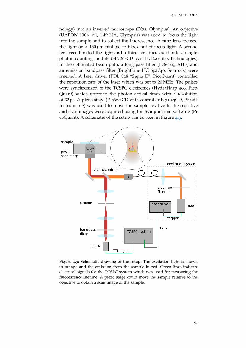
4.2 methods

nology) into an inverted microscope (IX71, Olympus). An objective(UAPON 100× oil, 1.49 NA, Olympus) was used to focus the lightinto the sample and to collect the fluorescence. A tube lens focusedthe light on a 150µm pinhole to block out-of-focus light. A secondlens recollimated the light and a third lens focused it onto a single-photon counting module (SPCM-CD 3516 H, Excelitas Technologies).In the collimated beam path, a long pass filter (F76-649, AHF) andan emission bandpass filter (BrightLine HC 692/40, Semrock) wereinserted. A laser driver (PDL 828 “Sepia II”, PicoQuant) controlledthe repetition rate of the laser which was set to 20 MHz. The pulseswere synchronized to the TCSPC electronics (HydraHarp 400, Pico-Quant) which recorded the photon arrival times with a resolutionof 32 ps. A piezo stage (P-562.3CD with controller E-710.3CD, PhysikInstrumente) was used to move the sample relative to the objectiveand scan images were acquired using the SymphoTime software (Pi-coQuant). A schematic of the setup can be seen in Figure 4.3.

Figure 4.3: Schematic drawing of the setup. The excitation light is shownin orange and the emission from the sample in red. Green lines indicateelectrical signals for the TCSPC system which was used for measuring thefluorescence lifetime. A piezo stage could move the sample relative to theobjective to obtain a scan image of the sample.

57

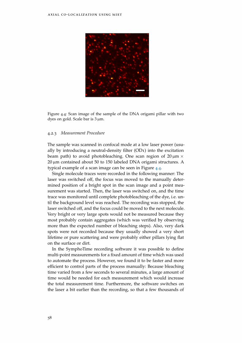
axial co-localization using miet

Figure 4.4: Scan image of the sample of the DNA origami pillar with twodyes on gold. Scale bar is 3µm.

4.2.3 Measurement Procedure

The sample was scanned in confocal mode at a low laser power (usu-ally by introducing a neutral-density filter (OD1) into the excitationbeam path) to avoid photobleaching. One scan region of 20µm ×20µm contained about 50 to 150 labeled DNA origami structures. Atypical example of a scan image can be seen in Figure 4.4.

Single molecule traces were recorded in the following manner: Thelaser was switched off, the focus was moved to the manually deter-mined position of a bright spot in the scan image and a point mea-surement was started. Then, the laser was switched on, and the timetrace was monitored until complete photobleaching of the dye, i.e. un-til the background level was reached. The recording was stopped, thelaser switched off, and the focus could be moved to the next molecule.Very bright or very large spots would not be measured because theymost probably contain aggregates (which was verified by observingmore than the expected number of bleaching steps). Also, very darkspots were not recorded because they usually showed a very shortlifetime or pure scattering and were probably either pillars lying flaton the surface or dirt.

In the SymphoTime recording software it was possible to definemulti-point measurements for a fixed amount of time which was usedto automate the process. However, we found it to be faster and moreefficient to control parts of the process manually: Because bleachingtime varied from a few seconds to several minutes, a large amount oftime would be needed for each measurement which would increasethe total measurement time. Furthermore, the software switches onthe laser a bit earlier than the recording, so that a few thousands of

58

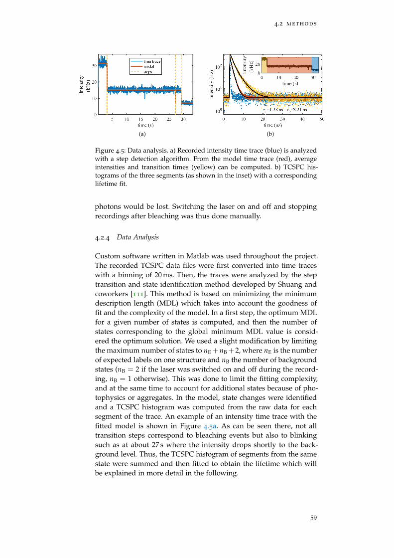
4.2 methods

(a) (b)

Figure 4.5: Data analysis. a) Recorded intensity time trace (blue) is analyzedwith a step detection algorithm. From the model time trace (red), averageintensities and transition times (yellow) can be computed. b) TCSPC his-tograms of the three segments (as shown in the inset) with a correspondinglifetime fit.

photons would be lost. Switching the laser on and off and stoppingrecordings after bleaching was thus done manually.

4.2.4 Data Analysis

Custom software written in Matlab was used throughout the project.The recorded TCSPC data files were first converted into time traceswith a binning of 20 ms. Then, the traces were analyzed by the steptransition and state identification method developed by Shuang andcoworkers [111]. This method is based on minimizing the minimumdescription length (MDL) which takes into account the goodness offit and the complexity of the model. In a first step, the optimum MDLfor a given number of states is computed, and then the number ofstates corresponding to the global minimum MDL value is consid-ered the optimum solution. We used a slight modification by limitingthe maximum number of states to nE +nB + 2, where nE is the numberof expected labels on one structure and nB the number of backgroundstates (nB = 2 if the laser was switched on and off during the record-ing, nB = 1 otherwise). This was done to limit the fitting complexity,and at the same time to account for additional states because of pho-tophysics or aggregates. In the model, state changes were identifiedand a TCSPC histogram was computed from the raw data for eachsegment of the trace. An example of an intensity time trace with thefitted model is shown in Figure 4.5a. As can be seen there, not alltransition steps correspond to bleaching events but also to blinkingsuch as at about 27 s where the intensity drops shortly to the back-ground level. Thus, the TCSPC histogram of segments from the samestate were summed and then fitted to obtain the lifetime which willbe explained in more detail in the following.

59

axial co-localization using miet

4.2.4.1 Lifetime Fitting

As can be seen from the blue curve in Figure 4.5b, the lowest intensitystate corresponds to the background with all fluorescence bleached.The peak visible is mainly due to photoluminescence of the gold [112].For the other TCSPC histograms, fluorescent lifetimes can be fittedusing the following model function

I(t|nj) = IRF(t)~nj

∑i=1

ai

τie−

tτi + a0IRF(t) + b, (4.6)

where the τi are the fluorescence lifetimes of nj emitters with am-plitudes ai, b is a constant background, a0 the scattering amplitude,IRF(t) is the instrument response function, and ~ denotes convolu-tion. For this fitting model, there are m = 2nj + 2 fit parameters. As agoodness-of-fit parameter we calculated the reduced χ2 value

χ2red = ∑

t

(I(t)− H(t))2

I(t)(M−m), (4.7)

where H(t) is the measured TCSPC histogram with M bins.Assuming that the second state corresponds to a single dye, the

fit function I(t|n = 1) was used and a lifetime τ1 obtained. For thehigher state, the model I(t|n = 2) was fitted to the data with thelifetime τ1 fixed from the previous fit to obtain a lifetime τ2.

Sometimes states did not correspond to bleaching molecules, whichmade the data more difficult to analyze. Possible reasons for this in-clude blinking of the dye and state switching (probably isomerizationof the dye Atto 647N or interactions of the dye with the environment).To identity those states, each histogram was first fitted with the samenumber of emitters as before and if the difference in lifetime wassmaller than 10 %, the state was considered to be the same as theprevious and histograms were summed up and fitted together.

The IRF was determined from measurements that contained nofluorescence signal but only gold photoluminescence (such as theblue TCSPC histogram in Fig. 4.5b). Time resolved measurements ofgold luminescence have shown that the decay is faster than picosec-onds which is much smaller than the response time of our detectorsor TCSPC hardware. Because the gold photoluminescence has a rel-atively broad emission spectrum, it can be used to measure the IRFat the same wavelength as the fluorescence emission of the dye. Thisis an advantage compared to other methods that use fore examplescattering to determine the IRF at a different wavelength since theseoften suffer from artifacts due to color shifts of the IRF [113]. How-ever, small shifts could still occur because of which our fitting routineincluded the color shift of the IRF as an additional parameter. After afirst run of the lifetime fitting for all molecules measured on one day,the mean value of all fitted color shifts was calculated and the datawas fitted again with this value fixed to reduce the number of freeparameters.

60

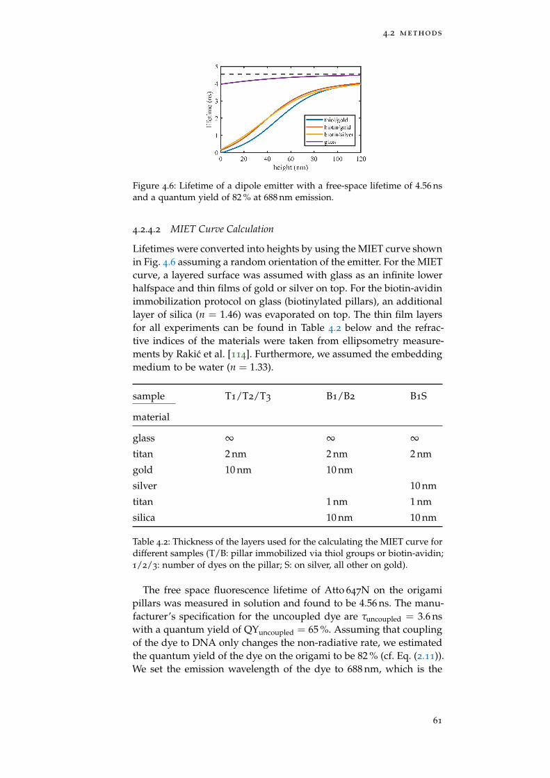
4.2 methods

Figure 4.6: Lifetime of a dipole emitter with a free-space lifetime of 4.56 nsand a quantum yield of 82 % at 688 nm emission.

4.2.4.2 MIET Curve Calculation

Lifetimes were converted into heights by using the MIET curve shownin Fig. 4.6 assuming a random orientation of the emitter. For the MIETcurve, a layered surface was assumed with glass as an infinite lowerhalfspace and thin films of gold or silver on top. For the biotin-avidinimmobilization protocol on glass (biotinylated pillars), an additionallayer of silica (n = 1.46) was evaporated on top. The thin film layersfor all experiments can be found in Table 4.2 below and the refrac-tive indices of the materials were taken from ellipsometry measure-ments by Rakic et al. [114]. Furthermore, we assumed the embeddingmedium to be water (n = 1.33).

sample T1/T2/T3 B1/B2 B1S

material

glass ∞ ∞ ∞

titan 2 nm 2 nm 2 nm

gold 10 nm 10 nm

silver 10 nm

titan 1 nm 1 nm

silica 10 nm 10 nm

Table 4.2: Thickness of the layers used for the calculating the MIET curve fordifferent samples (T/B: pillar immobilized via thiol groups or biotin-avidin;1/2/3: number of dyes on the pillar; S: on silver, all other on gold).

The free space fluorescence lifetime of Atto 647N on the origamipillars was measured in solution and found to be 4.56 ns. The manu-facturer’s specification for the uncoupled dye are τuncoupled = 3.6 nswith a quantum yield of QYuncoupled = 65 %. Assuming that couplingof the dye to DNA only changes the non-radiative rate, we estimatedthe quantum yield of the dye on the origami to be 82 % (cf. Eq. (2.11)).We set the emission wavelength of the dye to 688 nm, which is the

61

axial co-localization using miet

mean emission wavelength of Atto 647N within our emission filterwindow (692/40 nm bandpass).

4.2.4.3 Distance Estimation

For samples with dyes at more than one position, also the distancebetween the emitters along the optical axis can be estimated. Be-cause the distance is non-negative, the distribution of distances isexpected to be asymmetric. This can skew the mean and standarddeviation of these distributions, especially when the error is close tothe expected distance. Therefore, we would prefer a model that de-scribes the distribution. As an approximation, we will assume thatour measured heights are normally distributed. Churchman et al.showed that under this assumption the distribution of the distanceis non-Gaussian [115]. Instead, the probability density to measurea distance in one dimension r = |r2 − r1| given the true distanceµ = |r(true)

2 − r(true)1 | is

p(r|µ, σ) =

√2

πσ2 exp(−µ2 + r2

2σ2

)cosh

(µrσ2

), (4.8)

where σ2 = σ21 + σ2

2 is the sum of the variances of the positions ri. Weuse µ as an estimator for the average distance and σ for its precision.Only for small measurement errors or large distances, the distributionbecomes approximately Gaussian. More precisely, for µr

σ2 1 we findcosh

( µrσ2

)≈ 1

2 exp( µr

σ2

), then

p(r) ≈ 1√2πσ2

exp(−µ2 + r2

2σ2

)exp

(µrσ2

)=

1√2πσ2

exp(− (µ− r)2

2σ2

).

(4.9)

Fitting this distribution is accomplished by the maximum likelihoodmethod. For a set of observations ri the likelihood of these obser-vation given the parameters µ and σ is

P(ri|µ, σ) = ∏i

p(ri|µ, σ). (4.10)

The parameters are estimated by finding the minimum of the negativelog-likelihood

− log P(ri|µ, σ) = −∑i

log p(ri|µ, σ). (4.11)

62

4.3 results

4.3 results

4.3.1 Axial Localization of Single Emitters

Here, we want to measure the height of single Atto 647N emitterwhich is attached to a DNA origami pillar at a designed height of82 nm. The bleaching time traces were analyzed as described in Sec-tion 4.2.4. Since here only one lifetime is expected, all on-states in asingle time trace were combined and the TCSPC histogram was fit-ted with a mono-exponential function. Three different samples werestudied:

T1: DNA origami pillar immobilized via thiol groups on 10 nm gold

B1: DNA origami pillar immobilized via biotin on 10 nm gold and10 nm silica

B1S: DNA origami pillar immobilized via biotin on 10 nm silver and10 nm silica

In case of the biotinylated pillars, the surface was additionally coatedwith a BSA-biotin layer and incubated with NeutrAvidin to ensurespecific immobilization. Furthermore, a control measurement of bi-otinylated pillars immobilized on pure glass was performed. For thissample, we obtained an average lifetime of (4.2± 0.2) ns which agreeswith the theoretical expected value of 4.37 ns for the lifetime of thedye at the design height of 82 nm on top of a pure glass surface.

The measured lifetimes of the three samples were converted intoheights using the MIET curves in Fig. 4.6. The histograms of lifetimeand height are shown in Fig. 4.7. In all cases, a unimodal distributionwas found and fitted with a Gaussian function with offset. We inter-pret the offset as a result of bad fits or tilted pillars. The mean valuesand standard deviations of the Gaussians are listed in Table 4.3.

The heights of all samples are very similar to each other, but do notagree with the design height of 82 nm. Furthermore, we expected alarger height for the biotinylated samples as the BSA layer should addto the height of the pillar. Since the design height of the DNA origamiseemed to be underestimated in all cases, we performed an indepen-dent measurement of the DNA origami size by 3D DNA-PAINT. Forthis experiment, the pillar was labeled with docking strands at thebottom and top with a designed distance of 90 nm between them.The pillar was immobilized on a BSA-biotin coated glass coverslipand 3D DNA-PAINT imaging was performed. By means of astigmaticimaging, the 3D position of the docking sites could be measured, seeFig. 4.8 for the results. The distance between the two docking siteswas (84± 10) nm, which is about 7 % less than the designed distanceof 90 nm. Furthermore, the 3D DNA-PAINT measurement showed atilt distribution with an average tilt angle of (35± 21) with respectto the surface normal.

63

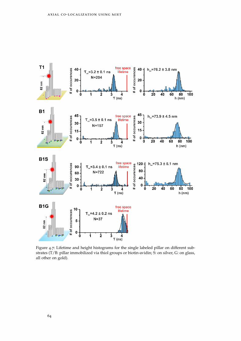
axial co-localization using miet

Figure 4.7: Lifetime and height histograms for the single labeled pillar on different sub-strates (T/B: pillar immobilized via thiol groups or biotin-avidin; S: on silver, G: on glass,all other on gold).

64

4.3 results

design reference measured sample method

height (nm) height (nm) height (nm)

90 84* 84± 10 B2G DNA-PAINT

82 76.5 76.2± 3.8 T1 MIET

82 76.5 73.9± 4.5 B1 MIET

82 76.5 75.3± 5.1 B1S MIET

Table 4.3: Heights of single labeled pillars. Comparison of design heightswith the measured values for different samples (T/B: pillar immobilized viathiol groups or biotin-avidin; 1/2: number of dyes on the pillar; S: on silver,G: on glass, all other on gold). The independent experiment using 3D DNA-PAINT suggests a shrinkage of the whole structure of about 7 %.*) This value is used to compute the reference value from the other designheights. smMIET experiments are in agreement with the reference values.

Deviations from the designed distances have been reported in theliterature before for DNA origami structures under similar experi-mental conditions [116]. Furthermore, the design height was calcu-lated using a simplified model of DNA which does neither take intoaccount interhelical distances, bending, nor twist. We therefore as-sume that a deviation of the designed height from the actual heightis the most probable explanation for our observations. By assuminga linear shrinkage of the whole structure, we calculated a new refer-ence distance from the design height. This agrees with our measuredheights within the error (see Table 4.3). For the T1 sample, we assumethat the height of the immobilization layer (thiol bonds) is negligibleand the pillar is vertical. For the biotinylated samples, the situationis more complicated: On one hand, the 3D DNA-PAINT suggest thatthe pillars are tilted which reduces our observed height. On the otherhand, the immobilization layer thickness is unknown and adds tothe measured height. By assuming a tilt angle of 35 as measured by3D DNA-PAINT, we estimate the height of the immobilization layerto about 12 nm. A more detailed analysis of the immobilization layerthickness can be found in Section 4.3.2.8. The above interpretation ofour measured heights for our three samples assumes that the heightsmeasured by MIET are unbiased. In the next section, we study howthe MIET curve can affect the accuracy of our MIET measurements.

4.3.1.1 MIET Curve Error Estimation

In the previous sections, we measured the height of emitters on aDNA origami structure and found that the measured values deviatedfrom the design values. We could explain the deviations by sampletilt and the unknown thickness of the biotin immobilization layer. An-other possible bias can be introduced when converting the lifetime to

65

axial co-localization using miet

θ (°)

# o

f o

ccu

ren

ces

0 20 40 60 800

25

50

75 (35 ± 21) °

(a)

0 25 50 75 100 1250

30

60

90

Length (nm)

# o

f o

ccu

ren

ces

(84 ± 10) nm

(b1)

(c)

(d)

(b2)θ

Figure 4.8: 3D DNA-PAINT experiment. a) The same DNA origami pillar asfor the MIET experiments was used and immobilized via biotin to the glasssurface. Docking strands were attached with a design distance of 90 nm. b1)Localization map of the DNA origami structures. b2) Astigmatic imagingyields a z position of each blinking event. Each point is a localization event.From the two point clouds, the length of the pillar and its tilt angle is esti-mated. c) Length histogram. The mean length is about 7 % shorter than thedesign value. d) Tilt distribution.The experiment and the data analysis were performed by Mario Raab. Thefigure was adapted from Ref. [110].

66

4.3 results

the height by means of the MIET curve. Here, we investigate the in-fluence of the MIET curve on the accuracy of the heights.

The theory of MIET enables us to calculate the exact dependence ofthe fluorescent lifetime of a dipole emitter on top of a metal surfacewith respect to its height. This curve, the MIET curve, is then used toestimate the height from the measured lifetime. Its shape depends onthe layer system of the surface as well as intrinsic properties of thedye (cf. Section 2.4). If these parameters are not precisely known, theheights measured by MIET will not be accurate. To estimate the error,we performed theoretical calculations of the MIET curve, varying theparameters up to 10 %. Our experimentally determined parametersfrom Section 4.2.4.2 were assumed as the ground truth and used forthe calculation of the true MIET curve τ(z|ptrue). Here, ptrue is theparameter vector of all parameters entering the calculation. Usually,a measured lifetime is converted into a height by using the invertedcurve z(τ|ptrue). This curve accurately predicts the height of an emit-ter with lifetime τ. However, if one parameter in p is estimated er-roneously, we would compute the corresponding MIET curve τ(z|p)and use its inverse z(τ|p) to convert the lifetime into a height. Theheight error is then ∆z = z(τ|p)− z(τ|ptrue).

In Fig. 4.9, we show the influence of six parameters on the axial lo-calization error. Each parameter was allowed to vary by ±10 % fromthe ground truth, and the height error is shown as a function of thevaried parameter and the true height. We investigated intrinsic pa-rameters such as the free space lifetime, the free space quantum yield,and the orientation1 as well as parameters of the metal film, such asthe thickness of the gold film, and the real and imaginary part of therefractive index of the gold. For the intrinsic parameters of the dye,the error increases with height whereas the parameters of the goldfilm show a minimum error around 50 nm. Below 20 nm, the errorby variations of the intrinsic parameters is less than 2 nm, but can in-crease to more than 5 nm above a height of 60 nm. Note that the errorhas an opposite sign when the free space lifetime and the quantumyield are over- or underestimated at the same time. In contrast, theerrors by over- or underestimating the imaginary part of the refrac-tive index of gold and the film thickness correlate with each other.Notably, the real part of the refractive index of the gold has almostno effect on the MIET curve. Apart from that, all other parametersinfluence the MIET curve.

The effect of a 10 % uncertainty in the parameters lead to an accu-racy of MIET on the order of 5 nm which is comparable to the preci-sion we obtained in our experimental results. However, the influencewas probably much smaller. Of all parameters we explored above,the free space lifetime showed the maximum error of 15 nm which,however, could be accurately measured in bulk. The measurement in

1 Here, the orientation was described by the ratio of vertical to parallel emitters in anensemble.

67

axial co-localization using miet

(a) (b)

(c) (d)

(e) (f)

Figure 4.9: Theoretical calculation of the height error when a parameter of the MIET curvecalculation varies up to 10 %. The black line indicates the “true” value of the parameterthat was used for the smMIET co-localization experiments. On the left side, we show theinfluence of some parameters of the dye: a) free space lifetime, c) free space quantumyield, and e) emitter orientation. On the right side, the influence of the metal thin filmis shown: b) gold thickness, d) real part of the refractive index of gold, and f) imaginarypart of the refractive index of gold. In the white parts of the plots, the absolute error islarger than 5 nm.

68

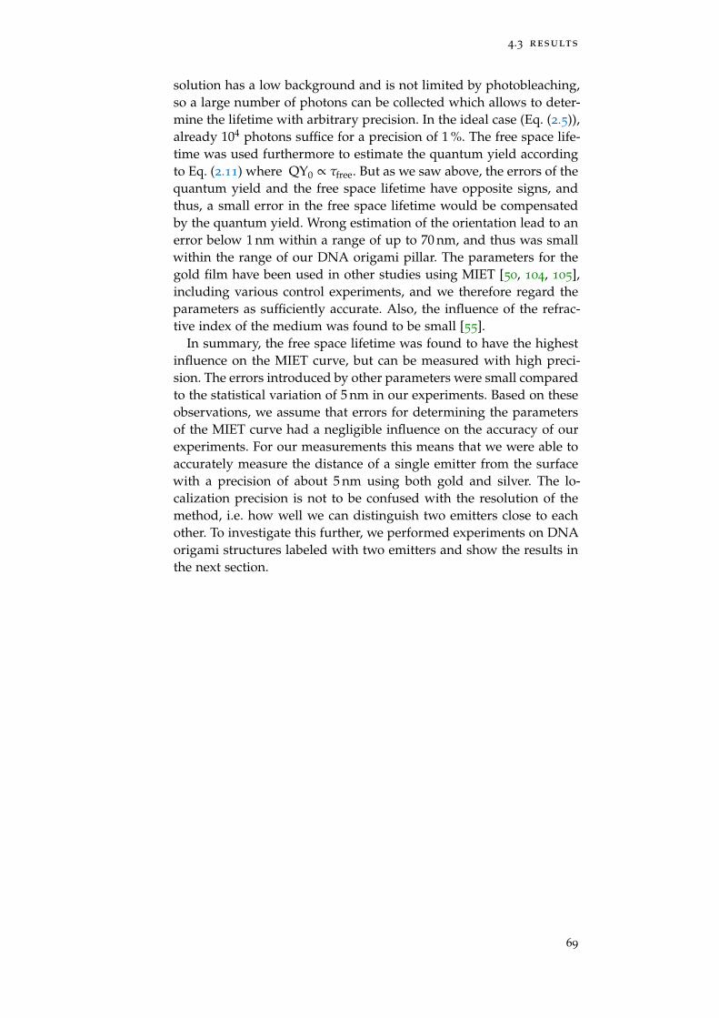
4.3 results

solution has a low background and is not limited by photobleaching,so a large number of photons can be collected which allows to deter-mine the lifetime with arbitrary precision. In the ideal case (Eq. (2.5)),already 104 photons suffice for a precision of 1 %. The free space life-time was used furthermore to estimate the quantum yield accordingto Eq. (2.11) where QY0 ∝ τfree. But as we saw above, the errors of thequantum yield and the free space lifetime have opposite signs, andthus, a small error in the free space lifetime would be compensatedby the quantum yield. Wrong estimation of the orientation lead to anerror below 1 nm within a range of up to 70 nm, and thus was smallwithin the range of our DNA origami pillar. The parameters for thegold film have been used in other studies using MIET [50, 104, 105],including various control experiments, and we therefore regard theparameters as sufficiently accurate. Also, the influence of the refrac-tive index of the medium was found to be small [55].

In summary, the free space lifetime was found to have the highestinfluence on the MIET curve, but can be measured with high preci-sion. The errors introduced by other parameters were small comparedto the statistical variation of 5 nm in our experiments. Based on theseobservations, we assume that errors for determining the parametersof the MIET curve had a negligible influence on the accuracy of ourexperiments. For our measurements this means that we were able toaccurately measure the distance of a single emitter from the surfacewith a precision of about 5 nm using both gold and silver. The lo-calization precision is not to be confused with the resolution of themethod, i.e. how well we can distinguish two emitters close to eachother. To investigate this further, we performed experiments on DNAorigami structures labeled with two emitters and show the results inthe next section.

69

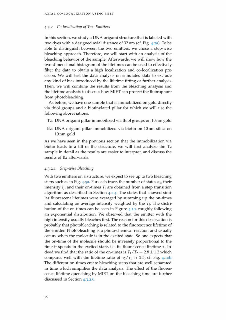
axial co-localization using miet

4.3.2 Co-localization of Two Emitters

In this section, we study a DNA origami structure that is labeled withtwo dyes with a designed axial distance of 32 nm (cf. Fig. 4.2a). To beable to distinguish between the two emitters, we chose a step-wisebleaching approach. Therefore, we will start with an analysis of thebleaching behavior of the sample. Afterwards, we will show how thetwo-dimensional histogram of the lifetimes can be used to effectivelyfilter the data to obtain a high localization and co-localization pre-cision. We will test the data analysis on simulated data to excludeany kind of bias introduced by the lifetime fitting or further analysis.Then, we will combine the results from the bleaching analysis andthe lifetime analysis to discuss how MIET can protect the fluorophorefrom photobleaching.

As before, we have one sample that is immobilized on gold directlyvia thiol groups and a biotinylated pillar for which we will use thefollowing abbreviations:

T2: DNA origami pillar immobilized via thiol groups on 10 nm gold

B2: DNA origami pillar immobilized via biotin on 10 nm silica on10 nm gold

As we have seen in the previous section that the immobilization viabiotin leads to a tilt of the structure, we will first analyze the T2

sample in detail as the results are easier to interpret, and discuss theresults of B2 afterwards.

4.3.2.1 Step-wise Bleaching

With two emitters on a structure, we expect to see up to two bleachingsteps such as in Fig. 4.5a. For each trace, the number of states ns, theirintensity Ij, and their on-times Tj are obtained from a step transitionalgorithm as described in Section 4.2.4. The states that showed simi-lar fluorescent lifetimes were averaged by summing up the on-timesand calculating an average intensity weighted by the Tj. The distri-bution of the on-times can be seen in Figure 4.10, roughly followingan exponential distribution. We observed that the emitter with thehigh intensity usually bleaches first. The reason for this observation isprobably that photobleaching is related to the fluorescence lifetime ofthe emitter. Photobleaching is a photo-chemical reaction and usuallyoccurs when the molecule is in the excited state. So one expects thatthe on-time of the molecule should be inversely proportional to thetime it spends in the excited state, i.e. its fluorescence lifetime τ. In-deed we find that the ratio of the on-times is T1/T2 = 2.8± 1.2 whichcompares well with the lifetime ratio of τ2/τ1 ≈ 2.5, cf. Fig. 4.10b.The different on-times create bleaching steps that are well separatedin time which simplifies the data analysis. The effect of the fluores-cence lifetime quenching by MIET on the bleaching time are furtherdiscussed in Section 4.3.2.6.

70

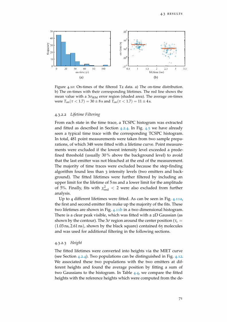
4.3 results

(a) (b)

Figure 4.10: On-times of the filtered T2 data. a) The on-time distribution.b) The on-times with their corresponding lifetimes. The red line shows themean value with a 3σSEM error region (shaded area). The average on-timeswere Ton(τ < 1.7) = 30± 8 s and Ton(τ < 1.7) = 11± 4 s.

4.3.2.2 Lifetime Filtering

From each state in the time trace, a TCSPC histogram was extractedand fitted as described in Section 4.2.4. In Fig. 4.5 we have alreadyseen a typical time trace with the corresponding TCSPC histogram.In total, 481 point measurements were taken from two sample prepa-rations, of which 348 were fitted with a lifetime curve. Point measure-ments were excluded if the lowest intensity level exceeded a prede-fined threshold (usually 30 % above the background level) to avoidthat the last emitter was not bleached at the end of the measurement.The majority of time traces were excluded because the step-findingalgorithm found less than 3 intensity levels (two emitters and back-ground). The fitted lifetimes were further filtered by including anupper limit for the lifetime of 5 ns and a lower limit for the amplitudeof 5%. Finally, fits with χ2

red < 2 were also excluded from furtheranalysis.

Up to 4 different lifetimes were fitted. As can be seen in Fig. 4.11a,the first and second emitter fits make up the majority of the fits. Thesetwo lifetimes are shown in Fig. 4.11b in a two dimensional histogram.There is a clear peak visible, which was fitted with a 2D Gaussian (asshown by the contour). The 3σ region around the center position (τc =

(1.03 ns, 2.61 ns), shown by the black square) contained 65 moleculesand was used for additional filtering in the following sections.

4.3.2.3 Height

The fitted lifetimes were converted into heights via the MIET curve(see Section 4.2.4). Two populations can be distinguished in Fig. 4.12.We associated these two populations with the two emitters at dif-ferent heights and found the average position by fitting a sum oftwo Gaussians to the histogram. In Table 4.4, we compare the fittedheights with the reference heights which were computed from the de-

71

axial co-localization using miet

(a) (b)

Figure 4.11: Lifetime Histograms of T2. a) The lifetime histogram of the lastbleached emitter is shown in yellow, the next in red, and all later emitters inblue. b) Lifetime histogram of the last bleached emitter (lifetime 1) and thesecond emitter (lifetime 2). The contours in black show a two-dimensionalGaussian fit to the peak and the black square shows the 3σ area used forfiltering.

(a) (b)

Figure 4.12: Height histograms of T2. a) All data with peaks at (54± 11) nmand (23.5± 5.4) nm, N = 137. b) Filtered data with peaks at (53.1± 4.5) nmand (23.6 ± 3.5) nm, N = 65. Both histograms were fitted with a doubleGaussian fit.

72

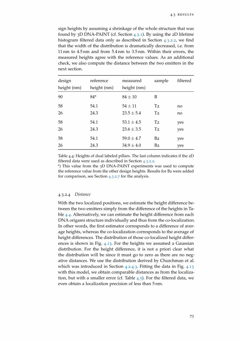
4.3 results

sign heights by assuming a shrinkage of the whole structure that wasfound by 3D DNA-PAINT (cf. Section 4.3.1). By using the 2D lifetimehistogram filtered data only as described in Section 4.3.2.2, we findthat the width of the distribution is dramatically decreased, i.e. from11 nm to 4.5 nm and from 5.4 nm to 3.5 nm. Within their errors, themeasured heights agree with the reference values. As an additionalcheck, we also compute the distance between the two emitters in thenext section.

design reference measured sample filtered

height (nm) height (nm) height (nm)

90 84* 84± 10 B

58 54.1 54± 11 T2 no

26 24.3 23.5± 5.4 T2 no

58 54.1 53.1± 4.5 T2 yes

26 24.3 23.6± 3.5 T2 yes

58 54.1 59.0± 4.7 B2 yes

26 24.3 34.9± 4.0 B2 yes

Table 4.4: Heights of dual labeled pillars. The last column indicates if the 2Dfiltered data were used as described in Section 4.3.2.2.*) This value from the 3D DNA-PAINT experiments was used to computethe reference value from the other design heights. Results for B2 were addedfor comparison, see Section 4.3.2.7 for the analysis.

4.3.2.4 Distance

With the two localized positions, we estimate the height difference be-tween the two emitters simply from the difference of the heights in Ta-ble 4.4. Alternatively, we can estimate the height difference from eachDNA origami structure individually and thus from the co-localization.In other words, the first estimator corresponds to a difference of aver-age heights, whereas the co-localization corresponds to the average ofheight differences. The distribution of those co-localized height differ-ences is shown in Fig. 4.13. For the heights we assumed a Gaussiandistribution. For the height difference, it is not a priori clear whatthe distribution will be since it must go to zero as there are no neg-ative distances. We use the distribution derived by Churchman et al.which was introduced in Section 4.2.4.3. Fitting the data in Fig. 4.13

with this model, we obtain comparable distances as from the localiza-tion, but with a smaller error (cf. Table 4.5). For the filtered data, weeven obtain a localization precision of less than 5 nm.

73

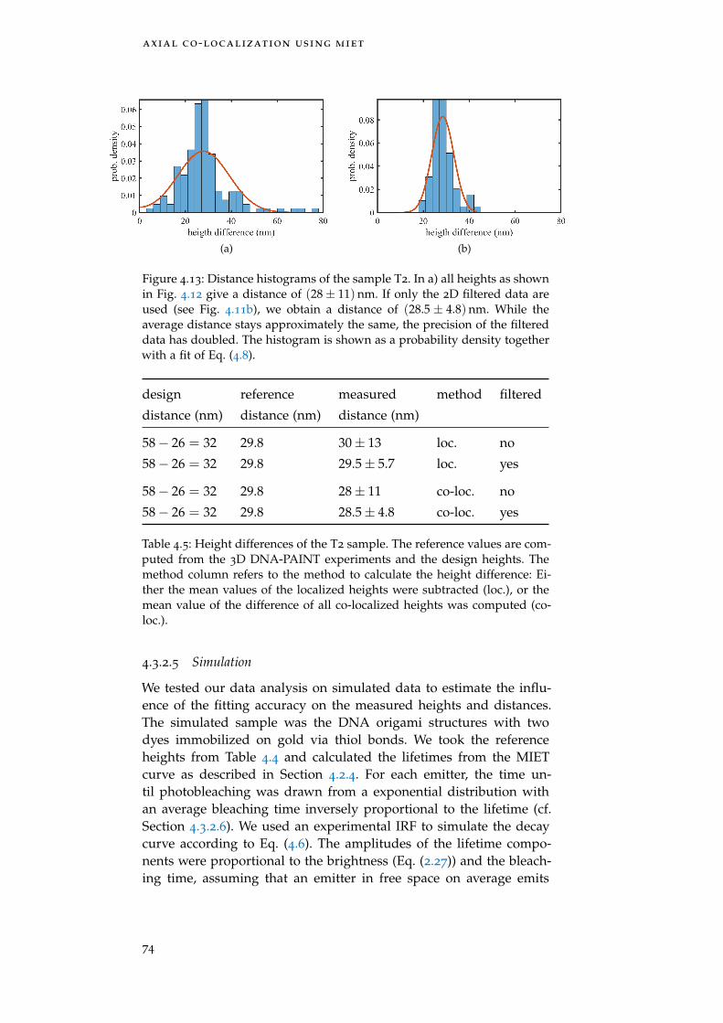
axial co-localization using miet

(a) (b)

Figure 4.13: Distance histograms of the sample T2. In a) all heights as shownin Fig. 4.12 give a distance of (28± 11) nm. If only the 2D filtered data areused (see Fig. 4.11b), we obtain a distance of (28.5 ± 4.8) nm. While theaverage distance stays approximately the same, the precision of the filtereddata has doubled. The histogram is shown as a probability density togetherwith a fit of Eq. (4.8).

design reference measured method filtered

distance (nm) distance (nm) distance (nm)

58− 26 = 32 29.8 30± 13 loc. no

58− 26 = 32 29.8 29.5± 5.7 loc. yes

58− 26 = 32 29.8 28± 11 co-loc. no

58− 26 = 32 29.8 28.5± 4.8 co-loc. yes

Table 4.5: Height differences of the T2 sample. The reference values are com-puted from the 3D DNA-PAINT experiments and the design heights. Themethod column refers to the method to calculate the height difference: Ei-ther the mean values of the localized heights were subtracted (loc.), or themean value of the difference of all co-localized heights was computed (co-loc.).

4.3.2.5 Simulation

We tested our data analysis on simulated data to estimate the influ-ence of the fitting accuracy on the measured heights and distances.The simulated sample was the DNA origami structures with twodyes immobilized on gold via thiol bonds. We took the referenceheights from Table 4.4 and calculated the lifetimes from the MIETcurve as described in Section 4.2.4. For each emitter, the time un-til photobleaching was drawn from a exponential distribution withan average bleaching time inversely proportional to the lifetime (cf.Section 4.3.2.6). We used an experimental IRF to simulate the decaycurve according to Eq. (4.6). The amplitudes of the lifetime compo-nents were proportional to the brightness (Eq. (2.27)) and the bleach-ing time, assuming that an emitter in free space on average emits

74

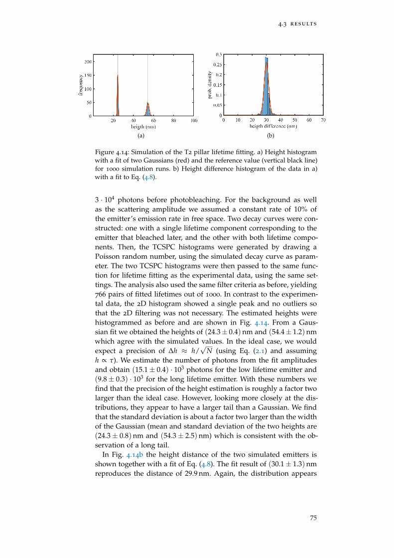
4.3 results

(a) (b)

Figure 4.14: Simulation of the T2 pillar lifetime fitting. a) Height histogramwith a fit of two Gaussians (red) and the reference value (vertical black line)for 1000 simulation runs. b) Height difference histogram of the data in a)with a fit to Eq. (4.8).

3 · 104 photons before photobleaching. For the background as wellas the scattering amplitude we assumed a constant rate of 10% ofthe emitter’s emission rate in free space. Two decay curves were con-structed: one with a single lifetime component corresponding to theemitter that bleached later, and the other with both lifetime compo-nents. Then, the TCSPC histograms were generated by drawing aPoisson random number, using the simulated decay curve as param-eter. The two TCSPC histograms were then passed to the same func-tion for lifetime fitting as the experimental data, using the same set-tings. The analysis also used the same filter criteria as before, yielding766 pairs of fitted lifetimes out of 1000. In contrast to the experimen-tal data, the 2D histogram showed a single peak and no outliers sothat the 2D filtering was not necessary. The estimated heights werehistogrammed as before and are shown in Fig. 4.14. From a Gaus-sian fit we obtained the heights of (24.3± 0.4) nm and (54.4± 1.2) nmwhich agree with the simulated values. In the ideal case, we wouldexpect a precision of ∆h ≈ h/

√N (using Eq. (2.1) and assuming

h ∝ τ). We estimate the number of photons from the fit amplitudesand obtain (15.1± 0.4) · 103 photons for the low lifetime emitter and(9.8± 0.3) · 103 for the long lifetime emitter. With these numbers wefind that the precision of the height estimation is roughly a factor twolarger than the ideal case. However, looking more closely at the dis-tributions, they appear to have a larger tail than a Gaussian. We findthat the standard deviation is about a factor two larger than the widthof the Gaussian (mean and standard deviation of the two heights are(24.3± 0.8) nm and (54.3± 2.5) nm) which is consistent with the ob-servation of a long tail.

In Fig. 4.14b the height distance of the two simulated emitters isshown together with a fit of Eq. (4.8). The fit result of (30.1± 1.3) nmreproduces the distance of 29.9 nm. Again, the distribution appears

75

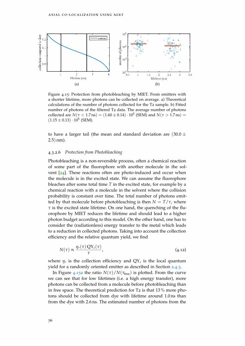
axial co-localization using miet

(a) (b)

Figure 4.15: Protection from photobleaching by MIET. From emitters witha shorter lifetime, more photons can be collected on average. a) Theoreticalcalculations of the number of photons collected for the T2 sample. b) Fittednumber of photons of the filtered T2 data. The average number of photonscollected are N(τ < 1.7 ns) = (1.60± 0.14) · 105 (SEM) and N(τ > 1.7 ns) =(1.15± 0.13) · 105 (SEM).

to have a larger tail (the mean and standard deviation are (30.0 ±2.5) nm).

4.3.2.6 Protection from Photobleaching

Photobleaching is a non-reversible process, often a chemical reactionof some part of the fluorophore with another molecule in the sol-vent [24]. These reactions often are photo-induced and occur whenthe molecule is in the excited state. We can assume the fluorophorebleaches after some total time T in the excited state, for example by achemical reaction with a molecule in the solvent where the collisionprobability is constant over time. The total number of photons emit-ted by that molecule before photobleaching is then N = T/τ, whereτ is the excited state lifetime. On one hand, the quenching of the flu-orophore by MIET reduces the lifetime and should lead to a higherphoton budget according to this model. On the other hand, one has toconsider the (radiationless) energy transfer to the metal which leadsto a reduction in collected photons. Taking into account the collectionefficiency and the relative quantum yield, we find

N(τ) ∝ηr(τ)QYr(τ)

τ, (4.12)

where ηr is the collection efficiency and QYr is the local quantumyield for a randomly oriented emitter as described in Section 2.4.3.

In Figure 4.15a the ratio N(τ)/N(τfree) is plotted. From the curvewe can see that for low lifetimes (i.e. a high energy transfer), morephotons can be collected from a molecule before photobleaching thanin free space. The theoretical prediction for T2 is that 13 % more pho-tons should be collected from dye with lifetime around 1.0 ns thanfrom the dye with 2.6 ns. The estimated number of photons from the

76

4.3 results

amplitudes of the lifetime fits of the T2 sample is shown in Fig. 4.15b.The mean values N(τ < 1.7 ns) = (1.60 ± 0.14) · 105 (SEM) andN(τ > 1.7 ns) = (1.15± 0.13) · 105 (SEM) show an increase of the lowlifetime photons by 40 %. Alternatively, the the number of photonscan be estimated from the intensity time trace. The number of pho-tons obtained from both methods show a good correlation (Pearson’sr = 0.92), but the mean values differ: The average number of photonsestimated from the intensity is N(τ < 1.7 ns) = (1.41± 0.12) · 105 forthe short lifetime and N(τ > 1.7 ns) = (1.30± 0.15) · 105 for the longlifetime which corresponds to an increase of 9 %. Because the numberof photons is roughly exponentially distributed, the standard devia-tion of the data is quite large (i.e. of the same order as the meanvalue). Combined with the low number of data points (N = 65) thismakes a reliable estimation of the ratio impossible. But whether weestimate the number of photons from fits or from the intensity levels,the trend is confirmed: more photons can be collected from emitterswith low lifetime before bleaching as predicted by our simple model.

4.3.2.7 Results for B2

After the comprehensive analysis of the thiol immobilized pillar above,we will briefly state the results for the biotinylated sample. The flowof analysis was the same as above.

From 231 point measurements with fitted lifetimes, our filter crite-ria excluded 70 from further analysis. In the 2D lifetime histogram,we observed again a main peak and fitted it by a 2D Gaussian. Inthe 3σ surrounding we found 132 points that were used for furtheranalysis. We observed that the width of the lifetime distribution isincreased compared to T2. Furthermore, we found a correlation be-tween the short and long lifetimes with a Pearson coefficient of r =

0.51. With r = 0.79, the correlation is even higher for the unfiltereddata.

From the height histogram shown in Fig. 4.16b we obtain twoheights of (59.0± 4.7) nm and (34.9± 4.0) nm which are larger thanthe heights obtained for the thiol immobilized pillar. The increasedheight can be attributed to the different immobilization method: whilethe thiol groups bind directly to the gold surface, the biotinylated pil-lars need an additional layer on the surface. The silica spacer is coatedwith biotinylated BSA and incubated with NeutrAvidin to which thepillars can bind. If the only difference between the T2 and B2 sampleis the immobilization layer, we could estimate its thickness from ourdata. However, in Section 4.3.1 we found that the biotinylated pillarsare tilted, which should result in a reduced height. The above men-tioned correlation between lifetimes is an indicator for a tilt distribu-tion, because the tilt would affect both heights and therefore lifetimes.The correlation is much larger than in simulations, so the fitting errordoes not explain the high correlation we observe here. It is also larger

77

axial co-localization using miet

(a) (b)

Figure 4.16: a) Height histogram of the biotinylated pillar. The heights ob-tained by the Gaussian fit are (59.0± 4.7) nm and (34.9± 4.0) nm. b) Esti-mation of the BSA-biotin-NeutrAvidin layer thickness and tilt angle. Theweighted regression of the heights of B1 and B2 versus T1 and T2 givesa thickness of 15.8 nm and a tilt angle of 39 (blue line). The dashed linerepresents the case of no tilt.

than in the thiol sample, consistent with the hypothesis of tilt in thebiotinylated sample but none (or less) in the thiol sample.

The distance distribution from co-localized emitters yields a dis-tance of (25.0± 7.7) nm. Although the expected distance of 29.8 nmis within the error of the measurement, it shows a tendency to beunderestimated. If we take the average tilt angle of 35 measured by3D DNA-PAINT into account, the expected distance becomes 24.5 nmand is close to the measured value. In the next section we will com-bine the data with our results from the thiol immobilized pillar toestimate the BSA layer thickness and the tilt.

4.3.2.8 Estimation of Immobilization Layer Thickness and Tilt

The measured heights of the B2 sample are significantly higher thanfor T2 (cf. Table 4.4). On the one hand, we would expect an increasein height because we do not know the height of the BSA-NeutrAvidinlayer below the pillar. On the other hand, we expect the biotin pillarsto be tilted as measured by 3D DNA-PAINT, which would again re-duce the observed height. Assuming the heights measured for T1 andT2 as ground truth and comparing them to the heights of the biotinsample, we obtained an estimate of the shift and the tilt. A weightedregression gave a layer thickness of 15.8 nm and a tilt angle of 39 (seeFig. 4.16a). If using the reference values calculated from the 3D DNA-PAINT experiment as ground truth instead, the values changed onlyslightly (15.1 nm and 38). These estimates are comparable to litera-ture values for BSA (14 × 4 × 4 nm3 for the dimer [117]) and Neu-trAvidin (5.8 ± 1.8 nm [49]) and the average tilt angle of 35 mea-sured by 3D DNA-PAINT. Ellipsometric measurements found thatthe layer thickness of BSA depends on the surface density as this willdetermine the orientation of the prolate BSA molecule in a mono-

78

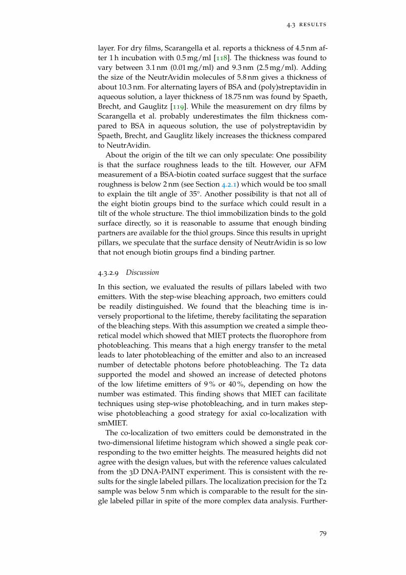
4.3 results

layer. For dry films, Scarangella et al. reports a thickness of 4.5 nm af-ter 1 h incubation with 0.5 mg/ml [118]. The thickness was found tovary between 3.1 nm (0.01 mg/ml) and 9.3 nm (2.5 mg/ml). Addingthe size of the NeutrAvidin molecules of 5.8 nm gives a thickness ofabout 10.3 nm. For alternating layers of BSA and (poly)streptavidin inaqueous solution, a layer thickness of 18.75 nm was found by Spaeth,Brecht, and Gauglitz [119]. While the measurement on dry films byScarangella et al. probably underestimates the film thickness com-pared to BSA in aqueous solution, the use of polystreptavidin bySpaeth, Brecht, and Gauglitz likely increases the thickness comparedto NeutrAvidin.

About the origin of the tilt we can only speculate: One possibilityis that the surface roughness leads to the tilt. However, our AFMmeasurement of a BSA-biotin coated surface suggest that the surfaceroughness is below 2 nm (see Section 4.2.1) which would be too smallto explain the tilt angle of 35°. Another possibility is that not all ofthe eight biotin groups bind to the surface which could result in atilt of the whole structure. The thiol immobilization binds to the goldsurface directly, so it is reasonable to assume that enough bindingpartners are available for the thiol groups. Since this results in uprightpillars, we speculate that the surface density of NeutrAvidin is so lowthat not enough biotin groups find a binding partner.

4.3.2.9 Discussion

In this section, we evaluated the results of pillars labeled with twoemitters. With the step-wise bleaching approach, two emitters couldbe readily distinguished. We found that the bleaching time is in-versely proportional to the lifetime, thereby facilitating the separationof the bleaching steps. With this assumption we created a simple theo-retical model which showed that MIET protects the fluorophore fromphotobleaching. This means that a high energy transfer to the metalleads to later photobleaching of the emitter and also to an increasednumber of detectable photons before photobleaching. The T2 datasupported the model and showed an increase of detected photonsof the low lifetime emitters of 9 % or 40 %, depending on how thenumber was estimated. This finding shows that MIET can facilitatetechniques using step-wise photobleaching, and in turn makes step-wise photobleaching a good strategy for axial co-localization withsmMIET.

The co-localization of two emitters could be demonstrated in thetwo-dimensional lifetime histogram which showed a single peak cor-responding to the two emitter heights. The measured heights did notagree with the design values, but with the reference values calculatedfrom the 3D DNA-PAINT experiment. This is consistent with the re-sults for the single labeled pillars. The localization precision for the T2

sample was below 5 nm which is comparable to the result for the sin-gle labeled pillar in spite of the more complex data analysis. Further-

79

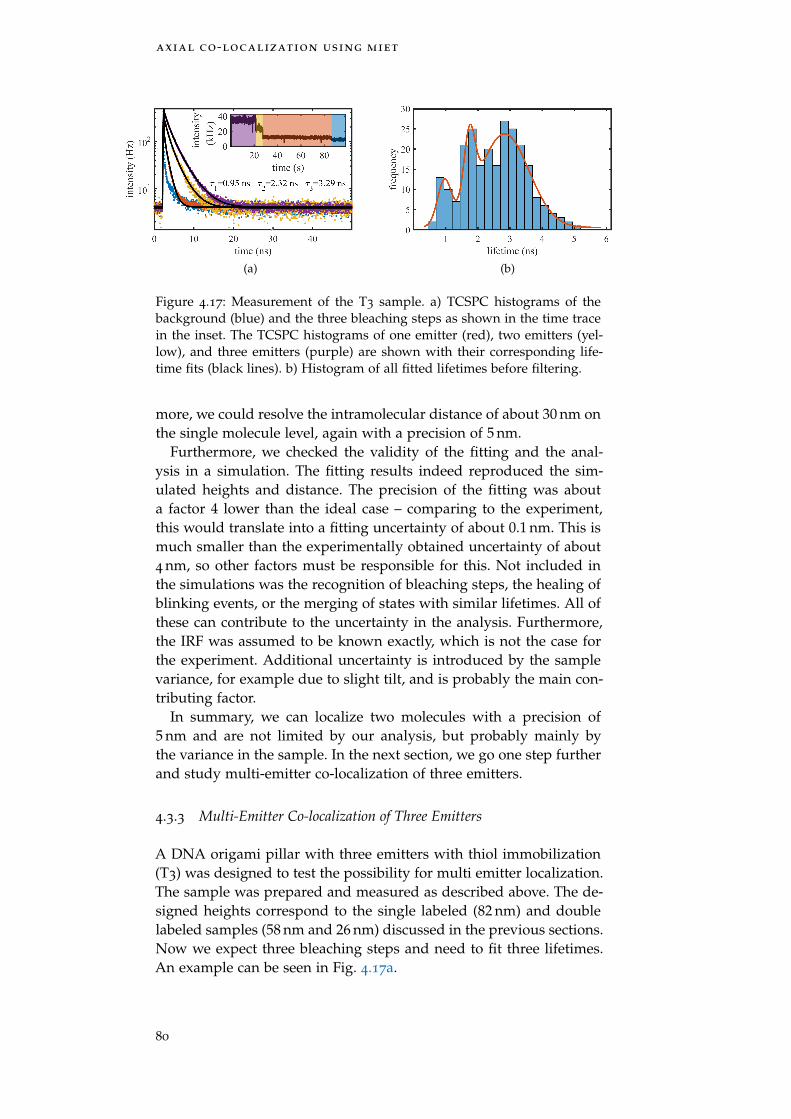
axial co-localization using miet

(a) (b)

Figure 4.17: Measurement of the T3 sample. a) TCSPC histograms of thebackground (blue) and the three bleaching steps as shown in the time tracein the inset. The TCSPC histograms of one emitter (red), two emitters (yel-low), and three emitters (purple) are shown with their corresponding life-time fits (black lines). b) Histogram of all fitted lifetimes before filtering.

more, we could resolve the intramolecular distance of about 30 nm onthe single molecule level, again with a precision of 5 nm.

Furthermore, we checked the validity of the fitting and the anal-ysis in a simulation. The fitting results indeed reproduced the sim-ulated heights and distance. The precision of the fitting was abouta factor 4 lower than the ideal case – comparing to the experiment,this would translate into a fitting uncertainty of about 0.1 nm. This ismuch smaller than the experimentally obtained uncertainty of about4 nm, so other factors must be responsible for this. Not included inthe simulations was the recognition of bleaching steps, the healing ofblinking events, or the merging of states with similar lifetimes. All ofthese can contribute to the uncertainty in the analysis. Furthermore,the IRF was assumed to be known exactly, which is not the case forthe experiment. Additional uncertainty is introduced by the samplevariance, for example due to slight tilt, and is probably the main con-tributing factor.

In summary, we can localize two molecules with a precision of5 nm and are not limited by our analysis, but probably mainly bythe variance in the sample. In the next section, we go one step furtherand study multi-emitter co-localization of three emitters.

4.3.3 Multi-Emitter Co-localization of Three Emitters

A DNA origami pillar with three emitters with thiol immobilization(T3) was designed to test the possibility for multi emitter localization.The sample was prepared and measured as described above. The de-signed heights correspond to the single labeled (82 nm) and doublelabeled samples (58 nm and 26 nm) discussed in the previous sections.Now we expect three bleaching steps and need to fit three lifetimes.An example can be seen in Fig. 4.17a.

80

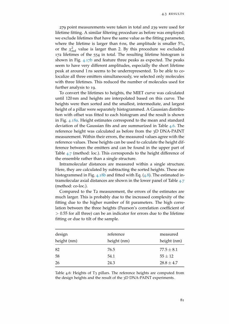
4.3 results

279 point measurements were taken in total and 239 were used forlifetime fitting. A similar filtering procedure as before was employed:we exclude lifetimes that have the same value as the fitting parameter,where the lifetime is larger than 6 ns, the amplitude is smaller 5%,or the χ2

red value is larger than 2. By this procedure we excluded172 lifetimes of the 554 in total. The resulting lifetime histogram isshown in Fig. 4.17b and feature three peaks as expected. The peaksseem to have very different amplitudes, especially the short lifetimepeak at around 1 ns seems to be underrepresented. To be able to co-localize all three emitters simultaneously, we selected only moleculeswith three lifetimes. This reduced the number of molecules used forfurther analysis to 19.

To convert the lifetimes to heights, the MIET curve was calculateduntil 120 nm and heights are interpolated based on this curve. Theheights were then sorted and the smallest, intermediate, and largestheight of a pillar were separately histogrammed. A Gaussian distribu-tion with offset was fitted to each histogram and the result is shownin Fig. 4.18a. Height estimates correspond to the mean and standarddeviation of the Gaussian fits and are summarized in Table 4.6. Thereference height was calculated as before from the 3D DNA-PAINTmeasurement. Within their errors, the measured values agree with thereference values. These heights can be used to calculate the height dif-ference between the emitters and can be found in the upper part ofTable 4.7 (method: loc.). This corresponds to the height difference ofthe ensemble rather than a single structure.

Intramolecular distances are measured within a single structure.Here, they are calculated by subtracting the sorted heights. These arehistogrammed in Fig. 4.18b and fitted with Eq. (4.8). The estimated in-tramolecular axial distances are shown in the lower panel of Table 4.7(method: co-loc.).

Compared to the T2 measurement, the errors of the estimates aremuch larger. This is probably due to the increased complexity of thefitting due to the higher number of fit parameters. The high corre-lation between the three heights (Pearson’s correlation coefficient of> 0.55 for all three) can be an indicator for errors due to the lifetimefitting or due to tilt of the sample.

design reference measured

height (nm) height (nm) height (nm)

82 76.5 77.5± 8.1

58 54.1 55± 12

26 24.3 28.8± 4.7

Table 4.6: Heights of T3 pillars. The reference heights are computed fromthe design heights and the result of the 3D DNA-PAINT experiments.

81

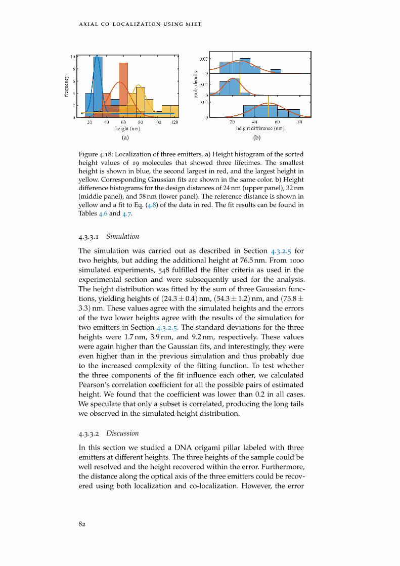
axial co-localization using miet

(a) (b)

Figure 4.18: Localization of three emitters. a) Height histogram of the sortedheight values of 19 molecules that showed three lifetimes. The smallestheight is shown in blue, the second largest in red, and the largest height inyellow. Corresponding Gaussian fits are shown in the same color. b) Heightdifference histograms for the design distances of 24 nm (upper panel), 32 nm(middle panel), and 58 nm (lower panel). The reference distance is shown inyellow and a fit to Eq. (4.8) of the data in red. The fit results can be found inTables 4.6 and 4.7.

4.3.3.1 Simulation

The simulation was carried out as described in Section 4.3.2.5 fortwo heights, but adding the additional height at 76.5 nm. From 1000

simulated experiments, 548 fulfilled the filter criteria as used in theexperimental section and were subsequently used for the analysis.The height distribution was fitted by the sum of three Gaussian func-tions, yielding heights of (24.3± 0.4) nm, (54.3± 1.2) nm, and (75.8±3.3) nm. These values agree with the simulated heights and the errorsof the two lower heights agree with the results of the simulation fortwo emitters in Section 4.3.2.5. The standard deviations for the threeheights were 1.7 nm, 3.9 nm, and 9.2 nm, respectively. These valueswere again higher than the Gaussian fits, and interestingly, they wereeven higher than in the previous simulation and thus probably dueto the increased complexity of the fitting function. To test whetherthe three components of the fit influence each other, we calculatedPearson’s correlation coefficient for all the possible pairs of estimatedheight. We found that the coefficient was lower than 0.2 in all cases.We speculate that only a subset is correlated, producing the long tailswe observed in the simulated height distribution.

4.3.3.2 Discussion

In this section we studied a DNA origami pillar labeled with threeemitters at different heights. The three heights of the sample could bewell resolved and the height recovered within the error. Furthermore,the distance along the optical axis of the three emitters could be recov-ered using both localization and co-localization. However, the error

82

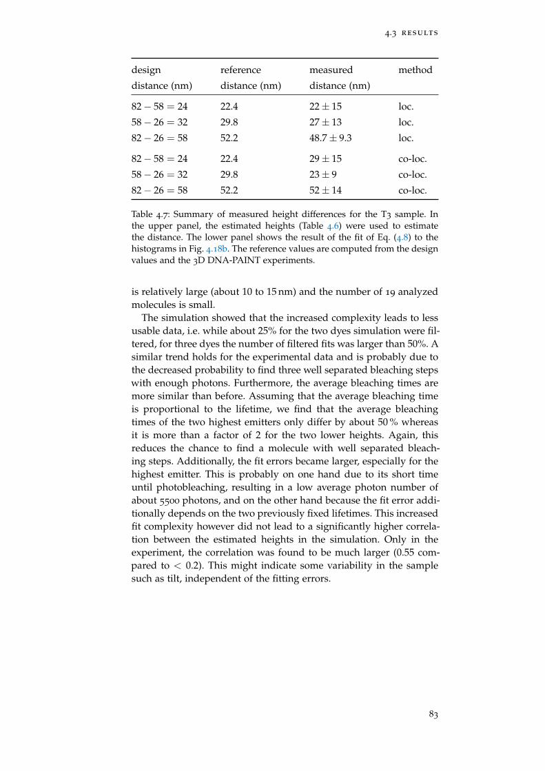
4.3 results

design reference measured method

distance (nm) distance (nm) distance (nm)

82− 58 = 24 22.4 22± 15 loc.

58− 26 = 32 29.8 27± 13 loc.

82− 26 = 58 52.2 48.7± 9.3 loc.

82− 58 = 24 22.4 29± 15 co-loc.

58− 26 = 32 29.8 23± 9 co-loc.

82− 26 = 58 52.2 52± 14 co-loc.

Table 4.7: Summary of measured height differences for the T3 sample. Inthe upper panel, the estimated heights (Table 4.6) were used to estimatethe distance. The lower panel shows the result of the fit of Eq. (4.8) to thehistograms in Fig. 4.18b. The reference values are computed from the designvalues and the 3D DNA-PAINT experiments.

is relatively large (about 10 to 15 nm) and the number of 19 analyzedmolecules is small.

The simulation showed that the increased complexity leads to lessusable data, i.e. while about 25% for the two dyes simulation were fil-tered, for three dyes the number of filtered fits was larger than 50%. Asimilar trend holds for the experimental data and is probably due tothe decreased probability to find three well separated bleaching stepswith enough photons. Furthermore, the average bleaching times aremore similar than before. Assuming that the average bleaching timeis proportional to the lifetime, we find that the average bleachingtimes of the two highest emitters only differ by about 50 % whereasit is more than a factor of 2 for the two lower heights. Again, thisreduces the chance to find a molecule with well separated bleach-ing steps. Additionally, the fit errors became larger, especially for thehighest emitter. This is probably on one hand due to its short timeuntil photobleaching, resulting in a low average photon number ofabout 5500 photons, and on the other hand because the fit error addi-tionally depends on the two previously fixed lifetimes. This increasedfit complexity however did not lead to a significantly higher correla-tion between the estimated heights in the simulation. Only in theexperiment, the correlation was found to be much larger (0.55 com-pared to < 0.2). This might indicate some variability in the samplesuch as tilt, independent of the fitting errors.

83

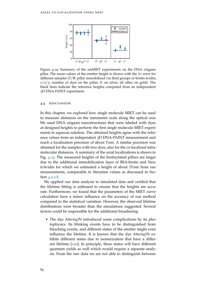
axial co-localization using miet

Figure 4.19: Summary of the smMIET experiments on the DNA origamipillar. The mean values of the emitter height is shown with the 1σ error fordifferent samples (T/B: pillar immobilized via thiol groups or biotin-avidin;1/2/3: number of dyes on the pillar; S: on silver, all other on gold). Theblack lines indicate the reference heights computed from an independent3D DNA-PAINT experiment.

4.4 discussion

In this chapter, we explored how single molecule MIET can be usedto measure distances on the nanometer scale along the optical axis.We used DNA origami nanostructures that were labeled with dyesat designed heights to perform the first single molecule MIET experi-ments in aqueous solution. The obtained heights agree with the refer-ence values from an independent 3D DNA-PAINT measurement andreach a localization precision of about 5 nm. A similar precision wasobtained for the samples with two dyes, also for the co-localized intra-molecular distances. A summary of the axial localizations is shown inFig. 4.19. The measured heights of the biotinylated pillars are largerdue to the additional immobilization layer of BSA-biotin and Neu-trAvidin for which we estimated a height of about 15 nm from ourmeasurements, comparable to literature values as discussed in Sec-tion 4.3.2.8.

We applied our data analysis to simulated data and verified thatthe lifetime fitting is unbiased to ensure that the heights are accu-rate. Furthermore, we found that the parameters of the MIET curvecalculation have a minor influence on the accuracy of our methodcompared to the statistical variation. However, the observed lifetimedistributions were broader than the simulations suggested. Severalfactors could be responsible for the additional broadening:

• The dye Atto 647N introduced some complications by its pho-tophysics. Its blinking events have to be distinguished frombleaching events, and different states of the emitter might eveninfluence the lifetime. It is known that the dye Atto 647N ex-hibits different states due to isomerization that have a differ-ent lifetime [120]. In principle, these states will have differentquantum yields as well which would require a separate analy-sis. From the raw data we are not able to distinguish between

84

4.4 discussion

the states, but since we know that the lifetime changes are small,we expect that this effect simply adds to the broadening of themeasured lifetime distribution.

• A broadening is induced if the dipole of the emitter is not freelyrotating. Atto 647N is not well water-soluble and thus mightstick to the DNA origami or the surface. The influence of theorientation could be alleviated by combining the lifetime mea-surement with an orientation measurement. The orientation canbe measured simultaneously to the lifetime either by defocusedimaging [102] as proposed in Ref. [51] or by making use of theangular distribution of emission (cf. Section 2.4) and calculat-ing the polar angle from the intensity of the high-angle andthe low-angle emission as in Ref. [103]. The former method hasthe advantage that the emitter can be localized laterally as welland would allow localization in 3D. Alternatively, the orienta-tion can be incorporated via modeling: It has been shown thata combination of FRET measurements with molecular dynam-ics simulation allows a direct comparison of the raw data withthe simulation and improves the accuracy of the FRET distancedistribution due to orientation effects [121]. This could also beapplied to MIET experiments to increase the accuracy since itaccounts also for restricted rotation which is difficult to mea-sure.

• Additional broadening probably stems from tilt of the DNAorigami structure which was also found in the 3D DNA-PAINTexperiment. Because MIET measures the distance with respectto the surface, the orientation of the structure with respect to thesurface normal is important. If the structure is immobilized onthe surface in a specific orientation (as our DNA origami struc-ture via thiol bonds), the interpretation of the heights directly re-lates to the axial distance on the structure. However, if the sam-ple is randomly oriented on the surface, the measured heightswill vary from molecule to molecule because MIET measuresthe projection of the 3D distance on the optical axis. It mightbe possible to reconstruct the 3D distance by back-projectionwhich is commonly used in electron microscopy and tomogra-phy [122].

MIET exploits the distance-dependent energy transfer to a metal andis thus similar to FRET. However, MIET has some advantages in com-parison to FRET: First, the orientation of the dyes plays a crucial rolefor the accuracy of FRET and it is not possible to measure the orienta-tion factor independently of the FRET distance. In contrast to this, theorientation for MIET can be measured simultaneously as discussedabove. Second, multi-distance measurements are possible with multi-pair FRET [123, 124], but are challenging due to the specific label-ing of multiple positions with different dyes and the complex instru-

85

axial co-localization using miet

mentation and data analysis. For MIET, only a single type of label isneeded and the setup can be a standard confocal microscope with thecapability to measure fluorescence lifetime. We have demonstratedthis by the co-localization of three emitters on the DNA origami pil-lar. In comparison to other near-field methods such as vaTIRF or SAFwhich are based on intensity measurements, MIET does not needinstrument-specific corrections for cross-talk or background intensi-ties. Furthermore, these methods are not able to resolve two emittersat the same time, limiting their applicability for intra-molecular dis-tance measurements.

MIET can measure intra-molecular distances in a range of 100 nmwith a precision of 5 nm. This bridges the gap between conventional3D superresolution methods with an axial resolution on the orderof 50 nm, and FRET with a sub-nanometer resolution but a limitedrange of 10 nm. The combination of MIET with lateral superresolu-tion techniques would enable the measurement of 3D distances. Witha beam splitter and a camera in the emission path, one could localizethe emitter laterally. This can be combined with defocused imaging tomeasure the orientation of the dipole as discussed above, or with a su-perresolution technique such as STORM, PALM, or DNA-PAINT. Asthese methods multiplex the localization of several emitters in time,this would also reduce the complexity of the lifetime fitting whenlocalizing many emitters. Alternatively, a method based on scanningcould be used: A fluorescence lifetime scan image was recently usedto localize single molecules in 3D using MIET [125]. For resolvingintra-molecular distances, one could use a maximum-likelihood ap-proach as in Ref. [126] to co-localize two emitters with different fluo-rescent lifetimes in a fluorescence lifetime image. Another scanning-based method is MINFLUX, a recently developed concept for localiz-ing emitters [127]. Here, the measured intensity at different positionswith a donut-shaped excitation PSF allows triangulating the emitterposition. The scanning-based methods have the advantage that alldetected photons can be used for the lateral and the axial localiza-tion, whereas the fluorescence intensity needs to be split in a com-bined wide-field/fluorescence-lifetime imaging setup. The combina-tion of MIET with one of these techniques would be a step towards3D isotropic imaging.

In summary, our experiments demonstrate that smMIET is able toresolve two emitters at 30 nm distance with a localization accuracy ofless than 5 nm on a single DNA origami structure. This opens up newpossibilities for resolving structures or structural changes in biomolec-ular complexes.

86

4.5 outlook – miet with dna-paint

4.5 outlook – miet with dna-paint

In the current approach for co-localization with smMIET we usedstep-wise photobleaching to distinguish between different emitters.The main limitations of this method are the limited photon numberand the need to fit a multi-exponential decay. Similar limitations areencountered in conventional superresolution techniques based on thelocalization of single molecules such as STORM or PALM. There, thenumber of photons limits the localization precision in a single frameand multiple emitters in a diffraction limited spot are difficult tofit [128]. DNA-PAINT can avoid those problems by decoupling thefluorophore from the label: The label is replaced by a short piece ofsingle stranded DNA (docking strand) and complementary strandsthat are labeled with a dye (imager strands) freely diffuse in thesolution. The transient binding and unbinding mimics the blinking(STORM) or photo-activation and bleaching (PALM). The advantageis that the binding kinetics is well known and thus can be easily tai-lored to the experiment. The applications of DNA-PAINT range frommodel systems such as DNA origami [79, 129] to whole cells [130].Usually, a TIRF illumination is used to avoid collection of light fromthe imager strands in solution, but also a spinning disk confocal mi-croscope has been used successfully [130].

A combination of DNA-PAINT with smMIET offers the advantagethat the fluorescence from different heights is multiplexed in time.The transient binding of the imager strand leads to sparse events onthe target molecule that can be detected by any burst search method.In contrast to photobleaching, this allows to label any number of dif-ferent positions on a single structure and in principle collect as manyphotons as desired. Additionally, it avoids fitting multi-exponentialdecays which should increase the accuracy of the method. In orderto be able to resolve two label positions, the fitting precision needsto be high enough. Long on-times are therefore desirable which canbe achieved by using a long sequence for the docking and imagerstrands.

For a combination with MIET, the techniques must be compatible.Since MIET is based on the fluorescence lifetime, it requires that thedye’s fluorescence decay is mono-exponential. In STORM or PALM,only a few labels show the desired blinking behavior and can be usedfor those techniques which makes it difficult to find a dye that satis-fies the condition of MIET at the same time. DNA-PAINT, in contrast,works with almost any organic dye, so a dye can be chosen that isbright and has a mono-exponential decay.

4.5.1 Proof-of-Principle Experiments

We performed preliminary experiments on DNA origami pillars. Thepillars were modified with DNA docking strands instead of dyes at

87

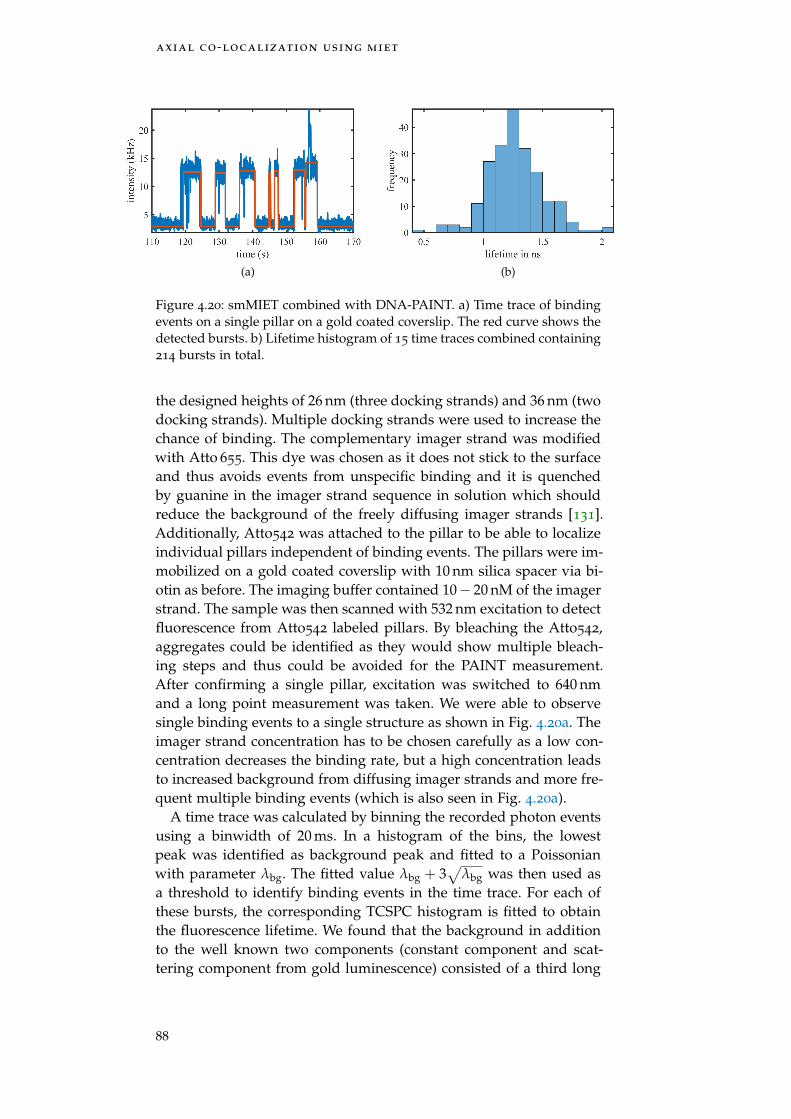
axial co-localization using miet

(a) (b)

Figure 4.20: smMIET combined with DNA-PAINT. a) Time trace of bindingevents on a single pillar on a gold coated coverslip. The red curve shows thedetected bursts. b) Lifetime histogram of 15 time traces combined containing214 bursts in total.

the designed heights of 26 nm (three docking strands) and 36 nm (twodocking strands). Multiple docking strands were used to increase thechance of binding. The complementary imager strand was modifiedwith Atto 655. This dye was chosen as it does not stick to the surfaceand thus avoids events from unspecific binding and it is quenchedby guanine in the imager strand sequence in solution which shouldreduce the background of the freely diffusing imager strands [131].Additionally, Atto542 was attached to the pillar to be able to localizeindividual pillars independent of binding events. The pillars were im-mobilized on a gold coated coverslip with 10 nm silica spacer via bi-otin as before. The imaging buffer contained 10− 20 nM of the imagerstrand. The sample was then scanned with 532 nm excitation to detectfluorescence from Atto542 labeled pillars. By bleaching the Atto542,aggregates could be identified as they would show multiple bleach-ing steps and thus could be avoided for the PAINT measurement.After confirming a single pillar, excitation was switched to 640 nmand a long point measurement was taken. We were able to observesingle binding events to a single structure as shown in Fig. 4.20a. Theimager strand concentration has to be chosen carefully as a low con-centration decreases the binding rate, but a high concentration leadsto increased background from diffusing imager strands and more fre-quent multiple binding events (which is also seen in Fig. 4.20a).

A time trace was calculated by binning the recorded photon eventsusing a binwidth of 20 ms. In a histogram of the bins, the lowestpeak was identified as background peak and fitted to a Poissonianwith parameter λbg. The fitted value λbg + 3

√λbg was then used as

a threshold to identify binding events in the time trace. For each ofthese bursts, the corresponding TCSPC histogram is fitted to obtainthe fluorescence lifetime. We found that the background in additionto the well known two components (constant component and scat-tering component from gold luminescence) consisted of a third long

88

4.5 outlook – miet with dna-paint

lifetime component (3 ns). This component stems from the freely dif-fusing imager strand in solution and roughly corresponds to the freespace lifetime of Atto 655 conjugated to DNA. For fitting the TCSPChistogram of a burst, this component was kept fixed and only its am-plitude was fitted. We excluded fits that have less than 103 photons ora χ2

red value larger than 1.5. In this way, we obtained the lifetime his-togram combining 15 time traces of single pillars shown in Fig. 4.20b.The distribution is relatively broad so that no clear peaks can be iden-tified. It is most likely that the bad signal-to-background ratio of thismeasurement is responsible for this. While for the step-wise bleach-ing experiments the gold luminescence was the main backgroundcontribution, here it is the fluorescence of diffusing imager strands.The additional long lifetime component increases the uncertainty inthe fit. Moreover, assuming that the lifetime is mono-exponential isa simplification. Although the MIET range of about 150 nm is smallcompared to half the extent of the confocal volume along z, about0.5µm, diffusing dyes close to the surface will be quenched by themetal and contribute with a smaller lifetime.

The best strategy for improvement would thus be to minimizethe contribution of imager strands by either decreasing the excita-tion volume or by chemically modifying the imager strand that it iscompletely quenched in solution. The former can be achieved by us-ing a focused total internal reflection (TIR) illumination such as inRefs. [132–134] and the concept of the latter is also known as molec-ular beacons [135]. Both approaches will be the focus of further re-search.

89

5D E A D - T I M E C O R R E C T I O N F O R T C S P C S Y S T E M S

In this chapter, a new method for dead-time correction of TCSPC sys-tems is presented. Our method is based on asynchronous recordingof photon arrival times as it is employed in modern TCSPC hardware.We developed a theoretical model for the TCSPC histogram distortedby the dead-time of the detector and the TCSPC electronics. Basedon this model, we implemented an algorithm to correct dead-timeartifacts in TCSPC histograms and verified the result by numericalsimulations and experiments.

This chapter is based on the publication:Sebastian Isbaner1, Narain Karedla1, Daja Ruhlandt, Simon ChristophStein, Anna Chizhik, Ingo Gregor, and Jörg Enderlein. “Dead-timecorrection of fluorescence lifetime measurements and fluorescencelifetime imaging.” In: Optics Express 24.9 (May 2, 2016), pp. 9429–9445.doi: 10.1364/OE.24.009429.

5.1 introduction

Fluorescence microscopy has become a powerful tool in biology andbio-medical diagnostics [6, 7]. Fluorescence detection is highly sensi-tive and stands out due to its superior selectivity with which struc-tures of interest can be labeled. In particular, multi-color fluorescencemicroscopy on differently labeled targets enables studying the rela-tive structural organization and dynamics from organelles to mole-cules of living cells. The labels are often distinguished based on theirspectral properties, i.e. their color or their excitation and emissionwavelengths. A further means of disentangling different dyes in afluorescence microscopy image is to use their fluorescence lifetime,see e.g. [136]. As with the spectral properties, which differ from dyeto dye, also the fluorescence lifetime is different between differentdyes and can be used to distinguish between them. Moreover, fluo-rescence lifetime measurements have become increasingly popularfor the quantification of Förster Resonance Energy Transfer (FRET)measurements in bio-imaging [95, 137, 138], because they allow foraccurate FRET rate estimates which are independent of intensity mea-surements that can be skewed by optical absorption, cross-talk, andscattering.

In this work, we consider a FLIM system which is based on a confo-cal scanning microscope [60] and uses TCSPC [33–35] for measuringthe fluorescence decay at every scan position. In TCSPC, one deter-mines the decay curve by exciting molecules with a periodic train of

1 These authors contributed equally to this work.

dead-time correction for tcspc systems

short laser pulses, and then measuring the time delay between therecorded fluorescence photons and the exciting laser pulses. Whenbuilding a histogram of these delay times, one obtains an estimate ofthe fluorescence decay curve which can be described with a single-or multi-exponential decay function. Modern TCSPC systems mea-sure the arrival times of detected photons and the laser pulses inde-pendently from each other, thereby avoiding a preference for earlyphotons which is known as the pile-up effect for classical TCSPChardware [34]. Although TCSPC is a very efficient techniques, it onlyworks at moderate count rates of a few percent of the laser repetitionrate. This is due to the so-called dead-time of the electronics and thedetector: After the successful detection (detector) or timing (electron-ics) of a photon, both detector and electronics need to recover andto return to an active state before being able to detect or record thenext photon. These recovery times are typically on the order of tens ofnanoseconds and limit the photon count rate at which the devices canoperate. But even when the average time between photons is on theorder of some percent of these dead-times, this leads to an increas-ing loss of detectable photons and to a distortion of the measuredfluorescence decay curve.

The common rule-of-thumb is to operate a TCSPC system only atcount rates below 1 % of the laser repetition rate because then photonlosses and distortions of dead-time effects are reduced. However, lowcount rates increase the time to obtain sufficient statistics for a fluores-cence decay curve which in turn limits the image acquisition speedin scanning microscopy. In FLIM, at each scan position during thesample scan with a laser-scanning confocal microscope, one recordsa TCSPC curve from which not only the fluorescence intensity butalso a lifetime value is extracted. For rapid FLIM image acquisition,one wants to maximize the count rate that should be limited onlyby photobleaching and phototoxicity, but not by potential dead-timeeffects in the TCSPC measurement. The demand for such fast FLIMsystems has led to the development of dedicated TCSPC systems suchas “FASTAC FLIM system” by the company Becker & Hickl or “rapid-FLIM” by PicoQuant which both are based on dedicated hardwarewith short dead-times. However, a data evaluation method that faith-fully reproduces the correct fluorescence decay curve even at highcount rates would also enable unbiased fast FLIM on existing setupswithout the need for dedicated hardware.

Here, we present a data evaluation method which provides dead-time corrected fluorescence decay estimates from TCSPC measure-ments at high count rates, and we demonstrate our method on FLIMof fluorescently labeled cells.

92

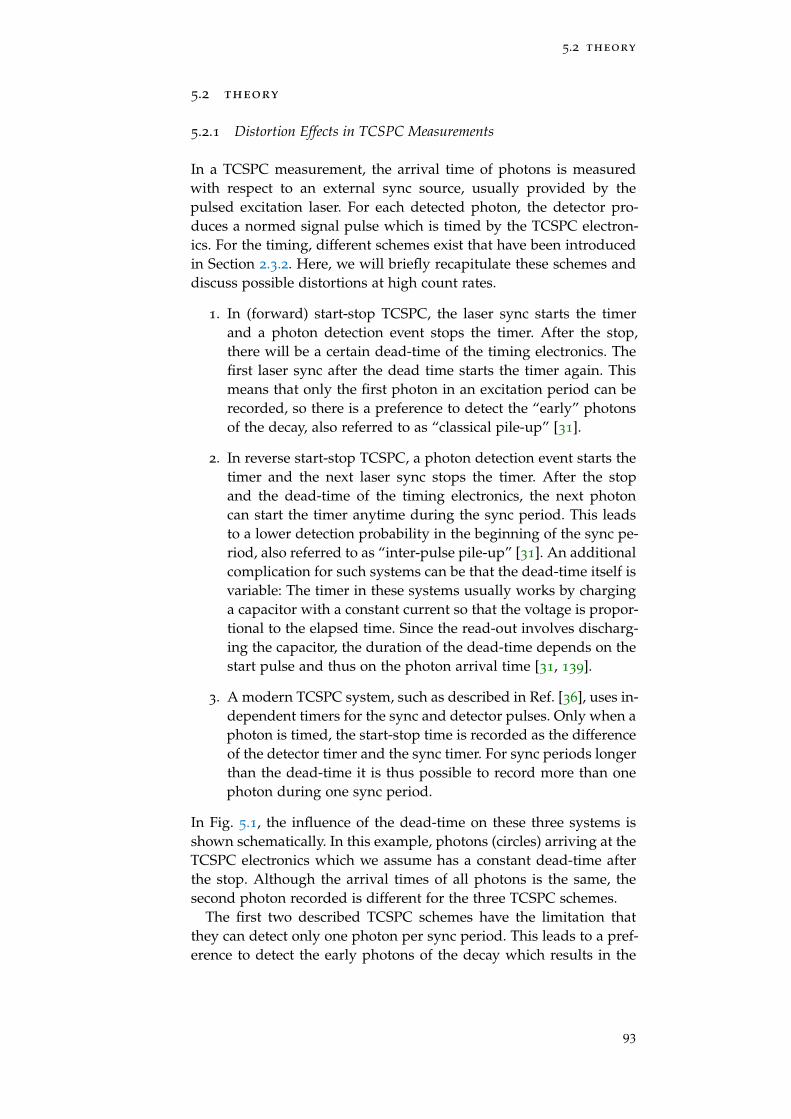
5.2 theory

5.2 theory

5.2.1 Distortion Effects in TCSPC Measurements

In a TCSPC measurement, the arrival time of photons is measuredwith respect to an external sync source, usually provided by thepulsed excitation laser. For each detected photon, the detector pro-duces a normed signal pulse which is timed by the TCSPC electron-ics. For the timing, different schemes exist that have been introducedin Section 2.3.2. Here, we will briefly recapitulate these schemes anddiscuss possible distortions at high count rates.

1. In (forward) start-stop TCSPC, the laser sync starts the timerand a photon detection event stops the timer. After the stop,there will be a certain dead-time of the timing electronics. Thefirst laser sync after the dead time starts the timer again. Thismeans that only the first photon in an excitation period can berecorded, so there is a preference to detect the “early” photonsof the decay, also referred to as “classical pile-up” [31].

2. In reverse start-stop TCSPC, a photon detection event starts thetimer and the next laser sync stops the timer. After the stopand the dead-time of the timing electronics, the next photoncan start the timer anytime during the sync period. This leadsto a lower detection probability in the beginning of the sync pe-riod, also referred to as “inter-pulse pile-up” [31]. An additionalcomplication for such systems can be that the dead-time itself isvariable: The timer in these systems usually works by charginga capacitor with a constant current so that the voltage is propor-tional to the elapsed time. Since the read-out involves discharg-ing the capacitor, the duration of the dead-time depends on thestart pulse and thus on the photon arrival time [31, 139].

3. A modern TCSPC system, such as described in Ref. [36], uses in-dependent timers for the sync and detector pulses. Only when aphoton is timed, the start-stop time is recorded as the differenceof the detector timer and the sync timer. For sync periods longerthan the dead-time it is thus possible to record more than onephoton during one sync period.

In Fig. 5.1, the influence of the dead-time on these three systems isshown schematically. In this example, photons (circles) arriving at theTCSPC electronics which we assume has a constant dead-time afterthe stop. Although the arrival times of all photons is the same, thesecond photon recorded is different for the three TCSPC schemes.

The first two described TCSPC schemes have the limitation thatthey can detect only one photon per sync period. This leads to a pref-erence to detect the early photons of the decay which results in the

93

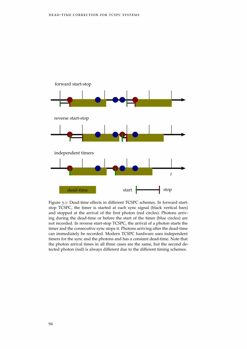
dead-time correction for tcspc systems

start

forward start-stop

reverse start-stop

independent timers

t

dead-time stop

Figure 5.1: Dead-time effects in different TCSPC schemes. In forward start-stop TCSPC, the timer is started at each sync signal (black vertical bars)and stopped at the arrival of the first photon (red circles). Photons arriv-ing during the dead-time or before the start of the timer (blue circles) arenot recorded. In reverse start-stop TCSPC, the arrival of a photon starts thetimer and the consecutive sync stops it. Photons arriving after the dead-timecan immediately be recorded. Modern TCSPC hardware uses independenttimers for the sync and the photons and has a constant dead-time. Note thatthe photon arrival times in all three cases are the same, but the second de-tected photon (red) is always different due to the different timing schemes.

94

5.2 theory

pile-up effect [31]. Note that the pile-up effect is fundamentally dif-ferent from dead-time distortions: Especially the classical pile-up offorward start-stop TCSPC does not depend on the dead-time and hasbeen addressed in several publications, see for example Refs. [140,141], and references therein. Reverse start-stop measurements sufferfrom pile-up as well as dead-time distortions [142]. An overview ondifferent start-stop TCSPC architectures and their pile-up behavior isgiven in Ref. [143]. Note that the independent timing scheme avoidsclassical pile-up effects completely as the timing can be executed any-time during the excitation period as soon as the electronics is ready.However, dead-time effects still distort the recorded fluorescence de-cay curve as we will see in the next section. In the following, we willfocus on TCSPC measurements with the recently developed new gen-eration of counting electronics that use independent timers and havea constant dead-time [36].

Apart from the TCSPC electronics, also detectors have a dead-time(cf. Section 2.3.1). A general classification in the literature of detectordead-times are the two categories of paralyzable and non-paralyzabledetectors [144]. In a non-paralyzable detector, any photons hitting thedetector during the dead-time are simply discarded. The photon hitrate ε can be estimated from the count rate R of a non-paralyzabledetector with dead-time D as ε =

Rnon−paralyzable1−DRnon−paralyzable

. This detector typereaches a constant count rate at saturation that is given as the inverseof the dead-time. The situation is more complicated in a paralyzabledetector: There, each photon hitting the detector during the dead-time is not counted but restarts the dead-time. At high photon fluxes,a further increase in photons leads to a decreasing count rate untilthe detector is incapable to detect any photons at all. Assuming Pois-son statistics for the number of photons hitting the detector, one findsRparalyzable = ε · e−εD. In contrast to the equation for non-paralyzabledetectors, this equation can be solved for ε only implicitly, for ex-ample by iteration. A typical example for a paralyzable detector is aGeiger counter. Single-photon avalanche diodes (SPAD) that are ac-tively quenched are an example of non-paralyzable detectors. Afterthe detection of a photon by an electron avalanche, the bias voltageof the photo-diode is lowered so that no new avalanche can be pro-duced (active quenching). When the bias is reset after the dead-time,the next photo-electron can again create a new avalanche which willtrigger a new detection event. For TCSPC, SPADs are commonly em-ployed as detectors. Because these detectors are most often activelyquenched, we assume a constant, i.e. non-paralyzable dead-time.

In this section we have reviewed the dead-times of detectors andTCSPC electronics. Especially older TCSPC electronics has non-constantdead-times, but also detectors can have variable dead-times. Here, wewill focus on the most recent generations of TCSPC electronics anddetectors that both have a constant dead-time.

95

dead-time correction for tcspc systems

5.2.2 Dead-time Effects on TCSPC Histograms

After we have discussed dead-time effects on the recorded photonsseparately for the electronics and the detector in the last section, wefocus now on the more realistic situation where the detector and theelectronics are connected in series, so both dead-time can affect themeasurement. The impact of both dead-times is schematically shownin Fig. 5.2. After each photon detection, the single-photon detectorhas to recover and is, during some dead-time D, unable to detectanother photon. This detector dead-time of length D is symbolized bythe small red rectangles in Fig. 5.2. In parallel, after timing a photondetection event, the timing electronics has also to recover, with dead-time E, before being able to record another photon detection event.This dead-time of duration E is symbolized by large green rectanglesin Fig. 5.2. Typically, one has E > D, but in the case of E < D, theelectronics recovers faster than the detector so that it will be alwaysready to time the next event from the detector. Then the problemreduces to a single dead-time problem which is a special case of thetheory developed below.

time

E

D

Figure 5.2: Schematic of possible effects of detector and electronics dead-time. A successfully detected and recorded photon (red circles) results ina dead-time of the detector (small red rectangles) and the electronics (largegreen rectangles). Photons detected during the electronics dead-time are notrecorded (blue circles), and photons hitting the detector during the detectordead-time are discarded (green circles). Note that the detector dead-timeoccurs after successful detection of a photon (red and blue circles), whilethe electronics dead-time only occurs after successfully timing a photon (redcircles).

Three scenarios for photons hitting the detector are now possible. Inthe best case, both detector and electronics are in their recovered rest-ing state and can detect and record the photon (red balls in Fig. 5.2).Or, the detector has already recovered from the previous photon de-tection event, but the electronics is still in its recovery and not yetready to record the detected photon (blue balls in Fig. 5.2). Or, in theworst case, the next photon hits the detector so closely to the previousone that the detector itself is still in its dead-time and cannot detectthe photon (green balls in Fig. 5.2). It is important to notice that thiscan even happen while the electronics itself would be already capa-ble to record another detection event (see the last event in Fig. 5.2where the small rectangle, delimiting the detector dead-time, extendsbeyond the large rectangle, which delimits the electronics dead-time).

96

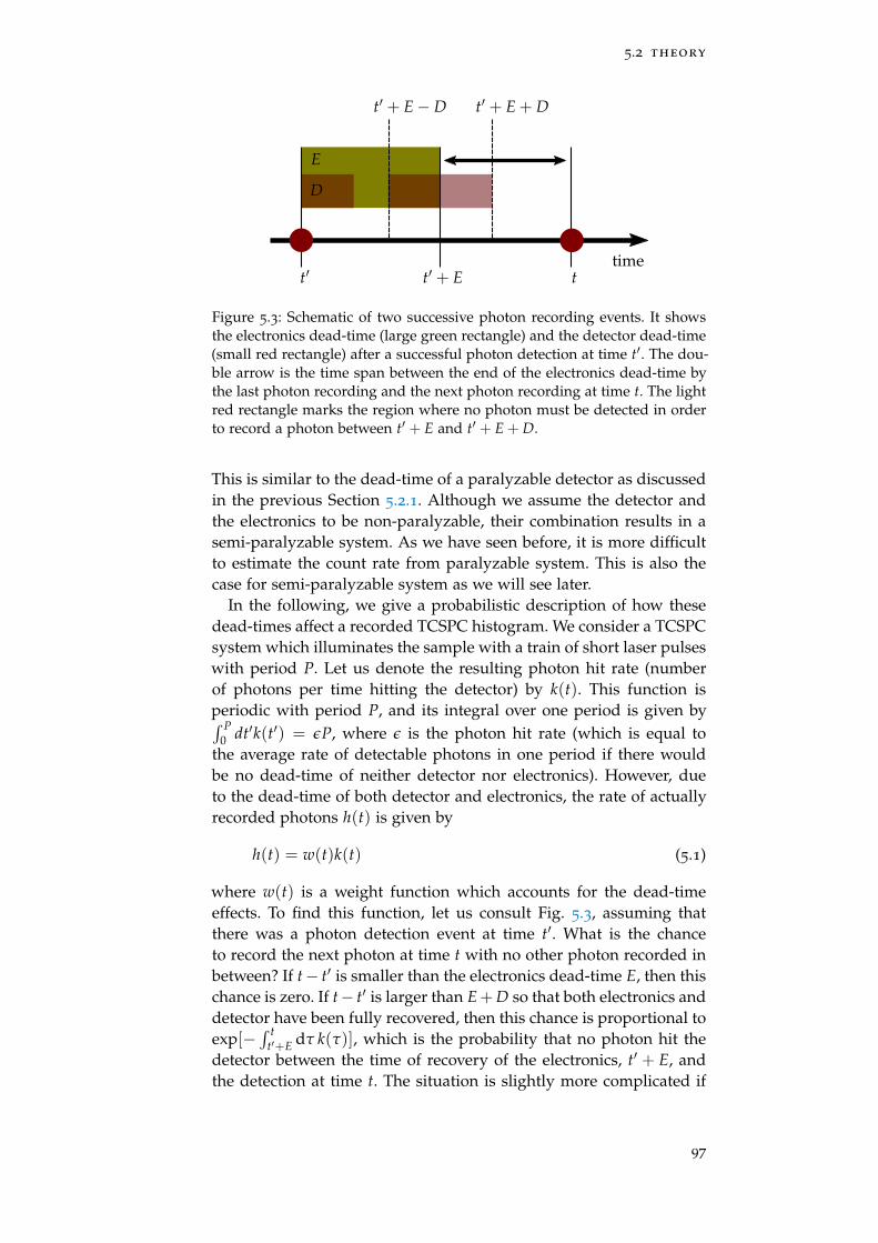
5.2 theory

time

E

t′ t′ + E

t′ + E + D

t

D

t′ + E− D

Figure 5.3: Schematic of two successive photon recording events. It showsthe electronics dead-time (large green rectangle) and the detector dead-time(small red rectangle) after a successful photon detection at time t′. The dou-ble arrow is the time span between the end of the electronics dead-time bythe last photon recording and the next photon recording at time t. The lightred rectangle marks the region where no photon must be detected in orderto record a photon between t′ + E and t′ + E + D.

This is similar to the dead-time of a paralyzable detector as discussedin the previous Section 5.2.1. Although we assume the detector andthe electronics to be non-paralyzable, their combination results in asemi-paralyzable system. As we have seen before, it is more difficultto estimate the count rate from paralyzable system. This is also thecase for semi-paralyzable system as we will see later.

In the following, we give a probabilistic description of how thesedead-times affect a recorded TCSPC histogram. We consider a TCSPCsystem which illuminates the sample with a train of short laser pulseswith period P. Let us denote the resulting photon hit rate (numberof photons per time hitting the detector) by k(t). This function isperiodic with period P, and its integral over one period is given by∫ P

0 dt′k(t′) = εP, where ε is the photon hit rate (which is equal tothe average rate of detectable photons in one period if there wouldbe no dead-time of neither detector nor electronics). However, dueto the dead-time of both detector and electronics, the rate of actuallyrecorded photons h(t) is given by

h(t) = w(t)k(t) (5.1)

where w(t) is a weight function which accounts for the dead-timeeffects. To find this function, let us consult Fig. 5.3, assuming thatthere was a photon detection event at time t′. What is the chanceto record the next photon at time t with no other photon recorded inbetween? If t− t′ is smaller than the electronics dead-time E, then thischance is zero. If t− t′ is larger than E+D so that both electronics anddetector have been fully recovered, then this chance is proportional toexp[−

∫ tt′+E dτ k(τ)], which is the probability that no photon hit the

detector between the time of recovery of the electronics, t′ + E, andthe detection at time t. The situation is slightly more complicated if

97

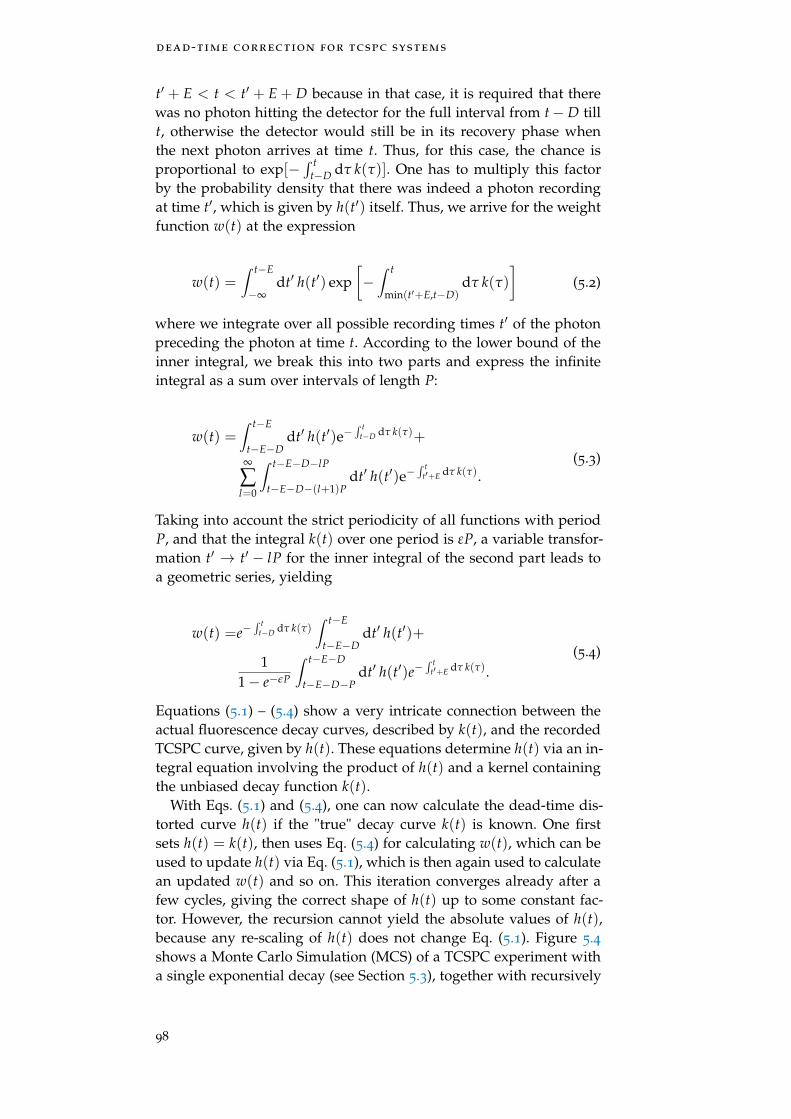
dead-time correction for tcspc systems

t′ + E < t < t′ + E + D because in that case, it is required that therewas no photon hitting the detector for the full interval from t−D tillt, otherwise the detector would still be in its recovery phase whenthe next photon arrives at time t. Thus, for this case, the chance isproportional to exp[−

∫ tt−D dτ k(τ)]. One has to multiply this factor

by the probability density that there was indeed a photon recordingat time t′, which is given by h(t′) itself. Thus, we arrive for the weightfunction w(t) at the expression

w(t) =∫ t−E

−∞dt′ h(t′) exp

[−∫ t

min(t′+E,t−D)dτ k(τ)

](5.2)

where we integrate over all possible recording times t′ of the photonpreceding the photon at time t. According to the lower bound of theinner integral, we break this into two parts and express the infiniteintegral as a sum over intervals of length P:

w(t) =∫ t−E

t−E−Ddt′ h(t′)e−

∫ tt−D dτ k(τ)+

∞

∑l=0

∫ t−E−D−lP

t−E−D−(l+1)Pdt′ h(t′)e−

∫ tt′+E dτ k(τ).

(5.3)

Taking into account the strict periodicity of all functions with periodP, and that the integral k(t) over one period is εP, a variable transfor-mation t′ → t′ − lP for the inner integral of the second part leads toa geometric series, yielding

w(t) =e−∫ t

t−D dτ k(τ)∫ t−E

t−E−Ddt′ h(t′)+

11− e−εP

∫ t−E−D

t−E−D−Pdt′ h(t′)e−

∫ tt′+E dτ k(τ).

(5.4)

Equations (5.1) – (5.4) show a very intricate connection between theactual fluorescence decay curves, described by k(t), and the recordedTCSPC curve, given by h(t). These equations determine h(t) via an in-tegral equation involving the product of h(t) and a kernel containingthe unbiased decay function k(t).

With Eqs. (5.1) and (5.4), one can now calculate the dead-time dis-torted curve h(t) if the "true" decay curve k(t) is known. One firstsets h(t) = k(t), then uses Eq. (5.4) for calculating w(t), which can beused to update h(t) via Eq. (5.1), which is then again used to calculatean updated w(t) and so on. This iteration converges already after afew cycles, giving the correct shape of h(t) up to some constant fac-tor. However, the recursion cannot yield the absolute values of h(t),because any re-scaling of h(t) does not change Eq. (5.1). Figure 5.4shows a Monte Carlo Simulation (MCS) of a TCSPC experiment witha single exponential decay (see Section 5.3), together with recursively

98

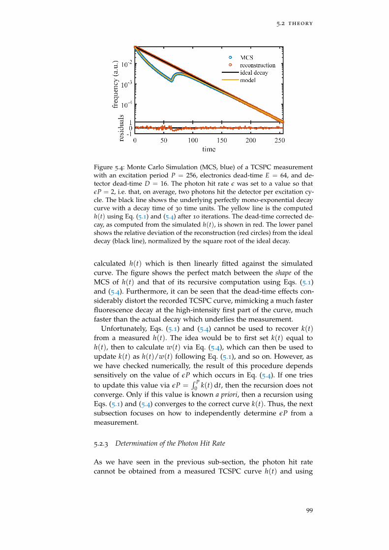
5.2 theory

Figure 5.4: Monte Carlo Simulation (MCS, blue) of a TCSPC measurementwith an excitation period P = 256, electronics dead-time E = 64, and de-tector dead-time D = 16. The photon hit rate ε was set to a value so thatεP = 2, i.e. that, on average, two photons hit the detector per excitation cy-cle. The black line shows the underlying perfectly mono-exponential decaycurve with a decay time of 30 time units. The yellow line is the computedh(t) using Eq. (5.1) and (5.4) after 10 iterations. The dead-time corrected de-cay, as computed from the simulated h(t), is shown in red. The lower panelshows the relative deviation of the reconstruction (red circles) from the idealdecay (black line), normalized by the square root of the ideal decay.

calculated h(t) which is then linearly fitted against the simulatedcurve. The figure shows the perfect match between the shape of theMCS of h(t) and that of its recursive computation using Eqs. (5.1)and (5.4). Furthermore, it can be seen that the dead-time effects con-siderably distort the recorded TCSPC curve, mimicking a much fasterfluorescence decay at the high-intensity first part of the curve, muchfaster than the actual decay which underlies the measurement.

Unfortunately, Eqs. (5.1) and (5.4) cannot be used to recover k(t)from a measured h(t). The idea would be to first set k(t) equal toh(t), then to calculate w(t) via Eq. (5.4), which can then be used toupdate k(t) as h(t)/w(t) following Eq. (5.1), and so on. However, aswe have checked numerically, the result of this procedure dependssensitively on the value of εP which occurs in Eq. (5.4). If one triesto update this value via εP =

∫ P0 k(t)dt, then the recursion does not

converge. Only if this value is known a priori, then a recursion usingEqs. (5.1) and (5.4) converges to the correct curve k(t). Thus, the nextsubsection focuses on how to independently determine εP from ameasurement.

5.2.3 Determination of the Photon Hit Rate

As we have seen in the previous sub-section, the photon hit ratecannot be obtained from a measured TCSPC curve h(t) and using

99

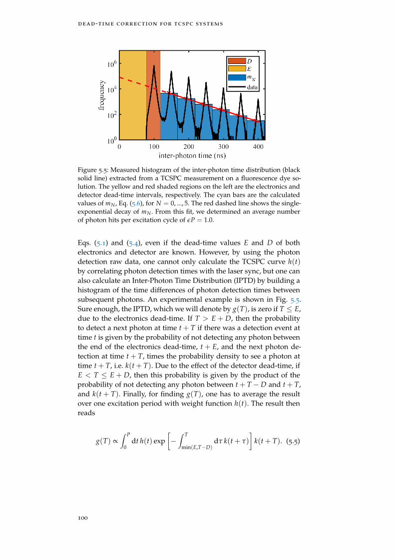
dead-time correction for tcspc systems

Figure 5.5: Measured histogram of the inter-photon time distribution (blacksolid line) extracted from a TCSPC measurement on a fluorescence dye so-lution. The yellow and red shaded regions on the left are the electronics anddetector dead-time intervals, respectively. The cyan bars are the calculatedvalues of mN , Eq. (5.6), for N = 0, ..., 5. The red dashed line shows the single-exponential decay of mN . From this fit, we determined an average numberof photon hits per excitation cycle of εP = 1.0.

Eqs. (5.1) and (5.4), even if the dead-time values E and D of bothelectronics and detector are known. However, by using the photondetection raw data, one cannot only calculate the TCSPC curve h(t)by correlating photon detection times with the laser sync, but one canalso calculate an Inter-Photon Time Distribution (IPTD) by building ahistogram of the time differences of photon detection times betweensubsequent photons. An experimental example is shown in Fig. 5.5.Sure enough, the IPTD, which we will denote by g(T), is zero if T ≤ E,due to the electronics dead-time. If T > E + D, then the probabilityto detect a next photon at time t + T if there was a detection event attime t is given by the probability of not detecting any photon betweenthe end of the electronics dead-time, t + E, and the next photon de-tection at time t + T, times the probability density to see a photon attime t + T, i.e. k(t + T). Due to the effect of the detector dead-time, ifE < T ≤ E + D, then this probability is given by the product of theprobability of not detecting any photon between t + T−D and t + T,and k(t + T). Finally, for finding g(T), one has to average the resultover one excitation period with weight function h(t). The result thenreads

g(T) ∝∫ P

0dt h(t) exp

[−∫ T

min(E,T−D)dτ k(t + τ)

]k(t + T). (5.5)

100

5.2 theory

The important point now is that, if one sums g(T) over subsequenttime intervals E + D + NP ≤ T < E + D + (N + 1)P of width P, withN being any non-negative integer, i.e. by calculating

mN =∫ E+D+(N+1)P

E+D+NPdT g(T) = C exp(−NεP), (5.6)

one finds that these integrals fall off as exp(−NεP), as also shown inFig. 5.5. Thus, by fitting the mN with an exponential function yieldsthe average number of photon hits per excitation cycle, εP. Knowingthis number, one can now use Eqs. (5.1) and (5.4) to recursively cal-culate the dead-time-corrected decay k(t) from the measured decayh(t).

5.2.4 Determination of Detector and Electronics Dead-times

For correctly recovering an unbiased decay curve from a measuredTCSPC curve, one needs to know the electronics and detector dead-times, E and D. An elegant way to determine both values is to mea-sure an autocorrelation function while illuminating the measurementsystem with a continuous-wave constant-intensity light source. This au-tocorrelation function A(t − t′) is proportional to the probability ofrecording a photon at some time t if there was a photon record-ing at time t′. If the light source has constant intensity (no time-dependence), the autocorrelation function depends only on the timedifference t− t′.

For deriving a theoretical expression for the autocorrelation func-tion, we will proceed in two steps. In a first step, we completely ig-nore the dead-time of the electronics and consider only the effect ofthe dead-time of the detector. Let us consider the probability den-sity to record a photon at time t if there was a photon recording attime t′, but no photon recording in between. This probability densityis zero if t − t′ ≤ D, and if t > t′ + D, it will be proportional toexp[−ε(t− t′ − D)] which is the probability that no photon hits thedetector between time t′ + D and time t. Here, ε is the constant aver-age photon hit rate. Thus, the normalized probability density f (t− t′)for detecting a photon at time t if there was a detection event at timet′ with no other photon detection in between is given by

f (t) =

0 if t ≤ D

ε exp [−ε(t− D)] if t > D.(5.7)

Next, let us consider the same probability density but now with ex-actly one intermediate photon recorded at any time t′′ in between.This probability density is zero if t − t′ ≤ 2D, and is otherwiseequal to the auto-convolution of f (t),

∫ t0 dt′′ f (t− t′′) f (t′′), computed

101

dead-time correction for tcspc systems

at time t − t′ − 2D > 0. By repeating this argument for all possiblenumbers of intermediate photon recordings, one finds the followingexpression for the autocorrelation function a(t) [145]:

a(t) =bt/Dc

∑j=1

f (j)(t) (5.8)

where f (j)(t) is the j-th auto-convolution of the function f (t) whichis recursively defined by

f (j)(t) =∫ t

0dt′ f (t′) f (j−1)(t− t′) (5.9)

and setting f (1)(t) = f (t). The upper limit in the summation (5.8)is the maximum possible number of photons which can be recordedwithin time t for a given detector dead-time D, where bt/Dc denotesthe largest integer number smaller than t/D.

Now we are ready to consider the general case of both detector andelectronics dead-time, assuming that D ≤ E (the case D > E reducesto the just considered case of a system having only detector dead-time D). Analogously to the derivation of a(t), we will again start byfinding an expression for the normalized probability density F(t− t′)to detect a photon at time t if there was a photon detection at time t′

but no other photon detection in between. Due to the electronics dead-time, this probability density is zero if t− t′ < E. The interesting casenow occurs if t− t′ > E but also t− t′ < E + D. In that case, it canhappen that a photon hits the detector shortly before the electronicsrecovers from its own dead-time so that no photon can be detecteddue to the detector dead-time although the electronics is again readyto process another detection event, see also Figs. 5.2 and 5.3. For thisintermediate time interval, E < t− t′ < E+D, the function F(t− t′) isproportional to the previously found autocorrelation a(t− t′) whichis exactly the chance to be able to see another photon at t if therewas one at time t′, when taking into account the detector dead-timealone. Finally, for time values t greater than t′+ E+ D, the probabilitydensity F will fall off exponentially as exp[−ε(t− t′−D− E)], whichis the probability that no photon hits the detector between time t′ +E + D and time t. In summary, we find

F(t) =

0 if t ≤ E

Z−1a(t) if E < t ≤ E + D

Z−1a(E + D) exp [−ε(t− E− D)] if t > E + D

(5.10)

102

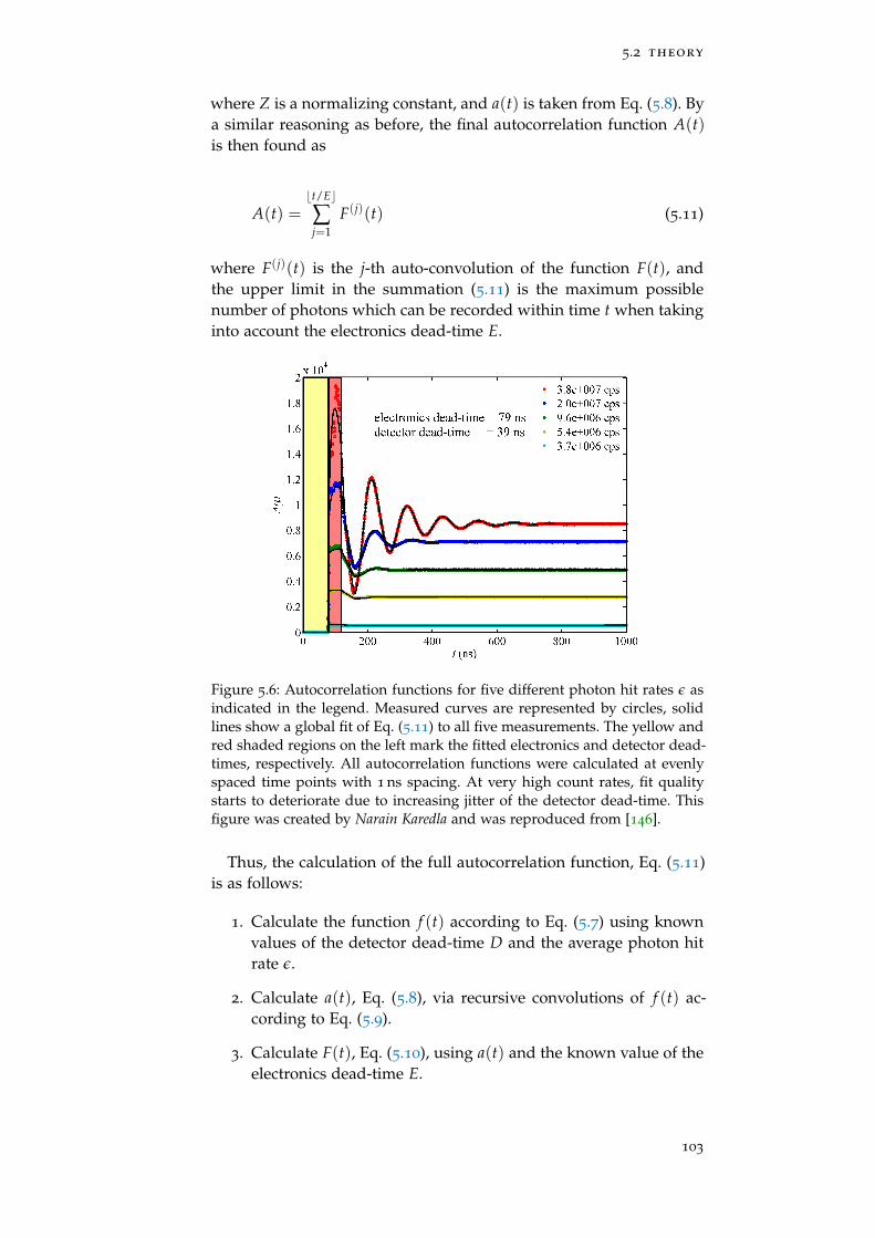
5.2 theory

where Z is a normalizing constant, and a(t) is taken from Eq. (5.8). Bya similar reasoning as before, the final autocorrelation function A(t)is then found as

A(t) =bt/Ec

∑j=1

F(j)(t) (5.11)

where F(j)(t) is the j-th auto-convolution of the function F(t), andthe upper limit in the summation (5.11) is the maximum possiblenumber of photons which can be recorded within time t when takinginto account the electronics dead-time E.

Figure 5.6: Autocorrelation functions for five different photon hit rates ε asindicated in the legend. Measured curves are represented by circles, solidlines show a global fit of Eq. (5.11) to all five measurements. The yellow andred shaded regions on the left mark the fitted electronics and detector dead-times, respectively. All autocorrelation functions were calculated at evenlyspaced time points with 1 ns spacing. At very high count rates, fit qualitystarts to deteriorate due to increasing jitter of the detector dead-time. Thisfigure was created by Narain Karedla and was reproduced from [146].

Thus, the calculation of the full autocorrelation function, Eq. (5.11)is as follows:

1. Calculate the function f (t) according to Eq. (5.7) using knownvalues of the detector dead-time D and the average photon hitrate ε.

2. Calculate a(t), Eq. (5.8), via recursive convolutions of f (t) ac-cording to Eq. (5.9).

3. Calculate F(t), Eq. (5.10), using a(t) and the known value of theelectronics dead-time E.

103

dead-time correction for tcspc systems

4. Calculate the final autocorrelation functions A(t), Eq. (5.11), viarecursive convolutions of F(t).

Although this may seem computationally expensive, it is not: Thenumerical calculation for one autocorrelation function with ca. 1000sampling points along the time axis needs only a fraction of a sec-ond on a conventional PC and using a non-compiled Matlab script.Thus, it can be easily used for fitting measured autocorrelation curvesand thus for extracting D, E and ε as fit parameters. An example forfive different count rates is shown in Fig. 5.6, using our TCSPC sys-tem as described in Section 5.3.4 with the laser in continuous wavemode. The sample was a dye solution of Atto 655 as described inSection 5.4.2. Autocorrelation curves of different count rates were fit-ted with a global model for E and D, but individual values for εP.From the fitted curves, we determined a detector dead-time of D =

(39.5± 0.6) ns (red shaded region in Fig. 5.6), and an electronics dead-time of E = (79.1± 0.4) ns (yellow shaded region in Fig. 5.6). The er-rors were obtained by bootstrapping the data into 14 bunches of 106

photons each and calculating mean and standard deviation.

104

5.3 methods

5.3 methods

5.3.1 Monte Carlo Simulations

Monte Carlo simulations of the TCSPC experiment were performedin the following way: First, for each excitation cycle, the number ofhitting photons was randomly drawn from a Poissonian distributionwith mean value εP. For each of these photons, the hit times with re-spect to the start of the corresponding excitation cycle were randomlydrawn from an exponential distribution with decay time τ, where τ

is the value of the mono-exponential fluorescence decay one wants tomodel. Knowing the excitation cycle and the hit time within this cy-cle for each photon, the global hit time is calculated for each photon,and then all these times are sorted in time. Then, the algorithm stepssequentially through these photon hit times and determines, for eachphoton, whether its hit time is still within the detector or electronicsdead-time interval of the previous validated photon detection event.If this is the case, then the photon is eliminated from the photonstream, and the algorithm proceeds to the next photon. Finally, fromthe remaining photon stream, the TCSPC and the IPTD histogramsare calculated.

5.3.2 Software

The software for the dead-time correction of fluorescence lifetimemeasurements used in this study is available for download1. It iswritten in Matlab with core parts outsourced to C++ MEX files for per-formance acceleration, which can be compiled under Windows orLinux using the provided build scripts. The algorithm recovers thetrue photon hit rate k(t) from the measured curve h(t) in an iter-ative fashion, starting from the guess k0(t) = h(t). In a next step,w0 [t|k0(t)] is computed via Eq. (5.4), and is used to update k(t) ask1(t) = h(t)/w0 [t|k0(t)]. This is repeated n times, until the relativechange in kn(t) is smaller than a predefined threshold. It was ob-served that convergence is usually fast requiring only about 2 to 5

iterations.

5.3.3 Setup for Cell Measurements

For FLIM measurements, we used a setup based on a commercial con-focal system (Microtime 200, PicoQuant, Berlin, Germany). Linearlypolarized light from a 640 nm diode laser (LDH-D-C-640, PicoQuant,Berlin, Germany), equipped with a clean-up filter (Z640/10, ChromaTechnology, Rockingham, VT, USA), was coupled into a polarization-maintaining single mode optical fiber. The laser driver (PDL 828 “Sepia

1 at https://projects.gwdg.de/projects/deadtimecorrectiontcspc

105

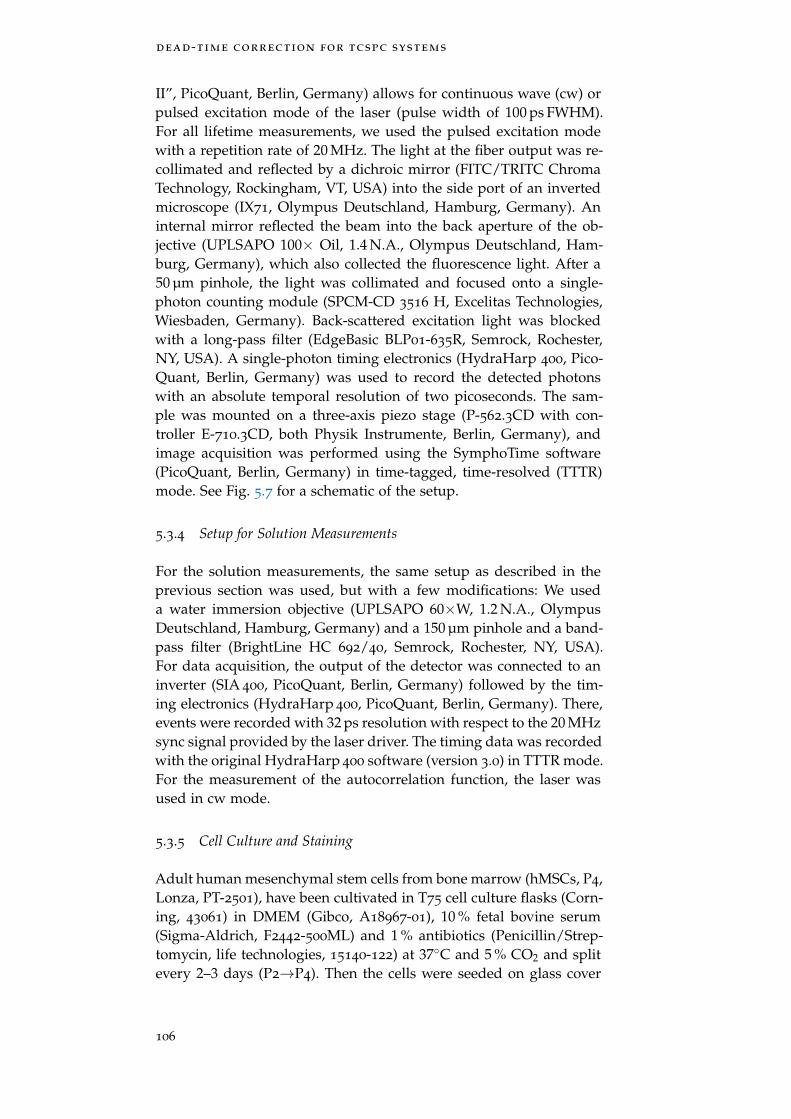
dead-time correction for tcspc systems

II”, PicoQuant, Berlin, Germany) allows for continuous wave (cw) orpulsed excitation mode of the laser (pulse width of 100 ps FWHM).For all lifetime measurements, we used the pulsed excitation modewith a repetition rate of 20 MHz. The light at the fiber output was re-collimated and reflected by a dichroic mirror (FITC/TRITC ChromaTechnology, Rockingham, VT, USA) into the side port of an invertedmicroscope (IX71, Olympus Deutschland, Hamburg, Germany). Aninternal mirror reflected the beam into the back aperture of the ob-jective (UPLSAPO 100× Oil, 1.4 N.A., Olympus Deutschland, Ham-burg, Germany), which also collected the fluorescence light. After a50 µm pinhole, the light was collimated and focused onto a single-photon counting module (SPCM-CD 3516 H, Excelitas Technologies,Wiesbaden, Germany). Back-scattered excitation light was blockedwith a long-pass filter (EdgeBasic BLP01-635R, Semrock, Rochester,NY, USA). A single-photon timing electronics (HydraHarp 400, Pico-Quant, Berlin, Germany) was used to record the detected photonswith an absolute temporal resolution of two picoseconds. The sam-ple was mounted on a three-axis piezo stage (P-562.3CD with con-troller E-710.3CD, both Physik Instrumente, Berlin, Germany), andimage acquisition was performed using the SymphoTime software(PicoQuant, Berlin, Germany) in time-tagged, time-resolved (TTTR)mode. See Fig. 5.7 for a schematic of the setup.

5.3.4 Setup for Solution Measurements

For the solution measurements, the same setup as described in theprevious section was used, but with a few modifications: We useda water immersion objective (UPLSAPO 60×W, 1.2 N.A., OlympusDeutschland, Hamburg, Germany) and a 150 µm pinhole and a band-pass filter (BrightLine HC 692/40, Semrock, Rochester, NY, USA).For data acquisition, the output of the detector was connected to aninverter (SIA 400, PicoQuant, Berlin, Germany) followed by the tim-ing electronics (HydraHarp 400, PicoQuant, Berlin, Germany). There,events were recorded with 32 ps resolution with respect to the 20 MHzsync signal provided by the laser driver. The timing data was recordedwith the original HydraHarp 400 software (version 3.0) in TTTR mode.For the measurement of the autocorrelation function, the laser wasused in cw mode.

5.3.5 Cell Culture and Staining

Adult human mesenchymal stem cells from bone marrow (hMSCs, P4,Lonza, PT-2501), have been cultivated in T75 cell culture flasks (Corn-ing, 43061) in DMEM (Gibco, A18967-01), 10 % fetal bovine serum(Sigma-Aldrich, F2442-500ML) and 1 % antibiotics (Penicillin/Strep-tomycin, life technologies, 15140-122) at 37C and 5 % CO2 and splitevery 2–3 days (P2→P4). Then the cells were seeded on glass cover

106

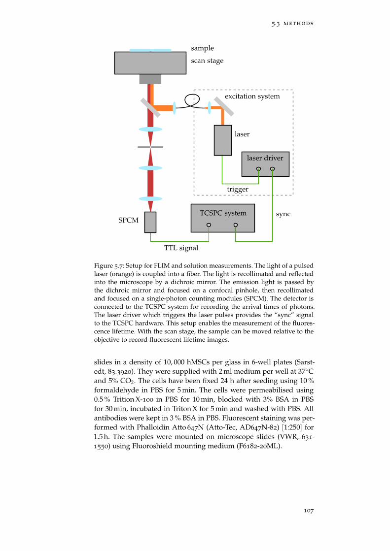
5.3 methods

laser driver

scan stage

sample

excitation system

TCSPC system

trigger

sync

TTL signal

laser

SPCM

Figure 5.7: Setup for FLIM and solution measurements. The light of a pulsedlaser (orange) is coupled into a fiber. The light is recollimated and reflectedinto the microscope by a dichroic mirror. The emission light is passed bythe dichroic mirror and focused on a confocal pinhole, then recollimatedand focused on a single-photon counting modules (SPCM). The detector isconnected to the TCSPC system for recording the arrival times of photons.The laser driver which triggers the laser pulses provides the “sync” signalto the TCSPC hardware. This setup enables the measurement of the fluores-cence lifetime. With the scan stage, the sample can be moved relative to theobjective to record fluorescent lifetime images.

slides in a density of 10, 000 hMSCs per glass in 6-well plates (Sarst-edt, 83.3920). They were supplied with 2 ml medium per well at 37Cand 5% CO2. The cells have been fixed 24 h after seeding using 10 %formaldehyde in PBS for 5 min. The cells were permeabilised using0.5 % Trition X-100 in PBS for 10 min, blocked with 3% BSA in PBSfor 30 min, incubated in Triton X for 5 min and washed with PBS. Allantibodies were kept in 3 % BSA in PBS. Fluorescent staining was per-formed with Phalloidin Atto 647N (Atto-Tec, AD647N-82) [1:250] for1.5 h. The samples were mounted on microscope slides (VWR, 631-1550) using Fluoroshield mounting medium (F6182-20ML).

107

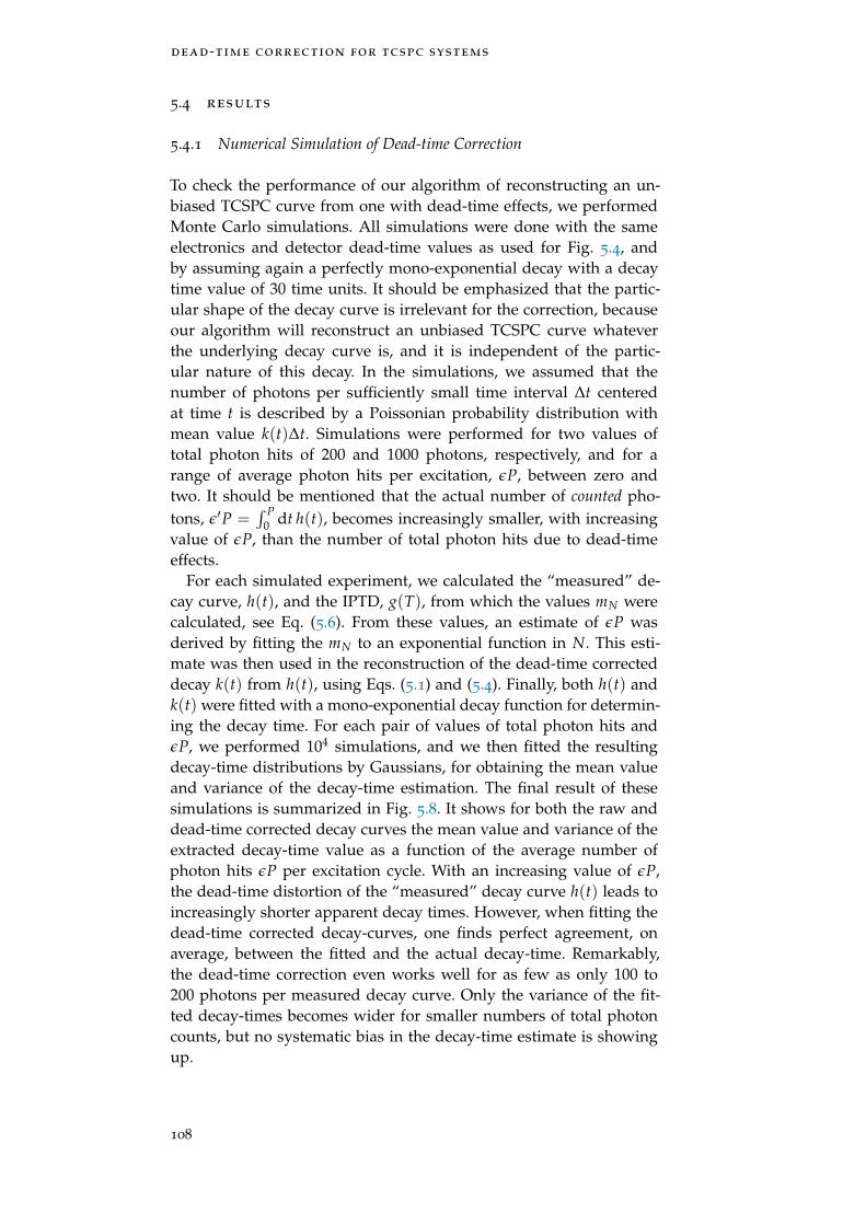
dead-time correction for tcspc systems

5.4 results

5.4.1 Numerical Simulation of Dead-time Correction

To check the performance of our algorithm of reconstructing an un-biased TCSPC curve from one with dead-time effects, we performedMonte Carlo simulations. All simulations were done with the sameelectronics and detector dead-time values as used for Fig. 5.4, andby assuming again a perfectly mono-exponential decay with a decaytime value of 30 time units. It should be emphasized that the partic-ular shape of the decay curve is irrelevant for the correction, becauseour algorithm will reconstruct an unbiased TCSPC curve whateverthe underlying decay curve is, and it is independent of the partic-ular nature of this decay. In the simulations, we assumed that thenumber of photons per sufficiently small time interval ∆t centeredat time t is described by a Poissonian probability distribution withmean value k(t)∆t. Simulations were performed for two values oftotal photon hits of 200 and 1000 photons, respectively, and for arange of average photon hits per excitation, εP, between zero andtwo. It should be mentioned that the actual number of counted pho-tons, ε′P =

∫ P0 dt h(t), becomes increasingly smaller, with increasing

value of εP, than the number of total photon hits due to dead-timeeffects.

For each simulated experiment, we calculated the “measured” de-cay curve, h(t), and the IPTD, g(T), from which the values mN werecalculated, see Eq. (5.6). From these values, an estimate of εP wasderived by fitting the mN to an exponential function in N. This esti-mate was then used in the reconstruction of the dead-time correcteddecay k(t) from h(t), using Eqs. (5.1) and (5.4). Finally, both h(t) andk(t) were fitted with a mono-exponential decay function for determin-ing the decay time. For each pair of values of total photon hits andεP, we performed 104 simulations, and we then fitted the resultingdecay-time distributions by Gaussians, for obtaining the mean valueand variance of the decay-time estimation. The final result of thesesimulations is summarized in Fig. 5.8. It shows for both the raw anddead-time corrected decay curves the mean value and variance of theextracted decay-time value as a function of the average number ofphoton hits εP per excitation cycle. With an increasing value of εP,the dead-time distortion of the “measured” decay curve h(t) leads toincreasingly shorter apparent decay times. However, when fitting thedead-time corrected decay-curves, one finds perfect agreement, onaverage, between the fitted and the actual decay-time. Remarkably,the dead-time correction even works well for as few as only 100 to200 photons per measured decay curve. Only the variance of the fit-ted decay-times becomes wider for smaller numbers of total photoncounts, but no systematic bias in the decay-time estimate is showingup.

108

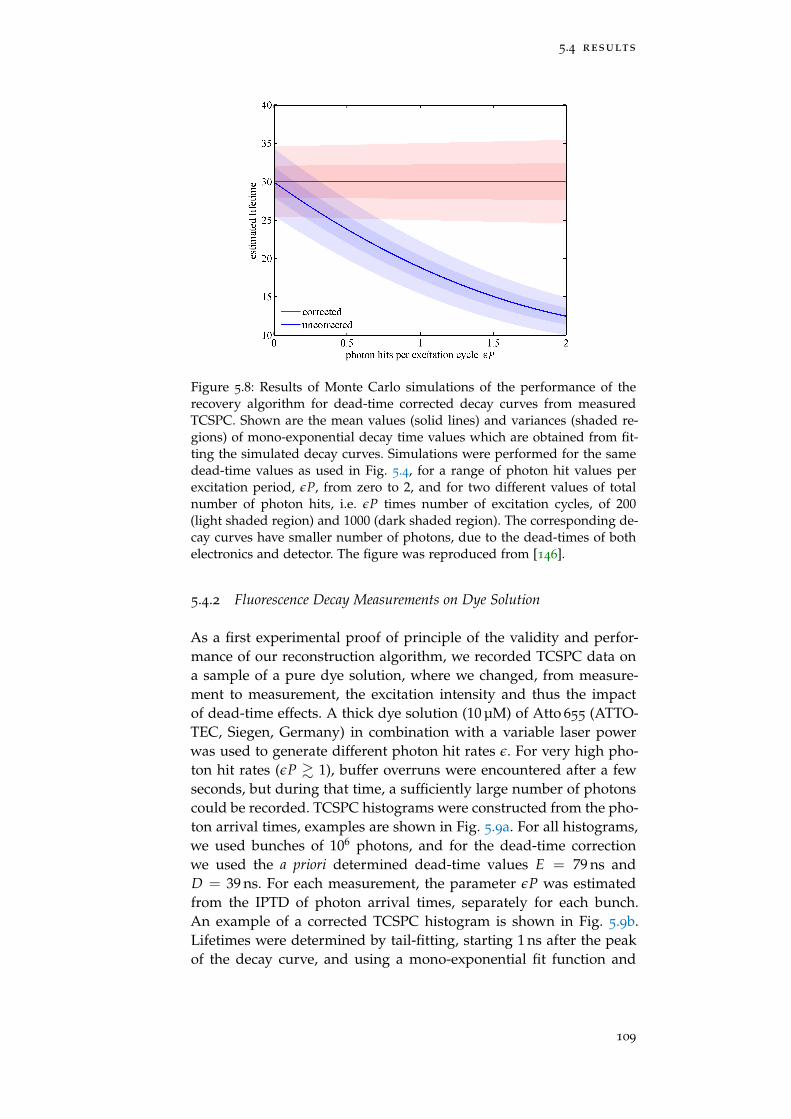
5.4 results

Figure 5.8: Results of Monte Carlo simulations of the performance of therecovery algorithm for dead-time corrected decay curves from measuredTCSPC. Shown are the mean values (solid lines) and variances (shaded re-gions) of mono-exponential decay time values which are obtained from fit-ting the simulated decay curves. Simulations were performed for the samedead-time values as used in Fig. 5.4, for a range of photon hit values perexcitation period, εP, from zero to 2, and for two different values of totalnumber of photon hits, i.e. εP times number of excitation cycles, of 200(light shaded region) and 1000 (dark shaded region). The corresponding de-cay curves have smaller number of photons, due to the dead-times of bothelectronics and detector. The figure was reproduced from [146].

5.4.2 Fluorescence Decay Measurements on Dye Solution

As a first experimental proof of principle of the validity and perfor-mance of our reconstruction algorithm, we recorded TCSPC data ona sample of a pure dye solution, where we changed, from measure-ment to measurement, the excitation intensity and thus the impactof dead-time effects. A thick dye solution (10 µM) of Atto 655 (ATTO-TEC, Siegen, Germany) in combination with a variable laser powerwas used to generate different photon hit rates ε. For very high pho-ton hit rates (εP & 1), buffer overruns were encountered after a fewseconds, but during that time, a sufficiently large number of photonscould be recorded. TCSPC histograms were constructed from the pho-ton arrival times, examples are shown in Fig. 5.9a. For all histograms,we used bunches of 106 photons, and for the dead-time correctionwe used the a priori determined dead-time values E = 79 ns andD = 39 ns. For each measurement, the parameter εP was estimatedfrom the IPTD of photon arrival times, separately for each bunch.An example of a corrected TCSPC histogram is shown in Fig. 5.9b.Lifetimes were determined by tail-fitting, starting 1 ns after the peakof the decay curve, and using a mono-exponential fit function and

109

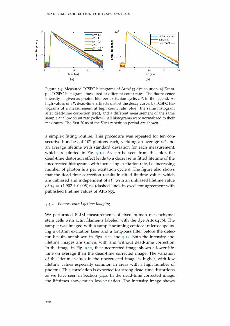
dead-time correction for tcspc systems

(a) (b)

Figure 5.9: Measured TCSPC histograms of Atto 655 dye solution. a) Exam-ple TCSPC histograms measured at different count rates. The fluorescenceintensity is given as photon hits per excitation cycle, εP, in the legend. Athigh values of εP, dead-time artifacts distort the decay curve. b) TCSPC his-tograms of a measurement at high count rate (blue), the same histogramafter dead-time correction (red), and a different measurement of the samesample at a low count rate (yellow). All histograms were normalized to theirmaximum. The first 20 ns of the 50 ns repetition period are shown.

a simplex fitting routine. This procedure was repeated for ten con-secutive bunches of 106 photons each, yielding an average εP andan average lifetime with standard deviation for each measurement,which are plotted in Fig. 5.10. As can be seen from this plot, thedead-time distortion effect leads to a decrease in fitted lifetime of theuncorrected histograms with increasing excitation rate, i.e. increasingnumber of photon hits per excitation cycle ε. The figure also showsthat the dead-time correction results in fitted lifetime values whichare unbiased and independent of εP, with an unbiased lifetime valueof τfl = (1.902± 0.005) ns (dashed line), in excellent agreement withpublished lifetime values of Atto 655.

5.4.3 Fluorescence Lifetime Imaging

We performed FLIM measurements of fixed human mesenchymalstem cells with actin filaments labeled with the dye Atto 647N. Thesample was imaged with a sample-scanning confocal microscope us-ing a 640 nm excitation laser and a long-pass filter before the detec-tor. Results are shown in Figs. 5.11 and 5.12. Both the intensity andlifetime images are shown, with and without dead-time correction.In the image in Fig. 5.11, the uncorrected image shows a lower life-time on average than the dead-time corrected image. The variationof the lifetime values in the uncorrected image is higher, with lowlifetime values especially common in areas with a high number ofphotons. This correlation is expected for strong dead-time distortionsas we have seen in Section 5.4.2. In the dead-time corrected image,the lifetimes show much less variation. The intensity image shows

110

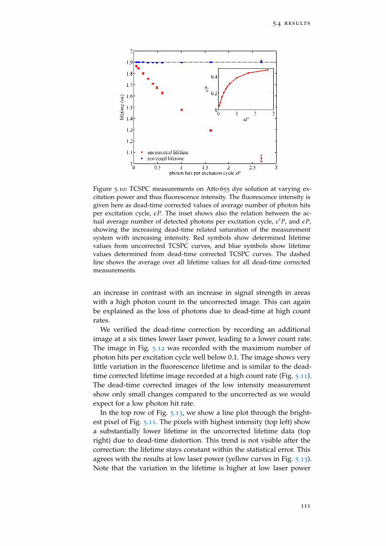
5.4 results

Figure 5.10: TCSPC measurements on Atto 655 dye solution at varying ex-citation power and thus fluorescence intensity. The fluorescence intensity isgiven here as dead-time corrected values of average number of photon hitsper excitation cycle, εP. The inset shows also the relation between the ac-tual average number of detected photons per excitation cycle, ε′P, and εP,showing the increasing dead-time related saturation of the measurementsystem with increasing intensity. Red symbols show determined lifetimevalues from uncorrected TCSPC curves, and blue symbols show lifetimevalues determined from dead-time corrected TCSPC curves. The dashedline shows the average over all lifetime values for all dead-time correctedmeasurements.

an increase in contrast with an increase in signal strength in areaswith a high photon count in the uncorrected image. This can againbe explained as the loss of photons due to dead-time at high countrates.

We verified the dead-time correction by recording an additionalimage at a six times lower laser power, leading to a lower count rate.The image in Fig. 5.12 was recorded with the maximum number ofphoton hits per excitation cycle well below 0.1. The image shows verylittle variation in the fluorescence lifetime and is similar to the dead-time corrected lifetime image recorded at a high count rate (Fig. 5.11).The dead-time corrected images of the low intensity measurementshow only small changes compared to the uncorrected as we wouldexpect for a low photon hit rate.

In the top row of Fig. 5.13, we show a line plot through the bright-est pixel of Fig. 5.11. The pixels with highest intensity (top left) showa substantially lower lifetime in the uncorrected lifetime data (topright) due to dead-time distortion. This trend is not visible after thecorrection: the lifetime stays constant within the statistical error. Thisagrees with the results at low laser power (yellow curves in Fig. 5.13).Note that the variation in the lifetime is higher at low laser power

111

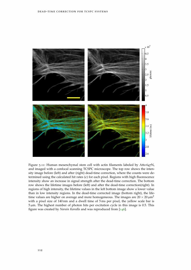
dead-time correction for tcspc systems

Figure 5.11: Human mesenchymal stem cell with actin filaments labeled by Atto 647N,and imaged with a confocal scanning TCSPC microscope. The top row shows the inten-sity image before (left) and after (right) dead-time correction, where the counts were de-termined using the calculated hit rates (ε) for each pixel. Regions with high fluorescenceintensity show an increase in signal strength after the dead-time correction. The bottomrow shows the lifetime images before (left) and after the dead-time correction(right). Inregions of high intensity, the lifetime values in the left bottom image show a lower valuethan in low intensity regions. In the dead-time corrected image (bottom right), the life-time values are higher on average and more homogeneous. The images are 20× 20µm2

with a pixel size of 140 nm and a dwell time of 5 ms per pixel, the yellow scale bar is5µm. The highest number of photon hits per excitation cycle in this image is 0.5. Thisfigure was created by Narain Karedla and was reproduced from [146].

112

5.4 results

compared to the corrected lifetime at high laser power because thenumber of recorded photons is smaller by about a factor of 5. If thelifetime was used, for example, to report on the FRET value, the dipin the lifetime curve (top right) can easily be misinterpreted as asignificant change. In the bottom row of Fig. 5.13 we show the TC-SPC histograms of the brightest pixel at high (bottom left, εP = 0.50)and low laser power (bottom right, εP = 0.09). The uncorrected andcorrected TCSPC curves show a negligible difference for the lowerphoton hit rate which is not the case for the curves shown for thehigh εP value. The fitted lifetime values of the corrected curves agreewithin their errors, whereas the values differ substantially for the un-corrected curves.

113

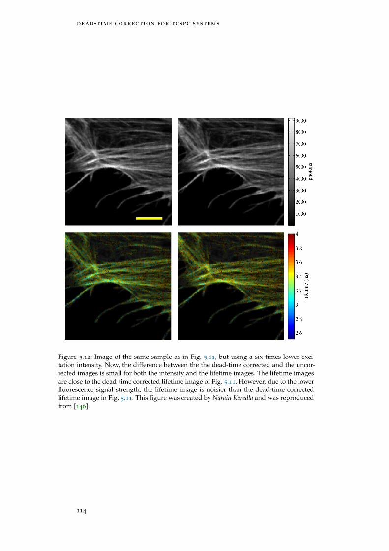
dead-time correction for tcspc systems

Figure 5.12: Image of the same sample as in Fig. 5.11, but using a six times lower exci-tation intensity. Now, the difference between the the dead-time corrected and the uncor-rected images is small for both the intensity and the lifetime images. The lifetime imagesare close to the dead-time corrected lifetime image of Fig. 5.11. However, due to the lowerfluorescence signal strength, the lifetime image is noisier than the dead-time correctedlifetime image in Fig. 5.11. This figure was created by Narain Karedla and was reproducedfrom [146].

114

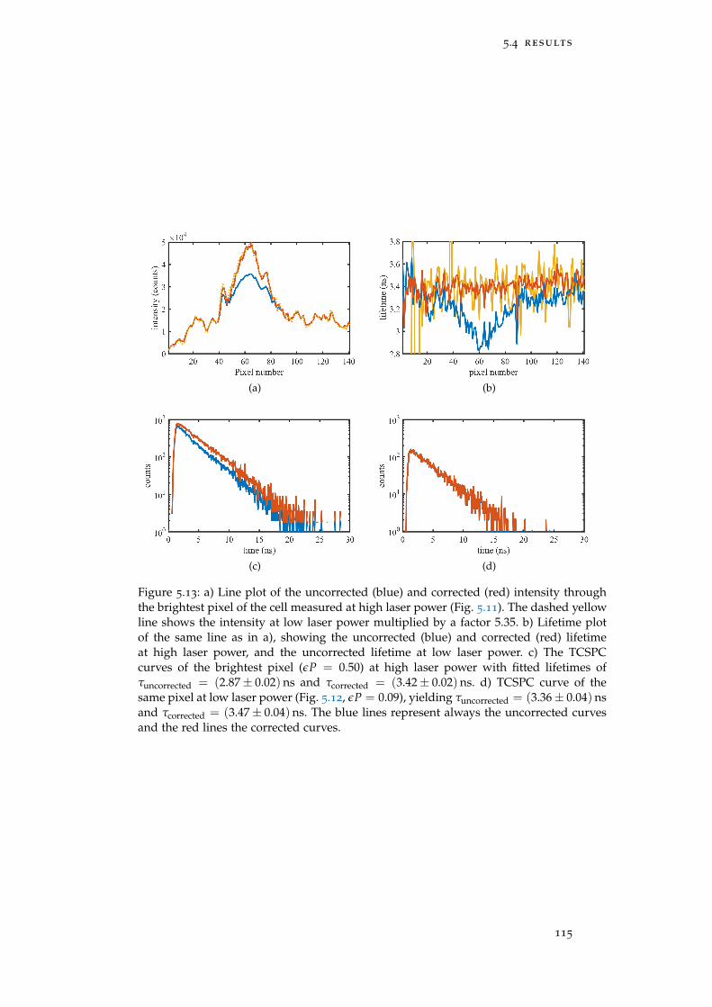
5.4 results

(a) (b)

(c) (d)

Figure 5.13: a) Line plot of the uncorrected (blue) and corrected (red) intensity throughthe brightest pixel of the cell measured at high laser power (Fig. 5.11). The dashed yellowline shows the intensity at low laser power multiplied by a factor 5.35. b) Lifetime plotof the same line as in a), showing the uncorrected (blue) and corrected (red) lifetimeat high laser power, and the uncorrected lifetime at low laser power. c) The TCSPCcurves of the brightest pixel (εP = 0.50) at high laser power with fitted lifetimes ofτuncorrected = (2.87± 0.02) ns and τcorrected = (3.42± 0.02) ns. d) TCSPC curve of thesame pixel at low laser power (Fig. 5.12, εP = 0.09), yielding τuncorrected = (3.36± 0.04) nsand τcorrected = (3.47± 0.04) ns. The blue lines represent always the uncorrected curvesand the red lines the corrected curves.

115

dead-time correction for tcspc systems

5.5 discussion

In this chapter, we have investigated how dead-time effects distort aTCSPC histogram at high count rates and presented an algorithm thatcorrects these effects in measurements. We developed a theoreticalmodel that describes the effects of constant detector and electronicsdead-times and have verified the model with simulations and mea-surements of fluorescence lifetimes. The model was furthermore usedto correct dead-time distorted TCSPC histograms of fluorescence de-cay and to estimate the actual photon hit rate from the data.

We measured the fluorescence lifetime of a dye in solution and of la-beled cells to verify the correction algorithm and test its performancein lifetime measurements and FLIM. With the correction, the fluores-cence lifetime of a dye solution was accurately reproduced up to aphoton hit rate of more than 2 photons per excitation cycle (εP = 2).In the uncorrected measurement, the lifetime was underestimated bymore than 50 % and the fluorescence intensity by a factor of 4. In theFLIM images recorded at high laser power, we found similar distor-tions that affected the lifetime accuracy and the image contrast. Thiscan have serious consequences on the interpretation of the data: InFRET measurements in cells for example, a region with lower life-times could be wrongly interpreted as increased FRET although thereal reason was dead-time distortions because the particular regionhad a higher labeling density than its surrounding. With the correc-tion, the measurement can be performed at a high count rate withoutcompromising the data accuracy.

Dead-time distortions in FLIM images are usually avoided by keep-ing the count rate low. A typical rule of thumb is that the count rateshould not exceed 1 % of the laser repetition rate [34]. However, thisreduces the measurement speed as more time is needed to acquirea sufficient number of photons. Because the dead-time correction al-lows imaging at a much higher count rate, it allows to speed up theimage acquisition. We have successfully performed measurements atεP = 2, which increases the photon hit rate by a factor of 200 com-pared to the rule of thumb of εP = 0.01. However, this does nottranslate in a speed up of 200×, because most of the photons are lostand do not contribute to the photon statistics of the measurement. Fora realistic speed up for FLIM we need to consider the real count rateε′P instead of εP, so that the number of photons that can be used forthe lifetime estimation is the same. We achieved a realistic count rateof about ε′P = 0.4, i.e. a realistic speed-up of 40×. This enables fastFLIM measurements which, for example, can be used to increase theframe rate of FLIM. Further, the speed-up makes it feasible to scan avast number of samples for high-throughput applications.

The dead-time correction can be useful also for other measurementtechniques apart from FLIM. The algorithm does not depend, in anyway, on the particular nature of the underlying fluorescence decay.

116

5.5 discussion

This enables the correction of multi-exponential decays as well astime-of-flight measurements which are employed for lidar [28] or inparticle physics [144]. In addition to restoring the shape of the decaycurve, also the intensity can be recovered. This increases the contrastof FLIM, but could be beneficial also for time-resolved fluorescenceanisotropy measurements [24]. The algorithm is furthermore not re-stricted to TCSPC measurements, but applicable to any single-eventcounting or timing measurement of two devices with constant dead-time connected in series.

We have shown that our dead-time correction algorithm recoversthe fluorescence lifetime and intensity from measurements at highcount rates. It can be applied to any event counting technique withdetector and electronics dead-time, and, thus, enable accurate mea-surements at high count rates. This allows faster data acquisition forhigh-throughput applications or for a better time resolution of con-secutive measurements.

117

6C O N C L U S I O N

In this work, we investigated three methods that extend the resolutionof a fluorescence microscope in different directions.

In Chapter 3, we showed how image scanning microscopy (ISM)can be used to increase the lateral resolution of a confocal spinningdisk setup. To this end, no modifications on the optical path of the mi-croscope were necessary. We developed a µManager plugin to controlthe synchronization of the spinning disk rotation with the illumina-tion which will be freely available. The CSDISM resolution improve-ment is comparable to other ISM based methods in the literature [65,67–69], while maintaining a low complexity of the setup. In fact, it iseasily possible to upgrade existing confocal spinning disk systems toa CSDISM system.

In Chapter 4, we used metal-induced energy transfer (MIET) to co-localize single emitters on a DNA origami structure along the opticalaxis. The axial resolution of most fluorescence microscopy methodsis lower than the lateral resolution. This is especially true for conven-tional superresolution methods like STED, STORM, or PALM whichachieve a lateral resolution below 20 nm. With MIET, we resolvedtwo emitters 30 nm apart from each other and measured their intra-molecular axial distance with 5 nm precision. MIET offers a range ofmore than 100 nm which is an order of magnitude larger than the dis-tances accessible by FRET. Thus, MIET can be used to study the struc-ture of large biomolecular complexes that are too large for FRET yettoo small for conventional (lateral) superresolution microscopy. Fur-thermore, the range and sensitivity of MIET can be tuned by choosingdifferent materials such as indium tin oxide, enabling measurementswith sub-nanometer accuracy [147]. The combination with a lateralsuperresolution technique can enable 3D imaging with an isotropicresolution of a few nanometers. This would allow to measure intra-molecular distances with unprecedented resolution and open a newchapter in the field of structure determination of biomolecular com-plexes.

In Chapter 5, we developed a dead-time correction that can be usedfor fast FLIM imaging. We estimated that a speed-up of 40× is possi-ble which drastically increases the data acquisition speed. This allowshigh-throughput applications of FLIM [148] or to increase the framerates to follow fast processes in cells. Apart from FLIM, the correctionalgorithm is applicable to other TCSPC based techniques such as li-dar or fluorescence anisotropy. In fact, the model of dead-time effectscan be applied to all single event counting devices with a constantelectronic and detector dead-time. Apart from correcting the TCSPC

conclusion

histogram, also the intensity is estimated. This might be interestingfor counting based method to measure radiation in particle and high-energy physics.

In conclusion, we have presented the increase of the lateral resolu-tion of a fluorescence microscope by CSDISM, the increase of the axialresolution by MIET, and the possibility to increase the time resolution(in terms of the frame rate) of a FLIM microscope by correcting dead-time distortions that limit the frame rate. In addition to the resolutionimprovement, the three methods have the advantage that they requirestandard instruments with little to no additional hardware, makingthem accessible for many researchers: For the dead-time correction,any TCSPC-based FLIM microscope can be used. MIET requires astandard FLIM microscope as well and metal-coated cover slips onthe sample side. For the CSDISM, an existing CSD setup can be up-graded with an FPGA card and then used with our software. We hopethat this accessibility enables many researchers to make use of thesetechniques and facilitate new discoveries.

120

AO T H E R C O N T R I B U T I O N S

Apart from the work presented in this thesis, I have contributed tothree other publications during the course of my PhD:

Thilo Baronsky, Daja Ruhlandt, Bastian Rouven Brückner, Jonas Schä-fer, Narain Karedla, Sebastian Isbaner, Dirk Hähnel, Ingo Gregor, JörgEnderlein, Andreas Janshoff, and Alexey I. Chizhik. “Cell–SubstrateDynamics of the Epithelial-to-Mesenchymal Transition.” In: Nano Let-ters 17.5 (May 10, 2017), pp. 3320–3326. doi: 10.1021/acs.nanolett.7b01558,

Arindam Ghosh, Sebastian Isbaner, Manoel Veiga-Gutiérrez, Ingo Gre-gor, Jörg Enderlein, and Narain Karedla. “Quantifying MicrosecondTransition Times Using Fluorescence Lifetime Correlation Spectros-copy.” In: The Journal of Physical Chemistry Letters 8.24 (Dec. 21, 2017),pp. 6022–6028. doi: 10.1021/acs.jpclett.7b02707,

and

Shama Sograte-Idrissi, Nazar Oleksiievets, Sebastian Isbaner, MarianaEggert-Martinez, Jörg Enderlein, Roman Tsukanov, and Felipe Opazo.“Nanobody Detection of Standard Fluorescent Proteins Enables Multi-Target DNA-PAINT with High Resolution and Minimal DisplacementErrors.” In: Cells 8.1 (Jan. 10, 2019), p. 48. doi: 10.3390/cells8010048.

On the following pages, I will give a short summary of each of theseprojects.

other contributions

a.1 cell–substrate dynamics of the epithelial-to-mesenchymal

transition

In this work, we studied the dynamics of the cell-substrate distanceduring the epithelial-to-mesenchymal transition. Epithelial cells arehighly polar cells and connect to each other to form epithelial sheets.These cells can become migratory mesenchymal stem cells which candifferentiate into a variety of other cell types. This process of chang-ing the phenotype is called the epithelial-to-mesenchymal transition(EMT) and is important in embryogenesis, fibrosis, wound healing,and cancer progression. In contrast to the epithelial cells, mesenchy-mal stem cells lack polarization and are usually widely dispersed.Therefore, the EMT is accompanied by changes of the dynamics ofcell-cell and cell-substrate interactions. Two phases of the EMT havebeen described: During the transitional state I, cells show an increasein cell-substrate dynamics for 4-9 h. In the following transitional stateII, cell adhesion leads to an increase and suppression of the fluctua-tions due to the complete loss of cell-cell contacts. However, a precisepicture of the process on a cellular or even subcellular level is lackingdue to limited spatial resolution especially along the optical axis.

Figure A.1: Cell–Substrate Dynamics of the Epithelial-to-Mesenchymal Tran-sition. In the graph, the average cell-substrate distance is shown for un-treated (blue) and TGF-β1 treated cells (red). The height initially increasesby more than 20 nm when EMT is induced by TGF-β1. The height is restoredabout 20 h after the treatment. Above, schematic drawings of cells show theordered epithelial state, the transitional state I with dissolution of cell-cellcontacts, the transitional state II where cells adhere to the substrate by form-ing actin stressfibers (red lines), and the mesenchymal state where cells arefully spread. The figure was reproduced from Ref. [149].

122

A.1 cell–substrate dynamics of the

epithelial-to-mesenchymal transition

Here, we used metal-induced energy transfer (MIET) to follow thedynamics of the cell-surface distance. MIET allows to measure thedistance of the basal membrane to the surface with about 3 nm accu-racy. We used the transforming growth factor-β1 (TGF-β1) to inducethe EMT in NMuMG cells, and then measured the height of the basalmembrane above the surface at different stages of the EMT. Our re-sults show that the cell-substrate distance increases during the initialstage of the EMT (see Fig. A.1). We found that this is accompaniedby a reduction in the number of focal adhesion points which enablesthe cells to lift-off from the surface. Then, the cell-substrate distancedecreases again until the initial distance is restored. We propose thatduring EMT, the cells enter a state of increased vertical motility dueto dynamic remodeling of adhesion sites. This state is transient andthe mesenchymal cells eventually become quiescent again, assumingthe smaller cell-substrate distance is an indicator of higher adhesionforces.

In conclusion, the MIET measurements enabled us to follow thecell-substrate dynamics of NMuMG cells undergoing EMT with un-precedented resolution. Our findings will help to better understandcellular remodeling processes associated with wound healing, embry-onic development, cancer progression, or tissue regeneration.

123

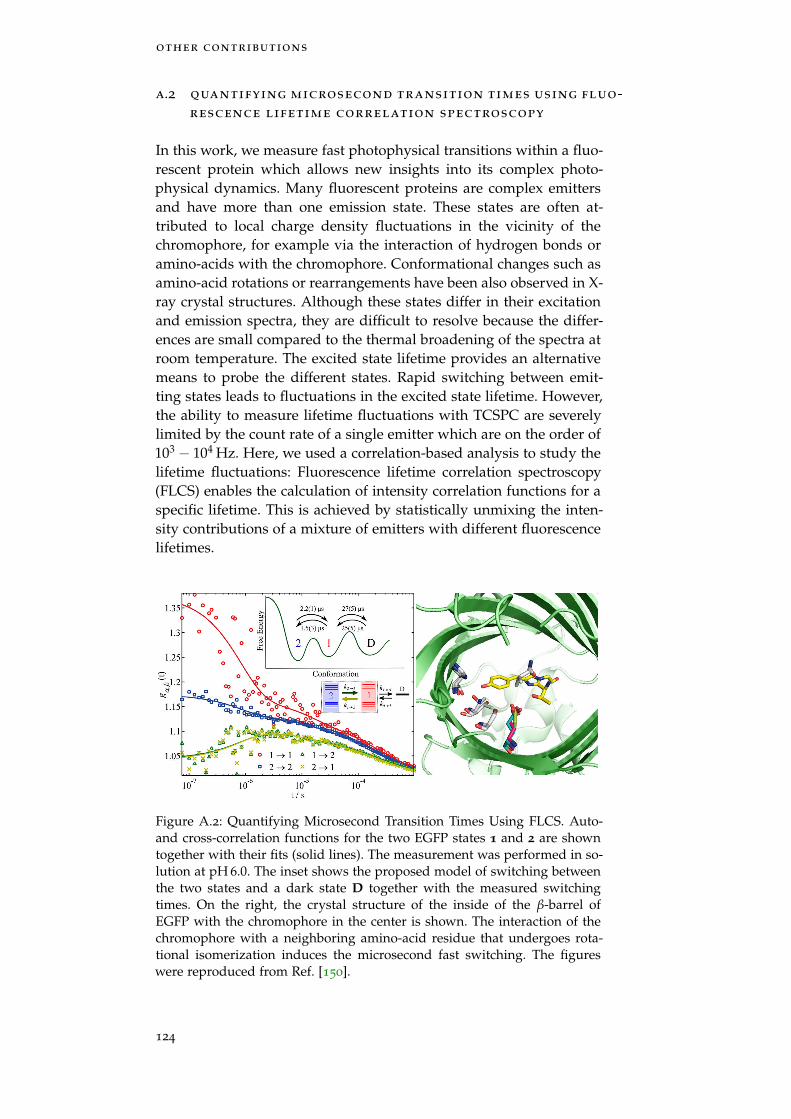
other contributions

a.2 quantifying microsecond transition times using fluo-rescence lifetime correlation spectroscopy

In this work, we measure fast photophysical transitions within a fluo-rescent protein which allows new insights into its complex photo-physical dynamics. Many fluorescent proteins are complex emittersand have more than one emission state. These states are often at-tributed to local charge density fluctuations in the vicinity of thechromophore, for example via the interaction of hydrogen bonds oramino-acids with the chromophore. Conformational changes such asamino-acid rotations or rearrangements have been also observed in X-ray crystal structures. Although these states differ in their excitationand emission spectra, they are difficult to resolve because the differ-ences are small compared to the thermal broadening of the spectra atroom temperature. The excited state lifetime provides an alternativemeans to probe the different states. Rapid switching between emit-ting states leads to fluctuations in the excited state lifetime. However,the ability to measure lifetime fluctuations with TCSPC are severelylimited by the count rate of a single emitter which are on the order of103 − 104 Hz. Here, we used a correlation-based analysis to study thelifetime fluctuations: Fluorescence lifetime correlation spectroscopy(FLCS) enables the calculation of intensity correlation functions for aspecific lifetime. This is achieved by statistically unmixing the inten-sity contributions of a mixture of emitters with different fluorescencelifetimes.

Figure A.2: Quantifying Microsecond Transition Times Using FLCS. Auto-and cross-correlation functions for the two EGFP states 1 and 2 are showntogether with their fits (solid lines). The measurement was performed in so-lution at pH 6.0. The inset shows the proposed model of switching betweenthe two states and a dark state D together with the measured switchingtimes. On the right, the crystal structure of the inside of the β-barrel ofEGFP with the chromophore in the center is shown. The interaction of thechromophore with a neighboring amino-acid residue that undergoes rota-tional isomerization induces the microsecond fast switching. The figureswere reproduced from Ref. [150].

124

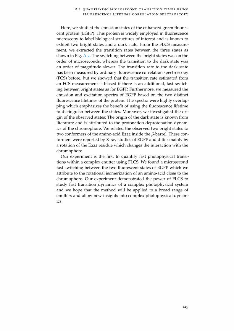
A.2 quantifying microsecond transition times using

fluorescence lifetime correlation spectroscopy

Here, we studied the emission states of the enhanced green fluores-cent protein (EGFP). This protein is widely employed in fluorescencemicroscopy to label biological structures of interest and is known toexhibit two bright states and a dark state. From the FLCS measure-ment, we extracted the transition rates between the three states asshown in Fig. A.2. The switching between the bright states was on theorder of microseconds, whereas the transition to the dark state wasan order of magnitude slower. The transition rate to the dark statehas been measured by ordinary fluorescence correlation spectroscopy(FCS) before, but we showed that the transition rate estimated froman FCS measurement is biased if there is an additional, fast switch-ing between bright states as for EGFP. Furthermore, we measured theemission and excitation spectra of EGFP based on the two distinctfluorescence lifetimes of the protein. The spectra were highly overlap-ping which emphasizes the benefit of using the fluorescence lifetimeto distinguish between the states. Moreover, we investigated the ori-gin of the observed states: The origin of the dark state is known fromliterature and is attributed to the protonation-deprotonation dynam-ics of the chromophore. We related the observed two bright states totwo conformers of the amino-acid E222 inside the β-barrel. These con-formers were reported by X-ray studies of EGFP and differ mainly bya rotation of the E222 residue which changes the interaction with thechromophore.

Our experiment is the first to quantify fast photophysical transi-tions within a complex emitter using FLCS. We found a microsecondfast switching between the two fluorescent states of EGFP which weattribute to the rotational isomerization of an amino-acid close to thechromophore. Our experiment demonstrated the power of FLCS tostudy fast transition dynamics of a complex photophysical systemand we hope that the method will be applied to a broad range ofemitters and allow new insights into complex photophysical dynam-ics.

125

other contributions

a.3 nanobody detection of standard fluorescent pro-teins enables multi-target dna-paint with high re-solution and minimal displacement errors

In this work, we demonstrate superresolution imaging of cellular or-ganelles with nanobodies that minimizes the displacement error tothe structure of interest. Superresolution fluorescence microscopy al-lows cell biologists to study cellular structures and proteins of interestat the nanoscale. DNA-PAINT is a superresolution techniques that isneither affected by fluorophore bleaching nor limited by the numberof spectrally distinguishable fluorophores for multi-target imaging.It is based on the transient binding and unbinding of short fluores-cently labeled oligonucleotides to complementary docking strands,labeling the structure of interest. Because the binding of the oligonu-cleotide to the docking strand is sequence-specific, sequential imag-ing of different targets can be realized (Exchange-PAINT). A resolu-tion below 10 nm for more than ten targets has been demonstratedon DNA origami structures. However, if the protein of interest is la-beled by conventional antibody immunostaining, the pure size of aprimary-secondary antibody complex introduces a displacement ofup to 25 nm between the target and the fluorophore. This is alsoknown as the linkage error and seriously limits the imaging reso-lution of superresolution microscopy. Several small probes have beendeveloped to overcome this problem, among them aptamers and single-domain antibodies (nanobodies). But of these, only few probes for dif-ferent targets are available, limiting the applicability of these probes.

Figure A.3: Multi-Target Exchange-PAINT with Nanobodies. Fluorescentproteins were fused to the protein of interest and expressed in cells. Nano-bodies modified with a short oligonucleotide for DNA-PAINT bound specif-ically to one of the fluorescent proteins (mTagBFP, EGFP, and mCherry).DNA-PAINT imaging was performed with an imager specific to the dock-ing strand on the nanobody. By sequentially introducing the different im-ager strands, a multi-targt superresolution image was obtained. This figurewas created by Roman Tsukanov.

126

A.3 multi-target exchange-paint with nanobodies

Here, we used small camelid nanobodies with a size of 2 to 3 nmwhich effectively minimize the fluorophore-target distance. The nano-bodies against three different standard fluorescent proteins were mod-ified with a docking strand for DNA-PAINT imaging. Cells weretransfected with plasmids expressing the fluorescent proteins fusedto a protein of interest to label the chromatin, the mitochondria, andthe golgi-apparatus, respectively. We performed Exchange-PAINT ex-periments for three targets on a custom-built widefield setup with aprogrammable microfluidic setup. We achieved a resolution of 20 nmwithin 35 minutes of acquisition per target. Superresolution imagesof the mitochondria, the golgi-apparatus, and the chromatin distribu-tion were obtained, see Fig. A.3. The structures in the superresolvedimages were in agreement with the direct observation of the fluores-cent proteins.

In summary, we demonstrated multi-target superresolution imag-ing of cellular organelles with Exchange-PAINT and nanobodies. Sincewe used readily available nanobodies against standard fluorescentproteins, our method enables researchers who use conventional fluo-rescent proteins to obtain superresolved images of at least three com-mon proteins with minimal fluorophore-target displacement error.

127

B I B L I O G R A P H Y

[6] Ulrich Kubitscheck. Fluorescence Microscopy: From Principles to Biological Ap-plications. John Wiley & Sons, June 19, 2017. 504 pp.

[7] Partha Pratim Mondal and Alberto Diaspro. Fundamentals of FluorescenceMicroscopy: Exploring Life with Light. Springer Science & Business Media,Dec. 12, 2013. 219 pp.

[8] M. Orrit and J. Bernard. “Single pentacene molecules detected by fluores-cence excitation in a p-terphenyl crystal.” In: Physical Review Letters 65.21

(Nov. 19, 1990), pp. 2716–2719. doi: 10.1103/PhysRevLett.65.2716.

[9] W. E. Moerner. “A Dozen Years of Single-Molecule Spectroscopy in Physics,Chemistry, and Biophysics.” In: The Journal of Physical Chemistry B 106.5(Feb. 1, 2002), pp. 910–927. doi: 10.1021/jp012992g.

[10] Stefan W. Hell and Jan Wichmann. “Breaking the diffraction resolutionlimit by stimulated emission: stimulated-emission-depletion fluorescencemicroscopy.” In: Optics Letters 19.11 (June 1, 1994), pp. 780–782. doi: 10.1364/OL.19.000780.

[11] Eric Betzig, George H. Patterson, Rachid Sougrat, O. Wolf Lindwasser,Scott Olenych, Juan S. Bonifacino, Michael W. Davidson, Jennifer Lippincott-Schwartz, and Harald F. Hess. “Imaging Intracellular Fluorescent Proteinsat Nanometer Resolution.” In: Science 313.5793 (Sept. 15, 2006), pp. 1642–1645. doi: 10.1126/science.1127344.

[12] Samuel T. Hess, Thanu P. K. Girirajan, and Michael D. Mason. “Ultra-High Resolution Imaging by Fluorescence Photoactivation LocalizationMicroscopy.” In: Biophysical Journal 91.11 (Dec. 1, 2006), pp. 4258–4272. doi:10.1529/biophysj.106.091116.

[13] Michael J. Rust, Mark Bates, and Xiaowei Zhuang. “Sub-diffraction-limitimaging by stochastic optical reconstruction microscopy (STORM).” In:Nature Methods 3.10 (Oct. 2006), pp. 793–796. doi: 10.1038/nmeth929.

[14] Andreas Gahlmann and W. E. Moerner. “Exploring bacterial cell biologywith single-molecule tracking and super-resolution imaging.” In: NatureReviews Microbiology 12.1 (Jan. 2014), pp. 9–22. doi: 10.1038/nrmicro3154.

[15] Lothar Schermelleh, Peter M. Carlton, Sebastian Haase, Lin Shao, LukmanWinoto, Peter Kner, Brian Burke, M. Cristina Cardoso, David A. Agard,Mats G. L. Gustafsson, Heinrich Leonhardt, and John W. Sedat. “Subd-iffraction Multicolor Imaging of the Nuclear Periphery with 3D StructuredIllumination Microscopy.” In: Science 320.5881 (June 6, 2008), pp. 1332–1336. doi: 10.1126/science.1156947.

bibliography

[16] Anna Löschberger, Sebastian van de Linde, Marie-Christine Dabauvalle,Bernd Rieger, Mike Heilemann, Georg Krohne, and Markus Sauer. “Super-resolution imaging visualizes the eightfold symmetry of gp210 proteinsaround the nuclear pore complex and resolves the central channel withnanometer resolution.” In: J Cell Sci 125.3 (Feb. 1, 2012), pp. 570–575. doi:10.1242/jcs.098822.

[17] Sebastian van de Linde, Mike Heilemann, and Markus Sauer. “Live-CellSuper-Resolution Imaging with Synthetic Fluorophores.” In: Annual Re-view of Physical Chemistry 63.1 (2012). PMID: 22404589, pp. 519–540. doi:10.1146/annurev-physchem-032811-112012.

[18] T. Ha, T. Enderle, D. F. Ogletree, D. S. Chemla, P. R. Selvin, and S. Weiss.“Probing the interaction between two single molecules: fluorescence res-onance energy transfer between a single donor and a single acceptor.”In: Proceedings of the National Academy of Sciences 93.13 (June 25, 1996),pp. 6264–6268. doi: 10.1073/pnas.93.13.6264.

[19] Mykola Dimura, Thomas O Peulen, Christian A Hanke, Aiswaria Prakash,Holger Gohlke, and Claus AM Seidel. “Quantitative FRET studies and in-tegrative modeling unravel the structure and dynamics of biomolecularsystems.” In: Current Opinion in Structural Biology. Carbohydrate–proteininteractions and glycosylation • Biophysical and molecular biological meth-ods 40 (Oct. 1, 2016), pp. 163–185. doi: 10.1016/j.sbi.2016.11.012.

[20] Robert P Hertzberg and Andrew J Pope. “High-throughput screening:new technology for the 21st century.” In: Current Opinion in Chemical Biol-ogy 4.4 (Aug. 1, 2000), pp. 445–451. doi: 10.1016/S1367-5931(00)00110-1.

[21] Rainer Pepperkok and Jan Ellenberg. “High-throughput fluorescence mi-croscopy for systems biology.” In: Nature Reviews Molecular Cell Biology 7.9(Sept. 2006), pp. 690–696. doi: 10.1038/nrm1979.

[22] Manuel A. Robbins. The Collector’s Book of Fluorescent Minerals. SpringerUS, 1983. XIII, 289.

[23] C. E. Mills. Bioluminescence of Aequorea. Bioluminescence of Aequorea, ahydromedusa. Jan. 11, 2009. url: http : / / faculty . washington . edu /

cemills/Aequorea.html (visited on 09/18/2018).

[24] J.R. Lakowicz. Principles of Fluorescence Spectroscopy. Springer US, 2013.

[25] Lothar Schermelleh, Rainer Heintzmann, and Heinrich Leonhardt. “A guideto super-resolution fluorescence microscopy.” In: The Journal of Cell Biology190.2 (July 26, 2010), pp. 165–175. doi: 10.1083/jcb.201002018.

[26] Stefan W. Hell. “Far-Field Optical Nanoscopy.” In: Science 316.5828 (May 25,2007), pp. 1153–1158. doi: 10.1126/science.1137395.

[27] Bo Huang, Mark Bates, and Xiaowei Zhuang. “Super-Resolution Fluores-cence Microscopy.” In: Annual Review of Biochemistry 78.1 (June 1, 2009),pp. 993–1016. doi: 10.1146/annurev.biochem.77.061906.092014.

130

bibliography

[28] Aongus McCarthy, Robert J. Collins, Nils J. Krichel, Verónica Fernández,Andrew M. Wallace, and Gerald S. Buller. “Long-range time-of-flight scan-ning sensor based on high-speed time-correlated single-photon counting.”In: Applied Optics 48.32 (Nov. 10, 2009), p. 6241. doi: 10.1364/AO.48.006241.

[29] John J. Degnan. “Photon-counting multikilohertz microlaser altimeters forairborne and spaceborne topographic measurements.” In: Journal of Geody-namics 34.3 (Oct. 1, 2002), pp. 503–549. doi: 10.1016/S0264- 3707(02)00045-5.

[30] Brent Schwarz. “LIDAR: Mapping the world in 3D.” In: Nature Photonics4 (July 1, 2010), pp. 429–430. doi: 10.1038/nphoton.2010.148.

[31] Wolfgang Becker. Advanced Time-Correlated Single Photon Counting Tech-niques. Ed. by A. W. Castleman, J.P. Toennies, and W. Zinth. Vol. 81. SpringerSeries in Chemical Physics. Berlin, Heidelberg: Springer Berlin Heidelberg,2005.

[32] M. D. Eisaman, J. Fan, A. Migdall, and S. V. Polyakov. “Invited ReviewArticle: Single-photon sources and detectors.” In: Review of Scientific In-struments 82.7 (July 1, 2011), p. 071101. doi: 10.1063/1.3610677.

[33] Wolfgang Becker. The bh TCSPC handbook. Becker & Hickl, 2014.

[34] Michael Wahl. Time-Correlated Single Photon Counting. 2014. url: https://www.picoquant.com/images/uploads/page/files/7253/technote_

tcspc.pdf (visited on 11/05/2018).

[35] Desmond O’Connor. Time-correlated single photon counting. Academic Press,1984. 299 pp.

[36] Michael Wahl, Hans-Jürgen Rahn, Ingo Gregor, Rainer Erdmann, and JörgEnderlein. “Dead-time optimized time-correlated photon counting instru-ment with synchronized, independent timing channels.” In: Review of Sci-entific Instruments 78.3 (Mar. 1, 2007), p. 033106. doi: 10.1063/1.2715948.

[37] Michael Wahl, Hans-Jürgen Rahn, Tino Röhlicke, Gerald Kell, Daniel Net-tels, Frank Hillger, Ben Schuler, and Rainer Erdmann. “Scalable time-correlated photon counting system with multiple independent input chan-nels.” In: Review of Scientific Instruments 79.12 (Dec. 1, 2008), p. 123113. doi:10.1063/1.3055912.

[38] Michael Wahl, Ingo Gregor, Mattias Patting, and Jörg Enderlein. “Fast cal-culation of fluorescence correlation data with asynchronous time-correlatedsingle-photon counting.” In: Optics Express 11.26 (Dec. 29, 2003), p. 3583.doi: 10.1364/OE.11.003583.

[39] Martin Böhmer, Michael Wahl, Hans-Jürgen Rahn, Rainer Erdmann, andJörg Enderlein. “Time-resolved fluorescence correlation spectroscopy.” In:Chemical Physics Letters 353.5 (Feb. 26, 2002), pp. 439–445. doi: 10.1016/S0009-2614(02)00044-1.

[40] Peter Kapusta, Michael Wahl, Aleš Benda, Martin Hof, and Jörg Ender-lein. “Fluorescence Lifetime Correlation Spectroscopy.” In: Journal of Fluo-rescence 17.1 (Dec. 27, 2006), pp. 43–48. doi: 10.1007/s10895-006-0145-1.

131

bibliography

[41] Ted A. Laurence, Achillefs N. Kapanidis, Xiangxu Kong, Daniel S. Chemla,and Shimon Weiss. “Photon Arrival-Time Interval Distribution (PAID):A Novel Tool for Analyzing Molecular Interactions.” In: The Journal ofPhysical Chemistry B 108.9 (Mar. 1, 2004), pp. 3051–3067. doi: 10.1021/jp036499b.

[42] Xavier Michalet, Shimon Weiss, and Marcus Jäger. “Single-Molecule Fluo-rescence Studies of Protein Folding and Conformational Dynamics.” In:Chemical Reviews 106.5 (May 1, 2006), pp. 1785–1813. doi: 10.1021/cr0404343.

[43] Valéry Zwiller, Hans Blom, Per Jonsson, Nikolay Panev, Sören Jeppesen,Tedros Tsegaye, Edgard Goobar, Mats-Erik Pistol, Lars Samuelson, andGunnar Björk. “Single quantum dots emit single photons at a time: An-tibunching experiments.” In: Applied Physics Letters 78.17 (Apr. 13, 2001),pp. 2476–2478. doi: 10.1063/1.1366367.

[44] K. H. Drexhage, H. Kuhn, and F. P. Schäfer. “Variation of the FluorescenceDecay Time of a Molecule in Front of a Mirror.” In: Berichte der Bunsen-gesellschaft für physikalische Chemie 72.2 (Mar. 1, 1968), pp. 329–329. doi:10.1002/bbpc.19680720261.

[45] Hans Kuhn. “Classical Aspects of Energy Transfer in Molecular Systems.”In: The Journal of Chemical Physics 53.1 (July 1970), pp. 101–108. doi: 10.1063/1.1673749.

[46] R. R. Chance, A. Prock, and R. Silbey. “Molecular fluorescence and energytransfer near interfaces.” In: Adv. Chem. Phys 37.1 (1978), p. 65.

[47] R. M. Amos and W. L. Barnes. “Modification of the spontaneous emissionrate of Eu3+ ions close to a thin metal mirror.” In: Physical Review B 55.11

(Mar. 15, 1997), pp. 7249–7254. doi: 10.1103/PhysRevB.55.7249.

[48] F. D. Stefani, K. Vasilev, N. Bocchio, N. Stoyanova, and M. Kreiter. “Surface-Plasmon-Mediated Single-Molecule Fluorescence Through a Thin Metal-lic Film.” In: Physical Review Letters 94.2 (Jan. 19, 2005), p. 023005. doi:10.1103/PhysRevLett.94.023005.

[49] Michael Berndt, Mike Lorenz, Jörg Enderlein, and Stefan Diez. “AxialNanometer Distances Measured by Fluorescence Lifetime Imaging Mi-croscopy.” In: Nano Letters 10.4 (Apr. 14, 2010), pp. 1497–1500. doi: 10.1021/nl100593x.

[50] Narain Karedla, Alexey I. Chizhik, Ingo Gregor, Anna M. Chizhik, OlafSchulz, and Jörg Enderlein. “Single-Molecule Metal-Induced Energy Trans-fer (smMIET): Resolving Nanometer Distances at the Single-Molecule Level.”In: ChemPhysChem 15.4 (Jan. 29, 2014), pp. 705–711. doi: 10.1002/cphc.201300760.

[51] Narain Karedla. “Single-Molecule Metal-Induced Energy Transfer: FromBasics to Applications.” PhD thesis. Göttingen: Universität Göttingen, Dec. 16,2016.

[52] John David Jackson. Classical electrodynamics. John Wiley & Sons, 2012.

132

bibliography

[53] Jörg Enderlein. “A Theoretical Investigation of Single-Molecule Fluores-cence Detection on Thin Metallic Layers.” In: Biophysical Journal 78.4 (Apr.2000), pp. 2151–2158. doi: 10.1016/S0006-3495(00)76761-0.

[54] Jörg Enderlein. “Single-molecule fluorescence near a metal layer.” In: Chem-ical Physics 247.1 (1999), pp. 1–9.

[55] Daja Ruhlandt. “Modeling electrodynamics in the vicinity of metal nano-structures.” PhD thesis. Göttingen: Universität Göttingen, 2018.

[56] Olaf Schulz, Christoph Pieper, Michaela Clever, Janine Pfaff, Aike Ruh-landt, Ralph H. Kehlenbach, Fred S. Wouters, Jörg Grosshans, GertrudeBunt, and Jörg Enderlein. “Resolution doubling in fluorescence microscopywith confocal spinning-disk image scanning microscopy.” In: Proceedingsof the National Academy of Sciences 110.52 (Dec. 24, 2013), pp. 21000–21005.doi: 10.1073/pnas.1315858110.

[57] Arthur Edelstein, Nenad Amodaj, Karl Hoover, Ron Vale, and Nico Stu-urman. “Computer Control of Microscopes Using µManager.” In: CurrentProtocols in Molecular Biology 92.1 (Oct. 1, 2010), pp. 14.20.1–14.20.17. doi:10.1002/0471142727.mb1420s92.

[58] Arthur D. Edelstein, Mark A. Tsuchida, Nenad Amodaj, Henry Pinkard,Ronald D. Vale, and Nico Stuurman. “Advanced methods of microscopecontrol using µManager software.” In: Journal of Biological Methods 1.2(Nov. 7, 2014), e10. doi: 10.14440/jbm.2014.36.

[59] Takeo Tanaami, Shinya Otsuki, Nobuhiro Tomosada, Yasuhito Kosugi, MizuhoShimizu, and Hideyuki Ishida. “High-speed 1-frame/ms scanning confo-cal microscope with a microlens and Nipkow disks.” In: Applied Optics41.22 (Aug. 1, 2002), pp. 4704–4708. doi: 10.1364/AO.41.004704.

[60] James Pawley. Handbook of Biological Confocal Microscopy. 3rd ed. 2006. NewYork, NY: Springer, Aug. 10, 2006. 985 pp.

[61] Shinya Inoue and Ted Inoue. “Direct-view high-speed confocal scanner:the CSU-10.” In: Collected Works Of Shinya Inoue: Microscopes, Living Cells,and Dynamic Molecules. World Scientific, 2008, pp. 903–946.

[62] Colin JR Sheppard. “Super-resolution in confocal imaging.” In: Optik 80.2(1988), pp. 53–54.

[63] M. Bertero, P. Brianzi, and E. R. Pike. “Super-resolution in confocal scan-ning microscopy.” In: Inverse Problems 3.2 (1987), p. 195.

[64] Claus B. Müller and Jörg Enderlein. “Image Scanning Microscopy.” In:Physical Review Letters 104.19 (May 10, 2010). doi: 10.1103/PhysRevLett.104.198101.

[65] Andrew G. York, Sapun H. Parekh, Damian Dalle Nogare, Robert S. Fis-cher, Kelsey Temprine, Marina Mione, Ajay B. Chitnis, Christian A. Combs,and Hari Shroff. “Resolution doubling in live, multicellular organismsvia multifocal structured illumination microscopy.” In: Nature Methods 9.7(July 2012), pp. 749–754. doi: 10.1038/nmeth.2025.

133

bibliography

[66] M. G. L. Gustafsson. “Surpassing the lateral resolution limit by a factor oftwo using structured illumination microscopy.” In: Journal of Microscopy198.2 (May 1, 2000), pp. 82–87. doi: 10.1046/j.1365-2818.2000.00710.x.

[67] Andrew G. York, Panagiotis Chandris, Damian Dalle Nogare, Jeffrey Head,Peter Wawrzusin, Robert S. Fischer, Ajay Chitnis, and Hari Shroff. “In-stant super-resolution imaging in live cells and embryos via analog im-age processing.” In: Nature Methods 10.11 (Nov. 2013), pp. 1122–1126. doi:10.1038/nmeth.2687.

[68] Stephan Roth, Colin JR Sheppard, Kai Wicker, and Rainer Heintzmann.“Optical photon reassignment microscopy (OPRA).” In: Optical Nanoscopy2.1 (Oct. 18, 2013), p. 5. doi: 10.1186/2192-2853-2-5.

[69] Giulia M. R. De Luca, Ronald M. P. Breedijk, Rick A. J. Brandt, ChristiaanH. C. Zeelenberg, Babette E. de Jong, Wendy Timmermans, Leila NahidiAzar, Ron A. Hoebe, Sjoerd Stallinga, and Erik M. M. Manders. “Re-scanconfocal microscopy: scanning twice for better resolution.” In: BiomedicalOptics Express 4.11 (Nov. 1, 2013), pp. 2644–2656. doi: 10.1364/BOE.4.002644.

[70] Ingo Gregor, Martin Spiecker, Roman Petrovsky, Jörg Großhans, RobertRos, and Jörg Enderlein. “Rapid nonlinear image scanning microscopy.”In: Nature Methods 14.11 (Nov. 2017), pp. 1087–1089. doi: 10.1038/nmeth.4467.

[71] Takuya Azuma and Takayuki Kei. “Super-resolution spinning-disk con-focal microscopy using optical photon reassignment.” In: Optics Express23.11 (June 1, 2015), pp. 15003–15011. doi: 10.1364/OE.23.015003.

[72] Shinichi Hayashi. “Resolution doubling using confocal microscopy viaanalogy with structured illumination microscopy.” In: Japanese Journal ofApplied Physics 55.8 (June 30, 2016), p. 082501. doi: 10.7567/JJAP.55.082501.

[73] E. N. Ward and R. Pal. “Image scanning microscopy: an overview.” In:Journal of Microscopy 266.2 (May 1, 2017), pp. 221–228. doi: 10.1111/jmi.12534.

[74] Colin J. R. Sheppard, Shalin B. Mehta, and Rainer Heintzmann. “Super-resolution by image scanning microscopy using pixel reassignment.” In:Optics Letters 38.15 (Aug. 1, 2013), p. 2889. doi: 10.1364/OL.38.002889.

[75] E. Abbe. “Beiträge zur Theorie des Mikroskops und der mikroskopischenWahrnehmung.” In: Archiv für mikroskopische Anatomie 9.1 (Dec. 1, 1873),pp. 456–468. doi: 10.1007/BF02956176.

[76] George Patterson, Michael Davidson, Suliana Manley, and Jennifer Lippincott-Schwartz. “Superresolution Imaging using Single-Molecule Localization.”In: Annual Review of Physical Chemistry 61.1 (2010), pp. 345–367. doi: 10.1146/annurev.physchem.012809.103444.

134

bibliography

[77] J. Vangindertael, R. Camacho, W. Sempels, H. Mizuno, P. Dedecker, andK. P. F. Janssen. “An introduction to optical super-resolution microscopyfor the adventurous biologist.” In: Methods and Applications in Fluorescence6.2 (2018), p. 022003. doi: 10.1088/2050-6120/aaae0c.

[78] Mike Heilemann, Sebastian van de Linde, Mark Schüttpelz, Robert Kasper,Britta Seefeldt, Anindita Mukherjee, Philip Tinnefeld, and Markus Sauer.“Subdiffraction-Resolution Fluorescence Imaging with Conventional Fluo-rescent Probes.” In: Angewandte Chemie International Edition 47.33 (Aug. 4,2008), pp. 6172–6176. doi: 10.1002/anie.200802376.

[79] Ralf Jungmann, Christian Steinhauer, Max Scheible, Anton Kuzyk, PhilipTinnefeld, and Friedrich C. Simmel. “Single-Molecule Kinetics and Super-Resolution Microscopy by Fluorescence Imaging of Transient Binding onDNA Origami.” In: Nano Letters 10.11 (Nov. 10, 2010), pp. 4756–4761. doi:10.1021/nl103427w.

[80] Manuel F. Juette, Travis J. Gould, Mark D. Lessard, Michael J. Mlodzianoski,Bhupendra S. Nagpure, Brian T. Bennett, Samuel T. Hess, and Joerg Bew-ersdorf. “Three-dimensional sub–100 nm resolution fluorescence microscopyof thick samples.” In: Nature Methods 5.6 (June 2008), pp. 527–529. doi:10.1038/nmeth.1211.

[81] Gleb Shtengel, James A. Galbraith, Catherine G. Galbraith, Jennifer Lippincott-Schwartz, Jennifer M. Gillette, Suliana Manley, Rachid Sougrat, Clare M.Waterman, Pakorn Kanchanawong, Michael W. Davidson, Richard D. Fet-ter, and Harald F. Hess. “Interferometric fluorescent super-resolution mi-croscopy resolves 3D cellular ultrastructure.” In: Proceedings of the NationalAcademy of Sciences 106.9 (Mar. 3, 2009), pp. 3125–3130. doi: 10.1073/pnas.0813131106.

[82] Reto Fiolka, Lin Shao, E. Hesper Rego, Michael W. Davidson, and MatsG. L. Gustafsson. “Time-lapse two-color 3D imaging of live cells with dou-bled resolution using structured illumination.” In: Proceedings of the Na-tional Academy of Sciences 109.14 (Apr. 3, 2012), pp. 5311–5315. doi: 10.1073/pnas.1119262109.

[83] Benjamin Harke, Chaitanya K. Ullal, Jan Keller, and Stefan W. Hell. “Three-Dimensional Nanoscopy of Colloidal Crystals.” In: Nano Letters 8.5 (May 1,2008), pp. 1309–1313. doi: 10.1021/nl073164n.

[84] Bo Huang, Wenqin Wang, Mark Bates, and Xiaowei Zhuang. “Three-DimensionalSuper-Resolution Imaging by Stochastic Optical Reconstruction Microscopy.”In: Science 319.5864 (Feb. 8, 2008), pp. 810–813. doi: 10.1126/science.1153529.

[85] N. Bourg, C. Mayet, G. Dupuis, T. Barroca, P. Bon, S. Lécart, E. Fort, and S.Lévêque-Fort. “Direct optical nanoscopy with axially localized detection.”In: Nature Photonics 9.9 (Sept. 2015), pp. 587–593. doi: 10.1038/nphoton.2015.132.

135

bibliography

[86] B. P. Olveczky, N. Periasamy, and A. S. Verkman. “Mapping fluorophoredistributions in three dimensions by quantitative multiple angle-total in-ternal reflection fluorescence microscopy.” In: Biophysical Journal 73.5 (Nov. 1,1997), pp. 2836–2847. doi: 10.1016/S0006-3495(97)78312-7.

[87] Wenjie Liu, Kimani C. Toussaint, Chukwuemeka Okoro, Dazhao Zhu,Youhua Chen, Cuifang Kuang, and Xu Liu. “Breaking the Axial Diffrac-tion Limit: A Guide to Axial Super-Resolution Fluorescence Microscopy.”In: Laser & Photonics Reviews 12.8 (Aug. 1, 2018), p. 1700333. doi: 10.1002/lpor.201700333.

[88] Andrea L. Stout and Daniel Axelrod. “Evanescent field excitation of fluo-rescence by epi-illumination microscopy.” In: Applied Optics 28.24 (Dec. 15,1989), pp. 5237–5242. doi: 10.1364/AO.28.005237.

[89] J. S. Burmeister, G. A. Truskey, and W. M. Reichert. “Quantitative analy-sis of variable-angle total internal reflection fluorescence microscopy (VA-TIRFM) of cell/substrate contacts.” In: Journal of Microscopy 173.1 (Jan. 1,1994), pp. 39–51. doi: 10.1111/j.1365-2818.1994.tb03426.x.

[90] K. Stock, R. Sailer, W. S. L. Strauss, M. Lyttek, R. Steiner, and H. Schneck-enburger. “Variable-angle total internal reflection fluorescence microscopy(VA-TIRFM): realization and application of a compact illumination de-vice.” In: Journal of Microscopy 211.1 (July 1, 2003), pp. 19–29. doi: 10.1046/j.1365-2818.2003.01200.x.

[91] Daniel R. Stabley, Thomas Oh, Sanford M. Simon, Alexa L. Mattheyses,and Khalid Salaita. “Real-time fluorescence imaging with 20 nm axial re-solution.” In: Nature Communications 6 (Sept. 22, 2015), p. 8307. doi: 10.1038/ncomms9307.

[92] Thomas Ruckstuhl and Dorinel Verdes. “Supercritical angle fluorescence(SAF) microscopy.” In: Optics Express 12.18 (Sept. 6, 2004), pp. 4246–4254.doi: 10.1364/OPEX.12.004246.

[93] Christian M. Winterflood, Thomas Ruckstuhl, Dorinel Verdes, and Ste-fan Seeger. “Nanometer Axial Resolution by Three-Dimensional Super-critical Angle Fluorescence Microscopy.” In: Physical Review Letters 105.10

(Aug. 31, 2010), p. 108103. doi: 10.1103/PhysRevLett.105.108103.

[94] Joran Deschamps, Markus Mund, and Jonas Ries. “3D superresolution mi-croscopy by supercritical angle detection.” In: Optics Express 22.23 (Nov. 17,2014), pp. 29081–29091. doi: 10.1364/OE.22.029081.

[95] Th Förster. “Zwischenmolekulare Energiewanderung und Fluoreszenz.”In: Annalen der Physik 437.1 (Jan. 1, 1948), pp. 55–75. doi: 10.1002/andp.19484370105.

[96] Daniel Nettels, Armin Hoffmann, and Benjamin Schuler. “Unfolded Pro-tein and Peptide Dynamics Investigated with Single-Molecule FRET andCorrelation Spectroscopy from Picoseconds to Seconds †.” In: The Journalof Physical Chemistry B 112.19 (May 2008), pp. 6137–6146. doi: 10.1021/jp076971j.

136

bibliography

[97] Rahul Roy, Sungchul Hohng, and Taekjip Ha. “A practical guide to single-molecule FRET.” In: Nature Methods 5.6 (June 2008), pp. 507–516. doi: 10.1038/nmeth.1208.

[98] Benjamin Schuler, Andrea Soranno, Hagen Hofmann, and Daniel Net-tels. “Single-Molecule FRET Spectroscopy and the Polymer Physics of Un-folded and Intrinsically Disordered Proteins.” In: Annual Review of Bio-physics 45.1 (July 5, 2016), pp. 207–231. doi: 10.1146/annurev-biophys-062215-010915.

[99] Achillefs N. Kapanidis, Nam Ki Lee, Ted A. Laurence, Sören Doose, Em-manuel Margeat, and Shimon Weiss. “Fluorescence-aided molecule sort-ing: Analysis of structure and interactions by alternating-laser excitationof single molecules.” In: Proceedings of the National Academy of Sciences101.24 (June 15, 2004), pp. 8936–8941. doi: 10.1073/pnas.0401690101.

[100] Barbara K. Müller, Evgeny Zaychikov, Christoph Bräuchle, and Don C.Lamb. “Pulsed Interleaved Excitation.” In: Biophysical Journal 89.5 (Nov. 1,2005), pp. 3508–3522. doi: 10.1529/biophysj.105.064766.

[101] John T. Fourkas. “Rapid determination of the three-dimensional orienta-tion of single molecules.” In: Optics letters 26.4 (2001), pp. 211–213.

[102] Martin Böhmer and Jörg Enderlein. “Orientation imaging of single moleculesby wide-field epifluorescence microscopy.” In: JOSA B 20.3 (Mar. 1, 2003),pp. 554–559. doi: 10.1364/JOSAB.20.000554.

[103] Richard Börner, Danny Kowerko, Stefan Krause, Christian von Borczyskowski,and Christian G. Hübner. “Efficient simultaneous fluorescence orientation,spectrum, and lifetime detection for single molecule dynamics.” In: TheJournal of Chemical Physics 137.16 (Oct. 28, 2012), p. 164202. doi: 10.1063/1.4759108.

[104] Alexey I. Chizhik, Jan Rother, Ingo Gregor, Andreas Janshoff, and JörgEnderlein. “Metal-induced energy transfer for live cell nanoscopy.” In: Na-ture Photonics 8.2 (Feb. 2014), pp. 124–127. doi: 10.1038/nphoton.2013.345.

[105] Anna M. Chizhik, Carina Wollnik, Daja Ruhlandt, Narain Karedla, AlexeyI. Chizhik, Lara Hauke, Dirk Hähnel, Ingo Gregor, Jörg Enderlein, FlorianRehfeldt, and Patricía Bassereau. “Dual-color metal-induced and Försterresonance energy transfer for cell nanoscopy.” In: Molecular Biology of theCell 29.7 (Apr. 1, 2018), pp. 846–851. doi: 10.1091/mbc.E17-05-0314.

[106] Matthew P. Gordon, Taekjip Ha, and Paul R. Selvin. “Single-moleculehigh-resolution imaging with photobleaching.” In: Proceedings of the Na-tional Academy of Sciences 101.17 (Apr. 27, 2004), pp. 6462–6465. doi: 10.1073/pnas.0401638101.

[107] Sarah R. Needham, Michael Hirsch, Daniel J. Rolfe, David T. Clarke, LauraC. Zanetti-Domingues, Richard Wareham, and Marisa L. Martin-Fernandez.“Measuring EGFR Separations on Cells with ∼10 nm Resolution via Flu-orophore Localization Imaging with Photobleaching.” In: PLOS ONE 8.5(May 1, 2013), e62331. doi: 10.1371/journal.pone.0062331.

137

bibliography

[108] Mario Raab, Ija Jusuk, Julia Molle, Egbert Buhr, Bernd Bodermann, DetlefBergmann, Harald Bosse, and Philip Tinnefeld. “Using DNA origami nanorulersas traceable distance measurement standards and nanoscopic benchmarkstructures.” In: Scientific Reports 8.1 (Jan. 29, 2018), p. 1780. doi: 10.1038/s41598-018-19905-x.

[109] Anastasiya Puchkova, Carolin Vietz, Enrico Pibiri, Bettina Wünsch, MaríaSanz Paz, Guillermo P. Acuna, and Philip Tinnefeld. “DNA Origami Nanoan-tennas with over 5000-fold Fluorescence Enhancement and Single-MoleculeDetection at 25 µM.” In: Nano Letters 15.12 (Dec. 9, 2015), pp. 8354–8359.doi: 10.1021/acs.nanolett.5b04045.

[110] Sebastian Isbaner, Narain Karedla, Izabela Kaminska, Daja Ruhlandt, MarioRaab, Johann Bohlen, Alexey Chizhik, Ingo Gregor, Philip Tinnefeld, JörgEnderlein, and Roman Tsukanov. “Axial Colocalization of Single Moleculeswith Nanometer Accuracy Using Metal-Induced Energy Transfer.” In: NanoLetters 18.4 (Apr. 11, 2018), pp. 2616–2622. doi: 10.1021/acs.nanolett.8b00425.

[111] Bo Shuang, David Cooper, J. Nick Taylor, Lydia Kisley, Jixin Chen, Wenx-iao Wang, Chun Biu Li, Tamiki Komatsuzaki, and Christy F. Landes. “FastStep Transition and State Identification (STaSI) for Discrete Single-MoleculeData Analysis.” In: The Journal of Physical Chemistry Letters 5.18 (Sept. 18,2014), pp. 3157–3161. doi: 10.1021/jz501435p.

[112] A. Mooradian. “Photoluminescence of Metals.” In: Physical Review Letters22.5 (Feb. 3, 1969), pp. 185–187. doi: 10.1103/PhysRevLett.22.185.

[113] Clifford B. Talbot, Rakesh Patalay, Ian Munro, Sean Warren, Fulvio Ratto,Paolo Matteini, Roberto Pini, H. Georg Breunig, Karsten König, Antony C.Chu, Gordon W. Stamp, Mark A. A. Neil, Paul M. W. French, and ChrisDunsby. “Application of ultrafast gold luminescence to measuring theinstrument response function for multispectral multiphoton fluorescencelifetime imaging.” In: Optics Express 19.15 (July 18, 2011), pp. 13848–13861.doi: 10.1364/OE.19.013848.

[114] Aleksandar D. Rakic, Aleksandra B. Djurišic, Jovan M. Elazar, and MarianL. Majewski. “Optical properties of metallic films for vertical-cavity opto-electronic devices.” In: Applied Optics 37.22 (Aug. 1, 1998), pp. 5271–5283.doi: 10.1364/AO.37.005271.

[115] L. Stirling Churchman, Henrik Flyvbjerg, and James A. Spudich. “A Non-Gaussian Distribution Quantifies Distances Measured with FluorescenceLocalization Techniques.” In: Biophysical Journal 90.2 (Jan. 2006), pp. 668–671. doi: 10.1529/biophysj.105.065599.

[116] Jürgen J. Schmied, Carsten Forthmann, Enrico Pibiri, Birka Lalkens, PhilippNickels, Tim Liedl, and Philip Tinnefeld. “DNA Origami Nanopillars asStandards for Three-Dimensional Superresolution Microscopy.” In: NanoLetters 13.2 (Feb. 13, 2013), pp. 781–785. doi: 10.1021/nl304492y.

[117] A. Bujacz. “Structures of bovine, equine and leporine serum albumin.”In: Acta Crystallographica Section D: Biological Crystallography 68.10 (Oct. 1,2012), pp. 1278–1289. doi: 10.1107/S0907444912027047.

138

bibliography

[118] A Scarangella, M Soumbo, C Villeneuve-Faure, A Mlayah, C Bonafos, M-CMonje, C Roques, and K Makasheva. “Adsorption properties of BSA andDsRed proteins deposited on thin SiO2 layers: optically non-absorbing ver-sus absorbing proteins.” In: Nanotechnology 29.11 (Mar. 16, 2018), p. 115101.doi: 10.1088/1361-6528/aaa68b.

[119] Karin Spaeth, Andreas Brecht, and Günter Gauglitz. “Studies on the Bi-otin–Avidin Multilayer Adsorption by Spectroscopic Ellipsometry.” In: Jour-nal of Colloid and Interface Science 196.2 (Dec. 1997), pp. 128–135. doi: 10.1006/jcis.1997.5200.

[120] Quan Wang and W. E. Moerner. “Lifetime and Spectrally Resolved Charac-terization of the Photodynamics of Single Fluorophores in Solution Usingthe Anti-Brownian Electrokinetic Trap.” In: The Journal of Physical Chem-istry B 117.16 (Apr. 25, 2013), pp. 4641–4648. doi: 10.1021/jp308949d.

[121] Martin Hoefling, Nicola Lima, Dominik Haenni, Claus A. M. Seidel, Ben-jamin Schuler, and Helmut Grubmüller. “Structural Heterogeneity andQuantitative FRET Efficiency Distributions of Polyprolines through a Hy-brid Atomistic Simulation and Monte Carlo Approach.” In: PLOS ONE 6.5(May 24, 2011), e19791. doi: 10.1371/journal.pone.0019791.

[122] Joachim Frank. Three-Dimensional Electron Microscopy of Macromolecular As-semblies: Visualization of Biological Molecules in Their Native State. OxfordUniversity Press, Feb. 2, 2006. 427 pp.

[123] Sanghwa Lee, Jinwoo Lee, and Sungchul Hohng. “Single-Molecule Three-Color FRET with Both Negligible Spectral Overlap and Long ObservationTime.” In: PLOS ONE 5.8 (Aug. 19, 2010), e12270. doi: 10.1371/journal.pone.0012270.

[124] Ingo H. Stein, Christian Steinhauer, and Philip Tinnefeld. “Single-MoleculeFour-Color FRET Visualizes Energy-Transfer Paths on DNA Origami.” In:Journal of the American Chemical Society 133.12 (Mar. 30, 2011), pp. 4193–4195. doi: 10.1021/ja1105464.

[125] Narain Karedla, Anna M. Chizhik, Simon C. Stein, Daja Ruhlandt, IngoGregor, Alexey I. Chizhik, and Jörg Enderlein. “Three-dimensional single-molecule localization with nanometer accuracy using Metal-Induced En-ergy Transfer (MIET) imaging.” In: The Journal of Chemical Physics 148.20

(May 24, 2018), p. 204201. doi: 10.1063/1.5027074.

[126] Mike Heilemann, Dirk P. Herten, Rainer Heintzmann, Christoph Cremer,Christian Müller, Philip Tinnefeld, Kenneth D. Weston, Jürgen Wolfrum,and Markus Sauer. “High-Resolution Colocalization of Single Dye Moleculesby Fluorescence Lifetime Imaging Microscopy.” In: Analytical Chemistry74.14 (July 2002), pp. 3511–3517. doi: 10.1021/ac025576g.

[127] Francisco Balzarotti, Yvan Eilers, Klaus C. Gwosch, Arvid H. Gynnå, VolkerWestphal, Fernando D. Stefani, Johan Elf, and Stefan W. Hell. “Nanome-ter resolution imaging and tracking of fluorescent molecules with minimalphoton fluxes.” In: Science (Dec. 22, 2016), aak9913. doi: 10.1126/science.aak9913.

139

bibliography

[128] Fang Huang, Samantha L. Schwartz, Jason M. Byars, and Keith A. Lidke.“Simultaneous multiple-emitter fitting for single molecule super-resolutionimaging.” In: Biomedical Optics Express 2.5 (May 1, 2011), pp. 1377–1393.doi: 10.1364/BOE.2.001377.

[129] Joerg Schnitzbauer, Maximilian T Strauss, Thomas Schlichthaerle, FlorianSchueder, and Ralf Jungmann. “Super-resolution microscopy with DNA-PAINT.” In: Nature Protocols 12.6 (May 18, 2017), pp. 1198–1228. doi: 10.1038/nprot.2017.024.

[130] Florian Schueder, Juanita Lara-Gutiérrez, Brian J. Beliveau, Sinem K. Saka,Hiroshi M. Sasaki, Johannes B. Woehrstein, Maximilian T. Strauss, Hein-rich Grabmayr, Peng Yin, and Ralf Jungmann. “Multiplexed 3D super-resolution imaging of whole cells using spinning disk confocal microscopyand DNA-PAINT.” In: Nature Communications 8.1 (Dec. 12, 2017), p. 2090.doi: 10.1038/s41467-017-02028-8.

[131] Sören Doose, Hannes Neuweiler, and Markus Sauer. “Fluorescence Quench-ing by Photoinduced Electron Transfer: A Reporter for ConformationalDynamics of Macromolecules.” In: ChemPhysChem 10.9 (July 13, 2009),pp. 1389–1398. doi: 10.1002/cphc.200900238.

[132] Thomas Ruckstuhl and Stefan Seeger. “Confocal total-internal-reflectionfluorescence microscopy with a high-aperture parabolic mirror lens.” In:Applied Optics 42.16 (June 1, 2003), pp. 3277–3283. doi: 10.1364/AO.42.003277.

[133] Kai Hassler, Marcel Leutenegger, Per Rigler, Ramachandra Rao, RudolfRigler, Michael Gösch, and Theo Lasser. “Total internal reflection fluores-cence correlation spectroscopy (TIR-FCS) with low background and highcount-rate per molecule.” In: Optics Express 13.19 (Sept. 19, 2005), pp. 7415–7423. doi: 10.1364/OPEX.13.007415.

[134] Marcel Leutenegger, Christian Ringemann, Theo Lasser, Stefan W. Hell,and Christian Eggeling. “Fluorescence correlation spectroscopy with a to-tal internal reflection fluorescence STED microscope (TIRF-STED-FCS).”In: Optics Express 20.5 (Feb. 27, 2012), pp. 5243–5263. doi: 10.1364/OE.20.005243.

[135] Sanjay Tyagi and Fred Russell Kramer. “Molecular Beacons: Probes thatFluoresce upon Hybridization.” In: Nature Biotechnology 14.3 (Mar. 1996),pp. 303–308. doi: 10.1038/nbt0396-303.

[136] Thomas Niehörster, Anna Löschberger, Ingo Gregor, Benedikt Krämer,Hans-Jürgen Rahn, Matthias Patting, Felix Koberling, Jörg Enderlein, andMarkus Sauer. “Multi-target spectrally resolved fluorescence lifetime imag-ing microscopy.” In: Nature Methods 13.3 (Mar. 2016), pp. 257–262. doi:10.1038/nmeth.3740.

[137] Robert M Clegg. “Fluorescence resonance energy transfer.” In: CurrentOpinion in Biotechnology 6.1 (Jan. 1, 1995), pp. 103–110. doi: 10.1016/0958-1669(95)80016-6.

140

bibliography

[138] Robert M. Clegg. “Chapter 1 Förster resonance energy transfer—FRETwhat is it, why do it, and how it’s done.” In: Fret and Flim Techniques.Vol. 33. Laboratory Techniques in Biochemistry and Molecular Biology.Elsevier, 2009, pp. 1–57. doi: 10.1016/S0075-7535(08)00001-6.

[139] Lior Turgeman and Dror Fixler. “The influence of dead time related dis-tortions on live cell fluorescence lifetime imaging (FLIM) experiments.” In:Journal of Biophotonics 7.6 (June 1, 2014), pp. 442–452. doi: 10.1002/jbio.201300018.

[140] C. C. Davis and T. A. King. “Correction methods for photon pile-up inlifetime determination by single-photon counting.” In: Journal of Physics A:General Physics 3.1 (1970), p. 101. doi: 10.1088/0305-4470/3/1/013.

[141] Christian Holzapfel. “On statistics of time-to-amplitude converter systemsin photon counting devices.” In: Review of Scientific Instruments 45.7 (1974),pp. 894–896. doi: 10.1063/1.1686762.

[142] Matthias Patting, Michael Wahl, Peter Kapusta, and Rainer Erdmann. “Dead-time effects in TCSPC data analysis.” In: Proc. SPIE 6583, Photon CountingApplications, Quantum Optics, and Quantum Cryptography. Ed. by Ivan Proc-hazka, Alan L. Migdall, Alexandre Pauchard, Miloslav Dusek, Mark S.Hillery, and Wolfgang P. Schleich. May 4, 2007, pp. 658307–658307–10. doi:10.1117/12.722804.

[143] Jochen Arlt, David Tyndall, Bruce R. Rae, David D.-U. Li, Justin A. Richard-son, and Robert K. Henderson. “A study of pile-up in integrated time-correlated single photon counting systems.” In: Review of Scientific Instru-ments 84.10 (Oct. 1, 2013), p. 103105. doi: 10.1063/1.4824196.

[144] Glenn F. Knoll. Radiation Detection and Measurement. John Wiley & Sons,Aug. 16, 2010. 857 pp.

[145] L. Fleury, J.-M. Segura, G. Zumofen, B. Hecht, and U. P. Wild. “Nonclas-sical Photon Statistics in Single-Molecule Fluorescence at Room Temper-ature.” In: Physical Review Letters 84.6 (Feb. 7, 2000), pp. 1148–1151. doi:10.1103/PhysRevLett.84.1148.

[146] Sebastian Isbaner, Narain Karedla, Daja Ruhlandt, Simon Christoph Stein,Anna Chizhik, Ingo Gregor, and Jörg Enderlein. “Dead-time correction offluorescence lifetime measurements and fluorescence lifetime imaging.”In: Optics Express 24.9 (May 2, 2016), pp. 9429–9445. doi: 10.1364/OE.24.009429.

[147] Robert J. Moerland and Jacob P. Hoogenboom. “Subnanometer-accuracyoptical distance ruler based on fluorescence quenching by transparent con-ductors.” In: Optica 3.2 (Feb. 20, 2016), pp. 112–117. doi: 10.1364/OPTICA.3.000112.

[148] Alessandro Esposito, Christoph P. Dohm, Matthias Bähr, and Fred S. Wouters.“Unsupervised Fluorescence Lifetime Imaging Microscopy for High Con-tent and High Throughput Screening.” In: Molecular & Cellular Proteomics6.8 (Aug. 1, 2007), pp. 1446–1454. doi: 10.1074/mcp.T700006-MCP200.

141

bibliography

[149] Thilo Baronsky, Daja Ruhlandt, Bastian Rouven Brückner, Jonas Schäfer,Narain Karedla, Sebastian Isbaner, Dirk Hähnel, Ingo Gregor, Jörg Ender-lein, Andreas Janshoff, and Alexey I. Chizhik. “Cell–Substrate Dynamicsof the Epithelial-to-Mesenchymal Transition.” In: Nano Letters 17.5 (May 10,2017), pp. 3320–3326. doi: 10.1021/acs.nanolett.7b01558.

[150] Arindam Ghosh, Sebastian Isbaner, Manoel Veiga-Gutiérrez, Ingo Gregor,Jörg Enderlein, and Narain Karedla. “Quantifying Microsecond TransitionTimes Using Fluorescence Lifetime Correlation Spectroscopy.” In: The Jour-nal of Physical Chemistry Letters 8.24 (Dec. 21, 2017), pp. 6022–6028. doi:10.1021/acs.jpclett.7b02707.

142

A C K N O W L E D G M E N T S

This thesis would not have been possible without the help of manypeople.

I would like to thank my supervisor Jörg Enderlein for his guidanceand his continuous support and motivation. I admire his insights andhis inexhaustible pool of ideas. It was a valuable experience to havethe freedom to try out many things in the lab or on the computer, andI learned a lot about single-molecule methods and imaging duringthis time. I could not have spent the last years better.

I thank Prof. Helmut Grubmüller and Prof. Andreas Janshoff for theirinput, their striking questions, and their time to discuss my work inthe thesis committee meetings.

The whole Enderlein group has been very supportive. I want tothank in particular Ingo Gregor for sharing his expertise and for his in-valuable help in the lab. My colleague Narain Karedla was an inspiringexample for me. I thank him for sharing his motivation and lab ex-perience, the stimulating discussions, and the good company. RomanTsukanov and his expertise on DNA origami came at the right time.He has been an excellent project manager and an untiring motivatorand I thank him for that. I thank Anna & Alexey Chizhik for sharingtheir experience on MIET and in the lab, for example the tutorial onthe preparation of clean coverslips and how to find cells under a mi-croscope. I thank Daja Ruhlandt for our many interesting discussionsabout MIET theory and lifetime fitting. I thank Simon Stein for sharinghis Matlab expertise, and especially the memorable coding session forthe implementation of the dead-time correction. I thank Shun Qin forhis collaboration in the CSDISM project and his persistence to makeit work. I thank my office mates Narain, Jan, Sid, and Aditya for theanimating discussions and the good working atmosphere. I highlyappreciate the professional and non-professional conversations andjoint activities with my colleagues Steffen, Arindam, Soheil, Christoph,and Akshita.

At my workplace at the third institute of physics, I have receivedhelp from many colleagues. I thank Dieter Hille and his team from themechanical workshop for realizing my ideas in aluminum and othermaterials, Thomas Geiling for his assistance with IT issues, and thesecretaries Elke Zech, Sabine Huhnold, Eva Ausmeier, and Nicole Rehbeinfor their help with administration and making my life easier.

The Göttingen campus has been a stimulating environment, andI want to thank the SFB 937 for connecting us PhD students andfor the funding of my work. I also thank Antje Erdmann from theIMPRS-PBCS office for always being approachable for questions andconcerns, especially during my time as student representative.

For proof-reading this thesis and for many helpful comments Ithank Narain, Roman, Christoph, and especially Sarah.

This document was typeset using LATEX and the classicthesis tem-plate developed by André Miede and Ivo Pletikosic.

C U R R I C U L U M V I TA E

Sebastian Isbaner

Place of birth: Bremerhaven

Nationality: German

academical background

2015 – present Doctoral Dissertation

Thesis: Extending Resolution in All Directions: ImageScanning Microscopy and Metal-induced Energy Transfer

Georg-August-Universität Göttingen, Göttingen

2011 – 2014 Master of Science in Physics

Thesis: Single Molecule Spectroscopy with AlternatingLaser Excitation

Ruprecht-Karls-Universität, Heidelberg

2010 – 2011 ERASMUS semester

Uppsala University, Uppsala

2008 – 2011 Bachelor of Science in Physics

Thesis: On Mechanical Properties of Metaphase Chromo-somes

Ruprecht-Karls-Universität, Heidelberg

2005 – 2008 Abitur

Advanced courses in physics and biology

HIGHSEA School Project at the Alfred-Wegener-Institut Bremerhaven

Schulzentrum Geschwister Scholl, Bremerhaven

scholarships

2017 DAAD Travel Grant

2008 – 2014 German National Academic Foundation(Studienstiftung des Deutschen Volkes)

publications

2019 Shama Sograte-Idrissi, Nazar Oleksiievets, Sebastian Is-baner, Mariana Eggert-Martinez, Jörg Enderlein, RomanTsukanov, and Felipe Opazo. “Nanobody Detection ofStandard Fluorescent Proteins Enables Multi-Target DNA-PAINT with High Resolution and Minimal DisplacementErrors.” In: Cells 8.1 (Jan. 10, 2019), p. 48. doi: 10.3390/cells8010048

2018 Sebastian Isbaner, Narain Karedla, Izabela Kaminska, DajaRuhlandt, Mario Raab, Johann Bohlen, Alexey Chizhik,Ingo Gregor, Philip Tinnefeld, Jörg Enderlein, and RomanTsukanov. “Axial Colocalization of Single Molecules withNanometer Accuracy Using Metal-Induced Energy Trans-fer.” In: Nano Letters 18.4 (Apr. 11, 2018), pp. 2616–2622.doi: 10.1021/acs.nanolett.8b00425

2017 Arindam Ghosh, Sebastian Isbaner, Manoel Veiga-Gutiérrez,Ingo Gregor, Jörg Enderlein, and Narain Karedla. “Quan-tifying Microsecond Transition Times Using FluorescenceLifetime Correlation Spectroscopy.” In: The Journal of Physi-cal Chemistry Letters 8.24 (Dec. 21, 2017), pp. 6022–6028. doi:10.1021/acs.jpclett.7b02707

Thilo Baronsky, Daja Ruhlandt, Bastian Rouven Brück-ner, Jonas Schäfer, Narain Karedla, Sebastian Isbaner, DirkHähnel, Ingo Gregor, Jörg Enderlein, Andreas Janshoff,and Alexey I. Chizhik. “Cell–Substrate Dynamics of theEpithelial-to-Mesenchymal Transition.” In: Nano Letters17.5 (May 10, 2017), pp. 3320–3326. doi: 10 . 1021 / acs .

nanolett.7b01558

2016 Sebastian Isbaner1, Narain Karedla1, Daja Ruhlandt, SimonChristoph Stein, Anna Chizhik, Ingo Gregor, and JörgEnderlein. “Dead-time correction of fluorescence lifetimemeasurements and fluorescence lifetime imaging.” In: Op-tics Express 24.9 (May 2, 2016), pp. 9429–9445. doi: 10.1364/OE.24.009429

2013 Yang Zhang, Sebastian Isbaner, and Dieter W. Heermann.“Mechanics of Sister Chromatids studied with a PolymerModel.” In: Frontiers in Physics 1 (2013). doi: 10.3389/fphy.2013.00016

1 These authors contributed equally to this work.

conferences

Talks

2018 Biophysics by the Sea, Alcudia

Single Molecule Metal-Induced Energy Transfer for Axial Localiza-tion

Quantitative Bio-Imaging (QBI), Göttingen

Superresolution Upgrade for Confocal Spinning Disk Systems

2017 Biophysics by the Sea, Alcudia

Superresolution Upgrade for Confocal Spinning Disk Systems usingImage Scanning Microscopy

PicoQuant 23rd International Workshop on Single MoleculeSpectroscopy and Super-resolution Microscopy in the Life Sci-ences, Berlin

Nanometer Axial Co-localization of Single Emitters Using Metal-induced Energy Transfer

SPIE Security and Defense: Commercial + Scientific Sensingand Imaging, Anaheim – invited talk

Dead-time Correction for TCSPC Systems

SPIE Photonics West BIOS, San Francisco

Superresolution Upgrade for Confocal Spinning Disk Systems usingImage Scanning Microscopy

2016 PicoQuant 22nd International Workshop on Single MoleculeSpectroscopy and Super-resolution Microscopy in the Life Sci-ences, Berlin

Dead-time Correction of Fluorescence Lifetime Measurements andFluorescence Lifetime Imaging

Biophysics by the Sea, Alcudia

Dead-time Correction of Fluorescence Lifetime Measurements andFluorescence Lifetime Imaging

2015 Novel Probes for Fluorescence Microscopy, Göttingen

Application of Metal-induced Energy Transfer to Study the Dynam-ics of Lipid Bilayers

Posters

2018 PicoQuant 24th International Workshop on Sin-gle Molecule Spectroscopy and Super-resolution Mi-croscopy in the Life Sciences, Berlin

Superresolution Upgrade for Confocal Spinning Disk Sys-tems

2016 International Discussion Meeting – FRET in Life Sci-ences II, Göttingen

Simultaneous Measurements of Thickness and Diffusion ofLipid Bilayers using MIET and 2f-FLCS

2015 Third Infinity, Göttingen

Simultaneous Measurements of Thickness and Diffusion ofLipid Bilayers using MIET and 2f-FLCS

teaching

2017 Methods Course: Basics of Fluorescence Microscopyand Spectroscopy in Biophysics

Göttingen University

2016 Tutor for Experimental Physics III: Oscillations andWaves

Göttingen University

2015 Tutor for Introduction into Biophysics

Göttingen University

2012 Tutor for Theoretical Physics II: Analytical Mechanicsand Thermodynamics

Heidelberg University

2012 Tutor for physics lab course

Heidelberg University

other professional activities

2016 – 2018 Student representative and board member of theIMPRS-PBCS graduate school, Göttingen

2016 Co-organizer of the retreat of the IMPRS-PBCS gradu-ate school

2015 Co-organizer student conference “Third Infinity”, Göt-tingen