Image-based finite element mesh construction for material microstructures

This article appeared in a journal published by Elsevier. The attachedcopy is furnished to the author for internal non-commercial researchand education use, including for instruction at the authors institution

and sharing with colleagues.

Other uses, including reproduction and distribution, or selling orlicensing copies, or posting to personal, institutional or third party

websites are prohibited.

In most cases authors are permitted to post their version of thearticle (e.g. in Word or Tex form) to their personal website orinstitutional repository. Authors requiring further information

regarding Elsevier’s archiving and manuscript policies areencouraged to visit:

http://www.elsevier.com/copyright

http://www.elsevier.com/copyright

Author's personal copy

Image-based finite element mesh construction formaterial microstructures

Andrew C.E. Reid a,b, Stephen A. Langer a,*, Rhonald C. Lua c, Valerie R. Co!man c,Seung-Ill Haan d, R. Edwin Garcı́a e

a Information Technology Laboratory, National Institute of Standards and Technology, Gaithersburg, MD 20899, United StatesbComputer Integration and Programming Solutions, 4520 East West Highway, Suite 620, Bethesda, MD 20814, United States

cMaterials Science and Engineering Laboratory, National Institute of Standards and Technology, Gaithersburg, MD 20899, United StatesdSamsung Corning Precision Glass, 544 MyungArm-Rhi, TaangJung-Myun, Asan-Si, ChungNam-Do, South Korea

eSchool of Materials Engineering, Purdue University, West Lafayette, IN 47907-2044, United States

Received 8 January 2008; received in revised form 8 February 2008; accepted 16 February 2008Available online 18 April 2008

Abstract

One way of computing the macroscopic behavior of a material sample with complex microstructure is to construct a finite elementmodel based on a micrograph of a representative slice of the material. The quality of the results produced with such a model obviouslydepends on the quality of the constructed mesh. In this article, we describe a set of routines that modify and improve the quality of a 2Dmesh. Most of the routines are guided by an e!ective element ‘‘energy” functional, which takes into account the shape quality of theelements and the homogeneity of the elements as determined from an underlying segmented image. The interfaces and boundaries inthe image arise naturally from the segmentation process. From these routines, we construct a close-to-automatic mesh generator thatrequires only a few inputs, such as the linear sizes of the largest and smallest features in the micrograph.! 2008 Elsevier B.V. All rights reserved.

PACS: 02.70.Dh; 02.70.!c

Keywords: Meshing; Mesh refinement; Microstructures; Finite element modeling; Shape quality; Homogeneity

1. Introduction

Finite element modeling is a technique which is at itsbest where analytical models are inapplicable because ofthe complex spatial geometry of the modeling domain.Even so, most finite element packages require as input anumerical representation of the model geometry in termsof simple building blocks. The boundaries of the domainare described by points, straight lines, planes, and simplecurves. In materials science, the starting point for the mod-eling e!ort is often a micrograph or other ‘‘analog” repre-sentation of the structure. An example is shown in Fig. 1.For these types of images, converting the boundaries to a

simple numerical representation by hand is a tedious task.In this paper, we will describe how the software packageOOF2 (named for ‘‘Object Oriented Finite-Elements”, ver-sion 2) [1–4] circumvents this di"culty by creating meshesdirectly from images, simultaneously identifying bound-aries in the image and bringing the finite element mesh intocorrespondence with these boundaries. With a unique,image-based, adaptive meshing technique, OOF2 is capableof parsing experimental data relating to polyphase, polydo-main materials with complex geometries into a representa-tion that is appropriate for use in a finite elementsimulation. Using this method, an explicit mathematicaldescription of the image boundaries is not required, andis not explicitly constructed.

The OOF tool (in its original version, OOF1, and thecurrent OOF2) has been used successfully in a wide variety

0927-0256/$ - see front matter ! 2008 Elsevier B.V. All rights reserved.doi:10.1016/j.commatsci.2008.02.016

* Corresponding author.E-mail address: [email protected] (S.A. Langer).

www.elsevier.com/locate/commatsci

Available online at www.sciencedirect.com

Computational Materials Science 43 (2008) 989–999


of applications, including studying the relationshipbetween thermal properties and the structure of plasma-sprayed zirconia coatings [6], the e!ects of microstructureon the macroscopic mechanical properties of glass-matrixcomposites [7], the role of texture in the macroscopicresponse of polycrystalline piezoelectric materials [8], andthe modeling and design of electrode microstructures inrechargeable lithium-ion batteries [9].

One option for forming a finite element mesh from animage is to do so directly, defining a square element foreach pixel [10,11]. This has two major pitfalls. First, it usu-ally creates too many elements – homogeneous regions canadequately be described by larger elements. Second, itintroduces jagged edges where the boundary in the realmaterial is smooth, which can lead to artificial featuressuch as stress concentrations at pixel corners. It is usefulto distinguish between the process of making a mesh ofthe image itself, which this direct approach does, and theprocess of making a mesh which approximates the underly-ing microstructure, using the image as necessarily approx-imate source data. The latter process gives higher qualitymeshes and is not encumbered by the discretization processthat created the image [1].

The OOF2 meshing scheme begins with a coarse, regu-lar, well-formed, space-filling mesh on the image, and thenbrings that mesh into correspondence with the image by aseries of mesh-modifying steps which preserve the space-filling and well-formed character of the mesh. Mesh-modi-fying steps may refine elements, replacing them with smal-ler elements, or may move nodes and boundaries around toalign them with image features. The elements are generallyat least several pixels in size, which promotes e"cient useof computational resources, and avoids accidental model-ing of image artifacts. User judgement may be employedin selecting mesh modification steps and their parametersto help ensure that it is the underlying physical structurewhich drives this process. Because the well-formed, space-filling character of the mesh is preserved, unmeshable voidscannot arise, and illegal (inverted or concave) elements canbe avoided.

2. Image-based meshing

The starting point for the OOF2 meshing scheme is animage which has been segmented, that is, broken up intodistinct sets of pixels, each of which corresponds to ahomogeneous part of the image. These image parts pre-sumably are microstructural features such as grains orinclusions for which the bulk material properties areknown (or can be assigned.) Image segmentation is a richtopic beyond the scope of this paper. For our purposeshere, we will assume that a segmentation of the imageexists, and also treat ‘‘pixel group”, ‘‘pixel category”, and‘‘material” as synonyms, although they have slightly di!er-ing technical meanings within the OOF2 program.1

The goal of the meshing process is then to create a meshwhose element boundaries lie approximately along thepixel group boundaries, and for which the elements them-selves are approximately regular in shape and homoge-neous, enclosing pixels of exactly one pixel group. Thetechnique used is to create an initial mesh that is a regular,space-filling grid of rectangles or triangles, with user-spec-ified dimensions, and then optimize this mesh and align itwith the boundaries of the microstructure using a varietyof tools described below. Several methods move the nodesin order to improve homogeneity or shape quality. Othermethods change the topology of the mesh by refining inho-mogeneous elements, merging homogeneous elements, orcorrecting for badly shaped elements.

2.1. Quantifying the quality of the mesh

For an automated meshing procedure to work, a figureof merit, or a quantitative measure of the quality of the ele-ments in the mesh, must be introduced that has as few com-ponents as possible. This quantitative measure must reflectthe degree to which the mesh represents the microstructure,and must also reflect the degree to which the mesh will giverise to good convergence behavior in the finite elementsolution step.

To this end, we define two element functionals, which wecall ‘‘energies”. The shape energy quantifies the quality ofthe shapes of elements, and the homogeneity energy mea-sures how well the mesh matches the pixel regions. Weuse the word ‘‘energy” because some of our mesh modifica-tion routines move the mesh nodes as if they were physicalparticles with potential energies given by the shape andhomogeneity functionals. For example, the anneal routine(see Section 2.2.1) moves nodes randomly and acceptsmoves that lower the energy. A mesh is a good finite ele-

Fig. 1. Microstructure image example: A micrometer scale SEM image ofplasma-etched Si3N4, provided by Chun-Hway Hsueh at Oak RidgeNational Laboratory [5].

1 A ‘‘pixel group” is a set of pixels from the image. Each pixel maybelong to many pixel groups simultaneously. A ‘‘material” defines the setof physical and crystallographic properties belonging to the microstruc-ture at the location of a pixel. Each pixel can belong to at most onematerial. A ‘‘pixel category” is a label indicating the set of groups andmaterials to which a pixel belongs. All pixels with the same category havethe same material and belong to the same groups.

990 A.C.E. Reid et al. / Computational Materials Science 43 (2008) 989–999


ment representation of the microstructure if a weightedaverage of the two energies, summed over elements, is low.

For the shape energy, it is useful to have an energy func-tion which has high values for large aspect ratios, since high-aspect-ratio elements can lead to slow convergence of thefinite element solver[12]. With such a function, the energyminimization scheme will favor low-aspect-ratio elements.Equilateral triangles and squares, which are ideal, have ashape energy of zero while thin and flat elements have higherenergies. Degenerate elements with colinear corners havethe maximum shape energy, which is normalized to 1.0.For triangular elements, the shape energy is taken to be

Eshape " 1! 4!!!3

p AL20 # L2

1 # L22

; $1%

where A is the area of the triangle and Li are the lengths ofthe sides. For quadrilateral (quad) elements, OOF calcu-lates a quality measure for each corner [13]

q " 2Ak

L20 # L2

1

; $2%

where Ak is the area of the parallelogram formed by the twoedges adjacent to the corner in question. L0 and L1 are thelengths of the adjacent sides. OOF2 calculates the shape en-ergy for a quad by constructing a weighted average fromthe q’s at the corner with the minimum q (qmin) and atthe corner opposite it (qopp).

Eshape " 1! $$1! wopp%qmin # woppqopp%; $3%

where wopp = 10!5 is an arbitrary small parameter. Theweighted average is taken to ensure that every node move-ment a!ects the energy. If instead Eshape were taken to be1 ! qmin, without involving qopp, it would be possible toconstruct a mesh in which the shape energy is completelyindependent of the position of some nodes. Some of themesh modification routines behave badly in the presenceof such ‘‘free” nodes.2

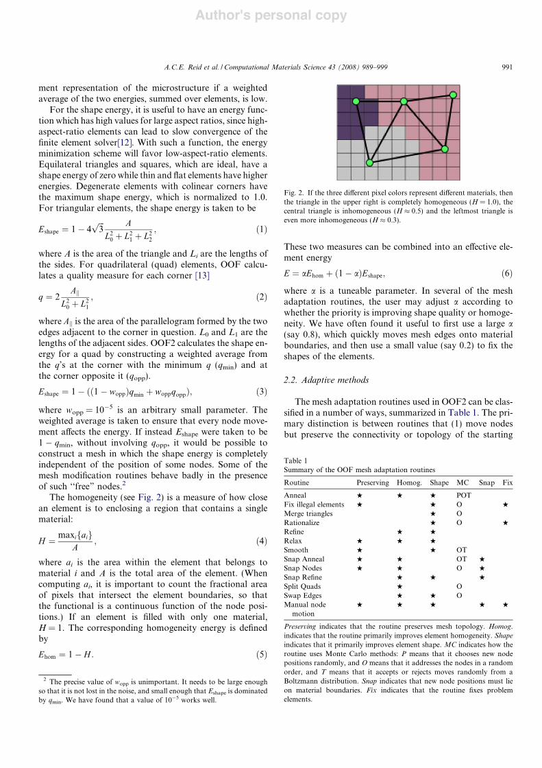
The homogeneity (see Fig. 2) is a measure of how closean element is to enclosing a region that contains a singlematerial:

H " maxifaigA

; $4%

where ai is the area within the element that belongs tomaterial i and A is the total area of the element. (Whencomputing ai, it is important to count the fractional areaof pixels that intersect the element boundaries, so thatthe functional is a continuous function of the node posi-tions.) If an element is filled with only one material,H = 1. The corresponding homogeneity energy is definedby

Ehom " 1! H : $5%

These two measures can be combined into an e!ective ele-ment energy

E " aEhom # $1! a%Eshape; $6%

where a is a tuneable parameter. In several of the meshadaptation routines, the user may adjust a according towhether the priority is improving shape quality or homoge-neity. We have often found it useful to first use a large a(say 0.8), which quickly moves mesh edges onto materialboundaries, and then use a small value (say 0.2) to fix theshapes of the elements.

2.2. Adaptive methods

The mesh adaptation routines used in OOF2 can be clas-sified in a number of ways, summarized in Table 1. The pri-mary distinction is between routines that (1) move nodesbut preserve the connectivity or topology of the starting

Fig. 2. If the three di!erent pixel colors represent di!erent materials, thenthe triangle in the upper right is completely homogeneous (H = 1.0), thecentral triangle is inhomogeneous (H & 0.5) and the leftmost triangle iseven more inhomogeneous (H & 0.3).

Table 1Summary of the OOF mesh adaptation routines

Routine Preserving Homog. Shape MC Snap Fix

Anneal w w w POTFix illegal elements w w O w

Merge triangles w ORationalize w O w

Refine w w

Relax w w w

Smooth w w OTSnap Anneal w w OT w

Snap Nodes w w O w

Snap Refine w w w

Split Quads w OSwap Edges w w OManual node

motionw w w w w

Preserving indicates that the routine preserves mesh topology. Homog.indicates that the routine primarily improves element homogeneity. Shapeindicates that it primarily improves element shape. MC indicates how theroutine uses Monte Carlo methods: P means that it chooses new nodepositions randomly, and O means that it addresses the nodes in a randomorder, and T means that it accepts or rejects moves randomly from aBoltzmann distribution. Snap indicates that new node positions must lieon material boundaries. Fix indicates that the routine fixes problemelements.

2 The precise value of wopp is unimportant. It needs to be large enoughso that it is not lost in the noise, and small enough that Eshape is dominatedby qmin. We have found that a value of 10!5 works well.

A.C.E. Reid et al. / Computational Materials Science 43 (2008) 989–999 991


mesh (e.g. Anneal, Snap Nodes), and (2) routines thatchange the topology by adding, removing, or reconnectingnodes (e.g. Refine, Snap Refine). Routines in both groupsare used to improve overall element energy.

Topology-preserving routines can improve the homoge-neity or shape energy of the elements in the mesh withoutincreasing the number of elements. Unless the initial gridis su"ciently fine, they usually cannot be used to resolvethe small features in a microstructure. Non-preserving rou-tines are used to achieve this task by subdividing existingelements and segments and spawning new elements andnodes. Once the desired element resolution is reached,topology-preserving routines can again be used to furtherimprove the mesh.

The columns marked Homog. and Shape in Table 1 indi-cate whether the routines are best at improving the homo-geneity or shape of the mesh elements. Routines with a starin both columns can be used for either purpose, or both atonce, by adjusting a in Eq. (6).

Because of the similarity of topology-preserving routinesto steps in a molecular dynamics simulation, some of theseroutines (e.g. Anneal, Smooth, Snap Anneal) incorporate atype of Metropolis Monte Carlo method [14]. The MonteCarlo randomness appears in three ways: (1) the algorithmmay address nodes or elements sequentially in a randomorder; (2) nodes may be moved to randomly chosen posi-tions; and (3) mesh modifications may be accepted orrejected at random, using a Boltzmann probability distri-bution. The quantity DE in the exponent of the Boltzmannfactor

P " exp$!DE=T % $7%

is the change in the energy (Eq. (6)) of the a!ected ele-ments. A change in the shape of some elements can be ac-cepted even if it leads to an increase in the overall elementenergy, with a probability given by P. This analogy withmolecular dynamics simulations can be pursued furtherby explicitly applying fictitious forces on the nodes thatmay drive the elements to improve their homogeneity orshape (e.g, the relax routine).

The Snap column in Table 1 marks routines that placenodes precisely at the interface between two di!erent pixelgroups. Snap routines are better at improving elementhomogeneity than element shape. Routines with a star inthe Fix column of the table are specialized for correctingor improving an element or group of elements created bythe other routines.

Most of these routines can be flexibly applied to anexplicitly selected set of elements, segments or nodes. Mostof the routines can also be targeted to elements or segmentsthat satisfy certain criteria, such as having a homogeneitybelow a certain threshold.

In the following sections, we describe each mesh adapta-tion routine used in OOF2. We also describe a combinationof these routines that seems e!ective in creating a mesh fora categorized microstructure. This sequence of routines is

applied in OOF2 after providing just a little input and oncestarted requires no feedback from the user.

2.2.1. AnnealThe Anneal routine moves nodes to random positions

(see Fig. 3(1A) and (1B)), accepting or rejecting movesaccording to a given criterion. It is similar to a simulatedannealing simulation in statistical mechanics, from whichit gets its name. Instead of minimizing the free energy ofa system of particles, it minimizes the e!ective energy ofa mesh. Annealing is useful when the mesh elements aresmall enough to resolve the features of a microstructure,but are not in quite the correct positions. It can usually finda happy medium in situations in which a trade-o! must bemade between element shape and homogeneity.

The general procedure for a single iteration of anneal isas follows:

(1) Create a list of target nodes and reorder them ran-domly to remove any potential artifacts from the ori-ginal ordering of nodes. This reordering is repeated atevery iteration.

(2) Give each node in the list a single chance to move to arandomly assigned new position. OOF2 computes thenew position from

xnew " xold # dx

ynew " yold # dy

dx and dy are random numbers chosen from a Gauss-ian distribution of width delta and mean 0.0.Fig. 3(1A) shows a target node that is about to moveto a new position. Before making the move, OOF2computes the total e!ective energy of all the neigh-boring elements of the node (E1, E2, E3, E4).

(3) After moving each node, an acceptance criterion isused to decide whether the move is acceptable. Anymoves that create illegal elements (see Section 2.2.5)are automatically rejected. OOF2 has a number ofdi!erent criteria to choose from: accepting all moves,only those that decrease the energy, or only those thatdecrease energy and meet specified additional con-straints on homogeneity and shape.

(4) If a legal move is unacceptable according to theacceptance criterion, OOF2 may still accept the moveif the annealing is being done at a non-zero tempera-ture T. The parameter T sets the e!ective temperatureof the annealing process. These moves are acceptedwith the probability P given in Eq. (7), where DE isthe di!erence in the e!ective energies of the newand old element configurations.

Successful annealing usually requires a number of itera-tions. On each iteration, OOF2 makes one attempt to moveeach node. OOF2 can be set to perform a fixed number ofiterations of anneal or to stop after some condition issatisfied. As with conventional simulated annealing or



Monte Carlo simulations, if the change in energy or theacceptance rate gets too small, the annealing process hasreached a point where it is no longer improving the meshe!ectively.

2.2.2. SmoothThe Smooth routine implements a ‘‘smart Laplacian”

algorithm[15]. It moves nodes to the average position oftheir neighbors (see Fig. 3(2A) and (2B)), if the movemeets a given criterion (such as lowering the local energy)and does not create illegal elements. This tends to smoothout gradients in node density and improve element shapes.Typically, Smooth ceases to make substantial changesafter about 3 iterations over the mesh. The general proce-dure for a single iteration is very similar to that forAnneal, except that in step 2, each target node is givena single chance to move to the average position of itsneighbors. For this purpose, neighbors are defined as

nodes that share a segment with the target node (N1,N2, N3, N4).

Smooth is most useful in applying the final touches to amesh. After the mesh has been adjusted so that all of thematerial boundaries correspond to element edges, applyingsmooth to all of the nodes that are not on material bound-aries will improve the quality of the elements in the interiorof each region, without a!ecting homogeneity.

2.2.3. Snap AnnealSnap Anneal is very similar to anneal. In Snap Anneal,

the trial move consists of placing the target node at anearby pixel boundary, called a transition point, locatedalong a segment that contains the target node as an end-point (see Fig. 3(3A) and (3B)). Snap Anneal would notexplore as many configurations as Anneal, but it can beuseful when a mesh is nearly correct but needs to be forcedinto alignment.

Fig. 3. Illustration of some node moves used in OOF2. (1A) and (1B) show a trial move of the Anneal routine. A target node is displaced by a randomvector whose components are taken from a Gaussian distribution. (2A) and (2B) show the trial move for the Smooth routine. The target node is placed atthe center of the four neighboring nodes N1, N2, N3 and N4. (3A) and (3B) show the trial move for the Snap Anneal routine. The target node is shifted tothe transition point (TP) along one of the edges incident at the target node.



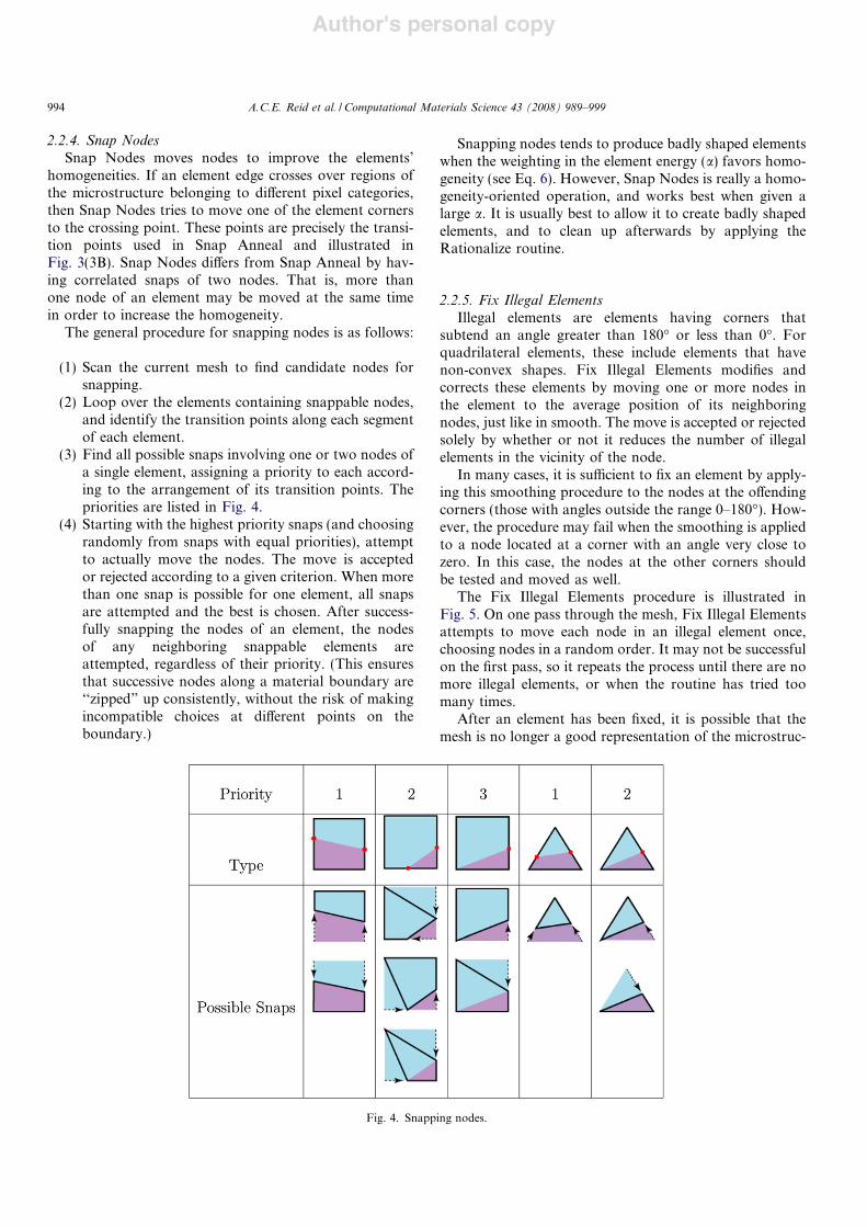
2.2.4. Snap NodesSnap Nodes moves nodes to improve the elements’

homogeneities. If an element edge crosses over regions ofthe microstructure belonging to di!erent pixel categories,then Snap Nodes tries to move one of the element cornersto the crossing point. These points are precisely the transi-tion points used in Snap Anneal and illustrated inFig. 3(3B). Snap Nodes di!ers from Snap Anneal by hav-ing correlated snaps of two nodes. That is, more thanone node of an element may be moved at the same timein order to increase the homogeneity.

The general procedure for snapping nodes is as follows:

(1) Scan the current mesh to find candidate nodes forsnapping.

(2) Loop over the elements containing snappable nodes,and identify the transition points along each segmentof each element.

(3) Find all possible snaps involving one or two nodes ofa single element, assigning a priority to each accord-ing to the arrangement of its transition points. Thepriorities are listed in Fig. 4.

(4) Starting with the highest priority snaps (and choosingrandomly from snaps with equal priorities), attemptto actually move the nodes. The move is acceptedor rejected according to a given criterion. When morethan one snap is possible for one element, all snapsare attempted and the best is chosen. After success-fully snapping the nodes of an element, the nodesof any neighboring snappable elements areattempted, regardless of their priority. (This ensuresthat successive nodes along a material boundary are‘‘zipped” up consistently, without the risk of makingincompatible choices at di!erent points on theboundary.)

Snapping nodes tends to produce badly shaped elementswhen the weighting in the element energy (a) favors homo-geneity (see Eq. 6). However, Snap Nodes is really a homo-geneity-oriented operation, and works best when given alarge a. It is usually best to allow it to create badly shapedelements, and to clean up afterwards by applying theRationalize routine.

2.2.5. Fix Illegal ElementsIllegal elements are elements having corners that

subtend an angle greater than 180" or less than 0". Forquadrilateral elements, these include elements that havenon-convex shapes. Fix Illegal Elements modifies andcorrects these elements by moving one or more nodes inthe element to the average position of its neighboringnodes, just like in smooth. The move is accepted or rejectedsolely by whether or not it reduces the number of illegalelements in the vicinity of the node.

In many cases, it is su"cient to fix an element by apply-ing this smoothing procedure to the nodes at the o!endingcorners (those with angles outside the range 0–180"). How-ever, the procedure may fail when the smoothing is appliedto a node located at a corner with an angle very close tozero. In this case, the nodes at the other corners shouldbe tested and moved as well.

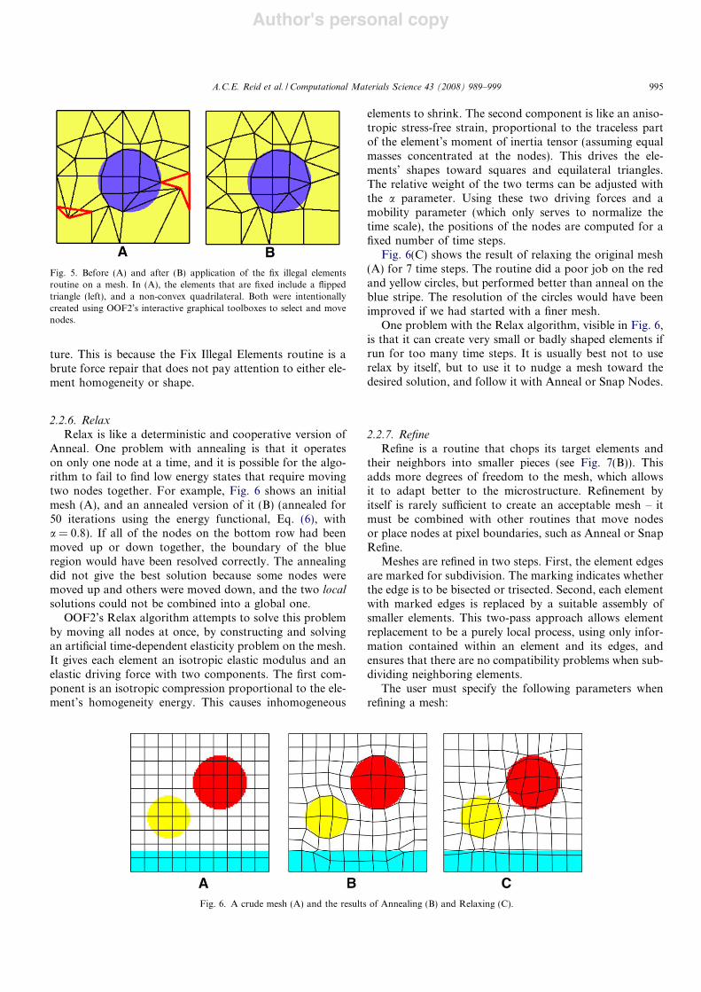
The Fix Illegal Elements procedure is illustrated inFig. 5. On one pass through the mesh, Fix Illegal Elementsattempts to move each node in an illegal element once,choosing nodes in a random order. It may not be successfulon the first pass, so it repeats the process until there are nomore illegal elements, or when the routine has tried toomany times.

After an element has been fixed, it is possible that themesh is no longer a good representation of the microstruc-

Fig. 4. Snapping nodes.



ture. This is because the Fix Illegal Elements routine is abrute force repair that does not pay attention to either ele-ment homogeneity or shape.

2.2.6. RelaxRelax is like a deterministic and cooperative version of

Anneal. One problem with annealing is that it operateson only one node at a time, and it is possible for the algo-rithm to fail to find low energy states that require movingtwo nodes together. For example, Fig. 6 shows an initialmesh (A), and an annealed version of it (B) (annealed for50 iterations using the energy functional, Eq. (6), witha = 0.8). If all of the nodes on the bottom row had beenmoved up or down together, the boundary of the blueregion would have been resolved correctly. The annealingdid not give the best solution because some nodes weremoved up and others were moved down, and the two localsolutions could not be combined into a global one.

OOF2’s Relax algorithm attempts to solve this problemby moving all nodes at once, by constructing and solvingan artificial time-dependent elasticity problem on the mesh.It gives each element an isotropic elastic modulus and anelastic driving force with two components. The first com-ponent is an isotropic compression proportional to the ele-ment’s homogeneity energy. This causes inhomogeneous

elements to shrink. The second component is like an aniso-tropic stress-free strain, proportional to the traceless partof the element’s moment of inertia tensor (assuming equalmasses concentrated at the nodes). This drives the ele-ments’ shapes toward squares and equilateral triangles.The relative weight of the two terms can be adjusted withthe a parameter. Using these two driving forces and amobility parameter (which only serves to normalize thetime scale), the positions of the nodes are computed for afixed number of time steps.

Fig. 6(C) shows the result of relaxing the original mesh(A) for 7 time steps. The routine did a poor job on the redand yellow circles, but performed better than anneal on theblue stripe. The resolution of the circles would have beenimproved if we had started with a finer mesh.

One problem with the Relax algorithm, visible in Fig. 6,is that it can create very small or badly shaped elements ifrun for too many time steps. It is usually best not to userelax by itself, but to use it to nudge a mesh toward thedesired solution, and follow it with Anneal or Snap Nodes.

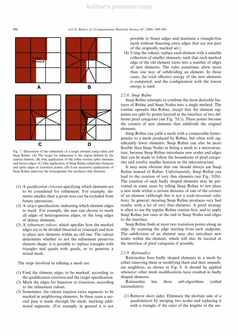
2.2.7. RefineRefine is a routine that chops its target elements and

their neighbors into smaller pieces (see Fig. 7(B)). Thisadds more degrees of freedom to the mesh, which allowsit to adapt better to the microstructure. Refinement byitself is rarely su"cient to create an acceptable mesh – itmust be combined with other routines that move nodesor place nodes at pixel boundaries, such as Anneal or SnapRefine.

Meshes are refined in two steps. First, the element edgesare marked for subdivision. The marking indicates whetherthe edge is to be bisected or trisected. Second, each elementwith marked edges is replaced by a suitable assembly ofsmaller elements. This two-pass approach allows elementreplacement to be a purely local process, using only infor-mation contained within an element and its edges, andensures that there are no compatibility problems when sub-dividing neighboring elements.

The user must specify the following parameters whenrefining a mesh:

Fig. 5. Before (A) and after (B) application of the fix illegal elementsroutine on a mesh. In (A), the elements that are fixed include a flippedtriangle (left), and a non-convex quadrilateral. Both were intentionallycreated using OOF2’s interactive graphical toolboxes to select and movenodes.

Fig. 6. A crude mesh (A) and the results of Annealing (B) and Relaxing (C).



(1) A qualification criterion specifying which elements areto be considered for refinement. For example, ele-ments smaller than a given area can be excluded fromfuture operations.

(2) A target specification, indicating which element edgesto mark. For example, the user can choose to markall edges of heterogeneous edges, or the long edgesof skinny elements.

(3) A refinement ruleset, which specifies how the markededges are to be divided (bisected or trisected) and howto place new elements within an old one. The rulesetdetermines whether or not the refinement preserveselement shape: it is possible to replace triangles withtriangles and quads with quads, or to generate amixed mesh.

The steps involved in refining a mesh are:

(1) Find the element edges to be marked, according tothe qualification criterion and the target specification.

(2) Mark the edges for bisection or trisection, accordingto the refinement ruleset.

(3) Sometimes, the ruleset requires extra segments to bemarked in neighboring elements. In these cases a sec-ond pass is made through the mesh, marking addi-tional segments. (For example, in general it is not

possible to bisect edges and maintain a triangle-freemesh without bisecting extra edges that are not partof the originally marked set.)

(4) Using the ruleset, replace each element with a suitablecollection of smaller elements, such that each markededge of the old element turns into a number of edgesof new elements. The rules sometimes allow morethan one way of subdividing an element. In thosecases, the total e!ective energy of the new elementsis computed, and the configuration with the lowestenergy is used.

2.2.8. Snap RefineSnap Refine attempts to combine the most desirable fea-

tures of Refine and Snap Nodes into a single method. Theroutine operates like Refine, except that the element seg-ments are split by points located at the interface of two dif-ferent pixel categories (see Fig. 7(C)). These points becomethe corners of new elements that subdivide the originalelements.

Snap Refine can yield a mesh with a comparable homo-geneity to a mesh produced by Refine, but often with sig-nificantly fewer elements. Snap Refine can also be moreflexible than Snap Nodes in fitting a mesh to a microstruc-ture, because Snap Refine introduces new nodes and edgesthat can be made to follow the boundaries of pixel catego-ries and resolve smaller features in the microstructure.

It may seem obvious that one should always use SnapRefine instead of Refine. Unfortunately, Snap Refine canlead to the creation of very thin elements (see Fig. 7(D)).The creation of such badly shaped elements may be pre-vented in some cases by telling Snap Refine to not placea new node within a certain distance of one of the cornersof an element (although this is not a scale-invariant solu-tion). In general, iterating Snap Refine produces very badresults, with a lot of very thin elements. A good strategyis often to use the regular Refine routine first, and to applySnap Refine just once at the end to Snap Nodes and edgesto the interface.

Snap Refine finds at most two transition points along anedge, by scanning the edge starting from each endpoint.The subdivision of an element may also introduce newnodes within the element, which will also be located atthe interface of pixel categories if possible.

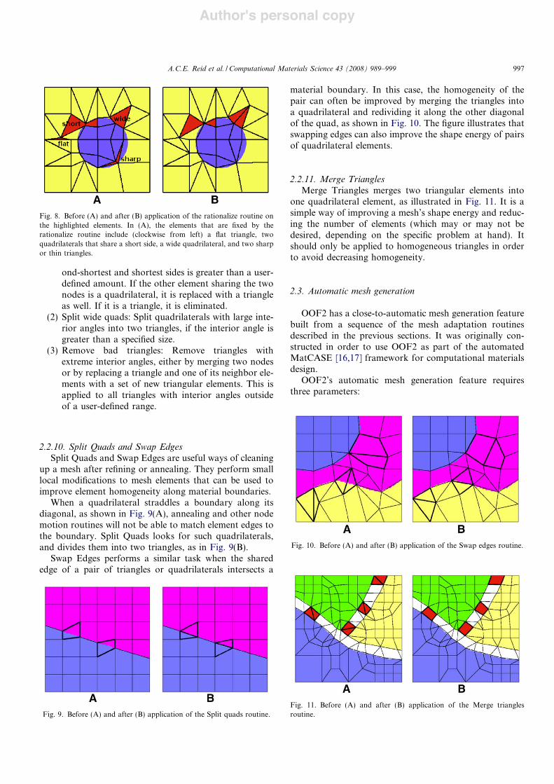
2.2.9. RationalizeRationalize fixes badly shaped elements in a mesh by

either removing them or modifying them and their immedi-ate neighbors, as shown in Fig. 8. It should be appliedwhenever other mesh modifications have resulted in badlyshaped elements.

Rationalize has three sub-algorithms (calledrationalizers):

(1) Remove short sides: Eliminate the shortest side of aquadrilateral by merging two nodes and replacing itwith a triangle, if the ratio of the lengths of the sec-

Fig. 7. Illustration of the refinement of a target element using refine andSnap Refine. (A) The target for refinement is the region defined by thecentral element. (B) One application of the refine routine splits elementsand bisects edges. (C) One application of Snap Refine subdivides elementsand splits edges at transition points. (D) Four successive applications ofSnap Refine improves the homogeneity but produces thin elements.



ond-shortest and shortest sides is greater than a user-defined amount. If the other element sharing the twonodes is a quadrilateral, it is replaced with a triangleas well. If it is a triangle, it is eliminated.

(2) Split wide quads: Split quadrilaterals with large inte-rior angles into two triangles, if the interior angle isgreater than a specified size.

(3) Remove bad triangles: Remove triangles withextreme interior angles, either by merging two nodesor by replacing a triangle and one of its neighbor ele-ments with a set of new triangular elements. This isapplied to all triangles with interior angles outsideof a user-defined range.

2.2.10. Split Quads and Swap EdgesSplit Quads and Swap Edges are useful ways of cleaning

up a mesh after refining or annealing. They perform smalllocal modifications to mesh elements that can be used toimprove element homogeneity along material boundaries.

When a quadrilateral straddles a boundary along itsdiagonal, as shown in Fig. 9(A), annealing and other nodemotion routines will not be able to match element edges tothe boundary. Split Quads looks for such quadrilaterals,and divides them into two triangles, as in Fig. 9(B).

Swap Edges performs a similar task when the sharededge of a pair of triangles or quadrilaterals intersects a

material boundary. In this case, the homogeneity of thepair can often be improved by merging the triangles intoa quadrilateral and redividing it along the other diagonalof the quad, as shown in Fig. 10. The figure illustrates thatswapping edges can also improve the shape energy of pairsof quadrilateral elements.

2.2.11. Merge TrianglesMerge Triangles merges two triangular elements into

one quadrilateral element, as illustrated in Fig. 11. It is asimple way of improving a mesh’s shape energy and reduc-ing the number of elements (which may or may not bedesired, depending on the specific problem at hand). Itshould only be applied to homogeneous triangles in orderto avoid decreasing homogeneity.

2.3. Automatic mesh generation

OOF2 has a close-to-automatic mesh generation featurebuilt from a sequence of the mesh adaptation routinesdescribed in the previous sections. It was originally con-structed in order to use OOF2 as part of the automatedMatCASE [16,17] framework for computational materialsdesign.

OOF2’s automatic mesh generation feature requiresthree parameters:

Fig. 8. Before (A) and after (B) application of the rationalize routine onthe highlighted elements. In (A), the elements that are fixed by therationalize routine include (clockwise from left) a flat triangle, twoquadrilaterals that share a short side, a wide quadrilateral, and two sharpor thin triangles.

Fig. 9. Before (A) and after (B) application of the Split quads routine.

Fig. 10. Before (A) and after (B) application of the Swap edges routine.

Fig. 11. Before (A) and after (B) application of the Merge trianglesroutine.



(1) A rough size of the elements in the initial mesh (max-scale). This should correspond to the linear size of thelargest features in the microstructure.

(2) A rough size for the smallest elements in the desiredmesh (minscale). This is the resolution to which theelements have to be refined by the mesh adaptationroutines, and should correspond to the linear size ofthe smallest features in the microstructure.

(3) A homogeneity threshold that determines whichelements will be refined. All elements whose homo-geneity is smaller than the threshold will be subdi-vided until the new elements’ homogeneities areabove threshold or the element sizes fall belowminscale.

These parameters may be estimated for a class of micro-structures based on the intuition of a materials engineer orfrom the nature of the physical problem.

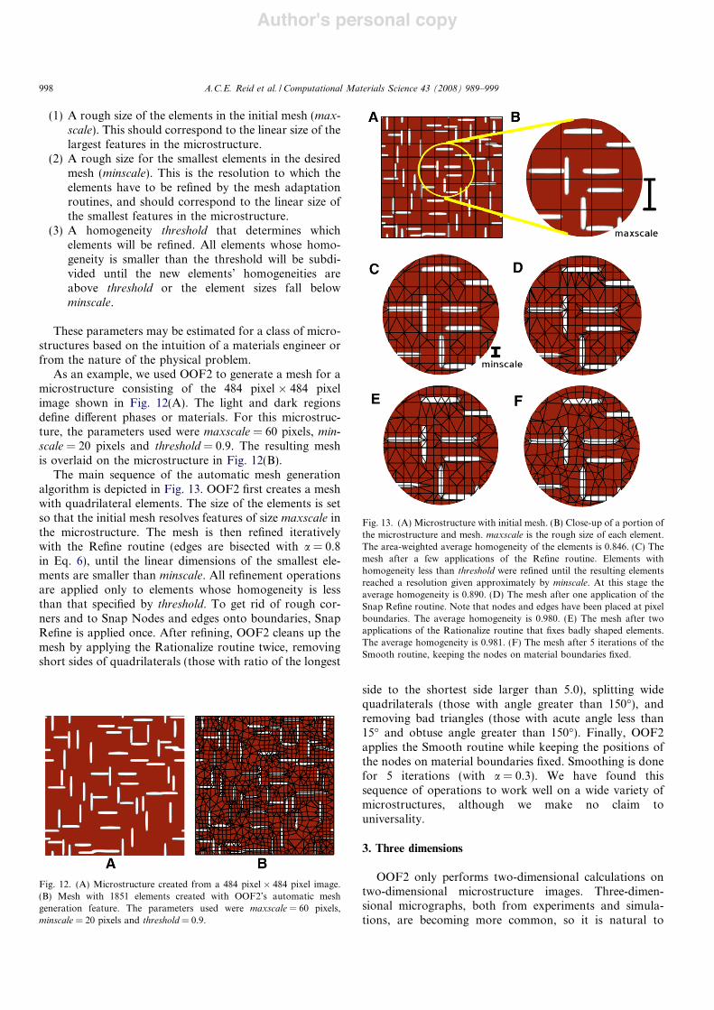
As an example, we used OOF2 to generate a mesh for amicrostructure consisting of the 484 pixel ' 484 pixelimage shown in Fig. 12(A). The light and dark regionsdefine di!erent phases or materials. For this microstruc-ture, the parameters used were maxscale = 60 pixels, min-scale = 20 pixels and threshold = 0.9. The resulting meshis overlaid on the microstructure in Fig. 12(B).

The main sequence of the automatic mesh generationalgorithm is depicted in Fig. 13. OOF2 first creates a meshwith quadrilateral elements. The size of the elements is setso that the initial mesh resolves features of size maxscale inthe microstructure. The mesh is then refined iterativelywith the Refine routine (edges are bisected with a = 0.8in Eq. 6), until the linear dimensions of the smallest ele-ments are smaller than minscale. All refinement operationsare applied only to elements whose homogeneity is lessthan that specified by threshold. To get rid of rough cor-ners and to Snap Nodes and edges onto boundaries, SnapRefine is applied once. After refining, OOF2 cleans up themesh by applying the Rationalize routine twice, removingshort sides of quadrilaterals (those with ratio of the longest

side to the shortest side larger than 5.0), splitting widequadrilaterals (those with angle greater than 150"), andremoving bad triangles (those with acute angle less than15" and obtuse angle greater than 150"). Finally, OOF2applies the Smooth routine while keeping the positions ofthe nodes on material boundaries fixed. Smoothing is donefor 5 iterations (with a = 0.3). We have found thissequence of operations to work well on a wide variety ofmicrostructures, although we make no claim touniversality.

3. Three dimensions

OOF2 only performs two-dimensional calculations ontwo-dimensional microstructure images. Three-dimen-sional micrographs, both from experiments and simula-tions, are becoming more common, so it is natural to

Fig. 12. (A) Microstructure created from a 484 pixel ' 484 pixel image.(B) Mesh with 1851 elements created with OOF2’s automatic meshgeneration feature. The parameters used were maxscale = 60 pixels,minscale = 20 pixels and threshold = 0.9.

Fig. 13. (A) Microstructure with initial mesh. (B) Close-up of a portion ofthe microstructure and mesh. maxscale is the rough size of each element.The area-weighted average homogeneity of the elements is 0.846. (C) Themesh after a few applications of the Refine routine. Elements withhomogeneity less than threshold were refined until the resulting elementsreached a resolution given approximately by minscale. At this stage theaverage homogeneity is 0.890. (D) The mesh after one application of theSnap Refine routine. Note that nodes and edges have been placed at pixelboundaries. The average homogeneity is 0.980. (E) The mesh after twoapplications of the Rationalize routine that fixes badly shaped elements.The average homogeneity is 0.981. (F) The mesh after 5 iterations of theSmooth routine, keeping the nodes on material boundaries fixed.



extend OOF to three dimensions. The meshing tools usedin OOF2 were designed with extensions to 3D in mind,and the OOF developers are currently working on a 3Dversion, OOF3D.

One of the biggest challenges in extending our meshingtechniques to three dimensions is in defining the energyfunctional. The definition of homogeneity energy transfersto 3D in a straightforward way, but the shape energy posesmore problems. One possibility is to define a quality mea-sure analogous to the expression in Eq. (1):

q3D " CV 2=S3 $8%

where V is the volume of the element, S is its surface area,and C is a normalization constant. (C " 216

!!!3

pfor a tetra-

hedron). Another possibility is to define q3D as the ratio ofthe radii of the inscribing and circumscribing spheres.Defining good quality measures for three-dimensional ele-ments is an area of active research [18,12].

3D meshing is bound to be more computationallydemanding, but many of the 2D mesh adaptation routineshave straightforward extensions to 3D. For most of thetopology-preserving routines, the di!erence between threeand two dimensions is simply the di!erence between doingMonte Carlo or molecular dynamics simulations for parti-cles in 3D instead of 2D. As for element refinement in 3D,there are clearly many more refinement possibilities so therule sets will be more complicated, even if we only considera single type of element (e.g. tetrahedrons). We have devel-oped a ruleset for refining a tetrahedron into smaller tetra-hedrons for all possible ways of bisecting some of its edges[19].

4. Summary

We have described a suite of 2D mesh adaptation rou-tines available in the software package OOF2. These rou-tines can be combined into a close-to-automatic meshgenerator, where the input consists of a segmented image,an upper size scale, a lower size scale, and a homogeneitythreshold. Future work may include comparing the qualityof elements generated using OOF2 with that of other meth-ods. Work extending the 2D mesh adaptation routines to3D meshes is also in progress.

The OOF2 program, including source code and usersmanuals, is available at http://www.ctcms.nist.gov/oof/oof2/.

Acknowledgement

Rhonald Lua and Edwin Garcı́a were supported in partby the National Science Foundation through InformationTechnology Research Grant DMR-0205232. OOF2 wasproduced by NIST, an agency of the US government,and by statute is not subject to copyright in the UnitedStates. Recipients of the software assume all responsibili-ties associated with its operation, modification andmaintenance.

References

[1] S.A. Langer, E.R. Fuller Jr., W.C. Carter, Computers in Science andEngineering 3 (3) (2001) 15–23.

[2] S.A. Langer, A.C.E. Reid, R.E. Garcı́a, S.-I. Haan, R.C. Lua, W.C.Carter, E.R. Fuller Jr., A. Roosen, <http://www.ctcms.nist.gov/oof/index.html>.

[3] S.A. Langer, A. Reid, S.-I. Haan, R.E. Garcı́a, <http://www.ctcms.nist.gov/langer/oof2man/index.html>.

[4] R.E. Garcı́a, A.C.E. Reid, S.A. Langer, W.C. Carter, in: D. Raabe,F. Roters, F. Barlat, L.-Q. Chen (Eds.), Continuum Scale Simulationof Engineering Materials, Wiley-VCH, 2004.

[5] F.B. Paul, E.Y. Sun, K.P. Plucknett, K.B. Alexander, C.-H. Hsueh,H.-T. Lin, S.B. Waters, C.G. Westmoreland, E.-S. Kang, K. Hirao,M.E. Brito, J. Am. Ceram. Soc. 81 (11) (1998) 2821–2830.

[6] A.D. Jadhav, N.P. Padture, E.H. Jordan, M. Gell, P. Miranzo, E.R.Fuller Jr., Acta Materialia 54 (12) (2006) 3343–3349.

[7] V. Cannillo, T. Manfredini, M. Montorosi, A. Boccaccini, Journal ofNon-Crystalline Solids 344 (2004) 88–93.

[8] R.E. Garcı́a, W.C. Carter, S.A. Langer, Journal of the AmericanCeramic Society 88 (3) (2005) 750–757.

[9] R.E. Garcı́a, Y.-M. Chiang, W.C. Carter, P. Limthongkul, C.M.Bishop, Journal of the Electrochemical Society 152 (1) (2005) A255–A263.

[10] E. Garboczi, D. Bentz, N. Martys, in: P.-Z. Wong (Ed.), Methods inthe Physics of Porous Media, Academic Press, San Diego, CA, 1999,pp. 1–41.

[11] A. Roberts, E. Garboczi, J. Am. Ceram. Soc. 83 (2000) 3041–3048.[12] J. Shewchuck, Eleventh International Meshing Roundtable, 115–126,

Sandia National Laboratories, Ithaca, New York, 2002.[13] GiD Manual, <http://gid.cimne.upc.es/>.[14] N. Metropolis, A. Rosenbluth, M. Rosenbluth, A. Teller, E. Teller,

Journal of Chemical Physics 21 (1953) 1087–1092.[15] L.A. Freitag, in: Trends in Unsaturated Mesh Generation, ASME

Applied Mechanics Division, vol. AMD 220, 1997, pp. 37–44.[16] <http://matcase.psu.edu/index.html>.[17] Z. Liu, L.-Q. Chen, P. Raghavan, Q. Du, J. Sofo, S. Langer, C.

Wolverton, Journal of Computer-Aided Materials Design 11 (2004)183–199.

[18] J. Shewchuck, Preprint, 2002.[19] Java Applet, <http://www.ctcms.nist.gov/~rlua/FE/refinery/>.


Image-based finite element mesh construction for material microstructures

Documents

Transcript of Image-based finite element mesh construction for material microstructures