lable at ScienceDirect

Building and Environment 46 (2011) 786e796

Contents lists avai

Building and Environment

journal homepage: www.elsevier .com/locate/bui ldenv

Illuminance-based slat angle selection model for automated control of split blinds

Jia Hu, Svetlana Olbina*

Rinker School of Building Construction, 304 Rinker Hall, University of Florida, Gainesville, FL 32611-5703, USA

a r t i c l e i n f o

Article history:Received 4 August 2010Received in revised form7 October 2010Accepted 12 October 2010

Keywords:Split-controlled blindsAutomated blind controlArtificial neural network (ANN)DaylightingUseful daylight illuminance (UDI)

* Corresponding author. Tel.: þ1 352 273 1166; faxE-mail address: solbina@ufl.edu (S. Olbina).

0360-1323/$ e see front matter � 2010 Elsevier Ltd.doi:10.1016/j.buildenv.2010.10.013

a b s t r a c t

Venetian blinds play an important role in controlling daylight in buildings. Automated blinds overcomesome limitations of manual blinds; however, the existing automated systems mainly control the directsolar radiation and glare and cannot be used for controlling innovative blind systems such as split blinds.This research developed an Illuminance-based Slat Angle Selection (ISAS) model that predicts theoptimum slat angles of split blinds to achieve the designed indoor illuminance. The model was con-structed based on a series of multi-layer feed-forward artificial neural networks (ANNs). The illuminancevalues at the sensor points used to develop the ANNs were obtained by the software EnergyPlus�. Theweather determinants (such as horizontal illuminance and sun angles) were used as the input variablesfor the ANNs. The illuminance level at a sensor point was the output variable for the ANNs. The ISASmodel was validated by evaluating the errors in the calculation of the: 1) illuminance and 2) optimumslat angles. The validation results showed that the power of the ISAS model to predict illuminance was94.7% while its power to calculate the optimum slat angles was 98.5%. For about 90% of time in the year,the illuminance percentage errors were less than 10%, and the percentage errors in calculating theoptimum slat angles were less than 5%. This research offers a new approach for the automated control ofsplit blinds and a guide for future research to utilize the adaptive nature of ANNs to develop a morepractical and applicable blind control system.

� 2010 Elsevier Ltd. All rights reserved.

1. Introduction

Daylight is an important source of energy in buildings. Anappropriate amount of daylight in a building improves the visualcomfort for its occupants and decreases the energy consumption ofthe buildings. Venetian blinds, as a common type of shading device,have beenwidely used for thermal and daylighting control. A blind’sdaylighting performance influences the energy consumption fromartificial lighting and the HVAC system as well as the occupants’comfort. However, occupants rarely change the position of manuallycontrolled or motorized Venetian blinds [1]. As an alternative,automated blinds were developed to overcome some limitations ofmanual blinds and to improve the thermal and daylighting perfor-mance [2e4]. The utilization of automated blinds helps meet therequirement for the occupants’ visual comfort and reduces energyconsumption.

Various control methods were developed to adjust the positionof the blinds. An automatic shading device controller based ona genetic algorithmwas used to adjust the position of the blinds bytaking into consideration the users’ wishes [5]. Koo et al. [2]

: þ1 352 392 9606.

All rights reserved.

developed a control method for the automated blinds that maxi-mized daylight penetration into a building and blocked directsunlight based on the occupants’ preferences. Daylighting controlsystems that integrate blinds control with lighting control providegreater energy savings. The use of automated blinds integratedwith on/off or dimmable lighting systems could block directsunlight, provide the design workplane illuminance, maximize theoutdoor view, and save energy [3,6e9]. The use of these integratedsystems can result in lighting energy savings of 30e77% [7,8].

The existing blind control systems, including the integrateddaylighting control systems, mainly control slat angles to blockdirect sunlight and to increase the daylight penetration [2,10]. On theother hand, maximizing the daylight penetration may cause over-heating and glare. Therefore, the desired daylighting performance isnot easily achieved. In addition, the existing control systems cannoteffectively control some innovative blind systems, such as split-controlled blinds [11]. The automated split-controlled blind systemutilizes the window in three subsections: a) the upper third, b) themiddle third, and c) the bottom third (Fig. 1). The split-controladjusts the slat position at different angles at a particular point intime, depending on the position of the slats within the height of thewindow. Therefore, the slats can have different tilt angles in eachsubsection of awindow [12]. In the upper section of thewindow, theblinds are tilted downward to the interior to redirect daylight to the

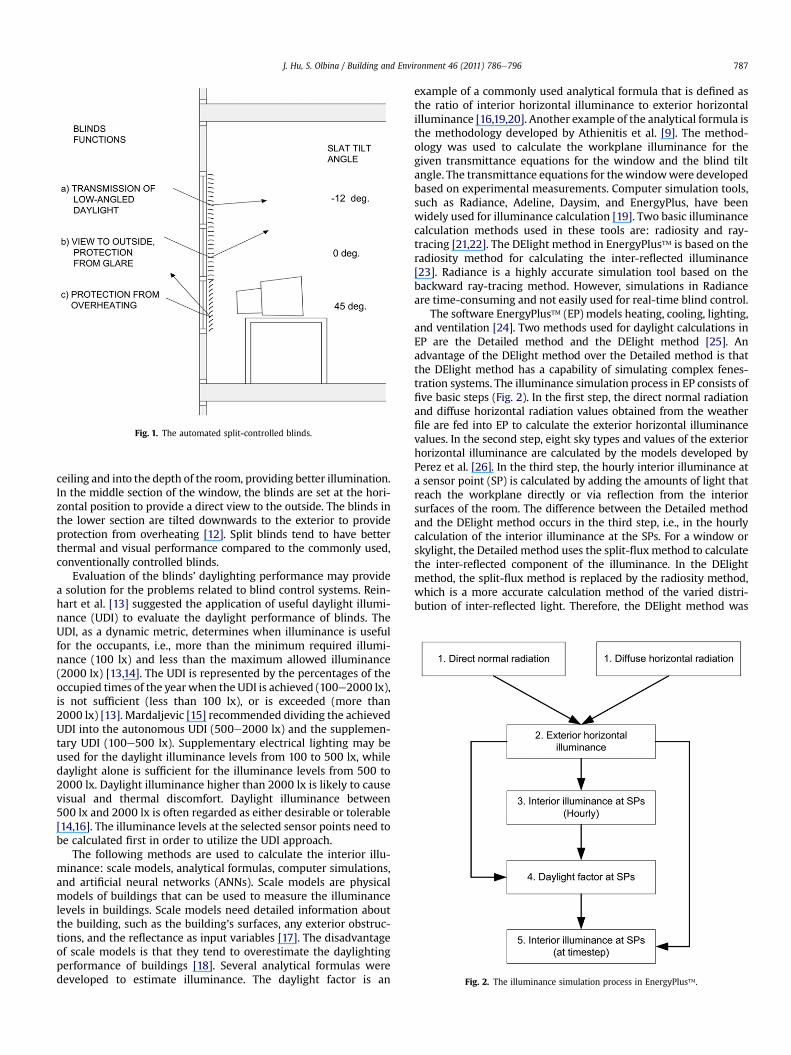
Fig. 1. The automated split-controlled blinds.

Fig. 2. The illuminance simulation process in EnergyPlus�.

J. Hu, S. Olbina / Building and Environment 46 (2011) 786e796 787

ceiling and into the depth of the room, providing better illumination.In the middle section of the window, the blinds are set at the hori-zontal position to provide a direct view to the outside. The blinds inthe lower section are tilted downwards to the exterior to provideprotection from overheating [12]. Split blinds tend to have betterthermal and visual performance compared to the commonly used,conventionally controlled blinds.

Evaluation of the blinds’ daylighting performance may providea solution for the problems related to blind control systems. Rein-hart et al. [13] suggested the application of useful daylight illumi-nance (UDI) to evaluate the daylight performance of blinds. TheUDI, as a dynamic metric, determines when illuminance is usefulfor the occupants, i.e., more than the minimum required illumi-nance (100 lx) and less than the maximum allowed illuminance(2000 lx) [13,14]. The UDI is represented by the percentages of theoccupied times of the year when the UDI is achieved (100e2000 lx),is not sufficient (less than 100 lx), or is exceeded (more than2000 lx) [13]. Mardaljevic [15] recommended dividing the achievedUDI into the autonomous UDI (500e2000 lx) and the supplemen-tary UDI (100e500 lx). Supplementary electrical lighting may beused for the daylight illuminance levels from 100 to 500 lx, whiledaylight alone is sufficient for the illuminance levels from 500 to2000 lx. Daylight illuminance higher than 2000 lx is likely to causevisual and thermal discomfort. Daylight illuminance between500 lx and 2000 lx is often regarded as either desirable or tolerable[14,16]. The illuminance levels at the selected sensor points need tobe calculated first in order to utilize the UDI approach.

The following methods are used to calculate the interior illu-minance: scale models, analytical formulas, computer simulations,and artificial neural networks (ANNs). Scale models are physicalmodels of buildings that can be used to measure the illuminancelevels in buildings. Scale models need detailed information aboutthe building, such as the building’s surfaces, any exterior obstruc-tions, and the reflectance as input variables [17]. The disadvantageof scale models is that they tend to overestimate the daylightingperformance of buildings [18]. Several analytical formulas weredeveloped to estimate illuminance. The daylight factor is an

example of a commonly used analytical formula that is defined asthe ratio of interior horizontal illuminance to exterior horizontalilluminance [16,19,20]. Another example of the analytical formula isthe methodology developed by Athienitis et al. [9]. The method-ology was used to calculate the workplane illuminance for thegiven transmittance equations for the window and the blind tiltangle. The transmittance equations for thewindowwere developedbased on experimental measurements. Computer simulation tools,such as Radiance, Adeline, Daysim, and EnergyPlus, have beenwidely used for illuminance calculation [19]. Two basic illuminancecalculation methods used in these tools are: radiosity and ray-tracing [21,22]. The DElight method in EnergyPlus� is based on theradiosity method for calculating the inter-reflected illuminance[23]. Radiance is a highly accurate simulation tool based on thebackward ray-tracing method. However, simulations in Radianceare time-consuming and not easily used for real-time blind control.

The software EnergyPlus� (EP) models heating, cooling, lighting,and ventilation [24]. Two methods used for daylight calculations inEP are the Detailed method and the DElight method [25]. Anadvantage of the DElight method over the Detailed method is thatthe DElight method has a capability of simulating complex fenes-tration systems. The illuminance simulation process in EP consists offive basic steps (Fig. 2). In the first step, the direct normal radiationand diffuse horizontal radiation values obtained from the weatherfile are fed into EP to calculate the exterior horizontal illuminancevalues. In the second step, eight sky types and values of the exteriorhorizontal illuminance are calculated by the models developed byPerez et al. [26]. In the third step, the hourly interior illuminance ata sensor point (SP) is calculated by adding the amounts of light thatreach the workplane directly or via reflection from the interiorsurfaces of the room. The difference between the Detailed methodand the DElight method occurs in the third step, i.e., in the hourlycalculation of the interior illuminance at the SPs. For a window orskylight, the Detailed method uses the split-fluxmethod to calculatethe inter-reflected component of the illuminance. In the DElightmethod, the split-flux method is replaced by the radiosity method,which is a more accurate calculation method of the varied distri-bution of inter-reflected light. Therefore, the DElight method was

Fig. 3. Floor plan and south elevation of the office space (unit: cm).

Table 1Visible transmittance and visible reflectance properties of the glass panes used inthe double-pane insulating glass unit (IGU).

Glass pane Visible reflectance Visible transmittance

Low-E 0.078a 0.84c

0.055b

Clear 0.08c 0.881c

a Exterior face of the glass pane (facing the outside space).b Interior face of the glass pane (facing the air space of the IGU).c Both faces of the glass pane.

J. Hu, S. Olbina / Building and Environment 46 (2011) 786e796788

selected for the illuminance calculation in this research. In the fourthstep, the daylight factors at the SPs are calculated. The value of thedaylight factor at an SP is obtained by dividing the hourly interiorhorizontal illuminance by the exterior horizontal illuminance. In thefifth step, the interior illuminances at the SPs at the timestep arecalculated. Timestep specifies the basic timestep for the simulation.For example, a value of four directs the program to use a timestep of15 min (i.e., 60 min/4). The daylight factor (DF) and exterior illumi-nance at each timestep are interpolated by hourly values of the DFand the exterior illuminance, respectively. Each timestep value of theinterior horizontal illuminance at an SP is calculated by multiplyingthe timestep value of the DF by the timestep value of the exteriorilluminance.

The ANNs are parallel computational models composed ofdensely interconnected adaptive processing units [27]. An importantfeature of the ANNs is their adaptive nature, where the ANNs “learnby example” to solve problems. The ANNs are superior in time series,regression, and approximation of non-linear processes whencompared to the conventional methods [28]. ANNs are broadlyapplied in the areas of the energy simulation andmodeling, such as,the prediction of the building’s energy consumption and the designand operation of the HVAC system [29,30]. An advantage of the ANNmodel is that it does not require detailed building information andcould train itself to adapt to complicated surroundings. Researchers,architects, and lighting designers would benefit from using neuralnetworks for daylighting evaluation studies [31]. Kazanasmaz et al.[31] applied a three-layer feed-forward artificial neural network tothe illuminance calculation. The input for the model included 13variables: hour, outdoor temperature, solar radiation, humidity, UVindex, UV dose, distance from windows, number of windows,orientation of room,floor identification, roomaspect ratio, and pointidentification. The output was the value of the illuminance at thesensor points. Kazanasmazet al. [31] used an illuminancepercentageerror to the validate prediction of the illuminance by the ANNs. Theresults showed the training error of the model was 1.08%, and thetesting error was 3.32%.

In this research, the ANNs were selected for the illuminancecalculation because of their strong adaptability to the complicatedenvironment and their short runtime. The objective of this researchwas to develop an Illuminance-based Slat Angle Selection (ISAS)model for automated split-controlled blinds in an office space byapplying both the ANN and UDI approaches. The ISAS model can beused for predicting the illuminance levels at various sensor pointsand for calculating the optimum slat angles for all three sections ofthe split blinds at a particular point in time. This research offersa new approach for the automated control of split blinds based onthe required workplane illuminance, and it expands the applicationof the ANNs into the illuminance prediction.

2. Development of a use case

This research consisted of three phases. In the first phase,a model of an office space was created in EnergyPlus� to obtainilluminance data that were needed to develop the ISAS model. Inthe second phase, the ISAS model based on the ANNs was devel-oped. In the third phase, the ISAS model was validated.

2.1. Description of an office space

In the first phase of the research, a model of an office space wascreated in EP as a use case to develop and validate the ISAS model(Fig. 3). The office space was located in Gainesville, Florida, USA(latitude 30�N, longitude 81.6�W) which has a hot and humidclimate. The dimensions of the office space were 3.6 m(width) � 5 m (length) � 3 m (height). A 1.8 m � 1.8 m window

with split-controlled blinds was installed in the south wall. Thewindowsill height was 0.9 m. The 24 mm thick double-pane insu-lating glass unit (IGU) was installed in the window. The IGU con-sisted of the 6 mm low-E glass pane at the exterior of the IGU,12 mm air space between the glass panes, and 6 mm clear glasspane at the interior of the IGU. The transmittance and reflectanceproperties of the glass were assumed to be constant. These valueswere inputted into the software EnergyPlus� (see Table 1).

J. Hu, S. Olbina / Building and Environment 46 (2011) 786e796 789

The split-controlled blinds had three sections (top, middle, andbottom) each of which had a height of 0.6 m. White aluminumblinds were installed inside the window. The slat width was2.5 cm, and the slat separation was 1.85 cm. The beam reflectanceand diffuse solar reflectance of the blinds were constant and wereset to 0.8. The slat angle was defined as the angle between thehorizontal plane and the slat plane. If the slats were titled down-ward to the exterior, the slat tilt angle was assigned a positivevalue. If the slats were titled downward to the interior, the slat tiltangle was assigned a negative value. If the slats were completelyopen (i.e., horizontal), the slat tilt angle was allocated to zero. Inthis research, the slat angle of the top section of the blinds changedfrom �90� to 0� in increments of 10�. The slat angle of the middleand bottom sections changed from 0� to 90� in increments of 10�.The illuminance levels were calculated at two sensor points (SP 1and SP 2). SP 1 and SP 2 were located at a height of 0.75 m from thefloor, and at a horizontal distance of 0.75 m, and 3.5 m from thewindow, respectively.

2.2. Simulation of interior horizontal illuminance in the office space

After the model of an office space was created, the values ofthe interior horizontal illuminances, Et, Em, and Eb, for the top,middle, and bottom sections of the blinds at the sensor pointswere obtained by the software EnergyPlus�. These illuminancevalues were used later to develop the ANNs. The illuminance E0represents the amount of light penetrating the room as a result ofleakage between the blinds and window frames when the splitblinds were completely closed. The hourly interior horizontalilluminance was simulated by EP for a total of 2340 occupiedhours (from 8 a.m. to 5 p.m.) throughout the year. The weather filefor Gainesville, Florida, USA was used, and January 1st was set toSunday. The value of the horizontal illuminance Et,m,b at a sensorpoint (SP) for slat angles t� (top section of the blinds), m� (middlesection of the blinds), and b� (bottom section of the blinds) wascalculated by Eq. (1).

Et;m;b ¼ Et þ Em þ Eb � 2 � E0 (1)

In order to calculate particular illuminances in Eq. (1), thespecific values of the slat tilt angles were used in each section of theblinds (see Table 2).

3. Development of the ISAS model

In the second phase of this research, the ISAS model wasdeveloped. The development of the ISAS model consisted of threestages (see Fig. 4). The ANNs for SP 1 and SP 2 were developed inStage (2) based on the possible parameters and the strategiesdefined in Stage (1). The illuminance values predicted by the ANNswere fed into a mathematical model developed in Stage (3) tocalculate the optimum slat angles.

Table 2Slat angles used to calculate specific illuminances in Eq. (1).

Illuminance Section of the blinds

Top Middle Bottom

Et,m,b t� m� b�

Et t� 90� 90�

Em �90� m� 90�

Eb �90� 90� b�

E0 �90� 90� 90�

3.1. Stage (1): defining parameters and strategies for artificialneural networks (ANNs)

Stage (1) consisted of three steps (Steps 1.1, 1.2, and 1.3) asindicated in Fig. 4. The possible architectures, and the input andoutput variables were selected, and allowable ranges of slat anglesfor which direct sunlight was blocked were calculated. Two strat-egies were then designed for developing the ANNs models (eitherthe strategy (1) or (2) as shown in Table 3).

3.1.1. Selection of possible architectures and input and outputvariables of the ANNs

Back-propagation artificial neural networks (ANNs) wereutilized in this research. Back-propagation ANNs are multi-layerfeed-forward networks and use the back-propagation learning rule,which was central to much of the work on learning in the ANNs[27]. The number of neurons in the input and output layers wasequal to the number of the input and output variables, respectively.Two different numbers of hidden layers and neurons that wereevaluated based on the errors obtained during the training stepwere:

1. One hidden layer with 5, 10, or 15 neurons; or2. Two hidden layers with 5, 10, or 15 neurons in each layer.

The number of hidden layers with a specific number of neuronsthat had the lowest errors was selected as the architecture of theANNs.

Three groups of possible input variables were tested to identifyfour basic input variables that caused the least errors in the results.These three groups of variables were:

Fig. 4. The process of development of the ISAS model.

Table 3Possible strategies for developing the ANN models.

Section of the blinds Strategy (1) Strategy (2)

Range of allowableslat angles

Range of months Number of theANN models

Range of allowableslat angles

Range of months (regardlessof the sun presence)

Number of theANN models

No direct sunlight Direct sunlight

Top �90�e0� Oct. to Feb. e 10 �90�e0� Jan. to Dec. 10�40�e0� e Mar. to Sep. 5

Middle 0�e90� Jan. to Dec. e 10 0�e90� Jan. to Dec. 10Bottom 0�e90� e Mar. to Oct. 10 0�e90� Jan. to Dec. 10

30�e90� Nov. to Feb. e 7

J. Hu, S. Olbina / Building and Environment 46 (2011) 786e796790

Group 1. Solar altitude angle, solar azimuth angle, global hori-zontal illuminance, and diffuse horizontal illuminance.Group 2. Solar altitude angle, solar azimuth angle, direct normalradiation, and diffuse horizontal radiation.Group 3. Solar altitude angle, solar azimuth angle, exteriorhorizontal beam illuminance, anddiffuse horizontal illuminance.

The other possible input variables considered in this researchincluded: slat angle, global horizontal radiation, dry bulb temper-ature, zenith luminance, relative humidity, and horizontal infraredradiation intensity from sky. These possible variables, together withthe four basic variables, were selected as the inputs of the ANNmodels to analyze whether the error showed a tendency todecrease. If the error decreased, the variables would be consideredas input variables.

The ANNs were used to predict illuminance at sensor pointsgenerated by each particular section of the split-controlled blinds,i.e., Et (top), Em (middle) and Eb (bottom) illuminances, as explainedin Section 2.2. Since two SPs were set up in the office space, thepossible output for each section of the blinds was either:

1. Illuminance at SP 1, or2. Illuminance at SP 2

Fig. 5. The cross section view of a section of the split-controlled blinds.

3.1.2. Calculation of ranges of allowable slat angles for split blindsThis section would first present a calculation of ranges of

months in a year during which the direct sunlight could reach theSPs, and then a calculation of ranges of allowable slat angles forwhich the direct sunlight could be blocked by blinds. The results ofthe illuminance obtained by EP showed that direct sunlight hada great influence on the illuminance at SP 1. The illuminance at SP 2was generally smaller than 900 lx for most of time and did not havea drastic fluctuation in the values. Thus, it was not necessary toevaluate illuminance at SP 2; therefore, only the illuminance at SP 1was evaluated when the ANNs were constructed.

The solar altitude angle and solar azimuth angle at two differentsun positions P1 and P2 were calculated in order to determine theranges of months in which direct sunlight could reach SP 1. Fig. 5shows the cross section view of a section of split-controlledblinds (e.g., middle section). It is assumed that the tilt angle of theslats in this section of the blinds is zero (i.e., completely open). Thesun positions are presented by Sun Path 1 (on a summer day) andSun Path 2 (on awinter day). When a sun pathwas located betweenthese two sun paths, the sunbeam could reach SP 1. Therefore, theslats needed to be adjusted to prevent direct sunlight from reachingSP 1. Sun positions P1, P2, P3 and P4 denote four sun positions atdifferent times during the day. The sun was located at positions P1and P3 at 12 p.m., at P2 in the morning and at P4 in the afternoon.

In order to calculate sun angles, the values of H1 and H2 need tobe determined. H0 denotes the vertical distance of SP 1 from thefloor. H1 denotes the vertical distance between the most bottom

slat of the blinds and SP 1. H2 denotes the vertical distance betweenthemost bottom slat and an upper slat, above which the slats of theblinds positioned at the zero angle prevent direct sunbeam fromreaching SP 1. The value of H2 is affected by the slat angles and theposition of the blinds within the height of the window. For the topsection of the blinds, H2 might be equal to the height of the topsection of the blinds, i.e., H2 ¼ 0.6 m, because the slat angle canreach �90�. For the middle and bottom sections of the blinds, H2was calculated by Eq. (2).

H2 ¼ D� tanðUÞ � H1 (2)

Where:

D ¼ Horizontal distance between SP 1 and the window.U ¼ Angle between the slat plane and the sunbeam plane (r)that passes through points P2 and SP 1. tan(U) ¼ S/L, whereS ¼ Slat separation and L ¼ Slat width.

At sun position P1, the solar azimuth angle g1 is equal to p, andthe solar altitude angle a1 is equal to tan�1[H1/(D � L)] (see Fig. 5).At sun position P2, the solar azimuth angle g2 is equal top � tan�1[W/(2 � (D þ d))] where W denotes the width of theblinds and d denotes the thickness of the south wall (see Fig. 3). Ifsolar azimuth angle g (measured from north clockwise), and sunprofile angle b are known, solar altitude angle a can be calculatedby Eq. (3) (see Fig. 6) [2].

a ¼ tan�1½tan ðbÞ � jcosðgÞj� (3)

Fig. 6. Relationship between sun profile angle, solar azimuth angle and solar altitudeangle (adapted from [2] with the permission from Elsevier).

J. Hu, S. Olbina / Building and Environment 46 (2011) 786e796 791

Eq. (3) was applied to calculate the solar altitude angle a2 at sunposition P2. The solar altitude angle a2 at sun position P2 wascalculated by Eqs. (4) and (5).

a2 ¼ tan�1½tan ðb2Þ � jcosðg2Þj� (4)

b2 ¼ tan�1½ðH1 þ H2Þ=D� (5)

The local time (LT) of each sun position needs to be calculated todetermine the period of time when the sun is located between SunPath 1 and Sun Path 2, i.e., the time when direct sunbeams canreach the window. The local time (LT) was calculated according tothe solar azimuth angle and solar altitude angle at sun positions P1and P2. A number of algorithms for calculating sun positions weredeveloped [32,33]. Eqs. (6) and (7) were used to calculate solarazimuth angles and solar altitude angles [34]. If the solar azimuthangle, solar altitude angle, and geometric longitude and latitude ofpositions P1 and P2 are provided, the solar declination (DEC) andhour angle (HRA) can be calculated from Eqs. (6) and (7). The LT canbe calculated by Eqs. (8) and (9) [34].

cosðgÞ ¼ ½sinðaÞ � sinðLÞ � sinðDECÞ�=½cosðaÞ � cosðLÞ� (6)

sinðaÞ ¼ cosðLÞ� cosðDECÞ� cosðHRAÞþ sinðLÞ� sinðDECÞ (7)

DEC ¼ sin�1f0:39795� cos½0:98563� ðDN � 173Þ�g (8)

HRA ¼ 15� �fLT þ ½4�ð15� �DTGMT � LÞþEOT �=60�12g (9)

Where:

g ¼ Solar azimuth anglea ¼ Solar altitude angleL ¼ Latitude (negative for Southern Hemisphere)DEC ¼ Solar declination (negative for Southern Hemisphere)HRA ¼ Hour angleDN ¼ The number of days elapsed in a given year up to a partic-ular dateLT ¼ Local timeDTGMT ¼ The difference between the Local Time (LT) andGreenwich Mean Time (GMT) in hoursEOT ¼ Equation of Time (min). This value is very small and wasset to zero in this research.

The ranges of months during which the direct sunlight mightreach SP 1 were, therefore, determined based on LT at sun

positions P1 and P2 (see Table 3). For example, under the strategy(1) for the top section of the blinds, the sun path was locatedbetween Sun Path 1 and Sun Path 2 from March to September.During this time period, direct sunlight might reach the window.For the middle section of the blinds, the sun path was not locatedbetween Sun Path 1 and Sun Path 2 for the entire year, i.e.,during the entire year direct sunlight did not reach the windowand SP 1.

During the months when direct sunlight could reach SP 1, theslats should be adjusted to block the sunbeams and to preventdirect sunlight at SP 1. The range of allowable slat angles for eachsection of the blinds should be determined for the specific rangeof months (e.g., March to September for the top section of theblinds for the strategy (1) in which the sun was located betweenSun Path 1 and Sun Path 2). Sunlight would not reach SP 1 if theallowable slat angles were used during this time period. Theranges of allowable slat angles for the office space are shown inTable 3.

3.1.3. Design of strategies for developing back-propagation ANNmodels

A preliminary study was conducted to test the possibility ofusing the slat angle as an input variable for the ANNs. In thispreliminary study, the ANN models that could be applied to themiddle section of the blinds were developed. The slat angle of theblinds was selected as an input variable of the ANN models besidesother possible input variables. The output was the illuminance at SP1 or SP 2 generated by themiddle section of the blinds, respectively.The results showed that if the slat angle was used as an input of theANN models, errors in illuminance values would be large. Hence,slat angle could not be used as an input variable. In other words,separate ANN models should be developed for each possible slatangle of the blinds (e.g., 0�, 10�, 20�,.). Therefore, two strategieswere proposed to construct the ANN models for each slat angle ofeach section of the blinds (see Table 3).

For the strategy (1), the ranges of allowable slat angles wereselected based on the ranges of months. Blinds that utilized theseranges of slat angles would prevent direct sunlight from pene-trating the window and reaching the SPs. The ANN models weredeveloped for each range of allowable slat angles and the corre-sponding months in which the specific range of slat angles wasused. The number of the ANN models corresponded to the numberof the allowable slat angles. For example, for the top section ofblinds, slat angles were divided into two ranges according to thetwo ranges of months. For the month range from March toSeptember, five ANN models were needed for predicting the illu-minance Et for the slat angles t ¼ �40�, �30�, �20�, �10�, and 0�,respectively. If more ranges of months and slat angles wereconsidered under the strategy (1), more ANN models would becreated and, thus, accuracy of the ANN models would increase.However, this approach would lead to overfitting and wouldcompromise the generality of models. In this research, only theranges of the allowable slat angles shown in Table 3 were used todevelop the ANN models.

For the strategy (2), the whole year was considered as a timeperiod regardless of the presence of direct sunlight. The slats couldhave any tilt angle (from 0� to 90� (or�90�) in 10� increments) and,therefore, blinds might not block direct sunlight during some timeperiods (see Table 3). The ANN models were developed for thespecific ranges of slat angles for the entire year without consideringthe ranges of months.

For both the strategy (1) and the strategy (2), the output of theANN models would be the illuminance values for the specificsection of the blinds: Et (top section), Em (middle section), and Eb(bottom section) according to Eq. (1).

Table 4Testing errors of the ANNs for SP 2 (lx).

Section ofthe blinds

Range ofmonths

Absolute value of the slat angle

0� 10� 20� 30� 40� 50� 60� 70� 80� 90�

Top Mar. to Sept. 6.2 6.9 6.9 7.8 8.5Oct. to Feb. 8.4 8.6 9.1 8.2 6.9 5.3 4.0 3.0 1.4 1.0

Middle Jan. to Dec. 7.5 6.6 5.8 4.9 4.1 3.3 2.6 1.7 1.0 1.0Bottom Mar. to Oct. 4.5 4.5 3.6 3.2 2.6 2.2 1.7 1.0 1.0 1.0

Nov. to Feb. 3.3 2.8 2.6 2.0 1.4 1.0 1.0

Table 5Testing errors of the ANNs for SP 1 that used the actual illuminance at SP 2 as aninput (lx).

Section ofthe blinds

Range ofmonths

Absolute value of the slat angle

0� 10� 20� 30� 40� 50� 60� 70� 80� 90�

Top Mar. to Sept. 1.0 1.0 1.0 1.0 1.0Oct. to Feb. 1.4 1.4 1.0 1.4 1.0 1.0 1.0 1.0 1.0 1.0

Middle Jan. to Dec. 1.7 1.0 1.0 1.0 1.0 1.0 1.0 1.0 1.0 1.0Bottom Mar. to Oct. 2.4 1.4 1.7 1.0 1.0 1.0 1.0 1.0 1.0 1.0

Nov. to Feb. 1.0 1.0 1.0 1.0 1.0 1.0 1.0

J. Hu, S. Olbina / Building and Environment 46 (2011) 786e796792

3.2. Stage (2): development of artificial neural networks (ANNs) forSP 1 and SP 2

In Stage (2) of the development of the ISAS model (see Fig. 4),the ANNs were trained, and the best neural network models wereselected. Separate ANN models were developed for SP 1 and SP 2.The ANNs for SP 2 were developed first because the output of theANNs for SP 2 might be used as input for the development of theANNs for SP 1. All the 2340 hours’ data (i.e., inputs and outputs ofthe ANNs) were divided into three datasets. For every fiveconsecutive hours’ data, the first, third, and fifth hours’ data wereused for training of the ANNs (step 2.1 in Fig. 4), the second hour’sdata were used for validation of the ANNs (step 2.2 in Fig. 4), andthe fourth hour’s data were used for testing the ANNs (step 2.3 inFig. 4). Therefore, the training dataset included 60% of the datawhile the validation and the testing datasets included 20% of thedata, respectively.

In step 2.1, the ANNs were trained by the batch training methodto update weights and biases. During the training process, theilluminance values were predicted by the ANNs, and validationerrors were calculated to evaluate the performance of the ANNs.Validation error was defined as RMSE (root mean square error) ofthe ANNs calculated by using the validation dataset. RMSE is equalto [

P(P � T)2/n]1/2 where P denotes the predicted illuminance

(obtained by ANNs), T denotes target illuminance (obtained by EP),and n denotes the number of samples. Training would be stopped ifthe number of iterations exceeded 2000, RMSE for the trainingdataset was less than 1.0, or the validation error increased for sixiterations. In step 2.2, the validation errors of the ANNs werecompared in order to select the best ANNs to be used to predictilluminance at the SPs. A different parameter setup in Stage (1)would generate different ANNs and, therefore, different validationerrors. The ANNs showing the least validation errors were selectedas the best models. In step 2.3, the testing errors were calculated toevaluate the generality of the ANN models selected in step 2.2.Testing error was defined as RMSE of the selected ANN modelcalculated by using the testing dataset. Small testing errors couldensure the generality of the ANNs.

3.2.1. Development and selection of the ANN models for SP 2In Stage (2), a variety of the ANNs was tested for the different

combinations of the possible parameters defined in Stage (1). Thepossible input variables (shown in Section 3.1.1) and the targetoutput illuminance values (i.e., illuminance obtained by EP) at SP 2were used to train the ANNs. The results showed that the four basicinput variables, i.e., solar altitude angle, solar azimuth angle, hori-zontal beam illuminance, and diffuse horizontal illuminance(Group 3 variables in Section 3.1.1) were sufficient to determine theilluminance at SP 2. These four variables caused the least errors inilluminance calculation obtained by EP under the strategy (1).Therefore, in this research, Group 3 variables were selected for thedevelopment of the ANNs. The results also showed that the ANNsdeveloped based on the strategy (1) had the least validation errors,and, thus, theywere selected as the bestmodels. The best ANNs hadtwo hidden layers, each of which included ten neurons.

At the end of Stage (2), the testing errors between the predictedilluminances and the target illuminances of the ANNs for SP 2 werecalculated to check the generality of the selected ANN models (seeTable 4). The testing errors were similar to the validation errors andwere influenced by the degree of fluctuation of the illuminance. Theerrors decreased when the illuminance had a low degree of fluc-tuation. For example, for the middle and bottom sections of blinds,errors decreased with the increase of the slat angles. For the topsection of the blinds, from March to September, errors increasedwith the increase of the slat angles. For the top section of the blinds,

from October to February, testing errors increased with the increaseof the slat angles from 0� to 20�, and then errors decreased with theincrease of the slat angles from 30� to 90�. Small errors guaranteedthe generality of the ANNs.

3.2.2. Development and selection of the ANN models for SP 1The process of developing neural networks and tests similar to

those for SP 2 were applied for SP 1 to select the best ANNs. The testresults showed that the input and output variables, the strategy fordeveloping the ANNs, and the number of hidden layers and neuronsused for the ANNs for SP 1 were the same as those for the ANNs forSP 2. The ANNs showing the least validation errors were selected asthe best models for SP 1. Besides the four basic input variables(Group 3 variables in Section 3.1.1), the illuminance at SP 2might betreated as an input variable for the development of the ANNs for SP1. Thus, two options were proposed to construct the ANNs for SP 1.In Option (1), the illuminance at SP 2was regarded as the fifth inputvariable for the ANNs besides the four basic input variables. InOption (2), only the four basic input variables (same as those for theANNs for SP 2) were used to construct the ANNs for SP 1.

In Option (1), the testing errors calculated by the ANNs weresimilar to the validation errors. The illuminance at SP 1 could beaccurately predicted if the actual illuminance at SP 2 was given.Most errors were small, i.e., they were equal to one (see Table 5).This means that if the actual illuminance at SP 2 was inputted intothe developed ANN models, the illuminance at SP 1 could be pre-dicted with high accuracy. However, the actual illuminance at SP 2was unknown and could not be used as an input variable. Therefore,the predicted illuminance at SP 2 (predicted by the ANNs for SP 2)was used instead of the actual illuminance at SP 2. For example, forthe top section of the blinds, the calculated testing errors of theANNs for SP 1 (see Table 6) would be larger than the errors of theANNs that used actual illuminance at SP 2 as an input variable (seeTable 5). The large testing errors indicated low accuracy in pre-dicting illuminance at SP 1.

In Option (2), the same four basic input variables as those usedfor the ANNs for SP 2 were used as input variables to construct theANNs for SP 1. The results showed that the final calculated valida-tion errors in Option (2) were similar to the errors obtained inOption (1). This research adopted Option (1) to construct the ANNsfor SP 1 because the ANN models of Option (1) would build the

Table 6Testing errors of the ANNs for SP 1 that used the predicted illuminance at SP 2 as aninput (lx).

Range of months Slat angle of the top section of the blinds

0� �10� �20� �30� �40� �50� �60� �70� �80� �90�

Mar. to Sept. 17.3 18.5 19.5 21.7 19.4Oct. to Feb. 20.8 15.8 8.0 5.1 9.4 13.0 12.2 10.6 4.4 2.6

J. Hu, S. Olbina / Building and Environment 46 (2011) 786e796 793

relationship between the illuminance values of two SPs, and theaccuracy of the predicted illuminance at SP 1 would increase withthe increased accuracy of the predicted illuminance at SP 2.

3.3. Stage (3): selection of optimum slat angles

In Stage (3) of the development of the ISAS model (see Fig. 4),a method for selecting optimum slat angles was created. Stage (3)consisted of three steps (3.1, 3.2, and 3.3). A mathematical model(see Eq. (10)) for selecting optimum slat angles for each section ofthe split blinds was developed in the step 3.1. In the step 3.2, theilluminance values obtained by ANNs were fed into this mathe-matical model in order to solve themathematical model. In the step3.3, the optimum slat angles were calculated by using this mathe-matical model.

Since the daylight illuminance values decrease exponentiallywith the increase of the distance from a window [35], the illumi-nance levels at SP 2 should bemaximized, and the illuminance levelsat SP 1 should be kept below the maximum illuminance value.According to the UDI approach, the illuminance at each SP should bea minimum of 500 lx to increase daylight penetration and amaximum of 2000 lx to avoid glare. Therefore, in Eq. (10), the obj-ective function was to maximize the illuminance level at SP 2, andthe constraint was to limit the illuminance at SP 1 within the rangeof specifiedmaximumvalues, Emax. The illuminances at SP 1 and SP 2for split-controlled blinds were calculated according to Eq. (1).

Max E2 ¼ Et;2 þ Em;2 þ Eb;2 � 2� E0;2 (10)

Subject to:

E1 ¼ Et;1 þ Em;1 þ Eb;1 � 2� E0;1 � Emax

t ¼ �90�; �80�;.; 0�

m; b ¼ 0�;.; 80�; 90�

Where:

E1 ¼ Horizontal illuminance at SP 1E2 ¼ Horizontal illuminance at SP 2Emax ¼Maximum illuminance set by occupants within the rangeof 500e2000 lx. In this research, Emax was set to 2000 lxaccording to the UDI approach.Et,1, Em,1 and Eb,1 ¼ Horizontal illuminances Et, Em, and Eb at SP 1for the top, middle, and bottom sections of the blinds, respec-tively. Et, Em, and Eb are indicated in Eq. (1).Et,2, Em,2 and Eb,2 ¼ Horizontal illuminances Et, Em, and Eb at SP 2for the top, middle and bottom sections of the blinds, respec-tively. Et, Em, and Eb are indicated in Eq. (1).E0,1 and E0,2 ¼ Horizontal illuminances at SP 1 and SP 2 in thecase of the three sections of the blinds being completely closed,respectively.t, m and b ¼ Slat tilt angles for the top, middle, and bottomsections of the blinds, respectively.

In this research, the calculated optimum slat angles maximizedthe illuminance level at SP 2 and limited the maximum predictedilluminance at SP 1 to 2000 lx. To beginwith, the illuminance valuesat SP 1 (Et,1, Em,1, and Eb,1) and at SP 2 (Et,2, Em,2, and Eb,2) for variouscombinations of slat angles t, m, and b were calculated by thedeveloped ANNs. Then, possible slat angles t, m, and b for eachsection of the blinds were fed into Eq. (10) to identify the optimumcombination of slat angles that caused the maximum illuminancevalues at SP 2. If the illuminance at SP 1 (Et,1, Em,1, and Eb,1) and at SP2 (Et,2, Em,2, and Eb,2) that were fed into Eq. (10) were obtained by EPinstead of by the ANNs, the optimum slat angles calculated by Eq.(10) were defined as actual optimum slat angles.

Heuristic algorithms, such as genetic algorithms, can solve Eq.(10). In this research, all possible combinations of slat angles weretested because the total number of combinations was only severalhundred (see Table 3). For example, from March to September,there were five possible angles for the top section of the blinds andten possible angles for the middle and bottom sections of theblinds. Therefore, the total number of combinations of slat angleswas 500 (5 � 10 � 10). It took 1.37 s for MATLAB Version 7.9 ona laptop with Pentium CPU 2.00 G and 2G RAM to calculate theoptimum slat angles in this case.

4. Validation of the ISAS model

In the third phase of this research, the accuracy of the ISASmodel was validated by evaluating two types of errors: 1) the errorsin the calculation of illuminance by the ANNs, and 2) the errors inthe calculation of the optimum slat angles of the blinds.

4.1. Errors in calculation of illuminance

In this research, the illuminance percentage error (IPE) was usedto define the errors in the calculation of illuminance by the ISASmodel. After the separate, predicted illuminances (e.g., Et) gener-ated by a specific section of the blinds (e.g., the top section) werecalculated by the ANNs, the total predicted illuminance generatedby the three sections of the blinds was calculated according to Eq.(1). Then the illuminance percentage error (IPE) was calculated forall occupied hours in a year according to Eq. (11).

IPE ¼ j½PðiÞ � AðiÞ�=AðiÞj (11)

Where

P(i) ¼ the predicted illuminance at a sensor point.A(i) ¼ the actual illuminance at a sensor point.i ¼ index that represents specific occupied hour.

The average IPE at SP 1 and SP 2 was 5.3%. Thus, the power of theISAS model to predict illuminance was 94.7%. The percentage of theoccupied time in the year for which the IPE fell in the particularrange of errors was analyzed for both the sensor points (Table 7). Forabout 90% of time during the year, the IPEs were less than 10% forboth SP 1 and SP 2. Therefore, the illuminance values predicted bythe ISAS model reasonably matched the actual illuminance values.

4.2. Errors in calculation of optimum slat angles

Figs. 7 and 8 show the predicted and actual values of illuminanceat SP 1 and SP 2, respectively, for 10 combinations of slat angles onOctober 12 at 12:00 p.m. The X-axis in both figures presents 10 out of700possible combinations of slat anglesof thesplit-controlledblindsat that particular point in time. For all the 10 slat angle combinations,the top blinds were completely open (0�), the middle blinds were

Table 7Percentage of the occupied time in the year for which the illuminance percentageerrors (IPEs) at SP 1 and SP 2 fell in the particular range of errors.

Sensor point Range of the IPEs

0e5% 5e10% 10e15% 15e20% 20e25% 25e30%

SP 1 63.8% 23.2% 6.8% 2.6% 2.0% 0.6%SP 2 64.4% 22.8% 6.9% 3.3% 1.3% 0.4%

Fig. 8. The predicted and actual illuminances at SP 2 (on Oct.12 at 12:00 p.m.).

J. Hu, S. Olbina / Building and Environment 46 (2011) 786e796794

closing from a 0�e40� tilt angle, and the bottom blinds were closingfrom a 70�e90� tilt angle. All 10 combinationsmet the constraints ofEq. (10), i.e., the predicted illuminance at SP 2 decreased in orderfrom the first combination (0�e0�e80�) to the tenth combination(0�e40�e70�) while the predicted illuminance at SP 1 was below2000 lx. For some hours, the ANNs tended to overestimate orunderestimate illuminances at SPs for various combinations of slatangles because of the generality of ANNs. For example, illuminancesmight be underestimated under some clear sky conditions andoverestimated under some overcast sky conditions.

If the calculated optimum slat angles for the top, middle, andbottom sections of the blinds were set to (qt1, qm1, qb1) at a particularpoint in time, for example, on October 12, at 12:00 p.m., then thecorresponding actual illuminances (calculated by EP) at SP 1 and SP2 for these slat angles were set to Ea1 and Ea2, respectively (see Figs. 7and 8). If the actual optimum slat angles were set to (qt2, qm2, qb2),then the corresponding actual illuminances at SP 1 and SP 2 for theseslat angles were set to E’a1 and E’a2, respectively (see Figs. 7 and 8).

The error in selection of the optimum slat angles (i.e., the differ-ence between the calculated and actual optimum slat angles) cor-responded to thepercentage difference (3’1 or 3’2) between the actualilluminance (at SP 1 or SP 2) for the calculated optimum slat angles(qt1, qm1, qb1) and the actual illuminance (at SP 1 or SP 2) for the actualoptimum slat angles (qt2, qm2, qb2). In other words, the percentageerror 3’1 at SP 1 was equal to j(Ea1 � E’a1)/E’a1j, and the percentageerror 3’2 at SP 2 was equal to j(Ea2� E’a2)/E’a2j. The percentage errors3’1 and 3’2 were calculated for all the occupied hours during the yearto validate the accuracy of the ISAS model for the selection of theoptimum slat angles. In order to calculate the percentage errors 3’1and 3’2, first the values of the actual illuminances at the SPs (E’a1 andE’a2) were selected from all the possible actual illuminance values atSPs for the different combinations of slat angles. Secondly, Eq. (10)was used to obtain the calculated optimum slat angles. The values

Fig. 7. The predicted and actual illuminances at SP 1 (on Oct.12 at 12:00 p.m.).

of the actual illuminances (Ea1 and Ea2) were determined for thesecalculated optimum slat angles.

The average percentage error 3’1 at SP 1was 1.5%, and the averagepercentage error 3’2 at SP 2 was 1.4%. Thus, the prediction power ofthe ISAS model for calculating optimum slat angles based on illu-minance was around 98.5%. The percent of the occupied time in theyear for which the percentage errors 3’1 and 3’2 fell in the particularrange of errors was analyzed for both sensor points (see Table 8). For90.3% of the time in the year, the error 3’1 at SP 1 was less than 5%. AtSP 2, for 94.4% of the time in the year, the error 3’2 was less than 5%.Therefore, the ISASmodelwas reasonably accurate in the calculationof the optimum slat angles based on illuminance.

Two reasons led to the occurrence of errors 3’1 and 3’2. Thefundamental reason was the existence of errors in the illuminanceprediction by the ANNmodels. Another reasonwas that the feasiblecombinations of slat angles for split blinds were selected based onthe illuminance at SP 1 that was less than 2000 lx. For example, forthe combination of slat tilt angles (qt1, qm1, qb1), the predicted illu-minance was less than 2000 lx, but the actual illuminance wasmore than 2000 lx which caused the ISAS model to select incorrectcombinations of slat angles. This phenomenon occurred especiallywhen the predicted illuminance at SP 1 was close to 2000 lx.

The accuracy of the ISAS model to calculate the optimum slatangles was evaluated also by comparing the predicted and actualUDIs at SP 1 and SP 2 (see Table 9). The annual UDIs calculated byusing illuminances E’a1 and E’a2 were defined as actual UDIs whilethe annual UDIs calculated by using illuminances Ea1 and Ea2 weredefined as predicted UDIs. At SP 1, the differences between thepredicted and actual UDIs of about 7.5% in a year occurred in theUDI ranges “500e2000 lx” and “> 2000 lx”. The UDI differences ofless than 0.5% were recorded in the UDI ranges “<100 lx” and“100e500 lx”. At SP 2, the UDI difference was 0.4% in a year for theUDI ranges “100e500 lx” and “500e2000 lx”. For the remaining

Table 8Percentage of the occupied time in the year for which the percentage errors 3’1 at SP1 and the percentage errors 3’2 at SP 2 fell in the particular range of errors.

Sensor point Range of errors

0 (no error) 0e5% 5e10% 10e15%

SP 1 35.1% 55.2% 6.4% 2.4%SP 2 35.1% 59.3% 3.1% 1.2%

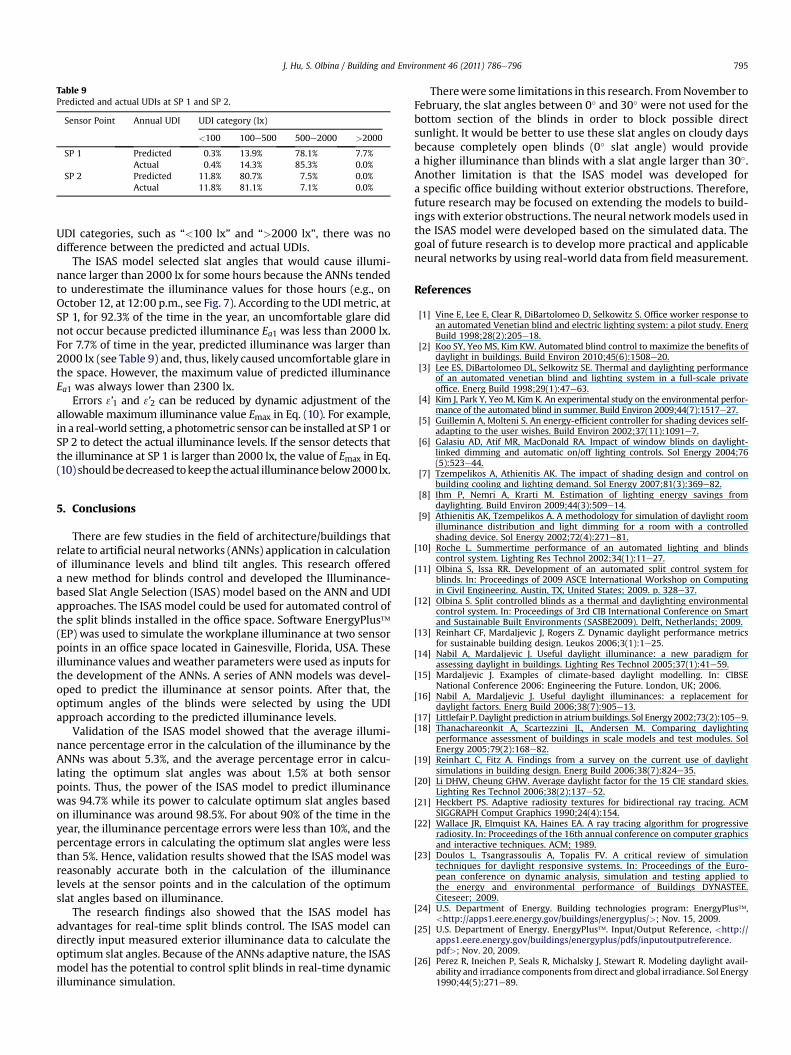
Table 9Predicted and actual UDIs at SP 1 and SP 2.

Sensor Point Annual UDI UDI category (lx)

<100 100e500 500e2000 >2000

SP 1 Predicted 0.3% 13.9% 78.1% 7.7%Actual 0.4% 14.3% 85.3% 0.0%

SP 2 Predicted 11.8% 80.7% 7.5% 0.0%Actual 11.8% 81.1% 7.1% 0.0%

J. Hu, S. Olbina / Building and Environment 46 (2011) 786e796 795

UDI categories, such as “<100 lx” and “>2000 lx”, there was nodifference between the predicted and actual UDIs.

The ISAS model selected slat angles that would cause illumi-nance larger than 2000 lx for some hours because the ANNs tendedto underestimate the illuminance values for those hours (e.g., onOctober 12, at 12:00 p.m., see Fig. 7). According to the UDI metric, atSP 1, for 92.3% of the time in the year, an uncomfortable glare didnot occur because predicted illuminance Ea1 was less than 2000 lx.For 7.7% of time in the year, predicted illuminance was larger than2000 lx (see Table 9) and, thus, likely caused uncomfortable glare inthe space. However, the maximum value of predicted illuminanceEa1 was always lower than 2300 lx.

Errors 3’1 and 3’2 can be reduced by dynamic adjustment of theallowable maximum illuminance value Emax in Eq. (10). For example,in a real-world setting, a photometric sensor can be installed at SP 1 orSP 2 to detect the actual illuminance levels. If the sensor detects thatthe illuminance at SP 1 is larger than 2000 lx, the value of Emax in Eq.(10) shouldbedecreased tokeeptheactual illuminancebelow2000 lx.

5. Conclusions

There are few studies in the field of architecture/buildings thatrelate to artificial neural networks (ANNs) application in calculationof illuminance levels and blind tilt angles. This research offereda new method for blinds control and developed the Illuminance-based Slat Angle Selection (ISAS) model based on the ANN and UDIapproaches. The ISASmodel could be used for automated control ofthe split blinds installed in the office space. Software EnergyPlus�(EP) was used to simulate the workplane illuminance at two sensorpoints in an office space located in Gainesville, Florida, USA. Theseilluminance values and weather parameters were used as inputs forthe development of the ANNs. A series of ANN models was devel-oped to predict the illuminance at sensor points. After that, theoptimum angles of the blinds were selected by using the UDIapproach according to the predicted illuminance levels.

Validation of the ISAS model showed that the average illumi-nance percentage error in the calculation of the illuminance by theANNs was about 5.3%, and the average percentage error in calcu-lating the optimum slat angles was about 1.5% at both sensorpoints. Thus, the power of the ISAS model to predict illuminancewas 94.7% while its power to calculate optimum slat angles basedon illuminance was around 98.5%. For about 90% of the time in theyear, the illuminance percentage errors were less than 10%, and thepercentage errors in calculating the optimum slat angles were lessthan 5%. Hence, validation results showed that the ISAS model wasreasonably accurate both in the calculation of the illuminancelevels at the sensor points and in the calculation of the optimumslat angles based on illuminance.

The research findings also showed that the ISAS model hasadvantages for real-time split blinds control. The ISAS model candirectly input measured exterior illuminance data to calculate theoptimum slat angles. Because of the ANNs adaptive nature, the ISASmodel has the potential to control split blinds in real-time dynamicilluminance simulation.

Therewere some limitations in this research. FromNovember toFebruary, the slat angles between 0� and 30� were not used for thebottom section of the blinds in order to block possible directsunlight. It would be better to use these slat angles on cloudy daysbecause completely open blinds (0� slat angle) would providea higher illuminance than blinds with a slat angle larger than 30�.Another limitation is that the ISAS model was developed fora specific office building without exterior obstructions. Therefore,future research may be focused on extending the models to build-ings with exterior obstructions. The neural networkmodels used inthe ISAS model were developed based on the simulated data. Thegoal of future research is to develop more practical and applicableneural networks by using real-world data from field measurement.

References

[1] Vine E, Lee E, Clear R, DiBartolomeo D, Selkowitz S. Office worker response toan automated Venetian blind and electric lighting system: a pilot study. EnergBuild 1998;28(2):205e18.

[2] Koo SY, Yeo MS, Kim KW. Automated blind control to maximize the benefits ofdaylight in buildings. Build Environ 2010;45(6):1508e20.

[3] Lee ES, DiBartolomeo DL, Selkowitz SE. Thermal and daylighting performanceof an automated venetian blind and lighting system in a full-scale privateoffice. Energ Build 1998;29(1):47e63.

[4] Kim J, Park Y, Yeo M, Kim K. An experimental study on the environmental perfor-mance of the automated blind in summer. Build Environ 2009;44(7):1517e27.

[5] Guillemin A, Molteni S. An energy-efficient controller for shading devices self-adapting to the user wishes. Build Environ 2002;37(11):1091e7.

[6] Galasiu AD, Atif MR, MacDonald RA. Impact of window blinds on daylight-linked dimming and automatic on/off lighting controls. Sol Energy 2004;76(5):523e44.

[7] Tzempelikos A, Athienitis AK. The impact of shading design and control onbuilding cooling and lighting demand. Sol Energy 2007;81(3):369e82.

[8] Ihm P, Nemri A, Krarti M. Estimation of lighting energy savings fromdaylighting. Build Environ 2009;44(3):509e14.

[9] Athienitis AK, Tzempelikos A. A methodology for simulation of daylight roomilluminance distribution and light dimming for a room with a controlledshading device. Sol Energy 2002;72(4):271e81.

[10] Roche L. Summertime performance of an automated lighting and blindscontrol system. Lighting Res Technol 2002;34(1):11e27.

[11] Olbina S, Issa RR. Development of an automated split control system forblinds. In: Proceedings of 2009 ASCE International Workshop on Computingin Civil Engineering. Austin, TX, United States; 2009. p. 328e37.

[12] Olbina S. Split controlled blinds as a thermal and daylighting environmentalcontrol system. In: Proceedings of 3rd CIB International Conference on Smartand Sustainable Built Environments (SASBE2009). Delft, Netherlands; 2009.

[13] Reinhart CF, Mardaljevic J, Rogers Z. Dynamic daylight performance metricsfor sustainable building design. Leukos 2006;3(1):1e25.

[14] Nabil A, Mardaljevic J. Useful daylight illuminance: a new paradigm forassessing daylight in buildings. Lighting Res Technol 2005;37(1):41e59.

[15] Mardaljevic J. Examples of climate-based daylight modelling. In: CIBSENational Conference 2006: Engineering the Future. London, UK; 2006.

[16] Nabil A, Mardaljevic J. Useful daylight illuminances: a replacement fordaylight factors. Energ Build 2006;38(7):905e13.

[17] Littlefair P.Daylight prediction in atriumbuildings. Sol Energy2002;73(2):105e9.[18] Thanachareonkit A, Scartezzini JL, Andersen M. Comparing daylighting

performance assessment of buildings in scale models and test modules. SolEnergy 2005;79(2):168e82.

[19] Reinhart C, Fitz A. Findings from a survey on the current use of daylightsimulations in building design. Energ Build 2006;38(7):824e35.

[20] Li DHW, Cheung GHW. Average daylight factor for the 15 CIE standard skies.Lighting Res Technol 2006;38(2):137e52.

[21] Heckbert PS. Adaptive radiosity textures for bidirectional ray tracing. ACMSIGGRAPH Comput Graphics 1990;24(4):154.

[22] Wallace JR, Elmquist KA, Haines EA. A ray tracing algorithm for progressiveradiosity. In: Proceedings of the 16th annual conference on computer graphicsand interactive techniques. ACM; 1989.

[23] Doulos L, Tsangrassoulis A, Topalis FV. A critical review of simulationtechniques for daylight responsive systems. In: Proceedings of the Euro-pean conference on dynamic analysis, simulation and testing applied tothe energy and environmental performance of Buildings DYNASTEE.Citeseer; 2009.

[24] U.S. Department of Energy. Building technologies program: EnergyPlus�,<http://apps1.eere.energy.gov/buildings/energyplus/>; Nov. 15, 2009.

[25] U.S. Department of Energy. EnergyPlus�. Input/Output Reference, <http://apps1.eere.energy.gov/buildings/energyplus/pdfs/inputoutputreference.pdf>; Nov. 20, 2009.

[26] Perez R, Ineichen P, Seals R, Michalsky J, Stewart R. Modeling daylight avail-ability and irradiance components fromdirect and global irradiance. Sol Energy1990;44(5):271e89.

J. Hu, S. Olbina / Building and Environment 46 (2011) 786e796796

[27] Hassoun MH. Fundamentals of artificial neural networks. Massahusetts: TheMIT Press; 1995.

[28] Karatasou S, Santamouris M, Geros V. Modeling and predicting building’senergy use with artificial neural networks: methods and results. Energ Build2006;38(8):949e58.

[29] Yokoyama R, Wakui T, Satake R. Prediction of energy demands using neuralnetwork with model identification by global optimization. Energ ConversManag 2009;50(2):319e27.

[30] Li Q, Meng Q, Cai J, Yoshino H, Mochida A. Predicting hourly cooling load inthe building: a comparison of support vector machine and different artificialneural networks. Energ Convers Manag 2009;50(1):90e6.

[31] Kazanasmaz T, Gunaydin M, Binol S. Artificial neural networks to predictdaylight illuminance in office buildings. Build Environ 2009;44(8):1751e7.

[32] Grena R. An algorithm for the computation of the solar position. Sol Energy2008;82(5):462e70.

[33] Blanco-Muriel M, Alarcón-Padilla DC, López-Moratalla T, Lara-Coira M.Computing the solar vector. Sol Energy 2001;70(5):431e41.

[34] Muneer T, Gueymard C, Kambezidis H. Solar radiation and daylight models.2nd ed. Oxford: Elsevier Ltd.; 2004.

[35] Bansal GD, Saxena BK. Evaluation of spatial illuminance in buildings. EnergBuild 1979;2(3):179e84.