ILA-2: AN INDUCTIVE LEARNING ALGORITHM FOR KNOWLEDGE DISCOVERY

ILA-2: An Inductive Learning Algorithm for Knowledge Discovery

Mehmet R. Tolun (*) Hayri Sever

Department of Computer Engineering Department of Computer Science

Eastern Mediterranean University Hacettepe University

Gazimagusa, T.R.N.C. Beytepe – Ankara

Turkey Turkey 06530

{[email protected]} {[email protected]}

Mahmut 8OXGD÷ Saleh M. Abu-Soud

Information Security Research Institute Department of Computer Science

7h%ø7$.�8(.$( Princess Sumaya University College for Technology

PK 21 Gebze Kocaeli P.O. Box 925819

Turkey 41470 Amman - Jordan 11110

{[email protected]} {[email protected]}

(*) Corresponding author

Running Title: ILA-2: An Inductive Learning Algorithm

This research is partly supported by the State Planning Organization of the Turkish Republic under the research

grant 97-K-12330. All of the data sets were obtained from the University of California-Irvine’s repository of

machine learning databases and domain theories, managed by Patrick M. Murphy. We acknowledge Ross

Quinlan and Peter Clark for the implementations of C4.5 and CN2 and also Ron Kohavi, for we have used

MLC++ library to execute OC1, CN2, and ID3 algorithms.

ILA-2: An Inductive Learning Algorithm 2

Abstract

In this paper we describe the ILA-2 rule induction algorithm which is the improved version of a novel

inductive learning algorithm, ILA. We first outline the basic algorithm ILA, and then present how the

algorithm is improved using a new evaluation metric that handles uncertainty in the data. By using a

new soft computing metric, users can reflect their preferences through a penalty factor to control the

performance of the algorithm. ILA has also a faster pass criteria feature which reduces the processing

time without sacrificing much from the accuracy that is not available in basic ILA.

We experimentally show that the performance of ILA-2 is comparable to that of well-known inductive

learning algorithms, namely CN2, OC1, ID3 and C4.5.

Keywords: Data Mining, Knowledge Discovery, Machine Learning, Inductive Learning, Rule Induction.

1. Introduction

A knowledge discovery process involves extracting valid, previously unknown, potentially

useful, and comprehensible patterns from large databases. As described in (Fayyad, 1996;

Simoudis, 1996), this process is typically made up of selection and sampling, preprocessing

and cleaning, transformation and reduction, data mining, and evaluation steps. The first step in

data-mining process is to select a target data set from a database and to possibly sample the

target data. The preprocessing and data cleaning step handles noise and unknown values as

well as accounting for missing data fields, time sequence information, and so forth. The data

reduction and transformation involves finding relevant features depending on the goal of the

task and certain transformations on the data such as converting one type of data to another

(e.g., changing nominal values into numeric ones, discretizing continuous values), and/or

defining new attributes. In the mining step, the user may apply one or more knowledge

discovery techniques on the transformed data to extract valuable patterns. Finally, the


evaluation step involves interpreting the result (or discovered pattern) with respect to the

goal/task at hand. Note that the data mining process is not linear and involves a variety of

feedback loops, as any one step can result in changes in preceding or succeeding steps.

Furthermore, the nature of a real-world data set, which may contain noisy, incomplete,

dynamic, redundant, continuos, and missing values, certainly makes all steps critical on the

path going from data to knowledge (Deogun et al., 1997; Matheus, Chan, and Piatetsky-

Shapiro, 1993).

One of the methods in data mining step is inductive learning, which is mostly concerned with

finding general descriptions of a concept from a set of training examples. Practical data

mining tools generally employ a number of inductive learning algorithms. For example,

Silicon Graphics’ data mining and visualization product MineSet uses MLC++ as a base for

the induction and classification algorithms (Kohavi, Sommerfield, and Dougherty, 1996). This

work focuses on establishing causal relationships to class labels from values of attributes via a

heuristic search that starts with values of individual attributes and continues to consider the

double, triple, or further combinations of attribute values in sequence until the example set is

covered.

Once a new learning algorithm has been introduced, it is not unusual to see follow-up

contributions appear that extend the algorithm in order to improve it in various ways. These

improvements are important in establishing a method and clarifying when it is and is not

useful. In this paper, we propose extensions to improve upon such a new algorithm, namely

the Inductive Learning Algorithm (ILA) introduced by Tolun and Abu-Soud (1998). ILA is a

consistent inductive algorithm that operates on non-conflicting example sets. It extracts a rule

set covering all instances in a given example set. A condition (also known as a description) is

defined as a pair of attribute and its value. The condition plays a building block in

constructing the antecedent of a rule in which there may be one or more conditions conjuncted


with one to another; the consequent of that rule is associated with a particular class. The

representation of rules in ILA is suitable for data exploration such that a description set in its

simplest form is generated to distinguish a class from the other ones.

The induction bias used in ILA selects a rule for a class from a set of promising rules if and

only if the coverage proportion of the rule1 is maximum. To implement this bias, ILA runs in

a stepwise forward iteration that cycles as many times as the number of attributes until all

positive examples of a single class is covered. Each iteration searches for a description (or a

combination of descriptions) that covers a relatively larger number of training examples of a

single class than the other candidates do. Having found such a description (or combination),

ILA generates a rule with the antecedent part consisting of that description. It then marks the

examples covered by the rule just generated so that they are not considered in further iteration

steps.

The first modification we propose is the ability to deal with uncertain data. In general, two

different sources of uncertainty can be distinguished. One of these is noise that is defined as

non-systematic errors in gathering or entering data. This may happen because of incorrect

recording or transcription of data, or because of incorrect measurement or perception at an

earlier stage. The second situation occurs when descriptions of examples become insufficient

to induce certain rules. In this paper, a data set is called inconsistent if descriptions of

examples are not sufficient to induce rules. This case is also known as incomplete data to

point out the fact that some relevant features are missing to extract non-conflicting class

descriptions. In real-world problems this often constitutes the greatest source of error, because

data is usually organized and collected around the needs of organizational activities that

causes incomplete data from the knowledge discovery task point of view. Under such


circumstances, the knowledge discovery model should have the capability of providing

approximate decisions with some confidence level.

The second modification is a greedy rule generation bias that reduces learning time at the cost

of increased number of generated rules. This feature is discussed in section 3. ILA-2 is an

extension of ILA with respect to the modifications stated above. We have empirically

compared ILA-2 with ILA using real-world data sets. The results show that ILA-2 is better

than ILA in terms of accuracy in classifying unseen instances, size of the classifiers and

learning time. Some well-known inductive learning algorithms are compared to our own

algorithm. These algorithms are ID3 (Quinlan, 1983), C4.5, C4.5rules (Quinlan, 1993), OC1

(Murthy, Kasif, and Salzberg, 1994) and CN2 (Clark and Niblett, 1989). respectively. Test

results with unseen examples also show that ILA-2 is comparable to both CN2 and C4.5

algorithms.

The organization of this paper is as follows: In the following section, we briefly introduce the

ILA algorithm, the execution of the algorithm for an example task is also presented. In section

3, modifications to ILA algorithm are described. In section 4, the time complexity analysis of

ILA-2 is presented. Finally, ILA-2 is empirically compared with five well-known induction

algorithms over nineteen different domains.

2. The ILA Inductive Learning Algorithm

ILA works in an iterative fashion. In each iteration the algorithm strives for searching a rule

that covers a large number of training examples of a single class. Having found a rule, ILA

first removes those examples from further consideration by marking them, and then appends

the rule at the end of its rule set. In other words, the algorithm works on a rules-per-class

1 the coverage proportion of a rule is computed as the proportion of the number of positive (and none ofnegative) examples covered over the size of description (i.e., the number of conjunctives) is maximum amongstthe others.


basis. For each class, rules are induced to separate examples in that class from the examples in

the other classes. This produces an ordered list of rules rather than a decision tree. The details

of ILA algorithm are given in Figure 1. A good description is a conjuncted pair of attributes

and their values such that it covers some positive examples and none of negative examples for

a given class. The goodness measure assesses the extent of goodness by returning the good

description with maximum occurrences of positive examples. ILA constructs production rules

in a general-to-specific way, i.e., starting off with the most general rule possible and

producing specific rules whenever it is deemed necessary. The advantages of ILA can be

stated as follows:

Figure 1

• The rules are in a suitable form for data exploration; namely a description of each

class in the simplest way that enables it to be distinguished from the other classes.

• The rule set is ordered in a more modular fashion, which enables to focus on a

single rule at a time. Direct rule extraction is preferred over decision trees, as the

latter are hard to interpret particularly when there is a large number of nodes.

2.1 Description of the ILA Algorithm with a Running Example

In describing ILA we shall make use of a simple training set. Consider the training set for

object classification given in Table 1, consisting of seven examples with three attributes and

the class attribute with two possible values.

Table 1

Let us trace the execution of the ILA algorithm for this training set. After reading the object

data, algorithm starts by the first class (yes), and generates hypothesis in the form of


descriptions as shown in Table 2. A description is a conjunction of attribute-value pairs, they

are used to form left-hand side of rules in the rule generation step.

Table 2

For each description the number of positive and negative instances are found. The descriptions

6 and 8 are the ones with the most positives and no negatives. Since description 6 is the first,

it is selected by default. Hence the following rule is generated:

Rule 1: IF shape = sphere -> class is yes

Upon generation of Rule 1, instances 2 and 6 covered by that rule are marked as classified.

These instances are no longer taken into account in hypothesis generation. Next time, the

algorithm generates descriptions shown in Table 3.

Table 3

In the second hypothesis space, there are four equivalent quality descriptions; 1, 2, 3 and 5.

The system selects the first description for a new rule generation.

Rule 2: IF size = medium -> class is yes

The item 1 covered by this rule is marked as classified, and next descriptions are generated

(Table 4).

Table 4.

This time only the second description satisfies the ILA quality criterion, and is used for the

generation of the following rule:


Rule 3: IF color = green -> class yes

Since example 4 is covered by this rule, it is marked as classified. All examples of the current

class (yes) are now marked as classified. The algorithm continues with the next class (no)

generating the following rules:

Rule 4: IF shape = wedge -> class is no

Rule 5: IF color = red and size = large -> class is no

Algorithm stops when all of the examples in the training set are marked as classified, i.e. all

the examples are covered by the current rule-set.

3. Extensions to ILA

Two main problems of ILA are over-fitting and long learning time. Over-fitting problem is

due to the bias that ILA tries to generate a consistent classifier on training data. However

training data, most of the time includes noisy examples causing over-fitting in the generated

classifiers. We have developed a novel heuristic function that prevents this bias in the case of

noisy examples. We also proposed another modification to make ILA faster, which considers

the possibility of generating more than one rule after the iteration steps.

The ILA algorithm and its extensions have been implemented by using the source code of

C4.5 programs. Therefore, in addition to extensions stated above, the algorithm has also been

enhanced by some features of C4.5, such as rule sifting and default class selection (Quinlan,

1993). During the classification process, the ILA system first extracts a set of rules using the

ILA algorithm. In the next step, the set of extracted rules for the classes are ordered to

minimize false positive errors, and then a default class is chosen. The default class is found as

the one with most instances not covered by any rule. Ties are resolved in favor of more


frequent classes. Once the class order and the default class have been established, the rule set

is subject to a post-pruning process. If there are one or more rules whose omission would

actually reduce the number of classification errors in training cases, the first such rule is

discarded and the set is checked again. This last step allows a final global scrutiny of the rule

set as a whole for the context it will be used.

ILA-2 algorithm can also handle continuous feature discretization through using the entropy-

based algorithm of Fayyad and Irani (1993). This algorithm uses a recursive entropy

minimization heuristic for discretization and couples this with a Minimum Description Length

criterion (Rissanen, 1986) to control the number of intervals produced over the continuous

space. In the original paper by Fayyad and Irani, this method was applied locally at each node

during tree generation. The method was found to be quite promising as a global discretization

method (Ting, 1994). We have used the implementation of Fayyad and Irani’s discretization

algorithm as provided within the MLC++ library (Kohavi, Sommerfeld, and Dougherty,

1996).

3.1 The Novel Evaluation Function

In general, an evaluation function’s score for a description should increase in proportion to

both the number of positive instances covered, denoted by TP, and the number of negative

instances not covered, denoted by TN. In order to normalize the score, a simple metric takes

into account the total number of positive instances, P, and negative instances, N, which is

given in (Langley, 1996) as

(TP + TN ) / (P + N),


where the resulting value ranges between 0 (when no positives and all negatives are covered)

and 1 (when all positives and no negatives covered). This ratio may be used to measure the

overall classification accuracy of a description on the training data.

Now, we may turn to description evaluation of the metric used in ILA, which can be

expressed as follows.

The description should not occur in any of the negative examples of the current class

AND must be the one with maximum occurrences in positive examples of the current

class.

Since this metric assumes, however, no uncertainty to be present in the training data, it

searches a given description space to extract a rule set that classifies training data perfectly. It

is, however, well-known fact that an application targeting real-world domains should address

how to handle uncertainty. Generally, uncertain tolerant classification requires relaxing the

constraint that the induced descriptions must classify the consistent part of training data (Clark

and Niblett, 1989), which is equivalent to say that classification methods should generate

almost true rules (Matheus, Chan, and Piatetsky-Shapiro, 1993). Considering this point, a

noise tolerant version of the ILA metric has been developed.

The above idea is also supported by one of the guiding principles of soft-computing: "Exploit

the tolerance for imprecision, uncertainty, and particular truth to achieve tractability,

robustness, and low solution cost" (Zadeh, 1994). Using these ideas, a new quality criterion is

established, in which the quality of a description (D) is calculated by the following heuristic:

Quality(D) = TP - PF * FN, where

TP (True Positives) is the number of correctly identified positive examples; FN (False

Negatives) is the number of wrongly identified negative examples; and PF (Penalty Factor) is


a user-defined parameter. Note that to reason about uncertain data, the evaluation measure of

ILA-2 maximizes the quality value of a rule for a given PF.

The Penalty Factor determines the negative effect of FN examples on the quality of

descriptions. It is similar to the well-known sensitivity measure used for accuracy estimation.

Usually sensitivity (Sn) is defined as the proportion of items that have been correctly predicted

to the number of items covered, i.e.,

Sn = TP / ( TP + FN ).

Sensitivity may be equivalently rewritten in terms of PenaltyFactor (PF) as

Sn = PF / ( PF + 1 ).

The user defined PF values may be converted to the sensitivity measure using the above

equation.

As seen in Figure 2, sensitivity value approaches to one as the penalty factor increases. The

advantage of the new heuristic may be seen by an example case. In respect to penalty factor of

five, let us have two descriptions one with TP=70 and FN=2, the other with TP=6 and FN=0.

The ILA quality criterion selects the second description. However, the soft criteria selects the

first one, which is intuitively more predictive than the second.

Figure 2

When penalty factor approaches to the number of training examples, the selection with the

new formula is the same as ILA criteria. On the other hand, a zero penalty factor means the

number of negative training examples has no importance and only the number of positive

examples are looked at, which is quite an optimistic choice.


Properties of classifiers generated by different values of penalty factor for splice dataset are

given in Table 5. The number of rules and the average number of conditions in the rules

increase as the penalty factor increases. As seen in Table 5, i.e., ILA with smaller penalty

factors, constructs smaller size classifiers.

Table 5

As seen from Figure 3, for all reasonable values of penalty factors, (1-30), we get better

results than ILA in terms of estimated accuracy. For this data set we get maximum estimated

accuracy prediction when penalty factor is 10. Increasing the penalty factor further does not

yield better classifiers. However, when we look at the accuracy on training data we see that

there is a proportional increase in the accuracy as the penalty factor increases.

Figure 3

3.2 The Faster Pass Criteria

In each iteration, after an exhaustive search for good descriptions in the search space, ILA

selects only one description to generate a new rule. This approach seems an expensive way of

rule extraction. However, it is possible that if there exists more than one description with the

same quality then all these descriptions may be used for possible rule generation. Usually the

second approach tends to decrease the processing time. On the other hand, this approach

might result in redundant rules with an increase in the size of the output rule-set.

The above idea was implemented in the ILA system and the option to activate this feature

referred to as FastILA. For example, in case of promoter data set FastILA reduced the

processing time from 17 seconds to 10 seconds. Also, the number of final rules decreased by

one and the total number of conditions by two. The experiments show that, if the size of the


classification rules is not extremely important and less processing time is desirable then

FastILA option would be more suitable to use.

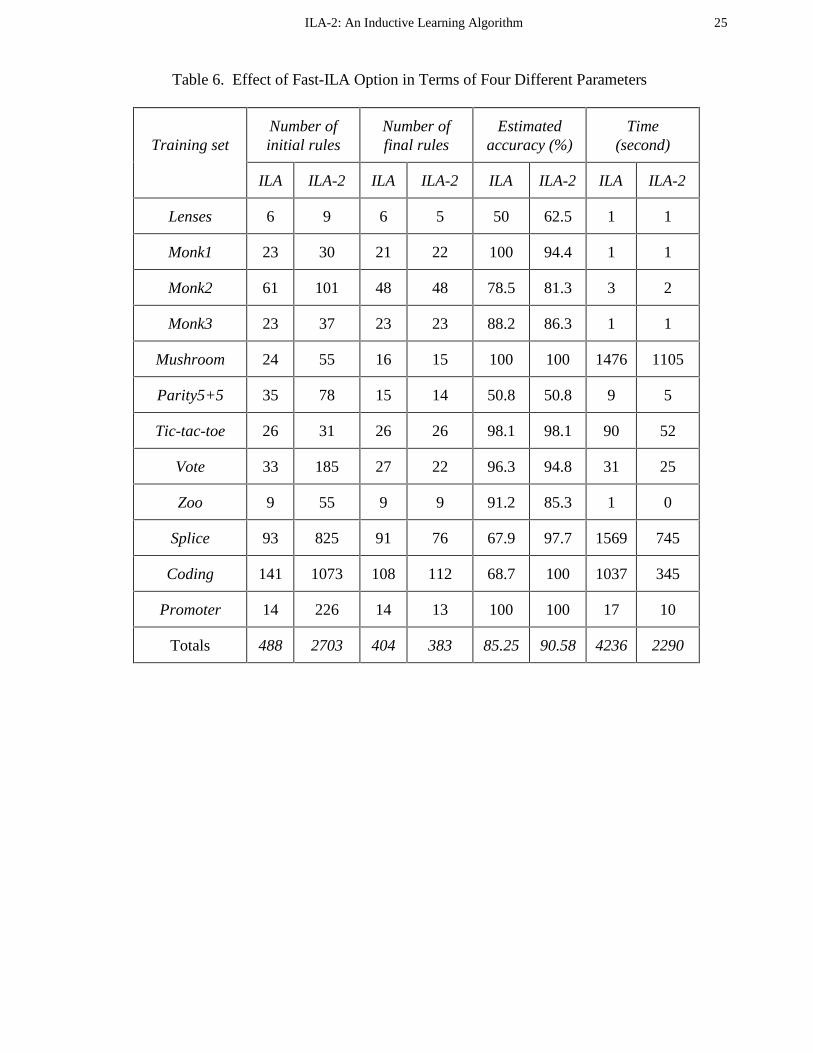
As seen in Table 6, ILA-2 (or ILA with fast pass criteria) generates a higher number of initial

rules than ILA, which amounts to about 5.5 on average for the evaluation data sets. This is

because of the faster pass criteria permits more than one rule to be asserted at once. However,

after the rule generation step is finished, the sifting process sifts all the unnecessary rules.

Table 6

4. The Time Complexity Analysis

In the time complexity analysis of ILA, only the upper bounds for the critical components of

the algorithm are provided because the overall complexity of any algorithm is domain-

dependent. Let us define following notation:

- e is the number of examples in the training set.

- Na stands for the number of attributes.

- c stands for the number of class attribute values.

- j is the number of attributes of the descriptions.

- S is the number of descriptions in the current test descriptions set.

The following procedure is applied when ILA-2 runs for a classification task: ILA-2 algorithm

comprises two main loops. The outer loop is performed for each class attribute value, which

takes time O(c). In the loop, first the size of the descriptions for the hypothesis space, also

known as version space, is set to one. A description is a combination of attribute-value pairs,

they are used as left-hand side of the IF-THEN rules in the rule generation step. Then an inner

loop is executed. The execution of the inner loop is continued until all examples of the current

class are covered by the generated rules or the maximum size for the descriptions is reached,

thus it takes time O(Na).


Inside the inner loop, first a set of temporary descriptions is generated for the given

description size using the training examples of the current class, O(e/c.Na). Then, occurrences

of these descriptions are counted, O(e.S). Next, good descriptions maximizing the ILA quality

measure are searched, O(S). If some good descriptions are found, they are used to generate

new rules. The examples matching these new rules are marked as classified, O(e/c). When no

description found passing the quality criteria the size of the descriptions for the next iteration

is incremented by one. Steps of the algorithm are given using short notations as follows;

for each class (c)

{

for each attribute (Na)

{

Hypothesis generation in the form of descriptions; // O((e/c) . Na)

Frequency counting for the descriptions; // O(e . S)

Evaluation of descriptions; // O(S)

Marking covered instances; // O(e/c)

}

}

Therefore, the overall time complexity is then given by

O(c.Na.(e/c.Na + e.S + S + e/c) ).

O(e.Na2 + c. Na.S.(e+1) + e.Na)

This may be simplified by replacing e+1 with e, and then the complexity becomes:

O(e.Na2 + c. Na.e.S + e.Na)

O(e. Na.(Na+c.S+1/c).

As 1/c is also comparatively small, then

O(e. Na.(Na+c.S).


Usually c.S is much larger than Na, e.g., in the experiments we selected S as 1500 while the

maximum Na was only 60. In addition c is also comparatively smaller than S. Therefore we

may simplify the complexity equation as:

O(e. Na.S).

So, the time complexity of the ILA is linear in the number of attributes and in the number of

examples. Also, the size of the hypothesis space (S) linearly affects the processing time.

5. Evaluation of ILA-2

For evaluation purposes of ILA-2 we have mainly used two parameters: the classifier size and

accuracy. Classifier size is the total number of conditions of the rules in the classifier. For

decision tree algorithms classifier size refers to the number of leaf nodes in the decision tree;

i.e., the number of regions that the data is divided by the tree. Accuracy is the estimated

accuracy on test data. We have used the hold out method to estimate the future prediction

accuracy on unseen data.

We have used nineteen different training sets from the UCI repository (Merz and Murphy,

1997). Table 7 summarizes the characteristics of these datasets. In order to test the algorithms

for the ability of classifying unseen examples a simple practice is to reserve a portion of the

training dataset as a separate test set, which is not used in building the classifiers. We have

employed the test sets related with these training sets from the UCI Repository in the

experiments, to estimate the accuracy of the classifiers’.

Table 7

In selecting the penalty factor (PF) as 1 and 5, we have considered the two ends and the

middle of the PF spectrum. In the higher end we observe that the ILA-2 performs like the

basic ILA, for this reason we have not included higher PF values in the experiments. The


lower end of the spectrum is zero, which eliminates the meaning of the PF. Therefore, PF=1 is

included in the experiments to see the results with the most relaxed (error tolerant) case. PF=5

case is selected as it represents a moderate case, which corresponds to sensitivity value of 0.83

in training.

We ran three different versions of ILA algorithm on these datasets: ILA-2 with penalty factor

set to 1 and 5, and the basic ILA algorithm. In addition, we ran three different decision tree

algorithms and two rule induction algorithms: ID3 (Quinlan, 1986), C4.5, C4.5rules (Quinlan,

1993), OC1 (Murthy Kasif, and Salzberg, 1994), and CN2 (Clark and Niblett, 1989).

Algorithms other than ILA-2 were run using the default settings supplied with their systems.

Estimated accuracies of generated classifiers on classifying the test sets are given in Table 8

on which our comparative interpretation is based. ILA algorithms have higher accuracies than

OC1 algorithm in classifying thirteen out of nineteen domains’ test sets. Compared to CN2,

ILA-2 performs better in eleven of the nineteen domains’ test sets and they have similar

accuracies in other two domains. ILA algorithms performed marginally better than C4.5

among the nineteen test sets, producing higher accuracies in ten domains’ test sets.

Table 8

Table 9 shows size of the output classifiers generated by the same algorithms above for the

same data sets. Results in the table prove that ILA-2 or ILA with the novel evaluation function

is comparable to C4.5 algorithms in terms of the generated classifiers’ size. When penalty

factor set to 1, ILA-2 usually produced the smallest size classifiers for the evaluation sets.

In regard to results in Table 9, it may be worth pointing out that ILA-2 solves over-fitting

problem of basic (certain) ILA, in a similar fashion to C4.5 solves the over-fitting problem of


ID3 (Quinlan, 1986). The sizes of classifiers generated by the corresponding classification

methods show the existence of this relationship clearly.

Table 9

6. Conclusion

We introduced an extended version of ILA, namely ILA-2, which is a supervised rule

induction algorithm. ILA-2 has additional features that are not available in basic ILA. A faster

pass criterion that reduces the processing time by employing a greedy rule generation strategy

is introduced. This feature, called fastILA, is useful for situations where a reduced processing

time is more important than the size of classification task performed.

The main contribution of our work is the evaluation metric utilized in ILA-2 for evaluation of

description(s). In other words, users can reflect their preferences via a penalty factor to tune

up (or control) the performance of ILA-2 system with respect to the nature of the domain at

hand. This provides a valuable advantage over most of the current inductive learning

algorithms.

Finally, using a number of machine learning and real-world data sets, we show that the

performance of ILA-2 is comparable to that of well-known inductive learning algorithms,

CN2, OC1, ID3 and C4.5.

As a further work, adapting different feature subset selection (FSS) approaches is planned to

be embedded into the system as a pre-processing step in order to yield a better performance.

With FSS, the search space requirements and the processing time will probably be reduced

due to the elimination of irrelevant attribute value combinations at the very beginning of the

rule extraction process.


References

Clark, P. and T. Niblett. 1989. The CN2 Induction Algorithm. Machine Learning 3: 261-283.

Deogun, J.S., V.V. Raghavan, A. Sarkar, and H. Sever. 1997. Data Mining: Research Trends,

Challenges, and Applications. Rough Sets and Data Mining: Analysis of Imprecise Data, (Ed.

T.Y. Lin and N. Cercone), 9-45. Boston, MA: Kluwer Academic Publishers.

Fayyad, U.M. 1996. Data Mining and Knowledge Discovery: Making Sense Out of Data.

IEEE Expert 11(5): 20-25.

Fayyad, U.M., and K.B. Irani. 1993. Multi-Interval Discretization of Continuous-Valued

Attributes for Classification Learning. In Proceedings of 13th International Joint Conference

on Artificial Intelligence, (Ed. R.Bajcsy,) 1022-1027. Philadelphia, PA: Morgan Kaufmann.

Kohavi, R., D. Sommerfield, and J. Dougherty. 1996. Data Mining Using MLC++: A

Machine Learning Library in C++. Tools with AI: 234-245.

Langley, P. 1996. Elements of Machine Learning. San Francisco: Morgan Kaufmann

Publishers.

Matheus, C.J., P.K. Chan, and G. Piatetsky-Shapiro. 1993. Systems for Knowledge Discovery

in Databases. IEEE Trans. on Knowledge and Data Engineering 5(6): 903-912.

Merz, C. J., and P. M. Murphy. 1997. UCI Repository of Machine Learning Databases,

http://www.ics.uci.edu/∼ mlearn/MLRepository.html. Irvine, CA: University of California,

Department of Information and Computer Science.

Murthy, S.K., S. Kasif, and S. Salzberg. 1994. A System for Induction of Oblique Decision

Trees. Journal of Artificial Intelligence Research 2: 1-32.


Quinlan, J.R., 1983. Learning Efficient Classification Procedures and their Application to

Chess End Games. In Machine Learning: An Artificial Intelligence Approach, (Eds, R.S.

Michalski, J.G. Carbonell, and T.M. Mitchell) 463-482. Palo Alto, CA: Tioga.

Quinlan, J.R. 1986. Induction of Decision Trees. Machine Learning 1: 81-106.

Quinlan, J.R. 1993. C4.5: Programs for Machine Learning. Philadelphia, PA: Morgan

Kaufmann.

Rissanen, J. 1986. Stochastic Complexity and Modeling. Ann. Statist. 14: 1080-1100.

Simoudis E., 1996. Reality Check for Data Mining. IEEE Expert, 11(5): 26-33.

Thornton, C.J., 1992. Techniques in Computational Learning-An Introduction. London:

Chapman and Hall.

Ting, K.M., 1994. Discretization of Continuous-valued Attributes and Instance-based

Learning. Technical Report 491, Univ. of Sydney, Australia.

Tolun, M.R., and S.M. Abu-Soud. 1998. ILA: An Inductive Learning Algorithm for Rule

Discovery. Expert Systems with Applications. 14: 361-370.

Zadeh, L. A. 1994. Soft Computing and Fuzzy Logic. IEEE Software. November: 48-56.


Table 1. Object Classification Training Set (Thornton, 1992).

Example no. Size Color Shape Class

1 medium Blue brick yes

2 small red wedge no

3 small red sphere yes

4 large red wedge no

5 large green pillar yes

6 large red pillar no

7 large green sphere yes


Table 2. The First Set of Descriptions

No Description True Positive False Negative

1 size = medium 1 0

2 color = blue 1 0

3 shape = brick 1 0

4 size = small 1 1

5 color = red 1 3

6 shape = sphere 2 0 √

7 size = large 2 2

8 color = green 2 0

9 shape = pillar 1 1


Table 3. The Second Set of Descriptions


1 size = medium 1 0 √

2 color = blue 1 0

3 shape = brick 1 0

4 size = large 1 2

5 color = green 1 0



Table 4. The Third Set of Descriptions


1 size = large 1 2

2 color = green 1 0 √



Table 5. Results for Splice Dataset with Different Values of Penalty Factors

PenaltyFactor

Number ofrules

Averagenumber ofconditions

Totalnumber ofconditions

Accuracy ontraining data

Accuracy ontest data

1 13 2.0 26 82.4% 73.4%

2 31 2.3 71 88.7% 81.6%

3 38 2.3 86 94.7% 87.6%

4 50 2.5 125 96.1% 87.2%

5 53 2.4 128 97.9% 86.9%

7 63 2.5 158 98.7% 85.4%

10 66 2.5 167 99.6% 88.5% √

30 87 2.6 228 100.0% 71.7%

ILA 91 2.6 240 100.0% 67.9%


Table 6. Effect of Fast-ILA Option in Terms of Four Different Parameters

Training setNumber ofinitial rules

Number offinal rules

Estimatedaccuracy (%)

Time(second)

ILA ILA-2 ILA ILA-2 ILA ILA-2 ILA ILA-2

Lenses 6 9 6 5 50 62.5 1 1

Monk1 23 30 21 22 100 94.4 1 1

Monk2 61 101 48 48 78.5 81.3 3 2

Monk3 23 37 23 23 88.2 86.3 1 1

Mushroom 24 55 16 15 100 100 1476 1105

Parity5+5 35 78 15 14 50.8 50.8 9 5

Tic-tac-toe 26 31 26 26 98.1 98.1 90 52

Vote 33 185 27 22 96.3 94.8 31 25

Zoo 9 55 9 9 91.2 85.3 1 0

Splice 93 825 91 76 67.9 97.7 1569 745

Coding 141 1073 108 112 68.7 100 1037 345

Promoter 14 226 14 13 100 100 17 10

Totals 488 2703 404 383 85.25 90.58 4236 2290


Table 7. The Characteristics Features of Tested Data-sets

DomainName

Number ofattributes

Number ofexamples intraining data

Number of classvalues

Number ofexamples in test

data

Lenses 4 16 3 8

Monk1 6 124 2 432

Monk2 6 169 2 432

Monk3 6 122 2 432

Mushroom 22 5416 2 2708

Parity5+5 10 100 2 1024

Tic-tac-toe 9 638 2 320

Vote 16 300 2 135

Zoo 16 67 7 34

Splice 60 700 3 3170

Coding 15 600 2 5000

Promoter 57 106 2 40

Australia 14 460 2 230

Crx 15 465 2 187

Breast 10 466 2 233

Cleve 13 202 2 99

Diabetes 8 512 2 256

Heart 13 180 2 90

Iris 10 100 3 50


Table 8. Estimated Accuracy’s of Various Learning Algorithms on Selected Domains

DomainName

ILA-2PF = 1

ILA-2PF = 5

ILA ID3C4.5-

prunedOC1

C4.5-rules

CN2

Lenses 62.5 50 50 62.5 62.5 37.5 62.5 62.5

Monk1 100 100 100 81.0 75.7 91.2 93.5 98.6

Monk2 59.7 66.7 78.5 69.9 65.0 96.3 66.2 75.4

Monk3 100 87.7 88.2 91.7 97.2 94.2 96.3 90.7

Mushroom 98.2 100 100 100 100 99.9 99.7 100

Parity5+5 50.0 51.1 51.2 50.8 50.0 52.4 50.0 53.0

Tic-tac-toe 84.1 98.1 98.1 80.9 82.2 85.6 98.1 98.4

Vote 97.0 96.3 94.8 94.1 97.0 96.3 95.6 95.6

Zoo 88.2 91.2 91.2 97.1 85.3 73.5 85.3 82.4

Splice 73.4 86.9 67.9 89.0 90.4 91.2 92.7 84.5

Coding 70.0 70.7 68.7 65.7 63.2 65.9 64.0 100

Promoter 97.5 97.5 100 100 95.0 87.5 97.5 100

Australia 83.0 76.5 82.6 81.3 87.0 84.8 88.3 82.2

Crx 80.2 78.1 75.4 72.5 83.0 78.5 84.5 80.0

Breast 95.7 96.1 95.3 94.4 95.7 95.7 94.4 97.0

Cleve 70.3 76.2 76.2 64.4 77.2 79.2 82.2 68.3

Diabetes 71.5 73.8 65.6 62.5 69.1 70.3 73.4 70.7

Heart 60.0 82.2 84.4 75.6 83.3 78.9 84.4 77.8

Iris 96.0 94.0 96.0 94.0 92.0 96.0 92.0 94.0


Table 9. Size of the Classifiers Generated by Various Algorithms

Domain NameILA-2,PF = 1

ILA-2,PF = 5

ILA ID3C4.5-

prunedC4.5-rules

Lenses 9 13 13 9 7 8

Monk1 14 37 58 92 18 23

Monk2 9 115 188 176 31 35

Monk3 5 48 63 42 12 25

Mushroom 9 13 22 29 30 11

Parity5+5 2 67 81 107 23 17

Tic-tac-toe 15 88 88 304 85 66

Vote 18 35 69 67 7 8

Zoo 11 16 17 21 19 14

Splice 26 128 240 201 81 88

Coding 64 256 319 429 109 68

Promoter 7 18 27 41 25 12

Australia 13 69 116 130 30 30

Crx 12 39 111 129 58 32

Breast 5 16 38 37 19 20

Cleve 8 55 64 74 27 20

Diabetes 6 22 33 165 27 19

Heart 1 25 19 57 33 26

Iris 5 16 4 9 7 5

Totals 238 1079 1570 2119 648 527


Figure 1. ILA Inductive Learning Algorithm


Figure 2. Penalty Factor vs. Sensitivity Values


Figure 3. Accuracy Values on Training and Test Data for the Splice Dataset.


For each class attribute value perform

{

1. Set j, which keeps the size of descriptions, to 1.

2. While there are unclassified examples in current class

and j is less than or equal to the number of attributes:

{

1. Generate the set of all descriptions in the current

class for unclassified examples using the current description size.

2. Update occurrence counts of all descriptions in the current set.

3. Find description(s) passing the goodness measure.

4. If there is any description that has passed the goodness measure:

{

1. Assert rule(s) using the ’good’ description(s).

2. Mark Items covered by the new rule(s) as classified.

}

Else increment description size j by 1.

}

}

Figure 1.


��

��

��

��

��

��

� � � � ��

3HQDOW\�IDFWRU

6HQVLWLYLW\

Figure 2.


0

20

40

60

80

100

1 3 5 10

ILA

penalty factor

Acc

ura

cy% Accuracy on

training data

Accuracy ontest data

Figure 3.

ILA-2: AN INDUCTIVE LEARNING ALGORITHM FOR KNOWLEDGE DISCOVERY

Documents

Transcript of ILA-2: AN INDUCTIVE LEARNING ALGORITHM FOR KNOWLEDGE DISCOVERY