II.B. Sistem Waktu Diskrit

1

Bab 2aSinyal-sinyal Waktu Diskrit

Kuliah PSD 01 (MFS4617)[email protected]

[email protected] II.A. Sinyal-sinyal Waktu Diskrit 2

Sinyal Waktu Diskrit• Kategori sinyal:

– Sinyal analog xa(t) � t bisa sembarang besaran fisik apapun �untuk PSD dianggap sebagai besaran waktu (detik);

– Sinyal digital x(n) � n merupakan bilangan bulat yang menyatakan instan diskrit dalam waktu � sinyal waktu-diskrit;

• Tanda panah ke-atas � cuplikan saat n=0;


Macam-macam Deret:1. Deret Cuplik satuan – unit sample

• Fungsi zeros(1,N)digunakan untuk menghasilkan sebuah vektor baris dengan data nol (‘0’) sebanyak N;

2


Macam-macam Deret:1. Deret Cuplik satuan – unit sample


Macam-macam Deret:2. Deret Langkah Satuan – unit step

• Fungsi ones(1,N)digunakan untuk menghasilkan sebuah vektor baris dengan data satu (‘1’) sebanyak N;


Macam-macam Deret:2. Deret Langkah Satuan – unit step

3


Macam-macam Deret:3. Deret Eksponensial Nilai-Real – Real-

valued exponential


Macam-macam Deret:3. Deret Eksponensial Nilai-Real – Real-

valued exponential


Macam-macam Deret:4. Deret Eksponensial Nilai-Kompleks –

Complex-valued exponential

4


Macam-macam Deret:4. Deret Eksponensial Nilai-Kompleks –

Complex-valued exponential


Macam-macam Deret:5. Deret Sinusoidal

• θ merupakan fase dalam radian;

• Untuk implementasi deret…(untuk 0 ≤ n ≤ 10)

)5.0sin(2)3/1.0cos(3)( nnnx πππ ++=


Macam-macam Deret:5. Deret Sinusoidal

5


Macam-macam Deret:6. Deret Acak

• Dicirikan dengan PDF – Probability Density Function;

• Menggunakan rand(1,N):– Deret acak dengan panjang N terdistribusi

merata (uniformly distributed) antara 0-1;• Menggunakan randn(1,N):

– Deret acak Gaussian dengan rerata 0 dan varians 1;


Macam-macam Deret:6. Deret Acak


Macam-macam Deret:7. Deret Periodik

• Sebuah deret dikatakan periodik jika

nNnxnx ∀+= ),()(

6


Macam-macam Deret:7. Deret Periodik


Operasi Deret:1-Penjumlahan sinyal

function [y,n] = sigadd(x1,n1,x2,n2)% implements y(n) = x1(n)+x2(n)% -----------------------------% [y,n] = sigadd(x1,n1,x2,n2)% y = sum sequence over n, which includes n1 and n2% x1 = first sequence over n1% x2 = second sequence over n2 (n2 can be different from n1)%n = min(min(n1),min(n2)):max(max(n1),max(n2)); % duration of y(n)y1 = zeros(1,length(n)); y2 = y1; % initializationy1(find((n>=min(n1))&(n<=max(n1))==1))=x1; % x1 with duration of yy2(find((n>=min(n2))&(n<=max(n2))==1))=x2; % x2 with duration of yy = y1+y2; % sequence addition


Operasi Deret:2-Perkalian sinyal

function [y,n] = sigmult(x1,n1,x2,n2)% implements y(n) = x1(n)*x2(n)% -----------------------------% [y,n] = sigmult(x1,n1,x2,n2)% y = product sequence over n, which includes n1 and n2% x1 = first sequence over n1% x2 = second sequence over n2 (n2 can be different from n1)%n = min(min(n1),min(n2)):max(max(n1),max(n2)); % duration of y(n)y1 = zeros(1,length(n)); y2 = y1; % y1(find((n>=min(n1))&(n<=max(n1))==1))=x1; % x1 with duration of yy2(find((n>=min(n2))&(n<=max(n2))==1))=x2; % x2 with duration of yy = y1 .* y2; % sequence multiplication

7


Operasi Deret:3-Penskalaan sinyal

• Masing-masing cuplikan dikalikan dengan suatu konstanta;

• Menggunakan operator ‘*’ pada MATLAB;


Operasi Deret:4-Penggeseran sinyal

• Masing-masing cuplikan x(n) digeser sebanyak k sehingga dihasilkan y(n) � y(n)={x(n-k)};

• Jika m=n-k � n=m+k � y(m+k)={x(m)};• Dengan demikian, operasi tidak berpengaruh pada

vektor x, tetapi vektor n berubah dengan menambahkan nilai k pada masing-masing elemen:

function [y,n] = sigshift(x,m,n0)% implements y(n) = x(n-n0)% -------------------------% [y,n] = sigshift(x,m,n0)%n = m+n0; y = x;


Operasi Deret:5-Pelipatan sinyal

• Pada operasi ini, tiap-tiap cuplikan dari x(n) dilipat pada n=0 � y(n) = {x(-n)};

• Untuk MATLAB digunakan bantuan fungsi fliplr untuk melipat x dan –fliplr untuk melipat indeks-nya:

function [y,n] = sigfold(x,n)% implements y(n) = x(-n)% -----------------------% [y,n] = sigfold(x,n)%y = fliplr(x); n = -fliplr(n);

8


Operasi Deret:6-Penjumlahan cuplikan

• Operasi ini berbeda dengan penjumlahan sinyal, karena yang dijumlahkan adalah tiap-tiap elemen dalam x(n) (semuanya) � y(n):

• Gunakan sum(x(n1:n2)); dalam MATLAB;


Operasi Deret:7-Perkalian cuplikan

• Operasi ini berbeda dengan perkalian sinyal, karena yang dikalikan adalah tiap-tiap elemen dalam x(n) (semuanya) � y(n):

• Gunakan prod(x(n1:n2)); dalam MATLAB;


Operasi Deret:8-Energi Sinyal

• Tanda bintang pada x(n) merupakan tanda konjugasi kompleks � perhatikan penempatan tandanya… � x*(n) � konjugasi (superscript), MATLAB-nya:

Ex = sum(x .* conj(x)); % suatu pendekatanEx = sum(abs(x).^2); % pendekatan lain

9


Operasi Deret:9-Daya Sinyal

• Daya rerata dari suatu sinyal periodik dengan periode dasar N…


Contoh 2.1: Pertanyaan


Contoh 2.1: Jawaban (a)n = [-5:5];x = 2*impseq(-2,-5,5)-impseq(4,-5,5);stem(n,x);title('Sequence in Example 2.1a');xlabel('n');ylabel('x(n)');axis([-5,5,-2,3])

10


Contoh 2.1: Jawaban (a)


Contoh 2.1: Jawaban (b)n = [0:20];x1 = n.*(stepseq(0,0,20)-stepseq(10,0,20));x2 = 10*exp(-0.3*(n-10)).*(stepseq(10,0,20)-stepseq(20,0,20));

x = x1+x2;stem(n,x);title('Sequence in Example 2.1b');xlabel('n');ylabel('x(n)');axis([0,20,-1,11])


Contoh 2.1: Jawaban (b)

11


Contoh 2.1: Jawaban (c)n = [0:50];x = cos(0.04*pi*n)+0.2*randn(size(n));stem(n,x);title('Sequence in Example 2.1c');xlabel('n');ylabel('x(n)');axis([0,50,-1.4,1.4])


Contoh 2.1: Jawaban (c)


Contoh 2.1: Jawaban (d)n=[-10:9];x=[5,4,3,2,1];xtilde=x' * ones(1,4);xtilde=(xtilde(:))';stem(n,xtilde);title('Sequence in Example 2.1d')xlabel('n');ylabel('xtilde(n)');axis([-10,9,-1,6])

12


Contoh 2.1: Jawaban (d)


Contoh 2.1: Jawaban (a,b,c dan d)



13


Contoh 2.2: Jawaban (a)[x11,n11] = sigshift(x,n,5);[x12,n12] = sigshift(x,n,-4);[x1,n1] = sigadd(2*x11,n11,-3*x12,n12);stem(n1,x1); title('Sequence in Example 2.2a')xlabel('n'); ylabel('x1(n)'); axis([min(n1)-1,max(n1)+1,min(x1)-1,max(x1)+1])set(gca,'XTickMode','manual','XTick',[min(n1),0,max(

n1)])


Contoh 2.2: Jawaban (a)


Contoh 2.2: Jawaban (b)[x21,n21] = sigfold(x,n);[x21,n21] = sigshift(x21,n21,3);[x22,n22] = sigshift(x,n,2);[x22,n22] = sigmult(x,n,x22,n22);[x2,n2] = sigadd(x21,n21,x22,n22);stem(n2,x2); title('Sequence in Example 2.2b')xlabel('n'); ylabel('x2(n)'); axis([min(n2)-1,max(n2)+1,0,40])set(gca,'XTickMode','manual','XTick',[min(n2),0,max(

n2)])

14


Contoh 2.2: Jawaban (b)


Contoh 2.2: Jawaban (a dan b)



15


Contoh 2.3: Jawabann = [-10:1:10]; alpha = -0.1+0.3j;x = exp(alpha*n);subplot(2,2,1); stem(n,real(x));title('real part');xlabel('n')subplot(2,2,2); stem(n,imag(x));title('imaginary part');xlabel('n')subplot(2,2,3); stem(n,abs(x));title('magnitude part');xlabel('n')subplot(2,2,4); stem(n,(180/pi)*angle(x));title('phase part');xlabel('n')


Contoh 2.3: Jawaban


Beberapa hasil Penting…• Sintesa cuplikan satuan (unit

sample synthesis) �sembarang deret x(n) dapat disintesa sebagai jumlahan deret cuplik satuan berbobot, tertunda dan terskala

• Sintesa ganjil & genap (even & odd synthesis) � deret bilangan-nyata x(n) dinamakan genap (even) jika:

xe(-n) = xe(n)• Dinamakan ganjil (odd) jika:

xo(-n) = -xo(n)

16


Beberapa hasil Penting…

• Dengan demikian sembarang deret x(n)dapat di-dekomposisi menjadi komponen genap dan ganjil:

x(n) = xe(n) + xo(n)• dengan bagian genap dan ganjilnya:

xe(n) = ½ [x(n)+x(-n)]xo(n) = ½ [x(n)-x(-n)]

• Matlabnya…


Beberapa hasil Penting…function [xe, xo, m] = evenodd(x,n)% Real signal decomposition into even and odd parts% -------------------------------------------------% [xe, xo, m] = evenodd(x,n)%if any(imag(x) ~= 0)

error('x is not a real sequence')endm = -fliplr(n);m1 = min([m,n]); m2 = max([m,n]); m = m1:m2;nm = n(1)-m(1); n1 = 1:length(n);x1 = zeros(1,length(m));x1(n1+nm) = x; x = x1;xe = 0.5*(x + fliplr(x));xo = 0.5*(x - fliplr(x));



17


Contoh 2.4: Jawabann = [0:10];x = stepseq(0,0,10)-stepseq(10,0,10);[xe,xo,m] = evenodd(x,n);subplot(1,1,1)subplot(2,2,1); stem(n,x); title('Rectangular pulse')xlabel('n'); ylabel('x(n)'); axis([-10,10,0,1.2])subplot(2,2,2); stem(m,xe); title('Even Part')xlabel('n'); ylabel('xe(n)'); axis([-10,10,0,1.2])subplot(2,2,4); stem(m,xo); title('Odd Part')xlabel('n'); ylabel('xe(n)'); axis([-10,10,-0.6,0.6])


Contoh 2.4: Jawaban


Beberapa hasil Penting…

• Deret Geometrik (Geometric Series)� deret eksponensial satu-sisi dalam bentuk {αn, n ≥ 0}, dengan α merupakan konstanta sembarang;

• Deret akan konvergen � |α| < 1;

18


Beberapa hasil Penting…• Korelasi Deret

(correlations of sequences) �mengukur derajat kesamaan dua deret;

• Definisi kroskorelasi…

• Definisi autokorelasi…

• Akan dibahas nanti…


Bersambung...

• Berikutnya...– 2B: Sistem-sistem Waktu Diskrit, Konvolusi dan

Persamaan Beda!

1

Bab 2bSistem-sistem Waktu Diskrit,

Konvolusi dan Persamaan BedaKuliah PSD 01 (MFS4617)

[email protected]

[email protected] II.B. Sistem Waktu Diskrit, Konvolusi dan PB

2

Pendahuluan

• Sistem diskrit � dinyatakan dengan operator T[.] yang membawa deret x(n) (eksitasi) menjadi deret lain y(n) (tanggap atau response) � y(n) = T[x(n)];

• Sistem diskrit � sinyal masukan menjadi sinyal keluaran;

• Sistem diskrit:– Linear, dan– Non-inear


3

Sistem Linearprinsip superposisi

tanggap impuls

2


4

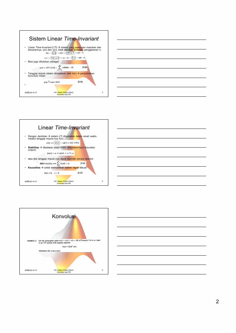
Sistem Linear Time-Invariant• Linear Time-Invariant (LTI) � sistem yang pasangan masukan dan

keluarannya, x(n) dan y(n), tidak berubah terhadap penggeseran n:

• Bisa juga dituliskan sebagai:

• Tanggap impuls sistem dinyatakan oleh h(n) � penjumlahan konvolusi linear:

•


5

Linear Time-Invariant• Dengan demikian � sistem LTI dinyatakan dalam ranah waktu

melalui tanggap impuls-nya h(n):

• Stabilitas � dikatakan stabil BIBO (Bounded-input Bounded-output):

• atau jika tanggap impuls-nya dapat dijumlah secara absolut:

• Kausalitas � untuk memastikan sistem dapat dibuat:


6

Konvolusi

3


7

Solusi Contoh 2.5


8

Solusi Contoh 2.5


9

Solusi Contoh 2.5n = -5:50;u1 = stepseq(0,-5,50); u2=stepseq(10,-5,50);% input x(n)x = u1-u2;% impulse response h(n)h = ((0.9).^n).*u1;subplot(1,1,1)subplot(2,1,1); stem(n,x); axis([-5,50,0,2])title('Input Sequence')xlabel('n'), ylabel('x(n)')subplot(2,1,2); stem(n,h); axis([-5,50,0,2])title('Impulse Response')xlabel('n'), ylabel('h(n)'); pause% output responsey = (10*(1-(0.9).^(n+1))).*(u1-u2)+(10*(1-(0.9)^10)*(0.9).^(n-9)).*u2;subplot(1,1,1)subplot(2,1,2); stem(n,y); axis([-5,50,0,8])title('Output Sequence')xlabel('n'), ylabel('y(n)')

4


10

Solusi Contoh 2.5

-5 0 5 10 15 20 25 30 35 40 45 500

0.5

1

1.5

2Input Sequence

n

x(n)

-5 0 5 10 15 20 25 30 35 40 45 500

0.5

1

1.5

2Impulse Response

n

h(n)


11

Solusi Contoh 2.5

-5 0 5 10 15 20 25 30 35 40 45 500

2

4

6

8Output Sequence

n

y(n)


12

Konvolusi Grafis

5


13

Konvolusi Grafis% input x(n)x = [3,11,7,0,-1,4,2]; nx = [-3:3];% impulse response h(n)h = [2,3,0,-5,2,1]; nh = [-1:4];subplot(1,1,1)% plot x(k) and h(k)subplot(2,2,1); stem(nx-0.05,x); axis([-5,5,-6,12]);hold on; stem(nh+0.05,h,':')title('x(k) and h(k)');xlabel('k');text(-0.5,11,'solid: x dashed: h'); hold off% plot x(k) and h(-k)subplot(2,2,2); stem(nx-0.05,x); axis([-5,5,-6,12]);hold on; stem(-fliplr(nh)+0.05,fliplr(h),':')title('x(k) and h(-k)');xlabel('k');text(-0.5,-1,'n=0')text(-0.5,11,'solid: x dashed: h'); hold off


14

Konvolusi Grafis% plot x(k) and h(-1-k)subplot(2,2,3); stem(nx-0.05,x); axis([-5,5,-6,12]);hold on; stem(-fliplr(nh)+0.05-1,fliplr(h),':')title('x(k) and h(-1-k)');xlabel('k');text(-1.5,-1,'n=-1')text(-0.5,11,'solid: x dashed: h'); hold off% plot x(k) and h(2-k)subplot(2,2,4); stem(nx-0.05,x); axis([-5,5,-6,12]);hold on; stem(-fliplr(nh)+0.05+2,fliplr(h),':')title('x(k) and h(2-k)');xlabel('k');text(2-0.5,-1,'n=2')text(-0.5,11,'solid: x dashed: h'); hold off


15

Solusi Contoh 2.6

-5 0 5

-5

0

5

10

x(k) and h(k)

k

solid: x dashed: h

-5 0 5

-5

0

5

10

x(k) and h(-k)

k

n=0

solid: x dashed: h

-5 0 5

-5

0

5

10

x(k) and h(-1-k)

k

n=-1

solid: x dashed: h

-5 0 5

-5

0

5

10

x(k) and h(2-k)

k

n=2

solid: x dashed: h

6


16

Konvolusi: Implementasi MATLAB

• Menggunakan fungsi conv();• y = conv(x,h);• Merujuk contoh 2.3:

– x = [3, 11, 7, 0, -1, 4, 2];– h = [2, 3, 0, -5, 2, 1];– y = conv(x,h);

• Perhatikan hasilnya…!• Agar diperoleh informasi waktu (diskrit):

• Sehingga:


17

Konvolusi: Implementasi MATLABfunction [y,ny] = conv_m(x,nx,h,nh)% Modified convolution routine for signal processing% --------------------------------------------------% [y,ny] = conv_m(x,nx,h,nh)% y = convolution result% ny = support of y% x = first signal on support nx% nx = support of x% h = second signal on support nh% nh = support of h%nyb = nx(1)+nh(1); nye = nx(length(x)) + nh(length(h));ny = [nyb:nye];y = conv(x,h);


18

Contoh 2.7: Penggunaan conv_m() untuk contoh 2.6

>> x = [3, 11, 7, 0, -1, 4, 2]; nx = [-3: 3];

>> h = [2, 3, 0, -5, 2, 1]; nh = [-1: 4];>> [y,ny] = conv_m(x,nx,h,nh)

y =

6 31 47 6 -51 -5 41 18 -22 -3 8 2

ny =

-4 -3 -2 -1 0 1 2 3 4 5 6 7

7


19

Korelasi: ditinjau kembali

• Kroskorelasi ryx(l) menggunakan persamaan:

rxy(l) = y(l) * x(-l)• Sedangkan autokorelasi rxx(l)

menggunakan persamaan:rxx(l) = x(l) * x(-l)

• Perhatikan contoh 2.8 berikut…


20

Contoh 2.8


21

Solusi Contoh 2.8>> x = [3, 11, 7, 0, -1, 4, 2]';>> h = [2, 3, 0, -5, 2, 1]';>> [y,H] = conv_tp(h,x)

y =

631476

-51-54118

-22-382

8


22

Solusi Contoh 2.8

H =

2 0 0 0 0 0 03 2 0 0 0 0 00 3 2 0 0 0 0-5 0 3 2 0 0 02 -5 0 3 2 0 01 2 -5 0 3 2 00 1 2 -5 0 3 20 0 1 2 -5 0 30 0 0 1 2 -5 00 0 0 0 1 2 -50 0 0 0 0 1 20 0 0 0 0 0 1


23

Persamaan Beda• Sebuah sistem LTI bisa dinyatakan melalui persamaan

beda:

• Jika an ≠ 0 maka persamaan bedanya ordenya N;• Praktisnya dihitung secara maju (dari n=-∞ hingga +∞),

sehingga:

• Penyelesaian persamaan ini dalam bentuk:


24

Persamaan Beda• Bagian homogen dinyatakan dengan:

• Dengan zk, k=1,…,N merupakan N akar dari persamaan karakteristik:

• Persamaan karakteristik ini penting untuk menentukan stabilitas sistem. Jika akara-akar zk memeuhi kondisi berikut ini, maka sebuah sistem kausal yang dinyatakan oleh persamaan 2.19 adalah stabil:

9


25

Pers. Beda: Implementasi MATLAB

• Menggunakan fungsi filter();– y = filter(b,a,x);

• dengan– b = [ b0, b1, …, bM];– a = [a0, a1, …, aN];


26

Contoh 2.9


27

Solusi Contoh 2.9% noise sequence 1x = [3, 11, 7, 0, -1, 4, 2]; nx=[-3:3]; % given signal x(n)[y,ny] = sigshift(x,nx,2); % obtain x(n-2)w = randn(1,length(y)); nw = ny; % generate w(n)[y,ny] = sigadd(y,ny,w,nw); % obtain y(n)=x(n-2)+w(n)[x,nx] = sigfold(x,nx); % obtain x(-n)[rxy,nrxy] = conv_m(y,ny,x,nx); % cross-corrlationsubplot(1,1,1)subplot(2,1,1);stem(nrxy,rxy)axis([-4,8,-50,250]);xlabel('lag variable l')ylabel('rxy');title('Crosscorrelation: noise sequence 1')gtext('Maximum')

10


28

Solusi Contoh 2.9% noise sequence 2x = [3, 11, 7, 0, -1, 4, 2]; nx=[-3:3]; % given signal x(n)[y,ny] = sigshift(x,nx,2); % obtain x(n-2)w = randn(1,length(y)); nw = ny; % generate w(n)[y,ny] = sigadd(y,ny,w,nw); % obtain y(n)=x(n-2)+w(n)[x,nx] = sigfold(x,nx); % obtain x(-n)[rxy,nrxy] = conv_m(y,ny,x,nx); % cross-corrlationsubplot(2,1,2);stem(nrxy,rxy)gtext('Maximum')axis([-4,8,-50,250]);xlabel('lag variable l')ylabel('rxy');title('Crosscorrelation: noise sequence 2')


29

Solusi Contoh 2.9

-4 -2 0 2 4 6 8-50

0

50

100

150

200

250

lag variable l

rxy

Crosscorrelation: noise sequence 1

Maximum

-4 -2 0 2 4 6 8-50

0

50

100

150

200

250

Maximum

lag variable l

rxy

Crosscorrelation: noise sequence 2


30

Contoh 2.10

11


31

Contoh 2.10


32

Solusi Contoh 2.10a=[1,-1,0.9];b=1;% Part a)x=impseq(0,-20,120);n=[-20:120];h=filter(b,a,x);subplot(2,1,1);stem(n,h)axis([-20,120,-1.1,1.1])title('Impulse Response');xlabel('n');ylabel('h(n)')%% Part b)x=stepseq(0,-20,120);s=filter(b,a,x);subplot(2,1,2);stem(n,s)axis([-20,120,-.5,2.5])title('Step Response');xlabel('n');ylabel('s(n)')%%print -deps2 ex021000.eps%% Part c)sum(abs(h))z=roots(a);magz=abs(z)subplot


33

Solusi Contoh 2.10

-20 0 20 40 60 80 100 120-1

-0.5

0

0.5

1

Impulse Response

n

h(n)

-20 0 20 40 60 80 100 120-0.5

0

0.5

1

1.5

2

2.5Step Response

n

s(n)

12


34

Solusi Contoh 2.10ans =

14.8785

magz =

0.94870.9487


35

Tanggap Masukan-Nol dan Kondisi-Nol

• Karena penyelesaian persamaan beda mulai dari n=0 (forward), maka diperlukan kondisi awal untuk x(n) dan y(n) untuk menentukan keluaran untuk n ≥ 0, sehingga persamaan beda dituliskan menjadi:

• dengan kondisi awal:

• Solusi persamaan (2.21) diperoleh dalam bentuk:

Zero-Input solution Zero-State

solution x(n)


36

Penapis Digital• Penapis FIR (Finite Impulse Response) juga dinamakan

non-rekursif atau moving average (MA) � jika tanggap impuls-nya berhingga, atau h(n)=0 untuk n < n1 dan n> n2 (filter(b,1,x)):

• Penapis IIR (Infinite Impulse Response) juga dinamakan rekursif (menggunakan keluaran sebelumnya) atau autoregressive (AR) (filter(b,a,x)):

13


37

Terima Kasih!

• Sinyal-Sinyal dan Sistem-sistem Diskrit selesai...

• Berikutnya:– 3A: Transformasi Fourier Waktu-Diskrit!

II.B. Sistem Waktu Diskrit

Documents

Transcript of II.B. Sistem Waktu Diskrit