1

CHAPTER 1

1.0 INTRODUCTION

1.1 Background Information

Over 60 per cent of Africans remain directly dependent on agriculture and natural

resources for their well-being and the African agriculture systems are being dominated by

three major characteristics: subsistence farming in the village community; the existence of

some (though rapidly diminishing) land in excess of immediate requirements, which permits

a general practice of shifting cultivation and reduces the value of land ownership as an

instrument of economic and political power; and the rights of each family (both nuclear and

extended) in a village to have access to land and water in the immediate territorial vicinity

(FAO, 2003; Todaro and Smith, 2009). In fact, agriculture has remained the backbone of

many developing countries because it plays important role largely through improving food

security, export earning and accounting for between 30% and 60% of their Gross Domestic

Product (GDP) as well as employing as much as 70% of the labour force and providing

income to a vast majority of the population (World Bank, 1996; Okuneye, 2001). Mixed

crop-livestock systems constitute the backbone of much agriculture in the tropics with the

demand for livestock products forecasted to skyrocket well into the next century (Delgado et

al., 1999). An understanding of the pathways that different production systems may follow in

Nigerian agriculture cannot therefore be overemphasized.

According to Akande (2005), Nigeria is the most populous country in Africa with a

population of over 130 million people and a domestic economy, which is dominated by

agriculture such that agriculture alone accounts for about 40% of the Gross Domestic Product

(GDP) and two thirds of the labour force. Besides, agriculture supplies food, raw materials

and generates household income for the majority of the people. Whereas the external sector is

2

dominated by petroleum, which generates 95% of Nigerian foreign exchange earnings,

agriculture contributes less than 5%.

The domestic economy where agriculture thrives must therefore be improved upon and

sustained, and if possible its external sector impact enhanced. This is because indication of

high potential for increased food production in Nigeria is glaring given that Nigeria has a

land area estimated at about 98.3 million hectares out of which about 71.2 million hectares

accounting for about 70% are cultivable while only about 34 million hectares accounting for

one third of total land area are under cultivation (Onyenweaku et al., 2008). Although the

large population and the demand for food are obvious, taking advantage of the abundant

arable land requires optimal allocation of the meagre resources at the disposal of the poor

resource farmers who provide for the majority of the nations food need and in this way

restrain a repetition of the past experiences where the nation had to resort to massive food

importation leading to rising food import bills (Adedipe et al., 1999; CBN, 1999).

Although food crop production has remained a major component of all production

activities in the agricultural sub-sector parading a large array of arables that include cereals

such as sorghum, maize, millet, rice, wheat; tubers such as yam and cassava; legumes such as

groundnut and cowpea; and others such as vegetables (Olayide et al., 1980; Akande, 2005),

the system has also the livestock component which need to be studied along side for

meaningful progress to be recorded in the sector based on policy recommendation from

balanced representation of two sub-sectors – crop and animal. Olayide et al. (1980) opined

that food crops production comes under different agricultural systems, most commonly as

mixed farming, mixed cropping or mono cropping with activities in the food crop sub-sector

continuing to dominate the category of farms variously referred to as smallholder farms,

small-scale farms, low-resource farms or small farms. This category of farmers represents as

3

much as 95% of the total food crop farming units in the country and produces about 90% of

the total food output (Okuneye and Okuneye, 1988).

Malnutrition has been one of the major problems besetting developing economies all over

the world. The bulk of food consumed by the populace of these countries is made up of

carbohydrates and very low protein particularly animal protein (Olurunfemi, 2006). Bearing

in mind that the farmers always produce to meet household demands before producing for the

market, there is great need to plan for these arable crop farmers with atleast monogastric

animals in view such as pig and poultry that provides a fast means of producing animal

protein. This is because these animals are combined by some of these arable crop farmers in

the study area, have higher fecundity rather than the ruminants and there are no known

religious norms against any of their production in the study area. Besides, these farms

characterized by low level of operation, illiteracy of operators, and a labour cost intensive

technology with hired labour cost constituting about 60% of total cash cost of production

(Olayemi, 1980, Aromolaran, 1992) are issues that make planning for them pertinent.

The farming system of these farmers is embedded in the household economy, which

integrates both production and consumption and is shaped by the multiple goals (Norman et

al., 1982). These multi-dimensional objectives that these small-scale farmers in Nigerian

agricultural context face are sometimes competitive, besides other complexities of their

production environment and decision variables which create decision problem in picking the

enterprise combinations that optimize their overall objective (Olayemi, 1980). Whereas at the

farm level for instance, households might strive for short-term cash income, food security,

minimum risk and long term viability; at the policy level, economic goals like income

distribution and employment may often be pursued (Schipper et al., 1995). However with the

modern technological advance that has been accompanied by a growth of scientific

techniques of analysis, a virtual revolution in many aspects of the agricultural sector inter

4

alia has been remarkable (Mehta, 1992). Increasing sustainability and targeting small-scale

farmers who constitute the bulk of agricultural practitioners are the principal policy issues

directed towards agricultural development (Udoh, 2000) and obviously the panacea to

meeting the food need of the nation.

Thornton and Herrero (2001) noted that increasing integration of crops and livestock is

going to occur over at least the next 30 years in sub-Saharan Africa. Given that the crop and

livestock sub-sectors in the study area are done by some of the farmers who integrate them,

understanding of the enterprise combination along these selected crops and animals would

pave the way for their expected fuller integration in the nearest future. Research has shown

that the demand for livestock products is rising globally and will increase significantly in the

coming decades because of income shifts, population growth, urbanization and changes in

dietary preferences (Delgado et al., 1999). It has also been advocated that the increased

demand for livestock products will be met mostly by increases in chicken and pig production;

a development that undoubtedly present opportunities for livestock keepers to intensify

production system (Staal et al., 2001). It would be well to plan for the arable farming

communities where livestock enterprises are operated alongside crop production in the light

of this scenario.

1.2 Problem Statement

Agriculture is highly dependent on climate variability (Salinger et al., 2005); a

phenomenon that has made the threat of climate change very urgent in Africa (Boko et al.,

2007). It has also been estimated that by 2100, Nigeria and other West African countries are

likely to have agricultural losses up to 40% of GDP due to climate change (Mendelson and

Dinar, 2003). African population on the other hand is projected to grow from 0.9 billion

people in 2005 to nearly 2 billion by 2050 (UNPD, 2007). Nigeria as the most populous

country in Africa has an estimated population of about 140 million (NPC, 2006). This

5

population pressure creates a food production planning problem if feeding the many mouths

could be realized. The many problems facing agricultural production in Nigeria have been

compounded by insufficient and inadequate infrastructure; land tenure, poor research and

extension services and suffocating marketing policy (Ilemobade, 1985; Obasanjo, 1990;

Olorunfemi, 2006). All these have a negative effect on the sector and its growth. The

deterioration condition of the agricultural sector that has led to the declining trend of

domestic food production has also been attributed to several other factors (Olorunfemi, 2006,

Olarinde et al., 2008).

Besides the discovery of oil resources, the prominent factor has been that of farmers

operating small farms in scattered plots using primitive tools and traditionally low yielding

inputs managed however by rational farmers (Akinyosoye, 2000). A striking characteristic

feature of farms in low-income countries like Nigeria is their variability; not only do farms

vary considerably from Africa to Latin America and from the Philippines to Nepal, but also

they vary from one village to another within small areas and from one farm to another within

a village (Mellor, 1980). This variation results from a wide range of physical, economic, and

cultural factors, all of which affect resource use (Mellor, 1980).

With particular reference to the southern states of Nigeria, where an inheritance

tenural arrangement is practised and farmland is seriously fragmented leading to individual

farmland shrinking in the years past, the phenomena has been prominent (Udoh, 2000 and

NEST, 1991). This situation has culminated in persistent food crises in Nigeria as the gap

between population and food production continues to widen (Igben and Banwo, 1982; World

Bank, 1992). This problem is compounded by the fact that the farming systems in Nigeria

generally, and in the rural areas in particular, where the actual production takes place are

made up of smallholder farms whose farm enterprises also include livestock. Thornton and

Herrero (2001) reported that modelling of crop and livestock enterprises has remained under-

developed and that although a wide variety of separate crop and livestock models exists, the

6

nature of crop-livestock, and their importance in smallholder farming systems make

integration difficult. Lack of reliable data and calibration are among issues that hinder its

applicability. This without doubt impede on the need to address optimization of farm

enterprises under mixed farming conditions.

In an attempt to increase food production, various food crop production programmes

have been embarked upon by the Federal and State Governments. For instance, the National

Accelerated Food Production Programme (NAFPP) designed to accelerate the production of

major staple crops through the introduction of high yielding seeds, supply of subsidized

inputs as well as provide support facilities like credit, marketing, storage and processing of

the early 1970’s; the Operation Feed the Nation (OFN) hoped to mobilize the general public

to participate in agricultural production of the 1976; and the Green Revolution Programme

(GRP) of the 1980s were discontinued in 1985 and were replaced by the Structural

Adjustment Programme (SAP) in 1986. (Kwanashie et al., 1998; Idachaba, 1985; Tanko and

Baba, 2010). In 1988, Nigeria developed a comprehensive agricultural policy document that

would guide the attainment of self-sufficiency in food and agricultural production. The

advent of democratically elected government in 1999 and thereafter came also with all forms

of food production initiatives which included cassava, rice, cocoyam etc. In spite of all these

food crop programmes, the growing concern about the capability of Nigerian agriculture to

satisfy the food requirements of her fast growing population with a declining Gross Domestic

Product (GDP) and to provide enough raw materials for agro-based industries has continued

to increase (Idachaba, 1985; Tanko and Baba, 2010).

Inspite of all these food crop production programmes of FGN over the years, the food

deficit has exacerbated leading to rapid increases in domestic food prices and increased

importation of food which the worsening position of the balance of payments in recent years

could no longer sustain (Tanko, 2004). Therefore, the need for the practicing farmers who

7

suffer from a dearth of valuable information and are struggling to optimize their objective

function subject to their resource constraints given a complex mixture of many variables has

led to the appropriateness of the following research questions:

1. What is the optimum cropping plan for arable crop and some selected livestock

enterprises in Abia State?

2. Given the resource restraints and possible alternative combinations to choose from,

how should the respective farmer allocate his/her resources to optimize gross returns?

3. Which crop or livestock enterprises should farmers in the study area produce so as to

attain the highest level of returns consistent with the level of demand?

4. Which of the factors of production is/are most limiting in the study area for each of

the arable crop and the selected livestock enterprises and what is/are their

implication(s)?

5. What is the minimum hectarage/stock size required for each of the farmers to

maximize returns?

6. What is the nature of competition of activities which did not enter the optimum plan

over those which did?

7. How would increasing or decreasing one or more resources affect the optimum mix of

activities and the value of the programme?

8. Is the optimum plan different from the existing crop-livestock farm plans for farmers?

1.3 Objectives of the Study

The broad objective of the study was to determine the optimum combination of arable

crop and selected livestock enterprises in Abia State.

The specific objectives were to:

8

1. determine the socio-economic characteristics of the respondents;

2. examine the various enterprise patterns for the selected arable crops and livestock

operated by farmers in Abia State;

3. analyze the farmers resource levels and other constraints in their crop and livestock

farm production;

4. develop optimum enterprise combination for sole crop/livestock and mixed

crop/animal mixtures considering the farmers’ resources that would maximize the

gross margin of farms in the study area;

5. determine which of the resources/factors of production is/are limiting in the study

area;

6. compare existing and optimum farm plans for farmers in terms of activities and

resource utilization;

7. Carry out sensitivity analysis on some of the resource restraint conditions

1.4 Justification for the Study

Most crop farm management or enterprise studies in Nigeria have been concerned

with analysis of existing performance in the arithmetic function or attempted the production

function analysis revealing the marginality conditions of resource use with respect to

production and at their best explored the stochastic function in their analysis (Diehl, 1982;

Okoli and Onwueme, 1980; Otoo et al., 1987; Onyenweaku et al., 2005). Such studies in

addition to being very partial in nature by addressing only the existing aspect in the

organization and operation of the crop and livestock farm enterprises also failed to answer

what would be the optimum combination of enterprises under given restraining conditions. It

is this gap that the present study aims to fill among others.

9

Mathematical programming models belonging to the general class of the allocation

models are used for determining optimal decisions and patterns of resource allocation

(Olayemi and Onyenweaku, 1999). They offer the best prospects for success in optimizing

work. Although they necessarily involve the linearization of many relationships, practitioners

find that this feature usually does not restrict the realism of these models too much

(Anderson, 1968; Olayide et al. 1980). Agricultural production planning therefore apart from

shedding light on efficient utilization of resources in the farm, makes possible the charting of

those courses of action that help in the attainment of maximum net returns and/or increased

farm incomes, and in this way bring a structural transformation of the present agricultural

economy, which is inevitable, if Nigeria is to meet her food requirements (Olayemi, 1980,

Tanko, 2004).

Thus the need for programming exercise to handle maximization of overall profit of a

farm business or minimization of cost of production given a number of constraints to be

accommodated in planning a farm cannot be overemphasized. Linear programming (LP), as

applied to farm planning represents a systematic method of determining mathematically the

optimum plan for the choice and combination of farm enterprises, so as to maximize income

or minimize costs within the limits of available farm resources (Yang,1965). Optimum

decision making which is based on a quantitative analysis for achieving “desired goal” has

been applied to Punjab farmers in India in spite of their complex situation compounded by

the difficulty of comprehending the techniques at the initial stage of their learning process

(Mehta, 1992). On technical stand, the Nigerian farmers like these Punjab farmers are small-

scale farmers who operate with crude implements, cultivate small pieces of land and have a

poor resource base. They are faced with the problem of optimal utilization of their meagre

resources to raise their incomes and consequently their living standards (Singh, 1978).

10

Bearing in mind the challenge to bring back the contribution of agriculture to the

Nigeria economy and the concern of global food crisis, a study of this nature is a worthy

adventure. Besides, most farm management studies in Abia State attempted production

function analysis revealing the marginality conditions of resource use with respect to

production of individual or selected enterprises. Such type of analysis in addition to being

very partial in nature addressed only the existing aspect in the organization and operation of

the farm business, and fails to answer as to what would be the optimum combination of

enterprises under given restraining conditions. With particular focus on the arable crop farms

and selected livestock enterprises, this study sought to contribute to knowledge in this way.

Developing a prototype enterprise plan in arable crop based production would be useful in the

extension education package for use by extension workers. This is because how the farmers

are to use any developed technologies and incentives would depend on their effective and

efficient utilization of their productive resources (Furton and Clark, 1982).

Generally, mathematical programming tools have been employed variously covering

wide range of activities like crop farming, mixed farming, horticultural crops, livestock alone,

various breeds and varieties, all sorts of combinations of different activities (Mehta, 1992). In

a regional/inter-regional framework, linear programming approach has been used for studies

in optimum resource allocation and resource requirements in many countries (Alam et al.,

1995; Sama, 1997; Alam, 1994; Onyenweaku, 1980; Schipper et al., 1995). Within Nigeria,

application of linear programming models to farm enterprises in various states has also been

reported (Osuji, 1978; Tanko, 2004). However, arable crop based farms or the livestock

component particularly animals whose production cycles last within a year are yet to be fully

targeted. Hassan et al. (2005) reported that the use of LP makes it possible to devise

equilibrium solution, which include the specification of products levels, factor and product

11

prices. The prototype enterprise combination expected from this study shall thus assist in

answering many resource allocation problems that would enhance farm productivity.

Achieving self-sufficiency in food crops among other things requires that, for the

indigenous food crop in which Nigeria has a comparative advantage over other nations of the

world, significant increases are experienced given the prevailing socio-cultural and economic

circumstances of Nigeria. Effective combination of measures aimed at increasing the level of

farm resources and making efficient use of the food sub-sector is one of the strategies

advocated to achieve significant increases in food production (Heady, 1952). Developing

optimum farm plan for small-holder farmers for this category of food crops could lead to the

resolution of the food crises given that the Nigerian farmer does not seem to exploit fully her

opportunities for capital formation, improved resource base, higher productivity, innovation

and improved management techniques (Olayemi, 1980). Given that the farmer is faced with

the challenge of rationing his scarce resources among intended activities as well as

optimizing the result of the rationing (Olayemi and Onyenweaku, 1999), require the choice of

approximate mix of crop activities and analysis of planning of mixed enterprises to achieve a

well defined technical relationship between inputs and outputs (Sama, 1997). This therefore

creates an allocation problem which the findings of the study have addressed for the selected

enterprises in Abia State.

Although some of the decision techniques employed required converting allocation

problems to mathematical form, making comprehension complex and beyond the farmers’

comprehension. Such complexities have been found to be overcome by Punjab farmers in

India over time (Mehta, 1992). Thus, with the passage of time just as was in the case of

Punjab farmers in India, the arable crop farmers would pick up the essentials and thus the

farmers would amongst the various possible solutions so obtained, be able to select the ‘most

efficient’ solution, and make their own decisions.

12

Besides all these, information from this study would be of benefit to decision makers,

and managers; in both private and public firms, students and researchers who need literature

from where to draw from in their work. In this way, it shall contribute in the improvement of

efficiency of arable crop production in the study area and consequent reduction of poverty as

the farmers’ earning capability would be improved upon if the recommendations derived

from the study are adhered to.

1.5 Limitation of the Study

The study did not cover all the farm enterprises undertaken by farmers in Abia State.

This was because of the elaborate nature of data collection for such a study and its heavy

financial implication on the researcher. Such kind of study is necessary where there is good

funding of such a research as it will give a holistic picture of the farming condition of the

entire State. Nevertheless, given the scope of the study as well as the use of cost route

approach in data collection, the researcher was financially strained in an attempt to keep track

of events and farm operations across the zones to ensure that the trained enumerators were on

course.

As a result of the obvious erratic electricity power generation, the researcher had to

expend good money at the level of data collation, computation, imputation and analysis as he

had to rely on use of generating set.

In spite of all these limitations, the findings and recommendations are very much

acceptable with respect to an average farmer among the selected enterprises of interest.

13

CHAPTER TWO

2.0 LITERATURE REVIEW

2.1 Historical Background of Linear Programming Theory

Linear programming is a mathematical procedure for determining optimal allocation

of scarce resources and has found practical application in almost all facets of business, from

advertising to production planning (Arsham, 2009). It is one of the mathematical

programming models which belong to the general class of allocation models used for

determining optimal decisions and patterns of resource allocation (Olayemi and

Onyenweaku, 1999). Linear programming is credited to George Dantzig for pioneering the

basic concepts used for framing and solving LP problems.

Linear programming problem is actually believed to have been first formulated and

solved in the late 1940’s. Today, the linear programming theory is being successfully applied

to problems of capital budgeting, design of diets, conservation of resources, games of

strategy, economic growth predictions and transportation systems (Arsham, 2009). Linear

Programming can be viewed as part of a great revolutionary development which has given

mankind the ability to state general goals and to lay out a path of detailed decisions to take in

order to ‘’best’’ achieve its goals when faced with practical situations of great complexity.

Our tool for doing this are ways to formulate real-world problems in detailed mathematical

terms (models), techniques for solving the models (algorithms), and engines for executing the

steps of algorithms (computers and software) (Dantzig, 2002). The historic appreciation of

linear programming is dated to the first formal activities of Operations Research initiated in

England during World War II, when a team of British scientists set out to make scientifically

based decisions regarding the best utilization of war material (Taha, 2007). It was not until

14

after the war that the ideas advanced in the military operations were adapted to improve

efficiency and productivity in the civilian sector (Taha, 2011).

Linear Programming began in 1947, shortly after World War II, and has been keeping

pace ever since with the extraordinary growth of computing power. Although it was first

proposed in 1947 by George B. Dantzig (in connection with the planning activities of the

military) the works of the pre-1947 era of Wassily Leontif who proposed a large but simple

matrix structure which he called the Inter-industry Input-Output Model of the American

Economy and Game theory by John Von Neuman in 1928 paved the way for the development

of LP and its extensions (Lenstra, et al. 1999; Kareen and Aderoba, 2008). Using the concept

that the Leontief model had to be generalized even though it was a steady-state model,

Dantzig satisfied the yearning of the Air Force for a highly dynamic model that is

computable, with the formulation of what he described as a time-staged, dynamic linear

program with a staircase matrix structure (Dantzig, 2002).

Between 1947 and 1949, during WWII, Dantzig worked on developing various plans

which the US military calls ‘’programs’’. After the war he was challenged to find an efficient

way to develop and solve these programs. Dantzig recognized that these programs could be

formulated as a system of linear inequalities and he introduced the concept of goal which

later today is called an objective function (Dantzig, 2002).

Precisely, the first problem Dantzig solved following his invention of LP in the

military, was a minimum cost diet problem that involved the solution of nine inequalities

(nutrition requirements) with seventy seven decision variables (source of nutrition). The

National Bureau of Standards supervised the solution process. It took the equivalent of one

man working 120 days using a hand-operated desk calculator to solve the problem.

Nowadays, a standard personal computer could solve this problem in less than one second

(Dantzig, 1990).

15

2.2 Definition and Explanation of Terms

2.2.1 Linear Programming

It is one of the mathematical programming models which belong to the general class of

allocation models used for determining optimal decisions and patterns of resource allocation

(Olayemi and Onyenweaku, 1999). The term “programming” in linear programming means

to plan and organise, that is, to program something by its solution; whereas the

“programming” in computer programming means to write codes for performing calculations.

The term “linear programming” was coined before the word “programming” become closely

associated with computer software (Arsham, 2009). According to Kareem and Aderoba

(2008) ‘linear’ implies that the relations involved are linear, while the term ‘programming’ in

the context means planning of activities.

2.2.2 Objective Function

This is one of the essential quantitative components of the LP that gives direction to

optimization. It is usually defined in clear mathematical terms. It is the decision stated in

mathematical terms, the elements involved on what result is required in LP (Lucey, 2002).

According to Olayemi and Onyenweaku (1999), objective function takes one of the several

forms:

i. Maximization of net revenue or gross margin from one or a combination of

enterprises.

ii. Minimization of production and/or transportation costs or minimization of the cost of

diets which meets specific nutritional requirements.

iii. Optimum subsidy policies required to achieve certain production targets.

16

2.2.3 Activity

Activity refers to the commodity being produced or the enterprise being undertaken.

The same commodity produced by different processes gives rise to different activities for the

purpose of linear programming. Olayemi and Onyenweaku (1999) reported that the four

general types of activities are real activities, intermediate activities, disposal activities usually

represented with slack variables and artificial activities which are included to make possible

the solution of some linear programme problems.

An activity according to Ten Berge et al. (2000) is a coherent set of operations (also

called ‘’production technology’’) with corresponding inputs and outputs resulting in e.g. the

delivery of a marketable product, the restoration of soil fertility, or the production of

feedstuffs for on-farm use. An activity is characterized by a set of coefficients (Technical

Coefficients or Input-Output Coefficients) that express the activity’s contribution to the

realization of user defined goals (or objective in modelling terms) (Ten Berge et al., 2000).

2.2.4 Input-Output and Net Price Coefficients

These are the quantities of resources required to produce a unit of an activity or output

or the unit resource requirement of an activity.

Net price coefficient on the other hand is the net value per unit of each activity. With

respect to a production activity, it is the gross value per unit of output less the variable cost

per unit while for a crop mixture; it is the total value of output per unit area less total variable

cost per unit area of all crops in the mixture. For a selling activity, the net price is the price

per unit of the product less the unit selling cost if any. For a capital borrowing activity, the

price coefficients is the prevailing market rate of interest while, for a labour hiring activity, it

is the ruling wage rate (Olayemi and Onyenweaku, 1999).

17

2.2.5 Resource Constraints

These are the restrictions limiting the level of attainment of an objective. Lucey

(2002) defined them as the factors that always exist which govern the achievement of the

objective. They could be resource constraints, institutional constraints and subjective

constraints. Resource constraints are related to the limited level of the farmer’s resources

which limit the scale of his operations; institutional constraints are related to government

agency specifications or government policies that affect production; while the subjective

constraints are imposed by the farmer himself and may be due to the farmer’s attitude to debt,

skill, consumption habit considerations and his other desirable activities for non-income

reasons (Olayemi and Onyenweaku, 1999).

2.2.6 Simplex Method

Lucey (2002) defined simplex method as a step by step arithmetic method of solving

LP problems whereby one moves progressively from a position of, say, zero production, and

therefore zero contribution, until no further contribution can be made. Each step produces a

feasible solution and an answer better than the one before, i.e. either greater contribution in

maximising problems, or less cost in minimising problems. Its mathematics is however

complex. Olayemi and Onyenweaku (1999) had defined it as an iterative procedure

developed for the solution of LP problems. It is the approach employed by the computer in

resolving large and complex problems involving many variables and resource constraints.

2.2.7 Optimum Combination of Enterprises

Different approaches that exist for modelling at farm level are thus grouped into two.

Positive approaches are defined by Flinchman and Jacquet (2003) as approaches that try to

model the actual behaviour of the farmer, while the normative approaches are approaches that

try to find the optimal solution to the problem of resource management and allocation

18

(Flinchman and Jacquet, 2003) or in other words, resource allocation is strictly based on

‘’best technical means’’ (De Wit, 1992). Positive approaches describe what happens in reality

and trying to understand it while normative approaches offer efficient and effective policy

options (Louchichi et al. 1999; Janssen and van Ittersum, 2007).

Modelling is a fundamental activity in the practice of economics generally and

management of agriculture in particular. Usually, econometric modelling is used when

dealing with empirical models while for mechanistic models, mathematical or optimization

models such as Linear Programming models are frequently used (Jansen and van Ittersum,

2007). When mechanistic models are used, LP or some derivatives of LP is used. Ten Berge

et al. (2000) offer a good explanation of the structure of a Linear Programming model for

farm analysis: LP represents the farm as a linear combination of so called ‘’activities’’.

Olayemi and Onyenweaku (1999) observed that the essence of LP is to consider the various

enterprises as well as the alternative methods of producing them in order to select that

combination which guarantees the most efficient allocation of available resources in

achieving the stated objective.

The biophysical and economic rules that determine the transformation of inputs to

outputs for a given activity are generally non-linear (Ten Berge et al., 2000). The definition

of activities must therefore ideally be such that all non-linearization are embedded in the

values of the input-output coefficients (or Technical Coefficients (TCs)). Technical

Coefficient Generators can then be defined as algorithm to translate data information into

coefficients that represent the input and the output coefficients for each discrete activity (Ten

Berge et al., 2000; Ruben and van Ruijven, 2001; Hengsdijk and van Ittersum, 2002). Output

levels might be realized with different levels of inputs for example substituting labour use by

pesticides. Different activities have to be defined to model these different input levels to

reach a certain output level (Ten Berge et al. 2000).

19

2.2.8 The Valuation of Scarce Resources

It is important management information to value the scarce or limiting resources. The

valuations of the limiting or binding or scarce resources are known as the dual prices or

shadow prices and are derived from the amount of the increase (or decrease) in contribution

that would arise if one or more (or one less) unit of the scarce resource was available (Lucey,

2002).

Shadow prices are marginal returns to increments of available resources. In a

maximization problem, they are income penalties and the shadow price of a scarce resource

shows by how much the value of the objective function or programme will increase by

increasing the level of the resource by one unit. Generally, only limiting resources or

excluded activities have positive shadow prices, i.e. their value is greater than zero.

However, any resource that is abundant, that is, not used up by the programme is not a

limiting resource and has a zero shadow price as it does not constrain the attainment of a

programme’s objective and vice versa (Olayemi and Onyenweaku, 1999).

2.2.9 Sensitivity Analysis and Parametric Programming

One major problem in the application of Linear Programming is the collection of

reliable and realistic data in terms of the input-output coefficients, aij, the coefficient of the

objective function, pj, and the right-side constraints bj. To overcome this problem, it is

important to study the behaviour of the optimum solution when these parameters are allowed

to vary (Olayemi and Onyenweaku, 1999). Sensitivity analysis is a post-optimality procedure

with no power of influencing the solution. It is used to investigate the effects of the

uncertainty on the model’s recommendation (Arsham, 2009). It was considered a constructive

step in learning about a model and the unique information gleaned can be displayed

20

systematically and instructively. It is the testing of a model for robustness, with respect to the

incorporated parameters (including assumptions and decision rules), and is thus sometimes

regarded as part of the validation phase (Anderson, 1968).

When one parameter such as the input-output coefficient aij or a coefficient of the

objective function, pj, or right-handed side constraints, bj is varied while all other parameters

are kept constant, we have what is called sensitivity analysis. This can be simply put as the

process of changing the values and relationships within the problem and observing the effects

on the solution with the aim to discover how sensitive is the optimal solution to the changes

made (Lucey, 2002). In optimizing models, it is the sensitivity of the objective function,

particularly in the region of the optimum, rather than of the optimal solution (which is usually

sensitive) that is of most interest (Anderson, 1968).

However, if two or more parameters such as two or more input-output coefficients,

coefficients of the objective function or the values of the right-hand side constraints are

jointly varied, we have what is referred to as parametric programming. The effect of the

variations is to enable us choose a particular optimum solution which conforms to our

production characteristics and resource constraints (Olayemi and Onyenweaku, 1999).

Modern parametric programming routine has been known to greatly facilitate sensitivity

analysis.

The major application of sensitivity analysis information for the decision maker is the

Marginal Analysis and the Factor Prioritization. Marginal analysis is a concept employed in

microeconomics where the marginal change in some parameter might be of interest to the

decision-maker. In optimization, the marginal analysis is employed primarily to explicate

various changes in the parameters and their impact on optimal value. The decision-makers

ponder what factors are important and have major impact on the decision outcome (Arsham,

2009). In practice, virtually all LP problems are solved by computer packages which

21

incorporate numerous facilities to test the sensitivity of the solution to changes in the problem

(Lucey, 2002).

2.2.10 Static and Dynamic Programming

Mathematical programming models may be static or dynamic. A model is static if

optimization is done for a single time as is usual in the conventional LP problems. It is

however dynamic if optimization is done for several time periods.

Olayemi and Onyenweaku (1999) observed that dynamic programming is used to

chart optimum growth paths for farm enterprise or for any other optimization problem which

is not static. The objective is not to optimize outcome for one period but to optimize overall

income from the production of various crops over a number of periods. Thus, it is a multi-

type decision problem in the sense that decision at one stage affects subsequent decision. The

rationing is said to be recursive and an overall optimality requires each subsequent decision

to be optimal at that stage with respect to the previous stage

Dynamic programming on the other hand has no method of its own for solution.

Solution is obtained on the basis of Bellman’s principle of optimality which states that “an

optimal solution is the solution obtained in such a way that, whatever the initial decision, the

remaining decision (for the remaining n-1 years) are optimal with regard to the consequence

of that initial decision. Markov Chain process is another technique sometimes used to solve

dynamic programming problems (Olayemi and Onyenweaku, 1999).

2.3 Assumptions, Advantages and Limitations of Linear Programming

2.3.1 Assumptions

There are six basic assumptions of Liner Programming (Olayemi and Onyenweaku,

1999). These assumptions include linearity assumption which requires the contribution of

22

each decision variables in both function and the constraints to be directly proportional to the

value of the variable; the additivity assumption which requires that the total contribution of

all the variables in the objective function and in the constraints to be direct sum of the

individual contributions of each variable; the certainty assumption which requires that all the

objective and constraint coefficient of the LP model to be deterministic meaning that they are

known constants; the divisibility assumption which implies that inputs and outputs are

infinitely divisible; finiteness which implies that a limit exists on the number of activities and

resources which can be programmed; and assumption of non-negativity of decision variable

which implies that negative quantities of resources cannot be used nor negative outputs

produced (Olayemi and Onyenweaku 1999; Taha, 2007).

2.3.2 Advantages and Limitations of Linear Programming

LP model has long been established as a standard planning tool in farm management

and has the following advantages:

a. The great advantage of programming is that it allows one to test a wide range of alternative

adjustments and to analyze their consequences thoroughly with a small input of managerial

time, i.e. it provides a means of analyzing a variety of alternative decisions (Beneke and

Winterboer, 1973).

b. LP in particular has become a very useful tool for planning in medium-range basis, where

it facilitates the establishment of operating plans or programs which use existing resources to

meet business requirements during a production season usually one year; and on long-range

basis, where capital budgeting, farm business policy, farm business image, possible structural

change and marketing strategy for development are programmed for the time horizon which

is usually between one to five years (Olayide and Heady, 1982).

23

c. LP provides the maximizing net returns from a combination of enterprises under given

conditions of resource restrictions. In other words, once the problem has been carefully stated

in all its possible ramifications, the solution desired does not depend on the personal factor of

the farm planner or researcher but automatically derived through computational procedure

embedded in the mathematics of LP. Output and input coefficients that are used in LP

problems for farm analysis tend to be very realistic since they are not based exclusively on

data from research farms, but are largely derived from practices and methods of operation

adopted by the farmer himself.

d. LP enables us to consider a far more detailed specification of constraints that can possibly

be handled through technique of farm planning such as budgeting and program planning.

e. The by-products obtained from results of LP planning exercises are often as useful in the

solutions themselves because they are capable of throwing considerable light on a number of

aspects of farm management by providing carefully meaningful assessment of; i) the quantum

of surplus farm resource as is found in the B-column of the last iteration, ii) the marginal

value productivity of different enterprises as is found in the Z-C value of fixed resources,

which can be used for comparing the value of resources within and between regions, iii) the

rate of interest that the farmer can justifiably pay on his borrowed funds, iv) the rate of wage

that the farmer can afford to pay for hired labour, and v) the competitive nature of the various

enterprises as found in the Z-C row of excluded activities.

In spite of the usefulness of LP in farm planning, it has several limitations. Olayide

and Heady (1982) pointed out areas in which the use of LP is subject to important limitations.

These are:

a. LP proceeds as if the price and input-output expectations that have been formulated are

equally reliable for all production activities. This leads to activities being treated as if they are

24

equally risky since the plan that results usually does not take the risk preferences of the

farmer into account. This limitation can be minimized by excluding enterprises that are

considered to be too risky from the plan by eliminating them from the range of activities

studied, or by limiting their scale to some pre-determined level by use of maximum

restriction.

b. Restrictions are sometimes difficult to specify. For a plan that typically looks ahead for a

year or more, it may be extremely difficult to know how much labour will be available during

the coming season. This is because the supply of hired labour may be unpredictable. Besides

this, in situations where the farmer uses credit in his business, he may be uncertain as to how

he could obtain more credit to implement his plan.

c. There are several hard facts that currently work against the widespread use of LP in

developing countries. Apart from the stringent demands on data, farm business tends to be

small. Since the cost of programming is a function of the complexity of farm business rather

than of size, the programming cost per naira of farm output, is likely to be higher than for

industrial farmers.

d. One of the major obstacles to wider use of LP is the lack of personnel with appropriate

training to organize and conduct farm programming services, especially in developing

countries. This is because LP requires thorough understanding of the technique, sufficient

knowledge of computer science for effective communication with computer scientists and

experts. In addition to worsening this situation, the use of a computer is very expensive in

terms of time, capital resource and manpower.

e. LP may sometimes be completely unthinking and its solution meaningless. This result from

the fact that once the activities, prices and restrictions have been set up, the solution process

grinds through to an end in the computer. Unless the tape can be examined and interpreted

25

along the way, one cannot tell whether an activity has not been discarded for a very relatively

unimportant reason. For instance, a little elasticity in the restriction would have kept it in the

program and hence made a higher income level possible.

f. LP problem may yield a solution that is not feasible, because some key constraints were not

taken into account or they cannot be meaningfully quantified.

g. The superiority of LP method of farm planning, with respect to its ability to handle a large

number of restrictions or constraints rests on the assumption of the availability of efficient

computer services. When such facilities are rare, this theoretical advantage needs to be

evaluated in the light of time, cost, and effort that are needed for solving LP problems with

the aid of desk calculators.

h. There are some unique difficulties in obtaining the relevant data for suitable specifications

of LP problems. For example, often not enough data are available for a detailed classification

of land in terms of productivity or suitability for different crops and enterprises. This is

largely true of farming in developing countries. In addition, not enough is known about the

coefficient of depreciation and a host of other inputs-output ratios. In general, the available

data do not often justify the use of such a technique as formal and exacting as LP. This

limitation can be overcome by undertaking basic and comprehensively representative farm

management research designed to obtain useful and usable input-output data.

As a result of the limitation or disadvantages associated with the LP technique, other

programming models can be used in analysis depending on the nature of the work. Usually,

when any of the assumptions of LP is relaxed, a resulting programming model arises. Such

programming models include goal programming, integer programming, non-linear

programming – quadratic and stochastic programming model. For studies on agricultural

production, the linear programming has been found very ideal.

26

With respect to agricultural production however, LP model has been found most useful and is

yet to gain its prominence in many developing countries.

2.4 Review of Empirical Literature

2.4.1 Determination of Optimum Enterprise Plans, Resource Level and Constraints

While farmers have different reasons for the cropping systems adopted and the

enterprises combined, two major reasons that are most outstanding are that of net income

stabilization and maximization. Income maximization entails comparison of costs and returns

from the different enterprises; and as a decision guide to farmers towards the realization of

their production goals, it is necessary that they know the most reliable number and types of

enterprises to combine (Chukwuji, 2008). Various approaches have been scientifically used

in studies that involved analysis of cropping patterns in many countries over time. In

Bangladesh, using the structured interview schedule as data collection tool, Shahidullah et al.

(2006), in greater Noakhali district investigated cropping patterns during the 2000/2001. A

total of 18 major cropping patterns were identified. The leading cropping pattern, which is

called Single T. Aman alone occupied 35% land of net cropped area and was the most

dominant cropping pattern. The study extended to determine cropping intensities and had the

average cropping intensity in the district as 163%. However, the region within the district

called Bamganj had the highest cropping intensity of 194% and another called Begumanj had

the lowest intensity of 115%.

Alam et al. (1995) using the LP model found that for the pure owner farms there were

thirty (28) cropping patterns in the existing plan among high land, medium high land and

medium low land across irrigated and non-irrigated farms, with seven (7) for the non-

irrigated high land and eight (8) for its irrigated counterpart; seven (7) for the non-irrigated

medium high land and five (5) for its non-irrigated counterpart; one (1) for each of the

27

irrigated and non- irrigated medium low lands. The leading cropping pattern in terms of

percentage among the existing plan came from the non-irrigated high land with 36.92% while

the least was 0.38% from the irrigated high land.

After optimization, two (2) crop enterprises were prescribed in each of the optimum

for farmers with limited capital and borrowed capital for highland non-irrigated farms; three

(3) and two (2) cropping patterns respectively for farmers with limited capital and borrowed

capital respectively for highland irrigated farms while two (2) and three (3) crop enterprises

respectively for limited and borrowed capital for medium high land irrigated; and one (1) for

the medium low land both for irrigated and non-irrigated. The total cropped area among the

existing crop plan and its optimum among farmers with limited and borrowed capital were

128.95 ha, 100.36 ha and 149.45 ha with cropping intensities of 172, 134 and 199

respectively. Similarly, for the Owner-cum-tenant farms, six (6) cropping patterns were found

among non-irrigated high land and eight (8) among the irrigated counterpart; five (5)

cropping patterns among the non-irrigated and irrigated medium high lands; one (1) cropping

patter each for the non-irrigated and irrigated medium lands bringing the total cropping

patterns to thirty (30). The leading cropping patterns for the existing plan were 49.35% and

56.70% from non-irrigated high land and 0.32% from irrigated high land and 0.61% from

non-irrigated high land as their least for owned and rented land respectively. However, the

total cropped area for the existing plan for the owned land and the rented land were 130.46 ha

and 108.69 ha respectively while the optimum plans for farmers with borrowed capital

between these two were 143.66ha and 12.37ha respectively. Cropping intensity was 175 and

173 for their existing farm plans and 193 and 192 for their optimum plans for the farmers

with borrowed capital.

The objective function of the study by Alam et al. (1995) was to maximize gross

margin on each farm simultaneously within a closed economic system in an annual cycle with

28

the land and capital as the most limiting resources in the context of Bangladesh farming.

Human labour and draft power were restrictive in certain periods of the year. It was also

assumed that farmers would like to ensure minimum cereal requirement of the farm family

out of their operation of the farm business. They incorporated six restrictions in their model

namely land, labour, human labour, bullock labour, tractor/power tiller, capital and minimum

cereal requirement constraints.

The use of remote sensing is among the new millennial approaches found to be

employed by scientists in determining cropping pattern and is believed to offer new

perspectives for investigating and monitoring natural resources. Panigrahy et al. (2005)

established the use of this approach in a study in Orissa State, part of the South-eastern Indian

subcontinent of a geographical area of 155,707 sq km. These researchers used the SPOT

VEGETATION (VGT) sensor to derive spatial maps of agricultural land use and to

determine cropping pattern, crop rotation and crop calendar in a rain fed subsistence

agricultural area of Orissa. Thirty nine date data were derived during May 2001 to May 2002

for use in the study. The results showed that most districts followed a single cropping pattern

system, rice being the base crop. Distribution pattern of rice and other crops in the main

season Kharif also matched well with information derived from conventional survey data.

The double cropping patterns occupied less than 20 percent of net sown area. Pulse crop

grown after Kharif rice emerged as the dominant double cropping system.

The situation in Orissa is chiefly due to high rice cultivation. Though rice is a vast

monoculture in the state, there is a great diversity in rice culture (Huke and Huke, 1982 and

1997). However, the use of Linear programming technique has over the past four decades

proven the best tool from policy point of view. To this, Olayide and Heady (1982) reported

that LP as a tool of farm planning is by far most useful from a practical and policy point of

29

view. Farmers’ profit cannot be maximized without optimum cropping patterns, which ensure

efficient utilization of available resources (Hassan et al., 2005).

2.4.2 Empirical Studies on Application of Linear Programming in Farm

Planning involving Crop Production

Radhakrishnan and Silvandhram (1975) used LP model to find out the optimum

cropping pattern in the pre and post development situations. Farm land, farm labour, capital

and water were the constraints used in the model. Their findings revealed that in the pre-

development conditions farmers were attaining optimality; therefore no income increase was

possible even if LP model readjustment were adopted. Under the post-development situation

however, farmers did not attain optimality. They suggested that if more capital was pumped

into through loaning, higher profits were possible.

Chaudhry (1976) used LP model for increasing income on the bullock operated farms

of 12 acres each of the owner operators, cash tenants and share tenant farms. Sample included

75 farms from Gujarat district of the Punjab, Pakistan. He concluded that with the given

resources and constraints, all the farms included in the sample were operating near optimal

level, and therefore adoption of LP solution would increase income non-significantly

(ranging from 0.4% to 4.73%). He suggested that provision of additional funds would

increase farm production. Aslam (1978) made a comparism of the result of the LP model of

agricultural production using the technical coefficients derived from production and profit

functions. Data were generated from a survey conducted in Faisalabad district, Pakistan. He

concluded that results from these models were quantitatively different from each other mainly

because input requirement per unit of output as determined from each approach were

different from the point of view of resource constraints.

Osuji (1978) also applied LP in his study on resource productivity in traditional

agriculture: a case study of selected villages in Imo State of Nigeria. He applied both the

30

production function alongside LP model. His objective was to examine cropping patterns and

enterprise combinations practised by farmers and where possible, identify sectors that militate

against food production in the area of study. The study established that marginal productivity

of family labour was negative showing excessive use of family labour in the area.

Inefficiency was also established both in the use of both family and hired labour. To

supplement the marginal analysis, LP technique employed identified crop mixtures that

would optimize farm income. Whereas some of the farmers from the production function

analysis cropped yam and cassava as sole, in line with their consumption pattern, the LP

technique did not include either of the two as sole crops as they were in very weak

competitive positions. The analysis thus favoured the strategy of mixed cropping at the level

of technology that existed and was practised by the farmers. The point of departure however

was the type of crops included in the mixtures. Optimum farm income was N4,118.00K for

rice farmers (Programme1) and N3,462.00K for non-rice farmers (Programme 2). Thus,

increasing rice cultivation is a way of increasing both farm income and food production. The

result of the parametric programming showed that an increase in land resource by 50%

resulted in farm income increasing by 15%. The same programme indicated that the absence

of labour hiring caused farm income to fall by over 22%. When wage rate was fixed at par

with government approved wage rate, farm income increased by 17%. Optimum enterprise

combination however remained unchanged in each case.

Bajwa (1978) used LP model for developing optimal plans for small farmers in Leisa

Tehsil of the Punjab, Pakistan and found that optimal cropping pattern solution increased

income by 2.2% as compared to the existing plan. Nadda et al. (1978) applied LP technique

in studying performance of hill farming in the Himachal Pradesh, India. Sample farms came

from the low hills, mid hills, and high hills. The model suggested that by growing fewer

crops, income would increase as compared to crop diversification followed under the existing

31

situation. He suggested cottage industry for better utilization of farm labour. Sharif (1979)

used LP model to determine the most profitable cropping pattern and maximum farm income

of the most common farm size of 12.5 acres each. The sample consisted of 20 farmers from

Toba Tak Singh Tehsil, Faisalabad district, Punjab, Pakistan. Overall cropped area decreased

by 2.18% over the existing one. Fallow-wheat and Fallow sugarcane turned out to be the

most profitable crop rotation.

Ahmad et al. (1990) used linear programming model to estimate cropping patterns

and net income. Data came from 20 canal irrigated bullock operated farms of 6.25 acres of

Samundri Teshsil of Faisalabad district in the Punjab. They found out there were significant

changes in the cropping patterns and little in net income in the optimal solution over the

actual one. Salman et al. (2001) introduced LP optimization model for analyzing inter

seasonal allocation of irrigation water in quantities and qualities and their impact on

agricultural production and income. The model was designed to serve as a decision making

tool for planners of agricultural production on both the district and regional levels. Hassan

(2004) used linear programming model to determine the optimum cropping patterns for the

irrigated Punjab with national and WTO price options. Result showed that the irrigated

agriculture in the Punjab is more or less operating at the optimal level. According to Hassan

et al. (2005) over all cropped acreage in the optimal solution decreased by 0.37% as

compared to the existing acreage. However, in the optimal cropping pattern some crops like

cotton and pulses gained acreage by 9-10% each, while maize and Basmati rice will remain

unchanged. On the other hand, crops like wheat, IRRI rice, potato and sugarcane lost acreage

by 4-11%. As a result of the optimum cropping pattern, income increased by 1.57%. Varying

the national prices of a single crop by 10-20% on both sides, while keeping prices of other

crops constant at the existing level, did not stimulate the acreage and production of the

concerned crop substantially, except that of cotton and Basmati rice. Increased prices of

32

wheat and sugarcane, on the other hand had adverse effect on the exportable crops (Hassan,

2004). Other studies that utilized LP model in Punjab agriculture include Mahmood and

Walter (1990); Bankar and Atre (1998); Bouman et al. (1999) among others.

Stroorvogel et al. (1997) used the LP model to maximize aggregate farm income by

selecting crops and technologies, subject to resource and sustainability constraints in

Guacimo Country in Costa Rica. Sustainability was measured as soil nutrient depletion and

biocide use. The effects of policy interventions were analyzed as land use scenarios. In

Guacimo, an environmental tax resulted in a small reduction in farm income. The study

proved a useful tool for the analysis of trade-offs between sustainability and economic

indicators.

Development and use of farm-level models has been a major activity of agricultural

economists in Canada for over about three decades, and major contributions of Canadian

agricultural economists to farm modelling has been documented (Klein and Narayan, 2008).

Ahmad (1978) determined the spatial optimal organization of crop production on the efficient

farm sizes of Manitoba Province of Canada using a multi-regional LP model which found

that total area allocation to crops under optimal solution was higher by 21% as compared to

actual acreage. Neto et al. (1997) studied crop pattern for irrigated district, Pernambuco,

Brazil using a Linear programming model with the objective function consisted into

maximizing the net income of the project, using the most cultivated crops in the area under

irrigated condition. The restrictions to the objective function were the monthly and annual

water volume, land and marketing. The modelled maximization of profits in the project area

was US$ 22,634 for the following crop pattern beans (714 ha); water melon (714 ha); green

pepper (714 ha); tomato (9428 ha); onion (357 ha); and banana (818 ha).

33

Casey et al. (1998) used LP model to investigate the economic potential of early

maturing soybeans (EMS) in the mid-latitude section of the Eastern Great Plains, USA, using

experimental research plot data. The study focussed on varieties maturing in early mid and

traditional soybeans variety (TS). The results indicated that when hired seasonal labour was

available, early soybean (EMS) rotated with grain sorghum and provided the highest returns

above the variable cost ($65927). When hired labour was not available, a combination of 235

acres of EMS rotated with wheat and 132 acres of TS soybean traditional variety rotated with

(26 acres) and grain sorghum (106 acres) and provided the highest returns above variable

costs ($48680). Early maturing soybeans were more profitable than the traditional variety

(TS). When hired seasonal labour was not available, a combination of EMS and TS

distributed labour and machinery field time over a large time, and thus enhanced farm

income.

In Bangladesh, Uddin et al. (1994) determined the optimum cropping plan for a

sample of 40 farms in the farming system research area. The results established the optimal

return with restricted capital at 49% higher than the existing return from the crop enterprise,

implying that serious efforts was needed to be directed to remove credit constraints for

improving farm incomes of the typical farms studied in the area. Before then, Quinn and

Harrington (1992) had illustrated an approach for providing India and Bangladesh with

district resource plans to help solve their regional water conflict using LP model representing

multipurpose river basin system. The concept of near optimality was employed to generate

variety of solutions in contrast to search only for a global optimum. Solutions obtained were

grouped into similar project designs by applying cluster analysis. The range of regional

alternatives available to India and Bangladesh aided in their negotiations.

In the UK, Barnes et al. (1993) used LP as an effective tool for the problem of

budgeting for optimal farm planning, alternative enterprise, how much and what type should

34

be entered into the scheme at National level and consequent effectiveness of set-aside in

reducing cereal production. This model was tried on a specialist UK cereal farm. The model

reflected a highly specialized and technically sophisticated farming system responsible for

thirty percent cereal production in UK. The results showed that the income of Mac Sharry

reforms on the farms of this type likely to be severe with total gross margin falling by

approximately 25%. Babatunde et al (2007a) examined the optimal crop combination in

small-scale irrigation farming that involved a total of 35 small-scale vegetable irrigators

randomly selected across 6 irrigation schemes and found out that optimal crop combination

was the tomato-based crop mixtures, consisting of tomato/cucumber/onion/okra/water melon.

The optimal value of the programme was CFA 329, 681. Carrot based system was the second

most profitable enterprises while the onion-based system was the least profitable enterprise.

Land was a limiting resource while labour, irrigation water and capital were non-limiting

resource in vegetable farming.

In Nigeria, Ogunfowora (1970) had highlighted the potential role of farming in the

food production sector of the Nigerian industry. He accomplished this by designing and

testing two models which characterized the peasant family farm operating entirely on a semi-

subsistence basis and a family farm with commercial orientation in the sense of incorporating

labour hiring and capital borrowing. The models revealed in their solution that there is a wide

range of income opportunities in peasant farming through efficient combination of farm

enterprises, increases in resource base and improvement in managerial ability required for

operation of larger farm units. Other studies in the 1970’s in Nigeria include Onyenweaku et

al. (1978/1979) who formulated a spatial equilibrium model for the analysis of inter-regional

competition in Nigerian agriculture. The objectives of the study were achieved through the

use of a spatial LP model comprising of 80 real activities and 84 restraints. The model

generated solutions providing information about specific variations in resources and demand.

35

Six producing regions and six spatially consuming each defined by the country’s ecological

zones were demarcated for the study. The study among other things revealed that if crop

production were allocated optimally among producing regions, in accordance with the

comparative advantage of regions, about 10.24 million hectares would be required to achieve

the national objective of self-sufficiency in food grain production under prevailing production

practices.

Olayemi and Olaomi (1995) developed a new solution procedure for a mathematical

LP model that could be optimized to obtain optimum crop combination for a mixed cropping

scheme. It was far more efficient than previous models because instead of formulating and

solving all LP problems associated with all possible crop-sub groups, the new procedure

formulated and solved few LP problems with respect to few crop-subgroups selected

systematically. Many hypothetical crop selection problems were simulated and solved to

demonstrate the superiority of the procedure over existing ones.

Aromolaran and Olayemi (1999) used LP model to generate solutions and the

resource allocation problem of small farmers in Oyo State, Nigeria. The results showed that

the low level of resource endowment of the farmers did not impose any severe limitation on

the satisfaction of their objective and for full satisfaction to be achieved they only needed to

allocate their present stock of resources more efficiently; with the present structure of the

objective function of the farmers, efficient and a sizeable output growth in farm production

may not be attainable; and since one of the major objectives of the farmers was to limit cash

expenditure on the farms, the farmers were not likely to respond well and farm capital

expansion stimulating policies and programs such as interest rate regulation, rural banking,

and softer and more favourable loan terms for agricultural credit.

36

2.4.3 Empirical Studies on Application of Linear Programmig in Farm

Planning involving Livestock Production

The impact of livestock in agrarian livelihood has not been emphasized as much as

that of crop. Relative to crop production, many studies have not been done in livestock

production with respect to determining the optimum farm plan. Nicholson et al. (1994)

developed a deterministic, multi-period linear programming (LP) model of dual-purpose

(milk-beef) cattle production system in the Sur del Lago region of Venezuela. The LP

selected animal, forage, and purchased feed activities subject to nutritional, land, and herd

composition constraints to maximize discounted herd net margin. Results from the analysis

indicated that alternatives to traditional nutritional management – especially the increased use

of locally available feeds such as molasses and urea – appear to be profitable and

nutritionally feasible. Moreover the benefits of using locally available feeds were multi-

faceted. Increased intensity of land use, permitted by improved nutritional management, may

help slow increases in land area required for cattle production, decrease the use of imported

feed grains, and benefit consumers by increasing milk and beef production.

However, the results show the benefits of adopting alternatives to current nutritional

management depend crucially on labour market factors, specifically, labour availability for

milking and pasture management on dual – purpose farms. Limiting the availability of hired

labour in the model – based on observed market outcomes in Western Venezuela –

dramatically reduced milk production, farm profitability, and the intensity of land use

compared to models without restrictions on the availability of workers.

2.4.4 Empirical Studies on Application of Linear Programming in Farm

Planning involving Crop – Livestock Integration

In West Asia and North Africa, better crop-livestock integration of farming systems

has been promoted for several decades as a way of improving the output of crop and livestock

37

(Thomson and Bahhady, 1995a). In East Punjab of India, Kahloon (1975) developed LP

model to compare relative profitability of dairy and crop farmers and concluded that incomes

could be increased significantly both in dairy farming and crop culture, provided complete

package of recommendations were adopted. The study established that in that area, dairying

was relatively more profitable than crop cultivation. Radhakrishnan and Sivandhram (1975)

used LP model to work out optimum crop production and livestock combination on the

average farm situation in East Punjab, India. They found out that adjustment of cropping

pattern to suit dairy farming would increase income by 44.21 percent, if number of milch

animals was increased to five heads per farm. Saini (1975) through the application of linear

programming found out that resources available for crops and dairying if used per

recommendations of the model would increase the benefits to the fixed farm resources by

61.14%, 55.76% and 68.2% on small, medium and large farms respectively in the East

Punjab, India.

Olowude (1974) had applied a dynamic linear programming model to determine

optimum combination of crops and poultry enterprises over a five-year period under a set of

farm-family resource constraints, consumption requirements and prices. The modelling

involved the selection of that combination of enterprises and resources through time that

maximizes the compounded values of farm income. The included enterprises are: mechanized

rice, unmechanized early rice, melon, tobacco, maize/cassava, guinea corn/yam, May-June

broilers and September-December broilers at the maximum levels. The rates of interest used

for compounding yearly farm incomes were between 3.5 per cent and 8.0 per cent. The

results reveal that the enterprise combination varies from four to eight.

Patton and Mullen (2001) used linear programming model for economic analysis of

farming systems in the NSW. They developed two farms and farming systems for the region:

farms and farming systems from east of Condobolin; and from the west of Condobolin.

38

Report showed that the optimal length of pasture was fairly insensitive to changing market

signals for both cropping and livestock commodities. Report also showed that although the

length of pasture is insensitive, the optimal mix of enterprises does change, highlighting the

importance of considering the interaction between enterprises in whole-farm analysis.

Thomson and Bahhady (1995c) used a model-farm approach to research on crop-

livestock integration. The crops on the model farms, the sheep flocks and the natural pastures

were combined to give three farm types consisting of different crop and sheep enterprise

mixes, together with natural pastures. A six-year project was conducted to show how better

crop-livestock integration and improved management increase the outputs of crops and sheep

products (Thomson and Bahhady, 1995c)

2.5 Contemporary Studies using Linear Programming

Although not much has been done in direct agricultural production planning using LP in the

State, related studies have been carried out within agro-allied industries in the present

millennium in Nigeria. Adejobi et al. (2003) applied Linear Goal Programming (LGP)

technique to model the farm-family crop enterprise with the view to develop an optimal crop

enterprise combination that would enable the small holder farmer meet their most important

goals of providing food for the family throughout the year, accumulating monetary income

and ensuring minimum use of paid labour. The results reveal that only 4 out of 18 basic

cropping activities identified in the study area entered the program. A striking feature of this

plan is that there is no sole cropping included in the model. This plan will utilize the

minimum cost of N6485.16/ha to produce the minimum food required, minimum income and

would ensure minimum use of paid labour. The result further showed that some household

resources such as land were in excess of actual household requirements.

39

Tanko (2004) applied the LP to optimum combination of farm enterprises in Kebbi

State, Nigeria and found that farm enterprises were not optimally allocated in the existing

plan and that significant increase in net farm income in the optimum over the existing plans

prevailed. Under the existing technology and resource availability, crop mixtures were in a

better position than sole crops. Results of the sensitivity analysis showed that increasing the

area under cultivation resulted in increase in the optimum farm income, which suggested that

more arable land should be employed in crop production.

Ohajianya and Oguoma (2009) analyzed resource allocation pattern for 120 food

crops farms in Imo State, Nigeria using the LP technique for optimizing resources. Results

showed a divergence between the existing and optimum farm plans under limited and

borrowed capital situations. The formulated optimum plans were subjected to sensitivity

analysis to enable choice of a particular optimum solution which conforms to the farms

production characteristics and resource constraints. Farm resources were not optimally

allocated and after optimization, farm income and employment of labour could be increased.

Results showed that increasing the area under cultivation by 2 hectares would result in

optimum farm income increasing by N80,994.00K and N67,521.60K representing 87.94%

and 54.18% under the limited and borrowed capital situations. The increase in revenue was as

a result of utilizing those resources that were idle when land posed a constraint to production.

Ibrahim et al (2009) used LP to determine optimal farm plan in evaluating food

security status of farming households and recommended that the production of Cassava,

Maize/Cowpea, and Benniseed and Groundnut/Yam enterprises at 0.64, 0.34, 0.35 and 0.22

ha respectively to yield a net return of 141, 692.89 naira. The study further established that

maize, cassava and yam were the food security crops, which effective allocation of resources

for increased production was recommended as well as introduction of participatory family

planning techniques among the food insecure households. Babatunde et al (2007a) examined

40

optimal farm plan in sweet potato cropping systems in Kwara State during the 2004 farming

season and found the average farm size as 0.91 ha. The optimal crop combination was sweet

potato/cassava cropping system and the optimal gross margin was N14766 per hectare. While

capital was a limiting resource, land and labour were non-limiting and there were 0.06 ha of

unused land and 3.13 man-days of unused labour. Increased capital investment was

recommended for increased production of the crop. In another work by Babatunde et al.

(2007b), optimal crop combination in small-scale vegetable irrigation farming scheme: Case

study from Niger Republic was investigated in the 2002 farming season. The study showed

that the optimal crop combination was the tomato-based crop mixtures consisting of

tomato/cucumber/onion/okra/watermelon. The optimal value of the programme was CFA

329, 681 which is N95, 014.25K at N145.00K per dollar where 1 US dollar is equivalent to

495 CFA as at the time of the study. This optimal was obtained by cultivating 0.165 hectare

of the enterprise at a gross margin of CFA 1, 998,069 per hectare.

Pepper/tomato/cucumber/watermelon,carrot/potato/pepper/onion/gardenegg,Onion/watermel

on/tomato/okra and cabbage/lettuce/pepper/onion enterprises did not enter the final plan,

since they have a non-zero opportunity cost indicating that they were not in the best

competitive positions as compared to tomato/cucumber/onion/okra/watermelon enterprise.

Land was the only limiting resource indicated by its opportunity cost of resources used.

Whereas there were 1, 589.7 man-days of unused labour, 405.7 ha cm3 of unused water and

CFA1, 07,444.8 of unused capital, the shadow price of land was CFA1, 998, 069, indicating

that by increasing land cultivation by one hectare, the gross margin would increase by CFA1,

998, 069.

2.6 The Difference between the Present Study and Other Studies

The present study differs from the reviewed empirical studies in that it focuses on

arable crop as well as selected livestock enterprises of which the production cycle is within a

41

year. Such types of enterprises represent the bulk of the farming systems in the southern part

of Nigeria particularly Abia State. Developing an optimum farm plan that negates this

categorization would hardly represent the true farm enterprises undertaken by the small scale

farmers in Abia State. Although in the southern part of Nigeria there are more crop-based

farmers than those practicing mixed farming, the existence of a sizeable number who engage

in these selected livestock enterprises is growing in this present time and cannot be neglected.

In addition, LP problems are solved bearing in mind the agro ecological situation of a

region/area in question. Some of the regions/areas where the LP was applied in previous

studies were areas where irrigation is practised or that have a different climatic condition

from the southern part of Nigeria; and for where the livestock and crop enterprises were

integrated, they were areas where there is a sizeable number of farmers who practised mixed

farming, a situation which contrast that of the study area. Besides, very few studies have been

done in the study area on the application of LP to farm planning.

42

CHAPTER 3

3.0 METHODOLOGY

3.1 Study Area

The study area was Abia State, located within the South East agro ecological zone of

Nigeria, whose rural population accounts for about 60% that engage in agriculture (Iloka and

Anuebunwa, 1995; Unamma et al., 1985). The state occupies an area of about 6420 km2 with

about 2.6 percent of the population of Nigeria; has an average population density of 364

persons per square kilometre with 63 percent (63%) involved in agricultural production and

an average household of 6 persons per family (NPC, 1991; World Bank, 2000; NPC, 2006).

Current Census statistics puts the state at a total population of 2,833,000 out of which 95%

are said to be Christians (NPC, 2006). However, the FRN Official Gazette (2009) puts Abia

State population at 2,847,380.

Abia State lies within latitude 4º 451 N and 6º 171 N of the equator and longitude 7º

00 E and 8º 00 E of the Greenwich Meridian. It has a tropical climate that is humid all year

round, with the rainy season that starts from March-October and dry season that occurs from

November-February. Annual rainfall ranges from 2000mm-2500mm and temperature ranges

between 22º C and 31º C (FOS, 1999). The state’s agriculture is rain fed and the rainfall

pattern bio-model with peaks in July and September respectively (Tanko and Opara, 2006).

Abia State shares common boundaries with Rivers State in the South, Imo State in the

West, Ebonyi and Enugu States in the North, and Akwa Ibom Sate in the East. It has

seventeen Local Government Areas which lie within three agricultural zones namely Aba,

Ohafia, and Umuahia. Aba zone consists of Aba North, Aba South, Obingwa, Ugwunagbo,

Ukwa East and Ukwa West Local Government Areas. Ohafia zone comprises Ohafia,

Arochukwu, Bende, Isiukwuato and Umunneochi Local Government Areas while Umuahia

43

zone is made up of Umuahia North, Umuahia South, Ikwuano, Isiala Ngwa North, Isiala

Ngwa South and Osisioma Local Government Areas. Abia State has about thirty eight (38)

blocks, two hundred and twenty eight (228) circles and one thousand, eight hundred and

twenty four contact farmers, with each farm family consisting of about 5-10 members who

are mainly small-scaled farmers (Oriaku, 2008).

The state is noted for palm oil production and most families engage in farming either

as a primary or a secondary occupation. Although farming activities such as sheep and goat

rearing, poultry and rabbit keeping, homestead fish farming and bee keeping are practiced

(FOS, 1999), the major engagement of the inhabitants is crop farming with very minor

livestock farming as in other South-East states (Unamma et al., 1985). Arable crops usually

cultivated in the state include cassava, yam, maize, melon, cocoyam, vegetable and fruits, and

these crops are grown on small holder plots usually, in mixtures of at least two simultaneous

crops (FOS, 1999; World Bank, 2000). Beside agricultural and forestry resources, Abia State

is also richly endowed with crude oil deposits, glass sand, limestone, salt, shale, clay,

gypsum, kaolin, phosphate, laterite, graphite, marble (Balogun, 2008; CN, 2008; FRN, 2009).

Within the rural communities, male youths engage in off-farm activities such as

‘Okada’ riding while the middle-aged who do not fancy that engage in hunting. Petty trading

is predominant in the area as well, particularly among the women folk.

3.2 Sampling Procedure

This study aimed at examining the optimization of arable crops and livestock

enterprises employed LP model. Data were collected from a sample size of 90 respondents

the multi-stage stratified random sampling technique. Each of the three zones of the

Agricultural Development Projects namely Aba, Ohafia and Umuahia were selected. This

was the first stage. The second stage involved listing all the blocks in each zone which at time

of this study were twelve, thirteen and thirteen in Aba, Ohafia, and Umuahia zones

44

respectively. A block was selected from each zone. The third stage involved the circle level,

whereby three circles were selected in each block. These gave a total of nine circles. The

fourth stage involved selecting a village (farming community) from each of the nine circles.

The farm household which is made up of the man, his wife and other dependents was

the primary unit from which data were collected. Ten potential arable crop - based farmers

were identified with the assistance of the village heads and the extension agents in each of the

nine villages so chosen across the three zones. A total of ninety respondents who engage in

arable crop farming and may alongside involve in poultry, piggery or fisheries production

enterprises assumed to be the major livestock enterprises undertaken in the study area were

randomly sampled for the study.

3.3 Method of Data Collection

Data source was of primary origin. Data collection was realized through the use of

structured questionnaire administered to each farm households in achieving the objectives of

the study. The cost-route approach based on forth night visit in the production season was

adopted.

Six ADP extension agents, two from each zone with three well-trained enumerators

were hired to assist the researcher in data collection using designed questionnaire.

3.3.1 Nature and Type of Data Collection and Procedure

Interview schedule and direct measurements where necessary were employed during

data collection:

a. Interview Schedules

According to frequency of collection, a once and for all data collection that involved

obtaining information on some socio-economic characteristics of the respondents such as age,

education, secondary occupation, household size, land tenure system etc. was done. This was

followed up with a once in two week’s visit in either the home or farm of the respondents.

45

Data collected in this second type were on each of the various crop and livestock

activities/enterprises and/or enterprise combinations. Labour use in terms of number of

people and hours by age, sex, hired and family, and by operation since last visit, quantity of

other inputs applied plot by plot since last visit, quantity of food consumed, sold or planted

since last visit, wage rate in cash and kind by sex and by age and by operation and data on

farm gate prices of commodities. Stock size, building capacity, feeds, medication and related

expenses as well as the various selling activities of the respective enterprises were solicited

for among others.

b. Measurement

Measurements were carried out particularly in the area of farm size and input quantities.

On farm size, measuring tape and compass were employed where necessary. The output from

the farms was also measured. The yields of various crops were obtained mainly by the use of

Yield Plot Method applied by Osuji (1978); and Tanko (2004). In the case of crop mixtures,

the average number of each crop was determined per hectare yields and applied to the total

hectares of each mixture. The prevailing market price was used to estimate potential gross

returns. Where vegetables were involved; a different approach was adopted bearing in mind

the local units of the harvest made. Harvested and consumed crops as well as the selected

livestock enterprises were also estimated.

Where livestock or animal enterprises were involved, measurements were taken using

weighing balance. Irrespective of enterprise, outputs were measured and converted to tons to

aid computation and programming. Feeds to livestock were measured to determine quantity

consumed.

3.4 Analytical Technique

The analytical tool used was the linear programming which is a mathematical

programming technique of solving constrained optimization problems whose objective

46

function and constraints are assumed linear (Osuji, 1978; Tanko, 2004). Linear programming

and descriptive statistics were used in the analysis of the data. Descriptive statistics were used

to address objectives 1 and 2 while the linear programming model that developed optimum

enterprise combination pattern for sole crop and crop mixes as well as for livestock mixes

that maximize gross margin of crop farms and animal farms together in the study was

employed to address objectives 3 to 7. The linear programme problems are characterized by

the large number of solutions that satisfy the basic conditions of each problem and the

selection of a particular solution as the best solution to a problem depending on the overall

objective that is implied in the statement of the problem.

Two production systems integrated along arable cop production system and selected

livestock production systems, made up of those animals whose production cycles could be

completed within a year were of interest. The study assumed that the farmers produced

commodities either of crop and/or livestock that generate gross revenue. However, part of the

household farm production is consumed and sold in the market thus describing a kind of a

semi-commercial family farm. This situation is similar to what obtains in Tamil Nadu in

India in which Kumar and Ramasamy (2003) undertook a study that modelled for resource

poor farmers who embark on agro forestry based crop production.

The objective function set for the study for the crop and livestock enterprises was to

maximize the return over variable cost (gross margin), where the return represented the

product term of average yield of enterprise and its unit price patterned following Uddin et al.,

(1994) with modification by incorporation of the livestock enterprises mainly monogastrics

or non-ruminants. The variance therefore is the absence of irrigation farming and tractor

hiring and the integration of selected livestock in the model. In order to maintain uniformity,

the output prices were taken as the harvest price and input prices as the actual market prices

at the time of application of inputs following Alam et al. (1995) and Tanko (2004).

47

3.4. 1. The Structure of the Model

The general deterministic LP model of the study is a gross margin maximization

model designed to find out the optimum solutions. The farm household which is the firm in

this case is to maximize an objective function by planting various combinations of selected

arable crops either in mixtures or as soles along side selected livestock mainly monogastrics.

Following Osuji (1978) and adaptive features from Alim et al (1995) and Tanko (2004), the

model is specified mathematically as:

m n m

Maximize Z = ∑PjXj - ∑ ∑ CijXij … (3.1)

j=1 i=1 j=1

Z is to be maximized subject to:

m

∑aijXj ≤ bi’s ... (3.2)

j=1

∑fkXj ≥ Fic(min) (minimum subsistence farm-family tuber/cereal crop requirement) ... (3.3)

∑fkcXj ≥ Fia(min) (minimum subsistence farm-family protein requirement) ... (3.4)

Xj ≥ 0 ... (3.5)

Which implies that all decision variables must be non-negative.

where

Z = Gross margin of total output

Xj = Decision variable, for instance the number of hectares the farmer devoted to the

production of a crop or a combination of crops or a combination of crops or livestock

capacities produced by farm.

48

Pj = The gross value per hectare of the jth activity be it crop or per livestock capacity for

livestock enterprises

Cij = Cost per unit of ith input used in the production of the jth activity

Xij = Quantity of ith input in jth activity

aij = the amount ‘‘a’’ of the resource ‘‘i’’ used in the production of one unit of ‘’j’’

b = level of available resources

bi = the level ‘’b’’ at which resources ‘’i’’ is available

m = number of activities in the programme

fk = food production in tons/hectare of kth tuber/cereal activity

fkc = livestock production in tons per livestock capacity of kcth protein activity

Fic(min) = Minimum quantity of tuber/cereal crops required by the farm family per annum in

tons (i=1,2,3...n)

Fia(min) = Minimum quantity of protein required by farm family per annum in tons (i =

1,2,3,...n)

3.4.2 The Basic Matrix

The basic matrix built for the study and the various activities considered in the

programme according to the three agricultural zones, their activity coefficients otherwise

resource requirements, their output prices and resource restrictions are shown in the

appendices accordingly.

3.5 Activities and Resource Constraints in the Model

In line with literature (Alim et al. 1995; Tanko 2004) and relative to the study area,

land and capital are usually the most limiting resources although at certain periods labour

may be restrictive. For this study the activities and restrictions that were included are

discussed:

49

3.5.1 Activities in the Model and the Price Coefficient ‘’Pj’’

The activities in the models can be grouped into crop production activities which are

either sole crops or crop mixtures, livestock production activities, human labour, and product

selling activities. For each of the crop production activities the unit of activity is one hectare.

The price coefficient ‘’Pj’’ of a production activity in the model is the gross value per hectare.

For a human labour activity, the ruling wage rate (naira per manday) is the price coefficient.

For a selling activity; the price coefficient is the price per ton of the product sold. To ensure

fuller utilization of capital and labour, labour activities were incorporated in the model even

though capital was not considered separately in the model.

1. Selling Activities

The final output of the various cropping and livestock activities sold is facilitated by

the selling activity. A production activity be it crop or livestock may have more than one

selling activities. For instance, layer production has egg selling activity as well as old layers

as part of the selling activities, while where crop mixtures such as yam/maize/melon

constitute an activity; there are yam selling, maize selling and melon selling. The price

coefficients for the selling activities were derived in Naira per ton for the respective

activities.

2. Transfer Activities

Transfer activities otherwise called the transfer rows provide a vehicle whereby the

services or output of one activity may be transferred in the model to another activity. The

coefficient for labour transfer activities appear in the programming matrix as -1 labour

receiving the transferred capital. The objective function coefficient for these activities was

put at zero since the labour transfer will not affect the gross farm income in any way.

Transfer equations occupy rows in the model in a manner similar to restrictions, but the

similarity as was reported by Tanko (2004) ends there.

50

3. Crop and Livestock Yields

The averages of yield figures and costs of seeds/planting materials, fertilizers, other

inputs for crop production and averages of yield figures and costs of livestock inputs were

respectively used to formulate the objective function for each zone and for the State. The

yield per hectare for crops or per livestock capacities for the livestock enterprises and their

respective price list of various commodities in different localities (zones) of the study area are

presented in Tables 4.2, 4.3 and 4.4 and 4.5 for the State.

4. Input Coefficients

The input coefficients (aij’s) which are the averages for all the farmers whether for the

arable crops or livestock enterprises are as indicated and defined in Appendices 5, 6, 7 and 8.

3.5.2 Resource Restrictions in the Model

Land, labour input, minimum tuber/cereal crop requirement and minimum protein

requirement in terms of livestock products were incorporated in the model. The minimum

requirement accounts for the crops or livestock needed to fulfil home consumption required

by subsistence farmers who are less market oriented. This assumption is inconsonance with

Alam et al. (1995), who affirmed that family food supply is a possible constraint in farm

planning. On land constraint, all the farmers are assumed to be operating rain fed agriculture

at variance with Alam et al. (1995) and Tanko (2004).

1. Land and Livestock Capacities

Only one type of land restriction was classified for crops. For the livestock

enterprises, livestock capacities were used as proxy to define size of farm. Livestock varied

from zone to zone. The other restrictions in the model included particularly for the selected

livestock enterprises were:

51

i) Each poultry enterprise be it broiler or layers was fixed at a capacity of 500 birds;

ii) Egg production was fixed at a capacity of 1000 crates;

iv)Pig enterprise was limited to a capacity of 15 pigs;

v) and the fish enterprise limited to a capacity of 1000 fish.

2. Labour Activities

Labour input was classified as human labour across enterprises. Labour activities

were not separated into family and hired labour but were treated together. However, labour

was classified into two broad classes accounting for crops and livestock enterprises assumed

to be grouped into four periods in each class respectively.

The first labour category was defined for crops as human labour requirement 1

defined as follows:

Land preparation and planting (abbreviated HLa1 LPP)

First weeding (abbreviated HLa1 1st weeding)

Second weeding (abbreviated HLa1 2nd weeding)

Crop Harvesting (abbreviated HLa1 CHarvesting)

Wage rate which is the remuneration per man-day made to labour in cash and in kind

was determined by taking the mean for the number of observations. In line with convention,

one man-day corresponds to 8 working hours.

The second labour category was defined for livestock as human labour requirement 2

defined as follows:

Livestock Feeding (abbreviated HLa11 Feeding)

Cleaning (abbreviated HLa11 Cleaning)

Sorting (abbreviated HLa11 Sorting)

52

Harvesting (abbreviated HLa11 Harvesting)

Wage rates differed in both human labour categories according to periods as well as

nature of farm operations. It was observed that for the crop enterprise category, wage was

highest during land preparation and planting relative to other periods while sorting and

harvesting had higher wage rates for the livestock category relative to feeding and cleaning.

Irrespective of livestock capacities the mean wage rates were determined based on the

number of observations.

3. Capital

Given that the farmers generally were small scale who were peasant or at best semi-

commercial and the generality of the farmers said they did not borrow capital, no provision

was made for capital borrowing in the model. The level of capital available to the farmers

was constrained to the amount used in buying seeds, other material inputs and as well as

paying for labour when need arises. Given that labour expenses and other costs of production

have been taken care of in the model, the issue of capital was not considered in the model.

Capital thus included working capital required in meeting day to day farm or production

expenses such as purchasing of seeds, and other agronomic inputs such as fertilizers, manures

and insecticides. The farmers relied on proceeds from previous harvests and were involved in

other off farm activities which made it possible for them to meet their capital need in their

small scale farming activities.

53

CHAPTER 4

4.0 RESULTS AND DISCUSSION

4.1 Socio-economic Characteristics of Respondents

A summary of the statistics of farmers in the study area on age, sex, marital status,

household size, educational experience and farming experience and for their farm size are

presented in Table 4.1 and 4.2 respectively. The results show that a typical farmer in Aba

zone was married, had about six members of his household, attained at least primary

education and cultivated 0.45 hectares of land; for Umuahia, an average farmer was married

and attained at least primary school and had a household size of six persons and cultivated

about 0.43 hectares of land while an average farmer in Ohafia zone had seven members in his

household and cultivated about 0.38 hectares of land.

The study further showed that within the three agricultural zones under survey, the

mean ages were 50 years, 54 years and 55 years for Aba, Umuahia, and Ohafia agricultural

zones respectively. Agricultural work in the study area not being mechanized is labour

intensive. Therefore, it is expected that the farmers within this age can readily provide a lot of

physical strength required for farm work. Nwaru (2004) had earlier opined that the ability of

a farmer to bear risk, be innovative and able to do manual work decreases with age. However,

there is need to motivate and stimulate more youths to take up agriculture to stabilize this age

gap. For the selected enterprises, the males are more into agriculture than their female

counterparts in the three agricultural zones. This agrees with the findings of Olaleye (2000),

that small-scale farming are being carried out mostly by males while the females involve in

light farm operations such as processing, harvesting and marketing. The finding tends to

suggest therefore that in Abia State, the males are the active participants in agricultural

production than the females.

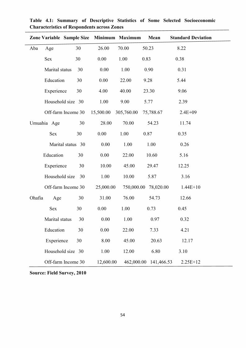
54

Table 4.1: Summary of Descriptive Statistics of Some Selected SocioeconomicCharacteristics of Respondents across Zones

Zone Variable Sample Size Minimum Maximum Mean Standard Deviation

Aba Age 30 26.00 70.00 50.23 8.22

Sex 30 0.00 1.00 0.83 0.38

Marital status 30 0.00 1.00 0.90 0.31

Education 30 0.00 22.00 9.28 5.44

Experience 30 4.00 40.00 23.30 9.06

Household size 30 1.00 9.00 5.77 2.39

Off-farm Income 30 15,500.00 305,760.00 75,788.67 2.4E+09

Umuahia Age 30 28.00 70.00 54.23 11.74

Sex 30 0.00 1.00 0.87 0.35

Marital status 30 0.00 1.00 1.00 0.26

Education 30 0.00 22.00 10.60 5.16

Experience 30 10.00 45.00 29.47 12.25

Household size 30 1.00 10.00 5.87 3.16

Off-farm Income 30 25,000.00 750,000.00 78,020.00 1.44E+10

Ohafia Age 30 31.00 76.00 54.73 12.66

Sex 30 0.00 1.00 0.73 0.45

Marital status 30 0.00 1.00 0.97 0.32

Education 30 0.00 22.00 7.33 4.21

Experience 30 8.00 45.00 20.63 12.17

Household size 30 1.00 12.00 6.80 3.10

Off-farm Income 30 12,600.00 462,000.00 141,466.53 2.25E+12

Source: Field Survey, 2010

55

However, in the opinion of Kebede (2001), women appear to be more efficient than

the men when it comes to frequent supervision and follow up of farm activities on the farm.

The predominance of the males in agricultural activities as shown in the three agricultural

zones surveyed could be justified by the cultural setting of the areas which grants the males

easy access to not only land but also other production inputs especially where majority of the

household heads are males. There is indication that majority of the farmers are mature in

handling agricultural activities appropriately given that in all the zones the generality of the

farmers were married.

The result of study showed that the level of illiteracy among farmers in the study area

is gradually decreasing given that the mean level of educational attainment of the farmers was

10 years for Ohafia, 11 years for Umuahia and 9 years for Aba. An average farmer in the area

can be said to be relatively literate. This contradicts the general view that majority of the

farmers are still uneducated. Exposure to education serves as a catalyst or elixir that activates

the engine of growth through efficient information acquisition and usage. Amaza and

Olayemi (2000) affirmed this and opined that educational attainment will enhance farmers’

use of improved technology hence their increased productivity.

The mean farming experience of the sampled farmers was 23 years, 29 years and 28

years for Ohafia, Umuahia and Aba agricultural zones respectively. Nwaru (2004) reported

that farmers count more on their experience than educational attainment in order to increase

their productivity. However, Kebede (2001) opined that age could be used as a proxy for

experience.

The mean household size of farmers in the three agricultural zones was 6, 6, and 7 for

Ohafia, Umuahia and Aba respectively. This implies that an average farmer’s household size

across the zones is relatively high. To this, Effiong (2005) explained enhances the availability

of family labour since it reduces labour cost in agricultural production. This is true in the

56

study area for arable crop-livestock production in the surveyed areas. However, Okike (2000)

reported that labour availability through large household sizes may not be a guarantee for

increased efficiency, particularly where majority of the household members are little

children. For such a situation, family labour may be underutilized given the small – scale

nature of food production activities.

The mean off-farm income for the sampled farmers in Aba, Umuahia and Ohafia

agricultural zones were N75,788.67, N78,020.00 and 141,466.53 respectively. This implies

that in all the agricultural zones the sampled farmers relatively have the wherewithal to

support their agricultural activities in spite of the almost absence of formal capital borrowing.

4.2 Crop and Livestock Yields and Value of Yield per Hectare and per Livestock

capacities

The yields of crops produced both as sole and as mixtures and their value of the yields

as well as those of the selected livestock mainly monogastrics combined by some of the

arable crop farmers are presented in Tables 4.2, 4.3 and 4.4 for Aba, Umuahia and Ohafia

agricultural zones.

57

Table 4.2: Yield, Value of Output and Farm Prices of Some Selected Arable Crops and Animal Produce for Aba Agricultural Zone, AbiaState

EnterpriseCrop Yield (tons per hectare) Price (N) per kg Price (N) per ton Value of output per ha (N)YamYam 4.713 130.00 130,000.00 611,000.00Cassava/MaizeCassava 6.291 25.35 25,350.00 159,476.85Maize 0.387 30.86 30,860.00 11,930.48Yam/ MelonYam 4.030 138.00 138,000.00 556,140.00Melon 0.105 46.00 46,000.00 4,834.60.00Cassava/MelonCassava 8.443 27.00 27,000.00 227,947.50Melon 0.250 52.00 52,000.00 13,000.00Maize/Yam/Telferia leafMaize 0.613 29.00 29,000.00 17,765.40Yam 3.056 120.00 120,000.00 366,672.00Telferia 0.059 50.00 50,000.00 2,950.00Cassava/Maize/MelonCassava 8.1747 26.00 26,000.00 212,542.20Maize 0.614 32.24 32,240.00 19,788.59Melon 0.2505 50.00 50,000.00 12,524.00Maize/Yam/MelonMaize 0.613 30.00 30,000.00 18,378.00Yam 3.196 140.00 140,000.00 447,482.00Melon 0.120 48.00 48,000.00 5,760.00Cassava/Maize/YamCassava 8.361 27.00 27,000.00 225,741.60Maize 0.613 35.00 35,000.00 21,441.00Yam 3.265 145.00 145,000.00 473,425.00Cassava/Maize/CocoyamCassava 3.137 23.91 23,910.00 75,000.89Maize 0.390 30.00 30,000.00 11,712.00Cocoyam 1.079 59.50 59,500.00 64,218.35Cassava/Maize/Yam/ mucuna floaneiCassava 4.052 25.09 25,090.00 101,652.13Maize 0.459 35.00 35,000.00 16,058.00Yam 3.460 150.00 150,000.00 519,000.00Mucuna floanei 0.197 116.67 116,670.00 22,972.32Cassava/Maize/Yam/CowpeaCassava 4.243 27.00 27,000.00 114,569.10Maize 1.697 30.00 30,000.00 50,895.00Yam 2.631 150.00 150,000.00 394,680.00Cowpea 0.374 59.85 59,850.00 22,377.92Cassava/Maize/Melon/mucuna floaneiCassava 6.279 27.09 27,090.00 170,084.57Maize 0.608 40.30 40,300.00 24,518.52Melon 0.250 50.00 50,000.00 12,500.00Mucuna floanei 0.197 116.60 116,600.00 22,958.54Cassava/Maize/Melon/CowpeaCassava 9.003 25.96 25,960.00 233,718.85Maize 0.610 30.07 30,070.00 18,342.70Melon 0.249 50.00 50,000.00 12,470.00Cowpea 0.119 60.00 60,000.00 7,140.00Cassava/Maize/Yam/MelonCassava 2.5761 26.09 26,090.00 67,210.45Maize 0.2782 33.78 33,780.00 9,397.60Yam 1.1739 135.00 135,000.00 9,397.60Melon 0.1164 49.98 49,980.00 5,817.67Cassava/Maize/Yam/Melon/Telferia leafCassava 7.6755 27.00 27,000.00 207,238.50Maize 0.6126 30.00 30,000.00 18,378.00Yam 4.5387 129.00 129,000.00 585,492.00Melon 0.30 51.47 51,470.00 15,441.00Telferia 0.2882 50.00 50,000.00 14,410.00Livestock EnterprisePoultry Yield (tons per 500 birds) Price (N) per kg Price (N) per ton Value of output per 500 birds (N)Broiler I 1.33 528.30 528,300.00 702,639.00Broiler II 1.23 500.00 500,000.00 615,000.00Fish Yield (tons per 1000 fish) Price (N) per kg Price (N) per ton Value of output per 1000 fish (N)Fish I 0.98 499.78 449,780.00 489,784.00Fish II 1.15 550.00 550,000.00 632, 500.00Pig Yield (tons per 15 pigs ) Price (N) per kg Price (N) per ton Value of output per 15 pigs (N)Pig 0.315 640.00 640,000.00 201,600.00

Source: Field Survey, 2010

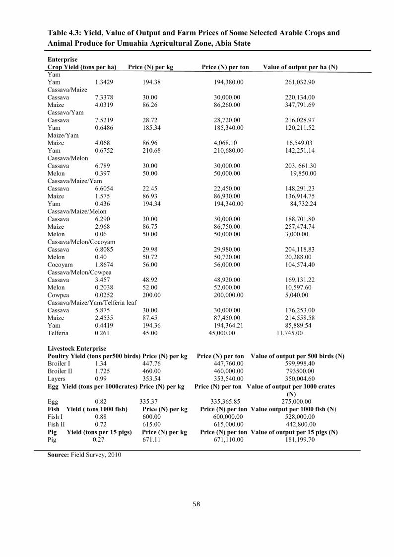
58

Table 4.3: Yield, Value of Output and Farm Prices of Some Selected Arable Crops andAnimal Produce for Umuahia Agricultural Zone, Abia State

EnterpriseCrop Yield (tons per ha) Price (N) per kg Price (N) per ton Value of output per ha (N)YamYam 1.3429 194.38 194,380.00 261,032.90Cassava/MaizeCassava 7.3378 30.00 30,000.00 220,134.00Maize 4.0319 86.26 86,260.00 347,791.69Cassava/YamCassava 7.5219 28.72 28,720.00 216,028.97Yam 0.6486 185.34 185,340.00 120,211.52Maize/YamMaize 4.068 86.96 4,068.10 16,549.03Yam 0.6752 210.68 210,680.00 142,251.14Cassava/MelonCassava 6.789 30.00 30,000.00 203, 661.30Melon 0.397 50.00 50,000.00 19,850.00Cassava/Maize/YamCassava 6.6054 22.45 22,450.00 148,291.23Maize 1.575 86.93 86,930.00 136,914.75Yam 0.436 194.34 194,340.00 84,732.24Cassava/Maize/MelonCassava 6.290 30.00 30,000.00 188,701.80Maize 2.968 86.75 86,750.00 257,474.74Melon 0.06 50.00 50,000.00 3,000.00Cassava/Melon/CocoyamCassava 6.8085 29.98 29,980.00 204,118.83Melon 0.40 50.72 50,720.00 20,288.00Cocoyam 1.8674 56.00 56,000.00 104,574.40Cassava/Melon/CowpeaCassava 3.457 48.92 48,920.00 169,131.22Melon 0.2038 52.00 52,000.00 10,597.60Cowpea 0.0252 200.00 200,000.00 5,040.00Cassava/Maize/Yam/Telferia leafCassava 5.875 30.00 30,000.00 176,253.00Maize 2.4535 87.45 87,450.00 214,558.58Yam 0.4419 194.36 194,364.21 85,889.54Telferia 0.261 45.00 45,000.00 11,745.00

Livestock EnterprisePoultry Yield (tons per500 birds) Price (N) per kg Price (N) per ton Value of output per 500 birds (N)Broiler I 1.34 447.76 447,760.00 599,998.40Broiler II 1.725 460.00 460,000.00 793500.00Layers 0.99 353.54 353,540.00 350,004.60Egg Yield (tons per 1000crates) Price (N) per kg Price (N) per ton Value of output per 1000 crates

(N)Egg 0.82 335.37 335,365.85 275,000.00Fish Yield ( tons 1000 fish) Price (N) per kg Price (N) per ton Value output per 1000 fish (N)Fish I 0.88 600.00 600,000.00 528,000.00Fish II 0.72 615.00 615,000.00 442,800.00Pig Yield (tons per 15 pigs) Price (N) per kg Price (N) per ton Value of output per 15 pigs (N)Pig 0.27 671.11 671,110.00 181,199.70

Source: Field Survey, 2010

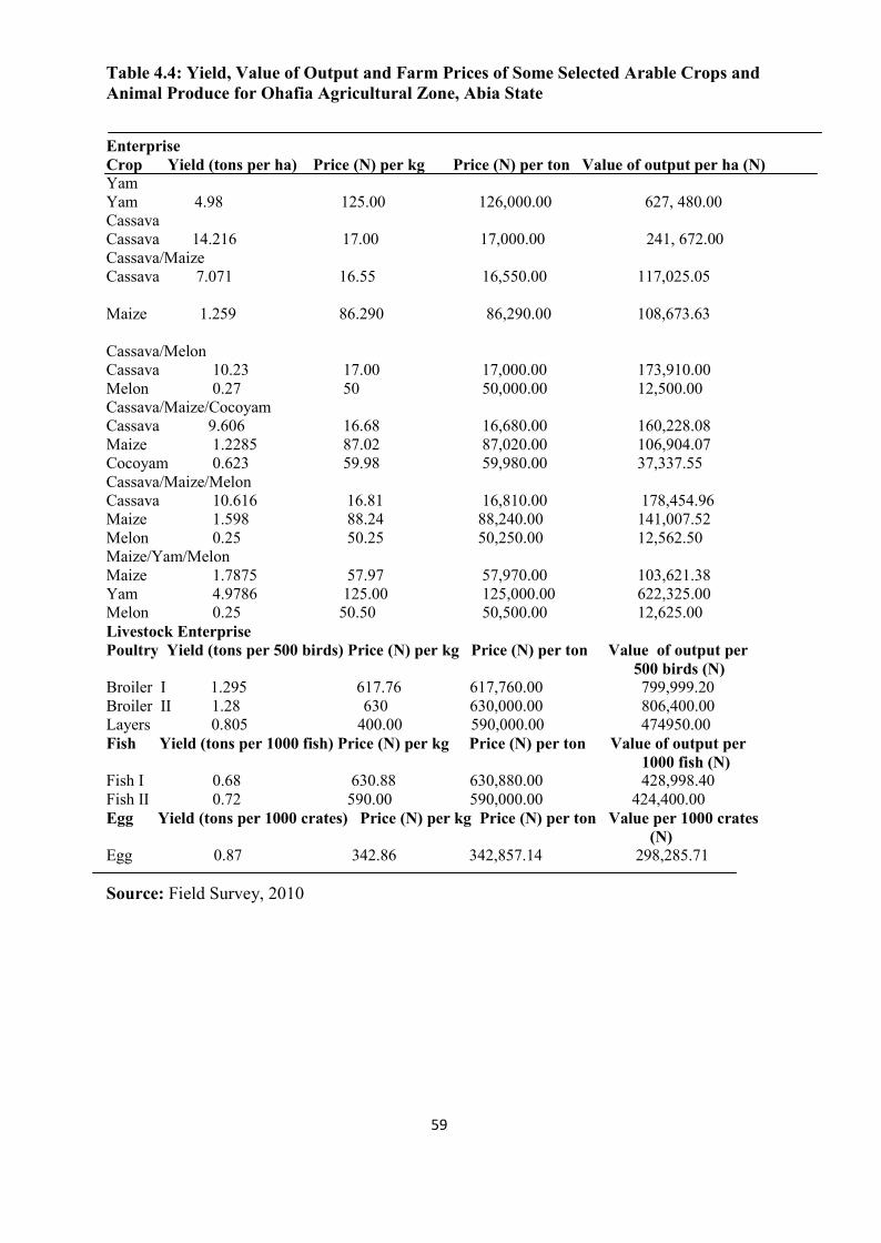
59

Table 4.4: Yield, Value of Output and Farm Prices of Some Selected Arable Crops andAnimal Produce for Ohafia Agricultural Zone, Abia State

EnterpriseCrop Yield (tons per ha) Price (N) per kg Price (N) per ton Value of output per ha (N)YamYam 4.98 125.00 126,000.00 627, 480.00CassavaCassava 14.216 17.00 17,000.00 241, 672.00Cassava/MaizeCassava 7.071 16.55 16,550.00 117,025.05

Maize 1.259 86.290 86,290.00 108,673.63

Cassava/MelonCassava 10.23 17.00 17,000.00 173,910.00Melon 0.27 50 50,000.00 12,500.00Cassava/Maize/CocoyamCassava 9.606 16.68 16,680.00 160,228.08Maize 1.2285 87.02 87,020.00 106,904.07Cocoyam 0.623 59.98 59,980.00 37,337.55Cassava/Maize/MelonCassava 10.616 16.81 16,810.00 178,454.96Maize 1.598 88.24 88,240.00 141,007.52Melon 0.25 50.25 50,250.00 12,562.50Maize/Yam/MelonMaize 1.7875 57.97 57,970.00 103,621.38Yam 4.9786 125.00 125,000.00 622,325.00Melon 0.25 50.50 50,500.00 12,625.00Livestock EnterprisePoultry Yield (tons per 500 birds) Price (N) per kg Price (N) per ton Value of output per

500 birds (N)Broiler I 1.295 617.76 617,760.00 799,999.20Broiler II 1.28 630 630,000.00 806,400.00Layers 0.805 400.00 590,000.00 474950.00Fish Yield (tons per 1000 fish) Price (N) per kg Price (N) per ton Value of output per

1000 fish (N)Fish I 0.68 630.88 630,880.00 428,998.40Fish II 0.72 590.00 590,000.00 424,400.00Egg Yield (tons per 1000 crates) Price (N) per kg Price (N) per ton Value per 1000 crates

(N)Egg 0.87 342.86 342,857.14 298,285.71

Source: Field Survey, 2010

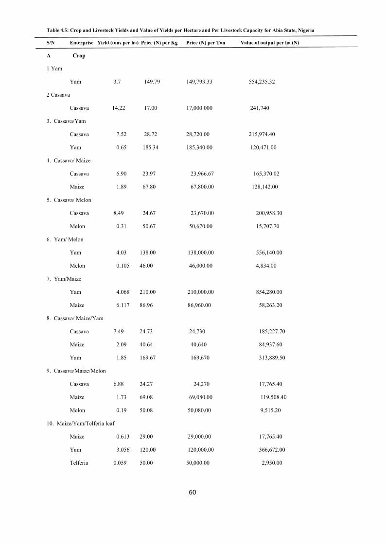
60

Table 4.5: Crop and Livestock Yields and Value of Yields per Hectare and Per Livestock Capacity for Abia State, Nigeria

S/N Enterprise Yield (tons per ha) Price (N) per Kg Price (N) per Ton Value of output per ha (N)

A Crop

1 Yam

Yam 3.7 149.79 149,793.33 554,235.32

2 Cassava

Cassava 14.22 17.00 17,000.000 241,740

3. Cassava/Yam

Cassava 7.52 28.72 28,720.00 215,974.40

Yam 0.65 185.34 185,340.00 120,471.00

4. Cassava/ Maize

Cassava 6.90 23.97 23,966.67 165,370.02

Maize 1.89 67.80 67,800.00 128,142.00

5. Cassava/ Melon

Cassava 8.49 24.67 23,670.00 200,958.30

Melon 0.31 50.67 50,670.00 15,707.70

6. Yam/ Melon

Yam 4.03 138.00 138,000.00 556,140.00

Melon 0.105 46.00 46,000.00 4,834.00

7. Yam/Maize

Yam 4.068 210.00 210,000.00 854,280.00

Maize 6.117 86.96 86,960.00 58,263.20

8. Cassava/ Maize/Yam

Cassava 7.49 24.73 24,730 185,227.70

Maize 2.09 40.64 40,640 84,937.60

Yam 1.85 169.67 169,670 313,889.50

9. Cassava/Maize/Melon

Cassava 6.88 24.27 24,270 17,765.40

Maize 1.73 69.08 69,080.00 119,508.40

Melon 0.19 50.08 50,080.00 9,515.20

10. Maize/Yam/Telferia leaf

Maize 0.613 29.00 29,000.00 17,765.40

Yam 3.056 120,00 120,000.00 366,672.00

Telferia 0.059 50.00 50,000.00 2,950.00

61

11.Maize/Yam/Melon

Maize 1.20 44.02 44,020.00 52,824.00

Yam 4.09 132.50 132,500.00 541,925.00

Melon 0.185 49.25 49,250.00 9,111.25

12. Cassava/Maize/Cocoyam

Cassava 5.92 23.52 23,523.33 139,258.11

Maize 0.81 58.51 58,510.00 47,393.10

Cocoyam 0.851 59.74 59,740.00 50,838.74

13. Cassava/Melon/cocoyam

Cassava 6.81 29.98 29,980.00 204,118.83

Melon 0.04 50.72 50,720.00 20,288.00

Cocoyam 1.867 56.00 56,000.00 104,574.40

14. Cassava/Melon/Cowpea

Cassava 3.46 48.92 48,920.00 169,652.13

Melon 0.204 52.00 52,000.00 10,597.60

Cowpea 0.025 200.00 200,000.00 5,040.00

15. Cassava/Maize/Yam/mucuna floanei

Cassava 4.052 25.09 25,090.00 101,652.13

Maize 0.459 35 35,000.00 16,058.00

Yam 3.460 150 150,000.00 519,000.00

Mucuna floanei 0.197 116.67 116,670.00 22,972.22

16. Cassava/Maize/Yam/Cowpea

Cassava 4.243 27 27,000.00 114,569.10

Maize 1.697 30 30,000.00 50,895.00

Yam 2.631 150 150,000.00 394,680.00

Cowpea

17. Cassava/ Maize/Melon/mucuna floanei

Cassava 6.279 27.09 27,090.00 170,084.57

Maize 0.608 40.30 40,300.00 24,518.52

Melon 0.250 50.00 50,000.00 12,500.00

Mucuna floanei 0.197 116.60 116,600.00 22,985.54

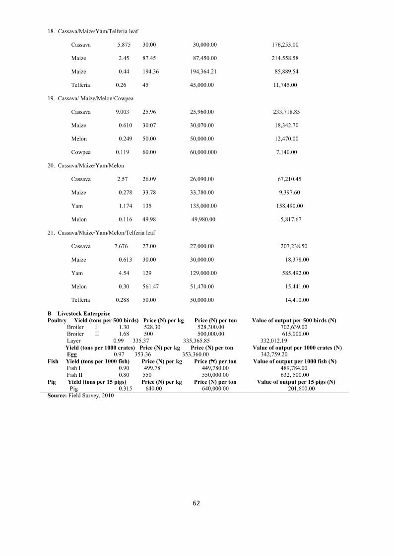
62

18. Cassava/Maize/Yam/Telferia leaf

Cassava 5.875 30.00 30,000.00 176,253.00

Maize 2.45 87.45 87,450.00 214.558.58

Maize 0.44 194.36 194,364.21 85,889.54

Telferia 0.26 45 45,000.00 11,745.00

19. Cassava/ Maize/Melon/Cowpea

Cassava 9.003 25.96 25,960.00 233,718.85

Maize 0.610 30.07 30,070.00 18,342.70

Melon 0.249 50.00 50,000.00 12,470.00

Cowpea 0.119 60.00 60,000.000 7,140.00

20. Cassava/Maize/Yam/Melon

Cassava 2.57 26.09 26,090.00 67,210.45

Maize 0.278 33.78 33,780.00 9,397.60

Yam 1.174 135 135,000.00 158,490.00

Melon 0.116 49.98 49,980.00 5,817.67

21. Cassava/Maize/Yam/Melon/Telferia leaf

Cassava 7.676 27.00 27,000.00 207,238.50

Maize 0.613 30.00 30,000.00 18,378.00

Yam 4.54 129 129,000.00 585,492.00

Melon 0.30 561.47 51,470.00 15,441.00

Telferia 0.288 50.00 50,000.00 14,410.00

B Livestock EnterprisePoultry Yield (tons per 500 birds) Price (N) per kg Price (N) per ton Value of output per 500 birds (N)

Broiler I 1.30 528.30 528,300.00 702,639.00Broiler II 1.68 500 500,000.00 615,000.00Layer 0.99 335.37 335,365.85 332,012.19

Yield (tons per 1000 crates) Price (N) per kg Price (N) per ton Value of output per 1000 crates (N)Egg 0.97 353.36 353,360.00 342,759.20

Fish Yield (tons per 1000 fish) Price (N) per kg Price (N) per ton Value of output per 1000 fish (N)Fish I 0.90 499.78 449,780.00 489,784.00Fish II 0.80 550 550,000.00 632, 500.00

Pig Yield (tons per 15 pigs) Price (N) per kg Price (N) per ton Value of output per 15 pigs (N)Pig 0.315 640.00 640,000.00 201,600.00

Source: Field Survey, 2010

63

4.3 Arable Land holdings of Farmers in the Study Area

The farm size of the respondents as it relates to their arable farm holdings in Aba, Umuahia

and Ohafia agricultural zones is presented in Table 4.6.

Table 4.6: Frequency Distribution of Farmers According to the Farm size in the Agricultural Zones

Zone Farm size Frequency Percentage

Aba 0.13 - 0.27 9 30.00

0.28 - 0.42 9 30.00

0.43 - 0.57 3 10.00

0.58 – 0.72 4 13.33

٤

0.88 – 1.02 1 3.33

1.03 – 1.17 2 6.67

٤

1.93 – 2.07 1 3.33

٤

3.88 – 4.02 1 3.33

Total 30 100

Mean 0.45ha

Standard Deviation 0.81

Umuahia 0.13 - 0.27 9 30.00

0.28 - 0.42 7 23.33

0.43 – 0.57 8 26.67

0.58 – 0.72 6 20.00

Total 30 100

Mean 0.43ha

Standard Deviation 0.17

Ohafia 0.13 - 0.27 7 23.33

0.28 – 0.42 8 26.67

0.43 – 0.57 6 20.00

0.58 – 0.72 8 26.67

0.73 – 0.87 1 3.33

Total 30 100

Mean 0.38ha

Standard Deviation 0.20

Source: Field Survey Data, 2010

64

The result showed that 60% of the farmers in Aba had farm size of less than or

about 0.42 hectares. Only 3.33% of the farmers had farm size of between 0.88 and 1.02 and

3.85 and 4.02 respectively. This also shows that farmers in Aba zone are small holder

farmers. This could be as a result of intense fragmentation of land which militates against

large scale production. The table shows the mean and standard deviation to be 0.45 and 0.81

respectively for Aba zone for instance. For all the sampled farmers in Umuahia, no farmer

had a farm holding of more than a hectare of farm land devoted to arable crop farming while

about 30% of the farmers had about 0.27 hectares or less and only 20% had between 0.50 and

0.72 hectares.

Table 4.6 also show that farmers in Ohafia zone were operating at a subsistent level of

farming so high to permit large scale production. In other words these farmers could be

referred to as small holder farmers (peasant farmers). The table also shows the mean and

standard deviation respectively to be 0.38 and 0.20. Relative to Aba that has a standard

deviation of 0.81; it implies that the size of the farms is relatively similar among the sampled

farmers. However in all the zones, therefore, all the arable crop farmers were small scaled

with their level increasing from Ohafia, Umuahia to Aba.

4.4 Results of the Linear Programming Simplex Tableau

4.4. 1 Existing and Optimum Cropping/Enterprise Patterns

The existing and optimum enterprise patterns for Aba, Umuahia and Ohafia

agricultural zones for the sampled farmers using the LP Simplex Tableau are presented in

Tables 4.7, 4.8 and 4.9 respectively. The study prescribed that for Aba zone, no sole crop

enterprises should be produced but crop mixtures. The result suggested that 0.31 hectare of

yam/maize/melon, 0.33 hectare of cassava/maize/cocoyam and 1.30 hectares of

cassava/maize/melon/mucuna floanei while 0.14 of 500 birds (70.00 birds) of broiler II, 0.11

of 1000 fish (110.00 fish) of fish II and 0.07 of 15 pigs (1.05 pigs) of livestock enterprises

65

should be produced. Results in Umuahia agricultural zone recommended 0.72 hectare of yam,

0.02 hectare of maize/yam and 3.26 hectares of cassava/yam/cowpea, while 0.11 of 15 pigs

(1.65 pigs) and 0.17 of 500 birds (85.00 birds) of broiler II were prescribed for production in

the livestock enterprise.

However, it was prescribed that 0.29 hectare of yam, 0.02 of cassava, 0.13 hectare of

cassava/maize/cocoyam, 0.14 of 500 birds (70.00 birds) of broiler II, 0.22 of 1000 fish

(220.00 fish) of fish I and 0.41 of 500 birds (205.00 birds) of Layer be produced to maximize

gross margin in Ohafia. It was only in Ohafia that there was a strong indication of more of

sole crop enterprise than crop mixtures though at relatively low level in terms of

recommended hectrage in the optimum plan.

When a representative sample for the entire Abia state was derived and the LP model

applied to the data, there was entirely a different recommendation. The model recommended

0.88ha of yam/maize, 0.21ha of cassava/melon/cocoyam, cassava/maize/melon/mucuna

floanei (0.91ha) and cassava/maize/yam/telferia leaf (0.08ha). However, 0.13 of 500 birds

(65.00 birds) of bro11, 0.67 of 500 birds (335.00 birds) of layer and 0.21 of 15 pigs (3.15

pigs) were prescribed for livestock enterprises in the state.

The implication therefore is that for an average farmer sampled in the state to maximise

gross margin, emphasis should be on Bro 11 done between August and December and the

layer enterprise according to the prescribed plan in the combination with the recommended

crop enterprises. Sole cropping pattern was not recommended in the plan at all. Table 4.10

shows the existing and optimum enterprise pattern for the selected enterprises in Abia State.

66

Table 4.7: Existing and Optimum Cropping/ Enterprise Patterns for Aba AgriculturalZone

Cropping/Enterprise pattern Existing plan (ha) Optimum plan (ha)Size of farm Percentage Size of farm Percentage

1. Yam 0.18 4.77 - -2. Cassava / Maize 0.57 15.12 - -3. Yam/ Melon 0.21 5.57 - -4. Cassava / Melon 0.19 5.04 - -5. Maize / Yam / Telferia 0.11 2.92 - -6. Cassava/ Maize/Melon 0.03 0.80 - -7. Yam/Maize/Melon 0.08 2.12 0.31 15.988. Cassava/Maize/Melon 0.24 6.37 - -9. Cassava/Maize/Cocoyam 0.31 8.22 0.33 17.0110. Cassava/Maize/Yam/mucuna

floanei0.13 3.45 - -

11. Cassava/Maize/Yam/Cowpea 0.13 3.45 - -12. Cassava/Maize/Melon/mucua

floanei0.33 8.75 1.30 67.09

13. Cassava/Maize/Melon/Cowpea 0.13 3.45 - -14. Cassava/Maize/Yam/Melon 0.28 7.43 - -15. Cassava/Maize/Yam/Melon/

Telferia

0.85 22.55 - -

16. Broiler 1 Jan-May 0.48 57.14 0.14 10017. Broiler 11 Aug-Dec 0.36 42.86 - -18. Fish 1 Jan-June 0.45 27.27 - -19. Fish 11 July- Dec 1.20 72.73 0.11 10020. Pig 1.40 100.00 0.07 100

Total Crop Area 3.77 1.94

% Sole 4.77 0.00% Crop Mixture 95.23 100Total Poultry 0.84 0.14

% Broilers 100 100Fish 1.65 0.11

% Fish 100 100

Source: Field Survey, 2010

67

Table 4.8: Existing and Optimum Cropping/Enterprise Pattern in UmuahiaAgricultural Zone, Abia State, Nigeria

Cropping/Enterprise pattern Existing plan (ha) Optimum plan (ha)Size of farm Percentage Size of farm Percentage

1. Yam 0.31 12.25 0.72 17.96

2. Cassava / Maize 0.25 9.88 - -

3. Cassava/Yam 0.12 4.74 - -

4. Maize/ Yam 0.14 5.53 0.03 0.75

5. Cassava/ Melon 0.22 8.70 - -

6. Cassava/ Melon/Yam 0.19 7.51 - -

7. Cassava/ Maize/ Melon 0.27 8.70 - -

8. Cassava/Melon/ Cocoyam 0.64 25.30 - -

9. Cassava/Melon/Cowpea 0.21 8.30 3.26 81.30

10. Cassava/Maize/Yam/Telferia 0.23 9.09 - -

11. Pig 0.19 100 0.11 100

12. Broilers 1 Jan-May 0.36 33.33 - -

13. Broilers 11 Aug-Dec 0.28 25.93 0.02 5.13

14. Layers/Egg- Jan-Dec 0.14 40.74 0.37 94.87

15. Fish 1-Jan-June 0.90 62.07 0.06 100

16. Fish 11 July-Dec 0.55 37.93 - -

Total crop area 2.53 4.01

% Sole 12.25 17.96

% Crop Mixture 87.75 82.05

Total Poultry 1.08 0.39

% Broilers 59.26 5.13

% Layers 40.74 94.87

Total Fisheries 1.45 0.10

100 100

Total Pig 0.19 0.11

% Pig 100 100

Source: Field survey, 2010

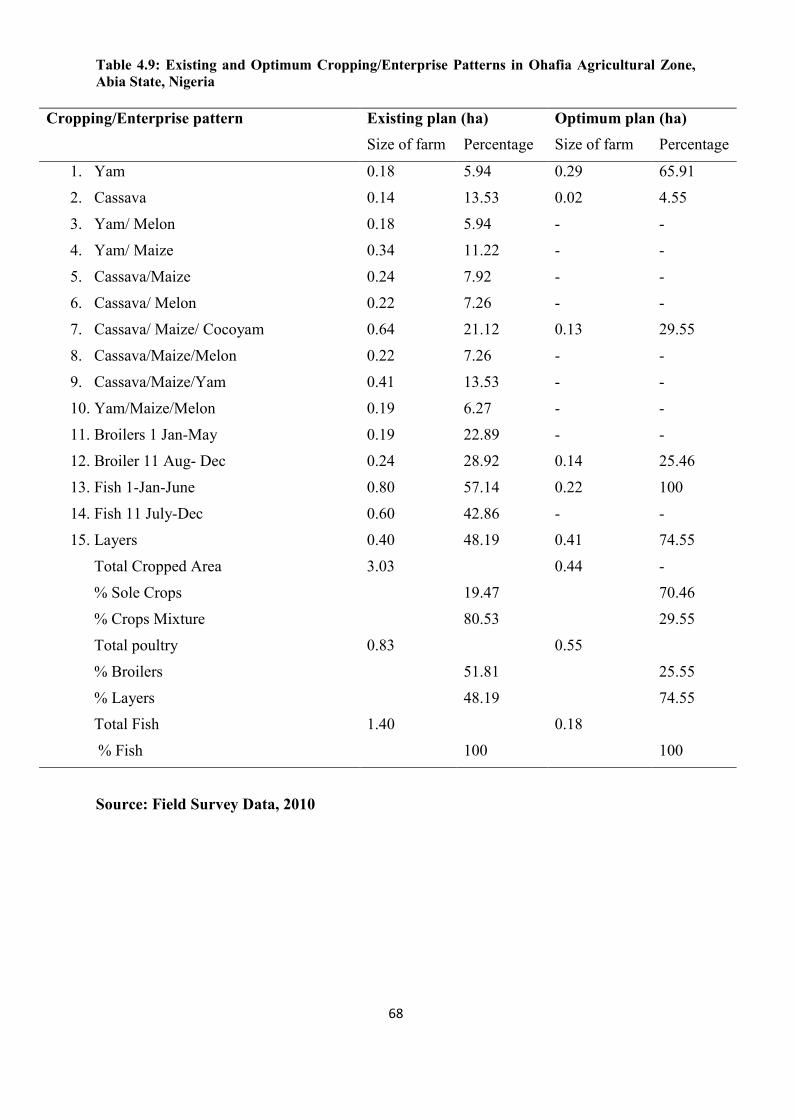
68

Table 4.9: Existing and Optimum Cropping/Enterprise Patterns in Ohafia Agricultural Zone,Abia State, Nigeria

Cropping/Enterprise pattern Existing plan (ha) Optimum plan (ha)Size of farm Percentage Size of farm Percentage

1. Yam 0.18 5.94 0.29 65.91

2. Cassava 0.14 13.53 0.02 4.55

3. Yam/ Melon 0.18 5.94 - -

4. Yam/ Maize 0.34 11.22 - -

5. Cassava/Maize 0.24 7.92 - -

6. Cassava/ Melon 0.22 7.26 - -

7. Cassava/ Maize/ Cocoyam 0.64 21.12 0.13 29.55

8. Cassava/Maize/Melon 0.22 7.26 - -

9. Cassava/Maize/Yam 0.41 13.53 - -

10. Yam/Maize/Melon 0.19 6.27 - -

11. Broilers 1 Jan-May 0.19 22.89 - -

12. Broiler 11 Aug- Dec 0.24 28.92 0.14 25.46

13. Fish 1-Jan-June 0.80 57.14 0.22 100

14. Fish 11 July-Dec 0.60 42.86 - -

15. Layers 0.40 48.19 0.41 74.55

Total Cropped Area 3.03 0.44 -

% Sole Crops 19.47 70.46

% Crops Mixture 80.53 29.55

Total poultry 0.83 0.55

% Broilers 51.81 25.55

% Layers 48.19 74.55

Total Fish 1.40 0.18

% Fish 100 100

Source: Field Survey Data, 2010

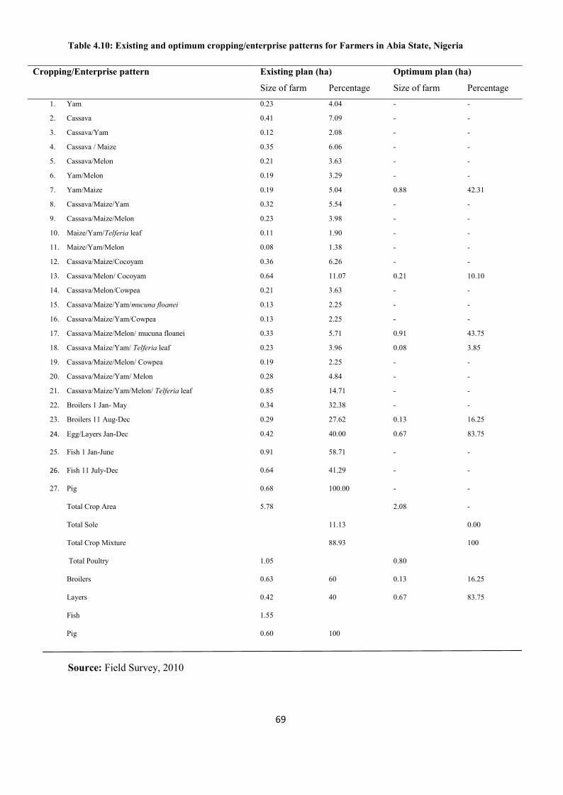
69

Table 4.10: Existing and optimum cropping/enterprise patterns for Farmers in Abia State, Nigeria

Cropping/Enterprise pattern Existing plan (ha) Optimum plan (ha)

Size of farm Percentage Size of farm Percentage1. Yam 0.23 4.04 - -

2. Cassava 0.41 7.09 - -

3. Cassava/Yam 0.12 2.08 - -

4. Cassava / Maize 0.35 6.06 - -

5. Cassava/Melon 0.21 3.63 - -

6. Yam/Melon 0.19 3.29 - -

7. Yam/Maize 0.19 5.04 0.88 42.31

8. Cassava/Maize/Yam 0.32 5.54 - -

9. Cassava/Maize/Melon 0.23 3.98 - -

10. Maize/Yam/Telferia leaf 0.11 1.90 - -

11. Maize/Yam/Melon 0.08 1.38 - -

12. Cassava/Maize/Cocoyam 0.36 6.26 - -

13. Cassava/Melon/ Cocoyam 0.64 11.07 0.21 10.10

14. Cassava/Melon/Cowpea 0.21 3.63 - -

15. Cassava/Maize/Yam/mucuna floanei 0.13 2.25 - -

16. Cassava/Maize/Yam/Cowpea 0.13 2.25 - -

17. Cassava/Maize/Melon/ mucuna floanei 0.33 5.71 0.91 43.75

18. Cassava Maize/Yam/ Telferia leaf 0.23 3.96 0.08 3.85

19. Cassava/Maize/Melon/ Cowpea 0.19 2.25 - -

20. Cassava/Maize/Yam/ Melon 0.28 4.84 - -

21. Cassava/Maize/Yam/Melon/ Telferia leaf 0.85 14.71 - -

22. Broilers 1 Jan- May 0.34 32.38 - -

23. Broilers 11 Aug-Dec 0.29 27.62 0.13 16.25

24. Egg/Layers Jan-Dec 0.42 40.00 0.67 83.75

25. Fish 1 Jan-June 0.91 58.71 - -

26. Fish 11 July-Dec 0.64 41.29 - -

27. Pig 0.68 100.00 - -

Total Crop Area 5.78 2.08 -

Total Sole 11.13 0.00

Total Crop Mixture 88.93 100

Total Poultry 1.05 0.80

Broilers 0.63 60 0.13 16.25

Layers 0.42 40 0.67 83.75

Fish 1.55

Pig 0.60 100

Source: Field Survey, 2010

70

4.4.2 Gross Margin among various Plans

The gross margins for the existing and optimum plans for selected farmers in Aba,

Umuahia and Ohafia agricultural zones as well as for the entire state are presented in Table

4.11.

Table 4.11: Gross Margin (in Naira) for Existing and Optimum Plans for the SelectedFarmers in the three Zones and the entire State

Existing Plan Optimum Plan Increase/Decrease Over Existing Plan

%

Zone

Aba 232,317.12 374,850.80 142,533.68 61.35

Umuahia 271,150.75 499,229.90 228,079.15 84.12

Ohafia 222,056.32 383,941.60 161,885.28 72.90

Abia State 259, 180.47 310,638.00 51,122.13 19.73

Source: Field Survey Data, 2010

Results in Table 4.11 indicate that optimum plans resulted in an increase in gross

margin over the existing plan across the zones by 84.12% in Umuahia, 72.90% in Ohafia and

61.35% in Aba. The findings were high relative to values obtained among crop farmers in

Niger State on raising their income level (Tanko and Baba, 2010). The introduction of

livestock enterprises among the crop enterprises could explain for the relatively high

optimum values relative to studies where only crop enterprises were evaluated.

The optimum gross margin derived from the State by the LP solution was however not

as high as was obtained from each of the zones. This implies that the selected farmers were

competitively better in maximizing gross margin within the zones than the State. Variability

in resource endowment does exist within zones, communities and even villages. Although by

pooling all the farmers together at State level, greater number of activities were considered

since the greater the activities ceteris paribus, the better the expected LP solution to be

derived, it does not always guarantee that better resource allocation would be made.

71

4.4.3 Labour Utilization

Labour utilization for the different agricultural zones is presented in Table 4.12 while

that for the entire state is presented in Table 4.13. The general observation was that more

labour was utilized in crop production than in livestock enterprises in the zones except

Ohafia. The optimum plan recommended that less labour be utilized for livestock than the

crop enterprises across the entire zone as prescribed but more labour be employed for

livestock than crop production in Ohafia. However, Umuahia had the least labour

requirement for livestock relative to other zones within the livestock optimum labour

utilization.

Table 4.12: Labour Utilization across the three Agricultural Zones

ZONE: Aba Umuahia Ohafia

PLAN: Existing Optimum Existing Optimum Existing Optimum

Crop

LPP 110 102.07 92 93.31 60 9.86

1st Weeding 90 21.79 110 102.21 70 14.36

2nd Weeding 90 58.98 70 134.18 80 12.34

Harvesting 120 98.73 110 237.63 90 22.25

Total 410 281.5 382 567.33 300 58.81

Livestock

Feeding 140 30.64 90 14.83 210 114.34

Cleaning 70 11.26 85 20.73 180 44.83

Sorting 10 1.58 12 0.31 15 2.65

Harvesting 15 0.28 9 0.12 5 0.44

Total 235 43.76 196 35.99 410 162.26

Source: Field Survey Data, 2010

N/B: LPP = Land preparation and planting

72

In Table 4.12, the prescribed labour utilization by the optimum plan in both crop and

livestock categories of the enterprises were less than as obtained in the existing plan except

for the crop category in Umuahia, where if converted to percentages indicate that while

94.04% of the labour requirements were prescribed in the optimum, only 66.09% were

recommended in the existing plan, while for livestock enterprises 33.91% was observed in

the existing plan as against 5.97% prescribed in the optimum plan. It is plausible that more

mandays of labour should be utilized for crop production than livestock enterprises. The

recommendation of less than a manday of labour for sorting and harvesting operation in say

Umuahia zone was basically because of the fish enterprises for which the assumption

underlying their inclusion in modelling was that disposing of products was done by

‘’clearance’’.

There is also disparity in labour utilization between the existing and optimum plans and

within the existing plans in each category for Table 4.13. Existing plans among the two

enterprises require that 56.71% of the entire mandays of labour be devoted to crop, while

43.29% utilized for livestock production for the State. However, the optimum plan

recommendation came to about 60.52% of labour requirement for crops and 39.48% for

livestock. The result shows that higher percentage of labour was required for crop than for

livestock relative to the plans.

73

Table 4.13: Labour Utilization among the Selected Enterprises in Abia State

Existing Optimum

Crop

LPP 113.3 96.16

1st Weeding 95 88.61

2nd Weeding 90 60.30

Harvesting 115 102.43

Total 413.3 347.5

Livestock

Feeding 215 188.23

Cleaning 77.5 38.47

Sorting 11 0.00

Harvesting 12 0.00

Total 315.5 226.7

Source: Field Survey Data, 2010

N/B: LPP = Land preparation and planting

4.4.4 Shadow Prices of Excluded Activities among Selected Farmers in Abia State

Shadow prices are marginal returns to investments of available resources. In a

maximization problem, they are income penalties; indicating the amount by which farm

income would be reduced if any of the excluded activities is forced into the programme.

Olayemi and Onyenweaku (1999) had earlier reported that any resource that is abundant, that

is not used up by a programme, is not a limiting resource and has a zero shadow price as it

does not constrain the attainment of a programme’s objective and vice versa. Usually

however, only the excluded activities have positive shadow prices. For the included activities,

shadow prices are zero. The higher the shadow price of an excluded activity, the lower is its

chance of being included in the final plan. The shadow prices of excluded activities obtained

74

as by-products of the linear programme solution for Aba, Umuahia and Ohafia agricultural

zones for the sampled farmers are presented in Tables 4.14, 4.15, 4.16 and 4.17 respectively.

Results in these tables indicate the amount by which gross margin would be reduced if any of

the activities appearing in the table is forced into the programme.

Table 4.14: Shadow Prices (in Naira) of Excluded Activities in Aba Agricultural Zone

S/N Excluded Activity Shadow Price

1 Yam 249.12

2. Cassava/Maize 33,901.86

3. Yam/Melon 45,545.61

4. Cassava/Melon 1,991.59

5. Maize/Yam/Telferia leaf 10,625.42

6. Cassava/Maize/Yam 38,387.92

7. Cassava/Maize/Melon 28,290.35

8. Cassava/Maize/Yam/Mucuna floanei 1,916.92

9. Cassava/Maize/Melon/Cowpea 20,596.82

10. Cassava/Maize/Yam/Melon 53,847.48

11. Cassava/Maize/Yam/Melon/Telferia leaf 8,729.18

12. Broiler II – Aug – Dec 165,200.80

13. Fish I – January – June 34,200.00

Source: Field Survey Data, 2010

In Aba agricultural zone, a total of about 13 activities were excluded from the

programme as indicated in Table 4.14. The situation in Aba agricultural zone showed that

among the excluded arable crop enterprises, cassava/maize/yam/melon mixture has the

highest shadow price of N53,847.48, while yam has the least shadow price of N249.12. This

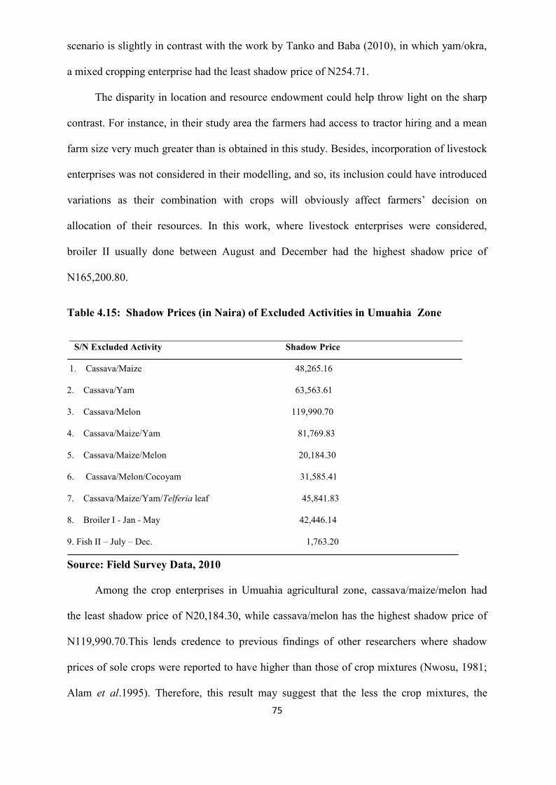
75

scenario is slightly in contrast with the work by Tanko and Baba (2010), in which yam/okra,

a mixed cropping enterprise had the least shadow price of N254.71.

The disparity in location and resource endowment could help throw light on the sharp

contrast. For instance, in their study area the farmers had access to tractor hiring and a mean

farm size very much greater than is obtained in this study. Besides, incorporation of livestock

enterprises was not considered in their modelling, and so, its inclusion could have introduced

variations as their combination with crops will obviously affect farmers’ decision on

allocation of their resources. In this work, where livestock enterprises were considered,

broiler II usually done between August and December had the highest shadow price of

N165,200.80.

Table 4.15: Shadow Prices (in Naira) of Excluded Activities in Umuahia Zone

S/N Excluded Activity Shadow Price

1. Cassava/Maize 48,265.16

2. Cassava/Yam 63,563.61

3. Cassava/Melon 119,990.70

4. Cassava/Maize/Yam 81,769.83

5. Cassava/Maize/Melon 20,184.30

6. Cassava/Melon/Cocoyam 31,585.41

7. Cassava/Maize/Yam/Telferia leaf 45,841.83

8. Broiler I - Jan - May 42,446.14

9. Fish II – July – Dec. 1,763.20

Source: Field Survey Data, 2010

Among the crop enterprises in Umuahia agricultural zone, cassava/maize/melon had

the least shadow price of N20,184.30, while cassava/melon has the highest shadow price of

N119,990.70.This lends credence to previous findings of other researchers where shadow

prices of sole crops were reported to have higher than those of crop mixtures (Nwosu, 1981;

Alam et al.1995). Therefore, this result may suggest that the less the crop mixtures, the

76

higher the shadow prices. For Ohafia agricultural zone, the selected mixed crop enterprise

was found to be in a better competitive position as compared to sole cropping and livestock

enterprises.

Shadow price of sole crop was relatively higher than those of crop mixtures. This lends

credence to previous findings (Adejobi et al, 2003; Tanko, 2004). The excluded mixed crop

enterprise was found to be relatively in a better competitive position as compared to sole

cropping and livestock enterprises except for cassava/maize/yam. However, fish I, done

usually between January and June had the least propensity to depress income among farmers.

This is at variance with the situation in Aba zone. This could be as a result of relative

exposure of farmers in across zones to technical know - how that could position one better

than the other for efficient management of the fishery resources of his farm.

Table 4.16 indicate that yam/melon mixture had the least shadow price for the crop

enterprises, while broiler I, done within January and May was less than Fish II for the

livestock enterprises excluded from the programme as well as the activity with the highest

shadow price. Fish II was thus the enterprises which if forced into the plan would depress

gross margin of the farmers in Ohafia zone the greatest.

Shadow prices of excluded activities in the Linear Programming solution for Abia State

are presented in Table 4.17. The Table shows that cassava/maize/yam/melon/telferia leaf, a

five crop enterprise had the least shadow price of N4,938.57. Fish I done within January and

June had the highest shadow price.

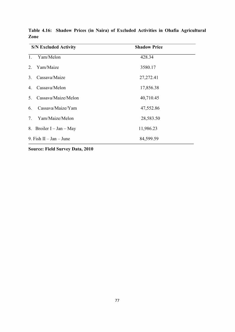
77

Table 4.16: Shadow Prices (in Naira) of Excluded Activities in Ohafia AgriculturalZone

S/N Excluded Activity Shadow Price

1. Yam/Melon 428.34

2. Yam/Maize 3580.17

3. Cassava/Maize 27,272.41

4. Cassava/Melon 17,856.38

5. Cassava/Maize/Melon 40,710.45

6. Cassava/Maize/Yam 47,552.86

7. Yam/Maize/Melon 28,583.50

8. Broiler I – Jan – May 11,986.23

9. Fish II – Jan – June 84,599.59

Source: Field Survey Data, 2010

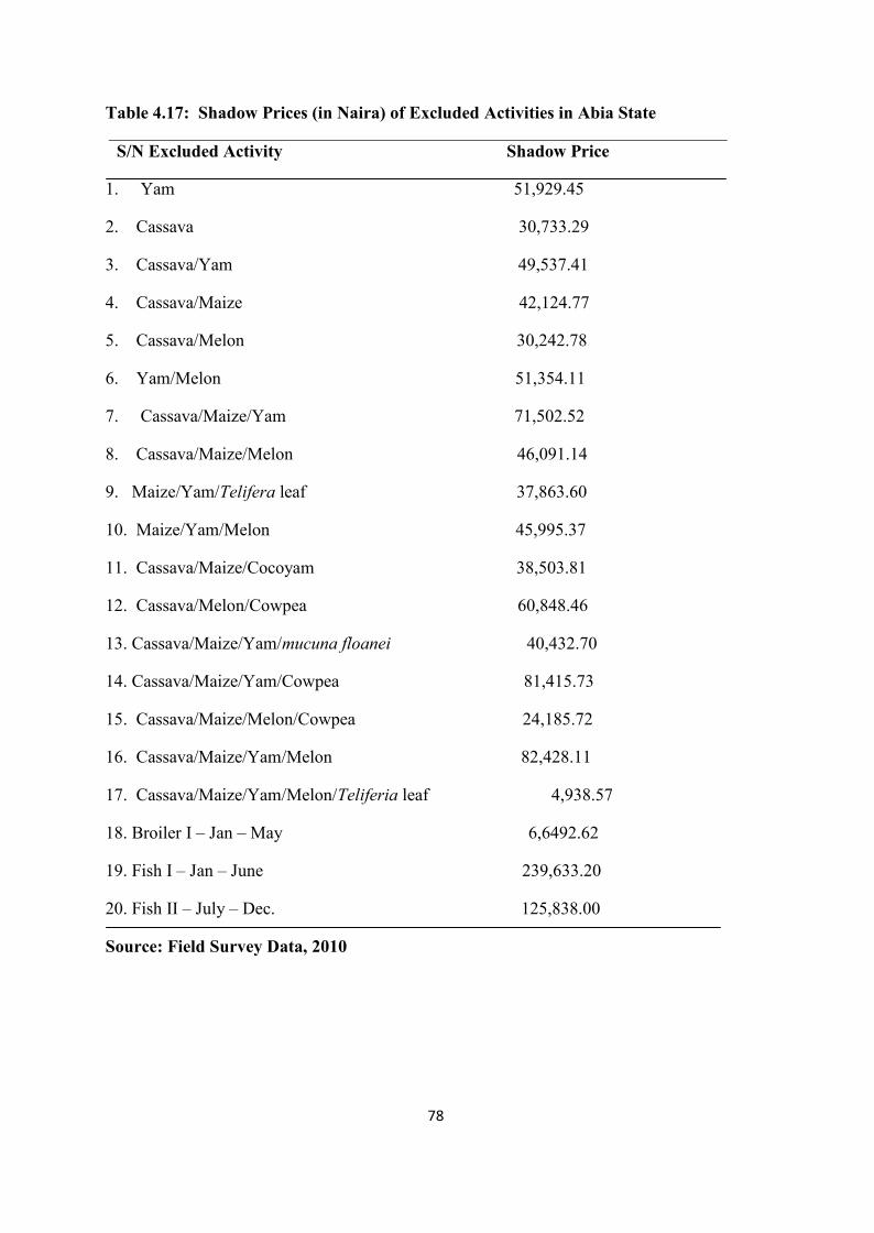
78

Table 4.17: Shadow Prices (in Naira) of Excluded Activities in Abia State

S/N Excluded Activity Shadow Price

1. Yam 51,929.45

2. Cassava 30,733.29

3. Cassava/Yam 49,537.41

4. Cassava/Maize 42,124.77

5. Cassava/Melon 30,242.78

6. Yam/Melon 51,354.11

7. Cassava/Maize/Yam 71,502.52

8. Cassava/Maize/Melon 46,091.14

9. Maize/Yam/Telifera leaf 37,863.60

10. Maize/Yam/Melon 45,995.37

11. Cassava/Maize/Cocoyam 38,503.81

12. Cassava/Melon/Cowpea 60,848.46

13. Cassava/Maize/Yam/mucuna floanei 40,432.70

14. Cassava/Maize/Yam/Cowpea 81,415.73

15. Cassava/Maize/Melon/Cowpea 24,185.72

16. Cassava/Maize/Yam/Melon 82,428.11

17. Cassava/Maize/Yam/Melon/Teliferia leaf 4,938.57

18. Broiler I – Jan – May 6,6492.62

19. Fish I – Jan – June 239,633.20

20. Fish II – July – Dec. 125,838.00

Source: Field Survey Data, 2010

79

4.4.5 Shadow Prices of Limiting Resources in the Optimized Plans in the Zones and

State

Any resource that is abundant, that is not used up by the programme, is not a limiting

resource and has a zero shadow price as it does not constrain the attainment of a programme’s

objective and vice versa (Olayemi and Onyenweaku, 1999). The status therefore of the

available resources in the optimized plans that constrained the attainment of the objective

programme for Aba, Umuahia, Ohafia agricultural zones as well as for the State is presented

in Tables 4.18.

Table 4.18: Shadow Prices (in Naira) of Limiting Resources across Zones and the State

Category Resource Shadow Price

Zones:

Aba

Human Labour I (1st Weeding)

Umuahia

Land I 42, 080.83

Human Labour 1 (Land Preparation andPlanting

600.00

Human Labour I (2nd weeding) 350.00

Human Labour I (Harvesting) 300.00

Human Labour II (Feeding) 8.49

Ohafia

Feed 228.73

Abia State

Land I 8, 338.54

Human Labour I (Harvesting) 231.09

Feed 5, 570.61

Source: Computed from Field Survey Data, 2010

80

Across the zones, Aba and Ohafia zones had only one resource each that was a limiting

resource whereas Umuahia zone had five resources that limited the attainment of the

objective function.

The basic resource that was limiting in Aba, which is Programme 1, was human labour

I (1st Weeding) for the crop category. It implies that none of the other basic resources

constrained the attainment of the objective function. Farmers in Aba zone therefore would

most likely achieve more in their drive to maximize gross return if more labour was available

and channelled to only 1st weeding. However, there were more basic resources that

constrained the attainment of the objective function for Programme 2, that is for Umuahia

zone. There were relatively more limiting resources in Umuahia than other zones and even

the State. Land for crop production, Human labour I (Land preparation and Planting), Human

Labour I (2nd Weeding), Human Labour I (Harvesting) and Human Labour II (Feeding) were

factors of production that constrained the attainment of objective function in this zone. Thus,

these five were the limiting factors of production in Umuahia zone. Within this zone,

resources for crop production were more limiting than those for animal production. Apart

from labour requirement for feeding, the other three labour requirements that constrained the

attainment of the objective function were for crop production. Generally, because crop

production requires more labour than animal production, more labour was required for crops

than for animal.

However, in Ohafia zone, feed was the only basic resource that was limiting and thus

constrained the attainment of the objective function in Programme 3. It was only in Ohafia

zone that feed intake was found to be the only limiting factor of production and none of the

resources available for crop production ever constrained attainment of the objective function

in the zone. At the State level however, land for crop production, human labour I (harvesting)

and feed resource were the limiting factors of production. Relative to Ohafia zone, the extent

81

to which feed constrained the attainment of the objective function was higher in the State

than the zone.

4.4.6 Minimum Staple Food/Livestock Requirements

The staple foods for farmers in the area were tubers and cereals for the crops and to

meet their protein needs, certain amounts of their livestock were consumed. Results of the

minimum staple and protein requirements by households (in tons) in existing and optimum

plans are presented in Table 4.19. Indication in the Table is that a typical farm household

required about 2.27 tons, 3.07 tons and 2.27 tons of tubers for farmers in Aba, Umuahia and

Ohafia Agricultural zones respectively, while 0.06 tons is required in Umuahia as against

0.36 tons for an average farm household in Aba Agricultural zone. The optimum plans for

these minimum requirements were satisfied adequately.

Generally, with respect to the tubers that appeared in the optimum plan, farmers in

Aba zone had 11.72 tons of tubers, 0.88 of cereals and a ton of their protein requirement in

excess of value in their existing requirements. Within the zones, the minimum staple food

requirements recommended by the programme was in excess of their existing plan the highest

for Ohafia; followed by Umuahia and then by Aba. At the state level, the recommendation

was less than the value in the respective zones. However, the minimum cereals requirement

prescribed by the programme for the State and the zones were satisfied in excess of the

existing plan but the prescribed cereals requirement was highest in Umuahia Zone. The

prescribed minimum protein requirement across the zones was also highest in Umuahia

followed by Ohafia, while Aba had the least.

82

Table 4.19: Minimum Staple and Animal Protein Requirements by Households (in tons) in the Plans

Farmer Category Existing Plan Optimum Plan Increase over Existing

Aba Yam 1.24 2.15 0.91

Cassava 1.03 11.84 10.81

Maize 0.36 1.24 0.88

Fish 0.13 0.62 0.49

Pig 0.02 0.53 0.51

Umuahia Yam 0.98 4.85 3.87

Cassava 1.29 11.26 9.97

Maize 0.06 1.16 1.10

Pig 0.03 0.27 0.24

Broiler 0.03 1.26 1.23

Layer 0.018 0.36 0.34

Fish 0.05 0.88 0.83

Ohafia Yam 1.34 8.79 7.45

Cassava 1.61 10.69 9.08

Maize 0.12 0.16 0.04

Cocoyam 0.34 0.39 0.05

Broiler 0.18 0.83 0.63

Fish 0.15 0.68 0.53

Layer 0.08 0.33 0.25

AbiaState

Yam 1.34 3.57 1.75

Cassava 1.13 7.15 7.33

Maize 0.47 1.14 0.72

Cocoyam 0.40 1.06 0.53

Broiler 0.21 0.68 0.15

Layer 0.01 0.66 0.65

Pig 0.06 0.28 0.22

Source: Field Survey Data, 2010

83

4.5 Sensitivity Analysis

The sensitivity of the plans to changes in some production variables was observed.

Following the findings of some researchers in the past (Osuji, 1978; Tanko, 2004), land and

labour are variables of utmost interest in such analysis. However, given that feed was

incorporated in the model for the livestock enterprises, the effect of increasing quantity of

feed available by 50 percent was also observed. In the first scenario, land resource was

increased by 50 percent, to see its effect on the optimum plan. In the second scenario, labour

was increased by 25 percent across each period for crops and decreased by same for livestock

in each zone to see their effect on the optimum plan; in the third scenario, wage was

decreased by 50 percent for both crops and livestock and finally, the effect of 50% increase in

the quantity of available feed on the programme was observed.

4.5.1 Effect of Increasing Area under Cultivation

In Aba agricultural zone, increasing the area under cultivation by 50 percent did not

increase the value of optimum gross margin in Programme 1. Moreover, all the activities that

appeared in programme 1 remained constant. On the activities remaining unchanged, a

similar response had been observed in previous research in another area (Tanko, 2004).

However, relative to Aba zone, experience in the field revealed that lands were left to lie

fallow for up to five years even when their owners had only very small scattered plots in a

farming season. There was a situation where farmers objected to the use of fertilizer to

improve soil fertility; advocating for its discontinuation, arguing that it inhibits mushroom

growth, which they seek to preserve. There is therefore some form of enlightenment to be

done over time and more to be done before an average farmer could by increasing land

available to him achieve increased gross margin in the zone.

84

In Umuahia agricultural zone however for the farmers, the value of the objective

function increased from N499,229.90 to N566,518.20 being an increase by N67,288.30,

representing 13.48% over that of Programme 2. It was also observed that the increase

affected cassava/melon/cowpea which increased by 2 hectares, from 3.26 hectares to 5.26

hectares while other activities remained unchanged.

The gross margin of an average farmer in Ohafia agricultural zone when land was

increased by 50 percent did not show any increase in the obtained original value. The

implication of this is that farmers in this zone would not increase their gross margin by

increasing the area under cultivation alone unlike the case in Umuahia zone. If more lands

were made available to the farmers, it may not necessarily improve on their gross margin in

the long run. Given that the zone is a major rice producing area in the State, and that rice

farming is done sole and was not among the arables of consideration could explain the

deviation in the zone from normalcy. The optimum recommendations by Programme 3 which

was at variance with the existing and quite lower than the observed could have been affected

by the uniqueness of the zone. The optimum recommendations remained unchanged when

subjected to sensitivity analysis.

When the gross margin for an average farmer in Abia State was examined for the

effect of increasing the area under cultivation, the objective function did not increase

significantly. The situation was in contrast to Tanko (2004). This could be because an

average farmer in the study area had very smaller farm size relative to Ekiti State where the

research by Tanko (2004) was carried out. Again increasing the gross margin of these farmers

who have established certain way of living around agriculture over time requires more than

just increase in the size of their farmland. Some other infrastructural development would be

put in place for any meaningful thing in this regard to be accomplished. Table 4.20 shows the

effect on optimum gross margin when land was increased by 50%.

85

Table 4.20: Comparing the Optimum Gross Margins when Land was increased by 50percent

Previous Optimum (N) Present Optimum (N) Increase (N) % Change

Zone

Aba 374,850.80 374,850.80 0.00 0.00

Umuahia 499,229.90 566,518.20 67,288.30 13.48

Ohafia 383,941.60 383,941.60 0.00 0.00

Abia State: 310,302.60 311,029.60 727.00 0.23

Source: Computed from Field Survey Data, 2010

4.5.2 Effect of Varying Labour Use on the Optimum Gross Margin

Labour use was increased by 25 percent of what was available across the zones for

crops, and decreased by the same for livestock to see their respective effects on the optimum

gross margin and the result is presented in Table 4.21. Increasing labour by 25% of that

available in Aba zone increased the value of the objective function by about N6,979.10,

which represent a marginal increase of only about 1.86% of the original value obtained in

Programme 1. Similarly, marginal increase of 3.04% which represent only about N15,159.90

increment to the initial optimum value of the objective function for Programme 2 was

observed. The value obtained in Ohafia agricultural zone seem to be insensitive to analysis as

labour was increased by 25%.

However, for the state, a slight increment of only 1.94% was observed for an average

farmer to improve his gross margin with addition of 25% of available labour for his farm

work.

86

Table 4.21: Comparing the Optimum Gross Margins when Labour was increased by 25percent

Category Previous Optimum (N) Present Optimum (N) Increase (N) % Change

Aba 374,850.80 381,829.90 6,979.10 1.86

Umuahia 499,229.90 514,389.80 15,159.90 3.04

Ohafia 383,941.60 383,941.60 0.00 0.00

Abia State 310,302.60 316,343.70 6, 041.10 1.94

Source: Computed from Field Survey Data, 2010

4.5.3 Effect of Varying Labour Wages on the Optimum Gross Margin

Given that high wage rate would depress gross margin, effect of reduction of wage rate

by 50 percent was also examined. The result is shown in Table 4.22. It was only in Umuahia

that percentage increase was relatively higher while Ohafia zone showed insensitivity to the

analysis when wage was reduced by 50%.

Table 4.22: Comparing the Optimum Gross Margins when Wage rate was reduced by50% across Crops and Livestock

Zone/State Previous Optimum (N) Present Optimum (N) Inc./Dec. (N) % Change

Aba 374,850.80 376,586.30 1,735.50 0.46

Umuahia 499,229.90 529,998.50 30,768.60 6.16

Ohafia 383,941.60 383,941.60 0.00 0.00

Abia 310,302.60 312,422.30 2,119.70 0.68

Source: Computed from Field Survey Data, 2010

4.5.4 Effect of Varying the Quantity of Feed used for Livestock production

Increasing the quantity of feed by 25% in Aba zone did not increase the optimum gross

margin for an average farmer. The 25% increase in the feed consumed by livestock in

87

Umuahia did not also increase the gross margin of an average farmer in the zone. Usually,

given the nature of the livestock enterprises generally speaking, a point of saturation is

always reached at which time it is advisable to dispose for sale perhaps the broiler or the

layer; continued feed intake when what is required of the birds have been achieved will if

anything else increase variable cost and as such even depress gross margin.

When feed consumed by livestock was increased by 25%, very marginal changes were

observed across all the zones. Incidentally, it was only here that Ohafia zone became

responsive to sensitivity analysis. By increasing feed by 25%, all the crop activities remained

unchanged at their levels prescribed by programme 3. However, the Layer production activity

increased from 0.41 units (205 birds) to 0.52 units (260 birds). It had however a very

marginal effect on the gross margin. Table 4.23 show the effect of varying quantity of feed

given to livestock and on the optimum gross margins recommended by the LP.

Table 4.23: Comparing the Optimum Gross Margins when Feed intake available tofarmers was increased by 25%

Zone Previous Optimum (N) Present Optimum (N) Inc. /Dec. (N) % Change

Aba 374,850.80 374,850.80 0.00 0.00

Umuahia 499,229.90 499,299.90 0.00 0.00

Ohafia 383,941.60 384,170.30 228,70 0.06

Abia 310,302.60 310,302.60 0.00 0.00

Source: Computed from Field Survey Data, 2010

88

CHAPTER 5

5.0 SUMMARY, CONCLUSION AND RECOMMENDATIONS

5.1 Summary

The study was carried out to examine the various enterprise combination patterns

operated by farmers who either are involved in selected arable crops or combine same with

livestock particularly monogastrics, develop feasible and optimum enterprise combination

pattern for sole and crop mixtures and selected animal enterprises, compare existing and

optimum farm plans for different agricultural zones and categories of farms and investigate

resource allocation in Abia State, Nigeria.

Primary data were collected on resource use and availability, input and output prices,

types of enterprise combination etc. of representative farms using the cost-route approach in

Abia State, during the 2010 farming season. Data were analyzed using descriptive statistics

and the linear programming model.

The results of the analysis showed that the generality of the farmers can no longer be

termed illiterates having attended at least primary school. The average number of years spent

in school ranged from 7 in Ohafia zone to 11 years in Umuahia zone. The optimum plans

suggested higher hectarage in Umuahia particularly almost implying that the normative figure

was different from the actual. Normative figure for Ohafia agricultural zone was particularly

in terms of hecatarage recommendation by the plan low relative to the existing situation.

Under the existing plan, farm resources were not utilized optimally. The crop

enterprises occupied 100% crop mixtures as against 4.77% and 95.23% of the existing plan

for Aba, 17.96% as against 12.25% sole and 82.04% as against 87.75% crop mixtures for

Umuahia while Ohafia occupied 29.55% of crop mixtures and 70.46% sole as against 19.47%

89

sole and 80.53% crop mixtures of its existing plan. Generally, 6 enterprises namely

cassava/maize/cocoyam (0.33ha), yam/maize/melon (0.31ha), cassava/maize/melon/mucuna

floanei (1.30ha), broiler I – Jan – May (0.14 of 500 birds), Fish II – July – Dec (0.11 of 1000

fish) and pig (0.1 of 15 pigs) were the optimum farm plans indicated for inclusion in Aba

agricultural zone; yam (0.72ha), maize/yam (0.02ha), cassava/yam/cowpea (3.26ha), pig

(0.11 of 15 pigs), broiler II – Aug – Dec (0.17 of 500 birds) and fish I – Jan – June (0.10 of

1000 fish) were prescribed by the optimum for Umuahia, while cassava/maize/cocoyam (0.13

ha), broiler II – August – December (0.14 of 500 birds), fish I – January – June (0.22 of 1000

fish) and Layers (0.41 of 500 birds) entered the optimum plan for Ohafia agricultural zone.

Gross margin of farm households in the optimum plans ranged from N374,850.80 in

Aba zone to N499,229.90 in Umuahia agricultural zone. The extent to which land

availability, labour and wage rate affected gross margin was tested by sensitivity analysis;

land availability when increased by 25% across the three zones resulted to 13.48% increase in

the gross margin, however there was no incremental effect on the prescribed optimum value

of the plan in Aba and Ohafia zones respectively.

Labour use when increased by 25% in all the zones across both crop labour and

livestock labour requirements did not have any effect on the gross margin for Ohafia.

However, it led to marginal increases by 1.86% for Aba, 3.04% for Umuahia and 1.84% of

the optimum value for the State. The wage rate when reduced by 25% had very relative

marginal incremental effect on gross margin in Aba and the State. In Umuahia zone gross

margin increased by 6.16%. Across the zones therefore, wage rate is thus relatively highest in

Umuahia.

90

5.2 Conclusion

The study concludes that farm resources were not optimally allocated in the existing

plan and crop mixtures were in a better competitive position than sole crops. The inclusion of

livestock enterprises among selected arable crops gives a fair representation of what obtains

in the study area given that the generality of the farmers do not necessarily hands off from

either category of enterprises completely. The combination of crop and livestock enterprises

contributed in improving the gross returns to the farmers in the study area.

5.3 Recommendations

Based on the findings of the study, the farm income of the farmers would improve if

the prototype combination of crop and livestock enterprises that emanated from the Linear

Programming could be integrated in the extension education package of the Abia state

Agricultural Development Project (ADP). Adequate supply of farm inputs and engagement in

extension programmes that would educate the farmers on efficient allocation of their

resources should be built in when developing a good extension package for Abia State.

Extension package should be zone sensitive for effectiveness.

Given that land was vividly shown to be the major limiting factor in Umuahia zone

particularly and the entire State relatively, more arable land should be employed in crop

production but not without consideration to improving on the environment where the farming

activities are done. This calls for a quick re-structuring of the Land use Decree so that land do

not continue to lie fallow for decades when it could have been given to practicing farmers as

a way of empowering them to do more and contribute to increasing agricultural productivity

in Nigeria.

Allocation of farm resources as prescribed by the plan would help farmers to achieve

food security, increase farm income in the long run as well as reduce farm production cost.

91

Effective farm advisory in the efficient allocation of farm resources and appropriate

enterprise patterns should be encouraged by the setting up of independent or private driven

extension service organizations to supplement government’s effort in extension service

through the ADPs. Non governmental organisations should look towards this area to

strengthen and invest in the economy through extension service delivery.

92

REFERENCES

Adedipe, N. O., A. Aliyu, Ahmed, H. U. and Fagade, S. O. (1999). Green RevolutionConcept and Agricultural research Implication for Food Security in Nigeria. In:National Agricultural Research Project. B. Shaib, N. O. Adedipe and A. Aliyu (Eds).Monograph No. 5, Federal Ministry of Agriculture and Water Resources, Abuja,Nigeria, pp. 230 - 241.

Adejobi, A. O., Komawa, P. M. Manyang, V. M. and J. K. Olayemi. (2003). Optimal CropCombinations under Limited Resources Use: Application of Linear GoalProgramming Model to Small holder farmers in the Drier Savannah Zone of Nigeria.Deutscher Tropentag, Cottingen, J. Technol. Inst. Inno. Sust. Rur. Developt., 17(1): 8– 10.

Ahmad, B. (1978). A model to determine the Impact of Improved Agricultural Efficiencyin Manitoba (Canada). PhD Thesis, Department of Agricultural Economics and FarmManagement, Winnipeg, Manitoba, Canada.

Ahmad, B., Akram, M. and Anwar, M. (1990). Potential for Increased Income on SmallFarms. Proceeding of the National Seminar on Economic Revival of Small Farmers,University of Agriculture, Faisalabad, Pakistan.

Akande, T. (2005). An Overview of the Nigerian Rice Economy. Paper Presented at theAnnual Conference of Nigerian Association of Agricultural Economists (NAAE) heldat the AMPHI theatre of the University Science and Technology, Port Harcourt,Nigeria.

Akinyosoye, V. O. (2000) Agricultural Development Projects (ADPs) and Food CropsProduction in Nigeria Since the 70s. Nigerian Agricultural Development Studies, 1:100-117.

Alam, M.S., Elias, S. M. and Rahman, M. M. (1995). Optimum Land Use Patternand Resource Allocation in a Growing Economy: A Closed Model Approach,Bangladesh J. Agric. Economics XVIII, 2: 15-37

Alam, M. S. (1994) Optimum Cropping Pattern of the Small Farmers Under Risk:A Microlevel Study in Bangladesh. Ph.D Thesis, Department of AgriculturalEconomics, Bangladesh Agricultural University Myemerisingh.

Amaza, P. S. and J. K. Olayemi (2001) Technical Efficiency in Food Crop Production inGombe State, Nigeria. The Nigerian Agricultural Journal Vol. 32. Pp. 140-151

Anderson, J. R. (1968). An Overview of Modelling in Agricultural Management. FarmEconomist Volume 11, No. 6Available online at http://ageconserach.umn.edu/bitstream/942/1/40030111.pdf

Arsham, H. (2009). Deterministic Modelling: Linear Optimization with Application.hhtp:www.mirrorservice.org/sites/home.ubalt.edu/ntsbarsh/Businee-stat, 9th Edition

93

Aromolaran, A. B. (1992). Multiple Objectives and Resource Allocation Behaviour ofSmall farmers in Ifedapo Area of Oyo State. PhD Thesis, Department of AgriculturalEconomics, University of Ibadan, Nigeria.

Aromolaran, A. B. and Olayemi, J. K. (1999). Multiple Objective Farm Planningfor Food Crop Farmers: A Goal Programming Approach, Discovery and Innovation,11, 1-2: 91-103.

Aslam, M. M. (1978). Model based on Tech. Coefficients derived from Production andProfit Functions. National Seminar on Econometric Models and Operational ResearchVol. 21. Pakistan Statistical Association, Faisalabad Chapter, Faisalabad.

Babatunde, R. O., Olorunsanya, E. O. Orebiyi, J. S. and Falola, A. (2007a). Optimal FarmPlan in Sweet Potato Cropping Systems: The Case of Offa and Oyun LocalGovernment Areas of Kwara State, North-Central Nigeria. Medwell Online. Agric.Journal 2(2): 285-289.

Babatunde, R. O., Omotesho, A. O. Olorunsanya, E. O. and Amadou, A. (2007b). OptimalCrop Combination in Small-Scale Vegetable Irrigation Farming Scheme: Case Studyfrom Niger Republic, Medwell Online Research J. Applied Sciences 2(5): 617-622.

Bajwa, M. A. (1978). Linear Programming Approach in Developing Cropping Pattern: ACase of Leiah Tehsil, District Muzaffer. Garh. National Seminar on EconometricModels and Operational Research Vol. 21. Pakistan Statistical Association.Faisalabad.

Balogun, E. D. (1986). Agricultural Development Strategies in Nigeria: Past,Present and Future’’, In: Nigeria Agricultural Outlook (with special reference toBudgets). Nigeria Association of Agricultural Economists, pp.111-122.

Balogun, O. (2008) Nigeria Atlas of Electoral Constituencies, Independent NationalElectoral Commission (INEC) Abuja.

Bankar, S. R. and Atre, A. A. (1998). Application of Linear Programming for Crop Planningin Water Shed. J. Maharashtra, Agricultural University, 1998 Publication 23(2): 159-161.

Barnes, D., Fearne, A. Lingard, J. and Tiffin, R. (1993). The Impact of set-aside on ArableFarming in the UK. Discussion Paper, Department of Agricultural Economics andFood Marketing, University of Newcastle, Upon Tyne, UK

Beneke, R. R. and Winterboer, R. (1973). Linear Programming Application to Agriculture.The Iowa State University Press, Aimer Iowa, 30pages.

Boko, M., I. Niang, A. Nyong, C. Vogel, A. Githeko, M. Medany, B. Osman-Elasha, R. Taboand P. Yanda (2007). Africa in Climate Change 2007: Impacts, Adaptation andVulnerability. Working Paper 2. In: The Fourth Assessment Report of theIntergovernmental Panel on Climate Change, M. L. Parry, O. F. Canziani, J. P.Palutikof, P. J. Van der Linden and C. E. Hanson (Eds), Cambridge University Press,Cambridge, UK, pp. 433-467.

94

Bouman, B. A. M., Jansen, H. G. D., Schipper, R. A. Nieuwenhyyse, A. Hengsdijk, H. andBouman, J. (1999). A Framework for Biophysical and Economic Land Use Analysisat Different sites. Agric. Ecosystem and Environ. 75(1-2): 55-73.

Cassey, W. P., Dumpler, T. J. Burton(Jnr), R. O., Sweeney, D. W. Featherstone, A. N. andGranade, G. V. (1998). A whole farm Economic analysis of Early maturing andTraditional Soya bean. J. Production Agric., 11(2): 240 – 246.

Central Bank of Nigeria (CBN) (1999). Nigeria’s Development Prospect. PovertyAssessment and Alleviation Study, Research Department, CBN in collaboration withWorld Bank, Washington DC.

Chaudhry, M. A. (1976). Impact of Optimal Cropping Pattern in Gujarat District, Punjab.Development Rev. 15(2): 218 – 222.

Chukwuji, O. C. (2008). Comparative Analysis of Enterprise Combination Costs and Returnsin Cassava-Based Food Crop Farming Systems in Delta State, Nigeria. AsianResearch Publishing Network (ARPN) J. Agric. and Bio. Sc. 3 (4): 27-32.

Corporate Nigeria, C N (2008). The Business, Trade and Investment Guide. CorporateGuides International Limited. www.corporate-Nigeria.net

Dantzig, G. B. (1990). The Diet Problem. Interface: 43-46

Dantzig, G. B. (2002). Linear Programming. Institute of Operations Research andManagement Sciences (INFORMS) Archives Vol. 50, No. 1, p.42-47.

De Wit, C. T. (1992). Resource Use Efficiency in Agriculture. Agric. Systems 40:125-151.

Delgado, C., Rosegrant, M., Steinfeld, H., Ehui, S. and Courbois, C. (1999) Livestock to2020: The Next Food Revolution. Food, Agriculture and the Environment DiscussionPaper 20. IFPRI/FAO/ILRI, Washington DC

Diehl, L. (1982) Small Holder Faming Systems with Yam in the Southern Guinea Savannahof Nigeria. Dientche Geseilschaft for Technische Zussammenrbeit, Germany.340pages.

Effiong, E. O. (2005). Efficiency of Production in Selected Livestock Enterprises in Akwa-Ibom State, Nigeria, Ph.D Thesis, Department of Agricultural Economics, MichaelOkpara University of Agriculture, Umudike, 137 pages.

Federal Office of Statistics (FOS) (1999). Poverty and Agricultural Sector inNigeria. FOS Abuja.

Federal Republic of Nigeria Official Gazette FRN (2009). Legal Notice on Publication of2006 Census Final Result. Number 2, Vol. 96, 2nd February.

Flinchman, G. and F. Jacquet (2003). Couplage des modeles agronomiques et.Economiques: Interet pour L’analyse des Politiques.. Cahiers D’economie etSociologie Rurales, 67: 1-20.

95

Food and Agriculture Organization (FAO) (2003). GES Operational Programme onSustainable Land Management (Draft) FAO, Rome.

Furtan, W. H. and Clark, J. S. (1982). The Economic Organization of Rural Households inSuskatchewan, Department of Agricultural Economics. Technical Bulletin, Universityof Suskachewan, Suskatoon, pp.1-82.

Hassan, I. (2004). Use of Linear Programming Model to Determine the Optimum CroppingPatterns for the Irrigated Punjab with National and WTO Price Options. PhD Thesis,Faculty of Agricultural Economics and Rural Sociology, University of Agriculture,Faisalabad. http/prr.hec.gov.pk/Thesis/31.pdf. (Accessed 24-04-2009).

Hassan, I., Ahmad, P., Akhter, M. and Aslam, M. (2005). Use of Linear Programming Modelto Determine the Optimum Cropping Pattern: A case Study of Punjab. Electronic. J.Environ. Agric. and Food Chem. (EJEAFChe), 4(1): 841-850.

Heady, E. O. (1952). Economics of Agricultural Production and Resource Use. EaglewoodCliffs, NJ: Prentice-Hall.

Hengsdijk, H. and van Ittersum, M. K. (2002). A Goal oriented Approach to Identify andEngineer Land use Systems. Agric. Systems 71: 231-247.

Huke, E. and R. Huke (1982). Rice area by Type of Culture: South, Southeast, and EastAsia. Manila (Philippines): International Rice Research Institute.

Huke, E. and Huke, R. (1997). Rice area by Type of Culture: South, Southeast, and EastAsia – Revised and Updated Data. Manila (Philippines): International Rice ResearchInstitute.

Ibrahim, H., Bello, M. and Ibrahim, H. (2009) Food Security and Resource Allocationamong Farming Households in North Central Nigeria. Pakistan J. Nutrition 8(8):1235-1239

Idachaba, F. S. (1985). Priorites for Nigerian Agriculture in the 5th NationalDevelopment Plan 1986 – 90. Occasional Paper 1. Federal Agricultural CoordinatingUnit (FACU), Ibadan, Nigeria.

Igben, M.S and Banwo, P. A. (1982). Grain resources and Food Search in Nigeria.Food Policy, 7 (3): 257-260.

Ilemobade, A. A. (1985). The Technology of Certainty: The Case of Animal Production andHealth. Inaugural Lecture Series 2. Federal University of Technology, Akure, Nigeria.42pages.

Iloka, A. W. and Anuebunwa, F. O. (1995). Problems in the Conduct of MonthlyTechnology Review Meeting in South-East Zone of Nigeria. Research Mimeograph.No. 3. NRCRI, Umudike, Nigeria.

96

Jansen, S. and van Ittersum, M. K. (2007). Assessing Farm Innovations and Responses toPolicies: A Review of Bio-economic farm models. Agricultural Systems 94: 622-636

Kareem, B. and Aderoba, A. A. (2008). Linear Programming based Effective Maintenanceand Manpower Planning Strategy: A Case Study. Inter. J. Computer, the Internet andManagement 16 (2): 26-34

Kahloon, A. S. (1975). Relative Profitability of Dairy Enterprises vis-a-vis Crop Cultivationin the Punjab. Indian J. Agric. Econ. 33(2): 12-18.

Kebede, T. A. (2001). Farm Household Technical Efficiency: A Stochastic Frontier Analysis:A Study of Rice Production in Mardi-Watershed in the Western Development Regionof Nepal. MSc Thesis, Department of Economics and Social Science, AgriculturalUniversity of Norway, 56 pages

Klein, K. K. and Narayanan, S. (2008). Farm Level Models: A Review of Development,Concepts and Applications in Canada. Canadian J. Agric. Econ. 40 (3): 351-368.

Kwanashie M., Ajilima, I. and Garba, A. (1998) ‘’The Nigerian Economy: Response ofAgriculture to Adjustment Policies’’. AERC Research Paper 78. African EconomicResearch Consortium, Nairobi, Kenya.

Lenstra, J. K., Rinnooy Kan, A. H. G. and Schrijver, A. (eds) (1999) History ofMathematical Programming: A Collection of Personal Reminiscences. ElsevierScience Publishers B.V., Amsterdam, The Netherlands.

Louhichi, K., Flinchman, G. and Zekri, S. (1999). A Bio-economic Model for Analysing theImpact of Soil and Water Conservation Policies Applied to a Tunisian Farm.Economic Rurale 252: 55-64.

Lucey, T. (2002). Quantitative Techniques. Sixth Edition ELST Edition. MPGBooks Ltd, Bodmin, Great Britain 558pages.

Mahmood, A. and Walter, F. (1990). Pakistan Agriculture, A Description of Pakistan’sAgricultural Economy. Pp. 68-76

Mehta, P. (1992). Optimizing Techniques in Agriculture. Satosh Kumar Jain for CBSPublishers and Distributor Delhi, India, 163pages.

Mellor, J. W. (1980). The Economics of Agricultural Development. Cornel UniversityPress, Ithaca, NY, Third Printing, 402pages.

Mendelson, R. and Dinar, A. A. (2003). Climate, Water and Agriculture, Land Economics 79

(3): 328 - 341

Nadda, A. (1978). Optimizing Crop Production Pattern in Different Agriclimatic Zonesof Himachal Pradesh. Indian J. Agric. Econ. 33(4): 22-28.

National Population Commission (1991). 1991 Population Census of FederalRepublic of Nigeria, Report Phase 11: 29-30.

97

National Population Commission, NPC (2006). National Census. National PopulationCommission’s Report, October, Abuja, Nigeria.

Nigerian Environmental Study/Action Team (NEST) (1991). Nigerian ThreatenedEnvironment. A National Profile, Intec Publication, Ibadan.

Neto, J. D., Azevedde, C. A., Frizzon, J. A. and Azevedo, C. A. L. (1997). Use of LinearProgramming for estimating Crop pattern for the Nilo Crelho Irrigation District.Revista Brasilura De Engenhana Agricola – e – Ambiental. September – December,pp. 9-12.

Nicholson, C. F., Lee, D. R. and Boisvert, R. N. (1994). An Optimization Model of the DualPurpose Cattle Production System in the Humid Lowlands of Venezuela. Agric.Systems 46: 331-334.

Norman, D. W., Simons, E. B. and Hays, H. M. (1982). Farming System in the NigerianSavannah: Research and Strategies for Development, West View Press, Colorado.

Nwaru, J. C. and Nnadozie, C. (2005). Impact of Credit Use on the Technical Efficiency ofArable Crop Farmers in Imo State, Nigeria. Proceedings of the 30th AnnualConference of the Agricultural Society of Nigeria held at University of Benin, BeninCity, Nigeria, October 9th – 13th: pp. 382-384.

Nwosu, A. C. (1981). Cropping Pattern and Resource Productivity: A ComparativeAnalysis of Profitability in Sole and Intercropping. Nigerian J. Agric. Sci. 3 (1): 24-27.

Obasanjo, O. (1990). Agriculture: The Bedrock of Development. Acceptance Speech, AfricanPrize for Leadership for the Sustainable end of Hunger, New York. In AfricanFarmer, No. 6(Dec.), pp. 41-43

Ogunfowora, O. (1970). A Linear Programming Analysis of Income Opportunitiesand Optimal Farm Plans in Peasant Farming. Bulletin of Rural Economics andSociology Vol. 5, No. 2, pp. 223 – 250.

Okeneye, R. A. and Okeneye, M. Y. (1988). Underdevelopment and Increased LabourProductivity: A Linear Programming Analysis of Family farms in Nigeria. PaperPresented at the 1987/88 Conference of Nigerian Association of AgriculturalEconomists (NAAE), Ibadan, Nigeria.

Okike, I. (2000) Crop Livestock Interactions and Economic Efficiency of farmers in theSavannah Zones of Nigeria, Ph.D Thesis, Department of agricultural Economics,University of Ibadan 155pp.

Okuneye, P. A. (2001). The Rising Cost of Food/Food Security in Nigeria and itsImplication for Poverty Reduction. Economic and Financial Review 39(4).

Okoli, O. O. and Onwueme, I. C. (1980). Yam and the African Food Crises. PaperPresented at the 3rd Triennial Symposium of the International Society for TropicalRoot Crops, Owerri, Nigeria, 17th-22nd August 1980.

98

Olarinde, L. O., Manyong, V. M. and Okoruwa, V. O. (2008). Analysing Optimum andAlternative Farm Plans for Risk Averse Grain Crop Farmers in Kaduna State,Northern Nigeria. World J. of Agricultural Sciences 4(1): 28-35.

Olayemi, J. K. (1980). Food Crop Production by Small Farmers in Nigeria. In:Nigeria Small Farmers: Problems and Prospects in Integrated Rural Development,Olayide, S. O., Eweka, J. A., Bello-Osagie, V. E. (eds)Centre for Agriculture andRural Development, University of Ibadan, Nigeria.

Olayemi, J. K. and Olaomi, J. O. (1995). A Mathematical Programming Procedure forfor selecting crops for Mixed Cropping Schemes. Ecological Modelling 79 Issue 1-3:1-9. Published by Elsevier Science B.V.

Olayemi, J. K. and Onyenweaku, C. E. (1999) Quantitative Methods for BusinessDecisions. Bosude Printers Limited, Ibadan, Nigeria. 346pages

Olayide, S. O. and Heady, E. O. (1982). Introduction to Agricultural ProductionEconomics. Ibadan University Press Publishing House, University of Ibadan, Nigeria319pages

Olayide, S. O., Eweka, J. A. and Osagie, B. (1980). Nigeria’s Small Farmers: Problems andProspects in Integrated Rural Development. Centre for Agricultural Research andDevelopment (CARD), University of Ibadan, Nigeria, p.67.

Olorunfemi, T. O. S. (2006). Linear Programming Application to Utilization of Duckweed(Lemna pancicostata) in Leasy-cost Ration Formulation for Broiler Finisher. AsianNetwork for Scientific Information. J. Applied Sc. 6(9): 1909-1914.

Olowude, S. A. (1974). Optimum Farm Planning Models for Enterprise Combination inWestern Nigeria. An Application of Dynamic Programming. Ph.D Thesis,Department of Agricultural Economics, University of Ibadan, June

Onyenweaku, C.E. (1980). A Linear Programming Analysis of Inter-regionalCompetition in Nigerian Agriculture, PhD Thesis, Department of AgriculturalEconomics, University of Ibadan,

Onyenweaku, C. E., Ogunfowora, O. and Falusi, A. O. (1978/1979). SpatialEquilibrium Analysis of Nigerian Agriculture. J. of Rural Economics andDevelopment 112(2): 1-14.

Onyenweaku, C.E., Igwe, K. C. and Mbanasor, J. A. (2005). Application ofStochastic Frontier Production Function to the Measurement of Technical Efficiencyin Yam Production in Nasarawa State, Nigeria. J. Sustain. Trop. Agric. Research 13:20-25.

Onyenweaku, C.E., Okoye, B.C., Asumugha, G. N., Okezie, C. A. and Tanko, L. (2008).Economic Assessment of the Trend in Cocoyam Production in Nigeria, 1960/1961-2006. Medwell Journals. Agric. J. 3(2): 99-101.

99

Oriaku, S. E. O. (2008). Effectiveness of Contact Farmers in the Diffusion of AgriculturalInnovations in Umuahia Agricultural Zone of Abia State. MSc Thesis, Department ofAgricultural Economics and Extension, Abia State University Uturu.

Osuji, L. O. (1978). Resource Productivity in Traditional Agriculture: A Study ofSome Selected Villages in Imo State of Nigeria, PhD. Thesis, Department ofAgricultural Economics, University of Ibadan, Nigeria.266pages.

Otoo, J.A., Asiru, O. O., Na, S. Y. and Hahn, S. K. (1987). Improved Technology forSeed Yam Production. 2nd Edition IITA Ibadan, Nigeria 56 pages.

Panigraphy, R. K., Panigrahy, S, Ray, S. S. and Parihar, J. S. (2005). Analysis of CroppingPattern and Crop Rotation of A Subsistence Agricultural Region using High TemporalRemote Sensing Data. Map India and Geomatics 2005 8th Annual InternationalConference 7 – 9 February, Hotel Taj Palace, New Dehi.

Patton, D. A. and Mullen, J. D. (2001). Farming Systems in the Central West ofNSW: An Economic Analysis. Economic Research Report No. 7, NSW Agriculture.Triangie.

Quinn, J. D. and Harrington, J. J. (1992). Generating Alternatives for Inter-jurisdictionalNational Resource Development Schemes in Greater Ganges River Basin’’. Papers inRegional Science. 71(4): 373 – 391.

Radhakrishan, S. A. and Silvandhram, B. (1975). Optimum Cropping Patterns for Smallfarms in a Minor Irrigation Project. Indian J. Agric. Econ. 33(2): 27-34.

Ruben, R. and van Ruijven, A. (2001). Technical Coefficients for Bio-economic FarmHousehold Models: A Meta-modelling Approach with Application for Southern Mali.Ecolo. Econ. 36: 427-441.

Saini, A. S. (1975). Impact of Dairy Enterprise on Farm income in Punjab. India J.Agric. Econ. 33(2): 6-12

Salinger, J., M. Sivakumar, V. K. and Motha, R. P. (2005). Increasing Climate Variabilityand Change: Reducing the Vulnerability of Agriculture and Forestry. Reprinted fromClimate Model Ensembles to Intra Decisions. Philosophical Transactions of the RoyalSociety, 365: 2163-2177

Salman, A. Z., Al-Karabheh, E. K. and Fisher, F. M. (2001). An Interseasonal AgriculturalWater Allocation (SAWAS). Agric. Systems 68(3): 233-52.

Sama, J.N. (1997). Raising Income Level of Farmer on Swazi Nation Land: AFarm Planning and Extension Approach. Uniswa J. Agriculture, 6(1): 5-14.

Schipper, R.A; Jansen, D. M. and Stoorvogel, J. J. (1995). Sub-regional LinearProgramming Models in Land Use Analysis. A Case Study of Neguev Settlement,Costa Rica, Netherlands. J. Agric. Science 43: 83-109.

100

Shahidullah, S. M., Talukder, M. S. A., Kabir, M. S., Khan, A. H. and Elahi, Nu-E (2006).Cropping Patterns in the South East Coastal Region of Bangladesh. J. Agric. andRural Develop.. Vol 4 No 1.

Sharif, M. (1979). Determining the Optimal Cropping pattern in Tehsil Toba Tek Singh: ALinear Programming Technique. MSc Thesis, Department of Agricultural Economics

Singh, K. (1978). Optimum Land Use Pattern and Resource Allocation in a GrowingEconomy.. Indian J. Agric. Econ, 33(1): 44-58

Staal, S. J., Ehui, S. and Tanner, J. C. (2001). Livestock-environment Interaction underIntensifying Production. In: Tradeoffs or Synergies? Agricultural Intensification,Economic Development and the Environment, D. R. Lee, and C. B. Barrett (Eds.),CAB International, Wallingford, UK, pp 345-64

Stroorvogel, J. J., Jansen, H. G. P. and Jansen, D. M. (1997). Agricultural Policies andEconomic Incentives for Sustainable Land Use, A Sub-regional Model for Costa Rica.Investgonecon Agravia, Economic 12: 5-15.

Taha, H.A. (2007). Operations Research. An Introduction, Eight Edition, PearsonEducation, Inc., Pearson Prentice Hull, USA, 813 pages.

Taha, H. A. (2011). Operations Research. An Introduction, Ninth Edition, InternationalEdition, Pearson Education. Inc., Pearson Prentice Hull, USA, 824 pages.

Tanko, L. (2004). Optimum Combination of farm Enterprises in Kebbi State,Nigeria: A Linear Programming Approach. PhD Dissertation, Michael OkparaUniversity of Agriculture, Umudike, Nigeria, 152 pages.

Tanko, L. and Opara, C. A. (2006). Profitability and Resource Productivity of Sole andIntercropping in Ikwuano Local Government area of Abia State, Nigeria. Proceedingsof the 40th Annual Conference of the Agricultural Society of Nigeria held at Umudike,October 16th – 20th, 2006: 167-170.

Tanko, L. and Baba, K. M. (2010). Raising Income level of Farmers in Niger State, Nigeria:A Linear Programming Approach. Research Finding of University Board of Research(UBR) Funded Study, Federal University of Technology, Minna, 55pages.

Ten Berge, H. F. M, Van Ittersum, M. K. Rossing, W. A. H. van de Ven, G. W. J. andSchans, J. (2000). Farming Options for the Netherlands explored by Multi-objectiveModelling. European J. of Agronomy 13: 263-277.

Thomson, E. F. and Bahhady, F. A. (1995a) A Model-farm Approach to Research on Crop-Livestock Integration – 11. Experimental Results. Agric. Systems 49: 17-30

Thomson, E. F. and Bahhady, F. A. (1995b) A Model-farm Approach to Research on Crop-Livestock Integration – 1. Conceptual Framework and Methods. Agric. Systems 49:1-16.

101

Thomson, E. F. and Bahhady, F. A. (1995c) A Model-farm Approach to Research on Crop-Livestock Integration – 111. Benefits of Crop-Livestock Integration and a Critique ofthe Approach. Agric. Systems 49: 31-44.

Thornton, P. K. and Herrero, M. (2001) Integrated Crop-livestock simulation models forScenario analysis and Impact assessment. Agric. Syst. 70: 581-602

Todaro, M. P. and Smith, S. C. (2009). Economic Development. Tenth Edition. AddisonWesley. An Imprint of Pearson Educational Limited, England, 861pages.

Uddin, T., Tahikder, R. K. and Alam, M. S. (1994). Optimum Cropping Plan for aSample of Farms in a Farming System Research Area of Bangladesh. Bangladesh J.Agric. Econ. XV11, 1 and 2: 85-96.

Uddin, T. (1995). An Economic Analysis of a Farming System and Determination ofOptimum Crop Plan in a Farming System Research Area of Bangladesh. MSc Thesis,Department of Agricultural Economics, Bangladesh Agricultural University,Mymesingh, May

Udoh, E.J. (2000). Land Management and Resource-Use Efficiency among Farmers inSouth-Eastern Nigeria. PhD Dissertation, University of Ibadan. 186pages.

Unamma, R. P. A., Odurukwe, S. O. Okere, H. E. Ene, L. S. O. and Okoh, O. O. (1985).Farming System in Nigeria: Report of Benchmark Survey of Farming System ofSouth East Agricultural Zone of Nigeria, NRCRI, Umudike, Nigeria, p.116.

United Nations Population Division (UNPD) (2007). World Population Prospects: The 2006Revision World Urbanization Prospects: The 2005 Revision.Population Division ofthe Department of Economic and Social Affairs of the United Nations Secretariat,http://esa.un.org/unpd Accessed 24 June, 2012

World Bank, (1992). World Development Report. Washington D.C: World Bank.

World Bank (1996). Nigeria Poverty in the midst of Poverty, the Challenge of Growth withInclusion. World Bank Poverty Assessment Handbook No. 14

World Bank (2000). World Bank Development Report 2000/2001: Attacking Poverty. WorldBank, Washington D.C, USA.

World Bank (2004). Distribution of Income Consumption’’. World DevelopmentIndicators. World Bank, Washington, DC.

Yang, W.Y. (1995). Methods of Farm Management Investigation for Improving FarmProductivity. FAO, Rome.

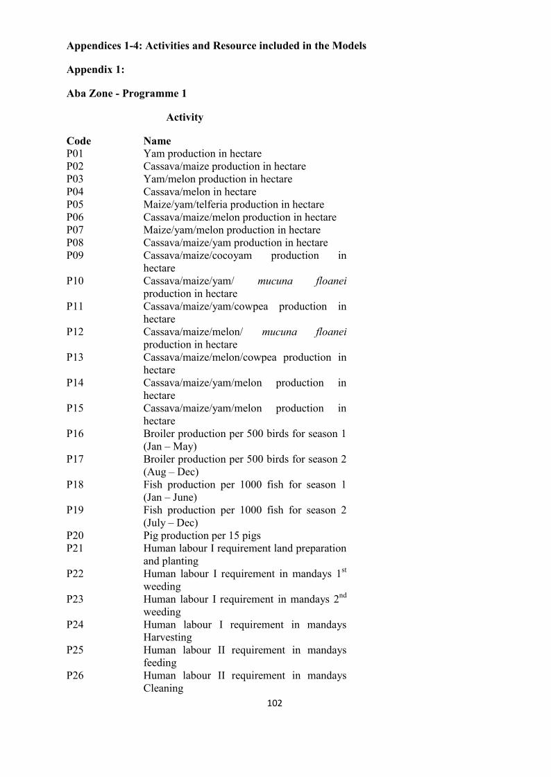
102

Appendices 1-4: Activities and Resource included in the Models

Appendix 1:

Aba Zone - Programme 1

Activity

Code NameP01 Yam production in hectareP02 Cassava/maize production in hectareP03 Yam/melon production in hectareP04 Cassava/melon in hectareP05 Maize/yam/telferia production in hectareP06 Cassava/maize/melon production in hectareP07 Maize/yam/melon production in hectareP08 Cassava/maize/yam production in hectareP09 Cassava/maize/cocoyam production in

hectareP10 Cassava/maize/yam/ mucuna floanei

production in hectareP11 Cassava/maize/yam/cowpea production in

hectareP12 Cassava/maize/melon/ mucuna floanei

production in hectareP13 Cassava/maize/melon/cowpea production in

hectareP14 Cassava/maize/yam/melon production in

hectareP15 Cassava/maize/yam/melon production in

hectareP16 Broiler production per 500 birds for season 1

(Jan – May)P17

P18

P19

Broiler production per 500 birds for season 2(Aug – Dec)Fish production per 1000 fish for season 1(Jan – June)Fish production per 1000 fish for season 2(July – Dec)

P20 Pig production per 15 pigsP21

P22

Human labour I requirement land preparationand plantingHuman labour I requirement in mandays 1st

weedingP23

P24

P25

P26

Human labour I requirement in mandays 2nd

weedingHuman labour I requirement in mandaysHarvestingHuman labour II requirement in mandaysfeedingHuman labour II requirement in mandaysCleaning

103

P27

P28

P29

Human labour II requirement in mandaysSortingHuman labour II requirement in mandaysHarvestingYam selling in naira per ton

P30 Cassava selling in naira per tonP31 Maize selling in naira per tonP32 Melon selling in naira per tonP33 Telferia selling in naira per tonP34 Cocoyam selling in naira per tonP35 Mucuna floanei selling in naira per tonP36 Cowpea selling in naira per tonP37 Broiler I selling in naira per ton for season 1P38 Broiler II selling in naira per ton for season 2P39P40

Fish I selling in naira per ton for season 1Fish II selling in naira per ton for season 2

P41 Pig selling in naira per ton

Resource Restrictions

Code NameR0 1 Land I for crop productionR02R03R04

Land II rep by stock capacity in 500 birdsLand III rep by stock capacity in 1000 fishLand IV rep by stock capacity in 15 pigs

R05 Human labour I requirement in mandaysland preparation and planting

R06

R07

R08

R09

R10

R11

R12

Human labour I requirement in mandays 1st

WeedingHuman labour I requirement in mandays 2nd

WeedingHuman labour I requirement in mandaysHarvestingHuman labour II requirement in mandaysFeedingHuman labour II requirement in mandaysCleaningHuman labour II Hiring requirement inmandays SortingHuman labour II Hiring requirement inmandays Harvesting

R13 Feed in tonsR14 Transfer row (yam in tons)R15 Transfer row (cassava in tons)R16 Transfer row (maize in tons)R17 Transfer row (melon in tons)

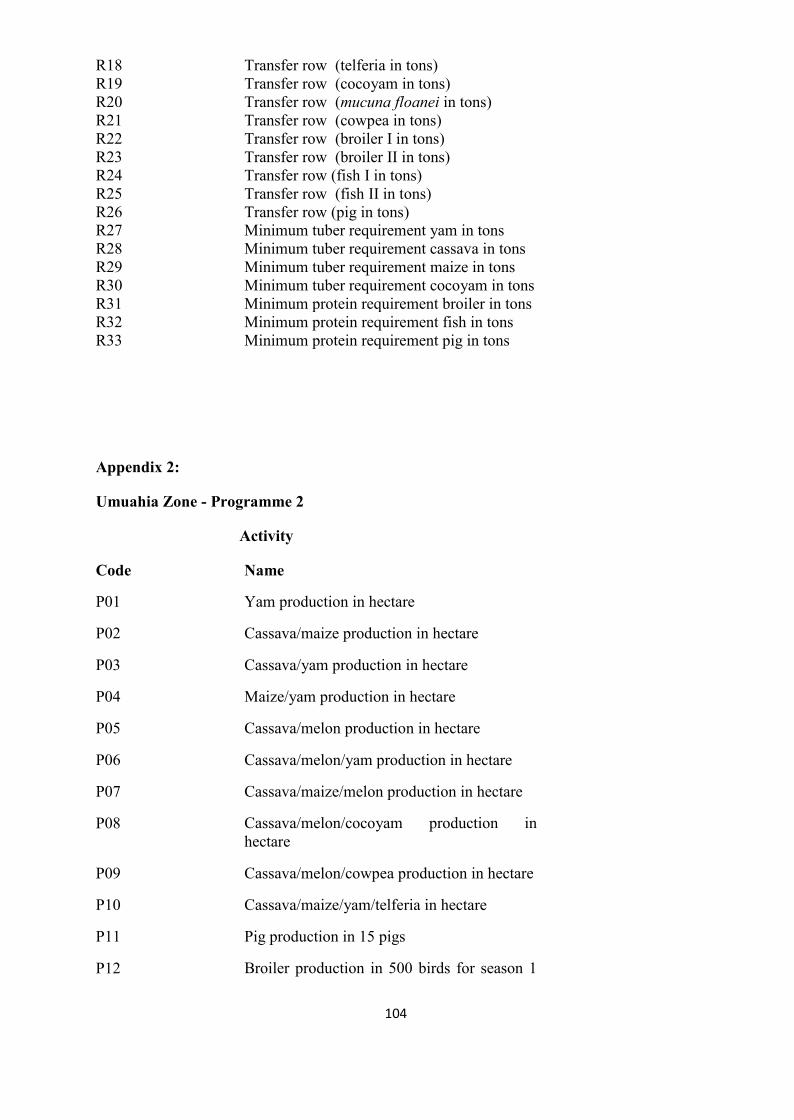
104

R18 Transfer row (telferia in tons)R19 Transfer row (cocoyam in tons)R20 Transfer row (mucuna floanei in tons)R21 Transfer row (cowpea in tons)R22 Transfer row (broiler I in tons)R23R24

Transfer row (broiler II in tons)Transfer row (fish I in tons)

R25R26

Transfer row (fish II in tons)Transfer row (pig in tons)

R27 Minimum tuber requirement yam in tonsR28 Minimum tuber requirement cassava in tonsR29 Minimum tuber requirement maize in tonsR30R31

Minimum tuber requirement cocoyam in tonsMinimum protein requirement broiler in tons

R32 Minimum protein requirement fish in tonsR33 Minimum protein requirement pig in tons

Appendix 2:

Umuahia Zone - Programme 2

Activity

Code Name

P01 Yam production in hectare

P02 Cassava/maize production in hectare

P03 Cassava/yam production in hectare

P04 Maize/yam production in hectare

P05 Cassava/melon production in hectare

P06 Cassava/melon/yam production in hectare

P07 Cassava/maize/melon production in hectare

P08 Cassava/melon/cocoyam production inhectare

P09 Cassava/melon/cowpea production in hectare

P10

P11

Cassava/maize/yam/telferia in hectare

Pig production in 15 pigs

P12 Broiler production in 500 birds for season 1

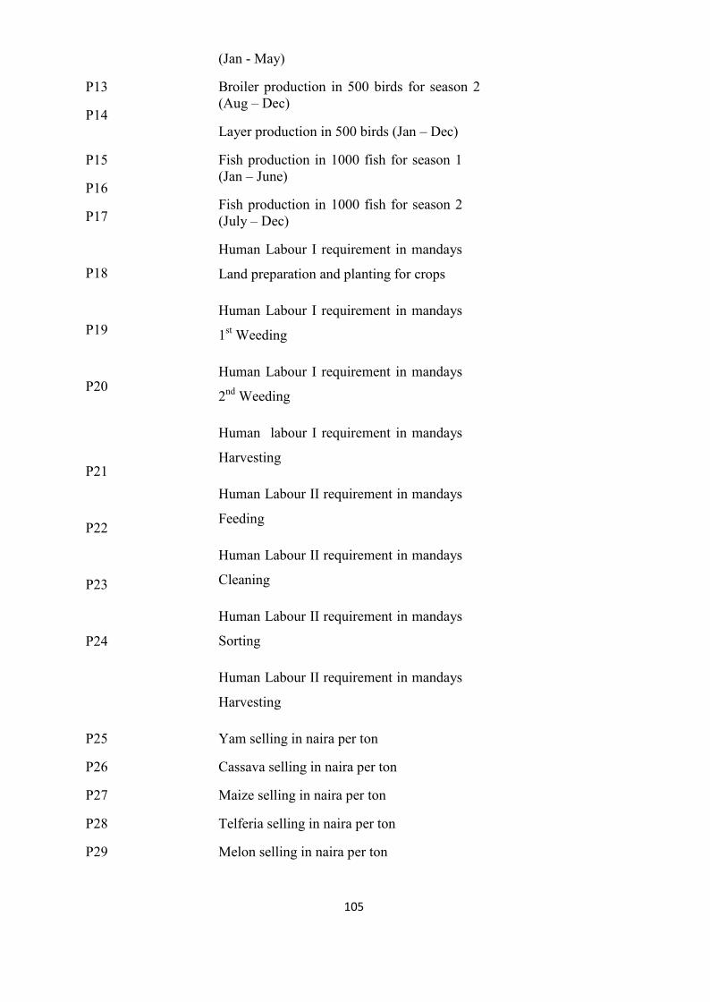
105

(Jan - May)

P13

P14

Broiler production in 500 birds for season 2(Aug – Dec)

Layer production in 500 birds (Jan – Dec)

P15

P16

P17

P18

P19

P20

P21

P22

P23

P24

Fish production in 1000 fish for season 1(Jan – June)

Fish production in 1000 fish for season 2(July – Dec)

Human Labour I requirement in mandays

Land preparation and planting for crops

Human Labour I requirement in mandays

1st Weeding

Human Labour I requirement in mandays

2nd Weeding

Human labour I requirement in mandays

Harvesting

Human Labour II requirement in mandays

Feeding

Human Labour II requirement in mandays

Cleaning

Human Labour II requirement in mandays

Sorting

Human Labour II requirement in mandays

Harvesting

P25 Yam selling in naira per ton

P26 Cassava selling in naira per ton

P27 Maize selling in naira per ton

P28 Telferia selling in naira per ton

P29 Melon selling in naira per ton

106

P30 Cocoyam selling in naira per ton

P31

P32

Cowpea selling in naira per ton

Pig selling in naira per ton

P33 Broiler selling in naira per ton for season 1

P34

P35

Broiler selling in naira per ton for season 2

Egg selling in naira per ton

P36 Layer selling in naira per ton

P37

P38

Fish 1 selling in naira per ton

Fish II Selling in naira per ton

Resource Restrictions

Code Name

R01

R02

R03

R04

R05

Land I for crop production in hectare

Land II rep by stock capacity in 15 pigs

Land III rep by stock capacity in 500 birds

Land IV rep by stock capacity in 1000 fish

Land V rep by stock capacity in 1000 crates

R06 Human labour I requirement in mandaysplanting

R07

R08

R09

R10

R11

R12

R13

R14

Human labour I requirement in mandays 1st

WeedingHuman labour I requirement in mandays 2nd

WeedingHuman labour I requirement in mandaysHarvestingHuman labour II requirement in mandaysFeedingHuman labour II requirement in mandaysCleaningHuman labour II Hiring requirement inmandays SortingHuman labour II Hiring requirement inmandays HarvestingFeed in tons

R15 Transfer row (yam in tons)

R16 Transfer row (cassava in tons)

107

R17 Transfer row (maize in tons)

R18 Transfer row (telfaria in tons)

R19 Transfer row (melon in tons)

R20 Transfer row (cocoyam in tons)

R21 Transfer row (cowpea in tons)

R22 Transfer row (pig in tons)

R23

R24

Transfer row (broiler I in tons)

Transfer row (broiler II in tons)

R25

R26

Transfer row (egg in tons)

Transfer row (layer in tons)

R27

R28

Transfer row (fish I in tons)

Transfer row (fish II in tons)

R29 Minimum tuber requirement Yam in tonsR30 Minimum tuber requirement Cassava in tonsR31 Minimum cereal requirement Maize in tonsR32 Minimum requirement Cocoyam in tonsR33 Minimum protein requirement Pig in tonsR34 Minimum protein requirement Broiler in tonsR35 Minimum protein requirement Layer in tonsR36 Minimum protein requirement Fish in tons

Appendix 3:

Ohafia Zone – Programme 3

Code Activity

P01

P02

P03

P04

P05

Yam production in hectare

Cassava production in hectare

Yam/melon production in hectare

Yam/maize production in hectare

Cassava/maize production in hectare

108

P06

P07

Cassava/melon production in hectare

Cassava/ maize/ cocoyam production inhectares

P08 Cassava/maize/melon production in hectare

P09 Cassava/maize/yam production in hectare

P10 Maize/yam/melon production in hectare

P11

P12

Broiler production in 500 birds for Season I(Jan-May)

Broiler production in 500 birds for Season II(Aug – Dec)

P13

P14

P15

P16

P17

P18

P19

P20

P21

P22

P23

P24

P25

P26

P27

P28

P29

P30

P31

P32

Fish production in 1000 fish for Season I (Jan– June)

Fish production in 1000 fish for Season II(July – Dec)

Layer production

Human labour I Planting and preparation forcrops

Human labour I requirement 1st weeding

Human labour I requirement 2nd weeding

Human labour I requirement Harvesting

Human labour II requirement Feeding

Human labour II requirement Cleaning

Human labour II Hiring Sorting

Human labour II Hiring Harvesting

Yam selling in naira per ton

Cassava selling in naira per ton

Maize selling in naira per ton

Melon selling in naira per ton

Cocoyam selling in naira per ton

Broiler I selling in naira per ton for season 1

Broiler II selling in naira per ton for season 2

Fish I selling in naira per ton for season 1

109

P33

P34

Fish selling II in naira per ton for season 2

Layer selling in naira per ton

Egg selling in naira per ton

Resources

Code Name

R01

R02

R03

R04

Land I for crop production in hectare

Land II rep by stock capacity in 500 birds

Land III rep by stock capacity in 1000 fish

Land IV rep by stock capacity in 1000 crates

R05 Human labour I requirement in mandayspreparation and planting

R06

R07

R08

R09

R10

R11

R12

R13

Human labour I requirement in mandays 1st

WeedingHuman labour I requirement in mandays 2nd

WeedingHuman labour I requirement in mandaysHarvestingHuman labour II requirement in mandaysFeedingHuman labour II requirement in mandaysCleaningHuman labour II Hiring requirement inmandays SortingHuman labour II Hiring requirement inmandays HarvestingFeed in tons

R14 Transfer row (yam in tons)

R15 Transfer row (cassava in tons)

R16 Transfer row (maize in tons)

R17 Transfer row (melon in tons)

R18 Transfer row (cocoyam in tons)

R19 Transfer row (broiler I in tons)

R20 Transfer row (broiler II in tons)

R21 Transfer row (fish I in tons)

R22

R23

Transfer row (fish II in tons)

Transfer row (layer in tons)

110

R24 Minimum tuber requirement yam in tonsR25 Minimum requirement cassava in tonsR26 Minimum cereal requirement maize in tonsR27 Minimum tuber requirement cocoyam in tonsR28 Minimum protein requirement broiler in tonsR29 Minimum protein requirement fish in tonsR30 Minimum protein requirement layer in tons

Appendix 4:

Abia State - Programme 4

Activity

Code NameP01 Yam production in hectareP02P03

Cassava production in hectareCassava/yam production in hectare

P04 Cassava/maize production in hectareP05 Cassava/melon in hectareP06 Yam/melon production in hectareP07 Yam/maize production in hectareP08 Cassava/maize/yam production in hectareP09 Cassava/maize/melon production in hectareP10 Maize/yam/telferia production in hectareP11 Maize/yam/melon production in hectareP12 Cassava/maize/cocoyam production in

hectareP13 Cassava/melon/cocoyam production in

hectareP14 Cassava/melon/cowpea production in hectareP15 Cassava/maize/yam/ mucuna floanei

production in hectareP16

P17

P18

P19

P20

P21

Cassava/maize/yam/cowpea production inhectareCassava/maize/melon/ mucuna floaneiproduction in hectareCassava/maize/yam/telferia production inhectareCassava/maize/melon/cowpea production inhectareCassava/maize/yam/melon production inhectareCassava/maize/yam/melon/telferiaproduction in hectare

P22 Broiler production per 500 birds for season 1(Jan – May)

P23

P24

Broiler production per 500 birds for season 2(Aug – Dec)Layer production per 500 birds January -December

111

P25

P26

Fish production per 1000 fish for season 1(Jan – June)Fish production per 1000 fish for season 2(July – Dec)

P27 Pig production per 15 pigsP28

P29

Human labour I requirement land preparationand plantingHuman labour I requirement in mandays 1st

weedingP30

P31

P32

P33

P34

P35

P36

Human labour I requirement in mandays 2nd

weedingHuman labour I requirement in mandaysHarvestingHuman labour II requirement in mandaysfeedingHuman labour II requirement in mandaysCleaningHuman labour II requirement in mandaysSortingHuman labour II requirement in mandaysHarvestingYam selling in naira per ton

P37 Cassava selling in naira per tonP38 Maize selling in naira per tonP39 Melon selling in naira per tonP40 Telferia selling in naira per tonP41 Cocoyam selling in naira per tonP42 mucuna floanei selling in naira per tonP43 Cowpea selling in naira per tonP44 Broiler I selling in naira per ton for season 1P45 Broiler II selling in naira per ton for season 2P46P47

Layer selling in naira per tonEgg selling in naira per ton

P48P49P50

Fish I selling in naira per ton for season 1Fish II selling in naira per ton for season 2Pig selling in naira per ton

Resource Restrictions

Code NameR01 Land I for crop productionR02R03R04R05

Land II rep by stock capacity in 500 birdsLand III rep by egg capacity in 1000 cratesLand IV rep by stock capacity in 1000 fishLand V rep by stock capacity in 15 pigs

R06 Human labour I requirement in mandaysland preparation and planting

R07 Human labour I requirement in mandays 1st

Weeding

112

R08

R09

R10

R11

R12

R13

Human labour I requirement in mandays 2nd

WeedingHuman labour I requirement in mandaysHarvestingHuman labour II requirement in mandaysFeedingHuman labour II requirement in mandaysCleaningHuman labour II Hiring requirement inmandays SortingHuman labour II Hiring requirement inmandays Harvesting

R14 Feed in tonsR15 Transfer row (yam in tons)R16 Transfer row (cassava in tons)R17 Transfer row (maize in tons)R18 Transfer row (melon in tons)R19 Transfer row (telferia in tons)R20 Transfer row (cocoyam in tons)R21 Transfer row (mucuna floanei in tons)R22 Transfer row (cowpea in tons)R23 Transfer row (broiler I in tons)R24R25R26R27

Transfer row (broiler II in tons)Transfer row (layer in tons)Transfer row (egg in tons)Transfer row (fish I in tons)

R28R29

Transfer row (fish II in tons)Transfer row (pig in tons)

R30 Minimum tuber requirement yam in tonsR31 Minimum tuber requirement cassava in tonsR32 Minimum tuber requirement maize in tonsR33R34R35

Minimum tuber requirement cocoyam in tonsMinimum protein requirement broiler in tonsMinimum protein requirement layer in tons

R36 Minimum protein requirement fish in tonsR37 Minimum protein requirement pig in tons