BioMed CentralBMC Bioinformatics

ss

Open AcceResearch articleIgTM: An algorithm to predict transmembrane domains and topology in proteinsPiedachu Peris*, Damián López and Marcelino Campos

Address: Departamento de Sistemas Informáticos y Computación. Universidad Politécnica de Valencia. Camí de Vera s/n 46071 Valencia. Spain

Email: Piedachu Peris* - pperis@dsic.upv.es; Damián López - dlopez@dsic.upv.es; Marcelino Campos - mcampos@dsic.upv.es

* Corresponding author

AbstractBackground: Due to their role of receptors or transporters, membrane proteins play a key rolein many important biological functions. In our work we used Grammatical Inference (GI) to localizetransmembrane segments. Our GI process is based specifically on the inference of Even LinearLanguages.

Results: We obtained values close to 80% in both specificity and sensitivity. Six datasets have beenused for the experiments, considering different encodings for the input sequences. An encodingthat includes the topology changes in the sequence (from inside and outside the membrane to itand vice versa) allowed us to obtain the best results. This software is publicly available at: http://www.dsic.upv.es/users/tlcc/bio/bio.html

Conclusion: We compared our results with other well-known methods, that obtain a slightlybetter precision. However, this work shows that it is possible to apply Grammatical Inferencetechniques in an effective way to bioinformatics problems.

BackgroundMembrane proteins are involved in a variety of importantbiological functions [1,2] where they play the role ofreceptors or transporters. The number of transmembranesegments of a protein and some characteristics such asloop lengths can identify features of the proteins, as wellas their role [3]. Therefore, it is very important to predictthe location of transmembrane domains along thesequence, since these are the basic structural buildingblocks defining the protein topology. Several works havedealt with this prediction task from different approaches,mainly using Hidden Markov Models (HMM) [4-6], neu-ral networks [7,8] or statistical analysis [9]. A rich litera-ture is available on proteins prediction. For reviews ondifferent methods for predicting transmembrane domainsin proteins, we refer the reader to [10-12].

This work addresses the problem of protein transmem-brane domains prediction by making use of a Grammati-cal Inference (GI) based approach. GI is a particular caseof Inductive Inference, an iterative process that takes intoaccount a set of facts and tries to obtain a model consist-ent with the available data. In GI the model resulting fromthe induction process is a formal grammar (that generatesa formal language) inferred from a set of sample strings,composed by a set M+ of strings belonging to a target for-mal language and, in some cases, another set M- of stringsthat do not belong to the language. The results of theinference process gives as the result a language (hypothe-sis) that, in essence, models all the common features ofthe strings. This grammatical approach is suitable for thetask due to the sequential nature of the information.Some works apply formal languages methods to molecu-

Published: 10 September 2008

BMC Bioinformatics 2008, 9:367 doi:10.1186/1471-2105-9-367

Received: 30 July 2007Accepted: 10 September 2008

This article is available from: http://www.biomedcentral.com/1471-2105/9/367

© 2008 Peris et al; licensee BioMed Central Ltd. This is an Open Access article distributed under the terms of the Creative Commons Attribution License (http://creativecommons.org/licenses/by/2.0), which permits unrestricted use, distribution, and reproduction in any medium, provided the original work is properly cited.

Page 1 of 11(page number not for citation purposes)

BMC Bioinformatics 2008, 9:367 http://www.biomedcentral.com/1471-2105/9/367

lar biology [13]. Figure 1 depicts a general GI scheme. Sev-eral classifications of the GI algorithms can be made, forinstance: when both sets are non-empty weremalgo[cont2]Algorithm refer to complete presentationalgorithms; positive presentation algorithms are thosethat use an empty M- set; taking into account these alge-braic properties of the obtained languages, it is possible todistinguish between characterisable and non-characterisa-ble algorithms. It is difficult to identify what informationis suitable to be considered into M-, therefore we will takeinto account only positive presentation in our approach.For more information, we refer the reader to [14-16].

Usually, the model used in GI is a finite state abstractmachine commonly named finite automata. HMMs areclosely related to finite automata, and therefore ourapproach is also related to several works that succesfullytackle this task [4-6]. Nevertheless, it is to note that thetopology of a HMM, number of states and their connec-tion, is a priori fixed by an expert that takes profit fromknown information. Once the topology is fixed, the avail-able data is used to set the probability of each transitionof the HMM. As stated above, the input of a GI algorithmis a set of sequences, therefore no aid from an expert isneeded, because both the topology of the automaton andthe probability between states is automatically stablishedby the algorithm.

Generally speaking, HMMs provide a good solution whenthe topology of the HMM can be fairly set. In that case, thesequences provided are used just to set the transitionprobabilities among states. A GI approach tries to extractmore information from the sequences and provides goodprediction tools using only sequential information. The

most important drawback of GI is the lack of enough datato infer proper models.

GI has been used previously in various bioinformaticsrelated tasks, such as gene-finding or prediction of coiledcoil domains [17]. The good performance of those worksleds us to apply GI algorithms to the prediction of otherdomains in proteins, such as transmembrane segments.

Our work takes into account a set of protein sequenceswith known evidence of transmenbrane domains. Firstly,these sequences are processed in order to distinguishamong inner, outer and transmembrane residues. Thislabelling allows to obtain an Even Linear structure (thatconsiders a relationship among the symbols in asequence, such that the first and the last symbols arerelated, the second and the last but one are also relatedand so on). It is possible to model this structure by usingan Even Linear Language (ELL) that can be learned usingGI techniques. The obtained language is then used tobuild a probabilistic transducer (an abstract machine thatprocesses an input sequence and obtains another outputsequence or transduction with an occurrence probability).The resulting transducer allows to process any unknownprotein sequence to obtain a transduction. The transduc-tion shows those detected transmembrane domains. Theexperimental results have been compared with TMHMM2.0 [4], Pred-TMR [9], Prodiv-TMHMM [6], HMMTOP 2.0[18,5], PHOBIUS [19-21], TMpred [22,23] and MEMSAT3[24].

Results and discussionIntroductionWe consider the prediction of transmembrane domains asa transduction problem. That is, given an amino acid

Process of a Grammatical Inference processFigure 1Process of a Grammatical Inference process. A formal language can be represented by means of an automaton or a grammar, that will be used together with the problem sequences in the analysis phase. The output of the analysis phase can be a transduction of the input sequence, an error-free form of the input, or a value that tells whether the sequence belongs to the language or not.

Training Set

G.Iprocess

FormalLanguage

ProblemSequence

Analysis

Membership checking, Transduction, Error correction, ...

Page 2 of 11(page number not for citation purposes)

BMC Bioinformatics 2008, 9:367 http://www.biomedcentral.com/1471-2105/9/367

sequence, the output of our system is a sequence with thesame length which distinguishes between those aminoacids that are within a transmembrane domain and thosethat are not.

The available data are transformed in a training set witheven linear structure. An item of the data set is a stringwhose first half is made up by the symbol sequence of theprotein and the second by the symbols of the expectedoutput string in reverse order. In order to learn the ELLwith this set, we considered as the main feature the seg-ments of a given length k set as a input parameter. Theclass of ktss languages is a well-known subclass of the reg-ular languages and it is characterized by the set of seg-ments of length k that appear in the words of thelanguage, therefore, we can take profit of previous learn-ing results in order to address this task [25-27].

The transducer is obtained using the structure of theinferred ELG (Even Linear Grammar). The generalmethod is described in Algorithm 1. Please refer to sectionNotation and definition to details.

Algorithm 1 Transmembrane Grammatical Inference approachInput:

• A set P of amino acid sequences with known transmembranedomains.

• A set L of domain labeled sequences. Each string x in P hasits corresponding string lx in L.

Output:

• A transducer to locate transmembrane domains.

Method:

• Combine the sets P and L to obtain the training set M with

strings

• Apply to the strings in M the transformation function σ

• Apply a GI algorithm for (a subclass of) regular languages

• Undo the transformation σ to obtain the ELG from the regu-lar language

• Return the transducer obtained from the ELG

End

The returned transducer can be used to analyse problemsequences to obtain the corresponding transduction.

DatasetsDue to the fact that each approach to transmembrane pre-diction uses its own dataset, in order to test our approachsix different datasets has been considered. The first onewas a set of 160 membrane proteins used in [4], which werefer to as the TMHMM set. Experimental topology data isavailable for these proteins, most of them have been ana-lysed with biochemical and genetic methods (these meth-ods are not always reliable), and only a small number ofmembrane protein domains of this dataset have beendetermined at an atomic resolution. The dataset contains108 multi-spanning and 52 single-spanning proteins. Theoriginal dataset was larger, but those proteins whith con-flicting topologies for different experiments were notincluded.

The second set used was TMPDB [28], whose latest ver-sion (Release 6.3) contains 302 transmembrane proteinsequences (276 alpha-helical sequences, 17 beta-strandedsequences and 9 alpha-helical sequences with short pore-forming alpha-helices buried in the membrane). Thetopologies of these sequences are based on definite exper-imental evidences such as X-ray crystallography, NMR,gene fusion technique, substituted cysteine accessibilitymethod, Asp(N)-linked glycosylation experiment andother biochemical methods. The third and fourth datasetsare subsets of TMPDB, where homologous proteins havebeen removed: the third set, TMPDB-α-nR, contains 230alpha-helix non redundant proteins; and the fourth setTMPDB-αβ-nR, has been obtained by adding 15 β-barrelproteins to the third set.

The fifth dataset used is the 101-Pred-TMR database, a setof 101 non-homologous proteins, extracted form Swiss-Prot database, used in [9,29]. These proteins were selectedfrom a set of 155 proteins, discarding those with morethan 25% of similarity.

The last dataset used was the MPTOPO dataset [30]. In itslast version (August 2007) the set contains 185 proteins:25 of them β-barrels and the rest α-helix transmembrane.All the segments have been experimentally validated. The3D structure of 119 of these proteins has been determinedusing x-ray diffraction or NMR methods, therefore, thesetransmembrane segments are known precisely. The rest oftransmembrane segments correspond to 41 helices thathave been identified by experimental techniques such asgene fusion, proteolytic degradation, and amino aciddeletion. The proteins whose topologies are based solelyon hydropathy plots have not been included in the data-set.

CodificationProtein sequences can be considered as strings from a 20symbols alphabet, where each symbol represents one of

xlxr

Page 3 of 11(page number not for citation purposes)

BMC Bioinformatics 2008, 9:367 http://www.biomedcentral.com/1471-2105/9/367

the amino acids. In order to reduce the alphabet size with-out loss of information, we considered an encoding basedon some properties of the amino acids (originally pro-posed by Dayhoff). The Table 1 shows the correspond-ence of each amino acid for Dayhoff encoding. Thisencoding has been previously used in some GI papers [31-33].

Performance measuresSeveral measures are suitable to evaluate the results. Someof them, addressing gene-finding problems, are reviewedin [34]. This measures can also be applied to functionaldomain location tasks. Among all the proposed measures,Sensitivity and Specificity are probably the most used. Intu-itively, Sensitivity (Sn) measures the probability of pre-dicting a particular residue inside a domain. Specificity(Sp) measures the probability of predicted residues to beactually into a domain. Therefore, Sn and Sp can be com-puted as follows:

Where:

True positives (TP): correctly localized amino acids intoa TM domain.

True Negatives (TN): correctly annotated amino acids outof a TM domain.

False positives (FP): amino acids out of a TM domainannotated as belonging to a domain.

False Negative (FN): amino acids into a TM domain notcorrectly localized (annotated as out of any domain).

Note that neither Sn nor Sp, took individually, constitutean exhaustive measure. A single value that summarizesboth measures into a better one is the Correlation Coeffi-

cient (CC), also referred to as Mathews Correlation Coeffi-cient [35]. It can be computed as follows:

Unfortunately, although CC has some interesting statisti-cal properties [34], it has also an undesirable drawback. Itis not defined if any factor of the root is equal to zero. Inthe literature there exist some measures that overcomethis inconvenient, in this work we will use the ApproximateCorrelation (AC) which is defined as follows:

We have to note that we were not able to calculate CC forevery sample of the testing set (independently the datasetconsidered). In those cases, the samples were not takeninto account. The Approximate Correlation AC has a100% coverage, including those samples for which it wasnot possible to calculate CC or Sp. This can explain the rel-evant difference between AC and CC observed in someexperiments. In addition to this, we have used the com-mon segment-based measure Segment overlap, (Sovδobs)defined by [36]:

where N is the total number of residues observed withinall the domains of the protein, s1 and s2 are two overlapedsegments, E is {end(s1); end(s2)}, B is {beg(s1); beg(s2)}and δ is a parameter for the accepted (maximal) deviation.We used a value of δ = 3.

We have also calculated the number of segments correctlypredicted at three accuracy thresholds: 100%, 90% and75%, that is, number of segments with the 100%, 90% ormore, and 75% or more of their amino acids are correctlypredicted. This measure is similar to Sensibility, but it isbased on segments. Therefore it is necessary to calculatealso the Sp measure in order to complement it. This meas-ure allows to obtain a reliable evaluation for those seg-ments that contain false negatives not only at theextremities of the segment. For example, this occurs whena viewed segment is recognized as more than one seg-ment, and there are some false negatives between two ofthis predicted segments. Figure 2 shows how this measureis calculated.

ExperimentationNote that our approach needs some information to learna model. In order to obtain probabilistic relevance in the

SnTP

TP FNSp

TPTP FP

=+

=+

CCTP TN FN FP

TP FN TN FP TP FP TN FN= ⋅ − ⋅

+ ⋅ + ⋅ + ⋅ +( ) ( )

( ) ( ) ( ) ( )

ACPTP

TP FNTP

TP FPTN

TN FPTN

TN FN

AC ACP

=+

++

++

++

⎡⎣⎢

⎤⎦⎥

= − ⋅

14

0 5 2( . )

SovN

min E max Bmax E min B

len sobs

s

δδ= − + +

− +∑1 11 1

( ) ( )( ) ( )

( )

Table 1: Amino acid encoding.

Amino acid Property Dayhoff

C sulfur polymerization aG, S, T, A, P small bD, E, N, Q acid and amide c

R, H, K, basic dL, V, M, I hydrofobic eY, F, W aromaticity f

The Dayhoff encoding takes into account the properties of each residue: sulfur polymerization, small, acid and amide, basic, hydrophobic and aromaticity. For example, for the input protein segment SVMEDTLLSVLFETYNPKVRPAQTVGDKVTVRV the output encoded sequence would be: beeeccbeebeefcbfcbdedbbcbebcdebede

Page 4 of 11(page number not for citation purposes)

BMC Bioinformatics 2008, 9:367 http://www.biomedcentral.com/1471-2105/9/367

test of our method, we followed a leaving one out scheme:each sample protein of the dataset is annotated using astraining set all the other samples. The process is repeateduntil all sample proteins have been used as test sequences.We carried out various experiments, taking into accountdifferent annotations for the test sequences. Each experi-ment was carried out over the six databases TMHMM,TMPDB, TMPDB-α-nR, TMPDB-αβ-nR, 101pred-tmr andMPTOPO. Note that all these sets but TMPDB have nonhomologous sequences.

We hereby provide a description of each experiment, allthe experiments but the last consider a previous reductionusing the Dayhoff code: The first one (exp1) considered atwo-classes encoding, that is, residues inside and outsidea transmembrane domain; the second experiment (exp2)added another class in order to consider the topology ofthe protein (inner and outer residues); the third experi-ment (exp3) also included a class to distinguish amongtransmembrane domains with previous inner and outerregions; the fourth (exp4) experiment took into accountthe previous encoding with a special labelling of the lastfive residues of each region preceding a transmembraneone; the fifth experiment (exp5) added special symbols totrack the transition to a transmembrane and out to one;the last experiment (exp6) did not consider the Dayhoffencoding and used the annotation of the second experi-ment.

Each of the experiments builds a different model for thelanguage of the TM proteins, that highlights differentspropierties of them, by searching different patterns amongthe amino acids, depending on whether they belong, forinstance, to a TM zone or not (exp1), to an inner or outerzone (exp2 and exp6), to a TM domain with previous inneror outer regions (exp3), to the sequence of the last 5 resi-dues that precede a TM segment (exp4), or to the set ofamino acids that represent a transition from a TM zone to

an inner or outer zone, or vice versa (exp5). Figure 3 showsthe annotation and encoding of an example sequence foreach different experimental configuration.

Once encoded the sequences, and for each of thedescribed encodings, a set of experiments were run to testthe best learning parameter of the inference algorithm.The best accuracy was obtained in the experiment with theconfiguration of exp5 and exp6. The HMM-based methodswe compared our system with, obtain a slightly better pre-cision. The difference in results can be explained with thefact that GI algorithms need a greater quantity of datathan the amount needed by Hidden Markov Models inorder to achieve the same accuracy.

The main advantage of our approach is that it learns thetopology of the model from samples, without the need ofthe external knowledge, as in HMM-based methods,where states and edges are determined by an expert. In aGI method, the automata are built by the algorithm,which stablishes the topology, number of states, the tran-sitions or edges between states and probabilities of transi-tion. Tables 2, 3, 4, 5, 6 show the experimental results ofthe fifth and sixth experiments (those which returned thebest results) with the six datasets.

Although it may seem erroneous or non-sense to build amodel to predict both α and β transmembrane domains,we would like to illustrate with this experiment the way aGI approach distinguishes from other approaches: if thedataset contains enough data (sequences in our case)from differents classes (α-helices and β-barrels), themodel obtained should be able recognize all the differentpatterns. Table 7 compares the results of the experimentcarried out over TMPDB-α-nR and TMPDB-αβ-nR data-sets. The results with TMPDB-αβ-nR are slightly worse,but it can be explained because the set of β-barrel proteinscontains only 15 sequences, and it is difficult to learn an

Example of segments correctly predicted with different levels of precisionFigure 2Example of segments correctly predicted with different levels of precision. The first line shows the protein to pre-dict, the second one is the prediction. This example shows a segment completely predicted (a), one segment correctly pre-dicted at least at 75\% (b) and one segment predicted at least at 90\% (c).

......bbbbbbbbbbbbbbbbbbb......aaaaaaa......cccccccccccc......

iiiiiiMMMMMMMMMMMMMMMMMMMooooooMMMMMMMiiiiiiMMMMMMMMMMMMoooooo

iiiiiiMMMMMMooMMMMiiiMMMMMoooooMMMMMMMiiiiiMMMMMMMMMMMMooooooo

Page 5 of 11(page number not for citation purposes)

BMC Bioinformatics 2008, 9:367 http://www.biomedcentral.com/1471-2105/9/367

accurate model from this set. In fact, when we train andtest with only this set of β-barrel proteins (which wouldbe TMPDB-β-nR) the result are roughly worse: (resultsfrom exp5) 0.506 for Sp, 0.170 for AC and 0.318 forSov3

obs; and in exp6:0.541 for Sp, 0.270 for AC and 0.584for Sov3

obs.

ConclusionThis work addresses the problem of the localization oftransmembrane segments within proteins by making useof Grammatical Inference (GI) algorithms. GI has beeneffectively used in some bioinformatic related tasks, such

as gene-finding or prediction of coiled coil domains. IgTMexploits the features of proteins by using Even Linear Lan-guages as the inferred class of languages. We tested differ-ent labellings for the input sequences, with the bestaccuracy achieved using a labelling that takes into accountseveral changes in the sequence topology: from inside andoutside the membrane to it and vice versa. We comparedour method with other methods to predict transmem-brane domains in proteins, obtaining slightly less accu-racy with respect to them. This should be due to the factthat in GI the training phase need more data than themost common approach, based on Hidden Markov Mod-

Examples of sequences annotated and codified for each experimentFigure 3Examples of sequences annotated and codified for each experiment. This figure shows the annotation and encoding of an example sequence for each different experimental configuration.

Sequence: MRVTAPRTLLLLLWGAVALTETWAGSHSMR

Dayhoff: edebbbdbeeeeefbbebebcbfbbbdbed

TM domains: 4-10, 20-25

exp1: edebbbdbeeeeefbbebebcbfbbbdbed...MMMMMMM.........MMMMMM.....

exp2: edebbbdbeeeeefbbebebcbfbbbdbedoooMMMMMMMiiiiiiiiiMMMMMMooooo

exp3: edebbbdbeeeeefbbebebcbfbbbdbedoooNNNNNNNiiiiiiiiiPPPPPPooooo

exp4: edebbbdbeeeeefbbebebcbfbbbdbedOOONNNNNNNiiiiIIIIIPPPPPPooooo

exp5: edebbbdbeeeeefbbebebcbfbbbdbedooocMMMMMMdiiiiiiiiaMMMMMboooo

exp6: MRVTAPRTLLLLLWGAVALTETWAGSHSMRoooMMMMMMMiiiiiiiiiMMMMMMooooo

Table 2: Experimental results TMHMM.

TMHMM database

Sn Sp CC AC Sov3obs 100% ≥ 90% ≥ 75%

igTM exp5 0.808 0.810 0.707 0.702 0.680 0.474 0.603 0.756

exp6 0.819 0.796 0.715 0.707 0.707 0.490 0.618 0.789

TMHMM 2.0 0.900 0.879 0.830 0.827 0.915 0.339 0.636 0.920Pred-TMR 0.786 0.898 0.769 0.767 0.843 0.200 0.378 0.723Prodiv-TMHMM 0.832 0.854 0.778 0.768 0.866 0.269 0.523 0.848HMMTOP 0.849 0.894 0.810 0.802 0.913 0.255 0.537 0.844PHOBIUS 0.891 0.850 0.804 0.924 0.936 0.367 0.635 0.902MEMSAT3 0.896 0.843 0.799 0.912 0.801 0.412 0.750 0.926TMpred 0.834 0.796 0.741 0.738 0.899 0.331 0.540 0.813

Experimental results and comparison with results of other methods, with the TMHMM α-helix database. As discussed in the Performance Measures section, 100%, ≤ 90% and ≥ 75% stand for segments correctly detected in that percentage.

Page 6 of 11(page number not for citation purposes)

BMC Bioinformatics 2008, 9:367 http://www.biomedcentral.com/1471-2105/9/367

els. In addition to this, many of the available predictiontools are closed, that is, there is no way to know exactly thetraining set used by the tools which we have comparedigTM with, therefore it is possible that some of our sixdatasets included proteins used by these tools in the train-ing phase (in this case, the tools we compare our algo-rithm with, would obtain better results). The sameproblem happens with online prediction tools, where thedata considered to build the tools is not available. Then,since the other methods can have been trained onsequences that share homology with the test set (or evensequences included in the test set), the comparison couldbe not very reliable. However, the obtained results showthat GI can be used effectively in bioinformatics relatedtasks. Furthermore, the main advantage of GI whenapplied to bioinformatics tasks is that an expert is not

needed in order to give additional information (in thiscase the topology of transmembrane proteins). An onlineversion of IgTM is publicly available at http://www.dsic.upv.es/users/tlcc/bio/bio.html

It remains as a future work to use this method togetherwith another one (based on HMM or not). This could leadto improve the performance. At present we are testingother inference algorithms to learn the automata, the useof new codings to the sequences [37,38], and the consid-eration of new datasets (for instance the Möller dataset[39]).

Table 3: Experimental results TMPDB.

TMPDB

Sn Sp CC AC Sov3obs 100% ≥ 90% ≥ 75%

igTM exp5 0.683 0.750 0.587 0.539 0.519 0.444 0.515 0.608

exp6 0.710 0.759 0.617 0.557 0.533 0.487 0.562 0.652

TMHMM 2.0 0.739 0.831 0.717 0.659 0.745 0.259 0.465 0.671Pred-TMR 0.777 0.899 0.785 0.756 0.831 0.209 0.426 0.736Prodiv-TMHMM 0.737 0.829 0.709 0.659 0.756 0.208 0.427 0.647HMMTOP 0.769 0.802 0.686 0.861 0.670 0.189 0.381 0.651PHOBIUS 0.775 0.786 0.686 0.670 0.811 0.258 0.452 0.693MEMSAT 3 0.775 0.793 0.668 0.671 0.783 0.278 0.487 0.692TMpred 0.702 0.755 0.615 0.598 0.746 0.222 0.361 0.572

Experimental results and comparison with results of other methods, with the TMPDB α-helix database. As discussed in the Performance Measures section, 100%, ≥ 90% and ≥ 75% stand for segments correctly detected in that percentage.

Table 4: Experimental results TMPDB-α-nR.

TMPDB-α-nR

Sn Sp CC AC Sov3obs 100% ≥ 90% ≥ 75%

igTM exp5 0.637 0.757 0.571 0.533 0.488 0.431 0.516 0.623

exp6 0.698 0.771 0.618 0.578 0.511 0.487 0.575 0.674

TMHMM 2.0 0.814 0.813 0.728 0.710 0.818 0.335 0.569 0.805Pred-TMR 0.775 0.826 0.696 0.700 0.823 0.183 0.376 0.688Prodiv-TMHMM 0.823 0.802 0.720 0.712 0.841 0.272 0.543 0.802HMMTOP 0.823 0.782 0.699 0.699 0.875 0.257 0.486 0.777PHOBIUS 0.845 0.791 0.717 0.860 0.881 0.333 0.559 0.847MEMSAT 3 0.820 0.808 0.711 0.714 0.828 0.328 0.582 0.808TMpred 0.765 0.747 0.643 0.643 0.813 0.264 0.441 0.673

Experimental results and comparison with results of other methods, with the TMPDB-α-nR α-helix database. As discussed in the Performance Measures section, 100%, ≤ 90% and ≥ 75% stand for segments correctly detected in that percentage.

Page 7 of 11(page number not for citation purposes)

BMC Bioinformatics 2008, 9:367 http://www.biomedcentral.com/1471-2105/9/367

MethodsIntroductionOur approach considers the concatenation of the proteinsymbols with the inverted annotation string, the wholeconsidered as an ELL string. We subsequently apply atransformation to it, in order to obtain a string belongingto a regular language. The transformation is done by join-ing the first symbol of the first half with the last of the sec-ond one, the second symbol of the first half with thesecond-last symbol, and so on. Then, a GI process learnsa language building a transducer that accepts the first partof each symbol (the one coming from the first half of thestring) and returns the second part as output. The testphase consists in using Viterbi's algorithm to analyse thestring. This algorithm returns the transduction that ismost likely to be produced by the input string.

Notation and definitionsLet Σ be an alphabet and Σ* the set of words over thealphabet. A language is any subset of Σ*, that is a set ofwords. For any word x over Σ* let xi denote the i-th symbolof the sequence. Let |x| denote the length of the word andlet xr denote the reverse of x. Let also λ denote the emptyword. A grammar is denoted by G = (N, Σ, P, S) where Nand Σ are the auxiliar and terminal alphabets, P is the setof productions and S ∈ N is the initial symbol or axiom.Intuitively, a grammar can be seen as a rewritting systemthat uses the set of productions to generate a set of wordsover Σ*. The language generated by a grammar G isdenoted by L(G).

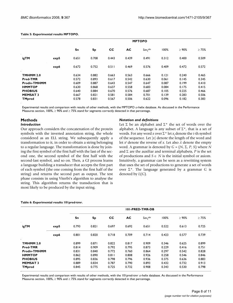
Table 5: Experimental results MPTOPO.

MPTOPO

Sn Sp CC AC Sov3obs 100% ≥ 90% ≥ 75%

igTM exp5 0.651 0.708 0.443 0.439 0.491 0.312 0.400 0.509

exp6 0.672 0.752 0.511 0.469 0.576 0.409 0.472 0.572

TMHMM 2.0 0.634 0.882 0.663 0.563 0.666 0.121 0.240 0.465Pred-TMR 0.572 0.893 0.617 0.542 0.630 0.061 0.145 0.345Prodiv-TMHMM 0.609 0.887 0.643 0.547 0.647 0.087 0.199 0.410HMMTOP 0.630 0.868 0.637 0.558 0.683 0.084 0.175 0.415PHOBIUS 0.640 0.884 0.670 0.576 0.687 0.105 0.225 0.466MEMSAT 3 0.667 0.821 0.581 0.584 0.701 0.139 0.283 0.506TMpred 0.578 0.831 0.567 0.506 0.622 0.096 0.182 0.383

Experimental results and comparison with results of other methods, with the MPTOPO α-helix database. As discussed in the Performance Measures section, 100%, ≥ 90% and ≥ 75% stand for segments correctly detected in that percentage.

Table 6: Experimental results 101pred-tmr.

101-PRED-TMR-DB

Sn Sp CC AC Sov3obs 100% ≥ 90% ≥ 75%

igTM exp5 0.793 0.821 0.697 0.692 0.651 0.522 0.613 0.725

exp6 0.801 0.820 0.718 0.709 0.714 0.423 0.577 0.739

TMHMM 2.0 0.899 0.871 0.822 0.817 0.909 0.346 0.625 0.899Pred-TMR 0.814 0.909 0.792 0.795 0.873 0.229 0.416 0.751Prodiv-TMHMM 0.831 0.840 0.772 0.760 0.864 0.297 0.542 0.828HMMTOP 0.862 0.890 0.811 0.808 0.926 0.258 0.546 0.846PHOBIUS 0.895 0.836 0.798 0.796 0.936 0.375 0.636 0.883MEMSAT 3 0.889 0.834 0.787 0.790 0.893 0.432 0.732 0.913TMpred 0.845 0.775 0.725 0.732 0.908 0.343 0.530 0.798

Experimental results and comparison with results of other methods, with the 101pred-tmr α-helix database. As discussed in the Performance Measures section, 100%, ≥ 90% and ≥ 75% stand for segments correctly detected in that percentage.

Page 8 of 11(page number not for citation purposes)

BMC Bioinformatics 2008, 9:367 http://www.biomedcentral.com/1471-2105/9/367

An Even Linear Grammar (ELG) is a context-free grammar[40] where the productions are of the forms:

The class of Even linear Languages (ELL) is a subclass ofthe context free languages and includes properly the classof regular languages. Given an ELG, it is possible to obtainan equivalent one where the productions are of the form:

The learning of ELL can be reduced to the inference of reg-ular languages [41]. The general algorithm consists intransforming the training strings through a function σ: Σ*→ [Σ × Σ]* ∪ [Σ]* defined as follows:

Intuitively, this function relates the first and last symbolsof the word, as well as the second and the last but one, andso on. Once applied the function σ, it is possible to useany regular language inference algorithm to learn a lan-guage over the alphabet [Σ × Σ]* ∪ [Σ]*, that is, the alpha-bet of paired symbols. The learned language can beprocessed to undo the transformation σ as follows:

Several inference algorithms are suitable to be applied,each obtaining a different solution. In fact, if the GI algo-rithm identifies a subclass of regular languages, then asubclass of ELL is obtained and applied with good per-formance.

A finite state transducer is an abstract machine formallydefined by a system τ = (Q, Σ, Δ, q0, QF, E) where: Q is a

set of states, Σ and Δ are respectively the input and outputalphabets, q0 is the initial state, QF ⊆ Q is the set of finalstates and E ⊆ (Q × Σ* × Δ* × Q) is the set of transitionsof the transducer. A transducer processes an input string(word of a language), and outputs another string. A suc-cessful path in a transducer is a sequence of transitions(q0, x1, y1, q1), (q1, x2, y2, q2), ..., (qn-1, xn, yn, qn) where qn ∈QF and for 1 ≤ i ≤ n: qi ∈ Q, xi ∈ Σ* and yi ∈ Δ*. Note thata path can be denoted as (q0, x1x2 ... xn, y1y2 ... yn, qn) when-ever the sequence of states are not of particular concern. Atransduction is defined as a function t: Σ* → Δ* where t(x)= y if and only if there exist a successful path (q0, x, y, qn).Figure 4 shows an example of transducer, and the trans-duction that an accepted sequence generates. We refer theinterested reader to [42].

Grammatical inference approach to transmembrane segments predictionWe consider the transmembrane segments predictionproblem as a transduction problem. That is, given anamino acid sequence, the output of our system is asequence with the same length which distinguishesbetween those amino acids within transmembrane seg-ment and those that are not. In our work, we took intoaccount the special features of our problem to propose amethod based on inference of ELL.

A xBy A B N x y x y

A x A N x

→ ∈ ∈ =

→ ∈ ∈

∗

∗

where and

where

, , , | | | |

,

Σ

Σ

A aBb A B N a b

A a A N a

→ ∈ ∈→ ∈ ∈ ∪

where

where

, , ,

, { }

ΣΣ λ

σ λ λσ

σ σ

( )

( ) [ ]

( ) [ ] ( ) ,

== ∈

= ∈ ∈ ∗

a a a

axb ab x a b x

where

where and

Σ

Σ Σ

∀ → ∈ →∀ → ∈

A ab B P A aBb

A a P

[ ]

[ ]

add the production to the ELG

add the production to the ELG

and all these produc

A a

A P

→∀ → ∈λ ttions to the ELG

Table 7: igTM experimental comparison when TMPDB-α-nR and TMPDB-αβ-nR datasets were taken into account.

Sn Sp CC AC Sov3obs 100% ≥ 90% ≥ 75%

TMPDB-αβ-nR exp5 0.618 0.732 0.545 0.498 0.462 0.412 0.481 0.564

exp6 0.676 0.750 0.600 0.542 0.476 0.471 0.547 0.621

TMPDB-α-nR exp5 0.637 0.757 0.571 0.533 0.488 0.431 0.516 0.623

exp6 0.698 0.771 0.618 0.578 0.511 0.487 0.575 0.674

A three states transducer exampleFigure 4A three states transducer example. A label x/y denotes that the transition symbol is x with output y. For instance, the transduction of baabaab is 1110001

b/0

a/1b/1a/0

a/1b/1 ABS

Page 9 of 11(page number not for citation purposes)

BMC Bioinformatics 2008, 9:367 http://www.biomedcentral.com/1471-2105/9/367

First of all, we had to transform the available data toobtain a training set with even linear structure. This setwas used to infer an ELL. The transducer is obtained usingthe structure of the inferred ELG. Given a ELG G = (N, Σ,P, S) that does not contain productions of the form A →a, a ∈ Σ, it is possible to obtain a transducer τ = (N, Σ, Σ,S, QF, E) where:

Example 1 shows how this transformation work.

Example 1 Given the ELG G = (N, Σ, P, S) with the produc-tions:

then, the transducer τ = (N, Σ, Σ, S, {B}, E) is obtained where:

The resulting transducer is shown in Figure 4.

As we stated before, the learning problem for ELL can bereduced to the problem of learning regular languages. Inour work, in order to learn the ELL, we use an algorithmto infer k-testable in the strict sense (k-TSS) languages [25-27]. The class of ktss languages is contained into the regu-lar languages one; it is characterized by the set of segmentsof length k that appear in the words of the language.

Our approach considered a set of protein sequences Pwith known transmembrane domains and another set Lof strings over an alphabet of labels Δ = {i, o, M}. For eachsequence x in P, a labeled sequence lx is obtained. Thelabelling allows to distinguish the transmembrane seg-ments from the non-transmembrane ones. That is, giventhe string x = x1x2 ... xn ∈ P and its corresponding labeledstring lx, = l1l2 ... ln ∈ L, li = M whenever xi correspond to atransmembrane segment, li = i, when correspond to ainner segment, and li = o, when correspond to a outer seg-ment.

These sets were combined to obtain another set, named

M, with the strings . Note that the strings in this set

have an even linear structure and an even length. The setM was used to obtain a probabilistic transducer by ELLinference. The general method is summarized in Algo-rithm 1.

The returned transducer can be used to analyse problemsequences to obtain the corresponding transduction. It ispossible that the transducer may result to be non-deter-ministic and the test sequences may not belong to the lan-guage accepted by the transducer. Therefore, an error-correcting parser (for instance Viterbi's algorithm) is nec-essary to analyze the test sequences. We employed a stand-ard configuration of Viterbi's algorithm used when a GIapproach is applied to pattern recognition tasks (i.e.[33]).

ComplexityThe igTM method is composed by two phases: inferenceand analysis. The first one consists in inferring an trans-ducer from the sequences of the dataset.

The execution time of the GI algorithm used in this workis linear with the size of the dataset. The space require-ments of this step is bounded by |Σ|k, where Σ is the alpha-bet of the samples and k is the parameter of the k-tssalgorithm. Therefore, depending on the parameter used,the automaton obtained can be relatively big. The trans-formation of the automaton into a transducer is boundedby a polynomial of degree k.

The execution time of the second phase, the analysis one,is linear respect the size of the string to analyse. The spacerequirements are bounded by the size of the transducerand the analized string.

Authors' contributionsPP wrote the software and carried out the experimenta-tion. MC performed the search of web resources. Allauthors contributed to the study and interpretation of theresults. The paper was written by PP and DL. DL conceivedthe research and supervised the whole process. All authorsread and approved the final manuscript.

AcknowledgementsThis work is partially supported by the Spanish Ministerio de Educ acion y Ciencia, under contract TIN2007-60769, and Generalitat Valenciana, con-tract GV06/068. We also gratefully acknowledge the helpful comments and suggestions of Jesús Salgado and his research group. The authors also thank to the anonymous referees, whose comments helped to improve this work.

References1. Wallin E, von Heijne G: Genome-wide analyses of integral

membrane proteins from eubacterial, archaean, and eukary-otic organisms. Protein Science 1998, 7(4):1029-1038.

2. Mitaku S, Ono M, Hirokawa T, M SBC, Sonoyama : Proportion ofmembrane proteins in proteomes of 15 single-cell organismsanalyzed by the SOSUI prediction system. Biophysical Chemistry1999, 82(2–3):165-171.

3. Sugiyama Y, Polulyakh N, Shimizu T: Identification of transmem-brane protein functions by binary topology patterns. In Pro-tein Engineering Design and Selection (PEDS) Volume 16. Issue 7 Oxfordpress; 2003:479-488.

4. Sonnhammer ELL, von Heijne G, Krogh A: A Hidden MarkovModel for Predicting Transmembrane Helices in Protein

Q A N A P

E A a b B A aBb PF = ∈ → ∈= → ∈

{ : ( ) }

{( , , , ) : ( ) }

λ

S aS bB

A aA bS

B aA bB

→→→

0 1

1 0

1 1

|

|

| | λ

ES a S S b B A a A

A b S B a A B b=

( , , , ), ( , , , ), ( , , , ),

( , , , ), ( , , , ), ( , ,

0 1 1

0 1 1,, )B

⎧⎨⎩

⎫⎬⎭

xlxr

Page 10 of 11(page number not for citation purposes)

BMC Bioinformatics 2008, 9:367 http://www.biomedcentral.com/1471-2105/9/367

Publish with BioMed Central and every scientist can read your work free of charge

"BioMed Central will be the most significant development for disseminating the results of biomedical research in our lifetime."

Sir Paul Nurse, Cancer Research UK

Your research papers will be:

available free of charge to the entire biomedical community

peer reviewed and published immediately upon acceptance

cited in PubMed and archived on PubMed Central

yours — you keep the copyright

Submit your manuscript here:http://www.biomedcentral.com/info/publishing_adv.asp

BioMedcentral

Sequences. In ISMB Edited by: Glasgow JI, Littlejohn TG, Major F,Lathrop RH, Sankoff D, Sensen C. AAAI; 1998:175-182.

5. Tusnády GE, Simon I: The HMMTOP transmembrane topologyprediction server. Bioinformatics 2001, 17(9):849-850.

6. Viklund H, Elofsson A: Best alpha-helical transmembrane pro-tein topology predictions are achieved using hidden Markovmodels and evolutionary information. Protein Science 2004,13(7):1908-1917.

7. Fariselli P, Casadio R: HTP: a neural network-based method forpredicting the topology of helical transmembrane domainsin proteins. Computer Applications in the Biosciences 1996, 12:41-48.

8. Gromiha MM, Ahmad S, Suwa M: Neural network-based predic-tion of transmembrane-strand segments in outer mem-brane proteins. Journal of Computational Chemistry 2004,25(5):762-767.

9. Pasquier C, Promponas V, Palaios G, Hamodrakas J, Hamodrakas S: Anovel method for predicting transmembrane segments inproteins based on a statistical analysis of the SwissProt data-base: the PRED-TMR algorithm. Protein Eng 1999,12(5):381-385.

10. Sadovskaya NS, Sutormin RA, Gelfand MS: Recognition of Trans-membrane Segments in Proteins: Review and Consistency-based Benchmarking of Internet Servers. J Bioinformatics andComputational Biology 2006, 4(5):1033-1056.

11. Bagos PG, Liakopoulos T, Hamodrakas SJ: Evaluation of methodsfor predicting the topology of beta-barrel outer membraneproteins and a consensus prediction method. BMC Bioinformat-ics 2005, 6:7.

12. Punta M, Forrest L, Bigelow H, Kernytsky A, Liu J, Rost B: Mem-brane protein prediction methods. Methods 2007,41(4):460-74.

13. Searls DB: The language of genes. Nature 2002, 420:211-217[http://www.isrl.uiuc.edu/~amag/langev/paper/searls02languageOfGenes.html].

14. Gold EM: Language identification in the limit. Information andControl 1967, 10:447-474.

15. Angluin D: Inductive inference of formal languages from posi-tive data. Information and Control 1980, 45:117-135.

16. Angluin D, Smith C: Inductive inference:Theory and Methods.Computing Surveys 1983, 15(3):237-269.

17. Peris P, López D, Campos M, Sempere JM: Protein Motif Predic-tion by Grammatical Inference. ICGI 2006:175-187.

18. HMMTOP 2.0 webserver [http://www.enzim.hu/hmmtop/]19. PHOBIUS webserver [http://phobius.sbc.su.se]20. Käll L, Krogh A, Sonnhammer ELL: Advantages of combined

transmembrane topology and signal peptide prediction – thePhobius web server. Nucleic Acids Research 2007:429-432.

21. Käll L, Krogh A, Sonnhammer ELL: A combined transmembranetopology and signal peptide prediction method. J Mol Biol2004, 338(5):1027-36.

22. TMpred webserver [http://www.ch.embnet.org/software/TMPRED_form.html]

23. Hofmann K, Stoffel W: TMBASE – A database of membranespanning protein segments. Biol Chem Hoppe-Seyler 1993,374(166):.

24. Jones DT: Improving the accuracy of transmembrane proteintopology prediction using evolutionary information. Bioinfor-matics 2007, 23(5):538-544.

25. Knuutila T: Inference of k-Testable Tree Languages. InAdvances in Structural and Syntactic Pattern Recognition: Proc of the Inter-national Workshop Edited by: Bunke H. Singapore: World Scientific;1992:109-120.

26. García P: learning k-testable tree sets from positive data. Techrep 1993 [http://www.dsic.upv.es/users/tlcc/tlcc.html]. DSIC, Univer-sidad Politécnica de Valencia

27. Yokomori T, Kobayashi S: Learning Local Languages and TheirApplication to DNA Sequence Analysis. IEEE Trans Pattern AnalMach Intell 1998, 20(10):1067-1079.

28. Ikeda M, Arai M, Okuno T, Shimizu T: TMPDB: a database ofexperimentally-characterized transmembrane topologies.Nucleic Acids Research 2003, 31:406-409.

29. Pashou EE, Litou ZI, Liakopoulos T, Hamodrakas SJ: waveTM:Wavelet-based transmembrane segment prediction. In SilicoBiology 2004, 4:.

30. Jayasinghe S, Hristova K, White SH: MPtopo: A database of mem-brane protein topology. Protein Sci 2001, 10:455-458.

31. Yokomori T, Ishida N, Kobayashi S: Learning local languages andits application to protein alpha-chain identification. IEEE Pro-ceedings of the Twenty-Seventh Annual Hawaii International Conference onSystem Sciences 1994:113-122.

32. Lopez D, Cano A, Vazquez de Parga M, Calles B, Sempere J, Perez T,Ruiz J, Garcia P: Detection of functional motifs in biose-quences: A grammatical inference approach. In Proc of the 5thAnnual Spanish Bioinformatics Conference Univ. Politécnica de Cat-alunya; 2004:72-75.

33. Lopez D, Cano A, Vazquez de Parga M, Calles B, Sempere J, Perez T,Campos M, Ruiz J, Garcia P: MOtif discovery by k-tss grammati-cal inference. Proc of the IJCAI-05 Workshop on Grammatical InferenceApplications: Successes and Future Challenges 2005.

34. Burset M, Guigo R: Evaluation of Gene Structure PredictionPrograms. Genomics 1996, 34(3):353-367.

35. Mathews B: Comparison of the predicted and observed sec-ondary structure of T4 phage lysozyme. Biochimica BiophysicaActa 1975, 405(2):442-451.

36. B R, C S, R S: Redefining the goals of protein secondary struc-ture prediction. J Mol Biol 1994, 235:13-26.

37. Murphy LR, Wallqvist A, MLevy R: Simplified amino acid alpha-bets for protein fold recognition and implications for folding.Protein Engineering 2000, 13(3):149-152.

38. Li T, Fan K, Wang J, Wang W: Reduction of protein sequencecomplexity by residue grouping. Protein Engineering 2003,16(5):323-330.

39. Möller S, Kriventseva EV, Apweiler R: A collection of well charac-terised integral membrane proteins. Bioinformatics 2000,16(12):1159-1160.

40. Hopcroft JE, Ullman JD: Introduction to Automata Theory, Languages andComputation Addison-Wesley; 1979.

41. Sempere JM, García P: A Characterization of Even Linear Lan-guages and its Application to the Learning Problem. In ICGI,Volume 862 of Lecture Notes in Computer Science Edited by: CarrascoRC, Oncina J. Springer; 1994:38-44.

42. Berstel J: Transductions and Context-Free Languages Teubner Studien-bücher, Stuttgart; 1979.

Page 11 of 11(page number not for citation purposes)