International Communications in Heat and Mass Transfer 36 (2009) 304–313

Contents lists available at ScienceDirect

International Communications in Heat and Mass Transfer

j ourna l homepage: www.e lsev ie r.com/ locate / ichmt

Identification of temperature and moisture content fields using a combined neuralnetwork and clustering method approach☆

Leandro dos Santos Coelho a, Roberto Zanetti Freire b, Gerson Henrique dos Santos b, Nathan Mendes b,⁎a Industrial and Systems Engineering Graduate Program, PUCPR/PPGEPS, Pontifical Catholic University of Paraná, Imaculada Conceição, 1155, Zip code 80215-901, Curitiba, Paraná, Brazilb Thermal Systems Laboratory, Mechanical Engineering Graduate Program, PUCPR/PPGEM/LST, Pontifical Catholic University of Paraná, Imaculada Conceição, 1155, Zip code 80215-901,Curitiba, Paraná, Brazil

☆ Communicated by W.J. Minkowycz.⁎ Corresponding author.

E-mail addresses: leandro.coelho@pucpr.br (L.S. Coe(R.Z. Freire), gerson.santos@pucpr.br (G.H. dos Santos),(N. Mendes).

0735-1933/$ – see front matter © 2009 Published by Edoi:10.1016/j.icheatmasstransfer.2009.01.012

a b s t r a c t

a r t i c l e i n f o

Available online 21 February 2009

Keywords:

Studies on the dynamics ofimportant insight on their ebuilding and soil can contr

TemperatureMoisture contentUnderground heatingArtificial Neural NetworksNonlinear identification

ibute to reduce building thermal gains or looses. Hygrothermal aspects can berelated to many attributes such as energy consumption, occupants' thermal comfort and health, and materialdeterioration. Recently, a great variety of mathematical models to predict thermal and moisture contentprofiles in porous media have been presented in the literature. Most of those models are based on analysis ofmultilayer measurements or on Fourier analysis. The development and validation of such mathematical

temperature and moisture content distributions in porous soils have providedffect on the building hygrothermal behavior, where the interaction between both

models facilitate the understanding of heat and moisture flows at different soil depths. In this research, aradial basis function neural network (RBF-NN) approach, combined with Gath–Geva clustering method inorder to predict the temperature and moisture content profiles in soils, has been presented. A set of dataobtained from the computation of the coupled heat and moisture transfer in porous soils for the Curitiba city(Paraná State, Brazil) weather data file has been used by the RBF-NN modeling method. Simulation resultsindicate the potentialities of the RBF-NNs to learn, for the one step ahead identification, the behavior oftemperature and moisture content profiles in the media at various depths.

© 2009 Published by Elsevier Ltd.

1. Introduction

The soil temperature and moisture dynamics are important para-meters in agronomy and engineering applications, such as the passiveheating and cooling of buildings, thermal comfort and agriculturalgreenhouses. Knowledge about the soil temperature and moisture con-tent, especially at the surface, provides important information on howthe soil affects the building energy and hygrothermal performance.

The analysis of the dynamic behavior of varying moisture andtemperature at different depths in soils has significant effects onthermal engineering design. Researchers have shown that variationson the soil temperature and humidity at shallow depths present sig-nificant fluctuation on both daily and annual basis [1–6]. According totheir studies, the heat flux within the soil is affected by several para-meters such as solar radiation, air temperature,wind speed, time of theyear, shading, soil properties etc., which present a seasonal or irregularvariation. For this reason, prediction of soil temperature and moisturecontent fields is a difficult task.

lho), roberto.freire@pucpr.brnathan.mendes@pucpr.br

lsevier Ltd.

Moreover, the presence of moisture can strongly affect the tem-perature distribution in soils due especially to the evaporation/condensationmechanisms and to the strong variation of their thermo-physical properties. Building simulation codes normally do not takeinto account the soil moisture effects for predicting the ground heattransfer, which can contribute to the mould and mildew growth at thesurfaces and consequently affect occupants' health.

The investigation of numerical methods capable to predict thehygrothermal behavior of soils, considering an accurate determinationof the spatial distributions of temperature and moisture content, isrelevant to evaluate scenarios of variation in time and location of thethermal properties of the floor and ground, mainly due to varyingmoisture content and ground types. Furthermore, the developmentand validation of such mathematical models facilitate the analysisprocedure of temperature and moisture profiles at various depthsbelow ground surface. Some mathematical models, developed to pre-dict the hygrothermal profiles, have been presented in the literature[5–9]. In recent years, Artificial Neural Networks (ANNs) have beenemployed, quite frequently, as a promising tool in many areas, such aspattern recognition, function approximation, system identification,and time series forecasting for supporting the modeling of complexsystems, which incorporate multiple parameters or variables. ANNsmodels are known as black-box models which are mainly identifiedusing input–output data. Due to their strong learning capabilities,

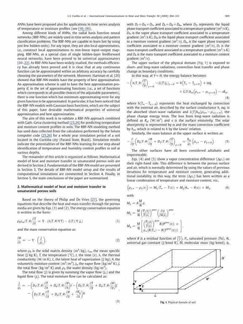
Fig. 1. Physical domain of soil.

305L.S. Coelho et al. / International Communications in Heat and Mass Transfer 36 (2009) 304–313

ANNs have been proposed also for applications in time series analysisof temperature or moisture profiles (see [10–19]).

Among different kinds of ANNs, the radial basis function neuralnetworks (RBF-NNs) arewidely used in time series analysis and patternclassification problems. The RBF-NNs are capable to learn fast by usingjust few hidden units). For any input, they are also local approximators,i.e., construct local approximations to non-linear input–output map-ping. RBF-NNs, as a special class of single hidden-layer feedforwardneural networks, have been proved to be universal approximators[20–22]. As RBF-NNs have beenwidely studied, themethods efficien-cy has already been proved and it is clear that at any continuousfunction can be approximated within an arbitrary accuracy by carefullychoosing the parameters of the network. Moreover, Hartman et al. [20]showed that RBF-NN models have the property of best approximation.An approximation scheme is said to have the best approximation pro-perty if, in the set of approximating functions (i.e., a set of functionswhich corresponds to all possible choices of the adjustable parameters),there is one function which has minimum approximating error for anygiven function to be approximated. Inparticular, it has been noticed thatthe RBF-NNmodelswith Gaussian basis functions, which are the subjectof this paper, have desirable mathematical properties of universalapproximation and best approximation.

The aim of this work is to validate a RBF-NN approach combinedwith Gath–Geva clusteringmethod [23,24] for predicting temperatureand moisture content profiles in soils. The RBF-NN modeling methodhas used data collected from the calculation performed by the Solumcomputer code [25,26] for a whole year simulation period of a soillocated in the Curitiba city (Paraná State, Brazil). Simulation resultsindicate the potentialities of the RBF-NNs learning for one step aheadidentification of temperature and humidity content profiles in soil atvarious depths.

The remainder of this article is organized as follows. Mathematicalmodel of heat and moisture transfer in unsaturated porous soils arederived in Section 2. Fundamentals of the RBF-NNmodel are presentedin Section 3. The details of RBF-NN model setup and the results ofcomputational simulations are commented in Section 4. Finally, inSection 5, the main conclusions of the paper are summarized.

2. Mathematical model of heat and moisture transfer inunsaturated porous soils

Based on the theory of Philip and De Vries [27], the governingequations that describe the heat andmass transfer through the porousmedia are given by Eqs. (1) and (2). The energy conservation equationis written in the form:

ρ0cm T; θð Þ ATAt

= j � λ T; θð ÞjTð Þ− L Tð Þ j:jvð Þ ð1Þ

and the mass conservation equation as:

AθAt

= − j � jρl

� �; ð2Þ

where ρ0 is the solid matrix density (m3/kg), cm, the mean specificheat (J/kg K), T, the temperature (°C), t, the time (s), λ, the thermalconductivity (W/m K), L, the latent heat of vaporization (J/kg), θ, thevolumetric moisture content (m3/m3), jv, the vapor flow (kg/m2 K), j,the total flow (kg/m2 K) and, ρl, the water density (kg/m3).

The total flow (j) is given by summing the vapor flow (jv) and theliquid flow (jl). The total moisture flow can be calculated as:

jρl

= − DT T; θð ÞATAx

+ Dθ T; θð ÞAθAx

� �i − DT T ; θð ÞAT

Ay+ Dθ T ; θð Þ Aθ

Ay

� �j

− DT T; θð ÞATAz

+ Dθ T ; θð ÞAθAz

+AKg

Az

� �k

;

ð3Þ

with DT=DTl+DTv and Dθ=Dθl+Dθv, where DTl represents the liquidphase transport coefficient associated to a temperature gradient (m2/sK),DTv is the vapor phase transport coefficient associated to a temperaturegradient (m2/s K), Dθl is the liquid phase transport coefficient associatedto a moisture content gradient (m2/s), Dθv is the vapor phase transportcoefficient associated to a moisture content gradient (m2/s), DT is themass transport coefficient associated to a temperature gradient (m2/s K)and Dθ is the mass transport coefficient associated to a moisture contentgradient (m2/s).

The upper surface of the physical domain (Fig. 1) is exposed toshort- and long-wave radiations, convection heat transfer and phasechange as boundary conditions.

In this way, at Y=H, the energy balance becomes:

− λ T ; θð ÞATAy

� �y=H

− L Tð Þjvð Þy=H = h T∞ − Ty=H

� �+ αqr

+ L Tð Þhm ρv;∞ − ρv;y=H

� �− eRol;

ð4Þwhere h(T∞−Ty=H) represents the heat exchanged by convectionwith the external air, described by the surface conductance h, αqr isthe absorbed short-wave radiation and L(T)hm(ρv,∞−ρv,y=H), thephase change energy term. The loss from long-wave radiation isdefined as Rol (W/m2) and ε is the surface emissivity. The solarabsorptivity is represented by α and the mass convection coefficientby hm, which is related to h by the Lewis' relation.

Similarly, the mass balance at the upper surface is written as:

− A

AyDθ T ; θð Þ Aθ

Ay+ DT T; θð ÞAT

Ay

� �y=H

=hmρl

ρv;∞ − ρy=H

� �: ð5Þ

The other surfaces have all been considered adiabatic andimpermeable.

Eqs. (4) and (5) show a vapor concentration difference (Δρν) ontheir right-hand side. This difference is between the porous surfaceand air, which is normally determined by using the values of previousiterations for temperature and moisture content, generating addi-tional instability. In this way, the term (Δρν) has been written as alinear combination of temperature and moisture content, viz.,

ρv;∞ − ρv sð Þ� �

= M1 T∞ − T sð Þð Þ + M2 θ∞ − θ sð Þð Þ + M3; ð6Þ

with

M1 = AMR

/;

M2 =MR

Ps sð ÞT sð Þ

� �prev A/Aθ sð Þ� �prev

;

M3 =MR

Ps sð ÞT sð Þ

� �prevR θprev sð Þ� �

+

/∞ R T∞ð Þ− R Tprev sð Þ� �� �24

35;

where R is a residual function of PsT

� �, Ps, saturated pressure (Pa), R,

universal gas constant (J/kmol K), M, molecular mass (kg/kmol), ϕ,

Fig. 2. Structure of the RBF-NN.

306 L.S. Coelho et al. / International Communications in Heat and Mass Transfer 36 (2009) 304–313

relative humidity, prev, previous iteration and A is the straight-linecoefficient from the approximation Ps

T

� �= AT + B.

The governing partial differential Eqs. (1)–(2) have been discretizedby using the control-volume formulation method [28]. The spatial in-terpolationmethod used is the control-difference scheme (CDS) and thetime derivatives are integrated using a fully implicit approach.

TheMTDMA (MultiTriDiagonal-Matrix Algorithm— [29])was usedto solve a 3-D model to robustly describe the physical phenomenaof the strongly coupled heat and mass transfer in porous soils. Inthis algorithm, the dependent variables are obtained simultaneously,avoiding numerical divergence caused by the evaluation of coupledterms from previous iteration values. In this way, the mass conserva-tion equation for an internal node was discretized as:

1Δt

+Dθe

Δx2+

Dθw

Δx2+

Dθn

Δy2+

Dθs

Δy2+

Dθf

Δz2+

Dθg

Δz2

� �θP +

DTe

Δx2+

DTw

Δx2+

DTn

Δy2+

DTn

Δy2+

DTf

Δz2+

DTg

Δz2

� �TP =

Dθe

Δx2θE +

DTe

Δx2TE +

Dθw

Δx2θW +

DTw

Δx2TW +

Dθn

Δy2θprevN +

DTn

Δy2TprevN +

Dθs

Δy2θprevS +

DTs

Δy2TprevS +

Dθf

Δz2θprevF +

DTf

Δz2TprevF +

Dθg

Δz2θprevG +

DTg

Δz2TprevG +

θ0PΔt

+KΔy

0BBB@

1CCCAð7Þ

Similarly, for the energy conservation, the following equation can bewritten:

LρlDθVeΔyΔzΔxe

+LρlDθVwΔyΔz

Δxw+

LρlDθVnΔxΔzΔyn

+LρlDθVsΔxΔz

Δys+

LρlDθVfΔxΔyΔzf

+

LρlDθVgΔxΔyΔzg

0BBB@

1CCCAθP +

ρ0cmΔxΔyΔzΔt

+λeΔyΔzΔxe

+LρlDTVeΔyΔz

Δxe+

λwΔyΔzΔxw

+LρlDTVwΔyΔz

Δxw+

λnΔxΔzΔyn

+LρlDTVnΔxΔz

Δyn+

λsΔxΔzΔys

+LρlDTVsΔxΔz

Δys+

λfΔxΔyΔzf

+LρlDTVgΔxΔy

Δzg

0BB@

1CCATP =

LρlDθVeΔyΔzΔxe

� �θE +

λeΔyΔzΔxe

+LρlDTVeΔyΔz

Δxe

� �TE +

LρlDθVwΔyΔzΔxw

� �θW +

λwΔyΔzΔxw

+LρlDTVwΔyΔz

Δxw

� �TW +

LρlDθVnΔxΔzΔyn

� �θprevN +

λnΔxΔzΔyn

+LρlDTVnΔxΔz

Δyn

� �TprevN +

LρlDθVsΔxΔzΔys

� �θprevS +

λsΔxΔzΔys

+LρlDTVsΔxΔz

Δys

� �TprevS +

LρlDθVfΔxΔyΔzf

!θprevF +

λfΔxΔyΔzf

+Lρf DTVfΔxΔy

Δzf

!TprevF +

LρlDθVgΔxΔyΔzg

!θprevG +

λgΔxΔyΔzg

+LρlDTVgΔxΔy

Δzg

!TprevG

+ρ0cmΔxΔyΔz

ΔtT0P

2666666666666664

3777777777777775

:

ð8ÞAsmentioned before, the difference of vapor concentration between

the porous surface and air was linearized in terms of temperature andmoisture content differences (see Eq. (6)) to strengthen the maindiagonal of the set of equations in the MTDMA form. In this way, themass conservation equation for a node located at the upper surface ofthe domain, using half-control volume, is defined as:

12Δt

+Dθe

2Δx2+

Dθw

2Δx2+

hmM2

ρlΔy+

Dθs

Δy2+

Dθf

2Δz2+

Dθg

2Δz2

� �θP +

DTe

2Δx2+

DTw

2Δx2+

hmM1

ρlΔy+

DTs

Δy2+

DTf

2Δz2+

DTg

2Δz2

� �TP =

Dθe

2Δx2θE +

DTe

2Δx2TE +

Dθw

2Δx2θW +

DTw

2Δx2TW +

Dθs

Δy2θprevS +

DTs

Δy2TprevS +

Dθf

2Δz2θprevF +

DTf

2Δz2TprevF +

Dθg

2Δz2θprevG +

DTg

2Δz2TprevG +

hmM1T∞ρlΔy

+hmM2θ∞ρlΔy

+hmM3

ρlΔy+

KΔy

+θ0P2Δt

0BBB@

1CCCAð9Þ

Analogously, for the energy conservation equation at the uppersurface, the following expression is obtained:

LρlDθVeΔyΔzΔxe

+LρlDθVwΔyΔz

Δxw+

LρlDθVnΔxΔzΔyn

+LρlDθVsΔxΔz

Δys+

LρlDθVfΔxΔyΔzf

+

LρlDθVgΔxΔyΔzg

0BBB@

1CCCAθP +

ρ0cmΔxΔyΔz2Δt

+λeΔyΔz2Δxe

+LρlDTVeΔyΔz

2Δxe+

λwΔyΔz2Δxw

+LρlDTVwΔyΔz

2Δxw+

LhmM1ΔxΔz + hcΔxΔz +λsΔxΔz2Δys

+LρlDTVsΔxΔz

2Δys+

λfΔxΔy2Δzf

+LρlDTVgΔxΔy

2Δzg

0BB@

1CCATP =

LρlDθVeΔyΔz2Δxe

� �θE +

λeΔyΔz2Δxe

+LρlDTVeΔyΔz

2Δxe

� �TE +

LρlDθVwΔyΔz2Δxw

� �θW +

λwΔyΔz2Δxw

+LρlDTVwΔyΔz

2Δxw

� �TW +

LρlDθVsΔxΔzΔys

� �θprevS +

λsΔxΔzΔys

+LρlDTVsΔxΔz

Δys

� �TprevS +

LρlDθVfΔxΔy2Δzf

!θprevF +

λfΔxΔy2Δzf

+LρlDTVfΔxΔy

2Δzf

!TprevF +

LρlDθVgΔxΔy2Δzg

!θprevG +

λgΔxΔy2Δzg

+LρlDTVgΔxΔy

2Δzg

!TprevG +

ρ0cmΔxΔyΔz2Δt

T0P + hcT∞ΔxΔz +

Lhm M1T∞ + M2θ∞ + M3ð ÞΔxΔz + αqrΔxΔz − eRolΔxΔz

2666666666664

3777777777775

ð10Þ

For the sake of brevity, the discretization equations for the othersurfaces with simpler boundary conditions were not presented in thispaper.

3. Description of radial basis function neural network

ANNs are originally inspired by the functionality of biologicalneural networks, which are able to learn complex functional relationsbased on a limited number of training data. The ANNs characteristicsof adaptive learning, generalization ability, fault tolerance, robustnessto noisy data, and parallel processing make them a very interestingoption for the systems identification.

ANNs have been proved to be capable of performing nonlinearmapping [30]. In this context, ANNs may serve as black-box models ofnonlinear systems and may be trained using input-output dataobtained from the system.

Several studies on modeling nonlinear systems have been accom-plished using RBFs or RBF-NNs [31–35]. Due to their nonlinearapproximation properties, RBF-NNs are able to model complex map-pings, while multilayer perceptron neural networks can only obtainedconsiderable results by means of multiple intermediary layers [35].Furthermore, one of the advantages of RBF-NNs compared tomultilayerperceptron, which is a classical and popular topology of ANN, is that thelinearly weighted structure of RBF-NNs, where parameters in the units

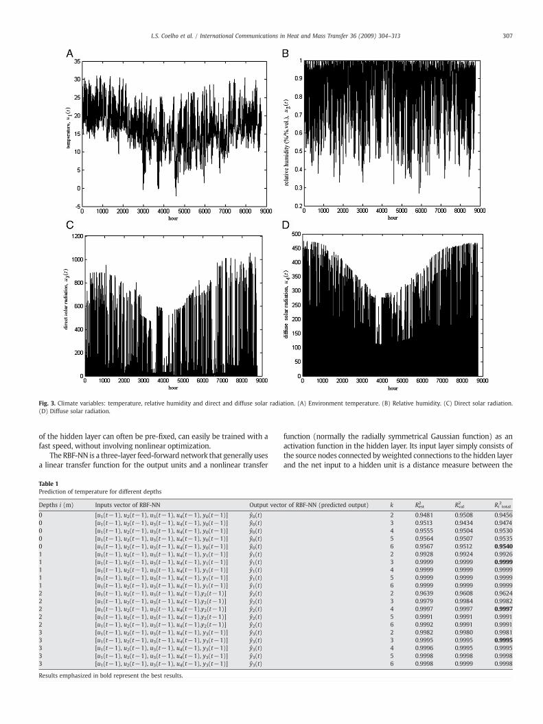
Fig. 3. Climate variables: temperature, relative humidity and direct and diffuse solar radiation. (A) Environment temperature. (B) Relative humidity. (C) Direct solar radiation.(D) Diffuse solar radiation.

307L.S. Coelho et al. / International Communications in Heat and Mass Transfer 36 (2009) 304–313

of the hidden layer can often be pre-fixed, can easily be trained with afast speed, without involving nonlinear optimization.

The RBF-NN is a three-layer feed-forward network that generally usesa linear transfer function for the output units and a nonlinear transfer

Table 1Prediction of temperature for different depths

Depths i (m) Inputs vector of RBF-NN Output vecto

0 [u1(t−1), u2(t−1), u3(t−1), u4(t−1), y0(t−1)] ŷ0(t)0 [u1(t−1), u2(t−1), u3(t−1), u4(t−1), y0(t−1)] ŷ0(t)0 [u1(t−1), u2(t−1), u3(t−1), u4(t−1), y0(t−1)] ŷ0(t)0 [u1(t−1), u2(t−1), u3(t−1), u4(t−1), y0(t−1)] ŷ0(t)0 [u1(t−1), u2(t−1), u3(t−1), u4(t−1), y0(t−1)] ŷ0(t)1 [u1(t−1), u2(t−1), u3(t−1), u4(t−1), y1(t−1)] ŷ1(t)1 [u1(t−1), u2(t−1), u3(t−1), u4(t−1), y1(t−1)] ŷ1(t)1 [u1(t−1), u2(t−1), u3(t−1), u4(t−1), y1(t−1)] ŷ1(t)1 [u1(t−1), u2(t−1), u3(t−1), u4(t−1), y1(t−1)] ŷ1(t)1 [u1(t−1), u2(t−1), u3(t−1), u4(t−1), y1(t−1)] ŷ1(t)2 [u1(t−1), u2(t−1), u3(t−1), u4(t−1).y2(t−1)] ŷ2(t)2 [u1(t−1), u2(t−1), u3(t−1), u4(t−1).y2(t−1)] ŷ2(t)2 [u1(t−1), u2(t−1), u3(t−1), u4(t−1).y2(t−1)] ŷ2(t)2 [u1(t−1), u2(t−1), u3(t−1), u4(t−1).y2(t−1)] ŷ2(t)2 [u1(t−1), u2(t−1), u3(t−1), u4(t−1).y2(t−1)] ŷ2(t)3 [u1(t−1), u2(t−1), u3(t−1), u4(t−1), y3(t−1)] ŷ3(t)3 [u1(t−1), u2(t−1), u3(t−1), u4(t−1), y3(t−1)] ŷ3(t)3 [u1(t−1), u2(t−1), u3(t−1), u4(t−1), y3(t−1)] ŷ3(t)3 [u1(t−1), u2(t−1), u3(t−1), u4(t−1), y3(t−1)] ŷ3(t)3 [u1(t−1), u2(t−1), u3(t−1), u4(t−1), y3(t−1)] ŷ3(t)

Results emphasized in bold represent the best results.

function (normally the radially symmetrical Gaussian function) as anactivation function in the hidden layer. Its input layer simply consists ofthe source nodes connected byweighted connections to the hidden layerand the net input to a hidden unit is a distance measure between the

r of RBF-NN (predicted output) k Rest2 Rval

2 Ri2total

2 0.9481 0.9508 0.94563 0.9513 0.9434 0.94744 0.9555 0.9504 0.95305 0.9564 0.9507 0.95356 0.9567 0.9512 0.95402 0.9928 0.9924 0.99263 0.9999 0.9999 0.99994 0.9999 0.9999 0.99995 0.9999 0.9999 0.99996 0.9999 0.9999 0.99992 0.9639 0.9608 0.96243 0.9979 0.9984 0.99824 0.9997 0.9997 0.99975 0.9991 0.9991 0.99916 0.9992 0.9991 0.99912 0.9982 0.9980 0.99813 0.9995 0.9995 0.99954 0.9996 0.9995 0.99955 0.9998 0.9998 0.99986 0.9998 0.9999 0.9998

Fig. 4. Estimated soil temperature at the surface (0 m) using RBF-NN. (A) Prediction oftemperature. (B) Prediction error.

Table 2Prediction of moisture content for different depths

Depths i (m) Inputs vector of RBF-NN Output vector of RBF-NN (predicted output) k Rest2 Rval

2 Ri2total

0 [u1(t−1), u2(t−1), u3(t−1), u4(t−1), y4(t−1)] ŷ4(t) 2 0.9869 0.9906 0.98880 [u1(t−1), u2(t−1), u3(t−1), u4(t−1), y4(t−1)] ŷ4(t) 3 0.9956 0.9974 0.99650 [u1(t−1), u2(t−1), u3(t−1), u4(t−1), y4(t−1)] ŷ4(t) 4 0.9965 0.9980 0.99720 [u1(t−1), u2(t−1), u3(t−1), u4(t−1), y4(t−1)] ŷ4(t) 5 0.9956 0.9961 0.99580 [u1(t−1), u2(t−1), u3(t−1), u4(t−1), y4(t−1)] ŷ4(t) 6 0.9964 0.9980 0.99711 [u1(t−1), u2(t−1), u3(t−1), u4(t−1), y5(t−1)] ŷ5(t) 2 0.3593 0.4920 0.41531 [u1(t−1), u2(t−1), u3(t−1), u4(t−1), y5(t−1)] ŷ5(t) 3 0.9811 0.9924 0.98671 [u1(t−1), u2(t−1), u3(t−1), u4(t−1), y5(t−1)] ŷ5(t) 4 0.8863 0.9495 0.91681 [u1(t−1), u2(t−1), u3(t−1), u4(t−1), y5(t−1)] ŷ5(t) 5 0.9996 0.9995 0.99971 [u1(t−1), u2(t−1), u3(t−1), u4(t−1), y5(t−1)] ŷ5(t) 6 0.9995 0.9995 0.99952 [u1(t−1), u2(t−1), u3(t−1), u4(t−1).y6(t−1)] ŷ6(t) 2 0.7115 0.7501 0.73072 [u1(t−1), u2(t−1), u3(t−1), u4(t−1).y6(t−1)] ŷ6(t) 3 0.9990 0.9989 0.99902 [u1(t−1), u2(t−1), u3(t−1), u4(t−1).y6(t−1)] ŷ6(t) 4 0.9998 0.9998 0.99982 [u1(t−1), u2(t−1), u3(t−1), u4(t−1).y6(t−1)] ŷ6(t) 5 0.9997 0.9997 0.99972 [u1(t−1), u2(t−1), u3(t−1), u4(t−1).y6(t−1)] ŷ6(t) 6 0.9998 0.9997 0.99973 [u1(t−1), u2(t−1), u3(t−1), u4(t−1), y7(t−1)] ŷ7(t) 2 0.1024 0.1024 0.10243 [u1(t−1), u2(t−1), u3(t−1), u4(t−1), y7(t−1)] ŷ7(t) 3 0.1137 0.1135 0.11363 [u1(t−1), u2(t−1), u3(t−1), u4(t−1), y7(t−1)] ŷ7(t) 4 0.9896 0.9690 0.97923 [u1(t−1), u2(t−1), u3(t−1), u4(t−1), y7(t−1)] ŷ7(t) 5 0.9996 0.9990 0.99933 [u1(t−1), u2(t−1), u3(t−1), u4(t−1), y7(t−1)] ŷ7(t) 6 0.9994 0.9990 0.9992

Results emphasized in bold represent the best results.

308 L.S. Coelho et al. / International Communications in Heat and Mass Transfer 36 (2009) 304–313

input presented at the input layer and the point represented by thehidden unit. The nonlinear transfer function (Gaussian function) isapplied to the network input to produce a radial function of the distance.The output units implement aweighted sum of the hidden unit outputs,i.e., a linear combination of the basis functions. In other words, the RBF-NN model can be viewed as a sequence of two mappings. The first is anonlinear mapping of the input data via the basis functions and thesecond is a linear mapping of the basis function outputs (i.e., nonlinearlytransformed inputs) via the weights to the network output.

For a RBF-NN, the adjustable parameters are the centers, widths, andoutput weights. The basic structure of the RBF-NN used in the presentpaper is shown in Fig. 2, which illustrates the relationship between them-dimensional input vector xaRm and then-dimensional output vectoryaRm, f: x→y. If thismapping is viewed as a function in the input space,learning can be seen as a function approximation problem. According tothis point of view, learning is equivalent to finding a surface in amultidimensional space that provides the best fit to the training data.

The nodeswithin each layer are fully connected to the previous layer.The input nodes (activation) are directly connected to the hidden layerneurons. There have been a number of popular choices for the basisfunctionϕj at thehidden layer of RBF-NNs. Themost common choice is aGaussian function. In this paper, the output of the j-th hidden neuronusing the symmetrical Gaussian function can be written as

/j xð Þ = exp −jjx−μ jjj2

σ2j

( )ð11Þ

where ||·|| is a norm on the input space, x=(x1, x2, …, xm)T is theinput vector, µj is the center vector (prototype vector), and σj is theradius width (spread or width of the radial basis function) of the j-thhidden node. The output layer represents the outputs of the RBF-NN,and each output node is a linear combination of the k radial basisfunctions of hidden nodes:

yi =Xk

j=1

wij � /j xð Þ ð12Þ

wherewij is the synaptic weight connecting hidden neuron j to outputneuron j and k is the number of the hidden layer neurons.

In this paper, the RBF-NN training is aimed at adjusting Gaussianbasis function centers, spread parameters, and weights to result inminimum sum-squared error for all the output units among all thepatterns.

The performance of a RBF-NN depends on the number andpositions of the radial basis functions, their shape, and the methodused for determining the synaptic weights. Among many learning

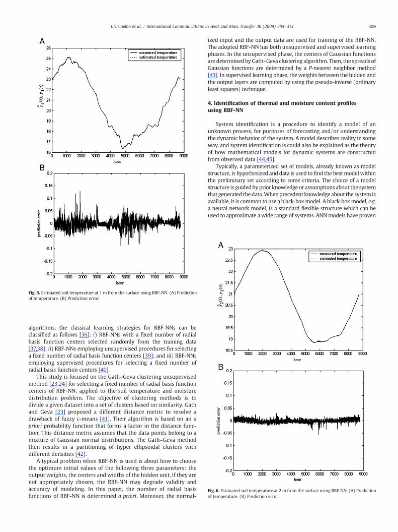
Fig. 6. Estimated soil temperature at 2 m from the surface using RBF-NN. (A) Predictionof temperature. (B) Prediction error.

Fig. 5. Estimated soil temperature at 1 m from the surface using RBF-NN. (A) Predictionof temperature. (B) Prediction error.

309L.S. Coelho et al. / International Communications in Heat and Mass Transfer 36 (2009) 304–313

algorithms, the classical learning strategies for RBF-NNs can beclassified as follows [36]: i) RBF-NNs with a fixed number of radialbasis function centers selected randomly from the training data[37,38]; ii) RBF-NNs employing unsupervised procedures for selectinga fixed number of radial basis function centers [39]; and iii) RBF-NNsemploying supervised procedures for selecting a fixed number ofradial basis function centers [40].

This study is focused on the Gath–Geva clustering unsupervisedmethod [23,24] for selecting a fixed number of radial basis functioncenters of RBF-NN, applied to the soil temperature and moisturedistribution problem. The objective of clustering methods is todivide a given dataset into a set of clusters based on similarity. Gathand Geva [23] proposed a different distance metric to resolve adrawback of fuzzy c-means [41]. Their algorithm is based on an apriori probability function that forms a factor in the distance func-tion. This distance metric assumes that the data points belong to amixture of Gaussian normal distributions. The Gath–Geva methodthen results in a partitioning of hyper ellipsoidal clusters withdifferent densities [42].

A typical problem when RBF-NN is used is about how to choosethe optimum initial values of the following three parameters: theoutput weights, the centers and widths of the hidden unit. If they arenot appropriately chosen, the RBF-NN may degrade validity andaccuracy of modeling. In this paper, the number of radial basisfunctions of RBF-NN is determined a priori. Moreover, the normal-

ized input and the output data are used for training of the RBF-NN.The adopted RBF-NN has both unsupervised and supervised learningphases. In the unsupervised phase, the centers of Gaussian functionsare determined by Gath–Geva clustering algorithm. Then, the spreads ofGaussian functions are determined by a P-nearest neighbor method[43]. In supervised learning phase, theweights between the hidden andthe output layers are computed by using the pseudo-inverse (ordinaryleast squares) technique.

4. Identification of thermal and moisture content profilesusing RBF-NN

System identification is a procedure to identify a model of anunknown process, for purposes of forecasting and/or understandingthe dynamic behavior of the system. Amodel describes reality in someway, and system identification is could also be explained as the theoryof how mathematical models for dynamic systems are constructedfrom observed data [44,45].

Typically, a parameterized set of models, already known as modelstructure, is hypothesized and data is used to find the bestmodel withinthe preliminary set according to some criteria. The choice of a modelstructure is guided byprior knowledge or assumptions about the systemthat generated thedata.Whenprecedent knowledge about the system isavailable, it is common to use a black-boxmodel. A black-boxmodel, e.g.a neural network model, is a standard flexible structure which can beused to approximate awide range of systems. ANNmodels have proven

Fig. 8. Estimated moisture content at the surface (0 m) using RBF-NN. (A) Prediction ofmoisture content. (B) Prediction error.

Fig. 7. Estimated soil temperature at 3 m from the surface using RBF-NN. (A) Predictionof temperature. (B) Prediction error.

310 L.S. Coelho et al. / International Communications in Heat and Mass Transfer 36 (2009) 304–313

to be successful nonlinear black-box model structures in manyapplications [45].

An identification case study based on the RBF-NN strategy appliedto the hygrothermal behavior of soils is evaluated in this section.Hourly values for the one-year simulation period for the Curitiba cityhave been collected. The input dada of outdoor air temperature andrelative humidity, direct and diffuse solar radiation and output oftemperature and moisture content of the soil have been chosen fortraining and validation of the proposed RBF-NN. A 10 year pre-simulation period has been applied in order to avoid the effect ofinitial conditions, since the time constant for the moisture transfer insoils are significantly high. The last year simulation results have beenused for an identification procedure. In this simulation, a constantconvective heat transfer coefficient of 10 W/m2 K, an absorptivity of0.5 and a constant long-wave radiation heat loss of 30 W/m2 havebeen used as boundary condition at the upper surface of a poroussandy silt soil. The other surfaces have been considered adiabatic andimpermeable. The hygrothermal properties of sandy silt soil weregathered from Oliveira et al. [46].

In this context, 8760 samples (1 sample to each hour) werecollected by the computer code. Those data are presented in Fig. 3.

The estimation procedure has been carried out in order to obtainthe soil hygrothermalmathematical model by using 4000 samples. Forthe validation procedure, the RBF-NN method has used signals ofsamples 4001 to 8760. The identification procedure by using RBF-NNtechnique based on Gath–Geva clustering is appropriate when thevalues of the performance index are permissible for the user's needs.

In this case, the objective is the harmonic mean maximization ofmultiple correlation indices on the estimation and validationprocedures. In the validation procedure, the multiple correlationindex function (Rest2 ) is given by:

R2est = 1−

P4000t=1

y tð Þ−y tð Þ� 2P4000t=1

y tð Þ−y½ �2ð13Þ

where y(t) is the output of the real system, ŷ(t) is the outputestimated by the RBF-NN, and y is the mean value of the system'soutput. For the validation procedure (verification of generalizationcapability) of the RBF-NN, the multiple correlation index (Rval2 ) hasbeen employed as follows:

R2val = 1 −

P8760t=4001

y tð Þ−y tð Þ� 2P8760

t=4001y tð Þ−y½ �2

ð14Þ

when the value R2=1.0 (even for the estimation as for validationprocedures), it indicates that the model obtained represents exactlythe system. A R2 value between 0.9 and 1.0 is considered acceptable

Fig.10. Estimatedmoisture content at 2m from the surface using RBF-NN. (A) Predictionof moisture content. (B) Prediction error.

Fig. 9. Estimatedmoisture content at 1 m from the surface using RBF-NN. (A) Predictionof moisture content. (B) Prediction error.

311L.S. Coelho et al. / International Communications in Heat and Mass Transfer 36 (2009) 304–313

for applications in identification and model-based controller designs[47]. Results emphasized in bold represent the best results.

The identification procedure realized by RBF-NN is divided intothree steps: i) choice of RBF-NN structure to represent the system;ii) optimization of RBF-NN by using Gath–Geva clustering method(centers of Gaussian functions), P-nearest neighbor method (spreadsof Gaussian functions) and pseudo-inverse (output weights ofnetwork); iii) evaluation of trained RBF-NN quality based on Rest

2

(estimation phase); and iv) evaluation of RBF-NNmodel for validationdata based on Rval

2 (validation phase). The computational programsand functions of RBF-NN and Gath–Geva clustering methods wereimplemented and processed into Matlab® (MathWorks Inc., MA) on a3.2 GHz Pentium IV processor with 2 MB of Random Access Memory.

In practice, system identification is an iterative procedure. The lackof a priori information regarding the system model will require thateach step initially must be examined. The mathematical modelemployed in this work to represent the soil temperature and moisturecontent profiles is a Nonlinear AutoRegressive with eXogenous inputs(NARX) model. In this case, the multivariable NARX model withseries-parallel conception is used for one-step ahead prediction withthe RBF-NN.

Several setups of RBF-NN have been tested to predict thetemperature or moisture content profiles at different depths in soils.Prediction results obtained from the RBF-NN model at 0 m (surface),1 m, 2 m and 3 m for soil temperature and moisture content arepresented in Tables 1 and 2. Also on these tables, the value of Ri2total

represents the mean harmonic of Rest2 and Rval2 . This parameter has the

property that if any element in Rest2 or Rval2 is small, the Ri

2total will be

small as well. If there are no small values, the harmonic averagewill belarge.

The notations for the estimated outputs of RBF-NN (see Tables 1and 2) are:

• k: number of radial basis functions of RBF-NN's hidden nodes;• “^”: estimated output by RBF-NN, and the variable without “^” is themeasured (real) output (temperature or moisture content in soil);

• ŷ0(t): estimated soil surface temperature (0 m);• ŷ1(t): estimated soil temperature for 1 m of surface;• ŷ2(t): estimated soil temperature for 2 m of surface;• ŷ3(t): estimated soil temperature for 3 m;• ŷ4(t): estimated moisture content for the surface (0 m);• ŷ5(t): estimated moisture content for 1 m of surface;• ŷ6(t): estimated moisture content for 2 m of surface;• ŷ7(t): estimated moisture content for 3 m of surface.

Figs. 4–11 show the best results obtained by RBF-NN (see Tables 1and 2) for one-step ahead prediction of thermal and moisture contentprofiles at depths of 0, 1, 2 and 3 m.

Results of the numerical simulations presented in Table 1 showedthat the RBF-NN model presented good performance to predicttemperature at different depths in soils (0m to 3m). The performanceindices are Ri2total≥0.9456 in all tested cases. In terms of prediction of

Fig.11. Estimatedmoisture content at 3m from the surface using RBF-NN. (A) Predictionof moisture content. (B) Prediction error.

312 L.S. Coelho et al. / International Communications in Heat and Mass Transfer 36 (2009) 304–313

moisture content at different depths (see Table 2), the simulationresults in Ri

2total≥0.9796 when the RBF-NN used k equal to 4–6

neurons (Gaussian functions) in hidden layer.

5. Conclusion and future research

The ANN approach, which is a non-linear black box model, seemsto be a useful alternative for modeling complex time series. Due totheir simple topological structure and universal approximation ability,RBF-NNs have been widely used in time-series forecasting, patternclassification, and nonlinear system modeling. RBF-NNs form adifferent class of ANN, which has certain advantages as betterapproximation capabilities, simpler network structures and fasterlearning algorithms. In RBF-NNs, the transformation from the inputspace to the space constructed by hidden layer is nonlinear, whereasthe transformation from the space constructed by hidden layer to theoutput space is linear.

In this study, a RBF-NN model combined with Gath–Gevaclustering method which can be used for determining thermal andmoisture content profiles in soil has been developed. For this purpose,a 1-year period hourly weather data has been numerically obtainedfrom input weather variables for the city of Curitiba (Paraná State,Brazil), such as temperature, relative humidity and direct and diffusesolar radiation and output of soil temperature and moisture contentwere used in the identification procedure.

The numerical results of the present study demonstrate that theproposed RBF-NN models are quite efficient in determining thermalandmoisture content profiles in soil in different depths (0m to 3m) inRi

2total termswhen the RBF-NNused 4 to 6 neurons in the hidden layer.Further investigation is needed on to improve the RBF-NN design

based on evolutionary algorithms and pruning approaches todetermining thermal and moisture content profiles.

References

[1] B.R. Anderson, Calculation of the steady-state heat transfer through a slab-on-groundfloor, Building and Environment 26(4) (1991) 405–415.

[2] M. Balghouthi, S. Kooli, A. Farhat, H. Daghari, A. Belghith, Experimentalinvestigation of thermal and moisture behaviors of wet and dry soils with buriedcapillary heating system, Solar Energy 79(6) (2005) 669–681.

[3] S.W. Rees, Z. Zhou, H.R. Thomas, The influence of soil moisture content variationson heat losses from earth-contact structures: an initial assessment, Building andEnvironment 36(2) (2001) 157–165.

[4] A. Dalinaidu, D.N. Singh, A field probe for measuring thermal resistivity of soils,Journal of Geotechnical and Geoenvironmental Engineering 130(2) (2004) 213–216.

[5] G. Mihalakakou, On the heating potential of a single buried pipe usingdeterministic and intelligent techniques, Renewable Energy 28(6) (2003)917–927.

[6] A.T.C. Goh, Modelling soil correlations using neural networks, Journal of Com-puting in Civil Engineering 9(4) (1995) 275–278.

[7] B.C. Liu, W. Liu, S.W. Peng, Study of heat and moisture transfer in soil with a drysurface layer, International Journal of Heat and Mass Transfer 48(21–22) (2005)4579–4589.

[8] H. Janssen, J. Carmeliet, H. Hens, The influence of soil moisture transfer on buildingheat loss via the ground, Building and Environment 39(7) (2004) 825–836.

[9] G.A. Ghali, Z.J. Svehik, The influence of sub-soil on the moisture regime in irrigatedfields, Agricultural Water Management 14(1–4) (1988) 307–316.

[10] G. Mihalakakou, On estimating soil surface temperature profiles, Energy andBuildings 34(3) (2002) 251–259.

[11] Y. Erzin, B.H. Rao, D.N. Sigh, Artificial neural network models for predictingsoil thermal resistivity, International Journal of Thermal Sciences 47 (2008)1347–1358.

[12] M.J. Cunningham, Inferring ventilation and moisture release rates from fieldpsychrometric data only system identification techniques, Building andEnvironment 36(1) (2001) 129–138.

[13] R. Karadag, Ö. Akgöbek, The prediction of convective heat transfer in floor-heatingsystems by Artificial Neural Networks, International Communications in Heat andMass Transfer 35(3) (2008) 312–325.

[14] Y. Varol, E. Avci, A. Koca, H.F. Oztop, Prediction of flow fields and temperaturedistributions due to natural convection in a triangular enclosure usingAdaptive-Network-Based Fuzzy Inference System (ANFIS) and Artificial NeuralNetwork (ANN), International Communications in Heat and Mass Transfer 34(7)(2007) 887–896.

[15] M. Raudenský, J. Horský, J. Krejsa, Usage of neural network for coupled parameterand function specification inverse heat conduction problem, InternationalCommunications in Heat and Mass Transfer 22(5) (1995) 661–670.

[16] K. Suleyman Yigit, H. Metin Ertunc, Prediction of the air temperature and humidityat the outlet of a cooling coil using neural networks, International Communicationsin Heat and Mass Transfer 33(7) (2006) 898–907.

[17] S. Deng, Y. Hwang, Solving the temperature distribution field in nonlinear heatconduction problems using the Hopfield neural network, Numerical Heat Transfer.Part B, Fundamentals 51(4) (2007) 375–389.

[18] S. Deng, Y. Hwang, Applying the Hopfield neural network to the solution of thetemperature distribution field in heat conduction problems, Numerical HeatTransfer. Part B, Fundamentals 50(6) (2006) 535–559.

[19] H. Deng, S. Guessasma, G. Montavon, H. Liao, C. Coddet, D. Benkrid, Combination ofinverse and neural network methods to estimate heat flux, Numerical HeatTransfer. Part B, Applications 47(6) (2005) 593–607.

[20] E.J. Hartman, J.D. Keeler, J.M. Kowalski, Layered neural networks with Gaussianhiddenunits as universal approximations, Neural Computation 2(2) (1990) 210–215.

[21] J. Park, I.W. Sandberg, Approximation and radial basis function networks, NeuralComputation 5(2) (1993) 305–316.

[22] T. Poggio, F.M. Girosi, Networks for approximation and learning, Proceedings of theIEEE 78(9) (1990) 1481–1497.

[23] G. Gath, A.B. Geva, Fuzzy clustering for the estimation of the parameters of thecomponents of mixtures of normal distributions, Pattern Recognition Letters 9(2)(1989) 77–86.

[24] J. Abonyi, B. Feil, S. Nemeth, P. Arva, Modified Gath–Geva clustering for fuzzy segsb:issue-nrmentationofmultivariable time-series, FuzzySets andSystems149(1) (2005)39–56.

[25] G.H. Santos, N. Mendes, Unsteady combined heat and moisture transfer inunsaturated porous soils, Journal of Porous Media 8(6) (2005) 493–510.

[26] G.H. Santos, N. Mendes, Simultaneous heat and moisture transfer in soilscombined with building simulation, Energy and Buildings 8(4) (2006) 303–314.

[27] J.R. Philip, D.A. De Vries, Moisture movement in porous media under temperaturegradients, Transactions — American Geophysical Union 38 (1957) 222–232.

[28] S. Patankar, Numerical Heat Transfer and Fluid Flow, Hemisphere Publishing Corp.,New York, 1980.

313L.S. Coelho et al. / International Communications in Heat and Mass Transfer 36 (2009) 304–313

[29] N. Mendes, P.C. Philippi, R. Lamberts, A newMathematical Method to Solve HighlyCoupled Equations of Heat and Mass Transfer in Porous Media, InternationalJournal of Heat and Mass Transfer 45(3) (2002) 509–518.

[30] G. Cybenko, Approximation by superposition of a sigmoidal function, Mathematicsof Control, Signal and System 2 (1989) 303–314.

[31] E. Divo, A.J. Kassab, Localized meshless modeling of natural-convective viscousflows, Numerical Heat Transfer. Part B, Fundamentals 53(6) (2008) 487–509.

[32] A. Garg, P.S. Sastry, M. Pandey, U.S. Dixit, S.K. Gupta, Numerical simulation andArtificial Neural Network modeling of natural circulation boiling water reactor,Nuclear Engineering and Design 237(3) (2007) 230–239.

[33] T.N. Singh, S. Sinha, V.K. Singh, Prediction of thermal conductivity of rock throughphysico-mechanical properties, Building and Environment 42(1) (2007) 146–155.

[34] J.L. Pedreño-Molina, J. Monzó-Cabrera, A. Toledo-Moreo, D. Sánchez-Hernández, Anovel predictive architecture for microwave-assisted drying processes based onneural networks, International Communications in Heat and Mass Transfer 32(8)(2005) 1026–1033.

[35] S. Haykin, Neural Networks: a Comprehensive Foundation, 2nd edition Prentice-Hall,Upper Saddle River, NJ, USA, 1998.

[36] N.B. Karayiannis, G.W.Mi, Growing radial basis neural networks:merging supervisedand unsupervised learning with network growth techniques, IEEE Transactions onNeural Networks 8(6) (1997) 1492–1506.

[37] D.S. Broomhead, D. Lowe, Multivariable functional interpolation and adaptive net-works, Complex Systems 2(3) (1988) 321–355.

[38] F.A. Guerra, L.S. Coelho, Multi-step ahead nonlinear identification of Lorenz'schaotic system using radial basis neural network with learning by clustering andparticle swarm optimization, Chaos, Solitons & Fractals 35(5) (2008) 967–979.

[39] J.E. Moody, C.J. Darken, Fast learning in networks of locally tuned processing units,Neural Computation 1 (2) (1989) 281–294.

[40] T. Poggio, F. Girosi, Regularization algorithms for learning that are equivalent tomultilayer networks, Science 247 (1990) 978–982.

[41] J.C. Bezdek, Pattern Recognitionwith Fuzzy Objective Function, Plenum Press, NewYork, NY, USA, 1981.

[42] M. Sciontia, J.P. Lanslots, Stabilisation diagrams: pole identification using fuzzy clus-tering techniques, Advances in Engineering Software 36(11–12) (2005) 768–779.

[43] J.A. Leonard, M.A. Kramer, Radial basis function networks for classifying processfaults, IEEE Control Systems 11(3) (1991) 31–38.

[44] L. Ljung, System Identification — Theory for the User, Prentice-Hall, Upper SaddleRiver, NJ, USA, 1987.

[45] L.S. Coelho, F.A. Guerra, Spline neural network design using improved differentialevolution for identification of an experimental nonlinear process, Applied SoftComputing 8 (2008) 1513–1522.

[46] A.A.M. Oliveira, D.S. Freitas, A.T. Prata, Influência das Propriedades do meio nasdifusividades doModelo de Phillip e DeVries em Solos Insaturados, Research Report.UFSC, 1993, (in Portuguese).

[47] B. Schaible, H. Xie, Y.C. Lee, Fuzzy logic models for ranking process effects, IEEETransactions on Fuzzy Systems 5(4) (1997) 545–556.