energies

Article

Identification of Critical Transmission Lines inComplex Power Networks

Ziqi Wang 1, Jinghan He 1,*, Alexandru Nechifor 2, Dahai Zhang 1 and Peter Crossley 2

1 Power System Protection and Control Research Laboratory, Beijing Jiaotong University,Shangyuancun No. 3, Haidian District, Beijing 100044, China; 14117390@bjtu.edu.cn (Z.W.);dhzhang1@bjtu.edu.cn (D.Z.)

2 School of Electrical and Electronic Engineering, The University of Manchester, Manchester M13 9PL, UK;alexandru.nechifor@manchester.ac.uk (A.N.); peter.crossley@manchester.ac.uk (P.C.)

* Correspondence: jhhe@bjtu.edu.cn; Tel.: +86-10-5168-3691

Received: 3 August 2017; Accepted: 25 August 2017; Published: 30 August 2017

Abstract: Growing load demands, complex operating conditions, and the increased use of intermittentrenewable energy pose great challenges to power systems. Serious consequences can occur whenthe system suffers various disturbances or attacks, especially those that might initiate cascadingfailures. Accurate and rapid identification of critical transmission lines is helpful in assessing thesystem vulnerability. This can realize rational planning and ensure reliable security pre-warning toavoid large-scale accidents. In this study, an integrated “betweenness” based identification method isintroduced, considering the line’s role in power transmission and the impact when it is removed froma power system. At the same time, the sensitive regions of each line are located by a cyclic additionalgorithm (CAA), which can reduce the calculation time and improve the engineering value of thebetweenness, especially in large-scale power systems. The simulation result verifies the effectivenessand the feasibility of the identification method.

Keywords: critical line; vulnerability; power flow redistribution; integrated betweenness; cyclicaddition algorithm

1. Introduction

Due to the expansion of power grids and increases in load demand, the power systems graduallyapproach their operating limits. This increases the uncertainty of the system dynamic behavior andthe risk of large blackouts [1]. Many power outages have occurred in recent years [2,3], for instance,the western North America blackouts in 1996 [4], the North American blackouts in 2003 [5], and theIndia blackouts in 2012 [6]. Frequent accidents expose the potential problems of current power systemanalysis methods, especially concerning system vulnerability.

In a blackout, critical lines often trigger or promote the failure propagation. These lines usuallyplay important roles in the network structure, and their disconnections greatly increase power systemvulnerability and can even cause serious consequences. Accurately identifying the critical transmissionlines can realize rational planning and provide reliable security pre-warning. It also helps to ensurecontrol measures are carried out effectively to avoid the occurrence of blackouts.

At present, researches on the identification of critical or vulnerable transmission lines are usuallybased on three main factors: the network topology [7–16], the electrical characteristics [17–23],and the failure mechanism [24–27]. Power grids can be conceptually described as networks, so thattopology-based theory provides a feasible way to study network vulnerability [7] and locate thecritical transmission lines [8,9]. Some indices, such as betweenness [10–13], are proposed to describethe importance of different components. In topology-based methods, the betweenness of an edge isdefined as the number of the shortest paths through it. Reference [14–16] indicated that the nodes

Energies 2017, 10, 1294; doi:10.3390/en10091294 www.mdpi.com/journal/energies

Energies 2017, 10, 1294 2 of 19

and lines with high betweenness and high degrees play key roles in guaranteeing the connectivityand stability of the grid. However, pure topology-based methods ignore the electrical characteristicsand often cannot completely reflect the complexity of operations [17]. Some researchers try to locateimportant substations and lines by using the electrical parameters [18–22]. An electrical betweennesswas proposed in Reference [19] to quantify the role of each line in the entire grid by using the sum ofabsolute value of power in different directions. Reference [20] improved the electrical betweennessby considering the maximal load demand and the capacity of generators in power grids. A conceptof network centrality for power systems based on system responses and topological features waspresented in Reference [21]. It aims to identify critical components with an equivalent electricalmodel. Chen et al. [22] calculated electrical efficiency based on the admittance matrix, but assumedthat power was transmitted through the most effective paths. In reality, power flow is not limitedto transfer along the lines with the smallest impedance, but in all possible ways. In Reference [23],a hybrid flow betweenness (HFB) based identification method was proposed. The new betweennesscovers the direction of power flow, the maximum transmission capacity, the electrical couplingdegree between different lines, and outage transfer distribution factor with a more comprehensiblephysical background. From the perspective of the development mechanism of large-scale blackouts,Reference [24] searched for sensitive transmission lines on the basis of the criticality of system cascadingcollapses. Wang et al. [25] used the fault chain theory to perform cascading failures initiated by faultson different transmission lines. The number of disconnected lines is basically used to derive thevulnerability index for identifying the sensitive initial lines. This type of method [24–27] is usuallybased on numerous simulations, and cannot reflect the actual power flow properties and operationalstates well.

It is reasonable to assess network vulnerability and identify critical transmission lines of powersystems with electrical and topological characteristics. However, the existing methods are mainly basedon the inherent parameters of the whole power system, without enough ability to take real-time datainto account. In this study, a new integrated betweenness is proposed to comprehensively considerthe function of a line and the impact when it is removed from a power system. Compared withprevious studies, the betweenness evaluates the role of the transmission line from the perspective ofthe power transmission distance, improves the impact analysis of fault flow distribution, and considersthe system security with the tolerance of the remaining network. At the same time, a new searchingalgorithm, named cyclic addition algorithm (CAA), is proposed to locate the sensitive regions that aresignificantly affected by a removed line. Thus the calculation time of the betweenness can be reducedand the new identification method is more valuable in engineering applications.

The rest of the paper is structured as follows: Section 2 introduces the definition and the calculationmethod of the integrated betweenness of a transmission line, which consists of the indices of the powertransmission, the fault flow distribution, and the influence on system security. Section 3 presents thedetailed identification process with integrated betweenness and CAA. The simulation results withthe IEEE 39-bus system are provided in Section 4, which prove the accuracy and effectiveness of theidentification method. Finally, conclusions are given in Section 5.

2. Integrated Betweenness to Identify Critical Lines

“Vulnerability” or its opposite concept “robustness” is often used to evaluate the ability of apower grid to provide key services or functions in normal operations, with random failures or underintentional attacks [18]. A critical transmission line plays an important role in maintaining the securityand stability of the power system. When it is removed due to external attacks or its own failure,the system may suffer from a serious impact, and even have a high probability of cascading trips.Therefore, the integrated betweenness proposed in this study comprehensively considers the role of atransmission line in a power system, the redistribution of power flow caused by a fault on the line,and the corresponding influence on system security.

Energies 2017, 10, 1294 3 of 19

Taking line i as an example, Di, Hi and Ci are respectively the indices of the power transmission,the fault flow distribution, and the influence on system security. The integrated betweenness Wi of linei can be calculated by:

Wi = D′i + H′i + C′iDi = DPi − DP0

Hi =∑

m∈ψZm

i

Bi

Ci =12 (C

ψi + Cmax

i )

(1)

where Di′, Hi

′, and Ci′ are normalized absolute values of Di, Hi, and Ci, as can be obtained by a linear

normalization method. The values of Di′, Hi

′ and Ci′ are all between 0 and 1. Di is the index of power

transmission, and is used to reflect the role of line i in the power transmission network. It can becalculated by the difference of the transmission distances of the whole power grid with and withoutline i. DP0 is the transmission distance of active power in the grid inclusive of line i, while DPi is thetransmission distance after the removal of line i; Hi is the index of fault flow distribution. It reflects theimpact caused by a fault on line i. Hi can be obtained by the ratio of the amount and the distributionentropy Bi of transferred power. Zm

i is the power change on line m when a fault happens on line i.Ψ is the set of lines with increased power. The greater the transferred power is, the larger the impactson the other lines are. The smaller the distribution entropy Bi is, the more concentrated the powerflow transfer is. A substantial increase in the transmission power can bring about harmful effects,such as the exposure of hidden failures. Ci is the index of influence on system security. Cψ

i and Cmaxi

are respectively the global and the maximum influence considering the tolerance of the remainingnetwork. The calculation method of Di, Hi, and Cmax

i is described in Sections 2.1–2.3.

2.1. The Index of Power Transmission

The importance of a line depends on its role in power transmission. The transmission distance ofactive power is defined as:

DP = ∑l∈T

∑g∈G,d∈L

|xl pl(g, d)| (2)

where xl is the electrical length of line l. It can be expressed by the reactance value, xl = xab, where xabis the element at row a and column b in the reactance matrix of a power grid; a and b are the two endsof line l; pl(g, d) is the active power on line l when power is transmitted from generator node g to loadnode d; G is the set of generators, L is the set of loads and T is the set of lines.

The above equation can be simplified to:

DP = ∑l∈T|xl ||pl | (3)

where pl is the total active power on line l, as calculated by a DC power flow model [28]:

pl = pab =θ(a)− θ(b)

xab(4)

where θ(a) and θ(b) are the phase angles of a and b. The index of power transmission of line i is [29]:

Di = DPi − DP0 (5)

where DP0 and DPi are the transmission distances with and without transmission line i. Di can expressthe change of the transmission distance of active power directly. From Equations (3)–(5), Di can beexpressed as:

Energies 2017, 10, 1294 4 of 19

Di = ∑l∈Ti

|∆θl | − ∑l∈T0

|∆θl | (6)

where ∆θl is the phase difference of the two ends of line l; T0 and Ti are the sets of lines in the systembefore and after the removal of line i. Based on DC power flow model, ∆θ can be calculated by:

∆θ = ATθ = ATB−1Ping (7)

where ∆θ is the matrix of phase difference; A is the node-branch incident matrix; B is the electricalsusceptance matrix; and, Ping is the vector of injected power. Equation (7) can be used to calculate∆θ0 and ∆θi, the matrixes of transmission distances with and without line i. Equation (5) can then beexpressed as:

Di =ri

∑a=1|∆θia| −

r0

∑a=1|∆θ0a| (8)

where r0 and ri are the numbers of lines in the system before and after the removal of line i; ∆θ0a and∆θia are the elements at row a in matrix ∆θ0 and ∆θi.

2.2. The Index of Fault Flow Distribution

Fim(g, d) is defined as the change of power on line m, as related to the power transferred from

generator g to load d, when a fault happens on line i. It can reflect the impact on line m caused by theremoval of faulty line i. Fi

m(g, d) can be calculated by the line outage distribution factor (LODF) [30]:

Fmi (g, d) = Pgd × LODFm

i (g, d) (9)

where LODFim(g, d) is the power increment of line m when unit power is transferred between generator

g and load d, and a fault happens on line i; Pgd is the power flow from generator g to load d, as calculatedby the power flow tracing method [31].

Considering the reverse overload, the change of power can be calculated as:

Zmi =

∣∣∣∣∣ ∑g∈G,d∈L

P0m(g, d) + ∑g∈G,d∈L

Fmi (g, d)

∣∣∣∣∣−∣∣∣∣∣ ∑g∈G,d∈L

P0m(g, d)

∣∣∣∣∣ (10)

where P0m(g, d) is the power flow on line m in normal operating condition, and Zim is the change of

power on line m when line i is disconnected. In the DC power flow model, Zim can also be obtained

using the calculation result of Equation (4). For the lines with increased power, the sharing ratio ofpower flow transfer on each line is:

δmi =

Zmi

∑m∈ψ

Zmi

(11)

where δim is the sharing ratio of line m when line i is disconnected; Ψ is the set of lines with increased

power. The entropy of the fault flow distribution is:

Bi = −∑m∈ψ

δmi ln δm

i (12)

The entropy Bi is used to describe the distribution of Zin, n = 1, 2, 3, . . . , m, . . . When the power

is uniformly distributed, each component will shoulder the burden equally. The sharing ratio of eachpath is δ = 1/N, where N is the number of transferable paths. Bi is the maximum, as is lnN. Similarly,the smaller the value of Bi is, the more concentrated the transferred power flow is [32]. It means thatthe disconnection of line i will have significant influence on a few lines, which may overload these

Energies 2017, 10, 1294 5 of 19

lines and even trigger a cascading failure. Thus, the index Hi can be used to show the distribution offault flow, i.e.,

Hi =

∑m∈ψ

Zmi

Bi(13)

2.3. The Index of Influence on System Security

Although the disconnections of some lines can cause a significant transfer of power flow,detrimental consequences may not be caused if other lines have large capacities and can successfullyshare the transferred power. Sometimes, the influence is not great, but the operating condition is closeto the safety limits, and the disconnection of a line may force the system into a dangerous operatingcondition. Hence it is important to consider the redistribution of power flow and the tolerance ofthe remaining network when evaluating the importance of a line in the whole system. In this paper,the global influence and the influence on each line caused by the removal of line i are analyzed. Theindex of the influence on line m is:

Cmi =

Zmi

Sm(14)

where Sm is the remaining available channel of line m before the removal of line i. The global influencecan by calculated by:

Cψi =

1r0 − 1 ∑

m∈ψ

Cmi (15)

where r0 is the number of lines in the power system, and CiΨ is the average value of Ci

m. The influenceon system security is:

Ci =12(Cψ

i + Cmaxi ) (16)

where Cimax is the maximum value of Ci

m, and Ci is the average value of the global influence and themaximal influence.

2.4. The Threshold of the Integrated Betweenness

If the removal of line i causes the overload of any other line in the power grid, line i can beconsidered a critical component [33]. In order to better assess whether the line is critical, threethresholds Dth, Hth and Cth are defined next:

(1) Dth:Dth = min

a∈T0|xa|

∣∣pcpa∣∣−min

b∈T0|xb||pb| (17)

where xa is the electrical length of line a; pcpa is the remaining available channel of line a; xb is theelectrical length of line b; pb is the total active power on line b; and, T0 is the set of lines in the powersystem. For line i, Di = DPi − DP0 and DPi has already subtracted |xi||pi|, so min |xb||pb| is alsosubtracted from Dth.

(2) Hth: Hi can reflect the impact caused by a fault on line i. To avoid missing critical lines,Hth should be the minimum Hi when one remaining line is overloaded after the fault. To get theminimum Hi, the entropy Bi of the fault flow distribution should be as large as possible and ∑

m∈ψZm

i in

Equation (13) should be as small as possible. Let us assume the smallest remaining available channel ofa transmission line is pmincp, and pmincp = minpcpa, a ∈ T0. Bi takes the maximum value, i.e., ln(r0 − 1),and ∑

m∈ψZm

i takes pmincp ignoring the complex conditions. The threshold of H is:

Energies 2017, 10, 1294 6 of 19

Hth =pmincp

ln(r0 − 1)(18)

(3) Cth: When only one remaining line is overloaded and other lines are not affected, Cimax = 1

and Ciψ =1/(r0 − 1). The threshold of C is:

Cth =12(1 +

1r0 − 1

) (19)

Wth equals to the sum of normalized Dth, Hth and Cth, i.e.,

Wth = D′th + H′th + C′th (20)

where Dth′, Hth

′ and Cth′ are normalized absolute values of Dth, Hth and Cth. The transmission line,

the integrated betweenness of which is greater than Wth, can be regarded as a critical component.The mathematical formulae for Dth, Hth, and Cth give out small values. Such small threshold valuesprevent missing the detection of critical lines. After the above process, these lines can be sortedaccording to W.

3. Identification Process with Integrated Betweenness and CAA

The integrated betweenness of each line is affected by the changes in the grid’s structure or theoperating mode. The calculation time is large when the approach is applied to the data of the wholepower network. In fact, Di, Hi, and Ci are all related to the changes of power flow before and afterline i is removed, where the changes mainly occur on particularly sensitive lines. Therefore, a cyclicaddition algorithm (CAA) is proposed to locate the sensitive regions which consist of the transmissionlines with large variations of power. The impact on the sensitive regions is analyzed rather than theimpact on the whole power network. Thus, the calculation time of the betweenness can be significantlyreduced and the proposed identification method is more suited to the real-time analysis.

The process to identify the critical transmission lines is shown in Figure 1. First, the basic data ofthe grid, such as the structural parameters and the information of power flow, are obtained. The datacan be collected by phasor measurement units (PMUs). When the network structure or operatingmode changes, the identification process of critical lines in this state will start. Possible changes ofthe network structure or operating mode include the disconnection/failure of primary equipment(generators, transformers, or lines), the connection/reconnection of primary equipment, and significantredistribution of power flow within the grid. Such changes can be caused by (1) faults, e.g., line trip,generator trip, and line failure; (2) planned adjustments, e.g., the operation of new generators/linesand planned load shedding. Then Wth and the integrated betweenness of each line are calculated:sensitive regions can be located by CAA, and the remaining regions are regarded as non-sensitiveregions in this study. Since the influence of the non-sensitive regions on the calculation results is quitesmall, those regions can be simplified as sources and loads. The number of lines and substations inthe system is greatly reduced after the simplification, so that the integrated betweenness W can becalculated more quickly. With the calculation method introduced in Section 2, W of each line can beobtained. Finally, the critical lines can be identified.

Energies 2017, 10, 1294 7 of 19Energies 2017, 10, 1294 7 of 19

Select line i

Search for the sensitive regions of line iwith CAA

Remove the lines and substations outside the sensitive regions and simplify the non-sensitive

regions into sources or loads

Caculate Di, Hi and Ci

Obtain the basic data of power network

Caculate Wth and W of each line

Get critical lines whose intergrated betweenness is greater than Wth and rank the

lines according to W

end

Does the structure or operating mode of power

system change?

Have all lines been analyzed?

Yes

No

Yes

No

i=i+1

Let i=1

Caculate Dth, Hth, Cth

Figure 1. The flow chart of the proposed identification method.

Location of Sensitive Regions with CAA

The power flow is transferred on all feasible paths, but the transferred power on each path is quite different. As can be seen from previous studies [26–31], when a transmission line is disconnected or removed from the power network, the power is usually transferred to other paths connected with the two-end nodes of the removed line, and mainly along the paths with short electrical distances, as is shown in Figure 2.

(a) (b)

Figure 2. (a) Power flow of the 6-bus system in normal operation; (b) The redistribution of power flow caused by the removal of line 1–3.

1

2

3

4 5 6

1

2

3

4 65

Figure 1. The flow chart of the proposed identification method.

Location of Sensitive Regions with CAA

The power flow is transferred on all feasible paths, but the transferred power on each path isquite different. As can be seen from previous studies [26–31], when a transmission line is disconnectedor removed from the power network, the power is usually transferred to other paths connected withthe two-end nodes of the removed line, and mainly along the paths with short electrical distances, as isshown in Figure 2.

Energies 2017, 10, 1294 7 of 19

Select line i

Search for the sensitive regions of line iwith CAA

Remove the lines and substations outside the sensitive regions and simplify the non-sensitive

regions into sources or loads

Caculate Di, Hi and Ci

Obtain the basic data of power network

Caculate Wth and W of each line

Get critical lines whose intergrated betweenness is greater than Wth and rank the

lines according to W

end

Does the structure or operating mode of power

system change?

Have all lines been analyzed?

Yes

No

Yes

No

i=i+1

Let i=1

Caculate Dth, Hth, Cth

Figure 1. The flow chart of the proposed identification method.

Location of Sensitive Regions with CAA

The power flow is transferred on all feasible paths, but the transferred power on each path is quite different. As can be seen from previous studies [26–31], when a transmission line is disconnected or removed from the power network, the power is usually transferred to other paths connected with the two-end nodes of the removed line, and mainly along the paths with short electrical distances, as is shown in Figure 2.

(a) (b)

Figure 2. (a) Power flow of the 6-bus system in normal operation; (b) The redistribution of power flow caused by the removal of line 1–3.

1

2

3

4 5 6

1

2

3

4 65

Figure 2. (a) Power flow of the 6-bus system in normal operation; (b) The redistribution of power flowcaused by the removal of line 1–3.

Energies 2017, 10, 1294 8 of 19

The topological analysis-based method can provide a quick and effective way to identify thenetwork structure and find propagation paths of power flow transfer [34]. Some new approaches,such as the compressive sensing-based approach [35] and graphical learning-based approach [36,37]were proposed in recent years. Based on Dijkstra’s algorithm [38], CAA is proposed in this study.The sensitive regions can be obtained through the cyclic addition of different lines. The following is adetailed description of the process.

Supposing there are a substations and b lines, all substations in the power grid can be simplifiedas nodes and form V according to graph theory, as is V = {v1, v2, ..., va}. All lines are represented bythe edge set E, E = {e1, e2, e3, . . . , eb}. V and E constitute G(V, E), the topology graph of the power grid.All different paths connecting vi and vj in graph G form set D(G, vi, vj), and the length of path d is l(d).The line reactance is used as the weight of an edge, and l(d) is the sum of the weights of all edges inpath d.

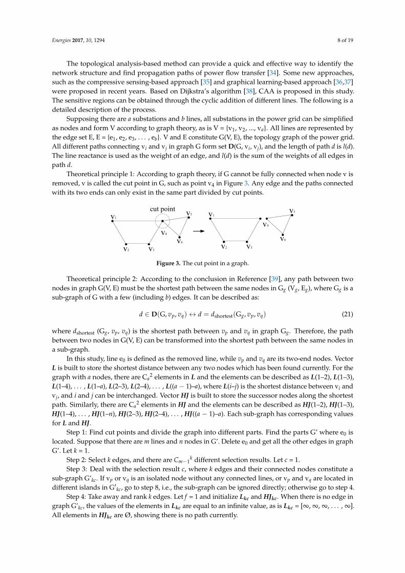
Theoretical principle 1: According to graph theory, if G cannot be fully connected when node v isremoved, v is called the cut point in G, such as point v4 in Figure 3. Any edge and the paths connectedwith its two ends can only exist in the same part divided by cut points.

Energies 2017, 10, 1294 8 of 19

The topological analysis-based method can provide a quick and effective way to identify the network structure and find propagation paths of power flow transfer [34]. Some new approaches, such as the compressive sensing-based approach [35] and graphical learning-based approach [36,37] were proposed in recent years. Based on Dijkstra’s algorithm [38], CAA is proposed in this study. The sensitive regions can be obtained through the cyclic addition of different lines. The following is a detailed description of the process.

Supposing there are a substations and b lines, all substations in the power grid can be simplified as nodes and form V according to graph theory, as is V = {v1, v2, ..., va}. All lines are represented by the edge set E, E = {e1, e2, e3, …, eb}. V and E constitute G(V, E), the topology graph of the power grid. All different paths connecting vi and vj in graph G form set D(G, vi, vj), and the length of path d is l(d). The line reactance is used as the weight of an edge, and l(d) is the sum of the weights of all edges in path d.

Theoretical principle 1: According to graph theory, if G cannot be fully connected when node v is removed, v is called the cut point in G, such as point v4 in Figure 3. Any edge and the paths connected with its two ends can only exist in the same part divided by cut points.

Figure 3. The cut point in a graph.

Theoretical principle 2: According to the conclusion in reference [39], any path between two nodes in graph G(V, E) must be the shortest path between the same nodes in Gg (Vg, Eg), where Gg is a sub-graph of G with a few (including b) edges. It can be described as:

shortest(G, , ) (G , , )p q g p qd v v d d v v D (21)

where dshortest (Gg, vp, vq) is the shortest path between vp and vq in graph Gg. Therefore, the path between two nodes in G(V, E) can be transformed into the shortest path between the same nodes in a sub-graph.

In this study, line e0 is defined as the removed line, while vp and vq are its two-end nodes. Vector L is built to store the shortest distance between any two nodes which has been found currently. For the graph with a nodes, there are Ca2 elements in L and the elements can be described as L(1–2), L(1–3), L(1–4), …, L(1–a), L(2–3), L(2–4), …, L((a − 1)–a), where L(i–j) is the shortest distance between vi and vj, and i and j can be interchanged. Vector HJ is built to store the successor nodes along the shortest path. Similarly, there are Ca2 elements in HJ and the elements can be described as HJ(1–2), HJ(1–3), HJ(1–4), …, HJ(1–n), HJ(2–3), HJ(2–4), …, HJ((a − 1)–a). Each sub-graph has corresponding values for L and HJ.

Step 1: Find cut points and divide the graph into different parts. Find the parts G’ where e0 is located. Suppose that there are m lines and n nodes in G’. Delete e0 and get all the other edges in graph G’. Let k = 1.

Step 2: Select k edges, and there are Cm−1k different selection results. Let c = 1. Step 3: Deal with the selection result c, where k edges and their connected nodes constitute a

sub-graph G’kc. If vp or vq is an isolated node without any connected lines, or vp and vq are located in different islands in G’kc, go to step 8, i.e., the sub-graph can be ignored directly; otherwise go to step 4.

Step 4: Take away and rank k edges. Let f = 1 and initialize Lkc and HJkc. When there is no edge in graph G’kc, the values of the elements in Lkc are equal to an infinite value, as is Lkc = [∞, ∞, ∞, …, ∞]. All elements in HJkc are Ø, showing there is no path currently.

Step 5: Put edge f back. The two-end nodes of f are vu and vv, vu and vv V’kc. Next apply the following judgment: If Lkc(u − v) < l(f), go directly to step 7. Otherwise, let Lkc(u − v) = l(f), HJkc(u − v) = v, and go to step 6.

cut pointv1

v2 v3

v4

v6

v5 v1

v2 v3

v4

v6

v5

Figure 3. The cut point in a graph.

Theoretical principle 2: According to the conclusion in Reference [39], any path between twonodes in graph G(V, E) must be the shortest path between the same nodes in Gg (Vg, Eg), where Gg is asub-graph of G with a few (including b) edges. It can be described as:

d ∈ D(G, vp, vq)↔ d = dshortest(Gg, vp, vq) (21)

where dshortest (Gg, vp, vq) is the shortest path between vp and vq in graph Gg. Therefore, the pathbetween two nodes in G(V, E) can be transformed into the shortest path between the same nodes ina sub-graph.

In this study, line e0 is defined as the removed line, while vp and vq are its two-end nodes. VectorL is built to store the shortest distance between any two nodes which has been found currently. For thegraph with a nodes, there are Ca

2 elements in L and the elements can be described as L(1–2), L(1–3),L(1–4), . . . , L(1–a), L(2–3), L(2–4), . . . , L((a − 1)–a), where L(i–j) is the shortest distance between vi andvj, and i and j can be interchanged. Vector HJ is built to store the successor nodes along the shortestpath. Similarly, there are Ca

2 elements in HJ and the elements can be described as HJ(1–2), HJ(1–3),HJ(1–4), . . . , HJ(1–n), HJ(2–3), HJ(2–4), . . . , HJ((a − 1)–a). Each sub-graph has corresponding valuesfor L and HJ.

Step 1: Find cut points and divide the graph into different parts. Find the parts G’ where e0 islocated. Suppose that there are m lines and n nodes in G’. Delete e0 and get all the other edges in graphG’. Let k = 1.

Step 2: Select k edges, and there are Cm−1k different selection results. Let c = 1.

Step 3: Deal with the selection result c, where k edges and their connected nodes constitute asub-graph G’kc. If vp or vq is an isolated node without any connected lines, or vp and vq are located indifferent islands in G′kc, go to step 8, i.e., the sub-graph can be ignored directly; otherwise go to step 4.

Step 4: Take away and rank k edges. Let f = 1 and initialize Lkc and HJkc. When there is no edge ingraph G’kc, the values of the elements in Lkc are equal to an infinite value, as is Lkc = [∞, ∞, ∞, . . . , ∞].All elements in HJkc are Ø, showing there is no path currently.

Energies 2017, 10, 1294 9 of 19

Step 5: Put edge f back. The two-end nodes of f are vu and vv, vu and vv ∈ V′kc. Next applythe following judgment: If Lkc(u − v) < l(f ), go directly to step 7. Otherwise, let Lkc(u − v) = l(f ),HJkc(u − v) = v, and go to step 6.

Step 6: Deal with Lkc and HJkc:For w (1 5 w 5 n, w 6= u, w 6= v):If Lkc(u− w) > Lkc(u− v) + Lkc(v− w), change the value of Lkc(u− w) into Lkc(u − v) + Lkc(v − w),

and change HJkc(u − w) into v; If Lkc(v − w) > Lkc(u − v) + Lkc(u − w), change the value of Lkc(v − w)into Lkc(u − v) + Lkc(u − w), and change HJkc(v − w) into u;

If Lkc(u − w) = Lkc(u − v) + Lkc(v − w) 6= ∞, insert v into HJkc(u − w); If Lkc(v − w) = Lkc(u − v) +Lkc(u − w) 6= ∞, insert u into HJkc(v − w); then go to step 7.

Step 7: If f = k, go to step 8; otherwise f = f + 1, then go back to step 5.Step 8: If c = Cm−1

k, go to step 9; otherwise c = c + 1, then go back to step 3.Step 9: if k = m−1, go to step 10; otherwise k = k + 1, then go back to step 2.Step 10: All the paths between vp and vq and their lengths can be got. Remove duplicate paths.Supposing that there are y paths between vp and vq, the lengths of all paths (l(1), l(2), ..., l(y)) can

be derived by the above process. According to the principle of electric circuits, the transferred powerflow on path d changes inversely with the length l(d). Thus, the power sharing coefficient of edge i is:

ξi = ∑o∈µ

1

l(o)y∑

s=1

1l(s)

(22)

where µ is the set of paths which contain line i. Judge whether the power sharing coefficient can satisfy:

ξi ≥ ξth (23)

where ξth is the threshold value, ξth ≥ 0. If (23) is satisfied, line i will be regarded as a sensitive line, asis closely related to line e0. The sensitive lines should be selected effectively and the sensitive regionswhich consist of sensitive lines should be fully connected. According to the definition of sensitivelines or transmission sections in Reference [40], the threshold value usually varies between 0.2 and 0.3.Based on the above analysis, the threshold ξth can be obtained by the following iterative process: ξth isinitialized with 0.3. If the sensitive regions are not fully connected, ξth will be decreased with a fixedstep size, until the requirement of full connection can be satisfied or the value of ξth is 0.

To improve the accuracy of integrated betweenness and to avoid missing sensitive lines, ξth canbe taken as 0 directly in an extreme situation.

Sensitive regions can be obtained by the above process. For G′ with m lines and n nodes,the calculation amount of the cyclic process in CAA in the worst condition is:

P =m−1

∑k=1

Ckm−1 · k · (4n− 6) (24)

where P = 1 means that one element in L or HJ is updated once. For G′ with m lines and n nodes. Cm−1k

is the number of sub-graphs with k lines. In the worst case, all sub-graphs can satisfy the requirementin step 3, and none will be ignored. 2(n − 2) + 1 elements in L and 2(n − 2) + 1 elements in HJ areupdated when one transmission line is put back through steps 5 and 6. The process of CAA onlycontains some simple comparisons based on a pure topology model. Therefore, the calculation time ofthe identification method can be significantly reduced. At the same time, it should be noticed that CAAis effective for most lines in power systems. For the lines which do not have other paths connectedwith their two ends, the removal of the lines can result in the islanding phenomenon. In these cases,the injected power of sources and absorbed power of loads in each island should be balanced first.

Energies 2017, 10, 1294 10 of 19

After that, the calculation of the integrated betweenness can be carried out using the analysis of thewhole power network.

4. Test Cases

In this section, IEEE 39-bus system is used as the test system to demonstrate the effectiveness ofthe proposed method.

4.1. Location of Sensitive Regions

4.1.1. Location of Sensitive Regions with CAA

Line e33 is taken as an example and used to show the detailed process to locate the sensitive regions.Firstly, all substations and lines are simplified as nodes and edges. Line e33 is the removed line,

while v26 and v29 are its two-end nodes. Divide the graph into different parts with cut points v26

and v16 in Figure 4. G’ which contains v26, v28, v29, e32, e33 and e34 is found, and then e33 is deleted.The edges e32 and e33 in graph G’ are taken away. Let k = 1. Select 1 edge, and it can be seen that thereis no path between v26 and v29 in all the sub-graphs with one edge and two nodes. Let k = 2. Takingsub-graph G’21 as an example, the sub-graph is shown in Figure 5. Since the topology of G′21 is simple,the power sharing coefficient of each edge can be obtained directly. To better illustrate the applicationof CAA, the calculation process is introduced in detail.

Energies 2017, 10, 1294 10 of 19

4. Test Cases

In this section, IEEE 39-bus system is used as the test system to demonstrate the effectiveness of the proposed method.

4.1. Location of Sensitive Regions

4.1.1. Location of Sensitive Regions with CAA

Line e33 is taken as an example and used to show the detailed process to locate the sensitive regions.

Firstly, all substations and lines are simplified as nodes and edges. Line e33 is the removed line, while v26 and v29 are its two-end nodes. Divide the graph into different parts with cut points v26 and v16 in Figure 4. G’ which contains v26, v28, v29, e32, e33 and e34 is found, and then e33 is deleted. The edges e32 and e33 in graph G’ are taken away. Let k = 1. Select 1 edge, and it can be seen that there is no path between v26 and v29 in all the sub-graphs with one edge and two nodes. Let k = 2. Taking sub-graph G’21 as an example, the sub-graph is shown in Figure 5. Since the topology of G’21 is simple, the power sharing coefficient of each edge can be obtained directly. To better illustrate the application of CAA, the calculation process is introduced in detail.

Figure 4. IEEE 39-bus system.

Figure 5. Topology of sub-graph G’21.

With the analysis of step 3, the sub-graph is kept. Take away and rank the 2 edges. Let f = 1, and initialize L21 and HJ21. The elements in L21 are [L21(26–28), L21(26–29), L21(28–29)]. The elements in HJ21 are [HJ21(26–28), HJ21(26–29), HJ21(28–29)]. L21 = [∞, ∞, ∞] and HJ21 = [Ø, Ø, Ø].

Put edge e34 back. The weight of the edge l(e34) is 0.0151, which is smaller than L21(28–29). Therefore, let L21(28–29) = 0.0151. After the step 5, L21 = [∞, ∞, 0.0151] and HJ21 = [Ø, Ø, 29]. Because L21(26–28) = L21(28–29) + L21(26–29) = ∞ and L21(26–29) = L21(28–29) + L21(26–28) = ∞, do nothing to L21 and HJ21 according to step 6. Go to step 7, i.e., f = f + 1 = 2. Then go back to step 5.

v1

v2

v3

v4v5

v6

v7

v8

v9

v10

v11

v12

v13

v14

v15

v16v17

v18

v19

v20

v21

v22

v23

v24

v25 v26

v27

v28v29

v30

v31

v32 v33v34 v35

v36

v37 v38

v39

e1

e2e3

e4 e30

e5

e6

e7

e8

e9

e10 e11e12

e13

e14

e15

e16

e17

e18

e19

e20

e21

e22

e23

e24

e25e26

e27

e28

e29

e31 e32

e33

e34

cut point

cut point

v26 v28 v29

e32 e34

Figure 4. IEEE 39-bus system.

Energies 2017, 10, 1294 10 of 19

4. Test Cases

In this section, IEEE 39-bus system is used as the test system to demonstrate the effectiveness of the proposed method.

4.1. Location of Sensitive Regions

4.1.1. Location of Sensitive Regions with CAA

Line e33 is taken as an example and used to show the detailed process to locate the sensitive regions.

Firstly, all substations and lines are simplified as nodes and edges. Line e33 is the removed line, while v26 and v29 are its two-end nodes. Divide the graph into different parts with cut points v26 and v16 in Figure 4. G’ which contains v26, v28, v29, e32, e33 and e34 is found, and then e33 is deleted. The edges e32 and e33 in graph G’ are taken away. Let k = 1. Select 1 edge, and it can be seen that there is no path between v26 and v29 in all the sub-graphs with one edge and two nodes. Let k = 2. Taking sub-graph G’21 as an example, the sub-graph is shown in Figure 5. Since the topology of G’21 is simple, the power sharing coefficient of each edge can be obtained directly. To better illustrate the application of CAA, the calculation process is introduced in detail.

Figure 4. IEEE 39-bus system.

Figure 5. Topology of sub-graph G’21.

With the analysis of step 3, the sub-graph is kept. Take away and rank the 2 edges. Let f = 1, and initialize L21 and HJ21. The elements in L21 are [L21(26–28), L21(26–29), L21(28–29)]. The elements in HJ21 are [HJ21(26–28), HJ21(26–29), HJ21(28–29)]. L21 = [∞, ∞, ∞] and HJ21 = [Ø, Ø, Ø].

Put edge e34 back. The weight of the edge l(e34) is 0.0151, which is smaller than L21(28–29). Therefore, let L21(28–29) = 0.0151. After the step 5, L21 = [∞, ∞, 0.0151] and HJ21 = [Ø, Ø, 29]. Because L21(26–28) = L21(28–29) + L21(26–29) = ∞ and L21(26–29) = L21(28–29) + L21(26–28) = ∞, do nothing to L21 and HJ21 according to step 6. Go to step 7, i.e., f = f + 1 = 2. Then go back to step 5.

v1

v2

v3

v4v5

v6

v7

v8

v9

v10

v11

v12

v13

v14

v15

v16v17

v18

v19

v20

v21

v22

v23

v24

v25 v26

v27

v28v29

v30

v31

v32 v33v34 v35

v36

v37 v38

v39

e1

e2e3

e4 e30

e5

e6

e7

e8

e9

e10 e11e12

e13

e14

e15

e16

e17

e18

e19

e20

e21

e22

e23

e24

e25e26

e27

e28

e29

e31 e32

e33

e34

cut point

cut point

v26 v28 v29

e32 e34

Figure 5. Topology of sub-graph G′21.

With the analysis of step 3, the sub-graph is kept. Take away and rank the 2 edges. Let f = 1,and initialize L21 and HJ21. The elements in L21 are [L21(26–28), L21(26–29), L21(28–29)]. The elementsin HJ21 are [HJ21(26–28), HJ21(26–29), HJ21(28–29)]. L21 = [∞, ∞, ∞] and HJ21 = [Ø, Ø, Ø].

Put edge e34 back. The weight of the edge l(e34) is 0.0151, which is smaller than L21(28–29).Therefore, let L21(28–29) = 0.0151. After the step 5, L21 = [∞, ∞, 0.0151] and HJ21 = [Ø, Ø, 29]. Because

Energies 2017, 10, 1294 11 of 19

L21(26–28) = L21(28–29) + L21(26–29) = ∞ and L21(26–29) = L21(28–29) + L21(26–28) = ∞, do nothing toL21 and HJ21 according to step 6. Go to step 7, i.e., f = f + 1 = 2. Then go back to step 5.

Similarly, put edge e32 back. L21 = [0.0474, 0.0625, 0.0151] and HJ21 = [28, 28, 29].The length of the shortest path between nodes v26 and v29 in graph G′

21 is 0.0625 according toL21(26–29). The successor node of v26 is v28, and the successor node of v28 is v29, which can be got byHJ21(26–29) and HJ21(28–29). Then the shortest path v26–v28–v29 can be obtained. The power sharingcoefficients of e32 and e34 are 1. ξth is set to 0.3. The sensitive region, which includes line e32 and e34 isnow derived.

By two simple comparisons, the analysis of all lines in the whole network can be simplified as theanalysis of two lines. The order of the matrixes, such as A and B in Equation (7), can be reduced from39 to 3 during the calculation of the integrated betweenness.

4.1.2. Comparison of CAA and Depth-First-Search Method

For the purpose of comparing the performance of CAA and Depth-First-Search (DFS) [41]algorithm, line e33 is used as an example. Both algorithms are used separately to find the pathsfrom v26 to v29 after line e33 is removed.

The CAA proposed in the study uses the topological method to search for all possible pathsconnecting the two-end nodes of the removed line and obtain the power sharing coefficients of differentedges. The DFS algorithm explores a graph by starting at a node and going as deep as possible.Such DFS traversal is a type of backtracking method, and therefore exhibits poor performance.

With CAA, the relevant sub-graph can be located at first, which effectively cleans up all uselessedges and reduces the search scope. Then, the path and its length can be obtained directly after twocomparisons. With DFS, v26 is set as the starting node. v25, v27 and v28 can be reached in the nextstep. The paths through v25 or v27 are not feasible by several explorations and backtracking. The onlyfeasible path is v26–v28–v29.

As can be seen from Section 4.1.1 and the above analysis, the proposed CAA can delete uselesslines and sub-graphs to avoid invalid search directions. In this case, the search results with CAA andDFS are identical, but the computation time with CAA is 78.6% shorter than that with DFS.

4.1.3. Accuracy Analysis of the Location Method

(1) To show the validity of the location method, branch e33 is removed at 0.5 s. The simulationresult based on PSASP is shown in Table 1. As can be seen from the simulation results, there is a largeincrease in the power transferred on the transmission lines in the sensitive regions, while the increaseson un-sensitive lines are much smaller.

Table 1. Simulation result when line e33 is removed.

Line Power Change (MW) Line Power Change (MW) Line Power Change (MW)

1 e34 189.7265 12 e13 0.584 23 e2 −0.68282 e32 186.0633 13 e10 0.103 24 e14 −0.68433 e9 2.514 14 e28 0.0099 25 e6 −0.88244 e7 2.4037 15 e29 0.0051 26 e25 −0.88415 e26 2.1787 16 e24 −0.0082 27 e16 −1.21616 e30 1.964 17 e27 −0.0305 28 e12 −1.31977 e19 1.3781 18 e23 −0.0328 29 e20 −1.37918 e18 1.3198 19 e22 −0.0565 30 e3 −1.46829 e21 1.2928 20 e8 −0.0709 31 e4 −2.1515

10 e17 1.2161 21 e15 −0.6759 32 e31 −2.225211 e11 0.5896 22 e1 −0.6828 33 e5 −2.3553

(2) Line e20 is removed at 0.2 s. The simulation result is shown in Table 2. When ξth is 0.3, there aree4, e5, e6, e8, e12, e16, e17, e18, e19, e21, e25, e26, e30, and e31 in sensitive regions. The first 14 brancheswith large power variations are included.

Energies 2017, 10, 1294 12 of 19

Table 2. Simulation result when line e20 is removed.

Line Power Change (MW) Line Power Change (MW) Line Power Change (MW)

1 e19 289.8958 12 e31 −63.5244 23 e10 −20.13392 e21 288.6156 13 e26 63.2027 24 e3 15.70693 e5 237.9716 14 e4 61.5607 25 e22 0.15934 e25 224.116 15 e9 −48.6027 26 e23 0.09915 e6 222.5013 16 e1 45.4289 27 e27 0.09726 e8 −208.162 17 e2 45.4289 28 e28 −0.0337 e18 81.8674 18 e15 45.2833 29 e33 0.02298 e12 −81.6569 19 e14 45.1093 30 e32 −0.02169 e17 75.1401 20 e7 −28.4259 31 e34 −0.0211

10 e16 −75.1401 21 e11 −25.1939 32 e24 0.018711 e30 −63.6899 22 e13 −25.0956 33 e29 −0.0182

4.2. Analysis of Identification Results

4.2.1. Identification Result with Integrated Betweenness and CAA

ξth is set as 0 to insure the accuracy of the identification. The capacity of each line is 5 timesthe initial active power. The sensitive regions can be located by CAA, and the non-sensitive regionsare simplified as sources and loads. Based on that, the integrated betweenness of each line can becalculated. For the lines whose removal can result in islanding phenomenon, the injected power ofsources and the absorbed power of loads in each island should be balanced. In this study, the absorbedpower of each load and the injected power of each source are reduced in proportion to their initialpower and according to the minimum load shedding method as described in Reference [42].

During the identification process, the shortest computation time of W for a single transmissionline is 0.515 ms, and the longest time for a single line is 8.416 ms. The computation time of the wholeprocess is 0.061 s. Without CAA, the computation time is 0.286 s when the approach is applied tothe data of the whole power network. The results prove that the CAA is effective in reducing thecomputation time.

The final results of the indices and the betweenness are shown in Table 3. Wth = 0.2546. e6, e14,e15, e19, e24, e26, and e28 cannot be regarded as critical lines. Compared with the results calculated bythe global network, the average error rate of index H with the data of sensitive regions is 2.8%, and theaverage error rate of index C is 1.02%. The average error rate of integrated betweenness W is 2.24%.The accurate identification result can still be obtained through the process of simplification.

Table 3. Calculation result of transmission lines.

LineIndex

W LineIndex

WD H C D H C

1 e27 0.7439 1 0.7975 2.5415 18 e18 0.0749 0.3855 0.0893 0.54972 e3 1 0.4868 0.8282 2.3150 19 e17 0.0845 0.4046 0.0590 0.54823 e20 0.6249 0.3874 0.9302 1.9426 20 e1 0.0454 0.1499 0.2332 0.42864 e31 0.5744 0.3437 1 1.9182 21 e2 0.0454 0.1499 0.2332 0.42865 e4 0.4285 0.3214 0.8308 1.5809 22 e13 0.0473 0.2791 0.0370 0.36366 e23 0.2676 0.5499 0.4379 1.2555 23 e30 0.0042 0.0887 0.2409 0.33397 e34 0.67893 0.3823 0.0890 1.1502 24 e5 0.0681 0.1215 0.0919 0.28168 e12 0.3574 0.4769 0.1919 1.0263 25 e33 0 0.2001 0.0626 0.26289 e21 0.1928 0.2595 0.5214 0.9738 26 e7 0.0397 0.1927 0.0276 0.2601

10 e29 0.0523 0.5406 0.3566 0.9495 27 e32 0 0.1421 0.0322 0.174311 e11 0.1849 0.6203 0.0867 0.8919 28 e6 0.0517 0.0467 0.0556 0.154112 e16 0.1981 0.4950 0.1285 0.8218 29 e24 0.0334 0.0832 0.0055 0.122213 e22 0.1972 0.5363 0.0419 0.7755 30 e28 0.0329 0.0760 0.0049 0.113914 e8 0.1445 0.3247 0.2794 0.7488 31 e14 0.0698 0.0247 0.0047 0.099315 e9 0.0232 0.6239 0.0892 0.7364 32 e15 0.0698 0.0247 0.0047 0.099316 e10 0.0957 0.4873 0.0881 0.6711 33 e19 0.0363 0.0231 0.0013 0.060717 e25 0.0434 0.2404 0.3199 0.6038 34 e26 0.0014 0.0190 0.0149 0.0354

Energies 2017, 10, 1294 13 of 19

4.2.2. Comparison of Lines with Different Integrated Betweenness

Taking lines e27, e20 and e29 as examples, the increased power of transmission lines at 1 s in IEEE39-bus system is shown in Figure 6, when e27, e20 and e29 are removed individually at 0.5 s.

Energies 2017, 10, 1294 13 of 19

4.2.2. Comparison of Lines with Different Integrated Betweenness

Taking lines e27, e20 and e29 as examples, the increased power of transmission lines at 1 s in IEEE 39-bus system is shown in Figure 6, when e27, e20 and e29 are removed individually at 0.5 s.

(a)

(b)

(c)

Figure 6. (a) Increased power of transmission lines at 1.0 s when line e27 is removed at 0.5 s, De27 = 0.743978 He27 = 1 Ce27 = 0.797568 We27 = 2.541546; (b) Increased power of transmission lines at 1.0 s when line e20 is removed at 0.5 s, De20 = 0.624963 He20 = 0.38749 Ce20 = 0.930231 We20 = 1.942685; (c) Increased power of transmission lines at 1.0 s when line e29 is removed at 0.5 s, De29 = 0.052351 He29 = 0.540608 Ce29 = 0.356604 We29 = 0.949563.

It can be seen clearly from Figure 6a that the total amount of power flow transfer is quite large and it is mainly concentrated on lines e24, e28, and e29 when line e27 is removed. It means that the disconnection of line e27 has significant influence on the power system. The comparison of Figure 6b,c shows that the transferred power is more concentrated when line e29 is removed. But the total transferred power and the global impact is less compared with the removal of line e20. The above phenomena are consistent with the values of D, H, and C, which proves the validity and rationality of the indices.

4.3. Comparison of Identification Results

To verify the effectiveness of the identification method with integrated betweenness, the top 10 lines are attacked. When compared with the attacks performed according to the hybrid flow betweenness (HFB) as introduced in reference [23], the number of islands, the total value of the loads, and the average vulnerability of the remaining network are shown in Figure 7. The loss of loads can be determined according to the minimum load shedding method [42]. The average

3 7 9 14 15 17 18 19 22 24 26 28 29 30 31 32 33 340

1

2

3

4

5

Serial number of tranmission line

P/p

.u.

1 2 3 4 5 6 7 14 15 17 18 19 21 25 26 280

0.5

1

1.5

2

2.5

Serial number of transmission line

P/p

.u.

3 7 9 14 15 17 18 19 22 23 24 27 28 30 31 32 33 340

1

2

3

Serial number of tranmission line

P/p

.u.

Figure 6. (a) Increased power of transmission lines at 1.0 s when line e27 is removed at 0.5 s,De27 = 0.743978 He27 = 1 Ce27 = 0.797568 We27 = 2.541546; (b) Increased power of transmission lines at1.0 s when line e20 is removed at 0.5 s, De20 = 0.624963 He20 = 0.38749 Ce20 = 0.930231 We20 = 1.942685;(c) Increased power of transmission lines at 1.0 s when line e29 is removed at 0.5 s, De29 = 0.052351He29 = 0.540608 Ce29 = 0.356604 We29 = 0.949563.

It can be seen clearly from Figure 6a that the total amount of power flow transfer is quite largeand it is mainly concentrated on lines e24, e28, and e29 when line e27 is removed. It means that thedisconnection of line e27 has significant influence on the power system. The comparison of Figure 6b,cshows that the transferred power is more concentrated when line e29 is removed. But the totaltransferred power and the global impact is less compared with the removal of line e20. The abovephenomena are consistent with the values of D, H, and C, which proves the validity and rationality ofthe indices.

4.3. Comparison of Identification Results

To verify the effectiveness of the identification method with integrated betweenness, the top 10lines are attacked. When compared with the attacks performed according to the hybrid flowbetweenness (HFB) as introduced in Reference [23], the number of islands, the total value of the

Energies 2017, 10, 1294 14 of 19

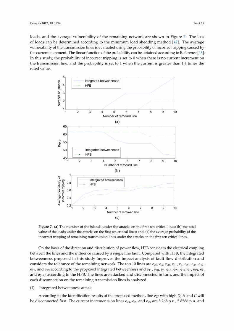
loads, and the average vulnerability of the remaining network are shown in Figure 7. The lossof loads can be determined according to the minimum load shedding method [42]. The averagevulnerability of the transmission lines is evaluated using the probability of incorrect tripping caused bythe current increment. The linear function of the probability can be obtained according to Reference [43].In this study, the probability of incorrect tripping is set to 0 when there is no current increment onthe transmission line, and the probability is set to 1 when the current is greater than 1.4 times therated value.

Energies 2017, 10, 1294 14 of 19

vulnerability of the transmission lines is evaluated using the probability of incorrect tripping caused by the current increment. The linear function of the probability can be obtained according to reference [43]. In this study, the probability of incorrect tripping is set to 0 when there is no current increment on the transmission line, and the probability is set to 1 when the current is greater than 1.4 times the rated value.

(a)

(b)

(c)

Figure 7. (a) The number of the islands under the attacks on the first ten critical lines; (b) the total value of the loads under the attacks on the first ten critical lines; and, (c) the average probability of the incorrect tripping of remaining transmission lines under the attacks on the first ten critical lines.

On the basis of the direction and distribution of power flow, HFB considers the electrical coupling between the lines and the influence caused by a single line fault. Compared with HFB, the integrated betweenness proposed in this study improves the impact analysis of fault flow distribution and considers the tolerance of the remaining network. The top 10 lines are e27, e3, e20, e31, e4, e23, e34, e12, e21, and e29 according to the proposed integrated betweenness and e11, e20, e3, e16, e29, e12, e1, e19, e7, and e5 as according to the HFB. The lines are attacked and disconnected in turn, and the impact of each disconnection on the remaining transmission lines is analyzed.

(1) Integrated betweenness attack

According to the identification results of the proposed method, line e27 with high D, H and C will be disconnected first. The current increments on lines e24, e28 and e29 are 5.268 p.u., 5.8586 p.u. and 5.4645 p.u. These lines exhibit high current increments and will therefore have a high risk of tripping. Then, line e3 is disconnected. It will have impact on several transmission lines, namely e1, e2, e6, e7, e14, e15, e25, e30, and e31. At the same time, the current on e24, e28, and e29 continues to rise and

1 2 3 4 5 6 7 8 9 101

2

3

4

5

Number of removed line

Num

ber o

f isl

ands

Integrated betweennessHFB

1 2 3 4 5 6 7 8 9 1045

50

55

60

65

Number of removed line

P/p

.u.

Integrated betweennessHFB

1 2 3 4 5 6 7 8 9 100.2

0.4

0.6

0.8

1

Number of removed line

Ave

rage

pro

babi

lity

of

inco

rrect

trip

ping

Intergrated betweennessHFB

Figure 7. (a) The number of the islands under the attacks on the first ten critical lines; (b) the totalvalue of the loads under the attacks on the first ten critical lines; and, (c) the average probability of theincorrect tripping of remaining transmission lines under the attacks on the first ten critical lines.

On the basis of the direction and distribution of power flow, HFB considers the electrical couplingbetween the lines and the influence caused by a single line fault. Compared with HFB, the integratedbetweenness proposed in this study improves the impact analysis of fault flow distribution andconsiders the tolerance of the remaining network. The top 10 lines are e27, e3, e20, e31, e4, e23, e34, e12,e21, and e29 according to the proposed integrated betweenness and e11, e20, e3, e16, e29, e12, e1, e19, e7,and e5 as according to the HFB. The lines are attacked and disconnected in turn, and the impact ofeach disconnection on the remaining transmission lines is analyzed.

(1) Integrated betweenness attack

According to the identification results of the proposed method, line e27 with high D, H and C willbe disconnected first. The current increments on lines e24, e28 and e29 are 5.268 p.u., 5.8586 p.u. and

Energies 2017, 10, 1294 15 of 19

5.4645 p.u. These lines exhibit high current increments and will therefore have a high risk of tripping.Then, line e3 is disconnected. It will have impact on several transmission lines, namely e1, e2, e6, e7,e14, e15, e25, e30, and e31. At the same time, the current on e24, e28, and e29 continues to rise and thesystem risk will be further increased. Following the disconnections of lines e20 and e31, the power flowis redistributed to lines e4, e5, e17, e18, and e19.

Islanding phenomenon occurs when e4 is disconnected. The network is split into a 6-node isolatedisland and a 33-node system. Although the network is forced to be divided into two parts, the totalamount of loads is reduced during the balance of the injected power of sources, and the absorbedpower of loads in each island. Therefore, the pressure on the transmission system and the overloadsof e1, e2, e7, e14, e15, e17, e18, e19, and e30 are relieved. Subsequently, e23 is disconnected. The nodev21 is separated from the network, and the current on e24, e28, and e29 is slightly decreased. After theattacks on e34, e12, e21, and e29, some nodes fall off, but the average vulnerability of the remaining lineskeeps increasing.

(2) HFB attack

When line e11 is disconnected, e9, e10, e14, and e15 will have a high risk of tripping. Then e20, e3,e16, e29, e12, and e1 are attacked one by one. Some transmission lines, such as e2, e6, e17, e18, e19, e21,e25, e26, and e30, are affected by the power flow transfer. Most of the current increments on these linesare between 0.2 and 0.3 p.u. and the maximum current increment is 4.4196 p.u. Subsequently, line e19

is disconnected and the node v15 is isolated from the network. Finally, e7 and e5 are attacked and theaverage probability of incorrect tripping is approximately 0.7.

It can be seen from Figure 7 that the islanding phenomenon is more obvious and the loss of loadsis greater under the integrated betweenness attack performed on the IEEE 39-bus system. The lineswith high betweenness play critical roles in the power grid. When nearly 30% of the lines are removedunder integrated betweenness attack, the loss of load remains at 24%, and the vulnerability of theremaining network is also greatly improved.

4.4. Extreme Cases and Real-Time Behavior

4.4.1. Extreme Cases

IEEE 39-bus system is used as the test system in this section. The injected and absorbed power ischanged to present some extreme cases.

(1) All the injected power of generators and the absorbed power of loads are reduced to 0.05 timesthe initial value. The calculation result is shown in Table 4. Based on the identification method, Wth =2.3149, and no line is selected to be a critical transmission line.

Table 4. Calculation result of transmission lines.

Line W Line W Line W Line W Line W

e1 0.2489 e8 0.5680 e15 0.0955 e22 1.2320 e29 0.6616e2 0.2489 e9 0.6824 e16 1.0743 e23 0.9019 e30 0.1394e3 1.6463 e10 0.6000 e17 0.5979 e24 0.1177 e31 1.1108e4 0.9140 e11 0.8219 e18 0.4032 e25 0.3507 e32 0.1483e5 0.2073 e12 0.9458 e19 0.0597 e26 0.0234 e33 0.2122e6 0.1092 e13 0.3337 e20 1.1916 e27 1.8976 e34 1.0783e7 0.2291 e14 0.0955 e21 0.5660 e28 0.1099

(2) All of the injected power of generators and the absorbed power of loads are increased 4.99 timesin respect to their initial values, to bring the system close to its stability limit. The disconnection of anyline will result in a serious consequence. In this case, Wth = 0.00822. The calculation result is shown inTable 5. All lines are regarded as critical transmission lines.

Energies 2017, 10, 1294 16 of 19

Table 5. Calculation result of transmission lines.

Line W Line W Line W Line W Line W

e1 0.4372 e8 0.7937 e15 0.0993 e22 1.2659 e29 0.9495e2 0.4372 e9 0.7544 e16 1.1781 e23 1.2555 e30 0.3339e3 2.3150 e10 0.6711 e17 0.6456 e24 0.1222 e31 1.9182e4 1.5848 e11 0.8919 e18 0.4753 e25 0.6090 e32 0.1743e5 0.2816 e12 1.1008 e19 0.0607 e26 0.03546 e33 0.2628e6 0.1541 e13 0.3636 e20 1.9426 e27 2.5415 e34 1.1502e7 0.2514 e14 0.0993 e21 0.9870 e28 0.1139

4.4.2. Real-Time Behavior of Power Grids with Different Scales

The computation times of test systems with various scales are statistically analyzed. The systemsinclude IEEE 39-bus system, IEEE118-bus system, and several large-scale systems, which are randomlysynthesized by IEEE standard 30-bus and 118-bus system [44]. The standard systems are connectedwith high-tension transmission lines. Each system is calculated ten times. The average computationtime of each test system is shown in Table 6.

Table 6. Computation time of different test systems.

Test System Number of Buses Computation Time (s)

IEEE39 39 0.061IEEE118 118 0.319SYN472 472 1.285

SYN1062 1062 2.891SYN3000 3000 7.639SYN7680 7680 32.268SYN12000 12,000 73.512

Based on the above data, the computation time can be qualitatively analyzed: the computationtime of the system with 39–5000 buses can be of the order of seconds, and the computation time of thesystem with 5000–10,000+ buses can be of the order of minutes.

The implementation of “real-time identification of critical lines” depends on two important parts:(1) measurement data acquisition; (2) data processing and analysis. The measurement data can beobtained by wide area measurement system (WAMS). According to Reference [45], WAMS is requiredto complete the measurement and transmission of PMU data in 30–50 ms for dynamic monitoring andreal-time decision-making purposes. Based on the data in Table 6, the time scale of the identificationprocess can be of the order of minutes.

5. Conclusions

In order to implement accurate and fast identification of critical lines, an integrated betweennessis proposed which considers the topological and electrical characteristics of the power network.The indices of power transmission, fault flow distribution, and the influence on system security areused to assess the importance of different lines with respect to the functionality of themselves, relevancewith other transmission lines, and system security. Although the three indices are different, they areall related to the changes in the power system before and after the removal of a line. Based on this,the sensitive regions containing lines with large variations of power are located by CAA. The analysisof the whole network is replaced by the analysis of sensitive regions, which reduces the calculationtime effectively and provides the possibility for real-time analysis in large-scale power systems.

This study focuses on the identification of critical lines which play important roles in powertransmission and whose disconnections have a great influence on system vulnerability. Together withthe transmission lines which are heavily overloaded or have high risks of failures, the identification

Energies 2017, 10, 1294 17 of 19

results can help formulate plans to avoid blackouts. The simulation results show that the proposedmethod is effective and practical.

Acknowledgments: This work was supported by the National Key R&D Program of China (2016YFB0900600)and the Fundamental Research Funds for the Central Universities (NO.2017YJS178).

Author Contributions: All authors contributed to the research in the paper. The work was carried out byZiqi Wang and performed under the advisement from Jinghan He, Alexandru Nechifor, Dahai Zhang andPeter Crossley.

Conflicts of Interest: The authors declare no conflict of interest.

References

1. Hong, S.; Cheng, H.; Zeng, P. An n–k analytic method of composite generation and transmission with intervalload. Energies 2017, 10, 168. [CrossRef]

2. Cai, Y.; Li, Y.; Cao, Y.; Li, W.; Zeng, X. Modeling and impact analysis of interdependent characteristics oncascading failures in smart grids. Int. J. Electr. Power Energy Syst. 2017, 89, 106–114. [CrossRef]

3. Zeng, K.; Wen, J.; Ma, L.; Cheng, S.; Lu, E.; Wang, N. Fast cut back thermal power plant load rejection andblack start field test analysis. Energies 2014, 7, 2740–2760. [CrossRef]

4. Kosterev, D.N.; Taylor, C.W.; Mittelstadt, W.A. Model validation for the 10 August 1996 WSCC system outage.IEEE Trans. Power Syst. 1999, 14, 967–979. [CrossRef]

5. Piacenza, J.R.; Proper, S.; Bozorgirad, M.A.; Hoyle, C.; Tumer, I.Y. Robust topology design of complexinfrastructure systems. ASCE-ASME J. Risk Uncertain. Eng. Syst. Part B Mech. Eng. 1999, 14, 967–979.

6. Rampurkar, V.; Pentayya, P.; Mangalvedekar, H.A.; Kazi, F. Cascading failure analysis for Indian power grid.IEEE Trans. Smart Grid 2016, 7, 1951–1960. [CrossRef]

7. Gao, J.; Liu, X.; Li, D.; Havlin, S. Recent progress on the resilience of complex networks. Energies 2015, 8,12187–12210. [CrossRef]

8. Gallos, L.K.; Cohen, R.; Argyrakis, P.; Bunde, A.; Havlin, S. Stability and topology of scale-free networksunder attack and defense strategies. Phys. Rev. Lett. 2005, 94, 188701. [CrossRef] [PubMed]

9. Schneider, C.M.; Moreira, A.A.; Andrade, J.S.; Havlin, S.; Herrmann, H.J. Mitigation of malicious attacks onnetworks. Proc. Natl. Acad. Sci. USA 2011, 108, 3838–3841. [CrossRef] [PubMed]

10. Holme, P.; Kim, B.J.; Yoon, C.N. Attack vulnerability of complex networks. Phys. Rev. E 2002, 65, 056109.[CrossRef] [PubMed]

11. Chen, X.; Sun, K.; Cao, Y.; Wang, S. Identification of vulnerable lines in power grid based on complex networktheory. In Proceedings of the Power Engineering-Society General Meeting, Tampa, FL, USA, 24–28 June 2007;pp. 1699–1704.

12. Dwivedi, A.; Yu, X.; Sokolowski, P. Identifying vulnerable lines in a power network using complex networktheory. In Proceedings of the IEEE International Symposium on Industrial Electronics, Seoul, Korea,5–8 July 2009; pp. 18–23.

13. Guo, J.; Han, Y.; Guo, C.; Lou, F.; Wang, Y. Modeling and vulnerability analysis of cyber-physical powersystems considering network topology and power flow properties. Energies 2017, 10, 87. [CrossRef]

14. Albert, R.; Albert, I.; Nakarado, G.L. Structural vulnerability of the North American power grid. Phys. Rev. E2004, 69, 025103. [CrossRef] [PubMed]

15. Rosas-Casals, M.; Valverde, S.; Sole, R.V. Topological vulnerability of the European power grid under errorsand attacks. Int. J. Bifurc. Chaos 2007, 17, 2465–2475. [CrossRef]

16. Crucitti, P.; Latora, V.; Marchiori, M. A topological analysis of the Italian electric power grid. Phys. A Stat.Mech. Appl. 2004, 338, 92–97. [CrossRef]

17. Hines, P.; Cotilla-Sanchez, E.; Blumsack, S. Do topological models provide good information about electricityinfrastructure vulnerability? Chaos 2010, 20, 033122. [CrossRef] [PubMed]

18. Cuadra, L.; Salcedo-Sanz, S.; Del Ser, J.; Jimenez-Fernandez, S.; Geem, Z.W. A critical review of robustness inpower grids using complex networks concepts. Energies 2015, 8, 9211–9265. [CrossRef]

19. Xu, L.; Wang, X.; Wang, X. Equivalent admittance small-world model for power system-II. Electricbetweenness and vulnerable line identification. In Proceedings of the Asia-Pacific Power and EnergyEngineering Conference, Wuhan, China, 27–31 March 2009; pp. 1–4.

Energies 2017, 10, 1294 18 of 19

20. Wang, K.; Zhang, B.; Zhang, Z.; Yin, X.; Wang, B. An electrical betweenness approach for vulnerabilityassessment of power grids considering the capacity of generators and load. Phys. A Stat. Mech. Appl. 2011,390, 4692–4701. [CrossRef]

21. Song, H.; Dosano, R.D.; Lee, B. Power grid node and line delta centrality measures for selection of criticallines in terms of blackouts with cascading failures. Int. J. Innov. Comput. Inf. Control 2011, 7, 1321–1330.

22. Chen, G.; Dong, Z.Y.; Hill, D.J.; Zhang, G.H. An improved model for structural vulnerability analysis ofpower networks. Phys. A Stat. Mech. Appl. 2009, 388, 4259–4266. [CrossRef]

23. Bai, H.; Miao, S. Hybrid flow betweenness approach for identification of vulnerable line in power system.IET Gener. Transm. Distrib. 2015, 9, 1324–1331. [CrossRef]

24. Salim, N.A.; Othman, M.M.; Musirin, I.; Serwan, M.S. Critical system cascading collapse assessment fordetermining the sensitive transmission lines and severity of total loading conditions. Math. Probl. Eng. 2013,2013, 965628. [CrossRef]

25. Wang, A.S.; Luo, Y.; Tu, G.; Liu, P. Vulnerability assessment scheme for power system transmission networksbased on the fault chain theory. IEEE Trans. Power Syst. 2011, 26, 442–450. [CrossRef]

26. Chen, J.; Thorp, J.S.; Dobson, I. Cascading dynamics and mitigation assessment in power system disturbancesvia a hidden failure model. Int. J. Electr. Power Energy Syst. 2005, 27, 318–326. [CrossRef]

27. Salim, N.A.; Othman, M.M.; Musirin, I.; Serwan, M.S.; Busan, S. Risk assessment of dynamic systemcascading collapse for determining the sensitive transmission lines and severity of total loading conditions.Reliab. Eng. Syst. Saf. 2017, 157, 113–128. [CrossRef]

28. Kim, S. Accuracy enhancement of mixed power flow analysis using a modified DC model. Energies 2016, 9,776. [CrossRef]

29. Zeng, K.; Wen, J.; Cheng, S.; Lu, E.; Wang, N. A critical lines identification algorithm of complex powersystem. In Proceedings of the Innovative Smart Grid Technologies Conference, Washington, DC, USA,19–22 February 2014; pp. 1–5.

30. Zhu, J. Optimal power flow. In Optimization of Power System Operation; Wiley-IEEE Press: Piscataway, NJ,USA, 2015.

31. Enshaee, A.; Enshaee, P. New reactive power flow tracing and loss allocation algorithms for power gridsusing matrix calculation. Int. J. Electr. Power. Energy Syst. 2017, 87, 89–98. [CrossRef]

32. Zhu, D.; Liu, W.; Lv, Q.; Wang, N. Forewarning of cascading failure based on comprehensive entropy ofpower flow. Appl. Mech. Mater. 2014, 615, 74–79. [CrossRef]

33. Wang, Q.; McCalley, J.D. Risk and “N − 1” Criteria Coordination for Real-Time Operations. IEEE Trans.Power Syst. 2013, 28, 3505–3506. [CrossRef]

34. Deka, D.; Backhaus, S.; Chertkov, M. Learning topology of distribution grids using only terminal nodemeasurements. In Proceedings of the IEEE International Conference on Smart Grid Communications, Sydney,Australia, 6–9 November 2016.

35. Babakmehr, M.; Simoes, M.G.; Wakin, M.B.; Harirchi, F. Compressive sensing-based topology identificationfor smart grids. IEEE Trans. Ind. Inform. 2016, 12, 532–543. [CrossRef]

36. Deka, D.; Backhaus, S.; Chertkov, M. Estimating distribution grid topologies: A graphical learningbased approach. In Proceedings of the 19th Power Systems Computation Conference, Genova, Italy,20–24 June 2016.

37. Deka, D.; Backhaus, S.; Chertkov, M. Learning topology of the power distribution grid with and withoutmissing data. In Proceedings of the European Control Conference, Aalborg, Denmark, 29 June–1 July 2016;pp. 313–320.

38. Wu, Y.; Li, X. Numerical simulation of the propagation of hydraulic and natural fracture using dijkstra’salgorithm. Energies 2016, 9, 519. [CrossRef]

39. Chai, D.; Zhang, D. Algorithm and its application to N shortest paths problem. J. Zhejiang Univ. 2002, 5,61–64. (In Chinese)

40. Luo, G.; Shi, D.; Chen, J.; Duan, X. Automatic identification of transmission sections based on complexnetwork theory. IET Gener. Transm. Distrib. 2014, 8, 1203–1210.

41. Berghammer, R.; Hofmann, T. Relational depth-first-search with applications. In Proceedings of the5th International Seminar on Relational Methods in Computer Science, Valcartier, QC, Canada, 9–14 January2000; pp. 167–186.

Energies 2017, 10, 1294 19 of 19

42. Li, Y.; Su, H. Critical line affecting power system vulnerability under N − k contingency condition.Electr. Power Autom. Equip. 2015, 3, 60–67. (In Chinese)

43. Yu, X.; Singh, C. A practical approach for integrated power system vulnerability analysis with protectionfailures. IEEE Trans. Power Syst. 2004, 19, 1811–1820. [CrossRef]

44. Xie, K.; Zhang, H.; Hu, B.; Cao, K.; Wu, T. Distributed algorithm for power flow of large-scale power systemsusing the GESP technique. Trans. China Electrotechn. Soc. 2010, 25, 89–95. (In Chinese)

45. Wu, J. New implementations of wide area monitoring system in power grid of China. In Proceedings of the2005 IEEE/PES Asia and Pacific Transmission and Distribution Conference and Exhibition, Dalian, China,14–18 August 2005.

© 2017 by the authors. Licensee MDPI, Basel, Switzerland. This article is an open accessarticle distributed under the terms and conditions of the Creative Commons Attribution(CC BY) license (http://creativecommons.org/licenses/by/4.0/).