Identification and mapping of soil erosion areas in the Blue Nile

Hydrol. Earth Syst. Sci., 14, 1167–1178, 2010www.hydrol-earth-syst-sci.net/14/1167/2010/doi:10.5194/hess-14-1167-2010© Author(s) 2010. CC Attribution 3.0 License.

Hydrology andEarth System

Sciences

Identification and mapping of soil erosion areas in the Blue Nile,Eastern Sudan using multispectral ASTER and MODIS satellitedata and the SRTM elevation model

M. El Haj El Tahir, A. K aab, and C.-Y. Xu

Department of Geosciences, University of Oslo, P.O. Box 1047 Blindern, 0316 Oslo, Norway

Received: 2 December 2009 – Published in Hydrol. Earth Syst. Sci. Discuss.: 12 January 2010Revised: 8 June 2010 – Accepted: 8 June 2010 – Published: 2 July 2010

Abstract. The area of the Upper Blue Nile in Eastern Su-dan is considered prone to soil erosion which is an impor-tant indicator of the land degradation process. In this study,an erosion identification and mapping approach is developedbased on adaptations to the regional characteristics of thestudy area and the availability of data. This approach isderived from fusion between remote sensing data and geo-graphical information systems (GIS). The developed modelis used to map the spatial distribution of soil erosion causedby the rains of 2006 using automatic classification of mul-tispectral Advanced Spaceborne Thermal Emission and Re-flection Radiometer (ASTER) imagery. Shuttle Radar To-pography Mission (SRTM) digital elevation model is usedto orthoproject ASTER data. A maximum likelihood classi-fier is trained with four classes, Gully, Flatland, Mountainand Water and applied to images from March and Decem-ber 2006. Validation is done with field data from Decemberand January 2006/2007. The results allow the identificationof erosion gullies and subsequent estimation of eroded area.Consequently, the results are up-scaled using Moderate Res-olution Imaging Spectroradiometer (MODIS) products of thesame dates. Because the selected study site is representativeof the wider Blue Nile region, it is expected that the approachpresented could be applied to larger areas.

1 Introduction

This paper is the second (the first is Xu et al., 2009) in aset of studies to evaluate the spatial and temporal variabilityof soil water in terms of natural factors as well as land-usechanges as fundamental factors for vegetation regenerationin arid ecosystems in the Blue Nile, Eastern Sudan. Thisstudy is concerned with evaluating the spatial distribution ofsoil erosion as one of the implications of soil degradation inthe study region. Such an evaluation is regarded as an impor-tant initial inventory in order to further assess the soil watercontent status (Gomer and Vogt, 2000). Erosion can be a re-sult of anthropogenic disturbance such as overgrazing, soilcrust disturbance, and climatic changes such as precipitationincreases. Or it can happen as a natural process. The im-portant natural factors controlling erosion are, among others,rainfall regime, vegetation cover, terrain, slope, aspect andriver flow network (Linsley et al., 1982). Fluctuating rain-fall amounts and intensities have significant impacts on soilerosion rates. Where rainfall intensity increases, erosion andrunoff increase at an even greater rate. On the other hand, de-creasing annual rainfall triggers system feedbacks related tothe decreased biomass production that lead to greater suscep-tibility of the soil to erode (Nearing et al., 2004). Because ofthe important role of direct rain drop impact, vegetation pro-vides significant protection against erosion by absorbing theenergy of the falling drops and generally reducing the dropsizes, which reach the ground. Vegetation may also providemechanical protection to the soil against soil erosion via the

Correspondence to:M. El Haj El Tahir([email protected])

Published by Copernicus Publications on behalf of the European Geosciences Union.

http://creativecommons.org/licenses/by/3.0/

1168 M. El Haj El Tahir et al.: Identification and mapping of soil erosion areas

26

562

563

Figure 1 Map of Sudan and the study region. The area is divided into two scales: 1) 564

ASTER (60 x 60) km2

for detailed classification and 2) MODIS (180 x 180) km2 for up 565

scaling and generalizing the results 566

567

568

569

570

2

1

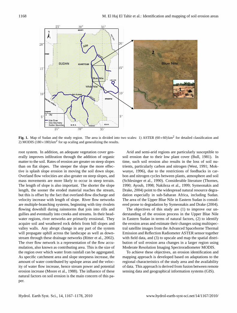
Fig. 1. Map of Sudan and the study region. The area is divided into two scales: 1) ASTER (60×60) km2 for detailed classification and2) MODIS (180×180) km2 for up scaling and generalizing the results.

root system. In addition, an adequate vegetation cover gen-erally improves infiltration through the addition of organicmatter to the soil. Rates of erosion are greater on steep slopesthan on flat slopes. The steeper the slope the more effec-tive is splash slope erosion in moving the soil down slope.Overland flow velocities are also greater on steep slopes, andmass movements are more likely to occur in steep terrain.The length of slope is also important. The shorter the slopelength, the sooner the eroded material reaches the stream,but this is offset by the fact that overland-flow discharge andvelocity increase with length of slope. River flow networksare multiple-branching systems, beginning with tiny rivuletsflowing downhill during rainstorms that join into rills andgullies and eventually into creeks and streams. In their head-water regions, river networks are primarily erosional. Theyacquire soil and weathered rock debris from hill slopes andvalley walls. Any abrupt change in any part of the systemwill propagate uphill across the landscape as well as down-stream through these drainage networks (Ritter et al., 2002).The river flow network is a representation of the flow accu-mulation, also known as contributing area. This is the size ofthe region over which water from rainfall can be aggregated.As specific catchment area and slope steepness increase, theamount of water contributed by upslope areas and the veloc-ity of water flow increase, hence stream power and potentialerosion increase (Moore et al., 1988). The influence of thesenatural factors on soil erosion is the main concern of this pa-per.

Arid and semi-arid regions are particularly susceptible tosoil erosion due to their low plant cover (Bull, 1981). Intime, such soil erosion also results in the loss of soil nu-trients, particularly carbon and nitrogen (West, 1991; Mok-wunye, 1996), due to the restrictions of feedbacks in car-bon and nitrogen cycles between plants, atmosphere and soil(Schlesinger et al., 1990). Considerable literature (Thornes,1990; Ayoub, 1998; Nakileza et al., 1999; Symeonakis andDrake, 2004) point to the widespread natural resource degra-dation especially in sub-Saharan Africa, including Sudan.The area of the Upper Blue Nile in Eastern Sudan is consid-ered prone to degradation by Symeonakis and Drake (2004).

The objectives of this study are (1) to improve our un-derstanding of the erosion process in the Upper Blue Nilein Eastern Sudan in terms of natural factors, (2) to identifythe erosion areas and estimate their changes using multispec-tral satellite images from the Advanced Spaceborne ThermalEmission and Reflection Radiometer ASTER sensor togetherwith field data, and (3) to upscale and map the spatial distri-bution of soil erosion area changes in a larger region usingModerate Resolution Imaging Spectroradiometer MODIS.

To achieve these objectives, an erosion identification andmapping approach is developed based on adaptations to theregional characteristics of the study area and the availabilityof data. This approach is derived from fusion between remotesensing data and geographical information systems (GIS).

Hydrol. Earth Syst. Sci., 14, 1167–1178, 2010 www.hydrol-earth-syst-sci.net/14/1167/2010/

M. El Haj El Tahir et al.: Identification and mapping of soil erosion areas 1169

2 Study area and data

2.1 Description of study area

The study area lies between latitudes 11◦ and 16◦ N and lon-gitudes 33◦ and 35◦ E (Fig. 1). It portrays different land usetypes including agriculture, forests and range areas. Agri-culture forms are small holdings, mechanized and river bankfarming. The area exhibits high land cover variability. It in-cludes for example the Ar Roseris power dam and its lake.There are a number of forests for example the Okalma forestreserve which is bound by Jabal Okalma (Jabal is the Arabicword for mountain) on the west and Jabal Zign (400 m a.s.l.)on the south east corner. Both mountains constitute a sourceof sheet floods towards the Okalma forest reserve. The forestreserve is a natural forest composed of a mixture of trees,mainly Acacia seyal and Balanites aegyptiaca plus otherspecies. There is a large variation of age groups from youngnew regeneration to large groups of forest stands. The forestis related to the surrounding societies providing diversifiedbenefits from the trees and the land. Regeneration and forestdevelopment factors are evident. Other areas are abandonedfallow land formed following abandonment of agriculturalcropping. To the south-east there is a seasonalKhor Dunya(a gully or a seasonal water course is locally known askhor),running from south west to north east until it joins the BlueNile. Thiskhor is characterised by the presence of degradedareas, natural regeneration, human activities such as agricul-ture, pastoralism and small settlements, as well as human in-tervention to reclaim the vegetation. Gully erosion stripes offthe fertile clay soils from the degradational clay plain form-ing bad-lands known locally as “Kerib” (Mirghani, 2007).

Observed data indicate that the mean annual precipitationin 2006 was 900 mm, of which around 90% is collected dur-ing the rainy season (April–October). For erosion we are in-terested in the inter-annual and not the annual total of rainfall.The maximum two or three rainy days in 2006 are of interestbecause it is the maximum rainfall that causes erosion. Themaximum rainfall occurred on 8 and 10 May with precipita-tion levels as high as 109.2 mm and 200.6 mm, respectively.The mean annual temperature is 28.8◦C. The lowest dailymean temperature is 13◦C and is measured in December.The highest mean daily temperature is 43.8◦C and is mea-sured in May. The runoff coefficient is 20–30% (Ahmed etal., 2006). The year 2006 was an exceptionally wet year. Thenormal mean annual rainfall is 500 mm (Abdulkarim, 2006).

2.2 Economic impacts of gully erosion in thestudy region

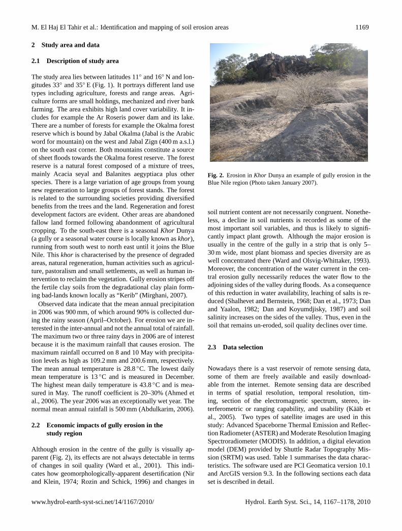
Although erosion in the centre of the gully is visually ap-parent (Fig. 2), its effects are not always detectable in termsof changes in soil quality (Ward et al., 2001). This indi-cates how geomorphologically-apparent desertification (Nirand Klein, 1974; Rozin and Schick, 1996) and changes in

27

571

Figure 2 Erosion in Khor Dunya an example of gully erosion in the Blue Nile region 572

(Photo taken January 2007) 573

574

Fig. 2. Erosion inKhor Dunya an example of gully erosion in theBlue Nile region (Photo taken January 2007).

soil nutrient content are not necessarily congruent. Nonethe-less, a decline in soil nutrients is recorded as some of themost important soil variables, and thus is likely to signifi-cantly impact plant growth. Although the major erosion isusually in the centre of the gully in a strip that is only 5–30 m wide, most plant biomass and species diversity are aswell concentrated there (Ward and Olsvig-Whittaker, 1993).Moreover, the concentration of the water current in the cen-tral erosion gully necessarily reduces the water flow to theadjoining sides of the valley during floods. As a consequenceof this reduction in water availability, leaching of salts is re-duced (Shalhevet and Bernstein, 1968; Dan et al., 1973; Danand Yaalon, 1982; Dan and Koyumdjisky, 1987) and soilsalinity increases on the sides of the valley. Thus, even in thesoil that remains un-eroded, soil quality declines over time.

2.3 Data selection

Nowadays there is a vast reservoir of remote sensing data,some of them are freely available and easily download-able from the internet. Remote sensing data are describedin terms of spatial resolution, temporal resolution, tim-ing, section of the electromagnetic spectrum, stereo, in-terferometric or ranging capability, and usability (Kaab etal., 2005). Two types of satellite images are used in thisstudy: Advanced Spaceborne Thermal Emission and Reflec-tion Radiometer (ASTER) and Moderate Resolution ImagingSpectroradiometer (MODIS). In addition, a digital elevationmodel (DEM) provided by Shuttle Radar Topography Mis-sion (SRTM) was used. Table 1 summarises the data charac-teristics. The software used are PCI Geomatica version 10.1and ArcGIS version 9.3. In the following sections each dataset is described in detail.

www.hydrol-earth-syst-sci.net/14/1167/2010/ Hydrol. Earth Syst. Sci., 14, 1167–1178, 2010


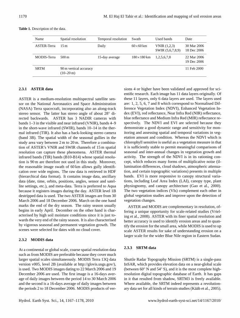
Table 1. Description of the data.

Name Spatial resolution Temporal resolution Swath Used bands Date

ASTER-Terra 15 m Daily 60×60 km VNIR (1,2,3) 30 Mar 2006SWIR (5,6,7,8,9) 18 Dec 2006

MODIS-Terra 500 m 15-day average 180×180 km 1,2,5,6,7,8 22 Mar 200619 Dec 2006

SRTM 90 m vertical accuracy 11 Feb 2000(10–20 m)

2.3.1 ASTER data

ASTER is a medium-resolution multispectral satellite sen-sor on the National Aeronautics and Space Administration(NASA) Terra spacecraft, incorporating also an along-trackstereo sensor. The latter has stereo angle of about 28◦ di-rected backwards. ASTER has 3 NADIR cameras withbands 1–3 in the visible and near infrared (VNIR), bands 4–9in the short-wave infrared (SWIR), bands 10–14 in the ther-mal infrared (TIR). It also has a back-looking stereo camera(band 3B). The spatial width of the seasonal gullies in thestudy area vary between 2 m to 20 m. Therefore a combina-tion of ASTER’s VNIR and SWIR channels of 15 m spatialresolution can capture these phenomena. ASTER thermalinfrared bands (TIR) bands (B10-B14) whose spatial resolu-tion is 90 m are therefore not used in this study. Moreover,the reasonable image swath of 60 km allows gully identifi-cation over wide regions. The raw data is retrieved in HDF(hierarchical data format). It contains image data, ancillarydata (date, time, orbits, positions, angles, sensor and satel-lite settings, etc.), and meta-data. Terra is preferred to Aquabecause it registers images during the day. ASTER level 1Bdestripped data is used. The two ASTER images are from 30March 2006 and 18 December 2006. March on the one handmarks the end of the dry season. The rainy season usuallybegins in early April. December on the other hand is char-acterised by high soil moisture conditions since it is just to-wards the very end of the rainy season. It is also characterisedby vigorous seasonal and permanent vegetation growth. Thescenes were selected for dates with no cloud cover.

2.3.2 MODIS data

At a continental or global scale, coarse spatial resolution datasuch as from MODIS are preferable because they cover muchlarger spatial scales simultaneously. MODIS Terra 13Q dataversion v005, level 2B (available athttp://glovis.usgs.gov/),is used. Two MODIS images dating to 22 March 2006 and 19December 2006 are used. The first image is a 16-days aver-age of daily images between the period 14 to 30 March 2006and the second is a 16-days average of daily images betweenthe periods 2 to 18 December 2006. MODIS products of ver-

sions 4 or higher have been validated and approved for sci-entific research. Each image has 11 data layers originally. Ofthese 11 layers, only 6 data layers are used. The layers usedare: 1, 2, 5, 6, 7 and 8 which correspond to Normalised Dif-ference Vegetation Index (NDVI), Enhanced Vegetation In-dex (EVI), red reflectance, Near Infra Red (NIR) reflectance,blue reflectance and Medium Infra Red (MIR) reflectance re-spectively. The NDVI and EVI are selected because theydemonstrate a good dynamic range and sensitivity for mon-itoring and assessing spatial and temporal variations in veg-etation amount and condition. Whereas the NDVI which ischlorophyll sensitive is useful as a vegetation measure in thatit is sufficiently stable to permit meaningful comparisons ofseasonal and inter-annual changes in vegetation growth andactivity. The strength of the NDVI is in its rationing con-cept, which reduces many forms of multiplicative noise (il-lumination differences, cloud shadows, atmospheric attenua-tion, and certain topographic variations) presents in multiplebands. EVI is more responsive to canopy structural varia-tions, including Leaf Area Index (LAI), canopy type, plantphysiognomy, and canopy architecture (Gao et al., 2000).The two vegetation indices (VIs) complement each other inglobal vegetation studies and improve upon the detection ofvegetation changes.

ASTER and MODIS are complementary in resolution, of-fering a unique opportunity for scale-related studies (Vriel-ing et al., 2008). ASTER with its finer spatial resolution andbetter accuracy is used to identify erosion areas and to quan-tify the erosion for the small area, while MODIS is used to upscale ASTER results for sake of understanding erosion on alarger scale for the wider Blue Nile region in Eastern Sudan.

2.3.3 SRTM data

Shuttle Radar Topography Mission (SRTM) is a single-passInSAR, which provides elevation data on a near-global scale(between 60◦ N and 54◦ S), and it is the most complete high-resolution digital topographic database of Earth. It has gapsin it that resulted from shadow, SRTM3 is freely available.Where available, the SRTM indeed represents a revolution-ary data set for all kinds of terrain studies (Kaab et al., 2005).


http://glovis.usgs.gov/


3 Methodology

3.1 Method overview

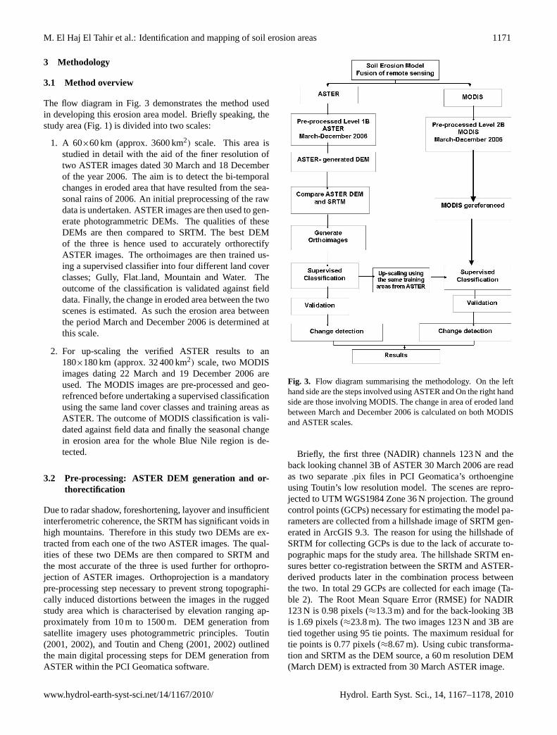
The flow diagram in Fig. 3 demonstrates the method usedin developing this erosion area model. Briefly speaking, thestudy area (Fig. 1) is divided into two scales:

1. A 60×60 km (approx. 3600 km2) scale. This area isstudied in detail with the aid of the finer resolution oftwo ASTER images dated 30 March and 18 Decemberof the year 2006. The aim is to detect the bi-temporalchanges in eroded area that have resulted from the sea-sonal rains of 2006. An initial preprocessing of the rawdata is undertaken. ASTER images are then used to gen-erate photogrammetric DEMs. The qualities of theseDEMs are then compared to SRTM. The best DEMof the three is hence used to accurately orthorectifyASTER images. The orthoimages are then trained us-ing a supervised classifier into four different land coverclasses; Gully, Flatland, Mountain and Water. Theoutcome of the classification is validated against fielddata. Finally, the change in eroded area between the twoscenes is estimated. As such the erosion area betweenthe period March and December 2006 is determined atthis scale.

2. For up-scaling the verified ASTER results to an180×180 km (approx. 32 400 km2) scale, two MODISimages dating 22 March and 19 December 2006 areused. The MODIS images are pre-processed and geo-refrenced before undertaking a supervised classificationusing the same land cover classes and training areas asASTER. The outcome of MODIS classification is vali-dated against field data and finally the seasonal changein erosion area for the whole Blue Nile region is de-tected.

3.2 Pre-processing: ASTER DEM generation and or-thorectification

Due to radar shadow, foreshortening, layover and insufficientinterferometric coherence, the SRTM has significant voids inhigh mountains. Therefore in this study two DEMs are ex-tracted from each one of the two ASTER images. The qual-ities of these two DEMs are then compared to SRTM andthe most accurate of the three is used further for orthopro-jection of ASTER images. Orthoprojection is a mandatorypre-processing step necessary to prevent strong topographi-cally induced distortions between the images in the ruggedstudy area which is characterised by elevation ranging ap-proximately from 10 m to 1500 m. DEM generation fromsatellite imagery uses photogrammetric principles. Toutin(2001, 2002), and Toutin and Cheng (2001, 2002) outlinedthe main digital processing steps for DEM generation fromASTER within the PCI Geomatica software.

28

575

Figure 3 Flow diagram summarising the methodology. On the left hand side are the 576

steps involved using ASTER and On the right hand side are those involving MODIS. 577

The change in area of eroded land between March and December 2006 is calculated on 578

both MODIS and ASTER scales 579

580

Fig. 3. Flow diagram summarising the methodology. On the lefthand side are the steps involved using ASTER and On the right handside are those involving MODIS. The change in area of eroded landbetween March and December 2006 is calculated on both MODISand ASTER scales.

Briefly, the first three (NADIR) channels 123 N and theback looking channel 3B of ASTER 30 March 2006 are readas two separate .pix files in PCI Geomatica’s orthoengineusing Toutin’s low resolution model. The scenes are repro-jected to UTM WGS1984 Zone 36 N projection. The groundcontrol points (GCPs) necessary for estimating the model pa-rameters are collected from a hillshade image of SRTM gen-erated in ArcGIS 9.3. The reason for using the hillshade ofSRTM for collecting GCPs is due to the lack of accurate to-pographic maps for the study area. The hillshade SRTM en-sures better co-registration between the SRTM and ASTER-derived products later in the combination process betweenthe two. In total 29 GCPs are collected for each image (Ta-ble 2). The Root Mean Square Error (RMSE) for NADIR123 N is 0.98 pixels (≈13.3 m) and for the back-looking 3Bis 1.69 pixels (≈23.8 m). The two images 123 N and 3B aretied together using 95 tie points. The maximum residual fortie points is 0.77 pixels (≈8.67 m). Using cubic transforma-tion and SRTM as the DEM source, a 60 m resolution DEM(March DEM) is extracted from 30 March ASTER image.



Table 2. Generation of DEM from two ASTER images. The table summaries the root mean square error (RMSE) for the ground controlpoints (GCPs) for 123N and 3B image channel.

Image Channel GCP RMSE X RMSE Y RMSE

ASTER March Nadir 123 N 29 0.98 pixels (13.3 m) 0.81 pixel (12.00 m) 0.65 pixel (8.01 m)ASTER March Back-looking 3B 29 1.69 pixels (23.8 m) 0.87 pixel (11.90 m) 1.31 pixel (17.3 m)ASTER December Nadir 123 N 31 1.08 pixels (14.6 m) 0.84 pixel (12.06 m) 0.67 pixel (8.29 m)ASTER December Back-looking 3B 31 1.72 pixels (24.2 m) 0.91 pixel (13.0 m) 1.47 pixel (20.4 m)

The same procedure is repeated using the second ASTERimage of 18 December. The RMS is shown in Table 2. Asecond 60 m resolution DEM (December DEM) is also ex-tracted.

3.3 ASTER classification

After orthoprojecting ASTER images using SRTM, the chan-nels that best describe the process of soil erosion are selected.Considering the spatial width of gullies, ASTER’s VNIR andSWIR channels at 15 m spatial resolution have been anal-ysed. Additional layers that represent some of the mostimportant natural factors causing erosion are added. Theselayers are elevation, slope, aspect, and river flow network.Therefore the final ASTER orthoimages used for classifica-tion consisted of 13 layers stacked together. These include:VNIR channels 1, 2 and 3, SWIR channels 4, 5, 6, 7, 8 and9, SRTM, slope, aspect, and river flow network. The lastthree layers; slope, aspect and river flow network are all cal-culated from SRTM in ArcGIS 9.3. Both slope and aspectare calculated from SRTM using a finite difference methodthat uses eight neighbours in ArcGIS. The two are then re-sampled to 15 m before adding them to the layer stack. Theriver flow network was estimated using the hydrologic anal-ysis package in ArcGIS 9.3 as follows. When working withraster DEMs and computing slopes between grid cells, theratio of the vertical and horizontal resolutions determines theminimum non-zero slope that can be resolved. In this study,the vertical resolution of the DEM is 1 m and a grid sizeis 15 m. Therefore the resolvable slope of 1/15=0.07. Thisvalue means that slopes on hillsides can be computed with arelatively small error. However, slopes in channels are oftenmuch smaller than this value. As a consequence, these ar-eas will appear horizontal in the DEM. Therefore in order toavoid this problem, ArcGIS 9.3 uses an eight direction (D8)flow model. The direction of flow is determined by findingthe direction of steepest descent, or maximum drop, fromeach cell. This is calculated as

maximum drop = change in z-value/distance

The distance is calculated between cell centres. There areeight valid output directions relating to the eight adjacentcells into which flow could travel. One challenge arises if all

neighbours are higher than the processing cell. In such a casethe processing cell is called a sink and has an undefined flowdirection because any water that flows into a sink cannot flowout. To obtain an accurate representation of flow directionacross a surface, the sinks should be filled. The minimumelevation value surrounding the sink will identify the heightnecessary to fill the sink so the water can pass through thecell. A digital elevation model free of sinks is called depres-sionless DEM. Using the depressionless DEM as an inputto the flow direction process, the direction in which waterwould flow out of each cell is determined. After determin-ing the flow direction, then the flow accumulation is deter-mined. Afterwards, a stream network is created by applyinga threshold value to select cells with high accumulated flowin order delineate the stream network. More details on thetechnique of deriving flow direction from a DEM and on howto create river network in ArcGIS can be found in Jenson andDomingue (1988) and in Tang and Liu (2008), among others.

After stacking all appropriate layers, then supervised max-imum likelihood classification is performed aided by the au-thors’ knowledge of the area. The image is trained intofour land cover types: Gully, Flatland, Mountain and Wa-ter. Water bodies are clear and easy to train considering thefine ASTER resolution for both periods of the year. Moun-tains are easily classified with the aid of the DEM. However,the most challenging task is to separate between Gully andFlat land since these two classes are bound to overlap andoverlapping training area boundaries reduces the reliabilityof the training sites. To avoid this kind of overlap, the fol-lowing steps were taken

1. MODIS vegetation indices (VI) are used as auxiliarydata to discriminate between training classes; Gully andFlat land. At first MODIS NDVI and EVI signatures areused to discriminate between two classes: stable vege-tation and unstable vegetation. The unstable vegetationis seasonal vegetation that grows during the rainy sea-son; this vegetation is flushed away with erosion, indi-cating that areas where there is unstable vegetation thereis also erosion. The stable vegetation on the other handis there throughout the year hence no erosion. WhereNDVI and EVI values are low, this is an indication oflimited, unstable vegetation hence higher erosion risk.



Higher values of NDVI and EVI indicate more stablevegetation.

2. The layer of river network is superimposed on top of theimage to help guide and discriminate between Gulliesand Flatland.

3. Care is taken when selecting the different bands both fordisplay, in either greyscale or as false colour compositesFCC.

4. Between each run and the next the classes are refined byvarying the number of training areas until better accura-cies are achieved.

As many training areas as possible are trained because gen-erally speaking, the more areas identified as training sites,the higher the accuracy of the classification. Once the train-ing areas are defined, then the signature separability valuesare studied. Signature separability is the statistical differ-ence between pairs of spectral signatures. It is expressedin terms of Bhattacharrya Distance and Transformed Diver-gence. These are measures of the separability of a pair ofprobability distributions. Both Bhattacharrya Distance andTransformed Divergence are shown as real values betweenzero and two. Zero indicates complete overlap between thesignatures of two classes; two indicates a complete separa-tion between the two classes. The higher the separability (i.e.more than 1.5) value the more accurate is the classificationaccuracy. The training areas are tuned until higher signatureseparability value of 1.5 or more are achieved. After achiev-ing the best accuracies, the signature statistics report is stud-ied in order to determine which channels of the 13 stackedlayers are more significant in delineating erosion gullies.

3.4 Post classification

ASTER classification is validated via running an automaticrandom accuracy assessment. The accuracy assessment isdesigned and implemented by generating a random sampleof 300 points and comparing it to the original orthorectifiedASTER image. ASTER image is used as a reference imagedue to lack of accurate and updated maps for the study area.Each of the 300 samples is assigned to the different classes.

Once the two ASTER images are successfully classifiedand validated, they are used to study the bi-temporal change.For each image the area represented by each of the fourclasses is calculated using the function Generate Area Re-port in PCI Geomatica. The areas in December image aresubsequently subtracted from their correspondent in Marchimage in order to calculate the changed area per class.

3.5 Upscaling using MODIS

Once ASTER classification results are accepted, the resultsare then up-scaled using MODIS. Upscaling allows general-isation of the results of ASTER classification to larger area

covering the whole of the Blue Nile region. MODIS is firstre-projected to UTM WGS1984 Zone 36 N. Thereafter, it istrained into four classes; Gully, Flatland, Mountain and Wa-ter. MODIS is trained using:

1. MODIS NDVI and EVI are used as auxiliary data to dis-criminate between training classes; Gully and Flatlanddiscriminating first between high values i.e. stable veg-etation i.e. no erosion and low values i.e. unstable veg-etation i.e. erosion areas.

2. The same training areas from ASTER which are con-verted into shape file and laid over the MODIS image toguide the training.

3. River flow network layer overlaid over the images toguide the training of gullies

MODIS classification is validated against field data in termsof registered digital photos with co-ordinates and time takenin January 2007 from different locations.

4 Results and discussion

4.1 Comparison of the three DEMs

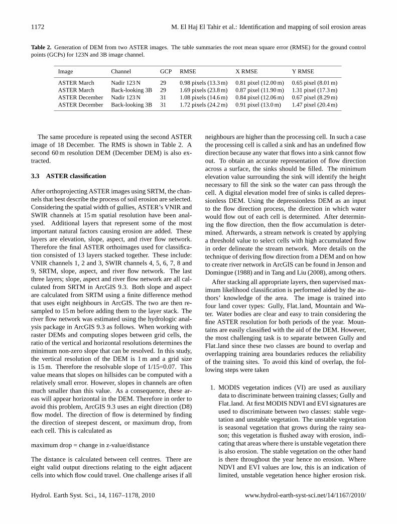
Because the two generated ASTER DEMs cannot be testedagainst an existing reference DEM, they are tested throughthe overlay of different orthoimages taken from different sen-sor positions (also know as multi-incidence angle image).For 30 March ASTER, two orthoimages are produced onefor 123 N and another for 3B using March DEM. The twoorthoimages are then overlaid to test if they overlap per-fectly well pixel-by-pixel using animation flickering tech-niques. The results showed that the two did not overlap per-fectly. The explanation for this is that the used March DEMhas vertical errors which translated into horizontal shifts be-tween the orthoprojected pixels. These shifts cause the twomulti-incidence images not to overlap perfectly. Next De-cember DEM is tested in a similar manner. The results of theflickering technique showed some vertical errors. It is thenconcluded that the two ASTER DEMs both suffer verticalerrors. Accordingly SRTM is selected as “reference DEM”for all further steps. In order to quantify the error of ASTERMarch and December DEMs, their contour lines are com-pared to those of SRTM (Fig. 4a and b, respectively). The de-picted test area in the figure represents rugged high-mountainconditions with elevations of up to 1500 m a.s.l., steep rockwalls, deep shadows that are without contrast. Therefore, thetest area is considered to represent a worst case for DEMgeneration from ASTER data.

Figure 4a and b shows that the contour lines of twoASTER DEMs (dotted lines) are different to those of theSRTM (solid lines) and that this difference increases withelevation. Figure 4b shows that December DEM has more



29

581

(a) (b) 582

Figure 4 Elevation differences between SRTM DEM (solid line) and ASTER (dotted 583

line) (a) ASTER March 2006 and (b) ASTER December 2006; all contour lines are 584

superimposed over a hillshade of the SRTM. The scenes mark a subset with a mix of 585

moderate to high topography representing the worst case scenario of DEM errors. 586

587

588

589

Fig. 4. Elevation differences between SRTM DEM (solid line) and ASTER (dotted line)(a) ASTER March 2006 and(b) ASTER December2006; all contour lines are superimposed over a hillshade of the SRTM. The scenes mark a subset with a mix of moderate to high topographyrepresenting the worst case scenario of DEM errors.

30

590

Figure 5 Comparisons between SRTM and ASTER DEM showing the relative error of 591

the two DEMs March and December from SRTM 592

593

594

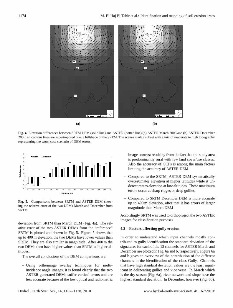
Fig. 5. Comparisons between SRTM and ASTER DEM show-ing the relative error of the two DEMs March and December fromSRTM.

deviation from SRTM than March DEM (Fig. 4a). The rel-ative error of the two ASTER DEMs from the “reference”SRTM is plotted and shown in Fig. 5. Figure 5 shows thatup to 400 m elevation, the two DEMs have lower values thanSRTM. They are also similar in magnitude. After 400 m thetwo DEMs then have higher values than SRTM at higher al-titudes.

The overall conclusions of the DEM comparisons are:

– Using orthoimage overlay techniques for multi-incidence angle images, it is found clearly that the twoASTER-generated DEMs suffer vertical errors and areless accurate because of the low optical and radiometric

image contrast resulting from the fact that the study areais predominantly rural with few land cover/use classes.Also the accuracy of GCPs is among the main factorslimiting the accuracy of ASTER DEM.

– Compared to the SRTM, ASTER DEM systematicallyoverestimates elevation at higher latitudes while it un-derestimates elevation at low altitudes. These maximumerrors occur at sharp ridges or deep gullies.

– Compared to SRTM December DEM is more accurateup to 400 m elevation, after that it has errors of largermagnitude than March DEM

Accordingly SRTM was used to orthoproject the two ASTERimages for classification purposes.

4.2 Factors affecting gully erosion

In order to understand which input channels mostly con-tributed to gully identification the standard deviation of thesignatures for each of the 13 channels for ASTER March andDecember are plotted in Fig. 6a and b, respectively. Figure 6aand b gives an overview of the contribution of the differentchannels in the identification of the class Gully. Channelsthat have high standard deviation values are the least signif-icant in delineating gullies and vice versa. In March whichis the dry season (Fig. 6a), river network and slope have thehighest standard deviation. In December, however (Fig. 6b),



31

595

596

Figure 6 The contribution of the different input channels in delineating gullies in 597

ASTER images a) March b) December 598

599

600

31

595

596

Figure 6 The contribution of the different input channels in delineating gullies in 597

ASTER images a) March b) December 598

599

600

Fig. 6. The contribution of the different input channels in delineat-ing gullies in ASTER images(a) March,(b) December.

Table 3. Classification report of ASTER images.

Image Average Overall Kappaaccuracy accuracy coefficient

ASTER March 93.4% 82.2% 0.82ASTER December 87% 75.2% 0.75

they have the lowest standard deviation values and hence theyare the most important in Gully classification. During andafter the rainy season, river network and slope are the mostimportant factors in the erosion process. In December rivernetworks continue to flow even when the rain has stoppedcarrying with the flow soil and weathered rock debris fromhill slopes and valley walls and as slope steepness increase,the amount of water contributed by upslope areas and the ve-locity of water flow increase, hence stream power and poten-tial erosion increase. As natural factors, river flow networkand slope are more important in causing erosion in the BlueNile region than aspect and elevation.

4.3 Validation of the classification outcome

ASTER classification reports (Table 3) shows an overall ac-curacy of 82.2% and 75.2% for March and December im-ages, respectively. And similarly for ASTER validation, the

32

Validation points

601

Figure 7 Regional spatial distribution map of seasonal gullies of the Blue Nile, Eastern 602

Sudan 603

604

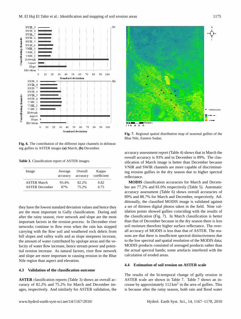
Fig. 7. Regional spatial distribution map of seasonal gullies of theBlue Nile, Eastern Sudan.

accuracy assessment report (Table 4) shows that in March theoverall accuracy is 93% and in December is 89%. The clas-sification of March image is better than December becauseVNIR and SWIR channels are more capable of discriminat-ing erosion gullies in the dry season due to higher spectralreflectance.

MODIS classification accuracies for March and Decem-ber are 77.2% and 81.0% respectively (Table 5). Automaticaccuracy assessment (Table 6) shows overall accuracies of89% and 88.7% for March and December, respectively. Ad-ditionally, the classified MODIS image is validated againsta set of thirteen digital photos taken in the field. Nine val-idation points showed gullies coinciding with the results ofthe classification (Fig. 7). In March classification is betterthan that of December because in the dry season there is lesssoil moisture therefore higher surface reflectance. The over-all accuracy of MODIS is less than that of ASTER. The rea-sons are that there is insufficient spectral distinctiveness dueto the low spectral and spatial resolution of the MODIS data;MODIS products consisted of averaged products rather thanthe actual spectral bands; some artefacts interfered with thecalculation of eroded areas.

4.4 Estimation of soil erosion on ASTER scale

The results of the bi-temporal change of gully erosion inASTER scale are shown in Table 7. Table 7 shows an in-crease by approximately 112 km2 in the area of gullies. Thisis because after the rainy season, both rain and flood water



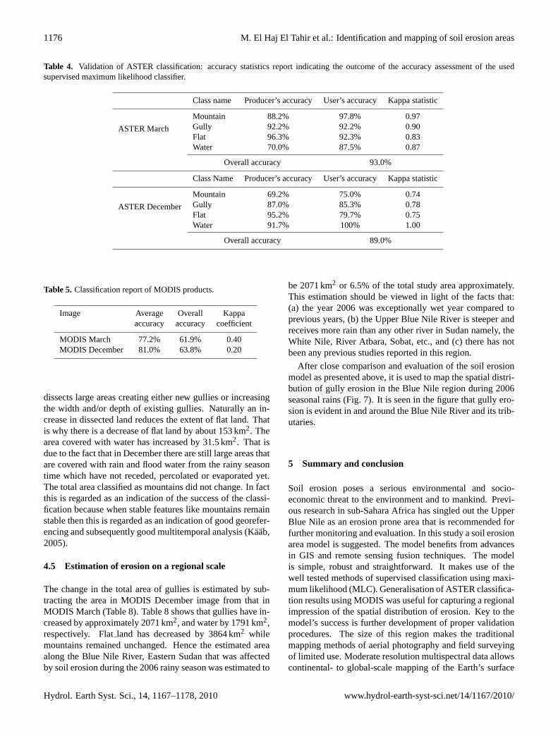
Table 4. Validation of ASTER classification: accuracy statistics report indicating the outcome of the accuracy assessment of the usedsupervised maximum likelihood classifier.

ASTER March

Class name Producer’s accuracy User’s accuracy Kappa statistic

Mountain 88.2% 97.8% 0.97Gully 92.2% 92.2% 0.90Flat 96.3% 92.3% 0.83Water 70.0% 87.5% 0.87

Overall accuracy 93.0%

ASTER December

Class Name Producer’s accuracy User’s accuracy Kappa statistic

Mountain 69.2% 75.0% 0.74Gully 87.0% 85.3% 0.78Flat 95.2% 79.7% 0.75Water 91.7% 100% 1.00


Table 5. Classification report of MODIS products.

Image Average Overall Kappaaccuracy accuracy coefficient

MODIS March 77.2% 61.9% 0.40MODIS December 81.0% 63.8% 0.20

dissects large areas creating either new gullies or increasingthe width and/or depth of existing gullies. Naturally an in-crease in dissected land reduces the extent of flat land. Thatis why there is a decrease of flat land by about 153 km2. Thearea covered with water has increased by 31.5 km2. That isdue to the fact that in December there are still large areas thatare covered with rain and flood water from the rainy seasontime which have not receded, percolated or evaporated yet.The total area classified as mountains did not change. In factthis is regarded as an indication of the success of the classi-fication because when stable features like mountains remainstable then this is regarded as an indication of good georefer-encing and subsequently good multitemporal analysis (Kaab,2005).

4.5 Estimation of erosion on a regional scale

The change in the total area of gullies is estimated by sub-tracting the area in MODIS December image from that inMODIS March (Table 8). Table 8 shows that gullies have in-creased by approximately 2071 km2, and water by 1791 km2,respectively. Flatland has decreased by 3864 km2 whilemountains remained unchanged. Hence the estimated areaalong the Blue Nile River, Eastern Sudan that was affectedby soil erosion during the 2006 rainy season was estimated to

be 2071 km2 or 6.5% of the total study area approximately.This estimation should be viewed in light of the facts that:(a) the year 2006 was exceptionally wet year compared toprevious years, (b) the Upper Blue Nile River is steeper andreceives more rain than any other river in Sudan namely, theWhite Nile, River Atbara, Sobat, etc., and (c) there has notbeen any previous studies reported in this region.

After close comparison and evaluation of the soil erosionmodel as presented above, it is used to map the spatial distri-bution of gully erosion in the Blue Nile region during 2006seasonal rains (Fig. 7). It is seen in the figure that gully ero-sion is evident in and around the Blue Nile River and its trib-utaries.

5 Summary and conclusion

Soil erosion poses a serious environmental and socio-economic threat to the environment and to mankind. Previ-ous research in sub-Sahara Africa has singled out the UpperBlue Nile as an erosion prone area that is recommended forfurther monitoring and evaluation. In this study a soil erosionarea model is suggested. The model benefits from advancesin GIS and remote sensing fusion techniques. The modelis simple, robust and straightforward. It makes use of thewell tested methods of supervised classification using maxi-mum likelihood (MLC). Generalisation of ASTER classifica-tion results using MODIS was useful for capturing a regionalimpression of the spatial distribution of erosion. Key to themodel’s success is further development of proper validationprocedures. The size of this region makes the traditionalmapping methods of aerial photography and field surveyingof limited use. Moderate resolution multispectral data allowscontinental- to global-scale mapping of the Earth’s surface



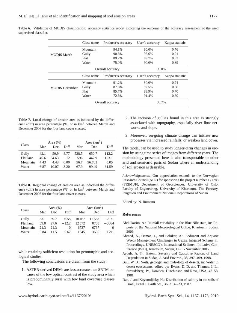
Table 6. Validation of MODIS classification: accuracy statistics report indicating the outcome of the accuracy assessment of the usedsupervised classifier.

MODIS March




MODIS December




Table 7. Local change of erosion area as indicated by the differ-ence (diff) in area percentage (%) or in km2 between March andDecember 2006 for the four land cover classes.

ClassArea (%) Area (km2)

Mar Dec Diff Mar Dec Diff

Gully 42.1 50.9 8.77 538.5 650.7 112.2Flat land 46.6 34.63 −12 596 442.9 −153.1Mountain 4.43 4.43 0.00 56.7 56.701 0.05Water 6.87 10.07 3.20 67.9 99.49 31.59

Table 8. Regional change of erosion area as indicated the differ-ence (diff) in area percentage (%) or in km2 between March andDecember 2006 for the four land cover classes.

ClassArea (%) Area (km2)

Mar Dec Diff Mar Dec Diff

Gully 33.1 39.7 6.55 10 467 12 538 2071Flat land 39.8 27.6 −12.2 12 572 8708 −3864Mountain 21.3 21.3 0 6737 6737 0Water 5.84 11.5 5.67 1845 3636 1791

while retaining sufficient resolution for geomorphic and eco-logical studies.

The following conclusions are drawn from the study:

1. ASTER-derived DEMs are less accurate than SRTM be-cause of the low optical contrast of the study area whichis predominantly rural with few land cover/use classeslow.

2. The incision of gullies found in this area is stronglyassociated with topography, especially river flow net-works and slope.

3. Moreover, on-going climate change can initiate newprocesses via increased rainfalls, or weaken land cover.

The model can be used to study longer-term changes in ero-sion by using time series of images from different years. Themethodology presented here is also transportable to otherarid and semi-arid parts of Sudan where an understandingof soil erosion is desirable.

Acknowledgements.Our appreciation extends to the NorwegianResearch Council (NFR) for sponsoring the project number 171783(FRIMUF), Department of Geosciences, University of Oslo,Faculty of Engineering, University of Khartoum, The Forestry,Irrigation and Environment National Corporations of Sudan.

Edited by: N. Romano

References

Abdulkarim, A.: Rainfall variability in the Blue Nile state, in: Re-ports of the National Meteorological Office, Khartoum, Sudan,2006.

Ahmed, A., Osman, I., and Babiker, A.: Sediment and AquaticWeeds Management Challenges in Gezira Irrigated Scheme in:Proceedings, UNESCO’s International Sediment Initiative Con-ference (ISIC), Khartoum, Sudan, 12–15 November 2006.

Ayoub, A. T.: Extent, Severity and Causative Factors of LandDegradation in Sudan, J. Arid Environ., 38, 397–409, 1998.

Bull, W. B.: Soils, geology, and hydrology of deserts, in: Water indesert ecosystems, edited by: Evans, D. D. and Thames, J. L.,Stroudsberg, Pa, Dowden, Hutchinson and Ross, USA, 42–58,1981.

Dan, J. and Koyumdjisky, H.: Distribution of salinity in the soils ofIsrael, Israel J. Earth Sci., 36, 213–223, 1987.



Dan, J. and Yaalon, D. H.: Automorphic saline soils in Israel, in:Aridic soils and geomorphic processes, edited by: Yaalon, D. H.,Cathena Verlag, 1, Braunschweig, Germany, 103–115, 1982.

Dan, J., Moshe, R., and Alperovitch, N.: The soils of Sede Zin,Israel J. Earth Sci., 22, 211–227, 1973.

Gao, X., Huete, A., Ni, W., and Miura, T.: Optical –biophysicalrelationships of vegetation spectra without background contami-nation, Remote Sens. Environ., 74, 609–620, 2000.

Gomer, D. and Vogt, T.: Physically based modelling of surfacerunoff and soil erosion under semi-arid Mediterranean condi-tions, the example of Oued Mina, Algeria, in: Soil Erosion:Application of Physically based models, edited by: Schmidt, J.,Springer Verlag, Berlin, Heidelberg, New York, 58–78, 2000.

Jenson, S. K. and Domingue, J. O.: Extracting Topographic Struc-ture from Digital Elevation Data for Geographic InformationSystem Analysis, Photogrammetric Engineering and RemoteSensing, 54(11), 1593–1600, 1988.

Kaab, A., Huggel, C., Fischer, L., Guex, S., Paul, F., Roer, I., Salz-mann, N., Schlaefli, S., Schmutz, K., Schneider, D., Strozzi, T.,and Weidmann, Y.: Remote sensing of glacier- and permafrost-related hazards in high mountains: an overview, Nat. HazardsEarth Syst. Sci., 5, 527–554, doi:10.5194/nhess-5-527-2005,2005.

Kaab, A.: Combination of SRTM3 and repeat ASTER data forderiving alpine glacier flow velocities in the Bhutan Himalaya,Rem. Sens. Environ., 94(4), 463–474, 2005.

Linsely, R. K., Kohler, M. A., and Paulhus, J. L. H.: Hydrol-ogy for Engineers, Third Edition, International Student Edition,McGraw-Hill Kogakusha, Ltd, New Delhi, India, 1982.

Mirghani, O.: Report on the Field Visit to Sennar and Blue NileStates, in: Field work report, 2007.

Mokwunye, U.: Nutrient depletion: sub-Saharan Africa’s greatestthreat to economic development, S.T.A.P. expert workshop onLand Degradation Dakar, Senegal, 1996.Moore, I. D., O’Loughlin, E. M., and Burch, G. J.: A contour-based topographic model for hydrological and ecological appli-cations, Earth Surf. Processes Landforms, 3(4), 305–320, 1988.

Nakileza, B., Nsubuga, E., Tenywa, M., and Lwakuba, A.: Rethink-ing Natural Resource Degradation in Semi-Arid Sub-SaharanAfrica: A review of soil and water conservation research andpractice in Uganda, with particular emphasis on the semi- aridareas, Overseas Development Institute (ODI) Report, 1999.

Nearing, M. A., Pruski, F. F., and O’Neal, M. R.: Expected cli-mate change impacts on soil erosion rates, a review, J. Soil WaterConservation, 59(1), 43–50, 2004.

Nir, D. and Klein, M.: Gully erosion induced in land size in a semi-arid terrain (Nahal Shiqma, Israel), Zeitschrift fur Geomorpholo-gie, 21, 191–201, 1974.

Ritter, F., Kochel, R., and Miller, J.: Process Geomorphology, 4thEd., McGraw-Hill, New York, 2002.

Rozin, U. and Schick, A.: Land use change, conservation measuresand stream channel response in the Mediterranean/semiarid tran-sition zone: Nahal Hoga, southern coastal plain, Israel, in: Ero-sion and sediment yield global and regional perspectives, IAHSpubl., 236, 427–443, 1996.

Schlesinger, W., Reynolds, J. F., Cunningham, G. L., Huenneke, L.F., Jarrell, W. M., Virginia, R. A., and Whitford, W. G.: Biologi-cal feedbacks in global desertification, Science, 247, 1043–1048,1990.

Shalhevet, J. and Bernstein, L.: Effects of vertically heterogeneoussoil salinity on plant growth and water uptake, Soil Science, 106,85-93, 1968.

Symeonakis, E. and Drake, N.: Monitoring Desertification andLand Degradation over Sub- Saharan Africa, Int. J. Rem. Sens.,25(3), 573–592, 2004.

Tang, C. and Liu, C.: Surface water hydrologic simulationof Qingshuijiang Watershed based on SRTM DEM, Proc.The International Society for Optical Engineering SPIE, 7143,doi:10.1117/12.812556, 2008.

Thornes, J. B.: The interaction of erosional and vegetation dynam-ics in land degradation: spatial outcomes, in: Vegetation and Ero-sion, edited by: Thornes, J. B., Chichester, John Wiley, 41–53,1990.

Toutin, T. and Cheng, P.: Comparison of automated digital elevationmodel extraction results using along-track ASTER and across-track SPOT stereo images, Optical Engineering, 41(9), 2102–2106, 2002.

Toutin, T. and Cheng, P.: DEM generation with ASTER stereo data,Earth Observation Magazine, 10(6), 10–13, 2001.

Toutin, T.: DEM generation from new VIR Sensors, IKONOS,ASTER and Landsat 7 Proceedings, IGARSS 01, Sydney, Aus-tralia 2001.

Toutin, T.: Three-dimensional topographic mapping with ASTERstereo data in rugged topography, IEEE Trans. Geosci. Rem.Sens., 40, 10, 2241–2247, 2002.

Vrieling, A., Jong, S., Sterk, G., and Rodrigues, S.: Timing of ero-sion and satellite data: A multi-resolution approach to soil ero-sion risk mapping, Int. J. Appl. Earth Obs., 10, 267–281, 2008.

Ward, D. and Olsvig-Whittaker, L.: Plant species diversity at thejunction of two desert biogeographic zones, Biodiversity Lett.,1, 172–185, 1993.

Ward, D., Feldman, K., and Avni, Y.: The effects of erosion loesson soil nutrients, plant diversity and plant quality in Negev desertwadis, J. Arid Environ., 48, 461–473, 2001.

West, N. E.: Nutrient cycling in soils of semiarid and arid regions,in: Semiarid Lands and Deserts: Soil Resource and Rehabili-tation, edited by: Skujins, J., Marcel Dekker, Inc., New York,295–332, 1991.

Xu, C-Y., Zhang, Q., El Hag El Tahir, M., and Zhang, Z.: Statisticalproperties of the temperature, relative humidity, and solar radi-ation in the Blue Nile- Eastern Sudan region, J. Theoret. Appl.Climatol., doi:10.1007/00704009-0225-7, 2009.


Identification and mapping of soil erosion areas in the Blue Nile

Documents

Transcript of Identification and mapping of soil erosion areas in the Blue Nile