arX

iv:p

hysi

cs/0

5071

36v2

[ph

ysic

s.so

c-ph

] 2

8 Ju

l 200

5 Ideal-Gas Like Markets: Effect of Savings

Arnab Chatterjee and Bikas K Chakrabarti

Theoretical Condensed Matter Physics Division and Centre for AppliedMathematics and Computational Science, Saha Institute of Nuclear Physics,Block-AF, Sector-I Bidhannagar, Kolkata-700064, India.arnab.chatterjee@saha.ac.in, bikask.chakrabarti@saha.ac.in

Summary. We discuss the ideal gas like models of a trading market. The effectof savings on the distribution have been thoroughly reviewed. The market withfixed saving factors leads to a Gamma-like distribution. In a market with quenchedrandom saving factors for its agents we show that the steady state income (m)distribution P (m) in the model has a power law tail with Pareto index ν equal tounity. We also discuss the detailed numerical results on this model. We analyze thedistribution of mutual money difference and also develop a master equation for thetime development of P (m). Precise solutions are then obtained in some special cases.

1 Introduction

The distribution of wealth among individuals in an economy has been animportant area of research in economics, for more than a hundred years. Pareto[1] first quantified the high-end of the income distribution in a society andfound it to follow a power-law

P (m) ∼ m−(1+ν), (1)

where P gives the normalized number of people with income m, and theexponent ν is called the Pareto index.

Considerable investigations with real data during the last ten years re-vealed that the tail of the income distribution indeed follows the above men-tioned behavior and the value of the Pareto index ν is generally seen to varybetween 1 and 3 [2, 3, 4, 5]. It is also known that typically less than 10% ofthe population in any country possesses about 40% of the total wealth of thatcountry and they follow the above law. The rest of the low income popula-tion, in fact the majority (90% or more), follow a different distribution whichis debated to be either Gibbs [3, 6, 7] or log-normal [4].

Much work has been done recently on models of markets, where economic(trading) activity is analogous to some scattering process [6, 8, 9, 10, 11, 12,13, 14, 15, 16] as in the kinetic theory [17] of gases or liquids.

2 Arnab Chatterjee and Bikas K Chakrabarti

We put our attention to models where introducing a saving propensity(or factor) [18] for the agents, a wealth distribution similar to that in thereal economy can be obtained [8, 12]. Savings do play an important role indetermining the nature of the wealth distribution in an economy and thishas already been observed in some recent investigations [19]. Two variants ofthe model have been of recent interest; namely, where the agents have thesame fixed saving factor [8], and where the agents have a quenched randomdistribution of saving factors [12]. While the former has been understood to acertain extent (see e.g, [20, 21]), and argued to resemble a gamma distribution[21], attempts to analyze the latter model are still incomplete (see however[22]). Further numerical studies [23] of time correlations in the model seem toindicate even more intriguing features of the model. In this paper, we intendto analyze the second market model with randomly distributed saving factor,using a master equation type approach similar to kinetic models of condensedmatter.

We have studied here numerically a gas model of a trading market. We haveconsidered the effect of saving propensity of the traders. The saving propensityis assumed to have a randomness. Our observations indicate that Gibbs andPareto distributions fall in the same category and can appear naturally in thecentury-old and well-established kinetic theory of gas [17]: Gibbs distributionfor no saving and Pareto distribution for agents with quenched random savingpropensity. Our model study also indicates the appearance of self-organizedcriticality [24] in the simplest model so far, namely in the kinetic theory ofgas models, when the stability effect of savings [18] is incorporated.

2 Ideal-gas like models

We consider an ideal-gas model of a closed economic system where total moneyM and total number of agents N is fixed. No production or migration occursand the only economic activity is confined to trading. Each agent i, individualor corporate, possess money mi(t) at time t. In any trading, a pair of tradersi and j randomly exchange their money [6, 7, 8], such that their total moneyis (locally) conserved and none end up with negative money (mi(t) ≥ 0, i.e,debt not allowed):

mi(t) + mj(t) = mi(t + 1) + mj(t + 1); (2)

time (t) changes by one unit after each trading. The steady-state (t → ∞)distribution of money is Gibbs one:

P (m) = (1/T ) exp(−m/T ); T = M/N. (3)

Hence, no matter how uniform or justified the initial distribution is, theeventual steady state corresponds to Gibbs distribution where most of the

Ideal-Gas Like Markets: Effect of Savings 3

people have got very little money. This follows from the conservation of moneyand additivity of entropy:

P (m1)P (m2) = P (m1 + m2). (4)

This steady state result is quite robust and realistic too! In fact, several vari-ations of the trading, and of the ‘lattice’ (on which the agents can be put andeach agent trade with its ‘lattice neighbors’ only), whether compact, fractal orsmall-world like [2], leaves the distribution unchanged. Some other variationslike random sharing of an amount 2m2 only (not of m1 +m2) when m1 > m2

(trading at the level of lower economic class in the trade), lead to even drasticsituation: all the money in the market drifts to one agent and the rest becometruely pauper [9, 10].

2.1 Effect of fixed or uniform savings

In any trading, savings come naturally [18]. A saving propensity factor λ istherefore introduced in the same model [8] (see [7] for model without savings),where each trader at time t saves a fraction λ of its money mi(t) and tradesrandomly with the rest:

mi(t + 1) = mi(t) + ∆m; mj(t + 1) = mj(t) − ∆m (5)

where∆m = (1 − λ)[ǫ{mi(t) + mj(t)} − mi(t)], (6)

ǫ being a random fraction, coming from the stochastic nature of the trading.

0 1 2 3m

0.0

0.5

1.0

1.5

2.0

2.5

Pf(m

)

λ = 0λ = 0.5λ = 0.9

0 1 2 3m

0

0.5

1

1.5

2

2.5

Pf(m

)

λ = 0.6λ = 0.8λ = 0.9

0 0.2 0.4 0.6m (1-λ)

0

2

4

6

Pf /(

1-λ)

(a)

(b)

~

~

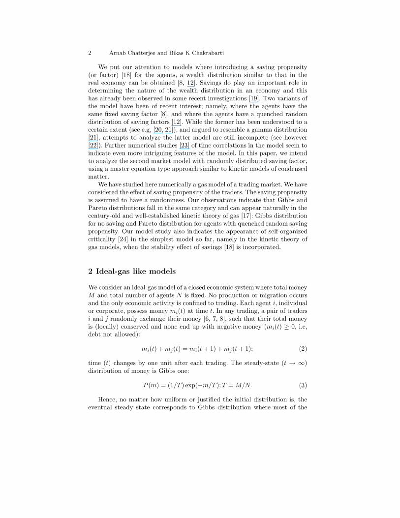
Fig. 1. Steady state money distribution (a) P (m) for the fixed λ model, and (b)Pf (m) for some specific values of λ in the distributed λ model. All data are forN = 200. Inset of (b) shows scaling behavior of Pf (m).

4 Arnab Chatterjee and Bikas K Chakrabarti

The market (non-interacting at λ = 0 and 1) becomes ‘interacting’ forany non-vanishing λ(< 1): For fixed λ (same for all agents), the steady statedistribution Pf (m) of money is exponentially decaying on both sides with themost-probable money per agent shifting away from m = 0 (for λ = 0) to M/Nas λ → 1 (Fig. 1(a)). This self-organizing feature of the market, induced bysheer self-interest of saving by each agent without any global perspective, isquite significant as the fraction of paupers decrease with saving fraction λ andmost people end up with some fraction of the average money in the market(for λ → 1, the socialists’ dream is achieved with just people’s self-interestof saving!). Interestingly, self-organisation also occurs in such market modelswhen there is restriction in the commodity market [11]. Although this fixedsaving propensity does not give yet the Pareto-like power-law distribution,the Markovian nature of the scattering or trading processes (eqn. (4)) is lostand the system becomes co-operative. Indirectly through λ, the agents getto know (start interacting with) each other and the system co-operativelyself-organises towards a most-probable distribution (mp 6= 0).

This has been understood to a certain extent (see e.g, [20, 21]), and arguedto resemble a gamma distribution [21], and partly explained analytically [22].

2.2 Effect of distributed savings

In a real society or economy, λ is a very inhomogeneous parameter: the interestof saving varies from person to person. We move a step closer to the realsituation where saving factor λ is widely distributed within the population[12, 13, 14].

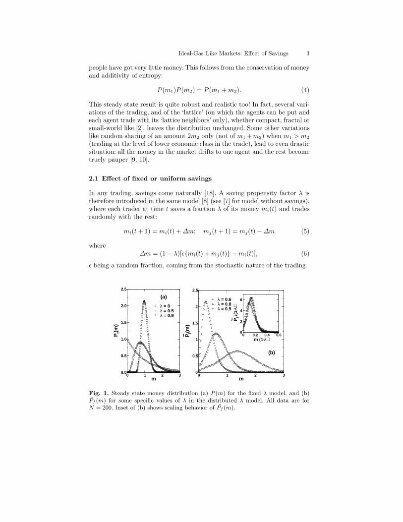
Fig. 2. Steady state money distribution P (m) for the distributed λ model with0 ≤ λ < 1 for a system of N = 1000 agents. The x−2 is a guide to the observedpower-law, with 1 + ν = 2.

Ideal-Gas Like Markets: Effect of Savings 5

The evolution of money in such a trading can be written as:

mi(t + 1) = λimi(t) + ǫij [(1 − λi)mi(t) + (1 − λj)mj(t)] , (7)

mj(t + 1) = λjmj(t) + (1 − ǫij) [(1 − λi)mi(t) + (1 − λj)mj(t)] (8)

One again follows the same trading rules as before, except that

∆m = ǫij(1 − λj)mj(t) − (1 − λi)(1 − ǫij)mi(t) (9)

here; λi and λj being the saving propensities of agents i and j. The agents havefixed (over time) saving propensities, distributed independently, randomly anduniformly (white) within an interval 0 to 1 agent i saves a random fractionλi (0 ≤ λi < 1) and this λi value is quenched for each agent (λi are indepen-dent of trading or t). Starting with an arbitrary initial (uniform or random)distribution of money among the agents, the market evolves with the trad-ings. At each time, two agents are randomly selected and the money exchangeamong them occurs, following the above mentioned scheme. We check for thesteady state, by looking at the stability of the money distribution in succes-sive Monte Carlo steps t (we define one Monte Carlo time step as N pairwiseinterations). Eventually, after a typical relaxation time (∼ 106 for N = 1000and uniformly distributed λ) dependent on N and the distribution of λ, themoney distribution becomes stationary. After this, we average the money dis-tribution over ∼ 103 time steps. Finally we take configurational average over∼ 105 realizations of the λ distribution to get the money distribution P (m).It is found to follow a strict power-law decay. This decay fits to Pareto law(1) with ν = 1.01 ± 0.02 (Fig. 2). Note, for finite size N of the market, thedistribution has a narrow initial growth upto a most-probable value mp afterwhich it falls off with a power-law tail for several decades. This Pareto law(with ν ≃ 1) covers the entire range in m of the distribution P (m) in the limitN → ∞. We checked that this power law is extremely robust: apart from theuniform λ distribution used in the simulations in Fig. 2, we also checked theresults for a distribution

ρ(λ) ∼ |λ0 − λ|α, λ0 6= 1, 0 < λ < 1, (10)

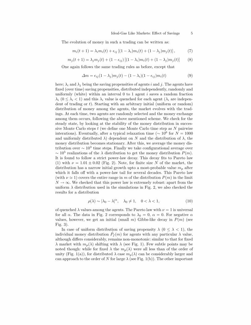
of quenched λ values among the agents. The Pareto law with ν = 1 is universalfor all α. The data in Fig. 2 corresponds to λ0 = 0, α = 0. For negative αvalues, however, we get an initial (small m) Gibbs-like decay in P (m) (seeFig. 3).

In case of uniform distribution of saving propensity λ (0 ≤ λ < 1), theindividual money distribution Pf (m) for agents with any particular λ value,although differs considerably, remains non-monotonic: similar to that for fixedλ market with mp(λ) shifting with λ (see Fig. 1). Few subtle points may benoted though: while for fixed λ the mp(λ) were all less than of the order ofunity (Fig. 1(a)), for distributed λ case mp(λ) can be considerably larger andcan approach to the order of N for large λ (see Fig. 1(b)). The other important

6 Arnab Chatterjee and Bikas K Chakrabarti

Fig. 3. Steady state money distribution P (m) in the model with for a system ofN = 100 agents with λ distributed as ρ(λ) ∼ λα, with different values of α. In allcases, agents play with average money per agent M/N = 1.

difference is in the scaling behavior of Pf (m), as shown in the inset of Fig.

1(b). In the distributed λ ensemble, Pf (m) appears to have a very simplescaling:

Pf (m) ∼ (1 − λ)F(m(1 − λ)), (11)

for λ → 1, where the scaling function F(x) has non-monotonic variationin x. The fixed (same for all agents) λ income distribution Pf (m) do nothave any such comparative scaling property. It may be noted that a smalldifference exists between the ensembles considered in Fig 1(a) and 1(b): while∫

mPf (m)dm = M (independent of λ),∫

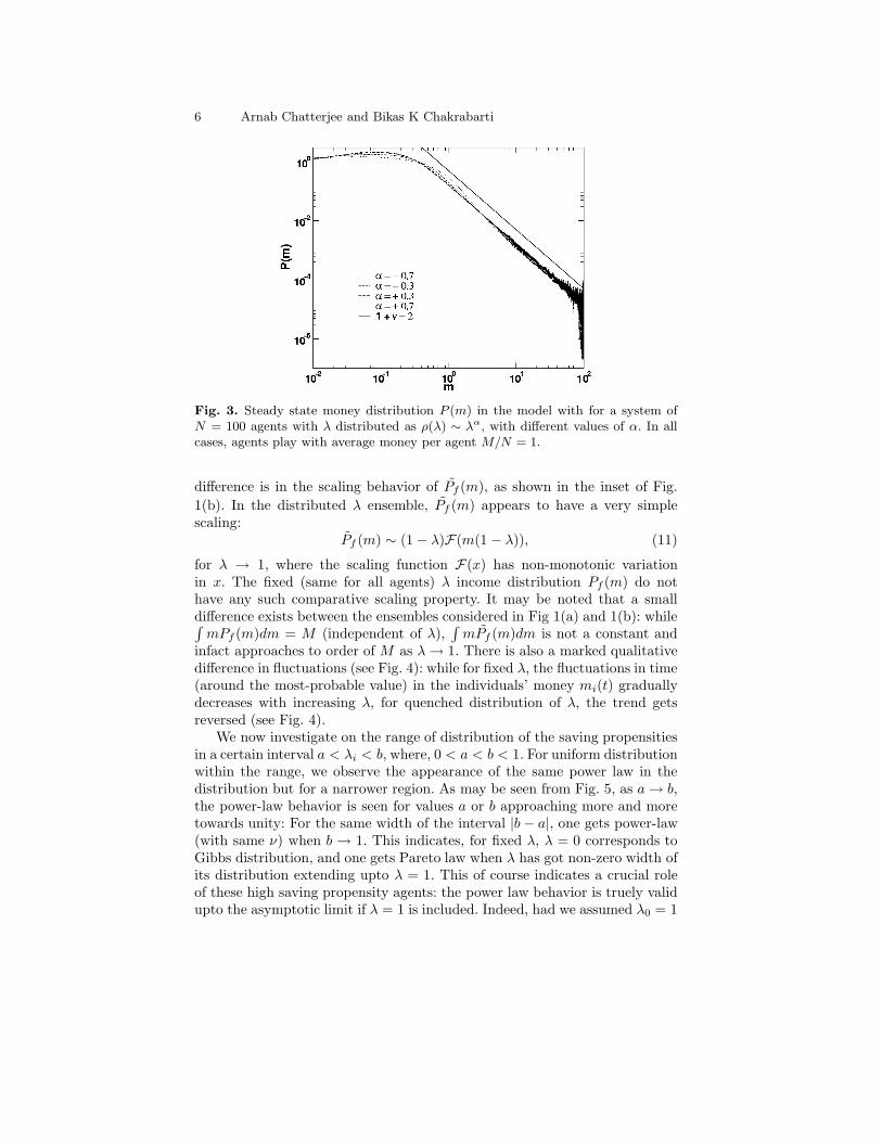
mPf (m)dm is not a constant andinfact approaches to order of M as λ → 1. There is also a marked qualitativedifference in fluctuations (see Fig. 4): while for fixed λ, the fluctuations in time(around the most-probable value) in the individuals’ money mi(t) graduallydecreases with increasing λ, for quenched distribution of λ, the trend getsreversed (see Fig. 4).

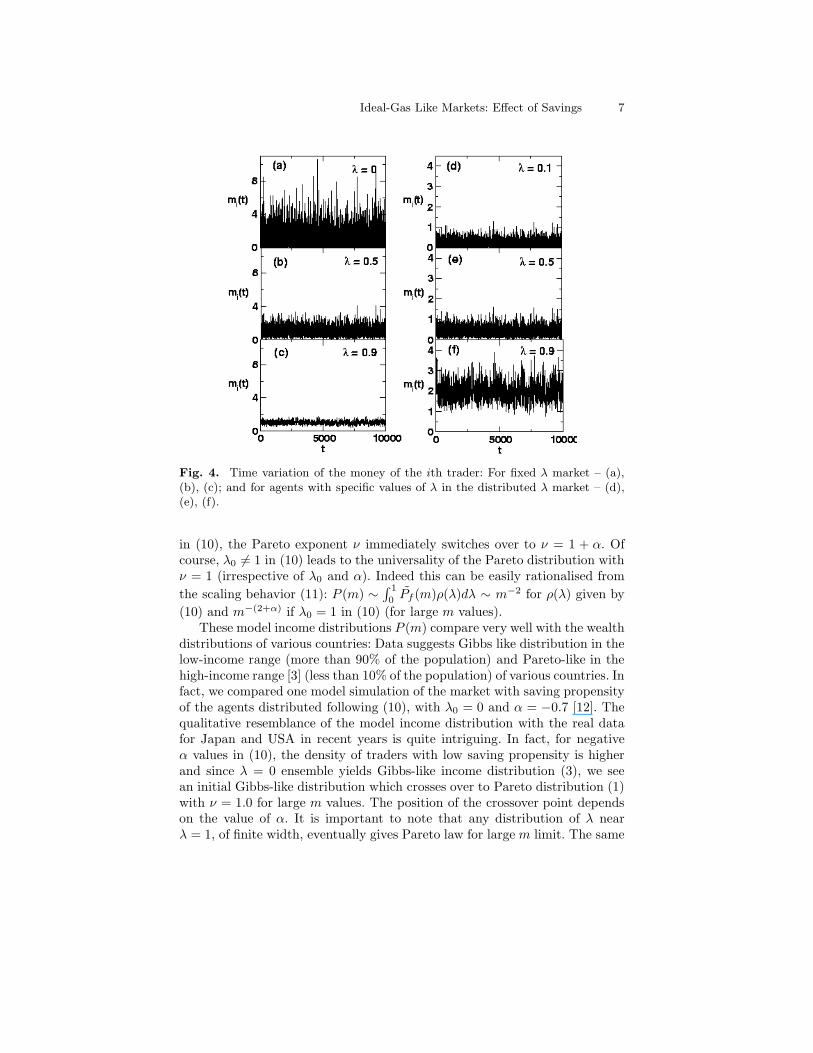
We now investigate on the range of distribution of the saving propensitiesin a certain interval a < λi < b, where, 0 < a < b < 1. For uniform distributionwithin the range, we observe the appearance of the same power law in thedistribution but for a narrower region. As may be seen from Fig. 5, as a → b,the power-law behavior is seen for values a or b approaching more and moretowards unity: For the same width of the interval |b − a|, one gets power-law(with same ν) when b → 1. This indicates, for fixed λ, λ = 0 corresponds toGibbs distribution, and one gets Pareto law when λ has got non-zero width ofits distribution extending upto λ = 1. This of course indicates a crucial roleof these high saving propensity agents: the power law behavior is truely validupto the asymptotic limit if λ = 1 is included. Indeed, had we assumed λ0 = 1

Ideal-Gas Like Markets: Effect of Savings 7

Fig. 4. Time variation of the money of the ith trader: For fixed λ market – (a),(b), (c); and for agents with specific values of λ in the distributed λ market – (d),(e), (f).

in (10), the Pareto exponent ν immediately switches over to ν = 1 + α. Ofcourse, λ0 6= 1 in (10) leads to the universality of the Pareto distribution withν = 1 (irrespective of λ0 and α). Indeed this can be easily rationalised from

the scaling behavior (11): P (m) ∼∫ 1

0 Pf (m)ρ(λ)dλ ∼ m−2 for ρ(λ) given by

(10) and m−(2+α) if λ0 = 1 in (10) (for large m values).These model income distributions P (m) compare very well with the wealth

distributions of various countries: Data suggests Gibbs like distribution in thelow-income range (more than 90% of the population) and Pareto-like in thehigh-income range [3] (less than 10% of the population) of various countries. Infact, we compared one model simulation of the market with saving propensityof the agents distributed following (10), with λ0 = 0 and α = −0.7 [12]. Thequalitative resemblance of the model income distribution with the real datafor Japan and USA in recent years is quite intriguing. In fact, for negativeα values in (10), the density of traders with low saving propensity is higherand since λ = 0 ensemble yields Gibbs-like income distribution (3), we seean initial Gibbs-like distribution which crosses over to Pareto distribution (1)with ν = 1.0 for large m values. The position of the crossover point dependson the value of α. It is important to note that any distribution of λ nearλ = 1, of finite width, eventually gives Pareto law for large m limit. The same

8 Arnab Chatterjee and Bikas K Chakrabarti

Fig. 5. Steady state money distribution in cases when the saving propensity λ isdistributed uniformly within a range of values: (a) width of λ distribution is 0.5,money distribution shows power law for 0.5 < λ < 1.0; (a) width of λ distribution is0.2, money distribution shows power law for 0.7 < λ < 0.9. The power law exponentis ν ≃ 1 in all cases. All data shown here are for N = 100, M/N = 1.

kind of crossover behavior (from Gibbs to Pareto) can also be reproduced in amodel market of mixed agents where λ = 0 for a finite fraction of populationand λ is distributed uniformly over a finite range near λ = 1 for the rest ofthe population.

We even considered annealed randomness in the saving propensity λ: hereλi for any agent i changes from one value to another within the range 0 ≤λi < 1, after each trading. Numerical studies for this annealed model did notshow any power law behavior for P (m); rather it again becomes exponentiallydecaying on both sides of a most-probable value.

3 Dynamics of money exchange

We will now investigate the steady state distribution of money resulting fromthe above two equations representing the trading and money dynamics. Wewill now solve the dynamics of money distribution in two limits. In one case,we study the evolution of the mutual money difference among the agents and

Ideal-Gas Like Markets: Effect of Savings 9

look for a self-consistent equation for its steady state distribution. In the othercase, we develop a master equation for the money distribution function.

10-5

10-4

10-3

10-2

10-1

100

101

10-2 10-1 100 101 102

P(m

)

m

m-2

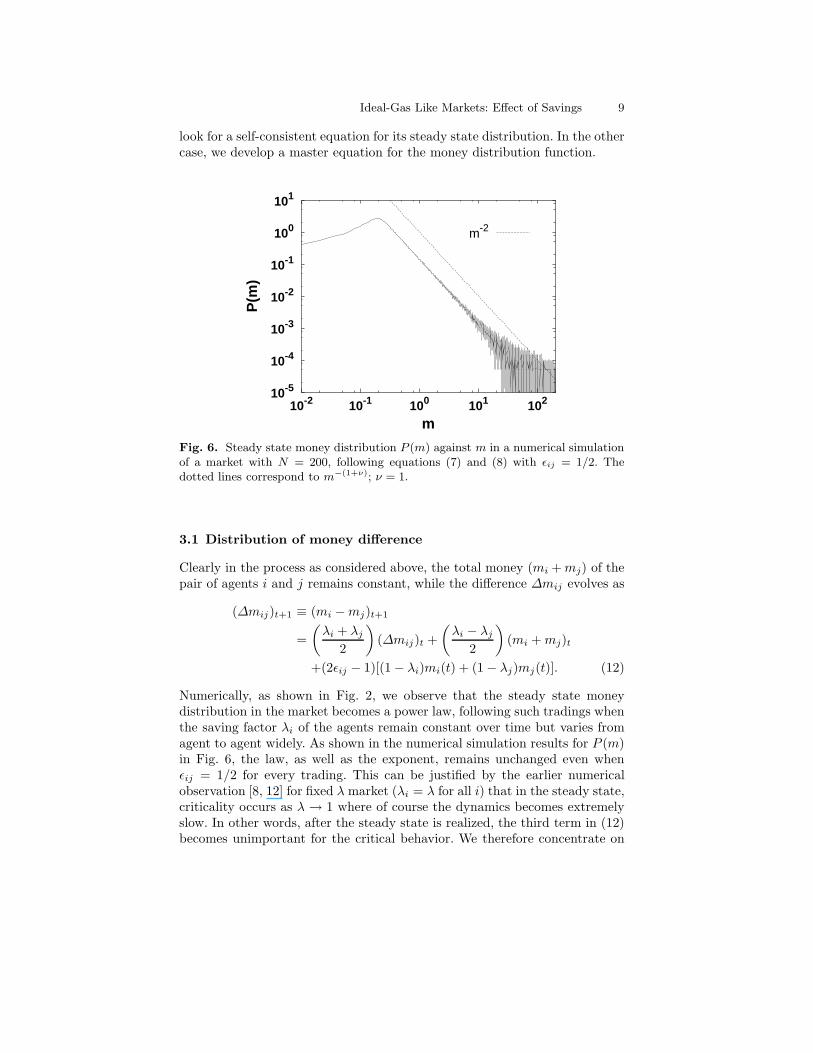
Fig. 6. Steady state money distribution P (m) against m in a numerical simulationof a market with N = 200, following equations (7) and (8) with ǫij = 1/2. Thedotted lines correspond to m−(1+ν); ν = 1.

3.1 Distribution of money difference

Clearly in the process as considered above, the total money (mi + mj) of thepair of agents i and j remains constant, while the difference ∆mij evolves as

(∆mij)t+1 ≡ (mi − mj)t+1

=

(

λi + λj

2

)

(∆mij)t +

(

λi − λj

2

)

(mi + mj)t

+(2ǫij − 1)[(1 − λi)mi(t) + (1 − λj)mj(t)]. (12)

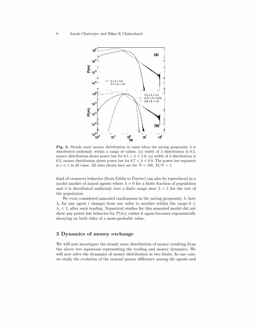
Numerically, as shown in Fig. 2, we observe that the steady state moneydistribution in the market becomes a power law, following such tradings whenthe saving factor λi of the agents remain constant over time but varies fromagent to agent widely. As shown in the numerical simulation results for P (m)in Fig. 6, the law, as well as the exponent, remains unchanged even whenǫij = 1/2 for every trading. This can be justified by the earlier numericalobservation [8, 12] for fixed λ market (λi = λ for all i) that in the steady state,criticality occurs as λ → 1 where of course the dynamics becomes extremelyslow. In other words, after the steady state is realized, the third term in (12)becomes unimportant for the critical behavior. We therefore concentrate on

10 Arnab Chatterjee and Bikas K Chakrabarti

this case, where the above evolution equation for ∆mij can be written in amore simplified form as

(∆mij)t+1 = αij(∆mij)t + βij(mi + mj)t, (13)

where αij = 12 (λi + λj) and βij = 1

2 (λi − λj). As such, 0 ≤ α < 1 and− 1

2 < β < 12 .

The steady state probability distribution D for the modulus ∆ = |∆m| ofthe mutual money difference between any two agents in the market can beobtained from (13) in the following way provided ∆ is very much larger thanthe average money per agent = M/N . This is because, large ∆ can appearfrom ‘scattering’ involving mi −mj = ±∆ and when either mi or mj is small.When both mi and mj are large, maintaining a large ∆ between them, theirprobability is much smaller and hence their contribution. Then if, say, mi islarge and mj is not, the right hand side of (13) becomes ∼ (αij + βij)(∆ij)t

and so on. Consequently for large ∆ the distribution D satisfies

D(∆) =

∫

d∆′ D(∆′) 〈δ(∆ − (α + β)∆′) + δ(∆ − (α − β)∆′)〉

= 2〈

(

1

λ

)

D

(

∆

λ

)

〉, (14)

where we have used the symmetry of the β distribution and the relationαij +βij = λi, and have suppressed labels i, j. Here 〈. . .〉 denote average overλ distribution in the market. Taking now a uniform random distribution ofthe saving factor λ, ρ(λ) = 1 for 0 ≤ λ < 1, and assuming D(∆) ∼ ∆−(1+γ)

for large ∆, we get

1 = 2

∫

dλ λγ = 2(1 + γ)−1, (15)

giving γ = 1. No other value fits the above equation. This also indicates thatthe money distribution P (m) in the market also follows a similar power lawvariation, P (m) ∼ m−(1+ν) and ν = γ. We will now show in a more rigorousway that indeed the only stable solution corresponds to ν = 1, as observednumerically [12, 13, 14].

3.2 Master equation and its analysis

We also develop a Boltzmann-like master equation for the time developmentof P (m, t), the probability distribution of money in the market [25, 26]. Weagain consider the case ǫij = 1

2 in (7) and (8) and rewrite them as

(

mi

mj

)

t+1

= A

(

mi

mj

)

t

where A =

(

µ+i µ−

j

µ−

i µ+j

)

; µ± =1

2(1 ± λ). (16)

Collecting the contributions from terms scattering in and subtracting thosescattering out, we can write the master equation for P (m, t) as

Ideal-Gas Like Markets: Effect of Savings 11

∂P (m, t)

∂t+P (m, t) = 〈

∫

dmi

∫

dmj P (mi, t)P (mj , t) δ(µ+i mi+µ−

j mj−m)〉,

(17)which in the steady state gives

P (m) = 〈

∫

dmi

∫

dmj P (mi)P (mj) δ(µ+i mi + µ−

j mj − m)〉. (18)

Assuming, P (m) ∼ m−(1+ν) for m → ∞, we get [25, 26]

1 = 〈(µ+)ν + (µ−)ν〉 ≡

∫ ∫

dµ+dµ−p(µ+)q(µ−)[

(µ+)ν + (µ−)ν]

. (19)

Considering now the dominant terms (∝ x−r for r > 0, or ∝ ln(1/x) for r = 0)in the x → 0 limit of the integral

∫ ∞

0m(ν+r)P (m) exp(−mx)dm, we get from

eqn. (19), after integrations, 1 = 2/(ν + 1), giving finally ν = 1 (details inAppendix).

4 Summary and Discussions

We have numerically simulated here ideal-gas like models of trading markets,where each agent is identified with a gas molecule and each trading as anelastic or money-conserving two-body collision. Unlike in the ideal gas, weintroduce (quenched) saving propensity of the agents, distributed widely be-tween the agents (0 ≤ λ < 1). For quenched random variation of λ among theagents the system remarkably self-organizes to a critical Pareto distribution(1) of money with ν ≃ 1.0 (Fig. 2). The exponent is quite robust: for savingsdistribution ρ(λ) ∼ |λ0−λ|α, λ0 6= 1, one gets the same Pareto law with ν = 1(independent of λ0 or α).

A master equation for P (m, t), as in (17), for the original case (eqns. (7)and (8)) was first formulated for fixed λ (λi same for all i), in [20] and solvednumerically. Later, a generalized master equation for the same, where λ isdistributed, was formulated and solved in [22] and [25]. We show here thatour analytic study clearly support the power-law for P (m) with the exponentvalue ν = 1 universally, as observed numerically earlier [12, 13, 14].

It may be noted that the trading market model we have talked about herehas got some apparent limitations. The stochastic nature of trading assumedhere in the trading market, through the random fraction ǫ in (6), is of coursenot very straightforward as agents apparently go for trading with some def-inite purpose (utility maximization of both money and commodity). We arehowever, looking only at the money transactions between the traders. In thissense, the income distribution we study here essentially corresponds to ‘papermoney’, and not the ‘real wealth’. However, even taking money and commod-ity together, one can argue (see [10]) for the same stochastic nature of thetradings, due to the absence of ‘just pricing’ and the effects of bargains in themarket.

12 Arnab Chatterjee and Bikas K Chakrabarti

Apart from the observation that Gibbs (1901) and Pareto (1897) distri-butions fall in the same category and can appear naturally in the century-oldand well-established kinetic theory of gas, that this model study indicatesthe appearance of self-organized criticality in the simplest (gas) model so far,when the stability effect of savings incorporated, is remarkable.

5 Acknowledgments

We are grateful to A. Chakraborti, S. Pradhan, S. S. Manna and R. B. Stinch-combe for collaborations at various stages of our study.

A Alternative solution of the steady state masterequation (18)

Let Sr(x) =∫ ∞

0dmP (m)mν+r exp(−mx); r ≥ 0, x > 0. If P (m) = A/m1+ν ,

then

Sr(x) = A

∫ ∞

0

dm mr−1 exp(−mx)

∼ Ax−r

rif r > 0

∼ A ln

(

1

x

)

if r = 0. (20)

From eqn. (18), we can write

Sr(x) =

〈

∫ ∞

0

dmi

∫ ∞

0

dmj P (mi)P (mj)(miµ+i + mjµ

−

j )ν+r exp[−(miµ+i + mjµ

−

j )x]〉

≃

∫ ∞

0

dmi Amr−1i 〈exp(−miµ

+i x)

(

µ+i

)ν+r〉

[∫ ∞

0

dmj P (mj)〈exp(−mjµ−

j x)〉

]

+

∫ ∞

0

dmj Amr−1j 〈exp(−mjµ

−

j x)(

µ−

j

)ν+r〉

[∫ ∞

0

dmi P (mi)〈exp(−miµ+i x)〉

]

(21)

or,

Sr(x) =

∫ 1

1

2

dµ+i p(µ+

i )

(∫ ∞

0

dmi Amr−1i exp(−miµ

+i x)

)

(

µ+i

)ν+r

+

∫ 1

2

0

dµ−

j q(µ−

j )

(∫ ∞

0

dmj Amr−1j exp(−mjµ

−

j x)

)

(

µ−

j

)ν+r,(22)

Ideal-Gas Like Markets: Effect of Savings 13

since for small x, the terms in the square brackets in (21) approach unity. Wecan therefore rewrite (22) as

Sr(x) = 2

[

∫ 1

1

2

dµ+(µ+)ν+rSr(xµ+) +

∫ 1

2

0

dµ−(µ−)ν+rSr(xµ−)

]

. (23)

Using now the forms of Sr(x) as in (20), and collecting terms of order x−r

(for r > 0) or of order ln(1/x) (for r = 0) from both sides of (23), we get (19).

References

1. Pareto V (1897) Cours d’economie Politique. F. Rouge, Lausanne2. Moss de Oliveira S, de Oliveira PMC, Stauffer D (1999) Evolution, Money, War

and Computers. B. G. Tuebner, Stuttgart, Leipzig3. Levy M, Solomon S (1997) New evidence for the power-law distribution of

wealth, Physica A 242:90-94; Dragulescu AA, Yakovenko VM (2001) Expo-nential and Power-Law Probability Distributions of Wealth and Income in theUnited Kingdom and the United States. Physica A 299:213-221; Aoyama H,Souma W, Fujiwara Y (2003) Growth and fluctuations of personal and com-pany’s income, Physica A 324:352

4. Di Matteo T, Aste T, Hyde ST (2003) Exchanges in Complex Networks: In-come and Wealth Distributions, cond-mat/0310544; Clementi F, Gallegati M(2005), Power Law Tails in the Italian Personal Income Distribution. PhysicaA 350:427–438

5. Sinha S (2005) Evidence for Power-law Tail of the Wealth Distribution in India,cond-mat/0502166

6. Chakrabarti BK, Marjit S (1995) Self-organization in Game of Life and Eco-nomics,Indian J. Phys. B69:681-698; Ispolatov S, Krapivsky PL, Redner S(1998) Wealth distributions in asset exchange models, Eur. Phys. J. B 2:267;

7. Dragulescu AA, Yakovenko VM (2000) Statistical Mechanics of Money, Eur.Phys. J. B 17:723-726

8. Chakraborti A, Chakrabarti BK (2000) Statistical Mechanics of Money: Effectsof Saving Propensity, Eur. Phys. J. B 17:167-170

9. Chakraborti A (2002) Distributions of money in model markets of economy,Int. J. Mod. Phys. C 13:1315

10. Hayes B (2002) Follow the Money, American Scientist, USA, 90:(Sept-Oct)400-405

11. Chakraborti A, Pradhan S, Chakrabarti BK (2001) A Self-organizing MarketModel with single Commodity, Physica A 297:253-259

12. Chatterjee A, Chakrabarti BK, Manna SS (2004) Pareto Law in a KineticModel of Market with Random Saving Propensity, Physica A 335:155

13. Chatterjee A, Chakrabarti BK; Manna SS (2003) Money in Gas-like Markets:Gibbs and Pareto Laws, Physica Scripta T 106:36

14. Chakrabarti BK, Chatterjee A (2004) Ideal Gas-Like Distributions in Eco-nomics: Effects of Saving Propensity, in Application of Econophysics, Proc.2nd Nikkei Econophys. Symp., Ed. Takayasu H, Springer, Tokyo, pp. 280-285

14 Arnab Chatterjee and Bikas K Chakrabarti

15. Sinha S (2003) Stochastic Maps, Wealth Distribution in Random Asset Ex-change Models and the Marginal Utility of Relative Wealth, Phys. ScriptaT106:59-64; Ferrero JC (2004) The statistical distribution of money and the rateof money transference, Physica A 341:575; Iglesias JR, Goncalves S, AbramsonG, Vega JL (2004) Correlation between risk aversion and wealth distribution,Physica A 342:186; Scafetta N, Picozzi S, West BJ (2004) A trade-investmentmodel for distribution of wealth, Physica D 193:338-352

16. Slanina F (2004) Inelastically scattering particles and wealth distribution in anopen economy, Phys. Rev. E 69:046102

17. See e.g, Landau LD, Lifshitz EM (1968), Statistical Physics. Pergamon Press,Oxford.

18. Samuelson PA (1980) Economics. Mc-Graw Hill Int., Auckland.19. Willis G, Mimkes J (2004) Evidence for the Independence of Waged and Un-

waged Income, Evidence for Boltzmann Distributions in Waged Income, andthe Outlines of a Coherent Theory of Income Distribution, cond-mat/0406694

20. Das A, Yarlagadda S (2003) Analytic treatment of a trading market model,Phys. Scripta T106:39-40

21. Patriarca M, Chakraborti A, Kaski K (2004) A Statistical model with a stan-dard Γ distribution, Phys. Rev. E 70:016104

22. Repetowicz P, Hutzler S, Richmond P (2004) Dynamics of Money and IncomeDistributions, cond-mat/0407770

23. Ding N, Xi N, Wang Y (2003) Effects of saving and spending patterns onholding time distribution, Eur. Phys. J. B 36:149

24. Bak P (1997) How Nature works. Oxford University Press, Oxford.25. Chatterjee A, Chakrabarti BK, Stinchcombe RB (2005) Master equation for a

kinetic model of trading market and its analytic solution, cond-mat/050141326. Chatterjee A, Chakrabarti BK, Stinchcombe RB (2005) Analyzing money dis-

tributions in ‘ideal gas’ models of markets, in ‘Practical Fruits of Econophysics’,Ed. Takayasu H, Springer-Berlag, Tokyo Proc. Third Nikkei Symposium onEconophysics, Tokyo, Japan, 2004, cond-mat/0501413

27. Dynan KE, Skinner J, Zeldes SP (2004) Do the rich save more ?, J. Pol. Econ.112: 397-444.