Hydrologic and geologic factors controlling surface and groundwater chemistry in Indian Wells-Owens...

Hydrologic and geologic factors controlling surface and

groundwater chemistry in Indian Wells-Owens Valley area,

southeastern California, USA

Cuneyt Gulera, Geoffrey D. Thyneb,*

aMersin Universitesi, Ciftlikkoy Kampusu, Jeoloji Muhendisligi Bolumu, 33343 Mersin, TurkeybColorado School of Mines, Department of Geology and Geological Engineering, 1500 Illinois Street, Golden, CO 80401, USA

Received 28 February 2002; accepted 19 August 2003

Abstract

The Indian Wells-Owens Valley area is located in the semi-arid Basin and Range province, which is characterized by

alternating mountains and alluvial basins. Surface water resources are limited in this arid region and water demand is mainly

met by groundwater pumpage. In a classic Basin and Range groundwater system, water flows from recharge areas in the

mountains to discharge areas in adjacent valleys. Discharge areas are generally occupied by playas where large amounts of salt

deposition occur due to evaporating groundwater.

Hydrochemical data from a total of 1368 spring, surface, and well water samples collected over an 80-year period were used

to evaluate water quality and to determine processes that control water chemistry. Q-mode hierarchical cluster analysis (HCA)

was employed for partitioning the water samples into hydrochemical facies, also known as water groups or water types. Five

major water groups resulted from the HCA analysis. The samples from the area were classified as recharge area waters (Ca–

Na–HCO3 water and Na–Ca–HCO3 water), transition zone waters (Na–HCO3–Cl water), and discharge area waters (Na–Cl

water and more concentrated Na–Cl water). Spatial plots of the major statistical groups show that the samples that belong to the

same group are located in close proximity to one another suggesting the same processes and/or flowpaths. Inverse geochemical

models of the statistical groups were developed using PHREEQC to elucidate the chemical reactions controlling water

chemistry. The inverse geochemical modeling demonstrated that relatively few phases are required to derive water chemistry in

the area. In a broad sense, the reactions responsible for the hydrochemical evolution in the area fall into four categories: (1)

silicate weathering reactions; (2) dissolution of salts; (3) precipitation of calcite, amorphous silica, and clay minerals; and (4)

ion exchange.

q 2003 Elsevier B.V. All rights reserved.

Keywords: Water chemistry; Cluster analysis; Geochemical modeling; PHREEQC; Basin and range; California

1. Introduction

The Indian Wells-Owens Valley area is located in a

relatively unpopulated region, which is currently

undergoing a significant increase in water demand.

0022-1694/$ - see front matter q 2003 Elsevier B.V. All rights reserved.

doi:10.1016/j.jhydrol.2003.08.019

Journal of Hydrology 285 (2004) 177–198

www.elsevier.com/locate/jhydrol

* Corresponding author. Tel.: þ1-303-273-3104; fax: þ1-303-

273-3859.

E-mail address: [email protected] (G.D. Thyne).

http://www.elsevier.com/locate/jhydrol

In the study area, there are a wide variety of climatic

conditions, hydrologic regimes, and geologic environ-

ments. Thus, the water samples from the area

represent a variety of water types having a wide

range of chemical composition. Due to both the

complexity of the groundwater flow system and the

overall lack of hydrochemical and hydrologic data for

much of the region, large uncertainties exist in the

current groundwater flow models. The complex

system is complicated by heavy pumping from valley

aquifers for agricultural and public use, disposal of

treated wastewater and possible groundwater flow

barriers.

Previous studies have shown that major-ion

chemistry of natural waters can often be explained

by the reaction of these waters with rocks or

sediments through which they flow (Back, 1966;

Garrels and MacKenzie, 1967; White et al., 1980;

Frape et al., 1984; Hem, 1989; Thomas et al., 1989).

The spatial variability observed in the composition of

these natural tracers can provide insight into aquifer

heterogeneity and connectivity as well as the physical

and chemical processes controlling water chemistry.

As a result, the use of major-ions as natural tracers has

become an accepted method to delineate flowpaths in

aquifers. Generally, the approach is to divide the

samples into hydrochemical facies, that is group

samples with similar chemical characteristics that can

then be correlated with location. Verification that

systematic variations along the flowpath are related to

reactions between groundwater and the aquifer

provides the hydrochemical evolution model for the

area. This information provides the context for

interpreting the spatial variations in water chemistry

and defining groundwater flowpaths.

In this study, physical, hydrogeologic, and hydro-

chemical information from the groundwater system

will be integrated and used to determine the main

factors and mechanisms controlling the chemistry of

surface and groundwaters in the area. The main issues

that will be addressed by this study include: (1) the

validity of statistical clustering techniques in classify-

ing the samples into hydrochemical facies on a

regional scale; (2) development of a hydrochemical

model for the region; (3) the relative importance of

hydrologic and geologic factors in controlling the

water chemistry; and (4) the assessment of the value

of this approach to delineate flowpaths.

2. Description of the study area

The study area lies within the south Lahontan

hydrologic region, California, and covers approxi-

mately 29,800 km2 stretching from Owens Valley

(OV) in the north to Indian Wells Valley (IWV) in the

south (Figs. 1 and 2). These valleys are young,

complex structural and topographic depressions and

are tectonically similar to other valleys in the Basin

and Range physiographic province. Both OV and

IWV are bordered on the west by the Sierra Nevada

with peaks rising from 1829 to 4417 m and on the east

by several ranges including the Inyo Mountains, the

Coso Range, and the Argus Range with elevations

ranging from 1500 to 2750 m. Topography of the

valley floors is relatively flat and slopes to the south

with elevations decreasing from 1100 m in the OV to

nearly 663 m in the vicinity of IWV.

The existing topographic relief between the ranges

(horsts) and the valley floors (grabens) of the area is

mostly the result of the tectonic activity and

faulting that occurred during the Late Cenozoic time

(Christensen, 1966). The area lies in close proximity

to several major active fault zones of California

Fig. 1. Location of the study area showing the hydrologic regions of

California.

C. Guler, G.D. Thyne / Journal of Hydrology 285 (2004) 177–198178

including the San Andreas fault (150 km to the

southwest), the Sierra Nevada frontal fault, Kern

Canyon fault, Death Valley-Furnace Creek fault zone,

Garlock fault, and Argus fault. Locally, complex

faulting occurs in all the bordering ranges (Fig. 2).

Several major, and numerous minor local faults that

propagate upwards from the underlying crystalline

basement dissect the basin-fill deposits. The majority

of these structural discontinuities have been deter-

mined by the aid of seismic refraction and gravimetric

studies (e.g. von Huene, 1960; Zbur, 1963).

Two contrasting climate regimes exist in the area.

High alpine to alpine climate conditions prevail in the

Sierra Nevada, which serves as the main recharge

area, and arid climate conditions dominate in the

adjoining alluvial-filled basins. Climate of the area is

mostly shaped by the Sierra Nevada range, which

forms a barrier to passing storms and creates a rain

shadow effect (Feth et al., 1964a; Whelan et al., 1989).

As a result, the mountain ranges in the area generally

receive progressively less precipitation from west to

east. Average rainfall on the valley floors ranges from

Fig. 2. Map of rock types and general features of the Indian Wells-Owens Valley area, California.

C. Guler, G.D. Thyne / Journal of Hydrology 285 (2004) 177–198 179

about 75–152 mm, whereas at the crest of the Sierra

Nevada average annual precipitation generally varies

from 508 to 1400 mm and occurs mostly as snowfall

(accounting for 90–95% of the regional precipi-

tation). The large altitude variations affect the

temperatures considerably. Average air temperature

in the valleys range from 3 8C in winter to 28 8C in

summer. Strong winds (annually averaging

13.2 km h21 in China Lake) occur in the late winter

and spring as a result of rapidly moving cold frontal

systems (Corbett, 1990). These winds occasionally

cause severe dust and sandstorms that can signifi-

cantly reduce visibility (Corbett, 1990) and pose

health risks to humans (Saint-Amand, 1986).

2.1. Lithology and mineralogy

The chemical composition of minerals in the

mountain ranges and basin-fill imposes a fundamental

constraint on the selection of the mineral phases that

will be used in geochemical calculations. Rocks and

unconsolidated deposits in the area can be divided

into five hydrogeologic units: (1) igneous and

metamorphic rocks; (2) volcanic rocks; (3) carbonate

rocks; (4) basin-fill deposits; and (5) playa deposits

(Fig. 2). Chemical analyses of the rock types from

various parts of the region are presented in Table 1.

Igneous rocks of Mesozoic age outcrop in many

mountain ranges and underlie most of the region at

depth (Kistler et al., 1965; McKee and Nash, 1967).

The granitic rocks range from gabbro to quartz

monzonite in composition, with quartz diorite making

up the bulk of the plutonic rock (Oliver, 1977). These

rocks are characterized by porphyritic texture, phe-

nocrysts of quartz, biotite, plagioclase, K-feldspar

(orthoclase), hornblende, olivine, and commonly

contain mafic inclusions. Metamorphic rocks of

Precambrian age are scattered throughout the area

and display very limited areal extension. Together,

igneous and metamorphic rocks constitute ,37% of

the surface lithology of the study area.

The volcanic rocks, including lava flows, tuffs, and

volcaniclastic sediments of Cenozoic age, crop out

extensively in the regions surrounding the Coso

Range (Lanphere et al., 1975). This unit is mainly

composed of Pleistocene, Pliocene, and Miocene

Table 1

Modal analyses of plutonic and volcanic rocks from the region

Sample no. 1 2 3 4 5 6 7 8 9 10a 11a

Location Argus range Inyo

mtns

El paso

Mtns

El paso

Mtns

Argus

range

Spangler

hills

Coso

range

Coso

range

Coso

range

Spangler

hills

Argus

range

Minerals Plutonic

rocks

Volcanic

rocks

K-feldspar 18.0 30.6 27.5 10.8 23.0 42.0 8.6 10.6 27.2 – 53.0

Plagioclase 55.6 35.1 36.8 56.1 42.0 21.0 62.7 55.2 38.1 28.0 27.0

Quartz 2.9 30.0 27.4 23.1 23.0 36.0 – – 32.9 2.0 11.0

Biotite – – – – 6.0 ,1.0 – – – – 4.0

Hornblende – – – – 4.0 ,1.0 – – – 63.0 –

Olivine – – – – – – 3.8 3.4 – – –

Clinopyroxene 10.9 0.8 3.3 4.5 – – 17.0 22.3 1.1 3.0 –

Calcite 0.6 0.2 0.2 0.1 – – 0.1 0.1 – – –

Opaque

minerals

7.7 2.9 3.5 3.8 1.0 ,1.0 7.3 7.2 0.7 1.0 2.0

Other

minerals

4.3 0.4 1.3 1.6 1.0 ,1.0 0.9 1.4 ,0.1 3.0 3.0

Modal analyses calculated from oxides. Dashes do not necessarily indicate that minerals are not present. Samples 1, 2, 3 and 4 are from Lee

(1984), Table 3. Corresponding sample numbers are GR-129, GR-131, GR-149 and GR-151, respectively. Samples 5 and 6 are from Smith

(1962), Table II. Corresponding sample numbers are GS-CG-1-60-6b and GS-CG-1-51-8b, respectively. Samples 7, 8 and 9 are from Duffield

et al. (1980), Table 2. Corresponding sample numbers are 2, 9 and 10, respectively. Samples 10 and 11are from Smith (1962),

Table I. Corresponding sample numbers are GS-CG-1-51-8a and GS-CG-1-60-4, respectively.a Dike rocks.


volcanic rocks including rhyolites, andesites, basalts,

olivine basalts, basaltic pyroclastic rocks. The volca-

nic rocks constitute 9% of the surface lithology.

Carbonate rocks constitute ,10% of the surface

lithology and consist of a wide variety of Paleozoic

and Mesozoic age rocks. There are Paleozoic and

Mesozoic age limestone, dolomite, marble, calcareous

shale and sandstone that outcrop along the flanks and

throughout some parts of the mountains.

The Quaternary–Tertiary basin-fill deposits are a

heterogeneous mixture of plutonic, volcanic and

sedimentary rock detritus ranging from clay to

boulder size. The mixture includes sand dune

deposits, stream alluvium, stream-terrace deposits,

coarse granitic debris flow, fan deposits, talus, slope

wash, and glacial deposits. The unconsolidated

materials deposited in fluvial and lacustrine environ-

ments of the valleys are relatively well sorted. The

basin-fill deposits vary greatly in lithology, both

vertically and areally. The percentage of silt and clay

in the alluvium generally increases toward the playa-

areas. Accordingly, the hydraulic properties of these

deposits can differ greatly over short distances, both

laterally and vertically. Thickness of basin-fill depos-

its ranges from zero at margins of valleys to as much

as 610 m in IWV (Zbur, 1963) and more than 2440 m

beneath Owens Lake (Hollett et al., 1991). The basin-

fill deposits cover ,40% of the study area.

Quaternary playa deposits, are a relatively homo-

geneous deposit composed of mainly lenticular layers

of interbedded salt deposits (evaporites), fine-grained

sands, silts, clays, and lacustrine limestone. The

evaporites are rich in sodium and calcium salts.

Magnesium salts are extremely rare (Droste, 1961).

Clay minerals primarily consist of illite and mon-

tmorillonite with lesser amounts of kaolinite and/or

chlorite. The ratios of illite:montmorillonite:kaolinite

and/or chlorite are 7:2:1 for Owens Lake, 4:5:1 for

China Lake (Droste, 1961). The relative abundance of

montmorillonite in China Lake sediments is related to

volcanic eruptions in Quaternary time (Droste, 1961).

The playa deposits cover ,5% of the study area.

3. Hydrology

Due to the modern arid climate, surface water is

scarce in the area and mostly occurs in manmade

reservoirs (e.g. Haiwee Reservoir and Lake Isabella).

However, during the Quaternary period, valley floors

were periodically occupied by a chain of lakes

(Duffield and Smith, 1978). Present day, these

locations are occupied by playas, known in different

localities as ‘salt lakes,’ ‘soda lakes,’ ‘alkali marshes,’

‘dry lakes’ or ‘borax lakes’ where the groundwater

discharges by evapotranspiration (Lee, 1912; Fenne-

man, 1931; Dutcher and Moyle, 1973). The largest of

the playas are Owens Lake, Searles Lake, and China

Lake (Fig. 2). Near the playas, evapotranspiration

constitutes the major flux of water out of the system.

Such conditions can produce high chemical concen-

trations in evaporating groundwater, which can result

in the precipitation of evaporate mineral deposits as

salt crusts (Farnham et al., 2000,). The most important

crust-forming minerals are halite, natron, borax,

thenardite, mirabilite, trona, burkeite, nahcolite,

gaylussite, and pirssonite (Droste, 1961; Saint-A-

mand, 1986; Smith et al., 1971).

In a classic Basin and Range groundwater system,

water flows from recharge areas in the mountains to

discharge areas in adjacent valleys (Maxey, 1968).

Groundwater occurs in two different porosity regimes:

(1) fracture porosity found in the mountain water-

sheds; and (2) intergranular porosity found mostly in

alluvial basin-fill aquifers. In the mountain water-

sheds, the water from precipitation at high altitudes

percolates into a network of interconnecting fractures

and faults existing within the igneous and meta-

morphic rocks, and under the influence of gravity

moves toward points of lower head. In contrast, the

groundwater in the alluvial aquifers moves through

sediments that form a porous medium. Berenbrock

and Schroeder (1994) estimate pre-development

travel times of approximately 6000–13,000 years

from the edges of the basin to the playa,

which correspond to groundwater velocities of

0.21–0.76 m/year.

The alluvial basin-fill aquifer in IWV is defined by

two components: (1) a shallow saline aquifer under

the playa (,150 m deep); and (2) a deep (610 m),

locally confined aquifer that extends throughout the

valley (Dutcher and Moyle, 1973). The shallow

aquifer consists of fine-grained lacustrine, alluvium,

playa, and sand dune deposits perched on low

permeability lacustrine clays near and around the

playa lakes (Kunkel and Chase, 1969). The shallow


aquifer does not yield water freely to wells and

contains water of poor quality (total dissolved solids

(TDS) . 1000 mg l21). The deep aquifer consists

predominantly of high permeability fine to coarse

sand and gravel, interbedded with silt and clay layers

of lacustrine deposits, especially near the playas.

The deep aquifer is currently being heavily pumped

for its fresh water supply in IWV (Berenbrock and

Martin, 1991).

4. Methodology

4.1. Database

Throughout the last 80 years, extensive hydro-

chemical data have been collected in the Indian

Wells-Owens Valley area. The database used by this

study is a compilation of most of these previously

collected data (spring, surface, and well water data).

This database was used for classification of waters

into hydrochemical facies, also known as ‘water

types’ or ‘water groups’. The entire database consists

of chemical analyses of 152 spring, 153 surface, and

1063 well samples; including temporal series

(samples collected over a period of time at the same

location). In the case of time series, more recent

and/or the more complete sample data were included

in the statistical analysis unless evaluation of temporal

effects was desired. Database construction procedures

are discussed in detail in Guler et al. (2002), where the

sources of the data are also presented. Of the 39

hydrochemical variables in the compiled database, the

variables Specific Conductance, pH, Ca, Mg, Na, K,

Cl, SO4, HCO3, SiO2, and F occur most often and

were utilized in the statistical analyses.

4.2. Statistical clustering

Cluster analysis was used to determine if the

samples can be grouped into statistically distinct

hydrochemical groups that may be significant in the

geologic context. A number of studies have used this

technique to successfully classify water samples

(Alther, 1979; Williams, 1982; Farnham et al., 2000;

Alberto et al., 2001; Meng and Maynard, 2001).

Comparisons based on multiple parameters from

different samples are made and the samples grouped

according to their ‘similarity’ to each other. The

classification of samples according to their parameters

is termed Q-mode classification. In this study,

Q-mode HCA was used to classify the samples into

distinct hydrochemical groups. Data treatment

procedures and detailed explanation of the HCA

clustering technique used by this study can be found

in Guler et al. (2002).

4.3. Aqueous geochemical modeling

Inverse modeling calculations were performed

using PHREEQC (Parkhurst and Appelo, 1999).

PHREEQC was also used to calculate aqueous

speciation and mineral saturation indices. The Geo-

chemist’s Workbenchw was used to plot mineral

stability diagrams (Bethke, 1994).

5. Results

5.1. Q-mode Hierarchical cluster analysis

A total of 1368 water samples from the Indian

Wells-Owens Valley area and surrounding mountains

are contained in the compiled database. Analysis of

temporal series, as well as statistical analysis of the

entire database suggested that relatively little change

occurred in the water quality of samples with time

(Guler, 2002; Guler et al., 2002). This indicates that

spatial variability is the most important source of

variation in the data. Therefore, removal of duplicate

(in some cases multiple) water samples from the same

location is warranted. Samples are given priority on

the basis of completeness of data and date of

collection. Removing the multiple samples reduced

the total to 579.

The statistical software (Statistica; StatSoft, Inc.,

1995) used in this study can only cluster a maximum

of 300 samples, clearly a shortcoming given 579

water samples. Therefore, a two-step approach, pre-

clustering and then clustering, was used. This

methodology (pre-clustering and clustering) is cur-

rently used in several clustering algorithms (e.g. SAS/

STAT release 6.03; SAS Institute, Inc., 1988) to

cluster samples.

First, 579 water samples were subdivided into

four major categories consisting of: (1) spring waters


(SP ¼ 118 samples); (2) surface waters (SU ¼ 137

samples); (3) shallow well waters (WS ¼ 264 sam-

ples); and (4) deep well waters (WD ¼ 60 samples).

Then, each data set was log-transformed and

standardized (to zero mean and unit variance) to

avoid misclassifications arising from the different

orders of magnitude of both parameter value and

the variance of the parameters analyzed (Johnson

and Wichern, 1992). Finally, each data set was

separately pre-clustered by using the Q-mode HCA

technique.

Pre-clustering of the four data sets resulted in a

total of 32 water subgroups (9 spring water, 7 surface

water, 10 shallow well water, and 6 deep well water).

Spring water subgroup 6 (SP6) was composed of one

sample, which had an abnormally low (erroneous)

silica value, and was excluded from further analysis.

For the remaining 31 subgroups, mean values for each

of the 11 parameters (Specific Conductance, pH, Ca,

Mg, Na, K, Cl, SO4, HCO3, SiO2, and F) were

calculated (Table 2). Finally, this reduced data

matrix (11 by 31) was clustered again, resulting in

Table 2

Subgroups (determined from HCA) that compose the five principal water groups and their mean water chemistry

Group Sub-group Na pH S. Cond. Ca Mg Na K Cl SO4 HCO3 SiO2 F TDS

1 SU7 11 7.2 48.0 1.6 0.2 0.8 0.7 0.7 1.8 6.2 – 0.0 8.9

SU6 30 7.1 41.0 3.3 0.6 4.3 0.6 0.6 0.8 25.1 20.0 0.1 42.9

SU5 25 7.7 111.7 11.9 1.5 10.5 1.3 2.4 3.0 69.7 23.7 0.3 89.5

SP9 15 7.2 92.5 11.6 1.2 12.1 0.9 1.2 0.8 70.6 22.2 0.8 70.7

2 WD4 7 9.7 547.0 2.1 0.2 96.1 1.3 10.5 19.2 182.1 28.1 0.4 248.9

WS1 30 8.3 490.0 10.6 2.5 97.9 4.5 51.2 19.1 179.5 35.4 0.8 317.6

WD5 12 8.5 838.0 7.3 1.1 171.0 2.9 63.1 35.6 309.7 36.2 3.2 475.3

SU1 20 8.1 310.3 38.3 5.3 22.7 2.1 7.0 20.0 177.7 34.8 0.7 219.7

SP8 8 8.0 272.6 22.4 1.8 31.0 1.0 5.6 19.7 124.4 32.3 2.6 205.2

SP7 18 7.1 397.8 42.3 8.6 29.3 2.8 15.2 38.0 177.5 37.3 0.6 308.1

WS2 55 7.9 642.0 34.0 7.1 88.0 4.0 82.6 65.6 145.4 32.7 0.9 385.1

WD6 20 7.9 481.0 31.6 7.7 66.2 4.0 36.0 62.9 167.0 29.8 0.6 322.4

SU2 31 8.0 629.2 67.8 19.5 44.8 4.7 19.3 80.4 294.2 32.8 0.8 417.2

SP5 28 7.9 550.2 63.0 15.2 32.9 3.2 25.6 68.7 220.6 25.1 0.3 344.2

3 WS3 36 7.6 2304.0 138.0 40.1 286.9 14.8 460.8 356.8 162.2 58.7 0.9 1396.9

WS4 45 7.6 1189.0 59.3 26.3 168.3 10.2 122.0 139.0 371.1 40.4 0.8 748.7

SU4 3 8.9 1276.7 30.1 40.6 201.9 17.4 158.2 13.7 487.3 – 0.0 705.6

SP4 27 7.7 855.1 95.9 29.1 70.8 3.9 46.3 211.9 274.8 36.4 1.2 646.2

WS8 17 8.2 1721.0 12.2 19.3 363.2 21.2 197.5 48.7 696.8 58.2 3.5 1043.5

WD2 13 8.4 2908.0 39.0 40.6 572.2 13.9 162.5 105.3 1398.6 33.7 2.0 1668.4

SU3 17 8.4 1524.1 75.7 55.7 180.3 15.5 113.6 203.3 489.3 34.7 1.8 925.2

SP1 10 7.9 1657.0 54.0 32.0 261.2 22.0 224.2 175.5 453.4 46.1 2.2 1063.5

"4 WS6 15 7.1 6968.0 342.9 78.1 1129.5 39.3 2243.3 440.0 112.2 8.5 1.8 4367.7

WD1 2 7.9 11200.0 502.0 25.4 1755.0 24.0 3615.0 223.2 19.5 – 2.3 6157.4

WS5 27 7.7 8762.0 167.3 157.9 1878.2 68.7 2189.3 1767.6 403.4 57.5 1.6 6538.5

SP2 7 7.0 6264.2 70.7 75.1 1287.0 77.6 1165.7 433.7 1541.1 101.8 1.7 4347.9

WS7 25 8.7 6784.0 9.7 14.7 1676.1 32.6 1680.2 488.1 996.8 20.6 3.6 4475.9

SP3 4 9.1 4160.0 4.4 3.4 967.8 77.3 464.5 336.3 1122.3 50.5 – 3206.3

5 WS10 7 9.5 71800.0 4.2 1.8 37300.0 1140.0 41442.9 7671.4 9379.6 31.4 11.7 96254.8

WS9 7 8.4 117657.0 252.3 265.6 55100.0 825.6 72357.1 5849.9 6745.1 12.5 29.2 147444.4

WD3 6 8.9 34440.0 52.7 55.8 10536.7 87.0 10046.7 3008.0 12580.7 46.5 40.8 30164.4

SU, Surface water (7 subgroups); SP, Spring water (8 subgroups); WS, Shallow Well water (10 subgroups); WD, Deep Well water

(6 subgroups). pH (standard units), Specific Conductance (mSiemens cm21), and mean concentrations and TDS (total dissolved solids) (mg l21).a Number of samples within respective subgroups.


a dendogram showing associations between

waters from different parts of the hydrologic system

(Fig. 3). Applying this two-step clustering technique,

the waters from the area were classified into five

principal hydrochemical facies or water types based

on the multivariate statistics. These are: Group-1

(Ca–Na–HCO3 water); Group-2 (Na–Ca–HCO3

water); Group-3 (Na–HCO3–Cl water); Group-4

(Na–Cl water); and Group-5 (more concentrated

Na–Cl water).

Table 3 shows the group means for each of the

parameters produced by the HCA analysis. These

values reveal some trends between the principal

groups. TDS seems to be a major distinguishing

factor with concentrations increasing in all major-ions

following the order: Group-1, Group-2, Group-3,

Group-4, and Group-5 (Table 3). Group-1 samples

have extremely low TDS values (average is

,67 mg l21), up to Group-5 samples that have the

highest TDS values (average is ,94,000 mg l21).

Although statistical analysis of data can be useful,

statistics have little meaning unless the underlying

physical or chemical processes are known and the

numerical relationships can be related to natural

processes. The relationship between the statistically-

defined clusters of samples and geographic location

was tested by plotting group values for each sample

on a shaded-relief site map using ArcView GIS

software (ESRI, 1996) (Fig. 4). The five groups are

separated geographically, as well as physiographi-

cally with good correspondence between spatial

locations and the statistical groups as determined by

the HCA. Samples that belong to the same group are

located in close proximity to one another suggesting

the same processes and/or flowpaths for these group

of samples. The high degree of spatial and statistical

coherence suggests that the changes between the

principal hydrochemical facies define the hydroche-

mical evolution of water in the region, but this

hypothesis requires further testing.

The majority of samples are located in IWV and the

adjacent Sierra Nevada. Discussion of results will

mainly relate to these data, although similar trends are

evident in the adjacent basin and ranges. The TDS of

water samples increase as the water moves eastward

from the Sierran recharge areas to the discharge areas

near and around the playas. The five principal

hydrochemical facies are plotted on a Piper diagram

(Piper, 1944) to illustrate chemical differences

between the groups and the geochemical changes

along the topographic flowpaths (Fig. 5). Groundwater

Fig. 3. Dendogram of Q-mode hierarchical cluster analysis (HCA)

showing associations between samples from different parts of the

hydrologic system. Line of asterisks defines “phenon line”, which is

chosen by analyst to select number of groups or subgroups. X-axis

shows subgroups of samples with number of samples in parentheses,

definitions are in Table 2.

Table 3

Mean parameter values for the precipitation (snow) and five principal water groups used in inverse modeling calculations

Group Na pH Ca Mg Na K Cl SO4 HCO3 SiO2 TDS

Snowb 18 5.9 0.8 0.2 0.4 0.4 0.5 1.1 3.6 0.2 5.6

1 81 7.3 7.3 0.9 7.2 0.9 1.3 1.6 44.7 21.5 67.5

2 229 8.0 37.1 8.5 67.1 3.6 41.1 50.9 195.4 32.5 355.7

3 168 7.9 76.5 33.7 236.4 12.9 199.1 192.1 442.3 42.7 1018.0

4 80 7.9 142.8 79.9 1574.3 52.0 1900.2 891.9 660.1 41.2 5133.4

5 20 8.9 105.6 110.3 35501.0 714.0 42844.0 5634.9 9417.9 33.7 93588.4

pH (standard units) and mean concentrations and TDS (total dissolved solids) (mg l21).a Number of samples within respective principal groups.b Snow (Sierra Nevada eastside), 1957–59, Feth et al. (1964b), Tables 1 and 2.


in the recharge area evolves from a dilute Ca–Na–

HCO3 water (1: average TDS is ,67 mg l21) to a

fresh Na–Ca–HCO3 water (2: average TDS is

,356 mg l21) to a more concentrated Na–HCO3–Cl

water (3: average TDS is ,1018 mg l21) to a brackish

Na–Cl water (4: average TDS is ,5133 mg l21) to a

Na–Cl brine (5: average TDS is ,94,000 mg l21,

with TDS locally as high as 370,000 mg l21) along the

topographic flowpath (Table 3 and Figs. 4 and 5).

Overall, the waters from the area can be classified

as recharge area waters (Group-1 and Group-2),

transition zone waters (Group-3) and discharge area

waters (Group-4 and Group-5).

Plotting the principal hydrochemical facies on

the site map shows that Group-1 waters, composed

of surface water subgroups 5, 6 and 7 (SU5, SU6,

SU7) and spring water subgroup 9 (SP9), are all

located in the recharge areas of the high Sierra

Nevada. In fact, most of the samples composing

Group-1 are above 2000 m. In Fig. 3, the clustering

of SP9 (spring) samples with the SU5, SU6 and

SU7 (surface water) samples reflect the short

groundwater flowpaths for the low TDS (dilute)

spring waters. Recharge to these springs probably

occur via fault and/or fracture controlled shallow

groundwater flowpaths. Similar values for surface

and spring water temperature support local recharge

to these springs. The importance of local fractures

and faults on surface and groundwater flow in the

Sierra Nevada has been noted (Howard et al.,

1997a,b).

Group-2 samples are mostly located below 2000 m

in the Sierra Nevada and other mountain ranges.

These areas provide the majority of recharge to the

basin-fill aquifers (Maxey, 1968). Group-3 samples

are usually located on the basin floors, and are

spatially between Group-2 and Group-4 samples as

expected since they represent the continued evolution

of water chemistry between recharge and discharge

zones. Group-4 samples are found in the discharge

areas (playas) and have the second highest TDS

concentration (average TDS is ,5133 mg l21) of all

the groups. Group-5 waters have the highest TDS

concentrations and coincide with the playa or nearby

discharge area (Fig. 4).

5.2. Hydrochemical evolution

A more detailed hydrochemical evolution pattern

is displayed in Fig. 6. The Cl, Na, K and SO4

concentrations show systematic increases with TDS.

The SiO2, Ca and Mg concentrations increase until

they reach mineral saturation, which is reflected in

the slower increase or even decrease in concen-

tration with increasing TDS as these solutes

precipitate along the groundwater flowpaths. The

plot shows three phases in the hydrochemical

evolution. The first phase is the evolution between

Groups 1 and 2, where the TDS increases

significantly, as do all the dissolved parameters.

The second phase includes the changes between

Groups 2 to 3 with the pH remaining constant or

slightly decreasing along the flowpath as TDS

Fig. 4. Spatial distribution of the statistically-defined five principal

water groups in the study area. Symbols indicate sample locations.


slowly increases with some parameters (Ca, Mg and

SiO2) remaining constant. The third phase is the

rapid increase in TDS between Group-3 and Groups

4 and 5.

These trends indicate that the reactions during the

short flow times in the fractured rock aquifer in the

Sierra Nevada are important in the initial hydro-

chemical evolution (Precipitation to Group-1 or

Group-1 to Group-2). The hydrochemical evolution

during the flow through the porous media basin

aquifers continues, with an increase in TDS, but not to

the degree as the early reactions. The final phase of

hydrochemical evolution occurs near the playa where

a very large increase in TDS are linked to increases in

Na, SO4, HCO3 and Cl, suggesting that dissolution of

salts are a significant control during this stage.

5.3. Geochemical modeling

5.3.1. Saturation data

Saturation indices are used to evaluate the degree

of equilibrium between water and minerals. Changes

in saturation state are useful to distinguish different

stages of hydrochemical evolution and help identify

which geochemical reactions are important in con-

trolling water chemistry. The saturation indices for

precipitation (snow) and the water groups are

compiled in Table 4.

Fig. 5. Piper diagram of the chemical evolution of groundwater in the study area (starting with precipitation (snow) and ending with playa-area

waters). Total dissolved solids (TDS) concentration increases with increasing group number.


The results of saturation calculations show that all

the facies (except Group-1) are supersaturated with

respect to kaolinite and smectite (Ca, Mg–saponite)

(Table 4). Halite and gypsum are undersaturated in

all facies suggesting that their soluble component Na,

Cl, Ca and SO4 concentrations are not limited by

mineral equilibrium. In contrast, calcite, K-feldspar,

hornblende and plagioclase reach saturation by

Group-2 as groundwater chemistry evolves along

the groundwater flowpaths. The groundwater satur-

ation indices for quartz and amorphous silica also

reach a constant saturated value in the facies three

samples. The primary minerals biotite and forsterite

are always undersaturated indicating that they will

dissolve along the flowpath. When groundwater

reach the playa areas, evapotranspiration concen-

trates the solutes and TDS increases rapidly. The

samples from the playa (facies 5) are supersaturated

with respect to several salt minerals, such as

gaylussite and pirssonite (Table 4), which have

been reported in salt crusts of the playas (Droste,

1961; Saint-Amand, 1986; Smith et al., 1971).

The pattern of saturation indices and TDS

increasing with decreasing elevation of sample

localities appears to define the topographic flowpath

of Sierra Nevada recharge moving towards

Fig. 6. Detailed evolution of hydrochemical facies from precipi-

tation (snow) to Group-5 in the study area. Note that pH values are

displayed in right-hand y-axis.

Table 4

Saturation indices of the snow and five principal water groups with respect to various mineral phases. Phases and thermodynamic data are from

PHREEQC and accompanying databases (Parkhurst and Appelo, 1999)

Phases Stoichiometry Snowa Group-1 Group-2 Group-3 Group-4 Group-5

Albite1 NaAlSi3O8 210.7 21.8 20.6 0.3 0.8 2.4Amorphous silica1 SiO2(a) 22.7 20.6 20.5 20.4 20.4 20.4Anorthite1 CaAl2Si2O8 212.9 24.2 22.9 22.5 22.6 22.6Biotite2 KMg3AlSi3O10(OH)2 256.1 236.3 227.4 225.8 224.2 216.6Calcite1 CaCO3 25.1 21.6 0.4 0.8 1.1 2.3Chalcedony1 SiO2 21.8 0.3 0.3 0.5 0.4 0.5Forsterite3 Mg2SiO4 223.0 213.0 27.4 26.8 25.9 21.6Gaylussite4 CaNa2(CO3)2:5H2O 221.8 213.5 28.5 26.8 24.9 0.6Gypsum1 CaSO4:2H2O 25.1 24.1 22.1 21.5 20.9 21.2Halite2 NaCl 211.2 29.5 27.1 25.9 24.2 21.6Hornblende3 Ca2Mg5Si8O22(OH)2 258.2 214.7 3.6 5.7 8.0 22.1Kaolinite1 Al2Si2O5(OH)4 0.2 4.4 2.9 3.3 2.8 1.0K-feldspar1 KAlSi3O8 28.1 20.2 0.5 1.4 1.6 3.0Nahcolite4 NaHCO3 28.6 26.3 24.9 24.0 23.1 21.2Pirssonite4 Na2Ca(CO3)2:2H2O 221.9 213.7 28.6 27.0 25.0 0.6Plagioclase5 Na0.62Ca0.38Al1.38Si2.62O8 28.2 20.1 0.3 1.0 0.9 1.8Quartz1 SiO2 21.3 0.7 0.8 0.9 0.8 0.9Saponite-Ca6 Ca0.165Mg3Al0.33Si3.67O10(OH)2 222.5 23.9 3.2 4.4 5.0 11.1Saponite-Mg6 Mg3.165Al0.33Si3.67O10(OH)2 222.5 24.0 3.2 4.4 5.0 11.2

Saturation index (SI) ¼ Log [Ion Activity Product]/KT ; where KT ¼ equilibrium constant at temperature T : Saturation indices were

calculated by the computer program PHREEQC (Version 2.0) (Parkhurst and Appelo, 1999). Sources of thermodynamic data: 1 ¼ PHREEQC,

2 ¼ MINTEQ, 3 ¼ WATEQ4F, 4 ¼ LLNL, 5 ¼ Calculated, 6 ¼ Geochemist’s Workbench (Bethke, 1994).a Mean snow chemistry of the eastside of the Sierra Nevada (Table 6, no. 6).


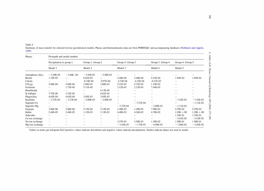
Table 5

Summary of mass transfer for selected inverse geochemical models. Phases and thermodynamic data are from PHREEQC and accompanying databases (Parkhurst and Appelo,

1999)

Phases Flowpath and model number

Precipitation to group-1 Group-1–Group-2 Group-2–Group-3 Group-3–Group-4 Group-4–Group-5

Model 1 Model 2 Model 3 Model 4 Model 5

Amorphous silica 22.49E-04 22.66E–04 23.54E-03 23.98E-03 – – – – –

Biotite 1.15E-05 – 6.81E-05 – 2.40E-04 2.40E-04 9.23E-04 1.85E-02 1.85E-02

Calcite – – -8.74E-04 -9.97E-04 -4.32E-04 -4.32E-04 -6.51E-03 – –

CO2(g) 5.68E-04 5.68E-04 3.68E-03 3.80E-03 5.21E-03 5.21E-03 1.19E-02 – –

Forsterite – 1.73E-05 5.11E-05 – 2.12E-03 2.12E-03 7.44E-03 – –

Hornblende – – – 6.13E-05 – – – – –

K-feldspar 3.75E-06 1.53E-05 – 6.81E-05 – – – – –

Plagioclase 4.63E-04 4.63E-04 2.85E-03 2.85E-03 – – – – –

Kaolinite 23.27E-04 23.27E-04 22.00E-03 22.00E-03 – – – 27.42E-03 27.42E-03

Saponite-Ca – – – – – 27.27E-04 – – 21.11E-02

Saponite-Mg – – – – 27.27E-04 – 22.80E-03 21.11E-02 –

Gypsum 3.86E-06 3.86E-06 5.15E-04 5.15E-04 1.40E-03 1.49E-03 7.90E-03 5.55E-02 5.55E-02

Halite 2.44E-05 2.44E-05 1.13E-03 1.13E-03 4.48E-03 4.24E-03 4.78E-02 1.28E þ 00 1.28E þ 00

Nahcolite – – – – – – – 1.35E-01 1.35E-01

Ca-ion exchange – – – – – – – 25.61E-02 25.43E-02

Na-ion exchange – – – – 3.27E-03 3.50E-03 1.38E-02 1.50E-01 1.50E-01

Mg-ion exchange – – – – 21.63E-03 21.75E-03 26.89E-03 21.86E-02 22.05E-02

Values in moles per kilogram H2O (positive values indicate dissolution and negative values indicate precipitation). Dashes indicate phase not used in model.

C.

Guler,

G.D

.T

hyn

e/

Jou

rna

lo

fH

ydro

log

y2

85

(20

04

)1

77

–1

98

18

8

the playa-areas. Fig. 6 shows that dissolved SiO2,

Ca and Mg equilibrium with aquifer minerals

(Table 5) are likely an important control on the

hydrochemical evolution.

5.3.2. Mineral stability diagrams

Another approach to test the proposed hydroche-

mical evolution is the use of mineral stability

diagrams (Drever, 1988). Fig. 7 shows four mineral

stability diagrams for the MgO–CaO–Al2O3–H2O–

SiO2 system (Fig. 7a), the CaO–Na2O–Al2O3–H2O–

SiO2 system (Fig. 7b), the Na2O–Al2O3–H2O–SiO2

system (Fig. 7c), and the K2O–Al2O3–H2O–SiO2

system (Fig. 7d). The values from 579 samples

representing each of the five principle water groups

are plotted on the diagrams to help define the reactions

that control the water chemistry. The majority of water

samples from Groups 1 and 2 plot in the kaolinite field

Fig. 7. Mineral stability diagrams for MgO-CaO-Na2O-K2O-Al2O3-H2O-SiO2 systems at 258C and 1 atmosphere (1.013 bars) total pressure.

Symbols show sample values from different water groups. Box ¼ Group-1, circle ¼ Group-2, triangle ¼ Group-3, star ¼ Group-4 and

plus ¼ Group-5.


or along the Ca–smectite and Mg–smectite boundary

suggesting that equilibrium with kaolinite or smectite

is an important process controlling water chemistry

(see Fig. 7a). Smectitic clay is a major component in

area lakebeds (Bischoff et al., 1997). In contrast, some

of the higher TDS samples extend into the plagio-

clase, albite and K-feldspar stability fields suggesting

equilibrium between clays and primary minerals is

likely not the main processes controlling the water

chemistry (Fig 7b–d). Lastly, the maximum dissolved

silica concentrations do not exceed 1022.75 mole/kg,

suggesting that dissolved silica is ultimately con-

trolled by equilibrium with an amorphous silica phase

rather than quartz or chalcedony. These observations

help to further constrain the hydrochemical evolution.

5.3.3. Inverse modeling

Inverse modeling is often used for interpreting

geochemical processes that account for the hydro-

chemical evolution of groundwater (Plummer et al.,

1983, 1992, 1994). This mass balance approach uses

two water analyses represent starting (initial) and

ending (final) water compositions along a flowpath to

calculate the moles of minerals and gases that must

enter or leave solution to account for the differences in

composition (Parkhurst et al., 1980). In geochemical

modeling, either forward or inverse, soundness of

results are dependent upon valid conceptualization of

the system, validity of basic concepts and principles,

accuracy of input data, and level of understanding of

the geochemical processes. We use the information

from the lithology, general hydrochemical evolution

patterns, saturation indices and mineral stability

diagrams to constrain the inverse models.

Inverse models for the observed changes between

precipitation and the five principal groups were

formulated. The average chemical parameter values

for the statistical clusters were used to represent

‘initial’ and ‘final’ waters along a groundwater

flowpath (Table 3). The inverse models were

formulated so that primary mineral phases including

K-feldspar, hornblende, forsterite, plagioclase and

biotite are constrained to dissolve until they reach

saturation, and calcite, amorphous silica, kaolinite and

smectite were set to precipitate once they reached

saturation. Halite and gypsum are included as sources

of Cl and SO4, respectively, and ion exchange, which

has been cited as an important process in groundwater

evolution in the area was included in models for

Groups 3, 4 and 5. Carbon dioxide gas was assumed to

be available throughout the flowpath. Usually a source

of CO2 would not be available in the groundwater

out of contact with the atmosphere, however, IWV is

a geothermal area. As the general geochemical

evolution showed the pH decreases slightly along

the groundwater flowpath (Groups 3 and 4) indicating

a continuous source of CO2 in addition to the

atmosphere. Finally, models for Group-5 included

playa salts such as mirabilite, nahcolite, gaylussite,

pirssonite and thenardite. Table 5 shows selected

results of the inverse modeling. The models in Table 5

were selected from all the possible models based on

the statistical measures calculated by PHREEQC

(sum of residuals and maximum fractional error)

and to represent different possible combinations of

reactants and products that can account for the change

in water chemistry. Except for model 4, there were

two equally valid, but different models for each

hydrochemical evolution step. One of the most

valuable aspects of using the mean values from

statistical clusters is that we maximize the ‘unique-

ness’ of the inverse modeling solution by producing

the minimum number of models, rather than the more

usual result of producing many non-unique models.

Thus, for model 1 the difference between the two

possible models is the dissolution of biotite or

forsterite. In reality, both minerals undergo dissol-

ution, but the modeling software produces only

models that use one of the two phases.

5.3.3.1. Evolution of precipitation (Snow) to Group-1

Waters. The extremely low TDS of the Group-1

waters suggests that the surface water does not remain

in contact with the surface bedrock long enough for

significant dissolution to occur. Dilute waters of

Group-1 are undersaturated with respect to calcite

(Table 4), indicating waters at the earliest stages of

evolution. This also suggests relatively short flow-

paths for this group of waters. In the high Sierra

Nevada, where Group-1 waters dominate, vegetation

is usually sparse with scattered coniferous trees and

shrubs, thus, the effect of vegetation on weathering

and consequently on water chemistry is assumed to be

minimal in the area.

Average snow chemistry of the eastern Sierra

Nevada (Table 6, no. 6) was used as the starting


solution for inverse geochemical modeling calcu-

lations. Snow chemistry of the eastern Sierra Nevada

is slightly acidic (pH 5.9) and is dominated by calcium

and bicarbonate (Table 6). Calcium, potassium, and

sulfate are noticeably enriched relative to precipitation

from the western Sierra Nevada suggesting the

importance of locally derived windblown dust (from

playas) on the precipitation chemistry of the area.

Dilute snowmelt runoff (dominated by Ca and

HCO3 ions) is an active agent in chemical weathering

reactions that are occurring in the alpine watersheds of

the Sierra Nevada. Even though the area is underlain by

granitic bedrock with poorly developed soils, inter-

actions between snowmelt runoff and soils and/or

rocks is important to the hydrochemistry of the alpine

watersheds (Williams and Melack, 1991b). Compari-

sons of 10 pairs of snow samples with snowmelt waters

flowing a short distance below the respective snow-

banks led Feth et al. (1964b) to conclude that when

snowmelt water comes in contact with the soil and

rock, the initial diverse character of the precipitation

largely disappears and the water rapidly increases in

TDS content.

Eolian gypsum and halite are the probable source

of SO4 and Cl for some of the Group 1, 2 and 3

waters. Oxidation of pyrite is also a potential source

of sulfur in the water samples. However, without

more detailed study the relative contribution of pyrite

oxidation cannot be quantified. This is also the case

for leaching of intergranular salts or fluid inclusions

of granitic rock minerals that potentially contribute

Cl into the groundwater system. Fuge (1979) showed

that unaltered granitic rocks from England and

Scotland contain salts in which one- to two-thirds

of the total Cl is soluble. Lacking better quantifi-

cation of the mineral contribution of sulfur and

chloride to the water chemistry, we will assume that

all sulfur and chloride are from eolian sources, as do

most prior workers (Garrels and MacKenzie, 1967;

Thomas et al., 1989).

The evolution of precipitation (Table 6, no. 6) to

Group-1 waters (Table 3) in the high Sierra Nevada

can be explained by the weathering of a relatively

small number of primary minerals found in the

crystalline bedrock. An inverse model describing the

evolution of precipitation (snow) to Group-1 water

Table 6

Precipitation chemistry of the Sierra Nevada region

1a 2a 3b 4b 5b 6b 7a 8b 9a

pH 5.34 5.10 – 5.86 5.82 5.92 4.88 4.87 5.19

Cond. 3.30 7.70 – 6.37 7.64 8.98 18.30 18.53 4.90

Ca 0.026 0.134 0.40 0.15 0.22 0.84 0.481 0.415 0.080

Mg 0.007 0.015 0.17 0.20 0.03 0.19 0.058 0.056 0.023

Na 0.030 0.085 0.46 0.49 0.46 0.43 0.354 0.463 0.092

K 0.027 0.059 0.32 0.32 0.25 0.41 0.149 0.129 0.027

Cl 0.099 0.184 0.50 0.54 0.48 0.47 0.323 0.250 0.223

SO4 0.096 0.442 0.95 1.06 0.63 1.14 1.849 1.862 0.399

HCO3 – – 2.88 3.31 2.00 3.59 – – –

NO3 0.143 0.893 0.07 0.008 0.133 0.15 2.653 2.665 0.360

NH4 0.031 0.375 – 0.20 0.00 0.00 0.997 0.925 0.132

SiO2 – – 0.16 0.18 0.14 0.17 – – –

(1). Winter snowfall (Sierra Nevada westside), 1985–88, N ¼ 834; Williams and Melack (1991a), Table 4. (2). Autumn snowfall (Sierra

Nevada westside), 1985–87, N ¼ 12; Williams and Melack (1991a), Table 10. (3). Snow (Sierra Nevada), Nmin ¼ 42; Nmax ¼ 79; Feth et al.

(1964a), Table 3. (4). Snow (Sierra Nevada westside), 1957–59, Nmin ¼ 20;, Nmax ¼ 29;, Feth et al. (1964b), Table 1 and 2. (5). Snow (Sierra

Nevada crest), 1957–59, Nmin ¼ 9; Nmax ¼ 31;, Feth et al. (1964b), Table 1 and 2. (6). Snow (Sierra Nevada eastside), 1957–59,

Nmin ¼ 10; ¼ 10, Nmax ¼ 18; ¼ 18, Feth et al. (1964b), Table 1 and 2. (7). Rain (Sierra Nevada westside), 1985–87, N ¼ 23; Williams and

Melack (1991a), Table 10 (8). Spring Rain (Sierra Nevada westside), April–June 1987, N ¼ 7; Williams and Melack (1991b), Table 1. (9). Wet

deposition (Sierra Nevada westside), 1981–84, N ¼ unknown, Stohlgren and Parsons (1987), Table 1.a Volume-weighted mean concentrations (mg l21), pH (standard units), and Conductance (mSiemens cm21).b Mean concentrations (mg l21), pH (standard units), and Conductance (mSiemens cm21).


can be written as:

PrecipitationþPlagioclaseþK-feldspar

þBiotiteorForsteriteþHaliteþGypsum

þCO2 gas!Ca–Na–HCO3water

þAmorphousSilicaþKaolinite ðModel1Þ

Model 1 shows that the amounts of biotite and

K-feldspar weathering are less than that of plagioclase

(Table 5). This difference in weathering rates is in

agreement with weathering rates of the respective

silicate minerals given by Lasaga et al. (1994) and fits

into a sequence of surface weathering proposed by

Goldich (1938), Feth et al. (1964a), Garrels and

MacKenzie (1967) have suggested that the weathering

of feldspars and biotite and the formation of kaolinite

largely account for the water composition in recharge

areas. In the Sierra Nevada, weathering is enhanced

by partial alteration and expansion of biotite, which

results in disintegration of the crystalline rock

(Wahrhaftig, 1965).

5.3.3.2. Evolution of Group-1 Waters to Group-2

Waters. Group-2 waters, which recharge the basin-fill

aquifer, are found in lower slopes of the Sierra Nevada

(generally below 2000 m) and dominate most of the

Coso Range. Calcite and kaolinite become super-

saturated in Group-2 water (Table 4). Given the climate

and vegetation, water-rock interaction is assumed to be

the principle mechanism for the evolution of water

chemistry evolution of Ca–Na–HCO3 (Group-1)

water to Na–Ca–HCO3 (Group-2) water.

An inverse modeling solution summarizing the

evolution of Group-1 water to Group-2 water in the

Sierra Nevada is:

Ca–Na–HCO3 water þ Plagioclase

þ K-feldspar or Biotite þ Hornblende

� or Forsterite þ Halite þ Gypsum

þ CO2 gas ! Na–Ca–HCO3 water

þ Amorphous Silica þ Calcite

þ Kaolinite ðModel 2Þ

Based on the models (Table 5), dissolved constituents

in the Group-2 waters come primarily from weath-

ering reactions of plagioclase, biotite, and hornblende

that form the granodioritic rocks and from dissolution

of windblown halite and gypsum. Elevated mag-

nesium concentrations in Group-2 waters are likely

related to the weathering of magnesium-rich minerals

(e.g. hornblende and biotite) that are commonly found

in granodioritic rocks of the area (Miller and Webb,

1940; Hopper, 1947; Feth et al., 1964a; Wahrhaftig,

1965; Blum et al., 1994). However, increase in

magnesium concentration in Group-2 waters (in the

Coso Range area) is most likely due to abundance of

olivine (forsterite) present (Duffield et al., 1980) in the

basalt flow indigenous to the southern edge of the

Coso Range.


Waters. As Group-2 waters recharge the basin-fill

aquifers and move toward central parts of the basins,

concentrations of major-ions increase, producing

Group-3 type water. Group-3 water is transitional in

character, chemically as well as geographically,

between Group-2 and Group-4 waters (Figs. 4 and 5).

The increase in major-ion concentrations of Group-3

waters is a result of groundwater interactions with the

basin-fill deposits. An inverse model for the processes

is:

Na–Ca–HCO3 water þ Biotite

þ Forsterite þ Halite þ Gypsum þ Na

� from ion exchange þ CO2 gas

! Na–HCO3 –Cl water þ Ca or

�Mg–Saponite þ Calcite þ Mg loss to

� ion exchange: ðModel 3Þ

The increase in playa deposits in areas where Group-

3 waters dominate suggest that salt dissolution may be

involved in the increases in Cl, Na, and SO4 concen-

tration. Weathering of the primary minerals results in

the formation of smectite and calcite. Formation of

smectite rather than kaolinite can be explained by the

abundant supply of Mg from dissolution of volcanic

materials such as forsterite, pyroxenes and basaltic


glass (Verhoogen et al., 1970). Since IWV is a

geothermal area, CO2 is assumed to be available along

the flowpath.


Waters. Groundwater in the alluvial basin-fill aquifer

evolves from Na–HCO3–Cl water to brackish Na–Cl

water in the areas peripheral to playas (Figs. 4 and 5,

Tables 3 and 5). These samples have a different

geochemistry than Group-1 to -3 waters exemplified

by increased TDS. The spatial correlation of the

basin-fill and playa deposits with Group-4 samples

suggests that lithology is important in the hydro-

chemical evolution. The increase in TDS is due to the

relatively large increases in Na, Cl, and SO4

concentrations suggesting that salt dissolution is the

major control. An inverse model explaining the water

chemistry along the flowpath can be written as:

Na–HCO3 –Cl water þ Biotite

þ Forsterite þ Halite þ Gypsum þ CO2

� gas þ Na from ion exchange !

Na–Cl water þ Mg–Saponite þ Calcite

þ Mg loss to ion exchange ðModel 4ÞMost of the salt dissolution occurs as groundwater

flows through the basin-fill deposits near playas.

These sediments contain evaporative salts buried by

sedimentation, which are mostly found in and around

the playa lakes. Ion exchange is also common in basin

sediments, with Ca and Mg ion concentrations

increasing only slightly, whereas Na and K increase

substantially along flowpaths (Table 3). Reader is

referred to Guler (2002) for a more complete

discussion of the modeling results.

The Coso Range is a geothermally active area

(Duffield et al., 1980; Moore et al., 1982). This means

that Group-3 water may be affected by mixing with

water from geothermal leakage in the southern part of

IWV (Whelan et al., 1989). This mixing scenario was

explored by modeling mixtures between two geother-

mal waters from the Coso area and Group-3 water to

create two synthetic Group-4 waters, called Mix 1 and

Mix 2 (Fig. 8). Similarities between concentrations of

some of the major and minor elements composing Mix

1 and Mix 2 and Group-4 water suggest that mixing may

be part of the hydrochemical evolution. However, the

present data are insufficient and more geothermal water

analyses with more reliable minor element data are

needed before a conclusive result can be determined.


Waters. High TDS waters from across the area

(represented by Group-4 and Group-5 water) are in

parts of the aquifer that are in close proximity to the

playa-areas. On the playa, high evaporation rates

produce concentrated brine solutions, which lead to

large horizontal and vertical density gradients in

underlying groundwater. Tyler and Wooding (1991)

Fig. 8. Fingerprint diagram with aqueous parameters on x-axis versus concentration in mg/L on y-axis. Diagram shows result of mixing between

two geothermal waters (Geo1 and Geo2) from the Coso geothermal wells with Group-3 water to try and create Group-4 water. Coso samples,

Geo1 from CGEH Well No. 1, Geo2 from Coso Well No. 1, samples 9 and 13, respectively (Fournier et al., 1980).


suggested a mixing mechanism in playa areas via

convective plumes or fingers, which develop into

large-scale convection cells. Their field data

suggested that convective fingering could be the

dominant transport process for solutes in the ground-

water beneath playas. A similar mixing mechanism

was also suggested by Duffy and Al-Hassan (1988) for

Pilot Valley in western Utah.

Attempts to match the Group-5 chemistry by

evaporation of Group-4 water (PHREEQC simu-

lation) failed, indicating that simple evaporation is

not the only process occurring on the playas. In

addition to evapotranspiration concentrating salts

dissolved in the water the dissolution of salts found

in the low permeability basin-fill deposits around

playas is also an important process. The relatively

high Na:Cl molar ratios of Group-4 and Group-5

waters (Na:Cl ¼ 1.28 for both groups) suggest that the

sodium and chloride contents of these samples is

mostly derived from halite dissolution, which would

result in a Na:Cl molar ratio close to one (Eugster and

Jones, 1979; Yechieli et al., 1996). Group-4 samples

are mostly from shallow wells (WS); (see Table 2)

and these groundwaters move toward the playa as

shallow subsurface flow (average depth of shallow

wells is 28.4 m). In addition to evapotranspiration

concentrating solutes at or very near the land surface,

groundwater moving toward the surface also flows

through salt deposits, which will dissolve increasing

ion concentrations.

5.3.3.6. An inverse model explaining the water-

chemistry can be written as:.

Na–ClwaterþBiotiteþHaliteþGypsum

þNahcoliteþNafromionexchange

!Na–ClwaterþKaoliniteþCaor

�Mg–SaponiteþCaandMgloss toion

�exchange: ðModel5Þ

The model includes dissolution of biotite, nahcolite

and halite, precipitation of kaolinite and Ca or Mg–

saponite and ion exchange (Ca and Mg replacing Na

in clays) (Table 5). In summary, the inverse

geochemical modeling demonstrated that relatively

few phases are required to derive observed changes in

water chemistry and to account for the hydrochemical

evolution of groundwater in the area (Table 5). In a

broad sense, the reactions responsible for the hydro-

chemical evolution of the groundwater fall into four

categories: (1) silicate weathering reactions (e.g.

feldspar and ferromagnesian mineral dissolution);

(2) dissolution of salts (e.g. halite and nahcolite);

(3) precipitation of calcite, amorphous silica and

clays; and (4) ion exchange. The mineral phases were

selected based on geologic descriptions and analysis

of rocks (Table 1), descriptions of sediments from the

area, stability diagrams (Fig. 7) and saturation data

(Table 4). From the inverse modeling, knowing the

exact weathering reactions is less important than

knowing the overall stoichiometry (Wolford et al.,

1996), which has been previously estimated for a part

of the study area by Feth et al. (1964a; Garrels and

MacKenzie (1967). These studies produced stoichi-

ometries similar to those derived by this study (Table

5), but this study is the first to define inverse models

for the complete flowpath, starting from recharge

as precipitation in high Sierras to discharge on

the playas.

5.4. Correlation of lithology and hydrochemical

evolutions

Groundwater in the region generally begins as a

Ca–Na–HCO3 type in the recharge areas of Sierra

Nevada, and chemically evolves along the flow-

paths as a function of the lithologies encountered.

Based on the saturation data, stability diagrams and

inverse models, the composition of groundwater

along a flowpath is primarily dependent upon (1)

chemistry of the starting water; and the (2) types

and relative solubility of the minerals available. We

have not attempted to quantify the kinetic effects

since mineral reaction rates and residence time of

the water (short in mountain watersheds and long

in alluvial basin-fill and playa deposits) is not well

constrained.

Based on our work, the general lithology,

including types and solubility of the minerals,

constitutes the greatest controlling factor on the

natural quality of the groundwater. To demonstrate

this point, lithology frequencies for each water

group were plotted by using the information


extracted from the GIS (Geographic Information

Systems) database developed for this study. As

shown in Fig. 9, TDSs content of the water groups

rapidly increase as the percentages of basin-fill and

playa deposits increase. This increase in concen-

tration is probably due to the more soluble material

in the basin-fill and playa deposits, coupled with

the lower permeability of these sediments that

increases the residence time of the groundwater.

6. Summary and concluding remarks

The results of this study show that analysis of

hydrochemical data using statistical techniques such as

cluster analysis coupled with inverse geochemical

modeling of the statistical clusters can help elucidate

the hydrologic and geologic factors controlling water

chemistry on a regional scale. It should be noted that

the cluster interpretations in this study are general and

made on a regional basis. Because of this, there may be

better interpretations within the context of a more

localized system.

The spatial variations observed in the statistical

groups correspond well to the topographic flowpaths.

The physical locations and chemical evolution of

groundwater represented by clusters Group-1,

Group-2, Group-3, Group-4, and Group-5, follow

the topographic flowpath: the recharge from the Sierra

Nevada (Group-1 and Group-2) flows into the alluvial

valleys, evolving through water-rock interaction into

Group-3 water. Subsequently, Group-3 water flows to

the discharge areas in and around the playa lakes,

which usually occupy the central portions of the

valleys, and evolve into discharge area waters

(Group-4 and Group-5).

Systematic changes in water chemistry along the

topographic flowpath were interpreted using saturation

indices and mineral stability diagrams in order to

formulate initial inverse models. Inverse modeling

identified three distinct hydrochemical phases that can

be attributed to water-rock interactions: (1) reactions

of snowmelt water with minerals and CO2 gas in

recharge areas; (2) reactions of groundwater with

aquifer material as it moves from recharge areas to

discharge (playa) areas; and (3) reactions of dischar-

ging groundwater with playa minerals (see Table 5 for

a complete list of minerals). It should be emphasized

that the inverse modeling results are not unique, as for

any hydrochemical evolution step more than one

model is usually found. Effects of vegetation and

microbial activity on the water chemistries have not

been evaluated in this study, however, in areas like the

Sierra Nevada, which has poorly developed soils

and sparse vegetation, these effects are likely to be

minimal.

We conclude that in the study area, chemical

composition of the surface and ground water are

Fig. 9. Plots of water group versus lithology frequency (water groups determined from HCA results).


mainly controlled by: (1) climate and chemical

composition of the precipitation; (2) aquifer litholo-

gy/mineralogy; (3) topography/physiography; and (4)

physical aspects of the hydrogeologic system. These

factors combine to create diverse water types that

change in compositional character spatially and

temporally as precipitation infiltrates the soil zone,

moves down a topographically-defined flowpath and

interacts with the minerals derived primarily from the

underlying bedrock. Evaporative concentration and

groundwater mixing appear to have lesser influence

on the chemistry of the groundwater from the playa

areas than salt dissolution. Finally, we assume that

since reasonable inverse geochemical models were

found for the topographic flowpaths, the statistically-

defined hydrochemical facies can be used effectively

to study the groundwater flow system and can be used

as a tool to verify aquifer connectivity.

Acknowledgements

The authors are thankful to the Editor and the

reviewers for their valuable suggestions. This paper is

based on part of the first author’s dissertation research

at the Colorado School of Mines, and he thanks

members of his dissertation committee.

References

Alberto, W.D., Del Pilar, D.M., Valeria, A.M., Fabiana, P.S.,

Cecilia, H.A., De Los Angeles, B.M., 2001. Pattern recognition

techniques for the evaluation of spatial and temporal variations

in water quality. A case study: Suquıa River Basin (Cordoba-

Argentina). Water Res. 35, 2881–2894.

Alther, G.A., 1979. A simplified statistical sequence applied to

routine water quality analysis: a case history. Ground Water 17,

556–561.

Back, W., 1966. Hydrochemical facies and ground-water flow

patterns in northern part of Atlantic coastal plain. US Geol.

Surv. Prof. Paper, 498-A.

Berenbrock, C., Martin, P., 1991. The ground-water flow system in

Indian Wells Valley, Kern, Inyo, and San Bernardino Counties,

California. US Geol. Surv. Water-Res. Invest. Rep., 89–4191.

Berenbrock, C., Schroeder, R.A., 1994. Ground-water flow

and quality, and geochemical processes, in Indian Wells

Valley, Kern, Inyo and San Bernardino Counties, California,

1987 – 88. US Geol. Surv. Water-Res. Invest. Rep.,

93–4003.

Bethke, C.M., 1994. The Geochemist’s Workbench, ver. 2.0: a

User’s Guide to Rxn, Act2, Tact, React, and Gtplot, University

of Illinois, Urbana.

Bischoff, J.L., Menking, K.M., Fitts, J.P., Fitzpatrick, J.A., 1997.

Climatic Oscillations 10,000–155,000 yr B.P. at Owens

Lake, California reflected in glacial rock flour abundance and

lake salinity in core OL-92. Quaternary Res. 48, 313–325.

Blum, J.D., Erel, Y., Brown, K., 1994. 87Sr/86Sr ratios of Sierra

Nevada stream waters: Implications for relative mineral weath-

ering rates. Geochim. Cosmochim. Acta 58, 5019–5025.

Christensen, M.N., 1966. Late Cenozoic crustal movements in the

Sierra Nevada of California. Geol. Soc. Am. Bull. 77, 163–182.

Corbett, L., 1990. The weather at NWC-Climatological data for

1945–1989: Temperature, relative humidity, precipitation and

evaporation, surface wind, station pressure, and solar radiation,

China Lake, California. Naval Weapons Center Tech. Mem.,

6738.

Drever, J.I., 1988. The Geochemistry of Natural Waters, Prentice-

Hall, Upper Saddle River, NJ.

Droste, J.B., 1961. Clay minerals in sediments of Owens, China,

Searles, Panamint, Bristol, Cadiz, and Danby Lake basins,

California. Geol. Soc. Am. Bull. 72, 1713–1722.

Duffield, W.A., Smith, G.I., 1978. Pleistocene history of volcanism

and the Owens River near Little Lake, California. J. Res. 6,

395–408.

Duffield, W.A., Bacon, C.R., Dalrymple, G.B., 1980. Late Cenozoic

volcanism, geochronology, and structure of the Coso Range,

Inyo County, California. J. Geophy. Res. 85, 2381–2404.

Duffy, C.J., Al-Hassan, S., 1988. Groundwater circulation in a

closed desert basin: topographic scaling and climatic forcing.

Water Resour. Res. 24, 1675–1688.

Dutcher, L.C., Moyle, W.R. Jr., 1973. Geologic and hydrologic

features of Indian Wells Valley, California. US Geol. Surv.

Water-Supply Paper, 2007.

ESRI (Environmental Systems Research Institute), 1996. Arc/View

GIS Manual,.

Eugster, H.P., Jones, B.F., 1979. Behavior of major solutes during

closed-basin brine evolution. Am. J. Sci. 279, 609–631.

Farnham, I.M., Stetzenbach, K.J., Singh, A.K., Johannesson, K.H.,

2000. Deciphering groundwater flow systems in Oasis Valley,

Nevada, Using trace element chemistry, multivariate statistics,

and Geographical Information System. Math. Geol. 32, 943–968.

Fenneman, N.M., 1931. Physiography of Western United States,

McGraw-Hill Book Company, New York.

Feth, J.H., Roberson, C.E., Polzer, W.L., 1964a. Sources of mineral

constituents in water from granitic rocks, Sierra Nevada,

California and Nevada. US Geol. Surv. Water-Supply Paper,

1535-I.

Feth, J.H., Rogers, S.M., Roberson, C.E., 1964b. Chemical

composition of snow in the northern Sierra Nevada and other

areas. US Geol. Surv. Water-Supply Paper, 1535-J.

Fournier, R.O., Thompson, J.M., Austin, C.F., 1980. Interpretation

of chemical analyses of waters collected from two geothermal

wells at Coso, California. J. Geophys. Res. 85, 2405–2410.

Frape, S.K., Fritz, P., McNutt, R.H., 1984. Water–rock interaction

and chemistry of groundwaters from the Canadian Shield.

Geochim. Cosmochim. Acta 48, 1617–1627.


Fuge, R., 1979. Water-soluble chlorine in granitic rocks. Chem.

Geol. 25, 169–174.

Garrels, R.M., MacKenzie, F.T., 1967. Origin of the chemical

compositions of some springs and lakes, In: Equilibrium

Concepts in Natural Waters, American Cancer Society,

Washington, DC.

Goldich, S.S., 1938. A study in rock-weathering. J. Geol. 46,

17–58.

Guler, C., 2002. Hydrogeochemical evaluation of the groundwater

resources of Indian Wells-Owens Valley area, southeastern

California [PhD. thesis]: Golden, Colorado School of Mines.

Guler, C., Thyne, G., McCray, J.E., Turner, A.K., 2002. Evaluation

of graphical and multivariate statistical methods for

classification of water chemistry data. Hydrogeol. J. 10,

455–474.

Hem, J.D., 1989. Study and interpretation of the chemical

characteristics of natural water. US Geol. Surv. Water-Supply

Paper, 2254.

Hollett, K.J., Danskin, W.R., McCaffrey, W.F., Walti, C.L., 1991.

Geology and water resources of Owens Valley, California. US

Geol. Surv. Water-Supply Paper, 2370-B.

Hopper, R.H., 1947. Geologic section from the Sierra Nevada to

Death Valley, California. Geol. Soc. Am. Bull. 58, 393–432.

Howard, P.A., McAlee, J., Gillespie, J.M., 1997a. The role of

fractures in surface and ground water flow: a field study of two

canyons in the southeastern Sierra Nevada. Geol. Soc. Am. 29,

20(Abstracts with Programs).

Howard, P.A., Oehlschlager, E.K., Gillick, J., McAlee, J.,

Sherman, A.T., Ostdick, J.R., Steward, D.C., Gillespie,

J.M., Thyne, G.D., 1997b. The Kern Plateau: a potential

extra-basinal source of groundwater recharge to the Indian

Wells Valley. Am. Assoc. Petrol. Geol. Bull. 81, 688(Pacific

Section Meeting, Abstracts).

von Huene, R.E., 1960. Structural geology and gravimetry of Indian

Wells Valley, southeastern California. PhD dissertation, Uni-

versity of California, Los Angeles.

Johnson, R.A., Wichern, D.W., 1992. Applied Multivariate

Statistical Analysis, Prentice-Hall International, Englewood

Cliffs, NJ.

Kistler,R.W.,Bateman,P.C.,Brannock,W.W.,1965. Isotopicagesof

minerals fromgranitic rocksof theCentralSierraNevadaandInyo

Mountains, California. Geol. Soc. Am. Bull. 76, 155–164.

Kunkel, F., Chase, G.H., 1969. Geology and ground water in Indian

Wells Valley, California. US Geol. Surv. Open-File Rept.

without a number.

Lanphere, M.A., Dalrymple, G.B., Smith, R.L., 1975. K–Ar ages of

Pleistocene rhyolitic volcanism in the Coso Range, California.

Geology 3, 339–341.

Lasaga, A.C., Soler, J.M., Ganor, J., Burch, T.E., Nagy, K.L., 1994.

Chemical weathering rate laws and global geochemical cycles.

Geochim. Cosmochim. Acta 58, 2361–2386.

Lee, C.H., 1912. Ground water resources of Indian Wells Valley,

California, California State Conservation Commission Rept.,

403–429.

Lee, D.E., 1984. Analytical data for a suite of granitoid rocks from

the Basin and Range province. US Geol. Surv. Bull., 1602.

Maxey, G.B., 1968. Hydrogeology of desert basins. Ground Water

6, 10–22.

McKee, E.H., Nash, D.B., 1967. Potassium–argon ages of granitic

rocks in the Inyo batholith, east-central California. Geol. Soc.

Am. Bull. 78, 669–680.

Meng, S.X., Maynard, J.B., 2001. Use of statistical analysis to

formulate conceptual models of geochemical behavior: water

chemical data from the Botucatu aquifer in Sao Paulo state,

Brazil. J. Hydrol. 250, 78–97.

Miller, W.J., Webb, R.W., 1940. Descriptive geology of the Kernville

quadrangle, California. Calif. J. Mines and Geol. 36, 343–378.

Moore, J.L., Austin, C.F., Prostka, H.J., 1982. Geology and

geothermal energy development at the Coso KGRA, In:

Transactions of third Circum-Pacific Energy and Mineral

Conference, Honolulu: Circum-Pacific Council for Energy and

Mineral Resources,.

Oliver, H.W., 1977. Gravity and magnetic investigations of the

Sierra Nevada batholith, California. Geol. Soc. Am. Bull. 88,

445–461.

Parkhurst, D.L., Appelo, C.A.J., 1999. User’s guide to PHREEQC

(ver. 2)—A computer program for speciation, batch-reaction,

one-dimensional transport, and inverse geochemical calcu-

lations. US Geol. Surv. Water-Resources Invest. Rept., 99–4259.

Parkhurst, D.L., Thorstenson, D.C., Plummer, L.N., 1980.

PHREEQE-A computer program for geochemical calculations.

US Geol. Surv. Water-Resources Invest. Rept., 80–96.

Piper, A.M., 1944. A graphic procedure in the geochemical

interpretation of water-analyses. Trans., Am. Geophys. Union

25, 914–923.

Plummer, L.N., 1992. Geochemical modeling of water-rock

interaction: past, present, future. In: Kharaka, Y.K., (Ed.),

Proceedings of the Seventh International Symposium on Water-

Rock Interaction, Amsterdam, pp. 23–33.

Plummer, L.N., Parkhurst, D.L., Thorstenson, D.C., 1983. Devel-

opment of reaction models for ground-water systems. Geochim.

Cosmochim. Acta 47, 665–686.

Plummer, L.N., Prestemon, E.C., Parkhurst, D.L., 1994. An

interactive code (NETPATH) for modeling net geochemical

reactions along a flow path. US Geol. Surv. Water-Resources

Invest. Rept., 94–4169.

Saint-Amand, P., 1986. Water supply of Indian Wells Valley,

California. Naval Weapons Center Tech. Pub., 6404.

SAS Institute, Inc, 1988. SAS/STAT user’s guide, release 6.03 edn,

SAS Institute Inc, Cary, NC, 1028.

Smith, G.I., 1962. Large lateral displacement on Garlock Fault,

California, as measured from offset dike swarm. Bull. Am.

Assoc. Petroleum Geologists 46, 85–104.

Smith, G.I., Friedman, I., McLaughlin, R.J., 1971. Studies of

Quaternary saline lakes-III. Mineral, chemical, and isotopic

evidence of salt solution and crystallization processes in Owens

Lake, California, 1969–1971. Geochim. Cosmochim. Acta 51,

811–827.

StatSoft, Inc., 1995. STATISTICA for Windows [Computer

program manual]. Tulsa, OK.

Stohlgren, T.J., Parsons, D.J., 1987. Variation of wet deposition

chemistry in Sequoia National Park, California. Atmos.

Environ. 21, 1369–1374.


Thomas, J.M., Welch, A.H., Preissler, A.M., 1989. Geochemical

evolution of ground water in Smith Creek Valley—a hydro-

logically closed basin in central Nevada. USA Applied

Geochem. 4, 493–510.

Tyler, S.W., Wooding, R.A., 1991. Experimental verification of

convection of ground water beneath salt lakes. EOS Trans. 72,

216(Abstracts with Programs).

Verhoogen, J., Turner, F.J., Weiss, L.E., Wahrhaftig, C., Fyfe, W.S.,

1970. The Earth, An Introduction to Physical Geology. Holt,

Rinehart and Winsto, Inc.

Wahrhaftig, C., 1965. Stepped topography of the southern Sierra

Nevada, California. Geol. Soc. Am. Bull. 76, 1165–1190.

Whelan, J.A., Baskin, R., Katzenstein, A.M., 1989. A water

geochemistry study of Indian Wells Valley, Inyo and Kern

Counties, California. Naval Weapons Center Tech. Pub., 7019.

White, A.F., Claassen, H.C., Benson, L.V., 1980. The effect of

dissolution of volcanic glass on the water chemistry in

a tuffaceous aquifer, Rainer Mesa, Nevada. US Geol. Surv.

Water-Supply Paper 1535-Q.

Williams, R.E., 1982. Statistical identification of hydraulic

connections between the surface of a mountain and internal

mineralized sources. Ground Water 20, 466–478.

Williams, M.W., Melack, J.M., 1991a. Precipitation chemistry in

and ionic loading to an Alpine basin, Sierra Nevada. Water

Resour. Res. 27, 1563–1574.

Williams, M.W., Melack, J.M., 1991b. Solute chemistry of

snowmelt and runoff in an Alpine basin, Sierra Nevada. Water

Resour. Res. 27, 1575–1588.

Wolford, R.A., Bales, R.C., Sorooshian, S., 1996. Development

of a hydrochemical model for seasonally snow-covered

alpine watersheds: Application to Emerald Lake watershed,

Sierra Nevada, California. Water Resour. Res. 32,

1061–1074.

Yechieli, Y., Ronen, D., Kaufman, A., 1996. The source and age of

groundwater brines in the Dead Sea area, as deduced from 36Cl

and 14C. Geochim. Cosmochim. Acta 60, 1909–1916.

Zbur, R.T., 1963. A geophysical investigation of Indian Wells Valley,

California. Naval Ordnance Test Station Tech. Pub., 2795.


Hydrologic and geologic factors controlling surface and groundwater chemistry in Indian Wells-Owens...

Documents

Transcript of Hydrologic and geologic factors controlling surface and groundwater chemistry in Indian Wells-Owens...