a g r i c u l t u r a l w a t e r m a n a g e m e n t 9 2 ( 2 0 0 7 ) 6 4 – 7 2

Hydrogeological assessment of serial biologicalconcentration of salts to manage saline drainage

S. Khan a,b,c,*, A. Abbas c, J. Blackwell a, H.F. Gabriel a,d, A. Ahmad a

aCharles Sturt University (CSU), Wagga Wagga, NSW 2678, AustraliabUNESCO IHP-HELP, Australiac Irrigation Systems, CSIRO Land and Water, Wagga Wagga, NSW 2678, AustraliadNIT, National University of Sciences & Technology (NUST), NUST Risalpur Campus, Risalpur Cantt. 24080, Pakistan

a r t i c l e i n f o

Article history:

Accepted 14 May 2007

Published on line 28 June 2007

Keywords:

Serial biological concentration

Irrigation

Saline drainage

Regional groundwater

Groundwater model

Waterlogging

a b s t r a c t

Serial biological concentration (SBC) of salts is an innovative technology to manage salts in

agricultural drainage. This approach utilises saline drainage water as a resource to produce

marketable crops and, therefore, provides a method to manage salts in a viable manner.

However, there are associated risks of development of a groundwater mound beneath the

treatment facility and the consequent threats of groundwater contamination. The water

table in the shallow aquifers often rises to the ground surface following irrigations and

rainfall events. In the SBC system, the intensive drainage system manages these events and

enables the water table to be lowered rapidly. This paper describes the hydrogeological

assessment of an SBC system to quantify the water table mound and the effect on the local

groundwater. The deep leakage rates and lateral flows to adjoining lands are determined in

order to assess the on-site and regional impacts under typical SBC operation. Modelling

results show that the net water table rise under a 50 ha site, in the first year of the system

operation, is about 1.3 m. However, there is no further water table rise during 25 years of

simulated operation, mainly because of the high drainage efficiency of the tile drainage

operation in the SBC system. The water table under the SBC site reaches quasi equilibrium

with periodic rise and fall around the tile drain depth. The deep leakage beneath the SBC

bays is approximately 1 mm/day which is around 10% of the saturated groundwater flow

above the tile drains. Simulation scenarios of various sizes of the SBC system in its present

hydrogeological settings suggest that the lateral extent of the groundwater mound does not

extend beyond 50 m from the outer edge of its bays. In order to develop SBC systems at other

locations, a GIS-based site suitability assessment model is recommended to evaluate the

SBC effect under different soil and hydrogeological conditions.

# 2007 Elsevier B.V. All rights reserved.

avai lable at www.sc iencedi rec t .com

journal homepage: www.e lsev ier .com/ locate /agwat

1. Introduction

Contaminated surface waters have been treated using a series

of vegetated wetlands where intense biological processing

* Corresponding author at: CSIRO Land and Water, Locked Bag 588, Wfax: +61 2 6933 2647.

E-mail addresses: Shahbaz.Khan@csiro.au (S. Khan), Akhtar.Abbashgabriel@csu.edu.au (H.F. Gabriel), aahmad@csu.edu.au (A. Ahmad).

0378-3774/$ – see front matter # 2007 Elsevier B.V. All rights reservedoi:10.1016/j.agwat.2007.05.011

occurs (Kivaisi, 2001). Although effective, this approach is a

non-production system. One option for managing inevitable

drainage water from irrigation or other contaminated surface

waters is to sequentially use and re-use it to grow increasingly

agga Wagga, NSW 2678, Australia. Tel.: +61 2 6933 2927;

@csiro.au (A. Abbas), jblackwell@csu.edu.au (J. Blackwell),

d.

a g r i c u l t u r a l w a t e r m a n a g e m e n t 9 2 ( 2 0 0 7 ) 6 4 – 7 2 65

salt-tolerant crops while concentrating the drainage to a

manageable level (Oron, 1993; Tanji and Karajeh, 1993). This

treatment system is known as ‘‘serial biological concentration

(SBC)’’. SBC systems have emerged as a viable option for using

saline waters for irrigated cropping. The system makes

productive use of waters considered unfit for general irrigation

and avoids the associated risks of saline water irrigation which

often proves non-sustainable environmentally (Jayawardane

et al., 1997; Jayawardane, 2000; Blackwell, 2000). Specifically,

the concept of SBC of salts aims to reduce drainage effluent

volumes from irrigated lands (Bethune et al., 2004). In 2003,

SBC was being applied on some 63,000 ha in the San Joaquin

Valley, California, where it is the basis of an Integrated On-

Farm Drainage Management System (Pratt Water Solutions,

2003). Blackwell (2000) and Jayawardane (2000) provided

design guidelines and the field performance of a land-based

sewage treatment system, Filtration, Land Treatment and

Effluent Reuse (FILTER) in Australia. The SBC system described

and analysed herein was based on the function and operation

of the FILTER system. FILTER is an effective treatment system

producing low nutrient drainage waters which meet Environ-

mental Protection Agency (EPA) criteria for discharge to

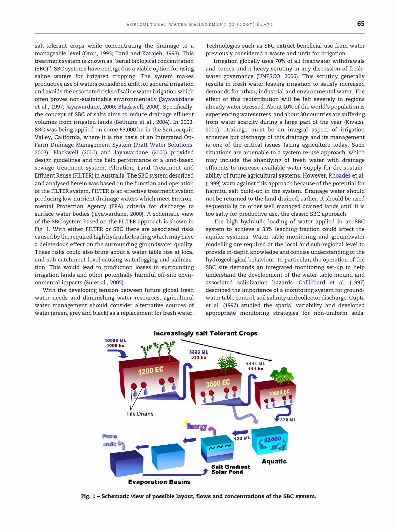
surface water bodies (Jayawardane, 2000). A schematic view

of the SBC system based on the FILTER approach is shown in

Fig. 1. With either FILTER or SBC there are associated risks

caused by the required high hydraulic loading which may have

a deleterious effect on the surrounding groundwater quality.

These risks could also bring about a water table rise at local

and sub-catchment level causing waterlogging and saliniza-

tion. This would lead to production losses in surrounding

irrigation lands and other potentially harmful off-site envir-

onmental impacts (Su et al., 2005).

With the developing tension between future global fresh

water needs and diminishing water resources, agricultural

water management should consider alternative sources of

water (green, grey and black) as a replacement for fresh water.

Fig. 1 – Schematic view of possible layout, flow

Technologies such as SBC extract beneficial use from water

previously considered a waste and unfit for irrigation.

Irrigation globally uses 70% of all freshwater withdrawals

and comes under heavy scrutiny in any discussion of fresh-

water governance (UNESCO, 2006). This scrutiny generally

results in fresh water leaving irrigation to satisfy increased

demands for urban, industrial and environmental water. The

effect of this redistribution will be felt severely in regions

already water stressed. About 40% of the world’s population is

experiencing water stress, and about 30 countries are suffering

from water scarcity during a large part of the year (Kivaisi,

2001). Drainage must be an integral aspect of irrigation

schemes but discharge of this drainage and its management

is one of the critical issues facing agriculture today. Such

situations are amenable to a system re-use approach, which

may include the shandying of fresh water with drainage

effluents to increase available water supply for the sustain-

ability of future agricultural systems. However, Rhoades et al.

(1999) warn against this approach because of the potential for

harmful salt build-up in the system. Drainage water should

not be returned to the land drained, rather, it should be used

sequentially on other well managed drained lands until it is

too salty for productive use, the classic SBC approach.

The high hydraulic loading of water applied in an SBC

system to achieve a 33% leaching fraction could affect the

aquifer systems. Water table monitoring and groundwater

modelling are required at the local and sub-regional level to

provide in-depth knowledge and concise understanding of the

hydrogeological behaviour. In particular, the operation of the

SBC site demands an integrated monitoring set-up to help

understand the development of the water table mound and

associated salinization hazards. Gallichard et al. (1997)

described the importance of a monitoring system for ground-

water table control, soil salinity and collector discharge. Gupta

et al. (1997) studied the spatial variability and developed

appropriate monitoring strategies for non-uniform soils.

s and concentrations of the SBC system.

a g r i c u l t u r a l w a t e r m a n a g e m e n t 9 2 ( 2 0 0 7 ) 6 4 – 7 266

Benyamini et al. (2005) installed monitoring systems perpen-

dicular to the parallel subsurface drains to study the

mechanisms of salinization and the dynamics of the water

table regime.

This paper describes the hydrogeological assessment of an

SBC trial in the Murrumbidgee Irrigation Area (MIA) in

southeast Australia. Owing to the hydrogeological system of

the MIA, the region has inherent drainage problems that have

been aggravated by intensive irrigation applications leading to

problems of rising water tables and salinization. By 2001, more

than 80% of the MIA had water tables within 2 m from the land

surface (Khan et al., 2001). The average volume of irrigation

water used per irrigation season (270 days) in the MIA is about

1000 GL with an average electrical conductivity (EC) of 0.1 dS/

m. Shallow groundwater salinity varies from less than 2 dS/m

to over 20 dS/m. In the MIA, the salt load diverted from the

Murrumbidgee River at Berembed Weir and delivered to

farmers’ paddocks each year is about 115,000 tonnes. The

estimated average (1999–2003) drainage volume of MIA is

212,340 ML per year (Pratt Water Solutions, 2003) with an

average winter salinity of 1.2 dS/m. These drainage volumes

are well below the long time average mainly because of

drought conditions. This study focuses on understanding the

groundwater dynamics of the SBC system with the shallow

aquifer and its interactions with the deeper groundwater. The

specific objectives are to determine groundwater movements

(both lateral and vertical) using a detailed monitoring network

and to evaluate regional impacts of the SBC system at different

scales using a groundwater model.

2. Hydrogeology of the study area

The study area is situated in the Murrumbidgee Irrigation Area

on the northern side of a fluvial plain formed by the

Murrumbidgee River. The climate of the MIA is characterised

as semi-arid with annual rainfall ranging from 256 to 609 mm

and average annual evaporation of 2100 mm. Average rainfall

gets closer to average evapotranspiration during the winter

months of June and July. The total irrigable area for the MIA is

156,605 ha and the main agricultural products are rice, grapes

and citrus. Rice is the dominant water user with more than

32,000 ha (14% of the total land use) in 2000. Rice growing

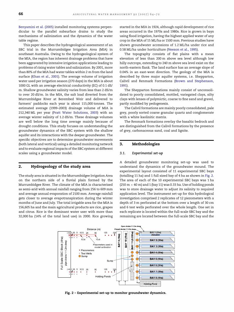
Fig. 2 – Experimental set-up to mo

started in the MIA in 1924, although rapid development of rice

areas occurred in the 1970s and 1980s. Rice is grown in bays

using flood irrigation, having the highest applied water of any

crop in the MIA of 15 ML/ha or 1500 mm. Previous studies have

shown groundwater accessions of 1.2 ML/ha under rice and

0.58 ML/ha under horticulture (Neeson et al., 1995).

The topography consists of flat plains with a mean

elevation of less than 200 m above sea level although low

hilly outcrops, extending to 240 m above sea level exist on the

north-eastern flank. The land surface has an average slope of

0.04% in an east-west direction. The geology of the MIA is

described by three major aquifer systems, i.e. Shepparton,

Calivil and Renmark Formations (Brown and Stephenson,

1991).

The Shepparton formations mainly consist of unconsoli-

dated to poorly consolidated, mottled, variegated clays, silty

clays with lenses of polymictic, coarse to fine sand and gravel,

partly modified by pedogenesis.

The Calivil formations are mainly poorly consolidated, pale

grey, poorly sorted coarse granular quartz and conglomerate

with a white kaolinitic matrix.

The Renmark formations overlay the basaltic bedrock and

are distinguished from the Calivil formations by the presence

of grey, carbonaceous sand, coal and lignite.

3. Methodologies

3.1. Experimental set-up

A detailed groundwater monitoring set-up was used to

understand the dynamics of the groundwater mound. The

experimental layout consisted of 11 experimental SBC bays

(totalling 11 ha) and 1 full sized bay of 4 ha as shown in Fig. 2.

The area of each of the 10 experimental SBC bays was 1 ha

(250 m � 40 m) and 1 (bay 11) was 0.33 ha. Use of holding ponds

was to store drainage water to adjust its salinity to required

application level. The instrument set-up for this hydrological

investigation comprised 2 replicates of 12 piezometers with a

depth of 3 m perforated at the bottom over a length of 30 cm

and 6 test wells perforated over the whole length. One set in

each replicate is located within the full-scale SBC bay and the

remaining are located between the full-scale SBC bay and the

nitor groundwater dynamics.

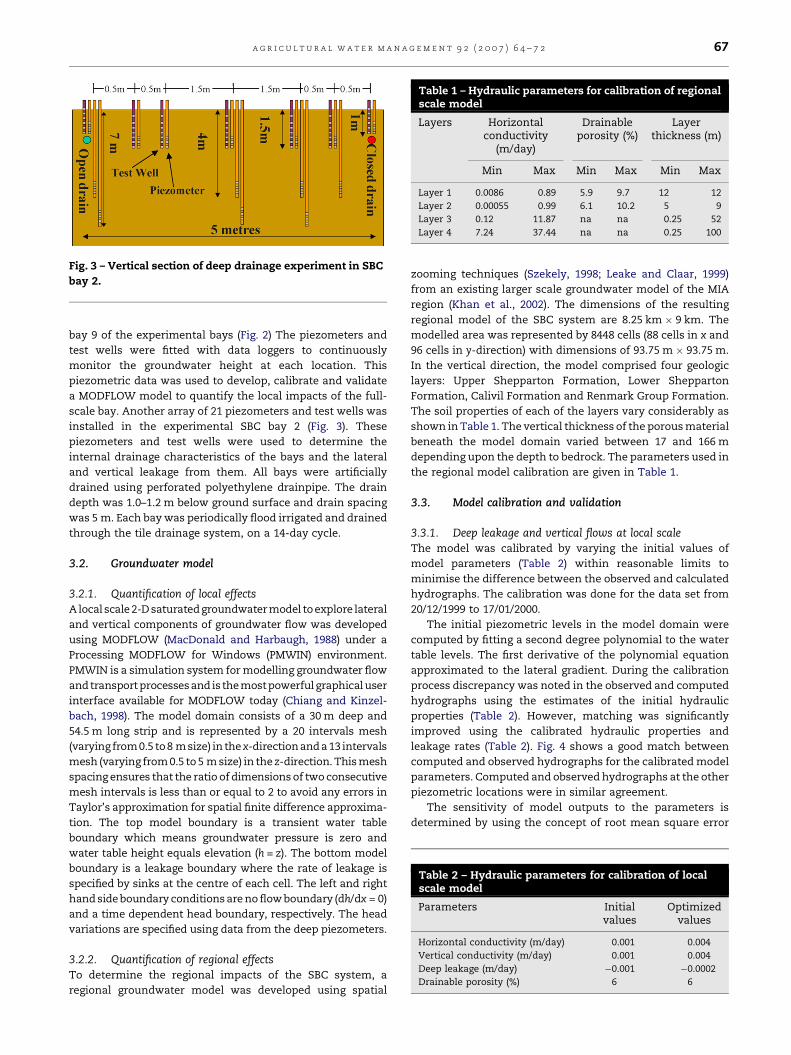
Fig. 3 – Vertical section of deep drainage experiment in SBC

bay 2.

Table 1 – Hydraulic parameters for calibration of regionalscale model

Layers Horizontalconductivity

(m/day)

Drainableporosity (%)

Layerthickness (m)

Min Max Min Max Min Max

Layer 1 0.0086 0.89 5.9 9.7 12 12

Layer 2 0.00055 0.99 6.1 10.2 5 9

Layer 3 0.12 11.87 na na 0.25 52

Layer 4 7.24 37.44 na na 0.25 100

Table 2 – Hydraulic parameters for calibration of localscale model

Parameters Initialvalues

Optimizedvalues

Horizontal conductivity (m/day) 0.001 0.004

Vertical conductivity (m/day) 0.001 0.004

Deep leakage (m/day) �0.001 �0.0002

Drainable porosity (%) 6 6

a g r i c u l t u r a l w a t e r m a n a g e m e n t 9 2 ( 2 0 0 7 ) 6 4 – 7 2 67

bay 9 of the experimental bays (Fig. 2) The piezometers and

test wells were fitted with data loggers to continuously

monitor the groundwater height at each location. This

piezometric data was used to develop, calibrate and validate

a MODFLOW model to quantify the local impacts of the full-

scale bay. Another array of 21 piezometers and test wells was

installed in the experimental SBC bay 2 (Fig. 3). These

piezometers and test wells were used to determine the

internal drainage characteristics of the bays and the lateral

and vertical leakage from them. All bays were artificially

drained using perforated polyethylene drainpipe. The drain

depth was 1.0–1.2 m below ground surface and drain spacing

was 5 m. Each bay was periodically flood irrigated and drained

through the tile drainage system, on a 14-day cycle.

3.2. Groundwater model

3.2.1. Quantification of local effectsA local scale 2-D saturatedgroundwater model toexplore lateral

and vertical components of groundwater flow was developed

using MODFLOW (MacDonald and Harbaugh, 1988) under a

Processing MODFLOW for Windows (PMWIN) environment.

PMWIN is a simulation system for modelling groundwater flow

and transport processes and is the mostpowerful graphical user

interface available for MODFLOW today (Chiang and Kinzel-

bach, 1998). The model domain consists of a 30 m deep and

54.5 m long strip and is represented by a 20 intervals mesh

(varying from 0.5 to 8 m size) in thex-direction and a 13 intervals

mesh (varying from 0.5 to 5 m size) in the z-direction. This mesh

spacing ensures that the ratio of dimensions of two consecutive

mesh intervals is less than or equal to 2 to avoid any errors in

Taylor’s approximation for spatial finite difference approxima-

tion. The top model boundary is a transient water table

boundary which means groundwater pressure is zero and

water table height equals elevation (h = z). The bottom model

boundary is a leakage boundary where the rate of leakage is

specified by sinks at the centre of each cell. The left and right

hand side boundary conditions are no flow boundary (dh/dx = 0)

and a time dependent head boundary, respectively. The head

variations are specified using data from the deep piezometers.

3.2.2. Quantification of regional effectsTo determine the regional impacts of the SBC system, a

regional groundwater model was developed using spatial

zooming techniques (Szekely, 1998; Leake and Claar, 1999)

from an existing larger scale groundwater model of the MIA

region (Khan et al., 2002). The dimensions of the resulting

regional model of the SBC system are 8.25 km � 9 km. The

modelled area was represented by 8448 cells (88 cells in x and

96 cells in y-direction) with dimensions of 93.75 m � 93.75 m.

In the vertical direction, the model comprised four geologic

layers: Upper Shepparton Formation, Lower Shepparton

Formation, Calivil Formation and Renmark Group Formation.

The soil properties of each of the layers vary considerably as

shown in Table 1. The vertical thickness of the porous material

beneath the model domain varied between 17 and 166 m

depending upon the depth to bedrock. The parameters used in

the regional model calibration are given in Table 1.

3.3. Model calibration and validation

3.3.1. Deep leakage and vertical flows at local scaleThe model was calibrated by varying the initial values of

model parameters (Table 2) within reasonable limits to

minimise the difference between the observed and calculated

hydrographs. The calibration was done for the data set from

20/12/1999 to 17/01/2000.

The initial piezometric levels in the model domain were

computed by fitting a second degree polynomial to the water

table levels. The first derivative of the polynomial equation

approximated to the lateral gradient. During the calibration

process discrepancy was noted in the observed and computed

hydrographs using the estimates of the initial hydraulic

properties (Table 2). However, matching was significantly

improved using the calibrated hydraulic properties and

leakage rates (Table 2). Fig. 4 shows a good match between

computed and observed hydrographs for the calibrated model

parameters. Computed and observed hydrographs at the other

piezometric locations were in similar agreement.

The sensitivity of model outputs to the parameters is

determined by using the concept of root mean square error

Fig. 4 – Calibrated computed and observed Pz-8

hydrographs.

Table 4 – Model sensitivity to deep leakage rates

Deep leakage (mm/day) ERMS (m) ESRMS (%)

�1 0.168 4.010

�0.4 0.0585 1.400

�0.2 0.0496 1.188

�0.09 0.0671 1.606

Fig. 5 – Validated computed and observed Pz-6

hydrographs.

a g r i c u l t u r a l w a t e r m a n a g e m e n t 9 2 ( 2 0 0 7 ) 6 4 – 7 268

(ERMS) and scale root mean square error (ESRMS) by the

following equations:

ERMS ¼1n

Xn

i¼1

½Wiðhi � HiÞ�2( )1=2

(1)

ESRMS ¼100ERMSPni�1ðhi � HiÞ

(2)

where n is the number of observations, Wi the weighting

factor, hi the computed head, Hi the observed head,Pn

i¼1ðhi �HiÞ is the accumulative difference between observed and

computed heads.

The ERMS and ESRMS obtained for different estimates of

vertical leakage and hydraulic conductivity parameters are

given in Tables 3 and 4. The model sensitivity is tested for four

scenarios of both vertical conductivity and deep leakage rates.

Table 3 shows that the model is not very sensitive to the

vertical hydraulic conductivity estimates in the range of 1 and

3 mm/day keeping both horizontal conductivity and deep

leakage constant for all cases: Kx = 4 mm/day and

q = �0.2 mm/day, respectively. The sensitivity to deep leakage

is tested at Kx = Kz = 4 mm/day for all cases. The guidelines on

groundwater modelling by the Murray Darling Basin Commis-

sion (Middlemis, 2001) show that the model calibration is good

if ESRMS is less than 5%. In the present study, assuming

isotropic soil hydraulic properties (Kx = Kz), the model results

show minimum ESRMS value (ESRMS < 1.2) for a vertical leakage

rate of 0.2 mm/day. The initial hydraulic heads derived from

the second order regression of the water table level on the 8th

of September 1999 were used to validate the model results.

Computed hydrographs for piezometers Pz-6 and Pz-8 (Fig. 2)

for the validation period are in close agreement with the

observed hydrographs (Figs. 5 and 6). To determine the leakage

Table 3 – Model sensitivity to vertical conductivity

Vertical conductivity (mm/day) ERMS (m) ESRMS (%)

3.0 0.0465 1.112

2.5 0.0456 1.090

2.0 0.0451 1.079

1.5 0.0454 1.087

1.0 0.0472 1.130

rate beneath the SBC system, two independent methods were

used:

(1) c

Fig

hyd

omputation of the leakage rate from the volumes of water

contained between the successive water table profiles after

the water table falls below the tile drains, and

(2) c

omputation of the time dependent vertical gradient and

leakage rate using Darcy’s flow formula.

In the first method, the drainage rate (Q) from the

underlying tile drains is computed using the concept of

declining of water table (Dd) over time (Dt) by the following

equation:

Q ¼ DdPd

Dt(3)

where Q is the drainage rate per unit area based on water table

measurements (m/day), Dd the change in water table depth

(m), Pd the drainable porosity (%), and Dt is the time interval

(day).

. 6 – Validated computed and observed Pz-8

rographs.

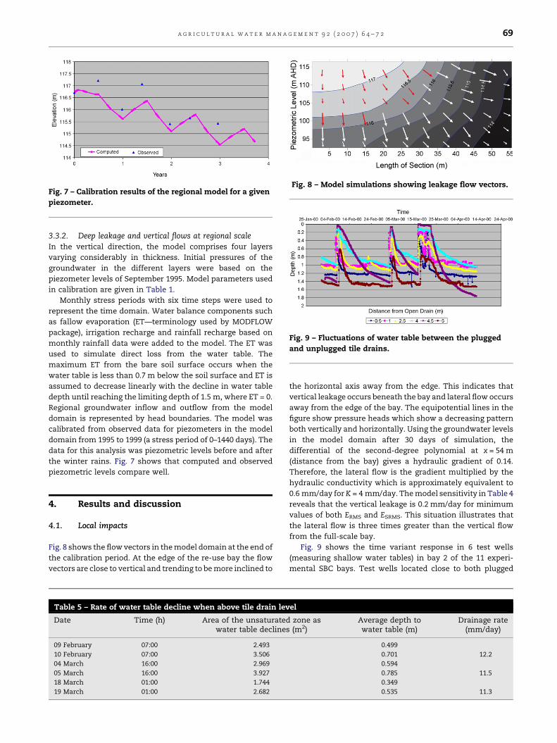
Fig. 7 – Calibration results of the regional model for a given

piezometer.

Fig. 8 – Model simulations showing leakage flow vectors.

Fig. 9 – Fluctuations of water table between the plugged

and unplugged tile drains.

a g r i c u l t u r a l w a t e r m a n a g e m e n t 9 2 ( 2 0 0 7 ) 6 4 – 7 2 69

3.3.2. Deep leakage and vertical flows at regional scaleIn the vertical direction, the model comprises four layers

varying considerably in thickness. Initial pressures of the

groundwater in the different layers were based on the

piezometer levels of September 1995. Model parameters used

in calibration are given in Table 1.

Monthly stress periods with six time steps were used to

represent the time domain. Water balance components such

as fallow evaporation (ET—terminology used by MODFLOW

package), irrigation recharge and rainfall recharge based on

monthly rainfall data were added to the model. The ET was

used to simulate direct loss from the water table. The

maximum ET from the bare soil surface occurs when the

water table is less than 0.7 m below the soil surface and ET is

assumed to decrease linearly with the decline in water table

depth until reaching the limiting depth of 1.5 m, where ET = 0.

Regional groundwater inflow and outflow from the model

domain is represented by head boundaries. The model was

calibrated from observed data for piezometers in the model

domain from 1995 to 1999 (a stress period of 0–1440 days). The

data for this analysis was piezometric levels before and after

the winter rains. Fig. 7 shows that computed and observed

piezometric levels compare well.

4. Results and discussion

4.1. Local impacts

Fig. 8 shows the flow vectors in the model domain at the end of

the calibration period. At the edge of the re-use bay the flow

vectors are close to vertical and trending to be more inclined to

Table 5 – Rate of water table decline when above tile drain lev

Date Time (h) Area of the unsaturatedwater table declines

09 February 07:00 2.493

10 February 07:00 3.506

04 March 16:00 2.969

05 March 16:00 3.927

18 March 01:00 1.744

19 March 01:00 2.682

the horizontal axis away from the edge. This indicates that

vertical leakage occurs beneath the bay and lateral flow occurs

away from the edge of the bay. The equipotential lines in the

figure show pressure heads which show a decreasing pattern

both vertically and horizontally. Using the groundwater levels

in the model domain after 30 days of simulation, the

differential of the second-degree polynomial at x = 54 m

(distance from the bay) gives a hydraulic gradient of 0.14.

Therefore, the lateral flow is the gradient multiplied by the

hydraulic conductivity which is approximately equivalent to

0.6 mm/day for K = 4 mm/day. The model sensitivity in Table 4

reveals that the vertical leakage is 0.2 mm/day for minimum

values of both ERMS and ESRMS. This situation illustrates that

the lateral flow is three times greater than the vertical flow

from the full-scale bay.

Fig. 9 shows the time variant response in 6 test wells

(measuring shallow water tables) in bay 2 of the 11 experi-

mental SBC bays. Test wells located close to both plugged

el

zone as(m2)

Average depth towater table (m)

Drainage rate(mm/day)

0.499

0.701 12.2

0.594

0.785 11.5

0.349

0.535 11.3

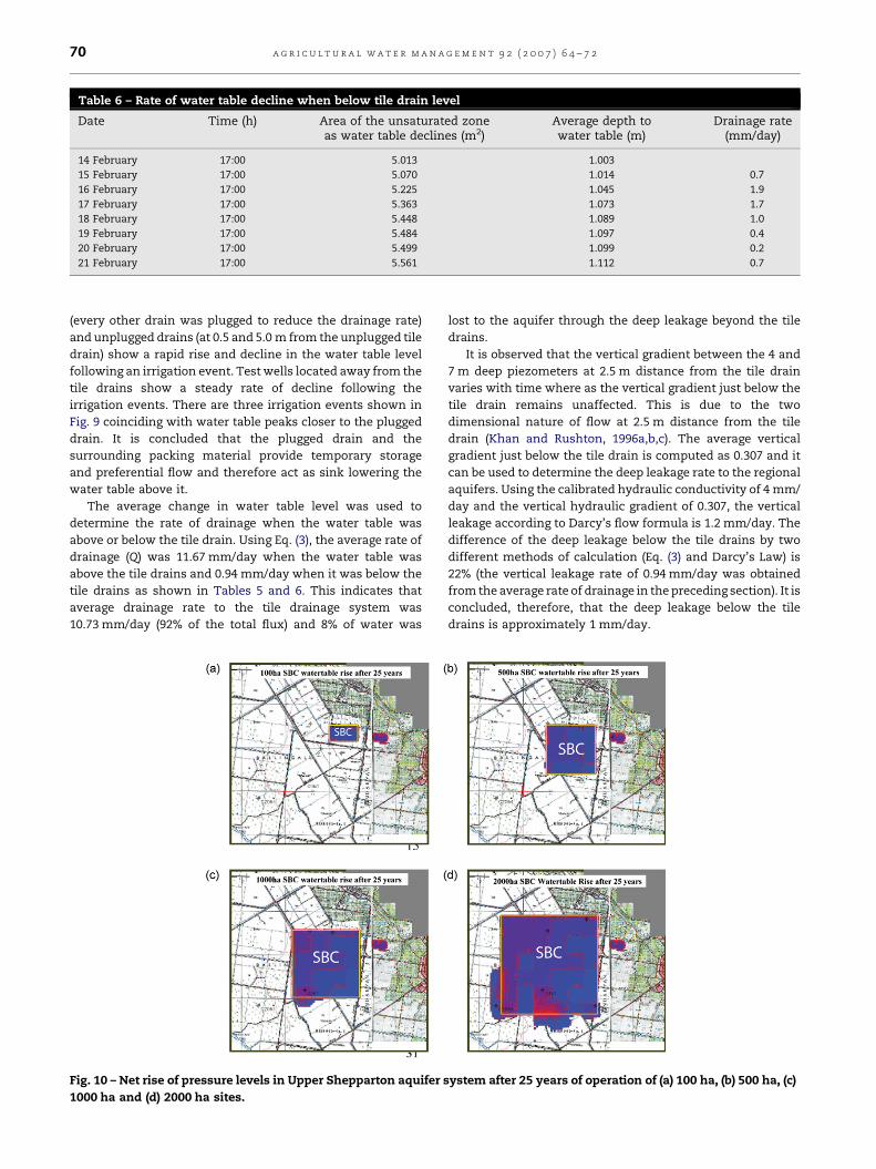
Table 6 – Rate of water table decline when below tile drain level

Date Time (h) Area of the unsaturated zoneas water table declines (m2)

Average depth towater table (m)

Drainage rate(mm/day)

14 February 17:00 5.013 1.003

15 February 17:00 5.070 1.014 0.7

16 February 17:00 5.225 1.045 1.9

17 February 17:00 5.363 1.073 1.7

18 February 17:00 5.448 1.089 1.0

19 February 17:00 5.484 1.097 0.4

20 February 17:00 5.499 1.099 0.2

21 February 17:00 5.561 1.112 0.7

a g r i c u l t u r a l w a t e r m a n a g e m e n t 9 2 ( 2 0 0 7 ) 6 4 – 7 270

(every other drain was plugged to reduce the drainage rate)

and unplugged drains (at 0.5 and 5.0 m from the unplugged tile

drain) show a rapid rise and decline in the water table level

following an irrigation event. Test wells located away from the

tile drains show a steady rate of decline following the

irrigation events. There are three irrigation events shown in

Fig. 9 coinciding with water table peaks closer to the plugged

drain. It is concluded that the plugged drain and the

surrounding packing material provide temporary storage

and preferential flow and therefore act as sink lowering the

water table above it.

The average change in water table level was used to

determine the rate of drainage when the water table was

above or below the tile drain. Using Eq. (3), the average rate of

drainage (Q) was 11.67 mm/day when the water table was

above the tile drains and 0.94 mm/day when it was below the

tile drains as shown in Tables 5 and 6. This indicates that

average drainage rate to the tile drainage system was

10.73 mm/day (92% of the total flux) and 8% of water was

Fig. 10 – Net rise of pressure levels in Upper Shepparton aquifer s

1000 ha and (d) 2000 ha sites.

lost to the aquifer through the deep leakage beyond the tile

drains.

It is observed that the vertical gradient between the 4 and

7 m deep piezometers at 2.5 m distance from the tile drain

varies with time where as the vertical gradient just below the

tile drain remains unaffected. This is due to the two

dimensional nature of flow at 2.5 m distance from the tile

drain (Khan and Rushton, 1996a,b,c). The average vertical

gradient just below the tile drain is computed as 0.307 and it

can be used to determine the deep leakage rate to the regional

aquifers. Using the calibrated hydraulic conductivity of 4 mm/

day and the vertical hydraulic gradient of 0.307, the vertical

leakage according to Darcy’s flow formula is 1.2 mm/day. The

difference of the deep leakage below the tile drains by two

different methods of calculation (Eq. (3) and Darcy’s Law) is

22% (the vertical leakage rate of 0.94 mm/day was obtained

from the average rate of drainage in the preceding section). It is

concluded, therefore, that the deep leakage below the tile

drains is approximately 1 mm/day.

ystem after 25 years of operation of (a) 100 ha, (b) 500 ha, (c)

a g r i c u l t u r a l w a t e r m a n a g e m e n t 9 2 ( 2 0 0 7 ) 6 4 – 7 2 71

4.2. Regional impacts

The following six scenarios were run to evaluate groundwater

impact for the following sizes of SBC operations:

� N

o SBC operation;

� 5

0 ha site;

� 1

00 ha site;

� 5

00 ha site;

� 1

000 ha site;

� 2

000 ha site.

For each of the proposed scenarios the model was run for 25

years. The difference in hydraulic pressures in layer-1 (Upper

Shepparton Formation) at the end of the simulation period

(25th year) was deduced from the base scenario (no SBC

operation). This allowed calculating the rise of piezometric

levels due to each of the operational scenarios.

The modelling results show that the overall water table rise

under the SBC site is around 1.3 m for the 50 ha site. This water

table rise occurs in the first year but it does not change during

the 25 years of operation, because of induced heavy drainage

from the tile drains laid at 1.2 m depth. The lateral spread of

the groundwater mound did not extend beyond 50 m from the

outer edge of the bays.

Fig. 10 shows the net water table change of the 100, 500, 1000

and 2000 ha sizes of operation of the SBC. Similar to the 50 ha

site, the overall depth to the water table under the SBC bays

remains at the depth of the tile drains which causes a rise of 1.0–

2.5 m (depending on initial depth to the water table) under the

site and to a distance of 50 m from the site. The water table

under SBC site reaches quasi equilibrium at the depth of the

drain with periodic rise and fall around the tile drain depth. The

increasing size of SBC (for example 2000 ha) shows slightly

increased interactions with surrounding areas, this causes

wider spreading of net water table change effects exacerbated

by spatially variable hydraulic conductivity and zones of

groundwater pumping influence from a nearby abstraction

bore. The long-term 25 year modelled operation of the SBC site

shows the tiledrains maintaining the water table atdrain depth.

5. Conclusions

The detailed monitoring of groundwater dynamics and the

modelling of the SBC operations demonstrate that the vertical

and lateral leakage at the edge of the bays is around 0.2 and

0.6 mm/day, respectively. The deep leakage beneath the SBC

bays is approximately 1 mm/day. The shallow initial water

table and the very low hydraulic conductivity keep the lateral

extension of the water table mound within 50 m. During the

irrigation/ponding operations 8% of the saturated ground-

water flow above the tile drains contributes to deep leakage.

The simulations show that the water table reaches a quasi

equilibrium at the depth of the drains with periodic rise and

fall in tune with irrigation application and drainage operation

whenever an SBC system with intensive tile drainage is set up

on heavy clay soils with low saturated hydraulic conductivity.

Modelling scenarios of various sizes of SBC sites suggest

that the overall water table levels remain at the depth of the

tile drains which brings about a groundwater mound of 1–

2.5 m on-site (depending on the initial water table depth) and

to a distance of 50 m laterally over time. The local and regional

impacts of SBC systems in lighter soils and prior stream areas

are likely to be quite different than those presented in this

study. In order to develop SBC operations at other locations, a

GIS-based site suitability assessment model is recommended

to assess the SBC effect under different soil and hydrogeolo-

gical conditions.

Acknowledgements

The authors wish to acknowledge the funding support of the

National Heritage Trust and The Cooperative Research Centre

for Sustainable Rice Production (CRC-Rice), which made this

work possible. Technical support provided by the Australia’s

Commonwealth Scientific and Industrial Research Organisa-

tion (CSIRO) scientists L. Short, L. Best, J. Townsend, N.

Jayawardane, T. Biswas and J. Foley is greatly appreciated.

Scientific comments from the anonymous reviewers and Joint

Editor-in-Chief Willy Dierickx have been very useful in

improving the quality of this paper.

r e f e r e n c e s

Benyamini, Y., Mirlas, V., Marish, S., Gottesman, M., Fizik, E.,Agassi, M., 2005. A survey of soil salinity and groundwaterlevel control systems in irrigated fields in the Jezre’el Valley,Israel. Agric. Water Manage. 76, 181–194.

Bethune, M.G., Gyles, O.A., Wang, Q.J., 2004. Options formanagement of saline ground water in an irrigated farmingsystem. Aus. J. Exp. Agric. 44, 181–188.

Blackwell, J., 2000. From saline drainage to irrigated production.Research project sheet 18, CSIRO Land and Water. Availableonline: http://www.clw.csiro.au/publications/projects/projects18.pdf.

Brown, C.R., Stephenson, A.E., 1991. Geology of the MurrayBasin South Eastern Australia, Bureau of Mineral Resources,Australia, Bulletin 235.

Chiang, W., Kinzelbach, W., 1998. Processing MODFLOW, aSimulation System for Modeling Groundwater Flow andPollution, User’s Manual, 325 pp.

Gallichard, J., Broughton, R.S., Ghany, M., El-Badry, O., 1997.Subsurface drainage of field test plots in the Nile Delta ofEgypt. J. Int. Commission Irrigation Drain. (ICID) 46 (2), 31–45.

Gupta, R.K., Mostaghimi, S., McClellan, P.W., Alley, M.M., Brann,D.E., 1997. Spatial variability and sampling strategies forNO3-N, P, and K determinations for site-specific farming.Trans. Am. Soc. Agric. Eng. 40 (2), 337–343.

Jayawardane, N., 2000. The FILTER System—turning effluentinto an asset. Research Project sheet 20, CSIRO Land andWater. Available online: http://www.clw.csiro.au/publications/projects/projects20.pdf.

Jayawardane, N.S., Cook, F.J., Blackwell, J., Ticehurst, J., Nicoll, G.Wallet, D.J., 1997. Final report on hydraulic flow propertiesof the FILTER system during the period November 1994 toNovember 1996. CSIRO Consultancy Report No. 97-42.

Khan, S., Rushton, K.R., 1996a. Reappraisal of flow to tile drains.I: Steady state response. J. Hydrol. 183, 351–366.

Khan, S., Rushton, K.R., 1996b. Reappraisal of flow to tile drains.II: Time-variant response. J. Hydrol. 183, 367–382.

a g r i c u l t u r a l w a t e r m a n a g e m e n t 9 2 ( 2 0 0 7 ) 6 4 – 7 272

Khan, S., Rushton, K.R., 1996c. Reappraisal of flow to tile drains.III: Drains with limited flow capacity. J. Hydrol. 183,383–395.

Khan, S., Best L., Wang, B., 2002. Surface-ground waterinteraction model of the Murrumbidgee Irrigation Area(development of the hydrogeological databases). CSIROLand and Water Technical Report 36/02. Available online:http://www.clw.csiro.au/publications/technical2002/tr36-02.pdf.

Khan, S., Short, L., Best, L., Townsend, J., Blackwell, J.,Jayawardane, J., Biswas, T., 2001. Hydrogeologicalassessment of onsite and regional impacts of FILTER andSBC. Technical Report Number 10/01, CSIRO GriffithLaboratory.

Kivaisi, A.K., 2001. The potential for constructed wetlands forwastewater treatment and reuse in developing countries: areview. Ecol. Eng. 16, 545–560.

Leake, S.A., Claar, D.V., 1999. Procedures and computerprograms for telescopic mesh refinements usingMODFLOW, USGS Open File Report Number 99-238.

MacDonald, M.G., Harbaugh, A.W., 1988. A modular threedimensional finite difference groundwater flow model:techniques of water-resources investigations of the UnitedStates Geological Survey, 586 pp. (Book 6, Chapter A1).

Middlemis, H., 2001. Groundwater Flow Modelling Guideline.Murray Darling Basin Commission, Canberra.

Neeson, R., Glasson, A., Morgan, A., Macalpine, S., Darnley-Naylor, M., 1995. On farm options: Murrumbidgee irrigationareas and districts land and water management plan. NewSouth Wales Agriculture Department, Sydney, pp. 121.

Oron, G., 1993. Recycling drainage water in San Joaquin Valley,California. J. Irrig. Drain. Eng. 119, 265–285.

Pratt Water Solutions, 2003. Sequential biologicalconcentration—review. A study conducted for the PrattWater Murrumbidgee valley water efficiency feasibilityproject. Dennis E Toohey and Associates, AgribusinessConsultants, Albury, NSW, Australia (unpublished).

Rhoades, J.D., Chanduvi, F., Lesch, S., 1999. Soil SalinityAssessment—Methods and Interpretation of ElectricalConductivity Measurements. FAO Irrigation and DrainagePaper 57, Rome, Italy.

Su, N., Bethune, M., Mann, L., Heuperman, A., 2005. Simulatingwater and salt movement in tile-drained fields irrigatedwith saline water under a serial biological concentrationmanagement scenario. Agric. Water Manage. 78, 165–180.

Szekely, F., 1998. Windowed spatial zooming in finite differencegroundwater flow models. Groundwater 36 (5), 718–721.

Tanji, K.K., Karajeh, F.F., 1993. Salt drain water reuse in agro-forestry systems. J. Irrig. Drain. Eng. 119, 170–180.

UNESCO, 2006. World Water Development Report 2—Water, AShared Responsibility. Available online: http://www.unesco.org/water/wwap/wwdr2/.