Hybrid Model of the Gasoline Engine for Misfire Detection 1 2

IEEE

Proo

f

IEEE TRANSACTIONS ON INDUSTRIAL ELECTRONICS, VOL. 58, NO. 8, AUGUST 2011 1

Hybrid Model of the Gasoline Enginefor Misfire Detection

1

2

Muddassar Abbas Rizvi, Aamer Iqbal Bhatti, Sr., Member, IEEE, and Qarab Raza Butt3

Abstract—This paper proposes a novel hybrid model for an4internal combustion engine, with the power generated due to5combustion as the input and the crankshaft speed fluctuations as6the output. The individual cylinders of the engine are considered7as subsystems for which a nonlinear model, based on the physical8principles, is derived. The proposed model is linearized at an oper-9ating point, and a switched linear model is formed. The simulation10results of the proposed model are validated by matching the results11with the experimentally observed data. Using the properties of the12validated model, it is shown that the crankshaft speed variations13observed in the engine are a Markov process. A novel algorithm14that is based on the Markov chain is proposed to detect the15misfire in the spark ignition engines. In the ensuing engine rig16experiments, an igniter misfire is introduced in the system and17is successfully detected. The analysis of the data shows that the18engine also has an air leakage in a cylinder (a developing misfire),19which is experimentally confirmed later.20

Index Terms—Discrete event model (DEM), hybrid systems,21Markov chains, mean value model (MVM), misfire detection,22spark ignition (SI) engine.23

I. INTRODUCTION24

THE complexity of automotive vehicles is increasing as25

more and more mechanically driven parts are being re-26

placed by electronically driven actuators. An electronic control27

unit (ECU) is being installed in modern vehicles, which not28

only monitors the sensors installed in the vehicle but also29

controls the electronic actuators. The ECU also provides a di-30

agnostic code to identify different faults present in the vehicle.31

Fault prognosis in automotives is being studied for integration32

in future vehicles. Murphey indicated that the development of33

computationally simpler fault diagnosis algorithms for auto-34

motive systems is considered as the most challenging problem35

[1]. The problem is still being addressed by the research com-36

munity [1]–[4]. A survey of different automotive models and37

fault diagnosis techniques found in literature is provided.38

A general survey indicates that the spark ignition (SI) engine39

is mathematically represented by either the mean value model40

Manuscript received May 3, 2010; revised July 27, 2010; acceptedSeptember 9, 2010. This work was supported in part by the Higher EducationCommission and in part by the ICT Research and Development Fund ofPakistan.

M. A. Rizvi and A. I. Bhatti Sr. are with the Mohammad Ali Jinnah Univer-sity, Islamabad 44000, Pakistan (e-mail: [email protected]; [email protected]).

Q. R. Butt is with the Center for Advanced Studies in Engineering, G-5/1,Islamabad, Pakistan (e-mail: [email protected]).

Color versions of one or more of the figures in this paper are available onlineat http://ieeexplore.ieee.org.

Digital Object Identifier 10.1109/TIE.2010.2090834

(MVM) [6], [7] or the discrete event model (DEM) [8]. The 41

MVM is based on the average torque generated in a complete 42

ignition cycle. The model therefore cannot efficiently detect any 43

fault during an individual stroke of an ignition cycle. The DEM 44

is a hybrid model, with states representing the compression, 45

ignition, expansion, and exhaust strokes described as nonlinear 46

differential equations. The engine state is defined by solving 47

all four nonlinear equations. Due to a high computational load, 48

both MVM and DEM are difficult to solve in embedded sys- 49

tems, and they could not attract the fault diagnostic community, 50

especially for misfire fault detection. Luo et al. mentioned that 51

the algorithms executed in the ECU are required to be simpler 52

than most models or signal-based algorithms proposed by the 53

academia [5]. Sood et al. proposed a kinematic model, with 54

the fuel as the input and the crankshaft velocity as the output 55

[9]. The model is based on forces acting on the piston due to 56

the combustion of fuel in the engine cylinder and load acting 57

on the engine. The model was used for the detection of the 58

misfire fault using parameter estimation, and it was concluded 59

that the model-based approach proved to be computationally 60

expensive. Wong et al. proposed an engine model based on the 61

experimental sample data using neural network methods [27]. 62

The model is, however, explicitly applicable only to idle speed 63

control applications. A hybrid modeling approach was used for 64

other automotive applications but not for fault detection [10], 65

[11]. An addition to hybrid modeling is the representation of 66

the discrete states as modes of hybrid system, and each mode 67

system is governed by different continuous dynamics. Mode 68

identification in the presence of fault is carried out by a rule- 69

based analysis of the analytic redundancy relations [29]. The 70

fault diagnosis is based on either model or signal data analysis. 71

Model-based fault diagnosis methods have the advantage that 72

the signal features associated with fault have a physical inter- 73

pretation [9], e.g., the discharge coefficient estimated using the 74

sliding mode observer provides an insight about the physical 75

significance of a parameter [6], [12]. Methods that are based 76

on MVEM were applied for fault diagnosis in coolant systems AQ277

[13], air paths before and after a throttle valve [14], etc. Most 78

of these techniques used state observers, parity equations, or 79

parameter estimation techniques for fault diagnosis [15]. The 80

parameter values forming the basis of fault detection in the 81

model-based method also change with the operating conditions, 82

like load, ambient temperature, pressure, vehicle aging, etc. 83

The value of the discharge coefficient estimated using the 84

sliding mode observer under different load conditions indicates 85

this parameter variation [6]. Sood et al. mentioned that fault 86

diagnosis using some parameters which are not constant leads 87

to the further increase in the complexity of the fault diagnostic 88

0278-0046/$26.00 © 2011 IEEE

IEEE

Proo

f

2 IEEE TRANSACTIONS ON INDUSTRIAL ELECTRONICS, VOL. 58, NO. 8, AUGUST 2011

problem [9]. The heavy computational load and the adaptive89

selection of the threshold values for fault detection added so90

much complexity that not only restricts their application only91

to offline fault detection but also increases the trend of using92

the statistical tools by the fault diagnostics and isolation (using93

control engineering tools) community [16]. The signal-basedAQ3 94

methods identify the features linked with faults in a signal.95

Residual analysis is carried out to identify these features.96

Crossman described some features associated with faults and97

methods to identify them [2].98

Misfire fault occurs when a combustion does not occur in99

one or more engine cylinders. It may occur due to a missing100

spark, an air leakage, or a fault in fuel injection. A number of101

techniques that are based on an artificial neural network were102

used to detect the misfire fault [4], [17]. Feldkamp proposed103

techniques that characterize fault states as hidden states in a104

hidden Markov model and used extended Kalman filter esti-105

mates for NN training [17]. It seems that the author implicitlyAQ4 106

assumed a stochastic analysis and a linearized version of some107

engine nonlinear models. Since the engine is a highly nonlinear108

system whose output depends on a large number of factors, it109

would be difficult to simulate all possible healthy and faulty110

conditions to train the neural network to ensure a robust fault111

detection. Montini proposed a wavelet-based analysis of the112

crankshaft speed fluctuation signal [18], and Rizzoni [19] and113

Sood [22] proposed different data classification methods to114

decide between the binary hypothesis conditions of the fault and115

no fault conditions using a correlation analysis of the data. Both116

wavelet- and correlation-based methods were computationally117

heavy, and the algorithm also needed heuristic guidelines to118

extract the features and to relate to the faults. Although the ap-119

plication of the Markov chains for fault diagnosis can be found120

in the literature [20], however, disturbances that are due to faults121

in dynamic systems have not been proved as a Markov process122

for fault diagnosis and isolation. This paper proves these dis-123

turbances as a Markov process. Morgan et al. indicated that the124

potential advantage of the application of the Markov chains is125

its ability to predict, and they applied it to predict the future con-126

centration of the elements in the lubricant analysis of the marine127

engine [20], where an early prediction is important due to the128

maintenance problems when the ship is at the sea [20]. Luo129

mentioned that the recently introduced new approaches for fault130

diagnosis combined model-based and data-driven techniques131

to obtain a better diagnostic performance [3]. A method that132

transforms the engine speed fluctuations to finite state automata133

is presented in the literature, which stressed on the implemen-134

tation using a field programmable gate array (FPGA) [23].AQ5 135

The objective of this paper is to develop a novel mathematical136

model for SI engines that can explain the crankshaft speed137

fluctuations when a deterministic input with a small randomly138

varying component is applied to the SI engine. The utility of the139

proposed model is expressed by presenting a novel method for140

misfire detection. The proposed method is based on the speed141

fluctuation of the crankshaft. The method is simple and cost142

effective, and it needs no additional installation as the sensor is143

preinstalled in all modern vehicles [21].144

This paper is organized as follows. Section II presents a145

hybrid mathematical model that is used to represent the steady-146

state behavior of the internal combustion (IC) engine [24], [25]. 147

A nonlinear model representing the motion of the piston in 148

the engine cylinders is derived using the physical principles 149

to represent the subsystems of the hybrid model. The non- 150

linear model is linearized at an operating point, and the engine 151

is taken as a switched linear hybrid system. The properties 152

of the proposed hybrid system are investigated. Section III 153

presents the statistical analysis of the system output against a 154

random variation of the inlet air, and finally, the fluctuation 155

in the crankshaft speed is proved to be a Markov process. 156

Section IV presents the algorithm for fault diagnosis, and a 157

comparison of the presented method with an existing method 158

is provided in Section V. The simulation and experimental 159

results are presented, analyzed, and discussed in Section VI. 160

The relative/receiver operating characteristic (ROC) analysis is 161

presented in Section VII. The concluding remarks are given in 162

Section VIII, and the references are given at the end. 163

II. SYSTEM MODELING 164

For system modeling, a four-cylinder four-stroke engine is 165

assumed, where the ignition occurs in only one cylinder at a 166

time. The pistons of the four cylinders are coupled to a common 167

shaft via a crankshaft. The power strokes of all cylinders are 168

separated from each other by 180◦, and they periodically occur 169

after two shaft revolutions, named as an ignition cycle. During 170

a power stroke, the air–fuel mixture is burnt inside the cylinder, 171

and pressure develops in the chamber of the cylinder, applying 172

force on the piston. The modeling is carried out in the following 173

two steps. 174

1) In the first step, a deterministic switched linear model, 175

with the power generated by the fuel combustion as the 176

input and the crankshaft angular velocity as the output, is 177

presented in Section II-A–II-E. 178

2) In the second step, the statistical properties of the air in- 179

take in the cylinder are studied to establish that the crank- 180

shaft speed fluctuations are Gaussian and Markov. The 181

properties of air are explored because the engine power is 182

manipulated by controlling the amount of air intake. 183

A. Hybrid Model 184

The SI engine is modeled as a hybrid system with four iden- 185

tical minimum phase LTI subsystems, where each subsystem AQ6186

represents an engine cylinder. A subsystem/cylinder is active 187

when it contributes power to the system, i.e., during a power 188

stroke. The subsystems are sequentially actuated during an 189

ignition cycle. The output of the system would be a vector 190

sum of the outputs of the subsystems. The following are the 191

modeling assumptions. 192

Assumption 1: The system operates at a steady-state condi- 193

tion on a constant load. 194

Assumption 2: The air–fuel ratio is stoichiometric. 195

Assumption 3: The whole energy is instantaneously added at 196

the beginning of the power stroke and is delivered to a storage 197

element (flywheel) at a constant rate. 198

Assumption 4: At any time instant, only one cylinder would 199

receive an input to become active, and it exerts force on the 200

IEEE

Proo

f

RIZVI et al.: HYBRID MODEL OF THE GASOLINE ENGINE FOR MISFIRE DETECTION 3

piston and other cylinders that are being passive due to suction.201

The compression and exhaust processes contribute to the engine202

load torque.AQ7 203

If the period of the ignition cycle is T , u(t) is the system204

input at time t during an ignition cycle, and ui(t) is the input of205

the ith subsystems. Based on Assumption 4206

ui(t) = u(t) when(i − 1)T

4< t <

iT

4, i = 1, 2, 3, 4 (1)

ui(t) = 0 otherwise. (2)

The framework of the hybrid model for a maximally balanced207

SI engine with four cylinders is represented as a five-tuple208

model 〈μ,X,Γ,Σ, φ〉. The basic definition of the model para-209

meters is given in the following.210

1) μ = {μ1, μ2, μ3, μ4}, where each element of the set211

represents the active subsystem of the hybrid model.212

2) X ∈ R2 represents the state variable of the continu-213

ous subsystems. It would be proved in the next section214

that vector X would have velocity and acceleration as215

components.216

3) Γ = {G(s)}, where G(s) is the transfer function of the217

linear subsystems. For the maximally balanced cylinder,218

the set contains a single element. The transfer function219

G(s) is derived in Sections II-B–II-D of this section. The220

model can be defined in state space as221

x(t) =AX + BU (3)y(t) =CX + DU (4)

where222

U ∈ R A ∈ R2×2 B ∈ R2×1 C ∈ R1×2 D ∈ R.

4) Σ : μ → μ represents the generator function that defines223

the activation of the next subsystem after the activity224

of the current subsystem end. The generator function is225

defined in terms of the crankshaft position as226

Σ =

⎧⎪⎪⎨⎪⎪⎩

μ1 4nπ ≤∫

θ1dt < (4n + 1)πμ2 (4n + 1)π ≤

∫θ1dt < (4n + 2)π

μ3 (4n + 2)π ≤∫

θ1dt < (4n + 3)πμ4 (4n + 3)π ≤

∫θ1dt < (4n + 4)π

(5)

where n = 0, 1, 2 and∫

θ1dt represents the instantaneous227

shaft position that identifies the output of the generator228

function.229

5) φ : Γ × μ × X × u → X defines the initial condition for230

the next subsystem after a switching event, where u231

represents the input of the active subsystem. Fig. 1 shows232

the subsystems and switching sequence of the proposed233

engine hybrid model.234

B. Nonlinear Subsystem Modeling235

Consider δQ as the amount of energy added in the system236

by burning the air–fuel mixture. Based on Assumption 3, the237

energy is instantaneously added in the cylinder. This will appear238

as an increase in the internal energy of the system239

δU = δQ. (6)

Fig. 1. Hybrid system with four subsystems.

A part of this internal energy is used to do work, and the rest of 240

the energy is drained in the coolant and exhaust system. If the 241

internal energy changes to work with the constant efficiency ηt, 242

then work δW is given by the energy balance equation as 243

δW = −ηtδU. (7)

Using (6) 244

δW = −ηtδQ. (8)

If p is the pressure due to the burnt gases, then the work done 245

during the expansion stroke is given by 246

W =

V 2∫V 1

pdV (9)

where V1 and V2 are the initial and final volumes of the cylinder 247

during expansion. For adiabatic expansion 248

pV γ = k1 (10)

where k1 and γ are constant. Hence, (9) becomes 249

W =

V 2∫V 1

k1V−γdV (11)

W = k1V −γ+1

2 − V −γ+11

−γ + 1. (12)

Consider the closed end of the piston as the origin. Also, 250

assume that A is the surface area of the piston and x is a 251

continuous variable that represents the instantaneous piston 252

position. When the piston moves a small distance δx from 253

its initial position x, where δx is constant and where it can 254

be arbitrarily chosen to be small, then the work done can be 255

expressed as 256

δW = k1[A(x + δx)]−γ+1 − [Ax]−γ+1

−γ + 1(13)

δW = k1A−γ+1

−γ + 1[(x + δx)−γ+1 − x−γ+1

](14)

δW =k1A

−γ+1

−γ + 1

[x−γ+1

(1 +

δx

x

)−γ+1

− x−γ+1

](15)

δW =k1A

−γ+1x−γ+1

−γ + 1

[(1 +

δx

x

)−γ+1

− 1

]. (16)

IEEE

Proo

f


Expanding (16) using a binomial series, neglecting the higher257

powers of δx, and simplifying258

δW = k1A−γ+1x−γδx. (17)

Using (8), (17) becomes259

δQ =k1A

−γ+1x−γδx

ηt. (18)

If F is the force applied by the burnt gases, m is the mass of the260

engine moving assembly (piston, connecting rod, crankshaft,261

and flywheel), k2 is the coefficient of friction, and k3 is the262

coefficient of elasticity, then the net force acting on the piston263

is given by264

md2x

dt2= F − k2

dx

dt− k3x (19)

md2x

dt2+ k2

dx

dt+ k3x = F. (20)

The net work done by the expanding gases against the load,265

friction, and elastic restoring forces when the piston moves by266

a small distance δx would be given as267 [m

d2x

dt2+ k2

dx

dt+ k3x

]δx = δW. (21)

Using (17), the aforementioned equation becomes268 [m

d2x

dt2+ k2

dx

dt+ k3x

]δx = k1A

−γ+1x−γδx. (22)

The displacement δx can be chosen to be constant and ar-269

bitrarily small. As the piston moves, the volume inside the270

combustion chamber increases, resulting in the reduction of the271

instantaneous pressure on the piston. The instantaneous power272

is therefore a function of the piston position. The instantaneous273

power delivered by the engine would be calculated by differen-274

tiation as275 [m

d3x

dt3+ k2

d2x

dt2+ k3

dx

dt

]δx = − k1γA−γ+1x−γ−1 dx

dtδx

(23)

md3x

dt3+ k2

d2x

dt2+ k3

dx

dt= − k1γA−γ+1x−γ−1 dx

dt.

(24)

Write (24) in terms of velocity v as276

md2v

dt2+ k2

dv

dt+ k3v = − γηt

k1A−γ+1x−γδx

ηt

v

xδx(25)

md2v

dt2+ k2

dv

dt+ k3v = γηtδQ

v

xδx(26)

md2v

dt2+ k2

dv

dt+ k3v =

γηtv

x

δQ

δt

δt

δx. (27)

Equation (27) represents a nonlinear model of the crankshaft277

speed when the power is provided to the engine by fuel ignition.278

C. Model Linearization 279

For model linearization, consider that the piston always 280

moves between two extreme positions xt and xb, where xt 281

represents the piston position at the top dead center (TDC) 282

and xb represents the piston position at the bottom dead center 283

(BDC). Therefore, x can never be zero, and the right-hand side 284

(RHS) of (27) is a smooth function. The model is therefore 285

linearized at the TDC. 286

If a constant finite power P is added to a cylinder when its 287

piston is at the TDC and the system delivers power P (x), then 288

the power delivered by system would be given as 289

md2v

dt2+ k2

dv

dt+ k3v =

γηvt

xP (x)

1v

(28)

md2v

dt2+ k2

dv

dt+ k3v =

γηt

xP (x). (29)

Linearizing the system at the TDC (x = xt) under the 290

steady-state condition, (29) is written as 291

md2v

dt2+ k2

dv

dt+ k3v =

γηt

xtP (x). (30)

Based on Assumption 3, the system is delivering power at 292

a constant rate; hence, P (x) is taken as constant. The RHS of 293

(30) is therefore constant, and the expression becomes a linear 294

differential equation. 295

D. Model Parameter Estimation 296

The engine operating power can be estimated by using the 297

manifold air pressure/manifold air flow sensors and by esti- 298

mating the mass of the fuel sprayed and the heat equivalent of 299

the fuel. The typical value of the efficiency of the SI engine 300

is nearly 35%. All of the parameters on the RHS of (30) are 301

known, except the elasticity k3 and friction coefficients k2. 302

The movement of the piston exhibits a periodic behavior, 303

with the same fundamental frequency as that of the rotational 304

speed of the engine shaft. This provides a heuristic guideline in 305

choosing the value of k3 as a function of the crankshaft angular 306

speed. The empirical choice is validated using the simulation 307

and experimental results reported later 308

k3 = ω2 = (2πN)2 (31)

where N is the engine speed in revolution per second. 309

During experimental verification, the load is also applied by 310

friction. Most frictional models described in literature are based 311

on the empirical relations as a polynomial in the engine speed. 312

A simplified frictional model is chosen, with a term containing 313

only the square of the engine speed 314

k2 = b ω2. (32)

On the basis of the simulation and experimental results, it is 315

established that the optimal selection of the value of b varies 316

between 0.2 and 0.5. The values of parameters k1 and k2 depend 317

on the operating point. The stability of the linearized subsystem 318

is ensured by the Routh–Hurwitz criteria. 319

IEEE

Proo

f


E. Model Properties320

The properties of the hybrid model when the engine is oper-321

ating under the steady-state conditions are presented as a set of322

propositions, lemmas, and theorems given in the following.323

Proposition 1: When the engine is running with a constant324

speed, the input to the engine system is a periodic impulse train325

with a period of T/4, where T is the period of the ignition326

cycle. This is because the energy is added in the engine as an327

impulse (Assumption 3), and the event of the addition of the328

energy occurs four times during an ignition cycle energy, i.e.,329

once in each cylinder.330

Lemma 1: Under the no misfire condition, the system output331

exhibits a periodic ac component with a period of T/4, where332

T represents the period of the ignition cycle (two revolutions).333

Proof: When all subsystems are identical and when they334

are represented by a linear model, then a periodic input with a335

period of T/4 would produce a periodic output with the same336

frequency.337

Lemma 2: When a cylinder misfires, the output of the system338

exhibits a periodic ac component with a period of T .339

Proof: The misfire can be considered as the loss of one340

of every fourth impulse of the input signal. The input signal is341

therefore periodic, with a period of T rather than T/4, and the342

output also exhibits a fundamental frequency of T .343

Lemma 3: Under the no misfire fault condition, the output344

contains four identical peaks in an ignition cycle.345

Proof: The input signal during an ignition cycle contains346

four impulses. As the subsystems are stable LTI minimum347

phase second-order systems, they exhibit one peak in the output348

against each impulse occurring in the impulse train input.349

Lemma 4: In the steady-state conditions with fault in the ith350

event, no peak would be observed due to the input of the ith351

subsystem.352

Proof: The absence of an impulse at the ith place in353

the input signal would result in the loss of the corresponding354

peak.355

The results of Lemmas 1, 2, 3, and 4 can be observed from356

the simulation and experiment results discussed later.357

Definition 1: The system is said to be in the steady state358

when the net change in the system output v(t) in one complete359

ignition cycle is zero360

v(t + T ) = v(t). (33)

Theorem 1: Under the steady-state and no fault conditions361

when the same input is given to the identical subsystems (max-362

imally balanced cylinders), the response of each subsystems363

would be independent.364

Proof: If u is the input to a subsystem, v(0) is the initial365

condition, and h(t) is the impulse response of a subsystem, then366

the output of the second subsystem (i.e., at time t, where T/4 <367

t < 2T/4) is given by368

v(t) = v(0) +

T4∫

0

h(t − τ)u(τ)dτ +

t∫T4

h(t − τ)u(τ)dτ.

(34)

Based on Lemma 1, the output signal is periodic, with a period 369

of T/4; therefore 370

v(T/4) = v(0) (35)

v(0) +

T4∫

0

h(t − τ)u(τ)dτ = v(0) (36)

and (34) becomes 371

v(t) = v(T/4) +

t∫T4

h(t − τ)u(τ)dτ. (37)

Hence, during the activation time of the second subsystem, 372

the output depends only on the input u(t) and the impulse 373

response of the second subsystem, and it is independent from 374

the response of the first subsystem. Similarly, it can be proved 375

that, under the steady-state conditions, the responses of all 376

cylinders are independent. 377

Proposition 2: For an EFI engine, the air intake in the AQ8378

cylinders is measured, and a fuel that is proportional to the 379

amount of air intake is sprayed into it. Therefore, the power 380

input to the system in the steady-state conditions is proportional 381

to the amount of air sucked. 382

The following corollaries that are based on the properties 383

of the proposed hybrid model would be used for onward sta- 384

tistical analysis and for the development of the fault detection 385

methodology. 386

Corollary 1: Four peaks would be observed in one ignition 387

cycle of a four-cylinder SI engine (Lemma 3). 388

Corollary 2: The amplitudes of the four observed peaks 389

represent four independent events (Theorem I). 390

Corollary 3: The crankshaft speed is proportional to the 391

input power (due to a linear model of the subsystems). 392


amount of air intake (based on Corollary 3 and Proposition 2). 394

III. STATISTICAL ANALYSIS 395

The air intake is considered as a random variable, and the 396

statistical analysis is carried out in the following steps. 397

1) Determine the probability density function (pdf) of the 398

random variable representing the peak values of the 399

velocity observed in an ignition cycle. 400

2) Form a collection of the aforementioned random variable. 401

3) Prove that the aforementioned collection is Gaussian and 402

Markov. 403

A. Step 1 404

Using Corollary 4, it can be established that the pdf of the 405

air intake in the engine cylinders and the crankshaft speed are 406

similar. The problem of finding the pdf of the peak value of the 407

velocity is therefore reduced to finding the pdf of the peaks of 408

the air intake. The pdf of the air intake is estimated by a series of 409

three hypothetical experiments representing the suction of air in 410

the engine cylinders. The hypothetical experiment is a statistical 411

IEEE

Proo

f


experiment which is not actually conducted, but the statistical412

properties of the events generated by it could be analyzed.413

1) Hypothetical Experiment 1: Consider a hypothetical ex-414

periment of counting the number of molecules sucked in the415

cylinder as the piston moves by a differential amount δx → 0.416

The sample space for this hypothetical experiment would be417

{Nmin, Nmin + 1, . . . , Nmax}, where Nmin represents the min-418

imum number of air molecules that are sucked during any419

differential movement δx (where δx → 0) and Nmax is defined420

vice versa. Each differential movement δx of the piston during421

the suction stroke produces an event of this experiment. A422

random variable ψi is defined on the sample space that assigns423

some probability P (·) to each element of this sample space.424

The pdf for this variable can be assumed to be uniform and425

independent and identically distributed as the amount of air426

sucked in the cylinder depends upon the pressure difference427

between the cylinders and the manifold, and the suction stroke428

of the SI engine always occur at a constant pressure.429

2) Hypothetical Experiment 2: The second hypothetical ex-430

periment is defined as counting the total number of molecules431

sucked by the cylinder as the piston moves from the TDC to432

the BDC. Each suction cycle would generate an event of this433

experiment. A random variable for the events of this experiment434

can be expressed as a sum of the large number of samples of435

hypothetical experiment 1436

ξk =∑

i

ψi. (38)

Using the central value theorem, it can be concluded that the437

pdf of this variable is a Gaussian distribution.438

3) Hypothetical Experiment 3: This hypothetical experi-439

ment is defined as counting the maximum number of molecules440

sucked by any of the four cylinders during an ignition cycle.441

A random variable of this experiment also represents the sum442

of the large number of samples of experiment 1, and hence,443

it is a Gaussian variable. If Xm,i is a random variable that444

represents the maximum air that is sucked in the ith cylinder445

and in the mth ignition cycle, where i ∈ {1, 2, 3, 4} and m ∈446

{1, 2, 3, . . .}, then Xm,i is a Gaussian variable.AQ9 447

B. Step 2448

Defining a collection Z of Xm,i and ignoring the index i for449

simplicity450

Z = {X1,X2, . . . , Xn} (39)

where n represents the number of samples, which can be very451

large. The collection Z is our variable of interest, which is452

claimed as Gaussian and Markov processes.453

C. Step 3454

In the following two sections, it is proved that collection Z is455

Gaussian and Markov.456

1) Proof (Collection Z Is Gaussian): Corollary 2 in457

Section II ensures the independence of the events of collection458

Z. The method of the proof is adopted from Speyer [26] and is459

applied to the problem at hand. The characteristic function of 460

the collection is 461

ΦZ(ω1, ω2, . . . , ωn) = E[ejωT Z ] (40)

where ω is the frequency variable. The exponent can be 462

expanded as 463

ωT Z =ω1X1 + ω2X2 + · · · + ωnXn (41)ωT Z =ωn(Xn − Xn−1) + (ωn + ωn−1)(Xn−1 − Xn−2)

+ · · · + (ωn + · · · + ω1)X1. (42)

Here, Xi − Xi−1 = ΔXi represents the difference between the 464

peak values of the air sucked during two successive ignition 465

cycles. Equation (34) therefore becomes 466

ΦZ(ω1, ω2, . . . , ωn) = E[ejωnΔXnej(ωn+ωn−1)ΔXn−1 · · ·

×ej(ωn+ωn−1+···+ω1)X1

](43)

ΦZ(ω1, ω2, . . . , ωn) = ΦΔXn(ωn)ΦΔXn−1(ωn + ωn−1) · · ·

× ΦX1(ωn + ωn−1 + · · · + ω1). (44)

The collection would be a Gaussian process if its characteristic 467

function is Gaussian. As X1 is Gaussian, the collection would 468

be a Gaussian if ΔXi is also Gaussian 469

ΔXn =Xn − Xn−1 (45)

Xn =Xn−1 + ΔXn. (46)

Xn and Xn−1 represent the maximum air sucked during differ- 470

ent strokes of two different ignition cycles of the engine. Using 471

Corollary 2, these strokes are independent, so Xn and ΔXn−1 472

are independent. The characteristic function of Xn becomes 473

ΦXn= ΦXn−1ΦΔXn

(47)

ΦΔXn=

ΦXn

ΦXn−1

. (48)

However, as both Xn and Xn−1 are Gaussian 474

ΦXn= e−

ω2σ2n

2 ΦXn−1 = e−ω2σ2

n−12 .

Hence 475

ΦΔXn= e−

ω2(σ2n−σ2

n−1)2 (49)

which is the characteristic function of a Gaussian random 476

variable with zero mean and variance σ2n − σ2

n−1. This indicates 477

that the difference between the maximum air sucked observed 478

during two consecutive ignition cycles is Gaussian. Consider 479

a collection of nonoverlapping increment Y . The collection 480

represents the difference between the maximum air sucked in 481

any of the four cylinders during two successive ignition cycles 482

for n ignition cycles 483

Y = {X1,X2 − X1, . . . , Xn − Xn−1}(50)

Y = {X1,ΔX2, . . . ,ΔXn}. (51)

IEEE

Proo

f


Based on Assumption 2, the suction in different cylinders is484

independent, which ensures that events of set Y also form485

a set of independent events. The distribution function of the486

nonoverlapping increment of the collection can be written as487

fX1,...,ΔXn(x1, x2 − x1, . . . , xn − xn−1)

=n∏

i=1

1σ√

2πe

−(xi−xi−1)2

2σ2 (52)

fX1,...,ΔXn(x1, x2 − x1, . . . , xn − xn−1)

=n∏

i=1

fΔXi(xi − xi−1) (53)

where x0 is assumed to be zero. This indicates that X is488

Gaussian. Using (44), it is established that collection z is489

Gaussian, and it has an independent increment.AQ10 490

2) Proof (Collection Z Is Markov): By definition491

FXn|X1,...,Xn−1(xn|x1, . . . , xn−1)

= P (Xn ≤ xn|X1 = x1, . . . , Xn−1 = xn−1). (54)

Given the past sequence, the RHS of the equation can be492

transformed in terms of increments493

FXn|X1,...,Xn−1(xn|x1, . . . , xn−1)

= P (Xn−Xn−1≤xn−xn−1|Xk−Xk−1 =xk−xk−1) (55)

where k = 1, 2, . . . , n − 1494

The independent increment property of the collection enables495

us to change the conditional probability with unconditional496

probability. Therefore497

FXn|X1,...,Xn−1(xn|x1, . . . , xn−1) = FΔXn(xn − xn−1).

(56)

It has been proved earlier that ΔXi is also Gaussian498

FΔXn(xn − xn−1) =

xn∫−∞

1σ√

2πe

−(η−xn)2

2σ2 dη (57)


xn∫−∞

1σ√

2πe

−η2−x2n+2ηxn

2σ2 dη (58)


∫ xn

−∞1

σ√

2πe

−η2−2x2n+2ηxn

2σ2 dη

e−x2n√

σ2π

(59)


∫ xn

−∞ fXnXn−1(η, xn−1)dη

fXn−1(xn−1)(60)

FΔXn(xn − xn−1) =FXn|Xn−1(xn|xn−1). (61)

Therefore, (56) becomes499

FXn|X1,...,Xn−1(xn|x1, . . . , xn−1) = FXn|Xn−1(xn|xn−1).(62)

The collection Z therefore represents a Markov process. The500

events of this collection are the maximum amount of air sucked501

in any cylinder during an ignition cycle. Based on Corollary 502

4, it is deduced that the collection of the events generated by 503

the peaks observed in the crankshaft speed is also Gaussian and 504

Markov. The basic philosophy of the proposed fault diagnostic 505

method is based on the peak velocities associated with four 506

identical subsystems. In a healthy engine, the largest peak 507

observed in an ignition cycle can belong to any of the four 508

cylinders with equal probability. Under faulty conditions, the 509

smallest peak would correspond to the faulty cylinder with 510

highest frequency due to power loss. The difference between 511

two consecutive peaks is therefore taken as a measure of the 512

power loss due to the faulty cylinder. 513

IV. FAULT DETECTION METHODOLOGY 514

There are two basic steps in most fault detection techniques, 515

i.e., residual generation and residual evaluation. In the proposed 516

algorithm, the difference between the peak values of the veloc- 517

ity in two consecutive cylinders is used for residual generation. 518

The step of residual evaluation is carried out using Markov 519

chains. 520

The instantaneous crankshaft speed is measured by acquiring 521

the data from the crankshaft speed sensor at a sufficiently high 522

data rate. The igniter signal is used to associate the data with 523

a specific cylinder. The peak value of the velocity during the 524

ignition stroke of each cylinder is identified in each ignition 525

cycle. If v1, v2, v3, and v4 are the peak values of the velocity in 526

the ith ignition cycle, a residual vector di is defined as 527

di = [v1 − v2 v2 − v3 v3 − v4 v4 − v1]. (63)

v1 in the fourth terms of the residual vector represents the shaft 528

velocity in the i + 1th ignition cycle, which is the next power 529

stroke after the fourth ignition stroke of the ith ignition cycle. 530

For a residual analysis using the Markov chains, a set of four 531

states si, i = 1, 2, 3, 4, is defined as 532

s1 : max(di) = 1, i = 1, 2, 3, 4 (64a)

s2 : max(di) = 2, i = 1, 2, 3, 4 (64b)

s3 : max(di) = 3, i = 1, 2, 3, 4 (64c)

s4 : max(di) = 4, i = 1, 2, 3, 4. (64d)

A single-state transition event from state si to sj in the mth 533

ignition cycles is defined as a matrix Fm, with one in the jth 534

row and in the ith column and zero elsewhere, i.e., 535

Fm =

⎡⎢⎣

0 0 0 00 0 1 00 0 0 00 0 0 0

⎤⎥⎦ . (65)

Equation (65) represents that the maximum power loss is ob- 536

served in the third cylinder in the mth ignition cycle and in the 537

second cylinder in the (m + 1)th ignition cycle. A matrix F 538

is defined by adding the state transition events of the multiple 539

ignition cycles as 540

F =∑m

Fm, m = 1, 2, 3, . . . . (66)

IEEE

Proo

f


Matrix F contains the frequency of occurrence of all state541

transitions as542

F =

⎡⎢⎣

f11 f12 f13 f14

f21 f22 f23 f24

f31 f32 f33 f34

f41 f42 f43 f44

⎤⎥⎦ (67)

where fij represents the frequency of arrival of the ith state543

from the jth state. The total number of arrival to the ith state544

from any other state is the sum of the ith row, i.e.,545

fi =4∑

j=1

fij , i = 1, 2, 3, 4. (68)

Matrix F is then converted to a state transition matrix P that is546

defined as547

P =

⎡⎢⎢⎢⎢⎢⎢⎢⎢⎢⎣

f11 f12 f13 f14

f1 f1 f1 f1

f21 f22 f23 f24

f2 f2 f2 f2

f31 f32 f33 f34

f3 f3 f3 f3

f41 f42 f43 f44

f4 f4 f4 f4

⎤⎥⎥⎥⎥⎥⎥⎥⎥⎥⎦

. (69)

The elements pij of matrix P represent the probability548

of the state transition to the ith state from the jth state549

(i, j {1, 2, 3, 4}). The matrix P satisfies the properties of the550

state transition matrix of a Markov chain, i.e.,551

pij ≥ 0, i = 1, 2, 3, 4 (70)∞∑

j=0

pij = 1, i = 1, 2, 3, 4. (71)

Using state transition matrix P and a vector p(0) that defines552

the initial fault probability of four cylinders, the fault probabil-553

ity after n transitions is predicted as554

p(n) = p(0)P (n). (72)

Assuming that all cylinders are equally probable for having a555

fault, the initial fault probability vector is defined as p(0) =556

[0.25 0.25 0.25 0.25]. Using eigenvalue decomposition (EVD)AQ11 557

of matrix P , the aforementioned expression can be written as558

p(n) = p(0)V D(n)V −1 (73)

where V is a matrix of eigenvectors and D is a diagonal matrix,559

with the eigenvalues of the state transition matrix on diagonal.560

The limiting state probability would be calculated under the561

limit n → ∞. Since matrix D is diagonal, the calculation of562

the arbitrary power of the matrix is simply a computation of563

the scalar power. When the algorithm converges in the faulty564

state, the probability of the occurrence of the faulty state is565

the highest, and also, the faulty state would jump to itself with566

highest frequency so that the diagonal element as well as the567

column and row sums corresponding to the faulty state in matrix568

F would be the largest. This heuristic result is also supported569

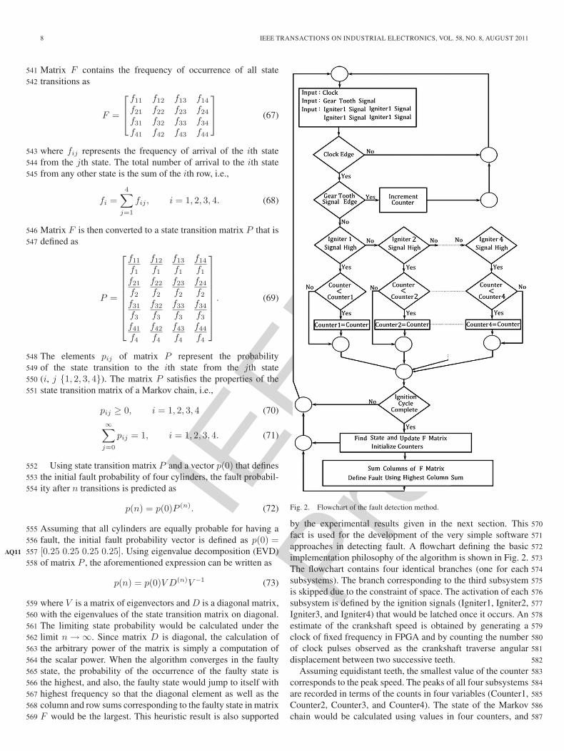
Fig. 2. Flowchart of the fault detection method.

by the experimental results given in the next section. This 570

fact is used for the development of the very simple software 571

approaches in detecting fault. A flowchart defining the basic 572

implementation philosophy of the algorithm is shown in Fig. 2. 573

The flowchart contains four identical branches (one for each 574

subsystems). The branch corresponding to the third subsystem 575

is skipped due to the constraint of space. The activation of each 576

subsystem is defined by the ignition signals (Igniter1, Igniter2, 577

Igniter3, and Igniter4) that would be latched once it occurs. An 578

estimate of the crankshaft speed is obtained by generating a 579

clock of fixed frequency in FPGA and by counting the number 580

of clock pulses observed as the crankshaft traverse angular 581

displacement between two successive teeth. 582

Assuming equidistant teeth, the smallest value of the counter 583

corresponds to the peak speed. The peaks of all four subsystems 584

are recorded in terms of the counts in four variables (Counter1, 585

Counter2, Counter3, and Counter4). The state of the Markov 586

chain would be calculated using values in four counters, and 587

IEEE

Proo

f


matrix F is modified. The fault would be identified by testing588

the sum of the columns of matrix F .589

V. COMPARISON OF THE METHODS590

The memory requirements and the number of computations591

during one complete ignition cycle can be taken as the criteria592

in comparing the algorithms. The comparison of the algorithm593

is made with the algorithm based on the cross-correlation of594

the observed signal xi and the signal with known faults xj595

[22]. Consider a vector with N samples in a complete ignition596

cycle. The cross-correlation coefficient of the data vector with597

a known fault vector is given by598

Sij =∑N

n=1 [(xi(n) − xi) (xj(n) − xj)]σiσj

.

A. Memory Comparison599

The method that is based on the cross-correlation needs N600

memory locations for the data and N memory location for601

each sample of the known fault. If N = 24, then 48 memory602

locations would be needed to detect any particular single fault603

under test. The proposed method needs only 25 memory lo-604

cations: a system counter, four counters of subsystems, four605

igniter signals, and 16 elements of the state transition matrix.606

The method can detect all possible single-fault cases.607

B. Number of Computations608

The method that is based on correlation will first calculate609

the velocity vector. The average and standard deviations of610

the velocity vectors are computed. The correlation coefficient611

would then be found by N multiplications, N additions, and a612

division for each fault. The proposed method needs only N + 8613

comparisons and 12 additions to identify all faults.614

If the signal of the multiple ignition cycle is tested, the615

memory requirement and the number of computations of the616

algorithm based on the correlation analysis would increase, but617

the memory requirements of the proposed method remain same.618

The methods that are based on model-based fault detection and619

wavelet-based techniques need floating point calculations, and620

they are computationally more expensive.621

The implementation philosophy and the flowchart of the622

proposed algorithm indicate the simplicity of the proposed fault623

diagnosis algorithm without floating point calculations, and its624

implementation on FPGA needs a short development time.625

VI. SIMULATION AND EXPERIMENTAL RESULTS626

A. Model Simulation627

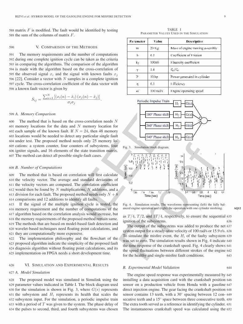
The proposed model was simulated in Simulink using the628

parameter values indicated in Table I. The block diagram used629

for the simulation is shown in Fig. 3, where G(s) represents630

the subsystem and Hi represents its health that scales the631

subsystem input. For the simulation, a periodic impulse train632

with a period of T was given to the system. The phase delay of633

the pulses to second, third, and fourth subsystems was chosen634

TABLE IPARAMETER VALUES USED IN THE SIMULATION

Fig. 3. Simulation block diagram.

Fig. 4. Simulation results. The waveforms representing (left) the fully bal-anced engine operation and (right) the operation with one cylinder misfiring. AQ12

as T/4, T/2, and 3T/4, respectively, to ensure the sequential 635

ignition of the subsystems. 636

The output of the subsystems was added to produce the net 637

system output for a steady-state velocity of 100 rad/s or 15.9 r/s. 638

To simulate the misfire event, the Hi of the faulty subsystem 639

was set to zero. The simulation results shown in Fig. 4 indicate 640

the time response of the crankshaft speed. Fig. 4 clearly shows 641

the speed fluctuations between different strokes of the engine 642

for the healthy and single-misfire fault conditions. 643

B. Experimental Model Validation 644

The engine speed response was experimentally measured by 645

installing a data acquisition card with the crankshaft position 646

sensor on a production vehicle from Honda with a gasoline 647

direct injection engine. The gear facing the crankshaft position 648

sensor contains 13 teeth, with a 30◦ spacing between 12 con- 649

secutive teeth and a 15◦ space between three consecutive teeth. 650

The extra tooth served as a reference in identifying the cylinder. 651

The instantaneous crankshaft speed was calculated using the 652

IEEE

Proo

f


Fig. 5. Experimental results. The waveforms representing (left) the fullybalanced engine operation and (right) the operation with one cylinder misfiring.AQ13

angular spacing between consecutive teeth and the time taken653

between two consecutive pulses. The data were acquired at654

an engine speed of approximately 1000 r/min by pressing the655

accelerator, and the load was provided to the engine by applying656

brakes. The manual control of the accelerator and the brake also657

caused some experimental error. The observed engine speed658

response is shown in Fig. 5. Under the no misfire condition, the659

instantaneous crankshaft velocity slightly fluctuates at approxi-660

mately 15.9 r/s. When a misfire is introduced in the engine, the661

velocity about which the fluctuation is observed is reduced to662

12.7 r/s.663

The comparisons of the experimental and simulation results664

shown in Figs. 4 and 5 indicate the following features.665

1) Under the no fault condition, the speed fluctuation is666

nearly 0.4 r/s in both the simulation and experimental667

results.668

2) Under the fault condition, the speed fluctuation is in-669

creased to nearly 1.6 r/s in both results.670

3) The average speed and the basic trend of the speed671

fluctuations in both experimental and simulation data are672

the same under both the faulty and no fault conditions.673

4) The experimental results also exhibit a random674

component.675

The similarity of the experimental and simulation results676

provides grounds for model validation and associated statistical677

analysis.678

To indicate the output of each subsystem, a 3-D plot is shown679

in Fig. 6, with the cylinder number along the y-axis, the power680

stroke along the x-axis, and the crankshaft speed along the681

z-axis. During a power stroke, the velocity is measured at six682

points, so the resolution of the plot is one-sixth of the power683

stroke. The outputs of subsystems can be observed in the plot684

along two edges that are parallel to the axis of the ignition cycle685

and on two slightly visible lines in between. A surface is created686

by joining the corresponding points on the cylinder axis. The687

mean elevation of the surface along the z-axis represents the688

crankshaft speed. The zoomed view of the surface shown in689

Fig. 6 shows the ripples in the surface. These ripples indicate690

the power variations in an ignition cycle. A complete ripple strip691

from cylinders 1 to 4 represents a complete ignition cycle.692

C. Misfire Detection Algorithm Simulation693

The misfire detection algorithm was simulated by generating694

the data using the hybrid model [24]. Random velocity fluc-695

Fig. 6. Experimental results. The surface representing (top) the cylinder 3misfiring and (middle) the no misfire portion of the zoomed edge of the middlefigure along (bottom) the ignition stroke axis. AQ14

tuations were introduced in the output data of the system by 696

adding noise to the data. The data sets with no fault, single 697

cylinder misfire fault, and double-misfire fault were generated. 698

The simulated data were processed using the proposed algo- 699

rithm, and the results are provided in Table II. The results 700

indicate that, under the no fault condition, the probability of the 701

fault remains almost the same for all cylinders, but under the 702

misfire conditions, the probability of the fault for the misfiring 703

IEEE

Proo

f


TABLE IISIMULATION RESULTS OF THE MISFIRE DETECTION ALGORITHM

cylinder becomes larger. Under the double-misfire condition,704

the probability increases for both misfiring cylinders.705

D. Misfire Experiment (The Third Spark Plug Is Removed)706

The pulses from the crankshaft speed sensor were received,707

and the crankshaft speed was calculated. The calculated speed708

was demultiplexed into four streams associated with each sub-709

systems using the igniter signal. The data of 46 ignition cycles,710

with the fault introduced in cylinder 3, were analyzed. The711

calculated matrix F is shown in the following:712

F =

⎡⎢⎣

0 0 0 00 0 0 00 0 35 10 0 1 9

⎤⎥⎦ . (74)

MATLAB could not perform the EVD of matrix F , so one extra713

transition is provided to all possible state transitions, i.e., F is714

initially taken as a matrix with all ones rather than as a null715

matrix. The resulting matrix F is shown in the following:716

F =

⎡⎢⎣

1 1 1 11 1 1 11 1 36 21 1 2 10

⎤⎥⎦ . (75)

The calculated value of the limiting state probability is717

P (∞) = [0.0645 0.0645 0.6452 0.2258]. (76)

The limiting probability indicated the highest probability of the718

fault in the third cylinder, which correctly indicated the fault.719

E. No Misfire Experiment 1 (All Spark Plugs Are Present)720

Under the no misfire condition, the data of 592 ignition721

cycles were analyzed. The resulting matrix F is722

F =

⎡⎢⎣

294 10 6 311 76 9 55 12 105 42 4 6 40

⎤⎥⎦ . (77)

If, initially, all of the cylinders are faulty with equal probability723

P (0) = [0.25 0.25 0.25 0.25]. (78)

The limiting state probability was estimated to be724

P (∞) = [0.5167 0.1777 0.2163 0.0893]. (79)

A misfire condition in cylinder 1 is detected even when no725

misfire is intentionally introduced in the system. To explore726

the result, another experiment was conducted to study the air727

TABLE IIILEAKAGE IN THE CYLINDERS

Fig. 7. Limiting probability convergence in the balanced engine.

leakage from the cylinders. In this experiment, all of the four 728

spark plugs were removed, and a pressure gauge was installed 729

in their position. The gauges were set to retain the peak value 730

of the observed air pressure. The pistons were moved by using 731

the starter motor. The maximum pressure was created in the 732

cylinders during the compression stroke and was retained by the 733

pressure gauge. The observed values of the cylinder pressure 734

are given in Table III. The results of this experiment indicate a 735

slight pressure loss (misfire) due to the air leakage in the first 736

cylinder. The result is promising as the fault is detected when 737

no perceptible symptoms of the fault were present in the engine 738

operation. The ECU was also not telling any fault. 739

F. No Misfire Experiment 2 (Balanced Engine) 740

An experiment was conducted on the engine, with the cylin- 741

ders in the maximally balanced conditions, and the limiting 742

probabilities are plotted after each ignition cycle to establish the 743

convergence rate of the algorithm. The plot is shown in Fig. 7, 744

with the probability of the misfire in each cylinder between 0.2 745

and 0.33. These results are fairly consistent with the simulation 746

results of the no fault condition given in Table II. 747

The experimental results of the hybrid model (Fig. 6) also 748

provide some insight in the fault diagnostic method. 749

1) The residual vector corresponds to the maximum down- 750

slope of the surface observed from one cylinder to the 751

next cylinder during an ignition cycle [refer to Fig. 6 752

(top)]. 753

2) The cylinder number where the maximum slope of the 754

surface is observed represents the state of the Markov 755

chain. 756

3) Under the no fault condition, the surface of the 3-D plot 757

of the hybrid model shown in Fig. 6 (middle) is fairly 758

smooth. The surface, however, lost its smoothness when 759

the misfire fault occurs, as shown in Fig. 6 (top). 760

To establish the accuracy of the prediction of the proposed 761

algorithm, the ROC analysis was performed. 762

IEEE

Proo

f


Fig. 8. ROC analysis of the fault detection algorithm.

VII. ROC ANALYSIS763

The objective of the ROC analysis is to study the accuracy764

of the algorithm as a function of n in (72). The analysis is765

performed for n = 0, n = 2, and n = 10. When n = 0, the state766

transition matrix is bypassed, and the fault decision is made767

purely on the basis of the observed residual. The proposed al-768

gorithm is essentially bypassed. When n = 2, a two-state ahead769

prediction is made, which is based on the past data, arranged as770

the state transition matrix. The affects of the algorithm would771

appear to some extent in the results. For n = 10, the results772

would be a closer approximation to the proposed algorithm,773

where n should be very large.774

For the ROC analysis, a binary classification {f3, nf} was775

assumed, where f3 represents a condition where the fault is776

present in the third cylinder and nf represents a condition777

where the fault is not present in the third cylinder. The lim-778

iting probability vector was calculated by the analysis of the779

experimental data of 50 ignition cycles, with the fault in the780

third cylinder. The estimated limiting probability vector was781

used to generate a predicted data set in each ignition cycle.782

These predicted data were used as a predicted instance and were783

classified to set {f3, nf}. The threshold for the classification784

was selected on the basis of the probability of the fault in the785

third cylinder, defined by the limiting probability vector. The786

predicted data set was then compared with the original data787

to identify the true positive events. The experiment was then788

repeated with the data from a maximally balanced cylinder789

with no misfire, and the false positive events were observed.790

Using the data of the true and false positive events, a confusion791

matrix was generated [28], and the data points were plotted on792

the ROC curve. Ten predicted data instances were generated,793

corresponding to each value of n, and were plotted on the ROC794

curve shown in Fig. 8. A convex hull and a chance line (major795

diagonal) were also plotted on the curve for analysis.796

Fig. 8 shows that all points corresponding to n = 0 are close797

to the chance line and are continuously crossing it, indicating798

a state of confusion. For n = 2, the cluster of points is shifted799

to the northwest side of the plot, indicating a better accuracy800

even with a rough approximation of the diagnosis algorithm.801

For n = 10, which is a better approximation of the proposed802

algorithm, the cluster of points is shifted further toward the803

northwest side and close to the convex hull, indicating even a804

better accuracy. This indicates that the residual analysis using 805

the limiting probability of the Markov chains results in a better 806

detection accuracy, with a small false alarm rate. 807

VIII. CONCLUSION 808

A hybrid switched linear model of the IC engine has been 809

proposed. This model is also extended for the analysis of 810

the probabilistic input variations. A fault diagnosis algorithm 811

that is based on the proposed model has also been presented. 812

The effectiveness of the hybrid model is established using 813

the simulation and experimental results. The effectiveness of 814

the proposed fault diagnosis algorithm is established using the 815

experimental results and the ROC analysis. It is also established 816

that the proposed algorithm is capable of detecting the incipient 817

faults to generate early fault warnings. The extension of the 818

proposed technique for the detection of multiple misfire, for 819

the misfire detection at low data rates that are compatible 820

to the ECU scan rate, and for the hardware development for 821

the proposed method is an area of future research for the 822

authors. 823

ACKNOWLEDGMENT 824

The authors would like to thank the research fellows of the 825

Control and Signal Processing Research Group, Mohammad 826

Ali Jinnah University, and the Center for Advanced Studies in 827

Engineering, Islamabad, Pakistan. 828

REFERENCES 829

[1] Y. L. Murphey, J. A. Crossman, Z. H. Chen, and J. Cardillo, “Automotive 830fault diagnosis—Part II: A distributed agent diagnostic system,” IEEE 831Trans. Veh. Technol., vol. 52, no. 4, pp. 1076–1098, Jul. 2003. 832

[2] J. A. Crossman, H. Guo, Y. L. Murphy, and J. Cardillo, “Automotive 833signal fault diagnostics—Part I: Signal fault analysis, signal segmentation, 834feature extraction and quasi-optimal feature selection,” IEEE Trans. Veh. 835Technol., vol. 52, no. 4, pp. 1063–1075, Jul. 2003. 836

[3] J. Luo, M. Namburu, and K. R. Pattipati, “Integrated model-based and 837data-driven diagnosis of automotive antilock braking system,” IEEE 838Trans. Syst., Man, Cybern. A, Syst., Humans, vol. 40, no. 2, pp. 321–336, 839Mar. 2010. 840

[4] M. Lee, M. Yoon, M. Sunwoo, S. Park, and K. Lee, “Development of 841a new misfire detection system using neural network,” Int. J. Automot. 842Technol., vol. 7, no. 5, pp. 637–644, 2006. 843

[5] J. Luo, K. R. Pattipati, L. Qiao, and S. Chigusa, “An integrated diagnos- 844tic development process for automotive engine control systems,” IEEE 845Trans. Syst., Man, Cybern. C, Appl. Rev., vol. 37, no. 6, pp. 1163–1173, 846Nov. 2007. 847

[6] Q. R. Butt and A. I. Bhatti, “Estimation of gasoline engine parameters 848using higher order sliding mode,” IEEE Trans. Ind. Electron., vol. 55, 849no. 11, pp. 3891–3898, Nov. 2008. 850

[7] E. Hendrick and S. C. Sorenson, “Mean value modeling of spark ignition 851engines,” presented at the Int. Congr. Expo., Detroit, MI, 1990, SAE 852Technical Paper 900616. 853

[8] A. Balluchi, L. Benvenuti, M. D. Di Benedetto, C. Pinello, and 854A. L. Sangiovanni-Vincentelli, “Automotive engine control and hybrid 855systems: Challenges and opportunities,” Proc. IEEE, vol. 88, no. 7, 856pp. 888–912, Jul. 2000. 857

[9] A. K. Sood, A. A. Fahs, and N. A. Henein, “Engine fault analysis: 858Part II—Parameter estimation approach,” IEEE Trans. Ind. Electron., 859vol. IE-32, no. 4, pp. 301–307, Nov. 1985. 860

[10] F. D. Torrisi and A. Bemporad, “HYSDEL—A tool for generating compu- 861tational hybrid models for analysis and synthesis problems,” IEEE Trans. 862Control Syst. Technol., vol. 12, no. 2, pp. 235–249, Mar. 2004. 863

[11] N. Giorgetti, G. Ripaccioli, and A. Bemporad, “Hybrid model predictive 864control of direct injection stratified charge engines,” IEEE/ASME Trans. 865Mechatronics, vol. 2, no. 5, pp. 499–506, Oct. 2006. 866

IEEE

Proo

f


[12] M. Iqbal, A. I. Bhatti, S. Iqbal, and Q. Khan, “Robust parameter esti-867mation of nonlinear systems using sliding mode differentiator observer,”868IEEE Trans. Ind. Electron., Feb. 2010, to be published.AQ15 869

[13] A. I. Bhatti, J. A. Twiddle, S. K. Spurgeon, and N. B. Jones, “Engine870coolant system fault diagnostics with sliding mode observers and fuzzy871analyser,” in Proc. IASTED Conf. Model., Identif. Control, Innsbruck,872Austria, 1999.873

[14] M. Nyberg and A. Perkovic, “Model based diagnosis of leaks in the air-874intake system of an SI-engine,” presented at the Int. Congr. Expo., Detroit,875MI, 1998, SAE Paper 980514.876

[15] R. Isermann, “Model based fault detection and diagnosis—Status and877applications,” Annu. Rev. Control, vol. 29, no. 1, pp. 71–85, 2005.878

[16] G. Biswas, M. O. Cardier, J. Lunze, L. T. Massuyes, and M. Staroswiecki,879“Diagnosis of complex systems: Bridging the methodologies of FDI and880DX communities,” IEEE Trans. Syst., Man, Cybern. B, Cybern., vol. 34,881no. 5, pp. 2159–2162, Oct. 2004.882

[17] L. A. Feldkamp, T. M. Feldkamp, and D. V. Prokhorov, “Adaptive classi-883fication,” in Proc. IEEE AS-SPCC, 2000, pp. 52–57.884

[18] M. Montini and N. Speciale, “Multiple misfire identification by a wavelet-885based analysis of crankshaft speed fluctuation,” in Proc. IEEE Int. Symp.886Signal Process. Inf. Technol., Aug. 2006, pp. 144–148.887

[19] G. Rizzoni, J. G. Pipe, R. N. Riggin, and M. P. VanOyen, “Fault isolation888and analysis for IC engine onboard diagnostics,” in Proc. 38th IEEE Veh.889Technol. Conf., Philadelphia, PA, 1988, pp. 237–244.890

[20] I. Morgan and H. Liu, “Predicting future states with n-dimensional891Markov chains for fault diagnosis,” IEEE Trans. Ind. Electron., vol. 56,892no. 5, pp. 1774–1781, May 2009.893

[21] J. Merkisz, P. Bogus, and R. Grzeszczyk, “Overview of engine misfire894detection methods used in on board diagnostics,” J. KONES Combust.895Engines, vol. 8, no. 1/2, pp. 326–341, 2001.896

[22] A. K. Sood, C. B. Friedlander, and A. A. Fahs, “Engine fault analysis:897Part I—Statistical methods,” IEEE Trans. Ind. Electron., vol. IE-32, no. 4,898pp. 294–300, Nov. 1985.899

[23] M. A. Rizvi, A. I. Bhatti, and Q. R. Butt, “Misfire detection in IC en-900gines using finite state automata,” in Proc. 15th Int. Conf. Soft Comput.901MENDEL, Brno, Czech Republic, Jun. 24–26, 2009, pp. 93–100.902

[24] M. A. Rizvi and A. I. Bhatti, “Hybrid model for early detection of misfire903fault in SI engines,” in Proc. IEEE 13th Int. Multitopic Conf., Nov. 2009,904pp. 1–6.905

[25] M. A. Rizvi, A. I. Bhatti, and Q. R. Butt, “Fault detection in a class of906hybrid system,” in Proc. ICET , Oct. 2009, pp. 130–135.907

[26] J. L. Speyer and W. H. Chung, Stochastic Processes, Estimation and908Control., 1st ed. Philadelphia, PA: SIAM, 2008, pp. 157–159.909

[27] P. K. Wong, L. M. Tam, K. Li, and C. M. Vong, “Engine idle speed910system modeling and control optimization using artificial intelligence,”911Proc. Inst. Mech. Eng. D, J. Automobile Eng., vol. 224, no. 1, pp. 55–72,912Jun. 2009.913

[28] T. Fawcett, “An introduction to ROC analysis,” Pattern Recognit. Lett.,914vol. 27, no. 8, pp. 861–874, Jun. 2006.915

[29] S. A. Arogeti, D. Wang, and C. B. Low, “Mode identification of hybrid916systems in the presence of fault,” IEEE Trans. Ind. Electron., vol. 57,917no. 4, pp. 1452–1467, Apr. 2010.918

Muddassar Abbas Rizvi received the B.S. de-919gree in electrical engineering from the University920College of Engineering, Taxila, Pakistan, in 1990921and the M.S. degree in systems engineering from922Quaid-e-Azam University, Islamabad, Pakistan. He923is currently working toward the Ph.D. degree at the924Mohammad Ali Jinnah University, Islamabad.925

He has an 18-year experience in electronic circuit926design and development. He has been working as a927Visiting Faculty Member with the National Univer-928sity of Science and Technology, Islamabad, for the929

last three years. He is the first author and coauthor of five conference papers. His930research interests include mathematical modeling, fault diagnostics, computer931programming, and electronic circuit designing.932

Aamer Iqbal Bhatti Sr. (SM’XX) received the AQ16933B.S. degree in electrical engineering from the AQ17934University of Engineering & Technology, Lahore, AQ18935Pakistan, in 1993, the M.S. degree in control systems AQ19936from the Imperial College of Science, Technology 937and Medicine, London, U.K., in 1994, and the Ph.D. 938degree in control engineering from the University of 939Leicester, Leicester, U.K., in 1998. 940

He worked on the idle speed control of the Ford 941Mondeo Engine for his Ph.D. research. He continued 942his stay at the University of Leicester for his post- 943

doctoral research on fault diagnostics and control of high-powered diesel 944engines, funded by Caterpillar. In 1999, he returned to Pakistan and started 945working for a consultancy firm (ERDC), providing services in the field of AQ20946aerospace controls, where he worked on nonlinear simulations of air vehicles, 947system identification, controller design for aerospace vehicles, and data acquisi- 948tion experiment design. He moved to Communications Enabling Technologies, 949Islamabad, Pakistan, in 2001, where he worked on the enhancements of the line 950echo cancellers used in VoIP. Later on, he cofounded the Center for Advanced 951Studies in Engineering (an engineering education institution) and CARE (an AQ21952R&D company). At CARE, he led a team that indigenously designed a radar 953signal processor and an ELINT system. In 2007, he joined the Mohammad Ali AQ22954Jinnah University, Islamabad, where he is currently a Professor of DSP and 955control systems with the Department of Electronic Engineering. He is the first 956author and coauthor of more than 35 refereed international papers, including 957four journal publications. His research interests are sliding mode applications 958and radar signal processing. 959

Qarab Raza Butt received the B.S. degree in me- AQ23960chanical engineering from the University College 961of Engineering, Taxila, Pakistan, in 1989, a post- 962graduate diploma in computer system software and 963hardware from the Computer Center, Islamabad, 964Pakistan, in 1990, and the M.S. degree in control AQ24965engineering from the Center for Advanced Studies 966in Engineering, Islamabad, in 2004, where he is 967currently working toward the Ph.D. degree. 968

Since 1990, he has been working in the industry 969as an Installation, Fabrication, and Design Engineer 970

for nearly 12 years. He is the first author and coauthor of more than 13 inter- 971national papers, including two journal publications. His research interests are 972mathematical modeling of dynamic systems for control and fault diagnostics. 973

IEEE

Proo

f

AUTHOR QUERIES

AUTHOR PLEASE ANSWER ALL QUERIES

AQ1 = Please verify the postal code provided.AQ2 = Please provide the expanded form of the acronym ‘MVEM.’AQ3 = Sentence was restructured to make it parallel. Please check if the thought is preserved.AQ4 = Please provide the expanded form of the acronym ‘NN.’AQ5 = The acronym ‘FPGA’ was defined as ‘field programmable gate array.’ Please check if appropriate.AQ6 = Please provide the expanded form of the acronym ‘LTI.’AQ7 = Sentence was restructured. Please check if the thought is preserved.AQ8 = Please provide the expanded form of the acronym ‘EFI.’AQ9 = Sentence was restructured. Please check if the thought is preserved.AQ10 = Sentence was restructured. Please check if the thought is preserved.AQ11 = Sentence was restructured. Please check if the thought is preserved.AQ12 = Fig. 4 caption was restructured. Please check if the thought is preserved.AQ13 = Fig. 5 caption was restructured. Please check if the thought is preserved.AQ14 = Fig. 6 caption was restructured. Please check if the thought is preserved.AQ15 = Please provide publication update in Ref. [12].AQ16 = Please provide membership history of author Aamer Iqbal Bhatti Sr.AQ17 = ‘Bachelor’s’ was captured as ‘B.S.’ Please check if appropriate.AQ18 = ‘UET’ was defined as ‘University of Engineering & Technology.’ Please check if appropriate.AQ19 = ‘Masters’ was captured as ‘M.S.’ Please check if appropriate.AQ20 = Please provide the expanded form of the acronym ‘ERDC.’AQ21 = Please provide the expanded form of the acronym ‘CARE.’AQ22 = Please provide the expanded form of the acronym ‘ELINT.’AQ23 = ‘Bachelor’s’ was captured as ‘B.S.’ Please check if appropriate.AQ24 = ‘Masters’ was captured as ‘M.S.’ Please check if appropriate.

END OF ALL QUERIES

IEEE

Proo

f

IEEE TRANSACTIONS ON INDUSTRIAL ELECTRONICS, VOL. 58, NO. 8, AUGUST 2011 1

Hybrid Model of the Gasoline Enginefor Misfire Detection

1

2

Muddassar Abbas Rizvi, Aamer Iqbal Bhatti, Sr., Member, IEEE, and Qarab Raza Butt3

Abstract—This paper proposes a novel hybrid model for an4internal combustion engine, with the power generated due to5combustion as the input and the crankshaft speed fluctuations as6the output. The individual cylinders of the engine are considered7as subsystems for which a nonlinear model, based on the physical8principles, is derived. The proposed model is linearized at an oper-9ating point, and a switched linear model is formed. The simulation10results of the proposed model are validated by matching the results11with the experimentally observed data. Using the properties of the12validated model, it is shown that the crankshaft speed variations13observed in the engine are a Markov process. A novel algorithm14that is based on the Markov chain is proposed to detect the15misfire in the spark ignition engines. In the ensuing engine rig16experiments, an igniter misfire is introduced in the system and17is successfully detected. The analysis of the data shows that the18engine also has an air leakage in a cylinder (a developing misfire),19which is experimentally confirmed later.20

Index Terms—Discrete event model (DEM), hybrid systems,21Markov chains, mean value model (MVM), misfire detection,22spark ignition (SI) engine.23

I. INTRODUCTION24

THE complexity of automotive vehicles is increasing as25

more and more mechanically driven parts are being re-26

placed by electronically driven actuators. An electronic control27

unit (ECU) is being installed in modern vehicles, which not28

only monitors the sensors installed in the vehicle but also29

controls the electronic actuators. The ECU also provides a di-30

agnostic code to identify different faults present in the vehicle.31

Fault prognosis in automotives is being studied for integration32

in future vehicles. Murphey indicated that the development of33

computationally simpler fault diagnosis algorithms for auto-34

motive systems is considered as the most challenging problem35

[1]. The problem is still being addressed by the research com-36

munity [1]–[4]. A survey of different automotive models and37

fault diagnosis techniques found in literature is provided.38

A general survey indicates that the spark ignition (SI) engine39

is mathematically represented by either the mean value model40

Manuscript received May 3, 2010; revised July 27, 2010; acceptedSeptember 9, 2010. This work was supported in part by the Higher EducationCommission and in part by the ICT Research and Development Fund ofPakistan.

M. A. Rizvi and A. I. Bhatti Sr. are with the Mohammad Ali Jinnah Univer-sity, Islamabad 44000, Pakistan (e-mail: [email protected]; [email protected]).

Q. R. Butt is with the Center for Advanced Studies in Engineering, G-5/1,Islamabad, Pakistan (e-mail: [email protected]).

Color versions of one or more of the figures in this paper are available onlineat http://ieeexplore.ieee.org.

Digital Object Identifier 10.1109/TIE.2010.2090834

(MVM) [6], [7] or the discrete event model (DEM) [8]. The 41

MVM is based on the average torque generated in a complete 42

ignition cycle. The model therefore cannot efficiently detect any 43

fault during an individual stroke of an ignition cycle. The DEM 44

is a hybrid model, with states representing the compression, 45

ignition, expansion, and exhaust strokes described as nonlinear 46

differential equations. The engine state is defined by solving 47

all four nonlinear equations. Due to a high computational load, 48

both MVM and DEM are difficult to solve in embedded sys- 49

tems, and they could not attract the fault diagnostic community, 50

especially for misfire fault detection. Luo et al. mentioned that 51

the algorithms executed in the ECU are required to be simpler 52

than most models or signal-based algorithms proposed by the 53

academia [5]. Sood et al. proposed a kinematic model, with 54

the fuel as the input and the crankshaft velocity as the output 55

[9]. The model is based on forces acting on the piston due to 56

the combustion of fuel in the engine cylinder and load acting 57

on the engine. The model was used for the detection of the 58

misfire fault using parameter estimation, and it was concluded 59

that the model-based approach proved to be computationally 60

expensive. Wong et al. proposed an engine model based on the 61

experimental sample data using neural network methods [27]. 62

The model is, however, explicitly applicable only to idle speed 63

control applications. A hybrid modeling approach was used for 64

other automotive applications but not for fault detection [10], 65

[11]. An addition to hybrid modeling is the representation of 66

the discrete states as modes of hybrid system, and each mode 67

system is governed by different continuous dynamics. Mode 68

identification in the presence of fault is carried out by a rule- 69

based analysis of the analytic redundancy relations [29]. The 70

fault diagnosis is based on either model or signal data analysis. 71

Model-based fault diagnosis methods have the advantage that 72

the signal features associated with fault have a physical inter- 73

pretation [9], e.g., the discharge coefficient estimated using the 74

sliding mode observer provides an insight about the physical 75

significance of a parameter [6], [12]. Methods that are based 76

on MVEM were applied for fault diagnosis in coolant systems AQ277

[13], air paths before and after a throttle valve [14], etc. Most 78

of these techniques used state observers, parity equations, or 79

parameter estimation techniques for fault diagnosis [15]. The 80

parameter values forming the basis of fault detection in the 81

model-based method also change with the operating conditions, 82

like load, ambient temperature, pressure, vehicle aging, etc. 83

The value of the discharge coefficient estimated using the 84

sliding mode observer under different load conditions indicates 85

this parameter variation [6]. Sood et al. mentioned that fault 86

diagnosis using some parameters which are not constant leads 87

to the further increase in the complexity of the fault diagnostic 88

0278-0046/$26.00 © 2011 IEEE

IEEE

Proo

f


problem [9]. The heavy computational load and the adaptive89

selection of the threshold values for fault detection added so90

much complexity that not only restricts their application only91

to offline fault detection but also increases the trend of using92

the statistical tools by the fault diagnostics and isolation (using93

control engineering tools) community [16]. The signal-basedAQ3 94

methods identify the features linked with faults in a signal.95

Residual analysis is carried out to identify these features.96

Crossman described some features associated with faults and97

methods to identify them [2].98

Misfire fault occurs when a combustion does not occur in99

one or more engine cylinders. It may occur due to a missing100

spark, an air leakage, or a fault in fuel injection. A number of101

techniques that are based on an artificial neural network were102

used to detect the misfire fault [4], [17]. Feldkamp proposed103

techniques that characterize fault states as hidden states in a104

hidden Markov model and used extended Kalman filter esti-105

mates for NN training [17]. It seems that the author implicitlyAQ4 106

assumed a stochastic analysis and a linearized version of some107

engine nonlinear models. Since the engine is a highly nonlinear108

system whose output depends on a large number of factors, it109

would be difficult to simulate all possible healthy and faulty110

conditions to train the neural network to ensure a robust fault111

detection. Montini proposed a wavelet-based analysis of the112

crankshaft speed fluctuation signal [18], and Rizzoni [19] and113

Sood [22] proposed different data classification methods to114

decide between the binary hypothesis conditions of the fault and115

no fault conditions using a correlation analysis of the data. Both116

wavelet- and correlation-based methods were computationally117

heavy, and the algorithm also needed heuristic guidelines to118

extract the features and to relate to the faults. Although the ap-119

plication of the Markov chains for fault diagnosis can be found120

in the literature [20], however, disturbances that are due to faults121

in dynamic systems have not been proved as a Markov process122

for fault diagnosis and isolation. This paper proves these dis-123

turbances as a Markov process. Morgan et al. indicated that the124

potential advantage of the application of the Markov chains is125

its ability to predict, and they applied it to predict the future con-126

centration of the elements in the lubricant analysis of the marine127

engine [20], where an early prediction is important due to the128

maintenance problems when the ship is at the sea [20]. Luo129

mentioned that the recently introduced new approaches for fault130

diagnosis combined model-based and data-driven techniques131

to obtain a better diagnostic performance [3]. A method that132

transforms the engine speed fluctuations to finite state automata133

is presented in the literature, which stressed on the implemen-134

tation using a field programmable gate array (FPGA) [23].AQ5 135

The objective of this paper is to develop a novel mathematical136

model for SI engines that can explain the crankshaft speed137

fluctuations when a deterministic input with a small randomly138

varying component is applied to the SI engine. The utility of the139

proposed model is expressed by presenting a novel method for140

misfire detection. The proposed method is based on the speed141

fluctuation of the crankshaft. The method is simple and cost142

effective, and it needs no additional installation as the sensor is143

preinstalled in all modern vehicles [21].144

This paper is organized as follows. Section II presents a145

hybrid mathematical model that is used to represent the steady-146

state behavior of the internal combustion (IC) engine [24], [25]. 147

A nonlinear model representing the motion of the piston in 148

the engine cylinders is derived using the physical principles 149

to represent the subsystems of the hybrid model. The non- 150

linear model is linearized at an operating point, and the engine 151

is taken as a switched linear hybrid system. The properties 152

of the proposed hybrid system are investigated. Section III 153

presents the statistical analysis of the system output against a 154

random variation of the inlet air, and finally, the fluctuation 155

in the crankshaft speed is proved to be a Markov process. 156

Section IV presents the algorithm for fault diagnosis, and a 157

comparison of the presented method with an existing method 158

is provided in Section V. The simulation and experimental 159

results are presented, analyzed, and discussed in Section VI. 160

The relative/receiver operating characteristic (ROC) analysis is 161

presented in Section VII. The concluding remarks are given in 162

Section VIII, and the references are given at the end. 163

II. SYSTEM MODELING 164

For system modeling, a four-cylinder four-stroke engine is 165

assumed, where the ignition occurs in only one cylinder at a 166

time. The pistons of the four cylinders are coupled to a common 167

shaft via a crankshaft. The power strokes of all cylinders are 168

separated from each other by 180◦, and they periodically occur 169

after two shaft revolutions, named as an ignition cycle. During 170

a power stroke, the air–fuel mixture is burnt inside the cylinder, 171

and pressure develops in the chamber of the cylinder, applying 172

force on the piston. The modeling is carried out in the following 173

two steps. 174

1) In the first step, a deterministic switched linear model, 175

with the power generated by the fuel combustion as the 176

input and the crankshaft angular velocity as the output, is 177

presented in Section II-A–II-E. 178

2) In the second step, the statistical properties of the air in- 179

take in the cylinder are studied to establish that the crank- 180

shaft speed fluctuations are Gaussian and Markov. The 181

properties of air are explored because the engine power is 182

manipulated by controlling the amount of air intake. 183

A. Hybrid Model 184

The SI engine is modeled as a hybrid system with four iden- 185

tical minimum phase LTI subsystems, where each subsystem AQ6186

represents an engine cylinder. A subsystem/cylinder is active 187

when it contributes power to the system, i.e., during a power 188

stroke. The subsystems are sequentially actuated during an 189

ignition cycle. The output of the system would be a vector 190

sum of the outputs of the subsystems. The following are the 191

modeling assumptions. 192

Assumption 1: The system operates at a steady-state condi- 193

tion on a constant load. 194

Assumption 2: The air–fuel ratio is stoichiometric. 195

Assumption 3: The whole energy is instantaneously added at 196

the beginning of the power stroke and is delivered to a storage 197

element (flywheel) at a constant rate. 198

Assumption 4: At any time instant, only one cylinder would 199

receive an input to become active, and it exerts force on the 200

IEEE

Proo

f


piston and other cylinders that are being passive due to suction.201

The compression and exhaust processes contribute to the engine202

load torque.AQ7 203

If the period of the ignition cycle is T , u(t) is the system204

input at time t during an ignition cycle, and ui(t) is the input of205

the ith subsystems. Based on Assumption 4206

ui(t) = u(t) when(i − 1)T

4< t <

iT

4, i = 1, 2, 3, 4 (1)

ui(t) = 0 otherwise. (2)

The framework of the hybrid model for a maximally balanced207

SI engine with four cylinders is represented as a five-tuple208

model 〈μ,X,Γ,Σ, φ〉. The basic definition of the model para-209

meters is given in the following.210

1) μ = {μ1, μ2, μ3, μ4}, where each element of the set211

represents the active subsystem of the hybrid model.212

2) X ∈ R2 represents the state variable of the continu-213

ous subsystems. It would be proved in the next section214

that vector X would have velocity and acceleration as215

components.216

3) Γ = {G(s)}, where G(s) is the transfer function of the217

linear subsystems. For the maximally balanced cylinder,218

the set contains a single element. The transfer function219

G(s) is derived in Sections II-B–II-D of this section. The220

model can be defined in state space as221

x(t) =AX + BU (3)y(t) =CX + DU (4)

where222

U ∈ R A ∈ R2×2 B ∈ R2×1 C ∈ R1×2 D ∈ R.

4) Σ : μ → μ represents the generator function that defines223

the activation of the next subsystem after the activity224

of the current subsystem end. The generator function is225

defined in terms of the crankshaft position as226

Σ =

⎧⎪⎪⎨⎪⎪⎩

μ1 4nπ ≤∫

θ1dt < (4n + 1)πμ2 (4n + 1)π ≤

∫θ1dt < (4n + 2)π

μ3 (4n + 2)π ≤∫

θ1dt < (4n + 3)πμ4 (4n + 3)π ≤

∫θ1dt < (4n + 4)π

(5)

where n = 0, 1, 2 and∫

θ1dt represents the instantaneous227

shaft position that identifies the output of the generator228

function.229

5) φ : Γ × μ × X × u → X defines the initial condition for230

the next subsystem after a switching event, where u231

represents the input of the active subsystem. Fig. 1 shows232

the subsystems and switching sequence of the proposed233

engine hybrid model.234

B. Nonlinear Subsystem Modeling235

Consider δQ as the amount of energy added in the system236

by burning the air–fuel mixture. Based on Assumption 3, the237

energy is instantaneously added in the cylinder. This will appear238

as an increase in the internal energy of the system239

δU = δQ. (6)

Fig. 1. Hybrid system with four subsystems.

A part of this internal energy is used to do work, and the rest of 240

the energy is drained in the coolant and exhaust system. If the 241

internal energy changes to work with the constant efficiency ηt, 242

then work δW is given by the energy balance equation as 243

δW = −ηtδU. (7)

Using (6) 244

δW = −ηtδQ. (8)

If p is the pressure due to the burnt gases, then the work done 245

during the expansion stroke is given by 246

W =

V 2∫V 1

pdV (9)

where V1 and V2 are the initial and final volumes of the cylinder 247

during expansion. For adiabatic expansion 248

pV γ = k1 (10)

where k1 and γ are constant. Hence, (9) becomes 249

W =

V 2∫V 1

k1V−γdV (11)

W = k1V −γ+1

2 − V −γ+11

−γ + 1. (12)

Consider the closed end of the piston as the origin. Also, 250

assume that A is the surface area of the piston and x is a 251

continuous variable that represents the instantaneous piston 252

position. When the piston moves a small distance δx from 253

its initial position x, where δx is constant and where it can 254

be arbitrarily chosen to be small, then the work done can be 255

expressed as 256

δW = k1[A(x + δx)]−γ+1 − [Ax]−γ+1

−γ + 1(13)

δW = k1A−γ+1

−γ + 1[(x + δx)−γ+1 − x−γ+1

](14)

δW =k1A

−γ+1

−γ + 1

[x−γ+1

(1 +

δx

x

)−γ+1

− x−γ+1

](15)

δW =k1A

−γ+1x−γ+1

−γ + 1

[(1 +

δx

x

)−γ+1

− 1

]. (16)

IEEE

Proo

f


Expanding (16) using a binomial series, neglecting the higher257

powers of δx, and simplifying258

δW = k1A−γ+1x−γδx. (17)

Using (8), (17) becomes259

δQ =k1A

−γ+1x−γδx

ηt. (18)

If F is the force applied by the burnt gases, m is the mass of the260

engine moving assembly (piston, connecting rod, crankshaft,261

and flywheel), k2 is the coefficient of friction, and k3 is the262

coefficient of elasticity, then the net force acting on the piston263

is given by264

md2x

dt2= F − k2

dx

dt− k3x (19)

md2x

dt2+ k2

dx

dt+ k3x = F. (20)

The net work done by the expanding gases against the load,265

friction, and elastic restoring forces when the piston moves by266

a small distance δx would be given as267 [m

d2x

dt2+ k2

dx

dt+ k3x

]δx = δW. (21)

Using (17), the aforementioned equation becomes268 [m

d2x

dt2+ k2

dx

dt+ k3x

]δx = k1A

−γ+1x−γδx. (22)

The displacement δx can be chosen to be constant and ar-269

bitrarily small. As the piston moves, the volume inside the270

combustion chamber increases, resulting in the reduction of the271

instantaneous pressure on the piston. The instantaneous power272

is therefore a function of the piston position. The instantaneous273

power delivered by the engine would be calculated by differen-274

tiation as275 [m

d3x

dt3+ k2

d2x

dt2+ k3

dx

dt

]δx = − k1γA−γ+1x−γ−1 dx

dtδx

(23)

md3x

dt3+ k2

d2x

dt2+ k3

dx

dt= − k1γA−γ+1x−γ−1 dx

dt.

(24)

Write (24) in terms of velocity v as276

md2v

dt2+ k2

dv

dt+ k3v = − γηt

k1A−γ+1x−γδx

ηt

v

xδx(25)

md2v

dt2+ k2

dv

dt+ k3v = γηtδQ

v

xδx(26)

md2v

dt2+ k2

dv

dt+ k3v =

γηtv

x

δQ

δt

δt

δx. (27)

Equation (27) represents a nonlinear model of the crankshaft277

speed when the power is provided to the engine by fuel ignition.278

C. Model Linearization 279

For model linearization, consider that the piston always 280

moves between two extreme positions xt and xb, where xt 281

represents the piston position at the top dead center (TDC) 282

and xb represents the piston position at the bottom dead center 283

(BDC). Therefore, x can never be zero, and the right-hand side 284

(RHS) of (27) is a smooth function. The model is therefore 285

linearized at the TDC. 286

If a constant finite power P is added to a cylinder when its 287

piston is at the TDC and the system delivers power P (x), then 288

the power delivered by system would be given as 289

md2v

dt2+ k2

dv

dt+ k3v =

γηvt

xP (x)

1v

(28)

md2v

dt2+ k2

dv

dt+ k3v =

γηt

xP (x). (29)

Linearizing the system at the TDC (x = xt) under the 290

steady-state condition, (29) is written as 291

md2v

dt2+ k2

dv

dt+ k3v =

γηt

xtP (x). (30)

Based on Assumption 3, the system is delivering power at 292

a constant rate; hence, P (x) is taken as constant. The RHS of 293

(30) is therefore constant, and the expression becomes a linear 294

differential equation. 295

D. Model Parameter Estimation 296

The engine operating power can be estimated by using the 297

manifold air pressure/manifold air flow sensors and by esti- 298

mating the mass of the fuel sprayed and the heat equivalent of 299

the fuel. The typical value of the efficiency of the SI engine 300

is nearly 35%. All of the parameters on the RHS of (30) are 301

known, except the elasticity k3 and friction coefficients k2. 302

The movement of the piston exhibits a periodic behavior, 303

with the same fundamental frequency as that of the rotational 304

speed of the engine shaft. This provides a heuristic guideline in 305

choosing the value of k3 as a function of the crankshaft angular 306

speed. The empirical choice is validated using the simulation 307

and experimental results reported later 308

k3 = ω2 = (2πN)2 (31)

where N is the engine speed in revolution per second. 309

During experimental verification, the load is also applied by 310

friction. Most frictional models described in literature are based 311

on the empirical relations as a polynomial in the engine speed. 312

A simplified frictional model is chosen, with a term containing 313

only the square of the engine speed 314

k2 = b ω2. (32)

On the basis of the simulation and experimental results, it is 315

established that the optimal selection of the value of b varies 316

between 0.2 and 0.5. The values of parameters k1 and k2 depend 317

on the operating point. The stability of the linearized subsystem 318

is ensured by the Routh–Hurwitz criteria. 319

IEEE

Proo

f


E. Model Properties320

The properties of the hybrid model when the engine is oper-321

ating under the steady-state conditions are presented as a set of322

propositions, lemmas, and theorems given in the following.323

Proposition 1: When the engine is running with a constant324

speed, the input to the engine system is a periodic impulse train325

with a period of T/4, where T is the period of the ignition326

cycle. This is because the energy is added in the engine as an327

impulse (Assumption 3), and the event of the addition of the328

energy occurs four times during an ignition cycle energy, i.e.,329

once in each cylinder.330

Lemma 1: Under the no misfire condition, the system output331

exhibits a periodic ac component with a period of T/4, where332

T represents the period of the ignition cycle (two revolutions).333

Proof: When all subsystems are identical and when they334

are represented by a linear model, then a periodic input with a335

period of T/4 would produce a periodic output with the same336

frequency.337

Lemma 2: When a cylinder misfires, the output of the system338

exhibits a periodic ac component with a period of T .339

Proof: The misfire can be considered as the loss of one340

of every fourth impulse of the input signal. The input signal is341

therefore periodic, with a period of T rather than T/4, and the342

output also exhibits a fundamental frequency of T .343

Lemma 3: Under the no misfire fault condition, the output344

contains four identical peaks in an ignition cycle.345

Proof: The input signal during an ignition cycle contains346

four impulses. As the subsystems are stable LTI minimum347

phase second-order systems, they exhibit one peak in the output348

against each impulse occurring in the impulse train input.349

Lemma 4: In the steady-state conditions with fault in the ith350

event, no peak would be observed due to the input of the ith351

subsystem.352

Proof: The absence of an impulse at the ith place in353

the input signal would result in the loss of the corresponding354

peak.355

The results of Lemmas 1, 2, 3, and 4 can be observed from356

the simulation and experiment results discussed later.357

Definition 1: The system is said to be in the steady state358

when the net change in the system output v(t) in one complete359

ignition cycle is zero360

v(t + T ) = v(t). (33)

Theorem 1: Under the steady-state and no fault conditions361

when the same input is given to the identical subsystems (max-362

imally balanced cylinders), the response of each subsystems363

would be independent.364

Proof: If u is the input to a subsystem, v(0) is the initial365

condition, and h(t) is the impulse response of a subsystem, then366

the output of the second subsystem (i.e., at time t, where T/4 <367

t < 2T/4) is given by368

v(t) = v(0) +

T4∫

0

h(t − τ)u(τ)dτ +

t∫T4

h(t − τ)u(τ)dτ.

(34)

Based on Lemma 1, the output signal is periodic, with a period 369

of T/4; therefore 370

v(T/4) = v(0) (35)

v(0) +

T4∫

0

h(t − τ)u(τ)dτ = v(0) (36)

and (34) becomes 371

v(t) = v(T/4) +

t∫T4

h(t − τ)u(τ)dτ. (37)

Hence, during the activation time of the second subsystem, 372

the output depends only on the input u(t) and the impulse 373

response of the second subsystem, and it is independent from 374

the response of the first subsystem. Similarly, it can be proved 375

that, under the steady-state conditions, the responses of all 376

cylinders are independent. 377

Proposition 2: For an EFI engine, the air intake in the AQ8378

cylinders is measured, and a fuel that is proportional to the 379

amount of air intake is sprayed into it. Therefore, the power 380

input to the system in the steady-state conditions is proportional 381

to the amount of air sucked. 382

The following corollaries that are based on the properties 383

of the proposed hybrid model would be used for onward sta- 384

tistical analysis and for the development of the fault detection 385

methodology. 386

Corollary 1: Four peaks would be observed in one ignition 387

cycle of a four-cylinder SI engine (Lemma 3). 388

Corollary 2: The amplitudes of the four observed peaks 389

represent four independent events (Theorem I). 390


input power (due to a linear model of the subsystems). 392


amount of air intake (based on Corollary 3 and Proposition 2). 394

III. STATISTICAL ANALYSIS 395

The air intake is considered as a random variable, and the 396

statistical analysis is carried out in the following steps. 397

1) Determine the probability density function (pdf) of the 398

random variable representing the peak values of the 399

velocity observed in an ignition cycle. 400

2) Form a collection of the aforementioned random variable. 401

3) Prove that the aforementioned collection is Gaussian and 402

Markov. 403

A. Step 1 404

Using Corollary 4, it can be established that the pdf of the 405

air intake in the engine cylinders and the crankshaft speed are 406

similar. The problem of finding the pdf of the peak value of the 407

velocity is therefore reduced to finding the pdf of the peaks of 408

the air intake. The pdf of the air intake is estimated by a series of 409

three hypothetical experiments representing the suction of air in 410

the engine cylinders. The hypothetical experiment is a statistical 411

IEEE

Proo

f


experiment which is not actually conducted, but the statistical412

properties of the events generated by it could be analyzed.413

1) Hypothetical Experiment 1: Consider a hypothetical ex-414

periment of counting the number of molecules sucked in the415

cylinder as the piston moves by a differential amount δx → 0.416

The sample space for this hypothetical experiment would be417

{Nmin, Nmin + 1, . . . , Nmax}, where Nmin represents the min-418

imum number of air molecules that are sucked during any419

differential movement δx (where δx → 0) and Nmax is defined420

vice versa. Each differential movement δx of the piston during421

the suction stroke produces an event of this experiment. A422

random variable ψi is defined on the sample space that assigns423

some probability P (·) to each element of this sample space.424

The pdf for this variable can be assumed to be uniform and425

independent and identically distributed as the amount of air426

sucked in the cylinder depends upon the pressure difference427

between the cylinders and the manifold, and the suction stroke428

of the SI engine always occur at a constant pressure.429

2) Hypothetical Experiment 2: The second hypothetical ex-430

periment is defined as counting the total number of molecules431

sucked by the cylinder as the piston moves from the TDC to432

the BDC. Each suction cycle would generate an event of this433

experiment. A random variable for the events of this experiment434

can be expressed as a sum of the large number of samples of435

hypothetical experiment 1436

ξk =∑

i

ψi. (38)

Using the central value theorem, it can be concluded that the437

pdf of this variable is a Gaussian distribution.438

3) Hypothetical Experiment 3: This hypothetical experi-439

ment is defined as counting the maximum number of molecules440

sucked by any of the four cylinders during an ignition cycle.441

A random variable of this experiment also represents the sum442

of the large number of samples of experiment 1, and hence,443

it is a Gaussian variable. If Xm,i is a random variable that444

represents the maximum air that is sucked in the ith cylinder445

and in the mth ignition cycle, where i ∈ {1, 2, 3, 4} and m ∈446

{1, 2, 3, . . .}, then Xm,i is a Gaussian variable.AQ9 447

B. Step 2448

Defining a collection Z of Xm,i and ignoring the index i for449

simplicity450

Z = {X1,X2, . . . , Xn} (39)

where n represents the number of samples, which can be very451

large. The collection Z is our variable of interest, which is452

claimed as Gaussian and Markov processes.453

C. Step 3454

In the following two sections, it is proved that collection Z is455

Gaussian and Markov.456

1) Proof (Collection Z Is Gaussian): Corollary 2 in457

Section II ensures the independence of the events of collection458

Z. The method of the proof is adopted from Speyer [26] and is459

applied to the problem at hand. The characteristic function of 460

the collection is 461

ΦZ(ω1, ω2, . . . , ωn) = E[ejωT Z ] (40)

where ω is the frequency variable. The exponent can be 462

expanded as 463

ωT Z =ω1X1 + ω2X2 + · · · + ωnXn (41)ωT Z =ωn(Xn − Xn−1) + (ωn + ωn−1)(Xn−1 − Xn−2)

+ · · · + (ωn + · · · + ω1)X1. (42)

Here, Xi − Xi−1 = ΔXi represents the difference between the 464

peak values of the air sucked during two successive ignition 465

cycles. Equation (34) therefore becomes 466

ΦZ(ω1, ω2, . . . , ωn) = E[ejωnΔXnej(ωn+ωn−1)ΔXn−1 · · ·

×ej(ωn+ωn−1+···+ω1)X1

](43)

ΦZ(ω1, ω2, . . . , ωn) = ΦΔXn(ωn)ΦΔXn−1(ωn + ωn−1) · · ·

× ΦX1(ωn + ωn−1 + · · · + ω1). (44)

The collection would be a Gaussian process if its characteristic 467

function is Gaussian. As X1 is Gaussian, the collection would 468

be a Gaussian if ΔXi is also Gaussian 469

ΔXn =Xn − Xn−1 (45)

Xn =Xn−1 + ΔXn. (46)

Xn and Xn−1 represent the maximum air sucked during differ- 470

ent strokes of two different ignition cycles of the engine. Using 471

Corollary 2, these strokes are independent, so Xn and ΔXn−1 472

are independent. The characteristic function of Xn becomes 473

ΦXn= ΦXn−1ΦΔXn

(47)

ΦΔXn=

ΦXn

ΦXn−1

. (48)

However, as both Xn and Xn−1 are Gaussian 474

ΦXn= e−

ω2σ2n

2 ΦXn−1 = e−ω2σ2

n−12 .

Hence 475

ΦΔXn= e−

ω2(σ2n−σ2

n−1)2 (49)

which is the characteristic function of a Gaussian random 476

variable with zero mean and variance σ2n − σ2

n−1. This indicates 477

that the difference between the maximum air sucked observed 478

during two consecutive ignition cycles is Gaussian. Consider 479

a collection of nonoverlapping increment Y . The collection 480

represents the difference between the maximum air sucked in 481

any of the four cylinders during two successive ignition cycles 482

for n ignition cycles 483

Y = {X1,X2 − X1, . . . , Xn − Xn−1}(50)

Y = {X1,ΔX2, . . . ,ΔXn}. (51)

IEEE

Proo

f


Based on Assumption 2, the suction in different cylinders is484

independent, which ensures that events of set Y also form485

a set of independent events. The distribution function of the486

nonoverlapping increment of the collection can be written as487

fX1,...,ΔXn(x1, x2 − x1, . . . , xn − xn−1)

=n∏

i=1

1σ√

2πe

−(xi−xi−1)2

2σ2 (52)

fX1,...,ΔXn(x1, x2 − x1, . . . , xn − xn−1)

=n∏

i=1

fΔXi(xi − xi−1) (53)

where x0 is assumed to be zero. This indicates that X is488

Gaussian. Using (44), it is established that collection z is489

Gaussian, and it has an independent increment.AQ10 490

2) Proof (Collection Z Is Markov): By definition491

FXn|X1,...,Xn−1(xn|x1, . . . , xn−1)

= P (Xn ≤ xn|X1 = x1, . . . , Xn−1 = xn−1). (54)

Given the past sequence, the RHS of the equation can be492

transformed in terms of increments493

FXn|X1,...,Xn−1(xn|x1, . . . , xn−1)

= P (Xn−Xn−1≤xn−xn−1|Xk−Xk−1 =xk−xk−1) (55)

where k = 1, 2, . . . , n − 1494

The independent increment property of the collection enables495

us to change the conditional probability with unconditional496

probability. Therefore497

FXn|X1,...,Xn−1(xn|x1, . . . , xn−1) = FΔXn(xn − xn−1).

(56)

It has been proved earlier that ΔXi is also Gaussian498


xn∫−∞

1σ√

2πe

−(η−xn)2

2σ2 dη (57)


xn∫−∞

1σ√

2πe

−η2−x2n+2ηxn

2σ2 dη (58)


∫ xn

−∞1

σ√

2πe

−η2−2x2n+2ηxn

2σ2 dη

e−x2n√

σ2π

(59)


∫ xn

−∞ fXnXn−1(η, xn−1)dη

fXn−1(xn−1)(60)

FΔXn(xn − xn−1) =FXn|Xn−1(xn|xn−1). (61)

Therefore, (56) becomes499

FXn|X1,...,Xn−1(xn|x1, . . . , xn−1) = FXn|Xn−1(xn|xn−1).(62)

The collection Z therefore represents a Markov process. The500

events of this collection are the maximum amount of air sucked501

in any cylinder during an ignition cycle. Based on Corollary 502

4, it is deduced that the collection of the events generated by 503

the peaks observed in the crankshaft speed is also Gaussian and 504

Markov. The basic philosophy of the proposed fault diagnostic 505

method is based on the peak velocities associated with four 506

identical subsystems. In a healthy engine, the largest peak 507

observed in an ignition cycle can belong to any of the four 508

cylinders with equal probability. Under faulty conditions, the 509

smallest peak would correspond to the faulty cylinder with 510

highest frequency due to power loss. The difference between 511

two consecutive peaks is therefore taken as a measure of the 512

power loss due to the faulty cylinder. 513

IV. FAULT DETECTION METHODOLOGY 514

There are two basic steps in most fault detection techniques, 515

i.e., residual generation and residual evaluation. In the proposed 516

algorithm, the difference between the peak values of the veloc- 517

ity in two consecutive cylinders is used for residual generation. 518

The step of residual evaluation is carried out using Markov 519

chains. 520

The instantaneous crankshaft speed is measured by acquiring 521

the data from the crankshaft speed sensor at a sufficiently high 522

data rate. The igniter signal is used to associate the data with 523

a specific cylinder. The peak value of the velocity during the 524

ignition stroke of each cylinder is identified in each ignition 525

cycle. If v1, v2, v3, and v4 are the peak values of the velocity in 526

the ith ignition cycle, a residual vector di is defined as 527

di = [v1 − v2 v2 − v3 v3 − v4 v4 − v1]. (63)

v1 in the fourth terms of the residual vector represents the shaft 528

velocity in the i + 1th ignition cycle, which is the next power 529

stroke after the fourth ignition stroke of the ith ignition cycle. 530

For a residual analysis using the Markov chains, a set of four 531

states si, i = 1, 2, 3, 4, is defined as 532

s1 : max(di) = 1, i = 1, 2, 3, 4 (64a)

s2 : max(di) = 2, i = 1, 2, 3, 4 (64b)

s3 : max(di) = 3, i = 1, 2, 3, 4 (64c)

s4 : max(di) = 4, i = 1, 2, 3, 4. (64d)

A single-state transition event from state si to sj in the mth 533

ignition cycles is defined as a matrix Fm, with one in the jth 534

row and in the ith column and zero elsewhere, i.e., 535

Fm =

⎡⎢⎣

0 0 0 00 0 1 00 0 0 00 0 0 0

⎤⎥⎦ . (65)

Equation (65) represents that the maximum power loss is ob- 536

served in the third cylinder in the mth ignition cycle and in the 537

second cylinder in the (m + 1)th ignition cycle. A matrix F 538

is defined by adding the state transition events of the multiple 539

ignition cycles as 540

F =∑m

Fm, m = 1, 2, 3, . . . . (66)

IEEE

Proo

f


Matrix F contains the frequency of occurrence of all state541

transitions as542

F =

⎡⎢⎣

f11 f12 f13 f14

f21 f22 f23 f24

f31 f32 f33 f34

f41 f42 f43 f44

⎤⎥⎦ (67)

where fij represents the frequency of arrival of the ith state543

from the jth state. The total number of arrival to the ith state544

from any other state is the sum of the ith row, i.e.,545

fi =4∑

j=1

fij , i = 1, 2, 3, 4. (68)

Matrix F is then converted to a state transition matrix P that is546

defined as547

P =

⎡⎢⎢⎢⎢⎢⎢⎢⎢⎢⎣

f11 f12 f13 f14

f1 f1 f1 f1

f21 f22 f23 f24

f2 f2 f2 f2

f31 f32 f33 f34

f3 f3 f3 f3

f41 f42 f43 f44

f4 f4 f4 f4

⎤⎥⎥⎥⎥⎥⎥⎥⎥⎥⎦

. (69)

The elements pij of matrix P represent the probability548

of the state transition to the ith state from the jth state549

(i, j {1, 2, 3, 4}). The matrix P satisfies the properties of the550

state transition matrix of a Markov chain, i.e.,551

pij ≥ 0, i = 1, 2, 3, 4 (70)∞∑

j=0

pij = 1, i = 1, 2, 3, 4. (71)

Using state transition matrix P and a vector p(0) that defines552

the initial fault probability of four cylinders, the fault probabil-553

ity after n transitions is predicted as554

p(n) = p(0)P (n). (72)

Assuming that all cylinders are equally probable for having a555

fault, the initial fault probability vector is defined as p(0) =556

[0.25 0.25 0.25 0.25]. Using eigenvalue decomposition (EVD)AQ11 557

of matrix P , the aforementioned expression can be written as558

p(n) = p(0)V D(n)V −1 (73)

where V is a matrix of eigenvectors and D is a diagonal matrix,559

with the eigenvalues of the state transition matrix on diagonal.560

The limiting state probability would be calculated under the561

limit n → ∞. Since matrix D is diagonal, the calculation of562

the arbitrary power of the matrix is simply a computation of563

the scalar power. When the algorithm converges in the faulty564

state, the probability of the occurrence of the faulty state is565

the highest, and also, the faulty state would jump to itself with566

highest frequency so that the diagonal element as well as the567

column and row sums corresponding to the faulty state in matrix568

F would be the largest. This heuristic result is also supported569

Fig. 2. Flowchart of the fault detection method.

by the experimental results given in the next section. This 570

fact is used for the development of the very simple software 571

approaches in detecting fault. A flowchart defining the basic 572

implementation philosophy of the algorithm is shown in Fig. 2. 573

The flowchart contains four identical branches (one for each 574

subsystems). The branch corresponding to the third subsystem 575

is skipped due to the constraint of space. The activation of each 576

subsystem is defined by the ignition signals (Igniter1, Igniter2, 577

Igniter3, and Igniter4) that would be latched once it occurs. An 578

estimate of the crankshaft speed is obtained by generating a 579

clock of fixed frequency in FPGA and by counting the number 580

of clock pulses observed as the crankshaft traverse angular 581

displacement between two successive teeth. 582

Assuming equidistant teeth, the smallest value of the counter 583

corresponds to the peak speed. The peaks of all four subsystems 584

are recorded in terms of the counts in four variables (Counter1, 585

Counter2, Counter3, and Counter4). The state of the Markov 586

chain would be calculated using values in four counters, and 587

IEEE

Proo

f


matrix F is modified. The fault would be identified by testing588

the sum of the columns of matrix F .589

V. COMPARISON OF THE METHODS590

The memory requirements and the number of computations591

during one complete ignition cycle can be taken as the criteria592

in comparing the algorithms. The comparison of the algorithm593

is made with the algorithm based on the cross-correlation of594

the observed signal xi and the signal with known faults xj595

[22]. Consider a vector with N samples in a complete ignition596

cycle. The cross-correlation coefficient of the data vector with597

a known fault vector is given by598

Sij =∑N

n=1 [(xi(n) − xi) (xj(n) − xj)]σiσj

.

A. Memory Comparison599

The method that is based on the cross-correlation needs N600

memory locations for the data and N memory location for601

each sample of the known fault. If N = 24, then 48 memory602

locations would be needed to detect any particular single fault603

under test. The proposed method needs only 25 memory lo-604

cations: a system counter, four counters of subsystems, four605

igniter signals, and 16 elements of the state transition matrix.606

The method can detect all possible single-fault cases.607

B. Number of Computations608

The method that is based on correlation will first calculate609

the velocity vector. The average and standard deviations of610

the velocity vectors are computed. The correlation coefficient611

would then be found by N multiplications, N additions, and a612

division for each fault. The proposed method needs only N + 8613

comparisons and 12 additions to identify all faults.614

If the signal of the multiple ignition cycle is tested, the615

memory requirement and the number of computations of the616

algorithm based on the correlation analysis would increase, but617

the memory requirements of the proposed method remain same.618

The methods that are based on model-based fault detection and619

wavelet-based techniques need floating point calculations, and620

they are computationally more expensive.621

The implementation philosophy and the flowchart of the622

proposed algorithm indicate the simplicity of the proposed fault623

diagnosis algorithm without floating point calculations, and its624

implementation on FPGA needs a short development time.625

VI. SIMULATION AND EXPERIMENTAL RESULTS626

A. Model Simulation627

The proposed model was simulated in Simulink using the628

parameter values indicated in Table I. The block diagram used629

for the simulation is shown in Fig. 3, where G(s) represents630

the subsystem and Hi represents its health that scales the631

subsystem input. For the simulation, a periodic impulse train632

with a period of T was given to the system. The phase delay of633

the pulses to second, third, and fourth subsystems was chosen634

TABLE IPARAMETER VALUES USED IN THE SIMULATION

Fig. 3. Simulation block diagram.

Fig. 4. Simulation results. The waveforms representing (left) the fully bal-anced engine operation and (right) the operation with one cylinder misfiring. AQ12

as T/4, T/2, and 3T/4, respectively, to ensure the sequential 635

ignition of the subsystems. 636

The output of the subsystems was added to produce the net 637

system output for a steady-state velocity of 100 rad/s or 15.9 r/s. 638

To simulate the misfire event, the Hi of the faulty subsystem 639

was set to zero. The simulation results shown in Fig. 4 indicate 640

the time response of the crankshaft speed. Fig. 4 clearly shows 641

the speed fluctuations between different strokes of the engine 642

for the healthy and single-misfire fault conditions. 643

B. Experimental Model Validation 644

The engine speed response was experimentally measured by 645

installing a data acquisition card with the crankshaft position 646

sensor on a production vehicle from Honda with a gasoline 647

direct injection engine. The gear facing the crankshaft position 648

sensor contains 13 teeth, with a 30◦ spacing between 12 con- 649

secutive teeth and a 15◦ space between three consecutive teeth. 650

The extra tooth served as a reference in identifying the cylinder. 651

The instantaneous crankshaft speed was calculated using the 652

IEEE

Proo

f


Fig. 5. Experimental results. The waveforms representing (left) the fullybalanced engine operation and (right) the operation with one cylinder misfiring.AQ13

angular spacing between consecutive teeth and the time taken653

between two consecutive pulses. The data were acquired at654

an engine speed of approximately 1000 r/min by pressing the655

accelerator, and the load was provided to the engine by applying656

brakes. The manual control of the accelerator and the brake also657

caused some experimental error. The observed engine speed658

response is shown in Fig. 5. Under the no misfire condition, the659

instantaneous crankshaft velocity slightly fluctuates at approxi-660

mately 15.9 r/s. When a misfire is introduced in the engine, the661

velocity about which the fluctuation is observed is reduced to662

12.7 r/s.663

The comparisons of the experimental and simulation results664

shown in Figs. 4 and 5 indicate the following features.665

1) Under the no fault condition, the speed fluctuation is666

nearly 0.4 r/s in both the simulation and experimental667

results.668

2) Under the fault condition, the speed fluctuation is in-669

creased to nearly 1.6 r/s in both results.670

3) The average speed and the basic trend of the speed671

fluctuations in both experimental and simulation data are672

the same under both the faulty and no fault conditions.673

4) The experimental results also exhibit a random674

component.675

The similarity of the experimental and simulation results676

provides grounds for model validation and associated statistical677

analysis.678

To indicate the output of each subsystem, a 3-D plot is shown679

in Fig. 6, with the cylinder number along the y-axis, the power680

stroke along the x-axis, and the crankshaft speed along the681

z-axis. During a power stroke, the velocity is measured at six682

points, so the resolution of the plot is one-sixth of the power683

stroke. The outputs of subsystems can be observed in the plot684

along two edges that are parallel to the axis of the ignition cycle685

and on two slightly visible lines in between. A surface is created686

by joining the corresponding points on the cylinder axis. The687

mean elevation of the surface along the z-axis represents the688

crankshaft speed. The zoomed view of the surface shown in689

Fig. 6 shows the ripples in the surface. These ripples indicate690

the power variations in an ignition cycle. A complete ripple strip691

from cylinders 1 to 4 represents a complete ignition cycle.692

C. Misfire Detection Algorithm Simulation693

The misfire detection algorithm was simulated by generating694

the data using the hybrid model [24]. Random velocity fluc-695

Fig. 6. Experimental results. The surface representing (top) the cylinder 3misfiring and (middle) the no misfire portion of the zoomed edge of the middlefigure along (bottom) the ignition stroke axis. AQ14

tuations were introduced in the output data of the system by 696

adding noise to the data. The data sets with no fault, single 697

cylinder misfire fault, and double-misfire fault were generated. 698

The simulated data were processed using the proposed algo- 699

rithm, and the results are provided in Table II. The results 700

indicate that, under the no fault condition, the probability of the 701

fault remains almost the same for all cylinders, but under the 702

misfire conditions, the probability of the fault for the misfiring 703

IEEE

Proo

f


TABLE IISIMULATION RESULTS OF THE MISFIRE DETECTION ALGORITHM

cylinder becomes larger. Under the double-misfire condition,704

the probability increases for both misfiring cylinders.705

D. Misfire Experiment (The Third Spark Plug Is Removed)706

The pulses from the crankshaft speed sensor were received,707

and the crankshaft speed was calculated. The calculated speed708

was demultiplexed into four streams associated with each sub-709

systems using the igniter signal. The data of 46 ignition cycles,710

with the fault introduced in cylinder 3, were analyzed. The711

calculated matrix F is shown in the following:712

F =

⎡⎢⎣

0 0 0 00 0 0 00 0 35 10 0 1 9

⎤⎥⎦ . (74)

MATLAB could not perform the EVD of matrix F , so one extra713

transition is provided to all possible state transitions, i.e., F is714

initially taken as a matrix with all ones rather than as a null715

matrix. The resulting matrix F is shown in the following:716

F =

⎡⎢⎣

1 1 1 11 1 1 11 1 36 21 1 2 10

⎤⎥⎦ . (75)

The calculated value of the limiting state probability is717

P (∞) = [0.0645 0.0645 0.6452 0.2258]. (76)

The limiting probability indicated the highest probability of the718

fault in the third cylinder, which correctly indicated the fault.719

E. No Misfire Experiment 1 (All Spark Plugs Are Present)720

Under the no misfire condition, the data of 592 ignition721

cycles were analyzed. The resulting matrix F is722

F =

⎡⎢⎣

294 10 6 311 76 9 55 12 105 42 4 6 40

⎤⎥⎦ . (77)

If, initially, all of the cylinders are faulty with equal probability723

P (0) = [0.25 0.25 0.25 0.25]. (78)

The limiting state probability was estimated to be724

P (∞) = [0.5167 0.1777 0.2163 0.0893]. (79)

A misfire condition in cylinder 1 is detected even when no725

misfire is intentionally introduced in the system. To explore726

the result, another experiment was conducted to study the air727

TABLE IIILEAKAGE IN THE CYLINDERS

Fig. 7. Limiting probability convergence in the balanced engine.

leakage from the cylinders. In this experiment, all of the four 728

spark plugs were removed, and a pressure gauge was installed 729

in their position. The gauges were set to retain the peak value 730

of the observed air pressure. The pistons were moved by using 731

the starter motor. The maximum pressure was created in the 732

cylinders during the compression stroke and was retained by the 733

pressure gauge. The observed values of the cylinder pressure 734

are given in Table III. The results of this experiment indicate a 735

slight pressure loss (misfire) due to the air leakage in the first 736

cylinder. The result is promising as the fault is detected when 737

no perceptible symptoms of the fault were present in the engine 738

operation. The ECU was also not telling any fault. 739

F. No Misfire Experiment 2 (Balanced Engine) 740

An experiment was conducted on the engine, with the cylin- 741

ders in the maximally balanced conditions, and the limiting 742

probabilities are plotted after each ignition cycle to establish the 743

convergence rate of the algorithm. The plot is shown in Fig. 7, 744

with the probability of the misfire in each cylinder between 0.2 745

and 0.33. These results are fairly consistent with the simulation 746

results of the no fault condition given in Table II. 747

The experimental results of the hybrid model (Fig. 6) also 748

provide some insight in the fault diagnostic method. 749

1) The residual vector corresponds to the maximum down- 750

slope of the surface observed from one cylinder to the 751

next cylinder during an ignition cycle [refer to Fig. 6 752

(top)]. 753

2) The cylinder number where the maximum slope of the 754

surface is observed represents the state of the Markov 755

chain. 756

3) Under the no fault condition, the surface of the 3-D plot 757

of the hybrid model shown in Fig. 6 (middle) is fairly 758

smooth. The surface, however, lost its smoothness when 759

the misfire fault occurs, as shown in Fig. 6 (top). 760

To establish the accuracy of the prediction of the proposed 761

algorithm, the ROC analysis was performed. 762

IEEE

Proo

f


Fig. 8. ROC analysis of the fault detection algorithm.

VII. ROC ANALYSIS763

The objective of the ROC analysis is to study the accuracy764

of the algorithm as a function of n in (72). The analysis is765

performed for n = 0, n = 2, and n = 10. When n = 0, the state766

transition matrix is bypassed, and the fault decision is made767

purely on the basis of the observed residual. The proposed al-768

gorithm is essentially bypassed. When n = 2, a two-state ahead769

prediction is made, which is based on the past data, arranged as770

the state transition matrix. The affects of the algorithm would771

appear to some extent in the results. For n = 10, the results772

would be a closer approximation to the proposed algorithm,773

where n should be very large.774

For the ROC analysis, a binary classification {f3, nf} was775

assumed, where f3 represents a condition where the fault is776

present in the third cylinder and nf represents a condition777

where the fault is not present in the third cylinder. The lim-778

iting probability vector was calculated by the analysis of the779

experimental data of 50 ignition cycles, with the fault in the780

third cylinder. The estimated limiting probability vector was781

used to generate a predicted data set in each ignition cycle.782

These predicted data were used as a predicted instance and were783

classified to set {f3, nf}. The threshold for the classification784

was selected on the basis of the probability of the fault in the785

third cylinder, defined by the limiting probability vector. The786

predicted data set was then compared with the original data787

to identify the true positive events. The experiment was then788

repeated with the data from a maximally balanced cylinder789

with no misfire, and the false positive events were observed.790

Using the data of the true and false positive events, a confusion791

matrix was generated [28], and the data points were plotted on792

the ROC curve. Ten predicted data instances were generated,793

corresponding to each value of n, and were plotted on the ROC794

curve shown in Fig. 8. A convex hull and a chance line (major795

diagonal) were also plotted on the curve for analysis.796

Fig. 8 shows that all points corresponding to n = 0 are close797

to the chance line and are continuously crossing it, indicating798

a state of confusion. For n = 2, the cluster of points is shifted799

to the northwest side of the plot, indicating a better accuracy800

even with a rough approximation of the diagnosis algorithm.801

For n = 10, which is a better approximation of the proposed802

algorithm, the cluster of points is shifted further toward the803

northwest side and close to the convex hull, indicating even a804

better accuracy. This indicates that the residual analysis using 805

the limiting probability of the Markov chains results in a better 806

detection accuracy, with a small false alarm rate. 807

VIII. CONCLUSION 808

A hybrid switched linear model of the IC engine has been 809

proposed. This model is also extended for the analysis of 810

the probabilistic input variations. A fault diagnosis algorithm 811

that is based on the proposed model has also been presented. 812

The effectiveness of the hybrid model is established using 813

the simulation and experimental results. The effectiveness of 814

the proposed fault diagnosis algorithm is established using the 815

experimental results and the ROC analysis. It is also established 816

that the proposed algorithm is capable of detecting the incipient 817

faults to generate early fault warnings. The extension of the 818

proposed technique for the detection of multiple misfire, for 819

the misfire detection at low data rates that are compatible 820

to the ECU scan rate, and for the hardware development for 821

the proposed method is an area of future research for the 822

authors. 823

ACKNOWLEDGMENT 824

The authors would like to thank the research fellows of the 825

Control and Signal Processing Research Group, Mohammad 826

Ali Jinnah University, and the Center for Advanced Studies in 827

Engineering, Islamabad, Pakistan. 828

REFERENCES 829

[1] Y. L. Murphey, J. A. Crossman, Z. H. Chen, and J. Cardillo, “Automotive 830fault diagnosis—Part II: A distributed agent diagnostic system,” IEEE 831Trans. Veh. Technol., vol. 52, no. 4, pp. 1076–1098, Jul. 2003. 832

[2] J. A. Crossman, H. Guo, Y. L. Murphy, and J. Cardillo, “Automotive 833signal fault diagnostics—Part I: Signal fault analysis, signal segmentation, 834feature extraction and quasi-optimal feature selection,” IEEE Trans. Veh. 835Technol., vol. 52, no. 4, pp. 1063–1075, Jul. 2003. 836

[3] J. Luo, M. Namburu, and K. R. Pattipati, “Integrated model-based and 837data-driven diagnosis of automotive antilock braking system,” IEEE 838Trans. Syst., Man, Cybern. A, Syst., Humans, vol. 40, no. 2, pp. 321–336, 839Mar. 2010. 840

[4] M. Lee, M. Yoon, M. Sunwoo, S. Park, and K. Lee, “Development of 841a new misfire detection system using neural network,” Int. J. Automot. 842Technol., vol. 7, no. 5, pp. 637–644, 2006. 843

[5] J. Luo, K. R. Pattipati, L. Qiao, and S. Chigusa, “An integrated diagnos- 844tic development process for automotive engine control systems,” IEEE 845Trans. Syst., Man, Cybern. C, Appl. Rev., vol. 37, no. 6, pp. 1163–1173, 846Nov. 2007. 847

[6] Q. R. Butt and A. I. Bhatti, “Estimation of gasoline engine parameters 848using higher order sliding mode,” IEEE Trans. Ind. Electron., vol. 55, 849no. 11, pp. 3891–3898, Nov. 2008. 850

[7] E. Hendrick and S. C. Sorenson, “Mean value modeling of spark ignition 851engines,” presented at the Int. Congr. Expo., Detroit, MI, 1990, SAE 852Technical Paper 900616. 853

[8] A. Balluchi, L. Benvenuti, M. D. Di Benedetto, C. Pinello, and 854A. L. Sangiovanni-Vincentelli, “Automotive engine control and hybrid 855systems: Challenges and opportunities,” Proc. IEEE, vol. 88, no. 7, 856pp. 888–912, Jul. 2000. 857

[9] A. K. Sood, A. A. Fahs, and N. A. Henein, “Engine fault analysis: 858Part II—Parameter estimation approach,” IEEE Trans. Ind. Electron., 859vol. IE-32, no. 4, pp. 301–307, Nov. 1985. 860

[10] F. D. Torrisi and A. Bemporad, “HYSDEL—A tool for generating compu- 861tational hybrid models for analysis and synthesis problems,” IEEE Trans. 862Control Syst. Technol., vol. 12, no. 2, pp. 235–249, Mar. 2004. 863

[11] N. Giorgetti, G. Ripaccioli, and A. Bemporad, “Hybrid model predictive 864control of direct injection stratified charge engines,” IEEE/ASME Trans. 865Mechatronics, vol. 2, no. 5, pp. 499–506, Oct. 2006. 866

IEEE

Proo

f


[12] M. Iqbal, A. I. Bhatti, S. Iqbal, and Q. Khan, “Robust parameter esti-867mation of nonlinear systems using sliding mode differentiator observer,”868IEEE Trans. Ind. Electron., Feb. 2010, to be published.AQ15 869

[13] A. I. Bhatti, J. A. Twiddle, S. K. Spurgeon, and N. B. Jones, “Engine870coolant system fault diagnostics with sliding mode observers and fuzzy871analyser,” in Proc. IASTED Conf. Model., Identif. Control, Innsbruck,872Austria, 1999.873

[14] M. Nyberg and A. Perkovic, “Model based diagnosis of leaks in the air-874intake system of an SI-engine,” presented at the Int. Congr. Expo., Detroit,875MI, 1998, SAE Paper 980514.876

[15] R. Isermann, “Model based fault detection and diagnosis—Status and877applications,” Annu. Rev. Control, vol. 29, no. 1, pp. 71–85, 2005.878

[16] G. Biswas, M. O. Cardier, J. Lunze, L. T. Massuyes, and M. Staroswiecki,879“Diagnosis of complex systems: Bridging the methodologies of FDI and880DX communities,” IEEE Trans. Syst., Man, Cybern. B, Cybern., vol. 34,881no. 5, pp. 2159–2162, Oct. 2004.882

[17] L. A. Feldkamp, T. M. Feldkamp, and D. V. Prokhorov, “Adaptive classi-883fication,” in Proc. IEEE AS-SPCC, 2000, pp. 52–57.884

[18] M. Montini and N. Speciale, “Multiple misfire identification by a wavelet-885based analysis of crankshaft speed fluctuation,” in Proc. IEEE Int. Symp.886Signal Process. Inf. Technol., Aug. 2006, pp. 144–148.887

[19] G. Rizzoni, J. G. Pipe, R. N. Riggin, and M. P. VanOyen, “Fault isolation888and analysis for IC engine onboard diagnostics,” in Proc. 38th IEEE Veh.889Technol. Conf., Philadelphia, PA, 1988, pp. 237–244.890

[20] I. Morgan and H. Liu, “Predicting future states with n-dimensional891Markov chains for fault diagnosis,” IEEE Trans. Ind. Electron., vol. 56,892no. 5, pp. 1774–1781, May 2009.893

[21] J. Merkisz, P. Bogus, and R. Grzeszczyk, “Overview of engine misfire894detection methods used in on board diagnostics,” J. KONES Combust.895Engines, vol. 8, no. 1/2, pp. 326–341, 2001.896

[22] A. K. Sood, C. B. Friedlander, and A. A. Fahs, “Engine fault analysis:897Part I—Statistical methods,” IEEE Trans. Ind. Electron., vol. IE-32, no. 4,898pp. 294–300, Nov. 1985.899

[23] M. A. Rizvi, A. I. Bhatti, and Q. R. Butt, “Misfire detection in IC en-900gines using finite state automata,” in Proc. 15th Int. Conf. Soft Comput.901MENDEL, Brno, Czech Republic, Jun. 24–26, 2009, pp. 93–100.902

[24] M. A. Rizvi and A. I. Bhatti, “Hybrid model for early detection of misfire903fault in SI engines,” in Proc. IEEE 13th Int. Multitopic Conf., Nov. 2009,904pp. 1–6.905

[25] M. A. Rizvi, A. I. Bhatti, and Q. R. Butt, “Fault detection in a class of906hybrid system,” in Proc. ICET , Oct. 2009, pp. 130–135.907

[26] J. L. Speyer and W. H. Chung, Stochastic Processes, Estimation and908Control., 1st ed. Philadelphia, PA: SIAM, 2008, pp. 157–159.909

[27] P. K. Wong, L. M. Tam, K. Li, and C. M. Vong, “Engine idle speed910system modeling and control optimization using artificial intelligence,”911Proc. Inst. Mech. Eng. D, J. Automobile Eng., vol. 224, no. 1, pp. 55–72,912Jun. 2009.913

[28] T. Fawcett, “An introduction to ROC analysis,” Pattern Recognit. Lett.,914vol. 27, no. 8, pp. 861–874, Jun. 2006.915

[29] S. A. Arogeti, D. Wang, and C. B. Low, “Mode identification of hybrid916systems in the presence of fault,” IEEE Trans. Ind. Electron., vol. 57,917no. 4, pp. 1452–1467, Apr. 2010.918

Muddassar Abbas Rizvi received the B.S. de-919gree in electrical engineering from the University920College of Engineering, Taxila, Pakistan, in 1990921and the M.S. degree in systems engineering from922Quaid-e-Azam University, Islamabad, Pakistan. He923is currently working toward the Ph.D. degree at the924Mohammad Ali Jinnah University, Islamabad.925

He has an 18-year experience in electronic circuit926design and development. He has been working as a927Visiting Faculty Member with the National Univer-928sity of Science and Technology, Islamabad, for the929

last three years. He is the first author and coauthor of five conference papers. His930research interests include mathematical modeling, fault diagnostics, computer931programming, and electronic circuit designing.932

Aamer Iqbal Bhatti Sr. (SM’XX) received the AQ16933B.S. degree in electrical engineering from the AQ17934University of Engineering & Technology, Lahore, AQ18935Pakistan, in 1993, the M.S. degree in control systems AQ19936from the Imperial College of Science, Technology 937and Medicine, London, U.K., in 1994, and the Ph.D. 938degree in control engineering from the University of 939Leicester, Leicester, U.K., in 1998. 940

He worked on the idle speed control of the Ford 941Mondeo Engine for his Ph.D. research. He continued 942his stay at the University of Leicester for his post- 943

doctoral research on fault diagnostics and control of high-powered diesel 944engines, funded by Caterpillar. In 1999, he returned to Pakistan and started 945working for a consultancy firm (ERDC), providing services in the field of AQ20946aerospace controls, where he worked on nonlinear simulations of air vehicles, 947system identification, controller design for aerospace vehicles, and data acquisi- 948tion experiment design. He moved to Communications Enabling Technologies, 949Islamabad, Pakistan, in 2001, where he worked on the enhancements of the line 950echo cancellers used in VoIP. Later on, he cofounded the Center for Advanced 951Studies in Engineering (an engineering education institution) and CARE (an AQ21952R&D company). At CARE, he led a team that indigenously designed a radar 953signal processor and an ELINT system. In 2007, he joined the Mohammad Ali AQ22954Jinnah University, Islamabad, where he is currently a Professor of DSP and 955control systems with the Department of Electronic Engineering. He is the first 956author and coauthor of more than 35 refereed international papers, including 957four journal publications. His research interests are sliding mode applications 958and radar signal processing. 959

Qarab Raza Butt received the B.S. degree in me- AQ23960chanical engineering from the University College 961of Engineering, Taxila, Pakistan, in 1989, a post- 962graduate diploma in computer system software and 963hardware from the Computer Center, Islamabad, 964Pakistan, in 1990, and the M.S. degree in control AQ24965engineering from the Center for Advanced Studies 966in Engineering, Islamabad, in 2004, where he is 967currently working toward the Ph.D. degree. 968

Since 1990, he has been working in the industry 969as an Installation, Fabrication, and Design Engineer 970

for nearly 12 years. He is the first author and coauthor of more than 13 inter- 971national papers, including two journal publications. His research interests are 972mathematical modeling of dynamic systems for control and fault diagnostics. 973

IEEE

Proo

f

AUTHOR QUERIES

AUTHOR PLEASE ANSWER ALL QUERIES

AQ1 = Please verify the postal code provided.AQ2 = Please provide the expanded form of the acronym ‘MVEM.’AQ3 = Sentence was restructured to make it parallel. Please check if the thought is preserved.AQ4 = Please provide the expanded form of the acronym ‘NN.’AQ5 = The acronym ‘FPGA’ was defined as ‘field programmable gate array.’ Please check if appropriate.AQ6 = Please provide the expanded form of the acronym ‘LTI.’AQ7 = Sentence was restructured. Please check if the thought is preserved.AQ8 = Please provide the expanded form of the acronym ‘EFI.’AQ9 = Sentence was restructured. Please check if the thought is preserved.AQ10 = Sentence was restructured. Please check if the thought is preserved.AQ11 = Sentence was restructured. Please check if the thought is preserved.AQ12 = Fig. 4 caption was restructured. Please check if the thought is preserved.AQ13 = Fig. 5 caption was restructured. Please check if the thought is preserved.AQ14 = Fig. 6 caption was restructured. Please check if the thought is preserved.AQ15 = Please provide publication update in Ref. [12].AQ16 = Please provide membership history of author Aamer Iqbal Bhatti Sr.AQ17 = ‘Bachelor’s’ was captured as ‘B.S.’ Please check if appropriate.AQ18 = ‘UET’ was defined as ‘University of Engineering & Technology.’ Please check if appropriate.AQ19 = ‘Masters’ was captured as ‘M.S.’ Please check if appropriate.AQ20 = Please provide the expanded form of the acronym ‘ERDC.’AQ21 = Please provide the expanded form of the acronym ‘CARE.’AQ22 = Please provide the expanded form of the acronym ‘ELINT.’AQ23 = ‘Bachelor’s’ was captured as ‘B.S.’ Please check if appropriate.AQ24 = ‘Masters’ was captured as ‘M.S.’ Please check if appropriate.

END OF ALL QUERIES

Hybrid Model of the Gasoline Engine for Misfire Detection 1 2

Documents

Transcript of Hybrid Model of the Gasoline Engine for Misfire Detection 1 2