Hybrid and multi-point formulations of the lowest-order mixed methods for Darcy's flow on triangles
22
INTERNATIONAL JOURNAL FOR NUMERICAL METHODS IN FLUIDS Int. J. Numer. Meth. Fluids 2008; 58:1041–1062 Published online 20 March 2008 in Wiley InterScience (www.interscience.wiley.com). DOI: 10.1002/fld.1785 Hybrid and multi-point formulations of the lowest-order mixed methods for Darcy’s flow on triangles Anis Younes 1, ∗, † and Vincent Fontaine 2 1 Institut de M´ ecanique des Fluides et des Solides, Universit´ e Louis Pasteur de Strasbourg-CNRS/UMR 7507, 2 rue Boussingault, F-67000 Strasbourg, France 2 Laboratoire de Physique des Bˆ atiments et des Syst` emes, Universit´ e de la R´ eunion, 15 avenue Ren´ e Cassin, BP 7151-97715 Saint-Denis Cedex 09 La R´ eunion, France SUMMARY Mixed finite element (MFE) and multipoint flux approximation (MPFA) methods have similar properties and are well suited for the resolution of Darcy’s flow on anisotropic and heterogeneous domains. In this work, the link between hybrid and MPFA formulations is shown algebraically for the lowest order mixed methods of Raviart–Thomas (RT0) and Brezzi–Douglas–Marini (BDM1) on triangles. The efficiency of the four mixed formulations (Hybrid RT0, MPFA RT0, Hybrid BDM1 and MPFA BDM1) is investigated on high anisotropic and heterogeneous media and for unstructured triangular discretizations. Numerical experiments show that the MPFA BDM1 formulation outperforms both Hybrid RT0 and Hybrid BDM1 in the case of anisotropic domains and highly unstructured meshes. Copyright 2008 John Wiley & Sons, Ltd. Received 1 July 2007; Revised 14 January 2008; Accepted 17 January 2008 KEY WORDS: mixed method; Raviart–Thomas space; Brezzi–Douglas–Marini space; hybrid formulation; multipoint flux approximation 1. INTRODUCTION We consider the numerical solution of the following partial differential equation (PDE): ∇ (−K∇ p) = f in P = P e on D −K P = g on N (1) ∗ Correspondence to: Anis Younes, Institut de M´ ecanique des Fluides et des Solides, Universit´ e Louis Pasteur de Strasbourg-CNRS/UMR 7507, 2 rue Boussingault, F-67000 Strasbourg, France. † E-mail: [email protected] Copyright 2008 John Wiley & Sons, Ltd.
-
Upload
independent -
Category
Documents
-
view
2 -
download
0
Transcript of Hybrid and multi-point formulations of the lowest-order mixed methods for Darcy's flow on triangles

INTERNATIONAL JOURNAL FOR NUMERICAL METHODS IN FLUIDSInt. J. Numer. Meth. Fluids 2008; 58:1041–1062Published online 20 March 2008 in Wiley InterScience (www.interscience.wiley.com). DOI: 10.1002/fld.1785
Hybrid and multi-point formulations of the lowest-order mixedmethods for Darcy’s flow on triangles
Anis Younes1,∗,† and Vincent Fontaine2
1Institut de Mecanique des Fluides et des Solides, Universite Louis Pasteur de Strasbourg-CNRS/UMR 7507,2 rue Boussingault, F-67000 Strasbourg, France
2Laboratoire de Physique des Batiments et des Systemes, Universite de la Reunion, 15 avenue Rene Cassin,BP 7151-97715 Saint-Denis Cedex 09 La Reunion, France
SUMMARY
Mixed finite element (MFE) and multipoint flux approximation (MPFA) methods have similar propertiesand are well suited for the resolution of Darcy’s flow on anisotropic and heterogeneous domains.
In this work, the link between hybrid and MPFA formulations is shown algebraically for the lowestorder mixed methods of Raviart–Thomas (RT0) and Brezzi–Douglas–Marini (BDM1) on triangles. Theefficiency of the four mixed formulations (Hybrid RT0, MPFA RT0, Hybrid BDM1 and MPFA BDM1) isinvestigated on high anisotropic and heterogeneous media and for unstructured triangular discretizations.
Numerical experiments show that the MPFA BDM1 formulation outperforms both Hybrid RT0 andHybrid BDM1 in the case of anisotropic domains and highly unstructured meshes. Copyright q 2008John Wiley & Sons, Ltd.
Received 1 July 2007; Revised 14 January 2008; Accepted 17 January 2008
KEY WORDS: mixed method; Raviart–Thomas space; Brezzi–Douglas–Marini space; hybrid formulation;multipoint flux approximation
1. INTRODUCTION
We consider the numerical solution of the following partial differential equation (PDE):
∇(−K∇ p) = f in �
P = Pe on ��D
−K�P��
= g on ��N
(1)
∗Correspondence to: Anis Younes, Institut de Mecanique des Fluides et des Solides, Universite Louis Pasteur deStrasbourg-CNRS/UMR 7507, 2 rue Boussingault, F-67000 Strasbourg, France.
†E-mail: [email protected]
Copyright q 2008 John Wiley & Sons, Ltd.
1042 A. YOUNES AND V. FONTAINE
where � is a bounded polygonal open set of R2, ��D and ��N are partitions of the boundary ��of � corresponding to Dirichlet and Neumann conditions and � the unit outward vector normal tothe boundary ��.
The PDE (1) is a very common mathematical model in physics used to simulate steady-statediffusion processes such as heat or mass transfer or flow in porous media.
In the context of flow in porous media, considered in this paper, the state variable p correspondsto the pressure or the piezometric head, K is a symmetric positive-definite permeability tensor andf the sink/source term.The mixed finite element (MFE) method is well suited for the discretization of (1) since it
is locally conservative and handles general irregular grids with anisotropic and heterogeneouspermeability [1].
The MFE method uses both the velocity and the pressure as primary unknowns. To this aim,Darcy’s velocity q is introduced as an additional unknown and PDE (1) is transformed to thefollowing system:
q = −K∇ p
∇q = f(2)
Mixed methods have been extensively employed during the past few years ([1–9], among others).For practical applications, lowest-order mixed methods of Raviart–Thomas (RT0) or Brezzi–Douglas–Marini (BDM1) are usually used and will be considered in the current paper. Both RT0and BDM1 use a piecewise constant approximation for the pressure [3]. The velocity space hasthree degrees of freedom with RT0 and six with BDM1.
In their original form, the mixed methods require the resolution of systems of algebraic equationsthat are typically indefinite [3, 10]. This problem is generally circumvented by hybridization [11],which is the most widely used approach. System (2) is solved in this case for the pressure Lagrangemultipliers at element edges.
Many authors tried to reduce the number of unknowns for RT0 and to find the link with thestandard finite volume method. For rectangular meshes, the RT0 mixed method can be reduced tothe standard cell-centred finite volume method, when numerical integration with quadrature rulesis used [12, 13]. This procedure was extended to triangular meshes [14, 15], but the diagonalizationof the elemental matrix by numerical quadrature appears to be an accurate approximation only iftriangles have three sharp angles. Reduction to one unknown per element without any numericalintegration has been obtained in [6, 8, 16] for triangular elements.
Recently, mixed methods were related to a new finite volume method called multipoint fluxapproximation (MPFA) method. The MPFA discretization is a control volume formulation wheremore than two pressure values are used in the flux approximation [17–20]. Indeed, it was shownin [21] that the RT0 MFE method is equivalent to a particular non-symmetric MPFA method,and this without any numerical integration. On the other hand, the use of a specific quadraturerule with BDM1 method allows for local flux elimination and can be shown to be equivalent to asymmetric MPFA method [22–26].
In this paper, we show algebraically the link between hybrid and MPFA formulations of bothRT0 and BDM1 methods on triangular meshes. These meshes are suitable for practical problemswith complex geometry and local mesh refinement. The efficiency and accuracy of the four mixedformulations (Hybrid RT0, MPFA RT0, Hybrid BDM1 and MPFA BDM1) are investigated onhigh anisotropic and heterogeneous media and with unstructured triangular discretizations.
Copyright q 2008 John Wiley & Sons, Ltd. Int. J. Numer. Meth. Fluids 2008; 58:1041–1062DOI: 10.1002/fld

HYBRID AND MULTI-POINT FORMULATIONS 1043
2. THE HYBRID FORMULATION OF RT0 AND BDM1
The idea of hybridization goes back to Fraeijs de Veubeke [27]. The assumption that the velocityis continuous across elements boundary is dropped. New variables corresponding to the pressure atedges, assumed to be constant for RT0 and linear for BDM1, are defined and viewed as Lagrangemultiplier. The velocity space can then be eliminated at the element level, and an extra equationis added to ensure continuity of the normal component of the velocity. The principal stages of thehybrid formulation of RT0 and BDM1 are summarized in this section.
2.1. Approximation spaces
Let us consider the triangular element A with three edges Ai and let A denote the reference trianglewith vertices (0,0), (1,0) and (0,1).
The solution of the system (2) is approximated over A by PA∈R, the constant value of P overthe element A. The velocity q over A is approximated by qA∈XA, where XA is the RT0 or theBDM1 space [1, 28].
With RT0, qA may be expressed as
qA=3∑
i=1QA
i xRT0i (3)
The normal component of the velocity, qA ·nAi , is constant over the edge Ai . The velocity insidethe element has three degrees of freedom: one degree of freedom per edge (see Figure 1).
The expressions of the vectorial basis functions, in the reference element, are given in Table Iand obtained from
xRT0i =(aRT0i +bRT0i x
cRT0i +bRT0i y
)for i=1, . . . ,3 (4)
where x, y are coordinates on the reference element.
1 2
3
0
1
RT1
1,1
BDM 1
1,2
BDM
1
3,1
BDM
1
3,2
BDM
1
2,2
BDM
1
2,1
BDM
0
3
RT
0
2
RT
A
1A
2A3A
element pressure
velocity for RT0
velocity for BDM1
edge pressures for RT0
edge pressures for BDM1
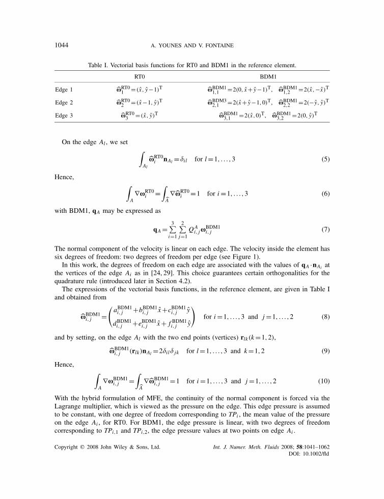
Figure 1. Degrees of freedom and basis functions for RT0 and BDM1 spaces on triangles.
Copyright q 2008 John Wiley & Sons, Ltd. Int. J. Numer. Meth. Fluids 2008; 58:1041–1062DOI: 10.1002/fld
1044 A. YOUNES AND V. FONTAINE
Table I. Vectorial basis functions for RT0 and BDM1 in the reference element.
RT0 BDM1
Edge 1 xRT01 =(x, y−1)T xBDM11,1 =2(0, x+ y−1)T, xBDM1
1,2 =2(x,−x)T
Edge 2 xRT02 =(x−1, y)T xBDM32,1 =2(x+ y−1,0)T, xBDM1
2,2 =2(−y, y)T
Edge 3 xRT03 =(x, y)T xBDM13,1 =2(x,0)T, xBDM1
3,2 =2(0, y)T
On the edge Al , we set ∫AlxRT0i nAl =�il for l=1, . . . ,3 (5)
Hence, ∫A∇xRT0i =
∫A∇xRT0i =1 for i=1, . . . ,3 (6)
with BDM1, qA may be expressed as
qA=3∑
i=1
2∑j=1
QAi, jx
BDM1i, j (7)
The normal component of the velocity is linear on each edge. The velocity inside the element hassix degrees of freedom: two degrees of freedom per edge (see Figure 1).
In this work, the degrees of freedom on each edge are associated with the values of qA ·nAi atthe vertices of the edge Ai as in [24, 29]. This choice guarantees certain orthogonalities for thequadrature rule (introduced later in Section 4.2).
The expressions of the vectorial basis functions, in the reference element, are given in Table Iand obtained from
xBDM1i, j =
(aBDM1i, j +bBDM1
i, j x+cBDM1i, j y
dBDM1i, j +eBDM1
i, j x+ f BDM1i, j y
)for i=1, . . . ,3 and j =1, . . . ,2 (8)
and by setting, on the edge Al with the two end points (vertices) rlk(k=1,2),
xBDM1i, j (rlk)nAl =2�il� jk for l=1, . . . ,3 and k=1,2 (9)
Hence, ∫A∇xBDM1
i, j =∫A∇xBDM1
i, j =1 for i=1, . . . ,3 and j =1, . . . ,2 (10)
With the hybrid formulation of MFE, the continuity of the normal component is forced via theLagrange multiplier, which is viewed as the pressure on the edge. This edge pressure is assumedto be constant, with one degree of freedom corresponding to TPi , the mean value of the pressureon the edge Ai , for RT0. For BDM1, the edge pressure is linear, with two degrees of freedomcorresponding to TPi,1 and TPi,2, the edge pressure values at two points on edge Ai .
Copyright q 2008 John Wiley & Sons, Ltd. Int. J. Numer. Meth. Fluids 2008; 58:1041–1062DOI: 10.1002/fld

HYBRID AND MULTI-POINT FORMULATIONS 1045
2.2. Discretization with RT0
The variational formulation of Darcy’s law (K−1q=−∇ p) is expressed using the vectorial basisfunctions xRT0i as test functions:∫
AK−1qAx
RT0i =−
∫A∇PxRT0i =
∫AP∇xRT0i −
3∑k=1
∫Ak
PxRT0i nk (11)
Using (5) and (6), we obtain ∫AK−1qAx
RT0i = PA−TPA
i (12)
Using (3), (12) can be expressed in the following matrix form:
3∑k=1
Bi,k QAk = PA−TPA
i (13)
where the elemental matrix B=[Bi,k] of dimensions (3×3) is defined by
Bi,k =∫AxRT0,Ti K−1xRT0k (14)
This matrix can be evaluated analytically in the reference element using
Bi,k =∫AxRT0,Ti K−1xRT0k (15)
where K−1= JTK−1 J/|J | corresponds to the analog tensor in the reference element, and J isJacobian matrix that is constant for triangular elements.
The matrix B is symmetric and positive definite. Equation (13) can be expressed as
QAi =
3∑k=1
B−1i,k (PA−TPA
k ) (16)
The mass balance equation in (2) is discretized using a finite volume formulation in space:
3∑i=1
QAi =|A| f A=QA
s (17)
f A is the mean value of f over the element A.Combining (16) and (17) gives
PA=3∑
i=1
�i�TPA
i + QAs
�(18)
where �i =∑3k=1 B
−1i,k and �=∑3
i=1 �i .Finally, the expression of the flux is given by replacing (18) in (16):
QAi = �i
�
3∑k=1
�kTPAk −
3∑k=1
B−1i,k TP
Ak + �i
�QA
s (19)
Copyright q 2008 John Wiley & Sons, Ltd. Int. J. Numer. Meth. Fluids 2008; 58:1041–1062DOI: 10.1002/fld

1046 A. YOUNES AND V. FONTAINE
The scalar unknowns with the hybrid formulation of RT0 are the mean pressures on the edges(TPA
i , i=1, . . . ,n f ).The final system of equations is obtained using continuity properties as follows:
• On all interior edges, continuity of the normal component of the velocity and edge pressurebetween the two adjacent elements A and B may be expressed as
TPAi =TPB
i and QAi +QB
i =0 (20)
• For a Dirichlet boundary edge Ai with a prescribed pressure TPbci , we have
TPAi =TPbc
i (21)
• For a Neumann boundary edge with a given flux Qbci
QAi =Qbc
i (22)
The hybrid formulation of RT0 gives a system for the number of edge unknowns with asymmetric positive matrix of a five-point stencil.
2.3. Discretization with BDM1
The variational formulation of Darcy’s law (K−1q=−∇ p) using the vectorial basis functionsxBDM1i, j as test functions may be expressed as∫
AK−1qAx
BDM1i, j =−
∫A∇PxBDM1
i, j =∫AP∇xBDM1
i, j −3∑
k=1
∫Ak
PxBDM1i, j nk (23)
Setting TPi,1 and TPi,2 to the edge pressure values at 13 and 2
3 of the edge and using (7), theprevious equation leads to
3∑k=1
2∑l=1
QAk,l
∫AxBDM1,Ti, j K−1xBDM1
k,l = PA−TPAi, j (24)
The element al matrix B=[Bi, j,k,l ] is of dimensions (6×6) with
Bi, j,k,l =∫AxBDM1,Ti, j K−1xBDM1
k,l (25)
where B is a positive-definite matrix evaluated analytically in the reference element.The same calculations as with the RT0 lead to
QAi, j =
3∑k=1
2∑l=1
B−1i, j,k,l(P
A−TPAk,l) (26)
and
PA=3∑
i=1
2∑j=1
�i, j�
TPAi, j +
QAs
�(27)
where �i, j =∑3k=1
∑2l=1 B
−1i, j,k,l and �=∑3
i=1∑2
j=1 �i, j .
Copyright q 2008 John Wiley & Sons, Ltd. Int. J. Numer. Meth. Fluids 2008; 58:1041–1062DOI: 10.1002/fld

HYBRID AND MULTI-POINT FORMULATIONS 1047
Replacing (27) in (26) leads to
QAi, j =
�i, j�
3∑k=1
2∑l=1
�k,lTPAk,l −
3∑k=1
2∑l=1
B−1i, j,k,lTP
Ak,l +
�i, j�
QAs (28)
With this formulation, the scalar unknowns are discrete pressures at edges (TPAi, j , i=1, . . . ,n f and
j =1, . . . ,2). The final system of equations is obtained using continuity properties as with RT0.The hybrid formulation of BDM1 leads to a system of twice the number of edge unknowns
with a symmetric positive matrix of a 10-point stencil.
3. THE MPFA METHOD ON TRIANGLES
3.1. The MPFA method
The MPFA discretization is a control volume formulation, where more than two pressure valuesare used in the flux approximation. The scheme reduces to a cell-centred stencil for the pressures[17–20].
The basic idea of the MPFA method is to divide each triangle into four subcells (Figure 2).Inside the subcell (xi ,x2i ,x,x
1i ) of the corner xi , we assume linear variation of the pressure between
�1i (the pressure at the midpoint edge x1i ), �2i (the pressure at the midpoint edge x2i ) and PA (thepressure at the centre x of element A) (Figure 2).
Therefore, subedge (half-edge) fluxes,(Q1
i =∫ x1i
xi−K∇P and Q2
i =∫ x2i
xi−K∇P
)
kx
ix
x2ix
1ix
1iQ
2iQ
jx
Figure 2. Triangle splitting into four subcells and linear pressure approximation on each subcell.
Copyright q 2008 John Wiley & Sons, Ltd. Int. J. Numer. Meth. Fluids 2008; 58:1041–1062DOI: 10.1002/fld

1048 A. YOUNES AND V. FONTAINE
kx ix
jx
1iQ
1A
2A
3A
4A
5A
Figure 3. The interaction region sharing vertex i .
taken positive for outflow, are given by(Q1
i
Q2i
)= 1
2|Txx1i x2i |
((x1i −xi )⊥K(x2i − x)⊥ (x1i −xi )⊥K(x−x1i )
⊥
(xi −x2i )⊥K(x2i − x)⊥ (xi −x2i )
⊥K(x−x1i )⊥
)︸ ︷︷ ︸
GAi
(�1i −PA
�2i −PA
)(29)
where |Txx1i x2i | is the area of the triangle spanned by the points x, x1i and x2i and, for example, the
vector (x1i −xi )⊥ is obtained by a �/2 rotation of the vector x1i −xi .All subcells sharing vertex xi create an interaction volume (see Figure 3).The discretization is accomplished by assuming continuous fluxes across each of the subedges
and a weak continuity condition of the pressure across the same edges. From these assumptions,an explicit discrete flux can be found after resolution of a local linear system and eliminating theedge pressure for each subedge of the interaction volume (see [19] for details). Each subedge fluxcan then be expressed explicitly as a weighted sum of the cell pressures of the interaction volume.For example, for Figure 3, we obtain
Q1i =
5∑k=1
tki PAk (30)
where tki are transmissibility coefficients and Ak are located at the gravity centre of the triangles.
3.2. Localization of continuity points: Symmetric or non-symmetric MPFA formulations
The final system of MPFA is obtained by expressing the mass balance over each triangle: sum ofthe six subedge fluxes of the element equals the sink/source term over that element. The resultingmass matrix can be symmetric or non-symmetric depending on the localization of the continuity
Copyright q 2008 John Wiley & Sons, Ltd. Int. J. Numer. Meth. Fluids 2008; 58:1041–1062DOI: 10.1002/fld
HYBRID AND MULTI-POINT FORMULATIONS 1049
kx
ixjx
x2ix
1ix 1
iQ
2iQ
w = 1.0
kx
ix
x 2ix
1ix 1
iQ
2iQ
w = 2/3
jx
xik
xij
Figure 4. Two locations of the continuity point at the subcell interface. Localpressure support for w=1.0 and 2
3 .
points. Indeed, as shown in [17], symmetry of the global matrix is guaranteed only if this propertyis respected for each local matrix GA
i .On the other hand, continuity of the pressure is generally prescribed at the element-edge
midpoint. This corresponds to w=|x1i −xi/xi j−xi |=1 with xi j =(xi +x j )/2 (see Figure 4). In thiscase, the local matrix GA
i in (29) is always non-symmetric.However, as shown in [30], there is flexibility in the location of the continuity point. Its position
can be chosen to lie at any point between the edge midpoint and the vertex (Figure 4).The symmetry is achieved when the continuity point is localized at w= 2
3 (Figure 4). In thiscase, x1i ,xi ,x
2i , x is a parallelogram and the local matrix GA
i in the half-edge fluxes expression(29) becomes
GsAi = 1
2|Txx1i x2i |
((xi j −xi )⊥K(x2i − x)⊥ (xi j −xi )⊥K(x−x1i )
⊥
(xi −xik)⊥K(x2i − x)⊥ (xi −xik)⊥K(x−x1i )⊥
)(31)
which can be shown to be symmetric when replacing x=(xi +x j +xk)/3, xi j =(xi +x j )/2, xik =(xi +xk)/2, x1i =xi/3+2xi j/3 and x2i =xi/3+2xik/3.
Therefore, one can obtain a symmetric MPFA formulation for general triangular elementswithout any approximate numerical integration. Recall that for quadrilateral grids, the MPFAmethod leads to a symmetric matrix only in the case of parallelograms (constant Jacobian).For quadrilateral elements, numerical quadrature allows the formulation of a symmetric MPFAformulation which, has similar convergence behaviour as the standard formulation for h2-perturbedparallelograms [22, 23, 26]. However, a loss of convergence has been observed for the symmetricMPFA formulation on rough grids [23, 26].
4. THE MPFA FORMULATION OF RT0 AND BDM1
In this section, we show, algebraically, the link between hybrid and MPFA formulations of bothRT0 and BDM1 mixed methods.
Copyright q 2008 John Wiley & Sons, Ltd. Int. J. Numer. Meth. Fluids 2008; 58:1041–1062DOI: 10.1002/fld

1050 A. YOUNES AND V. FONTAINE
4.1. The MPFA formulation of RT0
In the case of triangles, the inverse of the elemental matrix B, defined by (15), gives [16]
[B]−1= det(K)
|A|
⎡⎢⎢⎢⎣xi jK−1xi j xi jK−1xki xi jK−1x jk
xkiK−1xi j xkiK−1xki xkiK−1x jk
x jkK−1xi j x jkK−1xki x jkK−1x jk
⎤⎥⎥⎥⎦+ 1
3�
⎡⎢⎢⎣1 1 1
1 1 1
1 1 1
⎤⎥⎥⎦ (32)
The dimensionless shape coefficient � is defined by [6]
�=3∑j=1
Bi j (33)
Equation (18) becomes
PA=(TPA
1 +TPA2 +TPA
3
3
)+ �
3QA
s (34)
Recall that the fluxes across edges are given by
QAi =
3∑k=1
B−1i,k (PA−TPA
k ) (35)
The expression of TPA3 is obtained from (34) and is then replaced in (35). The substitution of (32)
into (35) gives the fluxes across the two first edges:
(QA
1
QA2
)= det(K)
|A|
⎛⎝x12K−1(x23−x12) x12K−1(x23−x31)
x31K−1(x23−x12) x31K−1(x23−x31)
⎞⎠⎛⎝(TPA1 −PA)
(TPA2 −PA)
⎞⎠
+QAs
⎛⎜⎜⎜⎝det(K)
|A| (x12K−1x23)�+ 1
3
det(K)
|A| (x32K−1x23)�+ 1
3
⎞⎟⎟⎟⎠ (36)
Using the following properties on triangles:
det(K)
|A| xi jK−1(x jk−xi j )= 1
4|Txx1i x2i |(x1i −xi )⊥K(x2i − x)⊥
det(K)
|A| xi jK−1(x jk−xki )= 1
4|Txx1i x2i |(x1i −xi )⊥K(x−x1i )
⊥(37)
Copyright q 2008 John Wiley & Sons, Ltd. Int. J. Numer. Meth. Fluids 2008; 58:1041–1062DOI: 10.1002/fld
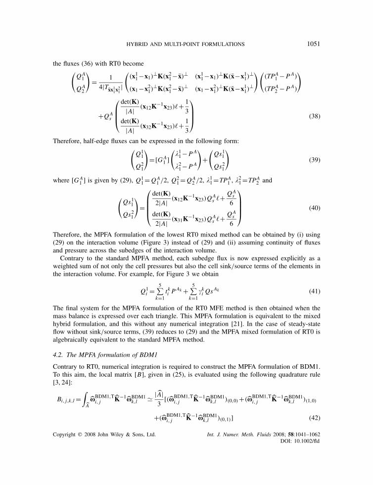
HYBRID AND MULTI-POINT FORMULATIONS 1051
the fluxes (36) with RT0 become(QA
1
QA2
)= 1
4|Txx11x21 |
((x11−x1)⊥K(x21− x)⊥ (x11−x1)⊥K(x−x11)
⊥
(x1−x21)⊥K(x21− x)⊥ (x1−x21)
⊥K(x−x11)⊥
)((TPA
1 −PA)
(TPA2 −PA)
)
+QAs
⎛⎜⎜⎝det(K)
|A| (x12K−1x23)�+ 1
3
det(K)
|A| (x32K−1x23)�+ 1
3
⎞⎟⎟⎠ (38)
Therefore, half-edge fluxes can be expressed in the following form:(Q1
1
Q21
)=[GA
1 ](
�11−PA
�21−PA
)+(Qs11
Qs21
)(39)
where [GA1 ] is given by (29), Q1
1=QA1 /2, Q2
1=QA2 /2, �11=TPA
1 , �21=TPA2 and
(Qs11
Qs21
)=
⎛⎜⎜⎜⎝det(K)
2|A| (x12K−1x23)QAs �+ QA
s
6
det(K)
2|A| (x31K−1x23)QAs �+ QA
s
6
⎞⎟⎟⎟⎠ (40)
Therefore, the MPFA formulation of the lowest RT0 mixed method can be obtained by (i) using(29) on the interaction volume (Figure 3) instead of (29) and (ii) assuming continuity of fluxesand pressure across the subedges of the interaction volume.
Contrary to the standard MPFA method, each subedge flux is now expressed explicitly as aweighted sum of not only the cell pressures but also the cell sink/source terms of the elements inthe interaction volume. For example, for Figure 3 we obtain
Q1i =
5∑k=1
tki PAk +
5∑k=1
�ki QsAk (41)
The final system for the MPFA formulation of the RT0 MFE method is then obtained when themass balance is expressed over each triangle. This MPFA formulation is equivalent to the mixedhybrid formulation, and this without any numerical integration [21]. In the case of steady-stateflow without sink/source terms, (39) reduces to (29) and the MPFA mixed formulation of RT0 isalgebraically equivalent to the standard MPFA method.
4.2. The MPFA formulation of BDM1
Contrary to RT0, numerical integration is required to construct the MPFA formulation of BDM1.To this aim, the local matrix [B], given in (25), is evaluated using the following quadrature rule[3, 24]:
Bi, j,k,l =∫AxBDM1,Ti, j K−1xBDM1
k,l � | A|3
[(xBDM1,Ti, j K−1xBDM1
k,l )(0,0)+(xBDM1,Ti, j K−1xBDM1
k,l )(1,0)
+(xBDM1,Ti, j K−1xBDM1
k,l )(0,1)] (42)
Copyright q 2008 John Wiley & Sons, Ltd. Int. J. Numer. Meth. Fluids 2008; 58:1041–1062DOI: 10.1002/fld

1052 A. YOUNES AND V. FONTAINE
Recall that from (9), we have on the edge Al with the two end points (vertices) rlk (k=1,2),
xBDM1i, j (rlk)nAl =2�il� jk for l=1, . . . ,3 and k=1,2 (43)
Therefore, using (42) and (43) to compute the local matrix [B] gives a block-diagonal matrix whereonly the two vectorial basis functions associated with a corner xi are coupled. The (6×6) linearsystem (26) reduces to three (2×2) linear systems (one for each vertex). For example, for vertex 1of coordinates (0,0) in Figure 3, only xBDM1
1,1 and xBDM12,1 are non-zero and the corresponding
(2×2) local system is
1
6
⎛⎝(xBDM1,T1,1 K−1xBDM1
1,1 )(0,0) (xBDM1,T1,1 K−1xBDM1
2,1 )(0,0)
(xBDM1,T1,1 K−1xBDM1
2,1 )(0,0) (xBDM1,T2,1 K−1xBDM1
2,1 )(0,0)
⎞⎠(QA1,1
QA2,1
)=(PA−TPA
1,1
PA−TPA2,1
)(44)
Substituting expressions of xBDM11,1 and xBDM1
2,1 from Table I in (44) and inverting the obtainedlocal system leads to the following formulation:(
Q1i
Q2i
)=[GsAi ]
(�1i −PA
�2i −PA
)(45)
where [GsAi ] is the local matrix given in (31) and Q1i =QA
1,1, Q2i =QA
2,1, �1i =TPA1,1, �2i =TPA
2,1.Therefore, this system is equivalent to the symmetric MPFA system obtained when the continuity
point is localized at w= 23 (Figure 4).
In conclusion, the MPFA formulation of the BDM1 mixed method on triangles is obtained byusing a special quadrature rule that reduces the BDM1 method to the symmetric MPFA method.
5. EFFICIENCY OF HYBRID AND MIXED FORMULATIONS OF RT0 AND BDM1
This section is devoted to the numerical efficiency and accuracy of the four mixed formulations(Hybrid RT0, MPFA RT0, Hybrid BDM1 and MPFA BDM1) on high anisotropic and heteroge-neous media with unstructured triangular discretizations.
Properties of the four mixed formulations are summarized in Table II. It is clear from this tablethat the MPFA RT0 is the less efficient formulation. This formulation is generally avoided forvery large systems. Indeed, this formulation does not lead to a symmetric positive-definite matrixfor general problems. Consequently, the obtained system cannot be solved with standard iterativesolvers based on the conjugate gradient method.
Table II. Properties of Hybrid RT0, MPFA RT0, Hybrid BDM1 and MPFA BDM1 formulations.
Hybrid RT0 MPFA RT0 Hybrid BDM1 MPFA BDM1
Numerical quadrature No No No YesSymmetric and positive-definite matrix Yes No Yes YesNumber of unknowns Nbr-edges Nbr-elements 2×Nbr-edges Nbr-elementsStencil 5 ≈15 10 ≈15
Copyright q 2008 John Wiley & Sons, Ltd. Int. J. Numer. Meth. Fluids 2008; 58:1041–1062DOI: 10.1002/fld
HYBRID AND MULTI-POINT FORMULATIONS 1053
The MPFA RT0 formulation is therefore excluded, and the rest of the paper is devoted to thenumerical efficiency of the three formulations: Hybrid RT0, Hybrid BDM1 and MPFA BDM1.These three formulations give symmetric positive-definite matrix systems.
5.1. Numerical experiments
We define a test problem to study the efficiency of mixed formulations. The system (1) is solvedon a unit square shape �=(0,1)2 domain with anisotropic and heterogeneous permeability field.The tensor coefficient and the true solution for the test problem are similar to the test problemgiven in [31]
K =[y2+�x2 (�−1)xy
(�−1)xy x2+�y2
](46)
P(x, y)=exp
(−20�
((x− 1
2
)2
+(y− 1
2
)2))
(47)
The behaviours of all formulations are studied numerically for different anisotropies and differenttriangular discretizations.
For practical test cases, a high accuracy for the velocity field is often required (as, for example,for the simulation of transport of contaminant). The velocity error is investigated in the discreteL2-norm defined by
evL2 =(∑
i|Ai |(qan,i −qi )2
/∑i
|Ai |)1/2
(48)
where |Ai | is the area of element i and qan,i the analytical velocity evaluated at the centre of iobtained by the derivation of (47).
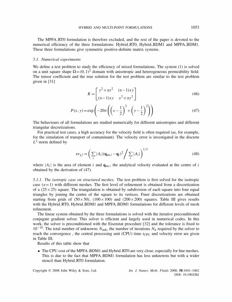
5.1.1. The isotropic case on structured meshes. The test problem is first solved for the isotropiccase (�=1) with different meshes. The first level of refinement is obtained from a discretizationof a (25×25) square. The triangulation is obtained by subdivision of each square into four equaltriangles by joining the centre of the square to its vertices. Finer discretizations are obtainedstarting from grids of (50×50), (100×100) and (200×200) squares. Table III gives resultswith the Hybrid RT0, Hybrid BDM1 and MPFA BDM1 formulations for different levels of meshrefinement.
The linear system obtained by the three formulations is solved with the iterative preconditionedconjugate gradient solver. This solver is efficient and largely used in numerical codes. In thiswork, the solver is preconditioned with the Eisenstat procedure [32] and the tolerance is fixed to10−16. The total number of unknowns Nunk, the number of iterations Nit required by the solver toreach the convergence , the central processing unit (CPU) time tCPU and velocity error are givenin Table III.
Results of this table show that
• The CPU cost of the MPFA BDM1 and Hybrid RT0 are very close, especially for fine meshes.This is due to the fact that MPFA BDM1 formulation has less unknowns but with a widerstencil than Hybrid RT0 formulation.
Copyright q 2008 John Wiley & Sons, Ltd. Int. J. Numer. Meth. Fluids 2008; 58:1041–1062DOI: 10.1002/fld
1054 A. YOUNES AND V. FONTAINE
TableIII.Results
ofHybridRT0,
HybridBDM1andMPF
ABDM1fordifferentmeshrefin
ements.
Mesh1
Mesh2
Mesh3
Mesh4
Hyb
rid
Hyb
rid
MPF
AHyb
rid
Hyb
rid
MPF
AHyb
rid
Hyb
rid
MPF
AHyb
rid
Hyb
rid
MPF
ART0
BDM1
BDM1
RT0
BDM1
BDM1
RT0
BDM1
BDM1
RT0
BDM1
BDM1
Nun
k38
0076
0025
0015
100
3020
010
000
6020
012
040
040
000
24040
028
080
016
000
0Nit
142
269
100
276
527
194
544
1033
380
1153
2057
760
t CPU
0.05
0.14
0.08
0.27
1.03
0.45
2.2
12.6
3.1
25.7
110
24.5
evL2
7.8×
2.5×
4.7×
3.95
×1.07
×2.27
×2.0×
7.2×
1.2×
1.15
×6.3×
8.1×
10−2
10−2
10−2
10−2
10−2
10−2
10−2
10−3
10−2
10−2
10−3
10−3
Copyright q 2008 John Wiley & Sons, Ltd. Int. J. Numer. Meth. Fluids 2008; 58:1041–1062DOI: 10.1002/fld
HYBRID AND MULTI-POINT FORMULATIONS 1055
10-1 100 101 102
10-2
10-1
Vel
ocity
err
or
CPU (s)
Hybrid_RT0 Hybrid_BDM1 MPFA_BDM1
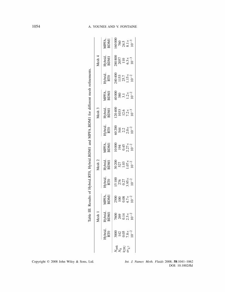
Figure 5. Velocity errors with Hybrid-RT0, Hybrid BDM1 and MPFA BDM1 for different meshes.
• The Hybrid BDM1 formulation requires less CPU time than Hybrid RT0 to achieve a fixedvelocity accuracy (Figure 5).
• In the case of structured mesh and isotropic domain, the MPFA BDM1 gives more accurateresults than Hybrid RT0 but less than Hybrid BDM1.
5.1.2. Effects of anisotropy. The test problem is now simulated with different anisotropy factorsand uses the coarser discretization described above.
Results of simulations, given in Table IV, show that
• The number of iterations and the CPU time increase when � increases for the three formula-tions.
• For anisotropic domains, the pressure solution presents non-physical oscillations (nega-tive values). These oscillations are much more pronounced with Hybrid RT0 than withHybrid BDM1 or MPFA BDM1.
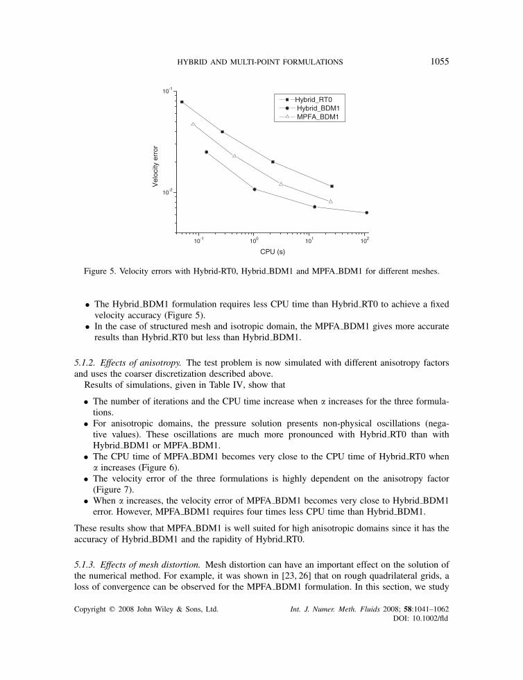
• The CPU time of MPFA BDM1 becomes very close to the CPU time of Hybrid RT0 when� increases (Figure 6).
• The velocity error of the three formulations is highly dependent on the anisotropy factor(Figure 7).
• When � increases, the velocity error of MPFA BDM1 becomes very close to Hybrid BDM1error. However, MPFA BDM1 requires four times less CPU time than Hybrid BDM1.
These results show that MPFA BDM1 is well suited for high anisotropic domains since it has theaccuracy of Hybrid BDM1 and the rapidity of Hybrid RT0.
5.1.3. Effects of mesh distortion. Mesh distortion can have an important effect on the solution ofthe numerical method. For example, it was shown in [23, 26] that on rough quadrilateral grids, aloss of convergence can be observed for the MPFA BDM1 formulation. In this section, we study
Copyright q 2008 John Wiley & Sons, Ltd. Int. J. Numer. Meth. Fluids 2008; 58:1041–1062DOI: 10.1002/fld

1056 A. YOUNES AND V. FONTAINE
TableIV.Results
ofHybridRT0,
HybridBDM1andMPF
ABDM1fordifferentanisotropy
factors.
�=1
�=1
0�=1
00�=1
000
Hyb
rid
Hyb
rid
MPF
AHyb
rid
Hyb
rid
MPF
AHyb
rid
Hyb
rid
MPF
AHyb
rid
Hyb
rid
MPF
ART0
BDM1
BDM1
RT0
BDM1
BDM1
RT0
BDM1
BDM1
RT0
BDM1
BDM1
Nit
142
269
100
209
338
121
326
472
179
627
549
240
t CPU
4.7×
0.14
7.8×
6.3×
0.17
9.3×
7.8×
0.23
0.1
0.12
50.25
0.12
10−2
10−2
10−2
10−2
10−2
P Min
−1.9
×−8
.5×
−5.1
×−5
.4×
−4.1
×−1
.2×
−0.22
−1.5
×−3
.8×
−3.43
−3×
−0.1
10−4
10−5
10−5
10−4
10−4
10−4
10−3
10−3
10−2
P Max
0.98
0.98
0.99
1.06
0.98
0.99
1.81
0.99
1.00
18.76
1.2
1.1
epL2
6.3×
1.9×
8×4.6×
1.8×
1.2×
5.6×
1.6×
2.9×
0.52
9.3×
2.6×
10−4
10−3
10−4
10−3
10−3
10−3
10−2
10−3
10−3
10−3
10−2
evL2
7.9×1
0−2
2.5×1
0−2
4.6×1
0−2
0.65
0.18
0.24
6.7
2.1
2.44
67.3
28.6
27
Copyright q 2008 John Wiley & Sons, Ltd. Int. J. Numer. Meth. Fluids 2008; 58:1041–1062DOI: 10.1002/fld
HYBRID AND MULTI-POINT FORMULATIONS 1057
1 10 100 1000
0.05
0.1
0.15
0.2
0.25
CP
U (
s)
Anisotropy factor
Hybrid_RT0 Hybrid_BDM1 MPFA_BDM1
Figure 6. CPU time with Hybrid RT0, Hybrid BDM1 and MPFA BDM1 for different anisotropy factors.
1 10 100 1000
0.01
0.1
1
10
100
Ve
locity e
rro
r
Anisotropy factor
Hybrid_RT0
Hybrid_BDM1
MPFA_BDM1
Figure 7. Velocity errors with Hybrid RT0, Hybrid BDM1 and MPFA BDM1for different anisotropy factors.
this effect on the behaviour of the solution of Hybrid RT0, Hybrid BDM1 and MPFA BDM1formulations.
The previous triangulations are obtained from subdivision of squares. To obtain a highly unstruc-tured triangulation, the centre of each square is moved randomly inside the square. Four differenttriangles are obtained by joining this point to the vertices of the square.
This procedure is performed at each level of refinement. Figure 8 shows the unstructuredtriangular mesh obtained from the coarser discretization.
Copyright q 2008 John Wiley & Sons, Ltd. Int. J. Numer. Meth. Fluids 2008; 58:1041–1062DOI: 10.1002/fld

1058 A. YOUNES AND V. FONTAINE
X
Y
0 0.2 0.4 0.6 0.8 10
0.2
0.4
0.6
0.8
1
Figure 8. Unstructured triangulation obtained from randomly moving the centre of squares.
Results for different unstructured meshes with a coefficient of anisotropy of �=50 are given inTable V and Figures 9 and 10. These results show that
• The symmetric MPFA formulation on triangles is highly efficient on unstructured meshes andMPFA BDM1 results are not deteriorated on unstructured meshes.
• The Hybrid RT0 gives less stable pressure results than Hybrid BDM1 and MPFA BDM1.The maximum pressure value with Hybrid RT0 is greater than 1 for all meshes.
• Concerning pressure errors, MPFA BDM1 is the more efficient method. Indeed, for a givenpressure error of 5×10⁻⁴, MPFA BDM1 spends 20 times less CPU time than Hybrid RT0and four times less than Hybrid BDM1 (Figure 9).
• Similar performances are obtained for MPFA BDM1 concerning velocity errors. Indeed,MPFA BDM1 can spend 10 times less CPU time than Hybrid RT0 and three times less thanHybrid BDM1 for a given velocity error (Figure 10).
These results show that the MPFA BDM1 formulation outperforms both Hybrid RT0 andHybrid BDM1 formulations for anisotropic domains and unstructured triangular meshes.
6. CONCLUSION
In this paper, hybrid and MPFA formulations of both RT0 and BDM1 mixed methods weredeveloped. The link between these formulations was shown algebraically for RT0 and BDM1 ontriangular meshes.
The MPFA RT0 formulation is obtained without any numerical integration from the mixedformulation. Whereas, the MPFA BDM1 formulation is obtained by using a special quadraturerule that reduces the BDM1 method to the symmetric MPFA method.
Copyright q 2008 John Wiley & Sons, Ltd. Int. J. Numer. Meth. Fluids 2008; 58:1041–1062DOI: 10.1002/fld

HYBRID AND MULTI-POINT FORMULATIONS 1059
TableV.Results
ofHybridRT0,
HybridBDM1andMPF
ABDM1fordifferentunstructured
meshesand
�=5
0.
Mesh1
Mesh2
Mesh3
Mesh4
Hyb
rid
Hyb
rid
MPF
AHyb
rid
Hyb
rid
MPF
AHyb
rid
Hyb
rid
MPF
AHyb
rid
Hyb
rid
MPF
ART0
BDM1
BDM1
RT0
BDM1
BDM1
RT0
BDM1
BDM1
RT0
BDM1
BDM1
Nun
k38
0076
0025
0015
100
3020
010
000
6020
012
040
040
000
24040
028
080
016
000
0Nit
305
453
164
590
901
323
1155
1788
646
2286
3551
1275
t CPU
0.06
0.22
0.1
0.5
1.75
0.59
4.25
21.5
4.7
50.3
188.9
38.9
P Min
−7.7
×−1
.6×
−4.0
×−6
.4×
−3.9
×−8
.5×
−6.8
×−8
.5×
−1.8
×−2
.1×
−2.1
×−4
.8×
10−2
10−3
10−3
10−3
10−4
10−4
10−4
10−5
10−4
10−4
10−5
10−5
P Max
1.4
0.98
1.00
71.1
0.99
0.99
71.03
0.99
90.99
91.01
0.99
90.99
9ep
L2
3.1×
1.8×
2.8×
7.8×
4.6×
6.3×
1.94
×1.14
×1.5×
4.9×
2.9×
3.8×
10−2
10−3
10−3
10−3
10−4
10−4
10−3
10−4
10−4
10−4
10−5
10−5
evL2
3.53
0.99
1.15
1.7
0.42
0.51
0.89
0.27
0.31
0.48
0.24
0.25
Copyright q 2008 John Wiley & Sons, Ltd. Int. J. Numer. Meth. Fluids 2008; 58:1041–1062DOI: 10.1002/fld

1060 A. YOUNES AND V. FONTAINE
10-1 100 101 102
10-5
10-4
10-3
10-2
P e
rror
CPU (s)
Hybrid_RT0 Hybrid_BDM1 MPFA_BDM1
Figure 9. Pressure errors with Hybrid RT0, Hybrid BDM1 and MPFA BDM1 on unstructured meshes.
10-1 100 101 102
100
V e
rror
CPU (s)
Hybrid_RT0 Hybrid_BDM1 MPFA_BDM1
Figure 10. Velocity errors with Hybrid RT0, Hybrid BDM1 and MPFA BDM1 on unstructured meshes.
Performance of the four mixed formulations (Hybrid RT0, Hybrid BDM1, MPFA RT0 andMPFA BDM1) was investigated on anisotropic and heterogeneous media with unstructured meshes.
The MPFA RT0 is the less efficient formulation. It uses fewer unknowns than Hybrid RT0 butthe matrix of the discrete system is non-symmetric and is not positive definite.
Numerical experiments show that, in general, BDM1 formulations (Hybrid BDM1 andMPFA BDM1) require less CPU time than Hybrid RT0 to achieve a fixed velocity accuracy. Theaccuracy of the MPFA BDM1 formulation is not deteriorated for highly unstructured triangularmeshes (contrarily to quadrilateral meshes where a loss of convergence can be encountered
Copyright q 2008 John Wiley & Sons, Ltd. Int. J. Numer. Meth. Fluids 2008; 58:1041–1062DOI: 10.1002/fld

HYBRID AND MULTI-POINT FORMULATIONS 1061
for rough grids). For highly anisotropic domains and unstructured meshes, the MPFA BDM1formulation outperforms both Hybrid RT0 and Hybrid BDM1 and appears to be the successfulchoice when a high accuracy for the velocity field is required.
REFERENCES
1. Durlofsky LJ. Accuracy of mixed and control volume finite element approximations to Darcy velocity and relatedquantities. Water Resources Research 1994; 21:965–973.
2. Darlow BL, Ewing RE, Wheeler MF. Mixed finite element method for miscible displacement problems in porousmedia. Society of Petroleum Engineers Journal 1984; 24:391–398.
3. Brezzi F, Fortin M. Mixed and Hybrid Finite Element Methods. Springer: New York, 1991.4. Bergamaschi L, Mantica S, Saleri F. Mixed finite element approximation of Darcy’s law in porous media.
Technical Report, CRS4, Cagliari, Italy, 1994.5. Mose R, Siegel P, Ackerer P, Chavent G. Application of the mixed hybrid finite element approximation in a
groundwater flow model: luxury or necessity? Water Resources Research 1994; 30:3001–3012.6. Younes A, Ackerer Ph, Mose R, Chavent G. A new formulation of the mixed finite element method for solving
elliptic and parabolic PDE with triangular elements. Journal of Computational Physics 1999; 149:148–167.7. Ackerer Ph, Younes A, Mose R. Modeling variable density flow and solute transport in porous medium: 1.
Numerical model and verification. Transport in Porous Media 1999; 35:345–373.8. Chavent G, Younes A, Ackerer Ph. On the finite volume reformulation of the mixed finite element method
for elliptic and parabolic PDE on triangles. Computer Methods in Applied Mechanics and Engineering 2003;192:655–682.
9. Younes A, Ackerer P, Lehmann F. A new mass lumping scheme for the mixed hybrid finite element method.International Journal for Numerical Methods in Engineering 2006; 67:89–107.
10. Chavent G, Jaffre J. Mathematical Models and Finite Elements for Reservoir Simulation. North-Holland:Amsterdam, 1986.
11. Roberts JE, Thomas JM. Finite elements methods (part 1). In Mixed and Hybrid Methods, Ciarlet PG, Lions JL(eds), vol. II. North-Holland: Amsterdam, 1989.
12. Russel TF, Wheeler MF. Finite element and finite difference methods for continuous flows in porous media. InThe Mathematics of Reservoir Simulation, Ewing RE (ed.). SIAM: Philadelphia, PA, 1983.
13. Weiser A, Wheeler MF. On convergence of block-centered finite differences for elliptic problems. SIAM Journalon Numerical Analysis 1988; 25:351–375.
14. Baranger J, Maitre JF, Oudin F. Application de la theorie des elements finis mixtes a l’etude d’une classede schemas aux volumes-differences finis pour les problemes elliptiques. Comptes Rendus de l’Academie desSciences Paris, Serie I 1994; 319:401–404.
15. Arbogast T, Kennan PT. Mixed finite element methods as finite difference methods for solving elliptic equationson triangular elements. Technical Report 93-53, Department of Computational and Applied Mathematics, RiceUniversity, 1984.
16. Younes A, Ackerer P, Chavent G. From mixed finite elements to finite volumes for elliptic PDE in 2 and 3dimensions. International Journal for Numerical Methods in Engineering 2004; 59:365–388.
17. Aavatsmark I, Barkve T, Bøe Ø, Mannseth T. Discretization on non-orthogonal, curvilinear grids for multiphaseflow. In Proceedings of 4th European Conference on the Mathematics of Oil Recovery, Christie MA, FarmerCL, Guillon O, Heinmann ZE (eds). Norway, 1994.
18. Edwards MG, Rogers CF. A flux continuous scheme for the full tensor pressure equation. Proceedings of the4th European Conference on the Mathematics of Oil Recovery, Røros, 1994.
19. Aavatsmark I. An introduction to multipoint flux approximations for quadrilateral grids. Journal of ComputationalGeosciences 2002; 6:404–432.
20. Edwards MG, Rogers CF. Finite volume discretization with imposed flux continuity for the general tensor pressureequation. Journal of Computational Geosciences 1998; 2:259–290.
21. Vohralik M. Equivalence between lowest-order mixed finite element and multi-point finite volume methods onsimplicial meshes. Mathematical Modelling and Numerical Analysis 2006; 40:367–391.
22. Klausen RA, Winther R. Convergence of multipoint flux approximations on quadrilateral grids. Numerical Methodsfor Partial Differential Equations 2006; 22:1438–1454.
23. Klausen RA, Winther R. Robust convergence of multi-point flux approximations on rough grids. NumerischeMathematik 2006; 104:317–337.
Copyright q 2008 John Wiley & Sons, Ltd. Int. J. Numer. Meth. Fluids 2008; 58:1041–1062DOI: 10.1002/fld

1062 A. YOUNES AND V. FONTAINE
24. Wheeler MF, Yotov I. A cell-centered finite difference method on quadrilaterals. In Compatible SpatialDiscretizations, Arnold DN, Bochev PB, Lehoucq RB, Nicolaides RA, Shashkov M (eds), IMA Vol. Ser., vol.142. Springer: New York, 2006; 189–207.
25. Wheeler MF, Yotov I. A multipoint flux mixed finite element method. SIAM Journal on Numerical Analysis2006; 44:2082–2106.
26. Aavatsmark I, Eigestad G, Klausen RA, Wheeler MF, Yotov I. Convergence of a symmetric MPFA methodon quadrilateral grids. Technical Report TR-MATH 05-14, Department of Mathematics, University of Pittsburgh,Pittsburgh, PA, 2005.
27. Fraeijs de Veubeke BX. Displacement and equilibrium models in the finite element method. In Stress Analysis,Zienkiewicz OC, Hollister G (eds). New York, 1965.
28. Brezzi F, Douglas Jr J, Marini LD. Two families of mixed finite elements for second order elliptic problems.Numerische Mathematik 1985; 47:217–235.
29. Brezzi F, Fortin M, Marini LD. Piecewise constant pressures for Darcy law. In Finite Elements Methods: 1970and Beyond, Franca LP (ed.). CIMNE: Barcelona, 2004.
30. Pal M, Edwards MG, Lamb AR. Convergence study of a family of flux-continuous, finite-volume schemes for thegeneral tensor pressure equation. International Journal for Numerical Methods in Fluids 2006; 51:1177–1203.
31. Le Potier C. Schema volumes finis pour des operateurs de diffusion fortement anisotropes sur des maillages nonstructures. Comptes Rendu Mathematique 2005; 12:921–926.
32. Eisenstat SC. Efficient implementation of a class of preconditioned conjugate gradient methods. SIAM Journalon Scientific and Statistical Computing 1981; 2:1–4.
Copyright q 2008 John Wiley & Sons, Ltd. Int. J. Numer. Meth. Fluids 2008; 58:1041–1062DOI: 10.1002/fld